Estimating Machinery Supply Elasticities Using … Machinery Supply Elasticities Using Output Price Booms ... biased estimate of the supply elasticity when supply and demand shocks

Finance and Economics Discussion SeriesDivisions of Research & Statistics and Monetary Affairs

Federal Reserve Board, Washington, D.C.

Estimating Machinery Supply Elasticities Using Output PriceBooms

Jesse Edgerton

2011-03

NOTE: Staff working papers in the Finance and Economics Discussion Series (FEDS) are preliminarymaterials circulated to stimulate discussion and critical comment. The analysis and conclusions set forthare those of the authors and do not indicate concurrence by other members of the research staff or theBoard of Governors. References in publications to the Finance and Economics Discussion Series (other thanacknowledgement) should be cleared with the author(s) to protect the tentative character of these papers.

Estimating Machinery Supply Elasticities Using Output

Price Booms

Jesse Edgerton∗

Federal Reserve Board

December 10, 2010

Abstract

Recent years have seen large increases in the prices of houses, farm products, andoil, often with little clear connection to economic fundamentals. These price increasescreated plausibly exogenous shifts in demand for construction, farm, and mining ma-chinery. This paper uses these demand shifts to estimate the elasticity of machinerysupply. Graphical evidence, OLS, and IV estimates all indicate that the quantity ofmachinery supplied increased rapidly during the booms, with only modest increases inprices. Pooled sample estimates of the supply elasticity are around 5, much larger thanthe estimate of 1 from Goolsbee [1998]. Results thus suggest that public policies thatstimulate investment demand will have only modest effects on the prices of investmentgoods.

JEL Codes: E22, H25, H32.Keywords: Investment, capital supply elasticity, bonus depreciation, expensing.

∗Email: [email protected]. Any views expressed here are those of the author only and need notrepresent the views of the Federal Reserve Board or the Federal Reserve System. I thank Robert Chirinko,Glenn Ellison, Jane Gravelle, Michael Greenstone, Anne Hall, Jerry Hausman, David Lebow, Steve Oliner,James Poterba, Nirupama Rao, Hui Shan, Dan Sichel, Johannes Spinnewijn, Jessica Stahl, Stacey Tevlin,and numerous seminar participants for helpful comments. Portions of the material in this paper originally cir-culated under the title, “Taxes and Used Equipment: Evidence from Construction Machinery” and appearedin Chapter 1 of my dissertation at the Massachusetts Institute of Technology.

1

1 Introduction

For many decades, policymakers have repeatedly attempted to stimulate business invest-

ment in productive equipment during periods of weak economic performance. For example,

expansionary monetary policy changes are intended in part to stimulate business investment

by reducing interest rates and encouraging bank lending. Fiscal policymakers often attempt

to encourage investment through changes to the tax code. Prominent recent examples in-

clude the temporary “bonus depreciation” provisions included in the packages of stimulus

legislation passed in 2002, 2003, 2008, 2009, and 2010. At the time of this writing, it appears

likely that further investment stimulus in the form of full expensing of equipment purchases

will be enacted through 2011.

The price elasticity of the supply of investment goods is a key parameter determining the

impact and incidence of these policies that intend to stimulate business investment. Many

seminal papers have implicitly or explicitly assumed that the supply of investment goods is

perfectly elastic—that is, that supply can increase to satisfy any increase in demand without

an increase in prices. Hall and Jorgenson [1967] and Summers [1981], for example, study

the impact of tax policy on investment decisions in partial equilibrium models where any

amount of physical capital can be purchased at a fixed price.1

Goolsbee [1998], however, emphasizes that the supply curve for investment goods may

be upward sloping.2 In the short run, policies designed to stimulate demand for investment

1General equilibrium models have often abstracted from the distinction between investment goods andother output. Standard Real Business Cycle models like that in King and Rebelo [1999] allow ouput to beallocated frictionlessly to either consumption or investment. An increase in investment might require anincrease in interest rates to dissuade consumption, but there is no sense in which an increasing amount ofconsumption must be foregone to produce an additional unit of capital when investment is high or growing.Modern DSGE models used for policy analysis (like those in Christiano, Eichenbaum, and Evans [2005],Smets and Wouters [2003], Edge, Kiley, and Laforte [2008], and Edge and Rudd [2010]) typically featurean adjustment cost that essentially makes some portion of investment disappear when investment wouldotherwise increase rapidly. This formulation captures the notion that an increasing amount of consumptionmust be foregone to produce a unit of capital when investment is growing rapidly. It does not, however,reflect the fact that the benefits of investment subsidies would be captured by suppliers of investment goods,a point stressed by Goolsbee [1998].

2Some economists prefer the term “supply relationship” to reflect the fact that a demand-invariant rela-tionship between price and the quantity supplied need not exist when markets are not perfectly competitive.Results in the paper do not depend on the assumption of competitive markets, but I use the familiar term

2

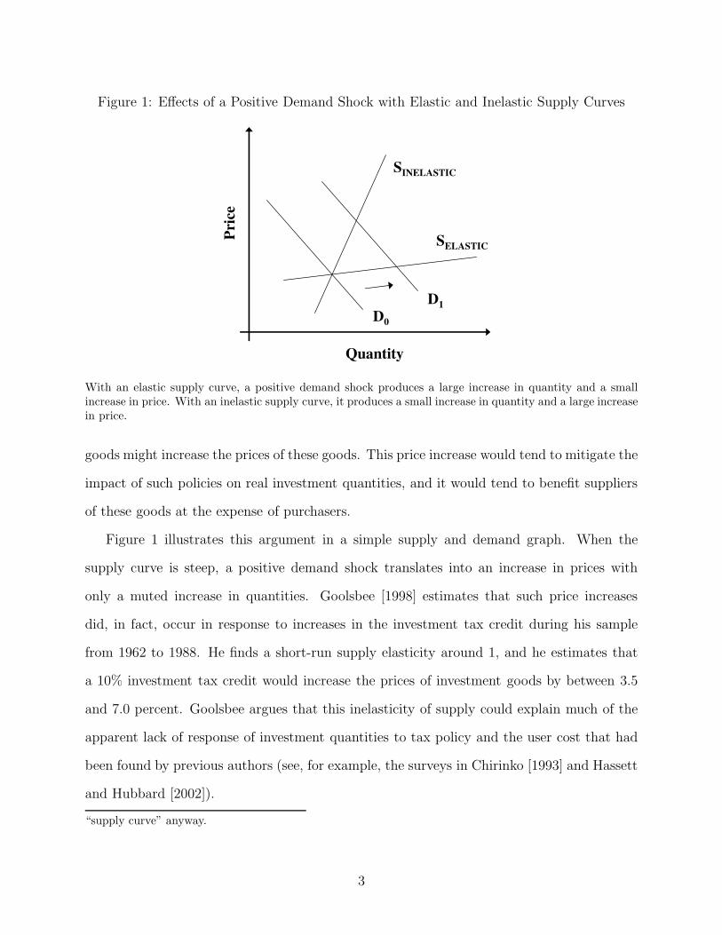
Figure 1: Effects of a Positive Demand Shock with Elastic and Inelastic Supply Curves

SINELASTIC

D0

D1

Quantity

Pri

ceSELASTIC

With an elastic supply curve, a positive demand shock produces a large increase in quantity and a smallincrease in price. With an inelastic supply curve, it produces a small increase in quantity and a large increasein price.

goods might increase the prices of these goods. This price increase would tend to mitigate the

impact of such policies on real investment quantities, and it would tend to benefit suppliers

of these goods at the expense of purchasers.

Figure 1 illustrates this argument in a simple supply and demand graph. When the

supply curve is steep, a positive demand shock translates into an increase in prices with

only a muted increase in quantities. Goolsbee [1998] estimates that such price increases

did, in fact, occur in response to increases in the investment tax credit during his sample

from 1962 to 1988. He finds a short-run supply elasticity around 1, and he estimates that

a 10% investment tax credit would increase the prices of investment goods by between 3.5

and 7.0 percent. Goolsbee argues that this inelasticity of supply could explain much of the

apparent lack of response of investment quantities to tax policy and the user cost that had

been found by previous authors (see, for example, the surveys in Chirinko [1993] and Hassett

and Hubbard [2002]).

“supply curve” anyway.

3

This paper provides new evidence on the supply elasticity of investment goods by exploit-

ing recent large increases in the prices of several types of output. During the last decade,

the prices of houses, farm products, and oil rose to astounding heights before crashing before

and during the financial crisis. The case of housing is particularly familiar, and it seems that

consensus opinion holds that these high prices resulted from a speculative bubble with little

relation to economic fundamentals.3

The reasons behind the increases in farm and oil prices are less well understood, and,

in fact, prices have rebounded substantially since the depths of the crisis. Mitchell [2008]

points to increased demand from worldwide biofuel production as the most important factor

in the rise in food commodity prices. Hamilton [2008] sees growth in demand from China

and other newly industrialized countries as a factor in recent oil price increases, but concedes

that, “The $140/barrel price in the summer of 2008 and the $60/barrel in November of 2008

could not both be consistent with the same calculation of a scarcity rent warranted by long-

term fundamentals.” Thus, at least some of the recent run-ups in goods prices appear to

have had little relation to economic fundamentals. At the very least, price increases have

been driven by increases in global demand and not by shocks to the supply of machinery

used to produce these goods.

These price increases did, however, lead to increased demand for this construction, farm,

and mining machinery. This paper uses these demand shifts to estimate machinery supply

curves. Textbook simultaneous equations models demonstrate that exogenous shifts in de-

mand can be used to identify supply curves (or vice versa). If the only variation in the data

comes from demand shifts, then ordinary least squares will correctly estimate the supply

curve. If there are also supply shocks in the data, then instrumental variables estimates ex-

ploiting an exogenous demand shifter can still correctly estimate the supply curve. I show in

this familiar setting that OLS “forward” regressions of quantity on price produce an upward-

3For example, Robert Solow wrote in the New York Review of Books, “The word ”bubble” is oftenmisused; but there was a housing bubble. Rising house prices induced many people to buy houses simplybecause they expected prices to rise; those purchases drove prices still higher, and confirmed the expectation.Prices rose because they had been rising.”

4

biased estimate of the supply elasticity when supply and demand shocks are uncorrelated,

while OLS “reverse” regressions of price on quantity produce a downward-biased estimate of

the supply elasticity. I argue that the most plausible story for a correlation between demand

and supply shocks in the data used in this paper would tend to bias results towards lower

elasticity estimates.

Graphical evidence, OLS estimates, and instrumental variables estimates all tell similar

stories. The supply of machinery supplied to the United States increased rapidly during the

output price booms, with only modest increases in prices. The price elasticity of construction

machinery supply is quite large—at least 10—while the supply elasticities of farm machinery

and mining machinery are around 3 and 5, respectively. Pooling the sample and weighting by

each type of machinery’s share of aggregate investment produces supply elasticity estimates

of at least 5, far larger than the estimate of 1 from Goolsbee [1998]. Even if the machinery

demand elasticity were as large as 1 in absolute value, these estimates would suggest that

only 17%, or 1/(1+5), of the value of tax incentives for invesment would be passed into

machinery prices.4

Finally, I discuss evidence suggesting that increased globalization of the machinery market

has contributed to the flattening of supply curves since the period studied by Goolsbee [1998].

The share of machinery investment that is imported from abroad has more than tripled since

the 1970s, and imports played an important role in the supply responses seen during the

boom periods studied in this paper. I conclude that policies that succeeded in stimulating

investment demand would be unlikely to simply push up the prices of investment goods, in

part due to elastic supply from abroad. However, to the extent that increased demand is

met with production from abroad, benefits to domestic manufacturers and their employees

may be limited.

This paper is most similar in spirit to Shea [1993], who uses “approximately exogenous”

demand shocks to estimate supply curves for many industries. He finds upward-sloping

4This calculation uses the approximation that the share −ηd/(ηs − ηd) of a small subsidy is passed tosuppliers in a competitive market, for ηd the elasticity of demand and ηs the elasticity of supply.

5

supply curves for many consumer and intermediate goods industries, but downward-sloping

supply curves for construction machinery and aircraft. This paper differs from Shea [1993] in

its focus on recent periods where the presence of large demand shocks is particularly clear,

in its focus on transparent, graphical presentation of results, and in the sign of its main

result. Other related papers include Hassett and Hubbard [1998] and Whelan [1999], which

question the robustness of Goolsbee’s results on other grounds. Sallee [2009] finds that tax

incentives for the purchase of hybrid cars had no effect on Toyota Prius prices, even though

Prius supply was quite inelastic.

The following section of the paper reviews the estimation of supply curves in a simul-

taneous equations setting. Section 3 discusses and describes the data. Section 4 presents

results, and Section 5 concludes.

2 The simultaneous equations model

Suppose price and quantity data are generated by the sytem of equations,

q = βp+ ǫs (1)

q = γ1p+ γ2z + ǫd (2)

p = πz + ν, (3)

where p and q are logarithms of prices and quantities, and constants and any other

exogenous variables are partialled out. Equations (1) and (2) are the “structural” supply

and demand equations, in the language of Hausman [1983]. The supply elasticity β is the

parameter of interest.5 The exogenous demand shifter z enters only the demand equation

and not the supply equation. Equation (3) relating p and z is a “reduced form” equation in

5Again, if markets are not competitive, there need not exist a demand-invariant supply curve that mapsthe market price into the quantity supplied. In this case, the parameter β should be thought of as a summarymeasure of the extent to which prices and quantities move together in response to demand shocks, regardlessof whatever structure might underlie this relationship. I continue to refer to β as the “supply elasticity” forbrevity and to facilitate comparison to Goolsbee’s results.

6

Figure 2: Demand Shocks Tracing Out the Supply Curve

S

D0

D1

D2

Quantity

Pri

ce

the language of Hausman [1983], but is commonly referred to as the “first stage” of two-stage

least squares (2SLS) estimation of equation (1).

Recall that asymptotic bias in the OLS estimate of β depends on the correlation of p and

the supply shocks ǫs,

plim βOLS = β +cov(ǫs, p)

var(p).

If we could examine data from a period with no supply shocks (ǫs = 0), then an OLS

regression of q on p would correctly estimate the supply elasticity. If instead we had data

from a period where demand shocks are large relative to suppy shocks, there would be large

demand-induced changes in p, with only small changes in ǫs. The numerator of the bias term

would be small, while the denominator would be large, and OLS would not be badly biased.

I claim that recent run-ups in commodity prices have created this kind of variation in

the data. There were large shocks to demand that likely swamp any shocks to supply.

Simple OLS regressions using data from the commodity price boom periods will probably

not produce badly biased supply elasticity estimates. Figure 2 depicts a situation like this

graphically.

7

It can be shown that the bias term can be written,

cov(ǫs, p)

var(p)=

var(ǫs)− cov(ǫs, (γ2z + ǫd))

(γ1 − β)var(p).

In a situation where supply shocks are uncorrelated with demand shocks (cov(ǫs, (γ2z+ǫd)) =

0), we can sign the OLS bias. Assuming that demand curves slope down (γ1 < 0) and supply

curves slope up (β > 0), the OLS estimate of β will be downward biased.

One could just as easily estimate the “reverse” supply equation relating prices to quan-

tities,

p =1

βq −

ǫsβ,

and thus one might wonder how this estimate is related to that of the forward equation.

Denote c = (1/β), and note that 1/c is a potential estimator for β, with,

plim cOLS =1

β+

cov(−ǫs/β, q)

var(q)=

1

β−

cov(ǫs, q)

βvar(q).

It can be shown that this bias term can be written,

cov(ǫs, q)

βvar(q)=

γ1βvar(ǫs)− cov(ǫs, (γ2z + ǫd))

(γ1 − β)var(q)

These results are derived in an appendix. Under the same assumptions (cov(ǫs, (γ2z+ ǫd)) =

0, γ1 < 0, and β > 0), we see that c is biased downwards, and thus that 1/c is biased upwards

as an estimator of β.

Because βOLS was biased downwards, the two estimators could be used to estimate upper

and lower bounds on β. It is well-known that the product βOLS × cOLS must equal the R2,

which is equal in both regressions. Thus the two estimates can provide tight bounds when

the R2 is high, but only loose bounds when it is low. Intuitively, if plotting a dataset of

(q, p) observations produces a loose cloud of points with no clear relationship between the

two variables, then regressing price on quantity would produce a horizontal regression line,

8

while regressing quantity on price would produce a vertical line. Alternatively, if price and

quantity have a clear linear relationship, then the forward and reverse regression lines will

be close together.

Of course, the two-stage least squares (2SLS) estimator may also be available, with,

plim β2SLS = β +cov(ǫs, z)

cov(p, z).

It is thus a consistent estimator of β whenever cov(ǫs, z) = 0. When instruments are valid

and supply and demand shocks are not badly correlated, we should see that forward and

reverse OLS and 2SLS estimates are all close together.6

It is worth considering what will happen if instruments are invalid. The denominator

of the 2SLS bias term will be positive as long as favorable supply shocks are not so highly

correlated with the instrument that p and z are negatively correlated, which, we will see,

is clearly not the case in the data used in this paper. Thus the sign of the bias will be

determined by the term cov(ǫs, z). In this paper, z represents the prices of houses, farm

products, and oil. I have argued that much of the variation in z in recent years has been

driven by speculative bubbles and demand shocks, rather than machinery supply shocks.

Nonetheless, plausible stories for correlation between ǫs and z may exist. I find the most

plausible story to be the following. Global demand or a housing bubble drove up aggregate

demand in the United States, increasing wages, interest rates, and other costs involved

6When multiple instrumental variables are available, Hahn and Hausman [2002] provide a formal speci-fication test based on the notion that forward and reverse 2SLS estimates should also be close together. Iexperimented with using multiple instruments to implement such tests with the data used in this paper. Un-fortunately, the output price variables that I use as instruments in this paper are highly colinear. Includingmore than of them tended to produce first stage estimates that made little sense, with, for example, someprice variables having the wrong sign. Although the forward and reverse IV estimates from these tests werestill often close together, I do not include them in the paper due to the poor performance of the first stage.The Hahn and Hausman [2002] test can be motivated by the concern that weak instruments combined

with finite sample bias could produce badly biased IV estimates. Hahn and Hausman [2002] show that thisbias will be most severe when the number of instruments is large, the explanatory power of the first stageis weak, and the error terms in the structural and first-stage equations are highly correlated. In the currentapplication, I use only one instrument, which produces a strong first stage, suggesting that the finite samplebias is not a serious concern. However, the lack of convincing identification when using multiple instrumentalvariables prevents me from conducting a convincing formal test.

9

in machinery production. There would thus be a correlation between strong demand for

machinery and unfavorable machinery supply shocks, which entails a negative correlation

between z and ǫs. In this setting, my estimates of the supply elasticity would be biased

downward.

Another story might be the following. Exogenous increases in the price of oil hurt the

economy, driving down real wages and other machinery production costs. There would

thus be a correlation between high oil prices and favorable supply shocks in machinery

manufacturing, which entails a positive correlation between z and ǫs and an upward bias in

supply elasticity estimates. In response, I would say first that this story is most plausible for

oil, as the relationship between oil price shocks and US recessions is well-known. But, I find

especially large supply elasticity estimates for construction machinery, where this story would

not apply. Second, the sample periods from which I produce supply elasticity estimates are

limited to the commodity boom periods, which fall primarily before the financial crisis and

recession could have begun driving down other input prices.

I thus find no concrete reasons to suspect that supply elasticity estimates will be biased

upward. Nonetheless, the validity of results still rests on the assumption that there were

no positive supply shocks keeping machinery prices low during the output price booms.

If, for example, there was a series of exogenous, increasing, positive productivity shocks

in machinery manufacturing during this period, then supply elasticity estimates could be

biased upward. Aggregate productivity growth was low during the commodity boom years

(Jorgenson, Ho, and Stiroh [2008], p. 6), so there is little reason to suspect there was a

sustained productivity boom in machinery manufacturing during this time.

3 Data

I use data from the National Income and Product Accounts of the Bureau of Economic

Analysis (BEA) to measure both machinery prices and quantities. Quantity data are based

10

on monthly surveys of shipments by U.S. manufacturers conducted by the Census Bureau.

The BEA then adjusts these domestic production numbers for imports and exports using

data from the International Trade Commission. The Bureau of Labor Statistics has its own

monthly survey asking U.S. machinery manufacturers about the prices they receive for their

output, and these data are used to create the Producer Price Indices (PPIs). The BEA uses

the PPIs to create price indices and measure real investment quantities. I use the BEA real

investment and price index series for construction machinery, farm machinery, and mining

and oilfield machinery. This is the same source of the data used for many of the results

in Goolsbee [1998]. To measure output price booms, I use the Case-Shiller National House

Price Index, the Census Bureau’s measure of construction spending on single-family homes,

the PPI for farm products, and the spot price of West Texas Intermediate Crude oil.7

One could be concerned about the quality of the price indices I will use to measure

machinery prices. The Producer Price Index data underlying the indices attempt to measure

all “changes in net revenues received by producers,” including manufacturer-to-customer

incentives like rebate programs and low-interest financing arrangements (Bureau of Labor

Statistics [2008]). It is still feasible that, despite the best efforts of the Bureau of Labor

Statistics, the indices fail to capture all relevant movements in machinery prices. If the

indices systematically overestimate prices when they are low and underestimate prices when

they are high, then price increases during commodity price booms could be underestimated,

and supply elasticity estimates could be upward biased. However, the results from Goolsbee

[1998] suggest that this effect could not be too large. His estimates suggest that a 10%

investment tax credit would increase capital goods prices by 4% on average, and close to 10%

for several types of equipment, including farm and mining machinery. If Goolsbee’s estimates

are correct, there cannot be much room for the PPI data to systematically understate price

7In some specifications I include additional control variables: the Baa corporate borrowing rate fromthe Federal Reserve’s H.15 release, hourly compensation for all persons in the manufacturing sector fromthe Bureau of Labor Statistics, the Producer Price Index for fuels and energy from the Bureau of LaborStatistics, the broad dollar exchange rate index from the Federal Reserve’s H.10 release, and real GrossDomestic Product from the Bureau of Economic Analysis.

11

Figure 3: Recent Output Price Booms

−1.5

−1

−.5

0

.5

1987 1990 1992 1995 1997 2000 2002 2005 2007 2010

Case−Shiller National House Price Index

Single−Family Residential Construction Spending

Houses

−.2

0

.2

.4

.6

1987 1990 1992 1995 1997 2000 2002 2005 2007 2010

Farm Products PPI

Farm Products

−.5

0

.5

1

1.5

1987 1990 1992 1995 1997 2000 2002 2005 2007 2010

West Texas Intermediate Crude Oil Price

Oil

All series logged, detrended, and normalized to 1995Q1. Vertical lines indicate the beginning and end ofperiods that I define as output price booms. The house price boom is from 2002Q1 to 2006Q1, the farm

products price boom from 2002Q2 to 2008Q3, and the oil price boom from 2001Q4 to 2008Q3.

12

changes.

I take logarithms of all series, regress them on a linear trend over the 15 years from 1988

to 2002, subtract the predicted values calculated using these coefficients over the full 1988 to

2010 period, and subtract off the value from 1995q1. The resulting detrended output price

series, normalized to 1995q1, appear in Figure 3. The recent boom and bust in prices is

quite apparent in all three figures. Housing prices rose by more than 30% from 2002 to 2006,

relative to their pre-2002 trend. Farm products prices rose more than 60%, and oil prices

rose 150%.8 Figure 3 also includes vertical lines that represent my subjective judgment of

the beginning and end of commodity price booms based on the data in the figure. These

are essentially the periods from trough to peak in the price series. However, the Case-Shiller

price index is very smooth, so I use the trough of the singe-family residential construction

spending series to date the beginning of the housing boom.

Figure 4 presents the detrended and normalized price and quantity series for all three

machinery types. It is immediately clear from the figure that there have been large swings

in quantities accompanied by small movements in prices for all three machinery types. For

example, construction machinery quantities grew by 44% during the housing boom relative

to their prior trend, while prices increased about 5%. Farm machinery quantities increased

by 40%, with an 8% increase in prices. Mining machinery quantities increased by 75%, with

about a 15% increase in prices.

The data in Figure 4 provide very transparent evidence that investment quantities fluc-

tuate far more than prices.9 Unless these movements were accompanied by large, well-timed

supply shocks, the data graphed in Figure 4 already suggest that supply elasticities must be

large. Also note from the figure that the beginning of the ouput price boom periods roughly

8These figures are actually changes in log points, which, of course, become poorer approximations topercentage changes when changes are large.

9In fact, these quantity fluctuations are not confined to the output price boom periods on which I focusin this paper. One might even argue that it should be obvious from looking at these simple charts thatquantities can fluctuate a great deal with only small movements in prices. One might thus question theusefulness of the results presented in this paper. I would remind anyone making this argument that theresults in Goolsbee [1998] indicate that prices should move one-for-one with quantities when there is a shiftin demand. Thus this paper is advancing an argument contrary to that currently in the literature.

13

Figure 4: Machinery Prices and Quantities

−1

−.5

0

.5

1988 1990 1992 1994 1996 1998 2000 2002 2004 2006 2008 2010

Price Index Real Investment

Construction Machinery

−1

−.5

0

.5

1988 1990 1992 1994 1996 1998 2000 2002 2004 2006 2008 2010


Farm Machinery

−1.5

−1

−.5

0

.5

1

1988 1990 1992 1994 1996 1998 2000 2002 2004 2006 2008 2010


Mining and Oilfield Machinery

All series logged, detrended, and normalized to 1995Q1. Vertical lines indicate the beginning and end ofdemand booms defined on the basis of output prices in Figure 3.

14

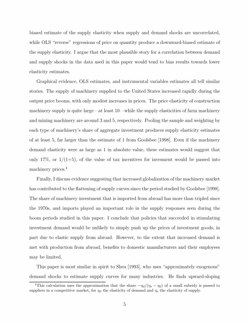
Figure 5: Recent Output Price Booms Tracing out Machinery Supply Curves

Forward Elasticity = 9.5, Reverse Elasticity = 11.6

−.3

−.2

−.1

0.1

.2.3

Pri

ce

−.3 −.2 −.1 0 .1 .2 .3Quantity

Construction Machinery


−.3

−.2

−.1

0.1

.2P

rice

−.1 0 .1 .2 .3 .4Quantity

Farm Machinery


−1

−.5

0.5

1P

rice

−1 −.5 0 .5 1Quantity

Mining and Oilfield Machinery

All series logged, detrended, and normalized to 1995Q1. Black lines are OLS regression lines from reverse(price on quantity) regressions. Grey lines are from forward (quantity on price) regressions.

15

coincides with a cyclical low point in machinery investment, as the U.S. was beginning its

recovery from the 2001 recession. As this is exactly the kind of time when policymakers

are likely to attempt to stimulate investment, it is an appropriate period during which to

estimate supply elasticities if one wishes to learn about the potential effectiveness of these

policies.10

4 Results

Figure 5 presents the data from the boom periods in Figure 4 in the same format as Figure

2, which illustrated how a shifting demand curve can trace out the supply curve. Each dot

in the scatter plots in Figure 5 is a quarterly data point, and the figures are constructed so

that the price and quantity axes have the same scale. It is clear in the figure that the supply

curves traced out during the output price boom periods are quite flat.

Table 1 presents regressions that quantify the results visible in Figures 4 and 5. Panel

A presents results for construction machinery, Panel B for farm machinery, and Panel C for

mining and oilfield machinery. Columns 1 and 2 present forward and reverse OLS regres-

sions over the sample period from 1988 to the end of the relevant output price boom. I

argued above that the forward and reverse estimates should provide lower and upper bounds

on the supply elasticity when supply curves slope up and supply and demand shocks are

uncorrelated. In panels A and C, the estimates in columns 1 and 2 provide only very wide

bounds on the supply elasticity, indicating that there is little clear relation between price and

quantity over the full sample, and thus suggesting that both supply and demand shifts may

sometimes be relevant in determining variation in prices and quantities. For construction

machinery in Panel A, the forward elasticity estimate is 0.54, and the reverse estimate is

10In fact, legislation did enact “bonus depreciation” tax provisions in 2002 and expand them in 2003. Asthese provisions were intended to create shifts in the demand curve for machinery, they could also potentiallybe of use in estimating the supply curve. However, several authors have presented estimates suggesting thatbonus depreciation had little impact on demand for the kinds of machinery studied here (see, for example,Cohen and Cummins [2006], Edgerton [2009], and House and Shapiro [2008]), so I do not pursue thisidentification strategy. Note also that as bonus depreciation is another potential demand shifter, there is nodirect channel through which ignoring it would bias my estimate of the supply elasticity.

16

159.7. For mining machinery in Panel C, the forward estimate is 3.5 and the reverse is 17.7.

In panel B, estimates suggest that farm machinery supply could even be downward sloping.

Columns 3 and 4 again present forward and reverse OLS estimates, but limit the sample

to the output price boom periods identified from Figure 3. Bounds on the elasticity estimate

are much tighter. For construction machinery in Panel A, the forward elasticity estimate is

9.5, and the reverse estimate is 11.6. For farm machinery in Panel B, the forward estimate

is 2.1 and the reverse is 6.7. For mining machinery in Panel C, the forward estimate is 5.2

and the reverse is 6.9.

Column 5 presents instrumental variables estimates using the appropriate series from

Figure 3 as an instrument for machinery prices. I use the series of single-family residential

construction spending as the instrument for construction machinery prices because the Case-

Shiller house price index is very smooth. Results differ relatively little from the OLS estimates

in Columns 3 and 4. For construction machinery, the Column 5 estimate of 13.0 is a bit

above the Column 4 reverse OLS estimate. For farm machinery, the Column 5 estimate of

2.1 is just above the Column 3 forward OLS estimate. For mining machinery, the column 5

estimate of 4.8 is just below the Column 3 estimate.

Columns 6 and 7 present instrumental variables results where the Baa borrowing rate

and hourly manufacturing compensation are included as additional exogenous controls in

the supply equation. Recall the concern voiced earlier that output price booms could push

up aggregate demand and thus increase the costs involved in machinery manufacturing.

Failure to properly control for these cost increases would result in a downward bias to the

supply elasticity estimate. There is no clear pattern across panels in changes to the supply

elasticity estimate when these controls are introduced, but, overall, changes are typically

small in magnitude and statistically insignificant.

Standard errors in all columns are computed using the Newey-West estimator with a

lag length of 4.11 That is, they are robust to heteroskedasticity and correlation between

11The standard errors for the “reverse” elasticity estimates in Columns 2 and 4 are computed using thedelta method around the reverse regression coefficient.

17

Table 1: Supply Elasticity Estimates

(1) (2) (3) (4) (5) (6) (7)Estimator OLS OLS OLS OLS 2SLS 2SLS 2SLSDirection Fwd. Rev. Fwd. Rev. – – –Sample Period Full Full Booms Booms Booms Booms Booms

Panel A: Construction MachineryPrice Elasticity .54 159.69 9.46 11.59 13.00 9.78 10.26

(1.80) (571.62) (1.08)∗∗∗ (1.71)∗∗∗ (2.39)∗∗∗ (1.11)∗∗∗ (1.67)∗∗∗

BAA Interest Rate -.54 -.48(.10)∗∗∗ (.18)∗∗∗

Manufacturing Compensation .57(.75)

Observations 73 73 17 17 17 17 17R2 .003 .003 .82 .82First Stage Coefficient .20 .22 .21Partial F Statistic 6.93 15.22 9.61Partial R2 .50 .60 .47

Panel B: Farm MachineryPrice Elasticity -1.17 -33.68 2.09 6.74 2.12 2.66 3.23

(1.16) (32.80) (.63)∗∗∗ (2.56)∗∗∗ (.81)∗∗∗ (.68)∗∗∗ (.79)∗∗∗

BAA Interest Rate -.44 -.34(.19)∗∗ (.19)∗

Manufacturing Compensation 1.26(.91)


Panel C: Mining and Oilfield MachineryPrice Elasticity 3.51 17.73 5.20 6.89 4.82 4.82 4.23

(.84)∗∗∗ (10.69)∗ (.71)∗∗∗ (1.13)∗∗∗ (.72)∗∗∗ (.76)∗∗∗ (.95)∗∗∗

BAA Interest Rate .0006 -.31(.56) (.54)

Manufacturing Compensation -3.52(3.21)


Columns 1 through 4 present OLS estimates of the price elasticity of machinery supply. Columns 1 and 3 arefrom the forward regression of log quantities on log prices. Columns 2 and 4 are from the reverse regressionof log prices on log quantities. Columns 5 through 7 present just-identified IV estimates using the outputprice series from Figure 3 as instruments. Standard errors (in parentheses) are Newey-West with a lag lengthof 4. The standard errors for the reverse regressions are computed using the delta method around the pointestimate. Columns 1 and 2 use the sample from 1988 to the end of the relevant output price boom. Columns3 through 7 limit the sample to the periods of output price booms identified from the data in Figure 3.

18

residuals up to four quarters away. In fact, standard errors rise less than 30% with the

Newey-West adjustment in all specifications. Because t-statistics are large, results remain

highly significant. Choosing a longer lag length has only inconsequential effects on results.

All three panels include information useful in assessing the quality of the first-stage

regression of machinery prices on output prices. The posited relationship would suggest that

coefficients on output prices should be positive, and all are. Partial F statistics and R2s are

comfortably large in all panels and columns, with the possible exception of Panel A. Stock,

Wright, and Yogo [2002] propose a rule of thumb based on their observation that hypothesis

tests using 2SLS standard errors should not overreject too badly when the F statistic in

the first stage exceeds 10.12 The F statistics of 6.9 and 9.6 in Columns 5 and 6 of Panel A

only narrowly miss this cutoff. All other F statistics in the table are well above 10. Hansen,

Hausman, and Newey [2008] prefer to focus on the closely-related “concentration parameter,”

K(F − 1), where K is the number of instruments. As this paper uses only one instrument in

all specifications, the concentration parameter is simply equal to the F statistic minus one.

Table 5 of their paper suggests that 2SLS (which is equivalent to LIML in the just-identified

case) is unlikely to suffer from substantial bias or size problems even when the concentration

parameter is in the mid-single digits, as it is in the aforementioned two columns.

Considering all estimates from Table 1, I conclude that the supply elasticity of construc-

tion machinery is at least ten, that of farm machinery is around three, and that of mining

and oilfield machinery is around five. Standard errors are less then one in most specifica-

tions, and all estimates are significantly different from zero at the one percent level. These

estimates and standard errors are unlikely to be significantly affected by a weak instruments

problem.

Table 2 presents results where all three types of machinery are pooled together. In

12In fact, their results are for the case where error terms are homoskedastic and uncorrelated acrossobservations. It nonetheless appears to be standard empirical practice to apply the rule of thumb whenstandard errors are clustered or robust to serial correlation, as in this application. To be clear, the Fstatistics reported in the table are based on the Newey-West covariance matrices and are noticeably smallerthan standard OLS F statistics.

19

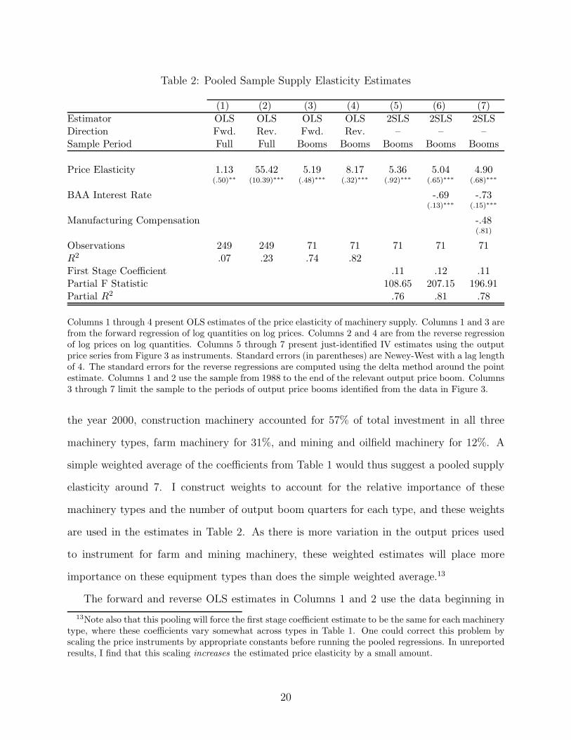
Table 2: Pooled Sample Supply Elasticity Estimates

(1) (2) (3) (4) (5) (6) (7)

Estimator OLS OLS OLS OLS 2SLS 2SLS 2SLSDirection Fwd. Rev. Fwd. Rev. – – –Sample Period Full Full Booms Booms Booms Booms Booms

Price Elasticity 1.13 55.42 5.19 8.17 5.36 5.04 4.90(.50)∗∗ (10.39)∗∗∗ (.48)∗∗∗ (.32)∗∗∗ (.92)∗∗∗ (.65)∗∗∗ (.68)∗∗∗

BAA Interest Rate -.69 -.73(.13)∗∗∗ (.15)∗∗∗

Manufacturing Compensation -.48(.81)


Columns 1 through 4 present OLS estimates of the price elasticity of machinery supply. Columns 1 and 3 arefrom the forward regression of log quantities on log prices. Columns 2 and 4 are from the reverse regressionof log prices on log quantities. Columns 5 through 7 present just-identified IV estimates using the outputprice series from Figure 3 as instruments. Standard errors (in parentheses) are Newey-West with a lag lengthof 4. The standard errors for the reverse regressions are computed using the delta method around the pointestimate. Columns 1 and 2 use the sample from 1988 to the end of the relevant output price boom. Columns3 through 7 limit the sample to the periods of output price booms identified from the data in Figure 3.

the year 2000, construction machinery accounted for 57% of total investment in all three

machinery types, farm machinery for 31%, and mining and oilfield machinery for 12%. A

simple weighted average of the coefficients from Table 1 would thus suggest a pooled supply

elasticity around 7. I construct weights to account for the relative importance of these

machinery types and the number of output boom quarters for each type, and these weights

are used in the estimates in Table 2. As there is more variation in the output prices used

to instrument for farm and mining machinery, these weighted estimates will place more

importance on these equipment types than does the simple weighted average.13

The forward and reverse OLS estimates in Columns 1 and 2 use the data beginning in

13Note also that this pooling will force the first stage coefficient estimate to be the same for each machinerytype, where these coefficients vary somewhat across types in Table 1. One could correct this problem byscaling the price instruments by appropriate constants before running the pooled regressions. In unreportedresults, I find that this scaling increases the estimated price elasticity by a small amount.

20

1988 and estimate very wide bounds on the supply elasticity. The estimates in Columns 3

and 4 use only the data from the output price boom periods, and estimate pooled supply

elasticities of 5.2 and 8.2. The instrumental variables specifications in Columns 5, 6, and

7 produce estimates of 5.4, 5.0, and 4.9, with standard errors all less than one. Again, the

reported partial F statistics and R2s indicate a very strong first stage and little reason to

be concerned about weak instruments. I thus conclude that the aggregate price elasticity of

supply for these three kinds of machinery is around 5.

4.1 Robustness

This section contains several tables that demonstrate the robustness of these results to a

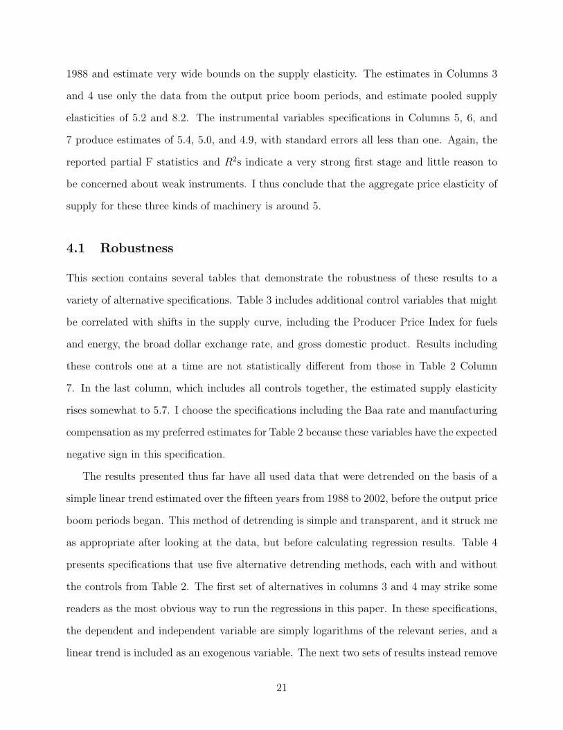
variety of alternative specifications. Table 3 includes additional control variables that might

be correlated with shifts in the supply curve, including the Producer Price Index for fuels

and energy, the broad dollar exchange rate, and gross domestic product. Results including

these controls one at a time are not statistically different from those in Table 2 Column

7. In the last column, which includes all controls together, the estimated supply elasticity

rises somewhat to 5.7. I choose the specifications including the Baa rate and manufacturing

compensation as my preferred estimates for Table 2 because these variables have the expected

negative sign in this specification.

The results presented thus far have all used data that were detrended on the basis of a

simple linear trend estimated over the fifteen years from 1988 to 2002, before the output price

boom periods began. This method of detrending is simple and transparent, and it struck me

as appropriate after looking at the data, but before calculating regression results. Table 4

presents specifications that use five alternative detrending methods, each with and without

the controls from Table 2. The first set of alternatives in columns 3 and 4 may strike some

readers as the most obvious way to run the regressions in this paper. In these specifications,

the dependent and independent variable are simply logarithms of the relevant series, and a

linear trend is included as an exogenous variable. The next two sets of results instead remove

21

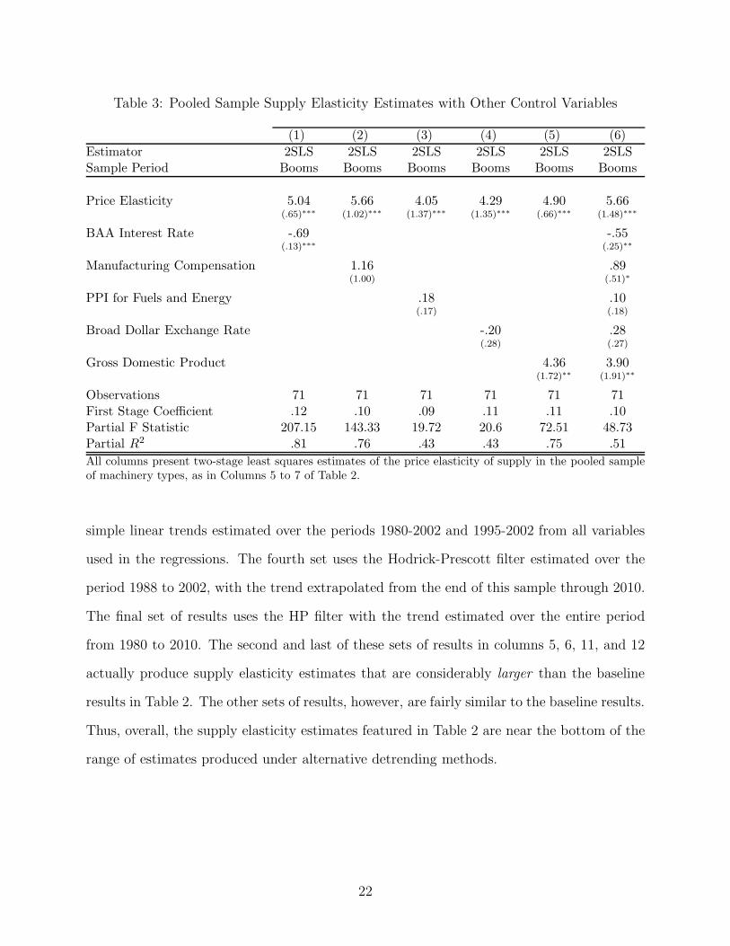
Table 3: Pooled Sample Supply Elasticity Estimates with Other Control Variables

(1) (2) (3) (4) (5) (6)

Estimator 2SLS 2SLS 2SLS 2SLS 2SLS 2SLSSample Period Booms Booms Booms Booms Booms Booms

Price Elasticity 5.04 5.66 4.05 4.29 4.90 5.66(.65)∗∗∗ (1.02)∗∗∗ (1.37)∗∗∗ (1.35)∗∗∗ (.66)∗∗∗ (1.48)∗∗∗

BAA Interest Rate -.69 -.55(.13)∗∗∗ (.25)∗∗

Manufacturing Compensation 1.16 .89(1.00) (.51)∗

PPI for Fuels and Energy .18 .10(.17) (.18)

Broad Dollar Exchange Rate -.20 .28(.28) (.27)

Gross Domestic Product 4.36 3.90(1.72)∗∗ (1.91)∗∗

Observations 71 71 71 71 71 71First Stage Coefficient .12 .10 .09 .11 .11 .10Partial F Statistic 207.15 143.33 19.72 20.6 72.51 48.73Partial R2 .81 .76 .43 .43 .75 .51

All columns present two-stage least squares estimates of the price elasticity of supply in the pooled sampleof machinery types, as in Columns 5 to 7 of Table 2.

simple linear trends estimated over the periods 1980-2002 and 1995-2002 from all variables

used in the regressions. The fourth set uses the Hodrick-Prescott filter estimated over the

period 1988 to 2002, with the trend extrapolated from the end of this sample through 2010.

The final set of results uses the HP filter with the trend estimated over the entire period

from 1980 to 2010. The second and last of these sets of results in columns 5, 6, 11, and 12

actually produce supply elasticity estimates that are considerably larger than the baseline

results in Table 2. The other sets of results, however, are fairly similar to the baseline results.

Thus, overall, the supply elasticity estimates featured in Table 2 are near the bottom of the

range of estimates produced under alternative detrending methods.

22

Table 4: Pooled Sample Supply Elasticity Estimates under Alternative Detrending Methods

(1) (2) (3) (4) (5) (6) (7) (8) (9) (10) (11) (12)

Estimator 2SLS 2SLS 2SLS 2SLS 2SLS 2SLS 2SLS 2SLS 2SLS 2SLS 2SLS 2SLSSample Period Booms Booms Booms Booms Booms Booms Booms Booms Booms Booms Booms BoomsTrend Type Linear Linear Linear Linear Linear Linear Linear Linear HP HP HP HPTrend Period 88-02 88-02 Booms Booms 80-02 80-02 95-02 95-02 88-02 88-02 80-10 80-10Controls No Yes No Yes No Yes No Yes No Yes No Yes

Price Elasticity 5.36 4.90 6.11 5.16 10.05 10.08 3.86 2.88 5.43 6.88 14.06 13.40(.92)∗∗∗ (.68)∗∗∗ (2.89)∗∗ (1.59)∗∗∗ (1.87)∗∗∗ (1.27)∗∗∗ (.77)∗∗∗ (1.01)∗∗∗ (1.46)∗∗∗ (2.29)∗∗∗ (2.43)∗∗∗ (2.32)∗∗∗

Observations 71 71 71 71 71 71 71 71 71 71 71 71First Stage Coeff. .11 .11 .08 .10 .09 .09 .17 .12 .20 .12 .04 .04Partial F Statistic 108.65 196.91 5.06 13.9 30.32 44.54 238.98 73.54 272.68 40.45 21.46 17.68Partial R2 .76 .78 .18 .31 .61 .64 .82 .60 .82 .48 .40 .36

All columns present two-stage least squares estimates of the price elasticity of supply in the pooled sample of machinery types, as in Columns 5to 7 of Table 2. Columns marked “Linear” use both dependent and independent variables that are constructed by removing a linear trend fromthe logarithm of the original series, where the trend is estimated over the indicated periods and extrapolated to the rest of the estimation period.Columns marked “HP” remove a trend estimated using the Hodrick-Prescott filter fit over the indicated periods. Columns with controls includethe Baa borrowing rate and manufacturing compensation, but coefficients are not reported.

23

Table 5: Pooled Sample Supply Elasticity Estimates under Alternative Detrending Methods using Full Estimation Sample

(1) (2) (3) (4) (5) (6) (7) (8) (9) (10) (11) (12)

Estimator 2SLS 2SLS 2SLS 2SLS 2SLS 2SLS 2SLS 2SLS 2SLS 2SLS 2SLS 2SLSSample Period Full Full Full Full Full Full Full Full Full Full Full FullTrend Type Linear Linear Linear Linear Linear Linear Linear Linear HP HP HP HPTrend Period 88-02 88-02 Full Full 80-02 80-02 95-02 95-02 88-02 88-02 80-10 80-10Controls No Yes No Yes No Yes No Yes No Yes No Yes

Price Elasticity 8.79 7.36 8.01 7.18 21.32 12.56 3.04 3.86 4.64 2.38 21.27 20.48(4.50)∗ (2.98)∗∗ (7.22) (3.94)∗ (14.57) (3.77)∗∗∗ (.88)∗∗∗ (1.95)∗∗ (2.61)∗ (5.83) (6.15)∗∗∗ (6.77)∗∗∗

Observations 229 229 229 229 229 229 229 229 229 229 229 229First Stage Coefficient .03 .04 .02 .03 .03 .06 .08 .04 .06 .03 .02 .02Partial F Statistic 2.06 2.98 .78 2.39 1.83 4.79 2.01 2.56 .86 2.81 9.24 7.72Partial R2 .07 .16 .03 .10 .03 .15 .14 .13 .09 .10 .10 .08

All columns present two-stage least squares estimates of the price elasticity of supply in the pooled sample of machinery types, as in Columns 5to 7 of Table 2. Columns marked “Linear” use both dependent and independent variables that are constructed by removing a linear trend fromthe logarithm of the original series, where the trend is estimated over the indicated periods and extrapolated to the rest of the estimation period.Columns marked “HP” remove a trend estimated using the Hodrick-Prescott filter fit over the indicated periods. Columns with controls includethe Baa borrowing rate and manufacturing compensation, but coefficients are not reported.

24

Finally, all of the instrumental variables results discussed thus far have used samples

limited to the output price boom periods. I have argued that economic conditions during

these periods, which began in the aftermath of the 2001 recession, were quite similar to those

under which policymakers might like to stimulate investment. Thus they are quite relevant

periods during which to estimate supply elasticities. One could nonetheless argue that elas-

ticities could as well be estimated with regressions run over longer samples. Unfortunately,

results using longer samples tend to suffer from a weaker first stage relationship between

output prices and machinery prices. Table 5 presents exactly the same specifications from

Table 4, but estimated over the sample from 1988 to the end of the output price booms.

Estimated supply elasticities actually rise relative to the estimates in Table 4 in all except

three specifications. However, the first stage partial F statistics are uniformly lower, and, in

fact, all are below 10, suggesting that these estimates could be affected by the weak instru-

ments problem. I thus focus on the results from specifications presented above using data

from the boom periods only.

I also note that unreported specifications including the “crash” period from the end of

the booms through 2010 perform even more poorly than those in Table 5. The first stage

relationship disappears or even turns negative, and supply elasticity estimates are highly

unstable. An explanation of these results is readily apparent from the data in Figures 3

and 4. During the crash periods when output prices and investment quantities were falling

rapidly, machinery prices moved relatively little. Although this fact hinders estimation of a

clean first stage relationship over the full sample, it also underscores the central observation

of this paper—that business cycle fluctuations in the quantity of machinery supplied are far

larger than fluctuations in prices.

4.2 Discussion

Goolsbee [1998] estimated a short-run capital supply elasticity around 1, while I have esti-

mated an elasticity of at least 5. The discrepancy does not stem from the particular types

25

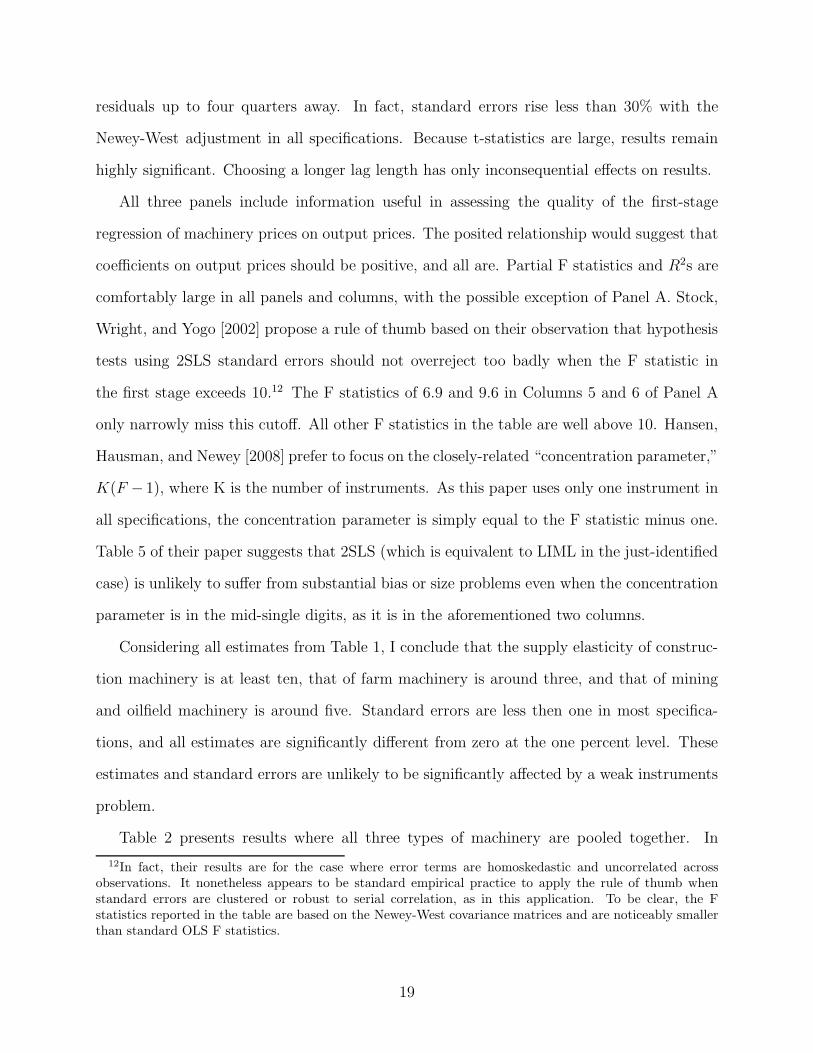
Figure 6: Imports as Share of Machinery Investment

0

.05

.1

.15

.2

.25

.3

.35

.4

1975 1980 1985 1990 1995 2000 2005 2010 2015

This figure presents total imports of construction, farm, and min-ing machinery (NAICS sector 3331) as a fraction of domestic in-vestment in these categories from 1978 to the present.

of machinery that I have studied in this paper. Goolsbee [1998] presents estimates of the

pass-through of investment tax credits into prices broken out by equipment types (p. 132).

His estimate for construction machinery is more than 20% higher than his estimate for the

pooled sample, and his estimates for farm and mining machinery are higher still. Thus

we should expect lower supply elasticity estimates for these types of equipment than for

Goolsbee’s pooled sample.

The question of what drives the discrepancy between my results and Goolsbee’s then

remains. Whelan [1999] replicates Goolsbee’s results and shows that they are not robust to

including simple controls for the prices of material inputs to production.14 Further, Shea

[1993] finds evidence that positive demand shocks actually reduced the prices of aircraft and

construction machinery when using data from roughly the same period as Goolsbee’s. Thus,

there are reasons to think that Goolsbee’s results may simply be spurious.

14In particular, the 1974 expansion of the investment tax credit nearly coincided with the beginning of theOPEC oil embargo in late 1973. During the period from then until the mid-1980s, the investment tax creditwas at its strongest historical level, and both oil and other commodity prices were well above their trendlevels. Figures in the paper suggest that year-to-year changes in equipment prices are more closely relatedto these input prices than to the investment tax credit.

26

Table 6: The Role of Imports in Machinery Supply Expansions DuringRecent Output Price Booms

Import Share Import Share Production Importsin Base Year of Increase Increase Increase

Construction 35% 57% 63% 114%Farm 21% 89% 26% 66%Mining 15% 21% 90% 187%

The first column presents imports as a fraction of domestic investment in thetrough year prior to the investment boom period (2002 for construction and farmmachinery and 2001 for mining machinery). The second column presents the increasein real imports as a fraction of the increase in domestic investment over the boomperiods. The third and fourth columns present the increase during the boom periodsin real domestic production and imports, respectively.

Nonetheless, I also consider the explanation that markets for machinery have changed

since the 1962-1988 period covered by Goolsbee’s data. For example, Goolsbee finds that

evidence for an effect of tax variables on prices is strongest for types of capital that were less

subject to import competition. Figure 6 plots construction, farm, and mining machinery

imports as a fraction of total domestic investment in these categories from 1978 to 2010, a

period for which consistent data are readily available. The figure shows that this import

share rose from around 10% in the mid-1970s to more than 35% at its peak in 2006. In fact,

Goolsbee’s estimates of the impact of the import share on the pass-through of tax incentives

into prices would suggest that the observed change in import share is more than enough to

reduce his estimated pass-through to zero (Goolsbee [1998], p. 140).15

Further, Table 6 shows that the expansion of imported machinery played an outsized role

in the overall supply expansion during the output price boom periods. For example, in 2002,

about 35% of construction machinery investment was imported from abroad. During the

period from 2002 to 2006, however, the increase in construction machinery imports consti-

15Note that Goolsbee’s import share variable is constructed as imports/(production + imports), whileFigure 6 plots imports/(production + imports − exports). The former measure increased from about 0.08in the late 1970s to 0.17 in the early 2000s and 0.25 in the mid-2000s. Goolsbee’s estimated coefficient onan interaction of this variable with his tax variable is 2.774, and the main effect of the tax variable is -.452.Thus the full effect of a change in the tax variable with the import share at 0.08 is -0.23, and the effect at0.17 is 0.02.

27

tuted about 57% of the total increase in investment. Production of construction machinery

increased about 63% during this period, while imports increased 114%.16 Data on both farm

and mining machinery also indicate that imports played a large role in the supply expansion,

relative to their fraction of investment prior to the boom.

5 Conclusion

The data presented in this paper speak very clearly: the quantity of machinery supplied

to the United States increased rapidly during the output price booms of the early-to-mid-

2000s, with only modest increases in prices. Estimates of the supply elasticity during these

episodes are around 5, much larger than the estimate of 1 from Goolsbee [1998]. Results thus

suggest that there is little reason to be concerned that public policies intended to stimulate

investment demand would simply push up the prices of investment goods. However, to

the extent that policymakers trying to stimulate investment are truly hoping to stimulate

domestic production and employment, an increasing share of imports will make their task

more complicated. The responses of machinery prices, production, and imports to investment

stimulus may now depend on factors like the relative availability of manufacturing capacity

in the United States and abroad.

Note finally that the results presented here need not suggest that policymakers’ attempts

to stimulate business investment in recent years have been successful. This paper’s results

do suggest that the impact of policies that succeeded in stimulating demand for investment

would not have been severely blunted by the inelasticity of machinery supply. However,

as noted earlier, there remains considerable debate over whether recent stimulus provisions

have, in fact, succeeded in stimulating demand.

16Note that there is no identity that must relate these numbers to each other, as machinery exports arealso a significant portion of domestic production. Further, the investment data from the BEA are adjustedfor the shares of machinery that are purchased by households and government, while the import and exportdata used here are not.

28

A Derivation of results in Section 2

Solve for p,

q = βp+ ǫs

γ1p+ γ2z + ǫd = βp+ ǫs

p =ǫs − (γ2z + ǫd)

(γ1 − β).

Plug into the OLS bias term,

cov(ǫs, p)

var(p)=

cov(ǫs,ǫs−(γ2z+ǫd)

(γ1−β))

var(p)

=var(ǫs)− cov(ǫs, (γ2z + ǫd))

(γ1 − β)var(p).

Solve for q,

p =ǫs − (γ2z + ǫd)

(γ1 − β)

1

βq −

ǫsβ

=ǫs − (γ2z + ǫd)

(γ1 − β)

q =βǫs − β(γ2z + ǫd)

(γ1 − β)+ ǫs

(γ1 − β)

(γ1 − β)=

γ1ǫs − β(γ2z + ǫd)

(γ1 − β).

Plug into the reverse OLS bias term,

cov(ǫs, q)

βvar(q)=

cov(ǫs,γ1ǫs−β(γ2z+ǫd)

(γ1−β))

βvar(q)

=

γ1βvar(ǫs)− cov(ǫs, (γ2z + ǫd))

(γ1 − β)var(q).

29

References

Bureau of Labor Statistics. BLS Handbook of Methods. 2008. URL

http://www.bls.gov/opub/hom/.

Robert S. Chirinko. Business fixed investment spending: Modeling strategies, empirical

results, and policy implications. Journal of Economic Literature, 31(4):pp. 1875–1911,

1993.

Lawrence J. Christiano, Martin Eichenbaum, and Charles L. Evans. Nominal rigidities and

the dynamic effects of a shock to monetary policy. Journal of Political Economy, 113(1),

2005.

Darrel S. Cohen and Jason G. Cummins. A Retrospective Evaluation of the Effects of

Temporary Partial Expensing. FEDS Working Paper Series, 2006(19), 2006.

Rochelle M. Edge and Jeremy B. Rudd. General-equilibrium effects of investment tax incen-

tives. FEDS Working Paper Series, 2010(17), 2010.

Rochelle M. Edge, Michael T. Kiley, and Jean-Philippe Laforte. Natural rate measures in an

estimated DSGE model of the U.S. economy. Journal of Economic Dynamics and Control,

32(8):2512 – 2535, 2008.

Jesse Edgerton. Taxes and business investment: New evidence from used equipment. Un-

published working paper, 2009.

Austan Goolsbee. Investment tax incentives, prices, and the supply of capital goods. The

Quarterly Journal of Economics, 113(1):121–148, 1998.

Jinyong Hahn and Jerry Hausman. A new specification test for the validity of instrumental

variables. Econometrica, 70(1):163–189, 2002.

Robert E. Hall and Dale W. Jorgenson. Tax policy and investment behavior. The American

Economic Review, 57(3):391–414, June 1967.

30

James D. Hamilton. Understanding crude oil prices. NBER Working Paper Series, (14492),

November 2008.

Christian Hansen, Jerry Hausman, and Whitney Newey. Estimation with many instrumental

variables. Journal of Business and Economic Statistics, 26(4):398–422, 2008.

Kevin A. Hassett and R. Glenn Hubbard. Are investment incentives blunted by changes in

prices of capital goods? International Finance, 1(1):103, October 1998.

Kevin A. Hassett and R. Glenn Hubbard. Chapter 20 tax policy and business investment.

volume 3 of Handbook of Public Economics, pages 1293 – 1343. Elsevier, 2002.

Jerry A. Hausman. Specification and estimation of simultaneous equation models. In

Z. Griliches and M. D. Intriligator, editors, Handbook of Econometrics, volume 1, chap-

ter 7, pages 391–448. Elsevier, 1983.

Christopher L. House and Matthew D. Shapiro. Temporary investment tax incentives: The-

ory with evidence from bonus depreciation. The American Economic Review, 98:737–

768(32), 2008.

Dale W. Jorgenson, Mun S. Ho, and Kevin J. Stiroh. A retrospective look at the U.S.

productivity growth resurgence. Journal of Economic Perspectives, 22(1):3 – 24, 2008.

Robert G. King and Sergio T. Rebelo. Chapter 14: Resuscitating real business cycles. volume

1, Part 2 of Handbook of Macroeconomics, pages 927 – 1007. Elsevier, 1999.

Donald Mitchell. A Note on Rising Food Prices. World Bank Policy Research Working

Papers, (4682), 2008.

James M. Sallee. The incidence of tax credits for hybrid vehicles. Working Paper 0815,

Harris School of Public Policy, University of Chicago, 2009.

John Shea. Do supply curves slope up? The Quarterly Journal of Economics, 108(1):1–32,

1993.

31

Frank Smets and Raf Wouters. An estimated dynamic stochastic general equilibrium model

of the euro area. Journal of the European Economic Association, 1(5):1123–1175, 2003.

James H. Stock, Jonathan H. Wright, and Motohiro Yogo. A survey of weak instruments and

weak identification in generalized method of moments. Journal of Business and Economic

Statistics, 20(4):518–529, 2002.

Lawrence Summers. Taxation and corporate investment: A Q-theory approach. Brookings

Papers on Economic Activity, 1981(1):67–140, 1981.

Karl Whelan. Tax incentives, material inputs, and the supply curve for capital equipment.

FEDS Working Paper Series, 1999(21), April 1999.

32

Estimating Machinery Supply Elasticities Using … Machinery Supply Elasticities Using Output Price Booms ... biased estimate of the supply elasticity when supply and demand shocks

Documents