Estimating long run effects in models with cross-sectional ...

Estimating long run effects in models with cross-sectional dependence using xtdcce2

Jan Ditzen

CEERP Working Paper No. 7 March 2019

Heriot-Watt University Edinburgh, Scotland EH14 4AS ceerp.hw.ac.uk

Estimating long run effects in models with

cross-sectional dependence using xtdcce2

Jan Ditzen∗

Centre for Energy Economics Research and Policy (CEERP)Heriot-Watt University, Edinburgh, UK

as of March 8, 2019

Abstract

This paper describes how to estimate long run effects in a large hetero-geneous panel data model with cross sectional dependence in Stata usingthe user written command xtdcce2. It builds on Chudik et al. (2016) andexplains how to estimate models using the CS-DL and CS-ARDL estima-tor. In addition it includes a method how to estimate an error correctionmodel.

keywords st0536, xtdcce2, parameter heterogeneity, dynamic panels,cross section dependence, common correlated effects, pooled mean-groupestimator, mean-group estimator, error correction model, ardl, long runcoefficients.

DRAFT

1 Introduction

The estimation of long run relationships is important in the empirical applica-tion of macroeconomics models. Long run relationships describe the steady statesolution and how a change in the steady state affect the long run relationshipbetween variables. Examples are the the relationship between macroeconomicvariables such as GDP and inflation or investments, exchange rates of differentcountries, effects of education or technological progress on economic growth.

In an econometric model, estimating a long run relationship implies to esti-mate coefficients which capture this relationship. A standard model in time se-ries econometrics is the error correction model, in which one term of the equation

∗Correspondence: Jan Ditzen, Centre for Energy Economics Research and Policy (CEERP)and Spatial Economics and Econometrics Centre (SEEC), Heriot-Watt University, EdinburghEH14 4AS, Scotland, United Kingdom; Email: [email protected], Web: www.jan.ditzen.net

1

captures the short and the other the long run movements (Engle and Granger,1987). In a panel data model with heterogeneous slope coefficients, the modelis estimated by the pooled mean group estimator (Shin et al., 1999), which wasimplemented into Stata using the user written command xtpmg (Blackburneand Frank, 2007). A related model is the ARDL model, implemented by theuser written ardl command in Stata (Kripfganz and Schneider, 2018).

A common problem in the estimation of panels with a large number of ob-servations across time and cross-sectional units is cross-sectional dependence.If not taken care of, it causes estimates to be inconsistent. Pesaran (2006) andChudik and Pesaran (2015) developed methods to estimate static and dynamicmodels. The idea of the so called common correlated effects estimators is toadd cross-sectional averages which approximate the cross-sectional dependence.This estimator was implemented into Stata in the static version by the user writ-ten command xtmg (Eberhardt, 2012) and in the dynamic version by xtdcce2

(Ditzen, 2018).Chudik et al. (2016) describe two methods to estimate the long run co-

efficients in large dynamic panel data models with cross-sectional dependence.This paper builds on their work and introduces an extended version of xtdcce2,which allows the estimation of the long run coefficients.1.

The remainder of the paper is structured as follows. The next section de-scribes the general model and the common correlated effects estimator. Thenthree different methods to estimate the long run coefficients are discussed, firstfrom a theoretical perspective, then from an applied perspective. Examples onhow to estimate the equations using xtdcce2 are given. The validity of theestimators is shown by a Monte Carlo Simulation and the paper closes with aconclusion.

2 Panel Model and CCE

There are several ways to introduce independence across cross-sectional units. Ifthe dependence is observable, it is obvious to use spatial econometric methods.This paper focuses on unobservable dependence across units. Therefore thecross-sectional dependence is modelled as a common factor, which is part ofthe error term. Chudik et al. (2011) and Chudik and Pesaran (2015) assumea dynamic ARDL(1,1) panel model with heterogeneous coefficients in the formof:

yi,t = αi + λiyi,t−1 + β0,ixi,t + β1,ixi,t−1 + ui,t (1)

ui,t =

mf∑l=1

γi,lft,l + ei,t (2)

with i = 1, ..., N and t = 1, ..., Ti,

1The estimation of long run coefficients is possible with xtcce2 version 1.33 and later. Thispaper refers to version 1.35 or later. Please see the authors webpage www.jan.ditzen.net forupdates.

2

where ei,t is a cross-section unit-specific IID error term. ft = (ft,1, ..., ft,mf)′ is

an unobserved common factors and mf is the number of factors. The commonfactors are covariance stationary, have absolute summable autocovariances, aredistributed independently over ei,t and the forth order moments are bounded.Assume that ft,l is a strong common factor which is possibly correlated with theregressor xi,t. The factor loadings γi = (γi,1, ..., γi,mf

) are heterogeneous andαi is a unit-specific fixed effect. The heterogeneous coefficients are randomlydistributed around a common mean, such that βi = β + vi, vi ∼ IID(0,Ωv),and λi = λ+ai, ai ∼ IID(0,Ωa), where Ωv and Ωa are the variance covariancematrices. λi lies strictly inside the unit circle to ensure a non explosive series.In addition, the random deviation of λi and βi are independently distributed ofthe error term and the common factors.

In case the explanatory variables are correlated with the common factors,leaving the factors out leads to an omitted variable bias. This renders theOLS residuals not iid anymore and OLS becomes inconsistent (Everaert and DeGroote, 2016). Pesaran (2006) and Chudik and Pesaran (2015) show that Eq.(3) can be estimated consistently by approximating the common factors withcross sectional averages. In a dynamic model the floor of 3

√T is added. The

estimated equation becomes:

yi,t = αi + λiyi,t−1 + β0,ixi,t + β1,ixi,t−1 +

pT∑l=0

δ′i,lzt−l + ei,t (3)

where zt = (yt−1, xt) are the cross sectional averages of the dependent and in-dependent variables. This estimator is commonly called the common correlatedeffects mean group estimator (CCEMG estimator). Important to note is, thatfor the cross sectional averages, only the base of the variables are added, but notfurther lags in order to avoid multicollinearity problems. The mean group co-efficient can then be estimated as the unweighted average of the cross sectionalindividual coefficients:

πMG =(λMG, β0,MG, β1,MG

)=

1

N

N∑i=1

πi (4)

The asymptotic variance of the mean group coefficients is the unweightedvariance of the cross sectional specific coefficients:

V ar(πMG) =1

N

N∑i=1

(πi − πMG) (πi − πMG)′

3 Estimating Long Run Relationships

Dynamic models allow the estimation of long run relationships. Long run rela-tionships origin from an underlying steady state of a macroeconomic model. In

3

econometric terms, they measure the effect of an explanatory variable on thesteady state value of the dependent variable. Three approaches how to estimatelong run relationships will be explained next.

Following the notation from equation 1 and assuming that model is in itssteady state with y∗t = y∗t−1 = y∗ and x∗t = x∗t−1 = x∗, the long run effect ofvariable x is defined as:

θi =β0,i + β1,i

1− λi.

Following the common correlated effects approach, the long run effects inequation 1 can be estimated in three ways, as a ECM or pooled mean group(PMG) model if it is an ARDL(1,1), or if it is a more general ARDL(py, px),directly without the short run coefficients (CS-DL) or indirectly with the shortrun coefficients (CS-ARDL).

3.1 Error Correction Approach

The first approach follows on the lines of Lee et al. (1997) and Shin et al. (1999),in which equation (3) is transformed into an error correction model:

∆yi,t =φi [yi,t−1 − θ0,i − θ1,ixi,t−1] + β0,i∆xi,t +

pT∑l=0


with

θi =β0,i + β1,i

1− λi(6)

φi = (1− λi) .

In the case without dependence in the residuals and homogeneous long runcoefficients (θi = θ ∀ i), the model can be estimated in Stata by the pooledmean group (PMG) estimator, implemented by Blackburne and Frank (2007).With cross sectional averages, xtdcce2 can estimated the equation using thelr() option. The ECM is transferred back into:

∆yi,t =φi [yi,t−1 − θ0,i − θ1,ixi,t−1] + β0,i∆xi,t +

pT∑l=0


=αi + γ1,iyi,t−1 + γ2,ixi,t−1 + β0,i∆xi,t +

pT∑l=0

δ′i,lzt−l + ei,t

where

γ1,i = −φi θ0,i =αi−γ1,i

θi =γ2,i

−γ1,i(8)

φi = (1 − λi) is the error-correction speed of adjustment parameter and[yi,t−1 − θ0,i − θ1,ixi,t−1] is the error correction term. In general, a long run

4

relationship exists if φ 6= 0 (Shin et al., 1999). β0,i captures the immediate orshort run effect of xi,t on yi,t. The long run or equilibrium effect is captured byθi. The long run effect measures how the equilibrium changes and φ representshow fast the adjustment occurs.

Besides the inclusion of the cross sectional averages, there is another im-portant difference. xtpmg calculates the long run coefficients using maximumlikelihood. xtdcce2 treats the long run coefficients, defined in lr(), as furthercovariates and estimates equation 8 entirely by OLS. To calculate the long runcoefficients, the unit specific coefficients are divided by the negative of the longrun cointegration vector such that θ1,i = −γ2,i/φi. The variances are calcu-lated using the Delta method. After the long run unit specific coefficients areobtained, the mean groups are calculated.

The PMG estimator assumes homogeneous long run and heterogeneous shortrun coefficients. xtdcce2 is build to handle both coefficients to be heteroge-neous. If the long run coefficient is pooled, then it takes the mean group esti-mate of the error speed of correction term. Thus the long run coefficient thenbecomes θp1 = −γp2/φMG.

Following Lee et al. (1997) and Shin et al. (1999), Blackburne and Frank(2007) explain the use of xtpmg by estimating a long-run consumption functionin the form of:

ci,t = θ0t + θ1tyi,t + θ2tφi,t + µi + εi,t, (9)

where ci,t log of consumption per capita, yi,t is log of real per capita incomeand πi,t is the inflation rate. The ARDL(1,1,1) of the specification is

ci,t = δ0,i + λici,t−1 + δ10,iyi,t + δ1,iyi,t−1 + δ20,iπi,t + δ2,iπi,t−1 + εi,t

and ECM representation of the model reads:2

∆ci,t = φi(ci,t−1 − θ1,iyi,t − θ2,iπi,t) + δ0,i + δ1,i∆yi,t + δ2,i∆πi,t + εi,t. (10)

xtdcce2 internally estimates (leaving out any cross sectional means):

∆ci,t = φici,t−1 + γ1,iyi,t + γ2,iπi,t + δ0,i + δ1,i∆yi,t + δ2,i∆πi,t + εi,t, (11)

Using the jasa2 dataset, the syntax for xtdcce2 is then:

xtdcce2 depvar[sr indepvars] , lr(lr indepvars) [lr options(string)]

where sr indepvars are the short run variables and the long run are definedin the option lr(). As the underlying model is an ARDL(1,1,1) model, the firstdifference of the explanatory variables is added to the short run part, directlybehind the dependent variable. For an ARDL(1,0,0) model, the differenceswould be omitted, for an ARDL(1,2,2) model, the second difference would beadded. The appendix 7.2 gives further details. Cross sectional averages aredefined by the crosssectional() option. As all variables are included, the

2The details of the transformation from the ARDL model to the ECM can be found in theappendix in 7.2.

5

shortcut all is used, which adds the base of all variables. The entire commandline and the output are:34

. xtdcce2135 d.c d.pi d.y if year >= 1962, ///> lr(L.c pi y) p(l.c pi y) cr(_all) cr_lags(2)(Dynamic) Common Correlated Effects Estimator - Pooled Mean Group

Panel Variable (i): id Number of obs = 719Time Variable (t): year Number of groups = 24

Degrees of freedom per group: Obs per group:without cross-sectional avg. min = 23 min = 29

max = 24 avg = 30with cross-sectional avg. min = 14 max = 30

max = 15Number of F(291, 428) = 3.61cross-sectional lags = 2 Prob > F = 0.00variables in mean group regression = 51 R-squared = 0.71variables partialled out = 240 Adj. R-squared = 0.51

Root MSE = 0.02CD Statistic = -0.25

p-value = 0.8062

D.c Coef. Std. Err. z P>|z| [95% Conf. Interval]

Short Run Est.

Mean Group:D.pi .0341953 .0343376 1.00 0.319 -.0331051 .1014958D.y .1658292 .0361585 4.59 0.000 .0949598 .2366986

Long Run Est.

Pooled:L.c -.4691509 .1162393 -4.04 0.000 -.6969757 -.241326pi -.1557539 .3383306 -0.46 0.645 -.8188697 .5073619y .8547452 .0984223 8.68 0.000 .661841 1.047649

Pooled Variables: L.c pi yMean Group Variables: D.pi D.yCross Sectional Averaged Variables: pi y cLong Run Variables: L.c pi yCointegration variable(s): L.cHeterogenous constant partialled out.

xtdcce2 estimates equation 8 entirely by OLS. To calculate the long runcoefficients, the coefficients are divided by the negative of the long run coin-tegration vector to match equation 10, θ1,i = −γ1,i/φi. The variances arecalculated using the Delta method as described in the Appendix.

First the long run coefficients for each cross section are computed and in asecond step the individual long run coefficients are averaged. As an example,

the average long run coefficient for ˆθ1 is calculated as: ˆθ1 = 1/N∑Ni=1 θ1,i =

1/N∑Ni=1(−γ1,i/φi). In the example here, φ is heterogeneous, but θ1 homoge-

neous. Thus the long run coefficient θ1 is calculated as θ1 = −γ1/(1/N∑Ni=1 φi).

3Following p = [T 1/3] would result in 3 lags. However as the panel is relatively short withT = 31 and the CD test statistic is in a non rejection region, the number of lags is set to 2.

4The syntax for xtdcce2 is discussed in the appendix 7.1.

6

An estimation of the same model, but with heterogeneous long and shortrun coefficients leads to the following result:

. xtdcce2135 d.c d.pi d.y if year >= 1962, ///> lr(L.c pi y) cr(_all) cr_lags(2)(Dynamic) Common Correlated Effects Estimator - Mean Group






p-value = 0.8638

D.c Coef. Std. Err. z P>|z| [95% Conf. Interval]

Short Run Est.

Mean Group:D.pi .0701836 .0424275 1.65 0.098 -.0129727 .15334D.y .0630114 .0514939 1.22 0.221 -.0379147 .1639375

Long Run Est.

Mean Group:L.c -.5849174 .0453523 -12.90 0.000 -.6738062 -.4960286pi -.3760294 .1470868 -2.56 0.011 -.6643143 -.0877445y .7848242 .0779883 10.06 0.000 .6319699 .9376785

Mean Group Variables: D.pi D.yCross Sectional Averaged Variables: pi y cLong Run Variables: L.c pi yCointegration variable(s): L.cHeterogenous constant partialled out.

The long run coefficients slightly changed and are in absolute value higher.

3.2 ARDL Approach

The more general representation of eq (1) as an ARDL(py, px) model is:

yi,t = αi +

py∑l=1

λl,iyi,t−l +

px∑l=0

βl,ixi,t−l + ui,t. (12)

Next, two further methods to estimate the long run coefficients are explained.The first one is the CS-DL method and directly estimates the long run coeffi-cients. The second method, the CS-ARDL estimator, uses an auxiliary regres-sion.

7

3.2.1 CS-DL

Under the assumption that λi lies in the unit circle, the general representationof an ARDL(py, px) model can be written as:

yi,t = θ0,i + θ1,ixi,t + δi(L)∆xi.t + ui,t (13)

where

δi(L) = −∞∑l=0

[λl+1i (1− λi)−1

β1,i

]Ll (14)

θ0,i = (1− λiL)−1αi (15)

ui,t = (1− λiL)−1ui,t (16)

(17)

and L is the lag operator. Chudik et al. (2016) show that Estimation (13) can bedirectly estimated by the common correlated effects estimator. The regression isaugmented by the differences of the explanatory variables (x), their lags and thecross-sectional averages. Following Pesaran (2006) the estimation is consistenteven if the errors are serially correlated.

For a general ARDL(py, px) model with added cross-sectional averages totake out the cross-sectional dependence, the estimated equation is:

yi,t = θ0,i + θ1,ixi,t +

px−1∑l=0

δi,l∆xi,t−l +

py∑l=0

γy,i,lyi,t−l +

px∑l=0

γx,i,lxi,t−l + ei,t,

(18)

where yi,t−l and xi,t−l are the cross sectional averages and p = px = [T 1/3] andpy = 0. The mean group coefficients are calculated as

θ0,MG =1

N

N∑i=1

θ0,i and θ1,MG =1

N

N∑i=1

θ1,i. (19)

The variance estimator is the same as in equation (4), but with the meangroup of the long run coefficients rather than of the short run coefficients:

V ar(θMG) =1

N

N∑i=1

(θi − θMG

)(θi − θMG

)′. (20)

A pooled estimation is possible as well. The estimator is the same as inPesaran (2006) and explained for xtdcce2 in Ditzen (2018).

8

Estimating the consumption model from equation (10), implies the followingequation with an ARDL(1,1,1) model with py = pc = pπ = 2 and p = 1:

ci,t =αi + θ1,iyi,t + θ2,iπi,t +

2∑l=0

δi,l∆Vi,t−l

+

2∑l=0

γy,i,lci,t−l +

2∑l=0

γx,i,lVi,t−l + ei,t

where Vi,t = (yi,t, πi,t). The model can be estimated using xtdcce2, by addingthe first difference of the variables aggregated in Vi,t, namely ∆yi,t and ∆πi,tas further explanatory variables, but they are excluded from the cross-sectionalaverages. As the long run effects are directly estimated, setting lr() is notnecessary. The output is:

. xtdcce2135 c pi y d.pi d.y d.(d.pi d.y) if year >= 1962, ///> p(pi y d.pi d.y d.(d.pi d.y)) cr(c pi y) cr_lags(2) pooledc(Dynamic) Common Correlated Effects Estimator - Pooled






p-value = 0.3728

c Coef. Std. Err. z P>|z| [95% Conf. Interval]

Pooled:pi -.3054825 .0831854 -3.67 0.000 -.4685228 -.1424422y .7540553 .1297665 5.81 0.000 .4997176 1.008393

D.pi .2381957 .147126 1.62 0.105 -.050166 .5265574D.y -.3622873 .1202688 -3.01 0.003 -.5980097 -.1265648

D2.pi -.0745891 .0879009 -0.85 0.396 -.2468716 .0976934D2.y .0766291 .0846078 0.91 0.365 -.0891992 .2424573

Pooled Variables: pi y D.pi D.y D2.pi D2.yCross-sectional Averaged Variables: pi y cHomogenous constant not displayed.

The coefficient on variable pi remains insignificant, the coefficient on y ispositive and significant. The results for the two coefficients are similar as thoseobtained in (Blackburne and Frank, 2007, p. 203). The variables in first differ-ences are only auxiliary and can be ignored.

A second example can be found in Chudik et al. (2013). The authors estimate

9

the long run effect of public debt on output growth with the following equation:

∆yi,t = ci + θ′ixi,t +

p−1∑l=0

γi,l∆xi,t−l + ωi,y∆yt +

3∑l=0

ωi,lxi,t−lei,t

where yi,t is the log of real GDP, and xi,t = (∆di,t, πi,t)′, di,t is log of debt to

GDP ratio and π is the inflation rate and p the number of lags. The results fromChudik et al. (2013, Table 18) with 1 lag (p = 1) in the form of an ARDL(1,1,1)model can be replicated as follows, where variable dp is π and debt is gd:5

. xtdcce2135 d.y dp d.gd d.(dp d.gd) ///> , cr(d.y dp d.gd) cr_lags(0 3 3) fullsample(Dynamic) Common Correlated Effects Estimator - Mean Group

Panel Variable (i): ccode Number of obs = 1601Time Variable (t): year Number of groups = 40

Degrees of freedom per group: Obs per group (T) = 40without cross-sectional averages = 35.025with cross-sectional averages = 26.025

Number of F(560, 1041) = 0.90cross-sectional lags 0 to 3 Prob > F = 0.93variables in mean group regression = 160 R-squared = 0.33variables partialled out = 400 Adj. R-squared = -0.04

Root MSE = 0.03CD Statistic = 1.11

p-value = 0.2667

D.y Coef. Std. Err. z P>|z| [95% Conf. Interval]

Mean Group:dp -.0889339 .0256445 -3.47 0.001 -.1391961 -.0386717

D.gd -.0865123 .0143 -6.05 0.000 -.1145398 -.0584849D.dp .0053284 .0413629 0.13 0.897 -.0757413 .0863981

D2.gd .0068065 .0148306 0.46 0.646 -.022261 .035874

Mean Group Variables: dp D.gd D.dp D2.gdCross Sectional Averaged Variables: D.y(0) dp(3) D.gd(3)Heterogenous constant partialled out.

The different lag structure is imposed adding a numlist to the cr lags()

option, rather than a single number. The first differences as part of the vector∆xi,t are added as d.(dp d.gd). The fullsample option is used to makeuse of the entire sample. Using three rather than one lag for the differences,hence an ARDL(3,3,3) model can be estimated as well, d.(dp d.gd) replacesL(0/2).d.(dp d.gd):

. xtdcce2135 d.y dp d.gd L(0/2).d.(dp d.gd) ///> , cr(d.y dp d.gd) cr_lags(0 3 3) fullsample(Dynamic) Common Correlated Effects Estimator - Mean Group


Degrees of freedom per group: Obs per group (T) = 39without cross-sectional averages = 30.275

5Note that the dependent variable δyi,t and the inflation rate δπi,t are in first differences.Those differences are not generated as new variables, Stata’s time series operators are used.

10

with cross-sectional averages = 21.275Number of F(720, 851) = 1.12cross-sectional lags 0 to 3 Prob > F = 0.06variables in mean group regression = 320 R-squared = 0.49variables partialled out = 400 Adj. R-squared = 0.05


p-value = 0.4681


Mean Group:dp -.0855843 .0400844 -2.14 0.033 -.1641483 -.0070202

D.gd -.0816584 .0196252 -4.16 0.000 -.1201231 -.0431936D.dp .0183591 .0478696 0.38 0.701 -.0754636 .1121817

LD.dp .0015577 .0373619 0.04 0.967 -.0716704 .0747857L2D.dp .0034021 .029477 0.12 0.908 -.0543718 .0611759D2.gd .0045224 .0144741 0.31 0.755 -.0238464 .0328912

LD2.gd -.0129676 .0134554 -0.96 0.335 -.0393396 .0134044L2D2.gd -.0095151 .0090814 -1.05 0.295 -.0273142 .0082841

Mean Group Variables: dp D.gd D.dp LD.dp L2D.dp D2.gd LD2.gd L2D2.gdCross Sectional Averaged Variables: D.y(0) dp(3) D.gd(3)Heterogenous constant partialled out.

The number of variables becomes rather large, but only the first two coeffi-cients are of interest.

3.2.2 CS-ARDL

An alternative to the CS-DL estimator is the CS-ARDL approach. In a firststep the short run coefficients are estimated and then the long run coefficientscalculated. The advantage of this approach is that a full set of estimates forthe long and the short run coefficients is obtained. The CS-ARDL model canbe rewritten as an ECM and therefore the long run estimates are numericallyequivalent.

Extending equation (12) with the cross-sectional averages to accommodatecross-sectional dependence leads to:

yi,t = αi +

py∑l=1

λl,iyi,t−l +

px∑l=0

βl,ixi,t−l +

p∑l=0

vt−l + ei,t. (21)

with

vt−l = (yi,t−l, xi,t−l)

The long run coefficients are calculated as:

θCS−ARDL,i =

∑pxl=0 βl,i

1−∑pyl=1 λl,i

(22)

A disadvantage of this approach is that px and py need to be known. xtdcce2supports only the calculation of heterogeneous coefficients. It can calculate

11

pooled coefficients in an ARDL model, however no standard errors have beenderived for the long run coefficient. xtdcce2 uses the delta method to calculatethe standard errors of the pooled long run coefficients.

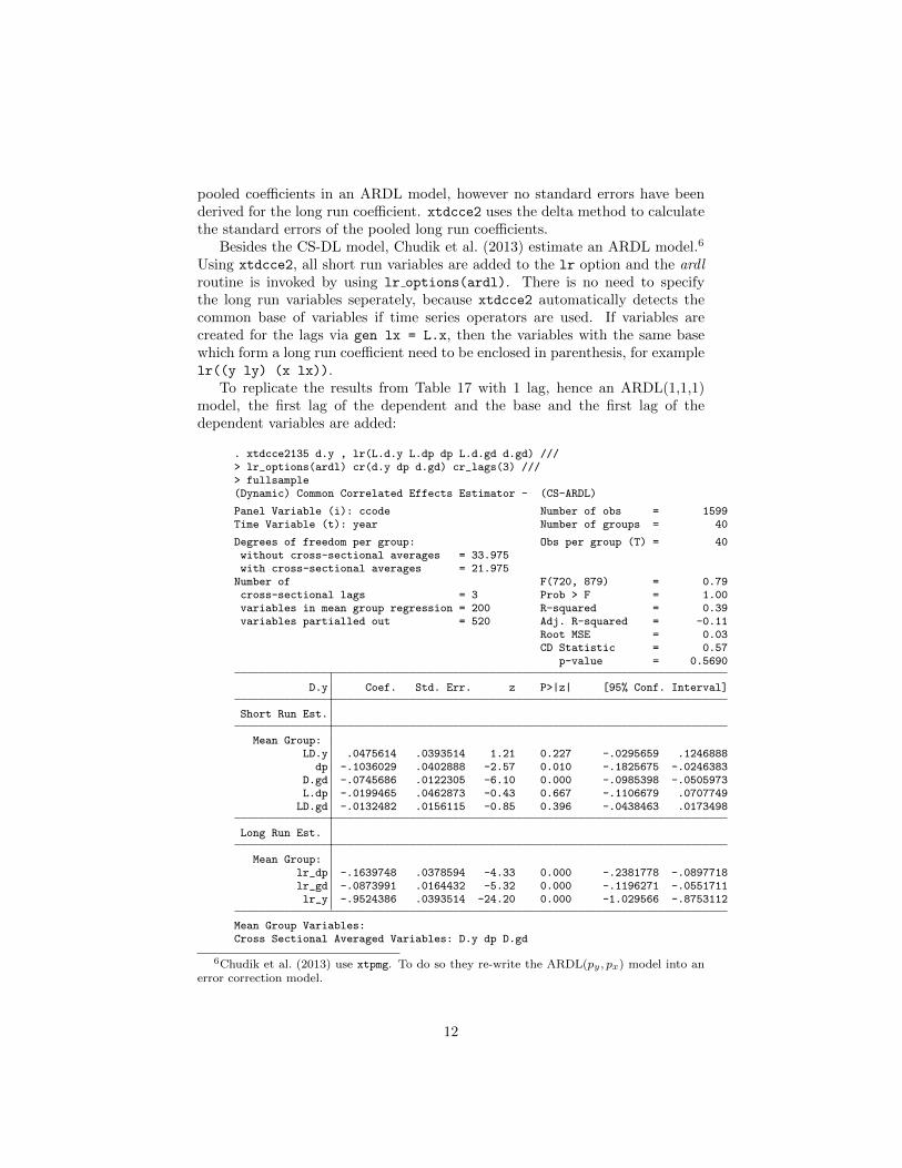
Besides the CS-DL model, Chudik et al. (2013) estimate an ARDL model.6

Using xtdcce2, all short run variables are added to the lr option and the ardlroutine is invoked by using lr options(ardl). There is no need to specifythe long run variables seperately, because xtdcce2 automatically detects thecommon base of variables if time series operators are used. If variables arecreated for the lags via gen lx = L.x, then the variables with the same basewhich form a long run coefficient need to be enclosed in parenthesis, for examplelr((y ly) (x lx)).

To replicate the results from Table 17 with 1 lag, hence an ARDL(1,1,1)model, the first lag of the dependent and the base and the first lag of thedependent variables are added:

. xtdcce2135 d.y , lr(L.d.y L.dp dp L.d.gd d.gd) ///> lr_options(ardl) cr(d.y dp d.gd) cr_lags(3) ///> fullsample(Dynamic) Common Correlated Effects Estimator - (CS-ARDL)



Number of F(720, 879) = 0.79cross-sectional lags = 3 Prob > F = 1.00variables in mean group regression = 200 R-squared = 0.39variables partialled out = 520 Adj. R-squared = -0.11


p-value = 0.5690


Short Run Est.

Mean Group:LD.y .0475614 .0393514 1.21 0.227 -.0295659 .1246888

dp -.1036029 .0402888 -2.57 0.010 -.1825675 -.0246383D.gd -.0745686 .0122305 -6.10 0.000 -.0985398 -.0505973L.dp -.0199465 .0462873 -0.43 0.667 -.1106679 .0707749

LD.gd -.0132482 .0156115 -0.85 0.396 -.0438463 .0173498

Long Run Est.

Mean Group:lr_dp -.1639748 .0378594 -4.33 0.000 -.2381778 -.0897718lr_gd -.0873991 .0164432 -5.32 0.000 -.1196271 -.0551711lr_y -.9524386 .0393514 -24.20 0.000 -1.029566 -.8753112

Mean Group Variables:Cross Sectional Averaged Variables: D.y dp D.gd

6Chudik et al. (2013) use xtpmg. To do so they re-write the ARDL(py , px) model into anerror correction model.

12

Long Run Variables: lr_dp lr_gd lr_yCointegration variable(s): lr_yHeterogenous constant partialled out.

The long run coefficients are labelled by the prefix lr . The mean groupcoefficients are calculated as the average of the cross-section individual coeffi-cients. For the ARDL(3,3,3) the 3 lags of the explanatory variables and thedependent variable are added. To improve readability, the different bases areenclosed into parenthesis:

. xtdcce2135 d.y , cr_lags(3) fullsample ///> lr(L(1/3).(d.y) (L(0/3).dp) (L(0/3).d.gd) ) ///> lr_options(ardl) cr(d.y dp d.gd)(Dynamic) Common Correlated Effects Estimator - (CS-ARDL)



Number of F(960, 602) = 0.96cross-sectional lags = 3 Prob > F = 0.71variables in mean group regression = 440 R-squared = 0.61variables partialled out = 520 Adj. R-squared = -0.03


p-value = 0.6108


Short Run Est.

Mean Group:LD.y .0123776 .0349374 0.35 0.723 -.0560984 .0808536

L2D.y -.1395721 .0948493 -1.47 0.141 -.3254733 .046329L3D.y -.0829106 .1072972 -0.77 0.440 -.2932092 .1273881

dp -.0707066 .0503045 -1.41 0.160 -.1693015 .0278883D.gd -.0853072 .0137595 -6.20 0.000 -.1122754 -.0583391L.dp -.0312738 .0513445 -0.61 0.542 -.1319071 .0693595

L2.dp .098219 .101743 0.97 0.334 -.1011937 .2976317L3.dp -.0424672 .0581718 -0.73 0.465 -.1564818 .0715474LD.gd -.0270313 .0204755 -1.32 0.187 -.0671624 .0130999

L2D.gd -.0114101 .012726 -0.90 0.370 -.0363525 .0135324L3D.gd .0283559 .0177672 1.60 0.110 -.0064671 .0631789

Long Run Est.

Mean Group:lr_dp -.0795232 .0587003 -1.35 0.176 -.1945738 .0355274lr_gd -.1198351 .0402246 -2.98 0.003 -.1986738 -.0409964lr_y -1.210105 .2006012 -6.03 0.000 -1.603276 -.8169339

Mean Group Variables:Cross Sectional Averaged Variables: D.y dp D.gdLong Run Variables: lr_dp lr_gd lr_yCointegration variable(s): lr_yHeterogenous constant partialled out.

As a final exercise, the ARDL(1,1,1) model used by Blackburne and Frank(2007) is estimated, but using the CS-ARDL estimator and heterogeneous co-

13

efficients:

. xtdcce2135 c if year >= 1962, ///> lr(L.c pi L.pi L(0/1).y) lr_options(ardl) ///> cr(_all) cr_lags(2)(Dynamic) Common Correlated Effects Estimator - (CS-ARDL)






p-value = 0.8638

c Coef. Std. Err. z P>|z| [95% Conf. Interval]

Short Run Est.

Mean Group:L.c .4150826 .0453523 9.15 0.000 .3261938 .5039714pi -.0948748 .0586788 -1.62 0.106 -.2098832 .0201335y .5397594 .0527499 10.23 0.000 .4363715 .6431474

L.pi -.0701836 .0424275 -1.65 0.098 -.15334 .0129727L.y -.0630114 .0514939 -1.22 0.221 -.1639375 .0379147

Long Run Est.

Mean Group:lr_c -.5849174 .0453523 -12.90 0.000 -.6738062 -.4960286

lr_pi -.3760294 .1470868 -2.56 0.011 -.6643143 -.0877445lr_y .7848242 .0779883 10.06 0.000 .6319699 .9376785

Mean Group Variables:Cross Sectional Averaged Variables: pi y cLong Run Variables: lr_c lr_pi lr_yCointegration variable(s): lr_cHeterogenous constant partialled out.

All long run coefficients are the same. The error speed of correction isdisplayed as variable lr c, which is 1− 0.4150, the coefficient of L.c.

4 Monte Carlo Simulation

The aims of the exercise are several fold. First of all the bias of the long runcoefficients is assessed. Additionally the standard errors of the long run coef-ficients are compared to their true values. For an empirical analysis, standarderrors are important.

The simulation is carried out on the lines of Chudik et al. (2016) and the

14

underlying DGP is an ARDL(2,1) model:7

yi,t = cyi + λ1,iyi,t−1 + λ2,iyt−2 + β0,ixi.t + β1,ixi,t−1 + ui,t

ui,t = γ′ift + εi,t

xi,t = cxi + αxiyi,t−1 + γxift + vxi,t

yi,t is the dependent variable and xi,t the only independent variable. For amatter of ease, it is assumed that only one explanatory variable exists and onlyone common factor exists. To generate the long run coefficients, first the longrun coefficient θi is drawn and then the short run coefficients are backed out,such that:8

θi ∼ IIDN(1, σ2θ), λ1,i = (1 + ξλi)ηλi, λ2,i = −ξλiηλi

β0,i = ξβiηβi, β1,i = (1− ξβi) ηβi, ηλi = IIDU(0, λmax)

ηβi = θi (1− λi,1 − λ2,i) , ξλi ∼ IIDU(0.2, 0.3), ξβi ∼ IIDU(0, 1)

To allow for a wide range of different results, two sets of coefficients are pro-duced. One in which the long run coefficients vary a lot and another one withlittle variation. This implies that ηλ,i is varied as well. The set is variedbetween (σ2

θ , λmax) = (0.2, 0.6) or (0.8, 0.8). The fixed effects are drawn ascyi ∼ IIDN(0, 1) and cxi = cyi + %cxi, %cxi ∼ IIDN(0.1).

The common factors are potentially correlated over time and calculated asft = ρfft−1 + ςft, ςft ∼ IIDN(0, 1 − ρ2

f ). The heterogeneous factor loading is

generated as γi = γ + ηiγ , ηiγ ∼ IIDN(0, σ2γ) and γx =

√bx, bx = 2

m(m+1) −2

m+1σ2γx with m = 1 and σ2

γ = σ2γx = 0.22. Two scenarios for ρf are considered,

one with correlated factors ρf = 0.6 and one with uncorrelated factors, ρf = 0.The error terms εi,t and vxi,t are generated such that they allow for au-

tocorrelation. εi,t also can inhibit cross-sectional dependence. For a furtherdiscussion of the parametrisation see the Appendix 7.4.

Multiple potential biases matter for the estimation of the coefficients. In asmall, finite sample the bias of the short run CCE estimators potentially arisesfrom three sources: the length of the time series, cross-sectional dependenceand heterogeneous slope coefficients. The first source relates to small T and thetime series bias of order T−1 (Hurwicz bias) and is expected to decrease withT →∞. The heterogeneous coefficients are assumed to be randomly distributedaround a common mean. As N converges to infinity, the mean group estimateconverges to its true parameter, ignoring any influence from the other two biases.Therefore the bias due to heterogeneous coefficients is expected to decreasewith an increase in N . The bias due to cross-sectional dependence needs to beseparated further. For a given T and an increase in N , weak cross sectional

7This paper focuses on the baseline cases with heterogeneous slopes and stationary factors.8Chudik et al. (2016, p. 103) have a for ηβi = θi/ (1 − λi,1 − λ2,i), thus they divide instead

of multiply. However given that ηβi = β0,i + β1.i and θi = ηβi/ (1 − λi,1 − λ2,i), a multiplieris correct.

15

dependence declines. Strong cross-sectional dependence does not decline whenN increases, but should not pose a problem as the cross-sectional averages takeit out.

As the long run coefficients of the CS-ECM and the CS-ARDL are the same,the Monte Carlo focuses on the CS-DL and CS-ARDL estimator. Four differentspecifications are considered. The baseline specification has correlated factorsand low values for the variance of the long run coefficients (σ2

θ = 0.2) and isequally spread across the autocorrelation coefficients (λmax = 0.6). The secondspecification includes low values of (σ2

θ , λmax), but correlated factors (ρf = 0.6).The last two specifications have high values for (σ2

θ , λmax) = (0.8, 0.8) and in-clude correlated and none correlated factors. The CS-DL and CS-ARDL, andfor Specification 1 results for the CS-ECM estimator are presented. Table 1summarizes the specifications:

[TABLE 1 here]

4.1 Results

Table 2 shows the bias of the mean group coefficient of the long run coefficientand Table 3 the bias of the standard errors. To allow a complete picture, Table2 shows the results for the CS-DL, CS-ARDL and CS-ECM estimator. In orderto shed light on a misspecified model, the bias of short run coefficients of aCS-ARDL estimation is presented in Table 4.

[TABLE 2 here]

The first panel of Table 2 displays the bias of the mean group estimates ofthe long run coefficients using the CS-DL estimator. The bias decreases with anincrease in T , however remains relatively stable with an increase in the numberof cross sections. An improvement of the estimates with an increase in T isconfirmed by the decrease of the root mean squared error. The CS-ARDL andCS-ECM results are identical. The level of the bias of those is much smaller,in a region well below 5%. The root mean squared error benefits from a largernumber of time periods and points that in large panels the estimates becomemore stable.

[TABLE 3 here]

The next table presents the bias of the estimates of the standard error. The

bias is calculated as the estimated standard error SE(θMG) minus its true value.The standard errors turn out to be upwards biased and increase slightly witha larger number of time periods. The upward bias is preferable over an under-estimation. However the bias reaches almost 100%, implying that t-statisticsbecome small and type 2 errors are more likely.

16

[TABLE 4 here]

The bias for the long run estimations of the CS-ARDL is influenced by thebias of the short run estimates. Therefore a difference in the bias between thetwo estimators should give some insights into the importance of estimating theshort run coefficients as well. Table 4 displays the short run coefficients of theCS-ARDL estimator. The bias for the contemporaneous value of βMG is small,the bias of the coefficient of the lagged variable is larger. Both coefficientsare exposed to a smaller bias if the number of time periods is increased. Thecoefficients of the lags of the dependent variable are biased towards differentdirections and both decline with T .

Overall the results are interesting in the sense that the CS-ARDL estima-tor outperforms the CS-DL estimator. This is despite the fact that the CS-DLestimator estimates directly the long run coefficients, while the CS-ARDL re-quires an estimation of the short run coefficients first. A possibility is, that thebias of the short run coefficients cancel each other out, a possibility seen bythe different directions of the biases of the short run coefficient of the laggeddependent variable. Additionally the CS-ARDL estimator needs to be specifiedmore carefully with respect to the number of lags of the independent and de-pendent variables. These additional set of information might benefit the bias ofthe estimator. This topic will be more discussed in the next section.

The results show, that all three estimator produce reasonable results, even insmall samples. However, two drawbacks remain, first of all the CS-DL estimatorperforms worse than the CS-ARDL estimator and secondly the standard errorsare overestimated for all three estimators.9

4.1.1 Misspecfied Model

As a robustness check to shed light on the behaviour of the estimators if thenumber of lags of the dependent and independent variable is accidentally largerthan of the DGP. Thus instead of the following command line:

xtdcce2135 y , lr(L(1/2).y x L.x) lr_options(ardl) cr_lags(cr_lags) cr(y x )xtdcce2135 y x d.x , cr_lags(0 cr_lags) cr(y x )

for the CS-ARDL and CS-DL estimator, the command lines are:

xtdcce2135 y , lr(L(1/3).y x L.x L2.x) lr_options(ardl) cr_lags(cr_lags) cr(y x )xtdcce2135 y x d.x d2.x , cr_lags(0 cr_lags) cr(y x )

An additional lag of the dependent and independent variables is added foreach model. Table 14 shows the results of the simulation with the misspecifiedestimation model. The bias for the CS-DL estimator is closer to zero than forthe correctly specified model. The CS-ARDL estimator suffers more, howeverthe bias remains substantially small. This points that the CS-ARDL estimator

9Tables 5 - 10 show the results for Specification 2 to 4 and are available in the appendix.In general results are similar to those from Specification 1 and therefore detailed analysis isleft to the reader.

17

is more vulnerable to misspecifications, while the CS-DL estimator seems to bemore robust.

[TABLE 14 here]

5 Conclusion

This paper reviewed three different methods to estimate long run coefficientsin dynamic panels with a large number of observations over time and cross-sectional units and with cross-sectional dependence. It uses an extended versionof xtdcce2 (Ditzen, 2018) which allows for the estimation of long run coeffi-cients using the CS-DL, CS-ARDL and CS-ECM estimator. Examples on howto apply xtdcce2 are given and options explained. A Monte Carlo simulationasses the bias of the mean group coefficient of the long and the short run es-timates. All three estimators perform well in terms bias. However standarderrors are overestimated. An alternative approach is to bootstrap standard er-rors or confidence intervals. However the difficulties are three fold. First of allthe dynamics of the model need to be preserved. Secondly the correlation of theerrors across time and cross-sectional units should not change as well. Finally,the question arises how to treat the common factors. Are the common factorstreated as determined or are they bootstrapped as well. All difficulties havebeen discussed on their own, but a combination of all has not been done and isleft for further research.

6 Acknowledgments

I am grateful to all participants of the Stata User Group Meeting in Zurich in2018, in particular Achim Ahrens and David Drukker for valuable comments andfeedback. I am grateful for help and comments from Kamiar Mohaddes, MarkSchaffer, Gregorio Tullio and plenty of users of xtdcce2, who gave valuablefeedback. All remaining errors are my own.

18

7 Appendix

7.1 The xtdcce2 command

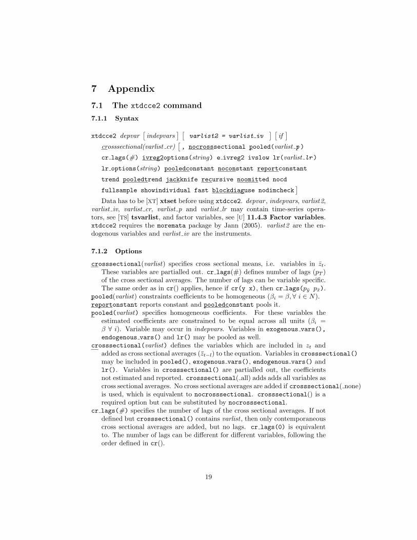
7.1.1 Syntax

xtdcce2 depvar[indepvars

] [varlist2 = varlist iv

] [if]

crosssectional(varlist cr)[, nocrosssectional pooled(varlist p )

cr lags(#) ivreg2options(string) e ivreg2 ivslow lr(varlist lr )

lr options(string) pooledconstant noconstant reportconstant

trend pooledtrend jackknife recursive noomitted nocd

fullsample showindividual fast blockdiaguse nodimcheck]

Data has to be [XT] xtset before using xtdcce2. depvar , indepvars, varlist2,varlist iv, varlist cr, varlist p and varlist lr may contain time-series opera-tors, see [TS] tsvarlist, and factor variables, see [U] 11.4.3 Factor variables.xtdcce2 requires the moremata package by Jann (2005). varlist2 are the en-dogenous variables and varlist iv are the instruments.

7.1.2 Options

crosssectional(varlist) specifies cross sectional means, i.e. variables in zt.These variables are partialled out. cr lags(#) defines number of lags (pT )of the cross sectional averages. The number of lags can be variable specific.The same order as in cr() applies, hence if cr(y x), then cr lags(py px).

pooled(varlist) constraints coefficients to be homogeneous (βi = β,∀ i ∈ N).reportonstant reports constant and pooledconstant pools it.pooled(varlist) specifies homogeneous coefficients. For these variables the

estimated coefficients are constrained to be equal across all units (βi =β ∀ i). Variable may occur in indepvars. Variables in exogenous vars(),

endogenous vars() and lr() may be pooled as well.crosssectional(varlist) defines the variables which are included in zt and

added as cross sectional averages (zt−l) to the equation. Variables in crosssectional()

may be included in pooled(), exogenous vars(), endogenous vars() andlr(). Variables in crosssectional() are partialled out, the coefficientsnot estimated and reported. crosssectional( all) adds adds all variables ascross sectional averages. No cross sectional averages are added if crosssectional( none)is used, which is equivalent to nocrosssectional. crosssectional() is arequired option but can be substituted by nocrosssectional.

cr lags(#) specifies the number of lags of the cross sectional averages. If notdefined but crosssectional() contains varlist , then only contemporaneouscross sectional averages are added, but no lags. cr lags(0) is equivalentto. The number of lags can be different for different variables, following theorder defined in cr().

19

nocrosssectional prevents adding cross sectional averages. Results will beequivalent to the Pesaran and Smith (1995) Mean Group estimator, or iflr(varlist) specified to the Shin et al. (1999) Pooled Mean Group estimator.

xtdcce2 supports instrumental variable regression using ivreg2. The IV spe-cific options are:ivreg2options passes further options on to ivreg2. See ivreg2, options

for more information.fulliv posts all available results from ivreg2 in e() with prefix ivreg2 .noisily shows the output of wrapped ivreg2 regression command.ivslow For the calculation of standard errors for pooled coefficients an aux-iliary regressions is performed. In case of an IV regression, xtdcce2 runs asimple IV regression for the auxiliary regressions. This is faster. If optionis used ivslow, then xtdcce2 calls ivreg2 for the auxiliary regression. This isadvisable as soon as ivreg2 specific options are used.

xtdcce2 is able to estimate long run coefficients. Three models are supported,an error correction model, the CS-DL and CS-ARDL method. No optionsfor the CS-DL method are necessary.lr(varlist): Variables to be included in the long-run cointegration vector.The first variable(s) is/are the error-correction speed of adjustment term.The default is to use the pmg model. In this case each estimated coefficientis divided by the negative of the long-run cointegration vector (the first vari-able). If the option ardl is used, then the long run coefficients are estimatedas the sum over the coefficients relating to a variable, divided by the sum ofthe coefficients of the dependent variable.lr options(string) Options for the long run coefficients. Options may be:ardl estimates the CS-ARDL estimator.nodivide, coefficients are not divided by the error correction speed of ad-justment vector.xtpmgnames, coefficients names in e(b p mg) and e(V p mg) match the nameconvention from xtpmg.

noconstant suppress constant term.pooledconstant restricts the constant to be the same across all groups (β0,i =

β0, ∀i).reportconstant reports the constant. If not specified the constant is treated

as a part of the cross sectional averages.trend adds a linear unit specific trend. May not be combined with pooledtrend.pooledtrend a linear common trend is added. May not be combined with

trend.jackknife applies the jackknife bias correction for small sample time series

bias. May not be combined with recursive.recursive applies recursive mean adjustment method to correct for small sam-

ple time series bias. May not be combined with jackknife.nocd suppresses calculation of CD test statistic.nomitted suppress checks for collinearity.showindividual reports unit individual estimates in output.fast omit calculation of unit specific standard errors.

20

fullsample uses entire sample available for calculation of cross sectional aver-ages. Any observations which are lost due to lags will be included calculatingthe cross sectional averages (but are not included in the estimation itself).The option does not remove any if statements. This means, that if an ifremoves certain cross-sectional units from the estimation sample, xtdcce2will not use those (as specified by if), even if fullsample is used.

blockdiaguse uses mata blockdiag rather than an alternative algorithm. matablockdiag is slower, but might produce more stable results.

7.1.3 Stored Values

Scalarse(N) number of observations e(N g) number of groupse(T) number of time periods e(K mg) number of regressorse(N partial) number of variables e(N omitted) number of omitted variables

partialled oute(N pooled) number of pooled variables e(mss) model sum of squaree(rss) residual sum of squares e(F) F statistice(ll) log-likelihood (only IV) e(rmse) root mean squared errore(df m) model degrees of freedom e(df r) residual degree of freedome(r2) R-squared e(r2 a) R-squared adjustede(cd) CD test statistic e(cdp) p-value of CD test statistice(cr lags) number of lags of cross sec-

tional averages

Scalars (unbalanced panel)e(Tmin) minimum time e(Tmax) maximum timee(Tbar) average time

Macrose(tvar) name of time variable e(idvar) name of unit variablee(depvar) name of dependent variablee(indepvar) name of independent vari-

ablese(omitted) name of omitted variables e(lr) long run variablese(pooled) name of pooled variables e(cmd) command linee(cmdline) command line including op-

tionse(version) xtdcce2 version, if xtdcce2,

version usede(insts) instruments (exogenous)

variablese(instd) instrumented (endogenous)

variables

Matricese(b) coefficient vector e(V) variance–covariance matrix

(mean group or individ-ual)

(mean group or individ-ual)

e(bi) coefficient vector e(Vi) variance–covariance matrix(individual and pooled) (individual and pooled)

Functionse(sample) marks estimation sample

7.2 ECM calculation

An general ARDL model is transformed to an ECM by adding and subtractingyi,t−1 and cross products of the contemporaneous value of x and β coefficients

21

it is not associated with in the level equation. For an ARDL(1,0):

yi,t = αi + λ1,iyi,t−1 + β0,ixi,t + ei,t

∆yi,t = αi + λ1,iyi,t−1 − yi,t + β0,ixi,t + ei,t

= (λ1,i − 1)

[yi,t−1 +

αiλ1,i − 1

+β0,i

λ1,i − 1xi,t

]+ ei,t

= − (1− λ1,i)

[yi,t−1 −

αi1− λ1,i

− β0,i

1− λ1,ixi,t

]+ ei,t

= φi [yi,t−1 − θ0,i − θ1,ixi,t] + ei,t

where

φi = − (1− λ1,i) , θ0,i =αi

1− λ1,i, θ1,i =

β0,i

1− λ1,i

For an ARDL(1,1):

yi,t = αi + λ1,iyi,t−1 + β0,ixi,t + β1,ixi,t−1 + ei,t

∆yi,t = αi + λ1,iyi,t−1 − yi,t + β0,ixi,t + β1,ixi,t−1+β1,ixi,t − β1,ixi,t + ei,t

= αi + (λ1,i − 1) yi,t−1 + xi,t (β0,i+β1,i) + β1,ixi,t−1−β1,ixi,t + ei,t

= (λ1,i − 1)

[yi,t−1 +

αiλ1,i − 1

+β0,i + β1,i

λ1,i − 1xi,t

]+ β1,i (xi,t−1 − xi,t) + ei,t

= φi [yi,t−1 − θ0,i − θ1,ixi,t]− β1,i∆xi,t + ei,t

where

φi = − (1− λ1,i) , θ0,i =αi

1− λ1,i, θ1,i =

β0,i + β1,i

1− λ1,i

For an ARDL(1,2):

yi,t =αi + λ1,iyi,t−1 + β0,ixi,t + β1,ixi,t−1 + β2,ixi,t−2 + ei,t

∆yi,t =αi + λ1,iyi,t−1 − yi,t + β0,ixi,t + β1,ixi,t−1

+β1,ixi,t − β1,ixi,t+β2,ixi,t − β2,ixi,t + ei,t

=αi + (λ1,i − 1) yi,t−1 + xi,t (β0,1+β1,i+β2,i) + β1,i (xi,t−1−xi,t)+ β2,i (xi,t−2−xi,t) + ei,t

= (λ1,i − 1)

[yi,t−1 +

αiλ1,i − 1

+β0,1 + β1,i + β2,i

λ1,i − 1

]− β1,i∆xi,t − β1,2∆2xi,t + ei,t

= φi [yi,t−1 − θ0,i − θ1,ixi,t]− β1,i∆xi,t − β2,i∆2xi,t + ei,t

where

φi = − (1− λ1,i) , θ0,i =αi

1− λ1,i, θ1,i =

β0,i + β1,i + β2,i

1− λ1,i

22

For an ARDL(2,1)

yi,t =αi + λ1,iyi,t−1 + λ2,iyi,t−2 + β0,ixi,t + β1,ixi,t−1 + ei,t

∆yi,t =αi + (λ1,i − 1) yi,t−1 + λ2,iyi,t−2 + β0,ixi,t + β1,ixi,t−1

+λ2,iyi,t−1 − λ2,iyi,t−1+β1,ixi,t − β1,ixi,t + ei,t

= (λ0,i+λ1,i − 1) yi,t−1 + xi,t (β0,i+β1,i)xi,t

+ β2,i (xi,t−1−xi,t) + λ2,i (yi,t−2−yi,t−1) + ei,t

= φi [yi,t−1 − θ0,i − θ1,ixi,t]− β1,i∆xi,t − λ2,i∆yi,t−1 + ei,t

where

φi = − (1− λ1,i − λ2,i) , θ0,i =αi

1− λ1,i − λ2,i, θ1,i =

β0,i + β1,i

1− λ1,i − λ2,i

7.3 Delta Method

7.3.1 ARDL Long Run Estimates

The delta method allows the calculation of an approximate probability distribu-tion for a matrix function a(β) based on a random vector with a known variance(see for example Hayashi, 2000, p. 93). Suppose that for the random vectorβi →p β and

√n(βi − β)→d N(0, σ). Denote the first derivatives of a(β) as

A(β) ≡ ∂a(β)

∂β′ .

Then the distribution of the function a() is

√n [a(βi)− a(β)]→d N (0, A(β)ΣA(β)′) .

The following ARDL(2,2) model, omitted the common factors without lossof generality, is estimated:

yi,t = αi + λ1,iyi,t−1 + λ2,iyi,t−2 + β1,ixi,t + β2,ixi,t−1 + ei,t

The long run coefficients are

φi = −(

1− λ1,i − λ2,i

)θ1,i =

β1,i + β2,i

1− λ1,i − λ2,i

Stacking the short run coefficients into πi = (λ1,i, λ2,i, β1,i, β2,i), then the vectorfunction a(πi) maps the short run coefficients into a vector of the short run andlong run coefficients a(πi) = (λ1,i, λ2,i, β1,i, β2,i, φi, θ1,i), where φi = 1 + λ1,i +

23

λ2,i and θ1,i =β1,i+β2,i

1−λ1,i−λ2,i. The covariance is matrix is

Σi =

V ar(λ1,i) Cov(λ1,i, λ2,i) Cov(λ1,i, β1,i Cov(λ1,i, β2,i)

. . .

. . .

V ar(β2,i)

The first derivative of vector a(πi) is:

A(πi) =

∂λ1,i

∂λ1,i

∂λ1,i

∂λ2,1

∂λ1,i

∂β1,i

∂λ1,i

∂β2,i

∂λ2,i

∂λ1,i

∂λ2,i

∂λ2,i

∂λ2,i

∂β1,i

∂λ2,i

∂β2,i

∂β1,i

∂λ1,i

∂β1,i

∂λ2,i

∂β1,i

∂β1,i

∂β1,i

∂β2,i

∂β2,i

∂λ1,i

∂β2,i

∂λ2,i

∂β2,i

∂β1,i

∂β2,i

∂β2,i

∂φi

∂λ1,i

∂φi

∂λ2,i

∂φi

∂β1,i

∂φi

∂β2,i

∂θ1,i∂λ1,i

∂θ1,i∂λ2,i

∂θ1,i∂β1,i

∂θ1,i∂β2,i

The derivatives are

∂φi∂λ1,i

=∂φi∂λ2,i

= 1

∂θ1,i

∂β1,i=∂θ1,i

∂β2,i=

1

1− λ1,i − λ2,i

∂θ1,i

∂λ1,i=∂θ1,i

∂λ2,i=

β1,i + β2,i

(1− λ1,i − λ2,i)2

and thus

A(πi) =

1 0 0 00 1 0 00 0 1 00 0 0 11 1 0 0

β1,i+β2,i

(1−λ1,i−λ2,i)2

β1,i+β2,i

(1−λ1,i−λ2,i)2

11−λ1,i−λ2,i

11−λ1,i−λ2,i

Then the covariance matrix including the long run coefficients is

Σlri = A(πi)ΣiA(πi)′

The same method as for φi is used for the calculation of variance for the longrun pooled coefficients. Assume that θ2 = λ2 + λ3, where λ2 and λ3 are pooledcoefficients. Then the tow corresponding to θ2 in A(.) includes a 1 in the columnscorresponding to the coefficients the long run coefficient is estimated from.

24

7.4 Monte Carlo GDP

The underlying DGP is:

yi,t = cyi + λ1,iyi,t−1 + λ2,iyt−2 + β0,ixi.t + β1,ixi,t−1 + ui,t

ui,t = γ′ift + εi,t

xi,t = cxi + αxiyi,t−1 + γxift + vxi,t

The cross-section specific fixed effects are generated as:

cyi ∼ IIDN(1, 1)

cxi = cyi + ςcxi, ςcxi ∼ IIDN(0, 1).

Dependence between xi,t, gi,t and cyi is introduced by adding cyi to the equationsfor cxi and cgi. First the long run coefficient θ is drawn and then the short runcoefficients are backed out.

θi ∼ IIDN(1, σ2θ)

λ1,i = (1 + ξλi)ηλi, λ2,i = −ξλiηλiβ0,i = ξβiηβi, β1,i = (1− ξβi) ηβiηλi = IIDU(0, λmax), ηβi = θi (1− λi,1 − λ2,i)

ξλi ∼ IIDU(0.2, 0.3), ξβi ∼ IIDU(0, 1)

The common factors are calculated as:

γi = γ + ηiγ , ηiγ ∼ IIDN(0, σ2γ)

γxi = γx + ηiγx, ηiγx ∼ IIDN(0, σ2γx)

σ2γ = σ2

γx = 0.22

γ =√bγ , bγ =

1

m− σ2

γ

where m is the number of unobserved factors. In comparison to Chudik andPesaran (2015) it is restricted to 1.

The error component of the variable x is generated as:

vxi,t = ρxivxi,t−1 + ςxi,t, ςxi,t ∼ IIDN(0, σ2vxi)

ρxi ∼ IIDU(0, 0.95)

ρf = 0 if serially uncorrelated factors, or if correlated ρf = 0.6

σ2vxi = σ2

vi =

(β0i

√1− [E(ρxi)]

2

)2

The errors are generated such that heteroskedasticity, autocorrelation and weakly

25

cross-sectional dependence is allowed.

εi,t = ρεiεi,t−1 + ζi,t

ζt = (ζ1,t, ζ2,t, ..., ζN,t) = αCSDSεt + eεt

⇒ ζt = (1− αCSDSε)−1eεt

eεt ∼ IIDN(0,1

2σ2i

(1− ρ2

εi

)), with σ2

i ∼ χ2(2)

ρεi ∼ IIDU(0, 0.8)

Sε =

0 1 0 0 . . . 012 0 1

2 0 0

0 12 0

. . ....

0 0. . .

. . . 12 0

... 12 0 1

20 0 . . . 0 1 0

26

7.5 Monte Carlo Results

Table(σ2θ , λmax) ρf LR SR

1 (0.2,0.6) 0 Table 2, 3 42 (0.2,0.6) 0.6 Table 5, 6 73 (0.8,0.8) 0 Table 8, 9 104 (0.8,0.8) 0.6 Table 11, 12 13

Table 1: Overview of Specifications. The DGP is yi,t = cyi + λ1,iyi,t−1 +λ2,iyt−2+β0,ixi.t+β1,ixi,t−1+γ′ift+εi,t, where θi = (β0,i+β1,i)/(1−λ1,i−λ2,i) ∼IIDN(1, σ2

θ). cyi ∼ IIDN(0, 1) and γi = γ + ηiγ , ηiγ ∼ IIDN(0, σ2γ). For a

further description see Section 7.4.

27

(N,T) Bias of θMG (x100) RMSE of θMG (x100)40 50 100 150 200 40 50 100 150 200

CS-DL40 -21.57 -21.04 -19.52 -18.73 -18.26 23.50 22.48 20.10 19.04 18.4650 -19.41 -19.15 -17.09 -16.64 -16.42 21.12 20.19 17.51 16.84 16.52100 -20.04 -18.76 -17.40 -17.08 -16.93 20.39 19.02 17.25 16.81 16.61150 -16.99 -16.41 -15.06 -14.72 -14.56 17.35 16.64 15.05 14.62 14.46200 -20.73 -19.62 -18.20 -17.72 -17.37 21.04 19.80 18.24 17.70 17.31

CS-ARDL40 -2.63 -1.64 -1.94 -0.64 -0.48 192.31 13.65 8.01 5.58 4.8050 -2.13 -186.07 -1.45 -0.75 -0.58 40.85 4049.97 6.53 5.47 4.36100 -3.53 -0.43 -1.21 -0.94 -0.65 182.04 24.21 4.64 3.46 2.96150 -4.93 -2.29 -1.31 -0.95 -0.59 34.46 7.20 3.69 2.69 2.48200 -2.63 -2.29 -1.63 -1.11 -0.61 23.47 8.54 3.76 2.73 2.22

CS-ECM40 -2.63 -1.64 -1.94 -0.64 -0.48 192.31 13.65 8.01 5.58 4.8050 -2.13 -186.07 -1.45 -0.75 -0.58 40.85 4049.97 6.53 5.47 4.36100 -3.53 -0.43 -1.21 -0.94 -0.65 182.04 24.21 4.64 3.46 2.96150 -4.93 -2.29 -1.31 -0.95 -0.59 34.46 7.20 3.69 2.69 2.48200 -2.63 -2.29 -1.63 -1.11 -0.61 23.47 8.54 3.76 2.73 2.22

Table 2: Monte Carlo results for θMG = 1/N∑Ni=1 θi for Specification 1 with

pT = [T 1/3], ρf = 0 and (σ2θ , λmax) = (0.2, 0.6). See Table 1 and Section 7.4 for

a description of the DGP.

28

(N,T) Bias of SE(θMG) (x100) RMSE of SE(θMG) (x100)40 50 100 150 200 40 50 100 150 200

CS-DL40 77.60 78.13 79.62 80.41 80.87 12.06 13.54 15.85 16.68 17.1950 79.26 79.52 81.55 81.99 82.20 11.40 12.63 14.87 15.66 16.13100 77.65 78.89 80.21 80.52 80.67 12.91 13.75 15.26 15.79 16.07150 81.66 82.23 83.56 83.89 84.05 14.17 14.81 16.01 16.39 16.60200 78.67 79.76 81.18 81.65 82.00 14.77 15.40 16.51 16.88 17.09

CS-ARDL40 96.34 97.31 97.02 98.30 98.47 187.57 10.94 14.57 15.84 16.5950 96.26 -84.65 96.93 97.62 97.79 36.00 4048.46 13.72 14.91 15.67100 93.68 96.69 95.94 96.20 96.48 180.31 24.47 14.53 15.41 15.85150 93.52 96.12 97.09 97.44 97.79 32.86 13.31 15.56 16.21 16.53200 96.62 96.96 97.62 98.14 98.63 21.64 14.47 15.98 16.60 16.93

CS-ECM40 96.34 97.31 97.02 98.30 98.47 187.57 10.94 14.57 15.84 16.5950 96.26 -84.65 96.93 97.62 97.79 36.00 4048.46 13.72 14.91 15.67100 93.68 96.69 95.94 96.20 96.48 180.31 24.47 14.53 15.41 15.85150 93.52 96.12 97.09 97.44 97.79 32.86 13.31 15.56 16.21 16.53200 96.62 96.96 97.62 98.14 98.63 21.64 14.47 15.98 16.60 16.93

Table 3: Monte Carlo results for SE(θMG) =√

1/N∑Ni=1(θi − θMG)2 for Spec-

ification 1 with pT = [T 1/3], ρf = 0 and (σ2θ , λmax) = (0.2, 0.6). See Table 2

and Section 7.4 for a description of the DGP.

(N,T) 40 50 100 150 200 40 50 100 150 200

Bias of β0,MG (x100) Bias of β1,MG (x100)40 0.92 0.36 0.59 0.21 0.35 15.69 13.26 4.67 3.13 2.2050 -1.63 0.20 -0.10 0.12 0.20 19.23 13.09 5.89 4.14 2.51100 -1.01 -0.12 0.08 0.14 0.01 16.95 13.06 5.90 3.44 2.50150 0.48 -0.76 -0.32 -0.04 0.04 16.59 13.39 6.04 3.66 2.73200 -1.38 -0.92 -0.22 -0.01 0.09 17.89 13.07 5.95 3.78 2.73

Bias of φ1,MG (x100) Bias of φ2,MG (x100)40 -15.46 -10.69 -4.34 -2.22 -1.77 13.70 10.78 6.32 3.42 2.4250 -15.59 -11.18 -4.43 -2.73 -1.83 12.25 10.31 5.12 3.75 2.50100 -16.52 -11.33 -4.65 -2.87 -2.19 16.12 12.37 6.62 4.22 2.43150 -17.08 -11.95 -5.10 -3.01 -2.30 21.70 18.34 7.88 5.94 3.59200 -16.13 -11.35 -4.88 -3.03 -2.15 16.96 14.00 7.13 4.62 3.10

Table 4: Monte Carlo results for the mean group coefficients of the short runcoefficients for Specification 1 with pT = [T 1/3], ρf = 0 and (σ2

θ , λmax) =(0.2, 0.6). See Table 1 and Section 7.4 for a description of the DGP.

29


CS-DL40 -22.20 -21.55 -19.72 -18.85 -18.39 24.09 22.95 20.30 19.17 18.5950 -20.00 -19.53 -17.33 -16.78 -16.53 21.68 20.62 17.75 16.98 16.63100 -20.71 -19.27 -17.62 -17.22 -17.02 21.02 19.53 17.46 16.94 16.70150 -17.57 -16.84 -15.24 -14.84 -14.65 17.92 17.06 15.23 14.74 14.55200 -21.37 -20.11 -18.42 -17.85 -17.46 21.68 20.28 18.47 17.83 17.40

CS-ARDL40 -8.65 -1.64 -2.43 -1.01 -0.72 87.34 31.89 8.18 5.67 4.8150 0.49 -1.36 -1.98 -1.08 -0.79 46.41 35.50 6.66 5.54 4.39100 -23.34 -2.60 -1.69 -1.27 -0.87 394.98 9.34 4.77 3.54 3.01150 -4.58 -3.30 -1.80 -1.25 -0.82 108.86 6.97 3.85 2.81 2.53200 -10.41 -3.29 -2.16 -1.45 -0.85 74.29 9.23 4.03 2.88 2.29


pT = [T 1/3], ρf = 0.6 and (σ2θ , λmax) = (0.2, 0.6). See Table 2 and Section 7.4

for a description of the DGP.


CS-DL40 76.98 77.62 79.43 80.29 80.74 11.93 13.46 15.81 16.67 17.1850 78.68 79.15 81.31 81.85 82.10 11.24 12.54 14.84 15.64 16.13100 77.00 78.39 80.00 80.39 80.58 12.82 13.69 15.24 15.78 16.07150 81.09 81.80 83.38 83.77 83.96 14.08 14.76 16.00 16.38 16.59200 78.03 79.28 80.96 81.52 81.91 14.70 15.35 16.49 16.88 17.08

CS-ARDL40 90.38 97.32 96.54 97.94 98.23 83.61 29.57 14.58 15.85 16.5950 98.84 97.02 96.40 97.29 97.58 42.69 33.93 13.73 14.91 15.67100 74.44 94.59 95.46 95.87 96.26 393.67 11.59 14.52 15.41 15.85150 93.86 95.13 96.61 97.15 97.56 107.24 13.16 15.56 16.21 16.53200 88.90 95.98 97.09 97.80 98.40 71.66 14.18 15.97 16.60 16.93



ification 2 with pT = [T 1/3], ρf = 0.6 and (σ2θ , λmax) = (0.2, 0.6). See Table 2


30

(N,T) 40 50 100 150 200 40 50 100 150 200



Table 7: Monte Carlo results for the mean group coefficients of the short runcoefficients for Specification 3 with pT = [T 1/3], ρf = 0.6 and (σ2



CS-DL40 -30.10 -29.30 -27.24 -26.12 -25.54 31.22 29.94 27.08 25.63 24.9550 -27.31 -26.84 -24.11 -23.63 -23.29 27.88 26.75 23.38 22.68 22.24100 -26.59 -25.02 -23.28 -22.85 -22.52 24.60 23.14 21.03 20.47 20.14150 -20.69 -20.03 -18.33 -17.94 -17.81 20.15 19.37 17.43 16.98 16.83200 -28.43 -26.93 -25.01 -24.40 -23.92 28.05 26.48 24.49 23.79 23.28

CS-ARDL40 1.41 -0.06 -2.08 -0.69 -0.55 66.86 36.72 11.30 7.84 6.8550 -23.32 -6.02 -2.00 -1.00 -0.84 340.46 143.68 9.82 8.47 6.67100 -12.22 -8.48 -1.41 -1.16 -0.65 194.50 147.12 6.47 4.63 4.03150 -6.73 0.25 -1.34 -1.05 -0.69 75.90 34.84 5.31 3.70 3.55200 -37.15 -17.69 -2.16 -1.58 -0.87 545.06 380.23 5.41 3.98 3.17


pT = [T 1/3], ρf = 0 and (σ2θ , λmax) = (0.8, 0.8). See Table 2 and Section 7.4 for

a description of the DGP.

31


CS-DL40 66.94 67.70 69.68 70.75 71.31 73.57 75.01 76.76 77.25 77.6250 67.91 68.34 70.90 71.35 71.67 68.99 70.12 72.06 72.69 73.03100 64.92 66.30 67.85 68.23 68.52 67.40 68.11 69.26 69.63 69.82150 74.14 74.76 76.35 76.71 76.84 69.13 69.66 70.53 70.79 70.93200 69.39 70.84 72.70 73.29 73.76 70.64 71.16 72.06 72.33 72.47

CS-ARDL40 97.12 95.71 93.77 95.10 95.23 79.39 71.01 71.97 72.99 73.5550 71.64 87.80 91.55 92.49 92.63 338.88 148.27 67.81 68.95 69.67100 77.62 80.94 87.19 87.41 87.86 195.75 156.44 67.04 67.89 68.23150 87.19 93.72 92.23 92.51 92.84 86.13 71.57 69.08 69.74 69.99200 60.93 79.79 94.85 95.41 96.10 541.60 381.86 70.37 71.01 71.30



ification 3 with pT = [T 1/3], ρf = 0 and (σ2θ , λmax) = (0.8, 0.8). See Table 2


(N,T) 40 50 100 150 200 40 50 100 150 200



Table 10: Monte Carlo results for the mean group coefficients of the short runcoefficients for Specification 3 with pT = [T 1/3], ρf = 0 and (σ2


32


CS-DL40 -30.98 -29.90 -27.48 -26.29 -25.67 32.06 30.48 27.31 25.80 25.0950 -28.01 -27.34 -24.38 -23.77 -23.39 28.67 27.33 23.65 22.80 22.35100 -27.27 -25.71 -23.53 -22.99 -22.62 25.21 23.77 21.26 20.60 20.23150 -21.32 -20.50 -18.49 -18.07 -17.92 20.75 19.81 17.59 17.10 16.94200 -29.22 -27.52 -25.28 -24.55 -24.03 28.84 27.08 24.75 23.93 23.40

CS-ARDL40 -5.01 -2.56 -2.62 -1.09 -0.82 64.97 22.93 11.44 7.94 6.8650 -6.79 -6.08 -2.65 -1.35 -1.00 81.88 28.84 9.90 8.47 6.67100 14.20 -3.47 -1.90 -1.49 -0.86 381.80 22.48 6.51 4.68 4.07150 -0.99 -2.16 -1.88 -1.31 -0.90 64.07 43.98 5.28 3.77 3.57200 -5.86 -5.53 -2.72 -1.92 -1.14 56.87 71.13 5.67 4.10 3.23


pT = [T 1/3], ρf = 0.6 and (σ2θ , λmax) = (0.8, 0.8). See Table 2 and Section 7.4

for a description of the DGP.


CS-DL40 66.10 67.13 69.45 70.59 71.18 73.35 74.93 76.74 77.25 77.6350 67.26 67.88 70.65 71.22 71.57 68.78 69.97 72.00 72.66 73.02100 64.32 65.70 67.62 68.10 68.43 67.31 68.04 69.24 69.62 69.82150 73.55 74.32 76.20 76.60 76.74 69.04 69.60 70.52 70.78 70.92200 68.61 70.26 72.44 73.15 73.64 70.57 71.11 72.04 72.32 72.47

CS-ARDL40 90.96 93.31 93.25 94.71 94.98 76.81 66.77 72.04 73.04 73.5750 87.08 87.74 90.94 92.16 92.48 85.22 62.87 67.91 69.00 69.68100 100.99 85.37 86.76 87.12 87.67 381.30 63.53 67.07 67.91 68.24150 92.56 91.46 91.73 92.26 92.64 79.58 74.77 69.13 69.76 70.00200 91.27 91.58 94.30 95.08 95.84 73.61 90.47 70.41 71.03 71.31


1/N∑Ni=1(θi − θMG)2 for

Specification 4 with pT = [T 1/3], ρf = 0.6 and (σ2θ , λmax) = (0.8, 0.8). See

Table 2 and Section 7.4 for a description of the DGP.

33

(N,T) 40 50 100 150 200 40 50 100 150 200

Bias of β0,MG (x100) Bias of β1,MG (x100)40 0.60 0.32 0.68 0.27 0.39 19.75 17.44 5.93 3.89 2.6950 -2.67 -0.17 -0.23 0.19 0.29 21.56 14.87 6.46 4.52 2.68100 -1.66 -0.56 0.03 0.25 0.04 16.31 12.88 5.90 3.33 2.42150 0.32 -0.84 -0.39 -0.04 0.04 19.89 15.89 7.16 4.26 3.21200 -1.84 -1.34 -0.26 -0.01 0.11 20.75 15.36 7.03 4.52 3.20


Table 13: Monte Carlo results for the mean group coefficients of the short runcoefficients for Specification 2 with pT = [T 1/3], ρf = 0.6 and (σ2



CS-DL40 -7.67 -7.28 -6.95 -6.28 -6.06 14.54 12.26 9.47 7.96 7.3850 -7.18 -7.52 -6.33 -6.13 -5.95 13.26 11.69 8.47 7.57 7.04100 -6.86 -5.91 -5.65 -5.56 -5.58 10.17 8.84 6.73 6.17 6.05150 -5.51 -5.49 -4.86 -4.73 -4.65 7.97 7.23 5.64 5.22 5.07200 -7.76 -7.06 -6.54 -6.36 -6.07 9.36 8.27 7.17 6.70 6.29

CS-ARDL40 -0.27 1.92 -0.74 -0.19 -0.29 191.07 20.76 9.12 6.19 5.4050 7.66 2.26 -0.49 -0.53 -0.46 102.70 36.44 7.39 6.17 4.90100 7.11 2.93 -0.43 -0.42 -0.52 153.49 33.15 5.16 3.80 3.35150 14.19 -1.35 -0.63 -0.54 -0.30 123.62 34.92 4.13 3.08 2.63200 4.84 0.88 -0.65 -0.53 -0.22 107.79 50.73 4.08 2.94 2.42


pT = [T 1/3], ρf = 0 and (σ2θ , λmax) = (0.2, 0.6), but with misspecified command

line. See Table 1 and Section 7.4 for a description of the DGP.

34

References

Blackburne, Edward F. and Mark W. Frank. 2007. “Estimation of nonstationaryheterogeneous panels.” The Stata Journal 7(2):197–208.

Chudik, Alexander, Kamiar Mohaddes, M. Hashem Pesaran and Mehdi Raissi.2013. “Debt, Inflation and Growth: Robust Estimation of Long-Run Effectsin Dynamic Panel Data Models.” Cambridge Working Papers in EconomicsDebt.

Chudik, Alexander, Kamiar Mohaddes, M. Hashem Pesaran and Mehdi Raissi.2016. Long-Run Effects in Large Heterogeneous Panel Data Models withCross-Sectionally Correlated Errors. In Essays in Honor of Aman Ullah (Ad-vances in Econometrics, Volumn 36), ed. R. Carter Hill, Gloria GonzAlez-Rivera and Tae-Hwy Lee. Emerald Group Publishing Limited pp. 85–135.

Chudik, Alexander and M. Hashem Pesaran. 2015. “Common correlated ef-fects estimation of heterogeneous dynamic panel data models with weaklyexogenous regressors.” Journal of Econometrics 188(2):393–420.

Chudik, Alexander, M. Hashem Pesaran and Elisa Tosetti. 2011. “Weak andstrong cross-section dependence and estimation of large panels.” The Econo-metrics Journal 14(1):C45–C90.

Ditzen, Jan. 2018. “Estimating dynamic common-correlated effects in Stata.”The Stata Journal 18(3):585 – 617.

Eberhardt, Markus. 2012. “Estimating panel time series models with heteroge-neous slopes.” The Stata Journal 12(1):61–71.

Engle, Robert F. and C. W. J. Granger. 1987. “Co-Integration and Error Cor-rection: Representation, Estimation, and Testing.” Econometrica 55(2):251.

Everaert, Gerdie and Tom De Groote. 2016. “Common Correlated Effects Es-timation of Dynamic Panels with Cross-Sectional Dependence.” EconometricReviews 35(3):1–31.

Hayashi, Fumio. 2000. Econometrics. Princeton: Princeton University Press.

Jann, Ben. 2005. “moremata: Stata module (Mata) to provide various func-tions.”.URL: https://ideas.repec.org/c/boc/bocode/s455001.html

Kripfganz, Sebastian and Daniel Schneider. 2018. “ardl: Estimating autoregres-sive distributed lag and equilibrium correction models.”.URL: https://ideas.repec.org/p/boc/usug18/09.html

Lee, Kevin, M. Hashem Pesaran and Ron Smith. 1997. “Growth and Con-vergence in a Multi-Country Empirical Stochastic Solow Model.” Journal ofApplied Economics 12(4):357–392.

35

Pesaran, M. Hashem. 2006. “Estimation and inference in large heterogeneouspanels with a multifactor error structure.” Econometrica 74(4):967–1012.

Pesaran, M. Hashem and Ron Smith. 1995. “Estimating long-run relationshipsfrom dynamic heterogeneous panels.” Journal of Econometrics 68(1):79–113.

Shin, Yongcheol, M. Hashem Pesaran and Ron P. Smith. 1999. “Pooled MeanGroup Estimation of Dynamic Heterogeneous Panels.” Journal of the Amer-ican Statistical Association 94(446):621 –634.

36

Estimating long run effects in models with cross-sectional ...

Documents