Estimating Impacts and Trade‐offs in Solar Geoengineering ...

Estimating Impacts and Trade-offs in SolarGeoengineering Scenarios With a MoistEnergy Balance Model

Nicholas J. Lutsko1 , Jacob T. Seeley2, and David W. Keith3

1Scripps Institution of Oceanography, University of California at San Diego, La Jolla, CA, USA, 2Harvard UniversityCenter for the Environment, Harvard University, Cambridge, MA, USA, 3John A. Paulson School of Engineering andApplied Sciences (SEAS), Harvard Kennedy School, Harvard University, Cambridge, MA, USA

Abstract There are large uncertainties in the potential impacts of solar radiation modification (SRM)and in how these impacts depend on the way SRM is deployed. One open question concerns trade-offsbetween latitudinal profiles of insolation reduction and climate response. Here, a moist energy balancemodel is used to evaluate several SRM proposals, providing fundamental insight into how the insolationreduction profile affects the climate response. The optimal SRM profile is found to depend on the intensityof the intervention, as the most effective profile for moderate SRM focuses the reduction at high latitudes,whereas the most effective profile for strong SRM is tropically amplified. The effectiveness of SRM is alsoshown to depend on when it is applied, an important factor to consider when designing SRM proposals.Using an energy balance model allows us to provide physical explanations for these results while alsosuggesting future avenues of research with comprehensive climate models.

1. IntroductionSolar geoengineering, or solar radiation modification (SRM), refers to proposals to reduce the amount ofsolar radiation incident on Earth's surface so as to partially offset the global warming effects of increasedatmospheric CO2 concentrations (Keith, 2013). A variety of SRM strategies has been suggested, fromterrestrial-based plans to brighten the roofs of buildings to space-based sunlight-reflecting mirrors, but themost commonly discussed proposal is injecting sulfate aerosol precursors into the stratosphere (Council,2015). Inspired by the observed cooling in response to large volcanic eruptions, sulfate injection wouldenhance the optical density of the stratospheric aerosol layer and appears to be the most technically feasiblemeans of producing a roughly uniform increase of the Earth's albedo (Irvine et al., 2016).

Much work has been done to understand the potential impacts of sulfate SRM since it was first proposedby Budyko (1977), mostly based on simulations with global climate models (GCMs). The recent Geoengi-neering Model Intercomparison Project (GeoMIP, Kravitz et al., 2011) provides a convenient resource foridentifying which of these impacts are robust across models, including, among other things, the tendencyof the tropics to overcool compared to the control climate (Govindasamy et al., 2003; Kravitz et al., 2013)and the weakening of the global hydrological cycle compared to the control climate (Bala et al., 2008; Tilmeset al., 2013). Recent modeling work has also investigated the possibility of optimizing SRM interventions toachieve specific climate objectives (Dai et al., 2018; Kravitz et al., 2017), moving the conversation away fromanalyzing the potential impacts of a particular intervention and toward designing interventions to achievespecific mitigation goals.

Nevertheless, there are still many open questions about the potential impacts of sulfate aerosol SRM. Onemajor issue is how the insolation reduction should be spatially distributed in order to achieve a specificobjective. Although the climate system's response to SRM scales to first order with the global mean radia-tive forcing (Modak & Bala, 2014), any SRM scenario involves trade-offs, as some regions will experience agreater compensation of warming than others, leading to concerns about equity. Certain SRM interventionswill also be more effective than others at countering the global impacts of increased CO2 concentrations.Previous SRM studies have typically assumed that the sulfate aerosol loading is adjusted so as to reduceinsolation by the same fractional amount (e.g., 1%) at all latitudes; however, there is no guarantee that

RESEARCH LETTER10.1029/2020GL087290

Key Points:• Simple energy balance models

can build intuition for the climatesystem's response to solar radia-tion management, complementingglobal climate model studies

• The most effective latitudinalprofile of insolation reductiondepends on the intensity of the solarradiation modification intervention

• The effectiveness of solar radiationmodification interventions dependson when they are applied not justhow they are applied

Supporting Information:• Supporting Information S1

Correspondence to:N. J. Lutsko,[email protected]

Citation:Lutsko, N. J., Seeley, J. T., &Keith, D. W. (2020). Estimatingimpacts and trade-offs in solargeoengineering scenarios with a moistenergy balance model. GeophysicalResearch Letters, 47, e2020GL087290.https://doi.org/10.1029/2020GL087290

Received 29 JAN 2020Accepted 6 APR 2020Accepted article online 17 APR 2020

©2020. American Geophysical Union.All Rights Reserved.

LUTSKO ET AL. 1 of 12

Geophysical Research Letters 10.1029/2020GL087290

this is the optimal distribution of aerosol loading for countering the effects of higher CO2 concentrations.For instance, Ban-Weiss and Caldeira (2010) and MacMartin et al. (2013) explored several scenarios foroptimizing SRM in GCMs and generally found that having larger reductions at higher latitudes best coun-teracted the temperature response while more tropically based insolation reductions better counteractedthe precipitation change. However, these studies relied on a single model each and considered a relativelysmall number of basis functions as part of their optimization procedure. Still lacking is intuition, basedon physical understanding, for how the climate system's response is affected by the latitudinal profile ofinsolation reduction.

In this study, we have sought to understand the potential impacts of different SRM scenarios on the climatesystem at a more fundamental level by using a one-dimensional moist energy balance model (EBM). EBMshave proven to be a useful idealized framework for addressing many climate questions (Armour et al., 2019;Budyko, 1969; Flannery, 1984; Frierson et al., 2007; Merlis & Henry, 2018; North, 1975; North et al., 1981;Merlis, 2014; Rose et al., 2014; Roe et al., 2015; Sellers, 1969) but so far have not featured in the SRM literature(though Merlis and Henry, 2018, briefly mention SRM in the context of simple estimates of polar amplifi-cation). While lacking the complexity and detail of comprehensive GCMs and also not simulating the rapidadjustments of the climate system to external forcing agents (e.g., Smith et al., 2018), the relative simplicity ofEBMs makes their results easier to interpret, providing confidence that the results are (qualitatively) robust.Furthermore, simple physical arguments can be used to extend EBM results beyond temperature, providingfirst-order estimates for how precipitation and the large-scale atmospheric circulation would change undera given SRM scenario.

Setting aside the engineering question of how to achieve a given aerosol loading distribution and not-ing that the global mean temperature change is largely constrained by the global mean radiative forcing(Modak & Bala, 2014), the EBM provides insight into the trade-offs between different latitudinal SRM pro-files. A “perfect” SRM scenario can, for example, be constructed to exactly cancel the CO2 forcing. Whilethis perfect SRM is an artifact of the idealized nature of the EBM, it is a useful first estimate for what anoptimal SRM profile would look like for a comprehensive GCM or for the climate system. We use the EBMto construct latitudinal profiles of insolation reduction that achieve specific objectives, such as minimizingthe radiative forcing needed to restore global average temperature, and then examine how these results varywith the strength of the SRM intervention.

We have also investigated the possibility that the effectiveness of SRM interventions is state dependent.EBMs are known to exhibit two forms of bistability and associated hysteresis: for cold enough condi-tions, they can jump to an ice-covered state, a transition referred to as the “snowball Earth instability”(e.g., Budyko, 1974; North, 1975; North et al., 1981), while for warmer conditions the ice caps have beenfound to be unstable, leading to the “small ice cap instability” (North et al., 1984; Rose & Marshall, 2009)(note that these studies mostly focused on dry EBMs, which diffuse dry static energy, whereas the EBM usedhere diffuses moist static energy). Wagner and Eisenman (2015) showed that the latter instability can beeliminated by including both a seasonal insolation cycle and an interactive ice albedo feedback in a dry EBM,agreeing with comprehensive model studies that typically find Arctic and Antarctic sea ice scaling approx-imately linearly with global mean temperature (Armour et al., 2011; Gregory et al., 2002; Winton, 2011).However, it is still possible that some weak hysteresis is present, such that the compensation of warming ina given SRM scenario depends on when SRM is implemented.

The possibility that the effectiveness of SRM interventions depends on when the SRM is implemented hasnot been investigated before but could be crucial for designing SRM proposals: when SRM is implementedmay be as important as how it is implemented. We have explored this issue in the context of three differentSRM scenarios, and our results suggest that investigating the state dependence of SRM interventions incomprehensive GCMs is an urgent topic of future SRM research.

2. The Moist Energy Balance ModelThe moist EBM simulates the evolution of zonal mean surface temperatures and includes interactive repre-sentations of radiative feedbacks and horizontal atmospheric energy transport, as well as seasonally varying

LUTSKO ET AL. 2 of 12

Geophysical Research Letters 10.1029/2020GL087290

solar insolation. The latter allows the EBM to capture the seasonal effectiveness of SRM interventions. Thegoverning equation of the EBM is (see, e.g., Merlis & Henry, 2018; Wagner & Eisenman, 2015)

C 𝜕T(t, 𝜙)𝜕t

= S(t, 𝜙)[1 − a(T)] − [A + BT(𝜙)] − ∇ · H(𝜙,T) + F(𝜙), (1)

where C is the heat capacity of the combined land surface and ocean mixed layer, T is surface temperature(in units K, though we will use ◦C for plotting and discussion purposes),𝜙 is latitude, t is time (in unit years),S is the insolation, a(T) is the albedo, A+BT is the outgoing longwave radiation, ∇ ·H is the convergence ofthe moist static energy (MSE) flux, and F is a radiative forcing, like that due to increased CO2 concentrations.

The insolation is given by (North et al., 1981)

S(t, 𝜙) = Q∕4 × (1 − 𝛾P2) − S1xcos(2𝜋t), (2)

where Q is the solar constant, 𝛾 is a constant, P2 = (3x2 − 1)∕2 is the second Legendre polynomial, x =sin(𝜙), and S1 determines the amplitude of the seasonal insolation cycle. The albedo takes the followingtemperature-dependent form (Eisenman & Wettlaufer, 2009):

a(T) =a0 + a1

2+

a0 − a1

2tanh

(T − T0

ht

), (3)

so that a gradually varies from an open water value, a0, to a sea ice value, a1, with smoothness parameterht. The temperature dependence allows the EBM to represent the ice-albedo feedback.

The MSE flux is parameterized by downgradient diffusion, with −∇ · H(𝜙) = 𝜕x[D(1 − x2)𝜕xh

], where h =

cpT +Lq∗(T) is the MSE in units of ◦C. L is the latent heat of vaporization of liquid water, is the surfacerelative humidity, q*(Ts) is the saturation specific humidity at the surface, and cp is the heat capacity of air ata constant near-surface pressure (1,000 hPa). We assume a fixed relative humidity of 80% at all latitudes andfor all forcings and calculate q* using the August-Roche-Magnus approximation (Lawrence, 2005). Althoughthe assumption of uniform relative humidity is standard in moist EBM studies (e.g., Armour et al., 2019;Flannery, 1984; Merlis & Henry, 2018), it is an important limitation of the present work, and future studiesshould investigate the influence of using more realistic relative humidity profiles. The diffusivity D is keptfixed in all experiments, though note that we thus neglect changes in atmospheric circulation, which wouldaffect the value of D (e.g., Caballero & Hanley, 2012; Shaw & Voigt, 2016). Larger values of D produce flattermeridional temperature gradients in the control climate but stronger polar amplification of warming.

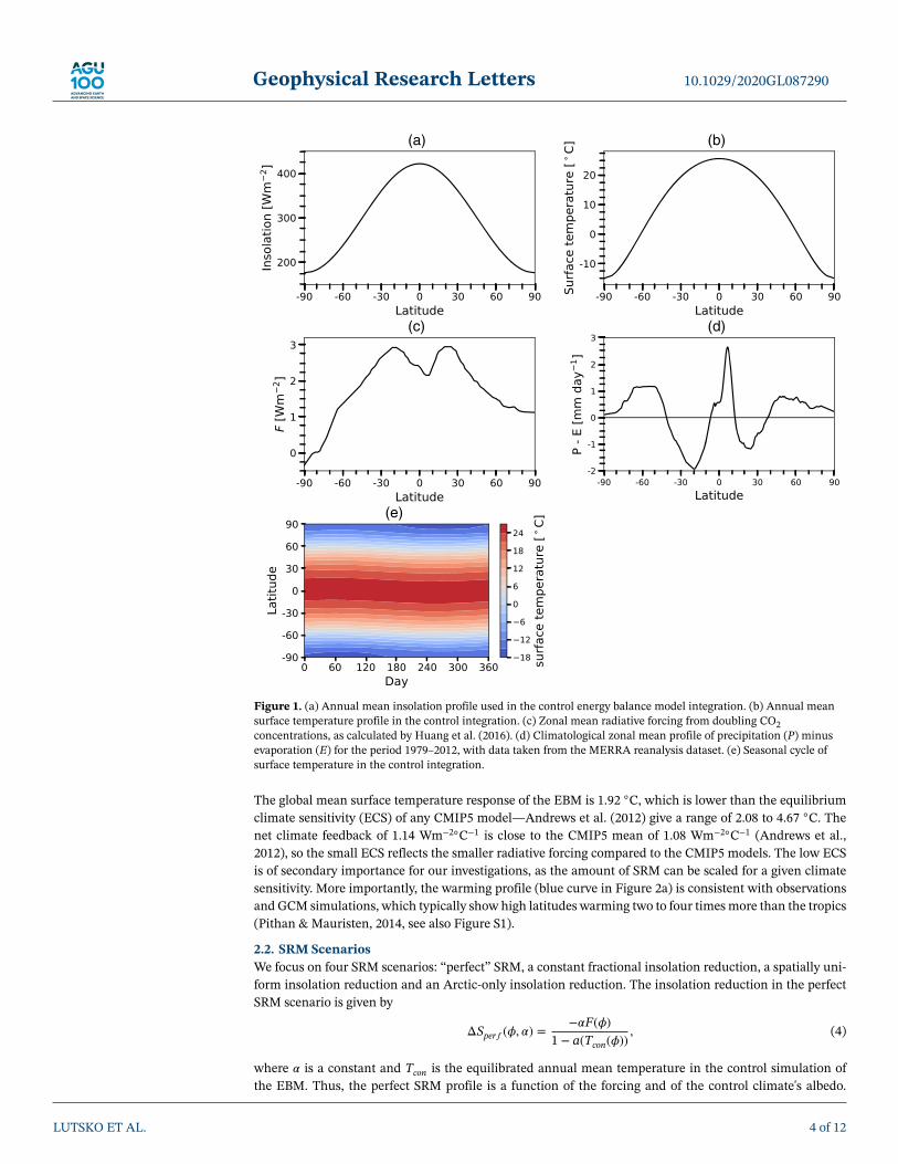
The EBM is numerically integrated with a second-order finite difference discretization for the diffusionoperator and a fourth-order Runge-Kutta time-stepping scheme (see Wagner & Eisenman, 2015, for details).The model domain spans both hemispheres (90◦S to 90◦N), with 360 grid points spaced uniformly in x.Model simulations last 100 model years, unless stated otherwise, with averages taken over the last year ofeach integration (the model equilibrates after roughly 20 years and has no internal variability, so averagingover the final year of the simulations is sufficient to obtain the true responses.). The parameter settings usedin our simulations are given in the supporting information, Table S 1, and the annual mean control (i.e., noSRM) insolation profile is shown in Figure 2a. In the absence of radiative forcing (F = 0), the moist EBMproduces an Earth-like surface temperature distribution, with a global mean surface temperature of 15.3 ◦C,an equator-to-pole temperature difference of 40 ◦C (Figure 1b), and a reasonable seasonal cycle of surfacetemperature (Figure 1e).

2.1. Response to 2XCO2To mimic global warming, we set F(𝜙) to the doubled CO2 radiative forcing profile calculated by Huang et al.(2016) (Figure 1c). This forcing is strongest in the subtropics and smallest at high latitudes (in fact, it is nega-tive over Antarctica) and was calculated directly with a radiative transfer code (we refer the reader to Huanget al., 2016, for more details). Hence, the forcing does not include the “rapid adjustments” which are oftenincluded as part of the radiative forcing from increased CO2 concentrations, and the global mean forcingof 2.2 Wm−2 is about 33% smaller than the typical global mean forcing in Coupled Model IntercomparisonProject Phase 5 (CMIP5) models (Forster et al., 2013). Nevertheless, this profile is a reasonable first-orderestimate of F(𝜙)2XCO2

, and it will be shown below that the latitudinal profile of the forcing is crucial forevaluating the potential impacts of SRM scenarios.

LUTSKO ET AL. 3 of 12

Geophysical Research Letters 10.1029/2020GL087290

Figure 1. (a) Annual mean insolation profile used in the control energy balance model integration. (b) Annual meansurface temperature profile in the control integration. (c) Zonal mean radiative forcing from doubling CO2concentrations, as calculated by Huang et al. (2016). (d) Climatological zonal mean profile of precipitation (P) minusevaporation (E) for the period 1979–2012, with data taken from the MERRA reanalysis dataset. (e) Seasonal cycle ofsurface temperature in the control integration.

The global mean surface temperature response of the EBM is 1.92 ◦C, which is lower than the equilibriumclimate sensitivity (ECS) of any CMIP5 model—Andrews et al. (2012) give a range of 2.08 to 4.67 ◦C. Thenet climate feedback of 1.14 Wm−2◦C−1 is close to the CMIP5 mean of 1.08 Wm−2◦C−1 (Andrews et al.,2012), so the small ECS reflects the smaller radiative forcing compared to the CMIP5 models. The low ECSis of secondary importance for our investigations, as the amount of SRM can be scaled for a given climatesensitivity. More importantly, the warming profile (blue curve in Figure 2a) is consistent with observationsand GCM simulations, which typically show high latitudes warming two to four times more than the tropics(Pithan & Mauristen, 2014, see also Figure S1).

2.2. SRM ScenariosWe focus on four SRM scenarios: “perfect” SRM, a constant fractional insolation reduction, a spatially uni-form insolation reduction and an Arctic-only insolation reduction. The insolation reduction in the perfectSRM scenario is given by

ΔSper𝑓 (𝜙, 𝛼) =−𝛼F(𝜙)

1 − a(Tcon(𝜙)), (4)

where 𝛼 is a constant and Tcon is the equilibrated annual mean temperature in the control simulation ofthe EBM. Thus, the perfect SRM profile is a function of the forcing and of the control climate's albedo.

LUTSKO ET AL. 4 of 12

Geophysical Research Letters 10.1029/2020GL087290

Figure 2. (a) Equilibrated, annual mean responses of the EBM's surface temperature to the radiative forcing from adoubling of CO2 concentrations (blue curve) and to the strong SRM interventions (green, orange, red, and gray curves).(b) Insolation reductions in the four strong solar radiation modification interventions. (c) Same as Panel (a) but for P -E, calculated using equation (8). (d) Same as Panel (a) but for the moist static energy. (e) Same as Panel (a) but for themeridional moist static energy (MSE) transport.

“Moderate” SRM is defined as 𝛼 = 0.5 (Keith & MacMartin, 2015), and “strong” SRM as 𝛼 = 1, which exactlycancels the forcing and restores the local radiative balance. The 𝛼 = 0.5 case does not cancel the forcingcompletely, so it may not be the optimal profile for moderate SRM, in terms of compensating for the effectsof global warming.

In the fractional reduction scenario S is reduced by the same fractional amount at all latitudes, as is commonin GCM simulations in which the solar constant is reduced. The fraction is chosen so that the global meaninsolation reduction is the same as in the moderate and strong perfect SRM scenarios:

ΔS𝑓 rac = −𝛽% × S(𝜙), (5)

where 𝛽 = ΔSper𝑓 (𝛼)

S(𝜙)× 100, with overlines denoting global means. 𝛽 = 0.48% and 0.96% in the moderate and

strong SRM scenarios, respectively. In the spatially uniform scenario the insolation is reduced at all latitudesby the global mean reduction in the perfect SRM scenario:

ΔS𝑓 rac = −ΔSper𝑓 (𝛼). (6)

ΔSper𝑓 is equal to 1.66 and 3.2 Wm−2 in the moderate and strong SRM scenarios, respectively. The Arctic-onlycase assumes SRM is only deployed at high northern latitudes, which has been suggested as a means of“refreezing” the Arctic while leaving the climates of lower latitudes unperturbed (Caldeira & Wood, 2008;Robock et al., 2008). In this case we set the insolation reduction at high latitudes to double the global meanreduction in the perfect SRM scenario (the choice of insolation reduction in the Arctic-only case is arbitrary,

LUTSKO ET AL. 5 of 12

Geophysical Research Letters 10.1029/2020GL087290

Figure 3. (a) Equilibrated, annual mean responses of the energy balance model's surface temperature to the radiativeforcing from a doubling of CO2 concentrations (blue curve) and to the moderate solar radiation modification (SRM)interventions (green, orange, red, and gray curves). The purple curve shown an SRM scenario designed to provide evengreater compensation of mean warming than the spatially uniform SRM, under moderate insolation reduction.(b) Insolation reductions in the four moderate SRM interventions and in the polar-amplified SRM scenario (purple).(c) Same as Panel (a) but for P - E, calculated using equation (8). (d) Same as Panel (a) but for the moist static energy.(e) Same as Panel (a) but for the meridional moist static energy (MSE) transport.

and we have used a large reduction to emphasize how inefficient the Arctic-only SRM is for counteringincreased CO2 concentrations.):

ΔS𝑓 rac = −ΔSper𝑓 (𝛼)[1 + tanh((𝜙 − 70◦)∕4◦)

], (7)

so that the insolation is only reduced poleward of 60◦N.

The annual mean insolation reductions in the strong SRM scenarios are shown in Figure 2b and in themoderate SRM scenarios in Figure 3b. The perfect SRM profile has the most typically-amplified profile ofinsolation reduction, with large reductions in the tropics and subtropics, and weak reductions near the poles,though the constant fractional SRM has a relatively similar pattern of insolation reduction, reflecting thefact that, in the absence of rapid adjustments, CO2 radiative forcing (and hence the perfect SRM) is alsotropically enhanced.

Note that in winter the spatially uniform, perfect SRM and Arctic-only scenarios would result in theinsolation being negative at high latitudes, so we set S to zero whenever this is the case.

3. Comparing SRM Scenarios3.1. Strong SRMThe annual mean temperature responses in the four strong SRM scenarios are shown by the red, orange,green, and gray curves in Figure 2a (see Figure S2 for seasonal responses). As expected, the perfect SRM

LUTSKO ET AL. 6 of 12

Geophysical Research Letters 10.1029/2020GL087290

compensates the warming exactly (green curve) (on seasonal timescales there is some residual warmingbecause we have used the annual mean temperature profile to define the perfect SRM profile, but this can beeliminated by prescribing a seasonally varying perfect SRM profile.). By contrast, the uniform fractional andspatially uniform cases overcool the climate system, particularly at high latitudes (red and orange curvesin Figure 2a, though note that there is a small residual warming at high northern latitudes in the uniformfractional case), leading to global mean coolings of −0.04 ◦C in the uniform fractional case and −0.21 ◦C inthe spatially uniform case. The stronger insolation reductions at high latitudes, relative to the perfect SRM,thus enhance the high-latitude albedo relative to the control climate in these scenarios, resulting in globalmean coolings.

The results of the strong uniform fractional and spatially uniform cases contrast with GCM studies, whichhave generally found that GCMs overcool in the tropics and have residual warming at high latitudes whenSRM interventions are applied (Govindasamy et al., 2003; Kravitz et al., 2013). However, this is a reflection ofthe strong polar amplification of warming, as the total cooling of the high latitudes is larger than the coolingof the tropics in these simulations (e.g., Figure 1 of Kravitz et al., 2013). Thus, our results are consistentwith the finding that SRM interventions lead to larger responses at high latitudes, and the fact that thepolar regions, rather than the tropics, experience overcooling in the EBM suggests that the diffusivity (D)or the ice-albedo feedback are stronger in our simulations than the effective diffusivities and high-latitudefeedbacks in typical GCMs, though we have not investigated this further.

The insolation reduction at high northern latitudes is larger in the Arctic-only case than in any of the otherSRM cases (Figure 2b) but the temperature compensation is much smaller—∼ 2 ◦C at most—highlightingthe role of energy transport for high-latitude warming. This compensation is mostly limited to north of 60◦N,and the global mean warming is slightly reduced to 1.78 ◦C in this scenario.

In addition to the temperature responses, the EBM can be used to estimate how the strength of the hydro-logic cycle would respond in these scenarios. To first order, changes in zonal mean precipitation minusevaporation (P − E) can be well approximated by assuming that changes in lower tropospheric water vapormixing ratios dominate over changes in the flow field (Held & Soden, 2006). Neglecting changes in moisturetransports, the response of P − E to a perturbation is then given by:

Δ(P − E) ≈ 𝛾ΔT(P − E), (8)

where 𝛾 ∼7% K−1. So the changes in P − E are large where the climatological P − E is large, and vice versa,following the “wet get wetter, dry get drier” paradigm. The climatological zonal mean profile of P−E, takenfrom the MERRA reanalysis dataset (Rienecker et al., 2011), is shown in Figure 1d. P−E is large and positivein the deep tropics, particularly over the Intertropical Convergence Zone in the Northern Hemisphere trop-ics, and large and negative in the subtropics, where most evaporation takes place. P − E is relatively smallat mid- and high-latitudes, where there is more precipitation than evaporation.

Figure 2c shows the changes in P − E predicted by combining equations (1) and (8) and using the climato-logical P − E. The global warming case shows an amplification of the climatological pattern with warming,which is exactly compensated by the perfect SRM, and is overcompensated by the uniform fractional andspatially uniform scenarios, especially at midlatitudes. This is as expected from the temperature changes.The Arctic SRM produces a small compensation of the changes in P − E at high latitudes in the NorthernHemisphere.

Finally, the EBM can provide insight into how horizontal atmospheric energy transports would change inthe various scenarios. The diffusive energy transport parameterization crudely represents the transport ofMSE, which in reality is achieved predominantly by the atmosphere's mean flow in the tropics and by eddiesat higher latitudes (e.g., Trenberth & Solomon, 1994; Trenberth & Stepaniak, 2003, see Figure S3 for theMSE transport in the control simulation). While it is difficult to infer how changes in MSE transport arepartitioned between eddies and the mean flow (e.g., see Figure 3a of Armour et al., 2019), they still give afirst-order indication of how the atmosphere's large-scale circulation responds to a given perturbation.

In the global warming simulation the meridional MSE gradients are increased between the tropics and themidlatitudes (blue curve in Figure 2d), leading to enhanced poleward MSE fluxes up to about 45◦ in eachhemisphere (Figure 2e). At higher latitudes the strong polar amplification of warming decreases the MSEgradient, and there are large reductions in the MSE transport to high latitudes in the equilibrated state.

LUTSKO ET AL. 7 of 12

Geophysical Research Letters 10.1029/2020GL087290

Climate model simulations typically find a larger increase in the meridional MSE transport at low andmidlatitudes, and a smaller reduction (or even a small increase) of the meridional MSE transport at highlatitudes, than seen here (Huang & Zhang, 2014; Zelinka & Hartmann, 2012). Our assumption of a spatiallyuniform radiative feedback (which also does not account for cloud changes) is likely a major factor in thisdiscrepancy (Huang & Zhang, 2014).

The perfect SRM exactly compensates the changes in the MSE profile, restoring the zonal mean MSE, andby extension the meridional energy transport, back to the control profile (green curves in Panels d and eof Figure 2). The overcooling of the high latitudes in the uniform fractional and spatially uniform scenar-ios cause strong reductions in the high-latitude MSE, so that in equilibrium the poleward MSE transportsincrease in these scenarios (Figure 2e, note again that in the Northern Hemisphere of the uniform fractionalcase the residual MSE transport is small). This further cools the tropics, as in both scenarios the low lati-tudes export more energy to high latitudes. The Arctic SRM substantially reduces the change in the NorthernHemisphere MSE gradient (gray curve in Figure 2e), compensating for a large fraction of the change inenergy transport at high northern latitudes (Figure 2e), though there is increased energy transport at lowand midlatitudes compared to the 2XCO2 scenario.

These circulation changes are sensitive to the details of our setup and ignore changes in the diffusivity D, sowe caution against overinterpreting the results shown here. However, these calculations illustrate that theprofile of insolation reduction can have a large impact on the response of the meridional MSE gradient and,by extension, on the atmosphere's large-scale circulation.

3.2. Moderate SRMFor moderate (𝛼 = 0.5) SRM, the perfect SRM, uniform fractional, and spatially uniform scenarios compen-sate slightly less than half of the temperature change in the 2XCO2 scenario (Figure 3a, seasonal responsesin Figure S4), with the global mean warming reduced to 1.08 ◦C in the perfect SRM scenario, 1.08 ◦C in theuniform fractional scenario and 1.03 ◦C in the spatially uniform scenario. The compensation of warming isvery similar between about 45◦S and 45◦N in all three cases, but the compensation at midlatitude and highlatitude is substantially larger for the spatially uniform case, resulting in smaller residual warming. The per-fect SRM compensates more of the high-latitude warming in the Northern Hemisphere than the uniformfractional SRM does but less of the high-latitude warming in the Southern Hemisphere, reflecting interhemi-spheric differences in the forcing (Figure 1c). The Arctic-only case is again ineffective at compensating thewarming, with the largest temperature difference from the 2XCO2 being only ∼1 ◦C, and the global meanwarming slightly reduced to 1.85 ◦C in this scenario.

The perfect SRM, uniform fractional, and spatially uniform scenarios result in substantial (∼50%) compen-sations of the changes in the hydrologic cycle at all latitudes (Figure 3c), and, following the temperaturechanges, the compensations are similar in the tropics, but the spatially uniform case compensates for moreof the changes at higher latitudes. The Arctic SRM produces a small compensation of Δ(P − E) at highlatitudes in the Northern Hemisphere.

The perfect SRM and uniform fractional cases result in relatively flat residual MSE responses in the trop-ics and subtropics (green and red curves in Figure 2d), so that the residual changes in the MSE transportare small (green and red curves in Figure 2e). In the spatially uniform case the MSE gradients betweenthe tropics and the midlatitudes are similar to the global warming case (even though the MSE response issmaller), so the MSE transport at low latitudes is relatively unaffected compared to the global warming case(compare blue and orange curves in Figure 2e). However, at higher latitudes the residual MSE transport ismuch smaller in the spatially uniform case than in the perfect SRM and uniform fractional cases, reflectingthe greater compensation of warming at high latitudes. Thus, the perfect SRM and uniform fractional casesprovide a better compensation of the meridional MSE gradient at low latitudes than the spatially uniformcase, while the spatially uniform case provides a better compensation at higher latitudes. The Arctic-onlycase compensates for some of the reduction in meridional MSE transport in the Northern Hemisphere butmuch less than the other three scenarios.

In summary, under a moderate SRM scenario the “perfect” SRM is not optimal, and a more polar-amplifiedinsolation reduction profile (i.e., with a larger insolation reduction at high latitudes compared to the perfectSRM) is most effective at compensating for warming. The spatially uniform profile provides the greatest

LUTSKO ET AL. 8 of 12

Geophysical Research Letters 10.1029/2020GL087290

Figure 4. (a) Annual and global mean temperature response for a simulation in which the forcing is linearly increased with time, reaching a value equal to adoubling of CO2 after 70 years (black curve). The colored curves show mean temperatures during branching simulations in which perfect SRM is implementedevery 10 years. The round markers show the global mean temperature response after the SRM has been implemented for 200 years. (b) Same as Panel (a) butthe uniform fraction SRM is implemented every 10 years, with the same global mean insolation reduction as in the corresponding perfect SRM branchingsimulations. (c) Same as Panel (a) but the spatially uniform SRM is implemented every 10 years, with the same global mean insolation reduction as in thecorresponding perfect SRM branching simulations.

compensation of warming, of P− E and of the changes to the MSE gradient among the four SRM scenarios.This is consistent with the fact that the pattern of warming in response to CO2 forcing is polar-amplified.

We have experimented with various polar-amplified insolation profiles and found that these can provideeven greater compensation of warming than the spatially uniform SRM under moderate SRM, particularlywhen there are minima in insolation reduction at midlatitudes. The purple lines in Figure 3 show an exampleof a profile given by

ΔSPA(𝜙, 𝛼) = 𝜇 × ([1 + 3∕4 tanh((𝜙 − 70◦)∕10◦)

]+[1 + tanh((𝜙 − 80◦)∕5◦)

]∕2 + W(𝜙)), (9)

where 𝜇 is scaled to ensure that the global mean insolation reduction is the same as in the perfect SRM casewith 𝛼 = 0.5 and

W(𝜙) ={

cos(|𝜙|) if |𝜙| ≤ 45◦

0 if |𝜙| > 45◦.

This profile has a large insolation reduction at high (>70◦) latitudes, weaker insolation reduction at mid-latitudes, and a secondary insolation reduction maximum in the deep tropics (Figure 3b) but keeps theglobal-mean insolation reduction the same as in the other moderate scenarios.

The new polar-amplified SRM profile provides even more compensation of warming than the spatiallyuniform SRM (global mean ΔT = 0.99 ◦C), more compensation of the P − E changes, and much bettercompensation of the MSE gradient and hence of the meridional energy transport changes.

4. State Dependence of SRM InterventionsTo investigate the state dependence of SRM, we have performed an experiment in which the forcing islinearly increased for 70 years, with the increments scaled so that F(𝜙) = F2XCO2(𝜙) after 70 years. Thismimicks the forcing in transient warming experiments in which the CO2 concentration is increased by 1%per year, leading to a doubling after 70 years. Every 10 years of the transient simulation, three new simula-tions are branched off in which the forcing is kept fixed, and the three major SRM interventions (perfect,fractionally-uniform and spatially-uniform) are applied. The insolation reductions are scaled so that the per-fect SRM cancels the forcing exactly in each branch, and the branch simulations are run for a further 200model years.

Figure 4 shows the global mean surface temperature responses in the three sets of branching simulations.When the perfect SRM is applied, the final equilibrated state is always the same (Panel a), as the EBM isrestored exactly back to the control climate. In this case then, the effectiveness of the SRM does not dependon when it is applied. By contrast, in the uniform fractional and, especially, the spatially uniform cases

LUTSKO ET AL. 9 of 12

Geophysical Research Letters 10.1029/2020GL087290

the final equilibrated states do depend on when the SRM is implemented (Panels b and c). In the uniformfractional case the equilibrium global mean surface temperature cools progressively as the SRM is appliedlater and later, so that if it is applied after 70 years the EBM is −0.04 ◦C cooler than if the SRM is appliedafter 10 years. In the spatially uniform case the EBM is −0.19 ◦C cooler when the SRM is applied after70 years than when it is applied after 10 years, primarily due to strong polar cooling, as seen in the strongSRM calculations of section 3.1.

We have found that the state dependence of the SRM interventions can be eliminated by disabling the icealbedo feedback, which we do by fixing the albedo profile as a(x) = 1 − a0 − a2P2(x), with a0 = 0.68 anda2 = −0.2, following Merlis and Henry (2018). Even with the spatially uniform SRM, the equilibrated statesare the same in this setup, regardless of when the SRM is applied (Figure S5). This demonstrates that thenonlinearity of the interactive ice albedo feedback is responsible for a state dependence in the EBM, causingthe effectiveness of certain SRM interventions to depend on when they are applied.

5. ConclusionUncertainty around SRM arises both from uncertainty in estimating the impact of a specific climate inter-vention and from the range of potential SRM methods and climate objectives (Ban-Weiss & Caldeira, 2010;Keith, 2013; Kravitz et al., 2016; MacMartin & Kravitz, 2019). The design challenge of SRM thus involvesaccurately predicting, and understanding, the climate's response to a large number of relevant scenarios.Most studies of SRM have used comprehensive GCMs, which allow for detailed investigations of the poten-tial impacts of SRM interventions but limit the ability to explore trade-offs between objectives and to gaina fundamental understanding of the climate dynamics that determine the response to SRM. Here, we haveused an idealized moist EBM to explore how the latitudinal profile of insolation reduction affects the climateimpacts of SRM. Using simple models builds understanding at a more basic level and provides insights intoregions of the SRM intervention design space, which can then be explored with GCMs. Our main findingsare as follows:

• The optimal SRM profile, in terms of countering the climate impacts of increased CO2 concentra-tions per Wm−2 of insolation reduction, depends on how much insolation reduction is applied. A morepolar-amplified SRM profile is most effective for weak/moderate SRM interventions, while a moretropically amplified SRM profile is most effective for strong SRM interventions.

• Given the latitudinal structures of the radiative forcing and the albedo in the control climate, a “perfect”SRM profile can be defined, which exactly cancels the forcing when strong SRM is applied. For weakerSRM interventions, however, this “perfect” profile is not the optimal profile of insolation reduction(see above item). We also note that the perfect SRM profile is an artifact of the simplicity of the EBM,which has a single state variable (T). Hence, by eliminating the temperature change, the perfect SRM alsoexactly cancels the changes in P − E and in the meridional energy transports. This would not likely bethe case in a GCM, as there may, for instance, be residual precipitation changes even if the temperaturechange is exactly compensated (see, e.g., Bala et al., 2008).

• When evaluating the potential impacts of an SRM intervention, it is important to consider the meridionaltemperature and moist static energy gradients, in addition to more common metrics such as temperatureand P − E. Since these meridional gradients are the drivers of the large-scale atmospheric circulation,compensating for their changes is key to minimizing the disruption to the atmospheric circulation. Exper-iments with GCMs could build on these results to explore how midlatitude eddy intensity depends on thelatitudinal gradient of SRM forcing.

• Arctic-only SRM is ineffective at countering the effects of global warming, as it ignores the horizontalenergy transports that are responsible for a substantial fraction of high-latitude warming.

• The impacts of SRM interventions depend on how much insolation reduction is required. The greaterthe forcing, and the more insolation reduction is required to counteract the forcing, the more likely anSRM intervention is to overcool (or undercool) the climate system. Verifying that this holds in GCMs isan urgent extension of the present work.

We hope that these results, obtained in the idealized setting of a moist EBM, can help guide future investi-gations with comprehensive climate models, and also provide confidence that certain aspects of the climatesystem's response to these SRM scenarios can be understood at a basic level. Future extensions of this workcould include investigating how the results are affected by using a meridionally varying surface relative

LUTSKO ET AL. 10 of 12

Geophysical Research Letters 10.1029/2020GL087290

humidity and by using spatially-varying temperature feedbacks (Roe et al., 2015), as well as the use of sim-ple theories for how atmospheric diffusivity changes with climate (Shaw & Voigt, 2016). Moving forward,it is clear that both idealized modeling work and comprehensive climate model simulations are needed tofully understand the benefits and trade-offs of the various proposed SRM scenarios, following the “modelhierarchy” approach which is central to modern climate science (Held, 2005).

ReferencesAndrews, T., Gregory, J. M., Webb, M. J., & Taylor, K. E. (2012). Forcing, feedbacks and climate sensitivity in CMIP5 coupled

atmosphere-ocean climate models. Geophysical Research Letters, 39, L09712. https://doi.org/10.1029/2012GL051607Armour, K. C., Eisenman, I., Blanchard-Wrigglesworth, E., McCusker, K. E., & Bitz, C. M. (2011). The reversibility of sea ice loss in a

state-of-the-art climate model. Geophysical Research Letters, 38, L16705. https://doi.org/10.1029/2011GL048739Armour, K. C., Siler, N., Donohoe, A., & Roe, G. H. (2019). Meridional atmospheric heat transport constrained by energetics and mediated

by large-scale diffusion. Journal of Climate, 32(12), 3655–3680.Bala, G., Duffy, P. B., & Taylor, K. E. (2008). Impact of geoengineering schemes on the global hydrological cycle. Proceedings of the National

Academy of Sciences, 105(22), 7664–7669.Ban-Weiss, G. A., & Caldeira, K. (2010). Geoengineering as an optimization problem. Environmental Research Letters, 5, 34,009.Budyko, M. L. (1969). The effect of solar radiation on the climate of the Earth. Tellus, 21, 611–619.Budyko, M. L. (1974). Simple albedo feedback models of the icecaps. Tellus, 26, 613–629.Budyko, M. L. (1977). On present-day climatic changes. Tellus, 29, 193–204.Caballero, R., & Hanley, J. (2012). Midlatitude eddies, storm-track diffusivity, and poleward moisture transport in warm climates. Journal

of the Atmospheric Sciences, 69(630), 3237–3250.Caldeira, K., & Wood, L. (2008). Global and Arctic climate engineering: Numerical model studies. Philosophical Transactions of the Royal

Society A: Mathematical, Physical and Engineering Sciences, 366(1882), 4039–4056.Council, N. R. (2015). Climate intervention: Reflecting sunlight to cool earth. Washington, DC: The National Academies Press.Dai, Z., Weisenstein, D. K., & Keith, D. W. (2018). Tailoring meridional and seasonal radiative forcing by sulfate aerosol solar geoengineer-

ing. Geophysical Research Letters, 45, 1030–1039. https://doi.org/10.1002/2017GL076472Eisenman, I., & Wettlaufer, J. S. (2009). Nonlinear threshold behavior during the loss of Arctic sea ice. Proceedings of the National Academy

of Sciences, 106(1), 28–32.Flannery, B. P. (1984). Energy balance models incorporating transport of thermal and latent energy. Journal of the Atmospheric Sciences,

41(3), 414–421.Forster, P. M., Andrews, T., Good, P., Gregory, J. M., Jackson, L. S., & Zelinka, M. (2013). Evaluating adjusted forcing and model spread for

historical and future scenarios in the CMIP5 generation of climate models. Journal of Geophysical Research: Atmospheres, 118, 1139–1150.https://doi.org/10.1002/jgrd.50174

Frierson, D. M. W., Held, I. M., & Zurita-Gotor, P. (2007). A gray-radiation aquaplanet moist GCM. Part II: Energy transports in alteredclimates. Journal of the Atmospheric Sciences, 64(23), 1680–1693.

Govindasamy, B., Caldeira, K., & Duffy, P. B. (2003). Geoengineering Earth's radiation balance to mitigate climate change from aquadrupling of CO2. Global and Planetary Change, 37, 157–168.

Gregory, J. M., Stott, P. A., Cresswell, D. J., Rayner, N. A., Gordon, C., & Sexton, D. M. H. (2002). Recent and future changes in Arctic seaice simulated by the HadCM 3 AOGCM. Geophysical Research Letters, 29(24), 2175. https://doi.org/10.1029/2001GL014575

Held, I. M. (2005). The gap between simulation and understanding in climate modeling. Bulletin of the American Meteorological Society,86(11), 1609–1614.

Held, I. M., & Soden, B. J. (2006). Robust responses of the hydrological cycle to global warming. Journal of Climate, 19(21), 5686–5699.Huang, Y., Tan, X., & Xia, Y. (2016). Inhomogeneous radiative forcing of homogeneous greenhouse gases. Journal of Geophysical Research:

Atmospheres, 121, 2780–2789. https://doi.org/10.1002/2015JD024569Huang, Y., & Zhang, M. (2014). The implication of radiative forcing and feedback for meridional energy transport. Geophysical Research

Letters, 41, 1665–1672. https://doi.org/10.1002/2013GL059079Irvine, P. J., Kravitz, B., Lawrence, M. G., & Muri, H. (2016). An overview of the Earth system science of solar geoengineering. WIREs

Climate Change, 7(6), 815–833.Keith, D. (2013). A case for climate engineering. Cambridge, Massachusetts: MIT Press.Keith, D., & MacMartin, D. G. (2015). A temporary, moderate and responsive scenario for solar geoengineering. Nature Climate Change, 5,

201–206.Kravitz, B., Caldeira, K., Boucher, O., Robock, A., Rasch, P. J., Alterskjær, K., et al. (2013). Climate model response from the Geoengineering

Model Intercomparison Project (GeoMIP). Journal of Geophysical Research: Atmospheres, 118, 8320–8332. https://doi.org/10.1002/jgrd.50646

Kravitz, B., MacMartin, D. G., Mills, M. J., Richter, J. H., Tilmes, S., Lamarque, J.-F., et al. (2017). First simulations of designing stratosphericsulfate aerosol geoengineering to meet multiple simultaneous climate objectives. Journal of Geophysical Research: Atmospheres, 122,12,616–12,634. https://doi.org/10.1002/2017JD026874

Kravitz, B., MacMartin, D. G., Wang, H., & Rasch, P. J. (2016). Geoengineering as a design problem. Earth System Dynamics, 7(2), 469–497.Kravitz, B., Robock, A., Boucher, O., Schmidt, H., Taylor, K. E., Stenchikov, G., & Schulz, M. (2011). The Geoengineering Model

Intercomparison Project (GeoMIP). Atmospheric Science Letters, 12(2), 162–167.Lawrence, M. G. (2005). The relationship between relative humidity and the dewpoint temperature in moist air: A simple conversion and

applications. Bulletin of the American Meteorological Society, 86(2), 225–234.Lutsko, N. J. (2020). SRM_EBM. https://doi.org/10.5281/zenodo.3738668MacMartin, D. G., Keith, D. W., Kravitz, B., & Caldeira, K. (2013). Management of trade-offs in geoengineering through optimal choice of

non-uniform radiative forcing. Nature Climate Change, 3(4), 365–368.MacMartin, D. G., & Kravitz, B. (2019). Mission-driven research for stratospheric aerosol geoengineering. Proceedings of the National

Academy of Sciences, 116(4), 1089–1094.Merlis, T. M. (2014). Interacting components of the top-of-atmosphere energy balance affect changes in regional surface temperature.

Geophysical Research Letters, 41, 7291–7297. https://doi.org/10.1002/2014GL061700

AcknowledgmentsWe thank Kate Ricke for the helpfulconversations and feedback and twoanonymous reviewers, whose closereadings and comments substantiallyimproved the manuscript. Data werenot used, nor created for this research,but a Jupyter notebook with the modeland analysis code for the figures in themain text and supplement is availableat Lutsko (2020).

LUTSKO ET AL. 11 of 12

Geophysical Research Letters 10.1029/2020GL087290

Merlis, T. M., & Henry, M. (2018). Simple estimates of polar amplification in moist diffusive energy balance models. Journal of Climate,31(15), 5811–5824.

Modak, A., & Bala, G. (2014). Sensitivity of simulated climate to latitudinal distribution of solar insolation reduction in solar radiationmanagement. Atmospheric Chemistry and Physics, 14(15), 7769–7779.

North, G. R. (1975). Theory of energy-balance climate models. Journal of the Atmospheric Sciences, 32(11), 2033–3043.North, G. R., Cahalan, R. F., & Coakley, J. A. (1981). Energy balance climate models. Reviews of Geophysics, 19(1), 91–121.North, G. R., Cahalan, R. F., & Coakley, J. A. (1984). The small ice cap instability in diffusive climate models. Journal of the Atmospheric

Sciences, 41(23), 3390–3395.Pithan, F., & Mauristen, T. (2014). Arctic amplification dominated by temperature feedbacks in contemporary climate models. Nature

Geoscience, 7(15), 181–184.Rienecker, M. M., Suarez, M. J., Gelaro, R., Todling, R., Bacmeister, J., Liu, E., et al. (2011). MERRA: NASA's modern-era retrospective

analysis for research and applications. Journal of Climate, 24, 3624–3648.Robock, A., Oman, L., & Stenchikov, G. L. (2008). Regional climate responses to geoengineering with tropical and Arctic SO2 injections.

Journal of Geophysical Research, 113, D16101. https://doi.org/10.1029/2008JD010050Roe, G. H., Feldl, N., Armour, K. C., Hwang, Y.-T., & Frierson, DarganM. W. (2015). The remote impacts of climate feedbacks on regional

climate predictability. Nature Geoscience, 8(2), 135–139.Rose, BrianE. J., Armour, K. C., Battisti, D. S., Feldl, N., & Koll, DanielD. B. (2014). The dependence of transient climate sensitivity and

radiative feedbacks on the spatial pattern of ocean heat uptake. Geophysical Research Letters, 41, 1071–1078. https://doi.org/10.1002/2013GL058955

Rose, BrianE. J., & Marshall, J. (2009). Ocean heat transport, sea ice, and multiple climate states: Insights from energy balance models.Journal of the Atmospheric Sciences, 66(9), 2828–2843.

Sellers, WD (1969). A global climatic model based on the energy balance of the earth-atmosphere system. Journal of Applied Meteorology,8, 392–400.

Shaw, T. A., & Voigt, A. (2016). What can moist thermodynamics tell us about circulation shifts in response to uniform warming?Geophysical Research Letters, 43, 4566–4575. https://doi.org/10.1002/2016GL068712

Smith, C. J., Kramer, R. J., Myhre, G., Forster, P. M., Soden, B. J., Andrews, T., et al. (2018). Understanding rapid adjustments to diverseforcing agents. Geophysical Research Letters, 45, 12,023–12,031. https://doi.org/10.1029/2018GL079826

Tilmes, S., Fasullo, J., Lamarque, J.-F., Marsh, D. R., Mills, M., Alterskær, K., et al. (2013). The hydrological impact of geoengineering in theGeoengineering Model Intercomparison Project (GeoMIP). Journal of Geophysical Research: Atmospheres, 118, 11,036–11,058. https://doi.org/10.1002/jgrd.50868

Trenberth, K. E., & Solomon, A. (1994). The global heat balance: Heat transports in the atmosphere and ocean. Climate Dynamics, 10,107–134.

Trenberth, K. E., & Stepaniak, D. P. (2003). Seamless poleward atmospheric energy transports and implications for the Hadley circulation.Journal of Climate, 16, 3706–3722.

Wagner, TillJ. W., & Eisenman, I. (2015). How climate model complexity influences sea ice stability. Journal of Climate, 28(10), 3998–4014.Winton, M. (2011). Do climate models underestimate the sensitivity of Northern Hemisphere sea ice cover?. Journal of Climate, 24(15),

3924–3934.Zelinka, M. D., & Hartmann, D. L. (2012). Climate feedbacks and their implications for poleward energy flux changes in a warming climate.

Journal of Climate, 25(2), 608–624.

LUTSKO ET AL. 12 of 12