Estimating Historical Wage Profiles - Wabash Collegepersweb.wabash.edu/facstaff/burnettj/EstimatingProfiles.pdfEstimating Historical Wage Profiles Joyce Burnette and Maria Stanfors

Estimating Historical Wage Profiles

Joyce Burnette and Maria Stanfors In 1974 Jacob Mincer suggested that the wage profiles of US workers could best be

described as a quadratic function of experience. Following Mincer, most labor economists use a

quadratic specification for experience-wage profiles (see Albrecht, Edin, Sundstrom and

Vroman, 1999; Anderson, Binder, and Krause, 2003; Blau and Kahn, 2003). Labor historians

have also favored the quadratic specification. Eichengreen (1984) uses a quadratic function of

experience to examine the wages of California workers in 1892. McHugh (1988) estimates the

earnings of workers at a North Carolina mill c. 1900 as a quadratic function of experience.

Goldin (1990) uses a quadratic function of either age or experience, depending on the data set.

Unfortunately the quadratic specification can be misleading. Murphy and Welch (1990)

examine the biases of the quadratic age-experience profile and conclude that it “results in

significantly biased estimates of the earnings profile” (p. 203). Specifically, they conclude that

The quadratic overstates initial earnings for all schooling groups and understates earnings at 10 years of experience for all groups. The quadratic also overstates earnings at midcareer and understates actual earnings at retirement. (p. 208)

Murphy and Welch recommend the quartic specification, which includes four powers of

experience rather than just two. In spite of their conclusion that the quadratic specification is

“unacceptable,” it continues to be widely used in labor economics.

Quadratic profiles are also misleading in historical data. Hatton (1997) shows that

quadratic age profiles “underpredict that wage from the age of 20 up to the early 30s and

overpredict it between the early 30s and the early 50s” (p. 41-41). He prefers the quadratic

spline function, which allows the parameters of the quadratic function to change after age 25.

Hatton shows that, while quadratic profiles suggest immigrants had slower wage growth than

natives, profiles based on a quadratic spline suggest that immigrants experienced as much or

more wage growth than natives. While some studies of the historical wage profiles have used

quartic or quadratic spline specifications (Burnette and Stanfors, 2012; Seltzer and Frank, 2007;

Seltzer, 2011), many continue to use the quadratic specification.

The purpose of this paper is to ask whether using quadratic profiles is a mistake. We

compare the quadratic, quartic, and quadratic spline functional forms. We find that the quadratic

profile is clearly inferior to the other two. Use of the quadratic wage profile leads to

underestimation of wage growth before age 25, or before 10 years of experience. Both the

quartic and spline functions are less misleading, but the spline consistently out-performs the

quartic.

DATA

Since we are interested in finding the best functional form for nineteenth-century wages

in general, we use data from three different countries to compare the three functional forms. For

the US and Sweden we have individual-level data from the 1890s. For Britain we have data

from earlier in the century (1833), but the data consists of average wages by age rather than wage

observations for individual workers.

The Swedish data are from the tobacco industry in 1898, and include survey responses

from all cigar firms in the country.1 Workers report weekly earnings, but since weekly hours are

also reported we construct hourly wages. We measure hourly wages in ore per hour, rather than

krona per hour, so that the natural log of the wage is positive.2 The data set does not contain a

measure of years of schooling, so we cannot compute the standard potential experience variable.

However, the survey does ask the worker the year they started in their current occupation. Thus

we do not know total labor market experience, but we do know total experience in the

occupation.

The US data are from a California state survey from 1891-92, and include men and

women working in a wide variety of industries and occupations.3 This data was converted to an

electronic data file by Carter, Ransom, Sutch, and Zhao, and has been used by Eichengreen

(1984) and Hatton (1997). A handful of individuals report an hourly wage, but most report a

daily or weekly wage. Information on hours worked per day is also provided, so daily and

weekly wages are converted to hourly wages. We measure hourly wages in cents per hour. This

1 Specialundersokningar Tobaksindustrien 1898, Statistiska avdelningen, HIII b:1, Kommerskolle- giets arkiv, National Archives (Riksarkivet), Stockholm. 2 An ore is one-hundredth of a krona. 3 Susan Carter, Roger Ransom, Richard Sutch, and Hongcheng Zhao, “Survey of 3493 Wage-Earners in California, 1892” Berkeley: Institute of Business and Economic Research, 1993.

data set does not contain a measure of years of education, but it does provide the age at which the

individual started work, so we construct a potential experience variable by subtracting the age at

which the individual started work from their current age.

For British manufacturing we have the average wage at each age rather than individual

data. The data are from a 1833 parliamentary survey of various manufacturing industries.4 We

use data on workers in the cotton industry in Lancashire and Glasgow and in the wool industry in

Leeds. For each industry the report lists the number of workers at each age and their average

wage. We use the number of workers at each age to weight the averages and the regressions. No

information on hours worked is available, so we report weekly earnings in shillings.

Descriptive statistics are presented in Table 1. In every case females earned lower wages

than males, were younger than males, and had less work experience. The British factory workers

were the youngest, and the Swedish tobacco workers were the oldest. Males in California were

on average 4 years younger than males in the Swedish tobacco industry. The gap in experience

(2.5 years) was smaller than this because experience is defined more broadly for California

workers. For California workers experience measures total experience, the number of years

since the individual started worker, while for the Swedish workers experience measures only the

years in the current occupation.

SPECIFICATIONS

Mincer (1974) recommends wage profiles based on experience rather than age. Most

modern studies use potential experience (age- years of schooling - 6) because actual experience

is rarely available. Potential experience is a noisy estimate of actual experience, but does reflect

the fact that people with more schooling start their working life later. In historical studies the

choice between age or experience is usually determined by the data available. Data on years of

schooling is often not available. We present age-earnings profiles for all three data sets, and

experience-earnings profiles for two data sets. The British data contain information on age only,

but the Californian and Swedish data sets both contain information on experience.

For each data set we compare three different functional forms against the simple

averages. We will compare the quadratic function against two alternatives that have been used in

the literature. The quadratic function is simply

4 “Report from Dr. James Mitchell to the Central Board of Commissioners,” P.P. 1834 (167) XIX.

€

lnwi = β0 + β1ti + β2ti2 +ε i

where t is either age or experience. Male and female profiles are estimated separately. Since in

this paper we are simply interested in how best to measure wage growth we do not include other

controls in the wage equation.

The first alternative is the quartic function, which was suggested by Murphy and Welch

(1990):

€

lnwi = β0 + β1ti + β2ti2 + β3ti

3 + β4ti4 +ε i .

The additional powers of age give the function more freedom to fit the data closely. Murphy and

Welch conclude that the quartic function avoids the mis-specification problems of the quadratic

funciton. The second alternative is the quadratic spline, suggested by Hatton (1997):

€

lnwi = β0 + β1ti + β2ti2 + β3si + β4si

2 +ε i. Here s is spline variable and is equal to

€

si =max[0,ti − k] where k is some constant. The spline allows for two different quadratic functions before and

after the kink-point at k. There is no a priori way to find the best k, but the researcher can try a

variety of potential kink-points and pick one that produces the best fit. In the estimates below we

choose the kink-point by trying at least ten regressions with different kink-points and choosing

the regression that gives the highest R-squared.

To compare the functional forms we graph all three specifications against the average

wage at each age to see which profile best fits that data. We also compare the R-squareds to see

which regression provides the best fit, and examine the residuals. Finally, we compare the

growth of wages implied by the various functional forms.

SWEDEN

We begin by comparing the performance of the quadratic, quartic, and spline functions

for Swedish tobacco workers. Figures 1 and 2 graph the estimated age-wage profiles for male

and female tobacco workers, along with the average wage at each age. The quadratic profile

clearly performs the worst. In both cases the quadratic over-predicts the wage at age 15 and

under-predicts the wage in the early 20s. For men the spline fits average wages better in the

early 20s, an avoids the wage decline in the 30s predicted by the quartic function. For women

the quartic and the spline are quite similar, though the quartic peaks higher and falls more.

To confirm the visual impression, we compare the R-squared’s and examine the residuals

from these regressions. Table 2 reports the R-squared from each regression. These numbers

confirm our impression that the spline fits slightly better than the quartic, while the quadratic

profiles are much worse. We also examine the functional form by examining the residuals.

Figure 3 graphs the average residual at each age from the quadratic profile. If the specification

were correct, the residuals should be random and exhibit no pattern. In fact, we find a definite

pattern in the data. Residuals are negative until age 18 and positive for ages 19 to 30, and there

is a clear pattern of increasing average residuals in the teen years. Residuals from the quartic

function (Figure 4) are more scattered, but show a tendency for residuals to be positive in the

early 20s and after age 40, and negative between ages 25 and 40. By contrast, residuals from the

spline function (Figure 5) do not have a systematic pattern.

Wage profiles are more commonly calculated as a function of experience rather than age.

For the Swedish tobacco workers we do not know total labor market experience, but we do know

the number of years each worker had spent in their current occupation. Wage as a function of

experience in the occupation is shown in Figures 6 and 7. As for the age-wage profiles, the

quadratic function does not fit the data very well. It over-predicts the wage of the new worker

and under-predicts the wages of workers with 5 to 10 years of experience. The R-squared’s

presented in Table 2 suggest that the spline provides a slightly better fit than the quartic, and that

both the spline and the quartic provide a much better fit than the quadratic. Males experienced

rapid wage growth during the first seven years in an occupation, but wages were flat thereafter.

Females experienced rapid wage growth for only four years, but continued to experience small

amounts of growth thereafter.

To see what impact functional form can have on estimated wage growth, we compare log

wage growth implied by the different functions. Table 3 shows wage growth as the gain in log

wage points between two ages (or years of experience). The growth rates predicted by the spline

are generally closest to growth rates implied by the simple averages. The quadratic is in most

cases quite misleading. The quadratic suggests that wages grew more between ages 20 and 30

than between ages 15 and 20, while the averages and the other two functions suggest the

opposite. The quadratic thus underestimates wage growth during the teen years and over-

estimates wage growth during the 20s. The story is similar for experience profiles. For men the

quadratic function underestimates wage growth during the first decade of experience and over-

estimates wage growth during the second decade. For women the quadratic function

underestimates wage growth during the first five years and over-estimates wage growth

thereafter. The quartic and the spline are both do a much better job of estimating wage growth

than the quadratic, and the spline does slightly better than the quartic. Wage growth implied by

the spline function is closer to that implied by the raw averages in 13 of the 16 cases in Table 3.

CALIFORNIA

Next we compare the wage profiles suggested by the three functional forms for California

workers. Figures 8 and 9 graph average and predicted wages against age for male and female

workers from California. For men the results are quite similar to those for Swedish workers.

Wages grew rapidly for males in their teens, and the quadratic function fails to capture this rapid

wage growth. The quadratic profiles over-estimates wages at age 15 and under-estimates wages

of workers in their 20s. The quartic and spline functions match the data more closely.

Differences are smaller for female workers. There are relatively few older females in this data

set, so average wages for women over age 20 are quite volatile. All three functional forms

predict similar wages for the younger women, but the quadratic function still over-estimates

wages at age 15. Table 4 shows that the spline function has a higher R-squared than either of the

other two functions in every case. The fit of the quadratic function is much worse for men and

only slightly worse for women.

We also examine the residuals for the age-wage profiles of male workers from California.

Figure 10 shows the average residuals from the quadratic specification. As for Swedish tobacco

workers, the residuals show a clear pattern. Residuals are negative at age 14 and increase over

the teen years. During the 20s residuals are systematically positive. Residuals also tend to be

negative after age 30. This clear pattern suggests mis-specification. Figure 11 shows residuals

from the quartic function. The pattern here is not as clear, but the residuals are all negative

before age 20, all positive for ages 20 to 50, and all negative for ages 26 to 35. Figure 12 shows

residuals from the spline function; these residuals to not have a clear pattern. These patterns

suggest that the spline function correctly specifies the experience-wage relationship, while the

other functions do not.

We know the age at which each Californian worker started work, so our experience

variable for these workers is closer to the potential experience variable commonly used in

modern studies. Figures 13 and 14 show the experience-wage profiles for male and female

workers. For men the quadratic function fails to capture the rapid increase in wages during the

first seven years of experience. The spline fits the data better than the quartic, which rises too

slowly in the range of 5 to 10 years of experience. For women the sample size is much smaller

so we have less precision. Women seem to have experienced less dramatic increases in wages

during their early years, so the quadratic function is not that much worse than the other two

functions. The spline function still gives the best R-squared, though (see Table 4).

Using the quadratic function leads us to seriously mis-estimate wage growth for male

workers. Table 5 shows that the quadratic function underestimates wage growth for teen age

males, and for males with less than 10 years of experience. The quadratic function then over-

estimates wage growth for middle-aged men (aged 30 to 50) and for men with 10 to 20 years of

experience. For women the quadratic function under-estimates wage growth in the teen years,

and in the first five years of experience, but not as badly as for men.

For male workers the California data gives us the same conclusion as the Swedish data:

the quadratic spline function fits somewhat better than the quartic function, while the quadratic

function is seriously misleading. For women there is less difference between the functions; the

spline provides the best fit, but the quadratic and quartic are not that far behind.

BRITAIN

We have data on British factory workers in 1833, but the data consists of average wages

at each age rather than individual data. Fortunately we also know the number of workers at each

age, so we can estimate weighted regressions using the number of workers at each age as the

weight. We do not have any information on experience, so we present only age-wage profiles

for these workers. This data set includes younger workers than the other data sets. There are

some workers as young as six in the data set, but we present the profiles from age eight.

Figures 15 to 17 present age-wage profiles for male workers in cotton factories in

Lancashire and Glasgow, and in wool factories in Leeds. Here the quadratic gets close to the

average wage for the youngest workers, but it still under-estimates wages for men 20-25 and

over-estimates wages of middle aged men. The splines fit the data best, particularly in the late

teens and early 20s.

Figures 18 to 20 present age-wage profiles for female workers. The quadratic profiles

exhibit the familiar pattern of over-estimating wages of youngest workers, under-estimating

wages around age 20, and over-estimated the wages of middle-aged workers. The quartic

profiles tend to predict declining wages between ages 25 and 35. The spline functions generally

give the best fit.

Table 6 compares the R-squared’s from the various regressions. In all cases the spline

gives the best fit. The quartic is close behind, but the quadratic is much worse. Table 7

compares the wage growth implied by the different profiles. For men the quadratic is not too bad

for ages 10 to 15, but seriously underestimates growth between ages 15 and 20, and over-

estimates growth between ages 20 and 30. For women the quadratic under-estimates wage

growth between ages 10 and 15, and seriously over-estimates wage growth between ages 20 and

30. Overall the spline function performs the best; its estimate of wage growth is closest to that

implied by the average wages three-fourths of the time.

CONCLUSION

Our conclusions are remarkably similar across all three countries. The quadratic spline

consistently provides the best fit. The quartic is only slightly worse, but the quadratic is

unacceptable. The quadratic produces seriously misleading estimates of wage growth. These

conclusions hold for all three countries, and for both age and experience profiles. Generally the

results are the same for both genders, though for women in California we found that the

quadratic function was not much worse than the others.

We conclude that the quadratic function should no be used to estimate the relationship

between age and wage, or between experience and wage, for nineteenth-century labor markets.

We recommend that quadratic specifications be replaced with the quadratic spline.

Bibliography Albrecht, James W., Edin, Per-Anders, Sundstrom, Marianne, and Vroman, Susan B., 1999, “Career Interruptions and Subsequent Earnings: A Reexamination Using Swedish Data,” Journal of Human Resources, 34:294-311. Anderson, Deborah J., Binder, Melissa, and Krause, Kate, 2003, “The Motherhood Wage Penalty Revisited: Experience, Heterogeneity, Work Effort, and Work-Schedule Flexibility” Industrial and Labor Relations Review, 56:273-294. Blau, Francine, and Kahn, Lawrence, 1996, “International Differences in Male Wage Inequality: Institutions versus Market Forces,” Journal of Political Economy, 104:791-837. Burnette, Joyce, and Stanfors, Maria, 2012, “Was there a Family Gap in Late Ninteenth Century Manufacturing? Evidence from Sweden,” The History of the Family, 17:31-50. Eichengreen, Barry, 1984, “Experience and the Male-Female Earnings Gap in the 1890s,” Journal of Economic History, 44:822-834. Goldin, Claudia, 1990, Understanding the Gender Gap: An Economic History of American Women, New York: Oxford University Press McHugh, Cathy, 1988, Mill Family: The Labor System in the Southern Cotton Textile Industry, 1880-1915, New York: Oxford University Press. Mincer, Jacob, 1974, Schooling, Experience, and Earnings, New York: NBER, Columbian University Press. Murphy, Kevin, and Welch, Finis, 1990, “Empirical Age-Earnings Profiles,” Journal of Labor Economics, 8:202-229. Seltzer, Andrew, 2011, “Female Salaries and Careers in British Banking, 1915-41,” Explorations in Economic History, 48:461-477. Seltzer, Andrew, and Frank, Jeff., 2007, “Promotion Tournaments and White Collar Careers: Evidence from Williams Deacon’s Bank, 1890-1941,” Oxford Economic Papers, 59:i49-i72.

Table 7 Wage Growth Among British Workers

Average Quadratic Quartic Spline MEN Lancashire Cotton 10 to 15 0.725 0.720 0.976 0.827 15 to 20 0.940 0.584 0.666 0.764 20 to 30 0.453 0.758 0.614 0.515 30 to 50 –0.258 –0.122 –0.319 –0.151 Glasgow Cotton 10 to 15 0.798 0.686 1.126 0.801 15 to 20 1.178 0.570 0.717 1.051 20 to 30 0.294 0.790 0.593 0.331 30 to 50 –0.136 0.183 –0.203 –0.051 Leeds Wool 10 to 15 0.734 0.631 0.951 0.781 15 to 20 0.758 0.526 0.642 0.801 20 to 30 0.531 0.738 0.605 0.525 30 to 50 –0.018 0.219 –0.093 –0.022 WOMEN Lancashire Cotton 10 to 15 0.650 0.458 0.738 0.666 15 to 20 0.360 0.351 0.357 0.422 20 to 30 0.112 0.381 0.140 0.092 30 to 50 –0.225 –0.524 0.009 –0.027 Glasgow Cotton 10 to 15 0.891 0.423 0.855 0.892 15 to 20 0.227 0.323 0.362 0.299 20 to 30 0.094 0.347 0.023 0.080 30 to 50 0.056 –0.504 0.024 –0.121 Leeds Wool 10 to 15 0.789 0.304 0.529 0.557 15 to 20 0.136 0.240 0.270 0.265 20 to 30 0.035 0.287 0.096 0.047 30 to 50 0.082 –0.198 –0.105 –0.027

Figure 1 Age-Wage Profiles for Male Tobacco Workers

1

1.5

2

2.5

3

3.5

4

10 20 30 40 50 60

Age

ln w

age Average

Quadratic

Quartic

Spline

The spline breaks at 20 years.

Figure 2 Age-Wage Profiles for Female Tobacco Workers

1

1.5

2

2.5

3

3.5

10 20 30 40 50 60

Age

ln w

age Average

QuadraticQuarticSpline

The spline breaks at 23 years.

Figure 3 Residuals from Quadratic Age-Wage Profiles for Male Tobacco Workers

-0.5

-0.4

-0.3

-0.2

-0.1

0

0.1

0.2

0.3

0.4

0.5

0.6

10 15 20 25 30 35 40 45 50

Age

Ave

rage

Res

idual

Figure 4 Residuals from Quartic Age-Wage Profiles for Male Tobacco Workers

-0.4

-0.3

-0.2

-0.1

0

0.1

0.2

0.3

0.4

10 15 20 25 30 35 40 45 50

Age

Ave

rage

Res

idual

s

Figure 5 Residuals from Quadratic Spline Age-Wage Profiles for Male Tobacco Workers

-0.25

-0.2

-0.15

-0.1

-0.05

0

0.05

0.1

0.15

10 15 20 25 30 35 40 45 50

Age

Ave

rage

Res

idual

s

Figure 6 Experience-Wage Profiles for Male Tobacco Workers

1.5

2

2.5

3

3.5

4

0 10 20 30 40

Experience

ln w

age Average


The spline breaks at 7 years of experience.

Figure 7

Experience-Wage Profiles for Female Tobacco Workers

1.5

1.7

1.9

2.1

2.3

2.5

2.7

2.9

3.1

3.3

0 10 20 30 40

Experience

ln w

age Average



Figure 8

Age-Wage Profiles for Male Workers from California

1

1.5

2

2.5

3

3.5

4

10 20 30 40 50 60

Age

ln w

age Average


The spline breaks at age 21.

Figure 9 Age-Wage Profiles for Female Workers from California

1

1.5

2

2.5

3

3.5

10 20 30 40 50 60

Age

ln w

age Average



Figure 10 Residuals from Quadratic Age-Wage Profiles for Male Workers from California

-0.5

-0.4

-0.3

-0.2

-0.1

0

0.1

0.2

0.3

10 20 30 40 50

Age

Avera

ge R

esi

du

als

Figure 11

Residuals from Quartic Age-Wage Profiles for Male Workers from California

-0.25

-0.2

-0.15

-0.1

-0.05

0

0.05

0.1

0.15

0.2

10 15 20 25 30 35 40 45 50

Age

Ave

rage

Res

idual

s

Figure 12 Residuals from Quadratic Spline Age-Wage Profiles for Male Workers from California

Figure 13 Experience-Wage Profiles for Males from California

1.5

2

2.5

3

3.5

4

0 5 10 15 20 25 30 35

Experience

ln w

ag

e AverageQuadraticQuarticSpline


-0.25

-0.2

-0.15

-0.1

-0.05

0

0.05

0.1

0.15

0.2

10 15 20 25 30 35 40 45 50

Age

Ave

rage

Res

idual

s

Figure 14 Experience-Wage Profiles for Females from California

1

1.5

2

2.5

3

3.5

0 5 10 15 20 25 30 35

Experience

ln w

age Average



Figure 15 Age-Wage Profiles for Males in the Lancashire Cotton Industry

0

0.5

1

1.5

2

2.5

3

3.5

4

5 15 25 35 45

Age

ln w

age Ave



Figure 16 Age-Wage Profiles for Males in the Glasgow Cotton Industry

0

0.5

1

1.5

2

2.5

3

3.5

4

5 15 25 35 45

Age

ln w

age Average

Quadratic

Quartic

Spline


Figure 17 Age-Wage Profiles for Males in the Leeds Wool Industry

0

0.5

1

1.5

2

2.5

3

3.5

4

5 15 25 35 45

Age

ln w

age Average



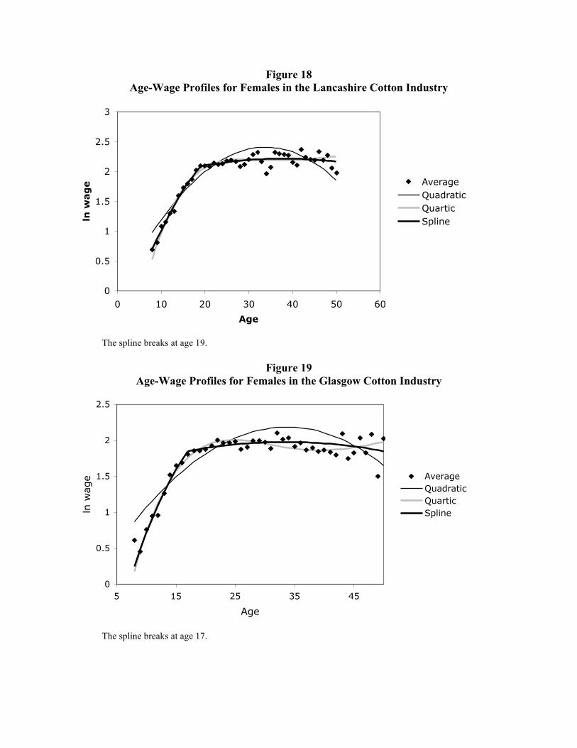
Figure 18 Age-Wage Profiles for Females in the Lancashire Cotton Industry

0

0.5

1

1.5

2

2.5

3

0 10 20 30 40 50 60

Age

ln w

ag

e AverageQuadraticQuarticSpline


Figure 19 Age-Wage Profiles for Females in the Glasgow Cotton Industry

0

0.5

1

1.5

2

2.5

5 15 25 35 45

Age

ln w

age Average



Figure 20 Age-Wage Profiles for Females in the Leeds Wool Industry

0

0.5

1

1.5

2

2.5

5 15 25 35 45

Age

ln w

age Average



Estimating Historical Wage Profiles - Wabash Collegepersweb.wabash.edu/facstaff/burnettj/EstimatingProfiles.pdfEstimating Historical Wage Profiles Joyce Burnette and Maria Stanfors

Documents