Estimating historical range and variation of landscape patch dynamics: limitations of the simulation approach

Page 1

Ecological Modelling 151 (2002) 29–49

Estimating historical range and variation of landscape patchdynamics: limitations of the simulation approach�

Robert E. Keane a,*, Russell A. Parsons a, Paul F. Hessburg b

a USDA Forest Ser�ice, Rocky Mountain Research Station, Fire Sciences Laboratory, P.O. Box 8089 Missoula, MT 59807, USAb USDA Forest Ser�ice, Pacific Northwest Research Station, Forestry Sciences Laboratory, Wenatchee, WA 98801, USA

Received 6 March 2001; received in revised form 25 September 2001; accepted 18 October 2001

Abstract

Landscape patterns in the northwestern United States are mostly shaped by the interaction of fire and succession,and conversely, vegetation patterns influence fire dynamics and plant colonization processes. Historical landscapepattern dynamics can be used by resource managers to assess current landscape conditions and develop target spatialcharacteristics for management activities. The historical range and variability (HRV) of landscape pattern can bequantified from simulated chronosequences of landscape vegetation maps and can be used to (1) describe temporalvariation in patch statistics, (2) develop limits of acceptable change, and (3) design landscape treatment guidelines forecosystem management. Although this simulation approach has many advantages, the limitations of this method havenot been explored in detail. To demonstrate the advantages and disadvantages of this approach, we performed severalsimulation experiments using the spatially explicit, multiple pathway model a LANDscape Succession Model(LANDSUM) to quantify the range and variability in six class and landscape pattern metrics for four landscapes inthe northwestern United States. First, we applied the model to spatially nested landscapes to evaluate the effect oflandscape size on the HRV pattern metrics. Next, we averaged the HRV pattern metrics across maps generated fromsimulation time spans of 100, 500, and 1000 years and intervals 5, 10, 25 and 50 years to assess optimal output generationparameters. We then altered the elevation data layer to evaluate effect of topography on pattern metrics, and cut variousshapes (circle, rectangle, square) from a landscape to examine landscape shape and orientation influences. Then, wealtered the input vegetation maps to assess the influence of initial conditions on landscape metrics output. Finally, asensitivity analysis of input fire probabilities and transition times was performed. Results indicate landscapes shouldbe quite large to realistically simulation fire pattern. Landscape shape, and orientation are critically important toquantifying patch metrics. Simulation output need only be stored every 20–50 years but landscapes should be simulatedfor long time periods (�1000 years). All landscapes are unique so conclusions generated here may not be entirelyapplicable to all western US landscapes. © 2002 Elsevier Science B.V. All rights reserved.

Keywords: Landscape pattern; Historical range and variation; Landscape fire succession modeling; Landscape pattern metrics

www.elsevier.com/locate/ecolmodel

� The use of trade or firm names in this paper is for reader information and does not imply endorsement by the U.S. Departmentof Agriculture of any product or service. This paper was written and prepared by U.S. Government employees on official time, andtherefore is in the public domain and not subject to copyright.

* Corresponding author. Tel.: +1-406-329-4846; fax: +1-406-329-4877.E-mail address: [email protected] (R.E. Keane).

0304-3800/02/$ - see front matter © 2002 Elsevier Science B.V. All rights reserved.

PII: S0 304 -3800 (01 )00470 -7

Page 2

R.E. Keane et al. / Ecological Modelling 151 (2002) 29–4930

1. Introduction

Vegetation pattern often reflects the cumulativeand interactive effects of disturbance regimes, bio-physical environments, and successional processes(Baker, 1989; Bormann and Likens, 1979; Crutzenand Goldammer, 1993; Pickett and White, 1985;Wright, 1974). Landscapes of the northwesternUnited States are primarily shaped by wildlandfire and vegetation succession, and conversely,these patterns will invariably influence future firepatterns, regeneration and colonization processes,and plant development (Hessburg et al., 1999a;Keane et al., 1998; Turner et al., 1994; Veblen etal., 1994). It follows, then, that some generalproperties of disturbance regimes may be de-scribed from spatio-temporal patch dynamics(Hessburg et al., 1999b; Forman, 1995; Swansonet al., 1990). For example, large patches mayindicate a fire regime dominated by large, severefires (Baker, 1989; Baker et al., 1991; Keane et al.,1999). Using this inference, patch and landscapecharacteristics can be used to assess, design, andplan ecosystem management activities (Baker etal., 1991; Keane et al., 2000). For example, therange of patch sizes on a landscape over time canbe used to design the size of a prescribed fire(Cissel et al., 1999; Swetnam et al., 1999; Mlade-noff et al., 1993). Current landscape conditionscan also be compared with summarized historicallandscape conditions to detect ecologically signifi-cant change, such as that brought on by fireexclusion and timber harvesting (Baker, 1992,1995; Cissel et al., 1999; Hessburg et al., 1999b;Landres et al., 1999).

Landscape structure and composition are usu-ally characterized from the spatial distribution ofpatches—a term synonymous with stands orpolygons (McGarigal and Marks, 1995). Manytypes of spatial statistics, often called class andlandscape metrics, are used to quantitatively de-scribe patch dynamics of landscapes (Turner andGardner, 1991; McGarigal and Marks, 1995).They are calculated by importing spatial thematicdata layers, usually from a Geographic Informa-tion System (GIS), into any of the many land-scape metrics programs available (e.g.FRAGSTATS, McGarigal and Marks, 1995, R.LE,

Baker and Cai, 1990). Landscape metrics statisti-cally portray distributions of patch shape, size,and adjacency by patch class (i.e. label or cate-gory) across many scales (e.g. individual patch,class, and landscape; Cain et al., 1997; Hargis etal., 1998). These metrics are important, because,they allow a consistent, comprehensive, and ob-jective comparison among and across landscapes,even though it is difficult to test these metrics forstatistical significance as yet (Turner and Gardner,1991).

The historical range and variability (HRV) oflandscape pattern characteristics provides a usefulconcept for planning and designing landscapetreatments (Parsons et al., 1999; Landres et al.,1999). In this paper, we define HRV as the quan-tification of temporal fluctuations in ecologicalprocesses and characteristics prior to Europeansettlement (i.e. before 1900). Naturally, HRV ishighly scale-dependent and inherently unstable.For instance, the variability of ponderosa pinecover across a landscape greatly depends on therange of years used to compute HRV statistics.Despite its drawbacks, the HRV concept has thepotential to be indispensable to ecosystem man-agement, because, it can be used to define limitsof acceptable change (Swetnam et al., 1999) forassessing stand or landscape condition to priori-tize for restoration treatments (Hessburg et al.,1999a). Since HRV estimates do not integratefuture trends in climate change and human activi-ties, we feel that HRV is not the final answer tospatial considerations in land management, but itdoes provide a good reference point for planningfuture management projects.

The range and variation of historical patchdynamics can be quantified from three mainsources. The best source is a chronosequence (i.e.a sequence of maps of one landscape from manytime periods), which can be input to landscapepattern analysis programs to compute HRV pat-tern results. Unfortunately, temporally deepchronosequences of historical landscape condi-tions are absent for many western landscapes,because, aerial photography or satellite imageryare rare or non-existent prior to 1930. Second,vegetation maps from many similar, unmanagedlandscapes, taken from one or more time periods,

Page 3

R.E. Keane et al. / Ecological Modelling 151 (2002) 29–49 31

can be gathered across a geographic region andinput to spatial analysis programs (Hessburg etal., 1999a). This spatial series essentially substi-tutes space for time (Hessburg et al., 1999c; Pick-ett, 1989) and assumes that because all landscapesin the series display highly similar environmental,disturbance, topographical, and biological condi-tions. Since aerial photographs are absent prior to1930, historical spatial series must be created fromcomparable remote, unsettled watersheds mappedwith the earliest imagery possible (Hessburg et al.,1999a). A big limitation of this approach source isthat subtle differences in landform, relief, soils,and climate make each landscape unique. How-ever, landscapes can be grouped according to theprocesses that govern vegetation, such as climate,disturbance, and species succession (Hessburg etal., 2000).

The third method of quantifying HRV involvessimulating a landscape to produce a chronose-quence of simulated maps to compute landscapemetrics. This approach assumes that successionand disturbance processes are simulated accu-rately in space and time, and that the spatialproperties of the disturbance simulation arereflected in the patch dynamics (Keane et al.,1999). Many spatially explicit ecosystem simula-tion models are available for quantifying HRVpatch dynamics (see Mladenoff and Baker, 1999),but most are computationally intensive, difficultto parameterize and initialize, and complex indesign, thereby making them difficult to use ineveryday management applications. On the otherhand, those models designed for managementplanning tend to oversimplify successional devel-opment and disturbance initiation, spread andeffects (Chew, 1997; Beukema and Kurtz, 1995;Keane et al., 1996, 1997).

Regardless of model complexity and detail,there are still other considerations associated withthe simulation approach for quantifying HRV.For example, the size, shape, orientation, topo-graphic complexity, initial conditions, and report-ing interval can influence spatial pattern dynamicsand associated estimates of HRV. This paperexplores the advantages and limitations of usingthe simulation approach to quantify the HRV oflandscape pattern dynamics. The LANDSUM

model (Keane et al., 1996) was used to spatiallysimulate historical succession and disturbanceprocesses on four very different landscapes in thePacific Northwest over 1000 years. Summarystatistics of selected class and landscape metricswere reported for each simulated landscape. Then,results from a series of simulation experiments arepresented to demonstrate some limitations of thesimulation approach and to provide importantinformation for interpreting these pattern statis-tics. Results from this effort can be used to planand implement landscape-scale ecosystem man-agement activities.

2. Methods

2.1. The model

The LANDscape Succession Model (LAND-SUM) is a spatially explicit vegetation dynamicssimulation C+ + program wherein succession istreated as a deterministic process and distur-bances (e.g. fire, insects, and disease) are treatedas a stochastic processes (Keane et al., 1997).LANDSUM simulates succession within a patch(adjacent similar pixels) or polygon using themultiple pathway fire succession modeling ap-proach presented by Kessell and Fischer (1981).This approach assumes all pathways of succes-sional development will eventually converge to astable or climax plant community called a poten-tial vegetation type (PVT; Fig. 1). A PVT iden-tifies a distinct biophysical setting that supports aunique and stable climax plant community undera constant climate regime. There is a single set ofsuccessional pathways for each PVT present on agiven landscape (Arno et al., 1985). Successionaldevelopment within a patch is simulated as achange in structural stage and cover type (to-gether called a succession class) simulated at anannual time step. The length of time a patchremains in a succession class (transition time,years) is an input parameter that is held constantthroughout the simulation. Disturbances disruptsuccession and can delay or advance the timespent in a succession class, or cause an abruptchange to another succession class. Occurrences

Page 4

R.E. Keane et al. / Ecological Modelling 151 (2002) 29–4932

of human-caused and natural disturbances arestochastically modeled from probabilities basedon historical frequencies. All disturbances weresimulated at a patch-scale, except for wildlandfire, which is discussed next.

The simulation of fire behavior and effects pre-sented a special challenge, because of LAND-SUM’s simplistic structure. Some spatial modelsassume a random or patch-to-patch fire spread(Beukema and Kurtz, 1995; Chew, 1997), whichmaintains map integrity but misrepresents the dy-namics of fire growth (Keane et al., 2000). Wild-land fires tend to split patches along topographic,fuel, moisture, or wind gradients and rarely followpatch boundaries (Finney, 1999). Inclusion of adetailed mechanistic fire growth model, such asFARSITE (Finney, 1998), into LANDSUM wasnot possible, because, the addition of requiredfuels and weather input data would create anoverly complex model that would find little use inmanagement. We decided to create a new versionof LANDSUM (version 2.0) that simulated spa-tial fire dynamics and its effect on landscape

pattern and composition using an approach thatbalanced simplicity and applicability with realism.

In general, the simulation of fire can be repre-sented by three phases, initiation; spread; andeffects. Ignition in LANDSUM is stochasticallysimulated from the fire probabilities assigned toeach initial polygon based on its PVT, cover type,and structural stage. The following three-parame-ter Weibull hazard function was employed toaccount for fuel buildup (i.e. years since burn—YSB, years) and a no-burn period directly after afire (REBURN, years).

Pf=� �

FRI��YSB−REBURN

FRIn(�−1)

(1)

where, � is the shape parameter (parameterized at2.0 for this study), FRI is the fire return intervalor the inverse of fire probability (years), and Pf isthe probability of fire. We estimated REBURN at3.0 years in this study. The probability Pf wasthen adjusted to account for the size of thepolygon and then compared with a random num-ber. If the random number was lower than Pf, a

Fig. 1. An example of the multiple successional pathway approach used to simulated succession in LANDSUM for the highelevation subalpine fir PVT (Keane et al., 2000). Cover types are SH, shrub/herb; WP, whitebark pine; LP, lodgepole pine; SF,subalpine fir. Structural stages are SGF, shrub/grass/forb; SIN, stand initiation; SEC, stem exclusion closed; SEO, stem exclusionopen; URI, understory reinitiation; OFM, old forest multistrata; OFS, old forest single strata.

Page 5

R.E. Keane et al. / Ecological Modelling 151 (2002) 29–49 33

fire was started on a randomly selected pixelwithin that polygon.

Fire was spread across the landscape at a pixel-level using directional vectors of wind and slope.Wind direction (degrees azimuth) is an initialinput to the model but then it is randomlymodified within 45 ° of the input direction foreach simulated fire. Wind speed (m s−1) is also aninput parameter that is randomly adjusted within0.5 times of a user-specified input value for eachfire. Slope (%) is calculated from a digital eleva-tion model (DEM), which is a required input mapin LANDSUM. The number of pixels to spreadthe fire in eight possible directions (N, NE, E, SE,S, SW, W, NW) is calculated from the followingrelationship, which we modified from Rothermel(1991).

spix= (windf)(slopef) (2)

where spix is the number of pixels to spread in adirection, windf and slopef are wind and slopefactors that are computed from the followingequations.

windf= (1+0.125�)(cos(abs(�s−�w))�0.6(3)

slopef=4

(1+3.5 e10�)(4)

where � is wind speed (mph), abs is absolutevalue, �s the spread direction, �w the wind direc-tion, and � is slope (rise over run; Rothermel,1991). The slope factor applies to only positiveslope values (upslope spread). Downslope spreadis computed as:

slopef=e3�2(5)

These equations were solved for each pixel ig-nited by the fire, originating from a randomlyselected fire start pixel mentioned above. Onlythose pixels of patches having assigned fire returnintervals less than the simulation time period wereallowed to burn, except for those patches wherePf was zero, such as in a recently burned patch.Rounding of the computed spix to the nearestpixel (30 m in this study) was stochastically deter-mined from a uniform random number generator.Initially, we let fires burn until they hit the land-scape boundary or an unburnable patch, but we

found that too much land that was burning on thesimulated landscapes. We then limited fire spreadby stochastically calculating a maximum fire size(FIRESIZE, ha) for each fire from the followingequation:

FIRESIZE=� ln(RN)� (6)

where � is the magnitude parameter that approxi-mated the average fire size (ha) estimated to beapproximately 10–50 ha in this study from theNIFMID data base (Schmidt et al., 2002), RN isa random number from a uniform probabilitydistribution, and � is a shape parameter estimatedas 3.0 for this study.

Fire effects were stochastically determinedwithin each burned stand. Probabilities of threefire severities (stand-replacement, mixed severity,and non-lethal surface fires) were assigned to eachmapped polygon (i.e. patch) based on PVT, covertype, and structural stage (Keane et al., 1996).The inverse of the sum of these probabilities wasused as FRI in Eq. (1), but in calculating fireeffects, these probabilities were relativized (scaledfrom 0.0 to 1.0) and a random number wascompared with the cumulative relativized proba-bility distribution to select the severity of the fireto simulate. We also included a slight chance (0.05probability) that the polygon would not burn atall. The selected fire severity would then deter-mine the appropriate successional pathway (seeFig. 1).

2.2. The landscapes

Four very different landscapes were used in thissimulation exercise (Fig. 2). The 516 917 ha Sel-way landscape in central Idaho represents thelargest simulation area with a wide diversity ofvegetation and biophysical settings (see Habeck,1972). The Dahlonega watershed in east-centralIdaho on the Salmon-Challis national forest is alarge landscape (22 338 ha) that contains relativelysimple succession and fire processes on a homoge-nous landscape. The Flathead and Grande Rondewatersheds are small landscapes (�20 000 ha)composed of a wide variety of PVT’s that containcomplex successional pathways and fire dynamics.Fire has played a critical role in shaping all four

Page 6

R.E. Keane et al. / Ecological Modelling 151 (2002) 29–4934

Fig. 2. The suite of simulation landscapes used in this simulation study. The sizes of the landscapes are (a) Grande Rhonde 7460ha; (b) Flathead 8945 ha; (c) Selway 516 917 ha; and (d) Dahlonega 22 338 ha.

of the selected landscapes. Four landscapes wereselected to evaluate applicability of results acrossdiverse settings.

Initial input maps for each landscape were cre-ated by delineating and digitizing polygons fromhistorical aerial photography (circa 1930s) byhighly trained personnel (Hessburg et al., 1999b).PVT, cover type, and structural stage wereclassified for each mapped polygon from vegeta-tion attributes interpreted from aerial photo-graphs. Landscapes were defined by watershedboundaries using the US Geological Survey (1987)hydrological unit code classification. Most succes-

sion pathway and patch-level disturbance parame-ters were taken from a previous modeling effortand then modified to represent local conditions(Keane et al., 1996). All fire parameters wereestimated from local fire atlases, previous firehistory studies and modeling efforts, and the spa-tially summarized NIFMID database (Keane etal., 1996; Schmidt et al., 2002).

2.3. The simulation experiments

We evaluated the effects of landscape size onpattern metrics using nested simulation land-

Page 7

R.E. Keane et al. / Ecological Modelling 151 (2002) 29–49 35

scapes within the large Selway watershed (516 917ha; Fig. 2). We selected a small 2500 ha2 studyarea near the center of the Selway landscape thatserved as the context landscape for comparison.We then progressively created three larger land-scapes that totally encompassed this smaller land-scape but were still smaller than the entire Selway,resulting in the creation of five nested landscapeswith similar distributions of PVT, cover types andstructural stages (Fig. 3a). We ran LANDSUMon these five landscapes for 1000 years, but onlyexported raster output maps for the small contextlandscape (2500 ha) at 50-year intervals for land-scape metric analysis. This experiment was de-signed to evaluate the importance of fires thatoriginate outside, and then spread into the contextarea, on overall landscape pattern dynamics.

We used the Dahlonega watershed to exploreeffects of landscape shape, topographic complex-

ity, and reporting interval on landscape metrics.Effects of reporting interval were determined bysimulating historical fire and succession processesfor 100, 500, and 1000 years and exporting outputmaps every 5 years. Pattern metrics were summa-rized across 5, 10, 20, 50, and 100-year intervals.Topography effects were evaluated by creatingfive new Dahlonega DEM’s by multiplying theoriginal DEM by the factors of 0.0 (flat), 0.2(hilly), 0.5 (half relief), 1.0 (normal relief) and 2.0(high relief), and simulating LANDSUM withnew DEM’s for 1000 years exporting maps every50 years. Effect of landscape shape was evaluatedby creating new landscapes from Dahlonega usingthe following shapes of roughly the same area,narrow vertical rectangle; narrow horizontalrectangle; wide rectangle; square; and circle, andexecuting LANDSUM for 1000 years with mapsoutput every 50 years (see Fig. 3b). Preliminary

Fig. 3. (a) The set of spatially nested Selway landscapes used to evaluate effect of landscape size on pattern metrics (sizes progressfrom context landscape=2500 ha, box 2=10 743 ha, box 3=45 753 ha, box 4=159 920 ha, Selway=519 917 ha). (b) The fivelandscape shapes created as subsets of the Dahlonega watershed to determine shape effects on patch dynamics (vertical rectangle,horizontal rectangle, fat rectangle, square, and circle).

Page 8

R.E. Keane et al. / Ecological Modelling 151 (2002) 29–4936

analyses revealed subtle, but potentially compli-cating, differences in landscape composition, to-pography and underlying PVT distributionbetween the different shapes, so we ran the finalanalyses of this experiment with both neutraltopography (no topography) and only a singlePVT for the whole landscape.

The Grande Ronde landscape was selected toevaluate the influence of initial conditions onpatch metric variability, because of its diversityof vegetation types. We created four initial land-scape composition maps of varying complexityby modifying the original Grande Ronde vegeta-tion layers. The first initial input map (namedTop 1) represented the coarsest approach, wherewe assigned only one successional class (themost dominant class in the original map) to allpolygons within a PVT. A second landscapemap (Top 3) was created by randomly assigningthe three most dominant succession classes to allpolygons in each PVT. The third initial maphad the five most dominant types (Top 5). Inthe last initial landscape map (Random), werandomly assigned every possible successionalclass to all the polygons across the landscape.Using each of the four initial conditions, we ex-ecuted LANDSUM for 1000 years with 50-yearoutput intervals.

A focused sensitivity analysis was performedon the Flathead landscape. We adjusted all fireprobabilities by multiplying them by 0.5, 1.5,and 2.0 and ran LANDSUM for 1000 yearswith a 50-year reporting interval. We also multi-plied the transition times between successionalclasses by the same three factors and executedLANDSUM under the same simulation con-straints. We used the same random number se-quence for all simulation experiments tominimize the effects of stochasticity on our re-sults.

2.4. Spatial pattern analysis

Simulated chronosequences were importedinto the FRAGSTATS spatial pattern analysis pro-gram to compute characterize patterns at twolevels (McGarigal and Marks, 1995). At theclass level, metrics were summarized by patch

type (cover type, structural stage) to provideconsistent detail and context for interpretinglandscape level results (Forman, 1995; Chen etal., 1996; Hargis et al., 1998). At the landscape-level, metrics were summarized for the entirelandscape without patch type stratification. Weselected the cover type and structural stagemaps for pattern analysis, because, we were in-terested in patch dynamics of composition andstructure.

We selected a limited number of spatial met-rics for comparing classes and landscapes.Hargis et al. (1998) found that only a small setof indices was needed, because of the redun-dancy and dependency among metrics (also seeTurner and Gardner, 1991). It was also impor-tant to match the landscape metric with the bio-logical processes that influence landscapestructure (Chen et al., 1996). We selected patchdensity (PD, patches per 100 ha), mean patchsize (MPS, ha), and landscape patch index (LPI)to represent the direct effect of disturbance pro-cesses on patch size. LPI is maximum percent ofthe landscape occupied by one patch selected,because, it represents the upward bounds ofpatch or burn size. We selected relative patchrichness (RPR), because, it reflects richness rela-tive to maximum possible richness on a scale of0–100 (100=all patch types possible). TheModified Simpson’s evenness index (MSIEI), ex-pressed as computed level of diversity dividedby the maximum possible diversity for a givenpatch richness, was selected, because, it describesthe degree to which the landscape is composedof one patch class. Lastly, contagion (CON-TAG), a number between 0 and 100, measuresthe interspersion and dispersion of patchesacross a landscape. Four statistics were used todescribe each of the six metrics. The averageacross the simulated chronosequence was usedas the target or reference metric. The standarderror was used to describe the variability in ametric. The maximum and minimum values es-tablished the range of observations. Resultsfrom simulation experiments were tested forstatistical significance using multivariate analysisof variance (MANOVA) in the SAS softwarepackage (SAS, 1990).

Page 9

R.E. Keane et al. / Ecological Modelling 151 (2002) 29–49 37

Fig. 4. Results from FRAGSTATS analysis of simulated Selway landscapes from LANDSUM over 1000 year span. These resultsprovide an illustration of the simulated landscape dynamics of various patch characteristics over simulation time. Fire statisticsinclude area burned over time (a), and percent of that area burned by severity class (b). Community dynamics shown are percentof area occupied by the three dominant cover type classes (c), and structural stages (d). Selected patch metrics over time are shownfor cover type (e), and for structural stage (f).

3. Results

The set of graphs in Fig. 4 illustrates the diver-sity of LANDSUM output generated for a por-tion of the Selway landscape. The temporaldistribution of burned area (Fig. 4a) and fireseverity (Fig. 4b) influenced the composition ofcover types (Fig. 4c) and structural stages (Fig.4d) on the landscape, and those simulated firescreated unique patch characteristics that varyacross time and differ for cover type (Fig. 4e) andstructural stage (Fig. 4f).

Results from the simulation experiments gener-ated some interesting trends (Tables 1 and 2).Effects of landscape size on patch dynamics in thesmallest 2500 ha context area were significant

(P�0.0001) for both cover type and structuralstage class and landscape metrics (Table 2). Forthe most part, these significant differences oc-curred between two groups: the smaller two land-scapes (2500 and 10 000 ha), and the larger threelandscapes (45 000, 159 920, and 516 917 ha, re-spectively). No significant differences within thosegroups were found (P�0.05). Interpretation oftrends was more difficult, complicated by substan-tial differences in trends between cover type andstructure maps. For example, variability in severalpatch metrics (MPS, PD, CONTAG) increasedwith increasing simulation landscape size forcover type maps (Table 1), but variability de-creased or had indeterminate trends for thosemetrics for structural stage maps. A clear trend of

Page 10

R.E. Keane et al. / Ecological Modelling 151 (2002) 29–4938

Tab

le1

Exp

erim

ent

resu

lts

for

the

land

scap

esi

ze,

shap

eto

pogr

aphy

,in

itia

lco

ndit

ions

,fir

epr

obab

iliti

esan

dsu

cces

sion

altr

ansi

tion

tim

esex

peri

men

tsfo

rco

ver

type

CO

NT

AG

(%)

RP

R(%

)M

SIE

I(n

oun

its)

MP

S(h

a)M

apat

trib

ute,

cove

rty

peP

D(1

00ha

−1)

LP

I(%

)

Mea

nS .

D.

Mea

nS.

D.

Mea

nS.

D.

Mea

nS.

D.

S.D

.E

xper

imen

tSc

enar

ioM

ean

S.D

.M

ean

16.8

46.

1151

.09

1.94

71.7

7L

ands

cape

size

5.29

Con

text

box

(250

0ha

)0.

640.

0421

.36

1.82

4.71

0.39

12.9

44.

5551

.21

3.15

71.4

35.

530.

460.

644.

820.

07B

ox2

(10

000

ha)

20.9

22.

0623

.43

10.3

254

.06

3.13

71.7

76.

180.

56B

ox3

(45

753

ha)

0.06

22.3

02.

164.

520.

4218

.91

8.87

55.0

53.

5276

.87

9.01

0.59

0.55

0.07

4.57

2.70

22.1

8B

ox4

(159

917

ha)

16.4

66.

3153

.10

4.20

75.8

58.

290.

59Se

lway

(519

917

ha)

0.08

20.8

62.

604.

860.

56

54.4

46.

8361

.15

4.28

28.2

52.

911.

840.

530.

500.

0614

.64

57.8

9C

ircl

eL

ands

cape

shap

e49

.02

5.94

51.6

37.

0022

.54

3.93

0.68

Squa

re0.

1151

.17

8.59

2.01

0.35

66.3

015

.38

59.0

56.

8517

.72

2.24

0.73

0.48

0.11

1.80

22.5

963

.89

Ver

tica

lre

ctan

gle

25.9

94.

6255

.22

2.69

27.8

22.

950.

65H

oriz

onta

lre

ctan

gle

0.05

53.4

011

.07

1.96

0.44

66.3

49.

6757

.88

6.69

17.2

02.

990.

510.

500.

091.

8314

.41

Wid

ere

ctan

gle

58.0

7

21.8

62.

8856

.77

1.88

44.4

44.

65L

ands

cape

topo

grap

hy0.

60N

eutr

alto

pogr

aphy

0.05

52.5

52.

501.

910.

0922

.19

2.26

57.3

02.

1845

.77

5.53

0.09

0.58

0.05

1.88

2.48

53.3

0F

lat

(dem

×0.

2)20

.96

3.76

57.9

51.

5546

.83

3.76

0.58

Rol

ling

relie

f(d

em×

0.5)

0.04

53.1

12.

831.

890.

1021

.37

3.52

56.9

92.

1344

.71

5.11

0.11

0.59

3.26

0.05

1.89

Nor

mal

relie

f(d

em×

1)53

.21

0.15

Incr

ease

dre

lief

(dem

×1.

5)21

.84

6.26

57.9

81.

8048

.15

4.76

0.57

0.04

53.0

93.

971.

891.

23O

rigi

nal

9.88

7.97

47.7

43.

4774

.92

2.91

0.74

0.07

25.0

113

.42

4.57

Lan

dsca

pein

itia

lco

ndit

ions

13.0

717

.72

48.7

47.

0471

.43

10.3

61.

570.

720.

134.

3149

.73

35.8

8T

op1

1.34

Top

38.

575.

5147

.49

4.58

74.9

22.

910.

750.

0726

.12

17.9

44.

588.

958.

1747

.16

3.50

75.2

43.

741.

250.

754.

830.

06T

op5

23.7

513

.83

9.03

12.3

548

.09

4.75

75.2

43.

090.

74R

ando

m0.

1026

.84

11.7

84.

211.

2325

.39

11.6

558

.60

4.95

97.3

54.

850.

150.

61F

ire

prob

abili

ties

a0.

100.

8924

.41

115.

74P

roba

bilit

ies×

10.

880.

1519

.910

.59

58.9

03.

6998

.41

3.98

0.60

0.07

Pro

babi

litie

s×0.

511

7.24

21.4

925

.01

17.2

958

.83

5.07

98.9

43.

340.

180.

610.

110.

9423

.21

110.

74P

roba

bilit

ies×

1.5

27.0

924

.81

60.3

18.

5798

.94

3.34

0.57

Pro

babi

litie

s×2.

00.

1811

7.60

64.3

40.

970.

2725

.39

11.6

558

.60

4.95

97.3

54.

850.

150.

61T

rans

itio

nti

mes

0.10

0.89

24.4

111

5.74

Tra

nsit

ion×

118

.42

6.00

Tra

nsit

ion×

0.5

56.9

02.

5599

.44

2.42

0.65

0.06

103.

2021

.84

1.00

0.17

20.3

811

.73

57.9

54.

2897

.88

5.69

0.20

0.61

0.99

0.07

Tra

nsit

ion×

1.5

106.

1626

.10

21.8

610

.89

Tra

nsit

ion×

2.0

58.7

93.

5597

.33

4.85

0.61

0.07

113.

1521

.83

0.91

0.16

Bol

dfac

epr

int

indi

cate

sov

eral

lsi

gnifi

cant

diff

eren

ces

(MA

NO

VA

,P

�0.

05)

byex

peri

men

t,w

ith

furt

her

bold

face

for

vari

able

ssi

gnifi

cant

lydi

ffer

ent

atP

�0.

05,

wit

hin

the

tabl

e.a

Ove

rall

MA

NO

VA

for

fire

prob

abili

ties

expe

rim

ent

for

cove

rty

pem

aps

was

sign

ifica

ntat

P�

0.00

29,

how

ever

,si

gnifi

canc

eof

indi

vidu

alva

riab

les

iscl

oude

dby

mul

tico

linea

rity

wit

hin

the

vari

able

set;

for

this

reas

on,

indi

vidu

alP

-val

ues

for

the

patc

hm

etri

cva

riab

les

are

not

sign

ifica

ntat

P�

0.05

.O

nly

cove

rty

pem

apst

atis

tics

are

show

ndu

eto

spac

eco

nsid

erat

ions

.

Page 11

R.E. Keane et al. / Ecological Modelling 151 (2002) 29–49 39

Tab

le2

Res

ults

for

the

repo

rtin

gin

terv

alex

peri

men

tfo

rco

ver

type

map

s

Con

tagi

onC

ON

TA

GM

PS

(ha)

RP

R(%

)M

SIE

I(n

oun

its)

Map

attr

ibut

e:co

ver

type

PD

(100

ha−

1)

LP

I(%

)(%

)

S .D

.M

ean

Exp

erim

ent

S.D

.In

terv

alM

ean

S.D

.M

ean

S.D

.M

ean

S.D

.P

erio

dM

ean

S.D

.M

ean

0.08

24.5

312

.37

59.1

01.

9348

.14

2.25

4.76

1.95

0.50

0.04

51.2

410

05

Rep

orti

ngin

terv

al0.

0824

.68

13.5

458

.89

1.79

47.9

84.

490.

500.

0410

100

51.0

42.

121.

960.

0924

.10

13.3

959

.53

1.65

49.0

75.

461.

970.

4950

.93

0.03

2.27

2010

01.

9750

0.08

18.0

87.

1060

.25

2.20

51.8

56.

420.

480.

0510

050

.78

2.08

1.94

50.

0920

.49

6.77

57.2

12.

1145

.32

4.83

0.57

0.05

500

51.7

42.

320.

0720

.72

7.16

57.0

02.

0244

.55

4.34

1.93

0.57

0.05

1.99

51.8

950

010

2.04

1.93

0.08

20.6

57.

0556

.94

2.14

44.2

34.

580.

580.

0620

500

51.8

40.

0919

.94

4.46

57.2

82.

3744

.94

5.80

1.93

0.57

0.06

2.29

51.9

750

050

0.10

18.6

95.

9357

.86

2.94

46.3

07.

590.

5610

00.

0750

051

.92

2.67

1.93

0.12

21.7

74.

9756

.66

2.27

43.8

64.

891.

880.

600.

053.

3853

.45

1000

50.

1121

.87

5.20

56.6

62.

1843

.73

4.56

0.59

0.05

1010

0053

.47

3.11

1.88

0.11

21.8

15.

1356

.72

2.21

44.0

14.

561.

880.

593.

100.

0520

1000

53.3

20.

1121

.37

3.52

56.9

92.

1344

.71

5.11

0.59

0.05

5010

0053

.21

3.26

1.89

0.09

20.6

04.

7557

.69

2.19

46.9

75.

750.

570.

061.

9110

010

0052

.41

2.57

Thi

sex

peri

men

tev

alua

ted

the

effe

cts

ofdi

ffer

ent

outp

utte

mpo

ral

reso

luti

on(i

nter

val)

,an

dle

ngth

ofsi

mul

atio

npe

riod

(per

iod)

.B

oldf

ace

indi

cate

ssi

gnifi

cant

over

all

effe

ct(P

�0.

0001

);fu

rthe

rbo

ldfa

cein

dica

tes

diff

eren

ces

sign

ifica

nt(a

tP

�0.

05or

bett

er)

for

agi

ven

patc

hm

etri

c.Si

gnifi

cant

effe

cts

wer

eob

serv

edfo

rle

ngth

ofsi

mul

atio

npe

riod

,bu

tno

tfo

rre

port

ing

inte

rval

.O

nly

cove

rty

pem

apst

atis

tics

are

show

ndu

eto

spac

eco

nsid

erat

ions

.

Page 12

R.E. Keane et al. / Ecological Modelling 151 (2002) 29–4940

decreasing MPS and increasing PD was observedwithin the context area as the simulation land-scape size was increased for structural stage maps,but that trend was less apparent for cover typemaps (Table 1).

The shape of the landscape also had a signifi-cant influence on class and landscape metrics overthe 1000-year simulation span (Table 1). Land-scape metrics for both cover type and structuralstage Dahlonega maps were significantly different(P�0.0001) for horizontal and vertical rectangles(see Fig. 3b) than for all other shapes. Principaldifferences were in PD and LPI, with substantiallylower LPI and higher PD for the horizontalrectangle than in the other shapes, as well as otherdifferences.

Topography had very little effect on either classor landscape metrics for the five Dahlonega simu-lation scenarios (Table 1); there was very littledifference between simulated patch metrics for thefive topographic scenarios (P�0.48). We ran thisentire experiment using only one PVT for theentire landscape, because of concern in differencesof fire frequency by PVT, and again found nosignificant differences between the five DEMinputs.

It appears that initial conditions (P�0.576) donot have a significant influence on summarizedclass and landscape metrics over the 1000-yeartime span (Table 1). It was inconsequentialwhether the initial Grande Ronde landscape wastotally homogeneous (one cover type and onestructural stage) or highly heterogeneous (randomassignment of all combinations of cover type andstructural stages) at the start of simulation, be-cause by approximately year 100, and certainly byyear 200, the simulated landscapes were quitesimilar in cover type and structural stage patchdistributions (Fig. 5).

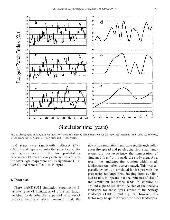
The reporting interval experiment on theDahlonega landscape produced interesting results.Pattern metrics for both cover type and structuralstage were not significantly different when sum-marized at 5-, 10-, 20- or 50-year intervals (P�0.98), but substantial differences were found whenmetrics were summarized at 100-year intervals(Table 2). Landscape and class metrics computedover simulation time spans of 100 years weresignificantly different to those computed over a500- or 1000-year period (P�0.0001, Table 2 andFig. 6). It appears likely, then, that a 100-yeartime span is too short for generating useful land-scape metrics summary statistics, regardless of thereporting interval.

Sensitivity analysis of the fire probabilitiesshowed the importance of these parameters ingenerating realistic landscape patterns (Table 1).Pattern statistics were significantly different forboth cover type (P�0.0029) and structural stage(P�0.0001) maps for each set of fire multipliers.For the structural stage maps, the set of simula-tion runs were clearly separated into two statisti-cally significant groups; those simulations wheremultipliers were less than or equal to 1 and simu-lations with multipliers �1. Separation was notso clear for the cover type maps, with variablegrouping and differences by patch metric. Struc-tural stage metrics show a distinct tendency to-ward patch aggregation as fire frequenciesincrease, and cover type metrics became morehighly variable with increasing fire frequency.

Results for transition time sensitivity analysiswere similar to those of the fire probabilitiesexperiment. Landscape patch metrics for struc-

Fig. 5. Effect of initial landscape complexity on landscapepatch metrics of cover type maps over 1000 year simulations,shown here for the contagion metric. Occasional peaks are theresult of very large fires. Initial conditions were modified toproduce a series of initial input maps varying in complexity, byassigning all polygons within a PVT to the single dominantsuccession class (Top1), top three dominant classes (Top 3),top five dominant classes (Top 5) or randomly assigned fromall possible combinations (Random).

Page 13

R.E. Keane et al. / Ecological Modelling 151 (2002) 29–49 41

Fig. 6. Line graphs of largest patch index for structural stage by simulation year for six reporting intervals, (a) 5 years; (b) 10 years;(c) 20 years; (d) 50 years; (e) 100 years; and (f) 250 years.

tural stage were significantly different (P�0.0013), and separated into the same two multi-plier groups seen in the fire probabilitiesexperiment. Differences in patch metric statisticsfor cover type maps were not as significant (P�0.0529) and were difficult to interpret.

4. Discussion

These LANDSUM simulation experiments il-lustrate some of limitations of using simulationmodeling to describe the range and variation ofhistorical landscape patch dynamics. First, the

size of the simulation landscape significantly influ-ences fire spread and patch dynamics. Small land-scapes did not experience the immigration ofsimulated fires from outside the study area. As aresult, the landscape fire rotation within smalllandscapes was often overestimated. This was es-pecially evident on simulated landscapes with thepropensity for large fires. Judging from our lim-ited results, it appears that the influence of size ofthe simulation landscape tends to stabilize ataround eight to ten times the size of the analysislandscape for those areas similar to the Selwaylandscape (Table 1 and Fig. 7). However, thisfactor may be quite different for other landscapes,

Page 14

R.E. Keane et al. / Ecological Modelling 151 (2002) 29–4942

such as Yellowstone National Park (Gardner etal., 1997) and Wisconsin, USA (He and Mlade-noff, 1999). Those biomes that experience largefires, such as boreal forests, may need much largersimulation areas to realistically simulate land-scape patch dynamics (Amiro et al., 2000). Wim-berly et al. (2000) also found that smallersimulation areas increased variation across modelruns for landscape composition metrics in theOregon Coast range where large fires arecommon.

Another important spatial characteristic thatinfluences patch dynamics was simulation land-scape shape, and, related to shape, landscapeorientation. Simulations on narrow, linear land-scapes will tend to underestimate fire spread andburned area (Table 1), because of the lack of fireimmigration as mentioned above, and also, be-cause, fires that originate in these elongated land-scapes tend to reach the landscape edge wellbefore reaching their full size. This effect wasaccentuated when the narrow portion of the land-scape was perpendicular to predominant winddirection; fires were quickly blown out of land-scape before they reached significant sizes. Therewas very little difference between the square andcircular landscapes, because, there was no short

axis to allow the orientation bias. Fire spreadsimulations on landscapes with elongated shapescreated smaller patches, particularly in structuralstage maps (Table 1), because of the decreasedpotential spread area and the interaction withlandscape edge. Our results agree with Camp etal. (1997) who also found that orientation of thetopography governs fire spread dynamics. Thoselandscapes having ridge systems that were alignedperpendicular to the wind flow and near land-scape edges had underestimated burned area, be-cause, both slope and wind reduce the width ofthe headfire (Finney, 1999). It appears landscapesdefined by watershed boundaries, especially thoseless than 50 000 ha, may make poor simulationareas, because of the tendency of watersheds to beelongated along river systems with the center ofthe landscape always the lowest in elevationthereby biasing fire ignition and spread.

To evaluate the effects of between-run variabil-ity on patch metric HRV, we conducted a MonteCarlo simulation, with 20 runs of 1000 years forthe Grande Rhonde landscape (Fig. 8). Althoughthere was substantial variability in the number,size and timing of fires, and corresponding com-munity dynamics, patch metric statistics remainedquite stable, with no significant differences in

Fig. 7. Effect of landscape size on MPS within 2500 ha context area in the Selway landscape. MPS within the context landscape isaffected by the size of the surrounding area; this influence appears to stabilize when size of the surrounding area is roughly eightto ten times the size of the context landscape.

Page 15

R.E. Keane et al. / Ecological Modelling 151 (2002) 29–49 43

Fig. 8. Range of results for 20 LANDSUM model runs of the same Grand Ronde landscape showing the inherent stochasticvariation in predictions of percent landscape for the dominant cover type (a) (ponderosa pine) and structural stage (b) (stemexclusion structure). Both cover type and structure show substantial changes between initial values and mean; this difference suggeststhat initial values fall outside the simulated range of variability.

patch metric statistics for either cover type (P�0.27) or for structural stage (P�0.99). This couldindicate that between-run variability is low andadequate landscape patch metric HRV dynamics

can be quantified from very few simulation runs.It was somewhat surprising that the initial con-

ditions of the simulation landscape did not seemto affect long-term patch dynamics. This is proba-

Page 16

R.E. Keane et al. / Ecological Modelling 151 (2002) 29–4944

bly because, the simplistic succession and firesimulation approach implemented in LANDSUMconstrained potential landscape trajectories andcaused most landscapes to eventually converge toa single equilibrium condition (Fig. 5). This sim-plistic approach usually generates landscape met-ric predictions with low variability (Fig. 8). Morecomplex landscape models tend to be highly sensi-tive to initial conditions and often predict differ-ent landscape trajectories with relatively minorchanges in initial landscape composition andstructure making predictions more highly variable(Keane et al., 1999; He and Mladenoff, 1999).The simplistic approach also resulted in question-able fire perimeters, which in turn affected therealism of resulting vegetation patterns. For ex-ample, Camp et al. (1997) found late-successionalforest stands tended to be located within a fairlyrestricted range of environmental conditions thatare somewhat predictable. To simulate accuratefire patterns, complex fire models requiring exten-sive daily weather (wind, temperature, humidity,precipitation) and fuel moisture input data areneeded, but these parameters are difficult to ob-tain across an entire landscape (Finney, 1999).

Two important criteria must be decided uponbefore a simulation approach can be adapted toquantify HRV of landscape conditions. First, anadequate simulation time span must be selectedthat matches model application objectives withcomputing resources. We found that shorter simu-lation periods (e.g. 100 years or less) may result ininadequate landscape patch metric statistics(Table 2). A likely reason for this difference isthat the 100-year simulation did not have thetemporal depth to include effects of fires in PVTswith long fire return intervals (Lertzman et al.,1998). We suggest that the simulation time spanbe at least ten times the longest fire return intervalon those sites that occupy at least 10% of thelandscape, but these thresholds will vary by land-scape. Second, the temporal density of chronose-quences (i.e. reporting interval) must be chosen asa compromise between available analysis re-sources, management objectives, and temporal au-tocorrelation (Baker et al., 1991). We found thatshort reporting intervals (5, 10, and 25 years) didnot result in more accurate pattern descriptions

when compared with those computed from mapsgenerated at 50-year intervals (Table 2). However,longer intervals of 100 and 250 years generatedsignificantly different results from the shorter in-terval chronosequences, because of vast differ-ences in the variance, maximum, and minimumvalues (Fig. 6). It appears that a 50-year reportinginterval is sufficient for LANDSUM applications.

The relative sensitivity of the fire probabilityand insensitivity of succession transition time in-put parameters were unexpected results in theLANDSUM simulation experiments. Less fre-quent fires (probabilities multiplied by 0.5) didnot influence long-term patch dynamics whencompared with the reference probability set (mul-tiplication factor of one), presumably, because,the full range of seral and climax cover type andstructural stage types remained on the landscape.However, when fire return intervals were short(multiplication factors of 1.5 and 2.0), the struc-tural stage and cover type patches became largeras more of the landscape moved into the singlestory, old growth structural stage and seral, fire-dependent ponderosa pine and larch cover typesthat are created by low severity fire (Keane et al.,1996). These results may indicate that fire proba-bilities, although important, need not be esti-mated with a high degree of accuracy, but theymust be consistently applied.

Differences in transition time sensitivity analy-ses were mostly evident at the extremes (multipli-cation factors of 0.5 and 2.0) and only forstructural stage maps and a small set of patternmetrics (Table 1). The lack of significant differ-ences across metrics, particularly in cover typemaps, was due to the dominant effects of simu-lated fires; high frequency fire on the Flatheadlandscape overwhelmed any effect of altered tran-sition times on patch size and density. However,transition times were very important for FlatheadPVTs with long fire return intervals, because,succession moved patches toward climax covertypes and structural stages before fires occurred,thereby reducing evenness and increasing conta-gion. This dynamic was especially important forstructural stage maps, because, there are only twoold growth structural stage categories while therecan be many old growth cover type categories,

Page 17

R.E. Keane et al. / Ecological Modelling 151 (2002) 29–49 45

which may explain why structural stage mapswere more sensitive to both fire probabilities andtransition times than cover type maps. Our resultsagree with He and Mladenoff (1999) who foundthat advancing succession results in larger andmore severe fires and coarse-grained patterns withthe LANDIS model.

The limitations of using a simulation approachto determine range and variation in pattern statis-tics as presented here may not apply to all land-scape fire succession models, because ofdifferences in model assumptions and design. Forinstance, topography did not influence fire patternin the LANDSUM experiments, because of theoverwhelming effect of the wind and, because ofthe way fire was simulated on the landscape.LANDSUM simulated fire spread until the firereached a size computed from a negative exponen-tial probability distribution (see Section 2). Thisresulted in realistic landscape fire rotation predic-tions but questionable simulated fire perimeters,

because, a few fires stopped halfway up steepmountain slopes. For comparison purposes, weallowed fires to burn in LANDSUM until theyreached unburnable polygons (e.g. rock, water,recent burns) or the landscape boundary, but theresult was about two to three times more burnedarea over 1000 years than would have normallyoccurred under native fire regimes. This is be-cause, the termination of fire spread is a complexprocess that depends not only on vegetation andfuels, as modeled in LANDSUM, but also ondaily weather, fuel loading, fuel moistures, fuelcontinuity, and vegetation structure (Agee et al.,2000), which are highly complex and difficult tosimulate in a spatial environment. Other firespread models terminate spread along topo-graphic controls to generate realistic fire regimes,but the generated patterns may not match thoseobserved on actual landscapes (Andrews, 1990).Land managers must select the appropriate fireand succession modeling scheme for theirapplication.

There are other drawbacks of the simulationmethod for the estimation and interpretation ofHRV landscape metrics that were not evaluated inthis study. First, map integrity is often compro-mised, because, spatial simulations of fire spreadwill dissect stands to create many smallerpolygons over long simulation times, especially inportions of the landscape where fires are common.This results in sustained increases in PD anddecreases in patch size throughout the simulation(Fig. 9). Still more confounding is that, in parts ofthe landscape that have long fire return intervals,patch boundaries often remain relatively un-changed from the initial conditions (Keane et al.,2000). Including the initial polygon layer andearly simulated layers with later simulatedchronosequences for computation of HRV patchstatistics is probably inappropriate, because ofthese differences in mapping resolution. Simulatedfires are mapped at 30-m pixel resolution whereasinitial polygons are created using much broadermapping criteria (e.g. minimum map units of 4ha). We aggregated the small polygons to mini-mum map units of 4 ha using standard GIStechniques to make all maps consistent (Fig. 9),but detail in fire simulations was lost. This is a

Fig. 9. Effect of the fine scale simulation of fires on landscapepatch metrics. Fine scale simulation of fires tends to increas-ingly fragment stand polygons over time, resulting in increas-ing PD (top, solid line) and decreasing contagion (bottom,solid line). To mitigate this effect, map chronosequences wereaggregated to 2 ha minimum map units using standard GIStechniques. Effect of the aggregation is shown for PD (top,dashed line) and for contagion (bottom, dashed line).

Page 18

R.E. Keane et al. / Ecological Modelling 151 (2002) 29–4946

problem for most landscape fire succession mod-els where fire spread is simulated as an indepen-dent disturbance process.

The classification resolution of modeled land-scape elements also affects HRV metrics (Wick-ham et al., 1997). Map elements wereconstrained to the states or successional classesrepresented in the multiple pathway model, nomatter how broadly or narrowly they weredefined. Landscape formations and features withunique species assemblages, such as seeps, ripar-ian bottoms, and frost pockets, which can di-rectly contribute to patch composition andstructure, were missing from this analysis, be-cause, they were not explicitly included in thepathway model. Inclusion of additional PVTs onthe landscape does not always increase classifica-tion resolution because many of the same covertypes and structural stages may occur across sev-eral PVTs.

It is extremely difficult to validate or assessaccuracy of landscape fire succession models, be-cause, temporally deep spatial data sets of fireand vegetation are rare. Instead, we comparedlandscape metrics of Selway fire perimeters com-piled by Rollins et al. (2002) with those fireperimeters simulated by LANDSUM for the Sel-way (Fig. 10). LANDSUM fires compared wellwith the Selway fires in area (Fig. 10c) and shape(Fig. 10a), but differed in fractal dimension. Thisis a result of scale and mapping resolutionsrather than simulation inaccuracies. Selway fireperimeters were coarsely drawn on low resolu-tion maps (1:100 000 mapscale) and then digi-tized into a GIS, whereas the LANDSUM firesare simulated on a fine scale, 30-m pixel rasterlayer. Consequently, scale inconsistencies over-whelm the simulated-to-reference comparisonand cause differences to appear in the metrics.This will be a problem for any spatial validationdataset.

5. Summary and conclusions

This paper demonstrates how the HRV oflandscape composition and structure can be de-scribed from class and landscape metrics com-

puted from simulated chronosequences. HRVstatistics can be used to assess, prioritize, com-pare, and design landscapes for possible restora-tion treatments. However, simulatedchronosequences rely on inexact computer mod-els that are based on oversimplifications of dis-turbance and succession processes that result inmajor limitations. These limitations are model-and landscape-specific so it is difficult to general-ize on techniques to mitigate the potential simu-lation shortcomings. But, using the LANDSUMmodel as an example, we found the followinglimitations of using simulation modeling to as-sess range and variation of landscape patch dy-namics.1. Simulation landscape size, shape, and orienta-

tion can affect patch dynamics by excludinglarge fires immigrating from outside the analy-sis landscape and by limiting fire spread, be-cause of biases in wind direction, topography,and landscape boundaries.

2. Input parameters need not be highly accuratebut they should be consistently applied andwithin at least 30% of the actual value.

3. Simulation periods should be at least ten timesthe longest fire return interval on the land-scape to ensure the effects of all fires arereflected in landscape patch statistics.

4. Output reporting interval need not be fre-quent. We suggest a 50-year interval is a goodcompromise between analysis capacity andpatch metric characterization.

Since long-term chronosequences of actuallandscapes are essentially unavailable, the simula-tion approach may be the only means availablefor quantifying pattern HRV. We believe land-scape fire succession models are not yet the per-fect tools to quantify patch dynamics, but theyprovide an alternative evaluation resource.

Acknowledgements

We thank Matt Rollins and Don Long ofUSDA Forest Service, Rocky Mountain ResearchStation for technical reviews, and Brion Salter,USDA Forest Service, Pacific Northwest Re-search Station for assistance in spatial pattern

Page 19

R.E. Keane et al. / Ecological Modelling 151 (2002) 29–49 47

Fig. 10. Validation of the spatial characteristics of the LANDSUM fire boundaries (dashed lines) compared with fire atlas perimeterscompiled by Rollins et al. (2002) (solid lines). All three metrics were computed using FRAGSTATS and the indices are defined inMcGarigal and Marks (1995).

analysis. This work was partially funded by agrant (NS-7327) from NASA’s Earth Science Ap-plications Division as part of the Food and Fiber

Applications of Remote Sensing (FFARS) pro-gram managed by the John C. Stennis SpaceCenter.

Page 20

R.E. Keane et al. / Ecological Modelling 151 (2002) 29–4948

References

Agee, J.K., Bahro, B., Finney, M.A., Omi, P.N., Sapsis, D.B.,Skinner, C.N., van Wagtendonk, J.W., Weatherspoon,C.P., 2000. The use of shaded fuelbreaks in landscape firemanagement. Forest Ecology and Management 127, 55–66.

Amiro, B.D., Chen, J.M., Liu, J., 2000. Net primary produc-tivity following fire for Canadian ecoregions. CanadianJournal of Forest Research 30, 939–947.

Andrews, P.L., 1990. Application of fire growth simulationmodels in fire management. In: Proceedings of the TenthConference on Fire and Forest Meteorology, April 17–21,Ottawa, Canada. Society of American Foresters, Washing-ton, DC, pp. 317–321.

Arno, S.F., Simmerman, D.G., Keane, R.E., 1985. Forestsuccession on four habitat types in western Montana.General Technical Report INT-177. US Department ofAgriculture, Forest Service, Intermountain Forest andRange Experiment Station, Ogden, UT, p. 74.

Baker, W.L., 1989. Effect of scale and spatial heterogeneity onfire-interval distributions. Canadian Journal of Forest Re-search 19, 700–706.

Baker, W.L., 1992. Effect of settlement and fire suppression onlandscape structure. Ecology 73 (5), 1879–1887.

Baker, W.L., 1995. Long-term response of disturbance land-scapes to human intervention and global change. Land-scape Ecology 10 (3), 143–159.

Baker, W.L., Cai, Y., 1990. The R.LE programs for multi-scaleanalysis of landscape structure using the GRASS geographi-cal information system. Landscape Ecology 7, 291–302.

Baker, W.L., Egbert, S.L., Frazier, G.F., 1991. A spatialmodel for studying the effects of climatic change on thestructure of landscapes subject to large disturbances. Eco-logical Modelling 56, 109–125.

Beukema, S.J., Kurtz, W.A., 1995. Vegetation Dynamics De-velopment Tool User’s Guide. ESSA Technologies, Van-couver, BC, Canada, p. 51.

Bormann, F.H., Likens, G.E., 1979. Pattern and Process in aForested Ecosystem. Springer, New York, p. 253.

Cain, D.H., Tiitters, K., Orvis, K., 1997. A multi-scale analysisof landscape statistics. Landscape Ecology 12, 199–212.

Camp, A.E., Oliver, C.D., Hessburg, P.F., Everett, R.L., 1997.Predicting late-successional fire refugia from physiographyand topography. Forest Ecology and Management 95,63–77.

Chen, J., Franklin, J.F., Lowe, J.S., 1996. Comparison ofabiotic and structurally defined patch patterns in a hypo-thetical forest landscape. Conservation Biology 10 (3),854–862.

Chew, J., 1997. Simulating landscape patterns and processes atlandscape scales. In: Proceedings of the 11th Annual Sym-posium on Geographic Information Systems. GIS WorldPublications, Fort Collins, Vancouver, BC, pp. 287–291.

Cissel, J.H., Swanson, F.J., Weisberg, P.J., 1999. Landscapemanagement using historical fire regimes: Blue River, Ore-gon. Ecological Applications 9 (4), 1217–1232.

Crutzen, P.J., Goldammer, J.G., 1993. Fire in the Environ-ment: The ecological, Atmospheric and Climatic Impor-tance of Vegetation Fires. Wiley, New York, p. 456.

Finney, M.A., 1998. FARSITE: Fire Area Simulator Modeldevelopment and evaluation. USDA Forest Service Gen-eral Technical Report RMRS-GTR-4, p. 47.

Finney, M.A., 1999. Mechanistic modeling of fire shape pat-terns. In: Mladenoff, D.J., Baker, W.L. (Eds.), SpatialModeling of Forest Landscape Change. Cambridge Uni-versity Press, Cambridge, UK, pp. 186–209.

Forman, R.T.T., 1995. Landscape Mosaics—The Ecology ofLandscapes and Regions. Cambridge University Press,UK, p. 632.

Gardner, R.H., Hargrove, W.W., Turner, M.G., Romme,W.H., 1997. Climate change, disturbances and landscapedynamics. In: Walker, B.H., Steffen, W.L. (Eds.), GlobalChange and Terrestrial Ecosystems, IGBP Book SeriesNumber 2. Cambridge University Press, Cambridge, UK,pp. 149–172.

Habeck, J.R., 1972. Fire ecology investigations in Selway-Bit-terroot wilderness—historical considerations and currentobservations. University of Montana Publication No. R1-72-001.

Hargis, C.D., Bissonette, J.A., David, J.L., 1998. The behaviorof landscape metrics commonly used in the study of habi-tat fragmentation. Landscape Ecology 13, 167–186.

Hessburg, P.F., Smith, B.G., Kreiter, S.G., et al., 1999a.Historical and current forest and range landscapes in theInterior Columbia River Basin and portions of the Kla-math and Great Basins. Part I: linking vegetation patternsand landscape vulnerability to potential insect and patho-gen disturbances. General Technical Report PNW-GTR-458. Pacific Northwest Research Station, Portland, OR,356 p.

Hessburg, P.F., Smith, B.G., Salter, R.B., 1999b. Detectingchange in forest spatial patterns from reference conditions.Ecological Applications 9 (4), 1232–1253.

Hessburg, P.F., Smith, B.G., Salter, R.B., 1999c. Using natu-ral variation estimates to detect ecologically importantchange in forest spatial patterns: a case study of the easternWashington Cascades. USDA Forest Service Research Pa-per PNW-RP-514, p. 64.

He, H.S., Mladenoff, D.J., 1999. Spatially explicit andstochastic simulation of forest landscape fire disturbanceand succession. Ecology 80 (1), 81–99.

Keane, R.E., Menakis, J.P., Long, D., Hann, W.J., Bevins, C.,1996. Simulating coarse scale vegetation dynamics usingthe Columbia River Basin Succession Model—CRBSUM.General Technical Report INT-GTR-340. US Departmentof Agriculture, Forest Service, Intermountain Forest andRange Experiment Station, Ogden, UT, p. 50.

Keane, R.E., Long, D.G., Basford, D., Levesque, B.A., 1997.Simulating vegetation dynamics across multiple scales toassess alternative management strategies. In: ConferenceProceedings-GIS 97, 11th Annual symposium on Geo-graphic Information Systems—Integrating spatial infor-mation technologies for tomorrow, February 17–20, 1997,

Page 21

R.E. Keane et al. / Ecological Modelling 151 (2002) 29–49 49

Vancouver, British Columbia, Canada. GIS World, Inc.,pp. 310–315.

Keane, R.E., Ryan, K., Mark, F., 1998. Simulating the conse-quences of fire and climate regimes on a complex landscapein Glacier National Park, USA. Tall Timbers 20, 310–324.

Keane, R.E., Morgan, P., White, J.D., 1999. Temporal patternof ecosystem processes on simulated landscapes of GlacierNational Park, USA. Landscape Ecology 14 (3), 311–329.

Keane, R.E., Garner, J., Teske, C., Stewart, C., Hessburg, P.,2000. Range and variation in landscape patch dynamics:implications for ecosystem management. In: Proceedings ofthe 1999 National Silviculture Workshop. Society of Amer-ican Foresters, Bethesda, MD, pp. 23–33.

Kessell, S.R., Fischer, W.C., 1981. Predicting postfire plantsuccession for fire management planning. General Techni-cal Report INT-94. US Department of Agriculture ForestService, Intermountain Research Station, p. 19.

Landres, P.B., Morgan, P., Swanson, F.J., 1999. Overview andthe use of natural variablility concepts in managing ecolog-ical systems. Ecological Applications 9 (4), 1179–1189.

Lertzman, K., Fall, J., Dorner, B., 1998. Three kinds ofheterogeneity in fire regimes: at the crossroads of firehistory and landscape ecology. Northwest Science 72, 4–23.

Mladenoff, D.J., Baker, W.L., 1999. Spatial Modeling ofForest Landscape Change: Approaches and Applications.Cambridge University Press, Cambridge, UK, p. 352.

Mladenoff, D.J., White, M.A., Pastor, J., Crow, T.R., 1993.Comparing spatial pattern in unaltered old-growth anddisturbed forest landscapes. Ecological Applications 3 (2),294–306.

McGarigal, K., Marks, B.J., 1995. FRAGSTATS: spatial patternanalysis program for quantifying landscape structure. Gen-eral Technical Report PNW-GTR-351. US Department ofAgriculture, Forest Service, Intermountain Forest andRange Experiment Station, Portland, OR, p. 122.

Parsons, D.J., Swetnam, T.W., Christensen, N.L., 1999. Usesand limitations of historical variability concepts in manag-ing ecosystems. Ecological Applications 9 (4), 1177–1179.

Pickett, S.T.A., 1989. Space for time substitution as an alter-native to long term studies. In: Likens, G.E. (Ed.), LongTerm Studies in Ecology: Approaches and Alternatives.Springer, New York, USA.

Pickett, S.T.A., White, P.S., 1985. The Ecology of NaturalDisturbance and Patch Dynamics. Academic Press, SanDiego, CA, p. 432.

Rollins, M.G., Swetnam, T.W., Morgan, P., 2002. Evaluatinga century of fire patterns in two Rocky mountainwilderness areas using digital fire atlases. Canadian Journalof Forest Research, 31, 2107–2123.

Rothermel, R.C., 1991. Predicting behavior and size of crownfires in the Northern Rocky Mountains. USDA ForestService Research Paper INT-438, p. 46.

SAS Procedures Guide Version 6, third ed. (1990). SAS Insti-tute, SAS Campus Drive, Cary, NC, p. 555.

Schmidt, K.M., Menakis, J.P., Hardy, C.C., Bunnell, D.L.,Sampson, N., 2002. Development of coarse-scale spatialdata for wildland fire and fuel management. General Tech-nical Report RMRS-GTR-CD-000. US Department ofAgriculture, Forest Service, Rocky Mountain ResearchStation, Ogden, UT, XX pp., in press.

Swanson, F.J., Franklin, J.F., Sedell, J.R., 1990. Landscapepatterns, disturbance, and management in the PacificNorthwest, USA. In: Zonnneveld, I.S., Forman, R.T.T.(Eds.), Changing Landscapes: An Ecological Perspective.Springer, New York, NY, pp. 191–213.

Swetnam, T.W., Allen, C.D., Betancourt, J.L., 1999. Appliedhistorical ecology: using the past to manage for the future.Ecological Applications 9 (4), 1189–1206.

Turner, M.G., Gardner, R.H. (Eds.), 1991. Quantitative Meth-ods in Landscape Ecology. Springer, New York, p. 536.

Turner, M.G., Hargrove, W.W., Gardner, R.H., Romme,W.H., 1994. Effects of fire on landscape heterogeneity inYellowstone National Park, Wyoming. Journal of Vegeta-tion Science 5, 731–742.

US Geological Survey, 1987. Digital Elevation Models DataUsers Guide. Department of the Interior, p. 38.

Veblen, T.T., Hadley, K.S., Nel, E.M., Kitzberger, T., Reid,M., Villalba, R., 1994. Disturbance regime and disturbanceinteractions in a Rocky Mountain subalpine forest. Journalof Ecology 82, 125–135.

Wickham, J.D., O’Neill, R.V., Riitters, K.H., Wade, T.G.,Jones, K.B., 1997. Sensitivity of selected landscape patternmetrics to land-cover misclassification and differences inland-cover composition. Photogrammetric Engineering andRemote Sensing 63 (4), 397–402.

Wimberly, M.C., Spies, T.A., Long, C.J., Whitlock, C., 2000.Simulating historical variability in the amount of oldforests in the Oregon Coast Range. Conservation Biology14 (1), 167–180.

Wright, H.E., 1974. Landscape development, forest fires andwilderness management. Science 186 (4163), 487–495.