Estimating Gender Differences in Access to Jobs

INSTITUT NATIONAL DE LA STATISTIQUE ET DES ETUDES ECONOMIQUES Série des Documents de Travail du CREST

(Centre de Recherche en Economie et Statistique)

n° 2009-09

Estimating Gender Differences in Access to Jobs : Females Trapped

at the Bottom of the Ladder

L. GOBILLON D. MEURS S. ROUX

Les documents de travail ne reflètent pas la position de l'INSEE et n'engagent que leurs auteurs. Working papers do not reflect the position of INSEE but only the views of the authors.

_____________________________________________ * We are grateful to the participants of seminars and conferences at the University of Hanover, INED (Paris), CREST (Paris), ESEM (Barcelona), EALE (Tallin) for their comments, and especially to Francis Kramarz and Ronald Oaxaca for interesting and useful discussions. 1. INED, PSE-INRA, CREST and CEPR. Address: Institut National d'Etudes Démographiques (INED), 133 Boulevard Davout, 75980 Paris Cedex 20, France. Email: [email protected] 2. University of Paris 10 (EconomiX) and INED. Address: Institut National d'Etudes Démographiques (INED), 133 Boulevard Davout, 75980 Paris Cedex 20, France. Email: [email protected] 3. CREST-INSEE and PSE-INRA. Centre de Recherche en Economie et Statistique (CREST), 15 Boulevard Gabriel Péri, 92245 Malakoff Cedex, France. Email: [email protected]

Estimating Gender Differences in Access to Jobs : Females Trapped at the Bottom of the Ladder *

Laurent GOBILLON1, Dominique MEURS2, Sébastien ROUX3

Abstract In this paper, we propose a job assignment model allowing for a gender difference in access to jobs. Males and females compete for the same job positions. They are primarily interested in the best-paid jobs. A structural relationship of the model can be used to empirically recover the probability ratio of females and males getting a given job position. As this ratio is allowed to vary with the rank of jobs in the wage distribution of positions, barriers in females' access to high-paid jobs can be detected and quantified. We estimate the gender relative probability of getting any given job position for full-time executives aged 40-45 in the private sector. This is done using an exhaustive French administrative dataset on wage bills. Our results show that the access to any job position is lower for females than for males. Also, females' access decreases with the rank of job positions in the wage distribution, which is consistent with females being faced with more barriers to high-paid jobs than to low-paid jobs. At the bottom of the wage distribution, the probability of females getting a job is 12% lower than the probability of males. The difference in probability is far larger at the top of the wage distribution and climbs to 50%. Keywords : gender, discrimination, wages, quantiles, job assignment model, glass ceiling. JEL Classification : J16, J31, J71

Estimation des différences d’accès aux emplois entre hommes et femmes : Les femmes sont bloquées en bas de l’échelle.

Résumé

Dans cet article, nous proposons un modèle d’assignation d’emploi dans lequel hommes et femmes n’ont pas les mêmes chances d’accéder aux différents emplois. Hommes et femmes sont en compétition pour les mêmes emplois. Ils cherchent tous à obtenir l’emploi le mieux rémunéré possible. Une relation structurelle du modèle est utilisée pour estimer empiriquement le rapport de probabilité entre une femme et un homme d’obtenir un emploi donné. Ce ratio peut dépendre du rang de l’emploi dans la distribution salariale de tous les emplois. Les barrières à l’encontre des femmes à l’entrée des emplois les mieux rémunérés peuvent ainsi être détectées et quantifiées. Nous estimons la probabilité relative des femmes par rapport aux hommes d’obtenir un emploi donné pour les cadres à temps complet âgés de 40 à 45 ans dans le secteur privé. Nous utilisons à cette fin une source administrative exhaustive de données françaises sur les salaires. Nos résultats montrent que la probabilité d’accès à chaque emploi est plus faible pour les femmes que pour les hommes. De plus, l’accès des femmes à un emploi donné est d’autant plus faible que le rang de cet emploi est élevé dans la distribution des salaires, ce qui est compatible avec l'existence pour les femmes de barrières plus importantes pour les emplois les mieux rémunérés que pour les emplois moins rémunérés. Dans le bas de la distribution des salaires, la probabilité qu’une femme obtienne un emploi est 12% plus faible que celle d’un homme. Dans le haut de la distribution, les probabilités d’accès diffèrent de 50%.

1 Introduction

A growing body of literature shows that the gender wage gap is mostly due to the under-representation

of females in well-paid occupations. This phenomenon has been called “a glass ceiling effect” to evoke the

idea that there is an unspoken rationale which impedes females from holding the highest positions in firms.

Following the strand of research initiated by Albrecht, Bjorklund and Vroman (2003), empirical papers use

quantile regressions to study the gender difference in access to jobs. They consider that there is a glass ceiling

when the gap between the highest centiles of males and females’s wage distribution is larger than the gap

between lower centiles.

We argue that this approach confuses two dimensions, the job position and the associated wage, possibly

leading to inaccurate interpretations. Figure 1 proposes a simple scheme illustrating this point. Suppose a

classic job ladder where the wage increases more than proportionally with the rank. Positions are occupied

alternately by a female and a male (axis 1). The gender quantile difference for high-paid jobs is larger than

for low-paid jobs, which means that the gender wage gap widens along the job ladder. It is tempting to

conclude that there is a glass ceiling but this interpretation is arguable as the odds of a female (or a male) to

occupy a position are roughly constant along the job ladder. It is possible to control for the unequal spacing

between the wages of consecutive positions considering the difference between the ranks of the gender wage

distributions instead of the quantiles. We obtain what seems to be a right answer as the gender rank difference

is constant along the job ladder (axis 2). However, this is misleading as a setting where there is an obvious

glass ceiling can also generate a constant gender rank difference. This is the case when the females occupy

the three lowest positions on the job ladder and the males occupy the three highest positions (axis 4).

[Insert F igure 1]

The confusion arises because the analysis is based on the ranks in the two gender wage distributions and

these ranks are not directly related to the position of jobs on a common job ladder. A sound analysis should

rather consider a hierarchy of job positions and investigate how the gender difference in access to jobs may

depend on the rank along this ladder. The simplest way to order jobs is probably to consider their rank in

the wage distribution of positions. A glass ceiling effect occurs when females have no access to the jobs with

the highest ranks in the wage distribution of positions. More generally, females are faced with barriers to

high-paid positions when their relative access to jobs compared to males decreases with the rank of jobs.

In this paper, we propose a job assignment model which shows how the relative access to jobs of males

and females influences their position along the job ladder. Workers rank jobs according to the wage. For

each position, competition occurs among workers who were not selected for a better job, and the employer

may favour males over females. We introduce an access function which measures the gender difference in

access to jobs depending on their rank in the wage distribution of positions. This function is defined as

the probability ratio of females and males getting a job of a given rank. In an empirical section, we use a

structural relationship of the model to assess the importance of the barriers to high-paid jobs that females

1

are faced with. Estimations are conducted for full-time executives aged 40-45 working in French private and

public firms.

Our work builds on the literature on job assignment models which posits the existence of heterogenous

job positions (see Sattinger, 1993; Teulings, 1995; Fortin and Lemieux, 2002; Costrell and Loury, 2004). In

our model, each position is characterized by a specific wage offer to applicants. Male and female workers

apply for the best-paid job. The match between each worker and the position is characterized by a quality

which affects the profit of the firm. The manager of the best-paid job selects the applicant who is the most

valuable. The manager of the second best-paid job hires an individual among the remaining workers, and so

on.

We assume that managers take into account the gender of applicants in their hiring process. Employers

may expect males to have an average productivity which is higher than the one of females, in line with some

statistical discrimination (Arrow, 1971; Phelps, 1972; Coate and Loury, 1993). They may also prefer to hire

males rather than females simply because of their tastes (Becker, 1971). Employers choose an applicant on

the basis of their utility which depends on the expected profit of the firm and their tastes. As the gender

may affect the employers’ utility through the two types of discrimination, females may have a lower access

to jobs than males. Barriers in the access to jobs are allowed to vary depending on the rank of the job in the

wage distribution of positions.

A simple way to characterize the gender relative access is to consider one female worker and one male

worker applying for the same job position. Their relative access to the job can then be defined as their relative

chances of getting the job. Accordingly, we define an access function h (u) as the probability ratio of a female

and a male getting a job of rank u. We formally define three particular cases: some uniform discrimination

against females in the access to jobs (h (u) = γ < 1 at all ranks), some barriers to high-paid jobs (h(.)

decreasing with the rank) and a sticky floor (h(u) > 1 at lower ranks). For a given access function and a

given share of females in the population of workers, the model predicts the numbers of males and females

competing for a job at each rank in the wage distribution of positions. It also predicts the gender quantile

difference for a given wage distribution of job positions. In a simulation exercise, we consider a constant

access function and allocate males and females into job positions with our model. We are able to exhibit an

empirical wage distribution1 for which the model predicts a gender quantile difference increasing with the

rank. Whereas the literature would conclude to the existence of a glass ceiling, there is none. Our illustrative

example thus confirms that the usual interpretation of the gender quantile difference can be misleading.

In the empirical part of the paper, we use a structural relationship derived from our model to estimate the

access function non parametrically from the ranks of males and females in the wage distribution of positions.

The estimations are conducted on some French data collected from the employers for tax purposes in 2003,

the Declarations Annuelles des Salaires (DADS). These data are exhaustive for the private sector.

Our analysis is related to a few empirical works which directly investigate the gender difference in positions

1This wage distribution is computed for full-time executives aged 40-45 in the banking industry.

2

along the job ladder. Pekkarinen and Vartiainen (2006) show on Finish data that among blue-collar workers,

females have to reach a higher productivity threshold to get promoted than males. Winter-Ebner and

Zweimuller (1997) find on Austrian data that the gender difference in detailed occupations remains mostly

unexplained after controlling for the differences in endowments and discontinuities in labor market experience.

However, this kind of studies is usually limited by the lack of detailed information on the individual positions

along the job ladder. Here, we consider that the wage is a reasonable proxy for the position in the job

hierarchy: a higher wage corresponds to a better position. Killinsworth and Reimers (1983) argue that

neither the type nor the rank of a position is perfectly indexed by the wage. This is particularly true for

blue collars for whom wages increase significantly with job tenure. Also, some blue collars occupy jobs which

are paid at the minimum wage but do not correspond to the same hierarchical position. Hence, we restrict

our attention to executives whose wage reflects more closely the rank along the job ladder. We only keep

full-time workers aged 40-45 for whom job positions can be considered to be on a single market in line with

our model.

Our results show that females have a lower access to jobs than males at all ranks in the wage distribution.

Also, their access decreases with the rank, which is consistent with more barriers to high-paid jobs than to

low-paid jobs. At the bottom of the wage distribution (5th percentile), the probability of females getting a

job is 12% lower than the probability of males. The difference in probability is far larger at the top of the

wage distribution (95th percentile) and climbs to 50%. We also restrict our analysis to specific industries as

they constitute more homogenous labour markets. We consider more specifically banking and insurance as

they are labour intensive with a large share of females, and have different wage policies in France. Banks

rely on a rigid job classification inherited from the early eighties when they belonged to the public sector. By

contrast, insurance companies propose some careers which are much more individualized. Regarding females,

there are far more barriers to high-paid jobs than to low-paid jobs in the insurance industry. Differences

in barriers are smaller in the banking industry. In particular, when approximating the access function with

a linear specification, we find that the slope of the access function is more than eight times steeper in the

insurance industry than in the banking industry. Also, at high ranks (95th percentile), the relative access to

jobs of females compared to males is nearly two times smaller in the insurance industry (27%) than in the

banking industry (60%).

We then extend our model to take into account the individual observed heterogeneity in the access to jobs.

We find that when controlling for age and being born in a foreign country, results remain unchanged. This

is in line with our use of an homogeneous population. We also make an alternative assumption on the extent

of the labour market, supposing that the competition of workers for jobs occurs within each firm rather than

on the national market. We estimate the average access function across large firms employing more than 150

full-time executives aged 40 − 45. When pooling all industries, results are quite similar to those obtained

when competition is supposed to occur on the national market. For the specific insurance industry, results

are a bit different as for females, we find less barriers to high-paid jobs than to low-paid jobs. This change is

3

generated by some heterogeneity in the level of wages among firms.

The rest of the paper is organized as follows. In section 2, we present our baseline model. Our econometric

strategy to estimate the access function is detailed in section 3. We then describe our dataset and report some

stylized facts in section 4. We comment our estimation results in section 5. Finally, the model is extended

to take into account the individual observed heterogeneity and segmented markets in section 6. Concluding

remarks are given in the last section.

2 The model

2.1 Setting

We first present a simple model where gender differences in access to jobs yield a specific assignment of male

and female workers into jobs and some gender differences in wages. Consider a countable number of workers

applying for a countable number of job positions. There is a proportion nm of males in the whole population

of workers which we rather refer to as the measure of males for clarity hereafter, and a measure nf = 1−nmof females. The workers do not differ otherwise. We now introduce some mechanisms which determine how

males and females are assigned to job positions.

The utility of a worker only depends on his daily wage. Hence, a worker is primarily interested in the job

yielding the highest wage. Job positions are heterogenous such that each job position is associated to a specific

fixed wage through a contract. This corresponds to a setting of imperfect information where employers do

not observe ex ante the match between the applicants and the job position when they post their job offer (see

Cahuc and Zylberberg, 2004, chapter 6 for a discussion). The wage associated to a contract is not allowed

to depend on the gender of the applicant. We suppose that two job positions cannot be associated with the

same wage offer so that each job can be uniquely identified by its rank in the wage distribution.2 Workers

apply for the best ranked job as it offers the highest wage. Those who are not selected apply for the second

best ranked job, and so on.

For any job position of given rank u, the manager screens all the applicants (that is to say, all the workers

not hired for jobs of higher rank). The match between the manager and any given worker i is characterized

by a quality εi (u) which determines the expected profit associated to the job through the expression:

Πu (i) = θj (u) exp [εi (u)] (1)

The multiplicative term θj (u) captures the expected productivity for each gender. There is some statistical

discrimination against females where the manager expects a lower average productivity for females than for

males. The manager observes the match quality so that he can evaluate how much profit he can make from the

job if hiring the applicant. However, the manager does not only take into account the profit when choosing

2The wage distribution is supposed to be exogenous. We could introduce some mechanisms on the labour market to endogenize

this distribution but it is beyond the scope of this paper as the wage setting is of no use in our empirical approach.

4

a worker but also his tastes for the gender of the worker. He thus rather considers his utility which is given

by:

Vu (i) = lnµ∗j(i) (u) + ln Πu (i) (2)

where j (i) is the gender of individual i and µ∗j (u) captures the taste of the manager for gender j. Taste

discrimination is taken into account by a lower taste parameter for females than for males. The utility of the

manager can be rewritten in reduced form as:

Vu (i) = lnµj(i) (u) + εi (u)

where lnµj (u) = lnµ∗j (u) + ln θj (u) captures all the gender-specific effects (which cannot be identified

separately in our application) and reflects the overall value of a gender for a job position at a given rank.

According to this specification, females’ access to jobs is allowed to vary with the position as the gender-

specific term varies with the rank of the position in the wage distribution: females may have a lower access

to better ranked jobs.

The manager chooses the applicant who grants him the highest level of utility. The maximization program

of the manager is then:

maxi∈Ω(u)

Vu (i) (3)

where Ω (u) is the set of workers available for the job (Ω (1) being the whole population of workers). This

set contains all the workers who were not selected for jobs of rank above u, i.e. who did not draw a match

quality high enough to get selected for those jobs. The set of workers available for the job of rank u can thus

be defined recursively as:

Ω (u) =i

∣∣∣∣for all u > u, Vu (i) < maxk∈Ω(u)

Vu (k)

(4)

The resulting allocation of workers is a Nash equilibrium. Workers have no incentive to move from their

position. This is because the worker occupying the best position has no incentive to move to a less-paid job.

The worker occupying the second best position cannot move to the best position as it is already occupied.

Hence, he has no incentive to move, and so on. Also, managers have no incentive to fire an employee as they

cannot find a better worker on the market. We assume that at the equilibrium, there is a bijection between

workers and job positions so that any job position is filled and any worker is employed.3

It is possible to determine for a given job, a closed formula for the probability that the selected worker is

of gender j under some additional assumptions. The maximization program of the manager given by (3) and

(4) is a multinomial model with two specificities. First, the choice set consists in all workers still available

after better ranked job positions have been filled. There would be a selection process based on match qualities

if the match quality of the workers available for the job was correlated with their match quality for better

ranked jobs. We suppose that the match qualities are drawn independently across jobs to avoid this kind

3In particular, this rules out the existence of workers not being hired and dropping out of the labour force, and job positions

being not filled possibly because the offered wage is below the reservation wage of available individuals.

5

of selection mechanism. Second, the choice set contains an infinite but countable number of workers. We

adapt the standard theory of multinomial choice models to this setting following Dagsvik (1994). For any

job of given rank u, the share of available workers being of gender j is given by nj(u)nf (u)+nm(u) where nj (u)

is the measure of gender-j workers available for a job of rank u (such that we have: nj (1) = nj). We

suppose that the points of the sequence j (i) , εi (u), i ∈ Ω (u) are the points of a Poisson process with

intensity measure nj(u)nf (u)+nm(u) exp(−ε)dε. In particular, this assumption ensures that for any given job, the

probability of preferring a worker in any given finite subgroup of available workers follows a logit model.

Under this assumption, the following formula is verified by the probability that the worker chosen for the job

of rank u is of gender j:

P (j (u) = j) = nj (u)φj (u) (5)

with

φj (u) =µj (u)

nf (u)µf (u) + nm (u)µm (u)(6)

where φj (u) is the unit probability of a gender-j worker getting the job. This probability depends on the

measures of available workers of each gender, as well as the specific value attributed by the manager to each

gender.

2.2 Characterization of the equilibrium

We can then determine for each gender j a differential equation which should be verified by the measure of

available workers at each rank. Consider an arbitrarily small interval du in the unit interval. The proportion

of jobs in this small interval is du since ranks are equally spaced (and dense) in the unit interval. The

measure of jobs occupied by workers of a given gender j is then nj (u)φj (u) du. For this gender, the measure

of workers available for a job of rank u− du can be deduced from the measure of workers available for a job

of rank u substracting the workers who get the jobs of ranks between u− du and u :

nj (u− du) = nj (u)− nj (u)φj (u) du (7)

From this equation, we obtain when du→ 0:

n′j (u) = φj (u)nj (u) (8)

For each gender, the decrease in the measure of available workers as the rank decreases can be expressed

as the product of the measure of available workers and their unit probability of getting a job. Replacing

the unit probability by its expression given by (6), we end up with two equations to determine, for the two

genders, the measures of available workers at each rank in the wage distribution of job positions. We have

the following existence theorem which proof is relegated in Appendix A:

Theorem 1 Suppose that µm (·) and µf (·) are C1 on (0, 1] and there is a constant c > 0 such that µm (u) > c

and µf (u) > c for all u ∈ (0, 1], then there is a unique two-uplet nf (·) , nm (·) verifying (8) where φj (·) is

given by (6).

6

We assume in our theorem that the gender-value functions must take their value above a strictly positive

threshold, such that males and females can access all jobs. This assumption is made for the unit probabilities

to be always well-defined as the denominator in their formula then cannot be zero. In some specific cases, we

can extend the model to the case where the access of a gender to some jobs is completely denied and show

that the model still has a solution. Consider for instance the case where females cannot access the best-paid

jobs of ranks above a given threshold u because of a glass ceiling effect but have access to all jobs of ranks

below this threshold. In that case, all the jobs of ranks above the threshold are occupied by males. For

jobs of rank below the threshold, there is then a measure nf of available females competing with a measure

nm − (1− u) of available males (provided that not all males have been hired for the best-paid jobs). It is

possible to apply our existence theorem on the subset of ranks below the threshold and get a global solution

on the whole set of ranks using a continuity argument.

Also note that the theorem can be extended to the case where the gender-value functions are not contin-

uous, but rather discontinuous at a finite number of ranks. First consider the case where there is only one

point of discontinuity. It is possible to apply the existence theorem separately for the subset of ranks below

that point, and the subset of ranks above that point. The solution on the whole set of ranks can be recovered

from the solutions on the two subsets of ranks using again a continuity argument. This procedure can easily

be extended to the case where there are more points of discontinuity.

2.3 Gender differences in access to job

We now characterize the gender difference in access to jobs under the conditions of our existence theorem.

We first consider the function which measures the relative preferences of managers for females compared to

males:

h (·) ≡µf (·)µm (·)

(9)

This function can be re-interpreted as a measure of the gender relative access to jobs and we label it the

“access function”. Indeed, consider one male worker and one female worker applying for a job position of

given rank u. These two workers have different chances of getting the job as they are not of the same gender.

The access function evaluated at rank u is the probability ratio of the female and the male being hired for

the job position as we have from equations (6) and (9):

h (u) =φf (u)φm (u)

(10)

When the access function takes the value one at all ranks, males and females have the same chances of getting

each job position. When the access function takes a value lower than one for a job position of given rank,

females have less chances than males of getting the job. This situation may correspond to the case where

there is some discrimination against females in the access to the job.

It is then possible to formally define some uniform discrimination against females in the access to jobs

7

considering that the chances of females getting a job are uniformly lower than the chances of males at all

ranks in the wage distribution of job positions:

Definition 1 There is some uniform access discrimination if for any u, h (u) = γ < 1.

By contrast, we can consider that there are more barriers for females to high-paid jobs than to low-paid

jobs when they have a lower access to jobs at higher ranks:

Definition 2 Females are faced with more barriers to high-paid jobs than to low-paid jobs if there are

some ranks u0 and u1 such that for any u ∈ ]u0, u1[ and v > u1, we have h (u) > h (v) and h (v) < 1.

Females are faced with more barriers to high-paid jobs than to low-paid jobs when the access function

is continuous, strictly decreasing and takes some values lower than one at the highest ranks. It is also case

when the access function is a two-step function with the second step at a value lower than one. In particular,

when the second step takes a zero value there is a glass ceiling: females have no access to the best-paid jobs.4

Finally, we can give a definition of the sticky floor which would correspond to females being preferred for

low-paid jobs:

Definition 3 There is a sticky floor if there are some ranks u0 and u1 such that for any u < u0 and for

any v ∈ ]u0, u1[, we have: h (u) > h (v) and h (u) > 1.

Note that it is possible to have for females a sticky floor and barriers to high-paid jobs at the same time.

We now consider an example of access function verifying each definition (uniform access discrimination,

more barriers to high-paid jobs and sticky floor) to shed some light on the mechanisms at stake in the model.

For each access function, we determine numerically for each gender the measure of available workers at each

rank at the equilibrium.5 For that purpose, we need to set the proportion of females nf to a given value which

is chosen to be 22.4%.6 For a job of rank u in the wage distribution of positions, denote by vj (u) = nj(u)nj

its

rank in the wage distribution of gender j. We plot vj (u) − u which has the following interpretation: when

vj (u) > u (resp. vj (u) < u), a gender-j worker holding a job of rank u in the wage distribution of positions is

4Very often in the literature, the glass ceiling is more loosely defined. It is considered that there is a glass ceiling effect when

the females’ access to jobs is particularly low for top positions.

5For females, we use the algorithm proposed by Bulirsch and Stoer (for the implementation, see Press et al., 1992, p.

724-732) to solve the differential equation giving nf (·). Plugging (6) into (8) for females, and using (10), we get: n′f (u) =nf (u)h(u)

nm(u)+nf (u)h(u). Summing (8) for the two genders and integrating between 0 and u, we also get: nf (u) + nm (u) = u. From

the two equations, we obtain the differential equation for females: n′f (u) =nf (u)h(u)

u−nf (u)+nf (u)h(u). This differential equation is

solved backward from the highest to the lowest rank using the initial condition nf (1) = nf . After the differential equation for

females has been solved, we deduce the solution for males using the relationship nm (u) = u− nf (u).

6This value corresponds to the proportion of females among workers aged 40 − 45 occupying full-time executive jobs in the

private sector (see next section for some details on the data).

8

ranked better (resp. worse) in the wage distribution of his gender. This means that the proportion of workers

holding a job of rank above u is lower (resp. higher) for gender-j workers than for the whole population.

We first consider the case where the access function is uniform and takes the value γ = .8 at all ranks.

We plot on Figure 2 for each gender, the difference between the rank in the wage distribution of that gender

and the rank in the wage distribution of job positions. We obtain for males a curve which is below zero and

U−shaped, and for females a curve which is above zero and bell shaped with a maximum .064 at the rank

u0 = .35. The intuitions behind the curves are the following (explanations on how mechanisms affect the

curves are given for females only for brevity). Males have a better access than females to jobs with a high

rank in the wage distribution of job positions and are more often hired. The proportion of males getting

high-paid jobs is thus larger than the proportion of females. When the rank decreases (but is higher than

u0), some more females are rejected to low-paid jobs. This makes the difference between the rank in the wage

distribution of females and the rank in the wage distribution of job positions increase. However, the stock of

males looking for a job decreases faster than the stock of females. This makes the number of males finding a

job decrease faster than the number of females and get very small. At ranks lower than u0, the number of

females finding a job is high enough to counterbalance their lower access to jobs and the rank in the wage

distribution of females thus gets closer to the rank in the wage distribution of job positions. As males still

have a better access to jobs of rank below u0, the proportion of males getting a job is still higher than the

proportion of females as the rank decreases. Hence, effects related to the difference in stock between males

and females get larger as the rank decreases and females finally catch up with males when the rank gets to

zero.

[ Insert F igure 2 ]

We then consider the case where females are faced with more barriers to high-paid jobs than to low-paid jobs,

and the access function is of the form: h (u) = .8− .3u. The curve of females represented on Figure 3 remains

bell shaped although the differences between the rank in the wage distribution of females and the rank in

the wage distribution of job positions are usually larger than in the case of a uniform access discrimination.

For instance, the maximum of the curve is now at .140 instead of .064. This is because the females’ access

to high-paid jobs is lower than in the previous case due to more barriers to high-paid jobs. More females are

thus available for less-paid jobs. Note however that the maximum of the curve is reached at a higher rank

than in the case of a uniform access discrimination (.42 instead of .35). Indeed, the access to jobs of females

increases as the rank decreases, and the difference between the rank in the wage distribution of females and

the rank in the wage distribution of job positions thus stabilizes more quickly.

[ Insert F igure 3 ]

We finally study a situation where there is at the same time more barriers to high-paid jobs and a sticky

floor, the access function being h (u) = 1.2− .4u. Curves represented on Figure 4 exhibit an intricate profile.

For females, the curve has the same profile as in the case of barriers to high-paid jobs for ranks above the

9

threshold u1 = .2. However, for ranks below u1, the difference between the rank in the wage distribution of

females and the rank in the wage distribution of job positions becomes negative and the profile is U -shaped.

This occurs because below the threshold u1, males have a lower access to jobs than females and their access

to jobs decreases as the rank decreases. Hence, curves are reversed compared to the profile associated to the

case where females are faced with more barriers to high-paid jobs.

[Insert F igure 4]

2.4 Gender quantile differences

The recent empirical literature on discrimination against females has focused on the difference between the

quantiles of the wage distributions of males and females. Typically, when this difference is increasing with the

rank, it is usually said that there is a glass ceiling (see Albrecht, Bjorklund and Vroman, 2003). However, this

intepretation does not rest on any straightforward rationale and has two caveats. First, it does not control for

the spacing between wages and thus mixes the rank of positions on the job ladder with earnings. Second, the

rank at which quantiles are computed has a different meaning for the two genders. For males, it corresponds

to the rank in the wage distribution of males. For females, it corresponds to the rank in the wage distribution

of females. In this subsection, we show that it is possible to generate a gender quantile difference which is

increasing with the rank even if there is no glass ceiling and the difference in access to jobs between males

and females is the same at all ranks.

We first solve the model when the access function is constant with h (u) = .672 at all ranks and the

proportion of females is the one in banking (28.7%).7 The numerical solution allows to compute vj (u) = nj(u)nj

as well as uj = v−1j which gives for a job of given rank in the wage distribution of gender j, its rank in the

wage distribution of job positions. We can then relate the quantile function of gender j denoted λj (·) to

the quantile function of job positions λ (·) through the relationship: λj (v) = λ [uj (v)]. The gender quantile

difference is given by:

(λm − λf ) (v) = λ [um (v)]− λ [uf (v)] (11)

We can compute the gender quantile difference using the solution uj (·) of the model and the wage distribution

of job positions in banking for λ (·). The gender quantile difference represented on Figure 5 is an increasing

function above rank .6. Whereas the increase is small just above that rank, the curve becomes very steep

above rank .9. The literature would conclude to a glass ceiling whereas there is none.

Also note that the profile of the gender quantile difference is very sensitive to the wage distribution of

job positions. Indeed, consider alternatively a wage distribution of job positions which is uniform on the

interval [α, α+ θ] where α and θ are some positive parameters, so that we have λ (u) = α+ θu. The gender

7These choices are made clear in the empirical section. Indeed, we will show that the difference in access to jobs between

males and females is nearly uniform in the banking industry and that the access function takes values close to .672 at all ranks.

10

quantile difference then corresponds to the gender rank difference up to a scale parameter.8 Figure 5 shows

that the gender quantile difference now has a bell shaped profile which is very different from the increasing

profile found earlier. This sensitivity of the gender quantile difference to the shape of the wage distribution

of job positions is another argument toward the unreliability of interpretations based on the profile of gender

quantile differences.

[ Insert F igure 5 ]

Economic interpretations should rather rely on the primitive function of a model which is the access function

in our case. We now propose an econometric approach to estimate the access function non parametrically

from the data.

3 Estimation strategy

3.1 Estimating the access function

We now show how the access function can be estimated from a cross-section dataset containing for each worker

some information on his gender and his wage. First recall that the access function can be reinterpreted as

the unit probability ratio of females and males getting a given job. From equation (8), each unit probability

can be rewritten as:

φj (u) =n′j (u)nj (u)

(12)

We introduce for gender-j workers, the random variable corresponding to their rank in the wage distribution

of job positions, Uj . The cumulative (resp. density) of this variable is denoted FUj (resp. fUj ). The cumulative

verifies the relationship: FUj (u) = nj (u) /nj . Hence, each unit probability can be rewritten as:

φj (u) =fUj (u)FUj

(u)(13)

The numerator and denominator of the gender-j unit probability only depend on the distribution of ranks of

gender-j workers in the wage distribution of job positions.

For a given gender, the numerator and denominator of the unit probability only depend on the distribution

of ranks of workers of that gender in the wage distribution of job positions. This means that in practice, the

ranks of workers of each gender in the wage distribution of job positions are enough to estimate the unit

probabilities, and thus the access function. These ranks can be computed very easily from the data.

For each gender, we construct some estimators of the numerator and denominator of the unit probability

of getting a job. The Rosenblatt-Parzen Kernel estimator of the density fUj (·) is given by:

fUj(u) =

1ωjNNj

∑i|j(i)=j

K

(u− uiωjN

)

8The value of the parameter θ is needed in our simulations and is fixed such that the variance of the uniform wage distribution

is the same as the variance of the wage distribution of job positions in the banking industry.

11

where K (·) is a Kernel, ωjN is the bandwidth, j (i) is the gender of individual i and ui is his rank in the wage

distribution of job positions. In our application, the Kernel is chosen to be Epanechnikov and the bandwidth

takes the value given by the rule of thumb (Silverman, 1986). A standard estimator of the cumulative FUj(·)

is given by:

FUj(u) =

u∫−∞

fUj(u) du

=1Nj

∑i|j(i)=j

L

(u− uiωjN

)

wherer L (u) =

u∫−∞

K (v) dv. For gender j, an estimator of the unit probability of getting a job is then

φj (u) = fUj(u) /FUj

(u). We finally obtain an estimator of the access function:

h (u) =φf (u)

φm (u)(14)

This estimator is computed for a grid of 1000 ranks in [0, 1] which are equally spaced. The confidence interval

of the access function at each rank is computed by bootstrap with replacement (100 replications).

3.2 Discussion

It is possible to reinterpret our estimator of the access function drawing a parallel between our specification

and duration models. Indeed, we implicitely assumed the existence of a timeline in our model, which runs in

the direction opposite to ranks. This is because workers prefer being hired for high-paid jobs, and only those

who are not selected turn to low-paid jobs. The unit probability of getting a job in a small rank interval

[u− du, u] for a worker available for jobs below rank u is similar to the instantaneous hazard of getting a

job in a small duration interval [t, t+ dt] for a worker still looking for a job after a duration t. For the two

frameworks to match, we just need the analogical duration to verify: Tj = 1− Uj .

The unit probability of getting a job can then be rewritten as the instantaneous hazard of the analogical

duration denoted λj (·).9 Indeed, we have: FUj(1− t) = STj

(t) and fUj(1− t) = fTj

(t) where STj(resp. fTj

)

is the survival (resp. density) function of the analogical duration. Hence, we obtain from (13):

φj (1− t) =fTj

(t)STj

(t)= λj (t)

Our empirical strategy thus amounts to estimate for each gender the density and survival functions of the

analogical duration to construct an estimator of the instantaneous hazard function. Our estimator of the

access function is then the ratio of the two gender instantaneous hazards.

9This approach is quite similar to Donald, Green and Paarsch (2000) who consider that wages are some non-negative

quantities such as time spells, and approximate their distribution parametrically using duration modelling. Whereas their

approach is descriptive, we are rather interested in recovering the key function of our theoretical model. Also, the variable that

we assimilate to a duration is the analogical duration (one minus the rank) rather than the wage.

12

An alternative approach could be to express for each gender, the instantaneous hazard function as the

derivative of the survival function. An estimator of the survival function is given by the Kaplan-Meier esti-

mator (see for instance Lancaster, 1990). The logarithm of a smoothed version of this estimator can then be

derived to recover the instantaneous hazard. Once again, the ratio of the two estimated gender instantaneous

hazards gives an estimator of the access function. We did not follow this path as the estimator we used was

more straightforward. However, the parallel with duration models will prove to be very useful when we will

extend our model to take into account some individual observed hetereogeneity.

4 Descriptive statistics

4.1 The data

The wage distributions of job positions, males and females are constructed from the Declarations Annuelles

de Donnees Sociales (DADS) or Annual Social Data Declarations database. These data are collected by

the French Institute of Statistics (INSEE) from the employers for tax purposes every year since 1994. They

are exhaustive for all private and public firms in the private sector. For each job, the data contain some

information on the industry, contract type (full-time/part-time), daily wage, socio-professional category, age,

sex and country of birth (France/foreign country10) of the employee. A limitation is that the education level

of employees is not reported.

As our model is static, we consider the single year 2003. For that year, there are 20, 599, 456 jobs in

1, 599, 865 firms. We want to restrict our attention to a subpopulation of workers for which the assumptions

of our model are more likely to be verified. Because of the mimimum wage, some blue collars and clerks may

be paid the same wage although they are ranked differently along the job ladder. Also, the job tenure has

an important effect on the wage of blue collars even if they do not move to another job position. We discard

low-skilled workers from our analysis to avoid these issues and rather focus on workers with an executive job

position (business managers, top executives, engineers and marketing staff). There are 2, 173, 975 executive

job positions in 318, 852 firms.

We want to study a homogenous market where males and females compete for the same positions. For

that purpose, we restrict our sample to executives working full time and aged 40− 45. Executive females still

on the market at those ages usually have not experienced career interruptions, are more career-oriented and

compete for jobs with males. Having a range of only six years for age limits the cohort effects. Table 1 shows

that for the 40 − 45 age bracket, there are 354, 968 executive job positions in 86, 989 firms. 22.4% of these

executives are females. The wage distribution is skewed to the right and the mean daily wage (139 euros) is

higher than the median daily wage (109 euros). The dispersion is very large and the standard error of wages

stands at 602 euros. There is a large gender gap in wages as the gender difference in median wage is as large

as 17 euros.

10For workers born in a foreign country, our data do not allow us to distinguish which country it is.

13

We will have a more careful look at two industries: banking and insurance. These industries share some

similarities as they are both labor-intensive and employ both a high proportion of executives. Also, the

proportion of females is above the average, which is quite usual in service industries: 28.7% (resp. 36.9%)

of executives are females in banking (resp. insurance). This ensures that there is a large pool of female

executives competing for promotion with their male counterparts. The common organizational features of

the two industries contrast with the differences in their wage structure. There is a far larger gender gap in

median wage for insurance (21 euros) than for banking (13 euros). Also, the wage dispersion is far larger

in the banking industry than in the insurance industry. It is of particular interest to study the females’

access to high-paid jobs in the two industries as the economic performances in these industries heavily rely

on the quality of the management of human resources (Bartel, 2004). A discrimination in access to jobs

against females may result in a less efficient matching between workers and job positions with large economic

consequences.

[ Insert Table 1 ]

4.2 Gender wage distributions

In line with the literature (Albrecht, Bjorklund and Vroman, 2003), we compare the wage distributions of

male and female full-time executives aged 40 − 45 working in a private or public firm. Figure 6 represents

for each gender, the wage distribution as a function of the rank.11 Males have a higher wage than females at

every rank and the gap widens as the rank increases. Figure 7 shows that the wage difference is 15% at the

bottom of the distribution (5th percentile) and that it goes up to 26% at the top of the distribution (95th

percentile). This increase is usually interpreted as a glass ceiling effect.

[ Insert F igures 6 and 7 ]

However, when computing the wage difference between males and females at a given rank, this rank does

not have the same definition for each gender. For males, it is the rank in the wage distribution of males. For

females, it is the rank in the wage distribution of females. There is no straightforward intuition on how the

difference between these two ranks is taken into account in the glass ceiling interpretation. It is possible to

link these two ranks in a descriptive way though, relating them to the rank in the wage distribution of job

positions.

Figure 8 represents the rank in the wage distribution of each gender as a function of the rank in the wage

distribution of job positions. If males and females had the same access to jobs (in particular, through the

same chances of being promoted), the two curves would be confounded with the bisector. This is not the case

for our sample. Consider for instance the rank .5 in the wage distribution of job positions. 50% of workers

(males or females) are paid more than the wage corresponding to this rank (which is the median). The rank

in the wage distribution of males (resp. females) corresponding to the median is .46 (resp. .63). Hence,

11Confidence intervals are not reported because they are nearly confounded with the curves as we have wealth of data.

14

whereas 54% of males get a wage higher than the median, this proportion is only 37% for females. The larger

the gap between these proportions at a given rank in the wage distribution of job positions, the less females

have access to jobs above this rank compared to males. In the next section, we rely on our model to evaluate

the difference in access to jobs between males and females at any given rank in the wage distribution of job

positions.

[ Insert F igure 8 ]

5 Results

Figure 9 represents the estimator of the access function h and the confidence interval at each rank of the wage

distribution of job positions. Recall that h (u) can be interpreted as the gender probability ratio of getting a

job at rank u. When h (u) > 1, females have a better access to the job than males. When h (u) < 1, males

have a better access to the job than females. As the access function takes values which are always lower than

one, the probability of getting a job at any rank is lower for females than for males. However, the values are

close to one for the first ranks, indicating that females and males are treated almost the same way for the

less-paid jobs. For instance, the probability of females getting a job at rank .05 is only 12% lower than the

probability of males as shown in Table 2. Between the ranks .2 and .8, the access to job slightly decreases

for females compared to males. After rank .8, the access function decreases more sharply pointing at the

difficulty females have getting hired. The probability of females getting a job at rank .95 is 50% lower than

the probability of males.

[ Insert F igure 9 ]

[ Insert Table 2 ]

We now look at the banking and insurance industries which are closely related as shown by the recent take-over

across these two industries. These industries have different wage policies. Banks rely on a job classification

and a regulation which are quite rigid as they are inherited from the period when banks belonged to the

public sector. Insurance companies give more weight to the individualization of careers (Dejonghes and

Gasnier, 1990). We find that there is a sharp constrast in the access function between the two industries. For

insurance, the access function decreases sharply from rank 1 to rank .3 pointing at more barriers for females

to high-paid jobs than to low-paid jobs (Figure 10). For banking, it decreases very slowly from rank .8 up to

the highest rank and the pattern is closer to some uniform discrimination (Figure 11).

We can assess more accurately to what extent there are more barriers to high-paid jobs than to low-paid

jobs from the slope of the access function. Indeed, the larger the slope, the larger the difference between the

barriers to high-paid jobs and low-paid jobs. We thus estimate a linear specification of the access function,

h (u) = a − b.u, and compare the value of the slope parameter b for all the pooled industries, banking and

insurance (see Appendix B for the details on the procedure). We obtain that for the pooled industries, an

increase of one decile in the wage distribution of job positions (∆u = .1) yields a decrease in the access to

15

jobs of females relative to males of 2.8% (b = .28) as shown in Table 3. Whereas the decrease is smaller in the

banking industry at .7%, it is more than two times larger in the insurance industry at 6.0%. Interestingly, a

statistical test shows that the linearity of the access function is not rejected at the five percent level for the

pooled industries, as well as for banking and insurance. As the slope of the access function is small in the

banking industry, we tried to approximate the access function of that sector with a constant specification:

h (u) = γ. The constant is estimated to be .672 and the specification is not rejected at the five percent level.

Hence, the access function in the banking sector is nearly constant.

[ Insert F igures 10 and 11 ]

[ Insert Table 3 ]

The example of these two industries confirms how difficult it is to interpret the gender quantile difference

expressed as a function of the rank in the gender wage distribution. As shown on Figures 12 and 13, the

gender wage difference exhibits a huge increase at the highest ranks. According to the literature, this would

suggest more barriers for females to high-paid jobs than to low-paid jobs in the two industries. Whereas

for insurance, this interpretation is consistent with the results of our model, this is much more arguable for

banking.

[ Insert F igures 12 and 13 ]

6 Individual and market heterogeneity

So far, we have considered that workers are heterogenous only in the gender dimension in the sense that all

workers of a given gender have ex-ante the same chances of getting a job of a given rank. However, in our

data, workers can differ in age and country of birth, and there is no reason why their access to jobs cannot be

influenced by these factors. As a consequence, we propose an extension of the model that takes into account

the individual observed characteristics.

Also, we implicitely assumed that all workers compete on the national market. This is arguable as some

individuals make their whole career in a large firm which can be considered as an internal market. We show

how to rewrite the model and redefine the access function under the alternative assumption that each firm

is a separate market and workers within each firm compete with each other but not with outsiders.

We provide some estimations of the access functions for each of these extensions in a last subsection.

6.1 Individual observed characteristics

Males may get the best jobs because they have some specific characteristics which make them more valuable

for the manager. We now show how the individual observed heterogeneity can be included in our model

and controlled for when estimating the access function. We suppose that an individual i of gender j can be

characterized by a vector Xi of observable attributes (different from his gender). We consider for simplicity

16

that each attribute only takes discrete values. The individual characteristics may directly influence the

productivity of the worker and thus the profit of the manager which is respecified as:

Πu (i) = θj(i) (u |Xi ) exp [εi (u)]

where θj (u |Xi ) not only captures gender differences in expected profit but also differences related to the

worker’s characteristics. The taste of the manager for workers may not only depend on their gender but

also on their characteristics (possibly in interaction with their gender) so that the utility of the manager is

rewritten as:

Vu (i) = lnµ∗j(i) (u |Xi ) + ln Πu (i)

where µ∗j (u |Xi ) is a taste parameter which can depend on the worker’s characteristics. The utility of the

manager in reduced form is given by:

Vu (i) = lnµj(i) (u |Xi ) + εi (u)

where lnµj (u |Xi ) = lnµ∗j (u |Xi )+ln θj (u |Xi ) captures all the effects related to the worker’s characteristics

(including his gender).

For a given job of rank u, Ω (u) is the set of all available workers whatever their characteristics. An

individual applying for the job competes with all the other workers in this set. We assume that the points

of the sequence j (i) , Xi, εi (u), i ∈ Ω (u) are the points of a Poisson process with intensity measurenj(u|X )

nf (u|X )+nm(u|X )P (X) exp(−ε)dε where P (X) is the probability of a worker having the characteristics X

and nj (u |X ) is the measure of gender-j workers with characteristics X available for a job of rank u. The

probability that the worker chosen for the job is of gender j then verifies the formula (5) except that the unit

probability is now:

φj (u |Xi ) = ψ−1 (u)µj (u |Xi ) (15)

where ψ (u) is a competition term verifying:

ψ (u) = nf (u)EXk

[µf (u |Xk ) |k ∈ Ωf (u)

]+ nm (u)EXk

[µm (u |Xk ) |k ∈ Ωm (u) ] (16)

with Ωj (u) the set of gender-j workers available for a job of rank u whatever their characteristics such that

Ω (u) = Ωm (u) ∪ Ωf (u), and nj (u) the measure of workers in this set. The workers included in this set

have some characteristics leading to a quality of matches with job positions which is on average lower than

the one of workers occupying jobs of higher rank. This is the result of a filtering process where the workers

with characteristics yielding better matches with job positions have succeeded more often in getting a job

which is better paid. In (16), EXk

[µj (u |Xk ) |k ∈ Ωj (u)

]is the average (exponentiated) effect of individual

characteristics (including gender) on the utility of the manager for workers available for a job of rank u.

When µj (u |Xi ) = µj (u), the formula (15) collapses into (6) which corresponds to the case where there is

no individual observed heterogeneity.

17

For gender j, we now determine the dynamics of the measure of individuals with characteristics X available

for a job of rank u. In fact, the measure of individuals available for a job of rank u−du can be deduced from

the measure of individuals available for a job of rank u substracting those who found a job of rank between

u− du and u:

nj (u− du |X ) = nj (u |X )− nj (u |X )φj (u |X ) du

Having du→ 0, we get:

n′j (u |X ) = φj (u |X )nj (u |X ) (17)

This formula is similar to (8) for a homogenous population of workers except that the unit probability now

depends on the measures of workers in competition for the job with characteristics other than X. It is possible

to show the following existence theorem which proof is relegated in Appendix A:

Theorem 2 Suppose that X can only take a finite number of values Xp, p = 1, ..., P ; µm (· |Xp ) and

µf (· |Xp ) are C1 on (0, 1] for each p; and there is a constant c > 0 such that µm (u |Xp ) > c and µf (u |Xp ) >

c for all u ∈ (0, 1] and all p. Then there is a unique 2P -uplet nf (· |Xp ) , nm (· |Xp )p=1,...,P verifying (17)

where φj (·) is given by (15).

We can introduce an access function for each subgroup of the population characterized by a set of char-

acteristics X:

h (u |X ) ≡µf (u |X )µm (u |X )

(18)

Using equations (15) and (18), the access function can be rewritten as:

h (u |X ) =φf (u |X )φm (u |X )

(19)

This formula is similar to the one obtained for a homogenous population. Interestingly, even if the workers

with characteristics X compete with some workers having other characteristics, h (u |X ) can be rewritten

as the unit probability ratio of females and males with characteristics X getting the job of rank u. This is

because females and males compete with exactly the same pool of individuals and the competition terms in

the unit probabilities of the two genders are the same.

Two different empirical exercices can be conducted in this setting. If the population subgroups for every

set of characteristics are large enough, it is possible to estimate an access function for each subgroup. The

access functions can then be compared across groups to assess whether, for females, the barriers to high-paid

jobs vary with characteristics. Another more general exercise consists in estimating an access function for the

whole population which is net of the effect of individual characteristics. Such an access function first need to

be defined. We make the additional assumption that the (exponentiated) effect of individual characteristics

(including gender) on the utility of the manager takes the following semi-parametric multiplicative form:

µj (u |X ) = µj (u) exp (Xδj) (20)

18

Under this assumption, the probability ratio of getting a job of rank u for a female and a male with the

characteristics of the reference category (i.e. such that X = 0) is: h (u) = µf (u) /µm (u). We call h (·) the

net access function and show how it is related to the access function of the whole population which was

defined in section 2 (re-labelled the gross access function). In fact, the unit probability of getting a job of

rank u for available gender-j workers verifies:

φj (u) = EXk

[φj (u |Xk ) |k ∈ Ωj (u)

]= ψ−1 (u) µj (u)EXk

[exp (Xkδj) |k ∈ Ωj (u) ] (21)

From (10) and (21), we get the following relationship:

h (u) = r (u) h (u) with r (u) =EXk

[exp (Xkδf ) |k ∈ Ωf (u) ]EXk

[exp (Xkδm) |k ∈ Ωm (u) ](22)

The gross access function h (·) can thus be decomposed multiplicatively into the net access function h (·) and

a corrective term corresponding to the gender ratio of the average (exponentiated) individual effects r (·).

There are two reasons for this ratio to differ from one: available male and female workers can have different

characteristics, and the return of the characteristics can differ across genders. The ratio varies across ranks

as the result of a filtering process. Among the workers of gender j, those with the highest expected value for

the manager (ie. those for which the effect of individual characteristics Xiδj is the highest) are usually going

to find a job first. A worker finding a job of a given rank is not used to compute the ratio at lower ranks.

We can construct an estimator of the net access function using (22). We have: h (u) = h (u) /r (u). An

estimator of the gross access function is given by (14). We need an estimator of the gender ratio of the

average (exponentiated) individual effects. We first explain how to estimate the coefficients of the individual

variables for each gender. As we have seen in section 3, the model can be seen formally as a duration model

where the time line is the axis of ranks running from u = 1 to u = 0. For each gender j, the unit probability

of getting a job of rank u is:

φj (u |X ) = ψ−1 (u) µj (u) exp (Xδj) (23)

which can be re-interpreted as an instantaneous hazard corresponding to a Cox model. It is possible to

estimate the coefficients of the individual variables from the partial likelihood computed for each of the two

gender subsamples. Denote by Pij (u |Xi ) the probability of a gender-j worker i with characteristics Xi of

getting a job of rank in the interval [u− du, u] conditionally on someone in the set of available workers Ωj (u)

getting a job of rank in that interval. This probability can be written as:

Pij (u |Xi ) =φj (u |Xi )∑

k∈Ωj(u)

φj (u |Xk )=

exp (Xiδj)∑k∈Ωj(u)

exp (Xkδj)(24)

The coefficients δj can be estimated maximizing the partial likelihood 1Nj

∑i|j(i)=j

lnPij (u |Xi ). We denote

19

by δj the corresponding estimator.12 We can then recover an estimator of the gender ratio of the average

(exponentiated) individual effects. Indeed, for gender j, an estimator of EXk[exp (Xkδj) |k ∈ Ωj (u) ] at any

observed rank ui ∈

1Nj, 2Nj, ..., 1

is given by:

Eij =1

Nj (ui)

∑k∈Ωj(ui)

exp(Xk δj

)(25)

where Nj (ui) is the number of gender-j workers in the sample available for the job of rank ui. It is possible

to construct a smooth estimator at any rank u using a kernel:

Ej (u) =∑

i|j(i)=j

pijEij with pij =K(u−ui

hjN

)∑

i|j(i)=jK(u−ui

hjN

) (26)

where K (·) is an Epanechnikov Kernel and hjN is the bandwidth chosen to take the value given by the rule of

thumb (Silverman, 1986). An estimator of the gender ratio of the average (exponentiated) individual effects

is then:

r (u) =Ef (u)

Em (u)(27)

We finally get an estimator of the net access function: h (u) = h (u) /r (u).

6.2 Segmented markets

We have supposed so far that all the workers compete for jobs on the national market. We now consider the

alternative situation where there are Z firms in the economy and each firm consists in a submarket of several

jobs. Workers compete for job positions on each submarket, but there is no competition across submarkets.

The assignment of workers to jobs within each firm is of the same type as the assignment on the national

market which has been described in the previous subsection. For a given firm z, the access function for a

subgroup of the population with characteristics X in the firm is defined as:

hz (u |X ) ≡µzf (u |X )µzm (u |X )

where u corresponds to the rank in the wage distribution of jobs positions within the firm, and µzj (u |X ) is

the taste parameter corresponding to gender j and characteristics X which enters the utility of the manager

written in reduced form.

We want to recover an access function for the whole population which is net of the effect of individual

characteristics. We first make the additional assumption that the (exponentiated) effect of individual charac-

teristics (including gender) on the utility of the manager takes the following semi-parametric multiplicative

12If the sets of coefficients obtained for the two genders are very similar, one may want to impose the restriction: δj = δ.

The coefficients can then be estimated maximizing the partial likelihood stratified by gender on the sample of all workers (see

Ridder and Tunali, 1999, for details).

20

form for each firm and job:13

µzj (u |X ) = µzj (u) exp (Xδj) (28)

Under this assumption, the probability ratio of getting a job of rank u in firm z for a female and a male

with the characteristics of the reference category (i.e. such that X = 0) is: hz (u) = µzf (u) /µzm (u), the net

access function of the firm computed at rank u. As we are interested in recovering an average net access

function for the whole population of workers, we focus on a weighted average of the net access functions of

firms where the weight is the proportion of workers in each firm (denoted pz):

h (u) = Ez

[pzhz (u)

](29)

In order to estimate the average net access function, we need to construct some estimators of the proportion

of workers and the net access function of each firm. An estimator of the proportion of workers in firm z is

given by pz = Nz

N where Nz is the number of workers in the firm. We can also construct an estimator of the

net access function of the firm from its relationship with the gross access function of the firm in the same

way as when workers compete on the national market. The relationship is given by:

hz (u) = rz (u) hz (u) with rz (u) =EXk

[exp (Xkδf )

∣∣∣k ∈ Ωzf (u)]

EXk[exp (Xkδm) |k ∈ Ωzm (u) ]

(30)

The estimator of the net access function of the firm is derived from some estimators of the gross access function

and the corrective term accounting for the individual observed heterogeneity. The gross access function of the

firm can be estimated using the approach of Section 3, and the estimator is denoted by hz (u). The corrected

term can be estimated in two stages. First, the coefficients of individual variables are computed maximizing

the partial likelihood stratified by firm on the subsample of the gender (Ridder and Tunali, 1999). Denote by

P zij (u |Xi ) the probability of a gender-j worker i in firm z with characteristics Xi of getting a job of rank in

the interval [u− du, u] conditionally on someone in the risk set Ωzj (u) getting a job of rank in that interval.

This probability can be written as:

P zij (u |Xi ) =φzj (u |Xi )∑

k∈Ωzj (u)

φzj (u |Xk )=

exp (Xiδj)∑k∈Ωz

j (u)

exp (Xkδj)(31)

The coefficients δj are then estimated maximizing the partial likelihood 1Nj

∑i|j(i)=j

lnP z(i)ij (u |Xi ) and we

denote by δj the corresponding estimator. For each firm z, we then apply the strategy explained in subsection

6.1 to recover an estimator of the gender ratio of the average (exponentiated) individual effects denoted by

rz (u). At a given rank u, an estimator of the net access function of a given firm is then hz (u) = hz (u) /rz (u),

and an estimator of the average net access function is given by:h (u) =

∑z

pzhz

(u) (32)

13In particular, the coefficients of the explanatory variables are supposed to be the same across firms. This assumption was

necessary to avoid some estimation problems due to the lack of observations in some firms to identify the coefficients of individual

variables.

21

For the sake of comparison, we will also compute an average gross access function in our application which

is obtained by replacing the estimated net access function of each firm in equations (32) by their estimated

gross access function.

6.3 Results

We now present the results for the two extensions of the model. We first comment the estimated net

access function obtained when workers compete on the national market. The individual explanatory variables

included in the specification are some dummies for each age between 41 and 45 (the reference category being

40), and a dummy for being born in a foreign country.14 Figure 14 shows that the net access function is just

above the gross access function. However, the two curves are very close, which is consistent with the average

effect of individual characteristics being similar for males and females available for a job at each rank. The

specific industries of banking and insurance also exhibit a pattern where the gross and net access functions

are nearly confounded (see Graphs A.1 and A.2 in appendix). Overall, the individual observed heterogeneity

captured by the variables in our data does not explain much of the gross access function.

[ Insert F igure 14 ]

We then turn to the estimation of the access function when competition occurs within each firm.15 We limit

our sample to large firms employing 150 full-time executives aged 40 − 45 or more. Indeed, many workers

getting their first job in a large firm make their whole career in that firm. In our sample, only .5% of firms

are large, but they employ 33% of workers. The median wage in large firms reaches 114 euros, which is a bit

larger than for the whole sample (109 euros). By contrast, the wages are far less dispersed with a standard

deviation of 132 euros compared to 602 euros for the whole sample. Figure 15 shows that the average access

function when workers compete on each submarket has a profile quite similar to the access function when all

workers of large firms compete on a common national market,16 although it is smoother probably because

the firm heterogeneity in the level of wages is conditioned out in the estimation.17 The similarity between the

two curves is confirmed when evaluating some linear specifications of the access function in the two cases.18

The estimated specifications are respectively h (u) = .74− .09u and h (u) = .69− .05u which are very close.

Interestingly, our linear specification test is rejected only when competition occurs on the national market

and not when it occurs on segmented submarkets. This difference arises because we conditioned out the firm

14The estimated coefficients of individual variables are reported in Tables A.1 and A.2.

15The estimated coefficients of individual variables are reported in Tables A.3 and A.4.

16As the gross and net access functions are usually close, the gross access functions are the ones used when comparing the

results obtained when the market is national and when the market is segmented.

17We did not represent the confidence intervals of the three curves on Figure 5 otherwise the figure would be too difficult to

read. The values of the curves at a given rank are usually not significantly different.

18The technical details are relegated in Appendix B.

22

heterogeneity only when workers compete on segmented submarkets.

[ Insert F igure 15 ]

We performed the same exercise for the insurance and banking industries (see Figures 16 and 17). For banking,

the average access function when competition occurs on each segmented submarket has a profile similar to

the access function when competition occurs on the national market. Curves seem to differ for insurance.

We estimated a linear specification of the two access functions to ease the comparison. We obtained for

insurance respectively h (u) = .93− .66u did competition occur on the national market and h (u) = .74− .41u

when it occurs on each segmented submarket. Hence, the access function would begin at a lower level when

competition occurs on each segmented submarket but its slope would be less steep, suggesting less barriers for

females in the access to high-paid jobs. The difference between the two access functions can be explained by

some heterogeneity in the level of wages among firms. This heterogeneity is wiped out only when competition

is supposed to occur within firms (this is because we conduct some within-firm estimations in the spirit of

what is done for linear panel data models). In any case, the differences in barriers to high-paid jobs and

low-paid jobs are more important in the insurance industry than in the banking industry and for pooled

industries. Our results are thus qualitatively robust to the assumption on the extent of the market where

workers compete for jobs.

[ Insert F igures 16 and 17]

7 Conclusion

In this paper, we proposed a job assignment model where there is a gender difference in access to jobs. Males

and females compete for some heterogenous job positions characterized by different levels of wages. Workers

want to get hired for the best-paid jobs. There are barriers which make females less likely to get some of the

job positions than males. Our model predicts how these barriers yield differences in the wage distributions of

the two genders. Simulations show that even if the gender relative access is constant across jobs, the model

can generate a gender quantile difference increasing with the rank. The literature would conclude to a glass

ceiling whereas there is none. This questions the validity of the usually glass ceiling interpretation.

We then used a structural relationship of the model to estimate the gender difference in access to jobs

at each rank of the wage distribution of positions. Our model was estimated on the 2003 Declarations

Annuelles des Salaires (DADS) which is exhaustive for all public and private firms. We found that at the

bottom of the wage distribution of positions, the probability of females getting a given job is 12% lower

than the probability of males. The difference between these probabilities is far larger at the top of the wage

distribution of positions and climbs to 50%. These results are in line with a lower access to high-paid jobs for

females. They are robust to the inclusion of individual observed heterogeneity in the analysis and to different

assumptions on the extent of the market on which workers are in competition for the job positions.

23

Our model was initially designed to study the consequences of gender differences in access to jobs on the

ranks of males and females in the wage distribution of job positions. Alternatively, it could be applied to

other subgroups of the population such as the French and the immigrants. Also, it could be interesting to

extend our model to a dynamic setting to study the changes in the ranks of males and females in the wage

distribution of job positions through job changes, promotions and lay-offs.

References

[1] Albrecht J., Bjorklund A. and S. Vroman (2003), “Is There a Glass Ceiling in Sweden?”, Journal of

Labour Economics, 21(1), pp. 145-177.

[2] Arrow J.K. (1971), The theory of discrimination, Working paper n30A, Princeton University, in O.

Aschenfelter & A. Rees Eds, 1974, Discrimination in Labor Markets, NJ: Princeton UP.

[3] Bartel A. (2004), “Human Resource Management and Organizational Performance: Evidence from Retail

Banking”, Industrial and Labor Relations Review, 57(2), 181-203.

[4] Becker G. (1971), The Economics of Discrimination, Second Edition, The University of Chicago Press,

178p.

[5] Cahuc P. and A. Zylverberg (2004), Labour Economics, 872p, MIT Press.

[6] Coate S. and G. Loury (1993), “Will affirmative action policy eliminate negative stereotypes?”, American

Economic Review, 83(5), pp. 1220-40

[7] Combes P., Duranton G., Gobillon L., Puga D. and S. Roux (2009), “The productivity advantages of

large cities: distinguishing agglomeration from firm selection”, CEPR Working paper 7191.

[8] Costrell R. and G. Loury (2004), “Distribution of Ability and Earnings in a Hierarchical Job Assignment

Model”, Journal of Political Economy, 112(6), pp. 1322-1363.

[9] Dagsvik J. (1994), “Discrete and Continuous Choice, Max-Stable Processes, and Independence from

Irrelevant Attributes”, Econometrica, 62(5), pp. 1179-1205.

[10] Dejonghe V. and C. Gasnier (1990), “Pratiques salariales et gestion du personnel dans les banques et

les assurances”, Travail et Emploi, 45(3), pp. 40-46.

[11] Donald S., Green D. and H. Paarsch (2000), “Differences in Wage Distributions between Canada and

the United States: An Application of a Flexible Estimator Distribution Functions in the Presence of

Covariates”, The Review of Economic Studies, pp. 609-633.

[12] Fortin N. and T. Lemieux (2002), “Are Women’s Wage Gains Men’s Losses? A Distributional Test”,

American Economic Review, 90(2), pp. 456-460.

24

[13] Killingsworth M. and C. Reimers (1983), “Race, Ranking, Promotions, and Pay at a Federal Facility: A

Logit Analysis”, Industrial and Labor Relations Review, 36, pp. 92-107.

[14] Knott M. (1974), “The distribution of the Cramer-von Mises statistic for small sample sizes”, Journal

of the Royal Statistical Society B, 36(3), pp. 430–438.

[15] Lancaster T. (1990), The Econometric Analysis of Transition Data, Cambridge University Press: Cam-

bridge.

[16] Lazear E. and S. Rosen. (1990), “Male-Female Wage Differentials in Job Ladders”, Journal of Labor

Economics, 8, pp. 106-123.

[17] Pekkarinen T. and J. Vartiainen, (2006), “Gender differences in promotion on a job ladder: Evidence

from Finnish metalworkers”, Industrial and Labor Relations Review, 59(2), pp. 285-301.

[18] Phelps E. (1972), “The statistical theory of racism and sexism”, American Economic Review, 62, pp.

639-651.

[19] Press W., Teukolsky S., Vettering W. and B. Flannery (1992), Numerical Recipes in C, Second Edition,

Cambridge University Press, 994p.

[20] Ridder G. and I. Tunali (1999), “Stratified partial likelihood estimation”, Journal of Econometrics,

92(2), 193-232.

[21] Sattinger M. (1993), “Models of the Distribution of Earnings”, Journal of Economic Literature, 31(2),

pp. 831-880.

[22] Silverman B. (1986), Density Estimation for Statistics and Data Analysis, Chapmal & Hall, 175p.

[23] Teulings C. (1995), “The Wage Distribution in a Model of the Assignment of Skills to Jobs”, Journal of

Political Economy, 103(2), pp. 280-315.

[24] Van der Vaart A.W. (1998), Asymptotic Statistics, 443p, Cambridge Series in Statistical and Probabilistic

Mathematics, Cambridge University Press.

[25] Winter-Ebmer R. and J. Zweimuller (1997), “Unequal assignment and unequal promotion in job ladders”,

Journal of Labor Economics, 15(1), pp. 43-71.

25

Appendix A : Proof of Theorems 1 and 2

First note that Theorem 1 is a special case of Theorem 2 where P is fixed to one. Hence, we only presents the

proof of Theorem 2. The proof revolves around the application of the Cauchy-Lipschitz theorem. Plugging

(16) into (15), and plugging the resulting expression into (17), we get for any j and p:

n′j (u |Xp ) =nj (u |Xp )µj (u |Xp )∑

j=f,m; q=1,...,P

nj (u |Xq )µj (u |Xq )(33)

Introduce the vectors

µ (u) =[µf(u∣∣X1

), .., µf

(u∣∣XP

), µm

(u∣∣X1

), ..., µm

(u∣∣XP

)]′n (u) =

[nf(u∣∣X1

), .., nf

(u∣∣XP

), nm

(u∣∣X1

), ..., nm

(u∣∣XP

)]′A stacked version of (33) is given by:

n′ (u) = g (u, n (u)) (34)

with:

g (u, n (u)) =n (u) . ∗ .µ (u)〈n (u) , µ (u)〉

where 〈·, ·〉 denotes the Euclydian scalar product and for any two vectors V1 and V2 of same dimension,

V1. ∗ .V2 is the vector where any element i is the product of the elements i of V1 and V2.

The equation (34) is a first-order differential equation. The denominators of all elements of g (·, ·) are

strictly positive on Φ = (0, 1] ×[0, nf

(X1)]× ... ×

[0, nf

(XP)]×[0, nm

(X1)]× ... ×

[0, nm

(XP)]

where

nj (Xp) is the measure of gender-j workers with characteristics Xp. This is because there is a constant c > 0

such that µm (u |Xp ) > c and µf (u |Xp ) > c for all p and all u ∈ (0, 1]. As µm (· |Xp ) and µf (· |Xp ) are C1

on (0, 1] for all p, it is then straightforward to show that g (·, ·) is C1 on Φ. This yields that on any compact

set [ε, 1] ×[0, nf

(X1)]× ... ×

[0, nf

(XP)]×[0, nm

(X1)]× ... ×

[0, nm

(XP)]

, g (·, ·) is Lipshitzienne and

(34) has a unique solution for n (·) on [ε, 1]. As this is true for ε arbitrarily close to zero, (34) has a unique

solution for n (·) on (0, 1].

26

Appendix B : Linear access function

In this appendix, we explain how to approximate the gross access function by a linear function of ranks. We

estimate a specification of the form: h (u) = a− b.u and test whether this specification fits the data. This is

done in the case of a national job market and some separate firm job submarkets.

B.1. National market

The random variable corresponding to the rank of a gender-j worker in the wage distribution of job positions

is denoted Uj . Its cumulative function is given by: FUj (u) = nj(u)nj

. Its quantile function is uj (·). We have

by definition:

v = FUj[uj (v)]

From this equation, we get:

FUf[uf (v)] = FUm

[um (v)] (35)

We use Nj

N where N = Nf +Nm as an estimator of nj . For a given linear specification of h (u), we can solve

the model for nf (u) and deduce nm (u) summing (8) for the two genders and integrating between 0 and u,

as we get the equality nm (u) = u − nf (u). We can then deduce the quantile function of Uj as it writes:

uj (v) = nj−1 (nj .v). The parameters a and b are estimated minimizing the distance between the left and

right-hand sides of (35) after replacing FUj, j ∈ m, f by their empirical counterparts. Denoting θ = (a, b),

the minimization program is:

minθ

C (θ) with C (θ) =

1∫0

[FUf

[uf (v)]− FUm [um (v)]]2du (36)

Details on how to evaluate the minimization criterium are given in Combes et al. (2009).

It is possible to use the minimization criterium to conduct a specification test. We have Nj

N

P→ pj (the

proportion of gender-j workers in the population) where N = Nf + Nm and pf + pm = 1. Using Donsker’s

theorem and Slutsky’s lemma (see Van der Vaart, 1998, example 20.11), we get:

N1/2

FUf[uf (v)]− v

FUm[um (v)]− v

=⇒

1√pfBf (v)

1√pmBm (v)

(37)

where Bf (·) and Bm (·) are some independent Brownian bridges.

Applying the continuous fonction Ψ (x1, x2) = (x1 − x2)2 to (37), we get:

N[FUf

[uf (v)]− FUm[um (v)]

]2=⇒

(1pf

+1pm

)B (v)2 (38)

27

where B (v) =(

1pf

+ 1pm

)−1/2 [1√pfBf (v)− 1√

pmBm (v)

]. It is easy to show that B (·) is a Brownian bridge.

Indeed, B (·) is Gaussian by construction and we have:

cov [B (u) , B (v)] =(

1pf

+1pm

)−1 [ 1pfcov [Bf (u) , Bf (v)] +

1pm

cov [Bm (u) , Bm (v)]]

=(

1pf

+1pm

)−1 [ 1pf

(u ∧ v − uv) +1pm

(u ∧ v − uv)]

= u ∧ v − uv

Integrating (38) over the [0, 1] interval, we obtain:

N

(1pf

+1pm

)−1

C (θ) =⇒1∫0

B (v)2dv

and the right-hand side follows a Cramer Van-Mises statistic which threshold at the 5% level is .46136 (see

Knott, 1974). We can approximate the left-hand side replacing pj by Nj

N and θ by θ, and then conduct a

specification test where the hypothesis we test is the equality (35).

B.2. Separated market for each firm

For any firm z, we consider that the gross access function takes the linear form hz (u) = a − b.u. We then

have:

dz (v) = 0 with dz (v) = F zUzf

[uzf (v)

]− FUz

m[uzm (v)] (39)

where F zUzj

(·) is the cumulative function of the random variable Uzj corresponding to the rank of a gender-j

worker in the wage distribution of job positions in firm z, and uzj (·) is the corresponding quantile function.

Denote:

dz (u) = F zUzf

[uzf (v)

]− F zUz

m[uzm (v)]

where F zUzj

(·) is the empirical counterpart of F zUzj

(·). We can recover an estimator of the parameters θ using

the minimization program:

minθ

CZ (θ) with CZ (θ) =∑z

P z1∫0

dz (u)2du

where P z is a weight (in practice, it is the proportion of workers in firm z). The minimization criterium can

be computed in a way similar to the one in (36).

Once again, it is possible to use the minimization criterium to conduct a specification test. We haveNz

j

N

P→ pzj (the proportion of gender-j workers in firm z) where N =Z∑z=1

Nzf +

Z∑z=1

Nzm and

Z∑z=1

pzf +Z∑z=1

pzm = 1.

28

Using again Donsker’s theorem and Slutsky’s Lemma, we get:

N1/2

F 1U1

f

[u1f (v)

]− v

F 1U1

m

[u1m (v)

]− v

...

FZUZf

[uZf (v)

]− v

FZUZm

[uZm (v)

]− v

=⇒

1√p1fB1f (v)

1√p1mB1m (v)

...

1√pZ

f

BZf (v)

1√pZ

m

BZm (v)

(40)

where Bzj (·), with j ∈ f,m and z ∈ 1, ..., Z are some independent Brownian Bridges.

Applying the continuous fonction Ψ (x1, ..., x2Z) =Z∑z=1

P z. (x2z−1 − x2z)2 to (40), we get:

N

Z∑z=1

P z.dz (v)2 =⇒Z∑z=1

P z.

(1pzf

+1pzm

)Bz (v)2

where Bz (·), z ∈ 1, ..., Z are some independent Brownian bridges. Integrating this equation over the [0, 1]

interval, we obtain:

N .

[Z∑z=1

P z.

(1pzf

+1pzm

)]−1

CZ (θ) =⇒1∫0

B (v)2dv

where the right-hand side follows a Cramer Van-Mises statistic. We can approximate the left-hand side

replacing pzj by Nzj

N and θ by θ, and then conduct a specification test where the hypothesis we test is the set

of equalities (39).

29

Figure 1: Gender quantile and rank differences in two different contexts

30

Figure 2: Difference between gender rank and job position rank: vj (u)− u,

h (u) = .8

−.07

5−.

05−.

025

0.0

25.0

5.0

75

0 .1 .2 .3 .4 .5 .6 .7 .8 .9 1

Females Males

Note: for a job of rank u in the wage distribution of positions, vj (u) = nj (u) /nj denotes the rank in the wage

distribution of gender-j workers. vj (u) is computed as the result of a differential equation as explained in Section 2.3.

The computation involves the use of the initial condition: nf = nf (1) = .224.

31

Figure 3: Difference between gender rank and job position rank: vj (u)− u,

h (u) = .8− .3u

−.15

−.1

−.05

0.0

5.1

.15

0 .1 .2 .3 .4 .5 .6 .7 .8 .9 1

Females Males

Note: for a job of rank u in the wage distribution of positions, vj (u) = nj (u) /nj denotes the rank in the wage

distribution of gender-j workers. vj (u) is computed as the result of a differential equation as explained in Section 2.3.

The computation involves the use of the initial condition: nf = nf (1) = .224.

32

Figure 4: Difference between gender rank and job position rank: vj (u)− u,

h (u) = 1.2− .4u

−.03

−.02

−.01

0.0

1.0

2.0

3

0 .1 .2 .3 .4 .5 .6 .7 .8 .9 1

Females Males

Note: for a job of rank u in the wage distribution of positions, vj (u) = nj (u) /nj denotes the rank in the wage

distribution of gender-j workers. vj (u) is computed as the result of a differential equation as explained in Section 2.3.

The computation involves the use of the initial condition: nf = nf (1) = .224.

33

Figure 5: Gender quantile difference (M-F), h(u) = .672

0.1

.2.3

.4

0 .2 .4 .6 .8 1

Empirical Uniform

Source: DADS, 2003, full-time executives of the banking industry aged 40-45.

Note: The curve labelled Empirical represents the gender quantile difference when the wage distribution of job

positions is supposed to be the empirical wage distribution in the banking sector (and the proportion of females is

fixed to the one in that industry: 28.7%). The curve labelled Uniform represents the gender quantile difference when

the wage distribution of job positions is supposed to be uniform over the interval [0,1.64] (the upper bound of the

interval ensuring that the gender quantile difference is of the same magnitude as for the curve Empirical). The gender

quantile difference is the difference between the quantile of males and the quantile of females.

34

Figure 6: Gender log-wage as a function of gender rank, pooled industries

23

45

67

8

0 .2 .4 .6 .8 1

Females Males

Source: DADS, 2003, full-time executives of the Private Sector aged 40-45.

35

Figure 7: Difference in log-wage (M-F) as a function of gender rank, pooled industries

0.1

.2.3

.4.5

.6.7

0 .2 .4 .6 .8 1

Source: DADS, 2003, full-time executives of the Private Sector aged 40-45.

Note: Bounds of the confidence interval estimated by bootstrap (100 replications) are represented in dashed lines.

36

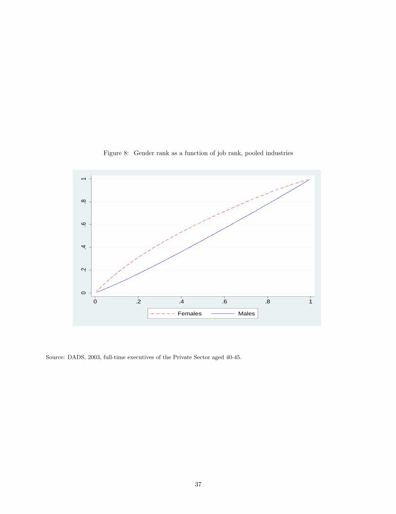
Figure 8: Gender rank as a function of job rank, pooled industries

0.2

.4.6

.81

0 .2 .4 .6 .8 1

Females Males

Source: DADS, 2003, full-time executives of the Private Sector aged 40-45.

37

Figure 9: Access function (F/M) as a function of job rank, pooled industries

0.4

.81.

21.

62

0 .2 .4 .6 .8 1

Source: DADS, 2003, full-time executives of the Private Sector aged 40-45.

Note: See Section 3 for details on the estimation method. Bounds of the confidence interval estimated by bootstrap

(100 replications) are represented in dashed lines.

38

Figure 10: Access function (F/M) as a function of job rank, insurance industry

0.4

.81.

21.

62

0 .2 .4 .6 .8 1

Source: DADS, 2003, full-time executives of the insurance industry aged 40-45.

Note: See Section 3 for details on the estimation method. Bounds of the confidence interval estimated by bootstrap

(100 replications) are represented in dashed lines.

39

Figure 11: Access function (F/M) as a function of job rank, banking industry

0.4

.81.

21.

62

0 .2 .4 .6 .8 1

Source: DADS, 2003, full-time executives of the banking industry aged 40-45.

Note: See Section 3 for details on the estimation method. Bounds of the confidence interval estimated by bootstrap

(100 replications) are represented in dashed lines.

40

Figure 12: Difference in log-wage (M-F) as a function of gender rank, insurance industry

0.1

.2.3

.4.5

.6.7

0 .2 .4 .6 .8 1

Source: DADS, 2003, full-time executives of the insurance industry aged 40-45.

Note: Bounds of the confidence interval estimated by bootstrap (100 replications) are represented in dashed lines.

41

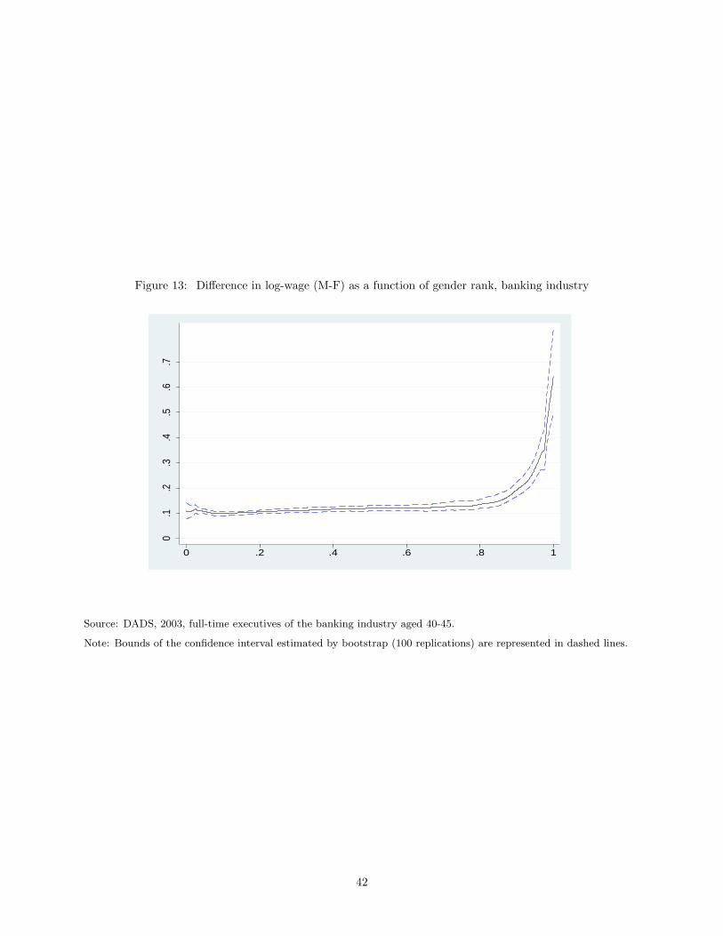
Figure 13: Difference in log-wage (M-F) as a function of gender rank, banking industry

0.1

.2.3

.4.5

.6.7

0 .2 .4 .6 .8 1

Source: DADS, 2003, full-time executives of the banking industry aged 40-45.

Note: Bounds of the confidence interval estimated by bootstrap (100 replications) are represented in dashed lines.

42

Figure 14: Access function (F/M) as a function of job rank, pooled industries,

individual observed heterogeneity taken into account

0.2

.4.6

.81

1.2

1.4

1.6

0 .2 .4 .6 .8 1

Gross Net

Source: DADS, 2003, full-time executives of the Private Sector aged 40-45.

Note: The curve labelled Gross (in black dashed line) represents the access function computed without taking into

account the individual observed heterogeneity. The curve labelled Net (in green solid line) represents the access

function obtained when taking into account the individual observed heterogeneity (see Section 6.1 for details on the

estimation method).

43

Figure 15: Average access function (F/M) as a function of job rank, large firms,

segmented markets

0.2

.4.6

.81

1.2

1.4

1.6

0 .2 .4 .6 .8 1

National Segmented Segmented, Net

Source: DADS, 2003, full-time executives aged 40-45 in firms employing more than 150 such executives.

Note: The curve labelled National (in black dashed line) represents the access function computed for the national

market without taking into account the individual observed heterogeneity. The curve labelled Segmented (in green

solid line) represents the average access function computed across segmented submarkets (each submarket being a

large firm) without taking into account the individual observed heterogeneity. The curve labelled Segmented, Net (in

orange long-dashed line) represents the average access function computed across segmented submarkets when taking

into account individual observed heterogeneity (See Section 6.2 for details on the estimation method).

44

Figure 16: Average access function (F/M) as a function of job rank, large firms,

insurance industry, segmented markets

0.2

.4.6

.81

1.2

1.4

1.6

0 .2 .4 .6 .8 1

National Segmented Segmented, Net

Source: DADS, 2003, full-time executives aged 40-45 in firms of the insurance industry employing more than 150 such

executives.

Note: The curve labelled National (in black dashed line) represents the access function computed for the national

market without taking into account the individual observed heterogeneity. The curve labelled Segmented (in green

solid line) represents the average access function computed across segmented submarkets (each submarket being a

large firm) without taking into account the individual observed heterogeneity. The curve labelled Segmented, Net (in

orange long-dashed line) represents the average access function computed across segmented submarkets when taking

into account individual observed heterogeneity (See Section 6.2 for details on the estimation method).

45

Figure 17: Average access function (F/M) as a function of job rank, large firms,

banking industry, segmented markets

0.2

.4.6

.81

1.2

1.4

1.6

0 .2 .4 .6 .8 1

National Segmented Segmented, Net

Source: DADS, 2003, full-time executives aged 40-45 in firms of the banking industry employing more than 150 such

executives.

Note: The curve labelled National (in black dashed line) represents the access function computed for the national

market without taking into account the individual observed heterogeneity. The curve labelled Segmented (in green

solid line) represents the average access function computed across segmented submarkets (each submarket being a

large firm) without taking into account the individual observed heterogeneity. The curve labelled Segmented, Net (in

orange long-dashed line) represents the average access function computed across segmented submarkets when taking

into account individual observed heterogeneity (See Section 6.2 for details on the estimation method).

46

Table 1: Descriptive statistics by subgroup of firms

Sector Nb. firms Nb. jobs % females Wages, all

Median Mean Std

All firms 86,989 354,968 22.4 109 139 602

Large firms 429 115,531 22.3 114 134 132

Banking 545 18,628 28.7 104 142 449

Banking, large firms 38 11,197 30.7 110 149 273

Insurance 507 9,360 36.9 107 125 74

Insurance, large firms 20 5,491 37.2 107 120 62

Source: DADS, 2003, full-time executives of the Private Sector aged 40-45.

Table 1: Descriptive statistics by subgroup of firms (cont.)

Sector Wages, Females Wages, Males

Median Mean Std Median Mean Std

All firms 96 119 434 113 145 642

Large firms 103 118 101 118 139 139

Banking 95 120 211 108 150 514

Banking, large firms 110 149 273 114 160 317

Insurance 94 105 49 115 136 84

Insurance, large firms 106 102 40 115 131 70

Source: DADS, 2003, full-time executives of the Private Sector aged 40-45.

47

Tab

le2:

Val

ues

ofth

eac

cess

func

tion

atdi

ffere

ntra

nks

p1p5

p10

p25

p50

p75

p90

p95

p99

All

firm

s.7

9.8

8.8

4.7

2.6

5.6

0.5

6.5

0.4

2

[.78,

.80]

[.86,

.91]

[.82,

.87]

[.71,

.74]

[.63,

.67]

[.58,

.62]

[.54,

.58]

[.49,

.52]

[.40,

.44]

Lar

gefir

ms

.75

.86

.74

.66

.73

.67

.61

.55

.42

[.73,

.77]

[.83,

.89]

[.71,

.78]

[.63,

.68]

[.70,

.77]

[.63,

.70]

[.57,

.64]

[.52,

.57]

[.39,

.46]

Ban

king

.80

.86

.78

.68

.68

.70

.71

.60

.48

[.76,

.85]

[.81,

.92]

[.72,

.83]

[.62,

.74]

[.63,

.74]

[.64,

.78]

[.64,

.77]

[.54,

.65]

[.41,

.55]

Ban

king

,la

rge

firm

s.8

4.8

9.9

3.6

9.7

1.6

7.6

4.4

7.3

5

[.79,

.90]

[.83,

.97]

[.84,

1.04

][.6

1,.7

9][.6

2,.8

0][.5

9,.7

6][.5

6,.7

1][.4

1,.5

4][.2

8,.4

4]

Insu

ranc

e1.

001.

03.9

1.7

3.6

2.4

9.2

8.2

7.2

7

[.93,

1.07

][.9

3,1.

10]

[.82,

1.00

][.6

7,.8

2][.5

5,.6

8][.4

3,.5

5][.2

4,.3

2][.2

3,.3

1][.2

2,.3

4]

Insu

ranc

e,la

rge

firm

s1.

061.

12.9

9.7

2.6

1.4

7.2

2.2

1.2

4

[.96,

1.17

][.9

9,1.

24]

[.85,

1.16

][.6

2,.8

8][.5

1,.7

1][.3

9,.5

3][.1

7,.2

8][.1

6,.2

6][.1

8,.3

2]

Sourc

e:D

AD

S,

2003,

full-t

ime

exec

uti

ves

of

the

Pri

vate

Sec

tor

aged

40-4

5.

Note

:See

Sec

tion

3fo

rth

ees

tim

ati

on

met

hod.

Bounds

of

the

confiden

cein

terv

als

rep

ort

edin

bra

cket

sare

esti

mate

dby

boots

trap

(100

replica

tions)

.

48

Table 3: Linear specification of the access function

Sector National market Segmented markets

Const Slope Stat Const Slope Stat

All firms .80 .28 .453

[.79,.81] [.26,.29]

Large firms .74 .09 .828 .69 .05 .434

[.72,.76] [.07,.14] [.64,.70] [-.02,.07]

Banking .71 .07 .066

[.67,.75] [-.01,.15]

Banking, large firms .83 .26 .077 .77 .25 .300

[.77,.89] [.16,.39] [.67,.82] [.11,.33]

Insurance .90 .60 .078

[.85,.95] [.54,.69]

Insurance, large firms .93 .66 .056 .74 .41 .339

[.82,1.01] [.53,.79] [.60,.79] [.23,.51]

Source: DADS, 2003, full-time executives of the Private Sector aged 40-45.

Note: We report the estimated coefficients of a linear specification of the access function, h (u) = a − b.u. Bounds

of the confidence intervals are estimated by bootstrap (100 replications) and are given in brackets. We also report

the statistic of a specification test for which the threshold at the 5% level is .461. The method used to estimate the

coefficients and to compute the test statistic is detailed in Appendix B.

49

Figure A.1: Average access function (F/M) as a function of job rank, insurance industry,

individual observed heterogeneity taken into account

0.2

.4.6

.81

1.2

1.4

1.6

0 .2 .4 .6 .8 1

Gross Net

Source: DADS, 2003, full-time executives of the insurance industry aged 40-45.

Note: The curve labelled Gross (in black dashed line) represents the access function computed without taking into

account the individual observed heterogeneity. The curve labelled Net (in green solid line) represents the access

function obtained when taking into account the individual observed heterogeneity (see Section 6.1 for details on the

estimation method).

50

Figure A.2: Average access function (F/M) as a function of job rank, banking industry,

individual observed heterogeneity taken into account

0.2

.4.6

.81

1.2

1.4

1.6

0 .2 .4 .6 .8 1

Gross Net

Source: DADS, 2003, full-time executives of the banking industry aged 40-45.

Note: The curve labelled Gross (in black dashed line) represents the access function computed without taking into

account the individual observed heterogeneity. The curve labelled Net (in green solid line) represents the access

function obtained when taking into account the individual observed heterogeneity (see Section 6.1 for details on the

estimation method).

51

Table A.1: Coefficients of individual variables for males

Sector age41 age42 age43 age44 age45 foreigner

All firms .033*** .057*** .071*** .072*** .088*** .101***

(.006) (.006) (.006) (.007) (.007) (.006)

Large firms .021 .031** .028** .047*** .056*** .148***

(.013) (.013) (.013) (.013) (.013) (.012)

Banking -.021 -.015 .038 -.014 -.016 .317***

(.030) (.030) (.030) (.030) (.030) (.031)

Banking, large firms .005 .012 -.020 -.032 -.019 .281***

(.044) (.045) (.045) (.045) (.046) (.045)

Insurance .032 .064 .020 -.001 .054 .126***

(.045) (.044) (.044) (.045) (.045) (.048)

Insurance, large firms -.020 -.010 -.089 -.117 -.059 .227***

(.072) (.072) (.069) (.072) (.072) (.079)

Source: DADS, 2003, full-time male executives of the Private Sector aged 40-45.

Note: The coefficients are estimated by maximizing the partial likelihood on the subsample of males (cf. Section 7.1).

Standard errors are given in parentheses. Level of significance: ***: 1%, **: 5%, *: 10%.

52

Table A.2: Coefficients of individual variables for females

Sector age41 age42 age43 age44 age45 foreigner

All firms -.023*** -.008 -.000 -.005 .015 .145***

(.012) (.012) (.012) (.012) (.012) (.011)

Large firms -.020 -.031 .014 .030 .059** .190***

(.024) (.024) (.024) (.024) (.025) (.023)

Banking -.061 -.023 .050 .010 .060 .359***

(.045) (.045) (.046) (.047) (.048) (.045)

Banking, large firms -.127** -.107* -.021 -.039 .005 .297***

(.064) (.063) (.064) (.066) (.069) (.064)

Insurance .015 -.070 .008 .049 .059 .148**

(.059) (.057) (.058) (.057) (.058) (.063)

Insurance, large firms -.182** -.317*** .028 .023 -.006 .160

(.088) (.089) (.091) (.093) (.092) (.107)

Source: DADS, 2003, full-time female executives of the Private Sector aged 40-45.

Note: The coefficients are estimated by maximizing the partial likelihood on the subsample of females (cf. Section

7.1). Standard errors are given in parentheses. Level of significance: ***: 1%, **: 5%, *: 10%.

53

Table A.3: Coefficients of individual variables for males, segmented markets

Sector age41 age42 age43 age44 age45 foreigner

Large firms .031** .059*** .082*** .126*** .155*** .074***

(.013) (.013) (.013) (.013) (.013) (.013)

Banking, large firms .026 .034 .006 .006 .014 .195***

(.045) (.045) (.046) (.046) (.047) (.046)

Insurance, large firms .017 .052 -.034 -.022 .030 .152*

(.073) (.073) (.070) (.073) (.073) (.081)

Source: DADS, 2003, full-time executives aged 40-45 in firms employing more than 150 such executives.

Note: The coefficients are estimated by maximizing the partial likelihood stratified by firm on the subsample of males

(cf. Section 7.2). Standard errors are given in parentheses. Level of significance: ***: 1%, **: 5%, *: 10%.

Table A.4: Coefficients of individual variables for females, segmented markets

Sector age41 age42 age43 age44 age45 foreigner

Large firms -.013 -.025 .042* .066*** .104*** .124***

(.024) (.024) (.025) (.025) (.026) (.024)

Banking, large firms -.106 -.075 .302 -.055 .065 .257***

(.066) (.064) (.065) (.067) (.070) (.065)

Insurance, large firms -.207** -.309*** .021 .052 -.008 .172

(.090) (.091) (.092) (.094) (.093) (.108)

Source: DADS, 2003, full-time executives aged 40-45 in firms employing more than 150 such executives.

Note: The coefficients are estimated by maximizing the partial likelihood stratified by firm on the subsample of

females (cf. Section 7.2). Standard errors are given in parentheses. Level of significance: ***: 1%, **: 5%, *: 10%.

54