Estimating a dynamic labour demand equation using small ...

Estimating a dynamic labour demand equationusing small, unbalanced panels: An application to

Italian manufacturing sectors

Giovanni S.F. Bruno+, Anna M. Falzoni§+

and Rodolfo Helg*++Universita Bocconi, Milano

§Universita degli Studi di Bergamo*LIUC - Universita Carlo Cattaneo

This version: July, 2005.

Abstract

We estimate a dynamic labour demand equation using a small unbal-anced panel data-set of italian manufacturing sectors.There are 31 sec-tors with an average group size of 24 time observations. The estimatoradopted is the Least Squares Dummy Variable estimator corrected for thefinite-sample bias (LSDVC) using the bias approximations derived in Bruno(2005a), which extend Bun and Kiviet’s (2003) to unbalanced panels. Itis implemented in Stata using Bruno’s (2005b) code XTLSDVC (availablefrom the SSC archive at http://ideas.repec.org/c/boc/bocode/s450101.html)The estimated long-run and short-run labour demand elasticities are in linewith the ranges indicated in Hamermesh (2000). In addition, their mag-nitudes are not positively affected by measures of sectoral internationalexposure, which rejects the Rodrick’s (1997) conjecture for Italy. This con-firms the results in Bruno, Falzoni, Helg (2004) obtained using a balanceddata set.JEL classification: F16, J23.Keywords: within estimator; bias approximations; international expo-

sure; dynamic labor demand equation; labour demand elasticities.

1. Introduction

This paper estimates a dynamic labour demand equation for Italy using an un-balanced panel data of manufacturing sectors, in an attempt to test for the jointpresence of sectoral international exposure (globalization) effects and output gen-erated external economies.Following Bruno, Falzoni and Helg (2004), the model specification accommo-

dates the presence of employment adjustment costs and allows for two types ofglobalization effects. First, a possible direct effect of globalization on labour pro-ductivity may emerge as formulated in Greenaway et al. (1999). Secondly, asemphasized by Dani Rodrik in his book “Has globalization gone too far?”(1997),the role played by international exposure in the labour market is not (or not only)that of a labour demand shifter, but rather of a force boosting the responsivenessof labour demand to changes in labour prices “regardless of economic structureand the identity of the trade partners” (Rodrik, 1997, 26). Our specification willpermit to test both effects in a unique estimation run by treating the globaliza-tion variable as a shifter for both the labour demand equation and the labourelasticity1. Also, by conditioning on a measure of sectoral output we can test forthe presence of output generated external economies.Three important econometric issues emerge in the empirical analysis, which

need a solution. First, as is well known the within (or LSDV) estimator fordynamic panel data models is not consistent for T fixed and N large (Nickell(1981)). Second, the cross-sectional dimension of our panel is small (there are31 manufacturing sectors with an average group size of 24 years), so that N-consistent GMM estimators -a by now standard alternative to the within estimatorfor dynamic panel data models- may be affected by a potentially severe smallsample bias (Kiviet (1995)). Finally, the unbalanced nature of our panel doesnot permit to correct the within estimator by applying the bias approximationformulae derived in Kiviet (1995), (1999) and Bun and Kiviet (2003), only validfor balanced panels. The adoption of those formulae as they are would in factrequire discarding the cross-sections (or time-series) causing unbalancedness witha potentially high loss of information. This has been the strategy followed inBruno, Falzoni and Helg (2004), which has led to the sacrifice of the sector”Radio, TV & Communication Equipment”.

1As opposed to the two-stage approach followed by Slaughter (2001), who first estimateslabour demand elasticities and then regress the estimated elasticities on a set of globalizationmeasures.

2

In the view of the above considerations, our estimation strategy will employ abias corrected LSDV estimator using the recent LSDV bias approximation formu-lae derived in Bruno (2005a), which extends Kiviet’s (1999) and Bun and Kiviet’s(2003) to (possibly) unbalanced panels.The received empirical literature on the labour market effects of globalization

is not conclusive. Bruno, Falzoni and Helg (2004) carry out a comparative studyon OECD countries, including Italy, using a specification similar to that adoptedin this paper, but on a balanced version of the data and with a restricted choice ofbias approximations, to find support for the Rodrik’s conjecture only in the casesof France and the UK.Slaughter (2001), adopting a two-stage approach on an industry-year panel

from 1961 through 1991 for the United States, provides mixed support to theview that trade contributed to increased elasticities. In the first stage, Slaughterfinds that demand for production labour has become more elastic in manufacturingoverall and in five of eight industries within manufacturing; the same is not truefor non-production labour. In the second stage, when estimated elasticities areregressed on a set of trade variables and industry dummies are included, Slaughterfinds many significant coefficients, with the expected sign. However, in a numberof cases, these predicted effects disappear when time dummies are introduced.For production workers as well as for non production workers, time results to bea very strong predictor of elasticity pattern. In sum, there appears to be a largeunexplained residual for changing factor demand elasticities2.The experience of dramatic changes in trade regimes in a number of developing

countries might be thought as the appropriate context to investigate the theoret-ical link between openness and labour demand elasticities. This approach is infact been followed by Krishna et al. (2001) and Fajnzylber and Maloney (2001),finding however no support to the conjecture of more-elastic labour demand inresponse to trade liberalization. Using Turkish plant-level data, Krishna et al.(2001) estimates a labour demand equation in which the wage variable is inter-acted with a liberalization dummy, capturing the effect of changes in trade policy.Overall, the results show that labour demand elasticities seem to be unresponsiveto openness. Only very mixed support and no consistent patterns for the ideathat trade liberalization has an impact on own wage elasticities also emerges inthe study by Fajnzylber and Maloney (2001). They use dynamic panel techniquesto estimate labour demand functions for manufacturing establishments in Chile,

2Applying a similar methodology, Faini et al. (1999) find some support to the hypothesis thatgreater globalisation is associated with larger elasticities for Italy during the period 1985-1995.

3

Colombia and Mexico.Finally, Greenaway et al. (1999) evaluate the impact of trade volumes on

employment through induced productivity changes. Adopting a dynamic labourdemand framework for the UK, they find that increases in trade volumes, bothin terms of imports and exports, cause reductions in the level of derived labourdemand, consistently with the view that increased openness serves to increase theefficiency with which labour is utilized in the firm. Greenaway et al. also analysesthe impact of trade changes on the slope of the derived labour demand introducinga term corresponding to interactions between the wage rate and import and exportvolumes. They find a positive effect of trade volumes on the labour demandelasticity but this impact is not significant3.Our emprical results are as follows. First, all testable regularity conditions im-

plied by cost minimising behaviour are always satisfied, with the estimated labourdemand elasticities, both short-run and long-run, being always significantly nega-tive and within the empirical ranges documented in Hamermesh (2000). Second,results for the bias-corrected LSDV estimators are robust to changes in the orderof the bias approximations and to different choices of the N-consistent estimatorused to initialize the bias correction. Third, the Rodrik’s conjecture is decidedlyrejected for all estimators used (bias-corrected and GMM), which confirms theresults for Italy in Bruno, Falzoni and Helg (2004). Fourth, the direct effect ofglobalization on labour demand is never found significant. Finally, we find robustevidence in favour of output generated external economies.The structure of the paper is as follow. The next section explains the bias

correction strategy. Section 3 set up the theoretical framework. Section 4 describesthe data. Estimation results are contained in Section 5.

2. Bias corrected LSDV estimators

In this section we review the existing results on the LSDV bias approximations fordynamic panels with N and T small, or only moderately large, and and their useto implement bias-corrected LSDV estimators. Consider the standard dynamicpanel data model

yit = γyi,t−1 + x0itβ + ηi + it; |γ| < 1; i = 1, ..., N and t = 1, ..., T, (2.1)

3Adopting a different methodology and focusing on the intersectoral dimension of the scaleeffect, Jean (2000) finds, for France, that trade openness can indeed have a significant effect onlabour demand elasticities.

4

where yit is the dependent variable; xit is the ((k − 1)× 1) vector of strictly ex-ogenous explanatory variables; ηi is an unobserved individual effect; and it is anunobserved white noise disturbance. Collecting observations over time and acrossindividuals gives

y = Dη +Wδ + ,

where y and W =

∙y−1...X

¸are the (NT × 1) and (NT × k) matrices of stacked

observations; D = IN ⊗ ιT is the (NT ×N) matrix of individual dummies, (ιTis the (T × 1) vector of all unity elements); η is the (N × 1) vector of individualeffects; is the (NT × 1) vector of disturbances; and δ =

∙γ...β0¸0is the (k × 1)

vector of coefficients.It has been long recognized that the LSDV estimator for model (2.1) is not

consistent for finite T . Nickell (1981) derives an expression for the inconsistencyfor N → +∞, which is O (T−1). Kiviet (1995) obtains a bias approximation thatcontains terms of higher order than T−1. In Kiviet (1999) a more accurate biasapproximation is derived. Bun and Kiviet (2003) reformulate the approximationin Kiviet (1999) with simpler formulae for each term.All foregoing bias approximations are derived for balanced panels. As such

they are useless in our case, unless we balance our panel at the cost of time orsector observations. This waste of information can be avoided, however, by usingthe bias approximations in Bruno (2005a) extending Bun and Kiviet’s (2003)formulae to unbalanced panels with a strictly exogenous selection rule. Bruno(2005a) defines the static selection indicator zit such that zit = 1 if (yit, xit) isobserved and zit = 0 otherwise. From this he also defines the dynamic selectionrule s (rit, ri,t−1) selecting only the observations that are usable for the dynamicmodel, namely those for which both current values and one-time lagged values areobservable:

sit =

½1 if (zi,t, zi,t−1) = (1, 1)0 otherwise

i = 1, ..., N and t = 1, ..., T.

Thus, for any i the number of usable observations is given by Ti =PT

t=1 sit. The

total number of usable observations is given by n =PN

i=1 Ti; and T = n/N denotesthe average group size. For each i define the (T × 1)-vector si = [si1..., siT ]0 andthe (T × T ) diagonal matrix Si having the vector si on its diagonal. Define alsothe (NT ×NT ) block-diagonal matrix S = diag (Si). The (possibly) unbalanced

5

dynamic model can then be written as

Sy = SDη + SWδ + S . (2.2)

The LSDV estimator is given by

δLSDV = (W0MsW )

−1W 0Msy,

whereMs = S

³I −D (D0SD)−1D0

´S

is the symmetric and idempotent (NT ×NT ) matrix wiping out individual meansand selecting usable observations.Bruno’s (2005a) bias approximation terms for unbalanced panels are then the

following

c1

³T−1´

= σ2tr (Π) q1; (2.3)

c2³N−1T

−1´= −σ2

hQW

0ΠMsW + tr

³QW

0ΠMsW

´Ik+1+

2σ2q11tr (Π0ΠΠ) Ik+1

¤q1;

c3

³N−1T

−2´= σ4tr (Π)

n2q11QW

0ΠΠ0Wq1 +

h³q01W

0ΠΠ0Wq1

´+

q11tr³QW

0ΠΠ0W

´+ 2tr (Π0ΠΠ0Π) q211

iq1o;

where Q = [E (W 0MsW )]−1 =

hW

0MsW + σ2tr (Π0Π) e1e01

i−1; W = E (W ); e1 =

(1, 0, ..., 0)0 is a (k×1) vector; q1 = Qe1; q11 = e01q1; LT is the (T × T ) matrix withunit first lower subdiagonal and all other elements equal to zero;L = IN ⊗ LT ;ΓT = (IT − γLT )

−1; Γ = IN⊗ΓT ; and Π =MsLΓ. Clearly, in any balanced designS ≡ INT , so Ms = I − D (D0D)−1D0, and the above terms reduce to Bun andKiviet’s (2003).With an increasing level of accuracy, the following three possible bias approx-

imations emerge

B1 = c1³T−1´

; B2 = B1 + c2³N−1T

−1´; B3 = B2 + c3

³N−1T

−2´. (2.4)

Approximations (2.4) depend upon the unknown parameters σ2 and γ, so theyare unfeasible for bias correction. The bias corrected LSDV estimator is then

6

implemented using the two-step procedure suggested by Kiviet (1995) and Bruno(2005b). The first step obtains estimates for σ2 and γ from some N−consistentestimator. The second step performs bias correction by depuring the LSDV esti-mator from the bias approximation of choice evaluated at the estimated σ2 and

γ, bBi, as follows:

LSDV Ci = LSDV − bBi, i = 1, 2 and 3. (2.5)

Possible consistent estimators for γ are Anderson and Hsiao (AH) and Arellanoand Bond (AB). Depending on the estimator of choice for γ, say h, a consistentestimator for σ2 is then given by

bσ2h = e0hMseh(N − k − T )

, (2.6)

where eh = y −Wδh, and h = AH, AB. Monte Carlo analysis in Bruno (2005b)demonstrates that for sample sizes comparable to ours all possible forms of LSDVCoutperforms LSDV and GMM estimators.

3. The Model

The theoretical model on which we base our empirical analysis has the feature ofproducing labour demand elasticities in one stage. We consider a sector in theeconomy with a large number of firms using the same technology. There are twodomestic production inputs, domestic labour l and capital k producing output q,with w and r being the compensations for l and k, respectively. The market forproduction factors is perfectly competitive, whereas no assumption is made onthe form of the output market.We allow for two distinct sources of external economies at the firm level. Those

generated by the sectoral production ; and those generated by the sectoral in-ternational exposure. Sectoral international exposure may foster technology ad-vancement and productivity growth through several channels, such as technologyadvancement embodied in imported capital goods and intermediate inputs, tech-nology transfers accompanying foreign direct investment, learning-by-exportingeffects, etc. The empirical literature on these issues is vast. A number of em-pirical works have resorted to firm and plant-level panel data to see whether thepredicted gains from trade liberalization have materialized in some recent episodesof drastic trade reform in the developing world and/or to see whether productivity

7

growth has been a result of increasing international integration and exposure indeveloped countries. Most of these studies find that trade reform in developingcountries was indeed accompanied by productivity growth, technology advance-ment, falling mark-ups and a reshuffling of resources toward the more efficientfirms, although in some cases the evidence may fail to convince because of thehurdles involved in the methodology used in these studies (see, among others,Tybout (2003) which reviews the plant-level evidence in the light of the new tradetheory, Bernard and Jensen (1999), Clerides, Lach and Tybout (1998), Pavcnik(2002)).With this in mind, we suppose that the firm technology exhibits constant

returns to scale with external economies generated by sectoral international expo-sure g and also by sectoral output y.We also allow for exogenous technical changecaptured by a time trend t :

q = f (k, l; y, g, t) , (3.1)

Given the property of constant returns to scale at the firm level, the sectoralproduction function is just the firm production function f with the aggregatesectoral variables as arguments and it is implicitely defined by

y = f (k, l; y, g, t) (3.2)

(see Bruno (2004) and the references threin). We suppose that f is invertible iny so that an equivalent form of the sectoral production function in (3.2) is thefollowing

y = F (k, l; g, t) .

We also suppose F homothetic.For given g and y the optimal aggregate input demands l∗ and k∗ must satisfy

the following cost minimisation problem:

minl,k[wl + rk : y = F (k, l; g, t)] (3.3)

We assume that the following labour demand equation emerges as a solution ofproblem (3.3).

ln l =¡βw + βwg ln g + βwt ln t

¢ln (w/r) + βy ln y + βg ln g + u+ , (3.4)

8

where βy, βw, βwg, βwt, βg and βx are constant parameters. The parameter βgmeasures the impact of g as a demand shifter, whereas βwg and βwt measure theimpact of g and the time trend t on the relative wage elasticity of the labourdemand function, which is given by

εlw ≡ ∂ ln l

∂ lnw= βw + βwg ln g + βwt ln t. (3.5)

In equilibrium, sectoral international exposure g may influence labour’s ownprice elasticity, as well as bring about a direct effect on labour demand acting asa demand shifter.To correctly interpret parameter estimates it is important to establish the

exact relationship between the parameters of the labour demand equation (3.4)and those of the underlying production function. Details on the recovering of theproduction function from (3.4) are shown in appendix. Basically, we first retrievethe underlying cost function by integrating (3.4), and then we obtain the followingproduction function from the cost function by duality:

y =

µ1

eu+ gβg

¶ 1βyµ −εlw1 + εlw

¶ εlwβy

(k)−εlw

βy (l)1+εlwβy . (3.6)

From (3.6) it is clear that for equation (3.4) to be theoretically consistent withboth cost minimizing behaviour (requiring a downward sloping labour demandcurve) and a regular production function (requiring a non negative labour marginalproductivity) the regularity condition εlw ∈ [−1, 0] must hold.Function (3.6) is homothetic of degree 1/βy and has a restricted translog form,

with a variable technical efficiency given by

A =

µ1

eu+ gβg

¶ 1βyµ −εlw1 + εlw

¶ εlwβy

. (3.7)

A depends on international exposure g, the stochastic shock , and labour demandelasticity εlw. If βwg = 0, then A reduces to the expression for technical efficiencyin Greenaway et al. (1999).Implementing this model empirically we can test for the presence of globaliza-

tion effects in the labour demand equation as broken down into 1) the Rodrik’sconjecture that βwg < 0, that is international exposure has a positive impact on|εlw|; and 2) a globalization’s direct effect on labour demand as measured by βg(Greenaway et al., 1999). We can also test for the presence of output generatedscale economies, which implies 0 < βy < 1.

9

4. Data Description

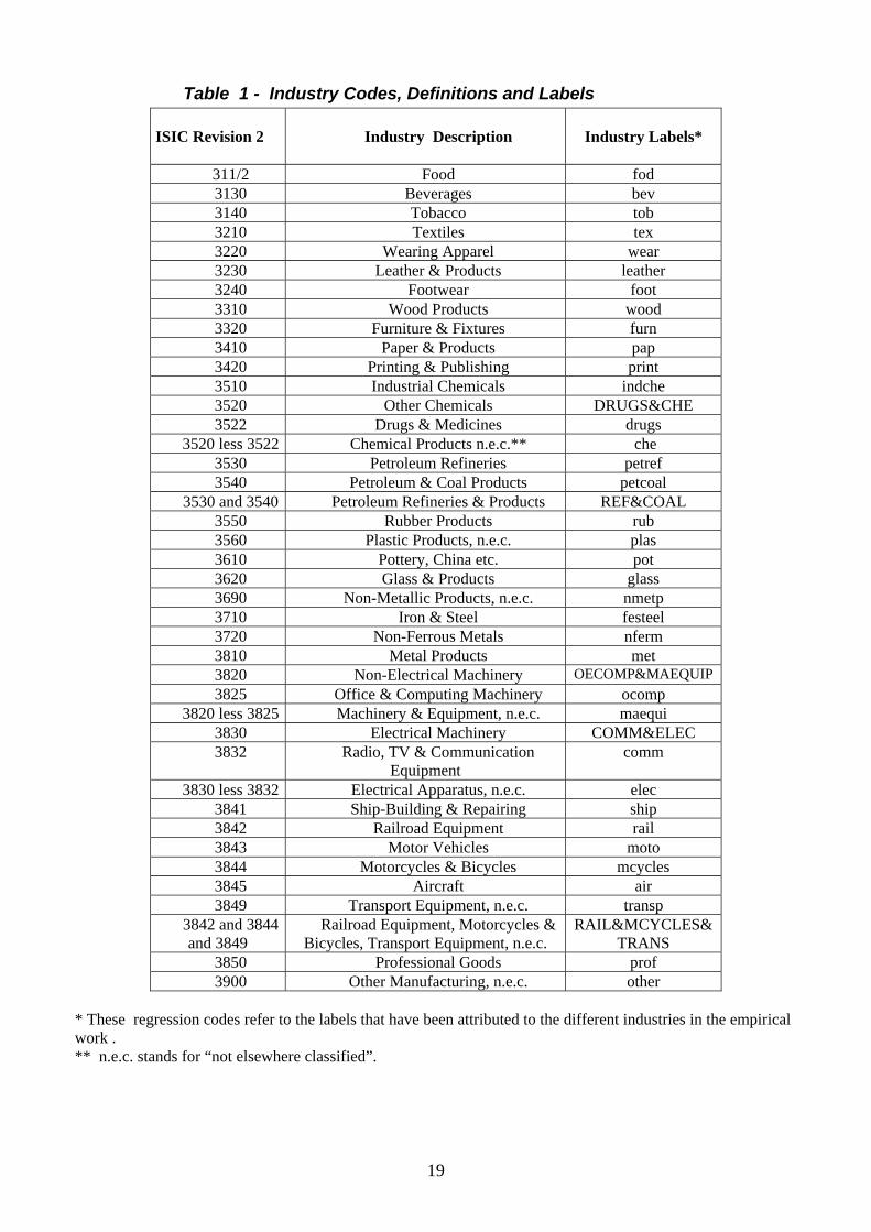
Our panel data set comes from the STAN database, a data set compiled bythe OECD and containing internationally comparable data. The industries aregrouped using the standard ISIC Revision 2 classification4. The data set orig-inally covered a panel of 40 manufacturing industries in the period 1970-1997across countries. Missing observations for some of the regression variables alongwith the loss of the first observation when taking lags, however, make the estima-tion sample unbalanced, reducing to N = 31 sectors (we lose Drugs; Chemicals;Office & Computing Machinery; Machinery & Equipment; Electrical Apparatus;Railroad Equipment; Motorcycles & Bicycles; Transport Equipment) with an av-erage group size of T = 24. Unbalancedness is not severe, as evidenced from thecomputation of the Ahrens and Pincus index of unbalancedness ω = 0.99, where

ω = N/

"T

NXi=1

(1/Ti)

#,

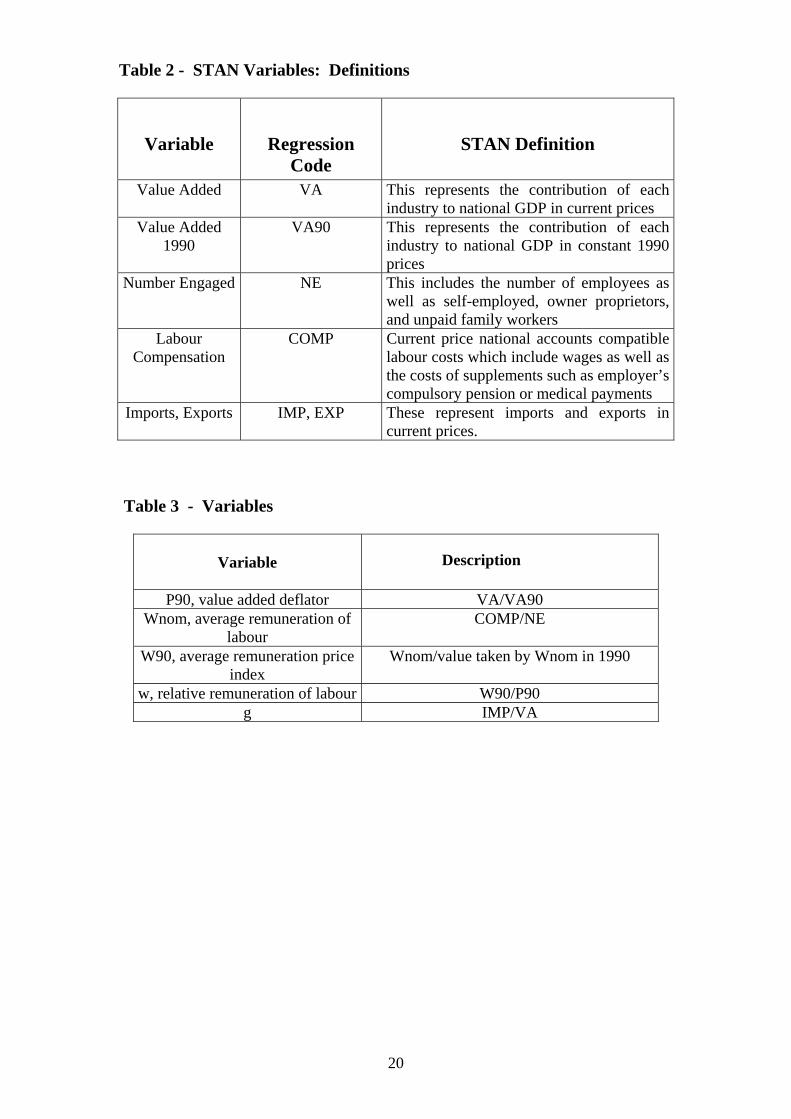
with 0 < ω ≤ 1 and ω = 1 when the panel is balanced (see Bruno (2005)).Nevertheless, balancing the data would have caused the loss of one further cross-section, namely Radio, TV & Communication Equipment, which we can avoid byusing the appropriate estimation techniques.The variables used in the empirical work are the following5. Our dependent

variable l is measured as “number engaged” (NE). The output variable y is proxiedby Value Added in constant 1990 prices (VA90). Relative wage of domestic labourw is constructed as follows: 1) we obtain average remuneration of labour by takingthe ratio of total labour cost to number engaged; 2) we divide this variable bythe price of capital p which is proxied by the value added deflator. As a proxyfor international integration, g, we utilize the share of import over value added6.The choice of this proxy to measure international integration is motivated by ourfocus on the substitution effect’s component of the labour demand elasticity. Infact, import penetration might well represent, at the same time, a measure ofsubstitution possibilities in production due to the availability of a larger variety

4Details concerning the industry description and the ISIC rev.2 code are given in Table 1.5Table 2 provides definitions for the variables of the STAN database that have been used

in the empirical implementation as given in the OECD STAN database manual, as well as thevariable codes used in the regression analysis.

6Further details regarding the construction of these variables are given in Table 3.

10

of inputs and a measure of the competitive pressure coming from the internationalmarkets.Figures 1 and 2 taken from Bruno, Falzoni and Helg (2004) provide a first

picture of the issue under analysis for some OECD countries. In the last decadesa generalised reduction in the demand for labour paralleled the developmentsin the international openness. Employment in the manufacturing industry hasbeen decreasing, in the face of an increasing integration into the world economy,although the correlation between the two phenomena is not high for Italy.

5. Estimation results

Our econometric model is based upon equation (3.4). Let N denote the numberof sectors and T the largest group size in the panel. We accommodate sector het-erogeneity by allowing u to vary across sectors. Since data on r are not availablewe proxy it by a complete set of time dummies, based on the assumption thatthe price of capital does not vary across sectors, as it would happen in the pres-ence of perfect capital markets. The time trend interacted with lnw allows forautonomous variations in labour demand elasticity. Time dummies and the inter-acted trend should also capture the effect of exogenous technical change. Thus,our empirical baseline equation is as follows

zit ln li,t = zit£¡βw + βwg ln gi,t + βwt ln ti,t

¢lnwi,t + βy ln yi,t (5.1)

+βg ln gi,t +T−1Xt=1

βtdt + ui + i,t

#,

where zit is the static selection rule, t = 1, ..., T , i = 1, ..., N .Equation (5.1) is static in nature, so it fails to incorporate labour adjustment

cost. This is can be taken into account by including the lagged dependent variableinto the right hand side of the baseline equation and replacing the static selectionrule zit with the dynamic selection rule sit derived from zit as in Section 2 :

sit ln li,t = sit£γ ln li,t−1 +

¡βw + βwg ln gi,t + βwt ln ti,t

¢lnwi,t (5.2)

+βy ln yi,t + βg ln gi,t +T−1Xt=1

βtdt + ui + i,t

#,

t = 1, ..., T , i = 1, ...,N.

11

In the empirical application our focus is on the long-run wage elasticity, whichdepends on ln g, ln t and the long-run parameters

βj = βj/ (1− γ) , j = w, wg, wt. (5.3)

according to the following formula7:

εlwi,t ≡ βw + βwg ln g + βwt ln t.

The simple long-run estimator obtained by using the bias-corrected LSDVestimator for the β’s into equation (5.3) is not unbiased to order O(T−1) as pointedout by Bun (2001). Therefore, to estimate the long-run coefficients we adoptthe estimator proposed by Bun (2001), based upon Pesaran and Zhao (1999),which is a more appropriate transformation of the bias-corrected LSDV short runestimator.Finally, since analytic expressions for the standard errors of all corrected es-

timators typically turns out to be very inaccurate, we estimate them by usingparametric bootstrap resampling schemes, as proposed in Bun and Kiviet (2001)and Bun (2001)8.Tables 4 to 7 present estimation results for equation (5.2). Table 4 reports

results for all possible bias-corrected LSDV estimators, based on bias approxima-tions bB1 bB2 and bB3 and initial estimators AH and AB, as explained in Section 2.For the sake of comparison, Tables 5 and 6 reports results for two different GMMestimators, respectively with strictly exogenous and predetermined regressors. Ineither case the number of GMM instruments is taken to a minimum to not exac-erbate the small-sample bias9. Results for the uncorrected LSDV are reported inTable 7.Overall, our estimates are statistically and economically satisfactory with all

regularity conditions satisfied. Results for the bias-corrected LSDV estimators arerobust to changes in the order of the bias approximations and to different choices

7To avoid that εlw become too large in absolute value when g is close to zero, the globalizationindex g is normalized so that g ≥ 1.

8All estimation work has been carried out in STATA 9 using for the bias-corrected LSDVestimators the user-written code XTLSDVC by Bruno (2005c) downloadable fromhttp://ideas.repec.org/c/boc/bocode/s450101.html9GMM estimation has been carried out in Stata 9 using the user-written code XTABOND2

by David Roodman (2005).

12

of the N-consistent estimator used to initialize the bias correction. In the GMMregressions the null hypothesis of no-second order correlation in the disturbancesof the first-differenced equation is never rejected at any conventional level of sig-nificance. The estimated coefficient on the one-time lagged employment level isalways significantly greater than zero and smaller than unity providing evidence ofsignificant adjustment costs. Our dynamic framework allows estimation of bothshort and long run constant output labour demand elasticities. Estimates arealways plausible. The mean value of the long run elasticity is for all countrieswithin the range estimates of other studies surveyed by Hamermesh (2000) and isrelatively robust to changes in estimation method. Moreover, all point estimatesfor the various sectors are negative.What is the role of increasing international integration? In our framework this

effect can work on labour demand through two channels: the direct effect and theeffect via elasticity (Rodrik’s conjecture). The Rodrik’s conjecture is decidedlyrejected for all estimators used (bias-corrected and GMM), which confirms theresults for Italy in Bruno, Falzoni and Helg (2004) and also those obtained bySlaughter (2001) for the US, by Krishna et al. (2001) for Turkey and Fajnzyl-ber and Maloney (2001) for a group of Latin American less developed countries.Fourth, differently from what found in Bruno, Falzoni and Helg (2004) the directeffect of globalization on labour demand is never found significant. This discrep-ancy may be due to the neglected sector in Bruno, Falzoni and Helg (2004) where asignificantly positive direct effect has been found in the bias corrected regressions.Finally, we find robust evidence in favour of output generated external economies.

6. Conclusions

This paper has estimated a dynamic labour demand equation for an unbalancedpanel data set of Italian manufacturing sectors. We have used both bias-correctedLSDV estimators and GMM estimators. Our findings are substantially robust tochanges in the estimator adopted. While we do not find support for either theRodrik’s conjecture or the presence of a direct globalization effect in the labourdemand equation, we can provide robust evidence in favour of output generatedexternal economies. Long run and short run estimated elasticities are alwaysplausible in both an economics and statistics sense.

13

References

[1] Ahn, S.C. and P. Schimdt, (1995), “Efficient Estimation of Models for Dy-namic Panel Data”, Journal of Econometrics, 68, 5-28.

[2] Arellano, M. and S. Bond, (1991), “Some Tests of Specification for PanelData: Monte Carlo Evidence and an Application to Employment Equations”,Review of Economic Studies, 58, 277-297.

[3] Blundell, R.W. and S.R. Bond, (1998), ”Initial Conditions and Moment Re-strictions in Dynamic Panel Data Models”, Journal of Econometrics, 87,115-143.

[4] Bruno, G.S.F. (2005a). “Approximating the bias of the LSDV estimator fordynamic unbalanced panel data models”. Economics Letters, 87, 361-366.

[5] Bruno, G.S.F. (2005b) “Estimation and inference in dynamic unbalancedpanel data models with a small number of individuals”. CESPRI WP n.165, Universita Bocconi-CESPRI, Milan.

[6] Bruno, G.S.F. (2005c) ”XTLSDVC: Stata module to estimate bias cor-rected LSDV dynamic panel data models,” Statistical Software ComponentsS450101, Boston College Department of Economics.

[7] Bruno, G.S.F. (2004). “On the Equivalence of Two Concepts of Returns toScale”. Bulletin of Economic Research, 56, 67-80.

[8] Bruno, G.S.F., Falzoni A.M. and R. Helg (2004), “Measuring the effect ofglobalization on labor demand elasticity: An empirical application to someOECD countries”, w.p. CESPRI n. 153, Universita Bocconi-CESPRI, Milano.

[9] Bun, M.J.G. (2001) “Bias Correction in the Dynamic Panel Data Model witha Nonscalar Disturbance Covariance Matrix” Tinbergen Institute DiscussionPaper TI 2001-007/4.

[10] Bun, M.J.G. and J.F. Kiviet, (2001), “The accuracy of inference in smallsamples of dynamic data models”, Tinbergen Institute D.P. 006/4.

[11] Bun, M.J.G. and J.F Kiviet (2003) “On the diminishing returns of higherorder terms in asymptotic expansions of bias” Economics Letters, 79, 145-152.

14

[12] Coe, D. and E. Helpman, (1995), ”International R&D spillovers”, EuropeanEconomic Review, 39, 859-87.

[13] Faini, R., A.M. Falzoni, M. Galeotti, R. Helg and A. Turrini, (1999), ”Import-ing jobs and exporting firms? On the wage and employment implications ofItalian trade and foreign direct investment flows”, Giornale degli Economistied Annali di Economia, 58 (1), 95-135.

[14] Fajnzylber, P. and W. Maloney, (2001), ”Labour demand and trade reformin Latin America”, World Bank Working Paper No. 2491, January.

[15] Feenstra, R. and G. Hanson, (2001), ”Global production sharing and risinginequality: A survey of trade and wages”, NBER W.P. 8372, July.

[16] Greenaway, D., R.C. Hine and P.Wright, (1999), ”An empirical assessmentof the impact of trade on employment in the United Kingdom”, EuropeanJournal of Political Economy, 15, 485-500.

[17] Hamermesh, D.S., (1993), Labor Demand, Princeton University Press, Prince-ton.

[18] Hamermesh, D.S., (2000), Demand for labor, in International Encyclopaediaof the Social & Behavioural Sciences

[19] Harris, M.N., and L. Matyas, (2000), “A comparative analysis of differentestimators for dynamic panel data models”, mimeo.

[20] Jean, S., (2000), ”The effect of international trade on labour-demand elastic-ities: intersectoral matters”, Review of International Economics, 8(3), 504-516.

[21] Kiviet, J.F., (1995), “On bias, inconsistency and efficiency of various estima-tors in dynamic panel data models”, Journal of Econometrics, 68, 53-78.

[22] Kiviet, J.F. (1999), “Expectation of Expansions for Estimators in a DynamicPanel Data Model; Some Results for Weakly Exogenous Regressors” in C.Hsiao, K. Lahiri, L-F Lee and M.H. Pesaran (eds.), Analysis of Panel Dataand Limited Dependent Variables, Cambridge University Press, Cambridge.

[23] Krishna, P., D. Mitra and S. Chinoy, (2001), ”Trade liberalization and labourdemand elasticities: evidence from Turkey”, Journal of International Eco-nomics, 55, 391-409.

15

[24] Nickell, S.J., (1981), “Biases in Dynamic Models with Fixed Effects”, Econo-metrica, 49, 1417-1426.

[25] Panagariya, A., (1999), Trade openness: consequences for the elasticity ofdemand for labor and wage outcomes, mimeo.

[26] Pesaran, M.H. and Z. Zhao (1999), “Bias Reduction in Estimating Long-runRelationships from Dynamic Heterogeneous Panels” in C. Hsiao, K. Lahiri,L-F Lee and M.H. Pesaran (eds.), Analysis of Panel Data and Limited De-pendent Variables, Cambridge University Press, Cambridge.

[27] Rauch, J.E. and V. Trindade, (2003), “Information, International Substi-tutability and Globalisation”, American Economic Review, 93, 775-791.

[28] Rodrik, D., (1997), Has globalisation gone too far?, Institute for InternationalEconomics, Washington DC.

[29] Roodman, D. (2003). ”XTABOND2: Stata module to extend xtabond dy-namic panel data estimator,” Statistical Software Components S435901,Boston College Department of Economics, revised 22 Apr 2005.

[30] Slaughter, M.J., (2001), ”International trade and labor-demand elasticities”,Journal of International Economics, 54, 27-56.

16

Appendix A

Basically, we first retrieve the underlying cost function by integrating (3.4),and then we obtain the production function from the cost function by duality. Forsimplicity, we limit to a specification with no time trend in the labour demandequation and let r = 1.The first step of the derivation is straightforward. From Shephard’s Lemma

and (3.4) we have∂C

∂w= l = eu+ yβyxβxgβgwβw+βwg ln g,

and so the (normalized) cost function must have the following restricted translogform:

C =

Z w

0

eu+ yβyxβxgβgωβw+βwg ln gdω =eu+ yβyxβxgβg

βw + βwg ln g + 1wβw+βwg ln g+1. (6.1)

It is a restricted form in that the interaction term between output and wage andthe squared wage do not enter the cost function specification.The second step goes as follows. Singling out w in

l = eu+ yβyxβxgβgwβw+βwg ln g.

yields

w =

µl

eu+ yβyxβxgβg

¶1/(βw+βwg ln g). (6.2)

Since C is a normalized cost function, we can write

C = wl + k. (6.3)

Thus, substituting for C from (6.1) and for w from (6.2) into (6.3) givesµl

eu+ yβyxβxgβg

¶1/(βw+βwg ln g)l+k =

eu+ yβyxβxgβg

βw + βwg ln g + 1

µl

eu+ yβyxβxgβg

¶1+ 1βw+βwg ln g

,

(6.4)which, after rearrangement and substituting for βw+βwg ln g from (3.5), gives thedesired production function.

y =

µ1

eu+ xβxgβg

¶ 1βyµ −εlw1 + εlw

¶ εlwβy

(k)− εlw

βy (l)1+εlwβy .

17

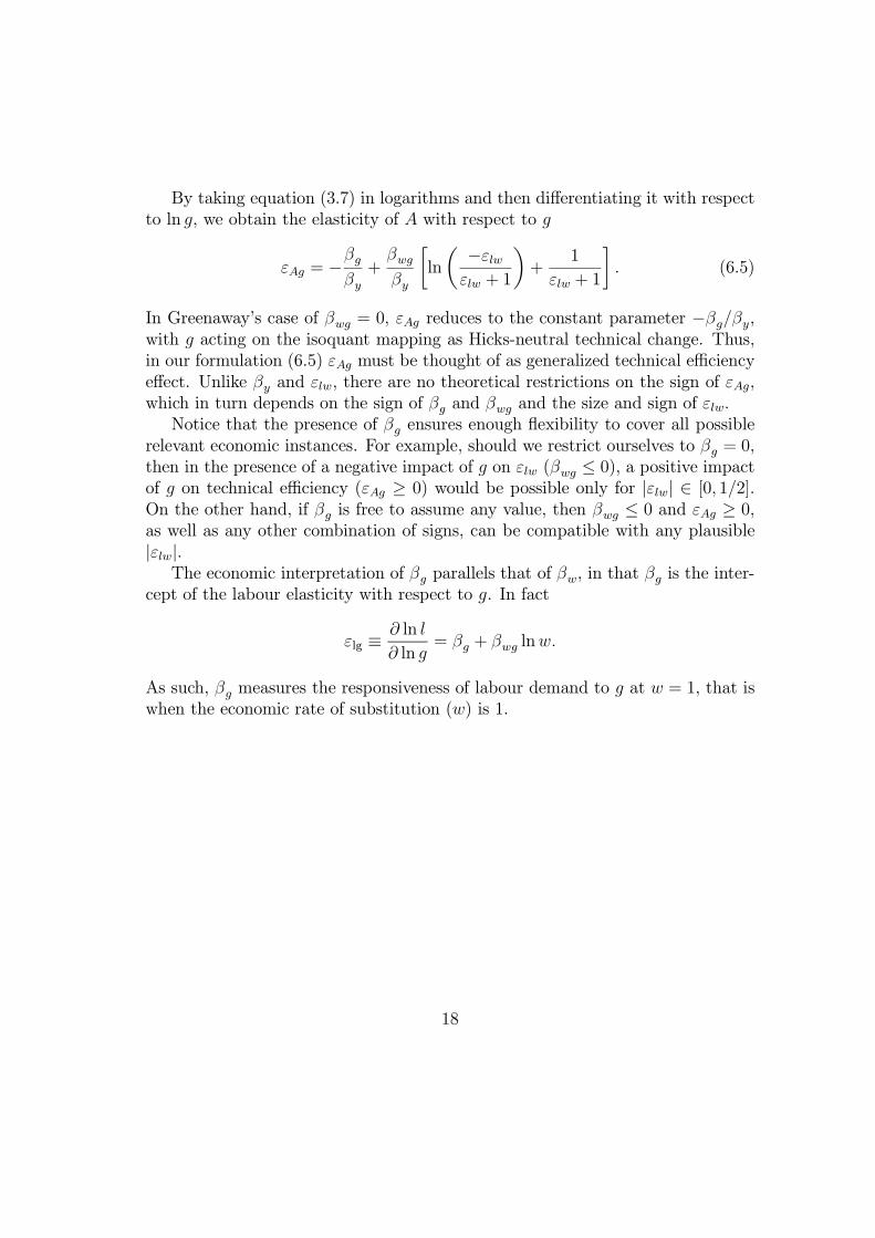
By taking equation (3.7) in logarithms and then differentiating it with respectto ln g, we obtain the elasticity of A with respect to g

εAg = −βgβy+

βwgβy

∙ln

µ −εlwεlw + 1

¶+

1

εlw + 1

¸. (6.5)

In Greenaway’s case of βwg = 0, εAg reduces to the constant parameter −βg/βy,with g acting on the isoquant mapping as Hicks-neutral technical change. Thus,in our formulation (6.5) εAg must be thought of as generalized technical efficiencyeffect. Unlike βy and εlw, there are no theoretical restrictions on the sign of εAg,which in turn depends on the sign of βg and βwg and the size and sign of εlw.Notice that the presence of βg ensures enough flexibility to cover all possible

relevant economic instances. For example, should we restrict ourselves to βg = 0,then in the presence of a negative impact of g on εlw (βwg ≤ 0), a positive impactof g on technical efficiency (εAg ≥ 0) would be possible only for |εlw| ∈ [0, 1/2].On the other hand, if βg is free to assume any value, then βwg ≤ 0 and εAg ≥ 0,as well as any other combination of signs, can be compatible with any plausible|εlw|.The economic interpretation of βg parallels that of βw, in that βg is the inter-

cept of the labour elasticity with respect to g. In fact

εlg ≡ ∂ ln l

∂ ln g= βg + βwg lnw.

As such, βg measures the responsiveness of labour demand to g at w = 1, that iswhen the economic rate of substitution (w) is 1.

18

19

Table 1 - Industry Codes, Definitions and Labels

ISIC Revision 2

Industry Description

Industry Labels*

311/2 Food fod 3130 Beverages bev 3140 Tobacco tob 3210 Textiles tex 3220 Wearing Apparel wear 3230 Leather & Products leather 3240 Footwear foot 3310 Wood Products wood 3320 Furniture & Fixtures furn 3410 Paper & Products pap 3420 Printing & Publishing print 3510 Industrial Chemicals indche 3520 Other Chemicals DRUGS&CHE 3522 Drugs & Medicines drugs

3520 less 3522 Chemical Products n.e.c.** che 3530 Petroleum Refineries petref 3540 Petroleum & Coal Products petcoal

3530 and 3540 Petroleum Refineries & Products REF&COAL 3550 Rubber Products rub 3560 Plastic Products, n.e.c. plas 3610 Pottery, China etc. pot 3620 Glass & Products glass 3690 Non-Metallic Products, n.e.c. nmetp 3710 Iron & Steel festeel 3720 Non-Ferrous Metals nferm 3810 Metal Products met 3820 Non-Electrical Machinery OECOMP&MAEQUIP 3825 Office & Computing Machinery ocomp

3820 less 3825 Machinery & Equipment, n.e.c. maequi 3830 Electrical Machinery COMM&ELEC 3832 Radio, TV & Communication

Equipment comm

3830 less 3832 Electrical Apparatus, n.e.c. elec 3841 Ship-Building & Repairing ship 3842 Railroad Equipment rail 3843 Motor Vehicles moto 3844 Motorcycles & Bicycles mcycles 3845 Aircraft air 3849 Transport Equipment, n.e.c. transp

3842 and 3844 and 3849

Railroad Equipment, Motorcycles & Bicycles, Transport Equipment, n.e.c.

RAIL&MCYCLES&TRANS

3850 Professional Goods prof 3900 Other Manufacturing, n.e.c. other

* These regression codes refer to the labels that have been attributed to the different industries in the empirical work . ** n.e.c. stands for “not elsewhere classified”.

20

Table 2 - STAN Variables: Definitions

Variable

Regression Code

STAN Definition

Value Added VA This represents the contribution of each industry to national GDP in current prices

Value Added 1990

VA90 This represents the contribution of each industry to national GDP in constant 1990 prices

Number Engaged NE This includes the number of employees as well as self-employed, owner proprietors, and unpaid family workers

Labour Compensation

COMP Current price national accounts compatible labour costs which include wages as well as the costs of supplements such as employer’s compulsory pension or medical payments

Imports, Exports IMP, EXP These represent imports and exports in current prices.

Table 3 - Variables

Variable

Description

P90, value added deflator VA/VA90 Wnom, average remuneration of

labour COMP/NE

W90, average remuneration price index

Wnom/value taken by Wnom in 1990

w, relative remuneration of labour W90/P90 g IMP/VA

Figure 1 - MANUFACTURING EMPLOYMENT IN OECD COUNTRIES (Logarithms)

10.5

11

11.5

12

12.5

13

13.5

1971

1973

1975

1977

1979

1981

1983

1985

1987

1989

1991

1993

1995

JapanFranceItalyUnited statesSpainSwedenUnited Kingdom

Source: OECD, STAN Database.

21

Figure 2 - IMPORT PENETRATION IN OECD COUNTRIES (Logarithms)

0.1

0.3

0.5

0.7

0.9

1.1

1971

1972

1973

1974

1975

1976

1977

1978

1979

1980

1981

1982

1983

1984

1985

1986

1987

1988

1989

1990

1991

1992

1993

1994

1995

1996

JapanFranceItalyUnited StatesSpainSwedenUnited Kingdom

Source: OECD, STAN Database.

22

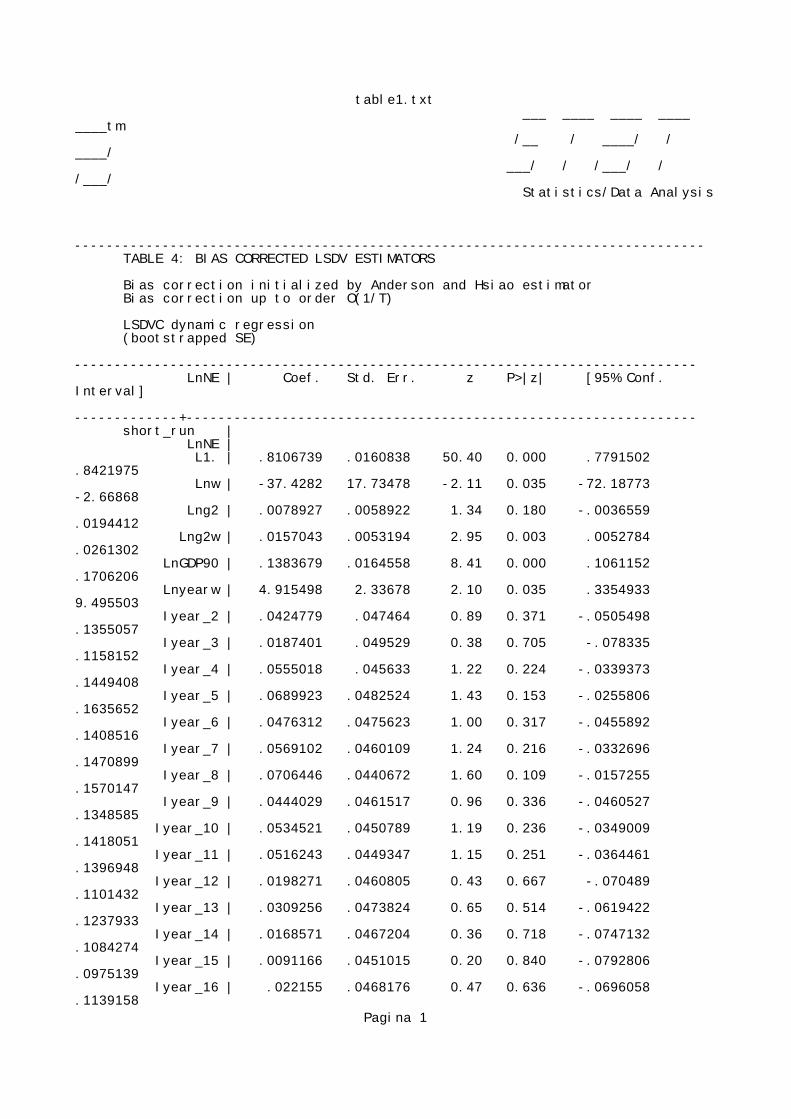
table1.txt ___ ____ ____ ____ ____tm /__ / ____/ / ____/ ___/ / /___/ / /___/ Statistics/Data Analysis ------------------------------------------------------------------------------- TABLE 4: BIAS CORRECTED LSDV ESTIMATORS

Bias correction initialized by Anderson and Hsiao estimator Bias correction up to order O(1/T) LSDVC dynamic regression (bootstrapped SE) ------------------------------------------------------------------------------ LnNE | Coef. Std. Err. z P>|z| [95% Conf. Interval] -------------+---------------------------------------------------------------- short_run | LnNE | L1. | .8106739 .0160838 50.40 0.000 .7791502 .8421975 Lnw | -37.4282 17.73478 -2.11 0.035 -72.18773 -2.66868 Lng2 | .0078927 .0058922 1.34 0.180 -.0036559 .0194412 Lng2w | .0157043 .0053194 2.95 0.003 .0052784 .0261302 LnGDP90 | .1383679 .0164558 8.41 0.000 .1061152 .1706206 Lnyearw | 4.915498 2.33678 2.10 0.035 .3354933 9.495503 Iyear_2 | .0424779 .047464 0.89 0.371 -.0505498 .1355057 Iyear_3 | .0187401 .049529 0.38 0.705 -.078335 .1158152 Iyear_4 | .0555018 .045633 1.22 0.224 -.0339373 .1449408 Iyear_5 | .0689923 .0482524 1.43 0.153 -.0255806 .1635652 Iyear_6 | .0476312 .0475623 1.00 0.317 -.0455892 .1408516 Iyear_7 | .0569102 .0460109 1.24 0.216 -.0332696 .1470899 Iyear_8 | .0706446 .0440672 1.60 0.109 -.0157255 .1570147 Iyear_9 | .0444029 .0461517 0.96 0.336 -.0460527 .1348585 Iyear_10 | .0534521 .0450789 1.19 0.236 -.0349009 .1418051 Iyear_11 | .0516243 .0449347 1.15 0.251 -.0364461 .1396948 Iyear_12 | .0198271 .0460805 0.43 0.667 -.070489 .1101432 Iyear_13 | .0309256 .0473824 0.65 0.514 -.0619422 .1237933 Iyear_14 | .0168571 .0467204 0.36 0.718 -.0747132 .1084274 Iyear_15 | .0091166 .0451015 0.20 0.840 -.0792806 .0975139 Iyear_16 | .022155 .0468176 0.47 0.636 -.0696058 .1139158

Pagina 1

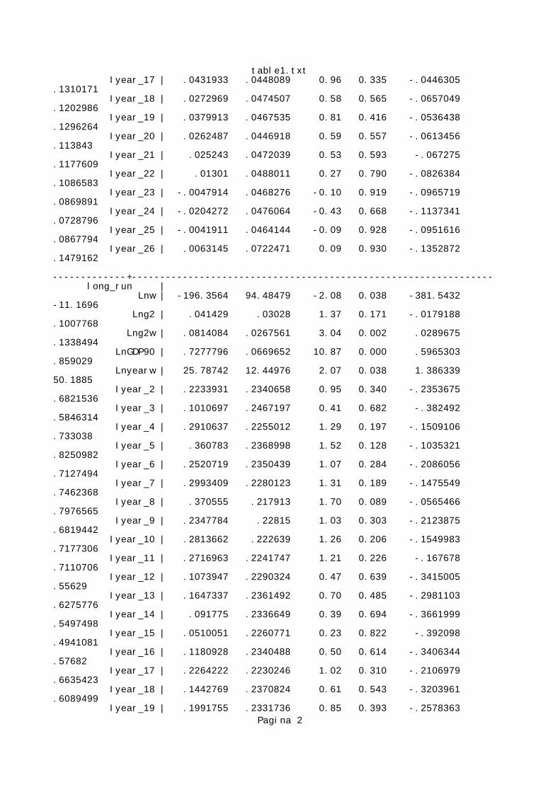
table1.txt Iyear_17 | .0431933 .0448089 0.96 0.335 -.0446305 .1310171 Iyear_18 | .0272969 .0474507 0.58 0.565 -.0657049 .1202986 Iyear_19 | .0379913 .0467535 0.81 0.416 -.0536438 .1296264 Iyear_20 | .0262487 .0446918 0.59 0.557 -.0613456 .113843 Iyear_21 | .025243 .0472039 0.53 0.593 -.067275 .1177609 Iyear_22 | .01301 .0488011 0.27 0.790 -.0826384 .1086583 Iyear_23 | -.0047914 .0468276 -0.10 0.919 -.0965719 .0869891 Iyear_24 | -.0204272 .0476064 -0.43 0.668 -.1137341 .0728796 Iyear_25 | -.0041911 .0464144 -0.09 0.928 -.0951616 .0867794 Iyear_26 | .0063145 .0722471 0.09 0.930 -.1352872 .1479162 -------------+---------------------------------------------------------------- long_run | Lnw | -196.3564 94.48479 -2.08 0.038 -381.5432 -11.1696 Lng2 | .041429 .03028 1.37 0.171 -.0179188 .1007768 Lng2w | .0814084 .0267561 3.04 0.002 .0289675 .1338494 LnGDP90 | .7277796 .0669652 10.87 0.000 .5965303 .859029 Lnyearw | 25.78742 12.44976 2.07 0.038 1.386339 50.1885 Iyear_2 | .2233931 .2340658 0.95 0.340 -.2353675 .6821536 Iyear_3 | .1010697 .2467197 0.41 0.682 -.382492 .5846314 Iyear_4 | .2910637 .2255012 1.29 0.197 -.1509106 .733038 Iyear_5 | .360783 .2368998 1.52 0.128 -.1035321 .8250982 Iyear_6 | .2520719 .2350439 1.07 0.284 -.2086056 .7127494 Iyear_7 | .2993409 .2280123 1.31 0.189 -.1475549 .7462368 Iyear_8 | .370555 .217913 1.70 0.089 -.0565466 .7976565 Iyear_9 | .2347784 .22815 1.03 0.303 -.2123875 .6819442 Iyear_10 | .2813662 .222639 1.26 0.206 -.1549983 .7177306 Iyear_11 | .2716963 .2241747 1.21 0.226 -.167678 .7110706 Iyear_12 | .1073947 .2290324 0.47 0.639 -.3415005 .55629 Iyear_13 | .1647337 .2361492 0.70 0.485 -.2981103 .6275776 Iyear_14 | .091775 .2336649 0.39 0.694 -.3661999 .5497498 Iyear_15 | .0510051 .2260771 0.23 0.822 -.392098 .4941081 Iyear_16 | .1180928 .2340488 0.50 0.614 -.3406344 .57682 Iyear_17 | .2264222 .2230246 1.02 0.310 -.2106979 .6635423 Iyear_18 | .1442769 .2370824 0.61 0.543 -.3203961 .6089499 Iyear_19 | .1991755 .2331736 0.85 0.393 -.2578363

Pagina 2

table1.txt.6561873 Iyear_20 | .1383651 .2235214 0.62 0.536 -.2997288 .576459 Iyear_21 | .1336213 .2358854 0.57 0.571 -.3287056 .5959482 Iyear_22 | .0707774 .2431877 0.29 0.771 -.4058617 .5474165 Iyear_23 | -.021597 .2354106 -0.09 0.927 -.4829933 .4397992 Iyear_24 | -.1031693 .2390672 -0.43 0.666 -.5717323 .3653938 Iyear_25 | -.0204023 .2334456 -0.09 0.930 -.4779472 .4371427 Iyear_26 | .0328895 .3589615 0.09 0.927 -.6706621 .7364411 ------------------------------------------------------------------------------ ------------------------------------------------------------------------------ LnNE | Coef. Std. Err. z P>|z| [95% Conf. Interval] -------------+---------------------------------------------------------------- long_run_el | -.6475386 .0738227 -8.77 0.000 -.7922285 -.5028487 ------------------------------------------------------------------------------ ------------------------------------------------------------------------------ LnNE | Coef. Std. Err. z P>|z| [95% Conf. Interval] -------------+---------------------------------------------------------------- short_run_el | -.1231323 .0179602 -6.86 0.000 -.1583336 -.087931 ------------------------------------------------------------------------------ Bias correction up to order O(1/NT) LSDVC dynamic regression (bootstrapped SE) ------------------------------------------------------------------------------ LnNE | Coef. Std. Err. z P>|z| [95% Conf. Interval] -------------+---------------------------------------------------------------- short_run | LnNE | L1. | .8126495 .0158263 51.35 0.000 .7816306 .8436685 Lnw | -37.12216 17.6889 -2.10 0.036 -71.79177 -2.452542 Lng2 | .0078467 .0058816 1.33 0.182 -.003681 .0193743 Lng2w | .0156998 .0053081 2.96 0.003 .0052962 .0261034 LnGDP90 | .1372427 .0163844 8.38 0.000 .1051299 .1693554 Lnyearw | 4.875314 2.330749 2.09 0.036 .3071288 9.443498 Iyear_2 | .0421273 .0474917 0.89 0.375 -.0509548 .1352094 Iyear_3 | .0183074 .0495482 0.37 0.712 -.0788053

Pagina 3

table1.txt.1154201 Iyear_4 | .0551259 .0456548 1.21 0.227 -.0343559 .1446078 Iyear_5 | .0686369 .0482708 1.42 0.155 -.0259721 .1632459 Iyear_6 | .0470595 .0475698 0.99 0.323 -.0461756 .1402945 Iyear_7 | .0564256 .0460083 1.23 0.220 -.0337489 .1466001 Iyear_8 | .0701574 .0440749 1.59 0.111 -.0162278 .1565426 Iyear_9 | .0438874 .0461523 0.95 0.342 -.0465694 .1343442 Iyear_10 | .0529692 .045086 1.17 0.240 -.0353977 .1413361 Iyear_11 | .0511603 .0449343 1.14 0.255 -.0369094 .13923 Iyear_12 | .0193066 .0460887 0.42 0.675 -.0710257 .1096389 Iyear_13 | .0304254 .0473971 0.64 0.521 -.0624711 .1233219 Iyear_14 | .0163609 .046725 0.35 0.726 -.0752184 .1079401 Iyear_15 | .0086886 .045108 0.19 0.847 -.0797214 .0970987 Iyear_16 | .0217807 .0468291 0.47 0.642 -.0700027 .1135641 Iyear_17 | .0428982 .0448219 0.96 0.339 -.0449511 .1307475 Iyear_18 | .0269744 .0474661 0.57 0.570 -.0660573 .1200062 Iyear_19 | .0377275 .0467736 0.81 0.420 -.0539471 .129402 Iyear_20 | .0259785 .0447128 0.58 0.561 -.0616571 .113614 Iyear_21 | .0249275 .0472197 0.53 0.598 -.0676214 .1174764 Iyear_22 | .0126378 .0488202 0.26 0.796 -.0830481 .1083236 Iyear_23 | -.0051507 .0468418 -0.11 0.912 -.096959 .0866575 Iyear_24 | -.0207319 .047625 -0.44 0.663 -.1140752 .0726114 Iyear_25 | -.0043476 .0464441 -0.09 0.925 -.0953763 .0866812 Iyear_26 | .0063016 .0723425 0.09 0.931 -.135487 .1480902 -------------+---------------------------------------------------------------- long_run | Lnw | -196.6925 95.87501 -2.05 0.040 -384.6041 -8.780961 Lng2 | .0415805 .0306718 1.36 0.175 -.0185352 .1016962 Lng2w | .0820619 .0270903 3.03 0.002 .0289659 .1351579 LnGDP90 | .7290957 .0679697 10.73 0.000 .5958775 .8623138 Lnyearw | 25.83159 12.63295 2.04 0.041 1.071477 50.59171 Iyear_2 | .2237871 .2378917 0.94 0.347 -.2424719 .6900462 Iyear_3 | .1001071 .2506878 0.40 0.690 -.391232 .5914462 Iyear_4 | .29191 .229205 1.27 0.203 -.1573235 .7411436 Iyear_5 | .3622911 .2407994 1.50 0.132 -.109667 .8342492

Pagina 4

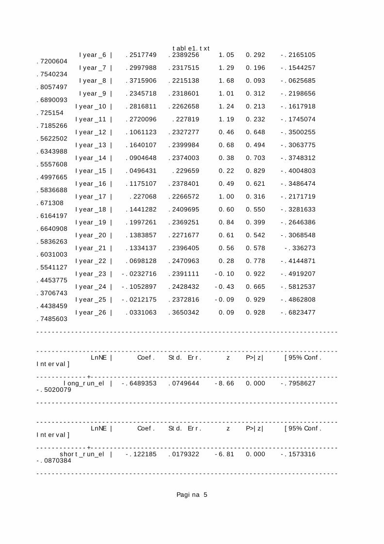
table1.txt Iyear_6 | .2517749 .2389256 1.05 0.292 -.2165105 .7200604 Iyear_7 | .2997988 .2317515 1.29 0.196 -.1544257 .7540234 Iyear_8 | .3715906 .2215138 1.68 0.093 -.0625685 .8057497 Iyear_9 | .2345718 .2318601 1.01 0.312 -.2198656 .6890093 Iyear_10 | .2816811 .2262658 1.24 0.213 -.1617918 .725154 Iyear_11 | .2720096 .227819 1.19 0.232 -.1745074 .7185266 Iyear_12 | .1061123 .2327277 0.46 0.648 -.3500255 .5622502 Iyear_13 | .1640107 .2399984 0.68 0.494 -.3063775 .6343988 Iyear_14 | .0904648 .2374003 0.38 0.703 -.3748312 .5557608 Iyear_15 | .0496431 .229659 0.22 0.829 -.4004803 .4997665 Iyear_16 | .1175107 .2378401 0.49 0.621 -.3486474 .5836688 Iyear_17 | .227068 .2266572 1.00 0.316 -.2171719 .671308 Iyear_18 | .1441282 .2409695 0.60 0.550 -.3281633 .6164197 Iyear_19 | .1997261 .2369251 0.84 0.399 -.2646386 .6640908 Iyear_20 | .1383857 .2271677 0.61 0.542 -.3068548 .5836263 Iyear_21 | .1334137 .2396405 0.56 0.578 -.336273 .6031003 Iyear_22 | .0698128 .2470963 0.28 0.778 -.4144871 .5541127 Iyear_23 | -.0232716 .2391111 -0.10 0.922 -.4919207 .4453775 Iyear_24 | -.1052897 .2428432 -0.43 0.665 -.5812537 .3706743 Iyear_25 | -.0212175 .2372816 -0.09 0.929 -.4862808 .4438459 Iyear_26 | .0331063 .3650342 0.09 0.928 -.6823477 .7485603 ------------------------------------------------------------------------------ ------------------------------------------------------------------------------ LnNE | Coef. Std. Err. z P>|z| [95% Conf. Interval] -------------+---------------------------------------------------------------- long_run_el | -.6489353 .0749644 -8.66 0.000 -.7958627 -.5020079 ------------------------------------------------------------------------------ ------------------------------------------------------------------------------ LnNE | Coef. Std. Err. z P>|z| [95% Conf. Interval] -------------+---------------------------------------------------------------- short_run_el | -.122185 .0179322 -6.81 0.000 -.1573316 -.0870384 ------------------------------------------------------------------------------

Pagina 5

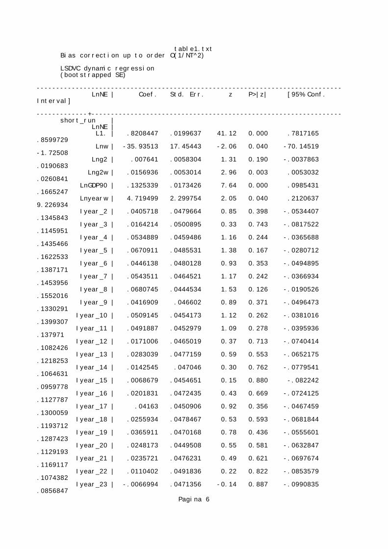
table1.txt Bias correction up to order O(1/NT^2) LSDVC dynamic regression (bootstrapped SE) ------------------------------------------------------------------------------ LnNE | Coef. Std. Err. z P>|z| [95% Conf. Interval] -------------+---------------------------------------------------------------- short_run | LnNE | L1. | .8208447 .0199637 41.12 0.000 .7817165 .8599729 Lnw | -35.93513 17.45443 -2.06 0.040 -70.14519 -1.72508 Lng2 | .007641 .0058304 1.31 0.190 -.0037863 .0190683 Lng2w | .0156936 .0053014 2.96 0.003 .0053032 .0260841 LnGDP90 | .1325339 .0173426 7.64 0.000 .0985431 .1665247 Lnyearw | 4.719499 2.299754 2.05 0.040 .2120637 9.226934 Iyear_2 | .0405718 .0479664 0.85 0.398 -.0534407 .1345843 Iyear_3 | .0164214 .0500895 0.33 0.743 -.0817522 .1145951 Iyear_4 | .0534889 .0459486 1.16 0.244 -.0365688 .1435466 Iyear_5 | .0670911 .0485531 1.38 0.167 -.0280712 .1622533 Iyear_6 | .0446138 .0480128 0.93 0.353 -.0494895 .1387171 Iyear_7 | .0543511 .0464521 1.17 0.242 -.0366934 .1453956 Iyear_8 | .0680745 .0444534 1.53 0.126 -.0190526 .1552016 Iyear_9 | .0416909 .046602 0.89 0.371 -.0496473 .1330291 Iyear_10 | .0509145 .0454173 1.12 0.262 -.0381016 .1399307 Iyear_11 | .0491887 .0452979 1.09 0.278 -.0395936 .137971 Iyear_12 | .0171006 .0465019 0.37 0.713 -.0740414 .1082426 Iyear_13 | .0283039 .0477159 0.59 0.553 -.0652175 .1218253 Iyear_14 | .0142545 .047046 0.30 0.762 -.0779541 .1064631 Iyear_15 | .0068679 .0454651 0.15 0.880 -.082242 .0959778 Iyear_16 | .0201831 .0472435 0.43 0.669 -.0724125 .1127787 Iyear_17 | .04163 .0450906 0.92 0.356 -.0467459 .1300059 Iyear_18 | .0255934 .0478467 0.53 0.593 -.0681844 .1193712 Iyear_19 | .0365911 .0470168 0.78 0.436 -.0555601 .1287423 Iyear_20 | .0248173 .0449508 0.55 0.581 -.0632847 .1129193 Iyear_21 | .0235721 .0476231 0.49 0.621 -.0697674 .1169117 Iyear_22 | .0110402 .0491836 0.22 0.822 -.0853579 .1074382 Iyear_23 | -.0066994 .0471356 -0.14 0.887 -.0990835 .0856847

Pagina 6

table1.txt Iyear_24 | -.0220543 .0479849 -0.46 0.646 -.116103 .0719944 Iyear_25 | -.0050521 .0467929 -0.11 0.914 -.0967645 .0866603 Iyear_26 | .0062565 .0733463 0.09 0.932 -.1374997 .1500127 -------------+---------------------------------------------------------------- long_run | Lnw | -198.4711 104.9382 -1.89 0.059 -404.1461 7.203984 Lng2 | .0421396 .0338627 1.24 0.213 -.0242299 .1085092 Lng2w | .0848319 .0305498 2.78 0.005 .0249554 .1447084 LnGDP90 | .7343622 .0770309 9.53 0.000 .5833844 .88534 Lnyearw | 26.0655 13.82719 1.89 0.059 -1.035288 53.16628 Iyear_2 | .2249516 .2647546 0.85 0.396 -.293958 .7438611 Iyear_3 | .0956902 .2796201 0.34 0.732 -.4523551 .6437356 Iyear_4 | .2950565 .254514 1.16 0.246 -.2037819 .7938949 Iyear_5 | .3682125 .2675497 1.38 0.169 -.1561753 .8926002 Iyear_6 | .2501976 .2660843 0.94 0.347 -.271318 .7717131 Iyear_7 | .301398 .2572079 1.17 0.241 -.2027203 .8055163 Iyear_8 | .3755988 .2462542 1.53 0.127 -.1070506 .8582483 Iyear_9 | .2334441 .2578167 0.91 0.365 -.2718674 .7387556 Iyear_10 | .2827462 .2515589 1.12 0.261 -.2103001 .7757925 Iyear_11 | .2730907 .2534652 1.08 0.281 -.223692 .7698734 Iyear_12 | .1005729 .2591709 0.39 0.698 -.4073927 .6085385 Iyear_13 | .1607934 .266906 0.60 0.547 -.3623328 .6839195 Iyear_14 | .0848068 .2637195 0.32 0.748 -.4320739 .6016875 Iyear_15 | .043782 .2555564 0.17 0.864 -.4570993 .5446634 Iyear_16 | .1148865 .2647531 0.43 0.664 -.4040201 .633793 Iyear_17 | .2295403 .2517317 0.91 0.362 -.2638448 .7229255 Iyear_18 | .1433089 .2677133 0.54 0.592 -.3813997 .6680174 Iyear_19 | .2018148 .2634266 0.77 0.444 -.3144918 .7181214 Iyear_20 | .1382834 .2521665 0.55 0.583 -.3559539 .6325207 Iyear_21 | .1323344 .2668904 0.50 0.620 -.3907612 .6554301 Iyear_22 | .0655617 .2749403 0.24 0.812 -.4733113 .6044346 Iyear_23 | -.0304885 .2661791 -0.11 0.909 -.55219 .4912129 Iyear_24 | -.1143584 .270314 -0.42 0.672 -.644164 .4154472 Iyear_25 | -.0248581 .2642243 -0.09 0.925 -.5427283 .4930121 Iyear_26 | .0340442 .4092848 0.08 0.934 -.7681392

Pagina 7

table1.txt.8362277 ------------------------------------------------------------------------------ ------------------------------------------------------------------------------ LnNE | Coef. Std. Err. z P>|z| [95% Conf. Interval] -------------+---------------------------------------------------------------- long_run_el | -.6544474 .0848239 -7.72 0.000 -.8206991 -.4881956 ------------------------------------------------------------------------------ ------------------------------------------------------------------------------ LnNE | Coef. Std. Err. z P>|z| [95% Conf. Interval] -------------+---------------------------------------------------------------- short_run_el | -.1181952 .0185026 -6.39 0.000 -.1544596 -.0819308 ------------------------------------------------------------------------------ Bias correction initialized by Arellano and Bond estimator Bias correction up to order O(1/T) LSDVC dynamic regression (bootstrapped SE) ------------------------------------------------------------------------------ LnNE | Coef. Std. Err. z P>|z| [95% Conf. Interval] -------------+---------------------------------------------------------------- short_run | LnNE | L1. | .81093 .0148334 54.67 0.000 .7818571 .840003 Lnw | -37.48922 17.29518 -2.17 0.030 -71.38715 -3.591292 Lng2 | .0068047 .0057475 1.18 0.236 -.0044601 .0180695 Lng2w | .0161855 .0049647 3.26 0.001 .0064549 .0259161 LnGDP90 | .1367775 .0153978 8.88 0.000 .1065984 .1669567 Lnyearw | 4.92383 2.278926 2.16 0.031 .4572169 9.390442 Iyear_2 | .0413684 .0450729 0.92 0.359 -.0469729 .1297097 Iyear_3 | .0177511 .0470518 0.38 0.706 -.0744688 .109971 Iyear_4 | .0548159 .0434931 1.26 0.208 -.030429 .1400608 Iyear_5 | .0684923 .0459993 1.49 0.136 -.0216646 .1586493 Iyear_6 | .0468161 .0452183 1.04 0.301 -.0418101 .1354423 Iyear_7 | .0563512 .0437722 1.29 0.198 -.0294407 .1421431 Iyear_8 | .0700905 .0419231 1.67 0.095 -.0120772 .1522582 Iyear_9 | .0438861 .0439847 1.00 0.318 -.0423224

Pagina 8

table1.txt.1300946 Iyear_10 | .0531657 .0430191 1.24 0.217 -.0311501 .1374816 Iyear_11 | .0515253 .0429092 1.20 0.230 -.0325751 .1356258 Iyear_12 | .0196222 .0439225 0.45 0.655 -.0664643 .1057087 Iyear_13 | .030718 .0451901 0.68 0.497 -.057853 .1192889 Iyear_14 | .0165165 .0445986 0.37 0.711 -.0708951 .1039282 Iyear_15 | .0089108 .0430013 0.21 0.836 -.0753701 .0931917 Iyear_16 | .0220088 .0446019 0.49 0.622 -.0654093 .1094269 Iyear_17 | .0430127 .0427683 1.01 0.315 -.0408115 .126837 Iyear_18 | .0272014 .0452964 0.60 0.548 -.0615779 .1159808 Iyear_19 | .0379497 .0446478 0.85 0.395 -.0495583 .1254578 Iyear_20 | .0263113 .0426756 0.62 0.538 -.0573314 .109954 Iyear_21 | .0251989 .0450321 0.56 0.576 -.0630624 .1134601 Iyear_22 | .0128658 .046526 0.28 0.782 -.0783234 .104055 Iyear_23 | -.0049918 .0446552 -0.11 0.911 -.0925144 .0825308 Iyear_24 | -.0206484 .0453304 -0.46 0.649 -.1094943 .0681975 Iyear_25 | -.0042492 .0442184 -0.10 0.923 -.0909156 .0824173 Iyear_26 | .0065919 .0689207 0.10 0.924 -.1284901 .1416739 -------------+---------------------------------------------------------------- long_run | Lnw | -196.8692 91.99204 -2.14 0.032 -377.1703 -16.5681 Lng2 | .0364071 .0294983 1.23 0.217 -.0214084 .0942227 Lng2w | .0837377 .0248645 3.37 0.001 .0350043 .1324712 LnGDP90 | .7212201 .0638432 11.30 0.000 .5960898 .8463505 Lnyearw | 25.85624 12.12139 2.13 0.033 2.098759 49.61373 Iyear_2 | .2184863 .222393 0.98 0.326 -.217396 .6543685 Iyear_3 | .0965984 .2345575 0.41 0.680 -.3631258 .5563226 Iyear_4 | .2882047 .2151328 1.34 0.180 -.1334479 .7098572 Iyear_5 | .3588637 .225967 1.59 0.112 -.0840234 .8017508 Iyear_6 | .2485808 .2235302 1.11 0.266 -.1895304 .686692 Iyear_7 | .2970887 .2171351 1.37 0.171 -.1284883 .7226657 Iyear_8 | .3684018 .2073267 1.78 0.076 -.0379512 .7747547 Iyear_9 | .2326552 .2175341 1.07 0.285 -.1937039 .6590143 Iyear_10 | .2803646 .2122427 1.32 0.187 -.1356236 .6963527 Iyear_11 | .271556 .2139177 1.27 0.204 -.147715 .6908271

Pagina 9

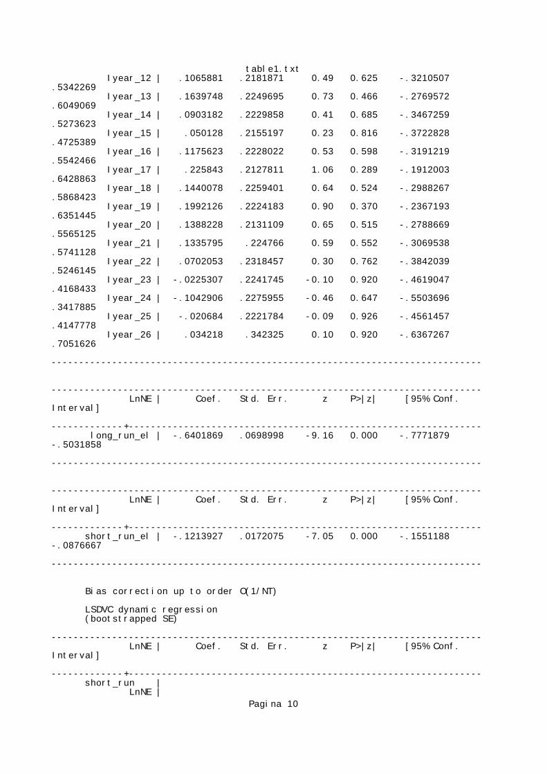
table1.txt Iyear_12 | .1065881 .2181871 0.49 0.625 -.3210507 .5342269 Iyear_13 | .1639748 .2249695 0.73 0.466 -.2769572 .6049069 Iyear_14 | .0903182 .2229858 0.41 0.685 -.3467259 .5273623 Iyear_15 | .050128 .2155197 0.23 0.816 -.3722828 .4725389 Iyear_16 | .1175623 .2228022 0.53 0.598 -.3191219 .5542466 Iyear_17 | .225843 .2127811 1.06 0.289 -.1912003 .6428863 Iyear_18 | .1440078 .2259401 0.64 0.524 -.2988267 .5868423 Iyear_19 | .1992126 .2224183 0.90 0.370 -.2367193 .6351445 Iyear_20 | .1388228 .2131109 0.65 0.515 -.2788669 .5565125 Iyear_21 | .1335795 .224766 0.59 0.552 -.3069538 .5741128 Iyear_22 | .0702053 .2318457 0.30 0.762 -.3842039 .5246145 Iyear_23 | -.0225307 .2241745 -0.10 0.920 -.4619047 .4168433 Iyear_24 | -.1042906 .2275955 -0.46 0.647 -.5503696 .3417885 Iyear_25 | -.020684 .2221784 -0.09 0.926 -.4561457 .4147778 Iyear_26 | .034218 .342325 0.10 0.920 -.6367267 .7051626 ------------------------------------------------------------------------------ ------------------------------------------------------------------------------ LnNE | Coef. Std. Err. z P>|z| [95% Conf. Interval] -------------+---------------------------------------------------------------- long_run_el | -.6401869 .0698998 -9.16 0.000 -.7771879 -.5031858 ------------------------------------------------------------------------------ ------------------------------------------------------------------------------ LnNE | Coef. Std. Err. z P>|z| [95% Conf. Interval] -------------+---------------------------------------------------------------- short_run_el | -.1213927 .0172075 -7.05 0.000 -.1551188 -.0876667 ------------------------------------------------------------------------------ Bias correction up to order O(1/NT) LSDVC dynamic regression (bootstrapped SE) ------------------------------------------------------------------------------ LnNE | Coef. Std. Err. z P>|z| [95% Conf. Interval] -------------+---------------------------------------------------------------- short_run | LnNE |

Pagina 10

table1.txt L1. | .812389 .0146827 55.33 0.000 .7836114 .8411667 Lnw | -37.24224 17.25805 -2.16 0.031 -71.06739 -3.417082 Lng2 | .0067095 .0057323 1.17 0.242 -.0045257 .0179447 Lng2w | .0162096 .0049454 3.28 0.001 .0065168 .0259024 LnGDP90 | .1358483 .0153404 8.86 0.000 .1057817 .1659149 Lnyearw | 4.891408 2.274039 2.15 0.031 .4343732 9.348442 Iyear_2 | .0410543 .0450835 0.91 0.362 -.0473076 .1294163 Iyear_3 | .017382 .0470615 0.37 0.712 -.0748568 .1096209 Iyear_4 | .0545049 .0434999 1.25 0.210 -.0307533 .1397632 Iyear_5 | .068207 .0460086 1.48 0.138 -.0219681 .1583822 Iyear_6 | .0463522 .0452178 1.03 0.305 -.042273 .1349774 Iyear_7 | .0559663 .0437717 1.28 0.201 -.0298247 .1417572 Iyear_8 | .0697037 .0419244 1.66 0.096 -.0124667 .1518741 Iyear_9 | .0434806 .0439919 0.99 0.323 -.0427419 .1297032 Iyear_10 | .0527974 .0430301 1.23 0.220 -.03154 .1371348 Iyear_11 | .0511814 .0429195 1.19 0.233 -.0329392 .135302 Iyear_12 | .0192303 .0439343 0.44 0.662 -.0668794 .1053401 Iyear_13 | .0303404 .0452023 0.67 0.502 -.0582545 .1189352 Iyear_14 | .0161339 .0446036 0.36 0.718 -.0712874 .1035553 Iyear_15 | .008586 .0430089 0.20 0.842 -.0757099 .0928819 Iyear_16 | .0217269 .044614 0.49 0.626 -.065715 .1091687 Iyear_17 | .0427877 .0427776 1.00 0.317 -.0410549 .1266303 Iyear_18 | .0269615 .0453121 0.60 0.552 -.0618485 .1157716 Iyear_19 | .0377568 .0446576 0.85 0.398 -.0497704 .125284 Iyear_20 | .0261202 .0426858 0.61 0.541 -.0575424 .1097828 Iyear_21 | .0249699 .045049 0.55 0.579 -.0633244 .1132642 Iyear_22 | .0125904 .0465383 0.27 0.787 -.078623 .1038038 Iyear_23 | -.0052602 .0446637 -0.12 0.906 -.0927995 .082279 Iyear_24 | -.0208785 .0453399 -0.46 0.645 -.1097432 .0679862 Iyear_25 | -.004361 .0442304 -0.10 0.921 -.091051 .082329 Iyear_26 | .0066037 .0689887 0.10 0.924 -.1286117 .1418191 -------------+---------------------------------------------------------------- long_run | Lnw | -197.0197 93.16465 -2.11 0.034 -379.619 -14.42032 Lng2 | .0362339 .0298391 1.21 0.225 -.0222497

Pagina 11

table1.txt.0947176 Lng2w | .0843484 .0251162 3.36 0.001 .0351216 .1335751 LnGDP90 | .721734 .0646164 11.17 0.000 .5950883 .8483798 Lnyearw | 25.87607 12.2759 2.11 0.035 1.815739 49.9364 Iyear_2 | .2185206 .2254847 0.97 0.332 -.2234213 .6604624 Iyear_3 | .0956567 .2378408 0.40 0.688 -.3705026 .561816 Iyear_4 | .288674 .2181256 1.32 0.186 -.1388444 .7161923 Iyear_5 | .359871 .2291007 1.57 0.116 -.089158 .8089 Iyear_6 | .2481673 .2266464 1.09 0.274 -.1960514 .6923861 Iyear_7 | .2973007 .220134 1.35 0.177 -.1341541 .7287554 Iyear_8 | .3690407 .2101884 1.76 0.079 -.042921 .7810024 Iyear_9 | .2323872 .2205708 1.05 0.292 -.1999236 .6646979 Iyear_10 | .2805424 .2151987 1.30 0.192 -.1412393 .702324 Iyear_11 | .2717815 .2169291 1.25 0.210 -.1533917 .6969546 Iyear_12 | .1056062 .2212496 0.48 0.633 -.3280351 .5392476 Iyear_13 | .1634025 .2281331 0.72 0.474 -.2837302 .6105352 Iyear_14 | .0892755 .2260931 0.39 0.693 -.3538589 .5324098 Iyear_15 | .0490816 .2185314 0.22 0.822 -.3792321 .4773952 Iyear_16 | .1171066 .22593 0.52 0.604 -.325708 .5599212 Iyear_17 | .2262866 .2157547 1.05 0.294 -.1965848 .649158 Iyear_18 | .1438897 .2291173 0.63 0.530 -.305172 .5929513 Iyear_19 | .199628 .2255109 0.89 0.376 -.2423651 .6416212 Iyear_20 | .1388772 .2160695 0.64 0.520 -.2846113 .5623658 Iyear_21 | .1334448 .2279121 0.59 0.558 -.3132548 .5801443 Iyear_22 | .0694906 .2350917 0.30 0.768 -.3912807 .530262 Iyear_23 | -.0237816 .2272992 -0.10 0.917 -.4692799 .4217166 Iyear_24 | -.1058803 .2307686 -0.46 0.646 -.5581784 .3464178 Iyear_25 | -.0212689 .2252898 -0.09 0.925 -.4628287 .4202909 Iyear_26 | .0344773 .347267 0.10 0.921 -.6461535 .715108 ------------------------------------------------------------------------------ ------------------------------------------------------------------------------ LnNE | Coef. Std. Err. z P>|z| [95% Conf. Interval] -------------+---------------------------------------------------------------- long_run_el | -.6408 .0707549 -9.06 0.000 -.779477 -.502123

Pagina 12

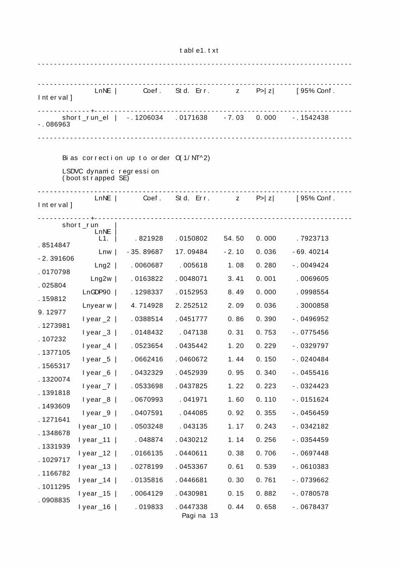
table1.txt ------------------------------------------------------------------------------ ------------------------------------------------------------------------------ LnNE | Coef. Std. Err. z P>|z| [95% Conf. Interval] -------------+---------------------------------------------------------------- short_run_el | -.1206034 .0171638 -7.03 0.000 -.1542438 -.086963 ------------------------------------------------------------------------------ Bias correction up to order O(1/NT^2) LSDVC dynamic regression (bootstrapped SE) ------------------------------------------------------------------------------ LnNE | Coef. Std. Err. z P>|z| [95% Conf. Interval] -------------+---------------------------------------------------------------- short_run | LnNE | L1. | .821928 .0150802 54.50 0.000 .7923713 .8514847 Lnw | -35.89687 17.09484 -2.10 0.036 -69.40214 -2.391606 Lng2 | .0060687 .005618 1.08 0.280 -.0049424 .0170798 Lng2w | .0163822 .0048071 3.41 0.001 .0069605 .025804 LnGDP90 | .1298337 .0152953 8.49 0.000 .0998554 .159812 Lnyearw | 4.714928 2.252512 2.09 0.036 .3000858 9.12977 Iyear_2 | .0388514 .0451777 0.86 0.390 -.0496952 .1273981 Iyear_3 | .0148432 .047138 0.31 0.753 -.0775456 .107232 Iyear_4 | .0523654 .0435442 1.20 0.229 -.0329797 .1377105 Iyear_5 | .0662416 .0460672 1.44 0.150 -.0240484 .1565317 Iyear_6 | .0432329 .0452939 0.95 0.340 -.0455416 .1320074 Iyear_7 | .0533698 .0437825 1.22 0.223 -.0324423 .1391818 Iyear_8 | .0670993 .041971 1.60 0.110 -.0151624 .1493609 Iyear_9 | .0407591 .044085 0.92 0.355 -.0456459 .1271641 Iyear_10 | .0503248 .043135 1.17 0.243 -.0342182 .1348678 Iyear_11 | .048874 .0430212 1.14 0.256 -.0354459 .1331939 Iyear_12 | .0166135 .0440611 0.38 0.706 -.0697448 .1029717 Iyear_13 | .0278199 .0453367 0.61 0.539 -.0610383 .1166782 Iyear_14 | .0135816 .0446681 0.30 0.761 -.0739662 .1011295 Iyear_15 | .0064129 .0430981 0.15 0.882 -.0780578 .0908835 Iyear_16 | .019833 .0447338 0.44 0.658 -.0678437

Pagina 13

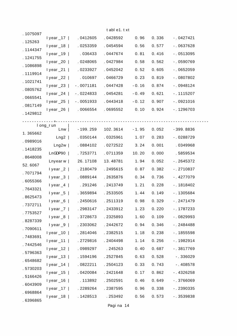
table1.txt.1075097 Iyear_17 | .0412605 .0428592 0.96 0.336 -.0427421 .125263 Iyear_18 | .0253359 .0454594 0.56 0.577 -.0637628 .1144347 Iyear_19 | .036433 .0447674 0.81 0.416 -.0513095 .1241755 Iyear_20 | .0248065 .0427984 0.58 0.562 -.0590769 .1086898 Iyear_21 | .0233927 .0452042 0.52 0.605 -.0652059 .1119914 Iyear_22 | .010697 .0466729 0.23 0.819 -.0807802 .1021741 Iyear_23 | -.0071181 .0447428 -0.16 0.874 -.0948124 .0805762 Iyear_24 | -.0224833 .0454281 -0.49 0.621 -.1115207 .0665541 Iyear_25 | -.0051933 .0443418 -0.12 0.907 -.0921016 .0817149 Iyear_26 | .0066554 .0695552 0.10 0.924 -.1296703 .1429812 -------------+---------------------------------------------------------------- long_run | Lnw | -199.259 102.3614 -1.95 0.052 -399.8836 1.365662 Lng2 | .0350144 .0325961 1.07 0.283 -.0288729 .0989016 Lng2w | .0884102 .0272522 3.24 0.001 .0349968 .1418235 LnGDP90 | .7253771 .0711359 10.20 0.000 .5859534 .8648008 Lnyearw | 26.17108 13.48781 1.94 0.052 -.2645372 52.6067 Iyear_2 | .2180479 .2495615 0.87 0.382 -.2710837 .7071794 Iyear_3 | .0889144 .2635876 0.34 0.736 -.4277079 .6055366 Iyear_4 | .291246 .2413749 1.21 0.228 -.1818402 .7643321 Iyear_5 | .3659894 .2533505 1.44 0.149 -.1305684 .8625473 Iyear_6 | .2450616 .2511319 0.98 0.329 -.2471479 .7372711 Iyear_7 | .2983147 .2433912 1.23 0.220 -.1787233 .7753527 Iyear_8 | .3728673 .2325893 1.60 0.109 -.0829993 .8287339 Iyear_9 | .2303062 .2442672 0.94 0.346 -.2484488 .7090611 Iyear_10 | .2814046 .2382515 1.18 0.238 -.1855598 .7483691 Iyear_11 | .2729816 .2404498 1.14 0.256 -.1982914 .7442546 Iyear_12 | .0989297 .245263 0.40 0.687 -.3817769 .5796363 Iyear_13 | .1594196 .2527845 0.63 0.528 -.336029 .6548682 Iyear_14 | .0822211 .2504123 0.33 0.743 -.408578 .5730203 Iyear_15 | .0420084 .2421648 0.17 0.862 -.4326258 .5166426 Iyear_16 | .113892 .2502591 0.46 0.649 -.3766069 .6043909 Iyear_17 | .2289264 .2387595 0.96 0.338 -.2390335 .6968864 Iyear_18 | .1428513 .253492 0.56 0.573 -.3539838 .6396865

Pagina 14

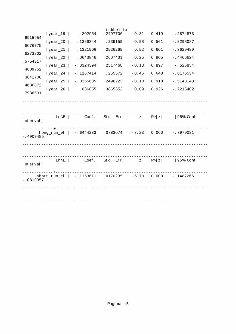
table1.txt Iyear_19 | .202054 .2497706 0.81 0.419 -.2874873 .6915954 Iyear_20 | .1389344 .239159 0.58 0.561 -.3298087 .6076775 Iyear_21 | .1321906 .2526269 0.52 0.601 -.3629489 .6273302 Iyear_22 | .0643846 .2607431 0.25 0.805 -.4466624 .5754317 Iyear_23 | -.0324394 .2517468 -0.13 0.897 -.525854 .4609752 Iyear_24 | -.1167414 .255572 -0.46 0.648 -.6176534 .3841706 Iyear_25 | -.0255635 .2496223 -0.10 0.918 -.5148143 .4636872 Iyear_26 | .036055 .3865352 0.09 0.926 -.7215402 .7936501 ------------------------------------------------------------------------------ ------------------------------------------------------------------------------ LnNE | Coef. Std. Err. z P>|z| [95% Conf. Interval] -------------+---------------------------------------------------------------- long_run_el | -.6444283 .0783074 -8.23 0.000 -.7979081 -.4909485 ------------------------------------------------------------------------------ ------------------------------------------------------------------------------ LnNE | Coef. Std. Err. z P>|z| [95% Conf. Interval] -------------+---------------------------------------------------------------- short_run_el | -.1153611 .0170235 -6.78 0.000 -.1487265 -.0819957 ------------------------------------------------------------------------------ -------------------------------------------------------------------------------

Pagina 15

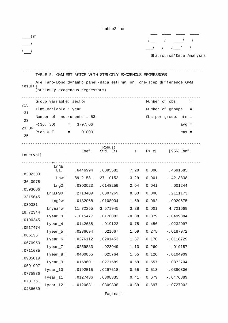
table2.txt ___ ____ ____ ____ ____tm /__ / ____/ / ____/ ___/ / /___/ / /___/ Statistics/Data Analysis ------------------------------------------------------------------------------- TABLE 5: GMM ESTIMATOR WITH STRICTLY EXOGENOUS REGRESSORS

Arellano-Bond dynamic panel-data estimation, one-step difference GMM results (strictly exogenous regressors) ------------------------------------------------------------------------------ Group variable: sector Number of obs = 715 Time variable : year Number of groups = 31 Number of instruments = 53 Obs per group: min = 23 F(30, 30) = 3797.06 avg = 23.06 Prob > F = 0.000 max = 25 ------------------------------------------------------------------------------ | Robust | Coef. Std. Err. z P>|z| [95% Conf. Interval] -------------+---------------------------------------------------------------- LnNE | L1. | .6446994 .0895582 7.20 0.000 .4691685 .8202303 Lnw | -89.21581 27.10152 -3.29 0.001 -142.3338 -36.0978 Lng2 | .0303023 .0148259 2.04 0.041 .001244 .0593606 LnGDP90 | .2713409 .0307269 8.83 0.000 .2111173 .3315645 Lng2w | .0182068 .0108034 1.69 0.092 -.0029675 .039381 Lnyearw | 11.72255 3.571945 3.28 0.001 4.721668 18.72344 Iyear_3 | -.015477 .0176082 -0.88 0.379 -.0499884 .0190345 Iyear_4 | .0142688 .019122 0.75 0.456 -.0232097 .0517474 Iyear_5 | .0236694 .021667 1.09 0.275 -.0187972 .066136 Iyear_6 | .0276112 .0201453 1.37 0.170 -.0118729 .0670953 Iyear_7 | .0259883 .023049 1.13 0.260 -.019187 .0711635 Iyear_8 | .0400055 .025764 1.55 0.120 -.0104909 .0905019 Iyear_9 | .0159601 .0271589 0.59 0.557 -.0372704 .0691907 Iyear_10 | .0192515 .0297618 0.65 0.518 -.0390806 .0775836 Iyear_11 | .0127436 .0308335 0.41 0.679 -.0476889 .0731761 Iyear_12 | -.0120631 .0309838 -0.39 0.697 -.0727902 .0486639

Pagina 1

table2.txt Iyear_13 | -.0022149 .0287526 -0.08 0.939 -.0585689 .0541391 Iyear_14 | -.0138214 .0286437 -0.48 0.629 -.069962 .0423191 Iyear_15 | -.0291769 .027802 -1.05 0.294 -.0836678 .025314 Iyear_16 | -.0218115 .0301898 -0.72 0.470 -.0809823 .0373594 Iyear_17 | -.0075547 .0285063 -0.27 0.791 -.063426 .0483167 Iyear_18 | -.0230511 .0268303 -0.86 0.390 -.0756375 .0295354 Iyear_19 | -.0188001 .0296374 -0.63 0.526 -.0768882 .0392881 Iyear_20 | -.0321314 .0336448 -0.96 0.340 -.0980739 .0338112 Iyear_21 | -.0293106 .0303225 -0.97 0.334 -.0887417 .0301205 Iyear_22 | -.0364441 .0289932 -1.26 0.209 -.0932698 .0203816 Iyear_23 | -.0552926 .0280318 -1.97 0.049 -.1102339 -.0003512 Iyear_24 | -.0745483 .0267633 -2.79 0.005 -.1270034 -.0220932 Iyear_25 | -.0736143 .0249463 -2.95 0.003 -.1225082 -.0247205 Iyear_26 | -.0990762 .0270481 -3.66 0.000 -.1520895 -.0460629 Iyear_27 | -.1025964 .0268747 -3.82 0.000 -.1552699 -.0499228 ------------------------------------------------------------------------------ Hansen test of overid. restrictions: chi2(22) = 0.00 Prob > chi2 = 1.000 Arellano-Bond test for AR(1) in first differences: z = -3.50 Pr > z = 0.000 Arellano-Bond test for AR(2) in first differences: z = 1.06 Pr > z = 0.287 ------------------------------------------------------------------------------ ------------------------------------------------------------------------------ LnNE | Coef. Std. Err. z P>|z| [95% Conf. Interval] -------------+---------------------------------------------------------------- long_run_el | -.6474651 .2198249 -2.95 0.003 -1.078314 -.2166161 ------------------------------------------------------------------------------ ------------------------------------------------------------------------------ LnNE | Coef. Std. Err. z P>|z| [95% Conf. Interval] -------------+---------------------------------------------------------------- short_run_el | -.2300447 .0305524 -7.53 0.000 -.2899263 -.1701632 ------------------------------------------------------------------------------ -------------------------------------------------------------------------------

Pagina 2

table3.txt ___ ____ ____ ____ ____tm /__ / ____/ / ____/ ___/ / /___/ / /___/ Statistics/Data Analysis ------------------------------------------------------------------------------- TABLE 6: GMM ESTIMATOR WITH PREDETERMINED REGRESSORS

Arellano-Bond dynamic panel-data estimation, one-step difference GMM results (wage and wage-interacted variables predetermined) ------------------------------------------------------------------------------ Group variable: sector Number of obs = 715 Time variable : year Number of groups = 31 Number of instruments = 53 Obs per group: min = 23 F(30, 30) = 2911.96 avg = 23.06 Prob > F = 0.000 max = 25 ------------------------------------------------------------------------------ | Robust | Coef. Std. Err. z P>|z| [95% Conf. Interval] -------------+---------------------------------------------------------------- LnNE | L1. | .4922812 .0702238 7.01 0.000 .354645 .6299173 Lnw | -230.116 135.0258 -1.70 0.088 -494.7618 34.52976 Lng2 | .0227056 .0371184 0.61 0.541 -.0500451 .0954564 LnGDP90 | .3498995 .1156731 3.02 0.002 .1231844 .5766145 Lng2w | -.0190264 .1031889 -0.18 0.854 -.221273 .1832202 Lnyearw | 30.27055 17.79227 1.70 0.089 -4.601661 65.14276 Iyear_3 | -.0019327 .0189148 -0.10 0.919 -.0390049 .0351396 Iyear_4 | .0297437 .027648 1.08 0.282 -.0244455 .0839329 Iyear_5 | .0387112 .0334291 1.16 0.247 -.0268088 .1042311 Iyear_6 | .0638456 .0329229 1.94 0.052 -.0006821 .1283732 Iyear_7 | .0607432 .0396668 1.53 0.126 -.0170024 .1384888 Iyear_8 | .0787872 .0432919 1.82 0.069 -.0060634 .1636378 Iyear_9 | .0592363 .045631 1.30 0.194 -.0301989 .1486714 Iyear_10 | .062163 .0506182 1.23 0.219 -.0370468 .1613728 Iyear_11 | .0584604 .0548961 1.06 0.287 -.049134 .1660547 Iyear_12 | .0398936 .0561255 0.71 0.477 -.0701104 .1498976

Pagina 1

table3.txt Iyear_13 | .0507115 .0540558 0.94 0.348 -.0552359 .1566589 Iyear_14 | .0385142 .0551001 0.70 0.485 -.06948 .1465083 Iyear_15 | .0181712 .0515524 0.35 0.724 -.0828695 .119212 Iyear_16 | .0227222 .0555048 0.41 0.682 -.0860652 .1315096 Iyear_17 | .0311841 .0554235 0.56 0.574 -.077444 .1398122 Iyear_18 | .0188988 .0552238 0.34 0.732 -.0893379 .1271355 Iyear_19 | .0180001 .055821 0.32 0.747 -.091407 .1274073 Iyear_20 | .0050346 .0537978 0.09 0.925 -.1004071 .1104763 Iyear_21 | .0073377 .0495461 0.15 0.882 -.089771 .1044463 Iyear_22 | .0005632 .0453577 0.01 0.990 -.0883362 .0894627 Iyear_23 | -.0225664 .0440338 -0.51 0.608 -.108871 .0637382 Iyear_24 | -.0464118 .044403 -1.05 0.296 -.13344 .0406165 Iyear_25 | -.0563096 .044302 -1.27 0.204 -.1431399 .0305208 Iyear_26 | -.0917605 .0447374 -2.05 0.040 -.1794442 -.0040768 Iyear_27 | -.0841389 .0510193 -1.65 0.099 -.184135 .0158571 ------------------------------------------------------------------------------ Hansen test of overid. restrictions: chi2(22) = 0.05 Prob > chi2 = 1.000 Arellano-Bond test for AR(1) in first differences: z = -3.03 Pr > z = 0.002 Arellano-Bond test for AR(2) in first differences: z = 0.67 Pr > z = 0.503 ------------------------------------------------------------------------------ ------------------------------------------------------------------------------ LnNE | Coef. Std. Err. z P>|z| [95% Conf. Interval] -------------+---------------------------------------------------------------- long_run_el | -.5193668 .3522883 -1.47 0.140 -1.209839 .1711056 ------------------------------------------------------------------------------ ------------------------------------------------------------------------------ LnNE | Coef. Std. Err. z P>|z| [95% Conf. Interval] -------------+---------------------------------------------------------------- short_run_el | -.2636923 .1711172 -1.54 0.123 -.5990758 .0716912 ------------------------------------------------------------------------------ -------------------------------------------------------------------------------

Pagina 2

table2bis.txt ___ ____ ____ ____ ____tm /__ / ____/ / ____/ ___/ / /___/ / /___/ Statistics/Data Analysis ------------------------------------------------------------------------------- TABLE 7: UNCORRECTED LSDV ESTIMATOR Fixed-effects (within) regression Number of obs = 746 Group variable (i): sector Number of groups = 31 R-sq: within = 0.9167 Obs per group: min = 24 between = 0.9964 avg = 24.1 overall = 0.9948 max = 26 F(31,684) = 589.35 corr(u_i, Xb) = 0.7801 Prob > F = 0.0000 ------------------------------------------------------------------------------ | Robust LnNE | Coef. Std. Err. t P>|t| [95% Conf. Interval] -------------+---------------------------------------------------------------- LnNE | L1. | .7853773 .0338631 23.19 0.000 .7188892 .8518655 Lnw | -41.08362 17.04076 -2.41 0.016 -74.5421 -7.625142 Lng2 | .0085294 .0078149 1.09 0.275 -.0068147 .0238735 LnGDP90 | .1529185 .0189588 8.07 0.000 .115694 .1901429 Lng2w | .0157304 .0064449 2.44 0.015 .0030762 .0283845 Lnyearw | 5.395321 2.245382 2.40 0.017 .9866522 9.803989 Iyear_2 | .0472819 .0215419 2.19 0.029 .0049857 .0895781 Iyear_3 | .0245648 .0122448 2.01 0.045 .0005229 .0486067 Iyear_4 | .0605583 .0113674 5.33 0.000 .0382391 .0828774 Iyear_5 | .0737663 .0106316 6.94 0.000 .0528918 .0946408 Iyear_6 | .0551844 .0112973 4.88 0.000 .0330028 .0773661 Iyear_7 | .0633166 .010129 6.25 0.000 .043429 .0832042 Iyear_8 | .0770761 .0106835 7.21 0.000 .0560998 .0980524 Iyear_9 | .0511848 .0101576 5.04 0.000 .031241 .0711286 Iyear_10 | .0597961 .0104721 5.71 0.000 .0392348 .0803575

Pagina 1

table2bis.txt Iyear_11 | .0577111 .0093223 6.19 0.000 .0394072 .0760149 Iyear_12 | .0266378 .0098778 2.70 0.007 .0072433 .0460323 Iyear_13 | .0374757 .0108269 3.46 0.001 .0162177 .0587336 Iyear_14 | .023361 .0161069 1.45 0.147 -.0082638 .0549859 Iyear_15 | .014739 .0108497 1.36 0.175 -.0065637 .0360418 Iyear_16 | .0270888 .0106069 2.55 0.011 .0062627 .0479149 Iyear_17 | .0471098 .0103967 4.53 0.000 .0266965 .0675231 Iyear_18 | .0315613 .0099891 3.16 0.002 .0119483 .0511744 Iyear_19 | .0415002 .0087121 4.76 0.000 .0243944 .0586059 Iyear_20 | .0298338 .0130546 2.29 0.023 .0042019 .0554657 Iyear_21 | .0294288 .009504 3.10 0.002 .0107683 .0480893 Iyear_22 | .0179452 .0096018 1.87 0.062 -.0009075 .0367978 Iyear_23 | -6.42e-06 .0095901 -0.00 0.999 -.0188361 .0188232 Iyear_24 | -.0163404 .008897 -1.84 0.067 -.0338092 .0011284 Iyear_25 | -.0020122 .0121639 -0.17 0.869 -.0258953 .0218709 Iyear_26 | .0064546 .0030329 2.13 0.034 .0004998 .0124095 _cons | -2.048579 .3967534 -5.16 0.000 -2.82758 -1.269578 -------------+---------------------------------------------------------------- sigma_u | .10399104 sigma_e | .04312569 rho | .85325624 (fraction of variance due to u_i) ------------------------------------------------------------------------------ ------------------------------------------------------------------------------ LnNE | Coef. Std. Err. t P>|t| [95% Conf. Interval] -------------+---------------------------------------------------------------- long_run_el | -.6312042 .0651798 -9.68 0.000 -.7591807 -.5032277 ------------------------------------------------------------------------------ ------------------------------------------------------------------------------ LnNE | Coef. Std. Err. t P>|t| [95% Conf. Interval] -------------+---------------------------------------------------------------- short_run_el | -.1354707 .024172 -5.60 0.000 -.182931 -.0880104 ------------------------------------------------------------------------------ -------------------------------------------------------------------------------

Pagina 2