Estimates of cetacean abundance in European Atlantic ... · Estimates of cetacean abundance in European Atlantic waters in summer ... (approximately in the case of ... entering data

Estimates of cetacean abundance in European

Atlantic waters in summer 2016 from the

SCANS-III aerial and shipboard surveys

May 2017

1

Estimates of cetacean abundance in European Atlantic waters in summer2016 from the SCANS-III aerial and shipboard surveys

Authors and Partners:

PS Hammond1, C Lacey1, A Gilles2, S Viquerat2, P Börjesson3, H Herr2, K Macleod4, V Ridoux5, MB Santos6, MScheidat7, J Teilmann8, J Vingada9, N Øien10

1. Sea Mammal Research Unit, University of St Andrews, Scotland, UK2. University of Veterinary Medicine, Hannover, Foundation, Germany

3. Swedish University of Agricultural Sciences, Sweden

4. Joint Nature Conservation Committee, UK

5. University of La Rochelle, France

6. Instituto Español de Oceanografía, Centro Oceanográfico de Vigo, Spain

7. Wageningen Marine Research, Netherlands

8. Department of Bioscience, Aarhus University, Denmark

9. Sociedade Portuguesa de Vida Selvagem, Portugal;

10. Institute of Marine Research, Norway

Additional project personnel:

Equipment development

Douglas Gillespie, Sea Mammal Research Unit, University of St Andrews, Scotland, UKRussell Leaper, School of Biological Sciences, University of Aberdeen, Scotland, UK

Aerial cruise leaders

Mario Acquarone, Arctic University of Norway, Tromsø, NorwayHelder Araújo, Sociedade Portuguesa de Vida Selvagem & Aveiro University, PortugalGhislain Dorémus & Olivier van Canneyt, Observatoire PELAGIS, FranceSteve Geelhoed & Hans Verdaat, Wageningen Marine Research, Netherlands

Ship cruise (co)leaders

Signe Sveegaard, Department of Bioscience, Aarhus University, DenmarkCamilo Saavedra & Xulio Valeiras, Instituto Español de Oceanografía, Centro Oceanográfico de Vigo, SpainJosé Antonio Vázquez, Alnilam Research and Conservation, Madrid, Spain

Acknowledgments:

We are grateful to all shipboard and aerial survey observers and the pilots, captains and crew of the survey

ships and aircraft, without whom this work would not have been possible.

The project was supported by funding from: Miljø- og Fødevareministeriet, Denmark; Agence des Aires

Marines Protégées, France; Bundesamt für Naturschutz, Germany; Rijkswaterstaat, Netherlands;

Havforskningsinstituttet, Norway; Sociedade Portuguesa de Vida Selvagem, Portugal; Instituto Español de

Oceanografía, Spain; Havs- och vattenmyndigheten, Sweden; Department for Environment, Food and Rural

Affairs, UK.

2

INTRODUCTION

A series of large scale surveys for cetaceans in European Atlantic waters was initiated in 1994 in the North Sea

and adjacent waters (SCANS 1995; Hammond et al. 2002) and continued in 2005 in all shelf waters (SCANS-II

2008; Hammond et al. 2013) and 2007 in offshore waters (CODA 2009). In the mid-1990s, the primary need for

a large-scale survey was to obtain the first comprehensive estimates of abundance of harbour porpoise in the

North Sea and adjacent waters so that estimates of bycatch could be placed in a population context. The

motivation for ongoing surveys is to provide the information on distribution and abundance of cetaceans

required by Member States to report on Favourable Conservation Status under the Habitats Directive and on

Good Environmental Status (GES) under the Marine Strategy Framework Directive (MSFD).

The frequency of these surveys was intended to be approximately decadal and a new survey was thus

scheduled for the mid-2010s. The previous SCANS projects had been supported by the European LIFE Nature

programme but a proposal for a SCANS-III project with a survey to take place in 2015 was rejected without

review. Member States nevertheless remained committed to the project and sufficient resources were

secured to conduct the SCANS-III survey in summer 2016. The supporting countries were: Denmark, France,

Germany, the Netherlands, Norway, Portugal, Spain, Sweden and the UK. An independent project supported

by Ireland, ObSERVE, is conducting surveys in Irish waters during the period 2015-2017.

A primary aim of SCANS-III was to provide robust large-scale estimates of cetacean abundance to inform the

upcoming MSFD assessment of GES in European Atlantic waters in 2018. Some surveys generating robust

estimates of abundance have been conducted since the SCANS-II/CODA in 2005/2007, as detailed in WGMME

(2016), but these do not provide comprehensive estimates of abundance for multiple species over the whole

of European Atlantic waters.

This report summarises design-based estimates of abundance for those cetacean species for which sufficient

data were obtained during SCANS-III: harbour porpoise, bottlenose dolphin, Risso’s dolphin, white-beaked

dolphin, white-sided dolphin, common dolphin, striped dolphin, pilot whale, all beaked whale species

combined, sperm whale, minke whale and fin whale.

3

METHODS

Study area and survey design

The initial objective of SCANS-III was to survey all European Atlantic waters from the Strait of Gibraltar in the

south to 62°N in the north and extending west to the 200 nm limits of all EU Member States. The final

surveyed area excluded offshore waters of Portugal and also excluded waters to the south and west of Ireland

which were surveyed by the Irish ObSERVE project. Coastal waters of Norway north to Vestfjorden were

included (Figure 1).

Figure 1. Area covered by SCANS-III and adjacent surveys. SCANS-III: pink lettered blocks were surveyed by air;blue numbered blocks were surveyed by ship. Blocks coloured green to the south, west and north of Irelandwere surveyed by the Irish ObSERVE project. Blocks coloured yellow were surveyed by the Faroe Islands aspart of the North Atlantic Sightings Survey in 2015.

Shelf waters were surveyed by seven aircraft (Fig 1, blocks A-Z), except the Skagerrak, Kattegat and Belt Seas,which were surveyed by the ship R/V Aurora (Fig 1, blocks 1 and 2). During the survey, the weather during thetime available to be allocated to block 1 was poor, so little ship survey effort was possible. As a result, thisblock was also surveyed by air (block P1) with design and coverage equivalent to the other aerial survey blocks– see below).

4

Offshore waters west of Scotland and in the central Bay of Biscay were surveyed by the ship M/V Skoven (Fig1, blocks 8 and 9). Offshore waters to the north and west of Spain were surveyed by the ship B/O AngelesAlvariño (Figure 1, blocks 11-13). The size and boundaries of survey blocks were determined primarily bylogistics but also to encompass designated/proposed protected areas in some cases. The relatively small sizeof the aerial survey blocks compared to the size of the ship survey blocks in the SCANS and SCANS-II surveysimproves, to some extent, the efficiency of the survey for abundance estimation for species with a patchydistribution within the study area, as discussed by MacLeod (2014) and Hammond et al. (2014).

Surveys within blocks were designed to provide equal coverage probability, using the equal spaced zig-zagoption in the survey design engine in software DISTANCE (Thomas et al. 2010). This ensures that each pointwithin a block has the same probability of being surveyed, allowing unbiased abundance estimation byextrapolating estimated sample density to the entire block.

For the aerial surveys, overall coverage probability was determined by available resources (total flying hours).Searching effort was distributed equally to all blocks (approximately in the case of blocks AA, AB and AC), withthe exception of blocks W and Z in Norwegian waters which were assigned approximately half and double thatprobability, respectively, because of expected differences in relative density. Within each aerial block, threesets of random transect lines were generated with the minimal aim that at least one set would be covered ineach block. If weather permitted, additional sets of transect lines would be covered; which blocks wouldreceive additional coverage depended on resources remaining, weather and national priorities. Additionalsmall survey blocks were created in two Norwegian fjords (Bognafjord near Stavanger (SVG) and TrondheimFjord (TRD)) as a trial to survey in these challenging areas.

For the ship surveys, overall coverage probability for each ship was determined by available resources (surveydays), accounting for some time expected to be unavailable for surveying due to poor weather. Some of theblocks were sub-divided to improve survey design efficiency. Block 2 was sub-divided into five sub-blocks tominimize time wasted off effort while transiting around islands in inner Danish waters. Each sub-block wasallocated equal coverage probability so they could be combined for analysis. The triangular NE corner of block8 and SE corner of block 9 were treated separately for survey design purposes but with the same coverageprobability as the rest of the block so they could be combined for analysis. The SW corner of block 9, atriangular area outside the 200 nm limits of France and Spain, was originally excluded from survey design butwas added in the field with the same coverage probability as the rest of the block.

Data collection

Aerial survey

Each of the seven aircraft accommodated three scientific crew members in addition to the pilot. One aircraft

had an additional three scientific crew working as an independent team. Target altitude was 600 feet (183 m)

and target speed was 90 knots (167 km.h-1). Two observers sat at bubble windows on the left and right sides of

the aircraft, and the third team member acted as navigator and data recorder for environmental and sightings

data, entering data into a laptop computer running dedicated data collection software. Sighting conditions

were classified subjectively as “good”, “moderate” or “poor” based primarily on sea conditions, water turbidity

and glare. When detected groups came abeam, data were recorded on time, declination angle to the detected

animal or group (from which perpendicular distance was calculated), cue, presence of calves, behaviour,

species composition and group size. Further details of field protocol are given in Gilles et al. (2009).

To collect data from which correction could be made for animals missed on the transect line, the circle-back or“racetrack” method of Hiby (1999) was used. In this approach, on detecting a group of animals, the aircraftcircles back to resurvey a defined segment of transect. The same method was used in SCANS-II (Hammond etal. 2013) and an equivalent method developed for tandem aircraft (Hiby & Lovell 1998) was used in SCANS(Hammond et al. 2002). Further details of this method are given in Scheidat et al. (2008).

In previous surveys, the circle-back method has only been used for harbour porpoise. In SCANS-III, we alsoimplemented this method for minke whale and for delphinids (bottlenose, common, striped, white-beaked,white-sided, and Risso’s dolphin) with the aim of correcting for animals missed on the transect line for thesespecies.

5

Ship survey

The method used on ships was a double platform line transect survey with two independent teams of

observers on each ship to generate data that would allow abundance estimates to be corrected for animals

missed on the transect line and also potentially for the effects of movement of animals in response to the ship

(Laake & Borchers 2004). This same approach was also used in SCANS, SCANS-II and CODA (Hammond et al.,

2002; CODA 2009; Hammond et al. 2013).

Each survey ship accommodated eight observers working in two teams. Target survey speed was 10 knots

(18.5 km.h-1) on all ships but was slower when surveying against heavy swell.

Two observers on one platform, known as Primary, searched with naked eye a sector from 90° (abeam)

starboard to 10° port or 90° port to 10° starboard out to 500 m distance. Two observers on the other, higher

platform, known as Tracker, searched from 500m to the horizon with high-power (15x80) and 7x50 binoculars.

Tracker observers tracked detected animals until they had passed abeam of the vessel. Observers not

searching acted as duplicate identifier, data recorder or rested. The duplicate identifier assessed whether or

not groups of animals detected by Tracker were re-sighted by Primary. Duplicates were classified as Definite

(D: at least 90% likely), Probable (P: between 50% and 90% likely), or Remote (R: less than 50% likely). The data

recorder recorded all sightings, effort and environmental data into a laptop computer running the LOGGER

software, modified specifically for SCANS surveys (Gillespie et al. 2010). Environmental data included sea

conditions measured on the Beaufort scale, swell height and direction, glare, visibility and sightability, a

subjective measure of conditions for detecting small cetaceans.

Data on sighting angle and distance for calculation of perpendicular distance were collected automatically,

where possible, as well as manually (Gillespie et al. 2010). Sighting angles were measured from an angle board

and on Tracker also using a small camera positioned on the underside of the binoculars that took snapshots of

lines on the deck parallel to the direction of the ship (Leaper and Gordon 2001). Distance to detected groups

was measured on Primary using purpose-designed and individually calibrated measuring sticks and on Tracker

as a binocular reticule reading and via a video-range technique (Gordon 2001). Angles and distances were

calculated from captured video frames using purpose-written software. Additional data collected from each

detected group of animals included: cue, species composition, group size, swimming direction and behaviour.

Data validation software was used to check all data at the end of each day, if possible.

Estimation of abundance

Aerial survey

Only survey effort collected under “good” and “moderate” conditions were used in analysis. Using the method

of Hiby and Lovell (1998), the effective strip width (ESW), including g(0), was estimated in “good” and

“moderate” sighting conditions ( g and m respectively). This analysis is described in detail in Hiby & Gilles

(2016).

For each species, abundance of animals in stratum v was estimated as:

v

m

msv

g

gsv

v

vv s

nn

L

AN

ˆˆ

ˆ

(Equation 1)

where Av is the area of the stratum, Lv is the length of transect line covered on-effort in good or moderate

conditions, ngsv is the number of sightings of groups that occurred in good conditions in the stratum, nmsv is the

number of sightings of groups that occurred in moderate conditions in the stratum and vs is the mean

observed group size in the stratum. Exploratory plots indicated no dependence of group size on perpendicular

distance, nor was group size found to be a significant explanatory variable for detection probability.

6

Group abundance by stratum was estimated by vvgroupv sNN /ˆˆ)( . Total animal and group abundances were

estimated by v

vNN ˆˆ and v

groupvgroup NN )()(ˆˆ , respectively. Densities were estimated by dividing the

abundance estimates by the area of the associated stratum. Mean group size across strata was estimated by

)(ˆ/ˆ][ˆ groupNNsE .

Coefficients of variation (CVs) and 95% confidence intervals (CIs) were estimated by bootstrapping within

blocks. A parametric bootstrap was used to generate estimates of ESW and these were combined with

encounter rates obtained from a nonparametric transect-based bootstrap procedure. The parametric

bootstrap procedure was based on the assumption that the ESW estimates in good and moderate conditions

were lognormally distributed random variables. Therefore, for each bootstrap pseudo-sample of transect lines,

a bivariate lognormal random variable was generated from a distribution with mean and variance-covariance

matrix equal to those estimated during the circle-back (“racetrack”) analysis (see Hiby & Gilles 2016). 95% CIs

were calculated using the percentile method.

Abundance of species (or species groupings) for which the circle-back procedure was not performed wasestimated using conventional line transect methods that assume certain detection on the transect line.Estimates for these species are thus underestimated to an unknown degree.

Analysis was conducted in R 3.2.2 x64 (R Core Team 2015) using the package ‘Distance‘ (Miller 2015).

Ship survey

Analysis of the shipboard data followed the double-platform line transect methodology used in the SCANS-II

survey (Borchers et al., 1998; Laake & Borchers 2004; Hammond et al., 2002; Hammond et al., 2013) using the

mrds analysis engine in software DISTANCE (Thomas et al., 2010). To estimate the probability of detection on

the transect line g(0), sightings made from the Tracker platform served as a set of binary trials in which success

corresponded to detection by observers on the Primary platform. The probability that a group of animals, at

given perpendicular distance x and covariates z, was detected from Primary is denoted p1(x,z) and modelled as

a logistic function (see equation 9 in Borchers et al. 1998).

The most robust mrds model for estimating detection probability from double-platform data is the partial (or

trackline) independence model, in which it is assumed that Tracker and Primary detection probabilities need

only be independent on the transect line (Borchers et al. 2006; Laake & Borchers 2004). This model uses the

Primary data to estimate detection probability assuming g(0 )= 1, and also the Tracker-Primary mark-recapture

data to estimate the conditional detection function to correct detection probability for g(0) < 1 (as described

above). This model was used as a default in analysis.

However, if there is undetected movement in response to the survey vessel, it is necessary to assume that

detection probabilities on Tracker and Primary are independent at all perpendicular distances and to use the

full independence model (Borchers et al. 2006; Laake & Borchers 2004). This model only uses the Tracker-

Primary mark-recapture data to estimate the conditional detection function and is less robust because it is

sensitive to non-independence of detection probabilities between Tracker and Primary at all perpendicular

distances (Borchers et al. 2006). Such non-independence typically results in a positive correlation in detection

probabilities and causes a negative bias in estimates of abundance. Nevertheless, this model should be used in

the presence of responsive movement prior to detection by Primary.

Attraction of common dolphins to survey ships has previously been shown to cause bias if the full

independence model is not used (Cañadas et al. 2009; Hammond et al. 2013). To determine whether the full

independence model needed to be used for any species, the extent of any responsive movement was explored

using data on swimming direction at first sighting using the method of Palka & Hammond (2001) and by

comparing perpendicular distances recorded by Tracker and Primary for duplicate sightings.

7

Explanatory covariates to model detection probability, in addition to perpendicular distance, included sea

conditions as indicated by Beaufort, glare, swell, a sightability index, visibility, group size and vessel. Model

selection was based primarily on Akaike’s Information Criterion (AIC) but by inspection of the QQ plot and the

Kolmogorov-Smirnov and Cramer-von Mises goodness of fit tests.

Perpendicular distance data for modelling detection probability were by default truncated at the largest

distance recorded by observers on Primary but, for each species, truncation at shorter distances was explored

to see if this improved estimation of detection probability. The choice of truncation distance was determined

by examining goodness of fit statistics (Kolmogorov-Smirnoff and Cramer-von Mises tests), while minimising

the amount of data lost. For harbour porpoise, data obtained while surveying in sea conditions of Beaufort 2

or less were used; for other species data from sea conditions of Beaufort 4 or less were used. Duplicates

classified as D and P were considered to be duplicates; those classified as R were not.

The abundance of groups was estimated using a Horvitz-Thompson-like estimator:

1

1

0

1

1

1n

jW

j dxW

)ˆ|z,x(p

N

(Equation 2)

where n1 is number of detections made from Primary, W is perpendicular truncation distance and are the

estimated parameters of the fitted detection function.

The abundance of individuals was estimated by replacing the numerator in the equation for estimating

abundance of groups with s1j, the group size of the jth group recorded from Primary. However, group sizes

recorded on Tracker are typically larger and likely to be more accurate than those recorded on Primary

because they were observed through binoculars and typically multiple times. Consequently, estimates of the

abundance of individuals were corrected by the ratio of the sum of Tracker group sizes to the sum of Primary

group sizes calculated from duplicate observations for each block or combination of blocks, depending on

sample size. If the group size correction was estimated as < 1, it was set to 1.

Estimates of mean group size were obtained by dividing abundance of individuals by abundance of groups.

Variances were estimated empirically; encounter rate variance was estimated using the method of Innes et al.

(2002).

Where there were insufficient duplicate sightings to support double-platform methods, conventional linetransect methods (assuming certain detection on the transect line) were used to obtain the detection function.

Presentation of abundance estimates

Estimates of abundance for each species are presented for each survey block and for the total survey area. Inaddition, for harbour porpoise, estimates are presented for ICES Assessment Units (AUs) (ICES 2014), see Fig 2,and also for the Norwegian coastal area north of 62°N.

For these estimates, the SCANS-III blocks were matched as closely as possible to the defined AUs, as follows:

Kattegat and Belt Seas: ship block 2;

North Sea: aerial blocks L-V, including P1, plus SVG, plus the eastern part of block C;

West Scotland: aerial blocks G-K;

Celtic and Irish Seas: aerial blocks B and D-F plus the western half of C;

Iberian Peninsula: aerial blocks AA, AB and AC;

Norwegian coast north of 62°N: aerial survey blocks W-Z and TRD.

For these combinations of aerial survey blocks, the subsets of the data were bootstrapped as described aboveto obtain appropriate estimates of variance.

8

Figure 2. ICES Assessment Units for harbour porpoise (ICES 2014).

For the bottlenose dolphin, ten AUs have been defined for resident or semi-resident coastal/inshorepopulations, and a single offshore “oceanic area” AU has been defined to cover all waters not covered by thecoastal/inshore AUs. It is not appropriate (nor possible) to separate out the coastal/inshore populations in theSCANS-III surveys so the total estimate represents these and the “oceanic area” combined.

For the minke whale, white-beaked dolphin and common dolphin, a single AU covering all European Atlanticwaters has been defined. For these, and all other species, the total abundance estimates represent the AU. Avery small proportion of the total estimates for minke whale and white-beaked dolphin were in Norwegiancoastal waters north of 62°N (2.2% and less than 1%, respectively).

RESULTS

Searching effort and sightings

Seven aircraft surveyed shelf waters of the European Atlantic, including Norwegian coastal waters, between 27June and 31 July 2016. Table 1 shows the amount of search effort on transect in each of the survey blocks.

Three ships surveyed waters beyond the continental shelf and inner Danish waters. Blocks 1 and 2 weresurveyed 5-24 July, block 8 was surveyed 29 June - 14 July, block 9 was surveyed 19 July - 4 August and blocks11-13 were surveyed 4-28 July. Table 2 shows the amount of search effort on transect in each of the surveyblocks. Figure 3 shows the searching effort achieved under all conditions.

Tables 3 and 4 show the total number of sightings of groups of the most commonly detected species on the

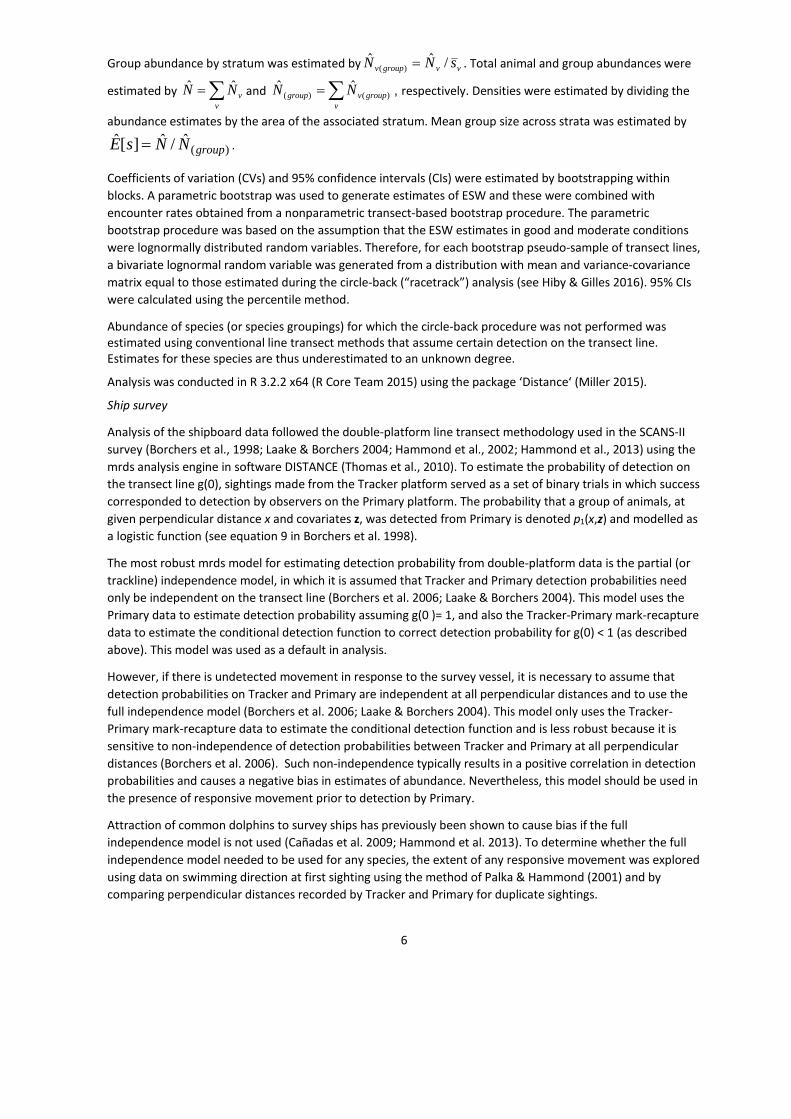
aerial survey and ship survey, respectively. Figure 4 shows the distribution of sightings of the most commonly

detected species.

9

Table 1. Area and searching effort (in “moderate” or “good” conditions, used in analysis) for each aerial survey

block. Primary search effort data were used in analysis to estimate encounter rate and group size (see

equation 1). Trailing search effort occurred during circle-back procedures and was used to estimate ESW,

including g(0). Block P1 is the same as ship block 1 (Table 2). Blocks SVG and TRD covered parts of Norwegian

fjords Bognafjord (near Stavanger) and Trondheim Fjord, respectively. Block SVG is included in the ICES North

Sea Assessment Unit (Table 32).

Block Region Surface area (km2)Primary search

effort (km)Trailing search

effort (km)

AA Iberian peninsula 12,015 588.9 5.4

AB Iberian peninsula 26,668 1,210.1 23.4

AC Iberian peninsula 35,180 1,393.1 13.0

B Celtic/Irish Seas 118,471 7,982.9 78.1

C Celtic/Irish Seas & North Sea 81,297 2,834.2 37.9

D Celtic/Irish Seas 48,590 1,707.5 16.8

E Celtic/Irish Seas 34,870 2,252.7 22.5

F Celtic/Irish Seas 12,322 619.8 4.1

G West Scotland 15,122 958.0 12.9

H West Scotland 18,634 812.9 17.0

I West Scotland 13,979 636.5 16.3

J West Scotland 35,099 704.4 6.4

K West Scotland 32,505 2,146.7 17.3

L North Sea 31,404 1,949.3 20.0

M North Sea 56,469 1,749.9 57.3

N North Sea 69,386 2,264.9 56.8

O North Sea 60,198 3,242.8 62.7

P North Sea 63,655 2,034.1 33.5

P1 North Sea 23,557 844.4 0.0

Q North Sea 49,746 1,856.5 75.0

R North Sea 64,464 2,178.7 40.5

S North Sea 40,383 1,370.9 15.1

T North Sea 65,417 2,259.1 24.0

U North Sea 60,046 1,741.8 15.3

V North Sea 38,306 1,129.8 11.7

W Norway 49,778 931.0 3.7

X Norway 19,496 1,039.4 22.7

Y Norway 18,779 713.3 7.0

Z Norway 11,228 1,764.4 29.2

SVG Norway (North Sea) 714 152.3 0.0

TRD Norway 966 179.7 2.5

Total 1,208,744 51,568.3 748.0

10

Table 2. Area and searching effort for each ship survey block. For estimation of harbour porpoise abundance(in blocks 1 and 2), search effort was limited to Beaufort 0-2. For estimation of abundance for all other species(in blocks 8-13), search effort was limited to Beaufort 0-4. Block 1 is the same as aerial block P1 (Table 1).

Block RegionSurface

area (km2)Search effort

Beaufort 0-4 (km)Search effort

Beaufort 0-2 (km)

1 Skagerrak/Kattegat 23,451 215.7

2 Kattegat & inner Danish waters 40,707 1,027.7

8 Atlantic - west of Scotland 159,669 2,084.7

9 Bay of Biscay 144,352 2,279.9

11 Atlantic - west of Spain 68,759 981.0

12 Atlantic - west of Spain / Bay of Biscay 111,115 1,629.7

13 Bay of Biscay 59,340 1,605.5

Figure 3. Total search effort achieved under all conditions in aerial (pink) and ship (blue) survey blocks.

11

Table 3. Total number of sightings of the most commonly detected species (or species groupings) from the

aerial survey recorded in “good” and “moderate” sighting conditions. Sightings on trailing search effort were

recorded on circle-back procedures and were used only to estimate ESW, including g(0).

SpeciesSightings on primary

search effortSightings on trailing

search effort

Harbour porpoise 1,602 67

Bottlenose dolphin 59 11

Risso’s dolphin 16 1

White-beaked dolphin 108 10

White-sided dolphin 7 1

Unid white-beaked or white-sided dolphin 11 0

Common dolphin 502 17

Striped dolphin 20 0

Unid common or striped dolphin 248 9

Unidentified dolphin 196 7

Pilot whale 79 0

Beaked whales (all species) 27 0

Minke whale 73 8

Table 4. Number of sightings of the most commonly detected species from the ship survey (harbour porpoise

Beaufort 0-2; all other species Beaufort 0-4). Tracker sightings and duplicates were used in mark-recapture

distance sampling analysis only to estimate detection probability and to correct estimates of mean group size.

Duplicates shown are Definite and Probable duplicates, as used in analysis.

SpeciesTotal

sightingsPrimarysightings

Trackersightings

Duplicates

Harbour porpoise 343 167 217 41

Bottlenose dolphin 27 15 18 6

Risso’s dolphin 5 4 3 2

White-sided dolphin 16 10 11 5

Unid white-beaked or white-sided dolphin 4 2 2 0

Common dolphin 106 82 52 28

Striped dolphin 104 56 69 21

Unidentified common or striped dolphin 126 44 96 14

Unidentified dolphin 53 17 37 1

Pilot whale 58 37 41 20

Beaked whales (all species) 65 35 38 8

Sperm whale 40 16 25 1

Minke whale 9 7 3 1

Fin whale (blocks 8 & 9) 276 205 133 62

Fin whale (blocks 11, 12 & 13) 708 368 486 146

12

Figure 4. Distribution of sightings used in analysis of the most commonly detected species. Underlying effort is

also that used in analysis: aerial survey - good and moderate conditions; ship survey - Beaufort 0-2 for harbour

porpoise, Beaufort 0-4 for all other species. (a) harbour porpoise; (b) bottlenose dolphin; (c) Risso’s dolphin;

(d) white-beaked (blue dot) and white-sided (red dot) dolphins. Continued on following pages.

(a) Harbour porpoise

(c) Risso’s dolphin (d) White-beaked and

white-sided dolphins

(b) Bottlenose dolphin

13

Figure 4 (continued). Distribution of sightings used in analysis of the most commonly detected species.

Underlying effort is also that used in analysis: aerial survey - good and moderate conditions; ship survey -

Beaufort 0-4. (e) common dolphin; (f) striped dolphin; (g) unidentified common or striped dolphin; (h) pilot

whale.

(e) Common dolphin (f) Striped dolphin

(g) Unid common or striped dolphin (h) Pilot whale

14

Figure 4 (continued). Distribution of sightings used in analysis of the most commonly detected species.

Underlying effort is also that used in analysis: aerial survey - good and moderate conditions; ship survey -

Beaufort 0-4. (i) beaked whales (Cuvier’s beaked whale - red dot; Gervais beaked whale - blue dot;

Unidentified beaked whale - pink square; Unidentified Mesoplodon - black triangle; Sowerby’s beaked whale -

green dot; Bottlenose whale - turquoise dot); (j) sperm whale; (k) minke whale; (l) fin whale.

(i) Beaked whales (j) Sperm whale

(k) Minke whale (l) Fin whale

15

Estimates of abundance

Aerial survey

A total of 290 circle-back (“racetrack”) procedures were achieved. Estimates of ESW, including g(0), were madeusing the combined data from all seven aircraft for harbour porpoise, all dolphin species combined (excludingpilot whale and killer whale) and minke whale. Estimates for harbour porpoise stratified by aircraft were alsoinvestigated. However, the numbers of potential re-sightings by individual aircraft were in most cases toosmall to estimate robust aircraft-based ESWs; therefore, the pooled ESW based on all seven aircraft, stratifiedby good and moderate conditions, was preferred (see Hiby & Gilles 2016 for details). For the minke whale,there were only eight potential re-sightings on trailing effort, which precluded robust estimation of ESW forgood and moderate conditions separately; therefore, ESW was estimated pooled across all conditions (seeHiby & Gilles 2016 for details).

Table 5 shows the estimates of ESW, including g(0), for harbour porpoise, all dolphin species combined(excluding pilot whale and killer whale) and minke whale.

Tables 6-16 show estimates of abundance for each block for harbour porpoise, minke whale, common dolphin,striped dolphin, unidentified common or striped dolphin, bottlenose dolphin, white-beaked dolphin, white-sided dolphin, Risso’s dolphin, pilot whale and beaked whales (all species combined).

Table 5. Estimates of ESW (CV in parentheses) and g(0) for harbour porpoise, all dolphin species combined

(excluding pilot whale and killer whale) and minke whale, for good and moderate sighting conditions during

the aerial survey. Note that ESW is the total effective strip width on both sides of the aircraft.

ESW (in meters), including g(0) g(0)

Conditions good moderate good moderate

Harbour porpoise 138 (0.16) 109 (0.17) 0.364 0.279

Dolphins (all species) 390 (0.13) 213 (0.14) 0.805 0.414

Minke whale 154 (0.42) 0.302

16

Table 6. Harbour porpoise abundance and density (animals/km2) estimates from the aerial survey. CV is thecoefficient of variation of abundance and density. CL low and CL high are the estimated lower and upper 95%confidence limits of abundance. Block P1 was also covered by ship block 1 (see Table 20).

Block Abundance Density Mean group size CV CL low CL high

AA 0 0 0 0.00 0 0

AB 2,715 0.102 1.21 0.31 1,350 4,737

AC 183 0.005 1.00 1.02 0 669

B 3,374 0.028 2.23 0.59 102 8,078

C 17,323 0.213 1.76 0.30 8,853 29,970

D 5,734 0.118 1.35 0.49 1,697 12,452

E 8,320 0.239 1.31 0.28 4,643 14,354

F 1,056 0.086 1.00 0.38 342 2,010

G 5,087 0.336 1.52 0.43 1,701 10,386

H 1,682 0.090 2.00 0.74 0 5,154

I 5,556 0.397 1.15 0.35 2,403 9,961

J 2,045 0.058 1.25 0.72 0 5,313

K 9,999 0.308 1.44 0.27 5,643 16,306

L 19,064 0.607 1.28 0.38 6,933 35,703

M 15,655 0.277 1.23 0.34 6,295 28,589

N 58,066 0.837 1.28 0.26 32,372 91,372

O 53,485 0.888 1.31 0.21 37,413 81,695

P 52,406 0.823 1.36 0.31 27,247 94,570

P1 25,367 1.077 1.39 0.30 10,114 41,642

Q 16,569 0.333 1.31 0.35 6,919 31,247

R 38,646 0.599 1.38 0.29 20,584 66,524

S 6,147 0.152 1.35 0.28 3,401 10,065

T 26,309 0.402 1.33 0.29 14,219 45,280

U 19,269 0.321 1.31 0.30 10,794 34,922

V 5,240 0.137 1.24 0.37 2,165 9,714

W 8,978 0.180 1.47 0.57 1,427 21,507

X 6,713 0.344 1.50 0.31 3,496 11,767

Y 4,006 0.213 1.24 0.40 1,603 8,209

Z 4,556 0.406 1.51 0.27 2,686 7,631

SVG 423 0.593 1.71 0.39 157 834

TRD 273 0.282 1.75 0.48 59 583

Total 424,245 0.351 1.35 0.17 313,151 596,827

17

Table 7. Bottlenose dolphin abundance and density (animals/km2) estimates from the aerial survey. CV is thecoefficient of variation of abundance and density. CL low and CL high are the estimated lower and upper 95%confidence limits of abundance. Blocks with no bottlenose dolphin sightings are excluded.

Block Abundance Density Mean group size CV CL low CL high

AB 735 0.028 3.25 0.70 0 1,932

AC 4,210 0.120 4.82 0.48 997 8,529

B 6,926 0.058 7.05 0.38 2,713 13,389

D 2,938 0.060 2.60 0.45 914 5,867

E 288 0.008 1.50 0.57 0 664

G 1,824 0.121 9.67 0.68 0 4,474

H 59 0.003 1.00 1.01 0 214

P 147 0.002 1.00 0.99 0 488

R 1,924 0.030 5.25 0.86 0 5,048

S 151 0.004 2.00 1.01 0 527

Total 19,201 0.016 4.53 0.24 11,404 29,670

Table 8. Risso’s dolphin abundance and density (animals/km2) estimates from the aerial survey. CV is thecoefficient of variation of abundance and density. CL low and CL high are the estimated lower and upper 95%confidence limits of abundance. Blocks with no Risso’s dolphin sightings are excluded.

Block Abundance Density Mean group size CV CL low CL high

AA 575 0.047 6.00 1.03 0 1,902

AB 640 0.024 2.00 0.62 0 1,556

AC 237 0.007 2.00 1.03 0 835

B 799 0.007 10.50 0.98 0 2,770

E 1,090 0.031 7.50 0.69 0 2,843

H 538 0.029 5.00 0.95 0 1,798

J 6,750 0.192 11.33 0.80 0 19,557

K 440 0.014 4.00 0.76 0 1,222

Total 11,069 0.009 7.06 0.51 2,794 24,412

18

Table 9. White-beaked dolphin abundance and density (animals/km2) estimates from the aerial survey. CV isthe coefficient of variation of abundance and density. CL low and CL high are the estimated lower and upper95% confidence limits of abundance. Blocks with no white-beaked dolphin sightings are excluded.

Block Abundance Density Mean group size CV CL low CL high

H 5,881 0.316 5.18 0.63 389 14,304

J 1,871 0.053 4.00 0.91 0 5,856

K 7,055 0.217 4.70 0.53 1,799 16,040

O 143 0.002 3.00 0.97 0 490

P 1,938 0.030 2.50 0.38 539 3,524

P1 72 0.003 1.00 0.88 0 196

R 15,694 0.243 3.70 0.48 3,022 33,340

S 868 0.021 3.00 0.69 0 2,258

T 2,417 0.037 3.43 0.46 593 5,091

V 261 0.007 3.00 0.98 0 933

X 88 0.005 1.00 0.92 0 275

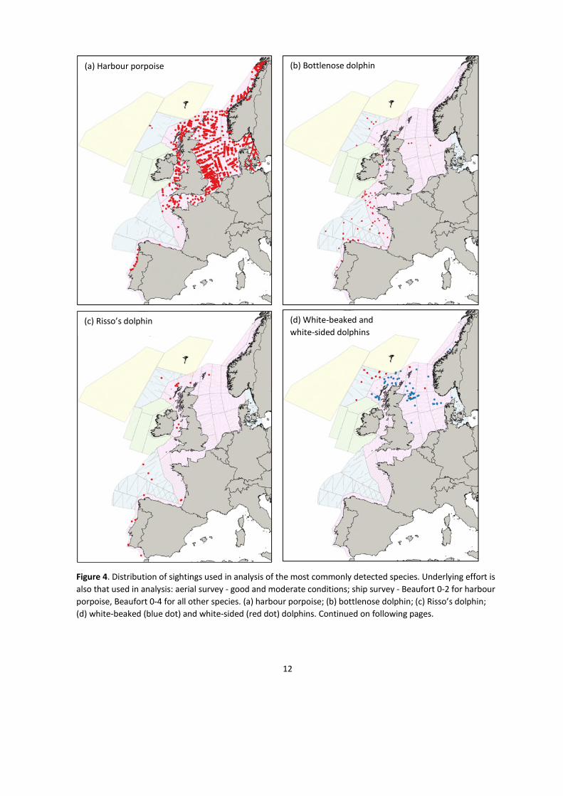
Total 36,287 0.030 3.86 0.29 18,694 61,869

Table 10. White-sided dolphin abundance and density (animals/km2) estimates from the aerial survey. CV isthe coefficient of variation of abundance and density. CL low and CL high are the estimated lower and upper95% confidence limits of abundance. Blocks with no white-sided dolphin sightings are excluded. Density of0.00 means that density was less than 0.005 animals/km2.

Block Abundance Density Mean group size CV CL low CL high

R 644 0.010 3.00 0.99 0 2,069

T 1,366 0.021 3.25 0.98 0 5,031

U 177 0.003 2.00 0.99 0 559

Total 2,187 0.002 3.02 0.70 0 6,071

Table 11. Common dolphin abundance and density (animals/km2) estimates from the aerial survey. CV is thecoefficient of variation of abundance and density. CL low and CL high are the estimated lower and upper 95%confidence limits of abundance. Blocks with no common dolphin sightings are excluded.

Block Abundance Density Mean group size CV CL low CL high

AA 18,458 1.536 17.94 0.64 3,297 51,064

AB 63,243 2.371 8.67 0.27 34,978 103,337

AC 71,082 2.020 12.00 0.31 36,898 124,302

B 92,893 0.784 7.49 0.27 52,766 149,494

D 18,187 0.374 10.06 0.41 4,394 33,077

J 4,679 0.133 20.00 0.95 0 16,108

Total 268,540 0.222 9.36 0.19 186,851 390,528

19

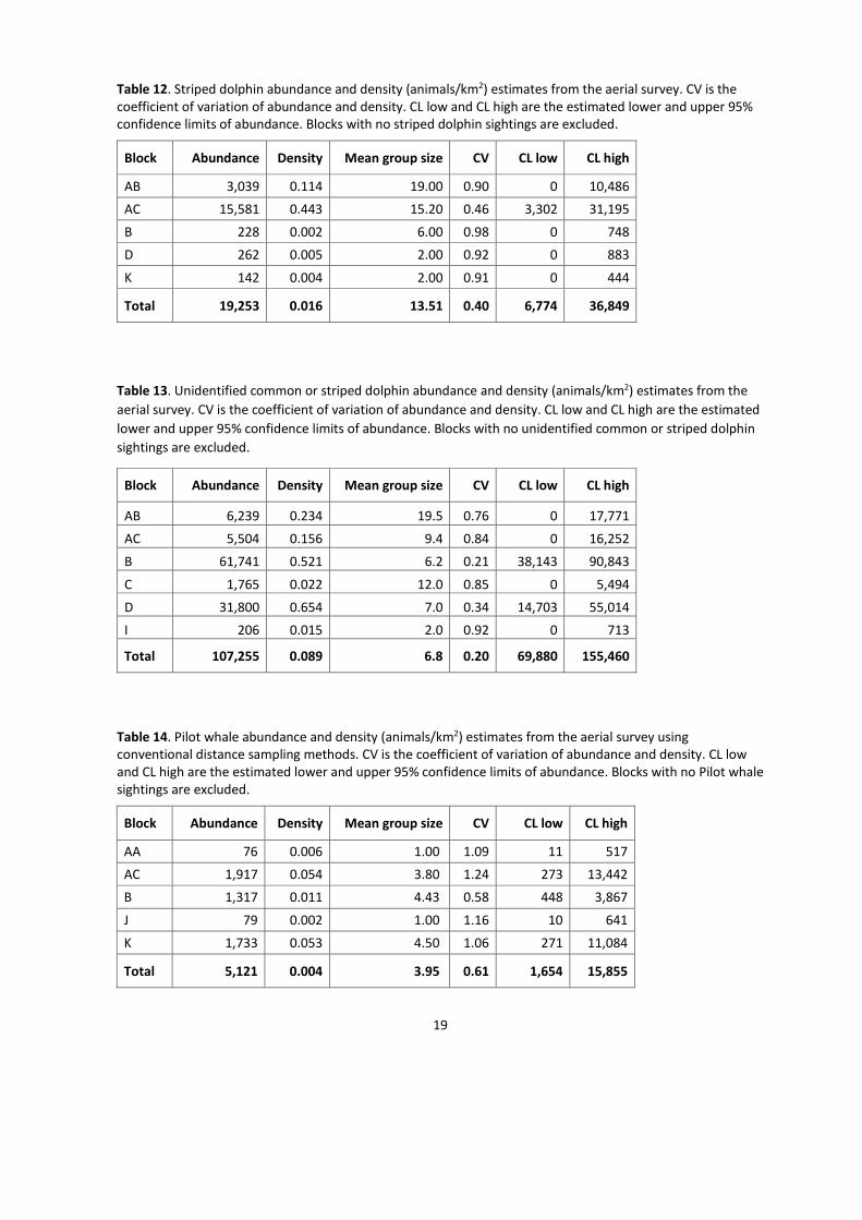
Table 12. Striped dolphin abundance and density (animals/km2) estimates from the aerial survey. CV is thecoefficient of variation of abundance and density. CL low and CL high are the estimated lower and upper 95%confidence limits of abundance. Blocks with no striped dolphin sightings are excluded.

Block Abundance Density Mean group size CV CL low CL high

AB 3,039 0.114 19.00 0.90 0 10,486

AC 15,581 0.443 15.20 0.46 3,302 31,195

B 228 0.002 6.00 0.98 0 748

D 262 0.005 2.00 0.92 0 883

K 142 0.004 2.00 0.91 0 444

Total 19,253 0.016 13.51 0.40 6,774 36,849

Table 13. Unidentified common or striped dolphin abundance and density (animals/km2) estimates from the

aerial survey. CV is the coefficient of variation of abundance and density. CL low and CL high are the estimated

lower and upper 95% confidence limits of abundance. Blocks with no unidentified common or striped dolphin

sightings are excluded.

Block Abundance Density Mean group size CV CL low CL high

AB 6,239 0.234 19.5 0.76 0 17,771

AC 5,504 0.156 9.4 0.84 0 16,252

B 61,741 0.521 6.2 0.21 38,143 90,843

C 1,765 0.022 12.0 0.85 0 5,494

D 31,800 0.654 7.0 0.34 14,703 55,014

I 206 0.015 2.0 0.92 0 713

Total 107,255 0.089 6.8 0.20 69,880 155,460

Table 14. Pilot whale abundance and density (animals/km2) estimates from the aerial survey usingconventional distance sampling methods. CV is the coefficient of variation of abundance and density. CL lowand CL high are the estimated lower and upper 95% confidence limits of abundance. Blocks with no Pilot whalesightings are excluded.

Block Abundance Density Mean group size CV CL low CL high

AA 76 0.006 1.00 1.09 11 517

AC 1,917 0.054 3.80 1.24 273 13,442

B 1,317 0.011 4.43 0.58 448 3,867

J 79 0.002 1.00 1.16 10 641

K 1,733 0.053 4.50 1.06 271 11,084

Total 5,121 0.004 3.95 0.61 1,654 15,855

20

Table 15. Beaked whale (all species) abundance and density (animals/km2) estimates from the aerial surveyusing conventional distance sampling methods. CV is the coefficient of variation of abundance and density. CLlow and CL high are the estimated lower and upper 95% confidence limits of abundance. Blocks with nobeaked whale sightings are excluded.

Block Abundance Density Mean group size CV CL low CL high

AC 581 0.017 1.83 0.530 212 1,593

B 101 0.001 1.50 0.774 26 400

H 100 0.005 2.00 1.106 14 733

J 325 0.009 1.50 0.621 91 1,163

K 211 0.006 2.00 0.904 41 1,091

U 75 0.001 1.00 1.040 12 457

V 97 0.003 1.00 1.020 16 607

Total 1,489 0.001 1.69 0.376 719 3,085

Table 16. Minke whale abundance and density (animals/km2) estimates from the aerial survey. CV is thecoefficient of variation of abundance and density. CL low and CL high are the estimated lower and upper 95%confidence limits of abundance. Blocks with no minke whale sightings are excluded.

Block Abundance Density Mean group size CV CL low CL high

AC 164 0.005 1.00 1.14 0 792

B 289 0.002 1.00 0.84 0 962

C 186 0.002 1.00 1.12 0 819

D 543 0.011 1.00 0.75 0 1,559

E 603 0.017 1.00 0.62 134 1,753

G 410 0.027 1.33 0.70 0 1,259

H 149 0.008 1.00 1.07 0 638

I 285 0.020 1.00 0.79 0 1,004

J 647 0.018 1.00 1.04 0 2,994

K 295 0.009 1.00 0.81 0 994

N 1,392 0.020 1.00 0.50 450 3,459

O 603 0.010 1.00 0.62 109 1,670

P 610 0.001 1.00 0.66 0 1,849

Q 348 0.007 1.00 0.76 0 1,121

R 2,498 0.039 1.18 0.61 604 6,791

S 383 0.010 1.00 0.75 0 1,364

T 2,068 0.032 1.10 0.81 290 6,960

U 895 0.015 1.00 0.85 0 3,139

V 440 0.011 1.00 1.14 0 1,979

X 122 0.006 1.00 1.09 0 496

Y 171 0.009 1.00 1.10 0 756

Total 13,101 0.011 1.05 0.35 7,050 26,721

21

Ship survey

For species with sufficient duplicate sightings, mark-recapture distance sampling methods were used toestimate detection probability and consequently abundance. There was no compelling evidence of movementin response to the ship in any species, so the partial independence model of detection probability was used inall cases. For sperm whale and minke whale, there were insufficient duplicate sightings to use mark-recapturedistance sampling methods to estimate detection probability so conventional “single observer” distancesampling methods, in which Tracker and Primary sightings are combined into a single dataset, were used. Datafrom both ships were analysed together to obtain common estimates of detection probability.

An exception to the above was for large baleen whales (including mostly fin whales), for which theperpendicular distance data were distributed very differently in blocks 8 and 9 (survey by M/V Skoven)compared to blocks 11, 12 and 13 (surveyed by B/O Angeles Alvariño). Consequently, the large baleen whaledata were analysed separately for blocks 8 and 9, and for blocks 11, 12 and 13.

For blocks 11, 12 and 13, the partial independence mrds model of detection probability was used as describedabove. For blocks 8 and 9, however, the conditional probability of detection (Primary detection of sightingsfirst made by Tracker) increased with increasing perpendicular distance, making the application of mrdsmodels of detection probability inappropriate. For blocks 8 and 9, therefore, the Tracker data weredisregarded and a conventional analysis of Primary data only was conducted, assuming g(0) = 1. Estimates forfin whales for blocks 8 and 9 are thus expected to be negatively biased.

Table 17 gives, for each species or species grouping, the perpendicular distance truncation selected, themethod used to estimate detection probability, and details of the best fitting detection probability models.

Table 18 gives the detection probabilities estimated using the models described in Table 17.

Table 19 gives the group size correction factors for each species or species grouping.

Table 17. Summary of data and models used to estimate detection probability for each species or speciesgrouping in the ship survey. Method: pi = mark-recapture distance sampling point (trackline) independencemodel; ds = conventional distance sampling model using Primary data only; so = “single observer”conventional distance sampling model using Primary and Tracker data combined. Detection function model:HR = hazard rate.

Species / species groupingTruncation

distance (m)Method

Primary detectionfunction model

(ds) & covariates

Conditional detectionfunction (mr)

covariates

Harbour porpoise 600 pi HR: Swell Beaufort

Bottlenose + Risso’s dolphin 885 (max) pi HR: null Perpendicular distance

White-sided dolphin 343 (max) pi HR: null null

Common + striped dolphin 2,000 pi HR: Beaufort Perpendicular distance

Pilot whale 1,500 pi HR: null Perpendicular distance

Beaked whales (all species) 2,000 pi HR: Sightability Perpendicular distance

Sperm whale 9,197 (max) so HR: Beaufort -

Large baleen whales (blocks 8& 9)

2,302 (max) ds HR: Swell -

Large baleen whales (blocks11, 12 & 13)

3,000 pi HR: SwellPerpendicular distance,

Beaufort, Swell

Minke whale 208 (max) so Uniform: null -

22

Table 18. Estimated detection probabilities within the truncation distance (see Table 17) for each species orspecies grouping in the ship survey. ESW is the estimated effective strip half-width. Figures in parentheses arecoefficients of variation (CV). The CV of ESW is the same as for overall probability of detection.

Species / species groupingAverage probability

of detectionassuming g(0)=1

Probability ofdetection on thetransect line, g(0)

Overall averageprobability of

detectionESW (m)

Harbour porpoise 0.709 (0.051) 0.221 (0.177) 0.156 (0.186) 93.6

Bottlenose + Risso’s dolphin 0.427 (0.146) 0.400 (0.348) 0.171 (0.377) 151

White-sided dolphin 0.829 (0.614) 0.455 (0.330) 0.377 (0.697) 129

Common + striped dolphin 0.131 (0.117) 0.421 (0.115) 0.055 (0.164) 110

Pilot whale 0.318 (0.173) 0.491 (0.217) 0.156 (0.277) 234

Beaked whales (all species) 0.217 (0.386) 0.263 (0.375) 0.057 (0.541) 114

Sperm whale 0.0095 (0.296) - 0.0095 (0.296) 87

Large baleen whales (blocks 8& 9)

0.343 (0.061) - 0.343 (0.061) 789

Large baleen whales (blocks11, 12 & 13)

0.505 (0.047) 0.614 (0.073) 0.310 (0.088) 933

Minke whale 1.0 - 1.0 208

Table 19. Group size correction factors (CV in parentheses) for each species or species grouping used tocorrect Primary group sizes in analysis.

Species Blocks Group size correction Sample size

Harbour porpoise 1-2 1.204 (0.150) 42

Bottlenose dolphin 8, 9, 12, 13 1.571 (0.265) 7

Risso’s dolphin 9 1 2

White-sided dolphin 8 0.826 (0.409) = 1 5

Common dolphin 8-13 0.956 (0.241) = 1 29

Striped dolphin 8, 9, 12, 13 1.993 (0.197) 20

Unid common or striped 8, 9, 12, 13 1.362 (0.205) 16

Pilot whale 8-13 1.156 (0.261) 20

Beaked whales (all species) 8-13 1.000 (0.427) 11

Sperm whale 8-13 1 1

Fin whale 8-9 1.057 (0.130) 62

Fin whale 11-13 1.059 (0.084) 171

Minke whale 8 1 9

Tables 20-31 show estimates of abundance for each ship block for harbour porpoise, bottlenose dolphin,Risso’s dolphin, white-sided dolphin, common dolphin, striped dolphin, unidentified common or stripeddolphin, pilot whale, beaked whales, sperm whale, minke whale and fin whale. Note that in Table 20 ashipboard estimate is given for block 1 but the coverage was poor and uneven so the estimate subsequentlyused in Tables 32 and 33 for this block is that from the aerial survey (block P1 in Table 6).

23

Table 20. Estimates of density (animals/km2) and abundance for harbour porpoise from the ship survey. CL lowand CL high are the estimated lower and upper 95% confidence limits.

BlockDensity(groups) CV

Groupsize CV

Density(animals) CV Abundance CL low CL high

1 0.854 0.354 1.56 0.137 1.33 0.472 31,249 6,111 159,786

2 0.686 0.292 1.52 0.036 1.04 0.304 42,324 23,368 76,658

Total 0.748 0.252 1.53 0.063 1.15 0.285 73,573 39,383 137,443

Table 21. Estimates of density (animals/km2) and abundance for bottlenose dolphin from the ship survey. CLlow and CL high are the estimated lower and upper 95% confidence limits.

BlockDensity(groups) CV

Groupsize CV

Density(animals) CV Abundance CL low CL high

8 0.0048 0.634 1.57 0.265 0.007 0.634 1,195 363 3,933

9 0.0087 0.557 4.71 0.404 0.041 0.633 5,928 1,818 19,334

12 0.0081 0.632 6.68 0.267 0.054 0.685 603 161 2,265

13 0.0041 1.056 3.14 0.265 0.013 1.056 769 122 4,840

Total 0.0053 0.478 3.61 0.291 0.019 0.532 8,496 3,089 23,369

Table 22. Estimates of density (animals/km2) and abundance for Risso’s dolphin from the ship survey. CL lowand CL high are the estimated lower and upper 95% confidence limits.

BlockDensity(groups) CV

Groupsize CV

Density(animals) CV Abundance CL low CL high

9 0.0058 0.720 3.00 0.629 0.017 0.818 2,515 579 10,927

Total 0.0058 0.720 3.00 0.629 0.017 0.818 2,515 579 10,927

Table 23. Estimates of density (animals/km2) and abundance for white-sided dolphin from the ship survey. CLlow and CL high are the estimated lower and upper 95% confidence limits.

BlockDensity(groups) CV

Groupsize CV

Density(animals) CV Abundance CL low CL high

8 0.0148 0.826 5.63 0.248 0.083 0.826 13,322 2,797 63,448

Total 0.0148 0.826 5.63 0.248 0.083 0.826 13,322 2,797 63,448

Table 24. Estimates of density (animals/km2) and abundance for common dolphin from the ship survey. CL lowand CL high are the estimated lower and upper 95% confidence limits.

BlockDensity(groups) CV

Groupsize CV

Density(animals) CV Abundance CL low CL high

8 0.005 0.787 13.86 0.280 0.07 0.940 10,601 1,958 57,405

9 0.152 0.594 6.84 0.202 1.04 0.718 150,208 39,190 575,716

11 0.062 0.701 8.09 0.160 0.50 0.633 34,570 8,154 146,570

12 0.012 0.559 5.03 0.532 0.06 0.543 643 206 2,007

13 0.009 0.695 5.99 0.393 0.05 0.653 3,110 861 11,236

Total 0.062 0.493 7.21 0.147 0.45 0.564 199,133 67,320 589,041

24

Table 25. Estimates of density (animals/km2) and abundance for striped dolphin from the ship survey. CL lowand CL high are the estimated lower and upper 95% confidence limits.

BlockDensity(groups) CV

Groupsize CV

Density(animals) CV Abundance CL low CL high

9 0.051 0.461 22.45 0.337 1.14 0.593 164,023 52,376 513,662

11 0.056 0.380 33.21 0.122 1.87 0.408 128,559 50,882 324,818

12 0.027 0.406 25.34 0.309 0.69 0.588 7,682 2,245 26,288

13 0.022 0.404 39.63 0.299 0.89 0.565 52,823 17,094 163,228

Total 0.029 0.313 27.56 0.175 0.80 0.346 353,087 178,935 696,736

Table 26. Estimates of density (animals/km2) and abundance for unidentified common or striped dolphin fromthe ship survey. CL low and CL high are the estimated lower and upper 95% confidence limits.

BlockDensity(groups) CV

Groupsize CV

Density(animals) CV Abundance CL low CL high

9 0.006 0.605 3.91 0.367 0.02 0.665 3,377 956 11,932

11 0.059 0.460 7.71 0.439 0.46 0.619 31,298 7,609 128,737

12 0.009 0.666 28.43 0.133 0.25 0.758 2,822 613 12,986

13 0.027 0.421 8.30 0.160 0.23 0.403 13,414 5,948 30,255

Total 0.015 0.327 7.67 0.279 0.11 0.414 50,912 20,312 127,613

Table 27. Estimates of density (animals/km2) and abundance for pilot whale from the ship survey. CL low andCL high are the estimated lower and upper 95% confidence limits.

BlockDensity(groups) CV

Groupsize CV

Density(animals) CV Abundance CL low CL high

8 0.0133 0.439 5.96 0.240 0.079 0.484 12,662 4,963 32,302

9 0.0075 0.654 2.89 0.189 0.022 0.770 3,125 763 12,801

11 0.0022 1.111 1.16 0.000 0.003 1.111 173 19 1,599

12 0.0066 0.528 4.39 0.439 0.029 0.718 320 77 1,322

13 0.0133 0.559 5.55 0.137 0.074 0.638 4,377 1,283 14,938

Total 0.0095 0.373 4.90 0.164 0.047 0.403 20,656 9,501 44,908

Table 28. Estimates of density (animals/km2) and abundance for beaked whales (all species combined) fromthe ship survey. CL low and CL high are the estimated lower and upper 95% confidence limits.

BlockDensity(groups) CV

Groupsize CV

Density(animals) CV Abundance CL low CL high

8 0.0161 0.747 1.37 0.220 0.022 0.698 3,505 983 12,499

9 0.0085 1.005 1.16 0.171 0.010 0.927 1,416 289 6,928

11 0.0070 0.825 1.00 0.000 0.007 0.825 484 108 2,171

12 0.0193 0.671 1.19 0.097 0.023 0.633 255 78 834

13 0.0442 0.629 1.62 0.161 0.072 0.632 4,244 1,317 13,683

Total 0.0160 0.603 1.39 0.126 0.022 0.576 9,905 3,364 29,162

25

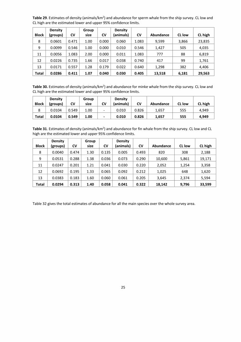
Table 29. Estimates of density (animals/km2) and abundance for sperm whale from the ship survey. CL low andCL high are the estimated lower and upper 95% confidence limits.

BlockDensity(groups) CV

Groupsize CV

Density(animals) CV Abundance CL low CL high

8 0.0601 0.471 1.00 0.000 0.060 1.083 9,599 3,866 23,835

9 0.0099 0.546 1.00 0.000 0.010 0.546 1,427 505 4,035

11 0.0056 1.083 2.00 0.000 0.011 1.083 777 88 6,819

12 0.0226 0.735 1.66 0.017 0.038 0.740 417 99 1,761

13 0.0171 0.557 1.28 0.179 0.022 0.640 1,298 382 4,406

Total 0.0286 0.411 1.07 0.040 0.030 0.405 13,518 6,181 29,563

Table 30. Estimates of density (animals/km2) and abundance for minke whale from the ship survey. CL low andCL high are the estimated lower and upper 95% confidence limits.

BlockDensity(groups) CV

Groupsize CV

Density(animals) CV Abundance CL low CL high

8 0.0104 0.549 1.00 - 0.010 0.826 1,657 555 4,949

Total 0.0104 0.549 1.00 - 0.010 0.826 1,657 555 4,949

Table 31. Estimates of density (animals/km2) and abundance for fin whale from the ship survey. CL low and CLhigh are the estimated lower and upper 95% confidence limits.

BlockDensity(groups) CV

Groupsize CV

Density(animals) CV Abundance CL low CL high

8 0.0040 0.474 1.30 0.135 0.005 0.493 820 308 2,188

9 0.0531 0.288 1.38 0.036 0.073 0.290 10,600 5,861 19,171

11 0.0247 0.201 1.21 0.041 0.030 0.220 2,052 1,254 3,358

12 0.0692 0.195 1.33 0.065 0.092 0.212 1,025 648 1,620

13 0.0383 0.183 1.60 0.060 0.061 0.205 3,645 2,374 5,594

Total 0.0294 0.313 1.40 0.058 0.041 0.322 18,142 9,796 33,599

Table 32 gives the total estimates of abundance for all the main species over the whole survey area.

26

Table 32. Estimates of total abundance and density (animals/km2) in the whole survey area for all species.

Species Abundance Density CV CL low CL high

Harbour porpoise 466,569 0.381 0.154 345,306 630,417

Bottlenose dolphin 27,697 0.015 0.233 17,662 43,432

Risso’s dolphin 13,584 0.008 0.441 5,943 31,047

White-beaked dolphin 36,287 0.020 0.290 18,694 61,869

White-sided dolphin 15,510 0.009 0.717 4,389 54,807

Common dolphin 467,673 0.261 0.264 281,129 777,998

Striped dolphin 372,340 0.208 0.329 198,583 698,134

Unid common or striped 158,167 0.088 0.188 109,689 228,069

Pilot whale 25,777 0.014 0.345 13,350 49,772

Beaked whales (all species) 11,394 0.006 0.503 4,494 28,888

Sperm whale 13,518 0.008 0.405 6,181 29,563

Minke whale 14,759 0.008 0.327 7,908 27,544

Fin whale 18,142 0.010 0.322 9,796 33,599

ICES Assessment Units

Estimates of harbour porpoise abundance for each ICES Assessment Unit (AU) are given in Table 33. For theKattegat and Belt Seas, ship block 2 is approximately equivalent to the AU but includes some waters to thesouth and excludes some waters to the north. For the North Sea, the combined area of the aerial survey blocksused is very similar (within a few percent) to the area of the AU.

For the West Scotland AU, offshore waters to the west of Scotland were covered by ship block 8, whereabundance has not been estimated because there were only 3 sightings of harbour porpoise in the west of thearea. Only a part of the Celtic/Irish Seas AU was covered by SCANS-III so the estimate for this area is notrepresentative of the whole AU. Waters to the south and west of Ireland were covered by Irish projectObSERVE and estimates of abundance for these waters are not yet available.

For the Iberian peninsula, the aerial survey covered all continental shelf waters; the AU includes waters off theshelf, which is unlikely to include harbour porpoises (none were seen in ship blocks 11, 12 and 13).

Table 33. Estimates of harbour porpoise abundance and density (animals/km2) in ICES Assessment Units, andNorwegian coastal waters north of 62°N. CV is the coefficient of variation of abundance and density. CL lowand CL high are the estimated lower and upper 95% confidence limits of abundance. All estimates are fromaerial survey except for the Kattegat and Belt Seas AU, which is from ship survey block 2. Note that the sum ofthe estimates for the Celtic/Irish Seas and North Sea AUs (372,073) is slightly smaller than the sum of thecontributing bocks (372,452); this is because block C spanned both AUs and was post-stratified in analysis.

Assessment Unit Abundance Density CV CL low CL high

Celtic/Irish Seas (partialcoverage only)

26,700 0.11 0.25 16,055 42,128

North Sea 345,373 0.52 0.18 246,526 495,752

West Scotland 24,370 0.21 0.23 15,074 37,858

Iberian peninsula 2,898 0.04 0.32 1,386 5,122

Kattegat and Belt Seas 42,324 1.04 0.30 23,368 76,658

Norwegian coastal waters 24,526 0.25 0.28 14,035 40,829

27

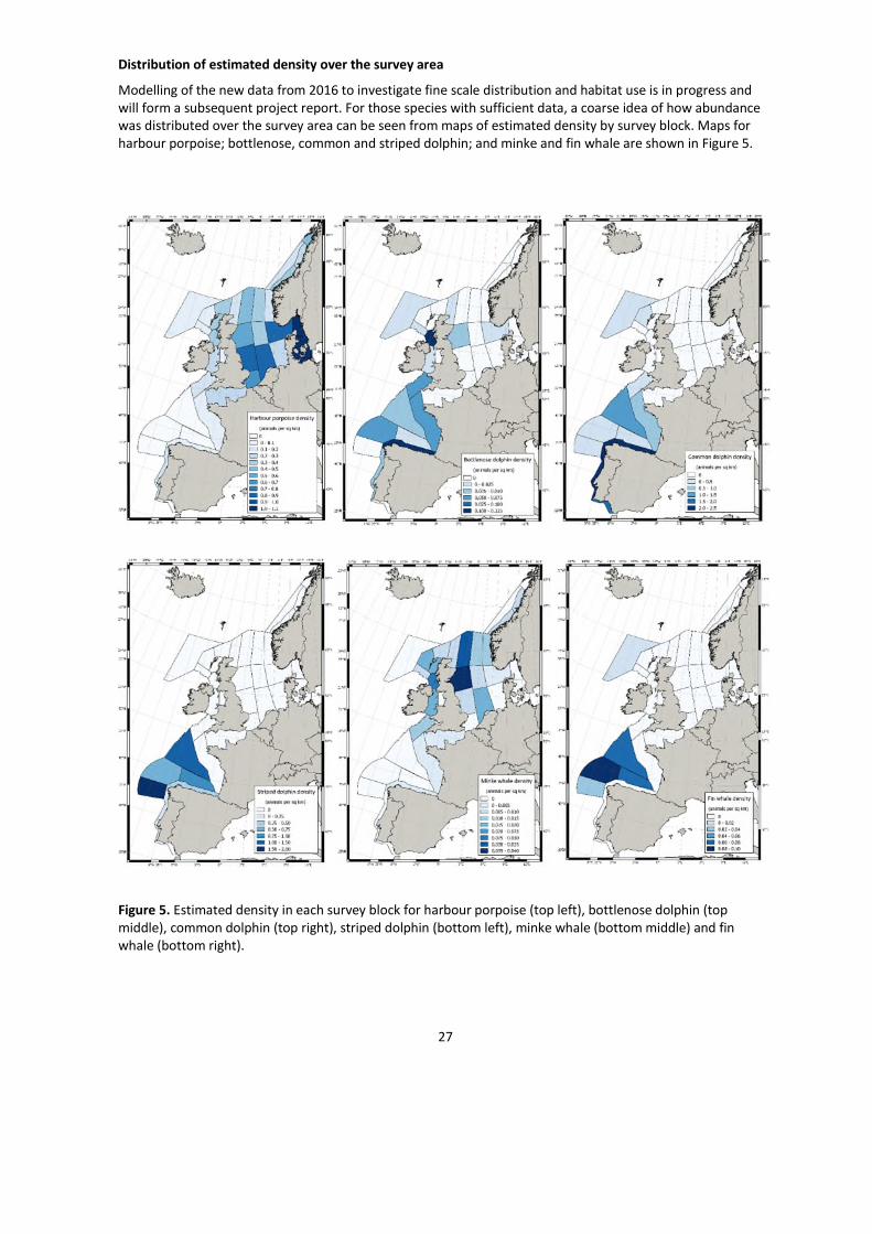
Distribution of estimated density over the survey area

Modelling of the new data from 2016 to investigate fine scale distribution and habitat use is in progress andwill form a subsequent project report. For those species with sufficient data, a coarse idea of how abundancewas distributed over the survey area can be seen from maps of estimated density by survey block. Maps forharbour porpoise; bottlenose, common and striped dolphin; and minke and fin whale are shown in Figure 5.

Figure 5. Estimated density in each survey block for harbour porpoise (top left), bottlenose dolphin (topmiddle), common dolphin (top right), striped dolphin (bottom left), minke whale (bottom middle) and finwhale (bottom right).

28

Responsive movement to survey ships and reanalysis of data from 1994 and 2005

There was no evidence of movement in response to the survey ships for any species in SCANS-III and,accordingly, point (trackline) independence models (Laake & Borchers 2004) were used to estimate detectionprobability for all species. In 2005, there was strong evidence of attraction for common dolphins and weakevidence of avoidance for harbour porpoise, white-beaked dolphin and minke whale so the full independencedetection probability model that allows for responsive movement (Borchers et al. 1998; Laake & Borchers2004) was used for all species (Hammond et al. 2013). In 1994, the only method of analysis available for two-team data was the full independence model.

Use of full independence models for all species was the only option in 1994 and justified in 2005, but thiscreates a potential problem for comparison with abundance estimates from 2016. The full independencemodel, while necessary if responsive movement needs to be accounted for, is not robust to any unmodelledheterogeneity (non-independence) in the probability of detection by the Tracker and Primary teams; this non-independence is likely to be a positive correlation, which generates negatively biased estimates. It is thereforelikely that published estimates of abundance for 1994 and 2005 are negatively biased. The point independencemodel (used for SCANS-III shipboard analysis) assumes non-independence only on the transect line and is thusmore robust and less likely to generate negatively biased estimates.

An additional consideration is that responsive movement in the form of avoidance, as suggested for harbourporpoise, white-beaked dolphin and minke whale in 2005, leads to negative bias. Accounting for this by usingthe full independence detection probability model should therefore lead to a higher estimate than using thepoint independence model. However, this was not the case (see below).

In summary, if estimates from 1994 and 2005 are subject to negative bias and estimates from 2016 are not,assessment of trends in abundance over time would be confounded with this difference and trends couldappear more positive than they are.

Consequently, it was decided to reanalyse the SCANS and SCANS-II shipboard data using the more robust pointindependence model of detection probability to create a comparable time series of estimates from 1994, 2005and 2016. Abundance was re-estimated for harbour porpoise, white-beaked dolphin and minke whale in 1994and 2005. Abundance was not re-estimated for common dolphin in 2005 because of the strong evidence ofattraction to the survey vessels in this species on SCANS-II, which could cause a substantial overestimate if notaccounted for using the full independence model (e.g. Cañadas et al. 2009). Abundance was also not re-estimated for bottlenose dolphin in 2005 because there were insufficient data to use any form of two-teamanalysis methods.

Aerial surveys are not subject to responsive movement - the tandem aircraft method used in 1994 and thecircle-back method used in 2005 and 2016 provide consistent estimates for harbour porpoise in all of the aerialsurveys.

However, the availability for the first time of g(0) estimates for dolphin species and for minke whale estimatedfor the SCANS-III aerial survey provided an opportunity to improve estimates of abundance for white-beakeddolphin, common dolphin, bottlenose dolphin and minke whale from the SCANS-II aerial survey in 2005.Published estimates had previously been corrected only for availability, based on dive data from studies inother areas (Hammond et al. 2013).

Table 34 shows the revised estimates of abundance for 1994 and 2005 compared to those previouslypublished in Hammond et al. (2002, 2013). Revised ship estimates are similar for minke whale but 20-50%larger for harbour porpoise and three times larger for white-beaked dolphin. These results confirm thatabundance was previously underestimated for harbour porpoise and, especially, for white-beaked dolphin.Revised aerial estimates using the SCANS-III estimates of g(0) are similar for dolphin species but smaller forminke whale.

29

Table 34. Revised estimates of abundance for 1994 and 2005 compared with previously published estimates(Hammond et al. 2002; 2013). Species: HP = harbour porpoise; WB = white-beaked dolphin; MW = minkewhale; BD = bottlenose dolphin; CD = common dolphin. All previously published ship estimates used the fullindependence (fi) model of detection probability except for bottlenose dolphin in 2005 for which the datawere sufficient only for a conventional “single observer” (so) analysis. All revised estimates used the pointindependence model of detection probability, except for bottlenose dolphin and common dolphin in 2005 (seeabove). Revised aerial estimates used SCANS-III estimates of g(0) for dolphins and minke whale. There wereno aerial estimates for white-beaked dolphin or minke whale in 1994.

Revised estimatesPreviously published estimates(Hammond et al. 2002; 2013)

Year Species Area N CV 95% CI N CV 95% CI

1994 HP Ship 358,807 0.20 292,995 0.16

1994 HP Aerial 48,370 0.30 48,371 0.30

1994 HP Total 407,177 0.18 288,920 - 573,838 341,366 0.14 260,000 - 449,000

1994 WB Ship 23,716 0.30 13,440 - 41,851 7,856 0.30 4,000 - 13,300

1994 MW Ship 9,685 0.23 6,199 - 15,132 8,445 0.24 5,000 - 13,500

2005 HP Ship 409,774 0.27 265,268 0.24

2005 HP Aerial 110,090 0.17 110,090 0.17

2005 HP Total 519,864 0.21 343,521 - 786,730 375,358 0.20 256,304 - 549,713

2005 WB Ship 33,119 0.41 11,659 0.34

2005 WB Aerial 4,569 0.54 4,878 0.57

2005 WB Total 37,689 0.36 18,898 - 75,164 16,536 0.30 9,245 - 29,586

2005 MW Ship 13,383 0.36 13,640 0.37

2005 MW Aerial 1,866 0.33 5,317 0.74

2005 MW Total 15,249 0.31 8,352 - 27,842 18,958 0.35 9,798 - 36,680

2005 BD Ship (so) 14,515 0.47 14,515 0.47

2005 BD Aerial 2,126 0.82 1,971 0.54

2005 BD Total 16,641 0.42 7,618 - 36,351 16,485 0.42 7,463 - 36,421

2005 CD Ship (fi) 36,225 0.21 36,225 0.21

2005 CD Aerial 18,730 0.47 19,995 0.51

2005 CD Total 54,955 0.21 36,607 - 82,498 56,221 0.23 35,748 - 88,419

Trends in abundance

Following the successful completion of the SCANS-III survey in 2016, there are now three estimates ofabundance for harbour porpoise, white-beaked dolphin and minke whale in the North Sea from SCANS,SCANS-II and SCANS-III, and it is justifiable to investigate trend over time. For minke whale in the North Sea,there are five additional estimates from the Norwegian Independent Line Transect Surveys (NILS) (Bøthun etal. 2009; Schweder et al. 1997; Skaug et al. 2004; Solvang et al. 2015). All these estimates relate to the NorthSea bounded by 62°N to the north but the earlier Norwegian estimates of minke whale abundance covered asmaller area between 56°N and 61°N. The most recent Norwegian minke whale estimate for 2009 includeswaters south to 53°N.

Although not covering exactly the same area, there are also three comparable estimates of abundance forharbour porpoise in the Skagerrak/Kattegat/Belt Seas area in 1994, 2005 and 2016, and two comparable

30

estimates for 2012 (Viquerat et al. 2014) and 2016 for the smaller Kattegat/Belt Seas area. Figure 6 shows theareas covered in these surveys compared to the area believed to represent a separate population (Sveegaardet al. 2015).

Figure 6. Areas covered during the three SCANS surveys and the “MiniSCANS” survey in 2012 (Viquerat et al.2014) in the Skagerrak/Kattegat/Belt Seas (coloured light blue) compared with the area believed to representa separate population (Sveegaard et al. 2015) (cross-hatched dark blue).

In any assessment of trend, it is important to consider the statistical power to detect a change in abundance of

a given magnitude. Simple power analyses (ignoring additional variance from variation in the number of

animals present in the area at the time of the survey) were conducted to determine the annual rate of decline

that could be detected with high (80%) power from the available estimates of abundance. Power was

calculated using the simplified inequality:

r2n3 > 12CV2 (Zα/2 + Zβ)2

where r = rate of change over the time period in question, n = the number of surveys during the time period,

CV = coefficient of variation of abundance, Zα/2 = the value of a standardised random normal variable for the

probability of making a Type I error, α (set to 0.05), Zβ is the value of a standardised random normal variable

for the probability of making a Type II error, β, and power is (1-β) (Gerrodette, 1987).

Figure 7 shows the estimates and trend lines fitted to three or more comparable estimates of abundance andTable 35 gives the results of the power calculations. These results show that there is no statistical support for achange in abundance over the period covered by the surveys for any species/region.

The annual rates of decline that can be detected with 80% power from the three estimates in the North Seaare 1.8% for harbour porpoise and 5% for white-beaked dolphin. For minke whale, the eight estimates for theNorth Sea are quite variable but have 80% power to detect a 0.5% annual rate of decline.

1994 2005 2012

2016Blocks 1+2

2016Block 2

31

Figure 7. Trend lines fitted to time series of three or more abundance estimates. Top left: harbour porpoise in

the Skagerrak/Kattegat/Belt Seas area (blue dots and line) – estimated rate of annual change = 1.24% (95%CI: -

39; 67%), p = 0.81. Estimates for the Kattegat/Belt Seas population area (see Figure 6) shown as red dots. Top

right: harbour porpoise in the North Sea – estimated rate of annual change = 0.8% (95%CI: -6.8; 9.0%), p = 0.18.

Bottom left: white-beaked dolphin in the North Sea – estimated rate of annual change = -0.5% (95%CI: -18; 22%),

p = 0.36. Bottom right: minke whale in the North Sea – estimated rate of annual change = -0.25% (95%CI: -4.8;

4.6%), p = 0.90. Error bars are log-normal 95% confidence intervals.

Table 35. Results of power calculations to determine the annual rate of decline that could be detected by the

available data with 80% power. n is the number of abundance estimates. CV = average CV of abundance for

the available estimates.

Species Region n CVAnnual rate of decline

detectable at 80% power

Harbour porpoise Skagerrak / Kattegat / Belt Seas 3 0.30 3.7%

Harbour porpoise North Sea 3 0.18 1.8%

White-beaked dolphin North Sea 3 0.36 5%

Minke whale North Sea 8 0.30 0.5%

0

20,000

40,000

60,000

80,000

100,000

1990 1994 1998 2002 2006 2010 2014 2018

Ab

un

dan

ce

Year

Harbour porpoise - Skagerrak / Kattegat /Belt Seas

0

10,000

20,000

30,000

40,000

50,000

60,000

1990 1995 2000 2005 2010 2015 2020

Ab

un

dan

ce

Year

White-beaked dolphin - North Sea

0

100,000

200,000

300,000

400,000

500,000

600,000

1990 1995 2000 2005 2010 2015 2020

Ab

un

dan

ce

Year

Harbour porpoise - North Sea

0

5,000

10,000

15,000

20,000

25,000

30,000

35,000

1985 1990 1995 2000 2005 2010 2015 2020

Ab

un

dan

ce

Year

Minke whale - North Sea

32

Discussion

We present here results from the third in a long-term time series (1994, 2005/07, 2016) of large-scalemultinational surveys of cetaceans in European Atlantic waters (Figure 8) allowing a snapshot view of howdistribution and abundance have varied over more than two decades. Except for Portuguese offshore waters,and waters to the south and west of Ireland, there are now two comprehensive and comparable summerdatasets for European Atlantic waters between 62°N and the Straits of Gibraltar. And there are three suchcomparable datasets for the North Sea and the Skagerrak/Kattegat/Belt Seas.

For harbour porpoise in the North Sea, a region that can be considered for assessment purposes as apopulation unit, our results show no evidence for trends in abundance since the mid-1990s. The same is thecase for white-beaked dolphin and minke whale in the North Sea, and for harbour porpoise in theSkagerrak/Kattegat/Belt Seas. Power to detect directional changes in abundance from large-scale sightingssurveys is generally low (Taylor et al. 2007) but the time span covered by the three SCANS surveys andreasonable precision in estimates means that the data have high power to detect changes of 2-5% per year.For minke whales where more surveys are available, there is high power to detect a 0.5% change in abundanceper year.

For most species for which we can estimate abundance from large-scale surveys, European Atlantic waters areat the edge of a wider North Atlantic range. Spatial variation in prey availability may lead to redistribution ofanimals and the distribution and abundance of these species in European waters may vary as a result of this.

Aerial vs ship survey

All three SCANS surveys have been conducted with a mix of aerial and shipboard surveys. In 1994, nine shipsand two aircraft were used and, in 2005, seven ships and three aircraft (Hammond et al. 2002; 2013). In 2016,seven aircraft and three ships were used, with shelf waters being entirely covered by air, except theKattegat/Belt Seas.

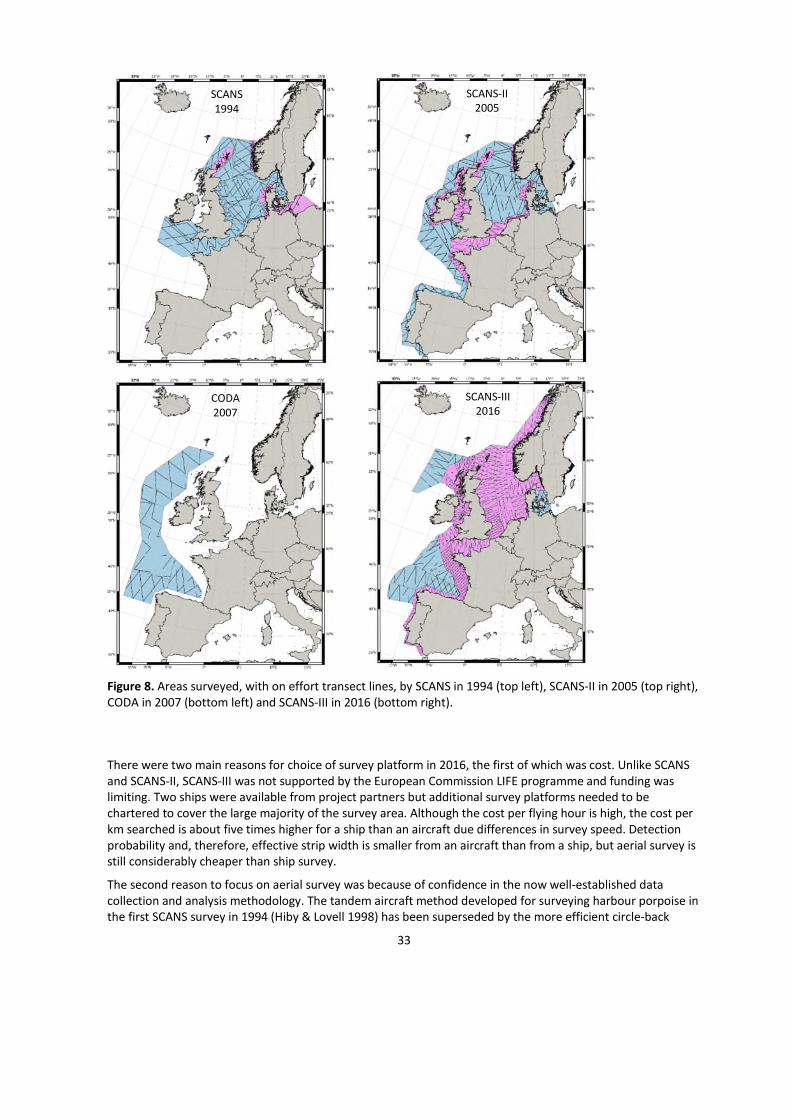
33

Figure 8. Areas surveyed, with on effort transect lines, by SCANS in 1994 (top left), SCANS-II in 2005 (top right),CODA in 2007 (bottom left) and SCANS-III in 2016 (bottom right).

There were two main reasons for choice of survey platform in 2016, the first of which was cost. Unlike SCANSand SCANS-II, SCANS-III was not supported by the European Commission LIFE programme and funding waslimiting. Two ships were available from project partners but additional survey platforms needed to bechartered to cover the large majority of the survey area. Although the cost per flying hour is high, the cost perkm searched is about five times higher for a ship than an aircraft due differences in survey speed. Detectionprobability and, therefore, effective strip width is smaller from an aircraft than from a ship, but aerial survey isstill considerably cheaper than ship survey.

The second reason to focus on aerial survey was because of confidence in the now well-established datacollection and analysis methodology. The tandem aircraft method developed for surveying harbour porpoise inthe first SCANS survey in 1994 (Hiby & Lovell 1998) has been superseded by the more efficient circle-back

SCANS1994

SCANS-II2005

CODA2007

SCANS-III2016

34

(“racetrack”) method first used in SCANS-II in 2005 (Hiby 1999). These methods have since been extensivelyused in regular surveys in European waters (e.g. Gilles et al. 2009; Scheidat et al. 2008; 2012).

The new development in SCANS-III was to employ the circle-back method for dolphin species (bottlenose,white-beaked, white-sided, common and striped) and for minke whale to obtain more appropriate correctionsfor missing animals on the transect line (i.e., g(0)). The smaller sample sizes for these species meant that somesimplifying assumptions had to be made. In particular, it was assumed that groups of these species spend asimilar proportion of time at the surface as harbour porpoise and that the rates and distribution of anydisplacement between the leading and trailing sections of effort are also similar to harbour porpoise.Nevertheless, these new estimates of g(0) are better than previously used corrections, which were limited toaccounting only for availability bias (not perception bias) based on surfacing rates available from other studiesand areas (see Hammond et al. 2013). Revised abundance estimates for dolphin species and minke whale fromSCANS-II in 2005 using these new estimates of g(0) are therefore a marked improvement.

Overall, while estimates for species not commonly seen in shelf waters have not been corrected, extension ofthe use of the circle-back method has allowed us to generate unbiased estimates of abundance for harbourporpoise, dolphin species and minke whale.

Anomalous data from M/V Skoven

On one of the ships (M/V Skoven), which surveyed offshore waters west of Scotland and the northern Bay ofBiscay, the data for large baleen whales (the large majority of which were fin whales) were compromised byatypical searching patterns by both Tracker and Primary observers. Tracker observers focussed too close to thetransect line resulting in their observations being aggregated at small perpendicular distances. This had theeffect that the conditional probability of detection by Primary observers was smaller close to the transect linethan further away, violating a fundamental principle of line transect sampling.

In addition, Primary observers tended to detect large baleen whales much further ahead of the vessel thandictated by the protocol (searching within 500m of the ship). Even if protocol is followed on the Primaryplatform, the easily detected blow of the fin whale may be detected in peripheral vision. This led to many finwhale groups either being detected by Tracker and Primary at the same time or being detected by Primarybefore Tracker, which cannot be included as Tracker “trials” in analysis. The lack of separation of Tracker andPrimary searching areas violates the requirement of the two-team tracker method.

The result of these anomalies in the large baleen whale data from M/V Skoven meant that it was not possibleto conduct a two-team analysis. Instead, fin whale abundance in areas surveyed by M/V Skoven (blocks 8 and9) was estimated from Primary platform data in a conventional single platform analysis. Fin whale abundancein these areas is therefore likely underestimated. These problems did not occur on the other ship surveyingoffshore waters and fin whale abundance in areas surveyed by B/O Angeles Alvariño (blocks 11, 12 and 13)was estimated using the planned two-team analysis.

The difficulty of conducting a two-team survey with the tracker protocol for large baleen whales has beenrecognised previously. The high visibility of fin whale blows and the long period that they are available to bedetected means that g(0) for this species is likely to be relatively close to 1. However, a single platformanalysis of the B/O Angeles Alvariño data generated a fin whale abundance estimate around 2/3rd of the size ofthe two-team analysis, implying that assuming g(0)=1 would lead to an underestimate.

The common and striped dolphin data collected on M/V Skoven were also anomalous in that the largemajority of Tracker sightings were made close to the transect line. Primary conditional detection probabilityalso increased with perpendicular distance but the sample sizes at distances greater than 100m were small;78% of Tracker sightings were made within 100m of the transect line. When data from the two ships wereanalysed together, the conditional detection probability did not increase with perpendicular distance so acombined analysis was judged to be appropriate for common and striped dolphins.

The anomalous data collected on M/V Skoven illustrate the importance of following data collection protocol. Ifthe large majority of Tracker trials are made very close to the transect line then random movement in eitherdirection will result in perpendicular distance tending to increase by the time the animals become available to

35

be seen by Primary observers. This seems likely to be the explanation for the apparent increase in Primaryconditional detection probability with perpendicular distance for fin whale and common/striped dolphins.

New information on distribution and abundance

Harbour porpoise

The observed distribution of harbour porpoises in 2016 was similar to that observed in SCANS-II in 2005

(Hammond et al. 2013) but one notable difference is that more sightings were made throughout the English

Channel (block C) in 2016 than previously. In 1994, no sightings were made in the Channel or the southern

North Sea (Hammond et al. 2002). In 2005, there were a number of sightings at the far western end of the

Channel (Hammond et al. 2013) and in the SAMM survey in 2012 there were sightings in both the western and

eastern parts, but not the central part (Laran et al., in press). The progressive spread of sightings into most of

the Channel over the past two decades indicates that harbour porpoise distribution has expanded, probably

from the North Sea and the Celtic Sea, and now encompasses the entire Channel, at least in summer.

In the ICES AUs (see Figure 2), the estimates in 2016 and 2005 are compatible in the Iberian peninsula AU(2,900, CV = 0.32 and 2,880, CV = 0.72, respectively), and in the West Scotland AU (24,400, CV = 0.23 and26,300, CV = 0.37). The southern part of the West Scotland AU was covered by the Irish ObSERVE project andinformation for this area is not yet available for 2016. In the Kattegat and Belt Seas AU, the estimate for 2016of 42,000 (CV = 0.23) is consistent in terms of area surveyed only with the estimate for 2012 of 40,000 (CV =0.24) (Viquerat et al., 2014). In the North Sea the estimate in 2016 (345,000, CV = 0.18) was similar to theestimate in 2005 (355,000, CV = 0.22; revised from Hammond et al. 2013) and 1994 (289,000, CV = 0.14;revised from Hammond et al. 2002), and to the model-based estimate using data from 2005-2013 of 361,000(0.20) (Gilles et al. 2016). Results of the trend analysis of estimates in the North Sea and theSkagerrak/Kattegat/Belt Seas show no support for changes in abundance since 1994.

The SCANS-III survey covered only a part of the Celtic and Irish Seas AU; the remaining part of the AU wascovered by the Irish ObSERVE project, for which no estimate is available yet. It is thus not possible to presentan estimate for this Assessment Unit at this time.

Bottlenose dolphin

The observed distribution of bottlenose dolphins in 2016 was similar to that observed in SCANS-II and CODA in2005/07 (Hammond et al., 2013; CODA 2009) but most of the offshore sightings in 2007 were made in theObSERVE survey area, for which information for 2016 is not yet available. The estimate of abundance for 2016of 27,700 (CV = 0.23) is smaller than that from 2005/07 of 35,900 (CV = 0.21) (WGMME 2017) but a directcomparison between estimates for 2016 and 2005/07 should not be made until estimates are available forequivalent areas.

White-beaked dolphin

The observed distribution of white-beaked dolphins in 2016 is similar to that observed in SCANS-II in 2005(Hammond et al., 2013) and in SCANS in 1994 (Hammond et al., 2002). The estimate of abundance in 2016 of36,300 (CV = 0.29) is very similar to the estimate from SCANS-II in 2005 of 37,700 (CV = 0.36) (revised fromHammond et al. 2013) but higher than the estimate from SCANS in 1994 of 22,600 (CV = 0.23) (revised fromHammond et al. 2002). Results of the trend analysis of estimates in the North Sea show no support for changesin abundance since 1994.

Common and striped dolphins

The observed distributions of common and striped dolphins in 2016 are similar to those observed in SCANS-IIand CODA in 2005/07 (Hammond et al., 2013; CODA 2009) and in the SAMM surveys in the Channel andFrench waters of the Bay of Biscay in summer 2012 (Laran et al., in press). Some sightings in 2005 and 2007were made in the ObSERVE survey area, in which information for 2016 is not yet available. The distribution ofcommon dolphins appears to be strongly concentrated in shelf waters but a substantial number ofunidentified common or striped dolphin sightings were also made in offshore waters, at least some of which

36

were likely to have been common dolphins. Striped dolphins appear to be strongly concentrated in offshorewaters but some of the unidentified sightings in shelf waters could have been striped dolphins.

The estimates of abundance in 2016 of 468,000 (CV = 0.26) common dolphin, 372,000 (CV = 0.33) stripeddolphin and 158,000 (CV = 0.19) unidentified common or striped dolphins sum to almost one million animals.These estimates are substantially larger than the estimates for 2005/2007 of 174,000 (CV = 0.27) commondolphin and 61,400 (CV = 0.93) striped dolphin, respectively (revised from Hammond et al., 2013; CODA 2009).A direct comparison between estimates for 2016 and 2005/07 should not be made until estimates areavailable for equivalent areas.

However, the estimate of common and striped dolphins in summer 2012 from the SAMM surveys in theChannel and French waters in the Bay of Biscay was around 700,000 animals (Laran et al., in press). The SAMMsurvey area did not include Spanish waters that were included in SCANS-III in 2016 and the estimate was notcorrected for animals missed on the transect line. The estimates from SCANS-III in 2016 and SAMM in 2012therefore appear to be compatible.

Long-finned pilot whale

The observed distribution of pilot whales was similar in 2016 to that observed in SCANS-II and CODA in2005/07 (Rogan et al., in press) but the majority of the sightings in 2007 were made in the ObSERVE surveyarea, for which information for 2016 is not yet available. The absence of information from Irish waters maypartly explain why the estimate of abundance for 2016 of 25,800 (CV = 0.35) is considerably smaller than thatfrom 2005/07 of 124,000 (CV = 0.35) (Rogan et al., in press) but a direct comparison should not be made untilestimates are available for equivalent areas.

Beaked whales (all species)

The observed distribution of beaked whales was similar in 2016 to that observed in CODA in 2007 (CODA 2009)and from opportunistic sightings (WGMME 2016). Some of these sightings were made in the ObSERVE surveyarea, for which information for 2016 is not yet available.

The estimate of abundance of all beaked whale species combined for 2016 of 11,400 (CV = 0.50) is similar tothe equivalent estimate from SCANS-II and CODA in 2005/2007 of 12,900 (CV = 0.31) (Rogan et al., in press)but a direct comparison should not be made until estimates are available for equivalent areas.

Sperm whale

The observed distribution of sperm whales was similar in 2016 to that observed in CODA in 2007 (Rogan et al.,in press). Some of these sightings were made in the ObSERVE survey area, for which information for 2016 isnot yet available.

The estimate of abundance of sperm whales in 2016 of 13,500 (CV = 0.41) is larger than the estimate fromCODA in 2007 of 2,600 (CV = 0.26) for identified sperm whales and the estimate of 5,600 (CV = 0.32) if aproportion of unidentified large whales is included (Rogan et al., in press). However, a direct comparisonshould not be made until estimates are available for equivalent areas.

Minke whale

Between 1994 and 2005 there was some evidence that minke whale distribution in the North Sea had shiftedto the south (Hammond et al. 2013). The observed distribution of minke whale in 2016 was similar to thatobserved in 2005 in the North Sea, and similar overall to that in 2005/07 (Hammond et al., 2013; Hammond etal., 2011). However, many sightings in 2007 were made in the Irish ObSERVE survey area, in which informationfor 2016 is not yet available.

The estimate of abundance in 2016 of 14,800 (CV = 0.33) is smaller than the estimate for 2005/07 from SCANS-II and CODA of 26,800 (CV = 0.35) (revised from Hammond et al. 2011). This may be partly because of the lackof an estimate in Irish waters but a direct comparison should not be made until estimates are available forequivalent areas. The estimate for 2016 in the North Sea was 8,900 (CV = 0.24), which is within the range ofprevious estimates from SCANS, SCANS-II and Norwegian surveys and results of the trend analysis of estimatesin the North Sea show no support for changes in abundance since 1989.

Fin whale

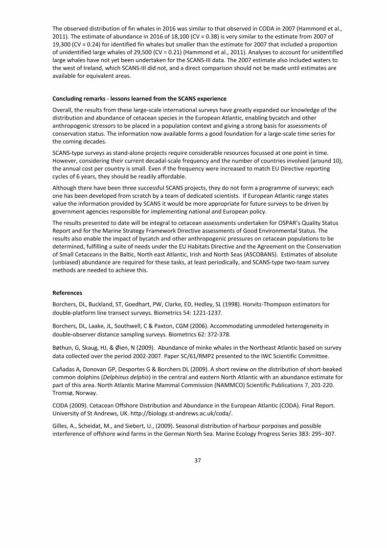
37

The observed distribution of fin whales in 2016 was similar to that observed in CODA in 2007 (Hammond et al.,2011). The estimate of abundance in 2016 of 18,100 (CV = 0.38) is very similar to the estimate from 2007 of19,300 (CV = 0.24) for identified fin whales but smaller than the estimate for 2007 that included a proportionof unidentified large whales of 29,500 (CV = 0.21) (Hammond et al., 2011). Analyses to account for unidentifiedlarge whales have not yet been undertaken for the SCANS-III data. The 2007 estimate also included waters tothe west of Ireland, which SCANS-III did not, and a direct comparison should not be made until estimates areavailable for equivalent areas.

Concluding remarks - lessons learned from the SCANS experience

Overall, the results from these large-scale international surveys have greatly expanded our knowledge of thedistribution and abundance of cetacean species in the European Atlantic, enabling bycatch and otheranthropogenic stressors to be placed in a population context and giving a strong basis for assessments ofconservation status. The information now available forms a good foundation for a large-scale time series forthe coming decades.

SCANS-type surveys as stand-alone projects require considerable resources focussed at one point in time.However, considering their current decadal-scale frequency and the number of countries involved (around 10),the annual cost per country is small. Even if the frequency were increased to match EU Directive reportingcycles of 6 years, they should be readily affordable.

Although there have been three successful SCANS projects, they do not form a programme of surveys; eachone has been developed from scratch by a team of dedicated scientists. If European Atlantic range statesvalue the information provided by SCANS it would be more appropriate for future surveys to be driven bygovernment agencies responsible for implementing national and European policy.

The results presented to date will be integral to cetacean assessments undertaken for OSPAR’s Quality StatusReport and for the Marine Strategy Framework Directive assessments of Good Environmental Status. Theresults also enable the impact of bycatch and other anthropogenic pressures on cetacean populations to bedetermined, fulfilling a suite of needs under the EU Habitats Directive and the Agreement on the Conservationof Small Cetaceans in the Baltic, North east Atlantic, Irish and North Seas (ASCOBANS). Estimates of absolute(unbiased) abundance are required for these tasks, at least periodically, and SCANS-type two-team surveymethods are needed to achieve this.

References

Borchers, DL, Buckland, ST, Goedhart, PW, Clarke, ED, Hedley, SL (1998). Horvitz-Thompson estimators for

double-platform line transect surveys. Biometrics 54: 1221-1237.

Borchers, DL, Laake, JL, Southwell, C & Paxton, CGM (2006). Accommodating unmodeled heterogeneity in

double-observer distance sampling surveys. Biometrics 62: 372-378.

Bøthun, G, Skaug, HJ, & Øien, N (2009). Abundance of minke whales in the Northeast Atlantic based on survey

data collected over the period 2002-2007. Paper SC/61/RMP2 presented to the IWC Scientific Committee.

Cañadas A, Donovan GP, Desportes G & Borchers DL (2009). A short review on the distribution of short-beakedcommon dolphins (Delphinus delphis) in the central and eastern North Atlantic with an abundance estimate forpart of this area. North Atlantic Marine Mammal Commission (NAMMCO) Scientific Publications 7, 201-220.Tromsø, Norway.

CODA (2009). Cetacean Offshore Distribution and Abundance in the European Atlantic (CODA). Final Report.University of St Andrews, UK. http://biology.st-andrews.ac.uk/coda/.

Gilles, A., Scheidat, M., and Siebert, U., (2009). Seasonal distribution of harbour porpoises and possibleinterference of offshore wind farms in the German North Sea. Marine Ecology Progress Series 383: 295–307.

38

Gilles, A, Viquerat, S, Becker, EA, Forney, KA, Geelhoed, SCV, Haelters, J, Nabe-Nielsen, J, Scheidat, M, Siebert,U, Sveegaard, S, van Beest, FM, van Bemmelen, R, Aarts, G (2016). Seasonal habitat-based density models for amarine top predator, the harbor porpoise, in a dynamic environment. Ecosphere 7(6):e01367.10.1002/ecs2.1367

Gillespie, DM, Leaper, R, Gordon, JCD, Macleod, K (2010). A semi-automated, integrated, data collection

system for line transect surveys. Journal of Cetacean Research and Management 11: 217-227.

Gordon, J (2001). Measuring the range to animals at sea from boats using photographic and video images.Journal of Applied Ecology 38: 879-887.

Hammond, P.S., Berggren, P., Benke, H., Borchers, D.L., Collet, A., Heide-Jørgensen, M.P., Heimlich, S., Hiby,A.R., Leopold, M.F., Øien, N., 2002. Abundance of harbour porpoises and other cetaceans in the North Sea andadjacent waters. J. Appl. Ecol. 39, 361–376.

Hammond, PS, MacLeod, K, Burt, L, Cañadas, A, Lens, S, Mikkelsen, B, Rogan, E, Santos, B, Uriarte, A, VanCanneyt, O, Vazquez, JA (2011). Abundance of baleen whales in the European Atlantic. Paper SC/63/RMP24presented to the IWC Scientific Committee.

Hammond, PS, Macleod, K, Berggren, P, Borchers, DL, Burt, ML, Cañadas, A, Desportes, G, Donovan, GP, Gilles,A, Gillespie, D, Gordon, J, Hedley, S, Hiby, L, Kuklik, I, Leaper, R, Lehnert, K, Leopold, M, Lovell, P, Øien, N,Paxton, C, Ridoux, V, Rogan, E, Samarra, F, Scheidat, M, Sequeira, M, Siebert, U, Skov, H, Swift, R, Tasker, ML,Teilmann, J, Van Canneyt, O Vázquez, JA. (2013). Cetacean abundance and distribution in European Atlanticshelf waters to inform conservation and management. Biological Conservation 164: 107-122.

Hammond, PS, Gillespie, D, Lovell, P, Samarra, F, Swift, R, Macleod, K, Tasker, ML, Berggren, P, Borchers, DL,

Burt, ML, Paxton, CGM, Cañadas, A, Desportes, G, Donovan, GP, Gilles, A, Lehnert, K, Siebert, U, Gordon, J,

Leaper, R, Leopold, M, Scheidat, M, Øien, N, Ridoux, V, Rogan, E, Skov, H, Teilmann, J, Van Canneyt, O &

Vázquez, JA (2014). Large scale surveys for cetaceans: Line transect assumptions, reliability of abundance

estimates and improving survey efficiency – A response to MacLeod. Biological Conservation 170: 338-339.

Hiby, AR & Lovell, P (1998). Using aircraft in tandem formation to estimate abundance of harbour porpoise.

Biometrics 54: 1280-1289.

Hiby, L (1999). The objective identification of duplicate sightings in aerial survey for porpoise. In: Garner, GW

et al. (Eds.) Marine Mammal Survey and Assessment Methods, Balkema, Rotterdam. Pp 179-189.

Hiby, L & Gilles, A (2016). Estimating effective strip width in SCANS-III aerial surveys. Internal SCANS-III project

report.

ICES (2014). General advice on OSPAR request on implementation of MSFD for marine mammals. ICES advice

2014, Book 1: 1.6.6.1.

Innes, S, Heide-Jørgensen, MP, Laake, JL Laidre, KL, Cleator, HJ, Richard, P & Stewart, REA (2002). Surveys of

belugas and narwals in the Canadian High Arctic in 1996. North Atlantic Marine Mammal Commission

(NAMMCO) Scientific Publications 4: 169-190. Tromsø, Norway.

Laake, JL & Borchers, DL (2004). Methods for incomplete detection at distance zero, in: Buckland, ST et al.

(Eds.), Advanced Distance Sampling. Oxford University Press, Oxford.

Laran, S, Authier, M, Blanck, A, Doremus, G, Falchetto, H, Monestiez, P, Pettex, E, Stephan, E, Van Canneyt, O,

& Ridoux, V. (in press). Seasonal distribution and abundance of cetaceans within French waters: Part II: The

Bay of Biscay and the English Channel. Deep Sea Research II. http://doi.org/10.1016/j.dsr2.2016.12.012

Leaper, R & Gordon, J (2001). Application of photogrammetric methods for locating and tracking cetacean

movements at sea. Journal of Cetacean Research and Management 3: 131-141.

MacLeod, CD (2014). One size does not necessarily fit all for cetacean abundance estimate survey design –

Reply to Hammond. Biological Conservation 170: 336-337.

39

Miller, DL (2015). Distance: Distance Sampling Detection Function and Abundance Estimation. R package

version 0.9.4. http://CRAN.R-project.org/package=Distance

Palka, DL & Hammond, PS (2001). Accounting for responsive movement in line transect estimates of

abundance. Canadian Journal of Fisheries and Aquatic Sciences 58, 777-787.

R Core Team (2015). R: A language and environment for statistical computing. R Foundation for Statistical

Computing, Vienna, Austria. https://www.R-project.org/.

Rogan, E, Cañadas, A, Macleod, K, Santos, B, Mikkelsen, B, Uriarte, A, Van Canneyt, O, Vazquez,A J &

Hammond, PS (in press). Distribution, abundance and habitat use of deep diving cetaceans in the North East

Atlantic. Deep Sea Research II. http://doi.org/10.1016/j.dsr2.2017.03.015

SCANS (1995). Distribution and abundance of the harbour porpoise and other small cetaceans in the North Sea

and adjacent waters. Final report under LIFE Nature project LIFE 92-2/UK/027.

SCANS-II (2008). Small Cetaceans in the European Atlantic and North Sea (SCANS-II). Final Report. University of

St Andrews, UK. http://biology.st-andrews.ac.uk/scans2/.

Scheidat, M, Gilles, A, Kock, K.-H, Siebert, U (2008). Harbour porpoise Phocoena phocoena abundance in the

southwestern Baltic Sea. Endangered Species Research 5: 215-223.

Scheidat, M., Verdaat, H., and Aarts, G., (2012). Using aerial surveys to estimate density and distribution ofharbour porpoises in Dutch waters. Journal of Sea Research 69: 1–7.

Schweder, T, Skaug, HJ, Dimakos, XK, Langas, M, Øien, N (1997). Abundance of northeastern Atlantic minke

whales, estimates for 1989 and 1995. Reports of the International Whaling Commission 47, 453-483.

Skaug, HJ, Øien, N, Schweder, T, Bøthun, G (2004). Abundance of minke whales (Balaenoptera acutorostrata)

in the Northeastern Atlantic. Canadian Journal of Fisheries and Aquatic Sciences 61, 870-86.

Solvang, HK, Skaug, HJ & and Øien, NI 2015. Abundance estimates of common minke whales in the Northeast

Atlantic based on survey data collected over the period 2008-2013. Paper SC/66a/RMP8 presented to the IWC

Scientific Committee.

Sveegaard, S, Galatius, A, Dietz, R, Kyhna, L, Koblitz, JC, Amundin, M, Nabe-Nielsen, J, Sinding, M-HS, Andersen,

LW & Teilmann, J (2015). Defining management units for cetaceans by combining genetics, morphology,

acoustics and satellite tracking. Global Ecology and Conservation 3: 839-850.

Taylor, BL, Martinez, M, Gerrodette, T, Barlow, J & Hrovat, YN (2007). Lessons from monitoring trends inabundance in marine mammals. Marine Mammal Science 23: 157–175.

Thomas, LT, Buckland, ST, Rexstad, EA, Laake, JL, Strindberg, S, Hedley, SL, Bishop, JRB, Marques, TA &

Burnham, KP (2010). Distance software: design and analysis of distance sampling surveys for estimating

population size. Journal of Applied Ecology 47: 5-14.

WGMME (2014). Report of the Working Group on Marine Mammal Ecology (WGMME), 10-13 March 2014,Woods Hole, Massachusetts, USA. ICES CM 2014/ACOM: 27.

WGMME (2016). Report of the Working Group on Marine Mammal Ecology (WGMME), 8-11 February 2016,

Madrid, Spain. ICES CM 2016/ACOM: 26.