Estimates of anthropogenic carbon in the Indian Ocean with allowance for mixing and timevarying airsea CO2 disequilibrium

Estimates of anthropogenic carbon in the Indian Ocean

with allowance for mixing and time-varying

air-sea CO2 disequilibrium

Timothy M. Hall,1 Darryn W. Waugh,2 Thomas W. N. Haine,2 Paul E. Robbins,3

and Samar Khatiwala4

Received 8 July 2003; revised 12 December 2003; accepted 7 January 2004; published 25 February 2004.

[1] We apply to the Indian Ocean a novel technique to estimate the distribution, totalmass, and net air-sea flux of anthropogenic carbon. Chlorofluorocarbon data are used toconstrain distributions of transit times from the surface to the interior that areconstructed to accommodate a range of mixing scenarios, from no mixing (pure bulkadvection) to strong mixing. The transit time distributions are then used to propagate tothe interior the surface water history of anthropogenic carbon estimated in a waythat includes temporal variation in CO2 air-sea disequilibrium. By allowing for mixingin transport and for variable air-sea disequilibrium, we remove two sources of positivebias common in other studies. We estimate that the anthropogenic carbon mass inthe Indian Ocean was 14.3–20.5 Gt in 2000, and the net air-sea flux was 0.26–0.36 Gt/yr.The upper bound of this range, the no-mixing limit, generally coincides with previousstudies, while the lower bound, the strong-mixing limit, is significantly below previousstudies. INDEX TERMS: 1635 Global Change: Oceans (4203); 4568 Oceanography: Physical:

Turbulence, diffusion, and mixing processes; 4806 Oceanography: Biological and Chemical: Carbon cycling;

4808 Oceanography: Biological and Chemical: Chemical tracers; KEYWORDS: carbon, ocean, transport,

mixing, age, Indian Ocean

Citation: Hall, T. M., D. W. Waugh, T. W. N. Haine, P. E. Robbins, and S. Khatiwala (2004), Estimates of anthropogenic carbon in

the Indian Ocean with allowance for mixing and time-varying air-sea CO2 disequilibrium, Global Biogeochem. Cycles, 18,

GB1031, doi:10.1029/2003GB002120.

1. Introduction

[2] The ocean sequesters a large fraction of the CO2

arising from human activity. While great progress has beenmade in estimating the distribution and mass of anthropo-genic carbon in the ocean from observations, considerableuncertainty remains. The task is difficult because theanthropogenic signal of dissolved inorganic carbon (DDIC)DIC) is of the order of 100 times smaller than natural DIC,which has complex, poorly known biochemical sources andsinks. Various DDIC inference techniques have been devel-oped [Brewer, 1978; Chen and Millero, 1979; Gruber et al.,1996; Goyet et al., 1999; Thomas and Ittekkot, 2001;McNeil et al., 2003], and while comparison among themshows qualitative agreement, there are considerable quanti-

tative differences [Wanninkhof et al., 1999; Sabine andFeely, 2001; Coatanoan et al., 2001].[3] Several assumptions are common to most DDIC

inference techniques, raising the possibility of overall biasacross the range of estimates. Chief among these are (1) theassumption that mixing is a negligible component oftransport and (2) the assumption of ‘‘constant disequilib-rium’’ that DDIC in surface waters has kept pace withincreasing atmospheric CO2. Both of these assumptionshave been questioned, but the errors incurred by makingthem have remained unclear. A number of studies havedemonstrated that eddy mixing along constant densitysurfaces (isopycnals) plays a major role in propagatingtracers [e.g., Jenkins, 1988; Robbins et al., 2000] and mustbe taken into account when interpreting tracer-derivedtimescales [e.g., Thiele and Sarmiento, 1990; Sonnerup,2001; Waugh et al., 2003]. Information on the mixing,however, has not generally been incorporated in theobservation-based DDIC estimates. In addition to theweak-mixing and constant disequilibrium assumptions,techniques that derive DDIC from total DIC measurementsaccount for biochemical sources and sinks of DIC byusing stoichiometric (Redfield) ratios among carbon, oxy-gen, and alkalinity, whose uncertainty impacts the DDICestimates [Wanninkhof et al., 1999].

GLOBAL BIOGEOCHEMICAL CYCLES, VOL. 18, GB1031, doi:10.1029/2003GB002120, 2004

1NASA Goddard Institute for Space Studies at Columbia University,New York, New York, USA.

2Department of Earth and Planetary Sciences, Johns HopkinsUniversity, Baltimore, Maryland, USA.

3Scripps Institution of Oceanography, University of California, SanDiego, California, USA.

4Lamont-Doherty Earth Observatory, Columbia University, Palisades,New York, USA.

Copyright 2004 by the American Geophysical Union.0886-6236/04/2003GB002120$12.00

GB1031 1 of 11

[4] In this study we apply to the Indian Ocean a techniquethat avoids these assumptions. As in other studies weexploit the fact that DDIC is well approximated as a passive,inert tracer transported by a steady state circulation onsurfaces of constant density (isopycnals) in response toanthropogenic forcing in surface waters. Unlike other stud-ies we relate interior DDIC to the DDIC history at thesurface in a way that explicitly allows for mixing. CFC-12data are used to constrain distributions of transit times fromthe surface to the interior that are designed to accommodateany proportion of diffusive mixing and bulk advection. Thetransit time distributions are then used to propagate to theinterior the surface history of DDIC estimated in a mannerthat allows for time-varying CO2 disequilibrium. Theassumptions of no mixing and constant disequilibrium bothlead to positive bias. By removing them, we obtain a rangeof values for Indian Ocean mass and net air-sea flux ofanthropogenic carbon, all of which are consistent with theCFC data. The upper limit of the range approximatelycoincides with previous studies, while the lower limit isroughly one third lower.

2. Methodology

[5] We exploit the approximation, also made in otherstudies, that DDIC penetrates the ocean as a passive, inerttracer. This is reasonable because, while the distribution ofDIC itself is controlled by biology, upper ocean productivityis limited by nutrients, not carbon, and thus to first order theaddition of anthropogenic carbon does not alter the rate ofbiological uptake and downward transport of carbon. Fur-thermore, as in other studies we assume the ocean circulationto be in steady state. McNeil et al. [2003] estimated frommodel studies that present-day secular change in the oceancirculation due to global warming alters carbon uptake byonly�1%. Decadal and shorter time variability in the interiorocean does not affect our analysis significantly because manydecades of tracer signal are integrated [Hall et al., 2002].However, annual and interannual variability of the outcropsof isopycnals causes uncertainty in estimating the histories ofsurface waters of DDIC and CFC-12 (see section 3.2).[6] We make use of the following relationship, valid for

any passive, inert tracer transported by a steady statecirculation in response to a uniform time-dependent surfaceforcing:

cV tð Þ ¼Z 1

0

cS t � t0ð ÞGV t0ð Þdt0; ð1Þ

where cS(t) is the tracer concentration assumed to beuniform on the surface region S and cV is the concentrationaveraged over a volume V that includes S. GV(t) is thedistribution of transit times since the water in V last madecontact with S, where it was labeled by tracer [Beining andRoether, 1996; Haine and Hall, 2002]. The mean tracerconcentration in the volume comprises all the pastcontributions on the surface, weighted by GV. The shapeof GV(t), determined by the nature of the transport, will beestimated in section 2.1 by CFC-12 observations andinversion of relationship (1).

[7] While relationship (1) can be generalized to includespatially varying tracer concentration on the surface [Haineand Hall, 2002], uniform concentration on the surface is agood approximation in this application. The main thermo-cline of the Indian Ocean is ventilated predominantly fromthe south, through either winter subduction or mode waterformation [Karstensen and Quadfasel, 2002], and anthro-pogenic tracers (or any air-sea flux anomaly) penetrate theupper ocean along isopycnals [Fine et al., 1981]. Thus wecan apply relationship (1) separately to northward transportalong each isopycnal in response to time-varying tracerconcentrations at the southern outcrop. Finally, becausetemperature is the most important factor determining boththe solubilities of the tracers we consider and the density ofseawater, tracer concentrations are approximately uniformalong the outcrops.[8] We neglect sources of water from the Red Sea. The

volume flux from these sources is only 1–2% of thesouthern source [Karstensen and Quadfasel, 2002; Boweret al., 2000], but because of the high temperature andsalinity their fractional DDIC contribution may be higher.(The solubility of DIC decreases with T and S, but DDICincreases because of nonlinearities in DIC’s dependence onT, S, alkalinity, and atmospheric CO2.) The error incurred bythis neglect is estimated in section 3.2.[9] Our analysis is performed separately on 15 isopycnals,

the deepest of which (s0 = 27.65) reaches an approximatedepth of 1500 m in southern midlatitudes. We find that thecontribution to the total inventory decreases rapidly withdensity, with s0 = 27.65 containing less than 2% of the totalDDIC (compared with s0 = 26.7, which contains 17% of thetotal). We assume that deeper isopycnals contribute insignif-icantly. North of 35�S the Indian Ocean is defined by itsbounding land masses, while to the south it includes thesector of the Southern Ocean between 20�E and 120�E. Thevolumes V in expression (1), over which the tracer concen-trations are averaged, are defined vertically by the separationof adjacent isopycnals, to the south by the outcrop regions(surfaces S) of the isopycnals, and to the north by surfaces ofconstant concentration c of a specified tracer. A series ofsuccessively larger volumes is thereby defined as a functionof c, the largest being the volume of the entire isopycnal slab.This formulation allows us to construct spatial distributionsof DDIC while at the same time enforcing certain globalconstraints (see section 2.1).

2.1. Constraining GGGGV(t)

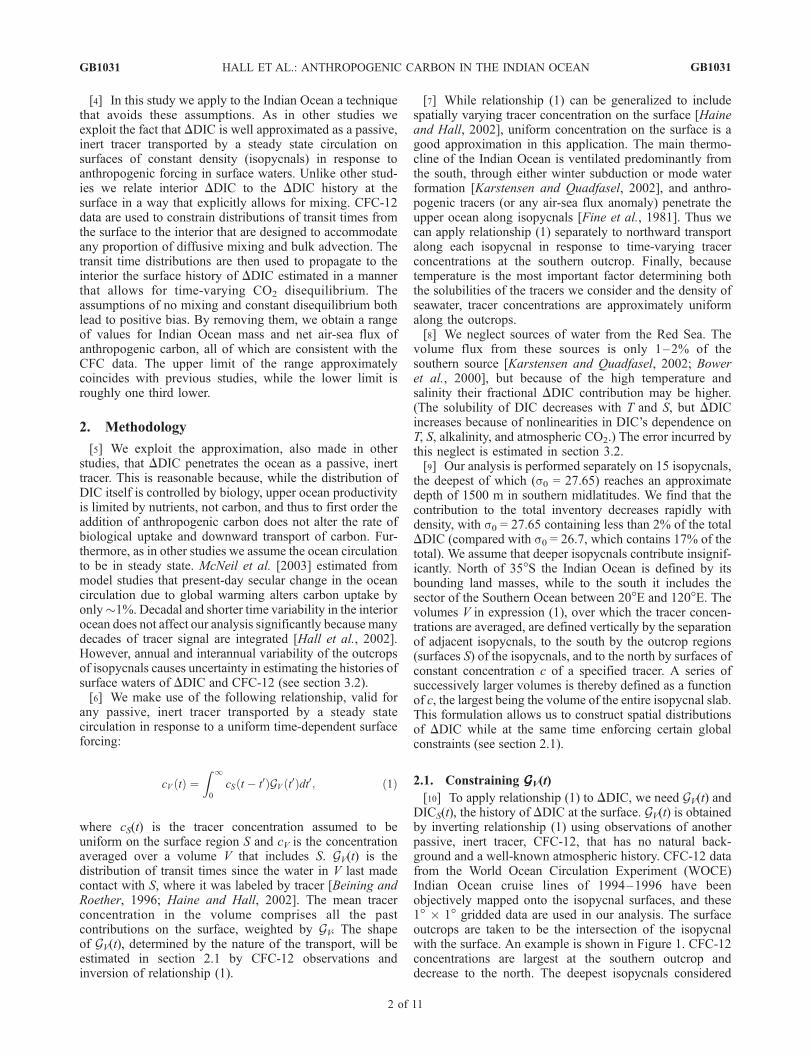
[10] To apply relationship (1) to DDIC, we need GV(t) andDICS(t), the history of DDIC at the surface. GV(t) is obtainedby inverting relationship (1) using observations of anotherpassive, inert tracer, CFC-12, that has no natural back-ground and a well-known atmospheric history. CFC-12 datafrom the World Ocean Circulation Experiment (WOCE)Indian Ocean cruise lines of 1994–1996 have beenobjectively mapped onto the isopycnal surfaces, and these1� 1� gridded data are used in our analysis. The surfaceoutcrops are taken to be the intersection of the isopycnalwith the surface. An example is shown in Figure 1. CFC-12concentrations are largest at the southern outcrop anddecrease to the north. The deepest isopycnals considered

GB1031 HALL ET AL.: ANTHROPOGENIC CARBON IN THE INDIAN OCEAN

2 of 11

GB1031

have negligible CFC-12 through much of the northernIndian Ocean. To obtain the surface history at the outcrops,CFC-12S(t), we use the atmospheric history [Walker et al.,2000] scaled to match the observed 1995 outcrop CFC-12concentrations. In this way the degree of saturation at theoutcrop is approximately included in CFC-12S(t). However,there is considerable uncertainty in CFC-12S(t), as theoutcrop location and CFC-12 saturation vary seasonally andthe observations are generally not taken at the time ofsubduction.[11] We apply expression (1) to CFC-12 and invert

parametrically for GV(t). The following functional form oftwo parameters is assumed:

GV tð Þ ¼ 1ffiffiffiffiffiffiffiffiffiffiffiffiffiffipPet2t

p e�Pet=4t � e�Pe t�tð Þ2=4tt� �

þ 1

2terf

ffiffiffiffiffiffiffiPet

4t

r !þ erf

ffiffiffiffiffiffiffiPe

4tt

rt� tð Þ

!" #; ð2Þ

where t is a timescale equal to twice the mean transit time(‘‘mean age’’) of all the fluid elements in V and Pe = UL/k isthe Peclet number, given a characteristic velocity scale U,length scale L, and diffusivity k. Large Pe corresponds toweak mixing. We discuss and illustrate this functional formin Appendix A.[12] A range of transport scenarios, from no mixing and

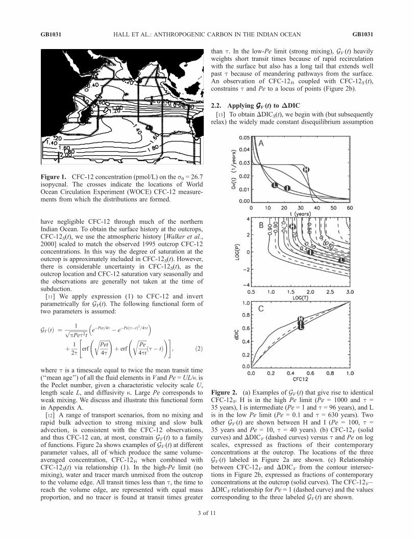
rapid bulk advection to strong mixing and slow bulkadvection, is consistent with the CFC-12 observations,and thus CFC-12 can, at most, constrain GV (t) to a familyof functions. Figure 2a shows examples of GV (t) at differentparameter values, all of which produce the same volume-averaged concentration, CFC-12V, when combined withCFC-12S(t) via relationship (1). In the high-Pe limit (nomixing), water and tracer march unmixed from the outcropto the volume edge. All transit times less than t, the time toreach the volume edge, are represented with equal massproportion, and no tracer is found at transit times greater

than t. In the low-Pe limit (strong mixing), GV (t) heavilyweights short transit times because of rapid recirculationwith the surface but also has a long tail that extends wellpast t because of meandering pathways from the surface.An observation of CFC-12V, coupled with CFC-12S (t),constrains t and Pe to a locus of points (Figure 2b).

2.2. Applying GGGGGGGGGV (t) to #DIC

[13] To obtain DDICS(t), we begin with (but subsequentlyrelax) the widely made constant disequilibrium assumption

Figure 1. CFC-12 concentration (pmol/L) on the s0 = 26.7isopycnal. The crosses indicate the locations of WorldOcean Circulation Experiment (WOCE) CFC-12 measure-ments from which the distributions are formed.

Figure 2. (a) Examples of GV (t) that give rise to identicalCFC-12V. H is in the high Pe limit (Pe = 1000 and t =35 years), I is intermediate (Pe = 1 and t = 96 years), and Lis in the low Pe limit (Pe = 0.1 and t = 630 years). Twoother GV (t) are shown between H and I (Pe = 100, t =35 years and Pe = 10, t = 40 years). (b) CFC-12V (solidcurves) and DDICV (dashed curves) versus t and Pe on logscales, expressed as fractions of their contemporaryconcentrations at the outcrop. The locations of the threeGV (t) labeled in Figure 2a are shown. (c) Relationshipbetween CFC-12V and DDICV from the contour intersec-tions in Figure 2b, expressed as fractions of contemporaryconcentrations at the outcrop (solid curves). The CFC-12V–DDICV relationship for Pe = 1 (dashed curve) and the valuescorresponding to the three labeled GV (t) are shown.

GB1031 HALL ET AL.: ANTHROPOGENIC CARBON IN THE INDIAN OCEAN

3 of 11

GB1031

that anthropogenic CO2 in the atmosphere (DCO2(t)) andDDICS(t) evolve in lockstep, so that one may be obtainedfrom the other using equilibrium carbon chemistry. Inmaking the constant disequilibrium assumption, it isrecognized that locally, CO2 across the air-sea interface isnot in chemical equilibrium, but it is assumed that thedegree of disequilibrium has not changed significantly sincepreindustrial times. Following Thomas et al. [2001], weform the difference time series DDIC(t) = DIC(t) �DIC(1780), where the year 1780 is selected as the start ofthe industrial era. (This definition is chosen for consistencywith other studies. In 1780 ice core records indicate thatatmospheric CO2 concentrations were about 280 ppm (E. M.Etheridge et al., Historical CO2 records from the Law DomeDE08, DE08-2, and DSS ice cores, in Trends: ACompendium of Data on Global Change, online databaseavailable at http://cdiac.ornl.gov/trends/trends.htm), whichis the preindustrial level assumed by Sabine et al. [1999]and others. Estimates of instantaneous air-sea fluxes are notaffected by the choice of preindustrial level.) The‘‘disequilibrium term,’’ assumed to be constant, is presentin both terms of the difference and thus cancels, leavingonly the equilibrium terms. We can therefore solve the well-documented equilibrium inorganic chemistry system [e.g.,Lewis and Wallace, 1988] to compute DDICS(t), givenobservations of temperature, salinity, alkalinity, and atmo-spheric DCO2(t). In these calculations we use the carbonatedissociation coefficients of Goyet and Poisson [1989]. Useof other published coefficients makes a negligible differencein our estimates.[14] The DDICS(t) is convolved with GV (t) for a range of

t and Pe, resulting in contours of volume-averagedconcentration, DDICV (Figure 2b). The intersection ofDDICV contours by a particular CFC-12V contour is theconstraint that the CFC-12V observation imposes on DDICV.Note that the chosen ranges of t and Pe are large enoughthat the CFC-12Vand DDICV contours are parallel in the lowand high limits. Any additional range of parameters resultsin no additional change in DDICV for a given CFC-12V. Theminimum (strong mixing) to maximum (no mixing) rangeof DDICV as a function of CFC-12V obtained from thecontour intersections is shown in Figure 2c. The tracer

concentrations are expressed as fractions of their contem-porary outcrop values, which renders the CFC-12-DDICrelationship independent of the isopycnal.[15] Because we assume steady state circulation, GV (t

0) inequation (1) depends on transit time t0 but not on calendardate t. Therefore, once GV (t

0) is constrained, it can beapplied to DDIC, via equation (1), at any t. In this way, ateach calendar year t we compute for each isopycnal s, themass DMDIC

s = Vs(DDICVs), where Vs is the volume of the

entire isopycnal slab. Summing over all isopycnals, we thenhave the history over the industrial era of anthropogeniccarbon mass, DMDIC(t), in the Indian Ocean, as well as thenet air-sea flux, DFDIC(t) = dDMDIC/dt, into the IndianOcean, at constant equilibrium (Figure 3).

2.3. Time-Varying CO2 Disequilibrium

[16] The assumption of constant disequilibrium is errone-ous. If the ocean were, on average, in equilibrium with theatmosphere in the preindustrial era but is now taking upsome fraction of anthropogenic carbon, then the meandisequilibrium must have changed. It is the disequilibrium,the difference in CO2 across the air-sea interface, that drivesthe net air-sea flux. The anthropogenic component of theflux into isopycnal s is

DFsDIC tð Þ ¼ k½DCO2 tð Þ � aDDICS tð Þ ; ð3Þ

where a is the equilibrium chemistry factor (dependent ontemperature, salinity, and alkalinity) that converts DICS tothe atmospheric CO2 with which it would be in equilibriumand k is the transfer coefficient, dependent on solubility andwind speed. If the disequilibrium has remained constantsince the preindustrial era, then DCO2(t) � aDDICS (t) = 0and DFDIC

s (t) = 0, inconsistent with the nonzero fluxcomputed by assuming constant disequilibrium in the CFC-12 method (Figure 3).[17] In order to resolve this inconsistency, we must

modify DDICS(t) and DFDICs (t) until they satisfy both

equation (3) and our relationship between DDICS (t) andDFDIC

s (t) via the CFC-12-constrained GV (t). That is, on eachisopycnal s we have two unknowns, DDICS(t) and

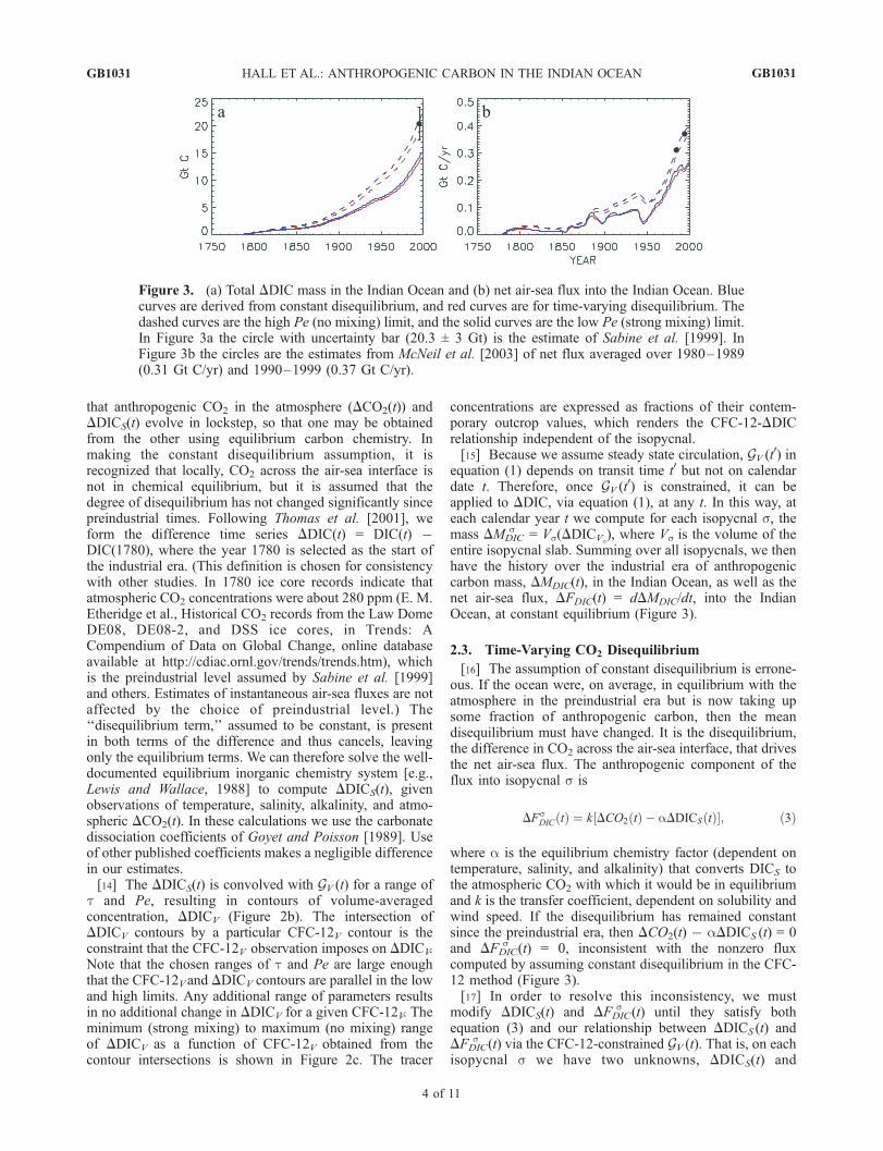
Figure 3. (a) Total DDIC mass in the Indian Ocean and (b) net air-sea flux into the Indian Ocean. Bluecurves are derived from constant disequilibrium, and red curves are for time-varying disequilibrium. Thedashed curves are the high Pe (no mixing) limit, and the solid curves are the low Pe (strong mixing) limit.In Figure 3a the circle with uncertainty bar (20.3 ± 3 Gt) is the estimate of Sabine et al. [1999]. InFigure 3b the circles are the estimates from McNeil et al. [2003] of net flux averaged over 1980–1989(0.31 Gt C/yr) and 1990–1999 (0.37 Gt C/yr).

GB1031 HALL ET AL.: ANTHROPOGENIC CARBON IN THE INDIAN OCEAN

4 of 11

GB1031

DFDICs(t), for which we solve simultaneously using

expression (3) and

DFsDIC tð Þ ¼ d

dtVs

Z 1

0

DDICS t � t0ð ÞGV t0ð Þdt0 �

; ð4Þ

the expression for the flux as the time rate of change of themass obtained from DDICS (t) via the CFC-12-constrainedGV (t). Equating equations (3) and (4) is the statement that theflux into the isopycnal slab must equal the mass rate ofchange within the slab and provides an integral equation forDDICS (t), which can be solved iteratively using the constantdisequilibrium history as the first guess. Once DDICS (t) isobtained, DFDIC (t) can be computed from equation (4).[18] In this solution we use values for the transfer

coefficient k estimated by Carr et al. [2002], who employedthe Wanninkhof [1992] wind speed parameterization andwind speeds from both Special Sensor Microwave Imager(SSM/I) and QuickSCAT scatterometer data. In addition, werequire the areas A of the outcrop regions, which we take toequal the areas between surface CFC-12 contours at thesouthern extremities of adjacent isopycnals. Importantly,our mass and net air-sea flux estimates are relativelyinsensitive to the large uncertainty in k and A because thecorrection due to the relaxation of constant disequilibrium,shown in section 3, is small. For example, ±50% uncertaintyin k causes approximately ±5% uncertainty in DDIC massand flux. The uncertainty in k impacts the magnitude of afirst-order correction but not the zeroth-order estimate.

2.4. Computing Spatial Distributions

[19] In the calculation as described so far, V is equal to theentire volume of an isopycnal slab, from the southernoutcrop to the northern continental boundary, and theresulting mass is the total anthropogenic carbon mass in theslab. However, to compute spatial DDIC distributions, weestimate averaged concentrations DDICV over a series ofvolumes V defined to the north by successively decreasingCFC-12 concentration contours. This formulation allowsus to construct the spatial distributions while at the sametime enforcing certain global constraints. If DMDIC

s (V) =V(DDICV) is the anthropogenic carbon mass in volume V ofan isopycnal slab s and DMDIC

s (V + dV) is the mass involume V + dV, then the mean concentration along thevolume tube dV parallel to the CFC-12 contour is

DDIC Vð Þ ¼ DMsDIC V þ dVð Þ � DMs

DIC Vð ÞdV

� dDMsDIC Vð ÞdV

: ð5Þ

We then transform from V coordinates to ‘‘CFC-12equivalent latitude,’’ the latitude that encompasses the samevolume as the CFC-12 contour defining V. Because CFC-12contours are oriented approximately zonally, the CFC-12equivalent latitude is similar to true latitude.[20] In this manner we can form maps of the inferred

DDIC that approximate zonally averaged latitude-depthdistributions. We can also plot the inferred DDIC on eachisopycnal versus longitude and latitude. Because we com-pute mean concentrations of DDIC (minimum to maximum)on CFC contours, the resulting DDIC contours on an

isopycnal are, by definition, parallel to the CFC-12 con-tours. Components of the DDIC distribution perpendicularto CFC-12 are unavailable from CFC-12 data alone. How-ever, contours of column DDIC, formed from verticalintegration over the isopycnals, are not necessarily parallelto contours of column CFC-12. The CFC-12 contourorientations vary with isopycnal, and the fractional contri-bution of an isopycnal to DDIC column values is notgenerally the same as its fractional contribution to CFC-12 column values.[21] The approach of estimating volume-averaged DDIC

is a modification of the technique described by Hall et al.[2002], who used tracer data to constrain the distributions oftransit times G(r, t) from the surface to particular locations r.We could follow that approach here to obtain point-wiseestimates of DDIC and then integrate spatially to arrive attotal mass. However, such a procedure does not takeadvantage of a global constraint on GV(t) (the spatial integralof G(r, t)), namely, that GV(t) is a monotonically decreasingfunction of t when V represents the entire closed domain ofthe isopycnal slab. In the approach employed here, thisconstraint is enforced because the functional form for GV(t)is monotonically decreasing. Thus in cases such as theIndian Ocean where we have tracer data covering the entiredomain, we use the approach developed here, while in caseswhere we analyze spatially limited data removed from thesurface source, we use the Hall et al. [2002] approach.

3. Results

3.1. Inventory and Uptake

[22] We now apply this technique to compute the totalmass, net air-sea flux, and spatial distribution of anthropo-genic carbon in the Indian Ocean. To the degree thetransport is in steady state, the constraint on DDIC imposedby 1995 CFC-12 observations applies over the entireindustrial era. We find that the mass of anthropogeniccarbon and its net air-sea flux have risen nearly steadilyin the industrial era (Figure 3). In the year 2000 we estimatethat the DDIC mass was 14.3–20.5 Gt and the net air-seaflux was 0.26–0.36 Gt/yr. The ranges are a result of theimperfect constraint CFC-12 imposes on DDIC in thepresence of mixing because of the tracers’ different histo-ries. They do not represent statistical uncertainty, and nointermediate ‘‘best estimate’’ is available.[23] Allowing for mixing significantly reduces the esti-

mate of mass and net air-sea flux of anthropogenic carbon.For the Indian Ocean in 2000 the strong-mixing limitis lower than the no-mixing limit by 6.2 Gt in mass and0.12 Gt/yr in net air-sea flux, reductions of 30% atconstant disequilibrium. The effect of mixing can be under-stood by examining the analyses that have neglected it.Typically, a tracer ‘‘age’’ is defined as the time since theobserved concentration of a tracer at an interior locationwas last exhibited at the surface. For example, CFC-12(t) =CFC-12S(t � TCFC), defining the CFC-12 age TCFC. Thetracer age is then applied to the surface history ofanthropogenic carbon to estimate the concentration ofDDIC at the location: DDIC(t) = DDICS(t � TCFC). In theabsence of mixing this is valid because there is a uniquetransit time from the surface source region to the interior

GB1031 HALL ET AL.: ANTHROPOGENIC CARBON IN THE INDIAN OCEAN

5 of 11

GB1031

location and the age of any tracer equals this transit time. Inthe presence of mixing, however, there is a wide distributionof transit times since water at the interior location was lastat the surface and the tracer age is an average over thedistribution, weighted by the tracer’s history [Waugh etal., 2003]. The age of a tracer such as CFC-12, whosehistory is shorter and more nonlinear than DDIC, preferen-tially weights young components of the transit timedistribution. The DDIC surface history is evaluated at toorecent a date, and the interior DDIC concentration isoverestimated. This bias is discussed in DDIC studies usingtracer ages [e.g., Gruber et al., 1996], and its impact isexamined in analyses of model data [Hall et al., 2002;Matear et al., 2003].[24] The no-mixing values are upper bounds on the mass

and net air-sea flux of anthropogenic carbon (Figure 3), butusing CFC-12 alone, they are not ruled out. The simulta-neous use of another tracer with a sufficiently distincthistory imposes additional, independent constraints onGV (t) and narrows the range of DDIC mass and net air-sea flux. Unfortunately, given uncertainties in the construc-tion of inventories from sparse data, CFC-11 and CFC-12are too similar to provide independent constraints on totalDDIC mass and net air-sea flux, while the peak in bombtritium history is too broad and weak in the SouthernHemisphere for its attenuation to offer much additionalconstraint.[25] However, if one restricts attention to diagnosing

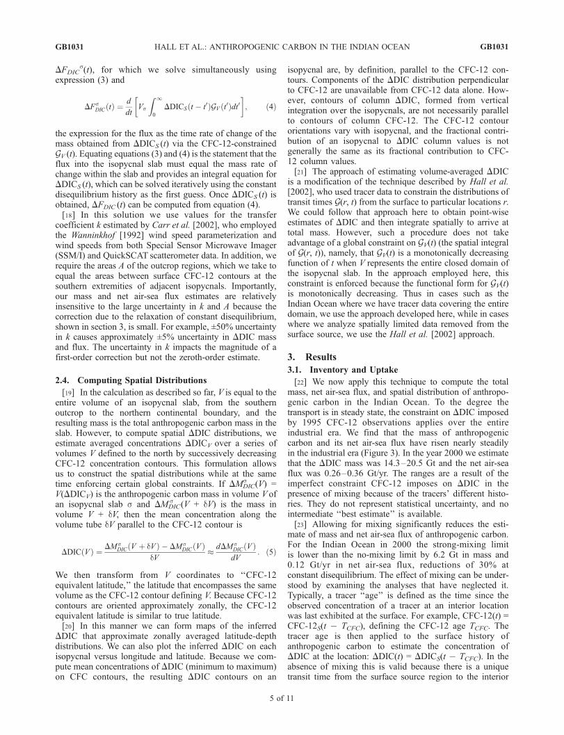
transport to locations of observation, rather than over theentire Indian Ocean domain, then formation of inventoriesis unnecessary and CFC-11 and CFC-12 data can be beused constructively in combination [Waugh et al., 2003].Figure 4 shows a scatterplot of the difference of CFC-11and CFC-12 concentration ages, t11 � t12, versus theCFC-12 concentration age, t12, for all data along the IndianOcean WOCE line IO3, a longitudinal transect at 20�S. Iftransport from the surface to the points along the transectwere purely bulk advective, then t11 would equal t12everywhere and the observations in Figure 4 would fallalong the zero line. This is clearly not the case. Mixing mustplay a role in the transport.[26] To quantify the role of mixing, we follow Waugh et

al. [2003] and use the two-parameter ‘‘inverse Gaussian’’(IG) form for G(t) (as opposed to GV (t)) to model the IO3CFC-11 and CFC-12 data. Surface time histories wereconstructed from the observed T and S, the solubilityfunctions of Warner and Weiss [1985], and the atmospherichistories of Walker et al. [2000]. (In this case, rather thanscaling the CFC histories by objectively mapped outcropconcentrations as was done for the inventory and uptakecalculations, we simply assume the saturations to be 100%.)The surface histories are convolved with the IG G(t), whoseparameters are selected such that the modeled t12 matchesthe observed t12 and Pe is constant along the transect. Thecurves in Figure 4 correspond to different assumed values ofPe. In the limit of high Pe (no mixing) the modeled CFC-11-CFC-12 relationship collapses to the zero line. Bycontrast, the curves for Pe � 10 match the observed CFC-11-CFC-12 relationship in detail, with the best fits occurringfor Pe � 1. (Curves with Pe � 1 fall too close together to be

distinguished by the data.) Analysis of other WOCE IndianOcean transects reveal similar behavior.[27] Although we have not directly used CFC-11 and

CFC-12 in combination to constrain DDIC inventory anduptake, the behavior shown in Figure 4 strongly suggests thatIndian Ocean transport is well outside the no-mixing, bulkadvective limit. As shown in Figure 3c, Pe � 1 places thedomain mean DDIC concentration in the lower half of therange determined from CFC-12 alone. This is in agreementwith the analysis of CFCs and tritium in combination in thesubpolar North Atlantic Ocean by Waugh et al. (D. W.Waugh et al., Transport times and anthropogenic carbon inthe subpolar North Atlantic Ocean, submitted to Deep-SeaResearch, 2003, hereinafter referred to as Waugh et al.,submitted manuscript, 2003), who obtained transit timedistributions in the strong-mixing limit and, consequently,DDIC concentrations significantly lower than estimatesfrom studies making the no-mixing assumption.[28] Permitting variable disequilibrium further reduces the

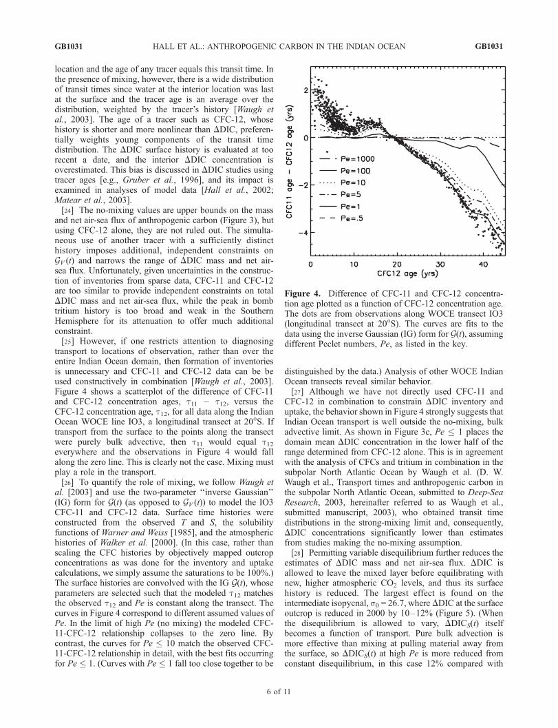
estimates of DDIC mass and net air-sea flux. DDIC isallowed to leave the mixed layer before equilibrating withnew, higher atmospheric CO2 levels, and thus its surfacehistory is reduced. The largest effect is found on theintermediate isopycnal, s0 = 26.7, where DDIC at the surfaceoutcrop is reduced in 2000 by 10–12% (Figure 5). (Whenthe disequilibrium is allowed to vary, DDICS(t) itselfbecomes a function of transport. Pure bulk advection ismore effective than mixing at pulling material away fromthe surface, so DDICS(t) at high Pe is more reduced fromconstant disequilibrium, in this case 12% compared with

Figure 4. Difference of CFC-11 and CFC-12 concentra-tion age plotted as a function of CFC-12 concentration age.The dots are from observations along WOCE transect IO3(longitudinal transect at 20�S). The curves are fits to thedata using the inverse Gaussian (IG) form for G(t), assumingdifferent Peclet numbers, Pe, as listed in the key.

GB1031 HALL ET AL.: ANTHROPOGENIC CARBON IN THE INDIAN OCEAN

6 of 11

GB1031

10%.) The reduced surface history is transported to theinterior, resulting in lower DDIC mass. Providing for time-dependent disequilibrium reduces the estimate of IndianOcean DDIC mass in 2000 by 0.9 Gt for strong mixing andby 1.8 Gt for no mixing, fractional reductions of 5–10%compared with the no-mixing, constant disequilibriumresult (Figure 3). The fractional reductions in net air-seaflux are similar.

3.2. Uncertainties

[29] There are several sources of uncertainty in ouranalysis. A first source comes from the objective mappingof CFC-12 from sparse cruise lines to gridded values onisopycnals. (CFC-12 measurement uncertainty itself is neg-ligible.) This mapping introduces uncertainty in the CFC-12isopycnal mean concentrations, which propagates nearlydirectly to uncertainty in inferred DDIC. This can be seensimply by mapping an uncertainty range of CFC-12V on thex axis of Figure 2c to a range of DDICV on the y axis. Theobjective mapping routine applied to the CFC-12 dataprovides an uncertainty for the CFC-12 inventory on eachisopycnal surface. These uncertainties varied from 7% to16%, with a value of 14% for s0 = 26.7, the surface havingthe largest CFC-12 and DDIC inventories.[30] A second source of error comes from our neglect of

Red Sea (RS) sources of tracer into the Indian Oceanthermocline. In order to put an upper bound on the DDICfrom these sources, we first note that You and Tomczak[1993] estimate �2% of the Indian Ocean thermocline tohave RS origin. The fractional contribution to the DDICinventory may be higher because the DDIC contributionincreases with T and S. To estimate the maximum possibleRS DDIC contribution, we make the unrealistic assumptionthat RS water spreads instantaneously throughout thethermocline so that all RS water carries the most recent(and highest) possible DDIC mole fraction. For T = 27� and

S = 40 typical of the RS, this is DDIC(2000) = 66 mmol/kg.Thus the upper bound on the RS contribution to theinventory is 0.02 66(V) = 0.9 Gt, where V = 5.3 107 km3 is the Indian Ocean thermocline volume computedfrom the objectively mapped isopycnic depth fields. Thismass represents 4–6% of our range on Indian Ocean DDICinventory.[31] In reality, the RS contribution will be significantly

smaller than the 0.9 Gt upper bound. First, the RS sourcetakes a finite time to propagate through the thermocline, somuch of its water mass is aged and carries an older, lowerDDIC signal. Second, there is a partially compensating errordue to the neglect of RS sources of CFC-12. We haveassumed that the entire CFC-12 inventory originates in thesouth and have therefore overestimated the role ofthe southern CFC-12 source. This causes our estimate ofthe transit time distribution (TTD) from southern sources tobe biased young, which in turn causes an overestimate ofthe southern DDIC source. This overestimate is of the sameorder as the underestimate due to direct neglect of the RSDDIC source, so there is a tendency for these errors tocancel.[32] While the RS source is only a small contributor to the

total Indian Ocean inventory, it is a significant contributorlocally in the Arabian Sea. Therefore our neglect of an RSsource causes our inferred DDIC distributions in the Ara-bian Sea to be biased low, possibly by one third (a 5% totalinventory error confined to 15% of the total volume).[33] A third source of uncertainty arises from the imper-

fectly known CFC-12 histories at the southern outcrops. Wehave used the objectively mapped 1995 observations at theoutcrops to scale the atmospheric CFC-12 history of Walkeret al. [2000], which provides a boundary condition thatimplicitly includes CFC-12 disequilibrium. However, theobjective mapping is least accurate in the Southern Ocean,where the observations are most scarce. Moreover, themeasurements are not generally made during the season ofsubduction. To make a rough estimate of the impact onDDIC of these uncertainties, we repeated the calculationsusing an equilibrium solubility calculation (100% satura-tion) for the CFC-12 outcrop histories, given the observed Tand S. This results in a change to the 1995 DDIC inventoryof �1.7 Gt, or 13% to 9% (strong-mixing to no-mixinglimits).[34] A fourth source of uncertainty arises from the

selection of a particular functional form for the TTD. Thisuncertainty is very difficult to quantify. However, becausethe IG form used here can closely mimic TTDs simulateddirectly in numerical models (Appendix A), we think thatits selection incurs an error that is small compared withother sources of uncertainty. In any case the IG form is astep beyond the assumption of no mixing that is implicit inprevious studies that use tracer ages to lag DDIC timeseries.[35] Finally, all techniques to estimate anthropogenic car-

bon concentrations in the ocean assume that DDIC propa-gates as a passive, inert tracer in a steady state circulation.This assumption causes error in DDIC inference to the extentthat ocean biota are evolving in response to increased carbonlevels and ocean circulation is evolving in response to global

Figure 5. Time series of DDIC surface concentration onthe s0 = 26.6 isopycnal assuming constant disequilibrium(dashed curve) and allowing time-varying disequilibrium inthe no-mixing (lower solid curve) and strong-mixing(higher solid curve) limits.

GB1031 HALL ET AL.: ANTHROPOGENIC CARBON IN THE INDIAN OCEAN

7 of 11

GB1031

warming. At present, these effects are likely small comparedwith other uncertainties, but their importance will grow in thefuture [e.g., Sarmiento et al., 1998].

3.3. Comparison With Other Estimates

[36] The upper bounds of our estimated ranges of anthro-pogenic carbon mass in the Indian Ocean and its net air-seaflux just encompass those of other studies, while the lowerbounds are significantly lower than other studies (Figure 3)because of the relaxation of the widely made assumptions ofno mixing and constant disequilibrium, which cause posi-tive bias. Sabine et al. [1999] estimated a 1995 mass of20.3 ± 3 Gt C, compared with our 13.1–18.8 Gt C. Thecentral value of their range falls very close to our 1995 no-mixing, constant disequilibrium curve, consistent withexpectation, as the Gruber et al. [1996] technique used bySabine et al. [1999] makes these approximations. (Gruber etal. [1996] make the no-mixing assumption by using tracerages to estimate disequilibrium terms, which are assumed tobe constant. They reduce sensitivity to the no-mixingassumption by restricting application to waters with tracerages less than a threshold.) McNeil et al. [2003], who alsomake these approximations by applying CFC-12 agesdirectly to DDIC surface history, assuming constantdisequilibrium, estimated a net air-sea flux into the IndianOcean averaged over the interval 1980–1989 of 0.31 Gt C/yrand over the interval 1990–1999 of 0.37 Gt C/yr, comparedwith our ranges of 0.22–0.28 Gt C/yr and 0.24–0.34 Gt C/yr,respectively. Their estimates also fall on our constantdisequilibrium, no-mixing curve.[37] Our bounds on the spatial distribution of DDIC

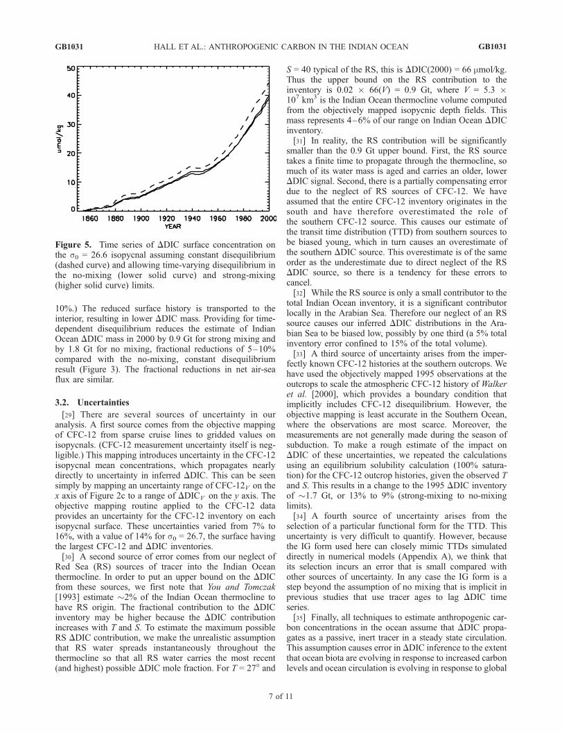
concentration are shown in Figure 6. DDIC penetrates mostdeeply in southern midlatitudes, the zone of subtropical

convergence, while below 800 m in the northern IndianOcean, there is little DDIC. This latitude-depth distributionis qualitatively similar to distributions of Sabine and Feely[2001], who compared the techniques of Gruber et al.[1996] and Chen and Millero [1979], although there arenumerous differences in detail. Our latitude-longitudedistribution of column inventories has an upper bound (nomixing) that peaks in southern midlatitudes at �40 mol/m2

and decreases to �15 mol/m2 in the Bay of Bengal. This issimilar in shape to but slightly lower in magnitude than thecolumn distribution estimated by Sabine and Feely [2001]using the Gruber et al. [1996] method. Our lower bound(strong mixing) is lower still, ranging from �30 mol/m2 tobelow 10 mol/m2. The Sabine and Feely [2001] distributionusing the Chen and Millero [1979] method has asignificantly stronger latitudinal gradient, ranging fromabove 55 mol/m2 to below 10 mol/m2.[38] A comparison of the mean vertical DDIC concentra-

tion profile estimated by Sabine et al. [1999] with ourinferred range is shown in Figure 7. Sabine et al. [1999]used the inference method of Gruber et al. [1996]. In thismethod, on isopycnals that are believed to be everywherecontaminated by anthropogenic carbon, tracer ages (e.g.,CFC ages) are used to estimate the DDIC air-seadisequilibrium, which amounts to a neglect of mixing.The disequilibrium is overestimated, leading to an under-estimate of the preindustrial background and, consequently,an overestimate of the anthropogenic component of totalobserved DIC (see Hall et al. [2002] for a more detaileddiscussion of this bias). In addition, the disequilibrium isassumed to be constant in time. Thus we expect the Sabineet al. [1999] DDIC profile to exhibit a high bias in shallowregions. On the other hand, for deeper isopycnals that arebelieved to have regions old enough to be uncontaminated

Figure 6. Ranges of the spatial distribution of DDIC. (a) Minimum and (b) maximum DDIC (mmol/kg)versus equivalent latitude and depth. (c) Minimum and (d) maximum column DDIC (mol/m2) versuslongitude and latitude.

GB1031 HALL ET AL.: ANTHROPOGENIC CARBON IN THE INDIAN OCEAN

8 of 11

GB1031

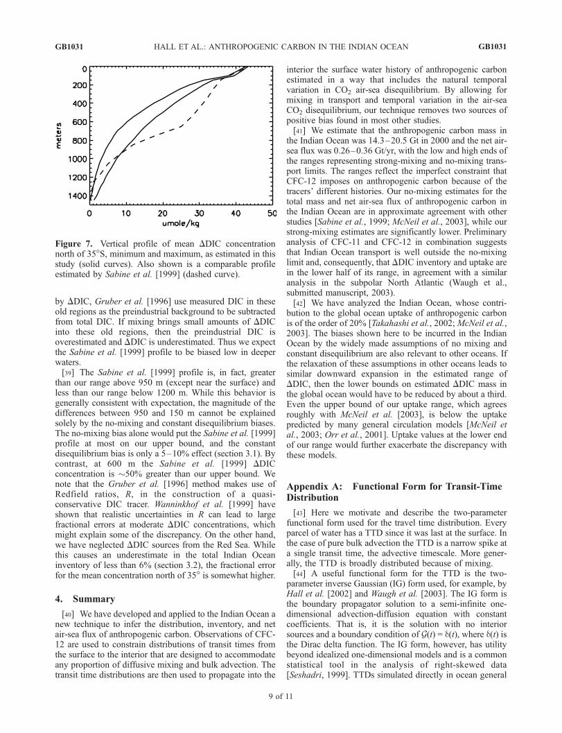
by DDIC, Gruber et al. [1996] use measured DIC in theseold regions as the preindustrial background to be subtractedfrom total DIC. If mixing brings small amounts of DDICinto these old regions, then the preindustrial DIC isoverestimated and DDIC is underestimated. Thus we expectthe Sabine et al. [1999] profile to be biased low in deeperwaters.[39] The Sabine et al. [1999] profile is, in fact, greater

than our range above 950 m (except near the surface) andless than our range below 1200 m. While this behavior isgenerally consistent with expectation, the magnitude of thedifferences between 950 and 150 m cannot be explainedsolely by the no-mixing and constant disequilibrium biases.The no-mixing bias alone would put the Sabine et al. [1999]profile at most on our upper bound, and the constantdisequilibrium bias is only a 5–10% effect (section 3.1). Bycontrast, at 600 m the Sabine et al. [1999] DDICconcentration is �50% greater than our upper bound. Wenote that the Gruber et al. [1996] method makes use ofRedfield ratios, R, in the construction of a quasi-conservative DIC tracer. Wanninkhof et al. [1999] haveshown that realistic uncertainties in R can lead to largefractional errors at moderate DDIC concentrations, whichmight explain some of the discrepancy. On the other hand,we have neglected DDIC sources from the Red Sea. Whilethis causes an underestimate in the total Indian Oceaninventory of less than 6% (section 3.2), the fractional errorfor the mean concentration north of 35� is somewhat higher.

4. Summary

[40] We have developed and applied to the Indian Ocean anew technique to infer the distribution, inventory, and netair-sea flux of anthropogenic carbon. Observations of CFC-12 are used to constrain distributions of transit times fromthe surface to the interior that are designed to accommodateany proportion of diffusive mixing and bulk advection. Thetransit time distributions are then used to propagate into the

interior the surface water history of anthropogenic carbonestimated in a way that includes the natural temporalvariation in CO2 air-sea disequilibrium. By allowing formixing in transport and temporal variation in the air-seaCO2 disequilibrium, our technique removes two sources ofpositive bias found in most other studies.[41] We estimate that the anthropogenic carbon mass in

the Indian Ocean was 14.3–20.5 Gt in 2000 and the net air-sea flux was 0.26–0.36 Gt/yr, with the low and high ends ofthe ranges representing strong-mixing and no-mixing trans-port limits. The ranges reflect the imperfect constraint thatCFC-12 imposes on anthropogenic carbon because of thetracers’ different histories. Our no-mixing estimates for thetotal mass and net air-sea flux of anthropogenic carbon inthe Indian Ocean are in approximate agreement with otherstudies [Sabine et al., 1999; McNeil et al., 2003], while ourstrong-mixing estimates are significantly lower. Preliminaryanalysis of CFC-11 and CFC-12 in combination suggeststhat Indian Ocean transport is well outside the no-mixinglimit and, consequently, that DDIC inventory and uptake arein the lower half of its range, in agreement with a similaranalysis in the subpolar North Atlantic (Waugh et al.,submitted manuscript, 2003).[42] We have analyzed the Indian Ocean, whose contri-

bution to the global ocean uptake of anthropogenic carbonis of the order of 20% [Takahashi et al., 2002; McNeil et al.,2003]. The biases shown here to be incurred in the IndianOcean by the widely made assumptions of no mixing andconstant disequilibrium are also relevant to other oceans. Ifthe relaxation of these assumptions in other oceans leads tosimilar downward expansion in the estimated range ofDDIC, then the lower bounds on estimated DDIC mass inthe global ocean would have to be reduced by about a third.Even the upper bound of our uptake range, which agreesroughly with McNeil et al. [2003], is below the uptakepredicted by many general circulation models [McNeil etal., 2003; Orr et al., 2001]. Uptake values at the lower endof our range would further exacerbate the discrepancy withthese models.

Appendix A: Functional Form for Transit-TimeDistribution

[43] Here we motivate and describe the two-parameterfunctional form used for the travel time distribution. Everyparcel of water has a TTD since it was last at the surface. Inthe case of pure bulk advection the TTD is a narrow spike ata single transit time, the advective timescale. More gener-ally, the TTD is broadly distributed because of mixing.[44] A useful functional form for the TTD is the two-

parameter inverse Gaussian (IG) form used, for example, byHall et al. [2002] and Waugh et al. [2003]. The IG form isthe boundary propagator solution to a semi-infinite one-dimensional advection-diffusion equation with constantcoefficients. That is, it is the solution with no interiorsources and a boundary condition of G(t) = d(t), where d(t) isthe Dirac delta function. The IG form, however, has utilitybeyond idealized one-dimensional models and is a commonstatistical tool in the analysis of right-skewed data[Seshadri, 1999]. TTDs simulated directly in ocean general

Figure 7. Vertical profile of mean DDIC concentrationnorth of 35�S, minimum and maximum, as estimated in thisstudy (solid curves). Also shown is a comparable profileestimated by Sabine et al. [1999] (dashed curve).

GB1031 HALL ET AL.: ANTHROPOGENIC CARBON IN THE INDIAN OCEAN

9 of 11

GB1031

circulation models generally have early peaks, representingadvective transport along some dominant pathway, andlong tails, due to along flow and lateral mixing [e.g.,Khatiwala et al., 2001; Haine and Hall, 2002; F. Primeau,Characterizing transport between the surface mixed layerand the ocean interior with a forward and adjoint globalocean transport model, submitted to Journal of PhysicalOceanography, 2003]. While the circulation is complex andtwo- or three-dimensional, the TTD can often (but notalways) be well fit by the IG form.[45] In this study we want to parameterize the TTD

averaged over a volume that includes, as one boundary,the surface source region. That is, we want to parameterize

GV tð Þ � 1

V

ZV

d3r G r; tð Þ: ðA1Þ

G(t) is the distribution of transit times since water in thevolume V (one boundary of which is the surface sourceregion) made last contact with the surface source region.The IG form for GV(t) is obtained by averaging the IG formover a one-dimensional ‘‘volume’’ extending from theorigin to some position whose value is expressed in terms ofmean transit time. One obtains functional form (2), whoseparameters are t, twice the mean transit time (‘‘mean age’’)of all the fluid elements in V, and Pe, the Peclet number,defined as the ratio of diffusive to advective timescales.[46] While the volume-TTD of real ocean domains may

differ considerably in detail from the IG form, there arecertain general properties of volume-TTD that the IG formcaptures: (1) For a closed domain, GV(t) is a nonincreasingfunction of t [Haine and Hall, 2002], simply the statementthat every parcel at transit time (‘‘age’’) t must have passedthrough every earlier transit time. (2) GV(t) is singular at t = 0[Holzer and Hall, 2000]. (3) The large t limit of GV (t) isexponential decay [Haine and Hall, 2002].[47] To illustrate the utility of the volume-IG form, we

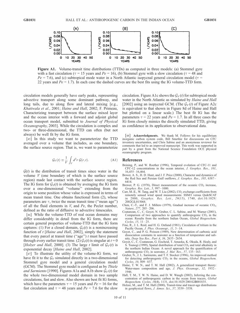
have fit it to the GV simulated directly in a two-dimensionalStommel gyre model and a general circulation model(GCM). The Stommel gyre model is configured as by Thieleand Sarmiento [1990]. Figures A1a and A1b show GV (t) forthe whole two-dimensional model domain in two samplecirculations, fast and slow. Also shown are best fit IG forms,which have the parameters t = 15 years and Pe = 16 for thefast circulation and t = 48 years and Pe = 7.6 for the slow

circulation. Figure A1c shows the GV (t) for subtropical modewater in the North Atlantic as simulated by Haine and Hall[2002] using an isopycnal GCM. (The GV (t) of Figure A2cis equivalent to that shown in Figure 8d of Haine and Hallbut plotted on a linear scale.) The best fit IG has theparameters t = 22 years and Pe = 1.7. In all three cases theIG form closely mimics the directly simulated TTD, givingus confidence in its application to observational data.

[48] Acknowledgments. We thank M. Follows for his equilibriuminorganic carbon system code, Bill Smethie for discussions on CFCinventory uncertainties, and Chris Sabine and an anonymous reviewer forcomments that led to an improved manuscript. This work was supported inpart by a grant from the National Science Foundation OCE physicaloceanography program.

ReferencesBeining, P., and W. Roether (1996), Temporal evolution of CFC-11 andCFC-12 concentrations in the ocean interior, J. Geophys. Res., 101,16,455–16,464.

Bower, A. S., H. D. Hunt, and J. F. Price (2000), Character and dynamics ofthe Red Sea and Persian Gulf outflows, J. Geophys. Res., 105, 6387–6414.

Brewer, P. G. (1978), Direct measurement of the oceanic CO2 increase,Geophys. Res. Lett., 5, 997–1000.

Carr, M.-E., W. Tang, and W. T. Liu (2002), CO2 exchange coefficients fromremotely sensed wind speed measurements: SSM/I versus QuikSCATin 2000, Geophys. Res. Lett., 29(15), 1740, doi:10.1029/2002GL015068.

Chen, C.-T., and F. J. Millero (1979), Gradual increase of oceanic CO2,Nature, 277, 205–206.

Coatanoan, C., C. Goyet, N. Gruber, C. L. Sabine, and M. Warner (2001),Comparison of two approaches to quantify anthropogenic CO2 in theocean: Results from the northern Indian Ocean, Global Biogeochem.Cycles, 15, 11–25.

Fine, R., J. L. Reid, and H. G. Ostlund (1981), Circulation of tritium in thePacific Ocean, J. Phys. Oceanogr., 11, 3–14.

Goyet, C., and P. G. Poisson (1989), New determination of carbonic aciddissociation constants in seawater as a function of temperature and sali-nity, Deep Sea Res., Part A, 36, 2635–2654.

Goyet, C., C. Coatanoan, G. Eischeid, T. Amaoka, K. Okuda, R. Healy, andS. Tsunogi (1999), Spatial distribution of total CO2 and total alkalinity inthe northern Indian Ocean: A novel approach for the quantification ofanthropogenic CO2 in seawater, J. Mar. Res., 57, 135–163.

Gruber, N., J. L. Sarmiento, and T. F. Stocker (1996), An improved methodfor detecting anthropogenic CO2 in the oceans, Global Biogeochem.Cycles, 10, 809–837.

Haine, T. W. N., and T. M. Hall (2002), A generalized transport theory:Water-mass composition and age, J. Phys. Oceanogr., 32, 1932–1946.

Hall, T. M., T. W. N. Haine, and D. W. Waugh (2002), Inferring the con-centration of anthropogenic carbon in the ocean from tracers, GlobalBiogeochem. Cycles, 16(4), 1131, doi:10.1029/2001GB001835.

Holzer, M., and T. M. Hall (2000), Transit-time and tracer-age distributionsin geophysical flows, J. Atmos. Sci., 57, 3539–3558.

Figure A1. Volume-transit time distributions (TTDs) as computed in three models: (a) Stommel gyrewith a fast circulation (t = 15 years and Pe = 16), (b) Stommel gyre with a slow circulation (t = 48 andPe = 7.6), and (c) subtropical mode water in a North Atlantic isopycnal general circulation model (t =22 years and Pe = 1.7). In each case the dashed curves are the best fits using the IG volume-TTD form.

GB1031 HALL ET AL.: ANTHROPOGENIC CARBON IN THE INDIAN OCEAN

10 of 11

GB1031

Jenkins, W. J. (1988), The use of anthropogenic tritium and helium-3 tostudy subtropical gyre ventilation and circulation, Philos. Trans. R. Soc.London, Ser. A, 325, 43–61.

Karstensen, J., and D. Quadfasel (2002), Water subducted into the IndianOcean subtropical gyre, Deep Sea Res., Part II, 49, 1441–1457.

Khatiwala, S., M. Visbeck, and P. Schlosser (2001), Age tracers in an oceanGCM, Deep Sea Res., Part I, 48, 1423–1441.

Lewis, E., and D. W. R. Wallace (1988), Program developed for CO2

system calculations, Rep. ORNL/CDIAC-105, U.S. Dep. of Energy,Oak Ridge Natl. Lab., Carbon Dioxide Inf. Anal. Cent., Oak Ridge, Tenn.

Matear, R. J., C. S. Wong, and L. Xie (2003), Can CFCs be used todetermine anthropogenic CO2?, Global Biogeochem. Cycles, 17(1),1013, doi:10.1029/2001GB001415.

McNeil, B. I., R. J. Matear, R. M. Key, J. L. Bullister, and J. L. Sarmiento(2003), Anthropogenic CO2 uptake by the ocean based on the globalchlorofluorocarbon data set, Science, 299, 235–239.

Orr, J. C., et al. (2001), Estimates of anthropogenic carbon uptake from fourthree-dimensional global ocean models, Global Biogeochem. Cycles, 15,43–60.

Robbins, P. E., J. F. Price, W. B. Owens, and W. J. Jenkins (2000), On theimportance of lateral diffusion for the ventilation of the lower thermoclinein the subtropical North Atlantic, J. Phys. Oceanogr., 30, 67–89.

Sabine, C. L., and R. A. Feely (2001), Comparison of recent Indian Oceananthropogenic CO2 estimates with a historical approach, Global Biogeo-chem. Cycles, 15, 31–42.

Sabine, C. L., R. M. Key, K. M. Johnson, F. J. Millero, A. Poisson, J. L.Sarmiento, D. W. R. Wallace, and C. D. Winn (1999), Anthropogenic CO2

inventory of the Indian Ocean, Global Biogeochem. Cycles, 13, 179–198.Sarmiento, J. L., T. M. C. Hughes, R. J. Stouffer, and S. Manabe (1998),Simulated response of the ocean carbon cycle to anthropogenic climatewarming, Nature, 393, 245–249.

Seshadri, V. (1999), The Inverse Gaussian Distribution: Statistical Theoryand Applications, Springer-Verlag, New York.

Sonnerup, R. E. (2001), On the relations among CFC derived water massages, Geophys. Res. Lett., 28, 1739–1742.

Takahashi, T., et al. (2002), Global air-sea CO2 flux based on climatologicalsurface ocean pCO2 and seasonal biological and temperature effects,Deep Sea Res., Part II, 49, 1601–1622.

Thiele, G., and J. L. Sarmiento (1990), Tracer dating and ocean ventilation,J. Geophys. Res., 95, 9377–9391.

Thomas, H., and V. Ittekkot (2001), Determination of anthropogenic CO2 inthe North Atlantic Ocean using water mass age and CO2 equilibriumchemistry, J. Mar. Syst., 27, 325–336.

Thomas, H., M. H. England, and V. Ittekkot (2001), An off-line 3D modelof anthropogenic CO2 uptake by the oceans, Geophys. Res. Lett., 28,547–550.

Walker, S. J., R. F. Weiss, and P. K. Salameh (2000), Reconstructed his-tories of the annual mean atmospheric mole fractions for the halocarbonsCFC-11, CFC-12, CFC-13, and carbon tetrachloride, J. Geophys. Res.,105, 14,285–14,296.

Wanninkhof, R. (1992), Relationship between wind speed and gasexchange ovver the oceann, J. Geophys. Res., 97, 7373–7382.

Wanninkhof, R., S. C. Doney, T.-H. Peng, J. L. Bullister, K. Lee, and R. A.Feely (1999), Comparison of methods to determine the anthropogenicCO2 invasion into the Atlantic Ocean, Tellus, Ser. B, 51, 511–530.

Warner, M. J., and R. F. Weiss (1985), Solubilities of chlorofluorocarbons11 and 12 in water and sea water, Deep Sea Res., Part A, 32, 1485–1497.

Waugh, D. W., T. M. Hall, and T. W. N. Haine (2003), Relationshipsamong tracer ages, J. Geophys. Res., 108(C5), 3138, doi:10.1029/2002JC001325.

You, Y., and M. Tomczak (1993), Thermocline circulation and ventilationin the Indian Ocean derived from water mass analysis, Deep Sea Res.,Part I, 40, 13–56.

�������������������������T. W. N. Haine and D. W. Waugh, Department of Earth and Planetary

Sciences, Johns Hopkins University, 3400 N. Charles Street, Baltimore,MD 21218, USA. ([email protected]; [email protected])T. M. Hall, NASA Goddard Institute for Space Studies, 2880 Broadway,

New York, NY 10025, USA. ([email protected])S. Khatiwala, Lamont-Doherty Earth Observatory, 61 Route 9W,

Palisades, NY 10964, USA. ([email protected])P. E. Robbins, Scripps Institution for Oceanography, 9500 Gilman Drive,

La Jolla, CA 92093, USA. ([email protected])

GB1031 HALL ET AL.: ANTHROPOGENIC CARBON IN THE INDIAN OCEAN

11 of 11

GB1031