Estimate of ILUC impact of EU rapeseed biodiesel based on ...

FINAL

EU ILUC Model W Lywood Nov 2013

1

Estimate of ILUC impact of EU rapeseed biodiesel based on historic

data

22 Nov 2013

Warwick Lywood

Lywood Consulting Ltd

Prepared for Sofiprotéol

FINAL


2

CONTENTS Page 1) Executive summary 3 2) Introduction 6

3) Modelling issues 6

3.1) Problems with equilibrium models 6 3.2) Causation and consumer demand 7 3.3) Model timescale transparency and reproducibility 7 3.4) Level of differentiation 7 3.5) Modelling outline 8

4) Accounting for co-products 9

4.1) Animal feed balance 9 4.2) Animal feed substitution ratios 11

4.3) Soy oil displacement 12 4.4) Potential limits to co-product substitution 12 4.5) Co-product consumption limit 12 4.6) Animal feed inclusion limits 13 4.7) Other uses of co-products 13

5) Regional source of additional feedstock 14 5.1) Rapeseed oil diversion from food 15 5.2) Rapeseed Trade 16 5.3) Regional source of additional rapeseed and soymeal 17 5.4) Cereals trade 5.5) Overall EU trade in temperate arable crops 17

6) Area growth v yield growth 18

6.1) Fixed yield growth or variable demand related yield growth 18 6.2) Model each crop singly or as a group of crops 18 6.3) Determination of yield change of a group of crops 19 6.4) Determination of relative changes due to yield growth and area growth 20 6.5) Use of long term trends 20 6.6) Accounting for underlying yield growth 21 6.7) Accounting for reduced yield on new cropland 22

7) Type of land converted 23 7.1) Land changes in the EU 24 7.2) Land changes in other countries 26

8) Carbon stock changes 26 8.1) Carbon stocks 26 8.2) Land reversion time 27

9) Results 27

9.1) Sensitivity to changes 28 10) Discussion 29

10.1) Accounting for biofuel co-products 29

11) References 31 12) Appendix 32

FINAL


3

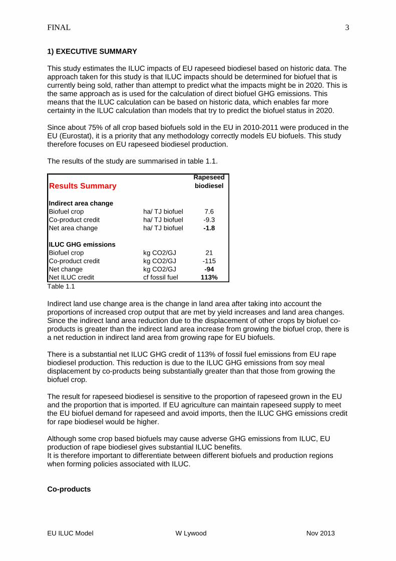
1) EXECUTIVE SUMMARY This study estimates the ILUC impacts of EU rapeseed biodiesel based on historic data. The approach taken for this study is that ILUC impacts should be determined for biofuel that is currently being sold, rather than attempt to predict what the impacts might be in 2020. This is the same approach as is used for the calculation of direct biofuel GHG emissions. This means that the ILUC calculation can be based on historic data, which enables far more certainty in the ILUC calculation than models that try to predict the biofuel status in 2020. Since about 75% of all crop based biofuels sold in the EU in 2010-2011 were produced in the EU (Eurostat), it is a priority that any methodology correctly models EU biofuels. This study therefore focuses on EU rapeseed biodiesel production. The results of the study are summarised in table 1.1.

Results SummaryRapeseed

biodiesel

Indirect area change

Biofuel crop ha/ TJ biofuel 7.6

Co-product credit ha/ TJ biofuel -9.3

Net area change ha/ TJ biofuel -1.8

ILUC GHG emissions

Biofuel crop kg CO2/GJ 21

Co-product credit kg CO2/GJ -115

Net change kg CO2/GJ -94

Net ILUC credit cf fossil fuel 113% Table 1.1

Indirect land use change area is the change in land area after taking into account the proportions of increased crop output that are met by yield increases and land area changes. Since the indirect land area reduction due to the displacement of other crops by biofuel co-products is greater than the indirect land area increase from growing the biofuel crop, there is a net reduction in indirect land area from growing rape for EU biofuels. There is a substantial net ILUC GHG credit of 113% of fossil fuel emissions from EU rape biodiesel production. This reduction is due to the ILUC GHG emissions from soy meal displacement by co-products being substantially greater than that those from growing the biofuel crop. The result for rapeseed biodiesel is sensitive to the proportion of rapeseed grown in the EU and the proportion that is imported. If EU agriculture can maintain rapeseed supply to meet the EU biofuel demand for rapeseed and avoid imports, then the ILUC GHG emissions credit for rape biodiesel would be higher. Although some crop based biofuels may cause adverse GHG emissions from ILUC, EU production of rape biodiesel gives substantial ILUC benefits. It is therefore important to differentiate between different biofuels and production regions when forming policies associated with ILUC. Co-products

FINAL


4

Analysis shows that high protein animal feed co-products such as rape meal and cereal bioethanol co-product (DDGS) displace a mixture of soy meal and cereals. The ratios by which rape meal and DDGS substitute for soy meal and wheat are calculated to balance the metabolisable energy and digestible protein in the animal feed. All EU rape meal is used as animal feed and there are no limits to increased use for animal feed to meet 8.5% biofuels energy use in 2020. Trade Analysis of historic data shows that:

There has been no diversion of rapeseed oil from food or animal feed use to fuel use.

About 75% of increased demand of rapeseed is met by increased EU production, while the rest is met by increased rapeseed imports.

Multi-year changes in EU cereals demand are met almost entirely by changes in EU production, rather than changes in trade.

All marginal soy meal is imported, mainly from S America.

The EU maintains self sufficiency in other temperate arable crops Yield growth v area growth The relative changes in crop output due to yield growth and area growth are determined using long term yield and area trends with a correction for underlying yield growth from autonomous technology development. The EU meets a significantly higher proportion of increased output from yield growth than N America, while N America meets a significantly higher proportion of increased output from yield growth than S America. Land use changes in EU Analysis of historic data shows that:

the EU has historically increased arable crop yields faster than the EU demand increases for these crops.

Instead of using the yield increases to give increased arable crop production for exports, the EU has maintained its self sufficiency of arable crops and used increased yields to reduce arable crop area.

It follows that increasing EU production for crops for biofuel will reduce the rate of abandonment of arable land in the EU and not cause changes to the quantity of crops exported to the rest of the world market.

Increases in EU harvested crop area are met in the short term by a reduction in the area of fallow and temporary grassland.

In the longer term the extra harvested crop area is met by a reduction in the rate of abandonment of arable land, with no impact on forest and permanent grassland.

Marginal abandoned land migrates to forest or grassland by natural succession, rather than by afforestation.

Reversion time When recently abandoned land is converted to cropland, or land that would otherwise be abandoned for agricultural use, continues to be used as cropland, the reversion time, rather than an amortisation period, should be used for determining the rate of change of carbon stock. A reversion period of 100 years has been used for the EU to account for land use change by natural succession.

FINAL


5

Comparison with other models The results of this study show substantially higher GHG emission benefits from indirect land use change than all other models for EU rape biodiesel. This is due to errors that have been identified with other models for calculating ILUC GHG emissions. Nearly all of these model errors lead to over-estimation of the negative impacts and under-estimation of the positive impacts of ILUC, especially for crops with high protein co-products grown within the EU (DGENER 2010, Lywood 2010). The main areas of error in other models are:

Not accounting for the displacement of soy meal by high protein biofuel co-products

Not accounting for increased yield growth as a result of increased demand growth

Not taking into account that in the EU, USA, Canada and Ukraine, additional land comes from a reduction in the rate of abandonment of arable land

Underestimating the proportion of additional demand for traditional EU crops, such as cereals and rapeseed that will be grown in the EU, rather than being imported.

Different existing and proposed models use a large variety of methods to avoid accounting properly for the displacement of soy meal by EU biofuel co-products. The latest proposal to avoid proper accounting for co-products is to use a co-product allocation, rather than co-product substitution methodology for the ILUC calculation (Marelli 2013, Lepage 2013). The use of a co-product allocation approach for calculating biofuel ILUC GHG emissions gives a flawed result (JEC 2011) and cannot be justified.

FINAL


6

2) INTRODUCTION In situations where farmers use previously uncultivated land to grow crops for biofuel production, there is direct land use change (LUC) and methods are included within the RED to calculate the GHG effect of LUC. For all other cases where crops are used to produce biofuel, this will increase the demand for the crop, so extra crop will be grown elsewhere and lead to other uncultivated land being converted to cropland. This is called indirect land use change (ILUC) and will cause potential changes to GHG emissions due to changes in carbon stock of the land. Since a primary purpose of biofuels is to reduce fuel GHG emissions, it is important that the GHG emissions impacts of ILUC are considered and that an agreed calculation method is developed. It is widely accepted that ILUC impacts vary depending on product pathways and the crops used in the production process, the region where the crop is grown and on the biofuel production pathway. Where biofuel production gives co-products that displace other animal feed crops, this will reduce the demand for these animal feed crops. This leads to a reduction in land use change which will offset the ILUC due to the biofuel crop. The net ILUC impact may therefore be either a penalty or a credit in GHG emissions. Various groups have tried to expand the scope of ILUC to consider other issues, such as biodiversity and social impacts and the impacts of yield changes. However all EU policies that affect agriculture may have biodiversity, social and yield change impacts and these issues are no more related to biofuels than to many other aspects of EU legislation affecting agriculture. This study therefore only considers the GHG emissions associated with ILUC. Indirect land use change effects cannot be measured directly, so they are modelled for each biofuel production pathway. A number of groups have used different modelling approaches to attempt to model ILUC changes, but there has so far been little attempt to reach an agreed approach for ILUC modelling. 3) MODELLING ISSUES Most of the work on ILUC modelling has been done using complex “equilibrium” models which predict the extra quantity of different crops that will be produced to meet a biofuel policy target, where these crops will be grown, the use of co-product, the proportion of increased output that will come from yield increases and area increases. Additional modules can be used to determine the ILUC impact. An alternative approach is to use simple spreadsheet models, based primarily on historic data. 3.1) Problems with equilibrium models There are several problems with the use of equilibrium models to determine ILUC impacts of particular biofuels and authors accept that current models are not appropriate for legislative purposes.

Equilibrium models are not transparent and many of the assumptions are not made clear.

The results of any model cannot be reproduced by other models

Some model elasticity parameters are arbitrary and very few have been related to relevant historic data.

Equilibrium models have large areas of uncertainty

Many aspects of the model have not been peer reviewed

FINAL


7

The architecture of most equilibrium models is based on trade modeling and makes it difficult to model some important aspects of ILUC, such as biofuel co-product displacement of other crops.

Equilibrium models do not have the detail to determine operation specific ILUC factors that would result for example from adopting policies to minimise ILUC effects.

3.2) Causation and consumer demand Economics of supply and demand dictate that higher demand for crops for biofuel use will drive higher prices, which on the supply side will drive investment for increased output, which will be met by yield growth and land area growth. On the demand side, higher prices will cause consumers to consume less, and drive reduced losses in the food chain. However, it has been argued (Bauen 2010, Overmars 2011) that it is not fair to attribute a reduction in biofuel ILUC impacts to a reduction in use for human food and animal feed. Simple models therefore have not taken account of the reduction in demand for food and feed. This may need to be considered further, but as with other simple models, this study does not take account of reductions in the total food and feed demand as a result of increased demand for biofuels. 3.3) Model timescale transparency and reproducibility There has been little if any discussion as to whether ILUC models should determine impacts that reflect the GHG impact of a possible biofuel scenario in 2020, or whether they should reflect the impact of current biofuel sales. All current equilibrium models try to determine the GHG impact of a 2020 scenario. However, the results from this work are being used to influence policy changes, which will change the scenario in 2020, such that the calculated 2020 ILUC impacts are no longer valid. The attempt to predict 2020 scenarios also generates a lot of uncertainty in the model as to what the biofuel scenario in 2020 might be and how it will be met. It is therefore much more appropriate to determine the ILUC impacts of current biofuel sales. The approach is therefore taken for this study that ILUC impacts should be determined for biofuels that are currently being sold (as for direct GHG emissions), rather than attempt to take a view on what the impacts might be in 2020. This approach means that the calculation can be primarily based on historic data and thus substantially reduces the uncertainty compared with models that are trying to predict a 2020 scenario. As with direct GHG emissions, the GHG calculations can be updated if new trends are seen as a result of increased biofuel production. In order to be reproducible by other modellers, the calculations in this study are based on widely available agreed data sets that are regularly updated. In this model all estimates of changes in trade, area growth, yield growth and EU land use are based on FAOSTAT, or USDA data. While FAOSTAT has data for all crops, USDA only has data for selected crops. However, USDA has more up to date than FAO data, especially for crop stock levels. Alternative methods have been used or considered in other simple models for analysing and representing these raw data for use in an ILUC model. Also concerns have previously been raised on the use of various methods. This study reviews alternative modelling methods and addresses concerns that have been raised, in order to justify the choice of the most appropriate methods. 3.4) Level of differentiation

FINAL


8

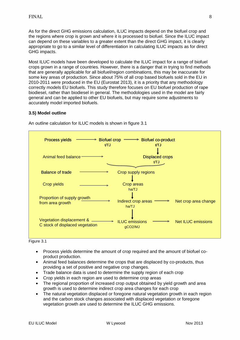
As for the direct GHG emissions calculation, ILUC impacts depend on the biofuel crop and the regions where crop is grown and where it is processed to biofuel. Since the ILUC impact can depend on these variables to a greater extent than the direct GHG impact, it is clearly appropriate to go to a similar level of differentiation in calculating ILUC impacts as for direct GHG impacts. Most ILUC models have been developed to calculate the ILUC impact for a range of biofuel crops grown in a range of countries. However, there is a danger that in trying to find methods that are generally applicable for all biofuel/region combinations, this may be inaccurate for some key areas of production. Since about 75% of all crop based biofuels sold in the EU in 2010-2011 were produced in the EU (Eurostat 2013), it is a priority that any methodology correctly models EU biofuels. This study therefore focuses on EU biofuel production of rape biodiesel, rather than biodiesel in general. The methodologies used in the model are fairly general and can be applied to other EU biofuels, but may require some adjustments to accurately model imported biofuels. 3.5) Model outline An outline calculation for ILUC models is shown in figure 3.1

Animal feed balance Displaced crops

t/TJ

Balance of trade Crop supply regions

Biofuel crop

t/TJ

Biofuel co-product

t/TJ

Process yields

Crop yields Crop areas

ha/TJ

Proportion of supply growth

from area growth Indirect crop areas

ha/TJ

ILUC emissions

gCO2/MJ

Vegetation displacement &

C stock of displaced vegetation

Net crop area change

Net ILUC emissions

Displaced crops

t/TJ

Balance of trade

Animal feed balance Displaced crops

t/TJ

Balance of trade Crop supply regions

Biofuel crop

t/TJ

Biofuel co-product

t/TJ

Process yields Biofuel crop

t/TJ

Biofuel co-product

t/TJ

Process yields

Crop yields Crop areas

ha/TJ

Proportion of supply growth

from area growth Indirect crop areas

ha/TJ

ILUC emissions

gCO2/MJ

Vegetation displacement &

C stock of displaced vegetation

Net crop area change

Net ILUC emissions

Displaced crops

t/TJ

Balance of trade

Figure 3.1

Process yields determine the amount of crop required and the amount of biofuel co-product production.

Animal feed balances determine the crops that are displaced by co-products, thus providing a set of positive and negative crop changes.

Trade balance data is used to determine the supply region of each crop

Crop yields in each region are used to determine crop areas

The regional proportion of increased crop output obtained by yield growth and area growth is used to determine indirect crop area changes for each crop

The natural vegetation displaced or foregone natural vegetation growth in each region and the carbon stock changes associated with displaced vegetation or foregone vegetation growth are used to determine the ILUC GHG emissions.

FINAL


9

There are a series of key issues in the modelling of ILUC impacts:

How much of which crops are displaced by biofuel co-products?

How much of the change in crop demands in the EU is met by increased production in the EU, how much is imported and where from?

How much of the increased production of each crop in each region is met by land area change and how much by yield growth?

What type of land is converted to cropland for biofuels?

What are the carbon stock changes from land conversion? These issues are analysed in sections 4 to 8. 4) ACCOUNTING FOR CO-PRODUCTS When crops such as oil seed rape and cereals are used for biofuel production, the oil or starch fraction is used for biofuels manufacture while all the remaining nutrients, including protein, are conserved and concentrated to provide high protein co-products. The co-products from rapeseed biodiesel and cereal bioethanol are respectively rape meal and distillers dried grains and solubles (DDGS). These co-products are used for animal feed, where they displace other crops or crop products. The land that is currently used to grow crops that are displaced by the biofuel co-products must be subtracted from the land used to grow the biofuels crop, in order to determine the net land use. Similarly the reduction in GHG emissions from land use change due to reduced demand growth for crops that are displaced by the biofuel co-products must be subtracted from those associated with the biofuels crop in order to determine the net GHG emissions from ILUC.

4.1) Animal feed balance

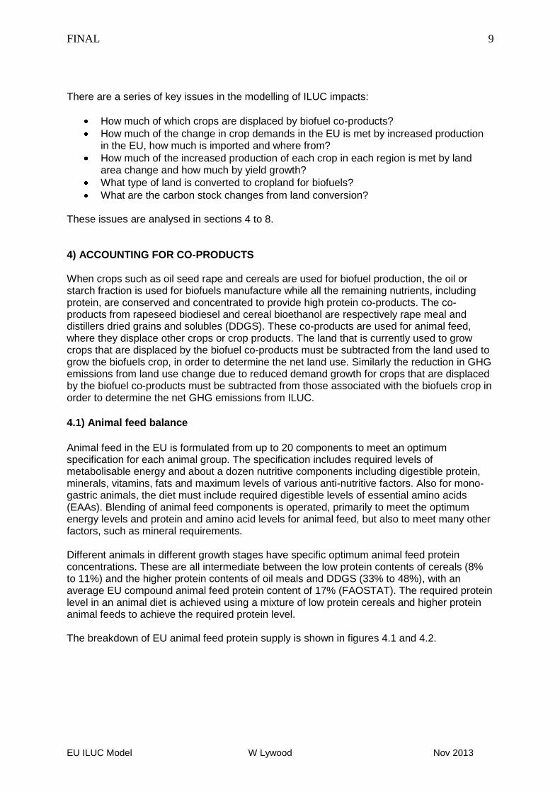
Animal feed in the EU is formulated from up to 20 components to meet an optimum specification for each animal group. The specification includes required levels of metabolisable energy and about a dozen nutritive components including digestible protein, minerals, vitamins, fats and maximum levels of various anti-nutritive factors. Also for mono-gastric animals, the diet must include required digestible levels of essential amino acids (EAAs). Blending of animal feed components is operated, primarily to meet the optimum energy levels and protein and amino acid levels for animal feed, but also to meet many other factors, such as mineral requirements. Different animals in different growth stages have specific optimum animal feed protein concentrations. These are all intermediate between the low protein contents of cereals (8% to 11%) and the higher protein contents of oil meals and DDGS (33% to 48%), with an average EU compound animal feed protein content of 17% (FAOSTAT). The required protein level in an animal diet is achieved using a mixture of low protein cereals and higher protein animal feeds to achieve the required protein level. The breakdown of EU animal feed protein supply is shown in figures 4.1 and 4.2.

FINAL


10

EU low protein animal feed supply

2009 mt/yr

Other

Cereals 0.5

Brans 1.7

Barley 2.7

Maize 4.2

Feed

Wheat 4.2

EU high protein animal feed supply

2009 mt/yr

Soybean

Meal 14.1

Rapeseed

Meal 4.2Other seed

Meals 2.9

Pulses 0.5

DDGS 0.8

Figure 4.1 source: FAO Figure 4.2 sources: FAO, Eurostat

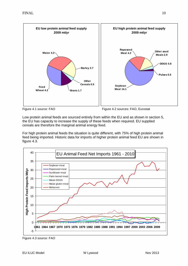
Low protein animal feeds are sourced entirely from within the EU and as shown in section 5, the EU has capacity to increase the supply of these feeds when required. EU supplied cereals are therefore the marginal animal energy feed. For high protein animal feeds the situation is quite different, with 75% of high protein animal feed being imported. Historic data for imports of higher protein animal feed EU are shown in figure 4.3.

EU Animal Feed Net Imports 1961 - 2010

-5

0

5

10

15

20

25

30

35

40

1961 1964 1967 1970 1973 1976 1979 1982 1985 1988 1991 1994 1997 2000 2003 2006 2009

Hig

h P

rote

in F

ee

d Im

po

rts

Mt/

yr

Soybean meal

Rapeseed meal

Sunflower meal

Palm kernel meal

Maize DDGS

Maize gluten meal

Molasses

Figure 4.3 source: FAO

FINAL


11

Soybean meal (SBM) is by far the major source of protein imports to the EU, accounting for about 96% of the total imported animal feed protein requirements. Soy meal imports adjust to meet EU demand, with a large increase from 1997 to 2000 following a ban on the use of animal protein for feed and a fall since 2007 as a result of increased production of EU biofuel co-products for animal feed. SBM imports are adjusted to meet the EU demand for animal feed protein and imported SBM can therefore be regarded as the marginal high protein feed. Biofuel co-products such as RSM have protein levels of about 34%, which are well above the average animal feed protein content and intermediate between cereals and SBM. They will therefore displace a mixture of EU cereals and imported SBM from animal diets. Animal feed dietary formulation targets are driven by economic considerations in the EU, so nutritionists use a linear programming model to determine the least cost formulation to meet the feed specification for each animal diet depending on the available animal feed components and their price. The linear model includes nutritional component mass and energy balances such that the animal feed materials will meet the energy and protein requirements for the animal group feed specification. The cost of high protein soy meal animal feed imported in the EU is substantially higher then lower protein feeds such as wheat, so there is a strong economic incentive to use it efficiently in animal feed diets, by accurately targeting optimum dietary protein and amino acid levels. There is no case in the EU (as is sometimes done in N America) for exceeding the protein requirements of the feed specification, since this will incur additional cost. 4.2) Animal feed substitution ratios Analysis of the results from linear formulation models (Lywood 2009a, Weightman 2010, ICCT 2011) shows that the ratios by which biofuel co-products displace other components is such as to maintain a balance for metabolisable energy and digestible protein for each animal group. The protein digestibility of different feeds depends on the animal types and on the other components in the oil meals and displaced crops. Linear models with variable quantities of other animal feed components show that biofuel co-products, as well as displacing a mixture of soy meal and cereal, will also displace other animal feed components (Weightman 2010, ICCT 2011) for any particular diet. However, the other animal feed components e.g. sunflower meal and maize gluten are co-products from the production of vegetable oils or wet corn milling, so the production of these components is fixed. They will therefore continue to be produced and will be used elsewhere in animal feed formulations to displace a mixture of soy meal and cereals in other animal diets. Therefore rape meal and DDGS will still indirectly replace cereals and imported soy meal. A list of published displacement ratios, where RSM is displacing soy meal and cereal are shown in table 4.1.

Substitution Ratios for EU Biofuel co-products

Source Co-product

Substution for

soy meal

Substution

for cereal

CE Delft 2008

Rape meal 0.66 0.26

Lywood et al 2009a

Rape meal 0.61 0.15

Ozdemir 2009 Rape meal 0.69 N/A

t / t of co-product

Table 4.1

FINAL


12

The data from Lywood et al 2009a was used in the E4tech model (Bauen 2010) and is used in this study.

4.3) Soy oil displacement.

Soy bean is primarily grown to supply soy meal (unlike other oilseeds, which are primarily

grown for the oil). Therefore when biofuel animal feed co-products displace soy bean meal

imported to the EU, the rate of increase of soy bean production will be reduced. This will in

turn reduce the supply of soy oil, which needs to be accounted for. Marginal soy oil is used to

produce biodiesel in Argentina, which is imported into the EU. Therefore the lost soy oil due

to the reduced rate of soy production will to some extent reduce the supply of biodiesel in the

EU and will need to be made up with other EU biofuels. In order to avoid further expansion of

the mode to other crops, the reduced soy oil has therefore been set off against EU rape

biodiesel. 4.4) Potential limits to co-product substitution Various concerns have been raised in other references as to the scope for the displacement of soy meal by biofuel co-products: Limit of scope for soy displacement Limit of co-product consumption Other uses of co-products 4.5) Co-product consumption limit It has been suggested (JEC 2011), that there could be a limit in being able to utilise all the biofuel co-products in the EU due to lack of soy meal capacity that could be replaced. It was also assumed by Overmars (2010) that for rapeseed and wheat that the co-products effectively used for animal feed was only between 50% and 90% of co-product production. Historically there has been no problem in being able to utilise biofuel co-products for animal feed. For example from 2010 to 2012 average UK prices for DDGS and RSM of 210 euro/t have been about 30% higher than the prices of cereals used for animal feed (Defra, LMC). The imports of animal feed components to the EU are shown in figure 4.3. While the increases in production of biofuel co-products has reduced EU soy meal import in recent years, 70% of all the protein in high protein animal feed was still being imported as soy meal in 2010 (FAOSTAT). The changes in the higher protein feed balance as a result of the EU moving from the position in 2011 to a position of 8.5% biofuels incorporation in EU road transport fuels (DGAGRI 2011) in 2020 with all the additional biofuel from EU rape biodiesel and cereal bioethanol is shown in table 4.2

FINAL


13

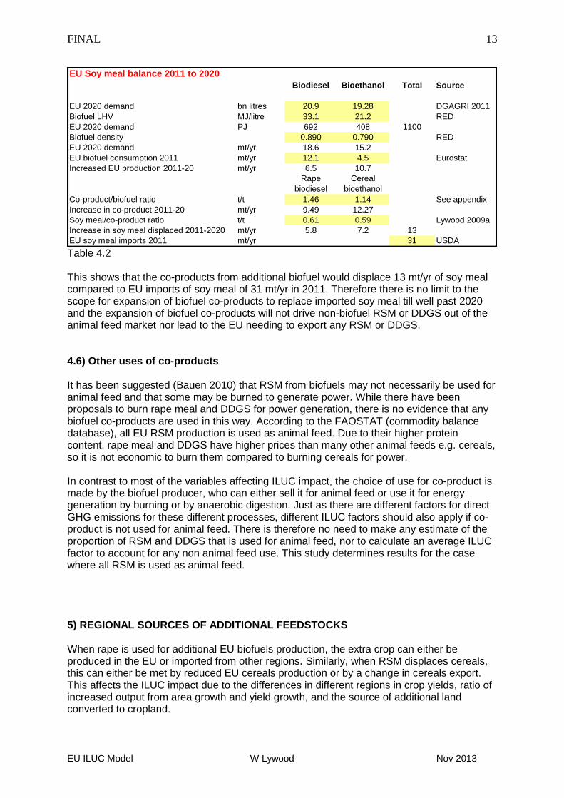
EU Soy meal balance 2011 to 2020

Biodiesel Bioethanol Total Source

EU 2020 demand bn litres 20.9 19.28 DGAGRI 2011

Biofuel LHV MJ/litre 33.1 21.2 RED

EU 2020 demand PJ 692 408 1100

Biofuel density 0.890 0.790 RED

EU 2020 demand mt/yr 18.6 15.2

EU biofuel consumption 2011 mt/yr 12.1 4.5 Eurostat

Increased EU production 2011-20 mt/yr 6.5 10.7

Rape

biodiesel

Cereal

bioethanol

Co-product/biofuel ratio t/t 1.46 1.14 See appendix

Increase in co-product 2011-20 mt/yr 9.49 12.27

Soy meal/co-product ratio t/t 0.61 0.59 Lywood 2009a

Increase in soy meal displaced 2011-2020 mt/yr 5.8 7.2 13

EU soy meal imports 2011 mt/yr 31 USDA Table 4.2 This shows that the co-products from additional biofuel would displace 13 mt/yr of soy meal compared to EU imports of soy meal of 31 mt/yr in 2011. Therefore there is no limit to the scope for expansion of biofuel co-products to replace imported soy meal till well past 2020 and the expansion of biofuel co-products will not drive non-biofuel RSM or DDGS out of the animal feed market nor lead to the EU needing to export any RSM or DDGS. 4.6) Other uses of co-products It has been suggested (Bauen 2010) that RSM from biofuels may not necessarily be used for animal feed and that some may be burned to generate power. While there have been proposals to burn rape meal and DDGS for power generation, there is no evidence that any biofuel co-products are used in this way. According to the FAOSTAT (commodity balance database), all EU RSM production is used as animal feed. Due to their higher protein content, rape meal and DDGS have higher prices than many other animal feeds e.g. cereals, so it is not economic to burn them compared to burning cereals for power. In contrast to most of the variables affecting ILUC impact, the choice of use for co-product is made by the biofuel producer, who can either sell it for animal feed or use it for energy generation by burning or by anaerobic digestion. Just as there are different factors for direct GHG emissions for these different processes, different ILUC factors should also apply if co-product is not used for animal feed. There is therefore no need to make any estimate of the proportion of RSM and DDGS that is used for animal feed, nor to calculate an average ILUC factor to account for any non animal feed use. This study determines results for the case where all RSM is used as animal feed. 5) REGIONAL SOURCES OF ADDITIONAL FEEDSTOCKS When rape is used for additional EU biofuels production, the extra crop can either be produced in the EU or imported from other regions. Similarly, when RSM displaces cereals, this can either be met by reduced EU cereals production or by a change in cereals export. This affects the ILUC impact due to the differences in different regions in crop yields, ratio of increased output from area growth and yield growth, and the source of additional land converted to cropland.

FINAL


14

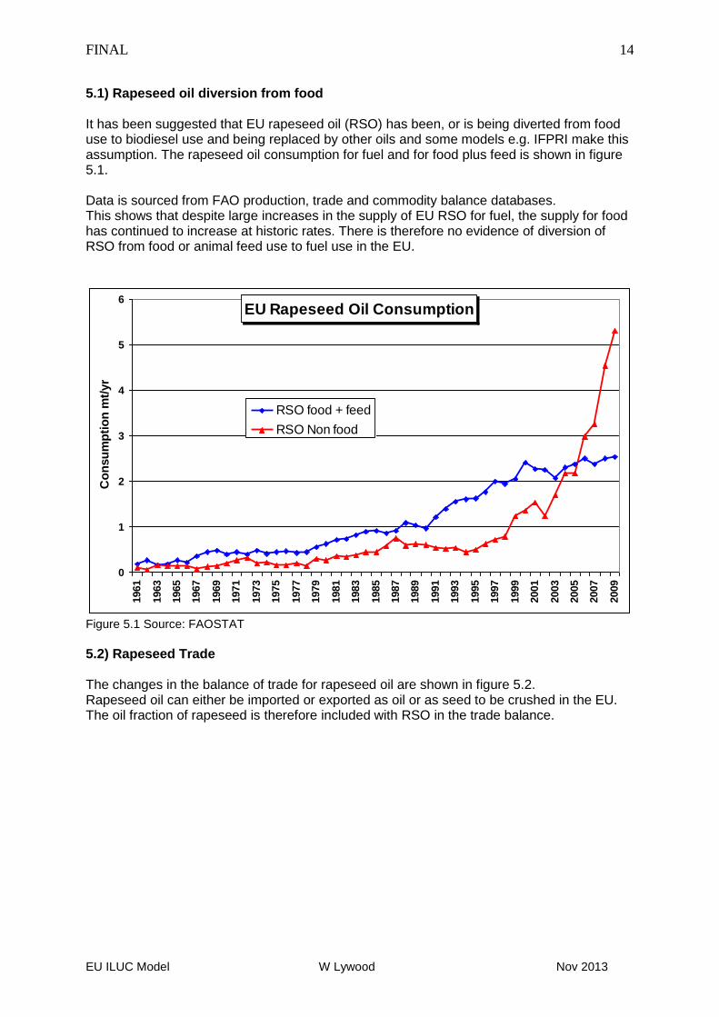
5.1) Rapeseed oil diversion from food It has been suggested that EU rapeseed oil (RSO) has been, or is being diverted from food use to biodiesel use and being replaced by other oils and some models e.g. IFPRI make this assumption. The rapeseed oil consumption for fuel and for food plus feed is shown in figure 5.1. Data is sourced from FAO production, trade and commodity balance databases. This shows that despite large increases in the supply of EU RSO for fuel, the supply for food has continued to increase at historic rates. There is therefore no evidence of diversion of RSO from food or animal feed use to fuel use in the EU.

EU Rapeseed Oil Consumption

0

1

2

3

4

5

6

1961

1963

1965

1967

1969

1971

1973

1975

1977

1979

1981

1983

1985

1987

1989

1991

1993

1995

1997

1999

2001

2003

2005

2007

2009

Co

nsu

mp

tio

n m

t/yr

RSO food + feed

RSO Non food

Figure 5.1 Source: FAOSTAT

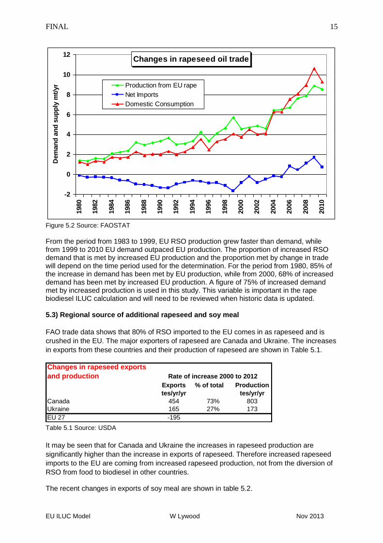
5.2) Rapeseed Trade The changes in the balance of trade for rapeseed oil are shown in figure 5.2. Rapeseed oil can either be imported or exported as oil or as seed to be crushed in the EU. The oil fraction of rapeseed is therefore included with RSO in the trade balance.

FINAL


15

Changes in rapeseed oil trade

-2

0

2

4

6

8

10

12

1980

1982

1984

1986

1988

1990

1992

1994

1996

1998

2000

2002

2004

2006

2008

2010

Dem

an

d a

nd

su

pp

ly m

t/yr Production from EU rape

Net Imports

Domestic Consumption

Figure 5.2 Source: FAOSTAT

From the period from 1983 to 1999, EU RSO production grew faster than demand, while from 1999 to 2010 EU demand outpaced EU production. The proportion of increased RSO demand that is met by increased EU production and the proportion met by change in trade will depend on the time period used for the determination. For the period from 1980, 85% of the increase in demand has been met by EU production, while from 2000, 68% of increased demand has been met by increased EU production. A figure of 75% of increased demand met by increased production is used in this study. This variable is important in the rape biodiesel ILUC calculation and will need to be reviewed when historic data is updated. 5.3) Regional source of additional rapeseed and soy meal

FAO trade data shows that 80% of RSO imported to the EU comes in as rapeseed and is

crushed in the EU. The major exporters of rapeseed are Canada and Ukraine. The increases

in exports from these countries and their production of rapeseed are shown in Table 5.1.

Exports % of total Production

tes/yr/yr tes/yr/yr

Canada 454 73% 803

Ukraine 165 27% 173

EU 27 -195

Changes in rapeseed exports

and production Rate of increase 2000 to 2012

Table 5.1 Source: USDA

It may be seen that for Canada and Ukraine the increases in rapeseed production are

significantly higher than the increase in exports of rapeseed. Therefore increased rapeseed

imports to the EU are coming from increased rapeseed production, not from the diversion of

RSO from food to biodiesel in other countries. The recent changes in exports of soy meal are shown in table 5.2.

FINAL


16

Changes in soymeal exports

tes/yr/yr % of total

Brazil 1694 40%

Rest of S America 1520 36%

USA 1057 25%

Rate of increase 2000 to 2012

Table 5.2 Source USDA

For calculating data for decreases in imported soy meal, EU imports are split between S America and N America in the same ratio as the recent increase in exports from exporting countries. 5.4) Cereals trade EU cereals, such as wheat, barley, maize and rye are to a large extent interchangeable, both in terms of what cereal crop is grown and in their use as animal feed. Therefore cereals are considered together for analysing the EU trade balance. The use of EU cereals for bioethanol production is only about 3% of total EU cereal production and is small compared to other changes in cereal supply and demand. Therefore the relationship between changes in cereal demand and trade is established from historic changes in the total EU balance of trade for cereals from 1960 to 2012 as shown in figure 5.3. This shows a four year moving averages for EU cereals production, net imports and consumption. Domestic consumption = domestic production + imports – exports + stock variation Changes in cereal stock levels are small and not shown. Four year averages are used to smooth the annual variations in cereal crop yields.

Changes in EU cereal trade

-50

0

50

100

150

200

250

300

350

19

60

19

63

19

66

19

69

19

72

19

75

19

78

19

81

19

84

19

87

19

90

19

93

19

96

19

99

20

02

20

05

20

08

20

11

De

ma

nd

an

d s

up

ply

mt/

yr

Production

Net Imports

Consumption

Figure 5.3 Source: USDA

It may be seen that during the steady climb in demand from 1963 to 1980, the increase in EU production lagged behind the change in demand, until it caught up with demand in 1984.

FINAL


17

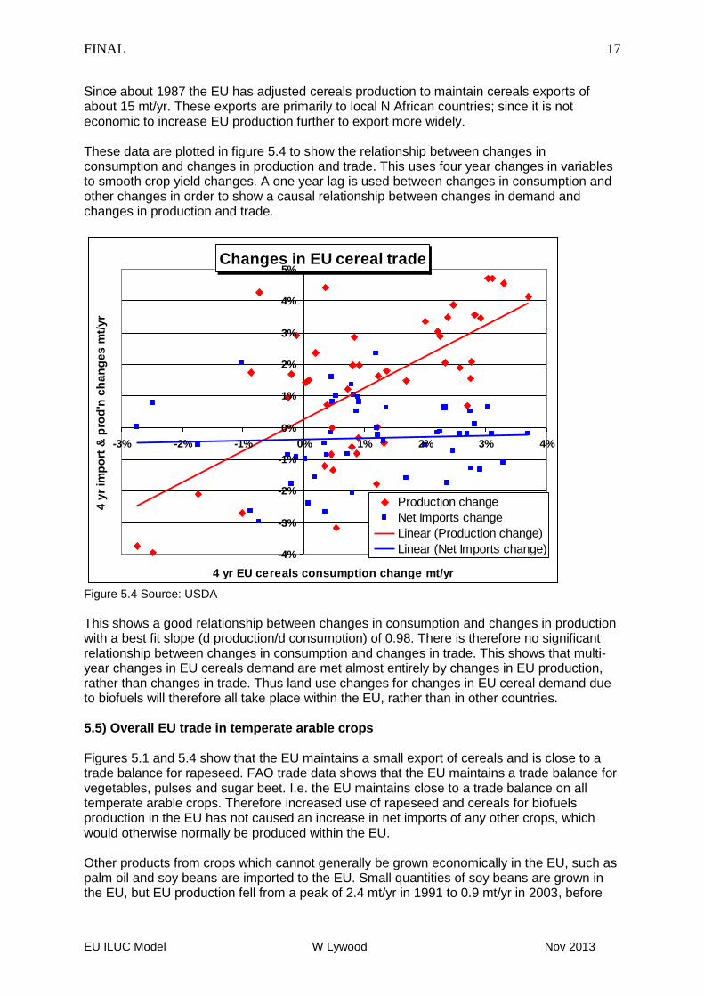
Since about 1987 the EU has adjusted cereals production to maintain cereals exports of about 15 mt/yr. These exports are primarily to local N African countries; since it is not economic to increase EU production further to export more widely. These data are plotted in figure 5.4 to show the relationship between changes in consumption and changes in production and trade. This uses four year changes in variables to smooth crop yield changes. A one year lag is used between changes in consumption and other changes in order to show a causal relationship between changes in demand and changes in production and trade.

Changes in EU cereal trade

-4%

-3%

-2%

-1%

0%

1%

2%

3%

4%

5%

-3% -2% -1% 0% 1% 2% 3% 4%

4 yr EU cereals consumption change mt/yr

4 y

r im

po

rt &

pro

d'n

ch

an

ge

s m

t/y

r

Production change

Net Imports change

Linear (Production change)

Linear (Net Imports change)

Figure 5.4 Source: USDA

This shows a good relationship between changes in consumption and changes in production with a best fit slope (d production/d consumption) of 0.98. There is therefore no significant relationship between changes in consumption and changes in trade. This shows that multi-year changes in EU cereals demand are met almost entirely by changes in EU production, rather than changes in trade. Thus land use changes for changes in EU cereal demand due to biofuels will therefore all take place within the EU, rather than in other countries. 5.5) Overall EU trade in temperate arable crops Figures 5.1 and 5.4 show that the EU maintains a small export of cereals and is close to a trade balance for rapeseed. FAO trade data shows that the EU maintains a trade balance for vegetables, pulses and sugar beet. I.e. the EU maintains close to a trade balance on all temperate arable crops. Therefore increased use of rapeseed and cereals for biofuels production in the EU has not caused an increase in net imports of any other crops, which would otherwise normally be produced within the EU. Other products from crops which cannot generally be grown economically in the EU, such as palm oil and soy beans are imported to the EU. Small quantities of soy beans are grown in the EU, but EU production fell from a peak of 2.4 mt/yr in 1991 to 0.9 mt/yr in 2003, before

FINAL


18

there was significant EU biofuel production. The decrease in EU soy production is therefore due to poor economics of growing soy in the EU and not to EU biofuel crop expansion. 6) AREA GROWTH v YIELD GROWTH When additional crop is produced to meet increased demand e.g. for biofuel use, the increased crop output is from a combination of area growth and yield growth. The fraction of increased output that will be met by yield growth (intensification) and by land area growth (expansion) will depend on the relative economics of obtaining increased output from yield improvements and from additional cultivated land area. The increased crop demand for biofuels can be treated in the same way as other increases in crop demand and will be met in a similar way as for historic demand changes. Although biofuel production has only increased significantly in the last few years, the way in which additional biofuel demand is being met can be determined by the way additional demand in general has been met over a substantially longer period of time. The relative proportions of increased output obtained by yield and by area increases for different crops on a regional basis can be determined by direct relationships between historic demand, yield and area changes. There are several independent choices to be made on how to determine and model the relative changes in yield and land area:

Fixed yield growth or variable yield growth

Model each crop on its own, or model groups of crops

Determination of yield and yield change of a group of crops

How to characterise historic data. 6.1) Fixed yield growth v variable demand related yield growth The split between yield growth and area growth can be modelled either by using an historic figure for yield growth and assuming that any additional increase in supply is met by area growth, or by using historic data to determine the relative proportions of extra production arising from yield growth and area growth. Most equilibrium models use the first approach, while simple models (Lywood 2009c, E4tech (Bauen 2010) and Overmars 2011) use the second approach. The second approach was shown to be the most appropriate method to represent yield and area changes (Lywood 2009b) and is the approach has been used in this study. 6.2) Model each crop singly or as a group of crops When there is an increase in demand for any crop, such as oilseed rape, due to increased demand for biofuel, this will displace other crops in a crop rotation and the rotation will be re-optimised around the additional crop. Continuous planting of cereal crops leads to decreasing yields due to establishment of pests and other factors and rapeseed acts as a break crop between cereal crops in the rotation and enables increase in cereal yields. It is therefore important to consider rotational crops as a group, rather than as single crops. The approach of using a group of crops was used by Overmars (2011) and has been adopted for this study. Increased use of cereals and oilseed rape for biofuel production should impact the area and yields of EU rotational arable crops, but not permanent crops. Therefore arable crops are used as the crop group to determine yield growth and area growth for rape and wheat in this study.

FINAL


19

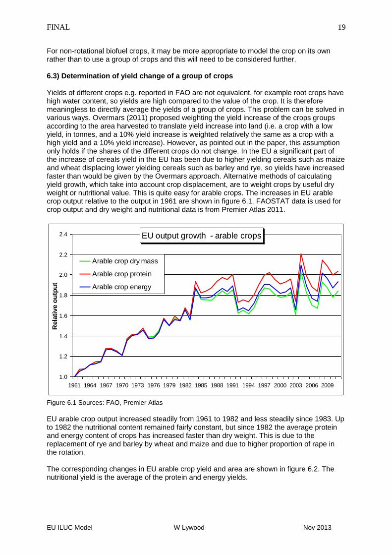
For non-rotational biofuel crops, it may be more appropriate to model the crop on its own rather than to use a group of crops and this will need to be considered further. 6.3) Determination of yield change of a group of crops Yields of different crops e.g. reported in FAO are not equivalent, for example root crops have high water content, so yields are high compared to the value of the crop. It is therefore meaningless to directly average the yields of a group of crops. This problem can be solved in various ways. Overmars (2011) proposed weighting the yield increase of the crops groups according to the area harvested to translate yield increase into land (i.e. a crop with a low yield, in tonnes, and a 10% yield increase is weighted relatively the same as a crop with a high yield and a 10% yield increase). However, as pointed out in the paper, this assumption only holds if the shares of the different crops do not change. In the EU a significant part of the increase of cereals yield in the EU has been due to higher yielding cereals such as maize and wheat displacing lower yielding cereals such as barley and rye, so yields have increased faster than would be given by the Overmars approach. Alternative methods of calculating yield growth, which take into account crop displacement, are to weight crops by useful dry weight or nutritional value. This is quite easy for arable crops. The increases in EU arable crop output relative to the output in 1961 are shown in figure 6.1. FAOSTAT data is used for crop output and dry weight and nutritional data is from Premier Atlas 2011.

EU output growth - arable crops

1.0

1.2

1.4

1.6

1.8

2.0

2.2

2.4

1961 1964 1967 1970 1973 1976 1979 1982 1985 1988 1991 1994 1997 2000 2003 2006 2009

Rela

tive o

utp

ut

Arable crop dry mass

Arable crop protein

Arable crop energy

Figure 6.1 Sources: FAO, Premier Atlas

EU arable crop output increased steadily from 1961 to 1982 and less steadily since 1983. Up to 1982 the nutritional content remained fairly constant, but since 1982 the average protein and energy content of crops has increased faster than dry weight. This is due to the replacement of rye and barley by wheat and maize and due to higher proportion of rape in the rotation. The corresponding changes in EU arable crop yield and area are shown in figure 6.2. The nutritional yield is the average of the protein and energy yields.

FINAL


20

EU average yield & area growth - arable crops

0.6

0.8

1.0

1.2

1.4

1.6

1.8

2.0

2.2

2.4

2.6

1961 1964 1967 1970 1973 1976 1979 1982 1985 1988 1991 1994 1997 2000 2003 2006 2009

Re

lati

ve

Yie

ld &

Are

a

Harvested crop area

Dry crop yield

Nutritional yield

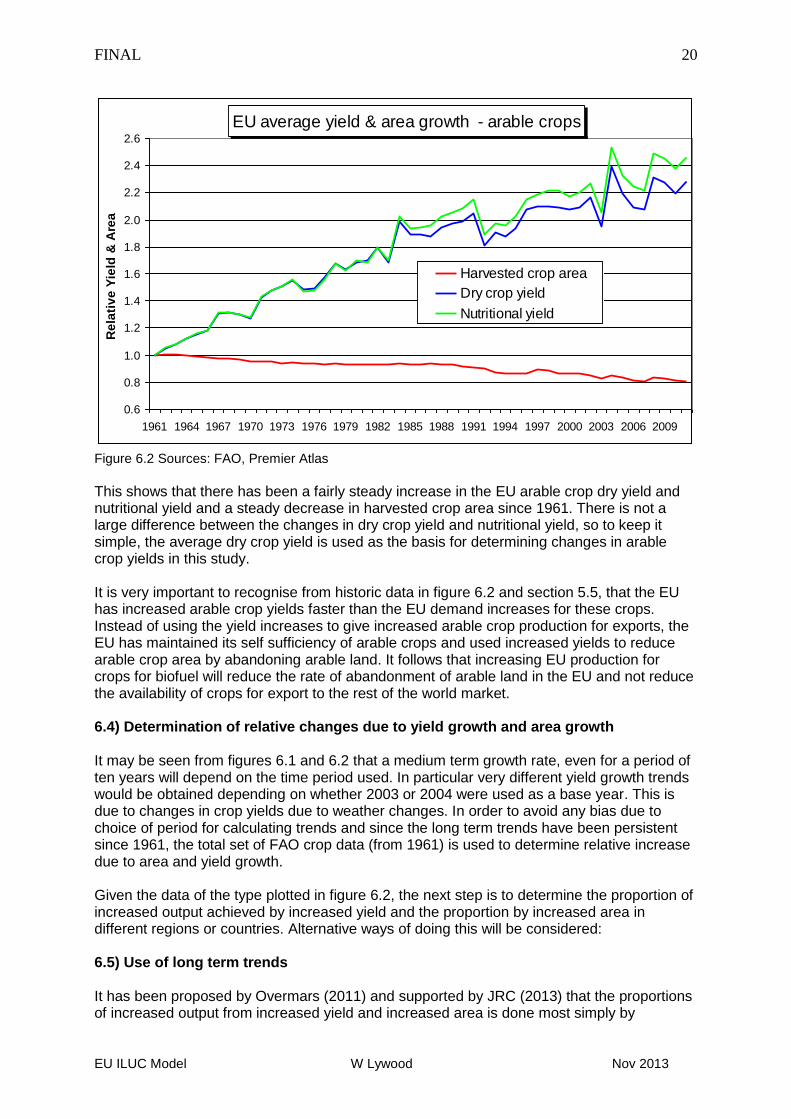
Figure 6.2 Sources: FAO, Premier Atlas

This shows that there has been a fairly steady increase in the EU arable crop dry yield and nutritional yield and a steady decrease in harvested crop area since 1961. There is not a large difference between the changes in dry crop yield and nutritional yield, so to keep it simple, the average dry crop yield is used as the basis for determining changes in arable crop yields in this study. It is very important to recognise from historic data in figure 6.2 and section 5.5, that the EU has increased arable crop yields faster than the EU demand increases for these crops. Instead of using the yield increases to give increased arable crop production for exports, the EU has maintained its self sufficiency of arable crops and used increased yields to reduce arable crop area by abandoning arable land. It follows that increasing EU production for crops for biofuel will reduce the rate of abandonment of arable land in the EU and not reduce the availability of crops for export to the rest of the world market. 6.4) Determination of relative changes due to yield growth and area growth It may be seen from figures 6.1 and 6.2 that a medium term growth rate, even for a period of ten years will depend on the time period used. In particular very different yield growth trends would be obtained depending on whether 2003 or 2004 were used as a base year. This is due to changes in crop yields due to weather changes. In order to avoid any bias due to choice of period for calculating trends and since the long term trends have been persistent since 1961, the total set of FAO crop data (from 1961) is used to determine relative increase due to area and yield growth. Given the data of the type plotted in figure 6.2, the next step is to determine the proportion of increased output achieved by increased yield and the proportion by increased area in different regions or countries. Alternative ways of doing this will be considered: 6.5) Use of long term trends It has been proposed by Overmars (2011) and supported by JRC (2013) that the proportions of increased output from increased yield and increased area is done most simply by

FINAL


21

comparing the relative slopes of the change in yield and change in area over time. The results from using this approach, in terms of compound annual growth rate (CAGR), are shown in table 6.1

Long term output trends 1961-2011

Average CAGR EU S America N America Ukraine

Output growth %/yr 1.2% 3.8% 1.9% 5.0%

Area growth %/yr -0.4% 1.9% 0.3% 2.1%

Yield growth %/yr 1.6% 1.9% 1.6% 3.0%

Proportion from area increase -0.35 0.50 0.16 0.41 Table 6.1 Source: FAOSTAT

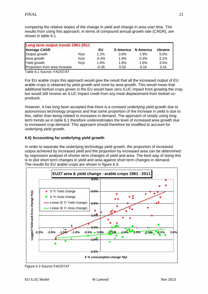
For EU arable crops this approach would give the result that all the increased output of EU arable crops is obtained by yield growth and none by area growth. This would mean that additional biofuel crops grown in the EU would have zero ILUC impact from growing the crop, but would still receive an ILUC impact credit from soy meal displacement from biofuel co-products. However, it has long been accepted that there is a constant underlying yield growth due to autonomous technology progress and that some proportion of the increase in yield is due to this, rather than being related to increases in demand. The approach of simply using long term trends as in table 6.1 therefore underestimates the level of increased area growth due to increased crop demand. This approach should therefore be modified to account for underlying yield growth. 6.6) Accounting for underlying yield growth In order to separate the underlying technology yield growth, the proportion of increased output achieved by increased yield and the proportion by increased area can be determined by regression analysis of shorter term changes of yield and area. The best way of doing this is to plot short term changes in yield and area against short term changes in demand. The results for EU arable crops are shown in figure 6.3.

EU27 area & yield change - arable crops 1961 - 2011

-2.0%

-1.0%

0.0%

1.0%

2.0%

3.0%

4.0%

-2.5% -2.0% -1.5% -1.0% -0.5% 0.0% 0.5% 1.0% 1.5% 2.0% 2.5% 3.0%

6 Yr consumption change %/yr

La

gg

ed

Yie

ld a

nd

Are

a c

ha

ng

e %

/yr 6 Tr Yield change

6 Yr Area change

Linear (6 Tr Yield change)

Linear (6 Yr Area change)

Figure 6.3 Source FAOSTAT

FINAL


22

Domestic consumption = domestic production + imports – exports + stock variation Six year average changes in yield, area and demand are used to reduce the variability due to weather induced yield changes. A one year lag is used between changes in demand and other changes because changes in demand are met mainly by changes in production in the following year, from changes in crop area and crop yield. This approach using lagged changes in yield and area provides a causal relationship between changes in demand and changes in crop area and yield. The results from fitting these data are summarised in table 6.2.

Short term regression fit

Region EU

Crops Arable

Change period (yrs) yr 6

Lag yr 1

Change in area/change in demand 0.16

Standard error 0.05

Change in yield/change in demand 0.83

Standard error 0.10

Proportion from area increase 16%

Underlying yield growth per yr 0.65% Table 6.2

The relative slopes of the yield and area lines show that 16% of the change in production growth is due to changes in area growth and 83% of change in production growth is due to yield growth. The intercept of the yield change line on the y axis indicates that the underlying technology induced yield growth is 0.65 % /yr. The intercept of the area change line on the x axis shows that additional EU crop area will not be needed until the growth rate in arable crop consumption exceeds 3 % yr. At lower growth rates, the additional crop demand will be met by a reduction in the rate of abandonment of arable land. A similar approach can be used for other regions. However, the accuracy of the equivalent fits for N America and S America are not as good as for the EU and the underlying yield growth is less clear. Therefore an underlying non demand related yield growth of 0.65%/yr (instead of zero in table 6.1) is applied for each of the regions that are relevant for this study. The long term trend results in table 6.1 have therefore been adjusted for an underlying growth rate of 0.65% /yr. These results, which are used in this study, are shown in table 6.3.

Demand related area and yield changes 1961-2011

Non demand related yield growth of 0.65%

Average CAGR EU S America N America Ukraine

Demand related area growth %/yr 0.22% 2.6% 1.0% 2.7%

Demand related yield growth %/yr 1.0% 1.3% 1.0% 2.3%

Proportion from area increase 0.18 0.67 0.49 0.54 Table 6.3

6.7 Accounting for reduced yield on new cropland

FINAL


23

The main effect of increased demand on yield growth is the increased yield on existing cropland. However, when new land is needed to grow extra crop, the new land may be more marginal than the existing cropland, so the yield on the new land will be lower than on existing land. This is sometimes termed “slippage” (Keeney 2005) or “yield drag” (Heiderer 2010). Thus combining the two effects of increased demand on yield: Net yield growth = yield growth on existing crop land - land area growth x ( 1- slippage factor ) Some equilibrium models use a factor for the fractional the yield on new land compared to existing cropland. For example, the IFPRI MIRAGE (IFPRI 2011) model uses a factor of 0.8. No analysis is provided for these factors and the values appear to be entirely arbitrary. When historic yield change data for example from FAO is collected on an average regional or country basis, it is the “net yield growth” shown in the equation above. Therefore these yield changes already take into account any effect of lower yield on new land as well as yield growth on existing land. Therefore as long as historic regional yield data is used to determine a relationship between changes in yield and crop area (as in sections 6.5 and 6.6), then any effects of “slippage” are automatically included in the analysis and there is no justification for any additional factor for a fractional yield on new land area. 7) TYPE OF LAND CONVERTED When more cropland area is needed for crops as a result of biofuels demand, this can be provided by converting grassland, forest, fallow land, temporary grassland, or previously abandoned land to cropland or by reducing the rate at which cropland is abandoned. Various approaches have been taken by different models to determine what types of land are converted to cropland in different countries and regions. EPA used data from the MODIS satellite imaging, from 2001 to 2004, which was analysed by Winrock (Winrock 2009). These data are used to determine the proportions by which new cropland displaces forest, grassland, savannah and shrub land. This approach was used in the E4tech (Bauen 2010) model. However, the accuracy of these data was poor and did not agree with FAO data. It was agreed (JRC ISPRA 2010b) that while suitable for determining the spread of land type at any given time, MODIS data is not sufficiently accurate for calculating land use changes. Other ILUC work uses models (Heiderer 2010, Overmars 2011, IFPRI 2011) to predict changes in land type and carbon stocks. However, these models have not been validated against historic data of land area changes and do not take account of the underlying changes on land use in different countries. Most of the discussion on global ILUC has been in terms of increasing cropland area for biofuels leading to increased deforestation, or conversion of grassland to cropland. However in regions such as the EU, USA, Canada and FSU, the area of arable land has been decreasing over time and has created idle land. Therefore the effect of increasing demand for biofuels crops will be to reduce the rate of creation of idle land, or to utilise unused or recently created idled land, rather than cause conversion of forest or grassland to cropland. This is not properly accounted for in any existing models. Within FAO databases land is broken down such that: Arable land area = harvested crop area + fallow land + temporary grassland Agricultural land area = arable land + permanent crops + permanent meadows and pasture

FINAL


24

Total land area = agricultural land + forest + other land “Other land” is primarily abandoned land, but also includes land for settlement and amenities Data for land usage is available from FAOSTAT crop database and resource database. These give annual area data for harvested crops and most land types: arable, permanent crop and pasture, however, forest area is only available for the years: 1990, 2000, 2005 and 2011. 7.1) Land changes in the EU The average areas of different categories of land in the EU and the average annual area changes are shown in table 7.1.

EU land areas and rates of change

Avg Area

1990-2011 1961- 2011 1990 - 2011 1995-2005

mha mha/yr mha/yr

Arable crops 77 -0.31 -0.39

Fallow + temp grassland 37 -0.17 -0.31

Arable land 114 -0.48 -0.70

Permanent crops 12 -0.04 -0.05

Permanent pasture 71 -0.27 -0.26

Forest area 151 0.64 0.63

Other land 70 0.38

Afforestation (Zanchi) 0.22

Average Area Change

Table 7.1 Source FAOSTAT, Zanchi

It may be seen that arable land area, permanent crops and pasture have all been decreasing, while forest area and “other land” have been increasing. However, these data do not provide an indication on whether a change in the rate of arable crop reduction will cause changes in forest area, or other land. This must be determined by a more detailed analysis.

EU arable land area

60

70

80

90

100

110

120

130

140

1961 1964 1967 1970 1973 1976 1979 1982 1985 1988 1991 1994 1997 2000 2003 2006 2009

La

nd

are

a k

ha

Harvested crop area

Arable land area

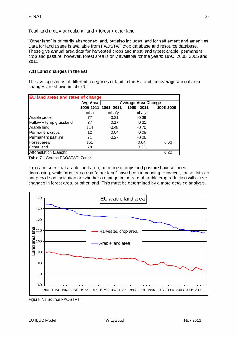
Figure 7.1 Source FAOSTAT

FINAL


25

The EU harvested crop area and arable land area are shown in figure 7.1. This shows that while the harvested crop area has been generally decreasing, it has sometimes increased for short periods in order to build crop stocks. However, the arable land area has continuously decreased over time. The continuous decrease in arable land area in the EU is fairly consistent across all EU Member States. The relationship between changes in harvested crop area and arable land area are shown in table 7.2. Changes in land area per change in arable crop area 1961-2011

Time period 2 yrs 4 yrs 6 yrs

Arable land 0.22 0.45 0.57Fallow + temp grassland -0.78 -0.55 -0.43 Table 7.2 Source FAOSTAT

This shows that short term increases in harvested area are accommodated by reductions in the area of fallow and temporary grassland. For example over 2 yrs the change in arable land area is only 22% of the change in harvested crop area, with a 78% change in fallow and temporary grassland. In the longer term the changes in arable crops area will lead to a higher change in arable land area. However, even over a period of six years only 57% of the change in harvested crop area results in a change in arable land area. Thus short term increase in EU crop output do not cause increase in arable land area, nor give any ILUC change. The changes in other land types as a result of changes in arable land area are shown in table 7.3. Changes in land areas per change in arable land area 1990 - 2011

Time period 6 yrs

Slope Standard error

Permanent crop area -0.04 0.06

Permanent pasture area -0.02 0.14

Forest area -0.02 0.12Other land -0.96 0.23 Table 7.3 Source FAOSTAT

Table 7.3 gives a slope of change in other land per unit change in arable land of -0.96, which shows that reductions in arable land area are primarily related to increases in “other land” area. There is no significant relationship between changes in arable land area and changes in permanent crop area, permanent pasture or forest area. Therefore over multi-year periods, increased EU harvested area for biofuel crops will come from a reduction in the rate of abandonment of arable land to idle land. When idle land reverts to forest, it is important to distinguish between reversion associated with afforestation (where forests are actively planted) and reversions due to natural succession (where land is left idle and may become forested). Work by Zanchi (2007) showed that the average rate of afforestation in the EU from 1995 to 2005 was 0.22 mha/yr. This rate of afforestation is very small compared to the area of “other land” (70 mha in table 7.1), such that only 0.3% of idle land is afforested in any year. Thus the rate of afforestation is limited by the amount of money available to plant forest, not by the amount of idle land available. The rate of afforestation in the EU will therefore not be significantly affected by the rate of planting biofuel crops such as wheat and rape.

FINAL


26

On the basis of this analysis, an increase in EU crop area for biofuel crops will be met in the short term by a reduction in the area of fallow and temporary grassland. In the longer term the extra area will be met by a reduction in the rate of abandonment of arable land. Abandoned land migrates to forest or grassland by natural succession. 7.2) Land changes in other countries The relative changes in land area in relevant countries since 1990 are shown in Table 7.4

Land area changes

Country Arable Forest

European Union -0.11% 0.24%

Canada -0.01% 0.00%

Ukraine -0.10% 0.04%

USA -0.15% 0.04%

Brazil 0.13% -0.33%Argentina 0.20% -0.10%

Average annual change in

total land area 1990 - 2011

Table 7.3 Source FAOSTAT

Table 7.3 shows that in the USA, Canada and Ukraine, arable area has been reducing and forest are has been increasing or static since 1990. Contrary to equilibrium model predictions, there has been no deforestation as a result of increased demand for arable land due to biofuels. FAO data shows that this was still the case since the growth of biofuels production from 2000. Therefore as for the case in the EU, the marginal changes in land demand as a result of biofuels growth have reduced the rate of abandonment of arable land. The split between the proportion of abandoned land that reverts to forest or grassland is based on natural vegetation maps and is shown in table 8.1. Table 7.3 shows that in Brazil and Argentina, there have been increases in arable land and decrease in forest area. This is consistent with other data that increased demand for soybean for animal feed has caused land use changes from forest to cropland. 8) CARBON STOCK CHANGES 8.1) Carbon stocks Data for changes in carbon stock resulting from changes between cropland and grassland or forest for relevant countries are taken from UK RFA guidance information (RFA 2008), which is calculated using IPCC rules. These data for carbon stock changes between cropland and grassland or forest for EU, USA, Canada and Ukraine are shown in table 8.1. The average carbon stock change for cropland reversion for these countries is calculated from these carbon stock changes and the proportion of each type of vegetation that cropland reverts to in each country. For S America where conversion to cropland is taking place, the average carbon stock change is from a combination of data in Heiderer 2010 and JRC IPST 2010. The data in these papers allow calculation of the average carbon stock changes per unit area for different countries and regions.

FINAL


27

C Stock changes

Land Reversion Grassland Forest

Reversion

to forest

Average C

stock change

t C /ha t C /ha t C /ha

Average EU 32 110 50% 71

US 11 95 50% 53

Canada 13 95 100% 95

Ukraine 35 99 0% 35

Land Conversion

Brazil IFPRI 2010 74

Aglink-Cosimo 75

Weightman 70

Argentina Aglink-Cosimo 66

Average S America 71 Table 8.1 Source RFA 2008,

8.2) Land reversion time When increased land for biofuel crops comes from a reduction in the rate of abandonment of arable land, there is no change in carbon stock, but the amount of carbon that would otherwise have been taken up (foregone carbon sequestration) must be accounted for (JRC 2010). When land is converted from pasture or forest to cropland, most of the changes in land carbon stock are irreversible and happen over a relatively short period of time. Under RED rules carbon stock changes from land conversion to cropland are amortised over 20 years. However, when abandoned cropland reverts to grassland or forest by natural succession, the carbon stock on the land accumulates over a long period of time (the land reversion period). If the land is converted back to cropland during this period only the carbon that has built up since abandonment is lost. When recently abandoned land is converted to cropland, or land that would otherwise be abandoned for agricultural use continues to be used as cropland, the reversion time, rather than the amortisation period, must be used for determining the rate of change of carbon stock. From literature (Poulton 2003, Post & Kwon 2000, Broadmeadow 2003), a reversion period of 100 years has been used to account for land use change by natural succession. There is a delay in changes in harvested crop area leading to changes in arable land and also during the initial establishment phase of forests, rates of carbon accumulation are substantially lower than average. However, to keep things simple, the rate of carbon accumulation has been taken to be linear with time, 9) RESULTS The complete calculation of GHG emissions for ILUC for rape biodiesel is shown in the appendix. The calculation is totally transparent from referenced data. The results are summarised in table 9.1.

FINAL


28

Results SummaryRapeseed

biodiesel

Indirect area change

Biofuel crop ha/ TJ biofuel 7.6

Co-product credit ha/ TJ biofuel -9.3

Net area change ha/ TJ biofuel -1.8

ILUC GHG emissions

Biofuel crop kg CO2/GJ 21

Co-product credit kg CO2/GJ -115

Net change kg CO2/GJ -94

Net ILUC credit cf fossil fuel 113% Table 9.1

Since the indirect land area reduction due to co-product crop displacement is greater than the indirect land area increase from growing the biofuel crop, there is a net reduction in the indirect land area. There is a substantial net ILUC credit of 113% of fossil fuel emissions from EU rape biodiesel production. This reduction is due to the ILUC GHG emissions from soy meal displacement by co-products being substantially greater than that those from growing the rape. Although some crop based biofuels may cause adverse GHG emissions from ILUC, EU production of rape biodiesel gives substantial ILUC benefits. It is therefore important to differentiate between different biofuels and production regions when forming policies associated with ILUC. 9.1) Sensitivity to changes Rapeseed import The result for rapeseed biodiesel is sensitive to the proportion of rapeseed grown in the EU and the proportion that is imported.

Impact of rapeseed import

Proportion of marginal rapeseed imported 25% 0

Net ILUC GHG emissions

Biofuel crop kg CO2/GJ 21 11

Co-product credit kg CO2/GJ -115 -118

Net change kg CO2/GJ -94 -107

Net ILUC credit cf fossil fuel 113% 128%

Rapeseed biodiesel

Table 9.2 If EU agriculture can increase rapeseed supply to meet the EU biofuel demand for rapeseed and avoid imports, then the ILUC GHG emissions credit for rape biodiesel would increase to 128% of fossil fuel emissions. Co-product allocation The comparison of accounting for co-products by using an energy allocation approach instead of a substitution approach is shown in figure 9.3. Energy allocation factors are calculated using data in the appendix. All other parameters are the same for both methods.

FINAL


29

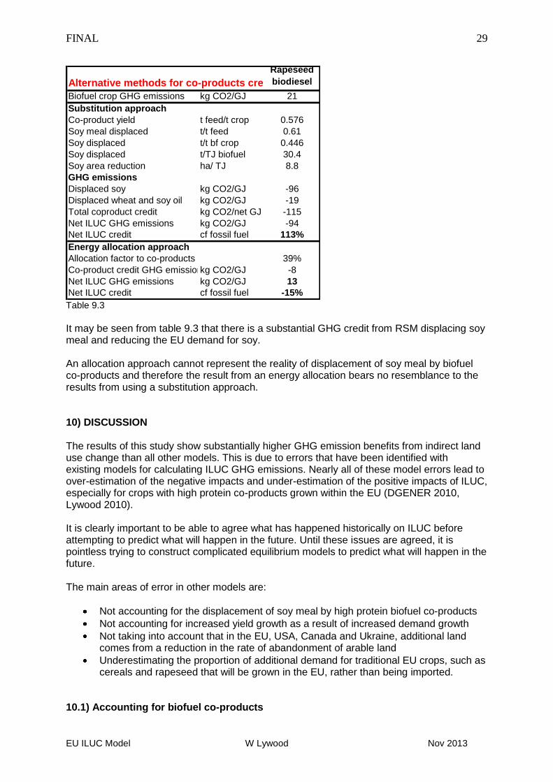
Alternative methods for co-products credit

Rapeseed

biodiesel

Biofuel crop GHG emissions kg CO2/GJ 21

Substitution approach

Co-product yield t feed/t crop 0.576

Soy meal displaced t/t feed 0.61

Soy displaced t/t bf crop 0.446

Soy displaced t/TJ biofuel 30.4

Soy area reduction ha/ TJ 8.8

GHG emissions

Displaced soy kg CO2/GJ -96

Displaced wheat and soy oil kg CO2/GJ -19

Total coproduct credit kg CO2/net GJ -115

Net ILUC GHG emissions kg CO2/GJ -94

Net ILUC credit cf fossil fuel 113%

Energy allocation approach

Allocation factor to co-products 39%

Co-product credit GHG emissionskg CO2/GJ -8

Net ILUC GHG emissions kg CO2/GJ 13

Net ILUC credit cf fossil fuel -15% Table 9.3

It may be seen from table 9.3 that there is a substantial GHG credit from RSM displacing soy meal and reducing the EU demand for soy. An allocation approach cannot represent the reality of displacement of soy meal by biofuel co-products and therefore the result from an energy allocation bears no resemblance to the results from using a substitution approach. 10) DISCUSSION The results of this study show substantially higher GHG emission benefits from indirect land use change than all other models. This is due to errors that have been identified with existing models for calculating ILUC GHG emissions. Nearly all of these model errors lead to over-estimation of the negative impacts and under-estimation of the positive impacts of ILUC, especially for crops with high protein co-products grown within the EU (DGENER 2010, Lywood 2010). It is clearly important to be able to agree what has happened historically on ILUC before attempting to predict what will happen in the future. Until these issues are agreed, it is pointless trying to construct complicated equilibrium models to predict what will happen in the future. The main areas of error in other models are:

Not accounting for the displacement of soy meal by high protein biofuel co-products

Not accounting for increased yield growth as a result of increased demand growth

Not taking into account that in the EU, USA, Canada and Ukraine, additional land comes from a reduction in the rate of abandonment of arable land

Underestimating the proportion of additional demand for traditional EU crops, such as cereals and rapeseed that will be grown in the EU, rather than being imported.

10.1) Accounting for biofuel co-products

FINAL


30

While it is well established that higher protein biofuel co-products such as rape meal and DDGS in the EU displace soy meal (table 4.1), no equilibrium models properly account for soy meal displacement (Lywood 2011) and new model methodologies are being proposed deliberately not to account for soy meal displacement. Different existing and proposed models use a large variety of methods to avoid accounting properly for the displacement of soy meal by EU biofuel co-products:

Not taking account of co-products at all e.g. IFPRI IMPACT and LEITAP (JRC ISPRA 2010)

Only taking account of the energy content of co-products e.g. GTAP, IFPRI MIRAGE 2010 (JRC IPST 2010, JRC ISPRA 2010)

Accepting the protein content is important by then using an arbitrary elasticity coefficient for soy meal displacement that is too low for to give significant soy meal displacement (IFPRI 2011)

Maintaining that soybean is grown primarily for the oil, rather than primarily for the meal e.g. GTAP, IFPRI (JRC IPST 2010, JRC ISPRA 2010, IFPRI 2011)

Assuming that some of the co-product is not used as animal feed (Overmars 2011)

Using an allocation approach, rather than a substitution approach (JRC 2013) In life cycle analyses it is generally accepted that it is better to use a substitution approach, rather than an allocation approach. For example JEC (2011 page 13) states: “We strongly favour this "substitution" method which attempts to model reality by tracking the likely fate of by-products. This approach … is increasingly used by scientists, and is the method of choice in the ISO standards for life-cycle analysis studies. Some other studies have used "allocation" methods whereby energy and emissions from a process are arbitrarily allocated to the various products according to e.g. energy content. Although such allocation methods have the attraction of being simpler to implement they have no logical or physical basis. It is clear that any benefit from a by-product must depend on what the by-product substitutes: all allocation methods take no account of this, and so are likely to give flawed results”. All current equilibrium ILUC models and most simple ILUC models use a substitution approach for co-products. Yet for a new simple model JRC are proposing to use an allocation approach for co-products (Marelli 2013). A similar method has been fed into European Parliament proposed ILUC amendments (Lepage 2013). The allocation approach used for co-products in the calculation of direct GHG emissions in the RED was justified only because it “produces results that are generally comparable with those produced by the substitution method.” (RED 2009). However, for the ILUC GHG emissions calculation able 8.3 shows the two methods give entirely different results. A co-product allocation approach for ILUC GHG emissions is a backward step and cannot be justified.

FINAL


31

11) REFERENCES

Bauen 2010A causal descriptive approach to modelling the GHG emissions associatecwith the indirect land use impacts

of biofuels, E4tech study for UK Dept for Transport, Oct 2010

Broadmeadow

2003

Forests, Carbon and Climate change, the UK contribution, Broadmeadow et al. 2003, for UK Foresrty

Comission

Bruinsma 2009The resource outlook in 2050 - By how much do land, water and crop yields need to increase by 2050, J

Bruinsma, FAO, Jun 2009

CE Delft 2008 CE Delft. Use of by-products from biofuels production. RFA Review of the Indirect Effects of Biofuels.2008.

DefraDefra statistics, https://www.gov.uk/government/publications?departments[]=department-for-environment-food-

rural-affairs&publication_filter_option=statistics

DGAGRI 2011Prospects for Agricultural Markets an Income in the European Union 2010-2020, European Commission,

March 2011. http://ec.europa.eu/agriculture/publi/caprep/prospects2010/fullrep_en.pdf

DGEnergy 2010The impact of land use change on greenhouse gas emissions from biofuels and bioliquids - Literature review,

DGEnergy, July 2010

EurostatSupply, transformation, consumption - renewables (biofuels) - annual data,

http://appsso.eurostat.ec.europa.eu/nui/show.do?dataset=nrg_1073a&lang=en, accessed Feb 2013

FAOSTAT FAOSTAT Crops database [Online] http://faostat.fao.org/site/567/default.aspx, accessed May 2013

FAOSTAT FAOSTAT Trade Database [Online] http://faostat.fao.org/site/406/default.aspx, accessed May 2013

FAOSTAT FAOSTAT Resources database [Online] http://faostat.fao.org/site/405/default.aspx, accessed May 2013

FAOSTAT FAOSTAT Commodity Balances [Online] http://faostat.fao.org/site/614/default.aspx, accessed May 2013

Heiderer 2010Biofuels: A new methodology to estimate GHG emissions from global land use change, Heiderer et al, JRC,

Sep 2010

ICCT 2011Estimating displacement ratios of wheat DDGS in animal feed rations in Great Britain, ICCT, Hazzledine et al,

Nov 2011

IFPRI 2010 Global trade and environmental impact study of the EU biofuels mandate, IFPRI, Mar 2010

IFPRI 2011Assessing the land use change consequence of European biofuel policies. D Labord Oct 2011

http://www.ifpri.org/sites/default/files/publications/biofuelsreportec2011.pdf.

JEC 2011Well-to-Wheels Analysis of Future Automotive Fuels and Powertrains in the European Context, Well-to-tank

report version 3c, CONCAWE, EUCAR & ECJRC, Jul 2011

JRC IPST 2010Impacts of the EU biofuel target on agricultural markets and land use - a comparative modelling assessment,

JRC IPST, 2010

JRC ISPRA 2010a Expert Consultation on:"Critical issues in estimating ILUC emissions", 9-10 November 2010, Ispra, Italy

JRC ISPRA 2010bIndirect land use change from increased biofuel demand - Comparison of models and results from marginal

biofuels production from different feedstocks, JRC Ispra, 2010

Keeney 2005Keeney R and Hertel T (2005) GTAP Technical Paper No. 25 - GTAP-AGR: A Framework for Analysis of

Multilateral Changes in Agricultural Policies [online]

Lepage 2013 Draft Report of the European Parliament Environment Committee on proposal to amend Directive 98/70/EC

LMC Ethanol Monthly Update, LMC International

Lywood 2009aImpact of protein concentrate co-products on the net land requirement for biofuel production in Europe,

Lywood et al, GCB Bioenergy Dec 2009

Lywood 2009bThe relative contributions of changes in yield and land area to increasing crop output, Lywood et al, GCB

Bioenergy Dec 2009

Lywood 2009c

Methodology for evaluation of Indirect Land Use Change from Biofuel crops and estimate of GHG emissions,

Lywood W, Mar 2009

Lywood 2010Issues of concern with models for calculating GHG emissions from indirect land use change, W J Lywood,

Oct 2010

Lywood 2011 Accounting for biofuel co-products in ILUC models: Where has all the protein gone?, W J Lywood Feb 2011

Marelli 2013Methodologies to assess ILUC, Marelli L, JRC, presentation at Workshop on Sustainable biofuels: addressing

ILUC, Feb 2013

Overmars 2011Indirect land use change emissions related to EU biofuel consumption: an analysis of historical data,

Overmars KP, Stehfest E, Ros JPM, Prins AG, j.envsci, Jan 2011

Ozdemir 2009Land substitution effects of biofuel side products and implications on the land area for EU 2020 biofuel

targets. Özdemir ED, Hardtlein M, Wiltrop L (2009), Energy Policy , 37, 2986-2996.

Post and Kwon

2000

Soil carbon sequestration and land-use change processes and potential, Post & Kwon 2000, Global Change

Biology

Poulton 2003Accumulation of carbon and nitrogen by old arable land reverting to woodland. Poulton, P.R., Pye, E.,

Hargreaves, P.R., Jenkinson, D.S., 2003. Glob. Change Biol. 9, 942-955.

Premier 2011 Premier Nutrition Products Ltd. Premier Atlas 2011

RED 2009 Renewable Energy Directive, EC, 26 Mar 2009.

RFA 2008 Carbon &Sustainability Reporting within the RTFO, Technical Guidance, Part 1, UK RFA, Jan 2008

USDA 2010USDA Foreign Agricultural Service, Production, supply and distribution online database

http://www.fas.usda.gov/psdonline/psdhome.aspx , accessed April 2013

Weightman 2010Opportunities for the avoidance of land-use change through substitution of soya bean meal and cereals in

European livestock diets with bioethanol co-products, Weightman et al, ADAS, GCB Bioenergy, July 2010

Winrock 2009 Global GHG emission factors for various land use transients, Winrock International, Mar 2009

Zanchi 2007 Afforestation in Europe, MEACAP, Zanchi et al, Jan 2007

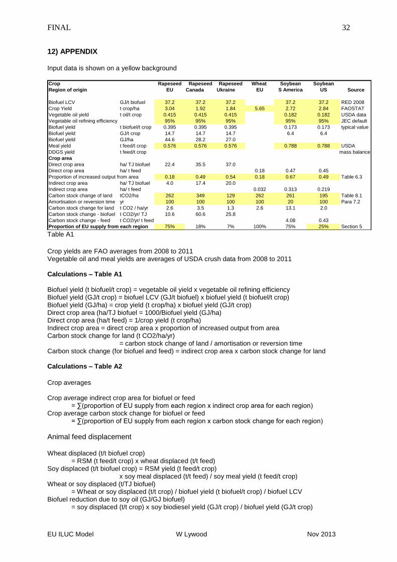
FINAL


32

12) APPENDIX Input data is shown on a yellow background

Crop Rapeseed Rapeseed Rapeseed Wheat Soybean Soybean

Region of origin EU Canada Ukraine EU S America US Source

Biofuel LCV GJ/t biofuel 37.2 37.2 37.2 37.2 37.2 RED 2008

Crop Yield t crop/ha 3.04 1.92 1.84 5.65 2.72 2.84 FAOSTAT

Vegetable oil yield t oil/t crop 0.415 0.415 0.415 0.182 0.182 USDA data

Vegetable oil refining efficiency 95% 95% 95% 95% 95% JEC default

Biofuel yield t biofuel/t crop 0.395 0.395 0.395 0.173 0.173 typical value

Biofuel yield GJ/t crop 14.7 14.7 14.7 6.4 6.4

Biofuel yield GJ/ha 44.6 28.2 27.0

Meal yield t feed/t crop 0.576 0.576 0.576 0.788 0.788 USDA

DDGS yield t feed/t crop mass balance

Crop area

Direct crop area ha/ TJ biofuel 22.4 35.5 37.0

Direct crop area ha/ t feed 0.18 0.47 0.45

Proportion of increased output from area 0.18 0.49 0.54 0.18 0.67 0.49 Table 6.3

Indirect crop area ha/ TJ biofuel 4.0 17.4 20.0

Indirect crop area ha/ t feed 0.032 0.313 0.219

Carbon stock change of land tCO2/ha 262 349 129 262 261 195 Table 8.1

Amortisation or reversion time yr 100 100 100 100 20 100 Para 7.2

Carbon stock change for land t CO2 / ha/yr 2.6 3.5 1.3 2.6 13.1 2.0

Carbon stock change - biofuel t CO2/yr/ TJ 10.6 60.6 25.8

Carbon stock change - feed t CO2/yr/ t feed 4.08 0.43

Proportion of EU supply from each region 75% 18% 7% 100% 75% 25% Section 5 Table A1

Crop yields are FAO averages from 2008 to 2011 Vegetable oil and meal yields are averages of USDA crush data from 2008 to 2011 Calculations – Table A1 Biofuel yield (t biofuel/t crop) = vegetable oil yield x vegetable oil refining efficiency Biofuel yield (GJ/t crop) = biofuel LCV (GJ/t biofuel) x biofuel yield (t biofuel/t crop) Biofuel yield (GJ/ha) = crop yield (t crop/ha) x biofuel yield (GJ/t crop) Direct crop area (ha/TJ biofuel = 1000/Biofuel yield (GJ/ha) Direct crop area (ha/t feed) = 1/crop yield (t crop/ha) Indirect crop area = direct crop area x proportion of increased output from area Carbon stock change for land (t CO2/ha/yr)

= carbon stock change of land / amortisation or reversion time Carbon stock change (for biofuel and feed) = indirect crop area x carbon stock change for land Calculations – Table A2

Crop averages Crop average indirect crop area for biofuel or feed

= ∑(proportion of EU supply from each region x indirect crop area for each region) Crop average carbon stock change for biofuel or feed

= ∑(proportion of EU supply from each region x carbon stock change for each region)

Animal feed displacement Wheat displaced (t/t biofuel crop)

= RSM (t feed/t crop) x wheat displaced (t/t feed) Soy displaced (t/t biofuel crop) = RSM yield (t feed/t crop)

x soy meal displaced (t/t feed) / soy meal yield (t feed/t crop) Wheat or soy displaced (t/TJ biofuel) = Wheat or soy displaced (t/t crop) / biofuel yield (t biofuel/t crop) / biofuel LCV Biofuel reduction due to soy oil (GJ/GJ biofuel)

= soy displaced (t/t crop) x soy biodiesel yield (GJ/t crop) / biofuel yield (GJ/t crop)

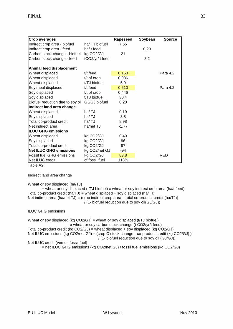
FINAL


33

Crop averages Rapeseed Soybean Source

Indirect crop area - biofuel ha/ TJ biofuel 7.55

Indirect crop area - feed ha/ t feed 0.29

Carbon stock change - biofuel kg CO2/GJ 21

Carbon stock change - feed tCO2/yr/ t feed 3.2

Animal feed displacement

Wheat displaced t/t feed 0.150 Para 4.2

Wheat displaced t/t bf crop 0.086

Wheat displaced t/TJ biofuel 5.9

Soy meal displaced t/t feed 0.610 Para 4.2

Soy displaced t/t bf crop 0.446

Soy displaced t/TJ biofuel 30.4

Biofuel reduction due to soy oil GJ/GJ biofuel 0.20

Indirect land area change

Wheat displaced ha/ TJ 0.19

Soy displaced ha/ TJ 8.8

Total co-product credit ha/ TJ 8.98

Net indirect area ha/net TJ -1.77

ILUC GHG emissions

Wheat displaced kg CO2/GJ 0.49

Soy displaced kg CO2/GJ 96

Total co-product credit kg CO2/GJ 97

Net ILUC GHG emissions kg CO2/net GJ -94

Fossil fuel GHG emissions kg CO2/GJ 83.8 RED

Net ILUC credit cf fossil fuel 113% Table A2

Indirect land area change Wheat or soy displaced (ha/TJ)

= wheat or soy displaced (t/TJ biofuel) x wheat or soy indirect crop area (ha/t feed) Total co-product credit (ha/TJ) = wheat displaced + soy displaced (ha/TJ) Net indirect area (ha/net TJ) = (crop indirect crop area – total co-product credit (ha/TJ))

/ (1- biofuel reduction due to soy oil(GJ/GJ)) ILUC GHG emissions Wheat or soy displaced (kg CO2/GJ) = wheat or soy displaced (t/TJ biofuel)

x wheat or soy carbon stock change (t CO2/yr/t feed) Total co-product credit (kg CO2/GJ) = wheat displaced + soy displaced (kg CO2/GJ) Net ILUC emissions (kg CO2/net GJ) = (crop C stock change - co-product credit (kg CO2/GJ) )

/ (1- biofuel reduction due to soy oil (GJ/GJ)) Net ILUC credit (versus fossil fuel)

= net ILUC GHG emissions (kg CO2/net GJ) / fossil fuel emissions (kg CO2/GJ)

Estimate of ILUC impact of EU rapeseed biodiesel based on ...

Documents