- i - Establishment of Appropriate Guidelines for Use of the Direct and Indirect Design Methods for Reinforced Concrete Pipe Prepared for: AASHTO Standing Committee on Highways Prepared by: Ian D. Moore, Neil A. Hoult and Katrina MacDougall Queen`s University Department of Civil Engineering, 58 University Avenue, Kingston, ON, K7L 3N6 Canada March 2014 The information contained in this report was prepared as part of NCHRP Project 20-07, Task 316, National Cooperative Highway Research Program. SPECIAL NOTE: This report IS NOT an official publication of the National Cooperative Highway Research Program, Transportation Research Board, National Research Council, or The National Academies.

Welcome message from author
This document is posted to help you gain knowledge. Please leave a comment to let me know what you think about it! Share it to your friends and learn new things together.
Transcript

- i -
Establishment of Appropriate Guidelines for Use of the Direct and Indirect Design Methods for Reinforced
Concrete Pipe
Prepared for:
AASHTO Standing Committee on Highways
Prepared by:
Ian D. Moore, Neil A. Hoult and Katrina MacDougall
Queen`s University
Department of Civil Engineering, 58 University Avenue, Kingston,
ON, K7L 3N6 Canada
March 2014
The information contained in this report was prepared as part of NCHRP Project 20-07, Task 316, National Cooperative Highway Research Program.
SPECIAL NOTE: This report IS NOT an official publication of the National Cooperative Highway
Research Program, Transportation Research Board, National Research Council, or The National Academies.

- ii -
Acknowledgements
This study was requested by the American Association of State Highway and
Transportation Officials (AASHTO), and conducted as part of National Cooperative
Highway Research Program (NCHRP) Project 20-07. The NCHRP is supported by
annual voluntary contributions from the state Departments of Transportation. Project 20-
07 is intended to fund quick response studies on behalf of the AASHTO Standing
Committee on Highways. The report was prepared by Ian Moore, Neil Hoult, and
Katrina MacDougall of Queen’s University. The work was guided by a task group
included Henry Cross (South Carolina DOT), Cecil L. Jones (Diversified Engineering
Services, Inc.), Michael G. Katona (Washington State University), Thomas P. Macioce
(Pennsylvania DOT), John J. Schuler(Virginia DOT), Scott A. Anderson (Federal
Highway Administration), and Josiah W. Beakley (American Concrete Pipe Association).
The project was managed by Waseem Dekelbab, NCHRP Senior Program Officer.
Disclaimer
The opinions and conclusions expressed or implied are those of the research agency
that performed the research and are not necessarily those of the Transportation
Research Board or its sponsoring agencies. This report has not been reviewed or
accepted by the Transportation Research Board Executive Committee or the Governing
Board of the National Research Council.
3
TABLE OF CONTENTS
SUMMARY ....................................................................................................................... 5
CHAPTER 1 BACKGROUND ............................................................................................. 7
CHAPTER 2 RESEARCH APPROACH .............................................................................. 8
CHAPTER 3 FINDINGS AND APPLICATIONS .................................................................. 9
3.1 Introduction ................................................................................................................. 9 3.2 Literature review and overview of the two design methods ......................................... 9
3.2.1 Introduction ..................................................................................................... 9 3.2.2 Early Theories .............................................................................................. 10 3.2.3 Pipe Design Developments of Heger and his coworkers ............................... 11 3.2.4 Common Elements of Pipe Design ............................................................... 12 3.2.5 Indirect Design Method ................................................................................. 14 3.2.6 Direct Design Method ................................................................................... 15 3.2.7 Pipe Loading ................................................................................................. 16 3.2.8 Pressure Distributions ................................................................................... 19 3.2.9 Comparison of Indirect and Direct Design ..................................................... 20 3.2.10 Experimental evidence of earth pressures or bending moments ................. 23 3.2.11 Advantages and disadvantages of Indirect Design and Direct Design ......... 24 3.2.12 Conclusions ................................................................................................ 26
3.3 Laboratory tests on small and medium sized reinforced concrete pipes .....................27 3.3.1 Introduction and Objectives .......................................................................... 27 3.3.2 Experimental Program .................................................................................. 28 3.3.3 Results and Discussion................................................................................. 42
3.4 Comparison of experimental results and design calculations .....................................56 3.4.1 Introduction ................................................................................................... 56 3.4.2 Live load moment ......................................................................................... 57 3.4.3 Limit States Tests ......................................................................................... 61 3.4.4 Comparisons to Design Estimates ................................................................ 62
3.5 Potential changes to Direct Design procedures ..........................................................70 3.5.1 Pipe geometries considered during the parametric study. ............................. 70 3.5.2 PipeCar calculations ..................................................................................... 70 3.5.3 Calculations using RESPONSE .................................................................... 72 3.5.4 Modified compression field theory for estimation of shear capacity ............... 74 3.5.5 Possible inclusion of strain-compatibility calculations in PipeCar .................. 75 3.5.6 Adjustment of expected moments to account for thick ring theory ................. 85 3.5.7 Potential consideration of plastic collapse mechanism .................................. 86
3.6 Comparison of Steel Requirements from the Indirect and Direct Design Methods......87 3.6.1 Introduction ................................................................................................... 87 3.6.2 Current differences for pipes under deep burial ............................................ 87 3.6.3 Proposed modification to account for thick ring theory .................................. 89 3.6.4 Possible modification to account for strain hardening of the reinforcing steel 89 3.6.5 Proposed modification to employ Modified Compression Field Theory ......... 90 3.6.6 Relative impact of different potential changes to Direct Design ..................... 90 3.6.7 Conclusions .................................................................................................. 91
3.7 Usage guidelines and Design specifications ............................................................ 100 3.7.1 Overview .................................................................................................... 100
4
3.7.2 Usage of Indirect Design and Direct Design ................................................ 101 3.7.3 Modification of Expected Moments During Direct Design to Account for Thick Ring Theory ......................................................................................................... 101 3.7.4 Modification of Moment Capacity During Direct Design to Employ Modified Compression Field Theory ................................................................................... 101 3.7.5 Modification of Load Spreading to Consider Depth to Crown, Springline and Invert ................................................................................................................... 101
CHAPTER 4 CONCLUSIONS AND SUGGESTED RESEARCH .................................... 102
ACKNOWLEDGEMENTS ...................................................................................................... 106
REFERENCES ................................................................................................................... 107
APPENDIX A Thick ring theory ......................................................................................... .A-1
APPENDIX B Plastic collapse .......................................................................................... .B-1
APPENDIX C Measurement of crack widths using PIV .................................................... C-1
APPENDIX D Proposed Usage Guidelines and Other Recommended Changes ............ D-1
5
SUMMARY
The performance of Indirect Design and Direct Design procedures for structural design of
reinforced concrete culverts was investigated. Tests performed on three 24 in. diameter and two
48 in. diameter pipes revealed that the Indirect Design procedure leads to safe load capacity
estimates, ranging from 54% to 81% of those observed in the buried pipe tests. Direct Design
calculations for those tests were also safe, with calculated load capacity falling between 19%
and 77% of the observed values. Furthermore, Direct Design estimates of expected moment
arising from the effects of surface loads on shallow buried pipes were between 3 and 4 times
higher than those calculated from strains measured during the experiments.
Semi-empirical design procedures like Indirect Design would normally be expected to produce
larger areas of required steel than design procedures based on rational assessments of
expected moment and moment capacity (like the calculations performed as part of the Direct
Design Method). As observed by others previously, the steel requirements calculated using
Direct Design for small diameter reinforced concrete pipes can actually be greater than those
that arise from Indirect Design. Various simplifications associated with Direct Design estimates
of moment capacity were examined, and it was found that these discrepancies between Direct
Design and Indirect Design outcomes can largely be addressed by using a ‘thick ring’ moment
adjustment factor to eliminate conservatism associated with thin ring theory, and by using
Modified Compression Field Theory to employ more sophisticated approximations for the
concrete response and to enforce compatibility between the steel reinforcing and the concrete.
Since these two techniques can be used to eliminate the larger estimates of steel area that may
otherwise arise from the Direct Design of small diameter pipes, and since both design methods
were found to produce safe designs, there appears to be no need for guidelines that restrict use
of either of the design procedures for pipes of specific diameter or burial depth.
Three changes to the AASHTO LRFD Bridge Design Specifications are recommended: the
introduction of a simple adjustment factor to eliminate conservatism associated with thin ring
theory, the introduction of commentary indicating that the evidence collected during this
research project supports a free choice by the designer regarding which design method to
employ, and the introduction of commentary which suggests that Modified Compression Field
Theory can be used to obtain more sophisticated estimates of flexural and shear capacity during
Direct Design. A change is also suggested regarding the calculation of load spreading below
surface loads. Calculations of surface load effects at the crown should continue to employ the

6
depth of burial to the top of the pipe, but calculations for surface load effects on springline and
invert moments could consider load spreading from the surface to the depth of burial of the
springline and invert, respectively.

7
CHAPTER 1 BACKGROUND
Currently, in the AASHTO LRFD Bridge Design Specifications, reinforced concrete pipe can be
designed according to one of two methods; the indirect design method or the direct design
method. The Indirect Design Method uses tables to select the appropriate pipe class (thickness,
reinforcement, and concrete strength) for a given fill height and installation type. The method is
based on three-edge-bearing tests and observed crack widths. The Direct Design Method is a
more theoretical design method where four separate structural design limit states are
considered: flexure, thrust, shear (diagonal tension), radial tension, and crack control. These
two methods may give different answers for design of equivalent pipe, depending upon size,
loading and installation requirements. The Indirect Design Method is based on a comparison of
field moments versus test moments. The Direct Design Method has simplifying assumptions for
reinforcement conditions, as well as limitations on the steel and concrete properties that may
not allow for a pipe to be designed to its true strength. There has been uncertainty regarding the
relative performance of both methods, whether they both produce safe designs for all situations,
and which method is most appropriate for specific pipe sizes and burial depths, to eliminate
unneeded expense. Recent suggestions for determining appropriate guidelines for which design
method to use have ranged from taking the lower steel area requirement of the two designs, to
using the Direct Design Method for pipes with an inner diameter larger than 36” and the Indirect
Design Method for pipes 36” and smaller.
Objectives
The objectives of this research are to:
(1) review the strengths and weaknesses of the Indirect and Direct Design methods and
compare their design outcomes (e.g. the areas of steel required for specific loading
conditions);
(2) conduct tests that permit evaluation of the performance of the two design methods
relative to measurements of demand (the loads that develop) and resistance (the ability
of the reinforced concrete test pipes to resist those demands);
(3) produce guidance regarding when each method is most appropriate, and possible
revisions to make their design outcomes more consistent (including revisions to the
AASHTO LRFD Bridge Design Specifications, Section 12).

8
CHAPTER 2 RESEARCH APPROACH
The project was divided into various tasks:
- a literature search to review the development of both design methods and to
summarize the strengths and weaknesses of the two procedures
- testing of small and medium diameter pipes to compare observed performance with
calculations according to Section 12 of the AASHTO LRFD Bridge Design Specifications
- work clarifying how both the service limit states and strength limit states apply to the
Indirect and Direct Design Methods in Section 12.10, to determine the reasons for differences
on outcomes from the two design procedures, and to prepare draft guidelines for when a
particular method may or may not be appropriate
- evaluation of potential changes to ultimate strength calculations during Direct Design
so the two methods might produce more similar design outcomes
- draft revisions to Section 12 of the AASHTO LRFD Bridge Design Specifications so
that both design methods more closely correlate
- identification of future research or immediate implementation if sufficient data already
exists
- preparation of this final report describing the entire research effort.
The research agency is Queen’s University (QU).

9
CHAPTER 3 FINDINGS AND APPLICATIONS
3.1 Introduction
The research findings are presented in the six following areas:
• An overview of the literature review and the two design methods, discussing their pros
and cons, their treatment of limit states, and previous studies examining their relative
performance;
• A description of the experimental work performed on small and medium sized reinforced
concrete pipes;
• A comparison of the experimental results and design calculations to gage the current
level of safety associated through comparisons of design calculations with observed
performance;
• The investigation of potential changes to the Direct Design procedures for estimating
ultimate moment capacity;
• A comparison of the steel requirements calculated using Direct Design and Indirect
Design, considering the current specifications and the effect of potential changes to
those specifications;
• A discussion of when to use Direct and Indirect Design, and proposed changes to the
AASHTO LRFD Bridge Design Specifications.
3.2 Literature review and overview of the two design methods
3.2.1 Introduction
Before the 19th century, little work was performed developing the theory of pipe design. Brown
(2002) presents a history of pipe-flow equations showing work in the development of flow
equations as early as 1770 by Antoine Chezy. In the 1900’s, as cities grew and the demand for
concrete pipes increased, so did the need for a standardized method of design to ensure the
adequate strength of pipes. With the addition of steel reinforcement to concrete pipe walls
around 1900, pipes were able to reach higher capacities and work began to determine the
strength required by these pipes (Ontario Concrete Pipe Association, 2011). The following
literature review outlines the development of pipe design theory beyond 1900, and discusses
the two current methods of pipe design: the Indirect Design Method and the Direct Design
Method. It also summarizes the current implementations of the two design methods as well as
10
previous research performed to evaluate and compare them. The review discusses studies of
both demand (the loads that develop on a buried rigid pipe) and the resistance (the ability of the
pipe to support the demand). The equations presented below are taken from the American
Association of State Highway and Transportation Officials LRFD Bridge Design Specifications
(2007) subsequently referred to as AASHTO LRFD Bridge Design Code. The acronym LRFD
stands for Load and Resistance Factor Design.
3.2.2 Early Theories
In the early 1900’s Marston developed a load theory to assess rigid pipes in the ground by first
analyzing their behavior in trench conditions. Marston used the theory of Janssen (1895) for
pressures in silos to develop his own theory in relation to pipes. He defined the gravity loading
on the pipe as the column of soil above the crown of the pipe across the width of the trench
excavation. This force was modified to account for the friction forces transferred across the
vertical planes on the sides of the trench (shear on the interfaces between the column of soil
and the undisturbed soil, Zhao and Daigle, 2001). Factors in Marston’s load equation include
the soil’s specific weight and type, the external diameter of the pipe and the trench width, and
soil parameters unit weight, coefficient of lateral earth pressure, and frictional strength along the
sides of the trench.
Marston also developed equations for the embankment condition, where he proposed that the
prism of soil overlying the pipe can be considered to have sides rising vertically upwards from
the pipe springlines, and these also transfer load to or from the surrounding soil by means of
friction (depending on whether the pipe is more compressible or less compressible that the soil
beside it, respectively).In 1932, Schlick, a colleague of Marston, developed an equation to
define the critical width at which point the trench burial load equation no longer applied and an
embankment load equation had to be employed (Moser, 2001). This width is known as the
transition width; the point where the weight of the soil column overlying a pipe in a wide trench is
equal to the embankment load.
Spangler (1933) later developed three installation conditions using Marston’s earth load theory
and worked to determine the strength of buried rigid pipe that was required to support the
predicted load. Spangler developed ratios, known as bedding factors, which related the cracking
load in buried rigid pipe installations to the cracking load in three-edge bearing tests. The
cracking load is reached when cracks of width measuring 0.01-in.at the inner or outer surface of
11
the pipe begin to form (ASTM C76-11). Bedding factors were developed for trench and
embankment conditions. However the trench bedding factor excluded the effects of lateral
pressure from the soil onto the pipe, and the embankment bedding factor only partially included
lateral pressure. The bedding conditions defined were developed to suit analysis and not ease
of construction (Concrete Pipe Design Manual, 2011).
3.2.3 Pipe Design Developments of Heger and his coworkers
In the 1970’s the American Concrete Pipe Association (ACPA) sponsored a research project
undertaken by Frank Heger and his colleagues from Simpson Gumpertz & Heger Inc. that
resulted in the Soil Pipe Interaction Design and Analysis (SPIDA) program. The development of
SPIDA was based on a number of research initiatives. Heger and McGrath (1980) presented a
design method that includes considerations for flexural strength involving reinforcement tension,
concrete compression, concrete radial tension, stirrup radial tension, and diagonal tension.
Limiting crack width of 0.01-inch was defined as a serviceability limit. Heger (1982) then
presented a new structural design method for reinforced concrete pipe based on extensive tests
performed on pipes, box sections, slabs and curved slabs. Additionally, Heger and McGrath
(1982) discussed use of new semi-empirical equations for the shear strength of pipe and
suggested how the shear design equations used at that time did not accurately assess shear
strength in pipe. Further work examining radial tension strength of pipes by Heger and McGrath
(1983) presented equations to predict radial tension strength from tests subjecting the inside
face of the curved member to flexural tension. These results were empirically determined from a
limited number of three edge bearing tests.
Heger and McGrath (1984) then studied crack widths during a number of tests on pipes, box
sections, straight and curved slabs, and suggested that other crack widths might be appropriate
(the use of crack width of 0.01-in as a serviceability limit was seemingly an arbitrary choice with
limited data connecting it to pipe durability). They presented design equations and a control
factor that permits consideration of various different crack widths, and these were incorporated
into the 1983 AASHTO Bridge Specification. Heger and Liepens (1985) examined the stiffness
of flexurally cracked reinforced pipe. They used correlations between computed and measured
deflections of pipe under three edge bearing and developed coefficients for calculation of wall
stiffness that were incorporated into the SPIDA program. In 1988, using SPIDA to run various
simulations, Heger developed a new idealized pressure distribution defining soil loads around
the circumference of concrete pipes, and recommended five new standard installation types.
12
Heger’s new pressure diagram differed from earlier established theories, and included the effect
of voids or zones of low stiffness backfill that often occur under the pipe haunches. Although the
results were based on limited field tests to support the theoretical calculations, other
researchers have reported test results that support Heger’s earth pressure distributions (e.g.
Wong et al. 2006).
3.2.4 Common Elements of Pipe Design
Introduction
Indirect Design is based on using the results of three-edge bearing tests and empirical ‘bedding
factors’ to consider the impact of burial on the load capacity. Direct Design was developed from
the finite element method (FEM) as discussed later in this section, and employs analysis of soil
and other loads to determine moment, thrust and shear in the pipe. Despite the differences in
loading analysis, certain aspects of pipe design are common to both approaches.
Installation Types
The original installation types were based on the early work of Marston (1913) and Spangler
(1933), however more recent research has led to modified installation types. The research
performed by Heger (1988) used a number of different simulations to develop the four Standard
Installation Direct Design (SIDD) installation types currently considered: Type I (highest quality),
Type II (lower quality), Type III (least quality), and Type IV (no quality control). These installation
conditions are used in both Indirect and Direct Design and as outlined in Table 1.
Concrete pipe analyses
Three computer analyses were developed in support of Direct Design by Heger and his
collaborators:
1. Soil Pipe Interaction Design and Analysis Program (SPIDA) – a finite element analysis
which explicitly models the soil, the pipe, and their interaction;
2. Standard Installation Direct Design (SIDD) – a structural analysis of the pipe ring using
the Heger soil pressure distributions to determine the moments, thrusts, and shears;
3. PIPECAR –employing moment, thrust and shear factors associated with the four
standard installation types, pipe self-weight, fluid, earth and vehicle loads.
13
Table 1. Standard embankment installation soils and minimum compaction requirements from
AASHTO LRFD Bridge Design Code Table 12.10.2.1-1.
Vertical Arching Factor
The vertical arching factor (VAF) is used to account for the manner in which load redistributes
within the soil as a result of the stiffness of the pipe relative to the stiffness of the soil
surrounding it. While the original concept of arching was based on Marston’s application of the
Janssen silo theory, similar arching factors can be calculated using elastic soil-pipe interaction
analyses like those of Burns and Richard (1964) and Hoeg (1968). The VAF varies depending
on the type of installation which influences the stiffness of the soil around the pipe. VAF is used
in both Indirect and Direct Design and is outlined in Table 12.10.2.1-3 in the AASHTO LRFD
Bridge Design Code and presented here in Table 2.
Table 2. Vertical arching factor from AASHTO LRFD Bridge Design Code Table 12.10.2.1-3
Installation Type VAF
Type 1 1.35
Type 2 1.40
Type 3 1.40
Type 4 1.45

14
3.2.5 Indirect Design Method
The Indirect Design Method, the most commonly used approach for concrete pipe design
(Erdogmus and Tadros, 2006), incorporates aspects of Marston and Spangler’s research with
modern changes implemented based on the work of Heger and his research collaborators. A
standard positive projection embankment loading condition is used as it is conservative for
every type of burial condition (AASHTO LRFD 12.10.2.1). The weight of soil above the pipe is
then multiplied by the VAF and added to the fluid load carried by the pipe. The total live load is
then calculated and kept separate. The two load totals are then divided by their respective
bedding factors and summed. The bedding factors for circular pipes are given in Table
12.10.4.3.2a-1 of the AASHTO LRFD Bridge Design Code and presented here in Table 3.
Additionally, there are also bedding factors specifically provided for live loads in Table
12.10.4.3.2c-1 of the AASHTO LRFD Bridge Design Code. Bedding factors quantify the
relationship between three-edge bearing test loads and field loading behavior. As described in
the American Concrete Pipe Design manual, modern bedding factors for Standard Installations
are based in reinforced concrete design theory and on a parametric study performed using
SIDD. The resulting total is then multiplied by a safety factor and divided by the pipe diameter
as per Equation 1.
𝐷𝐿𝑜𝑎𝑑 = ��𝑊𝐸+𝑊𝐹𝐵𝑓
� + 𝑊𝐿𝐵𝐿𝐿� × 𝐹.𝑆.
𝐷𝑖 1
The resulting value, known as a D-Load, is then used to determine the class of pipe from tables
in ASTM C76 (2011).
Table 3. Bedding Factors, Embankment Conditions, Bfe from AASHTO LRFD Bridge Design
Code Table 12.10.4.3.2a-1
Pipe Diameter Type 1 Type 2 Type 3 Type 4
12 in. 4.4 3.2 2.5 1.7
24 in. 4.2 3.0 2.4 1.7
36in. 4.0 2.9 2.3 1.7
72in. 3.8 2.8 2.2 1.7
144in. 3.6 2.8 2.2 1.7
There are five class types categorized into tables by 0.01in cracking capacity and ultimate
capacity. Each table is used to determine the amount of reinforcing steel required for a
specified pipe diameter, wall thickness and concrete strength to support the calculated loads.
15
ASTM C76 provides no specifications for shear reinforcement but the use of shear
reinforcement is not common in pipe design, Erdogmus and Tadros (2006).
3.2.6 Direct Design Method
Introduction
As indicated earlier, the Direct Design Method was developed using the finite element analysis
program SPIDA created by Heger and his colleagues in the 1970’s. This research project also
resulted in “ASCE 15-98: Standard Practice for Direct Design of Buried and Precast Concrete
Pipe Using Standard Installation”, which introduced the four standard installations as described
earlier. The Direct Design Method uses the same approach as the Indirect Design Method
specified by the American Association of State Highway and Transportation Officials (AASHTO)
to select installation type, and then for a given pipe diameter and wall thickness, calculate
vertical earth load, fluid load and live load. However, instead of using bedding factors and tables
to determine the amount of reinforcing steel (the Indirect Design approach), the Direct Design
Method requires thrust, shear and moment values to be determined and used to calculate steel
requirements based on conventional theories for design of reinforced concrete to withstand
flexure (Concrete Pipe Design Manual, 2011). A table of coefficients was developed and
presented in ASCE 15-98 that simplify the calculation of the moment, thrust, and shear acting
on the pipe. These coefficients are presented as Cmi, Cni, Cvi (their use is discussed further in a
subsequent section). Strength reduction factors are also included in the design including factors
for flexure, diagonal tension, radial tension and limiting crack width.
Design for Flexure
After moment and thrust acting on the pipe are calculated they are used in Equation 2 to
determine the amount of circumferential steel required.
𝐴𝑠 = 𝑔𝜑𝑑 − 𝑁𝑢 −�𝑔[𝑔(𝜑𝑑)2−𝑁𝑢(2𝜑𝑑−ℎ)−2𝑀𝑢]
𝑓𝑦≥ 0.07 2
The AASHTO LRFD Bridge Design Code provides a ratio to determine the amount of outside
steel needed from the amount of steel calculated for the inside layer. In addition, the code
provides equations for minimal requirements of steel to withstand flexure and shear. The
minimum amount of steel allowed for any case is 0.07in2/ft.
16
Design for Shear
The AASHTO LRFD Bridge Design Code provides equations for design in shear both with and
without stirrups. Pipe sections are investigated at the critical section where Mnu / Vu d =3.0.
Factored shear resistance Vr, for shear without stirrups, is found using Equation 3 where Vn is
found using Equation 4.
𝑉𝑟 = 𝜑𝑉𝑛 3
𝑉𝑛 = 0.0316𝑏𝑑𝐹𝑣𝑝�𝑓𝑐′(1.1 + 63𝜌) �𝐹𝑑𝐹𝑛𝐹𝑐� 4
The equations for variables in Equation 4 can be found in section 12.10.4.2.5 of the AASHTO
LRFD Bridge Design Code, as well as additional equations for reinforcement requirements
including expressions for flexural reinforcement and reinforcement for crack width control.
3.2.7 Pipe Loading
Dead Loading
For both Indirect and Direct Design, the methods for calculating fluid load and earth load are the
same. The fluid load is calculated from the internal volume of the pipe per unit length and the
density of water at 62.4 pcf as shown in Equation 5. The earth load is calculated from the soil
column method originally developed by Marston (1913). A VAF based on installation type is
selected and multiplied by the prism load of the soil column as shown in Equation 6. The pipe
load is calculated for the direct design method per unit length, as shown in Equation 7, from the
volume of concrete and density of concrete typically taken to be 150 pcf. However, the pipe load
is not included in the Indirect Design Method as it is “approximately accounted for by the weight
of the pipe acting in the 3-edge bearing test load condition” (Heger et al., 1985).
𝑊𝐹 = 𝜋𝑟𝑖2 ∙ 𝛾𝑤 5
𝑊𝐸 = 𝑉𝐴𝐹 ∙ 𝑃𝐿 = 𝑉𝐴𝐹 ∙ 𝛾𝑠[𝐻 + 0.0089𝐷0] 𝐷012
6
𝑊𝑃 = 𝜋(𝑟02 − 𝑟𝑖2) ∙ 𝛾𝑐 7
Live Loading
The effect of live load on the buried pipe is calculated by using the “worst-case” scenario of: (i) a
single dual wheel loading of the AASHTO design truck, (ii) two single dual wheels of AASHTO
design trucks in passing mode at a distance of 4ft apart, (iii) or two single dual wheels of two
alternate load vehicles in passing mode. The “worst-case” is dependent on the direction of
vehicular travel, pipe diameter and depth of cover. The details of loading case selection are

17
shown in Table 4. The downward distribution of load governed by the Live Load Distribution
Factor (LLDF) has been modified since the SIDD design method from 1.75 to 1.15. ASCE 15-98
originally specified a LLDF of 1.75 but it was later found that a more conservative value of 1.15
for select-granular and 1.00 for any other soil was more appropriate (Standard Practice for
Direct Design of Buried and Precast Concrete Pipe Using Standard Installation, 1998) (Concrete
Pipe Design Manual, 2011). In addition, the spacing between passing design trucks has been
modified from 6ft in ASCE 15-98 to 4ft in the AASHTO LRFD Bridge Design Code (2011)
creating a more critical loading case at shallower depths due to the interaction between load
spread areas. The live load spreading for a single wheel load is illustrated in Figure 1a while the
load spreading diagrams for multiple vehicles are given in Figures 1b and 1c. Very recently, the
live load distribution factor was adjusted for concrete pipes as a result of the finite element
analysis work of Petersen et al. (2010), so that for pipes of diameter less than 24 in., LLDF is
1.15, for pipes greater than 96 in, it is 1.75, and between 24 in. and 96 in. in diameter, it is
expressed as a linear function of internal diameter Di
𝐿𝐿𝐷𝐹 = 0.00833.𝐷𝑖 + 0.95 8
Although the ASCE 15-98 suggested that an impact factor (IM) not be used in live load
calculations, it has been included in the AASHTO LRFD Bridge Design Code (2011). This factor
accounts for the dynamic force of the moving design truck on the pipe (associated with the
vehicle hitting a pothole or other pavement irregularity). Furthermore, a multiple presence factor
(MPF) is outlined in the AASHTO LRFD Bridge Design Code, which is used to account for the
magnitude of truck loads when one or multiple lanes are occupied. When designing for a single
truck in one lane an MPF of 1.2 is used. This factor is reduced to 1.0 for two trucks passing as it
is unlikely that two overloaded trucks pass at the same instant. The truckload is divided by the
spread area, in Figure 1, to determine the full distribution of the load into the soil and increased
by the factors accounting for truck movement and overloading. Finally, the load is multiplied by
the lesser of the pipe diameter or the governing load length (Equations 9 and 10) to account for
the load distributed directly to the pipe as indicated in Equation 11 (Petersen et al., 2010).

18
Table 4. Critical Wheel Loads and Spread Dimensions at the Top of the Pipe (ACPA, 2011)
(a) (b)
(c)
Figure 1: Spread Load Area - (a) Single Dual Wheel (b) Two Single Dual Wheels of AASHTO
Design Trucks in Passing Mode (c) Two Single Dual Wheels of Two Alternate Loads in Passing
Mode (ACPA, 2011)
19
𝐿𝑡𝑔𝑜𝑣 = 𝑙𝑡12
;𝑓𝑜𝑟 𝐻 < 0.833 9
𝐿𝑡𝑔𝑜𝑣 = 𝑙𝑡12
+ 𝐿𝐿𝐷𝐹𝑖 ∙ 𝐻;𝑓𝑜𝑟 𝐻 ≥ 0.833 10
𝑊𝐿 = 𝑀𝑃𝐹 ∙ (1 + 𝐼𝑀) ∙ � 𝑃(1.67+1.15𝐻)(0.83+1.15𝐻)
� ∙ min �𝐷𝑖12
, 𝐿𝑡𝑔𝑜𝑣� 11
Design Forces
After determining the dead load, live load, fluid load and pipe load, the loads in combination with
the installation coefficients, given in the ASCE 15-98, are used to find the moment, thrust and
shear in the pipe at the crown, invert, springlines and critical shear locations as per Equations
12 to 14.
𝑀𝑖 = ∑𝐶𝑚𝑖𝑊𝑖 𝐷𝑖2
12
𝑁𝑖 = ∑𝐶𝑛𝑖𝑊𝑖 13
𝑉𝑖 = ∑𝐶𝑣𝑖𝑊𝑖 14
The loading coefficients (Cmi, Cni, Cvi) used to calculate the moment, thrust and shear on the
pipe in Equations 12 to 14 are based on the pressure distributions developed by Heger in his
research studies (Heger, 1988).
3.2.8 Pressure Distributions
In the concrete pipe design software package PIPECAR, there are additional pressure
distribution options that have been previously used in Direct Design: (i) the Paris distribution,
and (ii) the Olander distribution. The uniform pressure distribution presented by Paris (1921)
uses different uniform pressures along the top, sides and bedding of the pipe. The method also
requires a soil-structure interaction and lateral pressure coefficient as well as bottom reaction
widths for soil, water and live loading as well as pipe weight loading conditions (Simpson
Gumpertz & Heger Inc., 2004). The radial pressure distribution presented by Olander (1950)
uses two pressure bulbs to represent the pressure distribution on the pipe. Both these pressure
distributions can be used in place of the pressure distribution by Heger in PIPECAR when
analyzing loading on the pipe. As described in the AASHTO LRFD Bridge Design Code Section
C12.10.4.2.1, the design equations are applied after the moment, thrust and shear are
determined, and so design is not limited to any one assumed pressure distribution and any one
of the acceptable pressure distributions can be used.

20
PIPECAR also employs a modified version of live load spreading, where LLDF=1.15 to the pipe
crown, and then by LLDF=1.75 to a depth of ¾ of the way to the pipe invert. As a result, Direct
Design calculations performed using PIPECAR satisfy neither the 2007 or 2013 versions of the
AASHTO LRFD Bridge Design Specifications.
3.2.9 Comparison of Indirect and Direct Design
Erdogmus and Tadros (2006) present a comparison between Indirect and Direct Design
outlining both the more conservative and less conservative nature of the two design methods as
illustrated in Figure 2. Performing a parametric study for 48-in diameter pipes, they work to
establish governing failure types, flexure, crack control and shear, similar to the controlling
criteria summarized by Figure 3 from ASCE 15-98. The steps seen in the Indirect Design
represent the changes in pipe class from Class II at the lowest step to Class V at the highest;
each step signifying an increase in D-load of the pipe. Erdogmus et al. (2010) also state that
Direct Design provides a unique and conservative design. Indirect Design is an empirical
method where required steel reinforcement does not vary progressively with depth of cover, but
instead increases in finite steps.
Erdogmus and Tadros (2009) indicate that when buried, both the inner and outer reinforcement
layers in the pipe are in tension which is not reflected in the Direct Design method, leading to
over-conservatism in some cases. Also, the differences become more evident in pipes smaller
than 36in where there is only a single cage of reinforcement and behavior becomes more
complex.
The Direct Design Method allows the inputs to be varied (concrete strength, steel reinforcement
and crack control factor) in order to develop an optimum design. Erdogmus and Tadros (2006)
found that varying the steel strength had almost no effect on the capacity of the pipe where
flexure controls and none where cracking and shear govern (based on the assumption that
stirrups are not considered part of normal pipe design and thus were not present). The crack
control factor presented in Section 12 of the AASHTO LRFD Bridge Design Code indicates the
probability of a crack of a specified maximum width occurring. By changing the crack control
factor from between acceptable levels of 0.7 to 1.3 it was found that between the generally used
factor of 0.9 and a more conservative 1.3 there was little difference in the design of the pipe
(though when crack control is the governing limit state, an increase in the factor will decrease
steel area requirements). Erdogmus and Tadros (2006), performing an investigation for the
21
Nebraska Department of Roads (NDOR), found that NDOR’s pipe design policy relies on
interdependence between the Direct Design program PIPECAR and the indirect design based
ASTM C76 tables, resulting in some discrepancies in design.
Figure 2: Comparison of inner cage area as function of fill height based on Indirect and Direct
Design (Erdogmus and Tadros, 2006)
22
Figure 3: Plot of Required Inside Reinforcing Area versus Design Height of Earth Cover for
Typical Design with Surface Wheel Loads ASCE 15-98
In the second phase of their research, Erdogmus and Tadros (2009) conclude that, from a
designer’s perspective, the Direct Design Method should be used and that three edge bearing
tests and the 0.01-in crack control limit should no longer be observed. This conclusion was
based on the observation that three edge bearing tests do not represent an accurate simulation
of how pipes behave in the ground (they discount the ability of bedding factors to capture the
effect of burial). Additionally, they conclude that the crack control limit of 0.01-in has no
discernible technical origins and should be removed as a limit state. They argue that by limiting
the direct design method by using the results of three edge bearing tests and ASTM C76, which
was developed for Indirect Design, the potential of the Direct Design Method is unnecessarily
limited. They suggest that the Direct Design Method has room for improvement by better
accommodating material behavior and adjusting limit states. Erdogmus and Tadros (2009)
suggest that, due to the complex behavior of small diameter (<36-in) singly-reinforced pipe, the
Direct Design Method provides more conservative results than the Indirect Design Method and
should be re-evaluated to better represent the “true” behavior of these pipes.
23
Now, it is well established in reinforced concrete analysis that the tensile strength of concrete is
very low, to the point of being almost negligible, and that the reinforcing steel is not engaged
until the concrete cracks. Therefore the cracking of concrete does not constitute failure but is
necessary for the reinforced concrete system to function as designed. The same applies to
reinforced concrete pipes. Cracks developed in concrete pipes, even up until the 0.01-inch
crack width limit, do not therefore indicate that the pipe has reached its ultimate load capacity
(ACPA, 2007). As stated in the ASTM C76-06: “the 0.01-inch crack is a test criterion for pipe
tested in the three-edge-bearing test and is not intended as an indication of overstressed or
failed pipe under installation conditions”. The acceptance criterion of a 0.01-inch crack width
was suggested by Professor W.J. Schlick of Iowa State University to provide a consistency in
quality control of pipes, not as a performance criterion (according to ACPA, 1978). The number
was arbitrarily selected and is still used as an ASTM acceptance criterion (Heger and McGrath,
1984). Three-edge-bearing tests have shown that the pipe continues to perform beyond the
development of 0.01-inch width cracks (ACPA, 1976), and the industry maintains that even in
corrosive conditions the development of 0.01-inch crack does not lead to significant corrosion of
the reinforcement (ACPA, 1971). Heger and McGrath (1984) developed the crack control factor,
currently used in the Direct Design method, which indicates the probability that a specific size
crack will occur; this included cracks smaller and larger than the 0.01-inch crack.
3.2.10 Experimental evidence of earth pressures or bending moments
Some recent work has been reported to examine the performance of buried concrete pipe,
augmenting earlier tests that influenced the work of Marston, Spangler, Heger and others.
Wong et al. (2006) examined four installations of shallow buried reinforced concrete pipe using
Type 4 bedding. Pipe diameters ranged from 24 in. to 36 in., and burial depths ranged from 4.7
to 5.6 ft (1.4 to 1.7m). Conventional earth pressure cells were used to measure radial earth
pressure on the pipe, and these were compared to the Heger distributions. Bending moments
were not measured, but they noted that the current values of horizontal stresses produce
conservative calculations of design moment.
Becerril Garcìa (2012) (see also Moore et al., 2012) tested 24 in. and 48 in. diameter pipes at
burial depths of 2ft and 3ft, responding to single wheel pairs loaded with the fully factored loads
associated with a single axle AASHTO Design Truck. Strains and deformations were measured
in the pipe barrel, and these were used to calculate the moments at crown and invert. While that
24
work primarily focused on the structural response of the pipe joints, data of this kind may be
useful for assessing the effectiveness of moment estimates during direct design.
Lay (2012) tested 24-in diameter, Class V, reinforced concrete pipes under single design truck
axle load with 1ft, 2ft, and 3ft cover to determine the capacity of the pipe and compare the
observed behavior to the calculated results. He used measurements of wall strain to calculate
moments at the critical sections (crown, springlines and invert). It was found that the pipe did
not crack under working loads at the minimum burial depth of 1ft. Cracking occurred at fully
factored loads for the minimum burial depth of 1 ft, however the crack width limit was not
reached. At larger burial depths no cracks developed in the pipe under loads of up to 500kN
(more than the fully factored axle load). As expected, at the fully factored load, crown moments
and tensile strains decreased as the cover was increased. These results show that expected
load resistance of the pipe far exceeded the factored loads, and suggests there is significant
conservatism in design.
3.2.11 Advantages and disadvantages of Indirect Design and Direct Design
The pros and cons of the two design procedures can be assessed as follows. The advantages
of Indirect Design include:
- the simple manner by which the procedure incorporates considerations of soil-structure
interaction (the effect of soil support for different burial conditions is incorporated in the bedding
factors), including separate consideration of the soil-structure associated with earth loading and
surface (vehicle) loading;
- the ability to measure pipe strength using a straightforward laboratory test (the three
edge bearing test), so pipe capacity (D-load) can be readily measured and compared with a
project’s requirement;
- steel quantities, wall thicknesses, and steel locations that are prescribed in standards
(e.g. ASTM C76) so there is minimal need for engineering design, and the resulting pipes can
be readily checked against the amounts required for a specific project;
- design based on crack width which seeks to include considerations of durability on pipe
performance (though further work is needed to demonstrate the relationship between allowable
crack width and service life);
- crack measurement is at the surface of the concrete (rather than at the level of the
reinforcing steel), making it more readily obtained;

25
- the use of an actual test of moment capacity (i.e. D-load) which implicitly includes the
effect of multiple steel bars, nonlinear steel and concrete behavior and other factors on the pipe
strength.
Indirect Design has disadvantages which include:
- the need to perform tests on all sizes of pipe, including large diameter pipe structures
that require high capacity, specialized equipment;
- the use of bedding factors that were originally based on small segments (arcs) of pipe,
and which may never have been verified for large diameter structures using buried pipe tests;
- more recently adjustments to bedding factors that are based on analysis which relied
on the conservative, simplifying assumptions associated with Direct Design;
- bedding factors that neglect issues like moisture in the soil;
- cracking loads during three edge bearing tests that feature compressive thrusts that
are much lower than those that apply to the pipe when it is buried;
- the expense of testing pipe samples to confirm that they have the required capacity
(instead of relying on a calculation based on geometry and material properties);
- no adjustment of the crack width requirement (0.01 inches) to account for the
complexities of the environment (soil and groundwater acidity) and the detailed geometry and
materials properties of the pipe (wall thickness, number of steel layers, depth of cover to the
steel, cement chemistry);
- no explicit consideration of failure modes associated with shear and radial tension.
The advantages of Direct Design include:
- design flexibility which permits calculation of steel requirements for pipes of a wide
range of different diameters, wall thicknesses, steel strengths, and concrete strengths;
- its explicit consideration of soil-structure interaction during development of the moment,
shear, and thrust factors that are in common use;
- its explicit consideration of different failure modes, rather than reliance on the single
focus of Indirect Design (crack width);
- its inclusion of considerations of crack width based on empirical data (measurements
taken during three edge bearing tests);
- the use of elastic ring theory, and the availability of simple coefficients to facilitate
estimation of expected values of moment, thrust and shear using a spreadsheet or other simple
procedure.
26
The disadvantages of Direct Design include:
- its development of moment, shear and thrust factors based on 2D finite element
analyses, whereas response to vehicle load is strongly three dimensional;
- its use of elastic ring theory to estimate moment, thrust and shear whereas the pipe
behavior is nonlinear once cracking initiates
- its use of a single location at the maximum moment capacity (where a ‘plastic hinge’
develops), neglecting the need for a number of plastic hinges before the pipe reaches its load
capacity and collapses
- its reliance on software provided by third parties that may not necessarily satisfy the
AASHTO standards, or investments needed in development of in-house analyses
(spreadsheets or other) that may be challenging for DOTs and other stakeholders;
- its treatment of crack width using semi-empirical procedures based on data from three
edge bearing tests; crack widths are likely very different when the pipe is buried;
- the limited evaluations performed against measurements of actual pipe behavior (the
actual moments that develop, and the actual moment capacities);
- the current equation used to calculate ultimate moment examines only one layer of
reinforcement, and relies on other simplifications such as ductile plasticity after yield (it neglects
the possible strengthening effects of strain hardening);
- has been subject to very limited field evaluations of expected moment and moment
capacity, and may require recalibration when changes are made to procedures for estimating
expected moment (such as the recent changes to live load spreading under wheel and axle
loads, for pipes with diameter exceeding 24 inches).
3.2.12 Conclusions
It is concluded that work is warranted to investigate factors that have not been assessed by
other researchers, or which have not been explained fully:
a. The degree to which the current bedding factors used in Indirect Design reflect actual
buried pipe performance (i.e. the level of conservatism of Indirect Design assessments
of buried pipe strength)
b. The level of moment that develops in buried concrete pipe tests compared to the
moment demands (expected values) estimated during Direct Design (based on two
dimensional finite element analysis and the Heger Pressure Distributions), considering

27
performance of those Direct Design calculations for both shallow buried and deeply
buried pipes
c. The failure modes predicted during Direct Design compared to those observed in buried
reinforced concrete pipe tests, and the level of conservatism of Direct Design
assessments of buried pipe strength
d. The potential benefits of using Modified Compression Field theory to determine the
strength limits for reinforced concrete pipe during Direct Design (the moment and shear
capacities) instead of the design approximations for flexural and shear strength currently
employed; this includes consideration of both layers of reinforcing steel (for structures
with more than one) and more sophisticated treatment of shear strength
e. The level of conservatism that results when the effect of strain hardening in reinforcing
steel is neglected during Direct Design
f. The manner in which pipe diameter influences each of the aforementioned factors and
their influence on the relative performance of Direct and Indirect Design.
The remainder of this report presents the results of the investigation into issues a to f listed
above. It starts with details of the buried pipe tests that were performed.
3.3 Laboratory tests on small and medium sized reinforced concrete pipes
3.3.1 Introduction and Objectives
To develop a better understanding of how reinforced concrete pipes respond to both surface
and soil loading and the performance of the Indirect Design and Direct Design methods, full-
scale buried reinforced concrete pipe tests were performed on specimens with varying (1) inner
diameters, (2) reinforcement levels, (3) wall thicknesses, (4) cover depths, and (5) loading
regimes. The goals of this work were:
i. To measure how moments develop in shallow buried pipes responding to vehicle loads;
ii. To measure how moments develop in deeply buried pipes for different levels of
overburden pressure (equivalent to the effect of earth loads at various burial depths);
iii. To conduct ultimate limit state tests to bring the pipes to their performance limits and to
determine their capacities;
iv. To evaluate the effect of pipe diameter on both the moments that develop and the
moment capacity;
28
v. To evaluate the effect of reinforcement level and pipe strength on both the moments that
develop and the moment capacity;
vi. To evaluate the effect of wall type on both the moments that develop and the moment
capacity;
vii. To obtain data for pipe response in the three edge bearing test to support the Indirect
Design calculations.
The measurements are used in Section 3.4 to evaluate the effectiveness of both Indirect Design
and Direct Design in capturing these behaviors (involving comparisons between the
experiments and the design calculations).
The following sections outline the experimental program, the pipe specimens, the
instrumentation, and the test set-up. The results of the testing program are then presented and
discussed.
3.3.2 Experimental Program
Test matrix
Table 5 summarizes the complete test matrix. The goals outlined in the previous section were
addressed by subdividing the work into four test programs. The first, referred to as Program A,
investigated the impact of two different reinforcement levels (i.e. D-load capacities) on the
demand and resistance of buried 24 in. diameter pipes. The second, referred to as Program B,
examined 48 in. diameter pipes with different wall thicknesses but the same target strength
(capacity in a D-load test) to determine how the capacity of the buried pipes were affected. The
third, referred to as Program C, investigated the effects of deep burial on 24 in. diameter pipes.
The fourth, referred to as Program D, involved performing D-Load tests on the 48 in. diameter
pipes to complement measurements of strength in three-edge bearing for the 24 in. pipes
obtained from other sources (the manufacturer and as part of an earlier research project at
Queen’s).
Programs A and B examining pipes under shallow cover were conducted in the West half of the
large buried infrastructure test pit at Queen’s (as described by Moore, 2012). This permits
simulation of vehicle loads using a servo-controlled testing system supported by a reaction
frame anchored to the underlying rock, to apply vertical loads onto steel loading pads placed on
the ground surface (representing the contact areas associated with standard wheel pairs).
29
Program C was conducted using the Biaxial test cell, which simulates overburden pressures
that result during deep burial (Brachman et al., 2000, 2001). Program D was conducted using
the laboratory’s servo-controlled testing system to apply three-edge bearing loads onto the
pipes. Programs A and B involved examining the pipes at three different burial depths, while
Program C simulated a range of burial depths by increasing overburden pressures up to failure.
Table 5. Test matrix
Test
program
Facility Diameter
(in.)
Loading type Depths
(ft)
Goals
A West test pit 24 Earth & simulated vehicle 1, 2, and 4 i, iii, iv, v
B West test pit 48 Earth & simulated vehicle 1, 2, and 4 i, iii, iv, vi
C Biaxial cell 24 Earth load (deep burial) 1 to 152E ii, iii
D Load frame 48 Three edge bearing Unburied vii
Note – E: equivalent depth of burial for soil of density 130 pcf.
Instrumentation
All the test pipes had similar instrumentation to measure the strains, deflections, and
longitudinal crack development within the pipe during loading. The following sections describe
the use of strain gages and Particle Image Velocimetry. Diameter change measurement using
linear potentiometers and string potentiometers is described subsequently.
Strain Gages
Concrete surface strain gages manufactured by Vishay Micro-Measurements Co. were used to
measure the circumferential strain around the pipe. To ensure that the strains being measured
represented average strains rather than localized strains across an individual piece of
aggregate, the size of the strain gage was specifically chosen to be at least three times larger
than the largest aggregate size. The gages used were 2-inches in length with a resistance of
120 Ω (±0.2%). Each pipe had 8 strain gages to measure circumferential strain around a cross-
section of the pipe. Strain gages were located at the crown, invert, and springlines on both the
inner and outer surfaces of the pipe to capture the extreme fiber strains.
It is explained in a subsequent subsection how these measurements of surface strain were used
to calculate the curvatures and average strains that developed in the reinforced concrete pipe

30
wall during the pseudo-elastic (i.e. pre-cracking) phase of the concrete pipe response
(curvatures are subsequently used in Section 3.4 to estimate the experimental moments at
crown, springlines and invert, for comparison to the elastic moment estimates obtained during
Direct Design).
Strain measurement on the surface of reinforced concrete pipes has been used successfully in
other projects to determine strain, thrust and moment (e.g. Moore et al., 2012). However,
another approach is to measure strains directly on the steel reinforcing bars (e.g. Sargand et al.,
1995). That involves placing gages on the reinforcing steel prior to pipe manufacture, and so
prevents the use of pipes obtained directly from manufacturers, and raises questions regarding
whether the bond between the steel and concrete is degraded or enhanced. Strain gages
placed on the steel reinforcement do provide measurements beyond the point where the
concrete on the tensile face cracks (when surface gages generally cease to function), but it is
difficult or impossible to obtain reliable estimates of curvature from these strains, since non-
uniform strain distributions then develop along the reinforcing steel which depend on the
somewhat random location of the cracks in the concrete and local stress transfer to or away
from the rebar. This means that neither surface gages nor those placed on the reinforcement
can be used to provide reliable estimates of curvature after cracking, and surface gages were
used since these avoid the other issues mentioned earlier.
Particle Image Velocimetry
Digital cameras were used with a remote camera operation program (DSLR Remote Pro) from
Breeze Systems to take digital images of the crown and invert at five to ten second intervals
throughout the loading of the pipes. The images were processed using Particle Image
Velocimetry (PIV) to track the movement of subsets and from these movements the width of
longitudinal cracks could be determined. A texture was applied to the surface of the concrete
using spray paint to create a difference in color for the program to detect (White and Take,
2002). A linear potentiometer was installed below the support of the camera to detect any out of
plane movements of the camera. This movement was then factored into the analysis. Crack
width interpretation using PIV is explained in further detail in Appendix C.

31
Test Program A
Test Specimens
To investigate the effect of different reinforcement levels, two 24-inch diameter pipes were used
in Test Program A: a 24-inch, Wall C, Class IV-equivalent pipe and a 24-inch, Wall C, Class V-
equivalent pipe. All the pipes used in the testing program were manufactured in accordance with
ASTM C655M so references to pipe strength classes throughout this report represent equivalent
classes (i.e. they do not have the steel reinforcing specified in ASTM C76, but provide minimum
D-loads the same as those for C76 pipes). Both the Class IV and Class V-equivalent pipes had
an internal diameter of 24-inches with a wall thickness of 3.75-inches and a length of 8ft,
including the bell but excluding the spigot. The pipes were manufactured by M-CON Products
Ltd. of Ottawa, Ontario. The Class IV pipe was circumferentially reinforced with a single layer of
reinforcement centered in the pipe wall with a wire gage of W2.5 (0.025 in2) at 3-inch spacing.
This pipe had a concrete strength (f’c) of 10200psi and the reinforcement steel had yield
strength (fy) of 86300 psi and an ultimate strength of 90600 psi. The Class V pipe was
circumferentially reinforced with a single layer of reinforcement centered in the pipe wall with a
wire gage of D4 (0.04 in2) at 2.7-inch spacing. This pipe had a concrete strength (f’c) of 9600 psi
and the reinforcement steel had a yield strength (fy) of 84800 psi and a ultimate strength of
86600 psi. A summary of all test pipe specimen material properties is given in Table 6.
Arrangement in the Test Pit
Test Program A was conducted using an embankment installation within a 25-foot by 25-foot by
10-foot deep test pit, Figure 4 (the West pit at Queen’s, Moore, 2012). The pipes were oriented
north to south with the Class IV-equivalent pipe in the north position and the Class V-equivalent
pipe in the south position. To prevent interaction with the rigid boundary condition represented
by the concrete floor of the test pit, soil bedding that was 36 inches deep was prepared, with an
additional four inches of loose bedding to help prevent voids at the haunches. The pipe was
then buried in six to twelve inch lifts to a maximum cover depth of four feet (details of the backfill
soil and its compaction are described in a subsequent section).
Table 6. Description of Pipes Specimens
Pipe Inner
Diameter
Wall Type
Wall Thicknes
s
Class Equivalent f'c fy fu
Wire Gage
Spacing in2/ft

32
in in ksi in2 in Inside Outside 24 C 3.75 IV 10.1 86.3 90.6 0.025 3.0 0.100 n/a 24 C 3.75 V 9.6 84.8 86.6 0.04 2.7 0.179 n/a 48 B 5 III 8.4 70.3 79.8 0.04 2.0 0.239 0.239 48 C 5.75 III 8.4 70.3 79.8 0.04 2.7 0.179 0.179
a. Pipes placed before burial; b. Ultimate wheel pair load test
Figure 4. Testing of the 24 in. test pipes in the West test pit at the GeoEngineering Laboratory.
Instrumentation Layout
Before burial, each of the 24-inch pipes was instrumented with eight strain gages, four around
the outside circumference and four around the inside circumference, at the crown invert and
springlines. The strain gages were located at the cross section of the pipe located directly
beneath the steel loading pad (simulating a wheel pair).
Four linear potentiometers (LPs) were installed in the 24-inch pipes to measure changes in
horizontal and vertical diameter (conventionally called ‘pipe deflections’) at two locations in the
pipe. One pair of LPs was installed within 1-inch of the strain gages, under the wheel pad, and
37 inches from the joint connecting the North and South test pipes. The other pair of LPs was
located equidistant (37 inches) from the other end of the pipe (the North end of the North pipe or
the South end of the South pipe). In the Class IV pipe the pair of LPs under the wheel pad was
identified as LP1 and the pair opposite was identified as LP2. In the Class V pipe the pair of LPs
under the wheel pad was identified as LP2 and the pair opposite was identified as LP1. Linear
potentiometer measurements are accurate to 0.006 inches.
33
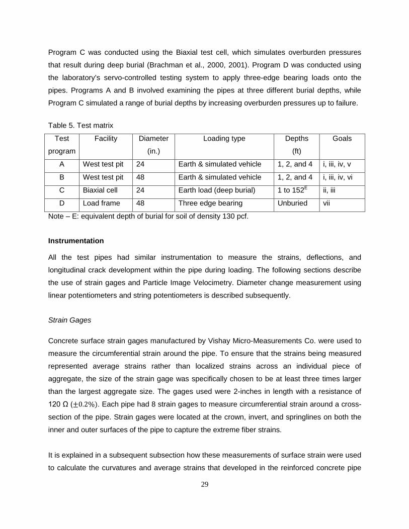
Two cameras were mounted in each pipe to monitor longitudinal crack development at the
crown and invert. The cameras were mounted near the wheel pad loading point, one camera
facing the crown and one camera facing the invert. A photo of the mounting system is shown in
Figure 5. The cameras were operated remotely using the DSLR Remote Pro Multi-Camera
software which permits pairs of photos to be taken simultaneously at five to ten second intervals
throughout the test.
Figure 5. SLR Camera mounting system to monitor crack widths during loading
Burial Conditions
A Topcon RL-H3C self-levelling laser level was used to ensure that lifts were consistent and did
not exceed 12 inches. A CPN MC-1DR-P Portaprobe nuclear densometer (ASTM D6938-08a)
was used to gather density, percent water content, and percent standard Proctor maximum dry
density (SPMDD) readings within each lift to ensure that the entire burial was consistent and
achieved minimum required soil density. Table 7 presents details of the level of compaction
achieved. Lougheed (2008) and Lay (2012) report that for this test soil, dry density measured
with the nuclear densometer ranged from 14% lower to 8% higher than density obtained using
the sand cone method (ASTM D1556-07), with mean dry density about 6% lower.
The pipes for Program A were installed using sandy gravel denoted GP-SP in the Unified
Classification System and A-1-a material by AASHTO, in accordance with Type 2 burial
conditions as per AASHTO (2009) to a minimum of 90 percent standard Proctor (i.e. 90% of the
maximum dry unit weight achieved for this soil using a standard Proctor test). The soil was
compacted in approximately 8-inch lifts using both small and large vibrating plate compacters to
34
achieve the required soil conditions. The average soil properties for the pipe burial are
described in the following table.
Table 7. Average Soil Compaction Properties for 24-inch Pipe Burial
24-inch Class IV Pipe Burial 24-inch Class V Pipe Burial
Dry Density
(pcf)
Water
Content (%)
Standard
Proctor (%)
Dry Density
(pcf)
Water
Content (%)
Standard
Proctor (%)
Bedding 130 3.2 91 129 2.9 91
Sidefill 128 3.0 90 128 3.2 90
Cover 129 4.1 91 130 4.2 92
Loading Regime
The pipes in test Program A were tested in eight stages involving cover depths of four feet, two
feet, and then one foot, and tested as summarized in the top eight loading stages listed in Table
8. The wheel pair configuration associated with the AASHTO design truck was applied at the
ground surface above the buried pipes using a steel axle frame with steel wheel pads loaded by
a 200-tonne (450 kips) hydraulic actuator. The actuator is supported over the test pit by a
reaction frame anchored into the underlying rock, and was aligned to apply a vertical load above
the centerline of the pipe. The steel wheel pads were 10-inches by 20-inches as specified by
AASHTO (2012) and were loaded by a steel axle frame that separated the wheel pads by 6ft
(again, in accordance with the standard). The axle frame transferred the load to the wheel pads
through spherical bearings to ensure there was negligible moment transfer. The axle frame was
aligned over the longitudinal axis of the pipe to simulate a truck travelling perpendicular across
the pipe’s longitudinal axis. To limit bearing failure of the soil under the loading pads during the
ultimate limit states test (test stages 4 and 8 presented in Table 8), enlarged wooden bearing
pads of length 37.4 in. and width 14.6 in. were placed below the steel pads to better distribute
the load. At each load stage, for four, two and one-foot cover, the loads were cycled three times
to ensure the soil beneath the load pads was compacted and that the results were obtained for
first loading (where permanent as well as recoverable deformations can be expected), and
second and third load cycles where recoverable (elastic) deformations dominated.

35
Test Program B
Test Specimens
To investigate the performance of larger diameter pipes, as well as the effects of different wall
thicknesses, two 48-inch diameter pipes were used in Test Program B: a 48-inch, Wall B, Class
III-equivalent pipe and a 48-inch, Wall C, Class III-equivalent pipe. The Wall B pipe had a wall
thickness of 5-inches and the Wall C pipe had a wall thickness of 5.75-inches. Both pipes had
an internal diameter of 48-inches with a length of 8ft, including the bell but excluding the spigot.
The pipes were manufactured by Hanson Pipe and Precast of Cambridge Ontario. The Wall B
pipe was circumferentially reinforced with a double layer of reinforcement with an average cover
of 1-inch and a wire gage of D4 (0.04in2) at 2-inch spacing. This pipe had a concrete strength
(f’c) of 84800psi and the reinforcement steel had yield strength (fy) of 70300psi and an ultimate
strength of 79800psi. The Wall C pipe was circumferentially reinforced with a double layer of
reinforcement with an average cover of 1-inch and a wire gage of D4 (0.04in2) at 2.7-inch
spacing. This pipe had a concrete strength (f’c) of 84800psi and the reinforcement steel had
yield strength (fy) of 70300psi and an ultimate strength of 79800psi. Table 6 summarizes the
material properties of these test pipes.
Arrangement in the Test Pit
Test Program B was conducted using a similar embankment installation to Test Program A
within the same 25-foot by 25-foot by 10-foot deep test pit. The 48 in. (1.2m) diameter pipes
were oriented east to west with the Wall C pipe in the east position and the Wall B in the west
position. A compacted soil foundation of 25 inches was prepared on top of the rigid concrete
floor with an additional three inches of loose bedding. Figures 6 and 7 illustrate pipe location
and surface loading.
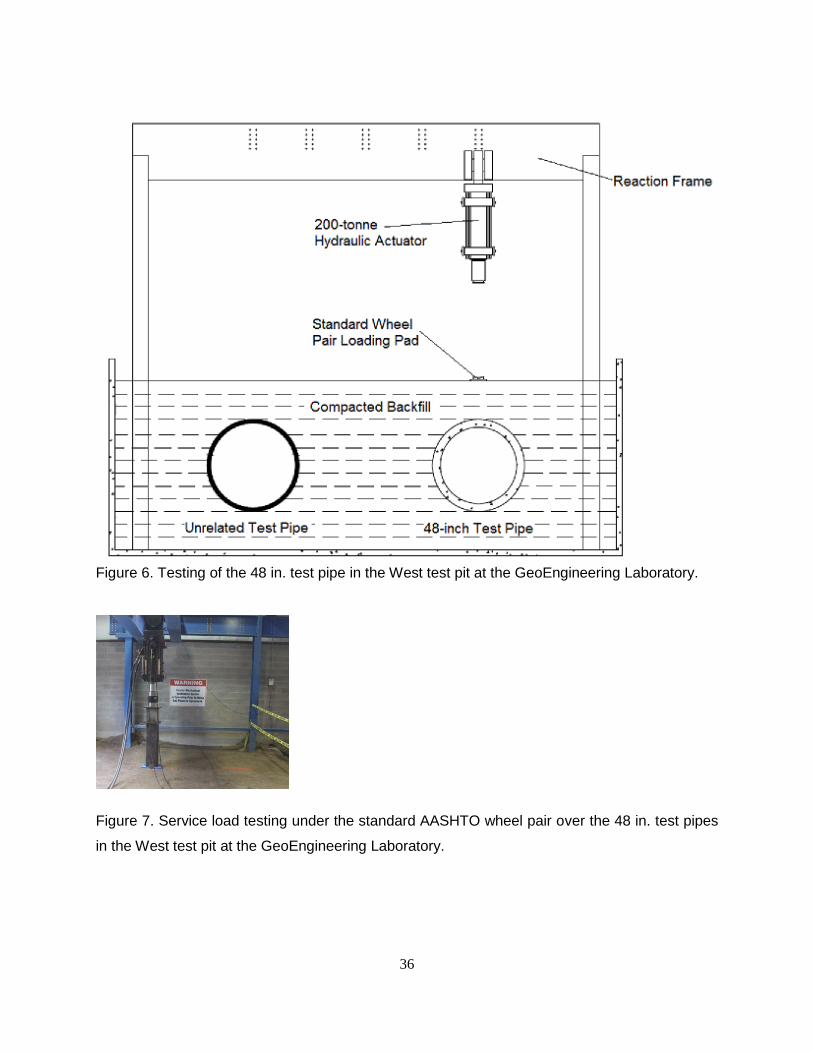
36
Figure 6. Testing of the 48 in. test pipe in the West test pit at the GeoEngineering Laboratory.
Figure 7. Service load testing under the standard AASHTO wheel pair over the 48 in. test pipes
in the West test pit at the GeoEngineering Laboratory.
37
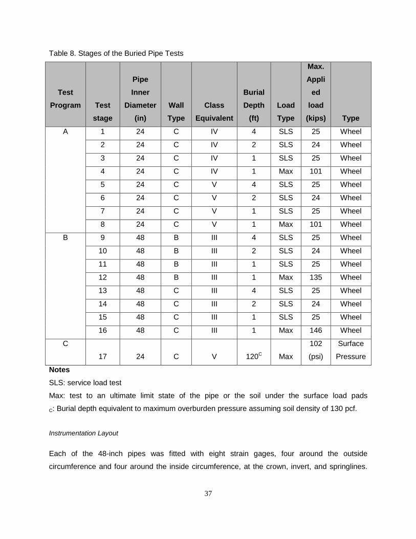
Table 8. Stages of the Buried Pipe Tests
Test Program Test
stage
Pipe Inner
Diameter (in)
Wall Type
Class Equivalent
Burial Depth
(ft) Load Type
Max. Appli
ed load
(kips) Type
A 1 24 C IV 4 SLS 25 Wheel
2 24 C IV 2 SLS 24 Wheel
3 24 C IV 1 SLS 25 Wheel
4 24 C IV 1 Max 101 Wheel
5 24 C V 4 SLS 25 Wheel
6 24 C V 2 SLS 24 Wheel
7 24 C V 1 SLS 25 Wheel
8 24 C V 1 Max 101 Wheel
B 9 48 B III 4 SLS 25 Wheel
10 48 B III 2 SLS 24 Wheel
11 48 B III 1 SLS 25 Wheel
12 48 B III 1 Max 135 Wheel
13 48 C III 4 SLS 25 Wheel
14 48 C III 2 SLS 24 Wheel
15 48 C III 1 SLS 25 Wheel
16 48 C III 1 Max 146 Wheel
C
17 24 C V 120C Max
102
(psi)
Surface
Pressure
Notes
SLS: service load test
Max: test to an ultimate limit state of the pipe or the soil under the surface load pads
C: Burial depth equivalent to maximum overburden pressure assuming soil density of 130 pcf.
Instrumentation Layout
Each of the 48-inch pipes was fitted with eight strain gages, four around the outside
circumference and four around the inside circumference, at the crown, invert, and springlines.
38
The strain gages were located at the cross section of the pipe located directly beneath the
wheel loading pad.
Four string potentiometers were installed in the 48-inch pipes to measure changes in horizontal
and vertical diameter at two locations in the pipe. One pair of string potentiometers was installed
within 1-inch of the strain gages while the other pair was located at the other end of the pipe, the
same distance from the end of the pipe as the first pair of LPs. In the Wall B pipe the pair of LPs
under the wheel pad was identified as SP2 and the pair opposite was identified as SP1. In the
Wall C pipe the pair of LPs under the wheel pad was identified as SP1 and the pair opposite
was identified as SP2. Strings potentiometers are accurate to 0.0005 inches.
Two cameras were mounted in each pipe to monitor longitudinal crack development at the
crown and invert in the same configuration as in the 24-inch pipes.
Burial Conditions
The burial process for the 48 in. pipes was identical to that used for the smaller diameter
specimens. The soil properties for the 48-inch pipe burial are shown in Table 9.
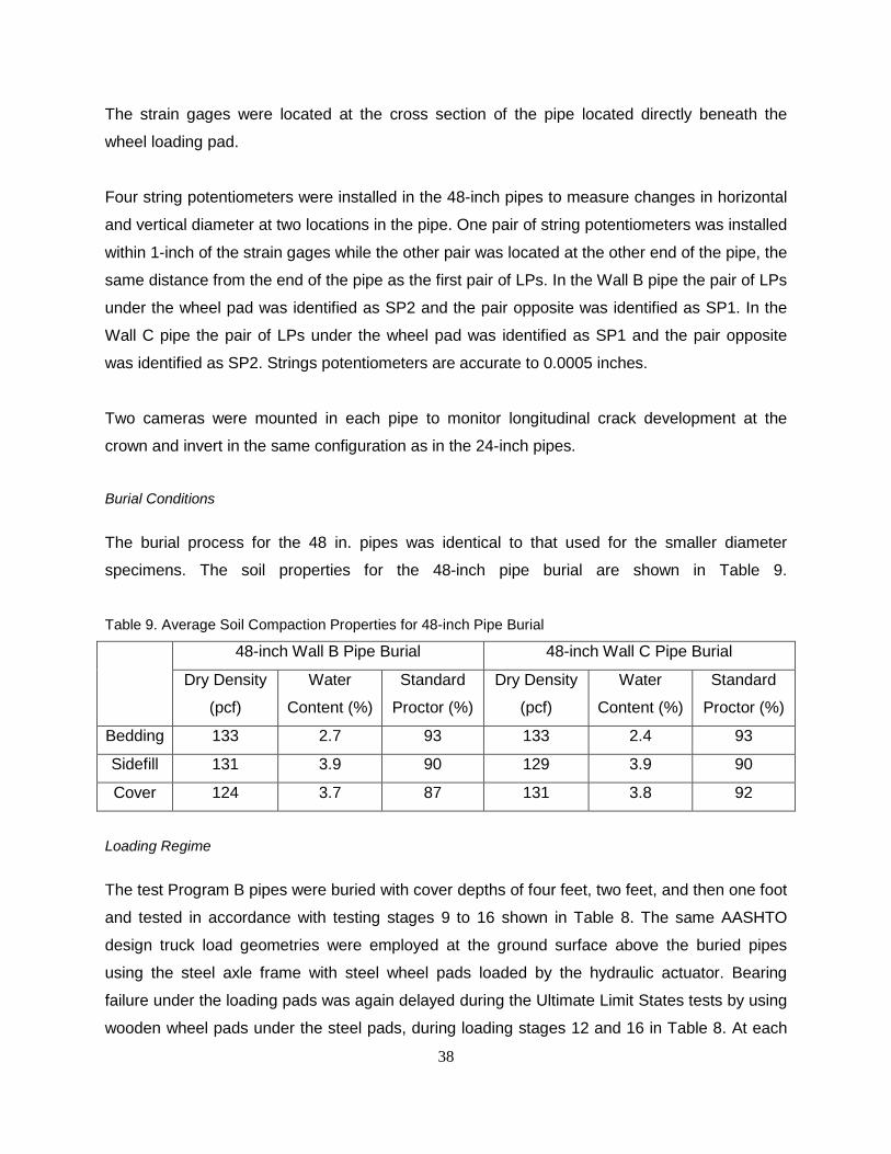
Table 9. Average Soil Compaction Properties for 48-inch Pipe Burial
48-inch Wall B Pipe Burial 48-inch Wall C Pipe Burial
Dry Density
(pcf)
Water
Content (%)
Standard
Proctor (%)
Dry Density
(pcf)
Water
Content (%)
Standard
Proctor (%)
Bedding 133 2.7 93 133 2.4 93
Sidefill 131 3.9 90 129 3.9 90
Cover 124 3.7 87 131 3.8 92
Loading Regime
The test Program B pipes were buried with cover depths of four feet, two feet, and then one foot
and tested in accordance with testing stages 9 to 16 shown in Table 8. The same AASHTO
design truck load geometries were employed at the ground surface above the buried pipes
using the steel axle frame with steel wheel pads loaded by the hydraulic actuator. Bearing
failure under the loading pads was again delayed during the Ultimate Limit States tests by using
wooden wheel pads under the steel pads, during loading stages 12 and 16 in Table 8. At each
39
loading stage, the loads were again cycled three times to gather information during the initial
load cycle and two subsequent ‘elastic’ load cycles.
Test Program C
Test Specimens
To investigate the behavior of pipes under deep burial and create a comparison to shallow
burial pipe, a 24-inch, Wall C, Class V-equivalent pipe was loaded under simulated deep burial.
The pipe had an internal diameter of 24-inches with a wall thickness of 3.75-inches and a length
of 8ft, including the bell but excluding the spigot. The pipe was manufactured by M-CON. This
pipe was circumferentially reinforced with a single layer of reinforcement centered in the pipe
wall with a wire gage of D4 (0.04 in2) at 2.7-inch spacing. This pipe had a concrete strength (f’c)
of 9600 psi and the reinforcement steel and a yield strength (fy) of 84800 psi and a ultimate
strength of 86600 psi. The pipe specimen material properties are summarized in Table 6.
Biaxial Test Cell
Test Program C was conducted in the biaxial test cell. This is a 6.6-foot by 6.6-foot by 5.2-foot
deep steel box with a rubber bladder under the lid that was used to apply a uniform pressure on
the ground surface over the 24-inch pipe to simulate deep burial. The pipe was horizontally
centered in the cell, with 24 inches between the wall of the pipe specimen and the edge of the
cell on each side, and 8 inches of soil under the pipe invert. A double layered friction treatment
was applied to each wall of the cell to reduce the effects of friction between the soil in the cell
and the cell wall. A single layer of polyethylene sheeting was attached to the four vertical walls
of the biaxial cell, lubricated with specially selected silicon grease, and then covered in a second
sheet of polyethylene without securing it to the cell walls in any other way. This creates a
boundary with very low friction values to reduce vertical load transfer through shear to the side
boundaries. In addition, lines were marked on both layers of friction treatment to assess the
movement between the two sheets after testing. Further description of the friction treatment
within the biaxial cell is provided by Tognon et al. (1999). Two settlement plates were placed
below and on either side of the pipe within the first soil lift, to monitor settlement and therefore
vertical strain in two short columns of test soil near the base of the test system. These
measurements can be used subsequently to estimate the modulus of the test soil.
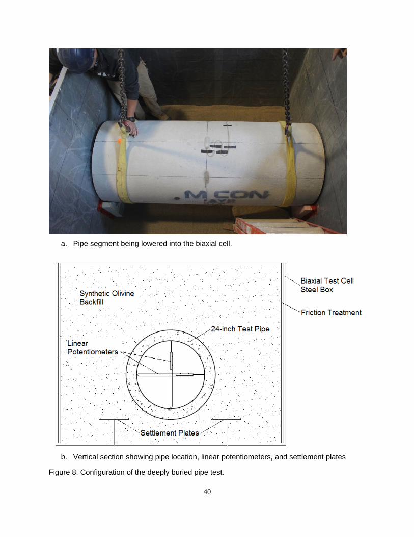
40
a. Pipe segment being lowered into the biaxial cell.
b. Vertical section showing pipe location, linear potentiometers, and settlement plates
Figure 8. Configuration of the deeply buried pipe test.
41
Instrumentation Layout
The 24-inch pipe was outfitted with eight strain gages, four around the outside circumference
and four around the inside circumference, at the crown, invert, and springlines. The strain gages
were located at the center cross section of the pipe. Two linear potentiometers were installed
within 1-inch of the strain gages to measure changes in horizontal and vertical pipe diameter at
the center of the pipe. SLR cameras were installed to monitor crack development at the crown
and invert. Two settlement plates buried within the first lift of the soil had shafts extending
through the base of the biaxial cell and attached to two linear potentiometers. These linear
potentiometers can be used to estimate vertical strains and therefore the modulus of the soil.
Burial Conditions
A Topcon RL-H3C self-levelling laser level was used to ensure that lifts were consistent and did
not exceed 12 inches. A CPN MC-1DR-P Portaprobe nuclear densometer was used to gather
density, percent water content, and percent standard Proctor maximum dry density (SPMDD)
readings within each lift to ensure that the entire burial was consistent and achieved minimum
required percent standard Proctor density. The pipe was then buried in 4 to 10-inch lifts. The
pipe in Test Program C was buried in the biaxial cell within synthetic olivine sand (a material
classified as SP by the unified classification system). Compaction details are shown in Table 10.
Table 10. Average Compaction Properties for 24-inch Deep Burial in Synthetic Olivine Sand
24-inch Class V Pipe Burial
Dry Density
(pcf)
Water
Content (%)
Standard
Proctor (%)
Bedding 101 0.5 71
Loading Regime
Test Program C was conducted within the biaxial cell using compressed air applied on the top of
the rubber bladder placed on the soil surface over the pipe (the bladder is very compliant and
remains in full contact with the soil surface). The pressure in the cell was steadily increased at a
rate of approximately 5.1psi/min (7.6ft cover/min). The test was run to a maximum pressure of
102 psi, approximately equivalent to a burial depth of 145 ft in the synthetic olivine backfill, or
113 ft of material with density of 130 pcf.
42
Test Program D
Pipe samples were tested in three edge bearing to determine D-Load, so comparisons can be
made between the response when buried and under three-edge bearing. Manufacturer data
showed that the 48-inch pipes were loaded until the required service limit, however the samples
showed no signs of cracking. To be able to compare 0.01-inch crack loads between three-edge
bearing loading and cracking performance when buried, the 48-inch pipes were tested in three
edge bearing until they reached the maximum allowable crack width (0.01 in.). The 24-inch
Class IV pipe was provided with D-Load data by the manufacturer up to the 0.01-inch crack
width. The D-Load data for the 24-inch Class V pipe was determined from previous testing
performed on another sample of the same pipe (manufactured at the same time and place as
the test pipe).
Instrumentation Layout
Two LPs were placed at the center of the pipe, one to measure change in vertical diameter and
the other to measure change in horizontal diameter. Two SLR cameras were set up to record
the development of cracks at the crown and invert during the experiment. The load cell attached
to the actuator recorded the amount of load being applied to the pipe.
Loading Regime
Following the ASTM C497-13 standard, the pipes were supported by two strips of wood which
were mounted on a steel I-beam. A flat piece of wood approximately ½-inch thick and a steel I-
beam were placed on top of the pipe to apply a line-load along the top of the pipe. The top I-
beam was loaded by the 200-tonne (450 kip) actuator.
3.3.3 Results and Discussion
Calculation of moment and thrust
To assess the impact of cover depth on the buried pipes, the strain readings were used to
calculate the curvature and average strain in the pipes to investigate how each pipe behaved
under loading. Using PIV technology, the development of cracks was monitored during loading
to monitor the occurrence of the critical crack of width 0.01-inches. The curvature of the pipe
wall was found using the strain readings and the wall thickness employing Equation 15.
43
𝜑 = 𝜀𝑖𝑛𝑠𝑖𝑑𝑒−𝜀𝑜𝑢𝑡𝑠𝑖𝑑𝑒𝑊𝑎𝑙𝑙 𝑇ℎ𝑖𝑐𝑘𝑛𝑒𝑠𝑠
15
The average strain in the pipe wall was found using the strain readings and Equation 16.
𝜀𝑎𝑣𝑒𝑟𝑎𝑔𝑒 = 𝜀𝑖𝑛𝑠𝑖𝑑𝑒+𝜀𝑜𝑢𝑡𝑠𝑖𝑑𝑒2
16
Test Program A
The purpose of this test program is to investigate the effects of live loading at shallow cover on
the service load response and the capacity of the 24 in. diameter pipes. For service load testing
at a burial depth of four, two and one foot, the pipes remained within the elastic limit. The results
of the moments calculated from those curvatures are presented in Section 3.4 where they are
compared to elastic design calculations.
Testing at one foot burial was undertaken to higher load levels, and established the capacity of
the pipe. The results for that Ultimate Limit States (ULS) test are presented in detail in the
following subsections.
Diameter Change
Both the Class IV and Class V pipe experienced minimal vertical diameter changes under
maximum loading at one foot burial depth as presented in Figure 8. The Class IV pipe
underwent 0.043-inches of vertical diameter decrease nearest the ‘wheel pair’ loading pad (LP1)
and 0.031-inches at the position further from the loading pad (LP2). The Class V pipe
experienced 0.064-inches of vertical diameter decrease nearest the ‘wheel pair’ loading pad
(LP1) and 0.027-inches at the location further from the loading pad (LP2).
Up to the service loads, the pipe behavior is linear and experiences only very small change in
diameter. After cracking occurs at approximately 60 kips, the change in diameter begins to
increase more significantly and becomes distinctly nonlinear. Before cracking occurs, the
vertical diameter decrease in both pipes is almost the same. However, immediately after
cracking the Class IV pipe experiences greater vertical diameter changes than the Class V pipe.
This is as expected since the Class V pipe has a greater area of steel to resist the bending
moments.
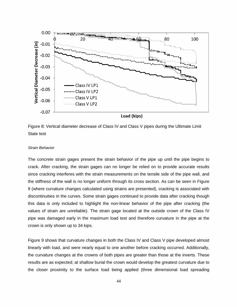
44
Figure 8: Vertical diameter decrease of Class IV and Class V pipes during the Ultimate Limit
State test
Strain Behavior
The concrete strain gages present the strain behavior of the pipe up until the pipe begins to
crack. After cracking, the strain gages can no longer be relied on to provide accurate results
since cracking interferes with the strain measurements on the tensile side of the pipe wall, and
the stiffness of the wall is no longer uniform through its cross section. As can be seen in Figure
9 (where curvature changes calculated using strains are presented), cracking is associated with
discontinuities in the curves. Some strain gages continued to provide data after cracking though
this data is only included to highlight the non-linear behavior of the pipe after cracking (the
values of strain are unreliable). The strain gage located at the outside crown of the Class IV
pipe was damaged early in the maximum load test and therefore curvature in the pipe at the
crown is only shown up to 34 kips.
Figure 9 shows that curvature changes in both the Class IV and Class V pipe developed almost
linearly with load, and were nearly equal to one another before cracking occurred. Additionally,
the curvature changes at the crowns of both pipes are greater than those at the inverts. These
results are as expected; at shallow burial the crown would develop the greatest curvature due to
the closer proximity to the surface load being applied (three dimensional load spreading
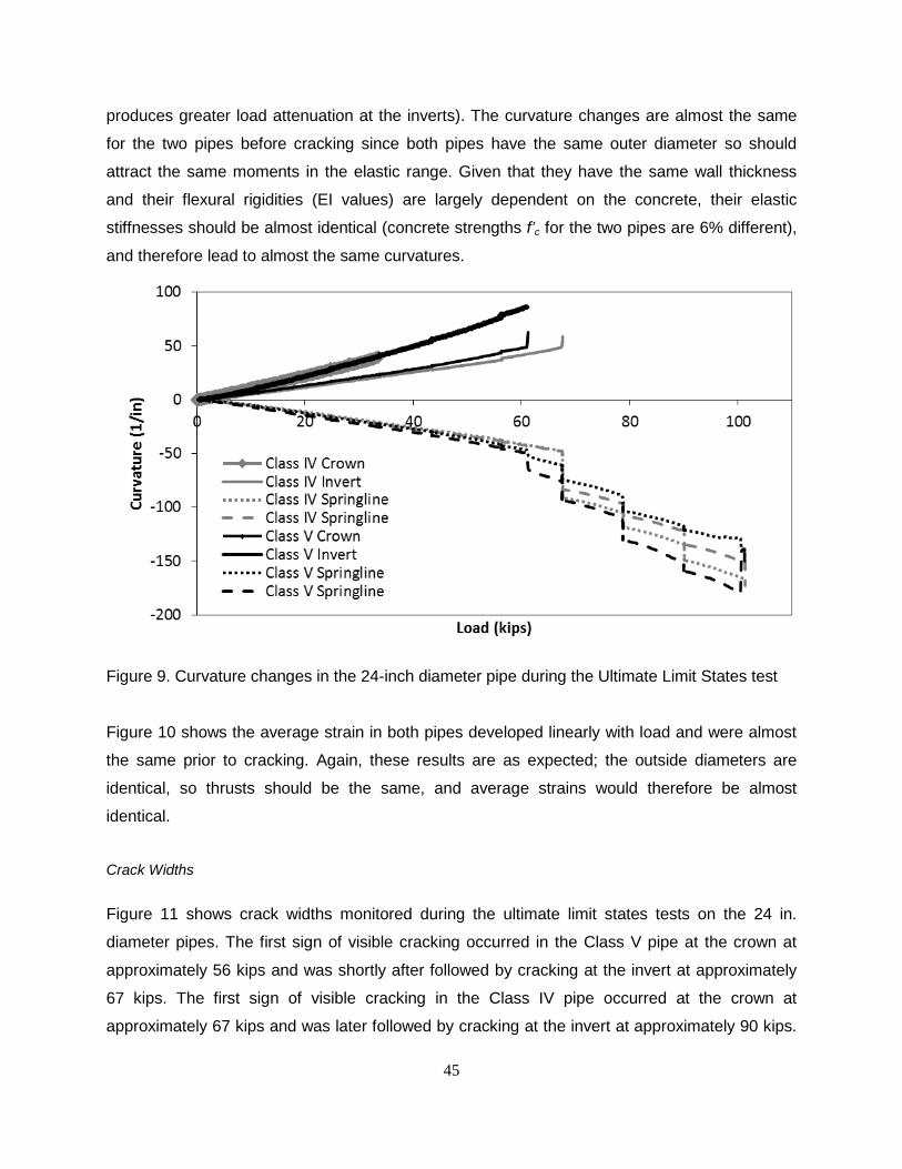
45
produces greater load attenuation at the inverts). The curvature changes are almost the same
for the two pipes before cracking since both pipes have the same outer diameter so should
attract the same moments in the elastic range. Given that they have the same wall thickness
and their flexural rigidities (EI values) are largely dependent on the concrete, their elastic
stiffnesses should be almost identical (concrete strengths f’c for the two pipes are 6% different),
and therefore lead to almost the same curvatures.
Figure 9. Curvature changes in the 24-inch diameter pipe during the Ultimate Limit States test
Figure 10 shows the average strain in both pipes developed linearly with load and were almost
the same prior to cracking. Again, these results are as expected; the outside diameters are
identical, so thrusts should be the same, and average strains would therefore be almost
identical.
Crack Widths
Figure 11 shows crack widths monitored during the ultimate limit states tests on the 24 in.
diameter pipes. The first sign of visible cracking occurred in the Class V pipe at the crown at
approximately 56 kips and was shortly after followed by cracking at the invert at approximately
67 kips. The first sign of visible cracking in the Class IV pipe occurred at the crown at
approximately 67 kips and was later followed by cracking at the invert at approximately 90 kips.

46
In both cases, cracking first occurred at the crown followed by cracking at the invert. This is as
expected due to the greater load attenuation at the invert.
Figure 10. Average strain increase with load for the 24-inch Diameter Classes IV and V pipes
during the ultimate limit state tests
Figure 11. Crack width development in 24-in diameter pipes during the ultimate limit state test
47
Performance of Class IV and Class V Pipe
As mentioned previously, pipes are designed to resist both a serviceability limit state and an
ultimate limit state. The serviceability of the pipe is governed by a maximum crack width of 0.01-
inches following development of the tensile cracking strain. The ultimate limit state of the pipe is
defined by the development of ultimate moment capacity at one location around the pipe
circumference.
The 0.01 in. design crack in the Class V-equivalent pipe developed at a surface load of 73 kips.
This crack width required a surface load of 101 kips for the pipe equivalent to Class IV, though
crack width reached 0.007 in. in the Class IV-equivalent pipe at 71 kips and crack growth
slowed dramatically beyond this load. Likely these variations are evidence of the inherent
variability of cracking behavior for brittle, non-homogenous materials like concrete.
According to the AASHTO LRFD loading conditions, pipes buried at 1-foot should be able to
resist a live wheel-pair load of 16 kips, factored by an impact factor of 1.289 and a multiple
presence factor of 1.2, resulting in a service load of 25 kips, and further factored by a live load
factor of 1.75, resulting in an ultimate load of 43 kips. No visible crack developed at any
locations until after both the service live load requirement and ultimate live load requirement, as
defined by AASHTO (2013) had been exceeded. The buried test pipes did not reach their
service live load limit requirements until loads 4.0 and 3.0 times greater than the calculated
0.01-inch crack load limit of the pipe, for the pipes equivalent to Class IV and V, respectively.
Test Program B
Introduction
The 48 in. diameter pipes loaded under four foot, two foot, and one foot burial at service loads
remained within the elastic zone and experienced no significant deflections or cracking. The
moments that developed during these service load tests are examined in Section 3.4 and only
the ultimate limit state test results are presented in the following section.
Diameter Change
Both the Wall B and Wall C pipes underwent minimal vertical diameter decrease under
maximum loading at one foot burial depth as can be seen in Figure 12. The Wall B pipe

48
underwent 0.250-inches of vertical diameter decrease nearest the wheel loading pad (SP2) and
0.136-inches of vertical diameter decrease at the position further from the ‘wheel pair’ loading
pad (SP1). The Wall C pipe underwent 0.140-inches of vertical diameter decrease nearest the
loading pad (SP1) and diameter decrease of 0.097-inches at the position further from the
loading pad (SP2). The pipe behavior was linear and stiff (with small changes in diameter
recorded) until between 25 to 30 kips where the rate of diameter change increased and became
nonlinear.
Figure 12. Vertical diameter decreases for wall B and wall C pipes during the ultimate limit
states tests.
Strain Behavior
As mentioned previously, concrete strain gages present the strain behavior of the pipe only up
until the pipe begins to crack. The Wall B pipe has a smaller wall thickness than the Wall C pipe,
but has more reinforcement. Both wall types are designed to have similar flexural capacity and it
is interesting therefore to determine whether they develop similar curvatures and crack widths.
In both pipes, the curvature at the crown exceeds the curvature at the invert which is to be
expected due to the proximity of the applied load, as can be seen in Figure 13. The curvature
developed linearly until cracking occurred between approximately 30 and 50 kips. The curvature
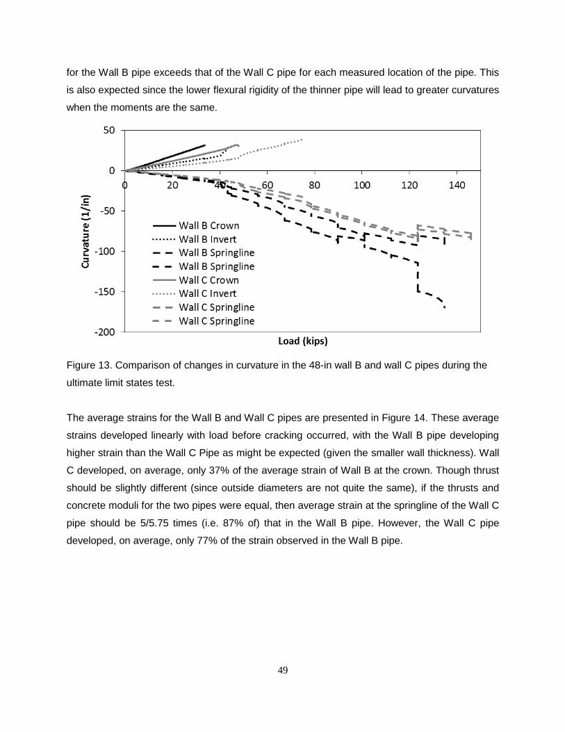
49
for the Wall B pipe exceeds that of the Wall C pipe for each measured location of the pipe. This
is also expected since the lower flexural rigidity of the thinner pipe will lead to greater curvatures
when the moments are the same.
Figure 13. Comparison of changes in curvature in the 48-in wall B and wall C pipes during the
ultimate limit states test.
The average strains for the Wall B and Wall C pipes are presented in Figure 14. These average
strains developed linearly with load before cracking occurred, with the Wall B pipe developing
higher strain than the Wall C Pipe as might be expected (given the smaller wall thickness). Wall
C developed, on average, only 37% of the average strain of Wall B at the crown. Though thrust
should be slightly different (since outside diameters are not quite the same), if the thrusts and
concrete moduli for the two pipes were equal, then average strain at the springline of the Wall C
pipe should be 5/5.75 times (i.e. 87% of) that in the Wall B pipe. However, the Wall C pipe
developed, on average, only 77% of the strain observed in the Wall B pipe.

50
Figure 14. Comparison of average strain in the 48-in wall B and wall C pipes during the ultimate
limit states test
Crack Width
Crack widths monitored during the ultimate limit states tests are presented in Figure 15. The first
sign of visible cracking occurred in the Wall B pipe at the crown at approximately 25 kips and
was followed by cracking at the invert at approximately 45 kips. The first sign of visible cracking
in the Wall C pipe occurred at the crown at approximately 45 kips and was later followed by
cracking at the invert at approximately 67 kips. In both cases, cracking first occurred at the
crown followed by cracking at the invert. This is as expected due to higher dimensional load
attenuation (spreading) at the invert. Cracking developed first in the Wall B pipe as expected
due to the lower thickness (strain associated with elastic bending in a flexural element is
proportion to moment divided by modulus times thickness squared). If moments and concrete
modulus are the same at the same value of surface load, strain to induce cracking should occur
in the Wall B pipe at loads (5/5.75)2 or 76% of those for the Wall C pipe. The ratio seen above is
25/45 = 56%. Possible explanations for this difference between observed and calculated
differences may be because of differences in the concrete moduli, initial strains resulting from
earth loading and the prior loading history, or soil support provided to the two different pipes.

51
Figure 15. Development of crack width in 48 in. diameter pipe during ultimate limit states test
Performance of Wall B and C
As mentioned previously, pipes are designed to resist both a serviceability limit state and an
ultimate limit state. As can be seen in Figure 15, at the full service load of 25 kips the Wall B
pipe has just begun to crack and there is no visible cracking in the Wall C pipe. At the ultimate
load of 43 kips, the Wall C pipe has begun to show a visible crack; however it is still below the
crack width limit of 0.01-inch. The pipes first reach the 0.01-inch cracking limit at loads of 61
kips and 75 kips, for Walls B and C, respectively.
Test Program C
Introduction
A 24-inch reinforced concrete pipe was tested to determine the response under deep burial. The
pipe was loaded in the biaxial test cell to a maximum pressure of 102 psi, equivalent to a burial
depth of approximately 145 ft in that synthetic olivine backfill, or 113 ft for backfill with density of
130 pcf.

52
Diameter Change
The pipe responded linearly with respect to overburden pressure until a surface pressure of 40
psi (approximately 45 feet of equivalent burial under soil of unit weight 130 pcf), where the rate
of diameter decrease began to increase nonlinearly due to cracking in the pipe. The pipe
reached a deflection of 0.16 inches at an overburden pressure of 102 psi, as shown in Figure
16.
Figure 16. Deflection of 24-in Class V, Wall C pipe under simulated deep burial
Strain Behavior
As opposed to the shallow buried tested pipes which had maximum curvature at the crown, this
simulated deep buried pipe had maximum curvature at the invert. The pipe behaved linearly
until cracking began at between 38 to 43 psi of overburden pressure, as shown in Figures 17
and 18.
0 20 40 60 80 100 120
-0.18
-0.16
-0.14
-0.12
-0.10
-0.08
-0.06
-0.04
-0.02
0.00
0 20 40 60 80 100
Simulated Burial Depth (ft)
Vert
ical
Dis
plac
emen
t (in
)
Overburden Pressure (psi)

53
Figure 17. Curvature in 24-in class V, wall C pipe under simulated deep burial
Figure 18. Average strain in 24-in class V, wall C pipe under deep burial
0 10 20 30 40 50 60 70
-200-150-100-50
050
100150200250
0 10 20 30 40 50 60 70
Simulated Burial Depth (ft)
Cur
vatu
re (1
/in)
Overburden Pressure (psi)
Biaxial CrownBiaxial SpringlineBiaxial SpringlineBiaxial Invert
0 10 20 30 40 50 60 70
-100-80-60-40-20
020406080
100
0 10 20 30 40 50 60 70
Simulated Burial Depth (ft)
Aver
age
Stra
in
Overburden Pressure (psi)
Biaxial CrownBiaxial SpringlineBiaxial SpringlineBiaxial Invert

54
Crack Width
Crack widths monitored during the test of the 24 in. diameter pipe under simulated deep burial
are presented in Figure 19. The first sign of visible cracking occurred at the invert at
approximately 36 psi of overburden pressure and was followed by cracking at the crown at
approximately 51 psi of overburden pressure. This was as expected due to the development of
higher curvature at the invert.
Figure 19. Crack width development in 24-in class V, wall C pipe under deep burial
Behavior of Deeply Buried Pipes
As mentioned previously, pipes are designed to resist both a serviceability limit state and an
ultimate limit state. The pipe first reached the 0.01-inch cracking limit at an overburden pressure
of approximately 60 psi.
Test Program D
Three edge bearing tests
D-Load data was provided by the manufacturer for the 24-inch Class IV pipe. A Class IV pipe
according to the ASTM C76 tables can support a D-Load up to 2000 pounds per foot length of
0 20 40 60 80 100 120
0.0000.0050.0100.0150.0200.0250.0300.0350.0400.0450.050
0 20 40 60 80 100
Equivalent Burial Depth (ft)
Cra
ck W
idth
(in)
Overburden Pressure (psi)
0.01-in Crack Width Limit24in Pipe Crown24in Pipe Invert

55
pipe per foot inner diameter (lbs/ft/ft) while producing a maximum crack width of 0.01 inches.
The 24-inch Class IV pipe used for Test Program A reached a D-Load of 3004lbs/ft/ft with a
crack width of 0.012-inch (0.3mm crack limit according to CSA A257-2009) and an ultimate
failure at a D-load of 3326lbs/ft/ft, according to the manufacturer’s data. The D-Load data for the
24-inch Class V pipe was based on load tests performed by David Becerril on previous pipe
samples.
The manufacturer provided three edge bearing data for the 48-inch pipes, for test Program B,
showing that the pipe did not develop a crack larger than the limiting crack width at the required
load for the 48-inch, Class III-equivalent, Wall B and Wall C pipe. However, the manufacturer
did not go beyond this load to show at what load the limiting crack width did occur. Therefore
additional D-load tests were conducted to determine under what D-load the limiting crack
developed.
Diameter Change
Both pipes did not deflect significantly until approximately 40 kips where the rate of deflection
began to increase nonlinearly due to cracking in the pipe. The Wall B pipe reached a deflection
of 1.10 inches at a load of 121 kips and the Wall C pipe reached a deflection of 0.84 inches at a
load of 100 kips, as shown in Figure 20.
Figure 20. Vertical diameter decrease in 48-in wall B and C pipes during the three edge bearing
tests (including pipe responses during unloading).

56
Crack Width
Crack widths monitored during the D-load tests on the 48 in. diameter pipes are presented in
Figure 21. The first sign of visible cracking in the Wall C pipe occurred at the invert and crown at
the same load of approximately 34 kips. The first sign of visible cracking in the Wall B pipe
occurred at the invert at a load of approximately 45 kips followed shortly after by cracking at the
crown at a load of 56 kips.
Figure 21. Development of crack width for 48-in wall B and C pipes during D-Load testing.
A Class III pipe according to the ASTM C76 tables can support a D-Load up to 1350lbs/ft/ft
while producing a maximum crack width of 0.01 inches. The Wall B pipe used in the test
reached a D-Load of 1862lbs/ft/ft to achieve a cracking limit of 0.01-inch cracking limit and the
Wall C pipe reached a D-Load of 1581lbs/ft/ft to achieve a cracking limit of 0.01-inch cracking
limit. This means both exceeded the load requirements equivalent to Class III pipe.
3.4 Comparison of experimental results and design calculations
3.4.1 Introduction
This section provides details of the comparisons made between test measurements and design
calculations. These comparisons are made to examine the performance of the Direct Design
and Indirect Design methods. In particular, these comparisons:
57
- provide evidence of the performance of the procedures available for estimating
expected moments resulting from live load during Direct Design
- provide evidence of the performance of the procedures available for estimating
expected moments resulting from earth load during Direct Design
- provide evidence of the performance of the moment capacity models available for use
in Direct Design
- provide evidence of the performance of load capacity estimation using Indirect Design
3.4.2 Live load moment
Experimental measurements of live load moment
Two sets of buried pipe tests were conducted to examine the performance of buried pipes, as
summarized in Table 11. Two 24 inch diameter pipes and two 48 inch diameter test pipes were
provided by Hanson and M Con by arrangement with the Ontario Concrete Pipe Association.
The pipes were tested at four different depths (1ft, 2 ft and 4ft) after burial within sandy gravel
backfill (an A-1-a material compacted to at least 90% of maximum dry unit weight determined
from a standard Proctor test). These tests were described in detail in Section 3.3.
Details of the steel and concrete for the four different test pipes employed are given in Table 12
(the pipe used for Test 3 was identical to 1B).
In each case, strains were measured on the inside and outside of the pipes at the crown,
springlines and invert. These measured strains have been used to determine the changes in
curvature at a specific value of surface load (a 24.7 kip force applied to a steel plate with
standard dimensions of a wheel pair). Modulus and thickness of each of the test pipes were
then used to calculate the test moments from the curvatures. A total of 36 such measurements
were made (3 locations around the pipe circumference for 4 test pipes tested at 3 different burial
depths).
Calculation of elastic moments due to surface loads in Direct Design
Three currently available methods for calculating the effect of live loads are examined. Each
procedure uses the concept of load spreading under a rectangular area where load is applied at
the ground surface. For surface contact area of length L0 and width W0 the applied load PL is

58
assumed to spread out according to a live load distribution factor (LLDF) to apply pressure
𝑝𝐿 across all or part of the outside diameter of the concrete
𝑝𝐿 = 𝑃𝐿(𝐿0+𝐿𝐿𝐷𝐹.𝐻)(𝑊0+𝐿𝐿𝐷𝐹.𝐻)
17
The surface area examined during design is that which provides the highest increases in vertical
pressure on the pipe considering the AASHTO design truck featuring i. a single wheel pair, ii. a
single axle (two wheel pairs), and iii. a tandem axle loading. For the comparisons being made
here to the moment values observed in the test pipes, the single wheel pair configuration of 20
inch length and 10 inch width is used, since that is the loading geometry that was used in the
experiments.
The procedures for approximating live load spreading with depth are as follows:
a) AASHTO (2007) specifies LLDF=1.15 for the granular test soil used in this project, and
indicates that H is the depth to the top of the pipe; this procedure will be subsequently
denoted ‘LRFD 2007’;
b) AASHTO (2013) was published towards the end of this project; the revised specification
defines LLDF to be a function of inside pipe diameter; for pipes with diameter 24 inch or
less, LLDF=1.15; for pipes with diameter 96 inches or more, LLDF=1.75; structures in
between these diameters feature intermediate values of LLDF; for the calculations
presented in this report, linear interpolation was used to give LLDF=1.35 for the 48 inch
diameter pipes; as with the previous AASHTO procedure, burial depth was defined to
the top of the pipe; this procedure will subsequently denoted ‘LRFD 2013’; it is identical
to LRFD 2007 for the 24 inch test pipes, but results in greater live load spreading (and
smaller moments) for the 48 inch test pipes;
c) ASCE (1998) specifies use of LLDF=1.15 to the top of the pipe, and then distribution
factor of 1.75 to a depth of H+0.75 OD; this procedure is implemented in program
PipeCar developed for the American Concrete Pipe Association, and will be
subsequently denoted ‘PipeCar’.
Total force per unit length along the pipe is calculated as pL multiplied by the lesser of W0 or
OD, where the vehicle is considered to be driving directly across the culvert (not along). This
takes account of the spreading dimension relative to the pipe size (if it is less than OD, then all
of the applied load is applied; if it is more, then only a portion of the load acts on the pipe). In the

59
tests being examined, the short dimension of the surface loading place was oriented parallel to
the pipe diameter, consistent with vehicles driving directly across the culvert.
Once total force per unit length along the pipe Wi is determined, it is used to calculate moment
based on two dimensional analysis that considers the pipe burial conditions and the soil-pipe
interaction. The procedure generally used is the procedure based on two dimensional finite
element analysis of an elastic ring outlined by ASCE (1998), where moments are given as
moment factors:
M = Cmi Wi (ID+OD)/4 18
where coefficients Cmi are given at three locations (crown, spring and invert) for five different
loading cases (pipe weight, earth loads, fluid loads, and deeply or shallow buried surface
loadings). Linear interpolation is used for burial depths between 1 ft (where factors WL2 apply)
and 1.75 OD (beyond which factors WL1 apply). For the type two burial conditions used in the
tests, the moment factors for live loading and earth loading are given in Table 13.
Table 14 summarizes the 36 values of moment obtained in the tests, as well moments obtained
by the three procedures described above. These results are also presented in Figure 22.
Another set of calculations is presented in the table and figure (denoted LRFD 2013+). These
results will be explained and discussed later in this section.
These comparisons indicate that:
- measured moment (i.e. moment evaluated from measured strains) is always
substantially lower than the calculated values
- moments measured at the crown are distinctly higher than those at the invert, whereas
the calculation provide invert moments that are much closer to those at the crown
To quantify the differences between ‘measured moments’ (moments obtained from measured
strains) and calculated values, ratios of calculated to test moment have been included in Table
14 and these are also shown in Figure 23. A perfect calculation procedure would provide a ratio
of 1. Given the need for safety in design, a ratio exceeding one is desirable, but perhaps not
higher than 2. The actual ratios vary widely, and many exceed 2 by a considerable margin.
Table 15 summarizes the means and standard deviations for the ratios:

60
- moments obtained using the LRFD 2007 approach are between 2.9 and 11.7 times
higher than the measured values, with an overall mean of 5 and a standard deviation of 2.2
- moments obtained using the LRFD 2013 approach are between 2.9 and 10.3 times
higher than the measured values, with an overall mean of 4.7 and a standard deviation over 1.9
- moments obtained using PipeCar (the ASCE, 1998) approach are between 1.5 and 15
times higher than the measured values, with an overall mean of 5.1 and a standard deviation of
over 3.
None of the procedures, therefore, are very effective at providing the moments resulting from
application of surface load (at least for these shallow buried pipes subjected to the actions of a
wheel pair). If the surface was paved, the discrepancies between calculated and test values
would be even higher. Furthermore, the recent change to the live load spreading approach
specified by AASHTO in 2013 did little to improve the calculations relative to the 2007
guidelines.
Values for individual cases in Figures 22 and 23 are summarized separately in Table 15 using
means and standard deviations of moment ratios for the crown, springline and invert positions.
These show that the discrepancies are substantially greater at the springline and invert, than at
the crown. This is due to the additional live load spreading (or load attenuation) that develops at
these greater depths, and this is the reason for the ASCE (1998) and PipeCar procedures for
using an additional depth of 0.75 OD with LLDF = 1.75 (to capture load spreading through the
pipe). It may also explain the reasons for the recent modifications to live load spreading
published by AASHTO in 2013, since this provides somewhat better moment estimates at the
invert, where moment is often most critical (those changes were based on three dimensional
analyses presented by Petersen et al., 2010). However, the use of a single effective pressure in
calculations of moment at all three positions (crown, springline and invert) does not address the
significant differences in distance from the ground surface to these three different locations – a
difference that is very substantial for large diameter pipes at shallow cover. For example, the 48
inch diameter pipe at 1 ft of cover has depth to invert that is five times higher than depth to
crown.
Therefore, to address this issue further, it is possible to use the different depths to each of these
locations in calculations of load spreading. A fourth set of calculations are therefore included in
Table E-4 and shown in Figures 22 and 23, where depth to:
61
- Crown is set as H (so values remain the same as those for LRFD 2013);
- Springline is set as H + OD/2; and
- Invert is set as H + OD.
These calculations are denoted ‘LRFD 2013+’ or ‘LRFD+’ in Figures 22 and 23, and Tables 14
and 15. This modified approach provides much more consistent estimates of moment at the
three circumferential locations, with mean of 2.6 and standard deviation of 1.2 Figure 23 shows
that except at five cases out of the 36, the ratios of calculated to test moment are between 1
and 4, with more than 2/3 being below 2.5. Instead of having invert moment ratios in Figure 23
almost all exceeding a value of 4 (just two of the LRFD 2007 and LRFD 2013 calculations fall
below this value), with one exception the LRFD+ calculations all fall below 4.
Calculation of elastic moments due to earth loads in Direct Design
The deeply buried test on the pipe of 24 inch diameter also included measurements of
circumferential strains on the inner and outer surfaces of the pipe, at crown, springline and
invert. These have also been used to estimate moments during the test, for comparison with
calculated values. Table 16 provides a summary of the test measurements of curvature at an
overburden pressure of 37.6 psi. These have been used to calculate test moments using pipe
modulus 5576 ksi and second moment of area 52.7 in4/ft. Also included are calculations using
the coefficients given in ASCE (1998). The ratios of design moment to test moment are 1.9, 1.6
and 1.5 at the crown, springline and invert, respectively. These ratios are similar to those
discussed in the previous section for live load using the procedure ‘LRFD 2013+’ (the current
AASHTO procedure modified to account for the increased burial depths to the springline and
invert).
3.4.3 Limit States Tests
In addition to undertaking six sets of service load testing under surface loads, five different
ultimate limit states tests were conducted on the buried concrete test pipes:
1A. 24 inch Class IV-equivalent test pipe at 1 ft of cover using an enlarged wheel pair
1B. 24 inch Class V-equivalent test pipe at 1 ft of cover using an enlarged wheel pair
2A. 48 inch Wall B test pipe at 1 ft of cover using an enlarged wheel pair
2B. 48 inch Wall C test pipe at 1 ft of cover using an enlarged wheel pair
3. 24 inch Class V-equivalent test pipe in the biaxial cell, increasing surface pressures
(representing overburden stresses)
62
In each case, the surface pressure representing the weight of a wheel pair (tests 1A to 2B) or
the overburden pressure (test 3) were increased progressively until a limit state was reached.
Cracking was monitored using digital images so that the crack widths could be measured using
particle image velocimetry and the applied loads which induce a 0.01 in. crack determined (see
Appendix C for explanation of crack width monitoring).
None of the pipes reached an ultimate strength limit, and so comparisons with design estimates
made in Tables 17 and 18 are for the surface loads (force in kips for the shallow buried tests or
pressure in psi for the simulation of deep burial) required to induce that 0.01 inch crack during
each of the limit states tests.
In the test on pipe 1A, after initial cracking the crack width increased rapidly up to approximately
0.007 inches, but crack growth then slowed dramatically, and finally passed the 0.01 inch mark
at a load over 100 kips. This is the only test where rate of crack growth was so irregular. To
relate that specific measurement to the other tests, a load limit of 73 kips was estimated based
on extrapolating its initial rate of crack width growth up to the 0.01 inch limit, and this additional
load limit is included in Table 17 in parentheses, for reference in the subsequent discussion.
3.4.4 Comparisons to Design Estimates
Table 17 shows the experimental measurements of limiting loads discussed in the previous
section, as well as D-load values for each pipe (expressed as total force on the pipe) and
estimates of the surface load that induces 0.01 in. cracks obtained using Indirect Design. These
show that the Indirect Design Method is providing estimates of the load limits for these test
pipes that are between 54% and 81% of the observations. This level of safety is likely
reasonable given the simplified nature of Indirect Design.
Table 18 shows the limiting loads measured in the experiments and the Direct Design estimates
of the surface loads to induce moment equal to the ultimate moment capacity of the pipe at 1ft
of cover. Also shown are the percentages of calculated load limit to the measured value. Since
most of the applied loads for these buried pipes result from the surface forces or applied surface
pressures, these ratios are a useful measure of the level of safety associated with the design
calculations. The percentages vary a great deal for the four shallow buried pipe experiments,
with pipes 1B and 2B having Direct Designs strength estimates 47% and 51% of the measured

63
values, pipe 1A having design strength of 19% of the measured value, and 2A having direct
design strength 71% of the measured value. Test 3 (the deep burial test on the same pipe type
as that used in 1B) featured calculated strength of 77% of the observed value.
The very low value of calculated to measured load limit in Test 1A may be partly a result of the
nonlinear crack growth with load observed in that test, which delayed development of the
0.01inch crack until load of 101 kips (see Figure 19). If the alternative value discussed earlier
was adopted, the calculated load capacity would have been 26% of the observed value.
These differences between calculated and observed load limits result from various causes.
Potential causes are,
a. Direct Design is based on the conservative use of elastic analysis of maximum expected
moment, where this is equated to the ultimate moment; the load limit observed in the
tests was the serviceability limit (the 0.01 in. crack) not ultimate moment
b. Conservative estimates of expected moment result from use of the AASHTO LRFD
procedures – as discussed in previous sections; the ratios of observed to calculated
moments are included in Table 17 (they appeared earlier in Table 14); however, these
ratios of calculated to measured moment are reasonably consistent (approximately 3 for
the shallow buried pipes and 2 for the deeply buried pipe), whereas the ratios of
observed load limits to the calculated values are far more variable.
Table 18 has been augmented to included calculations of the surface load limits made
considering the moment reduction factor being proposed for use in design of these thick-walled
pipes. The modified values of the surface loads that induce the ultimate moment capacity are
then about 5% higher, and this brings all of the calculated load limits somewhat closer to those
observed in the tests.
The current project involved testing of pipes of 24 in. and 48 in. diameter in Type 2 installations,
and additional testing is recommended to examine the performance of the Indirect Design and
Direct Design Methods for large diameter pipes and for other installation types. In particular,
buried pipe tests in the laboratory for pipes of 60 in. and 72 in. diameter would enable the levels
of safety associated with the existing design methods to be directly evaluated for these
important structures.

64
Table 11. Summary of tests performed and pipes employed.
Test Diameter Wall Burial ft Test cell
1A 24 in. C 1, 2, 4 West pit
1B 24 in. C 1, 2, 4 West pit
2A 48 in. B 1, 2, 4 West pit
2B 48 in. C 1, 2, 4 West pit
3 24 in. C 1 to 185B Biaxial A: Pipes were fabricated in accordance with ASTM C655M so these are equivalent classes. B: Simulated by applying overburden pressures
Table 12. Summary of materials and geometry of the test pipes.
Test Diameter in.
Asi in2/ft
Inner Cover
in.
Aso
in2/ft
Outer Cover
in.
Thick.
in.
f’c ksi
f’y ksi
Ec ksi
I in4/ft
1A 24 0.100 1.88 None 1.88 3.75 10.2 86.3 5461 53
1B, 3 24 0.179 1.88 None 1.88 3.75 9.6 84.8 5302 53
2A 48 0.239 1 0.239 1 5 8.4 70.3 4953 125
2B 48 0.179 1 0.179 1 5.75 8.4 70.3 5260 190
Table 13. Moment calculation factors for the test pipes; Installation Type 2 (ASCE, 1998).
Invert Springline Crown
WL1 WL2 We Wp WL1 WL2 We Wp WL1 WL2 We Wp
0.107 0.189 0.122 0.227 -0.078 -0.16 -0.09 -0.091 0.08 0.241 0.094 0.079

65
Table 14. Moments in the elastic range (curvature units: in-1x10⁶); 24.7 kips on a wheel pair
# Type Depth Test PipeCar Ratio LRFD 2007 Ratio LRFD 2013 Ratio LRFD+ Ratio
Cro
wn
24 in
dia
met
er
1 IV 4 7.8 2.4 6.1 2.57 5.8 2.5 5.8 2.5
2 IV 2 17.1 6.0 9.5 1.58 17.0 2.8 17.0 2.8
3 IV 1 28.2 9.3 16.9 1.82 29.4 3.2 29.4 3.2
4 V 4 7.2 2.2 6.1 2.82 5.8 2.7 5.8 2.7
5 V 2 18.8 6.0 9.5 1.58 17.0 2.8 17.0 2.8
6 V 1 35.8 10.8 16.8 1.55 29.4 2.7 29.4 2.7
48 in
dia
met
er
7 B 4 7.8 5.2 12.8 2.46 18.4 3.5 16.4 3.1
8 B 2 15.9 10.4 22.9 2.21 36.3 3.5 33.0 3.2
9 B 1 27.0 17.7 41.4 2.34 56.1 3.2 52.4 3.0
10 C 4 5.6 5.3 13.3 2.53 18.9 3.6 16.8 3.2
11 C 2 11.6 11.6 23.6 2.03 36.9 3.2 33.5 2.9
12 C 1 18.5 17.9 42.4 2.36 56.9 3.2 53.1 3.0
Spr
ingl
ine
24 in
dia
met
er
13 IV 4 -6.3 -1.8 -6.7 3.70 -5.0 2.8 -5.0 2.8 -3.4 1.9
14 IV 2 -15.3 -4.4 -10.6 2.41 -11.9 2.7 -11.9 2.7 -6.7 1.5
15 IV 1 -23.8 -6.0 -17.4 2.91 -19.5 3.3 -19.5 3.3 -10.3 1.7
16 V 4 -4.4 -1.3 -6.7 5.11 -5.0 3.8 -5.0 3.8 -3.4 2.6
17 V 2 -12.8 -4.0 -10.4 2.64 -11.9 3.0 -11.9 3.0 -6.7 1.7
18 V 1 -25.7 -6.5 -17.2 2.63 -19.5 3.0 -19.5 3.0 -10.3 1.6
48 in
dia
met
er
19 B 4 -4.2 -2.7 -14.2 5.23 -13.3 4.9 -11.8 4.3 -6.4 2.4
20 B 2 -7.7 -5.0 -24.2 4.85 -24.6 4.9 -22.4 4.5 -10.5 2.1
21 B 1 -10.2 -6.6 -37.0 5.60 -37.2 5.6 -34.8 5.3 -13.9 2.1
22 C 4 -4.2 -3.7 -15.7 4.31 -13.6 3.7 -12.0 3.3 -3.1 0.8
23 C 2 -7.3 -7.1 -24.9 3.49 -25.0 3.5 -22.7 3.2 -10.6 1.5
24 C 1 -8.8 -8.5 -37.9 4.46 -37.8 4.4 -35.3 4.1 -14.0 1.6
Inve
rt
24 in
dia
met
er
25 IV 4 5.3 1.7 9.3 5.66 6.6 4.0 6.6 4.0 4.0 2.4
26 IV 2 10.8 4.3 14.1 3.31 14.4 3.4 14.4 3.4 5.3 1.2
27 IV 1 14.6 5.7 21.9 3.84 23.0 4.0 23.0 4.0 7.6 1.3
28 V 4 3.8 1.1 9.4 8.58 6.6 6.1 6.6 6.1 4.0 3.6
29 V 2 9.9 3.4 14.1 4.22 14.4 4.3 14.4 4.3 5.3 1.6
30 V 1 21.6 6.5 21.6 3.30 23.0 3.5 23.0 3.5 7.6 1.2
48 in
dia
met
er
31 B 4 3.7 3.0 21.1 7.06 16.3 5.5 14.5 4.9 5.2 1.7
32 B 2 8.8 6.0 32.6 5.48 29.4 4.9 26.7 4.5 7.5 1.3
33 B 1 12.6 8.2 47.0 5.72 44.0 5.4 41.1 5.0 9.3 1.1
34 C 4 3.8 3.5 22.2 6.44 16.7 4.8 14.8 4.3 1.7 0.5
35 C 2 6.9 6.8 34.0 4.99 29.9 4.4 27.2 4.0 7.5 1.1
36 C 1 9.5 9.3 48.5 5.22 44.6 4.8 41.7 4.5 9.3 1.0
66
Table 15. Summary of performance of four different procedures for estimating elastic moments
in a buried concrete pipe; means and standard deviations for ratio of calculated moments
relative to the 36 different ‘measured’ values (moments calculated from measured strains).
Crown Springline Invert Overall
Moment Analysis
Method Mean
Standard
Deviation Mean
Standard
Deviation Mean
Standard
Deviation Mean
Standard
Deviation
LRFD 2007 3.07 0.35 3.80 0.93 4.59 0.77 3.82 0.95
LRFD 2013 2.92 0.22 3.60 0.77 4.37 0.69 3.63 0.85
LRFD 2013+ 2.92 0.22 1.80 0.44 1.50 0.78 2.07 0.81
PipeCar 2.16 0.42 3.94 1.08 5.32 1.50 3.81 1.70
Table 16. Summary of performance of the Direct Design procedure for estimating elastic
moments in a deeply buried concrete pipe; overburden pressure 37.6 psi, pipe modulus 5576
ksi, and I = 52.7 in4/ft.
Location Crown Springline Invert
Curvature (in.-1) x 106 47.0 -53.9 78.8
MTest in.kips/ft 13.8 -15.8 23.2
MLRFD in.kips/ft 26.0 -24.9 33.7
MLRFD/MTest 1.9 1.6 1.5
Table 17. Summary of tested strength and strength calculations using Indirect Design
Test Diameter Test load D-load ID load ID/test
1A 24 in. 101 kips
(73 kips) 48 kips 54.8 kips 54%
1B 24 in. 73 kips 50 kips 56.9 kips 78%
2A 48 in. 61 kips 62 kips 49.6 kips 81%
2B 48 in. 75 kips 64 kips 51.3 kips 68%
3 24 in. 60 psi 50 kips 34 psi 57%
67
Table 18. Summary of test loads and Direct Design calculations.
Test Diameter Test load
0.01 in.
crack
Direct
Design load
limit+
DD load limit considering
thickness correction
MCalc/MTest
1A 24 in. 101 kips
(73 kips)
19.2 kips
(19%)
20.3 kips
(20%) 3.2
1B 24 in. 73 kips
34.0 kips
(47%)
35.9 kips
(49%) 2.7
2A 48 in. 61 kips
43.4 kips
(71%)
45.1 kips
(74%) 3.0
2B 48 in. 75 kips
37.9 kips
(51%)
39.7 kips
(53%) 3.0
3 24 in. 60 psi
46.2psi
(77%)
49.2 psi
(84%) 1.9
Note: + While the Direct Design load limit was based on ultimate moment capacity, the limit seen
in the test was the 0.01 in. crack.

68
Figure 22. Comparison of 36 measured and calculated moments at the crown, springlines, and invert of the test pipes; four
calculation procedures.

69
Figure 23. Ratio of calculated to measured moments at crown, springline, and invert of the test culverts; four calculation procedures.

70
3.5 Potential changes to Direct Design procedures
3.5.1 Pipe geometries considered during the parametric study.
This section provides details of the input variables and results for various calculations of
moment capacity. Table 19 summarizes the geometry and properties of the pipes that were
used in the calculations.
Each of the moment capacity calculations detailed here are based on Type 2 installation, and
for a specific choice of wall type. The calculations are for pipes buried between 9ft and 30ft.
These are sufficiently remote from the ground surface to be unaffected by vehicle loads, and
thus avoid problems with ongoing changes in treatment of live load effects during design
(discussed earlier in the report).
While the required steel areas for other installation types or shallow buried structures
responding to the influence of vehicles will be different, the way the steel area requirements for
specific levels of ultimate moment are influenced by the calculation procedures will be largely
the same (changes in thrust values at different levels of required moment could change the
impact of the different calculation methods somewhat).
3.5.2 PipeCar calculations
PipeCar (2010) uses the AASHTO (2007) procedure (equation 12.10.4.2.4a-1) for estimating
moment capacity as a function of f’c (concrete strength), fy (yield strength of the reinforcing
steel), d (distance of the compression face to the centroid of tension reinforcement), h (wall
thickness of pipe), Mu (moment due to factored loads), Nu (thrust due to factored loads) and φ
(resistance factor for flexure). That equation simplifies the behavior by not explicitly considering
the compatibility of strains between the various components of the reinforced concrete cross-
section, with
- consideration of only the layer of steel closest to the extreme fiber placed in tension (it
neglects the impact of any other flexural steel);
- an approximation for the impact of compressive axial force on the strains and stresses in
the reinforced-concrete cross-section;

71
- a simplified lever arm between the concrete and the steel which is taken as a fixed
proportion of the total wall thickness;
- yield stress in the steel, rather than any higher stresses that might result from strain
hardening of the steel up to an ultimate stress; this is the conventional approach to
design of reinforced concrete elements, since the development of strain-hardening in the
steel generally requires strains that are associated with unacceptably large deflections;
- an approximation for the total compressive thrust carried by the concrete part of the
composite structure as a function of f’c.
Choices made in this analysis for concrete and steel material strength (f’c and fy) are consistent
with those associated with pipes prescribed in ASTM C76 based on Indirect Design. This
includes concrete strength of 4000 psi at lower levels of moment, rising to 6000 psi when pipes
of greater moment capacity are required (corresponding to larger D-loads in ASTM C76). Other
choices could of course be made when undertaking Direct Design, in accordance with the
specific materials being considered for manufacture of the reinforced concrete pipe, however
using the same material strengths enabled a direct comparison of the two approaches. Details
of the key input variables are provided in Tables 20 to 24 for pipes of 24 in., 36 in., 48 in., 60 in.,
and 72 in. diameter, respectively.
Tables 20 to 24 also provide minimum required areas of inner steel at the pipe invert (Asi)
calculated using PipeCar with two different values of steel yield stress. The results presented in
column (3) are for fy = 70 ksi. A second set of calculations, for fy = 76 ksi, are presented in
column (4). This was performed to obtain an estimate for the potential impact of strain-
hardening of the steel on the ultimate moment that might be calculated. This higher stress is
based on using peak rather than yield strength of the steel bars, which inherently assumes
imposed levels of curvature and average axial strain associated with applied moments and
thrusts that lead to strain levels for the inner steel sufficient to generate this higher level of
strength in the steel. Any combination of moment and thrust that leads to lower levels of strain
would produce less enhancement in the ultimate moment, and the design would then require a
greater amount of steel (an amount between the calculated values based on 70ksi and 76 ksi).
The comparison of solutions from PipeCar based on 70ksi and 76 ksi steel indicates the
potential level of enhancement in moment capacity (i.e. reductions in area of inner steel) that
might be achieved if a strain-compatibility calculation were undertaken considering the strain-
72
hardening characteristics of the steel (although such a strain compatibility approach is not used
by PipeCar).
To illustrate those comparisons graphically, Figures 23 to 28 have been prepared showing
minimum area of steel Asi for pipes of 24 in., 36 in., 48 in., 60 in., and 72 in., respectively. Four
sets of solutions are provided in each figure – two undertaken with PipeCar and two others that
are explained in subsequent subsections.
Inspection of Figures 24 to 28 indicates that:
- steel requirements for the smallest (24 in.) diameter pipe are set to the minimum
permitted in the standard (0.07 in2/ft) when moments are small (at burial depths below 13ft);
- if the beneficial effects of thrust are neglected, the required steel area calculated using
equation 12.10.4.2.4a-1 is inversely proportion to steel yield stress; for the combinations of
thrust and moment for all these design cases, the increase in steel yield stress from 70 ksi to 76
ksi has a maximum potential to reduce required steel by about 7%;
- when design is controlled by shear (rows marked in yellow on Tables 22 to 24 where
results are presented), then the steel yield stress has no influence on required area of steel;
these zones of shear force limit state are delimited on the Figures by sudden changes in the
slope of steel area as function of burial depth, or by a discontinuity in the steel requirements and
details of those changes to the ultimate limit state can also be identified directly in the tables.
To capitalize on the potential benefits of strain hardening, a calculation of moment capacity that
is considerably more complex would be needed, requiring explicit consideration of compatibility
between the steel reinforcement and the rest of the concrete. It is concluded that the additional
complexity of that calculation is not justified by the potential reductions in steel required.
However, the potential for incorporating that additional complexity into the calculation of moment
capacity is included in the proposed changes to the AASHTO LRFD Bridge Design
specifications drafted in Appendix D.
3.5.3 Calculations using RESPONSE
Overview of the program
While it was possible to obtain an upper bound estimate of the effects of steel strain hardening
on moment capacity using equation 12.10.4.2.4a-1, it is not possible to consider other aspects
73
of the moment capacity calculation to be evaluated using this simplified equation. Therefore, a
more advanced calculation procedure for the capacity of reinforced concrete moments is now
introduced.
The program RESPONSE (Bentz, 2000) forces strain-compatibility between steel and concrete,
and has therefore been used to evaluate the influence of some of the simplifying approximations
used in the development of equation 12.10.4.2.4a-1. It has been used with steel modeled as an
elastic-perfectly plastic material, so as to eliminate the potential impact of strain hardening of the
steel (considered in the previous section) relative to other effects investigated in the remaining
subsections.
RESPONSE forces strain-compatibility between steel and concrete using an iterative
calculation procedure, with area of steel selected after a sequence of trials illustrated in Figure
29, based on a solution tolerance tol. Tables 20 to 24 feature both the moment requirements
(column 8) and the ultimate moment obtained from RESPONSE after the iterative procedure
(columns 13 and 16). These values match because the iterative process has converged with a
tolerance sufficiently low to have most moments match to two significant figures.
Imposition of strain-compatibility and use of nonlinear stress block for concrete
Since RESPONSE forces strain-compatibility between the steel and concrete, and uses a
nonlinear stress-block for the concrete (based on a more advanced stress-strain curve for
concrete), a comparison can be made between the Asi requirements obtained from PipeCar and
those from RESPONSE, to reveal the impact of these issues on the estimated values of ultimate
moment (or the area of inner steel required to obtain a specific moment capacity).
Calculated values of a single layer of steel obtained using RESPONSE are given in column (13)
in Tables 20 to 24. These are plotted together with the PipeCar results on Figures 24 to 28.
With the exception of the steel requirements at low cover for the 24 in. diameter pipes and those
where shear governs (discussed further below), the steel areas obtained from RESPONSE fall
just below those from PipeCar with the same steel yield stress (70 ksi). Differences are greatest
for the small diameters pipes: calculated steel requirements are from 5 to 8% lower for the 24 in.
diameter pipe, 2 to 4% lower for 48 in. diameter pipes, and 2 to 3% lower for the 72 in. diameter
pipes.
74
Effect of a second layer of steel on calculations of inner steel requirements
Calculations for required area of inner steel at the invert have also been made considering two
layers of steel in RESPONSE, and these are included in Figures 24 to 28. These results are
based on the assumption that the outer steel area is equal to that used for the inner steel.
These were the proportions used in the 48 in. pipes tested for this project, though lower areas of
outside steel are prescribed in ASTM C76 for the pipes defined there for use with Indirect
Design.
Consideration of the second layer of steel makes a significant difference to steel area
requirements for small diameter pipes, with a reduction in Asi of from 24 to 28% for 24 in. pipes
buried at depths of 13 ft or more, a reduction of from 18 to 22% for 36 in. diameter pipes, a
reduction of from 11 to 16% for the 48 in. diameter pipes, and reductions less than 12% and 8%
for 60 in. and 72 in. diameter pipes, respectively. It appears that there may be significant benefit
in these more complex calculations of moment capacity based on two layers of steel reinforcing.
3.5.4 Modified compression field theory for estimation of shear capacity
The program RESPONSE also includes calculations of shear capacity based on use of the
Modified Compression Field Theory (Vecchio and Collins, 1986). The Modified Compression
Field Theory (MCFT) brings together material models for the concrete and steel with equilibrium
and compatibility considerations to model cracked reinforced concrete. The MCFT uses average
strain behavior and the material models to calculate the principal stresses, which are typically
composed of both compressive and tensile components. Unlike its predecessor, the
Compression Field Theory (Collins, 1978), the MCFT includes the tensile contribution of the
concrete through a careful consideration of aggregate interlock at the crack interface as well as
the tensile strength of the concrete between the cracks. The material models were initially
developed based on a series of panel tests (Vecchio and Collins, 1986) but the MCFT has since
been verified through extensive experimental testing. The MCFT forms the basis for the shear
design provisions of the Canadian Concrete Design Code (CSA, 2004), the Canadian Highway
Bridge Design Code (CSA, 2006) and the AASHTO bridge design manual (2013).
Importantly, in addition to imposing the strain-compatibility required to permit consideration of
nonlinear concrete behavior and more than one layer of reinforcing steel during calculations of
ultimate moment capacity, it includes more advanced estimates of shear capacity.
75
The potential effect of using this model on reducing steel requirements for shear can be seen by
examining zones where shear capacity controls design on Figures 24 to 28. For example,
Figure 27 shows Asi requirements for 60 in. diameter pipes between 18 and 22 ft of burial. The
RESPONSE calculations provide much lower steel areas, whether one or two layers of steel
reinforcing are considered. These improvements are also, however, a function of the strength of
the concrete being used, and whether or not stirrups are employed, and such choices influence
Asi considerably. For example, at burial depths greater than 28 ft for 72 in. pipe, the mandatory
use of stirrups is considered in PipeCar, and so the flexural steel requirements to control shear
strength drop dramatically. The RESPONSE calculations in this range are for the case where
stirrups are not employed, so the magnitude of Asi is larger.
3.5.5 Possible inclusion of strain-compatibility calculations in PipeCar
As indicated by the discussion above, the accuracy of PipeCar is limited by its use of equation
12.10.4.2.4a-1, although the steel area estimates from this equation appear to be conservative.
To include the more accurate analysis discussed previously would require the implementation of
the Modified Compression Field Theory within PipeCar. This can be done by using a layered
approach to analyze the cross section as detailed in Collins and Mitchell (1997) whereby an
initial strain state is assumed, and using the material models and the equations of the Modified
Compression Field Theory, the resultant forces acting on the section are determined. If the
resultant forces acting on the section are not in equilibrium (with the applied loads), a new
assumption about the strain state is made until equilibrium is achieved. In the current
implementation a second trial and error approach is used to determine the optimum amount of
steel to resist the applied loads determined from the Direct Design elastic analysis (as
discussed above). However, if this approach were implemented into PipeCar, the area of steel
could be solved for directly since moment equilibrium could be checked at the same time. The
output of the program would be the optimum area of steel required to resist the given loading
case as determined from the structural analysis.
The development of RESPONSE by Bentz was his doctoral research project, and the inclusion
of these much more complex calculations into a specialized concrete pipe analysis program
such as PipeCar would require considerable effort and the costs and potential benefits of that
work would need to be considered carefully.

76
Table 19. Pipe geometries.
Pipe diameter 24in 36in 48in 60in 72in Wall thickness 3.75in 4.75in 5.75in 6.75in 7.75in Outer diameter 31.5in 45.5in 59.5in 74in 88in
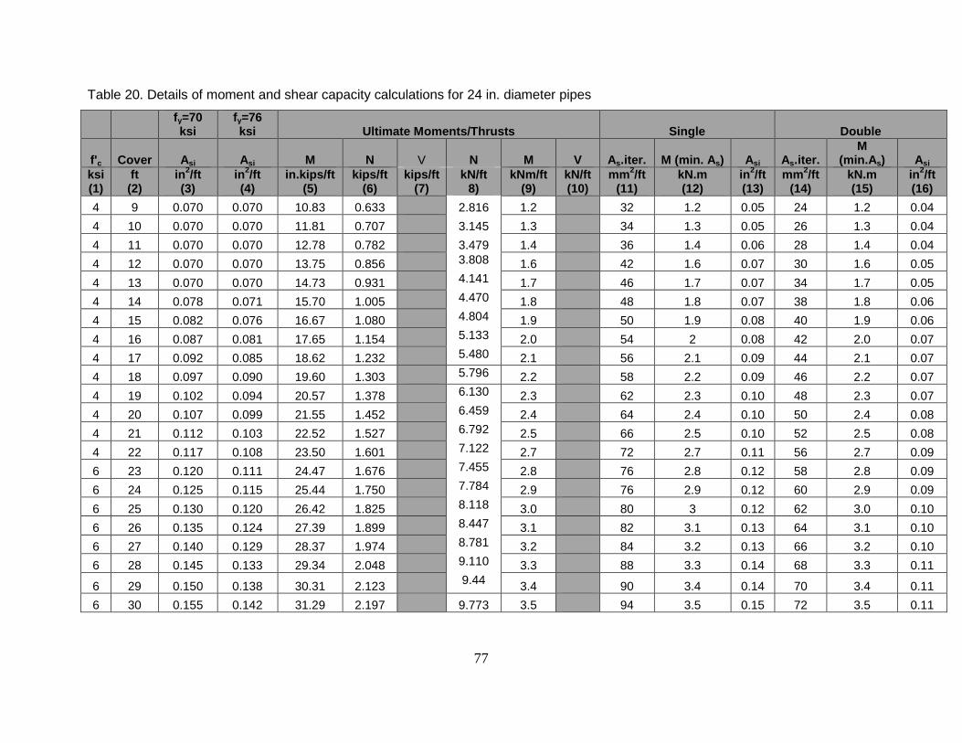
77
Table 20. Details of moment and shear capacity calculations for 24 in. diameter pipes
fy=70 ksi
fy=76 ksi Ultimate Moments/Thrusts Single Double
f'c Cover Asi Asi M N V N M V As.iter. M (min. As) Asi As.iter. M
(min.As) Asi ksi (1)
ft (2)
in2/ft (3)
in2/ft (4)
in.kips/ft (5)
kips/ft (6)
kips/ft (7)
kN/ft 8)
kNm/ft (9)
kN/ft (10)
mm2/ft (11)
kN.m (12)
in2/ft (13)
mm2/ft (14)
kN.m (15)
in2/ft (16)
4 9 0.070 0.070 10.83 0.633 2.816 1.2 32 1.2 0.05 24 1.2 0.04 4 10 0.070 0.070 11.81 0.707 3.145 1.3 34 1.3 0.05 26 1.3 0.04 4 11 0.070 0.070 12.78 0.782 3.479 1.4 36 1.4 0.06 28 1.4 0.04 4 12 0.070 0.070 13.75 0.856
3.808 1.6 42 1.6 0.07 30 1.6 0.05
4 13 0.070 0.070 14.73 0.931
4.141 1.7 46 1.7 0.07 34 1.7 0.05 4 14 0.078 0.071 15.70 1.005
4.470 1.8 48 1.8 0.07 38 1.8 0.06
4 15 0.082 0.076 16.67 1.080
4.804 1.9 50 1.9 0.08 40 1.9 0.06 4 16 0.087 0.081 17.65 1.154
5.133 2.0 54 2 0.08 42 2.0 0.07
4 17 0.092 0.085 18.62 1.232
5.480 2.1 56 2.1 0.09 44 2.1 0.07 4 18 0.097 0.090 19.60 1.303 5.796 2.2 58 2.2 0.09 46 2.2 0.07 4 19 0.102 0.094 20.57 1.378
6.130 2.3 62 2.3 0.10 48 2.3 0.07
4 20 0.107 0.099 21.55 1.452
6.459 2.4 64 2.4 0.10 50 2.4 0.08 4 21 0.112 0.103 22.52 1.527
6.792 2.5 66 2.5 0.10 52 2.5 0.08
4 22 0.117 0.108 23.50 1.601
7.122 2.7 72 2.7 0.11 56 2.7 0.09 6 23 0.120 0.111 24.47 1.676
7.455 2.8 76 2.8 0.12 58 2.8 0.09
6 24 0.125 0.115 25.44 1.750
7.784 2.9 76 2.9 0.12 60 2.9 0.09 6 25 0.130 0.120 26.42 1.825
8.118 3.0 80 3 0.12 62 3.0 0.10
6 26 0.135 0.124 27.39 1.899
8.447 3.1 82 3.1 0.13 64 3.1 0.10 6 27 0.140 0.129 28.37 1.974
8.781 3.2 84 3.2 0.13 66 3.2 0.10
6 28 0.145 0.133 29.34 2.048
9.110 3.3 88 3.3 0.14 68 3.3 0.11
6 29 0.150 0.138 30.31 2.123
9.44 3.4 90 3.4 0.14 70 3.4 0.11 6 30 0.155 0.142 31.29 2.197
9.773 3.5 94 3.5 0.15 72 3.5 0.11

78
Table 21. Details of moment and shear capacity calculations for 36 in. diameter pipes.
fy=70 ksi
fy=76 ksi Ultimate Moments/Thrusts/Shears Single Double
f'c Cover Asi Asi M N V N M V As.iter. M
(min.As) Asi As.iter. M
(min.As) Asi ksi (1)
ft (2)
in2/ft (3)
in2/ft (4)
in.kips/ft (5)
kips/ft (6)
kN/ft (7)
kN/ft (8)
kNm/ft (9)
kN/ft (10)
mm2/ft (11)
kN.m (12)
in2/ft (13)
mm2/ft (14)
kN.m (15)
in2/ft (16)
4 9 0.091 0.084 24.54 0.870 3.87 2.8 56 2.8 0.087 46 2.8 0.071 4 10 0.098 0.091 26.60 0.978 4.35 3.0 60 3.0 0.093 50 3.0 0.078 4 11 0.106 0.098 28.67 1.093 4.86 3.2 64 3.2 0.099 54 3.2 0.084 4 12 0.114 0.105 30.73 1.193 5.31 3.5 70 3.5 0.109 58 3.5 0.090 4 13 0.121 0.112 32.80 1.301 5.79 3.7 74 3.7 0.115 60 3.7 0.093 4 14 0.129 0.119 34.86 1.409 6.27 3.9 78 3.9 0.121 66 3.9 0.102 4 15 0.137 0.126 36.93 1.516 6.74 4.2 84 4.2 0.130 72 4.2 0.112 4 16 0.145 0.133 38.99 1.624 7.22 4.4 88 4.4 0.136 74 4.4 0.115 4 17 0.153 0.14 41.06 1.732 7.70 4.6 92 4.6 0.143 78 4.6 0.121 4 18 0.16 0.148 43.13 1.839 8.18 4.9 100 4.9 0.155 84 4.9 0.130 4 19 0.168 0.155 45.19 1.947 8.66 5.1 104 5.1 0.161 88 5.1 0.136 4 20 0.176 0.163 47.26 2.054 9.14 5.3 108 5.3 0.167 92 5.3 0.143 4 21 0.184 0.170 49.32 2.162 9.62 5.6 114 5.6 0.177 98 5.6 0.152 4 22 0.193 0.177 51.39 2.270 10.10 5.8 118 5.8 0.183 102 5.8 0.158 6 23 0.196 0.181 53.45 2.377 10.57 6.0 120 6.0 0.186 100 6.0 0.155 6 24 0.204 0.188 55.52 2.485 11.05 6.3 126 6.3 0.195 106 6.3 0.164 6 25 0.212 0.195 57.58 2.593 11.53 6.5 130 6.5 0.202 110 6.5 0.171 6 26 0.22 0.202 59.65 2.700 12.01 6.7 134 6.7 0.208 114 6.7 0.177 6 27 0.227 0.21 61.71 2.808 12.49 7.0 140 7.0 0.217 120 7.0 0.186 6 28 0.235 0.217 63.78 2.915 12.97 7.2 144 7.2 0.223 124 7.2 0.192 6 29 0.243 0.224 65.84 3.023 13.45 7.4 148 7.4 0.229 128 7.4 0.198 6 30 0.251 0.231 67.91 3.131 13.93 7.7 156 7.7 0.242 134 7.7 0.208
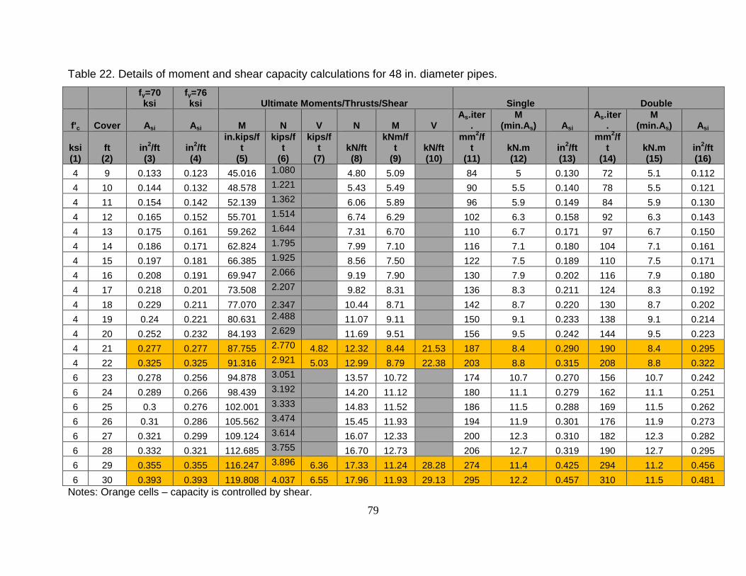
79
Table 22. Details of moment and shear capacity calculations for 48 in. diameter pipes.
fy=70 ksi
fy=76 ksi Ultimate Moments/Thrusts/Shear Single Double
f'c Cover Asi Asi M N V N M V As.iter
. M
(min.As) Asi As.iter
. M
(min.As) Asi
ksi (1)
ft (2)
in2/ft (3)
in2/ft (4)
in.kips/ft
(5)
kips/ft
(6)
kips/ft
(7) kN/ft (8)
kNm/ft
(9) kN/ft (10)
mm2/ft
(11)
kN.m (12)
in2/ft (13)
mm2/ft
(14) kN.m (15)
in2/ft (16)
4 9 0.133 0.123 45.016 1.080 4.80 5.09
84 5 0.130 72 5.1 0.112 4 10 0.144 0.132 48.578 1.221 5.43 5.49
90 5.5 0.140 78 5.5 0.121
4 11 0.154 0.142 52.139 1.362 6.06 5.89
96 5.9 0.149 84 5.9 0.130 4 12 0.165 0.152 55.701 1.514 6.74 6.29
102 6.3 0.158 92 6.3 0.143
4 13 0.175 0.161 59.262 1.644 7.31 6.70
110 6.7 0.171 97 6.7 0.150 4 14 0.186 0.171 62.824 1.795 7.99 7.10
116 7.1 0.180 104 7.1 0.161
4 15 0.197 0.181 66.385 1.925 8.56 7.50
122 7.5 0.189 110 7.5 0.171 4 16 0.208 0.191 69.947 2.066 9.19 7.90
130 7.9 0.202 116 7.9 0.180
4 17 0.218 0.201 73.508 2.207 9.82 8.31
136 8.3 0.211 124 8.3 0.192 4 18 0.229 0.211 77.070 2.347 10.44 8.71
142 8.7 0.220 130 8.7 0.202
4 19 0.24 0.221 80.631 2.488 11.07 9.11
150 9.1 0.233 138 9.1 0.214 4 20 0.252 0.232 84.193 2.629 11.69 9.51
156 9.5 0.242 144 9.5 0.223
4 21 0.277 0.277 87.755 2.770 4.82 12.32 8.44 21.53 187 8.4 0.290 190 8.4 0.295 4 22 0.325 0.325 91.316 2.921 5.03 12.99 8.79 22.38 203 8.8 0.315 208 8.8 0.322 6 23 0.278 0.256 94.878 3.051 13.57 10.72
174 10.7 0.270 156 10.7 0.242
6 24 0.289 0.266 98.439 3.192 14.20 11.12
180 11.1 0.279 162 11.1 0.251 6 25 0.3 0.276 102.001 3.333 14.83 11.52
186 11.5 0.288 169 11.5 0.262
6 26 0.31 0.286 105.562 3.474 15.45 11.93
194 11.9 0.301 176 11.9 0.273 6 27 0.321 0.299 109.124 3.614 16.07 12.33
200 12.3 0.310 182 12.3 0.282
6 28 0.332 0.321 112.685 3.755 16.70 12.73
206 12.7 0.319 190 12.7 0.295 6 29 0.355 0.355 116.247 3.896 6.36 17.33 11.24 28.28 274 11.4 0.425 294 11.2 0.456 6 30 0.393 0.393 119.808 4.037 6.55 17.96 11.93 29.13 295 12.2 0.457 310 11.5 0.481
Notes: Orange cells – capacity is controlled by shear.

80
Table 23. Details of moment and shear capacity calculations for 60 in. diameter pipes.
fy=70 ksi
fy=76 ksi Ultimate Moments/Thrusts/Shear Single Double
f'c Cover Asi Asi M N V M N V As.iter. M
(min.As) Asi As.iter
. M
(min.As) Asi
ksi (1)
ft (2)
in2/ft (3)
in2/ft (4)
in.kips/ft
(5) kips/ft
(6) kips/ft
(7) kN.m/ft
(8) kN/ft (9)
kN/ft (10)
mm2/ft (11)
kN.m (12)
in2/ft (13)
mm2/ft
(14) kN.m (15)
in2/ft (16)
4 9 0.181 0.166 73.19 1.263
8.3 5.618
114 8.3 0.177 103 8.3 0.160 4 10 0.194 0.179 78.65 1.437
8.9 6.392
122 8.9 0.189 111 8.9 0.172
4 11 0.207 0.191 84.11 1.611
9.5 7.166
130 9.5 0.202 119 9.5 0.184 4 12 0.221 0.204 89.58 1.785
10.1 7.940
138 10.1 0.214 127 10.1 0.197
4 13 0.235 0.216 95.04 1.959
10.7 8.714
146 10.7 0.226 135 10.7 0.209 4 14 0.248 0.229 100.50 2.132
11.4 9.484
156 11.4 0.242 145 11.4 0.225
4 15 0.262 0.241 105.96 2.306
12.0 10.258
164 12.0 0.254 154 12.0 0.239 4 16 0.276 0.254 111.43 2.480
12.6 11.032
172 12.6 0.267 163 12.6 0.253
4 17 0.290 0.267 116.89 2.654
13.2 11.806
180 13.2 0.279 172 13.2 0.267 4 18 0.334 0.334 102.49 3.667 5.552 11.6 16.312 24.70 220 11.6 0.341 228 11.7 0.353 4 19 0.396 0.396 107.18 3.878 5.790 12.1 17.250 25.76 234 12.1 0.363 240 12.1 0.372 4 20 0.459 0.459 111.88 4.088 6.027 12.6 18.184 26.81 248 12.6 0.384 254 12.6 0.394 4 21 0.521 0.521 116.57 4.298 6.265 13.2 19.118 27.87 268 13.2 0.415 274 13.2 0.425 4 22 0.584 0.584 121.27 4.508 6.502 13.7 20.053 28.92 286 13.7 0.443 292 13.7 0.453 6 23 0.365 0.347 149.67 3.713
16.9 16.516
228 16.9 0.353 215 16.9 0.333
6 24 0.379 0.374 155.13 3.872
17.5 17.224
236 17.5 0.366 223 17.5 0.346 6 25 0.412 0.412 135.36 4.045 7.215 15.3 17.993 32.09 312 15.3 0.484 314 15.3 0.487 6 26 0.462 0.462 140.05 5.349 7.452 15.8 23.794 33.15 322 15.8 0.499 324 15.8 0.502 6 27 0.512 0.512 144.75 5.559 7.69 16.4 24.728 34.21 337 16.2 0.522 344 16.4 0.533 6 28 0.562 0.562 149.44 5.769 7.927 16.9 25.662 35.26 349 16.5 0.541 374 16.9 0.580 6 29 0.612 0.612 154.14 5.979 8.164 17.4 26.596 36.32 377 17.4 0.584 416 17.4 0.645 6 30 0.662 0.662 158.83 6.19 8.402 17.9 27.534 37.37 396 17.9 0.614 438 17.9 0.679 Notes: Orange cells – capacity is controlled by shear.
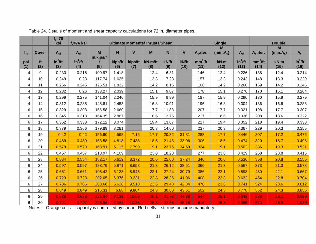
81
Table 24. Details of moment and shear capacity calculations for 72 in. diameter pipes.
fy=70 ksi fy=76 ksi Ultimate Moments/Thrusts/Shear Single Double
f'c Cover Asi Asi M N V M N V As.iter. M
(min.As) Asi As.iter. M
(min.As) Asi
psi (1)
ft (2)
in2/ft (3)
in2/ft (4)
in.kips/ft
(5) kips/ft
(6) kips/ft
(7) kN.m/ft
(8) kN/ft (9)
kN/ft (10)
mm2/ft (11)
kN.m (12)
in2/ft (13)
mm2/ft (14)
kN.m (15)
in2/ft (16)
4 9 0.233 0.215 109.97 1.418 12.4 6.31 146 12.4 0.226 138 12.4 0.214 4 10 0.249 0.23 117.74 1.625 13.3 7.23 157 13.3 0.243 148 13.3 0.229 4 11 0.266 0.245 125.51 1.832 14.2 8.15 168 14.2 0.260 159 14.2 0.246 4 12 0.282 0.26 133.27 2.039 15.1 9.07 178 15.1 0.276 170 15.1 0.264 4 13 0.299 0.275 141.04 2.246 15.9 9.99 187 15.9 0.290 180 15.9 0.279 4 14 0.312 0.288 148.81 2.453 16.8 10.91 196 16.8 0.304 186 16.8 0.288 6 15 0.329 0.303 156.58 2.660 17.7 11.83 207 17.7 0.321 198 17.7 0.307 6 16 0.345 0.318 164.35 2.867 18.6 12.75 217 18.6 0.336 208 18.6 0.322 6 17 0.362 0.333 172.12 3.074 19.4 13.67 227 19.4 0.352 218 19.4 0.338 6 18 0.379 0.366 179.89 3.281 20.3 14.60 237 20.3 0.367 229 20.3 0.355 6 19 0.42 0.42 156.90 4.568 7.15 17.7 20.32 31.81 288 17.7 0.446 307 17.2 0.476 6 20 0.489 0.489 163.58 4.818 7.433 18.5 21.43 33.06 306 18.5 0.474 320 18.7 0.496 6 21 0.579 0.579 168.91 5.115 7.799 19.1 22.75 34.69 324 19.1 0.502 336 19.3 0.521 6 22 0.457 0.457 210.97 4.109 23.8 18.28 277 23.8 0.429 268 23.8 0.415 6 23 0.534 0.534 182.17 5.619 8.372 20.6 25.00 37.24 346 20.6 0.536 358 20.8 0.555 6 24 0.597 0.597 188.79 5.871 8.658 21.3 26.12 38.51 366 21.3 0.567 373 21.3 0.578 6 25 0.661 0.661 195.42 6.123 8.945 22.1 27.24 39.79 386 22.1 0.598 430 22.1 0.667 6 26 0.723 0.723 202.05 6.376 9.231 22.8 28.36 41.06 408 22.8 0.632 454 22.8 0.704 6 27 0.786 0.786 208.68 6.628 9.518 23.6 29.48 42.34 478 23.6 0.741 524 23.6 0.812 6 28 0.849 0.849 215.31 6.88 9.804 24.3 30.60 43.61 502 24.3 0.778 552 24.3 0.856 6 29 0.688 0.688 221.94 7.132 10.09 25.1 31.73 44.88 547 25.1 0.848 638 25.1 0.989 6 30 0.721 0.707 228.56 7.384 10.38 25.8 32.85 46.16 616 25.8 0.955 670 25.8 1.039 Notes: Orange cells – capacity is controlled by shear; Red cells – stirrups become mandatory.

82
Figure 24. Comparison of inner steel requirements for 24 in. diameter reinforced
concrete pipe based on four different methods of calculation; Type 2 installation.
Figure 25. Comparison of inner steel requirements for 36 in. diameter reinforced
concrete pipe based on four different methods of calculation; Type 2 installation.
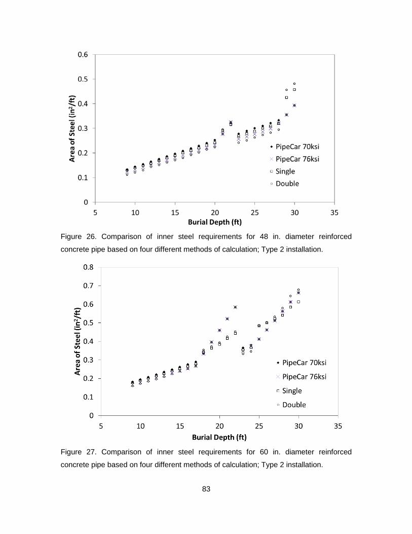
83
Figure 26. Comparison of inner steel requirements for 48 in. diameter reinforced
concrete pipe based on four different methods of calculation; Type 2 installation.
Figure 27. Comparison of inner steel requirements for 60 in. diameter reinforced
concrete pipe based on four different methods of calculation; Type 2 installation.
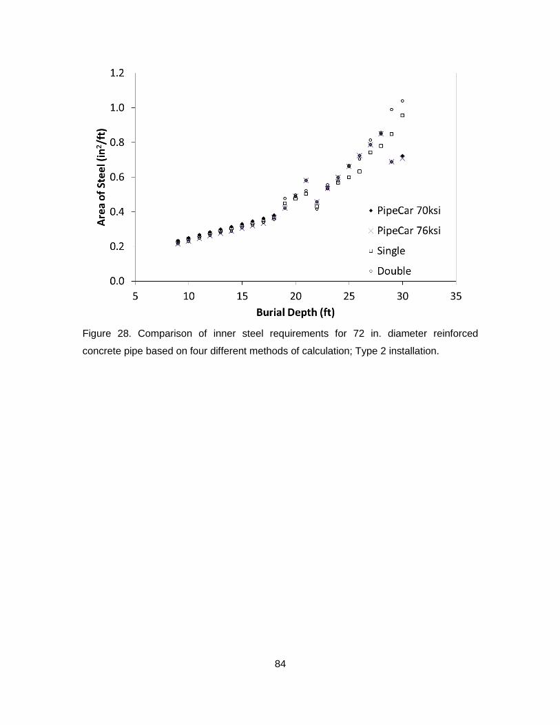
84
Figure 28. Comparison of inner steel requirements for 72 in. diameter reinforced
concrete pipe based on four different methods of calculation; Type 2 installation.
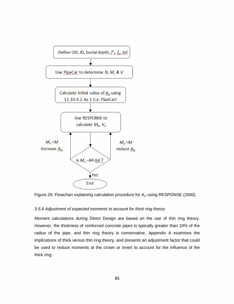
85
Figure 29. Flowchart explaining calculation procedure for Asi using RESPONSE (2000).
3.5.6 Adjustment of expected moments to account for thick ring theory
Moment calculations during Direct Design are based on the use of thin ring theory.
However, the thickness of reinforced concrete pipes is typically greater than 10% of the
radius of the pipe, and thin ring theory is conservative. Appendix A examines the
implications of thick versus thin ring theory, and presents an adjustment factor that could
be used to reduce moments at the crown or invert to account for the influence of the
thick ring:

86
Rt
MM
invertcrownthin
373.01,
−= 18
where t is the pipe thickness, R its average radius, and Mthin is the moment estimate from
Direct Design based on thin ring theory.
3.5.7 Potential consideration of plastic collapse mechanism
Direct Design evaluates the loads that induce the ultimate moment in the buried pipe by
equating maximum expected moment from elastic ring theory to the ultimate moment
capacity. However, pipe strength is not fully mobilized when moments reach the ultimate
value at a single location on the pipe circumference. Instead, a plastic collapse
mechanism for the pipe would involve four locations around the circumference reaching
the ultimate moment capacity.
Therefore, use of plastic collapse analysis to determine the ultimate load capacity of
buried concrete pipes has been examined in Appendix B.
This analysis approach would require additional research to determine the soil
characteristics required in the analysis for different burial conditions. In particular, the
earth pressure distributions currently used to estimate earth load effects would change,
and may approach those associated with flexible pipes (the development of a collapse
mechanism removes most of the flexural stiffness of the structure). However, the limiting
load obtained during each of the five limit states tests was controlled by the service limit
(the 0.01 in. crack), and none came close to generating the ultimate moment in the pipe.
For that reason, the development and implementation of analysis based on a plastic
collapse mechanism is not likely warranted, or should not be undertaken unless
enhancements were made to permit effective estimates of the loads required to produce
the limiting crack.

87
3.6 Comparison of Steel Requirements from the Indirect and Direct Design Methods
3.6.1 Introduction
Erdogmus et al. (2010) employed summary plots comparing the steel requirements
determined using Indirect Design and Direct Design. These are very effective in
illustrating the differences in outcomes from these two different design procedures, so
are used here to illustrate:
- the current outcomes of Indirect Design and Direct Design (summarized in
Table 25)
- the outcomes that would result if corrections for thick ring theory were included
in Direct Design (summarized in Table 26)
- the outcomes that would result if the maximum potential benefits of steel strain
hardening were achieved when undertaking Direct Design (summarized in Table 27)
- the outcomes that would result if Modified Compression Field Theory were used
and two bars of steel were considered when undertaking Direct Design (summarized in
Table 28)
All Indirect Design results are given for Wall C pipes defined in ASTM C76, since these
have lower steel areas than Wall B pipes. All pipes are considered for a Type 2
installation. Details of the calculation procedures, the input variables and the results
were given earlier.
3.6.2 Current differences for pipes under deep burial
Figure 30 shows the steel requirements associated with the existing design methods for
pipes of diameters 24 inches to 72 inches and cover depths between 1ft and 30ft. The
steel associated with Class II to Class V pipes defined in ASTM C76 are indicated, with
maximum bedding depths calculated using the Indirect Design Method. Surface loading
at shallow burial has been calculated based on AASHTO (2007) (not including
modifications approved in 2013). Each of those pipes has a minimum burial depth
associated with it also, set as one foot greater than the maximum limit of the previous
pipe class (e.g. the maximum cover permitted for the Class IV pipe of 72 in. diameter is
21 ft, and so the minimum shown for the Class V pipe is 22 ft).

88
Direct Design employs equation 12.10.4.2.4a-1 from the AASHTO LRFD Bridge Design
Specifications. This produces individual steel requirements for each burial depth, and the
solid lines show those steel requirements for each of the five pipe diameters with each
line color matching the symbol colors of the Indirect Design results. The calculations
performed by PipeCar are for live load effects use the live load spreading approach
recommended by the ACPA (1998), rather than the current or former AASHTO (2007,
2013) procedures. The objective with these plots is to illustrate differences between
Indirect and Direct Design outcomes rather than the different approaches for treating
surface live load, so the Direct Design estimates have been terminated at minimum
burial depth of 8ft.
The performance of the existing design methods can, therefore, be evaluated by
comparing the solid lines with the symbols. The ideal situation is when both design
methods produce identical steel requirements. In that case, the solid lines would just
touch the right hand end of each set of cover depths for a specific Indirect Design pipe
Class. This is not generally the case however. For the largest diameter (72 in.) pipe
results (shown in green), the Direct Design steel areas fall consistently below the Indirect
Design areas, falling more progressively to the right as burial depth (or pipe Class) is
increased.
For all of the smaller diameter pipes, the amounts of steel calculated using Direct Design
have ranges of burial depth where their areas are greater than those for the pipe
Classes associated with Indirect Design. This discrepancy is significant for 24 in. and 36
in. diameter pipes where Indirect Design indicates that a Class IV pipe should be
employed (burial depths from 15 to 22 ft), with area of steel from Direct Design falling
consistently above the results from Indirect Design.
It was shown in earlier sections of this report that both Indirect Design and Direct Design
resulted in conservative strength estimates for a number of test pipes. However, one key
objective of Project 20-07 Task 316 is to understand and reconcile the differences
between Direct and Indirect Design. A follow-on objective might be to change design so
that the areas of steel resulting from Direct Design are always less than or equal to
Indirect Design i.e. bringing the solid lines on Figure 30 to touch the right hand end of
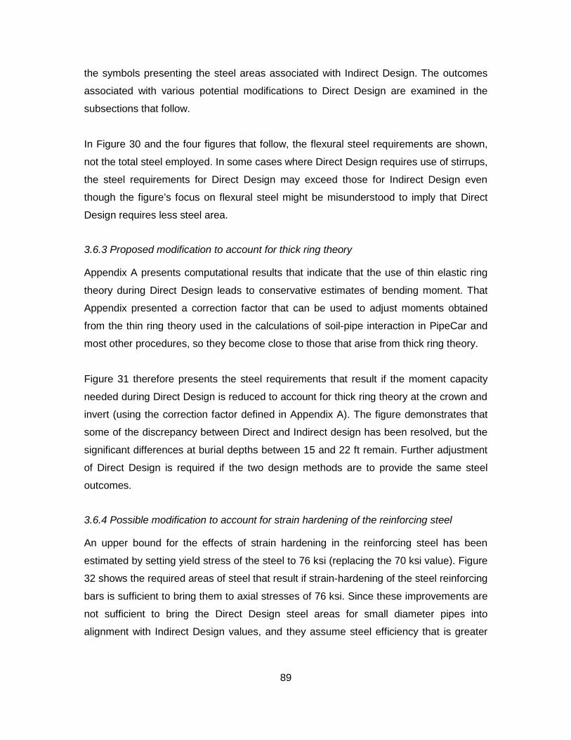
89
the symbols presenting the steel areas associated with Indirect Design. The outcomes
associated with various potential modifications to Direct Design are examined in the
subsections that follow.
In Figure 30 and the four figures that follow, the flexural steel requirements are shown,
not the total steel employed. In some cases where Direct Design requires use of stirrups,
the steel requirements for Direct Design may exceed those for Indirect Design even
though the figure’s focus on flexural steel might be misunderstood to imply that Direct
Design requires less steel area.
3.6.3 Proposed modification to account for thick ring theory
Appendix A presents computational results that indicate that the use of thin elastic ring
theory during Direct Design leads to conservative estimates of bending moment. That
Appendix presented a correction factor that can be used to adjust moments obtained
from the thin ring theory used in the calculations of soil-pipe interaction in PipeCar and
most other procedures, so they become close to those that arise from thick ring theory.
Figure 31 therefore presents the steel requirements that result if the moment capacity
needed during Direct Design is reduced to account for thick ring theory at the crown and
invert (using the correction factor defined in Appendix A). The figure demonstrates that
some of the discrepancy between Direct and Indirect design has been resolved, but the
significant differences at burial depths between 15 and 22 ft remain. Further adjustment
of Direct Design is required if the two design methods are to provide the same steel
outcomes.
3.6.4 Possible modification to account for strain hardening of the reinforcing steel
An upper bound for the effects of strain hardening in the reinforcing steel has been
estimated by setting yield stress of the steel to 76 ksi (replacing the 70 ksi value). Figure
32 shows the required areas of steel that result if strain-hardening of the steel reinforcing
bars is sufficient to bring them to axial stresses of 76 ksi. Since these improvements are
not sufficient to bring the Direct Design steel areas for small diameter pipes into
alignment with Indirect Design values, and they assume steel efficiency that is greater

90
than or equal to that which could be actually realized (these improvements may well be
optimistic), the issue of steel strain hardening is not considered further.
3.6.5 Proposed modification to employ Modified Compression Field Theory
Figure 33 shows how use of the Modified Compression Field Theory and consideration
of two layers of reinforcing steel influence Asi, the calculated value of inner steel required
at the invert of these pipes.
3.6.6 Relative impact of different potential changes to Direct Design
Figure 34 shows results for pipes of 24 in., 48 in. and 72 in. diameter, considering three
different alternatives for Direct Design calculations of Asi:
- Calculations based on equation 12.10.4.2.4a-1
- Calculations using equation 12.10.4.2.4a-1 but with required moment capacity
reduced to account for thick ring theory
- Calculations based on Modified Compression Field Theory obtained using
program RESPONSE, and considering two layers of reinforcing steel
For the smallest diameter pipes, the two changes to the calculation procedure each
reduce area of steel required. These could be combined to achieve even greater
reductions (i.e. Modified Compression Field Theory could be used to determine area of
steel required to achieve moments that were reduced to account for thick ring theory).
The results for pipe of intermediate size (48 in.) are similar, except in the two regions
where shear governs. In those regions, the Modified Compression Field Theory yields
higher areas of steel.
Results for the largest diameter pipe (72 in.) indicate that correction for thick ring theory
consistently reduces the amount of steel required. However, use of Modified
Compression Field Theory leads to increases in steel requirements for burial depths
between 18 and 21 ft, little change in requirements at burial depths from 23 to 28 ft, and
significant increases at greater depths where AASHTO currently requires use of stirrups.
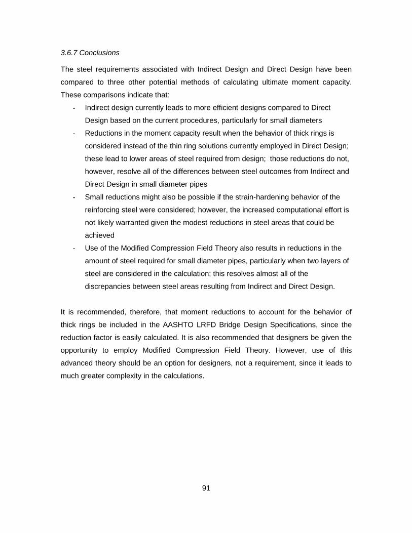
91
3.6.7 Conclusions
The steel requirements associated with Indirect Design and Direct Design have been
compared to three other potential methods of calculating ultimate moment capacity.
These comparisons indicate that:
- Indirect design currently leads to more efficient designs compared to Direct
Design based on the current procedures, particularly for small diameters
- Reductions in the moment capacity result when the behavior of thick rings is
considered instead of the thin ring solutions currently employed in Direct Design;
these lead to lower areas of steel required from design; those reductions do not,
however, resolve all of the differences between steel outcomes from Indirect and
Direct Design in small diameter pipes
- Small reductions might also be possible if the strain-hardening behavior of the
reinforcing steel were considered; however, the increased computational effort is
not likely warranted given the modest reductions in steel areas that could be
achieved
- Use of the Modified Compression Field Theory also results in reductions in the
amount of steel required for small diameter pipes, particularly when two layers of
steel are considered in the calculation; this resolves almost all of the
discrepancies between steel areas resulting from Indirect and Direct Design.
It is recommended, therefore, that moment reductions to account for the behavior of
thick rings be included in the AASHTO LRFD Bridge Design Specifications, since the
reduction factor is easily calculated. It is also recommended that designers be given the
opportunity to employ Modified Compression Field Theory. However, use of this
advanced theory should be an option for designers, not a requirement, since it leads to
much greater complexity in the calculations.

92
Table 25. Steel requirements calculated using existing procedures. Diameter 24in 36in 48in 60in 72in 24in 36in 48in 60in 72in
Thickness 3.75 4.75 5.75 6.75 7.75 3.75 4.75 5.75 6.75 7.75
Cover ft Asi in2/ft from C76 (for Indirect Design) Asi in2/ft from PipeCar (Direct Design)
1 0.12 0.27 0.470 0.700 0.990
2 0.07 0.08 0.160 0.240 0.360
3 0.07 0.07 0.140 0.210 0.300
4 0.07 0.07 0.140 0.210 0.300
5 0.07 0.07 0.140 0.210 0.300
6 0.07 0.07 0.140 0.210 0.300
7 0.07 0.07 0.140 0.210 0.300
8 0.07 0.07 0.140 0.210 0.300
9 0.07 0.07 0.140 0.210 0.300 0.070 0.091 0.133 0.181 0.233
10 0.07 0.07 0.140 0.210 0.360 0.070 0.098 0.144 0.194 0.249
11 0.07 0.08 0.160 0.240 0.360 0.070 0.106 0.154 0.207 0.266
12 0.07 0.08 0.160 0.240 0.360 0.070 0.114 0.165 0.221 0.282
13 0.07 0.08 0.160 0.240 0.360 0.070 0.121 0.175 0.235 0.299
14 0.07 0.08 0.160 0.240 0.600 0.078 0.129 0.186 0.248 0.312
15 0.07 0.14 0.260 0.410 0.600 0.082 0.137 0.197 0.262 0.329
16 0.07 0.14 0.260 0.410 0.600 0.087 0.145 0.208 0.276 0.345
17 0.07 0.14 0.260 0.410 0.600 0.092 0.153 0.218 0.290 0.362
18 0.07 0.14 0.260 0.410 0.600 0.097 0.160 0.229 0.334 0.379
19 0.07 0.14 0.260 0.410 0.600 0.102 0.168 0.240 0.396 0.420
20 0.07 0.14 0.260 0.410 0.600 0.107 0.176 0.252 0.459 0.489
21 0.07 0.14 0.260 0.410 0.600 0.112 0.184 0.277 0.521 0.579
22 0.07 0.14 0.260 0.410 0.990 0.117 0.193 0.325 0.584 0.457
23 0.12 0.27 0.470 0.700 0.990 0.120 0.196 0.278 0.365 0.534
24 0.12 0.27 0.470 0.700 0.990 0.125 0.204 0.289 0.379 0.597
25 0.12 0.27 0.470 0.700 0.990 0.130 0.212 0.300 0.412 0.661
26 0.12 0.27 0.470 0.700 0.990 0.135 0.220 0.310 0.462 0.723
27 0.12 0.27 0.470 0.700 0.990 0.140 0.227 0.321 0.512 0.786
28 0.12 0.27 0.470 0.700 0.990 0.145 0.235 0.332 0.562 0.849
29 0.12 0.27 0.470 0.700 0.990 0.150 0.243 0.355 0.612 0.688
30 0.12 0.27 0.470 0.700 0.990 0.155 0.251 0.393 0.662 0.721

93
Table 26. Inner steel requirements at the invert Asi in in2/ft calculated considering Thick Ring Theory Diameter 24 36 48 60 72
Thickness 3.75 4.75 5.75 6.75 7.75
Cover Thickness Correction 1-0.37(t/R)
ft 0.90 0.91 0.92 0.93 0.93
Asi in2/ft adjusting for thick ring theory
9 0.063 0.083 0.122 0.167 0.216
10 0.063 0.090 0.133 0.179 0.231
11 0.063 0.097 0.142 0.192 0.247
12 0.063 0.104 0.152 0.204 0.262
13 0.063 0.111 0.161 0.217 0.277
14 0.070 0.118 0.171 0.229 0.290
15 0.074 0.125 0.181 0.242 0.305
16 0.078 0.132 0.192 0.255 0.320
17 0.083 0.140 0.201 0.268 0.336
18 0.087 0.146 0.211 0.309 0.352
19 0.092 0.154 0.221 0.366 0.390
20 0.096 0.161 0.232 0.425 0.454
21 0.101 0.168 0.255 0.482 0.537
22 0.105 0.176 0.299 0.540 0.424
23 0.108 0.179 0.256 0.338 0.496
24 0.113 0.186 0.266 0.351 0.554
25 0.117 0.194 0.276 0.381 0.613
26 0.122 0.201 0.285 0.427 0.671
27 0.126 0.207 0.296 0.474 0.729
28 0.131 0.215 0.306 0.520 0.788
29 0.135 0.222 0.327 0.566 0.639
30 0.140 0.229 0.362 0.612 0.669

94
Table 27. Inner steel requirements at the invert Asi in in2/ft calculated considering potential benefits of
steel strain hardening and thick ring theory
Diameter 24 36 48 60 72 24 36 48 60 72
Thickness 3.75 4.75 5.75 6.75 7.75 3.75 4.75 5.75 6.75 7.75
Cover ft Asi in2/ft (Steel strain hardening) Asi in2/ft thick & steel hardening
9 0.07 0.084 0.123 0.166 0.215 0.063 0.077 0.113 0.154 0.200
10 0.07 0.091 0.132 0.179 0.23 0.063 0.083 0.122 0.166 0.213
11 0.07 0.098 0.142 0.191 0.245 0.063 0.090 0.131 0.177 0.227
12 0.07 0.105 0.152 0.204 0.26 0.063 0.096 0.140 0.189 0.241
13 0.07 0.112 0.161 0.216 0.275 0.063 0.102 0.148 0.200 0.255
14 0.071 0.119 0.171 0.229 0.288 0.064 0.109 0.157 0.212 0.267
15 0.076 0.126 0.181 0.241 0.303 0.068 0.115 0.167 0.223 0.281
16 0.081 0.133 0.191 0.254 0.318 0.073 0.122 0.176 0.235 0.295
17 0.085 0.14 0.201 0.267 0.333 0.077 0.128 0.185 0.247 0.309
18 0.09 0.148 0.211 0.334 0.366 0.081 0.135 0.194 0.309 0.340
19 0.094 0.155 0.221 0.396 0.42 0.085 0.142 0.204 0.366 0.390
20 0.099 0.163 0.232 0.459 0.489 0.089 0.149 0.214 0.425 0.454
21 0.103 0.17 0.277 0.521 0.579 0.093 0.155 0.255 0.482 0.537
22 0.108 0.177 0.325 0.584 0.457 0.097 0.162 0.299 0.540 0.424
23 0.111 0.181 0.256 0.347 0.534 0.100 0.165 0.236 0.321 0.496
24 0.115 0.188 0.266 0.374 0.597 0.104 0.172 0.245 0.346 0.554
25 0.12 0.195 0.276 0.412 0.661 0.108 0.178 0.254 0.381 0.613
26 0.124 0.202 0.286 0.462 0.723 0.112 0.185 0.263 0.427 0.671
27 0.129 0.21 0.299 0.512 0.786 0.116 0.192 0.275 0.474 0.729
28 0.133 0.217 0.321 0.562 0.849 0.120 0.198 0.296 0.520 0.788
29 0.138 0.224 0.355 0.612 0.688 0.124 0.205 0.327 0.566 0.639
30 0.142 0.231 0.393 0.662 0.707 0.128 0.211 0.362 0.612 0.656
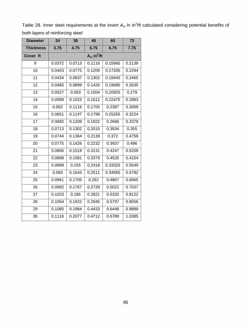
95
Table 28. Inner steel requirements at the invert Asi in in2/ft calculated considering potential benefits of
both layers of reinforcing steel
Diameter 24 36 48 60 72
Thickness 3.75 4.75 5.75 6.75 7.75
Cover ft Asi in2/ft
9 0.0372 0.0713 0.1116 0.15965 0.2139
10 0.0403 0.0775 0.1209 0.17205 0.2294
11 0.0434 0.0837 0.1302 0.18445 0.2465
12 0.0465 0.0899 0.1426 0.19685 0.2635
13 0.0527 0.093 0.1504 0.20925 0.279
14 0.0589 0.1023 0.1612 0.22475 0.2883
15 0.062 0.1116 0.1705 0.2387 0.3069
16 0.0651 0.1147 0.1798 0.25265 0.3224
17 0.0682 0.1209 0.1922 0.2666 0.3379
18 0.0713 0.1302 0.2015 0.3534 0.355
19 0.0744 0.1364 0.2139 0.372 0.4759
20 0.0775 0.1426 0.2232 0.3937 0.496
21 0.0806 0.1519 0.3131 0.4247 0.5208
22 0.0868 0.1581 0.3379 0.4526 0.4154
23 0.0899 0.155 0.2418 0.33325 0.5549
24 0.093 0.1643 0.2511 0.34565 0.5782
25 0.0961 0.1705 0.262 0.4867 0.6665
26 0.0992 0.1767 0.2728 0.5022 0.7037
27 0.1023 0.186 0.2821 0.5332 0.8122
28 0.1054 0.1922 0.2945 0.5797 0.8556
29 0.1085 0.1984 0.4433 0.6448 0.9889
30 0.1116 0.2077 0.4712 0.6789 1.0385

96
Figure 30. Requirements for inner steel at invert according to ASTM C76 for Indirect Design (Wall C)
and current AASHTO requirements for Direct Design (calculated using PipeCar)
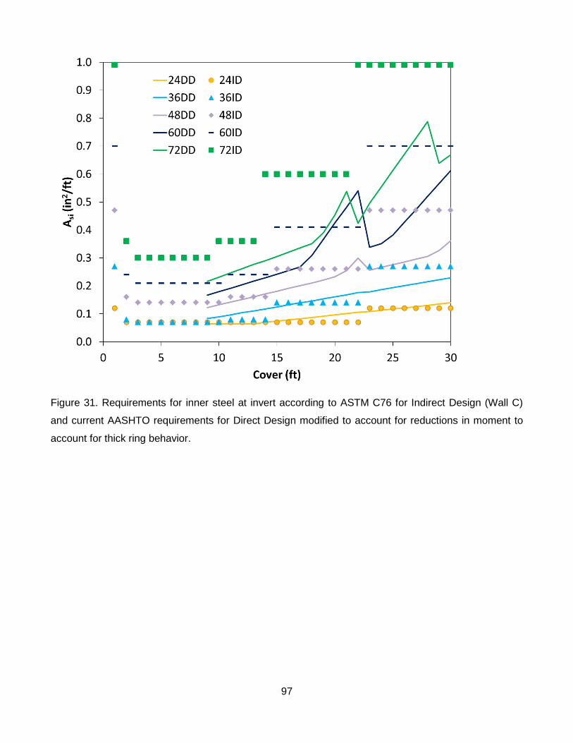
97
Figure 31. Requirements for inner steel at invert according to ASTM C76 for Indirect Design (Wall C)
and current AASHTO requirements for Direct Design modified to account for reductions in moment to
account for thick ring behavior.
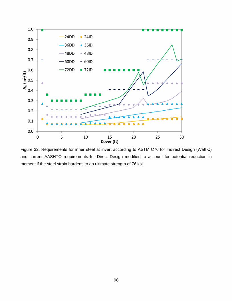
98
Figure 32. Requirements for inner steel at invert according to ASTM C76 for Indirect Design (Wall C)
and current AASHTO requirements for Direct Design modified to account for potential reduction in
moment if the steel strain hardens to an ultimate strength of 76 ksi.
99
Figure 33. Requirements for inner steel at invert according to ASTM C76 for Indirect Design (Wall C)
and current AASHTO requirements for Direct Design modified to employ Modified Compression Field
Theory calculations using RESPONSE and two layers of reinforcing steel.
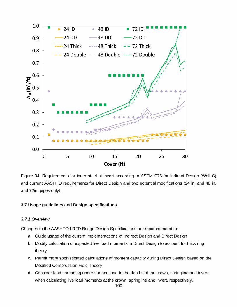
100
Figure 34. Requirements for inner steel at invert according to ASTM C76 for Indirect Design (Wall C)
and current AASHTO requirements for Direct Design and two potential modifications (24 in. and 48 in.
and 72in. pipes only).
3.7 Usage guidelines and Design specifications
3.7.1 Overview
Changes to the AASHTO LRFD Bridge Design Specifications are recommended to:
a. Guide usage of the current implementations of Indirect Design and Direct Design
b. Modify calculation of expected live load moments in Direct Design to account for thick ring
theory
c. Permit more sophisticated calculations of moment capacity during Direct Design based on the
Modified Compression Field Theory
d. Consider load spreading under surface load to the depths of the crown, springline and invert
when calculating live load moments at the crown, springline and invert, respectively.
101
3.7.2 Usage of Indirect Design and Direct Design
The calculations presented in the previous sections show that discrepancies between steel areas
associated with Indirect Design and Direct Design pipes under earth loads are resolved if more
sophisticated calculations of expected moment and moment capacity are employed. Testing of a 24 in.
diameter pipe under simulated deep burial also demonstrated that both Indirect Design and Direct
Design produce conservative (safe) estimates of load capacity.
The calculations of the moments expected in shallow buried concrete pipes were compared to
moments obtained from measured strains, and these reveal that the Direct Design procedure features
conservative estimates of expected moment under vehicle loads at shallow cover. Testing of 24 in. and
48 in. diameter pipes at shallow cover demonstrated that load capacities estimated using Indirect
Design and Direct Design are also conservative.
It is recommended therefore that the commentary to the AASHTO LRFD Bridge Design Specifications
include reference to these results, supporting the use of whichever design method is most convenient
for the user. Therefore, there is no apparent need to prevent use of Indirect Design when it produces
more efficient designs relative to Direct Design.
3.7.3 Modification of Expected Moments During Direct Design to Account for Thick Ring Theory
Changes to the AASHTO LRFD Bridge Design Specifications are recommended to incorporate moment
correction factors to account for thick ring theory. The recommended changes are given in Appendix D.
3.7.4 Modification of Moment Capacity During Direct Design to Employ Modified Compression Field Theory
Changes to the AASHTO LRFD Bridge Design Specifications are recommended to permit designers to
employ more sophisticated estimates of moment capacity during Direct Design. In particular, the use of
Modified Compression Field Theory should be mentioned.
3.7.5 Modification of Load Spreading to Consider Depth to Crown, Springline and Invert
Estimates of crown moment resulting from surface loads were reasonable and conservative relative to
the moments calculated from measured strains. However, moment estimates at the springline and
invert appeared excessively conservative. More consistent estimates of expected invert moment and
expected springline result can be obtained considering load spreading down to these specific locations,
rather than always calculating load spreading from the surface to the depth of the crown.
102
CHAPTER 4 CONCLUSIONS AND SUGGESTED RESEARCH
A literature review was undertaken to examine the background of reinforced concrete pipe design and
previous comparisons of Indirect Design and Direct Design methods. From that literature review, it was
concluded that:
• The degree to which Indirect Design reflects actual buried pipe performance requires
assessment, including experimental work for small diameter and large diameter reinforced
concrete pipes;
• The performance of Direct Design in estimating the level of moment that develops in buried
concrete pipes is unclear, and would benefit from experimental evaluation, both for shallow
buried and deeply buried pipes;
• Direct Design examines four different limit states, but would benefit from experimental
evaluation to see whether the design method correctly assesses the limit state that controls the
performance of shallow buried and deeply buried pipes;
• Modified Compression Field theory might be used to determine the strength limits for reinforced
concrete pipe during Direct Design (the moment and shear capacities) instead of the design
approximations for flexural and shear strength currently employed; this could include
consideration of multiple layers of reinforcing steel and more sophisticated treatment of shear
strength;
• Investigation is warranted regarding the level of conservatism that results when the effect of
strain hardening in reinforcing steel is neglected during Direct Design.
A program of laboratory testing was undertaken on two 24 in. and two 48 in. diameter pipes in
simulations of shallow and deep burial. For those test pipes and the backfill materials and burial
conditions examined,
• Indirect Design provided safe estimates of load capacity; the calculated load capacities ranged
from 54% to 81% of those observed in the tests;
• Moment estimates during Direct Design based on the ASCE moment factors from two
dimensional finite element analysis were conservative; moment estimates at the crown using
the LRFD procedures were on average 3 times those observed in the experiments; moment
estimates at the springlines were on average 3.6 times those observed in the experiments, and
moment estimates at the invert were over 4 times those observed in the experiments;
• Moment estimates at the springline and invert were improved if the load spreading depth was
adjusted so that it was the depth of the point in question (i.e. depth to the springline and depth
to the invert); this led to a mean ratio of the moment calculation to moment measurement of 2,
with a standard deviation of 0.8;
103
• The capacity limit states predicted using Direct Design were different to the limit states observed
during the reinforced concrete pipe tests; in each case, the load capacity was controlled by the
service limit (the 0.01 in. crack) instead of flexural failure; the Direct Design estimates of load
capacity were between 19% and 77% of the capacities observed during the tests; estimates for
24 in. diameter pipes at shallow cover were 19% and 47% of those observed, whereas
estimates for 48 in. diameter pipes were 51% and 71% of the observed strengths; the load
capacity calculated for the 24 in. diameter pipe under deep burial was 77% of the design
estimate.
Potential changes to the procedures for calculating the ultimate capacity of concrete pipes during
Direct Design were examined.
• Expected moments during Direct Design are currently estimated using thin elastic ring theory;
since concrete pipes generally have thickness greater than 10% of radius, the use of thin ring
theory is conservative; a moment reduction factor that accounts for ring thickness was
developed, and its use was examined; the correction is straightforward, and it eliminates some
of the discrepancy between required steel areas obtained using Direct Design and Indirect
Design;
• Plastic collapse analysis of a buried rigid pipe was examined, where full plastic moment is
mobilized at crown, springlines and invert; this calculation procedure would eliminate
conservatism associated with Direct Design’s matching of maximum elastic moment to moment
capacity; however, further work would be required to establish the soil characteristics and earth
pressure distributions for each of the standard bedding types (since the pipe would likely
respond as a flexible structure once hinges form at the crown, invert and springlines); because
the actual load limit seen in the laboratory tests was controlled by the service limit state (the
0.01 in. crack) rather than ultimate strength, the development of the plastic collapse analysis as
an alternative to the current approach used during Direct Design is not likely warranted and
should not be implemented unless a new procedure that effectively estimates crack widths for
specific load levels were implemented;
• Modified Compression Field theory was used to explore how the strength limits for reinforced
concrete pipe could be improved during Direct Design, to consider multiple layers of reinforcing
steel, strain hardening of the reinforcing steel, and more sophisticated treatment of shear
strength; this theory requires iterative calculations that impose compatibility between the layers
of steel reinforcing and the concrete;
• Modified Compression Field Theory led to modest reductions in steel requirements when used
for a single reinforcing cage in 24 in. and 36 in diameter pipes, with negligible changes for larger
structures;
104
• Modified Compression Field theory for two layers of steel reduced steel requirements for 24 in.
diameter pipe by from 24 to 28%, by 18 to 22% for 36 in. diameter pipe, by 11 to 16% for 48 in.
diameter pipe, and by less than 12% and 8% for 60 in. and 72 in. diameter pipes.
A comparison of the requirements for area of steel arising from the use of Indirect Design and
Direct Design indicated that Direct Design leads to less efficient designs for small diameter
structures at shallow cover. Most of that discrepancy is eliminated when thick ring theory is
considered (the moment adjustment factor described earlier), and Modified Compression Field
Theory is employed, though much of the underlying conservatism of the two procedures would
remain. Furthermore, the strength limit tests on shallow buried and deeply buried pipes indicated
that both design methods produce conservative estimates of the load capacity of the buried pipe.
Therefore, no restrictions are needed on use of Indirect Design and Direct Design. Modifications to
the AASHTO LRFD Bridge Design Specifications are proposed, where moment is adjusted to
account for thick ring theory, where the commentary specifically mentions the potential for use of
Modified Compression Field Theory (at the designer’s discretion), and so that the commentary
clearly states that both the Indirect Design Method and the Direct Design Method can be employed,
at the designer’s discretion.
Additional research is recommended to examine the performance of the Indirect Design and Direct
Design Methods for large diameter pipes, since testing in the current project was restricted to 24 in.
and 48 in. diameter structures. In particular, buried pipe tests in the laboratory for pipes of 60 in.
and 72 in. diameter would enable the levels of safety associated with the two design methods to be
directly evaluated for these important structures. Other testing that measures the load capacity of
buried pipes in other installation conditions would also be of value (the current project examined
Type 2 installations only).
It would be valuable to conduct research studies to determine the relationship between crack width
and reinforced concrete pipe durability so that the effect of crack width on service life and long term
pipe performance can be determined. This research may provide appropriate recommendations for
modifications to Direct Design and Indirect Design based on a defined long term performance and
limit state condition. Additionally, it could provide guidance for Engineers to evaluate cracks
between 0.01” and 0.10” as specified in the AASHTO Bridge Construction Specification Section
C27.6.4 or set new width limits based on the defined long term performance condition. However,
these studies will likely be complex and time consuming involving work to determine:
- how much deterioration can be tolerated in a reinforced concrete pipe (i.e. answering the
question ‘how much deterioration is too much deterioration?’), so that the end of service life can

105
be established (currently there is little information on the effects of deterioration on pipe
strength)
- the service life based on relationships between rates of pipe deterioration and crack width,
cover depth, total wall thickness, single versus multiple layers of reinforcement, soil conditions
(e.g. resistivity), stormwater and groundwater conditions (e.g. salinity), cement and concrete
properties and other factors that may influence performance.

106
ACKNOWLEDGEMENTS
The pipe samples tested in the project were provided by M-CON Products Ltd. of Ottawa,
Ontario and Hanson Pipe and Precast of Cambridge, Ontario. We acknowledge the excellent
contributions of Graeme Boyd and Brian Westervelt of Queen’s University who undertook most
of the earthworks and pipe loading, and assisted with the data acquisition, and Trevor Smith
who assisted with specimen preparation and who undertook the interpretation of crack widths.
107
REFERENCES
ACPA (1971). CP Info - Effects of Cracks in Reinforced Concrete Sanitary Sewer Pipes. American Concrete Pipe Association.
ACPA (1976). CP Info - Effects of Cracks in Reinforced Concrete Culvert Pipe. American Concrete Pipe Association.
ACPA (1978) CP Info - Significance of Cracks in Concrete Pipe. American Concrete Pipe Association.
ACPA (1998). Concrete Pipe Design Manual. American Concrete Pipe Association, USA.
ACPA (2007). CP Info – Crack in Installed Reinforced Concrete Pipe. American Concrete Pipe Association.
ACPA (2012). Brief History of ACPA. Retrieved September 26, 2012, from American Concrete Pipe Association: http://www.concrete-pipe.org/pages/history.html
AASHTO (2007) Load and Resistance Factor Design (LRFD) Bridge Design Specifications, 4th Edition, American Association of State Highway and Transportation Officials, Washington, D.C..
AASHTO (2013). AASHTO LRFD Bridge Design Specifications, 6th Edition, 2013 Interim Revisions. AASHTO, Washington, D.C.
ASTM C76-11 (2011) Standard Specification for Reinforced Concrete Culvert, Storm Drain, and Sewer Pipe. ASTM International, 100 Barr Harbor Drive, PO BoxC700, West Conshohocken, PA, 19428-2959 USA
ASTM C497-13 (2013) Standard Test Methods for Concrete Pipe, Manhole Sections or Tile. ASTM International, 100 Barr Harbor Drive, PO BoxC700, West Conshohocken, PA, 19428-2959 USA
ASTM D6938-10 (2010) Standard Test Method for In-Place Density and Water Content of Soil and Soil-Aggregate by Nuclear Methods (Shallow Depth), ASTM International, 100 Barr Harbor Drive, PO BoxC700, West Conshohocken, PA, 19428-2959 USA
Becerril Garcìa, D. (2012) Investigation of Culvert Joints Employing Large Scale Tests and Numerical Simulations, PhD Thesis, Department of Civil Engineering, Queen`s University, Kingston, Ontario.
Bentz, E.C. (2000). Sectional analysis of reinforced concrete members. PhD dissertation, University of Toronto, 2000.
Brachman, R.W.I., Moore, I.D. and Rowe, R.K. (2000). The design of a laboratory facility for evaluating the structural response of small-diameter buried pipes. Canadian Geotechnical Journal, Vol. 37, pp. 281-295.
Brachman, R.W.I., Moore, I.D. and Rowe, R.K. (2001). The performance of a laboratory facility for evaluating the structural response of small diameter buried pipes. Canadian Geotechnical Journal, Vol. 38, pp. 260–275.
Brown, Glenn. (2002). The History of the Darcy-Weisbach Equation for Pipe Flow Resistance. Environmental and Water Resources History 2002. ASCE 2004.
108
Burns J.Q. and Richard R.M. (1964). Attenuation of stresses for buried cylinders. Arizona University – Symposium of Soil-Structure Interaction – Proceedings (pp. 378-392)
Canadian Standards Association (CSA). 2004. Design of concrete structures, CSA A23. 3–04. CSA, Rexdale, Ontario.
Collins, M. P. (1978). Towards a rational theory for RC members in shear. Journal of the Structural Division, 104(4), 649-666.
Collins, M.P. and Mitchell, D. 1997. Prestressed Concrete Structures, Response Publications, Toronto, 766 pp.
Concrete Pipe Design Manual. (2011). American Concrete Pipe Association.
CSA (2006). Canadian Highway Bridge Design Code, CAN/CSA-S6-06. CSA, Rexdale, Ontario.
CSA (2009). A257 Series-09 Standards for concrete pipe and manhole sections. Canadian Standards Association.
Erdogmus, E. and Tadros, M. (2006).Behavior and Design of Buried Concrete Pipe.Nebraska Department of Roads.
Erdogmus, E. and Tadros, M. (2009).Behavior and Design of Buried Concrete Pipes Phase II - Final Report.Nebraska Department of Roads.
Erdogmus, E., Skourup, B.N., and Tadros, M. (2010) Recommendations for Design of Reinforced Concrete Pipe, Journal of Pipeline Systems Engineering and Practice, ASCE, Vol. 1, No. 1, pp. 25-32.
Heger, F. J. (1982). Structural Design Method for Precast Reinforced-Concrete Pipe.Transportation Research Record, 93-100.
Heger, F. J., & McGrath, T. (1984).Crack Width Control in Design of Reinforced Concrete Pipe and Box Sections. Journal of the American Concrete Institute, 81(2), 149-157.
Heger, F. J., & McGrath, T. J. (1982).Shear Strength of Pipe, Box Sections, and Other One-Way Flexural Members.79, 470-483.
Heger, F. J., & McGrath, T. J. (1983).Radial Tension Strength of Pipe and Other Curved Flexural Members. Journal of the American Concrete Institute, 80(1), 33-39.
Heger, F. J., & Liepins, A. A. (1985).Stiffness of Flexurally Cracked Reinforced Concrete Pipe.Journal of the American Concrete Institute, 82(3), 331-342.
Heger, F.J. (1988). New Installation Design for Buried Concrete Pipe.Pipeline Infrastructure. Proceedings of the Conference Sponsored by the Pipeline Division of the American Society of Civil Engineers.
Heger, F.J., Liepins A.A., Selig, E.T. (1985) SPIDA: An Analysis and Design System for Buried Concrete Pipe. Advances in Underground Pipeline Engineering. Proceedings of the International Conference sponsored by the Pipeline Division of the American Society of Civil Engineers.
Heger, F.J., McGrath T.J. (1980) Design Method for Reinforced Concrete Pipe and Box Sections. Transportation Research Board
109
Hoeg, K. (1968) Stresses against underground structural cylinders. American Society of Civil Engineers Proceedings, Journal of the Soil Mechanics and Foundations Division July, 1968 (pp.833-858)
Janssen, H.A. (1895). Versuche über Getreidedruck in Silozellen. Zeitschrift des Vereinesdeutscher Ingenieurs.
Lay, G.R. (2012) Response of reinforced concrete and corrugated steel pipes to surface load. Master’s Thesis, Department of Civil Engineering, Queen’s University, Kingston, Ontario.
Lougheed, A. C. (2008). Limit State Testing of a Buried Deep-Corrugated Large-Span Box Culvert, MASc thesis, Department of Civil Engineering, Queen’s University, Kingston On., Canada.
Marston, A., Anderson, A.O. (1913). The theory of loads on pipes in ditches and tests of cement and clay drain tile and sewer pipe. Iowa State College of Agriculture
McGrath, T.J. Tigue, D.B., Heger, F.J. (1988). Pipecar and BOXCAR – Micro Computer Programs for the Design of Reinforced Concrete Pipe and Box Sections. Presented to the January 1988 Annual Meeting of Transportation Research Board (TRB), Washington, D.C.
Moore, I.D. (2012) Large-scale laboratory experiments to advance the design and performance of buried pipe infrastructure, 2nd International Conference on Pipelines and Trenchless Technology, ASCE-China University of Geosciences, Wuhan, China, 11pp, October.
Moore, I.D., Becerril Garcia, D., Sezen, H. and Sheldon, T. (2012) Structural design requirements for culvert joints, NCHRP Web-only document 190, Contractor’s Final Report for NCHRP Project 15-38, April 2012 Transportation Research Board, Washington D.C., 387 pp.
Moser, A. (2001). Buried Pipe Design. McGraw-Hill.
OCPA (2010). Concrete Pipe Design Manual, Ontario Concrete Pipe Association, http://www.ocpa.com/_resources/OCPA_DesignManual.pdf
Olander, H.C. (1950). Stress Analysis of Concrete Pipe. United States Department of Interior Bureau of Reclamation.Denver Federal Center. Denver, Colorado
Ontario Concrete Pipe Association. (2011). Ontario Concrete Pipe Association. Retrieved from
Paris, J.M. (1921) Stress Coefficients for large horizontal pipes.Engineering News-Record v87, p768-771.
Petersen, D.,L., Nelson, C.R., Li, G., McGrath, T.J., and Kitane, Y. (2010) Recommended Design Specifications for Live Load Distribution to Buried Structures, 85pp.
Sargand, S.M., Hazen, G.A., Vaithianathan, E, and Hurd, J.O. (1995) Performance verification of a concrete pipe, Concrete International, July, pp. 23-27.
Simpson, Gumpertz & Heger Inc. (2004). PIPECAR. A Computer Program for the Analysis and Design of Circular and Horizontal Elliptical Reinforced Concrete Pipe Culverts.
Spangler, M.G. (1933).The Supporting Strength of Rigid Pipe Culverts, Bulletin 112, Iowa State College.
Standard Practice for Direct Design of Buried and Precast Concrete Pipe Using Standard Installation. (1998). Reston, Virginia: American Society of Civil Engineers.
110
Tognon, A.R., Rowe, R. K., and Brachman, R.W.I. (2009) Evaluation of side wall friction for a buried pipe testing facility, February 1999. Geotextiles and Geomembranes, 17: 193-212.
Vecchio, F. J., and Collins, M. P. 1986. The modified compression-field theory for reinforced concrete elements subjected to shear. ACI J., 83(2), 219-231.
White D.J. and Take W.A. (2002) GeoPIV: Particle Image Velocimetry (PIV) software for use in geotechnical testing. October 2002. Cambridge University Engineering Department.
Wong, L.S., Allouche, E.N., Dhar, A.S., Baumert, M. and Moore, I.D. (2006). Long term monitoring of SIDD Type IV installations, Canadian Geotechnical Journal Vol. 43, 392–408.
Zhao, J. Q., and Daigle, L. (2001). SIDD pipe bedding and Ontario Provincial Standards. Institute for Research in Construction, National Research Council Canada, Ottawa, Canada.

Appendix A Thick ring theory
A-1
Appendix A. Thick ring theory
A.1 Introduction ...................................................................................................................... A.1
A.2 Moment in thick rings from Roark’s Formulas for Stress and Strain .............................. A.1
A.3 Moments in thick rings obtained using finite element analysis ....................................... A.3
References ................................................................................................................................... A.5
A.1 Introduction
Current design calculations for reinforced concrete pipes employ thin ring theory. However,
reinforced concrete pipes often have a wall thickness that is significantly larger than 10% of the
pipe radius. As a result, conservative values of bending moment for smaller diameter pipes
where this ratio is higher may be the result. Finite element analysis has therefore been used to
evaluate how moment values might be adjusted to account for thick ring theory. The following
appendix commences with the use of results for thick rings presented in Roark’s Formulas for
Stress and Strain (Young and Budynas, 2002). It then reports on the results of finite element
calculations for pipes under the Paris earth pressure distribution. A simple linear design
approximation is provided where moments can be adjusted as a function of the ratio of pipe
thickness to radius.
A.2 Moment in thick rings from Roark’s Formulas for Stress and Strain
Young and Budynas (2002) provide results for stresses at the inner and outer surface at the
crown and springlines of a thick ring under opposing vertical forces. Table A-1 provides details
of the calculations. The solutions for circumferential stress σ provided by Young and Budynas
(2002) are based on a stress coefficient K where
bpK
πσ 2
= A-1
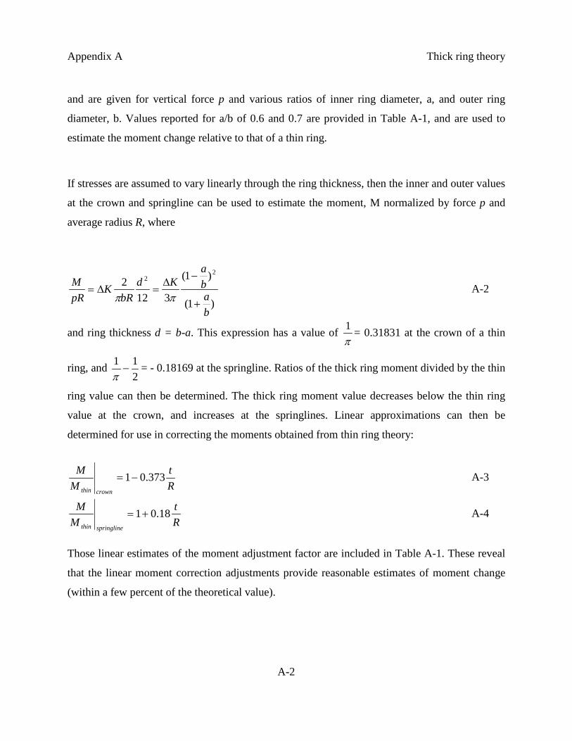
Appendix A Thick ring theory
A-2
and are given for vertical force p and various ratios of inner ring diameter, a, and outer ring
diameter, b. Values reported for a/b of 0.6 and 0.7 are provided in Table A-1, and are used to
estimate the moment change relative to that of a thin ring.
If stresses are assumed to vary linearly through the ring thickness, then the inner and outer values
at the crown and springline can be used to estimate the moment, M normalized by force p and
average radius R, where
)1(
)1(
3122
22
ba
ba
KdbR
KpRM
+
−∆=∆=
ππ A-2
and ring thickness d = b-a. This expression has a value of π1 = 0.31831 at the crown of a thin
ring, and 211
−π
= - 0.18169 at the springline. Ratios of the thick ring moment divided by the thin
ring value can then be determined. The thick ring moment value decreases below the thin ring
value at the crown, and increases at the springlines. Linear approximations can then be
determined for use in correcting the moments obtained from thin ring theory:
Rt
MM
crownthin
373.01−= A-3
Rt
MM
springlinethin
18.01+= A-4
Those linear estimates of the moment adjustment factor are included in Table A-1. These reveal
that the linear moment correction adjustments provide reasonable estimates of moment change
(within a few percent of the theoretical value).
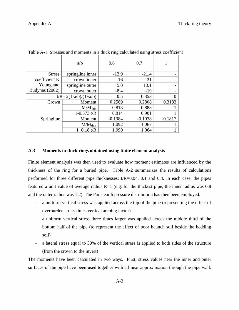
Appendix A Thick ring theory
A-3
Table A-1: Stresses and moments in a thick ring calculated using stress coefficient
a/b 0.6 0.7 1
Stress coefficient K
Young and Budynas (2002)
springline inner -12.9 -21.4 - crown inner 16 31 -
springline outer 5.8 13.1 - crown outer -8.4 -19 -
t/R= 2(1-a/b)/(1+a/b) 0.5 0.353 0 Crown
Moment 0.2589 0.2808 0.3183 M/Mthin 0.813 0.883 1
1-0.373 t/R 0.814 0.901 1 Springline Moment -0.1984 -0.1938 -0.1817
M/Mthin 1.092 1.067 1 1+0.18 t/R 1.090 1.064 1
A.3 Moments in thick rings obtained using finite element analysis Finite element analysis was then used to evaluate how moment estimates are influenced by the
thickness of the ring for a buried pipe. Table A-2 summarizes the results of calculations
performed for three different pipe thicknesses: t/R=0.04, 0.1 and 0.4. In each case, the pipes
featured a unit value of average radius R=1 (e.g. for the thickest pipe, the inner radius was 0.8
and the outer radius was 1.2). The Paris earth pressure distribution has then been employed:
- a uniform vertical stress was applied across the top of the pipe (representing the effect of
overburden stress times vertical arching factor)
- a uniform vertical stress three times larger was applied across the middle third of the
bottom half of the pipe (to represent the effect of poor haunch soil beside the bedding
soil)
- a lateral stress equal to 30% of the vertical stress is applied to both sides of the structure
(from the crown to the invert)
The moments have been calculated in two ways. First, stress values near the inner and outer
surfaces of the pipe have been used together with a linear approximation through the pipe wall.
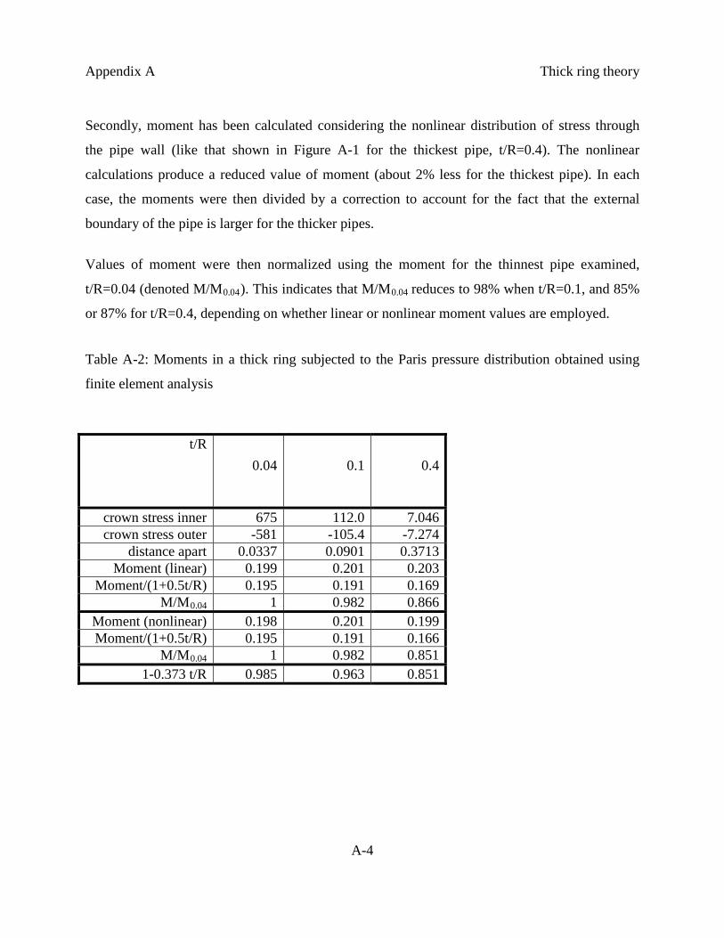
Appendix A Thick ring theory
A-4
Secondly, moment has been calculated considering the nonlinear distribution of stress through
the pipe wall (like that shown in Figure A-1 for the thickest pipe, t/R=0.4). The nonlinear
calculations produce a reduced value of moment (about 2% less for the thickest pipe). In each
case, the moments were then divided by a correction to account for the fact that the external
boundary of the pipe is larger for the thicker pipes.
Values of moment were then normalized using the moment for the thinnest pipe examined,
t/R=0.04 (denoted M/M0.04). This indicates that M/M0.04 reduces to 98% when t/R=0.1, and 85%
or 87% for t/R=0.4, depending on whether linear or nonlinear moment values are employed.
Table A-2: Moments in a thick ring subjected to the Paris pressure distribution obtained using
finite element analysis
t/R 0.04 0.1 0.4
crown stress inner 675 112.0 7.046 crown stress outer -581 -105.4 -7.274
distance apart 0.0337 0.0901 0.3713 Moment (linear) 0.199 0.201 0.203
Moment/(1+0.5t/R) 0.195 0.191 0.169 M/M0.04 1 0.982 0.866
Moment (nonlinear) 0.198 0.201 0.199 Moment/(1+0.5t/R) 0.195 0.191 0.166
M/M0.04 1 0.982 0.851 1-0.373 t/R 0.985 0.963 0.851
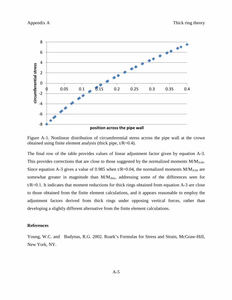
Appendix A Thick ring theory
A-5
Figure A-1. Nonlinear distribution of circumferential stress across the pipe wall at the crown obtained using finite element analysis (thick pipe, t/R=0.4). The final row of the table provides values of linear adjustment factor given by equation A-3.
This provides corrections that are close to those suggested by the normalized moments M/M0.04.
Since equation A-3 gives a value of 0.985 when t/R=0.04, the normalized moments M/M0.04 are
somewhat greater in magnitude than M/Mthin, addressing some of the differences seen for
t/R=0.1. It indicates that moment reductions for thick rings obtained from equation A-3 are close
to those obtained from the finite element calculations, and it appears reasonable to employ the
adjustment factors derived from thick rings under opposing vertical forces, rather than
developing a slightly different alternative from the finite element calculations.
References Young, W.C. and Budynas, R.G. 2002. Roark’s Formulas for Stress and Strain, McGraw-Hill,
New York, NY.
-8
-6
-4
-2
0
2
4
6
8
0 0.05 0.1 0.15 0.2 0.25 0.3 0.35 0.4
circ
umfe
rent
ial s
tres
s
position across the pipe wall
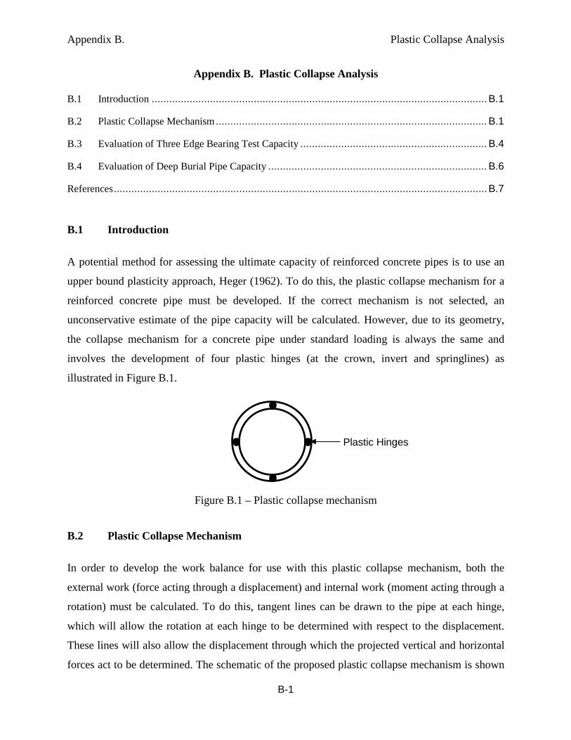
Appendix B. Plastic Collapse Analysis
B-1
Appendix B. Plastic Collapse Analysis
B.1 Introduction ................................................................................................................... B.1
B.2 Plastic Collapse Mechanism ............................................................................................. B.1
B.3 Evaluation of Three Edge Bearing Test Capacity ................................................................ B.4
B.4 Evaluation of Deep Burial Pipe Capacity ........................................................................... B.6
References ................................................................................................................................ B.7
B.1 Introduction
A potential method for assessing the ultimate capacity of reinforced concrete pipes is to use an
upper bound plasticity approach, Heger (1962). To do this, the plastic collapse mechanism for a
reinforced concrete pipe must be developed. If the correct mechanism is not selected, an
unconservative estimate of the pipe capacity will be calculated. However, due to its geometry,
the collapse mechanism for a concrete pipe under standard loading is always the same and
involves the development of four plastic hinges (at the crown, invert and springlines) as
illustrated in Figure B.1.
Figure B.1 – Plastic collapse mechanism
B.2 Plastic Collapse Mechanism
In order to develop the work balance for use with this plastic collapse mechanism, both the
external work (force acting through a displacement) and internal work (moment acting through a
rotation) must be calculated. To do this, tangent lines can be drawn to the pipe at each hinge,
which will allow the rotation at each hinge to be determined with respect to the displacement.
These lines will also allow the displacement through which the projected vertical and horizontal
forces act to be determined. The schematic of the proposed plastic collapse mechanism is shown
Plastic Hinges
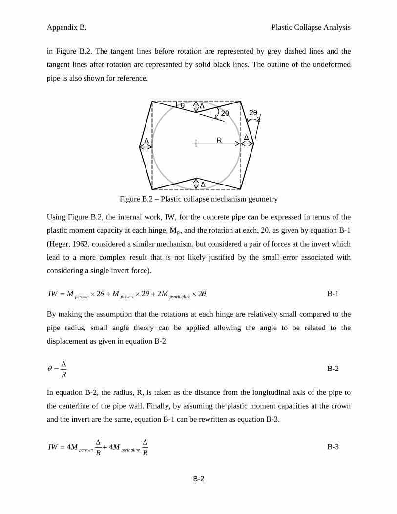
Appendix B. Plastic Collapse Analysis
B-2
in Figure B.2. The tangent lines before rotation are represented by grey dashed lines and the
tangent lines after rotation are represented by solid black lines. The outline of the undeformed
pipe is also shown for reference.
Figure B.2 – Plastic collapse mechanism geometry Using Figure B.2, the internal work, IW, for the concrete pipe can be expressed in terms of the
plastic moment capacity at each hinge, Mp, and the rotation at each, 2θ, as given by equation B-1
(Heger, 1962, considered a similar mechanism, but considered a pair of forces at the invert which
lead to a more complex result that is not likely justified by the small error associated with
considering a single invert force).
θθθ 2222 ×+×+×= epspringlinpinvertpcrown MMMIW B-1
By making the assumption that the rotations at each hinge are relatively small compared to the
pipe radius, small angle theory can be applied allowing the angle to be related to the
displacement as given in equation B-2.
R∆
=θ B-2
In equation B-2, the radius, R, is taken as the distance from the longitudinal axis of the pipe to
the centerline of the pipe wall. Finally, by assuming the plastic moment capacities at the crown
and the invert are the same, equation B-1 can be rewritten as equation B-3.
RM
RMIW psringlinepcrown
∆+
∆= 44 B-3
Δ
Δ
Δ
Δ
2θ θ
2θ
R
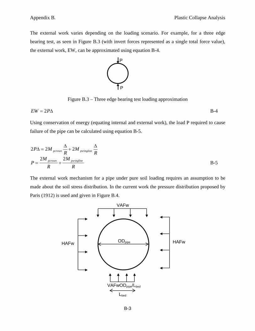
Appendix B. Plastic Collapse Analysis
B-3
The external work varies depending on the loading scenario. For example, for a three edge
bearing test, as seen in Figure B.3 (with invert forces represented as a single total force value),
the external work, EW, can be approximated using equation B-4.
Figure B.3 – Three edge bearing test loading approximation
∆= PEW 2 B-4 Using conservation of energy (equating internal and external work), the load P required to cause
failure of the pipe can be calculated using equation B-5.
RM
RMP psringlinepcrown
∆+
∆=∆ 222
RM
RM
P psringlinepcrown 22+= B-5
The external work mechanism for a pipe under pure soil loading requires an assumption to be
made about the soil stress distribution. In the current work the pressure distribution proposed by
Paris (1912) is used and given in Figure B.4.
P
P
HAFw
VAFw
HAFw ODpipe
Lbed
VAFwODpipe/Lbed

Appendix B. Plastic Collapse Analysis
B-4
Figure B.4 – Paris pressure distribution
Using the pressure distribution in Figure B.4, the external work, EW, can be calculated using
equation B-6.
∆−
−+∆××+
∆××= pipe
pipe
bedpipepipe
pipe HAFwDD
LDDVAFw
DVAFwEW
221
2
−
−+∆×××=
VAFHAF
DLD
DwVAFEWpipe
bedpipepipe 2
1 B-6
The applied load, w, can be due to both earth and vehicle loads (depending on the load
spreading). The length of bedding, Lbed, depends on the assumed bedding conditions and the
vertical arching factor, VAF, and the horizontal arching factor, HAF, are taken as 1.35 and 0.45,
respectively. The total applied load, w, can be calculated by setting equations B-3 and B-6 equal
to each other resulting in equation B-7.
RM
RM
VAFHAF
DLD
DwVAF psringlinepcrownpipe
bedpipepipe
∆+
∆=
−
−+∆××× 44
21
−
−+××
+=
VAFHAF
DLD
RDVAF
MMw
pipe
bedpipepipe
psringlinepcrown
21
44 B-7
B.3 Evaluation of Three Edge Bearing Test Capacity
As part of the current investigation, three edge bearing tests to failure were performed on two
specimens: a 48” class III B-wall (T-48-B) and a 48” class III C-wall (T-48-C). The material
properties and geometry are given in Table B-1 for each specimen. The radius for each pipe is
calculated as the distance from the longitudinal centreline of the pipe to the centre of the wall.
Also included in Table B-1 are three estimates of the plastic moment capacity, which were all
determined using a reinforced concrete sectional analysis program called Response-2000 (Bentz,
2000). The first value, Mpy, is the plastic moment capacity of one pipe length (2440 mm)
assuming only the steel yield strength is achieved. The second value, Mpu, is the plastic moment
capacity of one pipe length assuming the steel reaches its ultimate strength. The third value,
Appendix B. Plastic Collapse Analysis
B-5
Mpuaxial, is the plastic moment capacity of one pipe length that can be achieved in the presence of
a compressive axial force. The axial force was calculated through trial and error as the point
where the applied force, P, produced by equation B-5 and the axial compressive force, P/2,
required to calculate Mpuaxial converged to the same value of P.
Table B-1: Material and geometric properties for the three edge bearing test specimens T-48-B T-48-C D-24-C f'c, psi (MPa) 8350 (57.6) 8350 (57.6) 10150 (70) fy, ksi (MPa) 70.3 (485) 70.3 (485) 86.3 (595) fu, ksi (MPa) 79.8 (550) 79.8 (550) 90.6 (625) t, in (mm) 5 (127) 5.75 (146) 3.75 (95) R, in (mm) 26.5 (673) 26.9 (683) 13.9 (352) As, in2 (mm2) 0.04 (25.8) 0.04 (25.8) 0.025 (16.1) s, in (mm) 2 (51) 2.67 (68) 3 (76) Mpy, kip.ft (kNm) 51.6 (70) 46.5 (63) See sec. B.4 Mpu, kip.ft (kNm) 53.8 (73) 50.9 (69) See sec. B.4 Mpuaxial, kip.ft (kNm) 62.7 (85) 60.5 (82) See sec. B.4 Equation B-5 was then used to determine the load required to fail the pipe in a three edge bearing
test using three combinations of the plastic moment capacity: (i) Mpy at all 4 hinges (Py), (ii) Mpu
at all 4 hinges (Pu) and (iii) Mpu at the crown / invert and Mpuaxial at the springlines (Puaxial). The
results of each analysis are presented in Table B-2 as well as the actual maximum load applied to
the pipes during the three edge bearing test (Pexp) and the ratio of the predicted to experimental
capacity (Pred / Exp).
Table B-2: Estimated and experimental plastic collapse loads for three edge bearing tests
Pipe Pexp kips (kN)
Py kips (kN)
Py / Pexp Pu kips (kN)
Pu / Pexp Puaxial kips (kN)
Puaxial / Pexp
48in B wall 119 (530) 93 (416) 0.78 98 (434) 0.82 106 (470) 0.89 48in C wall 110 (489) 83 (368) 0.75 91 (404) 0.83 99 (440) 0.90 From Table B-2 it can be seen that assuming the yield strength of the steel governs the moment
capacity leads to a conservative estimate of the failure load. Using a moment based on the
ultimate strength of the steel improves the accuracy of the estimate while accounting for the
effects of axial load at the springlines leads to an accurate yet conservative estimate of the
ultimate limit state capacity.
Appendix B. Plastic Collapse Analysis
B-6
B.4 Evaluation of Deep Burial Pipe Capacity
A 24” specimen with the properties given in Table B-1 (denoted D-24-C) that was 1.95 m long
rather than 2.44 m was tested under simulated deep burial loading. The test was stopped at an
applied load of 750kPa, which had caused cracks of the order of 1 mm to develop at the crown
and the invert. Although the pipe was not taken to its ultimate limit state, the results of this test
will be used to evaluate the plastic collapse model. In order to use equation B-7, values for VAF,
HAF and Lbed are required. These values were assumed to be VAF = 1.35, HAF = 0.45 and Lbed
was taken as taken as half of the pipe diameter (0.4 m). Equation B-7 was then used to determine
the applied load required to fail the pipe using three combinations of the plastic moment
capacity: (i) Mpy at all 4 hinges (wy), (ii) Mpu at all 4 hinges (wu) and (iii) Mpu at the crown /
invert and Mpuaxial at the springlines (wuaxial). Mpy and Mpu were taken as 6.1 kNm and 6.4 kNm,
respectively, for a unit length of pipe. The value for Mpuaxial at the springlines and the crown /
invert was determined using trial and error, resulted in values of 11.7 and 8.2 kNm, respectively.
The results of each analysis are given in Table B-3 along with the ratio of the predicted value to
the experimental capacity (assumed to be 750 kPa in this case).
Table B-3: Estimated and experimental plastic collapse loads for deep burial experiment
wexp psi (kPa)
VAF = 1.35, HAF = 0.45 VAF=1.13, HAF=0.54 wy
psi (kPa) wy / wexp
wu psi (kPa)
wu / wexp
wuaxial psi (kPa)
wuaxial / wexp
wuaxial psi (kPa)
wuaxial / wexp
109 (750) 202 (139) 0.19 202 (146) 0.19 326 (225) 0.3 1340 (925) 1.23 Table B-3 indicates that there is not a significant difference between using a plastic moment
capacity based on the yield strength or the ultimate strength. Accounting for the axial force
acting on the hinge offers considerable benefit in terms of the predicted capacity; however, the
results still fall well short of the actual pipe capacity. The three main variables that can affect this
estimate are the VAF, HAF and Lbed. In terms of VAF, this value is potentially overestimated
given the boundary conditions of the pressure cell test. The HAF and Lbed are potentially
underestimated as the fill material was well compacted and the pipe was installed with a great
deal of care. To gain some insights into the sensitivity of the model to these parameters, a second
analysis was run with a VAF = 1.13 (a 20% decrease), HAF = 0.54 (a 20% increase) and Lbed =
ODpipe. The resulting pressure, wuaxial, was 925 kPa, which is greater than the applied pressure
reached during the experiment although it is worth noting that the pipe did not fail at that
Appendix B. Plastic Collapse Analysis
B-7
pressure. The results to this point suggest that the model may have merit although careful
thought needs to be given to the correct choice of backfill parameters. This is the subject of
ongoing investigation.
References
Bentz, E.C. (2000). Sectional Analysis of Reinforced Concrete Members. Ph.D. Dissertation,
University of Toronto, Toronto, Ontario, Canada.
Heger, F. (1962). A theory for the structural behavior of reinforced concrete pipe, DSc thesis,
M.I.T., Cambridge, MA, USA.
Paris, J.M. (1912). Stress Coefficients for Large Horizontal Pipes. Engineering News Record,
87(19), 768-771.
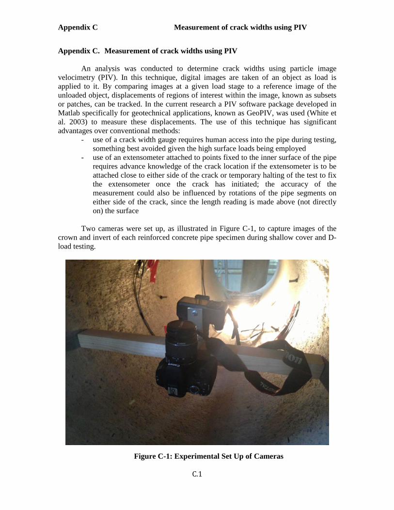
Appendix C Measurement of crack widths using PIV
C.1
Appendix C. Measurement of crack widths using PIV An analysis was conducted to determine crack widths using particle image
velocimetry (PIV). In this technique, digital images are taken of an object as load is applied to it. By comparing images at a given load stage to a reference image of the unloaded object, displacements of regions of interest within the image, known as subsets or patches, can be tracked. In the current research a PIV software package developed in Matlab specifically for geotechnical applications, known as GeoPIV, was used (White et al. 2003) to measure these displacements. The use of this technique has significant advantages over conventional methods:
- use of a crack width gauge requires human access into the pipe during testing, something best avoided given the high surface loads being employed
- use of an extensometer attached to points fixed to the inner surface of the pipe requires advance knowledge of the crack location if the extensometer is to be attached close to either side of the crack or temporary halting of the test to fix the extensometer once the crack has initiated; the accuracy of the measurement could also be influenced by rotations of the pipe segments on either side of the crack, since the length reading is made above (not directly on) the surface
Two cameras were set up, as illustrated in Figure C-1, to capture images of the
crown and invert of each reinforced concrete pipe specimen during shallow cover and D-load testing.
Figure C-1: Experimental Set Up of Cameras

Appendix C Measurement of crack widths using PIV
C.2
Images taken at loading increments of approximately 50kN of applied load were analysed using GEOpiv. To perform the analysis, the locations of the patches need to be selected. Since a PIV analysis can be performed once the test is completed, a priori knowledge of the crack location can be used to determine the required locations for the subsets to measure the crack width. A typical patch arrangement used in this analysis is shown in Figure C-2 using 64 by 64 pixel patches. One can see from the figure that two rows of subsets are used on either side of the crack. This is to overcome two sources of error that can occur when using PIV to measure crack widths: out of plane displacement and inclusion of tensile strains in the measurement. Out of plane displacement errors occur when the distance between the camera and the object being measured varies during the test (as would be the case for the crown of the reinforced concrete pipe that deflects towards the invert of the pipe as it is loaded). Depending on the extent of movement, this effect can lead to significant measurements errors as discussed elsewhere (Hoult et al. 2013). Additionally, when measuring the displacement between two patches, this displacement is due to the combined effects of the crack opening and the tensile strain that is developed between the two patches. By adding an additional two rows of patches the effects of these errors on the crack width measurements can be minimized as will be discussed. The results can then be used to determine the applied load that yielded a 0.25mm crack width in the pipe.
Figure C-2: Crack Width Analysis Patch Arrangement
A total of 36 patches were used to conduct the crack width analysis. Referring to Figure C-2 above, patch numbers 10-27 were created to solely determine uncorrected
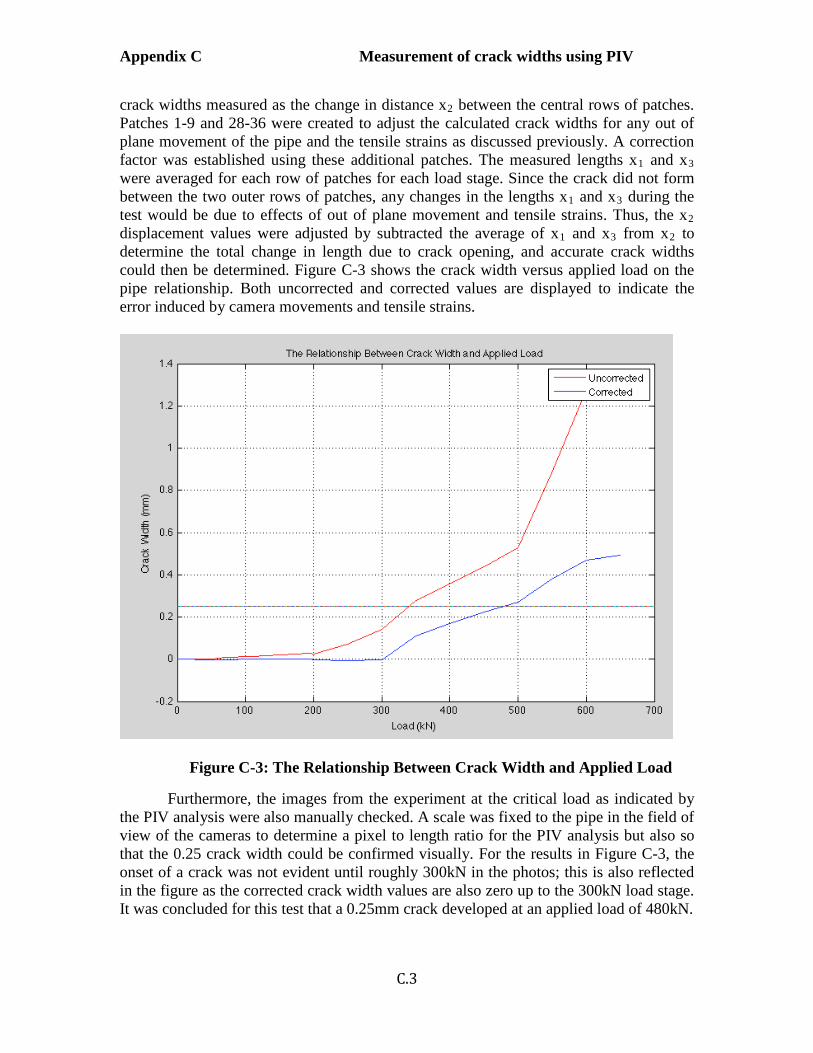
Appendix C Measurement of crack widths using PIV
C.3
crack widths measured as the change in distance x2 between the central rows of patches. Patches 1-9 and 28-36 were created to adjust the calculated crack widths for any out of plane movement of the pipe and the tensile strains as discussed previously. A correction factor was established using these additional patches. The measured lengths x1 and x3 were averaged for each row of patches for each load stage. Since the crack did not form between the two outer rows of patches, any changes in the lengths x1 and x3 during the test would be due to effects of out of plane movement and tensile strains. Thus, the x2 displacement values were adjusted by subtracted the average of x1 and x3 from x2 to determine the total change in length due to crack opening, and accurate crack widths could then be determined. Figure C-3 shows the crack width versus applied load on the pipe relationship. Both uncorrected and corrected values are displayed to indicate the error induced by camera movements and tensile strains.
Figure C-3: The Relationship Between Crack Width and Applied Load
Furthermore, the images from the experiment at the critical load as indicated by the PIV analysis were also manually checked. A scale was fixed to the pipe in the field of view of the cameras to determine a pixel to length ratio for the PIV analysis but also so that the 0.25 crack width could be confirmed visually. For the results in Figure C-3, the onset of a crack was not evident until roughly 300kN in the photos; this is also reflected in the figure as the corrected crack width values are also zero up to the 300kN load stage. It was concluded for this test that a 0.25mm crack developed at an applied load of 480kN.
Appendix C Measurement of crack widths using PIV
C.4
References Hoult, N.A., Take, W.A., Lee, C., and Dutton, M. (2013). “Experimental Accuracy of Two Dimensional Strain Measurements using Digital Image Correlation.” Eng. Struct., 46, 718-726. White, D.J., Take, W.A. and Bolton, M.D. (2003). “Soil deformation measurement using particle image velocimetry (PIV) and photogrammetry.” Géotechnique, 50(7), 619-631.
D-1
Appendix D: Proposed Usage Guidelines and Other Recommended Changes
D.1 Introduction ............................................................................................................................................................. 1
D.2 Thick ring theory ..................................................................................................................................................... 1
D.3 Usage Guidelines .................................................................................................................................................... 1
D.4 Modified Compression Field Theory ...................................................................................................................... 2
D.1 Introduction
Changes are suggested to the AASHTO LFRD Bridge Design Specifications to
- Account for thick ring theory
- Provide guidance on usage of the Indirect Design and Direct Design methods
- Include reference to the use of Modified Compression Field Theory and other more sophisticated approaches for
calculation of ultimate strength during Direct Design
D.2 Thick ring theory
The following modifications to the AASHTO LFRD Bridge Design Specifications are recommended. These issues are
dealt with in section 3.5.6 of the main report.
12.10.4.2.2 Analysis for Force Effects with the Pipe C12.10.4.2.2
Ring.
Force effects in the pipe shall be determined by an elastic analysis of the pipe ring under the assumed pressure distribution or a soil-structure analysis. If thin ring theory is employed, the expected moments NCHRP 20-07 Task 316 established that the at crown and invert can be adjusted to account for ring discrepancies in areas of flexural steel resulting thickness by from Direct and Indirect Design partly result from the Mthick =Mthin (1 – 0.373 t/R) use of thin ring theory. Adjustment to account for thick (12.10.4.2.2-1) ring theory resolves those discrepancies in part, though where: much of the conservatism of Direct Design remains (for Mthick = adjusted moment example, that associated with the estimation of expected Mthin = moment calculated using thin ring theory moment and consideration of ultimate limit state by t = thickness of the concrete pipe considering first plastic moment). R = average radius of the concrete pipe
D.3 Usage Guidelines
The following modifications to the AASHTO LFRD Bridge Design Specifications are recommended. The change in text
relates to the conclusions drawn about the conservatism of design are in Section 3.7.2 of the main body of the report.
12.10.1 General C12.10.1 The provisions herein shall apply to the structural These structures become part of a composite system

D-2
design of buried precast reinforced concrete pipes of comprised of the reinforced concrete buried section and circular, elliptical, and arch shapes. the soil envelope.
The structural design of the types of pipes indicated Standard dimensions for these units are shown in above may proceed by either of two methods: AASHTO M170M, (ASTM C 76M), M 206M (ASTM C 506M), M 207M (AASTM C 507M), and M242M (ASTM C 655M).
• The direct design method at the strength limit NCHRP 20-07 Task 316 established that while Direct state as specified in Article 12.10.4.2, or Design for small diameter pipes leads to higher The indirect design method at the service limit steel areas in some cases, these result from simplifying, state as specified in Article 12.10.4.3. conservative assumptions during Direct Design, and that
either design procedure can be employed.
D.4 Modified Compression Field Theory
The following modifications to the AASHTO LFRD Bridge Design Specifications are recommended, based on the
material presented in Sections 3.5.4 and 3.7.4.
12.10.4.2.4 Flexural Resistance at the Strength C12.10.4.2.4 Limit State NCHRP 20-07 Task 316 established that more sophisticated procedures can be employed for estimating the flexural and shear resistance at the strength limit state, such as Modified Compression Field Theory, to enforce compatibility between and steel and concrete components and account for multiple layers of steel reinforcement and nonlinear concrete and steel behavior.
Related Documents