ESTABLISHING A COMPUTERIZED MODEL FOR DESIGNING …

Journal of Engineering Science and Technology Vol. 16, No. 4 (2021) 3455 – 3480 © School of Engineering, Taylor’s University

3455

ESTABLISHING A COMPUTERIZED MODEL FOR DESIGNING DIFFERENT TYPES OF CONCRETE IN

TERMS OF STRENGTH, QUANTITY AND COST

AMR A. GAMAL1, MOHAMED S. BAKIR2,*, ANWAR MAHMOUD3, MOHAMED ABDEL-HAMID1

1Department of Civil Engineering, Faculty of Engineering at Shobra, Benha university, Benha, Egypt

2Department of Civil Engineering, Higher Technological Institute, Giza, Egypt 3Department of Material, Housing and Building National Research Centre, Giza, Egypt

*Corresponding Author: [email protected]

Abstract

The manual approach to design any concrete mixture needs to understand the American Concrete Institute (ACI) Code, including charts, tabular data, and curves. This usually demands interpolations in determining variables that lead to human errors in tracing out and estimating utilized values in the concrete mixture design process. Also, it becomes a tedious task to design the concrete mixture manually. Consequently, a computerized model had been developed using Microsoft Visual Studio for designing the mixtures of normal strength concrete (NC), lightweight concrete (LWC) and high strength concrete (HSC). The computerized model algorithm is created based on converting the ACI code charts and tabular data into mathematical equations. The model outputs included a user-friendly interface for quantifying the concrete mixture's ingredients and the optimal cost estimation. The computerized model accuracy is verified using two methods: first, comparing the concrete mixtures design using the manual design with those obtained from the developed computerized model; and second, comparing the compressive strength used in the computerized model with a field compressive strength obtained from a real concrete mixture that is cast and tested in the field. The results show the high accuracy of the developed model with an error of up to ±0.8%. The cost estimation is optimized with a precision that reaches 0% for the LWC and 0.4% for NC and HSC mixtures.

Keywords: Cost estimation, Concrete mixture design, Computerized model, Mathematical equations, Microsoft Visual studio program.

3456 A. A. Gamal et al.

Journal of Engineering Science and Technology August 2021, Vol. 16(4)

1. Introduction The importance of concrete as a construction material in modern communities is beyond description. It represents more than 60% of the building constructions in many developed countries due to its versatility, durability, and cost-effectiveness [1]. It is used for various construction projects such as small homemade, sidewalks, roads, bridges, flooring, dams, infrastructural facilities, huge building including foundations, basements, floors, columns and walls.

Concrete is a mixture of different materials, including coarse aggregates and fine aggregates, cement, admixtures and water. It has a density that ranges between 2240 kg/m3 and 2400 kg/m3 and a compressive strength that ranges from 17 MPa to 40 MPa [2]. In addition, the development of its compressive strength starts after seven days of curing, and it reaches 75% to 80% of the total compressive strength after 28 days of curing, while it achieves around 95 % of the strength after 90 days [3]. The quality of concrete does not depend only on its material quality; it also depends on the concrete mixture design. The concrete mixture design is the process of choosing the optimum concrete ingredients as well as estimating their relative quantities with respect to the economic side that satisfy the required properties such as workability, durability, consistency and compressive strength [4].

Due to the variations in the ingredient materials and their purpose, concrete can be classified into three main types: Normal or Conventional Concrete (NC), Light-Weight Concrete (LWC) and High Strength Concrete (HSC). NC is a concrete with a density ranges between 2240 kg/m3 to 2400 kg/m3 [2] and a compressive strength from 17 MPa to 40 MPa [3]. LWC is concrete with density ranges between 300 kg/m3 and 1840 kg/m3, and a compressive strength up to 17 MPa. It is classified as lightweight aggregate concrete, aerated or foamed concrete and no-fines concrete [5]. HSC is a concrete with a dry density greater than 2600 kg/m3, and a compressive strength exceeding 40 MPa [6, 7].

The concrete cost differs according to the aforementioned concrete types (NC, LWC and HSC). The cost is influenced by factors such as required strength, materials cost, delivery and pouring cost, which varies from one type of concrete to another.

The materials cost factor has the highest impact on concrete prices [8]. However, choosing appropriate concrete mixture's material and estimating their proper relative quantities is vital to avoid the low quality of concrete. For instance, between 1985 and 2006, about 86 cases of building collapse were stated in Nigeria due to the low quality of concrete due to incorrect calculation of concrete mixture ingredients` quantities [9]. Likewise, similar cases have been reported in Algeria [7, 10], Kenya, South Africa, Uganda and Thailand [11].

While the decision-makers are focusing on the importance of choosing the appropriate material for the concrete mixture, it is also essential to achieve the most economical concrete mixture design to enhance the feasibility of any construction. One of the well-known challenges was mentioned by Jha [12], who faced a situation that required building 1.77 million residences to accommodate about 18.78 million people, with the lowest possible construction cost.

That said, the construction cost can be reduced by achieving the optimum or the most economical concrete mixture design. Therefore, the literature focused on two

Establishing a Computerized Model for Designing Different Types of . . . . 3457


main methods to achieve the optimum concrete mixture design by reducing the errors that resulted from using the American Concrete Institute (ACI) code charts and tabular data. Using the charts and tabular data in the concrete mixture design provide the users with estimated quantities for concrete mixture`s materials instead of absolute accurate quantities, due to the human factor errors that can occur while using the charts. Accordingly, avoiding human errors in designing the material's quantities will benefit in optimizing the concrete cost [13, 14].

The two main methods to reach the optimal concrete mixture design are: a) Converting the ACI code's tabular data and graphs into mathematical equations to use in the concrete mixture design; b) Developing a computer software that automatically design the concrete mixtures`.

The dynamic optimization method was used to generate a model of equations for the cost optimization of NC mixture design by focusing on aggregates` type, aggregates` size, and cement class [15]. The multiple linear regression models was used to convert the ACI code graphs and tabular data [16] into mathematical equations for the LWC mixture design [13].

While Netbins 7.1 programming was used to develop a software known as CLETJER [14], following the British Department of Environment (BDOE) method for NC mixture design. The software error varied between -2.857% and 2.173%. A script was developed using MATLAB programming for designing the LWC mixture design, with an error between -1.92% and 0.48% [17]. In addition, MATLAB programming was used to generate a standalone application for HSC mixture designing [18]. The application gives the capability to design HSC mixtures with compressive strength above 60 MPa with error varying from 0.30% to 1.44%. While an HSC mixture calculator was developed based on the Indian Standard (IS) Codes using MATLAB programming, with an error between -0.0811% and 0.089% [19].

Through this brief review, it is shown that the computerized models became a common way to optimize the material quantities and the cost for the concrete mixtures due to its flexible usage, time-saving, neglected human error and higher accuracy. However, some research gaps are defined: 1) There is a lack of studies that develop a computerized model for designing the NC, LWC and HSC mixtures in the same model. The literature studies care only for developing a model for a single concrete mixture type. 2) To the best of our knowledge, no study includes the cost estimations for the concrete mixture materials considering the prices change over the time. 3) Although the previous studies evaluated the accuracy for the computerized model by comparing the results of the developed model with the result of the manual design, surprisingly, there is a few to no study that checks the accuracy by comparing the computerized model results with a field test result, for example, by comparing the computerized model's compressive strength with the field's compressive strength.

Therefore, the present study provides original contributions to the existing literature through, 1) Converting the ACI code charts and tabular data for the NC, LWC and HSC, into mathematical equations using a multiple linear regression model. 2) Defining an entire algorithm for the proposed computerized model, based on the mathematical equations that cover all the design and cost estimation steps for the NC, LWC and HSC mixture. 3) Using the Microsoft Visual Studio



Enterprise (MVSE) [20] for coding the algorithm to obtain a graphical user interface (GUI), which is user-friendly for practical implications (Appendix A). 4) Checking the computerized model's accuracy by comparing the manual design result and the field's compressive strength with the computerized model results.

2. Methods This study adopts a three-step sequential methodology, as illustrated in Fig. 1. The following subsections explain each the steps in details.

Fig. 1. A flow chart of the three-step methodology.

2.1. Generated ACI equations and the design steps In this section, we illustrate the followed approach to generate the equations from the tabular data in the American Concrete Institute (ACI) code for NC [2], LWC [16] and HSC [6].

First, we converted the tabular data into separate data points and plotted it in graphs using Microsoft Excel spreadsheets, where each graph contains some curves that traced out three points or more. Second, we plotted regression lines (linear, polynomial, exponential and logarithm) between the data points to get a regression equation consists of a dependent variable and independent variables, as shown in Figs. 2-12. Third, we choose the accurate regression equation for each curve based on the highest coefficient of determination (R2).

The Tabular data, the charts and the generated equations, are all explained in detail for NC, LWC and HSC, as shown in the next subsections.

2.1.1. NC mixture design The estimation of net mixing water (WNM) and entrained air (Ea) for NC depend on two main factors: maximum size of coarse aggregate (Sca) and slump range (SD) of fresh NC mixture [2].Therefore, we converted the ACI corresponding tabular data "ACI, table A1.5.3.3; approximate mixing water and air content requirements for different slumps and nominal maximum sizes of aggregates" into Eqs. (1)-(6) that can calculate the WNM and Ea for NC mixture, as shown in Fig. 2.

The water per cementitious material ratio (wcr) for NC mixture depends on compressive strength of concrete (fc) "ACI, table A1.5.3.4.a; relationships between water/cement ratio and compressive strength of concrete". Accordingly, Eq. (7) was developed to estimate wcr for NC, as shown in Fig. 3.

Moreover, the volume of dry loose coarse aggregate (VCL) is affected by fineness modulus of fine aggregate (Fm) and Sca as stated in "ACI, table A.1.5.3.6; volume of coarse aggregate per unit volume of concrete". Toward that, Eqs. (8)-(13) were generated to estimate the VCL for NC, as shown in Fig. 4.



Net Mixing Water (kg/m3)

Aggregate Max Size

(mm)

Slump (mm)

25 – 50 75 – 100 125 – 150

9.5 181 202 216 12.5 175 193 205 19 166 181 193 25 160 175 184

37.5 148 164 172 50 142 157 166 75 122 133 154

WNM, (25-50) = 7 x10-6 Sca4 – 0.0015 Sca

3 + 0.1243 Sca2 – 5.0668 Sca + 253.24 R² = 0.9986 (1)

WNM, (75-100) = 8 x10-6 Sca4 – 0.0018 Sca

3 + 0.1351 Sca2 – 4.9448 Sca+ 237.70 R² = 0.9992 (2)

WNM, (125-150) = -3 x10-6 Sca4 + 0.0003 Sca

3 + 0.0124 Sca2 – 1.9764 Sca+ 197.99 R² = 0.9993 (3)

Entrained air %

Aggregate Max Size

(mm)

Slump (mm)

25 - 50 75 - 100 125 - 150

9.5 4.5 6 7.5 12.5 4 5.5 7 19 3.5 5 6 25 3 4.5 6

37.5 2.5 4.5 5.5 50 2 4 5 75 1.5 3.5 4.5

Ea, (25-50) = 2 x10-6 Sca4 - 0.0003 Sca

3 + 0.02 Sca2 - 0.526 Sca+ 10.986 R² = 0.9915 (4)

Ea, (75-100) = 2 x10-6 Sca4 - 0.0003 Sca

3 + 0.0165 Sca2 - 0.4365 Sca+ 8.8901 R² = 0.9917 (5)

Ea, (125-150) = 7 x10-7 Sca4 - 0.0001 Sca

3 + 0.0081 Sca2 - 0.271 Sca+ 6.413 R² = 0.9983 (6)

Fig. 2. Generating the WNM and Ea equations for NC mixture.

Relationships between W/C and fc of concrete

Compressive Strength fc (MPa) 28 - days W/C

35 0.39 30 0.45 25 0.52 20 0.6 15 0.7

wcr = -0.366 ln(fc) + 1.6928 R² = 0.9994 (7)

Fig. 3. Generating the wcr equation for NC mixture.

Volume of Oven-Dry Loose Coarse Aggregates Per Unit Volume of Concrete for Different

Fineness Modulus of Fine Aggregate

Aggregate Max Size

(mm)

Fineness Modulus

2.4 2.6 2.8 3

9.5 0.5 0.48 0.46 0.44 12.5 0.59 0.57 0.55 0.53 19 0.66 0.64 0.62 0.6 25 0.71 0.69 0.67 0.65

37.5 0.75 0.73 0.71 0.69 50 0.78 0.76 0.74 0.72

VCL, (9.5) = -0.1 Fm + 1.02 R² = 1 (8) VCL, (12.5) = -0.1 Fm + 0.99 R² = 1 (9) VCL, (19) = -0.1 Fm + 0.95 R² = 1 (10) VCL, (25) = -0.1 Fm + 0.90 R² = 1 (11) VCL, (37.5) = -0.1 Fm + 0.83 R² = 1 (12) VCL, (50) = -0.1 Fm + 0.74 R² = 1 (13)

Fig. 4. Generating the VCL equations for NC mixture.

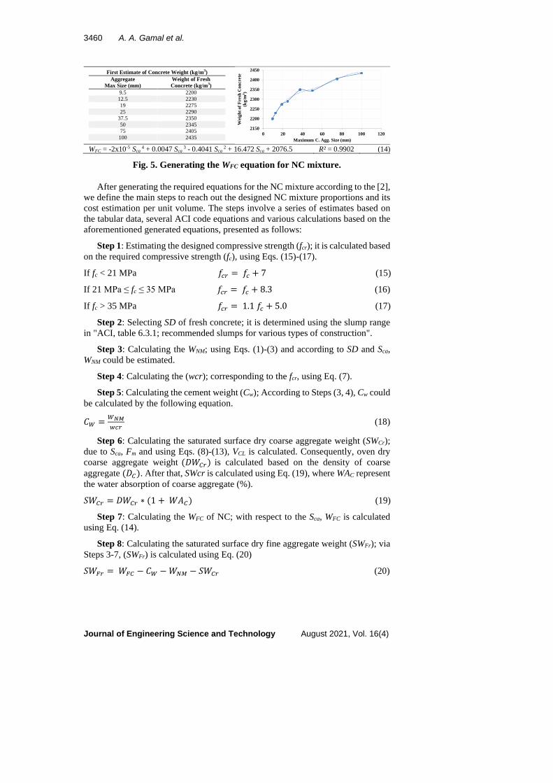
According to "ACI, table A.1.5.3.7.1; first estimate of mass of fresh concrete", we generated the weight of fresh concrete (WFC) which is based on the Sca (Eq. (14)), as shown in Fig. 5.

110

130

150

170

190

210

230

0 10 20 30 40 50 60 70 80

Net

Mix

ing

Wat

er (k

g/m

3 )

Maximum C. Aggregate Size (mm)

Slump 25 - 50Slump 75 - 100Slump 125 - 150

012345678

0 10 20 30 40 50 60 70 80E

ntai

ned

Air

%Maximum C. Aggregate Size (mm)

Slump 25 - 50Slump 75 - 100Slump 125 -150

0.3

0.4

0.5

0.6

0.7

0.8

10 15 20 25 30 35

Wat

er p

er C

emen

t (W

/C)

Compressive Strength fc (MPa)

0.4

0.5

0.6

0.7

0.8

2.3 2.4 2.5 2.6 2.7 2.8 2.9 3 3.1

Vol

ume

of C

oars

e A

ggre

gate

s (m

3 )

Fineness Modulus of Fine aggregate

C. Agg. 9.5 mm C. Agg. 12.5 mmC. Agg. 19.0 mm C. Agg. 25.0 mmC. Agg. 37.5 mm C. Agg. 50.0 mm



First Estimate of Concrete Weight (kg/m3) Aggregate

Max Size (mm) Weight of Fresh Concrete (kg/m3)

9.5 2200 12.5 2230 19 2275 25 2290

37.5 2350 50 2345 75 2405

100 2435

WFC = -2x10-5 Sca

4 + 0.0047 Sca 3 - 0.4041 Sca

2 + 16.472 Sca + 2076.5 R² = 0.9902 (14)

Fig. 5. Generating the WFC equation for NC mixture.

After generating the required equations for the NC mixture according to the [2], we define the main steps to reach out the designed NC mixture proportions and its cost estimation per unit volume. The steps involve a series of estimates based on the tabular data, several ACI code equations and various calculations based on the aforementioned generated equations, presented as follows:

Step 1: Estimating the designed compressive strength (fcr); it is calculated based on the required compressive strength (fc), using Eqs. (15)-(17).

If fc < 21 MPa 𝑓𝑓𝑐𝑐𝑐𝑐 = 𝑓𝑓𝑐𝑐 + 7 (15)

If 21 MPa ≤ fc ≤ 35 MPa 𝑓𝑓𝑐𝑐𝑐𝑐 = 𝑓𝑓𝑐𝑐 + 8.3 (16)

If fc > 35 MPa 𝑓𝑓𝑐𝑐𝑐𝑐 = 1.1 𝑓𝑓𝑐𝑐 + 5.0 (17)

Step 2: Selecting SD of fresh concrete; it is determined using the slump range in "ACI, table 6.3.1; recommended slumps for various types of construction".

Step 3: Calculating the WNM; using Eqs. (1)-(3) and according to SD and Sca, WNM could be estimated.

Step 4: Calculating the (wcr); corresponding to the fcr, using Eq. (7).

Step 5: Calculating the cement weight (Cw); According to Steps (3, 4), Cw could be calculated by the following equation.

𝐶𝐶𝑊𝑊 = 𝑊𝑊𝑁𝑁𝑁𝑁𝑤𝑤𝑐𝑐𝑐𝑐

(18)

Step 6: Calculating the saturated surface dry coarse aggregate weight (SWCr); due to Sca, Fm and using Eqs. (8)-(13), VCL is calculated. Consequently, oven dry coarse aggregate weight (𝐷𝐷𝐷𝐷𝐶𝐶𝑐𝑐) is calculated based on the density of coarse aggregate (𝐷𝐷𝐶𝐶). After that, SWcr is calculated using Eq. (19), where WAC represent the water absorption of coarse aggregate (%).

𝑆𝑆𝐷𝐷𝐶𝐶𝑐𝑐 = 𝐷𝐷𝐷𝐷𝐶𝐶𝑐𝑐 ∗ (1 + 𝐷𝐷𝑊𝑊𝐶𝐶) (19)

Step 7: Calculating the WFC of NC; with respect to the Sca, WFC is calculated using Eq. (14).

Step 8: Calculating the saturated surface dry fine aggregate weight (SWFr); via Steps 3-7, (SWFr) is calculated using Eq. (20)

𝑆𝑆𝐷𝐷𝐹𝐹𝑐𝑐 = 𝐷𝐷𝐹𝐹𝐶𝐶 − 𝐶𝐶𝑊𝑊 −𝐷𝐷𝑁𝑁𝑁𝑁 − 𝑆𝑆𝐷𝐷𝐶𝐶𝑐𝑐 (20)

2150

2200

2250

2300

2350

2400

2450

0 20 40 60 80 100 120

Wei

ght o

f Fre

sh C

oncr

ete

(kg/

m3 )

Maximum C. Agg. Size (mm)



Step 9: Correcting the ingredients` quantities; according to the moisture content of course and fine aggregates, the adjustments of aggregates for this moisture is calculated using Eqs. (21)-(23).

𝐷𝐷𝐷𝐷𝐶𝐶𝑐𝑐 = 𝐷𝐷𝐷𝐷𝐶𝐶𝑐𝑐 ∗ (1 + 𝑀𝑀𝐶𝐶𝐶𝐶) (21)

𝐷𝐷𝐷𝐷𝐹𝐹𝑐𝑐 = 𝐷𝐷𝐷𝐷𝐹𝐹𝑐𝑐 ∗ (1 + 𝑀𝑀𝐶𝐶𝐹𝐹) (22)

𝐷𝐷𝑁𝑁 = 𝐷𝐷𝑁𝑁𝑁𝑁 − 𝐷𝐷𝐷𝐷𝐶𝐶𝑐𝑐 ∗ (𝑀𝑀𝐶𝐶𝐶𝐶 −𝐷𝐷𝑊𝑊𝐶𝐶) − 𝐷𝐷𝐷𝐷𝐹𝐹𝑐𝑐 ∗ (𝑀𝑀𝐶𝐶𝐹𝐹 −𝐷𝐷𝑊𝑊𝐹𝐹) (23)

where 𝐷𝐷𝐷𝐷𝐶𝐶𝑐𝑐 : is the wet weight of coarse aggregate (kg/m3), 𝐷𝐷𝐷𝐷𝐹𝐹𝑐𝑐 : is the wet weight of fine aggregate (kg/m3), 𝐷𝐷𝐷𝐷𝐹𝐹𝑐𝑐 : is the dry weight of coarse aggregate (kg/m3), 𝑀𝑀𝐶𝐶𝐶𝐶 : is the moisture content of coarse aggregate (%), 𝑀𝑀𝐶𝐶𝐹𝐹 : is the moisture content of fine aggregate (%), 𝐷𝐷𝑊𝑊𝐹𝐹 : is the water absorption of fine aggregate (%).

Step 10: Estimating the Cost; the cost is estimated based on the prices of raw material and the inflation factor of prices in Egypt. A survey for twenty constituent materials of concrete dealers in Cairo city, Egypt, was carried out for the purpose of determining the average unit prices of constituent materials of concrete. The average unit prices were employed in the computerized model to estimate the hypothetical cost of concrete mixture. Moreover, the annual inflation rate of prices in Egypt is 15 % according to Central Agency for Public Mobilization and Statistics [21]. So, the accurate cost of 1 m3 for the concrete mixture (MP) is calculated using Eq. (24).

𝑀𝑀𝑝𝑝 = (� 𝑊𝑊𝑊𝑊𝐶𝐶𝐶𝐶1000∗𝑆𝑆.𝑂𝑂.𝐺𝐺𝑐𝑐

� ∗ 130 + � 𝑊𝑊𝑊𝑊𝐹𝐹𝐶𝐶1000∗𝑆𝑆.𝑂𝑂.𝐺𝐺𝑓𝑓

� ∗ 75 + (0.8 ∗ 𝐶𝐶𝑤𝑤) + (0.012 ∗ 𝐷𝐷𝑁𝑁)) ∗

(1 + 0.15)(𝐷𝐷𝐷𝐷−2019) (24)

where: 𝑆𝑆.𝑂𝑂.𝐺𝐺𝑐𝑐 is the specific gravity factor of coarse aggregate; 𝑆𝑆.𝑂𝑂.𝐺𝐺𝑓𝑓 is the specific gravity factor of fine aggregate; 𝐷𝐷𝐷𝐷 is the date of design.

2.1.2. LWC mixture design Regarding the LWC, It is mentioned that WNM and Ea that required to produce a SD, depend on the Sca [16]. Thus, we generated Eqs. (25)-(30) using "ACI, table 3.2; approximate mixing water and air content requirements for different slumps and nominal maximum sizes of aggregates" to calculate the WNM and Ea for LWC, as shown in Fig. 6.

Furthermore, calculating the wcr for LWC mixture differ based on the fc, as stated in "ACI, table 3.3; relationships between w/c and compressive strength of concrete". Toward that, Eq. (31) was developed to estimate the wcr of LWC mixture, as shown in Fig. 7.

Following the "ACI, table 3.5; volume of coarse aggregate per unit of volume of concrete", the VCL Eqs. (32)-(34) for LWC mixture are generated based on the values of Sca and Fm, as shown in Fig. 8.

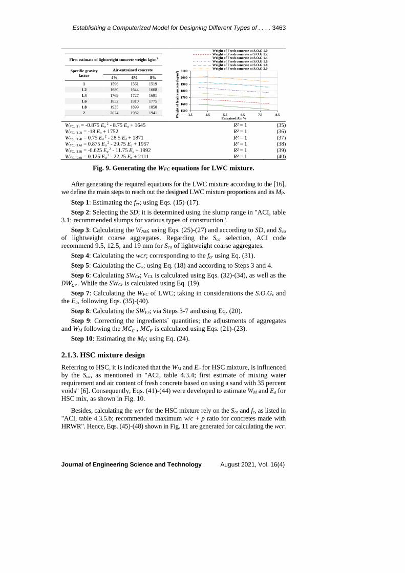
Moreover, Eqs. (35)-(40) were generated using "ACI, table 3.6; first estimate of weight of fresh lightweight concrete comprised of lightweight coarse aggregate and normal weight fine aggregate" in order to estimate the WFC for LWC mixture, which depend on a S.O.Gc and Ea, as shown in Fig. 9.



Net Mixing Water (kg/m3) Aggregate Max Size

(mm)

Slump (mm)

25 - 50 75 - 100 125 - 150

9.5 181 202 211 12.5 175 193 199 19 166 181 187

WNM, (25-50) = 0.0648 Sca

2 - 3.4251 Sca + 207.69 R² = 1 (25) WNM, (75-100) = 0.1215 Sca

2 - 5.6721 Sca + 244.92 R² = 1 (26) WNM, (125-150) = 0.2267 Sca

2 - 8.9879 Sca + 275.92 R² = 1 (27)

Entrained Air % Aggregate Max Size

(mm)

Slump (mm)

25 - 50 75 - 100 125 - 150

9.5 181 202 211 12.5 175 193 199 19 166 181 187

Ea, (25-50) = 0.0175 Sca

2 - 0.5526 Sca + 8.1667 R² = 1 (28) Ea, (75-100) = 0.0094 Sca

2 - 0.3745 Sca + 8.7051 R² = 1 (29) Ea, (125-150) = 0.0013 Sca

2 - 0.1964 Sca + 9.2436 R² = 1 (30)

Fig. 6. Generating the WNM and Ea equations for LWC mixture.

Relationships between W/C and fc of concrete

Compressive Strength fc (MPa) 28 - days W/C

34.5 0.40 27.6 0.48 20.7 0.59 13.8 0.74

wcr = -0.372ln(fc) + 1.7172 R² = 0.9999 (31)

Fig. 7. Generating the wcr equation for LWC mixture.

Volume of Oven-Dry Loose Coarse Aggregates Per Unit Volume of Concrete for Different

Fineness Modulus of Sand Aggregate Max Size

(mm)

Fineness Modulus

2.4 2.6 2.8 3

9.5 0.58 0.56 0.54 0.52 12.5 0.67 0.65 0.63 0.61 19 0.74 0.72 0.7 0.68

VCL, (9.5) = -0.1 Fm + 0.82 R² = 1 (32) VCL, (12.5) = -0.1 Fm + 0.91 R² = 1 (33) VCL, (19) = -0.1 Fm + 0.98 R² = 1 (34)

Fig. 8. Generating the VCL equations for LWC mixture.

160

170

180

190

200

210

7 9 11 13 15 17 19

Net

Mix

ing

Wat

er K

g/m

3

Maximum C. aggregate size (mm)

Slump 25 - 50Slump 75 -100Slump 125 - 150

3

4

5

6

7

8

9 11 13 15 17 19%

Ent

rain

ed A

ir

Maximum C. aggregate size (mm)


0.3

0.4

0.5

0.6

0.7

0.8

10 15 20 25 30 35

Wat

er p

er C

emen

t W

/C

Compressive Strength fc (MPa)

0.5

0.55

0.6

0.65

0.7

0.75

0.8

2.3 2.5 2.7 2.9

Vol

ume

of C

oars

e A

ggre

gate

s (m

3 )

Fineness Modulus

C.Agg. 9.5 mmC.Agg. 12.5 mmC.Agg. 19 mm



First estimate of lightweight concrete weight kg/m3

Specific gravity factor

Air-entrained concrete

4% 6% 8% 1 1596 1561 1519

1.2 1680 1644 1608 1.4 1769 1727 1691 1.6 1852 1810 1775 1.8 1935 1899 1858 2 2024 1982 1941

WFC, (1) = -0.875 Ea 2 - 8.75 Ea + 1645 R² = 1 (35)

WFC, (1.2) = -18 Ea + 1752 R² = 1 (36) WFC, (1.4) = 0.75 Ea

2 - 28.5 Ea + 1871 R² = 1 (37) WFC, (1.6) = 0.875 Ea

2 - 29.75 Ea + 1957 R² = 1 (38) WFC, (1.8) = -0.625 Ea

2 - 11.75 Ea + 1992 R² = 1 (39) WFC, (2.0) = 0.125 Ea

2 - 22.25 Ea + 2111 R² = 1 (40)

Fig. 9. Generating the WFC equations for LWC mixture.

After generating the required equations for the LWC mixture according to the [16], we define the main steps to reach out the designed LWC mixture proportions and its MP.

Step 1: Estimating the fcr; using Eqs. (15)-(17). Step 2: Selecting the SD; it is determined using the slump range in "ACI, table

3.1; recommended slumps for various types of construction". Step 3: Calculating the WNM; using Eqs. (25)-(27) and according to SD, and Sca

of lightweight coarse aggregates. Regarding the Sca selection, ACI code recommend 9.5, 12.5, and 19 mm for Sca of lightweight coarse aggregates.

Step 4: Calculating the wcr; corresponding to the fcr using Eq. (31). Step 5: Calculating the Cw; using Eq. (18) and according to Steps 3 and 4. Step 6: Calculating SWCr; VCL is calculated using Eqs. (32)-(34), as well as the

𝐷𝐷𝐷𝐷𝐶𝐶𝑐𝑐 . While the SWCr is calculated using Eq. (19). Step 7: Calculating the WFC of LWC; taking in considerations the S.O.Gc and

the Ea, following Eqs. (35)-(40). Step 8: Calculating the SWFr; via Steps 3-7 and using Eq. (20). Step 9: Correcting the ingredients` quantities; the adjustments of aggregates

and WM following the 𝑀𝑀𝐶𝐶𝐶𝐶 , 𝑀𝑀𝐶𝐶𝐹𝐹 is calculated using Eqs. (21)-(23). Step 10: Estimating the MP; using Eq. (24).

2.1.3. HSC mixture design Referring to HSC, it is indicated that the WM and Ea for HSC mixture, is influenced by the Sca, as mentioned in "ACI, table 4.3.4; first estimate of mixing water requirement and air content of fresh concrete based on using a sand with 35 percent voids" [6]. Consequently, Eqs. (41)-(44) were developed to estimate WM and Ea for HSC mix, as shown in Fig. 10.

Besides, calculating the wcr for the HSC mixture rely on the Sca and fc, as listed in "ACI, table 4.3.5.b; recommended maximum w/c + p ratio for concretes made with HRWR". Hence, Eqs. (45)-(48) shown in Fig. 11 are generated for calculating the wcr.

1500

1600

1700

1800

1900

2000

2100

3.5 4.5 5.5 6.5 7.5 8.5

Wei

ght o

f fre

sh c

oncr

ete

(kg/

m3 )

Entrained Air %

Weight of Fresh concrete at S.O.G 1.0Weight of Fresh concrete at S.O.G 1.2Weight of Fresh concrete at S.O.G 1.4Weight of Fresh concrete at S.O.G 1.6Weight of Fresh concrete at S.O.G 1.8Weight of Fresh concrete at S.O.G 2.0



The volume of dry rodded coarse aggregate (VCR) for HSC mixture can be calculated based on the Sca, as mentioned in "ACI, table 4.3.3; recommended volume of coarse aggregate per unit volume of concrete". VCR calculations are listed in Fig. 12, Eq. (49).

Mixing Water (kg/m3) Aggregate Max Size

(mm)

Slump (mm)

25 - 50 75 - 100 125 - 150

9.5 184 190 196 12.5 175 184 190 19 169 175 181 25 166 172 178

WM, (25-50) = -0.0119 Sca

3 + 0.7074 Sca 2 - 14.208 Sca + 265.36 R² = 1 (41)

WM, (75-100) = 0.0004 Sca 3 + 0.0489 Sca

2 - 3.2176 Sca + 215.82 R² = 1 (42) WM, (125-150) = 0.0004 Sca

3 + 0.0489 Sca 2 - 3.2176 Sca + 221.82 R² = 1 (43)

Relation between Aggregate Max size and Entrained Air %

Aggregate Max Size (mm) Entrained Air %

9.5 2.5 12.5 2 19 1.5 25 1

Ea = -0.0006 Sca 3 + 0.0358 Sca

2 - 0.7194 Sca + 6.6549 R² = 1 (44)

Fig. 10. Generating the WM and Ea equations for HSC mixture.

Relationships between (W/C + P) and fc of concrete Compressive Strength fc

(MPa) 28 - days

W/C + P Aggregate Max Size (mm)

9.5 12.5 19 25 48.32 0.5 0.48 0.45 0.43 55.12 0.44 0.42 0.4 0.38

62 0.38 0.36 0.35 0.34 68.9 0.33 0.32 0.31 0.3 75.79 0.3 0.29 0.27 0.27 82.68 0.27 0.26 0.25 0.25

wcr, (9.5) = -0.340ln(fc) + 1.7465 R² = 0.9957 (45) wcr, (12.5) = -0.383ln(fc) + 1.9332 R² = 0.9963 (46) wcr, (19) = -0.411ln(fc) + 2.0669 R² = 0.9919 (47) wcr, (25) = -0.435ln(fc) + 2.1811 R² = 0.9932 (48)

Fig. 11. Generating the wcr equations for HSC mixture.

Optimum Coarse Aggregate contents for max sizes of aggregates to be used with sand with F.M of 2.5 to 3.2 Aggregate Max

Size (mm) 9.5 12.5 19 25

Fractional volume of oven

dry rodded coarse

Aggregate (m3)

0.65 0.68 0.72 0.75

VCR = 2x10-5 Sca

3 - 0.0012 Sca 2 + 0.0297 Sca + 0.4614 R² = 1 (49)

Fig. 12. Generating the VCR equation for LWC mixture.

160165170175180185190195200

7 12 17 22

Mix

ing

Wat

er (K

g/m

3 )

Maximum C. Aggregate size (mm)


0

0.5

1

1.5

2

2.5

3

8 13 18 23

% E

ntra

ined

Air

Aggregate Max Size (mm)

0.2

0.25

0.3

0.35

0.4

0.45

0.5

0.55

45 55 65 75 85

(W/C

+ P

)

Compressive strength fc (MPa)

C. Aggregate 9.5 mmC. Aggregate 12.5 mmC. Aggregate 19.0 mmC. Aggregate 25.0 mm

0.64

0.66

0.68

0.7

0.72

0.74

0.76

6 11 16 21 26

Vol

ume

of C

oars

e A

ggre

gate

(m3 )

Aggregate Max Size (mm)



After generating the required equations for the HSC mixture according to the ACI code [6], we defined the main steps to reach out the designed HSC mixture proportions and its MP.

Step 1: Estimating the fcr; it is calculated based on the fc through Eq. (50).

𝑓𝑓𝑐𝑐𝑐𝑐 = 𝑓𝑓𝑐𝑐+9.6460.9

(50)

Step 2: Selecting the SD; according to ACI code (ACI 211.4R-93, 1998), it is recommended to add high range water reducer (HR) to adequate the water content at the mixture proportions. Hence, the proposed initial slump should range from 25 mm to 50 mm.

Step 3: Calculating the WM; using Eqs. (41)-(43) and due to SD and Sca, WM is calculated if the used fine aggregates` voids (Fv) are equal to 35%. But if Fv were not equal to 35 %, the WM should be adjusted by (WMC) using Eq. (51). Where Fv can be calculated using Eq. (52) based on density of fine aggregate (DF) and the S.O.Gf 𝐷𝐷𝑁𝑁𝐶𝐶 = (𝐹𝐹𝑉𝑉 − 35) ∗ 4.744 (51)

𝐹𝐹𝑉𝑉 = �1 − 𝐷𝐷𝐹𝐹𝑆𝑆.𝑂𝑂.𝐺𝐺𝑓𝑓∗1000

� ∗ 100 (52)

Step 4: Calculating the Ea; it refers to the Sca and it is calculated using Eq. (44).

Step 5: Calculating the wcr; corresponding to the fcr, using Eqs. (45)-(48).

Step 6: Calculating the Cw; following the Steps 3-5 and Eq. (18), the Cw is calculated.

Step 7: Calculating the fly ash weight (FAw); the FAw is calculated as a 20% percentage from the Cw. So, FAw and quantity of cement required for HSC mixture (Cwr) are calculated according to Eqs. (53)-(54)

Cwr = 0.8 * Cw (53)

FAw = 0.2 * Cw (54)

Step 8: Calculating the VCR; using Eq. (49).

Step 9: Calculating the fine aggregate volume (VF); using Eq. (55). Where 𝑆𝑆.𝑂𝑂.𝐺𝐺𝑐𝑐𝑐𝑐 is the specific gravity factor of cement and 𝑆𝑆.𝑂𝑂.𝐺𝐺𝐹𝐹𝐹𝐹 is the specific gravity factor of fly ash.

𝑉𝑉𝐹𝐹 = 1 – ( 𝐶𝐶𝑤𝑤𝐶𝐶𝑆𝑆.𝑂𝑂.𝐺𝐺𝑐𝑐𝑐𝑐∗1000

+ 𝐹𝐹𝐹𝐹𝑤𝑤𝑆𝑆.𝑂𝑂.𝐺𝐺𝐹𝐹𝐹𝐹∗1000

+ 𝑉𝑉𝐶𝐶𝐶𝐶 + 𝑊𝑊𝑁𝑁1000

+ 𝐸𝐸𝑎𝑎) (55)

Step 10: Calculating the HR; HR is estimated as 8 % of Cwr [6].

Step 11: Estimating the Cost; the MP is calculated using Eq. (56).

𝑀𝑀𝑝𝑝 = (� 𝐷𝐷𝑊𝑊𝐶𝐶𝐶𝐶1000∗𝑆𝑆.𝑂𝑂.𝐺𝐺𝑐𝑐

� ∗ 130 + � 𝐷𝐷𝑊𝑊𝐹𝐹𝐶𝐶1000∗𝑆𝑆.𝑂𝑂.𝐺𝐺𝑓𝑓

� ∗ 75 + (0.8 ∗ 𝐶𝐶𝑤𝑤𝑐𝑐) + (0.012 ∗ 𝐷𝐷𝑁𝑁) +

(13 ∗ 𝐹𝐹𝑊𝑊𝑤𝑤) + (5 ∗ 𝐻𝐻𝐻𝐻)) ∗ (1 + 0.15)(𝐷𝐷𝐷𝐷−2019) (56)

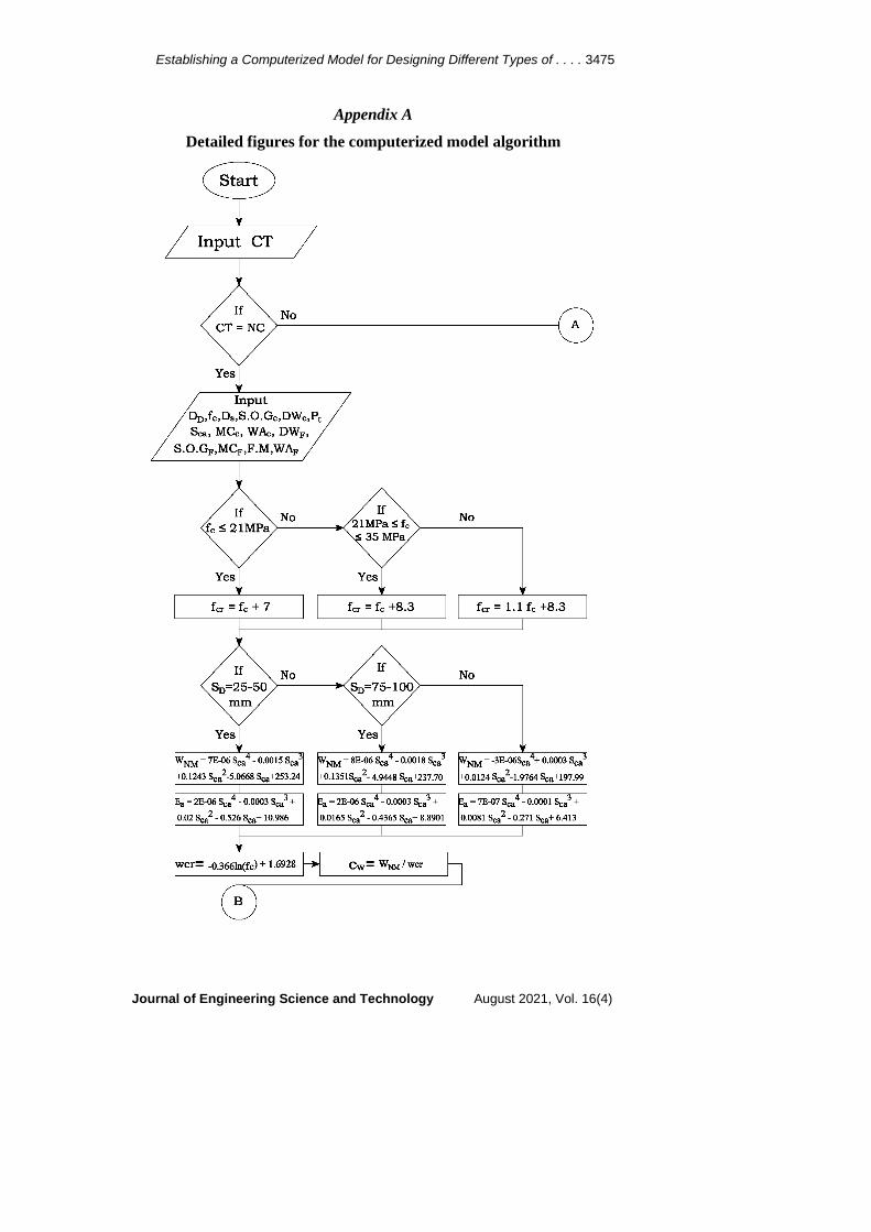
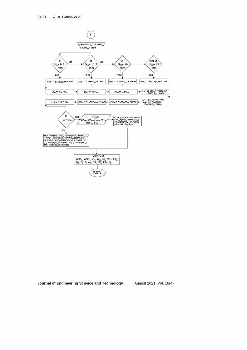
2.2. The computerized model's algorithm After determining the design steps of the NC, LWC and HSC mixtures, as shown in the previous section, we started to build the algorithm based on those design steps using the Microsoft Visual Studio Enterprise 2015 Version 14.0.23107.0 D14REL [20], as shown in Fig. 13. The algorithm starts by asking the user for choosing the



required concrete type (CT) between the NC, LWC and HSC. Then based on the chosen concrete type, other inputs are required, as summarized in Table 1.

Fig. 13. The algorithm of the computerized

model (Besides, detailed figures for the algorithm are attached in Appendix B).

Table 1. The required inputs of the computerized model. Inputs NC, LWC and HSC General DD, fc, SD CoarseAggregate Properties S.O.Gc, Sca, DC, MCC, WAC Fine Aggregate Properties S.O.Gf, Fm, DF, MCF, WAF Cement Properties Just for the HSC: S.O.Gce , S.O.GFA

Following the inputs, the computerized model starts to automatically follow the next steps in the algorithm (Fig. 13). At the final step, the model asks the user about the unit prices of mixtures ingredients in case the user has a specific price. If not, the model starts automatically to compute the cost estimation based on standard prices (we extracted them based on the Egyptian market prices for the row material). The outputs of the computerized model include a) the accurate quantities



of mixtures` ingredients per 1 m3; and b) the cost estimation per 1 m3. For the output details, see Table 2.

Table 2. The outputs of the developed computerized model.

Outputs The concrete mix

quantities per 1 m3 The cost per 1 m3

NC and LWC HSC NC and LWC HSC General fc, wcr,WFC fc,wcr,WFC, HR MP MP,HRP Coarse

Aggregate WWCr DWCr CAP CAP

Fine Aggregate WWFr DWFr FAP FAP

Cement Cw Cwr, FAw CP CP, FP Water WM WP

where: HRP is the price of high range water reducer quantity required for concrete mixture (L.E/m3); CAP is the price of coarse aggregate quantity required for concrete mixture (L.E/m3); FAP is the price of fine aggregate quantity required for concrete mixture (L.E/m3); CP is the price of cement quantity required for concrete mixture (L.E/m3); FP is the price of fly ash quantity required for concrete mixture (L.E/m3); WP is the price of water quantity required for concrete mixture (L.E/m3).

2.3. Check the accuracy of the computerized model We checked the accuracy of the model using two steps: First, we design the concrete mixture for NC, LWC and HSC based on the required compressive strength using the computerized model, and then compare the results with the manual design results.

Second, we use the resulted concrete mixture`s ingredients and batching them in the field to cast three standard cubes for each mixture and then testing the cubes using the compressive strength machine after 28 days of curing. We measure the field's compressive strength and compare it with the required compressive strength to check the accuracy of our results.

The properties of the material used in the three mixtures (NC, LWC and HSC) included: a) Crushed stones from a local source with a Sca of 12.5 mm were used as coarse aggregate, and the fine aggregate was sand with a rounded particle shape and smooth texture. b) Ordinary Portland cement of 42.5 grade with S.O.Gce of 3.15 was used in this experiment.

While for the HSC mixture, HR was used to achieve high workability with low wcr. Moreover, The fly ash was used with S.O.GFA of 2.64, as a 20% replacement for the Portland cement in HSC, as stated in [6].

Additionally, a set of laboratory tests were performed on the used materials to determine their properties, as shown in Table 3.

Table 3. The properties of the used material. Fine Aggregates Light weight Aggregates Coarse Aggregates Material type

-- 12.5 12.5 Sca (mm) 2.59 1.80 2.68 S.O.G 1650 1150 1600 D (kg/m3) 0.70 18 0.50 WA (%) 6.0 20 2.0 MC (%)



3. Results and Discussion By comparing the results of the manual design to those in the computerized model, the values of the difference (D) for the quantities of mixture`s ingredients and MP were extremely low. Referring to the positive values of D, it indicates that the manual design results are higher than computerized model results and the negative value of D indicates that the manual calculations results are lower than the computerized model results.

Pointing to the results of NC, the positive maximum value of (D) was 3.83 kg/m3 in WWFr with 0.565% and the negative maximum value of (D) was -0.95 kg/m3 in WM with -0.737 %, as shown in Table 4.

Table 4. The differences percentages between computerized model and the manual design for NC.

% D = 𝑫𝑫𝒁𝒁𝒁𝒁

* 100 (D) Z1 – Z2

Computerized Model (Z2)

Manual Design (Z1) Items

NC; fc = 32.78 MPa Type -0.737 - 0.95 128.85 127.9 WM (kg/m3) -0.240 -0.0008 0.3328 0.332 wcr 0.000 0 897.6 897.6 WWCr (kg/m3) 0.568 3.83 673.53 677.36 WWFr (kg/m3) -0.161 -0.85 527.95 527.1 Cw (kg/m3) -0.242 -1.49 614.27 612.78 MP (L.E/ m3)

Regarding the LWC, the positive maximum value of (D) was 0.003 kg/m3 in WM with 0.002 % and the negative maximum value of (D) was -0.19 kg/m3 in WWFr with -0.028%, as shown in Table 5.

Table 5. The differences percentages between computerized model and the manual design for LWC.


* 100 (D) Z1 – Z2



LWC; fc = 10 MPa Type 0.002 0.003 126.757 126.76 WM (kg/m3) 0.000 0 0.663 0.663 wcr 0.000 0 869.4 869.4 WWCr (kg/m3) -0.028 -0.19 675.09 674.9 WWFr (kg/m3) -0.007 0.02 263.85 263.87 Cw (kg/m3) -0.002 -0.01 415.36 415.35 MP (L.E/ m3)

Referring to HSC, the maximum positive value of D was 3.710 kg/m3 in DWFr with 0.760% and the maximum negative value of D was -0.505 kg/m3 in FAw with -0.406 %, as shown in Table 6.

Table 6. The differences percentages between computerized model and the manual design for HSC.


* 100

(D) Z1 – Z2



HSC; fc = 65.57 (MPa) Types -0.273 -0.494 181.154 180.66 WM (kg/m3) -0.068 -0.0002 0.2912 0.291 wcr -0.404 -2.011 497.661 495.65 Cwr (kg/m3) -0.406 -0.505 124.415 123.91 FAw (kg/m3) 0.000 0.000 1088 1088 DWCr (kg/m3) 0.760 3.710 488.13 491.84 DWFr (kg/m3) -0.404 -0.161 39.813 39.652 HR (kg/m3) -0.383 -10.053 2626.84 2616.787 MP (L.E/ m3)



We compared the computerized model result's error for the three concrete mixtures, as shown in Fig. 14. The LWC has the most accurate results of the three mixtures with an error percentage closer to zero. It is noticed that the coarse aggregates weight quantities for the three concrete mixtures are precisely the same as the manual design results. While the fine aggregates weight has a higher error value for both the NC and HSC. Besides, approximately the error percentages for the NC and HSC concrete mixtures are negative errors (less than 0.8%), which means that the computerized model will result in concrete mixture's quantities more than the actual quantities by about 0.8%, which can be considered as an acceptable error in designing.

Fig. 14. Error percentage of the computerized model results.

Referring to the computerized model's experimental verification, the field strength (ff) is compared with fc. The results showed that the ff of the NC, LWC and HSC concrete mixtures for the first trail batch has an acceptable average variation from the fc obtained from the computerized model by 11.25%, 9.10% and 9.86%, respectively, as shown in Table 7.

Table 7. The variation between experimental approach and computerized model results.

Type Program fc (MPa)

Field ff (MPa)

Variation D D (%)

NC 32.78 29.09 3.69 11.25 LWC 10 9.09 0.91 9.10 HSC 65.57 59.1 6.47 9.86

4. Conclusion This paper develops a computerized model using MVSE to achieve the optimum mixture design with compressive strength up to 60 MPa for NC, 17 MPa for LWC and 90 MPa for HSC. The model output includes the quantity and cost estimation of the concrete mixture`s ingredients. Moreover, the output results are very close to those obtained by manual calculation with errors less than 0.8% for all concrete mixtures, confirming the high accuracy of the developed computerized model. Another way to check the model's accuracy is by using the computerized model results to produce real concrete mixtures in the field. Then, we tested those concrete mixtures using the compressive strength machine after 28 days of curing to measure the compressive

-1

-0.8

-0.6

-0.4

-0.2

0

0.2

0.4

0.6

0.8

1

MIX

ING

W

AT

ER

CE

ME

NT

W

EIG

HT

CO

AR

SE

A

GG

RE

GA

TE

S

WE

IGH

T

FIN

E

AG

GR

EG

AT

ES

W

EIG

HT W

/C

PR

ICE

HR

WR

FL

Y A

SH

NCLWCHSC



strength. Comparing the compressive strength resulting from the field with the computerized model's compressive stress, we got an error difference up to 11.25%. The authors encourage future research to include additional types of concrete mixtures such as ultra-high-strength and reactive powder concrete and use advanced statistic tools in their programming languages to reduce the error differences.

Nomenclatures CP Price of cement, L.E/m3 Cw Cement weight, kg/m3 Cwr Cement weight for HSC mixture, kg/m3 CAP Price of coarse aggregates, L.E/m3 DC Density of coarse aggregates, kg/m3 DD Date of design DF Density of fine aggregates, kg/m3 DWCr Oven dry coarse aggregate weight, kg/m3 DWFr Oven dry fine aggregate weight, kg/m3 Ea Entrained air, % fc Compressive strength of concrete, MPa fcr Designed compressive strength of concrete, MPa ff Field compressive strength of concrete, MPa Fm Fineness modulus of fine aggregate FP price of fly ash, L.E/m3 Fv Fine aggregate voids, % FAw Fly ash weight, kg/m3 FAP price of fine aggregate, L.E/m3 HR High range water reducer weight, kg/m3 HRP Price of HR, L.E/m3 MP Cost of 1 m3 for the concrete mixture, L.E/m3 MCC Moisture content of coarse aggregate, % MCF Moisture content of fine aggregate, % Sca Maximum size of coarse aggregate, mm SD Fresh concrete slump range, mm SWCr Saturated surface dry coarse aggregate weight, kg/m3 SWFr Saturated surface dry fine aggregate weight, kg/m3 S.O.Gc Specific gravity factor of coarse aggregate S.O.Gf Specific gravity factor of fine aggregate S.O.Gce Specific gravity factor of cement S.O.GFA Specific gravity factor of fly ash VF Fine aggregate volume, m3 VCL Volume of dry loose coarse aggregate, m3 VCR Volume of dry rodded coarse aggregate, m3 wcr Water per cementitious material ratio WP Price of water, L.E/m3 WFC Weight of fresh concrete, kg/m3 WNM Net mixing water weight, kg/m3 WMC Adjustment of mixing water weight, kg/m3 WAF Water absorption of fine aggregate, % WAC Water absorption of coarse aggregate, % WWCr Wet weight of coarse aggregate, kg/m3



WWFr Wet fine aggregate weight, kg/m3 Abbreviations

ACI American Concrete Institute CT Concrete Type NC Normal Strength Concrete LWC Light Weight Concrete HSC High Strength Concrete MVSE Microsoft Visual Studio Enterprise GUI Graphical User Interface

References 1. Asamoah, R.O.; Ankrah, J.S.; Offei-Nyako, K.; and Tutu, E.O. (2016). Cost

analysis of precast and cast-in-place concrete construction for selected public buildings in Ghana. Journal of Construction Engineering, 2016(5), 1-10.

2. 211.1-91, A. (2002). Standard practice for selecting proportions for normal, heavyweight, and mass concrete. USA: ACI.

3. Derkowski, W.; Gwoźdiewicz, P.; Pantak, M.; Hojdys, L.; Slaga, L.; Krajewski, P.; Chudyba, K.; Schoenowitz-Żuradzka, S.; Hernández, D.F.O.; and Walczak, R. (2019). CONCRETE innovations in materials, design and structures. Proceedings of the fib Symposium. Krakow, Poland.

4. Labib, W.; and Eden, N. (2005). An investigation into the use of slate waste aggregate in concrete. Proceedings of the 2nd Scottish Conference for Postgraduate Researchers of the Built and Natural Environment (PRoBE). Rotterdam, Netherlands, 695-705.

5. Pirzad, A. (2017). Lightweight Concrete and its advantages compared with conventional concrete. Journal of Civil Engineering Researchers, 1(3), 5-12.

6. 211.4R-93, A. (1998). Guide for selecting proportions for high-strength concrete with Portland cement and fly ash. USA: ACI.

7. Mindess, S. (2019). Developments in the formulation and reinforcement of concrete (2nd Ed.). Woodhead Publishing.

8. Santamaria, J. and Valentin, V. (2018). Perceptions on construction-related factors that affect. USA: ACI.

9. Okovido, J.O. (2006). Incidence of collapse of buildings in Nigeria: An assessment of remote causes. NIStructE News, Quarterly Publication of the Nigerian Institution of Structural Engineers, 8-12

10. Kenai, S.; Attar, A.; and Menadi, B. (2008). Cement industry and concrete technology in Algeria: Current practices and future challenges. International Conference on Durability of Building Materials and Components. Istanbul, Turkey, 1-8.

11. Ekolu, S.O.; and Ballim, Y. (2006). Proceedings from the international conference on advances in engineering and technology. Chapter: Technology transfer to minimize concrete construction failure. Elsevier, 91-98.

12. Jha, S. (2013). Business standard. Retrieved December 6, 2013, from: http://www.business-standard.com/article/economy-policy/1-77-million-peop

http://www.business-standard.com/article/economy-policy/1-77-million-peop%20le-live-without-shelter-albeit-the-number-decline-over-a-decade-1131206008



le-live-without-shelter-albeit-the-number-decline-over-a-decade-1131206008 35_1.html.

13. Abdullahi, M.; Al-Mattarneh, H.M.A.; and Mohammed, B.S. (2009). Equations for mix design of structural lightweight concrete. European Journal of Scientific Research, 31(1), 132-141.

14. Adegbola, A.A.; and Dada, M.J. (2012). Development of mathematical equations and programs for the optimization of concrete mix designs. Indian Journal of Science and Technology, 5(11), 1-18.

15. Ziaei-Nia, A.; Tadayonfar, G.R.; and Eskandari-Naddaf, H. (2018). Dynamic cost optimization method of concrete mix design. Materials Today: Proceedings, 5(2), 4669-4677.

16. 211.2-98, A. (2004). Standard practice for selecting proportions for structural lightweight concrete. USA: ACI.

17. Abdullahi, M.; Al-Mattarneh, H.M.A.; Mohammed, B.S.; Sadiku, S.; Mustapha, K.N.; and Norhisham, S. (2010). A script file for mix design of structural lightweight concrete. Journal of Applied Sciences Research, 6(8), 1132-1141.

18. Makenya, A.R. and Paul, J.M. (2017). Potentiality of using a developed MATLAB program for the design of high strength concrete mixes. Journal of Civil Engineering Research, 7(3), 81-98.

19. Singh, S.; Kaur, G.; and Kaur, M. (2019). MATLAB based M-file and GUI for design of concrete mixes. International Journal of Emerging Technologies and Innovative Research, 6(5), 239-247.

20. Microsoft Visual Studio Enterprise (2015). Available from: https://visualstudio. microsoft.com/.

21. Plecher, H. Statista. 2019; Retrieved Jun 6, 2021, from: https://www.statista. com/statistics/377354/inflation-rate-in-egypt/.

http://www.business-standard.com/article/economy-policy/1-77-million-peop%20le-live-without-shelter-albeit-the-number-decline-over-a-decade-1131206008

https://visualstudio/

https://www.statista/



Appendix B

GUI of the computerized model algorithm





Appendix A

Detailed figures for the computerized model algorithm











ESTABLISHING A COMPUTERIZED MODEL FOR DESIGNING …

Documents