Welcome message from author
This document is posted to help you gain knowledge. Please leave a comment to let me know what you think about it! Share it to your friends and learn new things together.
Transcript


OTE/SPH OTE/SPHJWBK102-FM JWBK102-Farrell June 19, 2006 18:0 Char Count= 0
ESSENTIALS OFERROR-CONTROLCODING
Jorge Castiñeira Moreira
University of Mar del Plata, Argentina
Patrick Guy Farrell
Lancaster University, UK
iii

OTE/SPH OTE/SPH
JWBK102-FM JWBK102-Farrell June 19, 2006 18:0 Char Count= 0
ii

OTE/SPH OTE/SPHJWBK102-FM JWBK102-Farrell June 19, 2006 18:0 Char Count= 0
ESSENTIALS OFERROR-CONTROLCODING
i

OTE/SPH OTE/SPH
JWBK102-FM JWBK102-Farrell June 19, 2006 18:0 Char Count= 0
ii

OTE/SPH OTE/SPHJWBK102-FM JWBK102-Farrell June 19, 2006 18:0 Char Count= 0
ESSENTIALS OFERROR-CONTROLCODING
Jorge Castiñeira Moreira
University of Mar del Plata, Argentina
Patrick Guy Farrell
Lancaster University, UK
iii

OTE/SPH OTE/SPHJWBK102-FM JWBK102-Farrell June 19, 2006 18:0 Char Count= 0
Copyright C© 2006 John Wiley & Sons Ltd, The Atrium, Southern Gate, Chichester,
West Sussex PO19 8SQ, England
Telephone (+44) 1243 779777
Email (for orders and customer service enquiries): [email protected]
Visit our Home Page on www.wiley.com
All Rights Reserved. No part of this publication may be reproduced, stored in a retrieval system or
transmitted in any form or by any means, electronic, mechanical, photocopying, recording, scanning or
otherwise, except under the terms of the Copyright, Designs and Patents Act 1988 or under the terms of a
licence issued by the Copyright Licensing Agency Ltd, 90 Tottenham Court Road, London W1T 4LP, UK,
without the permission in writing of the Publisher. Requests to the Publisher should be addressed to the
Permissions Department, John Wiley & Sons Ltd, The Atrium, Southern Gate, Chichester, West Sussex PO19
8SQ, England, or emailed to [email protected], or faxed to (+44) 1243 770620.
Designations used by companies to distinguish their products are often claimed as trademarks. All brand names and
product names used in this book are trade names, service marks, trademarks or registered trademarks of their
respective owners. The Publisher is not associated with any product or vendor mentioned in this book.
This publication is designed to provide accurate and authoritative information in regard to the subject matter
covered. It is sold on the understanding that the Publisher is not engaged in rendering professional services. If
professional advice or other expert assistance is required, the services of a competent professional should be sought.
Other Wiley Editorial Offices
John Wiley & Sons Inc., 111 River Street, Hoboken, NJ 07030, USA
Jossey-Bass, 989 Market Street, San Francisco, CA 94103-1741, USA
Wiley-VCH Verlag GmbH, Boschstr. 12, D-69469 Weinheim, Germany
John Wiley & Sons Australia Ltd, 42 McDougall Street, Milton, Queensland 4064, Australia
John Wiley & Sons (Asia) Pte Ltd, 2 Clementi Loop #02-01, Jin Xing Distripark, Singapore 129809
John Wiley & Sons Canada Ltd, 6045 Freemont Blvd, Mississauga, ONT, L5R 4J3, Canada
Wiley also publishes its books in a variety of electronic formats. Some content that appears in print may
not be available in electronic books.
British Library Cataloguing in Publication Data
A catalogue record for this book is available from the British Library
ISBN-13 978-0-470-02920-6 (HB)
ISBN-10 0-470-02920-X (HB)
Typeset in 10/12pt Times by TechBooks, New Delhi, India.
Printed and bound in Great Britain by Antony Rowe Ltd, Chippenham, England.
This book is printed on acid-free paper responsibly manufactured from sustainable forestry in which at least two
trees are planted for each one used for paper production.
iv

OTE/SPH OTE/SPHJWBK102-FM JWBK102-Farrell June 19, 2006 18:0 Char Count= 0
We dedicate this book to
my son Santiago José,
Melisa and Belén,
Maria, Isabel, Alejandra and Daniel,
and the memory of my Father.
J.C.M.
and to all my families and friends.
P.G.F.
v

OTE/SPH OTE/SPH
JWBK102-FM JWBK102-Farrell June 19, 2006 18:0 Char Count= 0
vi

OTE/SPH OTE/SPHJWBK102-FM JWBK102-Farrell June 19, 2006 18:0 Char Count= 0
Contents
Preface xiii
Acknowledgements xv
List of Symbols xvii
Abbreviations xxv
1 Information and Coding Theory 11.1 Information 3
1.1.1 A Measure of Information 3
1.2 Entropy and Information Rate 4
1.3 Extended DMSs 9
1.4 Channels and Mutual Information 10
1.4.1 Information Transmission over Discrete Channels 10
1.4.2 Information Channels 10
1.5 Channel Probability Relationships 13
1.6 The A Priori and A Posteriori Entropies 15
1.7 Mutual Information 16
1.7.1 Mutual Information: Definition 16
1.7.2 Mutual Information: Properties 17
1.8 Capacity of a Discrete Channel 21
1.9 The Shannon Theorems 22
1.9.1 Source Coding Theorem 22
1.9.2 Channel Capacity and Coding 23
1.9.3 Channel Coding Theorem 25
1.10 Signal Spaces and the Channel Coding Theorem 27
1.10.1 Capacity of the Gaussian Channel 28
1.11 Error-Control Coding 32
1.12 Limits to Communication and their Consequences 34
Bibliography and References 38
Problems 38
vii

OTE/SPH OTE/SPHJWBK102-FM JWBK102-Farrell June 19, 2006 18:0 Char Count= 0
viii Contents
2 Block Codes 412.1 Error-Control Coding 41
2.2 Error Detection and Correction 41
2.2.1 Simple Codes: The Repetition Code 42
2.3 Block Codes: Introduction and Parameters 43
2.4 The Vector Space over the Binary Field 44
2.4.1 Vector Subspaces 46
2.4.2 Dual Subspace 48
2.4.3 Matrix Form 48
2.4.4 Dual Subspace Matrix 49
2.5 Linear Block Codes 50
2.5.1 Generator Matrix G 51
2.5.2 Block Codes in Systematic Form 52
2.5.3 Parity Check Matrix H 54
2.6 Syndrome Error Detection 55
2.7 Minimum Distance of a Block Code 58
2.7.1 Minimum Distance and the Structure of the H Matrix 58
2.8 Error-Correction Capability of a Block Code 59
2.9 Syndrome Detection and the Standard Array 61
2.10 Hamming Codes 64
2.11 Forward Error Correction and Automatic Repeat ReQuest 65
2.11.1 Forward Error Correction 65
2.11.2 Automatic Repeat ReQuest 68
2.11.3 ARQ Schemes 69
2.11.4 ARQ Scheme Efficiencies 71
2.11.5 Hybrid-ARQ Schemes 72
Bibliography and References 76
Problems 77
3 Cyclic Codes 813.1 Description 81
3.2 Polynomial Representation of Codewords 81
3.3 Generator Polynomial of a Cyclic Code 83
3.4 Cyclic Codes in Systematic Form 85
3.5 Generator Matrix of a Cyclic Code 87
3.6 Syndrome Calculation and Error Detection 89
3.7 Decoding of Cyclic Codes 90
3.8 An Application Example: Cyclic Redundancy Check Code for the Ethernet Standard 92
Bibliography and References 93
Problems 94
4 BCH Codes 974.1 Introduction: The Minimal Polynomial 97
4.2 Description of BCH Cyclic Codes 99
4.2.1 Bounds on the Error-Correction Capability of a BCH Code: The VandermondeDeterminant 102

OTE/SPH OTE/SPHJWBK102-FM JWBK102-Farrell June 19, 2006 18:0 Char Count= 0
Contents ix
4.3 Decoding of BCH Codes 104
4.4 Error-Location and Error-Evaluation Polynomials 105
4.5 The Key Equation 107
4.6 Decoding of Binary BCH Codes Using the Euclidean Algorithm 108
4.6.1 The Euclidean Algorithm 108
Bibliography and References 112
Problems 112
5 Reed–Solomon Codes 1155.1 Introduction 115
5.2 Error-Correction Capability of RS Codes: The Vandermonde Determinant 117
5.3 RS Codes in Systematic Form 119
5.4 Syndrome Decoding of RS Codes 120
5.5 The Euclidean Algorithm: Error-Location and Error-Evaluation Polynomials 122
5.6 Decoding of RS Codes Using the Euclidean Algorithm 125
5.6.1 Steps of the Euclidean Algorithm 127
5.7 Decoding of RS and BCH Codes Using the Berlekamp–Massey Algorithm 128
5.7.1 B–M Iterative Algorithm for Finding the Error-Location Polynomial 130
5.7.2 B–M Decoding of RS Codes 133
5.7.3 Relationship Between the Error-Location Polynomials of the Euclidean andB–M Algorithms 136
5.8 A Practical Application: Error-Control Coding for the Compact Disk 136
5.8.1 Compact Disk Characteristics 136
5.8.2 Channel Characteristics 138
5.8.3 Coding Procedure 138
5.9 Encoding for RS codes CRS(28, 24), CRS(32, 28) and CRS(255, 251) 139
5.10 Decoding of RS Codes CRS(28, 24) and CRS(32, 28) 142
5.10.1 B–M Decoding 142
5.10.2 Alternative Decoding Methods 145
5.10.3 Direct Solution of Syndrome Equations 146
5.11 Importance of Interleaving 148
Bibliography and References 152
Problems 153
6 Convolutional Codes 1576.1 Linear Sequential Circuits 158
6.2 Convolutional Codes and Encoders 158
6.3 Description in the D-Transform Domain 161
6.4 Convolutional Encoder Representations 166
6.4.1 Representation of Connections 166
6.4.2 State Diagram Representation 166
6.4.3 Trellis Representation 168
6.5 Convolutional Codes in Systematic Form 168
6.6 General Structure of Finite Impulse Response and Infinite Impulse Response FSSMs 170
6.6.1 Finite Impulse Response FSSMs 170
6.6.2 Infinite Impulse Response FSSMs 171

OTE/SPH OTE/SPHJWBK102-FM JWBK102-Farrell June 19, 2006 18:0 Char Count= 0
x Contents
6.7 State Transfer Function Matrix: Calculation of the Transfer Function 172
6.7.1 State Transfer Function for FIR FSSMs 172
6.7.2 State Transfer Function for IIR FSSMs 173
6.8 Relationship Between the Systematic and the Non-Systematic Forms 175
6.9 Distance Properties of Convolutional Codes 177
6.10 Minimum Free Distance of a Convolutional Code 180
6.11 Maximum Likelihood Detection 181
6.12 Decoding of Convolutional Codes: The Viterbi Algorithm 182
6.13 Extended and Modified State Diagram 185
6.14 Error Probability Analysis for Convolutional Codes 186
6.15 Hard and Soft Decisions 189
6.15.1 Maximum Likelihood Criterion for the Gaussian Channel 192
6.15.2 Bounds for Soft-Decision Detection 194
6.15.3 An Example of Soft-Decision Decoding of Convolutional Codes 196
6.16 Punctured Convolutional Codes and Rate-Compatible Schemes 200
Bibliography and References 203
Problems 205
7 Turbo Codes 2097.1 A Turbo Encoder 210
7.2 Decoding of Turbo Codes 211
7.2.1 The Turbo Decoder 211
7.2.2 Probabilities and Estimates 212
7.2.3 Symbol Detection 213
7.2.4 The Log Likelihood Ratio 214
7.3 Markov Sources and Discrete Channels 215
7.4 The BCJR Algorithm: Trellis Coding and Discrete Memoryless Channels 218
7.5 Iterative Coefficient Calculation 221
7.6 The BCJR MAP Algorithm and the LLR 234
7.6.1 The BCJR MAP Algorithm: LLR Calculation 235
7.6.2 Calculation of Coefficients γi (u′, u) 236
7.7 Turbo Decoding 239
7.7.1 Initial Conditions of Coefficients αi−1(u′) and βi (u) 248
7.8 Construction Methods for Turbo Codes 249
7.8.1 Interleavers 249
7.8.2 Block Interleavers 250
7.8.3 Convolutional Interleavers 250
7.8.4 Random Interleavers 251
7.8.5 Linear Interleavers 253
7.8.6 Code Concatenation Methods 253
7.8.7 Turbo Code Performance as a Function of Size and Type of Interleaver 257
7.9 Other Decoding Algorithms for Turbo Codes 257
7.10 EXIT Charts for Turbo Codes 257
7.10.1 Introduction to EXIT Charts 258
7.10.2 Construction of the EXIT Chart 259
7.10.3 Extrinsic Transfer Characteristics of the Constituent Decoders 261

OTE/SPH OTE/SPHJWBK102-FM JWBK102-Farrell June 19, 2006 18:0 Char Count= 0
Contents xi
Bibliography and References 269
Problems 271
8 Low-Density Parity Check Codes 2778.1 Different Systematic Forms of a Block Code 278
8.2 Description of LDPC Codes 279
8.3 Construction of LDPC Codes 280
8.3.1 Regular LDPC Codes 280
8.3.2 Irregular LDPC Codes 281
8.3.3 Decoding of LDPC Codes: The Tanner Graph 281
8.4 The Sum–Product Algorithm 282
8.5 Sum–Product Algorithm for LDPC Codes: An Example 284
8.6 Simplifications of the Sum–Product Algorithm 297
8.7 A Logarithmic LDPC Decoder 302
8.7.1 Initialization 302
8.7.2 Horizontal Step 302
8.7.3 Vertical Step 304
8.7.4 Summary of the Logarithmic Decoding Algorithm 305
8.7.5 Construction of the Look-up Tables 306
8.8 Extrinsic Information Transfer Charts for LDPC Codes 306
8.8.1 Introduction 306
8.8.2 Iterative Decoding of Block Codes 310
8.8.3 EXIT Chart Construction for LDPC Codes 312
8.8.4 Mutual Information Function 312
8.8.5 EXIT Chart for the SND 314
8.8.6 EXIT Chart for the PCND 315
8.9 Fountain and LT Codes 317
8.9.1 Introduction 317
8.9.2 Fountain Codes 318
8.9.3 Linear Random Codes 318
8.9.4 Luby Transform Codes 320
8.10 LDPC and Turbo Codes 322
Bibliography and References 323
Problems 324
Appendix A: Error Probability in the Transmission of Digital Signals 327
Appendix B: Galois Fields GF(q) 339
Answers to Problems 351
Index 357

OTE/SPH OTE/SPH
JWBK102-FM JWBK102-Farrell June 19, 2006 18:0 Char Count= 0
xii

OTE/SPH OTE/SPHJWBK102-FM JWBK102-Farrell June 19, 2006 18:0 Char Count= 0
Preface
The subject of this book is the detection and correction of errors in digital information. Sucherrors almost inevitably occur after the transmission, storage or processing of information indigital (mainly binary) form, because of noise and interference in communication channels,or imperfections in storage media, for example. Protecting digital information with a suitableerror-control code enables the efficient detection and correction of any errors that may haveoccurred.
Error-control codes are now used in almost the entire range of information communication,storage and processing systems. Rapid advances in electronic and optical devices and systemshave enabled the implementation of very powerful codes with close to optimum error-controlperformance. In addition, new types of code, and new decoding methods, have recently beendeveloped and are starting to be applied. However, error-control coding is complex, novel andunfamiliar, not yet widely understood and appreciated. This book sets out to provide a cleardescription of the essentials of the topic, with comprehensive and up-to-date coverage of themost useful codes and their decoding algorithms. The book has a practical engineering andinformation technology emphasis, but includes relevant background material and fundamentaltheoretical aspects. Several system applications of error-control codes are described, and thereare many worked examples and problems for the reader to solve.
The book is an advanced text aimed at postgraduate and third/final year undergraduatestudents of courses on telecommunications engineering, communication networks, electronicengineering, computer science, information systems and technology, digital signal processing,and applied mathematics, and for engineers and researchers working in any of these areas. Thebook is designed to be virtually self-contained for a reader with any of these backgrounds.Enough information and signal theory, and coding mathematics, is included to enable a fullunderstanding of any of the error-control topics described in the book.
Chapter 1 provides an introduction to information theory and how it relates to error-controlcoding. The theory defines what we mean by information, determines limits on the capacity ofan information channel and tells us how efficient a code is at detecting and correcting errors.Chapter 2 describes the basic concepts of error detection and correction, in the context of theparameters, encoding and decoding of some simple binary block error-control codes. Blockcodes were the first type of error-control code to be discovered, in the decade from about 1940to 1950. The two basic ways in which error coding is applied to an information system arealso described: forward error correction and retransmission error control. A particularly usefulkind of block code, the cyclic code, is introduced in Chapter 3, together with an example ofa practical application, the cyclic redundancy check (CRC) code for the Ethernet standard. InChapters 4 and 5 two very effective and widely used classes of cyclic codes are described,
xiii

OTE/SPH OTE/SPHJWBK102-FM JWBK102-Farrell June 19, 2006 18:0 Char Count= 0
xiv Preface
the Bose–Chaudhuri–Hocquenghem (BCH) and Reed–Solomon (RS) codes, named after theirinventors. BCH codes can be binary or non-binary, but the RS codes are non-binary and areparticularly effective in a large number of error-control scenarios. One of the best known ofthese, also described in Chapter 5, is the application of RS codes to error correction in thecompact disk (CD).
Not long after the discovery of block codes, a second type of error-control codes emerged,initially called recurrent and later convolutional codes. Encoding and decoding even a quitepowerful convolutional code involves rather simple, repetitive, quasi-continuous processes,applied on a very convenient trellis representation of the code, instead of the more complexblock processing that seems to be required in the case of a powerful block code. This makes itrelatively easy to use maximum likelihood (soft-decision) decoding with convolutional codes,in the form of the optimum Viterbi algorithm (VA). Convolutional codes, their trellis and statediagrams, soft-decision detection, the Viterbi decoding algorithm, and practical puncturedand rate-compatible coding schemes are all presented in Chapter 6. Disappointingly, however,even very powerful convolutional codes were found to be incapable of achieving performancesclose to the limits first published by Shannon, the father of information theory, in 1948. Thiswas still true even when very powerful combinations of block and convolutional codes, calledconcatenated codes, were devised. The breakthrough, by Berrou, Glavieux and Thitimajshimain 1993, was to use a special kind of interleaved concatenation, in conjunction with iterativesoft-decision decoding. All aspects of these very effective coding schemes, called turbo codesbecause of the supercharging effect of the iterative decoding algorithm, are fully described inChapter 7.
The final chapter returns to the topic of block codes, in the form of low-density parity check(LDPC) codes. Block codes had been found to have trellis representations, so that they couldbe soft-decision decoded with performances almost as good as those of convolutional codes.Also, they could be used in effective turbo coding schemes. Complexity remained a problem,however, until it was quite recently realized that a particularly simple class of codes, the LDPCcodes discovered by Gallager in 1962, was capable of delivering performances as good or betterthan those of turbo codes when decoded by an appropriate iterative algorithm. All aspects ofthe construction, encoding, decoding and performance of LDPC codes are fully described inChapter 8, together with various forms of LDPC codes which are particularly effective for usein communication networks.
Appendix A shows how to calculate the error probability of digital signals transmitted overadditive white Gaussian noise (AWGN) channels, and Appendix B introduces various topicsin discrete mathematics. These are followed by a list of the answers to the problems locatedat the end of each chapter. Detailed solutions are available on the website associated with thisbook, which can be found at the following address:
http://elaf1.fi.mdp.edu.ar/Error Control
The website also contains additional material, which will be regularly updated in responseto comments and questions from readers.

OTE/SPH OTE/SPHJWBK102-FM JWBK102-Farrell June 19, 2006 18:0 Char Count= 0
Acknowledgements
We are very grateful for all the help, support and encouragement we have had during the writingof this book, from our colleagues past and present, from many generations of research assistantsand students, from the reviewers and from our families and friends. We particularly thankDamian Levin and Leonardo Arnone for their contributions to Chapters 7 and 8, respectively;Mario Blaum, Rolando Carrasco, Evan Ciner, Bahram Honary, Garik Markarian and RobertMcEliece for stimulating discussions and very welcome support; and Sarah Hinton at JohnWiley & Sons, Ltd who patiently waited for her initial suggestion to bear fruit.
xv

OTE/SPH OTE/SPH
JWBK102-FM JWBK102-Farrell June 19, 2006 18:0 Char Count= 0
xvi

OTE/SPH OTE/SPHJWBK102-FM JWBK102-Farrell June 19, 2006 18:0 Char Count= 0
List of Symbols
Chapter 1
α probability of occurrence of a source symbol (Chapter 1)δ, ε arbitrary small numbersσ standard deviation�(α) entropy of the binary source evaluated using logs to base 2B bandwidth of a channelC capacity of a channel, bits per secondc code vector, codewordCs capacity of a channel, bits per symbold, i, j, k, l, m, n integer numbersEb average bit energyEb/N0 average bit energy-to-noise power spectral density ratioH (X ) entropy in bits per secondH (Xn) entropy of an extended sourceH (X/y j ) a posteriori entropyH (X/Y ) equivocationH (Y/X ) noise entropyHb(X ) entropy of a discrete source calculated in logs to base bI (xi , y j ) mutual information of xi , y j
I (X, Y ) average mutual informationIi information of the symbol xi
M number of symbols of a discrete sourcen length of a block of information, block code lengthN0/2 noise power spectral densitynf large number of emitted symbolsp error probability of the BSC or BECP power of a signalP(xi ) = Pi probability of occurrence of the symbol xi
P(xi/y j ) backward transition probabilityP(xi , y j ) joint probability of xi , y j
P(X/Y) conditional probability of vector X given vector YPij = P(y j/xi ) conditional probability of symbol y j given xi , also transition probability
of a channel; forward transition probabilityPke error probability, in general k identifies a particular index
xvii

OTE/SPH OTE/SPHJWBK102-FM JWBK102-Farrell June 19, 2006 18:0 Char Count= 0
xviii List of Symbols
PN noise powerPch transition probability matrixQi a probabilityR information raterb bit rates, r symbol rateS/N signal-to-noise ratioT signal time durationTs sampling periodW bandwidth of a signalx variable in general, also a particular value of random variable XX random variable (Chapters 1, 7 and 8), and variable of a polynomial
expression (Chapters 3, 4 and 5)x(t), s(t) signals in the time domainxi value of a source symbol, also a symbol input to a channelxk = x(kTs) sample of signal x(t)||X|| norm of vector Xy j value of a symbol, generally a channel output
Chapter 2
A amplitude of a signal or symbolAi number of codewords of weight iD stopping time (Chapter 2); D-transform domain variabled(ci , c j ) Hamming distance between two code vectorsDi set of codewordsdmin minimum distance of a codee error pattern vectorF a fieldf (m) redundancy obtained, code C0, hybrid ARQG generator matrixgi row vector of generator matrix Ggij element of generator matrixGF(q) Galois or finite fieldH parity check matrixh j row vector of parity check matrix Hk, n message and code lengths in a block codel number of detectable errors in a codewordm random number of transmissions (Chapter 2)m message vectorN integer numberP(i, n) probability of i erroneous symbols in a block of n symbolsP parity check submatrixpij element of the parity check submatrixpprime prime number

OTE/SPH OTE/SPHJWBK102-FM JWBK102-Farrell June 19, 2006 18:0 Char Count= 0
List of Symbols xix
Pbe bit error rate (BER)Pret probability of a retransmission in ARQ schemesPU(E) probability of undetected errorsPwe word or code vector error probabilityq power of a prime number pprime
q(m) redundancy obtained, code C1, hybrid ARQr received vectorRc code rateS subspace of a vector space V (Chapter 2)S syndrome vector (Chapters 2–5, 8)si component of a syndrome vector (Chapters 2–5, 8)Sd dual subspace of the subspace St number of correctable errors in a codewordtd transmission delayTw duration of a wordu = (u1, u2, . . . un−1) vector of n componentsV a vector spaceVn vector space of dimension nw(c) Hamming weight of code vector c
Chapter 3
αi primitive element of Galois field GF(q) (Chapters 4 and 5,Appendix B)
β i root of minimal polynomial (Chapters 4 and 5, Appendix B)c(X ) code polynomialc(i)(X ) i-position right-shift rotated version of the polynomial c(X )e(X ) error polynomialg(X ) generator polynomialm(X ) message polynomialp(X ) remainder polynomial (redundancy polynomial in systematic form)
(Chapter 3),pi (X ) primitive polynomialr level of redundancy and degree of the generator polynomial
(Chapters 3 and 4 only)r (X ) received polynomialS(X ) syndrome polynomial
Chapter 4
βl , αjl error-location numbers
i (X ) minimal polynomialμ(X ) auxiliary polynomial in the key equationσ (X ) error-location polynomial (Euclidean algorithm)τ number of errors in a received vector

OTE/SPH OTE/SPHJWBK102-FM JWBK102-Farrell June 19, 2006 18:0 Char Count= 0
xx List of Symbols
e jh value of an errorjl position of an error in a received vectorqi , ri , si , ti auxiliary numbers in the Euclidean algorithm (Chapters 4
and 5)ri (X ), si (X ), ti (X ) auxiliary polynomials in the Euclidean algorithm (Chapters 4
and 5)W (X ) error-evaluation polynomial
Chapter 5
ρ a previous step with respect to μ in the Berlekamp–Massey(B–M) algorithm
σ(μ)BM(X ) error-location polynomial, B–M algorithm, μth iteration
dμ μth discrepancy, B–M algorithm
lμ degree of the polynomial σ(μ)BM(X ), B–M algorithm
m estimate of a message vectorsRS number of shortened symbols in a shortened RS codeZ (X ) polynomial for determining error values in the B–M algorithm
Chapter 6
Ai number of sequences of weight i (Chapter 6)Ai, j,l number of paths of weight i , of length j , which result from
an input of weight lbi (T ) sampled value of bi (t), the noise-free signal, at time instant TC(D) code polynomial expressions in the D domainci i th branch of code sequence cci n-tuple of coded elementsCm(D) multiplexed output of a convolutional encoder in the D domainc ji j th code symbol of ci
C ( j)(D) output sequence of the j th branch of a convolutional encoder,in the D domain
c( j)i = (c( j)
0 , c( j)1 , c( j)
2 , . . .) output sequence of the j th branch of a convolutional encoderdf minimum free distance of a convolutional codedH Hamming distanceG(D) rational transfer function of polynomial expressions in the D
domainG(D) rational transfer function matrix in the D domain
G( j)i (D) impulse response of the j th branch of a convolutional
encoder, in the D domain
g( j)i = (g( j)
i0 , g( j)i1 , g( j)
i2 , . . .) impulse response of the j th branch of a convolutional encoder[GF(q)]n extended vector space

OTE/SPH OTE/SPHJWBK102-FM JWBK102-Farrell June 19, 2006 18:0 Char Count= 0
List of Symbols xxi
H0 hypothesis of the transmission of symbol ‘0’H1 hypothesis of the transmission of symbol ‘1’J decoding lengthK number of memory units of a convolutional encoderK + 1 constraint length of a convolutional codeKi length of the i th register of a convolutional encoderL length of a sequenceM(D) message polynomial expressions in the D domainmi k-tuple of message elementsn A constraint length of a convolutional code, measured in bitsPp puncturing matrix
S(D) state transfer functionsi (k) state sequences in the time domainsi (t) a signal in the time domainSi (D) state sequences in the D domainSj = (s0 j , s1 j , s2 j , . . .) state vectors of a convolutional encodersr received sequencesri i th branch of received sequence sr
sr, j i j th symbol of sri
T (X ) generating function of a convolutional codeT (X, Y, Z ) modified generating functionti time instantTp puncturing period
Chapter 7
αi (u) forward recursion coefficients of the BCJR algorithmβi (u) backward recursion coefficients of the BCJR algorithmλi (u), σi (u, u′), γi (u′, u) quantities involved in the BCJR algorithmμ(x) measure or metric of the event xμ(x, y) joint measure for a pair of random variables X and YμMAP(x) maximum a posteriori measure or metric of the event xμML(x) maximum likelihood measure or metric of the event xμY mean value of random variable Yπ (i) permutationσ 2
Y variance of a random variable YA random variable of a priori estimatesD random variable of extrinsic estimates of bitsE random variable of extrinsic estimatesE (i) extrinsic estimates for bit ihistE (ξ/X = x) histogram that represents the probability density functionI {.} interleaver permutation pE (ξ/X = x)IA, I (X ; A) mutual information between the random variables A and XIE , I (X ; E) mutual information between the random variables E and X

OTE/SPH OTE/SPHJWBK102-FM JWBK102-Farrell June 19, 2006 18:0 Char Count= 0
xxii List of Symbols
IE = Tr(IA, Eb/N0) extrinsic information transfer functionJ (σ ) mutual information functionJMTC number of encoders in a multiple turbo codeJ−1(IA) inverse of the mutual information functionL(x) metric of a given event xL(bi ) log likelihood ratio for bit bi
L(bi/Y), L(bi/Y n1 ) conditioned log likelihood ratio given the received
sequence Y , for bit bi
Lc measure of the channel signal-to-noise ratioLcY ( j) channel information for a turbo decoder, j th iterationLe(bi ) extrinsic log likelihood ratio for bit bi
L ( j)e (bi ) extrinsic log likelihood ratio for bit bi , j-th iteration
L ( j)(bi/Y) conditioned log likelihood ratio given the receivedsequence Y , for bit bi , j th iteration
MI × NI size of a block interleavernY random variable with zero mean value and variance σ 2
Yp(x) probability distribution of a discrete random variablep(X j ) source marginal distribution functionpA(ξ/X = x) probability density function of a priori estimates A for X = xpE (ξ/X = x) probability density function of extrinsic estimates E for
X = xpMTC the angular coefficient of a linear interleaverR j (Y j/X j ) channel transition probabilitysMTC linear shift of a linear interleaver
S ji = {Si , Si+1, . . . , Sj } generic vector or sequence of states of a Hidden Markov
sourceu current state valueu′ previous state valueX = Xn
1 = {X1, X2, . . . , Xn} vector or sequence of n random variables
X ji = {Xi , Xi+1, . . . , X j } generic vector or sequence of random variables
Chapter 8
δQij difference of coefficients Qxij
δRij difference of coefficients Rxij
A and B sparse submatrices of the parity check matrix H (Chapter 8)
A(i t)ij a posteriori estimate in iteration number it
d decoded vector
d estimated decoded vectord j symbol nodesd (i)
c number of symbol nodes or bits related to parity checknode hi
d ( j)v number of parity check equations in which the bit or
symbol d j participates

OTE/SPH OTE/SPHJWBK102-FM JWBK102-Farrell June 19, 2006 18:0 Char Count= 0
List of Symbols xxiii
dp message packet code vectordpn message packet in a fountain or linear random codeEx number of excess packets of a fountain or linear random
codef+(|z1|, |z2|), f−(|z1|, |z2|) look-up tables for an LDPC decoder implementation with
entries |z1|, |z2|f x
j a priori estimates of the received symbols
Gfr fragment generator matrix{Gkn} generator matrix of a fountain or linear random codehi parity check nodesIE,SND(IA, dv, Eb/N0, Rc) EXIT chart for the symbol node decoderIE,PCND(IA, dc) EXIT chart for the parity check node decoderL(b1 ⊕ b2), L(b1)[⊕]L(b2) LLR of an exclusive-OR sum of two bits
Lch = L (0)ch channel LLR
L (it)ij LLR that each parity check node hi sends to each symbol
node d j in iteration number it∣∣L Qxij
∣∣, ∣∣L f xj
∣∣, ∣∣L Rxij
∣∣, ∣∣L Qxj
∣∣ L values for Qxij, f x
j , Rxij , Qx
j , respectively
|Lz| an L value, that is, the absolute value of the natural logof z
M( j) set of indexes of all the children parity check nodesconnected to the symbol node d j
M( j)\i set of indexes of all the children parity check nodesconnected to the symbol node d j with the exclusion ofthe child parity check node hi
N (i) set of indexes of all the parent symbol nodes connected tothe parity check node hi
N (i)\ j set of indexes of all the parent symbol nodes connected tothe parity check node hi with the exclusion of theparent symbol node d j
Nt number of entries of a look-up table for the logarithmicLDPC decoder
Qxj a posteriori probabilities
Qxij estimate that each symbol node d j sends to each of its
children parity check nodes hi in the sum–productalgorithm
Rxij estimate that each parity check node hi sends to each of its
parent symbol nodes d j in the sum–product algorithms number of ‘1’s per column of parity check matrix H
(Chapter 8)tp transmitted packet code vectortpn transmitted packet in a fountain or linear random codev number of ‘1’s per row of parity check matrix H (Chapter 8)z positive real number such that z ≤ 1
Z (it)ij LLR that each symbol node d j sends to each parity check
node hi in iteration number it

OTE/SPH OTE/SPHJWBK102-FM JWBK102-Farrell June 19, 2006 18:0 Char Count= 0
xxiv List of Symbols
Appendix A
τ time duration of a given pulse (Appendix A)ak amplitude of the symbol k in a digital amplitude modulated signalNR received noise powerp(t) signal in a digital amplitude modulated transmissionQ(k) normalized Gaussian probability density functionT duration of the transmitted symbol in a digital
amplitude-modulated signalSR received signal powerU threshold voltage (Appendix A)x(t), y(t), n(t) transmitted, received and noise signals, respectively
Appendix B
φ(X ) minimum-degree polynomialF fieldf (X ) polynomial defined over GF(2)Gr group

OTE/SPH OTE/SPHJWBK102-FM JWBK102-Farrell June 19, 2006 18:0 Char Count= 0
Abbreviations
ACK positive acknowledgementAPP a posteriori probabilityARQ automatic repeat requestAWGN additive white Gaussian noiseBCH Bose, Chaudhuri, Hocquenghem (code)BCJR Bahl, Cocke, Jelinek, Raviv (algorithm)BEC binary erasure channelBER bit error rateBM/B–M Berlekamp–Massey (algorithm)BPS/bps bits per secondBSC binary symmetric channelch channelCD compact diskCIRC cross-interleaved Reed–Solomon codeconv convolutional (code)CRC cyclic redundancy checkdec decoderdeg degreeDMC discrete memoryless channelDMS discrete memoryless sourceDRP dithered relatively prime (interleaver)enc encoderEFM eight-to-fourteen modulationEXIT extrinsic information transferFCS frame check sequenceFEC forward error correctionFIR finite impulse responseFSSM finite state sequential machineGF Galois fieldHCF/hcf highest common factorIIR infinite impulse responseISI inter-symbol interferencelim limitLCM/lcm lowest common multipleLDPC low-density parity check (code)
xxv

OTE/SPH OTE/SPHJWBK102-FM JWBK102-Farrell June 19, 2006 18:0 Char Count= 0
xxvi Abbreviations
LLR log likelihood ratioLT Luby transformMAP maximum a posteriori probabilityML maximum likelihoodMLD maximum likelihood detectionmod moduloMTC multiple turbo codeNAK negative acknowledgementNRZ non-return to zerons non-systematicopt optimumPCND parity check node decoderRCPC rate-compatible punctured code(s)RLL run length limitedRS Reed–Solomon (code)RSC recursive systematic convolutional (code/encoder)RZ return to zeroSND symbol node decoderSOVA soft-output Viterbi algorithmSPA sum–product algorithmVA Viterbi algorithm

OTE/SPH OTE/SPHJWBK102-01 JWBK102-Farrell June 17, 2006 17:55 Char Count= 0
1Information and Coding Theory
In his classic paper ‘A Mathematical Theory of Communication’, Claude Shannon [1] intro-duced the main concepts and theorems of what is known as information theory. Definitionsand models for two important elements are presented in this theory. These elements are thebinary source (BS) and the binary symmetric channel (BSC). A binary source is a device thatgenerates one of the two possible symbols ‘0’ and ‘1’ at a given rate r, measured in symbolsper second. These symbols are called bits (binary digits) and are generated randomly.
The BSC is a medium through which it is possible to transmit one symbol per time unit.However, this channel is not reliable, and is characterized by the error probability p (0 ≤ p ≤1/2) that an output bit can be different from the corresponding input. The symmetry of thischannel comes from the fact that the error probability p is the same for both of the symbolsinvolved.
Information theory attempts to analyse communication between a transmitter and a receiverthrough an unreliable channel, and in this approach performs, on the one hand, an analysis ofinformation sources, especially the amount of information produced by a given source, and, onthe other hand, states the conditions for performing reliable transmission through an unreliablechannel.
There are three main concepts in this theory:
1. The first one is the definition of a quantity that can be a valid measurement of information,which should be consistent with a physical understanding of its properties.
2. The second concept deals with the relationship between the information and the source thatgenerates it. This concept will be referred to as source information. Well-known informationtheory techniques like compression and encryption are related to this concept.
3. The third concept deals with the relationship between the information and the unreliablechannel through which it is going to be transmitted. This concept leads to the definition ofa very important parameter called the channel capacity. A well-known information theorytechnique called error-correction coding is closely related to this concept. This type ofcoding forms the main subject of this book.
One of the most used techniques in information theory is a procedure called coding, which isintended to optimize transmission and to make efficient use of the capacity of a given channel.
Essentials of Error-Control Coding Jorge Castineira Moreira and Patrick Guy FarrellC© 2006 John Wiley & Sons, Ltd
1

OTE/SPH OTE/SPHJWBK102-01 JWBK102-Farrell June 17, 2006 17:55 Char Count= 0
2 Essentials of Error-Control Coding
Table 1.1 Coding: a codeword for each message
Messages Codewords
s1 101
s2 01
s3 110
s4 000
In general terms, coding is a bijective assignment between a set of messages to be transmitted,and a set of codewords that are used for transmitting these messages. Usually this procedureadopts the form of a table in which each message of the transmission is in correspondencewith the codeword that represents it (see an example in Table 1.1).
Table 1.1 shows four codewords used for representing four different messages. As seen inthis simple example, the length of the codeword is not constant. One important property of acoding table is that it is constructed in such a way that every codeword is uniquely decodable.This means that in the transmission of a sequence composed of these codewords there shouldbe only one possible way of interpreting that sequence. This is necessary when variable-lengthcoding is used.
If the code shown in Table 1.1 is compared with a constant-length code for the same case,constituted from four codewords of two bits, 00, 01, 10, 11, it is seen that the code in Table 1.1adds redundancy. Assuming equally likely messages, the average number of transmitted bitsper symbol is equal to 2.75. However, if for instance symbol s2 were characterized by aprobability of being transmitted of 0.76, and all other symbols in this code were characterizedby a probability of being transmitted equal to 0.08, then this source would transmit an averagenumber of bits per symbol of 2.24 bits. As seen in this simple example, a level of compression ispossible when the information source is not uniform, that is, when a source generates messagesthat are not equally likely.
The source information measure, the channel capacity measure and coding are all relatedby one of the Shannon theorems, the channel coding theorem, which is stated as follows:
If the information rate of a given source does not exceed the capacity of a given channel,then there exists a coding technique that makes possible transmission through this unreliablechannel with an arbitrarily low error rate.
This important theorem predicts the possibility of error-free transmission through a noisy orunreliable channel. This is obtained by using coding. The above theorem is due to ClaudeShannon [1, 2], and states the restrictions on the transmission of information through a noisychannel, stating also that the solution for overcoming those restrictions is the application ofa rather sophisticated coding technique. What is not formally stated is how to implement thiscoding technique.
A block diagram of a communication system as related to information theory is shown inFigure 1.1.
The block diagram seen in Figure 1.1 shows two types of encoders. The channel encoderis designed to perform error correction with the aim of converting an unreliable channel into

OTE/SPH OTE/SPHJWBK102-01 JWBK102-Farrell June 17, 2006 17:55 Char Count= 0
Information and Coding Theory 3
Sourceencoder
Noisy channel
Sourcedecoder
Channeldecoder
Destination
Source Channelencoder
Figure 1.1 A communication system: source and channel coding
a reliable one. On the other hand, there also exists a source encoder that is designed to makethe source information rate approach the channel capacity. The destination is also called theinformation sink.
Some concepts relating to the transmission of discrete information are introduced in thefollowing sections.
1.1 Information
1.1.1 A Measure of Information
From the point of view of information theory, information is not knowledge, as commonlyunderstood, but instead relates to the probabilities of the symbols used to send messagesbetween a source and a destination over an unreliable channel. A quantitative measure ofsymbol information is related to its probability of occurrence, either as it emerges from asource or when it arrives at its destination. The less likely the event of a symbol occurrence,the higher is the information provided by this event. This suggests that a quantitative measureof symbol information will be inversely proportional to the probability of occurrence.
Assuming an arbitrary message xi which is one of the possible messages from a set a givendiscrete source can emit, and P(xi ) = Pi is the probability that this message is emitted, theoutput of this information source can be modelled as a random variable X that can adopt any ofthe possible values xi , so that P(X = xi ) = Pi . Shannon defined a measure of the informationfor the event xi by using a logarithmic measure operating over the base b:
Ii ≡ − logb Pi = logb
(1
Pi
)(1)
The information of the event depends only on its probability of occurrence, and is notdependent on its content.

OTE/SPH OTE/SPHJWBK102-01 JWBK102-Farrell June 17, 2006 17:55 Char Count= 0
4 Essentials of Error-Control Coding
The base of the logarithmic measure can be converted by using
loga(x) = logb(x)1
logb(a)(2)
If this measure is calculated to base 2, the information is said to be measured in bits. If themeasure is calculated using natural logarithms, the information is said to be measured in nats.As an example, if the event is characterized by a probability of Pi = 1/2, the correspondinginformation is Ii = 1 bit. From this point of view, a bit is the amount of information obtainedfrom one of two possible, and equally likely, events. This use of the term bit is essentiallydifferent from what has been described as the binary digit. In this sense the bit acts as the unitof the measure of information.
Some properties of information are derived from its definition:
Ii ≥ 0 0 ≤ Pi ≤ 1
Ii → 0 if Pi → 1
Ii > I j if Pi < Pj
For any two independent source messages xi and x j with probabilities Pi and Pj respectively,and with joint probability P(xi , x j ) = Pi Pj , the information of the two messages is the additionof the information in each message:
Ii j = logb1
Pi Pj= logb
1
Pi+ logb
1
Pj= Ii + I j
1.2 Entropy and Information Rate
In general, an information source generates any of a set of M different symbols, which areconsidered as representatives of a discrete random variable X that adopts any value in the rangeA = {x1, x2, . . . , xM}. Each symbol xi has the probability Pi of being emitted and containsinformation Ii . The symbol probabilities must be in agreement with the fact that at least oneof them will be emitted, so
M∑i=1
Pi = 1 (3)
The source symbol probability distribution is stationary, and the symbols are independentand transmitted at a rate of r symbols per second. This description corresponds to a discretememoryless source (DMS), as shown in Figure 1.2.
Each symbol contains the information Ii so that the set {I1, I2, . . . , IM} can be seen as adiscrete random variable with average information
Hb(X ) =M∑
i=1
Pi Ii =M∑
i=1
Pi logb
(1
Pi
)(4)

OTE/SPH OTE/SPHJWBK102-01 JWBK102-Farrell June 17, 2006 17:55 Char Count= 0
Information and Coding Theory 5
Discretememorylesssource
xi , x j , ...
Figure 1.2 A discrete memoryless source
The function so defined is called the entropy of the source. When base 2 is used, the entropyis measured in bits per symbol:
H (X ) =M∑
i=1
Pi Ii =M∑
i=1
Pi log2
(1
Pi
)bits per symbol (5)
The symbol information value when Pi = 0 is mathematically undefined. To solve thissituation, the following condition is imposed: Ii = ∞ if Pi = 0. Therefore Pi log2
(1/
Pi) = 0
(L’Hopital’s rule) if Pi = 0. On the other hand, Pi log(1/
Pi) = 0 if Pi = 1.
Example 1.1: Suppose that a DMS is defined over the range of X, A = {x1, x2, x3, x4}, andthe corresponding probability values for each symbol are P(X = x1) = 1/2, P(X = x2) =P(X = x3) = 1/8 and P(X = x4) = 1/4.
Entropy for this DMS is evaluated as
H (X ) =M∑
i=1
Pi log2
(1
Pi
)= 1
2log2(2) + 1
8log2(8) + 1
8log2(8) + 1
4log2(4)
= 1.75 bits per symbol
Example 1.2: A source characterized in the frequency domain with a bandwidth of W =4000 Hz is sampled at the Nyquist rate, generating a sequence of values taken from the rangeA = {−2, −1, 0, 1, 2} with the following corresponding set of probabilities
{12, 1
4, 1
8, 1
16, 1
16
}.
Calculate the source rate in bits per second.Entropy is first evaluated as
H (X ) =M∑
i=1
Pi log2
(1
Pi
)= 1
2log2(2) + 1
4log2(4) + 1
8log2(8)
+2 × 1
16log2(16) = 15
8bits per sample
The minimum sampling frequency is equal to 8000 samples per second, so that the informationrate is equal to 15 kbps.
Entropy can be evaluated to a different base by using
Hb(X ) = H (X )
log2(b)(6)

OTE/SPH OTE/SPHJWBK102-01 JWBK102-Farrell June 17, 2006 17:55 Char Count= 0
6 Essentials of Error-Control Coding
Entropy H (X ) can be understood as the mean value of the information per symbol providedby the source being measured, or, equivalently, as the mean value experienced by an observerbefore knowing the source output. In another sense, entropy is a measure of the randomnessof the source being analysed. The entropy function provides an adequate quantitative measureof the parameters of a given source and is in agreement with physical understanding of theinformation emitted by a source.
Another interpretation of the entropy function [5] is seen by assuming that if n � 1 symbolsare emitted, nH (X ) bits is the total amount of information emitted. As the source generatesr symbols per second, the whole emitted sequence takes n/r seconds. Thus, information willbe transmitted at a rate of
nH (X )
(n/r )bps (7)
The information rate is then equal to
R = r H (X ) bps (8)
The Shannon theorem states that information provided by a given DMS can be coded usingbinary digits and transmitted over an equivalent noise-free channel at a rate of
rb ≥ R symbols or binary digits per second
It is again noted here that the bit is the unit of information, whereas the symbol or binarydigit is one of the two possible symbols or signals ‘0’ or ‘1’, usually also called bits.
Theorem 1.1: Let X be a random variable that adopts values in the range A = {x1 ,x2, . . . , xM} and represents the output of a given source. Then it is possible to show that
0 ≤ H (X ) ≤ log2(M) (9)
Additionally,
H (X ) = 0 if and only if Pi = 1 for some i
H (X ) = log2(M) if and only if Pi = 1/
M for every i (10)
The condition 0 ≤ H (X ) can be verified by applying the following:
Pi log2(1/Pi ) → 0 if Pi → 0
The condition H (X ) ≤ log2(M) can be verified in the following manner:Let Q1, Q2, . . . , QM be arbitrary probability values that are used to replace terms 1/Pi by
the terms Qi/Pi in the expression of the entropy [equation (5)]. Then the following inequalityis used:
ln(x) ≤ x − 1
where equality occurs if x = 1 (see Figure 1.3).

OTE/SPH OTE/SPHJWBK102-01 JWBK102-Farrell June 17, 2006 17:55 Char Count= 0
Information and Coding Theory 7
0.2 0.4 0.6 0.8 1 1.2 1.4 1.6 1.8 2–2
–1.5
–1
–0.5
0
0.5
1
x
y1,y2
y2=ln(x)
y1=x–1
Figure 1.3 Inequality ln(x) ≤ x − 1
After converting entropy to its natural logarithmic form, we obtain
M∑i=1
Pi log2
(Qi
Pi
)= 1
ln(2)
M∑i=1
Pi ln
(Qi
Pi
)and if x = Qi
/Pi ,
M∑i=1
Pi ln
(Qi
Pi
)≤
M∑i=1
Pi
(Qi
Pi− 1
)=
M∑i=1
Qi −M∑
i=1
Pi (11)
As the coefficients Qi are probability values, they fit the normalizing condition∑M
i=1 Qi ≤ 1,
and it is also true that∑M
i=1 Pi = 1.Then
M∑i=1
Pi log2
(Qi
Pi
)≤ 0 (12)
If now the probabilities Qi adopt equally likely values Qi = 1/
M,
M∑i=1
Pi log2
(1
Pi M
)=
M∑i=1
Pi log2
(1
Pi
)−
M∑i=1
Pi log2(M) = H (X ) − log2(M) ≤ 0
H (X ) ≤ log2(M) (13)

OTE/SPH OTE/SPHJWBK102-01 JWBK102-Farrell June 17, 2006 17:55 Char Count= 0
8 Essentials of Error-Control Coding
0 0.1 0.2 0.3 0.4 0.5 0.6 0.7 0.8 0.9 10
0.1
0.2
0.3
0.4
0.5
0.6
0.7
0.8
0.9
1
α
H(X)
Figure 1.4 Entropy function for the binary source
In the above inequality, equality occurs when log2
(1/
Pi) = log2(M), which means that Pi =
1/
M .The maximum value of the entropy is then log2(M), and occurs when all the symbols
transmitted by a given source are equally likely. Uniform distribution corresponds to maximumentropy.
In the case of a binary source (M = 2) and assuming that the probabilities of the symbolsare the values
P0 = α P1 = 1 − α (14)
the entropy is equal to
H (X ) = �(α) = α log2
(1
α
)+ (1 − α) log2
(1
1 − α
)(15)
This expression is depicted in Figure 1.4.The maximum value of this function is given when α = 1 − α, that is, α = 1/2, so that the
entropy is equal to H (X ) = log2 2 = 1 bps. (This is the same as saying one bit per binary digitor binary symbol.)
When α → 1, entropy tends to zero. The function �(α) will be used to represent the entropyof the binary source, evaluated using logarithms to base 2.
Example 1.3: A given source emits r = 3000 symbols per second from a range of foursymbols, with the probabilities given in Table 1.2.

OTE/SPH OTE/SPHJWBK102-01 JWBK102-Farrell June 17, 2006 17:55 Char Count= 0
Information and Coding Theory 9
Table 1.2 Example 1.3
xi Pi Ii
A 1/3 1.5849
B 1/3 1.5849
C 1/6 2.5849
D 1/6 2.5849
The entropy is evaluated as
H (X ) = 2 × 1
3× log2(3) + 2 × 1
6× log2(6) = 1.9183 bits per symbol
And this value is close to the maximum possible value, which is log2(4) = 2 bits per symbol.The information rate is equal to
R = r H (X ) = (3000)1.9183 = 5754.9 bps
1.3 Extended DMSs
In certain circumstances it is useful to consider information as grouped into blocks of symbols.This is generally done in binary format. For a memoryless source that takes values in therange {x1, x2, . . . , xM}, and where Pi is the probability that the symbol xi is emitted, the ordern extension of the range of a source has Mn symbols {y1, y2, . . . , yMn}. The symbol yi isconstituted from a sequence of n symbols xi j . The probability P(Y = yi ) is the probability ofthe corresponding sequence xi1, xi2, . . . , xin:
P(Y = yi ) = Pi1, Pi2, . . . , Pin (16)
where yi is the symbol of the extended source that corresponds to the sequence xi1, xi2, . . . , xin.Then
H (Xn) =∑y=xn
P(yi ) log2
1
P(yi )(17)
Example 1.4: Construct the order 2 extension of the source of Example 1.1, and calculate itsentropy.
Symbols of the original source are characterized by the probabilities P(X = x1) =1/2, P(X = x2) = P(X = x3) = 1/8 and P(X = x4) = 1/4.
Symbol probabilities for the desired order 2 extended source are given in Table 1.3.The entropy of this extended source is equal to
H (X2) =M2∑i=1
Pi log2
(1
Pi
)= 0.25 log2(4) + 2 × 0.125 log2(8) + 5 × 0.0625 log2(16)
+4 × 0.03125 log2(32) + 4 × 0.015625 log2(64) = 3.5 bits per symbol

OTE/SPH OTE/SPHJWBK102-01 JWBK102-Farrell June 17, 2006 17:55 Char Count= 0
10 Essentials of Error-Control Coding
Table 1.3 Symbols of the order 2 extended source and their probabilities for Example 1.4
Symbol Probability Symbol Probability Symbol Probability Symbol Probability
x1x1 0.25 x2x1 0.0625 x3x1 0.0625 x4x1 0.125
x1x2 0.0625 x2x2 0.015625 x3x2 0.015625 x4x2 0.03125
x1x3 0.0625 x2x3 0.015625 x3x3 0.015625 x4x3 0.03125
x1x4 0.125 x2x4 0.03125 x3x4 0.03125 x4x4 0.0625
As seen in this example, the order 2 extended source has an entropy which is twice that of theentropy of the original, non-extended source. It can be shown that the order n extension of aDMS fits the condition H (Xn) = nH (X ).
1.4 Channels and Mutual Information
1.4.1 Information Transmission over Discrete Channels
A quantitative measure of source information has been introduced in the above sections. Nowthe transmission of that information through a given channel will be considered. This willprovide a quantitative measure of the information received after its transmission through thatchannel. Here attention is on the transmission of the information, rather than on its generation.
A channel is always a medium through which the information being transmitted can sufferfrom the effect of noise, which produces errors, that is, changes of the values initially transmit-ted. In this sense there will be a probability that a given transmitted symbol is converted intoanother symbol. From this point of view the channel is considered as unreliable. The Shannonchannel coding theorem gives the conditions for achieving reliable transmission through anunreliable channel, as stated previously.
1.4.2 Information Channels
Definition 1.1: An information channel is characterized by an input range of symbols{x1, x2, . . . , xU }, an output range {y1, y2, . . . , yV } and a set of conditional probabilitiesP(y j/xi ) that determines the relationship between the input xi and the output y j . This con-ditional probability corresponds to that of receiving symbol y j if symbol xi was previouslytransmitted, as shown in Figure 1.5.
The set of probabilities P(y j/xi ) is arranged into a matrix Pch that characterizes completelythe corresponding discrete channel:
Pi j = P(y j/xi )

OTE/SPH OTE/SPHJWBK102-01 JWBK102-Farrell June 17, 2006 17:55 Char Count= 0
Information and Coding Theory 11
x1
y1
y2
y3
x2
P (y3 / x2)
P (y1 / x1)
P (y1 / x2)
P (y2 / x1)
P (y2 / x2)
P (y3 / x1)
Figure 1.5 A discrete transmission channel
Pch =
⎡⎢⎢⎢⎢⎣P(y1/x1) P(y2/x1) · · · P(yV /x1)
P(y1/x2) P(y2/x2) · · · P(yV /x2)
......
...
P(y1/xU ) P(y2/xU ) · · · P(yV /xU )
⎤⎥⎥⎥⎥⎦ (18)
Pch =
⎡⎢⎢⎢⎢⎣P11 P12 · · · P1V
P21 P22 · · · P2V
......
...
PU1 PU2 · · · PU V
⎤⎥⎥⎥⎥⎦ (19)
Each row in this matrix corresponds to an input, and each column corresponds to an output.Addition of all the values of a row is equal to one. This is because after transmitting a symbolxi , there must be a received symbol y j at the channel output.
Therefore,
V∑j=1
Pi j = 1, i = 1, 2, . . . , U (20)
Example 1.5: The binary symmetric channel (BSC).The BSC is characterized by a probability p that one of the binary symbols converts into the
other one (see Figure 1.6). Each binary symbol has, on the other hand, a probability of beingtransmitted. The probabilities of a 0 or a 1 being transmitted are α and 1 − α respectively.
According to the notation used,
x1 = 0, x2 = 1 and y1 = 0, y2 = 1

OTE/SPH OTE/SPHJWBK102-01 JWBK102-Farrell June 17, 2006 17:55 Char Count= 0
12 Essentials of Error-Control Coding
0
p
p
1
0
1
1 – p
1 – p
P(0) = α
P(1) = 1– α
Figure 1.6 Binary symmetric channel
The probability matrix for the BSC is equal to
Pch =[
1 − p pp 1 − p
](21)
Example 1.6: The binary erasure channel (BEC).In its most basic form, the transmission of binary information involves sending two different
waveforms to identify the symbols ‘0’ and ‘1’. At the receiver, normally an optimum detectionoperation is used to decide whether the waveform received, affected by filtering and noise inthe channel, corresponds to a ‘0’ or a ‘1’. This operation, often called matched filter detection,can sometimes give an indecisive result. If confidence in the received symbol is not high, itmay be preferable to indicate a doubtful result by means of an erasure symbol. Correction ofthe erasure symbols is then normally carried out by other means in another part of the system.
In other scenarios the transmitted information is coded, which makes it possible to detect ifthere are errors in a bit or packet of information. In these cases it is also possible to apply theconcept of data erasures. This is used, for example, in the concatenated coding system of thecompact disc, where on receipt of the information the first decoder detects errors and marksor erases a group of symbols, thus enabling the correction of these symbols in the seconddecoder. Another example of the erasure channel arises during the transmission of packetsover the Internet. If errors are detected in a received packet, then they can be erased, andthe erasures corrected by means of retransmission protocols (normally involving the use of aparallel feedback channel).
The use of erasures modifies the BSC model, giving rise to the BEC, as shown in Figure 1.7.For this channel, 0 ≤ p ≤ 1 / 2, where p is the erasure probability, and the channel model has
two inputs and three outputs. When the received values are unreliable, or if blocks are detected
p
p0
1
0
11− p
1− p
?
P (0) = α
P (1) = 1− α
x1
x2
y1
y2
y3
Figure 1.7 Binary erasure channel

OTE/SPH OTE/SPHJWBK102-01 JWBK102-Farrell June 17, 2006 17:55 Char Count= 0
Information and Coding Theory 13
to contain errors, then erasures are declared, indicated by the symbol ‘?’. The probabilitymatrix of the BEC is the following:
Pch =[
1 − p p 00 p 1 − p
](22)
1.5 Channel Probability Relationships
As stated above, the probability matrix Pch characterizes a channel. This matrix is of orderU × V for a channel with U input symbols and V output symbols. Input symbols are char-acterized by the set of probabilities {P(x1), P(x2), . . . , P(xU )}, whereas output symbols arecharacterized by the set of probabilities {P(y1), P(y2), . . . , P(yV )}.
Pch =
⎡⎢⎢⎢⎣P11 P12 · · · P1V
P21 P22 · · · P2V...
......
PU1 PU2 PU V
⎤⎥⎥⎥⎦The relationships between input and output probabilities are the following: The symbol y1
can be received in U different ways. In fact this symbol can be received with probability P11 ifsymbol x1 was actually transmitted, with probability P21 if symbol x2 was actually transmitted,and so on.
Any of the U input symbols can be converted by the channel into the output symbol y1.The probability of the reception of symbol y1, P(y1), is calculated as P(y1) = P11 P(x1) +P21 P(x2) + · · · + PU1 P(xU ). Calculation of the probabilities of the output symbols leads tothe following system of equations:
P11 P(x1) + P21 P(x2) + · · · + PU1 P(xU ) = P(y1)P12 P(x1) + P22 P(x2) + · · · + PU2 P(xU ) = P(y2)
...
P1V P(x1) + P2V P(x2) + · · · + PU V P(xU ) = P(yV )
(23)
Output symbol probabilities are calculated as a function of the input symbol probabilitiesP(xi ) and the conditional probabilities P(y j/xi ). It is however to be noted that knowledge ofthe output probabilities P(y j ) and the conditional probabilities P(y j/xi ) provides solutionsfor values of P(xi ) that are not unique. This is because there are many input probabilitydistributions that give the same output distribution.
Application of the Bayes rule to the conditional probabilities P(y j/xi ) allows us to determinethe conditional probability of a given input xi after receiving a given output y j :
P(xi/y j ) = P(y j/xi )P(xi )
P(y j )(24)

OTE/SPH OTE/SPHJWBK102-01 JWBK102-Farrell June 17, 2006 17:55 Char Count= 0
14 Essentials of Error-Control Coding
1/4
1
0
7/8
1/8
3/40
1
X Y
P (0) = 4/5
P (1) = 1/5
Figure 1.8 Example 1.7
By combining this expression with expression (23), equation (24) can be written as
P(xi/y j ) = P(y j/xi )P(xi )∑Ui=1 P(y j/xi )P(xi )
(25)
Conditional probabilities P(y j/xi ) are usually called forward probabilities, and conditionalprobabilities P(xi/y j ) are known as backward probabilities. The numerator in the above ex-pression describes the probability of the joint event:
P(xi , y j ) = P(y j/xi )P(xi ) = P(xi/y j )P(y j ) (26)
Example 1.7: Consider the binary channel for which the input range and output range are inboth cases equal to {0, 1}. The corresponding transition probability matrix is in this case equal to
Pch =[
3/4 1/41/8 7/8
]Figure 1.8 represents this binary channel.
Source probabilities provide the statistical information about the input symbols. In this caseit happens that P(X = 0) = 4/5 and P(X = 1) = 1/5. According to the transition probabilitymatrix for this case,
P(Y = 0/X = 0) = 3/4 P(Y = 1/X = 0) = 1/4P(Y = 0/X = 1) = 1/8 P(Y = 1/X = 1) = 7/8
These values can be used to calculate the output symbol probabilities:
P(Y = 0) = P(Y = 0/X = 0)P(X = 0) + P(Y = 0/X = 1)P(X = 1)
= 3
4× 4
5+ 1
8× 1
5= 25
40
P(Y = 1) = P(Y = 1/X = 0)P(X = 0) + P(Y = 1/X = 1)P(X = 1)
= 1
4× 4
5+ 7
8× 1
5= 15
40
which confirms that P(Y = 0) + P(Y = 1) = 1 is true.

OTE/SPH OTE/SPHJWBK102-01 JWBK102-Farrell June 17, 2006 17:55 Char Count= 0
Information and Coding Theory 15
These values can be used to evaluate the backward conditional probabilities:
P(X = 0/Y = 0) = P(Y = 0/X = 0)P(X = 0)
P(Y = 0)= (3/4)(4/5)
(25/40)= 24
25
P(X = 0/Y = 1) = P(Y = 1/X = 0)P(X = 0)
P(Y = 1)= (1/4)(4/5)
(15/40)= 8
15
P(X = 1/Y = 1) = P(Y = 1/X = 1)P(X = 1)
P(Y = 1)= (7/8)(1/5)
(15/40)= 7
15
P(X = 1/Y = 0) = P(Y = 0/X = 1)P(X = 1)
P(Y = 0)= (1/8)(1/5)
(25/40)= 1
25
1.6 The A Priori and A Posteriori Entropies
The probability of occurrence of a given output symbol y j is P(y j ), calculated using expression(23). However, if the actual transmitted symbol xi is known, then the related conditionalprobability of the output symbol becomes P(y j/xi ). In the same way, the probability of agiven input symbol, initially P(xi ), can also be refined if the actual output is known. Thus,if the received symbol y j appears at the output of the channel, then the related input symbolconditional probability becomes P(xi/y j ).
The probability P(xi ) is known as the a priori probability; that is, it is the probability thatcharacterizes the input symbol before the presence of any output symbol is known. Normally,this probability is equal to the probability that the input symbol has of being emitted by thesource (the source symbol probability). The probability P(xi/y j ) is an estimate of the symbolxi after knowing that a given symbol y j appeared at the channel output, and is called the aposteriori probability.
As has been defined, the source entropy is an average calculated over the information of aset of symbols for a given source:
H (X ) =∑
i
P(xi ) log2
[1
P(xi )
]
This definition corresponds to the a priori entropy. The a posteriori entropy is given by thefollowing expression:
H (X/y j ) =∑
i
P(xi/y j ) log2
[1
P(xi/y j )
]i = 1, 2, . . . , U (27)
Example 1.8: Determine the a priori and a posteriori entropies for the channel ofExample 1.7.
The a priori entropy is equal to
H (X ) = 4
5log2
(5
4
)+ 1
5log2(5) = 0.7219 bits

OTE/SPH OTE/SPHJWBK102-01 JWBK102-Farrell June 17, 2006 17:55 Char Count= 0
16 Essentials of Error-Control Coding
Assuming that a ‘0’ is present at the channel output,
H (X/0) = 24
25log2
(25
24
)+ 1
25log2 (25) = 0.2423 bits
and in the case of a ‘1’ present at the channel output,
H (X/1) = 8
15log2
(15
8
)+ 7
15log2
(15
7
)= 0.9968 bits
Thus, entropy decreases after receiving a ‘0’ and increases after receiving a ‘1’.
1.7 Mutual Information
According to the description of a channel depicted in Figure 1.5, P(xi ) is the probability thata given input symbol is emitted by the source, P(y j ) determines the probability that a givenoutput symbol y j is present at the channel output, P(xi , y j ) is the joint probability of havingsymbol xi at the input and symbol y j at the output, P(y j/xi ) is the probability that the channelconverts the input symbol xi into the output symbol y j and P(xi/y j ) is the probability that xi
has been transmitted if y j is received.
1.7.1 Mutual Information: Definition
Mutual information measures the information transferred when xi is sent and y j is received,and is defined as
I (xi , y j ) = log2
P(xi/y j )
P(xi )bits (28)
In a noise-free channel, each y j is uniquely connected to the corresponding xi , and so theyconstitute an input–output pair (xi , y j ) for which P(xi/y j ) = 1 and I (xi , y j ) = log2
1P(xi )
bits;that is, the transferred information is equal to the self-information that corresponds to the inputxi .
In a very noisy channel, the output y j and the input xi would be completely uncorrelated, andso P(xi/y j ) = P(xi ) and also I (xi , y j ) = 0; that is, there is no transference of information. Ingeneral, a given channel will operate between these two extremes.
The mutual information is defined between the input and the output of a given channel.An average of the calculation of the mutual information for all input–output pairs of a givenchannel is the average mutual information:
I (X, Y ) =∑i, j
P(xi , y j )I (xi , y j ) =∑i, j
P(xi , y j ) log2
[P(xi/y j )
P(xi )
]bits per symbol (29)
This calculation is done over the input and output alphabets. The average mutual informationmeasures the average amount of source information obtained from each output symbol.

OTE/SPH OTE/SPHJWBK102-01 JWBK102-Farrell June 17, 2006 17:55 Char Count= 0
Information and Coding Theory 17
The following expressions are useful for modifying the mutual information expression:
P(xi , y j ) = P(xi/y j )P(y j ) = P(y j/xi )P(xi )
P(y j ) =∑
i
P(y j/xi )P(xi )
P(xi ) =∑
j
P(xi/y j )P(y j )
Then
I (X, Y ) = ∑i, j
P(xi , y j )I (xi , y j )
= ∑i, j
P(xi , y j ) log2
[1
P(xi )
]− ∑
i, jP(xi , y j ) log2
[1
P(xi/y j )
](30)
∑i, j
P(xi , y j ) log2
[1
P(xi )
]= ∑
i
[∑j
P(xi/y j )P(y j )
]log2
1
P(xi )∑i
P(xi ) log2
1
P(xi )= H (X )
I (X, Y ) = H (X ) − H (X/Y )
(31)
where H (X/
Y ) = ∑i, j P(xi , y j ) log2
1P(xi /y j )
is usually called the equivocation.
In a sense, the equivocation can be seen as the information lost in the noisy channel, andis a function of the backward conditional probability. The observation of an output symbol y j
provides H (X ) − H (X/Y ) bits of information. This difference is the mutual information ofthe channel.
1.7.2 Mutual Information: Properties
Since
P(xi/y j )P(y j ) = P(y j/xi )P(xi )
the mutual information fits the condition
I (X, Y ) = I (Y, X )
And by interchanging input and output it is also true that
I (X, Y ) = H (Y ) − H (Y/X ) (32)
where
H (Y ) =∑
j
P(y j ) log2
1
P(y j )

OTE/SPH OTE/SPHJWBK102-01 JWBK102-Farrell June 17, 2006 17:55 Char Count= 0
18 Essentials of Error-Control Coding
which is the destination entropy or output channel entropy:
H (Y/X ) =∑i, j
P(xi , y j ) log2
1
P(y j/xi )(33)
This last entropy is usually called the noise entropy.Thus, the information transferred through the channel is the difference between the output
entropy and the noise entropy. Alternatively, it can be said that the channel mutual information isthe difference between the number of bits needed for determining a given input symbol beforeknowing the corresponding output symbol, and the number of bits needed for determininga given input symbol after knowing the corresponding output symbol, I (X, Y ) = H (X ) −H (X/Y ).
As the channel mutual information expression is a difference between two quantities, itseems that this parameter can adopt negative values. However, and in spite of the fact that forsome y j , H (X/y j ) can be larger than H (X ), this is not possible for the average value calculatedover all the outputs:∑
i, j
P(xi , y j ) log2
P(xi/y j )
P(xi )=
∑i, j
P(xi , y j ) log2
P(xi , y j )
P(xi )P(y j )
then
−I (X, Y ) =∑i, j
P(xi , y j ) log2
P(xi )P(y j )
P(xi , y j )≤ 0
because this expression is of the form
M∑i=1
Pi log2
(Qi
Pi
)≤ 0 (34)
which is the expression (12) used for demonstrating Theorem 1.1. The above expression canbe applied due to the factor P(xi )P(y j ), which is the product of two probabilities, so that itbehaves as the quantity Qi , which in this expression is a dummy variable that fits the condition∑
i Qi ≤ 1.It can be concluded that the average mutual information is a non-negative number. It can
also be equal to zero, when the input and the output are independent of each other.A related entropy called the joint entropy is defined as
H (X, Y ) = ∑i, j
P(xi , y j ) log2
1
P(xi , y j )
= ∑i, j
P(xi , y j ) log2
P(xi )P(y j )
P(xi , y j )+ ∑
i, jP(xi , y j ) log2
1
P(xi )P(y j )
(35)
Then the set of all the entropies defined so far can be represented in Figure 1.9. The circles defineregions for entropies H (X ) and H (Y ), the intersection between these two entropies is the mutualinformation I (X, Y ), while the differences between the input and output entropies are H (X/Y )and H (Y/X ) respectively (Figure 1.9). The union of these entropies constitutes the joint entropyH (X, Y ).

OTE/SPH OTE/SPHJWBK102-01 JWBK102-Farrell June 17, 2006 17:55 Char Count= 0
Information and Coding Theory 19
H (X )H (Y)
I (X,Y )
H (X/Y ) H (Y/X )
Figure 1.9 Relationships among the different entropies
Example 1.9: Entropies of the binary symmetric channel (BSC).The BSC is constructed with two inputs (x1, x2) and two outputs (y1, y2), with alphabets
over the range A = {0, 1}. The symbol probabilities are P(x1) = α and P(x2) = 1 − α, andthe transition probabilities are P(y1/x2) = P(y2/x1) = p and P(y1/x1) = P(y2/x2) = 1 − p(see Figure 1.10). This means that the error probability p is equal for the two possible symbols.The average error probability is equal to
P = P(x1)P(y2/x1) + P(x2)P(y1/x2) = αp + (1 − α)p = p
The mutual information can be calculated as
I (X, Y ) = H (Y ) − H (Y/X )
The output Y has two symbols y1 and y2, such that P(y2) = 1 − P(y1). Since
P(y1) = P(y1/x1)P(x1) + P(y1/x2)P(x2)= (1 − p)α + p(1 − α)= α − pα + p − pα = α + p − 2αp
(36)
the destination or sink entropy is equal to
H (Y ) = P(y1) log2
1
P(y1)+ [1 − P(y1)] log2
1
[1 − P(y1)]= � [P(y1)]
= � (α + p − 2αp)
(37)
p
p
1− p
1− p
x1
x2
X Y
P(x1) = α
P(x2) = 1 − α
y1
y2
Figure 1.10 BSC of Example 1.9

OTE/SPH OTE/SPHJWBK102-01 JWBK102-Farrell June 17, 2006 17:55 Char Count= 0
20 Essentials of Error-Control Coding
The noise entropy H (Y/X ) can be calculated as
H (Y/X )=∑i, j
P(xi , y j ) log2
1
P(y j/xi )
=∑i, j
P(y j/xi )P(xi ) log2
1
P(y j/xi )
=∑
i
P(xi )
[∑j
P(y j/xi ) log2
1
P(y j/xi )
]
= P(x1)
[P(y2/x1) log2
1
P(y2/x1)+ P(y1/x1) log2
1
P(y1/x1)
]+P(x2)
[P(y2/x2) log2
1
P(y2/x2)+ P(y1/x2) log2
1
P(y1/x2)
]= α
[p log2
1
p+ (1 − p) log2
1
(1 − p)
]+ (1 − α)
[(1 − p) log2
1
(1 − p)+ p log2
1
p
]= p log2
1
p+ (1 − p) log2
1
(1 − p)= �(p) (38)
Note that the noise entropy of the BSC is determined only by the forward conditional probabili-ties of the channel, being independent of the source probabilities. This facilitates the calculationof the channel capacity for this channel, as explained in the following section.
Finally,
I (X, Y ) = H (Y ) − H (Y/X ) = �(α + p − 2αp) − �(p) (39)
The average mutual information of the BSC depends on the source probability α and on thechannel error probability p.
When the channel error probability p is very small, then
I (X, Y ) ≈ �(α) − �(0) ≈ �(α) = H (X )
This means that the average mutual information, which represents the amount of informationtransferred through the channel, is equal to the source entropy. On the other hand, when thechannel error probability approaches its maximum value p ≈ 1/2, then
I (X, Y ) = �(α + 1/2 − α) − �(1/2) = 0
and the average mutual information tends to zero, showing that there is no transference ofinformation between the input and the output.
Example 1.10: Entropies of the binary erasure channel (BEC).The BEC is defined with an alphabet of two inputs and three outputs, with symbol prob-
abilities P(x1) = α and P(x2) = 1 − α, and transition probabilities P(y1/x1) = 1 − p andP(y2/x1) = p, P(y3/x1) = 0 and P(y1/x2) = 0, and P(y2/x2) = p and P(y3/x2) = 1 − p.

OTE/SPH OTE/SPHJWBK102-01 JWBK102-Farrell June 17, 2006 17:55 Char Count= 0
Information and Coding Theory 21
Now to calculate the mutual information as I (X, Y ) = H (Y ) − H (Y/X ),the following val-ues are determined:
P(y1) = P(y1/x1)P(x1) + P(y1/x2)P(x2) = α(1 − p)
P(y2) = P(y2/x1)P(x1) + P(y2/x2)P(x2) = p
P(y3) = P(y3/x1)P(x1) + P(y3/x2)P(x2) = (1 − α)(1 − p)
In this way the output or sink entropy is equal to
H (Y ) = P(y1) log2
1
P(y1)+ P(y2) log2
1
P(y2)+ P(y3) log2
1
P(y3)
= α(1 − p) log2
1
α(1 − p)+ p log2
1
p+ (1 − α)(1 − p) log2
1
(1 − α)(1 − p)
= (1 − p)�(α) + �(p)
The noise entropy H (Y/X ) remains to be calculated:
H (Y/X ) =∑i, j
P(y j/xi )P(xi ) log2
1
P(y j/xi )= p log2
1
p+ (1 − p) log2
1
(1 − p)= �(p)
after which the mutual information is finally given by
I (X, Y ) = H (Y ) − H (Y/X ) = (1 − p)�(α)
1.8 Capacity of a Discrete Channel
The definition of the average mutual information allows us to introduce the concept of channelcapacity. This parameter characterizes the channel and is basically defined as the maximumpossible value that the average mutual information can adopt for a given channel:
Cs = maxP(xi )
I (X, Y ) bits per symbol (40)
It is noted that the definition of the channel capacity involves not only the channel itself butalso the source and its statistical properties. However the channel capacity depends only onthe conditional probabilities of the channel, and not on the probabilities of the source symbols,since the capacity is a value of the average mutual information given for particular values ofthe source symbols.
Channel capacity represents the maximum amount of information per symbol transferredthrough that channel.
In the case of the BSC, maximization of the average mutual information is obtained bymaximizing the expression
Cs = maxP(xi )
I (X, Y ) = maxP(xi )
{H (Y ) − H (Y/X )}= max
P(xi ){�(α + p − 2αp) − �(p)} = 1 − �(p) = 1 − H (p)
(41)
which is obtained when α = 1 − α = 1/2.

OTE/SPH OTE/SPHJWBK102-01 JWBK102-Farrell June 17, 2006 17:55 Char Count= 0
22 Essentials of Error-Control Coding
If the maximum rate of symbols per second, s, allowed in the channel is known, then thecapacity of the channel per time unit is equal to
C = sCs bps (42)
which, as will be seen, represents the maximum rate of information transference in the channel.
1.9 The Shannon Theorems
1.9.1 Source Coding Theorem
The source coding theorem and the channel coding (channel capacity) theorem are the twomain theorems stated by Shannon [1, 2]. The source coding theorem determines a bound on thelevel of compression of a given information source. The definitions for the different classes ofentropies presented in previous sections, and particularly the definition of the source entropy,are applied to the analysis of this theorem.
Information entropy has an intuitive interpretation [1, 6]. If the DMS emits a large numberof symbols nf taken from an alphabet A = {x1, x2, . . . , xM} in the form of a sequence ofnf symbols, symbol x1 will appear nf P(x1) times, symbol x2, nf P(x2) times, and symbolxM , nf P(xM ) times. These sequences are known as typical sequences and are characterized bythe probability
P ≈M∏
i=1
[P(xi )]nf P(xi ) (43)
since
P(xi ) = 2log2[P(xi )]
P ≈M∏
i=1
[P(xi )]nf P(xi ) =
M∏i=1
2log2[P(xi )]nf P(xi ) =M∏
i=1
2nf log2[P(xi )]P(xi )
= 2nf
M∑i=1
p(xi ) log2[P(xi )]
= 2−nf H (X )
(44)
Typical sequences are those with the maximum probability of being emitted by the infor-mation source. Non-typical sequences are those with very low probability of occurrence. Thismeans that of the total of Mnf possible sequences that can be emitted from the informationsource with alphabet A = {x1, x2, . . . , xM}, only 2nf H (X ) sequences have a significant proba-bility of occurring. An error of magnitude ε is made by assuming that only 2nf H (X ) sequencesare transmitted instead of the total possible number of them. This error can be arbitrarily smallif nf → ∞. This is the essence of the data compression theorem.
This means that the source information can be transmitted using a significantly lower numberof sequences than the total possible number of them.

OTE/SPH OTE/SPHJWBK102-01 JWBK102-Farrell June 17, 2006 17:55 Char Count= 0
Information and Coding Theory 23
If only 2nf H (X ) sequences are to be transmitted, and using a binary format of representing in-formation, there will be nf H (X ) bits needed for representing this information. Since sequencesare constituted of symbols, there will be H (X ) bits per symbol needed for a suitable represen-tation of this information. This means that the source entropy is the amount of information persymbol of the source.
For a DMS with independent symbols, it can be said that compression of the informationprovided by this source is possible only if the probability density function of this source isnot uniform, that is, if the symbols of this source are not equally likely. As seen in previoussections, a source with M equally likely symbols fits the following conditions:
H (X ) = log2 M, 2nf(X ) = 2nf log2 M = Mnf (45)
The number of typical sequences for a DMS with equally likely symbols is equal to themaximum possible number of sequences that this source can emit.
This has been a short introduction to the concept of data and information compression.However, the aim of this chapter is to introduce the main concepts of a technique callederror-control coding, closely related to the Shannon channel coding (capacity) theorem.
1.9.2 Channel Capacity and Coding
Communication between a source and a destination happens by the sending of information fromthe former to the latter, through a medium called the communication channel. Communicationchannels are properly modelled by using the conditional probability matrix defined betweenthe input and the output, which allows us to determine the reliability of the information arrivingat the receiver. The important result provided by the Shannon capacity theorem is that it ispossible to have an error-free (reliable) transmission through a noisy (unreliable) channel,by means of the use of a rather sophisticated coding technique, as long as the transmissionrate is kept to a value less than or equal to the channel capacity. The bound imposed by thistheorem is over the transmission rate of the communication, but not over the reliability of thecommunication.
In the following, transmission of sequences or blocks of n bits over a BSC is considered. Inthis case the input and the output are n-tuples or vectors defined over the extensions Xn andY n respectively. The conditional probabilities will be used:
P(X/Y) =n∏
i=1
P(xi/y j )
Input and output vectors X and Y are words of n bits. By transmitting a given input vector X,and making the assumption that the number of bits n is relatively large, the error probability pof the BSC determines that the output vector Y of this channel will differ in np positions withrespect to the input vector X.
On the other hand, the number of sequences of n bits with differences in np positions isequal to (
nnp
)(46)

OTE/SPH OTE/SPHJWBK102-01 JWBK102-Farrell June 17, 2006 17:55 Char Count= 0
24 Essentials of Error-Control Coding
By using the Stirling approximation [6]
n! ≈ nn e−n√
2πn (47)
it can be shown that (nnp
)≈ 2n�(p) (48)
This result indicates that for each input block of n bits, there exists 2n�(p) possible outputsequences as a result of the errors introduced by the channel.
On the other hand, the output of the channel can be considered as a discrete source fromwhich 2nH (Y ) typical sequences can be emitted. Then the amount
M = 2nH (Y )
2n�(p)= 2n[H (Y )−�(p)] (49)
represents the maximum number of possible inputs able to be transmitted and to be convertedby the distortion of the channel into non-overlapping sequences.
The smaller the error probability of the channel, the larger is the number of non-overlappingsequences. By applying the base 2 logarithmic function,
log2 M = n [H (Y ) − �(p)]
and then
Rs = log2 M
n= H (Y ) − �(p) (50)
The probability density function of the random variable Y depends on the probability densityfunction of the message and on the statistical properties of the channel. There is in generalterms a probability density function of the message X that can maximize the entropy H (Y ).If the input is characterized by a uniform probability density function and the channel is aBSC, the output has a maximum entropy, H (Y ) = 1. This makes the expression (50) adopt itsmaximum value
Rs = 1 − �(p) (51)
which is valid for the BSC.This is indeed the parameter that has been defined as the channel capacity. This will therefore
be the maximum possible transmission rate for the BSC if error-free transmission is desiredover that channel. This could be obtained by the use of a rather sophisticated error codingtechnique.
Equation (51) for the BSC is depicted in Figure 1.11.The channel capacity is the maximum transmission rate over that channel for reliable trans-
mission. The worst case for the BSC is given when p = 1/2 because the extreme value p = 1corresponds after all to a transmission where the roles of the transmitted symbols are inter-changed (binary transmission).
So far, a description of the channel coding theorem has been developed by analysing thecommunication channel as a medium that distorts the sequences being transmitted.
The channel coding theorem is stated in the following section.

OTE/SPH OTE/SPHJWBK102-01 JWBK102-Farrell June 17, 2006 17:55 Char Count= 0
Information and Coding Theory 25
0 0.1 0.2 0.3 0.4 0.5 0.6 0.7 0.8 0.9 10
0.1
0.2
0.3
0.4
0.5
0.6
0.7
0.8
0.9
1
p
CS
Figure 1.11 Channel capacity for the BSC
1.9.3 Channel Coding Theorem
The channel capacity of a discrete memoryless channel is equal to
Cs = maxP(xi )
I (X, Y ) bits per symbol (52)
The channel capacity per unit time C is related to the channel capacity Cs by the expressionC = sCs. If the transmission rate R fits the condition R < C , then for an arbitrary value ε > 0,there exists a code with block length n that makes the error probability of the transmissionbe less than ε. If R > C then there is no guarantee of reliable transmission; that is, there isno guarantee that the arbitrary value of ε is a bound for the error probability, as it may beexceeded. The limiting value of this arbitrary constant ε is zero.
Example 1.11: Determine the channel capacity of the channel of Figure 1.12 if all the inputsymbols are equally likely, and
P(y1/x1) = P(y2/x2) = P(y3/x3) = 0.5
P(y1/x2) = P(y1/x3) = 0.25
P(y2/x1) = P(y2/x3) = 0.25
P(y3/x1) = P(y3/x2) = 0.25

OTE/SPH OTE/SPHJWBK102-01 JWBK102-Farrell June 17, 2006 17:55 Char Count= 0
26 Essentials of Error-Control Coding
x1
x2
x3
y1
y2
y3
X Y
Figure 1.12 Example 1.11
The channel capacity can be calculated by first determining the mutual information and thenmaximizing this parameter. This maximization consists of looking for the input probabilitydensity function that makes the output entropy be maximal.
In this case the input probability density function is uniform and this makes the outputprobability density function be maximum. However this is not always the case. In a generalcase, the probability density function should be selected to maximize the mutual information.For this example,
H (Y/X ) = P(x1)H (Y/X = x1) + P(x2)H (Y/X = x2) + P(x3)H (Y/X = x3)
and
H (Y/X = x1) = H (Y/X = x2) = H (Y/X = x3) = 1
4log2(4) + 1
4log2(4) + 1
2log2(2)
= 0.5 + 0.5 + 0.5 = 1.5
H (Y/X ) = 1.5
Therefore,
I (X, Y ) = H (Y ) − 1.5
The output entropy is maximal for an output alphabet with equally likely symbols, so that
H (Y ) = 1
3log2(3) + 1
3log2(3) + 1
3log2(3) = log2(3) = 1.585
Then
Cs = 1.585 − 1.5 = 0.085 bits per symbol
This rather small channel capacity is a consequence of the fact that each input symbol has aprobability of 1/2 of emerging from the channel in error.

OTE/SPH OTE/SPHJWBK102-01 JWBK102-Farrell June 17, 2006 17:55 Char Count= 0
Information and Coding Theory 27
1.10 Signal Spaces and the Channel Coding Theorem
The theory of vector spaces can be applied to the field of the communication signals and is avery useful tool for understanding the Shannon channel coding theorem [2, 5, 6].
For a given signal x(t) that is transmitted through a continuous channel with a bandwidthB, there is an equivalent representation that is based on the sampling theorem:
x(t) =∑
k
xk sinc(2Bt − k) (53)
where
xk = x(kTs) and Ts = 1/
2B (54)
with xk = x(kTs) being the samples of the signal obtained at a sampling rate 1/
Ts.
Signals are in general power limited, and this power limit can be expressed as a function ofthe samples xk as
P = x2 = x2k (55)
Assuming that the signal has duration T , this signal can be represented by a discrete numberof samples n = T
/Ts = 2BT . This means that the n numbers x1, x2, . . . , xn represent this
signal. This is true because of the sampling theorem, which states that the signal can beperfectly reconstructed if this set of n samples is known. This set of numbers can be thoughtof as a vector, which becomes a vectorial representation of the signal, with the property ofallowing us a perfect reconstruction of this signal by calculating
x(t) =∑
k
x(kTs) sinc( fst − k)
fs = 1
Ts
≥ 2W (56)
where W is the bandwidth of the signal that has to fit the condition
W ≤ B ≤ fs − W (57)
This vector represents the signal x(t) and is denoted as X = (x1, x2, . . . , xn) with n = 2BT =2W T . The reconstruction of the signal x(t), based on this vector representation [expression(53)], is given in terms of a signal representation over a set of orthogonal functions like thesinc functions. The representative vector is n dimensional. Its norm can be calculated as
||X||2 = x21 + x2
2 + · · · + x2n =
n∑i=1
x2i (58)
If the number of samples is large, n � 1, and
1
n||X||2 = 1
n
n∑i=1
x2i = x2
k = P (59)
||X|| =√
n P =√
2 BTP (60)

OTE/SPH OTE/SPHJWBK102-01 JWBK102-Farrell June 17, 2006 17:55 Char Count= 0
28 Essentials of Error-Control Coding
nPN|||| =NnP|||| =X
Figure 1.13 Vector representation of signals
so the norm of the vector is proportional to its power. By allowing the components of the vectorX vary through all their possible values, a hypersphere will appear in the corresponding vectorspace. This hypersphere is of radius ||X||, and all the possible vectors will be enclosed by thissphere. The volume of this hypersphere is equal to Vol,n = Kn||X||n.
As noise is also a signal, it can adopt a vector representation. This signal is usually passedthrough a filter of bandwidth B and then sampled, and so this set of samples constitutes avector that represents the filtered noise. This vector will be denoted as N = (N1, N2, . . . , Nn),and if PN is the noise power, then this vector has a norm equal to ||N|| = √
n PN. Thus, signalsand noise have vector representation as shown in Figure 1.13.
Noise in this model is additive and independent of (uncorrelated with) the transmitted signals.During transmission, channel distortion transforms the input vector X into an output vector Ywhose norm will be equal to ||Y|| = ||X + N|| = √
n(P + PN) [2] (see Figure 1.14). (Signaland noise powers are added as they are uncorrelated.)
1.10.1 Capacity of the Gaussian Channel
The Gaussian channel resulting from the sampling of the signals is a discrete channel, whichis described in Figure 1.15.
The variable N represents the samples of a Gaussian variable and is in turn a Gaussianrandom variable with squared variance PN. The signal has a power P. If all the variables arerepresented by vectors of length n, they are related by
Y = X + N (61)
nP
nPN
n (P + PN)
Figure 1.14 Vector addition of signals and noise

OTE/SPH OTE/SPHJWBK102-01 JWBK102-Farrell June 17, 2006 17:55 Char Count= 0
Information and Coding Theory 29
XY = X + N
N
Gaussian channel, signalsrepresented by real numbers
n1 n
i =1Σ X 2i P≤
Figure 1.15 Gaussian channel
If the number of samples, n, is large, the noise power can be calculated as the average of thenoise samples:
1
n
n∑i=1
N 2i = 1
n
n∑i=1
|Y − X|2 ≤ PN (62)
which means that
|Y − X|2 ≤ n PN (63)
This can be seen as the noise sphere representing the tip of the output vector Y around thetransmitted (or true) vector X, whose radius is
√n PN, which is proportional to the noise power
at the input. Since noise and transmitted signals are uncorrelated,
1
n
n∑i=1
y2i = 1
n
n∑i=1
x2i + 1
n
n∑i=1
N 2i ≤ P + PN (64)
Then
|Y|2 ≤ n(P + PN) (65)
and the output sequences are inside n-dimensional spheres of radius√
n(P + PN) centred atthe origin, as shown in Figure 1.16.
X
Sphere ofradius
nPN
n-dimensionalsphere of radius
n(P + PN)
Figure 1.16 A representation of the output vector space

OTE/SPH OTE/SPHJWBK102-01 JWBK102-Farrell June 17, 2006 17:55 Char Count= 0
30 Essentials of Error-Control Coding
Figure 1.16 can be understood as follows. The transmission of the input vector X gen-erates an associated sphere whose radius is proportional to the noise power of the channel,√
n PN. In addition, output vectors generate the output vector space, a hypersphere with radius√n(P + PN). The question is how many spheres of radius
√n PN can be placed, avoiding
overlapping, inside a hypersphere of radius√
n(P + PN)?For a given n-dimensional hypersphere of radius Re, the volume is equal to
Vol,n = Kn Rne (66)
where Kn is a constant and Re is the radius of the sphere. The number of non-overlappedmessages that are able to be transmitted reliably in this channel is [2, 6]
M = Kn [n(P + PN)]n/2
Kn(n PN)n/2=
(P + PN
PN
)n/2
(67)
The channel capacity, the number of possible signals that can be transmitted reliably, andthe length of the transmitted vectors are related as follows:
Cs = 1
nlog2(M) = 1
n
n
2log2
(1 + P
PN
)= 1
2log2
(1 + P
PN
)(68)
A continuous channel with power spectral density N0/2, bandwidth B and signal power Pcan be converted into a discrete channel by sampling it at the Nyquist rate. The noise samplepower is equal to
PN =∫ B
−B(N0/2) d f = N0 B (69)
Then
Cs = 1
2log2
(1 + P
N0 B
)(70)
A given signal with bandwidth W transmitted through this channel and sampled at theNyquist rate will fulfil the condition W = B, and will be represented by 2W = 2B samplesper second.
The channel capacity per second is calculated by multiplying Cs, the capacity per symbolor sample, by the number of samples per second of the signal:
C = 2BCs = B log2
(1 + P
N0 B
)bps (71)
This Shannon equation states that in order to reliably transmit signals through a given channelthey should be selected by taking into account that, after being affected by noise, at the channeloutput the noise spheres must remain non-overlapped, so that each signal can be properlydistinguished.
There will be therefore a number M of coded messages of length T , that is, of M codedvectors of n components each, resulting from evaluating how many spheres of radius
√n PN

OTE/SPH OTE/SPHJWBK102-01 JWBK102-Farrell June 17, 2006 17:55 Char Count= 0
Information and Coding Theory 31
can be placed in a hypersphere (output vector space) of radius√
n(P + PN), where
M =[√
n(P + PN)√n PN
]n
=(
1 + P
PN
)n/2
Assuming now that during time T , one of μ possible symbols is transmitted at r symbolsper second, the number of different signals that can be constructed is
M = μrT (72)
In the particular case of binary signals, that is for μ = 2, the number of possible non-overlapped signals is M = 2rT .
The channel capacity, as defined by Shannon, is the maximum amount of information thatcan be transmitted per unit time. The Shannon theorem determines the amount of informationthat can be reliably transmitted through a given channel. The number of possible messages oflength T that can be reliably transmitted is M.From this point of view, the combination of sourceand channel can be seen as a discrete output source Y with an alphabet of size M. The maximumentropy of this destination source (or information sink) is achieved when all the output symbolsare equally likely, and this entropy is equal to log2 M , which is in turn the amount of informationprovided at this sink. The maximum rate measured in symbols per second is then equal to(1/
T)
log2 M. The channel capacity is measured as the limiting value of this maximum ratewhen the length of the message tends to infinity:
C = limT →∞
1
Tlog2 M bps (73)
Then, taking into account previous expressions,
C = limT →∞
1
Tlog2 M = lim
T →∞1
Tlog2(μrT ) = lim
T →∞rT
Tlog2 μ = r log2 μ bps (74)
This calculation considers the channel to be noise free. For instance, in the case of the binaryalphabet, μ = 2 and C = r. The number of distinguishable signals for reliable transmission isequal to
M ≤(
1 + P
PN
)n/2
with n = 2BT (75)
C = limT →∞
1
Tlog2 M = lim
T →∞1
Tlog2
(1 + P
PN
)n / 2= 2BT
2Tlog2
(1 + P
PN
)= B log2
(1 + P
PN
)bps
(76)
Example 1.12: Find the channel capacity of the telephony channel, assuming that the min-imum signal-to-noise ratio of this system is
(P
/PN
)dB
= 30 dB and the signal and channeltransmission bandwidths are both equal to W = 3 kHz.
As (P/PN)dB = 30 dB and (P/PN) = 1000
C = 3000 log2(1 + 1000) ≈ 30 kbps

OTE/SPH OTE/SPHJWBK102-01 JWBK102-Farrell June 17, 2006 17:55 Char Count= 0
32 Essentials of Error-Control Coding
Binarysourceencoder
Binary to M-aryconverter
BSCencoder
BSCchannel
Source
Figure 1.17 An encoder for the BSC
1.11 Error-Control Coding
Figure 1.17 shows the block diagram of an encoding scheme. The source generates informationsymbols at a rate R. The channel is a BSC, characterized by a capacity Cs = 1 − �(p) and asymbol rate s. Mutual information is maximized by previously coding the source in order tomake it have equally likely binary symbols or bits. Then, an encoder takes blocks of bits andconverts them into M-ary equally likely symbols [1, 2] that carry log2 M bits per symbol each. Inthis way, information adopts a format suitable for its transmission through the channel. The BSCencoder represents each symbol by a randomly selected vector or word of n binary symbols.
Each binary symbol of the vector of length n carries an amount of information equalto log2 M
/n. Since s symbols per second are transmitted, the encoded source information
rate is
R = s log2 M
n(77)
The Shannon theorem requires that
R ≤ C = sCs
which in this case means that
log2 M
n≤ Cs
log2 M ≤ nCs (78)
M = 2n(Cs−δ) (79)
0 ≤ δ < Cs (80)
δ can be arbitrarily small, and in this case R → C.
Assume now that the coded vectors of length n bits are in an n-dimensional vector space. If thevector components are taken from the binary field, the coordinates of this vector representationadopt one of the two possible values, one or zero. In this case the distance between any twovectors can be evaluated using the number of different components they have. Thus, if c is agiven vector of the code, or codeword, and c′ is a vector that differs in l positions with respectto c, the distance between c and c′ is l, a random variable with values between 0 and n. Ifthe value of n is very large, vector c′ is always within a sphere of radius d < n. The decoderwill decide that c has been the transmitted vector when receiving c′ if this received vectoris inside the sphere of radius d and none of the remaining M − 1 codewords are inside that

OTE/SPH OTE/SPHJWBK102-01 JWBK102-Farrell June 17, 2006 17:55 Char Count= 0
Information and Coding Theory 33
sphere. Incorrect decoding happens when the number of errors produced during transmissionis such that the received vector is outside the sphere of radius d and lies in the sphere of anothercodeword different from c. Incorrect decoding also occurs even if the received vector lies inthe sphere of radius d, but another codeword is also inside that sphere. Then, the total errorprobability is equal to [5]
Pe = Ple + Pce (81)
where Ple is the probability of the fact that the received vector is outside the sphere of radius dand Pce is the probability that two or more codewords are inside the same sphere. It is noted thatthis event is possible because of the random encoding process, and so two or more codewordscan be within the same sphere of radius d.
Ple is the probability of the error event l ≥ d. Transmission errors are statistically indepen-dent and happen with a probability p < 1/2, and the number of errors l is a random variablegoverned by the binomial distribution
l = np, σ 2 = n(1 − p)p (82)
If the sphere radius is adopted as
d = nβ, p < β < 1/2 (83)
it is taken as slightly larger than the number of expected errors per word. The error probabilityPle is then equal to
Ple = P (l ≥ d) ≤(
σ
d − l
)2
= p(1 − p)
n(β − p)2(84)
and if the conditions expressed in (83) are true, then Ple → 0 as n → ∞.
On the other hand, in order to estimate the error probability, a number m is defined todescribe the number of words or vectors contained within the sphere of radius d surrounding aparticular one of the M codewords. As before, Shannon assumed a random encoding techniquefor solving this problem. From this point of view, the remaining M − 1 codewords are inside then-dimensional vector space, and the probability that a randomly encoded vector or codewordis inside the sphere containing m vectors is
m
2n(85)
Apart from the particular codeword selected, there exist M − 1 other code vectors, so thatusing equation (79)
Pce = (M − 1) m 2−n < M m 2−n < m 2−n 2n(Cs−δ)
= m 2−n 2n[1−�(p)−δ] = m 2−n[�(p)+δ](86)
All the m vectors that are inside the sphere of radius d, defined around the codeword c, haved different positions with respect to the codeword, or less. The number of possible codewordswith d different positions with respect to the codeword is equal to
(nd
). In general, the number

OTE/SPH OTE/SPHJWBK102-01 JWBK102-Farrell June 17, 2006 17:55 Char Count= 0
34 Essentials of Error-Control Coding
m of codewords inside the sphere of radius d is
m =d∑
i=0
(ni
)=
(n0
)+
(n1
)+ · · · +
(nd
), d = nβ (87)
Among all the terms in the above expression, the term(n
d
)is the largest, and it can be
considered as a bound on the sum of the d + 1 other terms as follows:
m ≤ (d + 1)
(nd
)= n!
(n − d)!d!(d + 1) (88)
Since d = nβ, and by using the Stirling approximation for the factorial number n! (n! ≈nn e−n
√2πn if n � 1),
m ≤ (d + 1)
(nd
)= 2n�(β) nβ + 1√
2πnβ(1 − β)
and by combining it with expression (86),
Pce ≤ nβ + 1√2πnβ(1 − β)
2−n[δ+�(p)−�(β)] = nβ + 1√2πnβ(1 − β)
2−n{δ−[�(β)−�(p)]} (89)
The above expression says that the random coding error probability Pce tends to zero if δ >
�(β) − �(p), which is a function of the parameter p, the error probability of the BSC, and ifn → ∞. Once again the error probability tends to zero if the length of the codeword tends toinfinity. The value of the parameter δ is the degree of sacrifice of the channel capacity, and itshould fit the condition 0 ≤ δ < Cs.
Finally, replacing the two terms of the error probability corresponding, respectively, to theeffect of the noise and to the random coding [5], we obtain
Pe = Ple + Pce ≤ p(1 − p)
n(β − p)2+ nβ + 1√
2πnβ(1 − β)2−n{δ−[�(β)−�(p)]} (90)
For a given value of p, if β is taken according to expression (83), and fitting also the conditionδ > �(β) − �(p), then δ′ = δ − [�(β) − �(p)] > 0 and the error probability is
Pe = Ple + Pce ≤ K1
n+ √
nK2 2−nK3 + K4√n
2−nK3 (91)
where K1, K2, K3 and K4 are positive constants. The first and third terms clearly tend to zero
as n → ∞, and the same happens with the term√
nK2 2−nK3 =√
nK2
2nK3if it is analysed using the
L’Hopital rule. Hence, Pe → 0 as long as n → ∞, and so error-free transmission is possiblewhen R < C.
1.12 Limits to Communication and their Consequences
In a communication system operating over the additive white Gaussian noise (AWGN) channelfor which there exists a restriction on the bandwidth, the Nyquist and Shannon theorems areenough to provide a design framework for such a system [5, 7].

OTE/SPH OTE/SPHJWBK102-01 JWBK102-Farrell June 17, 2006 17:55 Char Count= 0
Information and Coding Theory 35
M-aryencoder
Signalgenerator
Channel,C
x(t) y(t)
C = B log2(1 + S / N )
Signaldetector
M-arydecoder
Source
R = (log2 M) / T
M = 2RT
Figure 1.18 An ideal communication system
An ideal communication system characterized by a given signal-to-noise ratio PPN
= SN and
a given bandwidth B is able to perform error-free transmission at a rate R = B log2(1 + S/N ).The ideal system as defined by Shannon is one as seen in Figure 1.18 [5].
The source information is provided in blocks of duration T and encoded as one of the Mpossible signals such that R = log2 M
/T . There is a set of M = 2RT possible signals. The
signal y(t) = x(t) + n(t) is the noisy version of the transmitted signal x(t), which is obtainedafter passing through the band-limited AWGN channel. The Shannon theorem states that
limPe→0
limT →∞
log2 M
T= B log2
(1 + S
N
)(92)
The transmission rate of the communication system tends to the channel capacity, R → C ,if the coding block length, and hence the decoding delay, tends to infinity, T → ∞. Then,from this point of view, this is a non-practical system.
An inspection of the expression C = B log2 (1 + S/N ) leads to the conclusion that both thebandwidth and the signal-to-noise ratio contribute to the performance of the system, as theirincrease provides a higher capacity, and their product is constant for a given capacity, and sothey can be interchanged to improve the system performance. This expression is depicted inFigure 1.19.
For a band-limited communication system of bandwidth B and in the presence of whitenoise, the noise power is equal to N = N0 B, where N0 is the power spectral density of thenoise in that channel. Then
C
B= log2
(1 + S
N0 B
)There is an equivalent expression for the signal-to-noise ratio described in terms of the
average bit energy Eb and the transmission rate R.
If R = C then
Eb
N0
= S
N0 R= S
N0C(93)
C
B= log2
(1 + Eb
N0
C
B
), 2C/B = 1 + Eb
N0
(C
B
)(94)
Eb
N0
= B
C
(2C/B − 1
)(95)

OTE/SPH OTE/SPHJWBK102-01 JWBK102-Farrell June 17, 2006 17:55 Char Count= 0
36 Essentials of Error-Control Coding
0 2 4 6 8 10 12 14 16 18 2010−1
1
10
S/N (dB)
C/B bps/Hz
1
2
4
Realisable region
Figure 1.19 Practical and non-practical operation regions
The Shannon limit can be now analysed from equation
C
B= log2
(1 + Eb
N0
C
B
)(96)
making use of the expression
limx→0
(1 + x)1/x = e
where x = Eb
N0
(CB
).
Since log2(1 + x) = x 1x log2(1 + x) = x log2
[(1 + x)1/x
][7],
C
B= C
B
Eb
N0
log2
(1 + Eb
N0
C
B
)N0 B/C Eb
⇒ 1 = Eb
N0
log2
(1 + Eb
N0
C
B
)N0 B/C Eb(97)
If CB → 0, obtained by letting B → ∞,
Eb
N0
= 1
log2 (e)= 0.693

OTE/SPH OTE/SPHJWBK102-01 JWBK102-Farrell June 17, 2006 17:55 Char Count= 0
Information and Coding Theory 37
or (Eb
N0
)dB
= −1.59 dB (98)
This value is usually called the Shannon limit. This is a performance bound on the value ofthe ratio Eb
/N0, using a rather sophisticated coding technique, and for which the channel
bandwidth and the code length n are very large. This means that if the ratio Eb
/N0 is kept
slightly higher than this value, it is possible to have error-free transmission by means of theuse of such a sophisticated coding technique.
From the equation
2C/B = 1 + Eb
N0
(C
B
)(99)
a curve can be obtained relating the normalized bandwidth B/C (Hz/bps) and the ratio Eb
/N0.
For a particular transmission rate R,
2R/B ≤ 1 + Eb
N0
(R
B
)(100)
Eb
N0
≥(
B
R
) (2R/B − 1
)(101)
Expression (100) can be also depicted, and it defines two operating regions, one of practicaluse and another one of impractical use [1, 2, 5, 7]. This curve is seen in Figure 1.20, whichrepresents the quotient R/B as a function of the ratio Eb/N0. The two regions are separated bythe curve that corresponds to the case R = C [equation (99)]. This curve shows the Shannonlimit when R/B → 0. However, for each value of R/B, there exists a different bound, whichcan be obtained by using this curve.
Eb/N0 (dB)
0.10
1
10
100
R/B
−10 10 20 30 40 50
Practical region
Non-practicalregion
Bound –1.59 dB
0
Figure 1.20 Practical and non-practical operation regions. The Shannon limit

OTE/SPH OTE/SPHJWBK102-01 JWBK102-Farrell June 17, 2006 17:55 Char Count= 0
38 Essentials of Error-Control Coding
Bibliography and References
[1] Shannon, C. E., “A mathematical theory of communication,” Bell Syst. Tech. J., vol. 27,pp. 379–423, 623–656, July and October 1948.
[2] Shannon, C. E., “Communications in the presence of noise,” Proc. IEEE, vol. 86, no. 2,pp. 447–458, February 1998.
[3] McEliece, R. J., The Theory of Information and Coding, Addison-Wesley, Massachusetts,1977.
[4] Abramson, N., Information Theory and Coding, McGraw-Hill, New York, 1963.[5] Carlson, B., Communication Systems: An Introduction to Signals and Noise in Electrical
Communication, 3rd Edition, McGraw-Hill, New York, 1986.[6] Proakis, J. G. and Salehi, M., Communication Systems Engineering, Prentice Hall, New
Jersey, 1993.[7] Sklar, B., Digital Communications, Fundamentals and Applications, Prentice Hall, New
York, 1993.[8] Proakis, J. G., Digital Communications, 2nd Edition, McGraw-Hill, New York, 1989.[9] Adamek, J., Foundations of Coding: Theory and Applications of Error-Correcting Codes
with an Introduction to Cryptography and Information Theory, Wiley Interscience, NewYork, 1991.
�
Problems
1.1 A DMS produces symbols with the probabilities as given in Table P.1.1.
Table P.1.1 Probabilities of the
symbols of a discrete source
A 0.4
B 0.2
C 0.2
D 0.1
E 0.05
F 0.05
(a) Find the self-information associated with each symbol, and the entropy ofthe source.
(b) Calculate the maximum possible source entropy, and hence determine thesource efficiency.
1.2 (a) Calculate the entropy of a DMS that generates five symbols {A, B, C, D, E }with probabilities PA = 1/2, PB = 1/4, PC = 1/8, PD = 1/16 and PE =1/16.
(b) Determine the information contained in the emitted sequence DADED.

OTE/SPH OTE/SPHJWBK102-01 JWBK102-Farrell June 17, 2006 17:55 Char Count= 0
Information and Coding Theory 39
1.3 Calculate the source entropy, the transinformation I (X, Y) and the capacity ofthe BSC defined in Figure P.1.1.
p = 0.25 p = 0.25
0
1
P(0) = α = 0.2
P(1) = 1− α = 0.8
1 − p = 0.75
1 − p = 0.75
Figure P.1.1 A binary symmetric channel
1.4 Show that for the BSC, the entropy is maximum when all the symbols of thediscrete source are equally likely.
1.5 An independent-symbol binary source with probabilities 0.25 and 0.75 is trans-mitted over a BSC with transition (error) probability p = 0.01. Calculate the equiv-ocation H (X/Y) and the transinformation I (X, Y).
1.6 What is the capacity of the cascade of BSCs as given in Figure P.1.2?
0
0.1 0.1 0.1 0.1
0.9 0.9
0.90.91
0
1
P(0) = α
P(1) = 1 − α
Figure P.1.2 A cascade of BSCs
1.7 Consider a binary channel with input and output alphabets {0, 1} and the transi-tion probability matrix:
Pch =[3/5 2/51/5 4/5
]Determine the a priori and the two a posteriori entropies of this channel.
1.8 Find the conditional probabilities P(xi /yj ) of the BEC with an erasure probabil-ity of 0.469, when the source probabilities are 0.25 and 0.75. Hence find theequivocation, transinformation and capacity of the channel.
1.9 Calculate the transinformation and estimate the capacity of the non-symmetricerasure channel given in Figure P.1.3.

OTE/SPH OTE/SPHJWBK102-01 JWBK102-Farrell June 17, 2006 17:55 Char Count= 0
40 Essentials of Error-Control Coding
0.1
0
11−α = 0.7
α = 0.3 0
1
E
x1
x2
0.9
0.8
0.2
Figure P.1.3 A non-symmetric erasure channel
1.10 Figure P.1.4 shows a non-symmetric binary channel. Show that in this caseI (X, Y) = � [q + (1 − p − q)α] − α�(p) − (1 − α)�(q).
P(0) = α
P(1) = 1 − α
0
1
0
1
p
q
1− p
1− q
Figure P.1.4 A non-symmetric binary channel
1.11 Find the transinformation, the capacity and the channel efficiency of the sym-metric erasure and error channel given in Figure P.1.5.
0.9
0.9
0.08
0.08
00
1
E
0.02
0.02
11− α = 0.75
α = 0.25
Figure P.1.5 A symmetric erasure and error channel
1.12 Consider transmission over a telephone line with a bandwidth B = 3 kHz. Thisis an analogue channel which can be considered as perturbed by AWGN, andfor which the power signal-to-noise ratio is at least 30 dB.(a) What is the capacity of this channel, in the above conditions?(b) What is the required signal-to-noise ratio to transmit an M-ary signal able to
carry 19,200 bps?
1.13 An analogue channel perturbed by AWGN has a bandwidth B = 25 kHz and apower signal-to-noise ratio SNR of 18 dB. What is the capacity of this channelin bits per second?
�

OTE/SPH OTE/SPHJWBK102-02 JWBK102-Farrell June 17, 2006 18:2 Char Count= 0
2Block Codes
2.1 Error-Control Coding
One of the predictions made in the Shannon channel coding theorem is that a rather sophisticatedcoding technique can convert a noisy channel (unreliable transmission) into an error-freechannel (reliable transmission).
Demonstration of the theorem about the possibility of having error-free transmission isdone by using a coding technique of a random nature [1, 3]. In this technique, messagewords are arranged as blocks of k bits, which are randomly assigned codewords of n bits,n > k, in an assignment that is basically a bijective function characterized by the additionof redundancy. This bijective assignment allows us to uniquely decode each message. Thiscoding technique is essentially a block coding method. However, what is not completelydefined in the theorem is a constructive method for designing such a sophisticated codingtechnique.
There are basically two mechanisms for adding redundancy, in relation to error-controlcoding techniques [4]. These two basic mechanisms are block coding and convolutional coding.This chapter is devoted to block coding.
Errors can be detected or corrected. In general, for a given code, more errors can be detectedthan corrected, because correction requires knowledge of both the position and the magnitudeof the error.
2.2 Error Detection and Correction
For a given practical requirement, detection of errors is simpler than the correction of errors.The decision for applying detection or correction in a given code design depends on thecharacteristics of the application. When the communication system is able to provide a full-duplex transmission (that is, a transmission for which the source and the destination cancommunicate at the same time, and in a two way mode, as it is in the case of telephoneconnection, for instance), codes can be designed for detecting errors, because the correction isperformed by requiring a repetition of the transmission. These schemes are known as automaticrepeat reQuest (ARQ) schemes.
Essentials of Error-Control Coding Jorge Castineira Moreira and Patrick Guy FarrellC© 2006 John Wiley & Sons, Ltd
41

OTE/SPH OTE/SPHJWBK102-02 JWBK102-Farrell June 17, 2006 18:2 Char Count= 0
42 Essentials of Error-Control Coding
In any ARQ system there is the possibility of requiring a retransmission of a given message.There are on the other hand communication systems for which the full-duplex mode is notallowed. An example of one of them is the communication system called paging, a sending ofalphanumerical characters as text messages for a mobile user. In this type of communicationsystem, there is no possibility of requiring retransmission in the case of a detected error, and sothe receiver has to implement some error-correction algorithm to properly decode the message.This transmission mode is known as forward error correction (FEC).
2.2.1 Simple Codes: The Repetition Code
One of the simplest ways of performing coding is to repeat a transmitted symbol n times. Ifthis transmission uses a binary alphabet then the bit ‘1’ is usually represented by a sequenceof n ‘1’s, while the bit ‘0’ is represented by a sequence of n ‘0’s.
If errors happen randomly and with an error probability Pe = p [as happens in the case ofthe binary symmetric channel (BSC)], the binomial distribution describes the probability ofhaving i errors in a word of n bits:
P(i, n) =(
ni
)pi (1 − p)n−i ∼=
(ni
)pi p � 1(
ni
)= n!
i!(n − i)!
(1)
Usually the value of p is small enough to validate the approximation made in equation (1). Onthe other hand and for the same reason, it will be also true that if p � 1, then the probabilityof having i errors is higher than that of having i + 1 errors; that is, P(i + 1, n) � P(i, n).
For the particular case of a repetition code with n = 3 for instance, the codewords are (111)and (000). Usually, the former represents the bit ‘1’ and the latter represents the bit ‘0’. Anerror-detection rule will be that the reception of any of the possible three-bit words differentfrom the codewords (six in total) will be considered as an error event. Thus, error detection ispossible, and for instance the reception of the word (110) can be considered as an error event.Since codewords and, in general, binary words can be represented as vectors in a vector space,coding can be understood as a procedure in which the messages are represented by codewordsselected from an expanded vector space. Thus, coding basically means an expansion of thedimension of the message vector space from which some vectors are selected as codewords,while other vector are not. In this example there are eight vectors in the expanded vector space,from which only two are selected as codewords. The remaining six possible received patternsare considered error patterns. It can be said that this code can detect error patterns of one ortwo errors. By considering that the probability of having one error is higher than that of havingtwo errors, the patterns
(110), (101) and (011)
will be considered as transmitted sequences of three ‘1’s that, affected by noise, suffered fromone error. According to this rule, the decoder will decide that by receiving these words, thetransmitted codeword was (111), and the transmitted message was ‘1’. In the same way, thepatterns
(001), (010) and (100)
OTE/SPH OTE/SPHJWBK102-02 JWBK102-Farrell June 17, 2006 18:2 Char Count= 0
Block Codes 43
will be considered as sequences of three ‘0’s that, affected by noise, suffered from one error.According to this rule, the decoder will decide that on receiving these words, the transmittedcodeword was (000), and the transmitted message was ‘0’. This decoding rule cannot correcttwo-error patterns.
If this code is used in an error-detection scheme, a pattern of three errors cannot be detected,because such an error event means that, for instance, a sequence of three ‘0’s is converted into asequence of three ‘1’s, which is a valid codeword, and vice versa. When receiving this pattern,the decoder can only assume that it is a valid codeword, thus being unable to detect this errorevent. The word error probability (Pwe) for this case can be evaluated as
Pwe = P(3, 3) = p3
If this code is used in an error-correction mode, a two-error pattern event makes the decoderfail, and so the word error probability is given by the following expression:
Pwe = P(2, 3) + P(3, 3) = 3p2(1 − p) + p3= 3p2 − 2p3
In all the cases, Pe = p is the error probability the communication system has without theuse of coding. For the BSC, this probability is that of a given bit being converted into itscomplement. After the application of coding, Pwe measures the error probability per word. Ingeneral, this error probability will be smaller than the error probability of the uncoded system.However, the use of coding involves the transmission of redundancy, which means that thetransmission rate has deteriorated. At the end of this chapter, consideration will be given tomaking a fair comparison between the coded and uncoded cases (see Section 2.11.1).
The code rate is defined as the ratio between the number of information bits and the numberof coded bits:
Rc = k
n(2)
Repetition codes have a large error-detection/correction capability, but a very small coderate. In this book some other coding techniques will be analysed that provide an error-correctioncapability similar to the repetition code, but with a better code rate. They will be thus consideredas better coding techniques than repetition coding. The repetition code is a nice example thatshows the difference between error detection and correction.
2.3 Block Codes: Introduction and Parameters
Block coding of information is organized so that the message to be transmitted, basicallypresented in binary format, is grouped into blocks of k bits, which are called the message bits,constituting a set of 2k possible messages. The encoder takes each block of k bits, and convertsit into a longer block of n > k bits, called the coded bits or the bits of the codeword. In thisprocedure there are (n − k) bits that the encoder adds to the message word, which are usuallycalled redundant bits or parity check bits. As explained in the previous chapter, error-controlcoding requires the use of a mechanism for adding redundancy to the message word. Thisredundancy addition (encoding operation) can be performed in different ways, but always in away that by applying the inverse operation (decoding) at the decoder the message informationcan be successfully recovered.

OTE/SPH OTE/SPHJWBK102-02 JWBK102-Farrell June 17, 2006 18:2 Char Count= 0
44 Essentials of Error-Control Coding
The final step in the decoding process involves the application of the decoding procedure, andthen the discarding of the redundancy bits, since they do not contain any message information.These types of codes are called block codes and are denoted by Cb(n, k). The rate of the code,Rc = k/n, is a measure of the level of redundancy applied in a given code, being the ratio of thecoded bits that represent information or message bits. This is closely related to the increasedbandwidth needed in the transmission when coding is used.
If for example a block code with code rate Rc = 2/3 is utilized, then it should be takeninto account that in the same time T during which in the uncoded scheme the two signalsrepresenting the two message bits are transmitted, there now will be in the coded case threesignals transmitted, so that each signal has a duration that changes from being T/2 for theuncoded case to T/3 for the coded case. This means that the spectral occupancy is higherin the coded case. Equivalently, storing coded digital information will require more physicalspace than that of the uncoded information. Thus an important practical consideration is tokeep the code rate at a reasonable level, even though in general it leads to a trade-off withrespect to the error-correction capability of the code.
Since the 2k messages are converted into codewords of n bits, this encoding procedure canbe understood as an expansion of the message vector space of size 2k to a coded vector spaceof larger size 2n , from which a set of 2k codewords is conveniently selected. Block codes canbe properly analysed by using vector space theory.
2.4 The Vector Space over the Binary Field
A vector space is essentially a set of vectors ruled by certain conditions, which are verifiedby performing operations over these vectors, operations that are usually defined over a givenfield F .
The vector space V consists of a set of elements over which a binary operation calledaddition, denoted by the symbol ⊕, is defined. If F is a field, the binary operation calledproduct, denoted by the symbol •, is defined between an element of the field F and the vectorsof the space V . Thus, V is a vector space that is said to be defined over the field F [4–9].
The following conditions are verified for a given vector space:� V is a commutative group for the binary operation of addition.� For any a ∈ F and any u ∈ V , a • u ∈ V .� For any u, v ∈ V and any a, b ∈ F , a • (u + v) = a • u + a • v
and also (a + b) • (u) = a • u + b • u.� For any u ∈ V and any a, b ∈ F , (a • b) • u = a • (b • u).� If 1 is the unit element in F then 1 • u = u for any u ∈ V .
It is also true that for this type of vector space
� For any u ∈ V , if 0 is the zero element in F , 0 • u = 0.� For any scalar c ∈ F , c • 0 = 0.� For any scalar c ∈ F and any vector u ∈ V , (−c) • u = c • (−u) = −(c • u)where (−c) • u = c • (−u) is the additive inverse of c • u.

OTE/SPH OTE/SPHJWBK102-02 JWBK102-Farrell June 17, 2006 18:2 Char Count= 0
Block Codes 45
A very useful vector space for the description of block codes is the vector space definedover the binary field, or Galois field GF(2). Galois fields GF(q) are defined for all the primenumbers q and their powers. The binary field GF(2) is a particular case of a Galois field forwhich q = 2. Consider an ordered sequence of n components (a0, a1, . . . , an−1) where eachcomponent ai is an element of the field GF(2), that is, an element adopting one of the twopossible values 0 or 1. This sequence will be called an n-component vector. There will be totalof 2n vectors. The corresponding vector space for this set of vectors will be denoted as Vn .
The binary addition operation ⊕ is defined for this vector space as follows: if u =(u1, u2, . . . , un−1) and v = (v1, v2, . . . , vn−1) are vectors in Vn , then
u ⊕ v = (u1 ⊕ v1, u2 ⊕ v2, . . . , un ⊕ vn) (3)
where ⊕ is the classic modulo-2 addition. Since the sum vector is also an n-component vector,this vector also belongs to the vector space Vn , and so the vector space is said to be closedunder the addition operation ⊕. The addition of any two vectors of a given vector space is alsoanother vector of the same vector space.
Operations defined over the binary field are modulo-2 addition and multiplication. They aredescribed as follows:
Modulo-2 addition
0 ⊕ 0 = 0
0 ⊕ 1 = 1
1 ⊕ 0 = 1
1 ⊕ 1 = 0
Modulo-2 multiplication
0 • 0 = 0
0 • 1 = 0
1 • 0 = 0
1 • 1 = 1
Vn is a commutative group under the addition operation. The all-zero vector 0 = (0, 0, . . . , 0)is also in the vector space and is the identity for the addition operation:
u ⊕ 0 = (u1 ⊕ 0, u2 ⊕ 0, . . . , un ⊕ 0) = u (4)
and
u ⊕ u = (u1 ⊕ u1, u2 ⊕ u2, . . . , un ⊕ un) = 0 (5)
Each vector of a vector space defined over the binary field is its own additive inverse. It canbe shown that the vector space defined over GF(2) is a commutative group, so that associativeand commutative laws are verified. The product between a vector of the vectorial space u ∈ Vand a scalar of the binary field a ∈ GF(2) can be defined as
a • u = (a • u1, a • u2, . . . , a • un−1) (6)

OTE/SPH OTE/SPHJWBK102-02 JWBK102-Farrell June 17, 2006 18:2 Char Count= 0
46 Essentials of Error-Control Coding
where a • ui is a modulo-2 multiplication. It can be shown that the addition and scalar multi-plication fit the associative, commutative and distributive laws, so that the set of vectors Vn isa vector space defined over the binary field GF(2).
Example 2.1: The vector space of vectors with four components consists of 24 = 16 vectors:
V4 = {(0000), (0001), (0010), (0011), (0100), (0101), (0110), (0111),(1000), (1001), (1010), (1011), (1100), (1101), (1110), (1111)}
The addition of any two of these vectors is another vector in the same vector space:
(1011) ⊕ (0010) = (1001)
For each vector of this vector space, there are only two scalar multiplications:
0 • (1011) = (0000)1 • (1011) = (1011)
2.4.1 Vector Subspaces
For a given set of vectors forming a vector space V defined over a field F , it is possible tofind a subset of vectors inside the vector space V , which can obey all the conditions for alsobeing a vector space. This subset S is called a subspace of the vector space V . This non-emptysubset S of the vector space V is a subspace if the following conditions are obeyed:
� For any two vectors in S, u, v ∈ S, the sum vector (u + v) ∈ S.� For any element of the field a ∈ F and any vector u ∈ S, the scalar multiplication a • u ∈ S.
Example 2.2: The following subset is a subspace of the vector space V4:
S = {(0000), (1001), (0100), (1101)}
On the other hand, if {v1, v2, . . . , vk} is a set of vectors of the vector space V defined overF and a1, a2, . . . , ak are scalar numbers of the field F , the sum
a1 • v1 ⊕ a2 • v2 ⊕ · · · ⊕ ak • vk (7)
is called a linear combination of the vectors {v1, v2, . . . , vk}. Addition of linear combina-tions and multiplication of a linear combination by an element of the field F are also linearcombinations of the vectors {v1, v2, . . . , vk}.
Theorem 2.1: If {v1, v2, . . . , vk} are k vectors in V defined over F , the set of all the linearcombinations of {v1, v2, . . . , vk} is a subspace S of V .

OTE/SPH OTE/SPHJWBK102-02 JWBK102-Farrell June 17, 2006 18:2 Char Count= 0
Block Codes 47
Example 2.3: By considering two vectors (1001) and (0100) of the vector space V4, theirlinear combinations form the same subspace S as shown in the above example:
0 • (1001) ⊕ 0 • (0100) = (0000)0 • (1001) ⊕ 1 • (0100) = (0100)1 • (1001) ⊕ 0 • (0100) = (1001)1 • (1001) ⊕ 1 • (0100) = (1101)
A set of k vectors {v1, v2, . . . , vk} is said to be linearly dependent if and only if there existk scalars of the field F , not all equal to zero, such that a linear combination is equal to theall-zero vector:
a1 • v1 ⊕ a2 • v2 ⊕ · · · ⊕ ak • vk = 0 (8)
If the set of vectors is not linearly dependent, then this set is said to be linearly independent.
Example 2.4: Vectors (1001), (0100) and (1101) are linearly dependent because
1 • (1001) ⊕ 1 • (0100) ⊕ 1 • (1101) = (0000)
A set of vectors is said to generate a vector space V if each vector in that vector space is alinear combination of the vectors of the set.
In any vector space or subspace there exists a set of at least Bli linearly independent vectorsthat generate such a vectorial space or subspace.
For a given vector space Vn defined over GF(2), the following set of vectors
e0 = (1, 0, . . . 0)e1 = (0, 1, . . . , 0)...
en−1 = (0, 0, . . . , 1)
(9)
is the set of vectors ei that have a non-zero component only at position i . This set of vectors islinearly independent. Any vector of the vector space can be described as a function of this set:
(a0, a1, . . . , an−1) = a0 • e0 + a1 • e1 + · · · + an−1 • en−1 (10)
This set of linearly independent vectors{e0, e1, . . . , en−1
}generates the vector space Vn ,
whose dimension is n. If k < n, the set of linearly independent vectors {v1, v2, . . . , vk} gener-ates the vector space S of Vn through all their possible linear combinations:
c = m1 • v1 ⊕ m2 • v2 ⊕ · · · ⊕ mk • vk (11)
The subspace formed is of dimension k and it consists of 2k vectors. The number of com-binations is 2k because the coefficients mi ∈ GF(2) adopt only one of the two possible values0 or 1.

OTE/SPH OTE/SPHJWBK102-02 JWBK102-Farrell June 17, 2006 18:2 Char Count= 0
48 Essentials of Error-Control Coding
Another interesting operation to be considered is the inner product between two vectors.Given the vectors u = (u1, u2, . . . , un−1) and v = (v1, v2, . . . , vn−1), the inner product is de-fined as
u ◦ v = u0 • v0 ⊕ u1 • v1 ⊕ · · · ⊕ un−1 • vn−1 (12)
where additions and multiplications are done modulo 2.This product obeys the commutative, associative and distributive laws. If u ◦ v = 0 then it
is said that vectors u = (u1, u2, . . . , un−1) and v = (v1, v2, . . . , vn−1) are orthogonal.
2.4.2 Dual Subspace
If S is a k-dimensional subspace of the n-dimensional vector space Vn , the set Sd of vectors vfor which for any u ∈ S and v ∈ Sd, u ◦ v = 0 is called the dual subspace of S. It is possibleto demonstrate that this set is also a subspace of Vn . Moreover, it can also be demonstratedthat if the subspace S is of dimension k, the dual subspace Sd is of dimension (n − k). In otherwords,
dim(S) + dim(Sd) = n (13)
Example 2.5: For the vector space V4 over GF(2), the following set of vectors S ={(0000), (0011), (0110), (0100), (0101), (0111), (0010), (0001)} is a three-dimensional sub-space of V4 for which the one-dimensional subspace Sd = {(0000), (1000)} is the dual subspaceSd of S.
2.4.3 Matrix Form
The linearly independent vectors that generate a given space or subspace can be organized asrow vectors of a matrix. Such a matrix of size k × n is defined over GF(2), and is a rectangulararray of k rows and n columns:
G =
⎡⎢⎢⎢⎣g00 g01 · · · g0,n−1
g10 g11 · · · g1,n−1
......
...gk−1,0 gk−1,1 · · · gk−1,n−1
⎤⎥⎥⎥⎦ (14)
Each entry of this matrix belongs to the binary field GF(2), gi j ∈ GF(2). Each of its rows can beunderstood as a vector of dimension 1 × n. If the k rows of this matrix are linearly independent,they can be considered as a basis that generates 2k possible linear combinations that, as a set,becomes a k-dimensional vector subspace of the vector space Vn . This subspace is called therow space of G. It is possible to perform linear operations and permutations between rows, orsum of rows, over the matrix G but the subspace generated by the modified matrix G’ is thesame as that generated by the matrix G.

OTE/SPH OTE/SPHJWBK102-02 JWBK102-Farrell June 17, 2006 18:2 Char Count= 0
Block Codes 49
Example 2.6: In the following matrix G, the third row is replaced by the addition of thesecond and third rows, and the first and second rows are permuted, generating the matrix G′:
G =⎡⎣1 0 1 1 0
0 1 0 0 11 1 0 1 1
⎤⎦ G ′ =⎡⎣0 1 0 0 1
1 0 1 1 01 0 0 1 0
⎤⎦Both matrices generate the same subspace, which is the following three-dimensional sub-
space of the vector space V5:
0 • (10110) ⊕ 0 • (01001) ⊕ 0 • (11011) = (00000)0 • (10110) ⊕ 0 • (01001) ⊕ 1 • (11011) = (11011)0 • (10110) ⊕ 1 • (01001) ⊕ 0 • (11011) = (01001)1 • (10110) ⊕ 0 • (01001) ⊕ 0 • (11011) = (10110)0 • (10110) ⊕ 1 • (01001) ⊕ 1 • (11011) = (10010)1 • (10110) ⊕ 1 • (01001) ⊕ 0 • (11011) = (11111)1 • (10110) ⊕ 0 • (01001) ⊕ 1 • (11011) = (01101)1 • (10110) ⊕ 1 • (01001) ⊕ 1 • (11011) = (00100)
2.4.4 Dual Subspace Matrix
For the vector subspace S, which is the row space of the matrix G that has k linearly independentrows, if Sd is the dual subspace, the dimension of this dual subspace is n − k. Matrix G can bedescribed more compactly if its rows are denoted as row vectors of dimension 1 × n:
G =
⎡⎢⎢⎢⎣g0
g1...
gk−1
⎤⎥⎥⎥⎦ (15)
Let h0, h1, . . . , hn−k−1 be the linearly independent row vectors of a matrix for which Sd isthe row subspace. These vectors generate Sd. Therefore, a matrix H of dimension (n − k) × ncan be constructed using the vectors h0, h1, . . . , hn−k−1 as row vectors:
H =
⎡⎢⎢⎢⎣h0
h1...
hn−k−1
⎤⎥⎥⎥⎦ =
⎡⎢⎢⎢⎣h00 h01 · · · h0,n−1
h10 h11 · · · h1,n−1
......
...hn−k−1,0 hn−k−1,1 · · · hn−k−1,n−1
⎤⎥⎥⎥⎦ (16)
The row space of H is Sd, the dual subspace of S, which in turn is the row space of G. Sinceeach row vector gi of G is a vector in S, and each row vector h j of H is a vector in Sd, the innerproduct between them is zero, gi ◦ h j = 0. The row space of G is the dual space of the rowspace of H. Thus for each matrix G of dimension k × n with k linearly independent vectors,there exists a matrix H of dimension (n − k) × n with n − k linearly independent vectors, sothat for each row vector gi of G and each row vector h j of H it is true that gi ◦ h j = 0 [4].
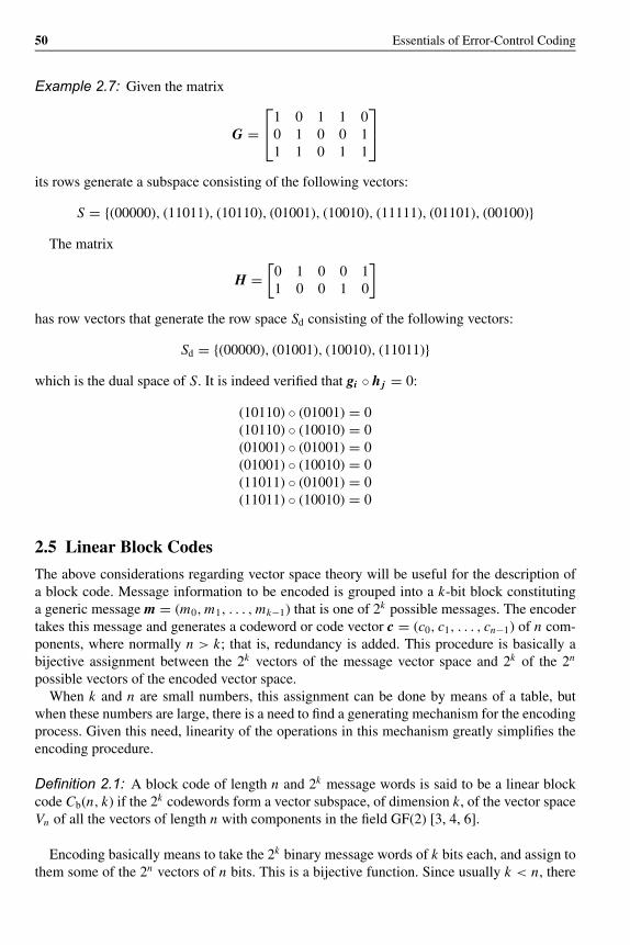
OTE/SPH OTE/SPHJWBK102-02 JWBK102-Farrell June 17, 2006 18:2 Char Count= 0
50 Essentials of Error-Control Coding
Example 2.7: Given the matrix
G =⎡⎣1 0 1 1 0
0 1 0 0 11 1 0 1 1
⎤⎦its rows generate a subspace consisting of the following vectors:
S = {(00000), (11011), (10110), (01001), (10010), (11111), (01101), (00100)}The matrix
H =[
0 1 0 0 11 0 0 1 0
]has row vectors that generate the row space Sd consisting of the following vectors:
Sd = {(00000), (01001), (10010), (11011)}which is the dual space of S. It is indeed verified that gi ◦ h j = 0:
(10110) ◦ (01001) = 0(10110) ◦ (10010) = 0(01001) ◦ (01001) = 0(01001) ◦ (10010) = 0(11011) ◦ (01001) = 0(11011) ◦ (10010) = 0
2.5 Linear Block Codes
The above considerations regarding vector space theory will be useful for the description ofa block code. Message information to be encoded is grouped into a k-bit block constitutinga generic message m = (m0, m1, . . . , mk−1) that is one of 2k possible messages. The encodertakes this message and generates a codeword or code vector c = (c0, c1, . . . , cn−1) of n com-ponents, where normally n > k; that is, redundancy is added. This procedure is basically abijective assignment between the 2k vectors of the message vector space and 2k of the 2n
possible vectors of the encoded vector space.When k and n are small numbers, this assignment can be done by means of a table, but
when these numbers are large, there is a need to find a generating mechanism for the encodingprocess. Given this need, linearity of the operations in this mechanism greatly simplifies theencoding procedure.
Definition 2.1: A block code of length n and 2k message words is said to be a linear blockcode Cb(n, k) if the 2k codewords form a vector subspace, of dimension k, of the vector spaceVn of all the vectors of length n with components in the field GF(2) [3, 4, 6].
Encoding basically means to take the 2k binary message words of k bits each, and assign tothem some of the 2n vectors of n bits. This is a bijective function. Since usually k < n, there

OTE/SPH OTE/SPHJWBK102-02 JWBK102-Farrell June 17, 2006 18:2 Char Count= 0
Block Codes 51
are more vectors of n bits than those of k bits, and so the selection of the vectors of n bitshas to be done using the lowest level of redundancy while maximizing the distance among thecodewords.
The set of 2k codewords constitute a vector subspace of the set of words of n bits. As aconsequence of its definition, a linear block code is characterized by the fact that the sum ofany of two codewords is also a codeword.
2.5.1 Generator Matrix G
Since a linear block code Cb(n, k) is a vector subspace of the vector space Vn , there will bek linearly independent vectors that in turn are codewords g0, g1, . . . , gk−1, such that eachpossible codeword is a linear combination of them:
c = m0 • g0 ⊕ m1 • g1 ⊕ · · · ⊕ mk−1 • gk−1 (17)
These linearly independent vectors can be arranged in a matrix called the generatormatrix G:
G =
⎡⎢⎢⎢⎣g0
g1...
gk−1
⎤⎥⎥⎥⎦ =
⎡⎢⎢⎢⎣g00 g01 · · · g0,n−1
g10 g11 · · · g1,n−1
......
...gk−1,0 gk−1,1 · · · gk−1,n−1
⎤⎥⎥⎥⎦ (18)
This is a matrix mechanism for generating any codeword. For a given message vector m =(m0, m1, . . . , mk−1), the corresponding codeword is obtained by matrix multiplication:
c = m ◦ G = (m0, m1, . . . , mk−1) ◦
⎡⎢⎢⎢⎣g00 g01 · · · g0,n−1
g10 g11 · · · g1,n−1
......
...gk−1,0 gk−1,1 · · · gk−1,n−1
⎤⎥⎥⎥⎦
= (m0, m1, . . . , mk−1) ◦
⎡⎢⎢⎢⎣g0
g1...
gk−1
⎤⎥⎥⎥⎦ = m0 • g0 ⊕ m1 • g1 ⊕ · · · ⊕ mk−1 • gk−1
(19)
Note that the symbol ‘◦’ represents the inner product between vectors or matrices, whereas thesymbol ‘•’ represents the multiplication by a scalar in the field GF(2) of a vector of the vectorspace or subspace used.
The rows of the generator matrix G generate the linear block code Cb(n, k), or, equivalently,the k linearly independent rows of G completely define the code.

OTE/SPH OTE/SPHJWBK102-02 JWBK102-Farrell June 17, 2006 18:2 Char Count= 0
52 Essentials of Error-Control Coding
Table 2.1 Codewords of a linear block code Cb(7, 4)
Message Codewords
0 0 0 0 0 0 0 0 0 0 0
0 0 0 1 1 0 1 0 0 0 1
0 0 1 0 1 1 1 0 0 1 0
0 0 1 1 0 1 0 0 0 1 1
0 1 0 0 0 1 1 0 1 0 0
0 1 0 1 1 1 0 0 1 0 1
0 1 1 0 1 0 0 0 1 1 0
0 1 1 1 0 0 1 0 1 1 1
1 0 0 0 1 1 0 1 0 0 0
1 0 0 1 0 1 1 1 0 0 1
1 0 1 0 0 0 1 1 0 1 0
1 0 1 1 1 0 0 1 0 1 1
1 1 0 0 1 0 1 1 1 0 0
1 1 0 1 0 0 0 1 1 0 1
1 1 1 0 0 1 0 1 1 1 0
1 1 1 1 1 1 1 1 1 1 1
Example 2.8: Consider the following generator matrix of size 4 × 7 and obtain the codewordcorresponding to the vector message m = (1001):
G =
⎡⎢⎢⎣g0
g1
g2
g3
⎤⎥⎥⎦ =
⎡⎢⎢⎣1 1 0 1 0 0 00 1 1 0 1 0 01 1 1 0 0 1 01 0 1 0 0 0 1
⎤⎥⎥⎦The corresponding codeword is
c = m ◦ G = 1 • g0 ⊕ 0 • g1 ⊕ 0 • g2 ⊕ 1 • g3 = (1101000) ⊕ (1010001) = (0111001)
Table 2.1 shows the code generated by the generator matrix G of this example.
2.5.2 Block Codes in Systematic Form
In Table 2.1 it can be seen that the last four bits of each codeword are the same as the messagebits; that is, the message appears as it is, inside the codeword. In this case, the first three bits arethe so-called parity check or redundancy bits. This particular form of the codeword is calledsystematic form. In this form, the codewords consist of the (n − k) parity check bits followed bythe k bits of the message. The structure of a codeword in systematic form is shown in Figure 2.1.
n − k parity check bits k message bits
Figure 2.1 Systematic form of a codeword of a block code

OTE/SPH OTE/SPHJWBK102-02 JWBK102-Farrell June 17, 2006 18:2 Char Count= 0
Block Codes 53
In the convention selected in this book, the message bits are placed at the end of the codeword,while the redundancy bits are placed at the beginning of the codeword, but this can be donethe other way round. However, the choice of convention does not modify the properties of agiven block code, although some mathematic expressions related to the code will of courseadopt a different form in each case. In the current bibliography on error-correcting codes, thesystematic form can be found adopting both of the two conventions described above.
A systematic linear block code Cb(n, k) is uniquely specified by a generator matrix of theform
G =
⎡⎢⎢⎢⎣g0
g1...
gk−1
⎤⎥⎥⎥⎦ =
⎡⎢⎢⎢⎣p00 p01 · · · p0,n−k−1
p10 p11 · · · p1,n−k−1
......
...pk−1,0 pk−1,1 · · · pk−1,n−k−1︸ ︷︷ ︸
submatrix P k × (n − k)
1 0 0 · · ·0 1 0 · · ·...
......
0 0 0 · · ·︸ ︷︷ ︸submatrix I k × k
00...1
⎤⎥⎥⎥⎦ (20)
which, in a compact notation, is
G = [P Ik] (21)
In systematic block coding, it is possible to establish an analytical expression betweenthe parity check and the message bits. If m = (m0, m1, . . . , mk−1) is the message vector andc = (c0, c1, . . . , cn−1) the coded vector, the parity check bits can be obtained as a function ofthe message bits using the following expression:
cn−k+i = mi
c j = m0 • p0 j + m1 • p1 j + · · · + mk−1 • pk−1, j 0 ≤ j < n − k(22)
These n − k equations are called the parity check equations.
Example 2.9: Consider the generator matrix of the linear block code Cb(7, 4), presented inthe previous example, and state the parity check equations for the following case:
c = m ◦ G = (m0, m1, m2, m3) ◦
⎡⎢⎢⎣1 1 0 1 0 0 00 1 1 0 1 0 01 1 1 0 0 1 01 0 1 0 0 0 1
⎤⎥⎥⎦Then the parity check equations adopt the form
c0 = m0 ⊕ m2 ⊕ m3
c1 = m0 ⊕ m1 ⊕ m2
c2 = m1 ⊕ m2 ⊕ m3
c3 = m0
c4 = m1
c5 = m2
c6 = m3

OTE/SPH OTE/SPHJWBK102-02 JWBK102-Farrell June 17, 2006 18:2 Char Count= 0
54 Essentials of Error-Control Coding
2.5.3 Parity Check Matrix H
As explained in previous sections, the generator matrix G contains k linearly independentvectors that generate the vector subspace S of the vector space Vn , which is in turn associatedwith a dual vector subspace Sd of the same vector space Vn that is generated by the rows of amatrix H. Each vector of the row space of the matrix G is orthogonal to the rows of the matrixH and vice versa.
The 2n−k linear combinations of the matrix H generate the dual code Cbd(n, n − k), whichis the dual subspace of the code Cb generated by the matrix G. The systematic form of theparity check matrix H of the code Cb generated by the generator matrix G is
H =
⎡⎢⎢⎢⎣1 0 · · · 00 1 · · · 0...
......
0 0 · · · 1︸ ︷︷ ︸submatrix I (n − k) × (n − k)
p00 p10 · · · pk−1,0
p01 p11 · · · pk−1,1
......
...p0,n−k−1 p1,n−k−1 · · · pk−1,n−k−1
⎤⎥⎥⎥⎦︸ ︷︷ ︸
submatrix PT (n − k) × k
= [In−k PT
](23)
where PT is the transpose of the parity check submatrix P. The matrix H is constructed so thatthe inner product between any row vector gi of G and any row vector h j of H is zero:
gi ◦ h j = pi j ⊕ pi j = 0 (24)
This condition can be summarized in the matrix expression
G ◦ HT = 0 (25)
It can also be verified that the parity check equations can be obtained from the parity checkmatrix H, so that this matrix also specifies completely a given block code. Since a codewordin systematic form is expressed as
c = (c0, c1, . . . , cn−k−1, m0, m1, . . . , mk−1) (26)
then since
c ◦ HT = m ◦ G ◦ HT = 0 (27)
for the row j of H,
c j ⊕ p0 j • m0 ⊕ p1 j • m1 ⊕ · · · ⊕ pk−1, j • mk−1 = 0 (28)
or, equivalently,
c j = p0 j • m0 ⊕ p1 j • m1 ⊕ · · · ⊕ pk−1, j • mk−1 0 ≤ j < n − k (29)
Example 2.10: Determine the parity check matrix H for the linear block code Cb(7, 4) gen-erated by the generator matrix
G =
⎡⎢⎢⎣1 1 0 1 0 0 00 1 1 0 1 0 01 1 1 0 0 1 01 0 1 0 0 0 1
⎤⎥⎥⎦

OTE/SPH OTE/SPHJWBK102-02 JWBK102-Farrell June 17, 2006 18:2 Char Count= 0
Block Codes 55
Since
G =
⎡⎢⎢⎣1 1 00 1 11 1 11 0 1︸ ︷︷ ︸submatrix P
1 0 0 00 1 0 00 0 1 00 0 0 1
⎤⎥⎥⎦︸ ︷︷ ︸
submatrix I
the parity check matrix H is constructed using these submatrices:
H =⎡⎣1 0 0 1 0 1 1
0 1 0 1 1 1 00 0 1 0 1 1 1
⎤⎦A practical implementation of these codes could be done using combinational logic for theparity check equations.
2.6 Syndrome Error Detection
So far the definitions for the generator and the parity check matrices of a given block codehave been presented. The codeword c = (c0, c1, . . . , cn−1) is such that its components are takenfrom the binary field GF(2), ci ∈ GF(2). As a consequence of its transmission through a noisychannel, this codeword could be received containing some possible errors. The received vectorcan therefore be different from the corresponding transmitted codeword, and it will be denotedas r = (r0, r1, . . . , rn−1), where it is also true that ri ∈ GF(2).
An error event can be modelled as an error vector or error pattern e = (e0, e1, . . . , en−1),whose components are also defined over the binary field, ei ∈ GF(2), and which is related tothe codeword and received vectors as follows:
e = r ⊕ c (30)
The error vector has non-zero components in the positions where an error has occurred.Once the error vector is determined, a task to be performed by the decoder, it is possible todo a correction of the received vector in order to determine an estimate of the valid codeword,and this can be done by using the expression
c = r ⊕ e (31)
Since any codeword should obey the condition
c ◦ HT = 0
an error-detection mechanism can be implemented based on the above expression, which adoptsthe following form:
S = r ◦ HT = (s0, s1, . . . , sn−k−1) (32)
This vector is called the syndrome vector. The detection operation is performed over thereceived vector, so that if this operation results in the all-zero vector, then the received vectoris considered to be a valid codeword; if otherwise, the decoder has detected errors.
Since r = c ⊕ e,
S = r ◦ HT = (c ⊕ e) ◦ HT = c ◦ HT ⊕ e ◦ HT = e ◦ HT (33)

OTE/SPH OTE/SPHJWBK102-02 JWBK102-Farrell June 17, 2006 18:2 Char Count= 0
56 Essentials of Error-Control Coding
If the error pattern is the all-zero vector, then the syndrome vector will also be an all-zerovector, and thus the received vector is a valid codeword. When the syndrome vector contains atleast one non-zero component, it will be detecting the presence of errors in the received vector.There is however a possibility that the syndrome vector can be the all-zero vector in spite ofthe presence of errors in the received vector. This is in fact possible if the error pattern is equalto a codeword; that is, if the number and positions of the errors are such that the transmittedcodeword is converted into another codeword. This error pattern will not be detected by thesyndrome operation. This is what is called an undetected error pattern, and as such is not withinthe error-correction capability of the code.
As said above, the undetected error patterns are characterized by satisfying the conditionS = e ◦ HT = 0; that is, these are the error patterns that are equal to one of the codewords(e = c). There will be therefore 2k − 1 undetectable non-zero error patterns.
According to the expression for calculating the syndrome vector, each of its bits can beevaluated as follows:
s0 = r0 ⊕ rn−k • p00 ⊕ rn−k+1 • p10 ⊕ · · · ⊕ rn−1 • pk−1,0
s1 = r1 ⊕ rn−k • p01 ⊕ rn−k+1 • p11 ⊕ · · · ⊕ rn−1 • pk−1,1
...sn−k−1 = rn−k−1 ⊕ rn−k • p0,n−k−1 ⊕ rn−k+1 • p1,n−k−1 ⊕ · · · ⊕ rn−1 • pk−1,n−k−1
(34)
The dimension of the syndrome vector is 1 × (n − k).
Example 2.11: For the same linear block code Cb(7, 4), as seen in previous examples, obtainthe analytical expressions for the syndrome vector’s bits.
If r = (r0, r1, r2, r3, r4, r5, r6)then
S = (s0, s1, s2) = (r0, r1, r2, r3, r4, r5, r6) ◦
⎡⎢⎢⎢⎢⎢⎢⎢⎢⎣
1 0 00 1 00 0 11 1 00 1 11 1 11 0 1
⎤⎥⎥⎥⎥⎥⎥⎥⎥⎦s0 = r0 ⊕ r3 ⊕ r5 ⊕ r6
s1 = r1 ⊕ r3 ⊕ r4 ⊕ r5
s2 = r2 ⊕ r4 ⊕ r5 ⊕ r6
The syndrome vector does not depend on the received vector, but on the error vector. Thus,solving the following system of equations
s0 = e0 ⊕ en−k • p00 ⊕ en−k+1 • p10 ⊕ · · · ⊕ en−1 • pk−1,0
s1 = e1 ⊕ en−k • p01 ⊕ en−k+1 • p11 ⊕ · · · ⊕ en−1 • pk−1,1
...sn−k−1 = en−k−1 ⊕ en−k • p0,n−k−1 ⊕ en−k+1 • p1,n−k−1 ⊕ · · · ⊕ en−1 • pk−1,n−k−1
(35)

OTE/SPH OTE/SPHJWBK102-02 JWBK102-Farrell June 17, 2006 18:2 Char Count= 0
Block Codes 57
will allow us to evaluate the error vector, which in turn will allow us to do an estimation ofa valid codeword. However, this set of (n − k) equations does not have a unique solution,but exhibits 2k solutions. This is due to the fact that there are 2k error patterns that producethe same syndrome vector. In spite of this, and because the noise power normally acts withminimum effect, the error pattern with the least number of errors will be considered to be thetrue solution of this system of equations.
Example 2.12: For the linear block code Cb(7, 4) of the previous example, a transmittedcodeword c = (0011010) is affected by the channel noise and received as the vector r =(0001010). The calculation of the syndrome vector results in the vector S = (001), which interms of the system of equations (35) becomes
0 = e0 ⊕ e3 ⊕ e5 ⊕ e6
0 = e1 ⊕ e3 ⊕ e4 ⊕ e5
1 = e2 ⊕ e4 ⊕ e5 ⊕ e6
There are 24 = 16 different error patterns that satisfy the above equations (see Table 2.2).Since errors in a codeword of n bits are governed by the binomial distribution, the error
pattern with i errors is more likely than the error pattern of i + 1 errors, which means thatfor channels like the BSC, the error pattern with the smallest number of non-zero componentswill be considered as the true error pattern. In this case the error pattern e = (0010000) isconsidered, among the 16 possibilities, to be the true error pattern, and so
c = r ⊕ e = (0011010) = (0001010) ⊕ (0010000)
Table 2.2 Error patterns that satisfy the equations of Example 2.12
e0 e1 e2 e3 e4 e5 e6
0 0 1 0 0 0 0
1 1 1 1 0 0 0
1 0 0 0 0 0 1
0 1 0 1 0 0 1
0 0 0 1 0 1 0
1 1 0 0 0 1 0
0 1 1 0 0 1 1
1 0 1 1 0 1 1
0 1 0 0 1 0 0
1 0 0 1 1 0 0
1 1 1 0 1 0 1
0 0 1 1 1 0 1
1 0 1 0 1 1 0
0 1 1 1 1 1 0
1 1 0 1 1 1 1
0 0 0 0 1 1 1

OTE/SPH OTE/SPHJWBK102-02 JWBK102-Farrell June 17, 2006 18:2 Char Count= 0
58 Essentials of Error-Control Coding
2.7 Minimum Distance of a Block Code
The minimum distance dmin is an important parameter of a code, especially for a block code.Before defining this parameter, other useful definitions related to the minimum distance arefirst provided [3, 4].
Definition 2.2: The number of non-zero components ci = 0 of a given vector c =(c0, c1, . . . , cn−1) of size (1 × n) is called the weight, or Hamming weight, w(c), of that vector.In the case of a vector defined over the binary field GF(2), the weight is the number of ‘1’s inthe vector.
Definition 2.3: The Hamming distance between any two vectors c1 = (c01, c11, . . . , cn−1,1
)and c2 = (
c02, c12, . . . , cn−1,2
), d(c1, c2), is the number of component positions in which the
two vectors differ.For instance, if c1 = (0011010) and c2 = (1011100), then d(c1, c2) = 3.
According to the above definitions, it can be verified that
d(ci , c j ) = w(ci ⊕ c j ) (36)
For a given code, the minimum value of the distance between all possible pairs of codewordscan be calculated. This minimum value of the distance evaluated over all the codewords of thecode is called the minimum distance of the code, dmin:
dmin = min{d(ci , c j ); ci , c j ∈ Cb; ci = c j
}(37)
Since, in general, block codes are designed to be linear, the addition of any two code vectorsis another code vector. From this point of view, any codeword can be seen as the additionof at least two other codewords. Since the Hamming distance is the number of positions inwhich two vectors differ, and on the other hand the weight of the sum of two vectors is theHamming distance between these two vectors, then the weight of a codeword is at the same timethe distance between two other vectors of that code. Thus, the minimum value of the weightevaluated over all the codewords of a code, excepting the all-zero vector, is the minimumdistance of the code:
dmin = min{w(ci ⊕ c j ); ci , c j ∈ Cb; ci = c j
} = min {w(cm); cm ∈ Cb; cm = 0} (38)
Therefore, the minimum distance of a linear block code Cb(n, k) is the minimum value of theweight of the non-zero codewords of that code.
As an example, the linear block code analysed in previous examples has minimum distancedmin = 3, because this is the minimum value of the weight evaluated over all the non-zerocodewords of this code (see Table 2.1).
2.7.1 Minimum Distance and the Structure of the H Matrix
There is an interesting relationship between the minimum distance dmin of a code and its paritycheck matrix H.

OTE/SPH OTE/SPHJWBK102-02 JWBK102-Farrell June 17, 2006 18:2 Char Count= 0
Block Codes 59
Theorem 2.2: Consider a linear block code Cb(n, k) completely determined by its paritycheck matrix H. For each codeword of Hamming weight pH, there exist pH columns of theparity check matrix H that when added together result in the all-zero vector. In the same way,it can be said that if the parity check matrix H contains pH columns that when added give theall-zero vector, then there is in the code a vector of weight pH [4].
In order to see this, parity check matrix H is described in the following form:
H = [h0, h1, . . . , hn−1
](39)
where hi is the i th column of this matrix. If a codeword c = (c0, c1, . . . , cn−1) has a weightpH, then there exist pH non-zero components in that vector ci1 = ci2 = · · · = cipH
= 1, forwhich 0 ≤ i1 < i2 < · · · < i pH
≤ n − 1.Since
c ◦ HT = 0
then
c0 • h0 ⊕ c1 • h1 ⊕ · · · ⊕ cn−1 • hn−1
= ci1 • hi1 ⊕ ci2 • hi2 ⊕ · · · ⊕ cipH•hipH
= hi1 ⊕ hi2 ⊕ · · · ⊕ hipH = 0(40)
Similarly, the second part of the theorem can be demonstrated.
The following corollary is then derived:
Corollary 2.7.1: For a linear block code Cb(n, k) completely determined by its parity checkmatrix H, the minimum weight or minimum distance of this code is equal to the minimumnumber of columns of that matrix which when added together result in the all-zero vector 0.
Example 2.13: For the linear block code Cb(7, 4), as seen in previous examples, whose paritycheck matrix is of the form
H =⎡⎣ 1 0 0 1 0 1 1
0 1 0 1 1 1 00 0 1 0 1 1 1
⎤⎦determine the minimum distance of this code.
It can be seen that the addition of the first, third and seventh column results in the all-zerovector 0. Hence, and because the same result cannot be obtained by the addition of only twocolumns, the minimum distance of this code is dmin = 3.
2.8 Error-Correction Capability of a Block Code
The minimum distance of a code is the minimum number of components changed by theeffect of the noise that converts a code vector into another vector of the same code. If havingtransmitted the codeword c the noise transforms this vector in the received vector r, the distancebetween c and r is the weight of the error pattern d(c, r) = w(e) = l, that is, the number of

OTE/SPH OTE/SPHJWBK102-02 JWBK102-Farrell June 17, 2006 18:2 Char Count= 0
60 Essentials of Error-Control Coding
positions that change their value in the original vector c due to the effects of noise. If the noisemodifies dmin positions, then it is possible in the worst case that a code vector is transformedinto another vector of the same code, so that the error event is undetectable. If the number ofpositions the noise alters is dmin − 1, it is guaranteed that the codeword cannot be convertedinto another codeword. Thus, the error-detection capability of a linear block code Cb(n, k) ofminimum distance dmin is dmin − 1. This is evaluated for the worst case, that is, for the casein which the error event of dmin bits happens over a codeword that has a Hamming weightdmin. However, there could be other detectable error patterns of the weight dmin. Based on thisanalysis, the error-detection capability of a code can be measured by means of the probabilitythat the code fails to determine an estimate of the codeword from the received vector, which isevaluated using the weight distribution function of the code. Since a detection failure happenswhen the error pattern is equal to a non-zero codeword,
PU(E) =n∑
i=1
Ai pi (1 − p)n−i (41)
where Ai is the number of codewords of weight i and p is the error probability for the BSC,for which this analysis is valid. When the minimum distance is dmin, the values of A1 to Admin−1
are all zero.
Example 2.14: For the linear block code Cb(7, 4), previously analysed values of the weightdistribution function are equal to
A0 = 1, A1 = A2 = 0, A3 = 7, A4 = 7, A5 = A6 = 0, A7 = 1
The probability of an undetected error is therefore
PU(E) =n∑
i=1
Ai pi (1 − p)n−i = 7p3(1 − p)4 + 7p4(1 − p)3 + p7 ≈ 7p3
where the approximation is based on the error probability for the BSC being a small numberp � 1.
In order to determine the error-correction capability of a linear block code Cb(n, k), aninteger number t that fits the condition
2t + 1 ≤ dmin ≤ 2t + 2 (42)
will represent the number of bits that can be corrected.If having transmitted a codeword c1 the noise effects transform this vector into the received
vector r , then with respect to another codeword c2 the following inequality will be true:
d(c1, r ) + d(c2, r ) ≥ d(c1, c2) (43)
By assuming an error pattern of t ′ errors, d(c1, r ) = t ′. As c1 and c2 are codewords,d(c1, c2) ≥ dmin ≥ 2t + 1 and
d(c2, r ) ≥ 2t + 1 − t ′ (44)

OTE/SPH OTE/SPHJWBK102-02 JWBK102-Farrell June 17, 2006 18:2 Char Count= 0
Block Codes 61
By adopting t ′ ≤ t ,
d(c2, r ) > t (45)
This means that for an error pattern of weight t or less, the distance between any other codewordc2 and the received vector r is higher than the distance between the codeword c1 and thereceived vector r , which is t ′ ≤ t . This also means that the probability P(r/c1) is higher thanthe probability P(r/c2) for any other codeword c2. This is the process of maximum likelihooddecoding, and in this operation the received vector r is decoded as the codeword c1. This waythe code is able to successfully decode any error pattern of weight t = ⌊ dmin−1
2
⌋, where �
means the largest integer number no greater than dmin−12
.As happened in the detection of errors, for the correction of errors there are more possible
correctable patterns than those determined by the number t . For a linear block code Cb(n, k)able to correct up to t errors, there are 2n−k correctable error patterns including the errorpatterns of t or fewer errors.
If a linear block code Cb(n, k), able to correct all the error patterns of weight t or less, isused in a transmission over the BSC with error probability p, the error probability of the codedsystem is given by
Pwe =n∑
i=t+1
(ni
)pi (1 − p)n−i (46)
In hybrid systems, where errors are in part corrected, and in part detected, these codes areutilized in such a way that error patterns of weight λ are corrected and error patterns of weightl > λ are detected. If the error pattern is of weight λ or less, the system corrects it, and if theerror pattern is of weight larger than λ, but less than l + 1, the system detects it. This is possibleif dmin ≥ l + λ + 1.
If for example the minimum distance of a linear block code Cb(n, k) is dmin = 7, this codecan be used for correcting error patterns of weight λ = 2 or less and detecting error patternsof weight l = 4 or less.
2.9 Syndrome Detection and the Standard Array
A linear block code Cb(n, k) is constructed as a bijective assignment between the 2k messagevectors and the set {c1, c2, . . . , c2k }. Each of these vectors is transmitted through the channeland converted into a received vector r that can be any vector of the 2n vectors of the vector spaceVn defined over the binary field GF(2). Any decoding technique is essentially a decision rule,based on the vector space Vn being partitioned into 2k possible disjoint sets D1, D2, . . . , D2k
such that the vector ci is in the set Di . There is a unique correspondence between the set Di
and the vector ci . If the received vector is in Di , it will be decoded as ci .The standard array is a method for doing this operation [4, 6]. The array is constructed in
the following way:A row containing the codewords, including and starting from the all-zero vector (0, 0, . . . , 0),
is constructed. This row contains 2k vectors taken from the whole set of 2n possible vectors.
c1 = (0, 0, . . . , 0) c2 c3 . . . c2k (47)

OTE/SPH OTE/SPHJWBK102-02 JWBK102-Farrell June 17, 2006 18:2 Char Count= 0
62 Essentials of Error-Control Coding
Then an error pattern e2 is selected and placed below c1 (the all-zero vector), and then the sumvector ci ⊕ e2 is placed below ci . This is done with all the error patterns taken from the vectorspace that have to be allocated, a total of 2n−k vectors.
c1 = (0, 0, . . . , 0) c2 . . . ci . . . c2k
e2 c2 ⊕ e2 . . . ci ⊕ e2 . . . c2k ⊕ e2...e2n−k c2 ⊕ e2n−k . . . ci ⊕ e2n−k . . . c2k ⊕ e2n−k
(48)
In this array the sum of any two vectors in the same row is a code vector. There are only 2n/2k
disjoint rows in this array. These rows are the so-called cosets of the linear block code Cb(n, k).The vector that starts each coset is called the leader of that coset, and it can be any vector ofthat row.
Example 2.15: For the linear block code Cb(5, 3) generated by the matrix given below,determine the standard array.
G =⎡⎣0 1 0 0 1
1 0 1 1 01 0 0 1 0
⎤⎦There are in this case 2k = 23 = 8 columns and 2n−k = 22 = 4 rows in the standard array.Table 2.3 shows the standard array for the code of Example 2.15.
The standard array can also be seen as constituted of 2k disjoint columns, and in each of thesecolumns are 2n−k vectors having as the first vector a code vector. These 2k disjoint columnsD1, D2, . . . , D2k can be used in a decoding procedure. If having transmitted a codeword ci ,the received vector is r, this received vector will be in Di if the error pattern that occurred is itscoset leader. In this case the received vector will be successfully decoded. If the error patternis not a coset leader, a decoding error happens. Due to this, the 2n−k coset leaders includingthe all-zero pattern are the correctable error patterns. It can be deduced that a linear block codeCb(n, k) can correct 2n−k error patterns.
In order to minimize the error probability, all the correctable error patterns, which are thecoset leaders, will have to be the most likely patterns. In the case of a transmission over theBSC, the most likely patterns are those of the lowest possible weight. Thus, each coset leaderwill be of the lowest possible weight among the vectors of that row. The decoding in thiscase will be maximum likelihood decoding, that is, minimum distance decoding, so that thedecoded code vector is at minimum distance with respect to the received vector.
Table 2.3 Standard array for the code of Example 2.15
0 0 0 0 0 1 1 0 1 1 1 0 1 1 0 0 1 0 0 1 1 0 0 1 0 1 1 1 1 1 0 1 1 0 1 0 0 1 0 0
1 0 0 0 0 0 1 0 1 1 0 0 1 1 0 1 1 0 0 1 0 0 0 1 0 0 1 1 1 1 1 1 1 0 1 1 0 1 0 0
0 0 0 1 0 1 1 0 0 1 1 0 1 0 0 0 1 0 1 1 1 0 0 0 0 1 1 1 0 1 0 1 1 1 1 0 0 1 1 0
0 0 0 0 1 1 1 0 1 0 1 0 1 1 1 0 1 0 0 0 1 0 0 1 1 1 1 1 1 0 0 1 1 0 0 0 0 1 0 1

OTE/SPH OTE/SPHJWBK102-02 JWBK102-Farrell June 17, 2006 18:2 Char Count= 0
Block Codes 63
In conclusion it can be said that a linear block code Cb(n, k) is able to detect 2n − 2k errorpatterns and correct 2n−k error patterns.
It can also be said thatFor a linear block code Cb(n, k) with minimum distance dmin, all the vectors of weight
t = ⌊ dmin−12
⌋or less can be used as coset leaders. This is in agreement with the fact that not
all the weight t + 1 error patterns can be corrected, even when some of them can be. On theother hand, all the vectors of the same coset have the same syndrome, whereas syndromes fordifferent cosets are different.
By taking a coset leader as the vector ei , any other vector of that coset is the sum of theleader vector and the code vector ci . For this case, the syndrome is calculated as
(ci ⊕ ei ) ◦ HT = ci ◦ HT ⊕ ei ◦ HT = ei ◦ HT (49)
The syndrome of any vector of the coset is equal to the syndrome of the leader of that coset.Syndromes are vectors with (n − k) components that have a bijective assignment with thecosets. For each correctable error pattern, there is a different syndrome vector. This allowsus to implement simpler decoding by constructing a table where correctable error patternsand their corresponding syndrome vectors are arranged, so that when the decoder makes thesyndrome calculation and knows the syndrome vector, it can recognize the corresponding errorpattern. Thus, the decoder is able to correct the received vector by adding the error pattern to thatreceived vector. Thus syndrome decoding consists of the following steps: With the informationprovided by the table S → e, the syndrome vector is calculated as a function of the receivedvector using S = r ◦ HT; then the decoder resorts to the table to identify which error patternei corresponds to the calculated syndrome vector and finally corrects the received vector bydoing ci = r ⊕ ei . This procedure can be used when the table S → e is of a reasonable size tobe implemented in practice.
Example 2.16: For the linear block code Cb(7, 4) with parity check matrix
H =⎡⎣ 1 0 0 1 0 1 1
0 1 0 1 1 1 00 0 1 0 1 1 1
⎤⎦there are 24 = 16 code vectors and 27−4 = 8 cosets, or correctable error patterns. The minimumdistance has also been calculated and is equal to dmin = 3 and so this code is able to correctany pattern of one error. In this case the total number of correctable error patterns is equal tothe number of error patterns the code can correct, and there are seven correctable error patternsand the all-zero error pattern, as the possible patterns. The table S → e for this code is seen inTable 2.4.
As an example, assume that the transmitted code vector was c = (1010001) and after thetransmission of this vector the received vector is r = (1010011), then the syndrome vectorin this case is r ◦ HT = (111) and so the leader of the corresponding coset is (0000010) andc = (1010001) = (1010011) ⊕ (0000010).

OTE/SPH OTE/SPHJWBK102-02 JWBK102-Farrell June 17, 2006 18:2 Char Count= 0
64 Essentials of Error-Control Coding
Table 2.4 Error patterns and their corresponding
syndrome vectors, Example 2.16
Error patterns Syndromes
1 0 0 0 0 0 0 1 0 0
0 1 0 0 0 0 0 0 1 0
0 0 1 0 0 0 0 0 0 1
0 0 0 1 0 0 0 1 1 0
0 0 0 0 1 0 0 0 1 1
0 0 0 0 0 1 0 1 1 1
0 0 0 0 0 0 1 1 0 1
2.10 Hamming Codes
A widely used class of linear block codes is the Hamming code family [11]. For any positiveinteger m ≥ 3, there exists a Hamming code with the following characteristics:
Length n = 2m − 1Number of message bits k = 2m − m − 1Number of parity check bits n − k = mError-correction capability t = 1, (dmin = 3)
The parity check matrix H of these codes is formed of the non-zero columns of m bits, andcan be implemented in systematic form:
H = [Im Q]
where the identity submatrix Im is a square matrix of size m × m and the submatrix Q consistsof the 2m − m − 1 columns formed with vectors of weight 2 or more.
For the simplest case, for which m = 3,
n = 23 − 1 = 7
k = 23 − 3 − 1 = 4
n − k = m = 3
t = 1(dmin = 3)
H =⎡⎣1 0 0 1 0 1 1
0 1 0 1 1 1 00 0 1 0 1 1 1
⎤⎦which is the linear block code Cb(7, 4) that has been analysed previously in this chapter. Thegenerator matrix can be constructed using the following expression for linear block codes ofsystematic form:
G = [QT I2m−m−1
]

OTE/SPH OTE/SPHJWBK102-02 JWBK102-Farrell June 17, 2006 18:2 Char Count= 0
Block Codes 65
In the parity check matrix H, the sum of three columns can result in the all-zero vector, and it isnot possible for the sum of two columns to give the same result, and so the minimum distanceof the code is dmin = 3. This means that they can be used for correcting any error pattern ofone error, or detecting any error pattern of up to two errors. In this case there are also 2m − 1correctable error patterns and on the other hand there exist 2m cosets, so that the number ofpossible correctable error patterns is the same as the number of different cosets (syndromevectors). The codes with this characteristic are called perfect codes. The code of Example 2.10is a Hamming code.
2.11 Forward Error Correction and Automatic Repeat ReQuest
2.11.1 Forward Error Correction
Communication systems that use the FEC approach are not able to request a repetition ofthe transmission of coded information. Due to this, all the capability of the code is used forerror correction. The source information generates a binary signal representing equally likelysymbols at a rate rb. The encoder takes a group of k message bits, and adds to it n − k paritycheck bits. This is the encoding procedure for a linear block code Cb(n, k) whose code rate isRc = k/n, with Rc < 1. Figure 2.2 shows a block diagram of an FEC communication system.
The transmission rate r over the channel has to be higher than the source information rate rb:
r =(n
k
)rb = rb
Rc
(50)
The code used in the FEC system is characterized by having a minimum distance dmin =2t + 1. The performance is evaluated of a communication system perturbed by additive whiteGaussian noise (AWGN) in the channel, leading to an error probability p � 1. The source(uncoded) information has an average bit energy Eb, so that the average bit energy for a codedbit is reduced to Rc Eb. The ratio Eb/N0 is equal to(
Eb
N0
)C
= Rc Eb
N0
= Rc
(Eb
N0
)(51)
As seen in Chapter 1, the quotient between the average bit energy Eb and the power spectraldensity N0 plays an important role in the characterization of communication systems, and itwill be used a basic parameter for comparison proposes.
In this section the difference between the coded and uncoded cases is analysed.
Encoder Transm. Channel + Receiver Decoder
Pe = p
r = rb
r = rb/RcRc = k /n Gn(f ) = No/2
Figure 2.2 Block diagram of an FEC system

OTE/SPH OTE/SPHJWBK102-02 JWBK102-Farrell June 17, 2006 18:2 Char Count= 0
66 Essentials of Error-Control Coding
There are two error probability definitions: the message bit error rate (BER) or bit errorprobability, denoted here as Pbe, and the word error probability, denoted as Pwe. A given linearblock code can correct error patterns of weight t , or less, in a block or codeword of n bits. Theword error probability is bounded by
Pwe ≤n∑
i=t+1
P(i,n) (52)
Assuming that the error probability of the channel is small, p � 1, the following approxi-mation can be made:
Pwe∼= P(t + 1,n) ∼=
(n
t + 1
)pt+1 (53)
This basically means that the words that the code cannot correct have t + 1 errors. Since thecodeword is truncated after decoding, in each uncorrected word there are
(kn
)(t + 1) message
bit errors, on average. If a large number N � 1 of words are transmitted, then Nk informationsource or message bits are transmitted, and the bit error probability is equal to
Pbe =(
kn
)(t + 1) NPwe
kN= 1
n(t + 1) Pwe (54)
Pbe∼=
(n − 1
t
)pt+1 (55)
For a communication system designed to operate over the AWGN channel, for which thepower spectral density is Gn( f ) = N0/2, and for which binary polar format and matchedfiltering are applied, the error probability Pe is given by (see Appendix 1)
Pe = Q
(√2
Eb
N0
)(56)
and then
p = Q
(√2
(Eb
N0
)C
)= Q
(√2Rc
Eb
N0
)(57)
The bit error probability for an FEC system is then
Pbe∼=
(n − 1
t
) [Q
(√2Rc
Eb
N0
)]t+1
(58)
An uncoded communication system has an error probability
Pbe∼= Q
(√2
Eb
N0
)(59)

OTE/SPH OTE/SPHJWBK102-02 JWBK102-Farrell June 17, 2006 18:2 Char Count= 0
Block Codes 67
Expressions (58) and (59) allow us to do a comparison between the coded and uncodedcases. This comparison will indicate if there is an improvement or not when using FEC error-control coding, with respect to the uncoded case. This comparison depends on the values of tand Rc, characteristic parameters of the code being used. Even for a good code, if the amountof noise power present in the channel is very large, the coded case usually performs worsethan the uncoded case. However, for a reasonable level of noise power, the coded case is betterthan the uncoded one if a good code is used. Now it is clear why the comparison between thecoded and uncoded case is not fair if it is done as in Section 2.2.1, in which the repetition codewas introduced, because in that comparison the rate of the code, 1/3, had not been taken intoaccount. The triple repetition of a bit means that the energy per information (message) bit isthree times higher, and this should be taken into account if a fair comparison is intended.
Example 2.17: The triple repetition codeBy making use of expressions (58) and (59) determine if the triple repetition code has a
good performance in comparison with the uncoded case, by plotting the bit error probabilityas a function of the parameter Eb/N0 for both cases.
In Figure 2.3 the bit error probability curve (dotted) describes the performance of the rep-etition code with n = 3 [theoretical estimation using (58)], and a simulation curve (dashed),with respect to uncoded binary transmission (solid curve), in both cases using polar format(A = ±1). This shows that the repetition code with n = 3 is even worse than uncoded trans-mission. This is because the code rate of the repetition code is very small with respect to itserror-correction capability.
In the chapters which follow, more efficient codes than the repetition code will be introduced.
Uncoded binary
Three-time repetition code, theoretical curve
Hard-decision decoding of a triple repetition code, simulation
−2 0 2 4 6 8 10 12
100
10−1
10−2
10−3
10−4
10−5
10−6
Eb/N0 (dB)
Pbe
Figure 2.3 Bit error probability for the three-time repetition code

OTE/SPH OTE/SPHJWBK102-02 JWBK102-Farrell June 17, 2006 18:2 Char Count= 0
68 Essentials of Error-Control Coding
2.11.2 Automatic Repeat ReQuest
ARQ communication systems are based on the detection of errors in a coded block or frame andon the retransmission of the block or frame when errors have been detected. In this case a two-way channel is needed in order to request retransmissions. For a given code, the error-detectioncapability possible in an ARQ system is higher than the error-correction capability of its FECcounterpart, because the error-control capability of the code is spent only on detection, whilethe correction requires not only the detection but also the localization of the errors. On theother hand, there is an additional cost in an ARQ system, which is the need for a retransmissionlink. There are also additional operations for the acknowledgement and repetition processesthat reduce the transmission rate of the communication system. A block diagram of an ARQsystem is seen in Figure 2.4.
Each codeword is stored in the transmitter buffer and then transmitted. This codeword canbe affected by noise, so that at the receiving end the decoder analyses if the received vectorbelongs or not to the code. A positive acknowledgement (ACK) is transmitted by the receiverif the received vector or word is a codeword; that is, the decoder did not detect any error in thatvector. Otherwise the decoder transmits a negative acknowledgement (NAK) if the decoderidentifies that the received vector has some errors, and is not a code vector. Upon receptionof a NAK message at the transmitter, the corresponding block in the transmitter buffer isretransmitted.
An ARQ system has a reduced transmission rate with respect to an FEC system as a resultof the retransmission process. In all of this, it is considered that the error probability over theretransmission channel is negligible. This means that the ACK and NAK messages do notsuffer from errors in their transmission. In this way, every word found to have transmissionerrors is successfully corrected by means of one or more retransmissions. In this case all theerror-control capability is spent on error detection, so that dmin = l + 1, and the system is ableto detect any error pattern of up to l errors. The error probability is determined by the event ofan undetected error pattern, that is, an error pattern with dmin = l + 1 or more errors:
Pwe =n∑
i=l+1
P(i,n) ∼= P(l + 1,n) ∼=(
nl + 1
)pl+1 (60)
Two-way channel
Datatransmission
Positive or negativeacknowledgement
ACK/NAK
Encoder
Transmitterbuffer
Decoder
Receiverbuffer
Figure 2.4 Block diagram of an ARQ system

OTE/SPH OTE/SPHJWBK102-02 JWBK102-Farrell June 17, 2006 18:2 Char Count= 0
Block Codes 69
Then the bit error probability is
Pbe =(
l + 1
n
)Pwe
∼=(
n − 1l
)pl+1 (61)
These expressions are similar to those given for the FEC system, and are obtained by replacingt by l.
Retransmissions happen with a certain probability. Retransmission is not required when thereceiver has received a valid codeword, an event with probability P(0, n), or when the numberof errors in the received vector produces an undetectable error pattern, an event with probabilityPwe. Therefore, the retransmission probability Pret is given by [3]
Pret = 1 − (P(0, n) + Pwe) (62)
Since usually Pwe � P(0, n),
Pret∼= 1 − P(0, n) = 1 − (1 − p)n ∼= np (63)
2.11.3 ARQ Schemes
2.11.3.1 Stop and wait
The stop-and-wait scheme is such that the transmission of a block or word requires the receptionof an acknowledgement (ACK or NAK) of the previous word. The transmitter does not sendthe following word until the present word has arrived. Figure 2.5 shows the operation of astop-and-wait ARQ scheme. This scheme requires storage of only one word at the transmitter,which means that the transmitter buffer is of minimum size, but the stopping time D could bevery long, and it is related to the transmission delay of the system, td, where D ≥ 2td.
Transmitter Receiver
1
2
2
2
2
1
ACK
NAK
Figure 2.5 Stop-and-wait ARQ scheme

OTE/SPH OTE/SPHJWBK102-02 JWBK102-Farrell June 17, 2006 18:2 Char Count= 0
70 Essentials of Error-Control Coding
Transmitter Receiver
4
1
4
2
3
3
4
1
4
2
3
3
Discarded
ACK
ACK
ACK
NAK
Figure 2.6 A go-back-N ARQ scheme
2.11.3.2 Go-back N
The go-back-N scheme involves a continuous transmission of words. When the receiver sendsa NAK, the transmitter goes back to the corresponding word, stored in the transmitter buffer,and restarts the transmission from that word. This requires the storage of N words in thetransmitter buffer, where N is determined by the round-trip delay of the system. The receiverdiscards the N − 1 words received after detecting one with errors in spite of the possibility oftheir being correctly received, in order to preserve the order of the word sequence. Thus thereceiver needs to store only one word. Figure 2.6 describes the process.
Figure 2.6 shows a go-back-N ARQ scheme with N = 2. Both the received word in whicherrors have been detected and the one which follows it are discarded.
2.11.3.3 Selective repeat
The selective-repeat scheme is the most efficient ARQ scheme in terms of transmission rate,but has the largest memory requirement. When a NAK arrives, the transmitter resends onlythe corresponding word, and the order of correctly received words is then re-established at thereceiver. Figure 2.7 illustrates the selective-repeat ARQ scheme.
In order to properly analyse the overall code rate or efficiency, Rc, of these ARQ schemes,it is necessary to take into account their statistics and delay times.
Transmitter Receiver
5
1
4
2
3
3
1
4
2
3
3
ACK
ACK
ACK
ACK
NAK
Figure 2.7 Selective-repeat ARQ scheme

OTE/SPH OTE/SPHJWBK102-02 JWBK102-Farrell June 17, 2006 18:2 Char Count= 0
Block Codes 71
2.11.4 ARQ Scheme Efficiencies
To determine the transmission efficiency of the ARQ transmission schemes, the effect of therepetitions or retransmissions in each type of scheme needs to be evaluated.
In schemes based on the retransmission of single words (or blocks, packets or frames),the total number of retransmissions is a random variable m determined by the retransmissionprobability
P(m = 1) = 1 − Pret, P(m = 2) = Pret(1 − Pret), etc.
The average number of transmissions of a word in order for it to be accepted as correct is
m = 1(1 − Pret) + 2Pret(1 − Pret) + 3P2ret(1 − Pret) + · · ·
= (1 − Pret)(1 + 2Pret + 3P2ret + · · · )
= 1
1 − Pret
(64)
On average the system must transmit nm bits to send k message bits. The efficiency thereforeis
R′c = k
nm= k
n(1 − Pret) = k
n(1 − p)n (65)
The transmission bit rate rb and r are related by
r = rb
R ′c
(66)
The probability of error p is calculated using the appropriate expression [as in equation (57),for example] with R
′c instead of Rc.
The previous expressions apply to systems where single words are retransmitted. In theform described by equations (65) and (66), they characterize the selective-repeat ARQ scheme.However, in the case of the stop-and-wait scheme, the transmission rate is reduced by the factor
Tw
Tw+D , where D ≥ 2td. The duration td is the channel delay, and Tw is the duration of the wordor packet, and so
Tw = n
r≤ k
rb
(67)
Therefore the efficiency of the stop-and-wait ARQ scheme is
R′c = k
n
(1 − Pret)
(1 + D/Tw)≤
(k
n
)(1 − Pret)(1 + 2tdrb
k
) (68)
The ratio D/Tw can be expressed as a function of fixed parameters of the system:
D
Tw
≥ 2tdrb
k(69)

OTE/SPH OTE/SPHJWBK102-02 JWBK102-Farrell June 17, 2006 18:2 Char Count= 0
72 Essentials of Error-Control Coding
A go-back-N ARQ scheme does not suffer from wasted transmitter stop times, but has torestart transmission when there are errors. For this case the average number of transmissionsof a word is
m = 1(1 − Pret) + (1 + N )Pret(1 − Pret) + (1 + 2N )P2ret(1 − Pret) + · · ·
= (1 − Pret)[1 + Pret + P2ret + P3
ret + · · · + NPret(1 + 2Pret + 3P2ret + · · · )]
= (1 − Pret)
[1
1 − Pret
+ NPret
(1 − Pret)2
]= 1 + NPret
1 − Pret
(70)
and so the transmission rate is modified by the factor
R′c = k
n
(1 − Pret)
(1 − Pret + NPret)≤
(k
n
)(1 − Pret)(
1 − Pret + (2tdrb
k
)Pret
) (71)
which involves use of the expression
N ≥ 2tdTw
(72)
Unlike in the case of a selective-repeat scheme, stop-and-wait and go-back-N schemesexhibit transmission efficiencies that depend on the channel delay. Thus the efficiency R
′c in
these latter cases is considered to be acceptable if 2tdrb � k. Even if 2tdrb > k, go-back-Nscheme operates better than stop-and-wait scheme if p is small.
Figure 2.8 shows the efficiencies relative to k/n of the three ARQ schemes. Selective repeatis the most efficient, assuming infinite transmitter memory. Go-back N also has good efficiencyif the channel delay is not too large. Channel delay is seen to have a significant effect on theefficiency of the stop-and-wait scheme, becoming unacceptably low if the delay is too long.Selective repeat is the best option in scenarios where high-transmission rates over channelswith large delays is required [4].
2.11.5 Hybrid-ARQ Schemes
Up to now the characteristics of FEC and ARQ coding schemes have been described. Theiressential difference resides in the possibility of having or not a return link for the transmission ofACK or NAK and to request a retransmission. From the operational point of view, FEC schemeshaving a constant coding rate, but not a return link over which to request a retransmission,must decode using only the received vector. As previously remarked, given a particular codewith minimum distance dmin, the number of errors it is capable of correcting, t = ⌊ dmin−1
2
⌋, is
less than the number it is capable of detecting, l = dmin − 1. In terms of the most recent andefficient coding techniques, like turbo and low-density parity check codes, it is necessary touse relatively long block lengths in order to obtain efficient and powerful error correction, andthe complexity of the decoding operation is normally high.

OTE/SPH OTE/SPHJWBK102-02 JWBK102-Farrell June 17, 2006 18:2 Char Count= 0
Block Codes 73
Probability p
10−8 10−7 10−6 10−5 10−4 10−3 10−2
0.9
0.8
0.7
0.6
0.5
0.4
0.3
0.2
0.1
0
1
Efficiency
Infinitememoryselectiverepeat
Stop and wait,td=10−2
Stop andwait, td=1
Stop and wait,td=10−1
Go-back N,N=128, N=32 andN=4
Figure 2.8 Efficiency relative to k/n for stop-and-wait, go-back-N and selective-repeat ARQ schemes,
with rb = 262, k = 262, n = 524; N = 4, 32 and 128 (go-back N ); and for td = 10−2, 10−1 and 1 (stop
and wait)
On the other hand, ARQ systems have a coding rate that varies with the channel noiseconditions. In addition, even the detection of very few errors leads to a retransmission andhence a loss of efficiency. In this sense, FEC systems maintain their code rate while cor-recting small numbers of errors without needing retransmissions. However, there exists thepossibility of erroneous decoding if the number of errors exceeds the correction capabilityof the code, and so the possibility of retransmission can lead to ARQ schemes being morereliable.
Depending therefore on the state of the channel, one or other of the systems will be moreefficient. This suggests that where possible a combination of the two techniques might operatemore efficiently than either on its own. This combination of ARQ and FEC schemes is calledhybrid ARQ. Here the FEC is used to correct small numbers of errors, which also will normallyoccur most often. Given that correction of only a small number of errors per word or packet isintended, the corresponding code can be quite simple. The FEC attempts correction of a word,and if the syndrome evaluated over the corrected word indicates that it is a valid codeword, thenit is accepted. If the syndrome indicates that errors are detected in the corrected word, then itis highly likely that there were more errors in the received word than the FEC could correct,and ARQ is used to ask for a retransmission.

OTE/SPH OTE/SPHJWBK102-02 JWBK102-Farrell June 17, 2006 18:2 Char Count= 0
74 Essentials of Error-Control Coding
There are two forms of hybrid ARQ, called type 1 and type 2. Hybrid-ARQ type 1 is typicallybased on a block code that is designed partly to correct a small number of errors and partlyto detect a large number of errors, as determined by the expression dmin ≥ l + λ + 1. So forexample a code with minimum distance dmin = 11 could be used to correct patterns of up toλ = 3 errors, and also to detect any pattern of up to l = 7 errors. It should be remembered thatl > λ always applies in the above expression.
As will be seen in the following chapters, block codes can often be decoded by solving asystem of equations. Appropriate construction of the system of equations allows the number oferrors in correctable error patterns to be controlled, permitting correction of all patterns of up toλ errors. The code can also have additional capability devoted to error detection. The decodertherefore attempts to correct up to λ errors per block or packet, and recalculates the syndromevector of the decoded word. If the syndrome is equal to zero, the word is accepted, and if not,a retransmission is requested. In general, compared to a purely ARQ scheme (non-hybrid), thecode rate Rc in a hybrid scheme will be less than that for a non-hybrid scheme. This reducesthe efficiency at low-error probabilities. However, at high-error probabilities the efficiency ofa non-hybrid scheme decreases more rapidly than that of a hybrid scheme as the error rateincreases.
Hybrid-ARQ-type 2 schemes generate an improvement in transmission efficiency by send-ing parity bits for error correction only when they are needed. This technique involves twokinds of codes, one a code C0(n, k) which has high rate and is used for error detection only,and the other a 1/2-rate code C1(2k, k) which has the property that the information bits canbe obtained from the parity bits by a process of inversion, and for that reason it is calledan invertible code. In what follows, a codeword will be represented in its systematic formas a vector where the parity bits are denoted as a function of the message (information)bits:
c = ( f (m0, m1, . . . , mk−1), m0, m1, . . . , mk−1) = ( f (m), m)
The operation of the hybrid-ARQ-type 2 scheme can be seen in Figures 2.9 and 2.10. In thesefigures the notation used is, for example, that c = (
f (m), m)
is the received version (affected bythe channel and so possibly containing errors) of c = ( f (m), m). Also, f (m) is the redundancyobtained using code C0, while q(m) is that using C1. The hybrid-ARQ-type 2 scheme operatesby repeatedly iterating between the two alternatives described in the flow charts of Figures 2.9and 2.10, respectively. In this iteration the transmission or retransmission is affected by sendingthe codeword produced by code C0 from the message itself, m, or by sending the redundancy(parity bits) of the codeword produced by code C1, q(m), respectively. The receiver stores thereceived versions of the message (information bits) or the redundancy (parity bits), respectively,depending on which alternative is being carried out. Having the message bits and the paritybits generated by code C1, the decoder in the receiver can apply error correction. As theredundancy and the message have the same number of bits, the retransmission does not lead toa loss of efficiency over a system that always retransmits the message m while also permittingan additional decoding process for more effective overall error control. The process continuesuntil the message bits are correctly decoded. For more details of hybrid-ARQ schemes, andparticularly of the invertible codes used in type 2, the reader is referred to the book by Lin andCostello [4].

OTE/SPH OTE/SPHJWBK102-02 JWBK102-Farrell June 17, 2006 18:2 Char Count= 0
No
No
No
Calculation of codewordc0 = (f (m),m)using code C0
Message fortransmission m
Calculation of redundancyq(m) using code C1,
stored but not transmitted
m is accepted
The transmitter sendsc0q = (f (q(m)),q(m))using code C0
q (m) is accepted,m is q −1(q(m))
q (m) and m estimate musing code C1
m is accepted
Yes
Yes
Yes
Second iteration alternative
First iterationalternative
m discarded, q (m) stored,NAK sent
s1= syndrome (q(m), m) = 0?
sqq = syndrome (c0q) = 0?
s0 = syndrome (c0) = 0?
c0q = (f (q(m)),q(m))
c0 = (f (m),m)
NAK sent and mstored
Figure 2.9 First alternative of the hybrid-ARQ-type 2 iterative scheme
75

OTE/SPH OTE/SPHJWBK102-02 JWBK102-Farrell June 17, 2006 18:2 Char Count= 0
76 Essentials of Error-Control Coding
Yes
Yes
Calculation of codewordc0 = (f (m),m)using code C0
Message for transmission m
Calculation of redundancyq(m)using code C1
m is accepted,ACK sent
No
No
First iteration alternative
Second iterationalternative
c0 = (f (m),m)
s0 = syndrome (c0) = 0m is accepted,
q(m) is discarded
q(m) and m used to correcterrors with code C1
s1= syndrome (q(m),m) = 0
q(m) is discarded, m isstored, NAK sent
Figure 2.10 Second alternative of the hybrid-ARQ-type 2 iterative scheme
Bibliography and References
[1] Shannon, C. E., “A mathematical theory of communication,” Bell Syst. Tech. J., vol. 27,pp. 379–423, 623–656, July and October 1948.
[2] Shannon, C. E., “Communications in the presence of noise,”Proc. IEEE, vol. 86, no. 2,pp. 447–458, February 1998.
[3] Carlson, B., Communication Systems. An Introduction to Signals and Noise in ElectricalCommunication, 3rd Edition, McGraw-Hill, New York, 1986.
[4] Lin, S. and Costello, D. J., Jr., Error Control Coding: Fundamentals and Applications,Prentice Hall, Englewood Cliffs, New Jersey, Ed. 1983 and 2004.
[5] MacWilliams, F. J. and Sloane, N. J. A., The Theory of Error-Correcting Codes, North-Holland, Amsterdam, 1977.

OTE/SPH OTE/SPHJWBK102-02 JWBK102-Farrell June 17, 2006 18:2 Char Count= 0
Block Codes 77
[6] Sklar, B., Digital Communications, Fundamentals and Applications, Prentice Hall, En-glewood Cliffs, New Jersey, 1993.
[7] Berlekamp, E. R., Algebraic Coding Theory, McGraw-Hill, New York, 1968.[8] Peterson, W. W. and Weldon, E. J., Jr., Error-Correcting Codes, 2nd Edition, MIY Press,
Cambridge, Massachusetts, 1972.[9] Hillma, A. P. and Alexanderson, G. L., A First Undergraduate Course in Abstract Algebra,
2nd Edition, Wadsworth, Belmont, California, 1978.[10] Allenby, R. B. J., Rings, Fields and Groups: An Introduction to Abstract Algebra, Edward
Arnold, London, 1983.[11] Hamming, R. W., “Error detecting and error correcting codes,” Bell Syst. Tech. J., vol. 29,
pp. 147–160, April 1950.[12] Proakis, J. G. and Salehi, M., Communication Systems Engineering, Prentice Hall,
Englewood Cliffs, New Jersey, 1993.[13] Proakis, J. G., Digital Communications, 2nd Edition, McGraw-Hill, New York, 1989.[14] McEliece, R. J., The Theory of Information and Coding, Addison-Wesley, Massachusetts,
1977.[15] Adamek, J., Foundations of Coding: Theory and Applications of Error-Correcting Codes
with an Introduction to Cryptography and Information Theory, Wiley Interscience, NewYork, 1991.
[16] Slepian, D., “Group codes for the Gaussian channel,” Bell Syst. Tech. J., vol. 47, pp. 575–602, 1968.
[17] Caire, G. and Biglieri, E., “Linear block codes over cyclic groups,” IEEE Trans. Inf.Theory, vol. 41, no. 5, pp. 1246–1256, September 1995.
[18] Forney, G. D., Jr., “Coset codes–part I: Introduction and geometrical classification,”IEEETrans. Inf. Theory, vol. 34, no. 5, pp. 1123–1151, September 1988.
�
Problems
2.1 For the triple repetition block code Cb(3, 1) generated by using the parity checksubmatrix P = [1 1], construct the table of all the possible received vectorsand calculate the corresponding syndrome vectors S = r • HT to determine cor-rectable and detectable error patterns, according to the error-correction capabil-ity of the code.
2.2 The minimum Hamming distance of a block code is dmin = 11. Determine theerror-correction and error-detection capability of this code.
2.3 (a) Determine the minimum Hamming distance of a code of code length n thatshould detect up to six errors and correct up to four errors per code vector,in a transmission over a BSC. (b) If the same block code is used on a binaryerasure channel, how many erasures in a block can it detect, and how many canit correct? (c) What is the minimum block length that a code with this minimumHamming distance can have?

OTE/SPH OTE/SPHJWBK102-02 JWBK102-Farrell June 17, 2006 18:2 Char Count= 0
78 Essentials of Error-Control Coding
2.4 A binary block code has code vectors in systematic form as given in Table P.2.1.
Table P.2.1 A block code table
0 0 0 0 0 0
0 1 1 1 0 0
1 0 1 0 1 0
1 1 0 1 1 0
1 1 0 0 0 1
1 0 1 1 0 1
0 1 1 0 1 1
0 0 0 1 1 1
(a) What is the rate of the code?(b) Write down the generator and parity check matrices of this code in systematic
form.(c) What is the minimum Hamming distance of the code?(d) How many errors can it correct, and how many can it detect?(e) Compute the syndrome vector for the received vector r = (101011) and
hence find the location of any error.
2.5 (a) Construct a linear block code Cb(5, 2), maximizing its minimum Hammingdistance.
(b) Determine the generator and parity check matrices of this code.
2.6 A binary linear block code has the following generator matrix in systematic form:
G =⎡⎣1 1 0 1 1 0 0 1 1 0 1 0 0
1 0 1 1 0 1 0 1 0 1 0 1 01 1 1 0 0 0 1 1 1 1 0 0 1
⎤⎦(a) Find the parity check matrix H and hence write down the parity check equa-
tions.(b) Find the minimum Hamming distance of the code.
2.7 The generator matrix of a binary linear block code is given below:
G =[1 1 0 0 1 1 1 00 0 1 1 1 1 0 1
]
(a) Write down the parity check equations of the code.(b) Determine the code rate and minimum Hamming distance.(c) If the error rate at the input of the decoder is 10−3, estimate the error rate at
the output of the decoder.

OTE/SPH OTE/SPHJWBK102-02 JWBK102-Farrell June 17, 2006 18:2 Char Count= 0
Block Codes 79
2.8 The Hamming block code Cb(15, 11) has the following parity check submatrix:
P =
⎡⎢⎢⎢⎢⎢⎢⎢⎢⎢⎢⎢⎢⎢⎢⎢⎢⎣
0 0 1 10 1 0 11 0 0 10 1 1 01 0 1 01 1 0 00 1 1 11 1 1 01 1 0 11 0 1 11 1 1 1
⎤⎥⎥⎥⎥⎥⎥⎥⎥⎥⎥⎥⎥⎥⎥⎥⎥⎦(a) Construct the parity check matrix of the code.(b) Construct the error pattern syndrome table.(c) Apply syndrome decoding to the received vector r = (011111001011011).
2.9 A binary Hamming single-error-correcting code has length n = 10. What is(a) the number of information digits k;(b) the number of parity check digits n − k;(c) the rate of the code;(d) the parity check equation;(e) the code vector if all the information digits are ‘1’s and(f) the syndrome if an error occurs at the seventh digit of a code vector?
2.10 Random errors with probability p = 10−3 on a BSC are to be corrected by arandom-error-control block code with n = 15, k = 11 and dmin = 3. What is theoverall throughput rate and block error probability after decoding, when the codeis used(a) in FEC mode and(b) in retransmission error correction (ARQ) mode?
2.11 An FEC scheme operates on an AWGN channel and it should perform with abit error rate Pbe < 10−4, using the minimum transmitted power. Options for thisscheme are the block codes as given in Table P.2.2.
Table P.2.2 Options for Problem 2.11
n k dmin
31 26 3
31 21 5
31 16 7
(a) Determine the best option if minimum transmitted power is required.(b) Calculate the coding gain at the desired Pbe with respect to uncoded trans-
mission.

OTE/SPH OTE/SPHJWBK102-02 JWBK102-Farrell June 17, 2006 18:2 Char Count= 0
80 Essentials of Error-Control Coding
2.12 An ARQ scheme operates on an AWGN channel and it should perform with abit error rate Pbe < 10−5. Options for this scheme are the block codes as givenin Table P.2.3.(a) Determine for each case the required value of r b/r .(b) Determine for each case the required value of Eb/N0.
Table P.2.3 Options for Problem 2.12
n k dmin
12 11 2
15 11 3
16 11 4
2.13 Show that the generator matrix of a linear block error-correcting code can bederived from the parity check equations of the code.
�

OTE/SPH OTE/SPHJWBK102-03 JWBK102-Farrell June 19, 2006 18:5 Char Count= 0
3Cyclic Codes
Cyclic codes are an important class of linear block codes, characterized by the fact of beingeasily implemented using sequential logic or shift registers.
3.1 Description
For a given vector of n components, c = (c0, c1, . . . , cn−1), a right-shift rotation of its compo-nents generates a different vector. If this right-shift rotation is done i times, a cyclically rotatedversion of the original vector is obtained as follows:
c(i) = (cn−i , cn−i+1, . . . , cn−1, c0, c1, . . . , cn−i−1)
A given linear block code is said to be cyclic if for each of its code vectors the i th cyclicrotation is also a code vector of the same code [1–3]. Also, remember that being a linear blockcode, the sum of any two code vectors of a cyclic code is also a code vector. As an example,the linear block code Cb(7, 4) described in Chapter 2 is also a cyclic linear block code.
3.2 Polynomial Representation of Codewords
Codewords of a given cyclic code Ccyc(n, k) can be represented by polynomials. These poly-nomials are defined over a Galois field GF(2m), being of particular interest those defined overthe binary field GF(2).
A polynomial is an expression in a variable X , constituted of terms of the form ci Xi , wherethe coefficients ci belong to the field GF(2m) over which the polynomial is defined, and theexponent i is an integer number that corresponds to the position of the coefficient or element ina given code vector. A polynomial representation c(X ) of a code vector c = (c0, c1, . . . , cn−1)is then of the form
c(X ) = c0 + c1 X + · · · + cn−1 Xn−1 ci ∈ GF(2m) (1)
Operations with polynomials defined over a given field are the same as usual, but followingthe operation rules defined over that field. If cn−1 = 1, the polynomial is called monic. In
Essentials of Error-Control Coding Jorge Castineira Moreira and Patrick Guy FarrellC© 2006 John Wiley & Sons, Ltd
81

OTE/SPH OTE/SPHJWBK102-03 JWBK102-Farrell June 19, 2006 18:5 Char Count= 0
82 Essentials of Error-Control Coding
the case of polynomials defined over the binary field GF(2), the operations are addition andmultiplication modulo 2, described in the previous chapter. The addition of two polynomialsdefined over GF(2), c1(X ) and c2(X ), is therefore the modulo-2 addition of the coefficientscorresponding to the same term Xi , that is, those with the same exponent (or at the sameposition in the code vector). If
c1(X ) = c01 + c11 X + · · · + cn−1,1 Xn−1
and
c2(X ) = c02 + c12 X + · · · + cn−1,2 Xn−1 (2)
then the addition of these two polynomials is equal to
c1(X ) ⊕ c2(X ) = c01 ⊕ c02 + (c11 ⊕ c12) X + · · · + (cn−1,1 ⊕ cn−1,2
)Xn−1 (3)
In this case, the degree of the polynomial, which is the highest value of the exponent overthe variable X , is n − 1. However the addition of any two polynomials can also be calculatedusing expression (3) even when the degrees of the polynomials are not the same.
The multiplication of two polynomials is done using multiplication and addition modulo 2.The multiplication of polynomials c1(X ) and c2(X ), c1(X ) • c2(X ), is calculated as
c1(X ) • c2(X ) = c01 • c02 + (c01 • c12 ⊕ c02 • c11) X + · · · + (cn−1,1 • cn−1,2
)X2(n−1)
(4)
Operations in expressions (3) and (4) are all additions and multiplications modulo 2. Additionand multiplication of polynomials obey the commutative, associative and distributive laws.
It is also possible to define division of polynomials. Let c1(X ) and c2(X ) be two polynomialsdefined over the binary field, both of the form of equation (2), and where c2(X ) �= 0, a non-zeropolynomial. The division operation between these two polynomials is defined by the existenceof two unique polynomials of the same binary field q(X ) and r (X ), called the quotient and theremainder, respectively, which fit the following equation:
c1(X ) = q(X ) • c2(X ) ⊕ r (X ) (5)
Additional properties of polynomials defined over the Galois field GF(2m) can be found inAppendix B.
In the following, and for notational simplicity, addition and multiplication will be denotedby ‘+’ and ‘.’, instead of being denoted by the modulo-2 operation symbols ‘⊕’ and ‘•’.
The polynomial description defined over a given Galois field, and, in particular, when it is thebinary field, allows us a more suitable analysis of a cyclic code Ccyc(n, k). In this polynomialrepresentation, the variable X is used in its exponential form X j , where j identifies the positionof ‘1’s in the code vector equivalent to the polynomial. This is the same as saying that if theterm X j exists in the polynomial corresponding to a given code vector, there is a one ‘1’ inposition j of that code vector or codeword, while if it does not exist, this position is occupied bya zero ‘0’. Therefore, the polynomial expression c(X ) of a code vector c = (c0, c1, . . . , cn−1)is of the form of equation (1)
c(X ) = c0 + c1 X + · · · + cn−1 Xn−1

OTE/SPH OTE/SPHJWBK102-03 JWBK102-Farrell June 19, 2006 18:5 Char Count= 0
Cyclic Codes 83
Thus, a polynomial for a code vector of n components is a polynomial of degree n − 1or less. Codewords of a given cyclic code Ccyc(n, k) will be equivalently referred to as codevectors or code polynomials.
3.3 Generator Polynomial of a Cyclic Code
The i-position right-shift rotation of a code vector c has the following polynomial expression:
c(i)(X ) = cn−i + cn−i+1 X + · · · + cn−i−1 Xn−1 (6)
The relationship between the i-position right-shift rotated polynomial c(i)(X ) and the originalcode polynomial c(X ) is of the form
Xi c(X ) = q(X )(Xn + 1) + c(i)(X ) (7)
The polynomial expression for the i-position right-shift rotated polynomial c(i)(X ) of theoriginal code polynomial c(X ) is then equal to
c(i)(X ) = Xi c(X ) mod (Xn + 1) (8)
Mod is the modulo operation defined now over polynomials; that is, it is calculated by takingthe remainder of the division of Xi c(X ) and Xn + 1.
Among all the code polynomials of a given cyclic code Ccyc(n, k), there will be a certainpolynomial of minimum degree [1]. This polynomial will have minimum degree r , so that inits polynomial expression the term of the form Xr will exist; that is, the coefficient cr willbe equal to ‘1’. Therefore, this polynomial will be of the form g(X ) = g0 + g1 X + · · · + Xr .If there is another polynomial with minimum degree, this polynomial would be of the formg1(X ) = g10 + g11 X + · · · + Xr . However, because the cyclic code Ccyc(n, k) is a linear blockcode, the sum of these two code polynomials should belong to the code, and this sum willend up being a polynomial of degree (r − 1), which contradicts the initial assumption thatthe minimum possible degree is r . Therefore, the non-zero minimum-degree code polynomialof a given cyclic code Ccyc(n, k) is unique. It is possible to demonstrate that in the non-zerominimum-degree polynomial of a given cyclic code Ccyc(n, k), g0 = 1. Then, the expressionfor such a non-zero minimum-degree polynomial of a given cyclic code Ccyc(n, k) is
g(X ) = 1 + g1 X + · · · + gr−1 Xr−1 + Xr (9)
On the other hand, polynomials of the form Xg(X ), X2g(X ), . . . , Xn−r−1g(X ) are all poly-nomials of degree less than n, and so by using expression (7) to express Xi g(X ), it can be seenthat division of each of these polynomials by the polynomial Xn + 1 will result in a quotientequal to zero, q(X ) = 0, which means that
Xg(X ) = g(1)(X )X2g(X ) = g(2)(X )...X (n−r−1)g(X ) = g(n−r−1)(X )
(10)

OTE/SPH OTE/SPHJWBK102-03 JWBK102-Farrell June 19, 2006 18:5 Char Count= 0
84 Essentials of Error-Control Coding
So these polynomials are right-shift rotations of the minimum-degree polynomial, and are alsocode polynomials. Since a cyclic code Ccyc(n, k) is also a linear block code, linear combinationsof code polynomials are also code polynomials, and therefore
c(X ) = m0g(X ) + m1 Xg(X ) + · · · + mn−r−1 Xn−r−1g(X )
c(X ) = (m0 + m1 X + · · · + mn−r−1 Xn−r−1
)g(X ) (11)
In expression (11), g(X ) is the non-zero minimum-degree polynomial of the cyclic codeCcyc(n, k), described in equation (9). Expression (11) determines that a code polynomial c(X )is a multiple of the non-zero minimum-degree polynomial g(X ). This property is very usefulfor the encoding and decoding of a cyclic code Ccyc(n, k). Coefficients mi , i = 0, 1, 2, . . . ,
n − r − 1, in expression (11) are elements of GF(2); that is, they are equal to zero or one. Thenthere will be 2n−r polynomials of degree n − 1 or less that are multiples of g(X ). These areall the possible linear combinations of the initial set of code polynomials so that they form acyclic code Ccyc(n, k). For a bijective assignment between the message and the coded vectorspaces, there should be 2k possible linear combinations. Therefore, 2n−r = 2k or r = n − k.In other words, r , the degree of the non-zero minimum-degree polynomial, is also the numberof redundancy bits the code adds to the message vector.
The non-zero minimum-degree polynomial is then of the form
g(X ) = 1 + g1 X + · · · + gn−k−1 Xn−k−1 + Xn−k (12)
Summarizing, in a linear cyclic code Ccyc(n, k), there is a unique non-zero minimum-degreecode polynomial, and any other code polynomial is a multiple of this polynomial.
The non-zero minimum-degree polynomial is of degree r , and any other code polynomialof the linear cyclic code Ccyc(n, k) is of degree n − 1 or less, and so
c(X ) = m(X )g(X ) = (m0 + m1 X + · · · + mk−1 Xk−1
)g(X ) (13)
where mi , i = 0, 1, 2, . . . , k − 1, are the bits of the message vector to be encoded. Since thenon-zero minimum-degree code polynomial completely determines and generates the linearcyclic code Ccyc(n, k), it is called the generator polynomial.
Example 3.1: Determine the code vectors corresponding to the message vectors m0 =(0000), m1 = (1000), m2 = (0100) and m3 = (1100) of the linear cyclic code Ccyc(7, 4) gen-erated by the generator polynomial g(X ) = 1 + X + X3.
The corresponding code vectors and code polynomials are listed in Table 3.1.
Table 3.1 Code polynomials of a linear cyclic code Ccyc(7, 4)
Message m Code vectors c Code polynomials c(X )
0000 0000000 0 = 0g(X )
1000 1101000 1 + X + X 3 = 1g(X )
0100 0110100 X + X 2 + X 4 = Xg(X )
1100 1011100 1 + X 2 + X 3 + X 4 = (1 + X )g(X )

OTE/SPH OTE/SPHJWBK102-03 JWBK102-Farrell June 19, 2006 18:5 Char Count= 0
Cyclic Codes 85
There are two important relationships between the generator polynomial g(X ) and thepolynomial Xn + 1. The first one is that if g(X ) is a generator polynomial of a given linearcyclic code Ccyc(n, k), then g(X ) is a factor of Xn + 1.
The demonstration of this is as follows: If the generator polynomial of degree r is multipliedby Xk , it converts into a polynomial of degree n, because n = k + r . By applying equation(8), and dividing Xk g(X ) by Xn + 1, the quotient q(X ) is equal to one, because these are twomonic polynomials of the same degree. Thus
Xk g(X ) = (Xn + 1) + g(k)(X ) = (Xn + 1) + a(X )g(X )(Xk + a(X )
)g(X ) = (Xn + 1) (14)
since g(k)(X ) is a code polynomial as it is a kth right-shift rotation of g(X ). Thus, g(X ) is afactor of Xn + 1.
The same can be stated in reverse; that is, if a polynomial of degree r = n − k is a factor ofXn + 1, then this polynomial generates a linear cyclic code Ccyc(n, k).
Any polynomial factor of Xn + 1 can generate a linear cyclic code Ccyc(n, k).
3.4 Cyclic Codes in Systematic Form
So far, the encoding procedure for a linear cyclic code Ccyc(n, k) has been introduced as amultiplication between the message polynomial m(X ) and the generator polynomial g(X ), andthis operation is sufficient to generate any code polynomial of the code. However, this encodingprocedure is essentially non-systematic. Given a polynomial that fits the conditions for beingthe generator polynomial of a linear cyclic code Ccyc(n, k), and if the message polynomial isof the form
m(X ) = m0 + m1 X + · · · + mk−1 Xk−1 (15)
then the systematic version of the linear cyclic code Ccyc(n, k) can be obtained by performingthe following operations [1–3]:
The polynomial Xn−km(X ) = m0 Xn−k + m1 Xn−k+1 + · · · + mk−1 Xn−1 is first formed, andthen divided by the generator polynomial g(X ):
Xn−km(X ) = q(X )g(X ) + p(X ) (16)
Here p(X ) is the remainder polynomial of the division of equation (16), which has degreen − k − 1 or less, since the degree of g(X ) is n − k. By reordering equation (16), we obtain
Xn−km(X ) + p(X ) = q(X )g(X )
where it is seen that the polynomial Xn−km(X ) + p(X ) is a code polynomial because it is afactor of g(X ). In this polynomial, the term Xn−km(X ) represents the message polynomial right-shifted n − k positions, whereas p(X ) is the remainder polynomial of this division and acts asthe redundancy polynomial, occupying the lower degree terms of the polynomial expressionin X . This procedure allows the code polynomial to adopt the systematic form
c(X ) = Xn−km(X ) + p(X )
= p0 + p1 X + · · · + pn−k−1 Xn−k−1 + m0 Xn−k + m1 Xn−k+1 + · · · + mk−1 Xn−1
(17)

OTE/SPH OTE/SPHJWBK102-03 JWBK102-Farrell June 19, 2006 18:5 Char Count= 0
86 Essentials of Error-Control Coding
that when expressed as a code vector is equal to
c = (p0, p1, . . . , pn−k−1, m0, m1, . . . , mk−1) (18)
Example 3.2: For the linear cyclic code Ccyc(7, 4) generated by the generator polynomialg(X ) = 1 + X + X3, determine the systematic form of the codeword corresponding to themessage vector m = (1010).
The message polynomial is m(X ) = 1 + X2, and as n − k = 7 − 4 = 3, the polynomialX3m(X ) = X3 + X5 is calculated. The polynomial division is done as follows:
X5 + X3 | X3 + X + 1X5 + X3 + X2 X2
− − − − − − −X2 = p(X )
Then
c(X ) = p(X ) + X3m(X ) = X2 + X3 + X5
and so
c = (0011010)
Table 3.2 shows the linear cyclic code Ccyc(7, 4) generated by the polynomial g(X ) =1 + X + X3, which is the same as that introduced in Chapter 2 as the linear block code Cb(7, 4).
Table 3.2 Linear cyclic code Ccyc(7, 4)
generated by the polynomial
g(X ) = 1 + X + X 3
Message m Code vector c
0 0 0 0 0 0 0 0 0 0 0
0 0 0 1 1 0 1 0 0 0 1
0 0 1 0 1 1 1 0 0 1 0
0 0 1 1 0 1 0 0 0 1 1
0 1 0 0 0 1 1 0 1 0 0
0 1 0 1 1 1 0 0 1 0 1
0 1 1 0 1 0 0 0 1 1 0
0 1 1 1 0 0 1 0 1 1 1
1 0 0 0 1 1 0 1 0 0 0
1 0 0 1 0 1 1 1 0 0 1
1 0 1 0 0 0 1 1 0 1 0
1 0 1 1 1 0 0 1 0 1 1
1 1 0 0 1 0 1 1 1 0 0
1 1 0 1 0 0 0 1 1 0 1
1 1 1 0 0 1 0 1 1 1 0
1 1 1 1 1 1 1 1 1 1 1

OTE/SPH OTE/SPHJWBK102-03 JWBK102-Farrell June 19, 2006 18:5 Char Count= 0
Cyclic Codes 87
3.5 Generator Matrix of a Cyclic Code
As seen in previous sections, a linear cyclic code Ccyc(n, k) generated by the generator polyno-mial g(X ) = 1 + g1 X + · · · + gn−k−1 Xn−k−1 + Xn−k is spanned by the k code polynomials,g(X ), Xg(X ), . . . , Xn−k g(X ), which can be represented as row vectors of a generator matrixof dimension k × n:
G =
⎡⎢⎢⎢⎢⎣g0 g1 g2 · · · gn−k 0 0 · · · 0
0 g0 g1 · · · gn−k−1 gn−k 0 · · · 0
......
......
...
0 0 · · · g0 g1 g2 · · · gn−k
⎤⎥⎥⎥⎥⎦ (19)
where g0 = gn−k = 1.
This generator matrix is not of systematic form. In general, and by operating over the rowsof this matrix, a systematic form generator matrix can be obtained.
Example 3.3: For the linear cyclic code Ccyc(7, 4) generated by the polynomial g(X ) =1 + X + X3, determine the corresponding generator matrix and then convert it into a systematicgenerator matrix.
In this case the matrix is of the form
G =
⎡⎢⎢⎣1 1 0 1 0 0 00 1 1 0 1 0 00 0 1 1 0 1 00 0 0 1 1 0 1
⎤⎥⎥⎦Linear row operations over this matrix can be carried out to obtain a systematic form of the
generator matrix. These row operations are additions and multiplications in the binary fieldGF(2). Thus, and by replacing the third row by the addition of the first and third rows, thematrix becomes
G ′ =
⎡⎢⎢⎣1 1 0 1 0 0 00 1 1 0 1 0 01 1 1 0 0 1 00 0 0 1 1 0 1
⎤⎥⎥⎦And replacing the fourth row by the addition of the first, second and fourth rows, the matrixbecomes
G′′ =
⎡⎢⎢⎣1 1 0 1 0 0 00 1 1 0 1 0 01 1 1 0 0 1 01 0 1 0 0 0 1
⎤⎥⎥⎦This last modified matrix G
′′generates the same code as that of the generator matrix G, but the
assignment between the message and the code vector spaces is different in each case. Observethat the modified and systematic generator matrix G
′′is the same as that of the linear block
code Cb(7, 4) introduced in Chapter 2.

OTE/SPH OTE/SPHJWBK102-03 JWBK102-Farrell June 19, 2006 18:5 Char Count= 0
88 Essentials of Error-Control Coding
Summarizing, the systematic form of a linear cyclic code Ccyc(n, k) and its correspondingexpressions are obtained by calculating the following:
The polynomial Xn−k+i , i = 0, 1, 2, . . . , k − 1, is divided by the generator polynomialg(X ):
Xn−k+i = qi (X )g(X ) + pi (X ) (20)
where pi (X ) is the remainder of the division and
pi (X ) = pi0 + pi1 X + · · · + pi,n−k−1 Xn−k−1 (21)
Since Xn−k+i + pi (X ) = qi (X )g(X ) is multiple of g(X ), it is a code polynomial. Its coeffi-cients can be ordered into a matrix
G =
⎡⎢⎢⎢⎢⎣p00 p01 · · · p0,n−k−1 1 0 0 · · · 0
p10 p11 · · · p1,n−k−1 0 1 0 · · · 0
...... · · · ...
......
... · · · ...
pk−1,0 pk−1,1 · · · pk−1,n−k−1 0 0 0 · · · 1
⎤⎥⎥⎥⎥⎦ (22)
This matrix is a generator matrix for the linear cyclic code Ccyc(n, k) in systematic form.Similarly, the corresponding parity check matrix H can also be found as follows:
H =
⎡⎢⎢⎢⎢⎣1 0 · · · 0 0 p00 p10 · · · pk−1,0
0 1 · · · 0 0 p01 p11 · · · pk−1,1
......
......
......
...
0 0 · · · 0 1 p0,n−k−1 p1,n−k−1 · · · pk−1,n−k−1
⎤⎥⎥⎥⎥⎦ (23)
Example 3.4: The polynomial X7 + 1 can be factorized as follows:
X7 + 1 = (1 + X )(1 + X + X3)(1 + X2 + X3)
Since n = 7, both the polynomials g2(X ) = 1 + X + X3 and g3(X ) = 1 + X2 + X3, whichare of degree r = n − k = 3, generate cyclic codes Ccyc(7, 4). In the same way, the polynomialg4(X ) = (1 + X )(1 + X + X3) = 1 + X2 + X3 + X4 generates a cyclic code Ccyc(7, 3).
The decomposition into factors of X7 + 1 is unique, and is of the form seen above, so thatthe different cyclic codes of length n = 7 can be identified and generated.
The cyclic code generated by the polynomial g1(X ) = 1 + X is a linear block code of evenparity. This is because its generator matrix is of the form
G1 =
⎡⎢⎢⎢⎢⎢⎢⎣1 1 0 0 0 0 00 1 1 0 0 0 00 0 1 1 0 0 00 0 0 1 1 0 00 0 0 0 1 1 00 0 0 0 0 1 1
⎤⎥⎥⎥⎥⎥⎥⎦

OTE/SPH OTE/SPHJWBK102-03 JWBK102-Farrell June 19, 2006 18:5 Char Count= 0
Cyclic Codes 89
which can be converted by Gaussian elimination (the general form of the process introducedin Example 3.3) into a matrix of systematic form
G ′1 =
⎡⎢⎢⎢⎢⎢⎢⎣1 1 0 0 0 0 01 0 1 0 0 0 01 0 0 1 0 0 01 0 0 0 1 0 01 0 0 0 0 1 01 0 0 0 0 0 1
⎤⎥⎥⎥⎥⎥⎥⎦where it is seen that the sum of any number of rows results in a codeword with an even numberof ‘1’s.
The generator polynomial g2(X ) = 1 + X + X3 corresponds to a cyclic Hamming code,as introduced in Example 3.2. The generator polynomial g3(X ) = 1 + X2 + X3 is also thegenerator polynomial of a cyclic Hamming code whose generator matrix in systematic formis equal to
G ′3 =
⎡⎢⎢⎣1 0 1 1 0 0 01 1 1 0 1 0 01 1 0 0 0 1 00 1 1 0 0 0 1
⎤⎥⎥⎦In this generator matrix, the submatrix P has at least two ‘1’s in each row, which makes it agenerator matrix of a Hamming code Cb(7, 4).
Both the generator polynomials g4(X ) = (1 + X )(1 + X + X3) = 1 + X2 + X3 + X4 andg5(X ) = (1 + X )(1 + X2 + X3) = 1 + X + X2 + X4 generate cyclic codes Ccyc(7, 3).
Finally, the generator polynomial g6(X ) = (1 + X + X3)(1 + X2 + X3) = 1 + X + X2 +X3 + X4 + X5 + X6 corresponds to a repetition code Ccyc(7, 1) with a generator matrix ofthe form
G7 = [1 1 1 1 1 1 1
]3.6 Syndrome Calculation and Error Detection
As defined in Chapter 2 for block codes, the received vector, which is the transmitted vectorcontaining possible errors, is r = (r0, r1, . . . , rn−1). This is a vector with elements of theGalois field GF(2), which can also have a polynomial representation
r (X ) = r0 + r1 X + r2 X2 + · · · + rn−1 Xn−1 (24)
Dividing this polynomial by g(X ) gives
r (X ) = q(X )g(X ) + S(X ) (25)
where the remainder of this division is a polynomial of degree n − k − 1 or less. Since acode polynomial is a multiple of g(X ), then if the remainder of the division (25) is zero, thereceived polynomial is a code polynomial. If the division (25) has a non-zero polynomial asthe remainder, then the procedure detects a polynomial that does not belong to the code. The

OTE/SPH OTE/SPHJWBK102-03 JWBK102-Farrell June 19, 2006 18:5 Char Count= 0
90 Essentials of Error-Control Coding
syndrome vector is again a vector of n − k components that are at the same time the coefficientsof the polynomial S(X ) = s0 + s1 X + · · · + sn−k−1 Xn−k−1.
The following theorem can be stated for the syndrome polynomial:
Theorem 3.1: If the received polynomial r (X ) = r0 + r1 X + r2 X2 + · · · + rn−1 Xn−1 gener-ates the syndrome polynomial S(X ), then a cyclic shift (rotation) of the received polynomialr (1)(X ) generates the syndrome polynomial S(1)(X ).
From equation (7),
Xr (X ) = rn−1(Xn + 1) + r (1)(X ) (26)
or
r (1)(X ) = rn−1(Xn + 1) + Xr (X ) (27)
If this expression is divided by g(X ),
f (X )g(X ) + t(X ) = rn−1g(X )h(X ) + X [q(X )g(X ) + S(X )] (28)
where t(X ) is the syndrome polynomial of r (1)(X ). Reordering this equation, we get
X S(X ) = [ f (X ) + rn−1h(X ) + Xq(X )] g(X ) + t(X ) (29)
which means that t(X ) is the remainder of the division of XS(X ) by g(X ), and so t(X ) =S(1)(X ). This procedure can be extended by induction in order to determine that S(i)(X ) is thesyndrome polynomial of r (i)(X ).
As in the case of any block code, if c(X ) = c0 + c1 X + · · · + cn−1 Xn−1 is a code polynomialand e(X ) = e0 + e1 X + · · · + en−1 Xn−1 is the error pattern in polynomial form, then
r (X ) = c(X ) + e(X ) = q(X )g(X ) + S(X ) (30)
and
e(X ) = c(X ) + q(X )g(X ) + S(X )
= f (X )g(X ) + q(X )g(X ) + S(X ) (31)
= [ f (X ) + q(X )] g(X ) + S(X )
If the received polynomial r (X ) is divided by the generator polynomial g(X ), the remainderobtained by this operation is the corresponding syndrome polynomial S(X ).
3.7 Decoding of Cyclic Codes
The decoding of cyclic codes can be implemented in the same way as for block codes. Atable S → e identifying the relationship between the syndromes and the error patterns can beconstructed first, and then the syndrome polynomial is evaluated for the received polynomialr (X ) by dividing this polynomial by the generator polynomial g(X ) to obtain the syndromepolynomial. The constructed table allows us to identify the error pattern that corresponds to

OTE/SPH OTE/SPHJWBK102-03 JWBK102-Farrell June 19, 2006 18:5 Char Count= 0
Cyclic Codes 91
Table 3.3 Single error patterns and their syndromes for the cyclic linear block code Ccyc(7, 4)
Error patterns (polynomial form) Syndrome polynomials Vector Form
e6(X ) = X 6 S(X ) = 1 + X 2 101
e5(X ) = X 5 S(X ) = 1 + X + X 2 111
e4(X ) = X 4 S(X ) = X + X 2 011
e3(X ) = X 3 S(X ) = 1 + X 110
e2(X ) = X 2 S(X ) = X 2 001
e1(X ) = X 1 S(X ) = X 010
e6(X ) = X 0 S(X ) = 1 100
the calculated syndrome, according to equation (31). The following is an example based onthe cyclic code Ccyc(7, 4).
Example 3.5: The cyclic linear block code Ccyc(7, 4) generated by the polynomial g(X ) =1 + X + X3, which has a minimum Hamming distance dmin = 3, can correct any single errorpattern. There are seven patterns of this kind. Table 3.3 shows single error patterns and theircorresponding syndromes for this cyclic linear block code. The all-zero pattern correspondsto the decoding of a code polynomial (i.e., the no-error case).
As in the block code case, once the syndrome has been calculated and the correspondingerror pattern found from the table, then the error-correction procedure is to add the errorpattern to the received vector. Of course, if an error-pattern polynomial has the form of a codepolynomial, then it will be undetectable and therefore uncorrectable, as both the syndrome andthe error pattern will be null vectors.
Theorem 3.1 is the basis of several other decoding algorithms for cyclic codes [1]. Oneof them is the Meggitt algorithm [5]. This decoder is based on the relationship between thecyclically shifted versions of a given codeword and their corresponding shifts in the receivedvector. It operates in a bit-by-bit mode, so that it first determines if the most significant bitcontains an error or not, and then cyclically shifts the received vector and the correspond-ing syndrome in order to analyse the following bits of the received vector. The algorithmdecides whether the most significant bit contains an error, or not, by determining if the syn-drome evaluated over the received polynomial corresponds to a syndrome for the error patternwith an error in the most significant bit. If this is the case, the algorithm changes that bit,and then accordingly modifies the corresponding syndrome. By continuing to cyclically shiftthe modified received vector and syndrome, errors will be corrected as they are shifted intothe most significant position. The algorithm accepts the received vector or polynomial as acode vector or polynomial if at the end of all the modifications the final version of the syndromepolynomial is the zero polynomial. Since the decoder operates only on the most significantbit, it is necessary to store only the syndromes corresponding to errors in that bit (as well as inother bits if correcting multiple errors), thus reducing the size of the table S → e.
As a result of this interesting property, which allows the cyclic decoding to be performed ina bit-by-bit mode, and with cyclic shifts of the received vector, cyclic codes are particularlyuseful for the correction of burst errors, either clustered within a given code vector or affecting

OTE/SPH OTE/SPHJWBK102-03 JWBK102-Farrell June 19, 2006 18:5 Char Count= 0
92 Essentials of Error-Control Coding
the first and the final parts of a code vector. In this case the error pattern is of the forme(X ) = X j B(X ), where 0 ≤ j ≤ n − 1, and B(X ) is a polynomial of degree equal to or lessthan n − k − 1, which will not contain g(X ) as a factor.
A modification of the Meggitt decoder is the error-trapping decoder. This algorithm isparticularly efficient in the correction of single error patterns, double error patterns in somecodes and burst errors. Its efficiency falls for other error patterns. The error-trapping decodercan be applied to error patterns with certain properties, such as a sequence of n − k bits orless placed the most significant positions of the received vector. In this case it is possible toshow that the error polynomial e(X ) is equal to Xk S(n−k)(X ), where S(n−k)(X ) is the syndromepolynomial of the received polynomial r (X ) shifted by n − k positions. This property makeseasier the correction of such an error pattern, because it is necessary to calculate only S(n−k)(X )and then add Xk S(n−k)(X ) to r (X ) . In the same way, it is possible to perform the decodingof error patterns of size n − k or less even when they do not occur in the most significantpositions of the code vector, hence the name of the error-trapping algorithm. It can be shownthat, for a given cyclic code, capable of correcting error patterns of t random errors or less,error-trapping happens if the weight of the syndrome vector is less than or equal to t . Detailsof this algorithm can be found in [1].
3.8 An Application Example: Cyclic Redundancy Check Codefor the Ethernet Standard
One of the most interesting applications of cyclic codes is the cyclic redundancy check (CRC)code utilized in the Ethernet protocol. The redundancy calculated by the systematic procedureof cyclic coding is placed in the so-called frame check sequence (FCS) field, which followsthe data block in the data frame of that protocol. The cyclic code used in this case is a cycliccode that adds 32 redundancy bits, and its corresponding polynomial generator is
g(X ) = X32 + X26 + X23 + X22 + X16 + X12 + X11 + X10 + X8 + X7 + X5 + X4 + X2 + X + 1
One interesting property of cyclic block codes is that the number of parity check bits thecode adds to the message vector is equal to the degree of the generator polynomial. Thus,and independently of the size of the data packet to be transmitted, the CRC for the standardEthernet, for instance, always adds 32 bits of redundancy.
In the case of the standard protocol Ethernet, the data packet size varies from k = 512to k = 12,144 bits. The k information bits are the first part of the whole message, and areconsidered as a polynomial m(X ), which is followed by the n − k = 32 redundancy bits thatresult from the division of the shifted message polynomial Xn−km(X ) by g(X ). The receiverdoes the same operation on the message bits, so that if the redundancy calculated at thereceiver is equal to the redundancy sent in the FCS, then the packet is accepted as a valid one.A retransmission of the packet is required if the recalculated redundancy is different from thecontents of the FCS.
Consider a simple example of this procedure, using the cyclic block code Ccyc(7, 4) in-troduced in Example 3.3. Assume that the message m = (1010) has to be transmitted. Afterencoding this message, the resulting code vector is c = (0011010), where the redundancy is inbold. One way of performing the decoding of this code vector is to recalculate at the receiverthe redundancy obtained by encoding the message vector m = (1010), and by verifying that

OTE/SPH OTE/SPHJWBK102-03 JWBK102-Farrell June 19, 2006 18:5 Char Count= 0
Cyclic Codes 93
Table 3.4 Minimum Hamming distance for different packet
configurations in the standard protocol Ethernet
Code length n Minimum Hamming distance dmin
3007–12,144 4
301–3006 5
204–300 6
124–203 7
90–123 8
this redundancy is equal to (001). An equivalent decoding method consists of evaluating thesyndrome vector over the whole code vector c = (0011010), in order to verify if this syndromevector is the all- zero vector. In the case of the Ethernet protocol, the decoding is performedas in the former case.
The code length can be variable in the Ethernet protocol, as we have seen. This makes theerror-detection capability also variable with the code length. In [6] the values of the minimumHamming distance as a function of the code length are presented, in the case of the standardEthernet protocol. Table 3.4 determines the minimum Hamming distance as a function of thecode length.
This means that, depending on the packet length, three to seven random errors will alwaysbe detectable, as well as certain patterns of much larger numbers of random errors and manyburst error patterns (in fact, any error pattern which is not a codeword).
Bibliography and References
[1] Lin, S. and Costello, D. J., Jr., Error Control Coding: Fundamentals and Applications,Prentice Hall, Englewood Cliffs, New Jersey, 1983.
[2] Carlson, B., Communication Systems: An Introduction to Signals and Noise in ElectricalCommunication, 3rd Edition, McGraw-Hill, New York, 1986.
[3] Sklar, B., Digital Communications, Fundamentals and Applications, Prentice Hall, En-glewood Cliffs, New Jersey, 1993.
[4] Berlekamp, E. R., Algebraic Coding Theory, McGraw-Hill, New York, 1968.[5] Meggitt, J. E., “Error correcting codes and their implementation,” IRE Trans. Inf. Theory,
vol. IT-7, pp. 232–244, October 1961.[6] Adamek, J., Foundations of Coding: Theory and Applications of Error-Correcting Codes
with an Introduction to Cryptography and Information Theory, Wiley Interscience, NewYork, 1991.
[7] Peterson, W. W. and Wledon, E. J., Jr., Error-Correcting Codes, 2nd Edition, MIY Press,Cambridge, Massachusetts, 1972.
[8] McEliece, R. J., The Theory of Information and Coding, Addison-Wesley, Massachusetts,1977.
[9] MacWilliams, F. J. and Sloane, N. J. A., The Theory of Error-Correcting Codes, North-Holland, Amsterdam, The Netherlands, 1977.

OTE/SPH OTE/SPHJWBK102-03 JWBK102-Farrell June 19, 2006 18:5 Char Count= 0
94 Essentials of Error-Control Coding
[10] Baldini, R., Coded Modulation Based on Ring of Integers, PhD Thesis, University ofManchester, Manchester, 1992.
[11] Baldini, R. and Farrell, P. G., “Coded modulation based on rings of integers modulo-q.Part 1: Block codes,” IEE Proc. Commun., vol. 141, no. 3, pp.129–136, June 1994.
[12] Piret, P., “Algebraic construction of cyclic codes over Z with a good Euclidean minimumdistance,” IEEE Trans. Inf. Theory, vol. 41, no. 3, May 1995.
[13] Hillma, A. P. and Alexanderson, G. L., A First Undergraduate Course in Abstract Algebra,2nd Edition, Wadsworth, Belmont, California, 1978.
[14] Allenby, R. B. J., Rings, Fields and Groups: An Introduction to Abstract Algebra, EdwardArnold, London, 1983.
�
Problems
3.1 Determine if the polynomial 1 + X + X 3 + X 4 is a generator polynomial of abinary linear cyclic block code with code length n ≤ 7.
3.2 Verify that the generator polynomial g(X) = 1 + X + X 2 + X 3 generates a binarycyclic code Ccyc(8, 5) and determine the code polynomial for the message vectorm = (10101) in systematic form.
3.3 A binary linear cyclic code Ccyc(n, k) has code length n = 7 and generator poly-nomial g(X) = 1 + X 2 + X 3 + X 4.(a) Find the code rate, the generator and parity check matrices of the code in
systematic form, and its Hamming distance.(b) If all the information symbols are ‘1’s, what is the corresponding code vector?(c) Find the syndrome corresponding to an error in the first information symbol,
and show that the code is capable of correcting this error.
3.4 Define what is meant by a cyclic error-control code.
3.5 A binary linear cyclic block code Ccyc(n, k) has code length n = 14 and generatorpolynomial g(X) = 1 + X 3 + X 4 + X 5.(a) If all the information symbols are ‘1’s, what is the corresponding code vector?(b) Find the syndrome corresponding to an error in the last information symbol.
Is this code capable of correcting this error?(c) Can cyclic codes be non-linear?
3.6 (a) Determine the table of code vectors of the binary linear cyclic block codeCcyc(6, 2) generated by the polynomial g(X) = 1 + X + X 3 + X 4.
(b) Calculate the minimum Hamming distance of the code, and its error-correction capability.

OTE/SPH OTE/SPHJWBK102-03 JWBK102-Farrell June 19, 2006 18:5 Char Count= 0
Cyclic Codes 95
3.7 A binary linear cyclic block code with a code length of n = 14 has the generatorpolynomial g(X) = 1 + X 2 + X 6.(a) Determine the number of information and parity check bits in each code
vector.(b) Determine the number of code vectors in the code.(c) Determine the generator and parity check matrices of the code.(d) Determine the minimum Hamming distance of the code.(e) Determine the burst error-correction capability of the code.(f) Describe briefly how to encode and decode this code.
3.8 For a given binary linear cyclic block code Ccyc(15, 11) generated by the poly-nomial g(X) = 1 + X + X 4,(a) determine the code vector in systematic form of the message vector m =
(11001101011) and(b) decode the received vector r = (000010001101011).
�

OTE/SPH OTE/SPH
JWBK102-03 JWBK102-Farrell June 19, 2006 18:5 Char Count= 0
96

OTE/SPH OTE/SPHJWBK102-04 JWBK102-Farrell June 19, 2006 18:6 Char Count= 0
4BCH Codes
BCH (Bose, Chaudhuri [1], Hocquenghem [2]) codes are a class of linear and cyclic blockcodes that can be considered as a generalization of the Hamming codes, as they can be designedfor any value of the error-correction capability t . These codes are defined in the binary fieldGF(2), and also in their non-binary version, over the Galois field GF(q). Included in this lattercase is the most relevant family of non-binary codes, which is the family of Reed–Solomoncodes [3], to be presented in Chapter 5.
4.1 Introduction: The Minimal Polynomial
As seen in the previous chapter, cyclic codes are linear block codes with the special property thatcyclically shifted versions of code vectors are also code vectors. As a special case introducedas an example of a linear block code, the Hamming code Ccyc(7, 4) has also been shown to bea cyclic code generated by the generator polynomial g(X ) = 1 + X + X3.
Cyclic codes have the property that the code vectors are generated by multiplying themessage polynomial m(X ) by the generator polynomial g(X ). In fact, in the non-systematicform the message polynomial m(X ) is multiplied by the generator polynomial g(X ), and inthe systematic form there is an equivalent polynomial q(X ) that is multiplied by the generatorpolynomial g(X ). Being a polynomial, g(X ) has to have roots that are in number equal to itsdegree. A generator polynomial with coefficients over GF(2) need not have all of its rootsbelonging to this field, as some of the roots can be elements of the extended field GF(2m). Thisconcept is described and clarified in Appendix B, in which an example of the extended fieldGF(23) = GF(8) is introduced.
As an example, the Hamming code Ccyc(7, 4) introduced in Chapters 2 and 3 is analysedhere, in order to see which are the roots of its generator polynomial g(X ) = g1(X ). Since anycode vector is generated by multiplying a given message vector by this generator polynomial,any code vector, seen as a code polynomial, will have at least the same roots as this generatorpolynomial, g(X ) = g1(X ). This allows us to construct a system of syndrome equations, asthe roots of the code polynomials are known. Taking into account the example in Table B.3of Appendix B, for the case of the extended Galois field GF(8), it is seen that α, which is aprimitive element of that field, is also a root of the primitive polynomial p(X ) = 1 + X + X3,
Essentials of Error-Control Coding Jorge Castineira Moreira and Patrick Guy FarrellC© 2006 John Wiley & Sons, Ltd
97

OTE/SPH OTE/SPHJWBK102-04 JWBK102-Farrell June 19, 2006 18:6 Char Count= 0
98 Essentials of Error-Control Coding
which should not be confused with the generator polynomial of the code under analysis, g1(X ).However, in this particular case, they are the same. Therefore it is possible to say that α is aroot of g1(X ) because, from Table B.3,
g1(α) = 1 + α + α3 = 1 + α + 1 + α = 0
If α is a root of g1(X ), then it is also a root of any code polynomial g1(X ) of the Hammingcode Ccyc(7, 4), and this allows us to state a first syndrome equation s1 = r (α). As the degreeof the generator polynomial is 3, there are still two other roots to be found for this polynomial.By substituting the element α2 of the extended field GF(8), it is found that
g1(α2) = 1 + α2 + α6 = 1 + α2 + 1 + α2 = 0
This verifies that α2 is a root of the generator polynomial g1(X ) of the Hamming codeCcyc(7, 4), and so it is also a root of any code polynomial of this code, allowing us to form asecond syndrome equation s2 = r (α2). By substituting all the elements of the extended field,it is possible to identify that α4 is the third root of the generator polynomial g1(X ) of the Ham-ming code Ccyc(7, 4), and also to state that 1, α3, α5 and α6 are not roots of that polynomial.Since α, α2 and α4 are roots of the polynomial g1(X ),
g1(X ) = (X + α)(X + α2)(X + α4)
= X3 + (α + α2 + α4)X2 + (α3 + α5 + α6)X + 1
= X3 + X + 1
By substituting in the expression for a received polynomial the roots α and α2, for instance,it is possible to find a system of two equations that allows the solution of two unknowns, whichare the position and the value of a single error in that polynomial.
In order to correct an error pattern containing two errors, for instance, it would be necessaryto have a system of at least four equations, to solve for the positions and values of the twoerrors. This would be the case of a linear block code able to correct error patterns of size t = 2.In the case of the Hamming code Ccyc(7, 4), there is just one additional root, α4, associatedwith the additional equation s4 = r (α4), making only three in all. This is not enough to allow theconstruction of a set of four equations, the minimal requirement for correcting error patterns ofsize t = 2. This is in agreement with the fact that this Hamming code Ccyc(7, 4), characterizedby a minimum Hamming distance dmin = 3, can correct only error patterns of size t = 1.
The other elements of the extended field GF(8), α3, α5 and α6, which were found not to beroots of the generator polynomial g1(X ) of the Hamming code Ccyc(7, 4), can however be theroots of another polynomial, and thus
g2(X ) = (X + α3)(X + α5)(X + α6)
= X3 + (α3 + α5 + α6)X2 + (α + α2 + α4)X + 1
= X3 + X2 + 1
This polynomial also generates a linear cyclic block code Ccyc(7, 4), as seen in Example 3.4 inChapter 3, because this polynomial is a factor of X7 + 1. In fact both polynomials g1(X ) andg2(X ) are factors of X7 + 1, and the remaining polynomial that gives the whole factorization

OTE/SPH OTE/SPHJWBK102-04 JWBK102-Farrell June 19, 2006 18:6 Char Count= 0
BCH Codes 99
of X7 + 1 is g3(X ) = X + 1, whose unique root is the element 1 of the extended field GF(8).In this way, all the non-zero elements of the extended field GF(8) are roots of X7 + 1.
The polynomial g1(X ) = �1(X ) is called the minimal polynomial of the elements α, α2
and α4, and it is essentially a polynomial for which these elements are roots [4]. In the sameway, g2(X ) = �2(X ) is called the minimal polynomial of the elements α3, α5 and α6, andg3(X ) = �3(X ) is the minimal polynomial of the element 1.
Since, for instance, the Hamming code Ccyc(7, 4) has a generator polynomial with just threeroots, and is not able to guarantee the correction of any error pattern of size t = 2, it would bepossible to add the missing root, α3, by forming a generator polynomial as the multiplication ofg1(X ) = �1(X ) and g2(X ) = �2(X ). However, it could be more appropriate to take the lowestcommon multiple (LCM) of these two polynomials, in order to avoid multiple roots, whichwill only add redundancy without improving the error-correction capability of the code. Notethat the degree of the generator polynomial is the level of redundancy added by the codingtechnique. Therefore, in this particular case, the minimum common multiple of g1(X ) = �1(X )and g2(X ) = �2(X ) will form a generator polynomial with roots α, α2, α3, α4, α5 and α6,so that α5 and α6 are also added automatically. Then the resulting generator polynomial is ofthe form
g4(X ) = �1(X )�2(X )
= (X3 + X + 1)(X3 + X2 + 1)
= X6 + X5 + X4 + X3 + X2 + X + 1
which is, as has been seen in Chapter 3, Example 3.4, the generator polynomial of a cyclicrepetition code with n = 7, Ccyc(7, 1), whose minimum Hamming distance is dmin = 7, ableto correct any error pattern of size t = 3 or less. This is in agreement with the fact that, in thiscase, there is a system of six equations that allows us to determine the positions and valuesof up to three errors in a given codeword, as a consequence of its generator polynomial g4(X )having as roots the elements α, α2, α3, α4, α5 and α6.
This introduction leads to a more formal definition of a BCH code.
4.2 Description of BCH Cyclic Codes
As said in the above sections, BCH codes are a generalization of Hamming codes, and theycan be designed to be able to correct any error pattern of size t or less [1, 2, 4]. In this sensethe generalization of the Hamming codes extends the design of codes for t = 1 (Hammingcodes) to codes for any desired higher value of t (BCH codes). The design method is based ontaking an LCM of appropriate minimal polynomials, as described in the previous section fora particular example.
For any positive integer m ≥ 3 and t < 2m−1, there exists a binary BCH code CBCH(n, k)with the following properties:
Code length n = 2m − 1Number of parity bits n − k ≤ mtMinimum Hamming distance dmin ≥ 2t + 1Error-correction capability t errors in a code vector

OTE/SPH OTE/SPHJWBK102-04 JWBK102-Farrell June 19, 2006 18:6 Char Count= 0
100 Essentials of Error-Control Coding
These codes are able to correct any error pattern of size t or less, in a code vector of lengthn, n = 2m − 1.
The generator polynomial of a BCH code is described in terms of its roots, taken from theGalois field GF(2m). If α is a primitive element in GF(2m), the generator polynomial g(X ) of aBCH code for correcting t errors in a code vector of length n = 2m − 1 is the minimum-degreepolynomial over GF(2) that has α, α2, . . . , α2t as its roots:
g(αi ) = 0, i = 1, 2, . . . , 2t (1)
It also true that g(X ) has αi and its conjugate as its roots (see Appendix B). On the otherhand, if �i (X ) is the minimal polynomial of αi then the LCM of �1(X ), �2(X ), . . . , �2t (X )is the generator polynomial g(X ):
g(X ) = LCM {�1(X ), �2(X ), . . . , �2t (X )} (2)
However, and due to repetition of conjugate roots, it can be shown that the generator poly-nomial g(X ) can be formed with only the odd index minimal polynomials [4]:
g(X ) = LCM {�1(X ), �3(X ), . . . , �2t−1(X )} (3)
Since the degree of each minimal polynomial is m or less, the degree of g(X ) is at most mt .As BCH codes are cyclic codes, this means that the value of n − k can be at most mt .
The Hamming codes are a particular class of BCH codes, for which the generator polynomialis g(X ) = �1(X ). A BCH code for t = 1 is then a Hamming code. Since α is a primitive elementof GF(2m), then �1(X ) is a polynomial of degree m.
Example 4.1: Let α be a primitive element of GF(24), as seen in Table B.4 of the Appendix B,then 1 + α + α4 = 0. From Table B.5 (Appendix B), the minimal polynomials of α, α3 andα5 are, respectively,
�1(X ) = 1 + X + X4
�3(X ) = 1 + X + X2 + X3 + X4
�5(X ) = 1 + X + X2
A BCH code for correcting error patterns of size t = 2 or less, and with block lengthn = 24 − 1 = 15, will have the generator polynomial
g(X ) = LCM {�1(X ), �3(X )}Since �1(X ) and �3(X ) are two irreducible and distinct polynomials,
g(X ) = �1(X )�3(X )
= (1 + X + X4)(1 + X + X2 + X3 + X4)
= 1 + X4 + X6 + X7 + X8
This is the BCH code CBCH(15, 7) with minimum Hamming distance dmin ≥ 5. Since thegenerator polynomial is of weight 5, the minimum Hamming distance of the BCH code whichthis polynomial generates is dmin = 5.

OTE/SPH OTE/SPHJWBK102-04 JWBK102-Farrell June 19, 2006 18:6 Char Count= 0
BCH Codes 101
In order to increase the error-correction capability to any error pattern of size t = 3 or less,the corresponding binary BCH code is CBCH(15, 5) with minimum distance dmin ≥ 7, whichcan be constructed using the generator polynomial
g(X ) = �1(X )�3(X )�5(X )
= (1 + X + X4)(1 + X + X2 + X3 + X4)(1 + X + X2)
= 1 + X + X2 + X4 + X5 + X8 + X10
This generator polynomial is of weight 7, and so it generates a BCH code of minimum Hammingdistance dmin = 7.
As a result of the definition of a linear binary block BCH code CBCH(n, k) for correctingerror patterns of size t or less, and with code length n = 2m − 1, it is possible to affirm thatany code polynomial of such a code will have α, α2, . . . , α2t and their conjugates as itsroots. This is so because any code polynomial is a multiple of the corresponding generatorpolynomial g(X ), and also of all the minimal polynomials �1(X ), �2(X ), . . . , �2t (X ). Anycode polynomial c(X ) = c0 + c1 X + . . . + cn−1 Xn−1 of CBCH(n, k) has primitive element αi
as a root:
c(αi ) = c0 + c1αi + · · · + cn−1α
i(n−1) = 0 (4)
In matrix form,
(c0, c1, . . . , cn−1) ◦
⎡⎢⎢⎢⎢⎢⎢⎢⎣
1
αi
α2i
...
α(n−1)i
⎤⎥⎥⎥⎥⎥⎥⎥⎦= 0 (5)
The inner product of the code vector (c0, c1, . . . , cn−1) and the vector of roots(1, αi ,
α2i , . . . , α(n−1)i)
is equal to zero. The following matrix can then be formed:
H =
⎡⎢⎢⎢⎢⎢⎢⎢⎢⎣
1 α α2 α3 · · · αn−1
1 α2 (α2)2 (α2)3 · · · (α2)n−1
1 α3 (α3)2 (α3)3 · · · (α3)n−1
......
......
...
1 α2t (α2t )2 (α2t )3 · · · (α2t )n−1
⎤⎥⎥⎥⎥⎥⎥⎥⎥⎦(6)
If c is a code vector, it should be true that
c ◦ H T = 0 (7)
From this point of view, the linear binary block BCH code CBCH(n, k) is the dual row space ofthe matrix H, and this matrix is in turn its parity check matrix. If for some i and some j , α j is theconjugate of αi , then c(α j ) = 0. This means that the inner product of c = (c0, c1, . . . , cn−1)

OTE/SPH OTE/SPHJWBK102-04 JWBK102-Farrell June 19, 2006 18:6 Char Count= 0
102 Essentials of Error-Control Coding
with the i th row of H is zero, so that these rows can be omitted in the construction of thematrix H, which then adopts the form
H =
⎡⎢⎢⎢⎢⎢⎢⎢⎢⎣
1 α α2 α3 · · · αn−1
1 α3 (α3)2 (α3)3 · · · (α3)n−1
1 α5 (α5)2 (α5)3 · · · (α5)n−1
......
......
...
1 α2t−1 (α2t−1)2 (α2t−1)3 · · · (α2t−1)n−1
⎤⎥⎥⎥⎥⎥⎥⎥⎥⎦(8)
Each element of the matrix H is an element of GF(2m), which can be represented as anm-component vector taken over GF(2), arranged as a column, which allows us to construct thesame matrix in binary form.
Example 4.2: For the binary BCH code CBCH(15, 7) of length n = 24 − 1 = 15, able tocorrect any error pattern of size t = 2 or less, and α being a primitive element of GF(24), theparity check matrix H is of the form
H =[
1 α α2 α3 α4 α5 α6 α7 α8 α9 α10 α11 α12 α13 α14
1 α3 α6 α9 α12 α0 α3 α6 α9 α12 α0 α3 α6 α9 α12
]
which can be described in binary form by making use of Table B.4 of Appendix B:
H =
⎡⎢⎢⎢⎢⎢⎢⎢⎢⎢⎢⎢⎢⎢⎢⎢⎣
1 0 0 0 1 0 0 1 1 0 1 0 1 1 1
0 1 0 0 1 1 0 1 0 1 1 1 1 0 0
0 0 1 0 0 1 1 0 1 0 1 1 1 1 0
0 0 0 1 0 0 1 1 0 1 0 1 1 1 1
· · ·1
· · ·0
· · ·0
· · ·0
· · ·1
· · ·1
· · ·0
· · ·0
· · ·0
· · ·1
· · ·1
· · ·0
· · ·0
· · ·0
· · ·1
0 0 0 1 1 0 0 0 1 1 0 0 0 1 10 0 1 0 1 0 0 1 0 1 0 0 1 0 10 1 1 1 1 0 1 1 1 1 0 1 1 1 1
⎤⎥⎥⎥⎥⎥⎥⎥⎥⎥⎥⎥⎥⎥⎥⎥⎦
4.2.1 Bounds on the Error-Correction Capability of a BCH Code:The Vandermonde Determinant
It can be shown that a given BCH code must have minimum distance dmin ≥ 2t + 1, so thatits corresponding parity check matrix H has 2t + 1 columns that sum to the zero vector. BCHcodes are linear block codes, and so the minimum distance is defined by the non-zero codevector of minimum weight. Should there exist a non-zero code vector of weight pH ≤ 2t , with

OTE/SPH OTE/SPHJWBK102-04 JWBK102-Farrell June 19, 2006 18:6 Char Count= 0
BCH Codes 103
non-zero elements c j1, c j2, . . . , cjpH
, then
(c j1, c j2, . . . , cjpH) ◦
⎡⎢⎢⎢⎢⎣α j1 (α2) j1 · · · (α2t ) j1
α j2 (α2) j2 (α2t ) j2
......
...
αjpH (α2)jpH · · · (α2t )jpH
⎤⎥⎥⎥⎥⎦ = 0 (9)
By making use of(α2t
)ji = (αji
)2tand as pH ≤ 2t , we obtain
(c j1, c j2, . . . , cjpH) ◦
⎡⎢⎢⎢⎢⎣α j1 (α j1)2 · · · (α j1)pH
α j2 (α j2)2 (α j2)pH
......
...
αjpH (αjpH )2 · · · (αjpH )pH
⎤⎥⎥⎥⎥⎦ = 0 (10)
which becomes a pH × pH matrix that fits the result indicated in equation (10) only if itsdeterminant is zero:
∣∣∣∣∣∣∣∣∣∣
α j1 (α j1)2 · · · (α j1)pH
α j2 (α j2)2 (α j2)pH
......
...
αjpH (αjpH )2 · · · (αjpH )pH
∣∣∣∣∣∣∣∣∣∣= 0 (11)
Extracting a common factor from each row, we get
α( j1+ j2+ ···+jpH)
∣∣∣∣∣∣∣∣∣∣
1 α j1 · · · (α j1)(pH−1)
1 α j2 (α j2)(pH−1)
......
...
1 αjpH · · · (αjpH )(pH−1)
∣∣∣∣∣∣∣∣∣∣= 0 (12)
This determinant is called the Vandermonde determinant, and is a non-zero determinant [4, 5].Thus, the initial assumption that pH ≤ 2t is not valid, and the minimum Hamming distance ofa binary BCH code is then equal to 2t + 1 or more. Demonstration of the non-zero propertyof the Vandermonde determinant is delayed until the next chapter, on Reed–Solomon codes.The parameter 2t + 1 is called the designed distance of a BCH code, but the actual minimumdistance can be higher.
Binary BCH codes can also be designed with block lengths less than 2m − 1, in a similarway to that described for BCH codes of length equal to 2m − 1. If β is an element of order nin the GF(2m), then n is a factor of 2m − 1. Let g(X ) be a minimum-degree binary polynomial

OTE/SPH OTE/SPHJWBK102-04 JWBK102-Farrell June 19, 2006 18:6 Char Count= 0
104 Essentials of Error-Control Coding
that has β, β2, . . . , β2t as its roots. Let �1(X ), �2(X ), . . . , �2t (X ) be minimal polynomialsof β, β2, . . . , β2t , respectively. Then
g(X ) = LCM {�1(X ), �2(X ), . . . , �2t (X )} (13)
Since βn = 1, β, β2, . . . , β2t are roots of Xn + 1. Therefore the cyclic code generated byg(X ) is a code of code length n. It can be shown, in the same way as for binary BCH codes ofcode length n = 2m − 1, that the number of parity check bits is not greater than mt , and thatthe minimum Hamming distance is at least dmin ≥ 2t + 1.
The above analysis provides us a more general definition of a binary BCH code [4]. If β
is an element of GF(2m) and u0 a positive integer, then the binary BCH code with a designedminimum distance d0 is generated by the minimum-degree generator polynomial g(X ) thathas as its roots powers of the element β, β, βn0+1, . . . , βn0+d0−2, with 0 ≤ i < d0 − 1:
g(X ) = LCM{�1(X ), �2(X ), . . . , �d0−2(X )
}(14)
Here, �i (X ) is the minimal polynomial of βu0+i and ni is its order. The constructed binaryBCH code has a code length equal to n:
n = LCM{n1, n2, . . . , nd0−2
}(15)
The designed binary BCH code has minimum distance d0, a maximum number m (d0 − 1)of parity check bits, and is able to correct any error pattern of size
⌊ d0−12
⌋.
When u0 = 1 then d0 = 2t + 1, and if β is a primitive element of GF(2m) then the codelength of the binary BCH code is n = 2m − 1. In this case the binary BCH code is said to beprimitive. When u0 = 1 and with d0 = 2t + 1, if β is not a primitive element of GF(2m) thenthe code length of the binary BCH code is not 2m − 1, but is equal to the order of β. In this casethe binary BCH code is said to be non-primitive. The requirement that the (d0 − 1) powers ofβ have to be roots of the generator polynomial g(X ) ensures that the binary BCH code has aminimum distance of at least d0.
4.3 Decoding of BCH Codes
The code polynomial, the error polynomial and the received polynomial are related by thefollowing expression:
r (X ) = c(X ) + e(X ) (16)
Syndrome decoding can be used with BCH codes, as they are linear cyclic block codes.Recall that, for a given code polynomial c(X ), c(αi ) = 0, and that this is equivalent to
c ◦ H T = 0 (17)
Combining this expression with that used to calculate the syndrome vector,
S = (s0, s1, . . . , s2t ) = r ◦ H T

OTE/SPH OTE/SPHJWBK102-04 JWBK102-Farrell June 19, 2006 18:6 Char Count= 0
BCH Codes 105
and the following set of equations is obtained:
si = r (αi ) = e(αi ) = r0 + r1(αi ) + · · · + rn−1(αi )n−1 (18)
with 1 ≤ i ≤ 2t.These equations allow us to calculate the i th component of the syndrome vector by replacing
the variable X with the root αi in the received polynomial r (X ). The syndrome vector consistsof elements of the Galois field GF(2m). Another method of evaluating these elements proceedsin the following way: The received polynomial is first divided by �i (X ), which is the minimalpolynomial corresponding to the root αi , so that �i (α
i ) = 0, and then
r (X ) = ai (X )�i (X ) + bi (X ) (19)
which gives, when substituting αi ,
r (αi ) = bi (αi ) (20)
Example 4.3: For the binary linear cyclic block code BCH CBCH(15, 7) able to correct anyerror pattern of size 2 or less, and if the received vector is of the form r = (100000001000000),which in polynomial form is equal to r (X ) = 1 + X8, determine the syndrome vector.
The above method leads to
s1 = r (α) = 1 + α8 = α2
s2 = r (α2) = 1 + α = α4
s3 = r (α3) = 1 + α9 = 1 + α + α3 = α7
s4 = r (α4) = 1 + α2 = α8
4.4 Error-Location and Error-Evaluation Polynomials
Rearranging equation (16), the code polynomial c(X ) is related to the received polynomialr (X ) and the error polynomial e(X ) as follows:
c(X ) = r (X ) + e(X ) (21)
All these polynomials are defined with coefficients over GF(2). Let us assume that the errorvector contains τ non-zero elements, representing an error pattern of τ errors placed at positionsX j1, X j2, . . . , X jτ , where 0 ≤ j1 < j2 < · · · < jτ ≤ n − 1.
The error-location number is then defined as
βl = α jl (22)
where l = 1, 2, 3, . . . ,τ .The syndrome vector components are calculated, as was stated in previous sections, by
replacing the variable X in the received polynomial r (X ) with the roots αi , i = 1, 2, . . . , 2t .It is then true that
si = r (αi ) = c(αi ) + e(αi ) = e(αi ) (23)

OTE/SPH OTE/SPHJWBK102-04 JWBK102-Farrell June 19, 2006 18:6 Char Count= 0
106 Essentials of Error-Control Coding
Thus, a system of 2t equations can be formed as follows:
s1 = r (α) = e(α) = e j1β1 + e j2β2 + · · · + e jτ βτ
s2 = r (α2) = e(α2) = e j1β21 + e j2β
22 + · · · + e jτ β
2τ
...
s2t = r (α2t ) = e(α2t ) = e j1β2t1 + e j2β
2t2 + · · · + e jτ β
2tτ
(24)
Variables β1, β2, . . . , βτ are unknown. An algorithm that solves this set of equations is adecoding algorithm for a binary BCH code. The unknown variables are the positions of theerrors. There are 2k different solutions for these equations, but in the random error case onlythe solution with the minimum weight will be the true solution.
In order to decode a binary BCH code, it is convenient to define the following polynomials:The error-location polynomial is defined as
σ (X ) = (X − α− j1)(X − α− j2) · · · (X − α− jτ ) =τ∏
l=1
(X − α− jl) (25)
and the error-evaluation polynomial is
W (X ) =τ∑
l=1
e jl
τ∏i=1i �=l
(X − α−ji) (26)
This last polynomial is needed only for non-binary (q ≥ 3) BCH codes, because in the binarycase the error values are always 1. The error values can be calculated from
e jl = W (α− jl)
σ ′(α− jl)(27)
where σ ′(X ) is the derivative of the polynomial σ (X ) with respect to X . Polynomials σ (X )and W (X ) are relative prime, since from the way they are defined, they do not have roots incommon. Certainly, if α−jh is a root of σ (X ), then
W (α−jh) =τ∑
l=1
e jl
τ∏i=1i �=l
(α−jh − α−ji) = ejh
τ∏i=1i �=l
(α−jh − α−ji) �= 0
On the other hand, the derivative of the error-location polynomial is equal to
σ′(X ) =
τ∑l=1
τ∏i=1i �=l
(X − α−ji) (28)
By replacing X with the root value α−jh,
σ′(α−jh) =
τ∏i=1i �=l
(α−jh − α−ji) (29)
So from the above equations,
ejh = W (α−jh)
σ ′(α−jh)

OTE/SPH OTE/SPHJWBK102-04 JWBK102-Farrell June 19, 2006 18:6 Char Count= 0
BCH Codes 107
Polynomials σ (X ) and W (X ) allow us to calculate the positions of the errors and to deter-mine their values by using expression (27). Additionally, the syndrome polynomial of degreedeg{S(X )} ≤ 2t − 1 is defined as
S(X ) = s1 + s2 X + s3 X2 + · · · + s2t X2t−1 =2t−1∑j = 0
s j + 1 X j (30)
If S(X ) = 0 then the received polynomial is a code polynomial or contains an uncorrectableerror pattern.
4.5 The Key Equation
There exists a relationship between the polynomials σ (X ), S(X ) and W (X ) which is called thekey equation, whose solution is a decoding algorithm for a BCH code. The following theoremstates this relationship:
Theorem 4.1: There exists a polynomial μ(X ) such that the polynomials σ (X ), S(X ) andW (X ) fit the key equation
σ (X )S(X ) = −W (X ) + μ(X )X2t (31)
This is the same as saying that
{σ (X )S(X ) + W (X ) } mod (X2t ) = 0 (32)
In the expression that defines the syndrome polynomial S(X ),
S(X ) =2t−1∑j= 0
s j+1 X j =2t−1∑j= 0
(τ∑
i=1
ejiαji( j+1)
)X j =
τ∑i=1
ejiαji
2t−1∑j= 0
(αji X ) j
S(X ) =τ∑
i=1
ejiαji
(αji X
)2t − 1(αji X
) − 1=
τ∑i=1
eji
(αji X
)2t − 1
X − α−ji(33)
and then
σ (X )S(X ) =τ∑
i=1
eji
(αji X
)2t − 1
X − α−ji
τ∏l=1
(X − α− jl) =τ∑
i=1
eji[(αji X )2t − 1
] τ∏i=1i �=l
(X − α− jl)
= −τ∑
i=1
eji
τ∏i=1i �=l
(X − α− jl) +⎡⎣ τ∑
i=1
ejiαji(2t)
τ∏i=1i �=l
(X − α− jl)
⎤⎦ X2t (34)
= −W (X ) + μ(X )X2t
The key equation offers a decoding method for BCH codes. In order to solve this equation,the Euclidean algorithm, which applies not only to numbers but also to polynomials, is utilized

OTE/SPH OTE/SPHJWBK102-04 JWBK102-Farrell June 19, 2006 18:6 Char Count= 0
108 Essentials of Error-Control Coding
[5]. A more detailed explanation of the key equation will be developed in Chapter 5 on Reed–Solomon codes. This equation is also involved in other decoding algorithms for binary BCHcodes, and for Reed–Solomon codes. One of them is the Berlekamp–Massey algorithm [8, 9],which will be described in Chapter 5.
4.6 Decoding of Binary BCH Codes Using the Euclidean Algorithm
For two given numbers A and B, the Euclidean algorithm determines the highest commonfactor (HCF) of these two numbers, C = HCF(A, B). It also finds two integer numbers, orfor our purpose, two polynomials S and T , such that
C = SA + TB (35)
This algorithm is useful for solving the key equation that involves the polynomials
−μ(X )X2t + σ (X )S(X ) = −W (X ) (36)
where X2t plays the role of A and the syndrome polynomial S(X ) plays the role of B.
4.6.1 The Euclidean Algorithm
Let A and B be two integer numbers such that A ≥ B, or equivalently let A and B be twopolynomials such that deg(A) ≥ deg(B). The initial conditions are r−1 = A and r0 = B. In arecursive calculation, and in the i th recursion, the value ri is obtained as the remainder of thedivision of ri−2 by ri−1; that is,
ri−2 = qiri−1 + ri (37)
where ri < ri−1 or, for polynomials, deg(ri ) < deg(ri−1).The recursive equation is then
ri = ri−2 − qiri−1 (38)
Expressions for si and ti can also be obtained as
ri = si A + ti B (39)
The recursion (38) is also valid for these coefficients:
si = si−2 − qi si−1
ti = ti−2 − qi ti−1 (40)
Then
r−1 = A = (1)A + (0)B
r0 = B = (0)A + (1)B(41)

OTE/SPH OTE/SPHJWBK102-04 JWBK102-Farrell June 19, 2006 18:6 Char Count= 0
BCH Codes 109
The initial conditions are
s−1 = 1, t−1 = 0 (42)
Example 4.4: Apply the Euclidean algorithm to the numbers A = 112 and B = 54.
112/54 = 2, remainder 4
4 = 112 + (−2) × 54
r1 = r−1 − q1r0
r−1 = 112, r0 = 54, r1 = 4
54/4 = 13, remainder 2
2 = 54 + (−13) × 4
r2 = r0 − q2r1
r2 = 2
4/2 = 2, remainder 0
Therefore, 2 is the HCF of 112 and 54.A more suitable way of implementing this algorithm is by constructing a table like Table 4.1.The HCF is 2 because the remainder in the next step in the table is 0. In each step of the
recursion, it happens that
112 = (1) × 112 + (0) × 54
54 = (0) × 112 + (1) × 54
4 = (1) × 112 + (−2) × 54
2 = (−13) × 112 + (27) × 54
Now Euclidean algorithm is applied to the key equation
−μ(X )X2t + σ (X )S(X ) = −W (X )
The polynomials involved are X2t and S(X ), and the i th recursion is of the form
ri (X ) = si (X )X2t + ti (X )S(X ) (43)
Table 4.1 Euclidean algorithm for evaluating the HCF of two integer numbers
i ri = ri−2 − qiri−1 qi si = si−2 − qi si−1 ti = ti−2 − qi ti−1
−1 112 – 1 0
0 54 – 0 1
1 4 2 1 −2
2 2 13 −13 27

OTE/SPH OTE/SPHJWBK102-04 JWBK102-Farrell June 19, 2006 18:6 Char Count= 0
110 Essentials of Error-Control Coding
Multiplying equation (43) by λ, we obtain
λri (X ) = λsi (X )X2t + λti (X )S(X ) = −W (X ) = −μ(X )X2t + σ (X )S(X ) (44)
where
deg (ri (X )) ≤ t + 1. (45)
Thus,
W (X ) = −λri (X )
σ (X ) = λti (X ) (46)
where λ is a constant that makes the resulting polynomial be a monic polynomial.
Example 4.5: For the binary linear cyclic block BCH code CBCH(15, 7) with t = 2 and forthe received vector r = (100000001000000), which in polynomial form is equal to r (X ) =1 + X8 (from Example 4.3), determine, by using the Euclidean algorithm, the decoded codepolynomial.
The syndrome vector components were calculated in Example 4.3:
s1 = r (α) = α2
s2 = r (α2) = α4
s3 = r (α3) = α7
s4 = r (α4) = α8
Therefore the syndrome polynomial is
S(X ) = α8 X3 + α7 X2 + α4 X + α2
Note that while operating over the extended Galois field GF(q), where q = 2m , the additiveinverse of any element of that field is that same element (see Appendix B), and the minus signsin equations (36), (44) and (46) convert into plus signs. The Euclidean algorithm is applied byconstructing Table 4.2.
When the degree of the polynomial in column ri (X ) is lower than the degree of the polynomialin column ti (X ), the recursion is halted. In this case,
ri (X ) = α5
ti (X ) = α11 X2 + α5 X + α3
Table 4.2 Euclidean algorithm for the key equation, Example 4.5
i ri = ri−2 − qiri−1 qi ti = ti−2 − qi ti−1
−1 X 2t = X 4 – 0
0 S(X ) = α8 X 3 + α7 X 2 + α4 X + α2 – 1
1 α4 X 2 + α13 X + α8 α7 X + α6 α7 X + α6
2 α5 α4 X + α8 α11 X 2 + α5 X + α3

OTE/SPH OTE/SPHJWBK102-04 JWBK102-Farrell June 19, 2006 18:6 Char Count= 0
BCH Codes 111
The polynomial ti (X ) is multiplied by an element λ ∈ GF(24), which is conveniently selectedto convert this polynomial into a monic polynomial. This value of λ is λ = α4. Therefore,
W (X ) = −λri (X ) = λri (X ) = α4α5 = α9
and
σ (X ) = λti (X ) = α4(α11 X2 + α5 X + α3
) = X2 + α9 X + α7
The following step consists of substituting in turn all the elements of the correspondingGalois field in the error-location polynomial, in order to determine its roots. This procedureis known as the Chien search [6]. Thus, variable X in the error-location polynomial σ (X ) isreplaced with 1, α, α2, . . . , αn−1, where n = 2m − 1. Since αn = 1 and α−h = αn−h , then ifαh is a root of the error-location polynomial σ (X ), αn−h is the corresponding error-locationnumber, which determines that bit rn−h is in error. In the binary case this information is enoughto do the error correction, because if the bit rn−h is in error, then its value is inverted to correctit.
Performing the above Chien search, the roots of the error-location polynomials are found tobe α− j1 = 1 and α− j2 = α7. Then, and since
α0 = α− j1 = α−0
j1 = 0
and
α7 = α− j2 = α−8
j2 = 8
Errors are located in positions j1 = 0 and j2 = 8. Values of the errors are determined byevaluating the derivative of the error-location polynomial
σ′(X ) = α9
Then, and by applying expression (27),
e j1 = W (α− j1)
σ ′(α− j1)= W (α0)
σ ′(α0)= α9
α9= 1
e j2 = W (α− j2)
σ ′(α− j2)= W (α7)
σ ′(α7)= α9
α9= 1
The result is obvious as this BCH code is a binary code, and so errors are always of value 1.The error polynomial is therefore
e(X ) = X0 + X8 = 1 + X8
After the correction of the received polynomial, done by using equation (21), the decodedpolynomial is the zero polynomial, that is, the all-zero vector.

OTE/SPH OTE/SPHJWBK102-04 JWBK102-Farrell June 19, 2006 18:6 Char Count= 0
112 Essentials of Error-Control Coding
Bibliography and References
[1] Bose, R. C. and Ray-Chaudhuri, D. K., “On a class of error correcting binary groupcodes,” Inf. Control., vol. 3, pp. 68–79, March 1960.
[2] Hocquenghem, A., “Codes correcteurs d’erreurs,” Chiffres, vol. 2, pp. 147–156, 1959.[3] Reed, I. S. and Solomon, G., “Polynomial codes over certain finite fields,” J. Soc. Ind.
Appl. Math., vol. 8, pp. 300–304, 1960.[4] Lin, S. and Costello, D. J., Jr., Error Control Coding: Fundamentals and Applications,
Prentice Hall, Englewood Cliffs, New Jersey, 1983.[5] Blaum, M., A Course on Error Correcting Codes, 2001.[6] Chien, R. T., “Cyclic decoding procedure for the Bose–Chaudhuri–Hocquenghem codes,”
IEEE Tans. Inf. Theory, vol. IT-10, pp. 357–363, October 1964.[7] Forney, G. D., Jr., “On decoding BCH codes,” IEEE Trans. Inf. Theory, vol. IT-11, pp. 59–
557, October 1965.[8] Berlekamp, E. R., “On decoding binary Bose–Chaudhuri–Hocq uenghem codes,” IEEE
Trans. Inf. Theory, vol. IT-11, pp. 577–580, October 1965.[9] Massey, J. L., “Step-by-step decoding of the Bose–Chaudhuri–Hocq uenghem codes,”
IEEE Trans. Inf. Theory, vol. IT-11, pp. 580–585, October 1965.[10] Sloane, N. J. A. and Peterson, W. W., The Theory of Error-Correcting Codes, North-
Holland, Amsterdam, The Netherlands, 1998.[11] Berlekamp, E. R., Algebraic Coding Theory, McGraw-Hill, New York, 1968.[12] Perterson, W. W. and Wledon, E. J., Jr., Error-Correcting Codes, 2nd Edition, MIY Press,
Cambridge, Massachusetts, 1972.[13] Wicker, S. B. and Bhargava, V. K., Reed–Solomon Codes and Their Applications, IEEE
Press, New York, 1994.[14] Shankar, P., “On BCH codes over arbitrary integer rings,” IEEE Trans. Inf. Theory, vol.
IT-25, pp. 480–483, 965–975, July 1979.
�
Problems
4.1 Verify that the polynomial p(X) = 1 + X2 + X5 is an irreducible polynomial. Itcan also be a primitive polynomial. What are the conditions for this to happen?
4.2 Construct the Galois field GF(25) generated by p(X) = 1 + X2 + X5, showing atable with the polynomial and binary representations of its elements.
4.3 Determine the minimal polynomials of the elements of the Galois field GF(25)constructed in Problem 4.2.
4.4 Determine the generator polynomial of the binary BCH code CBCH(31, 16) ableto correct error patterns of size t = 3 or less.

OTE/SPH OTE/SPHJWBK102-04 JWBK102-Farrell June 19, 2006 18:6 Char Count= 0
BCH Codes 113
4.5 Determine the generator polynomial of a binary BCH code of code length n = 31able to correct error patterns of size t = 2 or less. Also, determine the value ofk and the minimum Hamming distance of the code.
4.6 A binary cyclic BCH code CBCH(n, k) has code length n = 15 and generatorpolynomial g(X) = (X + 1)(1 + X + X4)(1 + X + X2 + X3 + X4).(a) What is the minimum Hamming distance of the code?(b) Describe a decoding algorithm for this code, and demonstrate its operation
by means of an example.Note: Use the Galois field GF(24) shown in Appendix B, Table B.4.
4.7 (a) Show that the shortest binary cyclic BCH code with the generator polyno-mial g(X) = (1 + X + X4)(1 + X + X2 + X3 + X4) has code length n = 15and minimum Hamming distance dmin = 5.
(b) Describe the Meggitt or an algebraic decoding method for the above code.(c) Use the decoding method you have described to show how errors in the first
two positions of a received vector would be corrected.
4.8 Use the BCH bound to show that the minimum Hamming distance of the cycliccode with block length n = 7 and g(X) = (X + 1)(1 + X + X3) is 4.(a) What is the minimum Hamming distance if n = 14 and why?
4.9 The binary cyclic BCH code CBCH(15, 7) is able to correct error patterns ofsize t = 2 or less, and has a generator polynomial of the form g(X) = (1 + X +X4)(1 + X + X2 + X3 + X4) = 1 + X4 + X6 + X7 + X8, which operates over theGalois field GF(24) (Appendix B, Table B.4).
Assume that the received vector is r = (100000001000000) and decode itusing the Euclidean algorithm.
4.10 Show that for a double-error-correcting cyclic code,
s3 = s21 + s2
1βl + s1β2l where βl = α jl
and hence find the errors in the received vector r = (000100111111011), giventhat the transmitted vector is from the cyclic BCH code CBCH(15, 7) generatedby g(X) = (1 + X + X4)(1 + X + X2 + X3 + X4).
4.11 For the binary BCH code CBCH(31, 21), obtained in Problem 4.5, perform thedecoding of the received polynomials:(a) r1(X) = X7 + X30;(b) r2(X) = 1 + X17 + X28.
�

OTE/SPH OTE/SPH
JWBK102-04 JWBK102-Farrell June 19, 2006 18:6 Char Count= 0
114

OTE/SPH OTE/SPHJWBK102-05 JWBK102-Farrell June 17, 2006 18:3 Char Count= 0
5Reed–Solomon Codes
Reed–Solomon (RS) codes are a class of linear, non-binary, cyclic block codes [1]. This class is asubfamily of the family of the linear, non-binary, cyclic BCH codes which form a generalizationover the Galois field GF(q) of the binary BCH codes introduced in Chapter 4 [2, 3]. Here q isa power of a prime number pprime, q = pm
prime, where m is a positive integer. These non-binaryBCH codes are usually called q-ary codes since they operate over the alphabet of q elementsof the Galois field GF(q), with q > 2. In this sense these codes are different from binary codes,which have elements taken from the binary field GF(2). This is why q-ary codes are also callednon-binary codes. All the concepts and properties verified for binary BCH codes are also validfor these non-binary codes.
5.1 Introduction
A block code Cb(n, k) defined over GF(q) is a subspace of dimension k of the vector spaceVn of vectors of n components, where the components are elements of GF(q). A cyclic q-arycode over GF(q) is generated by a generator polynomial of degree n − k whose coefficientsare elements of GF(q). This generator polynomial is a factor of Xn − 1. The encoding of q-arycodes is similar to the encoding of binary BCH codes.
Binary BCH codes can be generalized to operate over the Galois field GF(q):For any two positive integer numbers v and t , there exists a q-ary code of code length n =qv − 1, able to correct any error pattern of size t or less, which is constructed with at least2vt parity check elements. If α is a primitive element of the Galois field GF(qv), the generatorpolynomial of a q-ary BCH code able to correct any error pattern of size t or less is theminimum-degree polynomial with coefficients from GF(q) that has α, α2, . . . , α2t as its roots.If φi (X ) is the minimal polynomial of αi [2], then
g(X ) = LCM {φ1(X ), φ2(X ), . . . , φ2t (X )} (1)
The degree of each minimal polynomial is v or less. The degree of the generator polynomialg(X ) is at most 2vt , which means that the maximum number of parity check elements is 2vt . Inthe case of q = 2, the definition corresponds to the binary BCH codes presented in Chapter 4.
Essentials of Error-Control Coding Jorge Castineira Moreira and Patrick Guy FarrellC© 2006 John Wiley & Sons, Ltd
115

OTE/SPH OTE/SPHJWBK102-05 JWBK102-Farrell June 17, 2006 18:3 Char Count= 0
116 Essentials of Error-Control Coding
A special subfamily of q-ary BCH codes is obtained when v = 1, and they are the so-calledReed–Solomon codes, named in honour of their discoverers.
An RS code CRS(n, k) able to correct any error pattern of size t or less is defined over theGalois field GF(q), and it has as parameters
Code length n = q − 1Number of parity check elements n − k = 2tMinimum distance dmin = 2t + 1Error-correction capability t element errors per code vector
Ifα is a primitive element of GF(q) thenαq−1 = 1. An RS code CRS(n, k) of length n = q − 1and dimension k is the linear, cyclic, block RS code generated by the polynomial
g(X ) = (X − α)(X − α2
) · · · (X − αn−k)
= (X − α)(X − α2
) · · · (X − α2t)
(2)
= g0 + g1 X + g2 X2 + · · · + g2t−1 X2t−1 + g2t X2t
The difference with respect to the definition given for a binary BCH code is that coefficientsgi of this generator polynomial belong to the extended Galois field GF(q). On the other hand,the minimal polynomials are of the simplest form, �i (X ) = X − αi .
The most useful codes, in practice, of this class are defined over Galois fields of the formGF(2m), that is, finite fields with elements that have a binary representation in the form of avector with elements over GF(2). Each element αi is root of the minimal polynomial X − αi
so that X − αi is a factor of Xn − 1. As a consequence of this, g(X ) is also a factor of Xn − 1and hence it is the generator polynomial of a cyclic code with elements taken from GF(2m).Since operations are defined over GF(2m), where the additive inverse of a given element is thatsame element, addition and subtraction are the same operation, and so to say that αi is a rootof X − αi is the same as to say that it is a root of X + αi .
An RS code can be equivalently defined as the set of code polynomials c(X ) over GF(q) ofdegree deg{c(X )} ≤ n − 1 that have α, α2, . . . , αn−k as their roots [3]. Therefore c(X ) ∈ CRS
if and only if
c(α) = c(α2) = c(α3) = · · · = c(α2t ) = 0 where deg {c(X )} ≤ n − 1 (3)
This definition is in agreement with the fact that the corresponding generator polynomial hasα, α2, . . . , αn−k as its roots, and that any code polynomial is generated by multiplying a givenmessage polynomial by the generator polynomial. Then if
c(X ) = c0 + c1 X + · · · + cn−1 Xn−1 ∈ CRS,
it is true that
c(αi ) = c0 + c1αi + · · · + cn−1(αi )n−1 = c0 + c1α
i + · · · + cn−1α(n−1)i = 0, (4)
1 ≤ i ≤ n − k

OTE/SPH OTE/SPHJWBK102-05 JWBK102-Farrell June 17, 2006 18:3 Char Count= 0
Reed–Solomon Codes 117
5.2 Error-Correction Capability of RS Codes:The Vandermonde Determinant
Equation (4) states that the inner product between the code vector (c0, c1, . . . , cn−1) and the rootvector (1, αi , α2i , . . . , α(n−1)i ) is zero, for 1 ≤ i ≤ n − k. This condition can be summarizedin the form of a matrix, which is the parity check matrix H:
H =
⎡⎢⎢⎢⎢⎢⎣1 α α2 α3 · · · αn−1
1 α2 (α2)2 (α2)3 · · · (α2)n−1
1 α3 (α3)2 (α3)3 · · · (α3)n−1
......
......
...1 αn−k (αn−k)2 (αn−k)3 · · · (αn−k)n−1
⎤⎥⎥⎥⎥⎥⎦ (5)
In this matrix any set of n − k or fewer columns is linearly independent. In order to show this,consider a set of n − k columns i1, i2, . . . , in−k with 0 ≤ i1 < i2 < · · · < in−k ≤ n − 1. It willbe convenient to use the modified notation α j = αi j , where 1 ≤ j ≤ n − k. The set of columnsi1, i2, . . . , in−k is linearly independent if and only if the following determinant is zero [2]:∣∣∣∣∣∣∣∣∣
α1 α2 · · · αn−k
(α1)2 (α2)2 · · · (αn−k)2
......
...
(α1)n−k (α2)n−k · · · (αn−k)n−k
∣∣∣∣∣∣∣∣∣ �= 0 (6)
This determinant can be converted into
α1α2 . . . αn−k
∣∣∣∣∣∣∣∣∣1 1 · · · 1α1 α2 · · · αn−k...
......
(α1)n−k−1 (α2)n−k−1 · · · (αn−k)n−k−1
∣∣∣∣∣∣∣∣∣ (7)
= α1α2 . . . αn−k V (α1, α2, . . . , αn−k) �= 0
where V (α1, α2, . . . , αn−k) is the so-called Vandermonde determinant. Since αi �= 0, it will besufficient to prove that if V (α1, α2, . . . , αn−k) �= 0, then the n − k columns of the matrix H arelinearly independent. For n − k = 2 [3],∣∣∣∣ 1 1
α1 α2
∣∣∣∣ = α2 − α1 �= 0
If the polynomial
f (X ) =
∣∣∣∣∣∣∣∣∣1 1 · · · 1X α2 · · · αn−k...
......
Xn−k−1 (α2)n−k−1 · · · (αn−k)n−k−1
∣∣∣∣∣∣∣∣∣ (8)

OTE/SPH OTE/SPHJWBK102-05 JWBK102-Farrell June 17, 2006 18:3 Char Count= 0
118 Essentials of Error-Control Coding
is constructed, it can be seen that αi is root of that polynomial for 2 ≤ i ≤ n − k, since twocolumns of this determinant will be equal when X is replaced by αi , resulting in f (αi ) = 0.Therefore,
f (X ) = c(X − α2)(X − α3) · · · (X − αn−k) = (−1)n−k−1 cn−k∏j=2
(α j − X ) (9)
where c is a constant. Now
f (α1) = V (α1, α2, . . . , αn−k) (10)
and, by using determinant properties, the constant c can be obtained:
c = (−1)n−k−1
∣∣∣∣∣∣∣∣∣1 1 · · · 1α2 α3 · · · αn−k...
......
(α2)n−k−2 (α3)n−k−2 · · · (αn−k)n−k−2
∣∣∣∣∣∣∣∣∣ (11)
= (−1)n−k−1 V (α2, α3, . . . , αn−k)
Then, by induction, the value of c can be finally determined as
c = (−1)n−k−1n−k∏
2≤i< j≤n−k
(α j − αi ) (12)
By replacing X with α1 and including the value of the constant c from the above equation,we obtain
V (α1, α2, . . . , αn−k) =∏
1≤i< j≤n−k
(α j − αi ) (13)
Since αi = α ji and as α is a primitive element of GF(q), then it is also true that αi �=α j if i �= j so that V (α1, α2, . . . , αn−k) �= 0. As a consequence of this, there are n − k + 1columns that are linearly dependent; that is, there are n − k + 1 columns that added resultin the all-zero vector. Therefore the minimum distance of an RS code CRS(n, k) is equal tod min = n − k + 1 = 2t + 1.
Another conclusion derived from the above analysis is that RS codes are maximum separabledistance codes, since their minimum distance meets the Singleton bound dmin ≤ n − k + 1 withequality.
Example 5.1: Construct the Galois field GF(23) generated by the irreducible polynomialpi (X ) = 1 + X2 + X3.
If α is a primitive element of GF(23), then pi (α) = 1 + α2 + α3 = 0, or α3 = 1 + α2. TheGalois field GF(23) can be constructed, utilizing the above expression. Thus, for instance,α4 = αα3 = α(1 + α2) = α + α3 = 1 + α + α2. Table 5.1 shows the polynomial and binaryforms of the elements of the Galois field GF(23) generated by the irreducible polynomialpi (X ) = 1 + X2 + X3.

OTE/SPH OTE/SPHJWBK102-05 JWBK102-Farrell June 17, 2006 18:3 Char Count= 0
Reed–Solomon Codes 119
Table 5.1 Galois field GF(23) generated by pi (X ) = 1 + X 2 + X 3
Exponential form Polynomial form Binary form
0 0 0 0 0
1 1 1 0 0
α α 0 1 0
α2 α2 0 0 1
α3 1 + α2 1 0 1
α4 1 + α + α2 1 1 1
α5 1 + α 1 1 0
α6 α + α2 0 1 1
If this Galois field is compared with that introduced in Appendix B, generated by pi (X ) =1 + X + X3, then it is seen that the differences are in the polynomial and binary representationsfor each element.
Example 5.2: Construct the generator polynomial of an RS code CRS(7, 5) that operates overthe Galois field GF(23), which has pi (X ) = 1 + X2 + X3 as its primitive polynomial.
Since this RS code has n − k = 2, it is able to correct any error pattern of size t = 1.The corresponding generator polynomial is
g(X ) = (X + α)(X + α2) = X2 + (α + α2)X + α3 = X2 + α6 X + α3
5.3 RS Codes in Systematic Form
An RS code generated by a given generator polynomial of the form of (2) is a linear and cyclicblock RS code CRS(n, n − 2t) consisting of code polynomials c(X ) of degree n − 1 or less. Allthese polynomials are formed with coefficients that are elements of the Galois field GF(2m).Code polynomials are multiples of the generator polynomial g(X ), thus containing all its roots.
A message polynomial is of the form
m(X ) = m0 + m1 X + · · · + mk−1 Xk−1 (14)
This message polynomial is also formed with coefficients that are elements of GF(2m). Thesystematic form for these codes is obtained in the same way as for binary BCH codes, that is,by obtaining the remainder p(x) of the division of Xn−km(X ) by g(X ):
Xn−km(X ) = q(X )g(X ) + p(X ) (15)
Example 5.3: Determine the code vector in systematic form for the RS code of Example 5.2when the message to be transmitted is (001 101 111 010 011).
The message is converted into its polynomial form:
m(X ) = α2 + α3 X + α4 X2 + αX3 + α6 X4

OTE/SPH OTE/SPHJWBK102-05 JWBK102-Farrell June 17, 2006 18:3 Char Count= 0
120 Essentials of Error-Control Coding
Then
Xn−km(X ) = X7−5m(X )
= X2[α2 + α3 X + α4 X2 + αX3 + α6 X4
]= α2 X2 + α3 X3 + α4 X4 + αX5 + α6 X6
In systematic form,
α6 X6 + αX5 + α4 X4 + α3 X3 + α2 X2 |X2 + α6 X + α3
α6 X6 + α5 X5 + α2 X4 α6 X4 + X3 + α3 X2 + α2 X
X5 + α5 X4 + α3 X3+α2 X2
X5 + α6 X4 + α3 X3
α3 X4 + 0X3 + α2 X2
α3 X4 + α2 X3 + α6 X2
α2 X3 + αX2
α2 X3 + αX2 + α5 X
p(X ) = α5 X
The code polynomial is then
c(X ) = α5 X + α2 X2 + α3 X3 + α4 X4 + αX5 + α6 X6
which in vector form is equal to
(000 110 001 101 111 010 011)
It can be verified that this is a code vector or code polynomial by replacing the variable X inc(X ) with the roots α and α2, to see that the result is zero:
c(α) = α6 + α4 + α6 + α + α6 + α5 = α + α5 + α4 + α6 = 1 + 1 = 0
c(α2) = 1 + α6 + α2 + α5 + α4 + α4 = 1 + α6 + α2 + α5 = α4 + α4 = 0
5.4 Syndrome Decoding of RS Codes
After encoding a given message, the code polynomial
c(X ) = c0 + c1 X + · · · + cn−1 Xn−1
is transmitted and affected by noise, and converted into a received polynomial of the form
r (X ) = r0 + r1 X + · · · + rn−1 Xn−1

OTE/SPH OTE/SPHJWBK102-05 JWBK102-Farrell June 17, 2006 18:3 Char Count= 0
Reed–Solomon Codes 121
which is related to the error polynomial e(X ) = e0 + e1 X + · · · + en−1 Xn−1 and the codepolynomial c(X ) as follows:
r (X ) = c(X ) + e(X ) (16)
Let us assume that the error polynomial contains τ non-zero elements, which means thatduring transmission τ errors occurred, placed at positions X j1 , X j2 , . . . , X jτ , where 0 ≤ j1 <
j2 < · · · < jτ ≤ n − 1. In the case of a non-binary code defined over GF(2m), all the vectorsinvolved, the code vector, the received vector and the error vector, are formed from elementsof that field. In this case the error-correction procedure requires not only knowledge of theposition of the errors but also their values in GF(2m).
Let us again define the error-location number as
βi = α ji where i = 1, 2, 3, . . . , τ (17)
The syndrome calculation is performed in the same way as for the binary BCH codes, and itimplies the evaluation of the received polynomial r (X ), replacing the variable X by the rootsαi , i = 1, 2, . . . , 2t . Once again
r (αi ) = c(αi ) + e(αi ) = e(αi ) (18)
A system of equations is then formed with these expressions:
s1 = r (α) = e(α) = e j1β1 + e j2β2 + · · · + e jτ βτ
s2 = r (α2) = e(α2) = e j1β21 + e j2β
22 + · · · + e jτ β
2τ (19)
...
s2t = r (α2t ) = e(α2t ) = e j1β2t1 + e j2β
2t2 + · · · + e jτ β
2tτ
In the particular case of RS codes CRS(n, n − 2) that are able to correct any error pattern ofsize t = 1, syndrome calculation involves only two equations, which leads to a rather simplesolution
s1 = r (α) = e(α) = e j1β1 = e j1αj1
s2 = r (α2) = e(α2) = e j1β21 = e j1α
2 j1(20)
Then
e j1α2 j1
e j1α j1= α j1 = s2
s1
s1 = e j1αj1 = e j1
s2
s1
(21)
e j1 = s21
s2
This system has two equations and is able to determine two unknown variables, which are theerror location and the error value.

OTE/SPH OTE/SPHJWBK102-05 JWBK102-Farrell June 17, 2006 18:3 Char Count= 0
122 Essentials of Error-Control Coding
Example 5.4: For the case of the RS code of Example 5.3, assume that the received vector isr = (000 101 111 111 011) = (0 α5 α2 α3 α4 α4 α6). Determine the position and value of thesingle error that happened during transmission, and the corrected code polynomial.
s1 = r (α) = α6 + α4 + α6 + α + α2 + α5 = α2 + α6 = α
s2 = r (α2) = 1 + α6 + α2 + α5 + 1 + α4 = 1 + α4 = α6
α j1 = s2
s1
= α6
α= α5
e j1 = s21
s2
= α2
α6= α−4 = α3
Hence the error-location polynomial is
e(X ) = α3 X5
c(X ) = e(X ) + r (X )
= α5 X + α2 X2 + α3 X3 + α4 X4 + (α4 + α3)X5 + α6 X6
= α5 X + α2 X2 + α3 X3 + α4 X4 + αX5 + α6 X6
5.5 The Euclidean Algorithm: Error-Location andError-Evaluation Polynomials
As a result of the non-binary nature of these codes, there is a need to determine both thelocations and the values of the errors, so that the following two polynomials are defined [2, 3].
The error-location polynomial is
σ (X ) = (X − α− j1 )(X − α− j2 ) · · · (X − α− jτ ) =τ∏
l=1
(X − α− jl ) (22)
and the error-evaluation polynomial is
W (X ) =τ∑
l=1
e jl
τ∏i=1i �=l
(X − α− ji )
.
(23)
It can be shown that the error value is equal to
e jl = W (α− jl )
σ ′(α− jl )(24)
where σ ′(X ) is the derivative of the error-location polynomial σ (X ).

OTE/SPH OTE/SPHJWBK102-05 JWBK102-Farrell June 17, 2006 18:3 Char Count= 0
Reed–Solomon Codes 123
Polynomials σ (X ) and W (X ) are relative prime, since, in the way they are defined, they donot have any root in common. Therefore, if α− jh is a root of σ (X ), then
W (α− jh ) =τ∑
l=1
e jl
τ∏i=1i �=l
(α− jh − α− ji ) = e jh
τ∏i=1i �=l
(α− jh − α− ji ) �= 0
On the other hand, the derivative with respect to X of the polynomial σ (X ), σ ′(X ), is equalto
σ ′(X ) =τ∑
l=1
τ∏i=1i �=l
(X − α− ji ) (25)
By substituting for the variable X the value of the root α− jh , we get
σ ′(α− jh ) =τ∏
i=1i �=h
(α− jh − α− ji ) (26)
Thus, from the above equations,
e jh = W (α− jh )
σ ′(α− jh )
Roots of the polynomial σ (X ) determine the positions of the errors, and then polynomialW (X ) and equation (24) can be used to determine the values of the errors.
An additional polynomial, S(X ), called the syndrome polynomial, whose degree isdeg{S(X )} ≤ n − k − 1, is also defined as
S(X ) = s1 + s2 X + s3 X2 + · · · + sn−k Xn−k−1 =n−k−1∑
j=0
s j+1 X j (27)
If S(X ) = 0 then the corresponding received polynomial is a code polynomial belonging tothe RS code, i.e., r (X ) ∈ CRS(n, k), unless an uncorrectable error pattern has occurred.
As in the case of binary BCH codes, there is a relationship among the polynomials σ (X ),S(X ) and W (X ), which is called the key equation, whose solution is a decoding method for anRS code. The following theorem states this relationship:
Theorem 5.1: There exists a polynomial μ(X ), such that polynomials σ (X ), S(X ) and W (X )satisfy the key equation
σ (X )S(X ) = −W (X ) + μ(X )Xn−k (28)
This theorem has already been demonstrated in Chapter 4, for binary BCH codes.As an example, consider the family of RS codes CRS(n, n − 4) that are able to correct any
error pattern of size t = 2 or less. Errors are in positions j1 and j2, such that
0 ≤ j1 < j2 ≤ n − 1

OTE/SPH OTE/SPHJWBK102-05 JWBK102-Farrell June 17, 2006 18:3 Char Count= 0
124 Essentials of Error-Control Coding
The received polynomial is evaluated for the roots, leading to a system of four equations,with four unknown variables, which are the positions and the values of the two errors:
s1 = r (α) = e(α) = e j1αj1 + e j2α
j2
s2 = r (α2) = e(α2) = e j1α2 j1 + e j2α
2 j2
s3 = r (α3) = e(α3) = e j1α3 j1 + e j2α
3 j2
s4 = r (α4) = e(α4) = e j1α4 j1 + e j2α
4 j2
This system of four equations is non-linear, but solvable. The polynomials σ (X ) and W (X )are calculated as follows:
σ (X ) = (X − α− j1 )(X − α− j2 )
and
W (X ) = e j1 (X − α− j2 ) + e j2 (X − α− j1 )
These are co-prime polynomials for which 1 is the highest common factor. Roots of σ (X ) aredifferent from roots of W (X ). The values of the errors are
e j1 = W (α− j1 )
σ ′(α− j1 )and e j2 = W (α− j2 )
σ ′(α− j2 )
σ′(X ) = (X − α− j1 ) + (X − α− j2 )
Then
σ′(α− j1 ) = α− j1 − α− j2
σ′(α− j2 ) = α− j2 − α− j1
and
W (α− j1 ) = e j1 (α− j1 − α− j2 )
W (α− j2 ) = e j2 (α− j2 − α− j1 )
The syndrome polynomial is of the form
S(X ) = s1 + s2 X + s3 X2 + s4 X3
=3∑
j=0
s j+1 X j
=3∑
j=0
[e j1α
( j+1) j1 + e j2α( j+1) j2
]X j
= e j1αj1
3∑j=0
(α j1 X ) j + e j2αj2
3∑j=0
(α j2 X
) j

OTE/SPH OTE/SPHJWBK102-05 JWBK102-Farrell June 17, 2006 18:3 Char Count= 0
Reed–Solomon Codes 125
and by using the expression∑τ
j=0 X j = X τ+1−1X−1
,
S(X ) = e j1αj1
(α j1 X )4 − 1
α j1 X − 1+ e j2α
j2(α j2 X )4 − 1
α j2 X − 1= e j1
α4 j1 X4 − 1
X − α− j1+ e j2
α4 j2 X4 − 1
X − α− j2
S(X ) = − e j1
X − α− j1− e j2
X − α− j2+ X4
[e j1
α4 j1
X − α− j1+ e j2
α4 j2
X − α− j2
]Multiplying S(X ) by σ (X ),
σ (X )S(X ) = −e j1 (X − α− j2 ) − e j2 (X − α− j1 ) + X4μ(X ) = −W (X ) + X4μ(X )
which is the key equation corresponding to this example.
5.6 Decoding of RS Codes Using the Euclidean Algorithm
A simple example of the use of the Euclidean algorithm for factorizing two integer numberswas introduced in the previous chapter. This algorithm is now utilized for solving the keyequation in the decoding of RS codes [3]. The key equation is of the form
σ (X )S(X ) − μ(X )Xn−k = −W (X )
The algorithm is applied to the polynomials Xn−k and S(X ) so that the i th recursion is
ri (X ) = si (X )Xn−k + ti (X )S(X ) (29)
and
deg{ri (X )} ≤⌊n − k
2
⌋+ 1 (30)
On the other hand,
W (X ) = −λri (X ) (31)
σ (X ) = λti (X )
where λ is a constant that converts the polynomial into a monic polynomial.
Example 5.5: For the RS code CRS(7, 3) defined over GF(23), generated by the primitivepolynomial pi (X ) = 1 + X2 + X3, and for the received vector r = (000 000 011 000 111 000000), determine using the Euclidean algorithm the error polynomial and the decoded vector.
According to the received vector, the received polynomial is equal to
r (X ) = α6 X2 + α4 X4

OTE/SPH OTE/SPHJWBK102-05 JWBK102-Farrell June 17, 2006 18:3 Char Count= 0
126 Essentials of Error-Control Coding
Table 5.2 Euclidean algorithm for solving the key equation, Example 5.5
i ri = ri−2 − qiri−1 qi ti = ti−2 − qi ti−1
−1 Xn−k = X 4 0
0 S(X ) = α4 X 3 + α4 X 2 + α6 X 1
1 α3 X 2 + α2 X α3 X + α3 α3 X + α3
2 α4 X αX + α5 α4 X 2 + α3 X + α5
The syndrome vector components are
s1 = r (α) = α + α = 0
s2 = r (α2) = α3 + α5 = α6
s3 = r (α3) = α5 + α2 = α4
s4 = r (α4) = 1 + α6 = α4
The syndrome polynomial is then
S(X ) = α6 X + α4 X2 + α4 X3
The Euclidean algorithm is applied using Table 5.2.If the degree of the polynomial in the column ri (X ) is less than the degree of the polynomial
in the column ti (X ), then the recursion is halted. It also happens that α4 X is a factor ofα3 X2 + α2 X . Then
W1(X ) = α4 X
σ1(X ) = α4 X2 + α3 X + α5
The polynomial so obtained,σ1(X ), is multiplied by an element of the Galois fieldλ ∈ GF(23)in order to convert it into a monic polynomial. This value of λ is λ = α3. Then
W (X ) = λW1(X ) = α3α4 X = X
and
σ (X ) = λσ1(X ) = α3(α4 X2 + α3 X + α5
) = X2 + α6 X + α
The Chien search [5] (as described in Chapter 4) is then used to determine the roots of thiserror-location polynomial.
These roots are found to be α3 and α5. Therefore,
α3 = α− j1 = α−4
j1 = 4
and
α5 = α− j2 = α−2
j2 = 2

OTE/SPH OTE/SPHJWBK102-05 JWBK102-Farrell June 17, 2006 18:3 Char Count= 0
Reed–Solomon Codes 127
Errors are thus located at positions j1 = 4 and j2 = 2. The derivative of the error-locationpolynomial is
σ ′(X ) = α6
and so the error values are
e j1 = W (α− j1 )
σ ′(α− j1 )= W (α3)
σ ′(α3)= α3
α6= α−3 = α4
e j2 = W (α− j2 )
σ ′(α− j2 )= W (α5)
σ ′(α5)= α5
α6= α−1 = α6
The error polynomial is then
e(X ) = α6 X2 + α4 X4
so that the received vector is corrected by adding to it the error pattern, and thus the decodedvector is finally the all-zero vector.
5.6.1 Steps of the Euclidean Algorithm
For an RS code CRS(n, k) with error-correction capability t , where 2t ≤ n − k, and for areceived polynomial r (X ), application of the Euclidean algorithm involves the following steps[3]:
1. Calculate the syndrome vector components s j = r (α j ), 1 ≤ j ≤ n − k, and then constructthe syndrome polynomial
S(X ) =n−k∑j=1
s j X j+1 (32)
2. If S(X ) = 0 then the corresponding received vector is considered to be a code vector.3. If S(X ) �= 0 then the algorithm is initialized as
r−1(X ) = Xn−k
r0 = S(X )
t−1(X ) = 0 (33)
t0(X ) = 1
i = −1
4. Recursion parameters are determined as
ri (X ) = ri−2(X ) − q(X )ri−1(X ) (34)

OTE/SPH OTE/SPHJWBK102-05 JWBK102-Farrell June 17, 2006 18:3 Char Count= 0
128 Essentials of Error-Control Coding
and
ti (X ) = ti−2(X ) − q(X )ti−1(X ) (35)
This recursion proceeds as long as deg (ri (X )) ≥ t.5. When deg (ri (X )) < t , the recursion halts and a number λ ∈ GF(2m) is obtained and so
λti (X ) becomes a monic polynomial. Then
σ (X ) = λti (X ) (36)
and
W (X ) = −λri (X ) (37)
6. Roots of the polynomial σ (X ) are obtained by using the Chien search.7. Error values are calculated using
e jh = W (α− jh)
σ ′(α− jh)
8. The error polynomial is constructed using
e(X ) = e j1 X j1 + e j2 X j2 + · · · + e jτ X jτ (38)
9. Error correction is verified, such that if
e(αi ) �= r (αi ) for any i (39)
then error correction is discarded since (39) means that the number of errors was over theerror-correction capability of the code.
If
e(αi ) = r (αi ) for all i (40)
then
c(X ) = r (X ) + e(X )
5.7 Decoding of RS and BCH Codes Using theBerlekamp–Massey Algorithm
The Berlekamp–Massey (B–M) algorithm [2, 6, 7] is an alternative algebraic decoding algo-rithm for RS and BCH codes. In the case of binary BCH codes, there is no need to calculate theerror values, as it is enough to determine the positions of the errors to perform error correctionin GF(2). This is different from the case of non-binary BCH codes and RS codes, where botherror location and error values have to be determined to perform error correction.
In the case of BCH codes, equations (16) and (18) of Chapter 4 are still valid; that is,syndrome decoding involves the calculation of the 2t components of the syndrome vector
S = (s1, s2, . . . , s2t)

OTE/SPH OTE/SPHJWBK102-05 JWBK102-Farrell June 17, 2006 18:3 Char Count= 0
Reed–Solomon Codes 129
Syndrome vector components can be calculated by replacing the variable X with the differentroots αi , i = 1, 2, . . . , 2t , in the expression of the received polynomial r (X ). As both RS andBCH codes are linear, the syndrome depends only on the error event. Assume that the errorpattern contains τ errors in positions X j1 , X j2 , . . . , X jτ , so that the error pattern in polynomialform is
e(X ) = X j1 + X j2 + · · · + X jτ
Since syndrome components can be evaluated as a function of the error pattern,
s1 = α j1 + α j2 + · · · + α jτ
s2 = (α j1 )2 + (α j2 )2 + · · · + (α jτ )2 (41)
...
s2t = (α j1 )2t + (α j2 )2t + · · · + (α jτ )2t
The α ji values are unknown. Any algorithm able to find a solution to this system of equationscan be considered as a decoding algorithm for BCH codes. Equation (19) is the equivalentsystem of equations for RS codes.
A procedure to calculate values α j1 , α j2 , . . . , α jτ allows us to determine the error positionsj1, j2, . . . , jτ which in the case of binary BCH codes constitute enough information to performerror correction. The so-called error-location numbers are usually defined as
βi = α ji
By using this definition the system of equations (41) looks like the system of equations (24)of Chapter 4. Indeed, in the case of binary BCH codes, coefficients eji are all equal to unity,e ji = 1, giving
s1 = β1 + β2 + · · · + βτ
s2 = (β1)2 + (β2)2 + · · · + (βτ )2 (42)
...
s2t = (β1)2t + (β2)2t + · · · + (βτ )2t
The error-location polynomial can have a slightly different definition with respect to expres-sion (22), which is the following:
σBM(X ) = (1 + β1 X )(1 + β2 X ) . . . (1 + βτ X ) (43)
= σ + σ1 X + · · · + στ X τ
Roots of this polynomial are β−11 , β−1
2 , . . . , β−1τ , the inverses of the error-location numbers.
This is a modified definition of the error-location polynomial with respect to the definitiongiven for the decoding of RS codes using the Euclidean algorithm, as a tool for solving the keyequation. This modified definition is however more suitable for the description of the B–Malgorithm.

OTE/SPH OTE/SPHJWBK102-05 JWBK102-Farrell June 17, 2006 18:3 Char Count= 0
130 Essentials of Error-Control Coding
Coefficients of this modified polynomial can be expressed in the following manner:
σ0 = 1
σ1 = β1 + β2 + · · · + βτ
σ2 = β1β2 + β2β3 + · · · + βτ−1βτ (44)
...
στ = β1β2 . . . βτ
This set of equations is known as the elementary symmetric functions and is related to thesystem of equations (42) as follows:
s1 + σ1 = 0
s2 + σ1s1 = 0
s3 + σ1s2 + σ2s1 + σ3 = 0 (45)
...
sτ+1 + σ1sτ + · · · + στ−1s2 + στ s1 = 0
These equations are called Newton identities [2]. Thus, for instance,
s2 + σ1s1 = (β1)2 + (β2)2 + · · · + (βτ )2 + (β1 + β2 + · · · + βτ )(β1 + β2 + · · · + βτ ) = 0
since in GF(2m) the products βiβ j + β jβi = 0. The remaining Newton identities can be derivedin the same way.
5.7.1 B–M Iterative Algorithm for Finding the Error-Location Polynomial
The decoding procedure based on the B–M algorithm is now introduced [6, 7]. Demonstrationof its main properties can be found in [4]. The algorithm basically consists of finding thecoefficients of the error-location polynomial, σ1, σ2, . . . , στ , whose roots then determine theerror positions.
The B–M algorithm starts with the evaluation of the 2t syndrome vector components S =(s1, s2, . . . , s2t ), which then allow us to find the coefficients σ1, σ2, . . . , στ of the error-locationpolynomial, whose roots are the inverses of the error-location numbers β1, β2, . . . , βτ . In thecase of a binary BCH code, the final step is to perform error correction at the determinederror positions, and in the case of an RS code or a non-binary BCH code, the error values atthose positions have to be calculated, in order to finally perform error correction. As indicatedabove, the core of the B–M algorithm is an iterative method for determining the error-locationpolynomial coefficients σ1, σ2, . . . , στ .
The algorithm proceeds as follows [2]: The first step is to determine a minimum-degreepolynomial σ
(1)BM(X ) that satisfies the first Newton identity described in (45). Then the second
Newton identity is tested. If the polynomial σ(1)BM(X ) satisfies the second Newton identity in
(45), then σ(2)BM(X ) = σ
(1)BM(X ). Otherwise the decoding procedure adds a correction term to

OTE/SPH OTE/SPHJWBK102-05 JWBK102-Farrell June 17, 2006 18:3 Char Count= 0
Reed–Solomon Codes 131
σ(1)BM(X ) in order to form the polynomial σ
(2)BM(X ), able to satisfy the first two Newton identities.
This procedure is subsequently applied to find σ(3)BM(X ), and the following polynomials, until
determination of the polynomial σ(2t)BM (X ) is complete. Once the algorithm reaches this step, the
polynomial σ(2t)BM (X ) is adopted as the error-location polynomial σBM(X ), σBM(X ) = σ
(2t)BM (X ),
since this last polynomial satisfies the whole set of Newton identities described in (45).This algorithm can be implemented in iterative form. Let the minimum-degree polynomial
obtained in the μth iteration and able to satisfy the first μ Newton identities, denoted byσ
(μ)BM(X ), be of the form
σ(μ)BM(X ) = 1 + σ
(μ)1 X + σ
(μ)2 X2 + · · · + σ
(μ)lμ
Xlμ (46)
where lμ is the degree of the polynomial σ(μ)BM(X ). Then, a quantity dμ, called the μth discrep-
ancy, is obtained by using the following expression:
dμ = sμ+1 + σ(μ)1 sμ + σ
(μ)2 sμ−1 + · · · + σ
(μ)lμ
sμ+1−lμ (47)
If the discrepancy dμ is equal to zero, dμ = 0, then the minimum-degree polynomial σ(μ)BM(X )
satisfies (μ + 1)th Newton identity, and it becomes σ(μ+1)BM (X ):
σ(μ+1)BM (X ) = σ
(μ)BM(X ) (48)
If the discrepancy dμ is not equal to zero, dμ �= 0, then the minimum-degree polynomial
σ(μ)BM(X ) does not satisfy the (μ + 1)th Newton identity, and a correction term is calculated to
be added to σ(μ)BM(X ), in order to form σ
(μ+1)BM (X ).
In the calculation of the correction term, the algorithm resorts to a previous step ρ of theiteration, with respect to μ, such that the discrepancy dρ �= 0 and ρ − lρ is a maximum. The
number lρ is the degree of the polynomial σ(ρ)BM(X ).
Then
σ (μ+1)(X ) = σ (μ)(X ) + dμd−1ρ X (μ−ρ)σ (ρ)(X ) (49)
and this polynomial of minimum degree satisfies the (μ + 1)th Newton identity.The B–M algorithm can be implemented in the form of a table, as given in Table 5.3.
Table 5.3 B–M algorithm table for determining the error-location polynomial
μ σ(μ)BM(X ) dμ lμ μ − lμ
−1 1 1 0 −1
0 1 s1 0 0
1
··
2t

OTE/SPH OTE/SPHJWBK102-05 JWBK102-Farrell June 17, 2006 18:3 Char Count= 0
132 Essentials of Error-Control Coding
The minimum-degree polynomialσ(μ+1)BM (X ) in iterationμ + 1 can be calculated as a function
of the minimum-degree polynomial σ(μ)BM(X ) of the μth iteration as follows:
If dμ = 0 then σ(μ+1)BM (X ) = σ
(μ)BM(X ), lμ+1 = lμ.
If dμ �= 0, the algorithm resorts to a previous row ρ, such that dρ �= 0 and ρ − lρ is maximum.Then
σ(μ+1)BM (X ) = σ
μ
BM(X ) + dμd−1ρ X (μ−ρ)σ (ρ)(X ),
lμ+1 = max(lμ, lρ + μ − ρ),
dμ+1 = sμ+2 + σ(μ+1)1 sμ+1 + · · · + σ
(μ+1)lμ+1
sμ+2−lμ+1(50)
The above procedure has to be applied for the 2t rows of the table, until the minimum-degreepolynomial σ
(2t)BM (X ) is obtained, and finally this last polynomial is adopted as the error-
location polynomial σ(2t)BM (X ) = σBM(X ). In general, if the degree of σ
(2t)BM (X ) is larger than t ,
then it is likely that its roots do not correspond to the inverses of the real error-location numbers,since it is also likely that the error event was severe, and affected more than t elements, beingover the error-correction capability of the code.
After the determination of the error-location polynomial, the roots of this polynomial arecalculated by applying the Chien search, as used in Euclidean algorithm decoding, by replacingthe variable X with all the elements of the Galois field GF(q), 1, α, α2, . . . , αq−2, in theexpression of the obtained error-location polynomial, looking for the condition σBM(αi ) = 0.This procedure leads to an estimate of the error pattern of minimum weight, which solves thesystem of syndrome equations. This will be the true error pattern that occurred on the channelif the number of errors τ in this pattern is τ ≤ t .
Example 5.6: Apply the B–M algorithm to Example 4.3, which concerns the binary BCHcode CBCH(15, 7) with t = 2, and a received polynomial of the form r (X ) = 1 + X8.
The syndrome components were calculated in Example 4.3 as
s1 = r (α) = α2
s2 = r (α2) = α4
s3 = r (α3) = α7
s4 = r (α4) = α8
Table 5.4 is used to apply the B–M algorithm in order to determine the error-locationpolynomial for the case of Example 5.6.
As an example, row μ + 1 = 1 is obtained from information at row μ = 0 by evaluating
l1 = max(l0, l−1 + 0 − (−1)) = 1
σ(1)BM(X ) = σ
(0)BM(X ) + d0d−1
−1 X (0−(−1))σ (−1)(X ) = 1 + α21−1 X11 = 1 + α2 X
and
d1 = s2 + σ(1)1 s1 = α4 + α2α2 = 0

OTE/SPH OTE/SPHJWBK102-05 JWBK102-Farrell June 17, 2006 18:3 Char Count= 0
Reed–Solomon Codes 133
Table 5.4 B–M algorithm table, Example 5.6
μ σ(μ)BM(X ) dμ lμ μ − lμ ρ
−1 1 1 0 −1
0 1 α2 0 0
1 1 + α2 X 0 1 0 −1
2 1 + α2 X α10 1 1
3 1 + α2 X + α8 X 2 0 2 1 0
4 1 + α2 X + α8 X 2
The next step is performed using row μ = 1, whose information is useful to determine thevalues in row μ + 1 = 2, and since the discrepancy is zero, d1 = 0, then
σ(2)BM(X ) = σ
(1)BM(X ), l2 = l1 = 1 d2 = s3 + σ
(2)1 s2 = α7 + α2α4 = α10
The procedure ends at row μ = 4, where the error-location polynomial is finally
σBM(X ) = σ(4)BM(X ) = 1 + α2 X + α8 X2
whose roots are β−11 = 1 = α0 = α− j1 and β−1
2 = α7 = α−8 = α− j2 , and so error positionsare at j1 = 0 and j2 = 8.
The error-location polynomial σBM(X ) = 1 + α2 X + α8 X2 (B–M algorithm, Example 5.6)is obtained as a function of the error-location polynomial σ (X ) = α7 + α9 X + X2 (Euclideanalgorithm, Example 4.5) by multiplying σ (X ) = α7 + α9 X + X2 by α8. Therefore, both poly-nomials have the same roots. After performing error correction, the decoded polynomial is theall-zero polynomial, as in the case of Example 4.5.
5.7.2 B–M Decoding of RS Codes
RS codes are non-binary codes, and this means that a given error, located at a given position,can adopt any value among the elements of the Galois field GF(q) used for the design of thatcode. As explained above, this brings an additional step into the decoding of RS codes, whichis the need to determine not only the position but also the value of an error, to perform errorcorrection. The following examples can be used to illustrate that the error-location polynomial,calculated for a given error pattern, does not depend on the error value. Therefore the B–Malgorithm, which is in essence useful for determining this error-location polynomial, can beapplied in the same way as for binary BCH codes in order to determine the error-locationnumbers in the decoding of an RS code. Indeed, the B–M algorithm solves part of a systemof 2t equations, with 2t unknowns, by forming a system of t equations, to determine the tunknowns which are the positions of the errors. Therefore the system of equations (42) is tobe solved for determining error-location numbers in an RS code, whose complete system ofequations is of the form of (19). The difference between these two systems of equations is thatthe system of equations (19) leaves open the actual error values, while the system of equations(42) considers the existence of an error to be an error event of value 1.
Once the B–M algorithm determines the error-location polynomial, and by using the ChienSearch, its roots can be calculated, and the error positions are then determined. At this point,

OTE/SPH OTE/SPHJWBK102-05 JWBK102-Farrell June 17, 2006 18:3 Char Count= 0
134 Essentials of Error-Control Coding
error values can be obtained by using expressions (22)–(24), as done in the Euclidean algorithm.There is however an equivalent method, described by Berlekamp [4] for evaluating error values.This equivalent method requires the definition of the following polynomial [2]:
Z (X ) = 1 + (s1 + σ1) X + (s2 + σ1s1 + σ2) X2 + · · · +(sτ + σ1sτ−1 + σ2sτ−2 + · · · + στ ) X τ (51)
Error values at position βi = α ji are calculated as
e ji = Z(β−1
i
)∏τk=1k �=i
(1 + βkβ
−1i
) (52)
Example 5.7: Decode the received vector r = (000 000 011 000 111 000 000) for the RScode CRS(7, 3), over GF(8) (prime polynomial pi (X ) = 1 + X2 + X3), using the B–M algo-rithm (see Example 5.5).
According to the received vector, converted into its polynomial form
r (X ) = α6 X2 + α4 X4
the syndrome vector components are
s1 = r (α) = 0
s2 = r (α2) = α6
s3 = r (α3) = α4
s4 = r (α4) = α4
The B–M algorithm is applied by means of Table 5.5.The error-location polynomial is then
σBM(X ) = σ(4)BM(X ) = 1 + α5 X + α6 X2
whose roots are β−11 = α3 = α−4 = α− j1 and β−1
2 = α5 = α−2 = α− j2 , and so error positionsare j1 = 4 and j2 = 2.
Table 5.5 B–M algorithm table, Example 5.7
μ σ(μ)BM(X ) dμ lμ μ − lμ ρ
−1 1 1 0 −1
0 1 0 0 0
1 1 α6 1 0 −1
2 1 + α6 X 2 α4 2 0 1
3 1 + α5 X + α6 X 2 0 2 1
4 1 + α5 X + α6 X 2

OTE/SPH OTE/SPHJWBK102-05 JWBK102-Farrell June 17, 2006 18:3 Char Count= 0
Reed–Solomon Codes 135
The error-location polynomial σBM(X ) = 1 + α5 X + α6 X2 is obtained as a function of theerror-location polynomial σ (X ) = α + α6 X + X2 obtained for the same case by applying theEuclidean algorithm in Example 5.5, Table 5.2, by multiplying σ (X ) = α + α6 X + X2 by α6.Therefore both polynomials have the same roots.
Calculation of the error values requires to form the polynomial
Z (X ) = 1 + (s1 + σ1)X + (s2 + σ1s1 + σ2)X2 = 1 + α5 X + (α6 + α50 + α6)X2 = 1 + α5 X
Then
e j1 = Z(β−1
1
)∏2k=1k �=1
(1 + βkβ
−11
) = 1 + α5α3
(1 + α−5α3)= α5
α= α4
e j2 = Z(β−1
2
)∏2k=1k �=2
(1 + βkβ
−12
) = 1 + α5α5
(1 + α−3α5)= α2
α3= α6
Example 5.8: Decode the received vector r = (000 000 100 000 100 000 000) for an RScode CRS(7, 3) over GF(23) (prime polynomial pi (X ) = 1 + X2 + X3). In this example, theerror pattern presents the same error positions as in Example 5.7, but all errors are of value 1.
The received error vector represented in its polynomial form is
r (X ) = X2 + X4
The syndrome vector components are
s1 = r (α) = α5
s2 = r (α2) = α3
s3 = r (α3) = α3
s4 = r (α4) = α6
The B–M algorithm is applied by means of Table 5.6.The error-location polynomial is then
σBM(X ) = σ(4)BM(X ) = 1 + α5 X + α6 X2
Table 5.6 B–M algorithm table, Example 5.8
μ σ(μ)BM(X ) dμ lμ μ − lμ ρ
−1 1 1 0 −1
0 1 α5 0 0 −1
1 1 + α5 X 0 1 0
2 1 + α5 X α4 1 1 1
3 1 + α5 X + α6 X 2 0 2 1 0
4 1 + α5 X + α6 X 2

OTE/SPH OTE/SPHJWBK102-05 JWBK102-Farrell June 17, 2006 18:3 Char Count= 0
136 Essentials of Error-Control Coding
which is the same error-location polynomial calculated in Example 5.7, where the error patternhas errors at the same positions, but of different magnitude in comparison with the error patternof this example.
Roots of this polynomial are β−11 = α3 = α−4 = α− j1 and β−1
2 = α5 = α−2 = α− j2 , anderrors are at positions j1 = 4 and j2 = 2.
Error values are calculated by using the following polynomial:
Z (X ) = 1 + (s1 + σ1)X + (s2 + σ1s1 + σ2)X2
= 1 + (α5 + α5)X + (α3 + α5α5 + α6)X2
= 1 + α6 X2
So
e j1 = Z(β−1
1
)∏2k=1k �=1
(1 + βkβ
−11
) = 1 + α6α6
(1 + α−5α3)= α
α= 1
e j2 = Z(β−1
2
)∏2k=1k �=2
(1 + βkβ
−12
) = 1 + α6α10
(1 + α−3α5)= α3
α3= 1
5.7.3 Relationship Between the Error-Location Polynomials ofthe Euclidean and B–M Algorithms
Error-location polynomials defined in both of these algorithms are practically the same. As anexample, for the case of RS codes able to correct error patterns of size t = 2 or less, and forthe Euclidean algorithm, the error-location polynomial is equal to
σ (X ) = (X − α− j1 )(X − α− j2 )
= (X + α− j1 )(X + α− j2 )
= (X + β−1
1
)(X + β−1
2
)= (1 + β1 X )(1 + β2 X )/(β1β2)
= σBM(X )/(β1β2)
So, for the same error event, both the Euclidean and the B–M error-location polynomialshave the same roots, since they differ only by a constant factor. In general,
σ (X ) = σBM(X )∏τi=1βi
5.8 A Practical Application: Error-Control Coding forthe Compact Disk
5.8.1 Compact Disk Characteristics
The error-control coding system for the compact disk (CD) is perhaps one of the most interestingapplications of RS codes [8–15]. This system has been designed from the point of view of a

OTE/SPH OTE/SPHJWBK102-05 JWBK102-Farrell June 17, 2006 18:3 Char Count= 0
Reed–Solomon Codes 137
communication system, where the transmitter is the recording process, the channel is the diskand the receiver is the CD reader. This storage technique is used for both digital and analoginformation, like music for instance. In the case of dealing with analog signals, an analog-to-digital conversion of that signal is required. This is done over the right and left channels ofa stereo audio signal. The sampling frequency is 44.1 kHz, allowing the conversion of high-quality audio signals with spectral content up to 20 kHz into a digital format. The quantizationused is of 16 bits, so that the signal-to-quantization noise ratio is about 90 dB. Distortion istherefore around 0.005%. The sampling frequency has been selected as a function of parametersof the television signal,
{(625 − 37)/625} × 3 × 15,625 = 44.1 kHz
where 625 is the number of lines in PAL system, 37 is the number of unused lines, 3 is thenumber of audio samples recorded per line and 15,625 Hz is the line frequency [8–14].
The digitized information is then protected against noise by using RS codes, which in thecase of the error-correction coding for the CD are two shortened versions of the RS codeCRS(255, 251), which operate over the Galois field GF(28), able to correct error patterns ofsize t = 2 or less each, implemented in concatenated form.
The channel is a practical example of channels with burst errors, whose effect is diminishedin this coding technique by using concatenated RS codes and interleaving.
The two shortened versions of the RS code are concatenated by using an interleaver, givingform to the so-called cross-interleaved Reed–Solomon code. The analog signal is sampled bytaking six samples from each of the audio channels, the right and left channels, thus forminga group of 12 vectors of 16 bits each, that is, a vector of 24 bytes. This information is firstprocessed by an interleaver, and then input to the first encoder, which is a shortened versionCRS(28, 24) of the RS code CRS(255, 251). This encoder generates an output of 28 bytes that isinput to another interleaver, which in turn passes these 28-byte interleaved vectors to a secondencoder, another shortened version CRS(32, 28) of the RS code CRS(255, 251). The shorteningprocedure is described in Section 5.9.
The coded information is added to another byte, containing synchronization information,and is then modified by a process known as eight-to-fourteen modulation (EFM) before beingprinted on the disk surface in digital format. This modulation is applied on the one hand toremove low-frequency components in the spectrum of the signal so as to avoid interference withthe tracking control system needed for the reading of the disk, and on the other hand becausethe CD reader uses self-synchronization, that is, obtains a synchronization signal from thereceived signal itself, it is important to avoid long chains of ‘0’s, to keep the synchronizerlocked. In this particular case the EFM avoids the existence of chains of ‘0’s longer than 10.EFM is essentially a conversion of vectors of 8 bits into vectors of 14 bits, such that the runlength limited (RLL) conditions are obeyed. These RLL conditions are such that there shouldbe at least two ‘0’s between any two ‘1’s, and at most ten ‘0’s between any two ‘1’s. Sincethe vectors have to be concatenated, there is a need to add interconnecting vectors of 3 bits, inorder to maintain the RLL conditions over the concatenation of vectors. So finally each vectorof 8 bits is converted into a vector of 17 bits. At the end of the whole process, which involveserror-control coding, additional information and EFM, the six samples of audio stereo convertinto a sequence of 588 bits. This information is transferred to the disk surface at a speed of4.332 Mbps.

OTE/SPH OTE/SPHJWBK102-05 JWBK102-Farrell June 17, 2006 18:3 Char Count= 0
138 Essentials of Error-Control Coding
t
v(t)
Figure 5.1 Sampled audio signal
5.8.2 Channel Characteristics
The disk on which information is printed is a plastic disk covered by an aluminium–copperalloy, with a diameter of 120 mm, a thickness of 1.2 mm and a printed pit thickness of 1.6 μm.The CD reader has an AlGaAs laser of wavelength 0.8 μm that reads over the pits to detect theprinted value, at a constant speed of 1.25 m/s, and so the angular speed has to vary between8 and 3.5 revolutions per second. This is done to keep the data rate at a constant value. Theerror-control coding applied for CDs has a strong error-correction capability, and this makespossible simple manufacture of disks because errors expected due to imperfections in theprinting process are automatically corrected by the CD reader [10–14].
5.8.3 Coding Procedure
As described in the previous section, the coding procedure for the CD is a combination of RScodes and interleavers. The basic coding block is an array of six samples of 16 bits each takenover the right and left audio channels, resulting in an uncoded vector of 24 bytes. Figure 5.1represents the left or right audio signal that is sampled to form the uncoded vector.
These six samples are arranged in a vector as shown in Figure 5.2, where samples comingfrom the right and left channels are identified.
Interleaver I1 takes the even-numbered samples for each stereo channel and separates themfrom the odd-numbered samples, moving two time windows and filling the empty windows withprevious data. Encoder C1 is a shortened version CRS(28, 24) of the RS code CRS(255, 251)that adds 4 bytes to the uncoded information, generating a vector of 28 bytes. This is theso-called outer code.
Vector of 24 bytes
L L R R L L R R L L R R L L R R L L R R L L R R
Figure 5.2 Uncoded message format

OTE/SPH OTE/SPHJWBK102-05 JWBK102-Farrell June 17, 2006 18:3 Char Count= 0
Reed–Solomon Codes 139
Encoder C1 Interleaver I2 Encoder C2Interleaver I1 Interleaver E3
Figure 5.3 Coding procedure for the CD
Interleaver I2 generates a delay of 4 bytes over each processed vector with respect to theprevious vector, performing a variable-delay interleave for each position, but a constant-delayinterleave between consecutive positions. Encoder C2 is also a shortened version CRS(32, 28)of the RS code CRS(255, 251) that adds 4 bytes to the interleaved and coded vector receivedfrom interleaver I2, which is a vector of 28 bytes. This is the so-called inner code. Afterencoding, the resulting interleaved and coded vector is of 32 bytes. Interleaver I3 performsdelays and some element inversions to facilitate the operation of an interpolation procedurethat takes place after decoding, and that makes imperceptible in the recovered audio signal anyerrors produced by the whole decoder [8–10]. Figure 5.3 shows this interleaving and encodingprocedure.
The decoder performs the inverse of each of the operations described, in order to recoverthe information.
5.9 Encoding for RS codes CRS(28, 24), CRS(32, 28) and CRS(255, 251)
In its original design an RS code is designed for operation over the Galois field GF(2m), andits code length is n = 2m − 1. One interesting application of these codes is the design of RScodes over the extended Galois field GF(28) = GF(256), because any element of a code vectorin these codes is itself a vector of 8 bits, or a byte. An RS code designed over this field, ableto correct any error pattern of size t = 2 or less, is the RS code CRS(255, 251). A table ofthe codewords in this code would be enormous. However, the first page of the table (or setof codewords at the top of the table) would contain codewords with ‘0’s only in the mostsignificant message positions. Therefore a shortened RS code can be formed by taking thispage of codewords and deleting the positions that are ‘0’s in all the codewords on this page.More specifically, a shortened RS code can be constructed by setting sRS message symbolsto zero, where 1 ≤ sRS < k. Then the length of the code is n − sRS symbols, the number ofmessage symbols is k − sRS and the number of parity symbols is n − k as before, where allthe symbols remain in GF(2m). The generator polynomial and the error-correcting capabilityof the shortened code is the same as that of the unshortened code, but the code is no longercyclic since not all cyclic shifts of codewords in the shortened code are also in the shortenedcode. For this reason the shortened code is said to be quasi-cyclic.
In this way, an RS code can be designed without the restriction of having a fixed codelength n = 2m − 1, so that the code length can be significantly reduced, without losing anygood property of the main code. Thus, shortened RS codes CRS(28, 24) and CRS(32, 28)are obtained from the original RS code CRS(255, 251) by setting sRS = 227 and sRS = 223,respectively, and both the shortened codes have the same error-correction capability as thatof the main code CRS(255, 251), which is t = 2. The main code and the shortened versions ofthis code all have a minimum distance dmin = 5. These two codes are the constituent codes ofthe CD error-control coding system.

OTE/SPH OTE/SPHJWBK102-05 JWBK102-Farrell June 17, 2006 18:3 Char Count= 0
140 Essentials of Error-Control Coding
For the main code,
q = 2m = 28
n = 2m − 1 = 255
n − k = 2t = 255 − 251 = 4
dmin = 2t + 1 = 5
The shortened versions of the main code CRS(255, 251), the codes CRS(28, 24) andCRS(32, 28), all have the same parameters, except that the shortened codes have n = 28 andk = 24 for the former, and n = 32 and k = 28 for the latter.
The coding procedure for the CD utilizes an interleaver between these two shortened RScodes, which essentially creates a delayed distribution of the bytes in a given code vector. In thisway, the uncoded message of 24 bytes is first encoded by the shortened RS code CRS(28, 24)that generates a code vector of 28 bytes, and then the interleaver forms a vector of 28 bytescontaining bytes from previous code vectors generated by the first encoder. In this interleavingprocess, each element of the vector of 28 bytes generated by the first encoder is placed indifferent vectors of 28 bytes position by position. The resulting vector of 28 bytes is input tothe encoder of the shortened RS code CRS(32, 28) that adds 4 bytes to the vector and generatesat the end a code vector of 32 bytes.
An example of the operation of these shortened RS codes is introduced here. The encoderoperates in systematic form. A message vector, expressed in polynomial form m(X ), is multi-plied by X2t = X4, as usually done in the systematic encoding of an RS code, generating thepolynomial X4m(X ), which is then divided by the generator polynomial g(X ) of the code. Assaid above, this generator polynomial is the same as that of the main code, and is also the samefor both shortened versions of RS codes CRS(28, 24) and CRS(32, 28). Therefore, if t = 2, then
g(X ) = (X + α)(X + α2)(X + α3)(X + α4)
g(X ) = (X2 + α26 X + α3)(X2 + α28 X + α7)
g(X ) = X4 + (α26 + α28)X3 + (α7 + α54)X2 + (α31 + α33)X + α10
g(X ) = X4 + α76 X3 + α251 X2 + α81 X + α10 (53)
All operations performed in the calculation of this generator polynomial are done in GF(28).This is the generator polynomial of RS codes CRS(255, 251), CRS(28, 24) and CRS(32, 28). Asexplained above, systematic encoding of a given message polynomial m(X ) consists in takingthe remainder polynomial of the division of X4m(X ) by g(X ). This remainder polynomial isof degree 2t − 1 or less, and represents the 4 bytes added by this encoding.
As a result of both shortened RS codes having the same generator polynomial, in thisconcatenated scheme, the code vector generated by the outer code, the shortened RS codeCRS(28, 24), has to be altered, in order to conveniently enable operation of the second encoder.This is so because, as said above, the generator polynomial for both shortened RS codes in thisconcatenation is the same. Indeed, after the encoding of a vector of 24 bytes into a code vectorof 28 bytes, the resulting code vector belongs to the code, and so it is a multiple of g(X ). Evenafter shifting by 4 bytes the positions of this code polynomial before the second encoding, it isvery likely that the shifted code vector of the inner code is still a code vector of the shortened

OTE/SPH OTE/SPHJWBK102-05 JWBK102-Farrell June 17, 2006 18:3 Char Count= 0
Reed–Solomon Codes 141
More significant 12 bytes Less significant 12 bytes
4 parity bytes
Figure 5.4 Code vector generated by the shortened RS code CRS(28, 24)
RS code CRS(32, 28). If this is so, then in the systematic encoding procedure for the second(inner) encoder, it is very likely that the remainder, that is, the redundancy, will be a zeropolynomial, because the vector to be encoded already belongs to this code. For this reason, theparity bytes generated by the outer code, the shortened RS code CRS(28, 24), are placed in themiddle of the code vector before the inner encoding process, as shown in Figure 5.4 [9, 15].
Example 5.9: An arbitrary message vector m of 24 bytes will be encoded by the shortenedRS code CRS(28, 24) [15]:
m = (α100 α90 α80 α70 α0 0 0 α70 α60 α50 α200 α100 α2 α1 α0 0
α4 α3 α2 α1 α40 α30 α20 α10)
The convention used here is that the most significant element of the Galois field GF(28) =GF(256) is on the left, and the least significant element is on the right. The message vectoris composed of elements of the field; for example, element α2 has a binary representationof the form (00100000). The resulting encoded vector generated by the shortened RS codeCRS(28, 24), expressed in a way that the 4 bytes of the redundancy are in the middle of thecode vector, is
c1 = (α100 α90 α80 α70 α0 0 0 α70 α60 α50 α200 α100 α89 α139 α249
α228 α2 α1 α0 0 α4 α3 α2 α1 α40 α30 α20 α10)
Part of the polynomial division involved in the calculation of this code vector is as follows:
X4 + α76 X3 + α251 X2 + α81 X + α10 α100 X27 + α90 X26 + α80 X25 + α70 X24 + α0 X23
+ 0.X22 + 0.X21 + α70 X20 . . .
α100 X27 + α176 X26 + α96 X25 + α181 X24 + α110 X23
+ α77 X26 + α225 X25 + α61 X24 + α126 X23
+ α77 X26 + α153 X25 + α73 X24 + α158 X23 + α87 X22
+ α93 X25 + α188 X24 + α161 X23 + α87 X22
...

OTE/SPH OTE/SPHJWBK102-05 JWBK102-Farrell June 17, 2006 18:3 Char Count= 0
142 Essentials of Error-Control Coding
The division stops after 23 operations. The last part of this division is
α218 X4 + α41 X3 + α83 X2 + α251 X
α218 X4 + α39 X3 + α284 X2 + α44 X + α228
+α89 X3 + α139 X2 + α249 X + α228
The remainder polynomial is the calculated redundancy, which is, as said above, placed inthe middle of the message vector.
The second encoder in this concatenated scheme, for the shortened RS code CRS(32, 28),takes the code vector of 28 bytes generated by the first encoder, and operates in the same wayas that described above, in order to calculate the additional 4 bytes of redundancy. The numberof steps in the division is now 27, instead of 23. The encoded vector is finally of the form
c2 = (α100 α90 α80 α70 α0 0 0 α70 α60 α50 α200 α100 α89 α139 α249 α228
α2 α1 α0 0 α4 α3 α2 α1 α40 α30 α20 α10 α144 α68 α240 α5)
Now the redundant bytes are placed as traditionally done at the end of the resulting codevector, that is, in the least significant positions. It is noted here that in the real CD codingprocedure, there is an interleaver between these two concatenated encoders.
It is practically impossible to enumerate all the code vectors that form these codes, evenin the case of shortened RS codes. Any of the 256 elements of the field being used have thepossibility of being in each position of the message vector of 24 bytes. This means that thetotal number of code vectors in the shortened RS code CRS(28, 24) is
2km = 224×8 = 6.27710 × 1057
This is the size of the input of the table of code vectors, and also the number of message vectorsthat can be encoded. The shortened RS code CRS(32, 28) expands this vector space into a spaceof the following number of code vectors:
2nm = 228×8 = 2.69599 × 1067
The relationship between these quantities is
2nm/2km = 228×8/224×8 = 232 = 4.29 × 10⁹
which gives an idea of the expansion capability of the encoding procedure.
5.10 Decoding of RS Codes CRS(28, 24) and CRS(32, 28)
5.10.1 B–M Decoding
For both shortened versions of RS codes under analysis, the error-correction capability is t = 2,and so the error pattern polynomial is of the form
e(X ) = e j1 X j1 + e j2 X j2 (54)

OTE/SPH OTE/SPHJWBK102-05 JWBK102-Farrell June 17, 2006 18:3 Char Count= 0
Reed–Solomon Codes 143
where e j1 , e j2 , j1 and j2 are unknown variables. There are four unknown variables that can bedetermined by finding the solution of a linearly independent system of four equations. Afterdetermining the positions and values of these two errors, error-correction can be performed.
As explained in the previous section, the B–M algorithm [6, 7] can determine the error-location polynomial and then, together with expressions (51) and (52), it is possible to determinethe positions and values of the errors. In this case, both shortened RS codes have the sameerror-correction capability; that is, they are able to correct any error pattern of size t = 2 orless. The B–M table in this case contains rows from μ = −1 to μ = 4. The error-locationpolynomial for the shortened RS codes CRS (28, 24) and CRS (32, 28) is of the form
σ (X ) = 1 + σ1 X + σ2 X2 (55)
The following polynomial is also necessary for evaluating the error values:
Z (X ) = 1 + (S1 + σ )X + (S2 + σ1S1 + σ2)X2 (56)
Then
e j1 = Z(β−1
1
)∏2k=1k �=1
(1 + βkβ
−11
)e j2 = Z
(β−1
2
)∏2k=1k �=2
(1 + βkβ
−12
) (57)
The error polynomial is thus obtained, and is then added to the received polynomial r (X )to perform error correction.
Example 5.10: Decoding for the concatenation of the RS codes CRS(28, 24) and CRS(32, 28)of a code vector of 32 bytes. The received vector contains two errors at positions 8 and 16. Inthe particular example, errors are erasures of the elements at those positions, represented in thereceived vector with the symbol 0∗∗. The received vector r is the code vector calculated inExample 5.9 that when affected by the above error pattern becomes
r = (α100 α90 α80 α70 α0 0 0 α70 α60 α50 α200 α100 α89 α139 α249 0∗∗
α2 α1 α0 0 α4 α3 α2 0∗∗ α40 α30 α20 α10 α144 α68 α240 α5)
The syndrome vector components are
s1 = α31, s2 = α132, s3 = α121, s4 = α133
These values are necessary for applying the B–M algorithm (see Table 5.7).Therefore the error-location polynomial is equal to
σBM(X ) = 1 + σ1 X + σ2 X2 = 1 + α208 X + α24 X2
whose roots are
β−11 = α239 β−1
2 = α247

OTE/SPH OTE/SPHJWBK102-05 JWBK102-Farrell June 17, 2006 18:3 Char Count= 0
144 Essentials of Error-Control Coding
Table 5.7 B–M algorithm table, Example 5.10
μ σ(μ)BM(X ) dμ lμ μ − lμ
−1 1 1 0 −1
0 1 α31 0 0
1 1 + α31 X α126 1 0
2 1 + α101 X α128 1 1
3 1 + α101 X + α97 X 2 α32 2 1
4 1 + α208 X + α24 X 2 α168 2 2
Then the error-location numbers are
β1 = α−239 = α255−239 = α16 = α j1
β2 = α−247 = α255−247 = α8 = α j2
and so error positions are
j1 = 16 j2 = 8
The polynomial Z (X ) is, for this case,
Z (X ) = 1 + (s1 + σ )X + (s2 + σ1s1 + σ2)X2 = 1 + α165 X + α138 X2
and the error values at the error positions are
e j1 = Z(β−1
1
)∏2k=1k �=1
(1 + βkβ
−11
) = α128
e j2 = Z(β−1
2
)∏2k=1k �=2
(1 + βkβ
−12
) = α1 = α
The first decoder finds these two errors and adds the error polynomial
e(X ) = e j1 X j1 + e j2 X j2 = α128 X16 + αX8
to the received polynomial, converting the received vector
r = (α100 α90 α80 α70 α0 0 0 α70 α60 α50 α200 α100 α89 α139 α249 0∗∗
α2 α1 α0 0 α4 α3 α2 0∗∗ α40 α30 α20 α10 α144 α68 α240 α5)
into the decoded vector
c = (α100 α90 α80 α70 α0 0 0 α70 α60 α50 α200 α100 α89 α139 α249 α128
α2 α1 α0 0 α4 α3 α2 α1 α40 α30 α20 α10 α144 α68 α240 α5)

OTE/SPH OTE/SPHJWBK102-05 JWBK102-Farrell June 17, 2006 18:3 Char Count= 0
Reed–Solomon Codes 145
The first decoder ends its operation by truncating the corresponding redundancy and bypassing to the second decoder the following vector:
c′ = (α100 α90 α80 α70 α0 0 0 α70 α60 α50 α200 α100 α89 α139 α249
α128 α2 α1 α0 0 α4 α3 α2 α1 α40 α30 α20 α10)
The second decoder calculates the syndrome of this vector, which turns out to be the all –zero vector in this case, so that the vector is already a code vector. This example indicatesthat the concatenation, in this way, of two RS codes does not make much sense if both are ofsimilar characteristics, since the error-correction capability of the scheme is almost equal tothat of one of the two RS codes involved. In only a few cases is the second decoder able tocorrect errors effectively, as explained in more detail in Section 5.11 below. This emphasizesthe importance of the interleaver actually used in the coding procedure for the CD. Finally, thedecoded vector is
m = (α100 α90 α80 α70 α0 0 0 α70 α60 α50 α200 α100 α2 α1 α0 0
α4 α3 α2 α1 α40 α30 α20 α10)
which is the true message vector transmitted in this example.
5.10.2 Alternative Decoding Methods
As pointed out in previous sections, any algorithm able to solve the system of equations (19)can be used in a decoding algorithm for RS codes. Among these algorithms are the Euclideanalgorithm and the B–M algorithm, both introduced in previous sections in this chapter. In theparticular case of the concatenation of the RS codes CRS(28, 24) and CRS(32, 28), the error-correction capability of each of these codes is t = 2, so that the error pattern polynomial is ofthe form of (54), in which e j1 , e j2 , X j1 and X j2 are the unknown variables that are the positionsand values of the two possible errors. Since the number of unknown variables is 4, there must bea system of at least four equations to uniquely determine these unknown variables. This systemof equations comes from the calculation of the four syndrome vector components obtained byreplacing the variable X in the expression of the received polynomial r (X ) by the roots of thecorresponding Galois field α, α2, α3 and α4. The received vector is considered to be a validcode vector if the four components of the syndrome vector are all equal to zero. Otherwisethere is at least one error in the received vector. If the number of errors is equal to the minimumdistance of the code, in this case dmin = 5, then the received vector may convert into anothercode vector. In this case the error pattern is beyond the error-correction capability of the code.
The most well-known algorithms for decoding RS codes are those already introduced inprevious sections, the Euclidean and the B–M algorithms [2, 4, 6, 7], which can be implementedin either the time domain (as described in this chapter) or the finite field transform (spectral)domain [16]. Other algorithms can also be implemented. Among them, there exists a decodingalgorithm based on the direct solution of the corresponding system of equations, which, in thisparticular case, is of low complexity because a maximum of only two errors (t = 2) have tobe determined.

OTE/SPH OTE/SPHJWBK102-05 JWBK102-Farrell June 17, 2006 18:3 Char Count= 0
146 Essentials of Error-Control Coding
5.10.3 Direct Solution of Syndrome Equations
If the maximum number of errors to be corrected is relatively small, as it is in this case, then thedirect solution of the corresponding system of syndrome equations can be a simpler alternativeto the well-known decoding algorithms. In this case, the system of syndrome equations is ofthe form
s1 = e(α) = e j1β1 + e j2β2
s2 = e(α2) = e j1β21 + e j2β
22
s3 = e(α3) = e j1β31 + e j2β
32
s4 = e(α4) = e j1β41 + e j2β
42
(58)
where
β1 = α j1
β2 = α j2(59)
From equation (58), we can form the terms
s1s3 + s22
s1s4 + s2s3
s2s4 + s23
(60)
and by multiplying these terms by β21 , β1 and 1, respectively, the following equation is obtained:(
s1s3 + s22
)β2
1 + (s1s4 + s2s3)β1 + s2s4 + s23 = 0
In the same way, but multiplying now by β22 , β2 and 1, respectively, the following equation
is also obtained: (s1s3 + s2
2
)β2
2 + (s1s4 + s2s3) β2 + s2s4 + s23 = 0
These last two equations are almost the same, the difference being that the former is expressedin β1 and the latter is expressed in β2. They can however be combined into one equation as(
s1s3 + s22
)β2 + (s1s4 + s2s3) β + s2s4 + s2
3 = 0 (61)
where β = β1, β2 are the two roots of equation (61). Roots for this equation can be found byusing the Chien search over the possible values of β, which are the positions numbered from0 to 31 (α0 and α31) for the case of the RS code CRS(32, 28), and from 0 to 27 (α0 and α27) forthe case of the RS code CRS(28, 24), leading to the solution of roots β1 and β2. Another wayis that once one of the roots has been determined, then the other one can be obtained by using
β2 = β1 + s1s4 + s2s3
s1s3 + s22
(62)
an expression that comes from the well-known relationship of the roots of a quadratic equation.Once the values of the roots are determined, equation (58) can be solved to calculate the error

OTE/SPH OTE/SPHJWBK102-05 JWBK102-Farrell June 17, 2006 18:3 Char Count= 0
Reed–Solomon Codes 147
values. On the one hand,
s2 + s1β2 = e j1
(β2
1 + β1β2
)and thus
e j1 = (s2 + s1β2)/(β2
1 + β1β2
)(63)
On the other hand,
s2 + s1β1 = e j2
(β2
2 + β1β2
)and thus
e j2 = (s2 + s1β1)/(β2
2 + β1β2
)(64)
If the number of errors in the received vector is 2, then the solution is unique. Error correctionis then performed by adding the received vector to the error vector.
The complexity of this proposed direct-solution algorithm is less than the Euclidean algo-rithm complexity, since equation (61) is directly obtained with the syndrome vector compo-nents, and its roots are the error-location numbers β1 and β2, whose calculation leads to thewhole solution of the system. There is no need to look for the error-location polynomial σ (X ).It is just that the left-hand term in equation (61) is somehow an error-location polynomial forthis method, since if β is replaced by 1/X , and if the resulting polynomial is normalized to bemonic, then this expression becomes the error-location polynomial of the Euclidean algorithm(see Examples 5.5 and 5.7).
If the number of errors is different from 2, then it is quite likely that the system of syn-drome equations will be incorrectly solved. Therefore a suitable decoding process consists ofthree steps to sequentially evaluate three different situations. First, the four syndrome vectorcomponents have to be calculated. If all these components are equal to zero, the decodingprocedure adopts the received vector as a code vector. Otherwise the decoder assumes thatthe received vector has only one error, and performs error correction according to expressions(21), which are valid for determining the position and the value of one error. This procedure isvery simple. Expressions (21) can be used to calculate the magnitude and position of the error,and then the error correction is performed by using (16). After performing this single-errorcorrection, the syndrome of the corrected vector is calculated. If the syndrome vector is theall-zero vector, then the decoder considers that this correction was successful, and that thecorrected vector is a code vector. The decoding procedure halts at this step and proceeds tothe next received vector. Otherwise the decoder assumes that the received vector contains twoerrors, and proceeds to calculate the roots of equation (61) by means of the Chien search. Afterdetermining the values and positions of the two errors, error correction is again performed,another corrected vector is evaluated and the syndrome vector components are determined forthis corrected vector. If after the assumption of a two-error pattern the correction is successful;that is, the syndrome calculated over the corrected vector has all its components equal to zero,then the corrected vector is considered as a code vector. Otherwise the received vector is leftas it has been received, and the decoder proceeds to decode the next received vector.

OTE/SPH OTE/SPHJWBK102-05 JWBK102-Farrell June 17, 2006 18:3 Char Count= 0
148 Essentials of Error-Control Coding
Example 5.11: Solve Example 5.5, using expressions (61)–(64).According to the received polynomial
r (X ) = α6 X2 + α4 X4
the syndrome vector components are
s1 = r (α) = α8 + α8 = 0
s2 = r (α2) = α3 + α5 = α6
s3 = r (α3) = α5 + α2 = α4
s4 = r (α4) = 1 + α6 = α4
Equation (61) is of the form(s1s3 + s2
2
)β2 + (s1s4 + s2s3)β + s2s4 + s2
3
= [0.α4 + (α6)2]β2 + [0.α4 + α6α4]β + α6α4 + (α4)2
= α5β2 + α3β + α4
= 0
This equation has two roots, β1 = α2 and β2 = α4. This means that the first error is at positionj1 = 2, and the other error is at position j2 = 4.
Values of the errors are calculated by using (63) and (64):
e j1 = (s2 + s1β2)(β2
1 + β1β2
) = α6 + 0.α4
α4 + α2α4= α6
e j2 = (s2 + s1β1)(β2
2 + β1β2
) = α6 + 0.α2
α8 + α2α4= α4
The error polynomial is then
e(X ) = α6 X2 + α4 X4
and the transmitted vector was the all-zero vector.
5.11 Importance of Interleaving
In general terms, concatenation of RS codes is not efficient without interleaving [8, 9, 15].Burst errors are very common in the CD system, since information is printed in digital formatover the disk surface as a long and continuous spiral line, and so any scratch, rip or mark overthe surface can produce a serious damage of the printed information, that is, essentially a chainor burst of errors in the digital sequence. Interleaving plays an important role in reducing theeffect of this sort of error event.

OTE/SPH OTE/SPHJWBK102-05 JWBK102-Farrell June 17, 2006 18:3 Char Count= 0
Reed–Solomon Codes 149
At first sight, it seems that the concatenation of the two shortened RS codes of the CD system,with error-correction capability t = 2 each, could have an error-correction capability of t = 4errors in a code vector of 32 bytes, since the first encoder adds four redundancy elements tocorrect two errors, and the second encoder does the same to correct another two errors. Fromthis point of view, it would be necessary to solve a system of eight syndrome equations, inorder to determine four error positions and their four error values.
However, the most common way of decoding a serial concatenation of codes is to firstperform the operation of decoding the inner code, and then to pass the resulting vector tothe outer decoder. In this case, most of the error patterns of size larger than 2, t > 2, makethe decoder of the RS code CRS(32, 28) collapse, because its corresponding system of syndromeequations cannot be solved properly, and so this decoder passes the received vector to theouter decoder, which in turn cannot correct that error pattern either. Thus the concatenatedsystem is in the end incapable of correcting more than a few error patterns of size t = 3 ort = 4. The above explanation is true for the concatenation of two RS codes without usinginterleaving in between the two codes. Here is noted the importance of the interleaving/de-interleaving procedure, which causes a given burst error pattern, which is essentially a longchain of consecutive errors, be distributed over many different consecutive code vectors, eachone containing a small number of bytes in error. Thus, for instance, a burst error pattern of threeerrors, serially decoded without interleaving between the codes, generally cannot be corrected.However, this error pattern is converted by the interleaving procedure into single error patternsin three different received vectors, making the three-error event correctable, since the serialdecoders can manage error events of size t = 1. This is the essence of interleaving; that is, theinterleaving somehow randomizes and distributes a burst over many received vectors, reducingthe size of the error event per received vector.
By making use of the interleaver, the most common way of decoding in the CD system isto use the first decoder in erasure mode; that is, in a mode where it first detects errors and thenerases them, before passing the resulting vector to the second decoder. This means that the firstdecoder performs only error detection.
If the first decoder detects errors in the received vector, then it erases all its positions, de-interleaves the erased received vector and passes it to the second decoder. The second decoderknows which positions are erased, and therefore knows the positions of the possible errors. Thesystem of four syndrome equations of the second decoder is then able to determine the errorvalues in up to four of these error positions, thus performing the correction of error patterns ofsize t = 4 or less. The relationship between the positions of the code vectors of the RS codesCRS(32, 28) and CRS(28, 24) is illustrated in Figure 5.5.
The vector of 32 bytes is input to the first decoder. After determining the syndrome vectorand detecting errors, it erases and reorders the received vector, taking out the four parity bytesat positions 0, 1, 2 and 3 of the vector of 32 bytes, and passes to the second decoder a vector of28 bytes. This second decoder performs error correction and takes out bytes at positions 0, 1, 2and 3 of the vector of 28 bytes, to obtain the decoded vector of 24 bytes. This procedure wouldbe implemented taking into account the interleaver between the two codes in the CD system.Since the first decoder erases those received vectors found in error, and passes the erased vectorvia the de-interleaver to the second decoder, the whole error-control coding scheme for theCD is capable of correcting any error pattern of size t = 4 or less. The second decoder, whichcorresponds to the RS code CRS(28, 24), corrects these error patterns by solving a system of

OTE/SPH OTE/SPHJWBK102-05 JWBK102-Farrell June 17, 2006 18:3 Char Count= 0
150 Essentials of Error-Control Coding
0
1
2
3
4
5
6
7
8
9
10
11
12
13
14
15
0
1
2
3
4
5
6
7
8
9
10
11
12
13
14
15
16
17
18
19
20
21
22
23
24
25
26
27
28
29
30
31
16
17
18
19
20
21
22
23
24
25
26
27
β′i
βi
Parity bytes of the RS code (28, 24)
Parity bytes of the RS code (32, 28)
Figure 5.5 Relationship between positions of code vectors of the RS codes CRS(32, 28) and CRS(28, 24)
equations of the form
s1 = r (α) = e j1β1 + e j2β2 + e j3β3 + e j4β4
s2 = r (α2) = e j1 (β1)2 + e j2 (β2)2 + e j3 (β3)2 + e j4 (β4)2 (65)
s3 = r (α3) = e j1 (β1)3 + e j2 (β2)3 + e j3 (β3)3 + e j4 (β4)3
s4 = r (α4) = e j1 (β1)4 + e j2 (β2)4 + e j3 (β3)4 + e j4 (β4)4
where positions βi = α ji , 0 ≤ ji < 28, are known, as they are passed from the first decoder tothe second one. It is necessary to determine only the values of errors e ji . Interleaving provides

OTE/SPH OTE/SPHJWBK102-05 JWBK102-Farrell June 17, 2006 18:3 Char Count= 0
Reed–Solomon Codes 151
1
2
3
4
5
6
7
8
9
1 2 3 4 5 6 7 8 9 10 11 12 13 14 15 16 17
Maximum allowable size bursterror event
Erasure that collapses theconcatenated decoder
Figure 5.6 Limiting burst error pattern of error-correction coding for the CD
the whole coding system with a higher error-correction capability. This is briefly described inFigure 5.6.
In Figure 5.6 the horizontal axis is the time sequential order in which bytes are transmitted,whereas in the vertical axis the vector of 28 bytes received from the decoder of the RS codeCRS(32, 28) can be observed. This figure shows only the first 17 steps of the interleaving, andonly 9 bytes of the vector of 28 bytes. The whole array would have 112 columns and 28 rows,and it would be an array of vectors that the first decoder passes to the second decoder. Eachvector is distributed by the de-interleaving process, placing its bytes with consecutive delaysof size 4D, D being the size of a byte. The first vector coming from the decoder of the RScode CRS(32, 28) is for instance placed at positions numbered (1, 1), (2, 5), (3, 9), (4, 13),etc., as depicted in Figure 5.6 with oblique lines. The 4 bytes provided by the first encoder arediscarded here. If for instance two vectors of 32 bytes were found to have errors and erased,the second erased vector would be placed in positions numbered (1, 2), (2, 6), (3, 10), (4, 14),and so on. When the decoder of the RS code CRS(32, 28) receives a vector of 32 bytes, itcalculates the syndrome vector components, and if this vector is different from the all-zerovector, then instead of performing error correction, the decoder erases all the positions of thereceived vector. After this, the decoder takes out the 4 bytes of redundancy and places as acolumn the 28 resulting bytes, in 28 different columns, so that the first byte is the first in column1, the second byte is the second in column 5, the third byte is the third in column 9, and soon. Thus, the 28 received bytes of the received vector of 32 bytes that result from the removalof the first four redundant bytes become single bytes in 1 of 28 different columns or vectors.If for instance a burst error pattern of 32 bytes occurs, which could not be corrected if theconcatenated system does not use interleaving, it is converted by the interleaving procedureinto a series of 28 vectors with only one error in each, now able to be corrected by the seconddecoder that corresponds to the RS code CRS(28, 24).
The erasure technique is not very efficient if the received vector has only few errors, becausethe first decoder erases valid bytes, but if as happens usually in the CD channel a burst oferrors affects the received vector, the efficiency is very high. When a burst of 17 vectors of

OTE/SPH OTE/SPHJWBK102-05 JWBK102-Farrell June 17, 2006 18:3 Char Count= 0
152 Essentials of Error-Control Coding
32 bytes each affects the transmission, which is an error event that can be seen as affecting thefirst 17 columns in Figure 5.6, an erasure of 5 bytes happens in the column 17 of that array,which is a received vector for the second decoder. This column contains bytes of receivedvectors numbered 1, 5, 9, 13 and 17, which were received and erased by the first decoder aftertruncating 4 bytes of redundancy. The second decoder [RS code CRS(28, 24)] cannot correctthis error pattern. Therefore the whole system is able to correct a burst error event of 16 vectorsof 32 bytes, and so the total number of bits that can be corrected in a burst error pattern is
16 × 24 × 8 = 3072 bits
As seen in the above description of the interleaving procedure, there is a big difference inthe error-correction capability of the concatenated RS codes when interleaving is used. Thedifference with respect to the concatenation of the same RS codes without interleaving is nowevident, as in this latter case, error events of more than 2 bytes in a given vector normallycannot be corrected. As pointed out previously, the concatenation of the two RS codes withoutinterleaving has an error-correction capability similar to that of only one of the RS codes used.
RS codes demonstrate a very strong error-correction capability, especially against the bursterrors that happen in mobile communications and in the reading process of a CD. One of thereasons for such a high correction capability is that RS codes are non-binary, and their errorcorrection is performed over an element of a Galois field, that is, over a group of bits, no matterwhether one or all of them are in error. This error-correction capability increases enormouslyif these codes are implemented in serial concatenation with interleaving, which has the abilityto spread burst errors into several successive outer code vectors, converting burst errors intorandom-like errors.
Bibliography and References
[1] Reed, I. S. and Solomon, G., “Polynomial codes over certain finite fields,” J. Soc. Ind.Appl. Math., vol. 8, pp. 300–304, 1960.
[2] Lin, S. and Costello, D. J., Jr., Error Control Coding: Fundamentals and Applications,Prentice Hall, Englewood Cliffs, New Jersey, 1983.
[3] Blaum, M., A Course on Error Correcting Codes, 2001.[4] Berlekamp, E. R., Algebraic Coding Theory, McGraw-Hill, New York, 1968.[5] Chien, R. T., “Cyclic decoding procedure for the Bose–Chaudhuri–Hocquenghem codes,”
IEEE Tans. Inf. Theory, vol. IT-10, pp. 357–363, October 1964.[6] Massey, J. L., “Step-by-step decoding of the Bose–Chaudhuri–Hocquenghem codes,”
IEEE Trans. Inf. Theory, vol. IT-11, pp. 580–585, October 1965.[7] Berlekamp, E. R., “On decoding binary Bose–Chaudhuri–Hocquenghem codes,” IEEE
Trans. Inf. Theory, vol. IT-11, pp. 577–580, October 1965.[8] Sklar, B., Digital Communications, Fundamentals and Applications, Prentice Hall,
Englewood Cliffs, New Jersey, 1993.[9] Wicker, S. B. and Bhargava, V. K., Reed–Solomon Codes and Their Applications, IEEE
Press, New York, 1994.[10] Peek, J. B. H., “Communications aspects of the compact disc audio system,” IEEE Com-
mun. Mag., vol. 23, no. 2, pp. 7–15, February 1985.

OTE/SPH OTE/SPHJWBK102-05 JWBK102-Farrell June 17, 2006 18:3 Char Count= 0
Reed–Solomon Codes 153
[11] Hoeve, H., Timmermans, J. and Vries, L. B., “Error correction and concealment in thecompact disc system,” Philips Tech. Rev., vol. 40, no. 6, pp. 166–172, 1982.
[12] Immink, K. A. S., Coding Techniques for Digital Recorders, Prentice Hall, EnglewoodCliffs, New Jersey, 1991.
[13] Heemskerk, J. P. J. and Immink, K. A. S., “Compact disc: System aspects and modulation,”Philips Tech. Rev., vol. 40, pp. 157–164, 1982.
[14] Immink, K. A. S, Nijboer, J. G., Ogawa, H. and Odaka, K., “Method of coding binarydata,” United States Patent 4,501,000, February 1985.
[15] Castineira Moreira, J., Markarian, G. and Honary, B., An Improvement of Write/ReadCharacteristics in Optical Storage Systems (E. G. Compact Discs and CD-Roms), MScProject Report, Lancaster University, Lancaster, United Kingdom, 1996.
[16] Blahut, R. E., “Transform techniques for error control codes,” IBM J. Res. Dev., vol. 23,no. 3, May 1979.
[17] Sloane, N. J. A. and Peterson, W. W., The Theory of Error-Correcting Codes, North-Holland, Amsterdam, The Netherlands, 1998.
[18] Adamek, J., Foundations of Coding: Theory and Applications of Error-Correcting Codeswith an Introduction to Cryptography and Information Theory, Wiley Interscience, NewYork, 1991.
[19] Massey, J. L. and Blahut, R. E., Communications and Cryptography: Two Sides of OneTapestry, Kluwer, Massachusetts, 1994.
�
Problems
5.1 A cyclic code over GF(4) has the generator polynomial g(X) = X + 1, and is tohave a code length n = 3. The field elements are generated by the polynomialα2 + α + 1 = 0. Find the generator matrix of the code in systematic form, theminimum Hamming distance of the code and the syndrome vector if the receivedvector is r = (α α α).
5.2 (a) Determine the generator polynomial of an RS code CRS(n, k) that operatesover the field GF(24) and is able to correct any error pattern of size t = 2 orless.
(b) For the RS code of item (a), decode the received polynomial r (X) = αX3 +α11 X7 by using the Euclidean algorithm.
(c) For the RS code of item (a), decode the received polynomial r (X) = α8 X5.
5.3 (a) Determine the generator polynomial of an RS code that operates over the fieldGF(24) and is able to correct any error pattern of size t = 3 or less.
(b) Determine the values of n and k.
5.4 For the RS code of Problem 5.3, decode the received vector r = (000α7 00α3
00000α4 00) by using the Euclidean and the B–M algorithms.

OTE/SPH OTE/SPHJWBK102-05 JWBK102-Farrell June 17, 2006 18:3 Char Count= 0
154 Essentials of Error-Control Coding
5.5 Consider the RS code with symbols in GF(23), with three information symbols,k = 3, code length n = 7, and the generator polynomial g(X) = (X + α2)(X + α3)(X + α4)(X + α5) where α is a root of the primitive polynomial pi (X) = 1 + X + X3
used to represent the elements of GF(23).(a) How many symbol errors can this code correct?(b) Decode the received vector r = (0110111) to determine the transmitted code
vector.
5.6 The redundant symbols of a 1/2-rate RS code over GF(5) with code length 4 aregiven by
c1 = 4k1 + 2k2
c2 = 3k1 + 3k2
(a) Find the number of code vectors, the generator matrix and the Hammingdistance of the code.
(b) Show that the vector (1134) is not a code vector, and find the closest codevector.
5.7 An extended RS code over GF(22) has the following generator matrix:
G =⎡⎣1 α 1 0 0
1 α2 0 1 01 1 0 0 1
⎤⎦(a) What is the rate of the code, and its minimum Hamming distance?(b) Is r = (α2 α α 0 1 ) a code vector of this code?
(c) The received vector r = ( 0 α 1 α2 0 ) contains a single error: find itsposition and value.
5.8 Consider a shortened RS code CRS(8, 4) operating over the Galois field GF(24)with error-correction capability t = 2.(a) Obtain its generator polynomial, and then the code vector for the message
vector m = (α4 α7 0 α5 ).(b) Consider now that this code vector is input to a second shortened RS code
CRS(12, 8), also operating over the same field, and with the same generatorpolynomial and error-correction capability as the shortened RS code CRS(8, 4).Determine the resulting concatenated code vector.
(c) Use either the Euclidean or the B–M decoding algorithm to decode the result-ing concatenated code vector of item (b) when it is affected by either the errorpattern e(X) = X3 + X10 + X11 or the error pattern e(X) = X + X6 + X9.
5.9 The concatenated scheme of Problem 5.8 is now constructed using between thetwo concatenated codes a convolutional interleaver like that seen in Figure P.5.1.After the first encoding, a word of eight elements is generated. The first elementof this word is placed in the first position of the first column of the interleaver, the

OTE/SPH OTE/SPHJWBK102-05 JWBK102-Farrell June 17, 2006 18:3 Char Count= 0
Reed–Solomon Codes 155
1
2
3
4
5
6
7
8
2
3
4
5
6
7
8
1
Codewordfrom theRS code
(8, 4)
Input word tothe RS code(12, 8)
Figure P.5.1 An interleaver for a concatenation of two RS codes
second element in the second position of the second column of the interleaver, andso on. Then the resulting word is input to the second encoder to finally generatea codeword of 12 elements. Determine the increased error-correction capabilityof this scheme with respect to the direct concatenation performed in Problem 5.8.
�

OTE/SPH OTE/SPH
JWBK102-05 JWBK102-Farrell June 17, 2006 18:3 Char Count= 0
156

OTE/SPH OTE/SPHJWBK102-06 JWBK102-Farrell June 17, 2006 18:3 Char Count= 0
6Convolutional Codes
A second important technique in error-control coding is that of convolutional coding [1–6]. Inthis type of coding the encoder output is not in block form, but is in the form of an encodedsequence generated from an input information sequence. The encoded output sequence isgenerated from present and previous message input elements, in a continuous encoding processthat creates redundancy relationships in the encoded sequence of elements. A given messagesequence generates a particular encoded sequence. The redundancy in the encoded sequenceis used by the corresponding decoder to infer the message sequence by performing errorcorrection. The whole set of encoded sequences form a convolutional code Cconv, where thereexists a bijective (one-to-one) relationship between message sequences and encoded sequences.
From this point of view, a sequence can also be considered as a vector. Then, messagesequences belong to a message vector space, and encoded sequences belong to a code vectorspace. Message sequence vectors are shorter than code sequence vectors, and so there arepotentially many more possible code sequences than message sequences, which permits theselection of code sequences containing redundancy, thus allowing errors to be corrected. The setof selected sequences in the code vector space is the convolutional code. A suitable decodingalgorithm can allow us to determine the message sequence as a function of the receivedsequence, which is the code sequence affected by the errors on the channel.
In general terms, convolutional encoding is designed so that its decoding can be performedin some structured and simplified way. One of the design assumptions that simplifies decodingis linearity of the code. For this reason, linear convolutional codes are preferred. The sourcealphabet is taken from a finite field or Galois field GF(q). The message sequence is a sequenceof segments of k elements that are simultaneously input to the encoder. For each segment of kelements that belongs to the extended vector space [GF(q)]k , the encoder generates a segmentof n elements, n > k, which belongs to the extended vector space [GF(q)]n . Unlike in blockcoding, the n elements that form the encoded segment do not depend only on the segmentof k elements that are input at a given instant i , but also on the previous segments input atinstants i − 1, i − 2, . . . , i − K , where K is the memory of the encoder. The higher the levelof memory, the higher the complexity of the convolutional decoder, and the stronger the error-correction capability of the convolutional code. Linear convolutional codes are a subspaceof dimension k of the vector space [GF(q)]n defined over GF(q). Linear convolutional codes
Essentials of Error-Control Coding Jorge Castineira Moreira and Patrick Guy FarrellC© 2006 John Wiley & Sons, Ltd
157

OTE/SPH OTE/SPHJWBK102-06 JWBK102-Farrell June 17, 2006 18:3 Char Count= 0
158 Essentials of Error-Control Coding
exist with elements from GF(q), but in most practical applications, however, message andcode sequences are composed of elements of the binary field GF(2), and the most commonstructure of the corresponding convolutional code utilizes k = 1, n = 2. A convolutional codewith parameters n, k and K will be denoted as Cconv(n, k, K ).
6.1 Linear Sequential Circuits
Linear sequential circuits are an important part of convolutional encoders. They are constructedby using basic memory units, or delays, combined with adders and scalar multipliers thatoperate over GF(q). These linear sequential circuits are also known as finite state sequentialmachines (FSSMs) [7]. The number of memory units, or delays, defines the level of memory ofa given convolutional code Cconv(n, k, K ), determining also its error-correction capability. Eachmemory unit is assigned to a corresponding state of the FSSM. Variables in these machinesor circuits can be bits, or a vector of bits understood as an element of a field, group or ringover which the FSSM is defined [9–15]. In these algebraic structures there is usually a binaryrepresentation of the elements that adopt the form of a vector of components taken from GF(2).
FSSM analysis is usually performed by means of a rational transfer function G(D) =P(D)/Q(D) of polynomial expressions in the D domain, called the delay domain, wheremessage and code sequences adopt the polynomial form M(D) and C(D), respectively. Formultiple input–multiple output FSSMs, the relationship between the message sequences andthe code sequences is described by a rational transfer function matrix G(D).
A convolutional encoder is basically a structure created using FSSMs that for a given inputsequence generates a given output sequence. The set of all the code sequences constitutes theconvolutional code Cconv.
6.2 Convolutional Codes and Encoders
A convolutional encoder takes a k-tuple mi of message elements as the input, and generatesthe n-tuple ci of coded elements as the output at a given instant i , which depends not only onthe input k-tuple mi of the message at instant i but also on previous k-tuples, m j present atinstants j < i .
As an example, Figure 6.1 shows a convolutional encoder that at each instant i takes twoinput elements and generates at the same instant three output elements. Rectangular blocksidentify memory units or delays of duration D, which is defined as the time unit of the FSSM,
m(2)
m(1)
c(3)
c(2)
c(1)
Figure 6.1 A convolutional encoder

OTE/SPH OTE/SPHJWBK102-06 JWBK102-Farrell June 17, 2006 18:3 Char Count= 0
Convolutional Codes 159
m
c(2)
c(1)
Figure 6.2 Structure of a systematic convolutional encoder of rate Rc = 1/2
and is normally equal to the duration of an element of the Galois field GF(q) over which theFSSM operates. The circles containing plus signs represent GF(q) adders, and it is also possibleto have GF(q) multipliers. In general terms, equivalent convolutional encoders can exist, that is,convolutional encoders of different structures that generate the same convolutional code Cconv.
The quotient between the number of input elements k and the number of output elementsn defines what is called the rate of the convolutional code, Rc = k/n. In the case of theconvolutional encoder of Figure 6.1, for instance, this parameter is Rc = 2/3.
A differently structured convolutional encoder is shown in Figure 6.2, which is called a sys-tematic encoder, since the message elements appear explicitly in the output sequence togetherwith the redundant elements. In this case the rate of the convolutional code is Rc = 1/2.
Properties of convolutional coding will be illustrated by means of an example based on theconvolutional encoder seen in Figure 6.3. This convolutional encoder is an FSSM that operatesover the binary field GF(2) where the input message k-tuple is simply one bit, m, and at eachinstant i the encoder generates an output n-tuple of two bits c(1)
i and c(2)i . The input sequence
mi = (m0, m1, m2, . . .) generates two output sequences c(1) = (c(1)0 , c(1)
1 , c(1)2 , . . .) and c(2) =
(c(2)0 , c(2)
1 , c(2)2 , . . .). These two output sequences can be obtained as the convolution between
the input sequence and the two impulse responses of the encoder defined for each of itsoutputs. Impulse responses can be obtained by applying the unit impulse input sequencem = (1, 0, 0, . . .) and observing the resulting outputs c(1)
i and c(2)i . In general, a convolutional
encoder has K memory units (2 in this example), counting units in parallel (which occur whenk > 1) as a single unit, so that impulse responses extend for no more than K + 1 time units,and are sequences of the form
g(1) =(
g(1)0 , g(1)
1 , g(1)2 , . . . , g(1)
K
)g(2) =
(g(2)
0 , g(2)1 , g(2)
2 , . . . , g(2)K
)(1)
m S1 S2
c(2)
c(1)
Figure 6.3 Convolutional encoder of rate Rc = 1/2

OTE/SPH OTE/SPHJWBK102-06 JWBK102-Farrell June 17, 2006 18:3 Char Count= 0
160 Essentials of Error-Control Coding
Table 6.1 Generator sequences for the FSSM of Figure 6.3
i m S1 S2 c(1) c(2)
0 1 0 0 1 1
1 0 1 0 0 1
2 0 0 1 1 1
3 0 0 0 0 0
Impulse response analysis can be applied to the convolutional encoder, as seen in Figure 6.3,assuming that the FSSM starts in the all-zero state (00). Any state of the FSSM is described bythe state vectors S1 = (s01, s11, s21, . . .) and S2 = (s02, s12, s22, . . .). For a given input sequence,the evolution of the FSSM can be easily observed by means of a table that describes all theparameters of that FSSM. Table 6.1 shows the evolution of the FSSM of Figure 6.3, for theunit impulse input.
The value K + 1 (3 for this example) is called the constraint length of the convolutionalcode Cconv. It is measured in time units, and is the maximum number of time units that a givenbit of the input sequence can influence the output sequence values.
If the input is the unit impulse, then c(1) = g(1) and c(2) = g(2). For this example,
g(1) = (101)
g(2) = (111)
These vectors describe the impulse responses of the FSSM and they are also a description ofthe connections of the structure of the FSSM, so that when a given memory unit is connectedto an output, the corresponding bit in the impulse response vector is ‘1’, whereas for an absentconnection this bit is ‘0’.
The impulse responses are also known as the generator sequences of the convolutional codeCconv. From this point of view, it is possible to express the encoded sequences as
c(1) = u ∗ g(1)
c(2) = u ∗ g(2) (2)
where the operator ‘∗’ denotes discrete convolution modulo 2. This means that for an integernumber l ≥ 0,
c( j)l =
K∑i=0
ml−i g( j)i = ml g
( j)0 +ml−1g( j)
1 + · · · + ml−K g( j)K (3)
In the particular case of the example under analysis, the FSSM of Figure 6.3,
c(1)l =
2∑i=0
ml−i g(1)i = ml + ml−2
c(2)l =
2∑i=0
ml−i g(2)i = ml+ml−1 + ml−2

OTE/SPH OTE/SPHJWBK102-06 JWBK102-Farrell June 17, 2006 18:3 Char Count= 0
Convolutional Codes 161
Both output sequences are concatenated to form a unique output or code sequence:
c =(
c(1)0 c(2)
0 , c(1)1 c(2)
1 , c(1)2 c(2)
2 , . . .)
6.3 Description in the D-Transform Domain
As is well known in the field of signals and their spectra, convolution in the time domainbecomes multiplication in the spectral domain. This suggests a better description of convo-lutional codes based on expressions given in the D-transform domain. In this domain, alsocalled the delay domain D, convolution (∗) becomes multiplication, so that sequences adopt apolynomial form expressed in the variable D, where the exponent of this variable determinesthe position of the element in the sequence represented.
The message sequence m(l) = (m(l)0 , m(l)
1 , m(l)2 , . . .) can be represented in polynomial form
as
M (l)(D) = m(l)0 + m(l)
1 D + m(l)2 D2 + · · · (4)
Delay D can be interpreted as a shift parameter, and it plays the same role as the term Z−1 inthe Z transform.
Impulse responses can also adopt a polynomial form
g( j)i = (g( j)
i0 , g( j)i1 , g( j)
i2 , . . .) (5)
G( j)i (D) = g( j)
i0 + g( j)i1 D + g( j)
i2 D2 + · · · (6)
Polynomial expressions of the output sequences can be then obtained as a function of the aboveexpressions. Thus, and for the example of the FSSM in Figure 6.3,
C (1)(D) = M(D)G(1)(D) = M(D)(1 + D2) = c(1)0 + c(1)
1 D + c(1)2 D2 + · · ·
C (2)(D) = M(D)G(2)(D) = M(D)(1 + D + D2) = c(2)0 + c(2)
1 D + c(2)2 D2 + · · · (7)
By multiplexing output polynomials C (1)(D) and C (2)(D), the code sequence in polynomialform is finally obtained as
Cm(D) = C (1)(D2) + DC (2)(D2) (8)
Polynomial expressions of the impulse responses also indicate that the presence of a con-nection is described in polynomial form by the existence of the corresponding power of D(this term is multiplied by a ‘1’), while the absence of connection is seen as the absence ofsuch a term (this term is multiplied by a ‘0’). Polynomial expressions of the impulse responsescan also be considered as generator polynomials for each output sequence of the FSSM.
For more general structures of FSSMs or convolutional encoders where there is more thanone input and more than one output, the relationship between input i and output j is given bythe corresponding transfer function G( j)
i (D). In this input-to-output path the number of delaysor memory units D is called the length of the register. This number is equal to the degree of thecorresponding generator polynomial for such a path. To make sense, the last delay or register

OTE/SPH OTE/SPHJWBK102-06 JWBK102-Farrell June 17, 2006 18:3 Char Count= 0
162 Essentials of Error-Control Coding
stage should be connected to at least one output, so that the length Ki for the i th register isdefined as [1]
Ki = max1≤ j≤n
{deg
(g( j)
i (D))}
1 ≤ i ≤ k (9)
The memory order of the encoder K is obtained as a function of the above definition as
K = max1≤i≤k
Ki = max1≤ j≤n
1≤i≤k
{deg
(g( j)
i (D))}
(10)
If M (i)(D) is the polynomial expression of the input sequence at input i and C ( j)(D) is thepolynomial expression of the output j generated by this input, then the polynomial G( j)
i (D) =C ( j)(D)/M (i)(D) is the transfer function that relates input i and output j . In a more generalFSSM structure for which there are k inputs and n outputs, there will be kn transfer functionsthat can be arranged in matrix form as
G(D) =
⎡⎢⎢⎢⎢⎢⎢⎣G(1)
1 (D) G(2)1 (D) · · · G(n)
1 (D)
G(1)2 (D) G(2)
2 (D) · · · G(n)2 (D)
......
...
G(1)k (D) G(2)
k (D) · · · G(n)k (D)
⎤⎥⎥⎥⎥⎥⎥⎦ (11)
A convolutional code Cconv(n, k, K ) produces an output sequence expressed in polynomialform as
C(D) = M(D)G(D) (12)
where
M(D) = (M (1)(D), M (2)(D), . . . , M (k)(D)
)(13)
and
C(D) = (C (1)(D), C (2)(D), . . . , C (n)(D)
)(14)
so that after multiplexing,
Cm(D) = C (1)(Dn) + DC (2)(Dn) + · · · + Dn−1C (n)(Dn) (15)
Example 6.1: For the convolutional code Cconv(2, 1, 2) whose encoder is seen in Figure 6.3,determine the polynomial expression of the output for the input sequence (100011).
The input sequence in polynomial form is
M(D) = 1 + D4 + D5
The generator matrix is of the form
G(D) = [1 + D2 1 + D + D2
]

OTE/SPH OTE/SPHJWBK102-06 JWBK102-Farrell June 17, 2006 18:3 Char Count= 0
Convolutional Codes 163
S1(1)
S1(2)
c(2)
c(3)
c(1)
m(2)
m(1)
Figure 6.4 Encoder of convolutional code Cconv (3, 2, 1) of code rate Rc = 2/3
Then
C(D) = (C (1)(D) C (2)(D)
)= [
1 + D4 + D5] [
1 + D2 1 + D + D2]
= [1 + D2 + D4 + D5 + D6 + D7 1 + D + D2 + D4 + D7
]c(1) = (10101111)
c(2) = (11101001)
Finally, the output sequence is
c = (11, 01, 11, 00, 11, 10, 10, 11) .
Note that each output sequence of the encoder has K bits more than the corresponding inputsequence, making the code sequence 2K bits longer. The reason is that the output sequencesare determined by the generator sequences of the code, which in turn represent the impulseresponses of the encoder. It is as if K zeros were added to the input sequence to finally determinethe output sequence.
For the encoder of the convolutional code Cconv(3, 2, 1) seen in Figure 6.4, the input is nowa vector of 2 bits that generates an output vector of 3 bits at each instant i . Note that the inputbits are simultaneously applied, and output bits are consequently simultaneously generated ateach time instant. This code is of rate Rc = 2/3. The memory of this FSSM is defined by onedelay or register stage in each branch of the structure.
The input vector is
m =(
m(1)0 m(2)
0 , m(1)1 m(2)
1 , m(1)2 m(2)
2 , . . .)
(16)
and it is constructed using the input sequences
m(1) =(
m(1)0 , m(1)
1 , m(1)2 , . . .
)m(2) =
(m(2)
0 , m(2)1 , m(2)
2 , . . .)
(17)
Impulse responses are described as
g( j)i =
(g( j)
i,0 , g( j)i,1 , . . . , g( j)
i,K
)(18)

OTE/SPH OTE/SPHJWBK102-06 JWBK102-Farrell June 17, 2006 18:3 Char Count= 0
164 Essentials of Error-Control Coding
Table 6.2 Response to the unit impulse input m(1)
i m(1) s(1)1 s(2)
1 c(1) c(2) c(3)
0 1 0 0 1 1 1
1 0 1 0 1 1 0
2 0 0 0 0 0 0
which relate input i to output j . The impulse responses for the first input are given in Table 6.2.In this case the other input is set to zero m(2)
i = 0, ∀i . Impulse responses for the second inputare given in Table 6.3.
In this case the other input is set to zero, m(1)i = 0, ∀i .
Then
g(1)1 = (1 1) g(2)
1 = (1 1) g(3)1 = (1 0)
g(1)2 = (0 1) g(2)
2 = (0 0) g(3)2 = (1 1)
and the encoding equations can be expressed as
c(1)l = m(1)
l + m(1)l−1 + m(2)
l−1
c(2)l = m(1)
l + m(1)l−1
c(3)l = m(1)
l + m(2)l + m(2)
l−1
Thus, the code sequence is of the form
c =(
c(1)0 c(2)
0 c(3)0 , c(1)
1 c(2)1 c(3)
1 , c(1)2 c(2)
2 c(3)2 , . . .
)Expressions for the generator polynomials in the D domain are
G(1)1 (D) = 1 + D G(2)
1 (D) = 1 + D G(3)1 (D) = 1
G(1)2 (D) = D G(2)
2 (D) = 0 G(3)2 (D) = 1 + D
Thus, and if the input vector is for instance equal to
m(1) = (101) m(2) = (011)
Table 6.3 Response to the unit impulse input m(2)
i m(2) s(1)1 s(2)
1 c(1) c(2) c(3)
0 1 0 0 0 0 1
1 0 1 0 1 0 1
2 0 0 0 0 0 0

OTE/SPH OTE/SPHJWBK102-06 JWBK102-Farrell June 17, 2006 18:3 Char Count= 0
Convolutional Codes 165
then the corresponding polynomial expression is
M (1)(D) = 1 + D2 M (2)(D) = D + D2
C (1)(D) = M (1)(D)G(1)1 (D) + M (2)(D)G(1)
2 (D)
= (1 + D2)(1 + D) + (D + D2)D
= 1 + D
C (2)(D) = M (1)(D)G(2)1 (D) + M (2)(D)G(2)
2 (D)
= (1 + D2)(1 + D) + (D + D2)0
= 1 + D + D2 + D3
C (3)(D) = M (1)(D)G(3)1 (D) + M (2)(D)G(3)
2 (D)
= (1 + D2)(1) + (D + D2)(1 + D)
= 1 + D + D2 + D3
and the code sequence is
c = (111, 111, 011, 011)
The general structure of the encoder can be designed to have different memory levels Ki ineach of its branches. In this case, as noted previously, the memory of the encoder is defined asthe maximum register length. If Ki is the register length of the i th register, then the memoryorder is defined as [1]
K = max1≤i≤k
(Ki ) (19)
For a given convolutional code Cconv(n, k, K ), the input vector is a sequence of kL informa-tion bits and the code sequence contains N = nL + nK = n(L + K ) bits. The nK additionalbits are related to the memory of the FSSM or encoder. The amount
nA = n(K + 1) (20)
is the maximum number of output bits that a given input bit can influence. Then nA is theconstraint length of the code, measured in bits.
In general terms, an input of k bits generates an output of n bits, and it is said that the rateof a convolutional code Cconv(n, k, K ) is k/n. However, and for a given finite input sequenceof length L , the corresponding output sequence will contain n(L + K ) bits, as after the inputof the L vectors of k bits each, a sequence of ‘0’s is input to empty all the registers of theFSSM. From this point of view, the operation of the convolutional code is similar to that of ablock code, and the code rate would be
kL
n(L + K )(21)
This number tends to k/n for a sufficiently large input sequence of length L � K .

OTE/SPH OTE/SPHJWBK102-06 JWBK102-Farrell June 17, 2006 18:3 Char Count= 0
166 Essentials of Error-Control Coding
6.4 Convolutional Encoder Representations
6.4.1 Representation of Connections
As seen for instance in Figure 6.3, which is the encoder of a convolutional code Cconv(2, 1, 2), ineach clock cycle the bits contained in each register stage are right shifted to the following stage,and, on the other hand, the two outputs are sampled to generate the two output bits for each inputbit. Output values depend on the way the registers are connected to the outputs. A differentoutput sequence would be obtained if these connections were made in a different manner.
One form of describing a convolutional code Cconv(n, k, K ) is by means of a vector de-scription of the connections that the FSSM has, which are directly described by the vectorrepresentation of the generator polynomials g(1) and g(2) that correspond to the upper andlower branches of the FSSM of Figure 6.3, respectively. In this description, a ‘1’ means thatthere is connection, and a ‘0’ means that the corresponding register is not connected:
g(1) = (1 0 1)
g(2) = (1 1 1)
For a given input sequence, this code description can provide the corresponding outputsequence. This can be seen by implementing a table. For example, Table 6.4 describes theregister contents, the present state, the future state and the output values c(1) and c(2) when theinput sequence is m = (100011), for the FSSM of Figure 6.3.
The resulting output sequence is c = (1101110011101011). Table 6.5 is a useful tool forconstructing the corresponding state diagram of the encoder of Figure 6.3.
Note that in Table 6.5 there is no relationship between a row and the next or previous rows,and so in this sense it is different from Table 6.4, where this relationship indeed exists.
6.4.2 State Diagram Representation
The state of the FSSM that forms the encoder of a 1/n-rate convolutional code is defined as thecontents of its K register stages. The future state is obtained by shifting one delay D to the rightthe contents of the present state so that the empty stage generated in the left-most position
Table 6.4 Output sequence for a given input sequence to the encoder of Figure 6.3
Input mi State at ti State at ti+1 c(1) c(2)
– 0 0 0 0 – –
1 0 0 1 0 1 1
0 1 0 0 1 0 1
0 0 1 0 0 1 1
0 0 0 0 0 0 0
1 0 0 1 0 1 1
1 1 0 1 1 1 0
0 1 1 0 1 1 0
0 0 1 0 0 1 1
0 0 0 0 0 0 0

OTE/SPH OTE/SPHJWBK102-06 JWBK102-Farrell June 17, 2006 18:3 Char Count= 0
Convolutional Codes 167
Table 6.5 Table of all the possible transitions for constructing a state diagram of a
convolutional encoder
Input mi State at ti State at ti+1 c(1) c(2)
– 0 0 0 0 – –
0 0 0 0 0 0 0
1 0 0 1 0 1 1
0 0 1 0 0 1 1
1 0 1 1 0 0 0
0 1 0 0 1 0 1
1 1 0 1 1 1 0
0 1 1 0 1 1 0
1 1 1 1 1 0 1
is filled with the value of the input bit at that time instant. The state diagram is a pictorialrepresentation of the evolution of the state sequences for these codes. The FSSM encoder ofFigure 6.3 has, for instance, the state diagram shown in Figure 6.5 [2, 4].
In this particular case there are four states, labelled Sa = 00, Sb = 10, Sc = 01 and Sd = 11.There are only two transitions emerging from and arriving at any of these states, because thereare only two possible input values; that is, the input is either ‘1’ or ‘’0’. Transitions in Figure6.5 by convention are shown in input–output form.
The state diagram of a convolutional encoder shows an interesting characteristic of thesecodes. As described above, there are only two transitions emerging from a given state, but thereare, in this case, four states. Therefore there is some level of memory related to this fact, sinceif the FSSM is in a given state, it is not possible to go to any other state in an arbitrary manner,but only to two specific states as shown in the diagram. This sort of memory will be useful indetermining that some transitions are not allowed in the decoded sequence, thus assisting thedecisions required for error correction.
Sa = 0 0
0/00
1/0 1
Sb = 1 0 Sc = 0 1
Sd = 1 1
0/0 1
1/0 0
0/1 0
0/1 1
1/1 0
1/1 1
Figure 6.5 State diagram for the convolutional encoder of Figure 6.3

OTE/SPH OTE/SPHJWBK102-06 JWBK102-Farrell June 17, 2006 18:3 Char Count= 0
168 Essentials of Error-Control Coding
6.4.3 Trellis Representation
A way of representing systems based on FSSMs is the tree diagram [1, 2, 4]. This representationis useful to indicate the start of the state sequence, but however the repetitive structure of stateevolution is not clearly presented in this case. One of the interesting characteristics of thestate evolution of a convolutional code is precisely that after K + 1 initial transitions, the statestructure becomes repetitive, where K + 1 is the constraint length of the code.
On the one hand, the state diagram clearly shows the repetitive structure of the state evolutionof a convolutional code, but it is not clear for describing the initial evolution. On the other hand,the tree clearly shows the initial sequence, but not the repetitive structure of the state evolution.A representation that clearly describes these two different parts of the state structure of a givenconvolutional code is the so-called trellis diagram. Figure 6.6 depicts the trellis diagram of theconvolutional code Cconv(2, 1, 2) being used as an example.
The same convention used in the state diagram for denoting transitions is also adopted inthis trellis representation. This trellis diagram is a state versus time instant representation.There are 2K possible states in this diagram. As seen in Figure 6.6, the state structure becomesrepetitive after time instant t4. There are two branches emerging from and arriving at a givenstate, which correspond to transitions produced by the two possible inputs to the FSSM.
6.5 Convolutional Codes in Systematic Form
In a systematic code, message information can be seen and directly extracted from the encodedinformation. In the case of a convolutional code, this means that
c(i) = m(i), i = 1, 2, . . . , k (22)
g( j)i =
{1 j = i0 j �= i
(23)
t1 t2 t3 t4 t5 t60/00 0/00 0/00 0/00 0/00
1/00 1/00 1/00
1/11 1/11 1/11 1/11 1/11
0/11 0/11 0/11
1/01 1/01 1/01
0/01 0/01 0/01 0/01
1/10 1/10
0/10 0/10 0/101/10 1/10
Sa = 00
Sb = 10
Sc = 01
Sd = 11
Figure 6.6 Trellis representation of the convolutional code of Figure 6.3

OTE/SPH OTE/SPHJWBK102-06 JWBK102-Farrell June 17, 2006 18:3 Char Count= 0
Convolutional Codes 169
m(1)
c(1)
c(2)
Figure 6.7 A systematic convolutional encoder
The transfer function for a systematic convolutional code is of the form
G(D) =
⎡⎢⎢⎢⎣1 0 · · · 0 G(k+1)
1 (D) G(k+2)1 (D) · · · G(n)
1 (D)
0 1 · · · 0 G(k+1)2 (D) G(k+2)
2 (D) · · · G(n)2 (D)
......
......
......
0 0 · · · 1 G(k+1)k (D) G(k+2)
k (D) · · · G(n)k (D)
⎤⎥⎥⎥⎦ (24)
Example 6.2: Determine the transfer function of the systematic convolutional code as shownin Figure 6.7, and then obtain the code sequence for the input sequence m = (1101).
The transfer function in this case is
G(D) = [1 D + D2
]and so the code sequence for the given input sequence, which in polynomial form is m(D) =1 + D + D3, is obtained from
C (1)(D) = M(D)G(1)(D) = 1 + D + D3
C (2)(D) = M(D)G(2)(D) = (1 + D + D3
) (D + D2
) = D + D3 + D4 + D5
Then
c = (10, 11, 00, 11, 01, 01)
In the case of systematic convolutional codes, there is no need to have an inverse transferfunction decoder to obtain the input sequence, because this is directly read from the codesequence. However, for non-systematic convolutional codes, there needs to be an n × k matrixG−1(D), such that
G(D) ◦ G−1(D) = Ik Dl for some l ≥ 0 (25)
where Ik is the identity matrix of size k × k. For a given convolutional code Cconv(n, 1, K ), itcan be shown that its matrix G(D) has an inverse G−1(D) if and only if [16]
HCF{G(1)(D), G(2)(D), . . . , G(n)(D)
} = Dl , l ≥ 0 (26)

OTE/SPH OTE/SPHJWBK102-06 JWBK102-Farrell June 17, 2006 18:3 Char Count= 0
170 Essentials of Error-Control Coding
A convolutional code characterized by its transfer function matrix G(D), for which aninverse matrix G−1(D) exists, also has the property of being non-catastrophic [16].
Example 6.3: Verify that the following convolutional code Cconv(2, 1, 2) is catastrophic:
g(1)(D) = 1 + D
g(2)(D) = 1 + D2
Since
HCF{G(1)(D), G(2)(D)
} = 1 + D �= Dl , l ≥ 0
and applying the infinite input sequence
1 + D + D2 + · · · = 1
1 + D
the outputs for this encoder will be
c(1)(D) = 1
c(2)(D) = 1 + D
which give the finite output sequence c = (11, 01), followed by an infinite sequence of ‘0’s.Let us assume that the above infinite input sequence is transmitted, and that the encoder
generates the corresponding finite sequence c = (11, 01) followed by ‘0’s. Let us also assumethat, in the channel, the transmitted sequence is affected by errors in such a way that it isconverted into the sequence c = (00, 00) followed by ‘0’s. The decoder will receive the all-zero sequence, and in a linear code, this corresponds to the all-zero input sequence. Therefore,the decoder will decode the infinite input sequence 1 + D + D2 + · · · = 1/ (1 + D) as theall-zero input, thus producing an infinite number of errors, a catastrophic result.
Another characteristic of catastrophic convolutional codes is that their state diagrams showloops of zero weight at states that are different from the self-loop at state Sa. A very in-teresting characteristic of systematic linear convolutional codes is that they are inherentlynon-catastrophic [16].
6.6 General Structure of Finite Impulse Response and Infinite ImpulseResponse FSSMs
6.6.1 Finite Impulse Response FSSMs
Convolutional encoders are usually constructed using FSSMs. Figure 6.8 shows the structureof a finite impulse response (FIR) FSSM that can be used as part of a convolutional encoder.
The coefficients of these structures are taken from the Galois field over which they aredefined, ai ∈ GF(q). In the particular case of the binary field GF(2), they can be equal to one

OTE/SPH OTE/SPHJWBK102-06 JWBK102-Farrell June 17, 2006 18:3 Char Count= 0
Convolutional Codes 171
a1a0 a2
S1
S0
S2
an
m
Sn
c
Figure 6.8 An FIR FSSM
or zero. The transfer function for the FIR FSSM, as shown in Figure 6.8, is
G(D) = C(D)
M(D)= a0 + a1 D + a2 D2 + · · · + an Dn (27)
A transfer function for a particular case is obtained in the following section, and this proce-dure for obtaining transfer functions can be easily generalized to other cases.
6.6.2 Infinite Impulse Response FSSM
An infinite impulse response (IIR) structure contains feedback coefficients that connect theoutputs of the registers to an adder, placed at the input. A general structure for IIR FSSMs isshown in Figure 6.9.
The transfer function for this structure is shown to be
G(D) = C(D)
M(D)= a0 + a1 D + a2 D2 + · · · + an Dn
1 + f1 D + f2 D2 + · · · + fn Dn(28)
a0 a1 a2 an
S0
S1 S2 Sn
fnf2f1
m
c
Figure 6.9 An IIR FSSM

OTE/SPH OTE/SPHJWBK102-06 JWBK102-Farrell June 17, 2006 18:3 Char Count= 0
172 Essentials of Error-Control Coding
In general, convolutional encoders can be constructed by using either FIR or IIR FSSMs,and can generate systematic or non-systematic convolutional codes. There is a relationshipbetween the systematic and the non-systematic form of a given convolutional encoder.
6.7 State Transfer Function Matrix: Calculation of theTransfer Function
6.7.1 State Transfer Function for FIR FSSMs
The state transfer function for a convolutional encoder or FSSM can be defined in the sameway as for the input–output transfer function, a definition that is more conveniently done in theD domain. In order to introduce the state transfer function, the following FSSM, which is partof the encoder shown in Figure 6.3, is now presented in Figure 6.10, with a slightly differentnotation, which in this case shows the variables involved in the discrete time domain.
In this FSSM,
m(k) = s0(k)
c(1)(k) = s0(k) + s2(k) = s0(k) + s0(k − 2)
In the D domain,
C (1)(D) = S0(D) + D2S0(D) = (1 + D2)S0(D) = (1 + D2)M(D)
S0(D) = M(D)
where
s1(k) = s0(k − 1)
s2(k) = s0(k − 2)
S1(D) = DS0(D) = DM(D)
S2(D) = D2S0(D) = D2 M(D)
The transfer function is
G(D) = C (1)(D)
M(D)= 1 + D2
s0(k) s1(k) s2(k)
m(k)
c(1)(k)
s0(k – 1) s0(k – 2)
Figure 6.10 FIR FSSM in the discrete time domain

OTE/SPH OTE/SPHJWBK102-06 JWBK102-Farrell June 17, 2006 18:3 Char Count= 0
Convolutional Codes 173
and the state transfer function is
S(D) = [S0(D)/M(D) S1(D)/M(D) S2(D) /M(D)
] = [1 D D2
]The state transfer function can be used to determine the evolution of the states of the corre-
sponding FSSM with respect to a particular input sequence. In the case of the unit impulse inputsequence, M(D) = 1, this state transfer function describes the state sequence as sequences inthe D domain. When the FSSM is an FIR FSSM, the impulse response additionally describesthe shortest state sequence.
In this particular example, the state of the FSSM is defined by the pair (S1(D) S2(D)). Now,and for this example, the state impulse response is[
S0(D) S1(D) S2(D)] = [
1 D D2] • M(D)[
S0(D) S1(D) S2(D)] = [
1 D D2] • 1 = [
1 D D2]
S0 = (1, 0, 0, 0, 0, 0, . . .)
S1 = (0, 1, 0, 0, 0, 0, . . .)
S2 = (0, 0, 1, 0, 0, 0, . . .)
Therefore the state transitions vector for the impulse response is (S1 S2) =(00, 10, 01, 00, 00, . . .), which describes the shortest state transition of the FSSM, and is alsothe shortest sequence as seen in the corresponding trellis in Figure 6.6, described by the statesequence SaSbScSa. The output sequence of the FSSM is
C (1)(D) = (1 + D2)m(D) = 1 + D2
This output is of weight 2.The state transfer function is useful for determining analytically the state sequence of an
FSSM or convolutional encoder. For FIR FSSMs, the state S0 completely describes the stateevolution of the FSSM, and since S0(D) = M(D), the input sequence completely determinesthe state sequence.
6.7.2 State Transfer Function for IIR FSSMs
Let us consider the FSSM seen in Figure 6.11, which, as will be seen in the following section, ispart of the systematic convolutional encoder that is equivalent to the encoder shown in Figure6.3. In this figure variables are described in the discrete time domain.
A similar analysis to that presented for FIR FSSMs is the following:
s0(k) = m(k) + s2(k)
where
s1(k) = s0(k − 1)
s2(k) = s0(k − 2)
c(k) = s0(k) + s0(k − 1) + s0(k − 2)

OTE/SPH OTE/SPHJWBK102-06 JWBK102-Farrell June 17, 2006 18:3 Char Count= 0
174 Essentials of Error-Control Coding
s0(k) s1(k)s2(k)
m(k)
c(k)
s0(k – 1) s0(k – 2)
Figure 6.11 An IIR FSSM
In the D domain,
S1(D) = DS0(D)
S2(D) = D2S0(D)
S0(D) = M(D) + S2(D) = M(D) + D2S0(D)
S0(D) + D2S0(D) = M(D)
S0(D) = M(D)
1 + D2
C(D) = S0(D) + DS0(D) + D2S0(D) = (1 + D + D2)S0(D) = (1 + D + D2)M(D)
1 + D2
The transfer function is
G(D) = C(D)
M(D)= 1 + D + D2
1 + D2
and the state transfer function is [15]
S(D) =[
S0(D)
M(D)
S1(D)
M(D)
S2(D)
M(D)
]=
[1
1 + D2
D
1 + D2
D2
1 + D2
]The impulse response is now infinite, and it does not correspond to the shortest sequence of
the FSSM. The state transfer function can be used to identify which is the input for generatingthe shortest sequence. In this particular case, if the input is M(D) = 1 + D2, the correspondingstate sequence is
[S0(D) S1(D) S2(D)] =[
1
1 + D2
D
1 + D2
D2
1 + D2
]• M(D)
=[
1
1 + D2
D
1 + D2
D2
1 + D2
]• (1 + D2)
= [1 D D2
]

OTE/SPH OTE/SPHJWBK102-06 JWBK102-Farrell June 17, 2006 18:3 Char Count= 0
Convolutional Codes 175
which is the same as the shortest sequence of the IIR FSSM, as shown in the previous example.For a one input–one output FSSM with K registers, the state transfer function is defined as
S(D) =[
S0(D)
M(D)
S1(D)
M(D)· · · SK (D)
M(D)
](29)
6.8 Relationship Between the Systematic and the Non-Systematic Forms
The transfer function description of an FSSM encoder can be used to obtain the equivalentsystematic form of a given non-systematic encoder [7]. This conversion method consists ofconverting the transfer function of a non-systematic form, as given in expression (11), into anexpression of systematic form, like that of expression (24), by means of matrix operations.
Example 6.4: Determine the equivalent systematic version of the convolutional encoder gen-erated by the transfer function
G(D) = Gns(D) = [1 + D2 1 + D + D2
]The non-systematic convolutional encoder of the code described by this transfer function is
shown in Figure 6.3. The transfer function should adopt the form of equation (24) to correspondto a systematic convolutional encoder. In this case the procedure is quite simple, because itonly consists of dividing both polynomials of the transfer function by the polynomial 1 + D2.This procedure converts the transfer functions of the original convolutional code, which arein this case of FIR type, into transfer functions of IIR type. This division is done in orderto make the matrix transfer function contain the identity submatrix, which in this example isG11(D) = 1. The resulting transfer function is
Gs(D) =[
11 + D + D2
1 + D2
]According to this expression, a non-systematic convolutional code encoded with FIR transfer
functions has an equivalent systematic convolutional code encoded with IIR transfer functions,
like the corresponding FSSM as shown in Figure 6.11. Indeed the transfer function 1+D+D2
1+D2
is of the form of equation (28) with a0 = a1 = a2 = f2 = 1, f1 = 0, ai = fi = 0 for i > 2,and is implemented by an FSSM like that seen in Figure 6.11. Then equivalent systematicconvolutional encoder for the convolutional code of Example 6.4 is as seen in Figure 6.12.
Table 6.6 is a suitable tool for analysis of the convolutional encoder of Figure 6.12.The corresponding trellis, obtained from Table 6.6, is given in Figure 6.13.
m
c(1)
c(2)
Figure 6.12 Equivalent systematic convolutional encoder of the encoder of Figure 6.3

OTE/SPH OTE/SPHJWBK102-06 JWBK102-Farrell June 17, 2006 18:3 Char Count= 0
176 Essentials of Error-Control Coding
Table 6.6 Table for constructing the state diagram of the convolutional
encoder of Figure 6.12
Input mi State ti State at ti+1 c(1) c(2)
– 0 0 0 0 – –
0 0 0 0 0 0 0
1 0 0 1 0 1 1
0 0 1 1 0 0 0
1 0 1 0 0 1 1
0 1 0 0 1 0 1
1 1 0 1 1 1 0
0 1 1 1 1 0 1
1 1 1 0 1 1 0
It can be verified that transitions in the trellis of Figure 6.6, which corresponds to theconvolutional encoder of Figure 6.3, have the same output assignments as the trellis of Figure6.13, which corresponds to the equivalent convolutional encoder in systematic form.
The difference between the systematic and the non-systematic forms of the same convolu-tional code is in the way the input is assigned a given output. As in the case of block codes, thesystematic convolutional encoder (or systematic generator matrix) generates the same codeas its corresponding non-systematic encoder (or the corresponding non-systematic generatormatrix), but with different input–output assignments.
For the convolutional encoder in systematic form, as seen in Figure 6.12, the transfer functionmatrix and the state transfer function matrix are
G(D) =[
11 + D + D2
1 + D2
]and
S(D) =[
1
1 + D2
D
1 + D2
D2
1 + D2
]
0/00 0/00 0/00
1/10 1/10 1/101/10 1/10 1/10 1/10
t1 t2 t3 t4 t50/00 0/00 0/00 0/00 0/00
1/11 1/11 1/11 1/11 1/11
1/11 1/11 1/11
0/01 0/01 0/01
0/01 0/01 0/01 0/01
Sa = 00
Sb = 10
Sc = 01
Sd = 11
Figure 6.13 Trellis for the convolutional encoder of Figure 6.12

OTE/SPH OTE/SPHJWBK102-06 JWBK102-Farrell June 17, 2006 18:3 Char Count= 0
Convolutional Codes 177
a1a2a0
S0
S1 S2
f1 fn
an
c(2)c(1)
m
Sn
f2
Figure 6.14 General structure of systematic IIR convolutional encoders of rate Rc = 1/2
The shortest state sequence for the systematic convolutional encoder, characterized by beingimplemented using IIR transfer functions, does not correspond to the unit impulse input, whichin this case generates an infinite output or state sequence. The input that produces the shorteststate sequence can be obtained by inspection of the corresponding state transfer function,so that if this input sequence in polynomial form is equal to M(D) = 1 + D2, the systemgenerates the state sequence (S1 S2) = (00, 10, 01, 00, 00, . . .), that is, the shortest sequencein the trellis as seen in Figure 6.13. The corresponding output sequence, for this case, is
C (1)(D) = 1M(D) = 1 + D2
C (2)(D) = 1 + D + D2
1 + D2M(D) = 1 + D + D2
which is an output of weight 5.In the general case, IIR convolutional encoders of rate Rc = 1/2 are of the form as given in
Figure 6.14.The coefficients in this structure belong to the field over which the IIR FSSM is defined,
ai ∈ GF(q) and f j ∈ GF(q). In the particular case of encoders operating over GF(2), thesecoefficients will be 1 or 0. The transfer function matrix of the general structure of Figure 6.14for an IIR systematic convolutional encoder of rate Rc = 1/2 is shown to be [15]
G(D) =[
1a0 + a1 D + a2 D2 + · · · + an Dn
1 + f1 D + f2 D2 + · · · + fn Dn
](30)
6.9 Distance Properties of Convolutional Codes
One of the most significant parameters of an error-correcting or error-detecting code is theminimum distance of the code, normally evaluated as the minimum value of the distance thatexists between any two code vectors of the code. When the code is linear, it is sufficient to

OTE/SPH OTE/SPHJWBK102-06 JWBK102-Farrell June 17, 2006 18:3 Char Count= 0
178 Essentials of Error-Control Coding
determine the distance between any code vector and the all-zero vector, which is, in the end,the weight of that code vector [1, 2, 4, 5].
As seen for block codes, the minimum distance can be interpreted as the minimum-weighterror pattern that converts a given code vector into another code vector in the same code. Inthe case of convolutional codes, this becomes the number of errors that convert a given codesequence into another valid code sequence.
Since almost all convolutional codes of practical use are linear, the minimum distance of thecode can be determined by finding the code sequence of minimum weight. From this point ofview, the above analysis implies a search for the minimum number of errors that convert theall-zero sequence into another code sequence. This can be seen in the corresponding trellis ofthe convolutional code as a sequence that emerges from the all-zero state, normally labelled Sa,and arrives back at the same state after a certain number of transitions. Then the Hamming orminimum distance of the code can be determined by calculating the minimum weight amongall the sequences that emerge from and arrive back at the all-zero state Sa after a finite numberof transitions.
A tool for analysing the distance properties of a convolutional code is obtained by modifyingthe traditional state diagram, in such a way that the modified diagram starts and ends in theall-zero state Sa. In this modified diagram [1, 4], the self-loop that represents the transition fromstate Sa to itself is omitted. In this modified state diagram branches emerging and arriving at thestates are denoted by the term Xi , where i is the weight of the code sequence that correspondsto that branch.
For the example of the convolutional code Cconv(2, 1, 2),introduced in previous sections,the modified state diagram is shown in Figure 6.15.
Paths starting and arriving at the all-zero state Sa have a weight that can be calculated byadding the exponents i of the corresponding terms of the form Xi . In this case, for instance,the path SaSbScSa has a total weight 5, and path SaSbSdScSa is of weight 6. The remainingpaths include the loops SdSd and SbScSb that only add weight to the paths described above.Therefore the minimum distance in this code is equal to 5, and it is usually called the minimumfree distance, df = 5. The adjective free comes from the fact that there are no restrictions onthe length of the paths of the corresponding trellis or state diagram involved in its calculation.
For convolutional codes of more complex structure, the above calculation of the modifiedstate diagram, and its solution to determine the minimum free distance, is not that simple.
Sa Sb Sc
X
X 0
X
X2X2
X
Sd
X
Sa
Figure 6.15 Modified state diagram

OTE/SPH OTE/SPHJWBK102-06 JWBK102-Farrell June 17, 2006 18:3 Char Count= 0
Convolutional Codes 179
More complex modified diagrams are solved by means of the Mason rule over what is calledthe generating function T (X ) (see details in [1]). This generating function is defined as
T (X ) =∑
i
Ai Xi (31)
where Ai is the number of sequences of weight i . A simplified approach to finding the generat-ing function can be applied to the example under analysis, the convolutional code Cconv(2, 1, 2).Let us assume that the input to the modified state diagram is 1, and so the output of this diagramis then the generating function T (X ). In the following, the names of the states are used as phan-tom variables in order to estimate the generating function, obtained from the modified statediagram. This is a slight abuse of notation in which Sb, Sc and Sd, for instance, are utilized asvariables over the modified state diagram to determine the desired generating function T (X ).Thus,
Sb = X2 + Sc
Sc = XSb + XSd = Sd = XSb + XSd
T (X ) = X2Sc
Then
XSb = Sc − XSd = Sc(1 − X )
Sb = Sc(1 − X )
X
and
Sc(1 − X )
X= X2 + Sc
or
Sc = X3
1 − 2X
Hence,
T (X ) = X5
1 − 2X(32)
X5 |1 − 2X−X5 + 2X6 X5 + 2X6 + 4X7 + · · ·
2X6
− 2X6 + 4X7
4X7
The resulting expression T (X ) = X5 + 2X6 + 4X7 + · · · can be interpreted as follows:There is one path of weight 5, two paths of weight 6 and four paths of weight 7, and so on. The

OTE/SPH OTE/SPHJWBK102-06 JWBK102-Farrell June 17, 2006 18:3 Char Count= 0
180 Essentials of Error-Control Coding
minimum free distance of this code is therefore df = 5. The state diagram will be analysedfurther in Section 6.13.
6.10 Minimum Free Distance of a Convolutional Code
The minimum free distance determines the properties of a convolutional code, and it is definedas
df = min{d(ci , c j ) : mi �= m j
}(33)
where ci , c j are two code sequences that correspond to the message sequences mi �= m j . Theminimum free distance is defined as the minimum distance between any two code sequencesof the convolutional code. Assuming that the convolutional code is linear and that transmissionover the channel makes use of a geometrically uniform signal set [17–26], the calculation ofthe minimum distance between any two code sequences is the same as determining the weightof the sum of these two code sequences as
df = min{w(ci ⊕ c j ) : mi �= m j
} = min {w(c) : mi �= 0} (34)
That is, the all-zero sequence is representative of the code in terms of the minimum distanceevaluation of that code. This also implies that the minimum free distance of a convolutionalcode is the minimum weight calculated among all the code sequences that emerge from andreturn to the all-zero state, and that are not the all-zero sequences, c �= 0.
Example 6.5: Determine the minimum free distance of the convolutional code Cconv(2, 1, 2)used in previous examples, by employing the above procedure, implemented over the corre-sponding trellis.
The sequence corresponding to the path described by the sequence of states SaSbScSa , seenin bold in Figure 6.16, is the sequence of minimum weight, which is equal to 5. There areother sequences like those described by the state sequences SaSbScSbScSa and SaSbSdScSa thatboth are of weight 6. The remaining paths are all of larger weight, and so the minimum freedistance of this convolutional code is df = 5.
0 0 0
2 2 2 2
2 2 2
1 1 1
10 1 1
1 11 11 1 1
2
0 0 0 0 0 0 0 0 0 0
t1 t2 t3 t4 t5 t6 t7Sa = 00
Sb = 10
Sc = 01
Sd = 11
Figure 6.16 Minimum free distance sequence evaluated on the trellis

OTE/SPH OTE/SPHJWBK102-06 JWBK102-Farrell June 17, 2006 18:3 Char Count= 0
Convolutional Codes 181
In the case of convolutional codes the distance between any two code sequences is not clearlydetermined, since the transmission is done not in blocks of information but as a continuoussequence of bits with a degree of memory. However, when the all-zero sequence is transmitted,and this sequence is converted by the effect of the channel errors into another code sequence, itis clear that an undetectable error pattern has occurred. This is the same as in the case of blockcodes, where the minimum Hamming distance can be considered as the minimum number oferrors produced by the channel that have to occur in a transmitted code vector to convert it inanother code vector; these errors in fact then corresponding to an undetectable error pattern. Inthe case of convolutional codes, the weight of the minimum-weight undetectable error patternis also the same as the minimum free distance df of the code. The error-correction capabilityof the code is then defined as the number t of errors that can be corrected, which is equal to
t =⌊
df − 1
2
⌋(35)
This error-correction capability is obtained when error events are separated by at least theconstraint length of the code, measured in bits.
6.11 Maximum Likelihood Detection
For a given code sequence c generated by the encoder of a convolutional code, the channel noiseconverts this sequence into the received sequence sr, which is essentially the code sequence cwith errors produced in the transmission. An optimal decoder is one that is able to compare theconditional probabilities P(sr/c′) that the received sequence sr corresponds to a possible codesequence c′, and then decide upon the code sequence with the highest conditional probability:
P(sr/c′) = maxall c
P(sr/c) (36)
This is the maximum likelihood criterion. It is in agreement with the intuitive idea of decodingby selecting the code sequence that is most alike the received sequence. The application of thiscriterion in the case of convolutional decoding faces the fact that there are so many possiblecode sequences to be considered in the decoding procedure. For a code sequence of lengthL bits, there are 2Rc L possible sequences, where Rc is the rate of the code. The maximumlikelihood decoder selects a sequence c′, from the set of all these possible sequences, whichhas the maximum similarity to the received sequence.
If the channel is memoryless, and the noise is additive, white and Gaussian (AWGN), eachsymbol is independently affected by this noise. For a convolutional code of rate 1/n, theprobability of being alike to the received sequence is measured as
P(sr/c) =∞∏
i=1
P(sri / ci ) =∞∏
i=1
n∏j=1
P(sr, j i / c ji ) (37)
where on the trellis of the code sriis the i th branch of the received sequence sr, ci is the i th
branch of the code sequence c, sr, j i is the j th symbol of sri , and c ji is the j th code symbol of ci ,and where each branch is constituted of n code symbols. The decoding procedure consists ofselecting a sequence that maximizes the probability function (37). One algorithm that performsthis procedure for convolutional codes is the Viterbi decoding algorithm.

OTE/SPH OTE/SPHJWBK102-06 JWBK102-Farrell June 17, 2006 18:3 Char Count= 0
182 Essentials of Error-Control Coding
6.12 Decoding of Convolutional Codes: The Viterbi Algorithm
The Viterbi algorithm (VA) performs maximum likelihood decoding. It is applied to the trellisof a convolutional code whose properties are conveniently used to implement this algorithm.As explained above, one of the main problems that faces maximum likelihood decoding isthe number of calculations that have to be done over all the possible code sequences. The VAreduces this complexity of calculation by avoiding having to take into account all the possiblesequences. The decoding procedure consists of calculating the cumulative distance betweenthe received sequence at an instant ti at a given state of the trellis, and each of all the codesequences that arrive at that state at that instant ti . This calculation is done for all states of thetrellis, and for successive time instants, in order to look for the sequence with the minimumcumulative distance. The sequence with the minimum cumulative distance is the same as thesequence with the highest probability of being alike to the received sequence if transmissionis done over the AWGN channel.
The following example illustrates the application of the Viterbi decoding algorithm. Thedistance used as a measure of the decoding procedure is the Hamming distance; that is, thedistance between any two sequences is defined as the number of differences between these twosequences.
Example 6.6: Apply the Viterbi decoding algorithm to the convolutional code of Figure 6.12,whose trellis is seen in Figure 6.13, if the received sequence is sr = 11 01 01 00 11 . . . .
The first step in the application of this algorithm is to determine the Hamming distancebetween the received sequence and the outputs at the different states and time instants, overthe corresponding trellis. This is shown in Figure 6.17.
Message sequence 1 0 1 0 1
Code sequence 11 01 11 00 11
Received sequence 11 01 01 00 11
2 11 0 2
1 0 2
0 1 2 0
1 2 0
0 1 1
0 0 1 1
2 22 11 11
1
1 1 0 1 0 1 0 0 1 1t1 t2 t3 t4 t5 t7t6
Sa = 00
Sb = 10
Sc = 01
Sd = 11
Figure 6.17 Hamming distance calculations for the VA

OTE/SPH OTE/SPHJWBK102-06 JWBK102-Farrell June 17, 2006 18:3 Char Count= 0
Convolutional Codes 183
t1 t2 t3 t42 3
1
01
2
03
2
Sa = 00
Sd = 11
Sc = 01
Sb = 10
Sa = 00
Sd = 11
Sc = 01
Sb = 10
4
1 1 0 1 0 1t1 t2 t3 t4 t52 1
1 1 0 1 0 1 0 0
4
4
1
0 33
3
1
0
2
2
2
3
23
3
3
5
4
Figure 6.18 Survivor paths in the VA
The essence of the VA is that when two or more paths arrive at a given time instant and stateof the trellis, only one of them would have the minimum cumulative distance, and should beselected from among the others as the survivor. In fact, this decision procedure significantlyreduces the number of distance calculations required. Decisions of this kind start to be per-formed as soon as two or more paths arrive at the same state and time instant of the trellis.This happens after time instant t4 in this example, as seen in Figure 6.18.
In this particular example, at time instant t4, and at successive time instants, decisions can betaken at all the states of the trellis. The reason is that there are two paths arriving at each state, butonly one of them has the minimum Hamming distance in each case. The other path has a highercumulative Hamming distance, and it is discarded. However, it is seen that at time instant t5, instate Sb, there are two arriving paths that both have the same cumulative Hamming distance.In this case the decision is taken by randomly selecting one of these two possible paths as thesurvivor; the upper path in this example. On average, these random selections do not preventeffective operation of the VA: If the error pattern is within the error-correction capability ofthe code, then the decoded sequence does not pass through the state node concerned; if thecode’s correction capability has been exceeded, then the decoder fails anyway, and normallyoutputs a burst of errors in the decoded sequence.
The discarding procedure is successively applied to the following time instants over eachstate, now taking into account previous decisions already taken. After a given number of timeinstants, the procedure is truncated, and the sequence with the minimum cumulative Hammingdistance is selected as the decoded sequence. This is shown for this example in Figure 6.19.
As seen in Figure 6.20, the decision taken at time instant t6 has produced the correct decodedsequence. The sequence selected as the final survivor is that of minimum cumulative distance.Then, by looking at the information provided by the trellis of Figure 6.6, the transmittedmessage is finally determined by identifying along the decoded sequence which is the inputmessage bit that generated each of its transitions. In this example the decoder determines thatthe transmitted message was the sequence 10101 . . . , and at this point it can also determinethat the decoder could correct one error present at the received sequence sr. As is seen in thisexample, the Viterbi decoding algorithm leads directly to the estimated message sequence,and performs error correction without the need of decoding table look-up, or of algebraicequation solution, as in the case of traditional syndrome decoding of block codes. This fact

OTE/SPH OTE/SPHJWBK102-06 JWBK102-Farrell June 17, 2006 18:3 Char Count= 0
184 Essentials of Error-Control Coding
t1 t2 t32
1
0 3
0
22
3
Sa = 00
Sb = 10
Sc = 01
Sd = 11
1 1 0 1 0 1
t4 t51
31
2
2
0 0
t63
1
4
43
1 1
3
4
22dacc =
1dacc =
3dacc =
3dacc =
Figure 6.19 Viterbi decoding algorithm, time instant t6
makes convolutional codes particularly efficient in FEC systems, or in general, for those codingschemes where error correction is preferred over error detection.
In the above example, the decision determining the maximum likelihood path at time instantt6 was easily taken because the value of the minimum cumulative distance was unique. However,it is possible that at the moment of truncating the decoding sequence, to decide the final survivorsequence, more than one sequence could have the minimum value of the cumulative distance.To mitigate any problems this might cause, the algorithm operates as follows. As seen inFigure 6.19, the survivor paths at time instant t6 are the same in the first stage of the trellis(from t1 to t2). This indicates that, with high probability, the first two bits of the transmittedsequence were 11, which corresponds to the message bit 1. The survivors are also the same inthe second stage, but disagree in subsequent stages. If the message sequence, the code sequenceand the received sequence are long enough, it can be shown that survivor paths agree with highprobability at the time instant ti , and that the decoding decision taken at time ti is correct, if thesurvivor sequences are extended to time instant ti+J , where J is called the decoding length,measured in time instants. It can be heuristically shown that the error-correction capability ofthe convolutional code is maximized if J is approximately equal to five times the constraintlength of the code; that is, J ≈ 5(K + 1).
t1 t2 t3Sa = 00
Sb = 10
Sc = 01
Sd = 11
1 1 0 1 0 1
t4 t5
0 0
t6
1 1
1dacc =
3dacc =
4d acc =
4dacc =
t7
0 1
t8
1 1
Figure 6.20 Viterbi decoding algorithm, decoded sequence at time instant t8

OTE/SPH OTE/SPHJWBK102-06 JWBK102-Farrell June 17, 2006 18:3 Char Count= 0
Convolutional Codes 185
This implies that, on one hand, convolutional codes are more powerful for longer messages,and, on the other hand, it is necessary to add kK zeros to the end of the message sequence inorder to maintain the error-correction capability of the code at the end of a given message. Thismakes the trellis terminate in the all-zero state Sa, enabling the decoding of a unique survivor,as seen in Figure 6.20.
6.13 Extended and Modified State Diagram
The extended and modified state diagram is a useful tool for the analysis of convolutional codes.The exponent of the variable Xi is again used to indicate the weight of the corresponding branch,the exponent of the variable Y j is used to determine the length of the branch j and variable Zis present only in the description of a given branch when this branch has been generated by aninput ‘1’. The modified generating function T (X, Y, Z ) is then defined as
T (X, Y, Z ) =∑i, j,l
Ai, j,l X i Y j Zl (38)
where Ai, j,l is the number of paths of weight i , which are of length j , and which result froman input of weight l. The extended and modified state diagram of the convolutional codeCconv(2, 1, 2) of the example under analysis, whose trellis is seen in Figure 6.6, is seen inFigure 6.21.
If again the labels of the states are taken as phantom variables, and letting Sa = 1,
Sb = X2Y Z Sa + Y Z Sc, but Sa = 1
and so
Sb = X2Y Z + Y Z Sc
Sc = XY Sb + XY Sd
Sd = XY Z Sd + XY Z Sb
T (X, Y, Z ) = X2Y Sc
Sa Sb Sc
XY
1YZ
XYXYZSd
XYZ
X2YZ X2Y
Sa
Figure 6.21 Extended and modified state diagram

OTE/SPH OTE/SPHJWBK102-06 JWBK102-Farrell June 17, 2006 18:3 Char Count= 0
186 Essentials of Error-Control Coding
By operating over these phantom variables, it follows that
T (X, Y, Z ) = X5Y 3 Z
1 − XY Z (1 + Y )
X5Y 3 Z |1 − XY (1 + Y )Z−X5Y 3 Z + X6Y 4 Z2(1 + Y ) X5Y 3 Z + X6Y 4 Z2(1 + Y ) + · · ·
X6Y 4 Z2(1 + Y )−X6Y 4 Z2(1 + Y ) + X7Y 5 Z3(1 + Y )2
X7Y 5 Z3(1 + Y )2
Thus, the modified generating function for this example is equal to
T (X, Y, Z ) = X5Y 3 Z + X6Y 4 Z2(1 + Y ) + X7Y 5 Z3(1 + Y )2 + · · · (39)
There is a path of weight 5, with length 3 (three transitions), generated by an input ‘1’. Thereare also two paths of weight 6, which are X6Y 4 Z2 and X6Y 4 Z2Y , and both are generated byan input sequence of two ‘1’s, the former being of length 4 transitions and the latter of length5 transitions. The modified generating function is useful for assessing the performance of aconvolutional code.
6.14 Error Probability Analysis for Convolutional Codes
Bit error rate (BER) performance is a straightforward measure of the error-correction capabilityof any coding technique, and of course of convolutional codes. The most useful error probabilitymeasure is the bit error probability, but first it is simpler to analyse the so-called node errorprobability [1, 2, 4].
As described in previous sections, the all-zero sequence of a convolutional code can be usedto represent any code sequence in terms of the behaviour of the code in the presence of errors,and all sequences that emerge from and return to the all-zero state Sa can be seen as modifiedversions of the all-zero sequence that channel errors convert into other valid code sequences.The node error probability is the probability that an erroneous sequence which emerges fromthat node on the all-zero sequence (where a node is a state at a given time instant), and laterreturns to it, is selected as a valid code sequence. The erroneous sequence is selected as valid,instead of the correct sequence, if the number of coincidences the received sequence sr haswith respect to the erroneous code sequence is higher than the number of coincidences it haswith respect to the correct sequence (in this analysis, the all-zero sequence).
The erroneous paths are those defined by the modified generating function T (X, Y, Z ). Inthe example under analysis in the previous section [equation (39)], there will be a node errorif three or more bits in the received sequence sr, of the five positions in which the erroneousand the correct paths differ, are closer to the erroneous sequence than to the correct one. Thisindicates that the weight of the received sequence is 3 or larger. In the case of the binarysymmetric channel (BSC) with error or transition probability p, the probability Pe of this

OTE/SPH OTE/SPHJWBK102-06 JWBK102-Farrell June 17, 2006 18:3 Char Count= 0
Convolutional Codes 187
occurring is
Pe = P(3 or more ‘1’s in the received sequence) =5∑
e=3
(5e
)pe(1 − p)5−e
For paths of length 6, an error event of length 3 generates a sequence that can be adoptedas correct or not, with equal probability. Paths with weights equal to or larger than 4 will beerroneously decoded as
Pe =(
63
)p3(1 − p)3 +
6∑e=1
(6e
)pe(1 − p)6−e
In general, for an erroneous path of weight d ,
Pd =
⎧⎪⎪⎨⎪⎪⎩∑d
e=(d+1)/2
(de
)pe(1 − p)d−e d odd
1
2
(dd/2
)pd/2(1 − p)d/2 +
∑d
e=d/2+1
(de
)pe(1 − p)d−e d even
(40)
The node error probability is bounded by the union bound of all the possible events of thiskind, including all the possible erroneous paths at node j . This bound is given by
Pe( j) ≤∞∑
d=df
Ad Pd (41)
where Ad is the number of code sequences of weight d, since there are Ad paths of thatHamming weight with respect to the all-zero sequence. This bound is indeed independent ofj , and so it is equal to the desired node error probability, Pe( j) = Pe.
This error probability can be upper bounded. For d odd,
Pd =d∑
e=(d+1)/2
(de
)pe(1 − p)d−e <
d∑e=(d+1)/2
(de
)pd/2(1 − p)d/2
= pd/2(1 − p)d/2d∑
e=(d+1)/2
(de
)< pd/2(1 − p)d/2
d∑e=0
(de
)= 2d pd/2(1 − p)d/2 (42)
This expression is also valid for even values of d . The above bound can be used to provide anupper bound on the node error probability [1, 2, 4]:
Pe <
∞∑d=df
Ad
[2√
(1 − p)p]d
(43)

OTE/SPH OTE/SPHJWBK102-06 JWBK102-Farrell June 17, 2006 18:3 Char Count= 0
188 Essentials of Error-Control Coding
This expression is related to the generating function T (X ) = ∑∞d=df
Ad Xd , so that
Pe < T (X )
∣∣∣∣ X = 2√
(1 − p)p(44)
Since the error probability on a BSC is, in general, a small number p � 1, the abovesummation can be approximately calculated from its first term as follows:
Pe < Adf
[2√
p(1 − p)]df = Adf
2df [p(1 − p)]df/2 ≈ Adf2df pdf/2 (45)
Example 6.7: For the convolutional code Cconv (2, 1, 2), df = 5 and Adf= 1, and if for
instance p = 10−2, then
Pe < Adf2df pdf/2 = 1.25
(10−2
)2,5 ≈ 3.10−4
The above analysis corresponds to the evaluation of the node error probability. This analysiscan then be used to determine the bit error probability, or bit error rate.
In each error event, there are erroneous bits that are in number equal to the weight of theerroneous sequence. An estimate of the number of erroneous bits in a given time unit can bemade if the error probability Pd is modified by the total number of ‘1’s that all the sequencesof weight d have. This number can be divided by k, which is the number of message bitstransmitted in that time unit, in order to obtain
Pbe <1
k
∞∑d=df
Bd Pd (46)
where Bd is the total number of ‘1’s that all the sequences of weight d have.The extended and modified generating function is expressed as
T (X, Y, Z ) =∑i, j,l
Ai, j,l X i Y j Zl
where Ai, j,l is the number of paths of weight i , of length j , and generated by an input of weightl. This expression can be arranged to adopt the form
T (X, Z ) =∞∑
d=df
∞∑b=1
Ad,b Xd Zb (47)
and, by calculating its derivative with respect to Z ,
∂T (X, Z )
∂ Z
∣∣∣∣ Z = 1=
∞∑d=df
∞∑b=1
bAd,b Xd =∞∑
d=df
Bd Xd (48)
is obtained, where
Bd =∞∑
b=1
bAd,b (49)

OTE/SPH OTE/SPHJWBK102-06 JWBK102-Farrell June 17, 2006 18:3 Char Count= 0
Convolutional Codes 189
By using the calculated bound for Pd ,
Pd = 2d pd/2(1 − p)d/2 (50)
Pbe <1
k
∞∑d=df
Bd Pd = 1
k
∞∑d=df
Bd
[2√
p(1 − p)]d
= 1
k
∂T (X, Z )
∂ Z
∣∣∣∣∣∣ Z = 1X = 2
√p(1 − p)
(51)
Expression (51) can be simplified by assuming that the most significant term is the first ofthe summation, so that [1]
Pbe ≈ 1
kBdf
2df pdf/2 (52)
Example 6.8: For the case of the convolutional code Cconv(2, 1, 2), with df = 5 and Bdf= 1,
and since T (X, Y, Z ) = X5Y 3 Z1 + · · ·, then if for instance p = 10−3, the BER is equal toPbe < Bdf
2df pdf/2 = 1.25 × (10−3)2,5 ≈ 1.01 × 10⁻⁶.
6.15 Hard and Soft Decisions
So far most of the coding techniques introduced have made use of decoding algorithms based onwhat is called hard-decision detection. A hard-decision detector takes samples of the receivedsignal, determines whether each sample is over or under a given threshold and thus decideswhether the incoming signal represents a ‘1’ or a ‘0’. Samples are taken using a synchronizingsignal that is generated by other parts of the communication system, so that, from the decodingpoint of view, perfect synchronization is assumed.
This procedure is usually called hard-decision detection because the input signal, essentiallyin the form of a continuous waveform, is translated into a discrete alphabet in which there areonly two possible values for binary signalling, or q possible values for non-binary signalling.Therefore, continuous channel information is converted into discrete detected information.Based on this hard decision, in most of the codes already studied, the decoder was implementedby evaluating the Hamming distance, dH, between a code vector or sequence and a receivedvector or sequence.
However, when considering the concept of distance, a more intuitive idea is to think aboutthe so-called Euclidean distance, which is the real-number distance normally measured ingeometrical space. This concept known as the Euclidean distance d can be generalized fora vector space of dimension n. In this case and given the vectors c1 and c2, the Euclideandistance is the norm of the difference between these two vectors d = ||c1 − c2||. The reasonfor being interested in Euclidean distance is that it enables the use of soft-decision detection,which overcomes the loss of information inherent in hard-decision detection. In hard-decisiondetection, sampled values are converted into the same hard value no matter how close to, or faraway from, the decision threshold they are. In soft-decision detection, the distance of a samplevalue from the decision threshold is measured, and then used to enhance the decoding process.
The vector representation of code vectors of the triple repetition code and the even parity codewith n = 3, already described in Chapter 2, can help to introduce the concept and importanceof soft-decision detection and decoding. A given bit is usually transmitted or represented by a

OTE/SPH OTE/SPHJWBK102-06 JWBK102-Farrell June 17, 2006 18:3 Char Count= 0
190 Essentials of Error-Control Coding
0 1 1
1 0 1
0 0 0
1 1 0
1 1 1
0 1 0
1 0 0
0 0 1
x
y
z
Figure 6.22 Vector representation (polar format) of code vectors in a vector space of dimension n = 3
signal, such as a rectangular pulse of normalized amplitude ±1 in polar format. Code vectorscan be represented as vectors of a vector space, so that the Euclidean distance between anytwo of them can also be determined. Thus, for instance, both the triple repetition code and theeven parity code, defined for a code length of n = 3, have a vector representation in a vectorspace of dimension n = 3, as can be seen in Figure 6.22. In this figure the binary format isreplaced by the polar format (1 → +1, 0 → −1). Code vector projections over x , y, z are allequal to ±1.
Figure 6.22 shows a vector space of dimension n = 3. Thus, for instance, the Euclideandistance between the two code vectors (000) and (111) of the triple repetition code, representedin polar format, is equal to 2
√3. Synchronized samples taken of the received signal are the
n real numbers that are the coordinates of the received vector, which can also be representedin the same vector space of Figure 6.22. Then it is possible to evaluate the Euclidean distancebetween this received vector, and any code vector of a given code.
Example 6.9: Determine the Euclidean distance between the received vector and each of thecode vectors of the even parity code with n = 3, when the transmitted code vector is (101).The transmission is done in polar format. Assume that after this transmission over a Gaussianchannel, the received signal looks like that seen in Figure 6.23.
Figure 6.23 shows the code vector 101 (+1 −1 +1) of the even parity code with n = 3,which was transmitted in polar format through a Gaussian channel, and altered by the effectof this noise. This signal x(t) is sampled to obtain the following sampled values:
x(15) = −0.1072
x(45) = −1.0504
x(75) = +1.6875
The received vector is then r = (−0.1072 −1.0504 +1.6875 ). The noise-free vectors of thiscode are c1 = ( −1 −1 −1 ), c2 = ( −1 +1 +1 ), c3 = ( +1 −1 +1 ) and c4 = ( +1 +1 −1 ).If hard decisions are taken, the decoded vector would be equal to (001), and so the even paritycode would detect an error and would require a retransmission for a correct reception of thisinformation. However, if soft decisions are performed by calculating the Euclidean distance

OTE/SPH OTE/SPHJWBK102-06 JWBK102-Farrell June 17, 2006 18:3 Char Count= 0
Convolutional Codes 191
1.6875
–1.0504
–0.1072
0 10 20 30 40 50 60 70 80 90–2
–1.5
–1
–0.5
0
0.5
1
1.5
2
Figure 6.23 Signal resulting from the transmission of the code vector (101) in polar format over a
Gaussian channel
between the received vector and each of the code vectors, it would happen that
d(r , c1) =√
(−0.1072 + 1)2 + (−1.0504 + 1)2 + (1.6875 + 1)2 = 2.8324
and
d(r , c2) = 2.3396
d(r , c3) = 1.3043
d(r , c4) = 3.5571
A soft-decision decoder would then decide that the decoded vector is the code vector thathas the minimum Euclidean distance with respect to the received vector, and, in this case, thisdecoder will decide in favour of the correct code vector, which is c3. This is a simple exampleto show the essential difference between hard- and soft-decision detection, and the decodingadvantage that the latter provides.
Essentially, hard decision is closely related to the BSC, as introduced in Chapter 1, wheresymbols 0 and 1 have a probability p of being in error, and the output alphabet is also binary.This approach leads to the design of decoding algorithms that operate over the binary field,such as syndrome error detection and correction.
The BSC, characterized by being symmetric, binary and memoryless, can be extended insuch a way that each source symbol, either 0 or 1, is transmitted as a signal whose samplesbelong to a continuous alphabet with values in the range (−∞, +∞). This is the so-calledGaussian channel, and it is also a memoryless channel. A soft decision is performed if the

OTE/SPH OTE/SPHJWBK102-06 JWBK102-Farrell June 17, 2006 18:3 Char Count= 0
192 Essentials of Error-Control Coding
detector produces a value that belongs to a continuous alphabet (i.e., a real number), but thesame is also true, with little loss in performance advantage, even when the decision is performedby producing a discrete quantized value of the continuous alphabet. In general terms, the BERperformance of a soft-decision decoder will be better than that of a hard-decision decoder,for the same code, but this advantage is obtained in a trade-off with decoding complexity. Atfirst sight, soft decision can be applied without restrictions to the decoding of both block andconvolutional codes. However, and particularly in the case of long block codes, the calculationsinvolved are of such a complexity that optimal soft decision of these block codes is difficultto implement in practice. But it is possible to represent block codes, as well as convolutionalcodes, by means of a trellis [31]. In addition, the VA is easily modified to make use of soft-decision detection, so that optimal soft-decision trellis decoding is feasible for block codesusing the VA, with a consequent reduction in complexity. Powerful convolutional codes canalso be of considerable size, and therefore complex to decode. Again, however, the use of thesoft-decision VA will considerably reduce the complexity of optimal decoding of a powerfulconvolutional code.
6.15.1 Maximum Likelihood Criterion for the Gaussian Channel
As seen in Section 6.12, optimal decoding of convolutional codes is related to the maximumlikelihood algorithm, which essentially looks for the most likely code sequence among allpossible code sequences, based on the similarity of these sequences with respect to the receivedsequence.
The maximum likelihood criterion assumes that information bits or message bits are equallylikely. A given signal si (t) taken from the set of signals {si (t)}, with i = 0, 1, . . . , M − 1, istransmitted, and this signal is affected by noise to become the received signal r (t) = si (t) +n(t). At the time instant T, the signal is sampled, and the value of the sampled signal is
y(T ) = bi (T ) + n(T ) (53)
where bi (T ) represents the value of the noise-free signal that represents the transmitted symbol,and n(t) is a random Gaussian variable of zero mean value.
Since the decoder attempts to determine the value of a transmitted message bit based onthe received signal, and considering the binary case for instance, where there are just twotransmitted signals, the maximum likelihood criterion can be stated as follows:
P(s1/y) > P(s0/y) the decoder decides for hypothesis H1
P(s0/y) > P(s1/y) the decoder decides for hypothesis H0 (54)
Hypothesis H1 corresponds to the transmission of symbol ‘1’, and hypothesis H0 correspondsto the transmission of symbol ‘0’.
By using the Bayes rule, these conditional probabilities can be expressed in the followingmanner:
p(y/s1)P(s1) > p(y/s0)P(s0) the decoder decides for hypothesis H1
p(y/s1)P(s1) < p(y/s0)P(s0) the decoder decides for hypothesis H0 (55)

OTE/SPH OTE/SPHJWBK102-06 JWBK102-Farrell June 17, 2006 18:3 Char Count= 0
Convolutional Codes 193
or, equivalently,
p(y/s1)
p(y/s0)>
P(s0)
P(s1)the decoder decides for hypothesis H1
p(y/s1)
p(y/s0)<
P(s0)
P(s1)the decoder decides for hypothesis H0 (56)
which is known as the likelihood ratio. If the transmitted symbols are equally likely, then
p(y/s1)
p(y/s0)> 1 the decoder decides for hypothesis H1
p(y/s1)
p(y/s0)< 1 the decoder decides for hypothesis H0 (57)
Let us assume that the two possible transmitted signals were s1 and s0, such that the randomvariables obtained after sampling the corresponding signals are y(T ) = b1 + n and y(T ) =b0 + n. If the transmission is over an AWGN channel, the probability density function thatcharacterizes these random variables is of the form
p(n) = 1
σ√
2πe− 1
2 ( nσ )2
This expression describes the previously presented sampled random variables when b0 =b1 = 0. For the general case, where transmitted symbols are different from zero, the probabilitydensity function is also a Gaussian probability density function, but with a mean value that isequal to the noise-free value of that symbol.
The likelihood ratio can also be expressed in terms of these probability density functionsfor each of the transmitted symbols, so that if
1
σ√
2πe− 1
2
(y−b1
σ
)2
1
σ√
2πe− 1
2
(y−b0
σ
)2>
P(s0)
P(s1), the decoder decides for hypothesis H1 (58)
or, simplifying, if
e− 1
2
[(y−b1
σ
)2−(
y−b0σ
)2]
>P(s0)
P(s1), the decoder decides for hypothesis H1 (59)
By applying natural logarithms to both sides of the inequality, if
1
2σ 2
[(y − b1)2 − (y − b0)2
]> ln
(P(s1)
P(s0)
), the decoder decides for hypothesis H1
And, for equally likely symbols, if
(y − b1)2 > (y − b0)2 , the decoder decides for hypothesis H1 (60)
For the Gaussian channel, the maximum likelihood decision is equivalent to the softminimum-distance decision. This Euclidean distance is calculated between the sampled values

OTE/SPH OTE/SPHJWBK102-06 JWBK102-Farrell June 17, 2006 18:3 Char Count= 0
194 Essentials of Error-Control Coding
of the received signal and the values that should correspond to the elements of a given codesequence. The decision is taken over the whole code vector or sequence. Thus, the maximumlikelihood criterion is applied by considering which code vector or sequence is closest to thereceived vector or sequence, that is, which code vector or sequence minimizes the distancewith respect to the received vector or sequence.
In the case of block codes, the maximum likelihood criterion decides that the code vectorci is the decoded vector if
d(r , ci ) = min{d(r , c j )
}for all c j (61)
In the case of convolutional codes, the definition of block length is lost, since it becomessemi-infinite. As we saw above, however, for the current purpose it can be replaced by thedecoding length. A given code sequence c generated by a convolutional code converts intoa received sequence sr, which is essentially the code sequence c containing some errors,generated by the effect of the channel noise. An optimal decoder will compare the conditionalprobability P(sr/c′) with the received sequence sr corresponding to one of the possible codesequences c′, and will take the decision in favour of that code sequence that has the maximumprobability of being sr:
P(sr/c) = maxall c
sr/c (62)
6.15.2 Bounds for Soft-Decision Detection
A symmetric channel that models a soft-decision-detection scheme is, for example, that shownin Figure 6.24.
The number of symbols of the output alphabet of this soft-decision channel can be increaseduntil it is virtually converted into a continuous output channel. If, for instance, the soft-decisionchannel of Figure 6.24 would have an output alphabet of eight outputs, usually labelled outputs0–7, then when the detector provides output 7, for example, it gives decoding information thatmeans that the decoded bit is highly likely to be a ‘1’. If however the detected value was
0
1
0
1
2
3
Very reliable outputfor 0
Very reliable outputfor 1
Less reliable ouptutfor 0
Less reliable ouptutfor 1
Figure 6.24 A soft-decision channel

OTE/SPH OTE/SPHJWBK102-06 JWBK102-Farrell June 17, 2006 18:3 Char Count= 0
Convolutional Codes 195
a 4, it would be giving decoding information that means that the decoded bit is still a ‘1’,but with relatively low probability. This decision contains more information than that of ahard decision, which would just consist of deciding that the detected bit is a ‘1’ without anyadditional information about the reliability of that decision. This additional information wouldnot be useful if the bit was to be decoded alone. However, when bits are related to other bits in agiven code vector or code sequence, the additional information provided by the soft decisionshelps to improve the estimates of all the bits.
It can be shown that there is an additional coding gain of around 2.2 dB, if soft decision isapplied instead of hard decision. This is the case when the soft-decision detector operates over acontinuous output range. If instead the output is quantized using eight values or levels, then thiscoding gain is about 2 dB, and so there is not a significant improvement when using more thaneight quantization levels. Figure 6.25 shows the BER performance of the triple repetition code(n = 3) described in Chapter 2, with curves for both hard and unquantized soft-decision de-coding, as well as for no coding. It can be seen that the coding gain of the soft-decision decoderwith respect to the hard-decision decoder approaches asymptotically the value of 2.2 dB.
–2 0 2 4 6 8 10 12 1410–7
10–6
10–5
10–4
10–3
10–2
10–1
100
Eb/N0 (dB)
Pb
Repetition code, soft decision
Repetition code, hard decision
Uncoded transmission
Figure 6.25 A comparison between hard- and soft-decision decoding of the triple repetition code
(n = 3), and uncoded transmission

OTE/SPH OTE/SPHJWBK102-06 JWBK102-Farrell June 17, 2006 18:3 Char Count= 0
196 Essentials of Error-Control Coding
As pointed out in Chapter 2, the triple repetition code has a low code rate Rc = 1/3 thatproduces a poor BER performance, which is even worse than uncoded transmission, if a hard-decision decoder is utilized. A curious phenomenon is seen in Figure 6.25, where the BERperformance of the triple repetition code using a soft-decision decoder is practically coincidentwith that of uncoded transmission. This is so because, at the end of the day, the triple repetitionof a given bit is the same as to transmit it with a signal of three times more energy than inthe case of uncoded transmission. The soft-decision decoder takes advantage of this additionalenergy, so that repetition is in a way equivalent to an increase in the number of output levels ofthe detector to more than 2. As pointed out above, the improvement of applying soft decisionis not very significant for more than eight levels at the output of the soft-decision channel.
From this explanation it can be concluded that the triple repetition code is equivalent touncoded transmission if the redundancy added is understood as an increase of the bit energy, afact that should be taken into account in order to make a fair comparison of BER performances.This increase in the energy per bit, which is determined by the rate Rc of the code, is a penaltythat must be offset against the gain in performance offered by the error-correcting powerof the code. Seen in a rather different way, the triple repetition code is equivalent to uncodedtransmission where each bit is sampled three times at the detector. In the case of soft-decisiondecoding, the decoder uses the values of these three samples to evaluate the Euclidean distanceover an AWGN channel.
When its use is possible, soft-decision decoding provides a better BER performance thanthat of hard-decision decoding of the same code, for all the coding techniques presented inprevious chapters. Sometimes, however, it is impractical to use soft-decision decoding, asdiscussed previously. In the case of very long block length RS codes, for example, even soft-decision trellis decoding has an implementation complexity which makes it impractical formost applications.
6.15.3 An Example of Soft-Decision Decoding of Convolutional Codes
A soft-decision decoder for the convolutional code described in Figure 6.12, whose trellis is alsoseen in Figure 6.13, is presented in order to show differences between hard- and soft-decisiondecoding. In this example the message sequence is m = (10101), which after being encodedand transmitted in polar format, produces the code sequence c = (+1 +1 −1 +1 +1 + 1− 1 −1 + 1 +1). This sequence is transmitted over an AWGN channel.
Letsr = (+1.35 −0.15 −1.25 +1.40 −0.85 −0.10 −0.95 −1.75 +0.5 + 1.30) be the receivedsequence. The soft-decision VA [1–6] will be applied to decode this sequence. Then a com-parison with a hard-decision decoder is also presented.
The first step in the application of the soft-decision decoding algorithm is to calculate theEuclidean distance between the samples of the received signal and the corresponding outputsfor each transition of the trellis:
Message sequence m = 10101Code sequence c = +1 + 1 −1 +1 +1 + 1 −1 −1 +1 + 1Received sequence sr = +1.35 −0.15 −1.25 +1.40 −0.85 −0.10 −0.95
−1.75 +0.5 +1.30
If a hard-decision decoder operated on the received sequence, the sampled values of this re-ceived sequence would be converted by hard-decision detection into a set of values normalized

OTE/SPH OTE/SPHJWBK102-06 JWBK102-Farrell June 17, 2006 18:3 Char Count= 0
Convolutional Codes 197
t1 t2 t3 t41 2
1
1 23
4
13
3
Sa = 00
Sd = 11
Sc = 01
Sb = 10
2
1 0 0 1 0 0
4
3
4
Erroneousdecision
Figure 6.26 Hard-decision decoding of example of Section 16.15.3
to be equal to ±1; that is, the output alphabet is the binary alphabet in polar format, and the de-tection threshold would be set to zero. Therefore, and after converting the polar format into theclassic binary format, a trellis decoder would use the sequence 10 01 00 00 11 as the receivedsequence, which has three errors with respect to the true transmitted sequence 11 01 11 00 11.The error event in this case is such that the hard-decision Viterbi convolutional decoder fails attime instant t4, because at that stage of the algorithm, the decoder discards the true sequence,thus providing an incorrect decoded sequence. This can be seen in Figure 6.26.
Even when the algorithm still continues, to finally determine all the estimated bits of thesequence, the decoder has already produced a decoding mistake in the first part of the sequence,so that it will erroneously decode the whole received sequence.
Figure 6.27 is the trellis from Figure 6.13 in which now the transitions are denoted withthe corresponding output values in polar format, and input values are omitted. This trellisrepresentation will be useful for implementation of the soft-decision VA.
The squared Euclidean distance is the metric utilized to determine the minimum cumulativedistance of a given path. This cumulative distance is simply the sum of all the squared distancesinvolved in that path. The different paths arriving at a given node of the trellis are characterizedby the cumulative sum of squared distances for increasing time instants. In general, in a con-volutional code of rate 1/n, there will be 2n possible outputs for each transition of the trellis,
–1–1 –1–1 –1–1
+1+1 +1+1 +1+1 +1+1 +1+1
+1+1 +1+1 +1+1
–1+1 –1+1 –1+1
–1+1 –1+1 –1+1 –1+1
+1–1+1–1+1–1+1–1+1–1
+1–1+1–1
–1–1 –1–1 –1–1 –1–1 –1–1t1 t2 t3 t4 t5
Sa = 00
Sd = 11
Sc = 01
Sb = 10
Figure 6.27 Trellis of the convolutional encoder of Figure 6.12 with output values in polar format

OTE/SPH OTE/SPHJWBK102-06 JWBK102-Farrell June 17, 2006 18:3 Char Count= 0
198 Essentials of Error-Control Coding
which can be described as c0, c1, . . . , c2n−1. These vectors per transition have n components,adopting the form ck = (
c(0)k , c(1)
k , . . . , c(n−1)k
). For the particular example being studied, these
vectors are c0 = (−1 − 1), c1 = (−1 + 1), c2 = ( + 1 − 1), c3 = ( + 1 + 1). The received se-quence is also arranged as vectors of n components that are the samples of the received signal,which adopts the form sr (i−1) = (
s(0)r(i−1), s(1)
r(i−1), . . . , s(n−1)r(i−1)
). The squared values of the distance
between the received samples sr(i−1) = (s(0)
r(i−1), s(1)r(i−1), . . . , s(n−1)
r(i−1)
)at a given time instant ti
that defines the value for the transition i − 1 and some of the k possible output values for thattransition are calculated as
d2(i−1)(sr(i−1), ck) =
n−1∑j=1
(s( j)r(i−1) − c( j)
k )2 (63)
For a path of U transitions of the trellis, the cumulative squared distance is calculated as
d2U =
U+1∑v=2
d2v−1(sr(v−1), ck) (64)
where k varies according to the transition for which the cumulative squared distance is calcu-lated.
The following is the soft-decision decoding of the received sequence for the example pre-sented in this section.
As an example of the squared distance calculation, at time instant t2, the squared distanceof the transition from state Sa to the same state Sa is
d21 [(+1.35, −0.15), (−1, −1)] = (1.35 + 1)2 + (−0.15 + 1)2 = 6.245
All the remaining squared distances associated with the different transitions of the trelliscan be calculated as above, in order to determine, by addition of the corresponding values, thecumulative squared distances at each time instant and state (node of the trellis), as shown inFigures 6.28–6.30.
t1 t2 t3 t46.245 12.0675
1.445 11.4676.299
13.499
1.66712.699
12.267
12.900
+1.35 –0.15 –1.25 +1.40 –0.85 –0.10
16.7
15.699
16.499
2.499
Sa = 00
Sd = 11
Sc = 01
Sb = 10
Figure 6.28 Soft-decision decoding to determine the survivor at time instant t4 on the corresponding
trellis

OTE/SPH OTE/SPHJWBK102-06 JWBK102-Farrell June 17, 2006 18:3 Char Count= 0
Convolutional Codes 199
6.245 12.0675
1.445 11.467
1.667
12.267
+1.35 –0.15 –1.25 +1.40
6.299
13.499
12.699
–0.85 –0.10
2.499
24.064
21.064
10.064
6.864
–0.95 –1.75
17.664
6.864
17.864
13.264
Sa = 00
Sd = 11
Sc = 01
Sb = 10
t1 t2 t3 t4 t5
Figure 6.29 Soft-decision decoding to determine the survivor at time instant t5 on the corresponding
trellis
If a decision is taken at time instant t6, the received sequence is correctly decoded, since theminimum cumulative squared Euclidean distance is seen to be equal to d2
acum min = 7.204, forthe path that ends at the trellis node defined by the state Sb = 10, time instant t6, as seen inFigure 6.31.
The soft-decision Viterbi decoding of the received sequence of this example shows theadvantages of using this type of decoding. Once again, soft decision leads to a better decodingresult than that of hard decision. In the former case, the decoder is able to correctly estimatethe sequence at instant t4, and then successfully decode the whole sequence correctly. Incomparison, the hard-decision decoder was shown to fail, owing to a wrong decision made attime instant t4. In addition, the use of the squared Euclidean distance as a measure makes itquite unlikely that two paths arriving at the same node of the trellis would have the same valueof cumulative squared distance.
1.445 11.467
1.667
12.267
6.299
13.499
12.699
2.499
10.064
6.864
6.864
13.264
9.204
15.604
14.404
7.204
18.804
12.404
17.604
10.404
6.245
+1.35 –0.15 –1.25 +1.40 –0.85 –0.10 –0.95 –1.75 +0.50 +1.30
Sa = 00
Sd = 11
Sc = 01
Sb = 10
t1 t2 t3 t4 t5 t6
Figure 6.30 Soft-decision decoding to determine the survivor at time instant t6 on the corresponding
trellis

OTE/SPH OTE/SPHJWBK102-06 JWBK102-Farrell June 17, 2006 18:3 Char Count= 0
200 Essentials of Error-Control Coding
1.445
1.667
6.299
2.499
10.064
6.864
6.864 9.204
7.204
12.404
10.404
+1.35 –0.15 –1.25 +1.40 –0.85 –0.10 –0.95 –1.75 +0.50 +1.30
Sa = 00
Sd = 11
Sc = 01
Sb = 10
t1 t2 t3 t4 t5 t6
Figure 6.31 Soft-decision decoding to determine the final survivor on the corresponding trellis
In this example hard-decision decoding was seen to produce a burst of decoding errors. Thisis a characteristic of convolutional decoding in the presence of an error event that is over theerror-correction capability of the convolutional code. For this reason, convolutional codes arewidely used as the inner code of serially concatenated coding schemes where the outer code isnormally a code with high capability of correcting burst errors, like a Reed–Solomon (RS) code.Interleaving is also very commonly used between these two codes, as has been shown in Chap-ter 5 to be particularly efficient in the case of the cross-interleaved Reed–Solomon code codingscheme for the compact disk. In this way, with the help of the outer code and the interleaver,burst decoding errors produced by a collapsed convolutional decoder can be properly elimi-nated. This combination of convolutional (inner) codes and RS (outer) codes is found in manypractical applications, including digital satellite transmission and deep space communications.
6.16 Punctured Convolutional Codes and Rate-Compatible Schemes
Punctured convolutional codes are convolutional codes obtained by puncturing of some of theoutputs of the convolutional encoder. The puncturing rule selects the outputs that are eliminatedand not transmitted to the channel. Puncturing increases the rate of a convolutional code, andis a useful design tool because it makes it easy to achieve convolutional codes with relativelyhigh rates. This enhancement of code rate is desirable because low-rate codes are associatedwith a higher loss of bit rate, or a larger increase in transmission bandwidth, in comparisonwith uncoded transmission.
This procedure is applied to a base or mother code whose code rate is always smaller thanthe desired code rate, so that for a given block of k message bits, only a selection of the totalnumber n of coded bits that the base encoder produces are transmitted. This technique wasfirst introduced by Cain, Clark and Geist [30]. In general, the base code is a convolutional codeof rate Rc = 1/2 which is used to construct punctured convolutional codes of rate (n − 1)/n,with n ≥ 3. The main concept to keep in mind in the construction of a punctured convolutionalcode is that its trellis should maintain the same state and transition structure of the base codeof rate Rc = 1/2; that is, in this case, a trellis that looks like that of the Figure 6.6, where thereare two transitions emerging from and arriving at each state. This differentiates the trellis of apunctured convolutional code of rate (n − 1)/n from that of a convolutional code of the same

OTE/SPH OTE/SPHJWBK102-06 JWBK102-Farrell June 17, 2006 18:3 Char Count= 0
Convolutional Codes 201
rate constructed in the traditional way. In the latter case, the rate of the code determines theencoder structure, by requiring n − 1 parallel inputs, so that the resulting trellis will have 2n−1
transitions emerging from and arriving at each of its nodes. The punctured code trellis hastherefore fewer branches per state than that of the traditional code trellis. Thus the complexityof the trellis is reduced, so that it also reduces the decoding complexity, whether using VA,or the so-called BCJR algorithm described in Chapter 7. Another interesting application ofpunctured convolutional codes will also be introduced in Chapter 7, involving turbo codes.
The construction of a given punctured convolutional code requires the definition of thepuncturing rule; that is, the rule that determines which of the coded outputs are not transmittedto the channel. This puncturing rule can be properly described by means of a matrix, Pp,where a ‘1’ indicates that the corresponding output is transmitted, whereas a ‘0’ indicates thatthe corresponding output is not transmitted. The puncturing procedure has a period known asthe puncturing period Tp, so that the puncturing matrix is of size 2 × Tp when applied to a 1/2-rate base code such as the code generated by the encoder of Figure 6.3. In the puncturing matrixPp, the first row determines the output bits that can be transmitted (‘1’s) or not (‘0’s) generatedby the convolutional base encoder output c(1), and the second row determines the output bitsthat can be transmitted (‘1’s) or not (‘0’s) generated by the convolutional base encoder outputc(2). Read in column format, the puncturing matrix Pp defines for each transition or timeinstant, if the outputs c(1) and/or c(2) are transmitted or not.
Example 6.10: Construct a punctured convolutional code of rate Rc = 2/3, using as the basecode the convolutional code of rate Rc = 1/2 whose encoder is shown in Figure 6.3. Figure 6.32shows this punctured convolutional code of rate Rc = 2/3.
The construction of a punctured convolutional code of rate Rc = 2/3 is done by taking intoaccount the fact that the base encoder generates four output bits for every pair of input bits,and so the punctured encoder should transmit only three of these four outputs to obtain thedesired code rate Rc = 2/3. This obviously requires the elimination of one output every fouroutputs, making the corresponding puncturing period be equal to Tp = 2. A puncturing matrixfor this case would be of the form
Pp =[
1 11 0
]
m(1)
c b(2)
c b(1)
S1 S2
Puncturing ofoutputs cb
(1)
and cb(2)
of the baseconvolucionalcode
c(2)
c(1)
Figure 6.32 Punctured convolutional encoder of rate Rc = 2/3 based on a convolutional code of rate
Rc = 1/2

OTE/SPH OTE/SPHJWBK102-06 JWBK102-Farrell June 17, 2006 18:3 Char Count= 0
202 Essentials of Error-Control Coding
1/00 1/0 1/00
1/11 1/1 1/11 1/1 1/11
0/11 0/1 0/11
1/01 1/0 1/01
0/0 0/01 0/0 0/01
1/11/10
0/101/1
0/11/10
0/10
t1 t2 t3 t4 t5 t60/00 0/0 0/00 0/0 0/00
Sa = 00
Sb = 10
Sc = 01
Sd = 11
Figure 6.33 Trellis for a punctured convolutional code of rate Rc = 2/3 based on a convolutional code
of rate Rc = 1/2
As read in column format, the above matrix indicates that in the first transition or timeinstant both outputs c(1) and c(2) of the base convolutional encoder are transmitted, and in thefollowing time instant only c(1) is transmitted. In this way two input bits generate three outputbits, and the code rate is the desired rate Rc = 2/3. The trellis of this punctured convolutionalencoder, constructed from the base encoder as seen in Figure 6.3, has the trellis as shown inFigure 6.33, where in even time index transitions output c(2) is not transmitted.
After the puncturing procedure, the base code of rate Rc = 1/2 and minimum Hammingfree distance df = 5 converts into a punctured code of rate Rc = 2/3 and minimum Hammingfree distance df = 3. One path with the minimum Hamming weight of 3 is shown in boldin Figure 6.33. This minimum free distance reduction is a logical consequence of the puncturingprocedure, but in this case, however, the punctured convolutional code has the maximumavailable value of that parameter for convolutional codes of that rate. This is, in general, nottrue for punctured convolutional codes of rate (n − 1)/n. From this point of view, the puncturedconvolutional code of rate Rc = 2/3 has the same properties as the traditionally constructedconvolutional code of the same rate, but with the advantage of a lower decoding complexity.
Figure 6.34 shows the first two stages of the trellis of a convolutional code of rate Rc = 2/3constructed in the traditional way, which corresponds to the convolutional encoder as seen inFigure 6.4. It can be seen that the structural complexity of this trellis is higher than that of thetrellis in Figure 6.33. This complexity arises not only due to the four branches emerging fromand arriving at each node of the trellis, but also due to the larger number of bits per transition,so that both the number and the length of decoding distance calculations are increased.
Puncturing of convolutional codes emerges as a nice tool for the design of convolutionalcodes of a desired code rate, since this procedure only requires the use of a fixed base convolu-tional code of rate Rc = 1/2, together with a suitable puncturing matrix Pp. For a given baseconvolutional code of rate Rc = 1/2, and a given puncturing matrix of size 2 × Tp, changes inthe element values in the matrix Pp generate a family of punctured codes with different coderates. These code rates are in general larger than the initial code rate of the base code, and

OTE/SPH OTE/SPHJWBK102-06 JWBK102-Farrell June 17, 2006 18:3 Char Count= 0
Convolutional Codes 203
11/110
00/000
01/001
10/111
11/101
01/010
10/100
11/011
01/100
10/010
11/000
01/111
10/001
00/01100/101
00/110
11/110
00/000
01/001
10/111
Sa = 00
Sb = 10
Sc = 01
Sd = 11
Figure 6.34 Trellis for a convolutional code of rate Rc = 2/3 constructed in the traditional way
these different punctured convolutional codes are obtained by simply modifying the puncturingmatrix Pp. On the other hand, both the punctured encoder and decoder are based on the trellisstructure of the base convolutional code, so that they can adaptively operate in the family ofpunctured convolutional codes by just knowing the changes in the puncturing matrix Pp. Thisis called a set of rate-compatible punctured convolutional (RCPC) codes.
RCPC codes are very useful in automatic repeat request (ARQ) and hybrid-ARQ schemesin order to optimize the data rate and BER performance as a function of the signal-to-noiseratio of the channel. Thus, when the signal-to-noise ratio is high, high-rate codes (i.e., mediumerror-control capability codes) are used, and when the signal-to-noise ratio in the channel islow, relatively small-rate codes (i.e., high error-control capability codes) are then utilized. Therelative absence or presence of repeat transmission requests can be used to raise or lower the rateof the codes in the RCPC set, usually starting from a high rate. Other system requirements orstatus information can also be used to control the RCPC scheme, such as the quality-of-servicerequirements of a sender, or channel state information in a multiuser wireless system.
Bibliography and References
[1] Lin, S. and Costello, D. J., Jr., Error Control Coding: Fundamentals and Applications,Prentice Hall, Englewood Cliffs, New Jersey, 1983.
[2] Sklar, B., Digital Communications, Fundamentals and Applications, Prentice Hall, En-glewood Cliffs, New Jersey, 1993.

OTE/SPH OTE/SPHJWBK102-06 JWBK102-Farrell June 17, 2006 18:3 Char Count= 0
204 Essentials of Error-Control Coding
[3] Viterbi, A. J., “Error bounds for convolutional codes and an asymptotically optimumdecoding algorithm,” IEEE Trans. Inf. Theory, vol. IT-13, pp. 260–269, April 1967.
[4] Viterbi, A. J. and Omura, J. K., Principles of Digital Communication and Coding,McGraw-Hill, New York, 1979.
[5] Carlson, B., Communication Systems: An Introduction to Signals and Noise in ElectricalCommunication, 3rd Edition, McGraw-Hill, New York, 1986.
[6] Proakis, J. G. and Salehi, M., Communication Systems Engineering, Prentice Hall, En-glewood Cliffs, New Jersey, 1993.
[7] Heegard, C. and Wicker, S., Turbo Coding, Kluwer, Massachusetts, 1999.[8] Massey, J. L. and Mittelholzer, T., “Codes over rings – practical necessity,” AAECC
Symposium, Toulouse, France, June 1989.[9] Massey, J. L. and Mittelholzer, T., “Convolutional codes over rings,” Proc. Fourth Joint
Swedish–Soviet International Workshop Inf. Theory, Gottland, Sweden, August 27–September 1, 1989.
[10] Baldini, R., Coded Modulation Based on Ring of Integers, PhD Thesis, University ofManchester, Manchester, 1992.
[11] Baldini, R. and Farrell, P. G., “Coded modulation based on ring of integers modulo-q. Part2: Convolutional codes,” IEE Proc. Commun., vol. 141, no. 3, pp. 137–142, June 1994.
[12] Ahmadian-Attari, M., Efficient Ring-TCM Coding Schemes for Fading Channels, PhDThesis, University of Manchester, 1997.
[13] Lopez, F. J., Optimal Design and Application of Trellis Coded Modulation TechniquesDefined over the Ring of Integers, PhD Thesis, Staffordshire University, Stafford, 1994.
[14] Ahmadian-Attari, M. and Farrell, P. G., “Multidimensional ring-TCM codes for fadingchannels,” IMA Conf. Cryptography & Coding, Cirencester, vol. 18–20, pp. 158–168,December 1995.
[15] Castineira Moreira, J., Signal Space Coding over Rings, PhD Thesis, Lancaster University,Lancaster, 2000.
[16] Massey, J. L. and Sain, M. K., “Inverse of linear sequential circuits,” IEEE Trans. Comput.,vol. C17, pp. 330–337, April 1988.
[17] Forney, G. D., Jr., “Geometrically uniform codes,” IEEE Trans. Inf. Theory, vol. 37, no.5, pp. 1241–1260, September 1991.
[18] Forney, G. D., Jr., “Coset codes. Part I: Introduction and geometrical classification,” IEEETrans. Inf. Theory, vol. 34, no. 5, pp. 1123–1151, September 1988.
[19] Forney, G. D., Jr. and Wei, L.-F., “Multidimensional constellations. Part I: Introduction,figures of merit, and generalised cross constellations,” IEEE Select. Areas Commun., vol.7, no. 6, pp. 877–892, August 1989.
[20] Forney, G. D., Jr. and Wei, L.-F., “Multidimensional constellations. Part II: Voronoi con-stellations,” IEEE Select. Areas Commun., vol. 7, no. 6, pp. 941–956, August 1989.
[21] Ungerboeck, G., “Channel coding with multilevel/phase signals,” IEEE Trans. Inf. Theory,vol. IT-28, pp. 56–67, January 1982.
[22] Divsalar, D. and Yuen, J. H., “Asymmetric MPSK for trellis codes,” GLOBECOM’84,Atlanta, Georgia, pp. 20.6.1–20.6.8, November 26–29, 1984.
[23] Benedetto, S., Garello, R., Mondin, M. and Montorsi, G., “Geometrically uniform parti-tions of LxMPSK constellations and related binary trellis codes,” IEEE Trans. Inf. Theory,vol. 42, no. 2–4, pp. 1995–1607, April 1994.

OTE/SPH OTE/SPHJWBK102-06 JWBK102-Farrell June 17, 2006 18:3 Char Count= 0
Convolutional Codes 205
[24] Forney, G. D., Jr., “Coset codes. Part II: Binary lattices and related codes,” IEEE Trans.Inf. Theory, vol. 34, no. 5, pp. 1152–1187, September 1988.
[25] Castineira Moreira, J., Edwards, R., Honary, B. and Farrell, P. G., “Design of ring-TCMschemes of rate m/n over N -dimensional constellations,” IEE Proc. Commun., vol. 146,pp. 283–290, October 1999.
[26] Benedetto, S., Garello, R. and Mondin, M., “Geometrically uniform TCM codes overgroups based on LxMPSK constellations,” IEEE Trans. Inf. Theory, vol. 40, no. 1, pp.137–152, January 1994.
[27] Biglieri, E., Divsalar, D., McLane, P. J. and Simon, M. K., Introduction to Trellis-CodedModulation with Applications, McMillan, New York, 1991.
[28] Viterbi, A., “Convolutional codes and their performance in communication systems,”IEEE Trans. Commun. Technol., vol. COM-19, no. 5, pp. 751–772, October 1971.
[29] Omura, J. K., “On the Viterbi decoding algorithm,” IEEE Trans. Inf. Theory, vol. IT-15,pp. 177–179, January 1969.
[30] Cain, J. B., Clark, G. C. and Geist, J. M., “Punctured convolutional codes of rate (n-1)/nand simplified maximum likelihood decoding,” IEEE Trans. Inf. Theory, vol. IT-25, pp.97–100, January 1979.
[31] Honary B. and Markarian G., Trellis Decoding of Block Codes: A Practical Approach,Kluwer, Massachusetts, 1997.
�
Problems
6.1 (a) Determine the state and trellis diagram for a convolutional code with K = 2,code rate Rc = 1/3 and generator sequences given by the following polyno-mials:
g(1)(D) = D + D2, g(2)(D) = 1 + D and g(3)(D) = 1 + D + D2.
(b) What is the minimum free distance of the code?(c) Give an example to show that this code can correct double errors.(d) Is this code catastrophic?
6.2 A binary convolutional error-correcting code has k = 1, n = 3, K = 2, g(1)(D) =1 + D2, g(2)(D) = D and g(3)(D) = D + D2.(a) Draw the encoder circuit and its trellis diagram, and calculate the free dis-
tance of the code.(b) Is the code systematic or non-systematic?
6.3 (a) For the convolutional encoder of the Figure P.6.1,determine the generator polynomials of the encoder.
(b) Is this a catastrophic code? Justify the answer.(c) Determine the coded output for the input message m = (101).

OTE/SPH OTE/SPHJWBK102-06 JWBK102-Farrell June 17, 2006 18:3 Char Count= 0
206 Essentials of Error-Control Coding
m
c(2)
c(1)
Figure P.6.1 Convolutional encoder, Problem 6.3
6.4 Draw the trellis diagram of the binary convolutional encoder given in Figure P.6.2,for which Rc = 1/3.(a) What is the constraint length and the minimum free distance of the code
generated by this encoder?(b) Draw the path through the extended trellis diagram corresponding to the
input sequence m = (1110100), starting from the all-zero state, and thusdetermine the output sequence.
m
c(2)
c(3)
c(1)
Figure P.6.2 Convolutional encoder, Problem 6.4
6.5 (a) Draw the trellis diagram of the binary convolutional code generated by theencoder of Figure P.6.3, and determine its minimum free distance.
m
c(2)
c(1)
Figure P.6.3 Convolutional encoder, Problem 6.5
(b) Obtain the impulse response of the encoder, and its relationship with item (a).

OTE/SPH OTE/SPHJWBK102-06 JWBK102-Farrell June 17, 2006 18:3 Char Count= 0
Convolutional Codes 207
(c) Confirm the minimum free distance of this code using the generating functionapproach.
(d) What is the node error probability for this code on a BSC with p = 10−3?
m
c(1)
c(2)
Figure P.6.4 Convolutional encoder, Problem 6.6
6.6 The received sequence sr = (01 11 00 01 11 00 00 . . .) is applied to the inputof a decoder for the binary convolutional code generated by the encoder ofFigure P.6.4.(a) Determine the corresponding input sequence by using the Viterbi decoding
algorithm, assuming that the encoder starts in the all-zero state.
6.7 The trellis diagram of a binary error-correcting convolutional encoder is shownin Figure P.6.5.
0
1
0
1
0/00
1/10
1/11 0/01
Figure P.6.5 Trellis diagram, Problem 6.7
A sequence output by the encoder is transmitted over a channel subject to ran-dom errors, and is received as the sequence
sr = (11 10 11 00 11 . . .)
(a) Using the Viterbi decoding algorithm, find the sequence most likely to havebeen transmitted, and hence determine the positions of any errors whichmay have occurred during transmission.

OTE/SPH OTE/SPHJWBK102-06 JWBK102-Farrell June 17, 2006 18:3 Char Count= 0
208 Essentials of Error-Control Coding
(b) A sequence from the encoder of item (a) is transmitted over an AWGN chan-nel and is received as the sequence
sr = (33 10 23 00 33 . . .)
after soft-decision detection with four levels. Find the most likely error patternin the received sequence.
6.8 The convolutional encoder of IIR type and code rate Rc = 1/2, as seen in Fig-ure P.6.6, operates with coefficients over the binary field GF(2). Determine thetransfer function and the state transfer function matrices of this code.
a0
S0
S1 S2
a1
f1f2
a2
c(1)
c(2)
m
Figure P.6.6 Convolutional encoder, Problem 6.8
6.9 A binary convolutional error-correcting code has k = 1, n = 2, K = 2, g(1)(D) =1 + D + D2 and g(2)(D) = D + D2.(a) Draw the encoder circuit and its trellis diagram, and determine the rate and
the free distance of the code.(b) Is the code systematic or non-systematic?
6.10 An information sequence encoded using the encoder of Problem 6.9 is transmit-ted through a channel subject to random errors and received as the sequence.
sr = (10 01 00 01 11 11 10)
What is the information sequence?
�

OTE/SPH OTE/SPHJWBK102-07 JWBK102-Farrell June 17, 2006 18:4 Char Count= 0
7Turbo Codes
Berrou, Glavieux and Thitimajshima [1] introduced in 1993 a novel and apparently revolu-tionary error-control coding technique, which they called turbo coding. This coding techniqueconsists essentially of a parallel concatenation of two binary convolutional codes, decoded byan iterative decoding algorithm. These codes obtain an excellent bit error rate (BER) perfor-mance by making use of three main components. They are constructed using two systematicconvolutional encoders that are IIR FSSMs, usually known as recursive systematic convo-lutional (RSC) encoders, which are concatenated in parallel. In this parallel concatenation,a random interleaver plays a very important role as the randomizing constituent part of thecoding technique. This coding scheme is decoded by means of an iterative decoder that makesthe resulting BER performance be close to the Shannon limit.
In the original structure of a turbo code, two recursive convolutional encoders are arrangedin parallel concatenation, so that each input element is encoded twice, but the input to thesecond encoder passes first through a random interleaver [2, 3]. This interleaving procedure isdesigned to make the encoder output sequences be statistically independent from each other.The systematic encoders are binary FSSMs of IIR type, as introduced in Chapter 6, and usuallyhave code rate Rc = 1/2. As a result of the systematic form of the coding scheme, and thedouble encoding of each input bit, the resulting code rate is Rc = 1/3. In order to improvethe rate, another useful technique normally included in a turbo coding scheme is puncturingof the convolutional encoder outputs, as introduced in Chapter 6.
The decoding algorithm for the turbo coding scheme involves the corresponding decodersof the two convolutional codes iteratively exchanging soft-decision information, so that theinformation can be passed from one decoder to the other. The decoders operate in a soft-input–soft-output mode; that is, both the input applied to each decoder, and the resulting outputgenerated by the decoder, should be soft decisions or estimates [3]. Both decoders operateby utilizing what is called a priori information, and together with the channel informationprovided by the samples of the received sequence, and information about the structure of thecode, they produce an estimate of the message bits. They are also able to produce an estimatecalled the extrinsic information, which is passed to the other decoder, information that in thefollowing iteration will be used as the a priori information of the other decoder. Thus the firstdecoder generates extrinsic information that is taken by the second decoder as its a priori
Essentials of Error-Control Coding Jorge Castineira Moreira and Patrick Guy FarrellC© 2006 John Wiley & Sons, Ltd
209

OTE/SPH OTE/SPHJWBK102-07 JWBK102-Farrell June 17, 2006 18:4 Char Count= 0
210 Essentials of Error-Control Coding
information. This procedure is repeated in the second decoder, which by using the a prioriinformation, the channel information and the code information generates again an estimationof the message information, and also an extrinsic information that is now passed to the firstdecoder. The first decoder then takes the received information as its a priori information forthe new iteration, and operates in the same way as described above, and so on.
The iterative passing of information between the first and the second decoders continuesuntil a given number of iterations is reached. With each iteration the estimates of the messagebits improve, and they usually converge to a correct estimate of the message. The number oferrors corrected increases as the number of iterations increases. However, the improvement ofthe estimates does not increase linearly, and so, in practice, it is enough to utilize a reasonablesmall number of iterations to achieve acceptable performance.
One of the most suitable decoding algorithms that performs soft-input–soft-output decisionsis a maximum a posteriori (MAP) algorithm known as the BCJR (Bahl, Cocke, Jelinek,Raviv, 1974) algorithm [4]. Further optimizations of this algorithm lead to lower complexityalgorithms, like SOVA (soft-output Viterbi algorithm), and the LOG MAP algorithm, whichis basically the BCJR algorithm with logarithmic computation [2].
7.1 A Turbo Encoder
A turbo encoder constructed using two RSC encoders arranged in parallel, and combined witha random interleaver, together with a multiplexing and puncturing block, is seen in Figure 7.1.
In the traditional structure of a turbo encoder, the encoders E1 and E2 are usually RSCencoders of rate Rc = 1/2, such that c′
1 = c1, c′2 = c2 and the lengths of the sequences m,
c1 and c2, and c′1 and c′
2 are all the same. Then the overall turbo code rate is Rc = 1/3.Puncturing [2, 6] is a technique very commonly used to improve the overall rate of the code.The puncturing selection process is performed by periodically eliminating one or more of theoutputs generated by the constituent RSC encoders. Thus, for instance, the parity bits generatedby these two encoders can be alternately eliminated so that the redundant bit of the first encoderis first transmitted, eliminating that of the second decoder, and in the following time instantthe redundant bit of the second encoder is transmitted, eliminating that of the first. In this way,
Encoder E1
Encoder E2
Interleaver
m
c1
c2
c = (m, c ′1, c ′2)Multiplex& punctureblock
Figure 7.1 A turbo encoder

OTE/SPH OTE/SPHJWBK102-07 JWBK102-Farrell June 17, 2006 18:4 Char Count= 0
Turbo Codes 211
the lengths of c′1 and c′
2 are half the lengths of c1 and c2, respectively, and the resulting overallrate becomes Rc = 1/2. Puncturing is not usually applied to the message (systematic) bits,because this causes a BER performance loss.
There are two important components of a turbo encoder whose parameters have a majorinfluence on the BER performance of a turbo code: the first is the interleaver, especially itslength and structure, and the second is the use of RSC IIR FSSMs as constituent encoders [2, 3].The excellent BER performance of these codes is enhanced when the length of the interleaveris significantly large, but also important is its pseudo-random nature. The interleaving block,and its corresponding de-interleaver in the decoder, does not much increase the complexity ofa turbo scheme, but it does introduce a significant delay in the system, which in some casescan be a strong drawback, depending on the application. The RSC-generated convolutionalcodes are comparatively simple, but offer excellent performance when iteratively decodedusing soft-input–soft-output algorithms.
7.2 Decoding of Turbo Codes
7.2.1 The Turbo Decoder
Turbo codes are so named because of their iterative soft-decision decoding process, whichenables the combination of relatively simple RSC codes to achieve near-optimum performance.Turbo decoding involves iterative exchange between the constituent decoders of progressivelybetter estimates of the message bits, in a decoding procedure that is helped by the statisticalindependence of the two code sequences generated by each input bit. The turbo decoder isshown in Figure 7.2.
In the decoding procedure, each decoder takes into account the information provided bythe samples of the channel, which correspond to the systematic (message) and parity bits,
Interleaver
Interleaver
Dec. D1
Dec. D2
Systematic information
Parity bits from E1
Parity bits from E2
Channel data
De-interleaver
_
_
_
_
Figure 7.2 A turbo decoder

OTE/SPH OTE/SPHJWBK102-07 JWBK102-Farrell June 17, 2006 18:4 Char Count= 0
212 Essentials of Error-Control Coding
together with the a priori information that was provided by the other decoder, which wascalculated as its extrinsic information in the previous iteration. However, instead of making ahard decision on the estimated message bits, as done for instance in the traditional decoding ofconvolutional codes using the Viterbi algorithm, the decoder produces a soft-decision estimateof each message bit. This soft-decision information is an estimate of the corresponding bitbeing a ‘1’ or a ‘0’; that is, it is a measure of the probability that the decoded bit is a ‘1’ ora ‘0’. This information is more conveniently evaluated in logarithmic form, by using whatis known as a log likelihood ratio (LLR), to be defined below. This measure is very suitablebecause it is a signed number, and its sign directly indicates whether the bit being estimatedis a ‘1’ (positive sign) or a ‘0’ (negative sign), whereas its magnitude gives a quantitativemeasure of the probability that the decoded bit is a ‘1’ or a ‘0’. There are many algorithms thatoperate using LLRs, and perform decoding using soft-input–soft- output values. One of thesealgorithms is the BCJR algorithm [4]. Some background on the measures and probabilitiesinvolved in this algorithm is presented next, in order to then introduce the BCJR algorithm [3].
7.2.2 Probabilities and Estimates
The probability distribution is a useful description of a discrete random variable X whosevalues are taken from a discrete alphabet of symbols AX . The distribution (or histogram whenplotted graphically) is a function that assigns to each value of the variable the probability ofoccurrence of that value. In the case of continuous random variables, the histogram becomesthe so-called probability density function. A probability distribution for a discrete randomvariable is of the form
P(X = x) = p(x) ≥ 0 and∑x∈AX
p(x) = 1 (1)
where a non-negative number p(x) is assigned to each value of the random variable x ∈ AX .An equivalent quantity often utilized in decoding algorithms is the probability measure ormetric μ(x) of the event x ∈ AX . A measure or estimate of an event x ∈ AX of a discreterandom variable is a generalization of the probability distribution, where the restriction thatthe sum over all the probabilities in the distribution does not necessarily have to be equal to 1.Then the relationship between measures μ(x) and probabilities p(x) is given by
p(x) = μ(x)∑x∈A μ(x)
(2)
Measures have properties similar to those of probabilities. The marginal measure of an eventx ∈ AX , conditioned on a random variable Y , is obtained by summing over all the events ofthe associated random variable Y :
μ(x) =∑y∈AY
μ(x, y) (3)
where μ(x, y) is the joint measure for a pair of random variables X and Y . The Bayes rule isalso applicable to joint measures:
μ(x, y) = μ(y/x)μ(x) (4)

OTE/SPH OTE/SPHJWBK102-07 JWBK102-Farrell June 17, 2006 18:4 Char Count= 0
Turbo Codes 213
It is usually more convenient to convert products into sums by using measures in logarithmicform. In this case the measure is called a metric of a given variable:
L(x) = − ln(μ(x)) (5)
μ(x) = e−L(x) (6)
It is also true that
L(μ(x) + μ(y)) = − ln[e−L(x) + e−L(y)
](7)
and
L(μ(x)μ(y)) = L(x) + L(y) (8)
7.2.3 Symbol Detection
Symbol detection is performed in receivers and decoders, and it is applied in order to determinethe value of a given discrete random variable X by observing events of another random variableY , which is related to the variable X . Thus, for instance, a given discrete random variable Xthat takes values from the range of a discrete alphabet AX = {0, 1} can be the input of a binarysymmetric channel with transition or error probability p, and the corresponding output of thischannel can be the discrete random variable Y . If in this channel the output discrete randomvariable Y takes values from the discrete alphabet AY = {0, 1}, it is said that the channel is ahard-decision channel.
Another model is the Gaussian channel, where a given discrete random variable X withvalues taken from the discrete polar format alphabet AX = {+1, −1} generates a continuousrandom variable Y , which after being affected by white and Gaussian noise takes values fromthe set of real numbers AY = �. In general terms, a hard decision over X is said to occur whenafter observing the variable Y, the decoder or receiver makes a firm decision that selects oneof the two possible values of X , AX = {+1, −1}, a decision that will be denoted as x . Thisis the case of a decoder or receiver that takes samples of the received signal and comparesthese samples with a voltage threshold in order to decide for a ‘1’ or a ‘0’ depending on thiscomparison.
A soft decision of X is said to happen when after observing the variable Y the decoder orreceiver assigns a measure, metric or estimate μ(x) of X based on the observed value of Y .There are many ways of assigning a measure μ(x) of X , that is, to make a soft decision ofX , but the more significant ones are those provided by the maximum likelihood (ML) and themaximum a posteriori (MAP) decoding methods.
In the ML decoding method, the soft decision of X based on the event of the variable y ∈ AY
is given by the following conditional distribution function [3]:
μML(x) = p(y/x) = p(x, y)
p(x)(9)

OTE/SPH OTE/SPHJWBK102-07 JWBK102-Farrell June 17, 2006 18:4 Char Count= 0
214 Essentials of Error-Control Coding
In the MAP decoding method, the soft decision of X based on the event of the variabley ∈ AY is given by the following conditional probability distribution function:
μMAP(x) = p(x/y) = p(x, y)
p(y)(10)
The ML measure is not a probability distribution function because the normalizing condition,the sum over the alphabet of X , AX , should be equal to 1, is not obeyed in this case. However,it is obeyed in the case of the MAP estimation, which is indeed a probability density function.
The MAP measure is proportional to the joint probability p(x, y). Since
μMAP(x) ∝ p(x, y) (11)
then
μMAP(x) ∝ μML(x)p(x) (12)
7.2.4 The Log Likelihood Ratio
The LLR [2, 5] is the most common information measure or metric used in iterative decodingalgorithms, like the LOG MAP BCJR algorithm to be described below, and it is usually themeasure or the extrinsic estimate that each decoder communicates to the other in a turbodecoder.
The LLR for a bit bi is denoted as L(bi ), and it is defined as the natural logarithm of thequotient between the probabilities that the bit is equal to ‘1’ or ‘0’. Since this is a signednumber, this sign can be directly considered as representative of the symbol which is beingestimated, and so it is more convenient to define it as the quotient of the probability that thebit is equal to +1 or −1, using the polar format. This is the same as saying that the decisionis taken over the transmitted signal alphabet in the range {±1}, rather than over the binaryinformation alphabet {0, 1}. This estimate is then defined as
L(bi ) = ln
(P(bi = +1)
P(bi = −1)
)(13)
This definition will be found more convenient in the description of the decoding algorithms,where the sign of the LLR is directly used as the hard decision of the estimate, and its valueis utilized as the magnitude of the reliability of the estimate. Thus, a soft decision can beunderstood as a weighted hard decision.
Figure 7.3 shows the LLR as a function of the bit probability of the symbol +1, which ispositive if P(bi = +1) > 0.5 (symbol ‘1’ is more likely than symbol ‘0’), and it is negative ifP(bi = +1) < 0.5 (symbol ‘0’ is more likely than symbol ‘1’). The magnitude of this amountis a measure of the probability that the estimated bit adopts one of these two values.
From (13), and as P(bi = +1) = 1 − P(bi = −1), then [5]
eL(bi ) = P(bi = +1)
1 − P(bi = +1)(14)

OTE/SPH OTE/SPHJWBK102-07 JWBK102-Farrell June 17, 2006 18:4 Char Count= 0
Turbo Codes 215
0 0.1 0.2 0.3 0.4 0.5 0.6 0.7 0.8 0.9 1−8
−6
−4
−2
0
2
4
6
8Log likelihood ratio
P(bi=+1)
Figure 7.3 LLR as a function of the bit probability of the symbol +1
and also
P(bi = +1) = eL(bi )
1 + eL(bi )= 1
1 + e−L(bi )(15)
P(bi = −1) = e−L(bi )
1 + e−L(bi )= 1
1 + e+L(bi )(16)
Expressions (15) and (16) can be summarized as follows:
P(bi = ±1) = e−L(bi )/2
1 + e−L(bi )e±(L(bi )/2) = e−L(bi )/2
1 + e−L(bi )e(bi L(bi )/2) (17)
since the bit bi = ±1.
7.3 Markov Sources and Discrete Channels
As seen in Chapter 1, a discrete channel can be described by its corresponding transitionprobability matrix. The most commonly used model of a channel is the memoryless channel,where a given input sequence X1, X2, X3, . . . of statistically independent values taken froma discrete alphabet generates an output sequence Y1, Y2, Y3, . . . of values that are also takenfrom a statistically independent discrete alphabet. Under this assumption, the output conditional

OTE/SPH OTE/SPHJWBK102-07 JWBK102-Farrell June 17, 2006 18:4 Char Count= 0
216 Essentials of Error-Control Coding
probability is obtained as the product of the transition probabilities of the channel:
p(Y/X) =n∏
j=1
R j (Y j/X j ) (18)
where R j (Y j/X j ) is the channel transition probability p(y j/x j ) for the transmitted symbol x j .In this notation, x j represents the value of the signal at instant j , X j is a random variable thatrepresents x j and takes values from the discrete alphabet Ax , and X = Xn
1 = {X1, X2, . . . , Xn}is a vector or sequence of random variables. The difference between X j and x j is that the formeris the random variable, and the latter is a particular value of that random variable.
Since the channel is stationary, transition probabilities are time invariant. In general, the datasource is characterized by a uniformly distributed probability distribution function, which iscalled the source marginal distribution function p(X j ) of the system.
When the source output is a sequence of independent discrete data, then the source isconsidered to be a discrete memoryless source. However, this is not the most suitable modelfor the encoded output sequence generated by a trellis encoder, for instance, since the outputsymbols are related and the sequence contains some degree of memory. The behaviour ofthis sort of encoded sequences is more appropriately described by the model of the so-calleddiscrete hidden Markov source.
A sequence input to a channel is considered to be a discrete hidden Markov source ifits elements are selected from a discrete alphabet, and the joint probabilities of the symbolsequences are of the form
p(X) = p(X1)n∏
j=2
Q j (X j/X j−1) (19)
where the source transition probabilities are
Q(X j/X j−1) = p(X j−1, X j )
p(X j−1)(20)
These are the probabilities that describe the degree of dependence among the symbols generatedby a given discrete hidden Markov source. One important property of a discrete hidden Markovsource is that the corresponding probability distribution functions are such that
p(X j ) =∑
x j−1∈AX j−1
p(X j−1)Q j (X j/X j−1) (21)
The most relevant characteristic of a sequence generated by a discrete hidden Markov sourceis that, at any time instant j , knowledge of the symbol X j makes the past and future sequencesX J−1
1 = {X1, X2, . . . , X j−1} and Xnj+1 = {X j+1, X j+2, . . . , Xn} be independent from each
other. This allows us to do a decomposition of the sequence generated by a discrete hiddenMarkov source into three subsequences, and accordingly to write the corresponding probabilitydistribution function as the product of three factors [1, 3]:
p(X) = p(
X j−11 , X j , Xn
j+1
)= p
(X j−1
1 /X j
)p(X j )p
(Xn
j+1/X j)
(22)

OTE/SPH OTE/SPHJWBK102-07 JWBK102-Farrell June 17, 2006 18:4 Char Count= 0
Turbo Codes 217
This expression identifies the past, present and future sequences, and their statistical indepen-dence, a fact resulting from the use of the discrete hidden Markov source model. This propertywill be used in following sections.
The discrete hidden Markov source model is very suitable for describing the behaviourof the output of a trellis encoder, which generates a sequence of related or dependent symbolsthat are input to a discrete memoryless channel. Let B1, B2, B3, . . . be a sequence of branchesfrom the trellis of a given encoder, which assigns values of a discrete alphabet AB eachtransition or branch, and let X1, X2, X3, . . . be the sequence of values taken from a discretealphabet AX , such that X j is the output assigned a given transition or branch B j . Then thesequence X1, X2, X3, . . . can be considered as coming from a discrete hidden Markov source.This sequence is input to a discrete memoryless channel, and the resulting output sequenceY1, Y2, Y3, . . . can also be considered as a discrete hidden Markov source.
The trellis of an encoder, which essentially represents an FSSM, can be designed for eitherblock or convolutional codes, and is an example of the operation of a discrete hidden Markovsource. In a trellis encoder the output assigned to each branch represents the input value that istransmitted by means of an output sequence of related or dependant symbols. In this case theevent of the occurrence Br j = br j of a transition or branch of the trellis is described by theinput value m j that produces such a transition, the output value X j that is transmitted at thatbranch and the previous and present states Sj−1 and Sj that define that branch or transition.
In general, data input to an FSSM are supposed to be independent so that the joint probabilitydistribution function of a sequence of these input data is equal to the product
∏nj=1 p(m j ).
Therefore the transition probabilities of the source are equal to
Q j (br j/br j−1) ={
p(m j ) transition Sj−1 → Sj associated to m j , X j
0 transition Sj−1 → Sj does not exist(23)
When dealing with a given discrete hidden Markov source, the intention is to determine thehidden variables as a function of the observable variables. In the case of a discrete memorylesschannel through which a hidden Markov chain is transmitted, the intention is to determineinput variables represented by a sequence X, as a function of the observation of the outputvariables of the channel, represented by a sequence Y .
An iterative solution for the above problem is the Baum and Welch algorithm, which wasapplied to the decoding of convolutional codes by Bahl, Cocke, Jelinek and Raviv (BCJR)[4] in the design of the so-called BCJR algorithm. The aim of this algorithm is to determinean estimate or soft decision for a given sequence element at position j , X j , of the hiddenMarkov chain, by observing the output sequence of a discrete memoryless channel Y thatcorresponds to a given input sequence X. Thus, and by observing the output of the channelY = Y n
1 = {Y1, Y2, . . . , Yn} that corresponds to an input X, the following MAP estimate canbe calculated:
μMAP(X j ) = p(X j , Y) (24)
where Y is a vector that contains the observed output values. A maximum likelihood measureof the same event is
μML(X j ) = p(X j , Y)
p(X j )(25)

OTE/SPH OTE/SPHJWBK102-07 JWBK102-Farrell June 17, 2006 18:4 Char Count= 0
218 Essentials of Error-Control Coding
The algorithm estimates the joint probability p(X j , Y) that defines either of these twomeasures, and that can be factorized as in (22).
The Bayes rule and the following properties for joint events will be useful for obtainingexpressions for p(X j , Y):
For any two random variables X and Y , the joint probability of X and Y , P(X, Y ), can beexpressed as a function of the conditional probability of X and Y , P(X/Y ), as
P(X, Y ) = P(X/Y )P(Y ) (26)
For the joint events V = {X, Y }, W = {Y, Z} considered as other random variables, theBayes rule and expression (26) lead to the following expression:
P({X, Y }/Z ) = P(V/Z ) = P(V, Z )
P(Z )= P(X, Y, Z )
P(Z )= P(X, W )
P(Z )= P(X/W )P(W )
P(Z )(27)
P({X, Y }/Z ) = P(X/{Y, Z}) P(Y, Z )
P(Z )= P(X/{Y, Z})P(Y/Z ) (28)
On the other hand, and by applying the statistical properties of a Markov chain and of amemoryless channel,
p(
Y j/{
X j , Y j−11
})= p(Y j/X j ) (29)
and
p(
Y nj+1/
{Y j , X j , Y j−1
1
})= p(Y n
j+1/X j ) (30)
7.4 The BCJR Algorithm: Trellis Coding and DiscreteMemoryless Channels
So far, discrete hidden Markov sources and their relationship to soft-decision decoding havebeen described. The problem of the decoding of a turbo code is essentially to determine MAPestimates or soft decisions of states and transitions of a trellis encoder, seen as a discrete hiddenMarkov source whose output sequence is observed through a discrete memoryless channel.This is shown in Figure 7.4.
The discrete hidden Markov source, as given in Figure 7.4, represents a trellis encoder (foreither block or convolutional codes), or in general, an FSSM seen as a discrete source of finitestates. This discrete hidden Markov has U states u = 0, 1, 2, . . . , U − 1. The state of the source
HiddenMarkovsource
Discretememorylesschannel
Receiver
Figure 7.4 Scenario for the BCJR algorithm

OTE/SPH OTE/SPHJWBK102-07 JWBK102-Farrell June 17, 2006 18:4 Char Count= 0
Turbo Codes 219
in time instant i is denoted as Si , and its output is Xi . A sequence of states from time instanti to time instant j will be denoted as S j
i = {Si , Si+1, . . . , Sj }, and will be described by the
corresponding output sequence X ji = {Xi , Xi+1, . . . , X j }. Xi is the i th output symbol taken
from a discrete alphabet. The state transitions are determined by the transition probabilities
pi (u/u′) = P(Si = u/Si−1 = u′) (31)
and the corresponding outputs by the probabilities
qi (X/{u′, u}) = P(Xi = x/{Si−1 = u′, Si = u}) (32)
where x is taken from the discrete output alphabet.The discrete hidden Markov source generates a sequence Xn
1 that starts at state S0 = 0and ends at the same state S0 = 0. The output of the discrete hidden Markov source Xn
1
is the input of a noisy discrete memoryless channel that generates the distorted sequenceY n
1 = {Y1, Y2, . . . , Yn}. Transition probabilities of the discrete memoryless channel are definedas R(Y j/X j ), such that for every time instant 1 ≤ i ≤ n,
P(Y i
1/Xi1
) =i∏
j=1
R(Y j/X j ) (33)
The term R(Y j/X j ) determines the probability that at time instant j , the symbol Y j is theoutput of the channel if the symbol X j was input to that channel. This will happen with atransition probability P(y j/x j ) that the input symbol x j converts into the output symbol y j .
A decoder for this Markov process has to estimate the MAP probability of states and outputsof the discrete hidden Markov source by observing the output sequence Y n
1 = {Y1, Y2, . . . , Yn}.This means that it should calculate the probabilities
P(Si = u/Y n
1
) = P(Si = u, Y n
1
)P(Y n
1 )(34)
P({Si−1 = u′, Si = u}/Y n
1
) = P(Si−1 = u′, Si = u, Y n
1
)P(Y n
1 )(35)
The notation here is that the state Si defines a given state i in a trellis, whereas its particularvalue is obtained from an alphabet U of states of the trellis, with u = 0, 1, 2, . . . , U − 1.Therefore, in a trellis, the sequence Y n
1 = {Y1, Y2, . . . , Yn} is represented by a unique path.The following MAP probability is associated with each node or state of a trellis:
P(Si = u/Y n
1
)(36)
and the following MAP probability is associated with each branch or transition of the trellis:
P({Si−1 = u′, Si = u}/Y n
1
)(37)

OTE/SPH OTE/SPHJWBK102-07 JWBK102-Farrell June 17, 2006 18:4 Char Count= 0
220 Essentials of Error-Control Coding
The decoder will calculate these probabilities by observing the output sequence Y n1 =
{Y1, Y2, . . . , Yn}. The decoder can also calculate the joint probabilities
λi (u) = P(Si = u, Y n
1
)(38)
and
σi (u′, u) = P
(Si−1 = u′, Si = u, Y n
1
)(39)
Since for a given output sequence Y n1 = {Y1, Y2, . . . , Yn}, the probability P
(Y n
1
)is a constant
value, the quantities λi (u) and σi (u′, u) can be divided by P(Y n
1
)to determine the desired MAP
probabilities. Thus, there is a method for calculating the probabilities λi (u) and σi (u′, u). Thisis obtained by defining the probabilities
αi (u) = P(Si = u, Y i
1
)(40)
βi (u) = P(Y n
i+1/Si = u)
(41)
γi (u′, u) = P
({Si = u, Yi } /Si−1 = u′) (42)
Then
λi (u) = P(Si = u, Y n
1
) = P(Si = u, Y i
1
)P
(Y n
i+1/{
Si = u, Y i1
})(43)
where
P(Y n
i+1/{
Si = u, Y i1
}) = P(Si = u, Y n
i+1, Y i1
)P
(Si = u, Y i
1
) = P(Si = u, Y n
1
)P
(Si = u, Y i
1
) (44)
But since αi (u) = P(Si = u, Y i
1
),
λi (u) = P(Si = u, Y i
1
)P
(Y n
i+1/{
Si = u, Y i1
}) = αi (u)P(Y n
i+1/Si = u)
(45)
The above simplification is obtained by applying the property of discrete hidden Markovsources that states that, for a given event characterized by the state Si , past and future events donot depend on the value at this state, so that past, present and future events are all statisticallyindependent.
Then, and since βi (u) = P(Y n
i+1/Si = u),
λi (u) = αi (u)P(Y n
i+1/Si = u) = αi (u)βi (u) (46)
An equivalent expression can be obtained for σi (u′, u) as
σi (u′, u) = P(Si−1 = u′, Si = u, Y n
1
)= P
(Y n
i+1/{
Si−1 = u′, Si = u, Y i−11 , Yi
})P
(Si−1 = u′, Si = u, Y i−1
1 , Yi)
= P(Y n
i+1/Si = u)
P(Si−1 = u′, Si = u, Y i−1
1 , Yi)
= P(Si−1 = u′, Y i−1
1
)P
({Si = u, Yi } /Si−1 = u′) P(Y n
i+1/Si = u)
= P(Y n
i+1/Si = u)
P({Yi , Si = u} /
{Si−1 = u′, Y i−1
1
})P
({Si−1 = u′, Y i−1
1
})= P
(Y n
i+1/S1 = u)
P({Si = u, Yi } /Si−1 = u′) P
(Si−1 = u′, Y i−1
1
)(47)

OTE/SPH OTE/SPHJWBK102-07 JWBK102-Farrell June 17, 2006 18:4 Char Count= 0
Turbo Codes 221
Thus
σi (u′, u) = P(Si−1 = u′, Y i−1
1
)P
({Si = u, Yi } /Si−1 = u′) P(Y n
i+1/Si = u)
= αi−1(u′)γi (u′, u)βi (u)(48)
7.5 Iterative Coefficient Calculation
In the following, coefficients αi (u) and βi (u) are calculated by iteration as a function ofcoefficients γi (u′, u).
For i = 0, 1, 2, . . . , n, the definition of αi−1(u′) allows us to describe the term αi (u) as
αi (u) = P(Si = u, Y i
1
) = P(Si = u, Y i−1
1 , Yi)
(49)
αi (u) =U−1∑u′= 0
P(Si−1 = u′, Si = u, Y i−1
1 , Yi)
=U−1∑u′= 0
P(Si−1 = u′, Y i−1
1
)P
({Si = u, Yi } /{
Si−1 = u′, Y i−11
}) (50)
αi (u) =U−1∑u′= 0
P(Si−1 = u′, Y i−1
1
)P
({Si = u, Yi } /Si−1 = u′) =U−1∑u′= 0
αi−1(u′)γi (u′, u)
(51)For i = 0, the decoder utilizes the initial conditions α0(0) = 1 and α0(u) = 0, u = 0. In the
same way, for i = 1, 2, . . . , n − 1,
βi (u) =U−1∑u′= 0
P({
Si+1 = u′, Y ni+1
}/Si = u
)=
U−1∑u′= 0
P({
Si+1 = u′, Yi+1
}/Si = u
)P
(Y n
i+2/Si+1 = u′)βi (u) =
U−1∑u′= 0
= βi+1(u′)γi+1(u, u′) (52)
For i = n, the decoder utilizes the contour conditions βn(0) = 1 and βn(u) = 0, u = 0. Thisis true for a terminated trellis, that is, for a trellis that starts and ends in the zero state S0. Ifthis is not the case, then βn(u) = 1∀u.
On the other hand, values of γi (u′, u) are also calculated as
γi (u′, u) =∑AX
P(Si = u/Si−1 = u′)P(Xi = x/{Si−1 = u′, Si = u})P (Yi/Xi )
γi (u′, u) =∑AX
pi (u/u′)qi (X/{u′, u})R(Yi/Xi )(53)
The sum in the above expression is done over the entire input alphabet Ax .

OTE/SPH OTE/SPHJWBK102-07 JWBK102-Farrell June 17, 2006 18:4 Char Count= 0
222 Essentials of Error-Control Coding
The decoding procedure for calculating the values of λi (u) and σi (u′, u) is applied asfollows:
1. Set the initial conditions α0(0) = 1 and α0(u) = 0, u = 0, and the contour conditionsβn(0) = 1 and βn(u) = 0, u = 0 for u = 0, 1, 2, . . . , U − 1.
2. After receiving Yi , the decoder calculates γi (u′, u) with equation (53) and determines αi (u)with equation (51). The obtained values are stored for every i and every u.
3. After receiving the whole sequence Y n1 , the decoder recursively calculates the values βi (u)
by using expression (52). Once all the values βi (u) are determined, they can be multipliedby αi (u) and γi (u′, u) in order to determine values of λi (u) and σi (u′, u) according toexpressions (46) and (48).
Any event dependent on the trellis states can be measured by adding the correspondingprobabilities λi (u), and any event dependent on the trellis transitions can be measured byadding the corresponding probabilities σi (u′, u).
The iterative calculation of the values αi (u) is usually called the forward recursion, while theiterative calculation of values βi (u) is called the backward recursion. The input informationprobability is related to the values λi (u), and the coded information probability is related tothe values σi (u′, u).
Example 7.1: The BCJR algorithm is applied to the decoding of the block code Cb(5, 3) withminimum Hamming distance dmin = 2 and the generator matrix
G =⎡⎣1 0 1 0 0
0 1 0 1 00 0 1 1 1
⎤⎦In this code there are eight code vectors. The parity check matrix is conveniently obtained
by converting the generator matrix into systematic form. This can be done by adding the threerows of the generator matrix and by replacing the third row by this sum of rows. The resultingmatrix is of a systematic form
G ′ =⎡⎣1 0 1 0 0
0 1 0 1 01 1 0 0 1
⎤⎦Then
P ′ =⎡⎣1 0
0 11 1
⎤⎦and
H′ = [Iq P ′T ] =
[1 0 1 0 10 1 0 1 1
]= H

OTE/SPH OTE/SPHJWBK102-07 JWBK102-Farrell June 17, 2006 18:4 Char Count= 0
Turbo Codes 223
Table 7.1 Code vectors of the block code Cb(5, 3)
0 0 0 0 0
1 1 0 0 1
0 1 0 1 0
1 0 0 1 1
1 0 1 0 0
0 1 1 0 1
1 1 1 1 0
0 0 1 1 1
It is verified that
G ◦ HT =⎡⎣1 0 1 0 0
0 1 0 1 00 0 1 1 1
⎤⎦⎡⎢⎢⎢⎢⎣
1 00 11 00 11 1
⎤⎥⎥⎥⎥⎦ =⎡⎣0 0
0 00 0
⎤⎦ = 0
Matrix H is the parity check matrix of the code. The eight code vectors of this code can beobtained by multiplying the message vectors by the generator matrix G.
Table 7.1 allows us to determine the minimum weight, and therefore the minimum Hammingdistance of the code, which is pH = dmin = 2.
A trellis for this block code can be constructed, based on the information provided by thecode table, as shown in Figure 7.5.
It is assumed that the message bits that are input to the encoder of the block code are equallylikely. The operation of this code will be studied on the soft-decision, discrete, symmetric andmemoryless channel that is shown in Figure 7.6, whose transition probabilities are describedin Table 7.2. This channel has two inputs and four outputs, two of high reliability, and two oflow reliability.
It is assumed, in this example, that the transmitted code vector is c = (00000) and thecorresponding received vector is r = (10200). Note that elements of the transmitted vector areinputs of the channel of Figure 7.6, and elements of the received vector are outputs of that
1
0
0
0
1
000 0 0
01
1
111
1
1
1
0
Figure 7.5 A trellis for the block code Cb(5, 3)

OTE/SPH OTE/SPHJWBK102-07 JWBK102-Farrell June 17, 2006 18:4 Char Count= 0
224 Essentials of Error-Control Coding
0
1
0
1
2
3
High-reliabilityoutput for 0
High-reliabilityoutput for 1
Low-reliability outputfor 0
Low-reliability outputfor 1
Figure 7.6 A soft-decision discrete symmetric memoryless channel
channel. Table 7.3 shows the transition probabilities for the input elements ‘1’ and ‘0’ for eachreceived element.
The values γi (u′, u) are first calculated and then αi (u) and βi (u) can also be determined.First, the calculations are described in detail as
γ1(0, 0) =∑x∈Ax
P(S1 = 0/S0 = 0)P(X1 = x/{S0 = 0, S1 = 0})P(Y1/X1 = x)
= P(S1 = 0/S0 = 0)P(X1 = 0/{S0 = 0, S1 = 0})P(Y1/X1 = 0)
+P(S1 = 0/S0 = 0)P(X1 = 1/{S0 = 0, S1 = 0})P(Y1/X1 = 1)
= 0.5 × 1 × 0.3 + 0.5 × 0 × 0.15
= 0.15
γ1(0, 1) =∑
X
P(S1 = 1/S0 = 0)P(X1 = x/{S0 = 0, S1 = 1})P(Y1/X1 = x)
= P(S1 = 1/S0 = 0)P(X1 = 0/{S0 = 0, S1 = 1})P(Y1/X1 = 0)
+P(S1 = 1/S0 = 0)P(X1 = 1/{S0 = 0, S1 = 1})P(Y1/X1 = 1)
= 0.5 × 0 × 0.3 + 0.5 × 1 × 0.15
= 0.075
Table 7.2 Transition probabilities of the
channel of Figure 7.6
P(y/x)
x, y 0 1 2 3
0 0.5 0.3 0.15 0.05
1 0.05 0.15 0.3 0.5

OTE/SPH OTE/SPHJWBK102-07 JWBK102-Farrell June 17, 2006 18:4 Char Count= 0
Turbo Codes 225
Table 7.3 Transition probabilities for the received vector in Example 7.1
j 1 2 3 4 5
(P(y j/0), P(y j/1)) (0.3, 0.15) (0.5, 0.05) (0.15, 0.3) (0.5, 0.05) (0.5, 0.05)
γ2(0, 0) =∑
X
P(S2 = 0/S1 = 0)P(X2 = x/{S1 = 0, S2 = 0})P(Y2/X2 = x)
= P(S2 = 0/S1 = 0)P(X2 = 0/{S1 = 0, S2 = 0})P(Y2/X2 = 0)
+P(S2 = 0/S1 = 0)P(X2 = 1/{S1 = 0, S2 = 0})P(Y2/X2 = 1)
= 0.5 × 1 × 0.5 + 0.5 × 0 × 0.05
= 0.25
γ2(0, 1) = P(S2 = 1/S1 = 0)P(X2 = 0/{S1 = 0, S2 = 1})P(Y2/X2 = 0)
+P(S2 = 1/S1 = 0)P(X2 = 1/{S1 = 0, S2 = 1})P(Y2/X2 = 1)
= 0 × 0 × 0.5 + 0 × 0 × 0.05
= 0
γ2(0, 2) = P(S2 = 2/S1 = 0)P(X2 = 0/{S1 = 0, S2 = 2})P(Y2/X2 = 0)
+P(S2 = 2/S1 = 0)P(X2 = 1/{S1 = 0, S2 = 2})P(Y2/X2 = 1)
= 0.5 × 0 × 0.5 + 0.5 × 1 × 0.05
= 0.025
γ2(0, 3) = P(S2 = 3/S1 = 0)P(X2 = 0/{S1 = 0, S2 = 3})P(Y2/X2 = 0)
+P(S2 = 3/S1 = 0)P(X2 = 1/{S1 = 0, S2 = 3})P(Y2/X2 = 1)
= 0 × 0 × 0.5 + 0 × 0 × 0.05
= 0
In the same way, the following values are also determined:
γ2(1, 0) = 0 × 0 × 0.5 + 0 × 0 × 0.05 = 0
γ2(1, 1) = 0.5 × 1 × 0.5 + 1 × 0 × 0.05 = 0.25
γ2(1, 2) = 0 × 0 × 0.5 + 0 × 0 × 0.05 = 0
γ2(1, 3) = 0.5 × 0 × 0.5 + 0.5 × 1 × 0.05 = 0.025
γ3(0, 0) = 0.5 × 1 × 0.15 + 0.5 × 0 × 0.3 = 0.075
γ3(0, 1) = 0 × 0 × 0.15 + 0 × 0 × 0.3 = 0

OTE/SPH OTE/SPHJWBK102-07 JWBK102-Farrell June 17, 2006 18:4 Char Count= 0
226 Essentials of Error-Control Coding
γ3(0, 2) = 0.5 × 0 × 0.15 + 0.5 × 1 × 0.3 = 0.15
γ3(0, 3) = 0 × 0 × 0.15 + 0 × 0 × 0.3 = 0
γ3(1, 0) = 0.5 × 0 × 0.15 + 0.5 × 1 × 0.3 = 0.15
γ3(1, 1) = 0 × 0 × 0.15 + 0 × 0 × 0.3 = 0
γ3(1, 2) = 0.5 × 1 × 0.15 + 0.5 × 0 × 0.3 = 0.075
γ3(1, 3) = 0 × 0 × 0.15 + 0 × 0 × 0.3 = 0
γ3(2, 0) = 0 × 0 × 0.15 + 0 × 0 × 0.3 = 0
γ3(2, 1) = 0.5 × 1 × 0.15 + 0.5 × 0 × 0.3 = 0.075
γ3(2, 2) = 0 × 0 × 0.15 + 0 × 0 × 0.3 = 0
γ3(2, 3) = 0.5 × 0 × 0.15 + 0.5 × 1 × 0.3 = 0.15
γ3(3, 0) = 0 × 0 × 0.15 + 0 × 0 × 0.3 = 0
γ3(3, 1) = 0.5 × 0 × 0.15 + 0.5 × 1 × 0.3 = 0.15
γ3(3, 2) = 0 × 0 × 0.15 + 0 × 0 × 0.3 = 0
γ3(3, 3) = 0.5 × 1 × 0.15 + 0.5 × 0 × 0.3 = 0.075
γ4(0, 0) = 1 × 1 × 0.5 + 1 × 0 × 0.05 = 0.5
γ4(0, 1) = 0 × 0 × 0.5 + 0 × 0 × 0.05 = 0
γ4(1, 0) = 1 × 0 × 0.5 + 1 × 1 × 0.05 = 0.05
γ4(1, 1) = 0 × 0 × 0.5 + 0 × 0 × 0.05 = 0
γ4(2, 0) = 0 × 0 × 0.5 + 0 × 0 × 0.05 = 0
γ4(2, 1) = 1 × 0 × 0.5 + 1 × 1 × 0.05 = 0.05
γ4(3, 0) = 0 × 0 × 0.5 + 0 × 0 × 0.05 = 0
γ4(3, 1) = 1 × 1 × 0.5 + 1 × 0 × 0.05 = 0.5
γ5(0, 0) = 1 × 1 × 0.5 + 1 × 0 × 0.05 = 0.5
γ5(1, 0) = 1 × 0 × 0.5 + 1 × 1 × 0.05 = 0.05
Forward recursive calculation of the values αi (u) is started by setting the initial conditionsα0(m) = 0, m = 0:
α1(0) =U−1∑u′=0
α0(u′)γ1(u′, u)
=1∑
u′=0
α0(u′)γ1(u′, u)

OTE/SPH OTE/SPHJWBK102-07 JWBK102-Farrell June 17, 2006 18:4 Char Count= 0
Turbo Codes 227
= α0(0)γ1(0, 0) + α0(1)γ1(1, 0)
= 1 × 0.15 + 0 × 0 = 0.15
α1(1) = α0(0)γ1(0, 1) + α0(1)γ1(1, 1) = 1 × 0.075 + 0 × 0 = 0.075
α2(0) = α1(0)γ2(0, 0) + α1(1)γ2(1, 0) = 0.15 × 0.25 + 0.075 × 0 = 0.0375
α2(1) = α1(0)γ2(0, 1) + α1(1)γ2(1, 1) = 0.15 × 0 + 0.075 × 0.25 = 0.01875
α2(2) = α1(0)γ2(0, 2) + α1(1)γ2(1, 2) = 0.15 × 0.025 + 0.075 × 0 = 0.00375
α2(3) = α1(0)γ2(0, 3) + α1(1)γ2(1, 3) = 0.15 × 0 + 0.075 × 0.025 = 0.001875
α3(0) = α2(0)γ3(0, 0) + α2(1)γ3(1, 0) = 0.0375 × 0.075 + 0.01875 × 0.15 = 0.005625
α3(1) = α2(0)γ3(0, 1) + α2(1)γ3(1, 1) + α2(2)γ3(2, 1) + α2(3)γ3(3, 1)
= 0.0375 × 0 + 0.01875 × 0 + 0.00375 × 0.075 + 0.001875 × 0.15
= 0.0005625
α3(2) = α2(0)γ3(0, 2) + α2(1)γ3(1, 2) + α2(2)γ3(2, 2) + α2(3)γ3(3, 2)
= 0.0375 × 0.15 + 0.01875 × 0.075 + 0.00375 × 0 + 0.001875 × 0
= 0.00703125
α3(3) = α2(2)γ3(2, 3) + α2(3)γ3(3, 3)
= 0.00375 × 0.15 + 0.001875 × 0.075
= 0.000703125
α4(0) = α3(0)γ4(0, 0) + α3(1)γ4(1, 0) + α3(2)γ4(2, 0) + α3(3)γ4(3, 0)
= 0.005625 × 0.5 + 0.0005625 × 0.05 + 0.00703125 × 0 + 0.000703125 × 0
= 0.002840625
α4(1) = α3(0)γ4(0, 1) + α3(1)γ4(1, 1) + α3(2)γ4(2, 1) + α3(3)γ4(3, 1)
= 0.005625 × 0 + 0.0005625 × 0 + 0.00703125 × 0.05 + 0.000703125 × 0.5
= 0.000703125
α5(0) = α4(0)γ5(0, 0) + α4(1)γ5(1, 0)
= 0.002840625 × 0.5 + 0.000703125 × 0.05
= 0.00145546875

OTE/SPH OTE/SPHJWBK102-07 JWBK102-Farrell June 17, 2006 18:4 Char Count= 0
228 Essentials of Error-Control Coding
Backward recursive calculation of the values βi (u) is done by setting the contour conditionsβ5(0) = 1, β5(m) = 0, m = 0:
β4(0) = β5(0)γ5(0, 0) = 1 × 0.5 = 0.5
β4(1) = β5(0)γ5(1, 0) = 1 × 0.05 = 0.05
β3(0) = β4(1)γ4(0, 1) + β4(0)γ4(0, 0) = 0.05 × 0 + 0.5 × 0.5 = 0.25
β3(1) = β4(0)γ4(1, 0) + β4(1)γ4(1, 1) = 0.5 × 0.05 + 0.05 × 0 = 0.025
β3(2) = β4(0)γ4(2, 0) + β4(1)γ4(2, 1) = 0.5 × 0 + 0.05 × 0.05 = 0.0025
β3(3) = β4(0)γ4(3, 0) + β4(1)γ4(3, 1) = 0.5 × 0 + 0.05 × 0.5 = 0.025
β2(0) = β3(0)γ3(0, 0) + β3(1)γ3(0, 1) + β3(2)γ3(0, 2) + β3(3)γ3(0, 3)
= 0.25 × 0.075 + 0.025 × 0 + 0.0025 × 0.15 + 0.025 × 0
= 0.019125
β2(1) = β3(0)γ3(1, 0) + β3(1)γ3(1, 1) + β3(2)γ3(1, 2) + β3(3)γ3(1, 3)
= 0.25 × 0.15 + 0.025 × 0 + 0.0025 × 0.075 + 0.025 × 0
= 0.0376875
β2(2) = β3(0)γ3(2, 0) + β3(1)γ3(2, 1) + β3(2)γ3(2, 2) + β3(3)γ3(2, 3)
= 0.25 × 0 + 0.025 × 0.075 + 0.0025 × 0 + 0.025 × 0.15
= 0.005625
β2(3) = β3(0)γ3(3, 0) + β3(1)γ3(3, 1) + β3(2)γ3(3, 2) + β3(3)γ3(3, 3)
= 0.25 × 0 + 0.025 × 0.15 + 0.0025 × 0 + 0.025 × 0.075
= 0.005625
β1(0) = β2(0)γ2(0, 0) + β2(1)γ2(0, 1) + β2(2)γ2(0, 2) + β2(3)γ2(0, 3)
= 0.019125 × 0.25 + 0.0376875 × 0 + 0.005625 × 0.025 + 0.005625 × 0
= 0.004921875
β1(1) = β2(0)γ2(1, 0) + β2(1)γ2(1, 1) + β2(2)γ2(1, 2) + β2(3)γ2(1, 3)
= 0.0019125 × 0 + 0.0376875 × 0.25 + 0.005625 × 0 + 0.005625 × 0.025
= 0.0095625
β0(0) = β1(0)γ1(0, 0) + β1(1)γ1(0, 1)
= 0.004921875 × 0.15 + 0.0095625 × 0.075
= 0.00145546875

OTE/SPH OTE/SPHJWBK102-07 JWBK102-Farrell June 17, 2006 18:4 Char Count= 0
Turbo Codes 229
Once the values γi (u′, u), αi (u) and βi (u) have been determined, then the values λi (u) andσi (u′, u) can be calculated as
λ1(0) = α1(0)β1(0) = 0.15 × 0.004921675 = 0.00073828125
λ1(1) = α1(1)β1(1) = 0.075 × 0.0095625 = 0.0007171875
λ2(0) = α2(0)β2(0) = 0.00375 × 0.019125 = 0.0007171875
λ2(1) = α2(1)β2(1) = 0.01875 × 0.0376875 = 0.000706640625
λ2(2) = α2(2)β2(2) = 0.00375 × 0.005625 = 0.00002109375
λ2(3) = α2(3)β2(3) = 0.001875 × 0.005625 = 0.000010546875
With all the values already calculated, an estimate or soft decision can be made for each stepi of the decoded sequence. The coefficients λi (u) determine the estimates for input symbols‘1’ and ‘0’ when there is only one branch or transition of the trellis arriving at a given node,which then defines the value of that node. This happens for instance in the trellis of Figure 7.5at nodes λ1(0), λ1(1), λ2(0), λ2(1), λ2(2) and λ2(3):
λ1(0)
λ1(0) + λ1(1)= 0.5072 Soft decision for ‘0’ at position 1
λ1(1)
λ1(0) + λ1(1)= 0.4928 Soft decision for ‘1’ at position 1
λ2(0) + λ2(1)
λ2(0) + λ2(1) + λ2(2) + λ2(3)= 0.97826 Soft decision for ‘0’ at position 2
λ2(2) + λ2(3)
λ2(0) + λ2(1) + λ2(2) + λ2(3)= 0.0217 Soft decision for ‘1’ at position 2
Coefficients σi (u′, u) are then utilized for determining the soft decisions when there are twoor more transitions or branches arriving at a given node of the trellis, and when these branchesare assigned the different input symbols:
σ3(0, 0) = α2(0)γ3(0, 0)β3(0) = 0.0375 × 0.075 × 0.25 = 0.000703125
σ3(1, 0) = α2(1)γ3(1, 0)β3(0) = 0.01875 × 0.15 × 0.25 = 0.000703125
σ3(0, 2) = α2(0)γ3(0, 2)β3(2) = 0.0375 × 0.15 × 0.0025 = 0.0000140625
σ3(1, 2) = α2(1)γ3(1, 2)β3(2) = 0.01875 × 0.075 × 0.0025 = 0.000003515625
σ3(2, 1) = α2(2)γ3(2, 1)β3(1) = 0.00375 × 0.075 × 0.025 = 0.00000703125
σ3(3, 1) = α2(3)γ3(3, 1)β3(1) = 0.001875 × 0.15 × 0.025 = 0.00000703125
σ3(2, 3) = α2(2)γ3(2, 3)β3(3) = 0.00375 × 0.15 × 0.025 = 0.0000140625
σ3(3, 3) = α2(3)γ3(3, 3)β3(3) = 0.001875 × 0.075 × 0.025 = 0.000003515625

OTE/SPH OTE/SPHJWBK102-07 JWBK102-Farrell June 17, 2006 18:4 Char Count= 0
230 Essentials of Error-Control Coding
σ4(0, 0) = α3(0)γ4(0, 0)β4(0) = 0.005625 × 0.5 × 0.5 = 0.00140625
σ4(1, 0) = α3(1)γ4(1, 0)β4(0) = 0.0005625 × 0.05 × 0.5 = 0.0000140625
σ4(2, 1) = α3(2)γ4(2, 1)β4(1) = 0.00703125 × 0.05 × 0.05 = 0.000017578125
σ4(3, 1) = α3(3)γ4(3, 1)β4(1) = 0.000703125 × 0.5 × 0.05 = 0.000017578125
σ5(0, 0) = α4(0)γ5(0, 0)β5(0) = 0.002840625 × 0.5 × 1 = 0.0014203125
σ5(1, 0) = α4(1)γ5(1, 0)β5(0) = 0.000703125 × 0.05 × 1 = 0.00003515625
These values allow us to determine soft decisions for the corresponding nodes. For instance, forposition i = 3, the trellis transition probabilities involved in the calculation of a soft decisionfor ‘0’ are
σ3(0, 0) + σ3(1, 2) + σ3(2, 1) + σ3(3, 3)
σ3(0, 0) + σ3(1, 0) + σ3(0, 2) + σ3(1, 2) + σ3(2, 1) + σ3(3, 1) + σ3(2, 3) + σ3(3, 3)
= 0.49275
which is a soft decision for ‘0’ at position 3. The soft decision for ‘1’ at that position is then1 − 0.49275 = 0.5072. For position i = 4, the trellis transition probabilities involved in thecalculation of a soft decision for ‘0’ are
σ4(0, 0) + σ4(3, 1)
σ4(1, 0) + σ4(0, 0) + σ4(2, 1) + σ4(3, 1)= 0.97826
and the soft decision for ‘1’ at position i = 4 is
σ4(1, 0) + σ4(2, 1)
σ4(1, 0) + σ4(0, 0) + σ4(2, 1) + σ4(3, 1)= 0.021739
For position i = 5, the trellis transition probabilities involved in the calculation of a softdecision for ‘0’ are
σ5(0, 0)
σ5(0, 0) + σ5(1, 0)= 0.97584
and the soft decision for ‘1’ at position i = 5 is
σ5(1, 0)
σ5(0, 0) + σ5(1, 0)= 0.02415
Based on the above calculations, the decoder will decide that the decoded vector is d =(00100), which is not a code vector. The code vectors closest to the decoded vector are c =(00000) and c = (10100). Table 7.4 shows the distance between any code vector and thereceived vector r = (10200). This can help to understand why the decoder is not able tocorrectly decide on the true code vector in this case.
In the Table 7.4, distances are measured as soft distances calculated over the soft-decisionchannel of this example. In this table it is seen that the two code vectors c = (00000) andc = (10100) that are closest to the received vector r = (10200) have the same distance with

OTE/SPH OTE/SPHJWBK102-07 JWBK102-Farrell June 17, 2006 18:4 Char Count= 0
Turbo Codes 231
Table 7.4 Soft-decision distances from the code
vectors to the received vector r = (10200)
Code Vectors Distance to r = (10200)
1 0 2 0 0 d
0 0 0 0 0 0 0 0 0 0 3
1 0 0 1 1 3 0 0 3 3 10
0 1 0 1 0 0 3 0 3 0 9
1 1 0 0 1 3 3 0 0 3 10
0 0 1 1 1 0 0 3 3 3 8
1 0 1 0 0 3 0 3 0 0 3
0 1 1 0 1 0 3 3 0 3 8
1 1 1 1 0 3 3 3 3 0 9
respect to this vector, so that the decoder cannot correctly decode this error pattern. Howeversoft decisions or estimates for the bits of the received vector might be helpful to the user, andcould be iteratively updated to converge to the right solution if they were involved in a turbodecoding scheme with other component codes.
Example 7.2: Decode the received vector of Example 7.1 by using the ML Viterbi algorithm,where trellis transitions are assigned the conditional probability values of the channel utilizedin that example.
The ML Viterbi algorithm can be used for decoding the received vector of the Example7.1 if the trellis transitions in the corresponding trellis (Figure 7.5) are assigned the transitionprobabilities for the input elements ‘1’ and ‘0’ of the soft-decision channel used in that example(Figure 7.6). In this way, the decoding algorithm operates as shown in Figure 7.7, where, attime instant t3, decisions can be already taken, in order to decide which is the survivor pathamong those that arrive at a given node of the trellis.
0.15
0.05 0.3
0.15
0.3
0.150.50.3
0.50.15
0.3
0.3
0.05
0.15
t1 t2 t3t0
0
2
1
3
1 0 2
Figure 7.7 ML Viterbi decoding algorithm at time instant t3, Example 7.2

OTE/SPH OTE/SPHJWBK102-07 JWBK102-Farrell June 17, 2006 18:4 Char Count= 0
232 Essentials of Error-Control Coding
At time instant t3, and for state 0, there are two arriving branches with the cumulativeprobabilities
time instant t3, state 0 ⇒{
b1 → 0.3 × 0.5 × 0.15 = 0.0225(∗)b2 → 0.15 × 0.5 × 0.3 = 0.0225
At this trellis node the cumulative probability is equal for both arriving branches, and so anarbitrary decision is made in favour of the upper branch. This decision will influence the finaldecision that the decoding algorithm will take, which will fortuitously decide for the truevector. The decision taken at each node is denoted with an asterisk (∗).
The same procedure is applied to determine the soft decision for the other values of thisstate, and thus
time instant t3, state 1 ⇒{
b1 → 0.3 × 0.05 × 0.15 = 0.00225(∗)b2 → 0.15 × 0.05 × 0.3 = 0.00225
Once again, the decision for state 1 is determined by making the arbitrary choice that theupper branch is the survivor path. This repeated occurrence of the need to make an arbitrarychoice of survivor path is evidence that the received vector contains an error event that exceedsthe correcting power of the code, and is such that two code vectors are at the same distancefrom the received vector.
time instant t3, state 2 ⇒{
b1 → 0.3 × 0.5 × 0.3 = 0.045(∗)b2 → 0.15 × 0.5 × 0.15 = 0.01125
time instant t3, state 3 ⇒{
b1 → 0.3 × 0.05 × 0.3 = 0.0045(∗)b2 → 0.15 × 0.05 × 0.15 = 0.001125
Figure 7.8 shows the resulting situation after the discarding of some paths at time instant t3.For a clearer description of the calculations involved, each arriving path is marked with the
product of all the channel transition probabilities that contribute to the calculation of the softmetric of that path. Thus, for example, at time instant t4 the following decisions are taken:
time instant t4, state 0 ⇒{
b1 → 0.3 × 0.5 × 0.15 × 0.5 = 0.01125(∗)b2 → 0.3 × 0.05 × 0.15 × 0.05 = 0.0001125
time instant t4, state 1 ⇒{
b1 → 0.3 × 0.5 × 0.3 × 0.05 = 0.00225(∗)b2 → 0.3 × 0.05 × 0.3 × 0.5 = 0.00225
Figure 7.9 shows the resulting situation after the discarding of some paths at time instant t4.The final decision adopted at time instant t5 is then
time instant t5, state 0 ⇒{
b1 → 0.3 × 0.5 × 0.15 × 0.5 × 0.5 = 0.005625(∗)b2 → 0.3 × 0.5 × 0.3 × 0.05 × 0.05 = 0.0001125
The most likely path is the survivor path, as indicated in Figure 7.9 in bold, and the MLViterbi decoding algorithm decides for the code vector d = c = (00000). This decision isthe correct decision, but it is being obtained by chance, because of the two arbitrary upperbranch survivor path selections taken at time instant t3. If however the decision rule at thiscritical time instant, where cumulative probabilities are equal for two arriving branches at the

OTE/SPH OTE/SPHJWBK102-07 JWBK102-Farrell June 17, 2006 18:4 Char Count= 0
Turbo Codes 233
1 5.0
0.3
0.3
0.150.50.3
0.05
0
2
1
3
0.05
0.5
0.05
0.5
1 0 2 0
t1 t2 t3t0 t4
Figure 7.8 ML Viterbi decoding algorithm at time instant t4, Example 7.2
nodes corresponding to state 0 and state 1, was such that the lower branch had been selected,then the final result would have been to decode the code vector d = c = (10100), that is, theother code vector that is at the same distance as the code vector c = (00000) to the receivedvector r = (10200). This emergence of two equally possible codewords confirms the sameresult achieved by using the soft distances given in Table 7.3. Unless additional decodinginformation is available, if for instance the code is part of a turbo scheme, then there is noway to determine which codeword is the correct one. However, even in an iterative decodingalgorithm this sort of ambiguous situation can arise after a given number of iterations, seen asa fluctuating and alternating decision between code vectors that are at the same distance with
0.050.3
0.150.50.3
t1 t2 t3t0
0
2
1
0.05
0.5
t4 t5
1 0 2 0 0
0.5
Figure 7.9 ML Viterbi algorithm at time instant t5 and final decision, Example 7.2

OTE/SPH OTE/SPHJWBK102-07 JWBK102-Farrell June 17, 2006 18:4 Char Count= 0
234 Essentials of Error-Control Coding
respect to the received vector. Thus, the decision could fortuitously be in favour of the truecode vector or not depending on when the iteration of the algorithm is truncated.
This simple example shows the difference in decoding complexity between the BCJR algo-rithm and the ML Viterbi algorithm. In Example 7.3 it will be however evident that in spite ofthis higher complexity, the MAP BCJR decoding algorithm has a very efficient error-correctioncapability when it is involved in iterative decoding algorithms. In this sense, it can be said thatthe use of the MAP BCJR algorithm in the constituent decoders of an iterative turbo decodingscheme is much less complex than the use of the Viterbi decoding algorithm applied overthe trellis of the complete turbo code, which will be very complex, especially for large-sizeinterleavers.
7.6 The BCJR MAP Algorithm and the LLR
The LLR can also be defined for conditional probabilities. Indeed MAP decoding algorithmsperform a soft decision or estimation of a given bit conditioned or based on the reception ofsampled values of a given received sequence Y . In this case the LLR is denoted as L(bi/Y)and is defined as follows [2, 5]:
L(bi/Y) = ln
(P(bi = +1/Y)
P(bi = −1/Y)
)(54)
This estimation is based on the a posteriori probabilities of the bit bi that are determined initerative decoding algorithms as soft-input–soft-output decisions for each constituent decoderin the decoding of a turbo code.
Another useful conditional LLR is based on the ratio of the probabilities that the output ofan optimal decoder is yi if the corresponding transmitted bit xi adopts one of its two possiblevalues +1 or −1. In logarithmic form this conditional LLR is equal to
L(yi/xi ) = ln
(P(yi/xi = +1)
P(yi/xi = −1)
)(55)
For the additive white Gaussian noise (AWGN) channel and for transmitted bits in polarformat xi = ±1, which after transmission are received using an optimal receiver, the conditionalLLRs described in (55) take the form
P(yi/xi = +1) = 1√2πσ
e−Eb2σ2 (yi −1)2
(56)
P(yi/xi = −1) = 1√2πσ
e−Eb2σ2 (yi +1)2
(57)
L(yi/xi ) = ln
(e
−Eb2σ2 (yi −1)2
e−Eb2σ2 (yi +1)2
)= −Eb
2σ 2(yi − 1)2 + Eb
2σ 2(yi + 1)2 = 2
Eb
σ 2yi = Lc yi (58)
Thus, the conditional LLR for an AWGN channel is proportional to the value of the sampleof the optimally received signal yi , and the constant of proportion is Lc = 2Eb/σ
2, a measureof the signal-to-noise ratio in the channel.

OTE/SPH OTE/SPHJWBK102-07 JWBK102-Farrell June 17, 2006 18:4 Char Count= 0
Turbo Codes 235
7.6.1 The BCJR MAP Algorithm: LLR Calculation
The decoding algorithm introduced by Bahl, Cocke, Jelinek and Raviv [4] was first imple-mented for the trellis decoding of both block and convolutional codes, and, in comparison withthe well-known Viterbi decoding algorithm, the proposed BCJR algorithm did not provide anyparticular advantage, as its complexity was higher than that of the Viterbi decoder. However,this is a decoding algorithm that inherently utilizes soft-input–soft-output decisions, and thisbecomes a decisive factor for its application in the iterative decoding of turbo codes.
In the following, a description of the BCJR MAP decoding algorithm in terms of LLRs isdeveloped. The definition of an LLR as a logarithm of a quotient allows some of the constantterms involved to be cancelled, so that there is no need to calculate them in this form ofimplementation of the BCJR algorithm.
The BCJR MAP decoding algorithm determines the probability that a given transmitted bitwas a +1 or a −1, depending on the received sequence Y = Y n
1 . The LLR L(bi/Y) summarizesthese two possibilities by calculating a unique number
L(bi/Y) = ln
(P(bi = +1/Y)
P(bi = −1/Y)
)(59)
The Bayes rule is used to express (59) as
L(bi/Y) = ln
(P(bi = +1, Y)
P(bi = −1, Y)
)(60)
Figure 7.10 shows the middle part of the trellis that is seen in Figure 7.5, in polar format.Here, symbol ‘0’ is transmitted through the channel as −1, and symbol ‘1’ is transmittedthrough the channel as +1. As pointed out in previous sections, the use of the polar format isvery convenient if decoders make use of LLRs, since this is a signed quantity whose sign isthe hard-decision part of the decoded or estimated value, which was transmitted in normalizedform as either a +1 or a −1.
+1
–1
–1
+1
–1
+1
+1
–1
S2 S3
0
1
2
3
Figure 7.10 Trellis transitions of the block code Cb(5, 3)

OTE/SPH OTE/SPHJWBK102-07 JWBK102-Farrell June 17, 2006 18:4 Char Count= 0
236 Essentials of Error-Control Coding
In this case, for example in the transition from state S2 to state S3, the probability thatb3 = −1 is given by the probability that this state transition is one of the four possible trellistransitions for which b3 = −1. Then the probability that b3 = −1 is the addition of all theprobabilities associated with the information bit −1.
In general the estimation of the information bit bi is done over the trellis transition withwhich the bit is associated, defined from state Si−1 to state Si . Equation (60) is then written as
L(bi/Y) = ln
(∑{u′,u}⇒bi =+1 P(Si−1 = u′, Si = u, Y)∑{u′,u}⇒bi =−1 P(Si−1 = u′, Si = u, Y)
)
= ln
(∑{u′,u}⇒bi =+1 P(Si−1 = u′, Si = u, Y n
1 )∑{u′,u}⇒bi =−1 P(Si−1 = u′, Si = u, Y n
1 )
)(61)
Here {u′, u} ⇒ bi = +1 represents the set of all the transitions that correspond to the messageor information bit bi = +1. The same is true for {u′, u} ⇒ bi = −1 with respect to themessage bit bi = −1. Terms of the form σi (u′, u) = P(Si−1 = u′, Si = u, Y n
1 ) can be expressedas
σi (u′, u) = P
(Si−1 = u′, Si = u, Y n
1
)= P
(Si−1 = u′, Y i−1
1
)P
({Si = u, Yi } /Si−1 = u′) P(Y n
i+1/Si = u)
= αi−1(u′)γi (u′, u)βi (u) (62)
Then
L(bi/Y) = L(bi/Y n1 )
= ln
(∑{u′,u}⇒bi =+1 P(Si−1 = u′, Si = u, Y n
1 )∑{u′,u}⇒bi =−1 P(Si−1 = u′, Si = u, Y n
1 )
)
= ln
(∑{u′,u}⇒bi =+1 αi−1(u′)γi (u′, u)βi (u)∑{u′,u}⇒bi =−1 αi−1(u′)γi (u′, u)βi (u)
)(63)
7.6.2 Calculation of Coefficients γi (u′, u)
Coefficients αi−1(u′) and βi (u) are recursively calculated as functions of coefficients γi (u′, u),so that coefficients γi (u′, u) have to be evaluated first to obtain all the quantities involved in thisalgorithm. Equation (42) describes the coefficients γi (u′, u) and can be expressed in a moreconvenient way by making use of the properties described by expressions (26)–(30):
γi (u′, u) = P
({Si = u, Yi } /Si−1 = u′)= P(Yi/{u′, u})P(u/u′)
= P(Yi/{u′, u})P(bi ) (64)

OTE/SPH OTE/SPHJWBK102-07 JWBK102-Farrell June 17, 2006 18:4 Char Count= 0
Turbo Codes 237
The bit probability of the i th transition can be calculated by using expression (17):
P(bi ) = P(bi = ±1) = e−L(bi )/2
1 + e−L(bi )ebi L(bi )/2 = C1 ebi L(bi )/2 (65)
On the other hand, the calculation of the term P(Yi/{u′, u}) is equivalent to calculating theprobability P(Yi/Xi ), where Xi is the vector associated with the transition from Si−1 = u′ toSi = u, which in general is a vector of n bits. If the channel is a memoryless channel, then
P(Yi/{u′, u}) = P(Yi/Xi ) =n∏
k=1
P(yik/xik) (66)
where yik and xik are the bits of the received and transmitted vectors Yi and Xi , respectively.If transmission is done in polar format over the AWGN channel, the transmitted bits xik takethe normalized values +1 or −1, and [2]
Le(bi ) = ln
(∑{u′,u}⇒bi =+1 αi−1(u′)γi extr(u′, u)βi (u)∑{u′,u}⇒bi =−1 αi−1(u′)γi extr(u′, u)βi (u)
)(67)
P(Yi/{u′, u}) =n∏
k=1
1√2πσ
e− Eb
2σ 2
∑nk=1 (yik − xik)2
(68)
= 1(√2πσ
)n e− Eb2σ2
∑nk=1 (y2
ik+x2ik)e
Ebσ2
∑nk=1 (yik xik ) = C2 e
Ebσ2
∑nk=1 (yik xik ) (69)
where only the term eEbσ2
∑nk=1 (yik xik ) is significant because all the other terms in this expression
are constants. The expression for calculating coefficients γi (u′, u) is finally
γi (u′, u) = C ebi L(bi )/2 e
Ebσ2
∑nk=1 (yik xik )
, C = C1C2 (70)
The above coefficients can be calculated for the BCJR MAP decoding algorithm by takinginto account the channel information or sampled values Lc yik , and the a priori information foreach constituent decoder L(bi ). This latter information is the extrinsic information providedby the other decoder, information that has been calculated in the previous iteration. With thechannel and a priori estimations, the decoder is able to determine values of γi (u′, u) for all thetransitions of the trellis.
Forward recursive calculations allow us to determine values of coefficients αi−1(u′) as afunction of coefficients γi (u′, u), and this can be done while the signal is being received.After receiving the whole sequence Y n
1 , backward recursive calculation can be used to deter-mine values of coefficients βi (u). Conditional LLRs L(bi/Y n
1 ) can be finally calculated afterdetermining the values of coefficients αi−1(u′), γi (u′, u) and βi (u).
In this particular example, and as seen in Figure 7.5 for the trellis of the block code Cb(5, 3),transitions are assigned only one bit. In general, however, and particularly in the case of trellisesfor convolutional codes, trellis transitions are usually assigned one or more input bits, and more

OTE/SPH OTE/SPHJWBK102-07 JWBK102-Farrell June 17, 2006 18:4 Char Count= 0
238 Essentials of Error-Control Coding
than one output bits, in the format input bits/output bits. In the most common structures of turbocodes, constituent encoders are RSC encoders of code rate Rc = 1/2, and so the correspondingassignment for inputs in the trellis transitions is done with just one bit. In this latter case it ispossible to distinguish between the message information and the redundant information, in thecalculation of the coefficients γi (u′, u):
γi (u′, u) = C e(bi L(bi )/2) e
Lc2
∑nk=1 (yik xik )
= C e(bi L(bi )/2) eLc
2yi1xi1 e
Lc2
∑nk=2 (yik xik )
= C e(bi L(bi )/2) eLc
2yi1bi e
Lc2
∑nk=2 (yik xik )
= C e(bi L(bi )/2) eLc
2yi1bi γi extr(u′,u) (71)
The received bit yi1 in equation (71) corresponds to the transmitted bit xi1 = bi , which isthe message or source bit that appears first in the encoded sequence of each trellis transition,when systematic convolutional coding is used.
By taking into account the above considerations, and also that in the definition of the LLRL(bi/Y n
1 ), the numerator is composed of the terms associated with bi = +1, whereas thedenominator is composed of the terms associated with bi = −1, the LLR L(bi/Y n
1 ) can bewritten as
L(bi/Y n1 ) = ln
(∑{u′,u}⇒bi =+1 αi−1(u′)γi (u′, u)βi (u)∑{u′,u}⇒bi =−1 αi−1(u′)γi (u′, u)βi (u)
)
= ln
(∑{u′,u}⇒bi =+1 αi−1(u′) e+L(bi )/2 e+Lc yi1/2γi extr(u′, u)βi (u)∑{u′,u}⇒bi =−1 αi−1(u′) e−L(bi )/2 e−Lc yi1/2γi extr(u′, u)βi (u)
)= L(bi ) + Lc yi1 + Le(bi ) (72)
where
Le(bi ) = ln
(∑{u′,u}⇒bi =+1 αi−1(u′)γi extr(u′, u)βi (u)∑{u′,u}⇒bi =−1 αi−1(u′)γi extr(u′, u)βi (u)
)(73)
is the so-called extrinsic LLR that is the estimation or soft decision that each decoder com-municates to the other with respect to the information or message bit bi . This extrinsic LLRcontains the information provided by other bits related to bi that are different for each decoder,as a consequence of the fact that the same bit bi was interleaved and encoded in a differentmanner by each constituent encoder. This means that the bit bi has been encoded by encoderE1 of the turbo encoder together with a group of bits that is different from the one utilized byencoder E2.
In each iteration, each constituent decoder communicates to the other decoder the extrinsicLLR
Le(bi ) = L(bi/Y n1 ) − L(bi ) − Lc yi1 (74)
which is determined with the estimation of the message bit bi done by the decoder, from whichthe a priori information and the channel information used to calculate that estimation are

OTE/SPH OTE/SPHJWBK102-07 JWBK102-Farrell June 17, 2006 18:4 Char Count= 0
Turbo Codes 239
subtracted. This extrinsic information contains channel information that comes from an errorevent that is different for each received sequence, which in turn depends on which decoder isdetermining this information.
7.7 Turbo Decoding
So far the characteristics of the BCJR MAP algorithm usually implemented for the decoding ofturbo codes have been introduced. This decoding algorithm is essentially an iterative decodingalgorithm where each constituent decoder generates soft decisions or estimates of the messagebits that are calculated using the channel information obtained from the sampled values of thereceived sequence, and the a priori information that has been provided by the other decoderin the previous iteration. The information passed is the extrinsic LLR that each decoder hasdetermined in the previous iteration, which becomes the a priori information of the otherdecoder in the present iteration. This iterative procedure of interchanging information is suchthat, under certain conditions, estimates of the message bits are closer to the true values as thenumber of iterations increases.
A priori information is information that is neither related to the channel information (sampledvalues of the received sequence) nor related to the coding information (information providedby the trellis structure of the code). The first decoder does not have a priori informationfor the message bits in the first iteration, and so all the message bits in that circumstanceare equally likely. This means that the a priori LLR L(bi ) for the first decoder in the firstiteration is equal to zero, as seen in Figure 7.3, corresponding to the situation for whichP(bi = +1) = P(bi = −1) = 0.5.
The first decoder takes into account this initial a priori information and the channel infor-mation, which is essentially provided by the sampled values of the received sequence affectedby the channel factor Lc. This sequence LcY (1)
1 consists of the systematic or message bits,and of the parity check or redundancy bits. In most practical turbo codes, there is only onemessage or systematic bit, and also only one parity check bit, since puncturing is applied toboth outputs of the two constituent encoders to make the whole turbo code be of code ratek/n = 1/2. The example below shows that the use of puncturing is solved in the decodingprocess by filling with zeros those positions that were punctured in the received sequence foreach constituent decoder.
The first decoder utilizes its a priori information and its channel information to determinethe first estimate or LLR L (1)
1 (bi/Y). Here the subscript identifies the decoder that generatedthe LLR, and the superscript identifies the order or number of the iteration. In this calcula-tion the decoder needs to first determine the values of the coefficients γi (u′, u) and then tocalculate the values of the coefficients αi−1(u′) and βi (u), which in turn are necessary forfinally determining the LLR L (1)
1 (bi/Y). After determining these estimates, the decoder hasto communicate to the other decoder the extrinsic information. Extrinsic information is theinformation that includes neither the a priori information utilized in the present calculation ofL (1)
1 (bi/Y) nor the channel information of the message bit for which the extrinsic informationis calculated.
Extrinsic information L (1)e1 (bi ) is calculated by using expression (74). The second decoder
is then able to perform its estimations with the available information. This decoder makesuse of the received sequence LcY (1)
2 containing the samples of interleaved message bits, and

OTE/SPH OTE/SPHJWBK102-07 JWBK102-Farrell June 17, 2006 18:4 Char Count= 0
240 Essentials of Error-Control Coding
the samples of the corresponding parity check bits generated over the interleaved messagebits sequence by the encoder E2. If puncturing was applied, the punctured positions of theencoded sequence are filled with zeros in this sequence. The second decoder takes as its apriori information the extrinsic information L (1)
e1 (bi ) of each message bit bi , generated in thecurrent iteration by the first decoder. However, and since interleaving has also been applied tothe message bits, this extrinsic information should be reordered according to the interleavingrule, before being processed by the second decoder. If the forward operation of the interleaveris described by a function I {.}, then L (1)
2 (bi ) = I {L (1)e1 (bi )}. The second decoder takes the
information L (1)2 (bi ) as its a priori information, and together with the channel information
LcY (1)2 , it is able to determine the LLR L (1)
2 (bi/Y), and by applying equation (74), it can be
used to finally calculate the extrinsic information L (1)e2 (bi ) to be communicated to the first
decoder.Since the extrinsic information L (1)
e2 (bi ) corresponding to the message bit bi is affected byinterleaving, as the second decoder received the interleaved version, de-interleaving takes placefor reordering this information, before transmitting it to the first decoder. The de-interleavingoperation is defined by the operator I −1{.}. The extrinsic information provided by the seconddecoder is reordered to be converted into the a priori information of the first decoder, sothat L (2)
1 (bi ) = I −1{L (1)e2 (bi )}. In this second iteration the first decoder utilizes again the same
available channel information LcY (1)1 , but now the a priori information is different from zero,
because this information is updated by the extrinsic information provided by the second decoderin the first iteration. In this way the first decoder produces improved estimates or LLRs of themessage bits L (2)
1 (bi/Y). Figure 7.11 describes this iterative decoding procedure for turbo codes.
Example 7.3: This example shows a turbo code with 1/2-rate RSC constituent encoders, likethose introduced as IIR systematic convolutional encoders in Chapter 6. The block diagram ofone of these RSC encoders is shown in Figure 7.12.
The RSC encoder shown in Figure 7.12 has the trellis section shown in Figure 7.13.
For each constituent encoder of the turbo code, called encoders E1 and E2, the transferfunction is of the form
G(D) =[
11 + D + D2
1 + D2
]Each RSC code has minimum free distance df = 5. Since, as mentioned earlier, the polar
format is a more convenient way of describing variables in a turbo code, the trellis of Figure 7.13is depicted in Figure 7.14 with the assignment of inputs and outputs (variables x1 and x2) inpolar format.
Each constituent RSC encoder of the turbo scheme has a trellis of the form as given inFigure 7.14. For brevity, these encoders are usually described in octal notation, for describingthe connexions of the corresponding convolutional encoder. Thus, for this example, the con-volutional encoder is described as RSC code (111, 101) or (7, 5). Puncturing is also utilized inthis example to make the turbo code be of code rate Rc = 1/2. If all the outputs of these twoencoders and the corresponding message information were transmitted, the resulting code ratewould be Rc = 1/3. The puncturing rule adopted in this example is such that, alternately, oneof the two redundancy outputs is transmitted, while the other is not transmitted. Message bits

OTE/SPH OTE/SPHJWBK102-07 JWBK102-Farrell June 17, 2006 18:4 Char Count= 0
Turbo Codes 241
Channelinformation
A prioriinformation
A prioriinformation
Channelinformation
A prioriinformation
Channelinformation
Extrinsicinformation
Extrinsicinformation
Decoder D1iteration 1
Decoder D2iteration 1
Decoder D1iteration 2
L2(1)(bi) = I {Le1
(1)(bi)}
L1(2)(bi / Y )
L2(1)(bi / Y )
L1(1)(bi / Y )
LcY1 (1)
LcY2(1)L1
(1)(bi) = 0
Le1 (1)(bi) = L 1
(1)(bi/Y )−L 1 (1)(bi)−Lcyi1
Le2 (1)(bi) = L 2
(1)(bi / Y )−L 2 (1)(bi)−Lcyi2
L1(2)(b
i) = I −1 {Le2
(1)(bi)}
Figure 7.11 Iterative decoding of turbo codes
are not affected by the puncturing rule, as it is known that this can result in a reduction of theBER performance of the turbo code. The turbo code scheme is seen in Figure 7.15.
The puncturing rule adopted in this example of a turbo code is such that the systematic outputc(1)
1 is always transmitted, together with one of the two outputs c(2)1 or c(2)
2 that are alternatelytransmitted through the channel. In this case the puncturing matrices for each encoder of the

OTE/SPH OTE/SPHJWBK102-07 JWBK102-Farrell June 17, 2006 18:4 Char Count= 0
242 Essentials of Error-Control Coding
mc(2)
c(1)
Polarformat
x1
x2
Figure 7.12 An RSC IIR systematic convolutional encoder of rate k/n = 1/2
0/01
Si−1 Si0/00
0/00
1/11 1/11
01
1/101/10
00
10
110/01
Figure 7.13 Trellis section of the RSC encoder
–1/–1 +1
–1/–1 +1
Si−1 Si–1/–1 –1
–1/–1 –1
+1/+1 +1 +1/+1 +1
01
+1/+1 –1+1/+1 –1
00
10
11
Figure 7.14 Trellis with transition information in polar format

OTE/SPH OTE/SPHJWBK102-07 JWBK102-Farrell June 17, 2006 18:4 Char Count= 0
Turbo Codes 243
Polarform
x1
x2m
c1(1)
c1(2)
c2(1) c2
(2)
m2Block interleaver ofsize N×N
Puncturing
Figure 7.15 A 1/2 -rate turbo encoder
turbo code are respectively
P p1 =[
1 11 0
]
P p2 =[
0 00 1
]The interleaver can be a random or block interleaver. There are of course other types of
interleavers, but these two are the most common ones. In the case of Example 7.3, a blockinterleaver of size N × N = 4 × 4 is used. Input bit sequences consist of 16 message bits, andtwo of these 16 bits are determined so that the code sequence of the first encoder is terminated.A terminated code sequence in this example is one where the sequence starts at the all-zerostate (00), and ends in the same state.
Generally, the termination of the sequence can be ensured for the first encoder, but notnecessarily for the second encoder, since the interleaving procedure randomizes the input tothis second encoder. The puncturing rule is such that the parity check bits at odd positions of thefirst encoder and the parity check bits at even positions of the second encoder are those bits thatare being alternately transmitted together with the corresponding message or systematic bits.
This way there are 14 message bits, and two additional bits that are utilized to terminate thecode sequence generated by the first encoder.
The interleaved sequence is obtained, in a block interleaver, by writing the input bits inrow format, and reading them in column format. Thus, for instance, permutation of the blockinterleaver of Table 7.5 is the following:
I {.} =(
1 2 3 4 5 6 7 8 9 10 11 12 13 14 15 161 5 9 13 2 6 10 14 3 7 11 15 4 8 12 16
)The inverse operation consists of arranging the interleaved bits in row format, and reading
them in column format, as shown in Table 7.6.Therefore both the interleaving permutation I {.} and its corresponding inverse operation
are the same. This is true for block interleavers, but it is in general not true for other types of

OTE/SPH OTE/SPHJWBK102-07 JWBK102-Farrell June 17, 2006 18:4 Char Count= 0
244 Essentials of Error-Control Coding
Table 7.5 The block
interleaver of size 4 × 4
1 2 3 4
5 6 7 8
9 10 11 12
13 14 15 16
interleavers. Thus, if the operator I {.} is applied to the interleaved sequence(1 5 9 13 2 6 10 14 3 7 11 15 4 8 12 16
)then the de-interleaved sequence is(
1 2 3 4 5 6 7 8 9 10 11 12 13 14 15 16)
In the following, the operation of the encoder and the decoder of the turbo code of thisexample is described by using tables. Table 7.7 shows an example of a transmission where theinput or message sequence, the parity check sequence generated by each encoder, the outputsequence and the received sequences for each decoder are tabulated. The transmission is overan AWGN channel with σ = 1.2.
Table 7.8 shows the estimates or soft decisions L (1)1 (bi/Y) for the 16 message bits, generated
by the first decoder, which is denoted as Dec1, obtained by applying the BCJR MAP decodingalgorithm.
As seen in Table 7.8, this first estimation of the first decoder contains four errors (markedin bold) with respect to the message bit sequence actually transmitted.
The extrinsic LLR L (1)e1 (bi ) is also evaluated in this first iteration by the first decoder, and
these values are listed in Table 7.9. Note that this information should be interleaved beforebeing passed as a priori information to the second decoder.
The LLRs of Table 7.9 are the a priori values of the second decoder, which after inter-leaving and together with the corresponding channel information is able to determine theLLR L (1)
2 (bi/Y) for each bit. The second decoder determines the LLRs L (1)2 (bi/Y) in the first
iteration, and these values are listed in Table 7.10.At this stage the output of the second decoder still contains six message bit estimates in
error, as seen in Table 7.10. The extrinsic LLR L (1)e2 (bi ) for each bit can be calculated by this
second decoder as a function of the LLR L (1)2 (bi/Y). These values are listed in Table 7.11.
Table 7.6 The block
de-interleaver
1 5 9 13
2 6 10 14
3 7 11 15
4 8 12 16

OTE/SPH OTE/SPHJWBK102-07 JWBK102-Farrell June 17, 2006 18:4 Char Count= 0
Turbo Codes 245
Table 7.7 Input or message sequence, parity check sequence generated by each encoder, output
sequence, and received sequences for each decoder, for the turbo code of Example 7.3
Input Parity Parity Output Received Sequence Sequence
Sequence Cod1 Cod2 Sequence Sequence for Dec1 for Dec2
+1 +1 +1 +1 +1 +0.213 +0.364 +0.213 +0.364 +0.213 0.000
+1 −1 −1 +1 −1 −0.371 −0.351 −0.371 0.000 +0.539 −0.351
−1 +1 +1 −1 +1 +0.139 +1.818 +0.139 +1.818 +0.323 0.000
+1 −1 +1 +1 +1 +0.514 +1.646 +0.514 0.000 −1.701 +1.646
+1 +1 −1 +1 +1 +0.539 +0.388 +0.539 +0.388 −0.371 0.000
−1 −1 −1 −1 −1 −0.422 −2.587 −0.422 0.000 −0.422 −2.587
+1 +1 −1 +1 +1 +1.533 + 0.267 +1.533 +0.267 +2.028 0.000
+1 −1 −1 +1 −1 +1.457 −1.678 +1.457 0.000 −0.175 −1.678
−1 +1 −1 −1 +1 +0.323 +1.103 +0.323 +1.103 +0.139 0.000
+1 −1 −1 +1 −1 +2.028 −0.170 +2.028 0.000 +1.533 −0.170
+1 +1 −1 +1 +1 −0.414 +3.560 −0.414 +3.560 −0.414 0.000
+1 +1 −1 +1 −1 +1.482 −1.003 +1.482 0.000 −0.862 −1.003
−1 +1 −1 −1 +1 −1.701 +0.893 −1.701 +0.893 +0.514 0.000
+1 +1 −1 +1 −1 −0.175 −1.306 −0.175 0.000 +1.457 −1.306
−1 −1 +1 −1 −1 −0.862 −2.049 −0.862 −2.049 +1.482 0.000
−1 −1 −1 −1 −1 −0.918 −0.492 −0.918 0.000 −0.918 −0.492
Table 7.8 LLR estimates performed by the first decoder, in the first iteration
Position of bi L (1)1 (bi/Y) Estimated Bits Input or Message Bits
1 0.786280 +1 +1
2 −0.547963 −1 +13 0.499806 +1 −14 0.689170 +1 +1
5 0.641047 +1 +1
6 −0.584477 −1 −1
7 2.082215 +1 +1
8 1.987796 +1 +1
9 0.295812 +1 −110 2.808172 +1 +1
11 −0.050543 −1 +112 1.831479 +1 +1
13 −1.987958 −1 −1
14 0.165691 +1 +1
15 −2.243063 −1 −1
16 −2.247578 −1 −1

OTE/SPH OTE/SPHJWBK102-07 JWBK102-Farrell June 17, 2006 18:4 Char Count= 0
246 Essentials of Error-Control Coding
Table 7.9 Extrinsic LLRs calculated by
the first decoder, in the first iteration
L (1)e1 (bi )
0.490347
−0.032905
0.306964
−0.025372
−0.107293
0.001045
−0.046297
−0.036260
−0.152547
−0.008128
0.524750
−0.227359
0.374643
0.409279
−1.046018
−0.972807
This extrinsic information is de-interleaved to become the a priori information of the firstdecoder, in the second iteration. This decoder determines the LLRs L (2)
1 (bi/Y) based on this apriori information and the channel information, to give the estimates as listed in Table 7.12.
A comparison of these results with those of the first iteration in Table 7.8 shows that theestimates have improved, and the number of errors is reduced to 2.
Table 7.10 LLR estimations performed by the second
decoder, in the first iteration
Position of bi L (1)2 (bi/Y) Estimated Bits Input Bits
1 0.768221 +1 +1
2 0.784769 +1 +1
3 −0.207484 −1 −1
4 −1.748824 −1 +15 −0.186654 −1 +16 −0.373027 −1 −1
7 2.820018 +1 +1
8 0.309994 +1 +1
9 0.473731 +1 −110 2.068479 +1 +1
11 0.012778 +1 +1
12 −2.510279 −1 +113 1.363218 +1 −114 2.492216 +1 +1
15 2.181300 +1 −116 −2.559998 −1 −1

OTE/SPH OTE/SPHJWBK102-07 JWBK102-Farrell June 17, 2006 18:4 Char Count= 0
Turbo Codes 247
Table 7.11 Extrinsic LLRs calculated by the
second decoder, in the first iteration
L (1)e2 (bi )
−0.018059
0.143722
−0.503296
0.239134
0.361309
0.211449
0.011845
0.144303
−0.026075
−0.013736
0.063321
−0.267216
0.674047
0.504420
0.349821
−0.312420
The decoding procedure continues to alternate, with appropriate interleaving and de-interleaving, and so in each iteration the first decoder communicates to the second decoderextrinsic information that this second decoder uses as its a priori information, in order toproduce extrinsic information that the first decoder takes as its a priori information in the nextiteration. Extrinsic estimates calculated by the second decoder in the second iteration are listedin Table 7.13.
Table 7.12 LLR estimations performed by the first
decoder, in the second iteration
Position of bi L (2)1 (bi/Y ) Estimated Bits Input Bits
1 0.840464 +1 +1
2 −0.031009 −1 +13 0.044545 +1 −14 1.404301 +1 +1
5 0.846298 +1 +1
6 −0.406661 −1 −1
7 2.170691 +1 +1
8 2.562218 +1 +1
9 −0.343457 −1 −1
10 2.874132 +1 +1
11 0.431024 +1 +1
12 2.316240 +1 +1
13 −1.982660 −1 −1
14 0.550832 +1 +1
15 −2.811396 −1 −1
16 −2.825644 −1 −1

OTE/SPH OTE/SPHJWBK102-07 JWBK102-Farrell June 17, 2006 18:4 Char Count= 0
248 Essentials of Error-Control Coding
Table 7.13 Extrinsic LLRs calculated by the
second decoder, in the second iteration
L (2)e1 (bi )
0.064426
0.173966
−0.588380
0.189984
0.529265
−0.034277
0.052512
0.233310
−0.130874
0.026234
0.111812
−0.308991
0.756415
0.561614
0.380584
−0.336884
This is again converted by properly de-interleaving of the values into the a priori informationof the first decoder in the iteration number 3. The estimates at this stage of the decoding obtainedby the first decoder are given in Table 7.14.
In this third iteration the first decoder has been able to correctly decode the message sequence,and further iterations will not change this result, although individual bit estimates may continueto improve. However, the estimates increase magnitude as the number of iterations increases,and this sometimes brings overflow or underflow problems in practical calculations of thesequantities. This is the reason for the design of logarithmic versions of the iterative decodingalgorithms for turbo codes and other iteratively decoded codes, since logarithmic operationsgreatly reduce these calculation difficulties.
7.7.1 Initial Conditions of Coefficients αi−1(u′) and βi (u)
As pointed out in Section 7.5, coefficients αi−1(u′) and βi (u) are obtained by forward andbackward recursions respectively, and so it is necessary to set the initial and contour conditionsfor these calculations.
If a code sequence generated by one of the constituent encoders is terminated, usually atthe all-zero state, it is already known at the receiver that the initial state and the final stateof the decoded sequence should be the same state, as was the case in the previous example,where it was known that the decoded sequence should start and end at the all-zero state. Inthe decoder, knowledge of the initial state can be taken into account by setting α0(0) = 1 andα0(u) = 0, u = 0. For i = n, and in the case of a terminated sequence, knowledge of the endingstate can also be taken into account by setting the contour conditions βn(0) = 1 and βn(u) =0, u = 0. The sequence encoded by the second encoder is not usually terminated. Therefore

OTE/SPH OTE/SPHJWBK102-07 JWBK102-Farrell June 17, 2006 18:4 Char Count= 0
Turbo Codes 249
Table 7.14 LLR estimations performed by the first
decoder, in the third iteration
Position of bi L (3)1 (bi/Y) Estimated Bits Input Bits
1 0.981615 +1 +1
2 0.318157 +1 +1
3 −0.289548 −1 −1
4 1.543603 +1 +1
5 0.982070 +1 +1
6 −0.716361 −1 −1
7 2.273836 +1 +1
8 2.660691 +1 +1
9 −0.554936 −1 −1
10 2.969750 +1 +1
11 0.662567 +1 +1
12 2.407738 +1 +1
13 −2.161687 −1 −1
14 0.773773 +1 +1
15 −2.923458 −1 −1
16 −2.934754 −1 −1
this latter case can be taken into account by setting the contour conditions βn(u) = 1 ∀u. Thismeans that all the ending states in the corresponding trellis are equally likely.
7.8 Construction Methods for Turbo Codes
7.8.1 Interleavers
Interleaving is a widely used technique in digital communication and storage systems. Aninterleaver takes a given sequence of symbols and permutes their positions, arranging them ina different temporal order. The basic goal of an interleaver is to randomize the data sequence.When used against burst errors, interleavers are designed to convert error patterns that containlong sequences of serial erroneous data into a more random error pattern, thus distributingerrors among many code vectors [3, 7]. Burst errors are characteristic of some channels, likethe wireless channel, and they also occur in concatenated codes, where an inner decoderoverloaded with errors can pass a burst of errors to the outer decoder.
In general, data interleavers can be classified into block, convolutional, random, and linearinterleavers.
In a block interleaver, data are first written in row format in a permutation matrix, andthen read in column format. A pseudo-random interleaver is a variation of a block interleaverwhere data are stored in a register at positions that are determined randomly. Convolutionalinterleavers are characterized by a shift of the data, usually applied in a fixed and cumulativeway. Linear interleavers are block interleavers where the data positions are altered by followinga linear law.

OTE/SPH OTE/SPHJWBK102-07 JWBK102-Farrell June 17, 2006 18:4 Char Count= 0
250 Essentials of Error-Control Coding
7.8.2 Block Interleavers
As explained previously, block interleavers consist of a matrix array of size MI × NI where dataare usually written in row format and then read in column format. Filling of all the positionsin the matrix is required, and this results in a delay of MI × NI intervals. The operation can beequivalently performed by first writing data in column format and then by reading data in rowformat. The block interleaver introduced in Example 7.3 as part of a turbo coding scheme isan example of a block interleaver.
A block interleaver of size MI × NI separates the symbols of any burst error pattern oflength less than MI by at least NI symbols [3]. If, for example, a burst of three consec-utive errors in the following sequence is written by columns into a 4 x 4 de-interleaver(
1 5 9 13 2 6 10 14 3 7 11 15 4 8 12 16), then these errors will be separated by at least four
intervals
1 2 3 45 6 7 89 10 11 1213 14 15 16
The de-interleaved sequence in this case is
(1 2 3 4 5 6 7 8 9 10 11 12 13 14 15 16
)which confirms that the errors are separated by four positions.
In a given application of error-control coding, a block interleaver is selected to have a numberof rows that should be ideally larger than the longest burst of errors expected, and in practice atleast as large as the length of most expected bursts. The other parameter of a block interleaveris the number of columns of the permutation matrix, NI, which is normally selected to be equalto or larger than the block or decoding length of the code that is used. In this way, a burst of NI
errors will produce only one error per code vector. For error-correcting codes able to correctany error pattern of size t or less, the value of NI can be set to be larger than the expected burstlength divided by t .
7.8.3 Convolutional Interleavers
A convolutional interleaver is formed with a set of N registers that are multiplexed in such away that each register stores L symbols more than the previous register.
The order zero register does not contain delay and it consists of the direct transmission ofthe corresponding symbol. The multiplexers commute through the different register outputsand take out the ‘oldest’ symbol stored in each register, while another symbol is input tothat register at the same time [7]. The operation of convolutional interleaving is shown inFigure 7.16.
Convolutional interleavers are also known as multiplexed interleavers. The interleaver oper-ation can be properly described by a permutation rule defined over a set of N integer numbers

OTE/SPH OTE/SPHJWBK102-07 JWBK102-Farrell June 17, 2006 18:4 Char Count= 0
Turbo Codes 251
2L
L
(N –1)L
(N –1)L
L
2LChannel
Figure 7.16 A convolutional interleaver
ZN = {0, 1, . . . , N − 1}: (0 1 · · · N − 1
π{0} π{1} π{N − 1})
(75)
Expression (75) corresponds to the permutation rule of a given interleaver if the followingoperation performed over the set {π{0}, π{1}, . . . , π{N − 1}}:
{π{0}, π{1}, . . . , π{N − 1}} modulo N
results in the set of integer numbers ZN = {0, 1, . . . , N − 1}.
7.8.4 Random Interleavers
Random interleavers are constructed as block interleavers where the data positions are deter-mined randomly. A pseudo-random generator can be utilized for constructing these interleavers.The memory requirement of a random interleaver is of size MI × NI symbols, but and sincethere is the practical need of having two interleavers, one for being written (filled) and anotherone for being read (emptied), the actual memory requirement is then 2MI × NI symbols.
In a turbo coding scheme, the interleaver plays a very important role. In general, the BERperformance is improved if the length of the interleaver that is part of the scheme is increased.Either block or random interleavers can be used in a turbo code. In general, it is shown in[2] that block interleavers perform better than random interleavers if the size MI × NI ofthe interleaver is small, and random interleavers perform better than block interleavers whenthe size MI × NI of the interleaver is medium or large. The BER performance of a turbocode with large random interleavers is significantly better than that of a turbo code with blockinterleavers of the same size. This can be seen in Figure 7.17. However, the larger the interleaver,the larger is the delay in the system. Sometimes, and depending on the application, the delayoccasioned by a turbo code, or more precisely, by its interleaver, can be unacceptable for a givenpractical application, and so in spite of their impressive BER performance, turbo codes withlarge random interleavers cannot be used. This is the case for instance in audio applications,where sometimes the delay of a turbo code cannot be tolerated. If the delay is acceptable ina particular application, large random interleavers allow the turbo coding BER performanceto be close to the Shannon limit. It can be concluded that both families of turbo codes, those

OTE/SPH OTE/SPHJWBK102-07 JWBK102-Farrell June 17, 2006 18:4 Char Count= 0
252 Essentials of Error-Control Coding
Block Int. 13x13, 8952 transmitted blocks
Random Int. 13x13=169, 8952 transmitted blocks
Block Int. 31x31, 1575 transmitted blocks
Random Int. 31x31=961, 1575 transmitted blocks
Block Int. 81x81, 230 transmitted blocks
Random Int. 81x81=6561, 230 transmitted blocks
Block Int. 123x123, 100 transmitted blocks
Random Int. 123x123=15,129, 100 transmitted blocks
0 0.5 1 1.5 2 2.5 310–6
10–5
10–4
10–3
10–2
10–1
100
Eb/N0 (dB)
Pb
Figure 7.17 BER performance of a turbo code as a function of the type and size of the interleaver
constructed using small block interleavers, and those constructed with considerably largerrandom interleavers, can be used in practice, depending on the application. It has also beenshown in [2] that square block interleavers are better than rectangular block interleavers, andthat odd dimension interleavers are also better than even dimension interleavers. Therefore,the best selection of a block interleaver is obtained by using MI = NI, and by making MI andNI be odd numbers.

OTE/SPH OTE/SPHJWBK102-07 JWBK102-Farrell June 17, 2006 18:4 Char Count= 0
Turbo Codes 253
7.8.5 Linear Interleavers
Another kind of interleaver also utilized in turbo coding schemes is the linear interleaver.One interesting characteristic of this interleaver is that it has a mathematical expression forgenerating the interleaving permutation, which avoids the need to store all the structure of theinterleaver, usually in the form of a big memory allocation, which is the case for random orblock interleavers.
In general, turbo codes have an impressive BER performance in the so-called waterfallregion, which is where the curve of Pbe versus Eb/N0 falls steeply. There is also anothercharacteristic region of the turbo code BER performance curve, which is known as the errorfloor region. This floor region arises because of the degradation in the BER performancecaused by the relatively small minimum distance of a turbo code. This floor region is also aconsequence of the minimum distance of each of the constituent codes [2], so that the smallerthe minimum distance of the constituent codes, the higher is the BER at which the floor effectstarts appearing. In addition, the type and size of the interleaver plays an important role indetermining the minimum distance of the turbo code.
One solution for reducing the floor effect is the use of multiple turbo codes (MTC). Thesecodes consist of a modification of the classic structure of a turbo scheme, involving usually oneinterleaver and two constituent codes. In the general structure of an MTC, there are JMTC > 2constituent convolutional codes and JMTC − 1 interleavers, and the use of linear interleaversin an MTC scheme can be very effective.
A linear interleaver of length L I can be described by the following permutation rule:(0 1 · · · L I − 1
π{0} π{1} π{L I − 1})
(76)
where
π (i) = (i pMTC + sMTC) modL I (77)
In this expression pMTC, 0 ≤ pMTC ≤ L I − 1, is a parameter called the angular coefficient, andsMTC, 0 ≤ sMTC ≤ L I − 1, is a parameter called the linear shift. It is required that the highestcommon factor (HCF) between pMTC and L I be HCF (pMTC, L I) = 1. This definition is ex-tracted from [10], where the authors introduce an analysis of linear interleavers with regardto the minimum distance of an MTC. A conclusion obtained in that paper is that whereas theminimum distance of a traditional turbo code, constructed with two constituent convolutionalcodes and one interleaver, increases logarithmically with the size of the interleaver, the mini-mum distance of an MTC exhibits a higher increase that is of order L (JMTC−2)/JMTC
I . Therefore,linear interleavers appear to be easily constructed interleavers which also provide the turbocode with enhanced minimum distance properties, comparable to and even better than those ofturbo codes with other types of interleavers, such as dithered relative prime (DRP) interleavers[11] or S-random interleavers [12].
7.8.6 Code Concatenation Methods
Concatenation of codes [8] is a very useful technique that leads to the construction of veryefficient codes by using two or more constituent codes of relatively small size and complexity.Thus, a big, powerful code with high BER performance, but of impractical complexity, canbe constructed in an equivalent concatenated form by combining two or more constituent

OTE/SPH OTE/SPHJWBK102-07 JWBK102-Farrell June 17, 2006 18:4 Char Count= 0
254 Essentials of Error-Control Coding
Encoder C1(n1, k)
Encoder C2(n2, n1)
Channel
Decoder C1(n1, k)
Decoder C2(n2, n1)
k n1 n2
k n1 n2
Figure 7.18 Serial concatenation of codes
codes to provide the same performance at a lower cost in terms of complexity. The reducedcomplexity is important especially for the decoding of these codes, which can take advantageof the combined structure of a concatenated code. Decoding is done by combining two or morerelatively low complexity decoders, thus effectively decomposing the problem of the decodingof a big code. If these partial decoders properly share the decoded information, by using aniterative technique, for example, then there need be no loss in performance.
There are essentially two ways of concatenating codes: traditionally, by using the so-calledserial concatenation, and more recently, by using the parallel concatenated structure of the firstturbo coding schemes. Both concatenation techniques allow the use of iterative decoding.
7.8.6.1 Serial concatenation
Serial concatenation of codes was introduced by David Forney [8]. In a serial concatenatedcode a message block of k elements is first encoded by a code C1(n1, k), normally called theouter code, which generates a code vector of n1 elements that are then encoded by a secondcode C2(n2, n1), usually called the inner code, which generates a code vector of n2 elements.A block diagram of a serial concatenated code is seen in Figure 7.18. The decoding of theconcatenated code operates in two stages: first performing the decoding of the inner code C2
and then the decoding of the outer code C1. The decoding complexity decomposed into thesetwo decoders is much lower than that of the direct decoding of the whole code equivalent tothe concatenated code, and the error-control efficiency can be the same if the two decodersinteractively share their decoded information, as in turbo decoding.
An example of serial concatenation of codes, where a convolutional interleaver would beimplemented in between the two constituent encoders, is the coding scheme for the compactdisk, already described in Chapter 5.
7.8.6.2 Parallel concatenation
Parallel concatenation of codes was introduced by Berrou, Glavieux and Thitimajshima [1] asan efficient technique suitable for turbo decoding. Iterative decoding and parallel concatenationof codes are two of the most relevant concepts introduced in the construction of a turbo code,which have a strong influence on the impressive BER performance of these codes.
A simple structure for a parallel concatenated encoder is seen in Figure 7.19, which is theencoder of a turbo code of code rate Rc = 1/3.

OTE/SPH OTE/SPHJWBK102-07 JWBK102-Farrell June 17, 2006 18:4 Char Count= 0
Turbo Codes 255
Datainterleaver
m
c(1)
c(2)
m
c = (m,c(1),c(2))
Encoder of C1
Encoder of C2
Figure 7.19 A parallel concatenated code
A block or sequence of message bits m is input to the encoder of one of the constituentcodes C1, which in the case of convolutional codes is an FSSM, generating an output sequencec1. In addition, the same input sequence is first interleaved, and then input to the encoder ofthe second code C2, which in the case of convolutional codes is also an FSSM, generating anoutput sequence c2. The output of both encoders, c1 and c2, are multiplexed with the input mto form the output or code sequence c, so that the concatenated code is of code rate Rc = 1/3if all the multiplexed sequences are of the same length.
Puncturing can be applied to the encoder outputs, as described in Chapter 6, to modify thecode rate of the concatenated code. Both puncturing and parallel concatenation are suitabletechniques for the construction of a turbo code. Under certain conditions, the use of morethan two constituent codes, as in MTC schemes described previously, can lead to better BERperformance.
Example 7.4: Determine the BER performance curve of Pbe versus Eb/N0, for a turbo codeof rate Rc = 1/2 constructed using 1/2-rate RSC (5, 7) encoders, in a parallel concatenationlike that shown in Figure 7.20. Make use of the puncturing procedure of Example 7.3, such thatthe systematic bit is always transmitted, together with one of the outputs c(2)
1 or c(2)2 alternately.
Use a random interleaver of size L I = N × N = 100 × 100 = 10, 000.The simulation shown in Figure 7.21 was done by transmitting 400 blocks of 10,000 bits of
information each. This curve shows the three main regions of the BER performance of a turbocode [13]. In the first region, the parameter Eb/N0 is very low, and the code produces only adegradation of the average bit energy that results in a BER performance that is worse than thatof uncoded transmission (also seen in Figure 7.21). The next region is the so-called waterfallregion where the BER performance of the turbo code is impressively good, falling steeply overa small middle range of Eb/N0. Finally there is the so-called floor region, characterized bythe flattening of the curve, where the parameter Eb/N0 is relatively high, but the error ratedecreases only slowly.

OTE/SPH OTE/SPHJWBK102-07 JWBK102-Farrell June 17, 2006 18:4 Char Count= 0
256 Essentials of Error-Control Coding
Polarform
x1
x2m
c1 (1)
c1 (2)
m2
c 2 (1)
c2 (2)
Block or randominterleaver of sizeN×N
Puncturing
Figure 7.20 Turbo encoder with a block or random interleaver
0 0.5 1 1.5 2 2.5 3
10−1
10−2
10−3
10−4
10−5
10−6
100
Eb/N0 (dB)
Pb
Figure 7.21 BER performance curve of Pbe versus Eb/N0, for a turbo code of rate Rc = 1/2, 1/2-rate
RSC (5, 7) encoders with puncturing, random interleaver of size L I = N × N = 10, 000, decoded by
the LOG MAP BCJR algorithm with eight iterations, in comparison with uncoded transmission

OTE/SPH OTE/SPHJWBK102-07 JWBK102-Farrell June 17, 2006 18:4 Char Count= 0
Turbo Codes 257
7.8.7 Turbo Code Performance as a Function of Size and Type of Interleaver
The BER performance of binary turbo codes is evaluated as a function of the type and size ofthe interleaver. Simulations are done for the standard structure, involving the use of two 1/2-rateRSC (5, 7) encoders in parallel concatenation with puncturing, as in Example 7.3, to controlthe code rate, and either a block or a random interleaver, as shown in Figure 7.20. This turboscheme is decoded by using the LOG MAP BCJR algorithm with eight iterations. Simulationsare such that, depending on the size of the interleaver, the total number of transmitted bits isapproximately equal to 1.5 Mbits in each case.
7.9 Other Decoding Algorithms for Turbo Codes
The decoding algorithm already introduced in this chapter for decoding turbo codes is theMAP BCJR algorithm. This algorithm is in general of high complexity, and, on the other hand,sums and products involved in its calculation can lead to underflow and overflow problems inpractical implementations. These calculations also require considerable amount of memory tostore all the values, until a decoding decision is taken. A logarithmic version of this algorithmappears to be a solution for many of the above calculation problems that the original versionof the BCJR algorithm faces [2, 9]. The basic idea is that by converting calculations into theirlogarithmic form, products convert into sums. The logarithm of a sum of two or more termsseems to be a new complication, but this operation is solved by using the following equation:
ln(eA + eB) = max(A, B) + ln(1 + e−|A−B|) = max(A, B) + fc(|A − B|) (78)
where fc(|A − B|) is a correction factor that can be either exactly calculated or, in practicalimplementations of this algorithm, obtained from a look-up table.
The logarithmic version of the MAP BCJR algorithm greatly reduces the overflow andunderflow effects in its application. This logarithmic version is known as the LOG MAP BCJRalgorithm. As explained above, the correction term in equation (78) can be appropriately takenfrom a look-up table. Another and even simpler version of the LOG MAP BCJR algorithm isthe so-called MAX LOG MAP BCJR algorithm, in which the correction term is omitted in thecalculation, and the equation (78) is used by simply evaluating the MAX value of the involvedquantities. A detailed analysis can be found in [2], where it is shown that the MAX LOGMAP BCJR algorithm and the SOVA (soft-output Viterbi algorithm) are those of minimalcomplexity, but with a level of degradation in BER performance with respect to the LOGMAP BCJR algorithm. Therefore, as usual, decoding complexity is in a trade-off with BERperformance. The degradation in BER performance is around 0.6 dB between the best decoder,the LOG MAP BCJR decoder, and the worst, the SOVA decoder.
7.10 EXIT Charts for Turbo Codes
Stephan Ten Brink [13, 14] introduced a very useful tool for the analysis of iterative decoders,which is known as the extrinsic information transfer (EXIT) chart. This tool allows us to analysethe iteration process in decoders that utilize soft-input–soft-output estimates that are passedform one decoder to the other. This process of interchanging information is represented in agraphical chart that depicts the transfer of mutual information between the a priori informationthat is input to these decoders and the extrinsic information that is generated by these decoders.

OTE/SPH OTE/SPHJWBK102-07 JWBK102-Farrell June 17, 2006 18:4 Char Count= 0
258 Essentials of Error-Control Coding
The EXIT chart emerged as a development of another technique, known as density evolution,also applied to iteratively decoded coding schemes [28]. Both tools are suitable for the analysisof iterative decoding, but EXIT charts involve less-complex calculations and appear to be easierto use [13–20].
EXIT charts analyse the transfer between the a priori information, which in the case of theLOG MAP BCJR algorithm described in Section 7.6 is the LLR L(bi ) and acts as the input ofthe decoder, and the extrinsic information generated by the decoder, which in the case of theLOG MAP BCJR algorithm is denoted as the LLR Le(bi ). Both the a priori and the extrinsicinformation are measured by using the mutual information between these quantities and theinformation in the systematic or message bits. These quantities are related by expression (74).Following the notation introduced by S. Ten Brink [13, 14], expression (74) can be written as
Le(bi ) = L(bi/Y n1 ) − L(bi ) − Lc yi1 = Ei1 = Di1 − Ai1 − Yi1 (79)
where A identifies the a priori information, E identifies the extrinsic information and Yrepresents the channel information. All these quantities are LLRs like those described byexpression (59). The vector E will represent a set of values Ei and the same notation will beused for the rest of the quantities involved.
7.10.1 Introduction to EXIT Charts
As described in previous sections, the BER performance curve of Pbe versus Eb/N0 of a turbocode basically shows three main regions:
� A first region at low values of Eb/N0, where iterative decoding performs worse than uncodedtransmission, even for a large number of iterations.� A second region at low to medium values of Eb/N0, where iterative decoding is extremelyeffective. This is the waterfall region, where the performance increases, but not linearly, withan increase in the number of iterations.� A third region at higher value of Eb/N0, the error floor, where decoding converges in fewiterations, but performance increases only slowly as Eb/N0 increases.
The EXIT chart is an especially good tool for the analysis of the waterfall region, and alsoillustrates the behaviour of the code in the other two regions. The chart is constructed fromthe mutual information between the a priori information and the message bit information onthe one hand, and the mutual information between the extrinsic information and the messagebit information on the other. The a priori information and the extrinsic information are theinput and output measures, respectively that a given LOG MAP decoder utilizes for iterativedecoding.
As mentioned earlier, the performance of iterative decoding is enhanced by increasing thenumber of iterations, but the enhancement is not linear with this increase. It is found that therelative improvement in performance reaches a practical limit beyond which an increase inthe number of iterations does not result in a significant increase in coding gain. This fact isalso evident in the EXIT chart, a tool that can be used to determine the number of iterationsconsidered sufficient to achieve a given BER performance with a particular turbo codingscheme.

OTE/SPH OTE/SPHJWBK102-07 JWBK102-Farrell June 17, 2006 18:4 Char Count= 0
Turbo Codes 259
LOG MAP BCJRdecoder of code 2
LOG MAP BCJRdecoder of code 1
Inverseinterleaver
Interleaver
Interleaver
Informationbits
Parity check ofencoder 2
A1 E2
E1
D1
Y1 Y2
A2
D2
Parity check ofencoder 1
Figure 7.22 A priori, extrinsic and channel informations managed by a LOG MAP BCJR decoder
7.10.2 Construction of the EXIT Chart
In this section the EXIT chart of the turbo code of Example 7.4, when decoded using the LOGMAP BCJR decoder, will be constructed. This turbo code consists of two 1/2-rate RSC (5, 7)encoders, with a random interleaver of size N × N = 10, 000, and output puncturing appliedto make the code rate be Rc = 1/2. As in Example 7.3, the first encoder generates sequencesterminating in the all-zero state.
Figure 7.22 illustrates the operation of the LOG MAP BCJR decoder for this turbo code atan intermediate iteration.
The first decoder makes use of the a priori information, together with the channel informationof the systematic and parity check bits generated by the first encoder, to generate a vector D1 ofestimates or soft decisions with components Di = L(bi/Y1). This vector of estimates is usedby the first decoder to produce a vector of extrinsic information, which is properly interleavedto become the a priori information vector of the current iteration for the second decoder. Thisextrinsic information vector
E1 = D1 − A1 − Y1
with components
Ei1 = Le1(bi ) = L1(bi/Y1) − L1(bi ) − Lc yi1 = Di1 − Ai1 − Yi1
is generated by the first decoder as shown in Figure 7.11.

OTE/SPH OTE/SPHJWBK102-07 JWBK102-Farrell June 17, 2006 18:4 Char Count= 0
260 Essentials of Error-Control Coding
The second decoder processes its input information, which consists of the channel infor-mation Y2 formed from the samples of the received message or systematic bits, properlyinterleaved, and the samples of the received parity check bits that have been generated by thesecond encoder, together with the a priori information A2 received from the first decoder, andgenerates an extrinsic information vector
E2 = D2 − A2 − Y2
whose components are
Ei2 = Le2(bi ) = L2(bi/Y2) − L2(bi ) − Lc yi2 = Di2 − Ai2 − Yi2
as indicated in Figure 7.11. This extrinsic information becomes now the a priori informationvector A1 for the first decoder, in the next iteration.
As pointed out earlier, the EXIT chart is a representation of the relationship between twomutual informations: the mutual information between the a priori information and the messageinformation, and the mutual information between the extrinsic information and the messageinformation.
For the AWGN channel, the input and output variables are considered to be random variablesthat are related by
Y = X + n
or
y = x + n (80)
where X denotes a random variable that represents the message bits x that can take one of the twopossible values x = +1 or x = −1, Y denotes the random variable that results from the detectedsamples of the transmitted information and n denotes the noise random variable. The functionthat characterizes this channel is the Gaussian probability density function already introducedand described by equations (56) and (57). Then equation (58) determines the logarithmic valueof the conditional probability [14]:
L(y/x) = 2Eb
σ 2y = 2
σ 2y (81)
Here the average bit energy is equal to Eb = 1 for the normalized polar format adopted inthis case. This expression allows us to determine the random variable Y that represents thelogarithmic values of the samples of the received signal that are channel observations of theform
Y = 2
σ 2y = 2
σ 2(x + n) (82)
This can also be written as
Y = 2
σ 2y = μY x + nY (83)

OTE/SPH OTE/SPHJWBK102-07 JWBK102-Farrell June 17, 2006 18:4 Char Count= 0
Turbo Codes 261
where
μY = 2/σ 2 (84)
and nY is a random variable with zero mean value and variance
σ 2Y = 4/σ 2 (85)
The mean value and the variance of this random variable are related by
μY = σ 2Y /2 (86)
This relationship will be useful in the construction of the EXIT chart. In a turbo code, bothdecoders utilize the same decoding algorithm, and often also the same code, and therefore thesame trellis or code information. However, there is in general a slight difference between thefirst and the second constituent codes in a turbo scheme, which is that the first code usuallygenerates terminated sequences, whereas this is not necessarily the case for the sequencesgenerated by the second constituent code. This difference was the reason for the setting ofslightly different initial or contour conditions in the decoding algorithm used, the LOG MAPBCJR algorithm, as pointed out in previous sections. However, if the code sequences are longenough, then the terminated sequence effect can be neglected, so that both decoders operatein virtually the same way, and it will be sufficient to perform the EXIT chart analysis for onlyone of the decoders, for the first decoder, for instance.
7.10.3 Extrinsic Transfer Characteristics of the Constituent Decoders
EXIT charts are generated for the decoding operation of one of the constituent decoders of aturbo code. Since the mathematical complexity of the LOG MAP BCJR decoding algorithmis very high, then the analysis for EXIT charts is derived by Monte Carlo simulation over theparameters of interest.
Monte Carlo simulations of the operation of a LOG MAP BCJR decoder allow us to af-firm that the values of the a priori information A are independent and uncorrelated from theobservations or sampled values of the channel Y . On the other hand, the probability densityfunction, or more exactly, the histogram of the values of the extrinsic information E generatedby the LOG MAP BCJR decoder, is a Gaussian histogram (equivalent for the continuous caseto a Gaussian probability density function). It is also true that these values become the a priorivalues for the next iteration, so that a similar conclusion can be stated for the probability densityfunction of the a priori information.
The following figures show non-normalized histograms of the extrinsic information valuesgenerated by Monte Carlo simulation of the operation of a LOG MAP BCJR decoder forthe turbo code of Example 7.4. Figure 7.23 shows the non-normalized histogram of extrinsicestimates for the input ‘0’, which is proportional to the probability density function denotedas pE (ξ/x = −1), and Figure 7.24 shows the non-normalized histogram of extrinsic estimatesfor the input ‘1’, which is proportional to the probability density function denoted as pE (ξ/x =+1). Histograms are shown for different values of the parameter Eb/N0 = 0.5, 1.0, 1.5 and2.0 dB.

OTE/SPH OTE/SPHJWBK102-07 JWBK102-Farrell June 17, 2006 18:4 Char Count= 0
80 90 100 110 120 130 1400
500
100
1500
2000
2500
Eb / N0 = 0.5 dB
Eb / N0 = 1 dB
Eb / N0 = 1.5 dB
Eb / N0 = 2 dB
Figure 7.23 Non-normalized histogram for extrinsic estimates for the input symbol ‘0’ of a LOG MAP
BCJR decoder of a turbo code, as a function of Eb/N0
110 120 130 1400
3000
2500
2000
1500
1000
500
80 90 100
Eb /N0 = 0.5 dB
Eb /N0 = 1 dB
Eb /N0 = 2 dB
Eb /N0 = 1.5 dB
Figure 7.24 Non-normalized histogram for extrinsic estimations for the input symbol ‘1’ of a LOG
MAP BCJR decoder of a turbo code, as a function of Eb/N0
262

OTE/SPH OTE/SPHJWBK102-07 JWBK102-Farrell June 17, 2006 18:4 Char Count= 0
Turbo Codes 263
Figures 7.23 and 7.24 show that extrinsic estimates generated by a LOG MAP BCJR decoderof a turbo code are characterized by non-normalized Gaussian histograms, or extrapolating tothe continuous case, Gaussian probability density functions. If these histograms are depictedover the same abscissa, it can be seen that an increase of the parameter Eb/N0 produces ashift to the right of the extrinsic estimates for input ‘1’, and a shift to the left of the extrinsicestimates for input ‘0’; that is, they start to be more separated from each other.
These Monte Carlo simulations confirm that the extrinsic information E generated by aLOG MAP BCJR decoder can be modelled as an independent and Gaussian random variablenE of zero mean value and variance σ 2
E , which is added to the transmitted systematic bit xmultiplied by μE . This is true for both the extrinsic estimates for ‘0’, E (0) and for ‘1’, E (1).Therefore
E (0) = μE0x + nE0
E (1) = μE1x + nE1 (87)
where
μE0 = σ 2E0/2
and
μE1 = σ 2E1/2 (88)
An interesting observation can be made about Figure 7.25, where a detailed view of thenon-normalized histograms of the extrinsic informations for ‘0’ and for ‘1’ obtained by MonteCarlo simulations over the LOG MAP BCJR decoder of the turbo code of Example 7.4 ispresented. Bold lines describe the extrinsic estimates for ‘1’ and dotted lines describe theextrinsic estimates for ‘0’. The non-normalized histogram of the highest peak value correspondsto Eb/N0 = 0.2 dB, and then lower peak value histograms correspond in decreasing order toEb/N0 = 0.3, 0.4, 0.5 and 0.6 dB.
The circled line highlights the non-normalized histograms for ‘0’ and for ’1’ when Eb/N0 =0.6 dB, which is the first case for which the two peak values have different abscissa values.Now at this value of Eb/N0 = 0.6 dB, the BER performance curve of Figure 7.21, whichrelates to the same turbo code, is in the waterfall region that starts at Eb/N0 = 0.5 dB and endsat about 1.5 dB. For values of Eb/N0 lower than 0.5 dB, the non-normalized histograms for‘0’ and ‘1’ have their peaks at the same value of the abscissa, as seen in Figure 7.25.
Abscissa values of the peaks of the histograms in Figure 7.25 for low values of Eb/N0
are coincident due to the quantization effects of the histogram representation. This meansanyway that parameters μE0 and μE1 are in this case practically equal. The peak value ofthe histogram for ‘0’ is at the abscissa value μE0 that corresponds to the abscissa for theprobability density function for ‘0’, pE (ξ/X = −1), which is of the form pE (ξ/X = −1) =e−((ξ+μE0x)2)/2σ 2
E0/√
2πσE0. The peak value of the histogram for ‘1’ is at the abscissa value μE1
that corresponds to the abscissa for the probability density function for ‘1’, pE (ξ/X = +1),which is of the form pE (ξ/X = +1) = e−((ξ−μE1x)2)/2σ 2
E1/√
2πσE1. It will be observed bymeans of these simulations that when the values of μE0 and μE1 are similar, the code is in theBER performance region where the coded scheme is worse than uncoded transmission. As the

OTE/SPH OTE/SPHJWBK102-07 JWBK102-Farrell June 17, 2006 18:4 Char Count= 0
264 Essentials of Error-Control Coding
494 496 498 500 502 504 506 508 510
2000
1800
1600
1400
1200
1000
800
600
400
200
490 4920
Figure 7.25 Non-normalized histogram for extrinsic estimations for the input symbol ‘0’ of a LOG
MAP BCJR decoder of the turbo code of Example 7.4, for Eb/N0 = 0.2, 0.3, 0.4, 0.5 and 0.6 dB
values of μE0 and μE1 start to be significantly different, the turbo code performance movesinto the waterfall region.
These simulations are also useful to show that since the extrinsic information of a giveniteration becomes the a priori information of the following iteration, the a priori estimates Acan also be modelled as a Gaussian random variable n A of zero mean value and variance σ 2
A,which is added to the value of the transmitted systematic or message bit x multiplied by μA.Note that the interleaving or de-interleaving applied to convert the extrinsic information of thecurrent iteration into a priori information of the following iteration changes only the positionof the values of the estimations but not their statistical properties [13, 14]. Therefore,
A = μAx + n A (89)
where
μA = σ 2A/2 (90)
Thus, the probability density function for this random variable is equal to
pA(ξ/X = x) = e−
((ξ−(σ 2
A/2)x)2)/2σ 2
A
√2πσA
(91)

OTE/SPH OTE/SPHJWBK102-07 JWBK102-Farrell June 17, 2006 18:4 Char Count= 0
Turbo Codes 265
The mutual information between the random variable A, which represents the a prioriestimates, and the variable X , which represents the systematic or message bits, is utilized todetermine a measure of the a priori information. This mutual information can be calculatedas [22]
IA = I (X ; A) = 1
2
∑x=−1,+1
∫ ∞
−∞pA(ξ/X = x) log2
2pA(ξ/X = x)
pA(ξ/X = −1) + pA(ξ/X = +1)dξ
(92)where 0 ≤ IA ≤ 1.
Expression (92) can be combined with expression (91) to give
IA = 1 −∫ ∞
−∞
e−(ξ−σ 2A/2)/2σ 2
A√2πσA
log2(1 + e−ξ ) dξ (93)
The mutual information between the random variable E , which represents the extrinsicestimates, and the variable X , which represents the systematic or message bits, is also utilizedto determine a measure of the extrinsic information:
IE = I (X ; E) = 1
2
∑x=−1,+1
∫ ∞
−∞pE (ξ/X = x) log2
2pE (ξ/X = x)
pE (ξ/X = −1) + pE (ξ/X = +1)dξ
(94)where 0 ≤ IE ≤ 1.
The EXIT chart describes, for each value of Eb/N0, the relationship between the mutualinformation of the a priori information and the message bit information, IA, and the mutualinformation of the extrinsic information and the message bit information, IE . This extrinsicinformation transfer function is defined as
IE = Tr(IA, Eb/N0) (95)
The curve can be depicted by calculating, for a given value of IA, and a given value of theparameter Eb/N0, the corresponding value of IE . This calculation assumes that the a prioriinformation A given by expressions (89) and (90), with a probability density function describedby (91), has a determined value of IA, obtained for instance by using (93).
This a priori information is applied to the LOG MAP BCJR decoder together with a blockof code vectors affected by noise according to the value of the parameter Eb/N0 for whichthe EXIT chart is being calculated. The LOG MAP BCJR decoder generates a set or vectorE of extrinsic estimates characterized by a given value of IE . This value is obtained byMonte Carlo simulation via the extrinsic estimates E, by operating on the probability densityfunction pE (ξ/X = x) in expression (94). All the estimates that belong to the systematicor message bits ‘0’ will form the histogram hist E (ξ/X = −1) that represents the functionpE (ξ/X = −1), and all the estimates that belong to the systematic or message bits ‘1’ willform the histogram hist E (ξ/X = +1) that represents the function pE (ξ/X = +1). The mutualinformation IE = I (X ; E) can be then calculated over these histograms.
This procedure is described as follows for the Example 7.4. A vector of values of a prioriinformation A of size N × N = 10, 000 is generated by using expressions (89) and (90) for thisexample, for a given value of σA. At the same time, an array of code vectors is also generated

OTE/SPH OTE/SPHJWBK102-07 JWBK102-Farrell June 17, 2006 18:4 Char Count= 0
266 Essentials of Error-Control Coding
2.5
2
1.5
1
0.5
1230 1235 1240 1245 1250 1260 1265 127512701255
0
σA = 4.5σA = 4.5
σA = 2
σA = 2
Non-normalized histogram of the a priori information A applied when theinformation bit is '1'
Non-normalized histogram of the a priori information A applied when theinformation bit is '0'
Non-normalized histogram of the a extrinsic information E applied when theinformation bit is es '1'
Non-normalized histogram of the a extrinsic information E applied when theinformation bit is '0'
Figure 7.26 Non-normalized histograms of the a priori information A applied to a LOG MAP BCJR
decoder and the resulting non-normalized histograms of the extrinsic information E , for Example 7.4
with a block of message bits of size N × N = 10, 000 that, after being encoded by the code ofcode rate Rc = 1/2, becomes a transmitted array of size 2N × N = 20, 000 coded bits, whichare affected by noise according to the value of the parameter Eb/N0, in this case Eb/N0 = 1dB.The LOG MAP BCJR decoder generates with these inputs a vector of extrinsic informationE of size N × N = 10, 000. Figure 7.26 shows the results of this process, for Eb/N0 = 1dBand two values of σA, σA = 2 and σA = 4.5, which consist of the non-normalized histogramsof the extrinsic information values and of the applied a priori values.
These histograms allow the calculation of the mutual informations of the EXIT chart. Themutual information IA can be calculated by using expression (93), evaluated numerically, andthe corresponding value of the mutual information IE is also obtained by numerical integrationover the resulting histograms like those seen in Figure 7.26 for example, and by using expression

OTE/SPH OTE/SPHJWBK102-07 JWBK102-Farrell June 17, 2006 18:4 Char Count= 0
Turbo Codes 267
(94) in the form
IE = I (X ; E)
= 1
2
[∫ ∞
−∞hist E (ξ/X = +1) log2
2hist E (ξ/X = +1)
hist E (ξ/X = −1) + hist E (ξ/X = +1)dξ
+∫ ∞
−∞hist E (ξ/X = −1) log2
2hist E (ξ/X = −1)
hist E (ξ/X = −1) + hist E (ξ/X = +1)dξ
](96)
EXIT chart Eb/N0= 0 dB
EXIT chart Eb/N0= –0.75
EXIT chart Eb/N0= 0.75 dB
EXIT chart Eb/N0= 1.5 dB
EXIT chart Eb/N0= 2.25 dB
EXIT chart Eb/N0= 3 dB
0 0.1 0.2 0.3 0.4 0.5 0.6 0.7 0.8 0.9 10
0.1
0.2
0.3
0.4
0.5
0.6
0.7
0.8
0.9
1IE
IA
Figure 7.27 EXIT chart for the turbo code of Example 7.4, and different values of the parameter Eb/N0

OTE/SPH OTE/SPHJWBK102-07 JWBK102-Farrell June 17, 2006 18:4 Char Count= 0
268 Essentials of Error-Control Coding
00
0.9
0.9
1
1
0.8
0.8
0.7
0.7
0.6
0.6
0.5
0.5
0.4
0.4
0.3
0.3
0.2
0.2
0.1
0.1
IE;IA
IE;IA
EXIT chart, Eb/N0= 1 dB
EXIT chart, Eb/N0= 2 dB
Figure 7.28 Analysis of iterative decoding of turbo codes using EXIT charts
where hist E (ξ/X = +1) and hist E (ξ/X = −1) play the role of pE (ξ/X = +1) andpE (ξ/X = −1), respectively. Integrals in (96) are solved as discrete sums over the corre-sponding histograms.
Values of IA and IE can vary slightly depending on the error event simulated. For a fixederror event and a value of Eb/N0, and for different values of σA, the EXIT chart correspondingto that value of Eb/N0 can be depicted. The dependence of this EXIT chart on the value of theparameter Eb/N0 can also be determined. This is seen in Figure 7.27 where the EXIT chartfor the turbo code of Example 7.4 describes the mutual information IE as a function of themutual information IA, for different values of the parameter Eb/N0.
Similarly, an EXIT chart can also describe the mutual information IA as a function of themutual information IE , which can be useful for understanding the process in which the extrinsicinformation of the current iteration becomes the a priori information of the following iteration.This transfer function can be superposed over the transfer function of IE as a function of IA, tovisualize the process of information interchange in an iterative decoder. This will give a clearpicture of the transference of information.
This is seen in Figure 7.28, where the iterative decoding procedure is clearly represented. Theprocedure starts with the first decoder, and at the first iteration, when the a priori informationis equal to zero, resulting in a given value of the extrinsic information and also of the mutualinformation IE for a given value of Eb/N0. This extrinsic information becomes the a prioriinformation of the other decoder, assumed to be exactly the same as the first decoder, in thesame iteration, which now operates with a non-zero a priori information. The symmetry ofthe EXIT chart analysis seen in Figure 7.28 is due to the two constituent decoders being thesame, and operating under the same conditions. This process continues such that, for each

OTE/SPH OTE/SPHJWBK102-07 JWBK102-Farrell June 17, 2006 18:4 Char Count= 0
Turbo Codes 269
0 0.1 0.2 0.3 0.4 0.5 0.6 0.7 0.8 0.9 10
0.1
0.2
0.3
0.4
0.5
0.6
0.7
0.8
0.9
1IE
IA
Eb / N0 = 0.5 dB
Figure 7.29 Analysis of iterative decoding of the turbo code of Example 7.4 using EXIT charts when
Eb/N0 = 0.5 dB
updated value of IA, there is a corresponding value of IE (vertical transitions between the twocurves) and then this value of IE converts into the following value of IA for the other decoder(horizontal transitions between the two curves).
The curves in Figure 7.28 are for the iterative decoding of the turbo code of Example 7.4,using the LOG MAP BCJR algorithm, for two values of the parameter Eb/N0, 1 dB and 2 dB.It is seen that the number of significant iterations is larger in the case of Eb/N0 = 1dB. Thebehaviour described in Figure 7.28 for these two values of the parameter Eb/N0 indicatesthat the decoder is passing from the waterfall region to the error floor region of the BERperformance curve of this turbo code, that is, from a region where there are many significantiterations to another where there are few.
The iterative decoding procedure does not make sense (is ineffective) beyond the pointin which the curve IE = Tr(IA, Eb/N0) and its reversed axes version IA = Tr(IE , Eb/N0)intersect. This is seen in Figure 7.29 for the turbo code of Example 7.4 and for Eb/N0 = 0.5 dB.
As has been observed in Figures 7.21 and 7.25, the value of the parameter Eb/N0 = 0.5 dBdefines approximately the starting value for the waterfall region, but it is still a value at whicherror correction operates worse than uncoded transmission. This is clearly confirmed by theEXIT chart analysis as shown in Figure 7.29. This value of Eb/N0 is known as the thresholdof the coding scheme under iterative decoding [28].
Bibliography and References
[1] Berrou, C., Glavieux, A. and Thitimajshima, P., “Near Shannon limit error-correctingcoding and decoding: Turbo codes,” Proc. 1993 IEEE International Conference on Com-munications, Geneva, Switzerland, pp. 1064–1070, May 1993.
[2] Hanzo, L., Liew, T. H. and Yeap, B. L., Turbo Coding, Turbo Equalisation and Space-TimeCoding, for Transmission over Fading Channels, IEEE Press/Wiley, New York, 2001.

OTE/SPH OTE/SPHJWBK102-07 JWBK102-Farrell June 17, 2006 18:4 Char Count= 0
270 Essentials of Error-Control Coding
[3] Heegard, C. and Wicker, S., Turbo Coding, Kluwer, Massachusetts, 1999.[4] Bahl, L., Cocke, J., Jelinek, F. and Raviv, J., “Optimal decoding of linear codes for
minimising symbol error rate,” IEEE Trans. Inf. Theory, vol. IT-20, pp. 284–287, March1974.
[5] Hagenauer, J., Offer, E. and Papke, L., Iterative decoding of binary block and convolutionalcodes,” IEEE Trans. Inf. Theory, vol. 42, no. 2, pp. 429–445, March 1996.
[6] Cain, J. B., Clark, G. C. and Geist, J. M., “Punctured convolutional codes of rate (n-1)/n and simplified maximum likelihood decoding,” IEEE Trans. Inf. Theory, vol. IT-25,pp. 97–100, January 1979.
[7] Sklar, B., Digital Communications, Fundamentals and Applications, Prentice Hall, En-glewood Cliffs, New Jersey, 1993.
[8] Forney, G. D., Jr., Concatenated Codes, MIT press, Cambridge, Massachusetts, 1966.[9] Woodard, J.P. and Hanzo, L., “Comparative study of turbo decoding techniques,” IEEE
Trans. Veh. Technol., vol. 49, no. 6, November 2000.[10] He, Ch., Lentmaier, M., Costello, D. J., Jr. and Zigangirov, K. Sh., “Designing linear
interleavers for multiple turbo codes,” Proc. 8th International Symposium on Commu-nications Theory and Applications, St. Martin’s College, Ambleside, United Kingdom,pp. 252–257, July 2005.
[11] Crozer, S. and Guinand, P., “Distance upper bounds and true minimum distance resultsfor turbo-codes designed with DRP interleavers,” Proc. 3rd Internatioal Sympsium onTurbo Codes and Related Topics, Brest, France, pp. 169–172, September 2003.
[12] Dolinar, S. and Divsalar, D., “Weight distributions for turbo codes using random andnonrandom permutations,” JPL TDA Progress Report, pp. 56–65, August 1995.
[13] Ten Brink, S., “Convergence behaviour of iteratively decoded parallel concatenatedcodes,” IEEE Trans. Commun., vol. 49, pp. 1727–1737, October 2001.
[14] Ten Brink, S., “Convergence of iterative decoding,” Electron. Lett., vol. 35, no. 10, May1999.
[15] Ten Brink, S., Speidel, J. and Yan, R., “Iterative demapping and decoding for multilevelmodulation,” Proc. IEEE Globecom Conf. 98, Sydney, NSW, Australia, pp. 579–584,November 1998.
[16] Ten Brink, S., “Exploiting the chain rule of mutual information for the design of iterativedecoding schemes,” Proc. 39th Allerton Conf., Monticello, Illinois, October 2001.
[17] Tuchler, M., Ten Brink, S. and Hagenauer, J., “Measures for tracing convergence ofiterative decoding algorithms,” Proc. 4th IEEE/ITG Conf. on Source and Channel Coding,Berlin, Germany, pp. 53–60, January 2002.
[18] Ten Brink, S., Kramer, G. and Ashikhmin, A., “Design of low-density parity-check codesfor modulation and detection,” IEEE Trans. Commun., vol. 52, no. 4, April 2004.
[19] Ashikhmin, A., Kramer, G. and Ten Brink, S., “Extrinsic information transfer functions:A model and two properties,” Proc. Conf. Information Sciences and Systems, Princeton,New Jersey, March 20–22, 2002, pp. 742–747.
[20] Sharon, E., Ashikhmim, A. and Litsyn, S., “EXIT functions for the Gaussian channel,”Prov. 40th Annu. Allerton Conf. Communication, Control, Computers, Allerton, Illinois,pp. 972–981, October 2003.
[21] Battail, G., “A conceptual framework for understanding turbo codes,” IEEE J. Select.Areas Commun., vol. 16, no. 2, pp. 245–254, February 1998.

OTE/SPH OTE/SPHJWBK102-07 JWBK102-Farrell June 17, 2006 18:4 Char Count= 0
Turbo Codes 271
[22] Hamming, R. W., Coding and Information Theory, Prentice Hall, New Jersey, 1986.[23] Benedetto, S. and Montorsi, G., “Unveiling turbo codes: Some results on parallel con-
catenated coding schemes,” IEEE Trans. Inf. Theory, vol. 42, no. 2, pp. 409–428, March1996.
[24] Divsalar, D., Dolinar, S. and Pollara, F., “Iterative turbo decoder analysis based on gaussiandensity evolution,” Proc. MILCOM 2000, vol. 1, pp. 202–208, Los Angeles, California,October 2000.
[25] Ashikhmin, A., Kramer, G. and Ten Brink, S., “Extrinsic information transfer functions:Model and erasure channel properties,“ IEEE Trans. Inf. Theory, vol. 50, no. 11, pp. 2657–2672, November 2004.
[26] Meyerhans, G., Interleave and Code Design for Parallel and Serial Concatenated Con-volutional Codes, PhD Thesis, Swiss Federal Institute of Technology, University of NotreDame, Notre Dame, Australia, 1996.
[27] Barbulescu, S. A. and Pietrobon, S. S., “Interleaver design for turbo codes,” Electron.Lett., vol. 30, no. 25, pp. 2107–2108, December 1994.
[28] Schlegel, Ch. and Perez, L., Trellis and Turbo Coding, Wiley, New Jersey, March2004.
[29] Honary B. and Markarian G., Trellis Decoding of Block Codes: A Practical Approach,Kluwer, Massachusetts, 1997.
�
Problems
Concatenated Codes
7.1 The output codeword of a block code Cb(6, 3) generated by the generator matrix G
is then input to a convolutional encoder like that seen in Figure P.7.1, operating inpseudo-block form. This means that after inputting the 6 bits of the codeword of theblock code, additional bits are also input to clear the registers of the convolutionalencoder.(a) Determine the transpose of the parity check matrix of the block code, the
syndrome-error pattern table, the trellis diagram of the convolutional codeand its minimum free distance.
100101
010110
001011
G =
C (1)
C (2)
Figure P.7.1 Convolutional encoder in a serial concatenation with a block code

OTE/SPH OTE/SPHJWBK102-07 JWBK102-Farrell June 17, 2006 18:4 Char Count= 0
272 Essentials of Error-Control Coding
(b) Determine the minimum distance of the concatenated code.(c) Decode the received sequence r = (01 10 10 00 11 11 00 00) to find possible
errors, and the transmitted sequence.
7.2 The cyclic code Ccyc(3, 1) generated by the polynomial g(X) = 1 + X + X 2 is ap-plied on a given bit ‘horizontally’ and then a second cyclic code Ccyc(7, 3) gen-erated by the polynomial g(X) = 1 + X + X 2 + X4 is applied ‘vertically’ over thecodeword in an array code format, as seen in Figure P.7.2.(a) Determine the rate and error-correction capability of this array code.(b) What is the relationship between the error-correction capability of this array
code and the individual error-correction capabilities of each cyclic code?
k1
n1
k2
n2
Figure 7.2 An array code
(c) Construct the array code by applying first the cyclic code Ccyc(7, 3) and thenthe cyclic code Ccyc(3, 1) in order to compare with the result of item (b).
Turbo Codes
7.3 The simple binary array code (or punctured product code) has codewords withblock length n = 8 and k = 4 information bits in the format as given in FigureP.7.3.
1 2
3 4
5
6
7 8
Figure 7.3 A punctured array code
Symbols 1, 2, 3 and 4 are the information bits, symbols 5 and 6 are row checkbits and symbols 7 and 8 are column check bits. Thus bits 1, 2, 5 and 3, 4, 6, formtwo single-parity check (SPC) row component codewords, and bits 1, 3, 7 and 2,4, 8 form two SPC column component codewords, where each component codehas the parameters (n, k) = (3, 2).

OTE/SPH OTE/SPHJWBK102-07 JWBK102-Farrell June 17, 2006 18:4 Char Count= 0
Turbo Codes 273
This array code can be regarded as a simple form of turbo code. In terms of theturbo code structure shown in Figure P.7.4, the parallel concatenated componentencoders calculate the row and column parity checks of the array code, and thepermuter alters the order in which the information bits enter the column encoderfrom {1, 2, 3, 4} to {1, 3, 2, 4}. The multiplexer then collects the information andparity bits to form a complete codeword.
Column checks
Row checks
Permuter
Row encoder
Column encoder
Multiplexer
Information bits
Figure 7.4 An array code viewed as a turbo code
(a) What is the rate and Hamming distance of this code?(b) A codeword from the code is modulated, transmitted over a soft-decision dis-
crete symmetric memoryless channel like that seen in Figure P.7.5, with theconditional probabilities described in Table P.7.1, and received as the vector r
= (10300000). Using the turbo (iterative) MAP decoding algorithm, determinethe information bits that were transmitted.
0
1
0
1
2
3
High-reliabilityoutput for 0
High-reliabilityoutput for 1
Low-reliabilityoutput for 0
Low-reliabilityoutput for 1
Figure 7.5 A soft-decision discrete symmetric memoryless channel
Table P.7.1 Transition probabilities of the channel of Figure
P.7.5
P(y/x)
x, y 0 1 2 3
0 0.4 0.3 0.2 0.1
1 0.1 0.2 0.3 0.4

OTE/SPH OTE/SPHJWBK102-07 JWBK102-Farrell June 17, 2006 18:4 Char Count= 0
274 Essentials of Error-Control Coding
m
3-bit PRInterleaver
C(1)
C(2)
C(3)
Figure 7.6 A 1/3-rate turbo code
7.4 Determine the minimum free distance of each of the constituent codes of the1/3-rate turbo code encoded as shown in Figure P.7.6. Then, also determine theminimum free distance of this turbo code.
The 3-bit pseudo-random interleaver has the permutation rule
⎛⎝1 2 33 1 2
⎞⎠.
Table P.7.2 Input message vector
and received sequence, Problem 7.5
Input Sequence Received Sequence
−1 −0.5290 − 0.3144
−1 −0.01479 − 0.1210
−1 −0.1959 + 0.03498
+1 1.6356 − 2.0913
−1 −0.9556 + 1.2332
+1 1.7448 − 0.7383
−1 −0.3742 − 0.1085
−1 −1.2812 − 1.8162
+1 +0.5848 + 0.1905
+1 +0.6745 − 1.1447
−1 −2.6226 − 0.5711
+1 +0.7426 + 1.0968
+1 1.1303 − 1.6990
−1 −0.6537 − 1.6155
+1 2.5879 − 0.5120
−1 −1.3861 − 2.0449

OTE/SPH OTE/SPHJWBK102-07 JWBK102-Farrell June 17, 2006 18:4 Char Count= 0
Turbo Codes 275
7.5 For a turbo code with the structure of Figure 7.20, with a block interleaver of sizeN × N = 4 × 4 like that used in Example 7.3, constructed using 1/2-rate SRC (5,7) encoders and a puncturing rule like that utilized in Example 7.3, the input ormessage vector ism = (−1 −1 −1 +1 −1 +1 −1 −1 +1 +1 −1 +1 +1 −1 +1 −1
).This input
vector makes the first encoder sequence be terminated.(a) Determine the input for the second decoder, and the corresponding output of
the turbo code.(b) After being transmitted and corrupted by AWGN, the received sequence as
tabulated in Table P.7.2 is then applied to the decoder.Use the MAP BCJR decoding algorithm to determine the decoded sequence.Estimate the number of iterations needed to arrive at the correct solution in thisparticular case.
�

OTE/SPH OTE/SPH
JWBK102-07 JWBK102-Farrell June 17, 2006 18:4 Char Count= 0
276

OTE/SPH OTE/SPHJWBK102-08 JWBK102-Farrell June 17, 2006 18:5 Char Count= 0
8Low-Density Parity Check Codes
In his seminal 1949 paper [1], Shannon stated theoretical bounds on the performance oferror-correction coding. Since that time, many practical error-correction schemes have beenproposed, but none has achieved performances close to the ideal until the turbo coding scheme,described in Chapter 7, was discovered in 1993 by Berrou, Glavieux and Thitimajshima[3]. Following this stimulating discovery, 3 years later in 1996 MacKay and Neal [4, 5]rediscovered a class of codes first introduced by Gallager in 1962 [6], which are now rec-ognized also to have near-ideal performance. These Gallager codes are the subject of thischapter.
Gallager codes, now widely known as low-density parity check (LDPC) codes, are linearblock codes that are constructed by designing a sparse parity check matrix H, that is, forthe binary case, a matrix that contains relatively few ‘1’s spread among many ‘0’s. Gallager’soriginal paper, apart from various LDPC code constructions, also presented an iterative methodof decoding the codes, which was capable of achieving excellent performance. However, thecomplexity of the iterative decoding algorithm was beyond the capabilities of the electronicprocessors available then, which is why the codes were forgotten until 1996, even in spite ofan attempt by Tanner in 1981 [7] to revive interest in them.
The first construction method proposed for the design of the sparse parity check matrix Hassociated with these codes involves the use of a fixed number of ‘1’s per row and per columnof that matrix. In this case LDPC codes are said to be regular. However, the number of ‘1’s perrow and column can be varied, leading to the so-called irregular LDPC codes.
The bit error rate (BER) performance of LDPC codes is close to that of the turbo codes.Modified versions of the original scheme, basically implemented as irregular LDPC codes,and also operating over GF(q), with q = 4, 8 and 16 [8], are shown to perform even betterthan the best-known turbo codes, being very close to the Shannon limits. A common factorbetween LDPC codes and turbo codes is that the best BER performance of these codingtechniques is obtained when a pseudo-random process is applied to the design of parts of thesecoding schemes. Thus, this pseudo-random procedure is present in the design of the randominterleaver of a turbo code, and in the construction of the sparse parity check matrix H of anLDPC code.
Essentials of Error-Control Coding Jorge Castineira Moreira and Patrick Guy FarrellC© 2006 John Wiley & Sons, Ltd
277

OTE/SPH OTE/SPHJWBK102-08 JWBK102-Farrell June 17, 2006 18:5 Char Count= 0
278 Essentials of Error-Control Coding
8.1 Different Systematic Forms of a Block Code
As seen in Chapter 2, a systematic linear block code Cb(n, k) is uniquely specified by itsgenerator matrix, which in the case of systematic block codes is of the form
G =
⎡⎢⎢⎢⎣g0
g1...
gk−1
⎤⎥⎥⎥⎦ =
⎡⎢⎢⎢⎣p00 p01 · · · p0,n−k−1 1 0 0 · · · 0p10 p11 · · · p1,n−k−1 0 1 0 · · · 0...
......
......
......
......
pk−1,0 pk−1,1 · · · pk,n−k−1 0 0 0 · · · 1
⎤⎥⎥⎥⎦︸ ︷︷ ︸
Submatrix P k × (n − k)
︸ ︷︷ ︸Submatrix I k × k
(1)A shorter notation for this matrix is
G = [P Ik] (2)
where P is the parity submatrix and Ik is the identity submatrix of dimension k × k. In thisform of systematic encoding, the message bits appear at the end of the code vector.
The systematic form of the parity check matrix H of the code Cb generated by the generatormatrix G is
H =
⎡⎢⎢⎢⎣1 0 · · · 00 1 · · · 0...
......
0 0 · · · 1
p00 p10 · · · pk−1,0
p01 p11 · · · pk−1,1
......
...p0,n−k−1 p1,n−k−1 · · · pk−1,n−k−1
⎤⎥⎥⎥⎦ = [In−k PT]
︸ ︷︷ ︸Submatrix I(n − k) × (n − k)
︸ ︷︷ ︸Submatrix PT (n − k) × k
(3)
where PT is the transpose of the parity submatrix P . The parity check matrix H is such thatthe inner product between a row vector gi of the generator matrix G and a row vector h j ofthe parity check matrix H is zero; that is, gi and h j are orthogonal.
Therefore,
G ◦ HT = 0 (4)
and then
c ◦ HT = m ◦ G ◦ HT = 0 (5)
As will be seen in the following section, the design of an LDPC code starts with the con-struction of the corresponding parity check matrix H, from which an equivalent systematicparity check matrix is obtained, leading to formulation of the generator matrix G of the code.
The syndrome equation for a block code can be described in terms of the parity checkmatrix H, instead of in terms of the transpose of this matrix, HT , as it was done in Chapter 4.Then the code vector is generated from
c = GT ◦ m (6)

OTE/SPH OTE/SPHJWBK102-08 JWBK102-Farrell June 17, 2006 18:5 Char Count= 0
Low-Density Parity Check Codes 279
Since GT is a generator matrix of dimension n × k, and the message vector m is of dimensionk × 1, the result of the operation in (6) is a code vector c of dimension n × 1, which is a columnvector. If a code vector is generated by using expression (6), then the corresponding syndromedecoding is based on the calculation of a syndrome vector S of the form
S = H ◦ c (7)
which means that every code vector satisfies the condition
H ◦ c = 0 (8)
and that equation (4) is of the form
H ◦ GT = 0 (9)
Since the parity check matrix H is of dimension (n − k) × n, and the generator matrixGT is of dimension n × k, the syndrome condition is represented by a matrix of dimension(n − k) × k with all its elements equal to zero. This alternative way of encoding and decodinga block code indicates that the parity check matrix H contains all the necessary informationto completely describe the block code. On the other hand, expression (9) will be useful fordesigning an iterative decoder based on the sum–product algorithm, as will be shown in thefollowing sections.
8.2 Description of LDPC Codes
LDPC codes are usually designed to be linear and binary block codes. In this case there is agenerator matrix G that converts a message vector m into a code vector c by means of a matrixmultiplication. The corresponding parity check matrix H has the property that it is constructedwith linearly independent row vectors that form the dual subspace of the subspace generatedby the linearly independent row vectors of G. This means that every code vector satisfies thecondition H ◦ c = 0.
LDPC codes are designed by an appropriate construction of the corresponding parity checkmatrix H, which is characterized by being sparse. According to the definition given by Gallager,an LDPC code is denoted as CLDPC(n, s, v), where n is the code length, s is the number of ‘1’sper column, with in general s ≥ 3, and v is the number of ‘1’s per row. If the rows of the paritycheck matrix are linearly independent then the code rate is equal to (v − s)/v [4]. Otherwisethe code rate is
(n − s ′)/n, where s ′ is the actual dimension of the row subspace generated by
the parity check matrix H. This relationship is obtained by counting the total number of ‘1’sper row, and then per column, giving that ns = (n − k)v, which by algebraic manipulationleads to the expression for the code rate. If the LDPC code is irregular, the numbers of ‘1’s perrow v and/or per column s are not fixed, and so the rate of the code is obtained by using theaverage values of these parameters.
The code construction proposed by Gallager allowed him to demonstrate the main propertiesof these codes: the error probability decreases exponentially with increasing code block length,and the minimum distance of the code also increases with increasing code length. Tanner [7]generalized the Gallager construction, defining the so-called bipartite graphs, where equations

OTE/SPH OTE/SPHJWBK102-08 JWBK102-Farrell June 17, 2006 18:5 Char Count= 0
280 Essentials of Error-Control Coding
related to the graph are generalized to be independent equations for each graph condition,instead of being simply stated as parity check conditions.
8.3 Construction of LDPC Codes
8.3.1 Regular LDPC Codes
The construction method proposed by Gallager consists of forming a sparse parity check matrixH by randomly determining the positions of ‘1’s, with a fixed number of ones ‘1’s per columnand per row, thus creating a regular LDPC code. The condition on the number of ‘1’s percolumn and per row can be relaxed, provided that the number of ‘1’s per column s satisfiess > 2. In this case, the LDPC code is said to be irregular. The conditions to be satisfied in theconstruction of the parity check matrix H of a binary regular LDPC code are [9]
� The corresponding parity check matrix H should have a fixed number v of ‘1’s per row.� The corresponding parity check matrix H should have a fixed number s of ‘1’s per column.� The overlapping of ‘1’s per column and per row should be at most equal to one. This is anecessary condition for avoiding the presence of cycles in the corresponding bipartite graph.� The parameters s and v should be small numbers compared with the code length.
It is however very difficult to satisfy the third condition if the intention is to constructgood LDPC codes, because cycles are unavoidable in the bipartite graph of an efficient LDPCcode [18].
The above construction does not normally lead to the design of a sparse parity check matrixH of systematic form, and so it is usually necessary to utilize Gaussian elimination to convertthis resulting matrix into a systematic parity check matrix H′ = [In−k PT ], where In−k isthe identity submatrix of dimension (n − k) × (n − k). The initially designed sparse paritycheck matrix H is the parity check matrix of the LDPC code, whose generator matrix G is ofthe form G = [ P Ik ].
Summarizing the design method for an LDPC code, a sparse parity check matrix H = [A B]is constructed first, obeying the corresponding construction conditions. In general, this initialmatrix is not in systematic form. Submatrices A and B are sparse. Submatrix A is a squarematrix of dimension (n − k) × (n − k) that is non-singular, and so it has an inverse matrixA−1. Submatrix B is of dimension (n − k) × k.
The Gaussian elimination method, operating over the binary field, modifies the matrixH = [A B ] into the form H′ = [ Ik A−1 B ] = [ Ik PT ]. This operation is equivalent to pre-
multiplying H = [ A B ] by A−1. Once the equivalent parity check matrix H′ has been formed,the corresponding generator matrix G can be constructed by using the submatrices obtained,to give G = [ P Ik ]. In this way both the generator and the parity check matrices are defined,and the LDPC code is finally designed. Note that the matrices of interest are H and G.
LDPC codes can be classified, according to the construction method used for generating thecorresponding sparse parity check matrix H, into [11]
� random LDPC codes and� structured LDPC codes

OTE/SPH OTE/SPHJWBK102-08 JWBK102-Farrell June 17, 2006 18:5 Char Count= 0
Low-Density Parity Check Codes 281
In general, random LDPC codes show a slightly better BER performance than that of struc-tured LDPC codes, but these latter codes are much less complex to encode than the formercodes. The construction approach proposed by MacKay [4, 5] is random, while other ap-proaches include those based on finite field geometries, balanced incomplete block designsand cyclic or quasi-cyclic structures [10, 11].
8.3.2 Irregular LDPC Codes
As described in previous sections, an irregular LDPC code is one with a sparse parity checkmatrix H that has a variable number of ‘1’s per row or per column. In general, the BERperformances of irregular LDPC codes are better than those of regular LDPC codes. There areseveral construction methods for irregular LDPC codes [9].
8.3.3 Decoding of LDPC Codes: The Tanner Graph
As described in Section 8.1, an alternative encoding method for block codes operates on themessage vector m by means of the matrix operation c = GT ◦ m, where
GT =[
PT
Ik
]to generate the code vector c. The transmitted vector is affected by the channel noise to beconverted in the received vector r = c + n, which is the input information for traditionaldecoders of block codes based on calculation of the syndrome vector S = H ◦ r = H ◦ (GT ◦m + n) = H ◦ n. An alternative decoding algorithm is introduced in this section, also based onthis syndrome calculation. The essence of this decoding algorithm is to determine an estimateof a vector d that satisfies the condition H ◦ d = 0.
This algorithm is known as the sum–product algorithm, or belief propagation algorithm.This algorithm determines the a posteriori probability of each message symbol as a functionof the received signal, the code information, expressed in the case of LDPC codes as parityequations, and the channel characteristics. This algorithm is conveniently described over abipartite graph, called the Tanner graph [7], which is defined by the parity equations described inthe corresponding parity check matrix H. The bipartite graph depicts the relationship betweentwo types of nodes, the symbol nodes d j , which represent the transmitted symbols or bits, andthe parity check nodes hi , which represent the parity equations in which the bits or symbolsare related. Rows of the parity check matrix H identify the symbols involved in each parityequation, so that a given row describes a parity check equation, and positions filled with ‘1’sdetermine the positions of the symbols involved in that parity check equation. In this way,and for binary LDPC codes, if the entry {i, j} of the sparse parity check matrix H is equal toone, Hi j = 1, then there exists in the corresponding bipartite graph a connection between thesymbol node d j and the check node hi ; otherwise, the connection is not present.
The state of a given parity check node depends on the values of the symbol nodes actuallyconnected to it. In general, the parity check nodes connected to a given symbol node are saidto be the children nodes of that symbol node, and the symbol nodes connected to a given paritycheck node are said to be the parent nodes of that parity check node.
In the sum–product algorithm, each symbol node d j sends to each of its children paritycheck nodes hi an estimate Qx
i j of the probability that the parity check node is in state x , based

OTE/SPH OTE/SPHJWBK102-08 JWBK102-Farrell June 17, 2006 18:5 Char Count= 0
282 Essentials of Error-Control Coding
R x43
Q x43
d1 d2 d3 d4 dn
h1 h2 h3 hn−k
Symbol nodes
…
…
Parity checknodes
Figure 8.1 A Tanner graph, a bipartite graph linking symbol and parity check nodes
on the information provided by the other children nodes of that symbol node. On the otherhand, each parity check node hi sends to each of its parent symbol nodes d j an estimate Rx
i jof the probability that the parity equation i related to the parity check node hi is satisfied, ifthe symbol or parent node is in state x , by taking into account the information provided by allthe other parent symbol nodes connected to this parity check node. This is seen in the Tannergraph of Figure 8.1.
This is an iterative process of interchanging information between the two types of nodes onthe bipartite graph. The iterative process is halted if after calculating the syndrome conditionover the estimated decoded vector d , at a given iteration, the resulting syndrome vector is theall-zero vector. If after several successive iterations the syndrome does not become the all-zero vector, the decoder is halted when it reaches a given predetermined number of iterations.In both cases, the decoder generates optimally decoded symbols or bits, in the a posterioriprobability sense, but these will not form a code vector if the syndrome is not an all-zerovector. In this sense the sum–product algorithm performs in the same way as the MAP BCJRalgorithm, defining the best possible estimate of each symbol of the received vector, but notnecessarily defining the best estimate of the whole code vector that was initially transmittedthrough the channel. This is a consequence of the sum–product algorithm being a maximuma posteriori (MAP) decoding algorithm, whereas other decoding algorithms like the Viterbialgorithm are maximum likelihood (ML) decoding algorithms, which optimize the decodingof the whole code vector or sequence.
In general, iterative decoding of an LDPC code converges to the true message informationwhen the corresponding bipartite graph has a tree structure, that is, contains no cycles. However,the presence of cycles of relatively short lengths in the bipartite graph is virtually unavoidablewhen the corresponding LDPC code has good properties, but it is often possible to remove theshortest cycles (of length 4, 6, 8, etc.), or least reduce their number. The degrading effect ofshort-length cycles in the bipartite graph however diminishes as the code length increases andis strongly reduced if the code length is large (>1000 bits).
8.4 The Sum–Product Algorithm
In the following, the sum–product algorithm is described. The algorithm requires an initial-ization procedure that consists of determining the values Qx
i j , which are set to the a prioriestimates of the received symbols, denoted as f x
j , the probability that the j th symbol is x . This

OTE/SPH OTE/SPHJWBK102-08 JWBK102-Farrell June 17, 2006 18:5 Char Count= 0
Low-Density Parity Check Codes 283
information depends on the channel model utilized. In the case of the additive white Gaussiannoise (AWGN) channel, these probabilities are determined by using a Gaussian probabilitydensity function.
After the initialization, the interchange of information between the symbol and the paritycheck nodes begins. The information Rx
i j that each parity check node hi sends to its parentsymbol node d j is the probability that the parity check node hi is satisfied (that is, the paritycheck equation related to this node is satisfied) when the parent symbol node being informedis in state x . The probability of the parity check equation being satisfied is given by
P(hi/d j = x) =∑
d:d j =x
P(hi/d)P(d/d j = x) (10)
This probability is calculated over all the possible decoded vectors d for which the parity checkequation is satisfied, when the informed parent symbol node is in state x .
For the parity check node hi , the information to be sent to the parent symbol node d j iscalculated for each value of x and is given by
Rxi j =
∑d:d j =x
P (hi/d)∏
k∈N (i)\ j
Qdkik (11)
In this expression, N (i) represents the set of indexes of all the parent symbol nodes connectedto the parity check node hi , whereas N (i)\ j represents the same set with the exclusion of theparent symbol node d j . The probability P
(hi/d
)that the parity check equation is satisfied
or not is equal to 1 or 0 respectively, for a given vector d. The symbol node d j sends to itschildren parity check nodes hi the estimate Qx
i j , which is the estimate that the node is in statex according to the information provided by the other children parity check nodes connected toit. Then, and by using the Bayes rule,
P(d j = x/ {hi }i∈M( j)\i
) = P(d j = x
)P
({hi }i∈M( j)\i /d j = x)
P({hi }i∈M( j)\i
) (12)
The information that the symbol node d j sends to its children parity check nodes is then
Qxi j = αi j f x
j
∏k∈M( j)\i
Rxk j (13)
where M( j) represents the set of indexes of all the children parity check nodes connected tothe symbol node d j , whereas M( j)\i represents the same set with the exclusion of the childrenparity check node hi . The coefficient f x
j is the a priori probability that d j is in state x . Thenormalizing constant αi j is set to satisfy the normalizing condition
∑x Qx
i j = 1.In this way, the calculation of coefficients Qx
i j allow us to determine the values of thecoefficients Rx
i j that in turn can be used to perform an estimate for each value of the index j .This is in the end an estimate for each symbol of the received vector, represented in the binarycase by the estimates for the two possible values of the variable x . This estimate is equal to
d j = arg maxx
f xj
∏k∈M( j)
Rxkj (14)

OTE/SPH OTE/SPHJWBK102-08 JWBK102-Farrell June 17, 2006 18:5 Char Count= 0
284 Essentials of Error-Control Coding
which constitutes the estimate for the symbol at position j . If the estimated decoded vector dsatisfies the syndrome condition H ◦ d = S (in general expressed in the form of H ◦ d = 0),then the estimated decoded vector d is considered as a valid code vector c = d. Otherwise,and if the decoder reaches the predetermined limiting number of iterations without finding asuitable code vector that satisfies the above syndrome condition, then each symbol has beenoptimally estimated, even though not all the symbols of the code vector actually transmittedhave been correctly decoded.
8.5 Sum–Product Algorithm for LDPC Codes: An Example
In this example, the following fairly sparse parity check matrix H of dimension 8 × 12 cor-responds to a linear block code Cb(12, 4), of code rate Rc = 1/3, which is an irregular LDPCcode whose systematic generator matrix G is shown below:
H =
⎡⎢⎢⎢⎢⎢⎢⎢⎢⎢⎢⎣
0 1 0 1 0 1 1 1 0 0 0 11 0 1 1 0 0 0 0 1 0 0 00 1 0 0 1 0 1 0 0 0 0 11 0 0 1 0 0 0 0 0 1 1 00 0 1 0 1 1 0 0 0 1 0 01 0 1 0 0 0 1 1 0 0 1 00 1 0 0 0 1 0 1 1 1 0 00 0 0 0 1 0 0 0 1 0 1 1
⎤⎥⎥⎥⎥⎥⎥⎥⎥⎥⎥⎦
G =
⎡⎢⎢⎣1 1 1 1 1 0 0 0 1 0 0 00 0 1 1 0 0 0 1 0 1 0 01 1 1 0 1 0 0 1 0 0 1 01 0 0 1 1 1 0 1 0 0 0 1
⎤⎥⎥⎦The encoding procedure adopted here is the traditional one, where the code vector c is
generated by multiplying the message vector m by the generator matrix G, c = m ◦ G, so thatthe code vector satisfies the syndrome equation c ◦ HT = 0. As explained in Section 8.1, thereis an equivalent encoding method in which these operations are performed using c = GT◦ mand H ◦ c = 0.
In this example, the message vector is m = (1 0 0 0), which generates the code vectorc = (1 1 1 1 1 0 0 0 1 0 0 0). This code vector is transmitted in polar format as the vectort = (+1 +1 +1 +1 +1 −1 −1 −1 +1 −1 −1 −1). The transmission is done over anAWGN channel with a standard deviation of σ = 0.8, and as a result of the transmissionand the sampling procedure, the following received vector is obtained:
r = (+1.3129 +2.6584 +0.7413 +2.1745 +0.5981 −0.8323 −0.3962 −1.7586
+1.4905 +0.4084 −0.9290 +1.0765)
If a hard-decision decoder was utilized, then the decoded vector would be
(1 1 1 1 1 0 0 0 1 1 0 1)
so that the channel produced two errors, at positions 10 and 12.

OTE/SPH OTE/SPHJWBK102-08 JWBK102-Farrell June 17, 2006 18:5 Char Count= 0
Low-Density Parity Check Codes 285
As the channel in this transmission is the AWGN channel, coefficients f xj corresponding to
the received vector can be calculated using the Gaussian probability density function, and thus
f 0j = 1√
2πσe−(r j +1)2
/(2σ 2) (15)
f 1j = 1√
2πσe−(r j −1)2
/(2σ 2) (16)
These estimates require us to know the value of the standard deviation of the noise σ ; that is,they require knowledge of the channel characteristics. Table 8.1 shows the values obtained inthis particular case.
In Table 8.1 and the following tables, note that values are truncated to four decimal places,and so iterative calculation done with these truncated values could lead to slight differences innumerical results throughout the decoding. Thus, for example, the value of f 0
2 is small (1.43 ×10⁻⁵), but appears in the table as zero. The actual calculations were done more accuratelyusing MATLAB R© Program 5.3.
Values of the coefficients f xj represent the estimates of the channel information. The co-
efficients involved in the iterative calculation take into account the code structure, describedin the corresponding bipartite graph, which represent the parity check equations. Thus, thesyndrome condition, expressed either as H ◦ c = 0 or as c ◦ HT = 0, means that the multi-plication of the code vector c (using addition and multiplication over GF(2)) should be equalto the all-zero vector. Therefore the parity check equations can be written as
c2 ⊕ c4 ⊕ c6 ⊕ c7 ⊕ c8 ⊕ c12 = 0
c1 ⊕ c3 ⊕ c4 ⊕ c9 = 0
c2 ⊕ c5 ⊕ c7 ⊕ c12 = 0
c1 ⊕ c4 ⊕ c10 ⊕ c11 = 0
c3 ⊕ c5 ⊕ c6 ⊕ c10 = 0
c1 ⊕ c3 ⊕ c7 ⊕ c8 ⊕ c11 = 0
c2 ⊕ c6 ⊕ c8 ⊕ c9 ⊕ c10 = 0
c5 ⊕ c9 ⊕ c11 ⊕ c12 = 0
This information can be properly represented by means of the bipartite or Tanner graph, as isdone in Figure 8.2 for the example under analysis.
Each row of the parity check matrix H corresponds to a parity check equation, and thusto a parity check node. Each bit of the code vector corresponds to a symbol node. Thus, forinstance, the children parity check nodes of the symbol node 2 are the parity check nodes1, 3 and 7, whereas the parent symbol nodes of the parity check node 1 are the symbol nodes2, 4, 6, 7, 8 and 12.
The initialization of the sum–product algorithm is done by setting the two coefficients ofthe information to be sent from symbol nodes to parity check nodes in the first iteration,

OTE/SPH OTE/SPHJWBK102-08 JWBK102-Farrell June 17, 2006 18:5 Char Count= 0
Tabl
e8.
1V
alu
eso
fth
ere
ceiv
edvec
tor
and
corr
esp
on
din
gva
lues
of
coef
fici
ents
fx j
j1
23
45
67
89
10
11
12
r+1
.31
29
+2.6
58
4+0
.74
13
+2.1
74
5+0
.59
81
−0.8
32
3−0
.39
62
−1.7
58
6+1
.49
05
+0.4
08
4−0
.92
90
+1.0
76
5
t+1
+1+1
+1+1
−1−1
−1+1
−1−1
−1f0 j
0.0
07
60
.00
00
0.0
46
70
.00
02
0.0
67
80
.48
78
0.3
75
10
.31
81
0.0
03
90
.10
59
0.4
96
70
.01
72
f1 j0
.46
19
0.0
58
20
.47
33
0.1
69
70
.43
96
0.0
36
20
.10
88
0.0
01
30
.41
32
0.3
79
40
.02
72
0.4
96
4
286

OTE/SPH OTE/SPHJWBK102-08 JWBK102-Farrell June 17, 2006 18:5 Char Count= 0
Low-Density Parity Check Codes 287
1 2 3 4 5 6 7 8 9 10 11 12
1 2 3 4 5 6 7 8
Symbol nodes dj
Parity check nodes hi
Figure 8.2 Bipartite graph for the example introduced in Section 8.5
Q0i j and Q1
i j , to be equal to the estimates that come from the channel information f 0j and f 1
j ,respectively. Thus, for this example,
Q012 = 0.0000 Q1
12 = 0.0582
Q014 = 0.0002 Q1
14 = 0.1697
Q016 = 0.4878 Q1
16 = 0.0362
Q017 = 0.3751 Q1
17 = 0.1088
Q018 = 0.3181 Q1
18 = 0.0013
Q01,12 = 0.0172 Q1
1,12 = 0.4964
Q021 = 0.0076 Q1
21 = 0.4619
Q023 = 0.0467 Q1
23 = 0.4733
Q024 = 0.0002 Q1
24 = 0.1697
Q029 = 0.0039 Q1
29 = 0.4132
Q032 = 0.0000 Q1
32 = 0.0582
Q035 = 0.0678 Q1
35 = 0.4396
Q037 = 0.3751 Q1
37 = 0.1088
Q03,12 = 0.0172 Q1
3,12 = 0.4964
Q041 = 0.0076 Q1
41 = 0.4619
Q044 = 0.0002 Q1
44 = 0.1697
Q04,10 = 0.1059 Q1
4,10 = 0.3794
Q04,11 = 0.4967 Q1
4,11 = 0.0272

OTE/SPH OTE/SPHJWBK102-08 JWBK102-Farrell June 17, 2006 18:5 Char Count= 0
288 Essentials of Error-Control Coding
Q053 = 0.0467 Q1
53 = 0.4733
Q055 = 0.0678 Q1
55 = 0.4396
Q056 = 0.4878 Q1
56 = 0.0362
Q05,10 = 0.1059 Q1
5,10 = 0.3794
Q061 = 0.0076 Q1
61 = 0.4619
Q063 = 0.0467 Q1
63 = 0.4733
Q067 = 0.3751 Q1
67 = 0.1088
Q068 = 0.3181 Q1
68 = 0.0013
Q06,11 = 0.4967 Q1
6,11 = 0.0272
Q072 = 0.0000 Q1
72 = 0.0582
Q076 = 0.4878 Q1
76 = 0.0362
Q078 = 0.3181 Q1
78 = 0.0013
Q079 = 0.0039 Q1
79 = 0.4132
Q07,10 = 0.1059 Q1
7,10 = 0.3794
Q085 = 0.0678 Q1
85 = 0.4396
Q089 = 0.0039 Q1
89 = 0.4132
Q08,11 = 0.4967 Q1
8,11 = 0.0272
Q08,12 = 0.0172 Q1
8,12 = 0.4964
These initialization values allow the calculation of coefficients R0i j and R1
i j , which will beiteratively updated during the decoding. These values are the estimates that go from the paritycheck nodes to the symbol nodes, in the bipartite graph. Thus, for example, the coefficientR0
12 is the estimate that the child parity check node 1 sends to its parent symbol node 2, andis calculated assuming that its corresponding parity check equation, which is c2 ⊕ c4 ⊕ c6 ⊕c7 ⊕ c8 ⊕ c12 = 0, is satisfied, when the bit or symbol 2 is in state c2 = 0. In this sense, thereare 16 combinations (even number of ‘1’s) of the bits c4, c6, c7, c8 and c12 that can satisfysuch a condition. The probabilities associated to each combination are added to calculate theestimate R0
12 as
R012 = Q0
14 Q016 Q0
17 Q018 Q0
1,12 + Q014 Q0
16 Q017 Q1
18 Q11,12 + Q0
14 Q016 Q1
17 Q018 Q1
1,12 + Q014 Q0
16 Q117 Q1
18 Q01,12
+ Q014 Q1
16 Q017 Q0
18 Q11,12 + Q0
14 Q116 Q0
17 Q118 Q0
1,12 + Q014 Q1
16 Q117 Q0
18 Q01,12 + Q0
14 Q116 Q1
17 Q118 Q1
1,12
+ Q114 Q0
16 Q017 Q0
18 Q11,12 + Q1
14 Q016 Q0
17 Q118 Q0
1,12 + Q114 Q0
16 Q117 Q0
18 Q01,12 + Q1
14 Q016 Q1
17 Q118 Q1
1,12
+ Q114 Q1
16 Q017 Q0
18 Q01,12 + Q1
14 Q116 Q0
17 Q118 Q1
1,12 + Q114 Q1
16 Q117 Q0
18 Q11,12 + Q1
14 Q116 Q1
17 Q118 Q0
1,12
= 0.0051
In the same way the coefficient R112 is the estimate that the child parity check node 1 sends
to its parent symbol node 2, and is calculated assuming that its corresponding parity checkequation, which is c2 ⊕ c4 ⊕ c6 ⊕ c7 ⊕ c8 ⊕ c12 = 0 , is satisfied, when the bit or symbol 2 isin state c2 = 1. In this sense, there are again 16 combinations (odd number of ‘1’s) of the bitsc4, c6, c7, c8 and c12 that can satisfy such a condition. The probabilities associated with each

OTE/SPH OTE/SPHJWBK102-08 JWBK102-Farrell June 17, 2006 18:5 Char Count= 0
Low-Density Parity Check Codes 289
1 2 3 4 5 6 7 8 9 10 11 12
1 2 3 4 5 6 7 8
Symbol nodes dj
Parity check nodes hi
R012, R1
12
Q X17
Q X18
Q X14
Q X16
Q X14
Figure 8.3 Calculation of coefficients R012 and R1
12
combination are added to calculate the estimate R112 as
R112 = Q0
14 Q016 Q0
17 Q018 Q1
1,12 + Q014 Q0
16 Q017 Q1
18 Q01,12 + Q0
14 Q016 Q1
17 Q018 Q0
1,12 + Q014 Q0
16 Q117 Q1
18 Q11,12
+ Q014 Q1
16 Q017 Q0
18 Q01,12 + Q0
14 Q116 Q0
17 Q118 Q1
1,12 + Q014 Q1
16 Q117 Q0
18 Q11,12 + Q0
14 Q116 Q1
17 Q118 Q0
1,12
+ Q114 Q0
16 Q017 Q0
18 Q01,12 + Q1
14 Q016 Q0
17 Q118 Q1
1,12 + Q114 Q0
16 Q117 Q0
18 Q11,12 + Q1
14 Q016 Q1
17 Q118 Q0
1,12
+ Q114 Q1
16 Q017 Q0
18 Q11,12 + Q1
14 Q116 Q0
17 Q118 Q0
1,12 + Q114 Q1
16 Q117 Q0
18 Q01,12 + Q1
14 Q116 Q1
17 Q118 Q1
1,12
= 0.0020
The process of interchanging information can be seen in Figure 8.3.The node that is updated or informed does not participate in the calculation of the cor-
responding estimate. This makes the iterative decoding converge to the right solution. Thelarger the number of ‘1’s in each row of the parity check matrix, the larger is the number ofcombinations of the bits needed to calculate the coefficients R0
i j and R1i j . Tables 8.2 and 8.3
show the values of these coefficients in the form of a matrix, where index i corresponds to arow, and index j corresponds to a column. Table 8.2 represents coefficients R0
i j that are the
estimates for the bit or symbol x = 0, and Table 8.3 shows the values of coefficients R1i j that
are the estimates for the bit or symbol x = 1.To clarify notation, the value of R0
i j for indexes i = 4, j = 10 is equal to R04,10 = 0.0390.
Values of coefficients R0i j and R1
i j allow us to determine the first estimate of the decoded vector
Table 8.2 Values of coefficients R0i j , first iteration
1 2 3 4 5 6 7 8 9 10 11 12
1 0.0051 0.0017 0.0002 0.0001 0.0004 0.0006
2 0.0036 0.0009 0.0113 0.0043
3 0.0868 0.0109 0.0024 0.0100
4 0.0325 0.0889 0.0390 0.0088
5 0.0875 0.0925 0.0423 0.1049
6 0.0126 0.0100 0.0348 0.0431 0.0270
7 0.0250 0.0008 0.0016 0.0035 0.0037
8 0.1022 0.1101 0.0179 0.0912

OTE/SPH OTE/SPHJWBK102-08 JWBK102-Farrell June 17, 2006 18:5 Char Count= 0
290 Essentials of Error-Control Coding
Table 8.3 Values of coefficients R1i j , first iteration
1 2 3 4 5 6 7 8 9 10 11 12
1 0.0020 0.0007 0.0006 0.0008 0.0009 0.0002
2 0.0332 0.0324 0.0906 0.0372
3 0.0393 0.0035 0.0128 0.0043
4 0.0107 0.0305 0.0028 0.0299
5 0.0416 0.0398 0.0857 0.0333
6 0.0295 0.0280 0.0060 0.0188 0.0107
7 0.0089 0.0029 0.0046 0.0012 0.0003
8 0.0101 0.0264 0.0908 0.0197
d, using expression (14). Thus,
d1 ={
0 → f 01 × R0
21 × R041 × R0
61 =1 → f 1
1 × R121 × R1
41 × R161 =
1.13 × 10⁻⁸
4.85 × 10⁻⁶
}⇒ ′1′
d2 ={
0 → f 02 × R0
12 × R032 × R0
72
1 → f 12 × R1
12 × R132 × R1
72 == 1.58 × 10⁻¹⁰
4.06 × 10⁻⁸
}⇒ ′1′
d3 ={
0 → f 03 × R0
23 × R053 × R0
63
1 → f 13 × R1
23 × R153 × R1
63 == 3.59 × 10⁻⁸
1.785 × 10⁻⁵
}⇒ ′1′
d4 ={
0 → f 04 × R0
14 × R024 × R0
44
1 → f 14 × R1
14 × R124 × R1
44 == 3.31 × 10⁻¹⁰
3.19 × 10⁻⁷
}⇒ ′1′
d5 ={
0 → f 05 × R0
35 × R055 × R0
85
1 → f 15 × R1
35 × R155 × R1
85 == 7.007 × 10⁻⁶
6.20 × 10⁻⁷
}⇒ ′0′
d6 ={
0 → f 06 × R0
16 × R056 × R0
76
1 → f 16 × R1
16 × R156 × R1
76 == 3.39 × 10⁻⁹
5.34 × 10⁻⁹
}⇒ ′1′
d7 ={
0 → f 07 × R0
17 × R037 × R0
67
1 → f 17 × R1
17 × R137 × R1
67 == 2.73 × 10⁻⁹
6.37 × 10⁻⁹
}⇒ ′1′
d8 ={
0 → f 08 × R0
18 × R068 × R0
78
1 → f 18 × R1
18 × R168 × R1
78 == 7.96 × 10⁻⁹
1.03 × 10⁻¹⁰
}⇒ ′0′
d9 ={
0 → f 09 × R0
29 × R079 × R0
89
1 → f 19 × R1
29 × R179 × R1
89 == 6.52 × 10⁻⁹
4.98 × 10⁻⁷
}⇒ ′1′
d10 ={
0 → f 010 × R0
4,10 × R05,10 × R0
7,10
1 → f 110 × R1
4,10 × R15,10 × R1
7,10 == 1.62 × 10⁻⁶
1.17 × 10⁻⁸
}⇒ ′0′
d11 ={
0 → f 011 × R0
4,11 × R06,11 × R0
8,11
1 → f 111 × R1
4,11 × R16,11 × R1
8,11 == 2.12 × 10⁻⁶
7.91 × 10⁻⁷
}⇒ ′0′
d12 ={
0 → f 012 × R0
1,12 × R03,12 × R0
8,12
1 → f 112 × R1
1,12 × R13,12 × R1
8,12 == 9.23 × 10⁻⁹
8.87 × 10⁻⁹
}⇒ ′1′

OTE/SPH OTE/SPHJWBK102-08 JWBK102-Farrell June 17, 2006 18:5 Char Count= 0
Low-Density Parity Check Codes 291
The first estimate of the decoded vector is
d = (1 1 1 1 0 1 1 0 1 0 0 0
)which contains three errors with respect to the transmitted code vector c =(1 1 1 1 1 0 0 0 1 0 0 0)
The decoding process continues since the syndrome for this estimated vector is not theall-zero vector.
The next iteration starts with the calculation of the values of coefficients Q0i j and Q1
i j . Thesevalues are determined using expression (13), where there are normalizing coefficients so thatthe condition Q0
i j + Q1i j = 1 is satisfied. Thus, for example, the value of the coefficient Q0
12
is the estimate that the parent symbol node 2 sends to child parity check node 1, calculatedby forming the product of the estimates R0
k2 of all its children parity check nodes, exceptingthat of child node 1, which is the node that is being updated. In the same way, the value of thecoefficient Q1
12 is the estimate that the parent symbol node 2 sends to child parity check node1, calculated by forming the product of the estimates R1
k2 of all its children parity check nodes,excepting that of child node 1, which is the node that is being updated. In this notation, k is theindex of the child node, that is, the index of each of the parity check nodes that are connectedin the bipartite graph to the parent node 2. The calculated coefficients are normalized by usingthe normalizing constants.
The values of coefficients Q012 and Q1
12, in this example, are calculated as follows:
Q012 = α12 f 0
2 R032 R0
72
Q112 = α12 f 1
2 R132 R1
72
where
α12 = 1
f 02 R0
32 R072 + f 1
2 R132 R1
72
Figure 8.4 shows the flow of information and nodes participating in the calculation ofcoefficients Q0
12 and Q112 for this example.
Symbol nodes dj
Parity check nodes hi
1 2 3 4 5 6 7 8 9 10 11 12
1 2 3 4 5 6 7 8
R x32
R x72Q x
12
Figure 8.4 Calculation of the values of coefficients Q012 and Q1
12

OTE/SPH OTE/SPHJWBK102-08 JWBK102-Farrell June 17, 2006 18:5 Char Count= 0
292 Essentials of Error-Control Coding
Table 8.4 Values of the coefficients Q0i j , second iteration
1 2 3 4 5 6 7 8 9 10 11 12
1 0.0015 0.0004 0.6601 0.7898 0.9950 0.2731
2 0.0209 0.0691 0.0083 0.1014
3 0.0018 0.7843 0.6946 0.3068
4 0.0008 0.0004 0.9091 0.9008
5 0.0010 0.8294 0.5620 0.9777
6 0.0054 0.0056 0.0688 0.9710 0.5147
7 0.0014 0.6847 0.9954 0.0046 0.9239
8 0.5273 0.0031 0.9316 0.1838
Tables 8.4 and 8.5 show the calculated values of coefficients Q0i j and Q1
i j , respectively.
In the second iteration, the updated values of coefficients Q0i j and Q1
i j allow us to determine
the updated values of coefficients R0i j and R1
i j . This iteration is different from the first iteration
in the sense that coefficients Q0i j and Q1
i j now contain updated information, rather than simply
channel information. In this second iteration the calculation of values of coefficients R0i j and
R1i j leads to a new estimated decoded vector d , which again does not satisfy the syndrome
condition, and so the decoding process continues.In the example under analysis, the decoder is able to find the correct code vector after three
iterations, and is also able to correct the two errors that the hard-decision received vectorcontained. In this particular case the errors are in the message part of the code vector, that is, intwo of the four bits that are finally taken as the message bits, after truncating the redundancy.The iterative decoding algorithm is able to correct these two errors. Tables 8.6 and 8.7 illustratethe evolution of the decoding algorithm by presenting the values of the coefficients involved,until arriving at the final solution. These tables show values that are truncated to four decimalplaces, though actual values were determined in a more accurate way by using MATLAB R©
Program 5.3.The updated values of coefficients R0
i j and R1i j allow us to determine a new estimated decoded
vector. This second estimate of the decoded vector is shown in Table 8.8.
Table 8.5 Values of the coefficients Q1i j , second iteration
1 2 3 4 5 6 7 8 9 10 11 12
1 0.9985 0.9996 0.3399 0.2102 0.0050 0.7269
2 0.9791 0.9309 0.9917 0.8986
3 0.9982 0.2157 0.3054 0.6932
4 0.9992 0.9996 0.0909 0.0992
5 0.9990 0.1706 0.4380 0.0223
6 0.9946 0.9944 0.9312 0.0290 0.4853
7 0.9986 0.3153 0.0046 0.9954 0.0761
8 0.4727 0.9969 0.0684 0.8162

OTE/SPH OTE/SPHJWBK102-08 JWBK102-Farrell June 17, 2006 18:5 Char Count= 0
Low-Density Parity Check Codes 293
Table 8.6 Values of coefficients R0i j , second iteration
1 2 3 4 5 6 7 8 9 10 11 12
1 0.5416 0.5415 0.3704 0.4284 0.4581 0.5915
2 0.1622 0.1244 0.1709 0.0940
3 0.4572 0.5750 0.6095 0.3897
4 0.1723 0.1726 0.8999 0.9081
5 0.5390 0.4409 0.1859 0.4593
6 0.5118 0.5118 0.5135 0.4876 0.1027
7 0.3463 0.9150 0.6547 0.3453 0.6808
8 0.7713 0.4851 0.5172 0.4766
According to the values shown in Table 8.8, the estimated decoded vector in the seconditeration is d = (
1 1 1 1 1 0 0 0 1 0 0 1), which contains only one error, in the last bit, with
respect to the true code vector. This estimated decoded vector produces a non-zero syndromeso that the decoder proceeds to the third iteration. Again, values of coefficients Q0
i j and Q1i j
are updated, and they are shown in Tables 8.9 and 8.10.The updated values of coefficients R0
i j and R1i j of this third iteration are shown in Tables
8.11 and 8.12.With these values, a new estimate of the decoded vector is formed, as given in Table 8.13.According to the values shown in Table 8.8, the estimated decoded vector after the third
iteration is d = c = (1 1 1 1 1 0 0 0 1 0 0 0
), whose syndrome vector is the all-zero vector,
and so the decoder decides that this is a code vector and the decoded message vector is
m = (1 0 0 0
)Thus, the iterative decoding algorithm was able to correctly decode the received vector of
12 bits of this example. The minimum Hamming distance of the block code of this exampleis dmin = 4, as determined by inspection of the minimum weight among all the non-zero codevectors, or equivalently, by noting that there are four columns (columns 3, 4, 8, and 10 forinstance) in the corresponding parity check matrix H that when added result in the all-zerovector. This allows us to say that this code is able, using hard-decision decoding, to correct
Table 8.7 Values of coefficients R1i j , second iteration
1 2 3 4 5 6 7 8 9 10 11 12
1 0.4584 0.4585 0.6296 0.5716 0.5419 0.4085
2 0.8378 0.8756 0.8291 0.9060
3 0.5428 0.4250 0.3905 0.6103
4 0.8277 0.8274 0.1001 0.0919
5 0.4610 0.5591 0.8141 0.5407
6 0.4882 0.4882 0.4865 0.5124 0.8973
7 0.6537 0.0850 0.3453 0.6547 0.3192
8 0.2287 0.5149 0.4828 0.5234

OTE/SPH OTE/SPHJWBK102-08 JWBK102-Farrell June 17, 2006 18:5 Char Count= 0
Tabl
e8.
8E
stim
ate
of
the
dec
od
edvec
tor
afte
rth
ese
con
dit
erat
ion
r+1
.31
29
+2.6
58
4+0
.74
13
+2.1
74
5+0
.59
81
−0.8
32
3−0
.39
62
−1.7
58
6+1
.49
05
+0.4
08
4−0
.92
90
+1.0
76
5
t+1
+1+1
+1+1
−1−1
−1+1
−1−1
−1d
0 j0
.00
01
0.0
00
00
.00
16
0.0
00
00
.01
33
0.0
30
70
.05
03
0.0
46
50
.00
01
0.0
29
80
.02
40
0.0
01
9
d1 j
0.1
56
40
.00
95
0.0
93
30
.05
34
0.0
23
90
.00
16
0.0
11
80
.00
01
0.1
26
20
.00
66
0.0
01
10
.06
48
294

OTE/SPH OTE/SPHJWBK102-08 JWBK102-Farrell June 17, 2006 18:5 Char Count= 0
Table 8.9 Values of coefficients Q0i j , third iteration
1 2 3 4 5 6 7 8 9 10 11 12
1 0.0001 0.0000 0.9707 0.8503 0.9977 0.0197
2 0.0036 0.1078 0.0003 0.0047
3 0.0002 0.2909 0.7318 0.0436
4 0.0033 0.0003 0.3358 0.6910
5 0.0145 0.4130 0.9884 0.8426
6 0.0007 0.0161 0.8013 0.9974 0.9948
7 0.0002 0.6442 0.9949 0.0009 0.6807
8 0.1413 0.0005 0.9538 0.0310
Table 8.10 Values of coefficients Q1i j , third iteration
1 2 3 4 5 6 7 8 9 10 11 12
1 0.9999 1.0000 0.0293 0.1497 0.0023 0.9803
2 0.9964 0.8922 0.9997 0.9953
3 0.9998 0.7091 0.2682 0.9564
4 0.9967 0.9997 0.6642 0.3090
5 0.9855 0.5870 0.0116 0.1574
6 0.9993 0.9839 0.1987 0.0026 0.0052
7 0.9998 0.3558 0.0051 0.9991 0.3193
8 0.8587 0.9995 0.0462 0.9690
Table 8.11 Values of coefficients R0i j , third iteration
1 2 3 4 5 6 7 8 9 10 11 12
1 0.8153 0.8153 0.1651 0.0501 0.1833 0.8282
2 0.1117 0.0085 0.1143 0.1109
3 0.5885 0.7115 0.3092 0.5969
4 0.5627 0.5623 0.6896 0.3370
5 0.4418 0.1750 0.5579 0.5825
6 0.2129 0.2037 0.9758 0.7882 0.7897
7 0.4485 0.6784 0.5520 0.4485 0.6424
8 0.9252 0.8053 0.1639 0.8252
Table 8.12 Values of coefficients R1i j , third iteration
1 2 3 4 5 6 7 8 9 10 11 12
1 0.1847 0.1847 0.8349 0.9499 0.8167 0.1718
2 0.8883 0.9915 0.8857 0.8891
3 0.4115 0.2885 0.6908 0.4031
4 0.4373 0.4377 0.3104 0.6630
5 0.5582 0.8250 0.4421 0.4175
6 0.7871 0.7963 0.0242 0.2118 0.2103
7 0.5515 0.3216 0.4480 0.5515 0.3576
8 0.0748 0.1947 0.8361 0.1748
295

OTE/SPH OTE/SPHJWBK102-08 JWBK102-Farrell June 17, 2006 18:5 Char Count= 0
Tabl
e8.
13E
stim
ate
of
the
dec
od
edvec
tor
afte
rth
eth
ird
iter
atio
n
r+1
.31
29
+2.6
58
4+0
.74
13
+2.1
74
5+0
.59
81
−0.8
32
3−0
.39
62
−1.7
58
6+1
.49
05
+0.4
08
4−0
.92
90
+1.0
76
5
t+1
+1+1
+1+1
−1−1
−1+1
−1−1
−1d
0 j0
.00
01
0.0
00
00
.00
00
0.0
00
00
.00
77
0.0
30
50
.00
57
0.0
25
40
.00
02
0.0
27
30
.02
17
0.0
07
0
d1 j
0.1
41
20
.00
24
0.2
08
60
.01
22
0.0
07
80
.00
43
0.0
01
70
.00
01
0.0
39
40
.01
76
0.0
03
20
.00
60
296

OTE/SPH OTE/SPHJWBK102-08 JWBK102-Farrell June 17, 2006 18:5 Char Count= 0
Low-Density Parity Check Codes 297
any error pattern of size t = 1, with a residual error-correction capability that can be used tocorrect some error patterns of size larger than t = 1. Using a soft-decision decoding algorithm,the code can correct a double error pattern, as the above example confirms. In fact, using thesum–product decoding algorithm, the code is capable of correcting almost all possible doubleerror patterns.
However, the code rate in this example is Rc = 1/3, and according to a rather simple estimate,the product Rc(t + 1) gives an indication if the error-correction capability of a block code isefficient or not, when it is compared with uncoded transmission. A given block code performsbetter than uncoded transmission if the product Rc(t + 1) satisfies the condition Rc(t + 1) > 1.In this example, the product is equal to (1/3) × 2 = 0.667, so that the use of this simple codewould not produce a particular advantage with respect to uncoded transmission. This is notsurprising, because the example was introduced only for the purpose of explaining in somedetail how the sum–product algorithm operates. In addition, it is rather difficult to designgood, small, sparse parity check matrices with at least three ‘1’s per column, and a rather smallnumber of ‘1’s per row, as required in the classic construction of an LDPC or Gallager code.Apart from this constraint, the predicted poor overall performance of this simple code is due tothe fact that its Tanner graph (see Figure 8.2) contains several cycles of length 4 (the shortestpossible cycle length). As has already been mentioned, this degrades the performance of aniterative soft-decision decoding algorithm like the sum–product algorithm. Cycles of length 4are avoided if the corresponding parity check matrix H does not contain rectangular patternsof ‘1’s, as seen in the following matrix, which is another example of a parity check matrix Hwith length 4 cycles in its corresponding bipartite graph [13]:
H =
⎡⎢⎢⎢⎢⎣1 1 0 1 0 1 1 11 0 1 1 1 1 0 10 1 1 0 0 0 1 01 1 0 0 1 1 0 10 0 1 1 1 0 1 0
⎤⎥⎥⎥⎥⎦Similar rectangular patterns are of course also seen in the H matrix of the previously analysed
code, corresponding to the bipartite graph of Figure 8.2.Figure 8.5 shows the BER performance of the irregular LDPC code Cb(60, 30) with rate
Rc = 1/2, where the effect of varying the maximum or predetermined number of iterations ofthe sum–product decoding algorithm is clear.
LDPC codes of course behave in agreement with Shannon’s predictions, and so they performbetter for larger code lengths n. In the case of large-code length LDPC codes and for a sufficientnumber of iterations, the BER performance of LDPC codes is close to the Shannon limits.
8.6 Simplifications of the Sum–Product Algorithm
The aim of the sum–product decoding algorithm is to find a decoded vector d, which is anestimate of the code vector actually transmitted, c, able to satisfy the syndrome condition:
H ◦ d = 0

OTE/SPH OTE/SPHJWBK102-08 JWBK102-Farrell June 17, 2006 18:5 Char Count= 0
298 Essentials of Error-Control Coding
–2 –1 0 1 2 3 4 5 6 7 810–4
10–3
10–2
10–1
100
Eb/N0 (dB)
Pbe26 it
2 it
6 it
Uncoded transmission
14 it10 it
Figure 8.5 BER performance of the irregular LDPC code Cb(60, 30) of rate Rc = 1/2, as a function
of the number of iterations
As described in Section 8.3.3, in the sum–product algorithm, each symbol node d j sendsto each child parity check node hi the estimate Qx
i j , based on the information provided bythe other children parity check nodes that the corresponding parity check node is in statex . On the other hand, each parity check node hi sends to each parent symbol node d j theestimate Rx
i j , calculated with the information provided by the other symbol nodes, indi-cating that the corresponding parity check equation i is satisfied if the symbol node is instate x .
The channel information can be determined by using the following expression:
f 1j = 1
1 + e− 2Ay j
σ 2
(17)
so that
f 0j = 1 − f 1
j (18)
where y j is the channel output at time instant j , and bits are transmitted in polar format withamplitudes ± A. In general, in this text, the normalized polar format ±1 is utilized.
As has been seen in the example of Section 8.5, values of coefficients R0i j and R1
i j are
determined as a function of the values of coefficients Q0i j and Q1
i j by taking into account allthe combinations of code bits that satisfy the parity check equation related to that calculation.However, Mackay and Neal introduced in their paper [4] a calculation method that avoidshaving to take into account all these possibilities of the parity check equation in the calculationof values of coefficients R0
i j and R1i j .

OTE/SPH OTE/SPHJWBK102-08 JWBK102-Farrell June 17, 2006 18:5 Char Count= 0
Low-Density Parity Check Codes 299
The initialization of this modified version of the sum–product algorithm is the same asthat used in the traditional form of the algorithm, as performed for the example shown inSection 8.5.
Q0i j = f 0
j and Q1i j = f 1
j (19)
The modified version carries out the iterative calculation by implementing two steps, thehorizontal and the vertical steps, according to the form in which the values are taken from thecorresponding parity check matrix H. The quantity δQi j is calculated as
δQi j = Q0i j − Q1
i j (20)
and the quantity δRi j is also defined for a pair of values or nodes i and j as
δ Ri j =∏
j ′ ∈ N (i)\ j
δ Qi j ′ (21)
Remember that in these expressions N (i) represents the set of indexes of all the parent symbolnodes connected to the parity check node hi , whereas N (i)\ j represents the same set with theexclusion of the parent symbol node d j .
Coefficients R0i j and R1
i j are then calculated by performing
R0i j = 1/2
(1 + δ Ri j
)(22)
and
R1i j = 1/2
(1 − δRi j
)(23)
The coefficients Q0i j and Q1
i j are updated in the vertical step. They are determined for everypair of nodes i, j , and for every possible value of x , which in the binary case are x = 0 orx = 1, as follows:
Qxi j = αi j f x
j
∏i ′ ∈ M( j)\i
Rxi ′ j (24)
where M( j) represents the set of indexes of all the children parity check nodes connected tothe symbol node d j , whereas M( j)\i represents the same set with the exclusion of the childrenparity check node hi .
The coefficient f xj is the a priori probability that the symbol node d j is in state x . Constant
αi j is selected so that Q0i j + Q1
i j = 1.The estimate of the decoded vector for the current iteration requires the calculation of the
coefficients or a posteriori probabilities Q0j and Q1
j , which are equal to
Qxj = α j f x
j
∏i ∈ M( j)
Rxi j (25)
where, once again, constant α j is selected so that Q0j + Q1
j = 1.
The estimate of the decoded vector d can be finally obtained by calculating
�
d j = max(Qx
j
)(26)

OTE/SPH OTE/SPHJWBK102-08 JWBK102-Farrell June 17, 2006 18:5 Char Count= 0
300 Essentials of Error-Control Coding
which means that
if Q0j > Q1
j then�
d j = 0, else�
d j = 1 (27)
Example 8.1: Apply the Mackay–Neal simplified sum–product decoding algorithm to theexample of Section 8.5, in order to see the equivalence of this method with respect to thetraditional sum–product decoding algorithm.
The Mackay–Neal simplified sum–product decoding algorithm avoids having to take intoaccount all the combinations or possibilities that the corresponding parity check equation,associated with the calculation of the involved coefficient, is satisfied. The initialization pro-cedure is the same as that of the traditional algorithm, and it is the same for this example asthat used in Section 8.5. This means that, according to the values of Table 8.1, the initializationsets Q0
i j = f 0j and Q1
i j = f 1j .
The modified method is applied by forming, with the corresponding values, the followingcalculation matrices:
HQ0 =
⎡⎢⎢⎢⎢⎢⎢⎢⎢⎢⎢⎢⎢⎣
0 Q012 0 Q0
14 0 Q016 Q0
17 Q018 0 0 0 Q0
1,12
Q021 0 Q0
23 Q024 0 0 0 0 Q0
29 0 0 0
0 Q032 0 0 Q0
35 0 Q037 0 0 0 0 Q0
3,12
Q041 0 0 Q0
44 0 0 0 0 0 Q04,10 Q0
4,11 0
0 0 Q053 0 Q0
55 Q056 0 0 0 Q0
5,10 0 0
Q061 0 Q0
63 0 0 0 Q067 Q0
68 0 0 Q06,11 0
0 Q072 0 0 0 Q0
76 0 Q078 Q0
79 Q07,10 0 0
0 0 0 0 Q085 0 0 0 Q0
89 0 Q08,11 Q0
8,12
⎤⎥⎥⎥⎥⎥⎥⎥⎥⎥⎥⎥⎥⎦
HQ1 =
⎡⎢⎢⎢⎢⎢⎢⎢⎢⎢⎢⎢⎢⎣
0 Q112 0 Q1
14 0 Q116 Q1
17 Q118 0 0 0 Q1
1,12
Q121 0 Q1
23 Q124 0 0 0 0 Q1
29 0 0 0
0 Q132 0 0 Q1
35 0 Q137 0 0 0 0 Q1
3,12
Q141 0 0 Q1
44 0 0 0 0 0 Q14,10 Q1
4,11 0
0 0 Q153 0 Q1
55 Q156 0 0 0 Q1
5,10 0 0
Q161 0 Q1
63 0 0 0 Q167 Q1
68 0 0 Q16,11 0
0 Q172 0 0 0 Q1
76 0 Q178 Q1
79 Q17,10 0 0
0 0 0 0 Q185 0 0 0 Q1
89 0 Q18,11 Q1
8,12
⎤⎥⎥⎥⎥⎥⎥⎥⎥⎥⎥⎥⎥⎦These matrices can be subtracted to form the difference matrix
HδQ =
⎡⎢⎢⎢⎢⎢⎢⎢⎢⎢⎢⎢⎢⎣
0 δQ12 0 δQ14 0 δQ16 δQ17 δQ18 0 0 0 δQ1,12
δQ21 0 δQ23 δQ24 0 0 0 0 δQ29 0 0 0
0 δQ32 0 0 δQ35 0 δQ37 0 0 0 0 δQ3,12
δQ41 0 0 δQ44 0 0 0 0 0 δQ4,10 δQ4,11 0
0 0 δQ53 0 δQ55 δQ56 0 0 0 δQ5,10 0 0
δQ61 0 δQ63 0 0 0 δQ67 δQ68 0 0 δQ6,11 0
0 δQ72 0 0 0 δQ76 0 δQ78 δQ79 δQ7,10 0 0
0 0 0 0 δQ85 0 0 0 δQ89 0 δQ8,11 δQ8,12
⎤⎥⎥⎥⎥⎥⎥⎥⎥⎥⎥⎥⎥⎦

OTE/SPH OTE/SPHJWBK102-08 JWBK102-Farrell June 17, 2006 18:5 Char Count= 0
Low-Density Parity Check Codes 301
An example of the calculation of the parity check equation of the second row of the corre-sponding difference matrix HδQ is done here to illustrate the equivalence of this method withrespect to the traditional one. Thus, for instance, the value of the coefficient R0
21 is calculatedas
δR21 = δQ23 δQ24 δQ29
= (Q0
23 − Q123
) (Q0
24 − Q124
) (Q0
29 − Q129
)= (
Q023 Q0
24 − Q023 Q1
24 − Q123 Q0
24 + Q123 Q1
24
) (Q0
29 − Q129
)= Q0
23 Q024 Q0
29 − Q023 Q1
24 Q029 − Q1
23 Q024 Q0
29 + Q123 Q1
24 Q029 − Q0
23 Q024 Q1
29
+ Q023 Q1
24 Q129 + Q1
23 Q024 Q1
29 − Q123 Q1
24 Q129
By taking into account that
Q024 = 1 − Q1
24 and Q029 = 1 − Q1
29
then
R021 = (1/2) (1 + δR21)
= (1/2)(1 + Q0
23 Q024 Q0
29 − Q023 Q1
24 Q029 − Q1
23 Q024 Q0
29 + Q123 Q1
24 Q029 − Q0
23 Q024 Q1
29
+Q023 Q1
24 Q129 + Q1
23 Q024 Q1
29 − Q123 Q1
24 Q129
)= (1/2)
[1 + Q0
23 Q024 Q0
29 − Q023
(1 − Q0
24
)Q0
29 − Q123
(1 − Q1
24
)Q0
29 + Q123 Q1
24 Q029
−Q023
(1 − Q1
24
)Q1
29 + Q023 Q1
24 Q129 + Q1
23 Q024 Q1
29 − Q123
(1 − Q0
24
)Q1
29
]= (1/2)
[1 + Q0
23 Q024 Q0
29 − Q023 Q0
29 + Q023 Q0
24 Q029 − Q1
23 Q029 + Q1
23 Q124 Q0
29
+ Q123 Q1
24 Q029 − Q0
23 Q129 + Q0
23 Q124 Q1
29 + Q023 Q1
24 Q129 + Q1
23 Q024 Q1
29 − Q123 Q1
29
+ Q123 Q0
24 Q129
]= (1/2)
[2Q0
23 Q024 Q0
29 + 2Q123 Q1
24 Q029 + 2Q0
23 Q124 Q1
29 + 2Q123 Q0
24 Q129
+ 1 − Q023 Q0
29 − Q123 Q0
29 − Q023 Q1
29 − Q123 Q1
29
]= (1/2)
[2Q0
23 Q024 Q0
29 + 2Q123 Q1
24 Q029 + 2Q0
23 Q124 Q1
29 + 2Q123 Q0
24 Q129
+1 − Q023
(Q0
29 + Q129
) − Q123
(Q0
29 + Q129
)]= Q0
23 Q024 Q0
29 + Q123 Q1
24 Q029 + Q0
23 Q124 Q1
29 + Q123 Q0
24 Q129
Similarly, the calculation of the coefficient R121 gives
R121 = (1/2) (1 − δR21) = Q0
23 Q124 Q0
29 + Q123 Q0
24 Q029 + Q0
23 Q024 Q1
29 + Q123 Q1
24 Q129
This example illustrates the equivalence of these two methods.

OTE/SPH OTE/SPHJWBK102-08 JWBK102-Farrell June 17, 2006 18:5 Char Count= 0
302 Essentials of Error-Control Coding
8.7 A Logarithmic LDPC Decoder
Another important simplification of the sum–product algorithm makes use of logarithmic cal-culation, in order to convert products or quotients into additions or subtractions. However, anadditional complication arises, because there is a need to calculate the logarithm of a sum ofterms in this algorithm. The logarithmic decoder is constructed on the basis of the MacKay–Neal simplified sum–product decoding algorithm, and it is essentially a logarithmic refor-mulation of the original algorithm. The decoding complexity is thereby drastically reduced.Here, we recognize the significant contribution of Leonardo Arnone to the development of themethod presented in this section [12].
A useful expression for the development of this logarithmic algorithm is given for a numberz ≤ 1, which has an equivalent way of being expressed:
z = e−|Lz| → |Lz| = |ln (z) | (28)
The following expressions will also be useful in calculating the logarithm of a sum or adifference:
ln(em + en) = max(m, n) + ln(1 + e−|m−n|) (29)
ln(em − en) = max(m, n) + ln(1 − e−|m−n|), m > n (30)
The logarithmic decoder is basically implemented by performing the same steps as theMacKay–Neal simplified sum–product decoding algorithm, introduced in Section 8.6.
8.7.1 Initialization
In the initialization of the decoding algorithm, the values of coefficients Qxi j are set to be
equal to the a priori probabilities f xj of the symbols. Coefficient f x
j is the probability that
the j th symbol is equal to x . Thus, coefficients Q0i j and Q1
i j are set to be equal to f 0j and f 1
j ,respectively. Since f x
j is a probability, it is a number less than or equal to 1, and so
f xj = e
−∣∣∣L f x
j
∣∣∣ → ∣∣L f xj
∣∣ = ∣∣ln (f x
j
) ∣∣ (31)
and
Qxi j = e
−∣∣∣L Qx
i j
∣∣∣ → ∣∣L Qxi j
∣∣ = ∣∣ln (Qx
i j
) ∣∣ (32)
8.7.2 Horizontal Step
Equation (20) can be written as
e−|LδQi j | = e−
∣∣∣L Q0i j
∣∣∣ − e−
∣∣∣L Q1i j
∣∣∣(33)

OTE/SPH OTE/SPHJWBK102-08 JWBK102-Farrell June 17, 2006 18:5 Char Count= 0
Low-Density Parity Check Codes 303
As this quantity is signed, it is better to rewrite it as
δQi j = (−1)si j
∣∣∣e−|LδQi j |∣∣∣ = (−1)si j
∣∣∣∣e−∣∣∣L Q0
i j
∣∣∣ − e−
∣∣∣L Q1i j
∣∣∣∣∣∣∣ (34)
where
if∣∣L Q0
i j
∣∣ ≤ ∣∣L Q1i j
∣∣ then si j = 0
or
if∣∣L Q0
i j
∣∣ >∣∣L Q1
i j
∣∣ then si j = 1 (35)
Using expression (30),∣∣ln (∣∣e−|m| − e−|n|∣∣)∣∣ = min(|m|, |n|) + | ln(1 − e−||m|−|n||) |
then |LδQi j | can be written as
∣∣LδQi j
∣∣ = min(∣∣L Q0
i j
∣∣ , ∣∣L Q1i j
∣∣) +∣∣∣∣ln (
1 − e−
∣∣∣∣∣∣L Q0i j
∣∣∣−∣∣∣L Q1i j
∣∣∣∣∣∣)∣∣∣∣ (36)
or ∣∣LδQi j
∣∣ = min(∣∣L Q0
i j
∣∣ , ∣∣L Q1i j
∣∣) + f−(∣∣∣∣L Q0
i j
∣∣ − ∣∣L Q1i j
∣∣∣∣) (37)
where f− is a look-up table with entries |L Q0i j | and |L Q1
i j |.Expression (21) is written as
δ Ri j = e−|LδRi j | =∏
j ′ ∈ N (i)\ j
(−1)si j ′∣∣∣e−|Lδ Qi j ′ |
∣∣∣ = (−1)∑
si j ′∏
j ′ ∈ N (i)\ j
∣∣∣e−|Lδ Qi j ′ |∣∣∣ (38)
and then ∣∣Lδ Ri j
∣∣ =∑
j ′ ∈ N (i)\ j
∣∣LδQi j ′∣∣ (39)
sδ Ri j =∑
j ′ ∈ N (i)\ j
si j ′ (40)
or, equivalently,
δ Ri j = (−1)sδRi j
∣∣∣e−|LδRi j |∣∣∣ (41)
Coefficients R0i j and R1
i j can be obtained by using expressions (22) and (23) with the valuesof coefficients δ Ri j , and so in logarithmic form
ln(R0
i j
) = − ∣∣L R0i j
∣∣ = ln(
1 + (−1)sδRi j
∣∣∣e−|Lδ Ri j |∣∣∣) − ln (2) (42)

OTE/SPH OTE/SPHJWBK102-08 JWBK102-Farrell June 17, 2006 18:5 Char Count= 0
304 Essentials of Error-Control Coding
If sδ Ri j is even,∣∣L R0i j
∣∣ = ln (2) −∣∣∣ln (
1 +∣∣∣e−|Lδ Ri j |∣∣∣)∣∣∣ = ln (2) − f+
(∣∣Lδ Ri j
∣∣) (43)
If sδRri j is odd,∣∣L R0i j
∣∣ = ln (2) +∣∣∣ln (
1 −∣∣∣e−|Lδ Ri j |∣∣∣)∣∣∣ = ln (2) + f−
(∣∣Lδ Ri j
∣∣) (44)
where f+(|LδRri j |) and f−(|Lδ Ri j |) are obtained from look-up tables. In a similar way, andif sδ Ri j is even, then∣∣L R1
i j
∣∣ = ln (2) +∣∣∣ln (
1 −∣∣∣e−|Lδ Ri j |∣∣∣)∣∣∣ = ln (2) + f−
(∣∣Lδ Ri j
∣∣) (45)
and if sδ Ri j is odd,∣∣L R1i j
∣∣ = ln (2) −∣∣∣ln (
1 +∣∣∣e−|LδRi j |∣∣∣)∣∣∣ = ln (2) − f+
(∣∣Lδ Ri j
∣∣) (46)
8.7.3 Vertical Step
In this step, and in order to solve equation (24), it is convenient to define the following constant,for x = 0, 1:
cxi j = f x
j
∏i ′ ∈ M( j)\i
Rxi ′ j (47)
which, in logarithmic form, is equal to
ln(cx
i j
) = ln
(e−
∣∣∣Lcxi j
∣∣∣) = ln
(e−
∣∣∣L f xj
∣∣∣) +∑
i ′ ∈ M( j)\i
ln
(e−
∣∣∣L Rxi ′ j
∣∣∣)(48)
or
|Lcxi j | = |L f x
j | +∑
i ′∈M( j)\i
|L Rxi ′ j | (49)
Then
αi j = 1/(c0
i j + c1i j
)(50)
and hence
Q0i j = e
−∣∣∣L Q0
i j
∣∣∣ = e−
∣∣∣Lc0i j
∣∣∣e−
∣∣∣Lc0i j
∣∣∣ + e−
∣∣∣Lc1i j
∣∣∣ (51)
Expression (51) allows to determine |L Q0i j | as∣∣L Q0
i j
∣∣ = ∣∣Lc0i j
∣∣ − min(∣∣Lc0
i j
∣∣, ∣∣Lc1i j
∣∣) + f+(∣∣|Lc0
i j | − |Lc1i j |
∣∣) (52)

OTE/SPH OTE/SPHJWBK102-08 JWBK102-Farrell June 17, 2006 18:5 Char Count= 0
Low-Density Parity Check Codes 305
Similarly, ∣∣L Q1i j
∣∣ = ∣∣Lc1i j
∣∣ − min(∣∣Lc0
i j
∣∣, ∣∣Lc1i j
∣∣) + f+(∣∣|Lc0
i j | − |Lc1i j |
∣∣) (53)
In each iteration, the decoder determines an estimate of the decoded vector by using expres-sion (27). Two additional constants are defined to facilitate calculations, as done in the verticalstep. Since
Qxj = α j f x
j
∏i ∈ M( j)
Rxi j = α j f x
j Rxi j
∏i ′ ∈ M( j)\i
Rxi ′ j
the following constant is defined for x = 0, 1:
cxj = e−|Lcx
j | = f xj
∏i ∈ M( j)
Rxi j (54)
such that
|Lcxj | = |Lcx
i j | + |L Rxi j | (55)
The non-logarithmic value of the coefficient of interest is obtained as
Q0j = e
−∣∣∣L Q0
j
∣∣∣ = e−
∣∣∣Lc0j
∣∣∣e−
∣∣∣Lc0j
∣∣∣ + e−
∣∣∣Lc1j
∣∣∣ (56)
which, in logarithmic form, is∣∣L Q0j
∣∣ = ∣∣Lc0j
∣∣ − min(∣∣Lc0
j
∣∣, ∣∣Lc1j
∣∣) + f+(∣∣∣∣Lc0
j
∣∣ − ∣∣Lc1j
∣∣∣∣) (57)
Similarly, ∣∣L Q1j
∣∣ = ∣∣Lc1j
∣∣ − min(∣∣Lc0
j
∣∣, ∣∣Lc1j
∣∣) + f+(∣∣∣∣Lc0
j
∣∣ − ∣∣Lc1j
∣∣∣∣) (58)
An estimate of the decoded vector d is finally obtained by estimating each of its bits d j ,such that
if Q0j > Q1
j then�
d j = 0, else�
d j = 1 (59)
since
Q0j = e
−∣∣∣L Q0
j
∣∣∣and Q1
j = e−
∣∣∣L Q1j
∣∣∣Logarithmically,
if∣∣L Q0
j
∣∣ <∣∣L Q1
j
∣∣ then�
d j = 0, else�
d j = 1 (60)
8.7.4 Summary of the Logarithmic Decoding Algorithm
Initialization: Logarithmic values of coefficients |L Qxi j | are set equal to the logarithmic values
of the a priori probabilities of the symbols |L f xj |.
Horizontal step: Logarithmic values of the coefficients |L R0i j | and |L R1
i j | are calculated foreach pair i, j j , using (39)–(46).

OTE/SPH OTE/SPHJWBK102-08 JWBK102-Farrell June 17, 2006 18:5 Char Count= 0
306 Essentials of Error-Control Coding
Vertical step: Logarithmic values of the coefficients |L Q0i j | and |L Q1
i j | are calculated for eachpair i, j , using (49), (52) and (53).
Estimate of the decoded vector: An estimate of each symbol d j of the received vector is obtainedat the end of each iteration.
The values of coefficients |L Q0j | and |L Q1
j | are calculated by using (55), (57) and (58), and
the final estimate is determined by using (60). If H ◦ �
d = 0 then the decoded vector is a codevector, and the decoding halts. Otherwise the decoder performs the next iteration.
8.7.5 Construction of the Look-up Tables
The effective BER Performance of an LDPC Code depends, as usual, on the decoding algorithmused to decode it. In the case of the logarithmic version of the sum–product decoding algorithmproposed in this section, there is a need to construct the two look-up tables that are calledf+ (|z1| , |z2|) and f− (|z1|, |z2|). The maximum number of bits for representing numbers inthese tables is c, such that the maximum number of entries of these two tables is Nt = 2c. Theeffect of the quantization of the values in these tables is seen in Figures 8.6 and 8.7 wherethe BER performances of two LDPC codes, obtained by simulation, are depicted. One LDPCcode is of a relatively small size, with parity check matrix H1 of 30 rows and 60 columns,whereas the other code, extracted from MacKay’s website [26], is a medium-size LDPC code,with parity check matrix H2 of 504 rows and 1008 columns. Look-up tables were constructedusing numerical representations of c = 16 bits, so that the maximum number of entries in thesetables is Nt = 2c = 65,536.
Simulations show that small look-up tables of 256 entries can be used without producing asignificant loss in the BER performance of these LDPC codes.
An analysis of decoding complexity determines that if n is the number of columns of theparity check matrix H corresponding to a given LDPC code, and s is the average number of‘1’s per column in that matrix, the traditional sum–product algorithm requires the calculationof 6ns products and 5ns sums. In the case of the logarithmic algorithm, the calculation of 14nssums and 3ns subtractions is required. It is seen that the logarithmic decoder requires moresums than that of the traditional algorithm, but it should be taken into account that there isno need of performing products, which are essentially implemented as a considerable numberof sums in most of the practical implementations of this operation. Overall, the complexityof the logarithmic decoding algorithm is much less than that of the traditional sum–productalgorithm.
8.8 Extrinsic Information Transfer Charts for LDPC Codes
8.8.1 Introduction
So far the sum–product algorithm has been introduced as an efficient iterative decoding al-gorithm for decoding LDPC codes, and it has been presented in its traditional form, in the

OTE/SPH OTE/SPHJWBK102-08 JWBK102-Farrell June 17, 2006 18:5 Char Count= 0
Pbe
1 2 3 4 5 6 7 810–5
10–4
10–3
10–2
10–1
Table of 4096 entries of 2 bytes,Table of 512 entries of 2 bytes,and ideal f+ y f- functions
Table of 256 entries of 2 bytes
Table of 128 entries of 2 bytes
Table of 64 entries of 2 bytes
Uncoded transmission
Eb/N0
Figure 8.6 Logarithmic decoding of LDPC code Cb(60, 30)
1 1.5 2 2.5 3 3.510–4
10–3
10–2
10–1
Pbe
Tables of 4096 entriesand of 256 entries, of 2bytes
Table of 128 entries of 2 bytes
Table of 64 entries of 2 bytes
Uncoded transmission
Eb/N0
Figure 8.7 Logarithmic decoding of LDPC code Cb(1008, 504) [26]
307

OTE/SPH OTE/SPHJWBK102-08 JWBK102-Farrell June 17, 2006 18:5 Char Count= 0
308 Essentials of Error-Control Coding
MacKay–Neal simplified version, and in a logarithmic version (Section 8.7). These algorithmsoperate on the basis of a convergent updating of interchange information communicated be-tween the symbol nodes and the parity check nodes. In what follows, the convention
‘0’ → +1‘1’ → −1
is adopted to simplify the mathematical expressions involved in extrinsic information transfer(EXIT) chart analysis for LDPC codes.
A given LDPC code Cb(n, k), of code rate R = k/n has n symbol nodes and n − k paritycheck nodes, connected as described by the corresponding bipartite graph. The bit or symbold j participates in d ( j)
v parity check equations, which means that, in the corresponding bipartite
graph, this symbol node is connected to s( j) = d ( j)v parity check nodes, where s( j) is the number
of ‘1’s per column of the parity check matrix H. In the same way, the parity check node hi
relates d (i)c symbol nodes or bits in its corresponding parity check equation, so that in the
corresponding bipartite graph this parity check node is connected to v(i) = d (i)c symbol nodes.
In a regular LDPC code, the quantities s( j) = d ( j)v and v(i) = d (i)
c are the same for every rowand column, respectively.
Example 8.2: Form the sparse parity check matrix H of a regular LDPC code Cb(14, 7) ofcode rate Rc = 1/2 for which dv = 3 and dc = 6.
An example of a matrix of this kind is the following:
H =
⎡⎢⎢⎢⎢⎢⎢⎢⎢⎣
1 1 0 1 0 0 0 1 0 1 0 0 0 10 1 1 0 1 0 0 0 1 0 0 0 1 10 0 1 1 0 1 0 1 0 0 0 1 1 00 0 0 1 1 0 1 0 0 0 1 1 0 11 0 0 0 1 1 0 0 0 1 1 0 1 00 1 0 0 0 1 1 0 1 1 0 1 0 01 0 1 0 0 0 1 1 1 0 1 0 0 0
⎤⎥⎥⎥⎥⎥⎥⎥⎥⎦Example 8.2 is an illustrative example of a regular LDPC code that has a bipartite graph
like that of Figure 8.8, where it is seen that there are cycles of length 4, one of which is notedin bold line in this figure.
As seen in Figure 8.8, there are three connections emerging from each symbol node, and thereare six connections arriving at each parity check code. The bipartite graph can be interpretedas an interleaving of connections. This is seen in Figure 8.9.
The graphical representation as given in Figure 8.9 then allows us to see a given LDPC code asa code constructed using two encoders, each one with its corresponding decoder. There is a codefor the symbol nodes and another code for the parity check nodes, which are related througha connection interleaver like that seen in Figure 8.9. This connection interleaver acts duringthe iterative decoding process, which consists of the interchange of soft-decision information(LLRs) between the symbol node decoder (SND) and the parity check node decoder (PCND),as shown in Figure 8.10 [14]. The MAP decoder converts a priori and channel LLRs intoa posteriori LLRs. Both decoders, the SND and the PCND, perform this type of operation,generating LLRs as their outputs. If the a priori LLR is subtracted from the corresponding

OTE/SPH OTE/SPHJWBK102-08 JWBK102-Farrell June 17, 2006 18:5 Char Count= 0
Symbol nodes dj
1 2 3 4 5 6 7
Parity check nodes hi
1 2 3 4 5 6 7 8 9 10 11 12 13 14
Figure 8.8 A bipartite graph for a regular LDPC code
Symbol nodes dj
1 2 3 4 5 6 7
Parity check nodes hi
1 2 3 4 5 6 7 8 9 10 11 12 13 14
Figure 8.9 Connection interleaver for a regular LDPC code
SNDInverse connectioninterleaver
Connectioninterleaver
_
_
PCND
Channelinformation
syndromedetector
Figure 8.10 Interchange of LLRs between the SND and the PCND of an LDPC decoder
309

OTE/SPH OTE/SPHJWBK102-08 JWBK102-Farrell June 17, 2006 18:5 Char Count= 0
310 Essentials of Error-Control Coding
a posteriori LLR, then the extrinsic LLR is obtained. The extrinsic LLR of the current iterationthen becomes the a priori LLR for the next iteration.
From this point of view, an LDPC code can also be understood as a mixture of innerrepetition codes and a mixture of outer simple parity check codes, which operate like a serialconcatenated code [14]. This allows us to comprehend the similarity between LDPC codes andother iteratively decoded codes, like the turbo codes introduced in Chapter 7.
8.8.2 Iterative Decoding of Block Codes
The expression of the LLR has been introduced in Chapter 7, equation (13), which is rewrittenhere for clarity:
L(bi ) = ln
(P(bi = +1)
P(bi = −1)
)Remember that the sign of this quantity is the hard decision of the estimated value, while its
absolute value is the reliability of that decision. From this definition, the following expressionsare obtained:
eL(bi ) = P(bi = +1)
P(bi = −1)= P(bi = +1)
1 − P(bi = +1)
or
P(bi = +1) = eL(bi )
1 + eL(bi )(61)
and
P(bi = −1) = 1
1 + eL(bi )(62)
When decisions are taken conditioned to another variable, like a received vector Y , the LLRis of the form of equation (54) of Chapter 7, and considering equation (55) of Chapter 7, it canbe written as
L(bi/Y) = ln
(P(bi = +1/Y)
P(bi = −1/Y)
)= ln
(P(bi = +1)
P(bi = −1)
)+ ln
(P(yi/bi = +1)
P(yi/bi = −1)
)(63)
As described in previous sections, the sum–product algorithm operates over parity checkequations, so that it will be useful to determine the LLR of an exclusive-OR summation of twoor more bits. For this, and for the exclusive-OR sum of two bits,
P ((b1 ⊕ b2) = +1) = P(b1 = +1)P(b2 = +1) + (1 − P(b1 = +1))(1 − P(b2 = +1))(64)
P ((b1 ⊕ b2) = −1) = P(b1 = +1)P(b2 = −1) + (1 − P(b1 = +1))(1 − P(b2 = −1))(65)

OTE/SPH OTE/SPHJWBK102-08 JWBK102-Farrell June 17, 2006 18:5 Char Count= 0
Low-Density Parity Check Codes 311
where P(bi = +1) is given by equation (61). If bits b1 and b2 are generated by independentrandom sources, then
P ((b1 ⊕ b2) = +1) = 1 + eL(b1) eL(b2)(1 + eL(b1)
) (1 + eL(b2)
) (66)
P ((b1 ⊕ b2) = −1) = eL(b1) + eL(b2)(1 + eL(b1)
) (1 + eL(b2)
) (67)
and so [15]
L(b1 ⊕ b2) = ln
[P((b1 ⊕ b2) = +1)
P((b1 ⊕ b2) = −1)
]= ln
[1 + eL(b1)eL(b2)
eL(b1) + eL(b2)
]≈ sign(L(b1)) sign(L(b2)) min (|L(b1)|, |L(b2)|)
(68)
This operation deserves a distinguishing notation that is defined in [15], and that in this text isdescribed by the symbol[⊕]:
L(b1) [⊕] L(b2) = L(b1 ⊕ b2) (69)
The following rules apply to this operation:
L(b1) [⊕] ∞ = L(b1) (70)
L(b1) [⊕] − ∞ = −L(b1) (71)
L(b1) [⊕] 0 = 0 (72)
On the other hand, the expression can be extended to the operation over more than two bitsby induction
J∑j=1
[⊕]L(b j ) = L
(J∑
j=1
⊕b j
)= ln
[∏Jj=1
(eL(b j ) + 1
) + ∏Jj=1
(eL(b j ) − 1
)∏Jj=1
(eL(b j ) + 1
) − ∏Jj=1
(eL(b j ) − 1
)](73)
J∑j=1
[⊕]L(b j ) = L
(J∑
j=1
⊕b j
)≈
[J∏
j=1
sign(L(b j ))
]min
j=1...J|L(b j )| (74)
and by using
tan h(b/2) = eb − 1
eb + 1

OTE/SPH OTE/SPHJWBK102-08 JWBK102-Farrell June 17, 2006 18:5 Char Count= 0
312 Essentials of Error-Control Coding
it becomes
J∑j=1
[⊕]L(b j ) = L
(J∑
j=1
⊕b j
)= ln
[1 + ∏J
j=1 tan h(L(b j )/2
)1 − ∏J
j=1 tan h(L(b j )/2
)]
= 2 tan h−1
(J∏
j=1
tan h(L(b j )/2
))(75)
which can be approximately calculated as
J∑j=1
[⊕]L(b j ) = L
(J∑
j=1
⊕b j
)≈
(J∏
j=1
sign(L(b j ))
)min
j=1...J|L(b j )| (76)
8.8.3 EXIT Chart Construction for LDPC Codes
The transfer of mutual information between the SND and the PCND determines the EXIT chartfor an LDPC code. This analysis is simplified by applying it to a regular LDPC code; that is, anLDPC code where the number of ‘1’s per column and per row is fixed. An example of a regularLDPC code is presented in Example 8.2, whose bipartite graph is seen in Figures 8.8 and 8.9.The notation used in this section is the same as that used in the case of the EXIT chart analysisfor turbo codes, presented in Chapter 7 [19–22]. Thus, IA is the mutual information betweenthe information of symbols or bits that correspond to symbol nodes, those over which estimatesare performed, and the a priori information, in both cases determined by LLRs. Similarly, IE isthe mutual information between the information of symbols or bits that correspond to symbolnodes, and the extrinsic information. The EXIT chart for the SND and the PCND of an LDPCcode is described in terms of mutual information of the involved quantities, as described inChapter 7, and developed in the next section.
8.8.4 Mutual Information Function
For the AWGN channel, the relation of the average bit energy Eb and the noise power spectraldensity N0 is equal to Eb/N0 = 1
/[2Rcσ
2n
], where Rc is the code rate and σ 2
n = N0/2 is the
noise variance. Then the channel LLR Lch = L (0)ch is equal to
Lch = lnp(y/x = +1)
p(y/x = −1)= 2
σ 2n
y = 2
σ 2n
(x + n) (77)
where
p(y/X = x) = e−(y−x)2/2σ 2n
√2πσ 2
n
The variance σ 2ch can be expressed as
σ 2ch =
(2
σ 2n
σn
)2
= 4
σ 2n
= 8Rc
Eb
N0
(78)
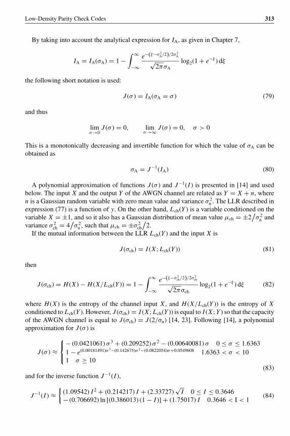
OTE/SPH OTE/SPHJWBK102-08 JWBK102-Farrell June 17, 2006 18:5 Char Count= 0
Low-Density Parity Check Codes 313
By taking into account the analytical expression for IA, as given in Chapter 7,
IA = IA(σA) = 1 −∫ ∞
−∞
e−(ξ−σ 2A/2)/2σ 2
A√2πσA
log2(1 + e−ξ ) dξ
the following short notation is used:
J (σ ) = IA(σA = σ ) (79)
and thus
limσ→0
J (σ ) = 0, limσ→∞ J (σ ) = 0, σ > 0
This is a monotonically decreasing and invertible function for which the value of σA can beobtained as
σA = J−1(IA) (80)
A polynomial approximation of functions J (σ ) and J−1(I ) is presented in [14] and usedbelow. The input X and the output Y of the AWGN channel are related as Y = X + n, wheren is a Gaussian random variable with zero mean value and variance σ 2
n . The LLR described inexpression (77) is a function of y. On the other hand, Lch(Y ) is a variable conditioned on thevariable X = ±1, and so it also has a Gaussian distribution of mean value μch = ±2
/σ 2
n andvariance σ 2
ch = 4/σ 2
n , such that μch = ±σ 2ch
/2.
If the mutual information between the LLR Lch(Y ) and the input X is
J (σch) = I (X ; Lch(Y )) (81)
then
J (σch) = H (X ) − H (X/Lch(Y )) = 1 −∫ ∞
−∞
e−(ξ−σ 2ch/2)/2σ 2
ch√2πσch
log2(1 + e−ξ ) dξ (82)
where H (X ) is the entropy of the channel input X , and H (X/Lch(Y )) is the entropy of Xconditioned to Lch(Y ). However, J (σch) = I (X ; Lch(Y )) is equal to I (X ; Y ) so that the capacityof the AWGN channel is equal to J (σch) = J (2/σn) [14, 23]. Following [14], a polynomialapproximation for J (σ ) is
J (σ ) ≈⎧⎨⎩
− (0.0421061) σ 3 + (0.209252) σ 2 − (0.00640081) σ 0 ≤ σ ≤ 1.6363
1 − e(0.00181491)σ 3−(0.142675)σ 2−(0.0822054)σ+0.0549608 1.6363 < σ < 101 σ ≥ 10
(83)and for the inverse function J−1(I ),
J−1(I ) ≈{
(1.09542) I 2 + (0.214217) I + (2.33727)√
I 0 ≤ I ≤ 0.3646− (0.706692) ln [(0.386013) (1 − I )] + (1.75017) I 0.3646 < I < 1
(84)

OTE/SPH OTE/SPHJWBK102-08 JWBK102-Farrell June 17, 2006 18:5 Char Count= 0
314 Essentials of Error-Control Coding
8.8.5 EXIT Chart for the SND
Since this analysis is restricted to regular LDPC codes, the number of parity equations inwhich a given symbol is present is constant and equal to dv. In the case of the Example 8.2,this parameter is dv = 3. The LLR that each symbol node d j sends to each parity check nodehi in the iteration number it is denoted as Z (i t)
i j , and the LLR that each parity check node hi
sends to each symbol node d j in the iteration number it is denoted as L (i t)i j .
Each symbol node has as its input information a channel LLR Lch = L (0)ch coming from the
channel, and an LLR L (i t)i ′ j that comes from each of its children parity check nodes. The symbol
node uses this information to generate the LLR Z (i t)i j to be sent to its dv children parity check
nodes, according to the expression
Z (i t)i j = Lch +
∑i ′∈M( j)\i
L (i t)i ′ j (85)
In expression (85) the LLR L (i t)i ′ j is the a priori LLR for the SND, Z (i t)
i j is the extrinsic LLR
generated by the SND and Lch = L (0)ch is the LLR from the channel. At the end of this current
iteration, the SND determines an estimate, which is in turn an LLR, useful to determine anestimate of each of the bits of the received code vector. This a posteriori estimate is equal to
A(i t)i j = Lch +
∑i∈M( j)
L (i t)i j (86)
The LLR is Z (i t)i j = |Lc−1
i j | − |Lc+1i j |, calculated using (49).
The EXIT chart for the SND is determined by the value of the mutual information functionfor the value σ of the standard deviation of the variable Z (i t)
i j described by expression (85).The logarithmic version of the sum–product algorithm defines a linear relationship between
the quantities involved in describing the operation of the SND, as seen in expression (85).Since channel LLRs and a priori LLRs are independent random variables, the variance of thevariable
Z (i t)i j = Lch +
∑i ′∈M( j)\i
L (i t)i ′ j
is equal to [14]
σ 2Zi j
= σ 2ch + (dv − 1) σ 2
A = 8Rc
Eb
N0
+ (dv − 1)[J−1(IA)
]2(87)
This leads to an analytical determination of the EXIT charts for LDPC codes, in comparisonwith the heuristically implemented method described for the EXIT charts of turbo codes. Oncethe standard deviation of the extrinsic LLRs generated by the SND has been determined, thenthe mutual information between these LLRs and the bit or symbol information is directlyobtained by using expressions (80) and (83) with σA = σ = σZi j ,
IE,SND(IA, dv, Eb/N0, Rc) = J
(√σ 2
ch + (dv − 1) σ 2A
)(88)

OTE/SPH OTE/SPHJWBK102-08 JWBK102-Farrell June 17, 2006 18:5 Char Count= 0
Low-Density Parity Check Codes 315
8.8.6 EXIT Chart for the PCND
Parity check nodes generate their LLRs taking into account the parity check equations that aredefined for each of them. The estimate or LLR is calculated assuming that the parity checkequation is satisfied. An LLR expression for a parity check equation has already been obtained,and it is given by the expression (73) in its exact version, or by (74) in its approximated version.They are conveniently rewritten for this case as
L (i t−1)i j = ln
⎡⎣∏I ′i ′=1
(eZ (i t−1)
i ′ j + 1)
+ ∏I ′i ′=1
(eZ (i t−1)
i ′ j − 1)
∏I ′i ′=1
(eZ (i t−1)
i ′ j + 1)
− ∏I ′i ′=1
(eZ (i t−1)
i ′ j − 1)⎤⎦ (89)
L (i t−1)i j ≈
[I ′∏
i ′=1
sign(
Z (i t−1)i ′ j
)]min
i ′=1...I
∣∣∣Z (i t−1)i ′ j
∣∣∣ (90)
Here Z (i t−1)i ′ j is the estimate generated in the previous iteration, adopted as the a priori value
for the current iteration.Remember that the convention adopted in [15] is that the bit or symbol ‘0’ is represented by
the signal +1, and the bit or symbol ‘1’ is represented by the signal −1. If the convention istaken the other way round, the argument in expressions (73) and (89) should be inverted. Thisexpression is a summation of LLRs defined by the operator [⊕]. In [16] and [17] it is shownthat the EXIT chart for the PCND for the AWGN channel can be approximately, but with highaccuracy, calculated as
IE,PCND(IA, dc) ≈ 1 − J(√
dc − 1 J−1(1 − IA))
(91)
It is more useful to determine the inverse function of (91), which defines the mutual infor-mation between the bits of the decoded vector and the a priori information, as a function ofthe mutual information between the bits of the decoded vector and the extrinsic information:
IA,PCND(IE, dc) ≈ 1 − J
(J−1(1 − IE)√
dc − 1
)(92)
Figure 8.11 shows the EXIT chart for the SND, for different values of the parameter dv, andFigure 8.12 shows the EXIT chart for the PCND, for different values of the parameter dc.
LDPC codes have a more analytical procedure for determining the EXIT charts than thatof turbo codes. In [16] it is shown that, for the erasure channel, optimum design of an LDPCcode is done by matching up the corresponding EXIT charts for the SND and the PCND. Thisconclusion is approximately valid for other channels including the AWGN channel. EXITcharts for LDPC codes are also useful for determining for instance a practical bound on thenumber of iterations for decoding LDPC codes. However, the EXIT chart analysis is alsoa good tool for the design of LDPC codes. An example of an LDPC code design is givenin [14].

OTE/SPH OTE/SPHJWBK102-08 JWBK102-Farrell June 17, 2006 18:5 Char Count= 0
316 Essentials of Error-Control Coding
00
0.9
0.8
0.7
0.6
0.5
0.4
0.3
0.2
0.1
0.1 0.2 0.3 0.4 0.5 0.6 0.7 0.8 0.9 1.0
1
IA,SND
IE,SND
dv = 9 dv = 7 dv = 5 dv = 3
Figure 8.11 EXIT chart for the SND
00
0.9
0.8
0.7
0.6
0.5
0.4
0.3
0.2
0.1
0.1 0.2 0.3 0.4 0.5 0.6 0.7 0.8 0.9 1.0
1
dc = 10
dc = 6
dc = 3
dc = 2
IE, PC ND
IA, PC ND
Figure 8.12 EXIT chart for the PCND

OTE/SPH OTE/SPHJWBK102-08 JWBK102-Farrell June 17, 2006 18:5 Char Count= 0
Low-Density Parity Check Codes 317
8.9 Fountain and LT Codes
8.9.1 Introduction
An interesting application field for LDPC codes is on the so-called erasure channel, introducedin Chapter 1, and its relationship with transmission in data networks. In data transmissionover networks like the Internet, information is usually fragmented into data packets of fixedsize before being transmitted through the network. For transmission, the information in eachpacket is usually encoded for detecting errors by using a cyclic redundancy check (CRC), andthe receiver detects errors by syndrome decoding applied over each data packet in order todecide whether it accepts the data packet, or requires its retransmission. When the syndromecalculation determines that the data packet is not a valid packet, then the system resorts to theretransmission procedure called automatic repeat request (ARQ), described in Chapter 2. Asecond channel in this duplex system is used for transmitting retransmission requests. Packetsfound to contain errors are discarded, given the expectation that they will be retransmitted.This is the traditional approach to error control in data networks, based on ARQ schemes.However, a retransmission implies reuse of the transmission channel, and therefore throughputis reduced.
A different approach to network error control is provided by the use of so-called fountaincodes [24, 27] in addition to the CRC. These codes generate data packets that are essentiallyrandom functions of the whole file to be transmitted. The transmitter floods the receiver withthese data packets, without needing to know which of them are correctly received. The receiverdiscards any packet containing errors, as determined by the CRC syndrome. If the original sizeof the whole file to be transmitted is K data packets, and if the decoder receives N data packets,then it is possible to correctly recover at the receiver the original information (i.e., the wholefile), provided N is sufficiently larger than K . How much larger N needs to be is determinedby the random functions used to generate the packets and by the error rate on the channel.
The process of discarding of data packets can be suitably modelled by the erasure channel,introduced in Chapter 1, in which a packet that is discarded can be regarded as a packeterasure. The probability of an erasure or discard is p for the binary erasure channel (BEC),and its capacity is equal to 1 − p, as calculated in Chapter 1. If this channel operates overa non-binary alphabet GF(q), for which q = 2m , then the erasure channel has an increasedcapacity of (1 − p) m. In the transmission of data packets of a fixed length of m bits, theerasure channel with non-binary alphabet GF(q) is a suitable model for the discarding of suchpackets, so that each data packet is represented by one of the q = 2m elements of GF(q).
As demonstrated by Shannon, the capacity of a given channel does not depend on theexistence or not of a physical means for requesting retransmissions. In the case of the q-aryerasure channel where q = 2m , this capacity remains equal to (1 − p) m independently of theexistence or not of retransmissions.
In a typical ARQ scheme, retransmissions are required regardless of the value of the erasureor discard probability p, and this process could become enormously demanding if, for instance,transmission is taking place in the presence of a very noisy channel. ARQ schemes are alsoimpractical in broadcast transmission scenarios, where the transmitter sends data packets to amultiplicity of users over independent or partially independent channels. Here the number ofretransmissions required could seriously decrease the throughput of the transmitter. The need

OTE/SPH OTE/SPHJWBK102-08 JWBK102-Farrell June 17, 2006 18:5 Char Count= 0
318 Essentials of Error-Control Coding
to maintain high throughput rates suggests the use of an FEC scheme for the transmissionof packets in data networks, in order to reduce, and preferably eliminate, retransmissions.As pointed out earlier, the capacity of the q-ary erasure channel remains equal to (1 − p) mindependently of the existence or not of retransmissions, and suitable erasure-correction codesexist to take advantage of this property.
One of the most efficient error-control techniques was introduced in Chapter 5, and is theReed–Solomon coding technique. An interesting property of a RS code CRS(N , K ) definedover GF(q), where q = 2m , is that if any K of the N transmitted symbols are received, theK information symbols can be successfully recovered. However, RS codes are complex todecode and encode, particularly if m is large, and so they do not appear to be the most suitablecodes for data networks, where packets are normally of a large size. In addition, the rate ofan RS code needs to be determined before transmission, and is difficult to change duringtransmission. Of course the transmission can start with the code rate set to match the capacityof the erasure channel. However, the erasure probability p, which determines the capacity, canchange during transmission over a network, as a function of the users locations, for instance.Therefore a dynamically variable code rate would be advantageous, and fountain codes appearable to provide it very effectively.
8.9.2 Fountain Codes
A fountain code [24, 27] can be seen as a code that generates a continuous flow of transmitteddata packets, simulating the action of water falling from a spring into a collecting receptacle,the data packet receiver. In this coding scheme, the whole information file to be transmitted isof size Km, such that there are K data packets of m bits each. The receiver collects a set ofK data packets or more, enough to successfully recover the original transmitted information.From this point of view, the rate of a fountain code tends to zero, because transmission issupposedly time unlimited. However, in a practical implementation, the number of data packetsto be transmitted is dynamically determined to be finite, according to the necessities describedearlier. This usually results in a variable, but relatively high code rate. The simplest fountaincode is the linear random code.
8.9.3 Linear Random Codes
Let a whole file of information be fragmented into K data packets dp1 dp2 . . . dpK . Eachtransmitted data packet contains m bits, and is going to be correctly received or not, dependingon the channel noise. Transmission is synchronous, and successive transmitted packets tpn areordered by a time index n. At time instant n, the encoder generates a random binary K -tuple{Gkn}, and then the transmitted packet tpn is the exclusive-OR sum of all the information datapackets for which the random bits in {Gkn} are equal to ‘1’:
tpn =K∑
k=1
dpk Gkn (93)
This encoding procedure can be seen as performed by an encoder whose generator matrixhas an increasing number of columns, and so at each time instant it adds another random (in

OTE/SPH OTE/SPHJWBK102-08 JWBK102-Farrell June 17, 2006 18:5 Char Count= 0
Low-Density Parity Check Codes 319
practice pseudo-random) column to its structure. An example of such a matrix could be thefollowing:
G =
⎡⎢⎢⎣1 1 0 1 0 1 · · ·0 1 1 0 1 1 · · ·1 0 0 0 1 1 · · ·0 0 1 1 1 0 · · ·
⎤⎥⎥⎦ (94)
The number of rows of this increasing matrix is K , and each of its semi-infinite number ofcolumns are successively generated as random K -tuples {Gkn}, where n = 1, 2, 3, . . . . For thegenerator matrix of (94), for example, the first transmitted data packet is the exclusive-OR sumof the original data packets dp1 and dp3, the second transmitted packet is the exclusive-ORsum of the original data packets dp1 and dp2, and so on.
The erasure channel will affect the transmission by erasing some of the transmitted datapackets, but the receiver collects a set of N data packets in order to form a matrix of sizeK × N , such that N = K + Ex , where Ex is the number of excess packets with respect to K ,which can be understood as the redundancy in the transmission using the fountain code. Thequestion that now arises is, can the original packets of information be successfully recoveredfrom these N received data packets? The receiver is assumed to know the so-called fragmentgenerator matrix Gfr, which is a matrix formed in the decoder from the N correctly receiveddata packets, and each column of this fragment matrix has a known value of time index n.If the decoder also knows the pseudo-random rule that generated the K -tuple columns of theincreasing matrix used by the encoder, then it is possible to recover the original information.
If N < K , then there is no way of successfully recovering the original information. For anynon-zero value of the excess Ex , there is the possibility of a successful recovery. In the case ofN = K , the original information can be recovered if an inverse matrix of the fragment generatormatrix Gfr exists. The probability of the existence of such an inverse matrix is determined in[24], and it is equal to(
1 − 2−K) (
1 − 2−(K−1)) · · · (1 − 1/8)(1 − 1/4)(1 − 1/2)
which turns out to be equal to 0.289 for any K > 10.If N > K , then the probability δ of the existence of an invertible submatrix of size K × K ,
in the fragment generator matrix Gfr, has to be determined. This probability, shown in [24],is to be bounded by a quantity that is a function of the excess Ex of data packets correctlyreceived:
δ ≤ 2−Ex (95)
This means that the probability of successful recovery of data packets is 1 − δ, and that thishappens if at least K + log2(1/δ) data packets are received.
Summarizing, the probability of successful recovery of the original information is equal to0.289 if no redundant data packets are received, and this probability increases to 1 − δ whenEx excess (redundant) packets are received.
However, the decoding complexity of these linear random codes is dominated by the inver-sion of the fragment generator matrix Gfr, which requires approximately K 3 binary operations,a limiting drawback for the transmission of a large number of large data packets, as is usuallynecessary in data networks.

OTE/SPH OTE/SPHJWBK102-08 JWBK102-Farrell June 17, 2006 18:5 Char Count= 0
320 Essentials of Error-Control Coding
8.9.4 Luby Transform Codes
Luby transform (LT) codes [25] appear to be more suitable for the erasure channel networkapplication. They can be understood as fountain codes characterized by a linear sparse matrixsimilar to that used to define an LDPC code.
These codes are designed using a statistical analysis that models the problem of throwingballs in order to fill a set of empty baskets. A first question arising from this particular problemis to determine how many balls should be thrown to ensure that there is at least one ball ineach basket. Another question is to determine the number of empty baskets that results fromthe throwing of a given number of balls at the set of baskets. Thus, for instance, if N balls arethrown at K baskets, K e−N/K is the expected number of empty baskets. This means that theexpected number of empty baskets is a small number δ if N > K ln(K/δ) [24, 27].
8.9.4.1 LT encoder
The encoder of an LT code takes a set of K data packets dp1 dp2 . . . dpK to generate the codeddata packet as follows:
A degree dn is selected from a degree distribution function ρ(d), conveniently designed asa function of the size K of the file to be encoded.
A set of dn data packets is selected in a uniform random manner to form the coded packettpn as the exclusive-OR of these packets.
This encoding mechanism is associated with a bipartite graph which is similar to that forLDPC codes, and which is formed between the coded data packets tpn and the informationpackets dpk .
A sparse graph is obtained when the average value of the degree dn is significantly smallerthan the number of information packets K . This encoding mechanism can be interpreted as anLDPC code.
8.9.4.2 LT decoder
Since the encoding of an LT code is similar to that of an LDPC code, creating the transmittedor coded data packets from the information source or message packets, the decoding of an LTcode consists of determining the vector dp as a function of the vector tp, which are related by theexpression tp = dp · G, where the matrix G corresponds to the bipartite graph of the encoding.Both sides of the transmission know this matrix, even when it is normally a pseudo-randomlygenerated matrix.
At first, this similarity with LDPC codes suggests the use of the sum–product algorithm fordecoding LT codes, but in this case the entities involved are packets that are either completelyreliable or completely unreliable (erased). This means that there are packets dpk with unityprobability of being true packets, or packets dpk that have all the same probability of not beingtrue packets. The decoding algorithm, in this case, operates in a very simple manner. In thedecoder coded packets tpn play the role of parity check nodes, and message packets dpk playthe role of symbol nodes. The decoder of an LT code then operates as follows:
1. It looks for a parity check node tpn that is connected to only one symbol node dpk . If thisis not the case, the algorithm cannot proceed to decode the coded packets.

OTE/SPH OTE/SPHJWBK102-08 JWBK102-Farrell June 17, 2006 18:5 Char Count= 0
Low-Density Parity Check Codes 321
2. It sets
dpk = tpn
3. It sums dpk to all the parity check nodes tp′n that are connected to dpk as
tpn′ = tpn′ + dpk, for all n′ for which the bits in Gn′k = 1
4. It removes all the connections related to symbol node dpk .5. Steps (1)–(4) are repeated for all dpk .
Example 8.3: For the LT code described by the following matrix G, determine the coded datapackets for the message packet set dp1dp2dp3 = (11, 10, 01), where the message data packetsconsist of two bits. Then decode the coded data packets.
G =⎡⎣1 1 0 1
0 0 1 10 1 1 0
⎤⎦According to the above generator matrix G, supposed to be randomly generated, the coded
data packets are
tp1 = dp1 = 11
tp2 = dp1 ⊕ dp3 = 10
tp3 = dp2 ⊕ dp3 = 11
tp4 = dp1 ⊕ dp2 = 01
This is expressed as the coded vector tp = (tp1 tp2 tp3 tp4) = (11, 10, 11, 01)The corresponding bipartite graph is of the form as given in Figure 8.13.The decoding procedure is then applied. A parity check node connected to only one symbol
node is found (11), and then that packet is assigned the decoded packet dp1 = tp1 = 11. Thisresult is added to the other parity check nodes connected to this symbol node, and then theconnections are removed. This is seen in Figure 8.14.
After removing connections, the algorithm searches for another parity check node that isconnected to only one symbol node, and chooses dp2 = 10. After appropriately summing theresult and removing connections, the final configuration seen in Figure 8.15 determines theend of the decoding by setting dp3 = 01.
10 11 0111
dp1 dp2 dp3
Figure 8.13 Bipartite graph for the LT code of Example 8.3

OTE/SPH OTE/SPHJWBK102-08 JWBK102-Farrell June 17, 2006 18:5 Char Count= 0
322 Essentials of Error-Control Coding
1001 11
11 dp2 dp3 11
1101 10
dp2 dp3
Figure 8.14 First steps in the decoding of the LT code of Example 8.3
A detailed description of the design of LT codes can be found in [24] and [25]. These codescan be used in many practical applications. One of them is as a coding technique for distributedmultiuser information storage systems, where stored coded files that have been damaged couldbe recovered by discarding (erasing) them and then decoding suitable combinations of codedfiles stored elsewhere in the system.
8.10 LDPC and Turbo Codes
A common characteristic of these two coding techniques, which are the most efficient of allthose described in this book, is that they can be iteratively decoded using alternating exchangesof soft-decision information. It is possible to demonstrate a certain degree of equivalencebetween the decoders for these two impressive error-control techniques, as seen in Section8.8.1 for instance. There are, however, some differences between them.
LDPC codes are extremely good in terms of the BER performance if the code length is largeenough. Thus, LDPC codes of length n = 10,000, for instance, have a BER performance curvethat is less than 0.1 dB from the Shannon limit. But these long block lengths lead to significantdecoding delay, and considerable encoding and decoding complexity.
On the other hand, turbo codes are constructed with relatively low complexity constituentcodes, and they also show a very good BER performance, but the error floor effect is presentat relatively high BERs. They are however more suitable for intermediate block or constraintlength applications.
For both turbo and LDPC codes, the original iterative decoding methods are more complexthan their logarithmic versions. Simplified variants of the logarithmic decoding algorithmslead to even lower complexity decoding algorithms, usually performed by applying max ormin functions. As might be expected, however, the trade-off is some level of degradation inthe corresponding BER performance.
10
01 01 01 01
11 dp3 1011 dp3
Figure 8.15 Final steps in the decoding of the LT code of Example 8.3

OTE/SPH OTE/SPHJWBK102-08 JWBK102-Farrell June 17, 2006 18:5 Char Count= 0
Low-Density Parity Check Codes 323
Bibliography and References
[1] Shannon, C. E., “A mathematical theory of communication,” Bell Syst. Tech. J., vol. 27,pp. 379–423, 623–656, July and October 1948.
[2] Shannon, C. E., “Communications in the presence of noise,” Proc. IEEE, vol. 86, no. 2,pp. 447–458, February 1998.
[3] Berrou, C., Glavieux, A. and Thitimajshima, P., “Near Shannon limit error-correctingcoding and decoding: turbo codes,” Proc. 1993 IEEE International Conference on Com-munications, Geneva, Switzerland, vol. 2, pp. 1064–1070, May 1993.
[4] MacKay, D. J. C. and Neal, R. M., “Near Shannon limit performance of low density paritycheck codes,” Electron. Lett., vol. 33, no. 6, March 13, 1997.
[5] MacKay, D. J. C. and Neal, R. M., “Good error-correcting codes based on very sparsematrices,” available at http://www.inference.phy.cam.ac.uk/mackay/CodesGallager.html
[6] Gallager, R. G., “Low-density parity-check codes,” IRE Trans. Inf. Theory, vol. IT-8, no.1, pp. 21–28, January 1962.
[7] Tanner, L. M., “A recursive approach to low complexity codes,” IEEE Trans. Inf. Theory,vol. 27, no. 5, pp. 533–547, 1981.
[8] Davey, M. C., Error-Correction Using Low-Density Parity-Check Codes, PhD Thesis,University of Cambridge, Cambridge, United Kingdom, 1999.
[9] Tang, H., Xu, J., Kou, Y., Lin, S. and Abdel-Ghaffar, K., “On algebraic construction ofGallager and circulant low-density parity-check codes,” IEEE Trans. Inf. Theory, vol. 50,no. 6, pp. 1269–1279, June 2004.
[10] Kou, Y., Lin, S. and Fossorier, M., “Low-density parity-check codes based on finitegeometries: A rediscovery and new results,” IEEE Trans. Inf. Theory, vol. 47, pp. 2711–2736, November 2001.
[11] Ammar, B., Honary B., Kou, Y., Xu J. and Lin, S., “Construction of low-density parity-check codes based on balanced incomplete block designs,” IEEE Trans. Inf. Theory, vol.50, no. 6, pp. 1257–1269, June 2004.
[12] Arnone, L., Gayoso, C., Gonzalez, C., and Castineira Moreira, J., “A LDPC logarithmicdecoder implementation,” Proc. VIII International Symposium on Communications The-ory and Applications, St. Martin’s College, Ambleside, United Kingdom, pp. 356–361,July 2005.
[13] LDPC toolkit for Matlab, available at http://arun-10.tripod.com/ldpc/generate.html[14] Ten Brink, S., Kramer, G. and Ashikhmin, A., “Design of low-density parity-check codes
for modulation and detection,” IEEE Trans. Commun., vol. 52, no. 4, pp. 670–678, April2004.
[15] Hagenhauer, J., Offer, E. and Papke, L., “Iterative decoding of binary block and convo-lutional codes,” IEEE Trans. Inf. Theory, vol. 42, no. 2, pp. 429–445, March 1996.
[16] Ashikhmin, A., Kramer, G. and Ten Brink, S., “Extrinsic information transfer functions:A model and two properties,” Proc. Conf. Information Sciences and Systems, Princeton,New Jersey, pp. 742–747, March 20–22, 2002.
[17] Sharon, E., Ashikhmim, A. and Litsyn, S., “EXIT functions for the Gaussian channel,”Prov. 40th Annu. Allerton Conf. Communication, Control, Computers, Allerton, Illinois,pp. 972–981, October 2003.
[18] Etzion, T., Trachtenberg, A. and Vardy, A., “Which codes have cycle-free Tanner graphs?”IEEE Trans. Inf. Theory, vol. 45, no. 6, pp. 2173–2180, September 1999.

OTE/SPH OTE/SPHJWBK102-08 JWBK102-Farrell June 17, 2006 18:5 Char Count= 0
324 Essentials of Error-Control Coding
[19] Ten Brink, S., “Convergence behaviour of iteratively decoded parallel concatenatedcodes,” IEEE Trans. Commun., vol. 49, pp. 1727–1737, October 2001.
[20] Ten Brink, S., Speidel, J. and Yan, R., “Iterative demapping and decoding for multilevelmodulation,” Proc. IEEE Globecom Conf. 98, Sydney, NSW, Australia, vol. 1, pp. 579–584, November 1998.
[21] Ten Brink, S., “Exploiting the chain rule of mutual information for the design of iterativedecoding schemes,” Proc. 39th Allerton Conf., Monticello, Illinois, October 2001.
[22] Tuchler, M., Ten Brink, S. and Hagenauer, J., “Measures for tracing convergence ofiterative decoding algorithms,” Proc. 4th IEEE/ITG Conf. Source and Channel Coding,Berlin, Germany, pp. 53–60, January 2002.
[23] McEliece, R. J., The Theory of Information and Coding, Addison-Wesley, Massachusetts,1977.
[24] MacKay, D. J. C., “Digital fountain codes,” available at http://www.inference.phy.cam.ac.uk/mackay/DFountain.html
[25] Luby, M., “LT codes,” available at http://www.inference.phy.cam.ac.uk/mackay/dfountain/LT.pdf
[26] MacKay, D. J. C., Web site available at http://www.inference.phy.cam.ac.uk/mackay/[27] MacKay, D. J. C., “Fountain codes,” IEE Proc. Commun., vol. 152, no. 6, pp. 1062–1068,
December 2005.[28] MacKay, D. J. C., Information Theory, Inference, and Learning Algorithms, Cambridge
University Press, Cambridge, United Kingdom, 2003.
�
Problems
8.1 (a) Determine the number and size of the short cycles in the bipartite graph of theirregular LDPC code Cb(12, 4) described in Section 8.5.
(b) Reduce the number of short cycles by changing the positions of ‘1’s in theparity check matrix of item (a), but keeping the number of ‘1’s per column thesame, s = 3.
(c) Does the modified Tanner graph correspond to the same LDPC code or to adifferent one?
8.2 A simple binary cyclic LDPC code can be constructed from the following circulantmatrix:
M =
⎡⎢⎢⎢⎢⎢⎢⎢⎢⎣
1 1 0 1 0 0 00 1 1 0 1 0 00 0 1 1 0 1 00 0 0 1 1 0 11 0 0 0 1 1 00 1 0 0 0 1 11 0 1 0 0 0 1
⎤⎥⎥⎥⎥⎥⎥⎥⎥⎦

OTE/SPH OTE/SPHJWBK102-08 JWBK102-Farrell June 17, 2006 18:5 Char Count= 0
Low-Density Parity Check Codes 325
(a) Determine the rank of the above matrix, and use that to find the cyclic andsystematic parity check matrices of the code, and its systematic generatormatrix.
(b) Calculate the average number of 1s per row and column of the two paritycheck matrices, and hence calculate the rate of the code, confirming that it isthe same in both cases, and also the same as the rate calculated from thedimensions of the parity check matrices. What is the Hamming distance of thecode?
(c) Sketch the Tanner graphs of the two parity check matrices and of the circulantmatrix, and determine the length of the shortest cycle in each case. Whichgraph might be best for decoding the code by means of the sum–productalgorithm?
8.3 For the LDPC code of Problem 8.2,(a) Use the systematic generator matrix found in part (a) of Problem 8.2 to deter-
mine the codeword corresponding to the message vector m = (100).(b) The codeword of part (a) of this problem is transmitted over an AWGN
channel in normalized polar format (±1), and is received as the vectorr = (
1.0187 −0.6225 2.0720 1.6941 −1.3798 −0.7431 −0.2565).
Using the sum–product algorithm, decode this received vector on each of the threeTanner graphs found in part (c) of Problem 8.2, and comment on the processesand the results obtained.
8.4 The block code Cb(5, 3) introduced in Example 7.1 in Chapter 7 has the followinggenerator and parity check matrices:
G =⎡⎣1 0 1 0 0
0 1 0 1 00 0 1 1 1
⎤⎦ , H =[1 0 1 0 10 1 0 1 1
]
In that example the codeword c = (00000) is transmitted over a soft-decisionchannel, and the corresponding received vector is r = (10200). This soft-decisionchannel is described in Chapter 7, in Figure 7.6 and Table 7.2.(a) Decode the received vector using the SPA over the parity check matrix H
to show that, after enough iterations, the decision of the decoder fluctuatesbetween the two code vectors c = (00000) and c = (10100), which are theclosest to the received vector r = (10200).
(b) Describe the deficiencies of the bipartite graph associated with the parity checkmatrix H of this code, with respect to the iterative passing of information.
�

OTE/SPH OTE/SPH
JWBK102-08 JWBK102-Farrell June 17, 2006 18:5 Char Count= 0
326

OTE/SPH OTE/SPHJWBK102-APPA JWBK102-Farrell June 17, 2006 18:5 Char Count= 0
Appendix A: Error Probability inthe Transmission of Digital Signals
The two main problems in the transmission of digital data signals are the effects of channelnoise and inter-symbol interference (ISI) [2, 4]. In this appendix the effect of the channelnoise, assumed to be additive white Gaussian noise (AWGN), is studied, in the absence ofinter-symbol interference.
A.1 Digital Signalling
A.1.1 Pulse Amplitude Modulated Digital Signals
A digital signal can be described as a sequence of pulses that are amplitude modulated. Thecorresponding signal is of the form
x(t) =k=∞∑
k=−∞ak p(t − kT ) (1)
where coefficient ak is the kth symbol of the sequence, such that the coefficient ak is one ofthe M possible values of the information to be transmitted, taken from a discrete alphabet ofsymbols. The pulse p(t) is the basic signal to be transmitted, which is multiplied by ak toidentify the different signals that make up the transmission.
The signal ak p(t − kT ) is the kth symbol that is transmitted at the kth time interval, whereT is the duration of such a time interval. Thus, the transmission consists of a sequence ofamplitude-modulated signals that are orthogonal in the time domain.
As seen in Figure A.1, the data sequence ak = A, 0, A, A, 0, A, corresponding to digitalinformation in binary format (101101), is a set of coefficients that multiply a normalized basicsignal or pulse p(t − kT ). If these coefficients are selected from an alphabet {0, A}, the digitaltransmission is said to have a unipolar format. If coefficients are selected from an alphabet
Essentials of Error-Control Coding Jorge Castineira Moreira and Patrick Guy FarrellC© 2006 John Wiley & Sons, Ltd
327

OTE/SPH OTE/SPHJWBK102-APPA JWBK102-Farrell June 17, 2006 18:5 Char Count= 0
328 Essentials of Error-Control Coding
A
0tk = 2
A p(t – 2T)T
Figure A.1 A digital signal
1
0t k
p(t – kT )
Figure A.2 A normalized pulse at time interval k multiplied by a given coefficient ak
{−A/2, A/2}, the digital transmission is said to have a polar format. In this latter case, thesequence of this example would be given by ak = A/2, −A/2, A/2, A/2, −A/2, A/2.
Index k adopts integer values from minus to plus infinity. As seen in Figure A.2, the basicsignal p(t) is normalized and of fixed shape, centred at the corresponding time interval k, andmultiplied by a given coefficient that contains the information to be transmitted. This basicnormalized pulse is such that
p(t) ={
1 t = 00 t = ±T, ±2T, . . .
(2)
The normalized pulse is centred at the corresponding time interval k and so its sample valueat the centre of that time interval is equal to 1, whereas its samples obtained at time instantsdifferent from t = kT are equal to 0. This condition does not necessarily imply that thepulse is time limited. Samples are taken synchronously at time instants t = kT , where k = 0,
±1, ±2, . . . , such that for a particular time instant t = k1T ,
x(k1T ) =∑∞
ak1p(k1T − kT ) = ak1
(3)
since (k1T − kT ) = 0, for every k, except k = k1.Conditions (2) describe the transmission without ISI, and are satisfied by many signal pulse
shapes. The classic rectangular pulse satisfies condition (2) if its duration τ is less than orequal to T . The pulse sin c(t) also satisfies the orthogonality condition described in the timedomain by equation (2), but it is a pulse that is unlimited in time, however. Figure A.3 showsthe transmission of the binary information sequence (11001), using sin c(t) pulses modulatedin a polar format. At each sampling time instant t = kT , the pulse being sampled has amplitudedifferent from 0, while the other pulses are all equal to 0.

OTE/SPH OTE/SPHJWBK102-APPA JWBK102-Farrell June 17, 2006 18:5 Char Count= 0
Appendix A: Error Probability in the Transmission of Digital Signals 329
–4 –2 0 2 4 6 8 10 12–1
–0.8
–0.6
–0.4
–0.2
0
0.2
0.4
0.6
0.8
1
Time, t
A
Figure A.3 A digital transmission using sinc (t) pulses modulated in polar format
Each pulse occurs in a time interval of duration T . The inverse of this duration is the symbolrate of the transmission, since it is the number of symbols that are transmitted in a unit of time(usually a second). The symbol rate r is then equal to
r = 1/T (symbols per second) (4)
which is measured in symbols per second. When the discrete alphabet used in the transmissioncontains only two symbols, M = 2, then it is binary transmission, and the correspondingsymbol rate r = rb is the binary signalling rate
rb = 1/Tb (bit per second) (5)
where T = Tb is the in time duration of each bit. The binary signalling rate is measured in bitsper second (bps).
A.2 Bit Error Rate
Figure A.4 shows the basic structure of a binary receiver.
Synchronization: T U
N0 / 2
x(t)Low passfilter H(f )
Samplingand hold
y(tk)
Thresholdxd(t)
y(t)
Figure A.4 A binary receiver

OTE/SPH OTE/SPHJWBK102-APPA JWBK102-Farrell June 17, 2006 18:5 Char Count= 0
330 Essentials of Error-Control Coding
The signal x(t) is a digital signal∑
k ak p(t − kT ), that is, an amplitude-modulated pulsesignal. This signal is affected by AWGN noise in the channel and is then input to the receiver.The first block in this receiver is a low pass filter that eliminates part of the input noise withoutproducing ISI, giving the signal y(t). The receiver takes synchronized samples of this signal,and generates after the sample-and-hold operation a random variable of the form
y(tk) = ak + n(tk) (6)
Sampled values y(tk) constitute a continuous random variable Y , and noise samples n(tk) takenfrom a random signal n(t) form a random variable n.
The lowest complexity decision rule for deciding the received binary value is the so-calledhard decision, which consists only of comparing the sampled value y(tk) with a threshold U ,such that if y(tk) > U , then the receiver considers that the transmitted bit is a 1, and if y(tk) < Uthen the receiver considers that the transmitted bit is a 0. In this way the received sampledsignal y(tk) is converted into a signal xhd(t), basically of the same kind as that expressed inequation (1), an apparently noise-free signal but possibly containing some errors with respectto the original transmitted signal.
The probability density function of the random variable Y is related to the noise, and toconditional probability of the transmitted symbols. The following hypotheses are relevant:
H0 is the hypothesis that a ‘0’ was transmitted ak = 0, Y = n
H1 is the hypothesis that a ‘1’ was transmitted ak = A, Y = A + n.
The probability density function of the random variable Y conditioned on the event H0 isgiven by
pY(y/H0) = pN(y) (7)
where pN(y) is the Gaussian probability density function.For hypothesis H1,
pY(y/H1) = pN(y − A) (8)
The probability density function in this case is shifted to the value n = y − A. Thus, theprobability density function for the noisy signal is the probability density function for thenoise-free discrete signal 0 or A (unipolar format) added to the probability density function ofthe noise pN(n). Figure A.5 shows the reception of a given digital signal performed using harddecision.
The probability density function for each signal is the Gaussian probability density functioncentred at the value of the amplitude that is transmitted.
Figure A.6 shows the shadowed areas under each probability density function that correspondto the probability of error associated with each hypothesis. Thus, the receiver assumes thatif Y < U , hypothesis H0 has occurred, and if Y > U, hypothesis H1 has occurred. Error

OTE/SPH OTE/SPHJWBK102-APPA JWBK102-Farrell June 17, 2006 18:5 Char Count= 0
Appendix A: Error Probability in the Transmission of Digital Signals 331
y(tk) A
xd(t) A
Tb / 2
U
0 11 0 0y(t)
A
0
0
0
tk Tb
tk Tb + Tb / 2
Figure A.5 Reception of a digital signal
Pe1 Pe0
U0 YA−3 −2 −1 0 1 2 3 4 5
py(y/H0) py(y/H1)
Figure A.6 Bit error rate calculation
probabilities associated with each hypothesis are described in Figure A.6, and are equal to
Pe0 = P(Y > U/H0) =∫ ∞
UpY(y/H0) dy (9)
Pe1 = P(Y < U/H1) =∫ U
−∞pY (y/H1) dy (10)

OTE/SPH OTE/SPHJWBK102-APPA JWBK102-Farrell June 17, 2006 18:5 Char Count= 0
332 Essentials of Error-Control Coding
The threshold value U should be conveniently determined. A threshold value U close to theamplitude 0 reduces the error probability associated with the symbol ‘1’, but strongly increasesthe error probability associate with the symbol ‘0’, and vice versa. The error probability ofthe whole transmission is an average over these two error probabilities, and its calculation canlead to a proper determination of the value of the threshold U:
Pe = P0 Pe0 + P1 Pe1 (11)
where P0 = P(H0), P1 = P(H1).P0 and P1 are the source symbol probabilities; that is, the probabilities of the transmission
of a symbol ‘0’ and ‘1’. The average error probability is precisely the mean value of the errorsin the transmission that takes into account the probability of occurrence of each symbol.
The derivative with respect to the threshold U of the average error probability is set to beequal to zero, to determine the optimal value of the threshold:
dPe/dU = 0 (12)
This operation leads to the following expression:
P0 pY (Uopt/H0) = P1 pY (Uopt/H1) (13)
If the symbols ‘0’ and ‘1’ of the transmission are equally likely
P0 = P1 = 1
2(14)
then
Pe = 1
2(Pe0 + Pe1) (15)
and the optimal value of the threshold is then
pY(Uopt/H0) = pY(Uopt/H1) (16)
As seems reasonable, the optimal value of the threshold U is set to be in the middle of the twoamplitudes, Uopt = A/2, if the symbol source probabilities are equal; that is, if symbols areequally likely (see Figure A.6).
The Gaussian probability density function with zero mean value and variance σ 2 charac-terizes the error probability of the involved symbols if they are transmitted over the AWGNchannel. This function is of the form
pN(y) = 1√2πσ 2
e− y2
2σ2 (17)
In general, this probability density function is shifted to a mean value m and has a varianceσ 2, such that
pN(y) = 1√2πσ 2
e− (y−m)2
2σ2 (18)

OTE/SPH OTE/SPHJWBK102-APPA JWBK102-Farrell June 17, 2006 18:5 Char Count= 0
Appendix A: Error Probability in the Transmission of Digital Signals 333
−2 −1 0 1 2 3 4 5 6
pN(y)
Q(k)
m + kσm
Figure A.7 Normalized Gaussian probability density function Q(k)
The probability that a given value of the random variable Y is larger than a value m + kσ isa function of the number k, and it is given by
P(Y > m + kσ ) = 1√2πσ 2
∫ ∞
m+kσ
e− (y−m)2
2σ2 dy (19)
These calculations are simplified by using the normalized Gaussian probability density func-tion, also known as the function Q(k) (Figure A.7):
Q(k) = 1√2π
∫ ∞
ke− (λ)2
2 dλ (20)
obtained by putting
λ = y − m
σ(21)
This normalized function can be used to calculate the error probabilities of the digital trans-mission described in equations (9) and (10).
Pe0 =∫ ∞
UpN(y) dy = 1√
2πσ 2
∫ ∞
Ue− y2
2σ2 dy = Q(U/σ ) (22)
and
Pe1 =∫ U
−∞pN(y − A) dy = 1√
2πσ 2
∫ U
−∞e− (y−A)2
2σ2 dy = Q((A − U ) / σ ) (23)
If U = Uopt, the curves intersect in the middle point Uopt = A/2.

OTE/SPH OTE/SPHJWBK102-APPA JWBK102-Farrell June 17, 2006 18:5 Char Count= 0
334 Essentials of Error-Control Coding
In this case these error probabilities are equal to
Pe0 = Pe1 = Q
(A
2σ
)(24)
Pe = 1
2(Pe0 + Pe1) = Q
(A
2σ
)This is the minimum value of the average error probability for the transmission of two equallylikely symbols over the AWGN channel. As seen in the above expressions, the term A/2σ (orequivalently its squared value) defines the magnitude of the number of errors in the transmis-sion, that is, the error probability or bit error rate of the transmission.
The result is the same for transmission using the polar format (ak = ±A/2), if the symbolamplitudes remain the same distance A apart.
The above expressions for the error probability can be generalized for the transmission ofM symbols taken from a discrete source, and they can also be described in terms of the signal-to-noise ratio. The power associated with the transmission of the signal described in equation(1) is useful for this latter purpose. Let us take a sufficiently long time interval T0, such thatT0 = NT, and N � 1. The amplitude-modulated pulse signal uses the normalized pulse
p(t) ={
1 |t | < τ/20 ||t | > τ/2
(25)
where τ ≤ T . Then the power associated with this signal is equal to
SR = 1
T0
∫ T0/2
−T0/2
(∑k
ak p(t − kT )2
)dt = 1
T0
∫ T0/2
−T0/2
∑k
a2k p2(t − kT ) dt
= 1
T0
∫ T0/2
−T0/2
k=N/2∑k=−N/2
a2k p2(t − kT ) dt
SR =∑
k
1
NT
∫ T/2
−T/2
a2k p2(t) dt = N0
NT
∫ T/2
−T/2
a20 p2(t) dt + N1
NT
∫ T/2
−T/2
a21 p2(t) dt
SR = P0
1
T
∫ τ/2
−τ/2
a20 p2(t) dt + P1
1
T
∫ τ/2
−τ/2
a21 p2(t) dt (26)
The duration of the pulse can be equal to the whole time interval T = τ = Tb, in this case itis said that the format is non-return-to-zero (NRZ), or it can be shorter than the whole timeinterval τ < Tb, then the format is said to be return-to-zero (RZ). For the NRZ format,
SR = A2/2 unipolar NRZ
SR = A2/4 polar NRZ
A ={√
2SR unipolar√4SR polar
(27)

OTE/SPH OTE/SPHJWBK102-APPA JWBK102-Farrell June 17, 2006 18:5 Char Count= 0
Appendix A: Error Probability in the Transmission of Digital Signals 335
A
0 0t
s1(t) s0(t)
A
t
TbTb
Figure A.8 Signalling in the NRZ unipolar format
If σ 2 is the noise power NR at the output of the receiver filter, then
(A
2σ
)2
= A2
4NR
={
(1/2)(S/N )R unipolar
(S/N )R polar(28)
Thus, unipolar format needs twice the signal-to-noise ratio to have the same BER performanceas that of the polar format.
The error probability was determined as a function of the parameter A/2σ . However, amore convenient way of describing this performance is by means of the so-called average bitenergy-to-noise power spectral density ratio Eb/N0. This new parameter requires the followingdefinitions:
Eb = SR
rb
average bit energy (29)
Eb
N0
= SR
N0rb
average bit energy-to-noise power spectral density ratio (30)
The average bit energy of a sequence of symbols such as those described by the digital signal(1) is calculated as
Eb = E
[a2
k
∫ ∞
−∞p2(t − k D) dt
]= E
[a2
k
∫ ∞
−∞p2(t) dt
]= a2
k
∫ ∞
−∞p2(t) dt (31)
The above parameters are calculated for the unipolar NRZ format. In this format a ‘1’ is usuallytransmitted as a rectangular pulse of amplitude A, and a ‘0’ is transmitted with zero amplitudeas in Figure A.8.
The average bit energy Eb is equal to
E1 =∫ Tb
0
s21 (t) dt = A2Tb
E0 =∫ Tb
0
s20 (t) dt = 0
Eb = P0 E0 + P1 E1 = 1
2(E0 + E1) = A2Tb
2(32)

OTE/SPH OTE/SPHJWBK102-APPA JWBK102-Farrell June 17, 2006 18:5 Char Count= 0
336 Essentials of Error-Control Coding
A /2
− A /2
t
Tb Tb
t
s1(t ) s0(t )
0 0
Figure A.9 Signalling in the NRZ polar format
Since the transmission is over the AWGN channel of bandwidth B and for the maximumpossible value of the symbol or bit rate rb = 2B, [1–4], the input noise is equal to
NR = σ 2 = N0 B = N0rb
2(33)
This is the minimum amount of noise that inputs the receiver if a matched filter is used [1–4].The quotient (A/2σ )2 can be now expressed as(
A
2σ
)2
= A2
4σ 2= 2Ebrb
4N0rb/2= Eb
N0
(34)
In the case of the NRZ polar format, where a ‘1’ is usually transmitted as a rectangular pulse ofamplitude A/2 and a ‘0’ is transmitted as a rectangular pulse of amplitude −A/2 (Figure A.9).
Then the average bit energy Eb is
E1 =∫ Tb
0
s21 (t) dt = A2Tb
4
E0 =∫ Tb
0
s20 (t) dt = A2Tb
4
Eb = P0 E0 + P1 E1 = 1
2(E0 + E1) = A2Tb
4(35)
and so (A
2σ
)2
= A2
4σ 2= 4Ebrb
4N0rb/2= 2Eb
N0
(36)
It is again seen that the polar format has twice the value of (A/2σ )2 for a given value ofEb/N0 with respect to the unipolar format:
(A
2σ
)2
={
Eb
N0unipolar
2Eb
N0polar
(37)

OTE/SPH OTE/SPHJWBK102-APPA JWBK102-Farrell June 17, 2006 18:5 Char Count= 0
Appendix A: Error Probability in the Transmission of Digital Signals 337
Now expressing the error probabilities of the two formats in terms of the parameter Eb/N0,we obtain
Pe =⎧⎨⎩ Q
(√Eb
N0
)unipolar
Q(√
2Eb
N0
)polar
(38)
This is the minimum value of the error probability and is given when the receiver uses thematched filter. Any other filter will result in a higher bit error rate than that expressed in (38).The matched filter is optimum in terms of maximizing the signal-to-noise ratio for the receptionof a given pulse shape, over a given channel transfer function, and affected by a given noiseprobability density function.
Bibliography
[1] Carlson, A. B., Communication Systems: An Introduction to Signals and Noise in ElectricalCommunication, 3rd Edition, McGraw-Hill, New York, 1986.
[2] Sklar, B., Digital Communications: Fundamentals and Applications, Prentice Hall,Englewood Cliffs, New Jersey, 1988.
[3] Couch, L. W., Digital and Analog Communications Systems, MacMillan, New York, 1996.[4] Proakis, J. G. and Salehi, M., Communication Systems Engineering, Prentice Hall,
Englewood Cliffs, New Jersey, 1994.

OTE/SPH OTE/SPH
JWBK102-APPA JWBK102-Farrell June 17, 2006 18:5 Char Count= 0
338

OTE/SPH OTE/SPHJWBK102-APPB JWBK102-Farrell June 17, 2006 18:5 Char Count= 0
Appendix B: Galois Fields GF(q)
This appendix is devoted to an introduction to finite fields, usually called Galois fields GF(q).A related algebraic structure called a group is first described. The aim of this appendix isto define polynomial operations over these algebraic structures. The main concept in termsof its utility for designing error-control codes is that a polynomial defined over a finite fieldGF(pprime) has roots in that field, or in one of its extensions GF(q). In the same way, eachelement a of the extended finite field GF(q) is a root of some polynomials with coefficients inthe finite field GF(pprime). The polynomial of minimum degree that satisfies this condition iscalled a minimum polynomial of a.
B.1 Groups
A group Gr is defined as a set of elements that are related by some specific operations. For agiven group Gr of elements, the binary operation ∗ is defined as an assignment rule for any twoelements of this group, a and b. In this rule these two elements are assigned a unique elementc of the same group, such that c = a∗b. This operation is said to be closed over the group Gr
because its result is another element of the same group. This operation is said to be associativeif it satisfies
a ∗ (b ∗ c) = (a ∗ b) ∗ c (1)
B.1.1 Definition of a Group Gr
A set of elements Gr over which the binary operation ∗ is defined is said to be a group, if thefollowing conditions are satisfied:
1. The binary operation ∗ is associative.2. The set of elements Gr contains an element e, such that for every element of the set a ∈ Gr,
e ∗ a = a ∗ e = a (2)
The element e is called the identity for the binary operation ∗.
Essentials of Error-Control Coding Jorge Castineira Moreira and Patrick Guy FarrellC© 2006 John Wiley & Sons, Ltd
339

OTE/SPH OTE/SPHJWBK102-APPB JWBK102-Farrell June 17, 2006 18:5 Char Count= 0
340 Essentials of Error-Control Coding
3. For every element of the set a ∈ Gr, there is another element of the same set a′ ∈ Gr, suchthat
a ∗ a′ = a′ ∗ a = e (3)
The element a′ is called the inverse element of a.
A group Gr is said to be commutative if, for every pair of its elements a, b ∈ Gr, it is truethat
a ∗ b = b ∗ a (4)
It can be shown that both the inverse element a′ of an element a and the identity e of thebinary operation defined over the group Gr are unique.
B.2 Addition and Multiplication Modulo m
For a set of elements Gr = {0, 1, 2, . . . , i, j, . . . , m − 1} that satisfies the conditions for beinga group, the addition operation ⊕ between any two of its elements i and j is defined as
i ⊕ j = r
r = (i + j)mod(m) (5)
that is, the addition of any two elements of the group i and j is the remainder of the divisionof the arithmetic addition (i + j) by m. This operation is called modulo-m addition.
Modulo-2 addition, for instance, is defined over the group Gr = {0, 1}:0 ⊕ 0 = 0,
1 ⊕ 1 = 0,
0 ⊕ 1 = 1,
1 ⊕ 0 = 1,
As an example, the last result comes from the calculation of 1 + 0 = 1, and 1/2 = 0 with re-mainder 1, then 1 ⊕ 0 = 1. A group constituted of pprime elements Gr = {1, 2, 3, . . . , pprime −1}, where pprime is a prime number. pprime : 2, 3, 5, 7, 11, . . . is a commutative group undermodulo-pprime addition.
Multiplication modulo-pprime between any two elements i and j is defined as
i ⊗ j = r
r = i j mod pprime (6)
For the binary group Gr = {0, 1}, this operation is determined by the following table:
0 ⊗ 0 = 0
1 ⊗ 1 = 1
0 ⊗ 1 = 0
1 ⊗ 0 = 0

OTE/SPH OTE/SPHJWBK102-APPB JWBK102-Farrell June 17, 2006 18:5 Char Count= 0
Appendix B: Galois Fields GF(q) 341
Table B.1 Modulo-2 addition
⊕ 0 1
0 0 1
1 1 0
As an example, the last result of the above table comes from the calculation of 1 × 0 = 0,and 0/2 = 0 with remainder 0, then 1 ⊗ 0 = 0.
B.3 Fields
The definition of groups is useful for introducing the definition of what is called a finitefield. A field is a set of elements F for which addition, multiplication, subtraction and divisionperformed with its elements result in another element of the same set. Once again, the definitionof a field is based on the operations described over such a field. For addition and multiplicationoperations, the following conditions define a field:
1. F is a commutative group with respect to the addition operation. The identity element forthe addition is called ‘0’.
2. F is a commutative group for the multiplication operation. The identity element for multi-plication is called ‘1’.
3. Multiplication is distributive with respect to addition:
a(b + c) = ab + ac (7)
The number of elements of a field is called the order of that field. A field with a finite numberof elements is usually called a finite field, or Galois field GF.
The inverse for the addition operation of an element of the field a ∈ F is denoted as −a, andinverse for the multiplication operation of an element of the field is denoted as a−1. Subtractionand division operations are defined as a function of the inverse elements as
a − b = a + (−b)
a/b = a(b−1) (8)
The set Gr = {0, 1} defined under addition and multiplication modulo 2 is such that Gr ={0, 1} is a commutative group with respect to the addition operation, and is also a commutativegroup with respect to the multiplication operation. This is the so-called binary field GF(2).
Operations in this binary field are defined by Tables B.1 and B.2.
Table B.2 Modulo-2 multiplication
• 0 1
0 0 0
1 0 1

OTE/SPH OTE/SPHJWBK102-APPB JWBK102-Farrell June 17, 2006 18:5 Char Count= 0
342 Essentials of Error-Control Coding
For a given prime number pprime, the set of integer numbers {0, 1, 2, 3, . . . , pprime − 1}is a commutative group with respect to modulo-pprime addition. The set of integer numbers{1, 2, 3, . . . , pprime − 1} is a commutative group with respect to multiplication modulo pprime.This set is therefore a field of order pprime. They are also called prime fields GF (pprime).
An extension of a prime field GF(pprime) is called an extended finite field GF(q) = GF(pmprime),
with m a positive integer number. This extended field is also a Galois field. Particular cases ofpractical interest are the finite fields of the form GF(2m), with m a positive integer number.
For a given finite field GF(q), and for an element of this field a ∈ GF(q), the powers ofthis element are also elements of the finite field, since the multiplication operation is a closedoperation. Therefore,
a1 = a, a2 = a • a, a3 = a • a • a . . .
are also elements of the same finite field GF(q). However, these powers will start to repeatbecause the field is a finite field, and its order is a finite number.
In other words, there should exist two integer numbers k and m, such that m > k andam = ak . Since a−k is the multiplicative inverse of ak , a−kam = a−kak , or am−k = 1. There istherefore a number n such that an = 1, and this number is called the order of the element a.Thus, powers a1, a2, a3, . . . , an−1 are all different and form a group under multiplication inGF(q).
It can be shown that if a is a non-zero element of the finite field GF(q), then aq−1 = 1. It isalso true that if a is a non-zero element of the finite field GF(q), and if n is the order of thatelement, then n divides q − 1.
A non-zero element a of a finite field GF(q) is said to be a primitive element of that fieldif the order of that element is q − 1. All the powers of a primitive element a ∈ GF(q) of afield generate all the non-zero elements of that field GF(q). Every finite field has at least oneprimitive element.
B.4 Polynomials over Binary Fields
The most commonly used fields are extensions of the binary field GF(2), and they are calledGalois fields GF(2m). Binary arithmetic uses addition and multiplication modulo 2. A polyno-mial f (X ) defined over GF(2) is of the form
f (X ) = f0 + f1 X + f2 X2 + . . . + fn Xn (9)
where the coefficients fi are either 0 or 1. The highest exponent of the variable X is called thedegree of the polynomial. There are 2n polynomials of degree n. Some of them are
n = 1 X, X + 1
n = 2 X2, 1 + X2, X + X2, 1 + X + X2
Polynomial addition and multiplication are done using operations modulo 2, and satisfy thecommutative, associative and distributive laws. An important operation is the division of twopolynomials. As an example, the division of polynomial X3 + X + 1 by the polynomial X + 1

OTE/SPH OTE/SPHJWBK102-APPB JWBK102-Farrell June 17, 2006 18:5 Char Count= 0
Appendix B: Galois Fields GF(q) 343
is done as follows:
X3 + X + 1 | X + 1− − − − − − −−
X3 + X2 X2 + X− − − − − − −
X2 + X + 1X2 + X− − − − −
r (X ) = 1
The division is of the form
f (X ) = q(X )g(X ) + r (X ) (10)
where, in this example,
r (X ) = 1
q(X ) = X + X2
Definition B.1: An element of the field a is a zero or root of a polynomial f (X ) if f (a) = 0.In this case a is said to be a root of f (X ) and it also happens that X − a is factor of thispolynomial f (X ).
Thus, for example, a = 1 is a root of the polynomial f (X ) = 1 + X2 + X3 + X4 , and soX + 1 is a factor of this polynomial f (X ). The division of f (X ) by X + 1 has the quotientpolynomial q(X ) = 1 + X + X3. Remember that the additive inverse of a, −a, is equal to a,a = −a, for modulo−2 operations.
Definition B.2: A polynomial p(X ) defined over GF(2), of degree m, is said to be irreducible,if p(X ) has no factor polynomials of degree higher than zero and lower than m.
For example, the polynomial 1 + X + X2 is an irreducible polynomial, since neither X norX + 1 are its factors. A polynomial of degree 2 is irreducible if it has no factor polynomialsof degree 1. A property of irreducible polynomials over the binary field GF(2), of degree m, isthat they are factors of the polynomial X2m−1 + 1. For example, the polynomial 1 + X + X3
is a factor of X23−1 + 1 = X7 + 1.Furthermore, an irreducible polynomial pi (X ) of degree m is a primitive polynomial if the
smallest integer number n, for which pi (X ) is a factor of Xn + 1, is n = 2m − 1. For example,the polynomial X4 + X + 1 is a factor of X24−1+1 = X15+1, and it is not a factor of anyother polynomial of the form Xn + 1, where 1 ≤ n < 15. This means that the polynomialX4 + X + 1 is a primitive polynomial.
Another interesting property of polynomials over GF(2) is that
( f (X ))2l = f (X2l) (11)

OTE/SPH OTE/SPHJWBK102-APPB JWBK102-Farrell June 17, 2006 18:5 Char Count= 0
344 Essentials of Error-Control Coding
B.5 Construction of a Galois Field GF(2m)
An extended Galois field contains not only the binary elements ‘0’ and ‘1’ but also the elementα and its powers. For this new element,
0α = α0 = 0
1α = α1 = α
α2 = αα, α3 = αα2
αiα j = αi+ j = α jαi
A set of these elements is
F = {0, 1, α, α2, . . . , αk, . . .} (12)
which contains 2m elements. Since a primitive polynomial pi (X ), over GF(2) of degree m, isa factor of X2m−1+1, and taking into account that pi (α) = 0,
X2m−1 + 1 = p(X )q(X )
α2m−1 + 1 = p(α)q(α) = 0 (13)
α2m−1 = 1
Therefore the set F is a finite set of 2m elements:
F = {0, 1, α, α2, . . . , α2m−2} (14)
The condition
i + j < 2m − 1 (15)
should be satisfied to make the set be closed with respect to the multiplication operation. Thismeans that if any two elements of the set αi and α j are multiplied, the result αk = αiα j shouldbe an element of the same set; that is, k < 2m − 1.
If
i + j = (2m − 1) + r, 0 ≤ r < 2m−1 (16)
then
αiα j = α(i+ j) = α(2m−1)+r = αr
and this result shows that the set is closed with respect to the multiplication operation. On theother hand, for a given integer number i , such that 0 < i < 2m−1,
α2m−1−i is the multiplicative inverse of αi (17)
Thus, the set F = {0, 1,α,α2, . . . ,α2m−2} is a group of order 2m − 1 with respect to themultiplication operation. To ensure that the set F is a commutative group under addition, the

OTE/SPH OTE/SPHJWBK102-APPB JWBK102-Farrell June 17, 2006 18:5 Char Count= 0
Appendix B: Galois Fields GF(q) 345
operation of addition in the set must be defined. For 0 ≤ i < 2m − 1, Xi is divided by p(X ),resulting in
Xi = qi (X )p(X ) + ai (X ) (18)
ai (X ) is of degree m − 1 or less, and a(X ) = ai0 + ai1 X + ai2 X2 + · · · + ai,m−1 Xm−1. For0 ≤ i, j < 2m − 1,
ai (X ) = a j (X ) (19)
If i = 0, 1, 2, . . . , 2m−2, there are 2m − 1 different polynomials ai (X ):
αi= qi (α)p(α) + ai (α) = ai (α)
αi= ai0+ai1 X + ai2 X2+ · · · + ai,m−1 Xm−1(20)
These polynomials represent 2m − 1 non-zero elements α0,α1,α2, . . . , α2m−2.There are 2m − 1 different polynomials in α over GF(2) which represent the 2m − 1 different
non-zero elements of the set F . This leads to a binary representation for each element of theset.
The addition operation is defined as
0 ⊕ 0 = 0
0 ⊕ αi = αi ⊕ 0 = αi
and
αi ⊕ α j= (ai0 ⊕ a j0) + (ai1 ⊕ a j1)X + (ai2 ⊕ a j2)X2+ · · · + (ai,m−1 ⊕ a j,m−1)Xm−1 (21)
where addition element by element is done modulo 2. This is the same as saying that theaddition of any two elements of the set F = {0, 1,α,α2, . . . ,α2m−2} is the exclusive-OR bitwiseoperation between the binary representation of those two elements, which are equivalent to thecorresponding polynomial expressions in α.
This set F of elements defined as above is commutative with respect to the addition operation,and the set of non-zero elements of F is commutative with respect to the multiplicationoperation. Therefore the set
F = {0, 1,α,α2, . . . ,α2m−2}is a Galois field or finite field of 2m elements, GF(2m).
Example B.1: Let m = 3, and pi (X ) = 1 + X + X3 a primitive polynomial over GF(2). Sincepi (α) = 1 + α + α3 = 0, then α3 = 1 + α. The field GF(23) can be constructed, making useof the above expression, in order to determine all the non-zero elements of that field. Thus, forexample, α4 = αα3 = α(1 + α) = α + α2.
Table B.3 shows all the elements of the Galois field GF(23) generated by pi (X ) = 1 + X +X3. Examples of the product and sum of two elements in this field are calculated as follows:
α4α6 = α10 = α10−7 = α3
α2 + α4 = α2 + α + α2 = α

OTE/SPH OTE/SPHJWBK102-APPB JWBK102-Farrell June 17, 2006 18:5 Char Count= 0
346 Essentials of Error-Control Coding
Table B.3 The Galois field GF(23) generated by pi (X ) = 1 + X + X 3
Exp. representation Polynomial representation Vector representation
0 0 0 0 0
1 1 1 0 0
α α 0 1 0
α2 α2 0 0 1
α3 1 +α 1 1 0
α4 +α +α2 0 1 1
α5 1 +α +α2 1 1 1
α6 1 +α2 1 0 1
The most commonly used way of determining the sum of two elements of a Galois field isby doing the bitwise exclusive-OR operation over the binary representations of these twoelements.
Example B.2: Determine the table of the elements of the Galois field GF(24) generated bythe primitive polynomial pi (X ) = 1 + X + X4.
According to the expression for the primitive polynomial, pi (α) = 1 + α + α4 = 0, or α4 =1 + α. The generated field GF(24) is shown in Table B.4.
B.6 Properties of Extended Galois Fields GF(2m)
Polynomials defined over the binary field GF(2) can have roots that belong to an extendedfield GF(2m). This is the same as what happens in the case of polynomials defined over the
Table B.4 The Galois field GF(24) generated by pi (X ) = 1 + X + X 4
Exp. representation Polynomial representation Vector representation
0 0 0 0 0 0
1 1 1 0 0 0
α α 0 1 0 0
α2 α2 0 0 1 0
α3 α3 0 0 0 1
α4 1 +α 1 1 0 0
α5 α +α2 0 1 1 0
α6 +α2 +α3 0 0 1 1
α7 1 +α +α3 1 1 0 1
α8 1 +α2 1 0 1 0
α9 α +α3 0 1 0 1
α10 1 +α +α2 1 1 1 0
α11 α +α2 +α3 0 1 1 1
α12 1 +α +α2 +α3 1 1 1 1
α13 1 +α2 +α3 1 0 1 1
α14 1 +α3 1 0 0 1

OTE/SPH OTE/SPHJWBK102-APPB JWBK102-Farrell June 17, 2006 18:5 Char Count= 0
Appendix B: Galois Fields GF(q) 347
set of real numbers, which can have roots outside that set; that is, roots that are complexnumbers.
As an example, the polynomial pi (X ) = 1 + X3 + X4 is irreducible over GF(2) since it hasno roots in that field, but it has, however, its four roots in the extended Galois field GF(24).By simply replacing the variable X in the expression for the polynomial with the elements asgiven in Table B.4 of the Galois field GF(24), it can be verified that α7, α11, α13 and α14 areindeed the roots of that polynomial. As a consequence of this,
pi (X ) = 1 + X3 + X4
= (X + α7)(X + α11)(X + α13)(X + α14)
= [X2 + (α7 + α11)X + α18][X2 + (α13 + α14)X + α27]
= [X2 + (α8)X + α3][X2 + (α2)X + α12]
= X4 + (α8 + α2)X3 + (α12 + α10 + α3)X2 + (α20 + α5)X + α15
= X4 + X3 + 1
The following theorem determines a condition to be satisfied by the roots of a polynomialtaken from an extended field. This theorem allows determination of all the roots of a givenpolynomial as a function of one of these roots β.
Theorem B.1: Let f (X ) be a polynomial defined over GF(2). If an element β of the extendedGalois field GF(2m) is a root of the polynomial f (X ), then for any positive integer l ≥ 0, β2l
is also a root of that polynomial.Demonstration of this theorem is based on equation (11), and is done by simply replacing
the variable X in the polynomial expression of f (X ) with the corresponding root
( f (β))2l = (0)2l = f (β2l) = 0
The element β2lis called the conjugate of β.
This theorem states that if β is an element of the extended field GF(2m) and also a root ofthe polynomial f (X ), its conjugates are also elements of the same field and roots of the samepolynomial.
Example B.3: The polynomial pi (X ) = 1 + X3 + X4 defined over GF(2) has α7 as one ofits roots. This means that, by applying Theorem B.1, (α7)2 = α14, (α7)4 = α28 = α13 and(α7)8 = α56 = α11 are also roots of that polynomial. This is the whole set of roots since thenext operation (α7)16 = α112 = α7 repeats the value of the original root.
In this example it is also verified that the root β = α7 satisfies the condition β2m−1 =β15 = (α7)15 = α105 = α0 = 1. In general, it is verified that β2m−1 = 1, because for an elementa ∈ G F(q), it is true that aq−1 = 1. Equivalently,
β2m−1 + 1 = 0
that is, β is a root of the polynomial X2m−1 + 1. In general, every non-zero element of theGalois field GF(2m) is a root of the polynomial X2m−1 + 1. Since the degree of the polynomial

OTE/SPH OTE/SPHJWBK102-APPB JWBK102-Farrell June 17, 2006 18:5 Char Count= 0
348 Essentials of Error-Control Coding
X2m−1 + 1 is 2m − 1, the 2m − 1 non-zero elements of GF(2m) are all roots of X2m−1 + 1.Since the zero element 0 of the field GF(2m) is the root of the polynomial X , it is possible tosay that the elements of the field GF(2m) are all the roots of the polynomial X2m + X .
B.7 Minimal Polynomials
Since every element β of the Galois field GF(2m) is a root of the polynomial X2m + X , thesame element could be a root of a polynomial defined over GF(2) whose degree is less than2m .
Definition B.3: The minimum-degree polynomial φ(X ), defined over GF(2) that has β as itsroot, is called the minimal polynomial of β. This is the same as to say that φ(β) = 0.
Thus, the minimal polynomial of the zero element 0 is X , and the minimum polynomial ofthe element 1 is 1 + X .
B.7.1 Properties of Minimal Polynomials
Minimal polynomials have the following properties [1]:
Theorem B.2: The minimum polynomial of an element β of a Galois field GF(2m) is anirreducible polynomial.
Demonstration of this property is based on the fact that if the minimal polynomial was notirreducible, it could be expressed as the product of at least two other polynomials φ(X ) =φ1(X ) φ2(X ), but since φ(β) = φ1(β) φ2(β) = 0, it should be true that either φ1(β) = 0 orφ2(β) = 0, which is contradictory with the fact that φ(X ) is of minimum degree.
Theorem B.3: For a given polynomial f (X ) defined over GF(2), and φ(X ) being the minimalpolynomial of β, if β is a root of f (X ), it follows that φ(X ) is a factor of f (X ).
Theorem B.4: The minimal polynomial φ(X ) of the element β of the Galois field GF(2m) isa factor of X2m + X .
Theorem B.5: Let f (X ) be an irreducible polynomial defined over GF(2), and φ(X ) be theminimal polynomial of an element β of the Galois field GF(2m). If f (β) = 0, then f (X ) =φ(X ).
This last theorem means that if an irreducible polynomial has the element β of the Galoisfield GF(2m) as its root, then that polynomial is the minimal polynomial φ(X ) of that element.
Theorem B.6: Let φ(X ) be the minimal polynomial of the element β of the Galois fieldGF(2m), and let e be the smallest integer number for which β2e = β, then the minimal poly-nomial of β is
φ(X ) =e−1∏i=0
(X + β2l)

OTE/SPH OTE/SPHJWBK102-APPB JWBK102-Farrell June 17, 2006 18:5 Char Count= 0
Appendix B: Galois Fields GF(q) 349
Table B.5 Minimal polynomials of all the elements of the Galois
field GF(24) generated by pi (X ) = 1 + X + X 4
Conjugate roots Minimal polynomials
0 X1 1 + X
α, α2, α4, α8 1 + X + X 4
α3, α6, α9, α12 1 + X + X 2 + X 3 + X 4
α5, α10 1 + X + X 2
α7, α11, α13, α14 1 + X 3 + X 4
Example B.4: Determine the minimal polynomial φ(X ) of β = α7 in GF(24). As seen inExample B.3, the conjugates β2 = (α7)2 = α14, β22 = (α7)4 = α28 = α13 and β23 = (α7)8 =α56 = α11 are also roots of the polynomial for which β = α7 is a root. Since β2e = β16 =(α7)16 = α112 = α7 = β, then e = 4 so that
φ(X ) = (X + α7)(X + α11)(X + α13)(X + α14)
= [X2 + (α7 + α11)X + α18][X2 + (α13 + α14)X + α27]
= [X2 + (α8)X + α3][X2 + (α2)X + α12]
= X4 + (α8 + α2)X3 + (α12 + α10 + α3)X2 + (α20 + α5)X + α15
= X4 + X3 + 1
The construction of the Galois field GF(2m) is done by considering that the primitive poly-nomial pi (X ) of degree m has α as its root, pi (α) = 0. Since all the powers of α generate allthe elements of the Galois field GF(2m), α is said to be a primitive element.
All the conjugates of α are also primitive elements of the Galois field GF(2m). In general, itcan be said that if β is a primitive element of the Galois field GF(2m), then all its conjugatesβ2l
are also elements of the Galois field GF(2m).Table B.5 shows the minimal polynomials of all the elements of the Galois field GF(24)
generated by pi (X ) = 1 + X + X4, as seen in Example B.2.
Bibliography
[1] Lin, S. and Costello, D. J., Jr., Error Control Coding: Fundamentals and Applications,Prentice Hall, Englewood Cliffs, New Jersey, 1983.
[2] Allenby, R. B. J., Rings, Fields and Groups: An Introduction to Abstract Algebra, EdwardArnold, London, 1983.
[3] Hillma, A. P. and Alexanderson, G. L., A First Undergraduate Course in Abstract Algebra,2nd Edition, Wadsworth, Belmont, California, 1978.
[4] McEliece, R. J., Finite Fields for Computer Scientists and Engineers, Kluwer, Mas-sachusetts, 1987.

OTE/SPH OTE/SPH
JWBK102-APPB JWBK102-Farrell June 17, 2006 18:5 Char Count= 0
350

OTE/SPH OTE/SPHJWBK102-ATP JWBK102-Farrell June 17, 2006 19:10 Char Count= 0
Answers to Problems
Chapter 1
1.1 (a) 1.32, 2.32, 2.32, 3.32, 4.32, 4.32, 2.22(b) 2.58, 86%
1.2 (a) 1.875 bits/symbol(b) 17 bits
1.3 0.722, 0.123, 0.1891.5 0.0703, 0.7411.6 0.31991.7 1, 0.8112, 0.91821.8 1, 0.25, 0.75, 1, 0.38, 0.431, 0.5311.9 0.767, 0.862 when α = 0.48
1.11 0.622, 0.781, 79.6%1.12 (a) 29,902 bps,
(b) 19.21 dB1.13 150,053 bps
Chapter 2
2.1 See Chapter 2, Section 2.22.2 5, 102.3 (a) 11 (b) n, 10 (c) 112.4 (a) 0.5
(b) G =⎡⎣0 1 1 1 0 0
1 0 1 0 1 01 1 0 0 0 1
⎤⎦ HT =
⎡⎢⎢⎢⎢⎢⎢⎣1 0 00 1 00 0 10 1 11 0 11 1 0
⎤⎥⎥⎥⎥⎥⎥⎦(c) 3(d) 1, 2(e) (110), error in sixth position
Essentials of Error-Control Coding Jorge Castineira Moreira and Patrick Guy FarrellC© 2006 John Wiley & Sons, Ltd
351

OTE/SPH OTE/SPHJWBK102-ATP JWBK102-Farrell June 17, 2006 19:10 Char Count= 0
352 Essentials of Error-Control Coding
2.5 A possible solution: G =[
1 1 1 1 01 0 1 0 1
], H =
⎡⎣1 0 0 1 10 1 0 1 00 0 1 1 1
⎤⎦2.6 (a)⎡⎢⎢⎢⎢⎢⎢⎢⎢⎢⎢⎢⎢⎢⎢⎣
1 0 0 0 0 0 0 0 0 0 1 1 10 1 0 0 0 0 0 0 0 0 1 0 10 0 1 0 0 0 0 0 0 0 0 1 10 0 0 1 0 0 0 0 0 0 1 1 00 0 0 0 1 0 0 0 0 0 1 0 00 0 0 0 0 1 0 0 0 0 0 1 00 0 0 0 0 0 1 0 0 0 0 0 10 0 0 0 0 0 0 1 0 0 1 1 10 0 0 0 0 0 0 0 1 0 1 0 10 0 0 0 0 0 0 0 0 1 0 1 1
⎤⎥⎥⎥⎥⎥⎥⎥⎥⎥⎥⎥⎥⎥⎥⎦(b) 7
2.7 (b) 0.25, 5 (c) 2.1 × 10⁻⁸
2.8 (a) H =
⎡⎢⎢⎣1 0 0 0 0 0 1 0 1 1 0 1 1 1 10 1 0 0 0 1 0 1 0 1 1 1 1 0 10 0 1 0 1 0 0 1 1 0 1 1 0 1 10 0 0 1 1 1 1 0 0 0 1 0 1 1 1
⎤⎥⎥⎦(c) (0110), error in the eighth position
2.9 (a) 6 (b) 4 (c) 0.6 (e) (0010111111) (f) (0110)2.10 (a) 0.73, 1.04 × 10⁻⁴ (b) 0.722, 4.5 × 10⁻⁷
2.11 (a) Option 3 (b) 1.5 dB2.12 (a) (12/11) rb, (15/11) rb, (16/11) rb (b) 7.2 dB, 6.63 dB, 5.85 dB
Chapter 3
3.1 It is for n = 63.2 (01010101)3.3 (a) 0.43, 4 (b) (0010111) (c) r (X ) = 13.5 (a) (00010111111111) (b) (00111), yes (c) Yes
3.6 (a)
00 0 0 0 0 0 001 1 0 1 1 0 110 1 1 0 1 1 011 0 1 1 0 1 1
(b) 4, l = 3, t = 13.7 (a) 8, 6 (b) 256 (d) 3 (e) 63.8 (a) (000011001101011) (b) A correctable error in the fifth position

OTE/SPH OTE/SPHJWBK102-ATP JWBK102-Farrell June 17, 2006 19:10 Char Count= 0
Answers to Problems 353
Chapter 4
4.2 Examples of two elements: α9 → α + α3 + α4 → 01011, α20 → α2 + α3 → 001104.3
α X1 1 + Xα, α2, α4, α8, α16 1 + X2 + X5
α3, α6, α12, α24, α17 1 + X2 + X3 + X4 + X5
α5, α10, α20, α9, α18 1 + X + X2 + X4 + X5
α7, α14, α28, α25, α19 1 + X + X2 + X3 + X5
α11, α22, α13, α26, α21 1 + X + X3 + X4 + X5
α15, α30, α29, α27, α23 1 + X3 + X5
4.4 g(X ) = 1 + X + X2 + X3 + X5 + X7 + X8 + X9 + X10 + X11 + X15
4.5 g(X ) = 1 + X3 + X5 + X6 + X8 + X9 + X10, 21, dmin = 74.6 (a) 64.7 g(X ) = 1 + X4 + X6 + X7 + X8, dmin = 54.8 (b) The consecutive roots are 1, α, α2; 24.9 e(X ) = 1 + X8
4.10 Errors at positions j1 = 11 and j2 = 44.11 (a) e(X ) = X7 + X30 (b) It does not detect the error positions
Chapter 5
5.1 G =[
1 1 01 0 1
], 2, α
5.2 (a) g(X ) = X4 + α13 X3 + α6 X2 + α3 X + α10 (b) e(X ) = αX3 + α11 X7
(c) e(X ) = α8 X5
5.3 (a) g(X ) = X6 + α10 X5 + α14 X4 + α4 X3 + α6 X2 + α9 X + α6 (b) (15, 9)5.4 e(X ) = α7 X3 + α3 X6 + α4 X12
5.5 (a) 2 (b) (1111111)
5.6 (a) 25, G =[
1 0 4 30 1 2 3
], 3 (b) (1234)
5.7 (a) 0.6, 3 (b) Yes, (c) Fifth position, α
5.8 (a) g(X ) = X4 + α13 X3 + α6 X2 + α3 X + α10,c(X ) = α5 X7 + α7 X5 + α4 X4 + α5 X2 + αX + α9
(b) c(X ) = α5 X11 + α7 X9 + α4 X8 + α5 X6 + αX5 + α9 X4
(c) e(X ) = X7 + X9, the decoder adds two errors,e(X ) = X5 + X2, successful decoding of the error pattern
5.9 It can correct burst errors of 64 bits

OTE/SPH OTE/SPHJWBK102-ATP JWBK102-Farrell June 17, 2006 19:10 Char Count= 0
354 Essentials of Error-Control Coding
Chapter 6
6.1 (b) 6 (d) No6.2 (a) 5 (b) Systematic6.3 (a) g(1)(D) = 1 + D2, g(2)(D) = D + D2 (b) Catastrophic (c) (10, 01, 11)6.4 (a) 2, 4 (b) (110, 101, 101, 011, 110, 011, 000)6.5 (a) 4 (b) ( 10, 11, 11) (c) T (X ) = X4 + 2X5 + 2X6 + . . . (d) 16 × 10−6
6.6 (a) m = (101000 . . .)6.7 (a) (11, 10, 01, 00, 11) (b) (00, 20, 20, 00, 00 . . . )6.8 See Section 6.66.9 (a) 0.5, 5 (b) Non-systematic
6.10 m = (1110010 . . .)
Chapter 7
7.1 (a) HT =
⎡⎢⎢⎢⎢⎢⎢⎣1 0 00 1 00 0 11 1 00 1 11 0 1
⎤⎥⎥⎥⎥⎥⎥⎦, dmin,CC = 4
(b) dmin,BC = 3, dmin,conc = 5(c) (11010000) decoded by the convolutional code, (110100) passed to the block code,(100)decoded message vector
7.2 (a) 1/7, dmin,conc = 12 (b) dmin,conc = 12 = 3 × 4 = dmin,(3,1) × dmin,(7,3) (c) Same as (b)7.3 (a) 0.5, 3 (b) (0000)7.4 3, 57.5 (a)
m =(−1 − 1, −1 − 1, −1 − 1, +1 − 1, −1 + 1, +1 − 1, −1 + 1, −1 − 1, +1 − 1,
+1 − 1, −1 − 1, +1 + 1, +1 − 1, −1 − 1, +1 − 1, −1 − 1
)(b) Message successfully decoded in three iterations
Chapter 8
8.1 (a) There are at least seven cycles of length 4; the‘1’s involved in these cycles are seenin matrix H below:
H =
⎡⎢⎢⎢⎢⎢⎢⎢⎢⎢⎢⎣
0 1 0 1 0 1 1 1 0 0 0 11 0 1 1 0 0 0 0 1 0 0 00 1 0 0 1 0 1 0 0 0 0 11 0 0 1 0 0 0 0 0 1 1 00 0 1 0 1 1 0 0 0 1 0 01 0 1 0 0 0 1 1 0 0 1 00 1 0 0 0 1 0 1 1 1 0 00 0 0 0 1 0 0 0 1 0 1 1
⎤⎥⎥⎥⎥⎥⎥⎥⎥⎥⎥⎦

OTE/SPH OTE/SPHJWBK102-ATP JWBK102-Farrell June 17, 2006 19:10 Char Count= 0
Answers to Problems 355
(b) In order to maintain s = 3, ‘1’s should be moved along the columns by replacementof ‘0’s by ‘1’s and vice versa, in the same column. Every position of a ‘0’ in the abovematrix cannot be filled by replacement with a ‘1’ unless another cycle is formed.(c) In general, it will correspond to another code.
8.2 (a) 4,
⎡⎢⎢⎣1 1 0 1 0 0 00 1 1 0 1 0 00 0 1 1 0 1 00 0 0 1 1 0 1
⎤⎥⎥⎦ ,
⎡⎢⎢⎣1 0 0 0 1 1 00 1 0 0 0 1 10 0 1 0 1 1 10 0 0 1 1 0 1
⎤⎥⎥⎦(b) 3, 12/7, 13/4, 13/7, 0.429, 4 (c) 6, 4, that of cycle length 6
8.3 (a) (1011100) (b) cyclic graph, decoded vectors in successive iterations:(1011000) , (1011001) , (1011101) , 1011100, successful decoding.
Systematic graph, decoded vectors in successive iterations:(1011000) , (1011011) , (1011011) , 1011000, 10110101, 1011101, unsuccessful decod-ing in six iterations.
8.4 (a) The decoder fluctuates between the two code vectors c = (00000) and c = (10100),which are those closest to the received vector r = (10200).(b) Connections between symbol nodes and parity check nodes are not enough for effec-tive belief propagation.

OTE/SPH OTE/SPHJWBK102-ATP JWBK102-Farrell June 17, 2006 19:10 Char Count= 0
356

OTE/SPH OTE/SPHJWBK102-IND JWBK102-Farrell June 17, 2006 19:11 Char Count= 0
Index
algorithmBCJR, 210, 218, 234Berlekamp-Massey, 128Chien search, 111, 126direct solution (of syndrome equations),
146Euclidean, 108, 122, 125soft output Viterbi algorithm (SOVA), 210sum-product (belief propagation), 281,
282Viterbi (VA), 182, 231
ARQ, 41, 68, 80, 317go back N, 70hybrid, 72selective repeat, 70stop and wait, 69
balanced incomplete block design, 281bandwidth, 5, 27, 40, 336bit, 1, 4bit rate, 71block length, 50byte, 139
channel, 1, 10additive white Gaussian noise (AWGN),
28, 40, 181, 213, 330binary/non-binary erasure, 12, 39, 315,
317, 319binary symmetric, 1, 11, 39, 188capacity, 1, 21, 24, 31, 39characteristics, 138, 213, 215
coding theorem, 2, 6, 25delay, 71discrete, 1, 30, 215, 218feedback, 12, 65memoryless, 191, 215, 218non-symmetric, 39, 40soft-decision (quantised), 194, 273stationary, 216
codearray, 272Bose, Chaudhuri, Hocquenghem (BCH),
97, 104block, 41, 43, 50, 77construction (of LDPC), 249cyclic, 81, 86, 97, 115, 272, 281cyclic redundancy check (CRC), 92, 317concatenated, 140, 154, 253, 271convolutional, 157efficiency, 71extended RS, 154fountain, 317, 318Gallager, 277Hamming, 64, 89, 98, 99, 100linear, 50, 157low density parity check (LDPC), 277linear random, 318Luby transform (LT), 317, 320minimum distance separable (MDS), 118multiple turbo code (MTC), 253non-binary/q-ary, 115, 317non-linear, 94non-systematic, 175
Essentials of Error-Control Coding Jorge Castineira Moreira and Patrick Guy FarrellC© 2006 John Wiley & Sons, Ltd
357

OTE/SPH OTE/SPHJWBK102-IND JWBK102-Farrell June 17, 2006 19:11 Char Count= 0
358 Index
code (Continued )packet/frame, 68, 71, 92, 317, 318perfect, 65product, 272punctured, 200, 209, 272quasi-cyclic, 139, 281rate, 43rate compatible, 200, 203regular/irregular LDPC, 280repetition, 42, 77Reed-Solomon (RS), 115, 136, 200segment (of sequence), 157sequence (of convolutional code), 161,
163, 165shortened, 139, 154single (simple) parity check (SPC), 88,
272, 310structured/random LDPC, 280systematic, 52, 119, 168, 278turbo, 201, 209variable length, 2vector, 50word, 2, 41, 50
concatenation, 140, 253parallel, 209, 254serial, 149, 200, 254
constraint length, 160, 184, 206
decoderalgebraic, 104, 125, 128complexity, 147, 201, 202, 234, 254, 257,
277, 281, 297, 302, 306, 322decoding (search) length, 184, 194delay, 251erasure, 149, 320error trapping, 92forward/backward recursion, 222, 237hard-decision, 67, 189inverse transfer function, 169iterative, 130, 209, 221, 239, 282, 310log-MAP, 210log sum-product, 302maximum a posteriori probability (MAP),
210, 214, 217maximum likelihood (ML), 182, 192, 217Meggitt, 91, 113
simplified sum-product, 297soft-decision, 189, 194, 208soft input, soft output, 209spectral domain, 145symbol/parity-check node, 308, 312, 314,
315syndrome, 55, 89, 104, 120turbo, 211, 239
delay (transform) domain (D-domain), 158,161, 172
D-domain sequence, 173detection
MAP, 214matched filter, 12ML, 181, 214soft-decision, 213symbol, 213
dimensionof block code 50of vector space/sub-space, 47
distance, 32, 58, 177BCH bound, 102, 113cumulative, 182, 197definition, 32, 58, 178designed, 103Euclidean, 189Free/minimum free, 178, 180, 274Hamming, 58, 182, 189minimum, 58soft, 193squared Euclidean, 197
encoderblock, 50catastrophic, 170, 205channel, 3connections, 160, 166, 281convolutional, 158memory, 159non-systematic, 175random, 33recursive systematic, 209, 240register length, 161representations, 166row/column, 273shortest state sequence, 174, 176

OTE/SPH OTE/SPHJWBK102-IND JWBK102-Farrell June 17, 2006 19:11 Char Count= 0
Index 359
source, 3state diagram, 166, 178, 185systematic, 52, 85, 159, 168, 176tree diagram, 168trellis diagram, 168, 176, 197, 202,
218turbo, 210
entropy, 4, 5, 6, 8a posteriori, 15a priori, 15conditional, 10forward/backward, 14mutual, 16, 20noise (error), 18, 20output (sink), 18source, 5, 8, 38
erasure, 12, 77, 149, 317equivocation, 17, 39error
bit error rate (BER), 329, 332burst, 91, 137, 159, 200, 249correction, 41, 43, 59detection, 41, 42, 55, 89event, 55floor, 253, 255pattern, 56, 91probability, 1, 61, 66, 68, 186random, 42, 62rate, 2, 66, 195undetected, 56, 68, 91, 181
EXIT chartfor turbo codes, 257, 259for LDPC codes, 306, 312, 314, 315
finite fieldbinary, 32, 45, 341conjugate element, 100, 347construction, 344extended, 97, 339Galois, 45, 339geometry, 281primitive element, 100, 342
finite state sequential machine (FSSM), 158impulse response sequence, 159finite impulse response (FIR), 170, 206generating function, 179, 207
infinite impulse response (IIR), 175, 208transfer function, 172
forward error control/correction, 42, 65, 79,184, 318
Gaussian elimination, 89graph
bipartite/Tanner, 279, 281, 287, 320cycles, 282, 297, 324parity-check node, 283symbol node, 283
group, 339
informationa priori, 209, 237, 239average, 4extrinsic, 209, 237measure, 1, 3mutual/transinformation, 10, 16, 39, 265,
312rate, 4, 5self, 38
inner product, 48, 51interleaving, 137, 148, 253
block, 243, 25, 243, 275convolutional, 154, 249, 250in compact disc, 138linear, 253of connections, 308permutation, 253, 273random/pseudo-random, 209, 249, 251,
274intersymbol interference (ISI), 328, 330
key equation, 107, 123, 125
L’Hopital’s rule, 5linear dependence/independence, 47log likelihood ratio (LLR), 214low pass filter, 330
Mason’s rule, 179matrix
generator, 48, 51, 53, 87, 162, 278, 319parity-check, 54, 58, 278puncturing, 201

OTE/SPH OTE/SPHJWBK102-IND JWBK102-Farrell June 17, 2006 19:11 Char Count= 0
360 Index
matrix (Continued )row operation, 48, 87row space, 48state transfer function, 172, 176transfer function, 158, 162, 170, 176transition probability, 39
message, 2, 3, 43modulo-2 addition/multiplication, 45, 82,
340
Newton identities, 130Nyquist, 5, 30, 34
octal notation, 240
parity-check, 43, 52equations, 53, 57
performance of coding, 23, 32, 34, 59, 65,67, 68, 77, 152, 200, 203, 234, 257,269, 277, 279, 281, 282, 297, 322
coding gain, 79, 195error floor, 253, 255EXIT chart, 257, 306soft-decision bound, 194waterfall region, 253, 255, 264, 269union bound, 187
polynomial, 339, 342code, 83, 100, 161error evaluation, 106, 122error location, 106, 122, 129generator, 83, 94, 112, 115irreducible, 100, 112, 343message, 85minimal, 97, 99, 112, 348monic, 81parity-check, 88, 94primitive, 97,112, 343remainder, 85roots, 97, 101, 343syndrome, 90, 123
power spectral density, 30, 65probability
a posteriori, 15, 219, 234, 281a priori, 15, 209backward, 14
Bayes’ rule, 13, 192, 212, 235, 283binomial distribution, 42channel, 13conditional, 10conditional distribution, 213density function, 24, 193, 212, 330distribution function, 212erasure, 12error, 1forward/transitional, 14, 39, 216joint, 14log likelihood ratio (LLR), 214, 234, 310marginal distribution, 216measure/metric, 212node error, 188output/sink, 13, 19source, 5, 38
Q-function, 66, 333
retransmission error control/correction, 12,41, 68, 80, 317
sampling, 5, 27, 30, 137, 189, 213, 329sequence, 157
data, 327generating function, 179, 185generator, 160survivor, 183
Shannon, 1, 2, 3, 10, 22, 34limit, 36, 37, 209, 277, 322theorems, 22, 25, 317
signalaverage energy, 65, 335digital, 327M-ary, 40non-return-to-zero (NRZ), 334polar, 67, 190, 196, 214, 328, 334pulse, 327pulse amplitude modulated, 327space, 27-to-noise ratio, 35, 40, 65, 234, 335unipolar, 327, 334vector, 27, 28
sink, 3, 19

OTE/SPH OTE/SPHJWBK102-IND JWBK102-Farrell June 17, 2006 19:11 Char Count= 0
Index 361
source, 1, 5binary, 1coding theorem, 22compression, 2discrete memoryless, 38efficiency, 38entropy, 5, 8, 38extended, 9information, 1, 6information rate, 5, 6, 65Markov, 215
standard array, 61Stirling’s approximation, 24, 35symbol, 3, 12, 213, 329syndrome, 55, 61, 89
equations, 97, 124, 129, 146vector, 55
systemscommunications, 3, 31, 34, 42, 65, 68, 92,
200compact disc (CD), 12, 136data networks/internet, 12, 92, 317duplex, 41, 317
trellis, 168, 192, 217, 223
Vandermonde determinant, 102, 117vector
basis, 48dual subspace, 48, 49space, 44, 189subspace, 46, 157
weight, 58
Related Documents