Essential University Physics Volume 1

Mechanics

OVERVIEW

PART ONE

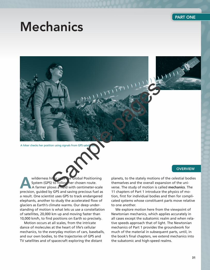
A wilderness hiker uses the Global Positioning System (GPS) to follow her chosen route. A farmer plows a field with centimeter-scale

precision, guided by GPS and saving precious fuel as a result. One scientist uses GPS to track endangered elephants, another to study the accelerated flow of glaciers as Earth’s climate warms. Our deep under-standing of motion is what lets us use a constellation of satellites, 20,000 km up and moving faster than 10,000 km/h, to find positions on Earth so precisely.

Motion occurs at all scales, from the intricate dance of molecules at the heart of life’s cellular mechanics, to the everyday motion of cars, baseballs, and our own bodies, to the trajectories of GPS and TV satellites and of spacecraft exploring the distant

planets, to the stately motions of the celestial bodies themselves and the overall expansion of the uni-verse. The study of motion is called mechanics. The 11 chapters of Part 1 introduce the physics of mo-tion, first for individual bodies and then for compli-cated systems whose constituent parts move relative to one another.

We explore motion here from the viewpoint of Newtonian mechanics, which applies accurately in all cases except the subatomic realm and when rela-tive speeds approach that of light. The Newtonian mechanics of Part 1 provides the groundwork for much of the material in subsequent parts, until, in the book’s final chapters, we extend mechanics into the subatomic and high-speed realms.

A hiker checks her position using signals from GPS satellites.

31

M02_WOLF0141_04_GE_C02.indd 31 08/05/20 4:37 PM

Sample

page

s

Learning OutcomesAfter finishing this chapter, you should be able to:

LO 2.1 Define fundamental motion concepts: position, velocity, acceleration.

LO 2.2 Distinguish instantaneous from average velocity and acceleration.

LO 2.3 Determine velocity and position when acceleration is constant.

LO 2.4 Describe how gravity near Earth’s surface provides an example of constant acceleration.

LO 2.5 Use calculus to deal with nonconstant acceleration.

Skills & Knowledge You’ll Need■■ Units for measuring space and time

(Section 1.2)

■■ Working with numbers using scien-tific notation and significant figures (Section 1.3)

■■ Your background in algebra and in-troductory calculus

Motion in a Straight Line

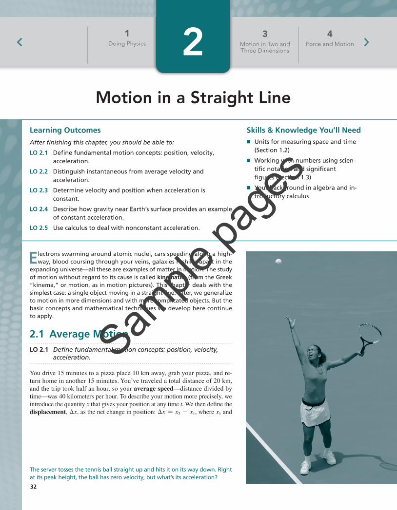
The server tosses the tennis ball straight up and hits it on its way down. Right at its peak height, the ball has zero velocity, but what’s its acceleration?

Electrons swarming around atomic nuclei, cars speeding along a high-way, blood coursing through your veins, galaxies rushing apart in the

expanding universe—all these are examples of matter in motion. The study of motion without regard to its cause is called kinematics (from the Greek “kinema,” or motion, as in motion pictures). This chapter deals with the simplest case: a single object moving in a straight line. Later, we generalize to motion in more dimensions and with more complicated objects. But the basic concepts and mathematical techniques we develop here continue to apply.

2.1 Average MotionLO 2.1 Define fundamental motion concepts: position, velocity,

acceleration.

You drive 15 minutes to a pizza place 10 km away, grab your pizza, and re-turn home in another 15 minutes. You’ve traveled a total distance of 20 km, and the trip took half an hour, so your average speed—distance divided by time—was 40 kilometers per hour. To describe your motion more precisely, we introduce the quantity x that gives your position at any time t. We then define the displacement, ∆x, as the net change in position: ∆x = x2 - x1, where x1 and

1 Doing Physics

4 Force and Motion

3 Motion in Two and Three Dimensions2

32

M02_WOLF0141_04_GE_C02.indd 32 08/05/20 4:37 PM

Sample

page

s

2.1 Average Motion 33

x2 are your starting and ending positions, respectively. Your average velocity, v, is displace-ment divided by the time interval:

v =∆x∆t 1average velocity2 (2.1)

where ∆t = t2 - t1 is the interval between your ending and starting times. The bar in v indicates an average quantity (and is read “v bar”). The symbol ∆ (capital Greek delta) stands for “the change in.” For the round trip to the pizza place, your overall displacement was zero, and therefore your average velocity was also zero—even though your average speed was not (Fig. 2.1).

Directions and Coordinate SystemsIt matters whether you go north or south, east or west. Displacement therefore includes not only how far but also in what direction. For motion in a straight line, we can describe both properties by taking position coordinates x to be positive going in one direction from some origin, and negative in the other. This gives us a one-dimensional coordinate system. The choice of coordinate system—both of origin and of which direction is positive—is entirely up to you. The coordinate system isn’t physically real; it’s just a convenience we create to help in the mathematical description of motion.

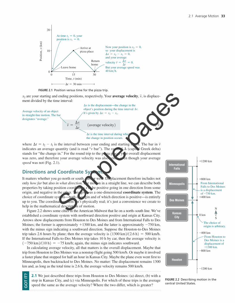
Figure 2.2 shows some cities in the American Midwest that lie on a north–south line. We’ve established a coordinate system with northward direction positive and origin at Kansas City. Arrows show displacements from Houston to Des Moines and from International Falls to Des Moines; the former is approximately +1300 km, and the latter is approximately -750 km, with the minus sign indicating a southward direction. Suppose the Houston-to-Des Moines trip takes 2.6 hours by plane; then the average velocity is 11300 km2/12.6 h2 = 500 km/h. If the International Falls-to-Des Moines trip takes 10 h by car, then the average velocity is 1-750 km2/110 h2 = -75 km/h; again, the minus sign indicates southward.

In calculating average velocity, all that matters is the overall displacement. Maybe that trip from Houston to Des Moines was a nonstop flight going 500 km/h. Or maybe it involved a faster plane that stopped for half an hour in Kansas City. Maybe the plane even went first to Minneapolis, then backtracked to Des Moines. No matter: The displacement remains 1300 km and, as long as the total time is 2.6 h, the average velocity remains 500 km/h.

∆x is the displacement—the change in the object’s position during the time interval ∆t. It’s given by ∆x = x2 - x1.Average velocity of an object

in straight-line motion. The bar designates “average.”

∆t is the time interval during which the change in position occurs.

0

10

150

Leave home

Arrive atpizza place

Returnhome

Time, t (min)

∆t = 30 min

Posi

tion,

x (

km)

30

20

At time t1 = 0, yourposition is x1 = 0.

Now your position is x2 = 0,so your displacement is∆x = x2 - x1 = 0,and your average

velocity v = = 0.

But your average speed was40 km>h.

∆x∆t

FIGURE 2.1 Position versus time for the pizza trip.

From Houston toDes Moines is adisplacement of+1300 km.

The choice oforigin is arbitrary.

+1200 km

+800 km

+400 km

0 km

-400 km

-800 km

-1200 km

N

S

From InternationalFalls to Des Moinesis a displacementof -750 km.

FIGURE 2.2 Describing motion in the central United States.

2.1 We just described three trips from Houston to Des Moines: (a) direct, (b) with a stop in Kansas City, and (c) via Minneapolis. For which of these trips is the average speed the same as the average velocity? Where the two differ, which is greater?G

OT

IT?

M02_WOLF0141_04_GE_C02.indd 33 08/05/20 4:37 PM

Sample

page

s

34 Chapter 2 Motion in a Straight Line

To get a cheap flight from Houston to Kansas City—a distance of 1000 km—you have to connect in Minneapolis, 700 km north of Kansas City. The flight to Minneapolis takes 2.2 h, then you have a 30-min layover, and then a 1.3-h flight to Kansas City. What are your average velocity and your average speed on this trip?

INTERPRET We interpret this as a one-dimensional kinematics problem involving the distinction between velocity and speed, and we identify three distinct travel segments: the two f lights and the layover. We identify the key concepts as speed and velocity; their distinction is clear from our pizza example.

DEVELOP Figure 2.2 is our drawing. We determine that Equation 2.1, v = ∆x/∆t, will give the average velocity, and that the average speed is the total distance divided by the total time. We develop our plan: Find the displacement and the total time, and use those values to get the average velocity; then find the total distance traveled and use that along with the total time to get the average speed.

EVALUATE You start in Houston and end up in Kansas City, for a displace-ment of 1000 km—regardless of how far you actually traveled. The total time for the three segments is ∆t = 2.2 h + 0.50 h + 1.3 h = 4.0 h. Then the average velocity, from Equation 2.1, is

v =∆x∆t

=1000 km

4.0 h= 250 km/h

However, that Minneapolis connection means you’ve gone an extra 2 * 700 km, for a total distance of 2400 km in 4 h. Thus your average speed is 12400 km2/14.0 h2 = 600 km/h, more than twice your aver-age velocity.

ASSESS Make sense? Average velocity depends only on the net dis-placement between the starting and ending points. Average speed takes into account the actual distance you travel—which can be a lot longer on a circuitous trip like this one. So it’s entirely reasonable that the average speed should be greater.

Speed and Velocity: Flying with a ConnectionEXAMPLE 2.1

2.2 Instantaneous VelocityLO 2.2 Distinguish instantaneous from average velocity and acceleration.

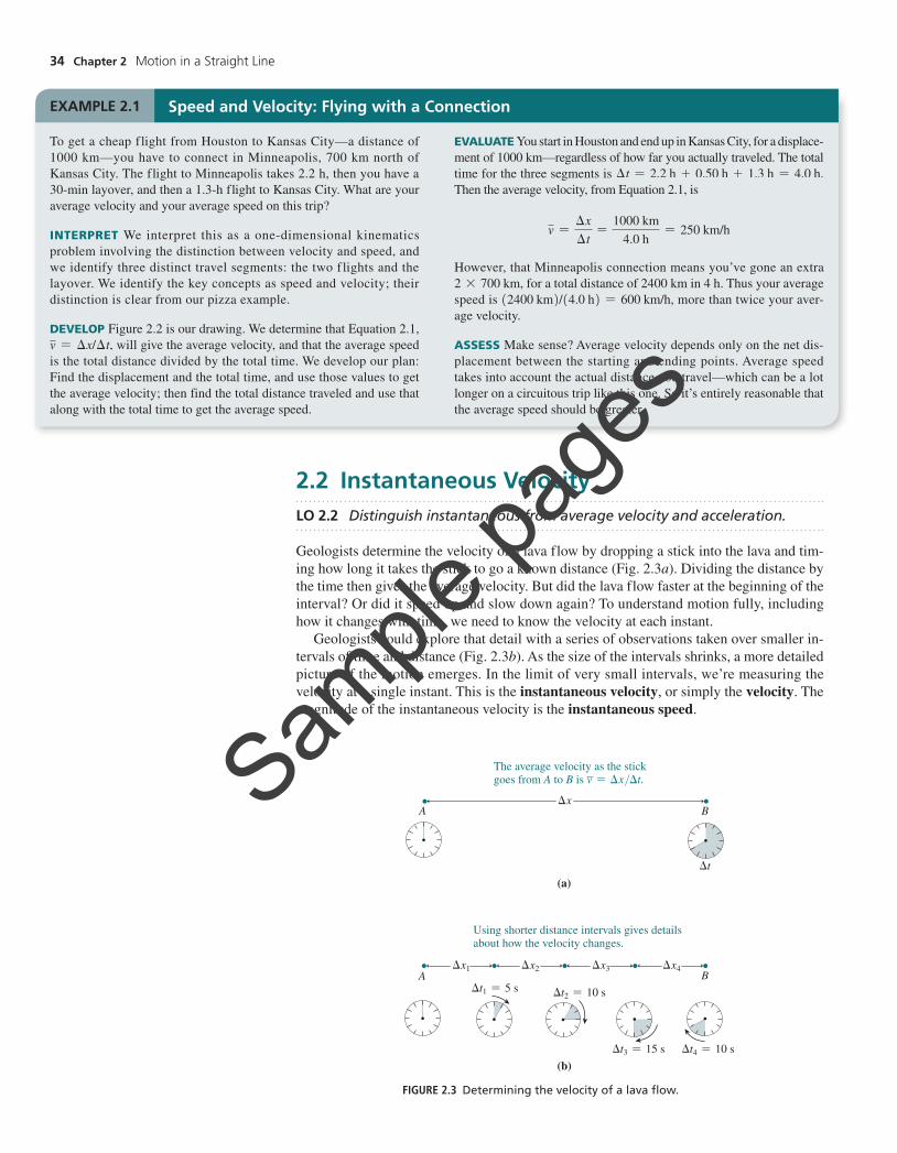
Geologists determine the velocity of a lava flow by dropping a stick into the lava and tim-ing how long it takes the stick to go a known distance (Fig. 2.3a). Dividing the distance by the time then gives the average velocity. But did the lava flow faster at the beginning of the interval? Or did it speed up and slow down again? To understand motion fully, including how it changes with time, we need to know the velocity at each instant.

Geologists could explore that detail with a series of observations taken over smaller in-tervals of time and distance (Fig. 2.3b). As the size of the intervals shrinks, a more detailed picture of the motion emerges. In the limit of very small intervals, we’re measuring the velocity at a single instant. This is the instantaneous velocity, or simply the velocity. The magnitude of the instantaneous velocity is the instantaneous speed.

The average velocity as the stick goes from A to B is v = ∆x>∆t.

Using shorter distance intervals gives details about how the velocity changes.

(a)

(b)

∆t

A B∆x

∆t1 = 5 s ∆t2 = 10 s

∆t3 = 15 s ∆t4 = 10 s

∆x1 ∆x2 ∆x3 ∆x4A B

FIGURE 2.3 Determining the velocity of a lava flow.

M02_WOLF0141_04_GE_C02.indd 34 08/05/20 4:37 PM

Sample

page

s

2.2 Instantaneous Velocity 35

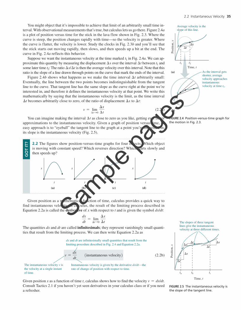
Given position x as a function of time t, calculus shows how to find the velocity v = dx/dt. Consult Tactics 2.1 if you haven’t yet seen derivatives in your calculus class or if you need a refresher.

Average velocity is theslope of this line.

As the interval getsshorter, average velocity approaches instantaneousvelocity at time t1.

(a)

(b)

Time, t

Posi

tion,

x

∆x∆t

t1 t2

t1

FIGURE 2.4 Position-versus-time graph for the motion in Fig. 2.3.

The slopes of three tangentlines give the instantaneousvelocity at three different times.

Time, t

Posi

tion,

x

ta tb tc

∆t

∆t

∆t

∆x

∆x∆x

FIGURE 2.5 The instantaneous velocity is the slope of the tangent line.

2.2 The figures show position-versus-time graphs for four objects. Which object is moving with constant speed? Which reverses direction? Which starts slowly and then speeds up?

t

x

t

x

(a)

t

x

(c)(b)

t

(d)

x

GO

T IT

?You might object that it’s impossible to achieve that limit of an arbitrarily small time in-

terval. With observational measurements that’s true, but calculus lets us go there. Figure 2.4a is a plot of position versus time for the stick in the lava flow shown in Fig. 2.3. Where the curve is steep, the position changes rapidly with time—so the velocity is greater. Where the curve is flatter, the velocity is lower. Study the clocks in Fig. 2.3b and you’ll see that the stick starts out moving rapidly, then slows, and then speeds up a bit at the end. The curve in Fig. 2.4a reflects this behavior.

Suppose we want the instantaneous velocity at the time marked t1 in Fig. 2.4a. We can ap-proximate this quantity by measuring the displacement ∆x over the interval ∆t between t1 and some later time t2: The ratio ∆x/∆t is then the average velocity over this interval. Note that this ratio is the slope of a line drawn through points on the curve that mark the ends of the interval.

Figure 2.4b shows what happens as we make the time interval ∆t arbitrarily small: Eventually, the line between the two points becomes indistinguishable from the tangent line to the curve. That tangent line has the same slope as the curve right at the point we’re interested in, and therefore it defines the instantaneous velocity at that point. We write this mathematically by saying that the instantaneous velocity is the limit, as the time interval ∆t becomes arbitrarily close to zero, of the ratio of displacement ∆x to ∆t:

v = lim∆tS0

∆x∆t

(2.2a)

You can imagine making the interval ∆t as close to zero as you like, getting ever better approximations to the instantaneous velocity. Given a graph of position versus time, an easy approach is to “eyeball” the tangent line to the graph at a point you’re interested in; its slope is the instantaneous velocity (Fig. 2.5).

Given position as a mathematical function of time, calculus provides a quick way to find instantaneous velocity. In calculus, the result of the limiting process described in Equation 2.2a is called the derivative of x with respect to t and is given the symbol dx/dt:

dxdt

= lim∆tS0

∆x∆t

The quantities dx and dt are called infinitesimals; they represent vanishingly small quanti-ties that result from the limiting process. We can then write Equation 2.2a as

v =dxdt 1instantaneous velocity2 (2.2b)

Instantaneous velocity is given by the derivative dx/dt—the rate of change of position with respect to time.

The instantaneous velocity v is the velocity at a single instant of time.

dx and dt are infinitesimally small quantities that result from the limiting procedure described in Fig. 2.4 and Equation 2.2a.

M02_WOLF0141_04_GE_C02.indd 35 08/05/20 4:37 PM

Sample

page

s


EXAMPLE 2.2 Instantaneous Velocity: A Rocket Ascends

The altitude of a rocket in the first half-minute of its ascent is given by x = bt2, where the constant b is 2.90 m/s2. Find a general expression for the rocket’s velocity as a function of time and from it the instan-taneous velocity at t = 20 s. Also find an expression for the average velocity, and compare your two velocity expressions.

INTERPRET We interpret this as a problem involving the compari-son of two distinct but related concepts: instantaneous velocity and average velocity. We identify the rocket as the object whose veloc-ities we’re interested in.

DEVELOP Equation 2.2b, v = dx/dt, gives the instantaneous veloc-ity, and Equation 2.1, v = ∆x/∆t, gives the average velocity. Our plan is to use Equation 2.3, dx/dt = nbtn-1, to evaluate the derivative that gives the instantaneous velocity. Then we can use Equation 2.1 for the average velocity, but first we’ll need to determine the displacement from the equation we’re given for the rocket’s position.

EVALUATE Applying Equation 2.2b with position given by x = bt2 and using Equation 2.3 to evaluate the derivative, we have

v =dxdt

=d1bt22

dt= 2bt

for the instantaneous velocity. Evaluating at time t = 20 s with b = 2.90 m/s2 gives v = 116 m/s. For the average velocity we need the total displacement at 20 s. Since x = bt2, Equation 2.1 gives

v =∆x∆t

=bt2

t= bt

where we’ve used x = bt2 for ∆x and t for ∆t because both position and time are taken to be zero at liftoff. Comparison with our earlier re-sult shows that the average velocity from liftoff to any particular time is exactly half the instantaneous velocity at that time.

ASSESS Make sense? Yes: The rocket’s speed is always increasing, so its velocity at the end of any time interval is greater than the average velocity over that interval. The fact that the average velocity is exactly half the instantaneous velocity results from the quadratic 1t22 depen-dence of position on time.

LANGUAGE Language often holds clues to the meaning of physical concepts. In this example we speak of the instantaneous velocity at a particular time. That wording should remind you of the limiting process that focuses on a single instant. In contrast, we speak of the average velocity over a time interval, since averaging explicitly involves a range of times.

Tactics 2.1 TAKING DERIVATIVES

You don’t have to go through an elaborate limiting process every time you want to find an instantaneous ve-locity. That’s because calculus provides formulas for the derivatives of common functions. For example, any function of the form x = btn, where b and n are constants, has the derivative

dxdt

= nbtn-1 (2.3)

Appendix A lists derivatives of other common functions.

where ∆v is the change in velocity and the bar on a indicates that this is an average value. Just as we defined instantaneous velocity through a limiting procedure, we define instantaneous acceleration as

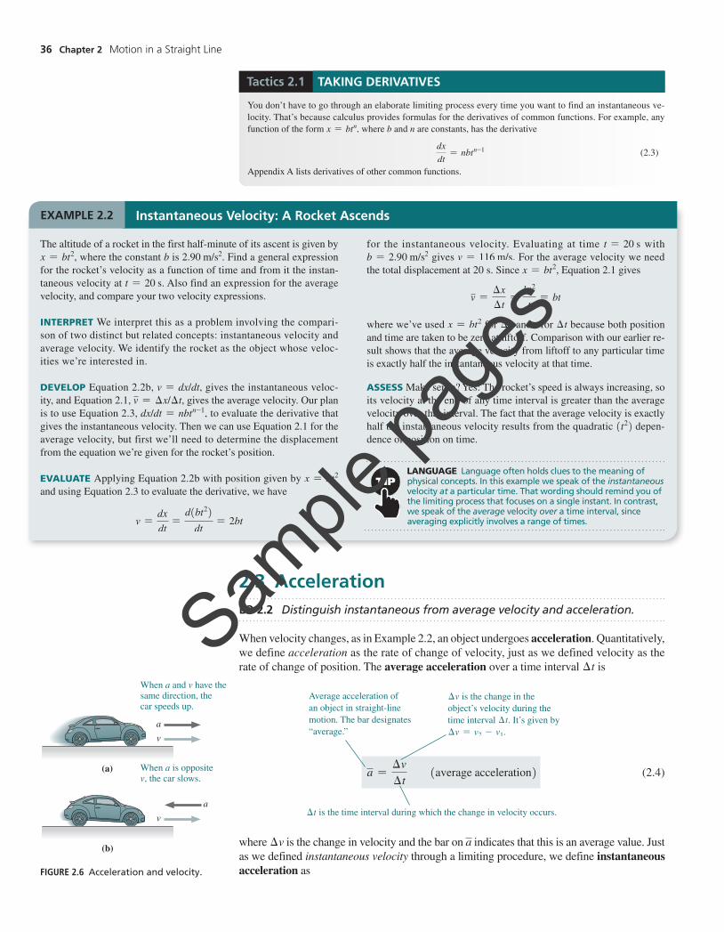
When a and v have thesame direction, the car speeds up.

When a is oppositev, the car slows.

(a)

(b)

v

a

v

a

FIGURE 2.6 Acceleration and velocity.

2.3 AccelerationLO 2.2 Distinguish instantaneous from average velocity and acceleration.

When velocity changes, as in Example 2.2, an object undergoes acceleration. Quantitatively, we define acceleration as the rate of change of velocity, just as we defined velocity as the rate of change of position. The average acceleration over a time interval ∆t is

a =∆v∆t 1average acceleration2 (2.4)

Average acceleration of an object in straight-line motion. The bar designates “average.”

∆t is the time interval during which the change in velocity occurs.

∆v is the change in the object’s velocity during the time interval ∆t. It’s given by ∆v = v2 - v1.

M02_WOLF0141_04_GE_C02.indd 36 08/05/20 4:37 PM

Sample

page

s

2.3 Acceleration 37

a = lim∆tS0

∆v∆t

=dvdt 1instantaneous acceleration2 (2.5)

As we did with velocity, we also use the term acceleration alone to mean instantaneous acceleration.

In one-dimensional motion, acceleration is either in the direction of the velocity or opposite it. In the former case the accelerating object speeds up, whereas in the latter it slows (Fig. 2.6). Although slowing is sometimes called deceleration, it’s simpler to use acceleration to describe the time rate of change of velocity no matter what’s happening. With two-dimensional motion, we’ll find much richer relationships between the directions of velocity and acceleration.

Since acceleration is the rate of change of velocity, its units are (distance per time) per time, or distance/time2. In SI, that’s m/s2. Sometimes acceleration is given in mixed units; for example, a car going from 0 to 60 mi/h in 10 s has an average acceleration of 6 mi/h/s.

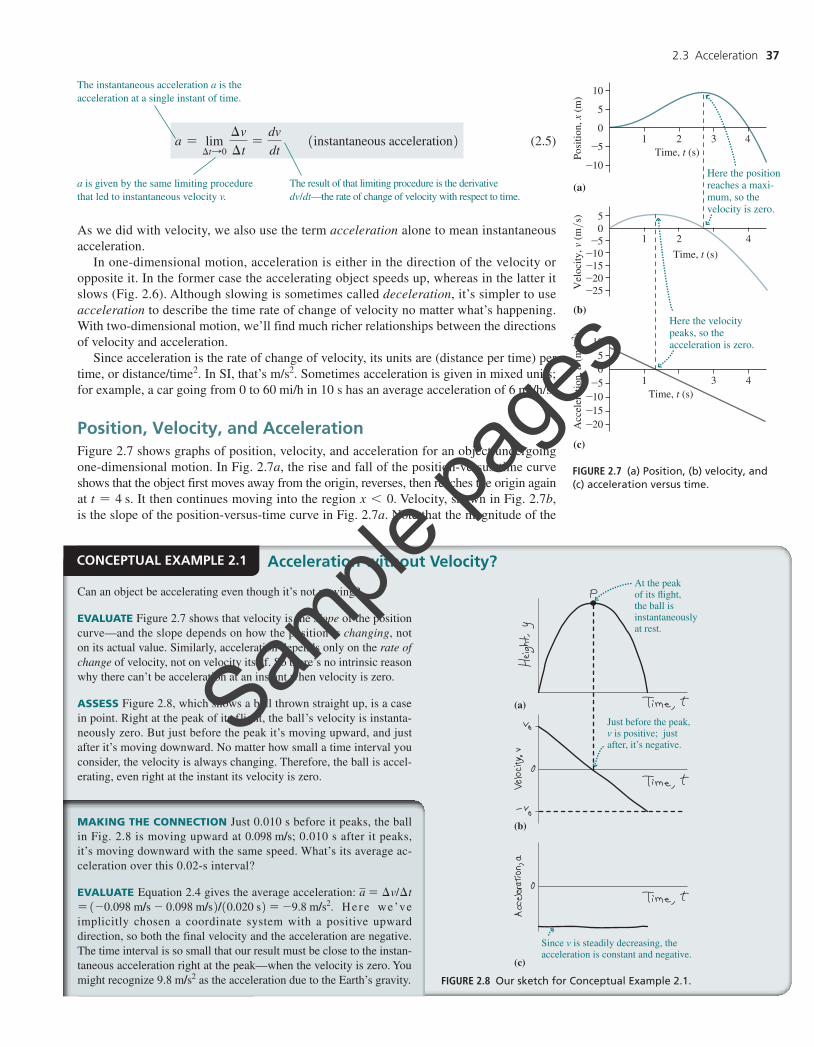
Position, Velocity, and AccelerationFigure 2.7 shows graphs of position, velocity, and acceleration for an object undergoing one-dimensional motion. In Fig. 2.7a, the rise and fall of the position-versus-time curve shows that the object first moves away from the origin, reverses, then reaches the origin again at t = 4 s. It then continues moving into the region x 6 0. Velocity, shown in Fig. 2.7b, is the slope of the position-versus-time curve in Fig. 2.7a. Note that the magnitude of the

Here the positionreaches a maxi-mum, so the velocity is zero.

Here the velocitypeaks, so the acceleration is zero.

(a)

(b)

(c)

10

50

-5-10-15-20-25

1050

-5-10-15-20

5

0

-5

-10

Vel

ocity

, v (

m>s)

Posi

tion,

x (

m)

Acc

eler

atio

n, a

(m>s2 )

1 2 3 4

1 2 4

1 3 4

Time, t (s)

Time, t (s)

Time, t (s)

FIGURE 2.7 (a) Position, (b) velocity, and (c) acceleration versus time.

The instantaneous acceleration a is the acceleration at a single instant of time.

The result of that limiting procedure is the derivative dv/dt—the rate of change of velocity with respect to time.

a is given by the same limiting procedure that led to instantaneous velocity v.

CONCEPTUAL EXAMPLE 2.1 Acceleration without Velocity?At the peak of its flight, the ball is instantaneously at rest.

Just before the peak,v is positive; justafter, it’s negative.

Since v is steadily decreasing, the acceleration is constant and negative.

(a)

(b)

(c)

Can an object be accelerating even though it’s not moving?

EVALUATE Figure 2.7 shows that velocity is the slope of the position curve—and the slope depends on how the position is changing, not on its actual value. Similarly, acceleration depends only on the rate of change of velocity, not on velocity itself. So there’s no intrinsic reason why there can’t be acceleration at an instant when velocity is zero.

ASSESS Figure 2.8, which shows a ball thrown straight up, is a case in point. Right at the peak of its flight, the ball’s velocity is instanta-neously zero. But just before the peak it’s moving upward, and just after it’s moving downward. No matter how small a time interval you consider, the velocity is always changing. Therefore, the ball is accel-erating, even right at the instant its velocity is zero.

MAKING THE CONNECTION Just 0.010 s before it peaks, the ball in Fig. 2.8 is moving upward at 0.098 m/s; 0.010 s after it peaks, it’s moving downward with the same speed. What’s its average ac-celeration over this 0.02-s interval?

EVALUATE Equation 2.4 gives the average acceleration: a = ∆v/∆t = 1-0.098 m/s - 0.098 m/s2/10.020 s2 = -9.8 m/s2. Here we’ve implicitly chosen a coordinate system with a positive upward direction, so both the final velocity and the acceleration are negative. The time interval is so small that our result must be close to the instan-taneous acceleration right at the peak—when the velocity is zero. You might recognize 9.8 m/s2 as the acceleration due to the Earth’s gravity. FIGURE 2.8 Our sketch for Conceptual Example 2.1.

M02_WOLF0141_04_GE_C02.indd 37 08/05/20 4:37 PM

Sample

page

s


velocity (that is, the speed) is large where the curve in Fig. 2.7a is steep—that is, where posi-tion is changing most rapidly. At the peak of the position curve, the object is momentarily at rest as it reverses, so there the position curve is flat and the velocity is zero. After the object reverses, at about 2.7 s, it’s heading in the negative x-direction, and so its velocity is negative.

Just as velocity is the slope of the position-versus-time curve, acceleration is the slope of the velocity-versus-time curve. Initially that slope is positive—velocity is increasing—but eventually it peaks at the point of maximum velocity and zero acceleration, and then it decreases. That velocity decrease corresponds to a negative acceleration, as shown clearly in the region of Fig. 2.7c beyond about 1.3 s.

Acceleration is the rate of change of velocity, and velocity is the rate of change of position. That makes acceleration the rate of change of the rate of change of position. Mathematically, acceleration is the second derivative of position with respect to time. Symbolically, we write the second derivative as d2x/dt2. Then the relationship among acceleration, velocity, and position can be written

a =dvdt

=ddt

adxdt

b =d2x

dt2 (2.6)

Equation 2.6 expresses acceleration in terms of position through the calculus operation of taking the second derivative. If you’ve studied integrals in calculus, you can see that it should be possible to go the opposite way, finding position as a function of time given acceleration as a function of time. In Section 2.4 we’ll do this for the special case of constant acceleration, al-though there we’ll take an algebra-based approach; Problem 93 obtains the same results using calculus. We’ll take a quick look at nonconstant acceleration in Section 2.6. The Application on this page provides an important technology that finds an object’s position from its acceleration.

2.3 An elevator is going up at constant speed, slows to a stop, then starts down and soon reaches the same constant speed it had going up. Is the elevator’s average accel-eration between its upward and downward constant-speed motions (a) zero, (b) down-ward, (c) first upward and then downward, or (d) first downward and then upward?

GO

T IT

?

2.4 Constant AccelerationLO 2.3 Determine velocity and position when acceleration is constant.

The description of motion has an especially simple form when acceleration is constant. Suppose an object starts at time t = 0 with some initial velocity v0 and constant accelera-tion a. Later, at some time t, it has velocity v. Because the acceleration doesn’t change, its average and instantaneous values are identical, so we can write

a = a =∆v∆t

=v - v0

t - 0or, rearranging,

v = v0 + at 1for constant acceleration only2 (2.7)

Velocity v as a function of time when acceleration a is constant.

Velocity changes linearly with time.

v0 is the initial velocity at time t = 0. Remember that this equation is only for the special case of constant acceleration!

SPECIAL CASES Many equations we develop are special cases of more general laws, and they’re limited to special circumstances. Equation 2.7 is a case in point: It applies only when acceleration is constant.

This equation says that the velocity changes from its initial value by an amount that is the product of acceleration and time.

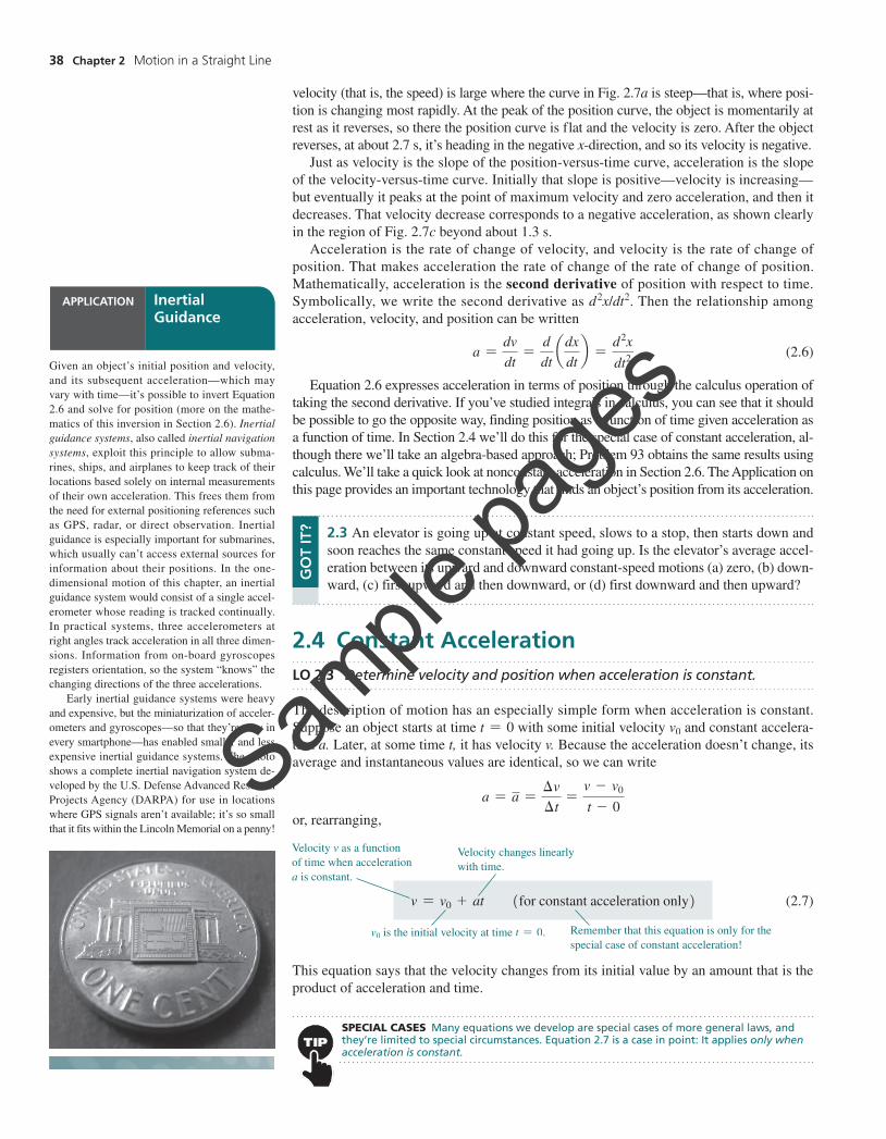
Given an object’s initial position and velocity, and its subsequent acceleration—which may vary with time—it’s possible to invert Equation 2.6 and solve for position (more on the mathe-matics of this inversion in Section 2.6). Inertial guidance systems, also called inertial navigation systems, exploit this principle to allow subma-rines, ships, and airplanes to keep track of their locations based solely on internal measurements of their own acceleration. This frees them from the need for external positioning references such as GPS, radar, or direct observation. Inertial guidance is especially important for submarines, which usually can’t access external sources for information about their positions. In the one- dimensional motion of this chapter, an inertial guidance system would consist of a single accel-erometer whose reading is tracked continually. In practical systems, three accelerometers at right angles track acceleration in all three dimen-sions. Information from on-board gyroscopes registers orientation, so the system “knows” the changing directions of the three accelerations.

Early inertial guidance systems were heavy and expensive, but the miniaturization of acceler-ometers and gyroscopes—so that they’re now in every smartphone—has enabled smaller and less expensive inertial guidance systems. The photo shows a complete inertial navigation system de-veloped by the U.S. Defense Advanced Research Projects Agency (DARPA) for use in locations where GPS signals aren’t available; it’s so small that it fits within the Lincoln Memorial on a penny!

APPLICATION Inertial Guidance

M02_WOLF0141_04_GE_C02.indd 38 08/05/20 4:37 PM

Sample

page

s

2.4 Constant Acceleration 39

Having determined velocity as a function of time, we now consider position. With con-stant acceleration, velocity increases steadily—and thus the average velocity over an interval is the average of the velocities at the beginning and the end of that interval. So we can write

v = 121v0 + v2 (2.8)

for the average velocity over the interval from t = 0 to some later time when the velocity is v. We can also write the average velocity as the change in position divided by the time interval. Suppose that at time 0 our object was at position x0. Then its average velocity over a time interval from 0 to time t is

v =∆x∆t

=x - x0

t - 0

where x is the object’s position at time t. Equating this expression for v with the expression in Equation 2.8 gives

x = x0 + vt = x0 + 121v0 + v2t (2.9)

But we already found the instantaneous velocity v that appears in this expression; it’s given by Equation 2.7. Substituting and simplifying then give the position as a function of time:

x = x0 + v0 t + 12 at2 1for constant acceleration only2 (2.10)

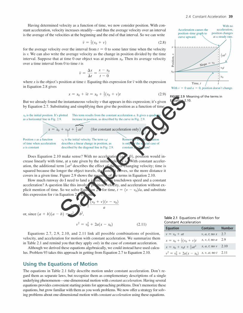
Does Equation 2.10 make sense? With no acceleration 1a = 02, position would in-crease linearly with time, at a rate given by the initial velocity v0. With constant acceler-ation, the additional term 12 at2 describes the effect of the ever-changing velocity; time is squared because the longer the object travels, the faster it moves, so the more distance it covers in a given time. Figure 2.9 shows the meaning of the terms in Equation 2.10.

How much runway do I need to land a jetliner, given touchdown speed and a constant acceleration? A question like this involves position, velocity, and acceleration without ex-plicit mention of time. So we solve Equation 2.7 for time, t = 1v - v02/a, and substitute this expression for t in Equation 2.9 to write

x - x0 = 12 1v0 + v21v - v02

a

or, since 1a + b21a - b2 = a2 - b2,

v2 = v02 + 2a1x - x02 (2.11)

Equations 2.7, 2.9, 2.10, and 2.11 link all possible combinations of position, velocity, and acceleration for motion with constant acceleration. We summarize them in Table 2.1 and remind you that they apply only in the case of constant acceleration.

Although we derived these equations algebraically, we could instead have used calcu-lus. Problem 93 takes this approach in getting from Equation 2.7 to Equation 2.10.

Using the Equations of MotionThe equations in Table 2.1 fully describe motion under constant acceleration. Don’t re-gard them as separate laws, but recognize them as complementary descriptions of a single underlying phenomenon—one-dimensional motion with constant acceleration. Having several equations provides convenient starting points for approaching problems. Don’t memorize these equations, but grow familiar with them as you work problems. We now offer a strategy for solv-ing problems about one-dimensional motion with constant acceleration using these equations.

x0 is the initial position. It’s plotted as a horizontal line in Fig. 2.9.

This term results from the constant acceleration a. It gives a quadratic increase in position, as described by the curve in Fig. 2.9.

Position x as a function of time when acceleration a is constant

v0 is the initial velocity. The term v0t describes a linear change in position, as described by the diagonal line in Fig. 2.9.

Remember that this equation is only for the special case of constant acceleration!

12

Acceleration causes theposition–time graph tocurve upward.

With noacceleration,

position changesat a steady rate.

With v = 0 and a = 0, position doesn’t change.

x

tTime, t

Posi

tion,

x

x0

v0tx0

Slope = v0

at2

FIGURE 2.9 Meaning of the terms in Equation 2.10.

Table 2.1 Equations of Motion for Constant Acceleration

Equation Contains Number

v = v0 + at v, a, t; no x 2.7

x = x0 + 121v0 + v2t x, v, t; no a 2.9

x = x0 + v0t + 12 at2 x, a, t; no v 2.10

v2 = v02 + 2a1x - x02 x, v, a; no t 2.11

}

M02_WOLF0141_04_GE_C02.indd 39 08/05/20 4:37 PM

Sample

page

s


The next two examples are typical of problems involving constant acceleration. Example 2.3 is a straightforward application of the equations we’ve just derived to a single object. Example 2.4 involves two objects, in which case we need to write equations de-scribing the motions of both objects.

INTERPRET Interpret the problem to be sure it asks about motion with constant acceleration. Next, identify the object(s) whose motion you’re interested in.

DEVELOP Draw a diagram with appropriate labels, and choose a coordinate system. For in-stance, sketch the initial and final physical situations, or draw a position-versus-time graph. Then determine which equations of motion from Table 2.1 contain the quantities you’re given and will be easiest to solve for the unknown(s).

EVALUATE Solve the equations in symbolic form and then evaluate numerical quantities.

ASSESS Does your answer make sense? Are the units correct? Do the numbers sound reason-able? What happens in special cases—for example, when a distance, velocity, acceleration, or time becomes very large or very small?

PROBLEM-SOLVING STRATEGY 2.1 Motion with Constant Acceleration

A jetliner touches down at 270 km/h. The plane then decelerates (i.e., undergoes acceleration directed opposite its velocity) at 4.5 m/s2. What’s the minimum runway length on which this aircraft can land?

INTERPRET We interpret this as being a problem about one- dimensional motion with constant acceleration and identify the airplane as the object of interest.

DEVELOP We determine that Equation 2.11, v2 = v02 + 2a1x - x02,

relates distance, velocity, and acceleration; so our plan is to solve that equation for the minimum runway length. We want the airplane to come to a stop, so the final velocity v is 0, and v0 is the initial touch-down velocity. If x0 is the touchdown point, then the quantity x - x0 is the distance we’re interested in; we’ll call this ∆x.

EVALUATE Setting v = 0 and solving Equation 2.11 then give

∆x =-v0

2

2a=

- 31270 km/h211000 m/km211/3600 h/s242

1221-4.5 m/s22 = 625 m

Note that we used a negative value for the acceleration because the plane’s acceleration is directed opposite its velocity—which we chose as the positive x-direction. We also converted the speed to m/s for compatibility with the SI units given for acceleration.

ASSESS Make sense? That 625 m is just over one-third of a mile, which seems a bit short. However, this is an absolute minimum with no margin of safety. For full-sized jetliners, the standard for minimum landing runway length is about 5000 feet or 1.5 km.

BE CAREFUL WITH MIXED UNITS Frequently, problems are stated in units other than SI. Although it’s possible to work consistently in other units, when in doubt, convert to SI. In this problem, the acceleration is originally in SI units but the velocity isn’t—a sure indication of the need for conversion.

EXAMPLE 2.3 Motion with Constant Acceleration: Landing a JetlinerWorked Example with Variation Problems

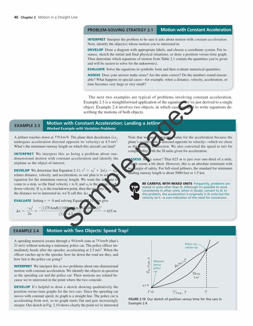
A speeding motorist zooms through a 50 km/h zone at 75 km/h (that’s 21 m/s) without noticing a stationary police car. The police officer im-mediately heads after the speeder, accelerating at 2.5 m/s2. When the officer catches up to the speeder, how far down the road are they, and how fast is the police car going?

INTERPRET We interpret this as two problems about one-dimensional motion with constant acceleration. We identify the objects in question as the speeding car and the police car. Their motions are related be-cause we’re interested in the point where the two coincide.

DEVELOP It’s helpful to draw a sketch showing qualitatively the position-versus-time graphs for the two cars. Since the speeding car moves with constant speed, its graph is a straight line. The police car is accelerating from rest, so its graph starts flat and gets increasingly steeper. Our sketch in Fig. 2.10 shows clearly the point we’re interested

EXAMPLE 2.4 Motion with Two Objects: Speed Trap!

FIGURE 2.10 Our sketch of position versus time for the cars in Example 2.4.

Motoristpassespolicecar.

Police carcatches up.

M02_WOLF0141_04_GE_C02.indd 40 08/05/20 4:37 PM

Sample

page

s

2.5 The Acceleration of Gravity 41

2.5 The Acceleration of GravityLO 2.4 Describe how gravity near Earth’s surface provides an example of

constant acceleration.

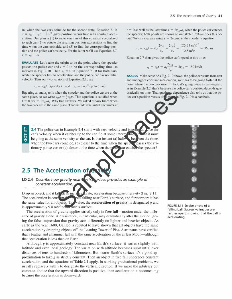
Drop an object, and it falls at an increasing rate, accelerating because of gravity (Fig. 2.11). The acceleration is constant for objects falling near Earth’s surface, and furthermore it has the same value for all objects. This value, the acceleration of gravity, is designated g and is approximately 9.8 m/s2 near Earth’s surface.

The acceleration of gravity applies strictly only in free fall—motion under the influ-ence of gravity alone. Air resistance, in particular, may dramatically alter the motion, giv-ing the false impression that gravity acts differently on lighter and heavier objects. As early as the year 1600, Galileo is reputed to have shown that all objects have the same acceleration by dropping objects off the Leaning Tower of Pisa. Astronauts have verified that a feather and a hammer fall with the same acceleration on the airless Moon—although that acceleration is less than on Earth.

Although g is approximately constant near Earth’s surface, it varies slightly with latitude and even local geology. The variation with altitude becomes substantial over distances of tens to hundreds of kilometers. But nearer Earth’s surface it’s a good ap-proximation to take g as strictly constant. Then an object in free fall undergoes constant acceleration, and the equations of Table 2.1 apply. In working gravitational problems, we usually replace x with y to designate the vertical direction. If we make the arbitrary but common choice that the upward direction is positive, then acceleration a becomes -g because the acceleration is downward.

in, when the two cars coincide for the second time. Equation 2.10, x = x0 + v0t + 1

2 at2, gives position versus time with constant accel-eration. Our plan is (1) to write versions of this equation specialized to each car, (2) to equate the resulting position expressions to find the time when the cars coincide, and (3) to find the corresponding posi-tion and the police car’s velocity. For the latter we’ll use Equation 2.7, v = v0 + at.

EVALUATE Let’s take the origin to be the point where the speeder passes the police car and t = 0 to be the corresponding time, as marked in Fig. 2.10. Then x0 = 0 in Equation 2.10 for both cars, while the speeder has no acceleration and the police car has no initial velocity. Thus our two versions of Equation 2.10 are

xs = vs0 t 1speeder2 and xp = 12 ap t

2 1police car2Equating xs and xp tells when the speeder and the police car are at the same place, so we write vs0 t = 1

2 ap t2. This equation is satisfied when

t = 0 or t = 2vs0 /ap. Why two answers? We asked for any times when the two cars are in the same place. That includes the initial encounter at

t = 0 as well as the later time t = 2vs0 /ap when the police car catches the speeder; both points are shown on our sketch. Where does this oc-cur? We can evaluate using t = 2vs0 /ap in the speeder’s equation:

xs = vs0 t = vs0 2vs0

ap=

2vs 02

ap=

122121 m/s22

2.5 m/s2 = 350 m

Equation 2.7 then gives the police car’s speed at this time:

vp = ap t = ap2vs0

ap= 2vs0 = 150 km/h

ASSESS Make sense? As Fig. 2.10 shows, the police car starts from rest and undergoes constant acceleration, so it has to be going faster at the point where the two cars meet. In fact, it’s going twice as fast—again, as in Example 2.2, that’s because the police car’s position depends qua-dratically on time. That quadratic dependence also tells us that the po-lice car’s position-versus-time graph in Fig. 2.10 is a parabola.

FIGURE 2.11 Strobe photo of a falling ball. Successive images are farther apart, showing that the ball is accelerating.

2.4 The police car in Example 2.4 starts with zero velocity and is going at twice the car’s velocity when it catches up to the car. So at some intermediate instant it must be going at the same velocity as the car. Is that instant (a) halfway between the times when the two cars coincide, (b) closer to the time when the speeder passes the sta-tionary police car, or (c) closer to the time when the police car catches the speeder?

GO

T IT

?

M02_WOLF0141_04_GE_C02.indd 41 08/05/20 4:37 PM

Sample

page

s


In Example 2.5 the diver was moving downward, and the downward gravitational accel-eration steadily increased his speed. But, as Conceptual Example 2.1 suggested, the accel-eration of gravity is downward regardless of an object’s motion. Throw a ball straight up, and it’s accelerating downward even while moving upward. Since velocity and acceleration are in opposite directions, the ball slows until it reaches its peak, then pauses instanta-neously, and then gains speed as it falls. All the while its acceleration is 9.8 m/s2 downward.

A diver drops from a 10-m-high cliff. At what speed does he enter the water, and how long is he in the air?

INTERPRET This is a case of constant acceleration due to gravity, and the diver is the object of interest. The diver drops a known dis-tance starting from rest, and we want to know the speed and time when he hits the water.

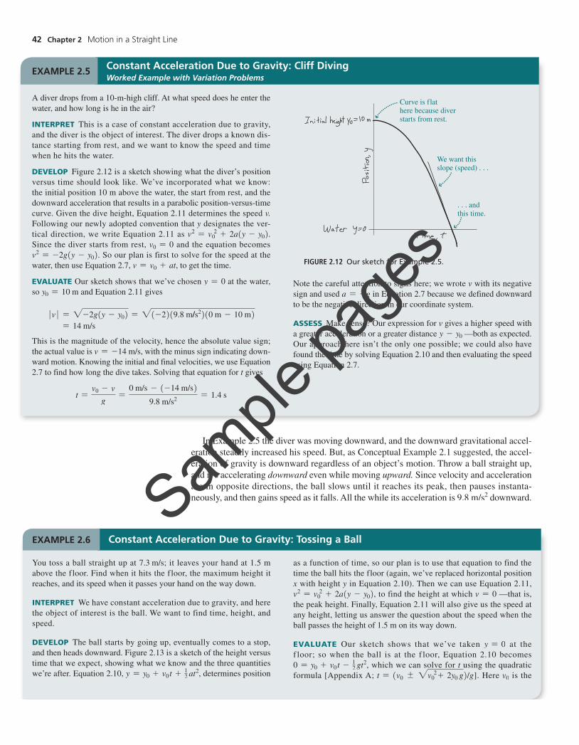
DEVELOP Figure 2.12 is a sketch showing what the diver’s position versus time should look like. We’ve incorporated what we know: the initial position 10 m above the water, the start from rest, and the downward acceleration that results in a parabolic position-versus-time curve. Given the dive height, Equation 2.11 determines the speed v. Following our newly adopted convention that y designates the ver-tical direction, we write Equation 2.11 as v2 = v 2

0 + 2a1y - y02. Since the diver starts from rest, v0 = 0 and the equation becomes v2 = -2g1y - y02. So our plan is first to solve for the speed at the water, then use Equation 2.7, v = v0 + at, to get the time.

EVALUATE Our sketch shows that we’ve chosen y = 0 at the water, so y0 = 10 m and Equation 2.11 gives

�v � = 2-2g1y - y02 = 21-2219.8 m/s2210 m - 10 m2 = 14 m/s

This is the magnitude of the velocity, hence the absolute value sign; the actual value is v = -14 m/s, with the minus sign indicating down-ward motion. Knowing the initial and final velocities, we use Equation 2.7 to find how long the dive takes. Solving that equation for t gives

t =v0 - v

g=

0 m/s - 1-14 m/s29.8 m/s2 = 1.4 s

Note the careful attention to signs here; we wrote v with its negative sign and used a = -g in Equation 2.7 because we defined downward to be the negative direction in our coordinate system.

ASSESS Make sense? Our expression for v gives a higher speed with a greater acceleration or a greater distance y - y0 —both as expected. Our approach here isn’t the only one possible; we could also have found the time by solving Equation 2.10 and then evaluating the speed using Equation 2.7.

EXAMPLE 2.5 Constant Acceleration Due to Gravity: Cliff DivingWorked Example with Variation Problems

Curve is flathere because diverstarts from rest.

We want this slope (speed) c

candthis time.

FIGURE 2.12 Our sketch for Example 2.5.

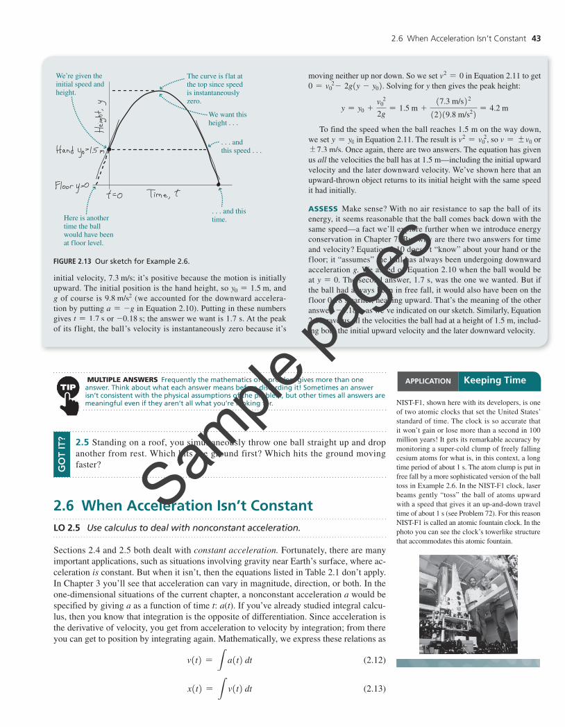
You toss a ball straight up at 7.3 m/s; it leaves your hand at 1.5 m above the floor. Find when it hits the floor, the maximum height it reaches, and its speed when it passes your hand on the way down.

INTERPRET We have constant acceleration due to gravity, and here the object of interest is the ball. We want to find time, height, and speed.

DEVELOP The ball starts by going up, eventually comes to a stop, and then heads downward. Figure 2.13 is a sketch of the height versus time that we expect, showing what we know and the three quantities we’re after. Equation 2.10, y = y0 + v0 t + 1

2 at2, determines position

as a function of time, so our plan is to use that equation to find the time the ball hits the floor (again, we’ve replaced horizontal position x with height y in Equation 2.10). Then we can use Equation 2.11, v2 = v0

2 + 2a1y - y02, to find the height at which v = 0 —that is, the peak height. Finally, Equation 2.11 will also give us the speed at any height, letting us answer the question about the speed when the ball passes the height of 1.5 m on its way down.

EVALUATE Our sketch shows that we’ve taken y = 0 at the f loor; so when the ball is at the f loor, Equation 2.10 becomes 0 = y0 + v0 t - 1

2 gt2, which we can solve for t using the quadratic formula [Appendix A; t = 1v0 { 2v0

2 + 2y0 g2/g]. Here v0 is the

EXAMPLE 2.6 Constant Acceleration Due to Gravity: Tossing a Ball

M02_WOLF0141_04_GE_C02.indd 42 08/05/20 4:37 PM

Sample

page

s

2.6 When Acceleration Isn’t Constant 43

initial velocity, 7.3 m/s; it’s positive because the motion is initially upward. The initial position is the hand height, so y0 = 1.5 m, and g of course is 9.8 m/s2 (we accounted for the downward accelera-tion by putting a = -g in Equation 2.10). Putting in these numbers gives t = 1.7 s or -0.18 s; the answer we want is 1.7 s. At the peak of its flight, the ball’s velocity is instantaneously zero because it’s

moving neither up nor down. So we set v2 = 0 in Equation 2.11 to get 0 = v0

2 - 2g1y - y02. Solving for y then gives the peak height:

y = y0 +v0

2

2g= 1.5 m +

17.3 m/s22

12219.8 m/s22 = 4.2 m

To find the speed when the ball reaches 1.5 m on the way down, we set y = y0 in Equation 2.11. The result is v2 = v0

2 , so v = {v0 or {7.3 m/s. Once again, there are two answers. The equation has given us all the velocities the ball has at 1.5 m—including the initial upward velocity and the later downward velocity. We’ve shown here that an upward-thrown object returns to its initial height with the same speed it had initially.

ASSESS Make sense? With no air resistance to sap the ball of its energy, it seems reasonable that the ball comes back down with the same speed—a fact we’ll explore further when we introduce energy conservation in Chapter 7. But why are there two answers for time and velocity? Equation 2.10 doesn’t “know” about your hand or the floor; it “assumes” the ball has always been undergoing downward acceleration g. We asked of Equation 2.10 when the ball would be at y = 0. The second answer, 1.7 s, was the one we wanted. But if the ball had always been in free fall, it would also have been on the floor 0.18 s earlier, heading upward. That’s the meaning of the other answer, -0.18 s, as we’ve indicated on our sketch. Similarly, Equation 2.11 gave us all the velocities the ball had at a height of 1.5 m, includ-ing both the initial upward velocity and the later downward velocity.

We’re given theinitial speed andheight.

Here is anothertime the ballwould have beenat floor level.

The curve is flat atthe top since speedis instantaneously zero.

We want thisheight c

candthis speed c

cand this time.

FIGURE 2.13 Our sketch for Example 2.6.

2.6 When Acceleration Isn’t ConstantLO 2.5 Use calculus to deal with nonconstant acceleration.

Sections 2.4 and 2.5 both dealt with constant acceleration. Fortunately, there are many important applications, such as situations involving gravity near Earth’s surface, where ac-celeration is constant. But when it isn’t, then the equations listed in Table 2.1 don’t apply. In Chapter 3 you’ll see that acceleration can vary in magnitude, direction, or both. In the one-dimensional situations of the current chapter, a nonconstant acceleration a would be specified by giving a as a function of time t: a(t). If you’ve already studied integral calcu-lus, then you know that integration is the opposite of differentiation. Since acceleration is the derivative of velocity, you get from acceleration to velocity by integration; from there you can get to position by integrating again. Mathematically, we express these relations as

v1t2 = La1t2 dt (2.12)

x1t2 = Lv1t2 dt (2.13)

MULTIPLE ANSWERS Frequently the mathematics of a problem gives more than one answer. Think about what each answer means before discarding it! Sometimes an answer isn’t consistent with the physical assumptions of the problem, but other times all answers are meaningful even if they aren’t all what you’re looking for.

2.5 Standing on a roof, you simultaneously throw one ball straight up and drop another from rest. Which hits the ground first? Which hits the ground moving faster?G

OT

IT?

NIST-F1, shown here with its developers, is one of two atomic clocks that set the United States’ standard of time. The clock is so accurate that it won’t gain or lose more than a second in 100 million years! It gets its remarkable accuracy by monitoring a super-cold clump of freely falling cesium atoms for what is, in this context, a long time period of about 1 s. The atom clump is put in free fall by a more sophisticated version of the ball toss in Example 2.6. In the NIST-F1 clock, laser beams gently “toss” the ball of atoms upward with a speed that gives it an up-and-down travel time of about 1 s (see Problem 72). For this reason NIST-F1 is called an atomic fountain clock. In the photo you can see the clock’s towerlike structure that accommodates this atomic fountain.

APPLICATION Keeping Time

M02_WOLF0141_04_GE_C02.indd 43 08/05/20 4:37 PM

Sample

page

s


These results don’t fully determine v and x; you also need to know the initial conditions (usu-ally, the values at time t = 0 ); these provide what are called in calculus the constants of inte-gration. In Problem 93, you can evaluate the integral in Equation 2.13 for the case of constant acceleration, giving an alternate derivation of Equations 2.7 and 2.10. Problems 88, 94, and 95 challenge you to use integral calculus to find an object’s position in the case of nonconstant accelerations, while Problem 96 explores the case of an exponentially decreasing acceleration.

Summary

Big Idea

The big ideas here are those of kinematics—the study of motion without regard to its cause. Position, velocity, and acceleration are the quantities that characterize motion:

Position Velocity

Rate ofchange

Rate ofchange

Acceleration

Key Concepts and EquationsAverage velocity and acceleration involve changes in position and velocity, respectively, oc-curring over a time interval ∆t:

v =∆x∆t

a =∆v∆t

Here ∆x is the displacement, or change in position, and ∆v is the change in velocity.Instantaneous values are the limits of infinitesimally small time intervals and are given

by calculus as the time derivatives of position and velocity:

v =dxdt

a =dvdt

∆t∆x

Time, t

Posi

tion,

x

This line’s slope is theaveragevelocity c

cand this line’s slope is the instantaneousvelocity.

∆t∆v

Time, t0

Vel

ocity

, v

cwhile theinstantaneousacceleration ais the slope of

this line.

The average acceleration ais this line’s slope c

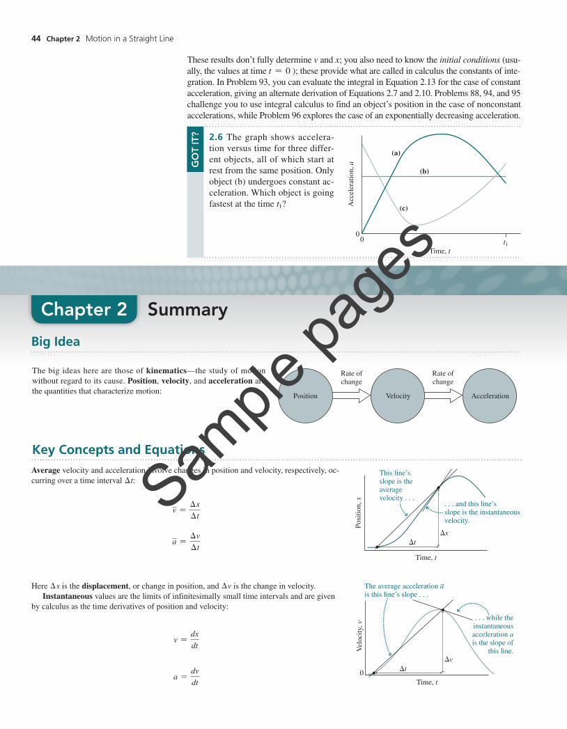
2.6 The graph shows accelera-tion versus time for three differ-ent objects, all of which start at rest from the same position. Only object (b) undergoes constant ac-celeration. Which object is going fastest at the time t1?

GO

T IT

?

(a)

(b)

(c)

0

Time, t

Acc

eler

atio

n, a

0 t1

Chapter 2

M02_WOLF0141_04_GE_C02.indd 44 08/05/20 4:37 PM

Sample

page

s

For Thought and Discussion 45

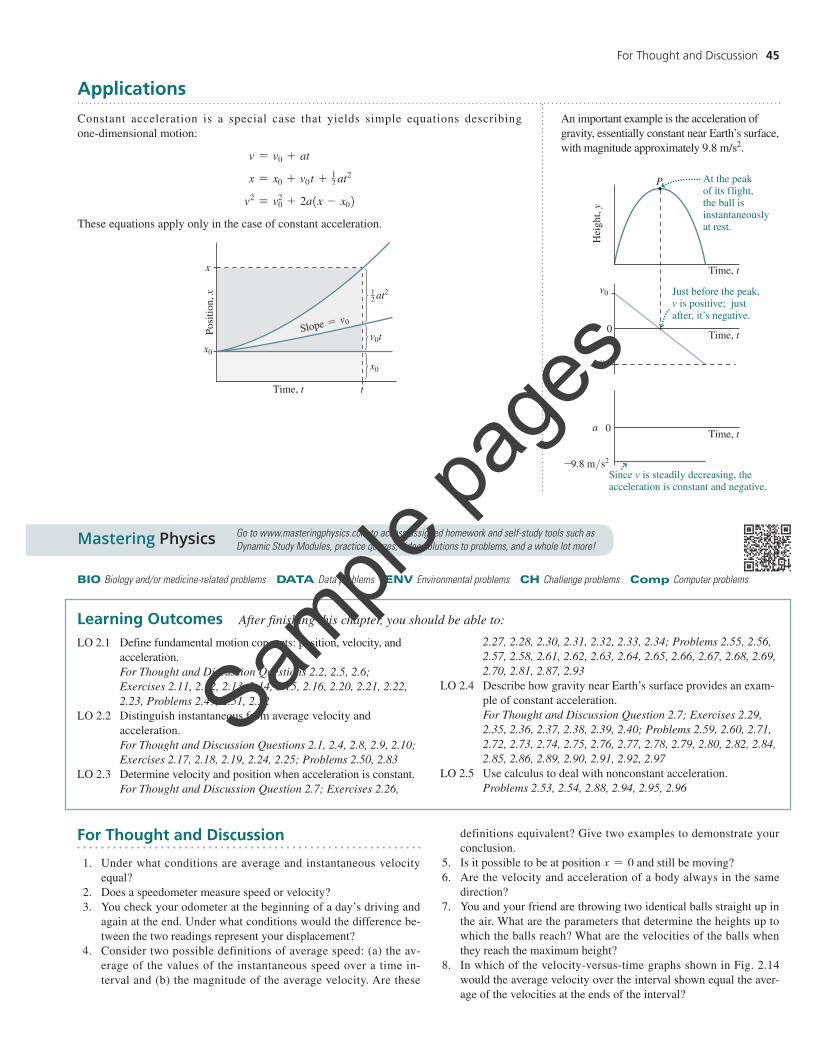
ApplicationsConstant acceleration is a special case that yields simple equations describing one-dimensional motion:

v = v0 + at

x = x0 + v0 t + 12 at2

v2 = v02 + 2a1x - x02

These equations apply only in the case of constant acceleration.

12

x

tTime, t

Posi

tion,

x

x0

v0tx0

Slope = v0

at2

An important example is the acceleration of gravity, essentially constant near Earth’s surface, with magnitude approximately 9.8 m/s2.

At the peak of its flight, the ball is instantaneously at rest.

Just before the peak,v is positive; justafter, it’s negative.

Since v is steadily decreasing, the acceleration is constant and negative.

v 0

v0

-v0

a 0

-9.8 m>s2

Hei

ght,

y

Time, t

Time, t

Time, t

P

LO 2.1 Define fundamental motion concepts: position, velocity, and acceleration.For Thought and Discussion Questions 2.2, 2.5, 2.6; Exercises 2.11, 2.12, 2.13, 2.14, 2.15, 2.16, 2.20, 2.21, 2.22, 2.23, Problems 2.49, 2.51, 2.52

LO 2.2 Distinguish instantaneous from average velocity and acceleration.For Thought and Discussion Questions 2.1, 2.4, 2.8, 2.9, 2.10; Exercises 2.17, 2.18, 2.19, 2.24, 2.25; Problems 2.50, 2.83

LO 2.3 Determine velocity and position when acceleration is constant.For Thought and Discussion Question 2.7; Exercises 2.26,

2.27, 2.28, 2.30, 2.31, 2.32, 2.33, 2.34; Problems 2.55, 2.56, 2.57, 2.58, 2.61, 2.62, 2.63, 2.64, 2.65, 2.66, 2.67, 2.68, 2.69, 2.70, 2.81, 2.87, 2.93

LO 2.4 Describe how gravity near Earth’s surface provides an exam-ple of constant acceleration.For Thought and Discussion Question 2.7; Exercises 2.29, 2.35, 2.36, 2.37, 2.38, 2.39, 2.40; Problems 2.59, 2.60, 2.71, 2.72, 2.73, 2.74, 2.75, 2.76, 2.77, 2.78, 2.79, 2.80, 2.82, 2.84, 2.85, 2.86, 2.89, 2.90, 2.91, 2.92, 2.97

LO 2.5 Use calculus to deal with nonconstant acceleration.Problems 2.53, 2.54, 2.88, 2.94, 2.95, 2.96

Mastering Physics Go to www.masteringphysics.com to access assigned homework and self-study tools such as Dynamic Study Modules, practice quizzes, video solutions to problems, and a whole lot more!

BIO Biology and/or medicine-related problems DATA Data problems ENV Environmental problems CH Challenge problems Comp Computer problems

Learning Outcomes After finishing this chapter, you should be able to:

For Thought and Discussion

1. Under what conditions are average and instantaneous velocity equal?

2. Does a speedometer measure speed or velocity?3. You check your odometer at the beginning of a day’s driving and

again at the end. Under what conditions would the difference be-tween the two readings represent your displacement?

4. Consider two possible definitions of average speed: (a) the av-erage of the values of the instantaneous speed over a time in-terval and (b) the magnitude of the average velocity. Are these

definitions equivalent? Give two examples to demonstrate your conclusion.

5. Is it possible to be at position x = 0 and still be moving?6. Are the velocity and acceleration of a body always in the same

direction?7. You and your friend are throwing two identical balls straight up in

the air. What are the parameters that determine the heights up to which the balls reach? What are the velocities of the balls when they reach the maximum height?

8. In which of the velocity-versus-time graphs shown in Fig. 2.14 would the average velocity over the interval shown equal the aver-age of the velocities at the ends of the interval?

M02_WOLF0141_04_GE_C02.indd 45 08/05/20 4:37 PM

Sample

page

s


b = 80 m/s, c = 4.9 m/s2, t is the time in seconds, and y is in me-ters. (a) Use differentiation to find a general expression for the rock-et’s velocity as a function of time. (b) When is the velocity zero?

Section 2.3 Acceleration20. You’re driving at the 50 km/h speed limit when you spot a sign

showing a speed-limit increase to 80 km/h. If it takes 15.7 s to reach the new speed limit, what’s your average acceleration? Express it in m/s2.

21. Starting from rest, a subway train first accelerates to 25 m/s and then brakes. Forty-eight seconds after starting, it’s moving at 18 m/s. What’s its average acceleration in this 48-s interval?

22. NASA’s New Horizons spacecraft was launched in 2006 and flew past Pluto in 2015. New Horizons’ solid-fuel booster rocket gave it an average acceleration of 6.16 m/s2, bringing it to a speed of 16.3 km/s before the booster dropped away. How long did this acceleration last?

23. An egg drops from a second-story window, taking 1.12 s to fall and reaching 11.0 m/s just before hitting the ground. On contact, the egg stops completely in 0.133 s. Calculate the magnitude of its average acceleration (a) while falling and (b) while stopping.

24. An airplane’s takeoff speed is 320 km/h. If its average accelera-tion is 2.9 m/s2, how much time is it accelerating down the run-way before it lifts off?

25. ThrustSSC, the world’s first supersonic car, accelerates from rest to 1000 km/h in 16 s. What’s its acceleration?

Section 2.4 Constant Acceleration26. You’re driving at 65 km/h when you apply constant acceleration

to pass another car. Twelve seconds later, you’re doing 85 km/h. How far did you go in this time?

27. Differentiate both sides of Equation 2.10, and show that you get Equation 2.7.

28. A 2016 study found that snakes’ heads, when striking, undergo average accelerations of about 40 m/s2, for a period of about 50 ms. Using these values, find (a) the maximum speed of the snake’s head and (b) the distance the head travels during the strike. Give your answers to one significant figure.

29. A rocket starts from rest and rises with constant acceleration to a height h, at which point it’s rising at speed v. Find expressions for (a) the rocket’s acceleration and (b) the time it takes to reach height h.

30. Starting from rest, a car accelerates at a constant rate, reaching 88 km/h in 12 s. Find (a) its acceleration and (b) how far it goes in this time.

31. A car initially moving at 90 km/h begins slowing at a constant rate 40 m short of a stoplight. If the car comes to a full stop just at the light, what is the magnitude of its acceleration?

32. In a medical X-ray tube, electrons are accelerated to a velocity of 108 m/s and then slammed into a tungsten target. As they stop, the electrons’ rapid acceleration produces X rays. Given that it takes an electron on the order of 1 ns to stop, estimate the dis-tance it moves while stopping.

33. California’s Bay Area Rapid Transit System (BART) uses an au-tomatic braking system triggered by earthquake warnings. The system is designed to prevent disastrous accidents involving trains traveling at a maximum of 112 km/h and carrying a total of some 45,000 passengers at rush hour. If it takes a train 24 s to brake to a stop, how much advance warning of an earthquake is needed to bring a 112-km/h train to a reasonably safe speed of 42 km/h when the earthquake strikes?

34. You’re driving at speed v0 when you spot a stationary moose on the road, a distance d ahead. Find an expression for the magni-tude of the acceleration you need if you’re to stop before hitting the moose.

BIO

BIO

5

Dis

tanc

e (m

) 4

3

2

1

1 2 3 4 5 6Time (s)

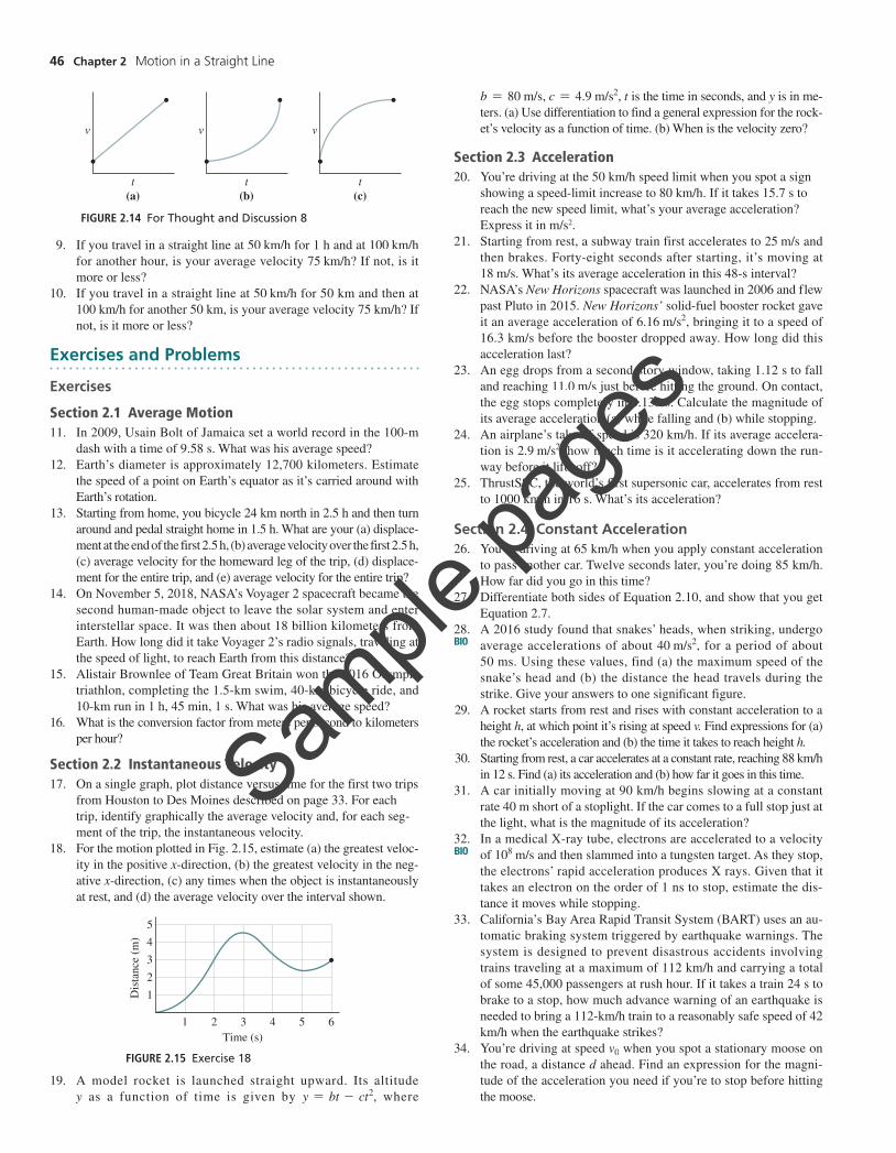
FIGURE 2.15 Exercise 18

9. If you travel in a straight line at 50 km/h for 1 h and at 100 km/h for another hour, is your average velocity 75 km/h? If not, is it more or less?

10. If you travel in a straight line at 50 km/h for 50 km and then at 100 km/h for another 50 km, is your average velocity 75 km/h? If not, is it more or less?

Exercises and Problems

Exercises

Section 2.1 Average Motion11. In 2009, Usain Bolt of Jamaica set a world record in the 100-m

dash with a time of 9.58 s. What was his average speed?12. Earth’s diameter is approximately 12,700 kilometers. Estimate

the speed of a point on Earth’s equator as it’s carried around with Earth’s rotation.

13. Starting from home, you bicycle 24 km north in 2.5 h and then turn around and pedal straight home in 1.5 h. What are your (a) displace-ment at the end of the first 2.5 h, (b) average velocity over the first 2.5 h, (c) average velocity for the homeward leg of the trip, (d) displace-ment for the entire trip, and (e) average velocity for the entire trip?

14. On November 5, 2018, NASA’s Voyager 2 spacecraft became the second human-made object to leave the solar system and enter interstellar space. It was then about 18 billion kilometers from Earth. How long did it take Voyager 2’s radio signals, traveling at the speed of light, to reach Earth from this distance?

15. Alistair Brownlee of Team Great Britain won the 2016 Olympic triathlon, completing the 1.5-km swim, 40-km bicycle ride, and 10-km run in 1 h, 45 min, 1 s. What was his average speed?

16. What is the conversion factor from meters per second to kilometers per hour?

Section 2.2 Instantaneous Velocity17. On a single graph, plot distance versus time for the first two trips

from Houston to Des Moines described on page 33. For each trip, identify graphically the average velocity and, for each seg-ment of the trip, the instantaneous velocity.

18. For the motion plotted in Fig. 2.15, estimate (a) the greatest veloc-ity in the positive x-direction, (b) the greatest velocity in the neg-ative x-direction, (c) any times when the object is instantaneously at rest, and (d) the average velocity over the interval shown.

v

t(a)

v

t(b)

v

t(c)

FIGURE 2.14 For Thought and Discussion 8

19. A model rocket is launched straight upward. Its altitude y as a function of time is given by y = bt - ct2, where

M02_WOLF0141_04_GE_C02.indd 46 08/05/20 4:37 PM

Sample

page

s

Exercises and Problems 47

Section 2.5 The Acceleration of Gravity35. A delivery drone drops a package onto a customer’s porch. If the

package can withstand a maximum impact speed of 8.00 m/s, what’s the maximum height from which the drone can drop the package?

36. Your friend is sitting 5.1 m above you on a tree branch. How fast should you throw an apple so it just reaches her?

37. A model rocket leaves the ground, heading straight up with speed v. Find expressions for (a) its maximum altitude and (b) its speed when it’s at half the maximum altitude.

38. A foul ball leaves the bat going straight up at 29 m/s. (a) How high does it rise? (b) How long is it in the air? Neglect the dis-tance between bat and ground.

39. A Frisbee is lodged in a tree 6.4 m above the ground. A rock thrown from below must be going at least 3 m/s to dislodge the Frisbee. How fast must such a rock be thrown upward if it leaves the thrower’s hand 1.3 m above the ground?

40. Space pirates kidnap an earthling and hold him on one of the so-lar system’s planets. With nothing else to do, the prisoner amuses himself by dropping his watch from eye level (170 cm) to the floor. He observes that the watch takes 0.95 s to fall. On what planet is he being held? (Hint: Consult Appendix E.)

Example VariationsThe following problems are based on two examples from the text. Each set of four problems is designed to help you make connections that enhance your understanding of physics and to build your confidence in solving problems that differ from ones you’ve seen before. The first problem in each set is essentially the example problem but with differ-ent numbers. The second problem presents the same scenario as the example but asks a different question. The third and fourth problems repeat this pattern but with entirely different scenarios.

41. Example 2.3: A jetliner touches down at 288 km/h. The plane then decelerates (i.e., undergoes acceleration directed opposite to its velocity) at 3.38 m/s2. What’s the minimum runway length on which this plane can land?

42. Example 2.3: A jetliner touches down at 275 km/h on a 1.2-km-long runway. What’s the minimum safe value for the magnitude of its acceleration as it slows to a stop?

43. Example 2.3: You’re driving at 45.0 km/h when you spot a moose in the road ahead. If your car is capable of slowing at 0.766 m/s2, how far from the moose do you need to hit the brakes?

44. Example 2.3: You’re driving at 45.0 km/h when you spot a moose in the road, 102 m ahead. What’s the minimum value for the magnitude of your braking acceleration if you’re to avoid hit-ting the moose?

45. Example 2.5: A diver drops from a 9.21-m high cliff. (a) At what speed does she enter the water? and (b) how long is she in the air?

46. Example 2.5: A diver drops from a cliff, and enters the water 1.05 s later. Find (a) the cliff height and (b) the speed with the diver enters the water.

47. Example 2.5: A delivery drone drops a well-cushioned package from a height of 12.5 m onto a customer’s porch. (a) At what speed does the package hit the porch? and (b) how long is it in the air?

48. Example 2.5: An online retailer makes deliveries by drone, and packages the goods so they can withstand an impact at up to 10.0 m/s. (a) What’s the maximum height from which the drone can safely drop a package? and (b) how long would a package dropped from this height be in the air?

Problems49. You allow 45 min to drive 30 km to the airport, but you’re caught

in heavy traffic and average only 15 km/h for the first 20 min. What must your average speed be on the rest of the trip if you’re to catch your flight?

50. You travel one-third of the distance to your destination at speed 2v, and the remaining two-thirds at speed v. Find an expression for your average speed in terms of v.

51. You can run 9.0 m/s, 20% faster than your brother. How much head start should you give him in order to have a tie race over 100 m?

52. A plane leaves London for Singapore, 10,886 km away. With a strong tailwind, its speed is 1040 km/h. At the same time, a sec-ond plane leaves Singapore for London. Flying into the wind, it makes only 765 km/h. When and where do the two planes pass each other?

53. An object’s posi t ion is given by x = bt + ct3, where b = 1.50 m/s, c = 0.640 m/s3, and t is time in seconds. To study the limiting process leading to the instantaneous velocity, calculate the object’s average velocity over time intervals from (a) 1.00 s to 3.00 s, (b) 1.50 s to 2.50 s, and (c) 1.95 s to 2.05 s. (d) Find the instantaneous velocity as a function of time by differentiating, and compare its value at 2 s with your average velocities.

54. An object’s position as a function of time t is given by x = bt4, with b a constant. Find an expression for the instantaneous ve-locity, and show that the average velocity over the interval from t = 0 to any time t is one-fourth of the instantaneous velocity at t.

55. In a 400-m drag race, two cars start at the same time, and each maintains a constant acceleration. The winner’s acceleration is 4.25 m/s2, and the winner reaches the finish line 248 ms before the loser does. By what distance is the loser behind when the winner reaches the finish line?

56. Squaring Equation 2.7 gives an expression for v2. Equation 2.11 also gives an expression for v2. Equate the two expressions, and show that the resulting equation reduces to Equation 2.10.

57. During the complicated sequence that landed the rover Curiosity on Mars in 2012, the spacecraft reached an altitude of 142 m above the Martian surface, moving vertically downward at 32.0 m/s. It then entered a so-called constant deceleration (CD) phase, during which its velocity decreased steadily to 0.75 m/s while it dropped to an altitude of 23 m. What was the magnitude of the spacecraft’s acceleration during this CD phase?

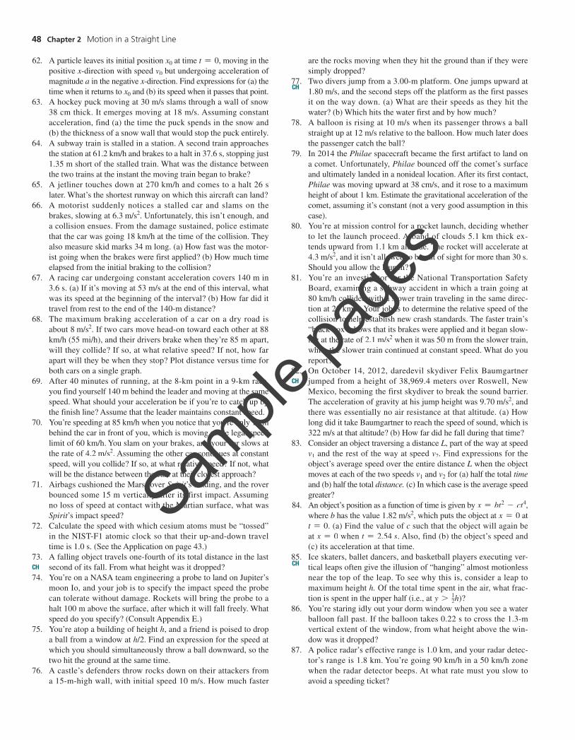
58. The position of a car in a drag race is measured each second, and the results are tabulated below.

Time t (s) 0 1 2 3 4 5

Position x (m) 0 1.7 6.2 17 24 40

Assuming the acceleration is approximately constant, plot po-sition versus a quantity that should make the graph a straight line. Fit a line to the data, and from it determine the approximate acceleration.

59. A fireworks rocket explodes at a height of 82.0 m, producing frag-ments with velocities ranging from 7.68 m/s downward to 16.7 m/s upward. Over what time interval are fragments hitting the ground?

60. The muscles in a grasshopper’s legs can propel the insect upward at 3.0 m/s. How high can the grasshopper jump?

61. On packed snow, computerized antilock brakes can reduce a car’s stopping distance by 51%. By what percentage is the stopping time reduced?

DATA

BIO

M02_WOLF0141_04_GE_C02.indd 47 08/05/20 4:37 PM

Sample

page

s


62. A particle leaves its initial position x0 at time t = 0, moving in the positive x-direction with speed v0 but undergoing acceleration of magnitude a in the negative x-direction. Find expressions for (a) the time when it returns to x0 and (b) its speed when it passes that point.

63. A hockey puck moving at 30 m/s slams through a wall of snow 38 cm thick. It emerges moving at 18 m/s. Assuming constant acceleration, find (a) the time the puck spends in the snow and (b) the thickness of a snow wall that would stop the puck entirely.

64. A subway train is stalled in a station. A second train approaches the station at 61.2 km/h and brakes to a halt in 37.6 s, stopping just 1.35 m short of the stalled train. What was the distance between the two trains at the instant the moving train began to brake?

65. A jetliner touches down at 270 km/h and comes to a halt 26 s later. What’s the shortest runway on which this aircraft can land?

66. A motorist suddenly notices a stalled car and slams on the brakes, slowing at 6.3 m/s2. Unfortunately, this isn’t enough, and a collision ensues. From the damage sustained, police estimate that the car was going 18 km/h at the time of the collision. They also measure skid marks 34 m long. (a) How fast was the motor-ist going when the brakes were first applied? (b) How much time elapsed from the initial braking to the collision?

67. A racing car undergoing constant acceleration covers 140 m in 3.6 s. (a) If it’s moving at 53 m/s at the end of this interval, what was its speed at the beginning of the interval? (b) How far did it travel from rest to the end of the 140-m distance?

68. The maximum braking acceleration of a car on a dry road is about 8 m/s2. If two cars move head-on toward each other at 88 km/h (55 mi/h), and their drivers brake when they’re 85 m apart, will they collide? If so, at what relative speed? If not, how far apart will they be when they stop? Plot distance versus time for both cars on a single graph.

69. After 40 minutes of running, at the 8-km point in a 9-km race, you find yourself 140 m behind the leader and moving at the same speed. What should your acceleration be if you’re to catch up by the finish line? Assume that the leader maintains constant speed.

70. You’re speeding at 85 km/h when you notice that you’re only 10 m behind the car in front of you, which is moving at the legal speed limit of 60 km/h. You slam on your brakes, and your car slows at the rate of 4.2 m/s2. Assuming the other car continues at constant speed, will you collide? If so, at what relative speed? If not, what will be the distance between the cars at their closest approach?

71. Airbags cushioned the Mars rover Spirit’s landing, and the rover bounced some 15 m vertically after its first impact. Assuming no loss of speed at contact with the Martian surface, what was Spirit’s impact speed?

72. Calculate the speed with which cesium atoms must be “tossed” in the NIST-F1 atomic clock so that their up-and-down travel time is 1.0 s. (See the Application on page 43.)

73. A falling object travels one-fourth of its total distance in the last second of its fall. From what height was it dropped?

74. You’re on a NASA team engineering a probe to land on Jupiter’s moon Io, and your job is to specify the impact speed the probe can tolerate without damage. Rockets will bring the probe to a halt 100 m above the surface, after which it will fall freely. What speed do you specify? (Consult Appendix E.)

75. You’re atop a building of height h, and a friend is poised to drop a ball from a window at h/2. Find an expression for the speed at which you should simultaneously throw a ball downward, so the two hit the ground at the same time.

76. A castle’s defenders throw rocks down on their attackers from a 15-m-high wall, with initial speed 10 m/s. How much faster

are the rocks moving when they hit the ground than if they were simply dropped?

77. Two divers jump from a 3.00-m platform. One jumps upward at 1.80 m/s, and the second steps off the platform as the first passes it on the way down. (a) What are their speeds as they hit the water? (b) Which hits the water first and by how much?

78. A balloon is rising at 10 m/s when its passenger throws a ball straight up at 12 m/s relative to the balloon. How much later does the passenger catch the ball?

79. In 2014 the Philae spacecraft became the first artifact to land on a comet. Unfortunately, Philae bounced off the comet’s surface and ultimately landed in a nonideal location. After its first contact, Philae was moving upward at 38 cm/s, and it rose to a maximum height of about 1 km. Estimate the gravitational acceleration of the comet, assuming it’s constant (not a very good assumption in this case).

80. You’re at mission control for a rocket launch, deciding whether to let the launch proceed. A band of clouds 5.1 km thick ex-tends upward from 1.1 km altitude. The rocket will accelerate at 4.3 m/s2, and it isn’t allowed to be out of sight for more than 30 s. Should you allow the launch?

81. You’re an investigator for the National Transportation Safety Board, examining a subway accident in which a train going at 80 km/h collided with a slower train traveling in the same direc-tion at 25 km/h. Your job is to determine the relative speed of the collision to help establish new crash standards. The faster train’s “black box” shows that its brakes were applied and it began slow-ing at the rate of 2.1 m/s2 when it was 50 m from the slower train, while the slower train continued at constant speed. What do you report?

82. On October 14, 2012, daredevil skydiver Felix Baumgartner jumped from a height of 38,969.4 meters over Roswell, New Mexico, becoming the first skydiver to break the sound barrier. The acceleration of gravity at his jump height was 9.70 m/s2, and there was essentially no air resistance at that altitude. (a) How long did it take Baumgartner to reach the speed of sound, which is 322 m/s at that altitude? (b) How far did he fall during that time?

83. Consider an object traversing a distance L, part of the way at speed v1 and the rest of the way at speed v2. Find expressions for the object’s average speed over the entire distance L when the object moves at each of the two speeds v1 and v2 for (a) half the total time and (b) half the total distance. (c) In which case is the average speed greater?

84. An object’s position as a function of time is given by x = bt2 - ct4, where b has the value 1.82 m/s2, which puts the object at x = 0 at t = 0. (a) Find the value of c such that the object will again be at x = 0 when t = 2.54 s. Also, find (b) the object’s speed and (c) its acceleration at that time.

85. Ice skaters, ballet dancers, and basketball players executing ver-tical leaps often give the illusion of “hanging” almost motionless near the top of the leap. To see why this is, consider a leap to maximum height h. Of the total time spent in the air, what frac-tion is spent in the upper half (i.e., at y 7 1

2h)?86. You’re staring idly out your dorm window when you see a water

balloon fall past. If the balloon takes 0.22 s to cross the 1.3-m vertical extent of the window, from what height above the win-dow was it dropped?

87. A police radar’s effective range is 1.0 km, and your radar detec-tor’s range is 1.8 km. You’re going 90 km/h in a 50 km/h zone when the radar detector beeps. At what rate must you slow to avoid a speeding ticket?

CH

CH

CH

CH

M02_WOLF0141_04_GE_C02.indd 48 08/05/20 4:37 PM

Sample

page

s

Essential University Physics Volume 1

Documents