Essays on the Structural Models of Executive Compensation

EssaysontheStructuralModelsof

ExecutiveCompensation

By

ChenLi

Adissertationsubmittedinpartialfulfillment

oftherequirementsforthedegreeof

DoctorofPhilosophy

(IndustrialAdministration)

attheTepperBusinessSchool

atCarnegieMellonUniversity

2013

DoctoralCommittee:

ProfessorGeorge‐LeviGayle

ProfessorJonathanGlover(Co‐chair)

ProfessorPierreJinghongLiang

ProfessorRobertA.Miller(Co‐chair)

Essays on the Structural Models of

Executive Compensation

Chen Li

Abstract

This dissertation is composed of three chapters in which I use both reduced-form

approach and structural approach to study executive compensation in S&P1500 �rms

from 1993 to 2005.

Chapter 1 provides the literature and methodology background of this dissertation.

I summarize existing accounting empirical studies on executive compensation under two

tasks, that is, (1) testing contract theory and (2) analyzing policies. I compare struc-

tural approach with reduced-form approach in terms of their scopes, execution, and

comparative advantages. Also, I brie�y introduce the steps of implementing structural

analysis and close this chapter with a high level plan for the following two chapters.

Chapter 2 focuses on the �rst task and is based on my job market paper entitled

"Mutual Monitoring within Top Management Teams: A Structural Modeling Investi-

gation". I study whether executive compensation re�ects that shareholders take advan-

tage of top managers�mutual monitoring. Mutual monitoring as a solution to moral

hazard has been extensively studied by theorists, but the empirical results are few and

mixed. This chapter semi-parametrically identi�es and tests three structural models

of principal-two-agent moral hazard. The Mutual Monitoring with Individual Util-

ity Maximization Model is the most plausible one to rationalize the data of executive

compensation and stock returns. The No Mutual Monitoring Model is also plausible

but relies on the assumption that managers have heterogeneous risk preferences across

�rm characteristics. The Mutual Monitoring with Total Utility Maximization Model

is rejected by the data. These results indicate that shareholders seem to recognize

and exploit complementary incentive mechanisms, such as mutual monitoring among

self-interested top executives, to design compensation.

Chapter 3 focuses on the second task and attempts to answer the question in its title,

�Do 2002 Governance Rules a¤ect CEOs�Compensation?�From two non-parametric

tests, I found that both the CEOs�compensation contract shape and the distribution

of gross abnormal return (performance measure) have signi�cantly changed after 2002.

These changes indicate that shareholders may have adjusted CEOs�compensation con-

tract to those governance rules. The results also give con�dence to a more sophisticated

test using structural approach based on welfare estimation.

1

Acknowledgements

Tobeadded

TABLE OF CONTENTS

1.0 LITERATURE AND METHODOLOGY BACKGROUND . . . . . . . 2

1.1 Introduction . . . . . . . . . . . . . . . . . . . . . . . . . . . . . . . . . . . 2

1.2 Literature Review . . . . . . . . . . . . . . . . . . . . . . . . . . . . . . . . 4

1.2.1 Testing contract theory: three questions . . . . . . . . . . . . . . . . . 4

1.2.1.1 Incentive problems targeted by compensation contracts . . . . 4

1.2.1.2 Consequences of compensation contracts . . . . . . . . . . . . 6

1.2.1.3 Design of compensation contracts . . . . . . . . . . . . . . . . 7

1.2.2 Analyzing policies . . . . . . . . . . . . . . . . . . . . . . . . . . . . . 8

1.3 A Comparison between Reduced-form Approach and Structural Approach . 9

1.3.1 Reduced-form approach . . . . . . . . . . . . . . . . . . . . . . . . . . 10

1.3.1.1 De�nition . . . . . . . . . . . . . . . . . . . . . . . . . . . . . 10

1.3.1.2 Research challenges . . . . . . . . . . . . . . . . . . . . . . . . 10

1.3.2 Structural approach . . . . . . . . . . . . . . . . . . . . . . . . . . . . 11

1.3.2.1 De�nition . . . . . . . . . . . . . . . . . . . . . . . . . . . . . 11

1.3.2.2 How it works . . . . . . . . . . . . . . . . . . . . . . . . . . . 12

1.4 When Do We Need Structural Approach? . . . . . . . . . . . . . . . . . . . 13

1.4.1 Research questions and advantages of reduced-form approach . . . . . 13

iv

1.4.2 Research questions and advantages of structural approach . . . . . . . 14

1.5 Implementing Structural Approach . . . . . . . . . . . . . . . . . . . . . . . 16

1.6 Plans for Chapter 2 and Chapter 3 . . . . . . . . . . . . . . . . . . . . . . . 22

2.0 MUTUAL MONITORINGWITHIN TOP MANAGEMENT TEAMS:

A STRUCTURAL MODELING INVESTIGATION . . . . . . . . . . . . 23

2.1 Introduction . . . . . . . . . . . . . . . . . . . . . . . . . . . . . . . . . . . 23

2.2 Models . . . . . . . . . . . . . . . . . . . . . . . . . . . . . . . . . . . . . . 31

2.2.1 Timeline . . . . . . . . . . . . . . . . . . . . . . . . . . . . . . . . . . 32

2.2.2 Technologies . . . . . . . . . . . . . . . . . . . . . . . . . . . . . . . . 34

2.2.3 Managers�Preferences . . . . . . . . . . . . . . . . . . . . . . . . . . . 37

2.2.4 Shareholder�s Cost Minimization Problem . . . . . . . . . . . . . . . . 38

2.2.4.1 Objective Function . . . . . . . . . . . . . . . . . . . . . . . . 38

2.2.4.2 Participation Constraint . . . . . . . . . . . . . . . . . . . . . 39

2.2.4.3 Incentive Compatibility Constraint . . . . . . . . . . . . . . . 42

2.2.5 Optimal Contracts . . . . . . . . . . . . . . . . . . . . . . . . . . . . . 46

2.2.6 Shareholder�s Pro�t Maximization . . . . . . . . . . . . . . . . . . . . 48

2.2.7 Summarizing the Three Models . . . . . . . . . . . . . . . . . . . . . . 50

2.3 Data . . . . . . . . . . . . . . . . . . . . . . . . . . . . . . . . . . . . . . . . 52

2.3.1 Heterogeneity in the Data . . . . . . . . . . . . . . . . . . . . . . . . . 52

2.3.2 Key Variables in the Optimal Contracts . . . . . . . . . . . . . . . . . 53

2.3.2.1 Abnormal Stock Returns . . . . . . . . . . . . . . . . . . . . . 53

2.3.2.2 Compensation . . . . . . . . . . . . . . . . . . . . . . . . . . . 54

2.3.2.3 Measurement Error . . . . . . . . . . . . . . . . . . . . . . . . 57

2.3.3 Bond Prices and a Dynamic Consideration . . . . . . . . . . . . . . . 58

v

2.4 Identi�cation . . . . . . . . . . . . . . . . . . . . . . . . . . . . . . . . . . . 59

2.4.1 No Mutual Monitoring Model . . . . . . . . . . . . . . . . . . . . . . 63

2.4.2 Mutual Monitoring with Total Utility Maximization Model . . . . . . 69

2.4.3 Mutual Monitoring with Individual Utility Maximization

Model . . . . . . . . . . . . . . . . . . . . . . . . . . . . . . . . . . . . 71

2.4.4 Summary of the Identi�cation Results . . . . . . . . . . . . . . . . . . 71

2.5 Estimation and Tests . . . . . . . . . . . . . . . . . . . . . . . . . . . . . . . 73

2.6 Results . . . . . . . . . . . . . . . . . . . . . . . . . . . . . . . . . . . . . . 76

2.6.1 Estimation of the Risk Aversion Parameter and Tests . . . . . . . . . 76

2.6.2 Discussion . . . . . . . . . . . . . . . . . . . . . . . . . . . . . . . . . 79

2.6.2.1 A Binary Illustration . . . . . . . . . . . . . . . . . . . . . . . 79

2.6.2.2 No Mutual Monitoring versus Mutual Monitoring with Individ-

ual Utility Maximization . . . . . . . . . . . . . . . . . . . . . 81

2.6.2.3 No Mutual Monitoring Model versus Mutual Monitoring with

Total Utility Maximization . . . . . . . . . . . . . . . . . . . . 82

2.7 Extension . . . . . . . . . . . . . . . . . . . . . . . . . . . . . . . . . . . . . 84

2.7.1 Counterfactual Estimation of Welfare Cost of Moral Hazard . . . . . . 84

2.7.2 Testing a Model Observationally Equivalent to Mutual Monitoring with

the Individual Utility Maximization Model . . . . . . . . . . . . . . . 85

2.8 Conclusion . . . . . . . . . . . . . . . . . . . . . . . . . . . . . . . . . . . . 88

3.0 DO 2002 GOVERNANCE RULES AFFECT CEOS�COMPENSATION? 92

3.1 Introduction . . . . . . . . . . . . . . . . . . . . . . . . . . . . . . . . . . . 92

3.2 Background . . . . . . . . . . . . . . . . . . . . . . . . . . . . . . . . . . . . 96

3.3 Data . . . . . . . . . . . . . . . . . . . . . . . . . . . . . . . . . . . . . . . . 97

vi

3.3.1 State variables . . . . . . . . . . . . . . . . . . . . . . . . . . . . . . . 97

3.3.1.1 Public state . . . . . . . . . . . . . . . . . . . . . . . . . . . . 98

3.3.1.2 Private state . . . . . . . . . . . . . . . . . . . . . . . . . . . . 99

3.3.1.3 Distribution of the states . . . . . . . . . . . . . . . . . . . . . 100

3.3.2 Abnormal Stock Returns . . . . . . . . . . . . . . . . . . . . . . . . . 100

3.3.3 Compensation . . . . . . . . . . . . . . . . . . . . . . . . . . . . . . . 102

3.4 Nonparametric Tests and Results . . . . . . . . . . . . . . . . . . . . . . . . 103

3.4.1 Estimating Optimal Compensation and Performance Measure . . . . . 104

3.4.2 Test on the Change in the Distribution of Gross Abnormal Return . . 105

3.4.2.1 Test statistic . . . . . . . . . . . . . . . . . . . . . . . . . . . 105

3.4.2.2 Result . . . . . . . . . . . . . . . . . . . . . . . . . . . . . . . 107

3.4.3 Test on the Change in the Optimal Contract Shape . . . . . . . . . . 108

3.4.3.1 Test statistic . . . . . . . . . . . . . . . . . . . . . . . . . . . 108

3.4.3.2 Result . . . . . . . . . . . . . . . . . . . . . . . . . . . . . . . 110

3.5 Conclusion . . . . . . . . . . . . . . . . . . . . . . . . . . . . . . . . . . . . 110

4.0 APPENDIX TO CHAPTER 2 . . . . . . . . . . . . . . . . . . . . . . . . . 112

4.1 Proofs . . . . . . . . . . . . . . . . . . . . . . . . . . . . . . . . . . . . . . . 112

4.2 Nonparametric Estimation of Compensation and

the Probability Density Function of Gross Abnormal Returns in Equilibrium 119

4.3 Tables . . . . . . . . . . . . . . . . . . . . . . . . . . . . . . . . . . . . . . . 120

5.0 APPENDIX TO CHAPTER 3 . . . . . . . . . . . . . . . . . . . . . . . . . 121

5.1 Calculation of wealth change in holding stock and/or options . . . . . . . . 121

5.2 Tables . . . . . . . . . . . . . . . . . . . . . . . . . . . . . . . . . . . . . . . 122

BIBLIOGRAPHY . . . . . . . . . . . . . . . . . . . . . . . . . . . . . . . . . . . . 123

1

1.0 LITERATURE AND METHODOLOGY BACKGROUND

1.1 INTRODUCTION

Shareholders use compensation contracts to mitigate the agency problems of executives.

Those problems stem from the con�icting interests between shareholders and executives

when ownership is separated from control, dating back to Berle and Means (1932). Executive

compensation has been of interests to academia, practice, and regulators. Researchers study

executive compensation in economics, �nance, accounting, and management. Their research

methods can be theoretical, empirical, experimental, and �eld survey. To contribute, this

dissertation uses nonparametric method and structural model approach, both new to the

accounting �eld, to study executive compensation. This chapter provides the literature and

methodology background.

Section 1 mainly focuses on empirical accounting literature in the past decade since a

thorough literature review by Bushman and Smith (2001) and concerns expressed by Ittner

and Larcker (2002), "there is almost always a very tenuous link between the theoretical

notions developed in principal-agent models and the actual research hypotheses and empirical

methods used in compensation research". The purpose of this section is not to provide a

complete review of previous studies on executive compensation, given that the body of this

literature is huge and there have been several existing excellent surveys by Rosen (1992),

2

Finkelstein and Hambrick (1996), Abowd and Kaplan (1999), Murphy (1999, 2012), Core et

al. (2003), Bertrand (2009), and Frydman and Jenter (2010) on empirical �ndings, Edmans

and Gabaix (2009) and Lambert (2001, 2006) on theoretical results, and various textbook

treatments of contract theory, for example, Bolton and Dewatripont (2005), among others.

Instead, I restrict the scope to accounting literature to which this dissertation attempts

to make contribution and I organize previous �ndings under two empirical tasks with which

this dissertation associates. First, some papers attempt to test contract theory that can

rationalize executive compensation. Interactions between theory and reality are at the core

of any scienti�c approach (Salanie, 2003) and executive compensation data by nature can help

us examine the empirical relevance of issues studied by contract theory. Second, policies that

a¤ect executive compensation have also been investigated. As Murphy (2012) emphasizes,

"government intervention has been both a response to and a major driver of time trends in

executive compensation over the past century, and that any explanation for pay that ignores

political factors is critically incomplete".

Except for these two tasks� own importance in intellectual inquiry, they also provide

a good ground on the methodology front for a sharp contrast between the reduced-form

approach which is more traditional in accounting and the structural approach which is new.

Section 2 compares those two available and complementary empirical approaches. Section

3 discusses the comparative advantages of the structural approach. Both sections revolve

around the two empirical tasks raised in section 1. Section 4 illustrates how to implement

the structural approach with critical steps and challenges highlighted. Section 5 sketches the

agenda of the following two chapters. One attempts to test multi-agent moral hazard models

in the context of top management teams�compensation design. The other investigates the

consequences of the 2002 governance rule on CEOs�compensation.

3

1.2 LITERATURE REVIEW

1.2.1 Testing contract theory: three questions

Salanie (2003) proposed three important empirical questions in general for researchers who

attempt to test contract theory. First, can we �nd convincing evidence for the presence of a

relevant amount of asymmetric information, or is it just a theorist�s tale? Second, is there

the e¤ect of the various contractual forms on the behavior of the agents who operate under

these contracts? Alternatively, do incentives matter? Third, are the observed contracts in

real world close enough to the optimum contracts derived from a theoretical analysis of the

situation?

These questions invite inquiries in the context of executive compensation. Correspond-

ingly, papers can be classi�ed into three groups based on their answers to the following three

questions. First, does executive compensation respond to certain agency problems caused

by the friction of information asymmetry? Second, do compensation contracts a¤ect execu-

tives�behaviors? Third, are the observed features of executive compensation consistent with

theoretical prediction on optimal design?

1.2.1.1 Incentive problems targeted by compensation contracts The theoretical

agency theory literature and empirical executive compensation literature developed together

at the very beginning. Seminal papers in agency theory by Holmstrom (1979, 1982) are

tested by Antle and Smith (1986) published in the Journal of Accounting Research. In

the past decade, empirical accounting researchers attempt to examine the following agency

problems using executive compensation data.

First, executive compensation by itself aims at solving certain incentive problems. Reex-

4

amining the adoption of relative performance evaluation (RPE) in Antle and Smith (1986),

Gong et al. (2011) and Albuquerque (2009) provide new evidence supporting the use of RPE.

They attribute previous weak support for RPE partially to the lack of detailed information

of compensation contract terms and misspeci�ed benchmark group.

Another three papers study the incentive provided in compensation around turnover.

Yermack (2006) �nds that severance pay deters leaving CEOs from withholding e¤ort and

making damage. Ittner et al. (2003) documents that the importance of the retention objec-

tive has a signi�cant positive in�uence on equity grants to newly hired key employees. Bal-

sam and Miharjo (2007) suggest that the negative relationship between voluntary turnover

and the intrinsic value of unexercisable in-the-money options, the time value of unexercised

options, and the value of restricted shares indicates a retention consideration.

Besides, Banker et al. (2013) study the moral hazard and adverse selection problem

re�ected in the cash compensation. Hanlon et al. (2003) look for evidence of long-term

incentive in the signi�cantly positive relationship between value of stock option and future

operating income. Knechel et al. (2013) �nd implicit incentives provided to Big 4 audit

partners.

Second, executive compensation also interacts with other incentive problems and/or mon-

itoring mechanisms. Ortiz-Molina (2007) examines the simultaneity of CEO compensation

and capital structure which re�ects the interest alignment problem of shareholders and debt-

holders. The paper �nds that pay-for-performance sensitivity decreases in straight-debt

leverage but increases with convertible debt. Stock option policy, among all compensation

components, is most sensitive to di¤erences in capital structure. The relationship between

CEO compensation and the independence of compensation consultants are studied by Mur-

phy and Sandino (2010) and Cadman et al. (2010). Karuna (2007) examines the in�uence

5

of product market competition on executive compensation and Aggarwal et al. (2012) �nd

that pay-performance incentive is negatively related to board size. Ferri and Sandino (2009)

�nd CEO pay decreased in �rms in which the proposal was approved relative to a control

sample of S&P500 �rms, suggesting a role of shareholders�activism. Roulstone (2003) �nds

that insider trading restrictions explain the cross-sectional di¤erence in the level of total

compensation and incentive-based compensation and equity-based incentive.

1.2.1.2 Consequences of compensation contracts Even though direct tests on the

�rm performance improvement attributed to incentive are rare except Aboody et al (2010)

who �nd option repricing increases operating income and cash �ows, there exist quite a few

papers documenting the e¤ects of compensation contract on executives�managerial activities.

As to �nancing and investing activities, Young and Yang (2011) reveal a positive associ-

ation between stock repurchases and earnings per share (EPS)-contingent compensation and

suggest net bene�ts to shareholders from this association. Cheng and Farber (2008) suggest

a decrease in option-based compensation reduces CEOs�incentives to take excessively risky

investments, resulting in improved pro�tability. Rajgopal and Shevlin (2002) stock options

provide managers with incentives to mitigate risk-related incentive problems.

A series of papers study how compensation contracts in�uence �nancial disclosures.

McAnally et al (2008) �nd that some managers may seek to miss earnings targets and bene�t

from lower strike price on subsequent option grants. Armstrong et al. (2010) �nd accounting

irregularities occur less frequently at �rms where CEOs have relatively higher levels of equity

incentives. Comprix and Muller (2006) use more income-increasing accounting estimates of

pension income when pension income has greater e¤ect on CEO cash compensation. Nagar

et al (2003), stock price-based compensation provides incentive to disclose private informa-

6

tion. Erkens (2011) �nds that �rms use time-vested stock-based pay to reduce the leakage of

R&D-related information to competitors through employee mobility. Mastsunaga and Park

(2001) �nd that CEOs tend to meet analyst forecast in the same quarter of last year.

Other behaviors are studied by Armstrong et al (2012) who �nd that tax directors are

incentivized to reduce tax expenses and Adams and Ferreira (2008) who �nd director atten-

dance is sensitive to monetary incentives.

1.2.1.3 Design of compensation contracts Accounting-based performance measures

are extensively examined. Tian et al (2012) look at the earnings component and �nd that

discretionary accrual receives less weight in CEOs�terminal year compensation. Boschen et

al (2003) examine the cumulated unexpected good performance and document that CEOs�

long-run cumulative �nancial gain from unexpectedly good accounting performance is not

signi�cantly di¤erent from zero, but that from unexpectedly good stock price performance

is signi�cantly positive. Indiejikian and Nanda (2002) �nd that CEOs�target bonuses are

negatively associated with a proxy for measurement noise in accounting-based performance

measures, and positively associated with proxies for �rms� growth opportunities and the

extent of executives�decision-making authority. Bushman et al. (2006) suggests that the

two roles of accounting information, that is valuation and incentive contracting, are related.

Cash compensation puts more weight on non-accounting public information captured by

stock returns. Banker et al. (2009) con�rm the relation of the two roles. Bushman et al.

(2004) study the role of earnings timeliness in contract design.

Non-accounting performance measures are also investigated. Stock price-based compen-

sation is studied by Jayaraman and Milbourn (2012) who �nd positive relationship between

pay-for-performance sensitivity and stock liquidity, Hanlon et al. (2003) who �nd that stock

7

option grant value is positively related to future operating income, which is discussed by

Larcker (2003), Leone et al (2006) who �nd that asymmetric sensitivity of CEO cash com-

pensation to stock returns re�ects that boards intend to reduce ex post settling up in cash

compensation. Dechow (2006) discusses this paper and cannot rule out other explanations.

Other performance measures studied include non-pro�t performance measure in hotel

managers�compensation contracts (Banker et al., 2000) and implicit �nancial incentives in

big 4 audit partners�compensation (Knechel et al., 2013).

1.2.2 Analyzing policies

Empirical research is expected to not only evaluate the consequences of previously adopted

policies but also predict the outcome of potential not-yet-adopted policies. However, the

latter goal requires a good understanding of policy-invariant factors in the decision-making

process of both shareholders and executives. Such knowledge can be hardly obtained with

traditional empirical method in accounting literature and thus is not provided. By contrast,

structural model approach which is relatively new to accounting literature has a comparative

advantage in this perspective and will be introduced soon. Before that, I review several

papers that evaluate the consequences of various policies.

The Sarbanes-Oxley Act has received much attention. Engel et al (2010) �nd that audit

committee compensation increases due to higher demand for monitoring after SOX. Carter et

al (2009) �nd that the weight of earnings increase in CEOs bonus increased with a decrease

in upward earnings management and the cash salary components decreased in the total

compensation after SOX. Nekipelov (2007) who estimates a structural model of a linear

contract in the apparel retail industry attributes the increase in executive compensation

(salary and bonus) across the passage of SOX to the increase of executive managers�risk

8

aversion. Cohen et al. (2007) document a decline in the pay-for-performance sensitivity after

SOX.

Some other policies a¤ecting executive compensation are examined too. Iskandar-Datta

and Jia (2013) �nd the adoption of clawback provisions do not in�uence either the level or the

design of CEOs�compensation contract. Chan et al. (2012) �nds that accounting restate-

ments decline after �rms initiate such provisions. Ozkan et al. (2012) �nd that the improved

earnings quality and comparability after the adoption of IFRS increases accounting-based

pay-for-performance sensitivity (PPS) and RPE. Skantz (2012) suggests that the voluntary

option expensing under SFAS 123 may have encouraged ine¢ ciency in CEO pay and the

mandatory expensing under SFAS 123(R) may have contributed to the reduction in that

ine¢ ciency.

1.3 A COMPARISON BETWEEN REDUCED-FORM APPROACH AND

STRUCTURAL APPROACH

Structural approach is usually contrasted with reduced-form approach which is more famil-

iar to accounting researchers and presented in section 1. Except the crucial di¤erences to

be discussed soon, it is equally important to realize that the structural approach and the

reduced-form approach have two things in common. First, each of the two approaches can

accomplish the two tasks in section 1, even though they take di¤erent procedures in testing

theories and come up with di¤erent metrics in policy analyses. Second, both approaches

provide quantitative understandings of economic concepts by estimating variables of inter-

est, even though the variables are selected based on research questions that each approach

is good at answering.

9

1.3.1 Reduced-form approach

1.3.1.1 De�nition To clarify, reduced-form approach can have multiple meanings. First,

reduced-form refers to the simultaneous equation regression in which all endogenous variables

only appear on the left hand side and they are explicitly represented as functions of the

exogenous explanatory right hand side variables and unobservables (Reiss and Wolak, 2007).

Second, reduced-form approach may refer to quasi-experimental design that identi�es and

estimates treatment e¤ect. This treatment e¤ect approach is compared with the structural

approach by Heckman and Vytlacil (table V, 2005) and surveyed by Imbens and Wooldridge

(2009). This line of research focuses on the e¤ects de�ned by quasi-experiments, rather than

parameters which have explicit economic meanings in theoretical models. Schroeder (2010)

introduces treatment e¤ect approach with accounting applications.

Third, reduced-form papers may use explicit economic models to motivate and interpret

empirical analyses and they approximate the economic models using simple econometric

techniques. Chetty (2009) reviews the su¢ cient statistic approach in public economic studies

in which the welfare analyses are not directly based on deep primitives but instead on

su¢ cient statistics derived from economic models.

1.3.1.2 Research challenges To accomplish the two tasks, that is, testing theories and

analyzing policies, reduced-form studies encounter at least three challenges. First, to test

contract theory, reduced-form approach takes an indirect way by testing implications of

models. It appeals to testing comparative statics implied by the equilibria of theoretical

models but leaves model structures and assumptions implicit. In order to stay close to the

underlying theoretical models, keeping all other things equal is required for this type of tests

(Heckman, 2000). This requirement becomes the main challenge, because quite often those

10

control variables implied by economic models can not be measured or observed.

Second, tests on incentive e¤ects, which try to detect causal e¤ects due to the adoption

of incentive devices, often encounter endogeneity problems. One standard solution is to

exploit instrumental variables to make the explanatory variables truly exogenous. However,

the econometric problems associated with weak instrumental variables render this method

unsatisfactory (Larcker and Rustitcus, 2010).

Third, to conduct policy analysis, this approach uses a di¤erence-in-di¤erence research

design and the policy change is treated as a natural experiment. The key issue here is to �nd

and justify the control group. It turns to be challenging when certain policies are universally

adopted by �rms whose data researchers have access to. For example, the lack of control

groups in most of the studies on SOX gives rise to mixed results, as Leuz (2007) and Dey

(2010) point out. Accounting researchers become more serious about the above econometric

issues. A group of thought-provoking discussions emerges in Chenhall and Moers (2007),

Larcker and Rusticus (2004, 2007), and Van Lent (2007).

1.3.2 Structural approach

1.3.2.1 De�nition By contrast, structural approach refers to �a branch of economics in

which economic theory and statistical method are fused in the analysis of numerical and insti-

tutional data�(Hood and Koopmans, 1953, pp. xv). Nowadays, researchers refer to models

that combine explicit economic theories with statistical models as structural econometric

models.

What separate structural models from nonstructural models is how clearly the connec-

tions are made between institutional, economic, and statistical assumptions and the esti-

mated relationships between variables of interest. (Reiss and Wolak, 2007) The structural

11

approach allows a seamless connection between economic theory and econometric estimation.

Under the structural approach, researchers analyze in rigorous theoretical terms how people

optimize in face of incentive mechanisms. Structural econometricians use the implications

of those mechanisms explicitly as a basis for their empirical investigation.

1.3.2.2 How it works To facilitate the comparison, here is a brief introduction of how

the structural approach works in the context of executive compensation research. A more

detailed illustration is in section 4. The goal of this approach is to make inference about

unobservable primitive variables from available data on executive compensation and stock

returns. When shareholders design optimal compensation contracts, they act as if they solve

an optimization problem based on some primitive variables. We use a theoretical model

to characterize the properties of shareholders� optimization problem. Solving the model

gives the optimal compensation and a set of equilibrium restrictions. These restrictions

are functions of compensation, stock returns, and primitives. They discipline the data and

the deeper parameters together, so that we can analyze them consistently within the same

framework and mitigate the empirical problem of missing variables.

These restrictions tell us theoretically how the parameters interact with the observables.

Along with exclusion restrictions, they help us uniquely recover those parameters from the

data. This crucial step is called identi�cation. Then, by examining the consistency between

the observed data pattern and the theoretical restrictions derived from the unobservables, we

can look for the estimates of parameters that minimize the loss function in this comparison

between population and sample properties. Eventually we can test the model by comparing

the theoretical restrictions and the sample version of the restrictions. Also, armed with

the time/policy-invariant parameters of preferences and technology that are recovered from

12

historical data and based on the theoretical model, we can predict the potential responses

to a policy change which has never happened.

1.4 WHEN DO WE NEED STRUCTURAL APPROACH?

Abowd and Kaplan (1999) propose six questions to answer in studies of executive compen-

sation. They are (1) how much does executive compensation cost the �rm? (2) how much is

executive compensation worth to the recipient? (3) how well does executive compensation

work? (4) what are the e¤ects of executive compensation? (5) how much executive compen-

sation is enough? (6) could executive compensation be improved? Both the reduced-form

and structural papers need to answer questions (1) and (2). These measurement issues

have been discussed by Antel and Smith (1985, 1986), Core and Guay (2002), and Hall and

Leibman (1998). The reduced-form approach and the structural approach complement each

other in answering remaining questions with each own comparative advantages.

1.4.1 Research questions and advantages of reduced-form approach

Reduced-form papers can answer question (4) by detecting managerial behaviors driven by

certain incentives embedded in compensation contracts, which have been summarized in

section 1. Overall, reduced-form approach mainly answers yes-or-no type of questions and

focuses on the sign (direction) of association/causality rather than attempts to quantify

causal e¤ects.

However, reduced-form approach has its own merits on at least three aspects. First,

papers with this approach can use simple econometric techniques to document robust empir-

ical regularities evidenced by statistically signi�cant non-zero coe¢ cients, for example, the

13

noise-signal trade-o¤ in weighting performance measures in contract design.

Second, this approach can support the existence of certain e¤ect, which may inspire

more sophisticated investigation using structural models. Third, reduced-form papers can

examine phenomena on which no theory has explained: Masulis et al. (2012) documents that

US �rms with foreign independent directors (FIDs) are associated with a greater likelihood

of intentional �nancial misreporting and higher CEO compensation.

1.4.2 Research questions and advantages of structural approach

Compared with reduced-form approach, studies taking the structural approach are able to

answer a set of questions that cannot be answered by the reduced-form research.

As to testing theory, �rst, the structural approach evaluates the predicting performance

of an economic model as a whole in order to distinguish between competing theories that

may be all able to rationalize the data generating process. The structural approach empha-

sizes the internal consistency in empirical investigation. The consistency is guaranteed by

explicitly building empirical analysis on economic models and compensates for the reduc-

tion of inference credibility due to using structures. When researchers pull all equilibrium

restrictions, the structural parameters discipline the data within the same framework. For

example, the risk aversion parameter a¤ects executives�decisions on both participation and

exerting e¤ort rather than shirking, and the technology captured by the distribution parame-

ters of outcome are shared by both shareholders and executives in each party�s optimization

problem.

Second, this approach makes transparent a track on assumptions which the rejection of

models is attributed to or which are required to draw causal economic inferences from the

distribution of data (for example, Gayle and Miller (2012)). This explicit tracking enables

14

empiricists to provide informative feedback to theoretical research, given that theorists care

about to what extent their models can help rationalize stylized facts. Only when we bring

theoretical structures literally to data, we can realize to what extent the theoretical structures

can be recovered from the data we want to understand. This is an important way to advance

our knowledge by empirical research. By contrast, reduced-form approach tends to appeal

to suboptimality/irrationality to explain the rejection of hypotheses which are derived from

economic models and thus seems to be less informative.

As to policy analysis, this approach can estimate primitive parameters which are time-

invariant and/or policy-invariant. Such robustness of estimation makes extrapolation reliable

and results comparable across studies. Those estimates are used to conduct counterfac-

tual analysis and welfare analysis (in both the evaluation and prediction of policies), When

changes in executives�well-beings are unobserved, a direct estimation of deadweight loss

is not possible. However, we can draw inferences about executives�preferences over risk

and e¤ort and �rms�productivity from observed compensation and stock returns through

structural parameter estimation. This information can help us predict the welfare changes

for a policy that has not yet been implemented. Instead of looking for a control group,

the counterfactual analysis uses the primitive parameters in structural models as an anchor

and compares the variables of interest before and after a policy based on the same research

subjects. It is appealing because social experiments, especially at the executive level, can be

almost impossible merely for a trial-and-error purpose.

15

1.5 IMPLEMENTING STRUCTURAL APPROACH

Nevo andWhinston (2010) summarize two signi�cant changes in empirical work since Leamer�s

(1983) article which criticized the state of applied econometric practice. On one hand,

econometric methods have been developed such as nonparametric and semiparametric es-

timation (Powell, 1994) and identi�cation based on minimal assumptions (Manski, 2003;

Tamer, 2010). On the other hand, structural models have been increasingly used. Below I

present the procedures of structural approach, based on a static single-agent moral hazard

model for the illustration purpose.1

� Step 1: Build an economic model

A well-de�ned economic model serves as the theoretical underpinning of a structural

analysis. This economic model is expected to capture the �rst order e¤ect re�ected in

the nonexperimental data under consideration. Structural modelers need to select between

alternative modeling options while building the economic model, although those options

may not give qualitatively di¤erent results in theoretical studies. As theorists, we take the

following steps to build a principal-agent model.

� (1.a) specify preferences and technologies

The economic model is built on players�utilities which rely on primitive parameters that

represent the preferences of both the principal and the agent in the simple moral hazard

model. In the context of executive compensation, the principal represents shareholders or

board and the agent represents a manager, for example the CEO.

1Guidelines of implementing the structural approach in other �elds can be found at Reiss and Wolak (2007,empirical industrial organization), and Strebulaev and Whited (2012, corporate �nance). For nonparametricapplication, see Matzkin (2007).

16

We need to consider modeling questions such as whether the magnitude of CEO�s risk

aversion is a¤ected by his wealth, whether the managerial e¤ort reduces CEO�s utility addi-

tively or multiplicatively from his pecuniary well-being, and whether the ine¢ ciency due to

hidden action should be attributed instead to CEO�s limited liability as well, etc.. Answers

to these questions ask for some respect on institutional knowledge.

Also, the technology needs to be speci�ed. For example, between a model with continuous

e¤ort and one with discrete e¤ort choices, which one would allow us to draw meaningful

inference about how much shareholders would lose if they failed to align CEO�s interest?

� (1.b) specify information structure and strategic interactions between players

We need to de�ne the common knowledge and the information asymmetry between con-

tracting parties. In a typical moral hazard model, CEO�s e¤ort is assumed to be unobservable

to shareholders, but preferences and technologies are common knowledge to both parties.

� (1.c) model and solve optimization problems with endogenous and exogenous variables

Researchers need to clearly state the constrained optimization problem for shareholders

to solve and managers�possible strategies. The solutions of the optimization problem, either

explicit or implicit, and equilibrium restrictions are derived. It is important to distinguish

between endogenous variables (determined within model) and exogenous variables (deter-

mined out of model), for at least two reasons. Comparative statics that are based on the

sensitivity of endogenous variables to exogenous variables can provide testable predications.

What�s more, in counterfactual analysis, researchers are interested in knowing how welfare

that usually depends on endogenous variables will vary with exogenous shocks.

� Step 2: Transit from an economic model to an econometric model

17

The transition from a theoretical economic model to an empirical econometric model is

accomplished by introducing stochastic components into the economic model. This is the

watershed where a theoretical model and a structural model depart. Below are the major

steps.

� (2.a) de�ne observable and unobservable variables

The goal of empirical studies is to make statistical inferences about unobservables from

observables. In addition to the classi�cation of endogenous and exogenous variables, another

key classi�cation of variables in a structural model is "observable vs unobservable" from the

perspective of researchers instead of players in the theoretical model. This classi�cation

depends on what data is available to researchers. For example, risk aversion and personal

e¤ort costs are common knowledge in a moral hazard model. In such a sense, they are

"observable" to the players. However, they cannot be directly measured by empiricists, so

they are unobservable. By contrast, CEO�s e¤ort choice is unobservable to both shareholders

and researchers, but the realization of performance measure can be observed by both players

in the model and researchers.

� (2.b) introduce stochastic components into the theoretical model

According to Reiss and Wolak (2007), there are potential four ways to introduce sto-

chastic components. I discuss them in the context of the simple moral hazard model of

executive compensation. The �rst channel is researchers�uncertainty about contracting en-

vironment. It refers to what researchers do not know in the contracting environment and has

been answered by step (2.a). The second channel is players�uncertainty about contracting

environment. It refers information asymmetry between shareholders and CEOs, which has

been discussed in step (1.b).

18

The third channel is optimization errors on the part of players. It allows players to

behave not so rationally as the model predicts, but the deviation from rationality should

be independent conditional on other variables of interest. For example, the executive com-

pensation may associate with multiple period stock returns. A static model or repeated

short-term model cannot capture it.

The fourth channel is measurement errors in observed variables. For example, we assume

that the optimal compensation cannot be directly observed, but instead we can observe the

compensation with errors.

For the above stochastic components, we need to make assumptions on both their func-

tional forms and distributions. For example, does the error term enter in an additive way

or a multiplicative way into the regression of optimal compensation? Is it necessary to

specify a parametric distribution for a random variable? Both Margiotta and Miller (2000)

and Gayle and Miller (2012) include an additive error item into the optimal compensation

regression. However, the former parameterizes the distribution of performance measure con-

ditional on equilibrium e¤ort as truncated normal, but the latter leaves that distribution to

be nonparametrically identi�ed.

� Step 3: Identify the structural model

Identi�cation concerns the empirical investigation with population values of parameters

or features of a structural model. Identi�cation is crucial in the structural approach. From

one structural model, we can derive a reduced-form model. However, the uniqueness of its

reverse process is not always guaranteed. The same observed empirical regularity can be gen-

erated by two completely di¤erent structural models. In such a case, so called identi�cation

failure, the two structural models are observationally equivalent. In other words, the ratio-

nale for the data cannot be uniquely determined even if we have in�nite data. Identi�cation

19

failure automatically implies inconsistency in estimation.

Take the compensation gap as an example. As we know from step 1, the optimal compen-

sation is the solution to shareholders�optimization problem and is a function of primitive

parameters representing preferences and technologies (or informativeness of performance

measure). The gap between two executives�compensation is essentially determined by the

di¤erences of their primitive parameters. A model in which the two executives have homoge-

nous preferences but di¤erent technologies and a model in which the two executives have

heterogeneous preferences but same technology can give rise to the same observed compen-

sation gap. The primitive parameter values underlying the two models and the implications

of the two models are distinct in principle. As a result, it is necessary to investigate whether

the available data can distinguish between these two models before estimating any features

of either model. This argument motivates chapter 2.

Another example is the outside option in the moral hazard model. Margiotta and Miller

(2000) discusses the incomplete identi�cation of this part in their model. Brie�y, without

further information on the demand and supply of managerial e¤orts, we cannot distinguish

the outside option from the multiplicative e¤ort cost in CEO�s utility. We can only identify

their ratio.

� (3.a) explore the sources of identi�cation

One source of identi�cation comes from equilibrium conditions derived from the model.

They can be equality restrictions or inequality restrictions. The relationships between en-

dogenous variables and exogenous variables and those between observable variables and

unobservables together discipline the data and parameters. These relationships can help us

set up a mapping from the joint distribution of observable variables to the structures of the

model. An N-to-one mapping implies there exist multiple equilibria, but the identi�cation

20

can still be achieved. However, a one-to-N mapping indicates identi�cation failure. The key

is to prove the uniqueness of the inverse process.

Another source of identi�cation is exclusion restrictions. By excluding an exogenous

variable from the moment conditions generated by equilibrium restrictions, we obtain more

orthogonal moments and identi�cation power.

� (3.b) choose between point identi�cation and set identi�cation

A parametric model with equality restrictions usually can be point identi�ed. However,

when a structural model involves strategic interactions, preferences some times are revealed

through inequalities in equilibrium. These inequality restrictions, if they are exploited in

order to fully represent the model, in nature prevent the model from point identi�cation.

Instead, researchers can only achieve set identi�cation with con�dence regions of parameters.

� Step 4: Estimate the structural model

Only after we prove that a structural model can be identi�ed from the data, we can move

forward to estimation. A traditional GMM estimator can be used if equilibrium restrictions

that constitute the moment conditions only incorporate explicit solutions of the theoretical

model. Otherwise, simulated moments may be used.

� Step 5: Application in testing theories and analyzing policies

I leave this step to chapter 2 for testing theories and to a continuing project Gayle et al.

(2013) for analyzing policies..

21

1.6 PLANS FOR CHAPTER 2 AND CHAPTER 3

Chapter 2, as a response to the �rst task, uses structural approach and nonparametric method

to test three multi-agent moral hazard models of top management teams. This chapter em-

phasizes the importance and advantages of the structural approach in distinguishing among

possible models that can be observationally equivalent in rationalizing the same dataset.

Chapter 3, as a response to the second task, conducts nonparametric analysis on the po-

tential e¤ects of the governance rules enacted around the year 2002 on CEOs�compensation

and emphasizes the importance of a careful reduced-form investigation before conducting a

fully structural analysis.

22

2.0 MUTUAL MONITORING WITHIN TOP MANAGEMENT TEAMS: A

STRUCTURAL MODELING INVESTIGATION

2.1 INTRODUCTION

Shareholders design optimal compensation to mitigate the moral hazard of hidden e¤ort and

free riding in top management teams. In a seminal paper, Fama (1980) points out that

"each manager has a stake in the performance of the managers above and below him and,

as a consequence, undertakes some amount of monitoring in both directions."1 Although

theoretical models have extensively explored how mutual monitoring is intertwined with

individual compensation in the optimal contract responding to moral hazard (Bolton and

Dewatripont 2005; Glover 2012), empirical studies mainly examine individual incentives to

understand top executive compensation (MacLeod 1995; Murphy 1999, 2012; Core et al.

2003). In general, overlooking the e¤ect of mutual monitoring as a self-policing vehicle

may lead to incomplete or even misleading evaluations of the severity of the moral hazard

problem and, thus, of the e¢ ciency of executive compensation. At the heart of this gap in

the literature is a question about the empirical relevance of mutual monitoring models: do

shareholders actually take advantage of mutual monitoring in optimal compensation design?

The research challenge is that mutual monitoring among top executives is rarely codi�ed

1A recent paper (Landier et al. 2012) provides evidence of bottom-up monitoring of CEOs by topexecutives who joined the �rm before the current CEO.

23

in their contracts or observed by outsiders. So far, a few indirect tests have produced only

mixed results by studying the association between �rm performance and the top executives�

cooperation/monitoring incentives proxied by relative properties of compensation.2 However,

the optimal compensation is usually derived from primitive parameters3 which also determine

the optimal e¤ort and output that shareholders prefer in equilibrium, creating an endogeneity

problem acknowledged by empiricists (Prendergast 1999; Core et al. 2003).

Taking a more direct approach, the empirical investigation in this paper identi�es and

tests three competing structural models that are explicitly based on theoretical models of

principal-multiagent moral hazard. I set up my models with one joint output (stock return),

one risk-neutral principal (shareholders), and two risk-averse agents (the two highest paid

managers), who have the same absolute risk aversion coe¢ cient but di¤er in their costs of

e¤ort. The three models di¤er in terms of how the shareholders provide managers with

incentives to participate and incentives to work rather than shirk. These di¤erences depend

on whether and how the managers monitor each other, as follows.

If shareholders believe the managers cannot e¤ectively side contract to monitor each

other, they have to provide the managers with individual incentives through the compensa-

tion contract. The �rst model, called no mutual monitoring, describes this case and serves as

a benchmark. Without mutual monitoring, the shareholders are concerned about managers�

unilateral shirking and design the optimal compensation such that both managers work-

ing (the optimal e¤ort pair throughout this paper) is a Nash equilibrium in the managers�

subgame. Alternatively, if shareholders believe managers can side contract on mutually

observable e¤orts, they will take advantage of the mutual monitoring in contract design

2Evidence in support of coorperation/monitoring can be found in Li (2011) and Bushman et al. (2012).Unsupportive evidence is provided by Main et al. (1993), Henderson and Fredrickson (2001), and Bushmanet al. (2012).

3For example, these deeper parameters can be managers�risk preferences, costs of e¤ort, and the relativeinformativeness of a performance measure on the equilibrium path versus o¤ the equilibrium path.

24

(Holmstrom and Milgrom 1990; Varian 1990; Ramakrishnan and Thakor 1991; Itoh 1993,

among others). The managers cooperate both to choose working as a Pareto-dominant equi-

librium and to agree on equal expected utility due to their equal bargaining power in the

private coordination process. Furthermore, if shareholders think the managers engage in

mutual monitoring to pursue group interests, the second model, called mutual monitoring

with total utility maximization, describes this case. In this model, the shareholders provide

the two managers with incentives only based on their total expected utility.4 By contrast,

if the managers pursue self-interest, the third model, called mutual monitoring with individ-

ual utility maximization, describes this case. Because each manager chooses working based

on individual rationality, shareholders need to tailor each of those two incentives to each

manager�s preference over his own expected utility maximization.5

The intuition for my empirical strategy is as follows. Even though we do not know how

shareholders design the incentives of the optimal contract in their minds, we do observe

the compensation they o¤er and the output the managers generate. Traditionally, we test

comparative statics, such as the relation between pay and performance, to infer what the

optimal contract may look like, for example, whether internal monitors are motivated to

monitor and enhance �rm value (Armstrong et al. 2010) or whether relative performance

evaluation is adopted (Antle and Smith 1986). Instead of focusing on the consequences of

the optimal contract, this paper directly examines the data restrictions required by an opti-

4This model has the essence of the mutual monitoring with utility transfer model in Itoh (1993, page 416).To make the current model less restrictive on the data, I drop Itoh�s assumption that the two managers cantransfer payments to share risk ex post. This assumption seems unrealistic among top executives and wouldbe rejected by the data. I retain only Itoh�s assumption on transferable utility in my model.

5This model essentially says that a Pareto-dominant strategy is played in equilibrium without utilitytransfer even though free-riding is optimal from the viewpoint of individual incentives. There are a fewmechanisms that can be empirically consistent with this model, for example, the explicit side contractswithout utility transfer in Itoh (1993), the �nitely repeated game with implicit side contracts in Arya etal. (1997), the in�nitely repeated game with implicit side contracts in Che and Yoo (2001), leadership bysetting example in Hermalin (1998), and the peer pressure in Kandel and Lazear (1992), among others.

25

mal contract to discipline parameters so that the observed compensation and stock returns

can be consistently understood within a uni�ed framework. Theory helps here because the

optimal contract can essentially be described by a well-de�ned theoretical model. If share-

holders honor their compensation arrangements with managers and managers exert optimal

e¤ort to generate stock returns as expected, then the observed compensation and stock re-

turns are random draws from the equilibrium of a theoretical model that characterizes that

optimal contract in shareholders�minds, after controlling for the heterogeneity in the data.

Intuitively, if the data restrictions implied by the equilibrium of the theoretical model are

statistically consistent with the observed data pattern, this consistency suggests that the

observed compensation schemes have the �avor of that model. In this paper, the ��avor�

refers to whether shareholders exploit mutual monitoring and how managers are engaged.

The purpose of the tests is to �nd out which type of model (contract) can explain the entire

data best, allowing the contract shape to vary with �rm characteristics, industrial sectors,

and macroeconomic �uctuations.

First I show that, without imposing on data the restrictions from shareholders�pro�t

maximization over the alternative e¤ort pairs of managers, the pattern of compensation and

stock returns can be empirically consistent with a model with or without mutual monitor-

ing. An important implication is that the descriptive properties of compensation, which

are usually based on comparative statics derived from the subset of equilibrium conditions,

may not be su¢ cient to help us distinguish the two types of models without considering

other restrictions that those confounding parameters need to satisfy. This partially helps to

illustrate why di¤erent research designs can lead to opposite results in the literature.

Then I exploit other equilibrium restrictions implied by this model, for example, share-

holders�preferences over all possible e¤ort pairs and managers�time-invariant preferences

26

over risk, to govern the identi�ed set of the risk aversion parameter to which all other prim-

itive parameters in the same model are indexed. These restrictions are summarized by a

criterion function that has a distance-minimizing property. If the model can explain the

data, there must exist some reasonable values of the risk aversion parameter in the identi�ed

set such that the criterion function reaches its lower bound.

Next, I bring the theoretical restrictions to the data I investigate. The measurement

of total compensation follows Antle and Smith (1985) by incorporating opportunity costs

of holding �rm stocks and stock options into managers�wealth.6 There are two noteworthy

features of the panel data I investigate, which cover S&P 1500 �rms from 1993 to 2005. First,

the two managers studied in this paper earn the highest total compensation for a given �rm-

year, and their compensation contracts are intensively equity based. This indicates not only

that they have signi�cant in�uence on the stock returns due to their occupational seniority

but also that they can substantially bene�t from the improvement of this joint output. This

tight interest alignment provides a channel and an incentive of sanction that favor the two

models in which shareholders take advantage of mutual monitoring (Kandel and Lazear

1992). Second, for 94 percent of the sample �rm-years, the two managers either hold a

functional position (CTO, CIO, COO, CFO, CMO)7 or sit on the top rank, including the

positions of president, chairman, CEO, and founder. These two types of positions are hardly

substitutable. As a result, it is reasonable to assume that shareholders prefer both managers

working to allowing either one to shirk.

To account for the measurement errors in the compensation and to acknowledge the

�exibility of shareholders�contract designs, this paper nonparametrically estimates both the

6Among followers are Hall and Liebman (1998), Margiotta and Miller (2000), Gayle and Miller (2009,2012), and Gayle et al. (2012).

7CTO: Chief Techonology O¢ cer, CIO: Chief Information O¢ cer, COO: Chief Operation O¢ cer, CFO:Chief Financial O¢ cer, CMO: Chief Marketing O¢ cer.

27

optimal compensation scheme as a function of the gross abnormal return and the density of

the gross abnormal return in equilibrium. To reduce the concern of overusing structures, the

nonparametric method in this paper enables exploiting the information from data as much

as possible and also avoids rejecting a model due to speci�c model assumptions on contract

form and distribution. This method shortens "the distance between those roads to the point

where now some econometric models are speci�ed with no more restrictions than those that

a theorist would impose" (Matzkin 2007, page 5311).

Last, I calculate the criterion function with the data for each model, such that I can

construct a hypothesis test for the model based on the con�dence region of the identi�ed set

of the risk aversion parameter. I use a similar testing strategy developed for the single-agent

model of moral hazard and hidden information by Gayle and Miller (2012), who investigate

the role of accounting information in CEOs�compensation contracts and are followed by

Gayle et al. (2012), who explore the consequences of the Sarbanes-Oxley Act on CEOs�

compensation. If the con�dence region is empty or only contains unreasonable values, the

model is rejected.

The main results emerge from the preceding steps, as follows. The mutual monitoring

with total utility maximization model is rejected, even under the least restrictive assumption

that managers have heterogeneous risk preferences across �rm types and industrial sectors.

The con�dence region is empty in large �rms of the primary sector and in small �rms with

high �nancial leverage of the service sector. The nonempty con�dence regions cover values

close to zero in all other �rms, indicating that to be reconciled with the data, this model

requires almost risk-neutral managers. Such near-risk neutrality contradicts the setup of

this model, which assumes that the managers are risk averse. This contradiction essentially

rejects this model.

28

Under the same heterogeneity assumption of risk aversion, both the no mutual monitor-

ing model and the mutual monitoring with individual utility maximization model cannot be

rejected. However, under the most restrictive assumption that managers have homogeneous

risk preference across �rm types and industries, only the mutual monitoring with individual

utility maximization model cannot be rejected. In this sense, the mutual monitoring with

individual utility maximization model is the most robust among the three models to ratio-

nalize the correlation between the observed top executive compensation and stock returns.

This result implies that we may need to account for the cross-sectional variation of mutual

monitoring in trying to understand the incentives embedded in executive compensation. In-

tuitively, enforceable mutual monitoring among top managers can help shareholders partially

save compensation cost. In turn, a large equity-based component in compensation aligns the

interests of a group of managers through a joint output that provides the channel and the

incentive for mutual punishment and reward.

Furthermore, I examine how shareholders perceive managers engaging in mutual mon-

itoring, which has not been tested previously in the literature. I �nd that shareholders

consider that the managers monitor each other to pursue self-interest rather than to pursue

their collective interests. This result has implications for how to account for the e¤ect of

mutual monitoring on compensation in empirical research. If shareholders take into account

the utility transfer that is implicitly assumed for total utility maximization, the shape of the

optimal compensation is more similar between managers than individual utility maximiza-

tion predicts. Previous studies using the closeness of managers�compensation schemes to

detect team incentives, for example, the pay disparity (Main et al. 1993) and the dispersion

of pay-performance-sensitivity (Bushman et al. 2012), do not support a dominant e¤ect of

cooperation/monitoring. The results in this paper suggest that moderate closeness can be

29

consistent with the model of mutual monitoring if managers are not identical and only care

about their own payo¤s. Consequently, this result implies that the proxy choice should ac-

count for the underlying incentive and enforcement mechanism of mutual monitoring, which

was ignored in previous studies.

The preceding more direct answers have the potential to advance our understanding of

how shareholders respond to the moral hazard in top management teams and how managers

are engaged in mutual monitoring. This enriched understanding can extend structural mod-

eling studies by suggesting that the mutual monitoring may be incorporated as a baseline

in rationalizing the curvature of executive compensation. This paper also sheds light on

studies that investigate the determinants and consequences of executive compensation by

calling attention to appropriate control for the implicit incentive e¤ect of mutual monitoring

in addition to traditional corporate governance factors, which rely on explicit provisions of

incentives. Instead of focusing on the similarity of compensation shape, researchers may

want to consider factors that a¤ect the enforcement of mutual monitoring such as reputa-

tion concern and group identity (Itoh 1990), corporate culture (Kreps 1990), and long-term

relationships (Arya et al. 1997; Che and Yoo 2001) suggested by theoretical studies, and the

team duration used by the empirical paper of Bushman et al. (2012).

The remaining is arranged as follows. In Section 2, I compare the static versions of

the three models. To incorporate dynamic considerations, I estimate and test the dynamic

versions of these models in later sections.8 Section 3 discusses the data and the nonparametric

estimation. Section 4 establishes the identi�cation. Section 5 introduces the estimation and

hypothesis tests. Section 6 reports and discusses the results. Section 7 discusses feasible

extensions, and Section 8 concludes.

8The dynamic version falls into the principal�agent moral hazard framework of Margiotta and Miller(2000), as descended from Grossman and Hart (1983) and Fudenberg et al. (1990).

30

2.2 MODELS

This section lays out the three principal-multiagent models of moral hazard as the theoretical

underpinning of the structural model identi�cation and the hypothesis tests. These models

aim to su¢ ciently distinguish the shareholders�perception on mutual monitoring up to the

extent that the primitive parameters can be recovered from the observed compensation

and abnormal stock returns. These models are not constructed to comprehensively explore

the delicate strategic interactions between shareholders and managers in complex reality.

However, as I gradually introduce the three models, I will discuss how these general models

can be empirically consistent with some well-established models in the theoretical literature

of multiagent moral hazard.

I model the shareholders�decision-making process following the two-step procedure in

Grossman and Hart (1983). I start from their second step by formulating the shareholders�

cost minimization problem. I assume throughout this paper that shareholders prefer moti-

vating both managers to work. In the following, I �rst introduce the three models�common

setups, including the timeline, technologies, managers�preferences, and shareholders�objec-

tive function. Then I discuss their di¤erences in terms of whether and how shareholders

take into account managers�mutual monitoring at the optimal contract design. If share-

holders take advantage of managers�mutual monitoring, they contrast implementing the

optimal e¤ort pair (both managers working) with the suboptimal e¤ort pair (both managers

shirking); otherwise, they are concerned about each manager�s unilateral shirking. If man-

agers can transfer utility, shareholders provide incentives based on managers�total utilities.

Otherwise, the incentive is consistent with each manager�s utility maximization.

At the end of this section, I discuss the �rst step of Grossman and Hart (1983) after

31

the optimal contracts are derived. In this step, shareholders compare their net bene�t from

implementing a given e¤ort pair of the two managers and select the optimal e¤ort that gives

the largest net bene�t among all possible e¤ort pairs.

2.2.1 Timeline

In a static model, the timeline of the interaction between the risk-neutral shareholders and

the two risk-averse managers9 is as follows. At the beginning of a period, the shareholders

propose a compensation scheme wi(x) for manager i; x is the joint output whose distribution

is conditional on the e¤ort choices of the two managers. Let V denote the �rm value at the

beginning of this period and ex denote the abnormal stock return realized from this period;

ex is the idiosyncratic component of the �rm�s stock return, which is under the control of themanagers. To be consistent with the tradition of agency models, I construct the performance

measure variable x, called gross abnormal return, as

x = ex+ w1V+w2V:

Facing the shareholders�o¤er, each manager decides whether to take the o¤er or reject.

If one manager rejects the o¤er, he gets his outside option. I assume neither manager can

operate the �rm by himself. This is realistic because modern �rms are large such that they

are rarely run by a single manager. As a result, one manager has to wait for another manager

to join the team and proceed together.

After accepting the shareholders� o¤er, each manager can choose between two e¤ort

levels, namely, working and shirking. The interdisciplinary knowledge set of managing large

9It might be interesting to explore the coordination among more than two managers, for example, em-bedding a coalition stability problem into the principal�agent setting. However, this is not the focus of thispaper and is thus left for future studies.

32

diversi�ed �rms requires that top managers work closely to make better decisions. The

frequent interaction in their routine work makes it possible for them to observe each other�s

e¤ort, but it can be hard to describe to anyone outside the teams10. I assume in all models

that the two managers can observe each other�s e¤ort choice, but the shareholders cannot

observe these choices. Such information asymmetry between the shareholders and managers

creates a moral hazard problem, considering that more managerial e¤ort can bene�t the

shareholders but is more costly to the managers. The moral hazard of hidden action is the

fundamental friction in single-agent models. In the multiagent models of this paper, there

is another friction called free riding. If one manager shirks, he can avoid his entire disutility

of working but only has to partially bear the loss from the reduction in output if the other

manager works. Thus each manager has an incentive to count on the other one and shirks.

To account for the unilateral shirking, it is necessary to specify the e¤ort choice for each

manager. Let j denote manager 1�s e¤ort choice and k denote manager 2�s. To sum up, I

de�ne the three mutually exclusive choices as

j(k) =

8>>>>><>>>>>:0; if manager 1(2) rejects the o¤er

1; if manager 1(2) accepts the contract but shirks later

2; if manager 1(2) accepts the contract and works later.

At the end of the period, the joint output x is realized and manager i gets paid according

to his compensation scheme wi(x). Conditioning on the managers�e¤ort choice (j; k), x is a

random draw from an independent and identical distribution across �rms in this static model

(or across both �rms and periods in a dynamic model), after controlling for the heterogeneity

in the data.

10This assumption rules out the revelation mechanism like Ma (1988).

33

2.2.2 Technologies

The technologies are captured by the probability density function (PDF) of the joint output

x conditional on the two managers�e¤ort choices. I denote f(x) as the PDF of x conditional

on both managers working, that is, the e¤ort pair on the equilibrium path. Throughout this

paper, I use the symbol E[�] to represent the expectation taken over f(x), orR� f(x)dx.

As to the PDFs of x conditional on managers�e¤ort pairs o¤ the equilibrium path, I

introduce likelihood ratios to distinguish between managers�unilateral shirking and simul-

taneous shirking. To be speci�c, when manager i chooses to shirk but the other manager

chooses to work, the product gi(x)f(x) denotes the corresponding PDF of x; gi(x) is the

likelihood ratio between the PDF of x conditional on manager i�s unilateral shirking over

the PDF of x conditional on the equilibrium e¤ort pair. In the single output framework,

without specifying the individual contribution as an additive or a multiplicative technol-

ogy, g1(x) 6= g2(x) simply means that shareholders can provide individual incentive to each

manager based on his distinct in�uence on the distribution of the gross abnormal return.11

This speci�cation is general enough to capture the performance evaluation that share-

holders may adopt in reality. To illustrate, one manager may mainly take charge of the

right-tail performance of the �rm, for instance, the head of a research and development de-

partment whose primary task is to maintain high growth or a Chief Marketing O¢ cer who is

responsible for continuous market expansion. By contrast, the other manager may be some-

one who monitors the downside risk of the �rm, for instance, a Chief Financial O¢ cer who

watches �nancial stress and bankruptcy risk or a Chief Executive O¢ cer who is responsible

for both tails of the gross abnormal return.

Assuming that one manager�s marginal in�uence on the PDF of x is unconditional on

11This setup is suggested by Margiotta and Miller (2000) in their discussion on extending their single-agentframework to a multiagent one.

34

the other manager�s e¤ort choice, the product g1(x)g2(x)f(x) is the PDF of x when both

managers choose to shirk. This can be proved in the following Lemma.12 Denote g(x) as the

likelihood ratio of the PDF of x conditional on both managers shirking over that conditional

on both managers working.

Lemma 1.

E[g(x)] �Zg1(x)g2(x)f(x)dx = 1:

Two points are noteworthy. First, the unconditional density assumption rules out the

possibility that the two managers have exactly the same marginal in�uence on the dis-

tribution of the gross abnormal return when they unilaterally shirk. Mathematically, the

stochastic nature of the likelihood ratio makes g1(x) 6= g2(x), because otherwise, E[gi(x)] =

E[g2i (x)] = 1 implies that gi(x) turns out to be a constant. Second, this unconditional

density assumption can be consistent with the production of substitutability, independence,

or complementarity. The stochastic property of production is captured by the di¤erence in

expected output, as follows: if the increment in expected output due to manager 1 switching

from shirking to working conditional on manager 2 working is larger than that increment

conditional on manager 2 shirking, then the production has a complementarity property; if

the former increment is smaller than the latter, the two managers are substituted in pro-

duction; if the two increments are the same, the production is considered as independent.

12All proofs are in Appendix A.

35

Formally,

fE[x j j = 2; k = 2]� E[x j j = 1; k = 2]g � fE[x j j = 2; k = 1]� E[x j j = 1; k = 1]g

=

�Zxf(x)dx�

Zxg1(x)f(x)dx

��Z

xg2(x)f(x)dx�Zxg1(x)g2(x)f(x)dx

�=

Zx [1� g1(x)] [1� g2(x)]f(x)dx8>>>>><>>>>>:> 0; complementary in production

= 0; independent in production

< 0; substitute in production.

Subsequently, I discuss four properties of the likelihood ratios. I denote in general

the PDF associated with a suboptimal e¤ort pair by the product h(x)f(x) and h(x) 2

fg1(x); g2(x); g(x)g. First, by the de�nition of the likelihood ratio, h(x) is nonnegative for

any x, that is, h(x) � 0;8x, and also it satis�es

E[h(x)] �Zh(x)f(x)dx = 1:

Second, I assume that an extraordinary output can be realized only when no one shirks. To

put it mathematically, h(x) satis�es

limx!1 h(x) = 0:

Third, I assume h(x) is bounded, which implies that the contract cannot achieve the �rst

best allocation by using a signal that can be perfectly informative at extreme realizations of

x (Mirreless 1975). Fourth, the shareholders and managers have con�icting interests in the

sense that shareholders can bene�t more if the managers work than if they shirk. To re�ect

such a con�ict, I assume that the expected gross abnormal return increases with the number

36

of working managers, namely,

Zxf(x)g(x)dx <

Zxf(x)gi(x)dx <

Zxf(x)dx:

2.2.3 Managers�Preferences

Each manager�s preference can be expressed using a negative exponential utility function

with multiplicatively separable preference on e¤ort.13 The two managers have the same

coe¢ cient of absolute risk aversion, denoted by �, but di¤er in the cost of e¤ort. The cost is

captured by the coe¢ cient e�ij(k) (i = 1; 2, j(k) = 1; 2) in the managers�utility functions as(2.1) and (2.2), de�ned later; e�1j (e�2k) corresponds to manager 1(2)�s e¤ort choice j(k). Formanager i, I assume 0 < e�i1 < e�i2, meaning that manager i would not choose to work if hefaced �xed compensation but instead would prefer shirking. To interpret shirking, managers

are not necessarily lazy, but instead they pursue their own bene�ts, which con�ict with the

shareholders�. Take empire building, for example. The managers may exert substantial labor

input to pick up projects that maximize their own private perks but not maximize the �rm�s

value.

Manager i�s compensation wi(x) is a function of the gross abnormal return x. The

expected utility is conditional on the distribution of x given the managers�e¤ort pair (j; k).

Formally,

Manager 1�s expected utility � �e�1jE [exp (��w1(x)) j j; k] ; (2.1)

Manager 2�s expected utility � �e�2kE [exp (��w2(x)) j j; k] : (2.2)

In particular, on the equilibrium path, manager i gets his expected utility from compensation

13The CARA utility function has obvious merit for tractability and is widely used in theoretical research,for example, the LEN model in agency theory.

37

under the distribution of x conditional on both managers working adjusted by manager i�s

e¤ort cost coe¢ cient with respect to working (e�i2): �e�i2 R vi(x)f(x)dx.As to the o¤-equilibrium path e¤orts, if manager i shirks but the other manager does

not, manager i�s expected utility is modi�ed by replacing his disutility coe¢ cient with the

one corresponding to shirking and replacing the distribution with that under manager i

unilaterally shirking: �e�i1 R vi(x)gi(x)f(x)dx.If both managers shirk, the disutility coe¢ cient remains e�i1, but the distribution is

replaced with that conditional on both managers shirking. Manager i�s expected utility is

represented by: �e�i1 R vi(x)g1(x)g2(x)f(x)dx or �e�i1 R vi(x)g(x)f(x)dx.2.2.4 Shareholder�s Cost Minimization Problem

2.2.4.1 Objective Function For now, I assume that the shareholders prefer both man-

agers working. The shareholders are assumed to be risk neutral, and thus their utility is

measured in monetary terms, including a cost and a bene�t. The shareholders� cost is

the total compensation paid to the two managers, which needs to be delicately tied to the

gross abnormal return x. The shareholders�bene�t is the expected �rm value growth con-

ditional on both managers working, which is a constant when managers�e¤ort choices are

�xed. Consequently, the shareholders�optimization problem is to minimize the expected

total compensation of the two managers. Furthermore, the expectation is taken over the dis-

tribution of the gross abnormal return conditional on both managers working. To simplify

notation, I de�ne the negative of manager i�s utility from compensation as

vi(x) � exp (��wi(x)) , i = 1; 2:

By de�nition vi(x) is monotonically decreasing in wi(x), so the objective function of the

38

cost-minimizing shareholders is equivalent to maximizing the following expected value:

Z[ln v1(x) + ln v2(x)] f(x)dx: (2.3)

This objective function in the shareholders�cost minimization problem is the same between

the three models. However, depending on whether the shareholders believe that the managers

can monitor each other and whether the shareholders perceive that the mutual monitoring

can be implemented by the managers�private agreement on utility transfer, shareholders

face di¤erent constraints across the three models. These di¤erences become clearer in the

following subsections.

2.2.4.2 Participation Constraint Shareholders design the optimal compensation con-

tracts such that, at the beginning of the period when managers decide whether to accept or

reject the job o¤er, each manager �nds that accepting the o¤er and working diligently during

the following period is weakly better than rejecting the shareholders�o¤ers to instead pursue

an outside option denoted by �e�0.14 Such a restriction is called the participation constraint,which places a bound on the set of feasible compensation schemes that shareholders can use

to minimize the cost. Because the managers�preferences can be preserved for an increasing

transformation, I normalize the utility function by dividing it with e�0, and thus the outsideoption is normalized to �1. Consequently, the e¤ort disutility coe¢ cient hereafter is the

ratio of that coe¢ cient over the outside option, that is,

�ij �e�ije�0 :

In both the no mutual monitoring model and the mutual monitoring with individual

14The outside option does not vary with the gross abnormal return, but this does not imply that thereservation compensation is zero.

39

utility maximization model, managers make e¤ort choices to maximize each manager�s own

expected utility such that the participation constraint is individualized to each manager�s

incentive. Formally, in (4) and (5), on the left-hand side of the top (bottom) line is manager

1 (2)�s expected utility, which consists of a CARA utility from compensation conditional on

the distribution of the joint output if both managers work and a multiplicative disutility

coe¢ cient associated with manager 1 (2) working. The expectation is taken over the dis-

tribution of x conditional on both managers working. On the right-hand side is manager

1 (2)�s outside option normalized to �1. The following weak inequalities re�ect managers�

preference over the two options:

� �12Zv1(x)f(x)dx � �1; (2.4)

��22Zv2(x)f(x)dx � �1: (2.5)

In contrast, in the mutual monitoring with total utility maximization model, the two

managers coordinate e¤orts through utility transfer in side contracts. Even though monetary

transfer between top executives is hardly seen and probably prohibited in many �rms15, and

thus not allowed in my model, there are other channels for executives to punish or reward

each other. For example, the two managers might use a side contract to split perquisites. The

total utility maximization model can be seen as incorporating their nonmonetary transfers

using a quasi-linear utility function that allows for transferable utility. My purpose is not to

defend the transferable utility assumption but instead to include a model that allows for a

richer set of side contracts, in the spirit of Itoh (1993).

The shareholders treat the two managers as a unitary decision maker, and thus the

contract is based merely on the managers�total utility. The group participation constraint

15Tirole (1992) points out that repeated interactions are the more plausible enforcement of side contracts.

40

says that the two managers can be collectively better o¤ by taking the shareholders�o¤er

and subsequently working than by rejecting the o¤er. The following inequality re�ects such a

restriction. The left-hand side is the sum of the two managers�expected utilities conditional

on both working, and the right-hand side is the total value of their outside options; that is,

��12Zv1(x)f(x)dx� �22

Zv2(x)f(x)dx � �2: (2.6)

Note that the summation of the two managers�utilities puts the same weight on each.

This implies an extra constraint in the mutual monitoring with total utility maximization

model, called the equal sharing rule. I assume that the two managers agree to equalize

expected utilities for any e¤ort pair.16 This rule may re�ect that the managers have equal

bargaining power in the top management team or that it is necessary to keep fairness to

reach an agreement on e¤ort coordination.

Taking into account the possibility of managers�e¤ort coordination in a side contract

based on such a sharing rule, shareholders provide equal expected utility to the two managers

in the optimal contract, when they both work and when they both shirk. As a result, in

equilibrium there is no utility transfer between the two managers. On the left-hand (right-

hand) side of equation (2.7) is the expected utility of manager 1 (2) given both managers

shirking. On the left-hand (right-hand) side of equation (2.8) is the expected utility of

manager 1 (2) given both managers working:

� �11Zv1(x)f(x)g(x)dx = ��21

Zv2(x)f(x)g(x)dx; (2.7)

��12Zv1(x)f(x)dx = ��22

Zv2(x)f(x)dx: (2.8)

16More generally, if the equal sharing rule is relaxed, the ratio of �1j and �2j will incorporate the relativebargaining power/allocation weight. Under this interpretation, the weight cannot be separately identi�ed,but does not need to be half-half any more.

41

2.2.4.3 Incentive Compatibility Constraint Given that shirking is more tempting

to the managers (�i1 < �i2), to induce both managers to work, the optimal compensation

contracts need to provide the managers su¢ cient incentive not only to accept the o¤ers

but also to exert e¤ort in line with the shareholders� interests. Such a restriction on the

shareholders�cost minimization problem is called the incentive compatibility constraint. It

is helpful to tabulate the expected utilities conditional on the four e¤ort pairs, shown in the

table following. In each of the four cells, manager 1�s (the row player) expected utility is in

the bottom left corner, and manager 2�s (the column player) is in the upper right corner.

Manager 2

Work Shirk

Manager 1

Work � �22E[v2(x)] ��21E[v2(x)g2(x)]

��12E[v1(x)] ��12E[v1(x)g2(x)]

� �22E[v2(x)g1(x)] � �21E[v2(x)g(x)]

Shirk ��11E[v1(x)g1(x)] ��11E[v1(x)g(x)]

In the no mutual monitoring model, shareholders only use monetary incentive to avoid

managers shirking. The informativeness of the gross abnormal return at each realization

di¤ers between the two managers. Shareholders design the optimal compensation to induce

one manager to work as a best response to the other manager�s working; that is, both

managers working is a Nash equilibrium in the two managers�subgame. The following two

inequalities re�ect this constraint.

42

In (2.9), the left-hand side is manager 1�s expected utility if both managers work, which

holds the same expression as previously de�ned in the participation constraint corresponding

to manager 1. The right-hand side is manager 1�s expected utility if manager 1 unilaterally

shirks. It is calculated by multiplying his shirking disutility coe¢ cient (�11) by the utility

from monetary compensation. And the expectation is taken over the distribution of the

gross abnormal return conditional on that manager 1 unitarily shirks. The inequality (2.10)

applies the same constraint, which provides working incentive to manager 2:

� �12Zv1(x)f(x)dx � ��11

Zv1(x)f(x)g1(x)dx; (2.9)

��22Zv2(x)f(x)dx � ��21

Zv2(x)f(x)g2(x)dx: (2.10)

In the mutual monitoring with total utility maximization model, the group incentive

compatibility constraint, as it is called, is again based on total utility, as in the participation

constraint, saying that both working is collectively preferred by the two managers to both

shirking. Mathematically, the total expected utility from both working is weakly larger than

that from both shirking, that is,

��12Zv1(x)f(x)dx� �22

Zv2(x)f(x)dx; (2.11)

� ��11Zv1(x)f(x)g(x)dx� �21

Zv2(x)f(x)g(x)dx: (2.12)

A caveat is that in this model, I implicitly assume that both working strictly Pareto

dominates unilateral shirking17. In principle, the optimal compensation schemes also need

to satisfy the other two inequality constraints such that both working Pareto dominates

17If the incentive compatibility constraints associated with unilateral shirking are binding, the identi�cationof the current model will not change as long as the incentive compatibility constraint in (2.11) remains bindingas assumed in the optimal contract in this paper. Otherwise, the binding constraints of unilateral shirking andthe non-binding constraint of both shirking would constitute another structural model essentially di¤erentfrom the one studied in this paper, which might give di¤erent predictions on the data-generating procss.

43

either one shirking. The intuition is that the optimal compensation needs to prevent a

shirker from bribing the worker with a perquisite transfer. This implies that shareholders

o¤er compensation such that the shirker�s utility after perquisite transfer, which equals half

of the total utility when he unilaterally shirks, should be no more than what he can get from

working, that is, half of the total utility when both managers work. This intuition applies

to both managers.18

Note that the empirical optimal contracting approach of this paper assumes that the

compensation must have already satis�ed these restrictions and that the researcher�s task

is to identify the primitive parameters, for example, the costs of e¤ort, from the data. In

Section 4, I show that the parameters introduced so far in the mutual monitoring with total

utility maximization model can be identi�ed as mappings of the risk aversion parameter and

quantities from the data-generating process; that is, extra constraints do not help identify

the parameters used earlier.19 Even though these two extra constraints would provide more

restrictions on the risk aversion parameter and might help us further shrink the set of the

identi�ed risk aversion parameter, assuming these two extra constraints are satis�ed would

not be a concern unless this model cannot be rejected, which is not found in this paper.

In the mutual monitoring with individual utility maximization model, the two separate

incentive compatibility constraints state for each manager that the expected utility condi-

18Formally, to guarantee that both working is Pareto dominant over either manager unilaterally shirking,the current compensation scheme needs to satisfy the following inequalities:

��12Zv1(x)f(x)dx� �22

Zv2(x)f(x)dx > ��11

Zv1(x)f(x)g1(x)dx� �22

Zv2(x)f(x)g1(x)dx

��12Zv1(x)f(x)dx� �22

Zv2(x)f(x)dx > ��12

Zv1(x)f(x)g2(x)dx� �21

Zv2(x)f(x)g2(x)dx:

If the two managers are identical in both e¤ort cost and productivity, these two inequalities will be auto-matically satis�ed when the compensation has strategic complementarity.19If exploiting these two extra constraints may change the prediction on the parameter value in the current

model, it indicates another model rather than a model nested into the current one. That would suggest testinga new model, which is a task independent of what is done in this paper.

44

tional on both working (on the left-hand side) is no less than the expected utility conditional

on both shirking (on the right-hand side). Equation (2.13) is the incentive compatibility

constraint for manager 1, and (2.14) is for manager 2:

��12Zv1(x)f(x)dx � ��11

Zv1(x)f(x)g(x)dx; (2.13)

��22Zv2(x)f(x)dx � ��21

Zv2(x)f(x)g(x)dx: (2.14)

Maximizing individual utility implies that the two managers cannot transfer utility. As

a result, compared with both working, unilateral shirking makes at least one manager worse

o¤ such that asymmetric e¤ort strategy cannot be sustained in the equilibrium of this model.

Consequently, shareholders are concerned only about the collusion in which both managers

shirk.

In this model, the two participation constraints and the two incentive compatibility

constraints are binding in equilibrium and make working a Pareto-dominant strategy for

each manager. As a result, the Pareto frontier meets at the outside option. Note that both

shirking is a Nash equilibrium in the managers� subgame due to the free rider problem.

However, the payo¤ of shirking is no more than working in the coalition such that neither

manager has an incentives to leave the coalition. Because the two managers cannot transfer

utility, they will not deviate from the point they can reach under the current contract with

a speci�c Pareto allocation weight on the managers�expected utilities. Note that the equal

sharing rule/bargaining power applies here too; that is, the weight of the two managers�

expected utility is the same.

Again, all this mutual monitoring with individual utility maximization model describes

is that no manager shirks even though there is a free rider opportunity and that working

is preferred only as a Pareto-dominant strategy rather than as a Nash equilibrium strategy.

45

Theoretical literature provides di¤erent mechanisms of mutual monitoring which guarantees

that Pareto dominance is played in equilibrium. Though they appeal to di¤erent equilibrium

concepts, they can be empirically consistent with the mutual monitoring with individual

utility maximization model set up here, for example, the explicit side contracts without

utility transfer in Itoh (1993), the �nitely repeated game with implicit side contracts in Arya

et al. (1997), the in�nitely repeated game with implicit side contracts in Che and Yoo (2001),

leadership by setting examples in Hermalin (1998), and Kandel and Lazear (1992) who model

peer pressure, among others. Ideally, if there is su¢ cient data, we may be able to distinguish

between those incentive mechanisms; however, doing so is neither possible given the data

available to this paper nor the focus here. In the Extension Section, I discuss in detail

to what extent an alternative model can be identi�ed, which is empirically consistent with

the mutual monitoring with individual utility maximization model, and features a trigger

strategy in repeated play with the rent of stay.

2.2.5 Optimal Contracts

The shareholders�cost minimization problem subject to the participation constraints and

the incentive compatibility constraints has a Lagrangian formulation. Thus the optimal

contract can be derived by solving the �rst-order conditions of the shareholders�constrained

optimization problem. The following proposition gives the optimal contract under each

model. Note that �ij and gi(x) are the same as previously de�ned, �1 is the shadow price

associated with manager 1�s incentive compatibility constraint and �2 with manager 2�s,

w�i (x) is the optimal compensation paid to manager i.

46

Proposition 2.

w�1(x) =1

�ln�12 +

1

�ln

�1 + �1 � �1

��11�12

�g1(x)

�; (2.15)

w�2(x) =1

�ln�22 +

1

�ln

�1 + �2 � �2

��21�22

�g2(x)

�: (2.16)

In the no mutual monitoring model, w�i (x) has exactly the same expression in (2.15) and

(2.16). In the mutual monitoring with total utility maximization model, �1 = �2 � �,

and g1(x) and g2(x) are replaced by g(x). In the mutual monitoring with individual utility

maximization model, only g1(x) and g2(x) are replaced by g(x).

The intuition is as follows. In the no mutual monitoring model, the incentives are based

on each manager�s own in�uence on the distribution of the gross abnormal return, so that

the optimal compensation accounts for the informativeness of the joint output di¤erently

between the two managers, that is, g1(x) and g2(x) enter the formula respectively. In the

other two models of mutual monitoring, the optimal contract merely prevents simultaneous

shirking, and thus relies on the informativeness of the joint output drawn from the distri-

bution conditional on both managers shirking, which is captured by g(x). Furthermore, in

the mutual monitoring with total utility maximization model, �1 and �2 are equal because

of the group incentive compatibility constraint. In the mutual monitoring with individual

utility maximization model, �1 and �2 are not the same because the incentive compatibility

constraint is individually speci�ed.

Importantly, if the observed compensation and stock returns are generated from the

equilibrium of a model, the managers� risk attitude (�), their e¤ort tastes (�ij), and the

informativeness of the performance signal (gi(x) or g(x)) together explain the compensation

shape of each manager. Relative features of the two managers�compensation schemes can

be rationalized by any of these three models, depending on the values of the preceding

47

primitive parameters. This again con�rms that the relative properties between the two

managers�compensations are not su¢ cient to distinguish the three models, which are sharply

distinct in terms of whether and how shareholders consider the mutual monitoring at optimal

compensation design.

Three more points can help us understand the form of the optimal contracts. First,

each manager gets his highest compensation denoted by wi(x) when the informativeness

of corresponding output realization is highest, i.e. gi(x) = 0 or g(x) = 0, given that the

shadow price and disutility coe¢ cients are all positive. Second, if the managers� e¤orts

are observable to shareholders, gi(x) or g(x) equals zero for any x. This is the �rst best

scenario without information asymmetry on e¤ort. Thus only the participation constraint is

binding for each manager at their e¤ort choice of working, and the shadow price of incentive

compatibility constraint drops. As a result, the optimal compensation equals (1=�) ln�i2,

which is the su¢ cient amount required to motivate manager i to work if his e¤ort can be

perfectly monitored by shareholders. Third, the optimal compensation increases with the

informativeness of the performance signal about working. While an output realization is

more likely drawn from the distribution under which manager i works, that is, gi(x) or g(x)

is smaller, he gets higher compensation at that signal, keeping all other things constant.

2.2.6 Shareholder�s Pro�t Maximization

Shareholders also need to compare the expected net bene�ts among di¤erent e¤ort pairs

and guarantee that motivating both managers to work is indeed better than motivating

other e¤ort pairs. This is the �rst step in the analysis of Grossman and Hart (1983). From

shareholders�viewpoint, the bene�t is the expected increase in the equity value of the �rm

in the contract period, which is calculated by multiplying the market value of the �rm at the

48

beginning of the period, as previously denoted by V , with the gross abnormal return x and

then taking expectation over the distribution of x conditional on the two managers�e¤ort

choices in that period; that is, E[V � x j j; k].

Shareholders�cost is the total compensation paid to the two managers. Denote wsi as

the optimal �xed compensation paid to manager i (i = 1; 2) if shareholders merely wish to

induce the manager to stay in the �rm but allow him to shirk. The superscript s refers to

shirking; wsi can be derived from an equation resembling a binding participation constraint at

shirking. In that equation, on one side is the value of manager i�s outside option normalized

to �1, and on the other side is manager i�s expected CARA utility from a �at compensation

wsi multiplied by his disutility coe¢ cient of shirking (�i1). Solving such an equation gives

the optimal compensation to induce manager i to shirk as

wsi =1

�ln�i1, for i = 1; 2:

Shareholders pay the two managers to deliver e¤orts and bene�t from the growth in �rm

value. Consequently, the net pro�t of motivating a particular e¤ort pair is the expected

residual of the �rm value growth deducted by the compensation cost. The expectation is

conditional on the managers�e¤ort choice. The optimal e¤ort pair to be implemented in the

three models is the same, that is, both managers work. However, the suboptimal benchmark

e¤ort pairs are di¤erent. In the no mutual monitoring model, the suboptimal e¤ort pair is

that no more than one manager works. Thus motivating both managers to work is preferred

49

by the shareholders if and only if

E[V � x� w�1(x)� w�2(x)] � maxf E[(V � x� ws1 � w�2(x)) � g1(x)];

E[(V � x� w�1(x)� ws2) � g2(x)];

E[(V � x� ws1 � ws2) � g1(x) � g2(x)]g: (2.17)

On the right-hand side of the preceding inequality, the �rst (second) term re�ects the share-

holders�net bene�t of having only manager 1 (2) shirking. The third item is the shareholders�

net bene�t of having both managers shirking.

By contrast, in the mutual monitoring with total utility maximization model and the

mutual monitoring with individual utility maximization model, there is only one benchmark

e¤ort pair, that is, both managers shirk. As a result, shareholders prefer motivating both

managers to work if and only if the net bene�t is higher by doing so than by taking the

alternative, that is,

E[V � x� w�1(x)� w�2(x)] � E[(V � x� ws1 � ws2) � g(x)]g:

2.2.7 Summarizing the Three Models

Before moving to the empirical implementation, I summarize the key di¤erences between

the three models. This comparison will guide the identi�cation procedure and the model

speci�cation test in later sections. Depending on whether shareholders exploit mutual mon-

itoring in the optimal compensation design and whether the two managers monitor each

other as a unitary decision maker or as individual decision makers, the three models di¤er

in the participation constraint, the incentive compatibility constraint, and the suboptimal

50

benchmark in the shareholders�pro�t maximization problem.

If shareholders do not take advantage of the mutual monitoring between the two man-

agers, the no mutual monitoring model characterizes this case. In this model, the partici-

pation constraint is speci�ed for each manager, depending on each manager�s di¤erentiated

marginal in�uence on the distribution of gross abnormal return. The incentive compatibility

constraint is separately speci�ed for each manager as well. The two managers choose working

in a Nash equilibrium. The likelihood ratio associated with each manager�s suboptimal e¤ort

is di¤erentiated between the two managers. Also, the shadow price of each manager�s incen-

tive compatibility constraint is distinct. To maximize the net pro�t, shareholders compare

between both managers working against at least one manager shirking.

If shareholders take advantage of mutual monitoring that managers can enforce through

side contracts, the other two models �t this class. Shareholders are only concerned about

both managers shirking. Furthermore, if the two managers choose e¤orts collectively, the

mutual monitoring with total utility maximization model characterizes this case. Both the

participation constraint and the incentive compatibility constraint are based on the total

utility of the two managers. This model requires both the likelihood ratio and the shadow

price of the incentive compatibility constraint to be symmetric between the two managers.

Otherwise, if the two managers only pursue self-interest, the mutual monitoring with indi-

vidual utility maximization model characterizes this case. The participation constraint and

incentive compatibility constraint are speci�ed for each manager. Shareholders again only

have to prevent the managers from both shirking. As a result, this model does not require

the shadow price to be equal but requires the likelihood ratio to be symmetric.

51

2.3 DATA

This section discusses the data source and the construction of key variables in the empirical

implementation of this paper. The sample period covers 1993 to 2005. The �rm characteristic

data come from the COMPUSTAT North America database. The stock returns are from

CRSP and Compustat PDE. The top executive compensation data come from the ExecComp

database.

2.3.1 Heterogeneity in the Data

In my framework, managers�preferences for e¤ort and risk do not change after they accept

the compensation contracts. However, managers with di¤erent preferences may sort into

di¤erent types of �rms. To account for the heterogeneity in the sample, �rms are grouped

by industrial sector, �rm size, and capital structure.

Following are the detailed procedures to categorize observations. First, I classify the

whole sample into three industrial sectors according to the Global Industry Classi�cation

Standard (GICS) code, denoting by Snt the nth �rm in year t. The primary sector (Snt = 1)

includes �rms in energy (GICS: 1010), materials (GICS: 1510), industrials (GICS: 2010,

2020, 2030), and utilities (GICS: 5510). The consumer good sector (Snt = 2) includes �rms

in consumer discretionary (GICS: 2510, 2520, 2530, 2540, 2550) and consumer staples (GICS:

3010, 3020, 3030). The service sector (Snt = 3) includes �rms in health care (GICS: 3510,

3520), �nancial (GICS: 4010, 4020, 4030, 4040), and information technology and telecom-

munication services (GICS: 4510, 4520, 5010). Next, in each industrial sector, I classify the

�rms based on the �rm size, which is measured by the total assets on the balance sheet and

denoted by Ant, and the capital structure, which is measured by the debt-to-equity ratio

52

and denoted by D=Ent. Each of the two variables can have two values, that is, small (S) or

large (L). If the total assets of �rm n in year t are below the median of total assets in its

sector, Ant = S; otherwise, Ant = L. The same rule applies to D=Ent. I denote �rm type as

Znt = (Ant; D=Ent), which has four combinations of Ant and D=Ent.

In Table 1, I summarize the �rm characteristics cross-sectionally. As to the �rm size, if

compared based on book value (measured by the total assets on the balance sheet), �rms in

the consumer goods sector on average have smaller book values than those in the primary

or service sector. If compared based on market value, the three sectors have close market

values. The debt-to-equity ratio re�ects the �rms�capital structure. It has the highest value

in the service sector and the biggest standard deviation as well. The yearly abnormal return

of a �rm is calculated by subtracting a market portfolio return from the �rm�s monthly

compounded return for a given �scal year. The abnormal return is not signi�cantly di¤erent

from zero in any sector.

[INSERT TABLE 1 HERE]

2.3.2 Key Variables in the Optimal Contracts

2.3.2.1 Abnormal Stock Returns For each �rm in each �scal year, I calculate a

monthly compounded return adjusted for splitting and repurchasing and subtract the re-

turn to a value-weighted market portfolio (NYSE/NASDAQ/AMEX) from the compounded

return to get the abnormal return for the corresponding �scal year. I drop �rm-year obser-

vations if the �rm changed its �scal year end such that all compensations and stock returns

are 12-month based.

The abnormal stock returns are summarized cross-sectionally in Table 2, conditional

on �rm size, capital structure, and industrial sector. They are all insigni�cantly di¤erent

53

from zero, which is consistent with an underlying assumption that each type of �rm faces a

competitive market.


2.3.2.2 Compensation When managers make e¤ort decisions, they care about their

overall wealth change implied by their compensation packages. In the ExecComp database,

available are salary, bonus, other annual compensation not properly categorized as salary

and bonus, restricted stock granted during the year, aggregate value of stock options granted

during the year as valued using S&P�s Black�Scholes methodology, amount paid under the

company�s long-term incentive plan, and all other compensation. However, managers�wealth

varies with their holdings in �rm-speci�c equity as well. They can always o¤set the aggre-

gate risks imposed in their compensation package by adjusting with a market portfolio but

cannot avoid being exposed to nondiversi�able risks of holding �rm stocks and options. As

a result, managers�wealth changes in holding �rm-speci�c equity are incorporated into to-

tal compensation given that they cannot diversify those idiosyncratic risks. Following the

concept of wealth change initiated by Antle and Smith (1985, 1986),20 I construct the to-

tal compensation by adding wealth change from holding options and wealth change from

holding stocks into all regular components provided in the database. These wealth changes

can be interpreted as opportunity costs of holding �rm-speci�c equity. Consequently, the

wealth change from holding stocks is equal to the beginning shares of held stocks multiplied

by the abnormal returns. By holding the options from existing grants rather than disposing

of this part of wealth into a market portfolio, the manager obtains the di¤erence between

the ending option value and the beginning option value multiplied by the market portfolio

20Among followers are Hall and Liebman (1998), Margiotta and Miller (2000), Gayle and Miller (2009,2012), and Gayle et al. (2011).

54

return.

The two managers studied in this paper are the two highest paid executives based on the

total compensation. Table 2 describes their compensation cross-sectionally. In all types of

�rms (classi�ed by �rm size and capital structure), the primary sector always provides the

lowest compensation for both managers, and the service sector always provides the highest.

In each sector, large �rms o¤er higher compensation for both managers than small �rms. As

to the distribution of compensation conditional on capital structure, in the primary sector

and the service sector, among �rms of similar size (either small or large), �rms of high

�nancial leverage (large debt-to-equity ratio) o¤er compensation no more than �rms of low

�nancial leverage. In the consumer goods sector, small �rms have the same direction, but

large �rms go in the opposite direction.

Table 3 summarizes the time-series properties of the key components of the total com-

pensation. A few things stand out. First, the compensation is heavily equity based for both

managers. The sum of the four equity-based components, that is, the values of restricted

stocks, values of granted options, changes in wealth from stocks held, and changes in wealth

from options held, on average accounts for more than 80 percent of the total compensation.

Second, the opportunity costs of holding �rm-speci�c equity are signi�cantly positive and

similarly high for both managers. This indicates that the potential nonpecuniary or non-

contractible bene�ts of holding the stocks or options from the current �rm are large for the

two highest paid managers. Third, the variation of the total compensation across years is

not negligible for either manager. This suggests that it is necessary to take into account the

e¤ect of the macroeconomic �uctuation on the compensation schemes.


Table 4 reports the position pro�les of the two managers. I classify the positions held

55

by the two highest paid managers into three categories. I count the frequency of holding

positions of certain categories as follows. �Functional" = 1 if the manager holds the posi-

tion of CTO, CIO, COO, CFO, or CMO, but not any other; otherwise, �Functional" = 0.

�General 1" = 1 if the manager holds the position of chairman, president, CEO, or founder,

but not any other; otherwise, �General 1" = 0. �General 2" = 1 if the manager holds the

position of executive vice-president, senior vice-president, vice-president, vice-chair, or other

(de�ned in the database), but not any other; otherwise, �General 2" = 0. �Functional &

General 1" = 1 if the manager simultaneously holds at least one position from each of the

Functional category and the General 1 category but none from the General 2 category; oth-

erwise, �Functional & General 1" = 0. The same rule applies to �Functional & General 2"

and �General 1 & General 2." �Functional & General 1 & General 2" = 1 if the manager

holds at least one position from each of the three categories; otherwise, the indicator equals

zero.


I �rst analyze the primary sector. The top three rows of Table 4 describe for each

manager the frequency of holding positions of only one category. Both of the two managers

rarely hold only the functional position. The highest paid managers have a larger chance to

sit on the top rank of the general position (General 1), and by contrast, the second highest

paid managers have a larger chance to sit on the low rank (General 2).

The three rows in the middle describe the two managers�title distributions when each

manager holds a position from only two categories in the same year. Comparing the top

two rows of the middle three with the row of �Functional" on the very top suggests that the

chance of managers to obtain high compensation from holding one more general position in

addition to the functional position is larger for the second highest paid managers than for

56

the highest paid managers. In contrast, the bottom row of the three shows that the highest

paid managers are more likely those who hold two general positions. In other words, holding

a general position helps managers more to get higher compensation.

The very bottom row in Table 4 presents a very similar distribution feature as what is

shown in the very top row for holding a functional position only. Here both managers rarely

hold positions from all of the three types. The consumer goods sector and the service sector

have exactly the same pattern as what was discussed previously for the primary sector.

2.3.2.3 Measurement Error To be consistent with the theoretical implication of the

performance measure and payment, the abnormal returns and total compensation need fur-

ther adjustment. First, the performance measure in the optimal contract should be closely

tied to managers�e¤ort but eliminate the stochastic disturbances that are out of managers�

control. Second, the performance measure should re�ect the notion of output sharing be-

tween shareholders and managers and thus needs to incorporate compensation payments.

Taking into account these two points, I construct the performance measure, or the gross

abnormal return, as I call it, in the following steps. First, I subtract market portfolio return

from the annual return to a �rm stock in the same corresponding �scal year and thus get the

residual that captures the idiosyncratic components in stock returns. This nondiversi�able

portion generates working incentives. Given that either the gross abnormal return or the

optimal compensation cannot be directly observed from the data, I construct their consis-

tent estimators as discussed later. Here exnt is the abnormal return and ewint is manager i�stotal compensation from �rm n in year t. (Znt; Snt) are �rm type variables, de�ned previ-

ously. I nonparametrically estimate the optimal compensation wint(xntjZ; S) using a kernel

57

regression (see Appendix B for details):

wint(xntjZ; S) = Et[ ewintjexnt; Vn;t�1; Zn; Sn], i = 1; 2;where Vn;t�1 is the market value of �rm n at the end of year t� 1. Then I calculate the

gross abnormal returns as

xnt � exnt + w1ntVn;t�1

+w2ntVn;t�1

:

Then the PDF of gross abnormal return xnt, that is, f(xntjZ; S), is nonparametrically esti-

mated as well by a kernel estimator.

2.3.3 Bond Prices and a Dynamic Consideration

In the static models, managers�outside options are constant over time. However, managers�

alternative career opportunities may �uctuate with the macroeconomy. Top managers may

lose their jobs or receive shrunken compensation packages in recession years. Also, top

managers studied by this paper are in late middle age on average, such that when they make

e¤ort choices, they may take into account consumption smoothing over the rest of their

lives. Given these factors, a natural extension of the static models is a dynamic version that

addresses the preceding two considerations.

The e¤ort-dependent utility function de�ned in (2.1) and (2.2) now has a new expression:

��ij1

bt�1Et

�exp

��wit(xt)bt+1

�j j; k

�; (2.18)

where bt is the bond price in year t, which pays a unit of consumption per period forever.21

Intuitively, now a manager consumes the interest of the bond purchased with the compensa-

tion in each period, that is, wit(xt)=bt+1. This re�ects his life-time consumption smoothing.21See the detailed construction of the bond prices in Gayle and Miller (2009, page 1748-1749).

58

Also, the cash certainty equivalent of the nonpecuniary bene�t of e¤ort is deferred one more

period to match the timing of compensation. It was (1=�) ln�ij in the static model, but now

it is [bt+1=�(bt� 1)] ln�ij in the dynamic version. I update the participation constraints and

incentive compatibility constraints in the static models with the new utility function. This

reinterpretation makes the models �t the framework of Margiotta and Miller (2000).22 The

same treatment is used by Gayle and Miller (2012, page 26). In the following sections, I

adopt the dynamic version of the three models to develop the identi�cation and hypothesis

tests.

2.4 IDENTIFICATION

This section establishes the identi�cation for each model laid out in Section 2. I �rst brie�y

recap what variables have been introduced into the three models of principal�multiagent

moral hazard, and then I classify these elements in the models into observables and unob-

servables from the perspective of researchers rather than the players in the models.

First, I introduce the technologies that are captured by the distribution of the gross

abnormal returns, respectively, when both managers choose equilibrium actions and when

they deviate from the equilibrium path. Then I specify the information asymmetry between

shareholders and the two managers, that is, managers� e¤orts are unobservable to share-

holders but observable between the managers. Second, I specify managers�preferences by

parameterizing two CARA utility functions with a common risk aversion parameter and dif-

ferent disutility coe¢ cients of e¤ort. I specify the shareholders�preferences by embedding a

constrained cost-minimization problem into their selection of managers�e¤ort pairs to max-

imize the net pro�t. Given these primitive preferences and distributions parameterized as

22This paper is descended from Grossman and Hart (1983) and Fudenberg et al. (1990).

59

stated, we can perfectly predict the endogenous decisions that are made within the model

by shareholders (compensation design that speci�es the managers�compensation as a func-

tion of the gross abnormal return) and by managers (choice among rejecting the job o¤er,

shirking, and working).

Before classifying the observables and unobservables, I make an assumption on the play-

ers�behavior in equilibrium for identi�cation purposes; that is, shareholders are assumed to

prefer both managers working, and the two managers are assumed to indeed work, as the op-

timal contracts intend to implement. These assumptions are natural. Because overall �rms

have been ongoing, it seems unlikely that the top executives shirked in general. Also, the top

managers�compensation is heavily tied to the stock returns and thus not �at, which would

contradict the prediction if shareholders prefer managers shirking and simply pay them with

constant wages, provided the moral hazard exists.

Given the above assumption on behavior, the optimal compensation schemes and the

distribution of the gross abnormal returns conditional on managers� equilibrium actions

are assumed to be observable with measurement errors and thus can be nonparametrically

identi�ed from the data. The unobservable primitive elements left for researchers to identify

include managers�preference parameters of risk and e¤ort as well as the distribution of gross

abnormal returns conditional on managers�o¤-equilibrium actions, which is pinned down to

the likelihood ratio between the distribution of the gross abnormal returns o¤ and on the

equilibrium path because the on-equilibrium-path distribution can be identi�ed from the

data.

Along with the behavioral assumption earlier made and some regularity conditions, the

equilibrium restrictions, for example, the �rst-order conditions derived in the Lagrangian for-

mulation of the shareholders�optimization problem (corresponding to Grossman and Hart�s

60

(1983) second step) and restrictions implied by shareholders�preferences over the optimal

e¤ort level (corresponding to their �rst step), can be used to derive the mappings from the

joint distribution of the observables to the distribution of a random quantity that is the

function of unobservable primitive elements. Such mappings bridge between observables and

unobservables and thus essentially help us identify the model.

If we are only interested in estimating some su¢ cient statistics of a particular aspect

of the economic model, for example, the pay-for-performance sensitivity given the primitive

preference parameters �xed, a reduced form regression can accomplish this task. However, if

I hope to test how well each entire model can rationalize the data of executive compensation

and abnormal stock returns, to estimate the primitive parameters for future counterfactual

analysis on contracting e¢ ciency, or to arrive at policy implications that can only be made

based on a particular model that �ts reality, I need to go further to identify and estimate

all the unobservable primitive elements (Matzkin 2007). To ful�ll the �rst task, this paper

takes three steps for each model, as follows.

In step 1, for one model, I assume that the risk aversion parameter is known and then

show that all other primitive parameters in that model can be identi�ed. Given the behav-

ioral assumption I make, managers play the equilibrium strategies (both work) as sharehold-

ers desire. If the data of compensation and stock returns are generated by a model, the

density of gross abnormal returns conditional on optimal e¤ort choice f(x) and the equilib-

rium compensation scheme wi(x) of manager i can be nonparametrically identi�ed directly

from the empirical distribution of the data. The optimal contract implies that both par-

ticipation constraints and incentive compatibility constraints are binding. The �rst-order

conditions in the Lagrangian formulation of the shareholders� cost minimization problem

together with some regularity conditions on the likelihood ratios allow me to derive each

61

structural parameter as a mapping of the risk aversion parameter and some quantities from

the data generating process.

In step 2, I exploit other restrictions implied by the model to bound the risk aversion

parameter. These restrictions include the shareholders�preferences over managers�e¤orts (in

inequalities) and other restrictions (in inequalities or equalities) tailored to each model. The

mix of equality and inequality restrictions prevents the risk aversion parameter from point

identi�cation. Instead, I use these restrictions to delimit the identi�ed set of this parameter.

These extra restrictions, along with the mappings derived in the �rst step, characterize the

identi�ed set of the risk aversion parameters.

These equilibrium restrictions constitute a function Q(�; x; w) in which the risk aversion

parameter is the only unknown that is left to be identi�ed and estimated. The Q(�; x; w)

function has a distance-minimizing feature; that is, if the data are generated from a process

that can be rationalized by the model and by the true value of the risk aversion parameter

��, we should have Q(��; x; w) = 0. To identify the model and estimate the risk aversion

parameter, I search for a range of the risk aversion parameter that asymptotically satis�es

this equation.

In step 3, I construct a hypothesis test for the model based on the identi�ed set of the

risk aversion parameter that indexes each model. Using a subsampling algorithm, I obtain

a consistent estimate of the 95 percent con�dence region of the risk aversion parameter that

is admissible to the model. If the model is observationally equivalent to the data generating

process, this interval should not be empty. Otherwise, we can reject the null hypothesis

that this model generates the data. Consequently, the con�dence region of the risk aversion

parameter provides a criterion on whether the model is rejected. Thus the estimation and the

hypothesis test are accomplished at the same time. In the following, I discuss the detailed

62

identi�cation and test for each model.

2.4.1 No Mutual Monitoring Model

The unobservable structural parameters in the no mutual monitoring model include each

manager�s e¤ort preference over working and shirking relative to his outside option (denoted

by �ij, which is the e¤ort disutility coe¢ cient in manager i�s utility functions when he chooses

e¤ort level j), the likelihood ratio of the distribution if manager i shirks over that if both

managers work (denoted by gi (x), and the subscript t in xt is dropped hereafter when it does

not cause confusion), and the risk aversion parameter �. I assume the data of compensation

and stock returns are repeatedly cross-sectional independent draws from the equilibrium of

this model. As a result, f(x) can be identi�ed directly from the empirical distribution of the

gross abnormal returns using a nonparametric density estimator. Also, following the same

logic, the optimal compensation can be nonparametrically identi�ed from the data as well.

Then I show that those unobservable structural parameters can be sequentially derived as

mappings of the risk aversion parameter and the observables.

First, I consider the disutility coe¢ cients of working, that is, �i2 for i = 1; 2. Share-

holders design the optimal compensation contracts such that, at the beginning of the period

when managers decide whether to accept or reject the job o¤er, each manager is indi¤erence

between rejecting the job to pursue an outside option and accepting the o¤er and working

diligently during the following period. In the economic model, this means that the participa-

tion constraint in the shareholders�optimization problem is binding, that is, each manager�s

expected utility conditional on his subsequent e¤ort choice (working) is equal to the value

of his outside option, which is normalized to be �1.

Rearranging the terms in the dynamic version of the (2.4) and (2.5) when the equalities

63

hold, we can �nd that only the disutility coe¢ cients �i2 and the risk aversion parameter

� are unknown. This indicates that if � can be identi�ed, then �i2 can be expressed as a

mapping of � and the observables. In this sense, �i2 are identi�ed respectively for i = 1; 2

up to the risk aversion parameter as follows:

�12(�) = Et[v1t(x; �)]1�bt ; (2.19)

�22(�) = Et[v2t(x; �)]1�bt : (2.20)

Next, I consider the likelihood ratios git(x) for i = 1; 2. In the formula of optimal

compensation (2.15) and (2.16), it is easy to check that the compensation reaches the highest

value when the likelihood ratio equals zero. Consequently, assuming the data satisfy this

restriction on the likelihood ratio, that is, limx!1 git(x) = 0, then wit � wit(xit) satisfying

git(xit) = 0 can be consistently estimated by the highest compensation. Now de�ne the

likelihood ratio git(x; �) (i = 1; 2) as a mapping of � and some quantities that can be

calculated from the data-generating process:

g1t(x; �) =1=v1t(x; �)� 1=v1t(x1; �)E [1=v1t(x; �)]� 1=v1t(x1; �)

; (2.21)

g2t(x; �) =1=v2t(x; �)� 1=v2t(x2; �)E [1=v2t(x; �)]� 1=v2t(x2; �)

: (2.22)

Note that the formula of git(x; �)(i = 1; 2) satis�es Et[git(x; �)] = 1, which is required by

the de�nition of the likelihood function, as well as git(xi; �) = 0, which is required by the

model. Also, in the functional form of the likelihood ratios, the only unknown is the risk

aversion parameter. This implies that these two ratios are identi�able up to the risk aversion

parameter as well.

Then I consider the disutility coe¢ cients of shirking, that is, �i1 for i = 1; 2. When

shareholders design the optimal contracts to induce both managers to work, they need to

64

provide su¢ cient incentive through the compensation not only to induce the managers to

stay in the �rm but also to motivate them to exert e¤ort in the shareholders�interests. As

a result, the optimal compensation schemes should make each manager�s expected utility

from working and receiving the monetary compensation at the end of the period the same as

his expected utility from shirking during the following period. In the economic model, this

means that the incentive compatibility constraint in the shareholders�optimization problem

is binding for each manager. In the econometric model, the data generated from this model

satisfy the two equalities held in the incentive compatibility constraints (2.9) and (2.10) as

well as the two equalities held in the participation constraints (2.4) and (2.5). These together

help us derive the disutility coe¢ cients �11(�) and �21(�) as the mappings of the risk aversion

parameter, as follows:

�11(�) = Et[v1t(x; �)g1t(x; �)]1�bt ; (2.23)

�21(�) = Et[v2t(x; �)g2t(x; �)]1�bt : (2.24)

Again, these two formulas imply that for any known risk aversion parameter �, the shirking

disutility coe¢ cient �i1 is the only unknown in the equations, and thus it can be identi�ed

from the data along with the risk aversion parameter for i = 1; 2.

Last, I consider the shadow price of each manager�s incentive compatibility constraint in

the Lagrangian formulation of the shareholders�cost minimization problem. Take manager

1, for example. I apply the property of the likelihood ratio g1t(x1) = 0 in the formula of

the optimal compensation w�1t(x) in (2.15) and evaluate both sides at x1. Note that on

the left-hand side of that formula, w1t(x1) can be identi�ed and estimated by the highest

compensation that manager 1 receives. On the right-hand side, given that the disutility

coe¢ cients have been identi�ed as previously and g1t(x1) drops o¤, only the shadow price �1

65

and the risk aversion parameter are left unknown. The same procedure applies to identifying

the shadow price for manager 2 (�2). Consequently, the two shadow prices can be expressed

as the mappings of the risk aversion parameter, as follows:

�1(�) = Et [v1t(x; �)] =v1t(x; �)� 1; (2.25)

�2(�) = Et [v2t(x; �)] =v2t(x; �)� 1: (2.26)

Collectively, all primitives in the model can be recovered from the data generating process

along with the risk aversion parameter.

Subsequently, I further explore other restrictions implied by the no mutual monitoring

model to delimit the identi�ed set of the risk aversion parameters. The �rst set of restrictions

refers to shareholders�preferences on pro�t maximization. As assumed, the shareholders pre-

fer motivating both managers to work to allowing either one or both of them to shirk. From

the shareholders�viewpoint, the bene�t of motivating both managers to work is the expected

increase in the equity value of the �rm in the contract period. Recall the mathematical ex-

pression of this pro�t maximization preference in (2.17). The net pro�t of motivating a

particular e¤ort pair is the residual of the �rm value growth deducted by the compensation

cost. I calculate the shareholders�net bene�t of motivating both managers to work and that

of motivating no more than one manager to work, respectively. Those equilibrium restric-

tions imply that this di¤erence should be nonnegative and constitute the following three

inequalities in (2.27), (2.28), and (2.29). �1t (�2t) re�ects that the shareholders�net bene�t

of motivating both managers to work is larger than that of having only manager 1 (2) shirk.

By contrast, �3t re�ects that shareholders�net bene�t is also larger than that of having both

66

managers shirk:

�1t(�) = E[V � x� w�1t(x)� w�2t(x)]� E[(V � x� ws1t � w�2t(x)) � g1t(x; �)] � 0;(2.27)

�2t(�) = E[V � x� w�1t(x)� w�2t(x)]� E[(V � x� w�1t(x)� ws2t) � g2t(x; �)] � 0;(2.28)

�3t(�) = E[V � x� w�1t(x)� w�2t(x)]� E[(V � x� ws1t � ws2t) � g1t(x; �) � g2t(x; �)]

� 0; (2.29)

where w�it(x) is manager i�s compensation if he works and is estimated from data, and wsit

is manager i�s �at compensation to meet his outside option when shareholders prefer him

shirking, that is,

wsit =bt+1

�(bt � 1)ln�i1(�), for i = 1; 2: (2.30)

The second set of restrictions stems from the requirement that both managers working

is the unique Nash equilibrium between the two managers. The incentive compatibility

constraint has guaranteed that for each manager, shirking is not a best response to the other

manager working such that the asymmetric e¤ort pairs are ruled out from being a potential

Nash equilibrium. To avoid �both managers shirk" being a Nash equilibrium in the subgame

of the two managers, the optimal contract ensures that shirking is never a best response

of one manager to the shirking of the other manager. In particular, manager 1�s expected

utility conditional on that he works but manager 2 shirks is higher than that conditional

on both he and manager 2 shirking. The inequality in (2.31) ((2.32)) following re�ects this

restriction for manager 1 (2). The �rst term of the top (bottom) line is manager 1 (2)�s

expected utility conditional on that he works but manager 2 (1) shirks. The second term

is manager 1 (2)�s expected utility conditional on both managers shirking. If the data are

67

generated from this model, then the following two inequalities should hold:

�4t(�) =n��12(�)

1bt�1E[v1t(x; �)g2t(x; �)]

o�

n��11(�)

1bt�1E [v1t(x; �)g1t(x; �)g2t(x; �)]

o> 0; (2.31)

�5t(�) =n��22(�)

1bt�1E[v2t(x; �)g1t(x; �)]

o�

n��21(�)

1bt�1E[v2t(x; �)g1t(x; �)g2t(x; �)]

o> 0: (2.32)

The third source of equilibrium restrictions comes from the requirement that the like-

lihood ratio gi(x) be nonnegative. Recall the identi�cation of xi, which is obtained by

satisfying gi(xi) = 0; 8 x > xi (i = 1; 2), the formula of gi(x) in (2.21) and (2.22) is guar-

anteed to be nonnegative. However, the product g1(x)g2(x) is another likelihood ratio such

that the following restriction must be satis�ed:

1t(�) = E[g1t(x; �) � g2t(x; �)] = 1:

Collectively, the preceding restrictions implied by the no mutual monitoring model can

be summarized by a function QN-M(�) as

QN-M(�) �TXt=1

(5Xk=1

[min(0;�kt(�)]2 + [1t(�)]

2

):

Note that the QN-M(�) function has a distance-minimizing feature, which is the sum of two

types of elements. The element corresponding to an equality restriction, that is, 1t(�) = 0,

is the square of 1t(�). The element corresponding to a nonnegative inequality restriction,

that is, �kt > 0, is the squared value of the minimum between �kt and zero. As a result,

QN-M(�) theoretically reaches zero if all restrictions implied by the model are satis�ed. Thus,

if a risk aversion parameter is admissible to the model, it belongs to the identi�ed set de�ned

68

as

�N-M � f� > 0 : QN-M(�) = 0g : (2.33)

2.4.2 Mutual Monitoring with Total Utility Maximization Model

The intuition of the identi�cation here is similar to that for the no mutual monitoring model.

The only departure is that the two di¤erences between the no mutual monitoring model and

the mutual monitoring with total utility maximization model lead to two extra restrictions

that the risk aversion parameter needs to satisfy.

The �rst di¤erence is that the two managers are now motivated as a single agent. This

implies that the shadow prices of the two managers�incentive compatibility constraints are

no longer di¤erentiable and thus (2.25) and (2.26) are equal such that

Et [v1t(x)] =v1t(x)� 1 = Et [v2t(x)] =v2t(x)� 1:

Consequently, the two managers�incentive compatibility constraints have the same shadow

price in the shareholders�optimization problem. Using (2.25) and (2.26), the shadow price

associated with manager 1 (2) enters into the following equality restriction as the �rst (sec-

ond) term:

2t(�) =Et[v1t(x; �)]

v1t(x; �)� Et[v2t(x; �)]

v2t(x; �)= 0:

The second di¤erence is that shareholders contrast the optimal e¤ort pair (both working)

with both shirking. This implies that the two managers�compensation schemes have the

same informative inference to back out the likelihood ratio gt(x). I ensure that the two

likelihood ratios are equal in unit mass by imposing the following restriction:

3t(�) = Et[1fg1t(x; �) = g2t(x; �)g � 1] � 0;

69

where 1fg1t(x; �) = g2t(x; �)g is an index function equal to 1 if the condition is satis�ed and

zero otherwise.23

I further explore other restrictions implied by the mutual monitoring with total utility

maximization model to bound the identi�ed set of the risk aversion parameters, which ap-

peal to shareholders�preferences on the optimal e¤ort level. Compared with the same set of

restrictions in the no mutual monitoring model, the di¤erence here is that the suboptimal

e¤ort level as a benchmark becomes both managers shirking, meaning that the shareholders

prefer incentivizing both managers working to both shirking. The top (bottom) inequality

expresses this restriction using the likelihood ratio with respect to manager 1 (2)�s compen-

sation:

�6t(�) = E[V � x� w�1t(x)� w�2t(x)]� E[V � x � g1(x;w1; w2)� ws1t � ws2t] � 0;

�7t(�) = E[V � x� w�1t(x)� w�2t(x)]� E[V � x � g2(x;w1; w2)� ws1t � ws2t] � 0;

where the �xed compensation paid to both managers if the shareholders prefer them shirking

(wsit) is the same as previously de�ned.

De�neQM-T(�) as subsequently to collect all the preceding restrictions implied by the mu-

tual monitoring with total utility maximization model. It has the same distance-minimizing

feature and has the following expression:

QM-T(�) �TXt=1

(7Xl=6

[min(0;�lt(�))]2 + [2t(�)]

2 + [min (0;3t(�))]2

):

Then the risk aversion parameter admissible to this model belongs to the set de�ned as

�M-T � f� > 0 : QM-T(�) = 0g : (2.34)

23This function-wise restriction is constructed in a way similar to the nonnegative restriction on likelihoodratio imposed in Gayle and Miller (2012).

70

2.4.3 Mutual Monitoring with Individual Utility Maximization

Model

Compared with the mutual monitoring with total utility maximization model, shareholders

still compare between symmetric e¤ort pairs but individualize the incentive for each manager.

To highlight the di¤erence between this model and the one with total utility maximization,

here the shadow price of the incentive compatibility constraint for each manager is distinct.

As a result, the associated restriction once used in the mutual monitoring with total utility

maximization model is dropped, that is, 2t(�). However, similar to the mutual monitoring

with total utility maximization model, the two compensation schemes of the two managers

have the same inference about the likelihood ratio because the contract is based on symmetric

e¤ort only. Thus the associated restriction maintains, that is, 3t(�).

Collecting the restrictions implied by the mutual monitoring with individual utility max-

imization model as

QM-I(�) �TXt=1

(7Xl=6

[min(0;�lt(�))]2 + [min (0;3t(�))]

2

);

I de�ne �M-I, a set of the risk aversion parameter admissible to this model, as

�M-I � f� > 0 : QM-I(�) = 0g : (2.35)

2.4.4 Summary of the Identi�cation Results

For each model, all primitives introduced into the econometric model can be recovered from

the data generating process along with the risk aversion parameter. Denote M 2 fN-M

(no mutual monitoring model), M-T (mutual monitoring with total utility maximization

model), M-I (mutual monitoring with individual utility maximization model)g. Denote the

71

set of structural parameters by

�N-M � (�11; �12; �21; �22; g1t (x) ; g2t (x) ; �1; �2);

�M-T � (�11; �12; �21; �22; gt (x) ; �);

�M-I � (�11; �12; �21; �22; gt (x) ; �1; �2):

The following proposition formally states this result.

Proposition 3. If the data are generated by one model M in the framework of this paper

with true risk aversion parameter ��, then ��M can be identi�ed from (xt; wit; wit) for i = 1; 2,

that is, ��M = �M (��).

In the previous subsections, the binding participation constraints and binding incentive

compatibility constraints in each model helped us derive the mappings from the risk aversion

parameter to the primitives in the model. The equilibrium restrictions customized to each

model help us bound the risk aversion parameter with which the model can rationalize

the data. The function QM(�) for each model M summarizes the equality and inequality

restrictions in equilibrium, and it is a function of observables and the risk aversion parameter,

which is the only unknown in the econometric model. Intuitively, if the model can rationalize

the data, there must exist some nonnegative values of the risk aversion parameter such that

the data restrictions embedded in the function QM(�) are satis�ed. In other words, the

corresponding set �M is nonempty. Formally, the following proposition establishes that the

restrictions implied by modelM set a sharp and tight bound for the identi�ed set of the risk

aversion parameter.24

Proposition 4. Consider any data generating process (xn, wn) that satis�es wn = w(xn) for

24A caveat is that the tight bound under the mutual monitoring with total utility maximization modelasks for the assumption that both working strictly Pareto dominates unilateral shirking in the managers�subgame.

72

8n. De�ne �M as before for each M 2 fN-M;M-T;M-Ig. If �M is not empty, then (xn, wn)

is observationally equivalent to every data process generated by the model M parameterized

by each � 2 �M . If �M is empty, then (xn, wn) is not generated by the model M .

2.5 ESTIMATION AND TESTS

Recall that the QM(�) function has a distance-minimizing feature. If the data are generated

by the model M , the observables in the data should satisfy the equilibrium restrictions

parameterized by the equalities and inequalities implied by the model. Mathematically, this

means that there must exist some nonnegative values of the risk aversion parameter � such

that the population value QM(�) is zero. As a result, I can de�ne for each model M the null

hypothesis and alternative hypothesis as

HM0 : QM(�) = 0 for some � > 0, i.e., the model M cannot be rejected

HMA : QM(�) > 0 for all �, i.e., the model M is rejected:

I calculate a sample analogue of QM(�), denoted by Q(N)M;ZS(�), for each �rm type Z in each

sector S by replacing each element in QM(�) with its sample analogue. In particular, the

expectation valued by an integral is consistently estimated by an average weighted by the

corresponding kernel densities. Here vit(xit) is replaced with exp��wit(xit)

bt+1

�, where wit =

maxfw1it; :::wNZSit g in the no mutual monitoring model, and is replaced with exp��wit(xt)bt+1

�,

where xt = maxfargmaxx(w1t(x)); argmaxx(w2t(x))g, in the other two models with mutual

monitoring. The value of Q(N)M;ZS(�) is the sum of yearly equality and inequality restrictions

within �rm type Z and industrial sector S. Formally, I obtain the sample analogue of QM(�)

73

for each model M 2 fN-M,M-T,M-Ig as follows:

Q(N)N-M;ZS(�) �

TXt=1

(5Xl=1

hmin(0;�

(N)it;ZS)

i2+h(N)1t;ZS

i2);

Q(N)M-T;ZS(�) �

TXt=1

(7Xl=6

hmin

�0;�

(N)it;ZS

�i2+h(N)2t;ZS

i2+hmin

�0;

(N)3t;ZS

�i2);

Q(N)M-I;ZS(�) �

TXt=1

(7Xl=6

hmin

�0;�

(N)it;ZS

�i2+hmin

�0;

(N)3t;ZS

�i2):

Let us summarize the di¤erences among the preceding three criterion functions. The

suboptimal e¤ort pair unfavorable to the shareholders is di¤erent between the no mutual

monitoring model and the other two models incorporating mutual monitoring such that the

restrictions corresponding to the shareholders�pro�t maximization are �(N)lt;ZS (l = 1; 2; 3) in

the criterion function of the no mutual monitoring model but �(N)lt;ZS (l = 6; 7) in the other two

models of mutual monitoring. The restriction on the uniqueness of Nash equilibrium is only

required by the no mutual monitoring model, so its criterion function Q(N)N-M ;ZS(�) includes

two unique terms �(N)lt;ZS) (l = 4; 5). The restrictions on the likelihood ratios generate the term

(N)1t;ZS in the no mutual monitoring model to guarantee that the likelihood ratio associated

with both managers shirking satis�es the integral-to-one property. The mutual monitoring

with total utility maximization model also has a unique restriction on the equalized shadow

prices of the two managers�incentive compatibility constraints, that is, (N)2t;ZS, because the

incentive compatibility constraint is based on total utility. In the two models of mutual

monitoring, the symmetric inference of the likelihood ratio requires that the two likelihood

ratios identi�ed separately from the two managers�compensation schemes be equal with unit

mass, which gives the last restriction, denoted by (N)3t;ZS.

The hypothesis test on each model M is based on the con�dence region of the risk aver-

sion parameter by which each model can be indexed. The intuition is that if the data are

74

generated from a process observationally equivalent to one model with some values of the

risk aversion parameter admissible to this model, then the corresponding criterion function

Q(N)M;ZS(�), which is evaluated by the observed data at a �xed risk aversion parameter belong-

ing to the identi�ed set, should be close enough to zero because of its distance-minimizing

feature. By contrast, if that model cannot rationalize the data, then at least one of those

restrictions summarized by the criterion function must be violated. Such violation makes the

test statistic, that is, the criterion function multiplied by its asymptotic convergence rate, go

to in�nity as the sample size N goes to in�nity. Consequently, if there do not exist positive

values of the risk aversion parameter that, together with the observed data, can make the

value of the test statistic small enough in a frequency sense, the model should be rejected.

De�ne the 95 percent con�dence region of the identi�ed set of the risk aversion parameter

under model M in �rm type Z and sector S as

�(N)M;ZS � f� > 0 : Na

ZS �Q(N)M;ZS(�) � cM95;ZSg;

where NaZS is the asymptotic convergence rate of Q

(N)M;ZS(�) with a = 2=3 and where c

M95;ZS

is the 95 percent critical value of the test statistic. This value can be consistently estimated

by the subsampling algorithm used in Gayle and Miller (2012), which is modi�ed from

Chernozhukov et al. (2007). Consequently, I reject the model M for �rm type Z in sector S

if the set �(N)M;ZS is empty. If it is not empty, I obtain the 95 percent con�dence region of the

risk aversion parameter set.

75

2.6 RESULTS

2.6.1 Estimation of the Risk Aversion Parameter and Tests

Table 5 reports the estimates of the risk aversion parameter under each model by �rm type

and sector as well as its economic meaning in terms of a certainty equivalent value of a gamble.

The three panels in the table correspond to the three models. The column �Risk Aversion"

reports the 95 percent con�dence region of the identi�ed set of the risk aversion parameter,

where a blank parenthesis means an empty set. The column �Certainty Equivalent" reports

the amount that a manager would like to pay to avoid a gamble with equal chance to win

or lose $1 million given his coe¢ cient of absolute risk aversion equal to the corresponding

value in the column �Risk Aversion."25


A comparison of con�dence regions between the three models shows that the level of the

estimated risk aversion parameter is highest under the no mutual monitoring model, is sec-

ond highest under the mutual monitoring with individual utility maximization model, and

is close to zero under the mutual monitoring with total utility maximization model when

the sets are not empty. Note that for the same industrial sector and �rm type, whenever,

between the no mutual monitoring model and the mutual monitoring with individual util-

ity maximization model, the con�dence regions are not perfectly overlapped, the mutual

monitoring with individual utility maximization model always covers the lower range of the

nonoverlapped interval, indicating that to rationalize the currently studied data of stock

returns and executive compensation, this model has to go with less risk averse managers.

25For a manager with risk aversion parameter �, the expected utility from a gamble with half chance towin or lose $1 million is EU = 0:5 � exp(�� (�1=b)) + 0:5 � exp(�� 1=b), where b is the mean of the bondprices in the sample period. Thus the certainty equivalent to this gamble is CE = �b

� lnEU .

76

To examine how sensitive the robustness of the model speci�cation test is to the as-

sumption on homogeneous risk preferences, I strengthen this assumption gradually. Take

the no mutual monitoring model in panel A of Table 5 as an example. Firstly, I assume

managers�risk preferences can vary with capital structure but stay the same among �rms

of similar size. The column �Homogenous within Size" reports the con�dence region over-

lapped among �rms that fall into the same size category. In the primary sector, the common

interval for small size �rms is (12.75, 16.25), which is the overlapped interval between (12.75,

26.38) of small size and small debt-to-equity ratio �rms and (0.89, 16.25) of small size and

large debt-to-equity ratio �rms. Similar analysis applies to the large size �rms and to other

sectors.

Second, I further strengthen the assumption on homogeneous risk preference by assuming

that managers in the same sector have the same magnitude of risk aversion. This assumption

makes it impossible to �nd an overlapped con�dence region within either the primary or

the consumer goods sector. This indicates a rejection of the model in these two sectors if

managers�risk attitudes are not sensitive to �rm-level characteristics. Only the service sector

survives this level of homogeneity by presenting a common con�dence region regardless of

�rm size and capital structure, which covers a range of (4.83, 7.85).

However, if managers�risk preferences cannot vary with industrial sector, �rm size, or

capital structure, then the last column, �Homogeneous across Sectors," shows that there is

no common interval of the con�dence regions of the risk aversion parameter, which means

that the no mutual monitoring model would be rejected if such an amount of homogeneity

in managers�risk preferences were to exist in the data. In panel B, for the mutual mon-

itoring with total utility maximization model, and in panel C, for the mutual monitoring

with individual utility maximization model, I do the same analysis and report the common

77

con�dence regions subject to di¤erent levels of homogeneity of managers�risk preferences.

The main results from the estimation of the risk aversion parameter are summarized as

follows. The no mutual monitoring model cannot be rejected in any type of �rm if managers�

risk preferences di¤er across �rm types. This model can rationalize the data with managers

who have heterogeneous risk preferences and are relatively more risk averse. If homogeneous

risk preferences are assumed regardless of �rm type, the no mutual monitoring model cannot

be rejected only in the service sector, which accommodates �rms with a larger size and

higher �nancial leverage. However, if the homogeneity in risk preferences is assumed across

industrial sectors, there is no common interval of the con�dence regions of the risk aversion

parameter. This means that this model is rejected if the managers are assumed to have

homogeneous risk preferences.

The mutual monitoring with total utility maximization model is rejected in three types

of �rms because of the empty identi�ed set of the risk aversion parameter, that is, large

�rms in the primary sector and small �rms with high �nancial leverage in the service sector.

However, when the identi�ed set is not empty, the estimated con�dence regions of the risk

aversion parameter all cover values close to zero. This indicates that the mutual monitoring

with total utility maximization model can rationalize the data in some types of �rms but has

to go with managers who are risk-neutral in an economic meaning. Such near risk neutrality

contradicts the model itself, which assumes up front that managers are risk-averse and the

moral hazard problem exists.26 This contradiction rejects the mutual monitoring with total

utility maximization model.

The mutual monitoring with individual utility maximization model can rationalize the

data in all types of �rms with less risk-averse managers. What�s more, when the homogeneous

26These assumptions rule out the possibility of achieving the �rst best allocation with risk neutral man-agers.

78

risk aversion assumption is put on data, this model survives up to the most restrictive case.

There is a common con�dence region sitting across all �rm types and industrial sectors

in the sample. This common interval covers a range lower than what single-agent models

predict, but it is still at a reasonable level. A comparable result is found in Gayle and Miller

(2012). In their paper, the estimated risk aversion parameter under a pure moral hazard

model is lower than that under a hybrid moral hazard model in which the CEO has private

information about the �rm�s states and shareholders pay a premium to induce truthful

report. In their pure moral hazard model, the states of the �rm are public information, and

managers� expected utilities are equalized across states such that the variation in CEOs�

compensation curvature is mitigated. Given that in the mutual monitoring with individual

utility maximization model, the two managers have the same risk aversion parameter and

same o¤-equilibrium distribution of the output, the results here can be compared with the

two-states setting in Gayle and Miller (2012). Overall, the mutual monitoring with individual

utility maximization model is more robust than the no mutual monitoring model in explaining

the observed executive compensation which attempts to mitigate the moral hazard in top

management teams.

2.6.2 Discussion

2.6.2.1 A Binary Illustration Before comparing the results in pair of the models, I use

a binary output example to illustrate how the risk aversion parameter (�) and the information

structure (f(x) and h(x)) interact in the estimation to reconcile with the curvature of the

compensation schemes. Each manager i = 1; 2 has two e¤ort options j 2 f1 = shirk; 2 =

workg and two outputs, either high or low, x 2 fxH ; xLg. The pay schedule is de�ned

as w(xk) for k = H;L. The following table gives the conditional probability prob(xjj),

79

that is, f(x) or f(x)h(x) in the continuous case. In particular, p � prob(xjwork) and

q � prob(xjshirk); subscripts correspond to no mutual monitoring (N) or mutual monitoring

(M).

Model With/Without Mutual Monitoring Without With

xnj i work, �i work i shirk, �i work i shirk, �i shirk

xH p qN (< p) qM (< p)

xL 1� p 1� qN 1� qM

The CARA utility function of manager i is speci�ed as ��i1e��w(x) if manager i shirks

and as ��i2e��w(x) if manager i works, for x 2 fxH ; xLg; � is the risk aversion parameter,

and �ij are the e¤ort disutility coe¢ cients, de�ned as before. Note 0 < �i1 < �i2.

The incentive compatibility constraint implies that for a given q 2 fqN ; qMg and

f�ijgi=1;2;j=1;2, the optimal compensation scheme for manager i satis�es the following in-

equality:

p � [��i2e��wi(xH)] + (1� p) � [��i2e��wi(xL)]

� q � [��i1e��wi(xH)] + (1� q) � [��i1e��wi(xL)]

=) (�i2p� �i1q)e��wi(xH) � (�i1 � �i2 + �i2p� �i1q)e��wi(xL)

=) e��[wi(xH)�wi(xL)] � �i1 � �i2�i2p� �i1q

+ 1: (2.36)

Note that the right-hand side of the last line is an amount negatively related to q because

�i1 < �i2.

From the shareholders� perspective, if manager i�s preference of risk and e¤ort costs

80

are �xed, the compensation spread wi(xH) � wi(xL) increases in q. From the researcher�s

perspective, the data tell about the spread (> 0) and p, which are both �xed. The two

models of mutual monitoring have qM < qN because the incentive compatibility constraint

is relaxed owing to mutual monitoring and thus the suboptimal e¤ort pair is both shirking.

Given the binding incentive compatibility constraint (equality held in (2.36)) and �xed wage

spread, � is expected to be smaller in these two models, which rationalize the same data as

the no mutual monitoring model does.

2.6.2.2 No Mutual Monitoring versus Mutual Monitoring with Individual Util-

ity Maximization From the preceding binary example, if the risk aversion is �xed, the

incentive is muted owing to using a contract with lower q. This implies that the compensa-

tion schemes that can be rationalized by a model using mutual monitoring tend to be �atter

(i.e., smaller wage spread). If the mutual monitoring with individual utility maximization

model is observationally equivalent to the no mutual monitoring model, shareholders seem

to have adopted a wage spread larger than they are supposed to use. This tends to suggest

a rejection of the model.

However, this is not true if the managers�risk aversion is actually lower than the level

indicated by the no mutual monitoring model. In such a case, there is more demand of

incentive in the contracts using mutual monitoring and thus a steeper compensation scheme

is needed for less risk-averse managers. The estimated risk aversion parameter under the

mutual monitoring with individual utility maximization model is indeed smaller than that

under the no mutual monitoring model. The con�dence regions of the mutual monitor-

ing with individual utility maximization model cover the lower range of the nonoverlapped

intervals between the two models in all �rms in the primary sector and consumer goods

81

sector as well as in the large �rms with low debt-to-equity ratio in the service sector. This

is consistent with the preceding theoretical prediction. Thus the mutual monitoring with

individual utility maximization model can rationalize the data. Because the variation in the

inference of two managers�compensation about the same joint signal is attributed to the

e¤ort disutilities, the managers appear to be less risk averse.

Recall that the shareholders�pro�t maximization restriction plays a key role in delim-

iting the identi�ed set of risk aversion parameters. The di¤erence in the suboptimal e¤ort

benchmark explains the two models�di¤erent predictions for the risk aversion parameter.

As the assumption on homogeneous risk preference is strengthened, shareholders�net pro�t

in implementing the optimal e¤ort pair (both managers work) shrinks correspondingly. This

is a welfare explanation for the rejection of the no mutual monitoring model when more

restrictive assumptions on homogeneous risk preference are taken.

Also, within the single output framework, the speci�cation of each manager�s individual

contribution to the joint performance in the no mutual monitoring model demonstrates that

individual incentives can be provided even with one single output. This rules out the pos-

sibility that the mutual monitoring with individual utility maximization model outperforms

simply because individual incentives are not plausible. Instead, the outperforming tends to

suggest that the shareholders indeed recognize the comparative advantage of using mutual

monitoring to mitigate the moral hazard in top management teams.

2.6.2.3 No Mutual Monitoring Model versus Mutual Monitoring with Total

Utility Maximization One key feature of the mutual monitoring with total utility max-

imization model is that it equalizes the expected utility between the two managers both on

and o¤ the equilibrium path. From the researcher�s viewpoint, when a model of less volatility

82

in managers�utility payo¤s across e¤ort levels can reconcile the observed curvature of the

compensation schemes, the managers will unsurprisingly appear to be less risk averse. In

such a sense, the risk aversion parameter is expected to be lower under the mutual monitor-

ing with total utility maximization model. To see this from the binary example, the mutual

monitoring with total utility maximization model makes � and q decrease on both sides such

that the wage spread may maintain. To rationalize the data, the no mutual monitoring

model works with high values in both � and q, and the mutual monitoring with total utility

maximization model works with low values in both � and q. Even if the group incentive

works well, it is not necessary that the contract be �at. A small � is not inconsistent with

the observed non�at compensation scheme.

However, the mutual monitoring with total utility maximization model is rejected because

the value of the risk aversion parameter, which makes the model able to rationalize the

data, is unrealistically small, which contradicts the assumption of risk-averse managers.

This rejection result also eases an earlier concern about missing restrictions to guarantee

that asymmetric e¤ort pairs are not in Pareto-dominant equilibrium. Testing additional

restrictions does not change the result of rejection. The question essentially is whether there

are other models that can better rationalize the observed compensation and stock returns.

The results in this paper answer this question a¢ rmatively. To be cautious, the test on this

model is a test joint with an assumption that both managers working is a Pareto-dominant

strategy.

There are several potential reasons for the rejection. First, the equal sharing rule can

be misspeci�ed. If the shareholders anticipate an incorrect sharing rule, they may fail to

induce proper incentives. In turn, if the real bargaining power within the team is away from

symmetry, the model can be rejected. Testing how sensitive the rejection of the mutual

83

monitoring with total utility maximization model is to the sharing weight can be a task

of future studies. However, the model with individual utility maximization also implicitly

assumes a symmetric bargaining power between the two managers because in equilibrium,

the Pareto-dominant allocation provides both managers the same expected utility at the

value of the same outside option. In such a sense, the equal sharing rule is less likely to be

the reason for rejection. Second, the side contracts of utility transfer are not enforceable in

reality, though side contracts without utility transfer may work as the mutual monitoring

with individual utility maximization model indicates. Managers failing to honor this type

of side contracts and converging to the bad equilibrium too often can cause the model to be

unable to rationalize the data. Third, the mutual monitoring with total utility maximization

model may better �t the moral hazard problem of lower level employees if there are easier

ways for them to transfer payment (utility). As a result, even though this model might have

an empirical ground, it cannot survive the test given the sample used in this paper.

2.7 EXTENSION

2.7.1 Counterfactual Estimation of Welfare Cost of Moral Hazard

Armed with the estimates of primitive parameters, a natural follow-up task is to estimate

the welfare cost of moral hazard. I consider three metrics, as follows.27 The �rst measure

of moral hazard cost, denoted by � 1, is the di¤erence between the expected output from

both managers working and that from at least one manager shirking, namely, the losses

shareholders would incur from managers shirking instead of working, or

� 1 � E[V x]�maxfE[(V xg1t(x; �)]; E[(V xg2t(x; �)]; E[(V xgt(x; �)]g: (2.37)

27Similar analysis can be found in Margiotta and Miller (2000) and Gayle and Miller (2009).

84

The second measure of moral hazard cost, denoted by � 2i, is the pecuniary bene�t the

manager i would gain from shirking instead of working. It is equal to the di¤erence between

the certainty equivalent to working under perfect monitoring (woi2) and that to shirking (woi1),

which are derived from participation constraint for i = 1; 2:

� 2i � woi2 � woi1 (2.38)

=bt+1

�(bt � 1)[ln�i2(�)� ln�i1(�)] : (2.39)

The third measure of moral hazard cost, denoted by � 3i, is the cost shareholders would be

willing to pay for perfect monitoring. It can be re�ected in the di¤erence between manager

i�s expected compensation under the current optimal contract (E [wi(x)]) and the certainty

equivalent to working under perfect monitoring, respectively, for manager i = 1; 2:

� 3i � E [wi(x)]� woi2: (2.40)

It could be interesting to investigate the e¢ ciency of the optimal compensation contract

by contrasting � 1 with � 2i and � 3i.

2.7.2 Testing a Model Observationally Equivalent to Mutual Monitoring with

the Individual Utility Maximization Model

In this section, I discuss another potentially testable model that is observationally equivalent

to the mutual monitoring with individual utility maximization model. It relies on self-

enforcing punishment in a repeated game in the spirit of folk theorem. The comparison is

summarized in the table below, followed by a detailed discussion.

85

Model Self-Enforcing Mutual Monitoring with

Punishment Individual Utility Maximization

� Equilibrium Subgame perfect Pareto dominant

� Managers�interaction Noncooperative Cooperative

� Research Unknown discount factor

challenge and pro�table deviation

� Most related Arya et al. (1997); Itoh (1993)

theory papers Che and Yoo (2001)

Bymodifying the game structure to create credible threats, (work, work) can be sustained

as a subgame-perfect equilibrium. This new structure is observationally equivalent to the

Pareto-dominant equilibrium in the mutual monitoring with individual utility maximization

model in the sense that the modi�cations do not a¤ect identi�cation because the threats are

o¤ the equilibrium path, that is, they are self-enforcing but are never played.

I assume that the two managers can observe each other�s e¤ort choice and that the trigger

strategy is based on this observation. Note that in the current mutual monitoring with

individual utility maximization model, both the participation constraint and the incentive

compatibility constraint are binding at the outside option which is normalized to �1. To

make the punishment strictly individually rational, the outside option in the current model

is renamed as �accept the o¤er but resign.� Then, I introduce the fourth option for the

managers to choose as �reject the o¤er,�which brings even lower utility for each manager,

but at the same level for each, regardless of what choice the other makes, say, a number

m < �1. That is, shareholders design the optimal contract such that there is some rent

86

for the managers to stay.28 So never forming the team, that is, �both managers reject,�

is a stage game Nash equilibrium with the payo¤s strictly lower than �accept and work.�

It is thus a self-enforcing punishment the managers can put on the shirker in the team.

Because shareholders want to keep both managers, the participation constraint will meet at

the option of �resign�rather than �reject.�The (work, work) equilibrium can be sustained

if the managers are patient and the pro�table deviation in the stage game is not very large.

Because (work, work) is supported by the trigger strategy as a subgame-perfect equi-

librium, the data are still generated from the equilibrium in which both managers work in

each period. In the in�nitely repeated game, (shirk, shirk) is not an equilibrium, and the

trigger strategy never happens. In such a sense, this structure is observationally equivalent

to the one laid out in the paper where the two managers play a Pareto-dominant strategy

(work, work). If a �nitely repeated model applies as Arya et al. (1997) suggests, presumably,

shareholders implement the group-incentive contract (the �rst period contract in their pa-

per) for a time duration longer than the duration of the two managers in the sample because

their second-period individual incentive contract is a credible threat but the contract type

is assumed the same in the panel data.

The mutual monitoring incentive arising from repeated interactions sounds appealing,

and there is a large body of theoretical research on this topic, though rare empirical study.

My model does not rule out this type of structure, which uses self-enforcing punishment in

a repeated game to support a subgame-perfect equilibrium, but there is no su¢ cient data

to distinguish it from the mutual monitoring with individual utility maximization model.

In particular, the �rst issue is that the discount factor needs to be estimated. It may be

borrowed from previous studies, so it may not be a severe concern. The second issue is

28MacLeod and Malcomson (1989) discuss the role of exit cost in a subgame-perfect equilibrium under asingle-agent setting, but here the idea of creating the rent of stay is similar.

87

that the pro�table deviation in the stage game needs to be identi�ed and estimated too,

regardless of the normalization in the rejection payo¤m. Accomplishing this task requires

other sources to identify and estimate the value of managers�options o¤ the equilibrium

path, but this is not infeasible.

2.8 CONCLUSION

Hidden action and free riding are two fundamental frictions in the moral hazard problem

in top management teams. To mitigate the problem, shareholders can base top managers�

individual compensation on stock performance and exploit mutual monitoring among man-

agers, as theory suggests. Previous structural estimation papers �nd that the welfare costs

of moral hazard can, to a large extent, help explain the increases in executive compensation

over past decades (Gayle and Miller 2009). To examine the importance of moral hazard

more closely, this paper investigates whether shareholders exploit uncodi�ed incentives, such

as mutual monitoring, in the optimal compensation design. This is an empirical question. If

shareholders only provide individual incentives in the optimal compensation, then it seems

meaningless to examine the consequences of group-based incentives, for example, studying

the association between the relative characteristics of top executive compensation and �rm

performance.

The theory-based empirical investigation in this paper attempts to answer the preceding

question more directly. This paper identi�es and tests three competing structural models

that are explicitly based on theoretical models of principal-multiagent moral hazard. The

three models are intended to capture the crucial considerations in shareholders� optimal

compensation design, that is, whether and how the managers can monitor each other. If

88

shareholders do not exploit the mutual monitoring, the no mutual monitoring model ap-

plies. If shareholders exploit the mutual monitoring, the other two models �t into this class.

Furthermore, if shareholders consider the two managers as a unitary decision maker, the

mutual monitoring with total utility maximization model characterizes this case. Otherwise,

if shareholders consider the two managers as self-interested decision makers, the mutual

monitoring with individual utility maximization model applies.

For each model, this paper exploits the equilibrium restrictions to delimit the identi�ed

set of the risk aversion parameter to which all other primitive parameters in the same model

can be indexed. The hypothesis tests are based on the con�dence region of the identi�ed

set. The nonparametric technique used in this paper can, to certain extent, alleviate concern

about overusing auxiliary assumptions. This concern applies to many structural modeling

papers. The set identi�cation method allows me to examine a richer set of equilibrium re-

strictions by incorporating both equality and inequality moment conditions into the criterion

functions of the tests.

To analyze the results of the hypothesis tests and draw conclusions, we need to delve

into a discussion about the assumption of homogeneity of managers�risk preferences. Under

the mutual monitoring with total utility maximization model, the identi�ed sets of the risk

aversion parameter are either empty or close to zero (meaning risk neutrality). If we assume

that the managers are risk averse to some degree, this model is rejected. Under the no

mutual monitoring model, the identi�ed sets are not empty, but they do not overlap across

�rm types and industrial sectors. To reconcile this model with the data, we have to assume

that managers�risk preferences vary with �rm size, capital structure, and industrial sector.

Although it is likely that top managers in general have a di¤erent risk attitude from ordinary

people, it is unclear to what extent they among themselves are distinguishable in terms of risk

89

aversion based on the characteristics of their employers. By contrast, the mutual monitoring

with individual utility maximization model predicts a common range of risk aversion across

all �rms. This model cannot be rejected even with the most stringent assumption that the

managers have homogenous risk preferences across all types of �rms and industrial sectors.

Therefore, this model has the most robust explanatory power for the correlation between

the observed executive compensation and stock returns.

Although the management literature has found that "attention to executive groups,

rather than to individuals, often yields better explanations of organizational outcomes"

(Hambrick, 2007, page 334), its emphasis is on behavioral integration and collective cog-

nition based on demographic characteristics. This paper may advance our understanding of

how economic incentives work in public �rms; that is, shareholders respond to moral haz-

ard by taking advantage of mutual monitoring in designing optimal compensation, and top

managers engage in mutual monitoring in self-interest.

Internal governance is gaining attention from both theorists (Acharya et al. 2011) and

empiricists (Armstrong et al. 2010; Landier et al. 2012). It is unlikely that outsiders know

more about the top executives than compensation designers. The unconditional explanation

provided by the mutual monitoring with individual utility maximization model tends to

suggest that, from the compensation designers�perspective, mutual monitoring as one type of

internal governance mechanism is exploited to mitigate the moral hazard in top management

teams, even though each manager engages in mutual monitoring only to maximize his own

utility. Armed with empirical evidence, this paper calls for attention to the positive e¤ects of

managerial coordination such as mutual monitoring in the same way that external governance

mechanisms, such as takeovers and labor market competition, have been well explored.

Also, the results in this paper invite two issues for future investigation. First, in this

90

paper I assume that the mutual monitoring is free for managers to enforce. Relaxing this

assumption can generate cross-sectional variation in the e¤ectiveness of mutual monitoring.

Traditionally, in studying the determinants and consequences of executive compensation,

researchers mainly focus on corporate governance factors relying on explicit provisions. This

paper suggests that researchers may also need to consider factors that a¤ect the enforcement

of mutual monitoring when managers are engaged as self-interested decision makers. For

example, theoretical studies have suggested factors such as reputation concern and group

identity (Itoh 1990), corporate culture (Kreps 1990), and long-term relationships (Arya et

al. 1997; Che and Yoo 2001), among other factors.

Second, it could be interesting to �gure out how the mutual monitoring is enforced,

which is under-explored in this paper. When coordination between managers turns out

to be useful to shareholders, investment in human resources to facilitate cooperation is

in demand. For example, maintaining a stable and close network within top management

teams may be bene�cial to a �rm, but could be otherwise detrimental if the managers tend to

collude against shareholders�interests. In this sense, investigating the nature of managerial

coordination in �rms, as this paper does, has real implications.

91

3.0 DO 2002 GOVERNANCE RULES AFFECT CEOS�COMPENSATION?

3.1 INTRODUCTION

The Sarbanes-Oxley Act of 2002 (SOX) is a legislative response taken by the U.S. govern-

ment to a wave of corporate governance failures at many prominent companies, along with

several other amendments to the U.S. stock exchanges�regulations.1 Existing studies have

investigated how this set of governance rules enacted in 2002 a¤ects �rm behaviors, for ex-

ample, switching the method of earnings management2, reducing investment3, and going

private/dark4. However, the in�uences of 2002 governance rules on CEOs�compensation are

under-explored. This is the focus of this paper.

The importance of examining CEOs�compensation is �rst determined by the goals that

the 2002 governance rules are expected to achieve. One primary goal of these rules is to im-

prove the corporate governance of U.S. �rms, for example, mitigating the agency problems in

incentive alignment between shareholders and top executives. One important incentive de-

1A timeline of these rules can be found at Chhaochharia and Grinstein (2007).2Cohen et al (2008) �nds that accrual-based earnings management declined after the passage of SOX,

but the real earnings management increased at the same time.3Bargeron et al. (2010) �nds that, compared with non-US �rms, US �rms reduced investment in R&D

and capital. This �nding is consistent with Cohen et al. (2007) and con�rms the view that SOX hasdiscouraged corporate risk-taking in investment. Kang et al. (2010) �nd that �rms apply a higher rate todiscount the payo¤ of investment projects and �rms with good governance, with a credit rating, and withearly compliance of SOX 404 have become more cautious about investment.

4Engel et al. (2006) �nd that small �rms chose to go private to avoide the cost of SOX. Leuz et al. (2007)show that the increased deregistration is mainly driven by �rms that go dark, rather than private.

92

vice used by shareholders is executive compensation contract. Naturally, in order to examine

the (un)intended e¤ects of 2002 governance rules on the U.S. economy, their consequences

for CEOs�compensation seem to be one signi�cant aspect.

Also, as the survey by Murphy (2012) summarizes, "government intervention has been

both a response to and a major driver of time trends in executive compensation over the

past century, and that any explanation for pay that ignores political factors is critically

incomplete". Along this line of research, this paper attempts to answer whether 2002 gover-

nance rules have in�uenced CEOs�compensation. The �ndings in this paper can enrich the

knowledge about how the private compensation contracts in S&P 1500 �rms react to the

governmental regulations, in the context of 2002 governance rules.

Even though in policy analysis a comprehensive evaluation based on welfare analysis

seems more desirable5, a careful examination on the changes in the basic properties of CEOs�

compensation contract, as a �rst pass test, is always needed. This paper just does this.

Intuitively, if simple tests on the changes of compensation curvature and distribution of

performance measure, as this paper does, indicate that there is no signi�cant change in these

basic properties of executive compensation, then more sophisticated welfare estimation based

on structural models may lose its credibility.

So far researchers have got only limited results on the consequences of 2002 governance

rules on CEOs�compensation. Carter et al. (2009) �nd that in the post-SOX era the weight

of earnings increase in CEOs�bonus increased and the cash salary components decreased in

the total compensation. Cohen et al. (2007) document a decline in the pay-for-performance

sensitivity after 2002.

5In a continuing project Gayle et al. (2013), we estimate a structural model of both moral hazard andhidden information and attempt to compare the agency costs associated with these two agency problemsacross the year 2002.

93

This paper is di¤erent from previous studies in several ways. First, CEOs�compensation

consists of total wealth. CEOs care about their overall wealth change implied by their

compensation packages. Following the concept of current income equivalent �rst adopted by

Antle and Smith (1985, 1986), and later used by Hall and Liebman (1998) and Margiotta and

Miller (2000), I construct the total compensation by adding wealth change in options held

and wealth change in stocks held into other regular components provided by the ExecComp

database including salary, bonus, options, restricted stocks, etc.. The wealth change in

holding stocks is equal to the beginning shares of held stocks multiplied by the raw abnormal

returns. By holding the options from existing grants rather than disposing this part of wealth

into a market portfolio, CEO obtains the net of ending option value and beginning option

value multiplied by market portfolio return. This net value is the wealth change in holding

options. Including the opportunity costs of holding �rm-speci�c equity enables us to fully

capture the incentive that shareholders impose on CEOs.

Second, I apply nonparametric estimation and test in this paper. I assume there are

measurement errors in the observed compensation and use a nonparametric regression to

estimate the optimal compensation as a function of stock returns. Then, I conduct a non-

parametric test on the change of compensation contract shape and a test on the change of

the distribution of performance measure that is based on stock returns. The nonparametric

estimation of the optimal compensation relies merely on the empirical distribution of the

stock returns rather than a particularly speci�ed contractual form. This approach gives us

more �exibility in comparing the curvature of compensation and drives the attention to any

prompt rational response in the optimal contract to 2002 governance rules.

Third, the design of empirical investigation is derived from a structural model by Gayle

and Miller (2012). Their model incorporates two agency problems, namely moral hazard and

94

hidden information. Accounting information is assumed to convey CEOs�hidden information

about �rms�prospect. The compensation contract shape can be di¤erent between the two

private states as they de�ne based on accounting return. Following this intuition, this paper

tests the change in contract shape and the change in the distribution of performance measure

not only for each public state speci�ed by industry, �rm size, and capital structure, but also

for private state.

Section 2 discusses the provisions in SOX and how they may a¤ect those two agency

problems and correspondingly CEOs� compensation contracts. This discussion helps me

justify using the structural model of Gayle and Miller (2012) to evaluate the consequences

of 2002 governance rules, from which the research design of this present paper is derived.

Section 3 discusses the data used in this chapter. I compile compensation data from

Compustat ExecComp, accounting data from Compustat Fundamentals Annual, and stock

market data from Compustat PDE. The sample covers 2,818 �rms and 6,450 CEOs over

�scal years from 1993 to 2005, which amounts to 24,535 observations. The size of the sample

is mostly limited up to the compensation data available in the ExecComp.

In section 4, using a nonparametric approach, I conduct a probability density equality

test on the change in the distribution of gross abnormal returns (performance measure) and a

model speci�cation test on the change in the optimal contract shape from the Pre-2002 period

to the Post-2002 period. I found that both changes are signi�cant, which is consistent with

Holmstrom and Kaplan (2003) who suggest that the overall corporate governance system in

U.S. can react quickly to address those problems evidenced by collapse of business monsters.

Section 5 concludes.

95

3.2 BACKGROUND

The 2002 governance rules can in�uence CEOs�compensation by changing the contracting

environment in terms of two types of agency problems, that is, hidden action problem due to

the information asymmetry between shareholders and a CEO in a �rm on the CEO�s produc-

tive e¤orts, namely moral hazard, and hidden information problem due to the information

asymmetry between the two contracting parties on the �rm�s states. CEOs may have supe-

rior knowledge about �rm prospects. This section uses provisions of SOX to illustrate the

potential in�uences, since SOX is more comprehensive than other contemporaneous rules.

As to the e¤ect of SOX on the moral hazard problem, its provisions serve as a double-

edged sword. For example, SOX Section 302 requires that the principal executive o¢ cer(s)

and the principal �nancial o¢ cer(s) should be responsible for establishing and maintaining

internal controls and for disclosing all signi�cant de�ciencies. This requirement may divert

CEOs�productive e¤orts and the stock market may not price the improvement on internal

controls. As a result, the performance measure (stock returns) may turn to be noisier and

the CEOs� cost of working for good performance of the stock returns increases as well.

Consequently, the cost of motivating the CEO to work increases.

However, other requirements may help align the interest between shareholders and CEOs.

SOX Section 304, which requires that the chief executive o¢ cer and chief �nancial o¢ cer

of the issuer shall reimburse the issuer for any compensation received during the 12-month

period following equity issue �ling due to misconduct in �nancial statement for that equity

issue. Such regulation makes the CEOs�compensation less liquid, so it can mitigate their

incentives to make myopic investment and to take opportunistic advantage by misreporting

�nancial states. As a result, the interests between shareholders and managers are aligned

96

more closely, which help shareholders mitigate the moral hazard problem.

As to the e¤ect of SOX on the hidden information problem, the prediction seems less

misty. For example, SOX Section 302 requires that the principal executive o¢ cer(s) and

the principal �nancial o¢ cer(s) certify in each annual or quarterly report �led or submitted

that the �nancial statements and other �nancial information include fairly present �nancial

conditions and results and do not contain any misleading statement. Enforcing truthful

statement of �nancial conditions makes the potential punishment on misreporting become

higher after 2002. As a result, the cost of inducing truth telling would be lower from the

perspective of shareholders.

3.3 DATA

3.3.1 State variables

To facilitate discussions on abnormal returns and compensation which are based on states, I

introduce the construction of state variables �rst. They have clear meanings in the underlying

economic model (Gayle and Miller, 2012) that inspires the reduced-form analysis in this

paper. One is public state, which is observable to both shareholders and CEOs at the

beginning of each contract period. This type of state variables is common knowledge and

does not invite any cost to reveal. The other one is private state, which is observable merely to

CEOs after they enter into the contract. Shareholders receive the report on the private state

variable from CEOs rather than observe that directly by themselves. In optimal contracts,

the private state variable is subject to truth telling constraints and induces cost to reveal. I

construct these two types of state variables with data available to us as follows.

97

3.3.1.1 Public state I use industry and time varying �rm characteristics to generate

the public state variables. First, I classify the whole sample into three industrial sectors

according to Global Industry Classi�cation Standard (GICS) code, denoting by Jnt for the

nth �rm in year t. The Primary sector (Jnt = 1) includes �rms in energy (GICS: 1010),

materials (GICS: 1510), industrials (GICS: 2010, 2020, 2030), or utilities (GICS: 5510). The

Consumer good sector (Jnt = 2) includes �rms in consumer discretionary (GICS: 2510, 2520,

2530, 2540, 2550) or consumer staples (GICS: 3010, 3020, 3030). The Service sector (Jnt

= 3) includes �rms in health care (GICS: 3510, 3520), �nancial (GICS: 4010, 4020, 4030,

4040), or information technology and telecommunication services (GICS: 4510, 4520, 5010).

Second, I use categorical variables based on �rm size and capital structure (debt-to-equity

ratio). The �rm size is measured by the total assets on balance sheet at the end of period

t and denoted by Ant. The capital structure is re�ected by the debt-to-equity ratio and

denoted by Cnt. Each of the two variables can have two values, i.e. Small (S) or Large (L).

If the total asset of �rm n in year t is below the median of total asset in its sector, Ant = S,

otherwise Ant = L. Same rules apply to Cnt. For each �rm in a given sector and year, the

public state could be one of the four possible combinations with regard to (Ant; Cnt), i.e.

(AS; CS), (AS; CL), (AL; CS), (AL; CL).

Finally, I construct an aggregate indicator variable, Znt = (Jn; Ant�1; Cnt�1), to denote

the observable state. Data used to measure Znt comes from Compustat.

The top two rows in Table 1 describe yearly change of �rm size (total assets) and that of

capital structure (debt-to-equity ratio) respectively, without distinguishing among industrial

sectors. The �rm size has been increasing and the increasing trend started around late 1990s

before the time of corporate governance scandals and subsequent rules. The capital structure

presents a smoother pattern.

98

The top two rows in Table 2 display more aggregate time-series pattern but for each

industrial sector. The public state variables are compared between the two periods, before

2002 and after 2002. The total asset increased after 2002 and the debt-to-equity ratio

decreased after 2002. The two dimensions of public state does not move systematically

and simultaneously, which justi�es the necessity of considering both together. Table 2 shows

cross-sectional characteristics of total assets, and debt-to-equity. In the Primary sector, both

the total asset and debt-to-equity ratio increased after 2002, but in the other two sectors,

only the �rm size increases.

3.3.1.2 Private state After accepting the contractual arrangement, CEOs collect and

convey their private information on the �rm prospect. The measure of the private state is

constructed by equity return evaluated at book value, which is consistent with the concept of

comprehensive income in accounting practice. Accounting numbers features the private state

in the theoretical framework because a lot of estimations are used to generate accounting

numbers. For example, accrual, de�ned as the di¤erence between realized cash �ow and

reported earnings, is one of the typical features of accounting as an information system. The

smoothing over periods require information about the state of �rm which may be excluded

from shareholders especially in modern �rms where the control right and ownership are

separated. Based on estimation, the accounting numbers can convey private information

about prospect to shareholders.

Speci�cally, I de�ne the private state as a binary variable, Snt. Snt = Bad if the account-

ing return rnt is lower than the average for all �rms within the same observable state Znt in

99

year t, otherwise Snt = Good.

rnt =Assetnt �Debtnt +Dividendnt

Assetn;t�1 �Debtn;t�1(3.1)

The third row in Table 1 describes the yearly change of accounting returns. It experienced

a drop around year 2000, again before the time of the governance rules. Table 2 shows

cross-sectional characteristics of the accounting return in Pre-2002 and Post-2002 period

respectively. Accounting return is highest in service sector before 2002 and in primary sector

after 2002 and the dispersion is highest in service sector whenever. Also, accounting returns

increased in primary sector and decreased in the other two after 2002.

3.3.1.3 Distribution of the states Table 6 displays the sample distribution across the

eight states (4 public * 2 private) for each sector. The number in the column Total is

the number of observations in the corresponding public state. No matter in Pre-2002 or

Post-2002 period, the sample clusters in two states, i.e. (AS; CS) and (AL; CL):The column

Bad/Good reports the ratio of sample size in the Bad state to that in the Good state given

certain public state. Overall the ratios are close to one, though it is more often that the Bad

state has slightly more observations than the Good state. This implies that the two private

states have balanced size and the accounting return is right-skewed.

3.3.2 Abnormal Stock Returns

I get raw prices and adjustment factors from the Compustat PDE dataset. For each

�rm in the sample, I calculate monthly compounded returns adjusted for splitting and re-

purchasing for each �scal year, and subtract return to a value-weighted market portfolio

(NYSE/NASDAQ/AMEX) from this raw return to get the raw abnormal return for its cor-

100

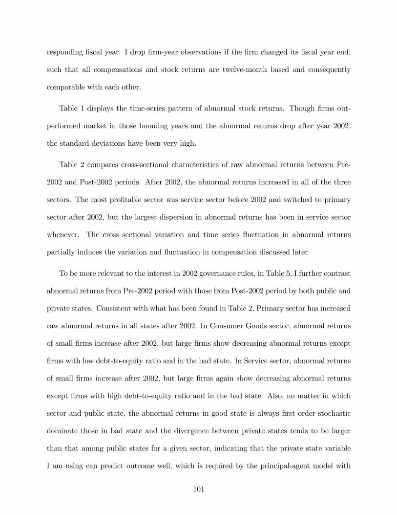
responding �scal year. I drop �rm-year observations if the �rm changed its �scal year end,

such that all compensations and stock returns are twelve-month based and consequently

comparable with each other.

Table 1 displays the time-series pattern of abnormal stock returns. Though �rms out-

performed market in those booming years and the abnormal returns drop after year 2002,

the standard deviations have been very high.

Table 2 compares cross-sectional characteristics of raw abnormal returns between Pre-

2002 and Post-2002 periods. After 2002, the abnormal returns increased in all of the three

sectors. The most pro�table sector was service sector before 2002 and switched to primary

sector after 2002, but the largest dispersion in abnormal returns has been in service sector

whenever. The cross sectional variation and time series �uctuation in abnormal returns

partially induces the variation and �uctuation in compensation discussed later.

To be more relevant to the interest in 2002 governance rules, in Table 5, I further contrast

abnormal returns from Pre-2002 period with those from Post-2002 period by both public and

private states. Consistent with what has been found in Table 2, Primary sector has increased

raw abnormal returns in all states after 2002. In Consumer Goods sector, abnormal returns

of small �rms increase after 2002, but large �rms show decreasing abnormal returns except

�rms with low debt-to-equity ratio and in the bad state. In Service sector, abnormal returns

of small �rms increase after 2002, but large �rms again show decreasing abnormal returns

except �rms with high debt-to-equity ratio and in the bad state. Also, no matter in which

sector and public state, the abnormal returns in good state is always �rst order stochastic

dominate those in bad state and the divergence between private states tends to be larger

than that among public states for a given sector, indicating that the private state variable

I am using can predict outcome well, which is required by the principal-agent model with

101

hidden information in state. Overall, �rms present di¤erent abnormal return distribution in

di¤erent states.

3.3.3 Compensation

CEOs care about their overall wealth change implied by their compensation packages. In

the ExecComp database, available to us are salary, bonus, other annual compensation not

properly categorized as salary and bonus, restricted stock granted during the year, aggregate

value of stock options granted during the year as valued using S&P�s Black Scholes methodol-

ogy, amount paid under the company�s long-term incentive plan and all other compensation.

CEOs�wealth changes with their holdings in �rm-speci�c equity as well. They can always

o¤set the aggregate risks imposed in their compensation package by adjusting their market

portfolio but cannot avoid being exposed to non-diversi�able risks of holding �rm stocks and

options. As a result, CEOs�wealth changes in holding �rm-speci�c equity are re�ected in

the value change given that they cannot diversify those idiosyncratic risks.

Following the concept of wealth change adopted by Antle and Smith (1985, 1986), Hall

and Liebman (1998), and Margiotta and Miller (2000), I construct the total compensation

by adding wealth change in options held and wealth change in stocks held into other regular

components like salary, bonus, options, restricted stocks, and so on. The wealth change in

holding stocks is equal to the beginning shares of held stocks multiplied by the raw abnormal

returns. By holding the options from existing grants rather than disposing this part of wealth

into a market portfolio, CEO obtains the net of ending option value and beginning option

value multiplied by market portfolio return. More detailed procedure goes to Appendix.

Table 3 shows the time-series pattern of each component as well as the total compensa-

tion. The documented soaring CEOs�compensation seems to be inverse after 2002. Also, I

102

�nd that the level and �uctuation in equity-based compensation components have more in�u-

ence on those of the total compensation, consistent with the previous analysis and justifying

the importance of adopting a more comprehensive measure of CEOs�wealth.

Table 4 summarizes total compensation by public and private states, again contrasting

Pre-2002 against Post-2002 period. The trend between the two periods is consistent with

that observed in abnormal returns in Table 5. The post-2002 compensation is always higher

or insigni�cantly lower than the pre-2002 compensation in all states in the three sectors.

Compensation in bad states is lower than that in good states all over the sample. Also,

large �rms seem to pay higher compensation, which is consistent with previous �ndings

from time-series change of compensation that the moral hazard cost can explain executive

compensation and large �rms have more severe problems to be compensated (Gayle and

Miller, 2009).

3.4 NONPARAMETRIC TESTS AND RESULTS

I conduct a probability density equality test on the change in the distribution of gross

abnormal returns (performance measure) and a model speci�cation test on the change in

the optimal contract shape from the Pre-2002 period to the Post-2002 period. I found that

both changes are signi�cant, which is consistent with Holmstrom and Kaplan (2003) who

suggest that the overall corporate governance system in U.S. can react quickly to address

those problems evidenced by collapse of business monsters.

In the structural estimation discussed in next subsections, the e¤ort costs corresponding

to working and shirking both change across the passage of 2002. These results imply that

the productivity changes, no matter it is captured by the managerial input (captured by

103

e¤ort costs) or by the output (captured by the distribution of the gross abnormal return).

As a response to the changes in these fundamentals, the optimal contract changes as well.

Before moving to the structural model identi�cation and estimation, I �rst explore the

empirical pattern of the gross abnormal return and optimal compensation for two reasons.

First, they are key elements in the model such that their changes from Pre-2002 to Post-2002

period re�ect the essential changes in other structural parameters, especially those measures

of agency costs. Second, the distribution of gross abnormal returns and the curvature of

the optimal compensation, which I focus on in this section, can be both nonparametrically

estimated before I introduce more complicated structures as I need for other primitives, for

instance the risk-aversion parameter. In this section, I brie�y describe the method used to

derive consistent estimators of these two variables, nonparametrically test on their changes

over the two periods and report the results of testing statistics.

3.4.1 Estimating Optimal Compensation and Performance Measure

Equity-based compensation is designed to align the interests of CEOs to shareholders and

consequently eliminate the moral hazard problem. While including stock returns into the

performance measure metric, I are aware of two issues. First, the stock return which is used

as a performance measure in the optimal contract should be closely tied to CEOs�e¤orts

but eliminate stochastic variations that are out of CEOs�control. Second, the performance

measure should re�ect the outcome sharing between shareholders and CEOs, that is, re�ect

returns before compensation payment.

Taking into account these two points, I construct the performance measure, gross ab-

normal return as I call, in the following steps. First I subtract the market portfolio return

from the annual return to a �rm stock in the same corresponding �scal year. The residual

104

captures the idiosyncratic components in �rm stock returns. This non-diversi�able portion

generates the incentive to work rather than shirk. Given that neither the gross abnormal

return nor the optimal compensation can be directly observed from the data, I construct

consistent estimators of them as discussed below.

exnt is the raw abnormal returns and ewmt is the total compensation of �rm n in year

t. (Znt; Snt) are state variables de�ned previously. First I nonparametrically estimate the

optimal compensation by running the following regression6

bwnt =XN

m=1;m 6=newmt � IfZmt = Znt; Smt = SntgK � exmt�exnthx

; vm;t�1�vn;t�1hv

�XN

m=1;m 6=nIfZmt = Znt; Smt = SntgK

� exmt�exnthx

; vm;t�1�vn;t�1hv

� (3.2)

where vn;t�1 is the market value of �rm n at the end of year t-1. Then I calculate the

gross abnormal returns by

xnt � exnt + bwntvn;t�1

(3.3)

Now the consistent estimate of optimal compensation conditional on state (Z; S) is given

by

wnt(xntjZ; S) =

XN

m=1;m 6=nbwmt � IfZmt = Z; Smt = SgK �xmt�xnthx

�XN

m=1;m 6=nIfZmt = Z; Smt = SgK

�xmt�xnt

hx

� (3.4)

3.4.2 Test on the Change in the Distribution of Gross Abnormal Return

3.4.2.1 Test statistic Given that the optimal compensation depends on the underlying

distribution of the performance measure (gross abnormal return in the paper), I �rst test the

6K(�) is a multivariate standard normal kernel density function as below.

K(�) = exp(�0:5 �

�xmt � xnt

hx

�2)� exp

(�0:5 �

�vmt � vnt

hv

�2) jSj�1=2

(2�)hxhv

where S = cov(ex; v), hx=v = 1:06 � sdx=v � N�1=5If�g , (x; v) = (ex; v)S�1=2; (ext; vt�1) are the raw abnormal

returns and raw one-year lagged market value.

105

change in the distribution of gross abnormal return from Pre-2002 to Post-2002. The riskier

the distribution of gross abnormal returns is in the mean-spread sense, the more costly is for

shareholders to motivate risk-averse CEOs.

The probability density function (PDF) of gross abnormal return xnt is nonparametrically

estimated by

f(xntjZ; S) =

XN

m=1IfZmt = Z; Smt = SgK

�xmt�xnt

hx

�XN

m=1IfZmt = Z; Smt = Sg

(3.5)

I have two series of gross abnormal returnsnx(N)nt

on=1;N1pre

from Pre-2002 period andnx(N)nt

on=1;N2post

from Post-2002 period. Assuming thatnx(N)nt

on=1;N1pre

has PDF fpre(�) andnx(N)nt

o1;N2post

has

PDF fpost(�)respectively. To test whether the underlying gross abnormal returns distribute

di¤erently between Pre-2002 versus Post-2002 period is equivalent to test on the equality

between the PDF in the two periods, i.e. test HPDF0 : fpre(x) = fpost(x) for almost all x.

Based on the test for equality of PDFs proposed by Li and Racine (2007, pp. 363), I cal-

culate the statistics T PDF by state and sector. T PDF follows standard normal distribution

N(0; 1):Please refer to the appendix for details of T PDF construction.

I have two series of gross abnormal returnsnx(N)nt

on=1;N1pre

andnx(N)nt

on=1;N2post

from Pre-

2002 and Post-2002 periods respectively. Assuming thatnx(N)nt

on=1;N1pre

has PDF fpre(�) andnx(N)nt

o1;N2post

has PDF fpost(�)respectively. To test whether the underlying gross abnormal

returns distribute di¤erently before versus after 2002 is equivalent to test on the equality

between the PDF of each of the two periods, or test HPDF0 : fpre(x) = fpost(x) for almost all

x. If HPDF0 is false, then the statistics T PDF constructed below has P (T PDF > C)! 1, for

any positive constant C. Based on the test for equality of PDFs proposed by Li and Racine

106

(2007, pp. 363), I calculate the statistics T PDF by state and sector at

T PDF = (N1N2h2)1=2

(Ibn � cn;b)b�b d�!N(0; 1)

where

Ibn =

�1

N1

�2 N1Xm=1

N1Xn=1

Kx�preh;mn +

�1

N2

�2 N2Xm=1

N2Xn=1

Kx�posth;mn � 2

N1N2

N1Xm=1

N2Xn=1

Kx�pre;x�posth;mn

cn;b =k(0)

h[1

N1+1

N2]

b�b2 = h

N1N2

8><>:PN1

m=1

PN1n=1(N2=N1)(K

x�preh;mn )

2 +PN2

m=1

PN2n=1(N1=N2)(K

x�posth;mn )2

+2PN1

m=1

PN2n=1(K

x�pre;x�posth;mn )2

9>=>;and the kernel density functions are de�ned as

Kx�preh;mn � (1=h)kx

�xpremt � xprent

h

�Kx�posth;mn � (1=h)kx

�xpostmt � xpostnt

h

�Kx�pre;x�posth;mn � (1=h)kx

�xpremt � xpostnt

h

�kx() =

1p2�b�x exp

(�12

�xmt � xnt

h

�2)

T PDF is a one-sided test, therefore I reject HPDF0 at level 1% if T PDF > 2:33; reject

HPDF0 at level 5% if T PDF > 1:64, and reject HPDF

0 at level 10% if T PDF > 1:28:

3.4.2.2 Result Table 7.1 reports the statistics T PDF for the 24 states (3 sectors * 2

private states * 4 public states). Except in the good state of (AS; CL) in the Primary sector

(the value of the static is 0.93) and in the bad state of (AS; CL) in the Consumer Goods

sector (the value of the static is 0.75), in all other states the values of T PDF are above

the critical value of 5% con�dence level (1.64). Consequently, we can reject HPDF0 in these

107

remaining 22 states.

This favorable result indicates that there may exist signi�cant changes in the distribu-

tion of gross abnormal returns from Pre-2002 period to Post-2002 period. The changes in

executive compensation, if any, cannot be only due to behavior changes of CEOs.

3.4.3 Test on the Change in the Optimal Contract Shape

3.4.3.1 Test statistic The test on the change in contract shape is equivalent to a model

speci�cation test on the signi�cance of a dummy variable in the standard Nadaraya-Watson

kernel regression of optimal compensation on the gross abnormal return. The dummy vari-

able I2002 equals to 1 if the observation is from Post-2002 period and equals to 0 otherwise.

The null hypothesis states as follows. HW0 : Pr [w (x; I2002) =W (x)] = 1 , meaning that

the contract shape is not signi�cantly di¤erent between Pre-2002 and Post-2002 period. The

testing statistic forHW0 is TW , which follows the standard normal distribution N(0; 1):Please

refer to the appendix for the detail of constructing TW .

The test on the change in contract shape is equivalent to a model speci�cation test on the

signi�cance of a dummy variable in the standard Nadaraya-Watson kernel regression of opti-

mal compensation on gross abnormal returns. The dummy variable I2002 equals to 1 if the ob-

servation is from Post-2002 period and equals to 0 otherwise. HW0 : Pr [w (x; I2002) =W (x)] =

1 or the contract shape is not signi�cantly di¤erent between Pre-2002 and Post-2002 period.

If HW0 is false, then the squared di¤erence in nonparametric estimates of the functions

w (x; I2002) and W (x) should be beyond certain critical values in the distribution of the

108

statistics TW . I tend to reject HW0 when TW is large. Speci�cally,

TW = ��111�Nh(p+q)=2 � �� h�(p+q)=2 12 � h(q�p)=2 22 � h(p+q)=2H�p 32

�d�!N(0; 1)

where

� =1

N

XN

n=1

�whn �WH

n

2An

I get two nonparametric estimators of optimal compensation, whn andWHn and their densities

fhn and fHn as follows.

whn �

XN

m=1wm � IfZm = Zn; Sm = SngKh

�xm�xnhx

; I2002m

�XN

m=1IfZm = Zn; Sm = SngKh

�xm�xnhx

; I2002m

�

WHn �

XN

m=1wm � IfZm = Zn; Sm = SngKH

�xm�xnhx

�XN

m=1IfZm = Zn; Sm = SngKH

�xm�xnhx

�fhn =

1

N

XN


�xm � xnhx

; I2002m

�fHn =

1

N

XN


�xm � xnhx

�

A is a non-negative N-dimension weighting vector with element corresponding to each

observation. An = 1 if xn falls into the 2.5%-97.5% range of gross abnormal returns within

the same state identi�ed by Zn and Sn, otherwise An = 0: p is the dimension of non-tested

regressors and q is the dimension of the tested regressors. p = q = 1 in the context.

Also,

�2nh =

XN

m=1w2m � IfZm = Zn; Sm = SngKh

�xm�xnhx

; I2002m

�XN


�xm�xnhx

; I2002m

� ��whn�2

109

�2nH =

XN

m=1w2m � IfZm = Zn; Sm = SngKh

�xm�xnhx

�XN


�xm�xnhx

� ��WHn

�2

�211 =2C11N

XN

n=1

(�2nh)2A2n

fhn

C12 =

�1

2p�

�p+q; C22 =

�1p2�

�p; C32 =

�1

2p�

�p; C11 =

�1

2p2�

�p+q

12 =C12N

XN

n=1

�2nhAnfhn

; 22 = �2C22N

XN

n=1

�2nhAnfHn

; 32 =C32N

XN

n=1

�2nHfAn

fHn

fAn =XN


�xm�xnhx

�AmXN


�xm�xnhx

�TW is a one-sided test, therefore I reject HW

0 at level 1% if TW > 2:33; reject HW0 at

level 5% if TW > 1:64, and reject HW0 at level 10% if TW > 1:28:

3.4.3.2 Result In Table 7.2 I report the test static for the change of compensation

contract shape (TW ) by state and sector, in the same manor as it is done for the test on the

change of the distribution of gross abnormal returns. In all states, the static is above 2.33.

It implies that the null hypothesis HW0 that there is no change in compensation contract

shape is rejected.

This result suggests that the contract shape has signi�cantly changed since 2002, and

thus it is worth taking further studies to estimate the quantitative welfare e¤ect and look

for the driving forces behind such changes.

3.5 CONCLUSION

As a legislative response to those corporate governance failures seen by the beginning of this

century, a set of rules including SOX and several other amendments on stock exchanges�

110

regulations were enacted. Regulatory intervention has been controversial because of the

"one-size-�t-all" criticism. It is important to examine whether those rules have in�uenced

the corporate governance of �rms. One aspect is executive compensation which re�ects both

executives�attributes captured by CEOs�preference parameters in structural models and

production technology captured by the distribution of performance measure.

As a �rst pass investigation, this paper nonparametrically tests the change of the dis-

tribution of the performance measure (gross abnormal returns) and the change of CEOs�

compensation contract shape. I �nd that both changes are signi�cant from Pre-2002 to

Post-2002 period. These �ndings about the basic properties of CEOs�compensation suggest

that the optimal compensation contracts between shareholders and CEOs may be adaptive

to the exogenous shock of 2002. The change in CEOs�compensation may not be purely

driven by behavioral change of CEOs but can also be the result of production change. Also,

the signi�cant change in contract shape indicates that agency costs embedded in the com-

pensation contracts may change after 2002 as well. This invites a more sophisticated study

using structural approach in Gayle et al. (2013).

111

4.0 APPENDIX TO CHAPTER 2

4.1 PROOFS

Proof of Lemma 1. The assumption that manager 1�s marginal in�uence on the distribution

of the single output x is unconditional on manager 2�s e¤ort choice implies that the deviation

of x�s probability density from manager 1 working to manager 1 shirking is the same no

matter whether manager 2 works or shirks, and vice versa. Denote f(�jj; k) as the PDF of

x conditional on the two managers�e¤ort choices, mathematically:

g1(x) � f(x j manager 1 shirks, manager 2 works)f(x j manager 1 works, manager 2 works) (4.1)

=g1(x)f(x)

f(x)(4.2)

=f(x j manager 1 shirks, manager 2 shirks)f(x j manager 1 works, manager 2 shirks) (4.3)

=f(x j manager 1 shirks, manager 2 shirks)

f(x)(4.4)

g2(x) � f(x j manager 1 works, manager 2 shirks)f(x j manager 1 works, manager 2 works) (4.5)

=g2(x)f(x)

f(x)(4.6)

=f(x j manager 1 shirks, manager 2 shirks)f(x j manager 1 shirks, manager 2 works) (4.7)

=f(x j manager 1 shirks, manager 2 shirks)

g1(x)f(x): (4.8)

112

Using (4.1) and (4.7) gives

Zg1(x)g2(x)f(x)dx

=

Zf(x j manager 1 shirks, manager 2 works)f(x j manager 1 works, manager 2 works)

� f(x j manager 1 shirks, manager 2 shirks)f(x j manager 1 shirks, manager 2 works)f(x)dx

=

Zf(x j manager 1 shirks, manager 2 shirks)

f(x)f(x)dx

= 1:

The last equality is by the de�nition of a PDF.

Proof of Proposition 2. See the �rst-order conditions (FOCs) in the proof of Proposition 3

later.

Proof of Proposition 3. No Mutual Monitoring Model

We want to show that �� = � (��). Suppose � is known. Write down the Lagrangian as

L = E [ln v1t(x) + ln v2t(x)]

��1��

1bt�112 Et [v1t(x)]� �

1bt�111 Et [v1t(x)g1(x)]

��2

��

1bt�122 Et [v2t(x)]� �

1bt�121 Et [v2t(x)g2(x)]

��3

��

1bt�112 Et [v1t(x)]� 1

��4

��

1bt�122 Et [v2t(x)]� 1

�: (4.9)

The First Order Condition (FOC hereafter) w.r.t. v1t(x) is

1=v1t(x) = (�1 + �3)�1

bt�112 � �1�

1bt�111 g1(x): (4.10)

113

FOC w.r.t. v2t(x) is

1=v2t(x) = (�2 + �4)�1

bt�122 � �2�

1bt�121 g2(x): (4.11)

Evaluate the FOCs at the threshold values of shirking distribution, respectively, to get

1=v1t(x1) = (�1 + �3)�1

bt�112 (4.12)

1=v2t(x2) = (�2 + �4)�1

bt�122 : (4.13)

Take the expectation of the FOCs over the distribution with both diligent managers to get

E [1=v1t(x)] = (�1 + �3)�1

bt�112 � �1�

1bt�111 (4.14)

E [1=v2t(x)] = (�2 + �4)�1

bt�122 � �2�

1bt�121 : (4.15)

The binding participation constraint for each manager gives

��12 = Et[v1t(x)]1�bt (4.16)

��22 = Et[v2t(x)]1�bt : (4.17)

The binding incentive compatibility constraint gives

�1

bt�111 Et [v1t(x)g1(x)] = �

1bt�121 Et [v2t(x)g2(x)] = 1: (4.18)

Multiply both sides of (4.10) and integrate over f(x); it follows that

1 = (�1 + �3)�1

bt�112 Et [v1t(x)]� �1�

1bt�111 Et [v1t(x)g1(x)] ; (4.19)

114

and plugging (4.16) and (4.17) into the preceding, it follows that

�3 = 1:

Multiply both sides of (4.11) and integrate over f(x); it follows that

1 = (�2 + �4)�1

bt�122 Et [v2t(x)]� �2�

1bt�121 Et [v2t(x)g2(x)] ; (4.20)

and plugging (4.17) and (4.18) into the preceding, it follows that

�4 = 1:

Multiplying (4.12) by Et [v1t(x)] and using �3 = 1, it follows that

Et [v1t(x)] =v1t(x1) = �1 + �3

�1 = Et [v1t(x)] =v1t(x1)� 1:

Similarly, multiplying (4.13) by Et [v2t(x)] and using �4 = 1, it follows that

Et [v2t(x)] =v2t(x2) = �2 + �4

�2 = Et [v2t(x)] =v2t(x2)� 1:

Equations (4.10), (4.12), and (4.14) together give

1=v1t(x1)� E [1=v1t(x)] = �1�1

bt�111

1=v1t(x1)� 1=v1t(x) = �1�1

bt�111 g1(x)

115

and

g1(x) =1=v1t(x)� 1=v1t(x1)E [1=v1t(x)]� 1=v1t(x1)

(4.21)

g2(x) =1=v2t(x)� 1=v2t(x2)E [1=v2t(x)]� 1=v2t(x2)

: (4.22)

Plug into (4.18); it follows that

��11 =

�Et[v1t(x)]� v1t(x1)1� v1t(x1)E[1=v1t(x)]

�1�bt��21 =

�Et[v2t(x)]� v2t(x2)1� v2t(x2)E[1=v2t(x)]

�1�bt:

Mutual Monitoring with Total Utility Maximization Model

We want to show that �� = � (��).

The Lagrangian for the shareholders�cost minimization problem is

L = Et [ln v1t(x) + ln v2t(x)] (4.23)

��0��

1bt�112 Et [v1t(x)] + �

1bt�122 Et[v2t(x)]� 2

�

��1

8>><>>:��

1bt�112 Et[v1t(x)] + �

1bt�122 Et[v2t(x)]

��

1bt�111 Et[v1t(x)g(x)] + �

1bt�121 Et[v2t(x)g(x)]

�9>>=>>; :

The First Order Condition (FOC hereafter) w.r.t. v1t(x) is

1=v1t(x) = �0�1

bt�112 + �1�

1bt�112 � �1�

1bt�111 g(x): (4.24)

FOC w.r.t. v2t(x) is

1=v2t(x) = �0�1

bt�122 + �1�

1bt�122 � �1�

1bt�121 g(x): (4.25)

116

Multiply both sides of (4.24) with v1t(x) and then integrating over f(x), we get

1 = (�0 + �1)�1

bt�112 Et[v1t(x)]� �1�

1bt�111 Et[v1t(x)g(x)]: (4.26)

Similarly, from (4.25), we get

1 = (�0 + �1)�1

bt�122 Et[v2t(x)]� �1�

1bt�121 Et[v2t(x)g(x)]: (4.27)

Recall that

g(x) = 0;8x > x:

Evaluate the FOCs at the threshold of the both-manager shirking distribution,

1=v1t(x) = (�0 + �1)�1

bt�112 (4.28)

1=v2t(x) = (�0 + �1)�1

bt�122 : (4.29)

Binding participation constraint gives

�1

bt�112 Et[v1t(x)] + �

1bt�122 Et[v2t(x)] = 2: (4.30)

Binding incentive compatibility constraint gives

�1

bt�112 Et[v1t(x)] + �

1bt�122 Et[v2t(x)] = �

1bt�111 Et[v1t(x)g(x)] + �

1bt�121 Et[v2t(x)g(x)]: (4.31)

The utility transfer constraint implies that the following equation is held if both managers

shirk:

�1

bt�111 Et[v1t(x)g(x)] = �

1bt�121 Et[v2t(x)g(x)]: (4.32)

Similarly, if both work,

�1

bt�112 Et[v1t(x)] = �

1bt�122 Et[v2t(x)]: (4.33)

117

Combining (4.30) and (4.31), we can immediately get

�1

bt�111 Et[v1t(x)g(x)] = �

1bt�121 Et[v2t(x)g(x)] = 1 (4.34)

�1

bt�112 Et[v1t(x)] = �

1bt�122 Et[v2t(x)] = 1 (4.35)

��12 = Et[v1t(x)]1�bt (4.36)

��22 = Et[v2t(x)]1�bt : (4.37)

Add (4.28) and (4.29). Then use binding IC and plug in (4.36) and (4.37):

2 = �0

��

1bt�112 Et[v1t(x)] + �

1bt�122 Et[v2t(x)]

�+ 0

��0 = 1:

Plug ��0 into (4.28) and (4.29); we get

��1 =

�Et[v1t(x)]

v1t(x)� 1�

=

�Et[v2t(x)]

v2t(x)� 1�:

Take the expectation over FOCs; we get

E[1=v1t(x)] = (�0 + �1)�1

bt�112 � �1�

1bt�111 (4.38)

E[1=v2t(x)] = (�0 + �1)�1

bt�122 � �1�

1bt�121 : (4.39)

Plug ��0 and ��1 into (4.28) and (4.38); we get

��11 =

�Et[v1t(x)]� v1t(x)1� v1t(x)E[1=v1t(x)]

�1�bt: (4.40)

118

Similarly, combining (4.29) and (4.39), we get

��21 =

�Et[v2t(x)]� v2t(x)1� v2t(x)E[1=v2t(x)]

�1�bt: (4.41)

Plug ��0 and ��1 into (4.24) and (4.25), respectively; using (4.38), (4.39), (4.32), and (4.33),

we get

1� v1t(x)=v1t(x)1� v1t(x)E[1=v1t(x)]

= g�(x) =1� v2t(x)=v2t(x)

1� v2t(x)E[1=v2t(x)]:

Mutual Monitoring with Individual Utility Maximization Model

See the proof for the no mutual monitoring model. The only di¤erence is that the

likelihood ratio is the same.

Proof of Proposition 4. In the cost minimization problem, the objective function is quasi-

concave and the constraints are linear in vi(x). Consequently, the FOCs that are used

to derive the parameters can uniquely determine the solution to the optimal contracting

problem if the complementary slackness conditions are satis�ed. This can be con�rmed by

multiplying the Lagrangian multiplier with the associated constraint and �nding that the

product equals zero. Then the proposition is proved.

4.2 NONPARAMETRIC ESTIMATION OF COMPENSATION AND

THE PROBABILITY DENSITY FUNCTION OF GROSS ABNORMAL

RETURNS IN EQUILIBRIUM

Either the gross abnormal return or the optimal compensation cannot be directly observed

from real data. I construct their consistent estimators as discussed subsequently. Here exntrepresents the abnormal returns, and ewimt is manager i�s total compensation from �rm n in

year t. (Znt; Snt) are �rm type variables, de�ned before. I nonparametrically estimate the

119

optimal compensation using the following kernel regression (Pagan and Ullah 1999):1

wint � Et[ ewintjexnt; Vn;t�1]=

PNm=1;m 6=n ewimt � IfZmt = Znt; Smt = SntgK � exmt�exnthx

; Vm;t�1�Vn;t�1hV

�PN

m=1;m 6=n IfZmt = Znt; Smt = SntgK� exmt�exnt

hx; Vm;t�1�Vn;t�1

hV

� ;

where Vn;t�1 is the market value of �rm n at the end of year t�1. Then I calculate the gross

abnormal returns by

xnt � exnt + w1ntVn;t�1

+w2ntVn;t�1

:

The PDF of gross abnormal return xnt is nonparametrically estimated by a kernel estimator:

f(xntjZ; S) =

PNm=1 IfZmt = Z; Smt = SgK

�xmt�xnt

hx

�PN

m=1 IfZmt = Z; Smt = Sg:

4.3 TABLES

1K(�) is a multivariate standard normal kernel density function:

K(�) = exp(�0:5 �

�xmt � xnt

hx

�2)� exp

(�0:5 �

�V mt � V nt

hV

�2) jSj�1=2

(2�)hxhV;

where S = cov(ex; V ), hx=V = 1:06 � sdx=V � N�1=5If�g , is a cross-validation bandwidth and (x; V ) =

(ex; V )S�1=2; (ext; Vt�1) are the raw abnormal returns and raw one-year lagged market value.120

Table 1: Cross-Sectional Summary on Firm Character-istics

Sector Primary Consumer ServiceGoods

Assets 4704 3059 4688(7423) (5035) (8307)

Debt/Equity 1.84 1.52 2.56(1.40) (1.41) (3.36)

Abnormal Returns -0.014 -0.026 -0.007(0.29) (0.31) (0.33)

Market Value 3285 3440 3417(4808) (5181) (5059)

Observations 6583 5004 8023

Note: Both Assets (the Total Assets on BalanceSheet) and Market Value are measured in mil-lions of 2006 $US. To calcuate the abnormal re-turn, for each �rm in the sample, I calculatemonthly compounded returns adjusted for split-ting and repurchasing for each �scal year, and sub-tract the return to a value-weighted market portfolio(NYSE/NASDAQ/AMEX) from the compoundedreturns for the corresponding �scal year. I drop �rm-year observations if the �rm changed its �scal yearend, such that all compensations and stock returnsare twelve-month based.

1

Table 2: Cross-Sectional Summary on Abnormal Stock Returns and Total Compensation

Abnormal Stock Returns Highest Compensation Second Highest Compensation

Sector Primary Consumer Service Primary Consumer Service Primary Consumer ServiceGoods Goods Goods

[A, D/E]

[S, S] -0.020 -0.030 -0.026 4746 6294 6877 1761 2042 2518(0.317) (0.339) (0.366) (8297) (11048) (10577) (2727) (3561) (3529)2284 1707 3079

[S, L] -0.005 -0.037 -0.009 3798 5039 6484 1523 1879 2552(0.325) (0.354) (0.335) (6020) (8379) (10064) (2221) (3018) (3424)1004 791 928

[L, S] -0.021 -0.028 -0.027 8409 10224 13994 3488 4050 5754(0.277) (0.276) (0.325) (10887) (13612) (15765) (4319) (4807) (5927)1003 791 928

[L, L] -0.017 -0.024 0.030 7501 11388 11483 3158 4506 4705(0.264) (0.296) (0.276) (10311) (13647) (13868) (3875) (4877) (5308)2292 1715 3088

Note: Compensation is measured in thousands of 2006 $US. Mean is reported and standard deviation is in theparenthesis below. In the �rst three columns, the third row for each type of �rms reports the number of observations.

2

Table3:Time-SeriesSummaryofCompensationComponentsforEachManager

Year

Salary

Bonus

Valuesof

Valuesof

ChangesinWealth

ChangesinWealth

Total

No.of

RestrictedStocks

GrantedOptions

from

StocksHeld

from

OptionsHeld

Compensation

Observations

1st

2nd

1st

2nd

1st

2nd

1st

2nd

1st

2nd

1st

2nd

1st

2nd

1993

545

413

347

240

9261

599

384

834

493

1186

468

4759

2457

1423

(265)

(209)

(408)

(315)

(290)

(230)

(1000)

(701)

(2000)

(1465)

(3653)

(2090)

(6920)

(4369)

1994

548

411

398

269

9773

852

492

1171

631

742

300

5045

2422

1561

(264)

(208)

(437)

(332)

(317)

(253)

(1320)

(873)

(2433)

(1557)

(2748)

(1765)

(7251)

(3634)

1995

518

407

402

272

107

79738

454

1050

561

813

300

4941

2519

1543

(262)

(207)

(444)

(328)

(332)

(273)

(1236)

(817)

(2375)

(1569)

(3024)

(1677)

(7505)

(4414)

1996

536

407

418

276

125

761007

630

1474

879

799

451

6059

3156

1610

(263)

(203)

(463)

(324)

(363)

(258)

(1504)

(1020)

(2818)

(1938)

(2934)

(2147)

(8478)

(4743)

1997

528

401

443

305

113

951098

739

1754

1230

1330

751

7472

4272

1682

(261)

(203)

(472)

(362)

(362)

(310)

(1574)

(1230)

(3113)

(2582)

(3949)

(2686)

(9566)

(6634)

1998

481

390

383

271

121

941112

798

1111

701

537

208

5487

3099

1679

(255)

(196)

(461)

(340)

(369)

(317)

(1601)

(1308)

(2637)

(2046)

(2921)

(1985)

(8420)

(5602)

1999

522

407

440

299

117

821256

852

1514

969

313

775788

3484

1482

(272)

(200)

(512)

(350)

(363)

(269)

(1705)

(1341)

(3061)

(2338)

(2585)

(1835)

(8544)

(6339)

2000

563

431

417

314

124

941306

941

1915

1347

1979

1071

9295

5510

1400

(283)

(217)

(486)

(399)

(394)

(306)

(1598)

(1455)

(3357)

(2667)

(4527)

(2974)

(10990)

(8244)

2001

590

444

411

274

148

114

1594

1132

2298

1569

2089

923

10471

5642

1418

(276)

(223)

(523)

(373)

(414)

(348)

(1910)

(1567)

(3561)

(2802)

(4277)

(2408)

(11265)

(7296)

2002

584

427

467

320

162

130

1429

947

1510

936

1825

781

8386

4308

1500

(279)

(205)

(539)

(410)

(435)

(359)

(1759)

(1393)

(2969)

(2200)

(4177)

(2312)

(10157)

(6403)

2003

600

441

528

352

219

174

1231

753

2379

1399

1075

616

8326

4666

1456

(282)

(207)

(589)

(429)

(505)

(414)

(1636)

(1114)

(3679)

(2577)

(3599)

(2712)

(9959)

(7130)

2004

584

432

599

398

288

218

1246

779

1753

1011

1458

772

8189

4381

1464

(278)

(203)

(617)

(437)

(551)

(438)

(1632)

(1234)

(3134)

(2226)

(3821)

(2715)

(9681)

(6124)

2005

563

430

597

388

345

267

1076

622

1286

807

1132

546

7473

3911

1392

(270)

(208)

(610)

(413)

(592)

(478)

(1555)

(1009)

(2883)

(2138)

(3528)

(2234)

(9825)

(6080)

Note:"1st"isthehighestpaidmanagerand"2nd"isthesecondhighestpaid.Eachcomponentismeasuredinthousandsof2006$US.Themeanofeach

componentisreportedwithstandarddeviationistheparenthesisbelow.TheChangesinWealthfrom

StocksHeldisequaltothebeginningsharesofheld

stocksmultipliedbytheabnormalreturns.TheChangesinWealthfrom

OptionsHeldisthedi¤erencebetweentheendingoptionvalueandthebeginning

optionvaluemultipliedbymarketportfolioreturn.

3

Table 4: The Distribution of Positions Held by the Two Highest Paid Managers

Sector Primary Consumer Goods Service

Compensation Rank 1st 2nd 1st 2nd 1st 2nd

Functional 0.01 0.01 0.01 0.01 0.01 0.02General 1 0.21 0.08 0.17 0.08 0.21 0.09General 2 0.18 0.51 0.23 0.50 0.23 0.51

Functional & General 1 0.04 0.10 0.06 0.11 0.04 0.08Functional & General 2 0.05 0.18 0.07 0.15 0.06 0.15General 1 & General 2 0.50 0.12 0.45 0.14 0.44 0.13

Functional & General 1 & 2 0.01 0.01 0.01 0.01 0.01 0.02

Number of observations 6583 6583 5004 5004 8023 8023

Note: "1st" is the highest paid manager and "2nd" is the second highest paid. Foreach type of manager, I count the frequency of holding certain types of positionsas follows. "Functional" = 1 if the manager holds one of the following positions:CTO, CIO, COO, CFO, CMO but not any others. "General 1" = 1 if the managerholds one of the following positions: Chairman, President, CEO, or Founder butnot any others. "General 2" = 1 if the manager holds one of the following posi-tions: Executive Vice-President, Senior Vice-President, Vie-President, Vice-Chair,or Other (de�ned in the database) but not any others. "Functional & General 1"= 1 if the manager holds at least one position from each of the Functional cate-gory and the General 1 category but none from the General 2 category. Same ruleapplies to "Functional & General 2" and "General 1 & General 2". "Functional &General 1 & General 2" = 1 if the manager holds at least one position from eachof the three categories.

4

Table 5: The Risk Aversion Parameter�s 95 % Con�dence Regions for Di¤erent Speci�cations

A: No Mutual Monitoring: di¤erent likelihood ratio/di¤erent shadow price of IC

Sector [A, D/E] Risk Certainty Homogeneous Homogeneous HomogeneousAversion Equivalent within Size within Sector across Sectors

Primary [S, S] (12.75, 26.38) (0.350, 0.589)[S, L] (0.89, 16.25) (0.027, 0.426) (12.75, 16.25)[L, S] (6.16, 33.62) (0.181, 0.665)[L, L] (0.89, 2.34) (0.027, 0.070) ( , ) ( , )

Consumer [S, S] (0.26, 3.79) (0.008, 0.113)Goods [S, L] (1.83, 33.62) (0.055, 0.665) (1.83, 3.79)

[L, S] (0.34, 1.13) (0.010, 0.034)[L, L] (0.70, 2.34) (0.021, 0.070) (0.70, 1.13) ( , )

Service [S, S] (4.83, 26.38) (0.143, 0.589)[S, L] (0.55, 12.75) (0.016, 0.350) (4.83, 12.75)[L, S] (1.44, 7.85) (0.043, 0.228)[L, L] (1.44, 20.7) (0.043, 0.507) (1.44, 7.85) (4.83, 7.85) ( , )

B: Mutual Monitoring with Total Utility Maximization: same likelihood ratio/same shadow price of IC


Primary [S, S] (0.10, 0.13) (0.003, 0.004)[S, L] (0.16, 0.21) (0.005, 0.006) ( , )[L, S] ( , ) ( , )[L, L] ( , ) ( , ) ( , ) ( , )

Consumer [S, S] (0.05, 0.06) (0.001, 0.002)Goods [S, L] (0.16, 0.21) (0.005, 0.006) ( , )

[L, S] (0.02, 0.03) (0.001, 0.001)[L, L] (0.03, 0.04) (0.001, 0.001) (0.03, 0.03) ( , )

Service [S, S] (2E-9, 0.03) (2E-9, 0.001)[S, L] ( , ) (, ) ( , )[L, S] (0.02, 0.02) (0.001, 0.001)[L, L] (0.05, 0.06) (0.001, 0.002) ( , ) ( , ) ( , )

C: Mutual Monitoring with Individual Utility Maximization: same likelihood ratio/di¤erent shadow price of IC


Primary [S, S] (0.10, 20.70) (0.003, 0.529)[S, L] (0.16, 12.75) (0.005, 0.370) (0.16, 12.75)[L, S] (0.05, 10.00) (0.002, 0.301)[L, L] (0.08, 1.83) (0.003, 0.059) (0.08, 1.83) (0.16, 1.83)

Consumer [S, S] (0.05, 2.98) (0.002, 0.095)Goods [S, L] (0.21, 20.70) (0.007, 0.529) (0.21, 2.98)

[L, S] (0.02, 0.89) (0.001, 0.028)[L, L] (0.03, 2.34) (0.001, 0.075) (0.03, 0.89) (0.21, 0.89)

Service [S, S] (2E-9, 33.62) (2E-9, 0.685)[S, L] (0.04, 16.25) (0.001, 0.447) (0.04, 16.25)[L, S] (0.02, 4.83) (0.001, 0.153)[L, L] (0.05, 33.62) (0.002, 0.685) (0.05, 4.83) (0.05, 4.83) (0.21, 0.89)

Note: IC is short for the incentive compatibility constraint. Column [A, D/E] de�nes the �rm type which is basedon �rm size (total assets, A) and capital structure (debt-to-equity ratio, D/E). S (L) means the correspondingelement is below (above) its sector median. The con�dence region is estimated by a subsampling procedure using300 replecations of subsamples with size equal to 15% of the full sample. The certainty equivalent is the amountpaid to avoid a gamble with equal probability to win and lose $1 million and is measured in $ million with themedian of the bond price in the sample period.

5

5.0 APPENDIX TO CHAPTER 3

5.1 CALCULATION OF WEALTH CHANGE IN HOLDING STOCK

AND/OR OPTIONS

Due to the data availability, for each sample year, we can not exactly observe all the inputs

of Black-Sholes formula for grants carried from years before 1993, the beginning year of our

sample. Compustat ExecComp dataset only provides the valuation information for those

options newly granted after year 1993, including number of underlying stock shares, exercise

prices, expiration dates and issue dates. However, we need to know these Black-Sholes

inputs for options granted before year 1993 to completely value the wealth change of CEOs

by estimating the value of unexercised options and updating it each year. Instead, we assume

that all options are not exercised until expiration dates. For the same reason, we apply FIFO

rule to derive Black-Sholes inputs for options granted before year 1993, i.e. earlier issued

options will be exercised earlier too. Together, we use the average length of holding period

for each CEO to infer the issue dates and exercised prices for options granted before 1993.

The same routines apply to those non-zero options granted before the year when the CEO

entered our sample. We apply the dividend-adjusted Black-Sholes formula to re-evaluate the

CEOs�call options for each CEO in each year. See footnote for the details.1

1Below c is the call option value, K is the exercise price, Tm is the time to maturity (in years), S is the

121

5.2 TABLES

underlying security price, q is the dividend yield, r is the risk free rate, � is implied volatility. N(�) de�nesa standard normal cumulative distribution function.

c = Se�qTmN(d1)�Ke�rTmN(d2)

d1 =ln(S=K) + (r � q + �2=2)Tm

�pTm

d2 = d1 � �pTm

122

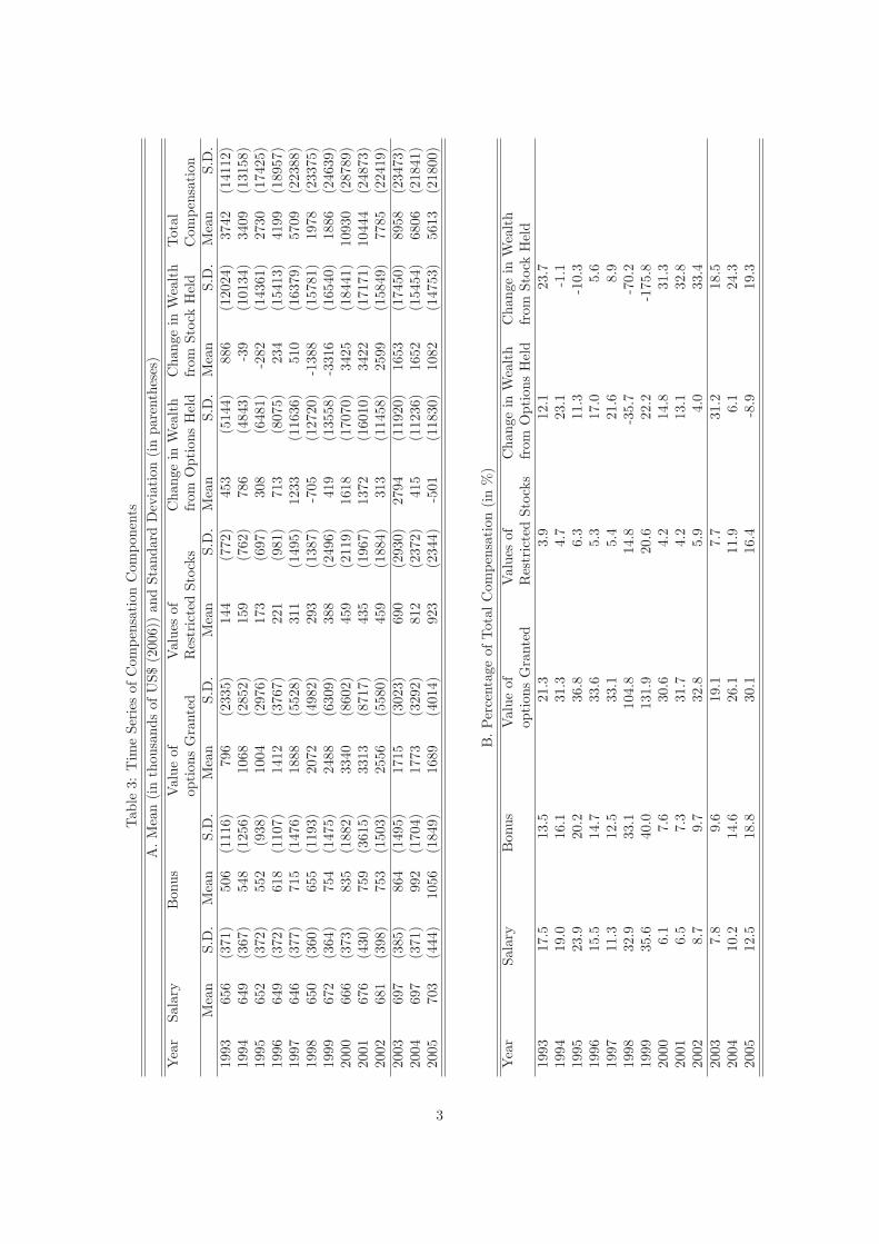
BIBLIOGRAPHY

Abowd, JM, and DS Kaplan, 1999, Executive compensation: Six questions that need an-

swering., Journal of Economic Perspectives 13, 145�167.

ACHARYA, VIRAL V., STEWART C. MYERS, and RAGHURAM G. RAJAN, 2011, The

internal governance of �rms, The Journal of Finance 66, 689�720.

Adams, RenèµNµEe B., and Daniel Ferreira, 2008, Do directors perform for pay?, Journal of

Accounting and Economics 46, 154 �171.

Aggarwal, Rajesh K., Mark E. Evans, and Dhananjay Nanda, 2012, Nonpro�t boards: Size,

performance and managerial incentives, Journal of Accounting and Economics 53, 466 �

487.

Albuquerque, Ana, 2009, Peer �rms in relative performance evaluation, Journal of Account-

ing and Economics 48, 69 �89.

Antle, Rick, and Abbie Smith, 1985, Measuring executive compensation: Methods and an

application, Journal of Accounting Research 23, 296�325.

, 1986, An empirical investigation of the relative performance evaluation of corporate

executives, Journal of Accounting Research 24, 1�39.

Armstrong, Chris, Alan Jagolinzer, and David Larcker, 2010, Performance-based incentives

for internal monitors, Rock Center for Corporate Governance at Stanford University Work-

ing Paper Series.

Armstrong, Christopher S., Jennifer L. Blouin, and David F. Larcker, 2012, The incentives

for tax planning, Journal of Accounting and Economics 53, 391 �411.

123

Armstrong, Christopher S., Wayne R. Guay, and Joseph P. Weber, 2010, The role of infor-

mation and �nancial reporting in corporate governance and debt contracting, Journal of


Arya, Anil, John Fellingham, and Jonathan Glover, 1997, Teams, repeated tasks, and implicit

incentives, Journal of Accounting and Economics 23, 7�30.

Balsam, Steven, and Setiyono Miharjo, 2007, The e¤ect of equity compensation on voluntary

executive turnover, Journal of Accounting and Economics 43, 95 �119.

Banker, Rajiv D, Masako N Darrough, Rong Huang, and Jose M Plehn-Dujowich, 2013,

The relation between ceo compensation and past performance, The Accounting Review

88, 1�30.

BANKER, RAJIV D., RONG HUANG, and RAMACHANDRAN NATARAJAN, 2009, In-

centive contracting and value relevance of earnings and cash �ows, Journal of Accounting

Research 47, 647�678.

Berle, Adolf Augustus, and Gardiner Coit Means, 1932, The modern corporation and private

property new york, macmillan reprinted in l944 edn.

Bertrand, Marianne, 2009, Ceos, Annual Review of Economics 1, 121�150.

Bolton, Patrick, and Mathias Dewatripont, 2005, Contract Theory (The MIT Press).

Boschen, John F., Augustine Duru, Lawrence A. Gordon, and Kimberly J. Smith, 2003,

Accounting and stock price performance in dynamic ceo compensation arrangements, The

Accounting Review 78, 143�168.

Bushman, Robert, Qi Chen, Ellen Engel, and Abbie Smith, 2004, Financial accounting

information, organizational complexity and corporate governence systems, Journal of Ac-

counting and Economics 37, 167�201.

Bushman, Robert, Zhonglan Dai, and Weining Zhang, 2012, Management team incentive

alignment and �rm value, working paper.

Bushman, Robert, Ellen Engel, and Abbie Smith, 2006, An analysis of the relation between

the stewship and valuation roles of earnings, Journal of Accounting Research 44, 53�83.

Bushman, Robert M., and Abbie J. Smith, 2001, Financial accounting information and

corporate governance, Journal of Accounting and Economics 32, 237�333.

124

Cadman, Brian, Mary Ellen Carter, and Stephen Hillegeist, 2010, The incentives of compen-

sation consultants and ceo pay, Journal of Accounting and Economics 49, 263 �280.

Carter, Mary Ellen, Luann J. Lynch, and Sarah L. C. Zechman, 2009, Changes in bonus

contracts in the post-sarbanes-oxley era, Review of Accounting Studies 14, 480�506.

Chan, Lilian H., Kevin C.W. Chen, Tai-Yuan Chen, and Yangxin Yu, 2012, The e¤ects of

�rm-initiated clawback provisions on earnings quality and auditor behavior, Journal of


Che, Yeon-Koo, and Seung-Weon Yoo, 2001, Optimal incentives for teams, American Eco-

nomic Review 91, 525�541.

Cheng, Qiang, and David B. Farber, 2008, Earnings restatements, changes in ceo compen-

sation, and �rm performance, The Accounting Review 83, 1217�1250.

Chenhall, Robert H, and Frank Moers, 2007, The issue of endogeneity within theory-based,

quantitative management accounting research, European Accounting Review 16, 173�196.

Chernozhukov, Victor, Han Hong, and Elie Tamer, 2007, Estimation and con�dence regions

for parameter sets in econometric models1, Econometrica 75, 1243�1284.

Chetty, Raj, 2009, Su¢ cient statistics for welfare analysis: A bridge between structural and

reduced-form methods, Annual Review of Economics 1, 451�488.

Coates, John C., 2007, The goals and promise of the sarbanes-oxley act, Journal of Economic

Perspectives 21, 91�116.

Cohen, Daniel A., Aiyesha Dey, and Thomas Z. Lys, 2007, The sarbanes oxley act of 2002:

Implications for compensation contracts and managerial risk-taking, working paper.

Comprix, Joseph, and Karl A. Muller, 2006, Asymmetric treatment of reported pension

expense and income amounts in ceo cash compensation calculations, Journal of Accounting

and Economics 42, 385 �416.

, 2011, Pension plan accounting estimates and the freezing of de�ned bene�t pension

plans, Journal of Accounting and Economics 51, 115 �133.

Core, John, and Wayne Guay, 2002, Estimating the value of employee stock option portfolios

and their sensitivities to price and volatility, Journal of Accounting Research 40, 613�630.

125

Core, John E., Wayne Guay, and David F. Larcker, 2003, Executive equity compensation

and incentives: A survey, Federal Reserve Bank of New York Economic Policy Review.

Core, John E., and Wayne R. Guay, 2001, Stock option plans for non-executive employees,

Journal of Financial Economics 61, 253 �287.

Dechow, Patricia M., 2006, Asymmetric sensitivity of ceo cash compensation to stock returns:

A discussion, Journal of Accounting and Economics 42, 193 �202 <ce:title>Conference

Issue on Implications of Changing Financial Reporting Standards</ce:title>.

Dey, Aiyesha, 2010, The chilling e¤ect of sarbanes�oxley: A discussion of sarbanes�oxley

and corporate risk-taking, Journal of Accounting and Economics 49, 53�57.

Edmans, Alex, and Xavier Gabaix, 2009, Is ceo pay really ine¢ cient? a survey of new

optimal contracting theories, European Financial Management 15, 486�496.

EncinosaIII, William E., Martin Gaynor, and James B. Rebitzer, 2007, The sociology of

groups and the economics of incentives: Theory and evidence on compensation systems,

Journal of Economic Behavior and Organization 62, 187 �214.

Engel, Ellen, Rachel M. Hayes, and Xue Wang, 2010, Audit committee compensation and the

demand for monitoring of the �nancial reporting process, Journal of Accounting and Eco-

nomics 49, 136 �154 <ce:title>Conference Issue on Current Issues in Accounting &

Reassessing the Regulation of Capital Markets</ce:title> <xocs:full-name>University of

Rochester, William E. Simon Graduate School of Business Administration</xocs:full-

name>.

ERKENS, DAVID H., 2011, Do �rms use time-vested stock-based pay to keep research and

development investments secret?, Journal of Accounting Research 49, 861�894.

Fama, Eugene F., 1980, Agency problems and the theory of the �rm, Journal of political

economy 88, 288�307.

Ferri, Fabrizio, and Tatiana Sandino, 2009, The impact of shareholder activism on �nancial

reporting and compensation: The case of employee stock options expensing, The Account-

ing Review 84, 433�466.

Finkelstein, Sydney, Donald C Hambrick, and Albert A Cannella, 1996, Strategic leadership

(West St. Paul, Minn.).

126

Frydman, Carola, and Dirk Jenter, 2010, Ceo compensation, Annual Review of Financial

Economics 2, 75�102.

Fudenberg, Drew, Bengt Holmstrom, and Paul Milgrom, 1990, Short-term contracts and

long-term agency relationships, Journal of Economic Theory 51, 1 �31.

Gayle, George-Levi, Chen Li, and Robert A. Miller, 2013, The consequences of 2002 gover-

nance rules on ceos�compensation, Tepper School of Business, Carnegie Mellon University,

Working Paper.

Gayle, George-Levi, and Robert A. Miller, 2009, Has moral hazard become a more important

factor in managerial compensation?, American Economic Review 99, 1740�1769.

, 2012, Identifying and testing models of managerial compensation, Tepper School of

Business, Carnegie Mellon University, Working Paper.

Glover, Jonathan, 2012, Explicit and implicit incentives for multiple agents, working paper.

Gong, Guojin, Laura Yue Li, and Jae Yong Shin, 2011, Relative performance evaluation

and related peer groups in executive compensation contracts, The Accounting Review 86,

1007�1043.

Grossman, Sanford J., and Oliver D. Hart, 1983, An analysis of the principal-agent problem,

Econometrica 51, pp. 7�45.

Hall, B., and J. Leibman, 1998, Are CEOs really paid like bureaucrats?, The Quarterly

Journal of Economics 103, 653�691.

Hambrick, Donald C, 2007, Upper echelons theory: An update., Academy of management

review 32, 334�343.

Hanlon, Michelle, Shivaram Rajgopal, and Terry Shevlin, 2003, Are executive stock op-

tions associated with future earnings?, Journal of Accounting and Economics 36, 3 �43

<ce:title>Conference Issue on</ce:title>.

Heckman, James J, 2000, Causal parameters and policy analysis in economics: A twentieth

century retrospective, The Quarterly Journal of Economics 115, 45�97.

, and Edward Vytlacil, 2005, Structural equations, treatment e¤ects, and econometric

policy evaluation1, Econometrica 73, 669�738.

127

Henderson, Andrew D., and James W. Fredrickson, 2001, Top management team coordina-

tion needs and the ceo pay gap: A competitive test of economic and behavioal views, The

Academy of Management Journal 44, 96�117.

Hermalin, Benjamin E., 1998, Toward an economic theory of leadership: Leading by example,

The American Economic Review 88, pp. 1188�1206.

Holmstrom, B., 1979, Moral hazard and observability, The Bell Journal of Economics 10,

74�91.

Holmstrom, Bengt, 1982, Moral hazard in teams, The Bell Journal of Economics 13, 324�

340.

, and Steven N. Kaplan, 2003, The state of u.s. corporate governance, European

Corporate Governance Institute Finance Working Paper Sepetember.

Holmstrom, Bengt, and Paul Milgrom, 1990, Regulating trade among agents, Journal of

Institutional and Theoretical Economics 146, 85�105.

Hood, William Calvin, Tjalling C Koopmans, and Yale Univesity, 1953, Studies in econo-

metric method . vol. 14 (Wiley New York).

Imbens, GuidoW, and Je¤rey MWooldridge, 2009, Recent developments in the econometrics

of program evaluation, Journal of Economic Literature 47, 5�86.

Indjejikian, Ra¢ J., and Dhananjay (DJ) Nanda, 2002, Executive target bonuses and what

they imply about performance standards, The Accounting Review 77, 793�819.

Iskandar-Datta, Mai, and Yonghong Jia, 2013, Valuation consequences of clawback provi-

sions, The Accounting Review 88, 171�198.

Itoh, Hideshi, 1990, Coalitions, incentives, and risk sharing, Unpublished manuscript.

, 1992, Cooperation in hierachical organizations: An incentive perspective, Journal

of Law, Economics and Organization 8, 321�345.

, 1993, Coalitions, incentives, and risk sharing, Journal of Economic Theory 60,

410�427.

128

Ittner, Christopher, and David Larcker, 2002, Empirical managerial accounting research:

are we just describing management consulting practice?, European Accounting Review 11,

787�794.

Ittner, Christopher D., Richard A. Lambert, and David F. Larcker, 2003, The structure and

performance consequences of equity grants to employees of new economy �rms, Journal of


Jayaraman, Sudarshan, and Todd T. Milbourn, 2012, The role of stock liquidity in executive

compensation, The Accounting Review 87, 537�563.

Kandel, Eugene, and Edward P. Lazear, 1992, Peer pressure and partnerships, Journal of

Political Economy 100, pp. 801�817.

Karuna, Christo, 2007, Industry product market competition and managerial incentives,

Journal of Accounting and Economics 43, 275 �297.

KNECHEL, W. ROBERT, LASSE NIEMI, and MIKKO ZERNI, 2013, Empirical evidence

on the implicit determinants of compensation in big 4 audit partnerships, Journal of

Accounting Research 51, 349�387.

Knez, Marc, and Duncan Simester, 2001, Firm-wide incentives and mutual monitoring at

continental airlines, Journal of Labor Economics 19, 743�772.

Kreps, D.M., 1990, Corporate culture and economic theory, Perspectives on positive political

economy 90, 109�10.

Lambert, Richard A., 2001, Contracting theory and accounting, Journal of Accounting and

Economics 32, 3 �87.

Lambert, Richard A, 2006, Agency theory and management accounting, vol. 1 . pp. 247�268

(Elsevier).

Landier, Augustin, Julien Sauvagnat, David Sraer, and David Thesmar, 2012, Bottom-up

corporate governance, Review of Finance.

Larcker, David F, 2003, Discussion of â¼AIJare executive stock options associated with future

earnings?â¼A·I, Journal of Accounting and Economics 36, 91�103.

, and Tjomme O Rusticus, 2007, Endogeneity and empirical accounting research,

European Accounting Review 16, 207�215.

129

Larcker, David F., and Tjomme O. Rusticus, 2010, On the use of instrumental variables in

accounting research, Journal of Accounting and Economics 49, 186 �205.

Leamer, Edward E, 1983, Let�s take the con out of econometrics, The American Economic

Review 73, 31�43.

Leone, Andrew J., Joanna Shuang Wu, and Jerold L. Zimmerman, 2006, Asymmetric sen-

sitivity of ceo cash compensation to stock returns, Journal of Accounting and Economics

42, 167 �192 <ce:title>Conference Issue on Implications of Changing Financial Reporting

Standards</ce:title>.

Leuz, Christian, 2007, Was the SArbanes-oxley act of 2002 really this costly? a discussion

of evidence from event returns and going-private decisions, Journal of Accounting and

Economics 44, 146�165.

Li, Qi, and Je¤rey Scott Rachine, 2006, Nonparametric Econometrics: Theory and Practice

(Princeton University Press).

Li, Zhichuan, 2011, Mutual monitoring and corporate governance, Arizona State University,

working paper.

Ma, Ching-To, 1988, Unique implementation of incentive contracts with many agents, The

Review of Economic Studies 55, 555�572.

Macho-Stadler, Ines, and J. David Perez-Castrillo, 1993, Moral hazard with several agents,

International Journal of Industrial Organization 11, 73�100.

MacLeod, W.B., 1995, Incentives in organizations: An overview of some of the evidence

and theory, Trends in Business Organization: Do Participation and Cooperation Increase

Competitiveness? pp. 832�854.

MacLeod, W. Bentley, and James M. Malcomson, 1989, Implicit contracts, incentive com-

patibility, and involuntary unemployment, Econometrica 57, pp. 447�480.

Main, Brian G. M., Charles A. O�Reilly III, and James Wade, 1993, Top executive pay:

Tournament or teamwork?, Journal of Labor Economics 11, 606�628.

Manski, Charles F, 2003, Partial identi�cation of probability distributions (Springer).

Margiotta, Mary M., and Robert A. Miller, 2000, Managerial compensation and the cost of

moral hazard, International Economic Review 41, 669�719.

130

Masulis, Ronald W., Cong Wang, and Fei Xie, 2012, Globalizing the boardrooméLµeæSshe

e¤ects of foreign directors on corporate governance and �rm performance, Journal of


Matsunaga, Steven R., and Chul W. Park, 2001, The e¤ect of missing a quarterly earnings

benchmark on the ceo�s annual bonus, The Accounting Review 76, 313�332.

Matzkin, Rosa L., 2007, Chapter 73 nonparametric identi�cation, vol. 6, Part B of Handbook

of Econometrics . pp. 5307 �5368 (Elsevier).

McAnally, Mary Lea, Anup Srivastava, and Connie D.Weaver, 2008, Executive stock options,

missed earnings targets, and earnings management, The Accounting Review 83, 185�216.

Mirrlees, J. A., 1975, The theory of moral hazard and unobservable behaviour, mimeo,

Oxford.

Murphy, K., 2012, Executive compensation: Where we are, and how we got there, Handbook

of the Economics of Finance. Elsevier Science North Holland (Forthcoming).

Murphy, Kevin J., 1999a, Chapter 38 executive compensation, vol. 3, Part B of Handbook of

Labor Economics . pp. 2485 �2563 (Elsevier).

, 1999b, Executive compensation, Working paper.

, and Tatiana Sandino, 2010, Executive pay and inndependent compensation consul-

tants, Journal of Accounting and Economics 49, 247 �262.

Nagar, Venky, Dhananjay Nanda, and Peter Wysocki, 2003, Discretionary disclosure and

stock-based incentives, Journal of Accounting and Economics 34, 283 �309.

Nekipelov, Denis, 2007, Empirical content of a continuous-time principal-agent model: The

case of the retail apparel industry, Working paper.

Nevo, Aviv, and Michael D Whinston, 2010, Taking the dogma out of econometrics: Struc-

tural modeling and credible inference, The Journal of Economic Perspectives 24, 69�81.

Ortiz-Molina, Hernan, 2007, Executive compensation and capital structure: The e¤ects of

convertible debt and straight debt on ceo pay, Journal of Accounting and Economics 43,

69 �93.

131

OZKAN, NESLIHAN, ZVI SINGER, and HAIFENG YOU, 2012, Mandatory ifrs adoption

and the contractual usefulness of accounting information in executive compensation, Jour-

nal of Accounting Research 50, 1077�1107.

Pagan, Adrian, and Aman Ullah, 1999, Nonparametric Econometrics (Cambridge University

Press).

Powell, James L, 1994, Estimation of semiparametric models, vol. 4 . pp. 2443�2521 (Else-

vier).

Prendergast, Canice, 1999, The provision of incentives in �rms, Journal of Economic Liter-

ature 37, 7�63.

Rajgopal, Shivaram, and Terry Shevlin, 2002, Empirical evidence on the relation between

stock option compensation and risk taking, Journal of Accounting and Economics 33, 145

�171.

Ramakrishnan, Ram T. S., and Anjan V. Thakor, 1991, Cooperation versus competition in

agency, Journal of Law, Economics and Organization 7, 248�286.

Reiss, Peter C, and Frank A Wolak, 2007, Structural econometric modeling: Rationales and

examples from industrial organization, vol. 6 . pp. 4277�4415 (Elsevier).

Rosen, S., 1992, Contracts and the market for executives, in L. Werin, and H. Wijkander,

ed.: Contract Economics pp. 181�211.

Roulstone, Darren T., 2003, The relation between insider-trading restrictions and executive

compensation, Journal of Accounting Research 41, 525�551.

Salanie, Bernard, 2003, Testing contact theory, CESifo Economic Studies 49, 461�477.

Schroeder, Douglas A., 2010, Accounting and causal e¤ects: econometric challenges

(Springer: New York).

SEC, 2002, Sarbanes-oxley act of 2002, .

Skantz, Terrance R., 2012, Ceo pay, managerial power, and sfas 123(r), The Accounting

Review 87, 2151�2179.

Tamer, Elie, 2010, Partial identi�cation in econometrics, Annual Review of Economics 2,

167�195.

132

Tirole, Jean, 1992, Collusion and the Theory of Organizationsvol. II . chap. 3, pp. 151�206

(Advances in Economic Theory Sixth World Congress).

Van Lent, Laurence, 2007, Endogeneity in management accounting research: A comment,

European Accounting Review 16, 197�205.

Varian, Hal. R., 1990, Monitoring agents with other agents, Journal of Institutional and

Theoretical Economics 146, 153�174.

White, Halbert, 1980, A heteroskedasticity-consistent covariance matrix estimator and a

direct test for heteroskedasticity, Econometrica: Journal of the Econometric Society pp.

817�838.

Yermack, David, 2006, Golden handshakes: Separation pay for retired and dismissed ceos,

Journal of Accounting and Economics 41, 237 �256.

Young, Steven, and Jing Yang, 2011, Stock repurchases and executive compensation contract

design: The role of earnings per share performance conditions, The Accounting Review 86,

703�733.

Zhang, Ivy Xiying, 2007, Economic consequences of the sarbaneséLµeæRZxley act of 2002,

Journal of Accounting and Economics 44, 74 �115 <ce:title>Conference Issue on Corpo-

rate Governance: Financial Reporting, Internal Control, and Auditing</ce:title>.

?

133

Essays on the Structural Models of Executive Compensation

Documents