Essays on the Skewness of Firm Fundamentals and Stock Returns By YUECHENG JIA Bachelor of Law & Bachelor of Economics Northeast University of Finance and Economics Dalian, Liaoning CHINA 2009 Master of Science in Finance Case Western Reserve University Cleveland, Ohio USA 2011 Submitted to the Faculty of the Graduate College of Oklahoma State University in partial fulfillment of the requirements for the Degree of Doctor of Philosophy May, 2016

Welcome message from author
This document is posted to help you gain knowledge. Please leave a comment to let me know what you think about it! Share it to your friends and learn new things together.
Transcript
Essays on the Skewness of Firm
Fundamentals and Stock Returns
By
YUECHENG JIA
Bachelor of Law & Bachelor of Economics
Northeast University of Finance and Economics
Dalian, Liaoning CHINA
2009
Master of Science in Finance
Case Western Reserve University
Cleveland, Ohio USA
2011
Submitted to the Faculty of theGraduate College of
Oklahoma State Universityin partial fulfillment ofthe requirements for
the Degree ofDoctor of Philosophy
May, 2016
Essays on the Skewness of Firm
Fundamentals and Stock Returns
Dissertation Proposal Approved:
Dr. Betty Simkins
Dissertation Advisor
Dr. David Carter
Dr. Ivilina Popova
Dr. Shu Yan
Dr. Jaebeom Kim
ii

ACKNOWLEDGMENTS
I 1 would like to express my deepest gratitude to my advisor and my academic god-
mother, Betty Simkins, for her patience, kindness, support and exceptional guidance
throughout my doctoral study, and to the rest of my dissertation committee − David
Carter, Ivilina Popova, Jaebeom Kim and especially Shu Yan − for their unbelievable
help.
I would also like to express my gratitude to several other faculty − Weiping Li,
Leonardo Madureira, Peter Ritchken, and Jiayang Sun for their roles in helping me set
up a solid theoretical foundation in Finance. I am also grateful to Ali Nejadmalayeri
and John Polonchek for their roles in creating a supportive environment to study.
I would like to thank my good friend and colleague, Hongrui Feng for our fruitful
interaction throughout the years.
Most importantly, none of these would have been possible without the love from
my family. Dad and Mom, thank you for bringing me to this beautiful world, loving
me and always having faith on me.
1Acknowledgements reflect the views of the author and are not endorsed by committee membersor Oklahoma State University.
iii
Name: Yuecheng Jia
Date of Degree: May, 2016
Title of Study: Essays on the Skewness of Firm Fundamentals and StockReturns
Major Field: Business Administration
Abstract: This dissertation investigates whether the skewness of firm fundamentalsis related to future firm performance and stock returns. Essay one discusses therecent research on the relation between higher-order moments of fundamentals andstock returns. Essay two discusses fundamental skewness and cross-sectional stockreturns. I present two distinct theoretical models of firm fundamentals with non-zero skewness. Both models imply a positive relation between the skewness of firmfundamentals and expected stock return. Consistent with the implication, I show thatthe skewness measures of firm fundamentals positively predicts cross-sectional stockreturns. I further find evidence supporting both models. That is, higher fundamentalskewness implies not only higher future firm growth option but also higher futurefirm profitability. The results cannot be explained by existing risk factors and returnpredictors including the skewness of stock returns. The third essay documents thatthe conditional skewness of aggregate corporate earnings negatively predicts the stockmarket returns for horizons beyond six months and up to eight years. The evidence isrobust to controlling for existing predictors such as the book-to-market ratio, interestterm spread, credit spread, and cay. I present a theoretical model that is consistentwith the empirical evidence. The interaction of the two key ingredients of the model,path dependence and non-Gaussian innovations in the aggregate corporate earningsprocess, implies the negative impact of productivity-enhancing technology spilloveron the stock market returns.

TABLE OF CONTENTS
Chapter Page
1 Introduction and Motivation 1
2 Higher-Order Moments of Fundamentals: Existence, Information
Contents and Their Implications on Macroeconomics and Financial
Markets 5
2.1 Introduction and Motivation . . . . . . . . . . . . . . . . . . . . . . . 5
2.2 The Existence and Variation of Fundamental Higher-Order Moments 7
2.2.1 Higher-Order Moments of Fundamentals at the Macro Level . 7
2.2.2 Higher-Order Moments of Fundamentals at the Micro Level . 12
2.3 The Origin (Formation) of the Fundamental Higher-Order Moments . 15
2.3.1 Fundamental Higher-Order Moments at the Macro Level . . . 15
2.3.2 Fundamental Higher-Order Moments at the Micro Level . . . 20
2.4 The Theoretical Framework for the Return Predictability of the Fun-
damental Higher-Order Moments . . . . . . . . . . . . . . . . . . . . 21
2.4.1 Return Predictability of the Higher-Order Moments of Firm
Fundamentals: Theoretical Framework . . . . . . . . . . . . . 22
2.4.2 Return Predictability of the Higher-Order Moments of Aggre-
gate Fundamentals: Theoretical Framework . . . . . . . . . . 25
2.5 What Can Fundamental Higher-Order Moments Predict? Empirical
Evidence . . . . . . . . . . . . . . . . . . . . . . . . . . . . . . . . . . 28
2.5.1 Micro Level Predictability . . . . . . . . . . . . . . . . . . . . 28
2.5.2 Macro Level Predictability . . . . . . . . . . . . . . . . . . . . 29
v

2.6 Conclusions . . . . . . . . . . . . . . . . . . . . . . . . . . . . . . . . 30
3 What Does Skewness of Firm Fundamentals Tell Us About Firm
Growth, Profitability, and Stock Returns 40
3.1 Introduction . . . . . . . . . . . . . . . . . . . . . . . . . . . . . . . . 40
3.2 Theoretical Models . . . . . . . . . . . . . . . . . . . . . . . . . . . . 44
3.2.1 Model 1: Growth Option . . . . . . . . . . . . . . . . . . . . . 44
3.2.2 Model 2: Conditional Skewness of Small Samples . . . . . . . 48
3.3 Data and Methodology . . . . . . . . . . . . . . . . . . . . . . . . . . 52
3.3.1 Definition of Skewness Measures . . . . . . . . . . . . . . . . . 53
3.3.2 Data Descriptions . . . . . . . . . . . . . . . . . . . . . . . . . 54
3.3.3 Econometric Methods . . . . . . . . . . . . . . . . . . . . . . 57
3.4 Empirical Evidence . . . . . . . . . . . . . . . . . . . . . . . . . . . . 58
3.4.1 Single Portfolio Sorts . . . . . . . . . . . . . . . . . . . . . . . 58
3.4.2 Double Portfolio Sorts . . . . . . . . . . . . . . . . . . . . . . 59
3.4.3 Fama-MacBeth Regressions . . . . . . . . . . . . . . . . . . . 60
3.4.4 Skewness and Firm Growth Option . . . . . . . . . . . . . . . 61
3.4.5 Skewness and Firm Profitability . . . . . . . . . . . . . . . . . 62
3.4.6 Comparison of Alternative Skewness Measures . . . . . . . . . 63
3.4.7 Robustness Checks . . . . . . . . . . . . . . . . . . . . . . . . 64
3.5 Conclusions . . . . . . . . . . . . . . . . . . . . . . . . . . . . . . . . 66
4 The Skewness of the Firm Fundamentals and Cross-Sectional Stock
Returns 83
4.1 Introduction . . . . . . . . . . . . . . . . . . . . . . . . . . . . . . . . 83
4.2 Literature Review . . . . . . . . . . . . . . . . . . . . . . . . . . . . . 88
4.2.1 Asset Prices and Non-Gaussian Shocks to Fundamentals . . . 88
4.2.2 The Path Dependence in Fundamentals . . . . . . . . . . . . . 90
vi

4.3 Stylized Facts and The Illustrative Example . . . . . . . . . . . . . . 91
4.3.1 Stylized Facts . . . . . . . . . . . . . . . . . . . . . . . . . . . 92
4.3.2 The Illustrative Example . . . . . . . . . . . . . . . . . . . . . 94
4.4 Model . . . . . . . . . . . . . . . . . . . . . . . . . . . . . . . . . . . 95
4.4.1 General Model . . . . . . . . . . . . . . . . . . . . . . . . . . 96
4.4.2 Model With Shocks Only to Earnings and the Risk-Free Rate 99
4.5 Data, Measures and Methodology . . . . . . . . . . . . . . . . . . . . 103
4.5.1 Data . . . . . . . . . . . . . . . . . . . . . . . . . . . . . . . . 103
4.5.2 Skewness Measures . . . . . . . . . . . . . . . . . . . . . . . . 104
4.5.3 Econometric Methods . . . . . . . . . . . . . . . . . . . . . . 106
4.6 Empirical Results . . . . . . . . . . . . . . . . . . . . . . . . . . . . . 108
4.6.1 Descriptive Statistics . . . . . . . . . . . . . . . . . . . . . . . 108
4.6.2 Stock Market Predictive Regressions . . . . . . . . . . . . . . 109
4.6.3 Discussion: Government Bond Yield and Earnings Skewness . 117
4.7 Conclusions . . . . . . . . . . . . . . . . . . . . . . . . . . . . . . . . 119
4.8 The skew-normal distribution . . . . . . . . . . . . . . . . . . . . . . 120
4.9 Solution to the model in Section 4.2 . . . . . . . . . . . . . . . . . . . 121
BIBLIOGRAPHY 144
vii

LIST OF FIGURES
Figure Page
2.1 Time Series of SUE Measures . . . . . . . . . . . . . . . . . . . . . . 39
3.1 Correlations of Sample Skewness and Changes of Sample Observations 68
4.1 Time Series of SUE Measures . . . . . . . . . . . . . . . . . . . . . . 138
4.2 Time Series Average and Volatility of SUEs . . . . . . . . . . . . . . 139
4.3 SKSUE1 and SKSUE2 . . . . . . . . . . . . . . . . . . . . . . . . . . . 140
4.4 SKSUE3 and SKSUE4 . . . . . . . . . . . . . . . . . . . . . . . . . . . 141
4.5 SKSUE1, SKSUE2 and Bond Yields . . . . . . . . . . . . . . . . . . . 142
4.6 SKSUE3, SKSUE4 and Bond Yields . . . . . . . . . . . . . . . . . . . 143
viii

LIST OF TABLES
Table Page
2.1 Firm Fundamentals and the Cross-Sectional Stock Returns . . . . . . 32
2.2 Firm Fundamentals and Aggregated Stock Market Returns . . . . . . 33
2.3 The Fundamental Higher-Order Moments at the Macro Level: Existence 34
2.4 The Fundamental Higher-Order Moments at the Micro Level: Existence 35
2.5 The Theoretical Foundation for the Formation of Fundamental Higher-
Order Moments . . . . . . . . . . . . . . . . . . . . . . . . . . . . . . 36
2.6 Skewness of the Firm Fundamentals . . . . . . . . . . . . . . . . . . . 37
2.7 Skewness of the Firm Fundamentals . . . . . . . . . . . . . . . . . . . 38
3.1 Data Description . . . . . . . . . . . . . . . . . . . . . . . . . . . . . 69
3.2 Returns and Characteristics of Decile Portfolios Sorted on Fundamen-
tal Skewness . . . . . . . . . . . . . . . . . . . . . . . . . . . . . . . . 70
3.3 Double Portfolio Sorts of Fundamental Skewness and Firm Character-
istics . . . . . . . . . . . . . . . . . . . . . . . . . . . . . . . . . . . . 71
3.4 Fama-MacBeth Regressions . . . . . . . . . . . . . . . . . . . . . . . 74
3.5 Future Firm Growth Option of Decile Portfolios Sorted on Skewness
Measures . . . . . . . . . . . . . . . . . . . . . . . . . . . . . . . . . . 75
3.6 Fama-MacBeth Regressions of Future Firm Growth Option . . . . . . 76
3.7 Future Firm Profitability of Decile Portfolios Sorted on Skewness Mea-
sures . . . . . . . . . . . . . . . . . . . . . . . . . . . . . . . . . . . . 77
3.8 Fama-MacBeth Regressions of Future Firm Profitability . . . . . . . . 78
3.9 Comparing Return Predictability of Alternative Skewness Measures . 79
ix

3.10 Long-Run Return Predictability . . . . . . . . . . . . . . . . . . . . . 80
3.11 Controlling for Return Skewness . . . . . . . . . . . . . . . . . . . . . 81
3.12 Additional Robustness Checks . . . . . . . . . . . . . . . . . . . . . . 82
4.1 The Illustrative Example . . . . . . . . . . . . . . . . . . . . . . . . . 122
4.2 Summary Statistics for Corporate Earnings . . . . . . . . . . . . . . . 123
4.3 Summary Statistics for Measures of the Skewness of Firm Fundamentals124
4.4 Correlation Matrix . . . . . . . . . . . . . . . . . . . . . . . . . . . . 125
4.5 Univariate Regressions . . . . . . . . . . . . . . . . . . . . . . . . . . 126
4.6 Multivariate Regressions . . . . . . . . . . . . . . . . . . . . . . . . . 128
4.7 Predictive Regressions Controlling Other Moments . . . . . . . . . . 130
4.8 Principle Component Analysis . . . . . . . . . . . . . . . . . . . . . . 132
4.9 Comparative Regressions . . . . . . . . . . . . . . . . . . . . . . . . . 133
4.10 Predictive Regressions Controlling Firm-Level SUE Skewness . . . . . 134
4.11 Bond Yield Predictability . . . . . . . . . . . . . . . . . . . . . . . . 135
4.12 Predictive Regressions with Long-Term Yield . . . . . . . . . . . . . . 136
x

CHAPTER 1
Introduction and Motivation
Firm fundamentals are underlying factors which can capture or affect actual business
operations and the future prospects of a firm. In general, variables such as prof-
itability, earnings, asset and their growth are considered firm fundamentals. It is well
documented in theory that the firm fundamentals can predict stock returns. For ag-
gregate stock market returns, a price change can be decomposed into earnings1 news
and discount rate news2. The cross-sectional stock returns can be linked to firm fun-
damentals through general equilibrium production economy by directly modeling or
specifying a stochastic discount factor with the firm fundamentals. Empirical research
confirms the predicting power of the firm fundamentals3 on the cross section of stock
returns and the time series of aggregate stock market returns4. These studies find
that the individual stock return is high when asset growth is low, gross profitability
is high, and return on equity is high 5. These studies also find that the aggregate
stock market return in excess of short-term interest rate is high when dividend-price
ratio and earnings-price ratio are high.
The documented relationship between the firm fundamentals and stock returns
is far from perfect. Previous research confirms that the distribution of the firm
1Ball, Sadka and Sadka (2009) argue that earning related variables are better than dividend asproxy for firm cash flows.
2See Campbell and Shiller (1988)3Belo and Lin (2011), Cooper, Gulen and Schill (2008), Hirshleifer, Hou, Teoh and Zhang (2004),
Hou, Xue and Zhang (2015), Novy-Marx (2013), Titman, Wei and Xie (2004), Lyandres, Sun andZhang (2008), Xing (2008)
4Firm fundamentals related predictors of aggregate stock market return include dividend growth,dividend price ratio, earning price ratio, earnings
5the fundamentals-related individual stock return predictors are summarized in table 1
1

fundamentals is time-varying (Givoly and Hayn (2000)) and highly negatively skewed
(Ball, Gerakos, Linnainmaa and Nikolaev (2015), Basu (1997), Givoly and Hayn
(2000), Gu and Wu (2003)). This time-varying skewness indicates the existence of
jumps in the firm fundamentals. If we consider a firm as a portfolio of projects, jumps
in the firm fundamentals can be caused by high sensitivity of the firm project portfolio
to certain economic shocks, including rare disaster shocks, small economic shocks and
upward trend shocks6. Firms have different exposures to the same economic shocks
if they have different portfolios of projects. If a firm’s investment in projects is
irreversible7, the exposure of firm’s project portfolio to economic shocks is persistent.
In this way, previous jumps (skewness) in the firm fundamentals contain information
on the exposure of the firm fundamentals to future economic shocks and future stock
returns.
Surprisingly, the information contained in the time-varying skewness of the firm
fundamentals regarding future stock returns is not addressed in the current literature.
Production-based asset pricing models assume shocks to the firm fundamentals are
all standard normal shocks with no skewness. The time-varying skewness of firm
fundamentals is also not embedded in the cash flow news of present-value equations.
Without considering the skewness of the firm fundamentals, previous models can
ignore important information contained in the firm fundamentals. In this dissertation,
two questions related to the skewness of the firm fundamentals are addressed: (1) How
is the skewness of the firm fundamentals related to stock returns? and (2) How can
the skewness of the firm fundamentals be measured?
To address the first question, I extend the framework of Lettau and Wachter (2011)
and allow shocks with a time-varying skewness to impact the firm fundamentals. This
6Similar to my argument, to capture the sensitivity of aggregate corporate cash flows to economicshocks, Longstaff and Piazessi (2004) use exponential-affine jump-diffusion processes to model cor-porate earnings.
7The irreversibility of firm investment is discussed in a sequence of paper such as Leahy (1993),Abel and Eberly (1996), Kogan (2001) and Lu Zhang (2005).
2

allows stock price function to contain a component of the time-varying skewness of the
firm fundamentals. To answer the second question and explore my model implications,
I construct measures of skewness of firm fundamentals at firm level and market level
using historical information8. I find the skewness of market-level firm fundamentals
can negatively predict the stock market returns. In contrast, the skewness of the
firm fundamentals at the firm level can positively predict future stock returns. The
opposite predictive relationships of the skewness of the firm fundamentals at the firm
level and market level require a unified theory taking into consideration the firm-level
heterogeneity and more empirical tests. My dissertation proposal proceeds as follows.
Chapter 2 surveys the literature on the fundamental higher-order moments, ex-
ploring their existence, formation, and implications on financial market and macroeco-
nomics. This literature review highlights the tension and limitations in recent research
on the higher-order moments. Papers discussing the predictive power of fundamen-
tal moments on asset prices ignore the microfoundation of fundamental higher-order
moments. Research on the information contents of higher order moments mostly uses
static models without implications on future asset prices and economic growth. Chap-
ter 3 and chapter 4, on one hand, provide novel measures of higher-order moments of
fundamentals which can predict future stock returns. On the other hand, these two
chapters are the first group of papers providing theoretical foundation to the return
predictive power of fundamental higher-order moments.
In chapter 3, I explore the relationship between the skewness of the firm fundamen-
tals and cross-sectional stock returns. I document a significantly positive predictive
relation between the skewness of the firm fundamentals and the cross-sectional stock
returns. The evidence is robust to alternative measures of the skewness of the firm
fundamentals and cannot be explained by existing return predictors. The findings are
consistent with my model of the firm fundamentals where the skewness of the firm
8I construct historical skewness of firm fundamentals following the methodology of Gu and Wu(2003).
3

fundamentals contains information about the firm growth option.
Chapter 4 examines the predictive power of the skewness of market-level firm
fundamentals on aggregate stock market excess returns. The skewness measures of
market-level firm fundamentals strongly negatively predict aggregate stock market
returns in excess of short-term interest rate; skewness of the firm fundamentals has
a positive relationship with the short-term/long-term bond yields. Using skewness of
the firm fundamentals, I can also decompose government bond yields into two opposite
components: the cash flow component which negatively predicts stock returns and
discount rate component which positively predicts stock returns.
The predictive signs of skewness of the firm fundamentals on cross-sectional stock
returns and the aggregate stock market returns are opposite. This is not surprising
since when individual stock measures are aggregated into stock market measures, the
correlations between individual stocks dominate the relationship9.
In general, this dissertation proposal shows that skewness is embedded in the firm
fundamentals including measures such as gross profitability, earnings, standardized
unexpected earnings and return on equity. The skewness of firm fundamentals can
strongly predict cross-sectional stock returns and aggregate market returns because it
can extract unique information on the timing of jumps in the firm fundamentals, the
skewness risk in a firm’s growth option, and the correlation of firms’ fundamentals
(cash flows) which can not be captured by other measures.
9This argument is in line with the return skewness predictability on firm versus aggregate returnsin Albuquerque (2012).
4

CHAPTER 2
Higher-Order Moments of Fundamentals: Existence, Information
Contents and Their Implications on Macroeconomics and Financial
Markets
2.1 Introduction and Motivation
Fundamentals are considered as the qualitative and quantitative information that
contributes to the economic well-being and the subsequent financial valuation of a
company, security or currency. At the macro-level, variables which are benchmarks
of the whole economy such as consumption, GDP growth and aggregate earnings are
considered as macroeconomic fundamentals. At the micro-level, firm fundamentals
are underlying factors which can capture or affect actual business operations and the
future prospects of a firm. Variables such as firm profitability, earnings, asset and
their growth are considered firm fundamentals. It is well documented in theory that
fundamentals at both macro and micro levels contain information on the economy
and thus the stock prices. For aggregate stock market returns, a price change can be
decomposed into earnings1 news and discount rate2 news. Macroeconomic fundamen-
tals can predict market returns since the fundamentals are related to earnings news.
The cross-sectional stock returns can be linked to firm fundamentals through general
equilibrium production economy by directly modeling or specifying a stochastic dis-
count factor with the firm fundamentals. Empirical research confirms the predicting
power of the firm fundamentals on the cross section of stock returns and the time
1Ball, Sadka and Sadka (2009) argue that earning related variables are better than dividend asproxy for firm cash flows.
2See Campbell and Shiller (1988)
5

series of aggregate stock market returns. These studies find that the individual stock
return is high when asset growth is low, gross profitability is high, and return on
equity is high.3 These studies also find that the aggregate stock market return in
excess of short-term interest rate is high when dividend-price ratio and earnings-price
ratio are high.4
The documented relationship between the level of fundamentals and stock returns
is far from complete. Recent research confirms that the level of macroeconomic fun-
damentals contains jumps, indicating that the fundamental volatility is persistent and
time-varying (Acemoglu, Mostagir, and Ozdaglar (2013), Bansal, Kiku, Shaliastovich,
and Yaron (2014), Segal, Shaliastovich and Yaron (2015), Piazzesi and Longstaff
(2004)). The time-varying volatility contains information on the fluctuation of the
economy, thus on the stock market returns. Moreover, if the good and bad jumps
in aggregate fundamentals are asymmetric, the fundamental skewness is also priced
in the aggregate stock market (Guo, Wang, and Zhou (2015), Jia and Yan (2016)).
On the other hand, recent literature documents that at the micro-level, the volatility
and skewness of firm fundamentals contain information on firms future growth option
(Jia and Yan (2016)) and have asset pricing implications (Dichev and Tang (2008),
Huang (2009), Jia and Yan (2016b)).
In this paper, I review this new fast-growing literature on the macroeconomic
and financial market implications of higher-order moments of fundamentals. I start
with the empirical evidence documenting that fundamentals, at both firm-level and
aggregate-level, contain time-varying volatility, non-Gaussian shocks, and skewness.
This is followed by a survey of the theory and models rationalizing the information
content of the higher-order moments. I then move on to the theoretical framework and
empirical results for the predictive power of higher-order moments of fundamentals
on macroeconomic quantity variables and asset prices. The last section concludes and
3The fundamentals-related individual stock return predictors are summarized in Table 2.1.4The fundamental related market return predictors are summarized in Table 2.2.
6

points out future directions for research in this area.
2.2 The Existence and Variation of Fundamental Higher-Order
Moments
In this part, I summarize the evidence and measures, from both theoretical and empir-
ical works, documenting the dynamics of the higher-order moments of fundamentals.
For an economic quantity variable to be meaningful, it should be persistent and have
sufficient variation (cross-sectional and time series). Fundamental higher-order mo-
ments satisfy all these conditions.
For fundamentals at the macro level, I first survey the literature and use additional
results to show that at the macro-level, not only returns but all kinds of fundamen-
tals are highly volatile. Moreover, the volatility of fundamentals is time-varying.
I then summarize previous literature to demonstrate the existence of non-Gaussian
shocks. The non-Gaussian shocks section is followed by a survey of the skewness and
lumpiness of aggregate fundamentals.5.These measures of higher-order moments are
related to economic states and business cycle. For fundamentals at the micro level, I
summarize different measures extracting the firm fundamental fluctuations and find
these measures have large time series and cross sectional variations. Table 2.3 and
2.4 summarize representative papers documenting the existence of the fundamental
higher-order moments.
2.2.1 Higher-Order Moments of Fundamentals at the Macro Level
Recent literature starts to pay attention to the information contained in the distribu-
tion of aggregate fundamentals. This section documents the properties and measures
5My concept of higher-order moments of fundamentals at the macro-level refers to the time serieshigher moments (volatility and skewness) of shocks to economic quantity variables of interest. Thisis distinct from the other uncertainty measures, such as parameter uncertainty, learning, robust-control, and ambiguity.
7
regarding the empirical distribution used in theoretical and empirical works. The fun-
damentals such as industrial production, earnings, consumption growth, and earnings
surprises have time-varying volatility and jumps (non-Gaussian shocks). The two
empirical regularities, non-Gaussian shocks and persistency of fundamentals, lead to
the time-varying skewness of fundamentals. On the other hand, the investment and
R&Ds at the aggregate level are lumpy, with infrequent and not persistent spikes in
certain periods. All the dynamics of the fundamental higher-order moments cannot
be captured by the level of fundamentals.
The Time-Varying Volatility of Fundamentals
The time-varying volatility of fundamentals first comes to the sight of researchers
from the model setting of the benchmark paper Bansal and Yaron (2004). They
specify the consumption growth process as:
xt = ρxt + φeσtet+1, (2.1)
σ2t+1 = σ2 + ν1(σ2
t − σ2) + σwwt+1, (2.2)
where xt is the consumption growth process; the consumption growth σt is time-
varying; and σt represents the time-varying economic uncertainty incorporated in
consumption growth rate xt. The time-varying consumption growth fluctuation, to-
gether with “a small long-run predictable component” can help to justify the eq-
uity premium puzzle. The time-varying consumption growth fluctuation is confirmed
by empirical evidence in Lettau and Wachter (2007) and Yang (2011). Lettau and
Wachter (2007) find evidence to support a shift to low consumption growth volatility
at the beginning of 1990s. In other words, consumption growth volatility has different
regimes. Yang (2011) uses graphical and empirical tests to show that the volatility
8
of both durable and non-durable consumption growth is time-varying. In the time
series, the consumption growth tends to be low (high) during recessions (expansions).
The consumption growth tends to decrease consecutively during recessions, and to
increase consecutively during expansions. Thus, the consumption growth volatility
increases when regime-switching happens.
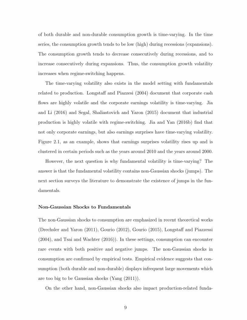
The time-varying volatility also exists in the model setting with fundamentals
related to production. Longstaff and Piazzesi (2004) document that corporate cash
flows are highly volatile and the corporate earnings volatility is time-varying. Jia
and Li (2016) and Segal, Shaliastovich and Yaron (2015) document that industrial
production is highly volatile with regime-switching. Jia and Yan (2016b) find that
not only corporate earnings, but also earnings surprises have time-varying volatility.
Figure 2.1, as an example, shows that earnings surprises volatility rises up and is
clustered in certain periods such as the years around 2010 and the years around 2000.
However, the next question is why fundamental volatility is time-varying? The
answer is that the fundamental volatility contains non-Gaussian shocks (jumps). The
next section surveys the literature to demonstrate the existence of jumps in the fun-
damentals.
Non-Gaussian Shocks to Fundamentals
The non-Gaussian shocks to consumption are emphasized in recent theoretical works
(Drechsler and Yaron (2011), Gourio (2012), Gourio (2015), Longstaff and Piazzessi
(2004), and Tsai and Wachter (2016)). In these settings, consumption can encounter
rare events with both positive and negative jumps. The non-Gaussian shocks in
consumption are confirmed by empirical tests. Empirical evidence suggests that con-
sumption (both durable and non-durable) displays infrequent large movements which
are too big to be Gaussian shocks (Yang (2011)).
On the other hand, non-Gaussian shocks also impact production-related funda-
9
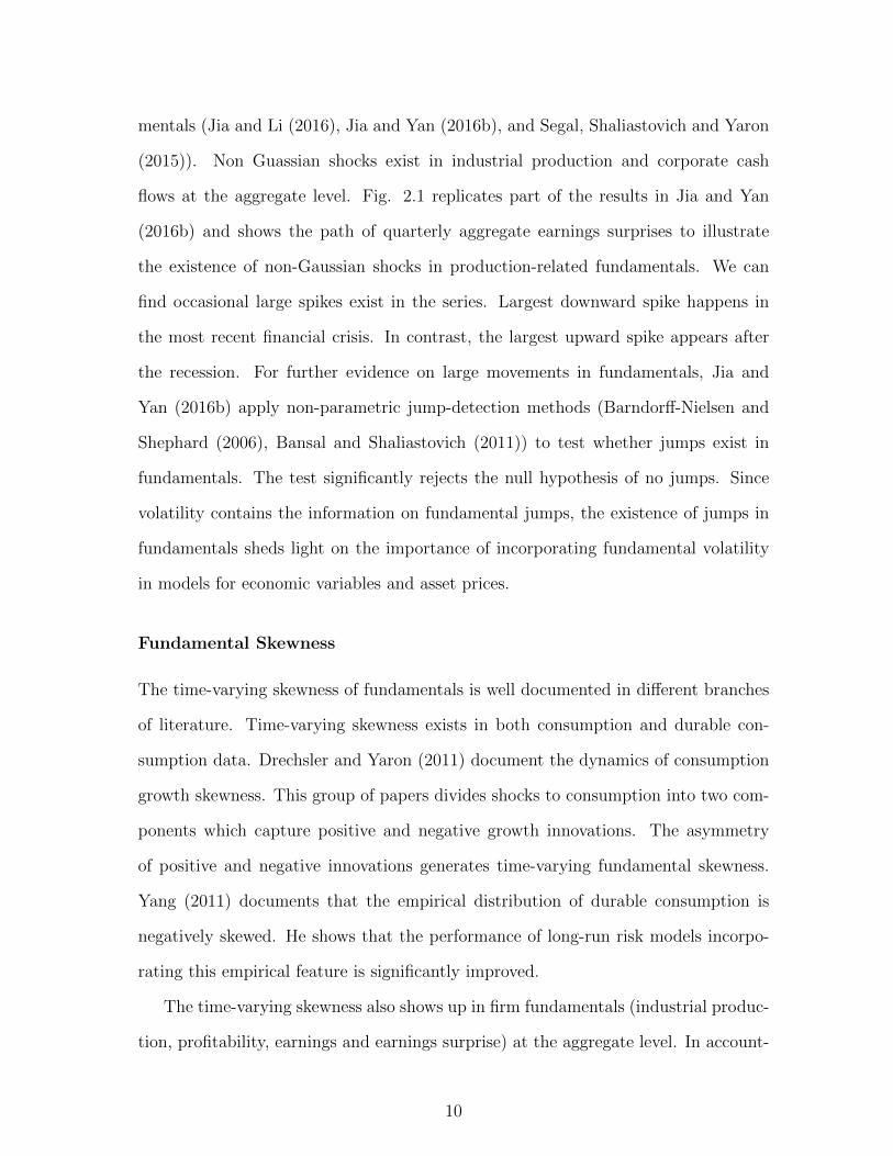
mentals (Jia and Li (2016), Jia and Yan (2016b), and Segal, Shaliastovich and Yaron
(2015)). Non Guassian shocks exist in industrial production and corporate cash
flows at the aggregate level. Fig. 2.1 replicates part of the results in Jia and Yan
(2016b) and shows the path of quarterly aggregate earnings surprises to illustrate
the existence of non-Gaussian shocks in production-related fundamentals. We can
find occasional large spikes exist in the series. Largest downward spike happens in
the most recent financial crisis. In contrast, the largest upward spike appears after
the recession. For further evidence on large movements in fundamentals, Jia and
Yan (2016b) apply non-parametric jump-detection methods (Barndorff-Nielsen and
Shephard (2006), Bansal and Shaliastovich (2011)) to test whether jumps exist in
fundamentals. The test significantly rejects the null hypothesis of no jumps. Since
volatility contains the information on fundamental jumps, the existence of jumps in
fundamentals sheds light on the importance of incorporating fundamental volatility
in models for economic variables and asset prices.
Fundamental Skewness
The time-varying skewness of fundamentals is well documented in different branches
of literature. Time-varying skewness exists in both consumption and durable con-
sumption data. Drechsler and Yaron (2011) document the dynamics of consumption
growth skewness. This group of papers divides shocks to consumption into two com-
ponents which capture positive and negative growth innovations. The asymmetry
of positive and negative innovations generates time-varying fundamental skewness.
Yang (2011) documents that the empirical distribution of durable consumption is
negatively skewed. He shows that the performance of long-run risk models incorpo-
rating this empirical feature is significantly improved.
The time-varying skewness also shows up in firm fundamentals (industrial produc-
tion, profitability, earnings and earnings surprise) at the aggregate level. In account-
10
ing literature, Basu (1997) and Givoly and Hayn (2000) among others report that the
profitability and corporate earnings at the market level have time-varying volatility
and are negatively skewed. Specifically, they use negative skewness of corporate earn-
ings as a measure of reporting conservativism. However, the skewness of fundamentals
in accounting literature is documented without considering its implication on asset
prices. In contrast, finance literature takes the empirical distribution of fundamentals
as given to generate implications. Segal, Shaliastovich and Yaron (2015) implicitly
discuss the implication of asymmetric good and bad fundamental uncertainties on
asset prices. Jia and Li (2016) and Jia and Yan (2016b) document that skewness of
industrial production and that of corporate earnings surprise are long-horizon stock
market return predictors. Skewness even appears in the expected fundamentals and
contains information on aggregate market. Colacito, Ghysels, Meng and Siwasarit
(2015) document the skewness in the distribution of professional forecasters expected
GDP growth can predict future equity excess returns.
Lumpiness of Fundamentals
This section discusses the higher-order moments of another type of aggregate funda-
mentals, the aggregate investment, which has a different pattern from consumption
or production related fundamentals. A large group of the literature (e.g. Caballero,
Engel, and Haltiwanger (1995), Caballero and Engel (1999), Cooper, Hailtwanger and
Power (1999), and Doms and Dunne (1998)) finds that a large fraction of the total
investment expenditure is concentrated in a single large episode. The likelihood of an
investment spike increases with the time since the last primary spike. The dynamics
of lumpy investment can also be captured by investment skewness. However, the
dynamics of investment is very different from other fundamental measures such as
consumption growth, earnings, and industrial production. The aggregate investment
is not persistent, with spikes interrupted by periods of smooth periods. In contrast to
11

other fundamentals, the magnitude of upward jumps in investment is larger than that
of downward jumps. Because of these two empirical regularities, lumpy investment is
closely related to business cycle but have less implications on asset prices.
In sum, the empirical evidence suggests that fundamentals at the aggregate level
are persistent with time-varying volatility and skewness. On the other hand, aggre-
gate investment is lumpy, with infrequent spikes but is not persistent. The volatility
and skewness of fundamentals contain information on the size, magnitude and the
direction of the jumps. Investment at the aggregate level also contains information
on economic well-being. Recent literature extracts information in the higher-order
moments (volatility, skewness, and lumpiness) of fundamentals to generate macroe-
conomic and asset pricing implications.
2.2.2 Higher-Order Moments of Fundamentals at the Micro Level
The fundamentals at the micro-level in this section refer to firm fundamentals such as
firm profitability, earnings and operating cash flows. The level of firm fundamentals
captures a firm’s one-period productivity and competition in the production market.
However, the level of firm fundamentals is not the full picture. Firm fundamentals, like
their counterparts at the aggregate level, contain jumps (skewness) (Ball, Gerakos,
Linnainmaa, and Nikolaev (2015), Gu and Wu (2003), Jia and Yan (2016a)) since
“Firms have ups and downs in the flow of their performance due to swings in their
own competitive positions” (Akbas, Jiang, and Koch (2015)). There are multiple
ways to capture the ups and downs in the firm fundamentals.
The fundamental skewness in Jia and Yan (2016), among others, is one efficient
way (model-free) to capture the firm fundamental fluctuation. Their measures of
12
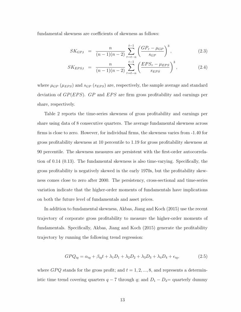
fundamental skewness are coefficients of skewness as follows:
SKGP,t =n
(n− 1)(n− 2)
t−1∑τ=t−n
(GPτ − µGP
sGP
)3
, (2.3)
SKEPS,t =n
(n− 1)(n− 2)
t−1∑τ=t−n
(EPSτ − µEPS
sEPS
)3
, (2.4)
where µGP (µEPS) and sGP (sEPS) are, respectively, the sample average and standard
deviation of GP (EPS). GP and EPS are firm gross profitability and earnings per
share, respectively.
Table 2 reports the time-series skewness of gross profitability and earnings per
share using data of 8 consecutive quarters. The average fundamental skewness across
firms is close to zero. However, for individual firms, the skewness varies from -1.40 for
gross profitability skewness at 10 percentile to 1.19 for gross profitability skewness at
90 percentile. The skewness measures are persistent with the first-order autocorrela-
tion of 0.14 (0.13). The fundamental skewness is also time-varying. Specifically, the
gross profitability is negatively skewed in the early 1970s, but the profitability skew-
ness comes close to zero after 2000. The persistency, cross-sectional and time-series
variation indicate that the higher-order moments of fundamentals have implications
on both the future level of fundamentals and asset prices.
In addition to fundamental skewness, Akbas, Jiang and Koch (2015) use the recent
trajectory of corporate gross profitability to measure the higher-order moments of
fundamentals. Specifically, Akbas, Jiang and Koch (2015) generate the profitability
trajectory by running the following trend regression:
GPQiq = αiq + βiqt+ λ1D1 + λ2D2 + λ3D3 + λ4D4 + εiq, (2.5)
where GPQ stands for the gross profit; and t = 1, 2, ..., 8, and represents a determin-
istic time trend covering quarters q − 7 through q; and D1 −D3= quarterly dummy
13

variables to account for potential seasonality in gross profits. The coefficient βiq
stands for the trajectory of profitability. When exercising their growth opportunity,
firms, especially small firms, can significantly increase their profits, thus generating
an upward trend. In contrast, the profit from firms in financial distress may shrink,
generating a downward trend. The trajectory measure in Akbas, Jiang, and Koch
(2015) can capture the firm expansion and shrinkage dynamics.
Interestingly, even though the skewness and trajectory of fundamentals are all
measures of fundamental higher-order moments, they have different information con-
tents since they have a correlation as low as 0.09. The low correlation between the
two measures also indicates the complexity of the “ups and downs in the flow of their
performance“.
Moreover, a branch of literature focuses on the volatility of fundamentals (Dichev
and Tang (2009), Huang (2009), Jayaraman (2008), Minton and Schrand (1999)).
The literature documents that the volatility of firm-level stock returns and cash flows
highly varies over time (Lee and Engle (1993)) and across firms (Black (1976), Christie
(1982), and Davis, Haltiwanger, Jarmin, and Miranda (2007), and Koren and Ten-
reyro (2006)). This group of literature uses firm-level time series volatility to measure
the fundamental variation. Acemoglu (2005), among others, finds that even cash flows
of large firms are highly volatile. In recent finance literature, papers assign economic
meaning to the cash flow volatility. The volatility of fundamentals, in finance litera-
ture (Dichev and Tang (2009), Huang (2009), Jayaraman (2008), Minton and Schrand
(1999)) captures the cash flow shortfalls of the firm.
In sum, the literature on firm-level fundamental moments documents that the firm
fundamentals have persistent time-varying higher-order moments. The implications
of the higher-order moments will be discussed in detail in the next several sections.
14

2.3 The Origin (Formation) of the Fundamental Higher-Order Moments
This section aims at discussing the theoretical foundation of fundamental higher-
order moments. I first discuss the three information channels of the fundamental
higher-order moments at the macro-level. The second part of this section explores
the information contained in the firm-level fundamental higher-order moments.
2.3.1 Fundamental Higher-Order Moments at the Macro Level
Three branches of literature discuss the information contents of macro-level higher-
order moments. One branch of the literature does simple decomposition of fundamen-
tal uncertainties into positive and negative uncertainties. However, this uncertainties
decomposition is too ad hoc to provide a full picture of fundamental higher-order
moments. The other two branches of the literature provide the microfoundation by
proposing that idiosyncratic firm-level or sectoral-level shocks can explain market-
level fundamental uncertainty. The mechanism is that idiosyncratic shocks can affect
not only the company itself but also its neighbor companies through the input-output
linkages. Table 2.5 summarizes the branches of literature related to the formation of
fundamental higher-order moments.
Fundamental Uncertainty Decomposition
The direction and magnitude of jumps in fundamentals vary across economic states.
In recessions, fundamentals such as capital stock, productivity and earnings are highly
likely to encounter crash risk (Rietz (1988), Barro (2006), Gabaix (2011a), Gourio
(2012), and Gourio (2015)). In contrast, fundamentals can significantly jump during
boom periods (Segal, Shaliastovich and Yaron (2015), Tsai and Wachter (2016)). In
the economy, there are “good“ and “bad“ jumps which are correspondent to booms
and recessions, respectively. Consequently, separate volatility measures incorporat-
ing good and bad jumps contains different information on financial market and the
15

economy.
Barndorff-Nielsen and Shephard (2010), Guo, Wang, and Zhou (2015), and Se-
gal, Shaliastovich and Yaron (2015), among others, decompose the overall shocks
to fundamentals into two separate uncertainties (jumps) which are volatilities cor-
respondent to positive and negative growth innovations. They find the good and
bad uncertainties have different directions in predicting economic growth and asset
prices. Moreover, based on their model settings, the skewness of fundamentals is the
difference between the good and bad uncertainties, capturing the asymmetry of good
and bad jumps.
“Good and bad“ decomposition provides a way to understand the information
contained in the higher-order moments of fundamentals. However, the decomposi-
tion is still at the macro-level without considering the relationship between firm-level
shocks and aggregate uncertainty. In other words, the model with good and bad de-
composition is a “top-down“ method, incorporating (modeling) empirical regularities
at the market level but leaving cross-sectional interactions untouched. This “top-
down“ approach to model economic uncertainty is widely used in finance and eco-
nomics literature (Bansal, Kiku, Shaliastovich, and Yaron (2014), Bansal and Yaron
(2004), Drechsler and Yaron (2011), Gourio (2012), Gourio (2015), Kaltenbrunner
and Lochstoer (2010), Fernandez-Villaverde, Guerron-Quintana, Rubio-Ramirez, and
Uribe (2011), Yang (2011)). However, the “top-down“ approach could lose significant
implications on the microfoundation of fundamental moments if individual firm risks
are inter-connected and non-diversifiable.
Two groups of recent papers, in contrast to Segal, Shaliastovich and Yaron (2015),
use “bottom-up“ approach by modeling firm-level interactions to explain the forma-
tion of the volatility and skewness of fundamentals.
16

The Granular Origins of Higher-Order Moments
The “diversification argument“ in Lucas (1977) demonstrates that when we aggre-
gate individual variables, idiosyncratic shocks would average out, and would only
have negligible aggregate effects. The first strong challenge on the diversification
argument is from Horvath (1998, 2000). Horvath argues, because of strong synchro-
nization mechanism among sectoral shocks, sectoral shocks themselves can generate
aggregate fluctuation. Dupor (1999) refutes Horvath by demonstrating Horvath can
only generate large fluctuation based on a moderate number of sectors (N=36). More
finely disaggregated sectors can diversify sector specific shocks.
Gabaix (2011) ends the debate between Horvath and Dupor. Gabaix shows that
Dupor’s reasoning holds only in a world of small firms because the central limit the-
orem can apply to the aggregation. Horvath’s argument holds when the economy
contains sufficiently many large firms. Gabaix (2011) shows that the diversification
argument breaks down because the distribution of firm sizes is fat-tailed which is
supported by the empirical evidence (Axtell (2001)). Gabaix finds that “the idiosyn-
cratic movements of the largest 100 firms in the United States appear to explain about
one-third of variation in output growth“. Economic fluctuations are attributable to
the “incompressible grains of economic activity, the large firms“. In other words,
the dynamics of higher-order moments of fundamentals can be summarized by the
behavior of large firms. This is the “granular“ hypothesis.
Specifically, Axtell (2001) and Gabaix (2009) find that the size distribution of U.S.
firms follows the Zipf distribution with exponent ζ = 1. Gabaix (2011) proves that
an economy with N firms whose growth rate volatility is σ and whose size S1, ..., SN
are drawn from a power law distribution P (S > x) = ax−ζ which is a fat-tailed distri-
bution, the ζ = 1. As the number of firm N goes to infinity, the GDP volatility σGDP
converges toνζlnN
σ, where νζ is a random variable with a distribution independent of
N and σ. When firm distribution follows Zipf’s law, GDP volatility decays like 1/lnN
17

rather than 1/√N . In sum, the volatility of fundamental higher-order moments can
be captured by the dynamics of large firms.
However, Gabaix (2011), among others, emphasizes the “granular“ origin of the
fundamental higher-order moments but ignores the synchronization mechanism among
sectors and firms (Horvath (1998)). The other group of papers, utilizing the input-
output linkage among sectors, generates the network origins of fundamental higher-
order moments.
The Network Origins of Higher-Order Moments
Firms, in one economy, can reinforce each other through the inter-firm linkages. If two
agents (firms) can mutually reinforce (offset) one another, they are called strategic
complements (strategic substitutes) (Bulow, Geanakoplos, and Klemperer (1985)).
Jovanovic (1987) presents that with strategic complements, any amount of ag-
gregate shocks (jumps) can be generated by games in which shocks to players are
independent. Durlauf (1993, 1994) show that strong strategic complements lead to
path dependence of aggregate fundamentals, i.e. the realized history affects the fu-
ture outcomes. As stated in Durlauf (1993), the path dependence means that “there
will be an especially strong relationship between the probability density of shocks
and the aggregate dynamics of the model as realizations in the tails of the density
determine whether the economy shifts across regimes“. Specifically, when it comes
to aggregate fundamentals such as industrial productivity, profitability and earnings,
Durlauf’s statement indicates the non-Gaussian shocks in the path dependent funda-
mentals can capture the information in the tails to determine whether regime-switch
appears in the economy. In summary, firm strategic complementarity leads to regime
switch of fundamentals, thus to the aggregate fundamental fluctuation.
Comparing with Jovanovic (1987) and Durlauf (1993), Bak, Chen, Scheinkman
and Woodford (1993) specify the resources of strategic complementarity as the supply
18

chains. They illustrate that because firms have input-output linkages, independent
shocks to individual sectors cannot be canceled out in the aggregate.
The master piece of work discussing the network origin of aggregate volatility is
Acemoglu, Carvalho, Ozdaglar, and Tahbaz-Salehi (2012). It provides a more general
and tractable framework to analyze input-output linkages than the above papers.
Acemoglu, Carvalho, Ozdaglar, and Tahbaz-Salehi (2012) demonstrate that “in the
presence of intersectoral input-output linkages, idiosyncratic shocks lead to aggregate
fluctuations”. Through the input-output linkages, shocks to suppliers can not only
affect their immediate customers (first-order interconnections), but also affect the
sequence of sectors interconnected to one another (higher-order interconnections),
creating a “cascade effect”. This cascade effect is especially large when one sector is
the supplier of multiple sectors.
Specifically, Acemoglu, Carvalho, Ozdaglar, and Tahbaz-Salehi (2012) define a
matrix of weighted degree to capture the share of one sector’s output in the input
supply of the other sector. In the competitive equilibrium, the aggregate volatility of
the economy can be represented by the following expression:
(V aryn)1/2 = Ω(1√n
+CVn√n
+
√τ2(Wn)
n), (2.6)
where τ2(Wn) captures the second-order inter-connectivity. The formula indicates
that the aggregate volatility is affected by the second-order inter-connections. The
second-order inter-connections stand for the shocks to one sector impact its immediate
customers’ customers. The cascade effect is embedded in the aggregate volatility
equation. The model by Acemoglu, Carvalho, Ozdaglar, and Tahbaz-Salehi (2012) is
also extended to incorporating even higher degrees (larger than 2) of interconnections.
(V aryn)1/2 = Ω(1√n
+CVn√n
+
√τ2(Wn)
n+ ...+
√τm(Wn)
n). (2.7)
19

In sum, the input-output linkages which are modeled by the network structure are
the origin of aggregate fluctuations. The “network origin” argument has both simi-
larity and huge differences with the “granular origin” argument. On one hand, the
shocks to sectors that are in more central positions in the network structure have
a much higher impact on aggregate output than shocks to marginal sectors. The
input-output linkage network structure plays the same role as the size distribution in
the “granular hypothesis”. On the other hand, the network origin argument focuses
on the input-output linkages. But the granular origin argument focuses on the asym-
metric impact of large firms on the aggregate fluctuations rather than that of small
firms. Moreover, the input-output linkages leads to sectoral comovement but granular
hypothesis cannot. Consequently, the dynamics of aggregate fluctuations generated
by network origin and granular origin can be very different. But both arguments give
rise to the microfoundation of aggregate higher-order moments for fundamentals.
2.3.2 Fundamental Higher-Order Moments at the Micro Level
Motivated by the granular argument and network argument for aggregate fundamen-
tal volatility, Kelly, Lustig and Van Nieuwerburgh (2014) use similar arguments to
build up the foundation for firm-level fundamental volatility. They model the firm
volatility in which “the customers’ growth rate shocks influence the growth rate of
their suppliers, larger suppliers have more customers, and the strength of a customer-
supplier link depends on the size of the customer firm”. They find the network model
can reproduce firm-level dynamics and size distribution dynamics. In the cross sec-
tion, larger firms and firms with less concentrated customer networks display lower
volatility.
Specifically, they define firm size Si,t with growth rate as gi,t+1, where
Si,t+1 = Si,texp(gi,t+1). (2.8)
20

They model the inter-firm relationship by assuming that supplier i’s growth rates
depend on its own idiosyncratic shock and a weighted average of the growth rates of
its customer j:
gi,t+1 = µg + γ∑
ωi,j,tgj,t+1 + εi,t+1. (2.9)
The weight ωi,j,t determines how strongly the supplier’s growth rate depends on the
growth rate of its customers. Kelly, Lustig and Van Nieuwerburgh (2014) combine
both the insights of network structure in Acemoglu (2012) and the insights of limited
diversification of large firm influence in Gabaix (2011).
In sum, the origin of both macro and micro level higher-order fundamental mo-
ments lies on two dimensions: the network structure of heterogeneous firms; and the
non-diversifiable influence of large firms.
2.4 The Theoretical Framework for the Return Predictability of the
Fundamental Higher-Order Moments
Previous sections survey the literature on the properties regarding fundamental higher-
order moments. At both macro and micro level, fundamental higher-order moments
are persistent, time-varying and related to business cycle; moreover, the variation
(formation) of fundamental higher-order moments lies in the granular networks of
heterogeneous firms. The overwhelming purpose of exploring the properties and for-
mation of fundamental higher-order moments is to extract the information contained
in these moments on future asset prices and macroeconomic quantity variables. This
section discusses the theoretical foundation on why the higher-order moments of fun-
damentals can predict future economic well-being (at the macro-level), future firm
fundamentals (at the micro-level), and asset prices (at both macro and micro levels).
21

2.4.1 Return Predictability of the Higher-Order Moments of Firm Fun-
damentals: Theoretical Framework
Based on previous literature, this section answers the question why, in theory, higher-
order moments of firm fundamentals can predict future cross-sectional stock returns
and future firm fundamentals. Two frameworks based on the production-based asset
pricing theory imply the return predictive power of firm fundamental higher-order
moments. The first framework is proposed by Jia and Yan (2016a), which can ac-
commodate the return predictability of all measures of firm fundamental higher-order
moments. The second framework is based on the networks in production (Herskovic
(2015), Kelly, Lustig, and Van Nieuwerburgh (2013)).
Fundamental Higher-Order Moments and Growth Option
The production-based asset pricing model, in a nutshell, decomposes the value of the
firm at time t into two components: the value of assets-in-place, At, and the present
value of the firm growth option, Gt.
Vt = At +Gt. (2.10)
Specifically, the growth option Gt is modeled as an European call option written on
At with expiration time T and a strike price of I, as the investment to undertake the
potential projects (Berk, Green, and Naik (1999), Bernardo, Chowdhry, and Goyal
(2007)). Previous literature assumes that the assets-in-place process At follows the
Geometric Brownian Motion.
dAt = µdt+ σdzt. (2.11)
22

Consequently, the growth option is given by the Black-Scholes formula as follows.
Gt = N(d1)At −N(d2)Ie−rT (2.12)
“Skewness has no role in this setting because the distribution of the assets-in-place
is log-normal” (Jia and Yan (2016a)). The Geometric Brownian Motion assumption
of assets-in-place is contradicted by the properties of the empirical distribution I doc-
umented in section 2. The firm fundamentals have large time-series & cross-sectional
volatility and skewness. Moreover, the firm fundamentals have certain trajectories. In
order to close the gap between theoretical models and empirical evidence, Jia and Yan
(2016a) extend production models such as Bernardo, Chowdhry, and Goyal (2007)
by allowing the distribution of logAt to have non-zero skewness. Considering the ups
and downs in the firm fundamentals, one can think of the fundamental process as
a jump-diffusion process (Bakshi, Cao, and Chen (1997) or Backus, Foresi, and Wu
(2004)). Since the growth option is written on the skewed assets-in-place process, the
skewness of firm fundamentals is priced in the value of growth option, thus the stock
returns (Jia and Yan (2016a)).
The skewed assets-in-place process does not need to be generated by a jump-
diffusion process. It can also be generated through a process for assets-in-place similar
to the Heston Volatility Model (Heston (1993)). The non-zero correlation between
the mean and volatility of fundamentals leads to a priced fundamental skewness risk
in the growth option value.
The framework of Jia and Yan (2016a) can accommodate the return predictive
power of other measures of fundamental higher-order moments. Since the volatility of
fundamentals is time-varying, the Geometric Brownian Motion hypothesis for assets-
in-place contradicts the empirical fact. One can extend the assets-in-place process
to be a process with time-varying volatility. Specifically, the process can be stated
23

as: dAt = µdt + σtdzt. Following the similar argument as in Jia and Yan (2016a),
the time-varying fundamental volatility risk is then embedded in the value of growth
option. The above argument indicates that the cash flow volatility can predict future
cross-sectional stock returns, which is confirmed by Huang (2009).
Firm fundamentals, as documented by Akbas, Jiang, and Koch (2015), have tra-
jectories (i.e. upward trend or downward trend). The trend in fundamentals again
obviously refutes the Geometric Brownian Motion of assets-in-place. To incorporate
the trajectory feature of fundamentals into the assets-in-place process, one can revise
the assets-in-place process to be path dependent, which means history of fundamen-
tals matters. One can also revise the growth option written on the fundamental
process to be a path dependent option instead of an European style option.
In sum, the higher-order moments of fundamentals can predict cross-sectional
stock returns because it captures the fundamental higher-order moment risk embed-
ded in the growth option written on fundamentals.
Granular Networks in Production
The granular origin and network origin embedded in a production model can also
generate implications of fundamental higher-order moments on cross-sectional stock
returns.
As discussed in Section 2, Kelly, Lustig, and Van Nieuwerburgh (2014) find that
firm-level cash flow volatility is driven by customer-supplier linkages. Herskovic
(2015), among others, examines asset pricing in a multisector model with sectors
connected through an input-output network. He documents that network concen-
tration and network sparsity for individual stocks are priced factors. Specifically,
network concentration factor is the “average of firm’s log output share weighted by
their own output share. The network sparsity factor measures the thickness and
scarcity of network linkages. An economy with high network concentration has few
24

large sectors with low return to input investment due to decreasing returns to scale.
Because of the network linkages, the lower productivity of large sectors spreads to
relatively small sectors. The aggregate output and aggregate consumption both de-
crease. On the other hand, when sparsity is high, the input-output linkages change,
causing aggregate consumption to increase.
When combining Kelly, Lustig, and Van Nieuwerburgh (2014) and Herskovic
(2015), one can map out the microfoundation for the relationship between fundamen-
tal higher-order moments and cross-sectional stock returns: the variation of network
concentration and sparsity leads to the change in fundamental higher-order moments
and the change in cross-sectional stock returns.
However, no direct research uses network or granular origins as the predictive
power of fundamental higher-order moments on cross-sectional stock returns.6 This
is the limitation of this line of the research which needs future efforts.
2.4.2 Return Predictability of the Higher-Order Moments of Aggregate
Fundamentals: Theoretical Framework
There are two branches of literature discussing the theoretical foundation for the
return predictive power of fundamental higher-order moments. The first group of
literature explores the return predictive power of fundamentals by incorporating fun-
damental jumps in the long-run risk framework. The second group of literature
employes the granular network among firms to provide microfoundation for the pre-
dictive power of fundamental higher-order moments.
6Kelly, Lustig, and Van Nieuwerburgh (2014) provide linkage between granular network andfirm fundamental volatility but have no linkage between firm fundamental volatility and returns.In contrast, Herskovic (2015) discusses the relationship between networks and cross-sectional stockreturns.
25
Long-Run Risk Framework with Jumps
The original long-run risk framework in Bansal and Yaron (2004) incorporates time-
varying dividend growth volatility7 to capture the higher-order moments of funda-
mentals. However, the time-varying volatility generated by an AR(1) process can
capture none of the fundamental jumps, fundamental leverage effect, or skewness
in fundamentals which are documented in previous literature (discussed in Section
2). Thus, the time-varying fundamental higher-order moments in the original long-
run risk framework have only second-order effects on aggregate equity returns. A
large group of papers incorporates the non-Gaussian shocks (or skewness) to explain
the relationship between fundamental higher-order moments and aggregate market
returns.
Drechsler and Yaron (2011), motivated by the empirical evidence in fundamentals,
revise the long-run risk framework by specifying the state vector of the economy
is driven by Poisson jump shocks. Benzoni, Dufresne, and Goldstein (2005) and
Eraker and Shaliastovich (2008) model fundamental jumps within the long-run risk
framework to explain index option return dynamics.
Yang (2011) documents that the empirical distribution of durable consumption
growth is negatively skewed. To incorporate the empirical distribution, Yang (2011)
specifies a time-varying long-run component in the volatility of durable consump-
tion growth. This specification captures the negative skewed consumption growth
dynamics and improves the performance of the original long-run risk model. Segal,
Shaliastovich and Yaron (2015) and Guo, Wang, and Zhou (2015) specify positive
and negative Poisson jumps in the long-run risk framework to explain the predictive
power of fundamental higher-order moments on aggregate returns. Specifically, Se-
gal, Shaliastovich and Yaron (2015) find that good uncertainty associated with good
jumps predicts an increase in future economic activity and is positively related to
7The time-varying volatility is generated by an AR(1) process.
26

future market returns. But the bad uncertainty associated with bad jumps has an
opposite effect on economic activity and market returns.
Incorporating non-Gaussian shocks is not restricted to long-run risk models. Gou-
rio (2012), Gourio (2015), and Longstaff and Piazzessi (2004) embed jumps or skew-
ness in slightly different model settings and find that incorporating higher-order mo-
ments of fundamentals can explain the equity premium puzzle, business cycle, and
credit spreads.
However, all the above models follow the “top-down” method that directly incor-
porates empirical evidence such as time-varying volatility and skewness in the model.
This group of models did not pay attention to the microfoundation of the fundamental
higher-order moments. In other words, the network and granular origins are not em-
bedded in the higher-order moments. A “bottom-up” method, building the aggregate
fundamental higher-order moments from granular network origin, can be very useful
in inspecting the mechanism and generating new implications for the fundamental
higher-order moments.
Granular Networks and Market Returns
Jia and Li (2016) and Jia and Yan (2016b) set up the framework to incorporate
network origin and granular origin in asset pricing models. In contrast to Herskovic
(2015), Jia and Li (2016) recover a firm stochastic discount factor with production
networks from the firm’s first-order condition.8 Jia and Yan (2016b) derive their firm
stochastic discount factor with non-diversifiable large firm influence.
Specifically, non-diversifiable jumps of large firms spread the shocks to other firms,
leading to the path dependence of fundamentals. Higher-order moments can capture
the path dependence of fundamentals. If the fundamental path is shifted to another
path (can be either riskier or safer), the fundamental moments change, and the risk of
8Herskovic (2015)’s stochastic discount factor is derived from investor’s utility regarding con-sumption.
27

the representative investor who holds the market portfolio is changed. Consequently,
the required return for the market portfolio is different.
2.5 What Can Fundamental Higher-Order Moments Predict? Empirical
Evidence
This section discusses the financial market and macroeconomic implications of the
fundamental higher-order moments. At both macro and micro levels, the fundamental
higher-order moments can predict not only asset prices but also a wide range of
fundamental variables. The predictive power of fundamental higher-order moments
has different information content than that of higher-order moments of returns at
both micro and macro levels.
2.5.1 Micro Level Predictability
It is well documented that measures of fundamental higher-order moments can pre-
dict cross-sectional stock returns. Huang (2009) documents that historical cash flow
volatility is negatively related to future cross-sectional stock returns. Consistent with
Huang (2009), Allayannis, Rountree, and Weston (2008) find that cash flow volatility
is negatively valued by investors, causing a decrease in future firm value. Jia and
Yan (2016a) find that historical skewness of firm fundamentals, such as skewness of
gross profitability and earnings per share, can positively predict cross-sectional stock
returns. Both Huang (2009) and Jia and Yan (2016a) report that the effect of fun-
damental higher-order moments cannot be driven out by the higher-order moments
of returns. Akbas, Jiang, and Koch (2015) find a positive relationship between firm
recent trajectory of gross profitability and cross-sectional stock returns. Both fun-
damental skewness and profit trajectory measures have long-horizon predictability.
Among the three measures (volatility, skewness, and trajectory), the predictability of
fundamental volatility and trajectory is relatively a phenomenon in small capitaliza-
28

tion stocks. In contrast, the fundamental skewness can predict stock returns even for
samples of large stocks.
The predictability of fundamental higher-order moments on returns is largely
considered to be consistent with rational asset pricing models because fundamen-
tal higher-order moments can predict a large group of fundamental variables. Cash
flow volatility has a positive relationship with a firm’s precautionary cash holdings
(Han and Qiu (2007)) since cash flow volatility can be viewed as a measure of cash
flow shortfalls. Earnings volatility has a strong predictive power on both short-term
and long-term earnings. The skewness of the firm fundamentals can positively predict
future gross profitability, return on equity, market to book ratio, and Tobin’s q (Jia
and Yan (2016a)). The profitability trajectory is strongly correlated with future gross
profitability and standardized unexpected earnings (Akbas, Jiang, and Koch (2015)).
2.5.2 Macro Level Predictability
At the aggregate level, the higher-order moments of fundamentals still have strong
predictive power on market returns and macroeconomic quantity variables.
Regarding the predictive power on macroeconomic quantity variables, Bloom
(2009) finds that fundamental volatility backed out from VIX index can negatively
predict future consumption and output growth rate because of delayed firms’ invest-
ment decisions. Jia and Yan (2016b) find that aggregate earnings skewness can predict
industrial production, bond yields, and the level of earnings. Segal, Shaliastovich, and
Yaron (2015) find that good and bad uncertainty have opposite influence on consump-
tion, output, and investment. Good uncertainty indicates an increase in the level of
fundamentals. In contrast, bad uncertainty forecasts a decline in fundamentals.
In terms of asset prices, Bansal and Yaron (2004) find that economic uncertainty is
a priced risk and is negatively related to price-dividend ratio. Bansal, Kiku, Shalias-
tovich, and Yaron (2014) develop a dynamic capital asset pricing model incorporat-
29

ing a fundamental volatility factor. The model calibration results indicate a nega-
tive relationship between fundamental uncertainty and market risk premia. Segal,
Shaliastovich, and Yaron (2015) find good and bad uncertainties can predict the
price-dividend ratio up to three-year horizon. As to the fundamental skewness, Jia
and Li (2016) and Jia and Yan (2016b) find that skewness of industrial production and
earnings can strongly negatively predict stock market excess returns from six-month
horizon to eight years horizon.
2.6 Conclusions
This paper outlines the major progress in the research of the fundamental higher-order
moments. I survey the existence, the formation, and the financial market and macroe-
conomics implications for the higher-order moments. The time-varying volatility and
the non-Gaussian shocks widely exist in all measures of fundamentals at both micro
and macro levels. According to the literature, the granular network among firms is
the origin of the fundamental higher-order moments. The fundamental higher-order
moments have strong predictive power on asset prices and macroeconomic quantity
variables.
From this survey article, we can see that one compelling motivation to survey this
literature is the differences in approaches between finance and economics research
on the higher-order moments of fundamentals. Finance literature, in general, inputs
time-varying volatility and non-Gaussian shocks in the asset pricing model to predict
asset prices and economic growth but ignores the microfoundation of fundamental
higher-order moments. In contrast, economics literature focuses on the mechanism
of higher-order moments, investigating the origin of the fundamental higher-order
moments but ignores the implications on the macroeconomics and asset prices. Only
the most recent research starts to bridge the inter-firm origin of fundamental higher-
order moments and asset prices. The relationship between the microfoundation of
30

fundamental higher-order moments and asset prices & macroeconomics urgently calls
for more future research.
31

Tab
le2.
1:F
irm
Fundam
enta
lsan
dth
eC
ross
-Sec
tion
alSto
ckR
eturn
sP
redic
tor
Definit
ion
Lit
era
ture
RO
EQ
uar
terl
yin
com
eb
efor
eex
trao
r-din
ary
item
sdiv
ided
by
one-
quar
ter-
lagg
edb
ook
equit
yH
ou,
Xue
and
Zhan
g(2
015)
RO
AQ
uar
terl
yin
com
eb
efor
eex
trao
r-din
ary
item
sdiv
ided
by
one-
quar
ter-
lagg
edto
tal
asse
tsH
ou,
Xue
and
Zhan
g(2
015)
RN
OA
Ret
urn
onnet
oper
atin
gas
sets
Sol
iman
(200
8)P
MP
rofit
mar
gin
Sol
iman
(200
8)A
TO
Ass
ettu
rnov
erSol
iman
(200
8)
Gro
ssP
rofita
bilit
yT
otal
reve
nue
min
use
sco
stof
goods
sold
div
ided
by
tota
las
sets
Nov
y-M
arx
(201
3)
Ass
etG
row
thY
ear-
on-y
ear
per
centa
gech
ange
sin
tota
las
sets
Coop
er,
Gule
nan
dSch
ill
(200
8)
Net
Op
erat
ing
Ass
ets
Op
erta
ing
asse
tsm
inus
deb
tin
-cl
uded
incu
rren
tliab
ilit
ies
Hir
shle
ifer
,H
ou,
Teo
han
dZ
han
g(2
004)
Inve
nto
ryG
row
thY
ear-
on-y
ear
per
centa
gech
ange
sin
inve
nto
ryB
elo
and
Lin
(201
1)
Fai
lure
Pro
bab
ilit
yM
easu
reof
corp
orat
efa
ilure
bas
edon
acco
unti
ng
and
mar
ket-
bas
edm
easu
res
Cam
pb
ell,
Hilsc
her
and
Szi
lagy
i(2
008)
32

Tab
le2.
2:F
irm
Fundam
enta
lsan
dA
ggre
gate
dSto
ckM
arke
tR
eturn
sP
red
icto
rD
efi
nit
ion
Lit
eratu
re
Ter
mS
pre
ad
Diff
eren
ceb
etw
een
the
long
term
yie
ldon
gover
nm
ent
bon
dan
dth
etr
easu
ry-
bill
Cam
pb
ell
(1987)
Def
au
ltP
rem
ium
Diff
eren
ceb
etw
een
yie
lds
of
AA
Aco
rpora
teb
on
ds
and
BB
Bco
rpora
teb
on
ds
Fam
aan
dF
ren
ch(1
992)
Skew
nes
sin
Exp
ecte
dM
acr
oF
un
dam
enta
lsT
he
thir
dm
om
ents
of
cross
-sec
tion
of
GD
Pfo
reca
stC
ola
cito
,G
hyse
lsan
dM
eng
(2013)
Con
sum
pti
on
,W
ealt
han
dIn
com
eR
ati
oT
he
dev
iati
on
from
conu
mp
tion
,la
bor
inco
me
an
dass
eth
old
ings
Let
tau
an
dL
ud
vig
son
(2001)
Inves
tmen
tto
Cap
ital
Rati
oT
he
rati
oof
aggre
gate
inves
tmen
tto
aggre
gate
cap
ital
for
the
wh
ole
econ
-om
yC
och
ran
e(1
991)
Div
iden
dP
rice
Rati
oT
he
diff
eren
ceb
etw
een
the
log
of
div
i-d
end
san
dth
elo
gof
lagged
pri
ceC
am
pb
ell
an
dS
hille
r(1988a)
Div
iden
dP
ayou
tR
ati
oT
he
diff
eren
ceb
etw
een
the
log
of
div
i-d
end
san
dth
elo
gof
earn
ings
Cam
pb
ell
an
dS
hille
r(1
988a)
Earn
ings
Pri
ceR
ati
oT
he
rati
oof
op
erati
ng
earn
ings
(bef
ore
dep
reci
ati
on
)in
the
pre
vio
us
fisc
alyea
rto
mark
eteq
uit
yin
the
pre
vio
us
month
Fam
aan
dS
chw
ert
(1977)
Book
toM
ark
etR
ati
oT
he
rati
oof
book
equ
ity
for
the
pre
vi-
ou
sfi
scal
yea
rto
mark
eteq
uit
yin
the
pre
vio
us
month
Lew
elle
n(2
004)
Acc
ruals
Th
ech
an
ge
inn
on
-cash
curr
ent
ass
ets
less
the
chan
ge
incu
rren
tliab
ilit
ies
ex-
clu
din
gth
ech
an
ge
insh
ort
-ter
mdeb
tan
dth
ech
an
ge
inta
xes
payab
le,m
inu
sd
epre
ciati
on
an
dam
ort
izati
on
exp
ense
Hir
shle
ifer
,H
ou
an
dT
eoh
(2009)
Equ
ity
Sh
are
inN
ewIs
sues
Th
era
tio
of
equ
ity
issu
ing
act
ivit
yas
afr
act
ion
of
tota
lis
suin
gact
ivit
yB
aker
an
dW
urg
ler
(2000)
Net
Equ
ity
Exp
an
sion
Th
era
tio
of
12-m
onth
movin
gsu
ms
of
net
issu
esby
NY
SE
list
edst
ock
sd
i-vid
edby
the
tota
len
d-o
f-yea
rm
ark
etca
pit
aliza
tion
of
NY
SE
stock
s
Wel
chan
dG
oyal
(2007)
33

Tab
le2.
3:T
he
Fundam
enta
lH
igher
-Ord
erM
omen
tsat
the
Mac
roL
evel
:E
xis
tence
Mea
sure
Fundam
enta
lV
aria
ble
Lit
erat
ure
Pan
elA
:T
ime-
Var
yin
gF
undam
enta
lV
olat
ilit
y
Vol
atilit
yC
onsu
mpti
onG
row
thB
ansa
lan
dY
aron
(200
4),
Let
tau
and
Wac
hte
r(2
007)
,L
ongs
taff
and
Pia
zzes
si(2
004)
Vol
atilit
yD
ura
ble
Con
sum
pti
onG
row
thY
ang
(201
1)V
olat
ilit
yE
arnin
gsL
ongs
taff
and
Pia
zzes
si(2
004)
,Jia
and
Yan
(201
6b)
Vol
atilit
yIn
dust
rial
Pro
duct
ion
Seg
al,
Shal
iast
ovic
h,
and
Yar
on(2
015)
,Jia
and
Li
(201
6)P
anel
B:
Non
-Gau
ssia
nShock
sto
Fundam
enta
ls
Non
-Gau
ssia
nShock
sC
onsu
mpti
onD
rech
sler
and
Yar
on(2
011)
,G
ouri
o(2
012)
,G
ouri
o(2
015)
,T
sai
and
Wac
hte
r(2
016)
,B
ansa
lan
dShal
ias-
tovic
h(2
011)
Non
-Gau
ssia
nShock
sP
roduct
ion
Seg
al,
Shal
iast
ovic
h,
and
Yar
on(2
015)
,Jia
and
Li
(201
6),
Jia
and
Yan
(201
6b)
Pan
elC
:F
undam
enta
lSke
wnes
sSke
wnes
sC
onsu
mpti
onG
row
thD
rech
sler
and
Yar
on(2
011)
Ske
wnes
sP
rofita
bilit
yan
dE
arnin
gsB
asu
(199
7),
Giv
oly
and
Hay
n(2
000)
,Seg
al,
Shal
ias-
tovic
h,
and
Yar
on(2
015)
,Jia
and
Li
(201
6),
Jia
and
Yan
(201
6b)
Pan
elD
:L
um
pin
ess
ofF
undam
enta
ls
Lum
py
Inve
stm
ent
and
R&
Ds
Cab
alle
ro,
Enge
l,an
dH
alti
wan
ger
(199
5),
Cab
alle
roan
dE
nge
l(1
999)
,C
oop
er,
Hai
ltw
ange
ran
dP
ower
(199
9),
Dom
san
dD
unne
(199
8)
34

Tab
le2.
4:T
he
Fundam
enta
lH
igher
-Ord
erM
omen
tsat
the
Mic
roL
evel
:E
xis
tence
Mea
sure
Fundam
enta
lV
aria
ble
Lit
erat
ure
Vol
atilit
yO
per
atin
gC
ash
Flo
ws
Allay
annis
,R
ountr
ee,
and
Wes
ton
(200
8),
Han
and
Qiu
(200
7),
Huan
g(2
009)
,Jay
aram
an(2
008)
,M
into
nan
dSch
rand
(199
9)V
olat
ilit
yE
arnin
gsD
ichev
and
Tan
g(2
009)
Ske
wnes
sG
ross
Pro
fita
bilit
yJia
and
Yan
(201
6a)
Ske
wnes
sE
arnin
gsG
uan
dW
u(2
003)
,Jia
and
Yan
(201
6a)
Tra
ject
ory
Gro
ssP
rofita
bilit
yA
kbus,
Jia
ng,
and
Koch
(201
5)
35

Tab
le2.
5:T
he
Theo
reti
cal
Fou
ndat
ion
for
the
For
mat
ion
ofF
undam
enta
lH
igher
-Ord
erM
omen
ts
Rar
eD
isas
ter
Rie
tz(1
988)
,B
arro
(200
6),
Ban
sal,
Kik
u,
Shal
ias-
tovic
h,
and
Yar
on(2
014)
,G
ouri
o(2
012)
,G
ouri
o(2
015)
,K
alte
nbru
nner
and
Loch
stoer
(201
0),
Fer
nan
dez
-V
illa
verd
e,G
uer
ron-Q
uin
tana,
Rubio
-Ram
irez
,an
dU
rib
e(2
011)
Rar
eB
oom
san
dD
isas
ters
Seg
al,
Shal
iast
ovic
h,
and
Yar
on(2
015)
,T
sai
and
Wac
hte
r(2
015)
The
Gra
nula
rO
rigi
nA
xte
ll(2
001)
,H
orva
th(1
998)
,H
orva
th(2
000)
,G
abai
x(2
011)
The
Net
wor
kO
rigi
nA
cem
oglu
,C
arva
lho,
Ozd
agla
r,an
dT
ahbas
-Sal
ehi
(201
2),
Bak
,C
hen
,Sch
einkm
anan
dW
oodfo
rd(1
993)
,D
url
auf
(199
3),
Durl
auf
(199
4),
Jov
anov
ic(1
987)
36
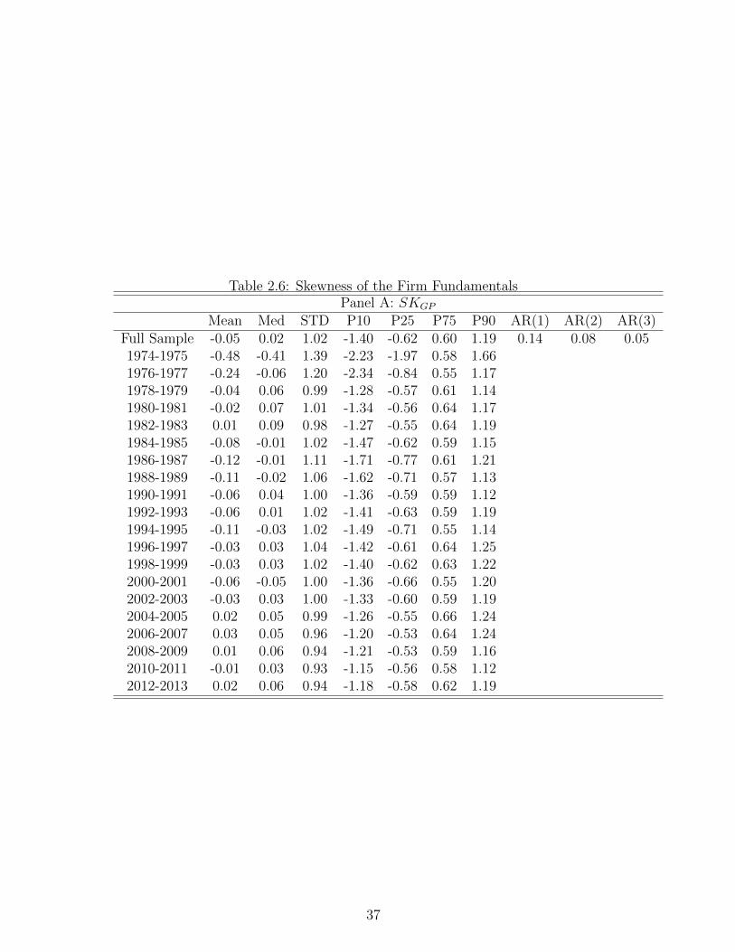
Table 2.6: Skewness of the Firm FundamentalsPanel A: SKGP
Mean Med STD P10 P25 P75 P90 AR(1) AR(2) AR(3)Full Sample -0.05 0.02 1.02 -1.40 -0.62 0.60 1.19 0.14 0.08 0.051974-1975 -0.48 -0.41 1.39 -2.23 -1.97 0.58 1.661976-1977 -0.24 -0.06 1.20 -2.34 -0.84 0.55 1.171978-1979 -0.04 0.06 0.99 -1.28 -0.57 0.61 1.141980-1981 -0.02 0.07 1.01 -1.34 -0.56 0.64 1.171982-1983 0.01 0.09 0.98 -1.27 -0.55 0.64 1.191984-1985 -0.08 -0.01 1.02 -1.47 -0.62 0.59 1.151986-1987 -0.12 -0.01 1.11 -1.71 -0.77 0.61 1.211988-1989 -0.11 -0.02 1.06 -1.62 -0.71 0.57 1.131990-1991 -0.06 0.04 1.00 -1.36 -0.59 0.59 1.121992-1993 -0.06 0.01 1.02 -1.41 -0.63 0.59 1.191994-1995 -0.11 -0.03 1.02 -1.49 -0.71 0.55 1.141996-1997 -0.03 0.03 1.04 -1.42 -0.61 0.64 1.251998-1999 -0.03 0.03 1.02 -1.40 -0.62 0.63 1.222000-2001 -0.06 -0.05 1.00 -1.36 -0.66 0.55 1.202002-2003 -0.03 0.03 1.00 -1.33 -0.60 0.59 1.192004-2005 0.02 0.05 0.99 -1.26 -0.55 0.66 1.242006-2007 0.03 0.05 0.96 -1.20 -0.53 0.64 1.242008-2009 0.01 0.06 0.94 -1.21 -0.53 0.59 1.162010-2011 -0.01 0.03 0.93 -1.15 -0.56 0.58 1.122012-2013 0.02 0.06 0.94 -1.18 -0.58 0.62 1.19
37
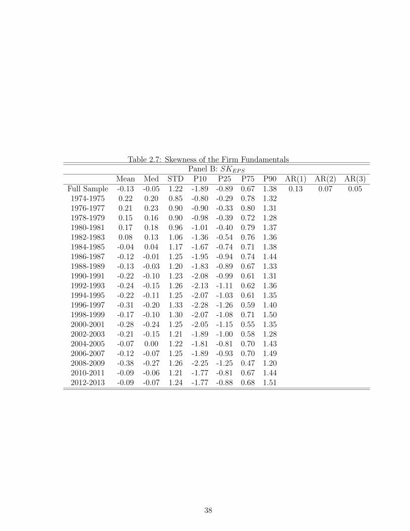
Table 2.7: Skewness of the Firm FundamentalsPanel B: SKEPS
Mean Med STD P10 P25 P75 P90 AR(1) AR(2) AR(3)Full Sample -0.13 -0.05 1.22 -1.89 -0.89 0.67 1.38 0.13 0.07 0.051974-1975 0.22 0.20 0.85 -0.80 -0.29 0.78 1.321976-1977 0.21 0.23 0.90 -0.90 -0.33 0.80 1.311978-1979 0.15 0.16 0.90 -0.98 -0.39 0.72 1.281980-1981 0.17 0.18 0.96 -1.01 -0.40 0.79 1.371982-1983 0.08 0.13 1.06 -1.36 -0.54 0.76 1.361984-1985 -0.04 0.04 1.17 -1.67 -0.74 0.71 1.381986-1987 -0.12 -0.01 1.25 -1.95 -0.94 0.74 1.441988-1989 -0.13 -0.03 1.20 -1.83 -0.89 0.67 1.331990-1991 -0.22 -0.10 1.23 -2.08 -0.99 0.61 1.311992-1993 -0.24 -0.15 1.26 -2.13 -1.11 0.62 1.361994-1995 -0.22 -0.11 1.25 -2.07 -1.03 0.61 1.351996-1997 -0.31 -0.20 1.33 -2.28 -1.26 0.59 1.401998-1999 -0.17 -0.10 1.30 -2.07 -1.08 0.71 1.502000-2001 -0.28 -0.24 1.25 -2.05 -1.15 0.55 1.352002-2003 -0.21 -0.15 1.21 -1.89 -1.00 0.58 1.282004-2005 -0.07 0.00 1.22 -1.81 -0.81 0.70 1.432006-2007 -0.12 -0.07 1.25 -1.89 -0.93 0.70 1.492008-2009 -0.38 -0.27 1.26 -2.25 -1.25 0.47 1.202010-2011 -0.09 -0.06 1.21 -1.77 -0.81 0.67 1.442012-2013 -0.09 -0.07 1.24 -1.77 -0.88 0.68 1.51
38
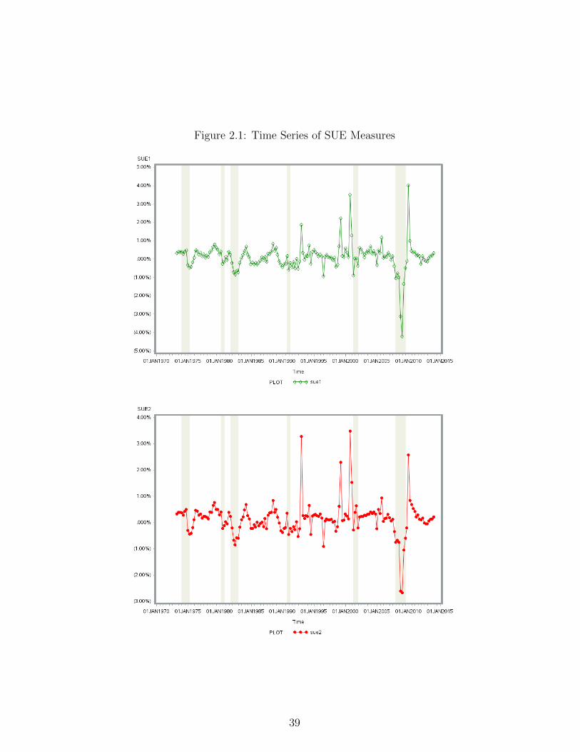
Figure 2.1: Time Series of SUE Measures
39
CHAPTER 3
What Does Skewness of Firm Fundamentals Tell Us About Firm
Growth, Profitability, and Stock Returns
3.1 Introduction
There is overwhelming evidence in the finance literature that measures of firm fun-
damentals such as ROE, profitability, investment, and asset growth predict cross-
sectional stock returns.1, Fama and French (2006a, 2008), Aharoni, Grundy, and
Zeng (2013), Novy-Marx (2013), and Hou, Xue, and Zhang (2014). Beyond the level,
a small number of papers have examined whether the second moment of firm funda-
mentals can predict stock returns and firm performance (e.g., Diether, Malloy, and
Scherbina (2002), Johnson (2004), Dichev and Tang (2009), and Gow and Taylor
(2009). However, little is known whether the higher moments of firm fundamentals
are related to stock returns. In this paper, I shed light on this research question by
providing two distinct theoretical models, both of which imply a positive relation be-
tween the skewness of firm fundamentals and stock returns. I further empirically test
the implications of the models and find supporting evidence for both models. Our
results cannot be explained by existing risk factors and return predictors including
the levels of firm fundamentals and the skewness of stock returns.
The first model is motivated by the line of research on firm growth opportunities
(e.g., Berk, Green and Naik (1999), Carlson, Fisher and Giammarino (2004), and
bernardo2007growth). In this framework, a firm has growth opportunities as part
1A partial list of recent studies include Cohen, Gompers, and Vuolteenaho (2002), Fairfield,Whisenant, Yohn (2003), Titman, Wei, and Xie (2004)
40

of the firm value, which are then valued as real options. Previous studies assume
(log) normal distribution for the firm assets-in-place. I specifically extend the model
of Bernardo, Chowdhry and Goyal (2007) by allowing the distribution of the firm
assets-in-place to have non-zero skewness. Using the recent findings in the option
pricing theory, I am able to derive the value and risk of the firm growth option.
Under very general conditions, the model yields two main implications: (1) the value
of the growth option increases with the skewness; and (2) the risk and return of the
total firm value increase with the skewness. Two insights are helpful in understanding
the model. First, as argued by Bernardo, Chowdhry and Goyal (2007), firm growth
opportunities have higher risk because of the implicit leverage of options and therefore
higher returns relative to the firm assets-in-place. Second, the asymmetry in option
payoffs implies that a higher skewness of the underlying process increases the expected
payoff of a call option.
The second model is rooted in the basic stock valuation equation, a mathematical
identity that relates firm cash flows and stock returns (e.g., Miller and Modigaliani
(1961), Campbell and Shiller (1988), and Vuolteenaho (2002). According to one
common interpretation of the equation, higher expected growth rate of firm cash
flows implies higher expected stock return if the book-to-market ratio is fixed. Fama
and French (2006a, 2008) emphasize that most stock return anomalies, no matter
whether they are rational or irrational, are consistent with the valuation equation. In
order to apply the equation, I provide a novel interpretation of the conditional sample
skewness of firm cash flows. The key ingredient of my argument is a link between
the skewness and the sampling properties of the growth rate process. I demonstrate
analytically and numerically that, for very general data-generating specifications, the
conditional sample skewness is positively correlated with the expected growth rate of
firm cash flows and therefore the expected stock return via the basic stock valuation
equation.
41

It is important to point out that the positive relation between the skewness of firm
fundamentals and stock returns differentiates this paper from the previous research
on the return predictability of stock return skewness.2 In this literature, the return
skewness is generally found to be negatively related to stock returns. To explain the
negative relation, researchers assume that investors prefer positively skewed stocks.
In contrast, my models are preference-free.
To empirically test the model implications, I use two skewness measures: SKGP ,
skewness of gross profitability (GP ) of Novy-Marx (2013), and SKEPS, skewness of
earnings per share.3 Strongly supporting the main implication of the two models,
both skewness measures are positively significant in predicting cross-sectional stock
returns. For example, when stocks are sorted on SKGP into decile portfolios, the
equal-weighted average next-quarter portfolio return increases from decile 1 to decile
10. The H-L spread between deciles 10 and 1 is 1.55% per quarter and statistically
significant at the 1% level. Value-weighting stock returns and adjusting returns by
the conventional risk factors do not change the results. The evidence is corroborated
by the estimates of Fama-MacBeth regressions, even in the presence of other return
predictors including the level of GP .
To identify which of the two models drives the return predictability, I further test
whether the skewness measures positively predict some widely accepted proxies of firm
growth option or firm profitability. In particular, I measure growth option by market-
asset-to-book-asset ratio (MABA) and Tobin’s q, and profitability by ROE and
GP . Interestingly, the evidence supports both models. The two skewness measures
positively predict not only the proxies of firm growth option but also the proxies of
2The literature on the stock return (co)skewness dates back to the seminal work of Kraus andLitzenberger (1976). Recent studies include Harvey and Siddique (2000), Dittmar (2002), Barone-Adesi, Gagliardini, and Urga (2004), Chung, Johnson, Schill (2006), Mitton and Vorkink (2007),Boyer, Mitton and Vorkink (2011), Engle (2011), Chang, Christoffersen, and Jacobs (2013), Conrad,Dittmar, and Ghysels (2013), and Chabi-Yo and LeisenRenault (2014).
3I have also considered alternative measures such as ROE (return on equity) and various versionsof earnings surprises. The results for the alternative measures are very similar and available uponrequest.
42

firm profitability. The results suggest that the skewness of firm fundamentals is a
powerful statistic as it captures different factors driving the firm value. Moreover,
the predictability is also significant in the long run.
Between the two skewness measures, SKGP dominates SKEPS in that the return
predictability of SKEPS is significantly reduced when SKGP is simultaneously used
as a predictor. This is not surprising given the strong predictive power of GP rela-
tive to other earnings-related measures of firm profitability. To address the concern
whether my findings are consequences of the existing evidence that return skewness
predicts stock returns, I conduct robustness checks by incorporating some widely used
measures of return skewness (e.g., Harvey and Siddique (2000), Boyer, Mitton and
Vorkink (2011), and Bali, Cakici, and Whitelaw (2011)). I do not find any changes
in my results after controlling for the skewness of stock returns.
In spite of a large body of research on higher moments of stock returns, to the best
of my knowledge, this paper is the first to examine the information content of higher
moments of firm fundamentals. A paper related to this paper is Scherbina (2008)
which examines the relation between a non-parametric skewness measure of analysts’
earnings forecasts and stock returns. There are two main differences between the two
papers. First, the skewness of analysts’ forecasts is not directly linked to the skewness
of firm fundamentals. Second but more importantly, Scherbina (2008) finds a negative
relation between her skewness measure and stock returns, opposite to my results.4 At
the aggregate market level, Colacito, Ghysels, and Meng (2013) show evidence that
the skewness of forecasts on the GDP growth rate made by professional forecasters
is related to stock market return. In a separate study, I consider the skewness of
aggregate stock market and find that it predicts stock market return.
The rest of the paper is organized as following. In Section 2, I present the theoret-
4I find, unreported in the paper, that the skewness of analyst’s forecasts is uncorrelated withthe skewness measures in this paper. In a separate study, I use the standard skewness measure ofanalysts’ forecasts and find that it positively predicts stock returns.
43

ical models and their implications. I describe the data and econometric methodology
in Section 3. Section 4 discusses the empirical evidence. Section 5 concludes.
3.2 Theoretical Models
I present two distinct models, both of which imply a positive relation between the
skewness of firm fundamentals and expected stock return. The first model is based
on the recent developments in the option pricing theory for non-normally distributed
underlying processes and the premise that the firm value contains a growth oppor-
tunity component. In the second model, I present a novel econometric approach of
inferring the growth rate of firm cash flows from the conditional sample skewness.
The argument, together with the basic stock valuation equation, implies the positive
return predictability.
3.2.1 Model 1: Growth Option
I follow the approach of Bernardo, Chowdhry and Goyal (2007) in modeling the
growth option of a firm.5 The value of the firm at time t, Vt = At + Gt, is de-
composed into two components: the value of assets-in-place, At, and the present
value of a growth opportunity, Gt, which is treated as a European call option on At
with time-to-expiration T and strike price I, regarded as an investment to undertake
the opportunity. Bernardo, Chowdhry and Goyal (2007) assume that At follows a
Geometric Brownian motion and consequently the value of Gt is given by the Black-
Scholes formula. Skewness has no role in this setting because the distribution of the
assets-in-place is log normal.
I extend the model of Bernardo, Chowdhry and Goyal (2007) by allowing the
distribution of logAT to have non-zero skewness. In the option pricing literature,
5It is also feasible to consider other models of growth options in the literature (e.g., Berk, Green,and Naik (1999) and Carlson, Fisher, and Giammarino (2004)). The parsimonious approach ofBernardo, Chowdhry and Goyal (2007) is especially convenient to motivate my empirical analysis.
44

one popular approach of generating non-zero skewness in the underlying stock price
or foreign exchange rate process is using the jump-diffusion processes (e.g., Bakshi,
Cao and Chen (1997)). But there is no empirical evidence whether jump-diffusion
specifications are suitable for firm fundamentals, which are infrequently observed with
noises. Therefore, I use the model-free approach of Backus, Foresi, and Wu (2004)
to incorporate non-zero skewness. In addition to skewness, Backus, Foresi, and Wu
(2004) consider the impact of non-zero excess kurtosis to option pricing. Because my
focus is skewness, I assume zero excess kurtosis to simplify my presentation.
Let γ denote the skewness of logAT . Proposition 1 of Backus, Foresi, and Wu
(2004) implies the following approximation of the option value:6
Gt ≈ AtΦ(d)− Ie−rTΦ(d− σ√T ) +
1
6Atφ(d)σ
√T (2σ
√T − d)γ, (3.1)
where r is the risk-free interest rate, σ is the annualized standard deviation of logAT ,
Φ(.) and φ(.) are the probability and density functions of the standard normal distri-
bution, and d is defined by:
d =log(At/I) + (r + σ2/2)T
σ√T
. (3.2)
When the skewness is zero, equation (3.1) becomes the Black-Scholes formula. With
non-zero skewness, the sign of the last term of equation (3.1) is determined by the sign
of 2σ√T − d. It is plausible to treat the growth opportunity as an out-of-the-money
call option because otherwise the firm would have exercised it. That is, I assume
At < I. Then it can be shown that 2σ√T − d > 0 if in addition the risk-free rate, r,
is not very high. Even for high value of r, 2σ√T − d > 0 holds if At is sufficiently
lower than I, that is, the option is deep out-of-the-money. Consequently, I obtain the
6The formula in Backus, Foresi, and Wu (2004) is for a call option on foreign exchange rate. Butit is straight forward to modify it for the call option on the assets-in-place with the assumption thatthe dividend yield on At is zero. Bakshi, Kapadia, and Madan (2003) also provide a similar analysis.
45

following proposition.
Proposition 1: If the firm’s growth opportunity is an (deep) out-of-the-money call
option, then G is monotonically increasing in the skewness of the log assets-in-place
distribution.
The above result is very intuitive because a higher positive skewness increases the
chance of an out-of-the-money call option to be in-the-money in the future. Backus-
ForesiWu2004 also provide the formula for the call option delta:
∆t = Φ(d) +1
6φ(d)(d2 − 3dσ
√T + 2σ2T − 1)γ. (3.3)
For zero skewness, equation (3.3) becomes Φ(d) which is the delta formula in the
Black-Scholes model. For non-zero skewness, the second term in equation (3.3) can
be either positive or negative. But when the option is deep out-of-the-money, At I,
or for large value of σ√T , it can be shown easily that the sign of the second term is
positive. In other words, the option delta is positively related to the skewness. Again,
this makes sense as the option writer needs to hedge more since the option is more
likely to be in-the-money in the future.
I next follow the argument of Bernardo, Chowdhry and Goyal (2007) to link the
fundamental skewness to expected stock returns. I assume that the risk and return
of any financial asset in the economy is captured by its β relative to the stochastic
discount factor. As an example, in the CAPM framework, β is just the market beta.
A higher value of β implies a higher value of the expected return. Let βAt and βGt
denote the betas of the assets-in-place and growth option. It is straight forward to
see that
βGt =dGt/dAtGt/At
βAt
=∆t
Gt/AtβAt . (3.4)
46

One can plug in the formulae of G and ∆ into equation (3.4) and show that βG > βA.
The conclusion can be obtained without using the pricing formulae but by noting
that Gt is a convex function of At. Intuitively, the growth option is riskier than the
underlying because the option is implicitly a leveraged position. I can write the beta
of the firm value as:
βt =At
At +Gt
βAt +Gt
At +Gt
βGt
=1 + ∆
1 +Gt/AtβAt . (3.5)
To understand the relation between βt and the skewness, γ, I consider the depen-
dence of 1+∆1+Gt/At
on γ. The problem is a little complicated because both the nu-
merator and denominator are increasing in γ for deep out-of-the-money options from
my earlier results. Note, however, that the term in the numerator containing γ is
16φ(d)(d2 − 3dσ
√T + 2σ2T − 1)γ and the term in the denominator containing γ is
16φ(d)σ
√T (2σ
√T − d)γ. It can be shown easily that for d 0, the numerator term
dominates the denominator term. I summarize the result in the next proposition.
Proposition 2: If the firm’s growth opportunity is a deep out-of-the-money call
option, then the β of firm’s total value is monotonically increasing in the skewness
of the log assets-in-place distribution. Therefore, higher value of skewness implies
higher value of expected stock return.
One caveat about this model is that the option pricing formulae are based on
the risk-neutral probability distribution but I can only estimate skewness using the
realized data. The probability transformation between the objective and risk-neutral
probability measures is unobserved. However, this problem is not very critical to
my empirical analysis on cross-sectional stock returns. Because the same probability
transformation is applied to all stocks at the same time, any cross-sectional property
under the risk-neutral probability measure should hold under the real probability
47

measure if the biases are about the same size across stocks.
3.2.2 Model 2: Conditional Skewness of Small Samples
In contrast to the real option approach in the first model, my second model follows an
econometric approach. The insight is a new way of interpreting the sample skewness
of time series processes in small samples. Let xt denote the time series process of
some measure of firm cash flows such as earnings per share. Using the past sample
of size n, xt−n+1, ..., xt, I estimate the conditional skewness, b, with the standard
formula:
b =m3
s3=
1n
∑ni=1(xt−n+i − x)3[
1n−1
∑ni=1(xt−n+i − x)2
]3/2 , (3.6)
where x is the sample mean, s is the sample standard deviation, and m3 is the sample
third central moment. I show next that b is informative about the order of the sample
observations of the change of x, defined as ∆xt = xt−xt−1. For presentation purpose,
assume zero initial value, xt−n = 0. Using the identity xt =∑n
i=1 ∆xt−n+i, I can
express the first three sample moments as:
x =1
n
n∑i=1
i∑j=1
∆xt−n+j
=1
n
n∑i=1
(n− i+ 1)∆xt−n+i, (3.7)
s2 =1
n− 1
n∑i=1
(i∑
j=1
∆xt−n+j − x
)2
=1
n− 1
n∑i=1
(i∑
j=1
j − 1
n∆xt−n+j −
n∑j=i+1
(1− j − 1
n
)∆xt−n+j
)2
, (3.8)
m3 =1
n
n∑i=1
(i∑
j=1
∆xt−n+j − x
)3
=1
n
n∑i=1
(i∑
j=1
j − 1
n∆xt−n+j −
n∑j=i+1
(1− j − 1
n
)∆xt−n+j
)3
. (3.9)
48

In the sample mean, x, earlier observations of ∆xt−n+i are clearly over-weighed
than later observations. To see how the location of an observation affects its weight
in s2 and m3, I consider two examples. For n = 3, simple calculations show:
s2 =2
3
(∆x2
2 + ∆x2∆x3 + ∆x23
),
m3 =1
9(∆x3 −∆x2)
(2∆x2
2 + 3∆x2∆x3 + 2∆x23
).
In this case, s2 is symmetric with respect to ∆x2 and ∆x3 while m3 is monotonically
increasing in ∆x3 −∆x2. For n = 4, I can write:
s2 =1
4
(3∆x2
2 + ∆x23 + 3∆x2
4 + 4∆x2∆x3 + 2∆x2∆x4 + 4∆x3∆x4
),
m3 =3
8(∆x4 −∆x2)
(∆x2
2 + ∆x24 + 2∆x2∆x3 + 2∆x2∆x4 + 2∆x3∆x4
).
In this case, s2 is symmetric with respect to ∆x2 and ∆x4. m3 is monotonically
increasing in ∆x4 −∆x2 if the second part of m3 is positive, which is the case when
∆x3 = 0. These two examples suggest that the sign and magnitude of m3 depend on
the order of observations ∆xini=1 but it is not the case for s2. So a high value of b
suggests high (low) values for more recent (earlier) observations of ∆xt.
It is messy to extend the above examples to general settings without specifying
the underlying data-generating process. In the following, I consider the class of AR(1)
processes:
xt = ρxt−1 + ut, (3.10)
where ρ ≤ 1 is a constant and ut is an iid standard white noise process. Note that
xt is a random walk when ρ = 1. The initial value x0 is set to be zero for simplicity.
There is no constant term on the right-hand side although including one does not
change the results.
Instead of providing analytical proofs, I conduct the following numerical exercise.
49

To be consistent with my later empirical work, I consider n = 8, 12, 16, and 20 and
ρ = 0.9, 0.95, and 1.7 To take into account of sampling errors, I use the Monte
Carlo simulation method to examine the correlations between the conditional sample
skewness and cross-sections of sample observations of ∆xt. The detailed steps are as
following.
• Step 1: For fixed n and ρ, independently generate N = 1, 000, 000 paths of
xt according to equation (3.10). Denote the observations of the ith path by
xitnt=0.
• Step 2: For the ith path, compute the sample skewness bi.
• Step 3: For each value of t = 2, ..., n, compute the correlation of bi and ∆xit
across the N sample paths and denote it by c(t).
Figure 3.1 shows the plots of c(t) as a function of t for different values of n and
ρ. Several interesting patterns emerge. First, for every (n, ρ) pair, the value of c(t)
is negative during the first half of the sample but positive during the second half
of the sample. Second, c(t) is monotonically increasing in t for the cases of n = 8,
from less than −0.2 to over 0.2 when ρ = 1. For the cases of n = 12, 16, 20, c(t)
is monotonically increasing except for the two ends of the sample. In these cases,
the minimum and maximum of c(t) still occur near the beginning and ending of the
sample, respectively. Third, when n is fixed, the increasing pattern of c(t) becomes
more significant as ρ increases to 1. Fourth, when ρ is fixed, the shape of c(t) becomes
flatter as n increases. The minimum and maximum of c(t) are located further away
from the first and last observations. These correlation patterns of c(t) are not sensitive
to the iid assumption for ut as I have checked various heteroscedastic specifications for
7The small sample sizes are appropriate when I consider low-frequency financial accounting datasuch as the quarterly earnings. Using larger sample sizes to estimate the conditional skewness isproblematic if the underlying data-generating mechanism is time-varying and non-stable. The near-unit-root or unit-root specification for x is also reasonable as most financial accounting variables arehighly persistent.
50
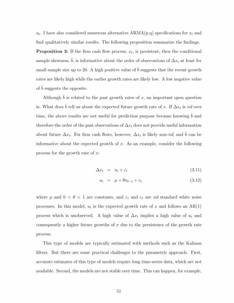
ut. I have also considered numerous alternative ARMA(p,q) specifications for xt and
find qualitatively similar results. The following proposition summarize the findings.
Proposition 3: If the firm cash flow process, xt, is persistent, then the conditional
sample skewness, b, is informative about the order of observations of ∆xt at least for
small sample size up to 20. A high positive value of b suggests that the recent growth
rates are likely high while the earlier growth rates are likely low. A low negative value
of b suggests the opposite.
Although b is related to the past growth rates of x, an important open question
is: What does b tell us about the expected future growth rate of x. If ∆xt is iid over
time, the above results are not useful for prediction purpose because knowing b and
therefore the order of the past observations of ∆xt does not provide useful information
about future ∆xt. For firm cash flows, however, ∆xt is likely non-iid, and b can be
informative about the expected growth of x. As an example, consider the following
process for the growth rate of x:
∆xt = ut + εt (3.11)
ut = µ+ θut−1 + et (3.12)
where µ and 0 < θ < 1 are constants, and εt and et are iid standard white noise
processes. In this model, ut is the expected growth rate of x and follows an AR(1)
process which is unobserved. A high value of ∆xt implies a high value of ut and
consequently a higher future growths of x due to the persistence of the growth rate
process.
This type of models are typically estimated with methods such as the Kalman
filters. But there are some practical challenges to the parametric approach. First,
accurate estimates of this type of models require long time-series data, which are not
available. Second, the models are not stable over time. This can happen, for example,
51

when there are structural breaks in the underlying data-generating process. Third, the
models are likely misspecified. Alternative ARMA specifications or regime-switching
models can provide similar fit of the same data.
Using the conditional sample skewness b to imply the expected growth rate of
x circumvents these problems. It doesn’t need long time series to estimate. More
importantly, it doesn’t rely on any parametric models. It allows many different types
of model specifications. I summarize my argument in the following proposition.
Proposition 4: If the growth rate of xt is positively autocorrelated, then a high
value of conditional sample skewness for small samples, b, implies that the future
growth rate of xt is likely high.
Proposition 4 has a direct implication about stock returns. According to the
basic stock valuation equation (e.g., Fama and French (2006a)), when everything else
is fixed, a higher expected growth rate of firm cash flows implies higher stock returns.
Combining this argument with Proposition 4, I obtain the following result.
Proposition 5: For relatively small time-series samples, higher value of the condi-
tional sample skewness of firm fundamentals, b, implies higher value of the expected
stock return.
In spite of different modeling approaches, both models generate the same positive
relation between the skewness of firm fundamentals and stock returns. Because the
two models are not mutually exclusive, which one of them drives the skewness and
return relation is an empirical issue. In my empirical analysis next, after I first test
the positive return predictability, I will investigate the validity of both models.
3.3 Data and Methodology
In this section, I first show the definitions of skewness measures of firm fundamentals.
I then describe the data. Finally, I discuss the econometric methods.
52

3.3.1 Definition of Skewness Measures
I consider two measures of firm fundamentals: gross profitability GP and earnings
per share EPS. There is significant evidence that GP positively predicts return (e.g.,
Novy-Marx (2013)). Earnings has been widely accepted as a measure of firm cash
flows. At the end of quarter t, I follow Gu and Wu (2003) to define skewness of
GP and EPS as the standard skewness coefficient of lagged observations during the
rolling window of quarters t− n to t− 1:
SKGP,t =n
(n− 1)(n− 2)
t−1∑τ=t−n
(GPτ − µGP
sGP
)3
, (3.13)
SKEPS,t =n
(n− 1)(n− 2)
t−1∑τ=t−n
(EPSτ − µEPS
sEPS
)3
, (3.14)
where µGP (µEPS) and sGP (sEPS) are, respectively, the sample average and standard
deviation of GP (EPS). In the benchmark case reported in the paper, I fix n = 8.
The results for n up to 20 are similar and available upon request. It should be pointed
out that GP is scaled by firm total asset but EPS is not scaled. This, however, is
not a problem for my econometric analysis because the skewness of either variable is
unit free due to the definition of skewness.
Note that I don’t use the GP and EPS of quarter t in constructing the skewness
measures at the end of quarter t because they are not reported until quarter t + 1.
When examining whether the skewness of earnings skewness up to quarter t predicts
the stock returns in quarter t+1, using future information that is available in quarter
t + 1 but not in quarter t biases the statistical inference. I in fact have conducted
(unreported) my analysis without skipping quarter t and have found even stronger
(but biased) results.8
8In a related paper, I consider the skewness of analysts’ earnings forecasts and show that itpositively predicts stock returns. Despite the similarities in return predictability, the informationcontent of the skewness of analysts’ forecasts is very different from that in the fundamental skewness.
53
3.3.2 Data Descriptions
Stock return and accounting data are obtained from the CRSP and COMPUSTAT.
I consider all NYSE, AMEX and NASDAQ firms in the CRSP monthly stock return
files up to December, 2013 except financial stocks (four digit SIC codes between 6000
and 6999) and stocks with end-of-quarter share price less than $5. I further require a
firm to have at least 16 quarters of gross profitability or earnings data during 1971–
2013 to be included in the sample of that skewness measure. The construction of
each observation of skewness measure needs observations of 8 consecutive quarters.
Because the first 2 years of data are used to construct the skewness measures, the
empirical analysis starts in 1973. For each quarter, the accounting variables are
defined as follows.
• GP : Following Novy-Marx (2013), gross profitability is quarterly revenues mi-
nus quarterly cost of goods sold scaled by quarterly asset total.
• EPS: Quarterly earnings per share before extraordinary items.
• MC: Market capitalization is the quarter-end shares outstanding multiplied by
the stock price.
• BM : Book-to-market ratio is the ratio of quarterly book equity to quarter-end
market capitalization. Quarterly book equity is constructed by following Hou,
Xue, and Zhang (2014) (footnote 9), which is basically a quarterly version of
book equity of Davis, Fama, and French (2000).
• MABA: Market-asset-to-book-asset ratio is defined as [Total Asset−Total Book
Common Equity+Market Equity]/Total Assets.
• Tobin’s q: It is defined as [Market Equity+Preferred Stock+Current Liabilities−Current
Assets Total+Long−Term Debt]/Total Assets.
54

• ROE: Return on equity is defined as income before extraordinary items (IBQ)
divided by 1-quarter-lagged book equity.
Firm size and book-to-market ratio are standard control variables in asset pricing
studies. MABA and Tobin’s q are often regarded as proxies of firm growth options
in the literature (e.g., Cao, Simin, and Zhao (2008)). ROE is a popular measure of
firm cash flows other than GP and has been shown to predict stock returns (e.g.,
Hou, Xue, and Zhang (2014)). The variables related to stock returns are defined in
the following.
• MOM : Momentum for month t is defined as the cumulative return between
months t − 6 and t − 1. I follow the convention in the literature by skipping
month t when MOM is used to predict returns in month t+ 1. I have also used
the cumulative return between months t − 11 and t − 1 and obtained similar
results.
• Idvol: Idiosyncratic volatility is, following Jiang, Xu, and Yao (2009), the stan-
dard deviation of the residuals of the Fama and French (1993) 3-factor model
using daily returns in the quarter.
• Idskew: Following Harvey and Siddique (2000) and Bali, Cakici, and Whitelaw
(2011), it is defined as the skewness of the regression residuals of the market
model augmented by the squared market excess return. I use daily returns in
the quarter to estimate the regression.
• Prskew: It is predicted idiosyncratic skewness defined in Boyer, Mitton, and
Vorkink (2010). I obtain the Prskew data from Brian Boyer’s website.
• MAX: Following Bali, Cakici, and Whitelaw (2011), it is the average of the
three highest daily returns in quarter t. Note that I use quarterly frequency
instead of monthly frequency.
55

I use Idvol as a control because a number of studies have documented that it predicts
returns (e.g., Ang, Hodrick, Xing, and Zhang (2006)). The skewness measures of stock
returns, Idskew, Prskew, and MAX are good controls to evaluate additional return
explanatory power of skewness of firm fundamentals. I have also considered total
return skewness of daily stock returns in the quarter and obtained similar results. I
winsorize all the variables except the stock return at 1% and 99% levels although the
results do not change significantly without winsorizing or winsorizing at 0.5% and
99.5% levels.
There are 350,050 and 384,402 firm-quarter observations for SKGP and SKEPS,
respectively. Panel A of Table 3.1 shows the summary statistics of SKGP and SKEPS.
On average, both SKGP and SKEPS are negative while SKGP is more negative than
SKGP . The large standard deviations and extreme percentile values indicate signifi-
cant cross-sectional variation of fundamental skewness across stocks. Both skewness
measures are positively autocorrelated but the first-order autocorrelation coefficients
(ρ1) are low, 0.14 and 0.13. The relatively low values of ρ1 is an artifact of my esti-
mation method of using non-overlapping samples. That is, I first use non-overlapping
samples to construct the skewness measures and then estimate an AR(1) regression
to get ρ1.
Panel B reports the average contemporaneous cross-sectional correlations of the
skewness measures and the control variables. SKGP and SKEPS are mildly correlated
with the correlation coefficient of 0.31, suggesting that the two measures may capture
different aspects of firm cash flows. SKGP is mildly correlated with MOM and GP
but uncorrelated with other controls. SKEPS seems to be slightly correlated with all
the control variables but none of the correlation coefficients is above 0.2.
56

3.3.3 Econometric Methods
I rely mostly on the portfolio sorts and cross-sectional regressions of Fama and Mac-
Beth (1973) for the empirical investigation. For single portfolio sorts, I rank stocks
on a skewness measure of firm fundamentals into decile portfolios and then consider
both equally-weighted and value-weighted portfolio returns. If the skewness is pos-
itively related to stock returns, I expect an increasing pattern of portfolio returns
from decile 1 to decile 10. For double portfolio sorts, I first rank stocks into quintiles
by a control variable such as MC and then further sort stocks within each portfolio
into quintiles by the skewness measure. If the control variable can explain the pre-
dictability of skewness, I expect the increasing pattern of returns in skewness to be
much less significant in each quintile of the control variable. To compute t-statistics
of average portfolio returns, I use the Newey-West adjusted standard errors because
of the persistence in the portfolio compositions.
For the Fama-MacBeth regressions, I expect the estimated average coefficient of
the skewness measure to be positive and significant. The cross-sectional regressions
allow us to examine the marginal effect of the skewness measure when controlling for
other variables known to predict stock returns. In the most general specification, I
include all the control variables in the regression. If the skewness measure captures
information about expected stock returns beyond that in other variables, the coef-
ficient of the skewness measure should be significant even in the presence of all the
control variables.
I also use the Fama-MacBeth regression approach to compare the explanatory
power of different skewness measures. To do so, I include the two skewness measures
in one regression. If the coefficient of one skewness measure is no longer significant
in the presence of the other, it indicates that the later skewness measure dominates
the first measure in the sense that it subsumes all the explanatory power of the first
measure.
57

3.4 Empirical Evidence
I show the results of portfolio sorts first and then the estimates of Fama-MacBeth
regressions. I next further examine the validity of the theoretical models. I conduct
robustness checks at the end of the section.
3.4.1 Single Portfolio Sorts
Table 3.2 reports the average returns and characteristics of the decile portfolios formed
by sorting stocks on the two skewness measures. When sorted on SKGP as in panel
A, the average equal-weighted quarterly return increases from decile 1 (2.99%) to
decile 10 (4.54%). The average H-L spread is 1.55% per quarter (or 6.20% per year)
and highly significant (t = 5.67). To make sure that the significant H-L spread is
not driven by higher stock risks, I estimate the risk-adjusted α using either the 3-
factor model of Fama and French (1996) or the 5-factor model of Fama and French
(2015).9 The risk-adjusted H-L spreads are even higher at 1.69% and 1.61%. The
value-weighted returns are very similar to but slightly smaller than the equal-weighted
returns, indicating that the results are not dominated by small stocks.
Next, I look at the characteristics of the equal-weighted decile portfolios. Low-
SKGP stocks have low past return, GP , and ROE but slightly higher book-to-market
ratio and idiosyncratic volatility. One reason of these patterns in control variables is
that low-SKGP stocks are past under-performers in terms of profitability. To make
sure that the return predictability of SKGP is not driven by the firm characteris-
tics, I will reexamine the predictability by double portfolio sorts and Fama-MacBeth
regressions.
The results of portfolios sorts on SKEPS in panel B are very close to those for
SKGP . The unadjusted and adjusted H-L spreads for SKEPS are actually slightly
9I have also used the 4-factor model of Carhart (1997). The results are similar and availableupon request.
58

higher than those for SKGP . The average unadjusted H-L spread is 1.66% per quarter
(or 6.64% per year) and highly significant (t = 4.20). The firm characteristics of the
decile portfolios also exhibit similar patterns as those in panel A.
Overall, I find a positive relation between the skewness of firm fundamentals and
future stock returns, consistent with the predictions of both theoretical models. The
results are robust regardless whether the returns are equal-weighted or value-weighted,
and unadjusted or risk-adjusted. I will present further evidence on which model is
more appropriate in explaining the return predictability.
3.4.2 Double Portfolio Sorts
I now investigate whether the predictability of the skewness measures are caused by
firm characteristics. I use the double portfolio sort approach by first sorting stocks on
firm characteristics and then sorting on the skewness measures. Table 3.3 reports the
average equal-weighted returns of double-sorted portfolios for the six characteristics
reported in Table 3.2. The results for value-weighted returns are very similar but
unreported for brevity. I have also examined a number of other control variables and
those results are available upon requests.
I first consider the results for SKGP in panel A. When stocks are initially ranked
by MC, the H-L spreads of the skewness quintiles show a decreasing pattern from
MC quintile 1 (2.51%) to MC quintile 5 (0.58%), suggesting that the predictability of
SKGP is stronger for small stocks. Among the other characteristics, the predictability
of SKGP is stronger for high MOM , GP , and Idvol stocks but there is no clear
pattern for BM and ROE. No matter which firm characteristic is considered, all H-L
spreads remain positive and most of them are statistically significant. The evidence
indicates that the return predictive power of SKGP can not be explained the firm
characteristics.
The results for SKEPS in panel B are generally similar to those for SKGP but
59

with some differences. The predictability of SKEPS is stronger for low BM and high
ROE stocks. The H-L spreads for GP quintiles exhibit a U-shape pattern. In sum,
the double sorts evidence for SKEPS is not as robust as for SKGP in the presence
of control variables. The predictability of SKEPS is particularly weaker for MOM ,
GP , and ROE quintiles as the average H-L spreads across the quintiles are smaller
in magnitude than that in single portfolio sorts. In particular, the H-L spread is
significant only for the highest ROE quintile. Some loss of statistical significance
can be attributed to the higher standard errors due to the smaller sample size of the
5×5 portfolios. Close inspection of the ROE quintiles reveals non-linear interactions
among stock return, SKEPS, and ROE. I will get a clearer picture when I estimate
Fama-MacBeth regressions where multiple control variables are jointly considered.
3.4.3 Fama-MacBeth Regressions
I now examine the return predictability of the skewness measures with the Fama-
MacBeth regressions, which allow us to control for multiple return predictors simul-
taneously. The results are reported in Table 3.4. I estimate eight regression models.
The first one uses a skewness measure as the only explanatory variable. Models (2)-
(7) examines the six control variables, one at a time. Because of different sample sizes
for the two skewness measures, I reestimate these models for each skewness measure.
Model (8) includes the skewness measure and all six control variables.
First, I consider the results for SKGP in panel A. The average coefficient of SKGP
in model (1) is positive and significant at the 1% level (0.24 and t = 6.18). Every
control variable but MC is significant when it is used alone to forecast returns. The
signs of the coefficients for the control variables except MC are consistent with those
documented in the literature (e.g., Fama and French (1992), Jegadeesh and Titman
(1993), Ang, Hodrick, Xing, and Zhang (2006), Novy-Marx (2013), and Hou, Xue, and
Zhang (2014) In model (8) where all controls are incorporated, the average coefficient
60

of SKGP is smaller in magnitude than that in model (1) but still significant at the
1% level (0.11 and t = 3.87). Interestingly, the average coefficient for MC is now
significant at the 10% level and has the same negative sign as that documented in
the literature.
Next, as shown in panel B, the estimation results for SKEPS are very similar to
those for SKGP . By itself, SKEPS positively predicts stock returns in model (1). The
average coefficient is 0.25 and significant at the 1% level (t = 4.73). When all the
control variables are included in model (8), the average coefficient of SKEPS remains
positive and significant at the 5% level (0.09 and t = 2.37). In sum, the results of
Fama-MacBeth regressions are consistent with those of portfolio sorts. Both skewness
measures of firm fundamentals positively predict stock returns. While in the presence
of control variables the evidence is not as significant as when they are absent, the
overall return predictability by the fundamental skewness cannot be explained by
other predictors.
3.4.4 Skewness and Firm Growth Option
I now test the firm growth option model by checking whether the skewness of firm
fundamentals is positively related to future firm growth opportunities. I use two
popular measures of firm growth option in the literature: MABA and Tobin’s q
(e.g., Cao, Simin and Zhao (2008)). I present evidence of both portfolio sorts and
Fama-MacBeth regressions.
Table 3.5 reports the average equal-weighted future MABA and Tobin’s q for the
next four quarters of the decile portfolios formed by sorting stocks on the skewness
measures. Value-weighted results are very similar and not reported for brevity. The
results support my argument that a higher value of skewness implies higher growth
opportunities. For both skewness measures, the H-L spreads in MABA and Tobin’s
q are all positive and significant at the 1% level for all four future quarters. The
61

magnitude of the H-L spreads is higher for SKEPS than for SKGP . The slow decaying
of the H-L spreads indicates that the impact of the skewness on firm growth option
is persistent.
In Table 3.6, I present the estimates of Fama-MacBeth regressions where the
dependent variable is the next-quarter MABA or Tobin’s q. The results for future
values of MABA and Tobin’s q are very similar and not reported. Again, the results
for the two proxies of firm growth options are very similar. When a skewness measure
is the only predictor, its estimated coefficient is positive and significant at the 1%.
Next, I consider the estimation results with all the control variables. Because both
MABA and Tobin’s q are persistent, I include their lagged values as additional control
variables in corresponding regressions. The coefficients on the skewness measures
with the controls included are much smaller but still significant at the 5% level.
The coefficient for SKEPS is always higher than the coefficient for SKGP , consistent
with the results of portfolio sorts. Taken together, the evidence of portfolio sorts
and Fama-MacBeth regressions support my model implication that firms with higher
fundamental skewness have higher growth options.
3.4.5 Skewness and Firm Profitability
I then turn attention to testing the second model by examining whether the skewness
of firm fundamentals is positively related to future profitability or growth of firm cash
flows. I gauge the firm profitability by two widely used measures in the literature:
ROE and GP .
Table 3.7 reports the average equal-weighted future ROE and GP for the next four
quarters of the decile portfolios formed by sorting stocks on the skewness measures.
The results for both SKGP and SKEPS indicate that high-skewness stocks have higher
profitability in the next four quarters. The H-L spreads of both ROE and GP are
positive and significant at the 1% level for all four quarters. The H-L spreads decline
62

gradually as horizon increases, suggesting mean reversion. But the slow reversion
indicates the impact of the skewness on firm profitability is persistent. There is an
interesting pattern between the two panels: The H-L spreads in ROE in panel B are
larger than those in panel A but the H-L spreads in GP in panel B are smaller than
those in panel A. This is not surprising as the skewness of earnings should be more
significant in predicting ROE while the skewness of GP should be more significant
in predicting GP .
Table 3.8 reports the estimation results of the Fama-MacBeth regressions where
the dependent variable is the next-quarter ROE or GP . The regressions evidence is
mostly consistent with the portfolio sorts evidence. Both skewness measures positively
predict future ROE and GP even in the presence of the control variables including
lagged ROE and GP . The only insignificant coefficient is for SKEPS when all controls
are included but it is still positive.
Overall, the above evidence supports the second model. Together with the ev-
idence in the previous section, the findings are consistent with both models. That
is, higher skewness of firm fundamental implies higher firm growth option as well as
higher growth rate of firm cash flows.
3.4.6 Comparison of Alternative Skewness Measures
It is interesting to compare the return predictive power of the two skewness measures.
To do this, I estimate Fama-MacBeth regressions with both skewness measures as
explanatory variables. The first regression contains no control variables while the
second regression includes all control variables. The estimation results are reported
in Table 3.9.
Without control variables, the average coefficient of SKGP is 0.19 and significant
at the 1% level (t = 5.67) while the average coefficient of SKEPS is 0.13 and only
significant at the 10% level (t = 1.93), indicating that the predictability of SKGP
63

dominates that of SKEPS. When all the control variables are incorporated, the
average coefficients of SKGP (0.11) remains significant at the 1% level but the average
coefficient of SKEPS is insignificant albeit positive (0.02). The evidence suggests
that the predictability of SKEPS is subsumed by SKGP and the control variables.
My findings support the argument of Novy-Marx (2013) that GP is one of the best
accounting measures of firm performance.
3.4.7 Robustness Checks
Long Horizons
I have shown earlier that the fundamental skewness predicts long-run firm growth
option and profitability. I now investigate if the return predictability holds for long
horizons. I estimate Fama-MacBeth regressions for returns in quarters t+ 2, ..., t+ 5
and report the results in Table 3.10. I only consider two regression specifications. In
model (1), the skewness is the only explanatory variable while model (2) also contains
all the control variables.
The results show that the skewness of fundamentals, particularly SKGP , can pre-
dict long-run returns. The coefficient on SKG in model (1) is positive and significant
at least at the 10% up to t + 5. Even in the presence of the control variables in
model (2), it is significant up to t + 3. The coefficient on SKEPS is always positive
but becomes insignificant beyond t + 2. As a whole, the return predictability holds
at least up to the third quarter. Note that if I use the cumulative returns as the
dependent variables, then all the coefficients will become significant. Among the con-
trol variables, GP is the strongest return predictor as its coefficient is positive and
significant up to t+ 5, consistent with the findings of Novy-Marx (2013).
64

Controlling for Return Skewness
One concern about my empirical results is whether the return predictability of the
fundamental skewness is related to the return predictability of the return skewness
documented in the literature. I address this issue by incorporating three popular
return skewness measures (MAX, Idskew, and Prskew) in the Fama-MacBeth re-
gressions of the fundamental skewness measures. Table 3.11 reports the estimation
results.
In models (1)–(3), I only use one of the three return skewness measures. MAX
and Prskew are significant but Idskew is insignificant in predicting returns. However,
the sign of average coefficient for MAX changes signs for different samples. Model
(4) use all three return skewness measures. MAX and Idskew are significant in the
sample of SKGP while Prskew is significant in the sample of SKEPS. For my samples,
the return skewness measures do not appear to consistently predict stock returns.
I next combine the skewness of fundamentals with the return skewness measures
in models (5) an (6). In model (5), I do not use any control variables. The average
coefficients of SKGP and SKEPS are positive and significant at the 1% level. Among
the skewness measures of returns, only MAX is significant at the 1% level for the
SKGP sample and Prskew is significant at the 10% level in the SKEPS. I now include
all the control variables in model (6). MAX and Prskew are marginally significant in
the sample of SKEPS. Most importantly, the average coefficients SKGP and SKEPS
are significant at the 1% level. The evidence indicates that my findings cannot be
explained by the skewness of stock returns.
Additional Tests
I perform some additional robustness checks and report the results in Table 3.12. For
brevity, I only consider two regression specifications. Model (1) only contains the
skewness measure as the explanatory variable while model (2) also contains all the
65

control variables.
First, I estimate panel regressions instead of Fama-MacBeth regressions and com-
pute t-statistics using two-way clustered standard errors. The coefficients on SKGPS
and SKEPS are similar to those of the Fama-MacBeth regressions in Table 3.4. As
expected, the t-statistics are smaller but remain significant at the 1% level for SKGP
and 10% level for SKEPS.
Next, I extend the panel regressions by adding the time fixed effect to take care
of the potential seasonality problem. The estimates with the time fixed effect are
almost identical to those without the time fixed effect.
Thirdly, I estimate Fama-MacBeth regressions with the industry fixed effect. The
coefficients on SKGPS and SKEPS are comparable to those reported in Table ??
without the industry fixed effect.
Finally, I estimate the basic Fama-MacBeth regressions for the skewness measures
that are constructed using the data of last 12 quarters instead of 8 quarters. The
results, particularly of model (2), are very close to those reported in Table 3.4 for
the benchmark case. Taken together, the results of these additional tests provide
further support my main model implication that the skewness of firm fundamentals
is positively related to stock returns.
3.5 Conclusions
I present two distinct models that relate the skewness of firm fundamentals to stock
returns. The first model hinges on the premise that the firm value contains a growth
option component and the fundamental skewness affects the option value. The second
model relies on the interpretation of the sample skewness of firm fundamentals as a
proxy of the expected growth rate of firm cash flows. Both models imply a positive
relation between the fundamental skewness and expected stock return.
Using two skewness measures of firm gross profitability and earnings per share,
66

I find strong evidence supporting both models. The skewness measures positively
predict not only cross-sectional stock returns but also future firm growth option and
growth rate of firm cash flows. The evidence cannot be explained by the existing risk
models and other return predictors including the skewness of stock returns.
Because the two models are based on the option pricing theory and the basic
stock valuation equation, I am, in the spirit of Fama and French (2006a, 2008),
agnostic about whether the return predictability of the skewness measures is rational
or irrational. Given the strong evidence of skewness in firm cash flows, the results
highlight the importance of incorporating the skewness measures of firm fundamentals
in asset pricing research.
67
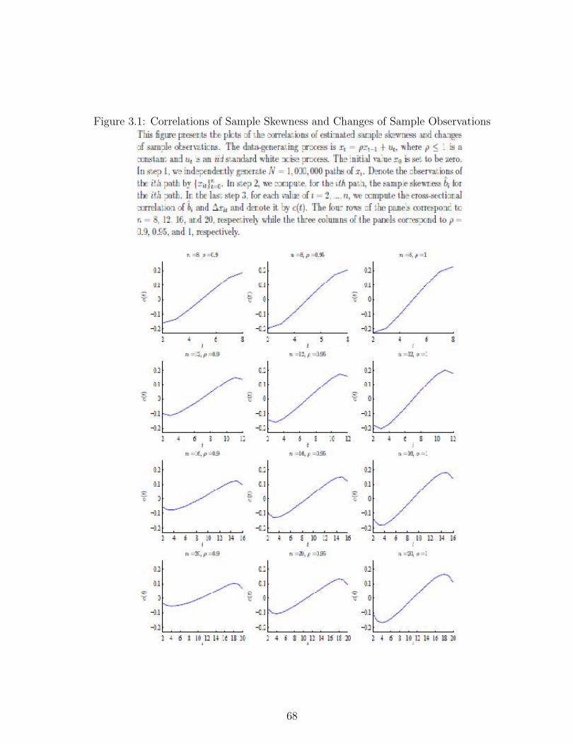
Figure 3.1: Correlations of Sample Skewness and Changes of Sample Observations
68
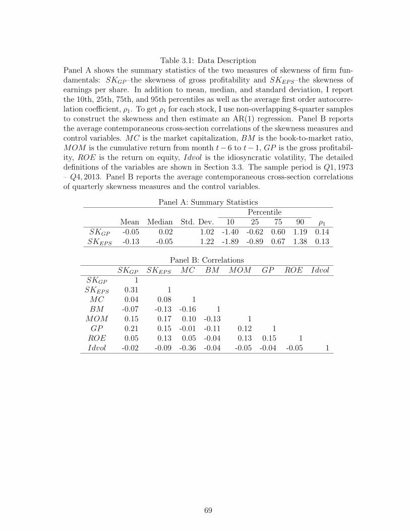
Table 3.1: Data DescriptionPanel A shows the summary statistics of the two measures of skewness of firm fun-damentals: SKGP–the skewness of gross profitability and SKEPS–the skewness ofearnings per share. In addition to mean, median, and standard deviation, I reportthe 10th, 25th, 75th, and 95th percentiles as well as the average first order autocorre-lation coefficient, ρ1. To get ρ1 for each stock, I use non-overlapping 8-quarter samplesto construct the skewness and then estimate an AR(1) regression. Panel B reportsthe average contemporaneous cross-section correlations of the skewness measures andcontrol variables. MC is the market capitalization, BM is the book-to-market ratio,MOM is the cumulative return from month t− 6 to t− 1, GP is the gross profitabil-ity, ROE is the return on equity, Idvol is the idiosyncratic volatility, The detaileddefinitions of the variables are shown in Section 3.3. The sample period is Q1, 1973– Q4, 2013. Panel B reports the average contemporaneous cross-section correlationsof quarterly skewness measures and the control variables.
Panel A: Summary StatisticsPercentile
Mean Median Std. Dev. 10 25 75 90 ρ1
SKGP -0.05 0.02 1.02 -1.40 -0.62 0.60 1.19 0.14SKEPS -0.13 -0.05 1.22 -1.89 -0.89 0.67 1.38 0.13
Panel B: CorrelationsSKGP SKEPS MC BM MOM GP ROE Idvol
SKGP 1SKEPS 0.31 1MC 0.04 0.08 1BM -0.07 -0.13 -0.16 1MOM 0.15 0.17 0.10 -0.13 1GP 0.21 0.15 -0.01 -0.11 0.12 1ROE 0.05 0.13 0.05 -0.04 0.13 0.15 1Idvol -0.02 -0.09 -0.36 -0.04 -0.05 -0.04 -0.05 1
69
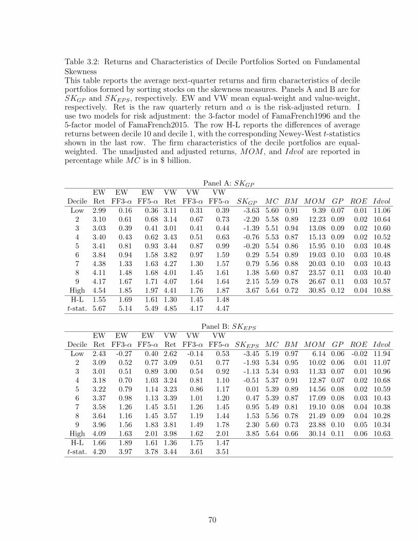
Table 3.2: Returns and Characteristics of Decile Portfolios Sorted on FundamentalSkewnessThis table reports the average next-quarter returns and firm characteristics of decileportfolios formed by sorting stocks on the skewness measures. Panels A and B are forSKGP and SKEPS, respectively. EW and VW mean equal-weight and value-weight,respectively. Ret is the raw quarterly return and α is the risk-adjusted return. Iuse two models for risk adjustment: the 3-factor model of FamaFrench1996 and the5-factor model of FamaFrench2015. The row H-L reports the differences of averagereturns between decile 10 and decile 1, with the corresponding Newey-West t-statisticsshown in the last row. The firm characteristics of the decile portfolios are equal-weighted. The unadjusted and adjusted returns, MOM , and Idvol are reported inpercentage while MC is in $ billion.
Panel A: SKGP
EW EW EW VW VW VWDecile Ret FF3-α FF5-α Ret FF3-α FF5-α SKGP MC BM MOM GP ROE IdvolLow 2.99 0.16 0.36 3.11 0.31 0.39 -3.63 5.60 0.91 9.39 0.07 0.01 11.06
2 3.10 0.61 0.68 3.14 0.67 0.73 -2.20 5.58 0.89 12.23 0.09 0.02 10.643 3.03 0.39 0.41 3.01 0.41 0.44 -1.39 5.51 0.94 13.08 0.09 0.02 10.604 3.40 0.43 0.62 3.43 0.51 0.63 -0.76 5.53 0.87 15.13 0.09 0.02 10.525 3.41 0.81 0.93 3.44 0.87 0.99 -0.20 5.54 0.86 15.95 0.10 0.03 10.486 3.84 0.94 1.58 3.82 0.97 1.59 0.29 5.54 0.89 19.03 0.10 0.03 10.487 4.38 1.33 1.63 4.27 1.30 1.57 0.79 5.56 0.88 20.03 0.10 0.03 10.438 4.11 1.48 1.68 4.01 1.45 1.61 1.38 5.60 0.87 23.57 0.11 0.03 10.409 4.17 1.67 1.71 4.07 1.64 1.64 2.15 5.59 0.78 26.67 0.11 0.03 10.57
High 4.54 1.85 1.97 4.41 1.76 1.87 3.67 5.64 0.72 30.85 0.12 0.04 10.88H-L 1.55 1.69 1.61 1.30 1.45 1.48t-stat. 5.67 5.14 5.49 4.85 4.17 4.47
Panel B: SKEPS
EW EW EW VW VW VWDecile Ret FF3-α FF5-α Ret FF3-α FF5-α SKEPS MC BM MOM GP ROE IdvolLow 2.43 -0.27 0.40 2.62 -0.14 0.53 -3.45 5.19 0.97 6.14 0.06 -0.02 11.94
2 3.09 0.52 0.77 3.09 0.51 0.77 -1.93 5.34 0.95 10.02 0.06 0.01 11.073 3.01 0.51 0.89 3.00 0.54 0.92 -1.13 5.34 0.93 11.33 0.07 0.01 10.964 3.18 0.70 1.03 3.24 0.81 1.10 -0.51 5.37 0.91 12.87 0.07 0.02 10.685 3.22 0.79 1.14 3.23 0.86 1.17 0.01 5.39 0.89 14.56 0.08 0.02 10.596 3.37 0.98 1.13 3.39 1.01 1.20 0.47 5.39 0.87 17.09 0.08 0.03 10.437 3.58 1.26 1.45 3.51 1.26 1.45 0.95 5.49 0.81 19.10 0.08 0.04 10.388 3.64 1.16 1.45 3.57 1.19 1.44 1.53 5.56 0.78 21.49 0.09 0.04 10.289 3.96 1.56 1.83 3.81 1.49 1.78 2.30 5.60 0.73 23.88 0.10 0.05 10.34
High 4.09 1.63 2.01 3.98 1.62 2.01 3.85 5.64 0.66 30.14 0.11 0.06 10.63H-L 1.66 1.89 1.61 1.36 1.75 1.47t-stat. 4.20 3.97 3.78 3.44 3.61 3.51
70
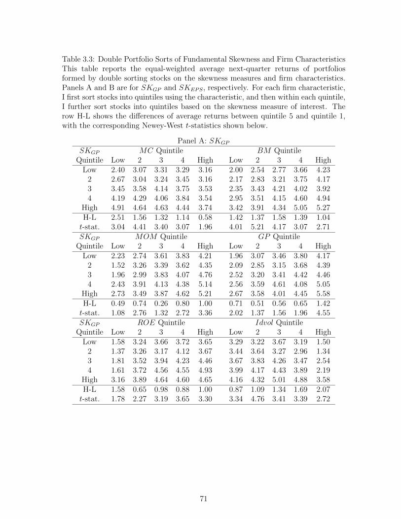
Table 3.3: Double Portfolio Sorts of Fundamental Skewness and Firm CharacteristicsThis table reports the equal-weighted average next-quarter returns of portfoliosformed by double sorting stocks on the skewness measures and firm characteristics.Panels A and B are for SKGP and SKEPS, respectively. For each firm characteristic,I first sort stocks into quintiles using the characteristic, and then within each quintile,I further sort stocks into quintiles based on the skewness measure of interest. Therow H-L shows the differences of average returns between quintile 5 and quintile 1,with the corresponding Newey-West t-statistics shown below.
Panel A: SKGP
SKGP MC Quintile BM QuintileQuintile Low 2 3 4 High Low 2 3 4 High
Low 2.40 3.07 3.31 3.29 3.16 2.00 2.54 2.77 3.66 4.232 2.67 3.04 3.24 3.45 3.16 2.17 2.83 3.21 3.75 4.173 3.45 3.58 4.14 3.75 3.53 2.35 3.43 4.21 4.02 3.924 4.19 4.29 4.06 3.84 3.54 2.95 3.51 4.15 4.60 4.94
High 4.91 4.64 4.63 4.44 3.74 3.42 3.91 4.34 5.05 5.27H-L 2.51 1.56 1.32 1.14 0.58 1.42 1.37 1.58 1.39 1.04t-stat. 3.04 4.41 3.40 3.07 1.96 4.01 5.21 4.17 3.07 2.71SKGP MOM Quintile GP Quintile
Quintile Low 2 3 4 High Low 2 3 4 HighLow 2.23 2.74 3.61 3.83 4.21 1.96 3.07 3.46 3.80 4.17
2 1.52 3.26 3.39 3.62 4.35 2.09 2.85 3.15 3.68 4.393 1.96 2.99 3.83 4.07 4.76 2.52 3.20 3.41 4.42 4.464 2.43 3.91 4.13 4.38 5.14 2.56 3.59 4.61 4.08 5.05
High 2.73 3.49 3.87 4.62 5.21 2.67 3.58 4.01 4.45 5.58H-L 0.49 0.74 0.26 0.80 1.00 0.71 0.51 0.56 0.65 1.42t-stat. 1.08 2.76 1.32 2.72 3.36 2.02 1.37 1.56 1.96 4.55SKGP ROE Quintile Idvol Quintile
Quintile Low 2 3 4 High Low 2 3 4 HighLow 1.58 3.24 3.66 3.72 3.65 3.29 3.22 3.67 3.19 1.50
2 1.37 3.26 3.17 4.12 3.67 3.44 3.64 3.27 2.96 1.343 1.81 3.52 3.94 4.23 4.46 3.67 3.83 4.26 3.47 2.544 1.61 3.72 4.56 4.55 4.93 3.99 4.17 4.43 3.89 2.19
High 3.16 3.89 4.64 4.60 4.65 4.16 4.32 5.01 4.88 3.58H-L 1.58 0.65 0.98 0.88 1.00 0.87 1.09 1.34 1.69 2.07t-stat. 1.78 2.27 3.19 3.65 3.30 3.34 4.76 3.41 3.39 2.72
71

72
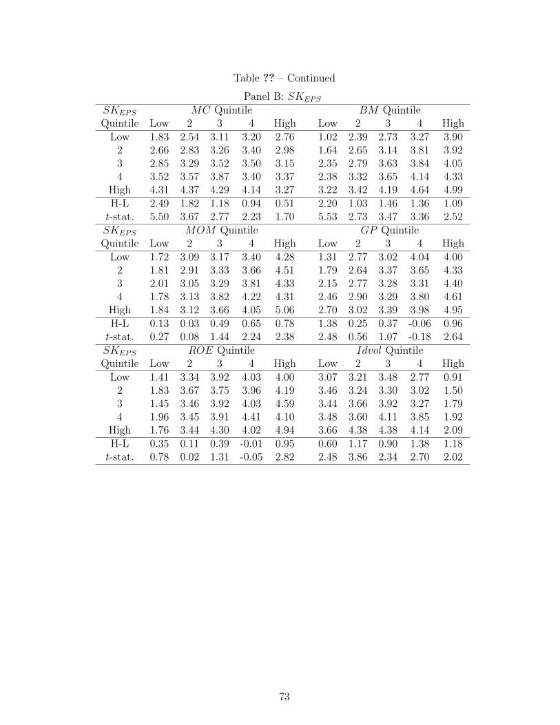
Table ?? – Continued
Panel B: SKEPS
SKEPS MC Quintile BM QuintileQuintile Low 2 3 4 High Low 2 3 4 High
Low 1.83 2.54 3.11 3.20 2.76 1.02 2.39 2.73 3.27 3.902 2.66 2.83 3.26 3.40 2.98 1.64 2.65 3.14 3.81 3.923 2.85 3.29 3.52 3.50 3.15 2.35 2.79 3.63 3.84 4.054 3.52 3.57 3.87 3.40 3.37 2.38 3.32 3.65 4.14 4.33
High 4.31 4.37 4.29 4.14 3.27 3.22 3.42 4.19 4.64 4.99H-L 2.49 1.82 1.18 0.94 0.51 2.20 1.03 1.46 1.36 1.09t-stat. 5.50 3.67 2.77 2.23 1.70 5.53 2.73 3.47 3.36 2.52SKEPS MOM Quintile GP QuintileQuintile Low 2 3 4 High Low 2 3 4 High
Low 1.72 3.09 3.17 3.40 4.28 1.31 2.77 3.02 4.04 4.002 1.81 2.91 3.33 3.66 4.51 1.79 2.64 3.37 3.65 4.333 2.01 3.05 3.29 3.81 4.33 2.15 2.77 3.28 3.31 4.404 1.78 3.13 3.82 4.22 4.31 2.46 2.90 3.29 3.80 4.61
High 1.84 3.12 3.66 4.05 5.06 2.70 3.02 3.39 3.98 4.95H-L 0.13 0.03 0.49 0.65 0.78 1.38 0.25 0.37 -0.06 0.96t-stat. 0.27 0.08 1.44 2.24 2.38 2.48 0.56 1.07 -0.18 2.64SKEPS ROE Quintile Idvol QuintileQuintile Low 2 3 4 High Low 2 3 4 High
Low 1.41 3.34 3.92 4.03 4.00 3.07 3.21 3.48 2.77 0.912 1.83 3.67 3.75 3.96 4.19 3.46 3.24 3.30 3.02 1.503 1.45 3.46 3.92 4.03 4.59 3.44 3.66 3.92 3.27 1.794 1.96 3.45 3.91 4.41 4.10 3.48 3.60 4.11 3.85 1.92
High 1.76 3.44 4.30 4.02 4.94 3.66 4.38 4.38 4.14 2.09H-L 0.35 0.11 0.39 -0.01 0.95 0.60 1.17 0.90 1.38 1.18t-stat. 0.78 0.02 1.31 -0.05 2.82 2.48 3.86 2.34 2.70 2.02
73
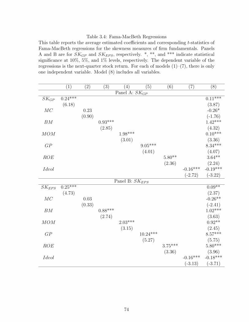
Table 3.4: Fama-MacBeth RegressionsThis table reports the average estimated coefficients and corresponding t-statistics ofFama-MacBeth regressions for the skewness measures of firm fundamentals. PanelsA and B are for SKGP and SKEPS, respectively. *, **, and *** indicate statisticalsignificance at 10%, 5%, and 1% levels, respectively. The dependent variable of theregressions is the next-quarter stock return. For each of models (1)–(7), there is onlyone independent variable. Model (8) includes all variables.
(1) (2) (3) (4) (5) (6) (7) (8)Panel A: SKGP
SKGP 0.24*** 0.11***(6.18) (3.87)
MC 0.23 -0.26*(0.90) (-1.76)
BM 0.93*** 1.42***(2.85) (4.32)
MOM 1.98*** 0.10***(3.01) (3.36)
GP 9.05*** 8.34***(4.01) (4.07)
ROE 5.80** 3.64**(2.36) (2.24)
Idvol -0.16*** -0.19***(-2.72) (-3.22)
Panel B: SKEPS
SKEPS 0.25*** 0.09**(4.73) (2.37)
MC 0.03 -0.26**(0.33) (-2.41)
BM 0.88*** 1.02***(2.74) (3.63)
MOM 2.03*** 0.92**(3.15) (2.45)
GP 10.24*** 8.57***(5.27) (5.75)
ROE 3.75*** 5.80***(3.36) (3.96)
Idvol -0.16*** -0.18***(-3.13) (-3.71)
74
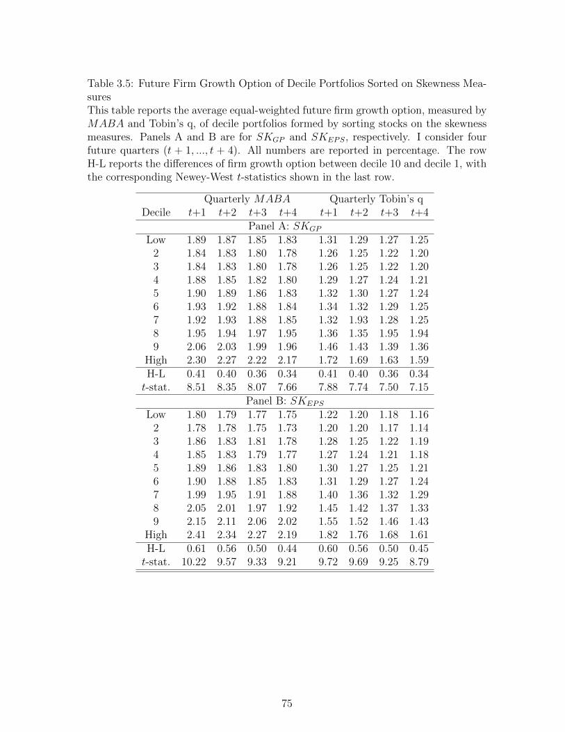
Table 3.5: Future Firm Growth Option of Decile Portfolios Sorted on Skewness Mea-suresThis table reports the average equal-weighted future firm growth option, measured byMABA and Tobin’s q, of decile portfolios formed by sorting stocks on the skewnessmeasures. Panels A and B are for SKGP and SKEPS, respectively. I consider fourfuture quarters (t + 1, ..., t + 4). All numbers are reported in percentage. The rowH-L reports the differences of firm growth option between decile 10 and decile 1, withthe corresponding Newey-West t-statistics shown in the last row.
Quarterly MABA Quarterly Tobin’s qDecile t+1 t+2 t+3 t+4 t+1 t+2 t+3 t+4
Panel A: SKGP
Low 1.89 1.87 1.85 1.83 1.31 1.29 1.27 1.252 1.84 1.83 1.80 1.78 1.26 1.25 1.22 1.203 1.84 1.83 1.80 1.78 1.26 1.25 1.22 1.204 1.88 1.85 1.82 1.80 1.29 1.27 1.24 1.215 1.90 1.89 1.86 1.83 1.32 1.30 1.27 1.246 1.93 1.92 1.88 1.84 1.34 1.32 1.29 1.257 1.92 1.93 1.88 1.85 1.32 1.93 1.28 1.258 1.95 1.94 1.97 1.95 1.36 1.35 1.95 1.949 2.06 2.03 1.99 1.96 1.46 1.43 1.39 1.36
High 2.30 2.27 2.22 2.17 1.72 1.69 1.63 1.59H-L 0.41 0.40 0.36 0.34 0.41 0.40 0.36 0.34t-stat. 8.51 8.35 8.07 7.66 7.88 7.74 7.50 7.15
Panel B: SKEPS
Low 1.80 1.79 1.77 1.75 1.22 1.20 1.18 1.162 1.78 1.78 1.75 1.73 1.20 1.20 1.17 1.143 1.86 1.83 1.81 1.78 1.28 1.25 1.22 1.194 1.85 1.83 1.79 1.77 1.27 1.24 1.21 1.185 1.89 1.86 1.83 1.80 1.30 1.27 1.25 1.216 1.90 1.88 1.85 1.83 1.31 1.29 1.27 1.247 1.99 1.95 1.91 1.88 1.40 1.36 1.32 1.298 2.05 2.01 1.97 1.92 1.45 1.42 1.37 1.339 2.15 2.11 2.06 2.02 1.55 1.52 1.46 1.43
High 2.41 2.34 2.27 2.19 1.82 1.76 1.68 1.61H-L 0.61 0.56 0.50 0.44 0.60 0.56 0.50 0.45t-stat. 10.22 9.57 9.33 9.21 9.72 9.69 9.25 8.79
75

Table 3.6: Fama-MacBeth Regressions of Future Firm Growth OptionThis table reports the average estimated coefficients and corresponding t-statistics ofFama-MacBeth regressions of future firm growth option on the skewness measures offirm fundamentals. Panels A and B consider MABA and Tobin’s q, respectively. Foreach skewness measure, the first regression only uses the skewness measure while thesecond regression contains all control variables, including the lagged value of the firmgrowth option proxy. *, **, and *** indicate statistical significance at 10%, 5%, and1% levels, respectively.
Panel A: MABALagged
SKGP MC BM MOM GP ROE Idvol MABA0.048***(11.17)0.012** 0.019*** -0.097*** 0.230*** 0.310** -0.027 0.001 0.870***(2.32) (3.23) (-4.36) (8.79) (2.09) (-0.73) (0.72) (44.84)SKEPS
0.076***(8.33)
0.010** 0.021*** -0.034*** 0.231*** 0.32** -0.31 0.009* 0.916***(1.99) (3.37) (-3.41) (7.54) (2.21) (-0.91) (1.75) (12.76)
Panel B: Tobin’s qLagged
SKGP MC BM MOM GP ROE Idvol Tobin’s q0.045***(10.02)0.010** 0.022*** -0.057*** 0.228*** 0.082 -0.171*** 0.001 0.868***(2.13) (3.47) (-2.65) (8.47) (1.00) (-3.76) (0.62) (43.77)SKEPS
0.073***(7.69)
0.014** 0.030*** -0.034*** 0.438*** 0.003 -0.124** 0.002 0.847***(2.06) (4.00) (-3.70) (8.24) (0.04) (-2.21) (1.38) (23.47)
76
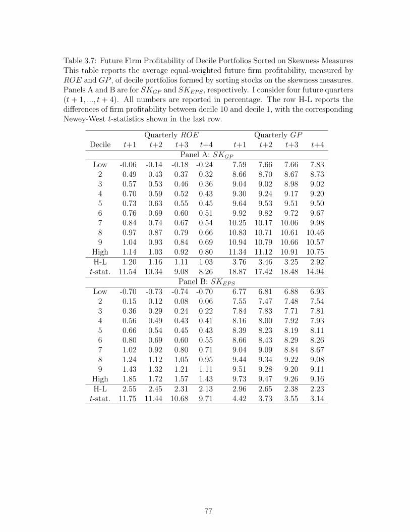
Table 3.7: Future Firm Profitability of Decile Portfolios Sorted on Skewness MeasuresThis table reports the average equal-weighted future firm profitability, measured byROE and GP , of decile portfolios formed by sorting stocks on the skewness measures.Panels A and B are for SKGP and SKEPS, respectively. I consider four future quarters(t + 1, ..., t + 4). All numbers are reported in percentage. The row H-L reports thedifferences of firm profitability between decile 10 and decile 1, with the correspondingNewey-West t-statistics shown in the last row.
Quarterly ROE Quarterly GPDecile t+1 t+2 t+3 t+4 t+1 t+2 t+3 t+4
Panel A: SKGP
Low -0.06 -0.14 -0.18 -0.24 7.59 7.66 7.66 7.832 0.49 0.43 0.37 0.32 8.66 8.70 8.67 8.733 0.57 0.53 0.46 0.36 9.04 9.02 8.98 9.024 0.70 0.59 0.52 0.43 9.30 9.24 9.17 9.205 0.73 0.63 0.55 0.45 9.64 9.53 9.51 9.506 0.76 0.69 0.60 0.51 9.92 9.82 9.72 9.677 0.84 0.74 0.67 0.54 10.25 10.17 10.06 9.988 0.97 0.87 0.79 0.66 10.83 10.71 10.61 10.469 1.04 0.93 0.84 0.69 10.94 10.79 10.66 10.57
High 1.14 1.03 0.92 0.80 11.34 11.12 10.91 10.75H-L 1.20 1.16 1.11 1.03 3.76 3.46 3.25 2.92t-stat. 11.54 10.34 9.08 8.26 18.87 17.42 18.48 14.94
Panel B: SKEPS
Low -0.70 -0.73 -0.74 -0.70 6.77 6.81 6.88 6.932 0.15 0.12 0.08 0.06 7.55 7.47 7.48 7.543 0.36 0.29 0.24 0.22 7.84 7.83 7.71 7.814 0.56 0.49 0.43 0.41 8.16 8.00 7.92 7.935 0.66 0.54 0.45 0.43 8.39 8.23 8.19 8.116 0.80 0.69 0.60 0.55 8.66 8.43 8.29 8.267 1.02 0.92 0.80 0.71 9.04 9.09 8.84 8.678 1.24 1.12 1.05 0.95 9.44 9.34 9.22 9.089 1.43 1.32 1.21 1.11 9.51 9.28 9.20 9.11
High 1.85 1.72 1.57 1.43 9.73 9.47 9.26 9.16H-L 2.55 2.45 2.31 2.13 2.96 2.65 2.38 2.23t-stat. 11.75 11.44 10.68 9.71 4.42 3.73 3.55 3.14
77
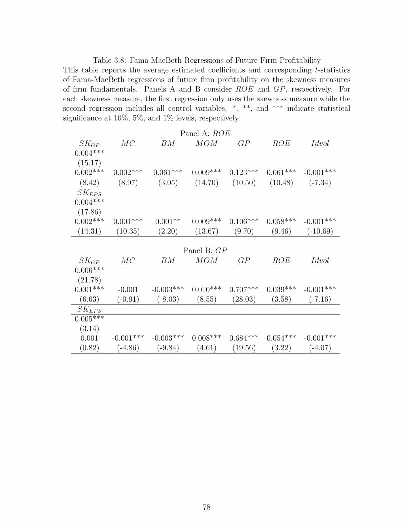
Table 3.8: Fama-MacBeth Regressions of Future Firm ProfitabilityThis table reports the average estimated coefficients and corresponding t-statisticsof Fama-MacBeth regressions of future firm profitability on the skewness measuresof firm fundamentals. Panels A and B consider ROE and GP , respectively. Foreach skewness measure, the first regression only uses the skewness measure while thesecond regression includes all control variables. *, **, and *** indicate statisticalsignificance at 10%, 5%, and 1% levels, respectively.
Panel A: ROESKGP MC BM MOM GP ROE Idvol
0.004***(15.17)
0.002*** 0.002*** 0.061*** 0.009*** 0.123*** 0.061*** -0.001***(8.42) (8.97) (3.05) (14.70) (10.50) (10.48) (-7.34)SKEPS
0.004***(17.86)
0.002*** 0.001*** 0.001** 0.009*** 0.106*** 0.058*** -0.001***(14.31) (10.35) (2.20) (13.67) (9.70) (9.46) (-10.69)
Panel B: GPSKGP MC BM MOM GP ROE Idvol
0.006***(21.78)
0.001*** -0.001 -0.003*** 0.010*** 0.707*** 0.039*** -0.001***(6.63) (-0.91) (-8.03) (8.55) (28.03) (3.58) (-7.16)SKEPS
0.005***(3.14)0.001 -0.001*** -0.003*** 0.008*** 0.684*** 0.054*** -0.001***(0.82) (-4.86) (-9.84) (4.61) (19.56) (3.22) (-4.07)
78

Table 3.9: Comparing Return Predictability of Alternative Skewness MeasuresThis table reports the average estimated coefficients and corresponding t-statistics ofFama-MacBeth regressions with both skewness measures. The dependent variable ofthe regressions is the next-quarter stock return. The first model does not use anycontrol variables while the second includes all the control variables. *, **, and ***indicate statistical significance at 10%, 5%, and 1% levels, respectively.
SKGP SKEPS MC BM MOM GP ROE Idvol0.19*** 0.13*(5.67) (1.93)
0.11*** 0.02 -0.33** 0.63*** 1.73*** 6.40*** 3.93** -0.22***(3.94) (0.39) (-2.27) (3.23) (2.65) (3.44) (2.33) (-3.50)
79
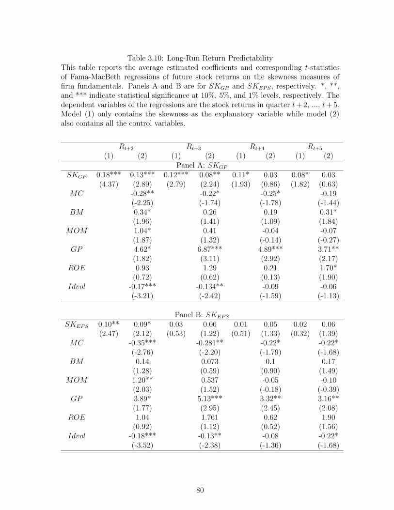
Table 3.10: Long-Run Return PredictabilityThis table reports the average estimated coefficients and corresponding t-statisticsof Fama-MacBeth regressions of future stock returns on the skewness measures offirm fundamentals. Panels A and B are for SKGP and SKEPS, respectively. *, **,and *** indicate statistical significance at 10%, 5%, and 1% levels, respectively. Thedependent variables of the regressions are the stock returns in quarter t+ 2, ..., t+ 5.Model (1) only contains the skewness as the explanatory variable while model (2)also contains all the control variables.
Rt+2 Rt+3 Rt+4 Rt+5
(1) (2) (1) (2) (1) (2) (1) (2)Panel A: SKGP
SKGP 0.18*** 0.13*** 0.12*** 0.08** 0.11* 0.03 0.08* 0.03(4.37) (2.89) (2.79) (2.24) (1.93) (0.86) (1.82) (0.63)
MC -0.28** -0.22* -0.25* -0.19(-2.25) (-1.74) (-1.78) (-1.44)
BM 0.34* 0.26 0.19 0.31*(1.96) (1.41) (1.09) (1.84)
MOM 1.04* 0.41 -0.04 -0.07(1.87) (1.32) (-0.14) (-0.27)
GP 4.62* 6.87*** 4.89*** 3.71**(1.82) (3.11) (2.92) (2.17)
ROE 0.93 1.29 0.21 1.70*(0.72) (0.62) (0.13) (1.90)
Idvol -0.17*** -0.134** -0.09 -0.06(-3.21) (-2.42) (-1.59) (-1.13)
Panel B: SKEPS
SKEPS 0.10** 0.09* 0.03 0.06 0.01 0.05 0.02 0.06(2.47) (2.12) (0.53) (1.22) (0.51) (1.33) (0.32) (1.39)
MC -0.35*** -0.281** -0.22* -0.22*(-2.76) (-2.20) (-1.79) (-1.68)
BM 0.14 0.073 0.1 0.17(1.28) (0.59) (0.90) (1.49)
MOM 1.20** 0.537 -0.05 -0.10(2.03) (1.52) (-0.18) (-0.39)
GP 3.89* 5.13*** 3.32** 3.16**(1.77) (2.95) (2.45) (2.08)
ROE 1.04 1.761 0.62 1.90(0.92) (1.12) (0.52) (1.56)
Idvol -0.18*** -0.13** -0.08 -0.22*(-3.52) (-2.38) (-1.36) (-1.68)
80
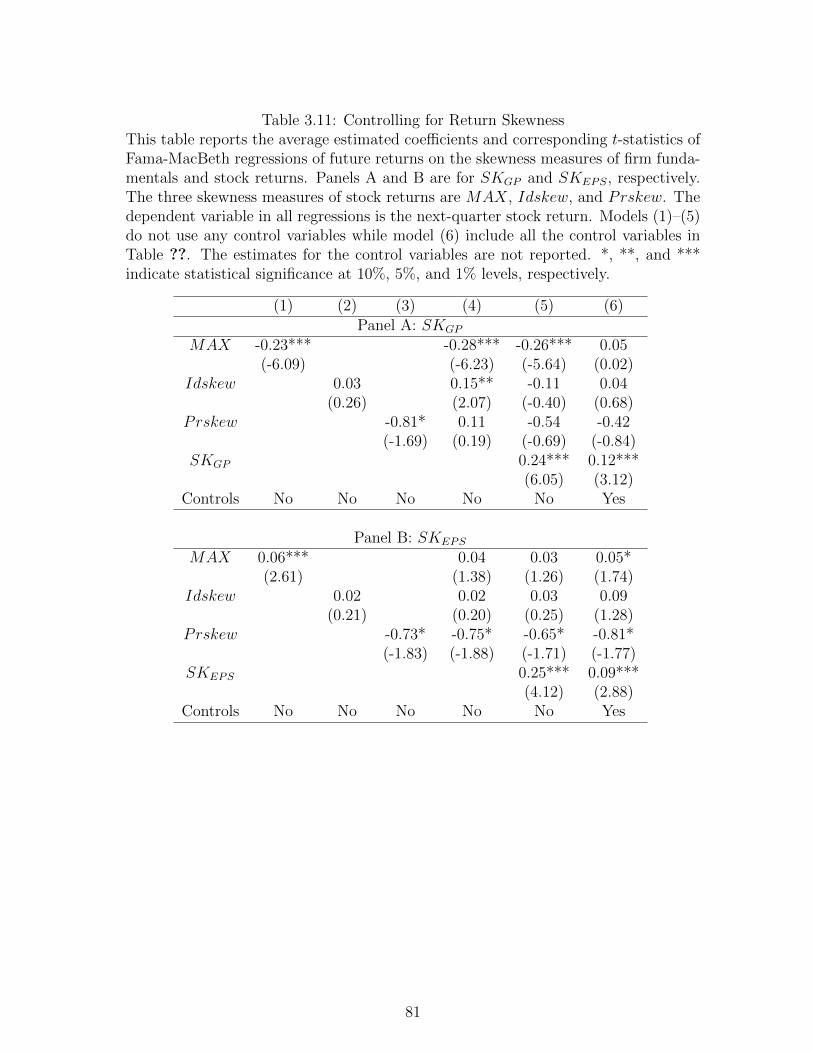
Table 3.11: Controlling for Return SkewnessThis table reports the average estimated coefficients and corresponding t-statistics ofFama-MacBeth regressions of future returns on the skewness measures of firm funda-mentals and stock returns. Panels A and B are for SKGP and SKEPS, respectively.The three skewness measures of stock returns are MAX, Idskew, and Prskew. Thedependent variable in all regressions is the next-quarter stock return. Models (1)–(5)do not use any control variables while model (6) include all the control variables inTable ??. The estimates for the control variables are not reported. *, **, and ***indicate statistical significance at 10%, 5%, and 1% levels, respectively.
(1) (2) (3) (4) (5) (6)Panel A: SKGP
MAX -0.23*** -0.28*** -0.26*** 0.05(-6.09) (-6.23) (-5.64) (0.02)
Idskew 0.03 0.15** -0.11 0.04(0.26) (2.07) (-0.40) (0.68)
Prskew -0.81* 0.11 -0.54 -0.42(-1.69) (0.19) (-0.69) (-0.84)
SKGP 0.24*** 0.12***(6.05) (3.12)
Controls No No No No No Yes
Panel B: SKEPS
MAX 0.06*** 0.04 0.03 0.05*(2.61) (1.38) (1.26) (1.74)
Idskew 0.02 0.02 0.03 0.09(0.21) (0.20) (0.25) (1.28)
Prskew -0.73* -0.75* -0.65* -0.81*(-1.83) (-1.88) (-1.71) (-1.77)
SKEPS 0.25*** 0.09***(4.12) (2.88)
Controls No No No No No Yes
81
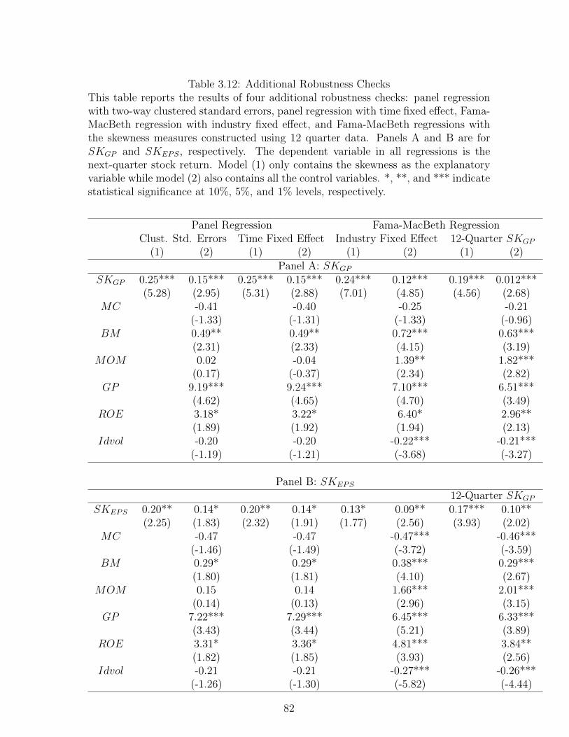
Table 3.12: Additional Robustness ChecksThis table reports the results of four additional robustness checks: panel regressionwith two-way clustered standard errors, panel regression with time fixed effect, Fama-MacBeth regression with industry fixed effect, and Fama-MacBeth regressions withthe skewness measures constructed using 12 quarter data. Panels A and B are forSKGP and SKEPS, respectively. The dependent variable in all regressions is thenext-quarter stock return. Model (1) only contains the skewness as the explanatoryvariable while model (2) also contains all the control variables. *, **, and *** indicatestatistical significance at 10%, 5%, and 1% levels, respectively.
Panel Regression Fama-MacBeth RegressionClust. Std. Errors Time Fixed Effect Industry Fixed Effect 12-Quarter SKGP
(1) (2) (1) (2) (1) (2) (1) (2)Panel A: SKGP
SKGP 0.25*** 0.15*** 0.25*** 0.15*** 0.24*** 0.12*** 0.19*** 0.012***(5.28) (2.95) (5.31) (2.88) (7.01) (4.85) (4.56) (2.68)
MC -0.41 -0.40 -0.25 -0.21(-1.33) (-1.31) (-1.33) (-0.96)
BM 0.49** 0.49** 0.72*** 0.63***(2.31) (2.33) (4.15) (3.19)
MOM 0.02 -0.04 1.39** 1.82***(0.17) (-0.37) (2.34) (2.82)
GP 9.19*** 9.24*** 7.10*** 6.51***(4.62) (4.65) (4.70) (3.49)
ROE 3.18* 3.22* 6.40* 2.96**(1.89) (1.92) (1.94) (2.13)
Idvol -0.20 -0.20 -0.22*** -0.21***(-1.19) (-1.21) (-3.68) (-3.27)
Panel B: SKEPS
12-Quarter SKGP
SKEPS 0.20** 0.14* 0.20** 0.14* 0.13* 0.09** 0.17*** 0.10**(2.25) (1.83) (2.32) (1.91) (1.77) (2.56) (3.93) (2.02)
MC -0.47 -0.47 -0.47*** -0.46***(-1.46) (-1.49) (-3.72) (-3.59)
BM 0.29* 0.29* 0.38*** 0.29***(1.80) (1.81) (4.10) (2.67)
MOM 0.15 0.14 1.66*** 2.01***(0.14) (0.13) (2.96) (3.15)
GP 7.22*** 7.29*** 6.45*** 6.33***(3.43) (3.44) (5.21) (3.89)
ROE 3.31* 3.36* 4.81*** 3.84**(1.82) (1.85) (3.93) (2.56)
Idvol -0.21 -0.21 -0.27*** -0.26***(-1.26) (-1.30) (-5.82) (-4.44)
82

CHAPTER 4
The Skewness of the Firm Fundamentals and Cross-Sectional StockReturns
4.1 Introduction
It has been well documented that macroeconomic fundamentals such as corporate
earnings, industrial production, and durable consumption growth are not normally
distributed. In particular, the conditional skewness of these variables are time-
varying. Recent studies have proposed models with time-varying volatility and jumps
that can capture these empirical regularities (e.g., Longstaff and Piazzessi (2004),
Drechsler and Yaron (2011), and Segal, Shaliastovich, and Yaron (2015)). But two
important questions remain unanswered. First, is the skewness of macroeconomic
fundamentals priced or in other words predictive of the stock market return? Second,
what are the “economic channels” linking the skewness with “technological aspects of
production, investment and financing opportunities” (Segal, Shaliastovich, and Yaron
(2015))?
This paper attempts to shed light on both questions. To answer the first question,
I present evidence that the conditional skewness of corporate earnings can strongly
predict stock market excess returns for horizons beyond six months and up to eight
years, even after controlling for standard predictors such as book-to-market ratio,
term spread, default spread, and cay (as in Lettau and Wachter (2001)). Regard-
ing the second question, I show that the predictive power of the conditional skew-
ness of corporate earnings can be explained by the interaction of two properties of
the underlying process of corporate earnings: (i) Path dependence; and (ii) Non-
Gaussian (skewed) shocks. Path dependence of corporate earnings is generated by
83

productivity-enhancing technology spillover, and non-Gaussian shocks refer to non-
normally distributed (skewed) innovations of the corporate earnings process. In this
setting, non-Gaussian shocks shift the economy across paths of different degrees of
technology spillover, leading to different risk profiles of the representative investor’s
wealth. As a result of path dependence, the corporate earnings skewness reflects the
degree of technology spillover and consequently predicts stock returns.
Path dependence means history matters, i.e. the realized history affects the future
outcomes. Durlauf (1993, 1994), for example, show that the aggregate output is path
dependent. In this article, I use the conditional skewness of the recent past to capture
the information contained in the “path” of corporate earnings. As stated in Durlauf
(1993), the path dependence also means that “there will be an especially strong
relationship between the probability density of shocks and the aggregate dynamics of
the model as realizations in the tails of the density determine whether the economy
shifts across regimes”. When it comes to corporate earnings, this statement indicates
the non-Gaussian shocks in the path dependent corporate earnings can capture the
information in the tails to determine whether regime-switch appears in the economy.
The conditional earnings skewness measures, simultaneously capturing the non-
Gaussian shocks and path dependence in corporate earnings, can identify the appear-
ance and timing of regime-switch in the economy. When the economy encounters a
large negative shock which shifts the corporate earnings to a bad path, the conditional
earnings skewness, at the occurrence of the jump, decreases sharply due to the large
drop in current period earnings. The sharp decrease in earnings skewness indicates an
increase in the risk for the market portfolio held by the representative investor. The
representative investor needs higher future compensation to bear higher risk. The
earnings skewness has a negative relationship with future market returns. Similarly,
at the occurrence of a positive jump in earnings, the conditional earnings skewness
increases sharply. The sharp increase in earnings skewness implies a decrease in the
84

risk of the market portfolio. The investor requires lower future compensation for the
higher earnings skewness.
Besides measuring the risk exposure of the market portfolio at the regime switch,
the earnings skewness can also measure the relative risk exposure of the market port-
folio regarding the timing of the regime switch. For example, a negative jump in
earnings is alleviated as the time goes on before another jump appears. During the
alleviation, the earnings skewness increases relative to the skewness at the occurrence
of the negative jump. The alleviation of the negative jump indicates a decrease of
the relative risk level in the market portfolio compared to that at the occurrence of
the jump, thus a negative relationship between skewness and future market returns.
In sum, the earnings skewness is a risk-based measure capturing the occurrence and
timing of earnings regime switch.
The above economic intuition is translated to my model by extending Lettau
and Wachter (2011) from two aspects. First, to capture the non-Gaussian shocks,
I specify the earnings growth shocks to follow the skew-normal distribution which
has a shape parameter for skewness. Second, the time-varying shape parameter of
the skew-normal shocks is path dependent, having two regimes with different autore-
gressive processes and different conditional innovations. The model yields a negative
relationship between earnings skewness and future stock returns.
I then go one step further to provide the microfoundation for earnings skewness.
The path dependence feature in corporate earnings can link the earnings skewness to
“technological aspects of production”. Durlauf (1993, 1994), among others, demon-
strate that the path dependence of aggregate output is generated by the interaction
of incomplete markets and strong technological complementarities. Following the line
of Durlauf’s argument, a large negative economy-wide shock (non-Gaussian) leads to
a loss of productivity-enhancing technological spillovers among firms, thus an indefi-
nite aggregate output loss. This economy-wide shock indefinitely moves the aggregate
85

output to a riskier “path”. The representative investor holding this portfolio of firms
(market portfolio) needs larger future compensations for this riskier “path” until a
subsequent favorable economy-wide shock. In summary, the earnings skewness pre-
dicts market returns by the force of path dependence.
To gauge the conditional skewness of corporate earnings, I consider five time series
measures: SKSUE1, SKSUE2, SKSUE3, SKSUE4, and SKEPS. The first four are the
conditional skewness of standardized unexpected earnings (SUE) using the historical
SUEs of prior 24 quarters. The last one is the skewness of aggregate earnings per
share constructed in the same way as the skewness of SUE measures. Specifically,
SKSUE1 is the skewness of earnings surprises where the surprise for a quarter is
the difference between earnings of the current quarter and the same quarter of last
year; SKSUE2 is similar to SKSUE1 but excluding “extraordinary items” in earnings.
SKSUE3 (SKSUE4) is the skewness of earnings surprises with SUEs defined as the
difference between realized earnings of the quarter and the median (mean) for that
quarter.
Consistent with the model, all five skewness measures negatively predict stock
market returns. For example, univariate regressions of stock market returns on skew-
ness of earnings indicate that a one unit increase in SKSUE1 leads to a 1.217% decrease
in the future one-year stock market return, 7.722% decrease in future five-year cu-
mulative market returns, and 16.886% decrease in future 10-year cumulative market
returns. When I use Nelson and Kim (1993) small sample bias adjustment for regres-
sion coefficients and P values, the coefficients for short-horizon prediction increase
by three-fold. In general, univariate regressions indicate the skewness of earnings can
predict future stock returns from two-quarters to eight-years ahead.
To further test the predicting power of earnings skewness measures, I then run
multivariate regressions and control for different groups of return predictors. First,
I control for standard market return predictors such as cay, book-to-market ratio,
86

term spread and default spread. The earnings skewnss measures can still significantly
predict stock market returns at different horizons. In the other group of regressions, I
control the historical mean and volatility of corporate earnings. The results indicate
that the skewness, but not the mean or volatility of corporate earnings, is the key
moment of corporate earnings that can predict stock market returns.
Of the five earnings skewness measures, SKSUE3 and SKSUE4 dominate the other
measures in the short horizons up to three years as other measures lose explanatory
power once controlling SKSUE3 or SKSUE4. However, SKSUE3 and SKSUE4 dominate
in the long horizons from four years to eight years. These results indicate that firm
cash flow risks are driven by multiple factors.
I then empirically inspect how earnings skewness can predict market returns. The
earnings skewness can be decomposed into two items: cross-sectional mean of the
firm-level earnings skewness (SKcs) and coskewness across firms (SKco). If as I ar-
gued, the explanatory power of earnings skewness on returns comes from the path
dependence, i.e. the time-varying “productivity-enhancing technology spillovers”, the
coskewness terms must drive the explanatory power of earnings skewness. The reason
is that productivity-enhancing technology spillover is an inter-firm relationship must
be captured by coskewness across firms but not mean firm-level earnings skewness.
Consequently, if I run predictive regressions of market returns at different horizons
on earnings skewness controlling for SKcs, an insignificant coefficient on SKcs but
significant coefficients on earnings skewness measures can support the path depen-
dence story. The regressions results confirm that the SKcs is the main component
in earnings skewness that can predict market returns. This test supports technology
spillover as the economic channels for return predictive power of earnings skewness.
This paper offers at least two solid contributions to the literature. First, in contrast
to ex-ante measures or other measures on the higher-order moments of economic
quantity variables, the conditional earnings skewness provides a new dimension on
87

scaling information contained in fundamentals. Second, one of the biggest challenges
of prior research on the higher-order moments of the fundamentals is to provide clear
economic channels for the higher-order moments to determine asset prices. To the
best of my knowledge, this paper is the first to clearly state the economic channels for
higher-order moments of fundamentals to affect asset prices. The economic channel in
this paper is the time-varying productivity-enhancing technological spillover captured
by the interaction of path dependence and non-Gaussian shocks of fundamentals.
The rest of the paper is organized as follows. Section 4.2 discusses the related
literature. In Section 4.3, I explore the empirical distribution of corporate earnings,
emphasizing the properties related to the higher-order moments of corporate earn-
ings. Section 3 also provides an illustrative example to give the economic intuition
of the conditional earnings skewness. Section 4.4 presents the model incorporating
the empirical facts. I describe the data and econometric methodology in Section 4.5.
Section 4.6 reports the empirical results. Section 4.7 concludes.
4.2 Literature Review
This paper bridges two lines of the literature. First, this paper contributes to the
literature on the relationship between higher-order moments and asset prices by doc-
umenting earnings skewness as a novel stock market return predictor. This paper is
also related to the literature on path dependence of aggregate output. The interac-
tion of path dependence and non-Gaussian shocks gives rise to the predictive power
of earnings skewness.
4.2.1 Asset Prices and Non-Gaussian Shocks to Fundamentals
The non-Gaussian shocks exist in all kinds of macroeconomic variables. The asset
pricing implications of the non-Gaussian shocks to fundamentals are well documented
in different strands of recent literature. Yang (2011) documents that the empirical
88

distribution of durable consumption growth is negatively skewed. Thus, non-Gaussian
shocks exist in the consumption growth. He shows that the performance of a long
run risk model incorporating this empirical feature is significantly improved. Non-
Gaussian shocks show up in corporate earnings at the market level. Basu (1997)
and Givoly and Hayn (2000) report that the corporate earnings are time varying
and negatively skewed. Longstaff and Piazzesi (2004) demonstrate that taking into
consideration the jumps risk in corporate earnings helps explain the equity premium
puzzle. Segal, Shaliastovich, and Yaron (2015) also add to this line of research by
documenting the asset pricing implications of the non-Gaussian shocks of industrial
production.
To capture the non-Gaussian shocks in fundamentals, the typical treatment in
previous literature is to specify jumps in the processes of consumption growth or
dividend. However, only jumps by themselves cannot fully capture the dynamics of
higher-order moments in fundamentals because of the potential leverage effects. On
the other hand, modeling time-varying volatility in a diffusion process to capture the
leverage effect cannot match the empirical distribution of macroeconomic variables
with discontinuous and clustered jumps since the diffusion process only allows a con-
tinuous path. The time-varying skewness of macroeconomic variables is generated by
a combination of jumps and leverage effect.
In this paper, I use the skew-normal shock to capture the mix of leverage effects
and jumps in corporate earnings dynamics. Colacito, Ghysels, Meng, and Siwasarit
(2015) demonstrate that the skewness pattern generated by skew-normal shocks, com-
paring with the pattern generated by jump-diffusion process, is closer to that in the
real data. In the Section 4.3, I document a strong leverage (or inverse leverage)
effect for different corporate earnings measures. The existence of leverage (inverse
leverage) effect indicates the importance of using skew-normal shocks to capture the
non-Gaussian shocks of corporate earnings.
89

4.2.2 The Path Dependence in Fundamentals
Path dependence, a term widely used in economics, political science and law, is
asserted as “history matters”. Specifically, an economy is called path dependent when
the effect of a shock on the level of aggregate output (corporate earnings) is permanent
in the absence of future offsetting shocks (Durlauf (1993)). Path dependence indicates
that multiple equilibrium exists in the economy. An economy-wide large shock can
move the economy to a different “path” if no future offsetting shocks occur. The path
dependence feature of the aggregate output implies that the statistics on realized
values of the output contains information on the future output, thus on asset prices
at the aggregate level.
It is well documented in the economics literature, especially growth theory, that
strong intertemporal complementarities between agents can imply that history has
long lasting effects (Arthur (1989), David (1986, 1988), Krugman (1991a, b)). Durlauf
(1993, 1994), among others, illustrate that the productivity-enhancing technology
spillover across firms can lead to path dependence in aggregate output.
Finance literature, in contrast to economics literature, concentrates on the econo-
metric expression, but not on the theory of path dependence features in finance data.
Cai (1994), Hamilton and Susmel (1994) and Gray (1996), among others, describe
the interest rate process as a path-dependent GARCH model. Specifically, there are
two regimes for the interest rate in their path-dependent GARCH model. Under
each regime, the interest rate conditional variances have different data generating
processes. For example, in regime 1 and period 1, the data generating process for
interest rate conditional variance is h11 = ω1 +a1ε20 +b1h0. And h12 = ω2 +a2ε
20 +b2h0
for regime 2. h11 (h12) stands for the conditional variance in period 1 under regime 1
(2). Moreover, the shocks also depend on previous states. For example, in period 2,
there are two possible unexpected changes: ε1|2, representing the unexpected change
in the short rate at period 1 given that the process was then in regime 2, and similarly
90
the ε1|1. Consequently, there are four possible expressions for interest rate conditional
variance h2 at period 2: ω1 + a1ε21|1 + b1h1|1, ω2 + a2ε
21|1 + b2h1|1, ω1 + a1ε
21|2 + b1h1|2
and ω2 + a2ε21|2 + b2h1|2. The conditional variance never converges to a single expres-
sion. In this specification, the conditional variance of interest rate specified in the
path dependent GARCH model depends not only on the current regime but also on
the entire history of the process since the unexpected changes of interest rates also
depends on regimes.
Gray (1996) finds this generalized path-dependent GARCH model has the best
performance among interest rate models. In my model, the treatment on the path
dependence of corporate earnings is in spirit similar to that in Gray (1996). The time-
varying skewness parameter in my model follows different processes under different
regimes. The skewness parameter depends on both ”current regime and past history
of process”.
The possible asset pricing implications of path dependence features embedded in
macroeconomic variables are surprisingly not addressed in previous economics or fi-
nance literature. This paper is the first to demonstrate that the path dependence
feature of corporate earnings, combined with non-Gaussian shocks, provides the ex-
planatory power of historical earnings skewness on market returns. Moreover, the
path dependence itself has economic intuition, which is the time-varying technology
spillover documented by Durlauf (1994). The path dependence, as an intermediary
in this paper, links “technological aspects of production” to earnings skewness, and
then to stock market returns.
4.3 Stylized Facts and The Illustrative Example
In this section, first I document two stylized facts about the market-level corporate
earnings: the existence of non-Gaussian shocks and path dependence. I use five
quarterly measures for corporate earnings: four earnings surprises measures (SUE1,
91

SUE2, SUE3, SUE4) and one earnings per share measure (EPS). The details
on data and measures are described in Section 4.5. All five measures are value-
weighted averages of the correspondent measures of individual firms. Second, I use
an illustrate example to demonstrate that the return predictive power of earnings
skewness comes from the interaction of path dependence and non-Gaussian shocks in
corporate earnings.
4.3.1 Stylized Facts
I use both figures and summary statistics to illustrate the existence of non-Gaussian
shocks in earnings. Figure 4.1 plots the time series of the quarterly corporate earnings
measures. Two salient stylized facts emerge. First, corporate earnings measures as
indicated in figure 4.1 are highly correlated with NBER business cycles. Corporate
earnings are high in booms and low in recessions. Second, corporate earnings are
highly volatile, with large movements clustered. These facts confirm the importance
of adding jumps in earnings as Longstaff and Piazzesi (2004) did.
Figure 4.2 plots the time series mean and volatility of corporate earnings. The
striking pattern is the high correlation between the first and second moments of
corporate earnings. The first plot in figure 4.2 indicates that SUE1 has an inverse
leverage effect, a positive relationship between its mean and variance. In contrast,
the second plot shows a strong negative relationship between mean and variance of
SUE3. The figure also reveals the limitation of previous studies only incorporating
the volatility of macroeconomic quantity variables. During certain periods such as
the financial crisis between 2007 and 2009, the volatility of corporate earnings jumps.
Simultaneously, the level of earnings also jumps. The second moment of fundamentals
cannot capture the co-jumps in the mean and volatility of fundamentals. To capture
the interaction of mean and variance of corporate earnings, we need to explore the
skewness.
92

Table 4.2 is consistent with the figures, showing that all five corporate earnings
measures are all skewed. Specifically, EPS, SUE1, and SUE2 are positively skewed.
But SUE3 and SUE4 are negatively skewed. I then calculate the correlations of non-
overlapping mean and variance for corporate earnings measures and report as “Lev”
in table 4.2. The signs of the correlations are consistent with the sign of earnings
skewness. Specifically, the mean-variance correlations of SUE1, SUE2 and EPS
are 0.27, 0.51 and 0.85, respectively. The correlations of SUE3 and SUE4 are -0.62
and -0.60. The consistent signs of skewness and mean-variance correlation measures
indicates the leverage effect (inverse leverage effect) is an important component of
corporate earnings skewness. One needs to consider earnings skewness, not just the
jumps in earnings to capture the non-Gaussian shocks in fundamentals.
The path dependence of aggregate output is widely discussed in previous eco-
nomics literature. There is no unified test for the path dependence. In this paper,
I use three tests to illustrate the different aspects of the path dependence. First, I
estimate the serial correlations for each corporate earnings measure. The unreported
results indicate that all earnings measures are very persistent. Specifically, the cur-
rent earnings measures have significant impact on earnings even more than five years
ahead. The strong autocorrelations imply earnings history matters for future earn-
ings. I then test whether there are different “paths” in corporate earnings. To do
this, I use the Bai-Perron test for structural breaks in the mean of earnings and the
Stock-Watson test for breaks in earnings variance. The Bai-Perron test rejects the
null hypothesis of no structural break in the mean. Simultaneously, Stock-Watson
test implies the existence of structural breaks in the earnings variance. The existence
of different regimes in earnings indicates there are different “paths” in earnings. Fur-
thermore, I also find that the band threshold autoregressions (TAR) with different
thresholds can fit the earnings data very well. The TAR implies there exists multiple
autoregressions for the earnings process.
93

In summary, this section documents two stylized facts in corporate earnings: (i)
Time-varying skewness exists in corporate earnings; and (ii) Path dependence. In sec-
tion 4.4, I incorporate the two stylized facts in the framework of Lettau and Wachter
to help understand the predictive power of earnings skewness on stock market returns.
4.3.2 The Illustrative Example
In this section, I illustrate how earnings skewness, capturing both path dependence
and non-Gaussian shocks, can predict future returns. As reported in Table 4.1, sup-
pose there exists an economy with 18 quarters (periods from 1 to 18) of history
including both booms and recessions. The level and eight-quarter rolling skewness
of earnings are reported for each quarter. In this economy, path dependence and
non-Gaussian shocks of earnings are captured by persistence (periods 1 through 8,
9 through 15), and jumps (periods 9 and 16) in earnings, respectively. Following
Lettau, Ludvigson, and Wachter (2007), I assume the representative agent cannot
observe the true state of the economy but infers it from the historical earnings data.
A negative jump (period 9) in the path-dependent earnings, by the knowledge of the
agent, indicates the occurrence of a bad state. Earnings skewness sharply decreases
at the occurrence of bad state from 0.16 in period 8 to -2.673 in period 9. The
representative agent incorporates into his information set this decrease in historical
earnings skewness, interpreting the decrease in earnings skewness as an increasing
risk level of the market portfolio. Around the occurrence of the bad state, the skew-
ness is negatively related to future returns since the representative investor needs
future compensation to hold the market portfolio with increasing risk indicated by
decreasing skewness. Similarly, the agent interprets the positive jump in period 16 as
a decrease in the risk of holding market portfolio. The positive jump corresponds to
a sharp increase in earnings skewness (2.356 in period 16). Thus, during the appear-
ance of the good state, the earnings skewness still has the negative relationship with
94

future market portfolio returns.
Besides identifying the occurrence of a regime switch, the earnings skewness also
provides an estimate of how long changes in a regime are expected to last. As shown
in the illustrative example, the earnings skewness, after the negative jump in period
9, monotonically increases from period 10 to period 15 right before the positive jump
in period 16. From the series of earnings skewness between period 10 and 15 after
the negative jump, the representative agent infers that the influence of the negative
jump in period 9 is gradually alleviated. The gradual alleviation (between period 10
and 15) of the negative impact indicates fallen risk in holding the market portfolio
compared with the risk at the occurrence of the bad state in period 9. The agent
thus requires less compensation in future market portfolio returns in periods 10 to
15 than that in period 9. By the same token, the monotonic decrease of skewness
after the initial positive jump in period 16 indicates a dilution of the positive news,
thus relatively increasing risk in holding the market portfolio compared with the
risk at the beginning of the good state in period 16. The investor requires higher
future compensation for the decreasing skewness. In sum, the time-varying earnings
skewness can predict future market returns because it contains information on the
representative agent’s future compensation on holding the market portfolio.
4.4 Model
In this section, I introduce a dynamic model taking into consideration both the path
dependence and non-Gaussian shocks in corporate earnings. In general, there are two
ways to model higher-order moments of corporate earnings and asset prices. One way
is to propose a general equilibrium model with a preference of producers, an endow-
ment, and the distribution of cash flows. The second approach is to directly specify
the stochastic discount factor and the distribution of corporate earnings, solving the
price function (statistical model). If the statistical model for corporate earnings and
95

asset prices coincides with the equilibrium production process, either of the two ap-
proaches can give correct implications on the relationship between the skewness of
corporate earnings and asset returns.
I employ the second approach by extending the framework of Lettau and Wachter
(2011) from two aspects: (i). the shocks to fundamentals in my model are skew-
normal shocks taking into consideration the non-Gaussian shocks in earnings; (ii). to
capture the path dependence feature, I specify the skewness parameter of skew-normal
shocks to have two regimes with different data generating processes. In the baseline
model, I assume there exists one representative investor and one representative firm.
I first present the general model with an arbitrary number of skewness shocks and
then show a specific case with only two shocks, one to corporate earnings, the other
to the interest rate.
4.4.1 General Model
Let Ht be a m × 1 vector of state variables at time t and εt+1 be a m × 1 vector of
shocks. I assume that the state variables evolve according to the vector autoregression
Ht+1 = Θ0 + ΘHt + σHεt+1, (4.1)
where Θ0 is m × 1, Θ is m × m, and σH is m × (m + 1). I then assume the
shocks εt+1 to be identically and independently distributed as skew-normal distri-
bution SKN(0, 1, νt). νt is the shape parameter. Specifically, the probability density
function (PDF) of εt+1 is
p(x) =1
σπexp(−(x− µ)2
2σ2)
∫ ν(x−µ)σ
−∞exp(−t
2
2)dt (4.2)
The PDF of skew-normal distribution is the PDF of the standard normal dis-
tribution weighted by its cumulative distribution function. The weight depends on
96

the shape parameter ν. When ν = 0, the skew-normal distribution degenerates to
the standard normal distribution. When ν > 0 (ν < 0), the positive (negative)
component of the standard normal PDF is over weighted relative to its negative (pos-
itive) component. In Appendix A, I introduce the lemmas related to skew-normal
distribution which are used in the model. By using the skew-normal distribution,
the skew-normal shocks εt+1 can capture the time-varying skewness existing in the
corporate earnings.
To incorporate the path dependence feature of earnings in my model, I assume
that the skewness parameter, νt+1 has two regimes, high (H) with the probability
PH to happen and low (L) with probability PL (1− PH) in each period. In different
regimes, the skewness parameter evolves in different AR(1) processes with different
autocorrelations (ρHν and ρLν). Moreover, the shocks are also regime dependent.
There are two shocks correspondent to regimes: ζνt+1|Ht and ζνt+1|Lt. Specifically,
ζνt+1|Ht (ζνt+1|Lt) is the shock to νt+1 if the shape parameter ν is in the high (low)
regime in period t. In sum, the skewness parameter can evolve following either of the
AR(1) process
νt+1 =
αHν + ρHννt + ζνt+1|Ht,
αHν + ρHννt + ζνt+1|Lt,
αLν + ρLννt + ζνt+1|Ht,
αLν + ρLννt + ζνt+1|Lt.
(4.3)
.
The above expression incorporates the path dependence feature because the shape
parameter νt+1 in (4.3) is determined not only by the current period shock ζν but
also by the past regime-dependent history. The four possible paths in (4.3) cannot
converge to one identical path, similar to the setting in Cai (1994) and Gray (1996).
This setting of path dependence makes my model parsimonious and tractable. We
97

can see in later section that the path dependence feature does not affect the solution
form of the contemporaneous price function but affects the future return dynamics.
I assume the earnings (xt), the earnings growth (∆xt) and the risk free rate (rft+1)
follow the general affine functions of the underlying state vector Ht:
xt = δ0 + δHt, (4.4)
∆xt = η0 + ηHt, (4.5)
rft+1 = α0 + αHt. (4.6)
Following the previous literature1 on the production based asset pricing (Belo,
Bazdresch, and Lin (2014), Belo, Vitorino, and Lin (2014) and Favilukis and Lin
(2013)), I assume the form of stochastic discount factor (SDF)2 takes the form
Mt+1 = exp(−rft+1 − σx∆xt+1). (4.7)
The stochastic discount factor is a function of the interest rate and the change in
earnings. Asset prices are determined by the following Euler equation:
P xnt = Et[Mt+1P
xn−1,t+1]. (4.8)
The price of the zero coupon equity can be determined recursively from equation
(4.8). In the Appendix B, I verify that (4.8) satisfies:
P xnt = exp(Axnt +Bx
ntHt), (4.9)
Axnt = µ+ log(2) +1
2κ1(κ1 + 2µ) + logΦ(
κ1νt√1 + ν2
t
), (4.10)
1Previous literature specifies the stochastic discount factor as a function of incremental produc-tivity. The incremental earnings can be specified as a function of incremental productivity.
2The form of stochastic discount factor is acceptable: There are two assets in this economy: bondand stock but the number of shocks is larger than or equal to 2; the market is incomplete, so thereare infinite number of SDFs.
98

Bxnt = −α− θBx
n−1 − σxθη, (4.11)
where
µ = −α0 − σxη0 + Axn−1 + θ0Bxn−1 − σxηθ0, (4.12)
κ1 = Bxn−1 − σxη. (4.13)
This general solution of the model shows that the skewness parameter νt can de-
termine contemporaneous stock price. To detect the return predictability of earnings
skewness, we need to look at the expression of future n periods cumulative return:
Rt+n = Pt+n/Pt. The future n periods return is a function of its contemporaneous
shape parameter νt+n. The νt+n is determined jointly by period t + 1 shock and the
whole past history of νt. Thus, the historical skewness contains information on future
market returns.
4.4.2 Model With Shocks Only to Earnings and the Risk-Free Rate
The model introduced in this section is a special case of the general model introduced
in last section since it has only two shocks, a shock to the earnings and a shock to
the risk-free rate. Let εt+1 denote a 2× 1 vector of independent skew-normal shocks.
The shape parameter νt still follows a path-dependent AR(1) process the same as
specified in last section. Let xt denote the level of the corporate earnings at time t.
I assume that the growth rate of earnings is conditionally skew-normal distributed
with a time-varying mean xt that follows a first-order autoregressive process
xt+1 = (1− Φx)g + Φxxt + σxεt+1, (4.14)
∆xt+1 = xt + σxεt+1, (4.15)
99

where σx is a 1 × 2 vector of loadings on the shocks ε and Φx is the autocorrela-
tion. I also specify a process for the risk free rate. Let rft+1 denote the continuously
compounded risk-free return between times t and (t+ 1). I assume that
rft+1 = (1− Φr)rf + Φrr
ft + σrεt, (4.16)
where σr is a 1 × 2 vector of loadings on the shocks ε, rf is the unconditional mean
of rft , and φr is the autocorrelation term.
Real Bonds
Let P rnt denote the price of an n-period real bond at time t. In the other words, P r
nt
denotes the time-t price of an asset with a fixed payoff of one at the time t+ n. The
price of this real bond can be determined through recursive substitution using the
same method as shown in the appendix B. I still use the following Euler equation for
recursive substitution:
Et[Mt+1Prn−1,t+1] = P r
nt. (4.17)
The boundary condition is P r0t = 1 since the bond pays a face value of 1 at maturity.
I conjecture the solution for the real bond as
P rnt = exp(Arn +Br
n,r(rft − r) +Br
ne∆xt). (4.18)
Solving (4.17) recursively, I get the following explicit solution for the real bond price:
P rnt = exp(Arn +Br
n,r(rft − r) +Br
ne∆xt), (4.19)
Arnt = γ + An−1 − (1− 2Φr)rf + log(2) +1
2κ2
1 + logΦ(κ1νt√1 + ν2
t
), (4.20)
Brnr = −Φr(1−Br
n−1,r), (4.21)
Brnx = −Φx(B
rn−1,x − σx), (4.22)
100
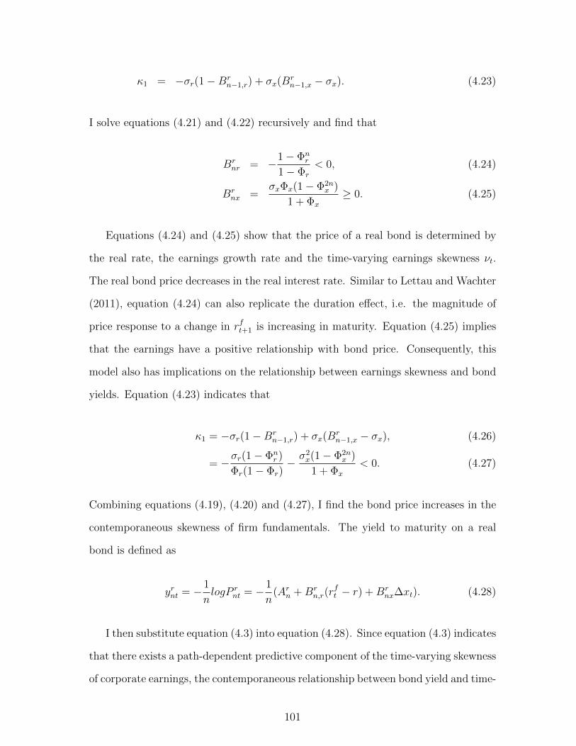
κ1 = −σr(1−Brn−1,r) + σx(B
rn−1,x − σx). (4.23)
I solve equations (4.21) and (4.22) recursively and find that
Brnr = −1− Φn
r
1− Φr
< 0, (4.24)
Brnx =
σxΦx(1− Φ2nx )
1 + Φx
≥ 0. (4.25)
Equations (4.24) and (4.25) show that the price of a real bond is determined by
the real rate, the earnings growth rate and the time-varying earnings skewness νt.
The real bond price decreases in the real interest rate. Similar to Lettau and Wachter
(2011), equation (4.24) can also replicate the duration effect, i.e. the magnitude of
price response to a change in rft+1 is increasing in maturity. Equation (4.25) implies
that the earnings have a positive relationship with bond price. Consequently, this
model also has implications on the relationship between earnings skewness and bond
yields. Equation (4.23) indicates that
κ1 = −σr(1−Brn−1,r) + σx(B
rn−1,x − σx), (4.26)
= −σr(1− Φnr )
Φr(1− Φr)− σ2
x(1− Φ2nx )
1 + Φx
< 0. (4.27)
Combining equations (4.19), (4.20) and (4.27), I find the bond price increases in the
contemporaneous skewness of firm fundamentals. The yield to maturity on a real
bond is defined as
yrnt = − 1
nlogP r
nt = − 1
n(Arn +Br
n,r(rft − r) +Br
nx∆xt). (4.28)
I then substitute equation (4.3) into equation (4.28). Since equation (4.3) indicates
that there exists a path-dependent predictive component of the time-varying skewness
of corporate earnings, the contemporaneous relationship between bond yield and time-
101

varying skewness of earnings becomes a predictive relationship, i.e. time-varying
skewness of earnings at time t, νt can predict the bond yield at time t + 1. So this
model indicates a positive relationship between bond yield and earnings skewness.
The predictive power of earnings skewness on yields is empirically tested in Section
4.6.3.
Equity
To model the equity, I first model a simpler case, the zero-coupon equity. I first
assume there exists an equity that only gets the earnings at time (t + n) but no
earnings in previous periods. Following Lettau and Wachter (2011), I refer to this
asset as zero-coupon equity. P ent denotes the price of the zero-coupon equity at time
t which will pay aggregate earnings at period (t+ n). I conjecture the solution form
for the zero-coupon bond the same as that for real bonds:
P xnt = exp(Axn +Bx
n,r(rft − r) +Bx
nx∆xt). (4.29)
The key difference between explicit solutions of the real bond and zero-coupon equity
is in the boundary conditions. I assume the boundary condition for zero-coupon
equity is P x0t/xt = 1. Even though the solution forms of the zero-coupon equity
and real bonds are the same, the difference in boundary conditions leads to different
calibration results. The solution for the zero-coupon equity is as follows:
P xnt = exp(Axn +Bx
n,r(rft − r) +Bx
nx∆xt), (4.30)
Axnt = γ + An−1 − (1− 2Φr)rf + log(2) +1
2κ2
1 + logΦ(κ1νt√1 + ν2
t
), (4.31)
Bxnr = −Φr(1−Bx
n−1,), (4.32)
Bxnx = −Φx(B
xn−1,x − σx), (4.33)
κ1 = −σr(1−Bxn−1,r) + σx(B
xn−1,x − σx). (4.34)
102

The parameters Axnt, Bxnr and Bx
ne have the same forms as those of real bonds.
My model implies a contemporaneous negative relationship between the skewness of
corporate earnings and the zero-coupon equity price. The market portfolio is the
aggregation of all zero coupon equities at different horizons. The solution for price of
the market portfolio is
Pmt =
∞∑n=1
exp(Axn +Bxn,r(r
ft − r) +Bx
nx∆xt). (4.35)
In summary, this set of models indicates that the earnings skewness has a positive
relationship with real bond yield and a negative relationship with contemporane-
ous market portfolio prices. If earnings skewness is persistent, the model indicates
earnings skewness has a positive relationship with future bond yields and a negative
relationship with future market portfolio (market index) returns.
4.5 Data, Measures and Methodology
4.5.1 Data
The quarterly earnings data is obtained from the COMPUSTAT database. To be
included in the sample, the firm must have at least 16 earnings observations in the
COMPUSTAT universe. I then take the value-weighted (weighted by the size of previ-
ous quarter) average of earnings per share and earnings surprises of individual firms to
get the earnings and earnings surprises measures at the market level. Book-to-market
ratio (B/M), default spread (DEF), term spread (TMS) and other fundamental vari-
ables are obtained from Amit Goyal’s website. The S&P 500 quarterly return data is
also obtained from Amit Goyal’s website3. I aggregate the quarterly S&P 500 returns
to obtain cumulative market returns for different horizons.
3The link for the website of Amit Goyal is http://www.hec.unil.ch/agoyal/.
103

4.5.2 Skewness Measures
Consistent with the arguments in Cai (1994) and Hamilton and Susmel (1994), the
parameters in a path-dependent autoregressive model are essentially intractable and
impossible to estimate due to the dependence of the skewness parameter νt on the
entire past history of the data. I use a non-parametric way to measure the path
dependent non-Gaussian shocks on earnings by estimating the coefficients of skewness
for earnings and earnings surprises. The five skewness measures (SKSUE1, SKSUE2,
SKSUE3, SKSUE4 and SKEPS) can be separated into three groups based on different
measures of corporate earnings. Specifically, SKSUE1 and SKSUE2 are time-series
skewness of earnings surprises with earnings surprises constructed using a random
walk model. SKSUE3 and SKSUE4 are skewness of earnings surprises with earnings
surprises defined using analyst earnings forecasts. SKEPS is the skewness of earnings
per share.
Historical SUE Skewness
I first construct four measures for standardized unexpected earnings (SUE): Follow-
ing the convention in Livnat and Mendenhall (2006), I define SUE1 for individual
stocks using the seasonal random walk model
SUE1t =EPSt − EPSt−4
Pt, (4.36)
where EPSt is the earnings per share before extraordinary items of quarter t, and Pt
is the stock price at the end of quarter t. I define SUE2 the same way as SUE1 but
excluding “extraordinary items”. I define SUE3 and SUE4 using analyst forecasts
(Livnat and Mendenhall (2006)) as
SUE3t =EPSt − EPSt
Pt, (4.37)
104

where EPSt is the median of analyst earnings forecast for quarter t made in the
90 days prior to the earning announcement date. SUE4 is defined similar to SUE3
except using the mean of analyst earning forecast.
I take the value-weighted averages (using market capitalization in previous quarter(t−
1)) of SUEs for each quarter. I construct skewness of aggregate SUE as the coefficient
of skewness of value-weighted SUEs during the rolling window of quarter t − n to
t− 1
SKSUE =n
(n− 1)(n− 2)
t−1∑τ=t−n
(SUEτ − SUE
s
)3
, (4.38)
where SUEτ is the value-weighted average quarterly standardized unexpected earn-
ings. SUE and s are sample averages and standard deviations of SUEs within the
rolling windows, respectively. I choose the benchmark case n = 24 for the rolling
window in this paper since the average length of the NBER business cycle is around
6 years. Using 24 quarters rolling window could largely filter out seasonality issues.
As a robustness check, I also used n = 16 and 20 and obtained similar results. I do
not use earnings or SUE information at quarter t because earnings at time t is not
reported until quarter t+ 1.
Historical Total Earnings Skewness
The historical total earnings skewness measure is defined in line with its SUE coun-
terparts. I first construct the value-weighted average (using market capitalization in
the last quarter (t− 1) of earnings per share. The total earnings skewness is defined
as the coefficient of corporate earnings skewness
SKEPS =n
(n− 1)(n− 2)
t−1∑τ=t−n
(TOTτ − TOT
s
)3
, (4.39)
where EPS is the value weighted average quarterly earnings per share. EPS and s are
the sample average and the standard deviation of EPS within the rolling windows,
105

respectively. The benchmark rolling window is 24 quarters in line with the designs
for SUE skewness measures.
4.5.3 Econometric Methods
When I regress returns of various holding periods on variables measured in previous
period, the regression coefficient is subject to an upward small-sample bias. This
bias is more severe when the sample size is small, the independent variable is highly
persistent or when the correlation between the regression errors and the innovations in
the independent variable is strong (Campbell, Lo and, Mackinlay (1997), Hirshleifer,
Hou, and Teoh (2009)). The t statistics and p value of the regression should also be
adjusted for the serial correlation.
I employ two methods to adjust the potential biases in the predictive regression.
I first use Newey and West (1987) standard errors with 12 lags for all the OLS regres-
sions to adjust the serial correlation. Since this method is quite stylized, the details
are ignored. The second approach is to bootstrap a randomization p-value for regres-
sion coefficients on the skewness of corporate earnings following the Nelson and Kim
(1993) procedure. Specifically, I simulate artificial series of returns and the indepen-
dent variable under the null hypothesis that earnings skewness has no predictability
by randomly drawing with replacement of the residual pairs from the return predictive
regression and a first-order autoregression of the earnings skewness. I then regress
the bootstrapped returns on the bootstrapped skewness of corporate earnings at the
market level to get the regression coefficient. This procedure is repeated for 10,000
times. The empirical distribution of the regression coefficient is generated under the
null hypothesis of no predictability. If there is a huge fraction of simulated regression
coefficients are further to zero than the regression coefficient from the true regression,
the null hypothesis must be accepted. The randomization p value is then the fraction
of the 10,000 simulated regression coefficients further away from zero than the actual
106

coefficient estimate.
To explore the economic significance of the return predictability of earnings skew-
ness, I also calculate the bias-adjusted regression coefficients following Kendall (1954),
Stambaugh (2000) and Hirshleifer, Hou, and Teoh (2009) by assuming there exists a
general autoregressive framework for return Rt and a return predictor Xt:
Rt = α + βXt−1 + ut, u ∼ i.i.d.N(0, σ2u), (4.40)
Xt = µ+ φXt−1 + νt, ν ∼ i.i.d.N(0, σ2ν). (4.41)
The bias in the OLS estimate of β in the predictive regression is proportional to
the bias in the OLS estimate of φ in the first-order autoregression for the earnings
skewness. Combining
E(β − β) =σuvσ2v
E(φ− φ), (4.42)
where φ is the OLS estimate of φ. Kendall (1954), Stambaugh (2000) prove that the
bias in the OLS estimate of φ is
E(φ− φ) = −1 + 3φ
n+O(n−2), (4.43)
where σuv, σv, and n are sample covariance, sample standard deviation and sample
size respectively. Combining equation (4.42) and equation , we can calculate the bias-
adjusted estimate of β in the predictive regression and that of φ in the autoregression
using the following formula:
βadj = β +σuvσ2v
1 + 3φadjn
, (4.44)
φadj =nφ+ 1
n− 3, (4.45)
107

where βadj is the bias-adjusted coefficient, φadj is the bias-adjusted estimate for φ. I
report the bias-adjusted coefficients and randomization P value for univariate regres-
sions.
4.6 Empirical Results
In this section, I empirically analyze the asset pricing implications of corporate earn-
ings skewness. Section 4.6.1 discusses the time series properties of corporate earnings
skewness measures. I then explore the market return predictability of this skewness
in Section 4.6.2. Section 4.6.2 also explores the coskewness of corporate earnings to
confirm the microfoundation of corporate earnings skewness. Finally, in Section 4.6.3,
I examine the predictability of earnings skewness on government bond yields. In this
section, I also detect the explanatory power of bond yields on returns and show it
can be decomposed into a cash flow part which is captured by earnings skewness and
a discount rate part.
4.6.1 Descriptive Statistics
Table 4.3 reports the summary statistics for the corporate earnings skewness mea-
sures and other control variables. Corporate earnings have significant time-varying
skewness. Of the five measures of corporate earnings skewness, SKSUE1, SKSUE2, and
SKEPS are on average significantly positive. In contrast, SKSUE3 and SKSUE4 are on
average slightly negatively skewed. The difference in the levels of corporate earnings
measures is consistent with the findings in Livnat and Mendenhall (2006) that differ-
ent types of SUEs capture different information. The corporate earnings skewness
measures are quite volatile. For example, SKEPS ranges from −5.56 to 8.52. Figures
4.3 and 4.4 confirm the fluctuation of earnings skewness. Moreover, these figures also
indicate the earnings skewness measures are procyclical, high in booms and low in
recessions. Moreover, consistent with my model assumption, the skewness measures
108

are highly persistent with first-order autocorrelations ranging from 0.87 to 0.96.
Table 4.4 reports the contemporaneous correlations of quarterly earnings skewness
measures and control variables. Of the five measures of earnings skewness, SKSUE1
and SKSUE2 are almost perfectly correlated. Similarly, SKSUE3 and SKSUE4 have
a large correlation of 0.99. The high correlations across skewness measures indicate
that the information contained in the skewness measures does not vary whether or
not I exclude special items for earnings or use the mean of analyst earnings forecasts.
The earnings skewness measures seem to be correlated with most control variables
as they are positively correlated with LTY, TBL and cay but negatively correlated
with TMS, BM, and DEF. Among the control variables, the earnings skewness mea-
sures have the strongest correlations with government bond yields. Specifically, the
correlations between long-term yield and skewness measures are around 0.52 to 0.55.
The correlations between short-term yield and skewness measures are between 0.5
to 0.62. The earnings skewness has a positive correlation with long-term/short-term
yields even though the two yields have different relationships with business cycles.
The implications of earnings skewness on bond yields will be discussed in Section
4.6.3.
4.6.2 Stock Market Predictive Regressions
In this section, I discuss the return predictability of the earnings skewness on stock
market excess returns using multiple econometric techniques and controlling for differ-
ent return predictors. The results indicate that earnings skewness is a robust market
return predictor. I also design tests to inspect whether or not the predictive power of
earnings skewness comes from earnings coskewness which is an inter-firm relationship.
A dominant role of coskewness term in the predictive power of earnings skewness sup-
ports my argument that the predictive power of earnings skewness comes from the
time-varying degree of technology spillover across firms.
109

Univariate Tests
Table 4.5 reports the results for the univariate regressions of corporate earnings skew-
ness measures on two-quarters ahead to eight-years ahead stock market returns in
excess of short-term risk-free rates. I skip one quarter for earnings skewness measures
to make sure accounting information is known to investors. For the OLS regressions,
Newey-West standard errors with 12 lags are used to adjust t statistics for each re-
gression. All earnings skewness measures have a negative relation with future stock
market excess returns. Earnings skewness can significantly predict future stock mar-
ket returns from two-quarters ahead to eight-years ahead. For example, a one unit
increase in SKSUE1 leads to 0.122 (coefficient is -1.217) percent decrease in one-year
cumulative stock market excess returns. The predicting power (parameters and t
statistics) of earnings skewness increases in horizon. The coefficient of eight-year re-
turns predictive regression (-16.886) is more than 15 times larger than that of the
one-year return predictive regression (-1.217). If daily returns are slightly predictable
by a slow moving variable, predictability adds up over long horizons. Corporate
earnings skewness measures are highly persistent, so the increase in predicting power
along horizons reflects a single underlying phenomenon that earnings skewness pre-
dicts stock returns. Among fundamental skewness measures, SKSUE1, SKSUE3 and
SKSUE4 have relatively stronger predicting power since they have predicting pow-
ers among all prediction horizons. SKSUE2 is relatively weaker in short horizon but
catches up after the four-year horizon.
To address the potential small-sample bias in the OLS regression, I report boot-
strapping randomization p values and bias adjusted coefficients following Nelson and
Kim (1993). The randomized p values (bias adjusted coefficients) are reported in the
row marked as Rand:P (Adj-β) in each panel of Table 4.5. In general, the results are
even stronger than those using OLS regressions. The return predictability patterns
differ for different earnings skewness measures. For random walk based SUE skewness
110

(SKSUE1 and SKSUE2), random p values show that they have predicting power start-
ing from short horizon, i.e. two-quarters ahead and four-quarters ahead, respectively.
Moreover, the bias-adjusted coefficients for SKSUE1 and SKSUE2 are larger than OLS
regression coefficients, especially in the short horizon regressions. The bootstrapping
results indicate that the explanatory power of random walk based SUE skewness on
returns seems to be underestimated by OLS regressions. Similarly, adjusting the small
sample bias does not affect the explanatory power of analyst forecasts based earnings
skewness (SKSUE3 and SKSUE4). Under adjustment of small sample bias, SKSUE3
and SKSUE4 can still significantly predict future market excess returns in all horizons.
However, the bootstrapping approach shows the explanatory power of analyst fore-
cast based earnings skewness is slightly overstated in the short run. Specifically, the
bias-adjusted coefficient for earnings skewness on the two-quarters ahead cumulative
market excess return is -0.434, smaller than the OLS regression coefficient of -0.578.
In contrast to the skewness of earnings surprise, the skewness of earnings per share
(SKEPS) has inferior explanatory power. The bias-adjusted approach indicates ran-
dom walk based earnings skewness measures have a stronger explanatory power than
measures based on analyst earnings forecasts. In summary, the univariate regressions
indicate a strong negative relationship between earnings skewness and future stock
market cumulative excess returns at different horizons from two-quarters to eight-year
aheads.
Multivariate Tests
To see whether corporate earnings skewness has incremental power to predict stock
market returns after controlling for other aggregate return predictors, I employ mul-
tivariate regressions in Table 4.6. I control for four popular return predictors whose
predicting power are confirmed in previous studies: book-to-market ratio (B/M), de-
fault spread (DEF), term spread (TMS) and consumption-wealth ratio (cay). The
111

Newey-West standard errors with 12 lags are used to adjust t statistics for regressions.
In general, consistent with univariate regressions, earnings skewness is a strong neg-
ative return predictor. The explanatory power of different skewness measures differs.
SKSUE1 and SKSUE2 are relative long-horizon return predictors, having predictive
power from one-year until eight-year horizons. In contrast, SKSUE3 and SKSUE4 are
short-run return predictors. They can predict stock market excess returns from two-
quarter to four-year horizons but lose predictive power in the long run after a 5-year
horizon. In contrast to earnings surprise skewness, the skewness of earnings per share
(SKEPS) loses explanatory power at all horizons when controlling for other return
predictors. The SKEPS seems to contain different information than earnings surprise
skewness measures.
Table 4.6 also shows that the R2s in long-horizon predictive regressions for SUE
skewness measures are quite high, around 0.86 to 0.90 in eight-year horizons. In
unreported tables, I regress stock market excess returns on four control variables but
not earnings skewness measures. The R2s of regressions are at most 0.60, consistently
smaller than those including earnings skewness. The differences in R2s indicate that
earnings skewness has strong economic significance in return predictions. Thus, the
path dependence feature of earnings skewness contains unique information on future
market returns.
To test whether skewness dominates other moments in corporate earnings, I then
run multivariate predictive regressions controlling the 24 quarters rolling mean and
volatility of corporate earnings measures (SUE1, SUE2, SUE3, SUE4, and EPS).
Table 4.7 shows that the explanatory power of earnings skewness is not affected even
when controlling for the mean and volatility of historical earnings. In contrast to the
coefficients on skewness, the coefficients of earnings mean and volatility are insignif-
icant in most regressions at different horizons. On the other hand, the monotonic
increasing pattern in horizons for coefficients does not exist for earnings mean and
112

volatility. This also indicates that the earnings mean and volatility measures do not
have significant return predictive power.
In summary, this section shows that the earnings skewness measures can predict
future market excess returns even when controlling for different variables, prevailing
return predictors or other moments of earnings.
Comparative Regressions
In light of previous findings, it is interesting to examine the relative predictive power
of different measures of earnings skewness. To do this, I first use principle component
analysis (PCA) to investigate whether the five earnings skewness measures have the
same information content. The results regarding PCA are shown in Table 4.8. I
then estimate predictive regressions with multiple earnings skewness measures as
explanatory variables. The estimated results are reported in Table 4.9.
In Table 4.8, I first include only random-walk model based earnings surprise skew-
ness, SKSUE1 and SKSUE2. The PCA analysis indicates that the first principle com-
ponent can explain more than 99 percent of the variation in these two skewness
measures. In other words, only one factor drives SKSUE1 and SKSUE2. The PCA
analysis shows the first principle can explain 94 percent of the variation in all four
earnings surprise skewness measures (SKSUE1, SKSUE2, SKSUE3 and SKSUE4). But
the first two principle components can cover most of the variation. If all five earnings
skewness measures are included in PCA, one needs three factors to explain the dy-
namics of the earnings skewness. The PCA analysis is consistent with the previous
findings: earnings skewness measures are driven by multiple factors and have different
explanatory power on future market returns.
I then do a return predictability horse race for different earnings skewness mea-
sures. Since SKSUE1 (SKSUE3) and SKSUE2 (SKSUE4) are driven by the same factor,
I ignore the comparative regressions among them. I compare the return predictive
113

power of earnings skewness measures on three-year, five-year and eight-year ahead
cumulative excess returns. The results are reported in Table 4.9. For each horizon in
model (1) through (3), I include two of the three measures (SKSUE1, SKSUE2, and
SKEPS) of earnings skewness as explanatory variables. This allows us to directly
compare the explanatory power of each pair. In model (4), I use all three measures.
In all the models, control variables are included in the regression specifications.
For three-year ahead return predictability, the estimates of model (1) indicate that
SKSUE3 dominates SKSUE1 as its coefficient is significant, however the coefficient for
SKSUE1 is insignificant. Models (2) and (3) indicate both SKSUE1 and SKSUE3
dominate SKEPS in the three-year return predictability. Model (4) indicates that
SKSUE3 dominate SKSUE1 and SKEPS in the short run. The pattern for five-year
ahead return predictability is different. SKSUE1 dominates the other two earnings
skewness measures. SKEPS marginally dominates SKSUE3. The results for five-year
return predictability are consistent with those in multivariate regressions since the
predictive power of SKSUE3 also disappears in predictive regressions with horizons
longer than four years. The results for eight-year return predictability confirms the
superiority of SKSUE1 in long run return predictability. In summary, the results
in this section indicate that earnings skewness measures have different information
content. SKSUE1 and SKSUE2 are relatively long run return predictors. In contrast,
SKSUE3 and SKSUE4 are short to medium run return predictors.
Economic Channels: Coskewness of Corporate Earnings
I demonstrate in the previous section that the microfoundation of earnings skewness
comes from the interaction of path dependence and non-Gaussian shocks, thus from
the productivity-enhancing technology spillover across firms. On the other hand, the
earnings skewness at the market level can be decomposed into two terms: average
firm-level earnings skewness and coskewness across firms. The productivity-enhancing
114

technology spillover, as an inter-firm relationship, must be strongly related to the
coskewness terms which capture the inter-firm interaction in the earnings skewness
measures. If the predictive power of earnings skewness on returns does come from
technological spillover across firms as argued in this paper, the “coskewness” of earn-
ings, but not the average firm-level earnings skewness, must dominate the prediction
of earnings skewness on returns. In this section, I first illustrate the decomposition
of earnings skewness into coskewness terms and average firm-level skewness terms. I
then estimate regressions to show coskewness of earnings dominates the return pre-
dicting power of earnings skewness.
Suppose there are N firms in one economy. The corporate earnings at the market
level are constructed by the cash flows of these N firms. Assuming equal weights
for simplicity, let ept = N−1∑N
i=1 eit be the time t aggregate corporate earnings,
ei = T−1∑T
t=1 eit be the mean sample earnings (earnings surprises) for firm i, and
ep = T−1∑T
t=1 ept be the mean sample market return. Then the sample skewness is
T−1∑t
(ept − ep)3 =1
N3
N∑i=1
1
T
∑t
(eit − ei)3
+3
TN3
∑t
N∑i=1
(eit − ei)∑i′ 6=i
(ei′t − ei′)2
+6
TN3
∑t
N∑i=1
(eit − ei)N∑i′>i
N∑l>i′
(ei′t − ei′)(elt − el).
The first term in the above equation is the mean of individual firm earnings skewness.
The second and third terms are coskewness terms capturing the average comovement
in one firm’s earnings with the earnings variance of the portfolio that comprises the
remaining firms. The coskewness of corporate earnings, depending on the cross-
sectional heterogeneity of firms’ earnings comovement, is a measure of the time-
varying technological spillover across firms.
115

The effect of earnings coskewness increases in the number of firms. If there are
N firms in the economy, there will be N(N − 1) +N !/[3!(N − 3)!] coskewness terms.
Since the number of firms in the economy is large, the amount of coskewness terms is
far larger than that of firm-level earnings skewness terms. This does not immediately
imply that coskewness terms dominate the magnitude of earnings skewness. But
when we compare the magnitude of corporate earnings skewness and mean firm-
level earnings skewness, we can find that coskewness terms dominate. In unreported
results, for example, the skewness of SUE1 (SUE2) in the full sample is 2.34 (4.03).
But the mean firm-level SUE1 skewness is -0.78 (-0.52). The difference between
aggregate earnings skewness and mean firm-level earnings skewness is the coskewness
of corporate earnings. The magnitude of coskewness is much larger than that of mean
firm-level skewness.
Even though the magnitude of coskewness dominates that of earnings skewness,
we cannot directly argue the return predicting power of earnings skewness comes
from earnings coskewness. To test whether earnings coskewness is the driving force
of the return predictability of earnings skewness, I estimate predictive regressions
with both earnings skewness and mean firm-level earnings skewness as explanatory
variables. If the earnings skewness measures outperform mean firm-level earnings
skewness, the earnings coskewness (productivity-enhancing technology spillover) is
the main component contributing to the return predictability of earnings skewness.
The regression results reported in Table 4.10 confirm my argument. In general,
adding in mean firm-level earnings skewness does not affect the return predictive
power of earnings skewness. Specifically, SKSUE1 and SKSUE2 can still significantly
predict future market returns even when controlling for mean firm-level skewness.
Comparing the predictive regression coefficients for SKSUE1 and SKSUE2 in Table
4 and 9, we can find that the coefficients of SKSUE1 and SKSUE2 controlling for
mean firm-level earning skewness are almost identical to those without controlling for
116

mean firm-level skewness. SKSUE3 (SKSUE4) outperforms mean firm-level earnings
skewness in return predictability with horizons shorter than or equal to 5 years.
The mean firm-level earnings skewness dominates SKSUE3 (SKSUE4) in long horizon
regressions. However, since SKSUE3 and SKSUE4 only have return predicting power
in short to medium run (2 quarters to 5 years), the significance of mean-firm level
SUE skewness can be absorbed by other return predictors. The results for SKSUE3
and SKSUE4 are still consistent with my argument.
In sum, the results in Table 4.10 indicate that the predictive power of earn-
ings skewness comes from that of earnings coskewness. The coskewness, capturing
the firm cash flow comovement, is a proxy for productivity-enhancing technology
spillover across firms. Thus, the confirmation of the return predicting power of earn-
ings coskewness provides the causality relationships from technology spillover to the
return predictability of earnings coskewness, and finally to the return predictability
of earnings skewness.
4.6.3 Discussion: Government Bond Yield and Earnings Skewness
This section reports the explanatory power of earnings skewness on government bond
yields. On one hand, the earnings skewness can predict future bond yields. On the
other hand, adding earnings skewness in the return predictive regressions with the
long-term yield as explanatory variable can filter out the cash flow component of
long-term yield.
Bond Yield Predictive Regressions
Table 4.11 reports the regressions of one-quarter or one-year ahead long-term/short-
term government bond yields and term spreads on aggregate SUE skewness measures.
Newey-West standard error with 12 lags is used for all regressions. Consistent with my
model prediction, aggregate fundamental skewness measures negatively predict long-
117
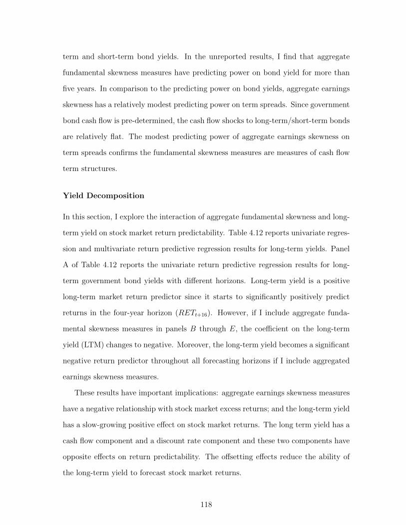
term and short-term bond yields. In the unreported results, I find that aggregate
fundamental skewness measures have predicting power on bond yield for more than
five years. In comparison to the predicting power on bond yields, aggregate earnings
skewness has a relatively modest predicting power on term spreads. Since government
bond cash flow is pre-determined, the cash flow shocks to long-term/short-term bonds
are relatively flat. The modest predicting power of aggregate earnings skewness on
term spreads confirms the fundamental skewness measures are measures of cash flow
term structures.
Yield Decomposition
In this section, I explore the interaction of aggregate fundamental skewness and long-
term yield on stock market return predictability. Table 4.12 reports univariate regres-
sion and multivariate return predictive regression results for long-term yields. Panel
A of Table 4.12 reports the univariate return predictive regression results for long-
term government bond yields with different horizons. Long-term yield is a positive
long-term market return predictor since it starts to significantly positively predict
returns in the four-year horizon (RETt+16). However, if I include aggregate funda-
mental skewness measures in panels B through E, the coefficient on the long-term
yield (LTM) changes to negative. Moreover, the long-term yield becomes a significant
negative return predictor throughout all forecasting horizons if I include aggregated
earnings skewness measures.
These results have important implications: aggregate earnings skewness measures
have a negative relationship with stock market excess returns; and the long-term yield
has a slow-growing positive effect on stock market returns. The long term yield has a
cash flow component and a discount rate component and these two components have
opposite effects on return predictability. The offsetting effects reduce the ability of
the long-term yield to forecast stock market returns.
118

4.7 Conclusions
Motivated by the empirical evidence that the distributions of macroeconomic funda-
mentals are skewed, this paper documents that the conditional skewness of aggregate
corporate earnings negatively predicts the stock market returns for horizons beyond
six months and up to eight years. The evidence is robust to controlling for standard
predictors such as the book-to-market ratio, interest rates, cay, and the first two mo-
ments of earnings. The results are also robust to alternative econometric estimation
methods.
I present a theoretical model that provides the microfoundation for the predictive
evidence. The model has two key ingredients: path dependence and non-Gaussian
innovations in the aggregate corporate earnings process, which are motivated by the
recent research on productivity-enhancing technology spillover. The interaction of
the two factors implies that the skewness of macroeconomic fundamentals not only is
time-varying but also negatively predicts the stock market returns.
119

4.8 The skew-normal distribution
I introduce in this section the skew-normal distribution and three related lemmas
used in the derivation of the model.
Skew-normal distribution (Azzalini (1985)). A skew-normal distribution SKN(µ, σ, ν)
with a local parameter µ, scale parameter σ, and shape parameter ν, has a probability
density function
p(x) =1
σπexp(−(x− µ)2
2σ2)
∫ ν(x−µ)σ
−∞exp(−t
2
2)dt. (4.46)
Lemma 1 (Azzalini (1985)): The closed form of a skew-normal distribution
SKN(µ, σ, ν) has the following closed form first three moments as follows:
mean = µ+ σΦ
√2
π, (4.47)
variance = σ2(1− 2Φ2
π), (4.48)
skewness =4− π
2
(Φ√
2/π)3
(1− 2Φ2/π)3/2. (4.49)
Lemma 2 (Linear Transformation):If a random variable x follows skew-normal distri-
bution SKN(0, 1, ν), the random variable Y = a+bx follows skew-normal distribution
SKN(a, b2, ν)
Lemma 3 (Colacito, Ghysels and Meng (2013)):If z follows SKN(µ, σ, ν), then
logEtexp(κ1z) = log(2) +κ1(κ1 + 2µ)
2+ logΦ(
νκ1√1 + ν2
) (4.50)
120

4.9 Solution to the model in Section 4.2
In this appendix, I describe the solution method for zero coupon bond. We conjecture
that the solution takes the form
P ent = exp(Aen +Be
nHt) (A1)
where P ent stands for the price of a time t equity with payoff only at period (t + n).
By the same token, P en−1,t+1 stands for the price of a time (t + 1) equity with payoff
only at period (t+ n− 1). Aen is a scalar and Ben is 1×m vector. Substituting (A1)
and (10) into (11) and expanding out the expectation following Lemma 3 implies
exp(Aen +BenHt) = Et[exp(−α0 − αHt − σeη0 + Aen−1 +Be
n−1θ0 − σeθ0η
+Ben−1θHt − σeηθHt + (Be
n−1 − σeησH)εt+1] (A2)
Matching coefficients lead to equations for Aent and Bent in (13) and (14) respectively.
121
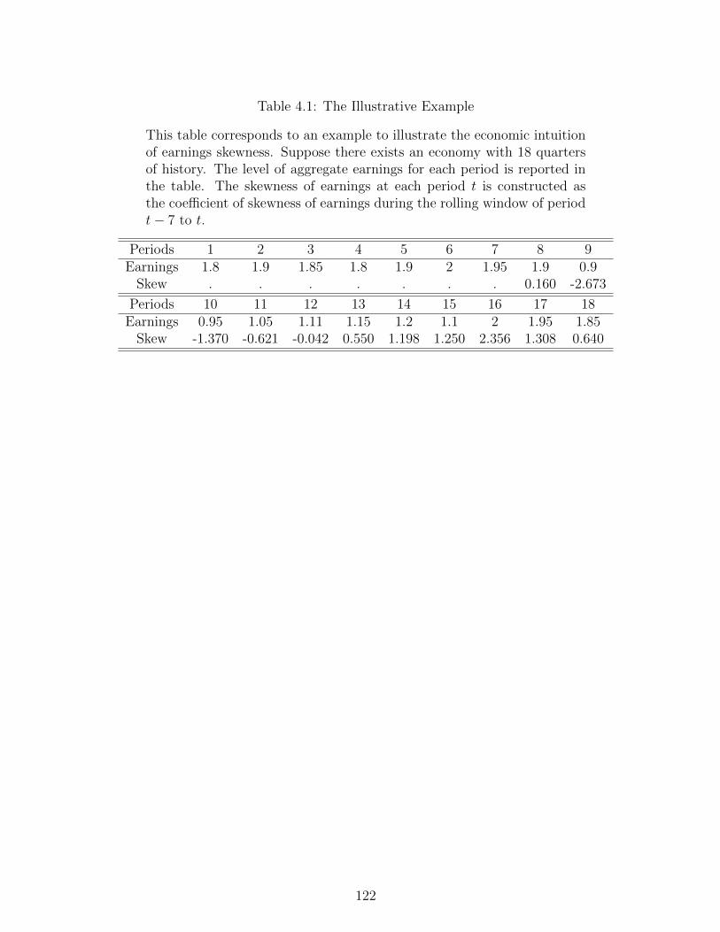
Table 4.1: The Illustrative Example
This table corresponds to an example to illustrate the economic intuitionof earnings skewness. Suppose there exists an economy with 18 quartersof history. The level of aggregate earnings for each period is reported inthe table. The skewness of earnings at each period t is constructed asthe coefficient of skewness of earnings during the rolling window of periodt− 7 to t.
Periods 1 2 3 4 5 6 7 8 9Earnings 1.8 1.9 1.85 1.8 1.9 2 1.95 1.9 0.9
Skew . . . . . . . 0.160 -2.673
Periods 10 11 12 13 14 15 16 17 18Earnings 0.95 1.05 1.11 1.15 1.2 1.1 2 1.95 1.85
Skew -1.370 -0.621 -0.042 0.550 1.198 1.250 2.356 1.308 0.640
122
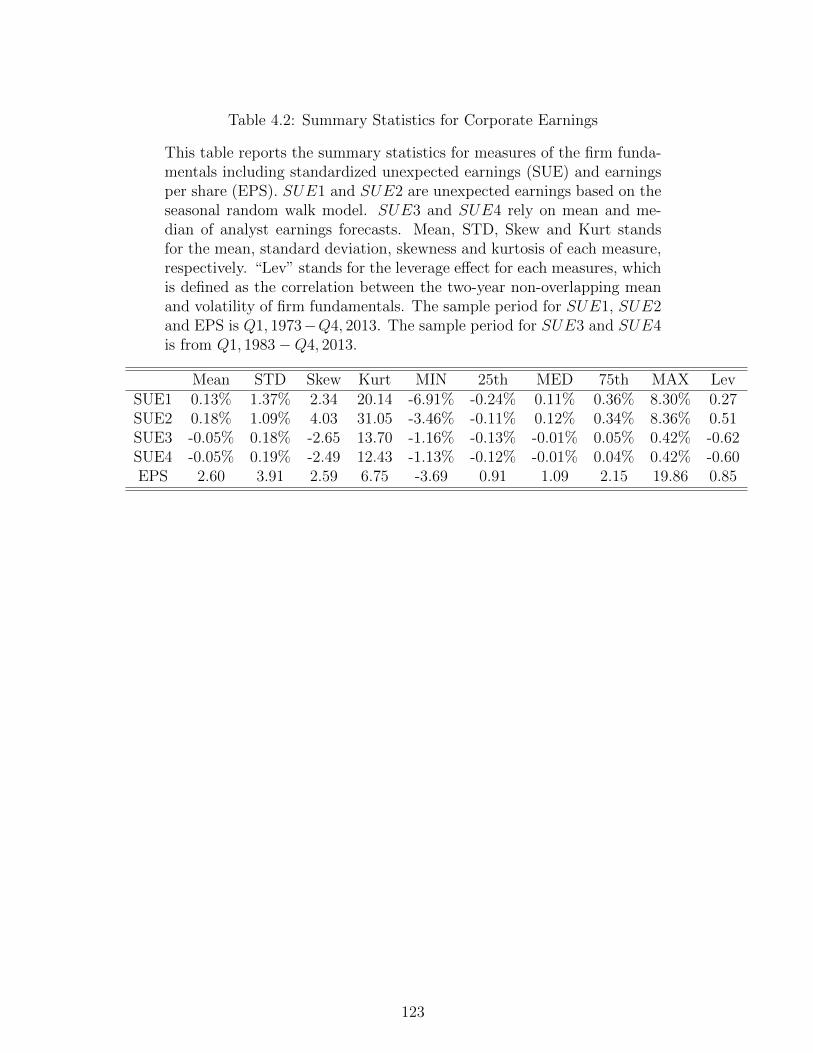
Table 4.2: Summary Statistics for Corporate Earnings
This table reports the summary statistics for measures of the firm funda-mentals including standardized unexpected earnings (SUE) and earningsper share (EPS). SUE1 and SUE2 are unexpected earnings based on theseasonal random walk model. SUE3 and SUE4 rely on mean and me-dian of analyst earnings forecasts. Mean, STD, Skew and Kurt standsfor the mean, standard deviation, skewness and kurtosis of each measure,respectively. “Lev” stands for the leverage effect for each measures, whichis defined as the correlation between the two-year non-overlapping meanand volatility of firm fundamentals. The sample period for SUE1, SUE2and EPS is Q1, 1973−Q4, 2013. The sample period for SUE3 and SUE4is from Q1, 1983−Q4, 2013.
Mean STD Skew Kurt MIN 25th MED 75th MAX LevSUE1 0.13% 1.37% 2.34 20.14 -6.91% -0.24% 0.11% 0.36% 8.30% 0.27SUE2 0.18% 1.09% 4.03 31.05 -3.46% -0.11% 0.12% 0.34% 8.36% 0.51SUE3 -0.05% 0.18% -2.65 13.70 -1.16% -0.13% -0.01% 0.05% 0.42% -0.62SUE4 -0.05% 0.19% -2.49 12.43 -1.13% -0.12% -0.01% 0.04% 0.42% -0.60EPS 2.60 3.91 2.59 6.75 -3.69 0.91 1.09 2.15 19.86 0.85
123
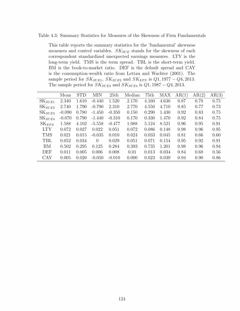
Table 4.3: Summary Statistics for Measures of the Skewness of Firm Fundamentals
This table reports the summary statistics for the ’fundamental’ skewnessmeasures and control variables. SKSUE stands for the skewness of eachcorrespondent standardized unexpected earnings measures. LTY is thelong-term yield. TMS is the term spread. TBL is the short-term yield.BM is the book-to-market ratio. DEF is the default spread and CAYis the consumption-wealth ratio from Lettau and Wachter (2001). Thesample period for SKSUE1, SKSUE2 and SKEPS is Q1, 1977 − Q4, 2013.The sample period for SKSUE3 and SKSUE4 is Q1, 1987−Q4, 2013.
Mean STD MIN 25th Median 75th MAX AR(1) AR(2) AR(3)SKSUE1 2.340 1.610 -0.440 1.520 2.170 4.160 4.630 0.87 0.78 0.75SKSUE2 2.740 1.790 -0.790 2.310 2.770 4.550 4.710 0.85 0.77 0.73SKSUE3 -0.090 0.780 -1.450 -0.350 0.150 0.290 1.430 0.92 0.83 0.75SKSUE4 -0.070 0.790 -1.440 -0.310 0.170 0.330 1.470 0.92 0.84 0.75SKEPS 1.588 4.102 -5.558 -0.477 1.088 5.124 8.521 0.96 0.95 0.91LTY 0.072 0.027 0.022 0.051 0.072 0.086 0.148 0.98 0.96 0.95TMS 0.021 0.015 -0.035 0.010 0.024 0.033 0.045 0.81 0.66 0.60TBL 0.052 0.034 0 0.029 0.051 0.071 0.154 0.95 0.92 0.91BM 0.502 0.295 0.125 0.284 0.393 0.735 1.201 0.98 0.96 0.94DEF 0.011 0.005 0.006 0.008 0.01 0.013 0.034 0.84 0.68 0.56CAY 0.005 0.020 -0.050 -0.010 0.000 0.023 0.039 0.94 0.90 0.86
124
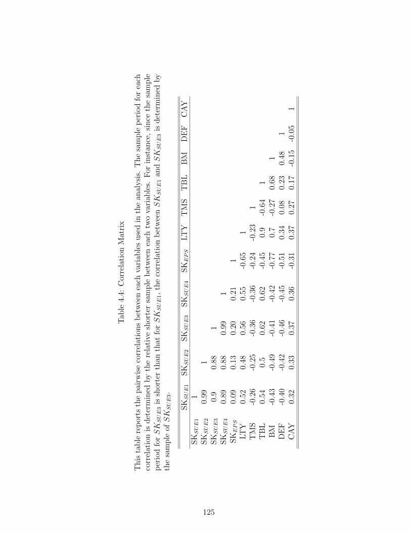
Tab
le4.
4:C
orre
lati
onM
atri
x
This
table
rep
orts
the
pai
rwis
eco
rrel
atio
ns
bet
wee
nea
chva
riab
les
use
din
the
anal
ysi
s.T
he
sam
ple
per
iod
for
each
corr
elat
ion
isdet
erm
ined
by
the
rela
tive
shor
ter
sam
ple
bet
wee
nea
chtw
ova
riab
les.
For
inst
ance
,si
nce
the
sam
ple
per
iod
forSKSUE
3is
shor
ter
than
that
forSKSUE
1,
the
corr
elat
ion
bet
wee
nSKSUE
1an
dSKSUE
3is
det
erm
ined
by
the
sam
ple
ofSKSUE
3.
SKSUE
1SKSUE
2SKSUE
3SKSUE
4SKEPS
LT
YT
MS
TB
LB
MD
EF
CA
YSKSUE
11
SKSUE
20.
991
SKSUE
30.
90.
881
SKSUE
40.
890.
880.
991
SKEPS
0.09
0.13
0.20
0.21
1LT
Y0.
520.
480.
560.
55-0
.65
1T
MS
-0.2
6-0
.25
-0.3
6-0
.36
-0.2
4-0
.23
1T
BL
0.54
0.5
0.62
0.62
-0.4
50.
9-0
.64
1B
M-0
.43
-0.4
9-0
.41
-0.4
2-0
.77
0.7
-0.2
70.
681
DE
F-0
.40
-0.4
2-0
.46
-0.4
5-0
.51
0.34
0.08
0.23
0.48
1C
AY
0.32
0.33
0.37
0.36
-0.3
10.
370.
270.
17-0
.15
-0.0
51
125
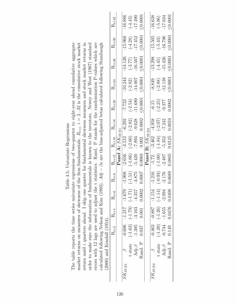
Tab
le4.
5:U
niv
aria
teR
egre
ssio
ns
The
table
rep
orts
the
tim
ese
ries
univ
aria
tere
gres
sion
sof
two-
quar
ter
toei
ght-
year
ahea
dcu
mula
tive
aggr
egat
em
arke
tre
turn
son
mea
sure
sof
skew
nes
sof
the
firm
fundam
enta
ls.Rt+i,i
=2...32
isth
ecu
mula
tive
stock
mar
ket
retu
rnunti
li
quar
ters
ahea
d.
Isk
ipon
equar
ter
for
fundam
enta
lsk
ewnes
sm
easu
res
and
stock
mar
ket
retu
rns
inor
der
tom
ake
sure
the
info
rmat
ion
offu
ndam
enta
lsis
know
nto
the
inve
stor
s.N
ewey
and
Wes
t(1
987)
stan
dar
der
rors
wit
h12
lags
are
use
dto
adju
stth
et
stat
isti
cs.
Ran
d.
Pst
ands
for
the
random
izat
ion
P-v
alues
whic
har
eca
lcula
ted
follow
ing
Nel
son
and
Kim
(199
3).Adj−β
sar
eth
ebia
s-ad
just
edb
etas
calc
ula
ted
follow
ing
Sta
mbau
gh(2
000)
and
Ken
dal
l(1
954)
.
Rt+
2Rt+
4Rt+
6Rt+
8Rt+
12
Rt+
16
Rt+
18
Rt+
20
Rt+
24
Rt+
28
Rt+
30
Rt+
32
Panel
A:SKSUE
1
SKSUE
1β
-0.6
06-1
.217
-1.6
79-1
.908
-2.6
56-4
.512
-6.2
92-7
.722
-10.
244
-14.
126
-15.
968
-16.
886
tst
ats
(-1.
63)
(-1.
79)
(-1.
71)
(-1.
51)
(-1.
66)
(-2.
66)
(-2.
82)
(-2.
54)
(-2.
82)
(-3.
77)
(-4.
28)
(-4.
43)
Adj-β
-1.3
95-3
.163
-4.3
57-4
.875
-5.4
20-7
.894
-9.6
28-1
1.68
0-1
4.00
7-1
6.50
7-1
7.45
2-1
7.49
0R
and.
P0.
037
0.00
10.
0002
0.00
070.
0068
0.00
20.
0002
≤0.
0001≤
0.00
01≤
0.00
01≤
0.00
01≤
0.00
01P
anel
B:SKSUE
2
SKSUE
2β
-0.4
63-0
.887
-1.1
54-1
.216
-1.7
2-3
.462
-4.9
58-6
.15
-8.8
49-1
3.29
8-1
5.50
5-1
6.63
8t
stat
s(-
1.20
)(-
1.26
)(-
1.14
)(-
0.93
)(-
1.00
)(-
1.84
)(-
2.07
)(-
2.25
)(-
2.88
)(-
4.45
)(-
5.43
)(-
5.86
)A
dj-β
-0.7
44-1
.655
-2.0
94-2
.176
-2.4
87-5
.352
-7.2
42-9
.377
-12.
138
-15.
426
-16.
796
-17.
034
Ran
d.
P0.
149
0.04
760.
0408
0.06
890.
0805
0.01
250.
0024
0.00
02≤
0.00
01≤
0.00
01≤
0.00
01≤
0.00
01
126

Tab
le4.
5–
Con
tinued
Rt+
2Rt+
4Rt+
6Rt+
8Rt+
12
Rt+
16
Rt+
18
Rt+
20
Rt+
24
Rt+
28
Rt+
30
Rt+
32
Panel
C:SKSUE
3
SKSUE
3β
-0.5
78-1
.263
-2.0
16-2
.521
-3.7
96-6
.139
-8.8
91-1
1.14
8-1
6.75
0-2
3.27
3-2
8.51
0-3
5.16
2t
stat
s(-
1.73
)(-
2.06
)(-
2.14
)(-
2.10
)(-
2.37
)(-
2.66
)(-
2.82
)(-
2.37
)(-
2.82
)(-
4.00
)(-
5.18
)(-
6.19
)A
dj-β
-0.4
34-0
.977
-3.7
09-6
.528
-7.2
06-1
0.55
0-1
2.38
2-1
4.35
2-1
9.21
7-2
4.91
1-2
9.96
6-3
7.08
0R
and.
P0.
0259
0.01
190.
0045
0.00
210.
0014
0.00
04≤
0.00
01≤
0.00
01≤
0.00
01≤
0.00
01≤
0.00
01≤
0.00
01P
anel
D:SKSUE
4
SKSUE
4β
-0.6
14-1
.336
-2.1
23-2
.66
-4.0
3-6
.619
-9.7
03-1
2.45
-17.
753
-23.
952
-28.
877
-35.
199
tst
ats
(-1.
80)
(-2.
09)
(-2.
17)
(-2.
15)
(-2.
47)
(-2.
81)
(-3.
08)
(-2.
72)
(-3.
17)
(-4.
31)
(-5.
45)
(-6.
36)
Adj-β
-0.3
91-0
.948
-3.6
67-6
.484
-7.5
08-1
1.42
1-1
3.42
9-1
5.47
7-2
0.22
8-2
5.52
5-3
0.39
9-3
7.11
2R
and.
P0.
0169
0.00
760.
003
0.00
120.
0007
0.00
03≤
0.00
01≤
0.00
01≤
0.00
01≤
0.00
01≤
0.00
01≤
0.00
01P
anel
E:SKEPS
SKEPS
β-0
.019
-0.0
29-0
.05
-0.0
82-0
.135
-0.1
71-0
.184
-0.2
-0.2
03-0
.212
-0.2
2-0
.239
tst
ats
(-0.
63)
(-0.
76)
(-0.
98)
(-1.
37)
(-1.
93)
(-2.
43)
(-2.
80)
(-3.
35)
(-3.
61)
(-3.
30)
(-3.
37)
(-3.
21)
Adj-β
-0.0
02-0
.003
-0.0
18-0
.048
-0.1
16-0
.176
-0.1
98-0
.212
-0.2
08-0
.219
-0.2
31-0
.249
Ran
d.
P0.
4821
0.39
750.
1182
0.02
720.
0026
≤0.
0001≤
0.00
01≤
0.00
01≤
0.00
01≤
0.00
01≤
0.00
01≤
0.00
01
127
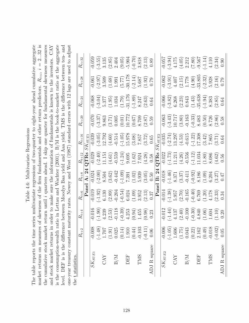
Tab
le4.
6:M
ult
ivar
iate
Reg
ress
ions
The
table
rep
orts
the
tim
ese
ries
mult
ivar
iate
regr
essi
ons
oftw
o-quar
ter
toei
ght-
year
ahea
dcu
mula
tive
aggr
egat
em
arke
tre
turn
son
mea
sure
sof
skew
nes
sof
the
firm
fundam
enta
lsan
dot
her
retu
rnpre
dic
tors
.Rt+i,i
=2...32
isth
ecu
mula
tive
stock
mar
ket
retu
rnunti
li
quar
ters
ahea
d.
Isk
ipon
equar
ter
for
fundam
enta
lsk
ewnes
sm
easu
res
and
stock
mar
ket
retu
rns
inor
der
tom
ake
sure
the
info
rmat
ion
offu
ndam
enta
lsis
know
nto
the
inve
stor
s.C
AY
isth
eco
nsu
mpti
on-w
ealt
hra
tio
inL
etta
uan
dW
achte
r(2
001)
.B
/Mis
the
book
-to-
mar
ket
rati
oat
the
aggr
egat
ele
vel.
DE
Fis
isth
ediff
eren
ceb
etw
een
Moodys
Baa
yie
ldan
dA
aayie
ld.
TM
Sis
the
diff
eren
ceb
etw
een
ten-
and
one-
year
trea
sury
const
ant
mat
uri
tyra
tes.
New
eyan
dW
est
(198
7)st
andar
der
rors
wit
h12
lags
are
use
dto
adju
stth
et
stat
isti
cs.
Rt+
2Rt+
4Rt+
6Rt+
8Rt+
12
Rt+
16
Rt+
20
Rt+
24
Rt+
28
Rt+
32
Panel
A:
24
QT
RsSKSUE
1
SKSUE
1-0
.008
-0.0
16-0
.019
-0.0
24-0
.029
-0.0
39-0
.070
-0.0
68-0
.061
-0.0
59(-
1.48
)(-
1.90
)(-
1.92
)(-
2.00
)(-
2.40
)(-
3.05
)(-
3.37
)(-
3.04
)(-
2.97
)(-
3.55
)C
AY
1.70
74.
239
6.13
08.
504
11.1
5112
.792
9.86
35.
377
3.50
93.
135
(1.9
1)(2
.53)
(2.8
9)(3
.62)
(4.6
1)(4
.60)
(3.7
1)(1
.95)
(1.6
8)(2
.85)
B/M
0.02
5-0
.118
-0.2
04-0
.442
-0.5
59-0
.514
0.00
51.
034
1.99
12.
404
(0.1
4)(-
0.39
)(-
0.54
)(-
1.09
)(-
1.24
)(-
1.05
)(0
.01)
(1.7
9)(5
.77)
(9.0
5)D
EF
1.91
04.
253
6.02
47.
391
9.69
515
.978
10.7
72-3
1.17
6-3
0.17
8-5
.904
(0.4
4)(0
.94)
(1.0
9)(1
.02)
(1.6
2)(3
.08)
(0.6
7)(-
1.89
)(-
2.14
)(-
0.70
)T
MS
-0.1
031.
455
3.95
25.
939
7.92
47.
857
8.70
98.
247
5.68
73.
818
(-0.
11)
(0.9
8)(2
.13)
(3.0
5)(4
.28)
(3.7
2)(2
.87)
(2.6
3)(1
.92)
(2.1
3)A
DJ
Rsq
uar
e0.
060.
230.
370.
500.
580.
650.
590.
640.
790.
89P
anel
B:
24
QT
RsSKSUE
2
SKSUE
2-0
.006
-0.0
12-0
.014
-0.0
18-0
.022
-0.0
35-0
.063
-0.0
66-0
.062
-0.0
57(-
1.05
)(-
1.44
)(-
1.38
)(-
1.46
)(-
1.73
)(-
2.74
)(-
3.43
)(-
3.82
)(-
3.91
)(-
3.94
)C
AY
1.60
64.
137
5.95
78.
371
11.2
1113
.297
10.7
176.
268
4.40
74.
175
(1.7
5)(2
.40)
(2.7
0)(3
.37)
(4.2
6)(4
.53)
(3.8
0)(2
.23)
(2.1
5)(4
.05)
B/M
0.04
3-0
.100
-0.1
65-0
.411
-0.5
56-0
.615
-0.1
630.
843
1.77
82.
212
(0.2
2)(-
0.30
)(-
0.40
)(-
0.92
)(-
1.12
)(-
1.22
)(-
0.33
)(1
.43)
(4.9
0)(7
.80)
DE
F2.
162
4.84
06.
769
8.18
611
.034
17.3
088.
483
-35.
638
-33.
805
-9.5
67(0
.49)
(1.0
6)(1
.20)
(1.0
9)(1
.80)
(3.4
2)(0
.50)
(-1.
94)
(-2.
32)
(-1.
14)
TM
S-0
.018
1.60
44.
178
6.20
48.
086
7.86
58.
726
8.38
35.
928
4.11
0(-
0.02
)(1
.10)
(2.3
3)(3
.27)
(4.6
2)(3
.71)
(2.8
6)(2
.85)
(2.1
6)(2
.34)
AD
JR
squar
e0.
050.
200.
340.
470.
560.
640.
580.
640.
790.
90
128

Tab
le4.
6–
Con
tinued Rt+
2Rt+
4Rt+
6Rt+
8Rt+
12
Rt+
16
Rt+
20
Rt+
24
Rt+
28
Rt+
32
Panel
C:
24
QT
RsSKSUE
3
SKSUE
3-0
.008
-0.0
18-0
.025
-0.0
33-0
.040
-0.0
35-0
.028
0.04
00.
114
-0.0
28(-
1.70
)(-
2.07
)(-
2.13
)(-
2.33
)(-
3.25
)(-
2.59
)(-
0.61
)(0
.46)
(1.8
2)(-
0.46
)C
AY
1.77
24.
369
6.41
98.
926
11.3
6612
.514
9.34
35.
449
5.11
35.
026
(1.9
4)(2
.41)
(2.8
8)(3
.89)
(4.5
8)(3
.79)
(2.6
8)(1
.58)
(1.9
2)(3
.67)
B/M
0.03
4-0
.104
-0.2
16-0
.474
-0.5
63-0
.355
0.46
21.
887
3.01
62.
662
(0.1
8)(-
0.29
)(-
0.49
)(-
1.03
)(-
1.23
)(-
0.72
)(0
.89)
(2.2
7)(6
.13)
(6.4
7)D
EF
1.55
93.
345
4.59
75.
430
6.39
315
.301
7.30
5-3
9.45
3-2
7.63
0-1
8.54
5(0
.33)
(0.7
2)(0
.85)
(0.7
3)(0
.87)
(2.3
3)(0
.36)
(-1.
85)
(-1.
68)
(-2.
50)
TM
S-0
.324
0.97
93.
202
4.89
36.
889
7.04
27.
103
5.94
13.
240
3.98
4(-
0.31
)(0
.64)
(1.7
5)(2
.60)
(4.2
5)(2
.75)
(1.6
0)(1
.54)
(1.1
4)(2
.02)
AD
JR
squar
e0.
060.
220.
380.
510.
590.
610.
490.
560.
750.
86P
anel
D:
24
QT
RsSKSUE
4
SKSUE
4-0
.009
-0.0
18-0
.025
-0.0
33-0
.040
-0.0
33-0
.021
0.03
20.
108
-0.0
29(-
1.71
)(-
2.02
)(-
2.08
)(-
2.27
)(-
3.14
)(-
2.31
)(-
0.45
)(0
.37)
(1.7
7)(-
0.49
)C
AY
1.75
34.
308
6.32
18.
787
11.2
0212
.398
9.33
65.
480
5.36
04.
952
(1.9
1)(2
.38)
(2.8
6)(3
.85)
(4.5
2)(3
.76)
(2.6
8)(1
.58)
(1.9
4)(3
.50)
B/M
0.03
3-0
.102
-0.2
12-0
.466
-0.5
52-0
.343
0.48
31.
849
2.97
32.
661
(0.1
7)(-
0.29
)(-
0.47
)(-
1.00
)(-
1.18
)(-
0.69
)(0
.93)
(2.2
6)(6
.22)
(6.7
6)D
EF
1.59
33.
442
4.76
45.
678
6.81
816
.047
9.07
6-4
0.30
8-2
8.24
1-1
8.68
2(0
.34)
(0.7
4)(0
.88)
(0.7
7)(0
.93)
(2.5
0)(0
.46)
(-1.
89)
(-1.
71)
(-2.
53)
TM
S-0
.326
0.98
93.
226
4.93
86.
945
7.06
47.
039
6.02
83.
303
4.00
4(-
0.31
)(0
.64)
(1.7
6)(2
.61)
(4.2
9)(2
.76)
(1.5
9)(1
.55)
(1.1
4)(2
.02)
AD
JR
squar
e0.
060.
220.
380.
510.
580.
610.
490.
560.
750.
86P
anel
E:
24
QT
RsSKEPS
SKEPS
0.00
030.
0005
0.00
060.
0003
0.00
01-0
.000
1-0
.000
5-0
.001
0-0
.001
0-0
.000
9(1
.25)
(1.3
2)(1
.37)
(0.7
1)(0
.10)
(-0.
10)
(-0.
74)
(-1.
41)
(-1.
58)
(-1.
68)
CA
Y1.
748
3.56
74.
935
5.18
56.
429
8.13
18.
234
8.92
19.
979
11.7
98(2
.76)
(3.3
6)(3
.44)
(3.1
1)(2
.92)
(3.6
3)(3
.99)
(4.6
5)(5
.56)
(5.9
9)B
/M0.
056
0.12
40.
180
0.19
10.
173
0.14
70.
223
0.34
40.
475
0.61
9(1
.08)
(1.4
7)(1
.69)
(1.5
7)(1
.55)
(1.2
3)(1
.59)
(2.6
1)(3
.54)
(4.9
7)D
EF
2.55
91.
862
1.06
1-1
.213
2.88
610
.777
4.14
8-8
.972
-11.
050
-11.
752
(0.9
6)(0
.45)
(0.1
8)(-
0.16
)(0
.38)
(1.2
0)(0
.35)
(-0.
76)
(-1.
05)
(-1.
57)
TM
S1.
347
2.54
53.
779
4.53
74.
789
3.47
11.
638
-1.2
74-1
.044
0.27
3(1
.67)
(2.2
9)(2
.80)
(2.5
5)(2
.83)
(1.8
5)(0
.61)
(-0.
46)
(-0.
42)
(0.1
1)A
DJ
Rsq
uar
e0.
080.
180.
260.
300.
370.
440.
390.
440.
500.
60
129
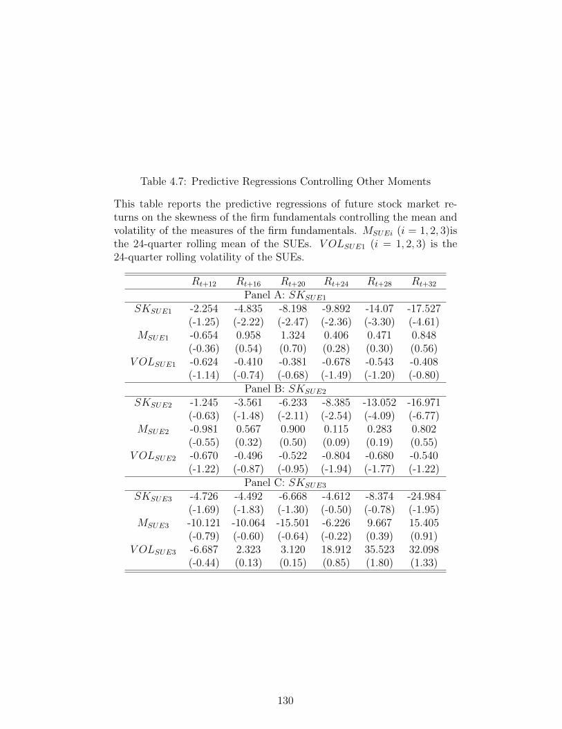
Table 4.7: Predictive Regressions Controlling Other Moments
This table reports the predictive regressions of future stock market re-turns on the skewness of the firm fundamentals controlling the mean andvolatility of the measures of the firm fundamentals. MSUEi (i = 1, 2, 3)isthe 24-quarter rolling mean of the SUEs. V OLSUE1 (i = 1, 2, 3) is the24-quarter rolling volatility of the SUEs.
Rt+12 Rt+16 Rt+20 Rt+24 Rt+28 Rt+32
Panel A: SKSUE1
SKSUE1 -2.254 -4.835 -8.198 -9.892 -14.07 -17.527(-1.25) (-2.22) (-2.47) (-2.36) (-3.30) (-4.61)
MSUE1 -0.654 0.958 1.324 0.406 0.471 0.848(-0.36) (0.54) (0.70) (0.28) (0.30) (0.56)
V OLSUE1 -0.624 -0.410 -0.381 -0.678 -0.543 -0.408(-1.14) (-0.74) (-0.68) (-1.49) (-1.20) (-0.80)
Panel B: SKSUE2
SKSUE2 -1.245 -3.561 -6.233 -8.385 -13.052 -16.971(-0.63) (-1.48) (-2.11) (-2.54) (-4.09) (-6.77)
MSUE2 -0.981 0.567 0.900 0.115 0.283 0.802(-0.55) (0.32) (0.50) (0.09) (0.19) (0.55)
V OLSUE2 -0.670 -0.496 -0.522 -0.804 -0.680 -0.540(-1.22) (-0.87) (-0.95) (-1.94) (-1.77) (-1.22)
Panel C: SKSUE3
SKSUE3 -4.726 -4.492 -6.668 -4.612 -8.374 -24.984(-1.69) (-1.83) (-1.30) (-0.50) (-0.78) (-1.95)
MSUE3 -10.121 -10.064 -15.501 -6.226 9.667 15.405(-0.79) (-0.60) (-0.64) (-0.22) (0.39) (0.91)
V OLSUE3 -6.687 2.323 3.120 18.912 35.523 32.098(-0.44) (0.13) (0.15) (0.85) (1.80) (1.33)
130

131

Table 4.8: Principle Component Analysis
This table reports the principle component analysis (PCA) for the skew-ness of the firm fundamentals. The PCA extracts the common componentsof the five fundamental skewness measures. The element in the table isthe cumulative percentage of the sample variance that the principle com-ponent can explain.
Proportion of Cumulative EigenvaluesElements 1 2 3 4 5
SKSUE1 & SKSUE2 0.994 1SKSUE1,2,3 0.949 0.996 1SKSUE1,2,3,4 0.943 0.997 1.000 1
SKSUE1,2,3,4 & SKEPS 0.784 0.959 0.998 1 1
132
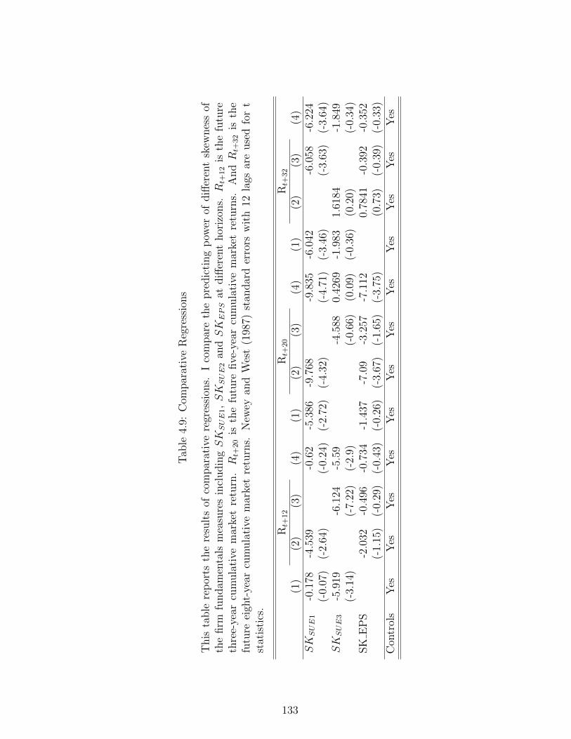
Tab
le4.
9:C
ompar
ativ
eR
egre
ssio
ns
This
table
rep
orts
the
resu
lts
ofco
mpar
ativ
ere
gres
sion
s.I
com
par
eth
epre
dic
ting
pow
erof
diff
eren
tsk
ewnes
sof
the
firm
fundam
enta
lsm
easu
res
incl
udin
gSKSUE
1,SKSUE
2an
dSKEPS
atdiff
eren
thor
izon
s.Rt+
12
isth
efu
ture
thre
e-ye
arcu
mula
tive
mar
ket
retu
rn.Rt+
20
isth
efu
ture
five
-yea
rcu
mula
tive
mar
ket
retu
rns.
AndRt+
32
isth
efu
ture
eigh
t-ye
arcu
mula
tive
mar
ket
retu
rns.
New
eyan
dW
est
(198
7)st
andar
der
rors
wit
h12
lags
are
use
dfo
rt
stat
isti
cs.
Rt+
12
Rt+
20
Rt+
32
(1)
(2)
(3)
(4)
(1)
(2)
(3)
(4)
(1)
(2)
(3)
(4)
SKSUE
1-0
.178
-4.5
39-0
.62
-5.3
86-9
.768
-9.8
35-6
.042
-6.0
58-6
.224
(-0.
07)
(-2.
64)
(-0.
24)
(-2.
72)
(-4.
32)
(-4.
71)
(-3.
46)
(-3.
63)
(-3.
64)
SKSUE
3-5
.919
-6.1
24-5
.59
-4.5
880.
4269
-1.9
831.
6184
-1.8
49(-
3.14
)(-
7.22
)(-
2.9)
(-0.
66)
(0.0
9)(-
0.36
)(0
.20)
(-0.
34)
SK
EP
S-2
.032
-0.4
96-0
.734
-1.4
37-7
.09
-3.2
57-7
.112
0.78
41-0
.392
-0.3
52(-
1.15
)(-
0.29
)(-
0.43
)(-
0.26
)(-
3.67
)(-
1.65
)(-
3.75
)(0
.73)
(-0.
39)
(-0.
33)
Con
trol
sY
esY
esY
esY
esY
esY
esY
esY
esY
esY
esY
esY
es
133
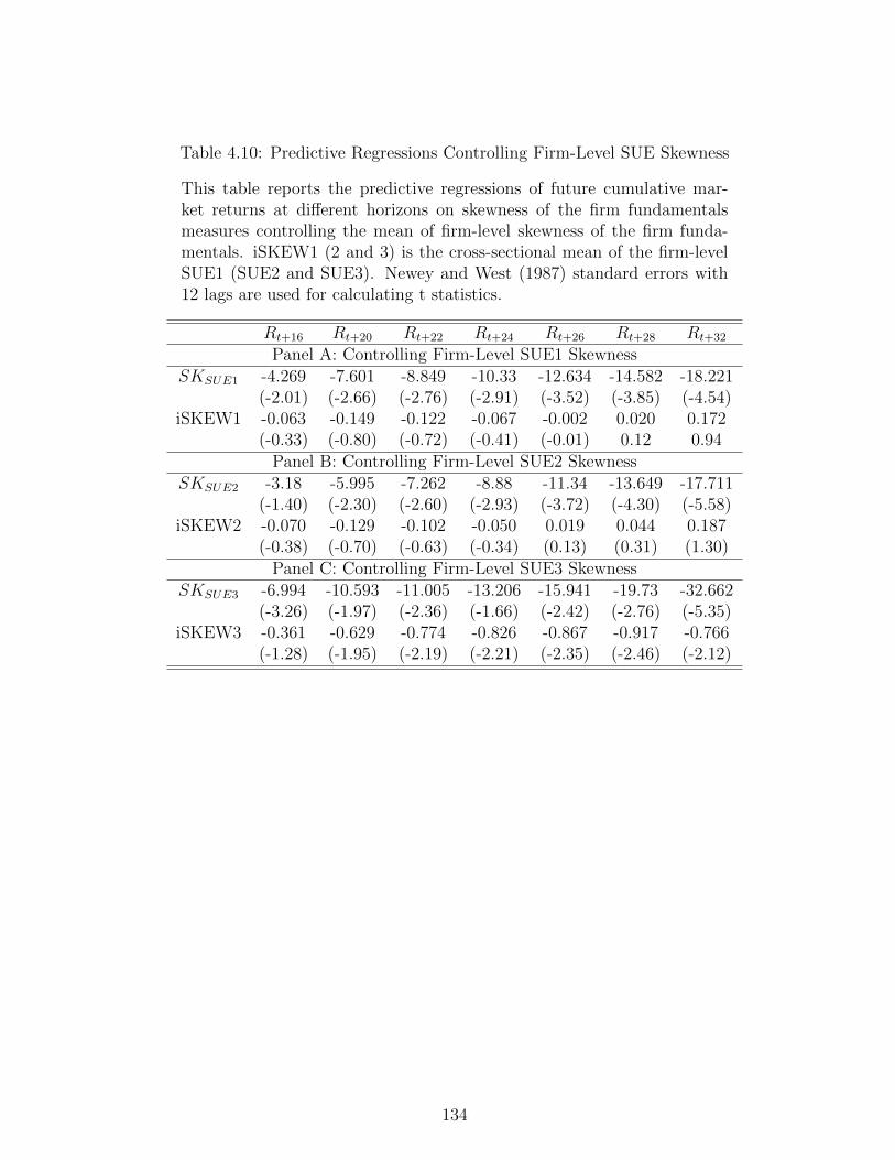
Table 4.10: Predictive Regressions Controlling Firm-Level SUE Skewness
This table reports the predictive regressions of future cumulative mar-ket returns at different horizons on skewness of the firm fundamentalsmeasures controlling the mean of firm-level skewness of the firm funda-mentals. iSKEW1 (2 and 3) is the cross-sectional mean of the firm-levelSUE1 (SUE2 and SUE3). Newey and West (1987) standard errors with12 lags are used for calculating t statistics.
Rt+16 Rt+20 Rt+22 Rt+24 Rt+26 Rt+28 Rt+32
Panel A: Controlling Firm-Level SUE1 SkewnessSKSUE1 -4.269 -7.601 -8.849 -10.33 -12.634 -14.582 -18.221
(-2.01) (-2.66) (-2.76) (-2.91) (-3.52) (-3.85) (-4.54)iSKEW1 -0.063 -0.149 -0.122 -0.067 -0.002 0.020 0.172
(-0.33) (-0.80) (-0.72) (-0.41) (-0.01) 0.12 0.94Panel B: Controlling Firm-Level SUE2 Skewness
SKSUE2 -3.18 -5.995 -7.262 -8.88 -11.34 -13.649 -17.711(-1.40) (-2.30) (-2.60) (-2.93) (-3.72) (-4.30) (-5.58)
iSKEW2 -0.070 -0.129 -0.102 -0.050 0.019 0.044 0.187(-0.38) (-0.70) (-0.63) (-0.34) (0.13) (0.31) (1.30)
Panel C: Controlling Firm-Level SUE3 SkewnessSKSUE3 -6.994 -10.593 -11.005 -13.206 -15.941 -19.73 -32.662
(-3.26) (-1.97) (-2.36) (-1.66) (-2.42) (-2.76) (-5.35)iSKEW3 -0.361 -0.629 -0.774 -0.826 -0.867 -0.917 -0.766
(-1.28) (-1.95) (-2.19) (-2.21) (-2.35) (-2.46) (-2.12)
134
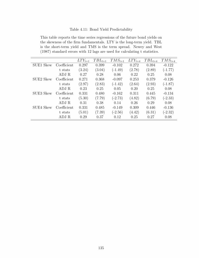
Table 4.11: Bond Yield Predictability
This table reports the time series regressions of the future bond yields onthe skewness of the firm fundamentals. LTY is the long-term yield. TBLis the short-term yield and TMS is the term spread. Newey and West(1987) standard errors with 12 lags are used for calculating t statistics.
LTYt+1 TBLt+1 TMSt+1 LTYt+4 TBLt+4 TMSt+4
SUE1 Skew Coefficient 0.297 0.399 -0.102 0.272 0.394 -0.122t stats (3.24) (3.04) (-1.49) (2.78) (2.89) (-1.77)ADJ R 0.27 0.28 0.06 0.22 0.25 0.08
SUE2 Skew Coefficient 0.271 0.368 -0.097 0.253 0.379 -0.126t stats (2.97) (2.83) (-1.42) (2.64) (2.93) (-1.87)ADJ R 0.23 0.25 0.05 0.20 0.25 0.08
SUE3 Skew Coefficient 0.331 0.480 -0.162 0.311 0.445 -0.134t stats (5.30) (7.79) (-2.73) (4.82) (6.79) (-2.33)ADJ R 0.31 0.38 0.14 0.26 0.29 0.08
SUE4 Skew Coefficient 0.331 0.485 -0.149 0.309 0.446 -0.136t stats (5.01) (7.39) (-2.56) (4.42) (6.31) (-2.32)ADJ R 0.29 0.37 0.12 0.25 0.27 0.08
135
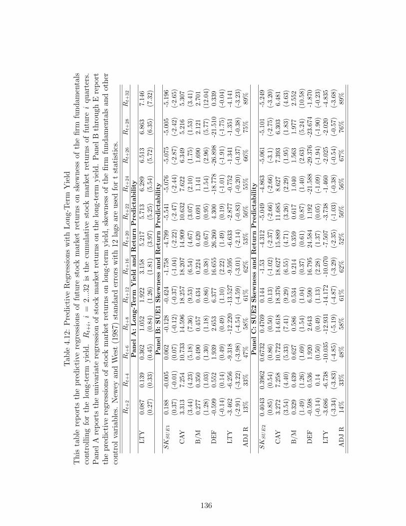
Tab
le4.
12:
Pre
dic
tive
Reg
ress
ions
wit
hL
ong-
Ter
mY
ield
This
table
rep
orts
the
pre
dic
tive
regr
essi
ons
offu
ture
stock
mar
ket
retu
rns
onsk
ewnes
sof
the
firm
fundam
enta
lsco
ntr
olling
for
the
long-
term
yie
ld.Rt+i,i
=2...32
isth
ecu
mula
tive
stock
mar
ket
retu
rns
offu
turei
quar
ters
.P
anel
Are
por
tsth
euniv
aria
tere
gres
sion
ofst
ock
mar
ket
retu
rns
onth
elo
ng-
term
yie
ld.
Pan
elB
thro
ugh
Ere
por
tth
epre
dic
tive
regr
essi
ons
ofst
ock
mar
ket
retu
rns
onlo
ng-
term
yie
ld,
skew
nes
sof
the
firm
fundam
enta
lsan
dot
her
contr
olva
riab
les.
New
eyan
dW
est
(198
7)st
andar
der
rors
wit
h12
lags
are
use
dfo
rt
stat
isti
cs.
Rt+
2R
t+4
Rt+
6R
t+8
Rt+
12
Rt+
16
Rt+
20
Rt+
22
Rt+
24
Rt+
26
Rt+
28
Rt+
32
PanelA:Long-T
erm
Yield
and
Retu
rnPre
dicta
bility
LT
Y0.
087
0.13
90.
362
1.0
52
1.9
22
3.1
58
5.2
17
5.7
13
6.2
89
6.5
13
6.8
63
7.1
46
(0.2
7)(0
.33)
(0.4
5)(0
.84)
(1.2
6)
(1.8
1)
(3.9
7)
(5.2
5)
(5.5
4)
(5.7
2)
(6.3
5)
(7.3
2)
PanelB:SUE1Skewness
and
Retu
rnPre
dicta
bility
SK
SUE1
0.18
8-0
.005
0.06
2-0
.128
-0.4
24
-1.7
58
-4.7
99
-5.5
41
-5.0
76
-5.0
75
-5.0
05
-5.1
96
(0.3
7)(-
0.01
)(0
.07)
(-0.1
2)
(-0.3
7)
(-1.0
4)
(-2.2
2)
(-2.4
7)
(-2.4
4)
(-2.8
7)
(-2.4
2)
(-2.6
5)
CA
Y3.
313
7.25
410
.733
14.5
96
18.2
57
18.2
07
14.9
09
10.6
32
7.6
22
6.3
49
5.2
16
5.3
07
(3.4
4)(4
.23)
(5.1
8)(7
.36)
(9.5
3)
(6.5
4)
(4.6
7)
(3.0
7)
(2.1
0)
(1.7
5)
(1.5
3)
(3.4
1)
B/M
0.27
70.
350
0.49
00.4
57
0.4
34
0.2
24
0.4
20
0.6
91
1.1
41
1.6
90
2.1
21
2.7
01
(1.2
8)(1
.03)
(1.3
0)(1
.18)
(0.8
6)
(0.3
8)
(0.6
7)
(0.9
5)
(1.5
4)
(2.9
6)
(5.7
7)
(12.0
4)
DE
F-0
.599
0.55
21.
939
2.6
53
6.3
77
16.6
55
26.2
60
4.3
00
-18.7
78
-26.8
98
-21.5
10
0.3
39
(-0.
14)
(0.1
4)(0
.49)
(0.4
9)
(1.1
0)
(2.2
2)
(1.4
9)
(0.1
9)
(-1.0
1)
(-1.9
1)
(-1.7
5)
(-0.0
4)
LT
Y-3
.462
-6.2
56-9
.318
-12.2
20
-13.5
27
-9.5
95
-6.6
33
-2.8
77
-0.7
52
-1.3
41
-1.3
51
-4.1
41
(-2.
91)
(-3.
22)
(-3.
98)
(-4.5
4)
(-4.5
9)
(-3.0
1)
(-2.1
4)
(-0.8
3)
(-0.2
0)
(-0.3
7)
(-0.3
8)
(-3.2
3)
AD
JR
13%
33%
47%
58%
61%
62%
53%
50%
55%
66%
75%
89%
PanelC:SUE2Skewness
and
Retu
rnPre
dicta
bility
SK
SUE2
0.40
430.
3962
0.67
320.4
769
0.1
44
-1.5
3-4
.312
-5.0
49
-4.8
63
-5.0
61
-5.1
01
-5.2
49
(0.8
5)(0
.54)
(0.8
6)(0
.50)
(0.1
3)
(-1.0
2)
(-2.3
7)
(-2.6
6)
(-2.6
6)
(-3.1
)(-
2.7
5)
(-3.2
0)
CA
Y3.
272
7.25
810
.722
14.6
18
18.3
76
18.6
27
15.8
89
11.6
85
8.6
27
7.3
93
6.3
03
6.4
81
(3.5
4)(4
.40)
(5.3
3)(7
.41)
(9.2
9)
(6.5
5)
(4.7
1)
(3.2
6)
(2.2
9)
(1.9
5)
(1.8
3)
(4.6
3)
B/M
0.32
90.
439
0.62
70.5
86
0.5
34
0.2
14
0.3
59
0.6
17
1.0
40
1.5
63
1.9
77
2.5
52
(1.4
9)(1
.26)
(1.6
9)(1
.54)
(1.0
4)
(0.3
7)
(0.6
1)
(0.8
7)
(1.4
0)
(2.6
3)
(5.2
4)
(10.5
8)
DE
F-0
.598
0.53
61.
920
2.6
43
6.5
90
16.7
95
24.5
84
1.1
92
-21.5
88
-29.3
76
-23.6
74
-1.8
70
(-0.
14)
0.14
(0.5
0)(0
.49)
(1.1
3)
(2.2
8)
(1.3
7)
(0.0
5)
(-1.0
9)
(-1.9
4)
(-1.9
0)
(-0.2
3)
LT
Y-3
.686
-6.7
38-1
0.03
5-1
2.9
31
-14.1
72
-10.0
70
-7.5
07
-3.7
38
-1.4
60
-2.0
25
-2.0
20
-4.8
35
(-3.
34)
(-3.
83)
(-4.
85)
(-5.1
9)
(-4.8
7)
(-3.2
9)
(-2.3
5)
(-1.0
3)
(-0.3
8)
(-0.5
4)
(-0.5
7)
(-3.6
8)
AD
JR
14%
33%
48%
58%
61%
62%
52%
50%
56%
67%
76%
89%
136
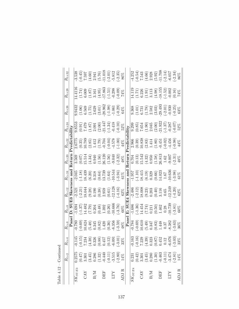
Tab
le4.
12–
Con
tinu
ed
Rt+
2R
t+4
Rt+
6R
t+8
Rt+
12
Rt+
16
Rt+
20
Rt+
22
Rt+
24
Rt+
26
Rt+
28
Rt+
32
PanelD:SUE3Skewness
and
Retu
rnPre
dicta
bility
SK
SUE3
0.25
75-0
.145
-0.7
80-1
.694
-2.5
21
-2.0
45
3.5
69
2.6
775
9.8
553
9.9
432
14.4
116
-3.5
38
(0.4
7)(-
0.15
)(-
0.69
)(-
1.37
)(-
2.2
1)
(-1.1
8)
(0.0
7)
(0.3
5)
(0.9
1)
(1.0
6)
(1.7
4)
(-0.4
5)
CA
Y3.
301
7.23
410
.624
14.4
8218.0
44
18.4
39
15.5
14
10.7
89
7.4
79
6.5
69
6.0
09
7.5
97
(3.4
5)(4
.38)
(5.4
8)(7
.79)
(9.2
8)
(6.2
0)
(4.3
4)
(2.8
5)
(1.8
7)
(1.7
5)
(1.8
7)
(4.6
0)
B/M
0.28
60.
326
0.34
50.
204
0.1
90
0.3
18
0.9
40
1.4
12
2.0
91
2.6
29
3.1
61
2.9
41
(1.3
2)(0
.88)
(0.8
2)(0
.48)
(0.3
8)
(0.6
4)
(1.5
6)
(1.7
9)
(2.0
0)
(3.0
1)
(4.9
5)
(5.7
6)
DE
F-0
.440
0.45
71.
420
1.39
22.9
59
13.7
39
26.1
20
-0.7
04
-21.4
47
-28.9
62
-17.8
63
-11.0
18
(-0.
11)
(0.1
2)(0
.36)
(0.2
6)(0
.61)
(1.6
4)
(1.5
6)
(-0.0
4)
(-1.3
4)
(-1.9
8)
(-1.5
1)
(-2.0
1)
LT
Y-3
.515
-6.0
91-8
.356
-10.
666
-12.1
28
-10.5
44
-9.0
40
-4.5
78
-0.4
18
-1.0
61
-0.2
98
-5.8
12
(-2.
80)
(-3.
01)
(-3.
59)
(-3.
76)
(-4.1
6)
(-3.9
4)
(-2.3
2)
(-1.0
0)
(-0.1
0)
(-0.2
9)
(-0.0
9)
(-2.3
5)
AD
JR
14%
33%
48%
60%
62%
61%
48%
44%
52%
64%
74%
86%
PanelE:SUE4Skewness
and
Retu
rnPre
dicta
bility
SK
SUE4
0.23
1-0
.163
-0.7
84-1
.686
-2.4
86
-1.9
57
0.7
04
2.9
66
9.2
99
9.3
68
14.1
19
-4.2
52
(0.4
2)(-
0.16
)(-
0.69
)(-
1.36
)(-
2.1
2)
(-1.1
0)
(0.1
3)
(0.3
9)
(0.8
5)
(1.0
1)
(1.7
1)
(-0.5
4)
CA
Y3.
301
7.22
910
.610
14.4
5418.0
08
18.4
15
15.5
42
10.8
38
7.6
54
6.7
31
6.2
26
7.5
43
(3.4
5)(4
.39)
(5.4
9)(7
.74)
(9.2
3)
(6.1
9)
(4.3
2)
(2.8
3)
(1.9
0)
(1.7
8)
(1.9
1)
(4.6
6)
B/M
0.28
00.
323
0.34
70.
211
0.2
03
0.3
29
0.9
50
1.4
14
2.0
45
2.5
82
3.1
13
2.9
28
(1.3
0)(0
.87)
(0.8
3)(0
.50)
(0.4
0)
(0.6
6)
(1.5
8)
(1.8
0)
(2.0
0)
(3.0
3)
(4.9
8)
(5.9
2)
DE
F-0
.463
0.45
21.
448
1.46
23.1
16
14.0
23
26.8
13
-0.4
51
-21.9
22
-29.4
93
-18.1
55
-11.7
08
(-0.
11)
0.12
0.37
0.28
0.6
51.6
71.6
2(-
0.0
2)
(-1.3
7)
(-2.0
1)
(-1.5
2)
(-2.1
4)
LT
Y-3
.474
-6.0
76-8
.382
-10.
739
-12.2
49
-10.6
36
-9.0
07
-4.4
56
-0.2
87
-0.9
30
-0.0
02
-6.0
57
(-2.
81)
(-3.
03)
(-3.
63)
(-3.
81)
(-4.2
0)
(-3.9
8)
(-2.3
1)
(-0.9
8)
(-0.0
7)
(-0.2
5)
(0.1
6)
(-2.3
4)
AD
JR
14%
33%
36%
60%
62%
61%
48%
44%
52%
63%
74%
86%
137

Figure 4.1: Time Series of SUE Measures
138
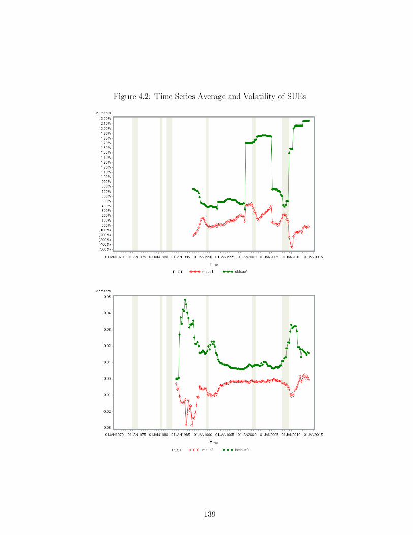
Figure 4.2: Time Series Average and Volatility of SUEs
139
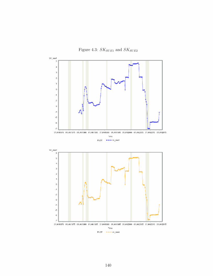
Figure 4.3: SKSUE1 and SKSUE2
140
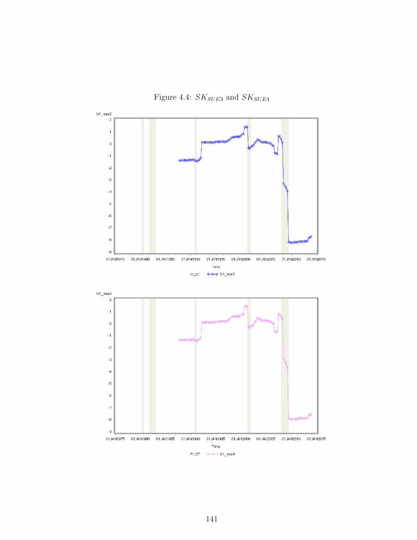
Figure 4.4: SKSUE3 and SKSUE4
141
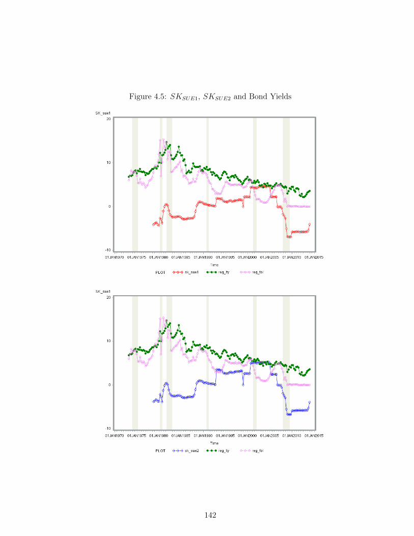
Figure 4.5: SKSUE1, SKSUE2 and Bond Yields
142
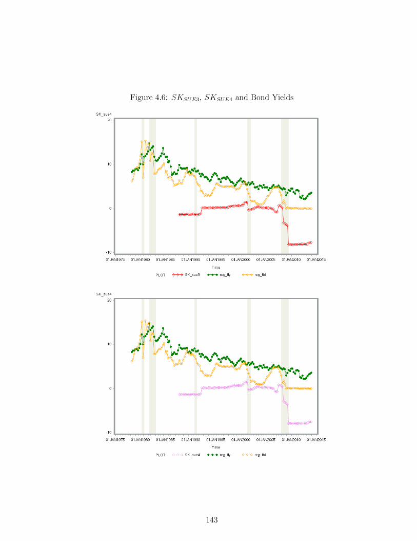
Figure 4.6: SKSUE3, SKSUE4 and Bond Yields
143

BIBLIOGRAPHY
[1] Andrew B Abel and Janice C Eberly. Optimal investment with costly reversibil-
ity. The Review of Economic Studies, 63(4):581–593, 1996.
[2] Daron Acemoglu, Vasco M Carvalho, Asuman Ozdaglar, and Alireza Tahbaz-
Salehi. The network origins of aggregate fluctuations. Econometrica,
80(5):1977–2016, 2012.
[3] Daron Acemoglu, Simon Johnson, and James A Robinson. Institutions as a
fundamental cause of long-run growth. Handbook of economic growth, 1:385–
472, 2005.
[4] Hengjie Ai, Mariano Massimiliano Croce, Anthony M Diercks, and Kai Li.
Production-based term structure of equity returns. Available at SSRN 2177191,
2013.
[5] Ferhat Akbas, Chao Jiang, and Paul Koch. The trend in firm profitability and
the cross section of stock returns. Available at SSRN, 2015.
[6] Rui Albuquerque. Skewness in stock returns: Reconciling the evidence on firm
versus aggregate returns. Review of Financial Studies, page hhr144, 2012.
[7] Andrew Ang, Robert J. Hodrick, Yuhang Xing, and Xiaoyan Zhang. The cross-
section of volatility and expected returns. Journal of Finance, 61:259–299,
2006.
[8] Robert L Axtell. Zipf distribution of us firm sizes. Science, 293(5536):1818–
1820, 2001.
144

[9] Adelchi Azzalini. A class of distributions which includes the normal ones. Scan-
dinavian journal of statistics, pages 171–178, 1985.
[10] Adelchi Azzalini and Alessandra Dalla Valle. The multivariate skew-normal
distribution. Biometrika, 83(4):715–726, 1996.
[11] Kerry Back. Asset pricing and portfolio choice theory. Oxford University Press,
2010.
[12] David K Backus, Silverio Foresi, and Liuren Wu. Accounting for biases in
black-scholes. Available at SSRN 585623, 2004.
[13] Per Bak, Kan Chen, Jose Scheinkman, and Michael Woodford. Aggregate fluc-
tuations from independent sectoral shocks: self-organized criticality in a model
of production and inventory dynamics. Ricerche Economiche, 47(1):3–30, 1993.
[14] Gurdip Bakshi, Charles Cao, and Zhiwu Chen. Empirical performance of alter-
native option pricing models. The Journal of finance, 52(5):2003–2049, 1997.
[15] Gurdip Bakshi, Nikunj Kapadia, and Dilip Madan. Stock returns characteris-
tics, skew laws, and the differential pricing of individual equity options. Review
of Financial Studies, 16:101–143, 2003.
[16] Turan G Bali, Nusret Cakici, and Robert F. Whitelaw. Maxing out: Stocks
as lotteries and the cross-section of expected returns. Journal of Financial
Economics, 99:427–446, 2011.
[17] Ray Ball, Joseph Gerakos, Juhani T Linnainmaa, and Valeri V Nikolaev. De-
flating profitability. Journal of Financial Economics (JFE), Forthcoming, pages
14–10, 2015.
[18] Ray Ball, Gil Sadka, and Ronnie Sdaka. Aggregate earnings and asset prices.
Journal of Accounting Research, 47:1097–1133, 2009.
145

[19] Ravi Bansal, Robert Dittmar, and Dana Kiku. Cointegration and consumption
risks in asset returns. Review of Financial Studies, 22(3):1343–1375, 2009.
[20] Ravi Bansal, Dana Kiku, Ivan Shaliastovich, and Amir Yaron. Volatility, the
macroeconomy, and asset prices. The Journal of Finance, 69(6):2471–2511,
2014.
[21] Ravi Bansal and Ivan Shaliastovich. Learning and asset-price jumps. Review
of Financial Studies, 24(8):2738–2780, 2011.
[22] Ravi Bansal and Amir Yaron. Risks for the long run: A potential resolution of
asset pricing puzzles. The Journal of Finance, 59(4):1481–1509, 2004.
[23] Ole E Barndorff-Nielsen and Neil Shephard. Econometrics of testing for jumps
in financial economics using bipower variation. Journal of financial Economet-
rics, 4(1):1–30, 2006.
[24] Sudipta Basu. The conservatism principle and the asymmetric timeliness of
earnings 1. Journal of accounting and economics, 24(1):3–37, 1997.
[25] David Bates. The crash of ’87: Was it expected? the evidence from options
markets. Journal of Finance, 46:69–107, 1991.
[26] Frederico Belo, Pierre Collin-Dufresne, and Robert S Goldstein. Dividend dy-
namics and the term structure of dividend strips. In AFA 2013 San Diego
Meetings Paper, 2013.
[27] Frederico Belo and Xiaoji Lin. The inventory growth spread. Review of Finan-
cial Studies, 25(1):278–313, 2012.
[28] Jonathan B Berk, Richard C Green, and Vasant Naik. Optimal investment,
growth options, and security returns. The Journal of Finance, 54(5):1553–1607,
1999.
146

[29] Antonio E Bernardo, Bhagwan Chowdhry, and Amit Goyal. Growth options,
beta, and the cost of capital. Financial Management, 36(2):1–13, 2007.
[30] Van Binsbergen, H Jules, and Ralph SJ Koijen. Predictive regressions: A
present-value approach. The Journal of Finance, 65(4):1439–1471, 2010.
[31] Fischer Black. Stuedies of stock price volatility changes. 1976.
[32] Oliver Boguth, Murray Carlson, Adlai J Fisher, and Mikhail Simutin. Leverage
and the limits of arbitrage pricing: Implications for dividend strips and the
term structure of equity risk premia. Available at SSRN 1931105, 2012.
[33] T. Bollerslev, G. Tauchen, and Hao Zhou. Expected stock return and variance
risk premium. Review of Financial Studies, 22:4463–4492, 2009.
[34] Brian Boyer, Todd Mitton, and Keith Vorkink. Expected idiosyncratic skew-
ness. Review of Financial Studies, 23:169–202, 2010.
[35] Jeremy I Bulow, John D Geanakoplos, and Paul D Klemperer. Multimarket
oligopoly: Strategic substitutes and complements. Journal of Political economy,
93(3):488–511, 1985.
[36] Ricardo J Caballero and Eduardo MRA Engel. Explaining investment dynamics
in us manufacturing: a generalized (s, s) approach. Econometrica, 67(4):783–
826, 1999.
[37] Ricardo J Caballero, Eduardo MRA Engel, John C Haltiwanger, Michael Wood-
ford, and Robert E Hall. Plant-level adjustment and aggregate investment dy-
namics. Brookings papers on economic activity, pages 1–54, 1995.
[38] John Y Campbell, Jens Hilscher, and Jan Szilagyi. In search of distress risk.
The Journal of Finance, 63(6):2899–2939, 2008.
147

[39] John Y. Campbell and Robert J. Shiller. Stock prices, earnings, and expected
dividends. Journal of Finance, 43:661–676, 1988.
[40] Mark M. Carhart. On persistence in mutual fund performance. Journal of
Finance, 52(1):57–82, 1997.
[41] Bo Young Chang, Peter Christoffersen, and Kris Jacobs. Market skewness
risk and the cross section of stock returns. Journal of Financial Economics,
107(1):46–68, 2013.
[42] Andrew A Christie. The stochastic behavior of common stock variances: Value,
leverage and interest rate effects. Journal of financial Economics, 10(4):407–
432, 1982.
[43] John H Cochrane. Production-based asset pricing and the link between stock
returns and economic fluctuations. The Journal of Finance, 46(1):209–237,
1991.
[44] John H Cochrane. The dog that did not bark: A defense of return predictability.
Review of Financial Studies, 21(4):1533–1575, 2008.
[45] Riccardo Colacito, Eric Ghysels, and Jianghan Meng. Skewness in expected
macro fundamentals and the predictability of equity returns: Evidence and
theory. University of North Carolina Working Paper, 2013.
[46] Jennifer Conrad, Robert F. Dittmar, and Eric Ghysels. Ex ante skewness and
expected stock returns. Journal of Finance, 61:85–124, 2013.
[47] Michael J Cooper, Huseyin Gulen, and Michael J Schill. Asset growth and the
cross-section of stock returns. The Journal of Finance, 63(4):1609–1651, 2008.
[48] Russell Cooper, John Haltiwanger, and Laura Power. Machine replacement and
the business cycle: lumps and bumps. Technical report, 1999.
148

[49] Mariano M Croce, Martin Lettau, and Sydney C Ludvigson. Investor infor-
mation, long-run risk, and the term structure of equity. Review of Financial
Studies, page hhu084, 2014.
[50] Mariano Massimiliano Croce. Long-run productivity risk: A new hope for
production-based asset pricing? Journal of Monetary Economics, 66:13–31,
2014.
[51] Zhi Da. Cash flow, consumption risk and cross section of stock returns. Con-
sumption Risk and Cross Section of Stock Returns (December 13, 2005), 2005.
[52] Zhi Da and Mitch Warachka. The disparity between long-term and short-term
forecasted earnings growth. Journal of Financial Economics, 100(2):424–442,
2011.
[53] Zhi Da and Mitchell Craig Warachka. Cashflow risk, systematic earnings revi-
sions, and the cross-section of stock returns. Journal of Financial Economics,
94(3):448–468, 2009.
[54] James L. Davis, Eugene F. Fama, and Kenneth R. French. Characteristics,
covariances, and average returns: 1929 to 1997. Journal of Finance, 55:389–
406, 2000.
[55] Steven J Davis, John Haltiwanger, Ron Jarmin, and Javier Miranda. Volatility
and dispersion in business growth rates: Publicly traded versus privately held
firms. In NBER Macroeconomics Annual 2006, Volume 21, pages 107–180. MIT
Press, 2007.
[56] Patrica M. Dechow and Douglas J. Skinner. Earnings management: Reconciling
the views of accounting academics, practitioners, and regulators. Accounting
Horizons, 14:235–250, 2000.
149

[57] Patricia M Dechow, Richard G Sloan, and Mark T Soliman. Implied equity
duration: A new measure of equity risk. Review of Accounting Studies, 9(2-
3):197–228, 2004.
[58] Francois Degeorge, Jayendu Patel, and Richard J. Zeckhause. Earnings man-
agement to exceed thresholds. Journal of Business, 72:1–33, 1999.
[59] Ilia D Dichev and Vicki Wei Tang. Matching and the changing properties of
accounting earnings over the last 40 years. The Accounting Review, 83(6):1425–
1460, 2008.
[60] Ilia D Dichev and Vicki Wei Tang. Earnings volatility and earnings predictabil-
ity. Journal of Accounting and Economics, 47(1):160–181, 2009.
[61] Karl B. Diether, Christopher J. Malloy, and Anna Scherbina. Differences of
opinion and the cross section of stock returns. Journal of Finance, 57(5):2113–
2141, 2002.
[62] Mark Doms and Timothy Dunne. Capital adjustment patterns in manufacturing
plants. Review of economic dynamics, 1(2):409–429, 1998.
[63] Itamar Drechsler and Amir Yaron. What’s vol got to do with it. Review of
Financial Studies, 24(1):1–45, 2011.
[64] Bill Dupor. Aggregation and irrelevance in multi-sector models. Journal of
Monetary Economics, 43(2):391–409, 1999.
[65] Steven N Durlauf. Nonergodic economic growth. The Review of Economic
Studies, 60(2):349–366, 1993.
[66] Steven N Durlauf. Path dependence in aggregate output. Industrial and Cor-
porate Change, 3(1):149–171, 1994.
150

[67] Eugene F. Fama and Kenneth R. French. The cross section of expected stock
returns. Journal of Finance, 47(2):427–465, 1992.
[68] Eugene F. Fama and Kenneth R. French. Common risk factors in the returns
on stocks and bonds. Journal of Financial Economics, 33(1):3–56, 1993.
[69] Eugene F. Fama and Kenneth R. French. Profitability, investment, and average
returns. Journal of Financial Economics, 82:491–518, 2006.
[70] Eugene F. Fama and Kenneth R. French. Dissecting anomalies. Journal of
Finance, 63:1653–1678, 2008.
[71] Eugene F. Fama and James D. MacBeth. Risk, return, and equilibrium: Em-
pirical tests. Journal of Political Economy, 81:607–636, 1973.
[72] Jesus Fernandez-Villaverde, Pablo A Guerron-Quintana, Keith Kuester, and
Juan Rubio-Ramırez. Fiscal volatility shocks and economic activity. Technical
report, National Bureau of Economic Research, 2011.
[73] Xavier Gabaix. Power laws in economics and finance. Technical report, National
Bureau of Economic Research, 2009.
[74] Xavier Gabaix. The granular origins of aggregate fluctuations. Econometrica,
79(3):733–772, 2011.
[75] Xavier Gabaix and Rustam Ibragimov. Rank- 1/2: a simple way to improve
the ols estimation of tail exponents. Journal of Business & Economic Statistics,
29(1):24–39, 2011.
[76] Nicolae Garleanu, Leonid Kogan, and Stavros Panageas. Displacement risk and
asset returns. Journal of Financial Economics, 105(3):491–510, 2012.
151

[77] Marc G Genton, Li He, and Xiangwei Liu. Moments of skew-normal random
vectors and their quadratic forms. Statistics & probability letters, 51(4):319–325,
2001.
[78] Dan Givoly and Carla Hayn. The changing time-series properties of earnings,
cash flows and accruals: Has financial reporting become more conservative?
Journal of Accounting and Economics, 29(3):287–320, 2000.
[79] Joao F Gomes, Leonid Kogan, and Lu Zhang. Equilibrium cross-section of
returns. 2003.
[80] Francois Gourio. Disasters risk and business cycles. Technical report, National
Bureau of Economic Research, 2009.
[81] Francois Gourio. Credit risk and disaster risk. Technical report, National
Bureau of Economic Research, 2011.
[82] Francois Gourio and Anil K Kashyap. Investment spikes: New facts and a
general equilibrium exploration. Journal of Monetary Economics, 54:1–22, 2007.
[83] Ian D. Gow and Daniel Taylor. Earnings volatility and the cross-section of
returns. Northwestern University Working Paper, 2009.
[84] John R. Graham, Campbell R. Harvey, and Shiva Rajgopal. The economic
implications of corporate financial reporting. Journal of Accounting and Eco-
nomics, 40:3–73, 2005.
[85] Zhaoyang Gu and Joanna Shuang Wu. Earnings skewness and analyst forecast
bias. Journal of Accounting and Economics, 35(1):5–29, 2003.
[86] Hui Guo, Kent Wang, and Hao Zhou. Good jumps, bad jumps, and conditional
equity premium. Bad Jumps, and Conditional Equity Premium (October 28,
2014), 2014.
152

[87] James D. Hamilton. Time Series Analysis. Princeton University Press, New
Jersey, 1994.
[88] Lars Peter Hansen, John C Heaton, and Nan Li. Consumption strikes back?
measuring long-run risk. Journal of Political Economy, 116(2):260–302, 2008.
[89] Campbell R. Harvey and Akhtar Siddique. Autoregressive conditional skewness.
Journal of Financial and Quantitative Analysis, 34:465–487, 1999.
[90] Campbell R. Harvey and Akhtar Siddique. Conditional skewness in asset pricing
tests. Journal of Finance, 55:1263–1295, 2000.
[91] Bernard Herskovic. Networks in production: Asset pricing implications. Avail-
able at SSRN 2615074, 2015.
[92] David Hirshleifer, Kewei Hou, Siew Hong Teoh, and Yinglei Zhang. Do in-
vestors overvalue firms with bloated balance sheets? Journal of Accounting
and Economics, 38:297–331, 2004.
[93] Harrison Hong, Jeffrey D. Kubik, and Amit Solomon. Security analysts career
concern and herding of earnings forecasts. The RAND Journal of Economics,
31:121–144, 2000.
[94] Harrison Hong, Terence Lim, and Jeremy C. Stein. Bad news travels slowly:
Size, analyst coverage, and the profitability of momentum strategies. Journal
of Finance, 55(1):265–295, 2000.
[95] Michael Horvath. Cyclicality and sectoral linkages: Aggregate fluctuations
from independent sectoral shocks. Review of Economic Dynamics, 1(4):781–
808, 1998.
[96] Michael Horvath. Sectoral shocks and aggregate fluctuations. Journal of Mon-
etary Economics, 45(1):69–106, 2000.
153

[97] Kewei Hou, Chen Xue, and Lu Zhang. Digesting anomalies: An investment
approach. Review of Financial Studies, 2014. forthcoming.
[98] Sudarshan Jayaraman. Earnings volatility, cash flow volatility, and informed
trading. Journal of Accounting Research, 46(4):809–851, 2008.
[99] Narasimhan Jegadeesh and Sheridan Titman. Returns to buying winners and
selling losers: Implications for stock market efficiency. The Journal of Finance,
48(1):65–91, 1993.
[100] Urban J Jermann. Asset pricing in production economies. Journal of monetary
Economics, 41(2):257–275, 1998.
[101] Yuecheng Jia and Weiping Li. Fundamental fluctuations, network origin, and
stock market returns. Oklahoma State University Working Paper, 2016.
[102] Yuecheng Jia and Shu Yan. Aggregate earnings skewness and stock market
returns. Oklahoma State University Working Paper, 2016.
[103] Yuecheng Jia and Shu Yan. What does skewness of firm fundamentals tell us
about firm growth, profitability, and stock returns. Oklahoma State University
Working Paper, 2016.
[104] George J Jiang, Danielle Xu, and Tong Yao. The information content of idiosyn-
cratic volatility. Journal of Financial and Quantitative Analysis, 44(01):1–28,
2009.
[105] Timothy C Johnson. Forecast dispersion and the cross section of expected
returns. Journal of Finance, 59(5):1957–1978, 2004.
[106] Boyan Jovanovic. Micro shocks and aggregate risk. The Quarterly Journal of
Economics, pages 395–409, 1987.
154

[107] Georg Kaltenbrunner and Lars A Lochstoer. Long-run risk through consump-
tion smoothing. Review of Financial Studies, 23(8):3190–3224, 2010.
[108] Aubhik Khan and Julia K Thomas. Idiosyncratic shocks and the role of noncon-
vexities in plant and aggregate investment dynamics. Econometrica, 76(2):395–
436, 2008.
[109] Leonid Kogan. An equilibrium model of irreversible investment. Journal of
Financial Economics, 62(2):201–245, 2001.
[110] Leonid Kogan. Asset prices and real investment. Journal of Financial Eco-
nomics, 73(3):411–431, 2004.
[111] M Koren and S Tenreyro. The growth and welfare effects of macroeconomic
volatility. Technical report, Working Paper, 2006.
[112] Smitu P Kothari and Jay Shanken. Book-to-market, dividend yield, and ex-
pected market returns: A time-series analysis. Journal of Financial Economics,
44(2):169–203, 1997.
[113] Alan Kraus and Robert Litzenberger. Skewness preference and the valuation of
risk assets. Journal of Finance, 31:1085–1100, 1976.
[114] Owen Lamont. Earnings and expected returns. The Journal of Finance,
53(5):1563–1587, 1998.
[115] John V Leahy. Investment in competitive equilibrium: The optimality of myopic
behavior. The Quarterly Journal of Economics, pages 1105–1133, 1993.
[116] Gary GJ Lee and Robert F Engle. A permanent and transitory component
model of stock return volatility. Available at SSRN 5848, 1993.
[117] Martin Lettau and Stijn Van Nieuwerburgh. Reconciling the return predictabil-
ity evidence. Review of Financial Studies, 21(4):1607–1652, 2008.
155

[118] Martin Lettau and Jessica A Wachter. Why is long-horizon equity less risky?
a duration-based explanation of the value premium. The Journal of Finance,
62(1):55–92, 2007.
[119] Martin Lettau and Jessica A Wachter. The term structures of equity and interest
rates. Journal of Financial Economics, 101(1):90–113, 2011.
[120] Jonathan Lewellen. Predicting returns with financial ratios. Journal of Finan-
cial Economics, 74(2):209–235, 2004.
[121] Jonathan Lewellen and Stefan Nagel. The conditional capm does not explain
asset-pricing anomalies. Journal of financial economics, 82(2):289–314, 2006.
[122] Erica XN Li, Dmitry Livdanw, and Lu Zhang. Anomalies. Review of Financial
Studies, page hhp023, 2009.
[123] Terence Lim. Rationality and analysts forecast bias. Journal of Finance,
56(1):369–385, 2001.
[124] Dmitry Livdan, Horacio Sapriza, and Lu Zhang. Financially constrained stock
returns. The Journal of Finance, 64(4):1827–1862, 2009.
[125] Joshua Livnat and Richard R Mendenhall. Comparing the post–earnings an-
nouncement drift for surprises calculated from analyst and time series forecasts.
Journal of Accounting Research, 44(1):177–205, 2006.
[126] Francis A Longstaff and Monika Piazzesi. Corporate earnings and the equity
premium. Journal of financial Economics, 74(3):401–421, 2004.
[127] Robert E Lucas. Understanding business cycles. In Carnegie-Rochester confer-
ence series on public policy, volume 5, pages 7–29. North-Holland, 1977.
156

[128] Evgeny Lyandres, Le Sun, and Lu Zhang. The new issues puzzle: Testing the
investment-based explanation. Review of Financial Studies, 21(6):2825–2855,
2008.
[129] Jinghan Meng. Skewness in opinions and the cross section of stock returns.
[130] Lior Menzly, Tano Santos, and Pietro Veronesi. Understanding predictability.
Journal of Political Economy, 112(1):1–47, 2004.
[131] Robert C. Merton. A simple model of capital market equilibrium with incom-
plete information. Journal of Finance, 42:483–510, 1987.
[132] Bernadette A Minton and Catherine Schrand. The impact of cash flow volatility
on discretionary investment and the costs of debt and equity financing. Journal
of Financial Economics, 54(3):423–460, 1999.
[133] Charles R Nelson and Myung J Kim. Predictable stock returns: The role of
small sample bias. The Journal of Finance, 48(2):641–661, 1993.
[134] Robert Novy-Marx. The other side of value: The gross profitability premium.
Journal of Financial Economics, 108:1–28, 2013.
[135] Patricia C O’brien. Analysts’ forecasts as earnings expectations. Journal of
accounting and Economics, 10(1):53–83, 1988.
[136] Jun Pan. The jump-risk premia implicit in options: Evidence from an integrated
time-series study. Journal of financial economics, 63(1):3–50, 2002.
[137] L’ubos Pastor and Robert F Stambaugh. Predictive systems: Living with im-
perfect predictors. The Journal of Finance, 64(4):1583–1628, 2009.
[138] Stephen H. Penman and Xiao-Jun Zhang. Accounting conservatism, the quality
of earnings, and stock returns. Accounting Review, 77(2):237–264, 2002.
157

[139] Jeffrey Pontiff and Lawrence D Schall. Book-to-market ratios as predictors of
market returns. Journal of Financial Economics, 49(2):141–160, 1998.
[140] Thomas A Rietz. The equity risk premium a solution. Journal of monetary
Economics, 22(1):117–131, 1988.
[141] Anna Scherbina. Suppressed negative information and future underperfor-
mance. Review of Finance, 12(3):533–565, 2008.
[142] Gill Segal, Ivan Shaliastovich, and Amir Yaron. Good and bad uncertainty:
Macroeconomic and financial market implications. Unpublished paper, 2015.
[143] Mark T Soliman. The use of dupont analysis by market participants. The
Accounting Review, 83(3):823–853, 2008.
[144] Tommy Sveen and Lutz Weinke. Lumpy investment, sticky prices, and the
monetary transmission mechanism. Journal of Monetary Economics, 54:23–36,
2007.
[145] Julia K Thomas. Is lumpy investment relevant for the business cycle? Journal
of Political Economy, 110(3):508–534, 2002.
[146] Sheridan Titman, K. C. John Wei, and Feixue Xie. Capital investments and
stock returns. Journal of Financial and Quantitative Analysis, 39:677–700,
2004.
[147] James Tobin. A general equilibrium approach to monetary theory. Journal of
money, credit and banking, 1(1):15–29, 1969.
[148] Jerry Tsai and Jessica A Wachter. Rare booms and disasters in a multisector
endowment economy. Review of Financial Studies, page hhv074, 2016.
[149] Brandt van Binsbergen and Koijen. On the timing and pricing of dividends.
American Economic Review, 102:1596–1618, 2012.
158

[150] Jules van Binsbergen, Wouter Hueskes, Ralph Koijen, and Evert Vrugt. Equity
yields. Journal of Financial Economics, 110(3):503–519, 2013.
[151] Stijn Van Nieuwerburgh, Hanno Lustig, Bryan Kelly, et al. Firm volatility in
granular networks. In 2014 Meeting Papers, number 253. Society for Economic
Dynamics, 2014.
[152] Tuomo Vuolteenaho. What drives firm-level stock returns? Journal of Finance,
57:233–264, 2002.
[153] Ross L. Watts. Conservatism in accounting part I: Explanations and implica-
tions. Accounting Horizons, 17:207–221, 2003.
[154] Gregory Waymire. Earnings volatility and voluntary management forecast dis-
closure. Journal of Accounting Research, pages 268–295, 1985.
[155] Yuhang Xing. Interpreting the value effect through the q-theory: An empirical
investigation. Review of Financial Studies, 21(4):1767–1795, 2008.
[156] Amihud Y. Illiquidity and stock returns: cross-section and time-series effects.
Journal of financial markets, 5(1):259–299, 2002.
[157] Shu Yan. Jump risk, stock returns, and slope of implied volatility smile. Journal
of Financial Economics, 99(1):216–233, 2011.
[158] Wei Yang. Long-run risk in durable consumption. Journal of Financial Eco-
nomics, 102(1):45–61, 2011.
[159] Lu Zhang. The value premium. The Journal of Finance, 60(1):67–103, 2005.
159

VITA
Yuecheng Jia
Candidate for the Degree of
Doctor of Philosophy
Dissertation: Essays on the Skewness of Firm Fundamentals and Stock Re-turns
Major Field: Finance
Biographical:
Education:
Completed the requirements for the Doctor of Philosophy degree in Finance atOklahoma State University in May, 2016.
Completed the requirements for Master of Science in Finance at Case WesternReserve University, Cleveland, Ohio in January, 2011.
Completed the requirements for Bachelor of Law at Dongbei University of Fi-nance and Economics, Dalian, Liaoning, China in June, 2009.
Experience:
Professional Memberships:
Related Documents