ESSAYS ON PATENT LITIGATION, PATENT MONETIZATION ...

ESSAYS ON PATENT LITIGATION, PATENT MONETIZATION,

AND ENTREPRENEURIAL FIRMS

A Dissertation

Submitted to the Faculty

of

Purdue University

by

Mingtao Xu

In Partial Fulfillment of the

Requirements for the Degree

of

Doctor of Philosophy

August 2020

Purdue University

West Lafayette, Indiana

ii

THE PURDUE UNIVERSITY GRADUATE SCHOOLSTATEMENT OF DISSERTATION APPROVAL

Dr. Richard Makadok, Co-Chair

Krannert School of Management, Purdue University

Dr. Tony W. Tong, Co-Chair

Leeds Business School, University of Colorado

Dr. Thomas Brush


Dr. Umit Ozmel


Approved by:

Dr. Yanjun Li


iii

To my parents and Ni.

iv

ACKNOWLEDGMENTS

In retrospect, my heartfelt feeling is how lucky I have been having such a fantastic

committee with members who are also my role models. At first, I want to thank

Prof. Richard Makadok for being my mentor and advisor all the time since the day I

embarked on the Ph.D. program. Rich fundamentally influenced my view regarding

research and scholarship. I always remember the sentence in his email signature: ”It

is better to fail in originality than to succeed in imitation.” It has been an honor to

be supervised by such a great mentor and scholar.

I also owe the greatest gratitude to Prof. Tony Tong for the numerous suggestions

he gave me and the experiences he shared with me, covering every facet of research,

academics, and life as an international student. Tony was also the first person to

introduce the topic of patent monetization to me. Regardless of the difficulties of

geographical distance, his mentorship, and his high standard towards research have

made countless contributions far beyond this dissertation and have helped me to

become an independent scholar.

I am also fortunate to have Prof. Umit Ozmel on my committee. She always

supports me, and every suggestion she gave, whether in a one-to-one meeting or a

seminar, was always insightful. Besides, Prof. Thomas Brush brought his familiarity

with the context and helped the dissertation with his comments and critics since the

ideation stage.

It would be impossible for me to finish the Ph.D. without the company of my

amazing colleagues who have seen my ups and downs every day of my Ph.D. life.

I thank Kubilay Cirik, whom I know before starting the doctoral program, for the

numerous conversations about academia and career. I also thank Dalee, Moon, and

v

Anpu in my cohort for their constant encouragement, support, research discussions,

as well as information for the job search. I am also indebted to Sandi, Daniel, Ashish,

Karen, and Nianchen, with whom I have shared offices. They have been incredible

office mates and friends, and have left me so many delightful memories of life at West

Lafayette. Also, I would like to express my gratefulness to my other colleagues and

friends, including Monica Guo, Crystal Bien, Jongsoo Kim, Joonhyung Bae, Cyril

Tae Um, Wenqian Wang, Koungjin Lim, Jing Tang, Jiabei Hu, Xuewen, Yifei, Hao,

and Kun.

In the end, no words can come close to describe my thankfulness to my parents

Cheng Xu and Shengxun Hu, for their selfless love and always being my mightiest

backup. During all these years when I pursue the degree, they are always there with

me though we are thousands of miles apart most of the time. Lastly, I want to

express with my whole heart my gratitude to Ni for entering my life, and for her

understanding and trust in me. I look forward to entering the next journey of our

life.

This research is funded in part by the Bilsland Dissertation Fellowship generously

granted by Purdue University Graduate School and Krannert School of Management.

Mingtao Xu is solely responsible for the contents of this research.

vi

TABLE OF CONTENTS

Page

LIST OF TABLES . . . . . . . . . . . . . . . . . . . . . . . . . . . . . . . . . . ix

LIST OF FIGURES . . . . . . . . . . . . . . . . . . . . . . . . . . . . . . . . . xi

ABBREVIATIONS . . . . . . . . . . . . . . . . . . . . . . . . . . . . . . . . . . xii

GLOSSARY . . . . . . . . . . . . . . . . . . . . . . . . . . . . . . . . . . . . . . xiii

ABSTRACT . . . . . . . . . . . . . . . . . . . . . . . . . . . . . . . . . . . . . xv

1 INTRODUCTION . . . . . . . . . . . . . . . . . . . . . . . . . . . . . . . . 11.1 The Value of Resources is in the Eye of the Beholder . . . . . . . . . . 11.2 The Multiplicity of Business Models Surrounding Intellectual Properties 11.3 Significance of the Context . . . . . . . . . . . . . . . . . . . . . . . . . 31.4 Outline of Essays . . . . . . . . . . . . . . . . . . . . . . . . . . . . . . 6

2 TROLLING FOR DOLLARS: A THEORY OF PATENTMONETIZATION, COMPETING BUSINESS MODELS, ANDNON-PRACTICING ENTITIES . . . . . . . . . . . . . . . . . . . . . . . . . 82.1 Introduction . . . . . . . . . . . . . . . . . . . . . . . . . . . . . . . . . 8

2.1.1 Impact of competing business models on strategic factor markets 82.1.2 Business models and patent monetization methods . . . . . . . 102.1.3 Technological versus exclusionary strength and relative

valuation by PEs and NPEs . . . . . . . . . . . . . . . . . . . . 112.2 Alternative Monetization of Patents: PEs, NPEs, and Defensive

Aggregators . . . . . . . . . . . . . . . . . . . . . . . . . . . . . . . . . 142.2.1 NPEs versus PEs . . . . . . . . . . . . . . . . . . . . . . . . . . 142.2.2 NPEs versus other Non-Practicing patent holders . . . . . . . . 17

2.3 The Model Setup . . . . . . . . . . . . . . . . . . . . . . . . . . . . . . 192.3.1 Patent and firm heterogeneity . . . . . . . . . . . . . . . . . . . 192.3.2 Decisions . . . . . . . . . . . . . . . . . . . . . . . . . . . . . . 21

2.4 Value Appropriation Mechanisms . . . . . . . . . . . . . . . . . . . . . 232.4.1 Practicing Monetization . . . . . . . . . . . . . . . . . . . . . . 242.4.2 Litigating Monetization . . . . . . . . . . . . . . . . . . . . . . 31

2.5 Equilibrium . . . . . . . . . . . . . . . . . . . . . . . . . . . . . . . . . 37

vii

Page2.5.1 Equilibrium monetization method as a function of

technological and exclusionary strength . . . . . . . . . . . . . 372.5.2 Equilibrium monetization method as a function of exclusivity

alone . . . . . . . . . . . . . . . . . . . . . . . . . . . . . . . . . 402.6 Extension: End Users as Litigation Targets . . . . . . . . . . . . . . . . 452.7 Empirical Implications . . . . . . . . . . . . . . . . . . . . . . . . . . . 452.8 Managerial Implications . . . . . . . . . . . . . . . . . . . . . . . . . . 462.9 Concluding Remarks, Caveats, Limitations, and Opportunities . . . . . 48

3 LITIGATING MONETIZATION AND PATENT TROLLS: EVIDENCEFROM THE PATENT MARKET . . . . . . . . . . . . . . . . . . . . . . . . 513.1 Introduction . . . . . . . . . . . . . . . . . . . . . . . . . . . . . . . . . 513.2 PAEs as Patent Intermediaries and Litigating Monetization as a

Business Model . . . . . . . . . . . . . . . . . . . . . . . . . . . . . . . 563.3 Theory . . . . . . . . . . . . . . . . . . . . . . . . . . . . . . . . . . . . 58

3.3.1 Technological strength and patent acquisition . . . . . . . . . . 583.3.2 Scope of property rights and patent acquisition . . . . . . . . . 613.3.3 Security of patent rights, invalidation risk and patent acquisition 65

3.4 Empirical Strategy . . . . . . . . . . . . . . . . . . . . . . . . . . . . . 663.4.1 Data . . . . . . . . . . . . . . . . . . . . . . . . . . . . . . . . . 663.4.2 Measures . . . . . . . . . . . . . . . . . . . . . . . . . . . . . . 683.4.3 Institutional background . . . . . . . . . . . . . . . . . . . . . . 693.4.4 Exposure to patent challenges . . . . . . . . . . . . . . . . . . . 74

3.5 Results . . . . . . . . . . . . . . . . . . . . . . . . . . . . . . . . . . . . 773.5.1 Technological strength, Scope, and PAE acquisition . . . . . . . 773.5.2 Invalidation risk and PAE acquisition: The impact of AIA . . . 82

3.6 Robustness . . . . . . . . . . . . . . . . . . . . . . . . . . . . . . . . . 863.6.1 Other measures of technological quality . . . . . . . . . . . . . . 863.6.2 Instrumental variable results on exclusion scope . . . . . . . . . 893.6.3 Other measures of the exclusion scope . . . . . . . . . . . . . . 893.6.4 Invalidation risk, the case of software patents . . . . . . . . . . 913.6.5 Intensive margin: Firm-level results on AIA and PAEs’

acquisitions . . . . . . . . . . . . . . . . . . . . . . . . . . . . . 973.7 Additional Analysis . . . . . . . . . . . . . . . . . . . . . . . . . . . . . 97

3.7.1 Family size, technological strength, and internationalization . . 973.7.2 Litigation history as a signal of litigating value . . . . . . . . . 1013.7.3 Litigation following PAE acquisition . . . . . . . . . . . . . . 102

3.8 Caveats and Boundary Conditions . . . . . . . . . . . . . . . . . . . . 1023.9 Concluding Remarks . . . . . . . . . . . . . . . . . . . . . . . . . . . 106

4 HOW DOES PATENT LITIGATION AFFECT ENTREPRENEURIALVENTURE FINANCING? . . . . . . . . . . . . . . . . . . . . . . . . . . . 1094.1 Introduction . . . . . . . . . . . . . . . . . . . . . . . . . . . . . . . . 109

viii

Page

4.2 Theory and Hypotheses . . . . . . . . . . . . . . . . . . . . . . . . . 1124.2.1 Patent litigation, Signaling, and Entrepreneurial Financing . . 1124.2.2 Heterogeneity among startups: Alternative Quality Signals . . 1144.2.3 Heterogeneity among plaintiffs: Being sued by PAEs . . . . . 116

4.3 Empirical Strategy . . . . . . . . . . . . . . . . . . . . . . . . . . . . 1174.3.1 Data and Sample Construction . . . . . . . . . . . . . . . . . 1174.3.2 Matching Procedures . . . . . . . . . . . . . . . . . . . . . . . 1184.3.3 Instrumental Variables . . . . . . . . . . . . . . . . . . . . . . 1194.3.4 Variables . . . . . . . . . . . . . . . . . . . . . . . . . . . . . . 1204.3.5 Regression Analysis . . . . . . . . . . . . . . . . . . . . . . . . 122

4.4 Results . . . . . . . . . . . . . . . . . . . . . . . . . . . . . . . . . . . 1234.5 Robustness . . . . . . . . . . . . . . . . . . . . . . . . . . . . . . . . 128

4.5.1 Time to the Next Round . . . . . . . . . . . . . . . . . . . . . 1284.5.2 Matched Locations . . . . . . . . . . . . . . . . . . . . . . . . 1324.5.3 Placebo Test . . . . . . . . . . . . . . . . . . . . . . . . . . . 134

4.6 Caveats . . . . . . . . . . . . . . . . . . . . . . . . . . . . . . . . . . 1374.7 Concluding Remarks . . . . . . . . . . . . . . . . . . . . . . . . . . . 137

BIBLIOGRAPHY . . . . . . . . . . . . . . . . . . . . . . . . . . . . . . . . . 140

A APPENDIX TO CHAPTER 2 . . . . . . . . . . . . . . . . . . . . . . . . . 159

B APPENDIX TO CHAPTER 3 . . . . . . . . . . . . . . . . . . . . . . . . . 163

C APPENDIX TO CHAPTER 4 . . . . . . . . . . . . . . . . . . . . . . . . . 182

VITA . . . . . . . . . . . . . . . . . . . . . . . . . . . . . . . . . . . . . . . . 189

ix

LIST OF TABLES

Table Page

2.1 Summary of Nine Equilibrium Sequences . . . . . . . . . . . . . . . . . . . 42

3.1 Variable Definitions . . . . . . . . . . . . . . . . . . . . . . . . . . . . . . . 70

3.2 Patent-Transaction-Level Descriptive Statistics . . . . . . . . . . . . . . . . 71

3.3 Technological strength, scope, and the likelihood of PAE acquisition . . . . 79

3.4 Invalidation Risk and PAE patent acquisition . . . . . . . . . . . . . . . . 83

3.5 Heterogeneous impact of invalidation risk on PAE acquisition . . . . . . . 87

3.6 Citations to Non-Patent Literature and the likelihood of PAE acquisition . 88

3.7 IV Regression of Patent Scope and PAE acquisition . . . . . . . . . . . . . 90

3.8 Alternative Measures of Patent Scope . . . . . . . . . . . . . . . . . . . . . 92

3.9 Software patents and PAE acquisition . . . . . . . . . . . . . . . . . . . . . 95

3.10 Firm-Level PAEs’ patent acquisitions . . . . . . . . . . . . . . . . . . . . . 98

3.11 Patent Family Size and the likelihood of PAE acquisition . . . . . . . . . 100

3.12 PAE acquisition and subsequent patent litigation . . . . . . . . . . . . . 103

4.1 Descriptive Statistics . . . . . . . . . . . . . . . . . . . . . . . . . . . . . 121

4.2 Validity of Instruments . . . . . . . . . . . . . . . . . . . . . . . . . . . . 124

4.3 2SLS Results on the Effect of Patent Litigation on VC Financing . . . . 126

4.4 Dynamic Effects of Patent Litigation on the Likelihood of VC Financing 127

4.5 Heterogeneous Effect of Patent Litigation on the Likelihood VC Financing 129

4.6 Heterogeneous Effect of Patent Litigation on VC Financing Amount . . . 130

4.7 Descriptive statistics for Hazard Models . . . . . . . . . . . . . . . . . . 131

4.8 Time to Next Round: Hazard Model Results . . . . . . . . . . . . . . . . 133

4.9 Effect of Patent Litigation on the Likelihood of VC Financing . . . . . . 135

x

Table Page

4.10 Effect of Patent Litigation on the Amount of VC Financing . . . . . . . 136

B.1 Top 20 PAEs with Most Patent Acquisitions . . . . . . . . . . . . . . . 173

B.2 Distribution of Exposure Index for CPC Subclasses . . . . . . . . . . . . 174

B.3 Correlation Matrix . . . . . . . . . . . . . . . . . . . . . . . . . . . . . . 175

B.4 Exploratory analysis on Technological Strengths and the Likelihood ofPAE acquisition . . . . . . . . . . . . . . . . . . . . . . . . . . . . . . . . 176

B.5 Alternative measures of Exposure and he impact of AIA . . . . . . . . . 178

B.6 Patent Acquisitions by Public PAEs 2007-2017 . . . . . . . . . . . . . . . 179

B.7 Firm-Level Variable Definitions . . . . . . . . . . . . . . . . . . . . . . . 179

B.8 Firm-Level Descriptive Statistics . . . . . . . . . . . . . . . . . . . . . . 180

B.9 CPC class and subclasses that received most PTAB petitions . . . . . . . 181

C.1 Descriptive Statistics of Alternative Matched Sample . . . . . . . . . . . 183

C.2 Correlation Table of Alternative Matched Sample . . . . . . . . . . . . . 184

C.3 Robustness: Effect of Patent Litigation on the Likelihood of ReceivingVC Financing . . . . . . . . . . . . . . . . . . . . . . . . . . . . . . . . . 187

C.4 Robustness: Effect of Patent Litigation on the Amount of VC Financing 188

xi

LIST OF FIGURES

Figure Page

1.1 Number of Patent Litigations by Quarter before and after AIA . . . . . . . 4

2.1 Timeline of the model . . . . . . . . . . . . . . . . . . . . . . . . . . . . . 23

2.2 Values from Practicing and Litigating monetization in x . . . . . . . . . . 30

2.3 The Litigating Game Tree . . . . . . . . . . . . . . . . . . . . . . . . . . . 33

2.4 Optimal Monetization Method . . . . . . . . . . . . . . . . . . . . . . . . . 39

2.5 Region of Optimal Monetization Method . . . . . . . . . . . . . . . . . . . 41

2.6 Equilibrium Monetization Method as a function of x . . . . . . . . . . . . 44

2.7 Value Appropriation and Patent Monetization Framework . . . . . . . . . 48

3.1 Share of PAEs’ Patent Acquisitions by Technology Fields . . . . . . . . . . 54

3.2 Observed patent acquisitions by PEs and PAEs . . . . . . . . . . . . . . . 64

3.3 Timeline of major events relevant to PAEs . . . . . . . . . . . . . . . . . . 69

3.4 Number of PTAB Complaints Filed by CPC Subclasses 2012/9-2019/3 . . 73

3.5 Share of PAEs’ Patent Acquisitions in All Transactions . . . . . . . . . . . 75

3.6 Age and PAE acquisition . . . . . . . . . . . . . . . . . . . . . . . . . . . . 80

3.7 Scope and PAE acquisition . . . . . . . . . . . . . . . . . . . . . . . . . . . 81

3.8 PAEs’ acquisitions by exposure to patent invalidation . . . . . . . . . . . . 84

3.9 Coefficient plot of exposure to invalidation and PAE acquisition . . . . . . 85

3.10 PAEs’ acquisition of Software Patents before and after AIA . . . . . . . . 94

3.11 Coefficient plot on Software Patents . . . . . . . . . . . . . . . . . . . . . . 96

3.12 Litigation History and PAE acquisition before and after AIA . . . . . . . 101

4.1 Matching Procedures . . . . . . . . . . . . . . . . . . . . . . . . . . . . . 119

B.1 Values from Practicing and Litigating Monetization . . . . . . . . . . . . 167

xii

ABBREVIATIONS

PE Practicing Entity

NPE Non-Practicing Entity

PAE Patent Assertion Entity

SEPs Standard Essential Patents

AIA America Invents Act

PTAB Patent Trial and Appeal Board

PGR Post-Grant Review

IPR Inter Partes Review

CBM Covered Business Methods

USPTO United States Patent and Trademark Office

CPC Cooperative Patent Classification

IPC International Patent Classification

FTC Federal Trade Commission

SFM Strategic Factor Market

VC Venture Capital

CVC Corporate Venture Capital

xiii

GLOSSARY

PAEs Patent Assertion Entities, also known as patent trolls, ”are busi-

nesses that acquire patents from third parties and seek to generate

revenue by asserting them against alleged infringers.”(Quote from

Federal Trade Commission (2016))

NPE a Non-Practicing Entity, as opposed to an PE (practicing en-

tity), owns and claims rights on patents but does not practice the

patented technology to produce and offer products and services.

BMPs Business method patents, a category of patents that do not cover

concrete inventions, but a new way of doing business, usually

combined with technology.

AIA America Invents Act, an act passed in 2011 and enacted in 2012

and 2013 that reforms the US patent system, established PTAB,

and changes the US patent system from first-to-invent to first

inventor-to-file.

PGR Post-Grant Review, a proceeding at PTAB that allows patents to

be challenged within nine months of its grant, the case must be

completed within 12 months from institution.

IPR Inter Partes Review, a proceeding at PTAB that allows a third

party to challenge the validity of patents that were granted more

than nine months prior, the case must be completed within 12

months from institution.

xiv

CBM Covered Business Methods, a transitional proceeding at PTAB

that specifically allows accused infringers of certain covered busi-

ness method patents to challenge the validity of patents, this

program is available until September 15, 2020. The case must be

completed within 12 months from institution.

CPC Cooperative Patent Classification is a patent classification system

cooperatively developed by the USPTO and the EPO (European

Patent Office)

Alice Alice Corp. v. CLS Bank International, 573 U.S. 208 (2014), was

a decision announced in June 2014 by the United States Supreme

Court on eligibility of software patents.

xv

ABSTRACT

Xu, Mingtao PhD, Purdue University, August 2020. Essays on Patent Litigation,Patent Monetization, and Entrepreneurial Firms. Major Professor: Richard Makadok.

This dissertation studies how patents are monetized via legal actions without prac-

ticing the technology and the implications to firms. In recent years, scholars in other

fields have extensively studied patent monetization and litigation regime, given the

importance of technological innovation and commercialization to the strategy field,

strategy scholars have been underrepresented on the topic of patent litigation and

monetization. In this dissertation, I develop a theory on how heterogeneity in firms’

business models monetizing resources determine firms’ heterogeneity in valuation and

acquisition of resources. Using a context of patents, we study two primary business

models monetizing patents, namely, the practicing monetization and litigating mone-

tization, which differ fundamentally in their value appropriation mechanisms. On the

one hand, the value appropriation mechanism for practicing monetization relies on

the value created by the firm’s deployment of the patented technology in the product

market, and from the restraint of rivalry via excluding competitors from accessing

the patented technology. On the other hand, litigating monetization depends on

the strength of legal actions and the ability to collect payments from target firms

to the patent-owning firm, in forms such as settlement fees and damages awarded

by the court. The theorization reclarifies the two types of patent heterogeneity: in-

novativeness and exclusivity, and theorize that differences in patents’ innovativeness

and exclusivity lead to differences in the expected profit from practicing and litigating

monetization, thus leading to a difference in optimal monetization strategy and firms’

different preferences for resource acquisition.

xvi

In Essay 1, we develop the aforementioned theory of patent monetization using

formal models to understand the relationships among firms’ business models, patent

characteristics, and the optimal monetization strategy. We show the situations where

litigating monetization can prevail and be the method that maximizes patents’ value.

We further predict that compared to patents that are practiced to produce products

or services, patents monetized in a litigating manner are ones that are relatively less

technologically innovative. Then, in Essay 2, I use the patent monetization context

to investigate how firms’ business models affect their resource acquisition behavior in

the factor market, i.e., the market of patents. Exploiting recent institutional changes

such as the enactment of the American Invents Act (AIA) that asymmetrically influ-

enced different business models, I show that firms specialize in litigating monetization

disproportionately acquire highly cited but old patents and patents that were litigated

before. Then Essay 3, rooted in the literature that patents are essential signals from

entrepreneurial firms to investors, I examine how disputes in patents in the form of

litigations affect entrepreneurial firms’ obtaining of external financing.

1

CHAPTER 1 INTRODUCTION

1.1 The Value of Resources is in the Eye of the Beholder

A firm’s ability to earn superior returns on resources purchased in the factor

market may depend upon the firm’s private information about the resource’s value

(Barney, 1986), but it also depends upon whether the firm can use the resource

to create value in a way that competing bidders cannot. Thus, resources, even as

mundane as product inventory, may be valued differently by firms, if they obtain dif-

ferent synergies by monetizing that inventory in different ways, such as sales, rentals,

leases, or subscriptions. For example, movie DVDs may be valued differently by

RedBox, Netflix, and Walmart, since their different monetization methods create dif-

ferent synergies. More generally, resource-market competition between firms from

different product markets (Markman et al., 2009) or with different business models

(Casadesus-Masanell and Zhu, 2010, 2013) can affect the valuation of any produc-

tive resource, the identity of the firm that ultimately acquires the resource, and the

amount of value the acquiring firm can both create with and appropriate from that

resource.

1.2 The Multiplicity of Business Models Surrounding Intellectual Prop-

erties

Patents are yet another type of resource where different firms may seek to obtain

different synergies, according to each firm’s capabilities and appropriation/monetization

strategy (Hsu and Ziedonis, 2013; Steensma et al., 2016). Research on the market

for technology views the external acquisition of patents as a substitute for firms’ in-

2

ternal development of technologies (Arora and Gambardella, 2010). Following this

logic, the value of the patent, represented in licensing, self-commercializing, or other

commercialization methods, primarily depends on the technical value of the patent

(Arora and Gambardella, 1994, 2010; Marx and Hsu, 2015) and its resulting value

as a signal of quality to external stakeholders (Hsu and Ziedonis, 2013). Using a

patent in this way not only requires that the implementation of the patent’s technol-

ogy, but also that the firm must prevent competitors from doing so as well (Capron

and Chatain, 2008). Therefore, a crucial intention for acquiring patents is to prevent

rivals from accessing the technology (Bessen and Maskin, 2009). The exclusionary

value of patents makes the idiosyncrasy of resource valuation more prominent in the

market for patents (Grimpe and Hussinger, 2014). Firms that monetize patents in

this conventional way are often called practicing entities (PEs). However, a firm can

also monetize patents without implementing the technology, or even without par-

ticipating in the product market. In particular, patent assertion entities (PAEs) or

non-practicing entities (NPEs), often labeled derisively as patent trolls in public pol-

icy discourse, represent a relatively new form of business (Steensma et al., 2016) that

monetize patents purely through litigation, with no intention of either entering the

product market or using their patents as a quality signal (Cohen et al., 2016).

So far, research on patent litigation and PAEs has explored such predatory meth-

ods (Cohen et al., 2020), as well as their impact on social welfare and their im-

plications for intellectual property policy (Appel et al., 2020). Little has studied

the factor-market competition between PEs and PAEs as they both seek to acquire

patents. Consequently, many questions remain unanswered, such as: How does the

competition between PE and PAE business models affect the market valuation of

patents? How much value can be appropriated from a patent by either PEs or PAEs?

What factors determine the amount of value that PEs or PAEs can appropriate from

a patent? Under what conditions would one expect PAEs to outbid PEs for a patent,

and vice versa? What are the consequences of lawsuits by PEs and PAEs?

3

As a starting point on the path toward answering these questions, in this dis-

sertation, we develop a formal model and then empirically test differences in the

practicing (PEs’) and the litigating (PAEs’) methods for patent monetization. On

the one hand, the value appropriation mechanism for practicing monetization relies

on the extra value created by the PE’s deployment of the patented technology in

the product market, and from the restraint of rivalry via excluding rivals from the

patented technology. On the other hand, the value appropriation mechanism for lit-

igating monetization depends on the payment of the litigating target, in forms of

either settlement fee or licensing fee. We re-clarify the two types of differences in

patents: innovativeness and exclusivity, and theorize that differences in patents’ in-

novativeness and exclusivity lead to differences in the expected profit from practicing

and litigating monetization, and deduce from the profit differential the optimal mon-

etization methods for patents. We show the situations where litigating monetization

can prevail and be the method that maximizes patents’ value. We further predict

that compared to patents that are practiced to produce products or services, patents

monetized in a litigating manner are ones that are exclusive but less innovative.

1.3 Significance of the Context

Because of the assertive nature of their business model, this relatively new type of

organization that specializes in the litigating monetization of patents is often called

Patent Assertion Entities (PAEs), Non-Practicing Entities (NPEs), or patent trolls.

PAEs’ business model for patents is different from that of practicing entities (PEs) or

practicing firms in that PAEs have no stake in the product market (Choi and Gerlach,

2018). Because PAEs do not produce any products or services using the patented

technologies, they are much less susceptible to counter lawsuits. Without much to

lose, PAEs exploit the judicial system aggressively to capture value from patents

via legal actions against other firms. Those actions bring extensive controversies

and criticisms (Cohen et al., 2016; Leiponen and Delcamp, 2019). Figure 1.1 shows

4

quarterly numbers of patent lawsuits initiated by PAEs and other entities at US

Federal District Courts from 2000 to 2018. As shown, most of the recent increase in

the number of patent litigations came from PAE plaintiffs. In some peak years, PAEs

make up more than 60% of all patent litigations filed in a year.

Figure 1.1.: Number of Patent Litigations by Quarter before and after AIA

Notes: (1) The x-axis is Year-Quarter that covers quarters from 2007 Q1 to 2018 Q4. The y-axis isthe count of patent litigations in each quarter with the shaded histograms indicate patent litigationsinitiated by PAEs. (2) Two vertical lines mark 2012 Q4 and 2013 Q2, which are the times when twobatches of the AIA statutes took effect. The AIA provisions that changed post-grant oppositionswent effective on Sept. 16th, 2012. (3) The graph shows the fast-increasing PAE litigations beforethe AIA, and its decline in the post-AIA period.

PAEs’ litigating monetization is also controversial at the policy level. The in-

tention for building a strong patent system is to encourage innovation, to lower the

transaction cost, to help the development of the market for technology (Arora and Fos-

furi, 2003), and to facilitate technology commercialization (Dechenaux et al., 2008).

PAEs’ activities of exploiting a strong patent system, however, could hurt innovation

(Abrams et al., 2019). Firms’ innovation can be harmed as frivolous litigations ini-

tiated by PAEs divert substantial resources of practicing firms to handling lawsuits

and threats. Such distractions deprive firms’ capabilities to innovate (Leiponen and

Delcamp, 2019). The negative consequences of legal actions by PAEs are especially

severe for small entrepreneurial firms, which consist of more than half of PAEs’ de-

5

fendants (Chien, 2013). As startups usually lack resources, the extra burden from

PAE activities slows the growth of startups and hurts startup employment (Smeets,

2014).

In recent years, scholars in economics, law, finance, public policy, and political

science have invested significant effort in studying patent monetization and PAEs who

exploit patent litigations. PAEs account for more than 60% of all patent infringement

litigations, and bring a total of nearly $10 billion litigation and settlement cost to

firms, 60% of the targeted firms had annual revenue below $100 million. Several large

PAEs are already publicly traded and some of them have accumulated huge patent

portfolios. In addition, such trolling behavior has been found in other industries of

intellectual properties, such as copyright trolls in the music industry (Simcoe and

Watson, 2019). With the significance of PAEs, scholars in other fields study PAEs

trying to figure out their role in the market for technology, and the future for the

development of intellectual property right (IPR). Extant studies have shown that PAE

activities negatively affect regional venture capital investment (Kiebzak et al., 2016),

small business employment (Appel et al., 2020), and firms corporate R&D investment

(Smeets, 2014). However, studies presented mixed findings regarding whether PAEs

acquire high or low-quality patents (Abrams et al., 2019; Feng and Jaravel, 2020)

Given the importance and interest of technological innovation and commercializa-

tion to the field, strategy scholars have been surprisingly silent on issues surrounding

PAEs and patent litigations. Thus, we join the current discussion and shed light on

PAEs patent acquisition behavior and the impact of patent litigations on ventures.

To solve the puzzling mixture of findings regarding patent acquisitions, we propose

that the value of technology is only reflecting one facet of patent quality, and PAEs

make their acquisition based on the exclusionary value of patents, which may not

necessarily be related to the technical value. For instance, a valuable technology that

is written poorly into a patent may still be highly valuable for practicing monetiza-

tion, but it may have no value in the eyes of PAEs for litigating monetization. This

dissertation deepens our understanding of patents and patent litigations and calls for

6

the attention to the exclusionary value of patents presented in patent acquisitions

and litigations.

1.4 Outline of Essays

Essay 1 develops a theory of patent monetization to understand how heterogene-

ity in firms and patents determines the optimal monetization strategy of patents. In

particular, we compare two methods of patent monetization: the practicing method,

with which value appropriation comes from the product market, and the litigating

method, with which firms appropriate value from litigations. We show that differ-

ences in the innovativeness of the patented technology and the exclusivity of the

patent lead to differences in the value that firms can appropriate from practicing

and litigating monetization. While litigating monetization can maximize value for

patents with medium innovativeness but medium to high exclusivity, highly innova-

tive patents are always best monetized via practicing monetization. Patents with low

innovativeness and exclusivity will stay in dormancy and are not actively practiced

or used in litigations. Comparing value appropriation from different monetization

methods, this paper sheds light on the question of how heterogeneity in firms’ value

appropriation mechanism determine their value the same patent, and how the valua-

tion affect their patent acquisition. We contribute to the strategy theory by studying

how firms’ different value appropriation mechanisms can affect their valuations of

resources. While extant literature has not yet formally modeled how firms’ differ-

ent resource valuations emerge from value appropriation mechanisms, we show that

resource characteristics, together with firms’ heterogeneity in monetizing resources

determine the optimal monetization methods of resources, and the best ownership

and allocation of resources among different firms.

Essay 2 empirically tests the relationship between firms value appropriation and

their factor market behavior by exploiting institutional changes aiming to restrain

patent assertion such as the enactment of the American Invents Act (AIA) and

7

patents’ different exposure to such changes. In September 2011, the AIA was passed

by Congress and was signed by President Obama. The provisions took effect in

September 2012 and March 2013. In general, AIA made it easier for other entities to

challenge the validity of granted patents, thus weakening the threat that the plain-

tiff posts to the defendant. While AIA weakened the complementary resources and

the business model of PAEs by regressing their aggressive patent litigations; AIA did

not significantly affect the value of PEs practicing-related complementary capabilities

and their value appropriation through practicing. The asymmetric impacts allow us

to test our theory and examine how AIA, via changing the value appropriation from

litigation, affect the dynamics in the market of patents. I find that PAEs dispro-

portionately acquire highly cited but old patents and patents that have a medium

exclusivity, as well as patents that were litigated before. Patents of the best and

newest technologies and patents that have the broadest scope, however, are rarely

acquired by PAEs.

In Essay 3, we examine the impact of patent litigation to firms obtaining external

financing. A large proportion of the recent surge of patent litigations has involved

entrepreneurial firms. While extant research mostly focuses on examining the impact

of patent litigations on firms internal development of technological capabilities, it is

understudied how litigations may also affect their acquiring of external resources. This

paper contributes to the literature on patent litigation and entrepreneurial financing

by examining how patent litigations affect ventures financing from venture capital

(VC). Using a carefully constructed matched sample linking patent litigations to VC-

backed firms and exploiting variations in practices among district courts, we find that

litigations reduce an entrepreneurial firms probability of receiving VC investment as

well as the amount of investment received. Besides, we find that the negative impacts

are less prominent when the startup has more quality signals, and the litigations is a

less negative signal.

8

CHAPTER 2 TROLLING FOR DOLLARS: A THEORYOF PATENT MONETIZATION, COMPETING BUSINESS

MODELS, AND NON-PRACTICING ENTITIES 1

2.1 Introduction

2.1.1 Impact of competing business models on strategic factor markets

One of the most interesting strategic phenomena in the twenty-first century econ-

omy is competition between firms with different business models (Casadesus-Masanell

and Zhu, 2010, 2013) – e.g., between Amazon and Wal-Mart, or between Craigslist

and newspapers. Technologies like mobile computing and artificial intelligence have

increased the frequency of disruptive innovations (Bower and Christensen, 1995) that

pit a conventional business model against a new upstart business model. So far, re-

search on this phenomenon has focused primarily on how it affects competition in

the product market, although it is clear that competing business models may also

affect the resource market as well (Markman et al., 2009). Existing research provides

few clues about how competing business models can affect the valuation of a produc-

tive resource, the identity of the firm that ultimately acquires the resource, and the

amount of value the acquiring firm can both create with and appropriate from that

resource.

In principle, a firm’s ability to earn superior returns on acquired resources may

depend upon whether the firm can use the resource to create value in a way that

competitors cannot. This reality has long been recognized in market for corporate

acquisitions, where “only when bidding firms enjoy private and uniquely valuable

1Co-authored with Richard Makadok.

9

synergistic cash flows with targets, inimitable and uniquely valuable synergistic cash

flows with targets, or unexpected synergistic cash flows, will acquiring a related firm

result in abnormal returns for the shareholders of bidding firms” (Barney, 1988). For

example, “financial buyers” like private equity firms, whose business model creates

value by exercising their own superior skills to improve an acquired business and

then sell it within a few years, often must bid against “strategic buyers” like the

business’s competitors, suppliers, or distributors, who create value by keeping the

business indefinitely and integrating it into their own operations in order to exploit

synergies (Blomkvist and Korkeamaki, 2017). A similar type of competition occurs

in the market for startup equity, where independent venture capital funds play the

role of the financial buyers, while corporate venture capital funds play the role of the

strategic buyers (Dushnitsky and Shaver, 2009). Indeed, even among strategic buyers,

there can be stark differences in the types of synergies that different acquirers seek

to obtain. For example, in 1999, Comcast and AT&T engaged in a bidding war for

cable television operator MediaOne, with very different synergies in mind. Comcast

sought MediaOne as a horizontal merger in order to broaden its geographic scope and

thereby increase scale economies in its existing business model, while AT&T sought

to create a new business model by vertically integrating with MediaOne in order to

reestablish the “last mile” connection that it had lost in the 1982 forced divestiture of

its regional operating companies.2 Even resources as mundane as product inventory

may be valued differently by firms, if they obtain different synergies by monetizing

that inventory in different ways, such as sales, rentals, leases, or subscriptions. For

example, movie DVDs may be valued differently by RedBox, Netflix, and Walmart,

since their business models monetize them differently.3

2Such differences in the types of synergies sought from an acquired resource also occur in the labormarket, where some firms pursue an exploration strategy of hiring new employees to initiate newactivities, while other firms pursue an exploitation strategy of hiring new employees to expand orenhance its existing activities, and these differences have been shown to affect the amount and typeof value created (Groysberg and Lee, 2009).3 Similarly, commercial real estate is valued differently by companies according to the type ofsynergies they can obtain from a property, as evidenced by the recent trend of U.S. shopping mallsreplacing defunct department stores with hotels (Frankel, 2018; Gose, 2018).

10

2.1.2 Business models and patent monetization methods

Patents are another type of resource where firms with different business models

may seek to obtain different synergies, according to each firm’s capabilities and ap-

propriation/monetization strategy (Steensma et al., 2016; Hsu and Ziedonis, 2013).

Most research on the market for technology views external acquisition of patents as

a substitute for firms’ internal development of technologies (Arora and Gambardella,

2010; Arora and Nandkumar, 2012). Following this logic, the value of the patent, rep-

resented in licensing, self-commercializing, or other commercialization methods, pri-

marily depends on the technological strength of the patent (Arora and Gambardella,

1994, 2010; Marx and Hsu, 2015) and its resulting value as a signal of quality to

external stakeholders (Hsu and Ziedonis, 2013).

This conventional use of a patent for competitive advantage not only requires that

the firm must implement the patent’s technology to increase its own economic value

creation, but also that it must prevent competitors from doing so as well (Capron

and Chatain, 2008). So, an important purpose of acquiring patents can be to prevent

rivals from using the technology (Bessen and Maskin, 2009; Cunningham et al., 2018).

Firms that monetize patents in this conventional way are often called “practicing

entities” (PEs).

However, a firm can also monetize patents in other ways that do not require it to

implement the technology, or even to compete in the product market at all. In par-

ticular, “non-practicing entities” (NPEs) or “patent assertion entities” (PAEs), often

labeled derisively as “patent trolls” in public policy discourse, represent a relatively

new business model (Steensma et al., 2016) that monetize patents purely through lit-

igation, with no intention of either entering the product market themselves or using

their patents as a quality signal (Cohen et al., 2016).

So far, research on NPE’s has focused on their predatory methods (Cohen et al.,

2020), and their implications for public welfare, technology diffusion, and intellectual

property policy (Appel et al., 2020; Tucker, 2014). Little if any research has studied

11

the factor-market competition between PEs and NPEs as they both seek to acquire

patents. Consequently, many questions remain unanswered, such as: How does the

competition between PE and NPE business models affect the market valuation of

patents? How much value can be appropriated from a patent by either PEs or NPEs?

What factors determine the amount of value that PEs or NPEs can appropriate from

a patent? Under what conditions would one expect NPEs to outbid PEs for a patent,

and vice versa?

These questions have economic, strategic, and public policy implications: From

an economic perspective, answering them may illuminate how markets for technology

work, including how PEs and NPEs differ in the types of patents they trade, and the

conditions under which NPEs may acquire patents from PEs, or vice versa. From

a strategic perspective, answering these questions may illuminate how factor market

competition differs when rival firms pursue different business models. From a public

policy perspective, these questions may help to craft targeted policies that would be

most effective at reducing the incentive for NPEs to acquire patents in the first place

by focusing on the particular types of patents that are most vulnerable to predatory

exploitation.

2.1.3 Technological versus exclusionary strength and relative valuation

by PEs and NPEs

As a starting point on the path toward answering these questions, this study devel-

ops a formal model to analyze the practicing (PE) and the litigating (NPE) methods

for patent monetization, comparing the value that each of these methods can capture

from a patent with a given set of characteristics. Although patents vary on many

characteristics, our model focuses especially on two important ones: their techno-

logical strength for creating value, and their exclusionary strength for appropriating

value. While the value that a PE derives from a patent depends upon both of these

characteristics, the value that a NPE derives from it depends only on its exclusionary

12

strength. After all, the NPE does not actually use the patent’s technology, so the

technology’s strength matters little, if at all, to the NPE’s valuation of the patent.

Hence, it has been observed that NPEs tend to buy lower quality “junk patents”

with negligible technological value but high litigation value (Choi and Gerlach, 2018;

Lemus and Temnyalov, 2017; Cohen et al., 2016). Thus, it seems obvious that a PE’s

valuation for a patent would exceed a NPE’s valuation when the patent’s technolog-

ical strength is sufficiently high, while a NPE’s valuation would exceed a PE’s when

the patent’s technological strength is sufficiently low. So, between these two extremes,

there must be some intermediate “boundary” level of technological strength at which

PE’s and NPE’s would value the patent equally.

What is less obvious, however, is the role of exclusionary strength: How does

a patent’s exclusionary strength affect its valuation by PEs versus NPEs? How do

exclusionary strength and technological strength interact to jointly affect a patent’s

valuation by PEs and NPEs? Does a patent’s exclusionary strength affect the “bound-

ary” level of technological strength where PEs and NPEs share the same valuation of

the patent? If so, how? To answer these questions, our model starts with the obser-

vation that, although greater exclusionary strength increases a patent’s value to both

PEs and NPEs, it increases at an increasing rate for PEs (i.e., convex) but increases

at a decreasing rate for NPEs (i.e., concave). Why this difference? Increasing a PE’s

ability to exclude competitors from using its patented technology will generally in-

crease both its margin and its market share, and since profit is, roughly speaking,

market size multiplied by both margin and market share, exclusionary strength must

have a quadratic effect on a PE’s profit, i.e., increasing marginal returns to exclu-

sion. By contrast, an NPE experiences diminishing marginal returns to exclusionary

strength because potential defendants differ in how profitable they are for the NPE

to pursue: Some defendants are easier to find, or are easier to prove an infringement

case against, or have less motivation or less ability to defend themselves against the

infringement claim. So, potential defendants differ in terms of the expected return

that a NPE can obtain on its investment in pursuing an infringement case. Naturally,

13

a profit-maximizing NPE would prefer to pursue the “lowest-hanging fruit” first – i.e.,

the defendant from whom they can get the highest expected return. After that, the

NPE would pursue the defendant with the second highest expected return, and then

the third, and so on – prioritizing defendants in decreasing order of expected return,

until the costs of litigating against the next defendant outweigh the expected benefits.

Thus, as exclusionary strength rises, the marginal defendant becomes successively less

profitable for the NPE to pursue. This difference between PEs and NPEs – with the

former having increasing marginal returns to exclusionary strength and the latter

having decreasing marginal returns – implies that exclusionary strength can have a

convex curvilinear effect on the “boundary” level of technological strength where PEs

and NPEs share the same valuation of the patent. Depending upon the exact loca-

tion of this curvilinear boundary and the particular level of technological strength,

the model finds that a variety of different scenarios are possible for the main effect

of a patent’s exclusionary strength on its relative valuation to PEs versus NPEs. We

analyze these scenarios and examine the conditions under which each scenario applies.

Finally, we also use our model to analyze one notorious practice of certain NPEs

– namely, litigation against firms that are merely end users of infringing products,

rather than against the producers of those products (Bernstein, 2016). NPEs may see

end-user firms as more attractive targets than producers of infringing products, for

two reasons: First, they may have little resources to mount a legal defense, which can

cost millions of dollars in terms of attorney fees, court costs, and diverted attention

of managers. Second, end users have less incentive to defend a product in court than

its actual producer would have. To capture this phenomenon, we extend the baseline

model to include end users who do not compete in the product market as a second

category of litigation targets.

The paper proceeds as follows: We first discuss how the monetization methods

of NPEs differ from those of other parties in the patent market. Then we present

a model of how monetization method affects a patent’s valuation. Next, we derive

conditions under which each method yields a higher valuation and use comparative

14

statics to study the effects of various parameters. Finally, we discuss the model’s

empirical implications, and the last section concludes.

2.2 Alternative Monetization of Patents: PEs, NPEs, and Defensive Ag-

gregators

2.2.1 NPEs versus PEs

A firm that owns patented technologies can affect market outcomes via two mech-

anisms – creating value and capturing value. On one hand, by practicing these tech-

nologies, it can create value for the economy, and thereby enhance societal welfare.

On the other hand, by excluding others from practicing these technologies (or threat-

ening to do so), it can capture value from the economy in a monopolistic way, and

thereby diminish societal welfare. So, the institutions of patenting represent an in-

herent societal compromise between these two effects. The underlying public policy

premise of allowing patents in the first place is that, in aggregate and over the long

term, their welfare-enhancing effects outweigh their welfare-diminishing effects, be-

cause the opportunity to patent provides an incentive for innovators and thereby

increases their motivation to innovate. However, this entire premise is predicated on

the assumption that the patent’s owner is a practicing entity (PE) that both creates

value by innovating and then practicing a new technology and captures a substan-

tial part of that value by temporarily monopolizing the practicing of that technology

until the patent expires, so that the exclusionary value capture incentivizes the inno-

vative value creation. This compromise between society and the patent holder only

makes sense if value is created by practicing the technology. Otherwise, it may be no

compromise at all.

By contrast, NPEs monetize only the exclusionary value of patents, not their prac-

ticing value. Rather than producing their own products or services themselves, NPEs

appropriate value from their patents by litigating against defendants who might be

perceived as infringing, by licensing to such defendants or to others, or sometimes by

15

arbitraging the patent market (Choi and Gerlach, 2018). Due to their focus on value

capture without any counterbalancing value creation, the growing activity of NPEs is

controversial (Cohen et al., 2016), and might be interpreted as contrary to the social

compact underlying the institution of patents. This activity has been shown to hurt

innovation and innovative firms’ performance (Abrams et al., 2019; Smeets, 2014).

Even when courts dismiss NPE-initiated lawsuits as frivolous, defendants must ex-

pend substantial resources for their defense. Many defendants find it cheaper and

easier to settle such lawsuits, even if they are frivolous, than to fight them. These

settlements often require defendants to sign nondisclosure and non-disparagement

agreements, which makes it difficult for defendants to help each other or to reveal

information that might be useful to future defendants. While large firms may have

the financial and human resource to defend against NPE lawsuits, small and mid-

size firms, which constitute more than half of the defendants of such lawsuits, suffer

more due to their limited capital and personnel, as well as reduced external support

from venture capitalists or other investors as a result of increased uncertainty about

the startup’s future performance (Chien, 2013; Kiebzak et al., 2016). In general,

NPE activities have negative effects on innovation (Tucker, 2014; Penin, 2012), en-

trepreneurial activities (Kiebzak et al., 2016), venture capital investment, and small

business employment (Appel et al., 2020). Indeed, the impact of NPEs on small

businesses has been poignantly publicized by Austin Meyer’s popular and humorous

documentary film “The Patent Scam.”

In addition to affecting innovation and firm performance, NPEs also disrupt the

market for technology, of which a substantial part is the patent market since patents

are relatively clearly defined and have high transferability. NPEs, as firms that spe-

cialize in patent monetization that lies between invention and commercialization,

claim to help inventors overcome the difficulty of identifying and reaching other po-

tential buyers of their technologies (Luo, 2014). However, research indicates that,

rather than brokering such transactions, NPEs usually accumulate large portfolios

of patents which they select patents not based on their technological value, but on

16

their easiness to assert in court. Thus, NPEs often acquire patents that are in dense

technology fields and have wide scope(Fischer and Henkel, 2012), issued by lenient

examiners (Feng and Jaravel, 2017), not critical to a firm’s business, and are more

litigation-prone (Abrams et al., 2019). Such findings suggest that NPEs buy “low

quality” patents with negligible commercial value but high litigation value (Choi and

Gerlach, 2018; Lemus and Temnyalov, 2017; Cohen et al., 2016). When NPEs’ ac-

quire patents, it worth noticing that NPEs often create numerous affiliated entities for

patent acquisition and patent holding, perhaps in order to hide the identities of the

individuals responsible for initiating litigation or to shield themselves from counter-

suits. For example, Intellectual Ventures, one of the world’s largest NPEs, tops the

list with several hundreds of affiliated entities.

As an important caveat to provide a balanced view, none of this discussion should

be interpreted to mean that only NPEs use patents in a predatory way, or to mean

that no PE ever engages in such predatory behavior. In fact, recent research by Cun-

ningham et al. (2018) indicates that PEs may sometimes acquire patents in order to

preclude research that could threaten their business interests (see Capron and Chatain

(2008) for a more general theory about this type of strategy). More generally, there

is evidence that, due to monopolistic behaviors by PEs, patents may sometimes do

more harm than good (Posner, 1975; Gilbert and Shapiro, 1990) including detrimental

effects on innovation (Williams, 2013) – even in the absence of NPEs.

NPEs have attracted research in fields of law and economics (Hovenkamp, 2013;

Chien, 2013; Cohen et al., 2016), such as the Federal Trade Commission (FTC) survey

on PAEs and their practices (Federal Trade Commission, 2016). But in strategy, it is

yet to be explored how their patent monetization affect the patent market and patent

strategies of firms. Extant studies have primarily focused on firms that appropriate

value of patents from product market profit (Gans and Stern, 2003; Marx et al.,

2014; Marx and Hsu, 2015; Gans and Persson, 2013) rather than through litigating

(Cotropia, 2008).

17

2.2.2 NPEs versus other Non-Practicing patent holders

In this section, we contrast NPEs from other types of organizations that hold

patents without practicing them to profit in the product market. For example, al-

though universities may also litigate infringements of their patents, they do not qualify

as true NPEs for several reasons: First, universities innovate the technologies that

they patent, while NPEs mostly buy patents without undertaking any innovative

activity. Second, litigation is not the main way that universities monetize their tech-

nology. Instead, the monetization of university-developed technology is more indirect:

A university’s technology is primarily a tool to boost its research reputation, which

enables it to attract more and better students who then pay more tuition, as well as

more and better faculty who then are awarded larger research grants from foundations

and agencies.

Recently, a new category of patent intermediaries, known as “defensive aggrega-

tors” (Hagiu and Yoffie, 2013) have emerged in response to NPEs.4 Like NPEs, they

acquire patents rather than developing technologies themselves, but they do so for

the opposite reason. Defensive aggregators, such as RPX Corporation,5 buy patents

from any party as long as the patent is potentially problematic,6 and license them

to subscribers seeking protection from litigation and harassment by NPEs. Defensive

aggregators’ revenue comes from licensing fees, subscription fees, litigation insurance,

and other business intelligence service fees of their customers. Defensive aggregators

often acquire and own a large number of patents, but unlike NPEs, their patent ac-

4Hagiu and Yoffie (2013) also mentioned other types of patent intermediaries. First, patent brokerswho do not buy patents but only connect patent sellers and buyers. Brokers can improve thesocial welfare by using their expertise to reduce the search cost and transaction cost in the marketof patents. Some examples are Thinkfire and IPValue. Second, patent pool, which is a pool ofpatents that practicing company put together and license to each other. Third, standard settingorganizations which are two-sided patent platforms but are already a failed trial. Fourth, superaggregators that combines the properties of defensive aggregators and offensive aggregators.5RPX is one of the most prominent and famous defensive aggregators, whose clients include Cisco,IBM, Intel, and Microsoft.6As written on the website of RPX(one of the largest defensive aggregators) website: “We wel-come inquiries from individual inventors/owners, academic institutions, brokers, technology transferoffices, corporate sellers, and non-practicing entities.”

18

quisitions are defensive, and they do not rely on litigation or the threat of litigation to

appropriate value from their patents.7 The pricing of the services, will depend on both

the technological value and the exclusionary value of patents. Naturally, defensive

aggregators often distance themselves from NPE’s and the derogatory “NPE” label.8

For example, RPX calls the business model of NPEs is “wasteful and dangerous.”9

Despite this stigma, positive views of NPEs do exist. For example, Sabattini

(2015) defines the NPE business model as a firm “that does not commercialize any

product or service, but fosters innovation by monetizing intellectual property rights

(IPRs) through licensing and technology transfer.” Some researchers argue that NPEs

are just a type of patent intermediaries (Haber and Werfel, 2016) that can improve

efficiency in the patent market (Steensma et al., 2016), and that can increase com-

petition, lower downstream prices, enhance consumer choice, and benefit innovation

(Geradin et al., 2012). Likewise, Lemus and Temnyalov (2017) theorize that the

patent privateering activities reduce the surplus of producing firms, but are in gen-

eral beneficial to R & D activities.

In this paper, we use the term “NPE” to refer only to offensive patent aggregators

who rely on litigation in their business models, and adopt the definition of NPEs as in

Hagiu and Yoffie (2013). We are agnostic with respect to the social welfare impact or

morality of NPEs and their activities. Rather than making such value judgments, we

simply approach the NPE phenomenon from a purely strategic perspective in order

to study the conditions under which NPE-style litigation maximizes a patent’s value.

Accordingly, we present a model that enables us to compare how the valuation of a

patent differs according to whether it is monetized via practicing or via litigating.

7See the article Patent Sales at http://www.rpxcorp.com/rpx-services/rpx-patent-sales/.8In some articles, “NPE” is a neutral term (Lemley and Feldman, 2016), but the other two names,“Non-practicing Assertion Entities” (NAE) and “patent troll” are always used derogatorily.9See http://www.rpxcorp.com/network/patent-risk/

19

2.3 The Model Setup

In the simple model presented below, we discuss the practicing and litigating

monetization of patents, with implications for the value of a patent to both PEs and

NPEs. Although this model certainly does not capture every detail of the phenomena,

it provides a basic broad-brush tool to analyze how the different monetization methods

of NPEs and PEs lead to their different valuation of patents, and hence to patent

ownership patterns.

2.3.1 Patent and firm heterogeneity

Patents, by definition, consist of a novel, useful, non-obvious invention and the

right to exclude others from using the invention (Lemley and Shapiro, 2005). Based

on this notion, we distinguish two dimensions on which patents can differ – their

technological strength for creating value, and their exclusionary strength for capturing

value. Let us consider each of these dimensions in turn.

In terms of a patent’s technological strength for creating value, it is generally un-

derstood that value creation can come either in the form of increasing a customer’s

willingness to pay for a product (i.e., product differentiation) or in the form of de-

creasing a firm’s cost to produce (i.e., efficiency) or some combination of the two

(Brandenburger and Stuart, 1996), and that both forms have similar effects on com-

petitive outcomes (except for a few unusual circumstances, e.g., Schmidt et al. (2016)).

For simplicity, we treat a patent’s technological strength v > 0 as simply the magni-

tude of cost reduction that the patented technology can provide to firms competing

in the product market. Specifically, we treat this as a reduction to the marginal cost

of each unit produced, and we leave other possible ways that the technology might

create value for future research.

In addition to differing in their technological strength, patents also differ in the

exclusionary strength of their right to stop or prevent others from using the technol-

ogy. Given a set of potential users, a patent with the greatest possible exclusionary

20

strength can prevent all unauthorized users from practicing the technology, while a

patent with the least possible exclusionary strength can prevent nobody from practic-

ing the technology. Much research has viewed the exclusionary strength of patents as

driven by the institutional and legal environment’s “appropriability regime” (Teece,

1986; Cohen et al., 2000; Arora and Ceccagnoli, 2006; Lerner, 2002), a factor that pre-

sumably would equally protect all patented technologies from all unauthorized users.

By contrast, we assume that a patent’s ability to prevent unauthorized use of its tech-

nology depends not only on the appropriability regime, but also on characteristics of

both the user and the patent itself. For example, some firms may have the right set

of technical, financial, and/or legal capabilities either to conceal their unauthorized

use of the patented technology, or to circumvent the patent by “inventing around” it

in order to practice the technology without technically infringing it (Mansfield, 1985;

Ziedonis, 2004; Lieberman and Montgomery, 1998), or to prevent or invalidate an

infringement claim. Likewise, even with the same technology, patents can be written

in drastically different ways that may differ in related technological classes, and in

the number, phrasing, breadth, and precision of claims. Other patent-specific factors

may also undermine the legal enforceability of a patent, such as obviousness of the

technology, ambiguity about who invented the technology, anticipation of the tech-

nology by others, indefiniteness of the patent’s language, insufficient disclosure of the

technology to enable its replication by others, concealment of other relevant informa-

tion in the patent application process, or inequitable conduct by the patent’s owner.

So, let x ∈ [0, 1) represent the exclusionary strength of a patent, representing the

scope of exclusion, and measured as the proportion of potential users that the patent

can actually prevent from using the technology. The remaining proportion of users,

(1 − x), are assumed to be immune from any infringement claims, perhaps due to

concealment of their activities, or circumventing the patent by “inventing around” it,

or some legal weakness in the patent itself, or some other reason.

Firms in our theory are categorized into two types: Practicing Entities (or prac-

ticing firms, PEs) and Non-Practicing Entities (NPEs). PEs and NPEs differ in their

21

value appropriation mechanism from a patent in that a PE’s monetization of the

patent will only be adopting the technology and use in the production of a product

(or service), while an NPE’s monetization of the patent will only be asserting patent

rights against the PEs in the market and being paid by PEs through settlement fees

or awarded court damages. Acknowledgedly, firms in reality may adopt dual value

appropriation mechanisms, but we study representative pure PEs and NPEs shed

more light on the mechanisms. There are several important implications from the

distinctions of PEs and NPEs. At first, the innovativeness of a patent has little to do

with the NPEs’ value appropriation, since it rely primarily on the exclusivity of the

patent to assert patent rights. However, for PEs who practice the patent, obviously

the innovativeness of a patent matter as the invention directly affect product market

profit, the degree of exclusivity also matters, not for the potentiality to profit from

litigating, but from the right to exclude other competitors in the product market to

restrain rivalry and obtain economic rent (Makadok, 2010). In addition, we introduce

another dimension of heterogeneity among PEs in that each firm have different ca-

pability in using the invention. Some firms may be more technologically capable so

that they may find ways to invent around, using the technology but not infringe the

patented invention, but some other firms may be less capable so that the only way to

use the technology is to obtain the right such as acquiring the patent. Firms differ in

their capability to appropriate from patents (Reitzig and Puranam, 2009), and also

in their capability to avoid being appropriated by other patent owners.

Thus, we write the value of a patent from litigating monetization as Πl(x) and

the value from practicing monetization as Πp(x, v).

2.3.2 Decisions

Below we outline decisions regarding practicing and litigating monetization. For

the patent market, we make no particular assumption about the market mechanism

by which the patent is offered for sale, nor any particular assumption about the selling

22

price of the patent. We assume only that the patent is sold to whichever type of firm

– either PE or NPE – has the highest expected net valuation for it, where a firm’s

expected net valuation is the difference between the expected amount of value that it

will appropriate from the patent and the expected costs that it will pay to maintain

the patent. We characterize decisions of firms in a game that proceeds as follows:

1. The technology is invented and patented by an independent inventor who lacks

the capability or motivation to monetize it in any way – neither through prac-

ticing nor through litigating.10 The inventor makes the patent available for sale,

both to a set of NPEs and also to n PEs in the industry where the patent can

create value.11

2. If a PE acquires the patent, then (1− x)n competing PEs have strong enough

technical and/or legal capabilities to use the technology without risk of being

sued for infringement. 12 Only the remaining xn competing PE firms will

actually be excluded from using the technology. The patent-owning PE’s profit

from practicing monetization realized with this partial exclusion is designated

as Πp.

3. If an NPE acquires the patent, it can assert patent rights against multiple PEs.

For a given PE j, the NPE can threat and demand a settlement fee Sj.

4. The threatened PE chooses whether to settle with the NPE or go to court based

on the demanded settlement fee (Sj). If the threatened PE settles, the NPE

realizes profit from litigating monetization Πl. If going to court, the PE will

incur a legal cost of Lj, and the NPE will also incur a legal cost of LN .

10We treat all expenses that the inventor paid in order to be granted the patent in the first place(e.g., research costs, legal costs) as sunk costs and therefore irrelevant to our analysis.11However, the patent may not actually be sold, even at a price of zero, because any firm thatobtains the patent from the inventor will subsequently have to pay some additional costs in order tomaintain the patent. This additional investment may include periodic fees for patent maintenanceor renewal and the possibility of filing for patent extensions. If the expected value of these costsexceed the expected value that a firm can appropriate from the patent, then that firm’s expectednet valuation for the patent is negative, in which case that firm will not purchase the patent. If nofirm purchases it, then the patent is deemed as dormant and remains the property of the inventor.Thus, the patent may not actually be sold, even if its price were zero.12For example, these capable PEs can use the technology without risk of being sued by concealingtheir activity, “inventing around” the patent, or exploiting some legal weaknesses in the patent

23

5. The court will decide the case to be a normal case or an exceptional case,

depending on whether the case is baseless. If the case is identified as normal,

the NPE has a positive chance of winning and each party is responsible for its

own legal fee. But if the case is baseless thus ruled to be exceptional, not only

will the NPE lose the lawsuit, but the NPE must also reimburse the prevailing

PE’s legal fee Lj.

6. In a normal case, then there is a probability of θj that the plaintiff NPE wins

and be awarded a damage of Dj, then the NPE realizes profit from litigating

monetization Πl.

We show the timeline of agents’ decisions in our setting in Figure 2.1.

Figure 2.1.: Timeline of the model

2.4 Value Appropriation Mechanisms

With the above setup regarding firm and patent heterogeneity and decisions made

by firms, below we discuss different value appropriation mechanisms and how the

heterogeneity in the valuation of resources emerges endogenously among firms that

differ in their use of resources (Chatain, 2014; Schmidt and Keil, 2013; Adegbesan,

2009).

24

2.4.1 Practicing Monetization

Product market demand

There are n firms competing in the product market with substitutable products

and assume that all these firms are potential users of the technology. Let qi, q−i be the

quantity of firm i and all other firms respectively, and define Q ≡ qi + q−i ≡∑N

i=1 qi.

For a firm i, its marginal cost of production is ci and the price of the product it

produces is pi, and. Then we follow a standard linear demand structure as employed

by Singh and Vives (1984) and Zanchettin (2006), and yield the industry’s inverse

demand function: p = A−BQ, where A,B > 0.13

Baseline case for product market competition

We normalize B = 1 and use the special case of Cournot quantity competition

(Cournot, 1838) with different firms having the same marginal cost, ci = c < 1 and

pi = p, ∀i. This yields the demand function for one firm: p = A−qi−∑

j 6=i qj = A−Q.

Each firm chooses quantity that maximizes its profit πi = qi(p(qi)− c). Then the best

response function is given by: qi = 12(A−

∑j 6=i qj−c). Then, summing all i firms’ best

response functions yields: 2Q = n − (n − 1)Q − nc. Solving for Q and substituting

it to the demand function, we obtain the quantity and the equilibrium price are:

Q =n

n+ 1(A− c) and p =

A

n+ 1+

n

n+ 1c. Then the output and profit for each firm

are:q∗i =A− cn+ 1

and πCi =(A− c)2

(n+ 1)2.

In this setting, we can see that all PE firms will earn the same profit so that all

firms are active in the industry. If one of the active PE firms possesses the patent, we

assume that the PE firm only seeks for profit gain from the product market by using

the technology itself to achieve cost reduction, and by acting to block other PE firms

13Derived from a representative consumer’s quadratic utility function: U = AQ −B2

(∑Ni=1 q

2i +

∑Ni=1

∑Nj=1

i 6=j

qiqj

)+m, where m is a numeraire good and A,B > 0.

25

from using the technology (Bessen and Maskin, 2009; Capron and Chatain, 2008).

Although PEs can choose practicing while simultaneously licensing the technology

to other players (Arora and Fosfuri, 2003), we argue that the value from practicing

exemplifies the technological strength of the patent, and the value from licensing

exemplifies the exclusionary value of the patent. After all, if the patent has no

exclusionary strength, then other firms could simply use the technology with impunity

and would therefore have no reason to pay to license the patent at all. So, our model

still captures these two parts of patents’ value.

Strength of PEs and patents’ imperfect exclusion

Assume that the patented technology can bring a net cost reduction of v ∈ (0, c)

to a practicing firm, which we designate the patent’s technological strength. In or-

der to preserve the right to exclude others from using the patented technology, the

patent’s owner must pay a fixed cost Cp required to maintain the patent. However,

patents neither grant perfectly effective protection of the technology nor guarantee

the exclusive use of the technology (Cohen et al., 2000). In fact, some firms will be

able to imitate or use the technology during the patent period by “inventing around”

the patent to avoid infringement (Gallini, 1992; Mansfield, 1985). Especially with the

publication of the technology in the application, the granted patent, or elsewhere,

other firms are likely to engage in such imitation if they are capable and find it prof-

itable (Horstmann et al., 1985). So, some firms, other than the patent-owning firm,

may also exploit the patented technology with impunity. Of course, firms differ in

their capability to exploit the technology while avoiding infringement. Firms with

deeper technical and/or legal resources are better able to create solutions (Ziedo-

nis, 2004) that bypass the patent and thereby use the patented technology without

infringing the patent (Agarwal et al., 2009).

Assume that we can rank all PE firms from the weakest to the strongest accord-

ing to their capability to bypass and “invent around” the patent. With a patent of

26

exclusivity x, a share of x ∈ [0, 1) PE firms that are weaker in their capability to

bypass and “invent around” are not able to disregard the patent and freely use the

technology. We refer to those PE firms as Weak User PE firms. However, the rest

(1− x)n firms, knowing the existence of patent as well as the technology, can figure

out a way to use the patented technology while still preventing any infringement ac-

cusation. We refer to those PE firms as Capable User PE firms. Thus, the sets of

Weak and Capable users differ across patents and each patent’s x captures its specific

exclusionary value (Ordover, 1991). If a patent has a high x, i.e., a high exclusionary

strength, then even firms with strong capabilities and deep pockets cannot bypass the

patent and use the technology without risking an infringement claim. On the other

hand, if a patent has a low x, i.e, a low exclusionary strength, perhaps because it was

badly written or perhaps because it is difficult to enforce for other reasons (e.g., ob-

viousness, ambiguous inventorship, anticipation by others, indefiniteness, insufficient

disclosure, concealment, or inequitable conduct), then even weak firms can bypass it

with impunity.

When a firm practices the patent and excludes xn rival firms from using the

technology, thus making those excluded firms disadvantaged in the market, 14 the

patent-owning firm’s profit under Cournot quantity competition is: 15

πCi =

(A− c+ (nx+ 1)v

n+ 1

)2

− Cp (2.1)

On the one hand, when the patent is extremely strong so that all other firms, no

matter how capable, cannot use the technology without infringing the patent, and

14When some firms have adopted the technology, the other firms that have not are in a disadvantage.In our model, we assume that those disadvantaged firms will not be driven out of the market, i.e.,the optimal quantity qi is non-positive, because they did not use that specific technology. Formally,this means that we assume the Nash Equilibrium output and profit margin of the disadvantagedfirms are still positive, or formally:

qiCdis = p− c =

A− c− (1− x)nv

n+ 1> 0⇒ A− c

n> (1− x)v

notice that when the patent is WTP-enhancing instead of cost-reducing (v < 0, as will be specifiedin the text later), the assumption automatically holds.15The focal firm’s quantity: qCi = A−c+(1+nx)v

n+1 , and the price: p = A+n(c−(1−x)v)n+1 .

27

only the patent-owning firm use the patented cost-reducing technology, x = n−1n

, the

profit of the patent-owning PE firm will be the maximal: πCi =(A−c+nvn+1

)2 − Cp. On

the other hand, in the situation where the patent has minimal power protecting the

technology such that all firms can use the technology while avoiding the patent, the

profit of the patent-owning firm will be: πCi =(A−c+vn+1

)2 − Cp.

Let Πpi be the profit gain of Firm i from practicing the patented technology. For

a Weak User PE firm, it will not be able to use the technology without acquiring

the right to use, so the value of the patent to such a PE firm will be the difference

between πCi (the profit with patent protection) and πCi (the profit without practicing

the patented technology):

ΠpWi = πCi − πCi =

(nx+ 1)2v2 + 2(nx+ 1)(A− c)v(n+ 1)2

− Cp (2.2)

However, for a Capable User, since it can invent around and will use the technology

even without acquiring the right and paying the fixed cost Cp, the value of the patent

purely comes in the exclusion of other PEs. Thus, the value of the patent lies in the

profit gain between the situation that the Capable User pays no cost to the patent but

that every other firm also uses the technology, and the situation where the Capable

User obtain πCi . Therefore, for such Capable PE firms:

ΠpCi = πCi − (πCi + Cp) =

(n2x2 + 2nx)v2 + 2nx(A− c)v(n+ 1)2

− Cp (2.3)

Comparing the payoff of the Weak User to that of the Capable User, the difference

is the pure benefits brought by the technology: Πti = ΠpW

i −ΠpCi = v2+2(A−c)v

(n+1)2. As we

can see, the technological benefit satisfies∂Πti∂v

> 0 and∂2Πti∂v2

> 0.

Up to this point, we have assumed that the patented technology reduces PEs’

per unit cost by v, without affecting customers’ willingness-to-pay (WTP), but the

situation for WTP-enhancing inventions is similar. The difference is that, instead of

reducing a PE firm’s marginal cost from c to c−v, which imposes the constraint that

v < c for all firm i, a WTP-enhancing innovation will increase A in consumers’ utility

28

function such that A will become A + ∆A. Therefore, the demand function of firms

that adopt the innovation will be different from that of firms that do not adopt the

innovation. But, ∆A enters the profit function πi in the same fashion as v. Thus,

the discussion above should still hold for WTP-enhancing innovations with a simple

replacement of v by −∆A.

Now that we incorporate both cost-reducing and WTP-enhencing inventions, we

can expand v’s domain to v ∈ (−∞, c). Without loss of generality, further simplifying

by normalizing c to zero, the profit gain from practicing a patent for a Weak User

and a Capable User are:

ΠpWi =

(nx+ 1)2v2 + 2A(nx+ 1)v

(n+ 1)2− Cp (2.4)

ΠpCi =

(n2x2 + 2nx)v2 + 2Anxv

(n+ 1)2− Cp (2.5)

For both Weak and Capable PE firms, defining the exclusivity x as the proportion

of product market rivals that a patent can exclude, and the innovativeness v as the

relative magnitude of cost reduction (or WTP enhancement), we propose that:

Proposition 1. As either a patent’s exclusivity x or its technological strength v in-

creases, the profit from practicing the patent increases at an increasing rate. In other

words, the profit from practicing a patent is both upward-sloping and convex in both

x and v. 16

Although the rationale for the upward slope in this proposition may be intuitively

obvious, the convexity rationale might not seem so intuitive, but can be understood

as follows: Increasing either a patent’s technological strength or its exclusivity in-

creases the magnitude of the patent holder’s competitive advantage in the product

market. In most market structures, 17 the optimal way for a firm to exploit such

16It worth noticing that although∂ΠpW

i

∂x =∂ΠpC

i

∂x and∂2ΠpW

i

∂x2 =∂2ΠpC

i

∂x2 , which means x the exclusivity

of the patent has the same marginal effect on the profit of both types of PEs,∂ΠpW

i

∂v >∂ΠpC

i

∂v and∂2ΠpW

i

∂v2 >∂2ΠpC

i

∂v2 , which reflect the fact that the technology itself has larger impact on firms thatcannot invent around and need the patent to adopt technology than firms that can find other waysto use the technology.17The exception is the Bertrand price competition with perfectly undifferentiated products.

29

a competitive advantage is by increasing both its margin and its output together,

rather than increasing only one individually. Since profit is, roughly speaking, the

product of margin and output, the multiplication of the two effects yields a quadratic

– i.e., convex – combined effect on profit. This convexity is indicated by the positive

coefficients on the quadratic terms (v2 and x2) in Eq. 2.4 and Eq. 2.5.

Due to the fixed cost Cp needed to practice the patented technology, there is a

minimum requirement on x to make practicing profitable enough to cover the fixed

investment. Let xp be the requirement for profitable practicing monetization in that

xp = minx|Πp(x) ≥ 0. In addition, profitable practicing monetization also requires

a sufficiently low fixed cost Cp, a sufficiently valuable technology (v), and a sufficiently

small number of firms competing to share the product market profit (n). So, we

propose that:

Corollary 1. When Cp < v2 + 2Avn+1

, there exists a unique xp ∈ [0, 1) such that when

x ≥ xp, Πp(x) ≥ 0, and xp has below properties:

(a) The more innovative the patent is (the higher the v), the lower the exclusivity

requirement (lower xp) for profitable practicing.

(b) The more difficult implementing the patent (the higher the Cp), the higher the

exclusivity requirement (higher xp) for profitable practicing.

(c) The more firms in the industry (the higher the n), the lower the exclusivity

requirement (xp) for profitable practicing.

The corollary above informs us that, when a patent can only reach a low exclusivity

and has a low x, the imitation problem from other PEs is severe, which reduces a

firm’s incentive to practice the patent (Polidoro and Toh, 2011). The requirement

of minimal exclusivity xp, however, depends on the innovativeness of the technology

itself, and also the cost to implement the patented technology.

Figure 2.2a plots the relationship between Πp and x, with dotted lines showing

effects of changes in the fixed cost (Cp) and the innovativeness of the patent (v).

30

0x

Π

xp

Unprofitable PracticingProfitable Practicing

1

Πp

Decreased Cp

Decreased v

(a) Practicing Monetization

0x

Π

xl

−Cl

Unprofitable LitigatingProfitable Litigating

1

ΠlDecreased Cl

(b) Litigating Monetization

Figure 2.2.: Values from Practicing and Litigating monetization in x

Note: The x-axis is exclusivity x, the y-axis is value Π. The Blue line is Πp and the

Orange line is Πl. Regions of profitable and unprofitable monetization are marked below

each graph.

31

2.4.2 Litigating Monetization

Unlike the practicing profit that comes from the product market, the litigating

monetization represents the scenario that a typical NPE can make a profit by threat-

ening legal action against PEs demanding monetary payment in exchange for dropping

this threat. After some initial communication and a hearing of initial evidence by the

court, if the target PE firm still does not pay, the NPE would proceed with a patent

infringement litigation against the firm. 18

After receiving an initial demand letter asking for a payment of S, the defendant

PE’s payoff to settle is −S. But if the PE choose to go to court, there are two cases. If

the case is viewed by the court as normal, the payoff of the defendant to fight at court

is −(θjDj +Lj), where Lj is the defendant firm’s legal cost, θj is the focal defendant

PE firm’s probability of losing to the plaintiff, and Dj is the damage the court would

order to be paid if it rules in favor of the plaintiff. For the plaintiff NPE, its payoff

for taking a normal case to court is θjDj − ct − LN , where ct is the NPE’s variable

cost to threaten one target, and LN is the NPE’s legal cost to pursue the trial. In

the normal case, both party pay their own legal fee.19 However, if the court rules the

case to be exceptional, the losing party must pay for the prevailing party’s reasonable

legal fee, in which case the payoffs would be 0 for the defendant and −(ct +LN +Lj)

for the plaintiff. 20 To qualify as an exceptional case, the court must find the lawsuit

to be both baseless and filed in bad faith.

We assume that if the defendant is a Capable User – e.g., it invented around

the patent and used a substitute technology in order to avoid infringing the focal

patent – its probability of losing to a plaintiff is θj = 0 and the case will be regarded

as exceptional. Therefore, in cases against a Capable User, not only will the NPE

plaintiff have no chance of winning, but will also have to pay the defendant its legal

18NPEs often acquire patents from individual patent holders, since individuals often have neitherthe skills nor the financial resources to finance the costs of such litigation (Haber and Werfel, 2016).19Under the British court rule, however, the prevailing party will always be awarded the legal feesby the losing party.2035 U.S.C. §285: ”The court in exceptional cases may award reasonable attorney fees to the pre-vailing party.”

32

fee, resulting in a negative payoff of −(Lj +LN + ct). Thus, an NPE will never take a

Capable User to court, and would not bother paying to threaten a Capable User with

a demand letter, because the threat would not be credible. So, a NPE will only target

Weak Users. Letting the Weak User and the NPE engage in a Nash Bargaining, the

equilibrium settlement fee S will be solved from:

max(S − ct − (θjDj − ct − LN))(−S − (−θjDj − Lj)) (2.6)

Further assuming Lj = L such that all PE firms have similar litigation cost, we

obtain:

Lemma 1. An NPE can maximize its expected profit from threatening one PE firm

by offer settle the litigation at a fee of S∗j = θjDj +L− LN

2.

In reality, NPEs usually seek to settle a litigation.21 According to the managing

director of IP Edge, an NPE firm: “The vast majority of patent lawsuits settle before

trial — 95 % to 97 % of them.”22 We describe the game of an NPE threatening a

target PE in the game tree in Figure 2.3, payoffs are written in the order of (V NPE,

V PE):

21However, if the plaintiff of a litigation is a PE, since they are evaluating the damage it experiencesin the product market, its likelihood to settle a litigation decreases with the increase in the valueand its strategic stake of the litigated patent (Somaya, 2003).22Source: https://www.iam-media.com/litigation/why-plaintiffs-us-patent-cases-who-understand-odds-victory-are-almost-always-best.

33

NPE

No Threat

(0,0)

Threat

PE

Trial

Court

Exceptional Cases, θj = 0

(−ct − LN − L, 0)

Normal Cases, θj > 0

(θjDj − ct − LN ,−θjDj − L)

Settle

(Sj − ct,−Sj)

Figure 2.3.: The Litigating Game Tree

Strength of PEs and litigation outcome probabilities.

Recall that a patent’s scope of exclusion divides PEs into Weak Users and Capable

Users. Let κj be the strength of a firm’s capability to use its own technical and/or

legal skills to circumvent the patent, so that firms with higher κj, are less likely to lose

to the plaintiff in court. Specifically, we rank firms by the strength of their capability

to circumvent the patent, from the weakest to the strongest, and define κj ∈ [0, 1) as

a firm’s percentile in the ranking among all the n PE firms. For Weak Users firms

with κj ∈ [0, x], we assume a linear relationship between the chance of a plaintiff win

θj and firm capability. Then for Capable Users with κj ∈ (x, 1), due to the fact taht

they successfully invented around and avoided infringing the patent, we assume that

θj = 0. Thus, we have:

Assumption 1. θj, the probability of losing to the plaintiff in a patent infringement

litigation, decreases with a defendant firm’s strength of the capability to invent around

(κj).

(a) θj = θ0 − ακj, and θ0 ≥ α, for Weak Users with κj ∈ [0, x] that cannot avoid

the patent.

(b) θj = 0, for Capable Users with κj ∈ (x, 1] that can avoid the patent.

34

This assumption also reflects the fact that NPEs as plaintiffs often target firms

that are less capable (Cohen et al., 2020). Thus, PEs that are incapable of inventing

around but are using the patented technology intentionally or unintentionally will be

NPEs’ targets for threatening.

Asserting strategy of NPE.

Using Assumption 1, we can write a price-discriminating NPE’s expected profit

from threatening to litigate one PE that use the patent as: πlj = S∗ − ct = (θ0 −

ακj)Dj + L−LN2− ct with ct being the marginal cost for validly threatening a firm.

23 Most patent litigations settle at the pre-trial hearing stage. For a threat to be

profitable, S∗ ≥ ct. Given the fact that while most PEs are not familiar with patent

litigations, NPEs are proficient in handling litigations and their cost sending letters

to threat multiple targets are low, we assume that:

Assumption 2. A PE’s cost to defend itself is higher than an NPE’s legal cost to

assert patent rights at court in that L ≥ LN + 2ct.

Thus, threatening a Weak User is always expected to be profitable in that πlj =

(θ0 − ακj)Dj + L−LN2− ct ≥ 0, for all firms with κj < x.

As Choi and Gerlach (2018) discussed, NPEs usually target multiple firms for

infringement cases. In particular, we assume that NPEs naturally pursue the “lowest-

hanging fruit” first before climbing up to pick fruit from the upper branches. That

is, we assume that a NPE first targets the weakest target in order to have the highest

probability of winning, and then the second weakest target, and so on until the

probability of winning drops too low to justify pursuing the next target. So, the

complete set of targets will be all Weak User firms with κj ∈ [0, x]. Thus, we can

23To validly threaten a firm requires initial research, sending a demand letter, and appearing at apre-trial hearing.

35

obtain an NPE’s total expected litigation monetization profit by summing the NPE’s

expected profit from all eligible Weak firms:

Πl = n

∫ x

0

πl(κ)dκ− C l (2.7)

with C l being the fixed cost for litigating monetization, including costs such as an

NPE’s patent search, research, and acquisition. For convenience, we let Dj = D,

meaning that the damage asserted by an NPE at court for infringing a given patent

is the same across all defendant PE firms. Thus, the total expected profit of the NPE

is:

Πl = −1

2αnDx2 + (Dθ0 +

L− LN

2− ct)nx− C l (2.8)

Notice that the profit from litigating monetization is not related to the innovativeness

of the technology itself, but is only a function of a patent’s exclusivity. And we

propose:

Proposition 2. As a patent’s exclusivity x increases, the expected profit from litigat-

ing the patent increases, but at a decreasing rate. In other words, the expected profit

from litigating a patent is both upward-sloping and concave in x.

The rationale for the upward slope part of Proposition 2 is that when exclusivity

increases, the patent-owning NPE can validly threaten more target firms. However,

because the NPE targets defendants in order from weaker to stronger, every additional

defendant targeted is more capable than the previous defendants, so that the NPE’s

probability of winning in court against the marginal defendant constantly decreases as

more defendants are targeted. This diminishing marginal benefit to the NPE implies

a concave profit function for litigating monetization. This concavity is indicated by

the negative coefficient on the quadratic term (x2) in Eq. 2.8.

However, litigating monetization is not guaranteed a positive profit due to the

existence of the fixed cost C l. So in order to cover this fixed cost of maintaining

the patent, there must be a significant mass of firms that are potential targets, i.e.,

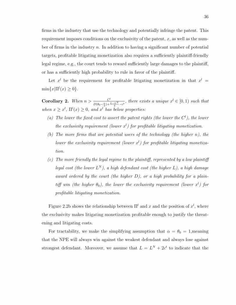
36

firms in the industry that use the technology and potentially infringe the patent. This

requirement imposes conditions on the exclusivity of the patent, x, as well as the num-

ber of firms in the industry n. In addition to having a significant number of potential

targets, profitable litigating monetization also requires a sufficiently plaintiff-friendly

legal regime, e.g., the court tends to reward sufficiently large damages to the plaintiff,

or has a sufficiently high probability to rule in favor of the plaintiff.

Let xl be the requirement for profitable litigating monetization in that xl =

minx|Πl(x) ≥ 0.

Corollary 2. When n > Cl

D(θ0−α2 )+L−LN2−ct

, there exists a unique xl ∈ [0, 1) such that

when x ≥ xl, Πl(x) ≥ 0, and xl has below properties:

(a) The lower the fixed cost to assert the patent rights (the lower the C l), the lower

the exclusivity requirement (lower xl) for profitable litigating monetization.

(b) The more firms that are potential users of the technology (the higher n), the

lower the exclusivity requirement (lower xl) for profitable litigating monetiza-

tion.

(c) The more friendly the legal regime to the plaintiff, represented by a low plaintiff

legal cost (the lower LN), a high defendant cost (the higher L), a high damage

award ordered by the court (the higher D), or a high probability for a plain-

tiff win (the higher θ0), the lower the exclusivity requirement (lower xl) for

profitable litigating monetization.

Figure 2.2b shows the relationship between Πl and x and the position of xl, where

the exclusivity makes litigating monetization profitable enough to justify the threat-

ening and litigating costs.

For tractability, we make the simplifying assumption that α = θ0 = 1,meaning

that the NPE will always win against the weakest defendant and always lose against

strongest defendant. Moreover, we assume that L = LN + 2ct to indicate that the

37

PE defendant has a similar legal fee compared to the NPE plaintiff. This yields the

simplified expression below for litigating monetization:

Πl = −1

2nDx2 + nDx− C l (2.9)

Notice that now for litigating monetization, we have that ∂Πl

∂x|x=1 = 0, indicating that

threatening the most capable user will bring the NPE zero marginal revenue.

2.5 Equilibrium

2.5.1 Equilibrium monetization method as a function of technological and

exclusionary strength

Based on the technological and exclusionary strengths of a patent, we determine

PEs’ and NPEs’ respective valuations for the patent, and these valuations in turn

determine the equilibrium ownership and use of the patent. There are three possible

mutually exclusive outcomes – The patent may be acquired and practiced by a PE

(outcome P for “practicing”), acquired and monetized litigatively by a NPE (outcome

L for “litigating”), or retained by the inventor and kept unused or dormant (outcome

D for “dormancy”).

For the relevancy of the technological value of the patent to our analysis, we

use the Weak User’s profit in Eq.2.4 as the payoff for practicing monetization and

compare it with that of litigating monetization in Eq.2.9. Define the strategy space

S = D,P, L, s ∈ S, and indicator functions 1D(s) = 1 if s = D, 1P (s) = 1 if s = P

, and 1L(s) = 1 if s = L. Let σ be the optimal strategy, then the optimal monetization

strategy of a patent is given by: σ(x, v) ≡ argmaxs1D0 + 1PΠp(x) + 1LΠl(x), or

simply:

σ(x, v) ≡ argmaxs1P (s)Πp(x, v) + 1L(s)Πl(x) (2.10)

Thus, on the two-dimensional plane of x and v, we derive regions on which each

of the three strategy options will prevail.

38

Proposition 3. With patents that differ in their exclusivity x and innovativeness v,

there exist xl, vp, and v∗ such that σ(x, v), the optimal monetization strategies for

patents are:

(a) Dormancy (D), for patents with x ≤ xl and v ≤ vp;

(b) Litigating Monetization (L), for patents with x > xl and v ≤ v∗;

(c) Practicing Monetization (P), for patents with (1) x ≤ xl and v > vp or (2)

x > xl and v > v∗.24

As an example, Figure 2.4 graphically shows a special case of Proposition 3 for a

particular set of values for the other parameters. The horizontal axis is the exclusivity

of a patent x and the vertical axis is the innovativeness of the patented invention v.

The three regions, i.e., D region, P region, and L region, are regions that each strategy

dominates. It is worth noticing that the relative size of regions in Figure 2.4 does

not imply the relative amount of patents in each region. In order to do so, we need a

distribution of all patents on the two-dimensional plane of x, v. To help illustrating

the figure, we define several points in Figure 2.4: Z1, Z2, Z3, and Z4. Z1 is point that

at the edge of for the D-P boundary, Z2 is the D-P-L intersection point, Z3 is the

peak point of the P-L boundary, and Z4 is the edge point for the P-L boundary.

Intuitively speaking, patents that have neither technological nor exclusionary

strength (the lower left region with x ≤ xZ2 = xl, and v below vp, which is repre-

sented by the Z1Z2 curve) remain dormant in the possession of the inventor. Patents

that reach a sufficient level of exclusivity (x > xZ2 = xl), but are weaker technically

(orange region where v is below v∗, as represented by the Z2Z3Z4 curve) are acquired

by a NPE and monetized via litigation. Only the technically strong patents (blue

region where v is above both the Z1Z2 curve and the Z2Z3Z4 curve). However, de-

pending on the patent’s exclusivity, the thresholds of minimum technological strength

for practicing monetization differ (vp for the P-D boundary shown as the Z1Z2 curve

, and v for the P-L boundary shown as the Z2Z3Z4 curve), with patents of medium

24 v > v∗ can also be written as x ∈ (0, x∗1) ∪ (x∗2, 1), where x∗1 < x∗2 are the two solutions toΠp −Πl = 0. Similarly, the condition of v ≤ v∗ can also be written as x ∈ [x∗1, x∗2].

39

exclusivity having the highest minimum technological strength required for practicing

to be the equilibrium outcome (Point Z3).

Figure 2.4.: Optimal Monetization Method

Note: The horizontal axis is exclusivity x, the vertical axis is innovativeness v. The Purple region is

the Dormancy region (D Region), the Blue region is the Practicing region (P Region), the Orange

region is the Litigating region (L Region).

Depending on different parameter configurations, there can be multiple scenarios

for optimal monetization methods. Figure 2.5 shows those scenarios on the two-

dimensional plane characterized by x and v. When the number of firms n increases,

the L region expands with the P-L boundary shifts up and the D-L boundary shifts

left. If the cost of implementing the patent (Cp) decreases, the P region expands with

the D-P boundary shifts down and the P-L boundary shifts down. A combination

of the above two effects result a shift from Figure 2.5a (which replicates the same

scenario in Figure 2.4) to a graph that is similar to Figure 2.5b in which the L region

significantly enlarged and the P region mainly concentrates on areas with patents of

either extremely high or extremely low exclusionary strength. As the NPE’s expected

40

damage from winning in court (D) decreases or the cost for initiating a campaign

against multiple defendant (C l) increases, the L region shrinks with the P-L boundary

shifts down, and the D-L boundary shifts right. The result is a shift from Figure 2.5b

to Figure 2.5c. But if D is sufficiently low or if C l is sufficiently high (or as an

extention, the NPE’s chance of winning at court (θ0) decreases), Figure 2.5c gets

transformed into a graph that looks like Figure 2.5d in which the L region completely

disappear and there is no room for litigating monetization to prevail.

2.5.2 Equilibrium monetization method as a function of exclusivity alone

The dotted horizontal lines in Figure 2.5 illustrate all possible scenarios for the

effect of patent exclusivity on the equilibrium monetization method. Depending on

the values of the other parameters, there are a total of nine sequences for how the

equilibrium monetization method changes as x increases from 0 to 1. We denote each

equilibrium sequence as an ordered list of the equilibrium monetization methods in the

order that appear as x increases from 0 to 1. For example, the equilibrium sequence

(D,L,P) means that the equilibrium monetization method is Dormancy, Litigating,

and Practicing for patents in regions x ∈ [0, xa), [xa, xb), and [xa, 1) respectively.

Proposition 4. There are nine possible sequences for how the equilibrium monetiza-

tion method changes as a function of the patent exclusionary strength x. These nine

scenarios are determined by the relative positions of xl, xp, x∗1, and x∗2, as shown

below in Table 2.1.

When will each of the equilibrium sequence appear depends on the positions of

xl, xp, x∗1, and x∗2. 25 Detailed conditions for each scenario are also given in Table

2.1. The nine plots in Figure 2.6 show the relative positions of Πp, Πl, and relevant

intersections.

25When

(D− 2v(v+1)

(n+1)2

)2

2(

Dn + 2v2

(n+1)2

)((Cl−Cp)+

v(v+2)

(n+1)2

) > 1, there exists x∗1, x∗2 ∈ R such that when x ∈ (x∗1, x∗2),

Πl > Πp. So, on the patent exclusivity dimension, there will be a convex region that the value fromlitigating monetization surpasses that of practicing monetization.

41

(a) (b)

(c) (d)

Figure 2.5.: Region of Optimal Monetization Method

Note: The x-axis is exclusionary strength x, the y-axis is technological strength v. ThePurple region is the Dormancy region (D Region), the Blue region is the Practicing region(P Region), the Orange region is the Litigating region (L Region). Thus, the borderline ofthe P Region and the L Region is the PE/NPE borderline. Letters in the graphs indicatethe index of equilibrium sequences as in Figure 2.6.

42

Table 2.1.: Summary of Nine Equilibrium Sequences

# Notation Optimal Strategies σ(x) Conditions

i (D) D for x ∈ [0, 1) xp > 1⋂xl > 1

ii (P) P for x ∈ [0, 1) xp < 0⋂x∗1 > 1

⋃x∗2 <

0⋃dx < 1

iii (D,P) D for x ∈ [0, xp) and P for x ∈[xp, 1)

xp ∈ (0, 1)⋂x∗1 > 1

⋃x∗2 <

xp⋃dx < 1

iv (D,L) D for x ∈ [0, xl) and L for x ∈ [xl, 1) xl ∈ (0, 1)⋂x∗1 < xl

⋂x∗2 >

1v (P,L) P for x ∈ [0, x∗1) and L for x ∈

[x∗1, 1)xp < 0

⋂x∗1 ∈ (0, 1)

⋂x∗2 >

1vi (P,L,P) P for x ∈ [0, x∗1), L for x ∈

[x∗1, x∗2) and P for x ∈ [x∗2, 1)xp < 0

⋂x∗1 > 0

⋃x∗2 < 1

vii (D,L,P) D for x ∈ [0, xl), L for x ∈ [xl, x∗2),and P for x ∈ [x∗2, 1)

xl ∈ (0, 1)⋂x∗1 < xl

⋂x∗2 ∈

(0, 1)viii (D,P,L) D for x ∈ [0, xp), P for x ∈ [xp, x∗1),

and L for x ∈ [x∗1, 1)xp ∈ (0, 1)

⋂x∗1 > xp

⋃x∗2 >

1ix (D,P,L,P) D for x ∈ [0, xp), P for x ∈ [xp, x∗1),

L for x ∈ [x∗1, x∗2), and P for x ∈[x∗2, 1)

xp ∈ (0, 1)⋂x∗1 > xp

⋂x∗2 <

1

We highlight three critical conditions that differentiate the above nine equilib-

rium sequences. First, when Cp and C l are sufficiently large, meaning the maximal

value appropriation from the patent cannot justify the cost to either practicingly

or litigatingly monetize the patent, the equilibrium sequence will be (D).26 Second,

when the technology is sufficiently valuable,27 and fixed cost of practicing (Cp) or

the number of firms in the market (n) is sufficiently small in that Cp(n + 1)2 ≤ 4,

which results xp < 0, then the equilibrium sequences will have no D region and start

from P. This means for patents with strong technological strength, practicing them

would be preferred even with even zero scope of exclusion, which is the case similar

to open knowledge. Third, when the technological value v or the NPE’s litigating

cost C l is sufficiently large, or when n, C l, and the damage awarded to te NPE (D)

are sufficiently small, in that they altogether satisfy v(2A+v+nv)1+n

− Cp > Dn2− C l, the

26The conditions for the equilibrium sequence (D) are Cp > v2 + 2Avn+1 and Cl > nD

2 .27To be specific, when v >

√Cp(n+ 1)2 + 1−A.

43

equilibrium sequences will end with P, which means patents with the widest scope of

exclusion will be optimally acquired by an PE to practice.

Also in Figure 2.5, we give example lines and show the index for each of the nine

situations in Table 2.1. Notice that the horizontal axis in Figure 2.5 is x, so the

horizontal lines in Figure 2.5 capture the optimal strategy on x given a fixed level of

v.

We now explain insights derived from the different equilibrium sequences. At first,

in some scenarios, in addition to the P region when the patent has high exclusivity on

x > x∗2, the existence of another P region on x ∈ [xp, x∗1). This reflects the fact that

a part of the practicing profit gain comes from the pure technological value of the

invention which is not related to exclusivity. Some good inventions with bad patents,

may still be practiced, but due to the low exclusivity, will be out of NPEs’ radar.

Second, regarding the thresholds for profitable monetization, xl is always greater

than zero since when x = 0, Πl = C l < 0. When the patent has no exclusivity, then

the patent would be completely useless for litigating monetization. When litigating

is profitable, there is always xl > 0. However, the threshold for profiting practicing

monetization, xp can be smaller than zero since even when x = 0, Πp = v2+2v(n+1)2

− Cp,

which is not necessarily negative. This captures the pure value of the technology, even

without any exclusion power of the patent, or without a patent at all. Third, when

x∗2 ∈ (0, 1), the most exclusive patents, i.e., patents with x ∈ [x∗2, 1), will always more

profitable monetized via practicing. This means that the profit from excluding other

PE rivals, together with the profit from the technology itself, dominate the profit from

litigating. Fourth, the least exclusive patents x < minxp, xl, will be unprofitable

either through litigating or practicing monetization, thus will stay in dormancy, due

to the existence of the fixed costs, Cp and C l, to initiate either monetization strategy.

Fourth, patents that will be litigated will always be patents with medium exclusivity

range, i.e., x ∈ x∗1, x∗2 and x > xl.

44

01x

Π

x∗1

−Cl

Πp = Πl

Dormancy

(a) Equilibrium Sequence: (D)

01x

Π

xl

−Cl Practicing

(b) Equilibrium Sequence (P)

01x

Π

xlxp

x∗−Cl

Πp = Πl

Dormancy Practicing

(c) Equilibrium Sequence (D,P)

01x

Π

xl

xpx∗1

−Cl

Πp = Πl

Dormancy Litigating

(d) Equilibrium Sequence (D,L)

01

x

Π

xl x∗1

−Cl

Πp = Πl

Practicing Litigating

(e) Equilibrium Sequence (P,L)

01x

Π

xl x∗1 x∗2

−Cl

Πp = Πl

Πp = Πl

Practicing Litigating Practicing

(f) Equilibrium Sequence (P,L,P)

0x

Π

xl xp x∗2−Cl

Πp = Πl

Dormancy Litigating Practicing

1

(g) Equilibrium Sequence (D,L,P)

01x

Π

xlxp x∗1

−Cl

Πp = Πl

DormancyPracticing Litigating

(h) Equilibrium Sequence (D,P,L)

0x

Π

xlxp x∗1 x∗2

−Cl

Πp = Πl

Πp = Πl

DormancyPracticing Litigating Practicing

1

(i) Equilibrium Sequence (D,P,L,P)

Figure 2.6.: Equilibrium Monetization Method as a function of x

Note: The horizontal axis is the exclusionary strength of patents x, the vertical axis is value Π.In each graph, Solid curves plots the value from practicing monetization (Πp) and Dash dot curvesplots the value from litigating monetization (Πl). Dormancy, Practicing, and Litigating regions, aswell as positions of xl, xp, x∗1, and x∗2, are marked in each graph.

45

2.6 Extension: End Users as Litigation Targets

One notorious practice of litigating patent monetization is targeting end users

of infringing products, rather than against the actual producers of those products

(Bernstein, 2016). NPE’s target end users may have little, if anything, to do with

each other, and these end users do not participate in the competition among producers

in the product market. Therefore, being able to target end users in patent litigations

additionally incentivizes litigating monetization. For a product whose end users are

in large number, NPEs may have relatively more to gain from owning a patent than

PEs. In this scenario, we use Πl(nU) and Πp(n) to denote the profit from litigating

monetization and practicing monetization as a function of number of targets nU , and

number of active producers in the industry n respectively.

Proposition 5. The more end users relative to producers in an industry (i.e., higher

nU/n ratio), the more profitable litigating monetization becomes, relative to practicing

monetization.

2.7 Empirical Implications

Our propositions suggest several avenues for future empirical research, provided

that a patent’s practicing value can be distinguished from its litigating value. It

may be possible to proxy for these values at the patent class level, since certain

patent classes are known to have, on average, relatively higher exclusionary strength

and/or practicing value than others. For example, regulations requiring clinical trials

make pharmaceutical patents especially difficult to “invent around,” while patents

for computer hardware are relatively easier to circumvent because the possibility of

recombining electronic components in multiple configurations offers “more than one

way to skin a cat.” It may also be possible to find proxies that distinguish patents

according to their practicing value. For example, among pharmaceutical patents,

some drugs are slight variations on existing molecules in longstanding therapeutic

46

classes and are therefore likely to have relatively low practicing value, while other

drugs pioneer entirely new types of molecules or entirely new therapeutic classes and

are therefore likely to have much higher practicing value.

It may be possible to test our propositions in situations where natural experiments

shift the litigating and/or practicing value of patents in ways that precipitate observ-

able sales of patents from PEs to NPEs or vice versa. For example, as one possible

natural experiment, the U.S. Food and Drug Administration’s 1997 deregulation of

direct-to-consumer advertising and the 1983 Orphan Drug Act both increased the

practicing value of pharmaceutical patents. Likewise, court rulings like the 2010 Bil-

ski v. Kappos and 2014 Alice v. CLS decisions on software and business-process

patents can suddenly shift the exclusionary value of specific patent classes. Broader

changes to the exclusionary value of patents across many classes may result from

patent reform legislation, such as the 2012 America Invents Act (AIA). Specifically,

the Act increased the cost for litigating by banning combining cases based on infring-

ing the same patent, thus increases the fixed cost that the plaintiff has to pay to

initiate a series litigations – i.e., our parameter C l. Second, the AIA paved ways for

easier patent invalidation by the defendants, thereby decreasing NPEs’ likelihood of

successfully extorting a PE firm – i.e., our parameter θj.

2.8 Managerial Implications

Since our model includes three different types of agents – inventors, practicing

entities, and non-practicing entities – we consider the managerial implications for

each of these three in turn. First, from an inventor’s perspective, the model provides

guidance about which type of buyer – PE or NPE – is likely to be willing to pay

more for any given type of patent. This guidance would be particularly helpful for

an inventor who may have never considered selling a patent to a NPE. At the very

least, it may enable an inventor to avoid wasting time selling a patent to a PE

when a NPE is clearly the optimal buyer. Moreover, when there are more potential

47

bidders for a patent, its selling price is likely to be higher ceteris paribus; this is

good news for inventors of patents whose characteristics put them on or near the

PE/NPE borderline, since these patents may appeal to both PEs and NPEs, and

thereby attract a larger number of bidders. When considering the impact of changing

the model’s parameters, inventors benefit from any parameter changes that diminish

the size of the dormancy region, such as reduced patent maintenance cost (lower C l

or Cp).

Second, from the perspective of a PE, our model provides guidance about what

type of patents it would benefit most from acquiring. It can be a waste of a PE’s time

and effort to seek to acquire patents in cases where a NPE has a clear incentive to

outbid it. Conversely, our model may also offer PEs some guidance about opportuni-

ties for patent divestitures. PEs may own large portfolios of patents, some of which

may have lost much of their technical and commercial value due to obsolescence, or

due to substitution by some other competing technology. As a patent’s commercial

value depreciates over time, a PE may benefit from divesting such a patent by sell-

ing it to an NPE, who would not care about its diminished technical value. A PE

may anticipate this eventuality, yet still be uncertain about the exact point at which

divestiture would yield the greatest value. Our model suggests that the optimal di-

vestiture point would be at the PE/NPE borderline in our figures. Depending upon

the underlying parameter values, this borderline may be a curvilinear function of ex-

clusionary strength (as in Figure 2.5b), or decreasing function (as in Figure 2.5c), or

even an increasing function. When considering the impact of changing the model’s

parameters, PEs benefit from any parameter changes that increase the size of the

practicing region, such as less rivalry in the product market (a smaller n).

Finally, some of the model’s implications for PEs apply to NPEs as well, but in

reverse. In terms of patent acquisition strategy, it can be a waste of a NPE’s time and

effort to seek to acquire patents in cases where a PE has a clear incentive to outbid

it. When considering the impact of changing the model’s parameters, NPEs benefit

from any parameter changes that increase the size of the litigating region. (After all,

48

a NPE cannot profit from litigating a patent that it does not own.) For example,

a more plaintiff-friendly legal regime in terms of a higher chance for plaintiff win (a

larger θj) and a higher expected damage award (a larger D) will both enlarge the

relative size of the litigating region compared to the practicing region.

2.9 Concluding Remarks, Caveats, Limitations, and Opportunities

In this paper, by decoupling the technological and exclusionary strength of the

patent, we study how firms’ value appropriation mechanisms relate to patent mon-

etization methods and implications in the market for patents. Relationships among

concepts are summarized below in Figure 2.7.

Figure 2.7.: Value Appropriation and Patent Monetization Framework

Different firms, with their different monetization mechanisms and different syner-

gies, have heterogeneous valuations for resources. Inspired by the NPE phenomenon,

this study contributes to resource-based theory by examining the role that differing

monetization mechanisms plays as a source of firms’ valuation of resources (Asmussen,

2015), and highlighting the resulting implications for the trading of resources (in this

case, patents) in a strategic factor market (Barney, 1986). Since the monetization

mechanism is one of the most important dimensions on which business models usu-

ally differ, our model also contributes to research on competing business models (e.g.,

49

Casadesus-Masanell and Zhu 2010, 2013) by shifting the focus of competition from

the product market to the resource market. We believe that the impact of competing

business models and differing monetization methods on the resource market, and not

just on the product market, is a topic that is ripe for future research.

This study also contributes to the literature in market for technology by analyzing

monetization methods based on differentiating the value of exclusion from the prac-

ticing value of the technology itself. Most extant research studies the value of patents

in general while not separating the two (Bessen, 2008; Harhoff et al., 2003; Lanjouw

et al., 1998). We argue that the technological value matters for firms that commer-

cialize the patented technology, whereas the exclusionary value of patents matters

for both practicing monetization and litigating monetization (Lemley and Shapiro,

2005). Moreover, our theory highlight firms’ difference in monetizing the exclusion-

ary value of patents. The exclusion in practicing monetization means excluding other

firms from using the technology in their products and services; but in litigating mone-

tization, it means being able to assert patent rights and profit from litigating (Chien,

2013). Thus, while firms that use practicing monetization prefer less infringement

to maximize their competitive advantage, firms that exploit litigating monetization

prefer more infringement in order to maximize the set of potential defendants. Exten-

sions of the model may incorporate characteristics of the industry and the product

market overlapping among PEs. Studying how they affect the competitive rivalry

among firms (Ross, 2014) in the factor market can also be fruitful.

In addition, given the significant attention given by other fields on the non-

practicing monetization of patents, we join the current discussion on Non-Practicing

Entities (NPEs) and shed light on their patent acquisition behavior. Existing studies

presented mixed findings regarding whether NPEs acquire high or low quality patents

(Feng and Jaravel, 2017; Abrams et al., 2013).In an effort to solve the puzzling mix-

ture of findings, we propose that the value of technology is only reflecting one facet of

patent quality, and NPEs make their acquisition based on the exclusionary value of

patents, which may not necessarily related to the technological value. For instance,

50

a valuable technology that is written badly into a patent may still be highly valuable

for practicing monetization, but it may have no value in eyes of NPEs for litigating

monetization. We found while practicing monetization is convex, litigating moneti-

zation is concave in patent’s exclusionary strength. This difference in value functions

have substantial implications for the optimal resource monetization, since it implies a

curvilinear boundary between the patents that are practiced by PEs and the patents

that are litigated by NPEs.

Although our model provides a starting point for understanding NPEs and com-

peting patent monetization methods, it certainly does not represent a complete theory

of these phenomena. We hope that future research will extend our model in ways that

overcome its limitations and omissions. One such limitation is that there are more

patent monetization methods than the two we considered (practicing and litigating),

such as licensing that does not involve threat of litigation (Fosfuri, 2006). However,

licensing is a form of contract whose value (represented in licensing fee) will hinge

on whether the ultimate value appropriation mechanism is from the product market

or from the threat to litigate. In this regard, licensing might be expected to behave

like an intermediate blend of practicing and litigating. So, it would be interesting

to extend the model and discusses various scenarios of licensing. A second limita-

tion is that we use a static model and assume that all uses of the patent and its

underlying technology happen instantaneously. However, in reality, litigation, tech-

nology adoption, and inventing around patents are dynamic processes that take time

(Gort and Klepper, 1982). In a dynamic model, differences in the speeds with which

these different processes occur might generate different results. Finally, although our

model focuses on the two specific aspects of patents – their technological strength

and their exclusionary strength – that seem to us to be the most important deter-

minants of monetization methods, these are certainly not the only two dimensions

on which patents differ, and may not be the only drivers of monetization decisions.

Accordingly, future theories of patent monetization may incorporate a broader range

of independent variables.

51

CHAPTER 3 LITIGATING MONETIZATION ANDPATENT TROLLS: EVIDENCE FROM THE PATENT

MARKET

3.1 Introduction

Innovation is a critical source of economic growth and firm profitability (Teece,

1986). To protect innovators’ profit and innovative efforts, patent grants their owners

a scope of exclusive rights of the technology (Kitch, 1977). Most firms that produce

or buy patents appropriate value from their product markets, either directly via prac-

ticing the technology in their products or services and excluding rivals from using it,

or indirectly by charging a licensing fee proportional to the licensees’ product mar-

ket profit. Such profiting from the product market, both directly and indirectly, is

referred to as the practicing monetization of patents. However, recent years have

witnessed the fast-growing business models used by firms to appropriate value from

patents through enforcement of patent rights. These business models share a feature

of aggressively using patent litigations to claim payments from other parties, such

practices are referred to as the litigating monetization of patents. Due to the as-

sertive nature of litigating monetization, firms that specialize in such business model

are called Patent Assertion Entities (PAEs). Hagiu and Yoffie (2013) defines PAEs

as arbitrageurs, first acquiring patents, typically from individual inventors or small

companies, and then seeking licensing revenues from operating companies through lit-

igation or the threat of litigation.

The key to PAEs’ source of profit is using lawsuits to assert patent rights. Since

PAEs do not practice the patented technologies, they are also referred to as Non-

Practicing Entities (NPEs) or patent trolls. Since PAEs have no stake in the product

52

market (Choi and Gerlach, 2018), in addition to potential patent invalidation, they are

almost immune to counter lawsuits. The immunity empowers PAEs to aggressively

exploit the judicial system sue other firms. The lawsuits disrupt the patent system

(Schwartz and Kesan, 2014) and bring wide controversies and criticisms to PAEs

(Lemus and Temnyalov, 2017; Cohen et al., 2016; Leiponen and Delcamp, 2019).

Figure 1.1 shows quarterly numbers of patent lawsuits initiated by PAEs and other

entities at US Federal District Courts from 2000 to 2018. At its peak, PAEs make

up more than 60% of all patent litigations filed (RPX, 2019).1 Also, recent changes

in the number of patent litigations are primarily driven by the changed behavior of

PAEs, partly due to the changing policy environment towards litigating monetization.

PAEs’ litigating monetization is controversial to policymakers. The intention for

building a strong patent system is to encourage innovation, to lower the transac-

tion cost, to develop of the market for technology (Arora and Fosfuri, 2003), and to

facilitate the commercialization of technologies (Dechenaux et al., 2008). However,

PAEs’ activities of exploiting the patent system could hurt innovation as frivolous

litigations distract substantial firm resources to handling lawsuits and threats mean-

while depriving firms’ capabilities to innovate (Leiponen and Delcamp, 2019). It is

especially consequential for entrepreneurial firms, which consist of more than half

of PAEs’ defendants (Chien, 2013; Hovenkamp, 2013). As startups usually lack re-

sources, they have to slow or even halt growth to deal with lawsuits (Smeets, 2014).

Several studies have found PAE activities negatively affect firm innovation (Tucker,

2014; Smeets, 2014; Penin, 2012), entrepreneurial activities (Kiebzak et al., 2016),

venture capital investment, and employment (Appel et al., 2020).

Nevertheless, positive views of PAEs emphasize their critical role in market for

technology. In a well-developed market for technology, the division between invention

and commercialization should increase welfare through the trade and specialization

(Arora et al., 2016). However, inventors often suffer from the difficulty of accessing

1Very often, PAEs use names of shell companies to sue, Hall (2019) quotes the number reported inLove et al. (2018) that more than 83% of post acquisition patent assertion comes from “aptly namedPAEs.”

53

potential buyers (Luo, 2014) and capturing inventors’ fair share of value creation.

PAEs’ existence can help overcome such inefficiencies, Lemus and Temnyalov (2017)

find that though patent privateering activities reduce surplus of producing firms, they

are in general beneficial to R&D activities. PAEs are said to “foster innovation by

monetizing intellectual property rights through licensing and technology transfer.”2

Some studies argue that PAEs are just another type of normal patent intermediaries

(Haber and Werfel, 2016) that use their expertise in finding complementaries among

patents in different domains to improve the efficiency of the patent market (Steensma

et al., 2016), and that can promote competition, lowers price, and benefit consumers

(Geradin et al., 2012).

The role of PAEs becomes more obscure when looking at their patent acquisi-

tions. Extant literature reports that PAEs acquire low-quality patents (Lerner, 2006;

Abrams et al., 2013). Specifically, PAEs tend to buy patents with wide scope, patents

that are in densely patented technology fields (Fischer and Henkel, 2012), that were

issued by lenient examiners (Feng and Jaravel, 2020), that are not critical to a firm’s

business and litigation-prone (Abrams et al., 2019), and that are close to the end of

their technological cycle (Fischer and Henkel, 2012; Orsatti and Sterzi, 2018). How-

ever, some others find that PAEs acquire high-quality patents with more citations

and claims (Fischer and Henkel, 2012; Shrestha, 2010). In fact, PAEs’ patent acqui-

sition is indeed highly concentrated in several technology fields in which there exists

numerous patent thickets and that are highly active in patent litigations, such at IT,

telecommunications, digital communications, and semiconductors. Figure 3.1 shows

PAEs’ shares in patent acquisitions by IPC technology fields.

In light of the academic interest in PAEs and the market for technology in gen-

eral, however, there has not been a theory to reconcile the seemingly contradictory

findings on PAEs’ patent acquisition. Trying to shed light on the issue, I start from

distinguishing business models of practicing and litigating monetization, which com-

bines different resources and generate different types of synergies with patents. In

2Matteo Sabattini, NPEs vs Patent Trolls: How to build a healthy innovation ecosystem.

54

Figure 3.1.: Share of PAEs’ Patent Acquisitions by Technology Fields

Notes: The x-axis ranks 35 International Patent Classification (IPC) technology fields as in(Schmoch, 2008) by the shares of PAE acquisitions in each field’s total transactions during 2007-2017.

55

this paper, I theorize on how PAEs’ business model shape their patent acquisition,

and compare it to that of other firms. Drawing insights from the litigating-oriented

to the practicing-oriented patent acquisitions, this study deepen our understanding

of the multifaceted value of patents.

This study also contributes to the literature of technology commercialization. Ex-

isting studies have primarily focused on practicing monetization via market entry or

licensing (Gans et al., 2008; Gans and Stern, 2003; Marx and Hsu, 2015). The litigat-

ing monetization strategy, though missing in strategy literature, has been discussed in

literatures of law (Allison et al., 2009, 2017), economics (Lemley and Feldman, 2016;

Choi and Gerlach, 2015, 2017; Turner, 2018), and policy (Cohen et al., 2017; Federal

Trade Commission, 2016). I argue that while the technological strength and the ex-

clusion scope of patents matter to practicing and litigating monetization in different

ways. A firm that seek product market profit is incentivized to deter infringement,

whereas a PAE is incentivized to allow (if not encourage) infringements. Furthermore,

compared to practicing monetization, litigating monetization is much more dependent

on the security of patent rights. When the regime is less friendly to patent owners,

patent assertion will also be less profitable. Besides, studies have primarily examined

uncertainties in the intellectual properties (IP) regime from events such as disclosure

(Hegde and Luo, 2017; Luck et al., 2020) and patent grant (Gans et al., 2008), few

has looked at circumstances where risks surrounding validity of patents increase, and

from an angle that look upstream to the acquisition of IP.

When primarily focusing on the acquisition of IP, this paper contributes to the

broader strategy literature by discussing how firms with competing business models

behave differently in the strategic factor market (SFM). Theoretical studies in SFM

have shown that firms’ idiosyncratic valuation and the subsequent acquisition of re-

sources originate from firms’ heterogeneous information and expectation of the value

creation (Barney, 1986; Makadok and Barney, 2001), firms’ existing resource stock

and the degree of complementarity between existing resources and the target resource

(Adegbesan, 2009; Dierickx and Cool, 1989), and firm’s position in the product mar-

56

ket (Schmidt and Keil, 2013; Chatain, 2014). However, extant literature has not

yet studied how firms’ heterogeneity in the type of complementarity drives different

expectations of the resource value and the equilibrium ownership and allocation of

resources among such different firms. This study fills in the gap of the existing lit-

erature and adds to the line of research that examines the competition of firms with

different business models in the SFM (Markman et al., 2009; Casadesus-Masanell and

Zhu, 2010, 2013).

3.2 PAEs as Patent Intermediaries and Litigating Monetization as a Busi-

ness Model

PAEs are a type of patent intermediaries. Based on the categorization by Hagiu

and Yoffie (2013), intermediaries that purchase patents from individuals and firms

can be either a defensive aggregator or an offensive aggregator.3 Defensive aggrega-

tors acquire patents from other parties and collect licensing, subscription, and other

business intelligence service fees from subscribers to protect those entities from litiga-

tions and harassment of patent trolls. Defensive aggregators often own large numbers

of patents, but unlike offensive aggregators, they do not rely on litigations or the

legal threats to appropriate value from firms. Two of the most prominent defensive

aggregators are RPX and Applied Security Trust (AST), whose clients include Cisco,

IBM, Intel, Toyota, Samsung, and Microsoft.4 While defensive aggregators usually

do not litigate their patents, offensive aggregators do the opposite and always litigate

and in many cases even assert their patents to profit from settlement fees, licensing

fees, and compensations out of litigations. By this definition, universities are also of-

3Hagiu and Yoffie (2013) also mentioned other types of patent intermediaries. First, patent brokerswho do not buy patents but only connect patent sellers and buyers. Second, patent pool, which isa pool of patents that practicing company put together and license to each other. Third, standardsetting organizations which are two-sided patent platforms. Fourth, super aggregators that havesome attributes of both defensive and offensive aggregators.4As written on the website of RPX, they are open to all sorts of entities interested in their patents:“We welcome inquiries from individual inventors/owners, academic institutions, brokers, technologytransfer offices, corporate sellers, and non-practicing entities.” Web: http://www.rpxcorp.com/rpx-services/rpx-patent-sales/

57

fensive (Lemley, 2007). But universities may have different motivation and incentives

compared to firms. In this study, to better focus on litigating monetization, PAEs or

patent trolls only refer to non-university offensive aggregators.

Regardless of the buyer type, patents are options that can be monetized in dif-

ferent ways (Cotropia, 2008), litigating monetization is a way to exercise, and it

has deterministic implications. In sum, though patents are essential for both busi-

ness models, they substantially differ in several aspects: (1) Source of competitive

advantage. when a firm adopts litigating monetization, the source of competitive

advantage is legal capabilities, while patents are somewhat substitutable. But for

a firm that practices certain technology, there are usually patents that are essential

and important so that the substitutability is low. (2) Attitude towards infringement.

Infringement is necessary for litigating monetization, and a large number of firms

infringing the patent benefits the value from litigating monetization. But infringe-

ment is detrimental to firms that profit from practicing the technology. (3) Timing of

value appropriation. Value appropriation of litigating monetization occurs after firms

have practiced or used the patented technology, whereas value appropriation from

practicing the patent starts with the initial practicing of the patent. (4) Sensitivity

to the property rights. Litigating monetization is very sensitive to changes in the

legal regime as the regime directly determines the strength of property rights. But

the sensitivity is much lower for practicing monetization, as their value appropriation

depends on a wide range of factors.

Unlike practicing monetization, for which profit comes from the product market,

litigating monetization typically starts with a PAE sending demand letters to target

firms asking for monetary payments and threatening to sue if targets do not pay.

An important feature of demand letters is that, since the PAE often does not have

resources and capabilities to evaluate the value of the patent to each target, the

PAE sends standard demand letters that list the infringed patents, give a number of

payment claimed, and request communications, without much discriminating upon

58

different targets.5 The PAE’s goal is to maximize the probability of targets’ yielding

to their demands without actually entering the expensive litigations.

The key to secure a payment by the target upfront without falling in the swamp

of patent litigations is that the settlement fee demanded by the PAE shall not exceed

the costs from possible litigations. Because if the threatened target decides to fight

at court and insists to the end, even if the plaintiff PAE wins, the PAE will also have

to spend significant time6 and legal cost to deal with the case. This indicates that

compared to getting straight payment of settlement fees, fighting at court is not in the

interest of plaintiff PAEs. Therefore an informed PAE would demand the maximal

monetary payment from a target firm such that settlements would be favored by the

target over litigations. In reality, PAEs almost always seek to settle a litigation while

PEs’ likelihood to settle a litigation as a plaintiff decreases with the PEs’ product

market stake of the litigated patent (Somaya, 2003). Such settlement, often in forms

of licensing fee, differs from licensing in practicing monetization in that such payments

are usually a lump-sum payment, instead of a percentage of profit shared with the

patent owner over future years.

3.3 Theory

3.3.1 Technological strength and patent acquisition

For a patent to be granted, the invention has to be novel, non-obvious, and useful

(Hall et al., 2005). In the patent market, variations in technological strength exists

in two dimensions. First, for technologies invented at the same time, there is a cross-

sectional variation of the technological quality among patents; second, for technologies

of the same quality but were invented in different time, there is a temporal variation

of the strength of the technology in that the best technologies patented ten years

5For an example of demand letter, see: https://www.nar.realtor/window-to-the-law/window-to-the-law-patent-troll-demand-letters6The average time from a complaint is filed at a district court to the trial is longer than two years(PriceWaterhouseCoopers, 2018; Lex Machina, 2019)

59

agao may no longer be valuable now. Below I discuss how these two dimensions of

technological strength matter for patent acquisition.

Since PAEs often seek to claim fees from multiple firms, PAEs want the technology

to be as widely “infringed” as possible to maximize value of each patent. Special-

izing in enforcing patent rights, PAEs’ essential resource is their acquaintance and

proficiency with the legal procedures regarding patents and patent lawsuits (Cohen

et al., 2016), and PAEs usually do not possess the capabilities to evaluate the value

that a technology brings to a specific firm or industry.7 Due to PAEs’ disinterest of

the technology itself, no matter what the technology is, if there are not a significant

number of adopters, the patent is of little value to PAEs since there is not a sufficient

number of firms that can be targets of PAEs’ assertions.8

Thus, for PAEs, without the ability to discern whether a patent is of high private

value for a firm, PAEs would go after high quality technologies that are generic and

attracts a large audience. However, the value of patent is highly firm-specific, since

product market profit a firm appropriates are determine by many complementary

resources other than the technology itself (Teece, 1986). Firms’ idiosyncratic comple-

mentary assets leads them to differ drastically in acquisition of patents. A patent of

low technological quality may still be acquire by firms to build a portfolio to protect

their own core technologies, while PAEs only acquire relatively high quality tech-

nologies that firms actually uses since it is the only ground for claiming infringement

payments.

Also, from the perspective of litigation, while PAEs do not distinguish among

defendants on whether they are rivals or clients since PAEs do not have product

market presence, PEs do not aggressively litigate unrelated firms outside their area

(Simcoe et al., 2009), especially not on potential clients. Thus, the more widely used

is the patented technology, the higher the likelihood of a patent to be acquired by a

7However, there are some exceptions, such as InterDigital, who produces lots of patents itself, thoughmany of InterDigital’s patents are criticized for low technological strength.8This also indicates that if there is only technology but no patent, with nothing to assert, thetechnology is useless to a PAE.

60

PAE buyer. Among patents in the same cohort, patents with higher quality in that

they on average generate more value are more likely to be purchased by PAEs.

Hypothesis 1a. Everything else equal, the better the technological quality such that

the more widely adopted is the patent, the probability of acquisition by a PAE as

compared to a PE.

However, the dilemma for PAEs is that, though patents of high technological qual-

ity are desired, they will also be expensive if PEs are also competing for ownership.

But, in addition the cross-sectional difference among technological quality, for the

same technology, its strength changes over time. For practicing monetization, a PE

either appropriate value by using the technology to gain competitive advantage via

differentiation or cost reduction(Bessen and Maskin, 2009; Porter, 1985) or from li-

censing the technology to other firms (Arora and Fosfuri, 2003). Either way, first,

when the technology is new, its contribution to the focal firm to improve a product or

a process is likely to be higher. Second, when the patent ages, the knowledge spillover

(Somaya, 2002; Agarwal et al., 2009) may enable other firms to be able to use the

technology, so that the superior profit the patent brings to the patent-owning firm

may be wiped out. Third, as the patent ages, there is a higher chance that upgraded

versions of the technology become available so that the old patent, though maybe

more radical than the new incremental patents, also becomes obsolete (Fischer and

Leidinger, 2014; Lanjouw, 1998; Pakes and Schankerman, 1984). When the techno-

logical strength is weakened, so is PEs’ valuation of the patent, but this means a good

opportunity for PAEs.

Although the weakened technological strength reduces the practicing value for

PEs, a PAE may be able to extract more litigating value from the patent. At first,

a PAE cannot commit and acquire a patents when the technology is still too new

and uncertain about whether it will accrue a significant number of adopters, who

are PAEs’ potential targets (Fischer and Leidinger, 2014). In addition, firms that

developed or used updated technologies that partially overlap with the old patent

61

could also be targets of PAEs. Therefore, the larger the age of a patent, the more

likely it will be purchased by PAEs.

In sum, PEs have high willingness-to-pay for new technologies, which often outbid

PAEs, for which patents are substitutable resources. But older technologies that were

of high quality before are likely to have accumulated more adopters that increases

the litigating value of the patent. I hypothesize that:

Hypothesis 1b. Everything else equal, the older the patent, the higher the probability

of acquisition by a PAE as compared to a PE.

3.3.2 Scope of property rights and patent acquisition

While the technological strength is important, the right to exclude is what de-

fines the scope of property rights. Sometimes, claiming a scope of property rights is

more important than the technology itself, as an example, the skyrocketing of soft-

ware patents in recent years is not well explained by changes in firms’ investment

in software, R&D, computer programmers or engineers employment, or productivity

growth, but is highly correlated to the change in the legal regime that strengthens

the effectiveness of the exclusion rights (Bessen and Hunt, 2007). For PEs and PAEs,

their monetization of the scope also differs.

For PEs, a patent neither provides perfect protection of the technology nor guar-

antees that the patent owner or the legitimate licensees enjoy the exclusive access to

the patented technology .9 In many technological fields, patents are not the primary

method for protecting intellectual properties (Cohen et al., 2000) since other firms

will often be able to imitate or use the technology and/or invent around to create

their own solution and avoid infringement (Gallini, 1992; Mansfield, 1985). Especially

with the publication of the technology in the patent application or other materials,

rivals will imitate if they find it profitable and if they are capable (Horstmann et al.,

9As stated on the website of World Intellectual Property Organization (WIPO): “(somepatents) would be so innovative that they give the owner a complete monopoly over anentire industry and are extremely valuable, often worth billions of dollars.” See: https ://www.wipo.int/sme/en/documents/valuingpatentsfulltext.html. Retrieved on May 16th, 2019.

62

1985). The result is that there are still a number firms can access technology (Lemley,

2008).

However, for whichever firm, having access to the technology does not guarantee

profitability (Teece, 1986), and a PE still have other methods to protect profit (Cohen

et al., 2000). So a patent with a narrow exclusion scope may still be well protected

in other ways so that the patent can be highly valuable. But rival firms differ in their

capabilities to create alternative solutions (Ziedonis, 2004; Polidoro and Toh, 2011)

and the strength of legal support team so that the firm can deter potential adversarial

accusations(Agarwal et al., 2009). So as the exclusion scope widens, more firms would

be unable to avoid this patent without infringing or licensing from the patent owner,

leading to a higher value appropriation of the firm that owns the patent (Klemperer,

1990). For a patent with a wide scope that other firms cannot avoid, the patent-

owning firm can not only use the patent itself, but also reap the licensing income

by allowing other firms to commercialize (Kamien and Tauman, 1986). Patents with

widest scopes becomes Standard Essential Patents (SEPs). For those patents with

widest scope of applications, they are so crucial and valuable, so that PEs will secure

their control and acquire at high prices in necessary.

Then as the exclusion scope of a patent widens, the increment of practicing value

of the patent comes from (1) an increased market share due to a reduced number of

firms competing using the technology and (2) a higher profit margin on each unit of

product or service. Given such dual profit gain, I argue that the value from practicing

monetization has an increasing return on the exclusion scope (Teece, 1998).10

10A formal framework is presented in Appendix B.1. Figure 3.2 plots the relationship between thepracticing value (Πp) and the exclusion scope (x) of the patent. As the exclusion scope increases,the practicing monetization becomes increasingly more profitable.The technological strength of thepatent is exogenous to this plot, with the same exclusion scope, a higher the technological strengthwill shift the curve in Figure 3.2 to higher. There is a minimum level for exclusion scope (x∗p)for practicing monetization to be profitable, due to the cost to implement the technology and tomaintain the patent (Cp). But, when the cost of implementation and maintenance is sufficientlylow, it is possible that even a technology has no exclusion scope (or in other words, the technologyis open knowledge), practicing monetization is still profitable for PEs. That profit will purely comefrom the value of the technology. The potential profitability from only the technology even withoutexclusion rights is a key difference of practicing monetization as compared to litigating monetization,which I will discuss in detail below.

63

As to PAEs, to improve profitability, they often target on firms that are less

capable to defend themselves (Cohen et al., 2020). For instance, a startup with zero

experience to patent litigations and weak legal or technological capabilities would

be a great target for PAEs since the startup will be more likely to yield to PAEs’

demands. Seeking to quickly settle the case, PAEs price the licensing based on the

potential legal cost but not the target’s product market profit. Thus, the weaker the

target firm, the higher the target’s predisposition to settle, and the higher the PAE’s

expected profit. However, the more firms a PAE sue, as easier targets are exhausted,

PAEs will have to spend more cost threating more difficult targets. Besides, the more

firms a PAE sue, the more assertive it behaves. Being more assertive will raise the red

flag for courts, which will be less likely to judge in favor of the PAE. Also, the more

firms a PAE sue, the more likely that the firm will find evidence to invalidate the

patent, once invalidated, there will be no more future profit from assertion. Hence,

as the exclusion scope of patents widens, litigating monetization will be faced with

a decreasing margin giving a downward sloping “demand” curve, unlike practicing

monetization, in which the marginal profit increases with the exclusion scope.

As a result, the increased difficulty in asserting the patent against firms leads to

a concave profit function for litigating monetization. Thus, everything else equal, the

profitability of litigating monetization increases with the exclusion scope of patents

at a decreasing rate.11 Figure 3.2 shows how profits for PEs and PAEs increase as

exclusion scope increases, as well as their regions of patent acquisition.

Given practicing monetization has an increasing return to scope and litigating

monetization has a decreasing return; while both PAEs and PEs would also prefer

patents with wider scope, it is unlikely that PAEs will outbid PEs on patent with

widest scopes, such as the SEPs. On the other hand, patents with narrow scope,

11Figure 3.2 shows the relationship between the litigating profit (Πl) and exclusion scope (x), andthe position of the minimal exclusion scope (x∗l) for profitable litigating monetization, the pointwhere the exclusion scope makes litigating monetization profitable enough to justify the threateningand litigating costs (Cl).

64

0 x

ΠPEΠPAE

Π

xl x∗1 x∗2

−Cl

ΠPE = ΠPAE

ΠPE = ΠPAE

PE PAE PE

Figure 3.2.: Observed patent acquisitions by PEs and PAEs

Notes: The horizontal axis is a patent’s exclusion scope x and the vertical axis is value Π. The solidcurve is the value appropriation of PEs (ΠPE) and the dashed line is the value appropriation byPAEs (ΠPAE). PEs have positive value even when the exclusion scope is close to zero, while PAEs’value is negative. PAEs’ return to exclusion scope is decreasing, whereas PEs’ return to exclusionscope is increasing. The simple model suggests PAEs are more likely to acquire patents with mediumscope, while patents of either very narrow or vary wide scopes are less likely to be acquired by PAEs.

65

though unprofitable for PAEs, PEs can have positive profit from the product market

using other measures to protect the technology. Thus, I hypothesize:

Hypothesis 2. There is an inverted U-shaped relationship between patent scope and

the probability of acquisition by a PAE as compared to a PE.

3.3.3 Security of patent rights, invalidation risk and patent acquisition

Aside from patent characteristics, institutions regarding security of intellectual

property rights is another factor determining value appropriation from patents (Teece,

1986), and this is especially so for litigating monetization. Only when the legal regime

is sufficiently supportive of patent rights can PAEs’ threat be valid. Currently, the

average success rate for patent holder in trial is more than 60%,12 and the median

damage payment awarded by the court is more than $5 million13(Lex Machina, 2019;

PriceWaterhouseCoopers, 2018). High cost of litigations put great threat on the

defendant, however, the threat is weakened if the defendant can easily challenge the

patent and seek for invalidation. When the challenge is successful, claims or the whole

patent will be invalidated and the patent holder will have zero profit. So the higher

the risk of invalidation, the lower the profitability from litigating monetization.

For PEs, though PEs also utilize patent litigations as a competitive strategy

against their product rivals (Lanjouw and Schankerman, 2001; Meurer, 1989) and

that invalidation risk also threats profitability of PE patent buyers, patented tech-

nologies is only one of the many factors that determine profitability. In addition, as

mentioned before, firms have multiple methods to protect the patented technology,

such as secrecy and complementary resources (Cohen et al., 2000). Hence, a PE’s

profit on the patent is much less affected by the validity of patents rights. So I hy-

12A trial can be a bench decision or a jury decision. In the two scenarios, the average success ratefor patent holders is more than 50% for bench trials, and is more than 70% for jury trials. (LexMachina, 2019; PriceWaterhouseCoopers, 2018)13During 2013-2017, the median damage awarded to PAE plaintiffs was $14.8 million and the medianfor PE plaintiffs was $4.2 million (PriceWaterhouseCoopers, 2018).

66

pothesize that as the risk of invalidation heightens, it negatively effects PAEs’ patent

acquisition relative to that of PEs:

Hypothesis 3. The higher the invalidation risk, the lower the probability of acquisi-

tion by a PAE as compared to a PE.

While the invalidation risk is institutional, the risk does not influence each patent

equally. Controversies over validity of patents are more likely to arise for patents

of weak technological strength in terms of low-quality technology and old patents.

Especially for old patents, as they were granted relatively early in the life cycle of the

technology, when patent examiners’ understanding of the technology is incomplete so

that inaccurate claims may be granted to patents.

Claim 1. The negative effect of institutional invalidation risk on PAE acquisition

will be larger for patents with low technological strength.

When a patent has an expansive scope, on the one hand, it may overlap with many

other patents and technologies so that more firms that feel threatened will have the

incentive to challenge the patent. Also, once challenged, it is likely that a part of the

claimed territory will be weakly justified when the patent was granted. Whichever

mechanism will hurt PAEs’ litigating monetization which solely depends on enforcing

patent rights.

Claim 2. The negative effect of institutional invalidation risk on PAE acquisition

will be larger for patents with wide scope.

3.4 Empirical Strategy

3.4.1 Data

To test the above hypotheses on patent monetization and PAEs’ preferences and

valuation of patents in the market, I first obtained the patent reassignment data from

the USPTO. The data contain roughly 8 million voluntarily reported assignments

67

that involve a total of around 13.1 million patents and patent applications reassigned

after the grant; the data range from the years 1970 to 2017(Marco et al., 2015).

However, not all of these assignments are valid transactions. Among these records,

I excluded employee assignments, which are assignments from employees to the em-

ployer firm and do not reflect market transactions. Employee assignments consist

of more than 80% of all records (Marco et al., 2015). Also, I only kept assignments

with the conveyance type of “assignment”, nor other types such as “merger”, “change

of name”, and “government interest agreement,” which represent other patent reas-

signment motivations that go beyond the current papers focus on the value of the

patent. Reassignments that occur between different subsidiaries of the same company

were also excluded. In addition, I limited the sample to transactions conducted from

2007-2017 to better focus on some major institutional changes in the 2010s’. After

these procedures, the data set contains more than 257,000 assignments and 830,000

patent-level transaction records.

Among these records, to identify transactions that involve PAEs, I used a name

list of entities. For this name list, I relied on the PAE identification from multiple

sources, including RPX,14 PlainSite.org,15 and other sources and then constructed a

list of PAEs that contains more than 5,200 entity names. With the names of PAEs, I

matched them with the assignee names of patent transactions to locate assignments

to PAEs. I was able to identify more than 23,000 assignments where the buyer was a

PAE. For those PAEs that acquire patents, it is worth noting that many of them are

affiliated entities that are used for patent transactions and patent holding for large

parent PAEs. For example, Intellectual Ventures is one of the world’s largest and

most famous PAEs; it tops the list with more than 1,000 affiliated entities and 548 of

them appear in the patent transaction data. Although thousands of PAEs participate

14Details on RPX’s procedures of identifying PAEs can be found in the RPXPatent Litigation and Marketplace Report, available at https://www.rpxcorp.com/wp-content/uploads/sites/6/2019/04/RPX-2018-Patent-Litigation-and-Marketplace-Report-Public-Excerpt-040919.pdf15PlainSite.Org gives lists of subsidiaries of several large PAEs, such as Intellectual Ventures andAcacia

68

in the patent market, most acquisitions are made by several of the largest ones. Table

B.1 gives the top 20 PAEs with the most patent acquisition records.16

In addition to PAE names and patent transactions, I obtained the patent char-

acteristics from PATSTAT and variables published by OECD. For data on patent

litigations, from LexMachina, I obtained the records of all the 68,000 patent litiga-

tions in the 91 regional Federal District Courts from January 2000 to March 2019 and

more than 10,000 patent challenge petitions filed at the PTAB from the establishment

of the PTAB in September 2012 to March 2019. With the litigation data, I was able

to identify all the litigation and challenge records for the transacted patents, which

are important in drawing conclusions on the litigating monetization of patents.

3.4.2 Measures

Regarding measures, the main dependent variable is a binary variable which equals

one if the acquiring entity of a transaction is a PAE and zero if a PE. Then, nor-

malized forward citation within five years of the application is used as a proxy for

the technological quality of patents. For patent age, I subtracted the date when the

patent application was filed from the transaction date.17 Then to measure patent

scope, from PatentsView, I obtained all the CPC codes associated with the trans-

acted patents. At the level of CPC subclasses, I counted how many subclasses each

patent spans, as my measure for the exclusion scope. Third, to capture the change in

the invaldiation risk, a post-AIA dummy variable was created which equals 1 if the

quarter is after 2012 Q3 and 0 otherwise. Definitions of key variables used in the anal-

16Among the Top 20 PAE entities in the table, some are different subsidiaries of the same parentPAE. For example, Intellectual Ventures I, Intellectual Ventures II, and several other entities inthe list are all subsidiaries of Intellectual Ventures. In the Top 20 list, subsidiaries of IntellectualVentures are: Intellectual Ventures I, Collahan Cellular, Ol Security, Gula Consulting, The InventionScience Fund I, Intellectual Ventures II, Empire Technology Development, and Xylon.17The patent grant date is not used because there is usually a gap between the application date andthe grant date, and the difference can be significant. There are patents that were granted more thanten years after the initial application date. So counting age from the application date is a bettermeasure, which I intend to use as proxy for the technological strength of patents.

69

ysis are given in Table 3.1. The descriptive statistics for the patent-transaction-level

data are given in Table 3.2. The correlation matrix is given in Table B.3.

3.4.3 Institutional background

To test the effect of invalidation risk on PAEs’ patent acquisition, I exploit re-

cent changes in the US patent system that weakens the power of assertive plaintiffs.

Specifically, I look into events following the enactment of America Invents Act (AIA)

which significantly changed the institution in the United States. Figure 3.3 shows

major events that modifies the US patent system, especially ones that are pertinent

to PAEs. As shown, while in the decade prior to AIA, several events confirmed the

patentability of business methods (with implementation using technologies) and the

method of awarding damages to plaintiffs, which laid the foundation of patent asser-

tions, after the enactment of AIA, executive actions from the White House and the

two major supreme court rulings of Alice v. CLS Bank and TC Heartland v. Kraft

Foods all aimed to restrain patent assertions.

Figure 3.3.: Timeline of major events relevant to PAEs

Notes: Since the enactment of AIA in 2012, a series of supreme court rulings continue the trend oflimiting the power of assertive plaintiffs and tightening the patentability of business methods.

On September 16th, 2011, President Obama signed the AIA, and the Act took

effect on September 16th, 2012. The AIA revised the inter partes reexamination – the

channel for challenging the validity of granted patents – and replaced it by the three

70

Table 3.1.: Variable Definitions

Variable Measure

PAE Buyer A binary variable which equals 1 when the buyer of a patentis a PAE, 0 otherwise.

Post A binary variable which equals 1 when the time of patentacquisition is after the enactment of AIA, 0 otherwise.

Technological Quality The number of forward citations a patent receives within fiveyears after its publication, normalized by the mean numberof patents in the same cohort (year and technology class).

Age Age (in years) since the filing of the patent application whenthe property was transacted.

Patent Scope The logarithm of the number of CPC subclasses a patentsspans, normalized by the mean number of patents in thesame cohort (year and technology class).

Family Size The number of patent offices where the same patent wasfiled, normalized by the mean family size of patents in thesame cohort (year and technology class).

N of Ind Claims The number of independent claims a patent has, normalizedthe mean number of patents in the same cohort (year andtechnology class).

NPL Citation The logarithm of the proportion of a patent’s backward ci-tation to non-patent literature (such as academic papers),normalized by the mean of patents in the same cohort (yearand technology class).

Generality A normalize Herfindahl Index of the diversity in IPC classesin forward citations a patent receive.

Exposure A patent’s exposure to post grant patent challenges, mea-sured at the level of CPC-subclasses by their shares in com-plaints filed to PTAB 2012-2019.

Software A binary variable which equals one if a patent is a softwarepatent.

Litigation History A binary which equals one if a patent was litigated prior tothe transaction.

Lit Future A binary variable which equals one if a patent was litigatedafter the transaction.

NWFC Z-Score Number of words in the first claim, z-score of the distributionwithin the art unit.

Toughness Toughness score of patent examiner.Tech Field Categorical variable of the 35 fields identified by the IPC-

Technology Concordance table.Year Quarter Year and quarter of the transaction.

Notes: Sources of patent data are USPTO and OECD (which is compiled from Patstat of EPO);PAE names are from RPX and other sources; and litigation data is from LexMachina. NWFC andToughness data is from Kuhn and Thompson (2019), Software patent data is from Webb et al.(2018).

71

Table 3.2.: Patent-Transaction-Level Descriptive Statistics

Statistic N Mean St. Dev. Min Pctl(25) Pctl(75) Max

PAE Buyer 830,400 0.06 0.24 0 0 0 1Post 830,400 0.53 0.50 0 0 1 1Forward Citations 829,751 1.62 5.13 0.00 0.21 1.42 373.16Raw Forward Citations 829,751 17.80 57.14 0.00 2.00 15.00 2, 810.00NPL Citation 828,780 0.46 0.55 0.00 0.00 0.85 3.85Raw NPL Citation 828,780 0.15 0.21 0.00 0.00 0.22 1.00Age† 830,400 6.75 5.72 −9.89 2.04 10.82 46.16Scope 829,751 0.69 0.27 0.24 0.47 0.84 2.83Raw Scope 829,751 1.99 1.29 1.00 1.00 2.00 30.00Family Size 829,751 1.08 1.00 0.08 0.35 1.48 15.72Raw Family Size 829,751 4.09 4.40 1.00 1.00 5.00 55.00N Ind. Claims 829,741 3.26 3.49 0.23 1.58 3.56 329.99Raw N Ind. Claims 830,390 6.99 10.68 1.00 2.00 7.00 868.00Generality 742,830 1.05 0.55 0.00 0.74 1.42 4.33Exposure 830,382 6.89 5.20 0.00 0.54 8.01 19.65Software 830,400 0.09 0.29 0 0 0 1Litigation History 830,400 0.01 0.10 0 0 0 1Litigation Future 830,400 0.02 0.13 0 0 0 1NWFC Z-Score 215,401 0.08 0.94 −24.77 −0.32 0.70 2.02Toughness 215,401 −0.01 1.00 −5.66 −0.75 0.67 8.23Year Quarter 830,400 2, 012.67 3.04 2, 007.00 2, 010.00 2, 015.25 2, 017.75

Notes: † Some transacted properties have Age smaller than zero because a patent application wasfiled after they were traded. In some cases, it was because the patent was extended so that a newapplication date was recorded.

72

proceedings of Inter Partes Review (IPR), Post-Grant Review (PGR),18 and Covered

Business Method Review (CBM).19 In the past, the patent would be reexamined by

patent examiners if challenged and the challenging party could NOT participate in

the process; but after the AIA, the challenging party was allowed participate in the

process and the cases would be handled centrally by the newly established Patent Trial

and Appeal Board (PTAB), which shortens the duration of each case from 4-8 years

to 1-1.5 years. Patent challenges are similar to infringe lawsuits where two parties

discover evidence regarding the validity of the patent. For the challenging party,

filing such a complaint has a time and monetary cost. Most often, the challenging

party was a defendant in previous patent lawsuits and seeks to invalidate patents

that were used against the defendant. Once the challenging party wins, the patent or

the complained claims of the patent, are often invalidated. So, with broadened fast

processing of patent challenges, the AIA incrased the risk of invalidation and reduced

the patent owner’s power to assert rights. 20

Figure 3.4 plots the by-subclass numbers of patent complaints filed from the es-

tablishment of the PTAB to March 2019. From the numbers, it is clear that G06F

and H04L are the CPC subclasses with most patent complaints.21

18Notably, IPR is a proceeding that allows any third party to challenge a patent that were grantedmore than nine months prior. In addition, PGR is a proceeding that allows patents to be challengedwithin nine months of its grant.19The CBM is a transitional program that is specifically for accused infringers to challenge thevalidity of the Covered Business Method Patents, and will be available until September 15, 2020.A CBM patent, according to 37 CFR 42.301, is a patent that (1) claims “a method used in thepractice, administration, or management of a financial product or service”, and (2) that its claimsdo not include ‘technological inventions.’”20The AIA also bans PAEs’ common cost-saving practice of combining litigations on the samepatents and strengthens the power of Prior Art in invalidating patents. Changes made by theAIA would not affect the profit from the product market of the patent much, if at all; however, itshould substantially affect PAEs’ litigating monetization strategy. First, in the past, PAEs couldcombine defendants that they claim are infringing the same patents before trial, thus saving PAEs’costs significantly. The AIA introduced a new statute, 35 U.S.C. 299, which states that “accusedinfringers may not be joined in one action as defendants or counterclaim defendants, or have theiractions consolidated for trial, based solely on allegations that they each have infringed the patentor patents in suit.” This restriction on the consolidation of defendants increases the cost that theplaintiff must pay to initiate litigation against a series of defendants.21Table B.9 gives descriptions of more relevant CPC patent subclasses with the most complaintsfiled at PTAB.

73

Figure 3.4.: Number of PTAB Complaints Filed by CPC Subclasses 2012/9-2019/3

Notes: (1) On the x-axis are patent CPC Subclasses ranked by total complaints filed to PTABsince its establishment to March 31st, 2019. The y-axis is the count complaints. (2) As shown inthe figure, subclasses G06F and H04L received the most complaints. Descriptions of the top CPCsubclasses are given in Table B.9.

74

After the AIA, which is a system-wide change of the legal institution regarding

patents, another critical rulings is the Alice v. CLS Bank in June 2014, in which the

Supreme Court ruled that the implementation an abstract idea on generic computers

is not patentable. Specifically, Supreme Court judges agreed that Alice’s patent

on a “computer-implemented scheme for mitigating ‘settlement risk,’” was invalid

(Supreme Court of United States, 2014). In the patent, the tackled “settlement risk”

refers to the risk that in a financial transaction only one party performs the action

while the other does not comply; here the proposed solution was simply by using

a third-party intermediary. This ruling puts challenges the validity of all software

patents, which have similar central claims and are most heavily used for strategic

purposes (Bessen and Hunt, 2007). Serrano and Ziedonis (2018) show that in IT-

related areas, PAEs are much more active patent buyers as compared to in areas such

as medical devices.22 Thus, Alice, I expect a further dip in PAEs’ patent acquisition

of software patents.23 Figure 3.5 shows quarterly shares of PAEs’ patent acquisitions

as the proportion of all patent transactions.

3.4.4 Exposure to patent challenges

Although the AIA allows patents to be challenges via IPR, PGR, and CBM pro-

ceedings, patents do not have the same exposure to the challenges after law change.

Patents in some areas, such as mechanical engineering, are rarely litigated in law-

suits before the AIA, indicating there are fewer controversies and conflicts regarding

those groups. So for those patents, even though the AIA expanded the channels for

challenges, they are not likely to be affected and the impact of the AIA will be low.

However, for some other areas, such as software and information technology, there

22Serrano and Ziedonis (2018) also shows that PAEs often acquire patents from failed IT startups.23Other Supreme Court rulings may have effect on the business model of PAEs as well. One exampleis TC Heartland v. Kraft Foods Group Brands in 2017. Before that ruling, patent owners could filethe infringement anywhere. But the ruling held that patent infringement may only be filed indistricts where the defendant resides, or where the defendant committed the alleged infringementand has a regular place of business. Therefore, this ruling is likely to affect the commonly used“venue shopping” practice by PAEs.

75

Figure 3.5.: Share of PAEs’ Patent Acquisitions in All Transactions

Notes: (1) The x-axis is Year-Quarter that covers from 2007 Q1 to 2017 Q4. The y-axis is the shareof PAE acquisitions among all transactions in a quarter. (2)The three vertical lines mark 2011 Q4,2012 Q4, and 2014 Q3 respectively, the time when the AIA was signed to bill, when the AIA statutestook effect, and the time of Alice v. CLS Bank. (3) Spikes in the data are resulted from majoracquisition events of large patent portfolios.

76

were many patent litigations before the AIA, and those previous conflicts and lawsuits

should provide incentive for the defendants and related parties of those litigations to

file complaints with the PTAB, trying to invalidate patents in those groups. We shall

expect aggressive patent invalidation efforts made after the AIA, especially from firms

that suffer from previous infringement accusations. Thus, patent in areas that are

heavily litigated are naturally more exposed to the risk of challenges, compared with

patent groups that are seldom litigated. This allows me to use the difference-in-

difference design with continuous treatment (Zwick and Mahon, 2017; Card, 1992;

Acemoglu and Autor, 2004).

To exploit the difference of exposure across different patent groups, I create a

measure for the exposure to the invalidation risks following AIA for each patent group

(Mezzanotti, 2017). I use the variation in each patent group’s representativeness in

patent complaints and calculate each patent group’s share in all the 11 thousand

patent complaints since the establishment of PTAB.24 Then for each patent group

(CPC subclass) s, its exposure to challenges is measured as:

Es =100ΣN

i=11s(i)

N(3.1)

where i is one patent-plaintiff-defendant observation, N is the total number of obser-

vations, and 1s(i) is an indicator function that equals one if the patent i is in CPC

subclass s, and 0 otherwise. The distribution of this index is described in Table B.2.

Then for each patent, its exposure is measured as the average of the exposure of the

patent subclasses that it is associated with. For example, US Patent 6922728 is a

challenged patent in CPC subclasses H04L and H04W, and its exposure is the average

of the exposures of CPC subclasses H04L and H04W. Formally, the calculation is:

ei =Σi∈sEsΣi∈s1

(3.2)

24One complaint may involve multiple patents, plaintiffs (petitioners) or defendants (patent owners),so I transform the data to the patent-plaintiff-defendant level to give more weight to patents thatappear in litigations multiple times and to patents that involve multiple plaintiffs and defendants.After this, for each litigated patent, I obtain its CPC subclasses.

77

Therefore, we obtain a patent-level index for its exposure to the post-AIA patent

challenges. I also use other measures to capture the variation in exposure to the

regime change. Details can be found in Appendix B.3.5.

3.5 Results

3.5.1 Technological strength, Scope, and PAE acquisition

To show differences of PAEs’ and PEs’ acquisition patterns, I estimate how in-

dependent variables affect the likelihood of a patent being acquired by a PAE, con-

ditional on the patent being traded. To test how are the technological strength and

scope of patents are related the likelihood of a patent being acquired by a PAE, I

estimate the below empirical model using linear, Logit, and Probit specifications:

yit = β0 + β1TechQualityi + β2Ageit + β3Scopei + β4Scope2i + β5Controls+ β6Xi + εit

(3.3)

Results are shown in Table 3.3, Model 1 estimates linear probability model, Model

2 estimates a Logit model with coefficients reported in Column 2 and marginal effects

reported in Column 3. Model 3 estimates a Probit model with coefficients reported

in Column 4 and marginal effects reported in Column 5. At first, Hypothesis 1a

is supported by the significant and positive coefficient on TechQuality. Combining

results from Colume 1, 3, and 5, on average, doubling the forward citation relative to

the mean is associated with a 0.6- 0.7 percentage point increase, in the likelihood of

the patent being acquired by a PAE. Given the overall mean probability of a traded

patent being acquired by a PAE is 6%, doubling the forward citation lead to a 10%-

16% increase of the probability of PAE acquisition. This shows PAEs are more likely

to acquire patents that have higher technological quality in their cohort.

Hypothesis 1b is also supported by the significant positive coefficient on Age.

The three models suggest that, on average, one year increase in the age of the patent

78

is associated with a 0.26 - 0.44 percentage point increase of the likelihood of being

purchased by a PAE. Figure 3.6 visualizes PAEs’ preference in old technologies. In

Panel 3.6a, there is a clear difference between age distributions of patents acquired

by PAEs and other firms, with the peak of PAEs’ acquisition much later than PE,

while PEs strongly prefer new patents. Panel 3.6b shows the overall trend that the

older the patent, the higher the share of PAEs in all acquisitions. Then in Panel 3.6c,

I estimate a univariate Cox Proportional Hazard model in which a dummy variable

of PAE is used to predict the age when the patent/application was transacted. This

plot also shows that PAEs’ timing of commitment to acquire patents is significantly

later than that of PEs.

Hypothesis 2 suggests an inverted U-shaped relationship between the exclusion

scope of patents and the likelihood of a PAE acquisition. Scope is already normalized

and is in logarithm form to correct for skewness. From Table 3.3, initial support for

this hypothesis comes from the negative and significant coefficient of Scope2 and the

positive and significant coefficient of Scope in all models. Second, a valid inverted

U-shaped relationship shall have positive and negative slopes at the minimum and the

maximum of the range of the independent variable of interest (Haans et al., 2016).

This requirement is also met. In our data, the minimum and maximum of Scope

are 0.24 and 2.83. Corresponding signs of slopes can be conveniently identified in

Figure 3.7 in which the three parabolas plot the three quadratic functions of Scope

estimated. Third, the turning point of the quadratic curve, x∗ = −β3/2β4, is around

1.15, which is well between the minimum and maximum of Scope. turning point

is at the 95th percentile of the data. This means that, for the top 5% of traded

patents with widest scope, the likelihood of a PAE acquisition declines, while for

the rest 95% of patents, the likelihood of a PAE acquisition increases as the scope

increases. When the turning point is close to the right end of the data, a valid

concern is that whether it is the outliers driving the results. I will test the validity

of the inverted U-shaped relationship using different specifications and alternative

measures in robustness checks.

79

Table 3.3.: Technological strength, scope, and the likelihood of PAE acquisition

Model 1 Model 2 Model 3LPM Logit Margins Probit Margins

Tech Quality 0.007∗∗∗ 0.215∗∗∗ 0.006∗∗∗ 0.102∗∗∗ 0.007∗∗∗

(0.000) (0.000) (0.000) (0.000) (0.000)Age† 0.440∗∗∗ 9.184∗∗∗ 0.264∗∗∗ 4.298∗∗∗ 0.315∗∗∗

(0.000) (0.000) (0.000) (0.000) (0.000)Tech Quality*Age −0.014∗ −1.162∗∗∗ −0.033∗∗∗ −0.388∗∗∗ −0.028∗∗∗

(0.072) (0.000) (0.000) (0.000) (0.000)Scope 0.039∗∗∗ 0.800∗∗∗ 0.023∗∗∗ 0.375∗∗∗ 0.027∗∗∗

(0.000) (0.000) (0.000) (0.000) (0.000)Scope2 −0.017∗∗∗ −0.359∗∗∗ −0.010∗∗∗ −0.160∗∗∗ −0.012∗∗∗

(0.000) (0.000) (0.000) (0.000) (0.000)Litigation History 0.071∗∗∗ 0.811∗∗∗ 0.034∗∗∗ 0.437∗∗∗ 0.047∗∗∗

(0.000) (0.000) (0.000) (0.000) (0.000)Post −0.008∗ −0.102 −0.003 −0.076∗ −0.006∗

(0.123) (0.105) (0.111) (0.019) (0.023)

Year-Quarter FE Yes Yes YesTech Field FE Yes Yes Yes

R2 0.071Adj. R2 0.071McFadden Pseudo-R2 0.163 0.159Num. obs. 829751 829751 829751∗∗∗p < 0.001, ∗∗p < 0.01, ∗p < 0.05, +p < 0.1

Notes: †Age is divided by 100 for better presentation in the table. P-values calculated using robuststandard errors are in parentheses. The table reports Linear, Logit, and Probit results testing therelationship between patent technological quality, age, scope and the likelihood of a PAE acquisitionconditional on an observed transaction. The normalized forward citations of a patent is used tocapture the cross-sectional variations in the Technological Quality, and the age of the technologywhen being acquired captures the temporal changes in technological strength. PAEs are more likelyto acquire good but old technologies are shown by the positive coefficient on NPL Citation and onAge. The linear term of Scope is highly significant and positive while the quadratic term is significantbut negative, suggesting the inverted U-shaped relationship between Scope and the probability PAEacquisition, with the peak at 95% percentile. Litigation history, year-quarter and technology fieldfixed effects are also included.

80

(a)

(b) (c)

Figure 3.6.: Age and PAE acquisition

Notes: Panel (a) shows the distribution of age of patents/applications acquired by PAEs and Non-PAEs. While other firms predominantly acquire new patents, PAEs’ preference significantly leantowards old patents. Panel (b) shows among all patents transacted, shares of PAE acquisitions foreach two-year age group (Patents with age larger than 18 years were coded as 18). As shown, PAEs’shares increases over the age of patents. The lower level of dashed line indicates PAEs’ reducedpatent acquisition after AIA. Panel (c) shows results of univariate Cox Proportional Hazard modelin which a dummy of PAE is used to predict the age when the patent/application was transacted.This plots also shows that PAEs’ timing of commitment to acquire patents is significantly later thanthat of other firms.

81

s

Figure 3.7.: Scope and PAE acquisition

Notes: The x-axis is Scope in log-scale. Density of Scope is plotted to y-axis on the left, whilethe three quadratic functions estimated in Table 3.3 are plotted to y-axis on the right. The dottedvertical line marks the peak of parabolas. There are around 5% of all observations fall at the rightside of the peak, consisting of around 40,000 patent transactions.

82

3.5.2 Invalidation risk and PAE acquisition: The impact of AIA

I argue that AIA heightens the institutional invalidation risk of patents, using

Exposure to measure different patent groups’ exposure to additional invalidation

risks after AIA, I estimate the following continuous treatment difference-in-differences

equation to test for Hypothesis 3:

yit = β0+β1Exposurei∗Postt+β2Exposurei+β3Postt+β4Controls+β5Xi+εit (3.4)

Post ∗ Exposure is the key variable in interest. Results from linear, Logit and

Probit models are reported in Table 3.4. In all models, the coefficient of Post ∗

Exposure is negative and highly significant, showing evidence that the AIA dampened

PAEs’ patent acquisition. An average patent, with its Exposure at the mean of 6.89,

is 0.7-2.1 percentage points less likely to be acquired by a PAE as compared to a PE.

To visualize differences in exposure to the heightened invalidation risk, Figure

3.8 divides all traded patents to Low, Medium, and High groups by the three equal

quantiles of their Exposure, and plots PAEs’ share in transactions for each group.

The pre-treatment trends among the three groups are parallel, with PAEs having

much higher share in acquisitions of patents more exposed to risks prior to the law

change. The peak can be observed at 2011 Q3 and 2011 Q4, when PAEs’ shares in

high, medium, and low groups were 0.18, 0.10, and 0.05, respectively. But following

AIA, PAEs’ acquisitions in all the three groups dropped, and the largest decline is in

the group with High exposure.

To further explore how the heightened risk of invalidation affect the probabil-

ity of PAE acquisition, I estimate the equation below for the time varying effect of

Exposurei ∗ Y Qt, where Y Qt are fixed effects for each quarter.

P (PAE|Transacted)it = β0+∑t

βtExposurei∗Y Qt+δ1Postt+δ2Controls+δ3Xi+εit

(3.5)

83

Table 3.4.: Invalidation Risk and PAE patent acquisition


Post*Exposure −0.003∗∗∗ −0.019∗∗∗ −0.001∗∗∗ −0.009∗∗∗ −0.001∗∗∗

(0.000) (0.000) (0.000) (0.000) (0.000)Exposure 0.001∗∗∗ 0.004∗∗∗ 0.000∗∗∗ 0.004∗∗∗ 0.000∗∗∗

(0.000) (0.000) (0.000) (0.000) (0.000)Tech Quality 0.007∗∗∗ 0.215∗∗∗ 0.006∗∗∗ 0.101∗∗∗ 0.007∗∗∗

(0.000) (0.000) (0.000) (0.000) (0.000)Age† 0.440∗∗∗ 9.159∗∗∗ 0.264∗∗∗ 4.294∗∗∗ 0.315∗∗∗

(0.000) (0.000) (0.000) (0.000) (0.000)Tech Quality*Age −0.011 −1.118∗∗∗ −0.032∗∗∗ −0.372∗∗∗ −0.027∗∗∗

(0.185) (0.000) (0.000) (0.000) (0.000)Scope 0.043∗∗∗ 0.839∗∗∗ 0.024∗∗∗ 0.387∗∗∗ 0.028∗∗∗

(0.000) (0.000) (0.000) (0.000) (0.000)Scope2 −0.019∗∗∗ −0.379∗∗∗ −0.011∗∗∗ −0.167∗∗∗ −0.012∗∗∗


(0.000) (0.000) (0.000) (0.000) (0.000)Post 0.008∗ 0.056 0.002 −0.002 −0.000

(0.125) (0.376) (0.380) (0.953) (0.954)



Notes: †Age is divided by 100 for better presentation in the table. P-values using robust standarderrors are in parentheses. The table reports Linear, Logit, and Probit results testing the impact ofheightened invalidation risk on the likelihood of PAE acquisition. All models use a difference-in-differences design with Exposure being a continuous treatment intensity. A higher Exposure meansthat the patent is more susceptible to invalidation. The variable of interest, Post*Exposure, is highlysignificant and negative, showing that the probability of PAE acquisition is negatively affected by theincreased invalidation risk following the AIA. All models include patent-level variables as controls,as well as year-quarter and tech field fixed effects.

84

Figure 3.8.: PAEs’ acquisitions by exposure to patent invalidation

Notes: (1) This figure plots PAEs’ share in transactions for patents of Low risk (solid), Mediumrisk (dotted), and High risk (dashed) of invalidation for the quarters from 2009 to 2015. Groupsof Low, Medium, and High are categorized by the three equal quantiles of their Exposure (2) Thetwo vertical lines mark 2011 Q4 and 2012 Q4 respectively, the time when the AIA was signed to billand the time when the AIA statutes regarding patent challenges took effect. (3) The pre-treatmenttrends among the three groups are parallel, with PAEs’ have much higher share in acquisitions ofpatents more representive in litigations. The peak is observed at 2011 Q3 and 2011 Q4, when PAEs’shares in high, medium, and low groups were 0.18, 0.10, and 0.05, respectively. But following thelaw change, PAEs’ acquisitions in all the three groups dropped, and the largest decline is in thegroup with High exposure.

85

With Exposure taking the mean value of 6.89, coefficients of each quarter βt, as

well as upper and lower bounds of the 95% interval are plotted in Figure 3.9. This

graph shows for a patent with average exposure to invalidation risk, its likelihood to

be purchased by PAE in each quarter as compared to a patent with zero exposure.

As can be seen, the coefficient was mostly positive prior to AIA. However, the coeffi-

cient turned mostly negative after AIA, indicating the litigation-prone patents which

were preferred by PAEs became less desirable due to the heightened invalidation risk.

Interestingly, though still mostly positive, the magnitude of the coefficient started to

decline several quarters prior to the formal enactment of AIA. This finding suggests

that PAEs’ decisions are not instantaneously following policy changes, but are proba-

bly planned beforehand when institutional changes are already being expected. Also

in the graph are shown the times of events in the legislation history of AIA. Also as

expected, we observe another negative impact after Alice.

Figure 3.9.: Coefficient plot of exposure to invalidation and PAE acquisition

Notes: Coefficients of Exposure*Quarter for each quarter, as well as upper and lower bounds of the95%interval are plotted, with Exposure taking the mean value. This graph shows for a patent withmean exposure to litigation risk, its likelihood to be purchased by PAE in each quarter, as comparedto a patent with zero exposure. The likelihood of PAE acquisition was positive prior to AIA, whilebecame negative after AIA, indicating the heightened risk for invalidation makes the litigation-pronepatents less desirable for PAEs.

86

Results regarding heterogeneous impacts of the heightened invalidation risk are

reported in Table 3.5 using linear, Logit, and Probit model. The main effect of

heightened invalidation risk is negative and highly significant, and the magnitude

does not differ substantially from results in Table 3.4. The negative impact, is less

severe for patents with higher technological qualities as shown by the positive sign

on Post ∗ Exposure ∗ TechQuality. These results verifies that the law change went

in the same direction as intended, that is, to weakening the power of weak patents.

In addition, I argued and expected a negative sign on Post ∗ Exposure ∗ Age, but

the results give limited support to the claim as the statistical significance of the

coefficient disappears after all two-way interaction terms were added. Also, results

on the interaction effect with patent scope is also mixed, and further examination is

needed.

In sum, the above evidence suggests that PAEs’ patent acquisition decreased fol-

lowing heightened invalidation risk the AIA, but the impact is less severe for patents

with higher technological quality, i.e., more forward citations.

3.6 Robustness

3.6.1 Other measures of technological quality

Citation to non-patent literature has been used as an indicator of the higher

technological quality of patents (Branstetter, 2005). Results are shown in Table 3.6,

the positive and significant signs on NPLCitations lends support to Hypothesis 1a

that PAEs are more likely to purchase patents of better technological quality, the

negative and significant sign on Post ∗Exposure verifies Hypothesis 3. The positive

and significant sign on NPLCitations ∗ Post ∗ Exposure lends support to Claim 1.

87

Tab

le3.

5.:

Het

erog

eneo

us

impac

tof

inva

lidat

ion

risk

onP

AE

acquis

itio

n

Mod

el1

Mod

el2

Mod

el3

Mod

el4

Mod

el5

Mod

el6

LP

ML

ogit

Marg

ins

Pro

bit

Marg

ins

LP

ML

ogit

Marg

ins

Pro

bit

Marg

ins

Post*Exposu

re

−0.0

04∗∗

∗−

0.0

44∗∗

∗−

0.0

01∗∗

∗−

0.0

21∗∗

∗−

0.0

02∗∗

∗0.0

01∗∗

0.0

06

0.0

00

0.0

07

0.0

01

(0.0

00)

(0.0

00)

(0.0

00)

(0.0

00)

(0.0

00)

(0.0

04)

(0.5

40)

(0.5

35)

(0.1

32)

(0.1

21)

Post

*E

xp

osu

re*A

ge†

−0.0

06∗∗

∗−

0.0

45∗∗

∗−

0.0

01∗∗

∗−

0.0

36∗∗

∗−

0.0

03∗∗

∗−

0.0

06∗∗

∗0.0

25

0.0

01

0.0

04

0.0

00

(0.0

00)

(0.0

01)

(0.0

01)

(0.0

00)

(0.0

00)

(0.0

00)

(0.2

48)

(0.2

77)

(0.7

50)

(0.7

60)

Post

*E

xp

osu

re*T

ech

Qu

ality

0.0

00∗∗

∗0.0

06∗∗

∗0.0

00∗∗

∗0.0

03∗∗

∗0.0

00∗∗

∗0.0

00∗∗

0.0

08∗∗

∗0.0

00∗∗

∗0.0

03∗∗

0.0

00∗∗

(0.0

00)

(0.0

00)

(0.0

00)

(0.0

00)

(0.0

00)

(0.0

29)

(0.0

00)

(0.0

00)

(0.0

07)

(0.0

04)

Post

*E

xp

osu

re*S

cop

e0.0

02∗∗

∗0.0

44∗∗

∗0.0

01∗∗

∗0.0

21∗∗

∗0.0

02∗∗

∗−

0.0

09∗∗

∗−

0.0

87∗∗

∗−

0.0

02∗∗

∗−

0.0

50∗∗

∗−

0.0

04∗∗

∗

(0.0

00)

(0.0

01)

(0.0

01)

(0.0

01)

(0.0

00)

(0.0

00)

(0.0

00)

(0.0

00)

(0.0

00)

(0.0

00)

Post

*E

xp

osu

re*S

cop

e2−

0.0

01∗

−0.0

15∗

−0.0

00∗

−0.0

07∗

−0.0

01∗

0.0

04∗∗

∗0.0

58∗∗

∗0.0

02∗∗

∗0.0

32∗∗

∗0.0

02∗∗

∗

(0.0

41)

(0.0

60)

(0.0

44)

(0.0

61)

(0.0

36)

(0.0

00)

(0.0

00)

(0.0

00)

(0.0

00)

(0.0

00)

Post

*E

xp

osu

re*L

it.

His

t.0.0

06∗∗

∗0.0

41∗∗

∗0.0

01∗∗

∗0.0

23∗∗

∗0.0

02∗∗

∗−

0.0

01

−0.0

03

−0.0

00

−0.0

02

−0.0

00

(0.0

00)

(0.0

00)

(0.0

00)

(0.0

00)

(0.0

00)

(0.3

47)

(0.7

36)

(0.7

24)

(0.6

27)

(0.6

15)

Tw

o-w

ay

Inte

ract

ion

sN

oN

oN

oY

esY

esY

esM

ain

Eff

ects

Yes

Yes

Yes

Yes

Yes

Yes

Yea

r-Q

uart

erF

EY

esY

esY

esY

esY

esY

esT

ech

Fie

ldF

EY

esY

esY

esY

esY

esY

es

R2

0.0

73

0.0

74

Ad

j.R

20.0

73

0.0

74

McF

ad

den

Pse

ud

o-R

20.1

64

0.1

60

0.1

65

0.1

60

Nu

m.

ob

s.829733

829733

829733

829733

829733

829733

∗∗∗ p<

0.00

1,∗∗p<

0.01

,∗ p<

0.05

,+p<

0.1

Not

es:†A

geis

div

ided

by

100

for

bet

ter

pre

senta

tion

.P

-valu

esu

sin

gro

bu

stst

an

dard

erro

rsare

inp

are

nth

eses

.T

he

tab

lere

port

sL

inea

r,L

ogit

,an

dP

rob

itre

sult

son

the

het

erog

eneo

us

imp

act

of

the

hei

ghte

ned

inva

lid

ati

on

risk

.T

he

main

DID

effec

tof

Post

*E

xp

osu

reis

neg

ati

ve.

Th

en

egat

ive

imp

act,

isle

ssse

vere

for

pat

ents

wit

hb

ette

rte

chn

olo

gie

san

dw

ith

past

law

suit

s.H

owev

er,

ther

eis

lim

ited

evid

ence

on

that

the

neg

ati

veim

pac

tis

mor

ese

vere

for

old

pat

ents

(hig

her

Age)

.A

llm

od

els

incl

ud

ep

ate

nt-

leve

lva

riab

les

as

contr

ols

,as

wel

las

year-

qu

art

eran

dte

chfi

eld

fixed

effec

ts.

88

Tab

le3.

6.:

Cit

atio

ns

toN

on-P

aten

tL

iter

ature

and

the

like

lihood

ofP

AE

acquis

itio

n

Mod

el1

Mod

el2

Mod

el3

Mod

el4

Mod

el5

Mod

el6

LP

ML

ogit

Marg

ins

Pro

bit

Marg

ins

LP

ML

ogit

Marg

ins

Pro

bit

Marg

ins

NP

LC

itati

on

s0.0

04∗∗

∗0.0

62∗∗

∗0.0

02∗∗

∗0.0

47∗∗

∗0.0

03∗∗

∗0.0

02∗

0.0

38∗

0.0

01∗

0.0

36∗∗

∗0.0

03∗∗

∗

(0.0

00)

(0.0

00)

(0.0

00)

(0.0

00)

(0.0

00)

(0.0

20)

(0.0

28)

(0.0

27)

(0.0

00)

(0.0

00)

NP

LC

itati

on

s*P

ost

−0.0

04∗∗

−0.1

41∗∗

∗−

0.0

04∗∗

∗−

0.0

55∗∗

∗−

0.0

04∗∗

∗

(0.0

02)

(0.0

00)

(0.0

00)

(0.0

00)

(0.0

00)

NP

LC

itati

on

s*E

xp

osu

re0.0

00+

0.0

03+

0.0

00+

0.0

01

0.0

00

(0.1

37)

(0.0

58)

(0.0

55)

(0.2

18)

(0.2

09)

NP

LC

itati

on

s*P

ost

*E

xp

osu

re0.0

01∗∗

∗0.0

17∗∗

∗0.0

00∗∗

∗0.0

07∗∗

∗0.0

01∗∗

∗

(0.0

00)

(0.0

00)

(0.0

00)

(0.0

00)

(0.0

00)

Post

*E

xp

osu

re−

0.0

03∗∗

∗−

0.0

27∗∗

∗−

0.0

01∗∗

∗−

0.0

13∗∗

∗−

0.0

01∗∗

∗

(0.0

00)

(0.0

00)

(0.0

00)

(0.0

00)

(0.0

00)

Post

0.0

10∗

0.1

13+

0.0

03+

0.0

21

0.0

02

(0.0

78)

(0.0

80)

(0.0

83)

(0.5

29)

(0.5

39)

Exp

osu

re0.0

01∗∗

∗0.0

04∗∗

∗0.0

00∗∗

∗0.0

04∗∗

∗0.0

00∗∗

∗

(0.0

00)

(0.0

01)

(0.0

01)

(0.0

00)

(0.0

00)

Age

0.4

35∗∗

∗8.3

97∗∗

∗0.2

43∗∗

∗4.0

63∗∗

∗0.2

99∗∗

∗0.4

37∗∗

∗8.3

95∗∗

∗0.2

44∗∗

∗4.0

66∗∗

∗0.3

00∗∗

∗

(0.0

00)

(0.0

00)

(0.0

00)

(0.0

00)

(0.0

00)

(0.0

00)

(0.0

00)

(0.0

00)

(0.0

00)

(0.0

00)

Sco

pe

0.0

36∗∗

∗0.7

17∗∗

∗0.0

21∗∗

∗0.3

31∗∗

∗0.0

24∗∗

∗0.0

41∗∗

∗0.7

60∗∗

∗0.0

22∗∗

∗0.3

44∗∗

∗0.0

25∗∗

∗

(0.0

00)

(0.0

00)

(0.0

00)

(0.0

00)

(0.0

00)

(0.0

00)

(0.0

00)

(0.0

00)

(0.0

00)

(0.0

00)

Sco

pe2

−0.0

14∗∗

∗−

0.2

84∗∗

∗−

0.0

08∗∗

∗−

0.1

19∗∗

∗−

0.0

09∗∗

∗−

0.0

16∗∗

∗−

0.3

05∗∗

∗−

0.0

09∗∗

∗−

0.1

28∗∗

∗−

0.0

09∗∗

∗

(0.0

00)

(0.0

00)

(0.0

00)

(0.0

00)

(0.0

00)

(0.0

00)

(0.0

00)

(0.0

00)

(0.0

00)

(0.0

00)

Lit

igati

on

His

tory

0.0

73∗∗

∗0.8

31∗∗

∗0.0

36∗∗

∗0.4

52∗∗

∗0.0

49∗∗

∗0.0

72∗∗

∗0.8

32∗∗

∗0.0

36∗∗

∗0.4

51∗∗

∗0.0

49∗∗

∗

(0.0

00)

(0.0

00)

(0.0

00)

(0.0

00)

(0.0

00)

(0.0

00)

(0.0

00)

(0.0

00)

(0.0

00)

(0.0

00)

Yea

r-Q

uart

erF

EY

esY

esY

esY

esY

esY

esT

ech

Fie

ldF

EY

esY

esY

esY

esY

esY

esR

20.0

70

0.0

72

Ad

j.R

20.0

70

0.0

72

McF

ad

den

Pse

ud

o-R

20.1

62

0.1

58

0.1

63

0.1

58

Nu

m.

ob

s.828780

828780

828780

828762

828762

828762

∗∗∗p<

0.0

01,∗∗p<

0.0

1,∗p<

0.0

5,+p<

0.1

Not

es:

P-v

alu

esu

sin

gro

bu

stst

and

ard

erro

rsare

inp

are

nth

eses

.T

he

tab

lere

port

sL

inea

r,L

ogit

,an

dP

rob

itre

sult

son

the

rela

tion

ship

bet

wee

nth

esh

are

ofN

PL

cita

tion

ofa

pat

ent

and

the

like

lih

ood

of

PA

Eacq

uis

itio

n.

NP

Lci

tati

on

isa

pro

xy

for

the

tech

nolo

gic

al

qu

ality

.O

vera

ll,

NP

Lci

tati

onis

pos

itiv

ely

rela

ted

toth

eli

keli

hood

of

aP

AE

acq

uis

itio

n.

89

3.6.2 Instrumental variable results on exclusion scope

Kuhn and Thompson (2019) propose using normalized number of words in the

first independent claim of the patent as a measure of patent scope, with a longer

claim meaning a narrower scope. Further, since the scope of the patent is influenced

by patterns of patent examiners, they propose exploiting the random assignment of

patent examiners25 and using the toughness of patent examiners as an instrument

of patent scope. The toughness of the examiner affects the scope of the patent,

but does not affect PAEs’ acquisition. Thus, below I employ their method and use

2SLS to test the curvilinear relationship between patent scope and the likelihood of

PAE acquisition. Since both Scope and Scope2 are in the RHS of models, we use

Toughness and Toughness2 as two instruments. Then I test for linear, Logit and

Probit links in Stage 2. Results are reported in Table 3.7.

The negative coefficients on NWFC2, though only at level of 0.10, lends support

to the quadratic relationship between PAE acquisition and patent scope hypothesized

in Hypothesis 2. The linear term has very small coefficient and is insignificant across

models, suggesting that the peak point of the parabolas is around zero. This indicates

for patents with the length of first claim below mean, the likelihood of PAE acquisition

increases with scope, while for patents with the length of first claim above mean, the

likelihood of PAE acquisition decreases with scope.

3.6.3 Other measures of the exclusion scope

In this section, I use other Scope measures as a robustness checks for Hypothesis

2. Results are reported in Table 3.8. At first, in Model 1-3, I explore the role of

Generality, which is the Herfindahl index of the diversity of forward citations a patent

received within five years of the application (Squicciarini et al., 2013). Generality

has significant and positive coefficient while Generality2 has a negative coefficient,

25Righi and Simcoe (2019) points out problems on the empirical assumptions regarding the assign-ment of examiners.

90

Table 3.7.: IV Regression of Patent Scope and PAE acquisition

Stage 1 Stage 2Model 1 Model 2 Model 3 Model 4NWFC LPM Logit Margins Probit Margins

Toughness −0.196∗∗∗

(0.000)Toughness2 −0.001

(0.417)NWFC 0.007 0.056 0.003 0.031 0.004

(0.357) (0.665) (0.676) (0.625) (0.636)NWFC2 −0.017 −0.373+ −0.023+ −0.170+ −0.022+

(0.130) (0.069) (0.073) (0.082) (0.085)Tech Quality 0.020∗∗∗ −0.001 −0.007 −0.000 −0.003 −0.000

(0.000) (0.359) (0.555) (0.565) (0.637) (0.644)Age 0.009∗∗∗ 0.004∗∗∗ 0.060∗∗∗ 0.004∗∗∗ 0.030∗∗∗ 0.004∗∗∗

(0.000) (0.000) (0.000) (0.000) (0.000) (0.000)Scope 0.022∗ 0.002 0.043 0.003 0.022 0.003

(0.002) (0.588) (0.185) (0.182) (0.205) (0.197)Scope2 −0.003 0.001 0.002 0.000 0.001 0.000

(0.035) (0.633) (0.781) (0.779) (0.821) (0.815)Litigation History −0.050 0.071∗∗∗ 0.722∗∗∗ 0.061∗∗∗ 0.373∗∗∗ 0.062∗∗∗

(0.227) (0.000) (0.000) (0.000) (0.000) (0.000)

R2 0.048 0.004Adj. R2 0.048 0.004McFadden Pseudo-R2 0.009 0.009Num. obs. 145221 145221 145221 145221∗∗∗p < 0.001, ∗∗p < 0.01, ∗p < 0.05, +p < 0.1

Notes: P-values computed using robust standard errors are in parentheses. The table reports 2SLSIV regression testing the quadratic relationship between patent scope and the likelihood of PAEacquisition. NWFC is the patent-level z-score from the distribution of the Number of Words in theFirst Claim for patents in each art unit. Following Kuhn and Thompson (2019), the higher thescore, the shorter the first claim, and the broader the scope. The negative coefficients on NWFC2

verifies the hypothesized quadratic relationship. The linear term has very small coefficient and isinsignificant across models, suggesting that the peak point of the parabola is around zero. Thisindicates for patents with the length of first claim below mean, the likelihood of PAE acquisitionincreases with scope, while for patents with the length of first claim above mean, the likelihood ofPAE acquisition decreases with scope.

91

confirming the quadratic relationship between the scope measure in terms of diversity

of patent citation and the likelihood of PAE acquisition. The turning point is around

1.2, which is well within the limits of data. Patent scope not in logarithm is the second

alternative measure of patent scope, reported in Model 4-6 of Table 3.8. The linear

term is again positive and highly significant and the quadratic term is negative and

significant across all models with control variables (Model 4-6), showing consistent

results with the main analysis and lending support to the proposed inverted U-shaped

relationship. The number of independent claims in a patent as another measure of

the exclusion scope of patents and results are in Model 7-9. The inverted U-shaped

relationship is also supported by signs of coefficients on the linear term N.IndClaims

and the quadratic term N.IndClaims2. The turning point is around 5.6 -6.1, which

is within the data region and is at around 86th-88th percentile. In addition, the slope

when scope is at its minimum of 0.22 is positive and the slope when scope is at its

maximum is negative. In sum, various other measures show additional evidence on

the inverted U-shaped relationship between scope and PAE acquisition.

3.6.4 Invalidation risk, the case of software patents

In the main analysis, I exploit the fact that patents of different groups have dif-

ferent exposure level to the AIA changes, and also find that G06F and H04L are the

leading patent subclasses in PTAB complaints. One important reason is that those

subclasses contain a large proportion of the most controversial type of patents – soft-

ware patents. The validity and patentability of software patents has been undergoing

heated debate since their existence and especially recently as they became increas-

ingly an issue in patent litigations. Thus, IPR and PGR do not affect all patents

homogeneously, and I argue that software patents have much higher exposure to the

impact of AIA. To identify software patents I use the method of Webb et al. (2018),

which is a revised method used in Bessen and Hunt (2007).

92

Tab

le3.

8.:

Alt

ernat

ive

Mea

sure

sof

Pat

ent

Sco

pe

Model1

Model2

Model3

Model4

Model5

Model6

Model7

Model8

Model9

LPM

Logit

Pro

bit

LPM

Logit

Pro

bit

LPM

Logit

Pro

bit

Genera

lity

0.017∗∗∗

0.350∗∗∗

0.146∗∗∗

(0.000)

(0.000)

(0.000)

Genera

lity

2−0.007∗∗∗

−0.139∗∗∗

−0.051∗∗∗

(0.000)

(0.000)

(0.017)

Post*Genera

lity

−0.000

−0.003

0.027

(0.862)

(0.953)

(0.299)

Post*Genera

lity

2−0.002

−0.046+

−0.030∗

(0.271)

(0.074)

(0.016)

PS

0.014∗∗∗

0.287∗∗∗

0.130∗∗∗

(0.000)

(0.000)

(0.000)

PS2

−0.002∗∗∗

−0.051∗∗∗

−0.022∗∗∗

(0.000)

(0.000)

(0.000)

Post*PS

−0.004∗

−0.114∗∗

−0.043∗

(0.041)

(0.085)

(0.187)

Post*PS2

0.001∗∗∗

0.026∗∗

0.012∗∗

(0.003)

(0.184)

(0.190)

NIn

dClaim

s0.250∗∗∗

2.003∗∗∗

1.165∗∗∗

(0.000)

(0.000)

(0.000)

NIn

dClaim

s2−0.063∗∗

−0.437+

−0.303∗

(0.005)

(0.011)

(0.002)

Post*N

Ind

Claim

s−0.323∗∗∗

−2.053∗∗∗

−1.185∗∗∗

(0.000)

(0.000)

(0.000)

Post*N

Ind

Claim

s20.312∗∗∗

2.044∗

1.220∗

(0.000)

(0.009)

(0.004)

Post*Exposu

re−0.002∗∗∗

−0.020∗∗∗

−0.010∗∗∗

−0.003∗∗∗

−0.019∗∗∗

−0.009∗∗∗

−0.003∗∗∗

−0.020∗∗∗

−0.010∗∗∗

(0.000)

(0.000)

(0.000)

(0.000)

(0.000)

(0.000)

(0.000)

(0.000)

(0.000)

Exposu

re0.001∗∗∗

0.008∗∗∗

0.006∗∗∗

0.001∗∗∗

0.006∗∗∗

0.005∗∗∗

0.001∗∗∗

0.008∗∗∗

0.006∗∗∗

(0.000)

(0.000)

(0.000)

(0.000)

(0.000)

(0.000)

(0.000)

(0.000)

(0.000)

Post

0.018∗∗∗

0.214∗∗

0.064+

0.010∗

0.139∗

0.026

0.017∗∗∗

0.127+

0.040

(0.003)

(0.003)

(0.082)

(0.067)

(0.071)

(0.504)

(0.001)

(0.049)

(0.233)

Controls

Yes

Yes

Yes

Yes

Yes

Yes

Yes

Yes

Yes

Year-QuarterFE

Yes

Yes

Yes

Yes

Yes

Yes

Yes

Yes

Yes

Tech

Field

FE

Yes

Yes

Yes

Yes

Yes

Yes

Yes

Yes

Yes

R2

0.071

0.072

0.072

Adj.

R2

0.071

0.072

0.072

McFadden

Pse

udo-R

20.157

0.153

0.162

0.158

0.162

0.158

Num.obs.

742062

742062

742062

828762

828762

828762

828752

828752

828752

∗∗∗ p<

0.0

01,∗∗p<

0.01

,∗ p<

0.05,

+p<

0.1

Note

s:P

-valu

esu

sin

gro

bu

stst

an

dard

erro

rsare

inp

are

nth

eses

.T

he

tab

lere

port

sre

sult

sfr

om

Lin

ear,

Logit

,an

dP

rob

itm

od

els

usi

ng

thre

ealt

ern

ati

ve

mea

sure

sof

pate

nt

scop

e.M

od

el1-3

use

norm

alize

dgen

erality

score

,M

od

el4-6

use

un

logari

thm

ized

norm

ali

zed

Pate

nt

Sco

pe,

an

dM

od

el7-9

use

the

norm

alize

dnu

mb

erof

ind

epen

den

tcl

aim

s.T

he

inver

ted

U-s

hap

edre

lati

on

ship

issu

pp

ort

edin

all

mea

sure

sby

the

posi

tive

an

dsi

gn

ifica

nt

coeffi

cien

tson

the

lin

ear

term

and

the

neg

ati

ve

and

sign

ifica

nt

coeffi

cien

tson

the

qu

ad

rati

cte

rm.

Nu

mb

erof

Ind

epen

den

tC

laim

sare

mea

sure

din

thou

san

ds

toam

plify

the

coeffi

cien

tsfo

rb

ette

rp

rese

nta

tion

.O

utl

iers

pate

nts

wit

hm

ore

than

ten

tim

esof

the

mea

nw

ere

excl

ud

ed.

All

mod

els

contr

ol

for

oth

erp

ate

nt

vari

ab

les,

yea

rqu

art

er,

an

dte

chn

olo

gy

fiel

dfi

xed

effec

ts.

93

Among 6,366,664 patents that were granted until August 2017, I identified a total

of 364,471 software patents, which is only 5.7% of all patents.26 Software patents

consist approximately 10% of all transactions. In addition, among all 7,322 PTAB

complaints that were filed since the establishment of PTAB to August 2017, 1,491 of

them are software patents, consisting 20.4% of all PTAB complaints. Setting software

patents apart from other patents and arguing software patents are the most affected

by the AIA is not to say that the AIA does not affect non-software patents. With

the enactment of AIA, all patents are exposed to challenges from new outlets. But

empirically, by employing a difference-in-difference specification, we shall observe the

effect of the AIA to be much more prominent on software patents. Figure 3.10 plots

the share of PAEs’ acquisition for software and non-software patents. As shown in

the figure, PAEs’ acquisiton in both software and non-software patents are negatively

affected. However, the effect is much larger for software patents.

I estimate the following equation using Software patents as the treated group:

yit = β0 + β1Softwarei + β2Postt + β3Alicet + β4Softwarei ∗ Postt

+ β5Softwarei ∗ Alicet + β6Controlsi + εit

(3.6)

Results of Linear, Logit, and Probit models are reported in Table 3.9. Coefficients

of Software∗Post is highly significant (p-value=0.000) and negative across all mod-

els, showing the evidence that the AIA has deincentived PAEs from acquiring software

patents. On average, after the enactment of the AIA, software patents are 1.2-5.1

percentage points less likely to be acquired by a PAE compared to other patents.

Interestingly, Alice v. CLS Bank, which is widely acknowledged to have challenged

the validity of software patents, seems to have no further impact to PAEs’ acqui-

sition of software patents. Figure 3.11 plot the dynamic coefficient of Software for

26The Webb et al. (2018) method for identifying software patents is more conservative than themethod employed by Bessen and Hunt (2007). Using the method of Bessen and Hunt (2007), thenumber of identified software patents is about five times more than that identified by the methodof Webb et al. (2018).

94

Figure 3.10.: PAEs’ acquisition of Software Patents before and after AIA

Notes: (1) This figure plots PAEs’ share in transactions for software and non-software patents forquarters from 2007 to 2017. (2) The two vertical lines mark 2011 Q4 and 2012 Q4 respectively,the time when the AIA was signed to bill and the time when the AIA statutes regarding patentchallenges took effect. (3) PAEs consists 10% to 18% of all acquisition of software patents, whiletheir shares for other patents were only between 4% to 10%. (4) Before the AIA, a parellel trendexisted for PAEs’ share in acquisitions of software and other patents, and their share in software wasconsistently higher. After the AIA, PAEs’ share in software patent acquisition significantly droppedcompared to non-software patents. (5) Transactions regarding mergers of firms and acquisitions oflarge patent portfolios with more than 50 patents in a single transaction are excluded. Data usedto produce this graph contain 502,312 patent-level transactions.

95

each quarter. As can be seen, PAEs’ acquisition of software patents started dropping

before Alice during the period when AIA shows its effect.

Table 3.9.: Software patents and PAE acquisition


Software*Post −0.051∗∗∗ −0.531∗∗∗ −0.012∗∗∗ −0.277∗∗∗ −0.016∗∗∗

(0.000) (0.000) (0.000) (0.000) (0.000)Software*Alice 0.004+ 0.211∗∗∗ 0.007∗∗∗ 0.130∗∗∗ 0.011∗∗∗

(0.144) (0.000) (0.000) (0.000) (0.000)Software 0.033∗∗∗ 0.210∗∗∗ 0.007∗∗∗ 0.130∗∗∗ 0.011∗∗∗

(0.000) (0.000) (0.000) (0.000) (0.000)NPL Citations 0.004∗∗∗ 0.062∗∗∗ 0.002∗∗∗ 0.047∗∗∗ 0.003∗∗∗

(0.000) (0.000) (0.000) (0.000) (0.000)Age 0.004∗∗∗ 0.084∗∗∗ 0.002∗∗∗ 0.041∗∗∗ 0.003∗∗∗

(0.000) (0.000) (0.000) (0.000) (0.000)Scope 0.037∗∗∗ 0.719∗∗∗ 0.021∗∗∗ 0.332∗∗∗ 0.024∗∗∗

(0.000) (0.000) (0.000) (0.000) (0.000)Scope −0.014∗∗∗ −0.285∗∗∗ −0.008∗∗∗ −0.120∗∗∗ −0.009∗∗∗


(0.000) (0.000) (0.000) (0.000) (0.000)Post −0.004 −0.027 −0.040

(0.481) (0.668) (0.217)Alice −0.050∗∗∗ −1.819∗∗∗ −0.792∗∗∗

(0.000) (0.000) (0.000)



Notes: P-values computed from robust standard errors are in parentheses. This table reports Linear,Logit, and Probit results on the relationship between being Software patent and the likelihood ofPAE acquisition following heightened invalidation risks following AIA and Alice v. CLS Bank.Software patents are identified using the algorithm provided in Webb et al. (2018) and is used as thegroup treated by law changes due to their high ambiguity in patentability and validity in the practiceof law. While the expected negative sign appears for Software*Post, Software*Alice is unexpectedlypositive.

96

Figure 3.11.: Coefficient plot on Software Patents

Notes: Coefficients of Software*Quarter for each quarter, as well as upper and lower bounds of the95%interval are plotted. This graph shows for the likelihood of a Software patent to be purchasedby PAE in each quarter, as compared to a non-Software patent. The likelihood of PAE acquisitionwas positive prior to AIA, while became negative after AIA, indicating the heightened risk forinvalidation makes the litigation-prone software patents less desirable for PAEs. Interestingly, Alicev. CLS Bank seems to have no further impact to PAEs’ acquisition of software patents.

97

3.6.5 Intensive margin: Firm-level results on AIA and PAEs’ acquisitions

As hypothesized, I argue that PAEs will acquire fewer patents due to the reduced

litigating value of patents after the legal regime shift due to the AIA and use patent

transaction-level data to test our hypothesis. To further validate our theoretical

prediction that the PAEs will acquire fewer patents after the enactment of AIA,

which represses PAEs’ patent conventional monetization method, for firms with data

availability, I aggregate their quarterly patent acquisitions and test the impact of the

AIA on their patent acquisitions. Since most PAEs are small private firms, for which

firm-level controls are lacking. But for public firms, I obtain their financial data from

Compustat. Details regarding the firm-level data is given in Appendix B.3.6.

Table 3.10 gives results from OLS and Negative Binomial count models. As I can

see, the strongly negative coefficient of Post∗TimeIndex suggests that after AIA, the

increasing trend of listed PAEs’ patent acquisition was stopped. Altogether, the anal-

ysis strongly supports Hypothesis 3 that after the AIA, the legal regime became less

plaintiff friendly, which reduced the expected profitability of litigating monetization,

resulting in PAEs significantly reducing their patent acquisition activity.

3.7 Additional Analysis

3.7.1 Family size, technological strength, and internationalization

The family size of a patent shows in how many jurisdictions’ patent offices are

the same invention protected (Lanjouw and Schankerman, 2001). Since filing for pro-

tection in multiple offices is costly and extra effort is usually needed to guarantee

the quality of patent in different countries, a larger family size of the patent indi-

cate a higher technological quality of the patents so that filing in multiple countries

is worthwhile, at least from the inventor’s perspective(Harhoff et al., 2003; Lanjouw

and Schankerman, 2004; Squicciarini et al., 2013).27 However, a larger size will not

27As a note on the limitation of using Citations as a measure of technological quality (Trajtenberg,1990; Hall et al., 2005; Moser et al., 2018; Harhoff et al., 1999), Abrams et al. (2013) report that

98

Table 3.10.: Firm-Level PAEs’ patent acquisitions

Model 1 Model 2 Model 3 Model 4OLS OLS NB NB

Post 48.518 39.403 0.119 0.403(0.263) (0.392) (0.562) (0.053)

Time Index 11.732 16.692 0.174∗∗∗ 0.091(0.227) (0.146) (0.000) (0.077)

Post*Time Index −22.882+ −27.823+ −0.504∗∗∗ −0.410∗∗∗

(0.092) (0.067) (0.000) (0.000)Net Income 0.153 0.000

(0.706) (0.848)Current Assets 0.029 0.001∗

(0.811) (0.034)Total Assets −0.028 −0.000

(0.613) (0.098)Cash −0.113 0.002∗∗

(0.546) (0.007)

Year-Quarter FE Yes Yes Yes YesFirm FE Yes Yes Yes Yes

R2 0.017 0.017Adj. R2 −0.015 −0.024Num. obs. 520 492 520 492Log-Likelihood −1655.041 −1558.836∗∗∗p < 0.001, ∗∗p < 0.01, ∗p < 0.05, +p < 0.1

Notes: P-values are in parentheses. As extra evidence for the negative impact of law changesfollowing AIA, the table reports OLS and Negative Binomial regression results on the effect of theAIA on PAEs’ firm-level patent acquisitions. The dependent variable is the number of patents afirm acquired in a quarter. Results of OLS and Negative Binomial count models are reported. Ingeneral, we observe a strong negative shift in public PAEs’ patent acquisition after AIA, as shownby the sign of the interaction term of (Post*Time Index).

99

make a patent more profitable for litigating monetization, unless the PAE initiate

lawsuits internationally.28 Unlike PEs which can appropriate monopolistic value in

internationally given legitimate patent rights (Harhoff et al., 2003; Lanjouw et al.,

1998), PAEs’ businesses are mostly domestic. Because the implementation of litigat-

ing monetization is highly dependent on a country’s legal regime and most PAEs’

businesses are primarily concentrated in the United States, so whether the patent is

protected in other countries does not matter much for the value appropriation in U.S.

courts.

Results using family size are reported in Table 3.11. The claim above suggests

a negative and significant coefficient for FamilySize, which is found in Model 4-6.

But, one interesting finding is that although FamilySize is negative, the negative

relationship between Family Size and PAE acquisition is almost neutralized during

post-AIA periods. There are two potential explanations to this finding. The first is

that after the AIA enactment, PAEs start to acquire patents with higher technological

quality, which is claimed in the main analysis. The second possibility is that due to

the less friendly institution in the United States, PAEs start to expand their activities

to other countries. Regarding the international activities of PAEs, Thumm (2018)

has documented the recent international expansion of PAEs to Europe.

patents that generate medium value receive more forward citations than patents of either high orlow value. Given that patent citations can be added by either the inventor or the examiner andrepresent the existing knowledge that the citing patent does not claim property rights on (Alcacerand Gittelman, 2006; Hall et al., 2005). So a higher citation can also be interpreted as the patenthas claimed a wide scope so that many following patents have to cite it to acknowledge its boundaryof property rights.28As a matter of fact, protecting the invention in a greater geographical scope gives a patent ownerthe right to exclude rivals in more regions. But such exclusion scope is different from the exclusionscope that is discussed in this paper. With litigating monetization primarily jurisdiction-specific,protecting the patent in other countries does not directly lead to increased litigating value in the focalcountry. Instead, a large family size should demonstrate its high practicing value (Dechezlepretreet al., 2017; Kabore and Park, 2019; Deng, 2007) due to high technological quality. However, whenlitigating monetization is international, greater family size does directly lead to higher litigatingvalue.

100

Tab

le3.

11.:

Pat

ent

Fam

ily

Siz

ean

dth

elike

lihood

ofP

AE

acquis

itio

n

Mod

el1

Mod

el2

Mod

el3

Mod

el4

Mod

el5

Mod

el6

LP

ML

ogit

Marg

ins

Pro

bit

Marg

ins

LP

ML

ogit

Marg

ins

Pro

bit

Marg

ins

Fam

ily

Siz

e0.

002∗∗∗

0.022∗∗∗

0.001∗∗∗

0.008∗∗

0.0

01∗∗−

0.0

08∗∗∗−

0.1

62∗∗∗−

0.0

05∗∗∗−

0.080∗∗∗−

0.006∗∗∗

(0.0

00)

(0.0

00)

(0.0

00)

(0.0

02)

(0.0

01)

(0.0

00)

(0.0

00)

(0.0

00)

(0.0

00)

(0.0

00)

Fam

ily

Siz

e*P

ost

0.0

08∗∗∗

0.1

53∗∗∗

0.0

04∗∗∗

0.0

76∗∗∗

0.006∗∗∗

(0.0

00)

(0.0

00)

(0.0

00)

(0.0

00)

(0.0

00)

Fam

ily

Siz

e*E

xp

osu

re0.

001∗∗∗

0.0

12∗∗∗

0.0

00∗∗∗

0.0

06∗∗∗

0.000∗∗∗

(0.0

00)

(0.0

00)

(0.0

00)

(0.0

00)

(0.0

00)

Fam

ily

Siz

e*P

ost*

Exp

osu

re−

0.0

00∗−

0.0

02

−0.0

00

−0.0

01

−0.

000

(0.0

83)

(0.1

03)

(0.1

06)

(0.3

31)

(0.3

32)

Pos

t*E

xp

osu

re−

0.0

02∗∗∗−

0.0

17∗∗∗−

0.0

00∗∗∗−

0.0

09∗∗∗−

0.001∗∗∗

(0.0

00)

(0.0

00)

(0.0

00)

(0.0

00)

(0.0

00)

Pos

t−

0.0

01

−0.1

06

−0.0

03

−0.0

82∗−

0.006∗

(0.9

06)

(0.1

10)

(0.1

14)

(0.0

16)

(0.0

19)

Exp

osu

re0.0

00∗∗∗−

0.0

07∗∗∗−

0.0

00∗∗∗−

0.0

02∗−

0.000∗

(0.0

00)

(0.0

00)

(0.0

00)

(0.0

33)

(0.0

27)

Con

trol

sY

esY

esY

esY

esY

esY

esY

ear-

Qu

arte

rF

EY

esY

esY

esY

esY

esY

esT

ech

Fie

ldF

EY

esY

esY

esY

esY

esY

esR

20.

071

0.0

73

Ad

j.R

20.

070

0.0

72

McF

add

enP

seu

do-

R2

0.1

62

0.1

58

0.1

64

0.1

60

Nu

m.

obs.

8287

80828780

828780

828762

828762

828762

∗∗∗p<

0.0

01,∗∗p<

0.0

1,∗p<

0.0

5,+p<

0.1

Not

es:

P-v

alu

esu

sin

gro

bu

stst

and

ard

erro

rsare

inp

are

nth

eses

.T

he

tab

lere

port

sL

inea

r,L

ogit

,an

dP

rob

itre

sult

son

the

rela

tion

ship

bet

wee

nth

efa

mil

ysi

zeof

the

pat

ent

and

the

likel

ihood

of

PA

Eacq

uis

itio

n.

Fam

ily

size

isa

pro

xy

for

the

tech

nolo

gic

al

stre

ngth

of

the

pate

nt.

Ove

rall

,fa

mil

ysi

zeis

pos

itiv

ely

rela

ted

toth

eli

keli

hood

of

aP

AE

as

the

bu

yer.

How

ever

,a

close

rlo

ok

reve

als

that

bef

ore

AIA

,th

ere

lati

on

ship

bet

wee

nw

asn

egat

ive,

bu

ttu

rned

pos

itiv

efo

rla

ter

years

inth

esa

mp

le.

Th

ep

osi

tive

rela

tion

ship

late

ron

isp

rob

ab

lyd

ue

toth

ein

tern

ali

zati

on

of

PA

Es

acti

vit

ies,

wh

ich

lead

them

top

urc

has

ep

aten

tsp

rote

cted

inoth

erco

untr

ies.

All

mod

els

incl

ude

liti

gati

on

his

tory

,ye

ar

qu

art

eran

dte

chn

olo

gy

fiel

dfi

xed

effec

ts.

101

3.7.2 Litigation history as a signal of litigating value

Litigation history is a control variable in all regressions, and it shows highly signif-

icant relationship with PAE acquisition. This is because litigation history is a direct

signal of a patent’s litigating value. Had a patent been involved in patent litigations,

it indicate the patent has a high litigating value and the theory predicts that the

patent will be more likely to be purchased by a PAE. For PEs, a patent involved in

litigations may discourage acquisition. But when PAEs select patents to acquire, the

ones that already have a history demonstrate their potential to initiate future patents.

Figure 3.12 shows that PAEs’ share in transactions of patents with litigation history

is much higher than its share in transactions of patents without litigation history.

Also, after the enactment of AIA, PAEs’ share in transactions of litigated patents

went higher, while its share in transactions of other patents went down.

Figure 3.12.: Litigation History and PAE acquisition before and after AIA

Notes: This graph visualizes PAEs’ disproportional interest in acquiring patents with a history oflawsuits, and the strengthened interests after AIA. PAEs’ share in transactions for patents withlitigation history is around 13%-15%, while their share in transactions for patents without litigationhistory is only around 5%. After AIA, PAEs’ acquisition of litigated patents went up from 13.2% to15.2%, while their share in transactions of never-litigated patents went down from 6.0% to 4.8%.

102

3.7.3 Litigation following PAE acquisition

I have argued that PAEs’ patent monetization rely on patent litigations so that

PAEs will purchase patents that have the potential to win lawsuits for them. To

validate this assumption, we should observe a strong association between an acquisi-

tion made by a PAE and the likelihood the the patent being litigated in the future.

We look at patents that were not litigated before transaction and examine how be-

ing purchased by a PAE relate to the patent’s chance of appearing at patent court

later on. Therefore, I change the dependent variable of models to the likelihood of

litigation for a patent, and limit our sample only to patents with no prior litigations

history. Our dependent variable is LitFuture which is a binary variable that equals

1 if a patent were litigated after the transaction and 0 otherwise.

Table 3.12 reports results from linear, Logit, and Probit models on the likelihood

of litigation after transaction. The coefficient of PAE Buyer is highly significant and

positive in all models. On average, a patent purchased by PAE is 3.7-5.5 percentage

points more likely to be litigated in the future, or 4.3 (e1.457) times more likely to

be litigated compared to a patent being purchased by an PE. After the AIA, with

monetization method being discouraged, the association between PAE acquisition

and litigation even strengthened, patents that acquired by PAEs are 8.5 percentage

points higher, or 11.1 times (e1.457+0.952) more likely to be litigated in the future.

Taking evidence together, PAEs’ patent acquisition became more parsimonious after

the regime change, but PAEs also became more aggressive in actively monetizing the

acquired assets.

3.8 Caveats and Boundary Conditions

First, for firms that intends to practice the technology, it is not necessary to acquire

the patent. Instead, obtaining a license (exclusive or non-exclusive) of the patent shall

be sufficient for practicing the technology. Thus, the data on patent acquisition of

firms do not fully reflect firms’ sourcing of external technologies and we do not intend

103

Table 3.12.: PAE acquisition and subsequent patent litigation


PAE Buyer 0.055∗∗∗ 1.457∗∗∗ 0.037∗∗∗ 0.643∗∗∗ 0.041∗∗∗

(0.000) (0.000) (0.000) (0.000) (0.000)PAE Buyer*Post 0.030∗∗∗ 0.952∗∗∗ 0.019∗∗∗ 0.388∗∗∗ 0.020∗∗∗

(0.000) (0.000) (0.000) (0.000) (0.000)

Controls Yes Yes YesYear-Quarter FE Yes Yes YesTech Subclass FE Yes Yes Yes


Notes: P-values using robust standard errors are in parentheses. The table reports Linear, Logit,and Probit results on the association between PAE acquisition and the likelihood that future litiga-tions. The sample contains all patent transacted from 2007-2017 but had no litigation history priotto transaction. Results show significant positive association between PAE acquisition and futurelitigation. On average, a patent purchased by a PAE is 4.3 (e1.457) times more likely, or 3.7-5.5percentage points higher, to be litigated compared to a patent purchased by an PE. The associationis strengthened after the enactment of AIA, with patents that acquired by PAEs are 11.1 times(e1.457+0.952) more likely, or 5.6-8.5 percentage point higher to be litigated. The results suggest thereliance on PAEs’ business model on litigation and also the increased litigation intensity of acquiredpatents following law changes. Patent-level controls, year-quarter and technology area fixed-effectsare included.

104

to. Since one of the key arguments of the paper is the different ways to appropriate

the exclusionary strength of patents, non-exclusive licensing agreements fall outside of

our research focus since a holder of non-exclusive licensing agreement cannot enforce

the exclusion rights of patents. In addition, if a practicing firm owns an exclusive

license, it reveals the firm’s intention to appropriate value from exclusion by ruling

out potential competitors. Since the firm is interested in both the technology and

exclusion, it is often the negotiation with the selling party that determine whether the

form of contract is either acquisition or exclusive licensing. Therefore, patents that

firms obtained exclusive licenses shall not exhibit drastically distinctive characteristics

compared to ones that firms acquired in the end. Thus, omission of exclusive licensing

shall not add severe challenges to results in the paper. 29

Second, regarding results on the impact institutional changes after AIA, it worth

clarifying potential confounding factors. One such factor is the Supreme Court ruling

Bilski v. Kappos case in June 2010 that sparked debates among law practitioners on

patentability of software patents. This case clarified what kind of software methods

are valid for patenting by redefining the “machine or transformation test,” which

basically tells that “a process is patentable if it is tied to a particular machine or it

transforms a particular article into a different state or thing.”30 However, the Bilski v.

Kappos is not likely to affect the patent acquisition of PAEs since it neither changed

the odds of the defendant to win (unlike the enactment of AIA), nor clarified the

patentability of business methods or software. Therefore, for PAEs, the invalidation

risk and the value from litigating monetization of patents did not change. Figure 3.5

show the peak of PAE lawsuits and patent acquisitions arrived after Bilski v. Kappos.

Third, evidence suggests that AIA was anticipated to pass when it was introduced

to the Congress again in 2011, after years of debate and failed bills. As PAEs are

mostly law experts, it is highly likely that the expectation of the passage of the AIA

29However, firms may prefer acquisition to exclusive licensing to 1) limit future cash outflow to thepatent owner, 2) eliminate uncertainties and potential disputes regarding the incomplete licensingcontract, especially on clauses such as sublicensing and calculation of licensing fee, and 3) to retainthe flexibility to sell or abandon the patent when the technology is no longer valuable to the firm.30Source: https://www.law.com/insidecounsel/almID/4dcafbe1160ba0ad57002df0/?slreturn=20190617003230

105

and following changes to the patent law may arrive, before the actual enactment of

AIA. Such anticipation may lead to PAEs early shift in patent acquisition, which may

dampen our empirical results. So, our results is only a conservative measure of the

impact of the Act.

Regarding boundary conditions, first, though I use a simple mapping of PEs to

practicing monetization and PAEs to litigating monetization, firms may use a hybrid

of two monetization methods. I use a strict definition of PAEs to refer to firms that

has no stake in the product market, but many PEs, especially ones that hold large

patent portfolios, also often have behaviors similar to those of PAEs. For example,

the semiconductor giant Qualcomm has been reportedly using its troll-like strategy

to “impose unfair licensing terms on customers and drive out competing manufactur-

ers.”31 In such cases, the litigating monetization may be used by firms with significant

stake in the product market to strengthen their market power and to restraint rivalry.

This hybrid business model is beyond the scope of this paper, our findings shed lights

on what type of patents may be suited for litigating monetization by PEs.

In the aforementioned example, the outcome of Qualcomm’s troll-like behavior,

and of most litigating monetization, is licensing payments. Licensing, though is not

explicitly discussed in the paper, its pricing can be explained by the value appro-

priation mechanisms behind. PAEs will price the licensing based on the litigating

value of the patent while PEs will price the licensing based on the practicing value

of the patent. Understandably, firms can apply both monetization logics together

when negotiating the licensing payment and choose the higher to maximize value

appropriation.

31But this practice causes controversies, Qualcomm was accused for “unfair” licensing terms. Source:Steven Titch, 2017, Forbes. Web: https://www.forbes.com/sites/realspin/2017/04/28/qualcomms-patent-trolling-habits-come-home-to-roost.

106

3.9 Concluding Remarks

This paper explore the litigating monetization of patents and how the implications

in the market for technology. Firms’ valuations of patents are revealed in their patent

acquisitions, which are factor market behavior from which firms expect to create rents

(Makadok, 2001; Barney, 1986). In this study, I present a theoretical perspective

and empirical findings towards a broader understanding of monetizing patents, and

provide insights explaining PAEs’ patents acquisitions in the market for technology.

Using patent transaction and litigation data and exploiting the enactment of the AIA,

I find support for all hypotheses. Empirical evidence suggests that patents with good

but old technologies are more likely to be acquired by PAEs. Second, there is an

inverted U-shaped relationship between patents’ exclusion scope and the likelihood

of being purchased by PAEs. Third, I find evidence supporting that the heightened

invalidation risk reduced PAEs’ patent acquisition.

Scholars of the market for technology have invested significant effort discussing

roles of different players during technology commercialization (Gans et al., 2008;

Gans and Stern, 2003; Arora and Gambardella, 2010) and uncertainties (Gans et al.,

2008; Hegde and Luo, 2017). Recently, the much neglected litigating monetization of

patents and its implication on firms and innovation have received extensive attention

(Cohen et al., 2020; Abrams et al., 2019), however its behavior in the market for tech-

nology is much less explored, this study contributes to the literature on by studying

PAEs position in patent acquisitions and how they respond to invalidation risks.

This study also contributes to the general strategy literature. Strategic factor

market (SFM) lies at the center of the theory of competitive advantage (Makadok

and Barney, 2001). Firms that compete in the same SFM for the resources often

have distinct business models (Schmidt and Keil, 2013). However, few studies have

explored the implications of different business models for the SFM. Using a patent

context, this study investigates how firms with distinct business models monetizing

patents show different patterns in the factor market. Specifically, PAEs, with no

107

stake in the product markets and expertise in litigating monetization, have different

preferences for patents as compared to PEs. Besides, by comparing the two value ap-

propriation mechanisms, this study also speaks to the growing literature of competing

business models in the strategy (Casadesus-Masanell and Zhu, 2010, 2013).

The study has some limitations. First, we use a dichotomy of practicing and

litigating monetization, but there are also other business models that are variants or

hybrid of the two stylized models. Second, the USPTO patent transaction data is

self-reported, though the reported patent transactions are sufficiently complete and

representative (Marco et al., 2015) so that there should not be significant caveats

regarding the selectivity issue. Third, though patent litigations play a vital role in

patent assertion and litigating monetization, most patent assertions are settled even

before the judicial filing of the case to the court (Hall, 2019). So the observable

litigations may only be the tip of an iceberg (Lemley et al., 2019), and the number of

patents used for litigating monetization may be much higher though the proportion

of litigated patents is small. Fourth, due to the lack of financial information on the

transactions, a direct measure of the litigating and practicing value of patents is

lacking.

This paper suggests several avenues for future research. First, scholars can con-

tinue to study what are the consequences of PAEs’ activities on threatened practicing

firms. In terms of competitive strategy, will firms try lobbying to weaken the com-

petitive advantage of the patent owners (Capron and Chatain, 2008) or will they

learn to take advantage of the legal system and to assert patent rights against their

rivals? As for innovation strategy, will firms change their directions of innovation and

reduce their investment in the areas with PAE activities or will firms file patents that

have high litigating value but low practicing value to exploit the litigating monetiza-

tion? With PAEs’ disproportional attention on software patents, the passing of AIA,

and the emerging of open source software, what will be the impact on the rate and

direction of the software innovations?

108

Second, while studies have looked at PAEs’ direct impact on firms that are at the

demand side of technologies, few have studied their impacts on inventors that are

the supply side of technologies. One exception is is Chari et al. (2015) that found

for individual inventors, small firms, and research institutions, the intermediation

of PAEs increases their patent output, but at the expense of patent quality. The

inventor, especially small firms and individuals, are often deterred from practicing the

patent due to the lack of complementary assets (Arora and Gambardella, 2010). By

enforcing patent rights, PAEs can incentivize inventors to conduct more innovation.

However, there is also evidence that patents are roadblocks, and the invalidation of

patents facilitate cumulative innovation (Galasso and Schankerman, 2015). It is yet

to be examined how do PAEs change the incentive of innovation for different market

players.

109

CHAPTER 4 HOW DOES PATENT LITIGATIONAFFECT ENTREPRENEURIAL VENTURE

FINANCING?

4.1 Introduction

Financial constraint has been one of the most critical issues for entrepreneurial

firms, and securing financial resources has been a vital task for startups’ perfor-

mance (Kerr and Nanda, 2011, 2015; Hall and Lerner, 2010). Extant studies of

entrepreneurial finance have extensively studied how venture capitals (VC) influ-

ence startups’ development, and the function of VC financing to startups is well-

documented. VC financing helps entrepreneurial firms access complementary re-

sources of other firms (Kortum and Lerner, 2000; Cumming, 2008; Blevins and Ragozzino,

2018; Dushnitsky and Shaver, 2009). From the perspective of startups, studies in en-

trepreneurship have examined how startups’ value-creating activities build up their

financial and human resources, technological capabilities, and complementary assets

(Lerner, 2002; Serrano and Ziedonis, 2018; Barney, 2018). However, few studies have

examined challenges for entrepreneurial firms that may destroy value and capabilities.

Among such factors that affect performance, litigations have been one of the vital yet

much neglected. Unlike other factors like financial and technological resources that

startups constantly pay attention to, startups pay little attention to legal issues until

when being hurt by lawsuits. Such events may bring astounding loss to firms and put

the survival of entrepreneurial firms at risk (Chien, 2013). Existing literature have

paid some attention to patent litigations (La Porta et al., 1997; Bessen and Hunt,

2007; Shane and Somaya, 2007). However, studies have mostly focused on the di-

rect cost of litigation, while much neglected is the hidden cost of patent litigation. In

110

addition to legal costs, damages, and settlement fees, patent litigation may change ex-

ternal stakeholders’ views on the startup (Barney, 2018). One of the central questions

to be answered is how will litigations affect entrepreneurial firms’ external financing.

For entrepreneurial firms, patents and the enforcement of patent rights have been

critical parts to maintain their incentive for innovation. However, the dark side of

patent rights will reveal itself when firms are sued for infringing others’ patents and

showed up at court as the defendant. Given information asymmetry between new

ventures and venture capitals, patents play a signaling role to demonstrate the ven-

ture’s quality (Hsu and Ziedonis, 2013), though the signaling function diminishes as

the information asymmetry reduces (Hoenen et al., 2014). Uncertainties surrounding

litigations may cause a delay in VC investment (Cockburn and MacGarvie, 2009).

Both the patent application and examination processes generate information on

the quality of new ventures that informs VCs (Haeussler et al., 2014). Studies have

shown that while some degree of patent litigation activities is positively related to

VC investment, excessive litigations dampen VC financing (Kiebzak et al., 2016).

Knowing that patent litigation is a time- and resource-consuming task that distracts

the limited resources of firms and impedes subsequent innovation (Mezzanotti, 2017),

VCs, as maximizers of their interest, will have to be more cautious evaluating the

future value of these defendant firms and figuring out whether what is behind the

litigation is a hoax like the ex-Theranos CEO Holmes or just a smoke bomb slander

from a competitor.

The stake of litigations is substantial: even without finding actual infringement,

defendants often suffer from reputation discounts (Tan, 2016) and reduced innova-

tion(?). In light of these negative impacts, as well as the ambiguity of defining the

boundary of patents and infringement, patent litigation has emerged to be a non-

market strategy that firms use to suppress competitors. Such reputation impact and

publicity of patent litigations imply that patent litigations are able to change the at-

titude of external stakeholders, such as VC investors that already confront significant

information asymmetry, drastically.

111

Given the theoretical significance and managerial relevance of VC financing and

patent litigations, this paper is intended to fill in the gap in the literature by ex-

amining how do patent litigations affect VC financing to entrepreneurial firms and

shed light on the mechanism through which the effect takes place. To investigate this

question, we construct a novel dataset linking patent litigations to VC-backed firms.

Using a carefully-matched sample, and exploiting variation in legal practices among

regions, our analyses show that patent litigations negatively affect firms’ probabil-

ity of receiving follow-on VC investment and the amount of investment received. In

addition, we find that heterogeneity in firms and plaintiffs affects the magnitude of

such unfavorable impacts in that the litigation is less detrimental to startups if the

startup possesses other quality signals and if the plaintiff’s threat is weaker.

This paper makes several contributions. First, while most studies in entrepreneur-

ship focus on how startups obtain resources and capabilities to build competitive

advantages, few have examined potential caveats that can potentially ruin startups’

effort. Adverse events, such as patent litigations, that can bring detrimental conse-

quences to startups has received little attention among scholars. Second, this paper

extends the theory of signaling and examines when the signal is negative due to an

external agent, how the signal will affect audiences and what factors moderate the

strength of such signals. Third, this is the first paper that examines the impact

of patent litigation on startups’ VC financing. Though past studies have examined

multiple factors that affect entrepreneurial firms’ VC financing (Hsu and Ziedonis,

2013), little attention has been given to the effect of patent litigations. It is well

noted that investors have been sensitive to the legal environment (La Porta et al.,

1997, 2000), but to what extent will VCs perception change after a firm is involved

in patent lawsuits is still mostly unknown. Fourth, we contribute to the literature on

litigations by deepening our knowledge on how heterogeneity among defendants and

plaintiffs affects the consequences of litigations. Along this line, we add to the current

discussion surrounding patent assertion entities (PAEs) when we further unveil het-

erogeneity among plaintiffs. We show that lawsuits initiated by PAEs, with their only

112

interest in claiming monetary settlement fees, though notorious for frivolous lawsuits,

are less detrimental to startup’s financing as compared to lawsuits initiated by other

plaintiffs.

4.2 Theory and Hypotheses

4.2.1 Patent litigation, Signaling, and Entrepreneurial Financing

In this section, we draw from information economics and argue that being sued is

a negative signal to investors so that VCs will devalue the future profitability of the

startup, resulting in negative consequences to the startups’ achievements of obtaining

external financing.

External financing plays a critical role in entrepreneurial firms’ development. En-

trepreneurial firms, though very often suffer from information asymmetry, try to sig-

nal to investors their quality. For entrepreneurial firms, one crucial signal they may

send is the patents they own (Hsu and Ziedonis, 2013). Producing patents is a costly

action that signals potential investors the technological capability and potential of

the firm. In addition to the positive signals firms may send to VCs, there are also

negative signals that firms may unintentionally send to investors. One of such signals

is being involved in patent litigations. Knowing that VCs are also firms which seek

to gain profit, while investing their limited resource in a firm, they expect the firm

to be profitable in the future to recover their investment. As external stakeholders,

patent conflicts raise investors’ suspicion of the profitability of the firm, which shall

negatively affect the likelihood of future investment in the focal entrepreneurial firm

(Bessen and Meurer, 2012). Thus, a negative impact on the firm’s future profitability

will discourage investors from investing in the firm. Even when the case finally settles,

possible reputation damage and subsequent licensing payments are additional costs

to the firm (Lemus and Temnyalov, 2017; Meurer, 1989).

Patent litigations are referred to as the ”Sport of Kings” (Kline, 2004). Patent

litigations bring significant costs in forms of attorney fees and other legal fees up to

113

millions of dollars to firms and consume lots of resources of firms. It is very often

for patent litigations to take years to resolve (Bessen and Meurer, 2013). Instead,

resources spent on patent litigation could have been used for developing a product or

other activities related to the business. The empirical literature has shown that the

results of such resource diversion can be the reduced function of patents as incentives

for innovation (Lanjouw and Schankerman, 2001), which leads to reduced investment

in R&D (Mezzanotti, 2017). In the long run, such underinvestment will negatively

affect firms’ future performance and social welfare (Jones and Williams, 1998).

Patent litigations are mostly initiated from strategic purposes by firms who seek

to protect their product market profit or expand their market share, or by entities

that merely seek to appropriate value from patent litigations (Hagiu and Yoffie, 2013).

Either case, however, will translate to a significant cost on the part of the defendant.

The plaintiff can be a competitor who initiates litigations as part of their competitive

strategy against rivals (Agarwal et al., 2009). Studies have shown that, especially for

large firms, filing patents have their value in establishing a legal fence that protects

firms’ focal technology while retaining the option to attach and disrupt competitors’

technology and operation, resulting in the so-called patent thicket (Cohen et al., 2000;

Paik and Zhu, 2016). In such scenarios, once a party initiates patent litigation, the

other party can make use of its patent stock to start a counterclaim and fight back.

The result is often a litigation war that lasts several years in different courts with

different patents involved. Though the legal and non-legal cost is high, such cost is

often unavoidable, since the plaintiff rival firm, would often seek for the injunction of

the product to achieve competitive objectives in the product market that is hard to

achieve through market strategies. Therefore, when a startup becomes the target of

the non-market strategy of litigation, without deep technology pocket to fight back

and related legal and financial resources, the startup may be severely disrupted, either

resulting spending tremendous amount of time and money in settling the case, or even

worse, has to respond by abstaining certain product and reorienting technological

developments. Litigations as signals raise investors’ expectations of the occurrence

114

of such events, which negatively affect their likelihood to invest in focal litigated

startups. Thus, we hypothesize:

Hypothesis 1a. Being litigated in patent lawsuits will negatively affect firms’ likeli-

hood of receiving venture capital financing.

Hypothesis 1b. Being litigated in patent lawsuits will negatively affect the amount

of venture capital financing that firms receive .

4.2.2 Heterogeneity among startups: Alternative Quality Signals

While we discussed the main effect of being sued for patent infringement, the

effect differs among the sued startups. Regarding the heterogeneity among startups,

since being sued is a negative signal to potential investors, we argue that possession

of other positive quality signals shall mitigate the negative impact of being sued. At

first, the number of quality signals shall be positively related to the age of the firm,

and when a firm is young, it has less information available to investors, thus being

sued shall significantly change investors’ attitude on the startup. However, for an

entrepreneurial firm that is several years in the market, its information will be much

more available to investors so that being sued is less a significant piece of information

regarding its quality.

Having more quality signals reduces the severity of being litigated. Besides,

younger firms are more vulnerable to negative consequences of patent litigations as

well so that investors have reason to believe that litigation may more significantly

impact the future profitability of the younger startup. It is known that young and

small firms are usually more vulnerable in the face of external shocks (Freeman et al.,

1983). Empirical studies on patent litigations have shown the detrimental effect of

litigation to small firms (Appel et al., 2020; Chien, 2013; Smeets, 2014), through

mechanisms of reduced VC investment and reduced innovation activities.

Compared to established firms, younger entrepreneurial firms are less experienced

in handling patent litigations. Younger entrepreneurial firms, when facing litigations,

115

suffer from the ”liability of newness” (Bruderl and Schussler, 1990; Freeman et al.,

1983). Thus, these startups have to initially spend time and money learning the in-

formation and knowledge about patent litigations. The treated firms in our sample,

being a defendant only once, are mostly never exposed to the realm of patent liti-

gations since they are also inexperienced in initiating litigations. If the firm chooses

to settle but not fight, then it is likely that next time other plaintiffs will claim in-

fringement using other patents. Thus, the inexperienced firm needs to learn how to

formulate and implement their legal strategy, which is a procedure that more time

and energy needs to be spent on, such that the effort that the firm can make in other

fronts will reduce, subsequently negatively affecting the firm’s chance of getting VC

financing.

Then, even after getting acquainted with patent litigations, compared to estab-

lished firms, younger firms have fewer resources to exploit to win a lawsuit. Unlike

established firms that often employ their own legal team, younger firms have to be

parsimonious and hire external lawyers to handle the lawsuit. During the process, the

litigation will consume a lot of time and energy of the top managers in startups, which

is a wasteful and unproductive way of allocating the precious human capital of top

managers (Somaya, 2003). Though VC’s involvement is vital to startup performance

(Fitza et al., 2009), when the resource is limited, the startup firm may have to prior-

itize the litigations over other investment opportunities. The result is a combination

of substitution and income effect that exhaust firm resources and impoverishes the

young firm.

Second, a more direct quality signal entrepreneurial firms have is the number of

previous rounds of investments it has successfully obtained. Endorsement by more

investors shall signal to future investors the potential of the startup, and thus making

being sued a less negative sign. In addition, from investors’ perspective, having more

previous rounds of investments means the startup has more resources to spare to

defend itself from the consequences of the litigation. Furthermore, the additional

investors in those rounds of investment can all lend resources to the startup to better

116

handle the litigation, because of their own stake in the startup. The number of

rounds of investment a firm received will affect venture capitalists’ evaluation of the

firm and thus affecting their investing decisions. A firm that already has a couple of

investors, especially prominent investors, may look more attractive to future investors

(Hellmann and Puri, 2002; Hsu, 2004; Kortum and Lerner, 2000).

Thus, we hypothesize:

Hypothesis 2a. The negative effect of being litigated on the likelihood of receiving

VC financing is smaller for firms with more substitute quality signals.

Hypothesis 2b. The negative effect of being litigated on the amount of VC financing

is smaller for firms with more substitute quality signals.

4.2.3 Heterogeneity among plaintiffs: Being sued by PAEs

We have argued how the characteristics of the defendant startup may moderate the

strength of the negative signal of being sued, but not less important is the character-

istics of the plaintiff. Among patent litigations, one of the most significant differences

among plaintiffs is whether the plaintiff is a PAE (Patent Assertion Entity). A PAE,

sometimes also called as NPE (Non-Practicing Entities) or patent trolls, are not com-

petitors of startups. The business model of PAEs is to litigate or threat to litigate

firms seeking for monetary settlement payments (Xu and Makadok, 2019). If being

sued by a PAE, then the cost is mostly settlement fees of a certain amount, without

further risking product market profit and the validity of the technology of the focal

firm.

If the plaintiff is a PAE, which is a firm that does not seek to practice the patent

but is trying to use the patent to assert patents rights and litigate, current literature

has documented negative impacts of PAE litigations (Appel et al., 2020; Cohen et al.,

2016), though a few studies also argue that PAEs can create value by improving the

efficiency in the patent market (McDonough III, 2006). In our case, when the plaintiff

is a PAE, due to their experience in patent litigations, PAEs can easily increase the

117

defendants’ cost to fight a case if these firms refuse to settle with the PAE and pay

upfront. When the plaintiff makes strategic moves regarding how and when to finalize

the patent litigation (Somaya, 2003), usually the defendant firm has no other choice

but to compromise and settle (or incurring the high cost of defending its patent

rights). Since PAEs are good at picking patents that are relatively broad, ambiguous,

and litigation-prone, lots of firms are subject to the threatening of PAEs (Abrams

et al., 2019).

To the extent that the venture capitalists are discouraged regardless of whether

the plaintiff is a PE or a PAE, other things equal, investors may be hesitant in

investing in firms that were involved as defendants of patent litigations and they may

devalue these firms. Thus, litigations initiated by PAEs shall post smaller threats to

the startup’s future product market profits compared to litigations initiated by rivals.

In the eyes of investors, being sued by a PAE is a less negative signal as compared

to being sued by a practicing entity or a rival, whose intention for litigation may be

beyond trolling. So we hypothesize:

Hypothesis 3a. The negative effect of being litigated on the likelihood of receiving

VC financing is smaller for startups sued by PAEs.

Hypothesis 3b. The negative effect of being litigated on the amount of VC financing

is smaller for startups sued by PAEs.

4.3 Empirical Strategy

4.3.1 Data and Sample Construction

We test our hypotheses using data on firms that were defendants of patent liti-

gations in any of the ninety-one regional Federal district courts during the eighteen

years from 2000 to 2019 using database provided by LexMachina. Then, to exam-

ine their receiving of venture financing, we obtain complete VC/PE investment data

from 1995 to 2019 from VentureXpert database provided by ThomsonONE. From

118

both databases, we retrieve firms’ names and manually did a cleaning of firm names

to match the two databases. Among the 130k+ firms that received venture financing,

we found that there were around five thousand firms that were sued in patent liti-

gations for at least once. Among those investee defendants, there are approximately

2,300 firms that were the defendant of only one lawsuit. It worth noticing that some

large corporations, such as Apple and Samsung, are sued for patent infringement

several dozen times every year. For these large corporations, on the one hand, many

of them already have sufficient internal financing and are no longer seeking exter-

nal investment; on the other hand, it is hard to identify the effect of litigations on

those companies. For clear identification, we decided to focus on firms that were

only litigated once and compare these firms that were never litigated. Thus, our

treated sample consists of these 2300 firms. In the next section, we give details about

procedures matching the treated firms to a comparable sample of control firms.

4.3.2 Matching Procedures

To identify the effect of patent litigations, ideally, we would want a group of

firms that were identical to the treated firms prior to the patent litigation as the

control group. The motivation for matching is because, among the more than 130

thousand companies that received investments during 1995-2019 in VentuerXpert,

only around 5 thousand were sued. Thus, there exists a high level of uncontrolled

firm heterogeneity that the litigated firm may differ from other firms in important

dimensions. Thus, to identify the impact of patent litigations, we shall compare the

set of litigated firms to a set of other firms similar in other dimensions but was not

affected by litigations. Therefore, we select treated firms that were only sued once,

and received 1-5 rounds of investments when sued. Also, the investments should be

received within ten years of firm founding. Then we match this set of firms to firms

that are in the same Industry Subgroup level 3 (the finest level in VentureXpert) and

were founded in the same year as the matched firm. Also, the control firms should

119

have received the same rounds of investment as the matched firm at the year when

the treated firm was litigated. In addition, the control firm received its most recent

”pre-litigation” investment in the same year as the treated firm. In addition to the

above exact matching, we conduct a 1:2 Nearest Neighbor matching for the total

amount of investment received before the year of litigation of the treated firm. The

final matched sample consists of 409 treated firms, and are matched to 724 control

firms. The period of study is five years before and after the treatment. In Figure 4.1,

we summarize the above matching procedures.

Figure 4.1.: Matching Procedures

4.3.3 Instrumental Variables

Though matching partially alleviate endogenous concern, there may still be some

unobserved factors that affect both the treatment variable of being litigated and the

outcome variables of VC investments. Thus, we further use the instrumental variable

approach. Since the instrumented variable is binary (being a defendant or not), we

need to avoid the forbidden regression (Angrist and Pischke, 2008; Balachandran,

2018).

120

In terms of operationalization, Step 1, we run a Probit model, using original

exogenous variables to estimate the probability of being a Defendant; Step 2, we

run the Stage 1 of 2SLS procedures, using estimated probability from Step 1 as the

instrument in the formal 2SLS procedure and estimate OLS models; Step 3 is the

Stage 2 of 2SLS, substitute the endogenous binary treatment variable with the fitted

value from Step 2.

Thus, in Step 1, we can use multiple exogenous variables to estimate the Probit

model. We exploit the location of firms and the variation in the legal environment of

the local region. The United States has 91 district court to which firms can file patent

lawsuits. Some districts are much friendlier to plaintiffs than others, thus attract

lots of patent lawsuits, adding the risk of being litigated to local entrepreneurial

firms. Specifically, variables we use include the numbers of patent lawsuits that were

granted a plaintiff win, that were granted a defendant win, that were allowed to be

transferred to another district, and that were put ”on hold” (or ”Stayed”) to wait for

the resolution of a parallel challenge towards the focal patents, as well as the mean

number of days to the outcome at the venture’s local district court in the three years

prior to the year of litigation.

4.3.4 Variables

Dependent variables. Based on our hypotheses, we use two dependent variables

in our statistical models. The first is the probability of receiving VC investment for

firm i at year j. Empirically, our DV Invit is a binary variable which equals one if

firm i received VC investments in year j. Then, to test hypotheses on the amount of

investment, our second DV is the logarithm of the amount of VC investment a focal

firm i receive at year j. The variable is calculated as Log(Amount+1). Third, we also

count the number of investments a firm i receive in year j.

Independent variables: For independent variables, Postit is a 0-1 binary variable

that equals one for firm i at year t if it is after litigation was filed. Firms in the

121

control group are assigned the same value as the treated firm that they were matched

to. Defi is a dummy variable that equals one for firms in the treated group. Thus,

the interaction term Defi ∗ Postit is our Diff-in-Diff variable that captures the main

effect on being litigated. Then, Ageit is a variable that equals the age of the firm at a

year. Similarly, the heterogeneous impact on firms of different ages will be captured

by the three-way interaction of Def ∗ Post ∗ Age. Roundit is a variable that gives

the number of rounds of investment firm i has raised at year t, so the moderating

effect will be captured by the three-way interaction of Def ∗ Post ∗ Round. PAEi

is a firm-level variable which equals 1 if firm i is sued by a PAE, and the three-way

interaction Def ∗ Post ∗ PAE captures how startups sued by PAEs may be affected

differently compared to other ones. In addition, CV CShareit is a variable which

captures the share of CVCs in an investment received by a startup in a year, it equals

zero if the firm received no investment from CVCs in that year.

As to the time window of the study, instead of using data of each firm for the

available years, we choose a time window of five years before and after the treated

year. Our original dataset is an unbalanced panel of 11,088 firm-year observations.

Table 4.1 reports summary statistics of variables.

Table 4.1.: Descriptive Statistics


Investment 11,088 0.28 0.45 0 0 1 1Ann. Rounds ofInv.

11,088 0.32 0.58 0 0 1 6

Ann. Inv. Amount 11,088 3.35 16.96 0 0 0.9 900Post 11,088 0.16 0.37 0 0 0 1Age 11,088 4.89 3.04 0 2 7 10Round 11,088 2.25 1.85 0 1 3 16PAE 11,088 0.17 0.37 0 0 0 1CVC Share 11,088 0.12 0.17 0 0 0.2 1

Notes: Firm-year observations of 1,133 firms, consisting of 409 treated firms and 724 control firms.

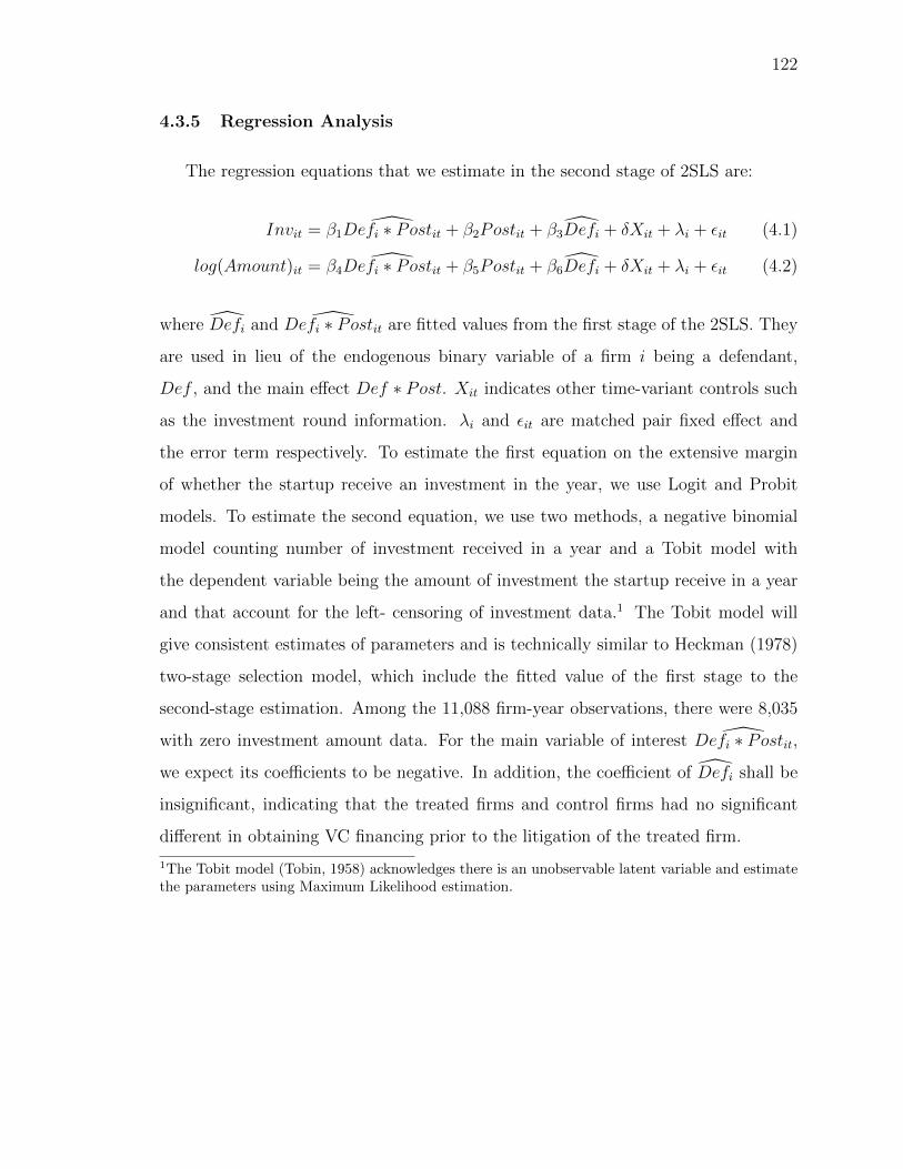
122

4.3.5 Regression Analysis

The regression equations that we estimate in the second stage of 2SLS are:

Invit = β1Defi ∗ Postit + β2Postit + β3Defi + δXit + λi + εit (4.1)

log(Amount)it = β4Defi ∗ Postit + β5Postit + β6Defi + δXit + λi + εit (4.2)

where Defi and Defi ∗ Postit are fitted values from the first stage of the 2SLS. They

are used in lieu of the endogenous binary variable of a firm i being a defendant,

Def , and the main effect Def ∗ Post. Xit indicates other time-variant controls such

as the investment round information. λi and εit are matched pair fixed effect and

the error term respectively. To estimate the first equation on the extensive margin

of whether the startup receive an investment in the year, we use Logit and Probit

models. To estimate the second equation, we use two methods, a negative binomial

model counting number of investment received in a year and a Tobit model with

the dependent variable being the amount of investment the startup receive in a year

and that account for the left- censoring of investment data.1 The Tobit model will

give consistent estimates of parameters and is technically similar to Heckman (1978)

two-stage selection model, which include the fitted value of the first stage to the

second-stage estimation. Among the 11,088 firm-year observations, there were 8,035

with zero investment amount data. For the main variable of interest Defi ∗ Postit,

we expect its coefficients to be negative. In addition, the coefficient of Defi shall be

insignificant, indicating that the treated firms and control firms had no significant

different in obtaining VC financing prior to the litigation of the treated firm.

1The Tobit model (Tobin, 1958) acknowledges there is an unobservable latent variable and estimatethe parameters using Maximum Likelihood estimation.

123

4.4 Results

At first, Table 4.2 reports the first two steps of our operationalization testing

the validity of the instruments. The first column reports the Probit model using

exogenous court variables to estimate the probability of a startup being sued. As

seen from the model, only the coefficient of Plaintiff Win is significant, meaning that

if the district ruled more cases with plaintiff win, then it is positively related to the

likelihood that the startup in the district is targeted for patent litigation. Second,

since we have two endogenous variables Def and Def ∗ Post, two instruments are

needed and they are Def and Def ∗ Post. Results show that the instruments are

highly correlated to the endogenous variables. Since only Plaintiff Win significantly

predicts the chance of a startup being sued, we only use that variable as the source

of our exogenous variation in the 2SLS procedure.

Full results of models testing Hypotheses 1a and 1b are reported in Table 4.3.

The Probit Model in the first column and only Plaintiff Win is used for exogenous

variation. After obtaining our instrument Prob(Def), it is used in the Stage 1 model.

To test the validity of the instrument, we conduct F-tests to each of our Stage 1

models to test the significance of instruments in predicting endogenous variables.

With a residual degree of freedom of 10,895, the F-statistics are beyond 100, which

are far above the commonly used threshold of 10, lending confidence for the validity

of the instrument. Our main variable of interest Def ∗ Post is negative with p-

values smaller than 0.001 in both Model 1 Probit and Model 2 Logit models. Also,

coefficients on Def are all insignificant, indicating that the defendant firm and the

matched firms are not statistically different in their obtaining of investment prior to

the litigation. The results lend strong support to Hypothesis 1a. On average, the

defendant firms are 7.4% less likely to receive investment in each year following the

litigation as compared to firms that were not sued.

Moreover, in both Negative Binomial and Tobit specifications, Def ∗ Post are

also significantly negative in predicting the amount of investment raised. The neg-

124

Table 4.2.: Validity of Instruments

Probit Stage 1-1 Stage 1-2Probit OLS OLS

DV: Probit(Def) Def Def*PostProb(Def) 0.746∗∗∗ −0.093∗

(0.000) (0.007)Prob(Def)*Post 0.001 1.004∗∗∗

(0.902) (0.000)Plaintiff Win 0.009∗

(0.049)Defendant Win 0.004

(0.549)Stayed Cases −0.009

(0.453)Transferred Cases −0.000

(0.950)Duration −0.000

(0.594)Age −0.004 0.002 −0.001

(0.799) (0.220) (0.376)Round 0.024 −0.006∗ 0.000

(0.406) (0.014) (0.843)CVC Share 0.175 0.009 0.002

(0.331) (0.683) (0.872)PAE 11.497 0.229∗∗∗ 0.084∗∗

(0.000) (0.000) (0.006)R2 0.420 0.582Adj. R2 0.410 0.574Num. obs. 3255 11088 11088F-statistic of Instruments 100.86 6312.3

∗∗∗p < 0.001, ∗∗p < 0.01, ∗p < 0.05, +p < 0.1

Notes: P-values reported in parentheses. In the Probit model, among five exogenous variables, only

the number of Plaintiff Cases is statistically significant. Our instruments are Prob(Def) ∗Post andProb(Def , with Prob(Def being the fitted value from the Probit model. Then, in OLS models of

Stage 1, Def and Def ∗Post are instrumented using Prob(Def and Prob(Def ∗Post Results showsProb(Def and Prob(Def ∗ Post are valid instruments.

125

ative binomial tells that the defendant firm on average receives ”0.3” fewer rounds

of investment each year. The Tobit model tells that, on average, the defendant firm

raises $6.5 million less in VC investments compared to control firms. The results

confirm our Hypothesis 1b that litigation negatively affects the amount of investment

startups receive from VCs.

Further results of the dynamic impact of being sued are reported in Table 4.4.

In these models, we re-estiamte Model 1 and Model 2 in Table 4.3 and interact

Def with Year dummies instead of a binary Post variable, with Year 0, the year

of the litigation to the treated firms, being the reference year. As presented in the

table, the difference between the treated firms and the control firms was insignificant

statistically prior to the litigation. Then the likelihood of the treated firms receiving

investments significantly dropped since the year they were sued. Over time, the effect

even escalated in magnitude, giving us additional evidence of the negative effect of

patent litigation on the startup’s likelihood of receiving investments.

After verifying the main effect, we proposed factors that mitigate the negative

impact of litigation, from the startup’s aspect and from the plaintiff’s aspect. When

the startup has more alternative quality signals, and when the plaintiff is weak, the

being targeted in patent litigations is less detrimental to the startup’s VC financing.

Results of models testing Hypotheses 2a and 3a are reported in Table 4.5. The sign

of the three-way interaction terms of Def ∗ Post ∗ Age and Def ∗ Post ∗Round are

expected to be positive, meaning firms with more alternative quality signals are af-

fected less by the litigation. We find evidence for Hypotheses 2a with the positive and

highly significant coefficient across models. Then, regarding plaintiff heterogeneity,

Def ∗ Post ∗ PAE is positive and significant, meaning litigations initiated by weak

plaintiffs, in this case, PAEs, are less detrimental to firm, lending support to Hypoth-

esis 3a. Then results testing Hypotheses 2b and 3b are reported in Table 4.6. Still,

the positive and significant coefficients on Def ∗Post∗Age, Def ∗Post∗Round, and

Def ∗ Post ∗ PAE verify that alternative quality signals from the startup and that

126

Tab

le4.

3.:

2SL

SR

esult

son

the

Eff

ect

ofP

aten

tL

itig

atio

non

VC

Fin

anci

ng

Pro

bit

Sta

ge

1S

tage2

Mod

el1

Mod

el2

Mod

el3

Mod

el4

DV

:P

rob

it(D

ef)

Def

Def

*P

ost

P(I

nv)

P(I

nv)

Nu

mIn

vA

mou

nt

Pro

bit

Marg

inL

ogit

Marg

inN

egB

inom

ial

Tob

it

Prob(Def

)0.

746∗∗∗−

0.093∗

(0.0

00)

(0.0

07)

Prob(Def

)∗Post

0.001

1.0

04∗∗∗

(0.9

02)

(0.0

00)

Age

−0.0

080.0

02

−0.

001

−0.

244∗∗∗−

0.074∗∗∗−

0.440∗∗∗−

0.0

73∗∗∗

−0.

298∗∗∗

−6.

506∗∗∗

(0.6

26)

(0.2

20)

(0.3

76)

(0.0

00)

(0.0

00)

(0.0

00)

(0.0

00)

(0.0

00)

(0.0

00)

Rou

nd

0.02

5−

0.006∗

0.000

0.377∗∗∗

0.113∗∗∗

0.674∗∗∗

0.1

13∗∗∗

0.413∗∗∗

10.2

87∗∗∗

(0.3

90)

(0.0

14)

(0.8

43)

(0.0

00)

(0.0

00)

(0.0

00)

(0.0

00)

(0.0

00)

(0.0

00)

CV

CS

har

e0.1

610.0

09

0.0

02

0.527∗∗∗

0.165∗∗∗

0.984∗∗∗

0.1

57∗∗∗

0.610∗∗∗

15.7

81∗∗∗

(0.3

72)

(0.6

83)

(0.8

72)

(0.0

00)

(0.0

00)

(0.0

00)

(0.0

00)

(0.0

00)

(0.0

00)

PA

E11.4

960.2

29∗∗∗

0.084∗∗

0.164

0.0

42

0.241

0.0

51

−0.

233

3.1

16

(0.0

00)

(0.0

00)

(0.0

06)

(0.6

38)

(0.7

10)

(0.6

89)

(0.6

59)

(0.5

94)

(0.7

98)

Def

−0.

101

−0.

024

−0.

145

−0.0

30

0.2

94

1.6

51

(0.7

97)

(0.8

36)

(0.8

31)

(0.8

02)

(0.5

51)

(0.9

05)

Def

*Pos

t−

0.322∗∗∗−

0.088∗∗∗−

0.524∗∗∗−

0.0

96∗∗∗

−0.

140

+−

5.693

+

(0.0

00)

(0.0

00)

(0.0

00)

(0.0

00)

(0.0

94)

(0.1

04)

Pla

inti

ffW

in0.

009∗∗

(0.0

05)

Log

(sca

le)

3.543∗∗∗

(0.0

00)

Mat

ched

Gro

up

FE

Yes

Yes

Yes

Yes

Yes

Yes

Yes

Yes

Yes

Nu

m.

obs.

3454

11088

11088

11088

11088

11088

11088

11088

11088

Lef

t-ce

nso

red

8035

R2

0.420

0.5

82

Ad

j.R

20.

410

0.5

74

McF

add

enP

seu

do-

R2

0.1

83

0.1

84

Wal

dT

est

1414.

869

∗∗∗ p<

0.00

1,∗∗p<

0.01

,∗ p<

0.0

5,+p<

0.1

Not

es:

P-v

alu

esre

por

ted

inp

aren

thes

es.

Ind

epen

den

tva

riab

leof

inte

rest

inS

tage

2Def

an

dDef∗Post

are

inst

rum

ente

du

sin

gDef

an

d

Def∗Post

wit

hDef

bei

ng

the

fitt

edva

lue

from

the

Pro

bit

mod

el.

127

Table 4.4.: Dynamic Effects of Patent Litigation on the Likelihood of VC Financing

Model 5 Model 6DV: P(Inv) P(Inv)

Probit Margin Logit MarginDef*Year-5 −0.502∗∗ −0.128 −0.786∗∗ −0.149∗∗

(0.002) (0.136) (0.004) (0.003)Def*Year-4 −0.347∗ −0.086 −0.530∗ −0.103∗

(0.014) (0.174) (0.027) (0.019)Def*Year-3 −0.116 −0.027 −0.166 −0.035

(0.379) (0.493) (0.456) (0.381)Def*Year-2 0.143 0.043 0.265 0.042

(0.259) (0.309) (0.214) (0.259)Def*Year-1 0.162 0.047 0.288 0.048

(0.181) (0.278) (0.160) (0.191)Def*Year1 −0.619∗∗∗ −0.167 −1.026∗∗∗ −0.184∗∗∗

(0.000) (0.107) (0.000) (0.000)Def*Year2 −0.980∗∗∗ −0.271+ −1.658∗∗∗ −0.292∗∗∗

(0.000) (0.096) (0.000) (0.000)Def*Year3 −1.242∗∗∗ −0.370+ −2.269∗∗∗ −0.370∗∗∗

(0.000) (0.094) (0.000) (0.000)Def*Year4 −2.102∗∗∗ −0.634+ −3.882∗∗∗ −0.626∗∗∗

(0.000) (0.091) (0.000) (0.000)Def*Year5 −2.944∗∗∗ −0.910+ −5.574∗∗∗ −0.877∗∗∗

(0.000) (0.090) (0.000) (0.000)Def −0.155 −0.049 −0.300 −0.046

(0.730) (0.712) (0.695) (0.738)Age −0.242∗∗∗ −0.069+ −0.425∗∗∗ −0.072∗∗∗

(0.000) (0.084) (0.000) (0.000)Round 0.434∗∗∗ 0.124+ 0.759∗∗∗ 0.129∗∗∗

(0.000) (0.084) (0.000) (0.000)CVC Share 0.289∗∗ 0.091 0.558∗∗ 0.086∗∗

(0.005) (0.128) (0.001) (0.007)PAE 0.415 0.128 0.691 0.136

(0.291) (0.410) (0.301) (0.342)Matched Group FE Yes Yes∗∗∗p < 0.001, ∗∗p < 0.01, ∗p < 0.05, +p < 0.1

Notes: P-values reported in parentheses. Post is replaced by Year dummies with Year 0, the yearof litigation, being the reference year.

128

the weak plaintiff mitigates the negative impact of being litigated on the amount of

VC investment received.

4.5 Robustness

4.5.1 Time to the Next Round

In the main analysis, we have shown that being litigated may reduce the probabil-

ity of the targeted startup receiving further investments. As a robustness check, we

test whether being litigated will delay the startup’s speed of reaching the next round

of financing. When a startup is sued, the investors may wait for the resolution of

the case and observe the consequences to the firm, thus causing a delay in obtaining

the next round of VC investment. Since receiving investment is a recurrent event for

firms, we use the Andersen-Gill model (Andersen and Gill, 1982), which is an exten-

sion to the widely used Cox proportional hazard model accommodating for recurrent

events. To conduct the analysis, we restructured the data and counted the number of

days to the next round (if there was one) of all 3,478 investment events of our firms

in the main analysis. Had there was not follow-on investment, the end of observation

period was set to Dec. 15th, 2019, which was the date of our latest update to data.

On average, it takes a startup in our sample four yearsto reach the next round. Table

4.7 gives the summary statistics.

Table 4.8 reports results of hazard models. The dependent variable of is the

number of days after an investment until the next round investment for a startup.

The status code, “Next Round”, is one if a follow-on investment is observed, the

status code is zero if no follow-on investment is observed. We expect the coefficient

of Def ∗ Post to be negative, meaning a decrease in the hazard of receiving the

next investment. The hypothesis is verified by the negative and significant sign of

Def ∗ Post and the insignificant Def across Models 1-5. On average, after being

sued, the hazard of receiving next round of investment of treated firms is merely

3.4% (e−3.388) of the hazard of their control counterparts. In both Model 3 and 5,

129

Tab

le4.

5.:

Het

erog

eneo

us

Eff

ect

ofP

aten

tL

itig

atio

non

the

Lik

elih

ood

VC

Fin

anci

ng

Mod

el1

Mod

el2

Mod

el3

Mod

el4

Mod

el5

Mod

el6

DV

:P

(Inv)

P(I

nv)

P(I

nv)

P(I

nv)

P(I

nv)

P(I

nv)

Logit

Marg

inP

rob

itM

arg

inL

ogit

Marg

inP

rob

itM

arg

inL

ogit

Marg

inP

rob

itM

arg

inD

ef−

0.1

97

−0.0

65

−0.4

18

−0.0

56

−0.5

44

−0.1

46

−0.8

94

−0.1

59

−0.1

48

−0.0

44

−0.2

64

−0.0

44

(0.6

24)

(0.5

62)

(0.5

45)

(0.6

37)

(0.1

72)

(0.2

18)

(0.1

98)

(0.1

92)

(0.1

72)

(0.2

18)

(0.1

98)

(0.1

92)

Def

*P

ost

−0.6

94∗∗

−0.1

69∗∗

−1.0

93∗∗

−0.1

96∗∗

−1.1

65∗∗

∗−

0.3

41∗∗

∗−

2.0

85∗∗

∗−

0.3

40∗∗

∗−

0.5

63∗∗

∗−

0.1

56∗∗

∗−

0.9

41∗∗

∗−

0.1

67∗∗

∗

(0.0

01)

(0.0

06)

(0.0

03)

(0.0

02)

(0.0

00)

(0.0

00)

(0.0

00)

(0.0

00)

(0.0

00)

(0.0

00)

(0.0

00)

(0.0

00)

Def*Post*Age

0.2

02∗∗

∗0.0

54∗∗

∗0.3

48∗∗

∗0.0

57∗∗

∗

(0.0

00)

(0.0

00)

(0.0

00)

(0.0

00)

Def*Post*Round

0.4

69∗∗

∗0.1

33∗∗

∗0.8

13∗∗

∗0.1

37∗∗

∗

(0.0

00)

(0.0

00)

(0.0

00)

(0.0

00)

Def*Post*PAE

1.3

63∗∗

∗0.4

16∗∗

∗2.5

11∗∗

∗0.4

03∗∗

∗

(0.0

00)

(0.0

00)

(0.0

00)

(0.0

00)

CV

CS

hare

0.4

49∗∗

∗0.1

24∗∗

∗0.8

03∗∗

∗0.1

27∗∗

∗0.3

77∗∗

∗0.1

17∗∗

∗0.7

16∗∗

∗0.1

10∗∗

∗0.5

39∗∗

∗0.1

66∗∗

∗1.0

01∗∗

∗0.1

59∗∗

∗

(0.0

00)

(0.0

00)

(0.0

00)

(0.0

00)

(0.0

00)

(0.0

00)

(0.0

00)

(0.0

00)

(0.0

00)

(0.0

00)

(0.0

00)

(0.0

00)

Age

−0.1

28∗∗

∗−

0.0

37∗∗

∗−

0.2

38∗∗

∗−

0.0

36∗∗

∗−

0.1

98∗∗

∗−

0.0

59∗∗

∗−

0.3

60∗∗

∗−

0.0

58∗∗

∗−

0.2

38∗∗

∗−

0.0

71∗∗

∗−

0.4

29∗∗

∗−

0.0

70∗∗

∗

(0.0

00)

(0.0

00)

(0.0

00)

(0.0

00)

(0.0

00)

(0.0

00)

(0.0

00)

(0.0

00)

(0.0

00)

(0.0

00)

(0.0

00)

(0.0

00)

Rou

nd

0.4

35∗∗

∗0.1

19∗∗

∗0.7

72∗∗

∗0.1

23∗∗

∗0.5

83∗∗

∗0.1

65∗∗

∗1.0

05∗∗

∗0.1

70∗∗

∗0.3

80∗∗

∗0.1

12∗∗

∗0.6

79∗∗

∗0.1

12∗∗

∗

(0.0

00)

(0.0

00)

(0.0

00)

(0.0

00)

(0.0

00)

(0.0

00)

(0.0

00)

(0.0

00)

(0.0

00)

(0.0

00)

(0.0

00)

(0.0

00)

PA

E0.2

52

0.0

84

0.4

93

0.0

76

0.5

35

0.1

70

0.8

91

0.1

76

0.9

26

0.3

39

1.6

28

0.3

22

(0.4

79)

(0.4

77)

(0.4

17)

(0.5

19)

(0.1

27)

(0.2

14)

(0.1

45)

(0.1

80)

(0.1

27)

(0.2

14)

(0.1

45)

(0.1

80)

Def

*A

ge

−0.0

54∗∗

−0.0

15∗∗

−0.0

95∗∗

−0.0

15∗∗

(0.0

07)

(0.0

05)

(0.0

06)

(0.0

05)

Post

*A

ge

−0.1

66∗∗

∗−

0.0

46∗∗

∗−

0.2

96∗∗

∗−

0.0

47∗∗

∗

(0.0

00)

(0.0

00)

(0.0

00)

(0.0

00)

Def

*R

ou

nd

−0.0

77∗∗

−0.0

23∗∗

−0.1

38∗∗

−0.0

23∗∗

(0.0

09)

(0.0

07)

(0.0

05)

(0.0

10)

Post

*R

ou

nd

−0.2

92∗∗

∗−

0.0

79∗∗

∗−

0.4

84∗∗

∗−

0.0

85∗∗

∗

(0.0

00)

(0.0

00)

(0.0

00)

(0.0

00)

Def

*P

AE

−0.6

56

−0.1

95

−1.1

79

−0.1

94

(0.0

09)

(0.0

07)

(0.0

05)

(0.0

10)

Post

*P

AE

−1.1

45∗∗

∗−

0.1

97∗∗

∗−

2.1

25∗∗

∗−

0.2

09∗∗

∗

(0.0

00)

(0.0

00)

(0.0

00)

(0.0

00)

Matc

hed

Gro

up

FE

Yes

Yes

Yes

Yes

Yes

Yes

Nu

m.

ob

s.11088

11088

11088

11088

11088

11088

McF

ad

den

Pse

ud

o-R

20.2

17

0.2

19

0.2

23

0.2

22

0.1

86

0.1

88

∗∗∗ p<

0.00

1,∗∗p<

0.0

1,∗ p<

0.05

,+p<

0.1

Not

es:

P-v

alu

esre

por

ted

inp

aren

thes

es.

Ind

epen

den

tva

riab

les

of

inte

rest

are

Def

*P

ost

*A

ge,

Def

*P

ost

*R

ou

nd

,an

dD

ef*P

ost

*P

AE

.A

lltw

o-w

ayin

tera

ctio

ns

are

incl

ud

ed.

All

mod

els

incl

ud

edm

atc

hed

pair

fixed

effec

ts.

130

Table 4.6.: Heterogeneous Effect of Patent Litigation on VC Financing Amount

Model 1 Model 2 Model 3 Model 4 Model 5 Model 6DV: Num Inv Amount Num Inv Amount Num Inv Amount

Neg Binom Tobit Neg Binom Tobit Neg Binom TobitDef 0.201 1.084 −0.181 −10.277 0.345 3.699

(0.680) (0.940) (0.712) (0.467) (0.470) (0.780)Def*Post −0.434 −11.966+ −1.026∗∗∗ −29.326∗∗∗ −0.185 −16.472∗∗∗

(0.059) (0.176) (0.000) (0.000) (0.224) (0.008)Def*Post*Age 0.207∗∗∗ 5.071∗∗∗

(0.000) (0.001)Def*Post*Round 0.359∗∗∗ 12.154∗∗∗

(0.000) (0.000)Def*Post*PAE 1.441∗∗∗ 49.285∗∗∗

(0.000) (0.000)CVC Share 0.488∗∗∗ 14.036∗∗∗ 0.410∗∗∗ 12.599∗∗∗ 0.611∗∗∗ 16.015∗∗∗

(0.000) (0.000) (0.000) (0.000) (0.000) (0.000)Age −0.158∗∗∗ −2.848∗∗∗ −0.244∗∗∗ −5.137∗∗∗ −0.291∗∗∗ −6.233∗∗∗

(0.000) (0.000) (0.000) (0.000) (0.000) (0.000)Round 0.470∗∗∗ 11.601∗∗∗ 0.577∗∗∗ 15.318∗∗∗ 0.417∗∗∗ 10.336∗∗∗

(0.000) (0.000) (0.000) (0.000) (0.000) (0.000)PAE −0.102 5.593 0.155 13.152 1.621 64.722∗

(0.813) (0.649) (0.719) (0.279) (0.065) (0.085)Def*Age −0.069∗∗ −2.087∗∗∗

(0.003) (0.004)Post*Age −0.194∗∗∗ −4.617∗∗∗

(0.000) (0.000)Def*Round −0.034 −1.839∗

(0.212) (0.035)Post*Round −0.240∗∗∗ −7.333∗∗∗

(0.000) (0.000)Def*PAE −1.796 −61.459∗

(0.044) (0.074)Post*PAE −1.551∗∗∗ −38.634∗∗∗

(0.000) (0.000)Log(scale) 3.532∗∗∗ 3.530∗∗∗ 3.540∗∗∗

(0.000) (0.000) (0.000)Matched Group FE Yes Yes Yes Yes Yes YesNum. obs. 11088 11088 11088 11088 11088 11088Left-censored 8035 8035 8035McFadden Pseudo-R2 0.167 0.148 0.172Wald Test 1520.156 1637.662 1425.849∗∗∗p < 0.001, ∗∗p < 0.01, ∗p < 0.05, +p < 0.1

Notes: Only Stage 2 of 2SLS results are reported. P-values are in parentheses. Independent vari-ables of interest are Def*Post*Age, Def*Post*Round, and Def*Post*PAE. Endogenous independent

variables in Stage 2 are instrumented using Def and its interaction terms obtained from Stage 1models of 2SLS. All two-way interactions are included. All models included matched pair fixedeffects.

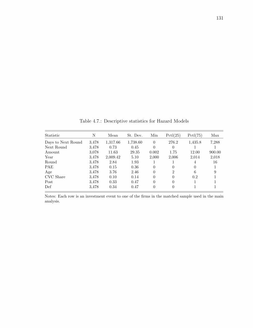
131

Table 4.7.: Descriptive statistics for Hazard Models


Days to Next Round 3,478 1,317.66 1,738.60 0 276.2 1,435.8 7,288Next Round 3,478 0.73 0.45 0 0 1 1Amount 3,078 11.63 29.35 0.002 1.75 12.00 900.00Year 3,478 2,009.42 5.10 2,000 2,006 2,014 2,018Round 3,478 2.84 1.93 1 1 4 16PAE 3,478 0.15 0.36 0 0 0 1Age 3,478 3.76 2.46 0 2 6 9CVC Share 3,478 0.10 0.14 0 0 0.2 1Post 3,478 0.33 0.47 0 0 1 1Def 3,478 0.34 0.47 0 0 1 1

Notes: Each row is an investment event to one of the firms in the matched sample used in the mainanalysis.

132

we find the interaction terms of Def ∗Post ∗Round positive and significant, lending

support to our hypotheses that alternative quality signals by having received more

rounds of investment mitigates the negative impact of being sued. There is some

evidence showing that lawsuits initiated by PAEs are less detrimental in reducing the

hazard of receiving investments.

4.5.2 Matched Locations

One limitation of the main analysis is that since we exploit variation among district

courts, we are not able to address other regional factors that potentially drive the

results. To address this issue, we adopted another matching method and intentionally

matched each treated firm with firms in the same metropolitan area. Thus, we have

several criteria in the matching (Angrist, 1998). First, the control firm must be in the

same Industry Subgroup as the treated firm in VentureXpert since different businesses

and industries have quite different venture financing environment. Second, the control

firm must be founded in the same State as the matched treated firm since the location

is known to affect venture financing. (Sorenson and Stuart, 2001). Third, the control

firm must have received the same rounds of investment as the treated firm at the year

when the treated firm was litigated. It is well known that in venture financing, to

invest or not and the amount of financing depends on how many series of financing

have the company already gone through. Fourth, we would want control firms to be

founded in similar years as the treated firms since firms are affected by the external

environment when they were founded, and such an imprinting process can be long-

lasting (Stinchcombe and March, 1965; Sydow et al., 2009). We operationalize by at

first categorizing founding years into several bins, divided by major macroeconomic

downturns such as the 2009 financial crisis, the 2000 internet bubble, and the 1990

Gulf war. Then, we require that control firms must be founded in the same year bins

as the treated firm. After matching the bins, among the firms remained, we pick up

to three firms with the closest founding years as the treated firm. Going through all

133

Table 4.8.: Time to Next Round: Hazard Model Results

Model 1 Model 2 Model 3 Model 4 Model 5Def −0.513 0.164 0.301 −2.934 0.380

(0.771 (0.918) (0.848) (0.121) (0.828)Def*Post −3.388∗∗∗ −3.540∗∗∗ −3.516∗∗∗ −8.342∗∗∗ −4.385∗∗∗

(0.000) (0.000) (0.000) (0.000) (0.000)Def*Post*Age −0.065 0.477∗∗∗

(0.109) (0.000)Def*Post*Round 1.198∗∗∗ 0.752∗∗∗

(0.000) (0.000)Def*Post*PAE 11.524∗∗∗ 2.994

(0.000) (0.390)Amount −0.006∗∗∗ −0.010∗∗∗ −0.008∗∗∗ −0.009∗∗∗ −0.009∗∗∗

(0.000) (0.000) (0.000) (0.000) (0.000)Age 0.015 0.043 0.029 0.028 0.056

(0.724) (0.462) (0.606) (0.596) (0.348)Round −0.080∗∗ −0.040 −0.073+ −0.048 −0.063+

(0.007) (0.167) (0.072) (0.132) (0.091)PAE 0.520 −0.077 −0.229 13.947∗ 3.895

(0.682) (0.947) (0.841) (0.039) (0.836)CVC Share −2.323∗∗∗ −2.142∗∗∗ −2.161∗∗∗ −2.270∗∗∗ −2.144∗∗∗

(0.000) (0.000) (0.000) (0.000) (0.000)Post*Age −0.695∗∗∗ −0.349∗∗∗

(0.000) (0.000)Def*Age 1.002∗∗∗ −0.075

(0.000) (0.377)Post*Round −0.818∗∗∗ −0.396∗∗

(0.000) (0.002)Def*Round −0.054 −0.119

(0.586) (0.288)Post*PAE −2.583∗∗∗ −1.869∗

(0.000) (0.043)Def*PAE −12.809+ −4.178

(0.056) (0.830)Matched Group FE Yes Yes Yes Yes YesYear FE Yes Yes Yes Yes YesObs. 3078 3078 3078 3078 3078Events 2286 2286 2286 2286 2286R2 0.361 0.361 0.550 0.463 0.560Chi2 1183.08 2005.48 2116.30 1637.18 2154.08∗∗∗p < 0.001, ∗∗p < 0.01, ∗p < 0.05, +p < 0.1

Notes: Andersen-Gill Model (Andersen and Gill, 1982) (An extension to Cox model with recur-rent events) results are reported with the Dependent Variable being the number of days until thenext round of investment. Results shows defendant firms experienced significant decrease in thehazard of receiving next round of investment as compared to the control firms, lending support toour hypothesized negative impact of patent lawsuits. When estimating models, if no investmentsobserved after For one firm, then observation period ends on Dec. 15th, 2019. Only Stage 2 of2SLS results are reported. P-values are in parentheses with standard errors clustered at firm-level.

Endogenous independent variables that include Def are instrumented using Def and its interactionterms obtained from Stage 1 models that follows same procedures as previous analysis and that arenot reported. All two-way interactions are included.

134

the procedures, we obtain a sample of 6,322 firms with 1,769 treated firms and 4,553

control firms. Table C.1 summarizes the data and Table C.2 reports the correlation

between variables.

We report the results of Linear Probability Models on the likelihood of VC financ-

ing in Table 4.9. Across Models 1-4 in the Table, the coefficient of Def ∗ Post is

negative and highly significant (three out of the four models have a p-value smaller

than 0.001, the other is also smaller the 0.05), lending strong support to our Hypothe-

ses 1a. On average, patent litigation leads to a drop of 2-3 percentage points in the

probability of getting a VC financing. Then in Table 4.10, we report two sets of results

on the effect of patent litigation on the logarithm amount of VC financing. Model

5-8 were estimated using fixed-effect panel regression, and Model 9-12 were estimated

using the Tobit model with industry and year fixed effects. The Tobit model fixes the

data censoring problem and produces consistent estimates of parameters (Amemiya,

1973). As we can see, in all models, Def ∗ Post is negative and highly significant

with p-values smaller than 0.01, lending evidence supporting Hypothesis 1b.

We also find that the three-way interaction of Def ∗ Post ∗ Age has positive

coefficients in Table 4.9 and Table 4.10. The finding lends support to our hypotheses,

while contradicting our findings in the main results. One plausible reason is that as

startups mature, the value at stake for patent litigations is also larger, thus making

the litigation more detrimental to investors as compared to litigations that target

young startups. But further studies shall be conducted to reveal the mechanism

behind the finding.

4.5.3 Placebo Test

Furthermore, we also conducted a placebo test that marked the original treated

group as a part of the control group and randomly selected 25% of the original control

group firm to be labeled as the treated company. Then, using this sample, we repeat

135

Table 4.9.: Effect of Patent Litigation on the Likelihood of VC Financing

Model 1 Model 2 Model 3 Model 4

Def*Post −0.023∗∗∗ −0.030∗∗∗ −0.012∗ −0.081∗∗∗

(0.006) (0.006) (0.006) (0.007)Def*Post*Age 0.003∗∗∗

(0.000)Def*Post*CVC −0.086∗∗∗

(0.012)

Round FE No Yes Yes YesFirm FE Yes Yes Yes YesYesr FE Yes Yes Yes Yes

R2 0.001 0.156 0.157 0.158Adj. R2 −0.112 0.061 0.062 0.064n 6322 6322 6322 6322Num. obs. 62690 62690 62690 62690∗∗∗p < 0.001, ∗∗p < 0.01, ∗p < 0.05, +p < 0.1

Notes: Standard errors reported in parentheses. The dependent variable is a binary variable whichequals one if a firm i received a VC financing at year t and zero otherwise. The table report linearprobability model results on the effect of patent litigation on the likelihood of VC financing. Thenegative and significant coefficients of Def ∗ Post show that the treated firms, after being sued areless likely to receive VC investments as compared to their matched counterparts, and lend supportto our hypothesis. Further, the age of the startup mitigate the negative effect of being sued, andthe negative impact is more severe for startups that were funded by CVCs.

136

Tab

le4.

10.:

Eff

ect

ofP

aten

tL

itig

atio

non

the

Am

ount

ofV

CF

inan

cing

Mod

el5

Mod

el6

Mod

el7

Mod

el8

Mod

el9

Mod

el10

Mod

el11

Mod

el12

OL

SO

LS

OL

SO

LS

Tob

itT

obit

Tob

itT

obit

Def

*P

ost

−0.0

81∗∗∗

−0.

089∗∗∗

−0.0

42∗∗

−0.

169∗∗∗

−0.4

84∗∗∗

−0.5

99∗∗∗

−0.

518∗∗∗

−1.1

86∗∗∗

(0.0

12)

(0.0

12)

(0.0

13)

(0.0

15)

(0.1

14)

(0.1

09)

(0.1

16)

(0.1

22)

Def

*P

ost

*CV

C−

0.2

33∗∗∗

−0.

282

(0.0

26)

(0.1

58)

Def

*P

ost

*A

ge0.0

04∗∗∗

0.0

57∗∗∗

(0.0

00)

(0.0

04)

Age

−0.1

21∗∗∗

−0.

121∗∗∗

−0.1

31∗∗∗

(0.0

03)

(0.0

03)

(0.0

03)

CV

C0.

204∗∗

(0.0

68)

logS

igm

a1.

359∗∗∗

1.2

45∗∗∗

1.24

4∗∗∗

1.2

44∗∗∗

(0.0

17)

(0.0

15)

(0.0

15)

(0.0

15)

Ind

ust

ryF

EY

esY

esY

esY

esN

oN

oN

oN

oF

irm

FE

Yes

Yes

Yes

Yes

Yes

Yes

Yes

Yes

Yea

rF

EY

esY

esY

esY

esY

esY

esY

esY

es

R2

0.0

010.

060

0.06

20.

062

Ad

j.R

2−

0.1

12−

0.04

6−

0.0

44−

0.0

44L

eft-

cen

sore

d56

057

5605

756

055

5605

7n

6322

6322

6322

6322

6322

6322

6322

6322

Nu

m.

ob

s.6269

062

690

6269

062

690

6269

062

690

6269

062

690

∗∗∗ p<

0.00

1,∗∗p<

0.01

,∗ p<

0.0

5,+p<

0.1

Not

es:

Sta

nd

ard

erro

rsre

por

ted

inp

aren

thes

es.

Dep

end

ent

vari

ab

leis

Log(A

mou

nt+

1),

wh

ich

isth

elo

gari

thm

of

the

am

ount

of

VC

inve

stm

ent

firm

ire

ceiv

edin

year

t.A

llm

od

els

incl

ud

edfi

rman

dye

ar

fixed

effec

ts.

137

our analysis of the two dependent variables. As expected, our variables of interest

showed no significance. Detailed results are not reported in the text.

4.6 Caveats

Though extant studies have exploited variations in regional court practices to

instrument for focal firms’ risk of being litigated (Kiebzak et al., 2016), the validity

of such instruments is challenged if firms choose locations or relocate based on the

friendliness of district court. However, given the overall small proportion of firms sued

and the abundance of other factors that entrepreneurs consider deciding for locations,

we do not think district courts practice in patent lawsuits post significant influence

on entrepreneurial firms’ location choice.

On the other side of the coin, another question to be asked is whether VCs tend to

refrain from investing in firms located in those litigious and plaintiff-friendly districts.

In the main analysis, we are not able to tell since locations are not matched. However,

in the robustness section, comparing firms with proximate locations that were sued

and not sued, we still find significant main effects of litigation, thus alleviating the

above concern. However, it is yet to be tested whether the entrepreneurial firms or

the VCs intentionally avoid districts with certain behavior in their legal practices.

In this study, we do not find conclusive evidence on whether the younger or older

firm is affected more by the litigation, and have proposed potential mechanisms.

Future studies can further explore more heterogeneity among defendant startups to

unveil the reason behind such heterogeneous impact of patent litigations.

4.7 Concluding Remarks

Scholarships in entrepreneurship have primarily focused on the building of re-

sources and capabilities. While securing access to resources and building capabilities

are essential to entrepreneurial firms’ competitive advantage, much less is known

about the events and actions that potentially hurt firms’ resources and capabili-

138

ties, thus destroying competitive advantage. Patent lawsuits, when faced by an en-

trepreneurial firm, is one of such events that can potentially ruin the efforts of the

startup.

In the past five years, patent litigations have received much attention from scholars

of multiple fields. For entrepreneurial firms, while most studies focus on how litiga-

tions affect their development of technological capabilities and complementary assets,

it is much neglected how litigations will affect their VC financing, which is one of the

most central issues for entrepreneurial firms. VCs’ involvement is even more critical

than providing financial resources, as they also lend other valuable complementary

assets to startups (Fitza et al., 2009; Teece, 1986).

This paper fills in the gap in the literature by looking into how patent litigations

affect a firm’s external financing from venture capitals. Using our matched firm-level

data that combines VC investment and litigation records, we find evidence support-

ing the view that patent litigations on average, negatively affect a firm’s chance as

well as the amount of obtaining VC financing. In addition, contrary to the view that

CVCs may provide complementary assets to the portfolio firm such that they will

be better dealing with patent litigations, we find that the negative impacts of liti-

gations are more prominent for firms that are backed by CVCs. Moreover, younger

entrepreneurial firms, due to their liability of newness and limited resources, are also

more affected by patent litigations.

With contributions of this paper, it also has some limitations, thus opening av-

enues for future extensions. First, we have not yet distinguished the patent litigations

initiated by rival firms from the ones initiated by PAEs. PAEs are said to initiate

frivolous litigations (Shrestha, 2010) based on low-quality patents and ambiguous

infringement charges. Thus, it can be expected that when litigated by a PAE, the

impact would be different from other situations. Future studies can further discuss

how the plaintiff of patent litigation affects the impact of patent litigation on VC

financing and other factors.

139

Another limitation of this study is that due to the scope of this paper, we do

not pay much attention to the two-side matching of the investment, i.e., we focus

on the firms receiving VC financing, but not on the VC/PE’s willingness to invest

in ventures. This limitation is also partly because we do not observe offers made by

VC/PEs but were rejected by venture firms. In the future, it would be interesting to

further the study by distinguishing the impact on the venture firms, as well as on the

VC/PEs.

Yet another future avenues of study is that, in addition to the impact of the focal

defendant firm, it worth exploring whether or how the impact of patent litigations will

spillover to other firms and organizations. Lemus and Temnyalov (2014, 2017) argue

that the litigation activities will, in the end, benefit the innovation of firms in the

industry. In addition, how will technology suppliers such as universities (Shane and

Somaya, 2007) be affected by patent litigations? When while VCs may be reluctant

financing firms with legal disputes, will universities tend to be more likely to help

firms with patent litigations. Future examination of the impact using firm-level data

could be a fruitful direction of study.

140

BIBLIOGRAPHY

Abrams, D. S., Akcigit, U., Oz, G., and Pearce, J. G. (2019). The patent troll:

Benign middleman or stick-up artist? National Bureau of Economic Research

Working Paper Series, No. 25713.

Abrams, D. S., Akcigit, U., and Popadak, J. (2013). Patent value and citations: Cre-

ative destruction or strategic disruption? National Bureau of Economic Research

Working Paper Series, No. 19647.

Acemoglu, D. and Autor, David H.and Lyle, D. (2004). Women, war, and wages:

The effect of female labor supply on the wage structure at midcentury. Journal of

Political Economy, 112(3):497–551.

Adegbesan, J. A. (2009). On the origins of competitive advantage: Strategic factor

markets and heterogeneous resource complementarity. Academy of Management

Review, 34(3):463–475.

Agarwal, R., Ganco, M., and Ziedonis, R. H. (2009). Reputations for toughness in

patent enforcement: implications for knowledge spillovers via inventor mobility.

Strategic Management Journal, 30(13):1349–1374.

Alcacer, J. and Gittelman, M. (2006). Patent citations as a measure of knowledge

flows: The influence of examiner citations. The Review of Economics and Statistics,

88(4):774–779.

Allison, J. R., Lemley, M. A., and Schwartz, D. L. (2017). How often do non-practicing

entities win patent suits? Berkeley Technology Law Journal, 32(1).

141

Allison, J. R., Lemley, M. A., and Walker, J. (2009). Extreme value or trolls on top?

the characteristics of the most-litigated patents. University of Pennsylvania Law

Review, 158(1):1–37.

Alvarez-Garrido, E. and Dushnitsky, G. (2016). Are entrepreneurial venture’s inno-

vation rates sensitive to investor complementary assets? comparing biotech ven-

tures backed by corporate and independent vcs. Strategic Management Journal,

37(5):819–834.

Amemiya, T. (1973). Regression analysis when the dependent variable is truncated

normal. Econometrica, 41(6):997–1016.

Andersen, P. K. and Gill, R. D. (1982). Cox’s regression model for counting processes:

A large sample study. The Annals of Statistics, 10(4):1100–1120.

Angrist, J. D. (1998). Estimating the labor market impact of voluntary military

service using social security data on military applicants. Econometrica, 66(2):249–

288.

Angrist, J. D. and Pischke, J.-S. (2008). Mostly harmless econometrics: An empiri-

cist’s companion. Princeton university press.

Appel, I., Farre-Mensa, J., and Simintzi, E. (2020). Patent trolls and startup em-

ployment. Journal of Financial Economics.

Arora, A. and Ceccagnoli, M. (2006). Patent protection, complementary assets, and

firms’ incentives for technology licensing. Management Science, 52(2):293–308.

Arora, A., Cohen, W. M., and Walsh, J. P. (2016). The acquisition and commercial-

ization of invention in american manufacturing: Incidence and impact. Research

Policy, 45(6):1113–1128.

Arora, A. and Fosfuri, A. (2003). Licensing the market for technology. Journal of

Economic Behavior & Organization, 52(2):277–295.

142

Arora, A. and Gambardella, A. (1994). Evaluating technological information and

utilizing it: Scientific knowledge, technological capability, and external linkages in

biotechnology. Journal of Economic Behavior & Organization, 24(1):91–114.

Arora, A. and Gambardella, A. (2010). The Market for Technology, volume Volume

1, pages 641–678. North-Holland.

Arora, A. and Nandkumar, A. (2012). Insecure advantage? markets for technology

and the value of resources for entrepreneurial ventures. Strategic Management

Journal, 33(3):231–251.

Asmussen, C. G. (2015). Strategic factor markets, scale free resources, and economic

performance: The impact of product market rivalry. Strategic Management Journal,

36:18261844.

Balachandran, S. (2018). Pipes or shackles? how ties to incumbents shape startup

innovation. Working Paper. Using investors’ investments in other projects as an

instrument for investing in the focal firm.

Barney, J. B. (1986). Strategic factor markets: Expectations, luck, and business

strategy. Management Science, 32(10):1231–1241.

Barney, J. B. (1988). Returns to bidding firms in mergers and acquisitions: Recon-

sidering the relatedness hypothesis. Strategic Management Journal, 9:71–78.

Barney, J. B. (2018). Why resource-based theory’s model of profit appropriation must

incorporate a stakeholder perspective. Strategic Management Journal, 39(13):3305–

3325.

Bass, F. M. (1969). A new product growth for model consumer durables. Management

Science, 15(5):215–227.

Bernstein, G. (2016). The end user’s predicament: User standing in patent litigation.

Boston University Law Review, 96(6):1929.

143

Bessen, J. (2008). The value of U.S. patents by owner and patent characteristics.

Research Policy, 37(5):932–945.

Bessen, J. and Hunt, R. M. (2007). An empirical look at software patents. Journal

of Economics & Management Strategy, 16(1):157–189.

Bessen, J. and Maskin, E. (2009). Sequential innovation, patents, and imitation. The

RAND Journal of Economics, 40(4):611–635.

Bessen, J. and Meurer, M. J. (2012). The private costs of patent litigation. Journal

of Law, Economics, and Policy, 9:59.

Bessen, J. and Meurer, M. J. (2013). The direct costs from npe disputes. Cornell L.

Rev., 99:387.

Blevins, D. P. and Ragozzino, R. (2018). An examination of the effects of venture

capitalists on the alliance formation activity of entrepreneurial firms. Strategic

Management Journal, 39(7):2075–2091.

Blomkvist, M. and Korkeamaki, T. (2017). Financial versus strategic bidders: Evi-

dence from unsuccessful takeover bids. Economics Letters, 159:142–144.

Bower, J. L. and Christensen, C. M. (1995). Disruptive technologies: Catching the

wave. Harvard Business Review.

Brandenburger, A. M. and Stuart, H. W. (1996). Value-based business strategy.

Journal of Economics & Management Strategy, 5(1):5–24.

Branstetter, L. (2005). Exploring the link between academic science and industrial

innovation. Annales d’Economie et de Statistique, pages 119–142.

Bruderl, J. and Schussler, R. (1990). Organizational mortality: The liabilities of

newness and adolescence. Administrative Science Quarterly, 35(3):530–547.

144

Capron, L. and Chatain, O. (2008). Competitors’ resource-oriented strategies: Acting

on competitors’ resources through interventions in factor markets and political

markets. Academy of Management Review, 33(1):97–121.

Card, D. (1992). Using regional variation in wages to measure the effects of the federal

minimum wage. ILR Review, 46(1):22–37.

Casadesus-Masanell, R. and Zhu, F. (2010). Strategies to fight ad-sponsored rivals.

Management Science, 56(9):1484–1499.

Casadesus-Masanell, R. and Zhu, F. (2013). Business model innovation and compet-

itive imitation: The case of sponsor-based business models. Strategic Management

Journal, 34(4):464–482.

Chari, M., Steensma, H. K., and Heidl, R. (2015). The influence of patent trolls on

the locus and quality of invention. Working Paper.

Chatain, O. (2014). How do strategic factor markets respond to rivalry in the product

market? Strategic Management Journal, 35(13):1952–1971.

Chien, C. (2013). Startups and patent trolls. Stanford Technology Law Review, 17:461.

Choi, J. P. and Gerlach, H. (2015). Patent pools, litigation, and innovation. The


Choi, J. P. and Gerlach, H. (2017). A theory of patent portfolios. American Economic

Journal: Microeconomics, 9(1):315–351.

Choi, J. P. and Gerlach, H. (2018). A model of patent trolls. International Economic

Review, 0(0).

Cockburn, I. M. and MacGarvie, M. J. (2009). Patents, thickets and the financing

of early-stage firms: Evidence from the software industry. Journal of Economics &

Management Strategy, 18(3):729–773.

145

Cohen, L., Golden, J. M., and Gurun, U. G. (2017). troll check? a proposal for

administrative review of patent litigation. Boston University Law Review, 97.

Cohen, L., Gurun, U., and Kominers, S. D. (2020). Patent trolls: Evidence from

targeted firms. Management Science.

Cohen, L., Gurun, U. G., and Kominers, S. D. (2016). The growing problem of patent

trolling. Science, 352(6285):521–522.

Cohen, W. M., Nelson, R. R., and Walsh, J. P. (2000). Protecting their intellectual

assets: Appropriability conditions and why U.S. manufacturing firms patent (or

not). National Bureau of Economic Research Working Paper Series, No. 7552.

Cotropia, C. A. (2008). Describing patents as real options. Journal of Corporation

Law, 34:1127.

Cournot, A.-A. (1838). Recherches sur les principes mathmatiques de la thorie des

richesses par Augustin Cournot. chez L. Hachette.

Cumming, D. (2008). Contracts and exits in venture capital finance. The Review of

Financial Studies, 21(5):1947–1982. 10.1093/rfs/hhn072.

Cunningham, C., Ederer, F., and Ma, S. (2018). Killer acquisitions. Working Paper.

Dechenaux, E., Goldfarb, B., Shane, S., and Thursby, M. (2008). Appropriability and

commercialization: Evidence from mit inventions. Management Science, 54(5):893–

906.

Dechezlepretre, A., Meniere, Y., and Mohnen, M. (2017). International patent

families: from application strategies to statistical indicators. Scientometrics,

111(2):793–828.

Deng, Y. (2007). The effects of patent regime changes: A case study of the european

patent office. International Journal of Industrial Organization, 25(1):121–138.

146

Dierickx, I. and Cool, K. (1989). Asset stock accumulation and sustainability of

competitive advantage. Management Science, 35(12):1504–1511.

Dushnitsky, G. (2012). Corporate Venture Capital in the Twenty-First Century: an

Integral Part of Firms’ Innovation Toolkit.

Dushnitsky, G. and Lenox, M. J. (2005). When do firms undertake r&d by investing

in new ventures? Strategic Management Journal, 26(10):947–965.

Dushnitsky, G. and Shaver, J. M. (2009). Limitations to interorganizational knowl-

edge acquisition: The paradox of corporate venture capital. Strategic Management

Journal, 30(10):1045–1064.

Federal Trade Commission (2016). Patent assertion entity activity: An FTC study.

Feng, J. and Jaravel, X. (2017). Who feeds the trolls? Patent trolls and the patent

examination process. Working Paper.

Feng, J. and Jaravel, X. (2020). Crafting intellectual property rights: Implications for

patent assertion entities, litigation, and innovation. American Economic Journal:

Applied Economics.

Fischer, T. and Henkel, J. (2012). Patent trolls on markets for technology - An

empirical analysis of NPEs’ patent acquisitions. Research Policy, 41(9):1519–1533.

Fischer, T. and Leidinger, J. (2014). Testing patent value indicators on directly ob-

served patent value – an empirical analysis of ocean tomo patent auctions. Research

Policy, 43(3):519–529.

Fitza, M., Matusik, S. F., and Mosakowski, E. (2009). Do vcs matter? the importance

of owners on performance variance in start-up firms. Strategic Management Journal,

30(4):387–404.

Fosfuri, A. (2006). The licensing dilemma: Understanding the determinants of the

rate of technology licensing. Strategic Management Journal, 27(12):1141–1158.

147

Frankel, M. (2018). Sears is closing more stores – and this mall operator is happy

about it. the motley fool.

Freeman, J., Carroll, G. R., and Hannan, M. T. (1983). The liability of newness: Age

dependence in organizational death rates. American Sociological Review, 48(5):692–

710.

Galasso, A. and Schankerman, M. (2015). Patents and cumulative innovation: Causal

evidence from the courts *. The Quarterly Journal of Economics, 130(1):317–369.

10.1093/qje/qju029.

Gallini, N. T. (1992). Patent policy and costly imitation. The RAND Journal of

Economics, 23(1):52–63.

Gans, J. S., Hsu, D. H., and Stern, S. (2008). The impact of uncertain intellec-

tual property rights on the market for ideas: Evidence from patent grant delays.


Gans, J. S. and Persson, L. (2013). Entrepreneurial commercialization choices and the

interaction between IPR and competition policy. Industrial and Corporate Change,

22(1):131–151.

Gans, J. S. and Stern, S. (2003). The product market and the market for ”ideas”: com-

mercialization strategies for technology entrepreneurs. Research Policy, 32(2):333–

350.

Geradin, D., Layne-Farrar, A., and Padilla, A. J. (2012). Elves or trolls? the role of

nonpracticing patent owners in the innovation economy. Industrial and Corporate

Change, 21(1):73–94. 10.1093/icc/dtr031.

Gilbert, R. and Shapiro, C. (1990). Optimal patent length and breadth. The RAND

Journal of Economics, 21(1):106–112.

Gort, M. and Klepper, S. (1982). Time paths in the diffusion of product innovations.

The Economic Journal, 92(367):630–653.

148

Gose, J. (2018). Stay longer, spend more: Shopping centers and hotels find common

ground.

Grimpe, C. and Hussinger, K. (2014). Resource complementarity and value capture

in firm acquisitions: The role of intellectual property rights. Strategic Management

Journal, 35(12):1762–1780.

Groysberg, B. and Lee, L.-E. (2009). Hiring stars and their colleagues: Exploration

and exploitation in professional service firms. Organization Science, 20(4):740–758.

Haans, R. F. J., Pieters, C., and He, Z.-L. (2016). Thinking about u: Theorizing

and testing u- and inverted u-shaped relationships in strategy research. Strategic

Management Journal, 37(7):1177–1195.

Haber, S. H. and Werfel, S. H. (2016). Patent trolls as financial intermediaries?

experimental evidence. Economics Letters, 149:64–66.

Haeussler, C., Harhoff, D., and Mueller, E. (2014). How patenting informs vc investors

the case of biotechnology. Research Policy, 43(8):1286–1298.

Hagiu, A. and Yoffie, D. B. (2013). The new patent intermediaries: Platforms,

defensive aggregators, and super-aggregators. Journal of Economic Perspectives,

27(1):45–66.

Hall, B. H. (2019). Is there a role for patents in the financing of new innovative firms?

Industrial and Corporate Change, 28(3):657–680.

Hall, B. H., Jaffe, A., and Trajtenberg, M. (2005). Market value and patent citations.

The RAND Journal of Economics, 36(1):16–38.

Hall, B. H. and Lerner, J. (2010). Chapter 14 - The Financing of R&D and Innovation,

volume Volume 1, pages 609–639. North-Holland.

149

Harhoff, D., Narin, F., Scherer, F. M., and Vopel, K. (1999). Citation frequency

and the value of patented inventions. The Review of Economics and Statistics,

81(3):511–515.

Harhoff, D., Scherer, F. M., and Vopel, K. (2003). Citations, family size, opposition

and the value of patent rights. Research Policy, 32(8):1343–1363.

Heckman, J. J. (1978). Dummy endogenous variables in a simultaneous equation

system. Econometrica, 46(4):931–959.

Hegde, D. and Luo, H. (2017). Patent publication and the market for ideas. Man-

agement Science, 64(2):652–672.

Hellmann, T. and Puri, M. (2002). Venture capital and the professionalization of

start-up firms: Empirical evidence. The Journal of Finance, 57(1):169–197.

Henderson, R. and Cockburn, I. (1996). Scale, scope, and spillovers: The determinants

of research productivity in drug discovery. The RAND Journal of Economics,

27(1):32–59.

Hoenen, S., Kolympiris, C., Schoenmakers, W., and Kalaitzandonakes, N. (2014).

The diminishing signaling value of patents between early rounds of venture capital

financing. Research Policy, 43(6):956–989.

Horstmann, I., MacDonald, G. M., and Slivinski, A. (1985). Patents as information

transfer mechanisms: To patent or (maybe) not to patent. Journal of Political

Economy, 93(5):837–858.

Hovenkamp, E. (2013). Predatory patent litigation: How patent assertion entities use

reputation to monetize bad patents. Working Paper.

Hsu, D. H. (2004). What do entrepreneurs pay for venture capital affiliation? The

Journal of Finance, 59(4):1805–1844.

150

Hsu, D. H. and Ziedonis, R. H. (2013). Resources as dual sources of advantage: Im-

plications for valuing entrepreneurial-firm patents. Strategic Management Journal,

34(7):761–781.

Jones, C. I. and Williams, J. C. (1998). Measuring the social return to r & d. The

Quarterly Journal of Economics, 113(4):1119–1135.

Kabore, F. P. and Park, W. G. (2019). Can patent family size and composition signal

patent value? Applied Economics.

Kamien, M. I. and Tauman, Y. (1986). Fees versus royalties and the private value of

a patent*. The Quarterly Journal of Economics, 101(3):471–491.

Kerr, W. R. and Nanda, R. (2011). Financing constraints and entrepreneurship.

Handbook of Research on Innovation and Entrepreneurship, page 88.

Kerr, W. R. and Nanda, R. (2015). Financing innovation. Annual Review of Financial

Economics, 7(1):445–462.

Kiebzak, S., Rafert, G., and Tucker, C. E. (2016). The effect of patent litigation and

patent assertion entities on entrepreneurial activity. Research Policy, 45(1):218–

231.

Kitch, E. W. (1977). The nature and function of the patent system. The Journal of

Law and Economics, 20(2):265–290.

Klemperer, P. (1990). How broad should the scope of patent protection be? The


Kline, D. J. (2004). Patent litigation: The sport of kings. Technology Review.

Kortum, S. and Lerner, J. (2000). Assessing the contribution of venture capital to

innovation. Rand Journal of Economics, 31(4):674–692.

Kuhn, J. M. and Thompson, N. C. (2019). How to measure and draw causal inferences

with patent scope. International Journal of the Economics of Business, 26(1):5–38.

151

La Porta, R., Lopez-de Silanes, F., Shleifer, A., and Vishny, R. (1997). Legal deter-

minants of external finance. The Journal of Finance, 52(3):1131–1150.

La Porta, R., Lopez-de Silanes, F., Shleifer, A., and Vishny, R. (2000). Investor

protection and corporate governance. Journal of Financial Economics, 58(1):3–27.

Lanjouw, J. O. (1998). Patent protection in the shadow of infringement: Simulation

estimations of patent value. The Review of Economic Studies, 65(4):671–710.

Lanjouw, J. O., Pakes, A., and Putnam, J. (1998). How to count patents and value

intellectual property: The uses of patent renewal and application data. The Journal

of Industrial Economics, 46(4):405–432.

Lanjouw, J. O. and Schankerman, M. (2001). Characteristics of patent litigation: A

window on competition. The RAND Journal of Economics, 32(1):129–151.

Lanjouw, J. O. and Schankerman, M. (2004). Patent quality and research produc-

tivity: Measuring innovation with multiple indicators. The Economic Journal,

114(495):441–465.

Leiponen, A. and Delcamp, H. (2019). The anatomy of a troll? patent licensing busi-

ness models in the light of patent reassignment data. Research Policy, 48(1):298–

311.

Lemley, M. A. (2007). Are universities patent trolls. Fordham Intell. Prop. Media &

Ent. LJ, 18:611.

Lemley, M. A. (2008). Ignoring patents. Mich. St. L. Rev., page 19.

Lemley, M. A. and Feldman, R. (2016). Patent licensing, technology transfer, and

innovation. American Economic Review: Papers & Proceedings, 106(5):188–92.

Lemley, M. A., Richardson, K., and Oliver, E. (2019). The patent enforcement iceberg.

Texas Law Review, 97(4):801–833.

152

Lemley, M. A. and Shapiro, C. (2005). Probabilistic patents. Journal of Economic

Perspectives, 19(2):75–98.

Lemus, J. and Temnyalov, E. (2014). Patent assertion and the rate of innovation.

Lemus, J. and Temnyalov, E. (2017). Patent privateering, litigation, and r&d incen-

tives. The RAND Journal of Economics, 48(4):1004–1026.

Lerner, J. (2002). 150 years of patent protection. The American Economic Review,

92(2):221–225.

Lerner, J. (2006). Trolls on state street?: The litigation of financial patents, 1976-

2005. Working Paper.

Lex Machina (2019). Patent litigation report. Report.

Lieberman, M. B. and Montgomery, D. B. (1998). First-mover (dis)advantages: Ret-

rospective and link with the resource-based view. Strategic Management Journal,

19(12):1111–1125.

Love, B. J., Richardson, K., Oliver, E., and Costa, M. (2018). An empirical look at

the brokered market for patents. Mo. L. Rev., 83:359.

Luck, S., Balsmeier, B., Seliger, F., and Fleming, L. (2020). Early disclosure of inven-

tion and reduced duplication: An empirical test. Management Science, 0(0):null.

Luo, H. (2014). When to sell your idea: Theory and evidence from the movie industry.


Makadok, R. (2001). Toward a synthesis of the resource-based and dynamic-capability

views of rent creation. Strategic Management Journal, 22(5):387–401.

Makadok, R. (2010). The interaction effect of rivalry restraint and competitive ad-

vantage on profit: Why the whole is less than the sum of the parts. Management

Science, 56(2):356–372.

153

Makadok, R. and Barney, J. B. (2001). Strategic factor market intelligence: An

application of information economics to strategy formulation and competitor intel-

ligence. Management Science, 47(12):1621–1638.

Mansfield, E. (1985). How rapidly does new industrial technology leak out? The

Journal of Industrial Economics, 34(2):217–223.

Marco, A. C., Myers, A. F., Graham, S. J., D’Agostino, P. A., and Apple, K. (2015).

The uspto patent assignment dataset: Descriptions and analysis. USPTO Economic

Working Paper.

Markman, G. D., Gianiodis, P. T., and Buchholtz, A. K. (2009). Factor-market

rivalry. The Academy of Management Review, 34(3):423–441.

Marx, M., Gans, J. S., and Hsu, D. H. (2014). Dynamic commercialization strate-

gies for disruptive technologies: Evidence from the speech recognition industry.


Marx, M. and Hsu, D. H. (2015). Strategic switchbacks: Dynamic commercialization

strategies for technology entrepreneurs. Research Policy, 44(10):1815–1826.

Maurer, N. and Haber, S. (2017). Patent trolls or patent elves? evidence from

publicly-traded patent assertion entities. IP2 Working Paper, No. 17003.

McDonough III, J. F. (2006). The myth of the patent troll: an alternative view of

the function of patent dealers in an idea economy. Emory LJ, 56:189.

Meurer, M. J. (1989). The settlement of patent litigation. The RAND Journal of

Economics, 20(1):77–91.

Mezzanotti, F. (2017). Roadblock to innovation: The role of patent litigation in

corporate R&D. Working Paper.

154

Moser, P., Ohmstedt, J., and Rhode, P. W. (2018). Patent citationsan analysis

of quality differences and citing practices in hybrid corn. Management Science,

64(4):1926–1940.

Ordover, J. A. (1991). A patent system for both diffusion and exclusion. Journal of

Economic Perspectives, 5(1):43–60.

Orsatti, G. and Sterzi, V. (2018). Do Patent Assertion Entities Harm Innovation?

Evidence from Patent Transfers in Europe. Cahiers du GREThA 2018-08, Groupe

de Recherche en Economie Thorique et Applique(GREThA).

Paik, Y. and Zhu, F. (2016). The impact of patent wars on firm strategy: Evidence

from the global smartphone industry. Organization Science, 27(6):1397–1416.

Pakes, A. and Schankerman, M. (1984). The Rate of Obsolescence of Patents, Re-

search Gestation Lags, and the Private Rate of Return to Research Resources, pages

73–88. University of Chicago Press.

Penin, J. (2012). Strategic uses of patents in markets for technology: A story of

fabless firms, brokers and trolls. Journal of Economic Behavior & Organization,

84(2):633–641.

Polidoro, F. J. and Toh, P. K. (2011). Letting rivals come close or warding them off?

the effects of substitution threat on imitation deterrence. Academy of Management

Journal, 54(2):369–392.

Porter, M. E. (1985). Competitive advantage: Creating and sustaining superior per-

formance. New York: Free Press.

Posner, R. A. (1975). The social costs of monopoly and regulation. Journal of Political

Economy, 83(4):807–827.

PriceWaterhouseCoopers (2018). 2018 patent litigation study. Report.

155

Reitzig, M. and Puranam, P. (2009). Value appropriation as an organizational capa-

bility: the case of IP protection through patents. Strategic Management Journal,

30(7):765–789.

Righi, C. and Simcoe, T. (2019). Patent examiner specialization. Research Policy,

48(1):137–148.

Ross, D. G. (2014). Taking a chance: A formal model of how firms use risk in strategic

interaction with other firms. Academy of Management Review, 39(2):202–226.

RPX (2019). Patent litigation and marketplace report. Report.

Sabattini, M. (2015). NPEs vs patent trolls: How to build a healthy innovation

ecosystem. www.ipwatchdog.com.

Schmidt, J. and Keil, T. (2013). What makes a resource valuable? identifying

the drivers of firm-idiosyncratic resource value. Academy of Management Review,

38(2):206–228.

Schmidt, J., Makadok, R., and Keil, T. (2016). Customer-specific synergies and

market convergence. Strategic Management Journal, 37(5):870–895.

Schmoch, U. (2008). Concept of a technology classification for country comparisons.

Final report to the World Intellectual Property Organisation (WIPO), WIPO.

Schwartz, D. L. and Kesan, J. P. (2014). Analyzing the role of non-practicing entities

in the patent system. Cornell Law Review, 99(2):425.

Serrano, C. J. and Ziedonis, R. (2018). How redeployable are patent assets? evidence

from failed startups. Journal article, National Bureau of Economic Research.

Shane, S. and Somaya, D. (2007). The effects of patent litigation on university

licensing efforts. Journal of Economic Behavior & Organization, 63(4):739–755.

Shrestha, S. K. (2010). Trolls or market-makers? an empirical analysis of nonprac-

ticing entities. Columbia Law Review, 110(1):114–160.

156

Simcoe, T. and Watson, J. (2019). Digital sampling, copyright assertion and creative

reuse. Working Paper.

Simcoe, T. S., Graham, S. J., and Feldman, M. P. (2009). Competing on standards?

entrepreneurship, intellectual property, and platform technologies. Journal of Eco-

nomics & Management Strategy, 18(3):775–816.

Singh, N. and Vives, X. (1984). Price and quantity competition in a differentiated

duopoly. The RAND Journal of Economics, 15(4):546–554.

Smeets, R. (2014). Does patent litigation reduce corporate R&D? An analysis of US

public firms. Working Paper.

Somaya, D. (2002). Patent strategy viewed through the lens of patent litigation. Thesis,

University of California, Berkeley. Copyright - Database copyright ProQuest LLC;

ProQuest does not claim copyright in the individual underlying works. Last updated

- 2016-05-13.

Somaya, D. (2003). Strategic determinants of decisions not to settle patent litigation.

Strategic Management Journal, 24(1):17–38.

Sorenson, O. and Stuart, T. E. (2001). Syndication networks and the spatial distribu-

tion of venture capital investments. American Journal of Sociology, 106(6):1546–

1588.

Squicciarini, M., Dernis, H., and Criscuolo, C. (2013). Measuring patent quality.

OECD Science, Technology and Industry Working Papers, No. 2013/03.

Steensma, H. K., Chari, M., and Heidl, R. (2016). A comparative analysis of patent

assertion entities in markets for intellectual property rights. Organization Science,

27(1):2–17.

Stinchcombe, A. L. and March, J. G. (1965). Social structure and organizations.

Handbook of organizations, 7:142–193.

157

Supreme Court of United States (2014). Alice Corp. Pty. Ltd. v. CLS Bank Intern.,

134 S. Ct. 2347, 2353, 189 L. Ed. 2d 296. Report.

Sydow, J., Schreygg, G., and Koch, J. (2009). Organizational path dependence:

Opening the black box. Academy of Management Review, 34(4):689–709.

Tan, D. (2016). Making the news: Heterogeneous media coverage and corporate

litigation. Strategic Management Journal, 37(7):1341–1353.

Teece, D. J. (1986). Profiting from technological innovation: Implications for inte-

gration, collaboration, licensing and public policy. Research Policy, 15(6):285–305.

Teece, D. J. (1998). Capturing value from knowledge assets: The new economy, mar-

kets for know-how, and intangible assets. California Management Review, 40(3):55–

79.

Thumm, N. (2018). The good, the bad and the ugly the future of patent assertion

entities in europe. Technology Analysis & Strategic Management, pages 1–11.

Tobin, J. (1958). Estimation of relationships for limited dependent variables. Econo-

metrica, 26(1):24–36.

Tong, T. W. and Li, Y. (2011). Real options and investment mode: Evidence from

corporate venture capital and acquisition. Organization Science, 22(3):659–674.

Trajtenberg, M. (1990). A penny for your quotes: Patent citations and the value of

innovations. The RAND Journal of Economics, 21(1):172–187.

Tucker, C. E. (2014). Patent trolls and technology diffusion: The case of medical

imaging. Working Paper.

Turner, J. L. (2018). Input complementarity, patent trolls and unproductive en-

trepreneurship. International Journal of Industrial Organization, 56:168–203.

Webb, M., Short, N., Bloom, N., and Lerner, J. (2018). Some facts of high-tech patent-

ing. National Bureau of Economic Research Working Paper Series, No. 24793.

158

Williams, H. L. (2013). Intellectual property rights and innovation: Evidence from

the human genome. Journal of Political Economy, 121(1):1–27.

Xu, M. and Makadok, R. (2019). Value appropriation mechanisms and resource

valuation: A theory of patent monetization. Working Paper.

Zanchettin, P. (2006). Differentiated duopoly with asymmetric costs. Journal of

Economics and Management Strategy, 15(4):999–1015.

Ziedonis, R. H. (2004). Don’t fence me in: Fragmented markets for technology and

the patent acquisition strategies of firms. Management Science, 50(6):804–820.

Zwick, E. and Mahon, J. (2017). Tax policy and heterogeneous investment behavior.

American Economic Review, 107(1):217–48.

159

APPENDIX A APPENDIX TO CHAPTER 2

A.1 Proofs

A.1.1 Proof of Lemma 1

It is clear that for the target PE firm, since S∗ ≤ θjDj +Lj, which is the expected

payoff had it choose to fight at court, the PE is willing to settle with the NPE. We

let Dj ≤ πCj , meaning the court will not award a damage larger than the defendant

firm’s profit to the plaintiff.

Then from the perspective of the NPE, if the defendant PE decides to fight,

even when the plaintiff NPE wins at the court, the payoff of the NPE will only be

E(πcourtj ) = θjDj −LN < S∗j . The difference is the legal fee that the defendant has to

pay under the American court rule that let each party bear their own legal fee.

This indicates that fighting at court is not to the plaintiff NPE’s best profit either.

So NPEs, with knowledge about the litigation cost of PEs and their odds at court,

would demand the maximal monetary payment S∗ such that it can expect a PE to

agree to settle other than fight.

A.1.2 Proof of Proposition 1

Signs of relevant first-order and second-order derivatives are given below:

∂ΠpWi∂v

= 2(nx+1)2v+2A(nx+1)(n+1)2

> 0,∂2ΠpWi∂v2

= 2(nx+1)2

(n+1)2> 0,

∂ΠpCi∂v

= 2(n2x2+2nx)v+2Anx(n+1)2

>

0,∂2ΠpCi∂v2

= 2(nx+1)2−2(n+1)2

> 0,∂ΠpCi∂x

=∂ΠpWi∂x

= 2n2v2x+2nv(v+A)(n+1)2

> 0,∂2ΠpCi∂x2

=∂2ΠpWi∂x2

=

2n2v2

(n+1)2> 0.

160

A.1.3 Proof of Corollary 1

Using Proposition 1, we know that maxΠp = Πp|x=1 = v2 + 2Avn+1− Cp. To

guarantee that maxΠp > 0 such that xp < 1, we obtain: Cp < v2 + 2Avn+1

.

Let Πp = 0, then we can solve for the minimum level of exclusivity that support

profitable practicing monetization xp:

xp =−A− v +

√Cp(n+ 1)2 + A2

nv

Thus we can obtain the signs of relevent first-order derivatives: ∂xp

∂v= −√Cp(n+1)2+A2−A

nv−2 <

0, ∂xp

∂Cp= 1

2nv(n+1)2√

Cp(n+1)2+A2> 0, ∂xp

∂n=

(v+1)√Cp(n+1)2+A2−Cp(n+1)−A

vn2√Cp(n+1)2+A2

< 0.


The proof is straightforward by taking the derivative of Πl with respect to x. When

the damage is positive (D > 0), the chance of a plaintiff win is positive (θ0−αx > 0),

and the cost of the defendant to defend itself is sufficiently large in that L ≥ LN +2ct,

we have ∂Πl

∂x= (D(θ0 − αx) + L−LN

2− ct)n > 0 and ∂2Πl

∂x2= −αDn < 0.

A.1.5 Proof of Corollary 2

From Proposition 2, we know that maxΠl = Πl|x=1 = −12αnD + (Dθ0 − ct +

L−LN2

)n− C l. To guarantee maxΠl ≥ 0 such that xl ≤ 1, we obtain the necessary

condition that: n ≥ Cl

D(θ0−α2 )+L−LN2−ct

. The condition is also sufficient because the

numerator is greater than zero by assumptions. In addition, the condition above is

a sufficient condition that guarantees the existence of real colutions of xl. Letting

Πl = 0, we can solve for the minimum level of exclusivity that support profitable

litigating monetization xl:

xl =θ0

α+L− LN − 2ct

2αD− 1

α

√(θ0 +

L− LN − 2ct

2D

)2

− 2αC l

nD(A.1)

161

To prove properties of xl, we define and use a tool Ψ =θ0+L−LN−2ct

2D√(θ0+L−LN−2ct

2D

)2− 2αCl

nD

> 1.

Then the corollary is straightforward by calculating ∂xl

∂D< 0, ∂xl

∂Cl> 0, ∂x

l

∂n= −Cl

n∂xl

∂Cl<

0, ∂xl

∂θ0= 1−Ψ

α< 0, ∂xl

∂ct= − 1

D∂xl

∂θ0> 0, ∂xl

∂LN= 1

2∂xl

∂ct> 0 and ∂xl

∂L= − ∂xl

∂LN< 0. The

results also match with intuitions regarding variables that affect patent litigations

and with findings in Lanjouw (1998) about the value of patent protection.

After simplifying by letting L = LN +2ct, we obtain Πl = −12αnDx2+Dθ0nx−C l.

When Πl = 0, we can solve for the minimum requirement for a patent’s exclusivity:

xl =θ0−

√θ20−

2αCl

nD

α.


(a) When Πp = 0, we have vp =

√1+Cp(n+1)2−A

1+nx. Also, notice that xl is xl after

we made simplifications of θ0 = 1, α = 1, and L = LN + 2ct. So we have

xl = 1 −√

1− 2Cl

Dn. When x > xl, Πl > 0. Thus, when x ≤ xl and v ≤ vp, a

patent is in D region with Πl ≤ 0 and Πl ≤ Πp.

(b) Solving Πp = Πl for v, we obtain: v∗ =−A+

√1+(1+n)2[(Cp−Cl)+nD(x−x2

2)]

1+nx. Thus,

when x > xl and v < v∗, a patent is in L region with Πl > 0 and Πl > Πp.

(c) After specifying the L and D region, then what remains on the plane is the P

region with is to the right of the D region and to the up of the L region, with

v > vp when x ≤ xl and v > v∗ when x > xl. It worth noticing that when

solving Πp = Πl for x, we obtain two solutions:

x∗1 =D − 2v(v+A)

(n+1)2−√

Λ(D + 2v2n

(n+1)2

) (A.2)

x∗2 =D − 2v(v+A)

(n+1)2+√

Λ(D + 2v2n

(n+1)2

) (A.3)

where Λ =(D − 2v(v+A)

(n+1)2

)2

− 2(Dn

+ 2v2

(n+1)2

)((C l − Cp) + v(v+2A)

(n+1)2

).

162

There are two real solutions to x∗ while there is only one solution to v∗, this

is represented in Figure 2.5 by the fact that for each x value on the curve that

splits the P region and the L region, there is only one v∗; while for a v value,

it can have two intersections with the P-L boundary, corresponding to the two

x∗ solutions.


Recall that: x∗1 =D− 2v(v+A)

(n+1)2−√

Λ(D+ 2v2n

(n+1)2

) , x∗2 =D− 2v(v+A)

(n+1)2+√

Λ(D+ 2v2n

(n+1)2

) , xl = 1 −√

1− 2Cl

Dn, and

xp = − 1n− A

nv+

√Cp(n+1)2+A2

nv. In addition, from Πl ≥ Πp ⇐⇒ x ∈ [x∗1, x∗2] and

xl > 0, we know that the Litigating region is a convex set on x|0 ≤ x < 1, meaning

there is only one segment on [0, 1) that the optimal monetization will be Litigating.

Also, as ∂Πp

∂x> 0 and ∂Πl

∂x> 0 ∀x ∈ [0, 1), we know that if there exists a Dormancy

region, it must be the first segment on [0, 1), before Litigating region or Practicing

region. Therefore, exhausting all combinations of D, L, P giving the constraints yields

nine possible equilibrium sequences in terms of patnets’ exclusionary strength x: (P),

(L,P), (P,L), (P,L,P), (D), (D,P), (D,L,P), (D,P,L), and (D,P,L,P).


The proof is straightforward by replacing nU in Πl with ρ = nU

n. Then it is easy

to find that Πl

Πp∝ ρ.

163

APPENDIX B APPENDIX TO CHAPTER 3

B.1 A Formal Framework

B.1.1 Patent characteristics

In this section, I derive the hypotheses in the main text formally using a simple

model following the basic framework in Xu and Makadok (2019). Let each patent be

characterized by its technological strength v and exclusion scope x. The technological

strength measures to what extent will the patent raise consumers’ willingness-to-pay

(WTP) or reduce the marginal production cost. For example, if a patent can increase

consumers’ WTP for the focal firm’s product or service by 10% , v = 0.1. The

exclusion scope x ∈ (0, 1) measures to what extent will the patent be effectively

exclude rivals in the same industry from using the technology either by inventing

around or simply disregard the patent since it is poorly written. For example, if a

patent can exclude half of the firms in the industry from using the technology, the

exclusion scope x = 0.5, and to an extreme when a hypothetical patent is so poorly

written that it can exclude no firm, then x→ 0.

B.1.2 Value capture

Let Πp be the expected profit gain from the product market assuming ownership

of the patent, and let Πl be the expected profit gain from the serial threatening of

litigating.

In the patent market, assuming a simple bidding model where a PE and a PAE

bid for the patent independently based on their assessment of patent value. Thus,

164

a firm’s strategy is either buy (B) or not buy (N) a patent i, denoted as σij ∈ Ω,

where Ω = B,N. If the firm chooses to buy the patent, then either Πl or Πp will be

realized based on the type of the firm, if the firm chooses not to buy, then its payoff

will be zero. Then let the profit from practicing and litigating monetization follow a

random utility structure:

Πp = V p − Cp + εp (B.1)

Πl = V l − C l + εl (B.2)

where εp and εl are the unobservable random component of Πp and Πl respectively,

V p is the value capture for practicing monetization and V l is the value capture for

litigating monetization.

The product market profit (Πp) is a function of both the technological value and

the exclusion scope of the patent, as well as the number of rivals in the market,

denote as V p(x, v,Np). The equilibrium price and quantity (and thus the revenue

and profit) of the focal firm’s product are completely determined by the dynamics of

the product market following an n-firm oligopoly structure. I write the value creation

from practicing monetization as:

V p =αv2

Np2 (B.3)

where α > 0 is a demand parameter and Np is the number of firms using the tech-

nology and competing in the product market. Thus, the profit from practicing the

patent Πp has increasing return in terms of the technological strength and is nega-

tively related to the number of rivals in the market. Formally, these mean: ∂V p

∂v> 0,

∂2V p

∂v2> 0, and ∂2V p

∂Np < 0.

For the litigating monetization business model, the profit does not directly depend

on the technological value of the patent (I will explain the indirect relation later in

the section), but directly the number of potential targets and the patent’s exclusion

scope. In addition, how much can litigating monetization appropriate from each firm

165

depending on the friendliness (or tolerance) of the legal regime to the plaintiff and its

serial threatening behavior. Considering the odds of winning at court and the damage

to be awarded if the patent owner wins, let D capture the expected damage award to

the plaintiff patent owner, with a higher D meaning a regime more friendly to patent

owners. Hence, the function of D is to affect the WTP of targets. Noticing that the

PAE does not have the capability nor the resource to evaluate and differentiate by

charging different D to different firms, the PAE will only estimate one D for each

specific patent, and try to ask each target firm to pay D.

So the profit from litigating monetization, Πl, is a function of n, x and D, denoted

as V l(x,N l, D), whereN l is the number of users of the PAE. The PAE will choose valid

targets from these N l firms. At first, ∂V l

∂N l > 0, meaning that the more potential target,

the more profitable is litigating monetization. This highlights the key distinction

between litigating monetization and practicing monetization that PAEs would want

as many firms to use the technology as possible while the PEs want as few firms use

as possible.

Second, as the exclusion scope of a patent increases, more and more firms can be

potential targets of threatening since they cannot avoid the patent. However, when

targeting on those additional firms, the business model of litigating monetization

will have a decreasing margin. The patent owner will start from threatening some

easy targets (entrepreneurial firms that lack legal and technological capabilities for

example) and get paid, but as the targets gets more capable, the expected payment

by will decrease. For example, if a patent is strong enough for a PAE threat Apple,

even if the PAE proceed, it is very unlikely that the threatening will be successful,

since Apple will not give in and pay settlement fee easily, and will use its strong legal

team to counter the threat. Therefore, Πl has properties: ∂V l

∂x> 0, ∂2V l

∂x2< 0, due to

the decreasing margin nature of its business model.

Third, let ρ be the invalidation risk of patent so that the damage award D reduces

as ρ increases D = (1 − ρ)D0. Thus, we expect ∂V l

∂ρ< 0, reflecting the fact that a

higher invalidation risk is detrimental for litigating monetization.

166

A patent with an exclusion scope of x means the patent will exclude a portion of

x firms from using the technology. In another sense, had the patent be in stealth and

all the firms are using the technology, then the patent will enable the PAE to target

on N lx firms, who are infringing the patent. For each firm, the likelihood of yielding

to the PAE is (1− 2δk), where k is the firm’s capability to avoid infringement. The

stronger the firm’s capability to avoid infringement, the less likely will it yield to

threats of PAEs. Thus, we have the value generated by litigating monetization:

V l =

∫ N lx

0

D(1− 2δk)dk = N lxD(1− δx) (B.4)

in which δ ∈ (0, 12) is a parameter.

However, to implement either monetization method, there are some costs. Let Cp

and C l be the cost an owning party has to pay to realize the patent’s practicing profit

and litigating profit respectively. Further assuming that there is some uncertainty

in both Cp and C l so that Cp and C l are two independent random variables with

probability density function fCp and fCl respectively. Thus, the value of the patent

to the PE is Πp = V p − Cp and the value of the patent to the PAE is Πl = V l − C l.

The two panels in Figure B.1 plot the curves for Πp and Πl.

167

0x

Π

xp∗

Unprofitable Practicing

Decreased v

Profitable

Πp

Cp

(a) Practicing Monetization

0x

Π

xl∗

Unprofitable Litigating Profitable Litigating

Decreased D

Πl

Cl

(b) Litigating Monetization

Figure B.1.: Values from Practicing and Litigating Monetization

Notes: The horizontal axis is a patent’s exclusion scope x and the vertical axis is value Π. In PanelB.1a, the Blue curve is the value appropriation from practicing monetization (Πp) and the Orangeline in Panel B.1b is the value appropriation from litigating monetization (Πl). Positions of costsmaintaining the patent and implementing the strategy of practicing monetization Cp and litigatingmonetization Cl are shown in each panel. The dashed curve in Panel B.1a shows the impact whenpatents’ technological strength (v) decreases. The dashed curve in Panel B.1b shows the impactwhen the expected damages awarded by the court (D) decreases. Regions of patents in terms of theexclusion scope for profitable and unprofitable monetization are marked accordingly.

B.1.3 The diffusion of the technology and active user firms

Let the diffusion of the innovation be exponential and the number of firms using

the technology and compete in the market be: Nt = eηvt, where η is a parameter.

This expression reflects the facts that the number of users increases over time (t), and

also that the stronger the technology (the higher v), the faster technological diffusion

(the higher Nt). It is assumed that among the patents in the same cohort,1 the better

technology, the more firms will use the technology.

However, with the existence of the patent, in practicing monetization, a share of x

among the Nt firms will be excluded so that the number of active competing firms is

Npt = (1−x)Nt = (1−x)eηvt. Let the length of the patent be T and assume that when

the patent expires, numerous firms will flood the market so that the profit becomes

1The same cohort means patents were granted around the same time and are in the same technologyclass

168

zero. Thus, at time t, the total product market profit that a firm can appropriate

from a patent by holding it until expiration is:2

V pt =

∫ T

t

αv2

Np(s)2ds (B.5)

=

∫ T

t

αv2

(1− x)2e2ηvsds (B.6)

=αv

2η(1− x)2

(e−2vηt − e−2vηT

)(B.7)

With the above value function, we have: ∂V p

∂x> 0, ∂2V p

∂x2> 0, which means that

the return from practicing monetization is increasing in terms of the exclusion scope

of the patent.

It worths noting that V p |x=0> 0, this reflects the fact that the technology has

value in commercialization, even without any value from exclusion, i.e., the technology

is an open innovation that diffuses fast among firms. Thus, we have:

Πpt =

αv

2η(1− x)2

(e−2vηt − e−2vηT

)− Cp + εp (B.8)

However, in litigating monetization, with the patent exists in stealth, all the Nt

firms are using the technology until the PAE starts to assert patent rights, thus

N l = Nt = eηvt. Also, instead of appropriating product market from a dynamic

market with more rivals, litigating monetization will assert patents rights against

available targets instantaneously:

V lt = N l(t)xD(1− δx) = eηvtxD(1− δx) (B.9)

Thus, we have the profit from litigating monetization at time t:

Πlt = eηvtxD(1− δx)− C l + εl (B.10)

2For the parsimony of the model, we do not include a discount factor. Nor do we use more compli-cated function forms of diffusion such as (Bass, 1969) because we only aim to capture the variationof numbers of users over time and among patents with different technological strength.

169

Then in the market for technology, the party whose bidding price is higher will

acquire the patent. So when observing a transaction, the probability that the PAE

wins the bidding is:

PrPAE = Pr(Πlt − Πp

t > 0)

(B.11)

= Pr

(eηvtxD(1− δx)− αv(e−2vηt − e−2vηT )

2η(1− x)2− C l + Cp > εp − εl

)(B.12)

B.1.4 Empirical hypotheses

For estimation, I use three specifications: Logit, Probit, and Linear Probability.

When assuming both εp and εl follow type I extreme value distribution, we have the

Logit equation below:

Logit(PrPAE) = log(PrPAE

1− PrPAE) = eηvtxD(1− δx)− αv(e−2vηt − e−2vηT )

2η(1− x)2− C l + Cp

(B.13)

and when assuming εp− εl is a standard normal random component in the Z-score of

the Normal distribution, we obtain the Probit equation as:

Φ−1(PrPAE) = eηvtxD(1− δx)− αv(e−2vηt − e−2vηT )

2η(1− x)2− C l + Cp (B.14)

When we use the right hand side of Eq.B.14 to directly model the probability, we

obtain the specification for linear probability model. Then, let yi be the dependent

variable in those regressions, then the empirical models that I estimate will have the

form:

yit = eηvitxiD(1− δxi)−αvi(e

−2viηt − e−2viηT )

2η(1− xi)2− C l + Cp + βXi + εit (B.15)

170

where X is the matrix of control variables and εi is the error term. Also recall that

D = (1−ρ)D0, the hypothesized effects of patent characteristics and the legal regime

can be written as the below FOCs:

∂yi∂vi

= Dxi(1− δxi)eηvitηt+α(

2ηvit−1e2ηvit

− 2ηviT−1e2ηviT

)η(1− xi)2

(Hypothesis 1a)

∂yi∂t

= Dxi(1− δxi)eηvitηvi +αv2

i

(1− xi)2e2ηvit(Hypothesis 1b)

∂yi∂xi

= D(1− 2δxi)eηvit − αvi(e


η(1− xi)3(Hypothesis 2)

∂yi∂ρ

= −eηvitxi(1− δxi)D0 (Hypothesis 3)

(B.16)

I start by checking the sign of∂yi∂vi

. At first, Dxi(1− δxi) > 0 since δ < 12. Then,

let f(z) =z − 1

ez. Then

df

dz=

2− zez

. When z ≥ 2,df

dz≤ 0. Thus, when ηvt ≥ 1,

meaning Nt > eηvt = e,(

2ηvt−1e2ηvt

− 2ηvT−1e2ηvT

)≥ 0 such that

∂yi∂vi

> 0. Hence, a sufficient

but not necessary condition for∂yi∂vi

> 0 is that there are more than three firms that

are potential users of the technology. From an economic perspective, this is likely to

hold in most scenarios, which leads to our Hypothesis 1a that the likelihood of PAE

acquisition is higher for patents which has stronger technology in the same cohort.

The logic of this result is that the likelihood of PAE acquisition increases with

the potential “popularity” of the technology. The more firms using the technology,

the more firms can PAEs target on, thus helping litigating monetization. However,

if the technology is being used by many firms, from the perspective of practicing

monetization, a PE cannot reap as much monopolistic product market profit. This

explains the finding that PAEs tend to acquire more-cited patents among patents in

the same cohort.

In addition, it is obvious to see that∂yi∂t

> 0. This result leads to the argument

underlying Hypotheses 1b that PAEs are not likely to outbid PEs for patents when

the patent has high technological value. Only when the technology becomes well-

established or obsolete (which imply that a patent is old), such that PEs’ valuation

171

of them depreciate, will PAEs outbid PEs and acquire those patents. In sum, PAEs

tend to acquire those good but old patents.

Regarding Hypothesis 2, we want to examine the sign of:

∂yi∂xi

= D(1− 2δxi)eηvit − αvi(e


η(1− x)3(B.17)

Let g(xi) = D(1 − 2δxi)eηvit and h(xi) =

αvi(e−2viηt − e−2viηT )

η(1− x)3. Then when

xi ∈ [0, 1), it is not difficult to see thatdg(xi)

dxi< 0 and

dh(xi)

dxi> 0. So g(xi)max =

g(0) = Deηvit and limx→1

g(xi) = D(1−2δ)eηvit. Also, we have h(xi)min = h(0) <αviηe2viηt

and limx→1

h(xi) = ∞. When e3ηvit >αviDη

, then h(0) < g(0), such that there exists a

x0 which satisfies∂yi∂xi≥ 0 if xi ≤ x0 and

∂yi∂xi

< 0 if xi > x0. These predictions

regarding an invert U-shaped relationship between the likelihood of PAE acquisition

and the exclusion scope of patents corresponds to my statements in Hypothesis 2.

For Hypothesis 3, since δ ∈ (0, 12), xi(1 − δxi) = xi − δx2

i > 0. Thus,∂yi∂ρ

=

−eηvit(xi − δx2i )D0 < 0. The higher the risk of invalidation, the less likely will the

patents be acquired by PAEs.

172

B.2 PAE Data Collection

In this section, I give the procedures of obtaining a list of names of PAEs that

involve in patent litigations. The data is from RPX Corporation3 , but since RPX do

not release their PAE list to non-enterprise subscribers, I use a more laborious route,

steps are given below.

The litigation records are open to non-enterprise subscribers, I obtained all the

litigations that involve PAEs. Then for each lawsuit, the party that was a PAE will

be labeled by RPX in red. After clicking to enter the page of that specific PAE, if

the entity had a parent company, then the name of the parent would also be given.

At last, after clicking to enter the view of the parent company, its associated entities

would be listed. Thus, I was able to obtain a list of PAEs that involved in patent

litigations as well as their parent companies, if there was one.

3Some patent aggregators try to set themselves apart from NPEs to avoid being linked to the stig-matized public image. RPX is an example, though RPX is an NPE by definition, it calls the businessmodel of NPEs is “Wasteful and Dangerous.” See http://www.rpxcorp.com/network/patent-risk/

173

B.3 Additional Tables

B.3.1 Largest PAEs

In Table B.1, I list the 20 PAE entities with most patent acquisitions from 1970

to 2017. Entities are not aggregated to parent level.

Table B.1.: Top 20 PAEs with Most Patent Acquisitions

Rank Name Patents Rank Name Patents

1 Polaris Innovations 3706 11 Godo Kaisha IP Bridge 1 13272 Round Rock Research 3689 12 North Star Innovations 12943 Rockstar Consortium US 2483 13 Ol Security 12594 Intellectual Ventures I 2359 14 Mosaid Technologies 12255 Callahan Cellular 1914 15 Level 3 Communications 11526 Rambus 1720 16 Gula Consulting 11507 Wi-Lan 1543 17 The Invention Science Fund I 11318 Industrial Technology Re-

search Institute1538 18 Intellectual Ventures II 993

9 Unwired Planet 1374 19 Empire Technology Develop-ment

965

10 Acacia Research Group 1346 20 Xylon 952

Notes: 1. Names of PAEs come from RPX. Numbers are aggregated from patent transactions fromthe beginning of the USPTO patent assignment dataset until the end of 2017. Patent count are atentity level and are not aggregated to parents. 2. In the list, Intellectual Ventures I, CollahanCellular, Ol Security, Gula Consulting, The Invention Science Fund I, Intellectual Ventures II,Empire Technology Development, and Xylon are all subsidiaries of Intellectual Ventures.

B.3.2 Calculation of the Exposure Index

The exposure index is aimed to capture the variation in the exposure to the

changes of the AIA among patent groups. While the AIA expanded channels for

patent challenges, not all patents are subject to the challenge in the same degree.

Patents of some patent groups were rarely involved in patent litigations before the

AIA. Among a total of 663 CPC subclasses, patents of 603 patent subclasses were

involved in litigations. And the index is computed as the share of a patent CPC sub-

class in all patent litigations at Federal district courts from 2000 to Spet. 15th 2012,

174

the day before the enactment of the AIA. The distribution is described below in the

table. Overall, the distribution is highly skewed, indicating the exposure to the AIA

shall greatly differ among different patent groups. While the Top 9 CPC subclasses

all has index more than 10, most CPC subclasses received very few litigations.

Table B.2.: Distribution of Exposure Index for CPC Subclasses

N Mean St. Dev. Min Pctl(25) Median Pctl(75) Max

603 0.439659 1.94 2.57e-4 1.11e-2 4.07e-2 0.139 19.6

B.3.3 Correlation Matrix of Patent-transaction-level Data

Table B.3 gives correlations between variables used in the analysis, as well as

several raw variables before normalization. Except for the correlation between the

raw variable and the normalized variable, there are not highly correlated variables,

thus we do not concern about collinearity.4

[Insert Table B.3 about here]

B.3.4 Exploratory Analysis

Table B.4 reports exploratory results on the relationship between patents’ techno-

logical strengths and the likelihood of PAE acquisition conditional on being traded.


4As the data show, there is a relatively high correlation between Patent Age and the Numberof Independent Claims, we pay attention this correlation and watch out for whether this affectsempirical estimates.

175

Tab

leB

.3.:

Cor

rela

tion

Mat

rix

12

34

56

78

910

11

12

13

1P

AE

2P

ost

−0.

06∗∗∗

3A

ge0.

10∗∗∗

0.15∗∗∗

4T

ech

Qu

alit

y0.0

2∗∗∗−

0.02∗∗∗−

0.0

6∗∗∗

5N

PL

Cit

atio

n0.

00−

0.0

2∗∗∗−

0.1

0∗∗∗

0.08∗∗∗

6S

cop

e0.0

0∗−

0.0

1∗∗∗−

0.10∗∗∗

0.14∗∗∗

0.09∗∗∗

7F

amil

yS

ize

0.01∗∗∗−

0.0

5∗∗∗−

0.05∗∗∗

0.18∗∗∗

0.09∗∗∗

0.2

1∗∗∗

8N

Ind

.C

laim

s0.

07∗∗∗−

0.0

9∗∗∗

0.34∗∗∗

0.01∗∗∗

0.0

0∗−

0.0

2∗∗∗

0.02∗∗∗

9G

ener

alit

y0.0

1∗∗∗−

0.0

4∗∗∗−

0.04∗∗∗

0.16∗∗∗

0.0

8∗∗∗

0.35∗∗∗

0.10∗∗∗

0.03∗∗∗

10L

it.

Fu

ture

0.12∗∗∗−

0.03∗∗∗

0.01∗∗∗

0.05∗∗∗

0.0

2∗∗∗

0.02∗∗∗

0.03∗∗∗

0.0

4∗∗∗

0.0

3∗∗∗

11L

it.

His

tory

0.0

4∗∗∗

0.01∗∗∗

0.09∗∗∗

0.0

3∗∗∗

0.0

1∗∗∗

0.01∗∗∗

0.03∗∗∗

0.0

8∗∗∗

0.02∗∗∗−

0.01∗∗∗

12E

xp

osu

re0.0

7∗∗∗

0.06∗∗∗

0.05∗∗∗

0.0

3∗∗∗

0.06∗∗∗−

0.03∗∗∗−

0.04∗∗∗

0.0

1∗∗∗−

0.03∗∗∗

0.04∗∗∗

0.0

2∗∗∗

13S

oftw

are

0.05∗∗∗

0.01∗∗∗

0.0

5∗∗∗

0.0

3∗∗∗

0.02∗∗∗

0.00∗∗−

0.0

3∗∗∗

0.0

3∗∗∗

0.01∗∗∗

0.04∗∗∗

0.0

3∗∗∗

0.25∗∗∗

14Y

ear-

Qu

arte

r−

0.06∗∗∗

0.86∗∗∗

0.1

9∗∗∗−

0.02∗∗∗−

0.02∗∗∗−

0.01∗∗∗−

0.0

5∗∗∗−

0.11∗∗∗−

0.04∗∗∗−

0.0

4∗∗∗

0.0

1∗∗∗

0.09∗∗∗

0.02∗∗∗

∗∗∗p<

0.0

01,∗∗p<

0.0

1,∗p<

0.0

5

176

Tab

leB

.4.:

Explo

rato

ryan

alysi

son

Tec

hnol

ogic

alStr

engt

hs

and

the

Lik

elih

ood

ofP

AE

acquis

itio

n

Mod

el1

Mod

el2

Mod

el3

Mod

el4

Mod

el5

Mod

el6

Mod

el7

Mod

el8

Mod

el9

LP

ML

ogit

Pro

bit

LP

ML

ogit

Pro

bit

LP

ML

ogit

Marg

ins

Pro

bit

Marg

ins

NP

LC

itati

on

0.0

01∗∗

∗0.0

11∗∗

0.0

10∗∗

∗0.0

01∗∗

∗0.0

23∗∗

∗0.0

66†∗

∗∗0.0

17∗∗

∗0.1

26†∗

∗∗

(0.0

00)

(0.0

02)

(0.0

00)

(0.0

00)

(0.0

00)

(0.0

00)

(0.0

00)

(0.0

00)

Age

0.0

04∗∗

∗0.0

82∗∗

∗0.0

40∗∗

∗0.0

04∗∗

∗0.0

83∗∗

∗0.0

02∗∗

∗0.0

40∗∗

∗0.0

03∗∗

∗

(0.0

00)

(0.0

00)

(0.0

00)

(0.0

00)

(0.0

00)

(0.0

00)

(0.0

00)

(0.0

00)

Lit

igati

on

His

tory

0.0

96∗∗

∗1.2

35∗∗

∗0.6

47∗∗

∗0.0

73∗∗

∗0.8

48∗∗

∗0.4

62∗∗

∗0.0

73∗∗

∗0.8

44∗∗

∗0.0

37∗∗

∗0.4

59∗∗

∗0.0

51∗∗

∗

(0.0

00)

(0.0

00)

(0.0

00)

(0.0

00)

(0.0

00)

(0.0

00)

(0.0

00)

(0.0

00)

(0.0

00)

(0.0

00)

(0.0

00)

Yea

r-Q

uart

erF

EY

esY

esY

esY

esY

esY

esY

esY

esY

esT

ech

Fie

ldF

EY

esY

esY

esY

esY

esY

esY

esY

esY

es

R2

0.0

60

0.0

70

0.0

70

Ad

j.R

20.0

60

0.0

70

0.0

70

McF

ad

den

Pse

ud

o-R

20.1

37

0.1

35

0.1

61

0.1

57

0.1

61

0.1

57

Nu

m.

ob

s.828780

828780

828780

829751

829751

829751

828780

828780

828780

∗∗∗ p<

0.00

1,∗∗p<

0.01

,∗ p<

0.0

5,+p<

0.1

Not

es:†

Th

eN

PL

cita

tion

vari

able

use

dto

calc

ula

tem

arg

inal

effec

tsis

mu

ltip

lied

by

100

for

bet

ter

pre

senta

tion

inth

eta

ble

.P

-valu

esca

lcu

late

du

sin

gro

bu

stst

and

ard

erro

rsar

ein

par

enth

eses

.T

he

tab

lere

port

sL

PM

,L

ogit

,an

dP

rob

itre

sult

sfo

rte

stin

gth

ere

lati

on

ship

bet

wee

nte

chn

olo

gic

al

stre

ngt

han

dth

ep

robab

ilit

yth

ata

trad

edp

ate

nt

or

an

ap

pli

cati

on

isacq

uir

edby

aP

AE

.I

use

the

norm

ali

zed

pro

port

ion

of

non

-pate

nt

back

ward

cita

tion

s(N

PL

Cit

atio

n)

ofa

pat

ent

toca

ptu

reth

ecr

oss

-sec

tion

al

vari

ati

on

sof

the

tech

nolo

gic

al

stre

ngth

,an

du

seth

eage

of

the

tech

nolo

gy

wh

enb

ein

gac

qu

ired

toca

ptu

reth

ete

mp

oral

chan

ges

inte

chn

olo

gic

al

stre

ngth

.T

he

main

effec

tof

both

NP

LC

itati

on

san

dA

ge

are

hig

hly

sign

ifica

nt

and

pos

itiv

e,su

pp

orti

ng

the

hyp

oth

eses

that

PA

Es

are

more

like

lyto

acq

uir

ep

ate

nts

of

good

bu

told

tech

nolo

gie

s.A

llm

od

els

incl

ude

ad

um

my

vari

able

ofw

het

her

ap

aten

tw

asli

tiga

ted

bef

ore

the

tran

sact

ion

,as

wel

las

year-

qu

art

eran

dte

chn

olo

gy

fiel

dfi

xed

effec

ts.

177

B.3.5 Alternative measures of the Exposure index and regression results

In the main analysis, I use each patent subclasses’ share in PTAB patent com-

plaints as the measure patents’ exposure to changes introduced by AIA.Other mea-

sures of the Exposure index are also calculated, including taking the maximum value

of the subclasses that a patent is associated with as the patent’s value instead of

taking the mean (Alternative Measure 1), using patent subclasses’ actual shares in

PTAB petitions instead of pre-AIA patent lawsuits (Alternative Measure 2), and nor-

malizing the exposure index by the share of the number of each patent subclass in

all granted patents (Alternative Measure 3). Results from all the other measures of

exposure do not qualitatively differ from what reported in the main analysis.

Results using the three alternative measures are reported in Table B.5. In calcu-

lating Alt Measure 2, I measure the exposure at patent subclass level as the share

of PTAB petitions of the subclass in all patent litigations from Sept 2012 to March

2019. In calculating Alt Measure 3, I normalize the original exposure index by the

share of the number of patents in each subclass’ in all granted patents in year 2006,

which is the middle year of 2000 and 2012. For all measures, a higher Exposure

will mean that patents in that subclass has received or the potential to receive more

patent challenges after AIA, which indicate high impact by the AIA.


B.3.6 Firm-level data

For data regarding public PAEs, I aggregate patent acquisitions of entities to their

parent companies, and then match with corporate information from COMPUSTAT.

Table B.6 shows total patent acquisitions for PAEs that are publicly traded in NYSE

or NASDAQ. For the subsample of publicly-traded PAEs, our data contains a total

of 29,225 transacted patents.

178

Tab

leB

.5.:

Alt

ernat

ive

mea

sure

sof

Exp

osure

and

he

impac

tof

AIA

Alt

ern

ativ

eE

xp

osu

reM

easu

re1

Alt

ern

ati

veE

xp

osu

reM

easu

re2

Alt

ern

ati

veE

xp

osu

reM

easu

re3

Mod

el1

Mod

el2

Mod

el3

Mod

el4

Mod

el5

Mod

el6

Mod

el7

Mod

el8

Mod

el9

LP

ML

ogit

Pro

bit

LP

ML

ogit

Pro

bit

LP

ML

ogit

Pro

bit

Post*Exposu

re−

0.00

2∗∗∗

−0.0

12∗∗∗

−0.

005∗∗∗

−0.0

03∗∗∗

−0.

023∗∗∗

−0.

011∗∗∗

−0.0

02∗∗∗

−0.

003

−0.0

02

(0.0

00)

(0.0

00)

(0.0

00)

(0.0

00)

(0.0

00)

(0.0

00)

(0.0

00)

(0.0

98)

(0.0

78)

Pos

t0.

004

−0.0

11

−0.

033

0.0

05

0.0

36

−0.

008

−0.0

04

−0.

090

−0.0

67∗

(0.3

04)

(0.8

68)

(0.3

27)

(0.0

00)

(0.1

11)

(0.1

11)

(0.3

27)

(0.1

59)

(0.0

46)

Exp

osu

re0.

001∗∗∗

0.0

10∗∗∗

0.007∗∗∗

0.0

01∗∗∗

−0.

002

0.0

01

0.0

01∗∗∗

0.007∗∗∗

0.0

05∗∗∗

(0.0

00)

(0.0

00)

(0.0

00)

(0.0

00)

(0.0

00)

(0.0

00)

(0.0

00)

(0.0

00)

(0.0

00)

Con

trol

sY

esY

esY

esY

esY

esY

esY

esY

esY

esY

ear-

Qu

arte

rF

EY

esY

esY

esY

esY

esY

esY

esY

esY

esT

ech

Fie

ldF

EY

esY

esY

esY

esY

esY

esY

esY

esY

es

R2

0.07

20.

072

0.071

Ad

j.R

20.

071

0.072

0.071

McF

add

enP

seu

do-

R2

0.1

63

0.1

59

0.164

0.1

60

0.163

0.1

59

Nu

m.

obs.

8297

2382

9723

8297323

829723

829723

829723

829722

829722

8297322

∗∗∗ p<

0.00

1,∗∗p<

0.01

,∗ p<

0.0

5N

otes

:P

-val

ues

are

inp

aren

thes

es.

Th

eta

ble

rep

ort

sL

PM

,L

ogit

,an

dP

rob

itre

sult

son

the

impact

of

the

AIA

an

dth

eli

keli

hood

of

aP

AE

acqu

isit

ion

.A

llm

od

els

use

asp

ecifi

cati

onof

diff

eren

ce-i

n-d

iffer

ence

sw

ith

aco

nti

nu

ou

str

eatm

ent

inte

nsi

ty.

Th

eva

riab

leof

inte

rest

isth

ein

tera

ctio

nte

rmP

ost*

Exp

osu

re.

179

Table B.6.: Patent Acquisitions by Public PAEs 2007-2017

Name Patents Name Patents

Quarterhill (Wi-LAN) 8777 SITO Mobile Ltd 141RPX Corp 5849 Universal Display Corp 106Acacia Research Corp 3414 Network-1 Technologies Inc 32TiVo Corp 2912 MGT Capital Investments Inc 20MOSAID 1951 Inventergy Global Inc 19Xperi Corporation (Tessera) 1827 Patriot Scientific Corp 13Great Elm Capital Group (Unwired Patents) 1498 Worlds Inc 9Rambus Inc 1179 Endeavor IP Inc 5Walker Innovation Inc 422 Finjan Holdings (Vringo) 5Spherix Inc 330 Asure Software Inc 2InterDigital Inc 278 Axogen Inc 2Marathon Patent Group Inc 225 VirnetX Holding Corp 2Document Security Systems Inc 207 Total 29225

Notes: The list of publicly listed PAEs is based on Maurer and Haber (2017). All numbers of patentsare aggregated to parent company and include patent acquisitions of associated entities. Some PAEschanged their names, and their former names of those PAEs are given in parentheses.

The two tables below give more details regarding firm-level data. Descriptions for

variables in the firm-level panel are given in Table B.7. Then, descriptive statistics

for the firm-level panel are given in Table B.8.

Table B.7.: Firm-Level Variable Definitions

Variable Definition

Post A binary variable which equals 1 when the time is after the im-plementation of AIA, 0 otherwise.

Time Index Time to AIA (in years), a variable that captures time trend.Total Acquisition A firm’s total number of patents acquired in a quarterCurrent Assets A firm’s current assets, which includes cash, short-term invest-

ments, inventories, and receivablesNet Income A firm’s net income, which is obtained by subtracting a firm’s loss

and expenses from all revenues and gains.Total Assets A firm’s total assets, which is current assets plus noncurrent assets,

including intangible assets.Cash A firm’s cash, which represents a firm’s cash and all securities

readily transferable to cash.

Notes: Firm-level financial data are from Compustat.

180

Table B.8.: Firm-Level Descriptive Statistics


Patents Acquired 520 52.24 247.68 0 0 24 3, 706Net Income 516 1.24 29.57 −208.62 −5.86 7.37 235.67Current Assets 504 268.35 273.82 0.18 49.00 405.59 1, 420.30Total Assets 505 570.02 745.22 0.19 68.93 690.97 3, 534.48Cash 494 111.42 116.40 0.002 17.95 154.03 687.20Post 520 0.56 0.50 0 0 1 1Time Index 520 0.12 3.13 −5.75 −2.50 2.75 5.00

Notes: The last nine public listed PAEs in Table B.6 are not included due to their extremely smallnumber of patent acquisitions. The time period is the 44 quarters from 2007 Q1 to 2017 Q4. Thereare missing firm-quarter observations because some firms went public after 2007 Q1.

B.3.7 Descriptions of CPC classes and subclasses

Table B.9 gives descriptions of the nine Cooperative Patent Classification (CPC)

patent subclasses that appeared in more than 600 patent challenge petitions filed to

PTAB from September 2012 to March 2019. They combined consist of more than 80%

of all the 10k PTAB complaints. All descriptions of CPC codes come from USPTO

website. The top two categories are G06F and H04L.

181

Table B.9.: CPC class and subclasses that received most PTAB petitions

CPC Code CPC Code Description Number ofPetitions

G06 Computing; Calculating; Counting.• G06F Electric digital data processing 1940• G06Q Data processing systems or methods, specially adapted for ad-

ministrative, commercial, financial, managerial, supervisory orforecasting purposes; systems or methods specially adapted foradministrative, commercial, financial, managerial, supervisory orforecasting purposes, not otherwise provided for.

1131

H04 Electric Communication Technique• H04L Transmission of digital information, e.g. telegraphic communica-

tion1918

• H04N Pictorial communication, e.g. television 879• H04W Wireless communication networks 774• H04M Telephonic communication 644Y10 Technical Subjects Covered by Former USPC• Y10S Technical subjects covered by former USPC cross-reference art

collections [XRACs] and digests757

• Y10T Technical subjects covered by former US classification 623A61 Medical or Veterinary Science; Hygiene• A61K Preparations for medical, dental, or toilet purposes 663

Notes: One complaint can involve multiple patents and each patent can have multiple patent classes.Number of complaints are counted at the level of complaint-patent-subclass observations.

182

APPENDIX C APPENDIX TO CHAPTER 4

C.1 The Role of CVC

From the perspective of investors, CVCs differ from other independent venture

capitals in their unique strategic motive in investing. CVCs very often offer additional

complementary assets to the invested firm (Alvarez-Garrido and Dushnitsky, 2016;

Teece, 1986) in exchange for the invested entrepreneurial firms advantage in producing

radical innovations, which give opportunities for new firm creation (Henderson, 1993;

Shane, 2001). Through CVC, new ventures provide established firms innovative ideas

and windows to boost their own innovation (Dushnitsky, 2012; Dushnitsky and Lenox,

2005). CVC investment has a higher option value compared to acquisitions and

grants the parent company more flexibility in developing new technologies (Tong and

Li, 2011). However, CVC are also cautious about their investment decisions; for

instance, when the intellectual property right (IPR) regime is weak, CVCs are less

likely to invest in new ventures (Dushnitsky and Shaver, 2009).

While the CVC bears its responsibility from the parent corporation to explore

new opportunities and gain a preview of the threats, when the venture that the CVC

invested in gets involved in patent litigations, rather than proactively respond and

fight side by side with the venture in the patent lawsuit for the portfolio firm, the

CVC and the corporation behind may be better off back out to the safe area and

keep some distance from the venture to avoid further exposure when necessary. If the

CVC is dragged into patent litigations of its portfolio companies, then these fights

may not be worth fighting since it does not align with the primary objective of the

CVC. For example, if one giant sued a peripheral venture that another giant has a

183

stake in, other than fight a full-blown litigation war, the other giant may save the

cost and try to move cautiously and reevaluate the venture instead.

On the other hand, with the involvement of the CVC before, other VCs and CVCs

will be less likely to have a major control right of the venture and thus be reluctant

to chip in, especially when the venture is recently facing a patent litigation. When

a VC invests, since its goal is to maximize the capital return, it will likely push the

venture to be acquired or go IPO (Cumming, 2008). However, from the perspective of

the existing CVC, it is not likely that either way will satisfy its interest in retaining

the control while exploit the innovation of the venture. As to another CVC, the

knowledge spillover to the previous CVC can be a potential concern (Henderson and

Cockburn, 1996). Thus, when a CVC is in place, the litigation will only exacerbate

the situation for the venture. Other potential investors would be even more prudent

viewing the focal venture. In addition, although the CVC may be capable of carrying

the invested venture to go through the patent litigation, we argue that doing so is

not to the best interest of the CVC.

C.2 Alternative Matching Procedures

Table C.1.: Descriptive Statistics of Alternative Matched Sample

Statistic N Mean Median St. Dev. Variance Min Max

Def 62690 0.28 0 0.45 0.20 0 1Post 62690 0.53 1 0.50 0.25 0 1Invl 62690 0.16 0 0.36 0.13 0 1Log(Amount) 62690 0.23 0 0.76 0.58 0 9.27Amount 62690 2.28 0 48.39 2341.59 0 10618CVC 62690 0.18 0 0.38 0.15 0 1LitAge 62690 16.69 11 18.24 332.84 0 214Year 62690 2010.06 2011 4.98 24.76 1995 2018Round 62690 2.47 2 2.42 5.85 0 20Founding Year 62690 1993.51 1998 18.74 351.10 1801 2016Treatment Year 62690 2010.19 2011 4.35 18.88 2000 2017

184

Tab

leC

.2.:

Cor

rela

tion

Tab

leof

Alt

ernat

ive

Mat

ched

Sam

ple

Ind

exV

aria

ble

12

34

56

78

910

11

1D

ef1

2P

ost

01

3In

vl

0.04

−0.

11

14

Log

(Am

ount)

0.05

−0.

09

0.6

91

5A

mou

nt

0.02

−0.

01

0.1

10.2

71

6C

VC

0.03

−0.

01

0.0

80.1

20.0

11

7L

itA

ge0.

06−

0.03

−0.1

2−

0.13

−0.0

1−

0.14

18

Yea

r−

0.01

0.4

5−

0.0

7−

0.06

00

−0.

02

19

Rou

nd

0.02

0.1

60.1

80.1

60.0

20.3

3−

0.13

0.2

21

10F

oun

din

gY

ear

−0.

060.0

10.1

20.1

20.0

10.1

4−

0.97

0.2

10.1

61

11T

reat

men

tY

ear−

0.01

−0.

09

00

00.0

10

0.8

0.1

20.2

31

185

To examine the heterogeneous effect on firms that were backed up by CVCs, we

add the interaction term Postit ∗ Defi ∗ CV Ci to the baseline model. Model 3 in

Table 3 confirms our hypotheses that CVC-backed firms, compared to firms invested

by independent VCs, suffer more in receiving venture funding. On average, after

litigation, the probability of a CVC-backed firm receiving a VC funding in a year is

0.086 lower than that of other firms. Similarly, Model 3 and Model 11 in Table 4

also show evidence that the amount of investment received by firms is also smaller

than other firms. On average, CVC-backed firms only received 75% -80% of the

investment that was received by other firms. Taken together, our results tend to

support the backing off of CVC.

To test the moderating effect of firm age, we add the three-way interaction to

the model Postit ∗ Defi ∗ LitAgei. If as hypothesized, patent litigations have a

more negative impact on less- established firms, then we should be able to observe a

negative coefficient. Model 4 in Table 4.9 shows a highly significant positive coefficient

on Postit ∗ Defi ∗ LitAgei. While being litigated results in a drop-in investment

probability of 0.081. On average, the negative impact is 0.003 lighter with one-

year increase of the firm age when experienced the first patent litigation being the

defendant. So, the result strongly supports Hypothesis 3a. Then we turn to Model

8 and Model 12 in Table 4.10. In both models, Postit ∗Defi ∗ LitAgei has a highly

significant positive coefficient of p-value smaller than 0.001. As the magnitude of

the moderating effect, compared to the coefficient of Postit ∗Defi, one-year increase

in the age when being the defendant for the first time, the negative impact of the

litigation reduced by 4.5% to 12.9% (0.004/0.031– 0.057/1.574).

C.3 Further refining of the matched sample

In addition to the main matched sample, we also did a stricter one to one matching

of firms. Instead of choosing up to three firms with similar founding years, in this

sample, we only match the treated firm to one firm that was founded at a year closest

186

to the treated firm. In addition, we only choose litigated firms with a litigation

year no later than 2013. The reason is that since the American Invents Act (AIA)

was enacted in September 2012. The Act established the Patent Trial and Appeal

Board (PTAB) and reformed Post-Grant Patent Review (PGR) and Inter Partes

Patent Review (IPR) procedures for easier challenges towards patent validity. The

influence on patent litigations could be substantial and since the enactment of AIA.

Many defendants of patent litigations started to choose to make a challenge to the

litigated patent at the PTAB. This could possibly complicate the treatment effect of

the litigation itself. By choosing litigation years until 2013 and adopted a stricter rule

of matching, we hope to further validate our findings reported before. In the end, we

were able to match 1231 litigated firms to 1257 control firms. This sample of 2488

firms is out the sample to check the robustness of our finding.

We replicate the analysis on the likelihood of venture funding and the amount of

venture funding using the new sample and report in Table table:litvcemr the results

from LPM with firm and year dummies. The three variables of interest are marked in

bold. The main effect Postit ∗Defi, showed a reduced level of significance due to the

correlation among variables. But the two interaction terms still strongly support our

hypotheses that while CVC investment exacerbates, firm age mitigates the adverse

impact of patent litigations.

Then Table table:litvcimr reports the fixed-effect model and Tobit model results

on the logarithm of the investment amount. The main effect in most models, except

ones with interaction terms with CVC was significant. Again, this confirms and

support Hypothesis 1b. The interaction terms with CVC and firm age are also highly

significant, thus lending additional support to Hypothesis 2b and Hypothesis 3b. The

reason that the main effect of the two models that include the CVC term is due to

the high correlation between the two interaction terms.

187

Table C.3.: Robustness: Effect of Patent Litigation on the Likelihood of ReceivingVC Financing

Model 13 Model 14 Model 15 Model 16

Post −0.031∗∗∗ −0.043∗∗∗ −0.043∗∗∗ −0.042∗∗∗

(0.010) (0.009) (0.009) (0.009)Post*Def −0.011 −0.010 0.009 −0.057∗∗∗

(0.008) (0.008) (0.008) (0.009)Post*Def *CVC −0.091∗∗∗

(0.014)Post*Def *LitAge 0.003∗∗∗

(0.000)Round 1 0.508∗∗∗ 0.504∗∗∗ 0.508∗∗∗

(0.009) (0.009) (0.009)Round 2 0.602∗∗∗ 0.597∗∗∗ 0.601∗∗∗

(0.011) (0.011) (0.011)Round 3 0.627∗∗∗ 0.621∗∗∗ 0.630∗∗∗

(0.014) (0.014) (0.014)Round 4 0.591∗∗∗ 0.589∗∗∗ 0.598∗∗∗

(0.015) (0.015) (0.015)Round 5+ 0.603∗∗∗ 0.606∗∗∗ 0.615∗∗∗

(0.015) (0.015) (0.015)Round 10+ 0.599∗∗∗ 0.613∗∗∗ 0.611∗∗∗

(0.032) (0.032) (0.032)

Firm FE Yes Yes Yes YesYesr FE Yes Yes Yes Yes

R2 0.001 0.156 0.157 0.159Adj. R2 −0.104 0.067 0.068 0.070n 2488 2488 2488 2488Num. obs. 26384 26384 26384 26384∗∗∗p < 0.001, ∗∗p < 0.01, ∗p < 0.05, +p < 0.1

Notes: Standard errors reported in parentheses. Dependent variable is Invl, which is a time-variantdummy variable which equals one if a firm i received a VC funding at year t.

188

Tab

leC

.4.:

Rob

ust

nes

s:E

ffec

tof

Pat

ent

Lit

igat

ion

onth

eA

mou

nt

ofV

CF

inan

cing

Mod

el17

Mod

el18

Mod

el19

Mod

el20

Mod

el21

Mod

el22

Mod

el23

Mod

el24

OL

SO

LS

OL

SO

LS

Tob

itT

ob

itT

ob

itT

ob

it

Def

0.4

07∗∗

∗0.5

65∗∗

∗0.5

57∗∗

∗0.5

77∗∗∗

(0.1

10)

(0.1

09)

(0.1

09)

(0.1

09)

Post

−0.0

36

−0.0

48∗

−0.0

48∗

−0.0

46∗

−1.0

20∗∗

∗−

1.5

47∗∗

∗−

1.5

39∗∗

∗−

1.5

69∗∗∗

(0.0

20)

(0.0

19)

(0.0

19)

(0.0

19)

(0.1

31)

(0.1

30)

(0.1

30)

(0.1

30)

Post

*D

ef−

0.0

49∗∗

−0.0

46∗∗

0.0

01

−0.1

24∗∗

∗−

0.3

33∗

−0.3

76∗

−0.2

43

−0.7

55∗∗∗

(0.0

18)

(0.0

17)

(0.0

18)

(0.0

20)

(0.1

59)

(0.1

52)

(0.1

59)

(0.1

66)

Post

*D

ef*C

VC

−0.2

37∗∗

∗−

0.4

83∗

(0.0

30)

(0.1

99)

Post

*D

ef*L

itA

ge

0.0

04∗∗

∗0.0

35∗∗∗

(0.0

01)

(0.0

05)

Lit

Age

−0.0

77∗∗

∗−

0.0

77∗∗

∗−

0.0

87∗∗∗

(0.0

03)

(0.0

03)

(0.0

04)

CV

C0.1

92

(0.1

09)

logS

igm

a1.3

33∗∗

∗1.2

19∗∗

∗1.2

18∗∗

∗1.2

18∗∗∗

(0.0

26)

(0.0

24)

(0.0

24)

(0.0

24)

Ind

ust

ryfi

xed

effec

tsY

esY

esY

esY

esN

oN

oN

oN

oF

irm

FE

Yes

Yes

Yes

Yes

Yes

Yes

Yes

Yes

Yea

rF

EY

esY

esY

esY

esY

esY

esY

esY

es

R2

0.0

01

0.0

63

0.0

66

0.0

65

Ad

j.R

2−

0.1

04

−0.0

36

−0.0

33

−0.0

34

Log

Lik

elih

ood

−13329.9

83−

12144.8

71−

12141.4

71−

12135.9

03

Lef

t-ce

nso

red

23481

23481

23481

23481

Un

cen

sore

d2903

2903

2903

2903

Rig

ht-

cen

sore

d0

00

0n

2488

2488

2488

2488

2488

2488

2488

2488

Nu

m.

ob

s.26384

26384

26384

26384

26384

26384

26384

26384

∗∗∗ p<

0.0

01,∗∗p<

0.01

,∗ p<

0.05,

+p<

0.1

Not

es:

Sta

nd

ard

erro

rsre

por

ted

inp

aren

thes

es.

Dep

end

ent

vari

ab

leis

Log(A

mou

nt)

wh

ich

isth

elo

gari

thm

of

the

am

ou

nt

of

VC

inve

stm

ent

firm

ire

ceiv

edin

year

t,an

dis

calc

ula

ted

asL

og(A

mou

nt+

1).

189

VITA

Mingtao Xu

Academic Position

Assistant Professor, Louisiana State University, E. J. Ourso College of Business 2020-

Education

Ph.D. in Strategy, Purdue University, 2020

M.S. in Business Administration, Emory University, 2015.

M.S. in Statistics, M.S. in Economics, Georgia Institute of Technology, 2013.

B.A. in Economics, University of International Business and Economics (UIBE), 2011.

Research Interests

Strategy, Innovation, Entrepreneurship, Property Rights, AI and Strategy, Economic Ge-ography.

Publications

How Property Rights Matter to Firm Resource Investment: Evidence from a Property LawEnactment, with Tony Tong and Wenlong He, Conditionally Accepted at OrganizationScience .

• Presentations:

– AOM Annual Meeting, 2018.

– Renmin Business School, Renmin University of China, 2018.

– Purdue Strategy Alumni Conference, 2018.

Working Papers

Trolling for Dollars: A Theory of Patent Monetization, Competing Business Models, andNon-Practicing Entities, with Richard Makadok, Reject and Resubmit at ManagementScience .

• Distinguished Student Paper Award, STR Division, the Academy of Management.

• Best Paper Proceedings, STR Division, the Academy of Management.

• Best Paper, Krannert Doctoral Research Symposium, 2018.

190

• Presentations:

– SMS Annual Conference, 2019.

– INFORMS Annual Meeting, 2019.


– Munich Summer Institute, 2019 (Poster).

– Strategy Science Conference, 2019 (Poster).

– School of Economics and Management, Tsinghua University, 2018.

– School of International Economics and Trade, UIBE, 2018.

Litigating Monetization and Trolls’ Taste: Evidence from the Patent Market.

• Best Paper Runner-up, Wharton Innovation Doctoral Symposium (WINDS), 2019.

• Best Paper Runner-up, Krannert Doctoral Research Symposium, 2019.

• Presentations:

– SMS Hangzhou Conference, 2020 (Scheduled).

– College of Business, Shanghai University of Finance and Economics.

– AOM, Vancouver, 2020 (Accepted);

– Industry Studies Association, MIT, 2020 (Accepted);

– SMS Berkeley Conference, 2020 (Accepted).

– Wharton Corporate Strategy and Innovation Conference (Poster), 2019.

– Wharton Innovation Doctoral Symposium, 2019.

– Penn Wharton China Center Innovation and IP Conference, 2019.

– Guanghua School of Management of Peking University, 2019.

– Purdue Strategy Area Proseminar, 2017.


Faster but More Fragile? Organizational Learning in the Presence of Machine Learning,with Natarajan Balasubramanian and Yang Ye, Resubmitted to Academy of Manage-ment Review .

• Presentations:

– SMS Hangzhou Conference, 2020 (Scheduled).

– SMS Virtual Annual Conference, 2020 (Scheduled).

How Does Patent Litigations Affect Entrepreneurial Venture Financing?

• Presentations:

– CEIBS (Scheduled).

– Antai College of Economics and Management, Shanghai Jiaotong University.

– College of Business, Shanghai University of Finance and Economics.

– School of Entrepreneurship and Management, ShanghaiTech University.



Agglomeration Density and Business-Consumer Matching: Evidence from Yelp.

• Accepted for North American Meetings of the Regional Science Association 2016.

191

Work in Progress

Property Rights and Vertical Integration, with Tony Tong and Wenlong He.

Interaction Effects of the Four Theories of Profit, with Richard Makadok.

Honors and Awards

• Distinguished Student Paper Award, STR Division, AOM, 2019.

• Best Paper Proceedings, STR Division, AOM, 2019.

• Bilsland Dissertation Fellowship (Awarded to one PhD student in the Krannert Schoolof Management), Purdue University Graduate School, 2019-2020.

• Ph.D. Student Service Award, Krannert School of Management, 2019.

• Outstanding Research Award, Krannert School of Management, 2018 and 2019.

• Krannert Certificate for Distinguished Teaching (Highest teaching award for Krannertinstructors), Purdue University, 2018 Spring and 2018 Fall.

• Graduate Assistantship, Purdue University, 2016-Present.

• Outstanding Reviewer Award, BPS Division, Academy of Management, 2016.

• Laney Graduate School Fellowship, Emory University, 2013-2015.

• Graduate Research Assistantship, Georgia Institute of Technology, 2012-2013.

• University Scholarship, UIBE, 2008-2010.

Conferences and Seminars

2020

• Strategic Management Virtual Conference (Scheduled).

• CEIBS (Scheduled).

• Antai College of Economics and Management, Shanghai Jiaotong University.

• College of Business, Shanghai University of Finance and Economics.

• School of Entrepreneurship and Management, ShanghaiTech University.

2019

• Wharton Corporate Strategy and Innovation Conference, Philadelphia, PA.

• INFORMS Annual Meeting, 2019.

• Strategic Management Society Annual Conference, Minneapolis, MN.

• Wharton Innovation Doctoral Symposium (WINDS), Philadelphia, PA.

• STR Dissertation Consortium, AOM Annual Meeting, Boston, MA.

• Academy of Management Annual Meeting, Boston, MA.

• Wharton China Center Innovation and Intellectual Property Conference, Beijing,China.

• Guanghua School of Management, Peking University.

• Munich Summer Institute, Munich, Germany.

192

• Northwestern Annual Empirical Research Conference on Standardization, Chicago,IL.

• Strategy Science Conference, Salt Lake City, UT.

2018

• Academy of Management Annual Meeting, Chicago, IL,.

• TIM Doctoral Consortium, AOM Annual Meeting, Chicago, IL.

• Krannert Doctoral Research Symposium.

• School of Economics and Management, Tsinghua University.

• School of International Trade and Economics, UIBE, Beijing, China.

• International Association for Chinese Management Research (IACMR), Wuhan, China.

• Renmin Business School, Renmin University of China.

• Purdue Strategy Doctoral Alumni Conference, West Lafayette, IN.

• Northwestern Annual Conference on Innovation Economics, Chicago, IL.

• Purdue Strategy Area Proseminar.

2017

• Strategic Management Society Annual Conference, Houston, TX.

• Northwestern Roundtable on Patents and Technology Standards, Chicago, IL.

• Purdue Strategy Area Proseminar.

Teaching Experiences

• Instructor, MGMT 352 Strategic Management, Purdue University, 2018 Spring andFall.

• Teaching Assistant, MGMT 690 EMBA Strategic Management, Purdue University.2019 Spring.

• Subject Assistant, Animated Mini-Lectures in Strategic Management, Purdue Uni-versity. 2016-2019.

Other Experiences

• Research Assistant to Prof. Richard Makadok, Purdue University, West Lafayette,IN, USA, 2016-2019.

• Research Assistant to Prof. Tony Tong, Purdue University, West Lafayette, IN, USA,2016-2017.

• Business Manager, Shaolin Institute, Norcross, GA, USA, 2016.

• Research Assistant to Prof. Vivek Ghosal, Georgia Institute of Technology, Atlanta,GA, USA, 2012-2013.

• Student Athlete Tutor, Georgia Tech Athletic Association, Atlanta, GA, USA, 2012.

• Instructor, New Oriental Education & Technology Group Inc., Beijing, China, 2010-2011.

193

Services

• Reviewer for STR and TIM Divisions of Academy of Management Annual Conference,2015-.

• President of Krannert Doctoral Student Association, Purdue University, 2018-2019.

• Co-organizer of Purdue Strategy Doctoral Alumni Reception at AOM, 2019.

• Senator of Department of Management, Purdue Graduate Student Government, 2017-2018.

Technical Skills

R, Mathematica, ArcGIS, MySQL, Stata, Python, Matlab, SAS, LATEX.

Professional Associations

Academy of Management, Strategic Management Society, INFORMS.

Languages

English, Chinese.

Hobbies

Kendo, Cartography.

Website

www.mingtaoxu.com

www.mingtaoxu.com

194

References

Prof. Richard MakadokBrock Family Chair in Strategic ManagementKrannert School of ManagementPurdue University425 W. State Street, Room 216 KCTRWest Lafayette, IN 47907Phone: +1 (765) 494-4271Mobile: +1 (678) 908-0847Fax: +1 (765) 494-0818E-mail: [email protected]

Prof. Tony W. TongProfessor of Strategy & EntrepreneurshipLeeds School of BusinessUniversity of Colorado491 Koelbel HallBoulder, CO 80309-0419Phone: +1 (303) 492-0141Fax: +1 (303) 492-5962E-mail: [email protected]

Prof. Thomas BrushProfessor of ManagementKrannert School of ManagementPurdue UniversityRoom 418, Krannert Building403 W. State StreetWest Lafayette, IN 47907-2056Phone: +1 (765) 494-4441Fax: +1 (765) 494-9658E-mail: [email protected]

Prof. Umit OzmelAssociate Professor of ManagementKrannert School of ManagementPurdue UniversityRoom 449, Krannert Building403 W. State StreetWest Lafayette, IN 47907-2056Phone: +1 (765) 496-2286E-mail: [email protected]

Updated: July 2020.

mailto:[email protected]

mailto: [email protected]



ESSAYS ON PATENT LITIGATION, PATENT MONETIZATION ...

Documents