Essays on Middlemen, Liquidity, and Unemployment

UNIVERSITY OF CALIFORNIA,IRVINE

Essays on Middlemen, Liquidity, and Unemployment

DISSERTATION

submitted in partial satisfaction of the requirementsfor the degree of

DOCTOR OF PHILOSOPHY

in Economics

by

Marshall Urias

Dissertation Committee:Professor Guillaume Rocheteau, Chair

Professor Eric SwansonProfessor Priya Ranjan

2018

c© 2018 Marshall Urias

DEDICATION

Dedicated to all the pie establishments in the southern California area. Bottom-crust,top-crust, double-crust—you all got me through the rougher times.

ii

TABLE OF CONTENTS

Page

LIST OF FIGURES v

LIST OF TABLES vi

ACKNOWLEDGMENTS vii

CURRICULUM VITAE viii

ABSTRACT OF THE DISSERTATION ix

1 An Integrated Theory of Intermediation and Payments 11.1 Introduction . . . . . . . . . . . . . . . . . . . . . . . . . . . . . . . . . . . . 11.2 Motivating Data . . . . . . . . . . . . . . . . . . . . . . . . . . . . . . . . . 41.3 Related Literature . . . . . . . . . . . . . . . . . . . . . . . . . . . . . . . . 71.4 Environment . . . . . . . . . . . . . . . . . . . . . . . . . . . . . . . . . . . . 81.5 Planner’s Problem . . . . . . . . . . . . . . . . . . . . . . . . . . . . . . . . 121.6 Decentralized Economy . . . . . . . . . . . . . . . . . . . . . . . . . . . . . . 13

1.6.1 Centralized Market . . . . . . . . . . . . . . . . . . . . . . . . . . . . 141.6.2 Retail Market . . . . . . . . . . . . . . . . . . . . . . . . . . . . . . . 151.6.3 Wholesale Market . . . . . . . . . . . . . . . . . . . . . . . . . . . . . 161.6.4 Bargaining Sets . . . . . . . . . . . . . . . . . . . . . . . . . . . . . . 171.6.5 Free Entry of Middlemen . . . . . . . . . . . . . . . . . . . . . . . . . 22

1.7 Non-Monetary Equilibrium . . . . . . . . . . . . . . . . . . . . . . . . . . . . 221.8 Limited Commitment . . . . . . . . . . . . . . . . . . . . . . . . . . . . . . . 281.9 Monetary Equilibria . . . . . . . . . . . . . . . . . . . . . . . . . . . . . . . 311.10 Conclusion . . . . . . . . . . . . . . . . . . . . . . . . . . . . . . . . . . . . . 42

2 Trade Intermediation 442.1 Introduction . . . . . . . . . . . . . . . . . . . . . . . . . . . . . . . . . . . . 442.2 Demand . . . . . . . . . . . . . . . . . . . . . . . . . . . . . . . . . . . . . . 522.3 Production . . . . . . . . . . . . . . . . . . . . . . . . . . . . . . . . . . . . 542.4 Intermediation . . . . . . . . . . . . . . . . . . . . . . . . . . . . . . . . . . . 582.5 Nash Bargaining . . . . . . . . . . . . . . . . . . . . . . . . . . . . . . . . . 632.6 Export Mode Selection . . . . . . . . . . . . . . . . . . . . . . . . . . . . . . 662.7 Equilibrium . . . . . . . . . . . . . . . . . . . . . . . . . . . . . . . . . . . . 69

iii

2.8 Results . . . . . . . . . . . . . . . . . . . . . . . . . . . . . . . . . . . . . . . 742.9 Conclusion . . . . . . . . . . . . . . . . . . . . . . . . . . . . . . . . . . . . . 81

3 A Note on Firm Entry and Liquidity 823.1 Introduction . . . . . . . . . . . . . . . . . . . . . . . . . . . . . . . . . . . . 823.2 A Stripped Down RN Model . . . . . . . . . . . . . . . . . . . . . . . . . . . 833.3 An Example . . . . . . . . . . . . . . . . . . . . . . . . . . . . . . . . . . . . 92

Bibliography 94

iv

LIST OF FIGURES

Page

1.1 Intermediated Industries in U.S. GDP . . . . . . . . . . . . . . . . . . . . . . 41.2 U.S. Retailers and Inventories . . . . . . . . . . . . . . . . . . . . . . . . . . 61.3 U.S. Payment Instruments in Retail Trade . . . . . . . . . . . . . . . . . . . 61.4 Pareto Frontiers for Ωr . . . . . . . . . . . . . . . . . . . . . . . . . . . . . . 191.5 Incentive Feasible Set and Pareto Frontier for Ωw . . . . . . . . . . . . . . . 201.6 Inventory Purchases in Pure Credit Economy . . . . . . . . . . . . . . . . . 251.7 Equilibrium in (q, n) . . . . . . . . . . . . . . . . . . . . . . . . . . . . . . . 271.8 Limited Commitment Retail Bargaining Set . . . . . . . . . . . . . . . . . . 301.9 Consumer’s Portfolio Decision . . . . . . . . . . . . . . . . . . . . . . . . . . 341.10 Middleman’s Inventory Decision . . . . . . . . . . . . . . . . . . . . . . . . . 351.11 Equilibria Inventory . . . . . . . . . . . . . . . . . . . . . . . . . . . . . . . 361.12 Equilibrium in (qw, n) . . . . . . . . . . . . . . . . . . . . . . . . . . . . . . . 391.13 Increase in θr . . . . . . . . . . . . . . . . . . . . . . . . . . . . . . . . . . . 401.14 Increase in θw . . . . . . . . . . . . . . . . . . . . . . . . . . . . . . . . . . . 411.15 Decrease in i . . . . . . . . . . . . . . . . . . . . . . . . . . . . . . . . . . . 42

2.1 Export Mode Sorting . . . . . . . . . . . . . . . . . . . . . . . . . . . . . . . 672.2 Relative Productivities of Direct-to-Indirect Export . . . . . . . . . . . . . . 692.3 Equilibrium Tightness and Fee . . . . . . . . . . . . . . . . . . . . . . . . . . 702.4 Increase in Efficiency of Intermediation (↑ γ) . . . . . . . . . . . . . . . . . . 722.5 Increase in Country Size (↑ Hi) . . . . . . . . . . . . . . . . . . . . . . . . . 73

3.1 Monetary Equilibrium in (q, n) . . . . . . . . . . . . . . . . . . . . . . . . . 863.2 Response of Expected Revenue to Credit Access . . . . . . . . . . . . . . . . 893.3 Response of Expected Revenue to Credit Access . . . . . . . . . . . . . . . . 91

v

LIST OF TABLES

Page

vi

ACKNOWLEDGMENTS

I am grateful to Guillaume Rocheteau, Eric Swanson, and Priya Ranjan for their insightsand suggestions which were essential.

I thank my family for showing unwavering support in all things.

I thank my colleagues for their friendship and sympathetic ears.

vii

CURRICULUM VITAE

Marshall Urias

EDUCATION

Doctor of Philosophy in Economics 2018University of California, Irvine Irvine, CA

Master of Arts in Economics 2015University of California, Irvine Fullerton, CA

Bachelor of Arts in Economics 2013California State University, Fullerton Fullerton, CA

Bachelor of Arts in Finance/Accounting 2013California State University, Fullerton Fullerton, CA

EXPERIENCE

Teaching Assistant 2013–2018University of California, Irvine Irvine, CA

Instructor 2016-2017California State University, Fullerton Fullerton, CA

viii

ABSTRACT OF THE DISSERTATION

Essays on Middlemen, Liquidity, and Unemployment

By

Marshall Urias

Doctor of Philosophy in Economics

University of California, Irvine, 2018

Professor Guillaume Rocheteau, Chair

Chapter 1 develops an integrated theory of intermediation and payments in wholesale and

retail goods markets. The model synthesizes the search-theoretic approach to intermedation

with the New Monetarist approach to payments. I consider two margins of intermediation,

inventory and entry, within pure credit and pure currency markets. In a pure credit economy,

the equilibrium is generically inefficient due to an inventory holdup problem and search

externalities. Improving the bargaining position of middlemen increases consumption and

entry. In a pure currency economy, there is a two-sided holdup problem associated with

middlemens’ inventory choice and consumers’ portfolio choice. This results in multiple steady

state equilibria and a non-monotone response of consumption and entry to fundamentals.

There exists a threshold nominal interest rate below which monetary policy is ineffective.

Chapter 2 explores how intermediation can affect the way in which firms engage in in-

ternational trade and the subsequent macroeconomic implications on prices, profits, and

intra-industry reallocation. Exporters must decide which markets to sell to and the mode

of product delivery. Alongside the conventional option of direct export, this model intro-

duces an additional indirect export channel: intermediation. Intermediation is modeled as

a Pissarides (2000) matching market which is then embedded within a standard intraindus-

try model of trade a la Melitz (2003). Firms determine the exporting channel on the basis

ix

of the variety being sold, the destination, and ease of finding a trade intermediary. Firms

endogenously select into export channels such that high productivity firms export directly,

moderate productivity firms export through intermediaries, and low productivity firms do

not export at all. The model is able to generate several stylized facts that have been observed

in empirical studies and offers tractable analytic explanations.

Chapter 3 explores the link between goods and labor markets in a New Monetarist model of

liquidity. The framework integrates a model of money and credit into a Mortensen-Pissarides

labor market in order to study the relationship between the availability of credit, firm entry,

and unemployment. I show that there exists a non-monotone relationship between credit and

unemployment even with a uniquely determined monetary equilibrium. Finally, I show that

the modeler’s choice of bargaining protocol can affect the qualitative relationship between

unemployment and credit.

x

Chapter 1

An Integrated Theory of

Intermediation and Payments

1.1 Introduction

There are few economic institutions as historically pervasive and essential as intermedi-

ated trade and payment arrangements. These two institutions are ubiquitous and naturally

emerge to alleviate inherent frictions afflicting economies so that agents can realize gains

from trade. Up until now, they have been studied independently even though the same set

of frictions matter for the development of both. Rubinstein & Wolinsky (1987) advocate

“a basic model that describes explicitly the trade frictions that give rise to the function of

middlemen,” yet assume that these frictions are not relevant when agents must settle trans-

actions. Monetary theorists venture to explain fiat money by acknowledging frictions in the

transactions process, yet these frictions do not affect the ability of agents to trade directly

with one another. In this paper, I develop a model which synthesizes the search-theoretic

approach to intermediation with the New Monetarist economics of payments. The unified

1

framework allows one to explore complementarities that exist between these institutions

leading to several new insights.

The structure of exchange considered here is decentralized trade with pairwise meetings of

agents where middlemen intermediate between consumers and producers. Middlemen have

costly access to a search technology allowing them to procure inventory from producers in

a wholesale market, and then sell inventory to consumers in a retail market. Prices and

quantities are determined by sequential bilateral bargaining and depend on the form of

payment arrangement used to settle transactions. The model exposits varying degrees of

contract enforcement which generates different payment arrangements. First, I consider a

pure credit economy where agents can fully commit to pay for current trades at a future

date. Second, I consider the case where agents can strategically default on debt which

endogenizes borrowing capacity. Third, I consider pure currency markets where credit is

infeasible thus requiring agents to use a liquid asset to trade. The model addresses how the

extent of intermediation, measured by entry and inventory, interacts with money and credit

toward achieving desirable allocations, affects the response of the economy to changes in

fundamentals, and influences the efficacy of monetary policy.

Equilibria are generically inefficient due to holdup problems and bargaining distortions. Even

when there is perfect contract enforcement in both wholesale and retail markets, consumption

falls short of the constrained efficient outcome due to an inventory holdup problem. Since

middlemen must purchase inventory prior to meeting a consumer, this cost is sunk in the

retail market leading to under-investment. Additionally, so long as middlemen do not possess

total bargaining power in retail markets, they fail to realize the full rate of return on their

inventory amplifying under-investment. Improving the bargaining position of middlemen—

increasing its bargaining power or outside option—increases the number of active middlemen

and improves the extensive margin of trade. The quantity per trade increases with retail

bargaining power and decreases with wholesale bargaining power due to search externalities.

2

Sequential bargaining in wholesale and retail markets allow the cost associated with the

holdup problem to be divided between middlemen and producers. More specifically, the

wholesale transaction internalizes the downstream search costs and distributes it between

middlemen and producers. If a middleman has complete bargaining power in wholesale

transactions, then the cost associated with the holdup problem is completely borne by the

producer.

When credit is not feasible in retail transactions, there exists a two-sided holdup problem:

one associated with inventory choices by middlemen and the other from portfolio choices

by consumers. Consequently, there exist multiple steady state equilibria. Moreover, there

is a non-monotone relationship between the quantity traded and the amount of entry. This

is counter to a monetary economy without intermediation. In short, even when consumers

choose to hold very large real balances, their consumption opportunities are still constrained

by middlemen’s inventory. When there are few middlemen, entry incentivizes consumers to

hold more real balances and results in more trade. When there are many middlemen, search

externalities cause middlemen to purchase fewer inventory which constrains consumption

opportunities and results in less trade.

Due to this two-sided holdup, there are two regimes that dictate the response of the equi-

librium to changes in fundamentals. Which regime the economy is in depends on the bar-

gaining power of middlemen in the wholesale market and the cost of entry. Low wholesale

bargaining power or high entry costs results in a regime characterized by few middlemen

and hence consumer’s liquidity constrains the allocation. High wholesale bargaining power

or low entry costs results in a regime with many middlemen and hence inventory constrains

the allocation. If the economy is in the former regime (liquidity constrained) then monetary

policy behaves as usual: lower nominal rates increase consumers’ real balances resulting in

more consumption and entry. If, however, the economy is in the latter regime (inventory

constrained), monetary policy is ineffective at some threshold nominal rate. Reducing the

3

nominal interest rate does not affect real balances because consumers anticipate that they

will not be able to use them given constrained inventory and monetary policy has no effect

on the quantity traded or the entry of middlemen.

The rest of the paper is as follows. Sections 1.2 and 1.3 show that intermediation activities

are relevant in real world economies and relate this paper to the literature on intermedia-

tion. Section 1.4 describes the intermediated economy and the role that money and credit

play in facilitating trades. Section 1.5 establishes the welfare criterion against which decen-

tralized equilibria is compared. Section 1.6 defines a decentralized equilibrium. Section 1.7

analyzes non-monetary equilibria, Section 1.8 non-monetary equilibria with strategic default

and endogenous debt limits, and Section 1.9 monetary equilibria. Section 1.10 concludes

and discusses how the framework can contribute to an intermediation theory of the firm.

1.2 Motivating Data

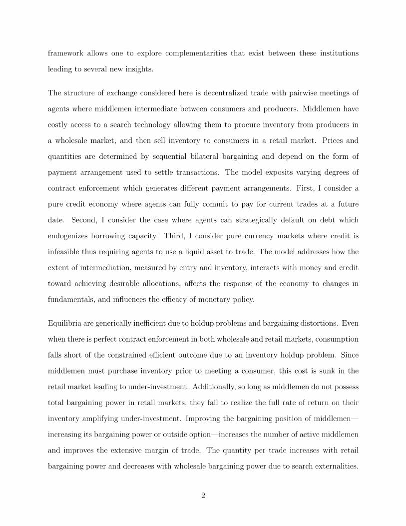
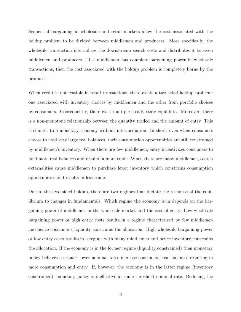
Apart from being anecdotally ubiquitous, intermediation activities constitute a non-trivial

share of the U.S. economy. As a rough estimate, shares of GDP attributed to intermediation

include retail trade (5.9 percent), wholesale trade (5.9 percent), finance and insurance (7.3

percent), transportation and warehousing (3 percent).1 This estimate, a conservative one at

that since it assumes zero value-added attributed to intermediation for all other industries,

suggests intermediation activities account for approximately 22.1 percent of 2016 U.S. GDP.

Moreover, disintermediation has not occurred. Figure 1.1 shows that this rough measure of

intermediation has been relatively stable, just shy of one-quarter of the U.S. economy, for

the last two decades.

Middlemen must exist because the benefits from intermediated trade are greater than those

from direct trade. One explanation is that direct trade is very costly. Evidence by McGraw

1The industry shares are taken from aggregate statistics published by the BEA.

4

0

5

10

15

20

25

1997 1998 1999 2000 2001 2002 2003 2004 2005 2006 2007 2008 2009 2010 2011 2012 2013 2014 2015 2016

Shares of GDP by Industry

35 Retail trade 34 Wholesale trade 55 Finance and insurance 40 Transportation and warehousing

Figure 1.1: Intermediated Industries in U.S. GDP

Hill (2013) estimates it takes on average 4.3 phone calls before a manufacturer finds a

consumer at a total cost of just over $589. Although producers often pine for “cutting

out the middleman,” too often they forget that they still have to provide their function. If

some producer bypasses intermediaries, it must incur the costs associated with distributing

the good to end consumers. A survey of 200 local food producers in California by Brimlow

(2016) found that 72 percent were selling out of the area to wholesale brokers. Producers

surveyed claimed it was difficult to find local buyers or that marketing and advertising costs

to sell locally would be too high. Middlemen provided a competitive advantage in delivering

goods to final consumers. The benefits of intermediated trade may be amplified when goods

are transported internationally. Intermediation has been a major driver of globalization

bringing goods and services from local producers to international consumers.

The process by which middlemen match with producers and consumers is itself a productive

process that uses resources. One of the most closely watched metrics to gauge retail perfor-

mance is average inventory turnover; the reciprocal of which is days inventory outstanding

(DOI). In a frictionless environment, middlemen could stock and sell inventories instanta-

neously and the DOI would be zero. However, it takes time to clear goods markets resulting

in varying DOIs across industries and firms. There is a large degree of heterogeneity both

5

across and within industries, but the average DIO in 2015 was 87.4 days. New logistic tech-

niques, like just-in-time (JIT) inventory management, are developed to mitigate the costs

associated with frictions. A model of intermediation in goods markets should take seriously

the frictions that preclude the instantaneous purchase and resale of inventory.

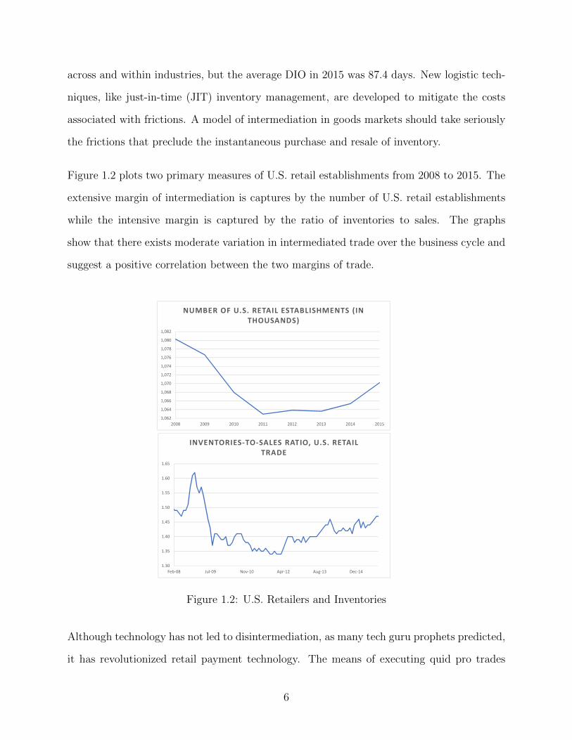
Figure 1.2 plots two primary measures of U.S. retail establishments from 2008 to 2015. The

extensive margin of intermediation is captures by the number of U.S. retail establishments

while the intensive margin is captured by the ratio of inventories to sales. The graphs

show that there exists moderate variation in intermediated trade over the business cycle and

suggest a positive correlation between the two margins of trade.

1,062

1,064

1,066

1,068

1,070

1,072

1,074

1,076

1,078

1,080

1,082

2008 2009 2010 2011 2012 2013 2014 2015

NUMBER OF U.S. RETAIL ESTABLISHMENTS (IN THOUSANDS)

1.30

1.35

1.40

1.45

1.50

1.55

1.60

1.65

Feb-08 Jul-09 Nov-10 Apr-12 Aug-13 Dec-14

INVENTORIES-TO-SALES RATIO, U.S. RETAIL TRADE

Figure 1.2: U.S. Retailers and Inventories

Although technology has not led to disintermediation, as many tech guru prophets predicted,

it has revolutionized retail payment technology. The means of executing quid pro trades

6

using currency or digital substitutes is experiencing a rapid evolution and it is important to

understand how the role of various retail payment instruments affect merchant behavior and

vice versa. The 2015 Survey of Consumer Payment Choice (SCPC) finds that while there

are nine identified payment instruments, consumers still predominantly use debit cards (32.5

percent of monthly payments), cash (27.1 percent), and credit cards (21.3 percent). The

present model takes seriously the frictions that generate a need for middlemen and various

payment arrangements.

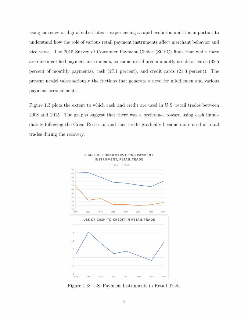
Figure 1.3 plots the extent to which cash and credit are used in U.S. retail trades between

2008 and 2015. The graphs suggest that there was a preference toward using cash imme-

diately following the Great Recession and then credit gradually became more used in retail

trades during the recovery.

40

45

50

55

60

65

70

75

80

85

90

2008 2009 2010 2011 2012 2013 2014 2015

SHARE OF CONSUMERS USING PAYMENT INSTRUMENT, RETAIL TRADE

Cash Credit

1

1.2

1.4

1.6

1.8

2

2.2

2008 2009 2010 2011 2012 2013 2014 2015

USE OF CASH-TO-CREDIT IN RETAIL TRADE

Figure 1.3: U.S. Payment Instruments in Retail Trade

7

This paper seeks to establish a connection between Figures 1.2 and 1.3. That is, is there

a relationship between the payment instruments available to consumers and the extent of

intermediated trade? To motivate this idea, consider the immediate aftermath of the Great

Recession: with a collapse in the availability of credit, consumers were forced to use cash

to execute retail trades. Scarce cash holdings limit the possible gains from trade thereby

reducing retail sales, increasing inventories, and causing some firms to be unprofitable. This

paper formalizes the relationship between cash, credit, and intermediated trades and includes

as measure of credit availability as reflected in Figure 1.3 as well as endogenous entry of firms

and investment in inventory reflected in Figure 1.2.

1.3 Related Literature

The study of middlemen and how their presence influences market allocations dates to

Rubenstein and Wolinsky (RW) who advocated “a basic model that describes explicitly the

trade frictions that give rise to the function of middlemen.” RW modeled the exchange pro-

cess and trading frictions between sellers, middlemen, and buyers thereby providing a frame-

work for endogenizing the extent of intermediation and its effect on the distribution of gains

from trade. Subsequent models, such as those by Nosal, Wong, and Wright (2011,2014,2016)

(NWW), expand on RW to include production, search costs, Nash bargaining, and occupa-

tional choice. The present paper seeks to contribute the study of middlemen in the spirit

of RW and NWW. The critical difference is that my paper integrates a rigorous theory of

payment arrangements into a model of intermediation while retaining the enriching features

found in NWW.

Also, different from NWW is that I consider an environment with infinite search and match-

ing costs for direct trade, thereby generating an essential role for middlemen. This follows

in the tradition of RW where middlemen are active in equilibrium only if they can match

8

with consumers at a faster rate than producers. In RW, these matching rates are exogenous

and so intermediated trade exists only if middlemen are endowed with a superior matching

technology. In my model middlemen are indeed endowed with superior matching technology,

but the rate at which intermediated trading opportunities arrive is endogenous and depends

on the strategic choices of all agents. More specifically, a middleman’s decision to enter the

market depends on its relative bargaining position and likelihood of engaging in trade, which

in turn is affected by the aggregate measure of active of middlemen.

There are various explanations for why middlemen are valuable. RW suggest that inter-

mediation is a way of alleviating search frictions by providing more frequent consumption

opportunities for consumers. Given some exogenous meeting process, some papers focus on

the role of middlemen as guarantors of quality (Biglaiser 1993, Li 1998) while others suggest

that middlemen can satisfy consumers’ demand for varieties of goods whereas individual

producers cannot (Johri & Leach 2002) (Shevchenko 2004). Watanabe (2010) argues that

middlemen have the advantage of inventory capacity relative to producers and that capacity

constraints are an important determinant for the endogenous meeting rates. My paper takes

the approach that middlemen alleviate search and matching frictions. This approach seems

natural given that I want to jointly model payment arrangements and intermediation, both

of which emerge from matching frictions and limited contract enforcement.

The literature on the coexistence of money and credit is robust. Lucas and Stokey (1987)

propose a model where the distinction between trades executed with cash versus credit

is exogenous. Subsequent work identified the fundamental frictions that generate a role

for monetary exchange, e.g., lack of commitment and record-keeping (Kocherlokata 1998).

Positing a costly record keeping technology endogenizes the composition of trades involving

cash or credit (Camera and Li 2008, Bethune, Rocheteau, and Rupert 2015, Lotz and Zhang

2016). I follow the spirit of this literature in that I model monetary exchange in anonymous

9

bilateral meetings and appeal to the inherent frictions in the environment to generate a role

for liquid assets. However, the availability of credit to consumers remains exogenous.

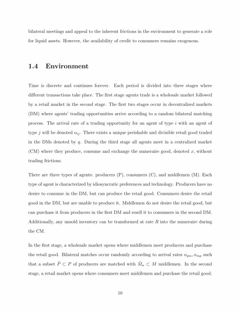
1.4 Environment

Time is discrete and continues forever. Each period is divided into three stages where

different transactions take place. The first stage agents trade is a wholesale market followed

by a retail market in the second stage. The first two stages occur in decentralized markets

(DM) where agents’ trading opportunities arrive according to a random bilateral matching

process. The arrival rate of a trading opportunity for an agent of type i with an agent of

type j will be denoted αij. There exists a unique perishable and divisible retail good traded

in the DMs denoted by q. During the third stage all agents meet in a centralized market

(CM) where they produce, consume and exchange the numeraire good, denoted x, without

trading frictions.

There are three types of agents: producers (P), consumers (C), and middlemen (M). Each

type of agent is characterized by idiosyncratic preferences and technology. Producers have no

desire to consume in the DM, but can produce the retail good. Consumers desire the retail

good in the DM, but are unable to produce it. Middlemen do not desire the retail good, but

can purchase it from producers in the first DM and resell it to consumers in the second DM.

Additionally, any unsold inventory can be transformed at rate R into the numeraire during

the CM.

In the first stage, a wholesale market opens where middlemen meet producers and purchase

the retail good. Bilateral matches occur randomly according to arrival rates αpm, αmp such

that a subset P ⊂ P of producers are matched with Mw ⊂ M middlemen. In the second

stage, a retail market opens where consumers meet middlemen and purchase the retail good.

10

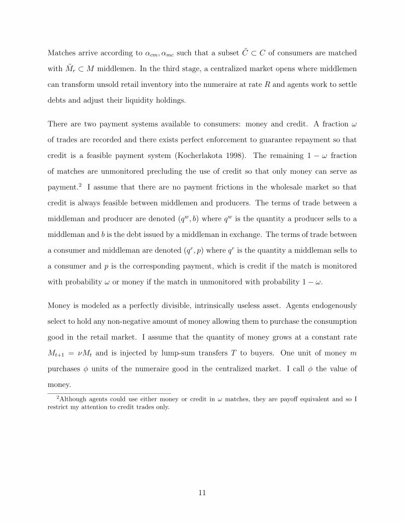
Matches arrive according to αcm, αmc such that a subset C ⊂ C of consumers are matched

with Mr ⊂M middlemen. In the third stage, a centralized market opens where middlemen

can transform unsold retail inventory into the numeraire at rate R and agents work to settle

debts and adjust their liquidity holdings.

There are two payment systems available to consumers: money and credit. A fraction ω

of trades are recorded and there exists perfect enforcement to guarantee repayment so that

credit is a feasible payment system (Kocherlakota 1998). The remaining 1 − ω fraction

of matches are unmonitored precluding the use of credit so that only money can serve as

payment.2 I assume that there are no payment frictions in the wholesale market so that

credit is always feasible between middlemen and producers. The terms of trade between a

middleman and producer are denoted (qw, b) where qw is the quantity a producer sells to a

middleman and b is the debt issued by a middleman in exchange. The terms of trade between

a consumer and middleman are denoted (qr, p) where qr is the quantity a middleman sells to

a consumer and p is the corresponding payment, which is credit if the match is monitored

with probability ω or money if the match in unmonitored with probability 1− ω.

Money is modeled as a perfectly divisible, intrinsically useless asset. Agents endogenously

select to hold any non-negative amount of money allowing them to purchase the consumption

good in the retail market. I assume that the quantity of money grows at a constant rate

Mt+1 = νMt and is injected by lump-sum transfers T to buyers. One unit of money m

purchases φ units of the numeraire good in the centralized market. I call φ the value of

money.

2Although agents could use either money or credit in ω matches, they are payoff equivalent and so Irestrict my attention to credit trades only.

11

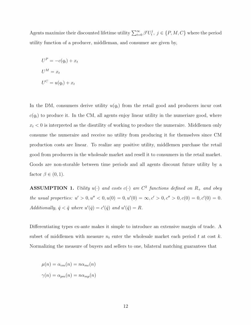
Agents maximize their discounted lifetime utility∑∞

t=0 βtU j

t , j ∈ P,M,C where the period

utility function of a producer, middleman, and consumer are given by,

UP = −c(qt) + xt

UM = xt

UC = u(qt) + xt

In the DM, consumers derive utility u(qt) from the retail good and producers incur cost

c(qt) to produce it. In the CM, all agents enjoy linear utility in the numeriare good, where

xt < 0 is interpreted as the disutility of working to produce the numeraire. Middlemen only

consume the numeraire and receive no utility from producing it for themselves since CM

production costs are linear. To realize any positive utility, middlemen purchase the retail

good from producers in the wholesale market and resell it to consumers in the retail market.

Goods are non-storable between time periods and all agents discount future utility by a

factor β ∈ (0, 1).

ASSUMPTION 1. Utility u(·) and costs c(·) are C2 functions defined on R+ and obey

the usual properties: u′ > 0, u′′ < 0, u(0) = 0, u′(0) = ∞, c′ > 0, c′′ > 0, c(0) = 0, c′(0) = 0.

Additionally, q < q where u′(q) = c′(q) and u′(q) = R.

Differentiating types ex-ante makes it simple to introduce an extensive margin of trade. A

subset of middlemen with measure nt enter the wholesale market each period t at cost k.

Normalizing the measure of buyers and sellers to one, bilateral matching guarantees that

µ(n) = αcm(n) = nαmc(n)

γ(n) = αpm(n) = nαmp(n)

12

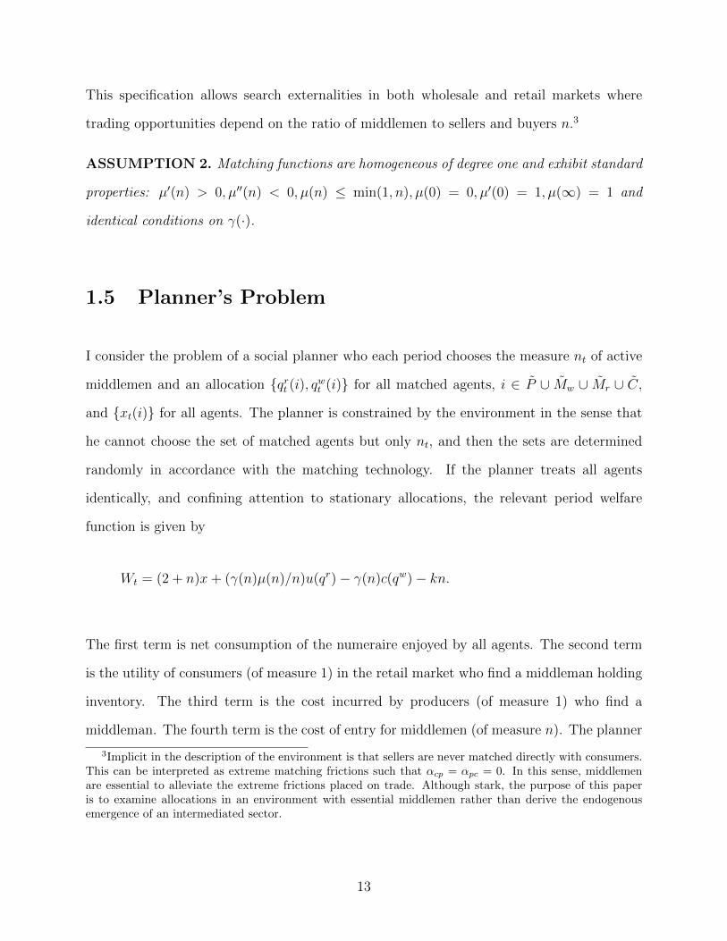
This specification allows search externalities in both wholesale and retail markets where

trading opportunities depend on the ratio of middlemen to sellers and buyers n.3

ASSUMPTION 2. Matching functions are homogeneous of degree one and exhibit standard

properties: µ′(n) > 0, µ′′(n) < 0, µ(n) ≤ min(1, n), µ(0) = 0, µ′(0) = 1, µ(∞) = 1 and

identical conditions on γ(·).

1.5 Planner’s Problem

I consider the problem of a social planner who each period chooses the measure nt of active

middlemen and an allocation qrt (i), qwt (i) for all matched agents, i ∈ P ∪ Mw ∪ Mr ∪ C,

and xt(i) for all agents. The planner is constrained by the environment in the sense that

he cannot choose the set of matched agents but only nt, and then the sets are determined

randomly in accordance with the matching technology. If the planner treats all agents

identically, and confining attention to stationary allocations, the relevant period welfare

function is given by

Wt = (2 + n)x+ (γ(n)µ(n)/n)u(qr)− γ(n)c(qw)− kn.

The first term is net consumption of the numeraire enjoyed by all agents. The second term

is the utility of consumers (of measure 1) in the retail market who find a middleman holding

inventory. The third term is the cost incurred by producers (of measure 1) who find a

middleman. The fourth term is the cost of entry for middlemen (of measure n). The planner

3Implicit in the description of the environment is that sellers are never matched directly with consumers.This can be interpreted as extreme matching frictions such that αcp = αpc = 0. In this sense, middlemenare essential to alleviate the extreme frictions placed on trade. Although stark, the purpose of this paperis to examine allocations in an environment with essential middlemen rather than derive the endogenousemergence of an intermediated sector.

13

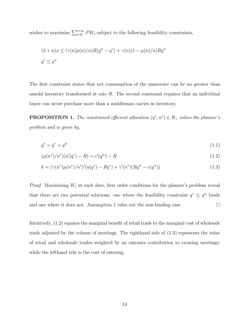
wishes to maximize∑t=∞

t=0 βtWt subject to the following feasibility constraints,

(2 + n)x ≤ (γ(n)µ(n)/n)R(qw − qr) + γ(n)(1− µ(n)/n)Rqw

qr ≤ qw

The first constraint states that net consumption of the numeraire can be no greater than

unsold inventory transformed at rate R. The second constraint requires that an individual

buyer can never purchase more than a middleman carries in inventory.

PROPOSITION 1. The constrained efficient allocation (q∗, n∗) ∈ R+ solves the planner’s

problem and is given by,

q∗ = qr = qw (1.1)

(µ(n∗)/n∗)(u′(qr)−R) = c′(qw)−R (1.2)

k = (γ(n∗)µ(n∗)/n∗)′(u(qr)−Rqr) + γ′(n∗)(Rqw − c(qw)) (1.3)

Proof. Maximizing Wt at each date, first order conditions for the planner’s problem reveal

that there are two potential solutions: one where the feasibility constraint qr ≤ qw binds

and one where it does not. Assumption 1 rules out the non-binding case.

Intuitively, (1.2) equates the marginal benefit of retail trade to the marginal cost of wholesale

trade adjusted by the volume of meetings. The righthand side of (1.3) represents the value

of retail and wholesale trades weighted by an entrants contribution to creating meetings;

while the lefthand side is the cost of entering.

14

1.6 Decentralized Economy

Having described the constrained efficient allocation, I now consider a decentralized economy

with intermediation and characterize stationary equilibria. I demonstrate that the efficient

allocation never obtains, and the efficiency of the equilibria depends on the bargaining po-

sition of middlemen and the payment systems used.

1.6.1 Centralized Market

Consumers enter the CM with wealth comprised of debt and money (b,m) ∈ R2+. Consumers

choose how much to work in order finance consumption, repay debt, and adjust money

holdings. They then enter the following period’s DM which yields expected utility V Ct (m).

maxx,m′

WCt (b,m) = x+ βV C

t+1(m′) s.t. x+ b+ φtm

′ = φtm+ T

Middlemen enter the CM with wealth comprised of net debt (credit from consumers less debt

owed to producers), unsold inventory, and money (b, q,m) ∈ R3+. They finance consumption

of the numeraire using net wealth, transforming unsold inventory at rate R, and working.

They then choose whether or not to enter the following period’s DM with expected utility

V M1 (m).

maxx,m

WMt (b, q,m) = x+ βmaxV M

1,t+1,WMt+1 s.t. x+ φtm

′ = b+Rq + φtm

A producer enters the CM with wealth comprised of credit and money Consumers enter

the CM with wealth comprised of debt and money (b,m) ∈ R2+ which it uses to finance its

15

consumption of the numeraire.

maxx,m

W P (b,m) = x+ βV P s.t. x+ φtm′ = b+ φtm

Substituting the budget constraints into their respective objective functions, the CM value

functions for agents are given by the following:

WCt (m) = φtm+ T + max

m′

[−φtm′ + βV C

t+1(m′)]

(1.4)

WMt (q,m, b) = Rq + φtm− b+ max

m′

[−φtm′ + βmaxV M

1,t+1(m′),WM

t+1(m′)]

(1.5)

W Pt (m, b) = b+ φtm+ max

m′

[−φtm′ + V P

t+1(m′)]

(1.6)

Notice that all agents’ CM value function are linear in wealth. When agents choose to acquire

liquid assets, the portfolio decisions are history independent so that there is a degenerate

distribution of asset holdings. This result is an artifact of quasi-linear preferences and delivers

tractable results without sacrificing economic insight.

1.6.2 Retail Market

Having characterized the CM value functions, I move back one stage to the retail market

where consumers and middlemen meet. A consumer entering the retail market finds a mid-

dleman with probability µ(n), and settles credit terms of trade (qr, br) with probability ω

or monetary terms of trade (qr, dr) with probability 1− ω. A consumer then enters the CM

with its net wealth. Using the linearity of the CM value function (1.4), the expected utility

to a consumer entering the retail market is given by

V Ct = µ(n) ω[u(qr)− br] + (1− ω)[u(qr)− φdr]+WC

t (m) (1.7)

16

A middleman enters the retail market with some amount of inventory purchased from a

producer, the corresponding debt, and money balances. With probability µ(n)/n he finds

a consumer and with probability ω accepts credit and with probability 1 − ω only accepts

cash. If the middleman does not find a consumer, he carries all unsold inventory and debt

into the CM. Using CM value function (1.5) I have that,

V M2,t (q, b, m) =

µ(n)

nω[br −Rqr] + (1− ω)[φdr −Rqr]+WM

t (q, b, m) (1.8)

Equation (1.8) shows that a middleman’s expected value in the retail market is the proba-

bility he finds a consumer times the value of the match, plus the guaranteed value of trans-

forming unsold inventory in the CM, plus the continuation value of entering next period’s

wholesale market. Note that terms of trade in the retail market depend on what occurred

in the wholesale market. If a middleman did not purchase any inventory in the wholesale

market (q = 0) then he surely cannot sell anything in the retail market. More generally, the

amount of inventory q constrains the set of feasible allocations in the retail market. This

will be discussed more thoroughly when I define the bargaining sets.

1.6.3 Wholesale Market

I now move back one stage to the wholesale market where middlemen purchase inventory

from producers. When a middleman enters the wholesale market he incurs entry cost k,

meets a producer with probability γ(n)/n, executes terms of trade (qw, bw) and then enters

the retail market. Otherwise he enters the retail market with zero inventory and zero debt.

V M1 = (γ(n)/n)V M

2 (qw,−bw) + (1− γ(n)/n)V M2 (0, 0)− k

17

Using the retail value function (1.8) I have that,

V M1,t (m) =

γ(n)

n

µ(n)

n(ω[br −Rqr] + (1− ω)[φdr −Rqr]) +Rqw − bw

+Wt(0, 0, m)−k

(1.9)

A middleman’s expected value in the wholesale market is the expected value of acquiring

inventory qw with probability γ(n)/n. The value of holding inventory includes the guaranteed

value of transforming it at rate R in the CM and repaying debts plus the value of carrying

inventory into the retail market. Of course, the value of inventory in the retail market

depends on the available payment instruments and resulting terms of trade. Suppose, for

example, that the terms of trade are such that the consumer receives the entire value of

surplus from a retail match. In this case, a middleman would only receive utility from

transforming inventory in the CM and would never choose to operate in the retail market.

This is an uninteresting equilibrium. To generate an equilibrium where consumers have an

opportunity to consume and middlemen actually behave as intermediaries (buy and resell)

it will be necessary to implement a bargaining protocol that gives the middleman some

bargaining power in the retail market.

A producer entering the wholesale market finds a middleman with probability γ(n), produces

the good at cost c(q), and receives credit to be settled in the CM.

V Pt (m) = γ(n)(−c(qw) + bw) +W P

t (0, m) (1.10)

1.6.4 Bargaining Sets

I now characterize the set of allocations that are incentive feasible—the terms of trade which

satisfy agents’ participation constraints. The gains from retail trades crucially depend on

18

the payment instrument used. For generality, I denote the payment made by a buyer by

pr ∈ br, φdr which may take the form of money or credit depending on the match.

First, I characterize the bargaining set that exists between a middleman and a consumer

in the retail market. If an agreement is reached, a consumer’s utility level is uC = u(qr) +

WC(−pr) and a middleman’s utility level is uM = WM(q − qr,−b + pr). If there is no

agreement then a consumer receives utility uC0 = WC(0) and a middleman receives utility

uM0 = WM(q,−b). Using the CM value functions, we can write the value of the surplus from

a match as follows:

uC − uC0 = u(qr)− pr

uM − uM0 = pr −Rqr

A proposed trade is incentive feasible only if both agents earn non-negative surpluses from the

agreement. The set of incentive feasible allocations is defined as Ωr = (qr, pr) : Rqr ≤ pr ≤

u(qr), qr ≤ qw) where the payment instrument may be either money or credit pr ∈ br, φdr.

The set can be constrained by two state variables: middlemen’s inventory holdings qw or

consumer’s real money balances φdr which are predetermined when agents enter the match.

A middleman can surely never sell more of the retail good than it has in inventory, and a

consumer can never purchase more than the value of his real money holdings. Formally, the

Pareto frontier of the bargaining set is described by

maxqr,dr

uc = u(qr)− pr + uC0

s.t. φdr −Rqr + uM0 ≥ uM

s.t. (qr, dr) ∈ [0, qw]× [0,m]

19

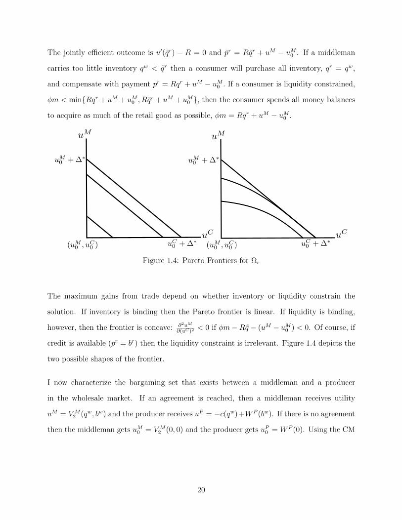
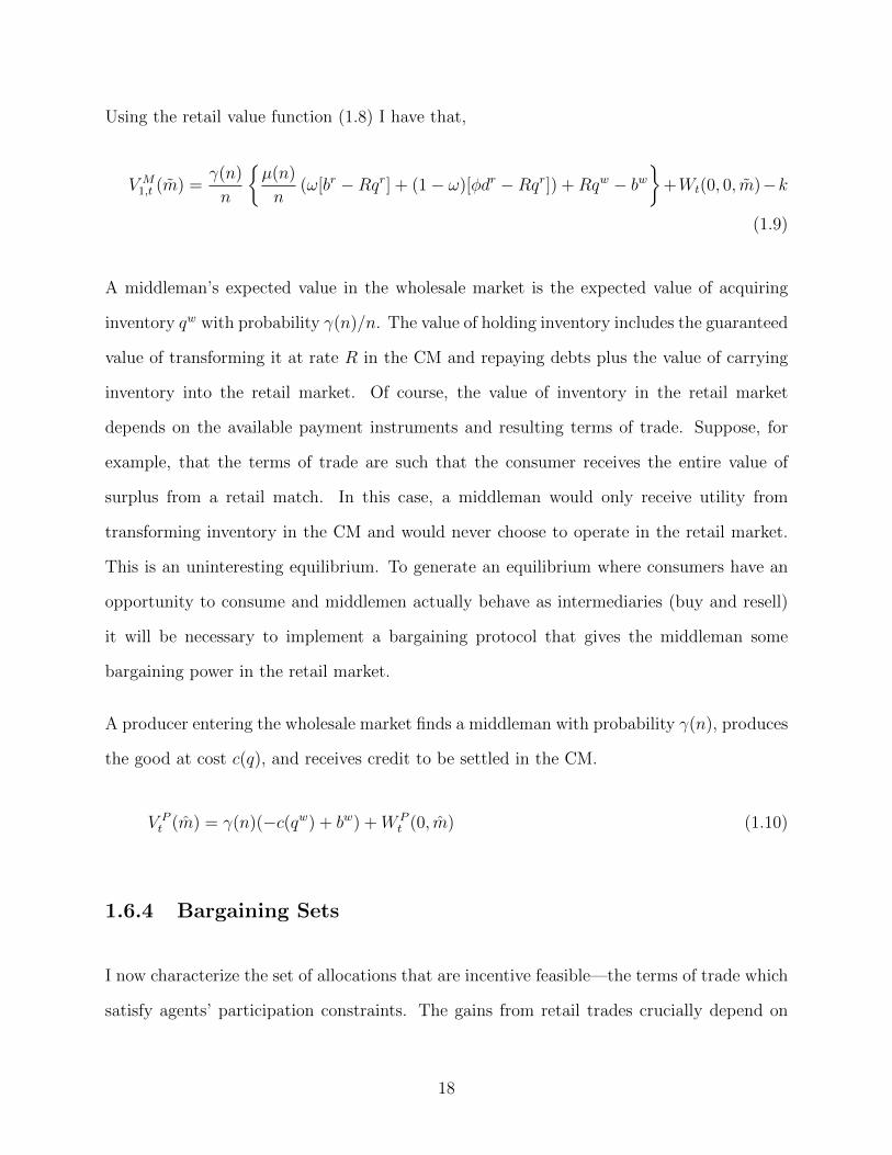
The jointly efficient outcome is u′(qr) − R = 0 and pr = Rqr + uM − uM0 . If a middleman

carries too little inventory qw < qr then a consumer will purchase all inventory, qr = qw,

and compensate with payment pr = Rqr + uM − uM0 . If a consumer is liquidity constrained,

φm < minRqr + uM + uM0 , Rqr + uM + uM0 , then the consumer spends all money balances

to acquire as much of the retail good as possible, φm = Rqr + uM − uM0 .

Figure 1.4: Pareto Frontiers for Ωr

The maximum gains from trade depend on whether inventory or liquidity constrain the

solution. If inventory is binding then the Pareto frontier is linear. If liquidity is binding,

however, then the frontier is concave: ∂2uM

∂(uC)2< 0 if φm−Rq − (uM − uM0 ) < 0. Of course, if

credit is available (pr = br) then the liquidity constraint is irrelevant. Figure 1.4 depicts the

two possible shapes of the frontier.

I now characterize the bargaining set that exists between a middleman and a producer

in the wholesale market. If an agreement is reached, then a middleman receives utility

uM = V M2 (qw, bw) and the producer receives uP = −c(qw)+W P (bw). If there is no agreement

then the middleman gets uM0 = V M2 (0, 0) and the producer gets uP0 = W P (0). Using the CM

20

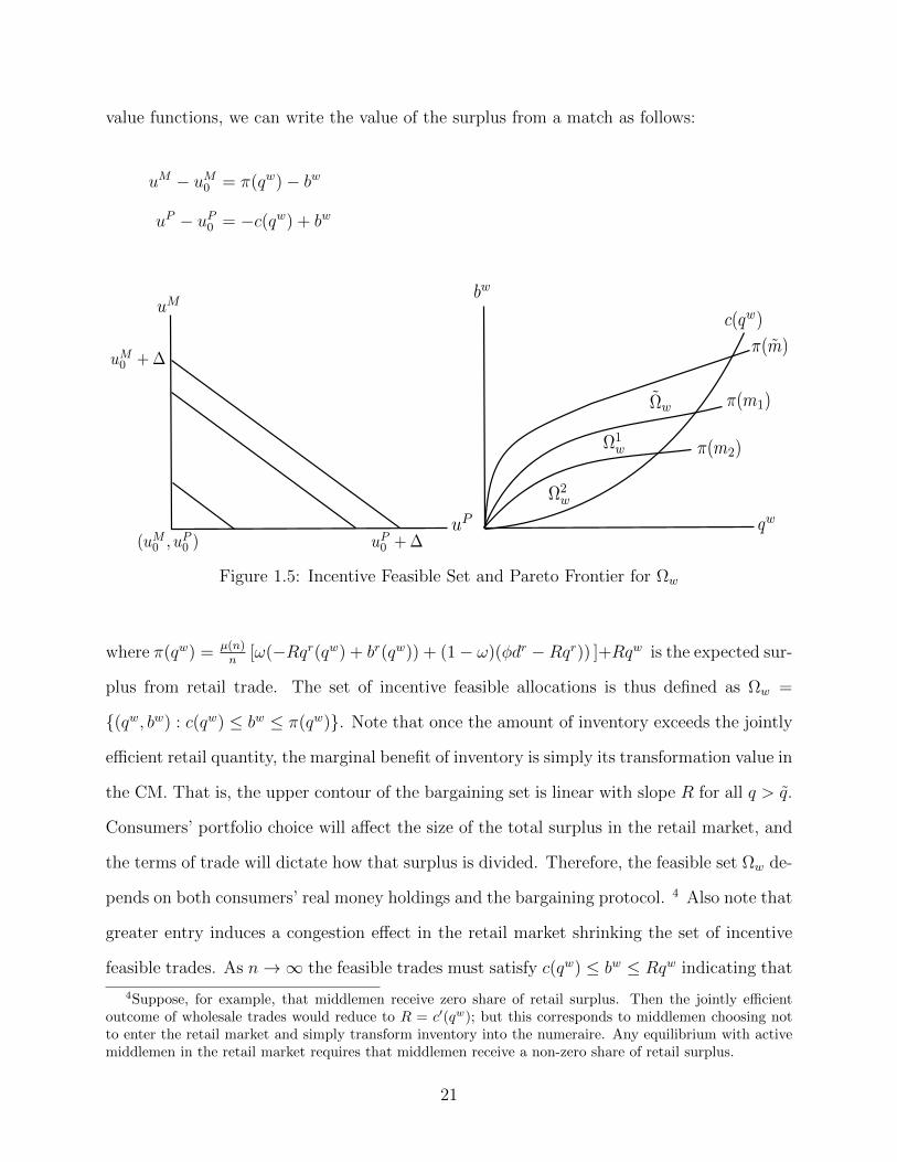
value functions, we can write the value of the surplus from a match as follows:

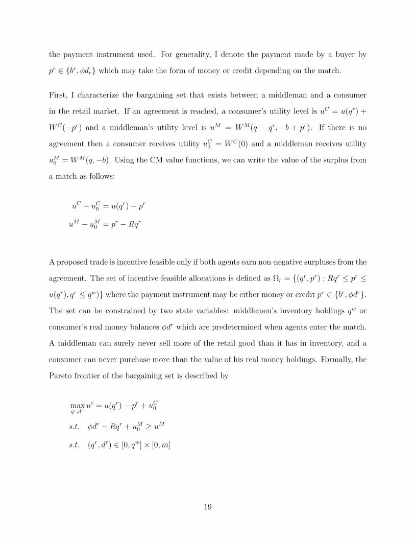
uM − uM0 = π(qw)− bw

uP − uP0 = −c(qw) + bw

Figure 1.5: Incentive Feasible Set and Pareto Frontier for Ωw

where π(qw) = µ(n)n

[ω(−Rqr(qw) + br(qw)) + (1− ω)(φdr −Rqr)) ]+Rqw is the expected sur-

plus from retail trade. The set of incentive feasible allocations is thus defined as Ωw =

(qw, bw) : c(qw) ≤ bw ≤ π(qw). Note that once the amount of inventory exceeds the jointly

efficient retail quantity, the marginal benefit of inventory is simply its transformation value in

the CM. That is, the upper contour of the bargaining set is linear with slope R for all q > q.

Consumers’ portfolio choice will affect the size of the total surplus in the retail market, and

the terms of trade will dictate how that surplus is divided. Therefore, the feasible set Ωw de-

pends on both consumers’ real money holdings and the bargaining protocol. 4 Also note that

greater entry induces a congestion effect in the retail market shrinking the set of incentive

feasible trades. As n→∞ the feasible trades must satisfy c(qw) ≤ bw ≤ Rqw indicating that

4Suppose, for example, that middlemen receive zero share of retail surplus. Then the jointly efficientoutcome of wholesale trades would reduce to R = c′(qw); but this corresponds to middlemen choosing notto enter the retail market and simply transform inventory into the numeraire. Any equilibrium with activemiddlemen in the retail market requires that middlemen receive a non-zero share of retail surplus.

21

middlemen only realize value from transforming inventory into the numeraire. Alternatively,

as −Rqr(qw) + br(qw) → 0 we again have that c(qw) ≤ bw ≤ Rqw. Whether the efficient

quantity traded is incentive feasible q∗ ∈ Ωw depends on the share of retail trade surplus a

middleman receives. Of course, if c(q∗) ≤ Rq∗ then the efficient quantity is incentive feasible

even when the middleman’s share of retail surplus approaches zero; although this is not true

in general and largely depends on the rate R at which a middleman can transform unsold

inventory.

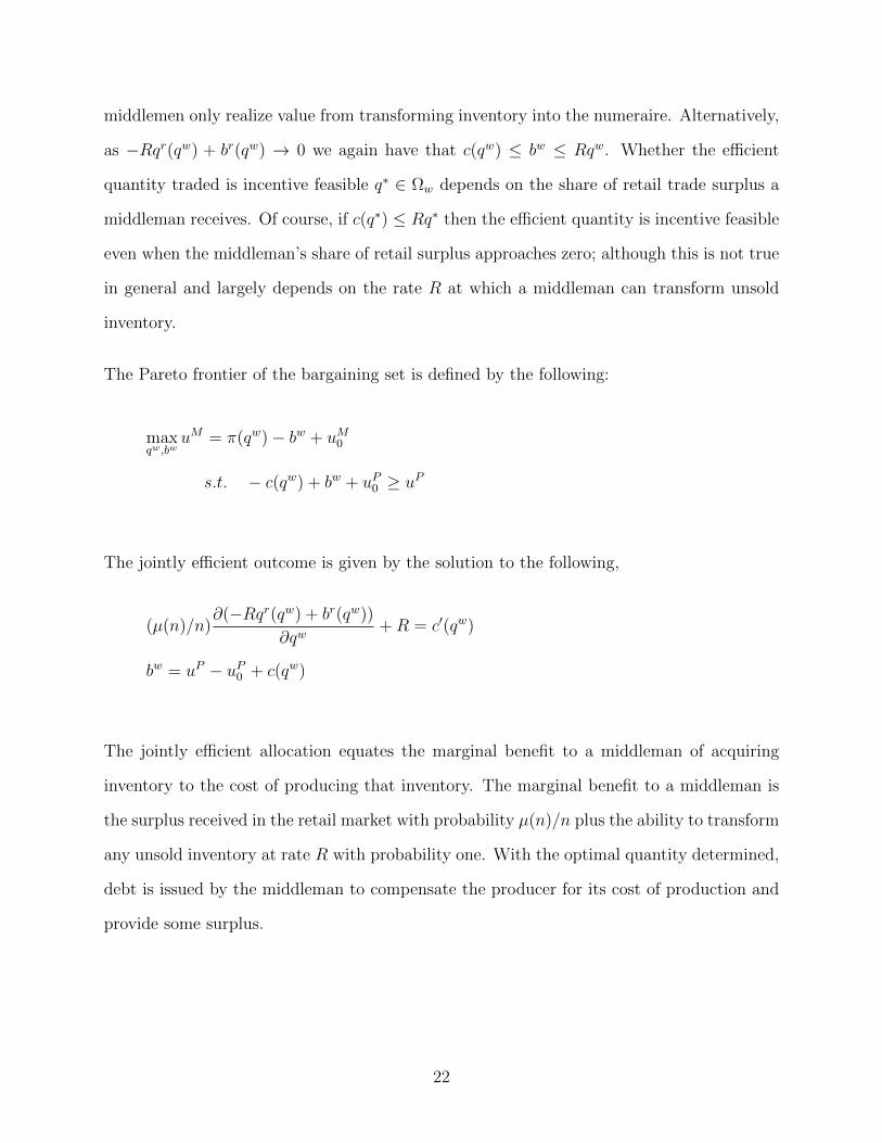
The Pareto frontier of the bargaining set is defined by the following:

maxqw,bw

uM = π(qw)− bw + uM0

s.t. − c(qw) + bw + uP0 ≥ uP

The jointly efficient outcome is given by the solution to the following,

(µ(n)/n)∂(−Rqr(qw) + br(qw))

∂qw+R = c′(qw)

bw = uP − uP0 + c(qw)

The jointly efficient allocation equates the marginal benefit to a middleman of acquiring

inventory to the cost of producing that inventory. The marginal benefit to a middleman is

the surplus received in the retail market with probability µ(n)/n plus the ability to transform

any unsold inventory at rate R with probability one. With the optimal quantity determined,

debt is issued by the middleman to compensate the producer for its cost of production and

provide some surplus.

22

The Pareto frontier is linear and strictly decreasing in the share of surplus received by

middlemen in the retail market,

uM − uM0 = (µ(n)/n)[−Rqr + pr] +Rqw − c(qw)− (uP − uP0 )

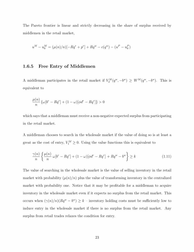
1.6.5 Free Entry of Middlemen

A middleman participates in the retail market if V M2 (qw,−bw) ≥ WM(qw,−bw). This is

equivalent to

µ(n)

nω[br −Rqr] + (1− ω)[φdr −Rqr] > 0

which says that a middleman must receive a non-negative expected surplus from participating

in the retail market.

A middleman chooses to search in the wholesale market if the value of doing so is at least a

great as the cost of entry, V M1 ≥ 0. Using the value functions this is equivalent to

γ(n)

n

µ(n)

nω[br −Rqr] + (1− ω)[φdr −Rqr] +Rqw − bw

≥ k (1.11)

The value of searching in the wholesale market is the value of selling inventory in the retail

market with probability (µ(n)/n) plus the value of transforming inventory in the centralized

market with probability one. Notice that it may be profitable for a middleman to acquire

inventory in the wholesale market even if it expects no surplus from the retail market. This

occurs when (γ(n)/n)(Rqw − bw) ≥ k – inventory holding costs must be sufficiently low to

induce entry in the wholesale market if there is no surplus from the retail market. Any

surplus from retail trades relaxes the condition for entry.

23

1.7 Non-Monetary Equilibrium

An equilibrium is defined as qw, qr, bw, br, dr, n and money holdings mj, j = C,M,P

where a bargaining protocol determines the terms of trade, free entry determines the measure

of active middlemen, and portfolio choices determine money holdings. As was mentioned

previously, the availability of credit versus money impacted the incentive feasible trades

in both retail and wholesale markets and affects the entry decision of middlemen. For

expositional clarity, I consider the limiting cases of a pure credit economy (ω = 1) and a

pure currency economy (ω = 0). It is straightforward to characterize all remaining equilibria

as the convex combination of these two limiting cases.

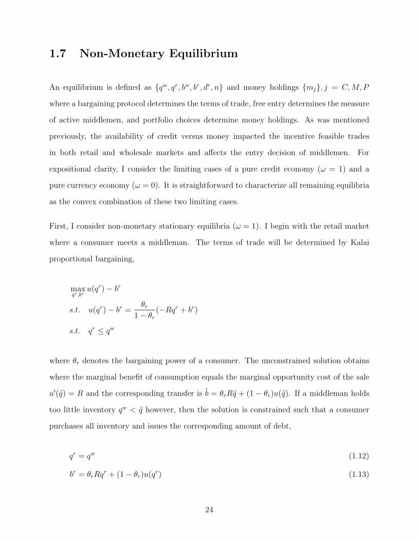
First, I consider non-monetary stationary equilibria (ω = 1). I begin with the retail market

where a consumer meets a middleman. The terms of trade will be determined by Kalai

proportional bargaining,

maxqr,br

u(qr)− br

s.t. u(qr)− br =θr

1− θr(−Rqr + br)

s.t. qr ≤ qw

where θr denotes the bargaining power of a consumer. The unconstrained solution obtains

where the marginal benefit of consumption equals the marginal opportunity cost of the sale

u′(q) = R and the corresponding transfer is b = θrRq + (1− θr)u(q). If a middleman holds

too little inventory qw < q however, then the solution is constrained such that a consumer

purchases all inventory and issues the corresponding amount of debt,

qr = qw (1.12)

br = θrRqr + (1− θr)u(qr) (1.13)

24

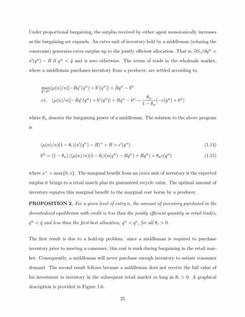
Under proportional bargaining, the surplus received by either agent monotonically increases

as the bargaining set expands. An extra unit of inventory held by a middleman (relaxing the

constraint) generates extra surplus up to the jointly efficient allocation. That is, ∂Sr/∂qw =

u′(qw) − R if qw < q and is zero otherwise. The terms of trade in the wholesale market,

where a middleman purchases inventory from a producer, are settled according to,

maxqw,bw

(µ(n)/n)[−Rqr(qw) + br(qw)] +Rqw − bw

s.t. (µ(n)/n)[−Rqr(qw) + br(qw)] +Rqw − bw =θw

1− θw(−c(qw) + bw)

where θw denotes the bargaining power of a middleman. The solution to the above program

is

(µ(n)/n)(1− θr)(u′(qw)−R)+ +R = c′(qw) (1.14)

bw = (1− θw) ((µ(n)/n)(1− θr)(u(qw)−Rqw) +Rqw) + θwc(qw) (1.15)

where x+ = max0, x. The marginal benefit from an extra unit of inventory is the expected

surplus it brings to a retail match plus its guaranteed recycle value. The optimal amount of

inventory equates this marginal benefit to the marginal cost borne by a producer.

PROPOSITION 2. For a given level of entry n, the amount of inventory purchased in the

decentralized equilibrium with credit is less than the jointly efficient quantity in retail trades,

qw < q and less than the first-best allocation, qw < q∗, for all θr > 0.

The first result is due to a hold-up problem: since a middleman is required to purchase

inventory prior to meeting a consumer, this cost is sunk during bargaining in the retail mar-

ket. Consequently, a middleman will never purchase enough inventory to satiate consumer

demand. The second result follows because a middleman does not receive the full value of

his investment in inventory in the subsequent retail market so long as θr > 0. A graphical

description is provided in Figure 1.6.

25

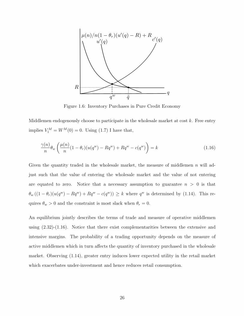
Figure 1.6: Inventory Purchases in Pure Credit Economy

Middlemen endogenously choose to participate in the wholesale market at cost k. Free entry

implies V M1 = WM(0) = 0. Using (1.7) I have that,

γ(n)

nθw

(µ(n)

n(1− θr)(u(qw)−Rqw) +Rqw − c(qw)

)= k (1.16)

Given the quantity traded in the wholesale market, the measure of middlemen n will ad-

just such that the value of entering the wholesale market and the value of not entering

are equated to zero. Notice that a necessary assumption to guarantee n > 0 is that

θw ((1− θr)(u(qw)−Rqw) +Rqw − c(qw)) ≥ k where qw is determined by (1.14). This re-

quires θw > 0 and the constraint is most slack when θr = 0.

An equilibrium jointly describes the terms of trade and measure of operative middlemen

using (2.32)-(1.16). Notice that there exist complementarities between the extensive and

intensive margins. The probability of a trading opportunity depends on the measure of

active middlemen which in turn affects the quantity of inventory purchased in the wholesale

market. Observing (1.14), greater entry induces lower expected utility in the retail market

which exacerbates under-investment and hence reduces retail consumption.

26

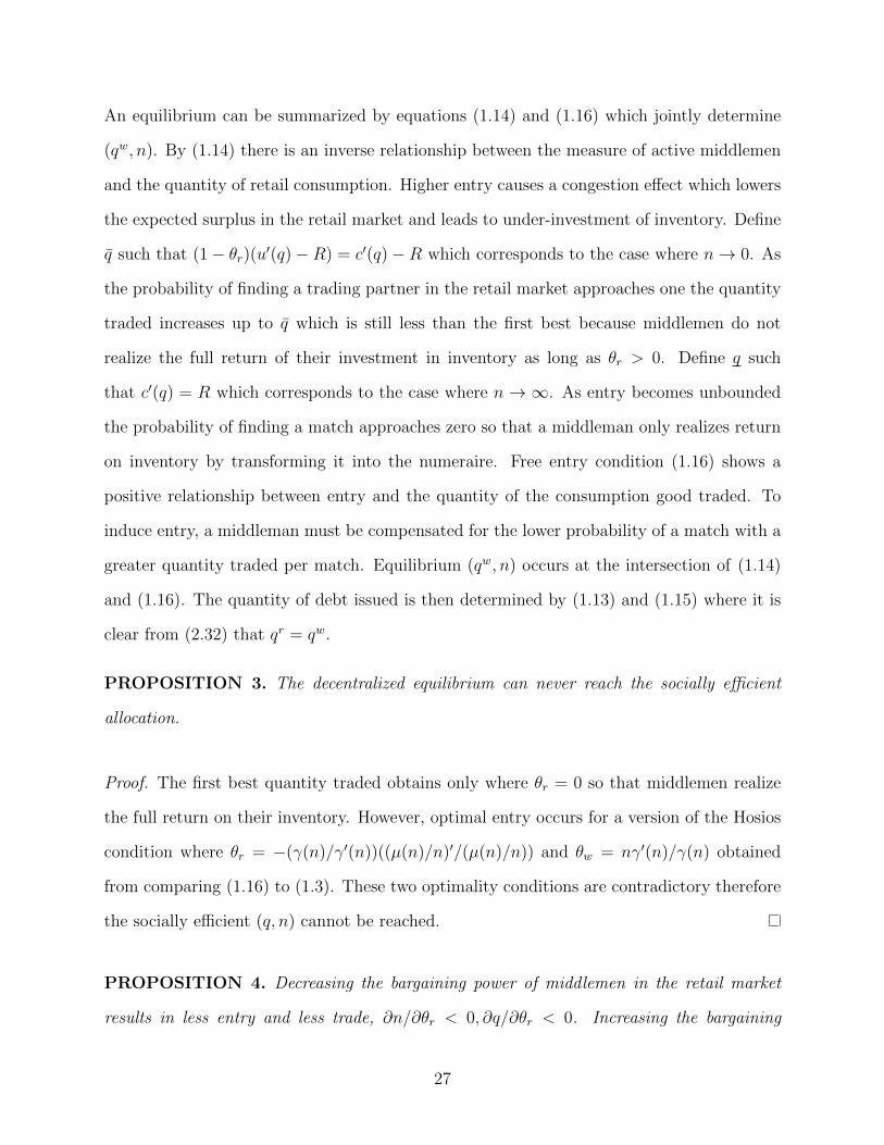
An equilibrium can be summarized by equations (1.14) and (1.16) which jointly determine

(qw, n). By (1.14) there is an inverse relationship between the measure of active middlemen

and the quantity of retail consumption. Higher entry causes a congestion effect which lowers

the expected surplus in the retail market and leads to under-investment of inventory. Define

q such that (1− θr)(u′(q)−R) = c′(q)−R which corresponds to the case where n→ 0. As

the probability of finding a trading partner in the retail market approaches one the quantity

traded increases up to q which is still less than the first best because middlemen do not

realize the full return of their investment in inventory as long as θr > 0. Define q such

that c′(q) = R which corresponds to the case where n → ∞. As entry becomes unbounded

the probability of finding a match approaches zero so that a middleman only realizes return

on inventory by transforming it into the numeraire. Free entry condition (1.16) shows a

positive relationship between entry and the quantity of the consumption good traded. To

induce entry, a middleman must be compensated for the lower probability of a match with a

greater quantity traded per match. Equilibrium (qw, n) occurs at the intersection of (1.14)

and (1.16). The quantity of debt issued is then determined by (1.13) and (1.15) where it is

clear from (2.32) that qr = qw.

PROPOSITION 3. The decentralized equilibrium can never reach the socially efficient

allocation.

Proof. The first best quantity traded obtains only where θr = 0 so that middlemen realize

the full return on their inventory. However, optimal entry occurs for a version of the Hosios

condition where θr = −(γ(n)/γ′(n))((µ(n)/n)′/(µ(n)/n)) and θw = nγ′(n)/γ(n) obtained

from comparing (1.16) to (1.3). These two optimality conditions are contradictory therefore

the socially efficient (q, n) cannot be reached.

PROPOSITION 4. Decreasing the bargaining power of middlemen in the retail market

results in less entry and less trade, ∂n/∂θr < 0, ∂q/∂θr < 0. Increasing the bargaining

27

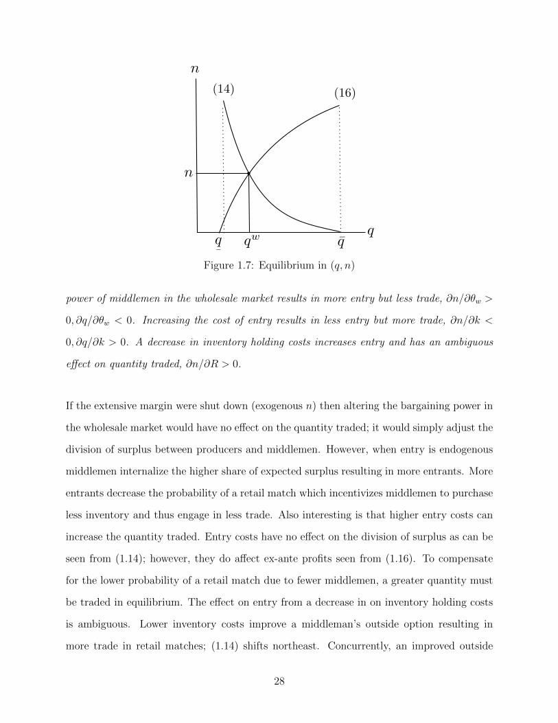
Figure 1.7: Equilibrium in (q, n)

power of middlemen in the wholesale market results in more entry but less trade, ∂n/∂θw >

0, ∂q/∂θw < 0. Increasing the cost of entry results in less entry but more trade, ∂n/∂k <

0, ∂q/∂k > 0. A decrease in inventory holding costs increases entry and has an ambiguous

effect on quantity traded, ∂n/∂R > 0.

If the extensive margin were shut down (exogenous n) then altering the bargaining power in

the wholesale market would have no effect on the quantity traded; it would simply adjust the

division of surplus between producers and middlemen. However, when entry is endogenous

middlemen internalize the higher share of expected surplus resulting in more entrants. More

entrants decrease the probability of a retail match which incentivizes middlemen to purchase

less inventory and thus engage in less trade. Also interesting is that higher entry costs can

increase the quantity traded. Entry costs have no effect on the division of surplus as can be

seen from (1.14); however, they do affect ex-ante profits seen from (1.16). To compensate

for the lower probability of a retail match due to fewer middlemen, a greater quantity must

be traded in equilibrium. The effect on entry from a decrease in on inventory holding costs

is ambiguous. Lower inventory costs improve a middleman’s outside option resulting in

more trade in retail matches; (1.14) shifts northeast. Concurrently, an improved outside

28

option encourages more entry which congests the wholesale market and decreases inventory

purchases; (1.16) shifts northwest.

PROPOSITION 5. The intermediation spread for middlemen is strictly positive and given

by,

(br − bw)(q) = (u(q)−Rq)(1− θr − (1− θr)(1− θw)µ(n)/n) + θw(Rq − c(q)).

The spread is increasing in the bargaining power of middlemen ∂(br − bw)/∂θw > 0, ∂(br −

bw)/∂θr < 0, the amount traded ∂(br−bw)/∂q > 0, inventory holding costs ∂(br−bw)/∂R > 0

and the measure of middlemen ∂(br − bw)/∂n > 0.

Of interest is the proportion of retail surplus captured by a middleman: (1 − θr − (1 −

θr)(1 − θw)µ(n)/n). The first term captures the primitive bargaining power of middlemen

in retail trade, whereas the second term reveals the interaction between wholesale and retail

trade. Suppose, for example, that a middleman has all bargaining power in wholesale trades

θw = 1. In this case, the producer is forced to internalize not only its own production

costs, but also the search costs associated with the retail market. That is, the wholesale

transaction internalizes the downstream search costs and distributes it between middlemen

and producers. This mechanism underlies the intuition for why ∂(br − bw)/∂n > 0. More

entry decreases the expected value of a retail match, and therefore requires a smaller payment

in wholesale trades. Concurrently, more entry does not affect the terms of trade in retail

matches. A middleman can extract up to the full surplus u(q)− c(q) when θr = 0, θw = 1.

1.8 Limited Commitment

Thus far I have assumed that credit is perfect. That is, there exists a record keeping technol-

ogy and enforcement mechanism that replicates perfect memory and ensures debt repayment.

29

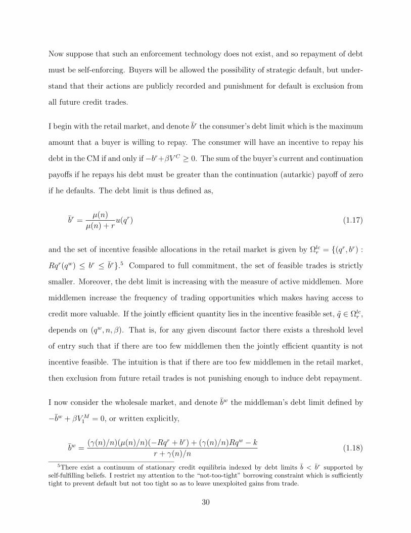
Now suppose that such an enforcement technology does not exist, and so repayment of debt

must be self-enforcing. Buyers will be allowed the possibility of strategic default, but under-

stand that their actions are publicly recorded and punishment for default is exclusion from

all future credit trades.

I begin with the retail market, and denote br the consumer’s debt limit which is the maximum

amount that a buyer is willing to repay. The consumer will have an incentive to repay his

debt in the CM if and only if−br+βV C ≥ 0. The sum of the buyer’s current and continuation

payoffs if he repays his debt must be greater than the continuation (autarkic) payoff of zero

if he defaults. The debt limit is thus defined as,

br =µ(n)

µ(n) + ru(qr) (1.17)

and the set of incentive feasible allocations in the retail market is given by Ωlcr = (qr, br) :

Rqr(qw) ≤ br ≤ br.5 Compared to full commitment, the set of feasible trades is strictly

smaller. Moreover, the debt limit is increasing with the measure of active middlemen. More

middlemen increase the frequency of trading opportunities which makes having access to

credit more valuable. If the jointly efficient quantity lies in the incentive feasible set, q ∈ Ωlcr ,

depends on (qw, n, β). That is, for any given discount factor there exists a threshold level

of entry such that if there are too few middlemen then the jointly efficient quantity is not

incentive feasible. The intuition is that if there are too few middlemen in the retail market,

then exclusion from future retail trades is not punishing enough to induce debt repayment.

I now consider the wholesale market, and denote bw the middleman’s debt limit defined by

−bw + βV M1 = 0, or written explicitly,

bw =(γ(n)/n)(µ(n)/n)(−Rqr + br) + (γ(n)/n)Rqw − k

r + γ(n)/n(1.18)

5There exist a continuum of stationary credit equilibria indexed by debt limits b < br supported byself-fulfilling beliefs. I restrict my attention to the “not-too-tight” borrowing constraint which is sufficientlytight to prevent default but not too tight so as to leave unexploited gains from trade.

30

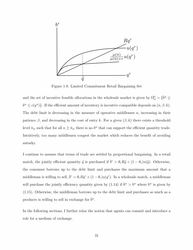
Figure 1.8: Limited Commitment Retail Bargaining Set

and the set of incentive feasible allocations in the wholesale market is given by Ωlcw = bw ≤

bw ≤ c(qw). If the efficient amount of inventory is incentive compatible depends on (n, β, k).

The debt limit is decreasing in the measure of operative middlemen n, increasing in their

patience β, and decreasing in the cost of entry k. For a given (β, k) there exists a threshold

level nw such that for all n ≥ nw there is no bw that can support the efficient quantity trade.

Intuitively, too many middlemen congest the market which reduces the benefit of avoiding

autarky.

I continue to assume that terms of trade are settled by proportional bargaining. In a retail

match, the jointly efficient quantity q is purchased if br > θrRq + (1 − θr)u(q). Otherwise,

the consumer borrows up to the debt limit and purchases the maximum amount that a

middleman is willing to sell, br = θrRqr + (1− θr)u(qr). In a wholesale match, a middleman

will purchase the jointly efficiency quantity given by (1.14) if bw > bw where bw is given by

(1.15). Otherwise, the middleman borrows up to the debt limit and purchases as much as a

producer is willing to sell in exchange for bw.

In the following sections, I further relax the notion that agents can commit and introduce a

role for a medium of exchange.

31

1.9 Monetary Equilibria

In this section, I investigate the role that money plays in facilitating trade within an in-

termediary sector. I assume that money is necessary in retail market transactions due to

anonymity and lack of record keeping, and that credit is feasible in the wholesale market

for simplicity.6 Money is modeled as a perfectly divisible, intrinsically useless asset. Agents

endogenously select to hold any non-negative amount of money allowing them to purchase

the consumption good in the retail market. I assume that the quantity of money grows at

a constant rate Mt+1 = νMt and is injected by lump-sum transfers T to buyers. One unit

of money m purchases φ units of the numeraire good in the centralized market. I call φ the

value of money.

The critical difference is the terms of trade in the retail market. Since credit is not feasible

between middlemen and consumers, the terms of trade in the retail market (qr, dr) indicate a

quantity of good exchanged for some amount of fiat money dr. In the CM all agents exchange

money and goods. In principle, any type of agent can choose to accumulate money in the

CM. As we will see, however, only consumers realize liquidity value from holding money in

the retail market.

For comparability with the pure credit economy, I continue to settle the terms of trade

according to proportional bargaining. In the retail market we have,

maxqr,dr

u(qr)− φdr s.t. u(qr)− φdr =θr

1− θr(−Rqr + φdr)

s.t. qr ≤ qw, dr ≤ m

6We may imagine that producers are sophisticated in the sense that they are able to record and recognizemembers of the intermediary sector. That is, each producer has technology which assigns a name to eachmiddleman and can find said middleman in the CM to collect on debts.

32

As before, the unconstrained solution is such that

u′(q) = R

φd = θrRq + (1− θr)u(q)

Now there are two constrained solutions. If inventory is insufficient we have that,

qr = qw

φdr = (1− θr)u(qr) + θrRqr

If money holdings are insufficient we have that,

φm = (1− θr)u(qr) + θrRqr (1.19)

There are two reasons why the jointly efficient trade may not obtain. First, a middleman

may purchase too little inventory since this investment decision is made ex-ante and bar-

gaining occurs ex-post. Second, a consumer may hold too few real money balances—also

the consequence of an ex-ante portfolio decision. In the former case, a consumer purchases

all available inventory in exchange for real money balances that gives the middleman a frac-

tion (1− θr) of the joint surplus. In the latter case, a consumer spends all real balances to

purchase inventory that gives the consumer a fraction θr of the surplus.

A consumer’s choice of money holdings is given by (1.4) where I substitute out V C using

(1.7),

maxm−(φt − βφt+1)m+ βµ(n)[u(qr(qw,m))− φdr(qw,m)] (1.20)

Notice that if φt/φt+1 < β then there is no solution to (1.1) since consumers would demand

infinite money balances. If φt/φt+1 = β then the cost of holding money is equated to the rate

33

of time preference and agents’ choice of money holdings is enough to purchase q and is not

unique. Finally, if φt/φt+1 > β then money is costly to hold and buyers do not carry more

money balances than they expect to spend in the retail market and the solution is unique.

I restrict my attention to stationary equilibria (i.e. qt = qt+1 = q) which requires that

aggregate real money balances are constant over time: φtMt = φt+1Mt+1. There is thus a

one-for-one mapping between the rate of money growth and the rate of inflation: φt+1/φt =

1/ν. Considering stationary equilibria, and using the proportional bargaining outcome,

consumers’ choice of real money balances follows

maxqr−iz(qr) + µ(n)θrSr(q

r) (1.21)

where (1+ i) = (1+r)ν is the nominal interest rate on an illiquid bond, z = φm, z(q) = (1−

θr)u(q) + θrRq is the mapping from real balances to consumption given by the proportional

bargaining solution, and Sr(q) = u(q)−Rq is the total surplus from retail trade. A consumer

weighs the cost of holding money −iz against the liquidity value it brings in the retail market

µ(n)θrSr(qr(z)). T o guarantee that the problem remains concave and admits a unique

maximum it must be the case that θr/(1 − θr) > i/µ(n). For a given level of entry, the

buyer must have enough bargaining power in the retail market for money to be valued in

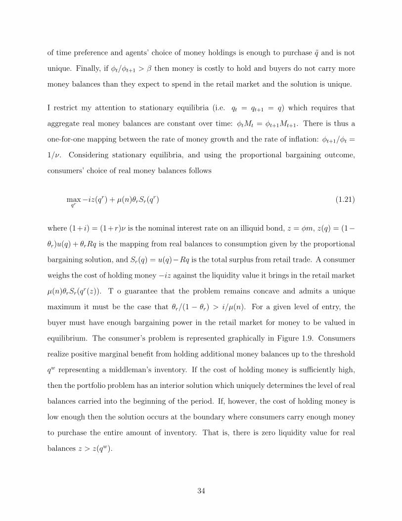
equilibrium. The consumer’s problem is represented graphically in Figure 1.9. Consumers

realize positive marginal benefit from holding additional money balances up to the threshold

qw representing a middleman’s inventory. If the cost of holding money is sufficiently high,

then the portfolio problem has an interior solution which uniquely determines the level of real

balances carried into the beginning of the period. If, however, the cost of holding money is

low enough then the solution occurs at the boundary where consumers carry enough money

to purchase the entire amount of inventory. That is, there is zero liquidity value for real

balances z > z(qw).

34

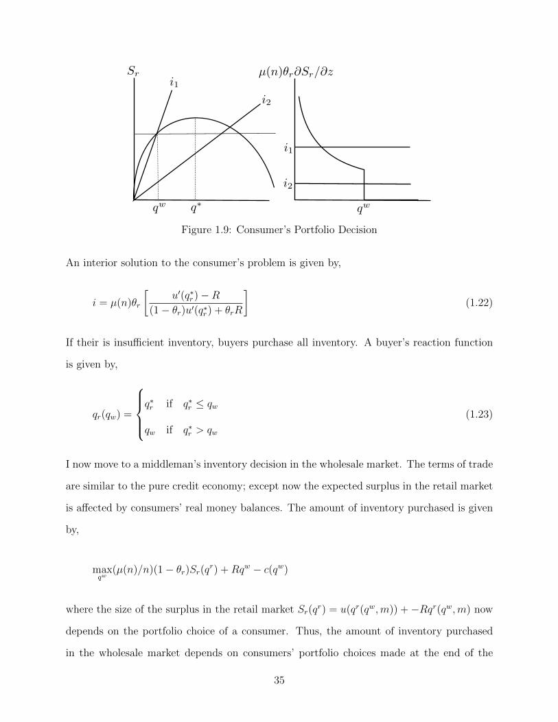
Figure 1.9: Consumer’s Portfolio Decision

An interior solution to the consumer’s problem is given by,

i = µ(n)θr

[u′(q∗r)−R

(1− θr)u′(q∗r) + θrR

](1.22)

If their is insufficient inventory, buyers purchase all inventory. A buyer’s reaction function

is given by,

qr(qw) =

q∗r if q∗r ≤ qw

qw if q∗r > qw

(1.23)

I now move to a middleman’s inventory decision in the wholesale market. The terms of trade

are similar to the pure credit economy; except now the expected surplus in the retail market

is affected by consumers’ real money balances. The amount of inventory purchased is given

by,

maxqw

(µ(n)/n)(1− θr)Sr(qr) +Rqw − c(qw)

where the size of the surplus in the retail market Sr(qr) = u(qr(qw,m)) +−Rqr(qw,m) now

depends on the portfolio choice of a consumer. Thus, the amount of inventory purchased

in the wholesale market depends on consumers’ portfolio choices made at the end of the

35

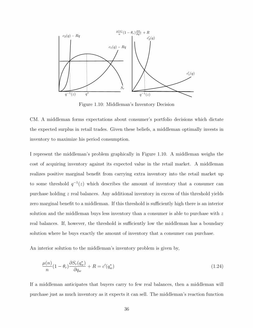
Figure 1.10: Middleman’s Inventory Decision

CM. A middleman forms expectations about consumer’s portfolio decisions which dictate

the expected surplus in retail trades. Given these beliefs, a middleman optimally invests in

inventory to maximize his period consumption.

I represent the middleman’s problem graphically in Figure 1.10. A middleman weighs the

cost of acquiring inventory against its expected value in the retail market. A middleman

realizes positive marginal benefit from carrying extra inventory into the retail market up

to some threshold q−1(z) which describes the amount of inventory that a consumer can

purchase holding z real balances. Any additional inventory in excess of this threshold yields

zero marginal benefit to a middleman. If this threshold is sufficiently high there is an interior

solution and the middleman buys less inventory than a consumer is able to purchase with z

real balances. If, however, the threshold is sufficiently low the middleman has a boundary

solution where he buys exactly the amount of inventory that a consumer can purchase.

An interior solution to the middleman’s inventory problem is given by,

µ(n)

n(1− θr)

∂Sr(q∗w)

∂qw+R = c′(q∗w) (1.24)

If a middleman anticipates that buyers carry to few real balances, then a middleman will

purchase just as much inventory as it expects it can sell. The middleman’s reaction function

36

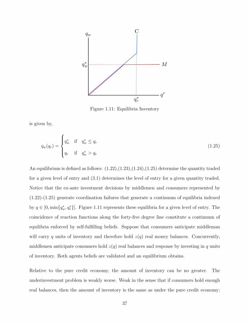
Figure 1.11: Equilibria Inventory

is given by,

qw(qr) =

q∗w if q∗w ≤ qr

qr if q∗w > qr

(1.25)

An equilibrium is defined as follows: (1.22),(1.23),(1.24),(1.25) determine the quantity traded

for a given level of entry and (3.1) determines the level of entry for a given quantity traded.

Notice that the ex-ante investment decisions by middlemen and consumers represented by

(1.22)-(1.25) generate coordination failures that generate a continuum of equilibria indexed

by q ∈ [0,minq∗w, q∗r]. Figure 1.11 represents these equilibria for a given level of entry. The

coincidence of reaction functions along the forty-five degree line constitute a continuum of

equilibria enforced by self-fulfilling beliefs. Suppose that consumers anticipate middleman

will carry q units of inventory and therefore hold z(q) real money balances. Concurrently,

middlemen anticipate consumers hold z(q) real balances and response by investing in q units

of inventory. Both agents beliefs are validated and an equilibrium obtains.

Relative to the pure credit economy, the amount of inventory can be no greater. The

underinvestment problem is weakly worse. Weak in the sense that if consumers hold enough

real balances, then the amount of inventory is the same as under the pure credit economy;

37

however, if consumers hold too few real balances then there is more underinvestment in

inventory. Making credit infeasible in the retail market (and so long as money is costly to

hold) necessitates a weakly smaller surplus in the retail market. This decreases the value of

holding inventory for a middleman.

Note the effect of nominal interest rates on the quantity of inventory. Conventionally, a

higher nominal interest rate increases the opportunity cost of holding money which leads to

fewer real balances and less trade. Consider, however, an equilibrium the consumer is at a

boundary solution. In this case, the choice of real money balances is unaffected by a small

change in the nominal interest rate. Even though the cost of holding money decreases, agents

will not accumulate more money because they know such extra balances will be useless given

that middlemen do not carry enough inventory. The quantity traded will only respond to the

nominal interest rate along the set of interior solutions to the consumer’s portfolio problem.

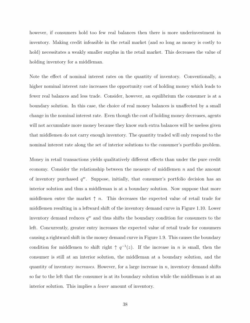
Money in retail transactions yields qualitatively different effects than under the pure credit

economy. Consider the relationship between the measure of middlemen n and the amount

of inventory purchased qw. Suppose, initially, that consumer’s portfolio decision has an

interior solution and thus a middleman is at a boundary solution. Now suppose that more

middlemen enter the market ↑ n. This decreases the expected value of retail trade for

middlemen resulting in a leftward shift of the inventory demand curve in Figure 1.10. Lower

inventory demand reduces qw and thus shifts the boundary condition for consumers to the

left. Concurrently, greater entry increases the expected value of retail trade for consumers

causing a rightward shift in the money demand curve in Figure 1.9. This causes the boundary

condition for middlemen to shift right ↑ q−1(z). If the increase in n is small, then the

consumer is still at an interior solution, the middleman at a boundary solution, and the

quantity of inventory increases. However, for a large increase in n, inventory demand shifts

so far to the left that the consumer is at its boundary solution while the middleman is at an

interior solution. This implies a lower amount of inventory.

38

PROPOSITION 6. When money is essential in retail trades, the response of inventory to

the measure of active middlemen is non-monotone. Define q = minqr, qw to be the quantity

traded given by (1.22),(1.24). We have that

∂q/∂n > 0 for (0, n)

∂q/∂n < 0 for (n,∞)

where n is such that qr = qw.

This is substantively different from the pure credit case due to the portfolio decision of

consumers. For (0, n) an increase in n incentivizes consumers to hold more money balances

and middlemen rationally respond by increasing their purchase of inventory. For (n,∞) an

increase in n incentivizes middlemen to purchase few inventories and consumers rationally

respond by holding fewer real balances.

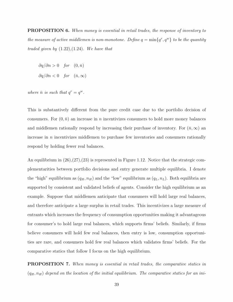
An equilibrium in (26),(27),(23) is represented in Figure 1.12. Notice that the strategic com-

plementarities between portfolio decisions and entry generate multiple equilibria. I denote

the “high” equilibrium as (qH , nH) and the “low” equilibrium as (qL, nL). Both equilibria are

supported by consistent and validated beliefs of agents. Consider the high equilibrium as an

example. Suppose that middlemen anticipate that consumers will hold large real balances,

and therefore anticipate a large surplus in retail trades. This incentivizes a large measure of

entrants which increases the frequency of consumption opportunities making it advantageous

for consumer’s to hold large real balances, which supports firms’ beliefs. Similarly, if firms

believe consumers will hold few real balances, then entry is low, consumption opportuni-

ties are rare, and consumers hold few real balances which validates firms’ beliefs. For the

comparative statics that follow I focus on the high equilibrium.

PROPOSITION 7. When money is essential in retail trades, the comparative statics in

(qH , nH) depend on the location of the initial equilibrium. The comparative statics for an ini-

39

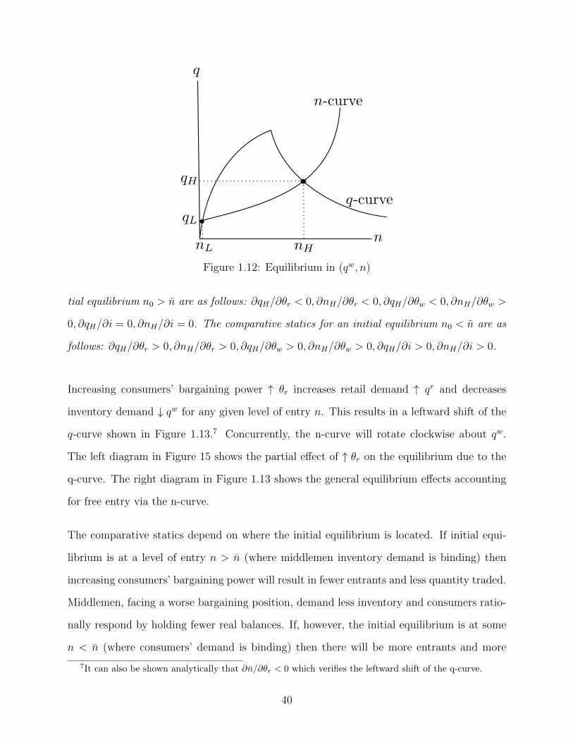
Figure 1.12: Equilibrium in (qw, n)

tial equilibrium n0 > n are as follows: ∂qH/∂θr < 0, ∂nH/∂θr < 0, ∂qH/∂θw < 0, ∂nH/∂θw >

0, ∂qH/∂i = 0, ∂nH/∂i = 0. The comparative statics for an initial equilibrium n0 < n are as

follows: ∂qH/∂θr > 0, ∂nH/∂θr > 0, ∂qH/∂θw > 0, ∂nH/∂θw > 0, ∂qH/∂i > 0, ∂nH/∂i > 0.

Increasing consumers’ bargaining power ↑ θr increases retail demand ↑ qr and decreases

inventory demand ↓ qw for any given level of entry n. This results in a leftward shift of the

q-curve shown in Figure 1.13.7 Concurrently, the n-curve will rotate clockwise about qw.

The left diagram in Figure 15 shows the partial effect of ↑ θr on the equilibrium due to the

q-curve. The right diagram in Figure 1.13 shows the general equilibrium effects accounting

for free entry via the n-curve.

The comparative statics depend on where the initial equilibrium is located. If initial equi-

librium is at a level of entry n > n (where middlemen inventory demand is binding) then

increasing consumers’ bargaining power will result in fewer entrants and less quantity traded.

Middlemen, facing a worse bargaining position, demand less inventory and consumers ratio-

nally respond by holding fewer real balances. If, however, the initial equilibrium is at some

n < n (where consumers’ demand is binding) then there will be more entrants and more

7It can also be shown analytically that ∂n/∂θr < 0 which verifies the leftward shift of the q-curve.

40

quantity traded. Greater bargaining power incentivizes consumers to hold more real bal-

ances and middlemen rationally respond by purchasing more inventory. In the extreme case

where θr = 1, the q-curve shifts far to the left and has a horizontal portion corresponding to

qw : c′(qw) = R indicating that middlemen do not realize any value from holding inventory

in the retail market. Concurrently, the n-curve rotates clockwise.

Figure 1.13: Increase in θr

Changes in bargaining power in the wholesale market have no effect on the q-curve but effect

entry through the n-curve. More bargaining power for middlemen generates a larger expected

surplus from entry which rotates the n-curve clockwise indicating more entry for any given

level of trade. If the initial equilibrium is at n > n then ∂n/∂θw > 0 and ∂q/∂θw < 0.

More entry induces congestion in the retail market resulting in downward movement along

the inventory demand curve. If the initial equilibrium is n < n then ∂n/∂θw > 0 and

∂q/∂θw > 0. More entry increases the expected value of retail trade for consumers who

respond by holding more real balances. These comparative statics are represented in Figure

1.14.

The above comparative statics suggest that the value of θw can determine where the initial

equilibrium lies. If θw is large, middlemen will receive a large fraction of its expected surplus

which incentivizes a large measure of entrants for any given quantity traded and the resulting

41

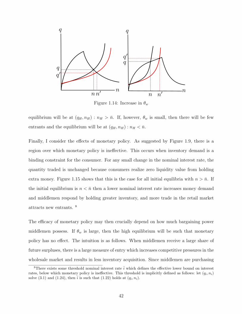
Figure 1.14: Increase in θw

equilibrium will be at (qH , nH) : nH > n. If, however, θw is small, then there will be few

entrants and the equilibrium will be at (qH , nH) : nH < n.

Finally, I consider the effects of monetary policy. As suggested by Figure 1.9, there is a

region over which monetary policy is ineffective. This occurs when inventory demand is a

binding constraint for the consumer. For any small change in the nominal interest rate, the

quantity traded is unchanged because consumers realize zero liquidity value from holding

extra money. Figure 1.15 shows that this is the case for all initial equilibria with n > n. If

the initial equilibrium is n < n then a lower nominal interest rate increases money demand

and middlemen respond by holding greater inventory, and more trade in the retail market

attracts new entrants. 8

The efficacy of monetary policy may then crucially depend on how much bargaining power

middlemen possess. If θw is large, then the high equilibrium will be such that monetary

policy has no effect. The intuition is as follows. When middlemen receive a large share of

future surpluses, there is a large measure of entry which increases competitive pressures in the

wholesale market and results in less inventory acquisition. Since middlemen are purchasing

8There exists some threshold nominal interest rate i which defines the effective lower bound on interestrates, below which monetary policy is ineffective. This threshold is implicitly defined as follows: let (qi, ni)solve (3.1) and (1.24), then i is such that (1.22) holds at (qi, ni).

42

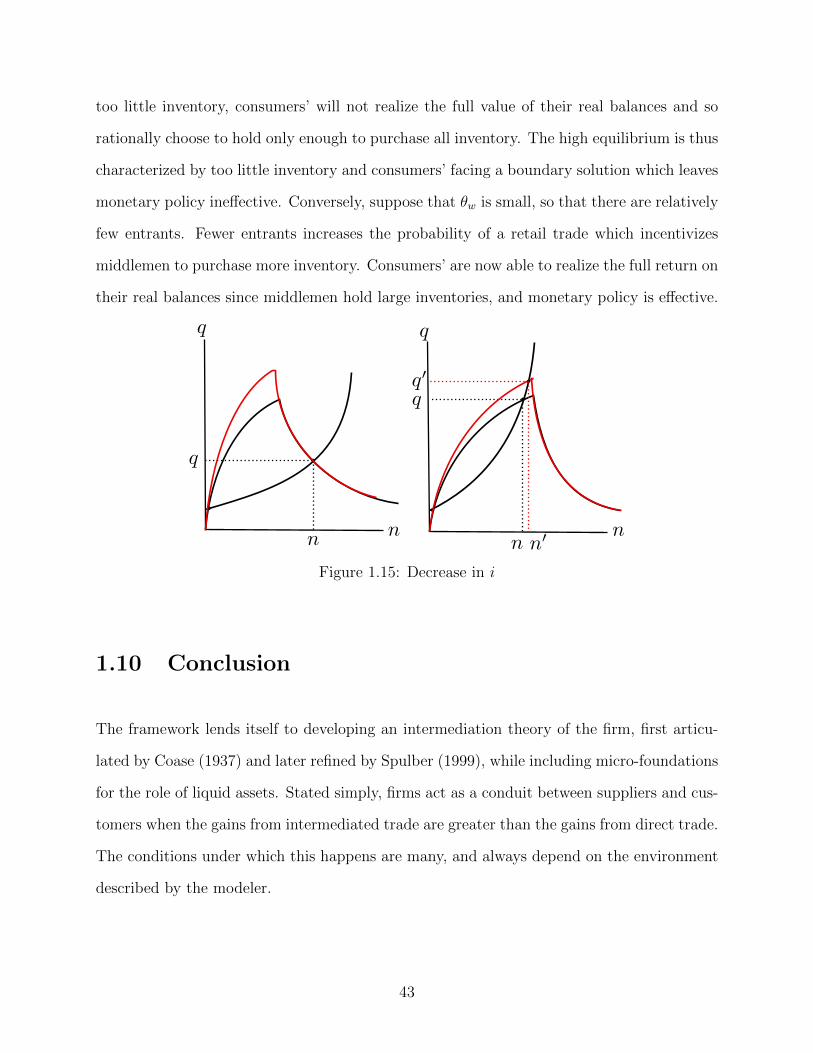
too little inventory, consumers’ will not realize the full value of their real balances and so

rationally choose to hold only enough to purchase all inventory. The high equilibrium is thus

characterized by too little inventory and consumers’ facing a boundary solution which leaves

monetary policy ineffective. Conversely, suppose that θw is small, so that there are relatively

few entrants. Fewer entrants increases the probability of a retail trade which incentivizes

middlemen to purchase more inventory. Consumers’ are now able to realize the full return on

their real balances since middlemen hold large inventories, and monetary policy is effective.

Figure 1.15: Decrease in i

1.10 Conclusion

The framework lends itself to developing an intermediation theory of the firm, first articu-

lated by Coase (1937) and later refined by Spulber (1999), while including micro-foundations

for the role of liquid assets. Stated simply, firms act as a conduit between suppliers and cus-

tomers when the gains from intermediated trade are greater than the gains from direct trade.

The conditions under which this happens are many, and always depend on the environment

described by the modeler.

43

Presently, middlemen are merchants who buy and resell goods without engaging in any

productive activity; while producers are a technology allowing for the manufacture of retail

goods. The model can be amended so that middlemen more closely resemble firms in the

conventional sense. Producers are reinterpreted as entrepreneurs who have an idea or ability

to generate some input into a larger production process. Middlemen are reinterpreted as firms

who purchase inputs from entrepreneurs, transform inputs into final consumption goods, and

sell to consumers. The value-adding productive process employed by middlemen/firms can

be formalized by positing a concave technology Q=G(q). Consumers then enjoy utility u(Q).

The reinterpreted framework places middlemen as the creators and operators of markets.

They form bid and ask prices, conduct transactions, and allocate goods. The theory offers

an explicit mechanism by which markets clear and equilibrium prices obtain rather than

resorting to the theoretical construct of a Walrasian auctioneer.

It is worthwhile to consider alternative market structures while retaining middlemen as an

explicit mechanism by which prices are set and quantities are determined. The obvious

market structure to explore would be competitive price posting which allows one to price

congestion in the market. This market structure may also be a more realistic representation

of middlemen as market-makers rather than merchants. Watanabe (2017) considers the case

of a monopolistic middleman who can choose whether to act as a merchant or a market-

maker.

44

Chapter 2

Trade Intermediation

2.1 Introduction

Conventional trade models largely abstract away from the role that intermediaries play

in exports despite empirical evidence that shows intermediation activities account for a

nontrivial share of international trade. For example, in the 1990’s Japan’s nine general

trading companies (known as soga shoshas) accounted for 40 and 70 percent of the country’s

exports and imports respectively (Jones 1998). In the early 1980’s only 300 Japanese trading

firms accounted for 80 percent of total Japanese trade and the ten largest of these firms

were responsible for 30 percent of Japan’s GNP (Rossman 1998). Statistics like these not

only show that trade flows are affected by intermediation activities, but also that trade

intermediaries may play a vital role in export driven growth. Hong Kong and Singapore are

examples of such entrepot economies where trading activities account for a sizable portion

of GDP growth. Feenstra (2003) finds that in 1998, total trade was 259 percent of GDP in

Hong Kong and 269 percent in Singapore. This striking statistic is largely due to the fact

that these countries provide a trading hub for much of Asia where trade is intermediated in

45

an open market. The existence of trade intermediation is not limited to East Asian nations.

Bernard et al. (2009) estimate that U.S. wholesalers and retailers account for approximately

11 and 24 percent of exports and imports respectively. Estimates by Bernard et al. (2011)

show that over one-quarter of all Italian exporters are intermediaries and that they account

for over 10 percent of total Italian exports. The share of intermediated trade varies not only

across countries but also across products. Ahn et al. (2011) show that trade intermediaries

tend to focus on particular countries but export a large variety of products whereas direct

exporters serve many countries with a narrow product range. These studies suggest that

intermediation is an important component of trade flows and varies with country, product,

and firm level characteristics.

Trade intermediation is not only interesting on account of its prevalence but also because it is

frequently the target of trade policy. One particularly expansive government policy was the

1982 U.S. Export Trading Company Act which sought to “encourage exports by facilitating

the formation and operation of export trading companies, export trade associations, and the

expansion of export trade services generally.” The policy aimed to utilize trade intermediaries

to lower the cost of exports, thereby boosting U.S. export growth and generating jobs.

Clearly, understanding the role that intermediaries play in shaping trade flows is important

for evaluating policy proposals.

This paper takes the position that trade intermediaries improve the efficiency of cross-border

distribution by reducing exporting firms’ transaction costs. By serving as cost minimizers,

intermediaries help link foreign producers with local consumers. This role both increases

firms’ potential foreign profits and augments the set of varieties available to consumers. It is

impossible, however, to evaluate the role of intermediaries in classical trade models because

it is assumed that exporting firms can seamlessly sell to foreign markets. A more realistic

assessment incorporates the additional costs required to delivered good overseas. New trade

theories account for these extra distribution costs through iceberg transport costs and a fixed

46

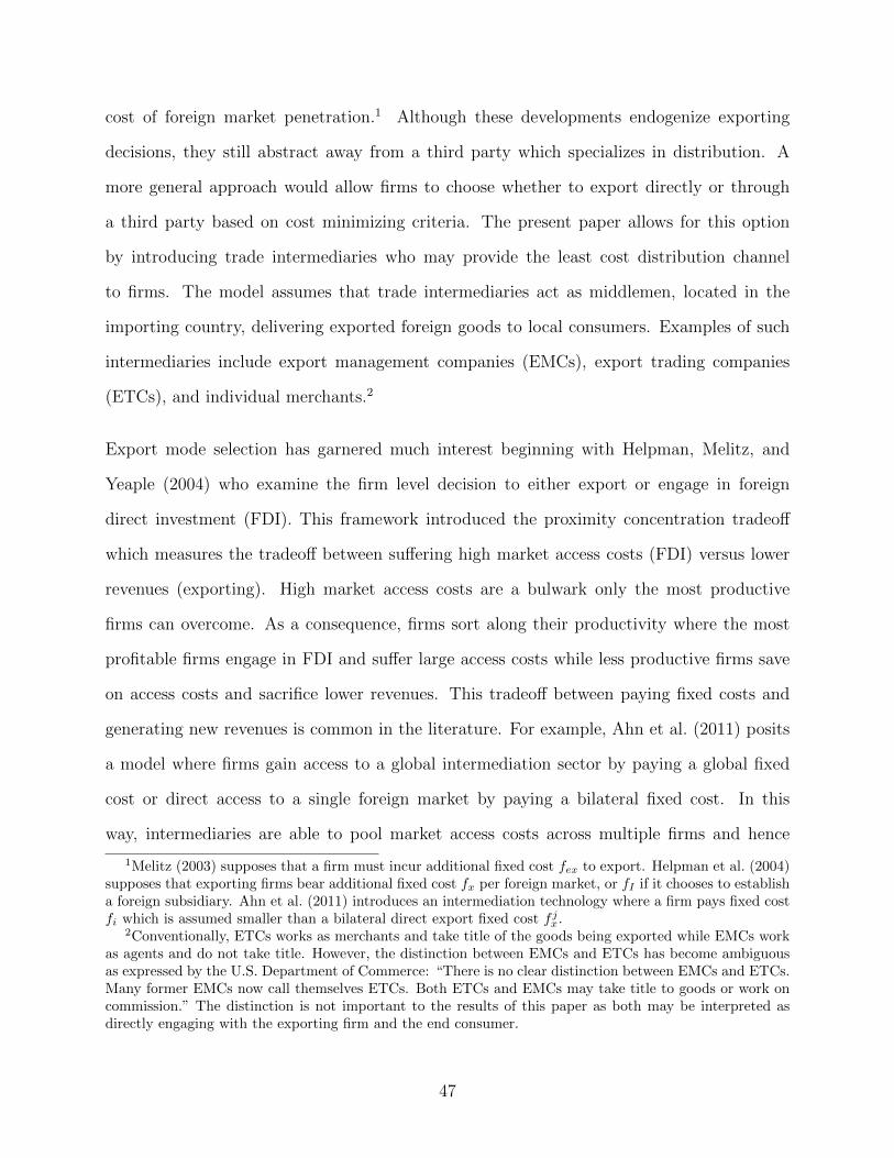
cost of foreign market penetration.1 Although these developments endogenize exporting

decisions, they still abstract away from a third party which specializes in distribution. A

more general approach would allow firms to choose whether to export directly or through

a third party based on cost minimizing criteria. The present paper allows for this option

by introducing trade intermediaries who may provide the least cost distribution channel

to firms. The model assumes that trade intermediaries act as middlemen, located in the

importing country, delivering exported foreign goods to local consumers. Examples of such

intermediaries include export management companies (EMCs), export trading companies

(ETCs), and individual merchants.2

Export mode selection has garnered much interest beginning with Helpman, Melitz, and

Yeaple (2004) who examine the firm level decision to either export or engage in foreign

direct investment (FDI). This framework introduced the proximity concentration tradeoff

which measures the tradeoff between suffering high market access costs (FDI) versus lower

revenues (exporting). High market access costs are a bulwark only the most productive

firms can overcome. As a consequence, firms sort along their productivity where the most

profitable firms engage in FDI and suffer large access costs while less productive firms save

on access costs and sacrifice lower revenues. This tradeoff between paying fixed costs and

generating new revenues is common in the literature. For example, Ahn et al. (2011) posits

a model where firms gain access to a global intermediation sector by paying a global fixed

cost or direct access to a single foreign market by paying a bilateral fixed cost. In this

way, intermediaries are able to pool market access costs across multiple firms and hence

1Melitz (2003) supposes that a firm must incur additional fixed cost fex to export. Helpman et al. (2004)supposes that exporting firms bear additional fixed cost fx per foreign market, or fI if it chooses to establisha foreign subsidiary. Ahn et al. (2011) introduces an intermediation technology where a firm pays fixed costfi which is assumed smaller than a bilateral direct export fixed cost f jx.

2Conventionally, ETCs works as merchants and take title of the goods being exported while EMCs workas agents and do not take title. However, the distinction between EMCs and ETCs has become ambiguousas expressed by the U.S. Department of Commerce: “There is no clear distinction between EMCs and ETCs.Many former EMCs now call themselves ETCs. Both ETCs and EMCs may take title to goods or work oncommission.” The distinction is not important to the results of this paper as both may be interpreted asdirectly engaging with the exporting firm and the end consumer.

47

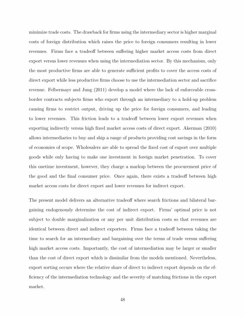
minimize trade costs. The drawback for firms using the intermediary sector is higher marginal

costs of foreign distribution which raises the price to foreign consumers resulting in lower

revenues. Firms face a tradeoff between suffering higher market access costs from direct

export versus lower revenues when using the intermediation sector. By this mechanism, only

the most productive firms are able to generate sufficient profits to cover the access costs of

direct export while less productive firms choose to use the intermediation sector and sacrifice

revenue. Felbermayr and Jung (2011) develop a model where the lack of enforceable cross-

border contracts subjects firms who export through an intermediary to a hold-up problem

causing firms to restrict output, driving up the price for foreign consumers, and leading

to lower revenues. This friction leads to a tradeoff between lower export revenues when

exporting indirectly versus high fixed market access costs of direct export. Akerman (2010)

allows intermediaries to buy and ship a range of products providing cost savings in the form

of economies of scope. Wholesalers are able to spread the fixed cost of export over multiple

goods while only having to make one investment in foreign market penetration. To cover

this onetime investment, however, they charge a markup between the procurement price of

the good and the final consumer price. Once again, there exists a tradeoff between high

market access costs for direct export and lower revenues for indirect export.

The present model delivers an alternative tradeoff where search frictions and bilateral bar-

gaining endogenously determine the cost of indirect export. Firms’ optimal price is not

subject to double marginalization or any per unit distribution costs so that revenues are

identical between direct and indirect exporters. Firms face a tradeoff between taking the

time to search for an intermediary and bargaining over the terms of trade versus suffering

high market access costs. Importantly, the cost of intermediation may be larger or smaller

than the cost of direct export which is dissimilar from the models mentioned. Nevertheless,

export sorting occurs where the relative share of direct to indirect export depends on the ef-

ficiency of the intermediation technology and the severity of matching frictions in the export

market.

48

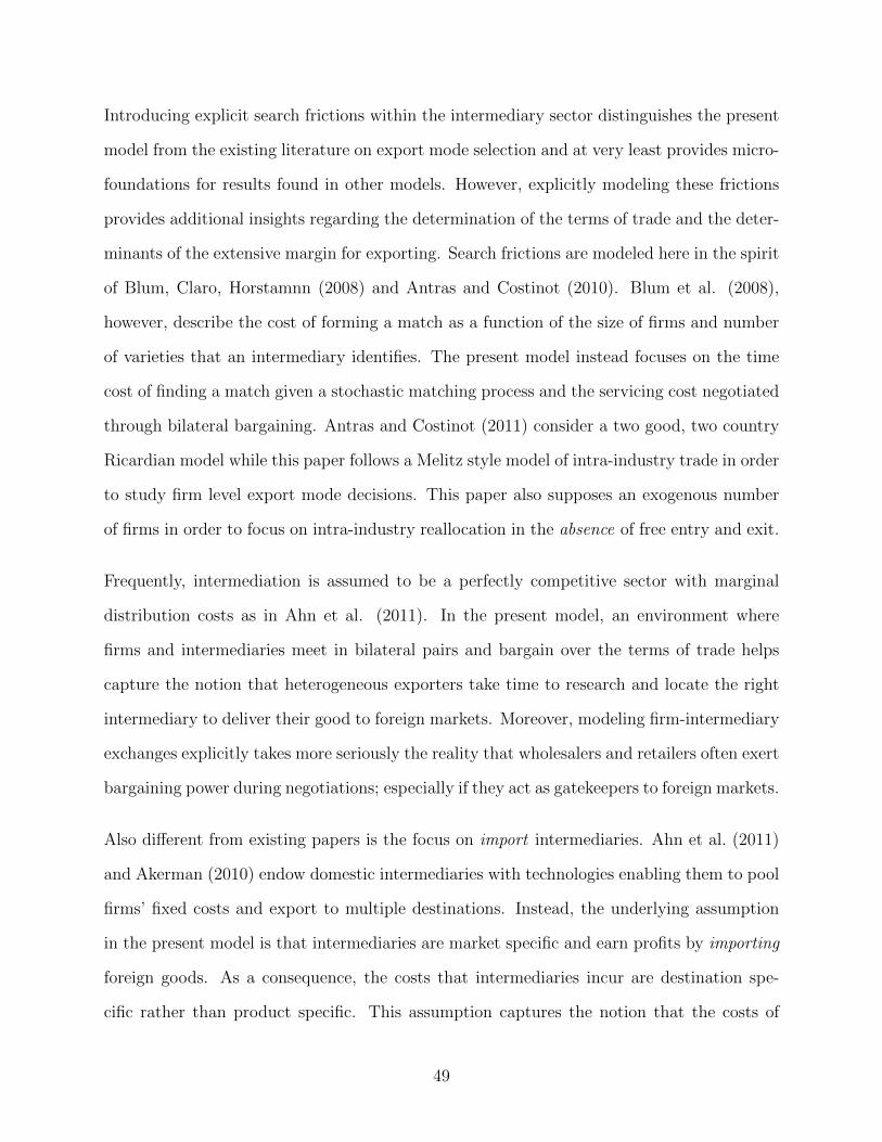
Introducing explicit search frictions within the intermediary sector distinguishes the present

model from the existing literature on export mode selection and at very least provides micro-

foundations for results found in other models. However, explicitly modeling these frictions

provides additional insights regarding the determination of the terms of trade and the deter-

minants of the extensive margin for exporting. Search frictions are modeled here in the spirit

of Blum, Claro, Horstamnn (2008) and Antras and Costinot (2010). Blum et al. (2008),

however, describe the cost of forming a match as a function of the size of firms and number

of varieties that an intermediary identifies. The present model instead focuses on the time

cost of finding a match given a stochastic matching process and the servicing cost negotiated

through bilateral bargaining. Antras and Costinot (2011) consider a two good, two country

Ricardian model while this paper follows a Melitz style model of intra-industry trade in order

to study firm level export mode decisions. This paper also supposes an exogenous number

of firms in order to focus on intra-industry reallocation in the absence of free entry and exit.

Frequently, intermediation is assumed to be a perfectly competitive sector with marginal

distribution costs as in Ahn et al. (2011). In the present model, an environment where

firms and intermediaries meet in bilateral pairs and bargain over the terms of trade helps

capture the notion that heterogeneous exporters take time to research and locate the right

intermediary to deliver their good to foreign markets. Moreover, modeling firm-intermediary

exchanges explicitly takes more seriously the reality that wholesalers and retailers often exert

bargaining power during negotiations; especially if they act as gatekeepers to foreign markets.

Also different from existing papers is the focus on import intermediaries. Ahn et al. (2011)

and Akerman (2010) endow domestic intermediaries with technologies enabling them to pool

firms’ fixed costs and export to multiple destinations. Instead, the underlying assumption

in the present model is that intermediaries are market specific and earn profits by importing

foreign goods. As a consequence, the costs that intermediaries incur are destination spe-

cific rather than product specific. This assumption captures the notion that the costs of

49

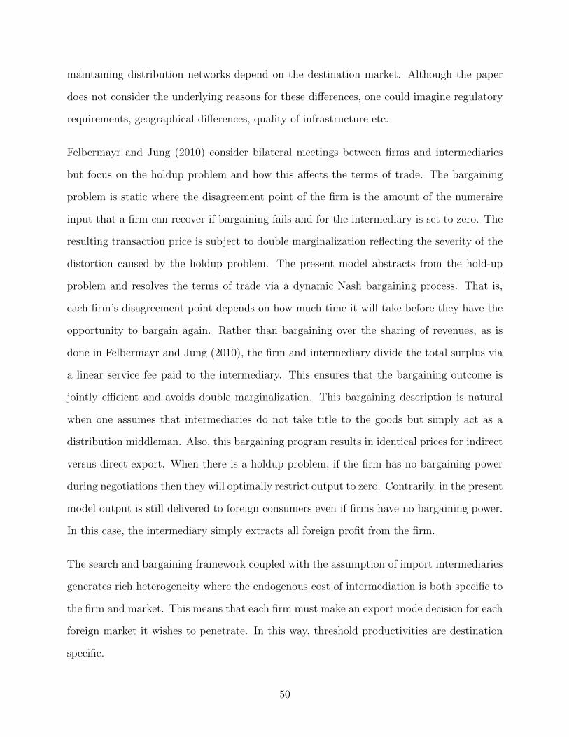
maintaining distribution networks depend on the destination market. Although the paper

does not consider the underlying reasons for these differences, one could imagine regulatory

requirements, geographical differences, quality of infrastructure etc.

Felbermayr and Jung (2010) consider bilateral meetings between firms and intermediaries

but focus on the holdup problem and how this affects the terms of trade. The bargaining

problem is static where the disagreement point of the firm is the amount of the numeraire

input that a firm can recover if bargaining fails and for the intermediary is set to zero. The

resulting transaction price is subject to double marginalization reflecting the severity of the

distortion caused by the holdup problem. The present model abstracts from the hold-up

problem and resolves the terms of trade via a dynamic Nash bargaining process. That is,

each firm’s disagreement point depends on how much time it will take before they have the

opportunity to bargain again. Rather than bargaining over the sharing of revenues, as is

done in Felbermayr and Jung (2010), the firm and intermediary divide the total surplus via

a linear service fee paid to the intermediary. This ensures that the bargaining outcome is

jointly efficient and avoids double marginalization. This bargaining description is natural

when one assumes that intermediaries do not take title to the goods but simply act as a

distribution middleman. Also, this bargaining program results in identical prices for indirect

versus direct export. When there is a holdup problem, if the firm has no bargaining power

during negotiations then they will optimally restrict output to zero. Contrarily, in the present

model output is still delivered to foreign consumers even if firms have no bargaining power.

In this case, the intermediary simply extracts all foreign profit from the firm.

The search and bargaining framework coupled with the assumption of import intermediaries

generates rich heterogeneity where the endogenous cost of intermediation is both specific to

the firm and market. This means that each firm must make an export mode decision for each

foreign market it wishes to penetrate. In this way, threshold productivities are destination

specific.

50

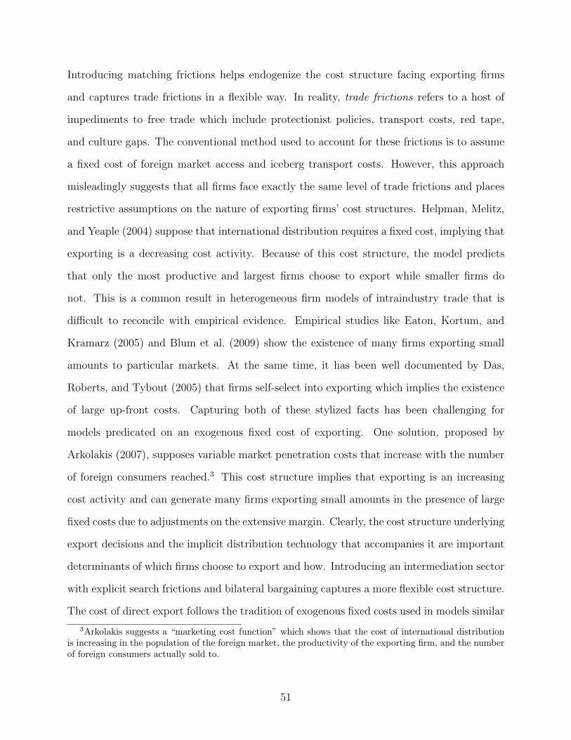
Introducing matching frictions helps endogenize the cost structure facing exporting firms

and captures trade frictions in a flexible way. In reality, trade frictions refers to a host of

impediments to free trade which include protectionist policies, transport costs, red tape,

and culture gaps. The conventional method used to account for these frictions is to assume

a fixed cost of foreign market access and iceberg transport costs. However, this approach

misleadingly suggests that all firms face exactly the same level of trade frictions and places

restrictive assumptions on the nature of exporting firms’ cost structures. Helpman, Melitz,

and Yeaple (2004) suppose that international distribution requires a fixed cost, implying that

exporting is a decreasing cost activity. Because of this cost structure, the model predicts

that only the most productive and largest firms choose to export while smaller firms do

not. This is a common result in heterogeneous firm models of intraindustry trade that is

difficult to reconcile with empirical evidence. Empirical studies like Eaton, Kortum, and

Kramarz (2005) and Blum et al. (2009) show the existence of many firms exporting small

amounts to particular markets. At the same time, it has been well documented by Das,

Roberts, and Tybout (2005) that firms self-select into exporting which implies the existence

of large up-front costs. Capturing both of these stylized facts has been challenging for

models predicated on an exogenous fixed cost of exporting. One solution, proposed by

Arkolakis (2007), supposes variable market penetration costs that increase with the number

of foreign consumers reached.3 This cost structure implies that exporting is an increasing

cost activity and can generate many firms exporting small amounts in the presence of large

fixed costs due to adjustments on the extensive margin. Clearly, the cost structure underlying

export decisions and the implicit distribution technology that accompanies it are important

determinants of which firms choose to export and how. Introducing an intermediation sector

with explicit search frictions and bilateral bargaining captures a more flexible cost structure.

The cost of direct export follows the tradition of exogenous fixed costs used in models similar

3Arkolakis suggests a “marketing cost function” which shows that the cost of international distributionis increasing in the population of the foreign market, the productivity of the exporting firm, and the numberof foreign consumers actually sold to.

51

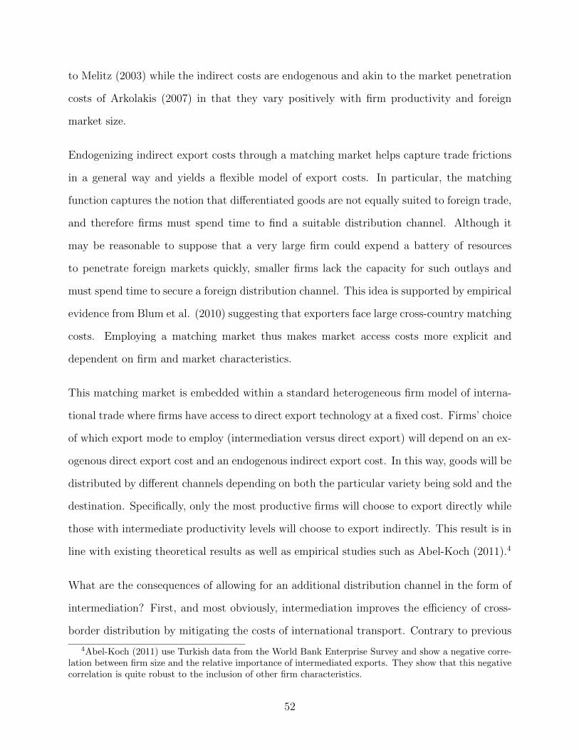
to Melitz (2003) while the indirect costs are endogenous and akin to the market penetration

costs of Arkolakis (2007) in that they vary positively with firm productivity and foreign

market size.

Endogenizing indirect export costs through a matching market helps capture trade frictions

in a general way and yields a flexible model of export costs. In particular, the matching

function captures the notion that differentiated goods are not equally suited to foreign trade,

and therefore firms must spend time to find a suitable distribution channel. Although it

may be reasonable to suppose that a very large firm could expend a battery of resources

to penetrate foreign markets quickly, smaller firms lack the capacity for such outlays and

must spend time to secure a foreign distribution channel. This idea is supported by empirical

evidence from Blum et al. (2010) suggesting that exporters face large cross-country matching

costs. Employing a matching market thus makes market access costs more explicit and

dependent on firm and market characteristics.

This matching market is embedded within a standard heterogeneous firm model of interna-

tional trade where firms have access to direct export technology at a fixed cost. Firms’ choice

of which export mode to employ (intermediation versus direct export) will depend on an ex-

ogenous direct export cost and an endogenous indirect export cost. In this way, goods will be

distributed by different channels depending on both the particular variety being sold and the

destination. Specifically, only the most productive firms will choose to export directly while

those with intermediate productivity levels will choose to export indirectly. This result is in

line with existing theoretical results as well as empirical studies such as Abel-Koch (2011).4

What are the consequences of allowing for an additional distribution channel in the form of

intermediation? First, and most obviously, intermediation improves the efficiency of cross-

border distribution by mitigating the costs of international transport. Contrary to previous

4Abel-Koch (2011) use Turkish data from the World Bank Enterprise Survey and show a negative corre-lation between firm size and the relative importance of intermediated exports. They show that this negativecorrelation is quite robust to the inclusion of other firm characteristics.

52

models, the costs of intermediation arise endogenously through the search and matching

framework and will depend on firm and export market characteristics. Second, intermedi-

aries act as market makers by enlarging the set of goods traded. In this way, intermediaries

have a positive welfare affect by allowing greater diversity of goods for consumers than would

exist in their absence. However, under certain conditions excessive intermediation can cause

the set of goods available to consumers to shrink. Third, intermediation benefits less pro-

ductive firms by providing access to foreign markets without paying high fixed costs from

direct export. Fourth, intermediation results in a decrease in aggregate productivity among

exported goods. It is interesting to note that there exist changes in aggregate productivity

despite the absence of free entry and exit among firms as in Melitz (2003). The present

model suggests that intermediation may be another channel that can affect aggregate pro-

ductivity. Fifth, intermediation is strictly welfare improving in that it lowers the price index

of importing nations and increases national income.

The model is able to generate stylized facts that have been identified across empirical studies.

Chief among them is that an increase in country specific fixed export costs increases the

share of trade performed by intermediaries. The model also correctly predicts that smaller

countries have a larger share of intermediated trade. Taken together, these results suggest

that trade intermediaries may be especially relevant for developing nations who are usually

small and costly for firms to penetrate.

2.2 Demand

There exists a discrete number of countries indexed i = 1, ..., N . Each country has a repre-

sentative consumer with Cobb-Douglas tastes for two types of goods,

U = c1−η0 Cη, η ∈ (0, 1) (2.1)

53

where c0 is a homogeneous good and C is a constant elasticity of substitution (CES) aggre-

gator over a continuum of horizontally differentiated goods indexed z ∈ Zi,

C =

( N∑i=1

∫Zi

ci(z)σ−1σ dz

) σσ−1

, σ ∈ (1,∞). (2.2)

The consumer’s problem is to maximize (2.1) subject to the budget constraint,

N∑i=1

(p0c0 +

∫Zi

pi(z)ci(z)dz

)≤ Y

where ci(z) is the consumption of variety z ∈ Zi produced in country i = 1, ..., N and Y is

the income of the domestic country. Consumers are assumed to own the firms and receive

lump sum profits of T in addition to wage w. Choosing the homogeneous good to be the

numeraire, p0 = 1, utility maximization yields a demand schedule for individual varieties

from a particular country,

ci(z) =

(pi(z)

P

)−σηY

P(2.3)

and for the homogeneous good,

c0 = (1− η)Y.

The demand for a particular variety is log linear in its own price pi(z) and income Y = Lw+T ,

both deflated by the domestic price index P =

(∑Ni=1

∫Zipi(z)1−σdz

) 11−σ

. The elasticity of

substitution across varieties σ = 1/(1− ρ) > 1 is assumed identical in all countries.5

5The assumption of constant elasticity of substitution abstracts the pro-competitive effects of trade lib-eralization for the sake of simplicity. The model could be amended to include variable markups.

54

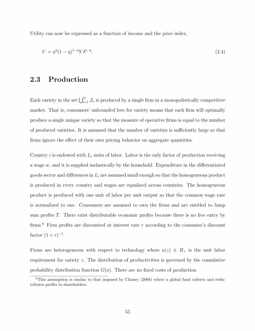
Utility can now be expressed as a function of income and the price index,

U = ηη(1− η)1−ηY P−η. (2.4)

2.3 Production

Each variety in the set⋃Ni=1 Zi is produced by a single firm in a monopolistically competitive

market. That is, consumers’ unbounded love for variety means that each firm will optimally

produce a single unique variety so that the measure of operative firms is equal to the number

of produced varieties. It is assumed that the number of varieties is sufficiently large so that

firms ignore the effect of their own pricing behavior on aggregate quantities.

Country i is endowed with Li units of labor. Labor is the only factor of production receiving

a wage w, and it is supplied inelastically by the household. Expenditure in the differentiated

goods sector and differences in Li are assumed small enough so that the homogeneous product

is produced in every country and wages are equalized across countries. The homogeneous

product is produced with one unit of labor per unit output so that the common wage rate

is normalized to one. Consumers are assumed to own the firms and are entitled to lump

sum profits T . There exist distributable economic profits because there is no free entry by

firms.6 Firm profits are discounted at interest rate r according to the consumer’s discount

factor (1 + r)−1.

Firms are heterogeneous with respect to technology where a(z) ∈ R+ is the unit labor

requirement for variety z. The distribution of productivities is governed by the cumulative

probability distribution function G(a). There are no fixed costs of production.

6This assumption is similar to that imposed by Chaney (2008) where a global fund collects and redis-tributes profits to shareholders.

55

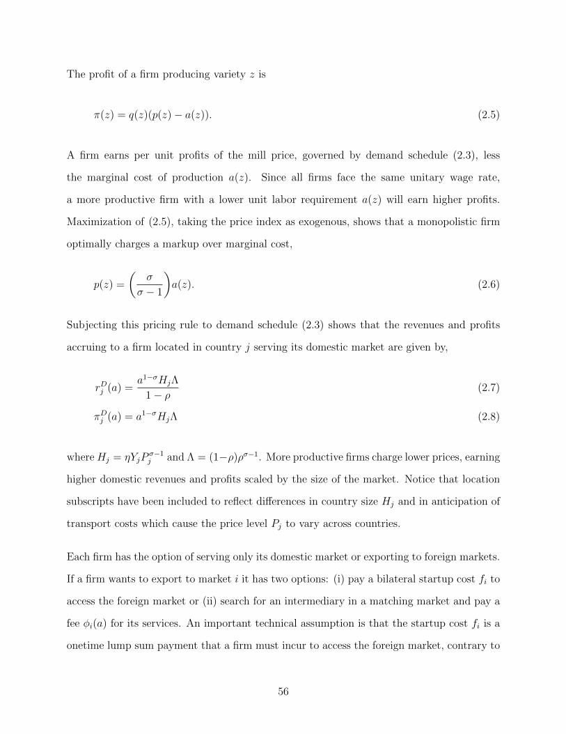
The profit of a firm producing variety z is

π(z) = q(z)(p(z)− a(z)). (2.5)

A firm earns per unit profits of the mill price, governed by demand schedule (2.3), less

the marginal cost of production a(z). Since all firms face the same unitary wage rate,

a more productive firm with a lower unit labor requirement a(z) will earn higher profits.

Maximization of (2.5), taking the price index as exogenous, shows that a monopolistic firm

optimally charges a markup over marginal cost,

p(z) =

(σ

σ − 1

)a(z). (2.6)

Subjecting this pricing rule to demand schedule (2.3) shows that the revenues and profits

accruing to a firm located in country j serving its domestic market are given by,

rDj (a) =a1−σHjΛ

1− ρ(2.7)

πDj (a) = a1−σHjΛ (2.8)

where Hj = ηYjPσ−1j and Λ = (1−ρ)ρσ−1. More productive firms charge lower prices, earning

higher domestic revenues and profits scaled by the size of the market. Notice that location

subscripts have been included to reflect differences in country size Hj and in anticipation of

transport costs which cause the price level Pj to vary across countries.

Each firm has the option of serving only its domestic market or exporting to foreign markets.

If a firm wants to export to market i it has two options: (i) pay a bilateral startup cost fi to

access the foreign market or (ii) search for an intermediary in a matching market and pay a

fee φi(a) for its services. An important technical assumption is that the startup cost fi is a

onetime lump sum payment that a firm must incur to access the foreign market, contrary to

56

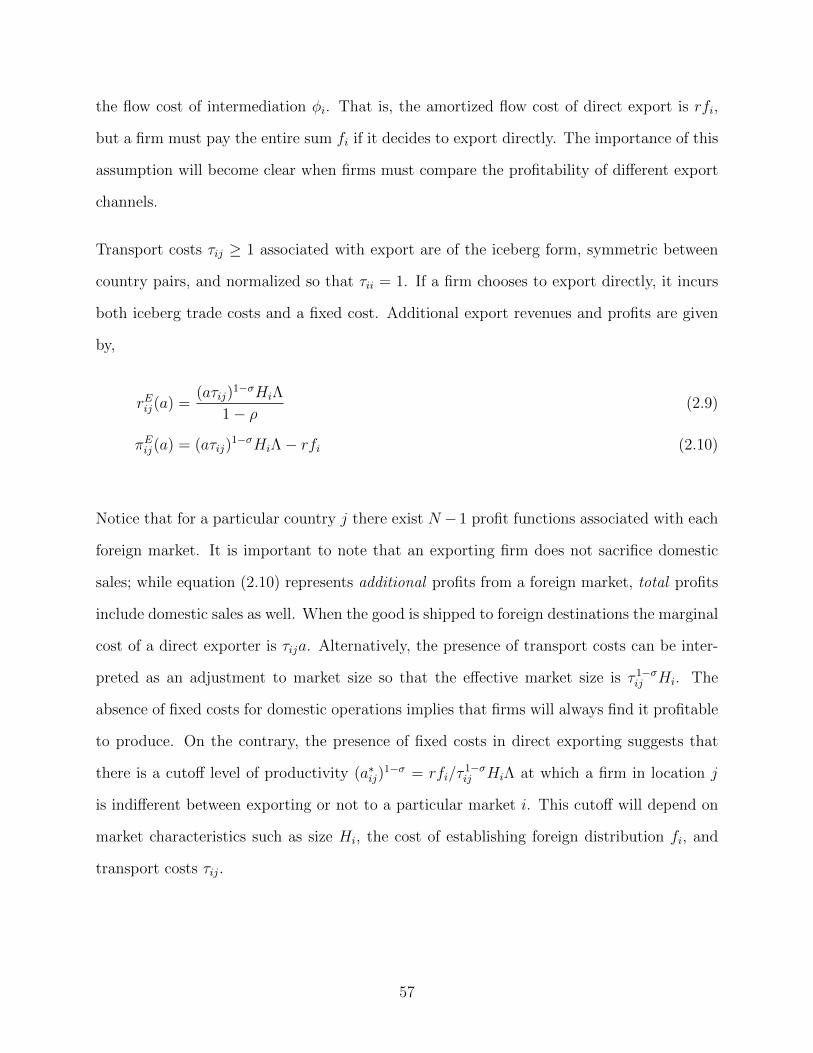
the flow cost of intermediation φi. That is, the amortized flow cost of direct export is rfi,

but a firm must pay the entire sum fi if it decides to export directly. The importance of this

assumption will become clear when firms must compare the profitability of different export

channels.

Transport costs τij ≥ 1 associated with export are of the iceberg form, symmetric between

country pairs, and normalized so that τii = 1. If a firm chooses to export directly, it incurs

both iceberg trade costs and a fixed cost. Additional export revenues and profits are given

by,

rEij(a) =(aτij)

1−σHiΛ

1− ρ(2.9)

πEij(a) = (aτij)1−σHiΛ− rfi (2.10)

Notice that for a particular country j there exist N − 1 profit functions associated with each

foreign market. It is important to note that an exporting firm does not sacrifice domestic

sales; while equation (2.10) represents additional profits from a foreign market, total profits

include domestic sales as well. When the good is shipped to foreign destinations the marginal

cost of a direct exporter is τija. Alternatively, the presence of transport costs can be inter-

preted as an adjustment to market size so that the effective market size is τ 1−σij Hi. The

absence of fixed costs for domestic operations implies that firms will always find it profitable

to produce. On the contrary, the presence of fixed costs in direct exporting suggests that

there is a cutoff level of productivity (a∗ij)1−σ = rfi/τ

1−σij HiΛ at which a firm in location j

is indifferent between exporting or not to a particular market i. This cutoff will depend on

market characteristics such as size Hi, the cost of establishing foreign distribution fi, and

transport costs τij.

57

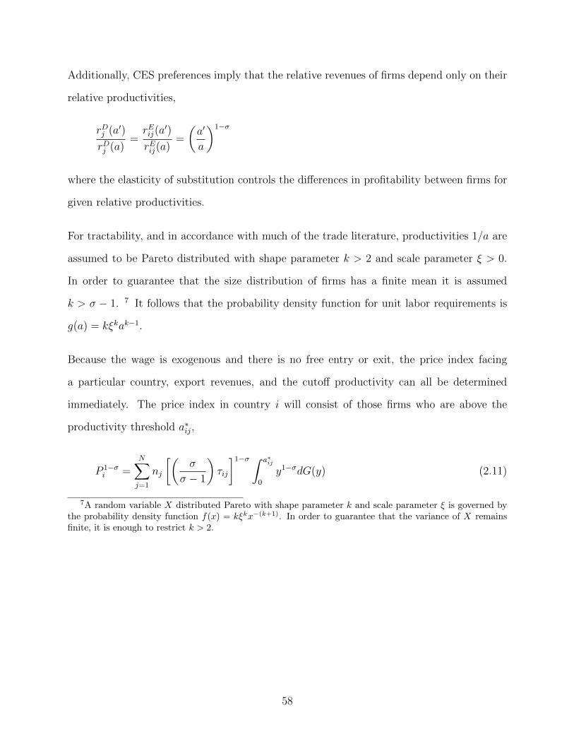
Additionally, CES preferences imply that the relative revenues of firms depend only on their

relative productivities,

rDj (a′)

rDj (a)=rEij(a

′)

rEij(a)=

(a′

a

)1−σ

where the elasticity of substitution controls the differences in profitability between firms for

given relative productivities.

For tractability, and in accordance with much of the trade literature, productivities 1/a are

assumed to be Pareto distributed with shape parameter k > 2 and scale parameter ξ > 0.

In order to guarantee that the size distribution of firms has a finite mean it is assumed

k > σ − 1. 7 It follows that the probability density function for unit labor requirements is

g(a) = kξkak−1.

Because the wage is exogenous and there is no free entry or exit, the price index facing

a particular country, export revenues, and the cutoff productivity can all be determined

immediately. The price index in country i will consist of those firms who are above the

productivity threshold a∗ij,

P 1−σi =

N∑j=1

nj

[(σ

σ − 1

)τij

]1−σ ∫ a∗ij

0

y1−σdG(y) (2.11)

7A random variable X distributed Pareto with shape parameter k and scale parameter ξ is governed bythe probability density function f(x) = kξkx−(k+1). In order to guarantee that the variance of X remainsfinite, it is enough to restrict k > 2.

58

Using this price index, we obtain the revenues of an exporting firm and the threshold pro-

ductivities.

Pi = (c1c2)−1/kY

− 1k− 1σ−1

i

rEij(a) = a1−σστ 1−σij Λη(c1c2)−(σ−1)

k Yσ−1k

i

a∗ij = (rfi)1

1−σ τ−1ij (ηΛ)1

σ−1 (c1c2)−1k Y

1ki

c1 =N∑j=1

njτ−kij (rfi)

− k1−σ−1

c2 =

(σ

σ − 1

)1−σkξk

k − σ + 1(ηΛ)−

1k− 1σ−1

The method of direct export described above is nearly identical to that considered by Chaney

(2008). The novelty here is that firms do not have to export directly. They may instead

choose to search for an intermediary. However, this search is costly to firms due to matching

frictions. Although firms do not have to incur a fixed cost of foreign distribution, they must

pay intermediaries a service fee φi(z) and engage in the costly search activity.

2.4 Intermediation

Conventional trade models largely assume that exporting firms can sell directly to foreign

consumers. In reality, not all firms engage in direct export because it requires dedication of

resources toward foreign market research, building a foreign sales and distribution structure,

and complying with the rules and regulations of foreign markets. Intermediaries, on the other

hand, save firms’ time and resources by providing knowledge of foreign market characteristics,

well established distribution networks, and expertise in export activities. In this way, indirect

export via intermediaries provides immediate access to foreign markets at potentially lower

cost.

59

There are many different ways a firm can choose to export indirectly. Exchange manage-

ment companies (EMCs), exchange trading companies (ETCs), export merchants, export

commission houses, and export brokers are all viable channels. Common to all is the provi-

sion of services enabling a firm to sell their product in foreign markets with limited direct

involvement. Payment methods vary, but the most common include fee-based contracts,

buy-and-sell arrangements, and commission-based contracts. The modeling assumption used

here is that all contracts are fee-based. This assumption implies that intermediaries never

take title to the goods so consumers do not face double marginalization. Fees charged by

intermediaries represent compensation for facilitating the sale of domestic goods to a foreign

market.

Each intermediary possesses the resources and/or knowledge to access a particular market

i and deliver the product from a firm in market j to consumers in market i. However,

to maintain access to this market it must pay a cost di. Market access costs pay for the

maintenance of existing distribution infrastructure which allows the delivery of product to

foreign consumers. An intermediary earns revenue by charging firms a fee φi(a) for the

service of connecting them with foreign markets.

Assuming a fee-based contract coupled with market access costs unrelated to the quantity

of production avoids any jointly inefficient outcomes that would disappear with a two-part

pricing scheme. Furthermore, the modeling assumptions preclude any wedge between whole-

sale and retail prices either due to additional per unit costs like in Ahn (2011) or the lack

of cross-border enforceable contracts as in Felbermayr and Jung (2010). Without a wedge,

the tradeoff that firms face when deciding on an export mode is not between low revenues

versus low fixed costs, as conventionally done, but rather between low fixed costs versus the

cost of search frictions, which are unrelated to firm revenues.

Firms meet intermediaries subject to search frictions, as described by the matching func-

tion m(uF , uI) where uF denotes the measure of unmatched firms and uI the measure of

60

unmatched intermediaries. The matching function is assumed to be increasing, concave, and

homogeneous of degree one. The rate at which firms meet intermediaries is m(1, θ) = µ(θ)

and the rate at which intermediaries meet firms is m(1/θ, 1) = µ(θ)/θ where θ = uI/uF is a

measure of export market tightness. Additionally, it is assumed that µ(0) = 0, µ′(0) = 1, and

µ(∞) = 1. Matches dissolve at an exogenous rate λ. Matches occur bilaterally between pairs

of countries: the thickness of each market depends on the number of firms and intermediaries

present between countries i and j. This assumes that there is a measure of intermediaries

looking to facilitate trade with a particular country. There are no externalities or congestion

effects between different export markets. With this in mind, it is appropriate to denote mar-

ket tightness as θij to reflect the fact that the global export market has been segmented into

N(N − 1) local export markets. For the remainder of the paper I will omit these subscripts,

but it should be understood that θ is a market tightness specific to a country pair.

Both firms and intermediaries maximize expected lifetime discounted profits. If a firm is

matched with an intermediary then it pays a fee φi(a) (which is allowed to vary with the

type of firm) for the intermediary’s service and stands to earn total variable export profits

of πij(a) = πDij (a) + πIij(a). If a firm is unmatched then it earns domestic profits of πDij (a). A

matched intermediary stands to earn the fee φi(a) while an unmatched intermediary earns

nothing. Regardless, the intermediary must pay a market access cost di.

Since firms are heterogeneous with respect to productivity, intermediaries face ex ante uncer-

tainty over what type of firm they will be matched with. Once a match is formed, however,

the intermediary learns the type of firm they have met and so there is no ex post uncer-

tainty. As a result, there is no asymmetric information during negotiations over the fee. An

intermediary’s decision to enter the export market will depend on the expected surplus of a

match which depends on the type of firm that it is matched with.

Let E(a) and D(a) denote the value function of a matched and unmatched firm respectively

and let T (a) and U denote the value function of a matched and unmatched intermediary

61

respectively. Suppressing the location subscripts for notational convenience, the value func-

tions of a firm and intermediary must satisfy the following Bellman equations,

rD(a) = πD(a) + µ(θ)[E(a)−D(a)] (2.12)

rE(a) = π(a)− φ(a) + λ[D(a)− E(a)] (2.13)

rT (a) = φ(a) + λ[U − T (a)]− d (2.14)

rU =µ(θ)

θ

∫ φ−1(d)

0

[T (a)− U ]dGT (a)− d (2.15)

Equation (2.12) shows that the discounted value of an unmatched firm equals instantaneous

profits from the domestic market plus the expected surplus of finding a match. Equation

(2.13) shows that a matched (exporting) firm earns instantaneous profits from exporting π(a),

pays an intermediation fee φ(a), and incurs an expected loss from exogenous separation. A

matched firm earns domestic profits plus additional export profits from the foreign market via

the intermediary. These additional foreign variable profits are determined by profit function

(2.5) subject to foreign demand (2.3),8

πIij(a) = (aτij)1−σHiΛ. (2.16)

Comparison to expression (2.10) shows that the fee associated with indirect export is analo-

gous to the amortized fixed cost associated with direct export. However, the cost of indirect

export φi(a) will be an endogenous outcome of the search and matching environment, whereas

rfi is strictly exogenous. This is different from much of the existing literature which treats

all fixed costs as exogenous.9

8Note that foreign variable profits are not equivalent to ex post foreign profits πIij(a)−φ(a). The distinction

is important since it will be variable profits that are part of the surplus that firms and intermediaries bargainover. The outcome of the bargaining will then yield ex post foreign profits.

9Note that revenues from indirect and direct export are identical which is in sharp contrast to much ofthe existing literature. This means that firms will weigh the amortized fixed cost of direct export against thefixed cost of indirect export when determining which export mode is optimal. This feature is different fromexisting papers where an intermediary sector forces additional per unit costs upon firms thereby loweringrevenues.

62

As was the case for direct export, note that expression (2.16) shows additional variable

profits from indirect export. Total variable profits from indirect export are given by,

πij(a) = a1−σΛ(Hj + τ 1−σij Hi). (2.17)

Equation (2.14) shows that a matched intermediary earns revenue of φ(a), has an expected

loss of surplus from exogenous separation, and must pay a cost d to maintain access to its

market. Using this Bellman equation, we can write an expression for the surplus from a

match,

T (a)− U =φ(a)− d− rU

r + λ.

Due to heterogeneity among firms, intermediaries face ex ante uncertainty and must form

beliefs about the type of firm they can expect to meet given the productivity distribution

G(a). An intermediary must decide whether a match is acceptable or wait to be matched

with a more desirable type in the future. The intermediary will only accept a match if its

value outweighs that of continuing to search for a potentially better firm,

T (a) ≥ U ⇔ φ(a)− d ≥ rU.

Because this surplus increases linearly with respect to the service fee, there exists some cutoff

fee φ(a) at which the firm is indifferent between searching and accepting a match. Allowing

for free entry on the side of the intermediaries guarantees that the value of being unmatched

is driven to zero in equilibrium U = 0. There is thus a simple relationship that must be

satisfied for the intermediary to cooperate with the matched firm,

φ(a) ≥ d.

63

That is to say, the revenue earned by the intermediary must at least cover the flow cost of

maintaining access to its distribution network. Equation (2.15) reflects the intermediary’s

expected surplus of finding an acceptable match while paying a cost d to maintain access to

its market. Note that higher a corresponds to a lower productivity firm and therefore the

fee φ is decreasing in a. Hence, a lower cutoff φ corresponds to an upper cutoff a. This is

why φ−1(d) is the upper integrating limit in expression (2.15).

2.5 Nash Bargaining

When a firm and an intermediary meet, they negotiate over the fee that will be charged.

Resolution of this negotiation is described by an asymmetric Nash bargaining game. Giving

the intermediary primitive bargaining power β, the Nash program is

maxφ(a)

(T (a)− U)β(E(a)−D(a))1−β (2.18)

which results in the usual proportional sharing rule,

T (a)− U =β

1− β(E(a)−D(a)). (2.19)

Notice that the threat point in (2.18) suggests that a firm chooses to continue searching for

an intermediary if negotiations fail. This will always be preferable direct export because the

startup cost fi is a onetime lump sum cost. If bargaining breaks down, no firm will find it

profitable to pay a lump sum cost relative to the flow cost of continued search.

From (2.13) and (2.14), expressions for the value of the surpluses are obtained,

E(a)−D(a) =π(a)− φ(a)− rD(a)

r + λ(2.20)

64

T (a)− U =φ(a)− d− rU

r + λ(2.21)

As long as there exist profits from entering the export sector, intermediaries will continue

to do so until the value of being unmatched is equal to zero. This provides a free entry

condition for intermediaries,

U = 0. (2.22)

Substituting (2.20) and (2.21) into the outcome of the Nash bargaining (2.19) and invoking

the free entry condition (2.22) yields an explicit expression for the negotiated fee,

φ(a) = β(π(a)− rD(a)− d) + d. (2.23)

The intermediary receives its reservation fee d and a fraction β of the total surplus created

by a match. The value of an unmatched firm is obtained from Bellman equations (2.12) and

(2.13),

rD(a) = s(θ)(π(a)− φ(a)) + (1− s(θ))πD(a) (2.24)

where s(θ) = µ(θ)/(r+λ+µ(θ)). This is then used to derive an expression for the negotiated

fee.

Proposition 1: An intermediary’s service fee reflects the state of the export market, bar-

gaining power, country specific costs, and the profitability of the matched firm. The cost of

intermediation thus captures both market specific and firm specific characteristics.

φ(a) =β(r + λ)(πI(a)− d)

r + λ+ (1− β)µ(θ)+ d. (2.25)

65

If the intermediary has all the bargaining power, β = 1, then the intermediary extracts all

foreign variable profits φ(a) = πI(a). If the firm has all the bargaining power, β = 0, then

the intermediary simply recovers the flow cost of maintaining access to its market φ(a) = d.

Any division of bargaining power, β ∈ (0, 1), leads to a fee which is a linear combination of

foreign profits and market access costs weighted by export market characteristics. The fixed

cost of indirect export is a function of effective market size (τijΛHj) and the elasticity of

substitution (σ) through the profit function. Notice that, unlike in Melitz (2003), export costs

vary with characteristics of the export market and country specific costs di. Quite dissimilar

from many models is the fact that it is possible for the cost of indirect export to exceed

the amortized cost of direct export. Usually, in order to get well behaved export sorting,

an exogenous ranking must be established between market access costs. Here however, the

indirect cost of market access is determined endogenously and allowed to be greater or less

than the direct cost. Nevertheless, there still exists well behaved, non-overlapping export

sorting as will be apparent in the next section.

If the separation rate is high, firms do not expect to be in a match for very long and therefore

value being matched more. That is, the effective bargaining power of a firm is reduced when

the likelihood of staying in a match decreases so the intermediary can demand a larger fee.

Conversely, if the separation rate is low then the intermediary has low effective bargaining

power and the fee will be small. If the level of tightness is high, then firms can expect to

find a match quickly which increases the value of its outside option and effectively increases

its bargaining power so the firm can demand a lower fee. If the level of tightness is low then

the effective bargaining power of a firm is low and the fee will be high. If market access costs

increase then the intermediary’s reservation fee increases and so too does the fee.

66

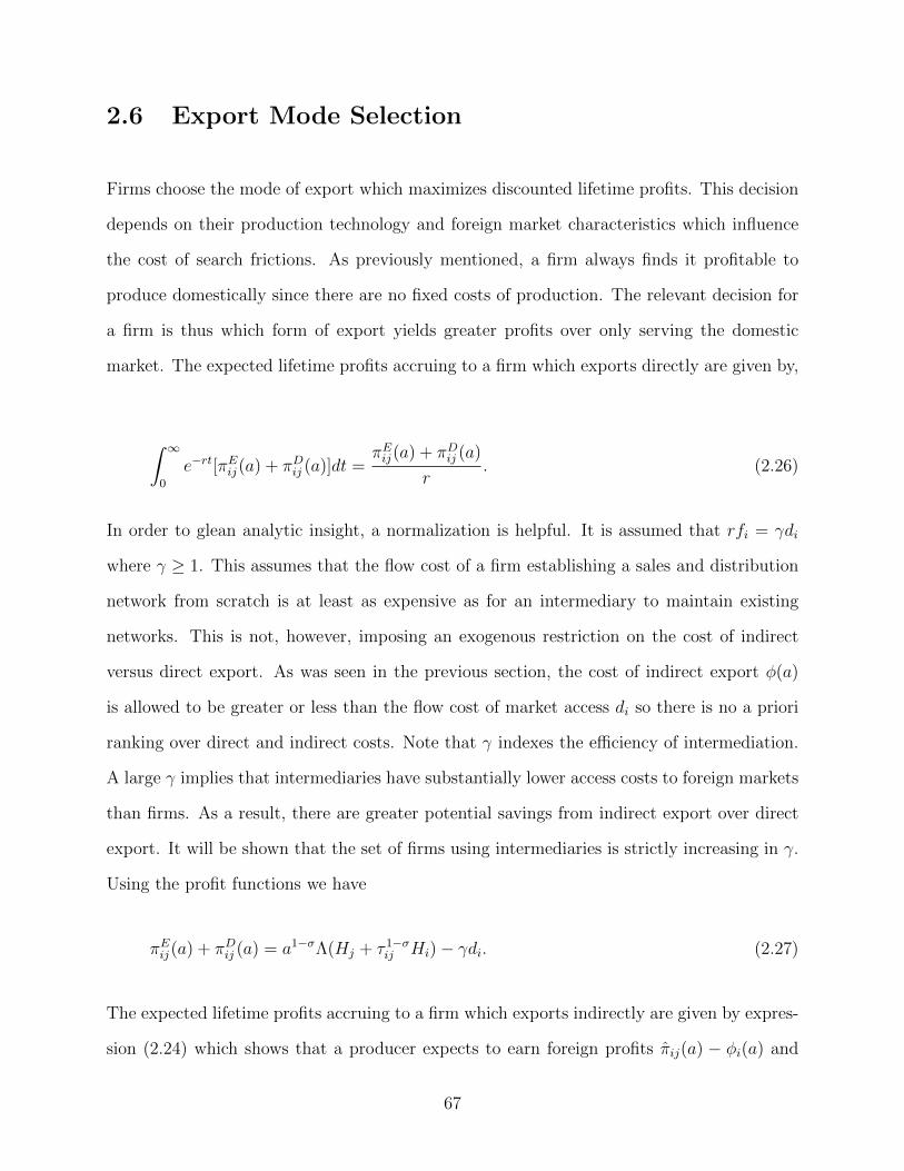
2.6 Export Mode Selection

Firms choose the mode of export which maximizes discounted lifetime profits. This decision

depends on their production technology and foreign market characteristics which influence

the cost of search frictions. As previously mentioned, a firm always finds it profitable to

produce domestically since there are no fixed costs of production. The relevant decision for

a firm is thus which form of export yields greater profits over only serving the domestic

market. The expected lifetime profits accruing to a firm which exports directly are given by,

∫ ∞0

e−rt[πEij(a) + πDij (a)]dt =πEij(a) + πDij (a)

r. (2.26)

In order to glean analytic insight, a normalization is helpful. It is assumed that rfi = γdi

where γ ≥ 1. This assumes that the flow cost of a firm establishing a sales and distribution

network from scratch is at least as expensive as for an intermediary to maintain existing

networks. This is not, however, imposing an exogenous restriction on the cost of indirect

versus direct export. As was seen in the previous section, the cost of indirect export φ(a)

is allowed to be greater or less than the flow cost of market access di so there is no a priori

ranking over direct and indirect costs. Note that γ indexes the efficiency of intermediation.

A large γ implies that intermediaries have substantially lower access costs to foreign markets

than firms. As a result, there are greater potential savings from indirect export over direct

export. It will be shown that the set of firms using intermediaries is strictly increasing in γ.

Using the profit functions we have

πEij(a) + πDij (a) = a1−σΛ(Hj + τ 1−σij Hi)− γdi. (2.27)

The expected lifetime profits accruing to a firm which exports indirectly are given by expres-

sion (2.24) which shows that a producer expects to earn foreign profits πij(a) − φi(a) and

67

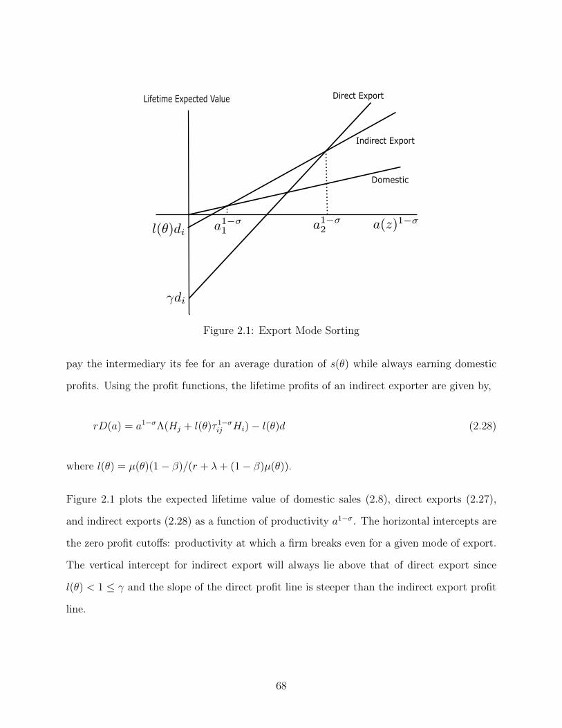
Direct Export

Domestic

Indirect Export

Lifetime Expected Value

Figure 2.1: Export Mode Sorting

pay the intermediary its fee for an average duration of s(θ) while always earning domestic

profits. Using the profit functions, the lifetime profits of an indirect exporter are given by,

rD(a) = a1−σΛ(Hj + l(θ)τ 1−σij Hi)− l(θ)d (2.28)

where l(θ) = µ(θ)(1− β)/(r + λ+ (1− β)µ(θ)).

Figure 2.1 plots the expected lifetime value of domestic sales (2.8), direct exports (2.27),

and indirect exports (2.28) as a function of productivity a1−σ. The horizontal intercepts are

the zero profit cutoffs: productivity at which a firm breaks even for a given mode of export.

The vertical intercept for indirect export will always lie above that of direct export since

l(θ) < 1 ≤ γ and the slope of the direct profit line is steeper than the indirect export profit

line.

68

Firms will choose to export indirectly only if rD(a) ≥ πDij (a). The productivity level at

which firms begin to export indirectly is given by,

a1−σ1 =di

τ 1−σij HiΛ. (2.29)

Firms will choose to export directly only if πEij(a) + πDij (a) ≥ rD(a). The productivity level

at which firms begin to export directly is given by,

a1−σ2 =(γ − l(θ))di

Λτ 1−σij Hi(1− l(θ)). (2.30)

Figure 2.1 reflects the fact that firms will always find it profitable to sell to its domestic

market. However, it may not always be profitable to export. Only the more productive

firms will choose to export. Firms with intermediate productivities will find it profitable

to search for an intermediary. The most productive firms will find it profitable to export

directly.

If search frictions were extreme (µ(θ) = 0) or firms held no bargaining power (β = 1),

then the intermediation sector would shut down and the indirect value line would coincide

with the domestic value line. In this case, a smaller subset of firms export with the cutoff

productivity given by γa1−σ1 . If there were no cost savings from intermediation (γ = 1), then

the direct export cutoff would coincide with the indirect export cutoff and no firm would

every choose to search for an intermediary. Taking the ratio of (2.29) and (2.30) provides

an expression for measuring the extent to which firms choose to search for an intermediary.

Proposition 2: The degree of export-mode sorting can be summarized by the following

expression,

(a2a1

)1−σ

=γ − l(θ)1− l(θ)

(2.31)

69

Figure 2.2: Relative Productivities of Direct-to-Indirect Export

The size of the intermediary sector depends on the efficiency of intermediation γ and the

state of the export market l(θ).

Expression (2.31) shows a positive relationship between the level of intermediation θ and

the measure of firms choosing to search for an intermediary. As the level of tightness in an

export market grows, firms benefit from both lower fees and a higher probability of finding

a match. As the efficiency of intermediation grows, γ → γ′, a larger set of firms will choose

to export indirectly for a given level of θ. Additionally, assigning the intermediary greater

bargaining power, β → β′, results in a smaller set of firms searching for an intermediary for

a given level of tightness.

2.7 Equilibrium

Equilibrium is defined in terms of export market tightness, service fee, and resulting export

cutoffs: (θ∗, φ∗, a1, a2). Equilibrium in the export market is determined by the behavior of

intermediaries of which there is an unbounded pool of prospective entrants. Each interme-

diary acts so that in equilibrium expected search costs equal the expected value of a match.

From Bellman equations (2.14), (2.15) for an intermediary and the free entry condition (2.22)

70

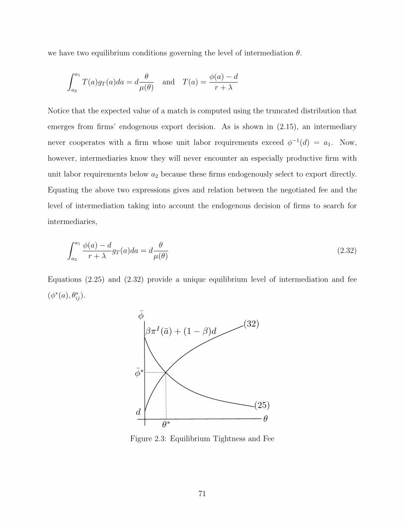
we have two equilibrium conditions governing the level of intermediation θ.

∫ a1

a2

T (a)gT (a)da = dθ

µ(θ)and T (a) =

φ(a)− dr + λ

Notice that the expected value of a match is computed using the truncated distribution that

emerges from firms’ endogenous export decision. As is shown in (2.15), an intermediary

never cooperates with a firm whose unit labor requirements exceed φ−1(d) = a1. Now,

however, intermediaries know they will never encounter an especially productive firm with

unit labor requirements below a2 because these firms endogenously select to export directly.

Equating the above two expressions gives and relation between the negotiated fee and the

level of intermediation taking into account the endogenous decision of firms to search for

intermediaries,

∫ a1

a2

φ(a)− dr + λ

gT (a)da = dθ

µ(θ)(2.32)

Equations (2.25) and (2.32) provide a unique equilibrium level of intermediation and fee

(φ∗(a), θ∗ij).

Figure 2.3: Equilibrium Tightness and Fee

71

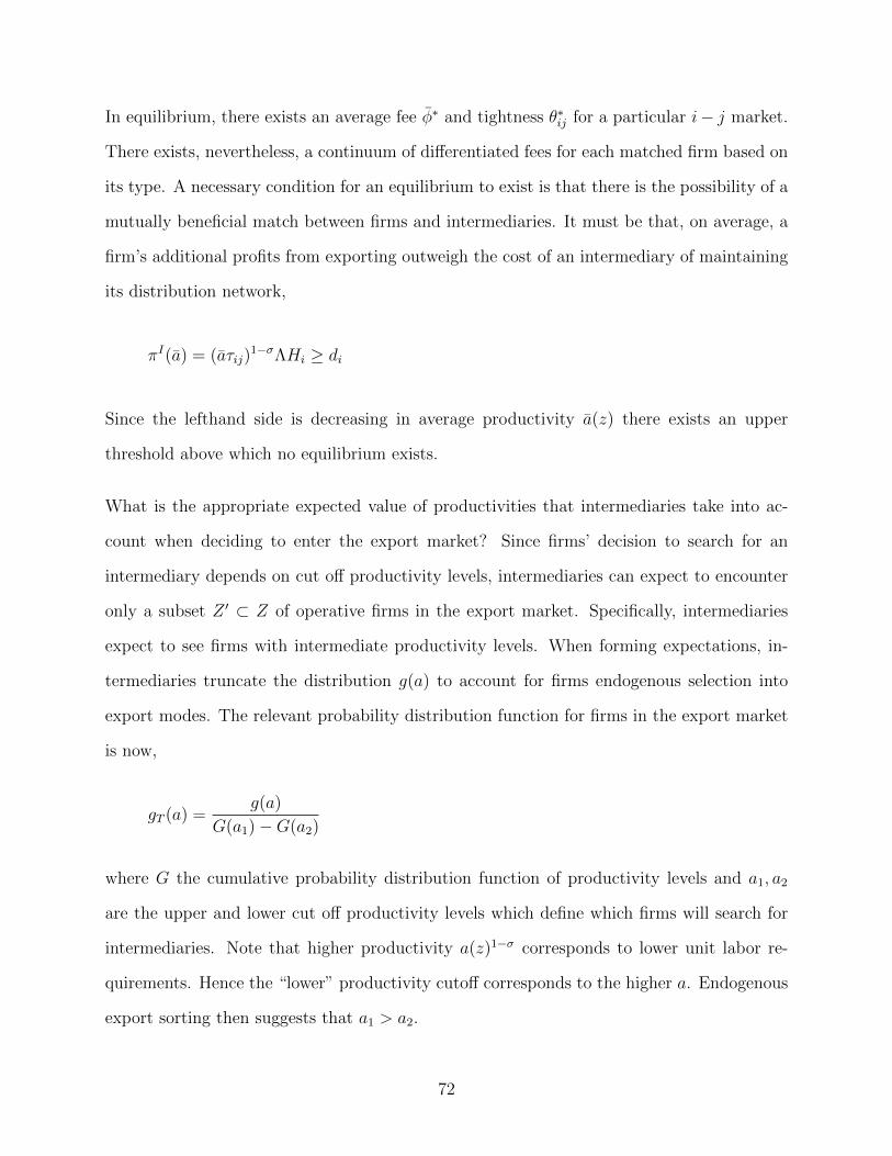
In equilibrium, there exists an average fee φ∗ and tightness θ∗ij for a particular i− j market.

There exists, nevertheless, a continuum of differentiated fees for each matched firm based on

its type. A necessary condition for an equilibrium to exist is that there is the possibility of a

mutually beneficial match between firms and intermediaries. It must be that, on average, a

firm’s additional profits from exporting outweigh the cost of an intermediary of maintaining

its distribution network,

πI(a) = (aτij)1−σΛHi ≥ di

Since the lefthand side is decreasing in average productivity a(z) there exists an upper

threshold above which no equilibrium exists.

What is the appropriate expected value of productivities that intermediaries take into ac-

count when deciding to enter the export market? Since firms’ decision to search for an

intermediary depends on cut off productivity levels, intermediaries can expect to encounter

only a subset Z ′ ⊂ Z of operative firms in the export market. Specifically, intermediaries

expect to see firms with intermediate productivity levels. When forming expectations, in-

termediaries truncate the distribution g(a) to account for firms endogenous selection into

export modes. The relevant probability distribution function for firms in the export market

is now,

gT (a) =g(a)

G(a1)−G(a2)

where G the cumulative probability distribution function of productivity levels and a1, a2

are the upper and lower cut off productivity levels which define which firms will search for

intermediaries. Note that higher productivity a(z)1−σ corresponds to lower unit labor re-

quirements. Hence the “lower” productivity cutoff corresponds to the higher a. Endogenous

export sorting then suggests that a1 > a2.

72

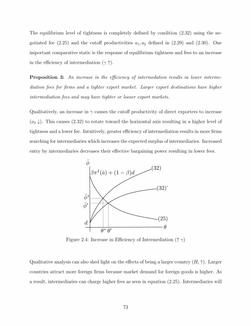
The equilibrium level of tightness is completely defined by condition (2.32) using the ne-

gotiated fee (2.25) and the cutoff productivities a1, a2 defined in (2.29) and (2.30). One

important comparative static is the response of equilibrium tightness and fees to an increase

in the efficiency of intermediation (γ ↑).

Proposition 3: An increase in the efficiency of intermedation results in lower interme-

diation fees for firms and a tighter export market. Larger export destinations have higher

intermediation fees and may have tighter or looser export markets.

Qualitatively, an increase in γ causes the cutoff productivity of direct exporters to increase

(a2 ↓). This causes (2.32) to rotate toward the horizontal axis resulting in a higher level of

tightness and a lower fee. Intuitively, greater efficiency of intermediation results in more firms

searching for intermediaries which increases the expected surplus of intermediaries. Increased

entry by intermediaries decreases their effective bargaining power resulting in lower fees.

Figure 2.4: Increase in Efficiency of Intermediation (↑ γ)

Qualitative analysis can also shed light on the effects of being a larger country (Hi ↑). Larger

countries attract more foreign firms because market demand for foreign goods is higher. As

a result, intermediaries can charge higher fees as seen in equation (2.25). Intermediaries will

73

begin entering the export market anticipating higher surpluses thus rotating (2.32) upward.

The average fee will certainly be higher, but the effect on tightness is ambiguous.

Figure 2.5: Increase in Country Size (↑ Hi)

Assuming Pareto distributed of productivities, the truncated distribution is given by

gT (a) =kak−1

ak1 − ak2. (2.33)

Substituting the negotiated fee (2.25) and the truncated pdf into equilibrium condition (2.32)

obtains,

∫ a1

a2

β(πI(a)− d)

r + λ+ (1− β)µ(θ)

kak−1

ak1 − ak2da = d

θ

µ(θ).

Substituting the expressions for foreign variable profits (2.16) and cutoff productivities

(2.29),(2.30) into the above will (after some algebraic trials) yield the condition for equi-

librium in the export market.

74

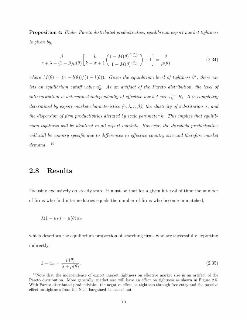
Proposition 4: Under Pareto distributed productivities, equilibrium export market tightness

is given by,

β

r + λ+ (1− β)µ(θ)

[k

k − σ + 1

(1−M(θ)

k−σ+11−σ

1−M(θ)k

1−σ

)− 1

]=

θ

µ(θ)(2.34)

where M(θ) = (γ − l(θ))/(1 − l(θ)). Given the equilibrium level of tightness θ∗, there ex-

ists an equilibrium cutoff value a∗2. As an artifact of the Pareto distribution, the level of

intermediation is determined independently of effective market size τ 1−σij Hi. It is completely

determined by export market characteristics (γ, λ, r, β), the elasticity of substitution σ, and

the dispersion of firm productivities dictated by scale parameter k. This implies that equilib-

rium tightness will be identical in all export markets. However, the threshold productivities

will still be country specific due to differences in effective country size and therefore market

demand. 10

2.8 Results

Focusing exclusively on steady state, it must be that for a given interval of time the number

of firms who find intermediaries equals the number of firms who become unmatched,

λ(1− uF ) = µ(θ)uF

which describes the equilibrium proportion of searching firms who are successfully exporting

indirectly,

1− uF =µ(θ)

λ+ µ(θ). (2.35)

10Note that the independence of export market tightness on effective market size in an artifact of thePareto distribution. More generally, market size will have an effect on tightness as shown in Figure 2.5.With Pareto distributed productivities, the negative effect on tightness through free entry and the positiveeffect on tightness from the Nash bargained fee cancel out.

75

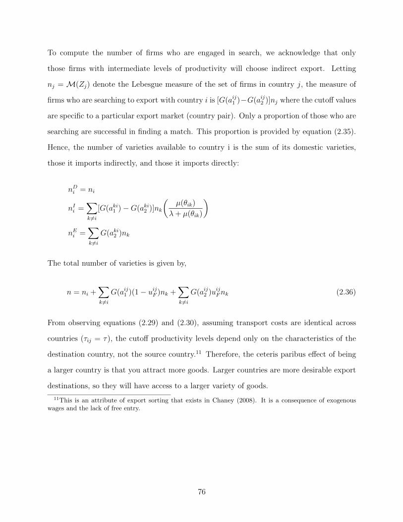
To compute the number of firms who are engaged in search, we acknowledge that only

those firms with intermediate levels of productivity will choose indirect export. Letting

nj = M(Zj) denote the Lebesgue measure of the set of firms in country j, the measure of

firms who are searching to export with country i is [G(aij1 )−G(aij2 )]nj where the cutoff values

are specific to a particular export market (country pair). Only a proportion of those who are

searching are successful in finding a match. This proportion is provided by equation (2.35).

Hence, the number of varieties available to country i is the sum of its domestic varieties,

those it imports indirectly, and those it imports directly:

nDi = ni

nIi =∑k 6=i

[G(aki1 )−G(aki2 )]nk

(µ(θik)

λ+ µ(θik)

)nEi =

∑k 6=i

G(aki2 )nk

The total number of varieties is given by,

n = ni +∑k 6=i

G(aij1 )(1− uijF )nk +∑k 6=i

G(aij2 )uijFnk (2.36)

From observing equations (2.29) and (2.30), assuming transport costs are identical across

countries (τij = τ), the cutoff productivity levels depend only on the characteristics of the

destination country, not the source country.11 Therefore, the ceteris paribus effect of being

a larger country is that you attract more goods. Larger countries are more desirable export

destinations, so they will have access to a larger variety of goods.

11This is an attribute of export sorting that exists in Chaney (2008). It is a consequence of exogenouswages and the lack of free entry.

76

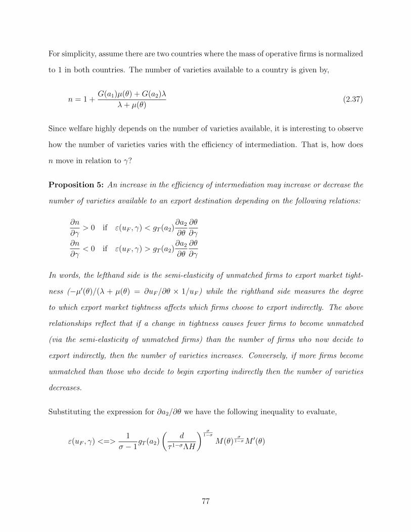
For simplicity, assume there are two countries where the mass of operative firms is normalized

to 1 in both countries. The number of varieties available to a country is given by,

n = 1 +G(a1)µ(θ) +G(a2)λ

λ+ µ(θ)(2.37)

Since welfare highly depends on the number of varieties available, it is interesting to observe

how the number of varieties varies with the efficiency of intermediation. That is, how does

n move in relation to γ?

Proposition 5: An increase in the efficiency of intermediation may increase or decrease the

number of varieties available to an export destination depending on the following relations:

∂n

∂γ> 0 if ε(uF , γ) < gT (a2)

∂a2∂θ

∂θ

∂γ

∂n

∂γ< 0 if ε(uF , γ) > gT (a2)

∂a2∂θ

∂θ

∂γ

In words, the lefthand side is the semi-elasticity of unmatched firms to export market tight-

ness (−µ′(θ)/(λ + µ(θ) = ∂uF/∂θ × 1/uF ) while the righthand side measures the degree

to which export market tightness affects which firms choose to export indirectly. The above

relationships reflect that if a change in tightness causes fewer firms to become unmatched

(via the semi-elasticity of unmatched firms) than the number of firms who now decide to

export indirectly, then the number of varieties increases. Conversely, if more firms become

unmatched than those who decide to begin exporting indirectly then the number of varieties

decreases.

Substituting the expression for ∂a2/∂θ we have the following inequality to evaluate,

ε(uF , γ) <=>1

σ − 1gT (a2)

(d

τ 1−σΛH

) σ1−σ

M(θ)σ

1−σM ′(θ)

77

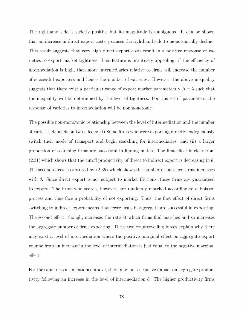
The righthand side is strictly positive but its magnitude is ambiguous. It can be shown

that an increase in direct export costs γ causes the righthand side to monotonically decline.

This result suggests that very high direct export costs result in a positive response of va-

rieties to export market tightness. This feature is intuitively appealing: if the efficiency of

intermediation is high, then more intermediaries relative to firms will increase the number

of successful exporters and hence the number of varieties. However, the above inequality

suggests that there exist a particular range of export market parameters γ, β, r, λ such that

the inequality will be determined by the level of tightness. For this set of parameters, the

response of varieties to intermediation will be nonmonotonic.

The possible non-monotonic relationship between the level of intermediation and the number

of varieties depends on two effects: (i) Some firms who were exporting directly endogenously

switch their mode of transport and begin searching for intermediaries; and (ii) a larger

proportion of searching firms are successful in finding match. The first effect is clear from

(2.31) which shows that the cutoff productivity of direct to indirect export is decreasing in θ.

The second effect is captured by (2.35) which shows the number of matched firms increases

with θ. Since direct export is not subject to market frictions, those firms are guaranteed

to export. The firms who search, however, are randomly matched according to a Poisson

process and thus face a probability of not exporting. Thus, the first effect of direct firms

switching to indirect export means that fewer firms in aggregate are successful in exporting.

The second effect, though, increases the rate at which firms find matches and so increases

the aggregate number of firms exporting. These two counterveiling forces explain why there

may exist a level of intermediation where the positive marginal effect on aggregate export

volume from an increase in the level of intermediation is just equal to the negative marginal

effect.

For the same reasons mentioned above, there may be a negative impact on aggregate produc-

tivity following an increase in the level of intermediation θ. The higher productivity firms

78

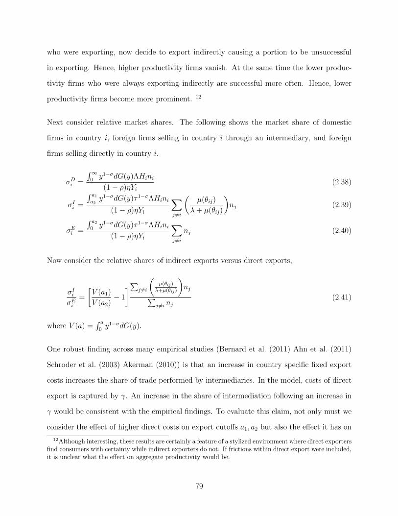
who were exporting, now decide to export indirectly causing a portion to be unsuccessful

in exporting. Hence, higher productivity firms vanish. At the same time the lower produc-

tivity firms who were always exporting indirectly are successful more often. Hence, lower

productivity firms become more prominent. 12

Next consider relative market shares. The following shows the market share of domestic

firms in country i, foreign firms selling in country i through an intermediary, and foreign

firms selling directly in country i.

σDi =

∫∞0y1−σdG(y)ΛHini

(1− ρ)ηYi(2.38)

σIi =

∫ a1a2y1−σdG(y)τ 1−σΛHini

(1− ρ)ηYi

∑j 6=i

(µ(θij)

λ+ µ(θij)

)nj (2.39)

σEi =

∫ a20y1−σdG(y)τ 1−σΛHini

(1− ρ)ηYi

∑j 6=i

nj (2.40)

Now consider the relative shares of indirect exports versus direct exports,

σIiσEi

=

[V (a1)

V (a2)− 1

]∑j 6=i

(µ(θij)

λ+µ(θij)

)nj∑

j 6=i nj(2.41)

where V (a) =∫ a0y1−σdG(y).

One robust finding across many empirical studies (Bernard et al. (2011) Ahn et al. (2011)

Schroder et al. (2003) Akerman (2010)) is that an increase in country specific fixed export

costs increases the share of trade performed by intermediaries. In the model, costs of direct

export is captured by γ. An increase in the share of intermediation following an increase in

γ would be consistent with the empirical findings. To evaluate this claim, not only must we

consider the effect of higher direct costs on export cutoffs a1, a2 but also the effect it has on

12Although interesting, these results are certainly a feature of a stylized environment where direct exportersfind consumers with certainty while indirect exporters do not. If frictions within direct export were included,it is unclear what the effect on aggregate productivity would be.

79

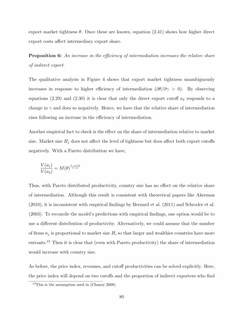
export market tightness θ. Once these are known, equation (2.41) shows how higher direct

export costs affect intermediary export share.

Proposition 6: An increase in the efficiency of intermediation increases the relative share

of indirect export.

The qualitative analysis in Figure 4 shows that export market tightness unambiguously

increases in response to higher efficiency of intermediation (∂θ/∂γ > 0). By observing

equations (2.29) and (2.30) it is clear that only the direct export cutoff a2 responds to a

change in γ and does so negatively. Hence, we have that the relative share of intermediation

rises following an increase in the efficiency of intermediation.

Another empirical fact to check is the effect on the share of intermediation relative to market

size. Market size Hj does not affect the level of tightness but does affect both export cutoffs

negatively. With a Pareto distribution we have,

V (a1)

V (a2)= M(θ)

1−σ+k1−σ

Thus, with Pareto distributed productivity, country size has no effect on the relative share

of intermediation. Although this result is consistent with theoretical papers like Akerman

(2010), it is inconsistent with empirical findings by Bernard et al. (2011) and Schroder et al.

(2003). To reconcile the model’s predictions with empirical findings, one option would be to

use a different distribution of productivity. Alternatively, we could assume that the number

of firms nj is proportional to market size Hi so that larger and wealthier countries have more

entrants.13 Then it is clear that (even with Pareto productivity) the share of intermediation

would increase with country size.

As before, the price index, revenues, and cutoff productivities can be solved explicitly. Here,

the price index will depend on two cutoffs and the proportion of indirect exporters who find

13This is the assumption used in (Chaney 2008)

80

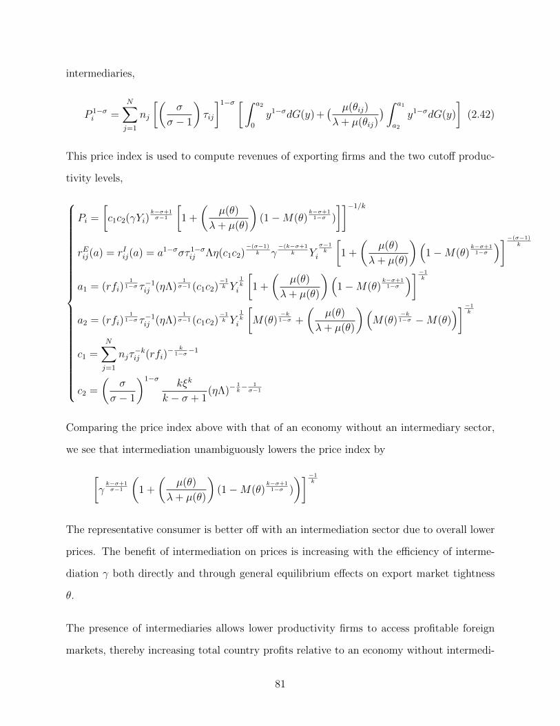
intermediaries,

P 1−σi =

N∑j=1

nj

[(σ

σ − 1

)τij

]1−σ [ ∫ a2

0

y1−σdG(y) +( µ(θij)

λ+ µ(θij)

) ∫ a1

a2

y1−σdG(y)

](2.42)

This price index is used to compute revenues of exporting firms and the two cutoff produc-

tivity levels,

Pi =

[c1c2(γYi)

k−σ+1σ−1

[1 +

(µ(θ)

λ+ µ(θ)

)(1−M(θ)

k−σ+11−σ )

]]−1/krEij(a) = rIij(a) = a1−σστ 1−σij Λη(c1c2)

−(σ−1)k γ

−(k−σ+1k Y

σ−1k

i

[1 +

(µ(θ)

λ+ µ(θ)

)(1−M(θ)

k−σ+11−σ

)]−(σ−1)k

a1 = (rfi)1

1−σ τ−1ij (ηΛ)1

σ−1 (c1c2)−1k Y

1ki

[1 +

(µ(θ)

λ+ µ(θ)

)(1−M(θ)

k−σ+11−σ

)]−1k

a2 = (rfi)1

1−σ τ−1ij (ηΛ)1

σ−1 (c1c2)−1k Y

1ki

[M(θ)

−k1−σ +

(µ(θ)

λ+ µ(θ)

)(M(θ)

−k1−σ −M(θ)

)]−1k

c1 =N∑j=1

njτ−kij (rfi)

− k1−σ−1

c2 =

(σ

σ − 1

)1−σkξk

k − σ + 1(ηΛ)−

1k− 1σ−1

Comparing the price index above with that of an economy without an intermediary sector,

we see that intermediation unambiguously lowers the price index by

[γk−σ+1σ−1

(1 +

(µ(θ)

λ+ µ(θ)

)(1−M(θ)

k−σ+11−σ )

)]−1k

The representative consumer is better off with an intermediation sector due to overall lower

prices. The benefit of intermediation on prices is increasing with the efficiency of interme-

diation γ both directly and through general equilibrium effects on export market tightness

θ.

The presence of intermediaries allows lower productivity firms to access profitable foreign

markets, thereby increasing total country profits relative to an economy without intermedi-

81

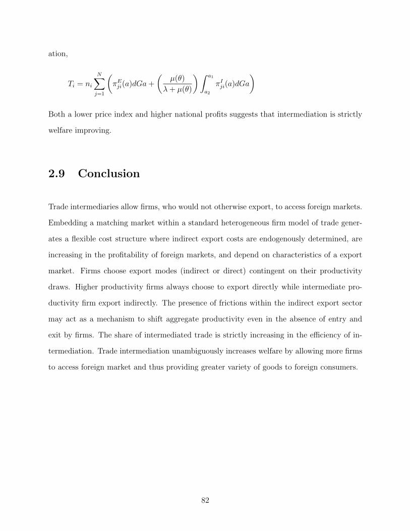
ation,

Ti = ni

N∑j=1

(πEji(a)dGa+

(µ(θ)

λ+ µ(θ)

)∫ a1

a2

πIji(a)dGa

)

Both a lower price index and higher national profits suggests that intermediation is strictly

welfare improving.

2.9 Conclusion

Trade intermediaries allow firms, who would not otherwise export, to access foreign markets.

Embedding a matching market within a standard heterogeneous firm model of trade gener-

ates a flexible cost structure where indirect export costs are endogenously determined, are

increasing in the profitability of foreign markets, and depend on characteristics of a export

market. Firms choose export modes (indirect or direct) contingent on their productivity

draws. Higher productivity firms always choose to export directly while intermediate pro-

ductivity firm export indirectly. The presence of frictions within the indirect export sector

may act as a mechanism to shift aggregate productivity even in the absence of entry and

exit by firms. The share of intermediated trade is strictly increasing in the efficiency of in-

termediation. Trade intermediation unambiguously increases welfare by allowing more firms

to access foreign market and thus providing greater variety of goods to foreign consumers.

82

Chapter 3

A Note on Firm Entry and Liquidity

3.1 Introduction

This note is intended to provide additional insight toward the link between goods and labor

markets in a New Monetarist model of liquidity as presented in Rocheteau and Nosal 2017

(RN). The framework integrates a model of money and credit into a Mortensen-Pissarides

labor market to study the relationship between the availability of credit, firm entry, and

unemployment.

First, RN show that the strategic complementarities between buyers’ choice of real money

balances and firms’ entry decision generate multiple monetary equilibria. As expected, this

multiplicity generates contrary comparative statics at the “high” equilibria (low unemploy-

ment and large trading volume) versus the “low” equilibria (high unemployment and low

trading volume). As credit becomes more accessible there is higher unemployment at the

“high” equilibrium, but lower unemployment at the “low” equilibrium. I show that the

non-monotone relationship between credit and unemployment does not rely on multiplicity.

I break the link between the measure of operative firms and retail trading frequency thereby

83

producing a unique equilibrium. Even with a uniquely determined monetary equilibrium,

there exists a non-monotone relationship between credit and unemployment dependent on

the value of money.

Second, I show that the modeler’s choice of bargaining protocol has a substantive impact

on the qualitative relationship between unemployment and credit. Under the benchmark

model considered by RN terms of trade are settled by proportional bargaining. I show

that Nash bargaining reverses the response of unemployment to credit observed by RN.

Specifically, more access to credit can decrease unemployment at the high equilibrium under

Nash, whereas there is an increase in unemployment under proportional bargaining. The

modeler’s choice of bargaining protocol is not innocuous.

3.2 A Stripped Down RN Model

Time is discrete and continues forever. Each period contains three subperiods where different

markets open sequentially. The first market is a labor market (LM) where firms hire workers

that produce a consumption good denoted q. The second market is a decentralized goods

market (DM) where consumers purchase q from firms in bilateral meetings. The final market

is a Walrasian market (CM) where debts are settled and portfolio choices are made and each

agent can produce the numeraire good at unit cost.

There are two types of agents, producers and consumers, who are completely characterized

by idiosyncratic preferences and technology. I begin with the firm. Each firm possesses a

technology to produce q units of a consumption good with one worker. To acquire a worker,

a firm posts vacancies at fixed cost k prior to the opening of a labor market (LM) where

workers and firms are randomly matched according to the matching function H(U, V ). Let

f(τ) = H(U, V )/U = H(1, τ) denote the probability that an unemployed worker finds a

84

job and f(τ)/τ the probability that a firm finds a worker. The matching function is strictly

increasing and concave in both of its arguments, and exhibits constant returns to scale. Once

a firm is matched with a worker, it produces q each period until the match is destroyed with

exogenous probability δ. The firm realizes match creation and destruction at the beginning

of the LM; therefore, a firm must wait one period after job destruction to search for a new

worker. For now, I take the wage w1 as exogenous and denote expected period profit by ρ.

The value of an employed firm is thus J = (ρ − w1)/(1 − β(1 − δ)). Free entry guarantees

that the ex-ante value of an employed firm is driven to zero in equilibrium,

k

(f(τ)

τ

)−1=

β

1− β(1− δ)(ρ− w1) (3.1)

which gives market tightness τ for any given expected revenue.

A firm’s expected revenue is determined in a decentralized goods market (DM) where firms

and buyers randomly meet in pairs to trade. In a fraction µ of matches there exists a perfect

record keeping technology and enforcement mechanism permitting the use of credit. The

remaining 1− µ trades are unmonitored precluding the use of credit and generating a need

for money.

Terms of trade in the DM will be settled according to proportional bargaining which promises

the buyer a fraction θ of the total match surplus. The jointly efficient outcome is q∗ : u′(q∗) =

1 with the corresponding issuance of debt b = (1−θ)u(q∗)+θq∗. Without loss of generality, I

assume that only credit is used in monitored matches. Since there are no debt limits, the first

best quantity q∗ will be traded in all monitored matched. In unmonitored matches, however,

q < q∗ will be purchased so long as money is costly to hold where d = z(q) = (1−θ)u(q)+θq

is the monetary payment. That is, a buyer will never carry more real money balances z then

he expects to spend d to acquire q units of the consumption good.

85

A worker may be employed or unemployed in any period. However, since portfolio decisions

are independent of current wealth, employment status has no effect on the buyer’s choice of

real money balances. The buyer’s optimal portfolio choice equates the cost of holding money

to the liquidity value it brings in the following DM,

maxz−iz + (1− µ)θ(u(q(z))− q(z))

where i = (γ − β)/β is the nominal interest rate on an illiquid bond. To guarantee that the

above problem is concave and admits an interior solution, we must have that (1−µ)θ/(1−θ) >

i. The cost of holding money must be low enough if money is to be valued in equilibrium.

Given that an interior solution exists, optimal money holdings satisfy the following,

i = (1− µ)θ

(u′(q)− 1

(1− θ)u′(q) + θ

). (3.2)

Given the optimal choice of money holdings, a firm’s expected revenue in the DM given by

ρ = (1− θ) [µ(u(q∗)− q∗) + (1− µ)(u(q(z))− q(z))] + q. (3.3)

A firm will always receive a fraction 1− θ of the joint surplus, where the value of the surplus

will be u(q∗)− q∗ with probability µ and u(q(z))− q(z) with probability (1− µ).

A stationary equilibrium is a tuple (q, τ) which satisfies (3.1)-(3.3). Notice that because

there are no matching frictions in the retail market the buyer’s portfolio choice can be solved

independently of the entry of firms. The model is solved recursively where (3.2) determines

the quantity traded in unmonitored matches and entry adjusts according to (3.1) and (3.3).

Finally, the equilibrium level of employment is determined by the steady state condition,

n =f(τ)

f(τ) + δ. (3.4)

86

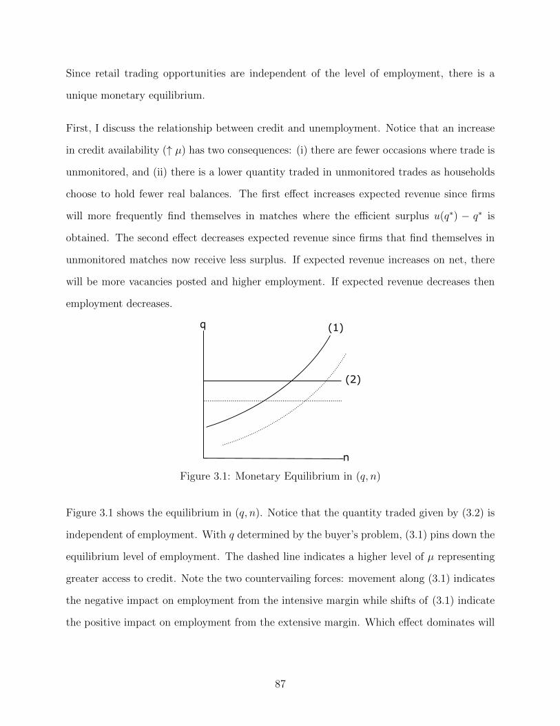
Since retail trading opportunities are independent of the level of employment, there is a

unique monetary equilibrium.

First, I discuss the relationship between credit and unemployment. Notice that an increase

in credit availability (↑ µ) has two consequences: (i) there are fewer occasions where trade is

unmonitored, and (ii) there is a lower quantity traded in unmonitored trades as households

choose to hold fewer real balances. The first effect increases expected revenue since firms

will more frequently find themselves in matches where the efficient surplus u(q∗) − q∗ is

obtained. The second effect decreases expected revenue since firms that find themselves in

unmonitored matches now receive less surplus. If expected revenue increases on net, there

will be more vacancies posted and higher employment. If expected revenue decreases then

employment decreases.

q

n

(1)

(2)

Figure 3.1: Monetary Equilibrium in (q, n)

Figure 3.1 shows the equilibrium in (q, n). Notice that the quantity traded given by (3.2) is

independent of employment. With q determined by the buyer’s problem, (3.1) pins down the

equilibrium level of employment. The dashed line indicates a higher level of µ representing

greater access to credit. Note the two countervailing forces: movement along (3.1) indicates

the negative impact on employment from the intensive margin while shifts of (3.1) indicate

the positive impact on employment from the extensive margin. Which effect dominates will

87

determine whether unemployment responds positively or negatively to increased access to

credit.

To be more precise, letting S(q) = u(q)− q we have that

∂ρ

∂µ∝ S(q∗)− Ω(q) (3.5)

where Ω(q) = S(q)− (u′(q)−1)2((1−θ)u′(q)+θ)u′′(q)

> 0.

If S(q∗)−Ω(q) > 0 firms expect higher profits when credit is more available and will respond

with greater entry and hence lower unemployment. If S(q∗) − Ω(q) < 0 firms expect lower

revenues, reduce entry, and higher unemployment results.

PROPOSITION 8. For a given bargaining power, there exists a unique threshold q(θ) ∈

[0, q∗] : Ω(q) = S(q∗) such that for all q ≤ q(θ) unemployment decreases as credit becomes

more available whereas for all q > q unemployment increases as credit becomes more avail-

able.

Proof. From (3.3) we have that,

∂ρ

∂µ∝ u(q∗)− q∗ + (1− µ)

∂S(q)

∂q

∂q

∂µ− S(q)

The only term left to compute is ∂q/∂µ which measures the degree to which consumers alter

their real money balances given a small change in credit access. This term is computed from

(3.2) using a simple application of implicit differentiation,

∂q

∂µ=S ′(q)[(1− θ)u′(q) + θ]

(1− µ)S ′′(q)< 0

88

COROLLARY 1. For a given bargaining power and nominal interest rate, there exists a

unique threshold µ(θ, i) ∈ [0, 1] such that for all µ ≤ µ unemployment increases as credit

becomes more available whereas for all µ > µ unemployment decreases as credit becomes

more available.

Proof. The buyer’s portfolio decision given by (3.2) shows a one-to-one mapping between q

and µ. Moreover, the relation is monotone decreasing for q ∈ (0, q∗] as shown in Proposition

1 proof.

Figure 3.2 illustrates Proposition 1 with a numerical example setting u(q) = 2√q and varying

bargaining powers. Given this functional form for utility, the threshold value addressed in

Proposition 1 can be solved closed form,

q =

(2θ − 1

2θ

)2

for θ ∈ (1/2, 1)

= 0 otherwise

The curves in Figure 3.2a represent Ω(q) and the jointly efficient surplus is S(q∗) = 1. Notice

that for bargaining powers one-half or less we have that q(θ ≤ 0.5) = 0 so that there is no set

of trades which increase expected revenue. More credit access causes firms to reduce entry

resulting in greater unemployment. However, for bargaining powers above one-half we have

that q(0.8) ≈ 0.1406 and q(0.6) ≈ 0.0278 indicating that for small volume trades expected

revenue increases as credit becomes more available; unemployment would in fact decline

following more access to credit. Greater bargaining power to the buyer increases q(θ).1 Of

course, the quantity traded is an equilibrium object given by (3.2). According to Corollary

1, for a given nominal interest rate there exists a threshold value µ(θ, i) corresponding to

that of q(θ). Given the functional form for utility, the locus of interest rates and credit access

1Giving all bargaining power to the buyer θ = 1 would shut down the market. To have bounded entryit must be the case that −k + βq < 0; if buyer’s have all the bargaining power then the firm’s expectedrevenue, q, is less than the capitalized entry cost k/β and the retail market shuts down.

89

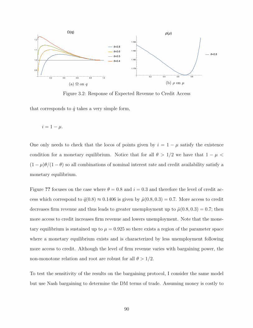
(a) Ω on q (b) ρ on µ

Figure 3.2: Response of Expected Revenue to Credit Access

that corresponds to q takes a very simple form,

i = 1− µ.

One only needs to check that the locos of points given by i = 1 − µ satisfy the existence

condition for a monetary equilibrium. Notice that for all θ > 1/2 we have that 1 − µ <

(1− µ)θ/(1− θ) so all combinations of nominal interest rate and credit availability satisfy a

monetary equilibrium.

Figure ?? focuses on the case where θ = 0.8 and i = 0.3 and therefore the level of credit ac-

cess which correspond to q(0.8) ≈ 0.1406 is given by µ(0.8, 0.3) = 0.7. More access to credit

decreases firm revenue and thus leads to greater unemployment up to µ(0.8, 0.3) = 0.7; then

more access to credit increases firm revenue and lowers unemployment. Note that the mone-

tary equilibrium is sustained up to µ = 0.925 so there exists a region of the parameter space

where a monetary equilibrium exists and is characterized by less unemployment following

more access to credit. Although the level of firm revenue varies with bargaining power, the

non-monotone relation and root are robust for all θ > 1/2.

To test the sensitivity of the results on the bargaining protocol, I consider the same model

but use Nash bargaining to determine the DM terms of trade. Assuming money is costly to

90

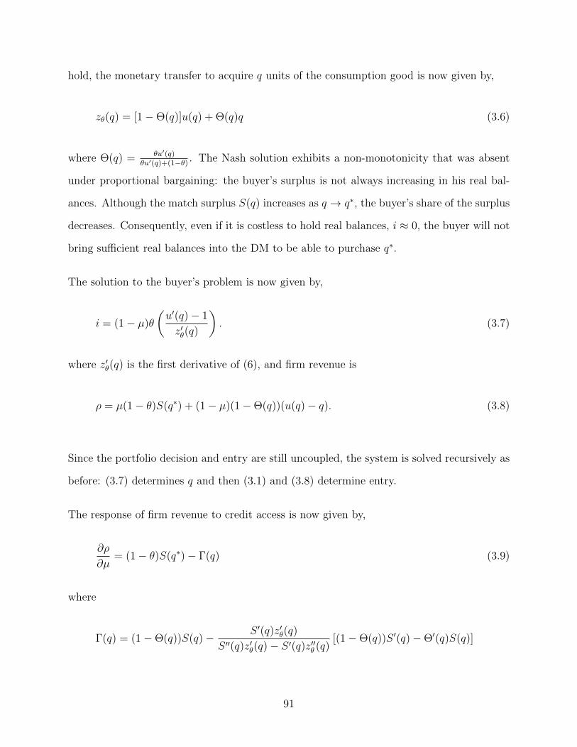
hold, the monetary transfer to acquire q units of the consumption good is now given by,

zθ(q) = [1−Θ(q)]u(q) + Θ(q)q (3.6)

where Θ(q) = θu′(q)θu′(q)+(1−θ) . The Nash solution exhibits a non-monotonicity that was absent

under proportional bargaining: the buyer’s surplus is not always increasing in his real bal-

ances. Although the match surplus S(q) increases as q → q∗, the buyer’s share of the surplus

decreases. Consequently, even if it is costless to hold real balances, i ≈ 0, the buyer will not

bring sufficient real balances into the DM to be able to purchase q∗.

The solution to the buyer’s problem is now given by,

i = (1− µ)θ

(u′(q)− 1

z′θ(q)

). (3.7)

where z′θ(q) is the first derivative of (6), and firm revenue is

ρ = µ(1− θ)S(q∗) + (1− µ)(1−Θ(q))(u(q)− q). (3.8)

Since the portfolio decision and entry are still uncoupled, the system is solved recursively as

before: (3.7) determines q and then (3.1) and (3.8) determine entry.

The response of firm revenue to credit access is now given by,

∂ρ

∂µ= (1− θ)S(q∗)− Γ(q) (3.9)

where

Γ(q) = (1−Θ(q))S(q)− S ′(q)z′θ(q)

S ′′(q)z′θ(q)− S ′(q)z′′θ (q)[(1−Θ(q))S ′(q)−Θ′(q)S(q)]

91

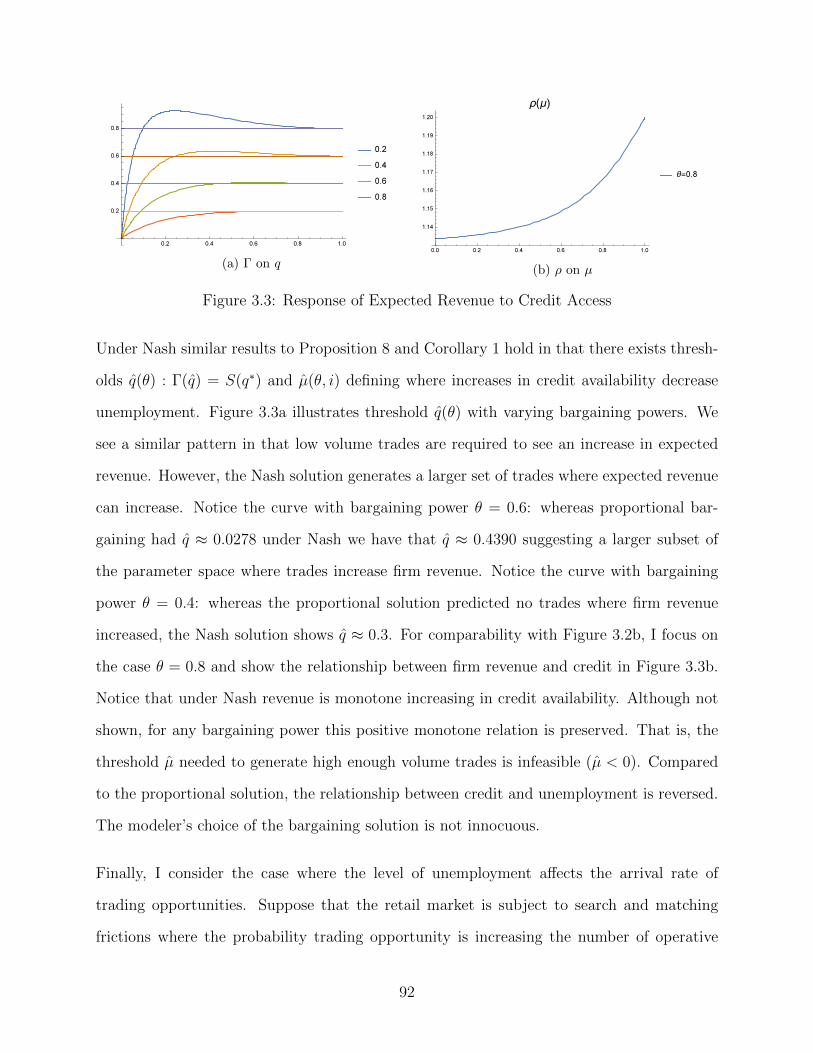
(a) Γ on q (b) ρ on µ

Figure 3.3: Response of Expected Revenue to Credit Access

Under Nash similar results to Proposition 8 and Corollary 1 hold in that there exists thresh-

olds q(θ) : Γ(q) = S(q∗) and µ(θ, i) defining where increases in credit availability decrease

unemployment. Figure 3.3a illustrates threshold q(θ) with varying bargaining powers. We

see a similar pattern in that low volume trades are required to see an increase in expected

revenue. However, the Nash solution generates a larger set of trades where expected revenue

can increase. Notice the curve with bargaining power θ = 0.6: whereas proportional bar-

gaining had q ≈ 0.0278 under Nash we have that q ≈ 0.4390 suggesting a larger subset of

the parameter space where trades increase firm revenue. Notice the curve with bargaining

power θ = 0.4: whereas the proportional solution predicted no trades where firm revenue

increased, the Nash solution shows q ≈ 0.3. For comparability with Figure 3.2b, I focus on

the case θ = 0.8 and show the relationship between firm revenue and credit in Figure 3.3b.

Notice that under Nash revenue is monotone increasing in credit availability. Although not

shown, for any bargaining power this positive monotone relation is preserved. That is, the

threshold µ needed to generate high enough volume trades is infeasible (µ < 0). Compared

to the proportional solution, the relationship between credit and unemployment is reversed.

The modeler’s choice of the bargaining solution is not innocuous.

Finally, I consider the case where the level of unemployment affects the arrival rate of

trading opportunities. Suppose that the retail market is subject to search and matching

frictions where the probability trading opportunity is increasing the number of operative

92

firms. Firms and buyers are matched in the DM according to a constant returns to scale

matching function M(B,F ) whose arguments are the measure of buyers and operative firms

respectively. Normalizing the measure of buyers to one, I have that the matching probabilities

are summarized by the measure of operative firms n: σ(n) = M(1, n) is the probability that

a buyer meets a firm, and σ(n)/n is the probability that a firm meets a buyer. Of course,

the measure of operative firms will depend on labor market conditions. We may then write

σ(n(τ)) to make explicit the link between the labor market and goods market.2 The solution

to the buyer’s problem is now given by,

i = σ(n(τ))(1− µ)θ

(u′(q)− 1

z′θ(q)

). (3.10)

and firm revenue is scaled by the probability of a match σ(n(τ))/n(τ)ρ.

3.3 An Example

I show the analytic properties of the model when the functional form for utility is u(q) =

2q1/2. Immediately we have that the quantity trade that maximizes joint surplus is q∗ = 1

which provides one unit of retail surplus to be split between sellers and buyers.

From Proposition 8, the threshold quantity traded is defined as Ω(q) = 1 which, given the

functional form above, simplifies to

2θq3/2 + (1− 6θ)q − (2− 6θ)q1/2 + (2− 2θ) = 1

2Previously, there was still a link between the goods and labor market but it was uni-directional: a buyersportfolio choice was based on the liquidity value realized in the goods market, and this in turn affected firmrevenue and their decision to enter the labor market. Now the link is bi-directional: labor market outcomesaffect the liquidity value of real balances, and the buyer’s choice of real balances affect firms labor marketprospects.

93

whose solution is

q =

(2θ − 1

2θ

)2

for θ ∈ (1/2, 1]

= 0 otherwise

Given q, the pairs (µ, i) which are consistent with buyers bringing in real money balances

z(q) are given by (3.2). If we take the nominal interest rate as given, then we retrieve the

threshold value µ from Corollary 1. I show here that (3.2) dramatically simplifies given the

functional form on utility.

i = (1− µ)θ

(u′(q)− 1

(1− θ)u′(q) + θ

)= (1− µ)θ

( (2θ−12θ

)−1 − 1

(1− θ)(2θ−12θ

)−1+ θ

)

= 1− µ

Given the function form for utility, there exists a simple linear relationship between credit

availability and the nominal interest rate that implicitly defines the threshold q.

94

Bibliography

Ahn, J., Khandelwal, A. K. & Wei, S.-J. (2011), ‘The Role of Intermediaries in FacilitatingTrade’, Journal of International Economics 84(1), 73–85.

Akerman, A. (2010), ‘A Theory on the Role of Wholesalers in International Trade based onEconomies of Scope’, Research Papers in Economics 1, 1–23.

Antras, P. & Costinot, A. (2010), ‘Intermediation and economic integration’, AmericanEconomic Review 100(2), 424–428.

Berentsen, A., Menzio, G. & Wright, R. (2008), ‘Inflation and unemploymenmt in the longrun’, American Economic Review 100(1), 371–98.

Bernard, A. B., Grazzi, M. & Tomasi, C. (2011), ‘Intermediaries in International Trade :Direct Versus Indirect Modes of export’, CEP Discussion Papers (199).

Bernard, A. B., Jensen, J. B., Redding, S. J. & Schott, P. K. (2009), ‘Wholesalers andRetailers in U.S. Trade’, US Census Bureau Center for Economic Studies .

Bethune, Z., Rupert, P. & Rocheteau, G. (2015), ‘Aggregate unemployment and householdunsecured debt’, Review of Economic Dynamics 18(1), 77–100.

Biglaiser, G. (1993), ‘Middlemen as experts’, The RAND Journal of Economics 24(2), 212–223.

Blum, B. S., Claro, S. & Horstmann, I. (2014), ‘Facts and Figures on Intermediated TradeFacts and Figures on Intermediated Trade’, 100(2), 419–423.

Blum, B. S., Claro, S. & Horstmann, I. J. (2009), ‘Intermediation and the nature of tradecosts: Theory and evidence’, University of Toronto .

Camera, G. & Li, Y. (2008), ‘Another example of a credit system that coexists with money’,Journal of Money, Credit, and Banking 40(6), 1295–1308.

Chaney, T. (2008), ‘Distorted gravity: The intensive and extensive margins of internationaltrade’, American Economic Review 98(4), 1707–21.

Coase, R. M. (1937), ‘The nature of the firm’, Economica 4, 386–405.

95

Cooley, T. & Quadrini, V. (2004), ‘Optimal time-consistent monetary policy in a Phillips-curve world’, Journal of Economic Theory 118(2), 174–208.

Das, S., Roberts, M. J. & Tybout, J. R. (2007), ‘Market entry costs, producer heterogeneity,and export dynamics’, Econometrica 75(3), 837–873.

Eaton, J., Kortum, S. & Kramarz, F. (2011), ‘An Anatomy of International Trade: EvidenceFrom French Firms’, Econometrica 79(5), 1453–1498.

Feenstra, R. C. (2003), ‘Intermediaries in Entrepot Trade: Hong Kong Re-Exports of ChineseGoods’, 71(6), 1695–1725.

Felbermayr, G. & Jung, B. (2007), ‘International Trade and Domestic Growth:Determinants,Linkages and Challenges’, Proceedings of OeNB Workshops (14).

Felbermayr, G. & Jung, B. (2011), ‘Trade intermediation and the organization of exporters’,Review of International Economics 19(4), 634–648.

Gong, X. (2017), ‘Middlemen: Intensive and extensive margins with endogenous meetingtechnology’.

Helpman, E., Melitz, M. J. & Yeaple, S. R. (2004), ‘Export Versus FDI With HeterogeneousFirms’, American Economic Review 94(1), 300–316.

Johri, A. & Leach, J. (2002), ‘Middlemen and the allocation of heterogeneous goods’, Inter-national Economic Review 43(2), 347–361.

Jones, G. (1998), Multinational Trading Companies in History and Theory, Routledge, Lon-don.

Kocherlokata, N. (1998), ‘Money is Memory’, Journal of Economic Theory 81(2), 232–251.

Lagos, R., Rocheteau, G. & Wright, R. (2017), ‘Liquidity: A new monetarist perspective’,Journal of Economic Literature 55(2), 371–440.

Lehmann, E. (2012), ‘A search model of unemployment and inflation’, Scandinavian Journalof Economics 114(1), 245–266.

Li, Y. (1998), ‘Middlemen and private information’, Journal of Monetary Economics42(1), 131–159.

Li, Y. (1999), ‘Money and middlemen in an economy with private information’, EconomicInquiry 37(1), 1–12.

Lotz, S. & Zhang, C. (2016), ‘Money and credit as means of payment: A new monetaristapproach’, Journal of Economic Theory 164, 68–100.

Market Microstructure (1999), 2 edn, Cambridge University Press.

Masters, A. (2007), ‘Middlemen in search equilibrium’, International Economic Review48(1), 343–362.

96

Masters, A. (2008), ‘Unpleasent middlemen’, Journal of Economic Behavior and Organiza-tion 68(1), 73–86.

Melitz, M. J. (2003), ‘The Impact of Trade on Intra-Industry Reallocations and AggregateIndustry Productivity’, 71(6), 1695–1725.

Money, Payments, and Liquidity (2017), 2 edn, The MIT Press.

Nosal, E., Wong, Y.-Y. & Wright, R. (2014a), ‘Buyers, sellers and middlemen: Variations insearch theory’, International Economic Review 55(2).

Nosal, E., Wong, Y.-Y. & Wright, R. (2014b), ‘More on middlemen: Equilibrium entry andefficiency in intermediated markets’, FRB of Chicago Working Paper (2014–2018), 1–53.

Nosal, E., Wong, Y.-Y. & Wright, R. (2016), ‘Who wants to be a middleman?’.

Petrosky-Nadeau, N. & Wasmer, E. (2015), ‘Macroeconomic dynamics in a model of goods,labor and credit market frictions’, Journal of Monetary Economics (72), 97–113.

Rocheteau, G. & Wright, R. (2005), ‘Money in search equilibrium, in competitive equilib-rium, and in competitive search equilibrium’, Econometrica 73(1), 175–202.

Rocheteua, G., Rupert, P. & Wright, R. (2007), ‘Inflation and unemployment in generalequilibrium’, Scandavian Journal of Economics 105, 837–855.

Rossman, M. (1998), ‘Export Trading Company Legislation: U.S. Response to JapaneseForeign Market Penetration’, Journal of Small Business Management (22), 69–93.

Rubinstein, A. & Wolinsky, A. (1987), ‘Middlemen’, The Quarterly Journal of Economics102(3), 581–594.

Schroder, P. J. H., Trabold, H. & Trubswetter, P. (2003), ‘Intermediation in Foreign Trade:When do Exporters Rely on Intermediaries?’, Traders pp. 1–19.

Shevchenko (2004), ‘Middlemen’, International Economic Review 45(1), 1–24.

Shi, S. (1998), ‘Search for a monetary propagation mechanism’, Journal of Economics Theory(81), 314–352.

Watanabe (2010), ‘A model of merchants’, Journal of Economic Theory 145(5), 1865–1889.

97