ESSAYS ON INTERNATIONAL TRADE AND - … · the gravity model adjusted trade intensity index can provide a useful analytical tool for identifying strategic or other deviations in trade

A NEW PERSPECTIVE ON CHINA TRADE GROWTH: APPLICATION OF A NEW INDEX OF BILATERAL TRADE INTENSITY

Christopher Edmonds*

Yao Li**

Abstract: This paper analyzes China’s trade relationships using a new trade intensity index,

which incorporates gravity model estimation, to compare observed trade levels with levels would

be expected to prevail given the economic, geographic, and cultural characteristics of the trading

partners. The index is calculated to study China’s bilateral trade intensity, and uses Japan as a

comparative case. Standard trade intensity index measures suggest China trades at a very

intensive level with countries in East and Southeast Asia (ESA) and at a low level with countries

in Europe (EU) and US-Canada (USC). The gravity model based index indicates that China’s

level of trade with countries in the ESA region is consistent with levels that would be expected

given the countries’ characteristics, while China’s level of trade with EU and USC are greater

than one would expect given their characteristics. The new index also reveals insights regarding

the evolution of China’s trade partners during the years 1988-2005. The paper’s results suggest

the gravity model adjusted trade intensity index can provide a useful analytical tool for

identifying strategic or other deviations in trade levels.

Key Words: Gravity model, Trade Intensity Index, Bilateral Trade, China

JEL codes: F14, F13, C43

* Assistant Professor (Specialist), College of Tropical Agriculture and Human Resources -- Center on the Family; Adjunct Fellow, East – West Center; and Cooperating Graduate Faculty, Department of Economics, UH-Manoa. University of Hawai'i – Manoa, 103D Miller Hall, 2515 Campus Road, Honolulu, Hawai’i 96822, USA. E-mail: [email protected]. ** Assistant Professor, College of Management and Economics at University of Electronic Science and Technology of China, No. 4 Section 2, North Jianshe Road, Chengdu, Sichuan 610054, China. E-mail: [email protected]

1

1. Introduction

Since China reopened its door to the world in the late 1970s, its international trade

policies have rapidly progressed from the prohibition of trade in all but a few products with a

few countries, to a relatively liberal stance towards both imports and exports in the world market.

Since reopening, China’s exports and imports have increased at a high rate (annual growth rates

of exports and imports averaged 10.8 percent and 11.2 percent, respectively, between 1978 and

2009).1 Within this overall growth trend, the level of growth in China’s trade with particular

countries varied markedly. Before liberalization, China’s foreign trade was oriented primarily

toward other Eastern Bloc countries, displaying a trading pattern typical of Eastern Bloc

countries. During the 1980s and 1990s, China’s trade refocused dramatically towards large

market economies (Europe and North America), Asian economies, and countries with large

endowments of natural resources. From 1980 to 2005, China’s trading partners increased from

87 to 182 out of 200 countries and regions reported by the International Monetary Fund

(Direction of Trade Statistics, 2008). China’s exports to both Europe and North America

expanded by more than 300 percent over the period of 1995-2005, while its imports from natural

resource abundant countries grew even more rapidly (Edmonds et al., 2006).

In this paper, we use a new trade intensity index--which we will refer to as the Gravity

Model Adjusted Trade Intensity (GMATI) index--to compare China’s bilateral trade with

particular countries to levels that would be expected to prevail given the structural characteristics

of China’s and the trading partnership’s economy. The standard and new trade intensity index

values are also calculated for Japan to provide a comparative case. Calculation of the GMATI

index indicates that the strength of trade relationships between China and countries in selected

1 Values are calculated from data (in constant 2000 US$) in World Development Indicators, World Bank (2007).

2

regions are generally explained by the cultural, economic, and geographic characteristics of the

trading economies. The new index also indicates the possibility of intervention or strategic trade

between China and some other regions (e.g., African countries), which can counteract or

magnify the effects of the cultural, economic, and geographic characteristics on trade. The paper

also reviews the definition of the trade intensity index and its previous applications in the

literature, and describes the estimation model and data sources used to compute GMATI values

for China. The paper’s final section presents results and the main conclusions that can be drawn

from the index estimates.

2. The Trade Intensity Index and measures of bilateral trade relationships

There is a large body of literature on the measurement and analysis of bilateral trade. In a

survey of the literature, Drysdale and Garnaut (1982) identified two basic approaches for

systematic studies of bilateral trade: the gravity model of bilateral trade introduced by Linder

(1961), Tinbergen (1962) and Linnemann (1966); and the trade intensity approach developed by

Brown (1949) and Kojima (1964). The gravity model approach assesses the intensity of between

two economies in proportion to their economic sizes (measured by GDP, population, per capita

GDP, area, etc.) and inversely proportional related to the distance (both geographical and cultural

distance) between them.

Computation of trade intensity indices provide a convenient approach for describing the

geographic distribution of country trade and for analyzing the strength of bilateral trade ties

between countries. A number of indicators have been used in empirical examinations of

international trade to measure the tendency for particular countries to trade. These indices gauge

the level of trade against the size of economies, and other structural characteristics considered

3

(e.g., distance between the countries) important in determining trade levels. The simplest index,

the trade share deflates the value of exports (or import or trade volume) and the trade share:

, where is the share of exports from country i to country j to country i’s total

exports to the world; is exports from country i to country j, and is the total exports of

country i to the world. The trade share is useful in comparing trade flows between two countries

over time. However, its usefulness in cross-country comparisons is limited since the measure

does not account for the effect of economy size on trade level and different sized economies can

be expected to trade in proportion to the size of their economies. The trade intensity index

addresses this shortcoming by measuring trade levels between country i and j in relation to

country j’s average trade share across all countries of the world.

TiW

Tijij xxS /= ijS

Tijx T

iWx

The Trade Intensity Index proposed by Brown (1949) and Kunimoto (1977) takes each

country’s total imports and exports as given, and divides the determinants of international trade

into two categories: factors that influence the levels of total imports and exports of the countries

in the world, and factors that influence their geographical distribution. The indicator assesses

actual trade against the flow of trade that would prevail in a hypothetical world of countries with

no “geographic specialization” in foreign trade. Under this hypothetical scenario, each country’s

total trade would be distributed across countries according to each trade partner’s share of world

trade. Symbolically, the hypothetical trade flows from country i to country j ( ijx ) would be:

)/()( WiWWWjiWij xxxxx −⋅= (1.1)

where ijx is country i’s exports to country j in the hypothetical world, is country i’s total

exports, is country j’s total imports, is the total world imports, and x

iWx

Wjx WWx Wi is country i's total

exports to the world. Actual trade flows from country i to country j differ from the hypothetical

4

value derived by equation (1.1) because of the presence of the factors that influence trade flows

between countries. Expressing actual and hypothetical trade flows as a ratio, we obtain the

geographic trade intensity index ( ): ijI

)( Wiww

Wj

iW

ij

ij

ijij xx

xxx

xx

I−

== (1.2)

where is country i’s actual exports to country j. If the trade intensity index equals 1, trade

partners are trading without geographic bias. Values of the index above (below) 1 indicates the

trade between two countries is more (less) intensive than expected.

ijx

Ng and Yeats (2003) introduced a distance adjustment to the trade intensity index in an

analysis of East Asia trade. Their index accounts for geographic distance while measuring each

country’s trade intensities to different trading partners. This approach first estimates the

following equation:

)ln()ln( distanceIij βα += (1.3)

where represents the intensity of country i’s export to country j, given distance between the

capitals of the two trading countries. The coefficient is estimated based on cross-sectional

time series data so captures the average effect of distance on trade intensities between pairs of

countries worldwide, and is used to predict -- the expected trade intensity assuming no

geographic specialization factors other than distance exist. The distance adjusted trade intensity

index is defined as . It measures the trade intensity caused by geographic specialization

factors other than distance. Again, a value greater (less) than 1 suggests the trade intensity is

above (below) expected after considering the effect of distance between them. Ng and Yeats’

ijI

β

ijI

ijij II ˆ/

5

estimation coefficients on distance is negative and statistically significant as expected, and has an

R square is of 0.672.

Building upon the Ng and Yeats approach, our GMATI Index combines the gravity

model and the trade intensity index approach to analyze and describe a countries’ bilateral trade.

Computation of the index proceeds by estimating each country’s expected exports and imports

( ) using a standard gravity model. Therefore, the variable we estimated is the trade value

instead of the intensity index. The estimated exports and imports are then used to calculate the

expected trade intensity between two countries, given that all countries trade as predicted by the

gravity model:

ijx

ww

Wj

iW

ijij x

xxx

Tˆˆ

ˆˆˆ = (1.4)

where , and ∑=j

ijiW xx ˆˆ ∑=i

ijWj xx ˆˆ ∑∑=i j

ijww xx ˆˆ .

The GMATI index is defined as (1.5) ijij TT ˆ/

where Tij uses the actual rather than estimates values of xij, xiW, xWj, and xww as in (1.4). This index

gauges the bilateral trade intensities based on countries’ characteristics as included in the gravity

model. If a country’s geographic specialization of foreign trade follows the prediction of gravity

model, its actual trade intensity should equal its expected trade intensity, i.e. GMATII= =1.

If the value of GMATI index is greater (smaller) than 1, it indicates that the trade intensity

between the two countries is greater (smaller) than the expected level based on the gravity model

estimations, (i.e. the strength of trade relationship between the two economies cannot be

completely explained by their economic, geographic and cultural characteristics described in the

gravity model). The GMATI index is used to investigate whether China has traded more

ijij TT ˆ/

6

intensively with some regions and countries in its trade expansion or whether the strength of the

trading relationship reflects global averages given the economic, geographic and cultural

characteristics of China and its trading partners.

3. Estimation Model

Our GMATI index adjusts for several factors found to empirically affect trade between

countries. Our specification of the gravity equation follows the specification in Clarete et al.

(2003), and is as follows:

tiitjtijijti PopYYYDI )/ln()ln()ln(ln[)ln( 41312,10, βββββ ++++= −−

]ln)ln()ln()/ln( ,8765 jijitjj SmctryAreaAreaPopY ββββ ++++

][ 1312,11109 jijiji IslandIslandContLandlLandl βββββ +++++

jtijijijiji ColComColColonyLang ,,17,16,15,14 ]45[ εββββ +++++ (1.6)

where i and j denotes trading partners (country i is the exporting country and j is the importing

country), and t denotes time. The variables on the left hand side are divided into three groups

denoted by the square brackets. The first group of variables (β1 to β8) captures notions of

economy size and country size which are considered fundamental in driving trade flows under

the gravity model. All the models estimates include these variables and together they are referred

to as the base gravity model. A second group of variables (β9 to β13) captures geographic

characteristics (aside from distance between countries) that are expected to influence trade. A

third group of variables (β14 to β17) captures shared historical and linguistic ties between

countries.

7

Notation of the variables in the model, and the expectation regarding the relationship

between the level of trade and each variable, are as follows:2

jtiI , denotes the value exports (or imports) in constant (year 2000) $US of country i to

country j at time t.

jiD , is the linear distance between capital cities of the trading countries. Distance is

expected to have a negative association with trade level since it proxies transport and

transaction costs.

Y is real GDP of country i or j in year t-1 (in constant year 2000 $US dollars). The

variable enters the model with a one year lag to address potential endogeneity between

trade levels and GDP. Larger economies are expected to trade more.

Pop is the population of country i or j in year t. Countries with larger populations are

generally expected to trade less because of their larger domestic markets.

Area is the land area (in square kilometers) of country i or j. Countries with large land

areas are expected to trade less because greater land area is associated with larger

internal markets and greater availability of resources domestically.

Smctry is a binary variable which is unity if both country i and j had constant boundaries

between 1988 and 2005.3 Countries with steady borders are expected to have higher

trade due to their greater stability and cultivation of trading relationships over time.

2 The rationale for the inclusion of particular variables and expectations regarding their relationship to trade levels is widely discussed in the literature developing and applying the gravity model of trade, for example see discussions in Linneman (1966), Krugman (1991), and Frankel (1997). 3 With the break up of the Former Soviet Union, Yugoslavia, and a few other countries, several new countries were formed after 1985, and interrupts time series data)

8

Landl is a binary variable which is unity if country i or j is landlocked (no sea ports of

direct sea access). Landlocked status is expected to be associated with lower trade due

to higher trade costs.

Cont is a binary variable which is unity if country i and j border one another. Countries

sharing a common land border are expected to trade more due to proximity and ease of

overland transport.

Island is a binary variable which is unity if country i or j is a small island country. Small

island countries are expected to trade at a higher rate due to limited domestic market

and natural resources.

Lang is a binary variable which equals 1 if i and j share a common language (zero

otherwise). Shared language and historical ties through colonialism are expected to

increase trade links between countries.

Colony is a binary variable which equals 1 if country i established a colony in country j or

vice versa.

Comcol is a binary variable which is unity if i and j were colonies of the same colonial

power.

45Col is a binary variable which is unity if i and j had a colonial relationship after 1945.

jti,ε represents the estimation residual (model error) and reflects the effect of other

influences on bilateral trade that are not included in the model.

The coefficients in equation (1.6) can be interpreted as measuring the elasticity of exports

with respect to changes in the explanatory variables. Following established practice, continuous

variables in the model expressed in logarithmic form in keeping with standard practice. Because

of potential endogeneity between trade levels and GDP, we estimate the model using real GDP

9

with a 1 year lag. As suggested by Anderson and Wincoop (2003), country specific dummies are

introduced into the regression to address the multilateral resistance problem.4

To examine whether China’s trading partners demonstrate a bias toward trade with

particular regions, such as East and Southeast Asian countries, African countries, or Middle East

countries, we introduce binary dummy variables to the gravity model. For example, a dummy

variable ChinaexESA takes a value of 1 if the exporter is China and the importer is an East or

Southeast Asian country and is assigned a value of zero otherwise. Altogether, 16 additional

dummies are considered in the panel estimates: ChinaexAFR, Chinaim

AFR, ChinaexESA, Chinaim

ESA,

ChinaexEU, Chinaim

EU, ChinaexLAC, ChinaimLAC, Chinaex

ME, ChinaimME, Chinaex

OCN, ChinaimOCN,

ChinaexUSC, Chinaim

USC, ChinaexFSR, and Chinaim

FSR, where the abbreviations are: Africa (AFR),

East and Southeast Asia (ESA), Europe (EU), Latin America and the Caribbean (LAC), Middle

East (ME), Oceania (OCN), United States and Canada (USC), and Former Soviet Republics

(FSR).5

4. Data Sources and Estimation Models

Data on exports used in the estimates are drawn from World Trade Analyzer 2008

(WTA)—a trade database provided by the International Trade Division of Statistics Canada—

which rectifies trade data of the United Nations Conference on Trade and Development 4 “Multilateral resistance” raises a complication in simple pairwise estimation of the gravity model. The more resistance there is to trade with one economy, the more trade is pushed toward other trade partners. Both theoretical [Anderson (1979)] and empirical [Anderson and Wincoop (2003), Subramanian and Wei (2007)] models have explored shown the effects of multilateral resistances on bilateral trade flows and shown that failure to account for such resistance results in misspecification of the standard gravity model. Several papers have developed methods to address multilateral resistance. Baldwin and Taglioni (2006) argue that country-pair dummies are superior to country dummy variables in panel regressions due to the existence of time-series bias. However, this approach cannot be applied in this instance because inclusion of the country-pair dummies precludes inclusion of time-invariant variables, such as distance, which are integral to the gravity model. Instead, country dummies are used in our regressions. In particular, each country has two specific dummies (e.g., Chinaex and Chinaim for China). The value of Chinaex (Chinaim) equals 1 if the exporter (importer) is China, and otherwise equals 0. 5 Lists of countries for each region are included in the Appendix.

10

(UNCTAD) so that exports reported by the exporting country are consistent with the imports

reported by the importing country. The original UNCTAD data does not ensure concordance

between exports to country B reported by country A and imports from country A reported by

country B. Use of the WTA data, where concordance is assured, means regressions run on

exports or imports produce equivalent results. We estimate our models for exports following

standard practice.

Data on distance between trading countries and related geographic characteristics are

obtained from the Centre d’Etudes Prospectives et d’Informations Internationales (CEPII)

database. 6 The database captures a number of geographic characteristics for 225 countries,

including the distance between the capital and largest cities of each pair of countries, and dummy

variables indicating whether a country is landlocked; and whether pairs of countries share a land

border, common language, or post-WWII colonial history. The final database yields a panel of

32,942 country pairs (involving 182 countries) during the period 1988 to 2005. The World

Bank’s World Development Indicators (WDI 2008) was the source of real GDP used in the

model.7

The gravity model is estimated using the standard generalized log-linear least squares

regression on cross-section data of selected individual years, as well as random effect GLS

regression on panel data.8 The panel estimator is expected to be more efficient since it makes use

of the fact that the level of trade between each country-pair is observed over time so the

estimation makes use of both the cross sectional and time series variation in trade in explaining 6 Available online at http://www.cepii.fr/anglaisgraph/bdd/distances.htm (last accessed on September 3, 2010) 7 Data of development indicators for Taiwan are obtained from ADB (2005). 8 We also tried Random Effect Tobit regression on panel data since the trade values are left censored at zero. However, the quadrature check provided by Stata 9.2 indicates that all our Tobit estimations are unreliable. Therefore, we can only use the GLS regression to estimate the model for country-pairs with positive trade, omitting country-pairs with zero trade. Accordingly, our model only explains the trade levels across countries rather than trade per se (i.e., the decision of whether to trade and the level of trade).

11

trade levels. On the other hand, the cross-sectional estimation results have the advantage of being

somewhat easier interpret, and by considering how cross-sectional estimates evolve over time,

one can gain useful insights into how the factors driving trade flows have changed over time.

5. Estimation Results and Trade Intensity Index Calculations

Next, we consider the results of our estimates. First, we review results form the single-

year gravity model estimates as an entrée to our empirical examination of the strength of China’s

trade relations (and compared to Japan as an early East Asian export-led high growth economy).

Moving on to the panel estimators, we review the random effects GLS gravity model estimates.

The section concludes by calculating the standard trade intensity and the GMATI indices and

comparing their values. Our ultimate purpose in estimating the gravity models is to obtain

estimation coefficients that can be applied in the GMATI index, but the legitimacy of the index

itself rests on the robustness and accuracy of the gravity model estimates.

Table 1 summarizes estimates from the OLS regressions for single years of cross-

sectional data between 1988 and 2005. Overall, the model estimates perform well, explaining

about 75% of the variation in trade between country pairs and most of the variables expected to

influence trade under the gravity model are significant (at 95% level) and have expected signs.

Estimates find exports increase with trading partners’ GDP and decrease as the distance between

trading economies increases. The GDP per capita and area variables are statistically significant

with negative signs in most years, as expected. Landlocked countries trade more than those with

access to sea, while island economies tend to trade less according to the models. Countries

sharing a common language or colonial history are found to trade more with each other, ceteris

12

paribus. Country pairs that share a land border or that had consistent boundaries throughout the

years covered in the dataset, also traded at higher volumes than others.

Table 2 summarizes the estimation results from the random effects GLS regressions. As

mentioned previously, country-pairs that did not engage in any trade are dropped from the

sample used in these estimates, so the estimator explains the level of trade between trading

economies. The dependent variable for specifications (1) to (3) is the value of exports between

each country pair. The dependent variable for regression (4) is the calculated export intensity

index (equation 1.3). R-squares ranged between 0.37 to 0.73 across the specifications, and the

estimation coefficients are statistically significant and similar across all 4 specifications (except

in specification (4) where the estimation coefficient on GDP per capita, land area, and dummies

capturing geographic characteristics were significant but had signs that are inconsistent with

theoretical expectations). Overall, results suggest the gravity model performs very well in

explaining the bilateral levels of trade, but less successfully in explaining values of the trade

intensity index. In the next section of this part of the paper, we use the estimation coefficients

from specification (3) in Table 2 in our computation of the GMATI index. We conclude by

examining the performance of these trade indicators in terms of its explanatory power and

consistency with predictions under the standard gravity model.

The estimates in Table 3 add regional trade dummy variables to investigate whether data

suggest there is evidence of regional bias in China’s trade partners. Estimation coefficients for all

the regional import dummies are all greater than 1 and significant at 5% level. The estimated

coefficient for ChinaimUSC is the largest among the regional import dummies, indicating that once

the effects of other factors influencing trade levels captured in the gravity model are considered,

China’s imports from United States and Canada actually occur at a higher level than from other

13

regions considered in the estimator. This was somewhat of a surprise given longstanding

complaints from some NA countries about the balance of trade with China.

In terms of exports, only the estimated coefficients for ChinaexAFR and Chinaex

ME are

positive and statistically significant at the 5% level. Both these coefficients have values greater

than 1, while export dummies for other regions were generally positive (except for FSR which

was negative), but not statistically significant. Along with the positive and significant

coefficients for imports from these regions, these results suggest that China’s overall trade level

with these two regions is higher than average after accounting for other gravity model factors. In

contrast, the results do not suggest that China exported excessively to countries in the EU or

USC regions, despite persistent trade surpluses, once the structural characteristics (captured in

the gravity model) of these country-pairs that are considered. It is also worth noting that

estimated coefficients of import dummies are greater than that of the corresponding export

dummies of each region. This may be attributable to China’s high levels of importation of

intermediate inputs for their manufacturing industries. Dean and Lovely (2009) estimate that

more than half of China’s exports are processing exports and about one third of China’s imports

are imports related to intermediate inputs related to export processing industries. Therefore,

China imports more actively than most other countries.

A few general conclusions can be drawn from the gravity model estimates reviewed

above. China’s trade does not demonstrate a bias toward trade with countries in the ESA region.

China’s exports to Africa and Middle East have been at higher levels than would be expected

given their characteristics as captured in the gravity model. China’s economy has demonstrated a

bias toward foreign trade. Its exports and imports are both at levels above what would be

expected given its characteristics, but import bias appears stronger.

14

We conclude our analysis by computing the standard trade intensity index and the

GMATI index for available country pairs over the period of 1988-2005. Results are too

numerous for them all to be reported, so we present results for index values of China’s trade

intensity with selected 25 countries in 8 regions in Table 4. Calculation of the GMATII for

individual country-pairs exactly follows equation (1.5). For calculating GMATII between China

and a region, such as the ESA region, we merely aggregate trade flows across all countries in the

region. Intra-regional exports (imports) are included in calculations of the regional exports to

(imports from) China since both intra- and inter-regional exports (imports) reflect the region’s

demand (supply) in the world market. This makes the regional values of the trade indices

comparable to values calculated for country-pairs (as presented in Table 4). However, treating

intra-regional trade as inter-regional trade raises standard “border puzzle” problems. 9

Nonetheless, we include intra-regional trade since excluding it in the calculation of the trade

intensity indices leads to overvaluation of the indices’ value. This is because trade with other

regions represents a relatively larger portion of total trade represented by trade with countries in

other regions if intra-regional trade is excluded.

Table 4 and the Appendix Table show that in 2005, the strade intensity index had values

of greater than one for: China’s exports to AFR, ESA, OCN, and USC, and for China’s imports

from AFR ESA and OCN. This same year, the standard intensity index is greater than 1 for

Japan’s exports to ESA, OCN, and USC, and imports from ESA, ME, OCN, and USC. These

results imply that China’s and Japan’s trade with these regions is above the world average level.

The corresponding values of the GMATI index reveal a different picture regarding which regions

were trading intensively with China and Japan. The GMATI index suggests that China exports

9 See Anderson and Wincoop, 2003.

15

and imports occurred at a level that was higher than would be expected with countries in the EU

and USC regions, and (only in 2005) imports intensively with AFR countries. For the case of

Japan, the GMATI index indicates that Japan exports most intensively with the EU and USC

regions, and imports most intensively with AFR, EU, ME, OCN, and USC.

Values of the standard trade intensity and GMATI indices vary markedly for given

regions, and distance appears to be the dominant factor in driving these differences. In countries

closer to China or Japan, the GMATI index generally suggests levels of trade are less intense

than the trade intensity index, and vice versa, which is consistent with the strong influence

distance (and associated trade costs) have on trade flows. The largest discrepancies observed in

the case of China’s exports are found in the cases of exports to the ESA and EU regions. The

standard trade intensity index suggests China exports very intensively to countries in the ESA

region, while the GMATI index suggests China’s level of exports to ESA countries are actually

well below levels that would be expected given global averages and the characteristics of these

economies. This is consistent with our conclusion drawn from Table 3. A possible explanation

for this is that China and the ESA economies produce similar goods for export (i.e., using

technologies and resource endowments at are similar), so these shared characteristics make their

exports competitive, counteracting the proximity advantage in trade between these countries.

Considering the case of EU-China trade, we find the opposite pattern between the two

indices, with the standard index suggesting China’s exports to the EU region occur at low

intensity while the GMATI shows exports occurred at a very intensive level. The differences

between the two indices reflect the role of proximity and other characteristics captured in the

GMATI index in generating the expected level of trade. When the value of the GMATI index is

greater than the standard index (as in the case of China-to-EU exports), it implies that the actual

16

level of trade is much greater than one would expect given the distance (both physical and

cultural) between China and the countries in the EU region. This may be a result of differences in

the technology or resource endowments of these countries which foster greater trade or may

reflect governments’ trade promotion efforts. Other notable cases where the standard and

GMATI indices yielded very disparate results were: (i) OCN and USC (China exports) and (ii)

ESA, EU, OCN, and USC (China imports).

Examining how values of the standard and GMATI indices change over time reveals the

changing trade relations between countries and the impact of trade policies on trade levels in

light of the fundamental characteristics of trading economies.. For example, Table 4 shows the

dramatic increase in the intensity of China’s exports to the USC and EU regions over the studied

period, and the contrasting (relatively stable) intensities for China’s imports from countries in

these regions. China’s trade policies generally focused on export promotion during the period

studied and the change in the index values seem to reflect this focus. On the other hand, China’s

exports to ESA region decrease between 1990 and 2005, falling from 0.33 to 0.25 during those

years. However, examination of this trend at the country-pair level shows only China’s exports to

Mongolia had a clear decreasing trend. Its export intensity for most ESA economies such as

Japan, South Korea, and India increased during the same period as listed in Table 4.

A possible explanation for these trends is that China's exports to countries in the ESA

region became shifted across countries within the region over time, with the shift in export shares

changing the most in countries that started out with the lowest levels of trade with China. So in

spite of the growth of Chinese exports, the portion of China’s total exports to ESA fell as

captured in a declining GMATI index value. For example, the value of the GMATI index for

China’s exports to South Korea is lower than the value of the index for the ESA regional; while

17

the index values for China’s exports to Japan are greater than the regional index in most years.

From 1990 to 2008, the average annual growth rate of China’s exports to South Korea was

29.7%, while the corresponding growth rate for China’s exports to Japan was 17.3%, and in 1990,

more than 17% of China’s exports went to Japan while only 1.3% went to South Korea. As

compared to 2005, when the share of China’s exports to Japan decreased to 11.7% and the share

of China’s exports to South Korea increased to more than 4.4%. Accordingly, while undergoing

a rapid rise in exports to these two ESA countries, China lowered its regional export intensity to

ESA due to shifts in the country destinations of its exports within the region.

The GMATI index values for China’s imports from the ESA region as a whole increased

steadily over the years studied, rising from 0.31 in 1990 to 0.45 in 2005. The GMATI Index for

individual ESA countries also shows increasing intensity of China’s imports from most ESA

countries (e.g., India, Japan, South Korea and Vietnam), as shown in Table 4. Overall, our

GMATI Index implies that the importance of exports to the ESA regional market for China’s

economy has declined over time, while the importance of imports from ESA, has increased.

These same calculations suggest China has traded more intensively with Africa over the

period considered (shown on the Appendix Table). The GMATI index for both China’s exports

and imports with Africa increased. Furthermore, the GMATI index for China’s imports from

Africa grew from less from 0.24 in 1990 to 1.24 in 2005, which is the fastest intensity growth of

China’s import among the 8 regions we studied. This may reflect diplomatic overtures China has

made toward Africa over the past decade and mirrors trends in China’s direct investment in the

region, which has generally targeted resource-extraction industries (Chan-Fishel, 2007).

However, when we look at GMATI Index values for individual African countries with China, we

see that values for imports from most of the Africa countries are less than one (with some below

18

0.5), especially for bigger African economies such as South Africa and Egypt. Therefore,

China’s impacts on Africa through trade are not as strong as suggested by standard trade

intensity measures.

6. Conclusions

In this paper, we investigate the strength of China’s trade ties with particular countries

and regions. To examine if a country is trading with a particular country or region at a higher or

lower rate than would be expected given the characteristics of the economies, we introduce the

GMATI index and apply it to measure China’s trade ties and their evolution over time. After

controlling for the effects of both geographic and cultural distance as well as economy size, the

GMATI index indicates that China trade with the ESA region and individual countries in the

region was less intensive, and was more intensive with EU and USC, than suggested by standard

intensity measures. The discrepancy between trade intensity measures may also reflect

differences in the underlying comparative advantage of trading economies or suggest effects of

government trade intervention (i.e., strategic trade policies). By examining the change of

GMATI index over time, we also find indications on that in terms of its exports to the ESA

region, China exports to individual ESA countries have shifted significantly over time. Trends

also suggest China’s exports to EU and USC countries have grown more intensive over time.

Lastly, GMATI index values show that China has traded (both exported and imported) with

African countries more intensively over time.

Although comparison of the GMATI index values with standard trade intensity measures

provides insight into the effects of economy sizes and distances between markets (both

geographical and cultural distance), more analysis is needed to explore the factors affecting these

19

trading patterns. Differences in the resource endowments, real exchange rates, macroeconomic

balances, and similar characteristics that drive underlying comparative advantage between

trading economies likely drive these differences, but more detailed analyses are beyond the scope

to the current paper and are left for future research.

20

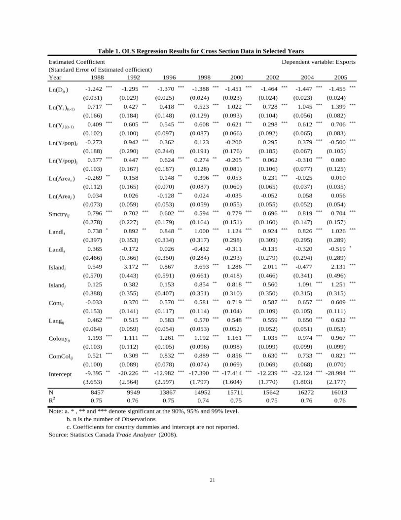
Table 1. OLS Regression Results for Cross Section Data in Selected Years Estimated Coefficient Dependent variable: Exports(Standard Error of Estimated oefficient)Year 1988 1992 1996 1998 2000 2002 2004 2005

Ln(Dij ) -1.242 *** -1.295 *** -1.370 *** -1.388 *** -1.451 *** -1.464 *** -1.447 *** -1.455 ***

(0.031) (0.029) (0.025) (0.024) (0.023) (0.024) (0.023) (0.024)Ln(Yi )(t-1) 0.717 *** 0.427 ** 0.418 *** 0.523 *** 1.022 *** 0.728 *** 1.045 *** 1.399 ***

(0.166) (0.184) (0.148) (0.129) (0.093) (0.104) (0.056) (0.082)

Ln(Yj )(t-1) 0.409 *** 0.605 *** 0.545 *** 0.608 *** 0.621 *** 0.298 *** 0.612 *** 0.706 ***

(0.102) (0.100) (0.097) (0.087) (0.066) (0.092) (0.065) (0.083)

Ln(Y/pop)i -0.273 0.942 *** 0.362 0.123 -0.200 0.295 0.379 *** -0.500 ***

(0.188) (0.290) (0.244) (0.191) (0.176) (0.185) (0.067) (0.105)Ln(Y/pop)j 0.377 *** 0.447 *** 0.624 *** 0.274 ** -0.205 ** 0.062 -0.310 *** 0.080

(0.103) (0.167) (0.187) (0.128) (0.081) (0.106) (0.077) (0.125)Ln(Areai ) -0.269 ** 0.158 0.148 ** 0.396 *** 0.053 0.231 *** -0.025 0.010

(0.112) (0.165) (0.070) (0.087) (0.060) (0.065) (0.037) (0.035)Ln(Areaj ) 0.034 0.026 -0.128 ** 0.024 -0.035 -0.052 0.058 0.056

(0.073) (0.059) (0.053) (0.059) (0.055) (0.055) (0.052) (0.054)

Smctryij 0.796 *** 0.702 *** 0.602 *** 0.594 *** 0.779 *** 0.696 *** 0.819 *** 0.704 ***

(0.278) (0.227) (0.179) (0.164) (0.151) (0.160) (0.147) (0.157)

Landli 0.738 * 0.892 ** 0.848 ** 1.000 *** 1.124 *** 0.924 *** 0.826 *** 1.026 ***

(0.397) (0.353) (0.334) (0.317) (0.298) (0.309) (0.295) (0.289)Landlj 0.365 -0.172 0.026 -0.432 -0.311 -0.135 -0.320 -0.519 *

(0.466) (0.366) (0.350) (0.284) (0.293) (0.279) (0.294) (0.289)Islandi 0.549 3.172 *** 0.867 3.693 *** 1.286 *** 2.011 *** -0.477 2.131 ***

(0.570) (0.443) (0.591) (0.661) (0.418) (0.466) (0.341) (0.496)

Islandj 0.125 0.382 0.153 0.854 ** 0.818 *** 0.560 1.091 *** 1.251 ***

(0.388) (0.355) (0.407) (0.351) (0.310) (0.350) (0.315) (0.315)

Contij -0.033 0.370 *** 0.570 *** 0.581 *** 0.719 *** 0.587 *** 0.657 *** 0.609 ***

(0.153) (0.141) (0.117) (0.114) (0.104) (0.109) (0.105) (0.111)Langij 0.462 *** 0.515 *** 0.583 *** 0.570 *** 0.548 *** 0.559 *** 0.650 *** 0.632 ***

(0.064) (0.059) (0.054) (0.053) (0.052) (0.052) (0.051) (0.053)Colonyij 1.193 *** 1.111 *** 1.261 *** 1.192 *** 1.161 *** 1.035 *** 0.974 *** 0.967 ***

(0.103) (0.112) (0.105) (0.096) (0.098) (0.099) (0.099) (0.099)ComColij 0.521 *** 0.309 *** 0.832 *** 0.889 *** 0.856 *** 0.630 *** 0.733 *** 0.821 ***

(0.100) (0.089) (0.078) (0.074) (0.069) (0.069) (0.068) (0.070)

Intercept -9.395 ** -20.226 *** -12.982 *** -17.390 *** -17.414 *** -12.239 *** -22.124 *** -28.994 ***

(3.653) (2.564) (2.597) (1.797) (1.604) (1.770) (1.803) (2.177)

N 8457 9949 13867 14952 15711 15642 16272 16013R2 0.75 0.76 0.75 0.74 0.75 0.75 0.76 0.76

Note: a. * , ** and *** denote significant at the 90%, 95% and 99% level. b. n is the number of Observations c. Coefficients for country dummies and intercept are not reported.Source: Statistics Canada Trade Analyzer (2008).

21

Table 2. Random Effects GLS Model for Panel Data

22

Estimated Coefficient(Standard Error)Regression (1) (2) (3) (4)

Dependent variable:

Ln(D ij ) -1.46 *** -1.39 *** -1.32 *** -1.34 ***

(0.016) (0.017) (0.017) (0.017)Ln(Y i ,t -1) 1.19 *** 1.19 *** 1.19 *** 0.25 ***

(0.029) (0.029) (0.029) (0.029)Ln(Y j,t -1) 0.73 *** 0.73 *** 0.73 *** 0.16 ***

(0.029) (0.029) (0.029) (0.028)Ln(Y it /pop it ) 0.56 *** 0.56 *** 0.56 *** -0.38 ***

(0.035) (0.035) (0.035) (0.034)Ln(Y jt /pop jt ) 0.57 *** 0.57 *** 0.57 *** -0.28 ***

(0.034) (0.034) (0.034) (0.033)Ln(Area i ) -3.20 *** 0.31 *** 0.30 *** -0.04 *

(1.005) (0.023) (0.023) (0.023)Ln(Area j ) -0.09 *** -0.03 -0.03 -0.02

(0.027) (0.030) (0.029) (0.030)Smctryij 1.47 *** 1.09 *** 0.70 *** 0.73 ***

(0.105) (0.108) (0.107) (0.108)Landli 0.59 *** 0.62 *** 0.58 ***

(0.180) (0.177) (0.178)Landlj -0.21 -0.22 -0.24

(0.178) (0.175) (0.175)Island i 0.40 * 0.68 *** -0.63 ***

(0.219) (0.216) (0.216)Island j 0.72 *** 0.63 * 0.64 ***

(0.178) (0.174) (0.175)Contij 1.00 *** 0.86 *** 0.82 ***

(0.077) (0.076) (0.077)Langij 0.53 *** 0.55 ***

(0.037) (0.037)Colonyij 0.44 *** 0.42 ***

(0.133) (0.134)ComColij 0.69 *** 0.67 ***

(0.044) (0.045)Col45 ij 1.30 *** 1.27 ***

(0.171) (0.172)

Notes: See bottom of table on the next page.

ln(Trade intensity index)

ln(Exports) ln(Exports) ln(Exports)

Table 2. (continued)

Estimated Coefficient(Standard Error)Regression (1) (2) (3) (4)

Dependent variable: ln(Exports) ln(Exports) ln(Exports)ln(Trade intensity index)

degrees of freedom (m) 8 13 17 1σu 1.43 1.43 1.40 1.43σe 1.13 1.13 1.13 1.10ρ (rho) 0.62 0.61 0.60 0.63θ (minimum) 0.38 0.38 0.37 0.39θ (mediam) 0.78 0.78 0.77 0.78θ (maximum) 0.82 0.82 0.81 0.82

Number of Observations 238,320 238,320 238,320 2,374,609Number of Groups 21,994 21,994 21,994 21,875

R2 (within) 0.160 0.160 0.160 0.001

R2 (between) 0.79 0.79 0.80 0.47

R2 (overall) 0.72 0.72 0.73 0.38Breuch-Pagan LM Test 4.E+05 4.E+05 4.E+05 4.E+05Wald Chi-square 124,615 125,544 129,897 19,619

Note: *, ** and *** denote significant at the 90%, 95% and 99% level.Coefficients for country dummies and intercept are not reported due tospace constraintSource: Statistics Canada Trade Analyzer (2008).

7

23

24

Table 3. Estimates of Random-effects GLS Regression

Variables Estimated Coefficient

Standard Errors Variables Estimated

CoefficientStandard

Errors

Ln(Dij ) -1.32 *** 0.02 ChinaexESA 0.29 0.61

Ln(Yi )(t-1) 1.19 *** 0.03 ChinaimESA 1.60 *** 0.62

Ln(Yj )(t-1) 0.73 *** 0.03 ChinaexAfr 1.50 *** 0.52

Ln(Y/pop)it 0.56 *** 0.03 ChinaimAfr 1.97 *** 0.53

Ln(Y/pop)jt 0.57 *** 0.03 ChinaexUSC 1.33 1.12

Ln(Areai ) 0.30 *** 0.02 ChinaimUSC 2.90 *** 1.12

Ln(Areaj ) -0.03 0.03 ChinaexLA 0.82 0.55

Smctryij 0.69 *** 0.11 ChinaimLA 1.34 ** 0.56

Landl 0.61 *** 0.18 China EU 0.80 0.56i ex

Landlj -0.21 0.17 ChinaimEU 1.85 *** 0.56

Islandli 0.68 *** 0.22 ChinaexME 1.46 ** 0.62

Islandlj 0.64 * 0.17 ChinaimME 2.48 *** 0.63

Contij 0.90 *** 0.08 ChinaexOCN 0.85 0.72

Langij 0.54 *** 0.04 ChinaimOCN 1.62 ** 0.73

Colonyij 0.43 *** 0.13 ChinaexUSSR -0.18 0.58

ComColij 0.69 *** 0.04 ChinaimUSSR 1.30 ** 0.58

col45ij 1.30 *** 0.17

degrees of freedom (m) 31 Number of Observations: 238,320σu 1.396 Number of Groups 21,994σe 1.129 R2 (within) 0.16ρ (rho) 0.605 R2 (between) 0.80θ (minimum) 0.3712 R2 (overal) 0.73θ (median) 0.7726 Breuch-Pagan LM Test 400,000θ (maximum) 0.8127 Wald Chi-square 130,041

Note:a. *, ** and *** denote significant at the 90%, 95% and 99% level. b. Coefficients for country dummies and intercept are not reported.Source: Statistics Canada Trade Analyzer (2008).

Table 4. Standard and Gravity Model Adjusted Export Trade Intensity Index of China and Japan with selected Regions and Countries

25

Export Intensity Index(Gravity Model Adjusted Export Intensity Index)

Exporter1990 1992 1994 1998 2002 2005 1990 1992 1994 1998 2002 2005

ImporterEast and Southeast Asia (ESA) 5.06 4.45 2.84 3.04 2.58 2.11 2.59 2.44 2.51 2.59 2.57 2.49

(0.33) (0.33) (0.24) (0.30) (0.25) (0.25) (0.11) (0.12) (0.16) (0.19) (0.19) (0.24)INDIA 0.16 0.28 0.87 0.82 1.14 1.20 0.87 0.77 0.72 0.83 0.58 0.65

(0.01) (0.02) (0.09) (0.09) (0.13) (0.17) (0.25) (0.25) (0.28) (0.38) (0.29) (0.42)INDONESIA 2.14 1.49 1.27 1.22 1.57 1.11 2.62 2.26 2.71 2.35 2.29 1.66

(0.30) (0.24) (0.24) (0.27) (0.34) (0.30) (0.36) (0.36) (0.54) (0.57) (0.59) (0.55)JAPAN/China1 2.55 2.71 3.15 3.49 3.13 2.67 1.34 1.46 1.51 1.76 2.23 2.37

(0.30) (0.39) (0.56) (0.75) (0.71) (0.78) (0.14) (0.17) (0.22) (0.29) (0.37) (0.50)MONGOLIA 16.26 24.58 10.24 3.62 3.74 3.42 1.57 1.66 1.80 1.31 0.66 0.99

(0.18) (0.31) (0.17) (0.08) (0.10) (0.13) (0.19) (0.23) (0.34) (0.35) (0.23) (0.52)SOUTH KOREA 0.63 1.62 1.66 2.29 2.14 1.97 3.12 2.71 2.77 2.79 3.16 3.48

(0.05) (0.14) (0.16) (0.22) (0.19) (0.21) (0.10) (0.10) (0.11) (0.12) (0.14) (0.18)VIETNAM 0.29 1.62 1.98 3.08 2.20 2.50 3.35 1.68 1.14 1.92 1.74 2.01

(0.01) (0.07) (0.10) (0.18) (0.13) (0.20) (0.44) (0.26) (0.22) (0.46) (0.46) (0.73)Europe (EU) 0.23 0.23 0.33 0.41 0.43 0.53 0.45 0.46 0.39 0.46 0.39 0.38

(1.31) (1.38) (2.10) (2.56) (2.67) (3.47) (2.71) (3.00) (2.84) (3.59) (3.21) (3.36)FRANCE 0.21 0.19 0.26 0.40 0.36 0.46 0.38 0.37 0.31 0.37 0.37 0.33

(1.15) (1.07) (1.56) (2.36) (2.03) (2.74) (2.14) (2.30) (2.06) (2.60) (2.76) (2.70)GERMANY 0.35 0.33 0.49 0.56 0.52 0.68 0.65 0.64 0.53 0.62 0.51 0.49

(2.14) (2.10) (3.22) (3.76) (3.54) (4.89) (4.15) (4.43) (4.02) (5.18) (4.57) (4.86)UK 0.16 0.19 0.33 0.39 0.46 0.65 0.58 0.60 0.58 0.65 0.52 0.50

(0.44) (0.53) (0.99) (1.20) (1.42) (2.17) (1.58) (1.82) (1.93) (2.41) (2.08) (2.24)USA & Canada (USC) 0.53 0.65 1.01 1.12 1.13 1.31 1.78 1.67 1.61 1.58 1.40 1.27

(0.69) (0.81) (1.36) (1.58) (1.65) (2.16) (1.90) (1.77) (1.95) (2.14) (2.13) (2.24)CANADA 0.20 0.25 0.34 0.34 0.42 0.56 0.70 0.72 0.47 0.52 0.56 0.55

(1.75) (2.14) (3.20) (3.45) (4.23) (6.37) (4.85) (5.06) (3.88) (4.94) (5.72) (6.55)USA 0.61 0.75 1.16 1.29 1.26 1.45 2.05 1.89 1.86 1.81 1.57 1.41

(0.52) (0.62) (1.03) (1.19) (1.21) (1.57) (1.44) (1.33) (1.49) (1.61) (1.56) (1.63)Source: Authors' estimates based on data from Statistics Canada Trade Analyzer (2008).Note: 1 The importer is Japan (China) when the exporter is China (Japan).

China Japan

Appendix Table. Standard and Gravity Model Adjusted Export Trade Intensity Index for China and Japan Trade with other Regions and Countries

Export Intensity Index(Gravity Model Adjusted Export Intensity Index)

ExporterImporter 1990 1992 1994 1998 2002 2005 1990 1992 1994 1998 2002 2005

Africa (AFR) 0.45 0.60 0.62 0.89 0.91 1.02 0.75 0.75 0.77 0.60 0.56 0.58(0.32) (0.44) (0.48) (0.68) (0.69) (0.87) (0.55) (0.60) (0.68) (0.56) (0.56) (0.68)

CONGO 0.10 0.38 0.23 1.50 0.66 1.31 0.41 0.33 0.18 0.09 0.17 0.07(0.19) (0.58) (0.27) (1.50) (0.54) (1.25) (0.82) (0.53) (0.25) (0.11) (0.19) (0.09)

EGYPT 0.44 0.68 0.56 0.61 0.91 0.68 0.42 0.42 0.44 0.45 0.40 0.36(0.17) (0.27) (0.24) (0.26) (0.40) (0.33) (0.19) (0.20) (0.24) (0.26) (0.25) (0.26)

SOUTH AFRICA 0.02 0.12 0.61 1.04 1.13 1.14 1.32 1.22 1.14 0.80 0.70 0.87(0.01) (0.04) (0.21) (0.38) (0.40) (0.47) (0.40) (0.39) (0.42) (0.34) (0.31) (0.46)

Latin America & Caribbean (LAC) 0.20 0.15 0.19 0.31 0.40 0.57 0.78 0.81 0.78 0.80 0.74 0.86(0.14) (0.11) (0.16) (0.28) (0.32) (0.53) (0.44) (0.49) (0.56) (0.66) (0.59) (0.81)

BRAZIL 0.36 0.10 0.19 0.42 0.52 0.80 0.78 0.57 0.59 0.69 0.62 0.68(0.16) (0.05) (0.09) (0.23) (0.26) (0.46) (0.30) (0.24) (0.29) (0.39) (0.35) (0.45)

CHILE 0.39 0.47 0.70 0.94 1.12 0.91 0.78 0.96 0.83 0.71 0.54 0.62(0.24) (0.31) (0.54) (0.77) (0.79) (0.75) (0.35) (0.48) (0.51) (0.49) (0.35) (0.49)

COLOMBIA 0.01 0.10 0.16 0.22 0.50 0.66 0.93 0.75 0.68 0.81 0.80 0.57(0.01) (0.06) (0.11) (0.16) (0.35) (0.53) (0.46) (0.39) (0.41) (0.55) (0.56) (0.47)

MEXICO 0.19 0.11 0.09 0.17 0.31 0.43 0.34 0.53 0.49 0.43 0.51 0.73(0.15) (0.08) (0.08) (0.15) (0.27) (0.43) (0.19) (0.31) (0.33) (0.33) (0.42) (0.71)

Middle East (ME) 0.71 0.69 0.78 0.74 0.92 0.93 1.20 1.22 0.87 0.99 0.91 0.80(0.25) (0.25) (0.30) (0.30) (0.36) (0.42) (0.51) (0.55) (0.44) (0.56) (0.54) (0.56)

JORDAN 0.62 0.87 0.89 0.64 1.23 1.35 0.35 0.66 0.40 0.72 0.45 0.49(0.38) (0.58) (0.66) (0.51) (0.97) (1.19) (0.25) (0.53) (0.38) (0.78) (0.52) (0.66)

SAUDI ARABIA 0.77 0.57 0.59 0.64 0.77 0.88 1.57 1.52 1.04 1.04 1.48 1.38(0.18) (0.14) (0.15) (0.17) (0.21) (0.28) (0.43) (0.45) (0.35) (0.40) (0.61) (0.69)

TURKEY 0.33 0.16 0.33 0.46 0.46 0.69 0.59 0.51 0.35 0.57 0.36 0.39(0.19) (0.09) (0.19) (0.27) (0.26) (0.45) (0.38) (0.35) (0.26) (0.44) (0.30) (0.37)

Oceania (OCN) 0.76 0.81 0.97 1.10 1.33 1.37 1.89 1.72 1.76 1.74 1.73 1.79(0.13) (0.15) (0.20) (0.24) (0.29) (0.35) (0.23) (0.23) (0.28) (0.31) (0.33) (0.42)

AUSTRALIA 0.89 0.92 1.11 1.21 1.43 1.49 2.01 1.86 1.89 1.84 1.76 1.82(0.15) (0.16) (0.22) (0.26) (0.29) (0.37) (0.23) (0.24) (0.28) (0.32) (0.32) (0.41)

NEW ZEALAND 0.38 0.55 0.61 0.84 1.01 1.00 1.62 1.45 1.51 1.48 1.76 1.83(0.08) (0.12) (0.15) (0.22) (0.26) (0.30) (0.23) (0.23) (0.28) (0.31) (0.39) (0.50)

PAPUA NEW GUINEA 0.40 0.45 0.39 0.38 0.29 0.49 1.13 1.30 1.33 1.42 0.72 0.73(0.09) (0.10) (0.10) (0.10) (0.08) (0.16) (0.15) (0.19) (0.23) (0.28) (0.15) (0.19)

Former Soviet Republics (FSR) - - 1.02 0.31 0.50 0.58 - - 0.24 0.16 0.16 0.36- - 0.39 (0.12) (0.19) (0.26) - - 0.23 (0.16) (0.17) (0.47)

RUSSIA - - 1.64 0.53 0.74 0.78 - - 0.37 0.22 0.24 0.71- - 0.44 (0.12) (0.18) (0.23) - - 0.30 (0.16) (0.20) (0.74)

Source: Authors' estimates based on data from Statistics Canada Trade Analyzer (2008).

China Japan

26

References

Anderson, James E. 1979. A Theoretical Foundation for the Gravity Equation. American Economic Review 69(1): 106-116.

Anderson, James E. and Eric van Wincoop. 2003. "Gravity with Gravitas: A Solution to the Border Puzzle," American Economic Review, vol. 93(1), 170-192.

Baldwin, Richard E. and Daria Taglioni. 2006. "Gravity for Dummies and Dummies for Gravity Equations". CEPR Discussion Paper No. 5850 Available online at http://ssrn.com/abstract=945443

Brown, A.J. 1949. Applied Economics: Aspects of World Economy in War and Peace. George Allen and Unwin, London.

Centre d'Etudes Prospectives et d'Informations Internationales Databases. 2005. Distances. CEPII Research Center. Available online at http://www.cepii.fr/anglaisgraph/bdd/distances.htm

Chan-Fishel, M. 2007. Environmental impact: more of the same. In F Manji and Stephen Marks (eds) African Perspectives on China in Africa. Oxford/Nairobi: Fahamu, 139-152.

Clarete, Ramon, Christopher Edmonds, and Jessica Seddon Wallack. 2003. “Asian regionalism and its effects on trade in the 1980s and 1990s” Journal of Asian Economics, Vol. 14, 91-131.

Judith M. Dean, Mary E. Lovely, and Jesse Mora. 2009 "Decomposing China–Japan–U.S. Trade: Vertical Specialization, Ownership, and Organizational Form." Journal of Asian Economics Vol 20: 596-610.

Drysdale, Peter and Ross Garnaut. 1982. “Trade Intensities and the Analysis of Bilateral Trade Flows in a Many-Country World: A Survey,” Hitotsubashi Journal of Economics, vol. 22, no. 2, (February)

Frankel, Jeffrey. 1997. Regional Trading Blocks and the World Economic System, Washington: Institute for International Economics.

Kojima, K. 1964. "The pattern of international trade among advanced countries," Hitotsubashi Journal of Economics. Vol. 5, pp. 16-36.

Kunimoto, Kazutaka. 1977. "Typology of Trade Intensity Indices," Hitotsubashi Journal of Economics. Vol. 17, No 2, pp. 15-32.

Krugman, P., 1991. Geography and Trade. Cambridge, MA: MIT Press.

Linder, S. 1961. An Essay on Trade and Transformation. New York, Wiley.

Linneman, Hans. 1966. An Econometric Study of International Trade Flows, Amsterdam: North Holland Publishing Company.

Ng, Francis and Alexander Yeats. 2003. Major East Asian Trade Trends, Washington: World Bank, processed.

27

StataCorp. 2003, Stata Time-Series Reference Manual: Release 8, College Station, TX: Stata Corporation

Subramanian, Arvind & Wei, Shang-Jin, 2007. "The WTO promotes trade, strongly but unevenly," Journal of International Economics, vol. 72(1), 151-175

Tinbergen, Jan. 1962. Shaping the World Economy: Suggestions for an International Economic Policy. New York: The Twentieth Century Fund.

Yergin, Daniel and Roberts, Scott. 2004. “Riding the Tiger: The Global Impact of China's Energy Quandary.” Cambridge Energy Research Associates.

28

Appendix: List of Regions and Countries included in the Dataset used in estimates

AFR—Saharan and Sub-Saharan Africa: Algeria, Angola, Benin, Burkina Faso, Burundi,

Cameroon, Central African Republic, Chad, Comoros, Congo, Congo Dem Rep, Cote

D’Ivoire, Djibouti, Egypt, Equatorial Guinea, Ethiopia, Gabon, Gambia, Ghana, Guinea,

Guinea-Bissau, Kenya, Liberia, Libya, Madagascar, Malawi, Mali, Mauritania, Mauritius,

Morocco, Mozambique, Niger, Nigeria, Rwanda, Senegal, Seychelles, Somalia, South

Africa, Sudan, Tanzania, Togo, Tunisia, Uganda, Zambia, Zimbabwe.

ESA—East and South/Southeast Asia: Bangladesh, Brunei Darussalam, Cambodia, Hong

Kong, India, Indonesia, Japan, Korea Republic, Laos People’s Democratic Republic,

Macao, Malaysia, Maldives, Mongolia, Myanmar, Nepal, Pakistan, Philippines,

Singapore, Sri Lanka, Taiwan, Thailand, Vietnam.

EU—Europe: Albania, Austria, Belgium-Luxembourg, Bosnia and Herzegovina,

Bulgaria, Croatia, Denmark, Finland, France, Germany, Gibraltar, Greece, Hungary,

Iceland, Ireland, Italy, Macedonia, Malta, Netherlands, Norway, Poland, Portugal,

Romania, Serbia-Mont., Slovenia, Spain, Sweden, Switzerland, United Kingdom.

FSR—Former Soviet Republics: Azerbaijan, Armenia, Belarus, Estonia, Georgia,

Kazakhstan, Kyrgyzstan, Latvia, Lithuania, Moldova, Russia, Tajikistan, Turkmenistan,

Ukraine, Uzbekistan.

LAC—Latin America and the Caribbean: Argentina, Bahamas, Barbados, Belize, Bolivia,

Brazil, Cayman Islands, Chile, Colombia, Costa Rica, Dominican Republic, Ecuador, El

Salvador, Greenland, Guatemala, Guyana, Haiti, Honduras, Jamaica, Mexico, Nicaragua,

Panama, Paraguay, Peru, St Pierre Miquelon, Suriname, Trinidad Tobago, Uruguay,

Venezuela.

ME—Middle East: Cyprus, Iraq, Israel, Jordan, Bahrain, Kuwait, Lebanon, Oman, Iran,

Saudi Arabia, United, Arab Emirates, Syrian Arab Republic.

OCN--Oceania: Australia, Fiji, Kiribati, New Caledonia, New Zealand, Papua New

Guinea, Solomon Islands.

USC—United States and Canada: USA, Canada

29