Essays on information gathering and the use of natural ...

Essays on information gathering and the use of

natural resources

Luca Di Corato

Submitted for the Degree of Doctor of Philosophy in Economics

University of York and Università di Padova

March 2008

1

2

Contents

Abstract 9

Abstract (in Italian) 11

Acknowledgements 15

Declaration 17

1 Introduction 19

2 Mechanism design for conservation contracts in developing coun-

tries 25

2.1 Introduction . . . . . . . . . . . . . . . . . . . . . . . . . . . . . . 25

2.2 The basic set-up . . . . . . . . . . . . . . . . . . . . . . . . . . . . 29

2.2.1 Landowner and government agency�s preferences . . . . . . 29

2.2.2 Conservation in First Best . . . . . . . . . . . . . . . . . . 33

2.3 Mechanism under adverse selection . . . . . . . . . . . . . . . . . 35

2.3.1 Analysis of the optimal Conservation Program . . . . . . . 39

2.3.2 Transfers . . . . . . . . . . . . . . . . . . . . . . . . . . . . 43

2.3.3 Optimal CP vs general subsidy . . . . . . . . . . . . . . . 44

2.4 Conservation program at work . . . . . . . . . . . . . . . . . . . . 45

3

2.5 Conclusions . . . . . . . . . . . . . . . . . . . . . . . . . . . . . . 47

3 Optimal conservation policy under imperfect intergenerational

altruism 51

3.1 Introduction . . . . . . . . . . . . . . . . . . . . . . . . . . . . . . 51

3.2 The basic set-up . . . . . . . . . . . . . . . . . . . . . . . . . . . . 55

3.2.1 Harvesting or conserving . . . . . . . . . . . . . . . . . . 57

3.3 Optimal harvest timing: imperfect altruism and naiveté . . . . . . 60

3.4 Optimal harvest timing: imperfect altruism and sophistication . . 63

3.4.1 A three governments model . . . . . . . . . . . . . . . . . 64

3.4.2 A I -governments model . . . . . . . . . . . . . . . . . . . 68

3.5 Government targeting and instability . . . . . . . . . . . . . . . . 71

3.6 Conclusions . . . . . . . . . . . . . . . . . . . . . . . . . . . . . . 72

4 Option value of old-growth forest and Pigovian taxation under

time inconsistency 73

4.1 Introduction . . . . . . . . . . . . . . . . . . . . . . . . . . . . . . 73

4.2 The basic set-up . . . . . . . . . . . . . . . . . . . . . . . . . . . . 78

4.2.1 Sketch of an agent with hyperbolic preferences . . . . . . . 79

4.2.2 Conserving or harvesting: time-consistent case . . . . . . . 81

4.3 Conserving or harvesting under time inconsistency . . . . . . . . . 82

4.3.1 Strategies under sophistication . . . . . . . . . . . . . . . . 83

4.3.2 Conservation or harvest: a discussion on timing . . . . . . 87

4.4 Regulatory intervention . . . . . . . . . . . . . . . . . . . . . . . . 88

4.4.1 Passage time . . . . . . . . . . . . . . . . . . . . . . . . . 88

4.4.2 Time for regulation . . . . . . . . . . . . . . . . . . . . . . 89

4.4.3 Numerical and graphical analysis . . . . . . . . . . . . . . 91

4

4.5 Conclusion . . . . . . . . . . . . . . . . . . . . . . . . . . . . . . . 93

5 Optimal pro�t sharing under the risk of expropriation 95

5.1 Introduction . . . . . . . . . . . . . . . . . . . . . . . . . . . . . . 95

5.2 The basic set-up . . . . . . . . . . . . . . . . . . . . . . . . . . . . 99

5.2.1 The HC�s and MNF�s objective functions . . . . . . . . . . 100

5.2.2 The bargaining . . . . . . . . . . . . . . . . . . . . . . . . 101

5.3 E¢ cient bargaining set under uncertainty and irreversibility . . . 103

5.3.1 The host country . . . . . . . . . . . . . . . . . . . . . . . 103

5.3.2 The multinational �rm . . . . . . . . . . . . . . . . . . . . 106

5.4 Nash bargaining and cooperative equilibrium . . . . . . . . . . . . 109

5.4.1 Cooperative equilibrium . . . . . . . . . . . . . . . . . . . 109

5.4.2 Some analytical results . . . . . . . . . . . . . . . . . . . . 110

5.4.3 Final considerations on the cooperative agreement . . . . . 114

5.5 Conclusions . . . . . . . . . . . . . . . . . . . . . . . . . . . . . . 115

6 Concluding remarks 117

A Appendix to Chapter 2 121

A.1 Proposition 2.1 . . . . . . . . . . . . . . . . . . . . . . . . . . . . 121

A.2 Proposition 2.2 . . . . . . . . . . . . . . . . . . . . . . . . . . . . 123

A.3 Larger total rents for the higher type . . . . . . . . . . . . . . . . 125

A.4 Proposition 2.3 . . . . . . . . . . . . . . . . . . . . . . . . . . . . 126

A.5 Proposition 2.4 . . . . . . . . . . . . . . . . . . . . . . . . . . . . 127

A.6 Binding perverse incentive constraint . . . . . . . . . . . . . . . . 128

A.7 Feasibility of a GS program . . . . . . . . . . . . . . . . . . . . . 129

A.8 Bunching types . . . . . . . . . . . . . . . . . . . . . . . . . . . . 131

5

B Appendix to Chapter 3 133

B.1 Strategies under naïve belief . . . . . . . . . . . . . . . . . . . . . 133

B.2 Proposition 3.3 . . . . . . . . . . . . . . . . . . . . . . . . . . . . 136

B.3 Strategies under sophisticated belief: three governments . . . . . . 137

B.3.1 Continuation value function . . . . . . . . . . . . . . . . . 137

B.3.2 Value function . . . . . . . . . . . . . . . . . . . . . . . . . 139

B.4 Proposition 3.6 . . . . . . . . . . . . . . . . . . . . . . . . . . . . 142

B.5 Strategies under sophisticated belief: I governments . . . . . . . . 144

B.5.1 Continuation value function . . . . . . . . . . . . . . . . . 144

B.5.2 Value function . . . . . . . . . . . . . . . . . . . . . . . . . 146

C Appendix to Chapter 4 151

C.1 Strategies under sophisticated belief . . . . . . . . . . . . . . . . . 151

C.2 Pigovian taxation . . . . . . . . . . . . . . . . . . . . . . . . . . . 153

References 154

6

List of Figures

Figures 4.1-4.4 . . . . . . . . . . . . . . . . . . . . . . . . . . . . . . . 92

7

8

Abstract

The objective in this thesis is to pose and to answer to some questions concerning

the role played by information in decisions on the economic allocation of natural

resources.

In chapter 2 the design of a voluntary incentive scheme for the provision of

ecosystem services is considered, having in mind the forested areas in develop-

ing countries where a governmental agency plans to introduce a set-aside policy.

Payments are o¤ered to the landowners to compensate the economic loss for not

converting land to agriculture. The information asymmetry between the agency

and the landowners on the opportunity cost of conservation gives incentive to

the landowners to misreport their own "type". A principal - agent analysis is

developed, adapted and extended to capture real issues concerning conservation

programs in developing countries. I show that the information asymmetry may

seriously impact on the optimal scheme performance and, under certain condi-

tions, may lead to pay a compensation even if any additional conservation is

induced with respect to that in absence of the scheme.

In chapter 3 an intergenerational dynamic game is solved under time- inconsis-

tency. The optimal harvest timing for a natural forest is determined under uncer-

tainty on the �ow of amenity value derived from conservation and irreversibility.

Due to time-varying declining discount rates intertemporal inconsistent harvest

9

strategies arise. The value of the option to harvest is eroded and earlier harvest

occurs under both the assumptions of naïve and sophisticated belief on future

generations time-preferences. This results in a bias toward the current gener-

ation grati�cation which a¤ects the intergenerational allocation of bene�ts and

costs from harvesting and conserving.

In chapter 4 a forest owner with hyperbolic time preferences is considered.

At each period the irreversible decision to harvest an old-growth forest could

be taken, while conservation is the alternative. Flows of future amenity value

are uncertain while the net value of stumpage timber is known and constant.

The decision problem is expressed as an optimal stopping problem and solved an-

alytically in a time-inconsistent framework under the assumption of sophisticated

belief on future trigger strategies. Premature harvesting occurs. To avoid socially

undesirable harvesting the impact of hyperbolic discounting must be accounted

and a modi�ed optimal pigovian tax on the wood revenues is proposed.

Finally, in chapter 5 a government bargains a mutually convenient agreement

with a foreign �rm to extract a natural resource. The �rm bears the initial in-

vestment in �eld research and infrastructures and earns as a return a share on the

pro�ts. The �rm must cope with uncertainty due to market conditions and, as

initial investment is totally sunk, also due to the risk of successive expropriation.

In a real options framework where the government holds an American call op-

tion on expropriation I show under which conditions Nash bargaining is feasible

and leads to attain a cooperative agreement maximizing the joint venture sur-

plus keeping into account both the sources of uncertainty on pro�t realizations.

I show that the investment trigger does not change under the threat of expropria-

tion, while the set of feasible bargaining outcomes is restricted and the distributive

parameter is adjusted to account for the additional risk of expropriation.

10

Abstract (in Italian)

L�obiettivo di questa tesi è quello di presentare e rispondere ad alcune domande

riguardanti il ruolo svolto dall�informazione nelle decisioni riguardanti l�allocazione

economica delle risorse naturali.

Nel capitolo 2, viene considerato uno schema volontario per l�incentivazione

della fornitura di servizi di ecosistema. In particolare, si fa riferimento

all�intervento da parte di un�agenzia governativa teso all�introduzione di un piano

di set-aside nelle aree boschive dei Paesi in via di sviluppo. Il piano prevede di

ricompensare tramite un trasferimento i proprietari terrieri per la perdita eco-

nomica so¤erta non convertendo l�area di proprietà ad agricoltura. L�asimmetria

informativa esistente tra agenzia e proprietario terriero rispetto al costo opportu-

nità della conservazione incentiva quest�ultimo a non rivelarne la corretta entità.

Viene quindi sviluppata un�analisi principale - agente adattata ed estesa al �ne

di incorporare gli aspetti problematici che caratterizzano i programmi per la con-

servazione in Paesi in via di sviluppo nella realtà. Viene mostrato il drastico im-

patto che l�informazione asimmetrica può avere sulla performance dello schema

ottimale. Si veri�ca che, sotto certe condizioni, paradossalmente si potrebbe

dover compensare anche un proprietario terriero che ha conservato nell�ambito

del programma la stessa area che avrebbe conservato in assenza del programma

governativo.

11

Nel capitolo 3, si risolve un gioco dinamico intergenerazionale tra agenti

incoerenti temporalmente. Il timing ottimale del taglio di una foresta natu-

rale viene determinato tenendo in considerazione l�incertezza relativa al valore

di cui si potrebbe bene�ciare attraverso la conservazione e l�irreversibilità delle

conseguenze del taglio una volta avvenuto. La strategia ottimale, a causa dei

tassi di preferenza intertemporale varianti col tempo, può risultare incoerente.

L�erosione del valore dell�opzione di taglio ne induce un esercizio più a¤rettato

sia sotto l�ipotesi di aspettative rispetto alle preferenze temporali delle future

generazioni di tipo naïve che di tipo so�sticato. Tutto ciò si ri�ette in una distor-

sione della ripartizione intergenerazionale dei bene�ci e dei costi derivanti dalla

gestione della risorsa a vantaggio della generazione vivente.

Nel capitolo 4, si assume che il proprietario privato di una foresta abbia

preferenze temporali iperboliche e possa decidere il taglio, con conseguenze ir-

reversibili della foresta, oppure conservarla. Il �usso di valore di cui bene�cia se

conserva è incerto mentre il valore netto del legno tagliato è noto e costante nel

tempo. Tale problema decisionale viene rappresentato nei termini di un problema

di optimal stopping time e risolto analiticamente in un contesto caratterizzato da

incoerenza temporale sotto l�ipotesi di aspettative di tipo so�sticato rispetto alle

strategie preferite in futuro. Ne risulta che il taglio è realizzato prematuramente.

Si mostra quindi come modi�care la tassa Pigouviana sul legno per evitare ef-

fetti socialmente non desiderati dovuti alla particolare de�nizione delle personali

preferenze temporali.

In�ne, nel capitolo 5 il governo di un Paese ospitante negozia con un�impresa

estera un accordo reciprocamente conveniente per lo sfruttamento di una risorsa

naturale. L�impresa dovrebbe farsi carico dell�investimento iniziale necessario a

sondare la consistenza del giacimento e a costruire le infrastrutture necessarie ot-

12

tenendo in cambio una quota sui pro�tti derivanti dall�estrazione.

L�impresa oltre a far fronte all�incertezza sui pro�tti futuri dovuta alle variabili

condizioni di mercato deve tener conto anche del rischio di una successiva es-

propriazione, dato che l�investimento e� totalmente irrecuperabile. Utilizzando

un modello teorico di opzioni reali in cui il governo può essere visto come de-

tenere un opzione di tipo American call sul�espropriazione, si mostra sotto quali

condizioni, tenendo conto dell�incertezza di mercato e dell�addizionale rischio di

espropriazione, un Nash Bargaining sia realizzabile e permetta di de�nire un

accordo che massimizzi il valore complessivo dell�attività economica. Tra i risul-

tati, si mostra che la soglia temporale alla quale sostenere in maniera ottimale

l�investimento non varia in presenza di una minaccia di espropriazione rispetto al

caso in cui tale rischio non esista, mentre l�insieme degli accordi potenzialmente

realizzabili si riduce. Si mostra in�ne come le quote sui pro�tti vadano aggiustate

per incorporare il rischio supplementare di espropriazione.

13

14

Acknowledgements

I am deeply indebted to my supervisors Bipasa Datta and Michele Moretto.

I am also grateful to Paola Valbonesi for having supervised me in the beginning.

My gratitude goes to them not only for their comments and suggestions but also

for their advice, guidance and patience.

Finally, this thesis is dedicated to who in the darkest hours of the night was

and will be there, close to me.

15

16

Declaration

An earlier version of chapter 2 has been presented at the European Summer

School in Resource and Environmental Economics �Trade, Property Rights and

Biodiversity�, San Servolo, Venice, July 4-10, 2007, at an Environmental and

Resource Economics seminar at the LERNA, Université de Toulouse I, Toulouse,

February 8, 2007, at the VIII annual BIOECON Conference �Economic Analysis

of Ecology and Biodiversity�, Kings College, Cambridge, August 29-30, 2006 and

at an internal seminar at the University of Padua. An earlier version has appeared

as �Marco Fanno�Working Paper no. 34/2006, University of Padua.

Chapter 4 will be presented at the AFSE annual Thematic Meeting "Frontiers

in Environmental economics and Natural Resources Management", Toulouse,

June 9-11, 2008. An earlier version of Chapter 4 has been presented at the

�Giornata Levi-Cases� doctoral seminar, Faculty of Economics, University of

Padua, November 23, 2007, at the IX annual BIOECON Conference �Economics

and Institutions for Biodiversity Conservation�, Kings College, Cambridge, Sep-

tember 19-21, 2007, and at an internal seminar at the University of Padua.

17

18

Chapter 1

Introduction

Natural resources play an important role for current and future societies since

they represent an endowment whose use is crucial to support human welfare

(Heal, 1998). The channels through which natural assets may impact on human

felicity are diverse. For resources such as oil, natural gas and minerals, utility

is derived mainly from their exploitation while for natural assets such as forests,

wetlands, watersheds and related environmental goods and services, welfare could

accrue not only from exploitation but also from conservation.

Decisions regarding the use of these assets must be taken in the light of cur-

rent and future costs and bene�ts. Normally, in order to assess actual net bene-

�ts and to support strategies, information should be gathered. Several research

questions may arise from this simple consideration and a number of them have

been answered by social scientists. Nevertheless, some questions still remain.

The objective of this thesis is to pose and to answer to some questions concerning

the role that information may play for decisions about the economic allocation of

natural resources.

In particular, chapter 2 investigates the problem related to the design of an

19

incentive-compatible conservation contract scheme which allowing for the collec-

tion of information needed to optimally allocate forested land to two alternative

uses: agriculture or ecosystem services provision. The idea behind a conserva-

tion contract is relatively simple: an environmental agency proposes to landown-

ers a contract scheme which specifying the extent of land that should be set

aside for conservation, and the transfer compensating for the economic loss suf-

fered for not converting such an extent to agriculture. The cost opportunity

of conservation varies among landowners according to the quality of their land

and it is often private information of landowners (Smith and Shogren, 2002).

The information asymmetry between the landowner and the agency is an ad-

vantage for the former in that, by misreporting the land type, she may be over-

compensated. This clearly represents a problem for the agency which must deal

with limited and costly raised funds for conservation.

In this chapter I deal with such a problem by developing a standard prin-

cipal - agent analysis, adapted and extended to capture real issues concerning

conservation programs in developing countries. In these countries a substantial

extent of land is still forested but "slash and burn" agriculture has become ag-

gressive (Brocas and Carrillo, 1998). I assume �rst, that the private level of

conservation may be positive and second, that agriculture is risky in that, due

to primitive agricultural practices, the crop yield may be severely reduced by ex-

ogenous shocks such as pest and soil erosion (Arguedas et al., 2007). The second

assumption represents a novelty in the conservation contracts literature but in

my opinion is an important issue to be considered since it may have an impact

on the actual extent of land conversion. Finally, imposing a restriction on the

set of feasible incentive-compatible contracts, I address another important aspect

concerning the perverse e¤ects which may be induced through the conservation

20

program. In fact, inconsistently with the agency target, the program may relax

credit constraints and give incentive to clear more land than that cleared without

a program.

In all three chapters 3, 4 and 5, the perspective on the role played by infor-

mation di¤ers from that in chapter 2. Within di¤erent contexts, decision-making

accounts for the value of information disclosing as time rolls on. In fact, if this is

the case, it may be pro�table to postpone a decision and to collect information

in order to reduce uncertainty about future realizations of bene�ts and costs.

This consideration becomes crucial, in particular, when the consequences of a de-

cision are costly or impossible to reverse (Arrow and Fisher, 1974; Henry, 1974).

In particular, the model set-up of chapters 3 and 4 is quite similar from a

technical point of view. In both chapters, I merge two di¤erent strands of litera-

ture: on the one hand the real option theory which emphasises the importance of

waiting for collecting information, on the other hand the literature on hyperbolic

time-preferences, where decision-makers a¤ected by time-varying impatience are

time-inconsistent and have incentive to rush because of future sub-optimal plan

revisions. The results provided in these two chapters extend the real options tool

box for the analysis of a wider class of economic problems entailing the exercise

of options similar to an "American put" such as an option to exit or an option

to shut down (Dixit and Pindyck, 1994).

Chapter 3 provides a rational for the observed tendency of governments to rush

in undertaking projects which irreversibly impact the stock of natural resources

available to future generations and for the time inconsistency of the conserva-

tion policies. An intergenerational dynamic game is considered to determine the

optimal conservation policy set by the government. I assume that the govern-

ment is truly democratic and at each time period perfectly represents the will

21

and the preferences of the politic body, namely the generation living at that time

period (Phelps and Pollak, 1968). Each generation is imperfectly altruist and

lives over a random lifespan bene�ting from its own welfare and that of follow-

ing generations. The value of the stand of forest is known and constant and

accrues to society when irreversible harvest occurs, while the �ow of amenity

value from conservation randomly �uctuates according to a geometric Brownian

motion and stops forever when the forest is harvested. Under these assumptions

I show that the government is equivalent to an hyperbolic agent with a �nite

number of selves. Intertemporal inconsistent harvest strategies arise and due to

time-varying declining discount rates, the value of keeping the option to harvest

is lowered. Therefore, an earlier harvest is induced under both the assumptions

of naïve and sophisticated belief on future generations time-preferences.

In chapter 4, the research question is how second best tools for govern-

ment intervention must be adjusted to account for non standard time prefer-

ences (Shogren, 2007). Goods and services provided by a natural forest when

conserved are public in nature and government intervention may be needed to

guarantee the intertemporal socially desirable allocation of this natural asset.

I show that a pigouvian tax on wood revenues should be modi�ed to lead agents

with hyperbolic time preferences toward the social optimum because otherwise

the policy target could not be met. In this chapter, the optimal stopping prob-

lem in continuous time solved in the previous chapter for a �nite number of

government "incarnations", is now solved for the case of a private forest owner

represented by an in�nite sequence of selves with hyperbolic time preferences.

The solution for this case is more tractable but is qualitatively equivalent to the

one for the �nite selves case.

In chapter 5, I analyse the problem of foreign direct investment for the

22

exploitation of a natural resource. In developing countries, due to limited budget

often the governments cannot a¤ord the initial investment for the exploitation of

their natural resources and attempt to attain a mutually convenient agreement

with foreign �rms willing to bear the initial costs. According to these agree-

ments, the �rm bears the initial investment in �eld research and infrastructures

and earns, as a return, a share of the pro�ts derived from the resource extraction.

In this context, when assessing the convenience of the investment, the �rm must

deal with pro�t uncertainty due to market conditions. Moreover, since the initial

investment is totally sunk, the �rm should also deal with the risk of successive

expropriation. In high-pro�t states in fact the host country�s government may

have incentive to expropriate. I develop the analysis in a real options framework

where the government is seen as holding an American call option on expropriation

while the �rm as holding a similar option on investment. Both parties wish to

attain an agreement matching their di¤erent economic interests. I show under

which conditions Nash Bargaining is feasible and leads to a cooperative agree-

ment maximizing the joint venture value, keeping into account both sources of

uncertainty on pro�ts.

In chapter 6, I provide a summary of the main issues discussed in this thesis

and suggestions for future research. All the proofs are available in the appendix.

23

24

Chapter 2

Mechanism design for

conservation contracts in

developing countries

2.1 Introduction

In the last decades the Payments for the provision of Ecosystem Services

(hereafter, PES) have become an increasingly popular instrument to induce the

provision of ecosystem services on private lands.1 The target for most of the land

managed under PES programs has usually been the conservation of biodiversity

and the soil protection (Salzman, 2005; Ferraro, 2001; Ferraro and Kiss, 2002;

Pagiola et al., 2002). Under a PES program a contract is usually proposed by a

governmental agency to a landowner. The landowner sets aside a part of her own

land and receives a compensation for the economic loss su¤ered. The contract is

1A well known example is given by the PSA (Pagos por Servicios Ambientales) programin Costa Rica (FONAFIFO, 2000; Pagiola et al., 2002; Salzman, 2005). For other exampleshttp://www2.gsu.edu/~wwwcec/special/ci/index.html.

25

designed to allow for the voluntary participation of the landowner to the program

and speci�es the extent of land that should be conserved and the compensation

paid for the environmental service provided. To guarantee a voluntary participa-

tion the payment should be at least equal to the landowners�opportunity cost

and no higher than the value of the bene�t provided.

The landowners know their property and the opportunity cost of managing

it for environmental services better than the governmental agency. Landowners

could then have incentive to misreport their true type in order to be over compen-

sated. This opportunistic behaviour produces an additional burden for the agency

and impacts on the total level of conservation which may be induced through a

program becoming a serious issue when funds for conservation are limited and/or

are costly raised through distortionary taxation. This problem is common to

a number of other situations where agents with di¤erent cost opportunity type

may take advantage of their private information and the principal searches to

di¤erentiate them through a proper contract scheme. In these cases mechanism

design theory can be used to design contract scheme which induces truth-telling

(Mirrlees 1971; Groves, 1973; Dasgupta, Hammond and Maskin, 1979; Baron

and Myerson, 1982; Guesnerie and La¤ont, 1984). This is what has been also

broadly done to deal with information failures impacting on the design of conser-

vation contracts (Smith and Shogren, 2002; Wu and Babcock, 1996; Smith, 1995;

Goeschl and Lin, 2004).

In the reality despite the fact that optimal incentive schemes could be de-

signed, PES programs are usually general subsidy schemes.2 A general subsidy

scheme is surely easier to implement but it allocates sub-optimally the funds for

2This is the case for example for the PSA program in Costa Rica where each land unitconserved is paid the same amount and any landowner in the country is allowed to participateand choose the extent of land to be conserved (Pagiola et al., 2004).

26

conservation in that overpays3 landowners which misreport their cost opportu-

nity4 type.

The aim of this chapter is to address such concern and design a voluntary

incentive scheme for habitat conservation in developing countries where a sub-

stantial extent of land is still forested but "slash and burn" practices have become

intense.

We investigates the adverse selection issue due to the information asymmetry

between the governmental agency and the landowner on the environmental char-

acteristics of each property. This set of characteristics a¤ects the land agricultural

productivity and determine the opportunity cost of each unit of land conserved.

We are clearly aware that reality is even more complex for the presence of moral

hazard in the contract compliance and for the asymmetry in gathering informa-

tion about conservation costs but we prefer to abstract from these issues and

work on a simpler model.5

We model the agricultural activity undertaken after land conversion as a risky

activity su¤ering exogenous shocks which negatively a¤ects the landowner�s crop

yield. This is an aspect which has not been considered in the previous contribu-

tions on this topic but that is in our opinion very relevant in that risk a¤ects the

landowner private allocation choice and consequently the actual cost opportu-

nity of conservation.6 Moreover, this consideration can be even more important

3This has probably been the case in Costa Rica where the compensation paid has been quiteattractive and a number of applications to the program were not considered because of fundinglimits (Pagiola et al., 2004).

4By principle also the di¤erent levels of bene�t provided by the service should be taken intoaccount. But as in the case of biodiversity conservation, such bene�t is extremely di¢ cult toassess. In contrast, to collect information on and estimate the landowner�s opportunity costmay be easier and less costly.

5See White (2002) for the moral hazard problem and Goeschl and Lin (2004) for the asym-metry in the information gathering.

6There have been in fact no studies up to date assessing how much land managed under aconservation program would have been cleared in the absence of the program.

27

in developing countries where the agricultural activity is still primitive and the

investment in technology is low.

The set-up of our model is completed by �rst, assuming that the level of con-

servation pursued by the governmental agency through the conservation program

is not �xed ex-ante but results from the social welfare maximization, second,

assuming that the private level of conservation is not necessarily zero but it is

optimally determined by the landowner according to the expected pro�t associ-

ated to converting land and third, introducing as in the paper by Motte et al.

(2004) a constraint on the surface conserved to control for the e¤ectiveness of the

policy.7 The purpose of this constraint is to control for a policy perverse e¤ect

which could induce landowners to clear more forest than they would have cleared

without a contract.

In this frame a program consistent with the conservation target is designed

to guarantee voluntary participation and truthful revelation of land opportunity

cost. We show that the information asymmetry may seriously impact on the

optimal second-best scheme leading under certain conditions to pooling types.

First best conservation can only be attained if raising funds for the transfers

comes at no cost. We also verify that even if any additional conservation is in-

duced with respect to the extent privately undertaken a compensation must be

paid in some cases to landowners. This is done only to induce them to reveal

their private information and limit the information rent that must be paid to

other types. We �nally prove that the program designed is the optimal or best

feasible contract scheme available and that social surplus under a general sub-

sidy conservation program cannot be higher than under the optimal second best

7In Motte et al. (2004) the information asymmetry is on the individual cost of clearinge¤ort. A "policy consistency" constraint is introduced in the standard principal-agent problemto restrict the set of incentive compatible contract schedules to the one where the conservationundertaken under the CP is at least equal to that without CP.

28

conservation program.

The structure of the chapter is the following: in section 2.2, the landowner

and governmental agency�s preferences are presented; the private allocation in

the absence of a conservation program and the �rst best allocation with a conser-

vation program in place are presented and discussed. In section 2.3, the second

best outcome is derived and its properties are discussed. Section 2.4 proposes a

parametric example of the optimal conservation program at work. Section 2.5

concludes.

2.2 The basic set-up

We assume that each landowner owns A units of land and that each plot is in

its pristine natural state. Each landowner�s plot is of the same size but not

necessarily has the environmental characteristics8 of the one owned by another

landowner. On these private lands the governmental agency (hereafter, GA) plans

to preserve some critical habitat for biodiversity conservation and to induce that

proposes a voluntary contract scheme. According to the scheme, each landowner

is paid to set aside a units of her plot for conservation. We further assume that

the GA and the landowners are risk-neutral agents and that the funding of the

transfers is raised as standard by taxation.

2.2.1 Landowner and government agency�s preferences

Each landowner�s plot is characterized by a set of characteristics, such as soil

quality, soil erosion and water and distance to market. We use a scale index

� to represent these characteristics (Wu and Babcock, 1996). This parameter

8Hereafter, we would simply use "type".

29

varies among landowners and de�nes their type. We assume that the agricul-

tural productivity of the plot is positively related to �. The index � is private

information of the landowner. However, it is common knowledge that it is drawn

from the interval � =��; ��with a cumulative distribution function F (�) and

a density function f (�). The density function is assumed to be strictly positive

on the support �. Moreover, f (�) satis�es the regularity conditions9 such that

@[F (�)=f(�)]@�

� 0.

Crop yield to the landowner is represented by

(1� v)Y�A� a; �

�(2.1)

where A� a is the surface cultivated, � is the land type and v is a random shock

which may reduce the crop production and could be related to the technologi-

cally primitive "slash and burn" agricultural practice that is typical in developing

countries still forested areas.10 We assume that v belongs to the set V = fv; vg

where 0 � v < v � 1 and it is equal to v or v with probability q and 1 � q

respectively. Therefore, the expected crop yield is

q (1� v)Y�A� a; �

�+ (1� q) (1� v)Y

�A� a; �

�(2.2)

= [1� v + q (v � v)]Y�A� a; �

�Assume that the production is increasing and concave in the units of land con-

verted, increasing in � and that the marginal product with respect to land is in-

creasing in the land type. This is equivalent to following set of

9Most parametric single-peak densities meet this su¢ cient condition (Bagnoli andBergstrom, 1989).10However, it could be assumed a constant yield and model in the same simple way a shock

on the price of the crop due to changing market conditions. This could be done at no cost andkeeping the model practically intact.

30

assumptions: Y1 > 0, Y11 < 0, Y2 > 0 and Y12 > 0 where Y1 = @Y=@�A� a

�;

Y2 = @Y=@�; Y11 = @2Y=@(A� a)2; Y12 = @2Y=@(A� a)�.

In the absence of a conservation program (hereafter, CP), the expected pro�ts

to each landowner�s A� a units of land are represented by

��A� a; �

�= p [1� v + q (v � v)]Y

�A� a; �

�� c

�A� a

�(2.3)

where p is the price of the product and c is the private cost for converting a unit

of land, i.e. the cost of clearing the new plot and settle it.

We assume as in Motte et al. (2004) that given the abundance of forested

land convertible the constraint on land availability is non binding. Other factors

like labour and other inputs, here represented by c; are scarcer and more costly

for the landowner. This means that even in the absence of a CP the landowner

do not convert all the available land (a > 0) : This is often the case in develop-

ing countries, where landowners are often credit-constrained and can a¤ord the

conversion cost just up to a certain extent of land.

In this situation, each landowner maximizes her expected rents with respect

to the converted surface (A� a)

maxA�a

��A� a; �

�= p [1� v + q (v � v)]Y

�A� a; �

�� c

�A� a

�Rearranging the �rst order condition (hereafter, foc)

p [1� v + q (v � v)]Y1�A� a; �

�= c (2.4)

it follows that

Y1�A� a; �

�=

c

p [1� v + q (v � v)]

31

The surface to be cultivated is determined equalising the expected marginal land

productivity with the private conversion cost. Note that being Y11 < 0 the surface

converted increases as the private conversion cost, c=p, decreases. The crop yield

depends on the magnitude of the exogenous shock and its likelihood and as one

can easily check in (2.4) the landowner convert more land as the expected yield

increases.

De�ne by A � ba (�) the private optimal level of conversion and substitute itinto the expected pro�t function to derive the level of expected pro�t

��A� ba (�) ; �� = p [1� v + q (v � v)]Y �A� ba (�) ; ��� c �A� ba (�)� (2.5)

If the GA announces a CP then a voluntary contract schedule f[a (�) ; T (�)] ;

� � � � �is proposed to landowners. In the contract a (�) represent the surface

of land type � to be conserved and T (�) is the relative transfer. If the landowner

accepts the contract then her expected program rents are given by

��A� a (�) ; �

�= �

�A� a (�) ; �

�+ T (�) (2.6)

= p [1� v + q (v � v)]Y�A� a (�) ; �

�� c

�A� a (�)

�+ T (�)

The GA�s objective11 is the maximization of the social surplus, W; with respect

to the pair [a (�) ; T (�)]. Social surplus is de�ned as

W = B (a (�))� (1 + �)T (�) + ��A� a (�) ; �

�(2.7)

where � is the shadow cost of public funds.12 The function B (a (�)) is the social

11The multi-agent problem faced by the GA can be analysed as a single-agent problem re-peated n times (Smith and Shogren, 2002).12Funds have been raised by taxes and this parameter re�ects the marginal deadweight loss

32

bene�t deriving from setting aside a (�) units of land. Social bene�t may include

the value of good and services such as �ood control, carbon sequestration, erosion

control, wildlife habitat, biodiversity conservation, recreation and tourism and

option and existence value associated to the habitat conserved. We assume that

B (a (�)) is increasing and strictly concave in its argument and that � � 0.

2.2.2 Conservation in First Best

We set up the standard mechanism design problem to derive as solution the op-

timal CP. As standard we �rst solve the problem in a �rst best situation where

there is perfect information and the GA knows each landowner�s type. The de�-

nition of the properties of the �rst best solution will be useful later when we will

refer to it as a benchmark. In this case the GA�s problem is given by:

maxa(�);T (�)

W = B (a (�))� (1 + �)T (�) + ��A� a (�) ; �

�(2.8)

s:t:

��A� a (�) ; �

�� �

�A� ba (�) ; ��

a (�) � ba (�) for all � 2��; ��

The �rst constraint is the individual rationality constraint which ensures volun-

tary participation to the program. It guarantees that the landowners are at least

not worse o¤ accepting the contract than not accepting it. This constraint is

type-dependent in that the return accruing to the landowner not participating

to the CP is related to the productivity of her own plot. The second constraint

is instead introduced to control that each landowner conserves at least the same

surface of land that she would have conserved without contract. Not introducing

from (distortionary) taxation (Wu and Babcock, 1996).

33

this constraint, the CP, could end up providing the perverse incentive to convert

more land.

Proposition 2.1 In �rst best the surface allocated to agriculture within the CP

is less than without the CP for every � 2��; ��.

See appendix A.1 for the proof.

From the foc of the maximization problem it comes out that if a (�) = aFB (�)

the following relation must hold if

p [1� v + q (v � v)]Y1�A� a (�) ; �

�= c+

B0 (a (�))

(1 + �)(2.9)

The GA maximizes its objective function with respect to a (�) when accepting

the contract the landowner equalizes her expected land marginal productivity

with her private cost of clearing land plus the negative externality generated by

converting. The surface converted still depends on the private clearing cost and

on the expectations in terms of crop yield. The risk in the production can have

important consequences in landowner decisions and it has to be considered when

a CP is designed. Internalizing the social cost of her action the landowner reduces

the surface of land converted. Note in (2.9) that the marginal social bene�t is

adjusted by (1 + �) and this re�ects the existence of a trade o¤ between the cost

of raising funds for the payments and the marginal bene�t from conservation.

In fact, as � increases the surface cultivated is larger and less conservation is

achieved.

The transfer is paid to each landowner accordingly to her type and is given

by

T FB(�) = ��A� ba (�) ; ��� � �A� aFB (�) ; �� (2.10)

34

2.3 Mechanism under adverse selection

The GA announces the voluntary contract scheme f[a (�) ; T (�)] ; � � � � �g.

Now, there is no perfect information and the landowners have more information

about their type than the GA which only knows the types distribution; F (�).

In this context the �rst-best contract schedule may not be incentive compatible

and there could be incentive for some landowners to mimic and earn a positive

information rent. Hence, the contract schedule should be designed such that for

each landowner it is optimal to report the land type truthfully.13 The participa-

tion must be voluntary and after observing the contract schedule proposed, each

landowner chooses whether to enter or not into the CP.

To induce truth-telling an incentive compatibility constraint has to be added

to the principal-agent problem. This will restrict the set of feasible contract

schedules and the resulting optimal CP will be a second best solution.

If type-� landowner chooses the contract designed for type-e� landowners,[a(e�); T (e�)], her expected program rents are

�(A� a(e�); �) = p [1� v + q (v � v)]Y �A� a(e�); ��� c�A� a(e�)�+ T (e�)(2.11)

Instead, if she chooses the schedule designed for her type, [a(�); T (�)] ;her ex-

pected program rents are

��A� a (�) ; �

�= p [1� v + q (v � v)]Y

�A� a(�); �

�� c

�A� a(�)

�+ T (�)

(2.12)

A contract schedule f[a (�) ; T (�)] ; � � � � �g satis�es the incentive compatibility

13In addition to be voluntary the CP mechanism must satisfy a truth-telling condition (Das-gupta, Hammond and Maskin, 1979).

35

constraint if and only if

��A� a (�) ; �

�� �(A� a(e�); �); for all � and e� 2 ��; �� (2.13)

This means that type-� landowners always prefer [a (�) ; T (�)] to all other avail-

able contract schedules. Voluntary participation is instead guaranteed imposing

as above in the �rst best case the incentive rationality constraint

��A� a (�) ; �

�� �

�A� ba (�) ; �� (2.14)

De�nition 2.1 A CP is feasible if it satis�es both the incentive compatibility

constraint and the individual rationality constraint.

Under asymmetric information the GA�s problem is then given by

maxa(�);T (�)

E� [W ] =

Z �

�

[B (a (�)) + ��A� a(�); �

�� �T (�)]f (�) d�

s:t:

d��A� a (�) ; �

�� �

�A� ba (�) ; ��

��A� a (�) ; �

�� �(A� a(e�); �)

a (�) � ba (�) for all � 2��; ��

(2.15)

Now, we rearrange the incentive rationality and compatibility constraints and

restate (2.15) in order to derive and describe the properties of the optimal second

best contract schedule (see the appendix for the proofs).

36

Proposition 2.2 A contract schedule f[a (�) ; T (�)] ; � � � � �g is incentive

compatible if and only if

(a) a0 (�) � 0

(b) T 0 (�) =�p [1� v + q (v � v)]Y1

�A� a (�) ; �

�� ca0 (�)

The di¤erential equation stated by the �rst condition (a) and the monotonicity

constraint (b) de�ne the local incentive constraints set, which ensures local truth-

telling and completely characterizes a truthful direct revelation mechanism14

(La¤ont and Martimort, 2002).

Condition (a) simply states that an incentive compatible program requires

to conserve more units of land where land productivity is low. The landowner�s

private land allocation is de�ned by Y1�A� a; �

�= c

p[1�v+q(v�v)] while under CP

in that there is more conservation Y1�A� a (�) ; �

�� c

p[1�v+q(v�v)] . Hence, from

condition (b) it follows T 0 (�) � 0. This means that under an incentive compatible

CP the GA must lower total transfers as land productivity increases. Otherwise,

every landowner would have an incentive to mimic the highest land type in that

for this type a larger compensation would be paid conserving less (condition a).

Instead, the existence of this trade-o¤ should reduce the incentive to misreport.

However, even if the total transfer decreases with �, the highest type landowner

must end up earning larger total rents because otherwise she would mimic a lower

type choosing the best combination between contract requirement and relative

compensation (see appendix A.3).

14In the appendix we show that the landowner neither lie globally and that the local incentiveconstraints imply also global incentive constraints.

37

Proposition 2.3 For any incentive compatible CP, the individual rationality

constraint is satis�ed for all � when

��A� a

���; ��� �

�A� ba ��� ; �� � 0 (2.16)

Provided that it holds, this is su¢ cient condition for all the land types.

This means that if the highest type enters into the CP, all the other types may

do the same in that their total rents are not reduced.

Proposition 2.4 The GA�s problem in equation (2.15) can be reformulated as

follows:

a)

maxa(�)

Z �

�

� [a (�) ; �] f (�) d�

s:t:

a0 (�) � 0

a (�) � ba (�) (2.17)

where

� [a (�) ; �]=B (a (�))

(1 + �) [1� v + q (v � v)]+pY�A� a (�) ; �

�+

-c�A� a (�)

�[1� v + q (v � v)]+

�

(1 + �)pY2

�A� a(�); �

� F (�)f (�)

38

b) Given the optimal conservation schedule, aSB (�), derived from (2.17), the

optimal transfer schedule, T SB(�), is de�ned by

T SB(�) = �Z �

�

�p [1� v + q (v � v)]Y1

�A� aSB (�) ; �

�� caSB 0(�)d�+

+T SB(�) (2.18)

where T SB(�) is the minimum transfer such that (2.16) holds.

The problem in (2.15) may be solved in three steps. At �rst, determine aSB (�)

solving the problem in (217). Second, minimize ��A� aSB

���; ��subject to

(2.16) with respect to T (�). Third, substitute aSB (�) and T SB(�) in (2.18) and

compute the optimal transfer schedule.

2.3.1 Analysis of the optimal Conservation Program

We characterize some of the properties of the solution to (2.17) through the

analysis of the constraints introduced into the problem. First, let start with

the perverse incentive constraint taking apart for the moment the monotonicity

constraint. The problem in (2.17) can be represented by the following Lagrangian:

L =

Z �

�

� [a (�) ; �] f (�) d� + � (�) (a (�)� ba (�))Under imperfect information the necessary conditions for an optimum include:

@L

@a (�)=

B0 (a (�))

(1 + �) [1� v + q (v � v)] � pY1�A� a (�) ; �

�+

c

[1� v + q (v � v)]+

� �

(1 + �)pY12

�A� a (�) ; �

� F (�)f (�)

+ � (�) = 0 (L.1)

� (�) (a (�)� ba (�)) = 0; � (�) � 0 (L.2)

39

Consider an interval [�1; �2] ���; ��with �1 < �2 and suppose a (�) = ba (�) and

� (�) > 0: Substituting (2.5) into (L:1)

� (�) = � B0 (ba (�))(1 + �) [1� v + q (v � v)] +

�

(1 + �)pY12

�A� ba (�) ; �� F (�)

f (�)(2.19)

Note that when � = �, F (�) = 0 and considering that B0 (a (�)) > 0 by assump-

tion

� (�) = � B0 (ba (�))(1 + �) [1� v + q (v � v)] < 0

By contradiction we can then prove that at least for � = �, � (�) must be null

and the constraint is not binding. This means that in lowest type land more

conservation is undertaken under the CP than without it. It follows that � < �1.

To analyze what happens in the rest of the interval one should study the derivative

of � (�)

�0 (�) = � B00 (ba (�))(1 + �) [1� v + q (v � v)]ba0 (�)+ (2.20)

� �

(1 + �)

�pY112

�A� ba (�) ; �� F (�)

f (�)ba0 (�)� pY122 �A� ba (�) ; �� F (�)

f (�)+

�pY12�A� ba (�) ; �� @ [F (�) =f (�)]

@�

�

At this point, given that any particular form has been assumed for the functions

in the program �0 (�) can take both signs in [�1; �2] : This implies that the perverse

incentive constraint may be binding somewhere.

From (2.19) � (�) � 0 when

�p [1� v + q (v � v)]Y12�A� ba (�) ; �� F (�)

f (�)� B0 (ba (�)) (2.21)

The intuition behind (2.21) is straightforward, if the marginal cost of information

40

(LHS) is greater then the marginal social bene�t from conservation (RHS) then

the extent of conservation under CP is equalivalent to that privately undertaken.

If (2.21) does not hold then additional conservation can be induced implementing

a CP. If this is the case then a (�) > ba (�) and � (�) = 0: It follows that the

optimal a (�) must satisfy the following condition:

B0 (a (�))

(1 + �) [1� v + q (v � v)] � pY1�A� a (�) ; �

�+

c

[1� v + q (v � v)]+

� �

(1 + �)pY12

�A� a (�) ; �

� F (�)f (�)

= 0 (2.22)

Now, we focus on the monotonicity constraint. From condition (a) in Proposition

2.2 an optimal second best CP requires aSB0 (�) � 0. It can be proved that when

aSB (�) = ba (�) the monotonicity constraint is always satis�ed on the interval[�1; �2] (see the appendix A.6).

Let consider then the case aSB (�) > ba (�) :Di¤erentiating (2.22) and solving foraSB0 (�):

aSB0 (�) =pY12(A�aSB(�);�)+� F (�)f(�)

pY122(A�aSB(�);�)+�pY12(A�aSB(�);�) @[F (�)=f(�)]@�

!B00(aSB(�))+pY11(A�aSB(�);�)+� F (�)f(�)pY112(A�aSB(�);�)

(2.23)

where ! = 1= (1 + �) [1� v + q (v � v)] and � = �=1 + �.

Our model is general and given that no assumptions have been introduced for

the sign of the third derivatives Y122 (a(�); �), Y112 (a(�); �) we can just say that

the monotonicity constraint may or may not hold. Providing that it does then

f�aSB (�) ; T SB (�)

�; � � � � �g is the optimal solution and it is separating in

that all types choose the contract intended for them. In this case the optimal

41

extent of conservation in second best must satisfy the following relation

Y1�A� a (�) ; �

�=

1

p [1� v + q (v � v)]

�c+

B0 (a (�))

(1 + �)

�+ (2.24)

� �

(1 + �)Y12�A� a(�); �

� F (�)f (�)

Considering the restrictions imposed on Y�A� a (�) ; �

�and comparing the �rst-

best optimal allocation rule in (2.9) and the second best one in (2.24) it follows

that

aFB (�) � aSB (�)8� 2 � =��; ��

(2.25)

Proposition 2.5 Under symmetric information, the extent of conserved land is

never less than that under asymmetric information.

This distortion is due to the presence of the factor

�

(1 + �)Y12�A� a(�); �

� F (�)f (�)

This term represents the e¤ect of the information rent that must be paid to

landowners in order to give them appropriate incentives to truthfully report their

type. Note that there is no distortion only for the landowners who own the lowest

type land (since F (�) = 0). Decreasing the surface of land conserved by higher

land type holders (aSB0 (�)) and the compensation paid (T 0 (�) � 0) to higher

land type holders the optimal scheme proposed reduces the information rents

that must paid to the lower land type holders.

Proposition 2.6 If � = 0 then the optimal CP is �rst best.

First-best conservation can be attained under asymmetric information only in

the case where the social cost for raising funds to pay ecosystem services is null.

42

Finally if the monotonicity constraint does not hold15 then�aSB (�) ; T SB (�)

�is not the solution to the GA problem. The solution (see appendix A.8), which

involves bunching types on the whole support or on some intervals can be derived

using the Pontryagin principle (Guesnerie and La¤ont , 1984; La¤ont and Marti-

mort, 2002). When it is not possible to separate the types, the GA must consider

that the CP may be costly in that higher type compensation may be paid to each

landowner and less conservation than expected may �nally be undertaken.

2.3.2 Transfers

When the perverse incentive constraint is not binding and the monotonicity con-

straint holds the transfers can be computed simply substituting aSB���and

aSB (�) into (2.18). If the perverse incentive constraint is binding, the com-

pensation structure changes. As proved in the appendix (A.6) the monotonicity

constraint holds and the contract schedule is separating and all landowners who

conserve ba (�) within the contract receive the same transfer (T 0 (�) = 0). In

particular, if �-type landowners conserve ba ��� then all the landowners in the in-terval

��1; �

�where a (�) = ba (�) ; will not receive any compensation. Instead if

a (�) = ba (�) is undertaken in [�1; �2] and this interval is strictly included in ��; ��then all the landowners in that interval will be paid the compensation computed

for �2 for conserving the same extent of land they would have conserved privately.

The GA is essentially paying them to correctly reveal their cost type.

However, without a constraint on the consistency of the policy, less conserva-

tion could have been induced for certain cost types and then controlling for this

perverse e¤ect of the CP at least avoids that payments are destined to convert

more land (Motte et al. 2004). This could be actually the case in developing

15That is aSB0 (�) > 0 or aSB0 (�) changes sign on the support �.

43

countries where landowners are normally credit constrained and can a¤ord the

conversion cost up to a certain extent of land. Under the program instead this

constraint is relaxed in that conserving land is paying a certain return represented

by the transfer and they may plan to convert more land.16

2.3.3 Optimal CP vs general subsidy

As said in the introduction the PES programs are implemented as general sub-

sidy schemes (hereafter, GS). In practice any landowner may enter the program,

choose the extent of land to conserve and earn a �xed compensation T /ha/year.

In principle, the GA should �x T in order to attract cheapest land which cost

opportunity is low. Now, suppose that the GA plans to develop a GS conserva-

tion program in areas where � � � � �: A GS scheme is equivalent to o¤er the

contract schedule f�a (�) ; T � a (�)

�; � � � � �g where a (�) is the surface that the

landowners voluntarily decides to conserve under the program. It can be proved

(see appendix A.7).

Proposition 2.7 Social surplus from agricultural production and habitat con-

servation is greater under the optimal conservation program (CP) than under a

general subsidy conservation program (GS).

The GS contract schedule f�a (�) ; T � a (�)

�; � � � � �g belongs to the feasible

set in that it satis�es the incentive rationality and compatibility constraints. But,

since f�aSB (�) ; T SB (�)

�; � � � � �g is the best feasible contract schedule and it

is the unique solution to the GA�s maximization problem, social surplus cannot

be lower under the optimal CP than under the GS.

16In these countries land is surely cheaper than investing in technology to enhance the pro-ductivity of converted land.

44

A GA implementing the optimal CP designed needs to gather speci�c infor-

mation regarding for example the structure of the landholder�s pro�t function,

the social bene�t function, the cost of raising money, the distribution of types

and with respect to the shock, the set of possible outcomes and their probability.

The collection of this information could be costly and make less signi�cant the

gain in welfare that undoubtely may be attainted implementing this program. In

fact, adding this cost to the information rent that must be paid to the landowners

to reveal their type could more than balance this gain and justify the choice quite

common in the reality of implementing general subsidy scheme.17

2.4 Conservation program at work

Let now illustrate the characteristics of the mechanism under incentive compati-

bility by using an example. Assume

(i) B(a) = �a� a2

2as social bene�t function,

(ii) Y (A� a; �) =�A� a

�� � (A�a)

2

2as agricultural production function,

(iii) the uniform distribution of � with F (�) = ������ ; f (�) =

1��� and

(iv) � > a; � > A� a; � � A+ cp[1�v+q(v�v)] ; k = [1� v + q (v � v)] :

Without any CP, the amount of land conserved is

ba(�) = A� � + c

pk

17See Crepin (2005) and Arguedas et al. (2007).

45

With CP in place, �rst best allocations are given by

aFB(�) =1

1 + (1 + �) pk

���A� �

�pk � c

�(1 + �) + �

�T FB(�) =

�ba(�)� aFB(�)� "pk �A� ��� c�ba(�) + aFB(�)�2

#

Note that as proved the perverse incentive constraint does not bind in a �rst best

scenario.

Now, assume that aSB (�) > ba (�). The monotonicity constraint holds given

that

aSB0 (�) = � pk (1 + 2�)

1 + pk (1 + �)� 0

Second best allocations are then given by

aSB(�) =1

1 + (1 + �) pk

���A� �

�pk � c

�(1 + �) + � � (� � �) pk�

�Comparing aSB(�) with aFB(�) one can see easily realize the impact of information

asymmetry. The term representing the e¤ect of the information rent is

� (� � �) pk�

1 + (1 + �) pk

The land to be conserved decreases with � and in this manner the optimal mech-

anism reduce the amount of information rent that should be paid to the low type

landowners to correctly reveal their type. If � = � the surface conserved is as ex-

pected not distorted. To derive the transfer function T SB(�) must be determined:

46

Minimizing ��A� aSB

���; ��subject to (2.16) with respect to T (�), it follows

T SB(�) = ��A� ba ��� ; ��� � �A� aSB ��� ; ��

=�ba(�)� aSB(�)� "pk �A� ��� c�ba(�) + aSB(�)�

2

#

The transfer function is then given by

T SB(�) =�ba(�)� aSB(�)� "pk �A� ��� c�ba(�) + aSB(�)�

2

#+

+pk (1 + 2�)

1 + pk (1 + �)

Z �

�

�pk�� � (A� aSB(�))

�� cd�

Note that T SB0(�) � 0 and that the contract proposed is separating. The value

of the private information is higher for the low types and this types have no

incentive to reveal their true cost if an informational rent is not paid.

2.5 Conclusions

Combining agriculture and habitat protection is an appealing but extremely chal-

lenging target. The debate over this issue in the past decades has highlighted the

idea that ecosystem services are valuable and that conservation is an alterna-

tive land use. This is important in order to support the implementation of PES

programs in developing countries not as the way richer countries subsidize the

welfare of the poorer but as a tool for promoting their development paying them

for the valuable contribution they can provide conserving the habitat.

However, some potential weaknesses in the PES programs implementation

must be overcome. We refer in particular to the lack of proper targeting and the

use of undi¤erentiated transfers (World Bank, 2000).

47

This chapter draws using the mechanism design theoretical framework a con-

servation program which allows for the di¤erentiation of the payments with re-

spect to the opportunity cost of providing ecosystem services. The contract sched-

ule proposed in alternative to the more common general subsidy scheme keeps into

account the risk of poor crop yield which characterizes the agricultural activity

in developing countries and control for the likely perverse e¤ect that a conser-

vation program could have once a compensation is paid, namely less conversion

than that which would be observed without a conservation policy. The recogni-

tion of the incentive for the rational landowner to select, even misreporting, the

best combination of conservation and agriculture leads to impose in addition to

the incentive rationality also the incentive compatibility of the contract schedule

that should be announced. Transfers and contract requirements are then set to

reduce information rents that must be paid for collecting private information on

the conservation costs and maximize social welfare. We verify comparing the two

alternatives that a gain in welfare can be attained implementing our incentive

compatible program.

In the light of the debate on the opportunity of implementing incentive com-

patible programs for conservation we believe that our attempt to contribute to the

broad literature on this topic is completely justi�ed and that our framework al-

lows for the analysis of several aspects characterizing this issue. Nevertheless, the

analysis in this chapter may be weak in some respects and more research would

be needed. In particular, we recognize the lack of an explicit modelling of the

credit constraint for the landowners. Another aspect deserving more research is

the relationship between the probability of unfavourable crop yields and the envi-

ronmental characteristics of the land which may be converted to agriculture. This

analysis could be developed in the standard principal - agent framework where

48

di¤erently from the model here presented the private information on � enters into

the problem not only a¤ecting the land productivity but also the probability of a

scarce crop yield and as a direct consequence the actual probability that a certain

land type will be cleared. Finally, in our view the uncertainty in the return from

agriculture and the irreversibility of the conversion process matters and must be

introduced into the mechanism design problem. Actually, the landowner can be

seen as holding a portfolio including two assets, the land converted paying a risky

return represented by the crop yield and the land conserved paying a certain re-

turn given by the transfer. It would be interesting to study in which proportions

the two assets are held in the light of the uncertainty on the agricultural return

and of the irreversibility characterizing the decision to convert. We think that

extending the research presented in this chapter in the directions brie�y sketched

in these �nal lines may add insight to the analysis and signi�cantly contribute to

the literature on conservation contracts.

49

50

Chapter 3

Optimal conservation policy

under imperfect intergenerational

altruism

3.1 Introduction

In the debate on the reasons of natural resource depletion, an important role

has been always given to the time preference or myopia resulting from discounted

pay-o¤s attached to natural assets conservation. While this is surely a convincing

argument, in my opinion however it is not su¢ cient to explain two characteristics

of current conservation policies: excessive rush and time-inconsistency (Brocas

and Carrillo, 1998; Hepburn, 2003). In this direction, one striking example is

given by the management of publicly owned natural forests in Indonesia where

despite a sustainable exploitation of this natural asset has been targeted by the

government there is evidence of a faster depletion rate and of time-inconsistency

in the application of the policy (Atje and Roesad, 2004).

51

Environmental issues such as forest conservation and species preservation are

often characterized by the impact of uncertainty on the pay-o¤s and by the irre-

versibility of some decisions once taken. In such a context because of the attached

option value waiting before taking an irreversible decision and collect informa-

tion to reduce uncertainty may be a reasonable strategy (Arrow and Fisher, 1974;

Henry, 1974; Dixit and Pindyck, 1994). As said above instead this seems not to

be the case in the reality where often governments revise previous conservation

policies and rush in undertaking projects which have irreversible impact on nat-

ural assets endowment and on the related provision of goods and services (Brocas

and Carrillo, 1998).

The aim of this chapter is to give a rationale for haste and time-inconsistency

developing the analysis of optimal conservation policies in an intergenerational

framework where imperfect altruism is assumed.

In dynamic welfare economics the debate on the issue of intergenerational al-

truism and discounting is not a new one. It starts with a paper on optimal growth

written by Ramsey (1928) where despite being termed "ethically indefensible" dis-

counting at a constant rate of time-preference is allowed. In addition, Ramsey

assumes perfect intergenerational altruism which implies that "each generation�s

preference for its own consumption relative to the next generation�s consump-

tion is no di¤erent from their preference for any future generation�s consumption

relative to the succeeding generation".1 Phelps and Pollack (1968) instead dis-

cuss this assumption and extend the analysis introducing the possibility that a

"truly democratic" government being representative of an "imperfectly altruistic"

current generation de�nes its optimal policies according to its time preferences.

In a similar framework I intend to solve the classic problem of optimal timing

1Phelps and Pollack (1968), p. 185.

52

of irreversible harvest with known and constant value of the wood harvested and

uncertain �ow of amenity value from conservation2 (Reed, 1993; Conrad, 1997).

Each generation is imperfectly altruistic and its welfare depends on its own and

on future generations�consumption. Di¤erently from Phelps and Pollack (1968)

I allow for a �nite number of succeeding generations living over a random period

of time drawn by a birth/death Poisson process. Each generation compares the

level of welfare deriving from harvesting the forest with the one attached to the

conservation and sets a critical level for the amenity value that once met makes

optimal to cut.

I show that solving the intergenerational problem described above is equivalent

to solving the standard optimal stopping problem in continuous time relaxing the

assumption of exponential discounting and allowing for a decision-maker using

an hyperbolic discount function3 which takes the functional form introduced by

Harris and Laibson (2004). As noted by Strotz (1956) discount functions with

time-varying declining discount rates implies inconsistent planning and belonging

to that set this is also the case for the hyperbolic one.

I assume that the current generation is not able to impose any conservation

plan to the following generations and I solve the problem by backward induction

under the two standard assumptions of naïve and sophisticated belief on future

generations time preferences (Strotz, 1956; Pollak; 1968). In the �rst case the

current generation irrationally believes that future generations will act according

to its own discount function as if they were committed.4 I �nd that under naïve

2Reed (1993) and Conrad (1997) determine the optimal harvest timing under a constanttime preference rate. In an intergenerational framework this is equivalent to solve the problemunder the assumption of perfect altruism.

3This is not a complete novelty in the real options literature. See Grenadier and Wang (2007)where the timing of investment is studied under the assumption of an hyperbolic discountingentrepreneur.

4One may think to a generation irrationally con�dent in an ine¤ective commitment device.

53

belief the critical amenity value level that must be met to harvest the forest is

higher than that in the benchmark case represented by the solution of the same

problem under perfect altruism. This implies that in expected terms the forest

will be harvested earlier. The intuition behind this result is that the bias for

current generation�s grati�cation relative to the future generations�grati�cation

due to imperfect altruism and the generational transition rate lowers the value

attached to wait for collecting information and reduce uncertainty on bene�t

from conservation and induces haste in the exercise of the option to harvest.

The conservation plan de�ned by current generation is de�ned on the basis of

incorrect beliefs and is time-inconsistent in that the following generation will

revise the previous policy setting a time trigger determined according to its own

time preferences.

The solution of the problem under the assumption of sophisticated belief has

even stronger implications for conservation and intergenerational forest value dis-

tribution. In fact, having perfect foresight with respect to future generations�

strategies each generation internalizes the cost of sub-optimal (from its time per-

spective) future conservation plans and sets an higher critical threshold for har-

vesting relative to the "naïve generation". In this case the value of waiting is

further eroded by an additional e¤ect due to sophistication and I �nd that the

critical thresholds set by each generation for harvesting the forest are increasing

in the number of generations ahead. This makes sense considering that the less

generations will succeed the less is the cost due their sub-optimal behaviour.

The chapter is structured as follows. In section 1, the set of assumptions

on which I set up the model is presented. In this section I also brie�y present

the basic model by Conrad (1997) that will be used later as a benchmark. In

section 3.2, the problem is solved under naïve belief and the solution is derived

54

and discussed. In section 3.3, I �rst solve under sophistication the problem for

a three succeeding generations model. This allows to take things simpler at

no cost in terms of insight. I �nally provide the solution for the general case

with a �nite number of generations. In Section 3.4 I present and discuss an

alternative application of the model based on political parties turnover at the

government. Section 3.5 concludes. All the proofs and the details regarding the

solving procedure are available in the appendix.

3.2 The basic set-up

Note that when harvest occurs the forest provides to the generation living at

that time the value represented by wood revenue, the �ow of amenity value stops

forever and no value will accrue to succeeding generations.

Consider a government representing the will and the preferences of the gen-

eration currently belonging to the body politic. Assume that each generation is

risk neutral and that its welfare depends on its own and on future generations�

consumption but that the value of future generations�consumption relative to its

own is lowered by a constant factor 0 < � � 1: If 0 < � < 1 the current generation

is imperfectly altruistic while if � = 1 it is perfectly altruistic. Being risk-neutral

to maximize the welfare objective function is equivalent to the maximization of

the sum of current and discounted future generations�consumption of the value

generated by harvesting or conserving the forest. Note that when harvest occurs

the forests provides to the generation living at that time the value represented

by wood revenue while the �ow of amenity value stops forever and no value will

accrue to succeding generations. Assume also that each generation i discounts

exponentially at a constant time preference rate � and lives over a random period

55

of time delimited by its birth at ti and the birth of the next generation at ti+1

with births occurring according to a Poisson process with intensity5 � 2 [0;1): It

can be easily shown that given the assumptions above

De�nition 3.1 For any � 2 (0; 1] and � 2 [0;1) the generation i discount

function is given by

Di(t; s) =

8><>: e��(s�t) if s 2 [ti; ti+1]

�e��(s�t) if s 2 [ti+1; 1](3.1)

for s > t and ti � t � ti+1

This stochastic function discounts at time t a $1 pay-o¤ accruing to generation

i at time s. Generation i is discounting exponentially at rate � consumption

occurring over its lifespan while consumption by future generations is additionally

discounted by the factor �: This functional form is equivalent to the one introduced

by Harris and Laibson (2004) to model an hyperbolic discounting agent6 and

as one can easily note consumption is discounted at a declining discount rate7

showing preference for the current relative to future generations consumption.

Moreover as noted by Strotz (1956), being time-varying this preferences implies

inconsistent planning. This means that each generation wish to revise according

to its own time perspective and discount function the time trigger for harvesting

determined by the previous generation.

In this frame I further and �nally assume that the current generation is not

able to commit future generations to any conservation strategy and that each

generation de�nes its optimal conservation plan on the basis of its expectations

5This parameter represents the rate of generational transition.6See Grenadier and Wang (2007) for an equivalent hyperbolic investor discount function.7As 1�e

��

e�� < 1��e���e�� , the discount rate between two consecutive periods t and t+1 increases

as date t comes close.

56

on the future generations optimal conservation plans. In this respect, as long as

the absence of an e¤ective commitment device may or may be not realized two

di¤erent types of belief, respectively sophisticated and naïve, should be taken into

consideration to model the decision-making process (Strotz, 1956; Pollak; 1968).

3.2.1 Harvesting or conserving

Let us focus on the management of a natural forest by each government8 in the

light of the bene�ts and costs described above. The target is given by the maxi-

mization of the represented politic body welfare with respect to the two possible

management policies, namely conservation and total and irreversible harvest.9

In the �rst case the net value of stumpage timber, M; is known and constant.

Instead, if the forest is conserved at each time period t an uncertain �ow of

amenity value,10 A = A(t);accrues to the society. Such �ow randomly �uctuates

according to the following geometric Brownian motion

dA(t) = �A(t)dt+ �A(t)dz (3.2)

where � > 0 is the mean drift rate, � � 0 is the standard deviation rate and

fz(t)g is a standard Wiener process.11

Each government can be viewed as holding an option to harvest which pays

8From now on being totally representative of the current politic body preferences, eachgeneration will be represented by the government in charge over its lifespan.

9This makes sense considering that recovering the forest in the initial state couldtake time. From a century up to several millennia, according to the cases(http://en.wikipedia.org/wiki/Old_growth_forest).10De�ned by the sum of option and existence values and of the value attached to the pro-

vision of services such as �ood control, carbon sequestration, erosion control, wildlife habitat,biodiversity conservation, recreation and tourism (Reed, 1993; Conrad, 1997).11Where the usual conditions, E [dz(t)] = 0 and E

�dz(t)2

�= dt are satis�ed. The upward

drift draws the increasing consideration of society for the amenity services and the varianceparameter captures the uncertainty about their actual and future value (Reed, 1993; Conrad,1997).

57

a dividend represented by the �ow A(t) if unexercised. Harvesting being an

irreversible action, an option value may be attached to the decision to conserve

in that this strategy allows to the decision maker to collect information about

the uncertain �ow of amenity value. The question to be answered is then when

is harvesting optimal with respect to conserving from the time perspective of the

current generation. This can be decided solving the underlying stochastic optimal

stopping problem.

Under the standard assumption of constant time-preference rate (� = 1) the

solution to this problem has been provided by Conrad (1997). In the following

I brie�y describe how the problem has been solved and the characteristics of the

solution.

Denote by V (A) the value function that the government want to maximize.

The Bellman equation of this problem is given by

V (A) = maxA

�M;Adt+ e��dtE [V (A+ dA)]

(3.3)

where � is the time-preference rate.

De�nition 3.2 In the continuation region, A � A�; the value function, V (A);

solves the following second-order non-homogenous di¤erential equation12

1

2�2A2V 00(A) + �AV 0(A)� �V (A) = �A; for A � A� (3.4)

where A� represents the level of amenity value delimiting the continuation region

where the option to harvest is kept alive. At A� conserving or harvesting is

indi¤erent and as soon as this level is hit the option is killed. Assuming13 � > �

12This equation is obtained using Ito�s lemma to expand (3.3).13Note that if � � � conserving forever is the optimal plan.

58

(3.4) can be solved attaching the following value-matching and a smooth-pasting

conditions to guarantee optimality:14

V (A�) = M (3.5)

V 0(A�) = 0 (3.6)

Proposition 3.1 Under constant time-preference the solution to the optimal stop-

ping problem in (3.3) is given by

A� =�1

�1 � 1M(�� �) (3.7)

V (A) =

8><>:M1��1

�AA�

��1 + A��� for A > A�

M for A � A�(3.8)

where �1 is the negative root of the characteristic equation15

�2�(� � 1)=2 + �� � �:

The �rst term on the RHS of (3.8) represents the value of the option to harvest

and it vanishes as A ! 1. The second term is the expected present value of

the randomly �uctuating �ow A which accrues intertemporally to the society if

the forest is never cut down: As soon as A � A� the option is exercised and the

generation living at that time bene�ts from revenue M . Note that in this case,

being � = 1; the discount function Di(t; s) reduces to the standard exponential

form. This implies that the optimal harvest trigger strategy is time-consistent

and that the conservation policy will not be revised by future governments.

14In the real options literature this is used as a no-arbitrage condition (Dixit, 1993).15The solution is �1 = (

12 �

��2 )�

q( 12 �

��2 )

2 + 2��2 < 0

59

3.3 Optimal harvest timing: imperfect altruism

and naiveté

I relax now the assumption of perfect altruism and I assume that 0 < � < 1.

When in charge each government may exercise the option to harvest and earn

the payo¤M or keep it alive and let current generation bene�ting from its and

future generations�consumption of the goods and services provided by the forest.

The option if not exercised is then left as a legacy to the succeeding government

which in turn may or may not exercise it.

In this frame the solution to the optimal stopping problem that the current

government solves to set its optimal harvest time trigger will be represented by

the outcome of the game played over several periods by this government and the

future ones and will internalize the e¤ect of harvesting trigger strategies set by

future governments according to their time perspective.

Let denote the current government by 0 and solve the problem under the

assumption of naïve belief on future governments�harvesting strategies. Being

"naïve" the current governement believes that all succeeding governments will set

their policies according to its discount function that is given by

D0(t; s) =

8><>: e��(s�t) if s 2 [0; t1]

�e��(s�t) if s 2 [t1; 1]

for s > t and 0 � t � t1

This implies that all the succeeding governments are considered by the current

practically as perfect altruistic and discounting exponentially at the same con-

stant rate �:

60

According toD0(t; s) the current government discounts by e��(s�t) the pay-o¤s

from forest management occurring at s < t1 and by �e��(s�t) the pay-o¤s occurring

at s � t1: Also in this case, the optimal timing for the option exercise will be given

by a critical threshold for the amenity value. If the next generation is born before

such critical threshold is met the current generation enjoys the �ow of amenity

value, A; for the period [0; t1] and the continuation value V Nc (A) which is given by

the expected present value of the pay-o¤s attached to future governments�strate-

gies.

If as incorrectly believed all future governments are discounting at the constant

rate � the optimal stopping problem they solve to de�ne the harvest timing is

equivalent to the one solved by Conrad (1997). Hence, their critical trigger and

value function will be respectively given by A� and V (A).

Given that the current government lowers by � all pay-o¤s from future exer-

cise it follows that V Nc (A) = �V (A): Now, let VN (A) and AN be respectively the

current government�s value function and the optimal exercise threshold. In this

case, the Bellman equation is given by

V N (A) = maxA

�M;Adt+ e��dtE

�e��dtV N(A+ dA)

�+ (3.9)

+�1� e��dt

�E�e��dtV Nc (A+ dA)

�De�nition 3.3 In the continuation region, A � AN ; the value function, V N (A) ;

solves the following second-order non-homogenous di¤erential equation16

1

2�2A2V N

00(A) + �AV N

0(A)� �V N(A) (3.10)

= ��A+ �

�V Nc (A)� V N(A)

�; for A � AN

16This equation is obtained using Ito�s lemma to expand (3.9) (Dixit and Pindyck, 1994).

61

At the critical threshold AN ; where keeping the option open or exercising it is in-

di¤erent, the value-matching and smooth-pasting conditions respectively require

V N(AN) = M (3.11)

V N 0(AN) = 0 (3.12)

Proposition 3.2 Under declining time-preference rate and naïve belief the solu-

tion to the optimal stopping problem in (3.9) is given by

AN =

"�2

�2 � 1� � �2 � �1

(1� �1) (�2 � 1)

�ANA�

��1#M

��� ��

�(3.13)

V N(A) =

8>>>><>>>>:

hM � �M 1

1��1

�ANA�

��1 � AN � ����

�i�AAN

��2+

+ �M1��1

�AA�

��1 + A� ����

�for A > AN

M for A � AN

(3.14)

where � = �+�����+��� � 1 and �2 � �1 is the negative root of the characteristic

equation17 �2�(� � 1)=2 + �� � (�+ �) : See B.1 for the solving procedure.

Proposition 3.3 Under declining time-preference rate and naïve belief each gov-

ernment exercises the option to harvest at AN > A�:

The time trigger for a naïve and imperfectly altruistic government is higher

than the perfect altruistic one (see B.2 for the proof). The intuition behind

this result is that the value of keeping alive the option has lower value in this

case because due to its present-biased preferences the present value of the utility

17The solution is �2 = (12 �

��2 )�

q( 12 �

��2 )

2 + 2(�+�)�2

62

resulting from the decisions of the future governments is lower than the one under

perfect altruism (0 < � < 1; � < 1). There is then incentive for this generation to

anticipate future ones in the exercise of the option and this incentive increases as

less altruistic are the generations and the higher is the generational transition rate

(dANd�< 0; dAN

d�> 0). Note that the plan here de�ned is irrational in that is based

on the false belief of being able to have the subsequent generations committed to

the policy de�ned by the current one. Actually, as soon as the following generation

will be born at t = t1 the harvest trigger adopted will not be A� as incorrectly

believed by the current government but higher and �xed according to its discount

function D1(s; t): This will happen also when succeeding generations will enter

into the politic body at t2; t3 and so on. Note that if also the future governments

are naïve then the problem they solve to �x the harvest time trigger is equivalent

to one solved in this section and the time trigger is given by AN > A�:

3.4 Optimal harvest timing: imperfect altruism

and sophistication

Assume now sophistication18 and imperfect altruism (0 < � < 1). In this case

the current government has perfect foresight and anticipates that each future

government is imperfect altruistic and will de�ne its optimal harvesting strategy

according to its own hyperbolic discount function Di(t; s). From the current

government time-perspective all the future governments�harvest time triggers are

sub-optimal and being this perfectly anticipated a cost attached to sub-optimality

18The agent decision making is based on rational expectations about future strategies(O�Donoghue and Rabin, 1999).

63

enters into its welfare maximization problem.19 This will produce an additional

e¤ect on the optimal harvest timing with respect to the naïve case where only a

present-bias e¤ect is present.

In the next paragraph the implications of perfect foresight will be shown

through a three succeeding governments model where each government sets the

optimal conservation policy �xing a critical threshold for the exercise of the option

to harvest. Finally, I will present the solution to the same problem for the general

case with a �nite number of governments I.

3.4.1 A three governments model

LetG0 be the current government. On each interval dt the subsequent government

G1 is in power with probability �dt . Once G1 has replaced G0, according to the

same process it will be replaced by G2 which will be in charge forever. Given

this structure the solution to the optimal stopping problem faced by G0 will be

derived using backward induction and will be represented by a subgame-perfect

equilibrium sequence of critical thresholds.

Consider G2. Let AS;2 and V S2 (A) denote its trigger value and her value

function: Since it faces eternity, its maximization problem reduces to the time-

consistent case and

AS;2 = A� (3.15)

V S2 (A) = V (A) (3.16)

19A sophisticated agent may follow two strategies: the "strategy of precommitment" whichconsists in committing to a certain plan of action and the "strategy of consistent planning"which leads the agent not to choose the plans that are going to be disobeyed in the future(Strotz, 1956).

64

Now, G1 is in charge. Its plan is de�ned knowing that G2 would exercise the

option to harvest at AS;2. Having present-biased preferences G2�s value function

is worth for G1 only � times its value. Note that the problem for G1 is equivalent

to the problem solved for a naive government (AN , V N(A)): The main di¤erence

is represented by the fact that now the underlying beliefs are rationally formed.

It follows that

AS;1 = AN (3.17)

V S1 (A) = V N(A) (3.18)

Finally, it is time forG0 to formulate its optimal harvest plan. Denote respectively

by AS;0 and V S0 (A) its value function and its trigger strategy and let VSc;1(A)

represent its valuation of the exercise decisions that could be taken by G1 and G2

which strategies are perfectly anticipated (AS;1; AS;2). The continuation value,

V Sc;1(A); is recursively determined. If G1 is in charge when the trigger AS;1 is hit

then the option is exercised and the payo¤ for G0 is �M . Instead if G2 replaces G1

before AS;1 is met, then the G0 continuation value is equal to G1�s continuation

value V Sc;2(A) = �VS2 (A):

De�nition 3.4 In the continuation region, A � AS;1; the continuation value

function, V Sc;1(A); solves the following second-order non-homogenous di¤erential

equation

1

2�2A2V S

00

c;1 (A) + �AVS0

c;1 (A)� �V Sc;1(A) (3.19)

= ���A+ �

��V S2 (A)� V Sc;1(A)

� for A � AS;1

65

By the continuity of V Sc;1(A) it follows that

V Sc;1(AS;1) = �M (3.20)

Solving (3.19) subject to (3.20) (see appendix B.3.1) one can derive

V Sc;1(A) = �

(�M � V S2 (AS;1)

�� A

AS;1

��2+ V S2 (A)

)for A � AS;1 (3.21)

Having determined G0�s continuation value I can now solve its optimal stopping

problem represented by the following Bellman equation

V S0 (A) = maxA

�M;Adt+ e��dtE

�e��dtV S0 (A+ dA)

�+ (3.22)

+�1� e��dt

�E�e��dtV Sc;1(A+ dA)

�De�nition 3.5 In the continuation region, A � AS;1; the value function, V S0 (A);

solves the following second-order non-homogenous di¤erential equation

1

2�2A2V S

00

0 (A) + �AV S0

0 (A)� �V S0 (A) (3.23)

= ��A+ �

�V Sc;1(A)� V S0 (A)

�for A � AS;0

The solution can then be derived solving (3.23) subject to the value-matching

and smooth-pasting conditions respectively requiring

V S0 (AS;0) =M (3.24)

V S0

0 (AS;0) = 0 (3.25)

66

Proposition 3.4 Under declining time-preference rate and sophisticated belief

the solution to the optimal stopping problem in (3.22) is given by

AS;0 =

��� ��

�(M

(�2 � 1)

"�2 � �

�2 � �1(1� �1)

�AS;0AS;2

��1#+ (3.26)

�P0;1A

�2S;0

(�2 � 1)

)

V S0 (A) =

8>>>><>>>>:(P0;0 � P0;1 logA)A�2 + � M

1��1

�AAS;2

��1+

+�

����

�A for A > AS;0

M for A � AS;0

(3.27)

where P0;1 = ��M�V S2 (AS;1)12�2(2�2�1)+�

�1

AS;1

��2> 0 and AS;0 > AS;1 > AS;2 (see B.3.2

and B.4).

Proposition 3.4 con�rms the existence of an additional e¤ect if sophistication

is assumed. The exercise timing of the option to harvest and the value function

are in fact a¤ected by taking into account which threshold will be chosen by the

following government and by how worth is for the current generation the value

accruing to the following generations. For G2 being the last generation there is

any incentive to rush and anticipate. Instead, both G1 and G0 undervalue in

that imperfect altruists the utility accruing to the following generations and this

implies that there is a lower cost opportunity in taking the decision to harvest.

This in turn lowers the value of the option to wait and induces earlier harvest.

Having �xed a higher threshold, harvest by G1 is more likely in expected terms

and this lowers the value of following generations exercises for G0: It follows that

G0 has even less incentive to wait and this lead to �x an higher threshold with

respect to G1:

67

3.4.2 A I -governments model

I generalize the previous model allowing for I governments randomly stepping in

o¢ ce. I describe in this section only the procedure that should be followed to

solve the problem and the solutions. All the details are provided in the appendix

(see B.5.1 and B.5.2).

As for the three-governments I use for the solution of the problem the back-

ward induction concept. The solutions for governments GI and GI�1 are known

and are respectively given by�AS;I = A

�; V SI (A) = V (A)and fAS;I�1 = AN ;

V SI�1(A) = VN(A)

: Instead, for i � I � 2, the solutions may be derived recur-

sively keeping into account that at the tail of the program AS;I�1 = AN and

V Sc;I(A) = �V (A). Let V Si+1(A) and VSc;i+1(A) be respectively the value function

for Gi+1 and the value for Gi of the pay-o¤s attached to the strategies of the

following I � i governments.

De�nition 3.6 In the continuation region, A � AS;i+1; the continuation value

function, V Sc;i+1(A); solves the following second-order non-homogenous di¤erential

equation

1

2�2A2V S

00

c;i+1(A) + �AVS 0

c;i+1(A)� �V Sc;i+1(A) (3.28)

= ���A+ �

�V Sc;i+2(A)� V Sc;i+1(A)

�for A � AS;i+1

This equation is then solved attaching the condition V Sc;i+1(AS;i+1) = �M that as

explained in the previous section holds by the continuity of V Sc;i+1(A):

The Bellman equation for Gi+1 is given by

V Si+1(A) = maxA

�M;Adt+ e��dtE

�e��dtV Si+1(A+ dA)

�+ (3.29)

+�1� e��dt

�E�e��dtV Sc;i+2(A+ dA)

�68

De�nition 3.7 In the continuation region, A � AS;i+1; the value function,

V Si+1(A); solves the following second-order non-homogenous di¤erential equation

1

2�2A2V S

00

i+1 (A) + �AVS 0

i+1(A)� �V Si+1(A) (3.30)

= ��A+ �

�V Sc;i+2(A)� V Si+1(A)

�for A � AS;i+1

This equation can be solved subject to the value-matching and smooth-pasting

conditions respectively requiring

V Si+1(AS;i+1) = M (3.31)

V S0

i+1(AS;n+1) = 0 (3.32)

Proposition 3.5 Under declining time-preference rate and sophisticated belief

the solution to the optimal stopping problem in (3.29) for i + 1 � I � 2 is given

by

AS;i+1 =M

�2 � 1

��� ��

�"�2 � �

�2 � �11� �1

�AS;i+1A�

��1#+ (3.33)

+

I�2�iXk=1

kPi+1;n (logAS;i+1)k�1A

�2S;i+1

�2 � 1

��� ��

�

V Si+1(A) =

8>>>>>><>>>>>>:

A ���� + �

M1��1

�AA�

��1 ++I�2�iXk=0

Pi+1;k (logA)k A�2 for A > AS;i+1

M for A � AS;i+1

(3.34)

where AS;I = A�, AS;I�1 = AN : See the appendix B.5.2 for the computation

69

of coe¢ cients Pi+1;k.

Proposition 3.6 Under declining time-preference rate and sophisticated belief

and for � 2 (0; 1) the government exercises the option to harvest

at AS;0 > AS;1 > ::: > AS;i+1 > AS;i > ::: > AS;I�1 > AS;I :

See B.4 for the proof.

Proposition 3.6 implies that the continuation region enlarges as i increases

and that the more governments the current government has ahead the higher is

the critical threshold. This result generalizes the one provided in Proposition 3.4.

Provided that A > AS;I it follows that in expected terms the more governments

are ahead the less patient is the current government and the more likely is the

harvesting. With respect to a naïve government, the current sophisticated gov-

ernment takes into account the burden represented by the sub-optimality (from

its time perspective) of future policies. The more governments will succeed the

more eroded will be the value attached to the option to wait. The anticipation

of future generations exercises is needed in that their harvest plans negatively

a¤ect the current generation welfare and this could be done only �xing an higher

threshold making so more likely the option exercise over the life of current gen-

eration. Finally the e¤ect of changes in � and � on the thresholds is con�rmed

(dASd�< 0; dAS

d�> 0).

70

3.5 Government targeting and instability

I suggest an alternative interpretation of the model.20 Consider a political party,21

say X, assume that it is risk-neutral and currently in charge at the government.

Suppose that it discounts exponentially at rate � the pay-o¤s occurring over all

periods but that undervalues pay-o¤s occurring in the future periods by a fac-

tor 0 < � � 1 to account for the probability of being in charge in the future

periods. Assume � = p + (1 � p)a � 1 where p is the exogenous probability

of winning an electoral round. Hence, each party gives weight 1 to social wel-

fare when it is in charge and weight a � 1 when it is not. This could be due

for example to the fact that political parties are aware that people when voting

takes into account only their conduct when in charge. Di¤erently from Bro-

cas and Carrillo (1998) I suppose that due to populist or other parties pressure

and/or unexpected events the current government may suddenly fall according to

a Poisson process with intensity � 2 [0;1) and that an electoral round follows.

Hence, each government is in o¢ ce for a period lasting from an electoral round

(ti) to the subsequent (ti+1). The period in o¢ ce, (ti; ti+1); and future periods

(ti+1; 1) for each of these government are set randomly according to the oc-

currence of the political crisis. It is not di¢ cult to see that on the basis of the

assumptions made each government is an hyperbolic discounting decision maker

and that its discount function is represented by (3.1). It follows that the analysis

provided in the previous sections can be seen under a new light. In fact, it could

allow for the investigation of the impact that the choice of di¤erent social ob-

jective functions by the political parties has on harvest timing and conservation

20A similar frame is provided by Brocas and Carrillo (1998) to justify imperfect intergenera-tional altruism.21We assume that also all the other parties currently not governing but competing with X at

each electoral round have the same preferences.

71

policy consistency. Moreover, allowing for random electoral rounds additional

insight may be provided incorporating into the analysis the role of political in-

stability that is driven in this framework by the magnitude of �. This frame is

quite realistic and may represent another argument for explaining the rush in

irreversible harvesting and the time inconsistency of conservation policies.

3.6 Conclusions

This chapter extends the model for the de�nition of optimal harvest timing un-

der a real options approach by Conrad (1997) to a framework in which time-

inconsistent preferences are considered. These preferences have been and are a

research object which captures the interests of researchers in various �elds of eco-

nomics (Strotz, 1956; Phelps and Pollak, 1968; Harris and Laibson, 2004; Laibson,

1996, 1997; O�Donoghue and Rabin, 1999; Brocas and Carrillo, 2005; Dasgupta

and Maskin, 2005).

I set up a model which gives a rationale to the governments�haste in un-

dertaking irreversible projects leading to the commercial exploitation of natural

resources such as forests and to the time-inconsistency of conservation policies.

As proved by the results provided in this chapter imperfect intergenerational

altruism induces governments to rush the exercise of the option to harvest and

leads through the inconsistent time-preferences to which it gives rise to inconsis-

tent conservation policy.

72

Chapter 4

Option value of old-growth forest

and Pigovian taxation under time

inconsistency

4.1 Introduction

The use of option theory has become relevant in resource and environmental

economics1 (Brennan and Schwartz, 1985; Mcdonald and Siegal, 1986; Merton,

1998). This approach postulates that when decisions are characterized by irre-

versibility and uncertainty the option value of waiting for additional information2

about future bene�ts and costs should be taken into account in the decision-

making process (Arrow and Fisher, 1974; Henry, 1974; Dixit and Pindyck; 1994).

The standard real options approach is based on the assumption of agents

1See also for example Clarke and Reed (1989), Reed (1993), Conrad (2000), Bulte et al.(2002), Kassar and Lasserre (2004), Insley and Rollins (2005).

2"When the purchase of an option or delay of an irreversible action allows an individualto ascertain the true state with certainty, option value is equivalent to the expected value ofperfect information. When delay only a¤ords the opportunity for probability revision (imperfectlearning), option value will equal the expected value of information" (Conrad, 1980).

73

which exponentially discount future payo¤s at a constant rate. Such assumption

allows to characterize agent�s decision-making as time-consistent.

A constant rate of time preference is a strong assumption that has been and

is broadly discussed in economics since Strotz (1956) who proposed declining dis-

count rates as an alternative3. The debate has become stronger when also exper-

imental evidence in psychology has supported the idea of an individual taste for

immediate grati�cation.4 Such evidence con�rms Strotz�s conjecture of individ-

uals discounting at declining rates and recommends to model discount functions

as hyperbolas rather than exponential functions.

However, as noted by Strotz (1956) declining discount rates almost always

implies time-inconsistent planning.5 Time-inconsistency results from time prefer-

ences changing over time i.e. the discount rate between two succeeding periods t

and t+1 increases as t comes close. This means that individuals could reconsider

their plans at later dates and disobey the optimal plans originally de�ned.

In the last several years, the attention of economists on the implications of

hyperbolic discounting in the economic analysis has increased and led to contri-

butions in di¤erent �elds.6 Also in resource economics there is increasing interest

but just few contributions7 determining how hyperbolic discounting can impact

the management of natural resources (Shogren, 2007).

This chapter aims is to contribute in two directions. First, I want to assess

how the assumption of hyperbolic discounting a¤ects the timing of the decision

3Referring to exponential discounting, Strotz (1955) argues that there is �no reason why anindividual should have such a special discount function�(p.172).

4See Loewenstein and Prelec (1992) for a review.5Heal (1998) shows that logarithmic discounting is an exception.6See for example contributions by Laibson (1996, 1997), O�Donoghue and Rabin (1999),

Brocas and Carrillo (2004, 2005), Harris and Laibson (2004), Dasgupta and Maskin (2005),Salanie and Treich (2006) and Frederick, Loewenstein and O�Donoghue (2002) for a review. Seealso Rubinstein (2003) for a more cautious position on the use of hyperbolic discounting.

7See for example Hepburn (2003) and Hepburn and Koundouri (2007).

74

to harvest a stand of old-growth forest.8 I combine two di¤erent strands of lit-

erature: the real option theory introduced above which remarks the importance

of waiting for new information and the literature on hyperbolic time-preferences

where individuals showing time-varying impatience may have incentive to rush

because of future sub-optimal decisions. Up to my knowledge this chapter repre-

sents the second attempt of introducing hyperbolic discounting in the real options

framework. The �rst is by Grenadier and Wang (2007) where the optimal timing

of investment under uncertainty and time-inconsistent preferences is determined.

Di¤erently from them the problem solved in this chapter is instead equivalent to

the optimal disinvestment timing of an activity when a �ow of value is paid as a

dividend if the shut-down option is kept alive.9

Second, I investigate the implications of hyperbolic discounting on second-best

public policies used to guarantee the socially optimal allocation of forest resources

when markets fail. As I show in this chapter second-best policy tools should be

designed to account for the behavioural failure arising from time-inconsistent

preferences in that otherwise they may miss the policy target (Shogren, 2007).

I start presenting the model by Conrad (1997) that will serve as benchmark.

In this time-consistent framework, harvesting is irreversible, the value of the wood

harvested is known while future �ows of amenity value are uncertain and follow a

geometric Brownian motion. Conrad (1997) solves the optimal stopping problem

in continuous time and provide the analytical solutions for the value function

and the critical level of amenity needed to sustain forest conservation. The main

8This is a standard problem that has been solved in a time-consistent framework usingoption-pricing theory (Reed, 1993; Conrad, 1997)

9Technically their problem resembles to optimal timing for exercising an American call optionwhile in this paper the problem is equivalent to optimal timing for exercising an American putoption. An important di¤erence is given by the dividend earned, in fact, when holding theinvestment option the dividend paid is null while holding the harvesting/disinvestment optiona "dividend" represented by the �ow of amenity value is paid.

75

insight in this paper is represented by the impact of the option value on the

de�nition of the harvest timing.

I solve then the same problem but in a time-inconsistent framework. Here,

the decision-maker is represented by a sequence of in�nite succeeding selves with

time-inconsistent preferences. Each of them determines the optimal threshold

for the exercise of the harvest option according to her discount function and to

her belief about future selves behaviour. Each self is assumed sophisticated and

perfectly foresee that her time-preferences are going to change over time (Strotz,

1956; Pollak; 1968). I solve the problem on the basis of a result contained in

Di Corato (2007) where a similar problem is solved for a �nite number of selves

by backward induction. The solution is represented by the limit to which the

critical threshold determined for a �nite number of selves converges when the

number of selves tends to in�nity and still incorporates the insight behind the

assumption of hyperbolic time preferences. It is in fact easy to show that the

critical threshold for the exercise of the option to harvest is higher than the one

for a time-consistent agent. The intuition behind this result is that the value

of keeping open the option to harvest is less worth for a time-inconsistent agent

in that at �rst impatience induces her to undervalue future payo¤s and second

because the sub-optimality (from her time perspective) of future selves�decisions

is anticipated. This means that an e¤ect other than the �rst due to a preference

for current satisfaction is introduced by perfect foresight. Being sub-optimal

in their decisions, the current self must anticipate future selves and so a higher

threshold for the amenity value is �xed. A higher threshold in fact implies that in

expected terms harvesting occurs earlier. This is done at a cost that is represented

by giving up important amenity value �ows but this cost is undervalued by our

time-inconsistent agent.

76

The solution to the optimal stopping problem is derived as a steady state so-

lution. Interestingly the critical threshold is represented by a convex combination

of the thresholds that would be �xed by two time-consistent agents which di¤ers

in the discount rate. The higher discount rate term captures the taste for the

present grati�cation and represents the short-run oriented view of the agent while

the other partially correcting the �rst stands for the long-run view and is derived

using a lower discount rate.

It follows that taking the Marshallian threshold of the time-consistent agent

as a benchmark the hyperbolic discounting agent seems to exercise the option to

harvest even if the expected net present value is negative but this is simply due

to not having rede�ned the benchmark for the higher subjective discount rate.

Finally, I move the analysis to public intervention studying Pigovian taxation

of wood revenues to correct market failures in the provision of ecosystem services.

Having proved that hyperbolic discounting induce premature harvesting I show

how the optimal taxation must be redesigned to internalize the behavioral failure

due to time inconsistency and hit the environmental policy target.

The chapter is organized as follows. In section 4.2, I present the basic model

basic and provide the solution to the standard time-consistent problem. In Section

4.3 the optimal timing of harvesting is studied under time-inconsistent preferences

and a discussion of the results is provided. Section 4.4 proposes the analysis

of regulatory intervention with the help of a numerical and graphical analysis.

Section 4.5 concludes.

77

4.2 The basic set-up

Consider a privately owned stand of old-growth forest where the net value of

stumpage timber, M; is known and constant. The old-growth forest generates

at time t a �ow of amenity value arising from services such as �ood control,

carbon sequestration, erosion control, wildlife habitat, biodiversity conservation,

recreation and tourism, option and existence values (Reed, 1993; Conrad, 1997).

De�ne by A = A(t) the rent that society is willing to pay for the provision of

such services.10 Assume that due to the uncertainty on the future evaluation of

amenity services A(t) is a stochastic process following geometric Brownian motion

dA(t) = �A(t)dt+ �A(t)dz (4.1)

where � is the mean drift rate, � is the standard deviation rate and fz(t)g is a

standard Wiener process.11

Consider now that the owner12 can either conserve or totally harvest the

forest. Assume the decision to harvest is irreversible.13 This is similar to having

an option: at each time-period one can exercise the option, harvest and get

the payo¤ M or keep it open, wait and get as a dividend the �ow A(t). Since

harvesting is an irreversible action while preserving is not, there is an option value

10Considering that amenity services have generally public-good nature not all the value gen-erated could accrue to the forest owner.11Where the usual conditions, E [dz(t)] = 0 and E

�dz(t)2

�= dt are satis�ed. The upward

drift draws the increasing consideration of society for the amenity services and the varianceparameter captures the uncertainty about their actual and future value (Reed, 1993; Conrad,1997). Nevertheless, the drift could be negative if for example scienti�c progress in chemistrymakes less worth the genetic information provided through biodiversity conservation (Bulte etal., 2002).12From now on, referring to the private owner of the stand of forest I will use the term agent

and by using the term decision I will always refer to the decision to harvest or conserve.13This seems plausible considering that depending on the location the

regeneration process could last from a century up to several millennia(http://en.wikipedia.org/wiki/Old_growth_forest).

78

attached to the decision to preserve in that the latter action allows the decision

maker for waiting and updating information about the �ow of amenity value. In

this framework, the question is when it would be optimal to exercise such option.

The answer lies in the solution of an optimal stopping problem in continuous

time.

4.2.1 Sketch of an agent with hyperbolic preferences

Assume that the agent is time-varying impatient, risk neutral and that she can-

not commit to follow any plan. Having a taste for present grati�cation our

agent overvalues current payo¤s with respect to future ones. This present-biased

(O�Donoghue and Rabin, 1999) preferences have been originally modelled by Laib-

son (1996, 1997) as quasi-hyperbolic using a discrete-time functional form intro-

duced by Phelps and Pollak (1968) to study intergenerational time preferences.14

In this framework, such formulation cannot be applied and thus, to model

hyperbolic preferences I will use the hyperbolic continuous-time discount function

proposed by Harris and Laibson (2004).

In the version presented by Grenadier and Wang (2006), each self n�s present

period lasts a random lenght of time and is equal to Ln = ln+1� ln where ln; ln+1

are respectively the birth date of self n and self n + 1:Each self takes decisions

only in the present period and doing it she keeps into account what future selves

may decide when they will be in charge. Future for self n lasts from ln+1 to 1:

The birth of future selves is a Poisson process with intensity � 2 [0;1): The self

n�s life, Ln, is then stochastic and distributed exponentially with parameter �.

Self n discounts exponentially with instantaneous discount rate � the present

14Generalizations in continuous-time are presented in Barro (1999) and Luttmer and Mariotti(2000).

79

and future payo¤s but she values the future payo¤s less because of the additional

discount factor 0 < � � 1. Her discount function, Dn(l; t); is given by

Dn(l; t) =

8><>: e��(t�l) if t 2 [ln; ln+1]

�e��(t�l) if t 2 [ln+1; 1](4.2)

for t > l and ln � l � ln+1

Each self n when in charge takes decisions discounting present and future accord-

ing to her own discount function Dn(l; t).

As noted by Strotz (1956), changing time-preferences are time-inconsistent.

This can be easily veri�ed comparing the per-period discount rate between the

present and the future, 1��e���e�� ; with the per-period discount rate between any

two future periods 1�e��e�� : As

1�e��e�� < 1��e��

�e�� , the discount rate between two

consecutive periods t and t+ 1 increases as date t comes close.

Time-inconsistency may have serious implications on the individual planning

because in the absence of any commitment device a decision taken by a previous

self and entailing a future payo¤ may be considered not optimal by a future self

and reconsidered.

In the continuous-time formulation of hyperbolic preferences, the degree of

time-inconsistency is driven by � and �:15 It increases as � ! 0 and as � ! 1

(Harris and Laibson, 2004). Finally, note that this functional form allows also for

the representation of standard time-consistent preferences (� = 1 or � = 0).

15The hazard rate of transition from the present to the future (Harris and Laibson, 2004).

80

4.2.2 Conserving or harvesting: time-consistent case

Let V (A) be the value function that the agent want to maximize16. The Bellman

equation for her problem is

V (A) = max

�M;Adt+

1

1 + �dtE [V (A+ dA; t+ dt)]

�(4.3)

where � is the instantaneous discount rate. Expanding (4.3) by Ito�s lemma, in the

continuation region the value function, V (A); solves the following second-order

non-homogenous di¤erential equation

1

2�2A2V 00(A) + �AV 0(A)� �V (A) = �A; for A � A� (4.4)

where A� is the critical amenity value or the point at which the agent is indi¤erent

between conserving and harvesting.

Assume17 � > � and solve (4.4) attaching a value-matching condition (4.5)

and a smooth-pasting condition (4.6) to guarantee optimality:18

V (A�) = M (4.5)

V 0(A�) = 0 (4.6)

The critical amenity A� is

A� =�1

�1 � 1M(�� �) (4.7)

16The optimal stopping problem for a time-consistent agent has been solved in Conrad (1997)and to save space the interested reader is referred to his paper for the details.17Note that if � � � it will be never optimal to harvest.18It rules out arbitrary exercise of the option to harvest at a di¤erent point (Dixit, 1994).

81

where �1 is the negative root of the characteristic equation19 �2�(��1)=2+����:

The value accruing to the agent is

V (A) =M

1� �1

�A

A�

��1+

A

�� � for A > A� (4.8)

The �rst term on the RHS of (4.8) resembles the value of the option to harvest

and it goes to zero as A ! 1. The second term is the expected value of never

harvesting and it is given by the discounted �ow of amenity value A: As soon as

A � A� the option is exercised and V (A) =M .

4.3 Conserving or harvesting under time incon-

sistency

Assume that the agent has sophisticated belief20 (Strotz, 1956; Pollak; 1968).

Having perfect foresight she knows in advance that her preferences will change as

time rolls on and that she will wish to revise his original harvest plan according

to her own Dn(l; t). This leads a rational agent to take decisions over her lifes-

pan which accounts for the sub-optimality (from her time perspective) of future

selves�strategies. Actually, a sophisticated agent could choose a "strategy of pre-

commitment" which consists in committing herself to a certain plan of action and

never revise the critical threshold originally �xed for the exercise of the option to

harvest (Strotz, 1956). This may be possible if an e¤ective commitment device

exists but this has been excluded by assumption in order to study the more in-

teresting and real case of an agent not able to tie her hands. Let then proceed to

19The solution is �1 = (12 �

��2 )�

q( 12 �

��2 )

2 + 2��2 < 0

20In a di¤erent framework, the solution to the optimal stopping problem under naïve beliefis provided in Di Corato (2007).

82

the next paragraph and de�ne the optimal strategy for this agent.

4.3.1 Strategies under sophistication

In Di Corato (2007), the optimal harvest time trigger is determined solving for

a �nite number of hyperbolic selves by backward induction. In this paper it

is proved that the critical threshold �xed for harvesting by each self increases

monotonically with the number of selves ahead. Hence, one may conjecture that

the critical threshold for the �rst self in the sequence has a limit to which converges

when the number of selves ahead tends to in�nity. By assuming the existence of

an in�nite number of selves it follows that the optimization problem that each

self must solve should be the same and that the position in the sequence, n; does

not matter: Every self is going to play the same strategy in this intra-personal

game and its outcome will be determined imposing stationarity to the solution of

the optimization problem.

Denote by AS the steady state solution:Now, consider the current self and

let ~A represent her conjecture on the future selves�timing trigger. Assume that

current self�s optimal trigger, H( ~A), depends on her conjecture.21 Let V S(A; ~A)

and V Sc (A; ~A) be respectively current self�s value function and continuation value

function:The continuation value function is the current self�s valuation of the

decisions that could be taken once the succeeding self is born. According to (4.2)

the current self has present-biased preferences and the payo¤ from future selves�

decisions accrues to her only for � times its value.

Given that all future selves are supposed to exercise the option to harvest at

21Note that if H( ~A) = ~A then AS = ~A:

83

the same ~A then V Sc (A; ~A) is given by

V Sc (A; ~A) =

8><>:�

�M1��1

�A~A

��1+ A

���

�for A > ~A

�M for A � ~A

(4.9)

The Bellman equation for the current self is given by

V S(A; ~A) = maxA

nM;Adt+ e��dtE

he��dtV S(A+ dA; ~A)

i+ (4.10)

+�1� e��dt

�Ehe��dtV Sc (A+ dA;

~A)io

The current self de�nes her optimal exercise trigger, AS; maximizing her value

function. V S(A; ~A) solves in the continuation region (A � ~A) the following

di¤erential equation

1

2�2A2

@2V S(A; ~A)

@A2+ �A

@V S(A; ~A)

@A� �V S(A; ~A)

= �hA+ �

�V Sc (A;

~A)� V S(A; ~A)�i

for A � ~A (4.11)

where V Sc (A; ~A) is de�ned by (4.9).

At the critical amenity value, AS, the value-matching and smooth-pasting

conditions require

V S(H( ~A); ~A) = M (4.12)

@V S(H( ~A); ~A)

@A= 0 (4.13)

84

Plugging (4.9) into (4.11) and attaching the two boundary conditions one can

solve the di¤erential equation and �nd

H( ~A) =

24 �2�2 � 1

� � �2 � �1(1� �1) (�2 � 1)

H( ~A)~A

!�135M ��� ��

�(4.14)

V S(H( ~A); ~A) =M

1� �2

241� � H( ~A)~A

!�135� A

H( ~A)

��2+�M

1� �1

�A~A

��1+ A

��

�� �

�for A > ~A (4.15)

Now, recalling that in the steady-state equilibrium H(AS) = AS and substituting

into H( ~A) and V S(A; ~A) it follows that

AS =(1� �) (�� �)

(1� �) (�� �) + � (�+ �� �)

��2

�2 � 1M (�+ �� �)

�+ (4.16)

+� (�+ �� �)

(1� �) (�� �) + � (�+ �� �)

��1

�1 � 1M (�� �)

�= (1� �)A�� + �A�

V S(A) =

8>>>>><>>>>>:(1� �)

�M1��2

�AAS

��2+ A

�+���

�+

+�

�M1��1

�AAS

��1+ A

(���)

�for A > AS

M for A � AS

(4.17)

where � = �(�+���)(1��)(���)+�(�+���) � 1, �2 is the negative root of the equation

22

�2�(� � 1)=2 + �� � (�+ �) and A�� = �2�2�1

M (�+ �� �) :

22The solution is �2 = (12 �

��2 )�

q( 12 �

��2 )

2 + 2(�+�)�2 < 0

85

Proposition 4.1 Under sophistication and for any � such that 0 < � < 1 the

agent exercises the option to harvest at AS > A�:

The critical threshold, AS; is a convex combination of two time-consistent

critical thresholds, A�and A��; respectively determined for the discount rates

� and � + �: As expected @AS=@� < 0 and @AS=@� > 0. This means that the

sophisticated critical threshold decreases with the degree of time-inconsistency.

Both � and � are important to rule the intrapersonal con�ict between di¤erent

levels of patience in discounting and consequently �xing the critical threshold

for the exercise of the cutting option. Note that AS is always higher than A�

(0 < � < 1; � < 1; A�� > A� ).

The present value of the payo¤ resulting from future selves�decisions is lower

than that one for a time-consistent agent and consequently there is a lower in-

centive for keeping open the option to harvest and waiting for more information.

The value function in (4.17) is a weighted sum of two time-consistent value

functions respectively weighted by 1� � and �:23 Both terms measures the value

of the option to wait until AS has been hit and the expected present value of

the �ow of amenity value if AS is never touched but using two di¤erent discount

rates, respectively �+ � and �.

Note that if � > 0 and � ! 0 then AS ! A�� = �2(�2�1)

M (�+ �� �) > A�:

The extreme impatience leads the agent to practically burn value. In this extreme

case the time trigger can be determined using the standard real option analysis

with a time-consistent agent discounting the future at a rate adjusted by �. The

higher discount rate internalizes the fear of a "catastrophic" future self arrival

that would result in this case as � ! 0 in the loss of any kind of revenue.

23In Grenadier and Wang (2007), a similar result is derived solving an investment timingproblem.

86

These results are in line with �ndings in Harris and Laibson24 (2004) and

in particular with the second interpretation they give to the discount function

drawn by (4.2). They consider the birth of the succeeding self as an event likely

to happen every instant and use for each self a deterministic discount function,

Dn(t); simply equal to the expected value of the stochastic discount function in

(4.2). For each self at the birth:

Dn(t) = e��te��t +�1� e��t

��e��t

= (1� �)e�(�+�)t + �e��t

The discount function, Dn(t); is a convex combination of two exponential discount

functions with two di¤erent discount rates, respectively � + � and �; and it is

straightforward to relate this result with (4.16) and (4.17).

4.3.2 Conservation or harvest: a discussion on timing

The trigger amenity value A� is the level of bene�ts from conservation at which a

time-consistent agent will �nd it pro�table to exercise the option to harvest. Note

that A� is lower than M (�� �) which represents a myopic �ow-equivalent cost

of preservation. The option value multiple �1= (�1 � 1) lowers the critical trigger

because the agent wants to take into account the irreversibility of harvesting and

the uncertainty. This means that waiting and gathering more information on

the randomly �uctuating amenity value A before harvesting could be a sensible

strategy. Furthermore, as @A�=@� < 0;an increase in uncertainty over future

level of A implies an increase in the wedge between A� and M (�� �) and as a

24Harris and Laibson (2004) deals with intertemporal consumption and show that even ifobservationally not equivalent the dynamically-inconsistent optimization problem has the samevalue function of a related dynamically-consistent optimization problem.

87

consequence an additional increase in the waiting time before harvesting.

Proposition 4.1 states that time-inconsistent preferences lead to premature

harvesting. Even if under sophisticated belief the e¤ect is mitigated by the agent

internalizing future sub-optimality, premature harvesting occurs under both the

assumptions on self-awareness. Note that as @AS=@� < 0; @AS=@� > 0; an in-

crease in the strength of time-inconsistency induces an increase in the wedge

between AS and A� with a further decrease in waiting time before harvesting.

Taking A� as benchmark for decision making it can also be proved AS >

M (�� �) > A�: In other words, the agent may seem to exercise the option to

harvest even if the expected net present value is negative.25 This is simply due

to the de�nition of the Marshallian trigger using (�� �) instead of the higher

adjusted rate (�� �) =�:

Given that @AS=@� < 0 then also with time-inconsistent preferences an in-

crease in uncertainty over future level of A implies lower critical thresholds and

as a consequence an increase in the waiting time before harvesting.

4.4 Regulatory intervention

4.4.1 Passage time

The amenity value �ow A randomly �uctuates following the process in (4.1).

Above, di¤erent optimal stopping problems have been solved. The solutions

provide timing thresholds at which it is optimal to exercise the option to harvest.

Denote by A(t) = A a generic time trigger. The process (4.1) stops as soon as

the absorbing barrier A has been hit. The probability of ever reaching the barrier

25For � = �� = (�1�1)[(���)+��2][�(1��1)(1��2)�(�2��1)(�+���)]

the option value is null.

88

A starting from the current A0 > A is given by:

P�A0; A

�=

8><>:1 if � � �2=2�AA0

�(2���2)=�2if � > �2=2

(4.18)

Note that when � � �2=2 there is a drift which does not bring away A from

the barrier and the probability of attaining A is unity. Instead, when � > �2=2

the upward drift moves A away from the barrier and reduces the probability of

absorption to P�A0; A

�< 1: In other words, there is a non-zero probability of

never hitting the barrier.

Given that A follows a stochastic process then also the option exercise time

T = inf�t > 0 j A(t) = A

�is a stochastic variable. If the process (4.1) starts at

A0 then the expected time at which the barrier is reached is:

E(T ) =

8><>: 1 if � � �2=22

2���2 ln�AA0

�if � < �2=2

(4.19)

Notice that as expected when the drift moves A away from the

barrier26 E(T ) =1 (Dixit, 1993).

4.4.2 Time for regulation

In the management of forest resources, decision-making relies not only on market

rules. Market institutions work e¢ ciently when the goods and services provided

by forests are private but they fail when these have public nature. Given that in

some cases the expected private timing of harvesting an old-growth forest may

not be socially acceptable and regulatory measures are needed to �x a nonmarket

allocative rule correcting market failures.

26This happens even when � = �2=2: See for a deeper analysis Cox and Miller (1965).

89

In forest economics, the design of policy intervention has not taken into ac-

count behavioural anomalies such as hyperbolic discounting. Above it has been

shown that hyperbolic discounting can have serious implications on the option

exercise timing and can induce premature harvesting. When policy measures are

designed to cope with market failures in forestry, ignoring such behavioural failure

could potentially lead to miss the policy target.

Suppose that the policy maker has identi�ed the date T as socially optimal

for cutting the forest. Also assume that the policy tool used to drive the agents

to the exercise of the cutting option at this date is a Pigovian tax on the wood

revenues. A tax on the revenues makes less desirable to harvest and lowers the

amenity critical threshold at which the forest owner exercises the cutting option.

Authorities must evaluate the opportunity of regulation and in order to make

it the analysis provided in the previous subsection could be useful. Starting from

the current A0 > AS and if � � �2=2; according to (4.18) and (4.19) it is unlikely

that the barrier As may ever be met. In this case, policy intervention may not

be required. Instead, if � < �2=2 then P (A0; AS) = 1 and regulatory measures

could be needed to move toward the socially optimal target.

Denote by T S the private harvesting timing. Given that A follows a stochastic

process then also T S becomes a stochastic variable and using (4.19) it is possible

to calculate E�T S�:

Suppose that the regulator use this rule to �x the tax:

E�T S�� T = m (4.20)

where m � 0 is a constant parameter which represents a safety margin chosen by

the regulator to de�ne the interval into which private harvest should occur (Dosi

90

and Moretto, 1996, 1997). The parameterm represents a safety margin chosen by

the regulator when designing the environmental policy. The tax, �; that should

be levied on the wood revenue is then computed using (4.7), (4.16) and (4.19).

Proposition 4.2 Under the policy rule E�T S�� T = m, the optimal tax is

�S = 1� A0�A� + (1� �)A�� e

���2

2���(m+T ) (4.21)

If E�T S�> T +m, the regulator considers the expected private harvesting time

socially acceptable and no taxes will be levied. Notice that, as @�=@� < 0; a

decrease in � leads to an increase in the tax rate, �S; that should be charged

on the wood revenues. Ignoring the behavioural failure due to people exhibiting

changing time preferences means that the tax rate is calculated assuming � = 1:

Actually, the tax rate turns out to be too low and being the critical threshold As

too high, it leads the policy to miss the target, namely to E�T S�< T +m (see

C.2 for the procedure and the proof).

4.4.3 Numerical and graphical analysis

Some numerical solutions represented by graphs will help to illustrate the results

provided in the previous sections. For the parameters we share I will use the

values used in the numerical analysis provided in Conrad (1997), while for the

others I will choose reasonable values. Let M = $550� 106, � = 0:06; � = 0:05;

� = 0:33; A0 = 5; T = 150 and m = 10: Note that the value set for � = 0:33 is

chosen to analyse cases where it is actually likely that harvest occurs (� < �2=2):

Finally, � and � are taken from the sets 0 < � � 1 and 0 < � � 0:14:

Given the values hypothesized the expected private harvest timing is repre-

sented in Figure 4.1. As one can see in expected terms all private forest owner

91

hyperbolic types miss the policy target (T = 150). Moreover, earlier harvest

occurs as the magnitude of time-inconsistency increases. Note that for A (t)

starting at A0 = 5 the expected harvest timing for a time consistent agent is

about T = 150 while it decreases rapidly and is dramatically equal to 0 for some

time inconsistent forest owners.

Now, let consider the government intervention through pigovian taxation on

wood revenues. Taxes are �xed according to the rule in (20). Figure 4.3 shows the

level of taxation required to meet the policy target E�T S�= T+m = 160: Figure

4.2 and �gure 4.4 shows instead respectively the impact of taxation on expected

harvest timing when the hyperbolic nature of the agent is not accounted and

the error made when setting the tax. Note that only the time consistent agent

(� = 1) meets the policy target and that for certain hyperbolic types the impact

of taxation may be even null.

92

4.5 Conclusion

This chapter has illustrated the implications of the assumption of hyperbolic time

preferences in a speci�c context. According to previous contributions on optimal

harvest timing, ongoing uncertainty induces agents to defer harvesting in order

to keep open the option to harvest and to wait for collecting new information on

the revenues from conservation. In this chapter I show that the e¤ect due to the

presence of option value may instead be signi�cantly lowered if hyperbolic time

preferences are assumed. Premature harvesting may occur in that the agent has

incentive to rush in order to anticipate future selves�time-inconsistent and sub-

optimal behaviour. In some extreme cases and if the long-run discount rate � is

used as a benchmark, harvest with negative expected NPVmay occur. The e¤ects

on the optimal rule of changes in uncertainty and in other parameters have been

discussed. In this framework, I show and discuss how the regulator may intervene

to correct market failures in presence of hyperbolic agents. As illustrated also

with the help of a numerical and graphical analysis the regulator must adjust the

optimal pigovian tax to account for the behavioural failure introduced by such

time preferences. This is crucial to avoid that the environmental policy target is

dramatically missed.

93

94

Chapter 5

Optimal pro�t sharing under the

risk of expropriation

5.1 Introduction

Natural resources such as oil, natural gas and minerals represent a crucial endow-

ment for many countries in that the pro�ts deriving from the exploitation may

fund their economic growth and welfare.1 Developing countries in particular are

often rich in natural resources but must often deal with the limited availability of

funds to be destined to the exploration of resources �elds and to the infrastruc-

tures required to extract such resources. Foreign direct investment (hereafter,

FDI) may allow to overcome these di¢ culties in that multinational �rms (here-

after, MNF) may be willing to bear the initial costs and extract the resource if

an adequate return on their investment is paid.

Unfortunately, matching the economic interests of both parties is challenging

and in particular once the investment in the project has been made undertaken.

1See Brunnschweiler and Bulte (2008) for an empirical analysis and a critical discussion ofthe so-called "resource curse".

95

In fact, being the investment for the exploitation of natural resources high spe-

ci�c and totally sunk in nature, the HC may be tempted to exercise the option

to expropriate the MNF investment and run the entreprise on its own (Guasch

et al., 2003; Engel and Fischer, 2008). Expropriation is an extreme but still com-

mon event in developing and even developed countries.2 When pro�ts are high

and the government is under populist pressures such opportunistic behaviour be-

comes particularly likely. Moreover, due to the weakness of the legal framework

regulating the agreements between a sovereign country and a foreign �rm and to

the scarce weight of the threat of a fall of future FDI, the temptation is hard to

resist in that bene�ts may largely cover the costs.

As long as there is a light penalty or no penalty at all for the violation of

the agreement�s terms it will be hard to have an HC credibly committed to their

respect (Schnitzer, 1999). Hence, it follows that in addition to uncertainty about

market conditions the MNF must account also for the possibility of expropriation

as a source of uncertainty on the return on investment.

In order to meet the economic interests of both parties and reduce the risk

of expropriation pro�t sharing agreements have been often proposed (Engel and

Fischer, 2008). Through these arrangements a share of the pro�ts from resources

extraction is o¤ered by the host country (hereafter, HC) to the MNF as a return

on the investment made.

The aim of this chapter is to present a model of cooperative bargaining where

uncertainty on pro�t level and risk of expropriation are considered and to in-

vestigate the impact they could have on the possibility of signing a mutually

convenient agreement.

2Data on expropriations have been collected and presented in several studies. See Tomz andWright (2007) for expropriations from 1900 to 1959, Kobrin (1984) from 1960 to 1979, Minor(1994) from 1980 to 1992 and �nally Hajzler (2007) which updates available data to 2006.

96

This analysis is developed in a real options framework in that both the ini-

tial investment and the expropriation are economic decisions characterized by

uncertainty in the pay-o¤s and irreversibility. In particular, as one can easily

see both players, the MNF and the HC, can be viewed as respectively holding an

American call option on investment and expropriation3 (Dixit and Pindyck, 1994;

Mahajan, 1990).

Due to uncertainty about market conditions driven by a geometric Brown-

ian motion, waiting before exercising both options is valuable in that additional

information on pro�t future realizations can be collected.

Both parties have di¤erent economic targets but share the interest in reaching

an agreement that makes them better o¤ with respect to the alternative scenario

where the extractive project is not undertaken. Before the extraction starts then

mutual interest induces them to bargain on a sharing rule which maximizes the

joint venture total rents. This situation resemble to a cooperative game which

outcome can be determined applying the Nash Bargaining Solution concept.

The merger of the cooperative bargaining and real options frameworks pro-

posed in this chapter is the �rst attempt to shed light on the use of pro�t sharing

to shape agreements for the exploitation of natural resources under the risk of

expropriation. Up to my knowledge only few contributions have approached the

expropriation applying option pricing methods and di¤erently from this chapter

they were only focused on pricing its risk (Mahajan, 1990; Clark, 1997, 2003).

In this set-up, I present the conditions under which the bargaining may suc-

ceed and leads the two parties to attain a cooperative agreement which maximizes

the joint venture value.

An interesting �nding is given by the invariance of the investment time trigger.

3The only di¤erence is the sort of dividend paid to the HC if the option to expropriate isnot exercised and that is represented by the HC�s share of pro�ts �xed through the bargaining.

97

With or without expropriation risk the MNF invests at the same level of the

state variable. The impact of the threat of expropriation is instead evident in

the de�nition of the set of feasible levels of the distributive parameter. I show in

fact that this set shrinks as expropriation risk increases leading at the extreme to

the bargaining failure. Finally, under the risk of expropriation I prove that the

share accruing to the MNF must be higher than without. This makes economic

sense and two possible explanations can justify this result. On the one hand, this

wedge can be simply seen as the way the MNF is compensated for facing this

additional risk, while on the other hand the wedge may be viewed as balancing

for the fact that the HC�s participation to the venture is compensated not only

through the share on pro�ts but also indirectly through the option to expropriate

that the HC gets as soon as the investment is undertaken.

The remainder of the chapter is organized as follows. In section 5.2 the basic

ingredients to set up the model are presented. In section 5.3 I determine the

e¢ cient bargaining set on which the cooperative game is played. In section 5.4

the cooperative game outcome is derived and the agreement between the parties

is characterized and deeply discussed. Section 5.5 �nally concludes.

98

5.2 The basic set-up

Consider a project for the extraction of a natural resource in the HC. Assume that

the extraction of such resource is lucrative and generates a �ow of non-negative4

pro�ts �t which randomly �uctuates over time following a geometric Brownian

motion with instantaneuos growth rate � � 0 and instantaneous volatility � � 0:

d�t = ��tdt+ ��tdZt; �0 = � (5.1)

where fZtg is a standard Wiener process where the conditions, E [dZt] = 0 and

E [dZ2t ] = dt are satis�ed. The �ow of pro�ts is modelled in a simple way but at

no cost in that one may interpret �t as a reduced form of a more complex model

�t = � (vt) where vt is a vector representing the several variables (market price,

technology, taxes, market shocks, etc.) which may a¤ect such �ow in the reality

(Moretto and Valbonesi, 2007).

Denote by I the sunk investment that the MNF is willing to make to explore

the �eld and set up the required extractive infrastructure. As return on such

investment the MNF is entitled to a share of the pro�ts from resources extraction.

For simplicity assume that the venture that the two parties may agree to

jointly run has a term su¢ ciently long that can be approximated by in�nity. If

the bargaining on pro�t sharing is feasible the two parties agree to divide each

unit of pro�t in two parts, respectively � to the MNF and 1� � to the HC where

0 < � < 1.

The MNF holds then an option to invest in a project paying if undertaken

the �ow of pro�ts characterized above. The MNF faces uncertainty about market

conditions and may gain by waiting for information relative to pro�t realization.

4Note that �t = 0 is an absorbing barrier.

99

Market is not the only source of pro�t uncertainty for the MNF in that it has

to take into account also the risk of being expropriated by HC. Once the speci�c

investiment I has been undertaken the HC has in fact the opportunity of expro-

priating MNF and run the venture on its own . But expropriation does not come

at no cost and then let E represent the sunk cost attached to the expropriation

and assume for simplicity that it is known and constant. This cost may include

for instance the compensation that following a legal recourse by the MNF an in-

ternational court may impose to the HC,5 the cost associated to the fall of future

FDI due to the loss of reputation, the cost related to the lack of the technological

and managerial competences to run the �rm alone. Di¤erently from previous

contributions which applies option theory to evaluate the option to expropriate

a dividend represented by the pro�t share 1� � is paid if the option is not killed.

Finally, given uncertainty about market conditions drawn by (5.1) also for the

HC waiting to collect information on pro�t �ow is valuable.

Expropriation may in fact results costly if it is very likely that after a legal

recourse by the MNF an international arbitration is going to set an high com-

pensation payment. Other considerations may include the lack of the necessary

expertise to run the �rm technology or the cost that the loss of reputation after

an expropriation could have in terms of future foreign investments in the country.

5.2.1 The HC�s and MNF�s objective functions

Being the MNF a foreign �rm the HC cares only for the rents accruing to it

and has as unique objective their maximization (Engel and Fischer, 2008). Such

rents are represented by the share of pro�ts to which it is entitled as long as the

5Also the cost opportunity of the funds destined to pay the compensation should be takeninto account.

100

venture is jointly run and by the entire pro�t once expropriation has occurred.

The expected present value of such pro�ts stream is represented by

H (�; �) = E[e��TF

] �G (�; �) (5.2)

=� ��F

�� (E

"Z TH

0

e��t (1� �)�tdt+Z 1

THe��t�tdt j �t = �

#)

where � (> �) is the discount rate and TH = inf(t > 0 j �t = �H) and T F

= inf(t > 0 j �t = �F ) are respectively the stochastic expropriation time and the

stochastic investment time. The HC�s value is represented by the value function

G (�; �) discounted by the stochastic discount factor���F

��and it is a function of

the distributive parameter �:6

On the other side, the MNF maximizes instead the expected present value of

the share of pro�ts, �; that is given by

F (�; �) = E

"Z TH

0

e��t��tdt j �t = �#

(5.3)

The economic convenience of the investment I is assessed by the MNF consistently

with the threat of expropriation which presence is represented by the upper limit

of the integral in (5.3). So far I have implicitly assumed that TH > T F (�F < �H)

because as it will become clear later it is the only case which makes economic

sense.

5.2.2 The bargaining

The MNF and the HC have di¤erent economic interest as shown by their objective

function but share the interest of reaching an agreement on the distribution of

6See Dixit and Pindyck (1994, p. 315) for the computation of the expected values.

101

the rents deriving from the resource extraction. The two parties must sign a

binding agreement before the venture starts and determine the sharing rule, ��;

which maximizes the size of the "pie" they are going to share. This bargaining

game can be solved by using the Nash Bargaining solution concept (Nash, 1950;

Harsany, 1977).

The basic situation behind a Nash bargaining is very simple. Two agents may

share a pie of size one and each of them simultaneuosly and without knowing the

other agent�s proposal presents to a referee her request. If the two requests are

feasible, an agreement is reached and the pie is divided accordingly. Otherwise,

the game ends and the two agents obtain the disagreement pay-o¤. Note that to

two requests are feasible if both parties have a positive share (0 < �� < 1) and

their sum is equal to 1. This implies that only internal solutions are considered.

The HC and MNF have the same information on the future dynamics of �t and

are averse to the risk of internal con�ict. Hence, both parties can be represented

by a concave Von Neumann-Morgenstern functionsW (H) and U (F ) respectively

de�ned on the HC�s and MNF�s expected share of rents. If an agreement cannot

be reached, the resource is not extracted and both parties earn the disagreement

utility levels bw = 0 and bv = 0. The bargaining failure is the worst scenario thatmay occur in that both parties could get more cooperating. The Nash bargaining

solution can be determined maximizing the following joint objective function7

r = log[W (H)� bw] + log [U (F )� bu] (5.4)

7See Breccia and Salgado-Banda (2005) and Moretto and Rossini (1995,1996) for bargaininggames over a Nash product driven by a geometric Brownian motion.

102

5.3 E¢ cient bargaining set under uncertainty

and irreversibility

I de�ne in this section the set where the two parties play the e¢ cient bargaining

through which they will attempt to set the mutually agreed distribution of the

rent from the resource extraction. As I will show in the next sections the de�-

nition of the set is a¤ected by both the timing of investment and the timing of

expropriation.

5.3.1 The host country

The HC�s problem is given by the maximization of (5.2) with respect to TH :

This is a stochastic dynamic programming problem which solution can be deter-

mined applying the standard option pricing analysis8 (Dixit and Pindyck, 1994).

Being T F determined by the MNF it enters into the HC�s problem as an exoge-

nously given parameter. Hence, suppose for the moment that HC is assessing the

proceedings just a while after the MNF has undertaken the investment:

Let VH (�; �) represent the expected present value of the stream of pro�ts

gained if the option to expropriate is never exercised. Such function is given by

VH (�; �) = E

�Z 1

0

e��t (1� �)�tdt j �t = ��

(5.5)

= E

�Z 1

0

e�(���)t (1� �)�dt�

= (1� �) �

(�� �)

where � > � is the discount rate9 (Harrison, 1985).

8As discussed in the introduction the option to expropriate resembles to an American calloption.

9Note that if � � � it would be never optimal for the MNF to invest and any pro�t would

103

Let OH (�; �) represent the value of such option and denote by �H the critical

threshold at which it is optimal to kill the option. In the region � < �H the

option is unexercised and by applying Ito�s lemma its expected capital gain is

given by

E [dOH (�; �)] =

�1

2�2�2O

00

H (�; �) + ��O0

H (�; �)

�dt (5.6)

In equilibrium10 the expected capital gain must be equal to the normal return,

�OH (�; �) dt; it follows then

1

2�2�2O

00

H (�; �) + ��O0

H (�; �)� �OH (�; �) = 0 (5.7)

This di¤erential equation has solution

OH (�; �) = AH�� (5.8)

where � is the positive root of the quadratic equation11 �2�(� � 1)=2 + �� � �:

As standard in the solution to (5.7) the term with the negative root is null to

consider that when � ! 0 the option is valueless.

Now, one can jointly determine the constant AH and �H by solving for the

value-mathing and smooth-pasting12 conditions

OH (�H ; �) = ��H

(�� �) � E (5.9)

O0

H (�H ; �) =�

(�� �) (5.10)

be shared.10If a market for trading options to expropriate existed, in equilibrium the return from keeping

the option must be equal to what the holder would receive selling the option and putting theproceeds in the bank at rate �:11The solution is � = (12 �

��2 ) +

q( 12 �

��2 )

2 + 2��2

12It rules out the arbitrary exercise of the option to expropriate at a di¤erent point (Dixit,1993).

104

The RHS of (5.9) represents the net bene�t and cost of the expropriation. Note

that (5.9) is equivalent to

OH (�H ; �) =�H

(�� �) � (VH (�H ; �) + E)

with the �rst term representing the expected present value of the entire �ow of

pro�ts and the second term standing for the the cost associated to the expro-

priation. The cost is given by the sum of the expected present value at �H of

the share, 1� �; of the joint-venture future pro�ts which are implicitly given up

expropriating and of the expropriation E.

Attaching (5.9) and (5.10) to (5.8) and solving for �H and AH yields

�H =�

� � 1(�� �)�

E (5.11)

AH =

��

�H(�� �) � E

����H (5.12)

Finally, plugging (5.12) into (5.8) and adding (5.5) gives

G (�; �) =

8><>:h� �H(���) � E

i ���H

��+ (1��)

(���)� for � < �H

�(���) � E for � � �H

(5.13)

In the �rst line equation, the �rst term represents the value of the option to

expropriate while the second stands for the rents gained by the HC if the option

is never exercised. On the second line instead the discounted net pay-o¤ accruing

to the HC once expropriation has occurred.

Note that �H is decreasing in �: This implies that as � ! 1; the expropriation

becomes in expected terms more likely. This result simply con�rms the reducing

e¤ect that pro�t sharing agreements should have on the risk of expropriation.

105

5.3.2 The multinational �rm

The MNF maximizes (5.3) with respect to T F and takes TH as given: Also in

this case the underlying stochastic dynamic programming problem can be solved

applying the option pricing analysis.13

Let VF (�; �) represent the expected present value of the stream of pro�ts

gained by the HC

VF (�; �) = E

"Z TH

0

e��t��tdt j �t = �#

(5.14)

= E

"Z TH

0

e�(���)t��dt

#

=�

(�� �)

"� � �H

��

�H

��#

From (5.14) follows that the MNF is accounting for the existence of the threshold

�H at which if reached the �ow represented by its share of pro�ts will stop.14

Now, let F (�; �) represent the value of the option to invest and �F be the

critical threshold at which it is optimal to invest. Applying Ito�s lemma to F (�; �)

such option has in the continuation region, � < �F ; an expected capital gain given

by

E [dF (�; �)] =

�1

2�2�2F

00(�; �) + ��F

0(�; �)

�dt (5.15)

By the asset market equilibrium condition the expected capital gain must be

equal to the normal return �F (�; �) dt and the following relationship must hold

1

2�2�2F

00(�; �) + ��F

0(�; �)� �F (�; �) = 0 (5.16)

13Technically the option to invest and the option to expropriate are similar in that they bothresemble to an American call option.14This means that at least from the MNF perspective the threshold �H is an absorbing barrier

for (5.1). The other is given but for both parties by �t = 0.

106

The solution to this di¤erential equation is again given by

F (�; �) = AF�� (5.17)

As above and for the same reasons the term with the negative root is dropped

out.

Appending to (5.16) the value-mathing and smooth-pasting conditions respec-

tively requiring

F (�F ; �) = VF (�; �)� I (5.18)

=�

(�� �)

"�F � �H

��

�H

��#� I

F0(�F ; �) = V

0

F (�; �) (5.19)

=�

(�� �)

"1� �

��F�H

���1#

and solving the system

8>><>>:AF�

�F =

�(���)

��F � �H

��F�H

���� I

AF����1F = �

(���)

�1� �

��F�H

���1�

yields

�F =�

� � 1(�� �)�

I (5.20)

AF =

(�

(�� �)

"�F � �H

��F�H

��#� I)���F (5.21)

Note �F < �H and that the threshold for the exercise of the option does not

take into account the risk of expropriation. This can be easily seen by letting

�H ! 1 and solving the MNF�s problem. The threshold would be the same.

107

This represents an interesting result meaning that the timing of the investment is

not a¤ected by the presence of expropriation risk. It does not come as a surprise

in that it follows from the dynamic programming principle of optimality applied

to solve the problem. If at t = 0 the MNF �xes �F as the optimal time trigger

for the investment then the same trigger should be optimal for every t > 0;

independently on any possible event occuring after �F :15

Note also that �F is decreasing in �. The higher the share the earlier the

investment occurs. This makes sense considering that the joint venture time

horizon is restricted by �H which is decreasing in � as well. Being in fact the

expropriation more likey for high �, the MNF rushes to have su¢ cient time to

bene�t from the joint venture before being expropriated.

Substituting (5.21) into (5.17) gives

F (�; �) =

8>>>>><>>>>>:

��

(���)

��F � �H

��F�H

���� I��

��F

��for � < �F

�(���)

�� � �H

���H

���� I for �F � � < �H

�I for � � �H

(5.22)

This function represents the expected present value of the net payo¤ accruing to

the �rm if the project is undertaken. The MNF is aware that investing is implicitly

giving an option to expropriate to the HC and internalizes the risk of this event in

the evaluation of the investment opportunity through the term �H

��F�H

��: Note

in fact that �H��F�H

��= �H � E[e��T

H j �t = �F ] which represents the amount of

rents expropriated by the HC discounted for the random time period starting at

T F and ending at TH :16

Finally, from (5.22) follows that �F < �H is the only case to matter in our

15See Moretto and Valbonesi (2007) and chapters 8 and 9 in Dixit and Pindyck (1994) forsimilar results.16See again Dixit and Pindyck (1994, p. 315) for further details.

108

analysis in that for �F � �H the investment would be expropriated as soon as it

is undertaken and would result in a loss equal to �I . This in turn implies that

only the situations where E > I should be considered.

5.4 Nash bargaining and cooperative equilibrium

The bargaining on the distributive parameter � must occur before the resource

extraction starts (� < �F < �H). In this region the MNF�s and the HC�s value

function are respectively given by (5.22) and (5.2). Provided that F (�; �) >

0 must be positive for the bargaining to make economic sense,17 one can easily

note that both derivatives, dF (�;�)d�

and dG(�;�)d�

; are positive. This implies that

the bargaining must occur just a "while" before the critical threshold for the

investment (�F ) has been hit. It follows that the objective function (5.4) to be

maximized should be evaluated at �F .

5.4.1 Cooperative equilibrium

Now, denote respectively byW (H) = H1�p and U (F ) = F q the HC�s and MNF�s

utility functions where 0 � p < 1 and 0 < q � 1 represent the respective degree

of relative risk aversion and let the two parties play the cooperative game at T F :

The equilibrium agreement will be represented by the level of �� which maximizes

the objective function in (5.4).

Recalling that the proceedings are evaluated at �F ; that bw = bu = 0 and

di¤erentiating (5.4) with respect to � the f.o.c. of the maximization problem is

given by1� p

H (�F ; ��)

dH (�F ; ��)

d�+

q

F (�F ; ��)

dF (�F ; ��)

d�= 0 (5.23)

17This holds if ��EI

�1��< 1:

109

Given that �F=�H = E=I and rearranging (5.23) the relation that must hold in

order to have a feasible agreement in equilibrium is given by

�1�

�EI

�1��1� �

�EI

�1�� : � � ��h� �

�EI

�1��i� � 1� ��

h� �

�EI

�1��i = � (5.24)

where � = 1�pq:

I note that for the condition in (5.24) to hold

�� >� � 1

� ��EI

�1�� (5.25)

Being � > 1, E > I it follows that there are values of �� which can support a

cooperative outcome in the feasible set 0 < �� < 1. Moreover, as E ! 1; the

feasible region enlarges and at the limit has the following lower bound

��� >� � 1�

(5.26)

where ��� is the distributive parameter de�ned if there is no expropriation risk

or expropriation is extremely unlikely (�H ! 1): This implies that as long as

the expropriation is perceived as a sensible threat the region which sustains a

cooperative outcome is smaller and this makes more di¢ cult to attain a mutually

convenient agreement.

5.4.2 Some analytical results

In this section I derive and discuss some results which characterizes the properties

of the cooperative agreement. The magnitude of E it is not the only factor

a¤ecting the outcome of the bargaining in that the extent of the feasible region

110

is in�uenced through � also by � and �.

For simplicity, in the following I assume

E = I (5.27)

where > 1: This is an useful and reasonable assumption that relating the cost

of expropriation to the scale of the investment expropriated allows to discuss the

implications that the magnitude of the penalty18 may have on the HC�s oppor-

tunistic behaviour. The parameter can also be interpreted as a measure of HC�s

respect of property and contract law. The higher is the higher is time trigger

at which the HC exercises the option to expropriate.

Under no risk of expropriation

If ! 1; �H ! 1 in that the expropriation is too costly for the HC. In this

case the region where feasible ��� can be set is given by

1� 1

�< ��� < 1 (5.28)

Plugging (5.27) into (5.24) and solving for ���

��� = 1� 1

�

�

� + 1> 1� 1

�(5.29)

Equation (5.29) subject to (5.28) can be used to draw and discuss the outcome

of the cooperative game for di¤erent � and �: In particular

(i) as � ! 1; � ! 1 and �F ! 1. In this case even if the threat of ex-18Being out of the focus of this paper it is not important to directly relate such penalty to

an international court or to the market for foreign direct investment.

111

propriation is practically extinguished the joint extractive project is never

undertaken because of uncertainty about market conditions which makes

always optimal for the MNF to wait.

(ii) as � ! 0; if � > 0 then � ! �=� and �F !���

�I and

��� = 1� ��

�

(� + 1)< 1

This result implies that when the uncertainty about market conditions falls

the cooperative sharing rule is shaped by the drift, �; and the discount rate,

�; and adjusted for the respective relative risk adversions.

(iii) as � ! 0; if � = 0 then � !1 and �F !�����

�I and

��� = 1

In this scenario the feasible region drawn by (5.28) collapses and the bar-

gaining fails. Note that for this set of parameters both value functions

become linear. This means that to be maximised extreme � must be chosen

(1 or 0): This makes the two parties�requests�not conciliable and leads to

the bargaining failure.

112

Under the risk of expropriation

Let turn now to the situations where the risk of expropriation is sensible. The

feasible region for �� is given by

1� 1� 1��� � 1�� < �

� < 1 (5.30)

Instead, plugging (5.27) into (5.24) and solving for �� yields

�� = 1� 1� 1��� � 1��

��1� � 1��

�� 1��

� (1� � 1��) + 1� 1�� > 1�1� 1��� � 1�� (5.31)

Note that �� < 1 if and only if � >� ��1 � �

��1:

It follows that

(a) as � ! 1; � ! 1 and both �H ! 1 and �F ! 1. As in the previous

section because of high uncertainty the joint extractive project never starts.

(b) as � ! 0; if � > 0 then � ! �=� and �F !���

�I; �H !

���

�E and

�� = 1���1� � ���

�

��� � � ���

�

���� � � ���

�

�� � � ���

�

���� � � ���

�

�+ �

�1� � ���

�

�

In this case for the �� to be feasible it must be � >� ���� � �

�

��1: With

respect to (ii) it is evident that here the threat of expropriation plays a role

in that

�� > ���

(c) as � ! 0; if � = 0 then � !1, �F !�����

�I ; �H !

�����

�E and �� = 1:

Note that as � ! 1; 1�� ! 0 and thus the same discussion provided in

(iii) applies.

113

5.4.3 Final considerations on the cooperative agreement

I propose now two alternative but related interpretations of a result that is ob-

tained rearranging (5.31) as follows

�� � ��� ="1

�

�

� + 1��1� 1��� � 1��

���1� � 1��

�� 1��

� (1� � 1��) + 1� 1��

#� 0 (5.32)

Under the risk of expropriation the share of pro�ts accruing to the MNF is higher

than under no risk. This makes economic sense in that to induce the MNF to

invest the HC must pay a premium for the risk of expropriation. The amount of

this compensation is represented by the term into square brackets.

But changing perspective another interesting explanation could be given to

this wedge. As discussed above as soon as the MNF invests the HC can exercise

the option to expropriate. Being this anticipated by both parties one can see

the option to expropriate and get the entire �ow of pro�ts as the way HC is

compensanted for taking part to the joint venture in addition to the share 1� �.

This is taken into account when de�ning the distributive parameter, ��; which is

consequently adjusted. It follows that then (5.32) express the way the two parties

price the option to expropriate at �F . This is an important aspect which deserves

some comment. Note in fact that after the investment is undertaken the value of

the option to expropriate will randomly �uctuates. This implies that according

to the values taken the government may wish to reconsider the distribution of the

pro�ts. There could be then incentive for the so-called "creeping expropriation"

(Schnitzer, 1999). This is the increasingly common practice by which governments

subtly violate the agreements through a change in the �scal treatment of MNF�s

earnings, or a change in the regulations regarding the �rm�s activity or simply

imposing a new pro�t sharing rule.

114

5.5 Conclusions

Foreign investment may allow to developing countries to undertake the exploita-

tion of their natural resources. The scarcity of this resources makes these projects

a lucrative business for both parties and allow to developing countries to invest the

proceeds in the provision of public goods and infrastructures needed for economic

growth.

The room for these entreprises is unfortunately quite often limited by the

presence of expropriation risk. Expropriation is a temptation hard to resist in

particular when pro�ts are high and governments have to deal with populist pres-

sure for their redistribution. Moreover, being the punishment for such extreme

act generally low with respect to bene�ts expropriation is de�nitely a sensible

option in many cases.

The introduction of pro�t sharing agreements may reduce expropriation risk.

In this chapter this cooperative situation is completely characterized by a model

where the cooperative bargaining theoretical framework meets the real options

approach.

The �ndings are interesting and are represented by the invariance of the in-

vestment time trigger with respect to the presence of expropriation risk, the

restriction of the set of feasible bargains due to the threat of expropriation and

the need to pay a premium to the MNF for the additional risk.

I believe that this framework may be extended at least in two respects. First,

in this chapter I have considered only the case in which the governments takes all

the "pie". It would be interesting to generalize the model and allow also for the

risk of the so-called "creeping expropriation" (Schnitzer, 1999). Second, and in

some respects related to the �rst point, the impact of shocks on the government

115

time preferences should be internalized in the model. I refer in particular to

shocks caused by the random occurrence of political and economic events such as

political crisis due to populist and political parties pressures and macroeconomic

events which suddenly changes the economic scenario.

116

Chapter 6

Concluding remarks

In this thesis I have analysed several issues regarding the use of natural resources

and their importance for social welfare. The analysis has been developed by

looking at the role played by information in each context. In this �nal chapter, I

intend to summarise the main issues discussed and I will identify lines for future

research.

In chapter 2, I have applied the mechanism design theory to design a conser-

vation program which di¤erentiate payments with respect to the opportunity cost

of providing ecosystem services. Poor targeting and sub-optimal use of the scarce

funding available for conservation often characterizes the general subsidy schemes

through which conservation programs are implemented in the reality (Salzman,

2005). The contract schedule proposed in this chapter can guarantee superior

results in terms of targeting and e¢ cient use of the funding. Nevertheless, when

comparing the two schemes, one should also take into account the cost of the

information required to implement the scheme and the rents that must be paid

to induce revelation of true types.

117

These costs could be high and the actual welfare gain may be too little to

justify the adoption of the scheme I propose (Crépin, 2005; Arguedas et al.,

2007). In this respect, I have highlighted the impact that keeping into account

the risk of poor crop yield and the related lower level of land converted by credit

constrained landowners, could have when assessing possible welfare gains. Two

aspects that deserve more future research are an explicit modelling of the credit

constraint for the landowners in the model and exploring the relationship between

the probability of unfavourable crop yields and the environmental characteristics

of the land to be converted. Finally, an interesting extension for future research

in this �eld will be the analysis of the mechanism design issues in a dynamic

continuous time frame where uncertainty in the return from agriculture and the

irreversibility of the conversion process once undertaken are considered.

In chapters 3 and 4, the model for an optimal harvest timing under a real

options approach of Conrad (1997) is extended to incorporate hyperbolic time-

inconsistent preferences. These preferences have been analysed in various �elds

of economics while have been hardly considered by resource economists (Shogren,

2007). I have attempted to start �lling the gap �rst, by generalizing Conrad�s

basic model and second, by addressing in chapter 4 issues related to the impact

of non-standard time preferences on the second best tools used to correct market

failures in the provision of natural goods and services. The �ndings are inter-

esting and, as shown chapter 3, provide a robust explanation about the haste of

governments in undertaking projects irreversibly impacting on the intertemporal

allocation of natural assets and to the time inconsistency of their conservation

policies.

118

As highlighted in chapter 1, I contribute also to the real options literature

presenting a more general framework for the evaluation of options such as the

option to exit, to shut-down, or to abandon (Dixit and Pindyck, 1994). This

framework can be easily applied to the analysis of several economic problems

entailing the exercise of these options. One possible way one can enrich the

model will be to extend the role of government targeting and political instability

on environmental policies.

In chapter 5, the interesting problem of expropriation has been investigated.

Foreign investment may allow to developing countries to undertake the exploita-

tion of their natural resources. The derived revenue could then be used to fund

their welfare improvement and their economic growth. Unfortunately, this op-

portunity can be discouraged by the risk of expropriation. Expropriation is a

temptation hard to resist for the host country�s government, in particular, when

pro�ts are high. The introduction of pro�t sharing agreements has been sug-

gested to reduce such risk. In this chapter, I have modelled in an original way

this situation merging the cooperative bargaining and the real options theoretical

frameworks. The �ndings seem encouraging and although the model presented

in this thesis is very simple, it provides signi�cant insight for the analysis of the

issue. I believe that this framework may be easily extended to capture other

aspects of the more complex reality. This should be done at least in two respects.

First, generalizing the model to allow also for the risk of the so-called "creeping

expropriation" (Schnitzer, 1999). This extension requires in order to capture all

the renegotiation aspects to develop a full contract game in a dynamic framework.

119

This would allow to investigate the increasingly common practice by govern-

ments to violate the initial agreement terms, for instance by changing the �scal

treatment of foreign �rms�earnings, regulation on �rms�activity or the pro�t

sharing rule. Second, and somehow related to the previous point, I would suggest

to internalize the impact of suddenly occurring shocks such as pressures on the

government exerted by political parties, social and macroeconomic events (Engel

and Fischer, 2008).

120

Appendix A

Appendix to Chapter 2

A.1 Proposition 2.1

The Lagrangian of the maximization problem in (2.8) is

L = B (a (�)) + (1 + �)��A� a (�) ; �

�� ��

�A� a (�) ; �

�+

+ (�)���A� a (�) ; �

�� �

�A� ba (�) ; ���+ � (�) (a (�)� ba (�))

where (�) and � (�) are the lagrangian multipliers attached to the constraints.

Necessary conditions which must hold for an optimum are

@L

@a (�)= B0 (a (�))� (1 + �)

�p [1� v + q (v � v)]Y1

�A� a (�) ; �

�� c+

(L.1)

+(��+ (�))@��A� a (�) ; �

�@a (�)

+ � (�) = 0

121

@L

@��A� a (�) ; �

� = ��+ (�) = 0 (L.2)

(�)���A� a (�) ; �

�� �

�A� ba (�) ; ��� = 0; (�) � 0 (L.3)

� (�) (a (�)� ba (�)) = 0; � (�) � 0 (L.4)

Under perfect information the payments are set to compensate the landowners

for their actual economic loss. Hence, ��A� a (�) ; �

�= �

�A� ba (�) ; ��. It is

then easy to check that (L:3) holds being by (L:2); (�) = � � 0:

Now, assume aFB (�) > ba (�) and � (�) = 0 and substitute (L:2) into (L:1):

Rearranging it follows that

Y1�A� aFB (�) ; �

�=

1

p [1� v + q (v � v)]

"c+

B0�aFB (�)

�(1 + �)

#>

c

p [1� v + q (v � v)]

= Y1�A� ba (�) ; ��

and given the restrictions on the shape of Y�A� a (�) ; �

�Y1�A� aFB (�) ; �

�> Y1

�A� ba (�) ; ��

A� aFB (�) < A� ba (�) aFB (�)aFB (�) > ba (�)

Our inital assumption is con�rmed.

Checking instead the conjecture aFB (�) = ba (�) and � (�) � 0 it is not di¢ cultto prove that falls by contradiction in that substituting (L:2) and (2.4) into (L:1)

we get

� (�) = �B0 (ba (�)) < 0122

A.2 Proposition 2.2

If the contract schedule f[a (�) ; T (�)] ; 0 � � � 1g is incentive compatible the

landowners maximize their program rents by revealing their true land type �.

Hence, � must be the solution of the following maximization problem:

maxe�h��A� a(e�); ��i = p [1� v + q (v � v)]Y �A� a(e�); ��+

�c�A� a(e�)�+ T (e�) (A.2.1)

If � is the solution then the following �rst and second order conditions must hold:

@h�(A� a(e�); �)i

@e�������e�=� = �

�p [1� v + q (v � v)]Y1

�A� a (�) ; �

�� ca0 (�)+

+T 0(�) = 0 (A.2.2)

@2h�(A� a(e�); �)i

@e�2������e�=� = p [1� v + q (v � v)]Y11

�A� a(�); �

�a0 (�)2+

(A.2.3)

��p [1� v + q (v � v)]Y1

�A� a(�); �

�� ca00 (�) + T 00(�) � 0

Condition (b) of Proposition 2.2 can be derived from (A.2.2).

123

Given that in the optimal contract schedule (A.2.2) must hold for every �; it

follows that its derivative with respect to � must be zero:

p [1� v + q (v � v)] [Y11�A� a(�); �

�a0 (�)� Y12

�A� a(�); �

�]a0 (�)+ (A.2.4)

��p [1� v + q (v � v)]Y1

�A� a(�); �

�� ca00 (�) + T 00(�) = 0

Comparing (A.2.3) and (A.2.4):

p [1� v + q (v � v)]Y12�A� a(�); �

�a0 (�) � 0 (A.2.5)

Condition (a) follows considering that by assumption Y12�A� a(�); �

�> 0 and

p [1� v + q (v � v)] � 0.

Now, we prove that conditions (a) and (b) are met only if the contract schedule

is incentive compatible. For every � and e� 2 ��; �� ;��A� a(�); �

�� �(A� a(e�); �) � Z �

e�@�(A� a(�); �)

@�d� (A.2.6)

where

@�(A� a(�); �)@�

= ��p [1� v + q (v � v)]Y1

�A� a(�); �

�� ca0 (�) + T 0(�)

(A.2.7)

By condition (b) T 0 (�)) =�p [1� v + q (v � v)]Y1

�A� a (�) ; �

�� ca0 (�) :

Plugging it into (A.2.7)

@�(A� a(�); �)@�

= �p [1� v + q (v � v)]�Y1�A� a(�); �

�+

�Y1�A� a (�) ; �

��a0 (�) (A.2.8)

124

If � 2he�; �i with � � e� then Y1 �A� a(�); �� � Y1 �A� a (�) ; �� � 0 since

Y12�A� a(�); �

�� 0 by assumption. If condition (a) holds (a0 (�) � 0) then the

integrand in (A.2.6) is nonnegative and ��A� a (�) ; �

�� �(A � a(e�); �) � 0:

By the same arguments, if � � e� then the integrand in (A.2.6) is nonposi-tive. But considering that we are integrating backwards then it still follows

��A� a (�) ; �

�� �(A� a(e�); �) � 0:

A.3 Larger total rents for the higher type

Total di¤erentiating the program rent function in (2.12)

@���A� a (�) ; �

��@�

= ��p [1� v + q (v � v)]Y1

�A� a(�); �

�� c�a0 (�)+

(A.3.1)

+p [1� v + q (v � v)]Y2�A� a(�); �

�+ T 0(�)

plugging condition (b) into (A.3.1), and considering that Y2�A� a(�); �

�> 0 the

following relation holds

@���A� a (�) ; �

��@�

= p [1� v + q (v � v)]Y2�A� a(�); �

�> 0 (A.3.2)

125

A.4 Proposition 2.3

By the envelope theorem and using (2.4)

@���A� ba (�) ; ���@�

= ��p [1� v + q (v � v)]Y1

�A� ba (�) ; ��� cba0 (�)+

+ p [1� v + q (v � v)]Y2�A� ba (�) ; �� (A.4.1)

= p [1� v + q (v � v)]Y2�A� ba (�) ; �� > 0

Under the CP a(�) � ba (�) : Comparing (2.5) with (2.17) and being Y12 > 0 it

follows that@���A� ba (�) ; ���@�

�@���A� a (�) ; �

��@�

(A.4.2)

That is, ��A� a (�) ; �

�� �

�A� ba (�) ; �� is non increasing in �:

Hence, if ��A� a

���; ��

� ��A� ba ��� ; �� � 0 then

��A� a (�) ; �

�� �

�A� ba (�) ; �� � 0 for every � < �.

126

A.5 Proposition 2.4

Denote the term [1� v + q (v � v)] by k and use condition (b) in proposition 2.2

to rearrange T (�) as follows

T (�) = T (�)�Z �

�

T 0(�)d�

= T (�)�Z �

�

�pkY1

�A� a (�) ; �

�� ca0 (�) d�

= T (�) +

Z �

�

d�pkY

�A� a (�) ; �

�� c

�A� a (�)

�d�

d�+

�Z �

�

pkY2�A� a(�); �

�d�

= T (�) +�pkY

�A� a

���; ��� c

�A� a

����

+

��pkY

�A� a (�) ; �

�� c

�A� a (�)

�� k

Z �

�

pY2�A� a(�); �

�d�

= ��A� a

���; ����pkY

�A� a (�) ; �

�� c

�A� a (�)

�+

� kZ �

�

pY2�A� a(�); �

�d� (A.5.1)

Substituting (A.5.1) into (2.15)

E� [W ] =

Z �

�

fB (a (�)) + (1 + �) pkY�A� a (�) ; �

�� c

�A� a (�)

�gf (�) d�+

+�k

Z �

�

Z �

�

pY2�A� a(�); �

�d�f (�) d� � ��

�A� a

���; ��

Integrating by parts the last term of E� [W ]

E� [W ] =

Z �

�

fB (a (�)) + (1 + �) pkY�A� a (�) ; �

�� c

�A� a (�)

�gf (�) d�+

+ �k

Z �

�

pY2�A� a(�); �

�F (�) d� � ��

�A� a

���; ��

127

=

Z �

�

fB (a (�)) + (1 + �)�pkY

�A� a (�) ; �

�� c

�A� a (�)

��+

+ �kpY2�A� a(�); �

� F (�)f (�)

gf (�) d� � ���A� a

���; ��

= (1 + �) k

Z �

�

� [a (�) ; �] f (�) d� � ���A� a

���; ��

(A.5.2)

To maximize (A.5.2) or (2.17) is equivalent.

A.6 Binding perverse incentive constraint

By condition (a) in Proposition 2.2 aSB0 (�) � 0. Set aSB (�) = ba (�) : Totallydi¤erentiate (2.4)

�p [1� v + q (v � v)]�Y11�A� ba (�) ; ��ba0 (�)� Y12 �A� ba (�) ; ��� = 0

Solving for ba0 (�) ; it followsba0 (�) = Y12

�A� ba (�) ; ��

Y11�A� ba (�) ; �� < 0 (A.6.1)

This means that the monotonicity constraint is always satis�ed on the interval

[�1; �2].

Substituting ba (�) into condition (b) of Proposition 2.2T 0 (�) =

�p [1� v + q (v � v)]Y1

�A� ba (�) ; �� � cba0 (�) = 0

If type � landowners conserve ba ��� then minimizing T SB(�) such that (2.16) holdsinvolves

T SB(�) = 0 (A.6.2)

128

Moreover, if �2 = � being T 0 (�) = 0 it follows that all the landowners undertaking

a (�) = ba (�) in the interval ��1; �� will not get any compensation.A.7 Feasibility of a GS program

Under the GS program T (�) = T � a (�) and the landowner chooses to conserve

a (�). It follows that

��A� a (�) ; �

�+ T � a (�) � �

�A� ba (�) ; �� (A.7.1)

and this meet the incentive rationality requirement.

If conditions (a) and (b) of Proposition 2.2 are met then the GS program is

incentive compatible. The landowner�s rent is given by

��A� a (�) ; �

�= �

�A� a (�) ; �

�+ T � a (�) (A.7.2)

= p [1� v + q (v � v)]Y�A� a (�) ; �

�� c

�A� a (�)

�+ T � a (�)

Maximizing (A.7.2) with respect to a (�) the landowner de�nes the surface to be

conserved. From the foc

Y1�A� a (�) ; �

�=

c+ T

p [1� v + q (v � v)] (A.7.3)

Di¤erentiating totally (A.7.3) and solving for a0 (�)

a0 (�) =Y12�A� a (�) ; �

�Y11�A� a (�) ; �

� < 0 (A.7.4)

and condition (a) is satis�ed.

129

If T (�) = T � a (�) then T 0 (�) = T � a0 (�) : Substituting T 0 (�) into condition

(b)

T � a0 (�) =�p [1� v + q (v � v)]Y1

�A� a (�) ; �

�� ca0 (�) (A.7.5)

The relation is satis�ed considering that rearranging (A.7.3)

T = p [1� v + q (v � v)]Y1�A� a (�) ; �

�� c (A.7.6)

130

A.8 Bunching types

Bunching arises if the monotonicity constraint does not hold. We solve then

(2.17) following Guesnerie and La¤ont (1984). Restate the problem as follows

maxa(�); (�)

Z �

�

� [a (�) ; �] f (�) d�

s:t:

(�) = a0 (�) (C1)

(�) � 0 (C2)

where a (�) and (�) are respectively the state and the control variable. Attaching

the multiplier � (�) to (C2) the Hamiltonian for the problem is given by

H(a; ; �; �) = � [a (�) ; �] f (�)� � (A.8.1)

From the Pontryagin principle:

�0 (�) = �@H@a

= �@� [a (�) ; �]@a (�)

f (�) (A.8.2)

� (�) (�) = 0; � (�) � 0 (A.8.3)

Suppose the existence of an interval where the monotonicity constraint (C2) is

not binding. On this interval, � (�) = 0 everywhere and �0 (�) = 0. In this case

the optimal solution is aSB (�) :

131

Consider now an interval [�m; �M ] ���; ��where a0 (�) = 0. It follows that

(�) = 0 and a (�) is constant and equal to a constant h. Observing that on

the left and on the right of [�m; �M ] (C2) is not binding by continuity of � (�) it

follows that � (�m) = � (�M) = 0: Integrate (A.8.2) on [�m; �M ]:

Z �M

�m

@� [k; �]

@a (�)f (�) d� = 0

or

Z �M

�m

�pY1 (h; �) f (�) +

�

(1 + �)pY12 (h; �)F (�)

�d� (A.8.4)

=

Z �M

�m

1

1� v + q (v � v)

"B0�A� h

�(1 + �)

+ c

#f (�) d�

One could compute the unknown �m; �M and h, setting the values which satis�es

(A.8.4) and h = aSB (�m) = aSB (�M).

To summarize if a0 (�) > 0 on the whole support, �, then the agency will

bunch types. All landowners will retire the same amount of land, a (�) = h, and

receive the same transfer T (�). Since landowner�s pro�t is costly for the agency

then the optimal transfer, T SB(�); is such that ��A� h; �

�= �

�A� h; �

�:There

is no alternative for the GA if she wants to keep feasible the program. If a0 (�)

> 0 on some intervals of � but a0 (�) � 0 on others then it is not possible to

separate some �. The solution will pool some segments of the interval � with

a0 (�) � 0 and others with a0 (�) > 0: On these segments the landowners retire

the same amount of land and get the same transfer.

132

Appendix B

Appendix to Chapter 3

B.1 Strategies under naïve belief

Equation (3.10) can be rearranged as

1

2�2A2V N

00(A) + �AV N

0(A)� (�+ �)V N(A) (B.1.1)

= �"A

�1 +

��

�� �

�+ ��

M

1� �1

�A

A�

��1#for A � AN

The solution to the homogenous part is1

V Nh (A) = k2A�2

where �2 = (12� �

�2)�

q(12� �

�2)2 + 2(�+�)

�2< 0:

Suppose that the particular solution takes the form V Np (A) = c1A�1 + c2A:

Plug this candidate and its �rst two derivatives, V N0

p (A) = �1c1A�1�1 + c2 and

1The solution should have the form V Nh (A) = k1A�2+k2A

�2 where k1 and k2 are coe¢ cientsto be speci�ed and �2 > 0 and �2 < 0 are the roots of the characteristic equation �2�(� �1)=2+��� (�+ �) : As A!1; the value of the option to harvest (V Nh (A)) should go to zero.Since �2 > 0 then k1 must be zero because if not V Nh (A)!1 as A!1:The same argumentholds when this functional form is used later.

133

V N00

p (A) = (�1 � 1) �1c1A�1�2 into (B.1.1)

1

2�2A2 (�1 � 1) �1c1A�1�2 + �A

��1c1A

�1�1 + c2�+ (B.1.2)

� (�+ �)�c1A

�1 + c2A�= �

"A

�1 +

��

�� �

�+ ��

M

1� �1

�A

A�

��1#

In order to �nd the coe�cients c1 and c2 (B.1.2) can be reduced to

�1

2�2 (�1 � 1) �1c1 + ��1c1 � �

�c1 � �c1 = ��� M

1� �1

�1

A�

��1[�� (�+ �)] c2 = �

�1 +

��

�� �

�

The candidate solution satis�es (B.1.1) if the following coe�cients are set

c1 =�M

1� �1

�1

A�

��1c2 =

�1 +

��

�� �

�1

(�+ �� �) =�

�� �

where � = �+�����+��� � 1:

The general solution is given by the sum of V Nh (A) and VNp (A): Substituting

c1 and c2 into V Np (A) it follows that

V N(A) = k2A�2 +

�M

1� �1

�A

A�

��1+ A

�

�� � (B.1.3)

At the critical amenity value, AN , the value-matching and smooth-pasting con-

ditions respectively require V N(AN) =M and V N0(AN) = 0:

134

Solving the system

8><>: k2A�2N +

�M1��1

�ANA�

��1 + AN ���� =M

k2�2A�2�1N + �M �1

1��1

�ANA�

��1 1AN+ �

��� = 0

one could �nd the optimal threshold (3.13) and

k2 = � 1�2[ �M�11��1

(ANA)�1 + �AN

��� ](AN)��2 and �nally, plugging k2 into (B.1.3) the

value function (3.14)

V N(A) = � 1

�2

"�M

�11� �1

�ANA�

��1+ AN

��

�� �

�#�A

AN

��2+

+�M

1� �1

�A

A�

��1+ A

��

�� �

�=

"M � �M 1

1� �1

�ANA�

��1� AN

��

�� �

�#�A

AN

��2+

+�M

1� �1

�A

A�

��1+ A

��

�� �

�for A > AN

135

B.2 Proposition 3.3

To prove this proposition one should look for the �xed point solution for f (x) = x;

where

f (x) =M�� ��

�1

�2 � 1

���2 � �

�2 � �11� �1

� xA�

��1�(B.2.1)

Note that f 0 (x) > 0 and f 00 (x) � 0. At A�, f (x) takes the following value

f (A�) = M�� ��

�1

�2 � 1

���2 � �

�2 � �11� �1

�(B.2.2)

> M�� ��2 � 1

��2 �

�2 � �11� �1

�= A�

Given that f 0 (x) > 0, f 00 (x) � 0 and f (A�) > A� it follows that there is a unique

�xed point AN > A� such that f (AN) = AN .

136

B.3 Strategies under sophisticated belief: three

governments

B.3.1 Continuation value function

Equation (3.19) can be rearranged as

1

2�2A2V S

00

c;1 (A) + �AVS0

c;1 (A)� (�+ �)V Sc;1(A) (B.3.1.1)

= ��[A+ �V S2 (A)] for A � AS;1

The solution for the homogenous part is given by

V Sc;1h(A) = k2A�2

Suppose that the particular solution takes the form V Sc;1p(A) = w1A�1 + w2A:

Substitute the conjectured form and its �rst two derivatives, �1w1A�1�1+w2 and

(�1 � 1) �1c1A�1�2 into (B.3.1.1)

1

2�2A2 (�1 � 1) �1w1A�1�2 + �A

��1w1A

�1�1 + w2�+

� (�+ �)�w1A

�1 + w2A�= ��

"A

�1 +

�

�� �

�+ �

M

1� �1

�A

AS;2

��1#

and solve for the undetermined coe�cients w1 and w2

�1

2�2 (�1 � 1) �1 + ��1 � �

�w1 � �w1 = ��� M

1� �1

�1

AS;2

��1[�� (�+ �)]w2 = ��

�1 +

�

�� �

�137

The solution V Sc;1p(A) veri�es (B.3.1.1) if the following coe�cients are set

w1 =�M

1� �1

�1

AS;2

��1w2 =

�

(�� �)

The continuation value function is then given by

V Sc;1(A) = kA�2 +�M

1� �1

�A

AS;2

��1+

�

(�� �)A = (B.3.1.2)

kA�2 + �V S2 (A)

and solving (B.3.1.2) subject to the value-matching condition V Sc;1(AS;1) = �M

one can derive

k = �

(M

"1� 1

1� �1

�AS;1AS;2

��1#� AS;1(�� �)

)A��2S;1

= �

(M �

"M

1� �1

�AS;1AS;2

��1+

AS;1(�� �)

#)A��2S;1

= ��M � V S2 (AS;1)

�A��2S;1

and

V Sc;1(A) =

(�M

"1� 1

1� �1

�AS;1AS;2

��1#� �

(�� �)AS;1

)�A

AS;1

��2+ (B.3.1.3)

+�M

1� �1

�A

AS;2

��1+

�

(�� �)A

= �

(�M � V S2 (AS;1)

�� A

AS;1

��2+ V S2 (A)

)

Note that (B.3.1.1) is solved just appending a value matching condition. Here, I

do not need to impose a smooth-matching condition to guarantee the optimality

138

of AS;1 because I are taking it as given and optimally determined maximizing

V S1 (A).

B.3.2 Value function

Equation (3.23) can be restated as

1

2�2A2V S

00

0 (A) + �AV S0

0 (A)� (�+ �)V S0 (A) (B.3.2.1)

= �(A+ ��

"�M � V S2 (AS;1)

�� A

AS;1

��2+ V S2 (A)

#)for A � AS;0

The solution to the homogenous part is standard

V S0h(A) = k2A�2

Guessing for the particular solution to (B.3.2.1) one should be more careful and

consider that V Sc;1(A) contains the A�2 term. This means that there may be a

potential problem with the conjectured functional form of the solution due to

resonance. Suppose then that the particular solution takes the form

V S0p(A) = q1A+ q2A�1 + q3A

�2 logA+ q4A�2

Substitute it and its �rst two derivatives into (B.3.2.1)

V S0

0p (A) = q1 + �1q2A�1�1 + q3�2A

�2�1 logA+ q3A�2�1 + q4�2A

�2�1

V S00

0p (A) = �1 (�1 � 1) q2A�1�2 + q3�2 (�2 � 1)A�2�2 logA+

+q3�2A�2�2 + q3 (�2 � 1)A�2�2 + q4�2 (�2 � 1)A�2�2

139

The guessed solution veri�es (B.3.2.1) if the following parameter are set

q1 =

��

�� �

�q2 = �

M

1� �1A��1S;2

q3 = ���

�M

�1� 1

1��1

�AS;1AS;2

��1�� AS;1

(���)

�A��2S;1

12�2 (2�2 � 1) + �

= ����M � V S2 (AS;1)

�A��2S;1

12�2 (2�2 � 1) + �

q4 = 0

The general solution is then given by

V S0 (A) = k2A�2 +

��

�� �

�A+ �

M

1� �1

�A

AS;2

��1+ (B.3.2.2)

��� M � V S2 (AS;1)12�2 (2�2 � 1) + �

�A

AS;1

��2logA

At the critical amenity value, AS;0, the value-matching and smooth-pasting con-

ditions respectively require V S0 (AS;0) =M and V S0

0 (AN) = 0: Solving the system

8>>>>>>>><>>>>>>>>:

k2A�2S;0 +

�����

�AS;0 + �

M1��1

�AS;0AS;2

��1+

��� M�V S2 (AS;1)12�2(2�2�1)+�

�AS;0AS;1

��2logAS;0 =M

k2�2A�2�1S;0 +

�����

�+ � M�1

1��1

�AS;0AS;2

��1+

��� M�V S2 (AS;1)12�2(2�2�1)+�

�AS;0AS;1

��2 (1+�2 logAS;0)AS;0

= 0

140

yields

k2 = A��2S;0

(M �

��

�� �

�AS;0 � �

M

1� �1

�AS;0AS;2

��1+

+��M � V S2 (AS;1)

12�2 (2�2 � 1) + �

�AS;0AS;1

��2logAS;0

)

Plugging P0;1 = ��M�V S2 (AS;1)12�2(2�2�1)+�

�1

AS;1

��2> 0 and P0;0 = k2 into (B.3.2.2), (3.26)

and (3.27) are �nally derived.

141

B.4 Proposition 3.6

Following Grenadier and Wang (2007) I prove these two propositions by induction

logic. It can be easily proved using results provided in the three governments

model that AS;I�1 > AS;I , V Sc;I�1(A) < V Sc;I(A) and VSI�1(A) < V SI (A). Assume

now, for a generic 1 � i � I � 1; that AS;i > AS;i+1, V Sc;i(A) < V Sc;i+1(A) and

V Si (A) < VSi+1(A): If our conjecture is correct AS;i�1 > AS;i, V

Sc;i�1(A) < V

Sc;i(A)

and V Si�1(A) < VSi (A) must hold for the same i:

Equation (3.30) and the boundary conditions (3.31) and (3.32) can be used

to characterize V Si (A) as the function expressing the value of an asset paying a

dividend equal to�A+ �V Sc;i+1(A)

and a strike price M when the time trigger

AS;i has been hit. This asset resembles to a standard American put option. I can

use the same arguments for V Si�1(A). Comparing the two assets note that the only

di¤erence is in the dividend paid as V Sc;i+1(A) > VSc;i(A) by assumption. Provided

that the �rst option is paying an higher dividend it should then be exercised later.

This implies that AS;i�1 > AS;i and that V Si�1(A) < VSi (A) being lower the option

value for the second asset.

I characterize now by the same logic V Sc;i(A) that in fact can be seen as the func-

tion representing the value of an asset paying a dividend equal to��A+ �V Sc;i+1(A)

and �M as strike price when the time trigger AS;i has been hit (use equa-

tion (3.28) and V Sc;i(AS;i) = �M). It is easy to see that the value of this as-

set is equivalent to �V Si (A) + (1� �)�V Sc;i+1(A): The same holds for V Sc;i�1(A)

which is equivalent to �V Si�1(A) + (1� �)�V Sc;i(A): By the result proved above

�V Si (A) > �VSi�1(A): Being by assumption V

Sc;i(A) < V

Sc;i+1(A) and AS;i > AS;i+1

it follows that (1� �)�V Sc;i+1(A) > (1� �)�V Sc;i(A): Hence, comparing the two

options V Sc;i�1(A) < VSc;i(A):

142

Finally, by proposition 3.3 AN = AS;1 > AS;2 = A� and by proposition 3.6, be-

ing AS;i decreasing in i; AS;0 > AS;I�1 = AN = AS;1: It follows

that AS;0 > AS;1 > AS;2:

143

B.5 Strategies under sophisticated belief: I gov-

ernments

B.5.1 Continuation value function

I solve for the continuation value function by the backward induction solution

concept. Set i = I � (j + 1) and suppose that for j = 1; 2; :::; I � 1; is given by

V Sc;i+1(A) = VSc;I�j(A) = �V (A) +

j�1Xn=0

QI�j;n (logA)nA�2 (B.5.1.1)

where QI�j;n are parameters to be determined. To verify that (B.5.1.1) is the

appropriate continuation value function I �rst check if it holds for the government

I � 2. In this case

V Sc;I�1(A) =�M

1� �1

�A

A�

��1+

�

�� �A+QI�1;0A�2 (B.5.1.2)

Solving V Sc;I�1(A) subject to VSc;I�1(AS;I�1) = �M for QI�1;0 yields

QI�1;0 = �

(M

"1� 1

1� �1

�AS;I�1A�

��1#� AS;I�1�� �

)(AS;I�1)

��2 (B.5.1.3)

Plugging (B.5.1.3) into (B.5.1.2)

V Sc;I�1(A) =�M

1� �1

�A

A�

��1+

�

�� �A+ (B.5.1.4)

+�

(M

"1� 1

1� �1

�AS;I�1A�

��1#� AS;I�1�� �

)(AS;I�1)

��2 =

= �

([M � V (AS;I�1)]

�A

AS;I�1

��2+ V (A)

)

144

knowing that AS;I�1 = AN = AS;1 and comparing V Sc;I�1(A) with (3.21) it follows

that (B.5.1.1) is veri�ed.

Second, if our conjecture is correct then (B.5.1.1) must hold also for i+1 = I�j

. By induction then V Sc;i+2(A) = V Sc;I�j+1(A): Plugging VSc;I�j(A), its two �rst

derivatives and V Sc;I�j+1(A) into (3.28)

�1

2�2�1 (�1 � 1) + ��1 � �

��M

1� �1

�A

A�

��1+ �A� ��V (A)+ (B.5.1.5)

+

�1

2�2�2 (�2 � 1) + ��2 � (�+ �)

� j�1Xn=0

QI�j;n (logA)nA�2+

+1

2�2

j�1Xn=0

nQI�j;n (logA)n�1A�2

�2�2 � 1 +

n� 1logA

�+

+�

"�A

�� � +j�1Xn=0

nQI�j;n (logA)n�1A�2

#� � �A

�� �+

+�

"�V (A) +

j�1Xn=0

QI�j+1;n (logA)nA�2

#

=1

2�2

j�1Xn=0

nQI�j;n (logA)n�1A�2

�2�2 � 1 +

n� 1logA

�+

+�

j�1Xn=0

nQI�j;n (logA)n�1A�2 + �

j�1Xn=0

QI�j+1;n (logA)n�1A�2 = 0

Now, group the terms by (logA)k A�2 for k = 0; 1:::; j� 1: To satisfy (B.5.1.5) all

the coe¢ cients for each (logA)k A�2 must be null. It follows

�2

2[(2�2 � 1) (k + 1)QI�j;k+1 + (k + 2)(k + 1)QI�j;k+2] + (B.5.1.6)

+�(k + 1)QI�j;k+1 + �QI�j+1;k = 0

145

Rearrange (B.5.1.6)

QI�j;k+1 =

��2

2(k + 2)QI�j;k+2 +

�QI�j+1;k(k + 1)

�(B.5.1.7)

where = �h�2

2(2�2 � 1) + �

i�1:

By conjecture (B.5.1.1) and QI�1;1 = 0 it follows that QI�j;k = 0 for k � j.

Solving the recursive (B.5.1.7) yields

QI�j;k = �

k

"QI�j+1;k�1 +

j�k�2Xs=0

� �2

2

�sQI�j+1;k+s

Qst=0(k + t)

#(B.5.1.8)

for k = 1; 2; :::j � 1. Note that by continuity of V Sc;i+1(A) I may append

V Sc;i+1(AS;i+1) = �M to (B.5.1.1) and solve for QI�j;0

QI�j;0 = �

(M

"1� 1

1� �1

�AS;I�jA�

��1#� AS;I�j�� �

)(AS;I�j)

��2 (B.5.1.8)

�j�1Xn=1

QI�j;n (logAS;I�j)n

= � [M � V (AS;I�j)] (AS;I�j)��2 �j�1Xn=1

QI�j;n (logAS;I�j)n

where AS;I�j = AS;i+1 is the optimal time trigger for i + 1 = I � j that can be

determined maximizing the value function Si+1(A) = SI�j(A):

B.5.2 Value function

I proceed in this section as above. First suppose that for j = 1; 2; :::; I; V Si+1(A) =

V SI�j(A) takes the following functional form

V SI�j(A) = A�

�� � + �M

1� �1

�A

A�

��1+

j�1Xn=0

PI�j;n (logA)nA�2 (B.5.2.1)

146

where PI�j;n are parameters to be determined. To verify that (B.5.2.1) is the

correct conjecture I check if it holds for the government I � 1. Solving V SI�1(A)

subject to V SI�1(AS;I�1) =M for PI�1;0 yields

PI�1;0 =

(M

"1� �

1� �1

�AS;I�1A�

��1#� AS;I�1

�

�� �

)(AS;I�1)

��2 (B.5.2.2)

Substituting (B.5.2.2) into V SI�1(A) it turns out that VSI�1(A) = V

N(A) = V S1 (A)

where as I know AS;I�1 = AN = AS;1. Now, I must check if (B.5.2.1) is the

appropriate form also for the generic government i+ 1 = I � j:

I plug V Si+1(A) = VSI�j(A); V

S0I�j(A), V

S00I�j(A) and V

Sc;i+2(A) = V

Sc;I�j+1(A) into

(3.30)

�1

2�2�1 (�1 � 1) + ��1 � �

��M

1� �1

�A

A�

��1+ A� A��+ �

�� � (B.5.2.3)

+

�1

2�2�2 (�2 � 1) + ��2 � (�+ �)

� j�1Xn=0

PI�j;n (logA)nA�2+

+1

2�2

j�1Xn=0

nPI�j;n (logA)n�1A�2

�2�2 � 1 +

n� 1logA

�+

+�

"A

�

�� � +j�1Xn=0

nPI�j;n (logA)n�1A�2

#� � �M

1� �1

�A

A�

��1+

+�

"�V (A) +

j�1Xn=0

PI�j+1;n (logA)nA�2

#=

1

2�2

j�1Xn=0

nPI�j;n (logA)n�1A�2

�2�2 � 1 +

n� 1logA

�+

+�

j�1Xn=0

nPI�j;n (logA)n�1A�2 + �

j�1Xn=0

PI�j+1;n (logA)nA�2 = 0

147

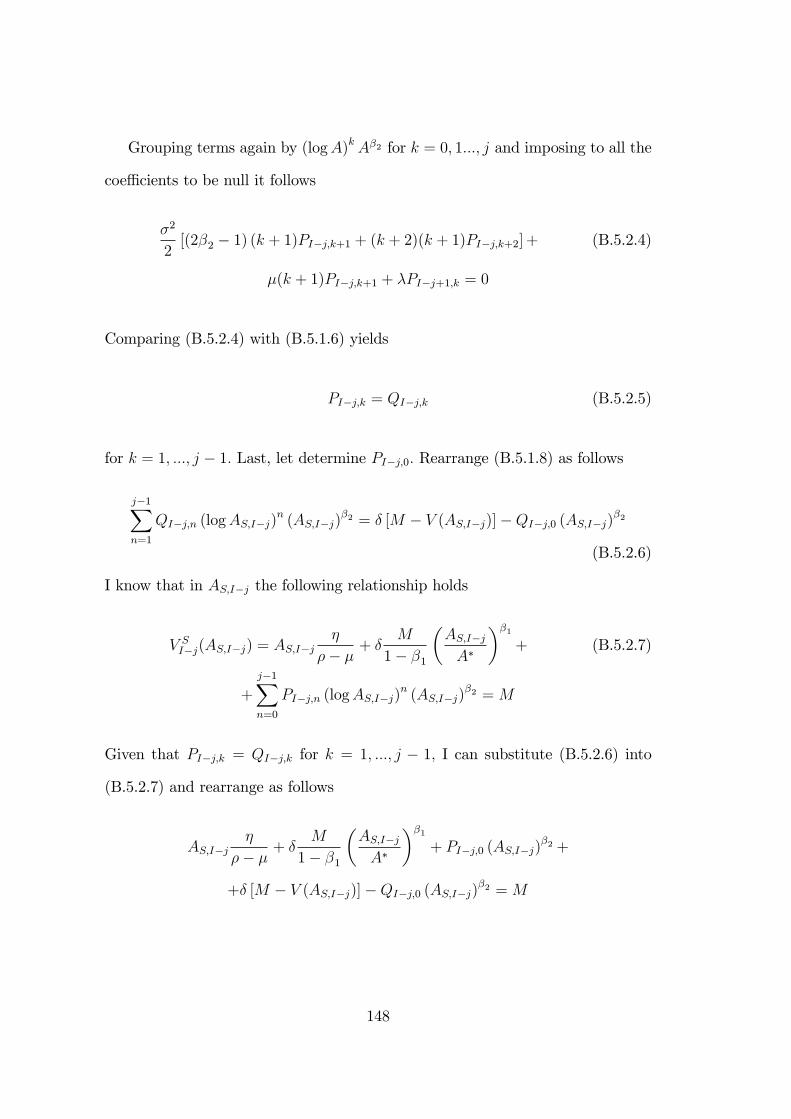
Grouping terms again by (logA)k A�2 for k = 0; 1:::; j and imposing to all the

coe¢ cients to be null it follows

�2

2[(2�2 � 1) (k + 1)PI�j;k+1 + (k + 2)(k + 1)PI�j;k+2] + (B.5.2.4)

�(k + 1)PI�j;k+1 + �PI�j+1;k = 0

Comparing (B.5.2.4) with (B.5.1.6) yields

PI�j;k = QI�j;k (B.5.2.5)

for k = 1; :::; j � 1: Last, let determine PI�j;0: Rearrange (B.5.1.8) as follows

j�1Xn=1

QI�j;n (logAS;I�j)n (AS;I�j)

�2 = � [M � V (AS;I�j)]�QI�j;0 (AS;I�j)�2

(B.5.2.6)

I know that in AS;I�j the following relationship holds

V SI�j(AS;I�j) = AS;I�j�

�� � + �M

1� �1

�AS;I�jA�

��1+ (B.5.2.7)

+

j�1Xn=0

PI�j;n (logAS;I�j)n (AS;I�j)

�2 =M

Given that PI�j;k = QI�j;k for k = 1; :::; j � 1; I can substitute (B.5.2.6) into

(B.5.2.7) and rearrange as follows

AS;I�j�

�� � + �M

1� �1

�AS;I�jA�

��1+ PI�j;0 (AS;I�j)

�2 +

+� [M � V (AS;I�j)]�QI�j;0 (AS;I�j)�2 =M

148

and after a bit of algebra I determine

PI�j;0 = QI�j;0 + (1� �)�M � AS;I�j

�+ �� �

�(AS;I�j)

��2 (B.5.2.8)

Appending the standard boundary conditions to V SI�j(A) one can derive �nally

AS;I�j = AS;i+1:

149

150

Appendix C

Appendix to Chapter 4

C.1 Strategies under sophisticated belief

Rearrange equation (4.11) as

1

2�2A2

@2V S(A; ~A)

@A2+ �A

@V S(A; ~A)

@A� (�+ �)V S(A; ~A) = (C.1.1)

�"A

�1 +

��

�� �

�+ ��

M

1� �1

�A~A

��1#for A � ~A

The solution to the homogenous part is1

V S(A; ~A) = k2A�2

Suppose that the particular solution takes the form V Sp (A;~A) = c1A

�1 + c2A:

Plug this candidate@V Sp (A;

~A)

@A= �1c1A

�1�1+c2 and@2V Sp (A;

~A)

@A2= (�1 � 1) �1c1A�1�2

1The solution should have the form V Sh (A;~A) = k1A

�2 + k2A�2 where k1 and k2 are co-

e¢ cients to be speci�ed and �2 > 0 and �2 < 0 are the roots of the characteristic equation�2�(�� 1)=2+��� (�+ �) : As A!1; the value of the option to harvest (V Sh (A; ~A)) shouldgo to zero. Since �2 > 0 then k1 must be zero because if not V Sh (A; ~A)!1 as A!1:

151

into (C.1.1)

1

2�2A2 (�1 � 1) �1c1A�1�2 + �A

��1c1A

�1�1 + c2�+

� (�+ �)�c1A

�1 + c2A�= �

"A

�1 +

��

�� �

�+ ��

M

1� �1

�A~A

��1#

and solve for the undetermined coe¢ cients

�1

2�2 (�1 � 1) �1 + ��1 � �

�c1 � �c1 = ��� M

1� �1

�1~A

��1[�� (�+ �)] c2 = �

�1 +

��

�� �

�

The candidate solution satis�es (C.1.1) if the following parameter are set

c1 =�M

1� �1

�1~A

��1c2 =

�1 +

��

�� �

�1

(�+ �� �) =�

�� �

The particular solution is then

V Np (A) =�M

1� �1

�A~A

��1+ A

�

�� �

The general solution is given by the sum of V Sh (A; ~A) and VSp (A; ~A)

V N(A) = k2A�2 +

�M

1� �1

�A~A

��1+ A

�

�� � (C.1.2)

At the critical amenity value, AN , the value-matching and smooth-pasting con-

ditions respectively require V S(H( ~A); ~A) = M and @V S(H( ~A); ~A)@A

= 0: Solving the

152

system 8><>: k2(H( ~A))�2 + �M

1��1

�H( ~A)~A

��1+H( ~A) �

��� =M

k2�2(H( ~A))�2�1 + �M �1

1��1

�H( ~A)~A

��1 1H( ~A)

+ ���� = 0

yields

H( ~A) =

24 �2�2 � 1

� � �2 � �1(1� �1) (�2 � 1)

H( ~A)~A

!�135M ��� ��

�

V S(H( ~A); ~A) =M

1� �2

241� � H( ~A)~A

!�135� A

H( ~A)

��2+�M

1� �1

�A~A

��1+ A

��

�� �

�for A > ~A

Finally imposing the intra-personal steady-state condition H(AS) = AS and

V S(A;AS) = VS(A) the solution follows

AS =

��2

�2 � 1� � �2 � �1

(1� �1) (�2 � 1)

�M

��� ��

�V S(A) = M

"1� �1� �2

�A

AS

��2+

�

1� �1

�A

AS

��1#+ A

��

�� �

�

C.2 Pigovian taxation

The regulator�s rule is given by

E�T S�� T = m (C.2.1)

First, recall that � < �2=2 and that by (4.19) E(T S) = 22���2 ln

�ASA0

�: Second,

If a pigovian tax is levied on M then

ATS =�1� �S

�[(1� �)A�� + �A�]

153

Substitution into (C.2.1) yields

2

2�� �2 ln�ATSA0

�= T +m (C.2.2)

ln

�ATSA0

�=

��� �

2

2

��T +m

��1� �S

�AS = A0e

����2

2

�(T+m)

�S = 1� A0ASe���2

2���(T+m)

We prove now that if �S is determined not considering the behavioural failure

then E�T S�<�T +m

�: Suppose is given by

�S = 1� A0A�e

����2

2

�(T+m)

If this is the case then

E�T S�=

2

2�� �2 ln

0@ A0A� e

���2

2���(T+m)AS

A0

1A=

2

2�� �2 ln�ASA�e���2

2���(T+m)

�=

2

2�� �2

����2

2� �

��T +m

�+ ln

�ASA�

��=

�T +m

�+

2

2�� �2 ln�ASA�

�<�T +m

�

154

Bibliography

[1] Arguedas, C., G. Meijerink and D.P. van Soest, 2007. Biodiversity conser-

vation, asymmetric information and the role of �xed costs. Tilburg, Tilburg

University.

[2] Arrow, K.J. and A.C. Fisher, 1974. Environmental preservation, uncertainty

and irreversibility. Quarterly Journal of Economics, 88, 312-319.

[3] Atje, R. and K. Roesad, 2004. Who should own Indonesia�s forests?: Explor-

ing the links between economic incentives, property rights and sustainable

forest management. WPE 076. Jakarta, Indonesia: Centre for Strategic and

International Studies. Available at http://www.csis.or.id/papers/wpeO76.

[4] Bagnoli, M. and T. Bergstrom, 1989. Log-concave probability and its appli-

cations. CREST WP # 89-23, University of Michigan.

[5] Baron, D. and R. Myerson, 1982. Regulating a monopolist with unknown

costs. Econometrica, 50, 911-930.

[6] Barro, R., 1999. Laibson meets Ramsey in the neoclassical growth model.

Quarterly Journal of Economics. 114, 4, 1125-52.

[7] Breccia, A. and H. Salgado-Banda, 2005. Competing or colluding in a sto-

155

chastic framework. Birkbeck Working Papers in Economics and Finance

0504, Birkbeck, School of Economics, Mathematics & Statistics.

[8] Brennan, M.J. and E.S. Schwartz, 1985. Evaluating natural resource invest-

ments. Journal of Business, 58, 135-157.

[9] Brocas, I. and J.D. Carrillo, 2005. A theory of haste. Journal of Economic

Behavior and Organization , 56(1), 1-23.

[10] Brocas, I. and J.D. Carrillo, 2004. Entrepreneurial Boldness and Excessive

Investment. Journal of Economics and Management Strategy, 13 (2), 321�

350.

[11] Brocas, I. and J.D. Carrillo, 1998. A theory of haste with applications to

impulse buying and destruction of the environment. CEPRDP 2027, London.

[12] Brunnschweiler, C. N. and E. H. Bulte, 2008. The natural resource curse

revisited and revised: a tale of paradoxes and red herrings. Journal of Envi-

ronmental Economics and Management, forthcoming.

[13] Bulte, E., D.P. van Soest, G.C. van Kooten and R.A. Schipper, 2002. Forest

Conservation in Costa Rica When Nonuse Bene�ts Are Uncertain but Rising.

American Journal of Agricultural Economics, 84, 150�60.

[14] Clark, E., 2003. Pricing the cost of expropriation risk. Review of Interna-

tional Economics, 11, 412-422.

[15] Clark, E., 1997. Valuing political risk. Journal of Internation Money and

Finance, 16, 477-490.

[16] Clarke, H.R. and W.J. Reed, 1989. The tree-cutting problem in a stochastic

environment. Journal of Economic Dynamics and Control, 13, 569-595.

156

[17] Conrad, J.M., 2000. Wilderness: options to preserve, extract, or develop.

Resource and Energy Economics, 22 (3), 205-219.

[18] Conrad, J.M., 1997. On the option value of old-growth forest. Ecological

Economics, 22, 97-102.

[19] Conrad, J.M., 1980. Quasi-option value and the expected value of informa-

tion. Quarterly Journal of Economics, 95, 813-820.

[20] Cox, D.R. and H.D. Miller, 1965. The theory of stochastic process. London:

Chapman and Hall.

[21] Crépin, A., 2005. Incentives for wetland creation. Journal of Environmental

Economics and Management, 50, 598�616.

[22] Dasgupta, P.S., P.J. Hammond and E.S. Maskin, 1979. The implementation

of social choice rules: some results on incentive compatibility. Review of

Economic Studies, 46, 185-216.

[23] Dasgupta, P.S. and E.S. Maskin, 2005. Uncertainty and hyperbolic discount-

ing. American Economic Review, 95 (4), 1290-1299.

[24] Dixit, A.K. and R.S. Pindyck, 1994. Investment under uncertainty. Princeton

University Press, Princeton, NJ.

[25] Dixit, A.K., 1993. The art of smooth pasting. Chur, CH: Harwood Academic

Publisher.

[26] Di Corato, L., 2007. Optimal harvesting under imperfect intergenerational

altruism. Mimeo, University of Padua.

157

[27] Dosi, C. and M. Moretto, 1997. Pollution accumulation and �rm incentives

to accelerate technological change under uncertain private bene�ts. Environ-

mental and Resource Economics, 10, 285-300.

[28] Dosi, C. and M. Moretto, 1996. Toward green technologies: switching rules

and environmental policies. Rivista Internazionale di Scienze Economiche e

Commerciali, 43, 13-30.

[29] Engel, E. and R. Fischer, 2008. Optimal resource extraction contracts under

threat of expropriation. NBER Working Paper No. W13742. Available at

SSRN: http://ssrn.com/abstract=1086993.

[30] Ferraro, P.J. and A. Kiss, 2002. Direct payments for biodiversity conserva-

tion. Science, 298, 1718-1719.

[31] Ferraro, P.J., 2001. Global habitat protection: limitations of development in-

terventions and a role for conservation performance payments. Conservation

Biology, 15 (4), 1-12.

[32] FONAFIFO, 2000. El desarollo del sistema Pago de Servicios Ambientales

en Costa Rica. San José, Costa Rica: Fondo Nacional de Financiamiento

Forestal (FONAFIFO).

[33] Frederick, S., G. Loewenstein and T. O�Donoghue, 2002. Time discounting

and time preference: a critical review. Journal of Economic Literature, 40

(2), 351-401.

[34] Goeschl, T. and T. Lin, 2004. Endogenous information structures in envi-

ronmental contracting. Sta¤Paper No. 479, Department of Agricultural and

Applied Economics, University of Wisconsin-Madison.

158

[35] Grenadier, S.R. and N. Wang, 2007. Investment under uncertainty and time-

inconsistent preferences. Journal of Financial Economics, 84, 2�39.

[36] Groves, T., 1973. Incentive in teams. Econometrica, 41, 617-631

[37] Guesnerie, R. and J.J. La¤ont, 1984. A complete solution to a class of

Principal-Agent problems with an application to the control of a self-

managed �rm. Journal of Public Economics, 25, 329-369.

[38] Guasch, J.L., J.J. La¤ont and S. Straub, 2003. Renegotiation of concession

contracts in Latin America. Policy Research Working Paper Series 3011, The

World Bank, revised.

[39] Hajzler, C., 2007. Expropriation of foreign direct investments, 1990-2006.

Unpublished Paper, University of Western Ontario.

[40] Harsany, J., 1977. Rational behaviour and bargaining equilibrium in games

and social situations. Cambridge, Cambridge University Press.

[41] Harris, C. and D. Laibson, 2004. Instantaneous grati�cation. Working paper,

Harvard University.

[42] Heal, G.M., 1998. Valuing the Future: economic theory and sustainability.

Columbia University Press.

[43] Harrison, M. J., 1985. Brownian motion and stochastic �ow systems. New

York: Wiley.

[44] Henry, C., 1974. Investment decisions under uncertainty: the irreversibility

e¤ect. American Economic Review, 64, 1006-1012.

[45] Hepburn, C.J. and P. Koundouri, 2007. Recent advances in discounting:

Implications for forest economics. Journal of Forest Economics, 13, 169-189.

159

[46] Hepburn, C.J., 2003. Resource collapse and hyperbolic discounting. Discus-

sion Paper 159, Oxford University, Department of Economics.

[47] Insley, M. and K. Rollins, 2005. On solving the multirotational timber har-

vesting problem with stochastic prices: a linear complementarity formula-

tion. American Journal of Agricultural Economics, 87 (3), 735�755.

[48] Kassar, I. and P. Lasserre, 2004. Species preservation and biodiversity value:

a real options approach. Journal of Environmental Economics and Manage-

ment, 48(2), 857-879.

[49] Kobrin, S. J., 1984. Expropriations as an attempt to control foreign �rms in

LDCs: trends from 1960 to 1979. International Studies Quarterly, vol. 28, 3,

329-348.

[50] La¤ont, J.J. and D. Martimort, 2002. The theory of incentives: the Principal-

Agent model. Princeton University Press.

[51] Laibson, D., 1996. Hyperbolic discounting, undersaving, and savings policy.

NBER Working Paper No. 5635.

[52] Laibson, D., 1997. Golden eggs and hyperbolic discounting. Quarterly Jour-

nal of Economics, 62 (2), 443-478.

[53] Loewenstein, G. and D. Prelec, 1992. Anomalies in intertemporal choice:

evidence and an interpretation. Quarterly Journal of Economics, 107, 573-

598.

[54] Luttmer, E. and T. Mariotti, 2003. Subjective discounting in an exchange

economy. Journal of Political Economy, 111, 959�989.

160

[55] Mirrlees, J.A., 1971. An exploration in the theory of optimum income taxa-

tion. Review of Economic Studies, 38, 175-208.

[56] Motte, E., J.M. Salles and L. Thomas, 2004. Information asymmetry and

incentive policies to farmers for conserving biodiversity in forested areas in

developing countries. Montpellier, LAMETA, mimeo.

[57] Mcdonald, R. and D. Siegal, 1986. The value of waiting to invest. Quarterly

Journal of Economics, 101, 707-728.

[58] Merton, R.C., 1998. Applications of option-pricing theory: twenty-�ve years

later. American Economic Review, 88, 323-349.

[59] Minor, M. S., 1994. The demise of expropriation as an Instrument of LDC

Policy, 1980-1992. Journal of International Business Studies, vol. 25, 1, 177-

188.

[60] Mahajan, A., 1990. Pricing expropriation risk. Financial Management, 19,

77-86.

[61] Moretto, M. and G. Rossini, 1996. Pro�t sharing regulation and repeated

bargaining with a shut-down option. Review of Economic Design, 2, 1, 339-

368.

[62] Moretto, M. and G. Rossini, 1995. The shut-down option and pro�t sharing.

Journal of Comparative Economics 21, 154-186.

[63] Moretto, M. and P. Valbonesi, 2007. Firm regulation and pro�t sharing: a

real option approach. The B.E. Journal of Economic Analysis and Policy,

vol.7, 1 (Topics), Article 56.

[64] Nash, J., 1950. The bargaining problem. Econometrica, vol. 18, 2, 155-162.

161

[65] O�Donoghue, T. and M. Rabin, 1999. Doing it now or later. American Eco-

nomic Review, 89, 103-124.

[66] OECD, 1999. Handbook of incentive measures for biodiversity: design and

implementation, OECD, Paris.

[67] Pagiola, S., P. Agostini , J. Gobbi , C. de Haan, M. Ibrahim, E. Murgueitio,

E. Ramírez, M. Rosales and J.P. Ruíz, 2004. Paying for biodiversity conser-

vation services in agricultural landscapes. Environment Department Paper

No. 96. Washington: World Bank.

[68] Pagiola, S., N. Landell-Mills and J. Bishop, 2002. Making market-based

mechanisms work for forests and people. In Pagiola, S., J. Bishop and

N. Landell-Mills (eds.), Selling forest environmental services: market-based

mechanisms for conservation and development. London: Earthscan.

[69] Phelps, E. S. and R.A. Pollak, 1968. On second-best national saving and

game equilibrium growth. Review of Economic Studies, 35, 185-199.

[70] Pollak, R.A., 1968. Consistent Planning. Review of Economic Studies, 35

(2), 201-208.

[71] Reed, W.J., 1993. The decision to conserve or harvest old-growth forest.

Ecological Economics, 8, 45�69.

[72] Rubinstein, A., 2003. Economics and psychology? The case of hyperbolic

discounting. International Economic Review 44 (4), 1207-1216.

[73] Salanie, F. and N. Treich, 2006. Over-savings and hyperbolic discounting.

European Economic Review, 50 (6), 1557-1570.

162

[74] Salzman, J.E., 2005. Creating markets for ecosystem services: notes from the

�eld. New York University Law Review, vol. 80, no. 6. Available at SSRN:

http://ssrn.com/abstract=796772.

[75] Schnitzer, M., 1999. Expropriation and control rights: a dynamic model of

foreign direct investment. International Journal of Industrial Organization,

vol. 17, 8, 1119-1137.

[76] Shogren, J.F., 2007. Behavior in forest economics. Journal of Forest Eco-

nomics, 12, 233-235.

[77] Smith, R. and J. Shogren, 2002. Voluntary incentive design for endangered

species protection. Journal of Environmental Economics and Management,

43, 169-187.

[78] Smith, R., 1995. The Conservation Reserve Program as a least-cost land

retirement mechanism. American Journal of Agricultural Economics, 77, 93-

105.

[79] Strotz, R.H., 1956. Myopia and inconsistency in dynamic utility maximiza-

tion. Review of Economic Studies, 23, 165-80.

[80] Tomz, M. and M. Wright, 2007. Sovereign theft: theory and evi-

dence about default and expropriation. Paper presented at the Con-

ference on Populism in Natural Resoruces, held at the Kennedy

School of Government, Harvard University, 1-2 November 2007.

Available at http://ksghome.harvard.edu/~whogan/Populism_Nat_Res/

Populism_Agenda_�les/TomzWrightExpropriationDefault.pdf

[81] White, B., 2002. Designing voluntary agri-environmental policy with hidden

163

information and hidden action: a note. Journal of Agricultural Economics,

53, 353-360.

[82] World Bank, 2000. Ecomarkets Project: project appraisal document. Report

No. 20434-CR. Washington: World Bank.

[83] Wu, J. and B.A. Babcock, 1996. Contract design for the purchase of environ-

mental goods from agriculture. American Journal of Agricultural Economics,

78, 935-945.

[84] http://en.wikipedia.org/wiki/Old_growth_forest

164