University of Arkansas, Fayetteville University of Arkansas, Fayetteville ScholarWorks@UARK ScholarWorks@UARK Graduate Theses and Dissertations 8-2019 Essays on Human Capital Formation in Developing Countries Essays on Human Capital Formation in Developing Countries Alexander Sergeevich Ugarov University of Arkansas, Fayetteville Follow this and additional works at: https://scholarworks.uark.edu/etd Part of the Behavioral Economics Commons, Economic Theory Commons, Education Economics Commons, Growth and Development Commons, and the Labor Economics Commons Citation Citation Ugarov, A. S. (2019). Essays on Human Capital Formation in Developing Countries. Graduate Theses and Dissertations Retrieved from https://scholarworks.uark.edu/etd/3349 This Dissertation is brought to you for free and open access by ScholarWorks@UARK. It has been accepted for inclusion in Graduate Theses and Dissertations by an authorized administrator of ScholarWorks@UARK. For more information, please contact [email protected].

Welcome message from author
This document is posted to help you gain knowledge. Please leave a comment to let me know what you think about it! Share it to your friends and learn new things together.
Transcript
University of Arkansas, Fayetteville University of Arkansas, Fayetteville
ScholarWorks@UARK ScholarWorks@UARK
Graduate Theses and Dissertations
8-2019
Essays on Human Capital Formation in Developing Countries Essays on Human Capital Formation in Developing Countries
Alexander Sergeevich Ugarov University of Arkansas, Fayetteville
Follow this and additional works at: https://scholarworks.uark.edu/etd
Part of the Behavioral Economics Commons, Economic Theory Commons, Education Economics
Commons, Growth and Development Commons, and the Labor Economics Commons
Citation Citation Ugarov, A. S. (2019). Essays on Human Capital Formation in Developing Countries. Graduate Theses and Dissertations Retrieved from https://scholarworks.uark.edu/etd/3349
This Dissertation is brought to you for free and open access by ScholarWorks@UARK. It has been accepted for inclusion in Graduate Theses and Dissertations by an authorized administrator of ScholarWorks@UARK. For more information, please contact [email protected].
Essays on Human Capital Formation in Developing Countries
A dissertation submitted in partial fulfillmentof the requirements for the degree ofDoctor of Philosophy in Economics
by
Alexander UgarovLomonosov Moscow State University
Bachelor of Science in Economics, 2002Lomonosov Moscow State UniversityMaster of Science in Economics, 2004
August 2019University of Arkansas
This dissertation is approved for recommendation to the Graduate Council.
Arya Gaduh, Ph.D.
Dissertation Director
Robert Costrell, Ph.D. Gary Ferrier, Ph.D.
Committee Member Committee Member

Abstract
Differences in human capital explain approximately one-half of the productivity vari-
ation across countries. Therefore, we need to understand drivers of human capital accumu-
lation in order to design successful development policies. My dissertation studies formation
and use of human capital with emphasis on its less tangible forms, including skills, abilities
and know-how.
The first chapter of my dissertation explores the effects of occupational and educational
barriers on human capital stock and aggregate productivity. I find that students’ academic
skills have very small impact on occupational choice in most developing countries. This
finding suggests a higher incidence of occupational barriers in developing countries. I
evaluate the productivity losses resulting from occupational barriers by calibrating a general
equilibrium model of occupational choice. According to my estimation, developing countries
can increase their GDP by up to twenty percent by reducing the barriers to the level of a
benchmark country (US).
In the second chapter of my dissertation, I study the effects of economic growth on
education quality. Several models of human capital accumulation predict that incomes have
a positive causal effect on human capital for given levels of education by increasing the
consumption of educational goods. The paper tests this prediction by using a within country
variation in incomes per-capita across different cohorts of US immigrants. Wages of US
migrants conditional on years of education serve as a measure of education quality. I find
that average domestic incomes experienced by migrants in age from zero to twenty years
have a significant positive effect on their future earnings in the US.
The third chapter studies the effects of employee-driven technology spillovers on tech-
nology adoption. It challenges the theoretical result of Franco and Filson (2006) by assuming
that workers are risk averse and that the number of competitors is finite. In this more realistic
scenario spillovers significantly reduce payoffs from adopting advanced technologies.

©2019 by Alexander UgarovAll Rights Reserved

Acknowledgments
I am deeply grateful to my advisor Prof. Arya Gaduh for continued guidance and
support throughout my last four years at the University of Arkansas. Most of all, I am
grateful for the opportunity to freely pursue questions of my own choice but also for words
of encouragement whenever these choices led me to a roadblock. The dissertation would not
have a chance to take its current shape without my advisor’s inputs.
I want to express my gratitude to other committee members who also contributed to
this work. I am grateful to Prof. Robert Costrell for writing a very inspiring 2004 paper
with Glenn Loury which helped me to create first drafts of the theoretical model in the first
chapter. I also need to thank Robert Costrell for thoughtful comments on early drafts of my
job market paper and for proofreading parts of this dissertation. My gratitude also extends
to Gary Ferrier for numerous comments during research seminars and for proofreading the
dissertation and suggesting a multitude of small improvements.
Several University of Arkansas faculty members provided very valuable comments on
parts of this dissertation. In particular, I want to thank Professors Dongya Koh, Andrew
Horowitz, and Difei Geng. I want to thank Professor Galina Vereshchagina (Arizona State)
for proofreading and making valuable suggestions on the early draft of the third chapter in
my dissertation. The dissertation also benefited from comments and suggestions made by
participants of several professional conferences including AEA2018 and MEA2017 and from
comments of anonymous referees at the Journal of Economic Growth.

Contents
Introduction . . . . . . . . . . . . . . . . . . . . . . . . . . . . . . . . . . . . . 1
Chapter 1: Talent Misallocation across Countries: Evidence from
Educational Achievement Tests . . . . . . . . . . . . . . . . . . . . . 3
1 Abstract . . . . . . . . . . . . . . . . . . . . . . . . . . . . . . . . . . . . . 3
2 Introduction . . . . . . . . . . . . . . . . . . . . . . . . . . . . . . . . . . . 3
3 The Importance of Skills . . . . . . . . . . . . . . . . . . . . . . . . . . . . 8
4 Validity of Occupational Sorting Measures . . . . . . . . . . . . . . . . . . 12
5 Model . . . . . . . . . . . . . . . . . . . . . . . . . . . . . . . . . . . . . . 20
6 Inference . . . . . . . . . . . . . . . . . . . . . . . . . . . . . . . . . . . . . 26
7 Results . . . . . . . . . . . . . . . . . . . . . . . . . . . . . . . . . . . . . . 34
8 Conclusion . . . . . . . . . . . . . . . . . . . . . . . . . . . . . . . . . . . . 38
9 Bibliography . . . . . . . . . . . . . . . . . . . . . . . . . . . . . . . . . . . 41
10 Appendix . . . . . . . . . . . . . . . . . . . . . . . . . . . . . . . . . . . . 44
Chapter 2: Income Effects on Education Quality . . . . . . . . . . . . 54
1 Abstract . . . . . . . . . . . . . . . . . . . . . . . . . . . . . . . . . . . . . 54
2 Introduction . . . . . . . . . . . . . . . . . . . . . . . . . . . . . . . . . . . 54
3 When Do Incomes Affect Education Quality? . . . . . . . . . . . . . . . . . 57
4 Identification Approach . . . . . . . . . . . . . . . . . . . . . . . . . . . . . 60
5 Data . . . . . . . . . . . . . . . . . . . . . . . . . . . . . . . . . . . . . . . 65
6 Results . . . . . . . . . . . . . . . . . . . . . . . . . . . . . . . . . . . . . . 67
7 Robustness . . . . . . . . . . . . . . . . . . . . . . . . . . . . . . . . . . . . 71

8 Conclusion . . . . . . . . . . . . . . . . . . . . . . . . . . . . . . . . . . . . 74
9 Bibliography . . . . . . . . . . . . . . . . . . . . . . . . . . . . . . . . . . . 76
10 Appendix . . . . . . . . . . . . . . . . . . . . . . . . . . . . . . . . . . . . 78
Chapter 3: Technology Spillovers and Suboptimal Rent Sharing . . 85
1 Abstract . . . . . . . . . . . . . . . . . . . . . . . . . . . . . . . . . . . . . 85
2 Introduction . . . . . . . . . . . . . . . . . . . . . . . . . . . . . . . . . . . 85
3 Model . . . . . . . . . . . . . . . . . . . . . . . . . . . . . . . . . . . . . . 89
4 Quantitative Analysis . . . . . . . . . . . . . . . . . . . . . . . . . . . . . . 105
5 Conclusion . . . . . . . . . . . . . . . . . . . . . . . . . . . . . . . . . . . . 117
6 Bibliography . . . . . . . . . . . . . . . . . . . . . . . . . . . . . . . . . . . 119
7 Appendix . . . . . . . . . . . . . . . . . . . . . . . . . . . . . . . . . . . . 121
Conclusion . . . . . . . . . . . . . . . . . . . . . . . . . . . . . . . . . . . . . . 135

Introduction
The richest five percent of countries have approximately fifty times higher GDP per
capita by purchasing power parity as compared to the poorest five percent of countries (Jones,
2014). Differences in human capital explain approximately half of this gap with roughly equal
proportions corresponding to education quantity (years) and education quality (Schoellman,
2012; Manuelli and Seshadri, 2014). These calculations put the contribution of human capital
in front of both physical capital and technologies. Therefore, we need to understand drivers
of human capital accumulation in order to design successful development policies.
Three chapters of my dissertation study different aspects of formation and use of human
capital in developing countries. This topic is far from being new, but existing literature tends
to concentrate on more easily observable educational achievements or years of education as
a measure of human capital. In contrast, my research contributes to the emerging literature
on less tangible forms of human capital accumulation such as skills, abilities and know-how.
The first chapter of my dissertation studies the effects of occupational and educational
barriers on human capital stock and aggregate productivity. I use PISA data on on expected
occupational choice of students to measure the magnitude of these barriers and their impact
on aggregate productivity. In most developing countries students’ academic skills have
very small impact on occupational choice , which is consistent with a higher incidence of
occupational barriers. Next, I evaluate the efficiency losses associated with occupational
barriers by calibrating a model of occupational choice based on the Roy (1951) framework.
The effects of occupational barriers on productivity are relatively modest. According to my
estimation, developing countries in my sample can increase the agrregate productivity by up
to twenty percent by reducing the barriers to the level of a benchmark country (US).
In the second chapter of my dissertation, I study the effects of economic growth on
education quality. Several models of human capital accumulation predict that incomes have
a positive causal effect on human capital for given levels of education by increasing the
consumption of educational goods. The paper tests this prediction by using a within country
1

variation in incomes per-capita across different cohorts of US immigrants. Wages of US
migrants conditional on years of education serve as a measure of education quality. I find
that average domestic incomes experienced by migrants when they were growing up (0-20yr
old) indeed have a significant positive effect on their future earnings in the US for migrants
at all education levels.
My third chapter studies the effects of employee-driven technology spillovers on incen-
tives for technology adoption. It challenges the theoretical result of Franco and Filson (2006)
by assuming that the workers face liability constraints and the number of competitors is finite.
I find that if a gap between old and new technology is large enough, technology spillovers
significantly and negatively affect the value from investing in a new technology. Technology
spillovers can also affect the choice of location for high-technology firm or its subsidiary
towards the location with a higher local level of technology. On another hand, conditional
on entry, high-technology forms in presence of spillovers use very efficient employment and
turnover policies. It means that FDI policies affecting the entry decision are more important
compared to the policies directed to stimulate technology transfer from existing firms.
2

Chapter 1: Talent Misallocation across Countries: Evidence from Educa-
tional Achievement Tests
1 Abstract
Despite growing evidence on occupational and educational barriers in developing coun-
tries, there are few estimates of their effect on the aggregate productivity. This paper
measures the magnitude of these barriers and their impact on aggregate productivity using
the data on expected occupational choice of students. First, I document striking differences
in the impact of students’ academic skills on occupational choice across countries. In most
developing countries academic skills of students have relatively little effect on skill intensity
or earning potential of expected occupations. The observed lower sorting on skills suggests
a higher incidence of occupational barriers in developing countries. Next, I evaluate the
productivity costs of these sorting patterns by attributing them to latent occupational
barriers and calibrate a model of occupational choice based on the Roy (1951) framework.
I calibrate the model by combining the data skills and expected occupations from the PISA
database with the data from nationally-representative samples of working adults. I find that
occupational barriers are particularly high in developing countries in my sample and that
their elimination can increase the aggregate output by up to twenty five percent.
2 Introduction
Workers are not always optimally assigned to jobs, because other factors besides skills
and preferences affect job assignment. For example, La Porta et al (1999) find that private
firms are very often led by the relatives of owners, who use poor management practices
(Bloom and van Reenen, 2007). Job referrals can also lower the quality of workers due to
favoritism (Beamer and Magruder, 2012; Fafchamps and Moradu, 2015). Ethnic and caste
discrimination can also lead to the mismatch between worker’s skills, preferences and jobs
(Banerjee and Knight, 1985; Hnatkovska et al, 2012). As evident from these examples, the
3

talent misallocation can result both from the barriers faced by minorities as well as from
more idiosyncratic and more latent barriers, resulting from favoritism and nepotism.
How large are these occupational barriers and how much do they affect the aggregate
productivity? This paper measures the productivity losses resulting from both group-based
and more latent occupational barriers, such as the differences in social connections or credit
constraints in education. The losses resulting from these latent occupational barriers are
harder to measure because we cannot attribute them to a particular group identifiable in
statistics. Nevertheless, it is important to understand their magnitude in order to choose
development policy priorities.
I find that the occupational barriers translate into sizable effects for the aggregate
productivity. For example, Brazil can gain around 20-25% in aggregate output by reducing
the barriers to the US level. This estimate results from a calibration of Roy model of
occupational choice to the combination of Census data and data on cognitive skills and
occupational choice of current high school students. The number includes both short-term
gains of higher ability sorting across occupations and the potential effects of better sorting
on physical and human capital accumulation.
The main piece of motivating evidence for this study comes from the Program of
International Student Assessment (PISA). I find large cross-country differences in the rela-
tionship between academic skills in PISA and expected occupational choice. This difference
in sorting is large enough that one has to apply around 90% random resorting of students
between reported future occupations to move from the highest sorting level (Czech Republic)
to the lowest sorting level in my sample (Costa Rica). The sorting patterns are consistent
whether I consider a single-dimensional ability or a vector of academic and non-cognitive
skills. In developing countries in my sample, academic skills tend to have a lower impact on
occupational choice. Because we know about the large role of cognitive and academic skills
in determining labor market outcomes in developed countries (Gould, 2002; Borghans et al,
2016), the difference in sorting patterns based on skills is highly suggestive of the presence
4

of occupational barriers or differences in technology.
The first part of the paper describes two novel country-level measures of occupational
sorting based on academic skills. These variables reflect the statistical dependency between
students’ skills and their expected occupations in PISA 2015 dataset. I show that the
occupational sorting measures for students have a strong correlation with the occupational
sorting measures for working adults.
In the second part of my paper, I construct and estimate the model of occupational
choice to measure the productivity implications of observed differences in sorting patterns.
The model is based on the Roy (1951) framework with Frechet-distributed skills (talents) in
professional and non-professional occupations. The model includes occupational barriers in
the form of a random event preventing a worker from taking a professional occupation.
I calibrate the model’s parameters by using the combination of representative samples of
working adults and PISA data on academic abilities and expected occupations of high school
students for 22 countries. In the first stage, I calibrate the talent distribution parameters
to the longitudinal US data while assuming no occupational barriers. Next, I use the
simulated method of moments to estimate country-specific productivities and the incidence
of occupational barriers for all the countries in my sample. The model provides an almost
perfect fit for the average cognitive skill, wage and employment in each occupational category
for most countries, despite using just four country-specific parameters for six empirical
moments. I find that the incidence of occupational barriers in most developed countries
except for Japan and the Republic of Korea is close to zero. For developing countries, the
calibration implies that up to 70% of individuals are constrained in their occupational choice.
I use the calibrated model to study the productivity gains from reducing the incidence
of occupational barriers to zero. The productivity gains depend both on the incidence of
occupational barriers and on the productivity of professional and non-professional occupa-
tions. According to my calculation, removing occupational barriers results in approximately
23% gain in productivity in Brazil and about 16% in Mexico. The gains for most developed
5

countries do not exceed 7%. I find that the magnitude of productivity effects varies little with
the value of elasticity of substitution between professional and non-professional occupations.
The results also do not significantly change if instead of occupational barriers I use a random
wage distortions model similar to Hsieh et al (2018). As my first-stage calibration to the US
data assumes no frictions, these results can be also interpreted as the lower bound estimates
of productivity gains from reducing the occupational barriers to the level of the US.
My paper contributes to the literature on aggregate effects of talent misallocation.
In contrast to my paper, previous research concentrates on occupational barriers faced by
minorities. For example, Hsieh et al (2018) find that removing occupational barriers for
women and racial minorities explains approximately a quarter of the economic growth in
the US in 1960-2010. Lee (2016) finds that the occupational barriers faced by women in
non-agricultural jobs reduce the output by approximately six percent on average in the
sample of around 60 countries. Mies, Monge-Naranjo and Tapita (2018) measure the barriers
faced by different gender and age groups and also find large productivity losses. This study
potentially captures both the barriers faced by the minorities as well as more latent barriers,
such as credit constraints and family connections on the labor market.
The model in this paper also differs from most other models of talent misallocation
based on the Roy model framework as it allows for correlation between the talents in different
areas. The correlation between talents is usually assumed to equal zero (Lee, 2016; Hsieh et
al, 2018; Mies, Monge-Naranjo and Tapia, 2018), because the identification of the correlation
parameter is problematic in the presence of only wage and occupational choice data. In
this paper, I assume that the individual’s performance on PISA academic proficiency test
represents one of the talents. This assumption allows me to use the distribution of test
scores in each occupational group to identify the correlation between talents. I find that the
correlation between talents is positive and that its value strongly affects my results.
The second contribution of the paper is the measurement of the role of academic skill in
occupational sorting for a large set of developed and developing countries. Until 2012 most
6

studies of skill effects on wages and occupational choice rely on small samples from developed
countries (Neal and Johnson, 1996). In last five years, studies based on new international
datasets demonstrate a large variation in returns to skill in developing countries for adult
respondents (Hanushek et al, 2017). This paper, to my knowledge, is the first to study
the impact of skill as perceived by students making educational decisions, which potentially
differs from the actual returns.
My paper also relates to the credit constraints literature by providing upper bounds on
effects of credit constraints in education. The occupational barriers in this paper potentially
capture the effects of credit constraints in higher education. There is no widely accepted view
on the incidence and effects of credit constraints in the USA with most studies finding no
effect (Kean and Wolpin, 2001) or moderate effects (Brown, Scholz and Seshadri, 2012). The
evidence for developing countries is even scarcer but tends to find more significant barriers
(Attanasio and Kaufmann, 2009). Consistent with most of the previous literature, I find
that the incidence of all kinds of occupational barriers, including the barriers resulting from
credit constraints, is low in developed countries. On other hand, my findings are consistent
with a large role of credit constraints in a few developing countries in my sample.
The rest of the paper is organized as follows. In Section 2, I describe the construction
of occupational sorting measures. It starts with explaining the logic of occupational sorting
measures in the subsection 2.1. The second subsection explains the procedures and the data
used to construct the variables. In subsection 2.2, I analyze the alternative explanations
for the variation in measures which do not involve the actual occupational sorting. I
also demonstrate the correlation between the sorting measures based on PISA scores with
similar measures constructed on the adults’ sample. The concluding subsection analyzes the
correlation of my measures with other measures of inequality and social mobility as well as
with different variables which previous literature expects to correlate with the occupational
sorting. Section 4 sets up the theoretical model and describes the calibration approach.
Section 5 describes the effects of occupational barriers on productivity differences and the
robustness of my results to different modeling choices and calibration approaches.
7

3 The Importance of Skills
3.1 Intuition
In this section, I construct two country-level measures of occupational sorting based on
academic skill. The objective is two-fold. First, I want to construct occupational sorting
measures that can reveal any cross-country differences in efficiencies of labor sorting across
countries. Second, it can be used to limit the choice of sorting and matching models in the
future to make models more consistent with new empirical evidence.
Both measures describe sorting across occupations based on skills. Most single-index
matching models of job assignments (Sattinger, 1979; Costrell and Loury, 2004) predict
either positive assortative matching or negative assortative matching with skill perfectly
predicting job assignment in both cases. Noisier or weaker sorting in this setup indicates
the mismatch between skills and jobs. For example, the productivity of a surgeon is more
sensitive to his cognitive skills than the productivity of a janitor. If in some country A,
low-skilled individuals become surgeons, while high-skilled individuals become janitors, the
output of country A reduces relative to its potential output. My measures of occupational
sorting will be low in country A as skills there have only a small impact on the occupational
choice.
For each country I measure the dependency between academic skills and future occu-
pations for the representative sample of high school students. These measures differ from
the returns to skill (Hanushek, 2017) in two key aspects. First, instead of labor incomes
my variables use occupations as the main labor market outcome variable. Second, my
measures rely on expected self-reported outcomes instead of actual outcomes. By using
high school students my approach eliminates the confounding reverse effect of occupation
on cognitive skill resulting from high-skilled workers receiving more on-the-job training in
cognitive tasks. Instead, PISA measures the academic skill for individuals at the same stage
of life with relatively homogeneous backgrounds. It allows me to interpret the variation in
achievement scores more as a difference in actual abilities rather than a difference in skills
8

used in workplace.
3.2 Data
My main data comes from the Program for International Student Assessment (PISA) 2015
micro dataset. The Program conducts the survey of skills, background, and attitudes of
15-year old high school students. The 2015 dataset covers 72 countries, including at least 40
developing countries. On average, each country’s sample contains a nationally representative
sample of 7500 students with a maximum of 32330 students for Spain and a minimum of
1398 for Puerto-Rico. The sample is stratified by school with an average of 140 students
coming from each school.
My measures of occupational sorting utilize the students’ self-reported expected occu-
pation and data on their cognitive and non-cognitive skills. The future occupation variable
comes from the responses to the PISA question ”What kind of job do you expect to have when
you are about 30 years old?” Almost 80% of students have indicated some future occupation
with the remaining 20% either giving a vague description, stating no future employment
(housewife, student, unemployed), or answering that they do not know the answer.
PISA also provides the measurement of abilities both through the PISA subject scores
(mathematics, reading and science) and through the psychological self-assessment. For each
subject score PISA reports 10 plausible values. Each plausible value constitutes one random
draw from the conditional distribution of score based on student’s responses. I calculate my
sorting measures for each plausible value separately and then calculate the average.
The dataset also contains three metrics constructed from different self-assessment
questions, which I use to proxy for non-cognitive skills. ”Collaboration and Teamwork
disposition” metric shows the degree to which students enjoy cooperation. ”Student Atti-
tudes, Preferences and Self-related beliefs: Achieving motivation (WLE)” metrics describes
the student’s drive for achievement. Finally the third measure ”Subjective well-being: Sense
of Belonging to School (WLE)” can proxy both for interpersonal skills and for the school
learning atmosphere.
9

3.3 Measuring Occupational Sorting
In this section I construct two measures of dependency between skills and the occupa-
tional choice to capture the occupational sorting based on skills. The first measure is a
single-dimensional Spearman rank correlation between skill and occupational prestige score.
My second measure is the multi-dimensional chi-square (Cramer V) for the dependency
between the achievement scores, motivation, gender and occupations. To my knowledge,
these measures are novel in the literature with the closest analogue being skill mismatch
measures (Sicherman, 1991; Slonimczyk, 2011; Guvenen et al, 2015). In contrast to the
skill mismatch measures, my measures describe not the dependency between current skills
and current occupations, but the dependency between skills close to high school graduation
and the intended occupational choice. It solves the problem of skill endogeneity in which
the occupation chosen affects measured skills. My second measure also allows to study the
sorting based on multiple characteristics of students and does not require any assumptions
on the intensity of skill use in different occupations (in contrast to Guvenen et al, 2015).
Spearman rank correlation. The first approach relies on the assumption that both
skill and occupational assignment can be described by single-dimensional indexes. The first
principal component of student’s reading and mathematics score describes the aggregate
academic skill. I use the ISEI occupational prestige score to proxy for the skill intensity of
different occupations. The occupational prestige score assigns a number to each occupation
according to the combination of average years of education of workers in this occupation
and the average wage. The first measure is the Pearson correlation between the percentile
of a student by skill in the national sample distribution and the percentile of student by the
prestige of expected occupation in the national sample.
Most studies of returns to skill also assume that both skills and labor outcome are
single-dimensional. In these studies numeracy skills or aptitude tests often describe the
skill (Neal and Johnson, 1996; Hanushek et al, 2013), while the wage rate is the outcome
10

variable. The cross-country comparisons also require an assumption that countries have
a similar ranking of occupations by sensitivity of productivity to skill (same occupations
ladder). Using country-specific ranking of occupations based on average incomes in each
occupation does not significantly affect my results as I show in Appendix 1.
Cramer V. If skills are actually multi-dimensional, then using the single-dimensional in-
dexes might indicate a strong skill mismatch in cases when sorting is perfectly optimal
(Lindenlaub, 2016). The second occupational sorting measure instead uses several dimen-
sions to describe skill and do not assume a particular ordering of occupations. It measures
the dependency between the students’ characteristics and their expected occupations. I use
the vector of reading and mathematics scores to describe cognitive skills, and motivation to
describe non-cognitive skills. Then for each of the three skill measures I separate a national
sample into four quartiles. The skill category of a student is a combination of her reading,
mathematics and motivation quintiles as well as gender, giving in total 128 categories. I also
separate all the reported expected occupations into 10 aggregate occupations based on the
digit of occupational code in ISCO-08 classification. The value of the multidimensional index
is equal to the χ2 statistics of dependency between skill and occupation categories scaled to
0-1 range according to the sample size (Cramer V statistic):
V =
√χ2
N min(k − 1, r − 1)
In this equation N corresponds to the sample size, k = 128 is the number of rows (skill
categories) in the correspondence table and r = 10 is the number of columns or occupations.
In contrast to the single-dimensional measure, the multidimensional index does not
rely on the assumption that there is a common ladder of occupations across countries based
on their skill intensity. If, for example, a job of a computer programmer in Poland is more
skill-intensive than a job of a doctor, the multidimensional measure will still be high as long
as high-skilled students want to become programmers rather than doctors. On other hand,
11
this measure hardly relates to actual returns to skill. Even if the best workers sort into the
least demanding jobs, the multidimensional index can still be very high. Both measures vary
from 0 to 1 with 1 indicating the perfect dependency between skills and occupational choice.
For both variables a higher level of dependency indicates a lower level of skill misallocation.
Occupational sorting measures strongly vary between countries in my sample. Czech
Republic has the highest values of both single-dimensional and multidimensional measures,
indicating the highest impact of skills on occupational choice or the lowest skill misallocation.
The correlation between the rank of ability and the occupational prestige rank is equal to
0.58, while the multi-dimensional index (Cramer V) is equal to 0.24. Costa Rica lies on
the other side of the spectrum with the single-dimensional measure equal to 0.05 and the
multi-dimensional measure equal to 0.096. Surprisingly USA lies in the middle of distribution
for both the single-dimensional measure and for the multi-dimensional one.
Two measures of occupational sorting are also highly correlated. The Pearson correla-
tion between the two variables equals to 0.87 (Table 1). This high correlation implies that
the variation in the first single-dimensional measure of occupational sorting does not result
from the variation in prestige of particular occupations or in the role of non-cognitive skills,
as the calculation of multi-dimensional measure does not utilize these assumptions.
4 Validity of Occupational Sorting Measures
Before proceeding to further analysis I need to make sure that my measures of occupa-
tional sorting based on skills and expectations of students indeed describe the occupational
choice of working adults. There are two validity concerns which I need to address in
this section. My first concern is that proficiency scores from some countries contain more
measurement noise which lowers the occupational sorting measures. It can happen if, for
example, students’ in these countries systematically apply less effort on the PISA test. I
test this alternative explanation by considering variation in effort My second concern is that
the variation in occupational sorting is driven by the variation in the accuracy of future
12

job reporting. For example, one can imagine a scenario in which both countries A and
B have same rules for job assignments based on skills, but students in country A perfectly
predict their future occupations, while the predictions of students from country B are close to
random. In this scenario countries would differ in occupational sorting if we measure it based
on students’ reports, but would have same occupational sorting based on actual occupations.
Overall, I find that the measurement noise for cognitive skills has little explanatory power for
my measures, and that the sorting measures based on students’ data correlate with similar
sorting measures for adult workers, supporting the validity of my approach. In the last part
of this section I also consider the correlation between my measures of occupational sorting
and different institutional and economic variables potentially affecting sorting.
4.1 Skill Measurement
First, I study the role of noise in the measurement of academic skills. First, the systematic
variation in measurement noise can come from the variation in students’ effort. Zamarro,
Hitt and Mendez (2016) suggest that the variation in students effort on the test explains at
least one third of cross-country variation in country average PISA scores. This is problematic
for my sorting measures, because if some students put less effort, their scores do not reflect
their academic skills.
To measure the effort, I use the average time taken by students to complete a cognitive
test and the number of skipped answers. I consider an answer to be skipped if it’s not
answered or answered in less than two seconds, assuming that two seconds is not enough
for a thoughtful answer. My analysis does not reveal any systematic relationship between
the average number of skipped answers and the measures of occupational sorting. The
average time to complete the cognitive part also tends to be higher in countries with weaker
sorting on skills. This is the opposite of what one should expect if one tries to explain lower
occupational sorting measures through the lack of effort in answering cognitive questions.
The noise in skill measurement can also result from the fact that each student replies
13

to only a small set of questions, which can not cover the potential knowledge expected from a
high school student. To measure this noise, I use the variation in plausible scores for each of
the three tested academic subjects. I find a weak negative correlation between my measures
of occupational sorting and the dispersion of plausible values for mathematics and a weak
positive correlation for the reading plausible values dispersion. Overall, there is no evidence
that the measurement of knowledge drives the cross-country variation in perceived returns
to skill.
4.2 Occupational Choice Measurement
Do sorting measures for students reflect the actual sorting of working adults? The observed
variation in my occupational sorting measures can result from the noise in reporting of future
occupations because students cannot perfectly predict their preferences and opportunities
in fifteen years from the moment of survey. While my data does not provide a direct way
to measure the discrepancies between expected and reported occupations, I use two indirect
approaches to address this concern. First, I construct the measures of occupational sorting
based on adult workers for a subsample of countries to . Second, I measure the percentage
of uncertain answers for occupations in each country.
I use the data on skills and occupations of working adults from the Programme for the
International Assessment of Adult Competencies (PIAAC) to answer this question. For a
subset of mostly OECD countries PIAAC provides the data on occupations, earnings and
literacy and numeracy skills of adult workers. This dataset allows me to construct the
measure of occupational sorting for working adults and contrast it with already calculated
variables of occupational sorting.
On the first calculation step, I recode the ISCO-8 occupation code into the occupational
prestige index (ISEI) by using ISCOISEI routine for Stata1. Then I calculate the percentile
of each worker in the country’s distribution of occupational prestige to obtain a measure
1Written by J. Hendrickx, https://ideas.repec.org/e/phe38.html
14

of job allocation. The conversion to percentiles pursues the same goal as the conversion
done for the PISA measures: it produces a measure of job assignment which is free from
cross-country differences in occupational distributions.
On the second step, I construct the index of ability, which is equal to the first principal
component of numeracy and literacy skills in PIAAC. The actual measure of occupational
sorting is the Spearman rank correlation between the ability and the occupational prestige
score. I compare the resulting variable with the sorting measures calculated from the PISA
dataset. Table 1 describes the pairwise correlations between the PISA-based misallocation
measures and the PIAAC-based measure for adult workers.
There is a strong and positive correlation between the previously constructed measures
based on PISA and the measures for working adults constructed from the PIAAC data. For
a limited sample of 22 countries for which the data is available both in PIAAC and PISA, the
Pearson correlation coefficient is 0.53 and it is significant at 5%. The correlation between
the single-dimensional measure for working adults and the multi-dimensional measure for
students is also positive, but is relatively weak and not statistically significant for this
sample size. Overall, these calculations suggest that the perceived returns to skill actually
measure some characteristics of actual labor market assignments, whether they result from
employment or educational decisions.
The indirect way to measure the reporting noise in occupations is to use the percentage
of uncertain answers in each country. The percentage of uncertain answers reflects the
quality of information students have about occupations, which determines the level of noise.
The percentage of uncertain answers has a positive and statistically significant, but weak
correlation with my occupational sorting measures. The Pearson correlation is equal to 0.38
for the first single-dimensional measure and 0.31 for the second multi-dimensional measure
(Cramer V).
15

4.3 Correlates of Skill Misallocation
In the first subsection, I demonstrate that there is a wide variation in the role of academic
skills in occupational sorting across countries. What drives these differences?
Here I explore several theories of ability sorting existing in the literature. The goal of
this exercise is not to identify the causal link, but to limit the range of potential explanations
of observed occupational sorting patterns. Pairwise correlations in these regard (Table 2)
fulfill my goal and allow to avoid both multicollinearity and power issues given the small
sample size. Below I consider several potential correlates and determinants of my sorting
measures and describe their fit with the data.
Inequality and Social Mobility. Income inequality as measured by the Gini coeffi-
cient has a very strong and negative correlation with both measures of skill allocation. More
unequal countries tend to have a lower sorting on skills or higher perceived skill misallocation.
The correlation coefficient is equal to -0.69 for the first measure and -0.82 for the second. In
both cases the coefficient is significant at 1% level despite a small sample size of 43 countries.
The correlation also holds on the more uniform subset of European countries.
The observed positive correlation between inequality and occupational sorting is sur-
prising and suggests that the trade-off between inequality of opportunities and inequality
of outcomes (described by Benabou, 2000) is either weak or non-existent in my sample.
In other words, more equal countries have lower inequality of opportunities. This finding
is consistent with the labor matching model of Costrell and Loury(2004), who find that
under some (plausible) assumptions a decrease in quality of information on skill leads to
skill misallocation and higher wage inequality.
Intergenerational elasticity of incomes from Corak (2013) also correlates with my
occupational sorting measures, but these correlations can follow from the known correlation
between the intergenerational income elasticity and the income inequality (Corak, 2006).
The Inequality of Opportunities index (IoP), which is produced by Brunori (2016) for
selected European countries, measures the variance in incomes explained by observable
16

uncontrollable circumstances (such as parental education, parental occupations and gender).
My calculations do not show any significant correlation between the IoP index and the
occupational sorting measures. However, the low significance can be explained by the low
sample size (of only 15 countries).
Educational Institutions. High tuition costs of higher education and borrowing
constraints can prevent some students from getting skilled occupations despite high ability.
I use the government expenditures per tertiary student (UNESCO) as a percentage of GDP
per capita to proxy for tuition costs. My analysis still suggests no significant correlation
between the government expenditures and the sorting measures (Table 2).
I also consider the opportunity that the students’ occupational expectations become
less noisy closer to the graduation. As all students report their occupational choice at the age
of 15, the difference in high school graduation age implies that some students are much closer
to the moment of implementing their occupational decisions. It is then natural to assume
that students which are closer to graduation, are going to report more deliberate choices.
The average graduation age by country (also from UNESCO) accounts for this factor.
The data shows an opposite pattern: countries with a higher graduation age demon-
strate a stronger link between skills and occupational choice. This link, however, does not
hold on the subsample of European countries, suggesting that the correlation might be just
a statistical artifact.
Labor Institutions. Hiring an employee with a right skillset is in the best interest
of private firms. Hence the institutions which restrict firms in their ability to hire, promote
or fire workers might negatively affect the efficiency of sorting. Here I consider the public
ownership of employers which can limit the role of profit incentives and lower the efficiency of
sorting. I also consider labor union density rate and collective barganing coverage of unions,
because labor unions restrict firms’ compensation and employment decisions.
I do not find support for the idea that unions or public ownership negatively affect
occupational sorting. On the opposite, many European countries score high on occupational
17

sorting measures despite powerful labor unions and high public employment. Both measures
of occupational sorting strongly and positively correlate with the percentage of public em-
ployment and the collective bargaining coverage, but weakly with the union density rate.
The potential explanation for the observed positive correlation is that both unions and the
proportion of public employment have a very weak effect on occupational sorting of students.
Despite restricting occupational mobility and wages they do not prevent individuals from
choosing occupations at the start of the career. At the same time, both unionization rates
and collective bargaining correlate with occupational sorting through other omitted factors
such as the Gini coefficient.
Productivity (and other macroeconomic variables). In Porzio (2017) the in-
dustries with a higher technological distance to frontier can have more polarized inter-firm
distribution of skill. It happens due to complementarity between worker’s and manager’s
human capital under the assumption that more advanced technologies are more intensive in
terms of manager’s talent. I use log GDP per capita and Total Factor Productivity (TFP),
as calculated from Penn World Tables 9.0 to proxy for the technological distance to frontier.
I also include two characteristics of financial sector development (stock market capitalization
and the domestic credit to private sector, World Bank), as the financial sector can increase
the return to ability through better matching capital with ability. I also expect the rate of
economic growth to correlate with sorting if cognitive and non-cognitive skills matter more
in adopting new technologies in contrast to manual and specific skills (Hanushek et al, 2017).
Both sorting measures have small correlation with the level of economic development
as measured by GDP per capita. On average, rich countries tend to have stronger sorting on
skill, but due to the small coefficient magnitude and the small sample size the connection is
not statistically significant even at 5%. Two measures of financial sector development also
do not have any statistically significant correlation with sorting measures.
Sorting measures tend to be lower in countries experiencing rapid economic growth
in last 10 years. The correlation is marginally significant at 5% for the first measure and
18

marginally insignificant for the second. The direction of correlation contrasts with Hanushek
et al (2017), who observe a strong positive correlation between economic growth and returns
to skills for adult workers.
Political Institutions. Murphy, Schleifer and Vishny (1991) and Acemoglu (1995)
explain how a higher productivity of rent-seeking activities results in an inefficient occupa-
tional choice. Additionally, the elite can use the restriction on social mobility to limit de
facto political power of other classes in the sense of Acemoglu and Robinson (2008). I use
the variable of Control of Corruption and Constraint on Executive to control for rent-seeking
opportunities. The variables of Democracy and Polity, Political Competition and Executive
Recruitment describe the political inclusiveness to test for the second hypothesis. All the
variables, except for World Bank’s Control of corruption, come from Polity IV dataset.2
The connection between the political institutions and the sorting on academic skills
is relatively weak. All correlations have expected positive signs, but only the democracy
index is significant at 5%. While these results do not show a significant role of political
institutions, the institutions can still matter either for sorting in executive positions or for
sorting between different majors.
Business Institutions. According to Acemoglu, Antras and Helpman (2007) and
Cole, Greenwood and Sanchez (2016), contracting institutions complement advanced tech-
nologies. If more advanced technologies also involve higher returns to skill, the quality of
institutions should positively correlate with the strength of sorting on ability. I use the
contract enforcement cost and the Distance to Frontier variable from the ”Doing Business”
database3 of World Bank to measure the quality of contracting institutions.
According to my calculations, the quality of contracting institutions does correlate
with higher occupational sorting, though the correlation is relatively weak. Higher contract
enforcement costs correspond to lower sorting measures with statistical significance at 1% for
2Polity IV Annual Time-Series 1800-2017, Center for Systemic Peace,http://www.systemicpeace.org/inscrdata.html.
3Doing Business, The World Bank (http://www.doingbusiness.org).
19

the first measure (rank correlation between skill and occupational prestige) and significance
at 5% for the second multi-dimensional measure.
Trade Openness. In the famous anti-utopia of Young (1958) competition with foreign
producers forces United Kingdom to transition to a more meritocratic system. This reasoning
finds more theoretical support in Itshoki, Helpman and Redding (2010) who predict that
opening a country to trade should result in better inter-firm sorting of workers. Table 2
uses three different variables to explore this hypothesis: the proportion of trade (export plus
import) relative to GDP, the costs to import and export from World Bank and the applied
weighted average tariff (World Bank).
Table 2 demonstrates a strong correlation between the trade openness and the sorting
measures. The share of foreign trade (sum of export and import) in GDP positively correlates
with both measures, but is significant only at 5%. One of the reasons for low significance
is a large variation in the share due to large variation in country sizes. The residual from
the regression of trade share on log population is statistically significant at 1% for both
measures. Both average trade costs per container and the applied weighted average tariff
on all goods relate to lower sorting measures and are highly statistically significant. The
correlation holds both on the whole sample and on the sub-sample of European countries.
Summing up, both measures of occupational sorting demonstrate strong and positive
correlation with trade openness measures and strong and negative correlation with Gini
coefficients. It implies that the theoretical explanation of occupational sorting patterns
should also generate higher inequality in countries with weaker sorting. The strength of
occupational sorting based on skills tends to be higher in countries with good political and
business institutions.
5 Model
So far, I find that there is a large variation in the role of cognitive skills in occupational
choice between countries. How large will the productivity gains be if a country with the worst
20

sorting based on skills improve its occupational sorting to the best possible level? In this
section I construct and calibrate the model to, first, explain the difference in sorting patterns
by using both variation in technology and matching frictions and, second, to measure the
productivity losses resulting from the frictions.
My model is based on the Roy (1951) model with Frechet-distributed skills which is
also used in Lagakos and Waugh (2012) and Hsieh et al (2018). This is a static model with
a continuum of workers and firms taking one of J economic occupations. Each worker has a
vector of occupation-specific talents drawn from the multidimensional Frechet distribution.
Into this framework, I introduce the labor market frictions in the form of occupational
barriers preventing a subset of workers from taking a skilled occupation. By matching the
size of these frictions to the data and calculating the output in the model, I estimate the
potential productivity gains from removing the sorting frictions.
Workers. Each worker is endowed with a vector of talents ε ∈ RJ drawn from
the multidimensional Frechet distribution. Following Lagakos and Waugh (2012), I assume
that the talents are correlated between occupations resulting in the following cumulative
distribution function:
F (ε1, ε2, ..εJ) = exp
−[ J∑j=1
ε−θj1−ρj
]1−ρ , j ∈ {A, S,NS} (1)
In this expression, ρ ∈ [0, 1] represents the correlation between the talents. If ρ = 0, the
talents are completely independent and if ρ = 1 we get into the world of single-dimensional
skill as in Sattinger (1979), Costrell and Loury (2004) or Groes, Kircher and Manovski
(2014). By allowing ρ to vary, I take a more realistic middle ground, allowing both the
extreme cases and some imperfect correlation4.
To make the model’s calibration more tractable and robust I assume that the talents
include talents for non-skilled occupations (j = NS), talents for skilled occupations (j = S)
4This particular CDF results from the Clayton’s copula transformation of independent Frechet-distributed random variables.
21

and the academic talent (j = A). The academic talent does not directly affect worker’s
productivity, but determines the performance on academic achievement tests. In empirical
studies, academic achievement tests have significant and robust correlation with lifetime
labor outcomes (Borghans et al, 2016). By including the academic ability into the list of
talents, I tie the unobserved talents in occupation to the measured PISA outcome and impose
additional discipline on measurement of talents correlation ρ.
Parameters θ describe the shapes of talent distribution in each occupation. The
variation in θ also distinguishes this model from the model of Hsieh et al (2018), which
assumes constant θ across all occupations. Higher θ means that the distribution of talents
in occupation j is more compressed and has thinner tails. For example, one can expect that
an individual talent in most non-skilled occupations (dish washing, truck driving) does not
vary as much as a talent in skilled occupations such as programming or composing music.
In the model this scenario translates to lower θ for skilled occupations.
Worker’s occupation-specific productivity hij depends on education si, learning effort
ei and the talent εij:
hij = εijeηi sβji (2)
Here 0 < si < 1 represents worker’s education measured as the proportion of life
spent in school and βj > 0 is the return to education in occupation j. In the absence
of occupational barriers, workers choose their occupation j and education s to maximize
utility, which is equal to after-tax wages T (wij) = T (w(εij, si)) accumulated during the
working period of life 1− sij minus the disutility of pursuing a particular occupation Cj:
U = maxj∈{NS,S},si
[T (wij)(1− sij)− Cj] (3)
The function of after-tax income T (·) is a continuously differentiable strictly increasing
function. I use the following functional form which is a slightly simplified version of the tax
22

function used in Guvenen, Kuruscu and Ozkan (2014):
T (w) = λ0 + λ1wλ2 (4)
The disutility Cj of pursuing an occupation j incorporates both amenities associated
with an occupation and the monetary costs of attaining it (such as tuition). It can take
negative values if amenities of professional occupations outweigh tuition costs and disutility
of additional education. I normalize the disutility to zero for non-professional occupations
and do not impose any constraints on the disutility of professional occupations.
If s∗ij is the optimal education for worker i conditional on choosing occupation j, then
the optimal choice of occupation j∗i is:
j∗i = arg maxj∈{NS,SC}
[T (wij)(1− s∗ij)]
Firms. The economy includes two intermediate service sectors corresponding to non-
professional and professional occupations and one final goods production sector. Each firm
producing the intermediate service hires only one worker. The output of a firm in occupation
j hiring a worker i equals to the worker’s occupation-specific human capital hij:
yij = hij
The intermediate output of each occupation Yj is equal to the sum of outputs of all
workers employed in the occupation:
Yj =
∫j∗i (ε)=j
yijdF (ε), j = NS, S (5)
The final good is produced by a representative firm from intermediate products Yj
23

supplied by workers from both occupations and capital K:
Y = Kα(ASY
σ−1σ
S + ANSYσ−1σ
NS
)σ(1−α)σ−1
(6)
To close the model, I assume that firms have access to capital at fixed country-specific
rate rJ . Most countries in my sample, except the US, are small enough in terms of investment
to have little effect on the world interest rates. The assumption of access to the world
market of capital allows me to abstract from household’s saving decisions. The assumption
of country-specific interest rate potentially account for country-specific investment risks and
taxes.
Equilibrium. In equilibrium, the perfect competition on the market of intermediate
goods guarantees that the prices of intermediate services pj of each occupation are equal to
their marginal contribution to the output of the final good:
pj =∂Y
∂Yj=
(Y
Yj
) 1σ
Aj (7)
The market of capital clears by equalizing the marginal product with the required
return on investment:
rj = αKα−1(ASY
σ−1σ
S + ANSYσ−1σ
NS
)σ(1−α)σ−1
(8)
Perfect competition on the market of intermediate goods guarantees that each worker
is paid a full product of his labor as long as there are no additional frictions assumed. If pi is
the price of intermediate service in terms of the final good, the worker i’s wage in occupation
j is:
wij = pjyij = εijeηi sβji (9)
By substituting the equation (4) into the utility function (3) and finding the first-order
24

condition one can obtain an expression for the optimal choice of education. The optimal
choice of education is the same for all the workers taking the same occupation, meaning that
talents affect education only through the occupational choice:
s∗ij =βj
1 + βj(10)
Given the after-tax income function, the optimal choice of effort is:
e∗ = (ηλ1λ2pjεijsβji )
1(1−λ2η) (11)
Occupational Barriers. To explain the difference in sorting patterns between coun-
tries, I assume that some workers are restricted from taking skilled occupations. The
restriction can happen for at least two reasons. First, some individuals can be constrained
from accessing higher education due to credit constraints (Flug et al, 1998; Cordoba and
Ripoll, 2011), effectively preventing them from getting many skilled jobs. Next, workers can
believe that they lack the connections necessary to obtain a skilled occupation even after
investing in education. This belief can be justified as shown, for example, by Zimmerman
(2017) who finds that graduating from elite educational institutions in Chile increases the
student’s chance of reaching the elite status afterwards only if combined with elite private
schooling. It suggests that a prior elite status of family might be a prerequisite for taking
some jobs.
The model incorporates barriers by assuming that with a probability q a worker cannot
choose a skilled occupation. The occupational barrier is independent from the worker’s skill
q = E(q|ε) and is not observed in the data. Workers know if the barrier is present before
making investments in education. If a worker faces a barrier, he always takes the unskilled
occupation.
More formally, let ζi be the binomial random variable taking the value 1 with proba-
bility q. I assume that ζi is independent from ability. The occupational choice in the model
25

with barriers is given by the following expression:
j∗(εi, ζi) =
arg maxj∈{NS,S}[wij(1− s∗ij)], ζi = 0
NS, ζi = 1; (Prob(ζi = 1) = q)
(12)
The incidence of occupational barriers directly affects both the occupational sorting
on ability and the productivity of the economy. As long as some workers with high talent
in skilled occupations face a binding barrier on entering skilled occupations, the supply of
talent in skilled occupation goes down. It results in an increase in equilibrium skill prices,
which attracts the less talented unconstrained workers and reduces the average ability in the
skilled group.
The effect of occupational barriers on the average talent in the unskilled occupation is
ambiguous and depends on the correlation parameter ρ between the talents. If the correlation
is high, the barrier tends to increase the talent pool in the unskilled group as talented skilled
workers tend to be also talented unskilled workers. If the correlation is low, occupational
barriers can lower the average talent in both occupations.
6 Inference
6.1 Estimation Approach
The model as given by equations (1)-(7) and (10) contains 12 parameters, including the
returns to education βj. In order to measure the potential productivity losses from occupa-
tional barriers I have to pin down the values of all of the model’s parameters. I achieve this
goal through a combination of direct matching, normalization and joint calibration.
There are several parameters which can be matched directly or taken from the lit-
erature. The equation (10) connects the proportion of life spent in formal schooling with
the returns to education. This allows me to directly match country and occupation-specific
returns to education βj to the average proportion of life spent in school sj for each country in
26

my sample. Country-specific returns help to explain a large variation in years of education
across countries for workers taking non-professional jobs. I also calibrate the model with
identical returns to education to find that, first, the model fit becomes significantly worse and,
second, the productivity effects of occupational barriers demonstrate only a weak response
to this change.
I classify occupations into skilled and non-skilled according to the occupational prestige
index (ISEI). All the occupations with ISEI equal or higher than 50 are considered to be
skilled or professional occupations in my sample while all the occupations with ISEI less
than 50 are non-skilled. The group of skilled occupations roughly corresponds to a group of
professional occupations with a large proportion of medical workers, engineers, lawyers and
other professions requiring advanced degrees. As all individuals in my sample have at least
some high school education, the proportion of workers choosing skilled occupations varies
between 22% to 48% and allows for relatively precise estimation. Non-skilled occupations
in my classification still often require specific skills (manufacturing supervisor, nurse), but
usually not a graduate degree.
I rely on existing literature to quantify the elasticity of substitution between profes-
sional and non-professional occupations σ, because my data lacks the time variation in human
capital to estimate it directly. Katz and Murphy (1992) limit the range of σ to the interval of
[1, 2]. Following Jones (2014) I choose σ = 1.3 as my preferred parameter value, but report
the main results for the range of values.
To estimate the country-specific parameters of after-tax income function (4), I use
the OECD dataset on total labor income tax for different levels of income5. The dataset
describes tax as a proportion of total labor income for different levels of labor income. For
each country the data provides seven data points to estimate three parameters λ0, λ1, λ2.
The chosen functional form provides a very good fit to the data with R2 = 0.98 and results
in sensible top labor tax rates.
5OECD tax database, Table I.5
27

In the estimation of talent distribution parameters, the paper assumes that inherent
talents are equal across countries. In the calibration, the talent distribution parameters
θS, θNS, θC and ρ are not country-specific. Hence I can estimate these parameters by using
the moments from one country in which frictions can be neglected and then estimate the
frictions for other countries holding the distribution of talents constant. I also allow for
cross-country variation in technology, which is needed to explain the large cross-country
variation in wages observed in the data.
My calibration approach for the rest of the parameters includes two steps. On the first
step, I estimate the distribution of talents and technology parameters in a country with little
labor market frictions. For this country, I assume that the incidence of occupational barriers
is zero (q = 0). On the second step, I estimate the technology parameters AS, ANS, and the
incidence of occupational barriers for the sample of 22 countries from which I have enough
data to calculate all the empirical moments.
I use the combined data from NYLS, PISA and from representative samples of adult
workers to perform my two-stage calibration. The sample of adult workers is based on
national census data (for Brazil, Mexico and the US) and the PIAAC survey (for other
countries). I use the national census data because the PIAAC data are unavailable or
incomplete for these countries. To make adult PIAAC population comparable to PISA
sample of high school students, I select in PIAAC only the individuals with at least 10 years
of education.
6.2 SMM Estimation
I use the simulated method of moments (McFadden, 1989) to jointly estimate both the
distribution of talents on the first stage and the country specific parameters on the second
stage. The SMM objective function is the weighted sum of squared distance between
empirical and model-generated moments:
28

β = argminβ
[(m(X)−m(β)))′W (m(X)−m(β))]
The optimal weighting matrix W equals to the inverse of empirical moments’ covariance
matrix (Gourieroux, Monfort and Renault, 1993). To approximate the optimal weighting
matrix I use the two-stage estimation strategy. On the first stage of SMM estimation I use
the identity weighting matrix. The weighting matrix for the second stage is calculated as in
the inverse covariance matrix of moments at the first-stage solution. The first-stage estimates
are consistent as long as the model is correctly specified, meaning that the model-generated
covariance matrix is a consistent estimate of the actual covariance matrix of the empirical
moments. This approach avoids the need to bootstrap the data from the two different
samples of adults and students.
First-Stage (Talent Distribution). Following the long tradition of macroeconomic
modeling, I pick the US as the benchmark country to make a first-stage estimation of
the talent distribution parameters. The US has liberal labor market legislation with few
restrictions on hiring and firing and relatively low minimum wage. In 2018 the US had
the second-highest value of index of labor freedom after Singapore6. Title VII of Civil
Rights Act of 1964 specifically prohibits labor discrimination on the basis of sex, race, skin
color, religion and national origin. Equal Pay Act of 1964 additionally require employers
to provide equal pay to male and female employees performing the same task. Off course,
the US is not completely free of occupational and especially educational barriers. Brown,
Scholz and Seshadri (2012) and Caucutt and Lochner (2012) provide evidence that credit
constraints significantly affect human capital accumulation in the US. As I do not account
for these inefficiencies during the first stage of my calibration, my second-stage estimates of
occupational barriers essentially measure the incidence of occupational barriers with respect
to the baseline level of the US.
6Heritage Foundation Index of Economic Freedom, https://www.heritage.org/index/about
29

In order to fully utilize the dynamic aspect of my data, I extend the baseline model in
two ways. First, I assume that workers draw idiosyncratic wage shocks εjw in each period.
Shocks are independent both across periods and between occupations. Second, I assume
that switching occupations involves paying a one-period wage penalty which is equal to the
proportion of wage φwij received in this period in a new occupation. The penalty prevents
excessive occupational mobility.
The model also allows for the ability measurement error. The observed ability is
ηo = η + σεε, ε ∼ N(0, 1). In calibration the observed ability corresponds to the individual’s
percentile on the Armed Services Vocational Aptitude Battery test (ASVAB) transformed
to a standard normal variable.
I use the relatively rich National Longitudinal Survey of Youth 1997 cohort (NLSY-97)
dataset to construct most of my empirical moments7. NLSY97 is a longitudinal dataset of
Americans born between 1980 and 1984. At 2015 the survey respondents were approximately
30 year old which is comparable to the age for which PISA students report their future
occupations. The dataset also reports ASVAB test scores which I use to construct my
measure of academic ability.
My first moment is the share of workers with skilled occupations in the adult sample.
This moment increases with the skill price of skilled labor pS and decreases with the shape
parameter of the talent distribution θNS (Figure 1). Next, average log-wages in each occupa-
tional group identify skill prices pS, pNS as both wages increase with skill prices. I use skill
prices and the equation (7) to calculate productivities AS, ANS.
I use OLS regression coefficients of log-wages on ability as two additional moments.
Returns to ability monotonically increase with an increase in correlation ρ between talents
and decrease with measurement noise σε. Average ability of skilled workers also helps to
identify the measurement noise σε as ability decreases with the measurement noise.
7Bureau of Labor Statistics, U.S. Department of Labor. National Longitudinal Survey of Youth 1997cohort, 1997-2013 (rounds 1-16). Produced by the National Opinion Research Center, the University ofChicago and distributed by the Center for Human Resource Research, The Ohio State University. Columbus,OH: 2015.
30

Long-run variation of wages helps to identify the dispersion of talent in skilled oc-
cupations θS. This moment is equal to the standard deviation of individual’s average
log-wage. In this calculation, I use wage observations starting from the age of 25 to reduce
contribution of transitional/part-time jobs taken during college. I also use the variation of
year-to-year changes in log-wages to identify the variance of wage shock σw and the frequency
of occupation switches to identify switching costs φ.
Parameter(s)Identifying Moment Data Sourceβj Average years of education by occupation ACS-2015θNS St. dev. of wages (long-run) NLSY-97θS Return to ability in professional occupations NLSY-97ρ Return to ability in non-professional occupations NLSY-97pj, j = NS, S Average wage by occupation NLSY-97σε Average ability in professional occupations NLSY-97σw St.dev. of wage changes NLSY-97C Occup. share of professionals NLSY-97φ Frequency of occup. changes NLSY-97
The model matches the US data almost perfectly which is not surprising as it is exactly
identified. The coefficient estimates and their standard errors are reported in Table 3. The
values of standard errors demonstrate that the empirical moments are able to identify the
model’s parameters with relatively high precision.
As expected, I find that talent is more scarce in skilled occupations with θS estimate
varying around 2.6, while the shape parameter for skilled occupations is around θNS = 10.8.
It means that while the distribution of talent in the skilled occupation has a lower median,
it has a higher mean and much higher variance. The correlation between skills equals to
approximately 0.5. The positive correlation between talents ρ and lower θS leads workers
with higher academic skills to skilled occupations where they are more likely to get a high
draw of talent.
I also estimate the standard deviation of ability’s measurement noise at σε = 1.29.
Given that the ability is a standard normal variable by assumption, the impact of noise on
reported ASVAB is slightly higher than the effect of the true ability variation. Alternatively,
I can intepret this finding as a lower correlation between the academic and productive talents
31

as compared to the correlation between the productive talents.
Second-Stage Estimation. The second-stage calibration estimates four country-
specific productivity parameters, including skill prices/productivities (pS, pNS/As, ANS), disu-
tility of professional occupations C and the incidence of occupational barriers q. I use six
empirical moments to estimate the model’s parameters.
I use PIAAC and representative national country samples to calculate average wages
for skilled and non-skilled occupations. As before, average wages identify skill prices pNS, pS.
I use the share of workers in professional occupations to estimate the disutility of professional
occupations C. The share of workers in professional occupations monotonically decreases
with respect to C (Figure 2).
Three moments help to estimate the incidence of occupational barriers q. Average
ability of skilled workers as calculated from PISA decreases with q. Occupational barriers
force individuals with high abilities and talents to take non-professional occupations while
decreasing the threshold of moving to professional occupations for unconstrained individuals.
Two moments specifically measure these effects: the 90th percentile of ability in non-
professional occupations and the 10th percentile of ability in professional occupations. Figure
2 demonstrates that the ability at the 90th percentile experiences strong and monotonic
growth in response to an increase in the incidence of occupational barriers.
The second-stage model includes the ability measurement error, though the level of
noise in PISA is not necessarily the same as in the ASVAB used for the first-stage cali-
bration. Straightforward approach would be to include the measurement noise in the list
of country-specific parameters, but this approach entails reducing degrees of freedom and
making the estimates less stable. Instead my baseline calibration uses the uniform level of
ability measurement noise for all the countries. I calibrate the model for different level of
measurement noise from 0 to 1.5 to find that the levels σε from 0.4 to 0.6 result in convergence
for all the countries in my sample. Taking this into account, I assume the standard deviation
of measurement noise σε to be 0.5 for all of my reported estimates. In the robustness section,
32

I also describe calibration results for country-specific levels of measurement noise.
Parameter(s)Identifying Moment Data Sourceβj Average years of education by occupationPIAAC/CensusAj, j = NS, S Average wage by occupation PIAAC/CensusC Occupational share of skilled workers PIAAC/Censusq Average ability of skilled workers PISA- Ability at 90% for non-professionals PISA- Ability at 10% for professionals PISA
6.3 Incidence of Occupational Barriers
Consistent with large variation in ability sorting, I find a large cross-country variation in
the proportion of individuals facing occupational barriers. Brazil and Mexico experience the
highest proportion of constrained workers with 72% in Brazil and 67% in Mexico (Table 6). In
contrast, I find very little occupational barriers in European countries where the proportion
of constrained individuals q varies from 1% in Belgium to 6% in Lithuania. United States
as well as Japan and the Republic of Korea, according to my estimation, have significant
occupational barriers ranging from 15% in US to 37% in Japan.
The incidence of occupational barriers is strongly correlated with my measures of
occupational sorting. The correlation of q with the first single-dimensional measure is equal
to -0.73 and the correlation with the multi-dimensional sorting measure is even higher in
magnitude at -0.88 Finding high correlation is not surprising given that q is identified based
on the average academic ability of students choosing professional occupations in PISA,
and both sorting measures also use the academic skills in PISA. More interestingly, the
incidence of occupational barriers q relates more to the initial measures of sorting (single-
and multi-dimensional) than with the average ability used to identify it (for which the
correlation is just -0.6). It suggests that the measurement of occupational barriers takes into
account other factors affecting occupational sorting, such as the production technology.
8The correlation is negative because occupational barriers reduce sorting.
33

There is little evidence on the prevalence of occupational or educational barriers across
countries to compare with my estimates, but scarce available evidence is consistent with my
results. In case of Mexico, Attanasio and Kaufman (2009) find that for Mexican households
with below median income the expected personal returns to education have no significant
correlation with college enrollment decision. It implies that a significant portion of Mexican
population (on the order of 30-70%) is credit-constrained in choosing college education and
eventually accessing professional occupations. There are several estimates of the role of
credit constraints in the US post-secondary education, but the estimates vary from no effect
of credit constraints on educational choices (Kean and Wolpin, 2001) to less than 8% in
(Carneiro and Heckman, 2002) and up to 50% in Brown, Scholz and Seshadri (2012) for the
sample of households in Health and Retirement Survey.
7 Results
7.1 Productivity Effects
With parameter estimates at hand, I can proceed to evaluate the effects of occupational
barriers on productivity. For each country, the potential gain equals to the percentage gain
in output resulting from setting a proportion of constrained individuals q to zero. Given
the lack of reliable estimates of the elasticity of substitution between skilled and unskilled
workers (σ) I calculate and report the productivity losses for a most common range of values
of σ in the literature from 1.1 to 2.
In order to calculate the country’s aggregate product I need to generalize my calculation
to the whole country’s labor force. In many developing countries the labor force includes a
large group of workers with no education beyond the middle school. These workers do not
participate in PISA surveys and hence the distribution of academic talents for this workers is
a priori unknown. In the output calculation, I assume that the distribution of talents among
workers without high school education is identical to the observed population of high school
graduates. This assumption leads to an underestimation of aggregate product but does not
34

affect my estimates of relative productivity losses.
I use the following approach to calculate the productivity losses. First, I estimate the
aggregate output of a country accounting for workers with less than 8 years of education.
Next, I use information on country’s capital stock K from Penn Tables to calculate the
country-specific interest-rate rj. Finally, I calculate equilibrium skill prices, new equilibrium
capital and output under an assumption of zero occupational barriers. Hence, my produc-
tivity losses incorporate effects from better sorting between occupations as well as dynamic
effects resulting from higher capital and higher learning effort e.
The productivity gains are large for countries with significant occupational barriers.
For Brazil I predict that the output of high-school graduates would increase by 21-26%
depending on the value of elasticity of substitution σ (Table 8). In Mexico the potential
gain is around 14-17%. I estimate little to no gains in output for most European countries,
excluding UK(10%), Greece (9%) and Italy (7%).
I find sizable potential gains for Asian countries in my sample. For Japan, the potential
gains are estimated to be around 16% and for Korea it is around 14%. Both countries have a
relatively small gap in average ability between professional and non-professional occupations,
resulting in high estimated occupational barriers of approximately 40% in both countries.
Increasing the elasticity of substitution between occupational services has only a small
positive effect on the potential productivity gains (Table 8). On one hand, a higher elasticity
means a larger increase in the share of skilled occupations after removing the barriers. On
another hand, a higher elasticity of substitution results in a smaller effect of human capital
increase in skilled occupation on the aggregate productivity Y .
The magnitude of productivity effects depends both on the incidence of occupational
barriers and on the country’s technology ANS, AS. The role of technology is the most evident
in the cases of Israel and Republic of Korea. According to my estimates, Israel has less
occupational barriers than Korea, but higher potential productivity gains from removing
them. The difference is explained by the fact that Israel is absolutely and relatively more
35

productive in skilled labor. Hence resorting the workers towards skilled occupations produces
larger productivity gains.
Almost all the productivity gains result from improvement in sorting. For example, for
my preferred value of σ = 1.3, the share of skilled occupations in Brazil increases just by 4
percentage points from 22 to 26 percent. In contrast, the average talent of skilled workers
increases by 56% due to higher sorting while the average talent of unskilled workers also
increases by 2%. The average human capital increases proportionally to average talent due
to higher learning effort and higher education.
The Role of Talent Correlation. How does the correlation of talents ρ affect my
results? To answer this question, first, I re-estimate the distribution of skills based on the
US data under the restriction that the correlation of skills is almost zero (ρ = 0.05). I then
re-estimate the productivity losses with the resulting talent distributions parameters.
Fixing the correlation of talents at zero results in a bad model’s fit during the first-stage
calibration. Assuming low correlation of talents results in under-fitting the difference in
average abilities between skilled and non-skilled workers and also to the underestimation of
the proportion of skilled workers in the sample.
The model’s fit for other countries during the second stage calibration also worsens.
The estimation of measured productivity losses is then not reliable due to a poor model’s
fit. Ignoring the model’s fit concerns, the magnitude of productivity losses goes down if one
assumes a low talent correlation (ρ = 0.05). Overall, this exercise suggests that the value of
talent correlation affects both the ability of the model to fit the data and the magnitude of
measured productivity losses.
7.2 Robustness
In this section, I explore the robustness of my results with respect to an alternative model
of frictions and to alternative calibration approaches.
Country-Specific Measurement Noise. The observed variation in ability distribu-
36

tion between individuals choosing professional and non-professional occupations can result
not only from occupational barriers but also from the measurement noise. While PISA tests
follow the standard protocol and theoretically should have similar noise levels, different school
system and different culture can affect the informativeness of educational achievement scores.
The variation in noise levels across countries can also translate in differences in observable
ability distributions I use to calibrate the incidence of occupational barriers q. To address
this concern, I estimate the model with country-specific ability measurement noise σε.
I find that accounting for country-specific measurement noise has a relatively minor
effect on estimated incidence of occupational barriers. The incidence goes down slightly
for Latin American countries, Japan, Korea and Greece, but goes up to 10-20% for other
European countries. The magnitude of productivity effects goes down for most countries, but
remains comparable to baseline estimates. Chile is an exception, where instead of previously
high estimated barriers the new calibration attributes previous empirical patterns to the
measurement noise. The calibrated measurement error varies a lot across countries with σε =
1.36 in Mexico and σε = 0.07 in Slovenia. This variation indicates rather poor identification
of model’s parameters.
Model of Wage Distortions. In the alternative model of labor frictions I assume
that workers face idiosyncratic wage shocks in form of discrimination taxes. This setup is
similar to the setup used by Hsieh et al (2018), but the group identity, which determines the
size of the distortion in their model, is not observed in my case. Instead all the workers a
priori face random shocks which distort the relationship between wages and productivities.
The wage equals to:
w′ij = pjhij exp(−τγtij)
In this expression tij is a random variable distributed according to a generalized Pareto
distribution with a shape parameter 2, scale 1 and location at zero.If this variable takes a
high value, the wage paid to the worker in occupation j is drastically reduced, forcing to shift
to another occupation. This wage shock can represent taste-based discrimination of workers
37

or the outcomes of some unobserved bargaining process. The parameter τ ≥ 0 measures the
impact of the random distortion t on wages.
Table 9 reports the parameter estimates for the wage distortions model. The model
achieves a good though imperfect fit to empirical moments despite an overidentification (4
parameters for 6 empirical moments). It passes the Hansen’s overidentification test for 11
countries out of 22 in my sample, which is only slightly less than the preferred model of
occupational barriers. For remaining countries the error remains relatively small.
The alternative model of wage distortions produces very similar estimates for potential
productivity gains compared to the occupational barriers model. For most countries with
poor occupational sorting on ability, such as Brazil and Mexico, the predicted productivity
losses are slightly higher. In contrast to the baseline model of occupational barriers, the wage
distortion model predicts significant productivity gains from eliminating sorting frictions even
for European countries. For example, it predicts the potential GDP gain of 13% for UK,
12% for Greece and 7% for Italy (Table 9). The increase in predicted losses happens because
the wage distortions model can capture all the transitory wage shocks, which can also affect
the occupational sorting.
8 Conclusion
This paper studies the role of academic skills in occupational choice. It constructs two
measures of occupational sorting from PISA 2015 microdata which measure the statistical
dependency between academic skills and expected future occupations for 52 developed and
developing countries. I show that both measures are highly mutually consistent. The
measures of occupational sorting for students also highly correlate with similar measures
constructed for working adults.
The data indicates a strong cross-country variation in the role of academic skills and
non-cognitive abilities in occupational choice. In countries with lowest role of skill, including
most Latin American countries in the sample, I observe almost no connection between
38

students’ performance on educational achievement tests and skill intensity of students’
expected occupations. Overall, academic skills affect the occupational choice much more
in developed countries and in countries with relatively low levels of inequality.
To estimate the implications of sorting patterns for cross-country productivity varia-
tion, I construct and estimate a macroeconomic model of occupational choice. The model
follows the general framework of Lee (2016) and Hsieh et al (2018), but workers face a
random barrier preventing them from taking professional occupations instead of group-based
distortion taxes. The model allows me to estimate both the incidence of occupational barriers
across countries and potential productivity gains from eliminating these barriers.
The first finding of my calibration exercise is that the difference in students sorting
patterns across future occupations implies very high magnitude of occupational barriers in
several countries in my sample. For example, the data is consistent with about 70% of
high school students being unable to pursue professional occupations in Brazil. My second
finding is that occupational barriers have significant but not drastic effects on aggregate
productivity. Countries with highest occupational barriers can increase their GDP by about
20-25% by removing the barriers. Given that the US in 2015 had 3.6 higher GDP per
capita by PPP compared to Brazil, occupational barriers make a moderate contribution into
explaining cross-country productivity differences.
It is unlikely that the variation in measurement noise in educational achievements tests
explains the observed sorting patterns. OECD uses standardized procedures to conduct
educational testing across countries. I also find that students in countries with lower
role of skills in occupational choice spend similar time on finishing the test and skip only
slightly more answers as compared to students in countries with most efficient sorting. The
model’s calibration with country-specific measurement noise also results in similar estimates
of occupational barriers while reducing the estimation efficiency.
This project leaves several potential directions for future research. First, from a policy
point of view there is a need to identify specific barriers restricting occupational choice
39

in countries with poor sorting on academic skills. Second, accounting for occupational
barriers reduces the variation in estimated productivities of professional and non-professional
occupations. It suggests that the presence of frictions can change the growth accounting
calculations, making the growth accounting with sorting frictions an interesting direction for
future research.
40

9 Bibliography
[1] Attanasio and Kaufmann (2009) ”Educational Choices, Subjective Expectations, andCredit Constraints,” NBER Working paper No. 15087.
[2] Banerjee B and J.B.Knight. (1985) ”Caste discrimination in the Indian urban labourmarket,” Journal of Development Economics, 17(3), 277-307.
[3] Beaman L., and J. Magruder (2012) ”Who Gets the Job Referral? Evidence from aSocial Networks Experiment,” American Economic Review, 102(7), 3754-3593.
[4] Baumol, W. J. (1990) “Entrepreneurship: Productive, Unproductive, and Destructive,”Journal of Political Economy, 98(5 Part 1), 893-921.
[5] Bils, M. and P. J. Klenow (2000) ”Does Schooling Cause Growth?,” American EconomicReview, 77, 1421-1449.
[6] Bloom, N., and J. Van Reenen (2010) “Why do management practices differ acrossfirms and countries?” Journal of Economic Perspectives, 24(1), 203-224.
[7] Borghans L., B, Golsteyn, J, Heckman and J. Humphries (2016) ”What grades andachievement tests Measure,” IZA Discussion paper No. 10356.
[8] Brown M., J. Scholz and A. Seshadri (2012) ”A New Test of Borrowing Constraints forEducation,” Review of Economic Studies, 79, 511538.
[9] Brunori P. (2016) The Perception of Inequality of Opportunity in Europe, Review ofIncome and Wealth, 63(3), 464-491.
[10] Carneiro O. and J. Heckman (2002) ”The Evidence on Credit Constraints in Post-Secondary Schooling,” Economic Journal, 112, 705-734.
[11] Caselli, F. and N. Gennaioli (2013), “Dynastic Management,” Economic Inquiry, 51(1),971-996.
[12] Corak M. (2006) ”Do Poor Children Become Poor Adults? Lessons from a Cross Coun-try Comparison of Generational Earnings Mobility,” Research on Economic Inequality,13 (1), 143-188.
[13] Corak M. (2013) ”Income Inequality, Equality of Opportunity, and IntergenerationalMobility,” Journal of Economic Perspectives, 27(3), 79-102.
[14] Cordoba, J. C. and M. Ripoll (2013) “What Explains Schooling Differences acrossCountries?” Journal of Monetary Economics, 60(2), 184-202.
[15] Costrell R. and G. Loury (2004), ”Distribution of Ability and Earnings in a HierarchicalJob Assignment Model,” Journal of Political Economy, 112(6), 1322-1363.
[16] Fafchamps M. and A. Moradu (2015) ”Referral and Job Performance: Evidence fromthe Ghana Colonial Army,” Economic development and cultural change, 63(4), 715-751.
41

[17] Flug K., A. Spilimbergo, E. Wachtenheim (1998) ”Investment in education: do eco-nomic volatility and credit constraints matter?” Journal of Development Economics,55(2),465-481.
[18] Gourieroux C., A. Monfort and E. Renault (1993) ”Indirect inference,”, Journal ofApplied Econometrics, 8(S1), 85-118.
[19] Groes F. , P. Kircher and I. Manovski (2016), ”The U-Shapes of Occupational Mobility,”Review of Economic Studies, 82(2), 659692.
[20] Guvenen F. , B. Kuruscu, S. Tanaka and D. Wiczer (2015), ”Multidimensional skillmismatch,” NBER working paper 21376.
[21] Hanushek E., Guido Schwerdt, S. Wiederhold, L. Woessmann (2013) ”Returns to skillsaround the world: Evidence from PIAAC,” European Economic Review, 73(C), 103-130.
[22] Hanushek E., Guido Schwerdt, S. Wiederhold, L. Woessmann (2017) ”Coping withchange: International differences in the returns to skills,” Economics Letters, 153, 15-19.
[23] Hnatkovska V., A. Lahiri and S. Paul (2012) ”Castes and Labor Mobility,” AmericanEconomic Journal: Applied Economics, 4(2), 274-307.
[24] Hsieh C., E. Hurst, C.I.Jones and P. Klenow (2018) ”The Allocation of Talent and U.S.Economic Growth,” NBER Working Paper No. 18693.
[25] Jones B. (2014) ”The Human Capital Stock: A Generalized Approach.” AmericanEconomic Review, 104 (11), 3752-77.
[26] Katz L. and K. Murphy (1992), ”Changes in Relative Wages, 1963-1987: Supply andDemand,” Quarterly Journal of Economics, 107(1), 35-78.
[27] Kean M. and K. Wolpin (2001) ”The Effect of Parental Transfers and Borrowing Con-straints on Educational Attainment,” International Economic Review, 42, 1051-1103.
[28] Lagakos D. and M. Waugh (2012) ”Selection, Agriculture, and Cross-Country Produc-tivity Differences,” American Economic Review, 103(2), 948-980.
[29] Lee M. (2016) ”Allocation of Female Talent and Cross-Country Productivity Differ-ences,” SSRN working paper https://ssrn.com/abstract=2567345.
[30] Lindenlaub L. (2016) ”Sorting Multidimensional Types: Theory and Application,”Review of Economic Studies, 84, 718-789
[31] Manuelli R. E. and A. Seshadri (2014) ”Human Capital and the Wealth of Nations,”American Economic Review, 104(9), 2736-2762.
[32] McFadden D. (1989) ”A method of simulated moments for estimation of discrete re-sponse models without numerical integration,” Econometrica: Journal of the Econo-metric Society, 995-1026.
42
[33] Mies V., Monge-Naranjo A. and M. Tapia (2018) ”On the Assignment of Workers toOccupations and the Human Capital of Countries,” Society of Economic DynamicsWP1192.
[34] Murphy, K. M., Shleifer, A. and Vishny, R. W. (1991). “The Allocation of Talent:Implications for Growth,” Quarterly Journal of Economics, 106(2), 503-530.
[35] Neal A. and W. Johnson (1996) ”The Role of Premarket Factors in Black-White WageDifferences,” Journal of Political Economy, 104(5), 869-895.
[36] Roy A. (1951) ”Some thoughts on the distribution of earnings,” Oxford EconomicPapers, 3(2), 135-146.
[37] Sattinger M. (1979) ”Differential rents and the distribution of earnings,” Oxford Eco-nomic Papers, 31(1), 60-71.
[38] Slonimczyk F. (2013) ”Earnings inequality and skill mismatch in the U.S.: 19732002,”Journal of Economic Inequality, 11(2), 163-194.
[39] Zamarro G., C. Hitt, and I. Mendez (2017) ”When Students Dont Care: ReexaminingInternational Differences in Achievement and Non-cognitive Skills,” EDRE workingpaper 2016-18.
[40] Zimmerman S. (2016) ”Making the one percent: The role of elite universities and elitepeers,” NBER working paper No. w22900.
43

10 Appendix
A1: Does Occupational Prestige Measure Future Rewards?
My first occupational sorting measure uses the occupational prestige index of occupation as
a proxy for skill intensity. The occupational prestige index might not be an equally good
measure of skill intensity for all countries in my sample. For example, skill requirements
for engineers might higher than the skill requirement for doctors in Mexico with the reverse
order in the US.
To address this concern, I construct a different proxy of skill intensity. The alternative
proxy uses country-specific average incomes by occupation, calculated based on reported
parents incomes from PISA. For occupation j in country i this variable equals to the average
incomes of those students’ families from country i, in which the parent with the highest
occupational prestige score has an occupation j. Family income levels in PISA 2015 are
given in six country-specific intervals. Suppose, a student reports the highest income level
(6) and the student’s father is a doctor and the mother is a primary school teacher. In this
case the income level of family is attributed to the occupation of a doctor as this occupation
has the highest occupational prestige score among the two. This calculation does not account
for the income generated by the second-highest occupational code, but the error should be
small as long as there is either a strong marital sorting or low employment levels of mothers.
The income-based single-dimensional sorting measure equals to the correlation between
the student’s percentile by skill and the student’s percentile by average income of expected
occupation. The data allows me to calculate the measure only for 15 countries. For this
limited sample of countries, the correlation between the old occupational prestige-based and
the new income-based sorting measures equals to 0.8. It implies that using the occupational
prestige score as a uniform proxy for income in different countries does not introduce
significant distortion into my results.
44

A2: Calculation of Empirical Moments
I use the combination of several datasets to calculate the empirical moments used in the
calibration. The data on average academic skills comes from PISA dataset. I use PIAAC
for the data on occupational structure, average wages and average years of education. Due
to lack of data in PIAAC I use the 5% 2010 Census for the Brazil, 10% 2010 Population and
Housing Census for Mexico and 2015 American Community Survey (1%) for the USA. All
the international data are downloaded from the I-Pums International9. Below I describe the
calculation steps for each of the samples.
PISA. My sample for the calculation of the average ability includes all the high school
students with non-missing data on reading and numeracy skills. I exclude observations in
which students expect to take future jobs of engineer, doctor or lawyer without expecting
to obtain higher education, because I assume that these professions require at least college
education in all the countries in my sample. The plausible value of academic ability equals
to the first principal components of reading and mathematics plausible values. The ability
variable equals to the average across ten plausible values of ability. I consider all occupations
with the occupational prestige score equal or higher than 50 to be skilled (professionals).
PIAAC. I use the data from the Programme for the International Assessment of Adult
Competencies (PIAAC) to calculate occupational shares and average log-wages. I limit the
sample to employees having paid work. I also require that workers have finished high school
to make the sample of working adults consistent with the PISA sample. I take earnings
per hour in 2013 US dollars expressed through the purchasing power parity (earnhrpppw
variable). The earnings are winsorized at 1% from both lower and upper end to remove
outliers. Workers are considered to be professionals (skilled) if the occupational prestige
index of their actual main occupation is equal or higher than 50. To calculate the average
log-wage and the occupational shares I use weighting according to the final sample weight
9Minnesota Population Center. Integrated Public Use Microdata Series, International: Version 7.0[dataset]. Minneapolis, MN: IPUMS, 2018. https://doi.org/10.18128/D020.V7.1
45

(spfwt0) and the statistical routines specifically developed for the PIAAC data (piaactab
and piaacdes procedures for Stata).
Census data (Brazil, Mexico, USA). The sample includes only workers with at
least high school education in ages from 24 to 50 years old (prime age adults). Workers
have to be paid employees, who are not disabled and work at least 30 hours per week on
average on their main job during the last month (Mexico and Brazil) or last year (USA).
For Mexico and Brazil the wage calculation starts from the income earned during the last
month expressed in 2010 US dollars by PPP. I divide this number by 4.35 (weeks in a month)
multiplied by the number of hours worked per week. For USA the wage equals to the income
from wages divided by the estimated number of hours worked in last year. The number
of hours worked in last year is equal to 40 multiplied by the number of weeks worked. I
winsorize log-wages at 1% to remove outliers. All the empirical moments are weighted by
the final sample weight.
46

A3: Tables
Table 2: Correlations between the occupational sorting measures
ρ(PIAAC)Cramer V(PISA)ρ (PISA)ρ(PIAAC) 1Cramer V(PISA) 0.337 1ρ(PISA) 0.533∗∗ 0.872∗∗∗ 1∗ p < 0.10, ∗∗ p < 0.05, ∗∗∗ p < 0.01
47

Table 3: Proximate Causes of Occupational Sorting
Rank Rank, EuropeCramer VCramerV, Europeb b b b
Inequality and Social MobilityGini coefficient -.693∗∗∗ -.246 -.821∗∗∗ -.505∗∗
Education Gini coefficient -.546∗∗∗ -.172 -.548∗∗∗ -.284Intergen. income elasticity -.315 .318 -.592∗∗ -.632Inequality of Opportunity .367 .367 -.011 -.011Educational SystemsAverage high school graduation age .449∗∗∗ -.0621 .574∗∗∗ .2Gov. spending per tert. student -.0626 -.0605 .148 .0765Labor InstitutionsPublic employment(% of total) .489∗∗ .017 .747∗∗∗ .528∗
Union density rate .0031 -.45∗ .29 .0224Coll. bargaining coverage .356∗ -.123 .517∗∗ .0741Productivity and Economic FactorsLog GDP per capita -.0383 .0584 -.273 -.14Econ. growth (2005-2014) -.33∗ -.132 -.18 .117TFP -.0548 -.173 .0217 -5.9e-04Stock market(% of GDP) -.171 .0988 -.0783 1.3e-04Domestic credit to private sector .0737 -.236 -.0183 -.351Political InstitutionsPolity .339 .562 .234 .278Democracy .441∗ .542 .322 .257Constraint on Chief Executive .402 .619 .305 .365Executive Recruitment .204 .619 .113 .365Political Competition .329 .181 .227 -.0533Control of Corruption -.243 .0434 -.29∗ -.152Business InstitutionsDistance to Frontier(WB) .283∗ -.34 .297∗ -.074Contract enforcement cost -.378∗∗ -.0325 -.373∗∗ -.213Bankruptcy recov. rate .235 -.12 .29∗ .0477Trade OpennessTrade(% of GDP) .295∗ .375∗ .352∗ .44∗
Trade costs (USD per container) -.645∗∗∗ -.537∗∗ -.659∗∗∗ -.415∗
Applied weighted average tariff -.432∗∗ -.339 -.493∗∗∗ -.176* indicates significance at 5% level, ** 1% level and *** at 0.1% level.
Table 4: Parameter Estimates and Model Fit for the USA
Parameter θNS θSC ρ σε CValue 10.75 2.60 0.49 1.29 6.74St. error ( 0.92)( 0.06)( 0.05)( 0.12)( 0.64)
Moment ModelDataOccup. share skilled 0.35 0.35Aver. logwage unskilled 2.81 2.81Aver. logwage skilled 3.15 3.16Aver. abil. skilled 0.46 0.46Returns (unsk) 0.06 0.06Returns(skilled) 0.10 0.10Std(logwage) LR 0.38 0.38Std(logwage) SR 0.33 0.33Switch rate 0.10 0.10
48

Table 5: Parameter Estimates and Model Fit for Mexico
Parameter pSC pNS C qValue 2.80 2.38 0.65 0.58St. error ( 0.03)( 0.10)( 0.04)( 0.06)
Moment ModelDataOccup. share skilled 0.24 0.23Aver. logwage unskilled 1.16 1.17Aver. logwage skilled 1.95 1.95Aver. abil. skilled 0.25 0.25Std(logwage) 0.59 0.70
Table 6: Parameter Estimates and Model Fit for Brazil
Parameter pSC pNS C qValue 3.25 3.11 0.55 0.66St. error ( 0.02)( 0.07)( 0.04)( 0.03)
Moment ModelDataOccup. share skilled 0.22 0.22Aver. logwage unskilled 1.27 1.28Aver. logwage skilled 2.07 2.07Aver. abil. skilled 0.20 0.20Std(logwage) 0.64 0.78
Table 7: Occupational Barriers and Potential Productivity Gains
Country ErrorANS AS q GDP gain(perc.)Capital gainBrazil 0.00 0.950.450.72 21.50 21.51Chile 0.00 0.900.670.51 16.82 16.81Mexico 0.00 0.990.350.67 14.76 14.77Belgium 0.00 0.960.790.05 1.36 1.35Czech 0.01 0.850.530.12 2.16 2.16Denmark 0.01 0.920.920.08 2.68 2.68France 0.01 1.010.660.01 0.14 0.13Greece 0.01 0.940.530.38 8.06 8.05Italy 0.00 1.150.540.39 6.88 6.88Netherlands 0.00 0.880.890.19 5.72 5.71Norway 0.00 0.950.830.21 5.32 5.31Poland 0.01 0.860.690.39 11.16 11.15Slovakia 0.01 0.850.600.28 5.37 5.40Slovenia 0.00 0.790.730.07 2.07 2.06UK 0.00 0.830.910.30 8.32 8.31Israel 0.00 0.580.960.31 11.97 11.99Japan 0.00 0.840.840.45 15.85 15.84Korea 0.00 1.010.610.52 14.00 13.99New Zealand 0.00 0.870.910.16 4.52 4.51
49
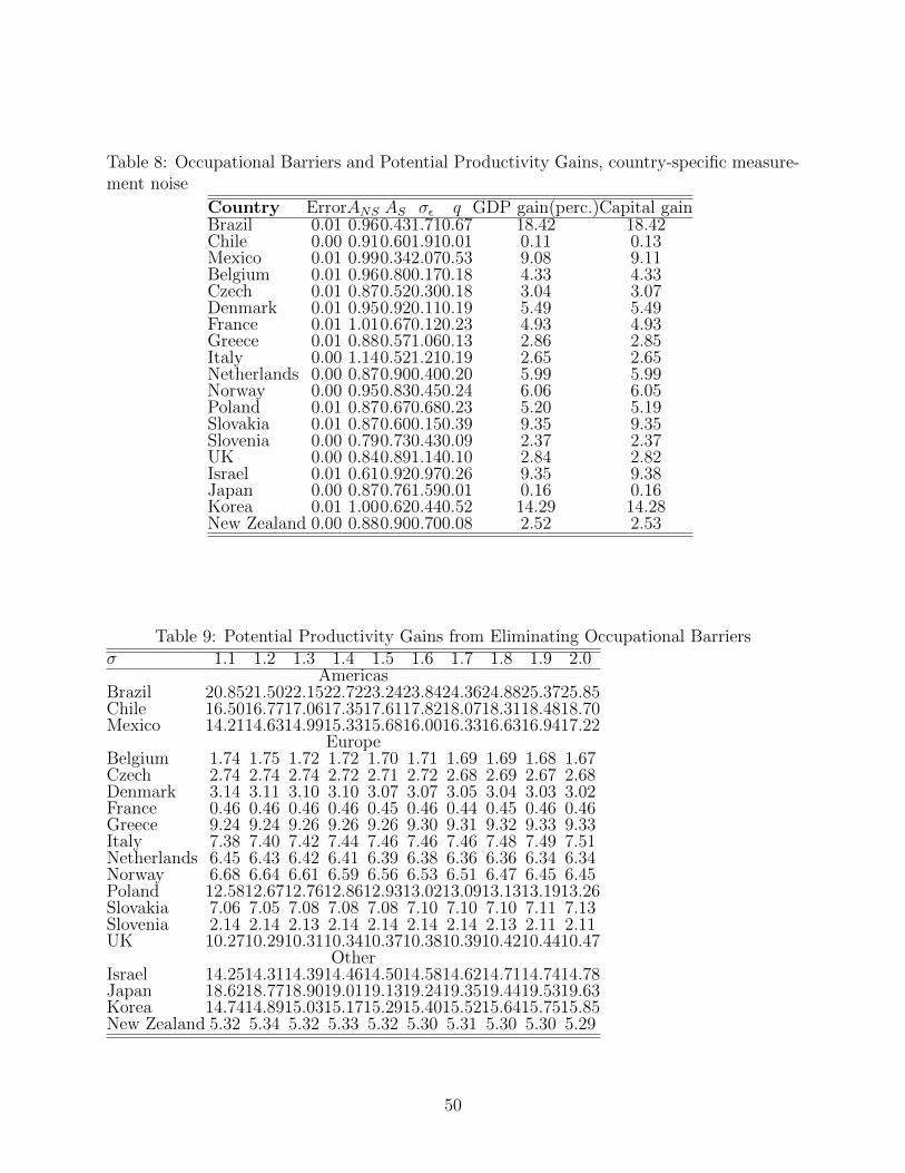
Table 8: Occupational Barriers and Potential Productivity Gains, country-specific measure-ment noise
Country ErrorANS AS σε q GDP gain(perc.)Capital gainBrazil 0.01 0.960.431.710.67 18.42 18.42Chile 0.00 0.910.601.910.01 0.11 0.13Mexico 0.01 0.990.342.070.53 9.08 9.11Belgium 0.01 0.960.800.170.18 4.33 4.33Czech 0.01 0.870.520.300.18 3.04 3.07Denmark 0.01 0.950.920.110.19 5.49 5.49France 0.01 1.010.670.120.23 4.93 4.93Greece 0.01 0.880.571.060.13 2.86 2.85Italy 0.00 1.140.521.210.19 2.65 2.65Netherlands 0.00 0.870.900.400.20 5.99 5.99Norway 0.00 0.950.830.450.24 6.06 6.05Poland 0.01 0.870.670.680.23 5.20 5.19Slovakia 0.01 0.870.600.150.39 9.35 9.35Slovenia 0.00 0.790.730.430.09 2.37 2.37UK 0.00 0.840.891.140.10 2.84 2.82Israel 0.01 0.610.920.970.26 9.35 9.38Japan 0.00 0.870.761.590.01 0.16 0.16Korea 0.01 1.000.620.440.52 14.29 14.28New Zealand 0.00 0.880.900.700.08 2.52 2.53
Table 9: Potential Productivity Gains from Eliminating Occupational Barriersσ 1.1 1.2 1.3 1.4 1.5 1.6 1.7 1.8 1.9 2.0
AmericasBrazil 20.8521.5022.1522.7223.2423.8424.3624.8825.3725.85Chile 16.5016.7717.0617.3517.6117.8218.0718.3118.4818.70Mexico 14.2114.6314.9915.3315.6816.0016.3316.6316.9417.22
EuropeBelgium 1.74 1.75 1.72 1.72 1.70 1.71 1.69 1.69 1.68 1.67Czech 2.74 2.74 2.74 2.72 2.71 2.72 2.68 2.69 2.67 2.68Denmark 3.14 3.11 3.10 3.10 3.07 3.07 3.05 3.04 3.03 3.02France 0.46 0.46 0.46 0.46 0.45 0.46 0.44 0.45 0.46 0.46Greece 9.24 9.24 9.26 9.26 9.26 9.30 9.31 9.32 9.33 9.33Italy 7.38 7.40 7.42 7.44 7.46 7.46 7.46 7.48 7.49 7.51Netherlands 6.45 6.43 6.42 6.41 6.39 6.38 6.36 6.36 6.34 6.34Norway 6.68 6.64 6.61 6.59 6.56 6.53 6.51 6.47 6.45 6.45Poland 12.5812.6712.7612.8612.9313.0213.0913.1313.1913.26Slovakia 7.06 7.05 7.08 7.08 7.08 7.10 7.10 7.10 7.11 7.13Slovenia 2.14 2.14 2.13 2.14 2.14 2.14 2.14 2.13 2.11 2.11UK 10.2710.2910.3110.3410.3710.3810.3910.4210.4410.47
OtherIsrael 14.2514.3114.3914.4614.5014.5814.6214.7114.7414.78Japan 18.6218.7718.9019.0119.1319.2419.3519.4419.5319.63Korea 14.7414.8915.0315.1715.2915.4015.5215.6415.7515.85New Zealand 5.32 5.34 5.32 5.33 5.32 5.30 5.31 5.30 5.30 5.29
50

Table 10: Potential Productivity Gains for the Wage Distortions Model
Country ErrorANS AS σε τ GDP gain(perc.)Brazil 0.02 0.860.610.501.31 28.89Chile 0.00 0.850.750.500.54 22.80Mexico 0.00 0.940.440.501.14 18.45Belgium 0.02 0.940.840.500.03 5.33Czech 0.02 0.860.530.500.03 3.92Denmark 0.00 0.930.930.500.02 3.95France 0.04 1.020.670.500.09 7.21Greece 0.02 0.910.570.500.30 12.30Italy 0.01 1.120.580.500.15 6.80Netherlands 0.00 0.870.910.500.03 5.58Norway 0.00 0.930.860.500.05 6.64Poland 0.01 0.860.700.500.13 10.46Slovakia 0.01 0.840.620.500.04 5.42Slovenia 0.00 0.790.740.500.01 2.94UK 0.00 0.800.980.500.14 13.40Israel 0.00 0.571.010.500.17 17.99Japan 0.00 0.820.890.500.32 18.92Korea 0.00 0.980.680.500.54 17.03New Zealand 0.00 0.850.940.500.02 5.04
51
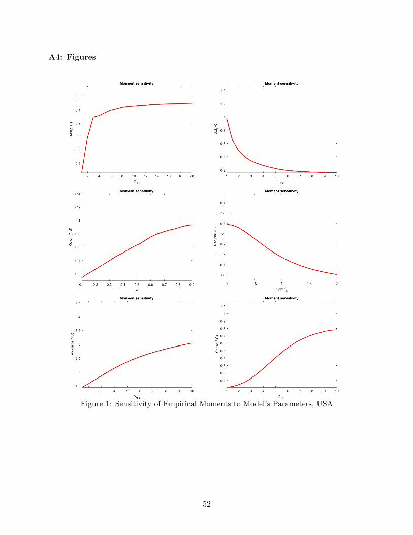
A4: Figures
Figure 1: Sensitivity of Empirical Moments to Model’s Parameters, USA
52

Figure 2: Sensitivity of Empirical Moments to Parameters in the Model with Barriers(Mexico)
53

Chapter 2: Income Effects on Education Quality
1 Abstract
Better education quality improves productivity and income, but do incomes explain
disparities in education quality between rich and poor countries? Several models of human
capital accumulation predict that incomes have a positive causal effect on human capital for
given levels of education by increasing the consumption of educational goods. The paper
tests this prediction by using a within country variation in incomes per-capita across different
cohorts of US immigrants. Wages of US migrants conditional on years of education serve as a
measure of education quality. I find that average domestic incomes experienced by migrants
in age from zero to twenty years have a significant positive effect on their future earnings in
the US. I show that the selection of migrants is unlikely to account for this result which is
also robust to multiple specifications and sub-samples.
2 Introduction
The rapid educational expansion of the last 50 years has largely failed to improve the
learning outcomes in developing countries. According to the 2018 World Bank’s Development
Report, average years of education has increased from 2.1 years in 1950 to 7.2 years in
2010. Yet, in the leading international assessments of literacy and numeracy (PIRLS and
TIMSS) the average student in low-income countries performs worse than 95% of students in
high-income countries. Poor learning outcomes in developing countries have strong negative
effects on incomes, explaining as much of the cross-country income variation as the difference
in years of education (Schoellman, 2012; Cubas, Ravikumar, and Ventura, 2016).
Several recent studies single out income as the main explanatory variable. The models
of Manuelli and Seshadri (2014) and Erosa, Koreshkova, and Restuccia (2010) postulate
that a higher country-level productivity increases the equilibrium education quality through
higher expected incomes. In these models households invest more in educational goods
54

if they expect higher skill prices in the future, which translates to a positive correlation
between income and education quality. It implies that relatively small technology differences
cause most of the cross-country income variation by creating incentives for human capital
accumulation. The existence of this channel would justify shifting the focus of economic
development from education quality policies towards more general growth policies.
This paper measures the effect of economic growth on the education quality. I regress
the wages of U.S. immigrants on per-capita incomes in their home countries averaged across
the first 20 years of workers life. The wages of U.S. immigrants proxy for their education
quality as in Hendricks (2002) and Schoellman (2012). In contrast to previous studies,
which study the cross-country correlation between domestic incomes and returns to domestic
education for migrants (Hendricks, 2002; Schoellman, 2012; Li and Sweetman, 2014), I
isolate the effect of incomes on migrant’s wages from slow-changing institutional and cultural
factors by including country fixed effects and using the variation in incomes between different
cohorts. The country fixed effects capture all the slow-changing determinants of education
quality and remove the associated omitted variable bias.
I find that even controlling for time-invariant cross-country differences, average income
when young correlates with education quality. Increasing average income in the first 20
years of an individual’s life by 100% corresponds roughly to an increase in wages by 5-7%
for high school graduates and by 12-15% for college graduates. The correlation holds both
for low-income and high-income source countries. The selection of migrants increases with
incomes in their source countries, but controlling for selection have a relatively small effect
on my estimates.
The paper makes two contributions to the literature. First, it develops and tests a
new approach to measure inter-temporal variation in education quality. This approach is
applicable for studies of effects of any country-level time-varying factors on human capital
accumulation, such as educational reforms, conflicts and hunger. Previous estimates of
education quality are based on educational achievement tests (Altinok, Angrist, and Patrinos,
55

2018; Hanushek and Kimko, 2000). These estimates are available for a relatively small set
of countries and measure only the academic skills of students in contrast to a wider set of
worker’s productive skills. My approach allows to evaluate human capital of individuals born
from 1950’s to 1980’s which is well beyond the scope of most educational achievements tests.
I show in Appendix A that the new approach also produces the estimates consistent with
the educational achievement scores.10
Second, my finding of positive correlation between growth and education quality in the
cross-country setting is novel in this literature. While several papers find the connection
between household incomes and human capital investments on sub-sountry level (Foster and
Rosenzweig, 1996; Munshi and Rosenzweig, 2006; Attanasio, Cattan, Fitzsimons, Meghir,
and Rubio-Codina, 2015), there are almost no studies on the national level11. The response
of human capital investment to both incomes and skill prices is likely to be much weaker
on the national level. While an increase in demand for education at the local level can
induce, for example, hiring more teachers from other regions, on the national level the pool
of teachers is less elastic. The lower elasticity of supply of educational goods can explain
why human capital investments react to the change in household incomes or regional skill
prices, but not to the change in aggregate per-capita incomes.
The paper is organized as follows. In Section 3 I briefly describe theoretical mecha-
nisms predicting the positive correlation between expected skill prices and education quality.
Section 4 then proceeds to discuss the empirical model, the identification approach and its
potential issues. Section 5 describes my sample and the construction of income measures.
Section 6 provides the main estimation results of effect of GDP per capita when young on
wages of migrants in the US. Section 7 contains numerous robustness checks, including the
10The third approach is to use the wages of stayers from nationally representative samples, which alsosuffers from the sample limitations. In the unreported estimation I use the pooled representative samplesfrom Brazil, Canada, India, Indonesia, Mexico and Venezuela to measure the effect of incomes when youngon future wages. This approach also does not find any positive income effects on education quality (futurewages).
11Altinok, Angrist, and Patrinos (2018) also find the positive correlation between economic growth andaverage achievement tests scores by using a smaller and shorter sample of countries
56

estimation in first differences and instrumental variable estimation. I show that a positive
correlation between GDP per-capita when young and education quality persists for different
subgroups of countries and different education levels and does not come from the confounding
age or year-of-immigration effects.
3 When Do Incomes Affect Education Quality?
A number of known theoretical mechanisms predicts a positive effect of incomes on
education quality. First, if households are credit-constrained, then an increase in income can
increase investments in quantity and quality of education Galor and Zeira (1993) or improve
quality due to better ability sorting (Mestieri, 2014). Banerjee (2004) also points out that
human capital investments increase with incomes even in absence of credit constraints as
long as households assign symbolic value to education of their offspring. In other words,
education increases with income if households value education on its own merit regardless
of its productivity benefits.
Education quality can also increase with incomes if current incomes reflect future skill
prices and the consumption of some market goods enters human capital production function
as in Erosa, Koreshkova, and Restuccia (2010) and Manuelli and Seshadri (2014). Below
I describe a stylized model to illustrate this mechanism. The model relies on the slightly
modified Jones (2007) framework.
Households indexed by i maximize cumulative lifetime wages net of education costs.
Wages are equal to the human capital multiplied by skill price ωij. Human capital is produced
according to the Cobb-Douglas production function from a combination of years of education
si and educational market goods qi:
wi = ωijh(si, qi) = ωijqαi s
φi
57

The objective function of household i is:
maxqi,si
∫ ∞s
ωijw(qi, si) exp[−(r+δ)t]dt−C(qi) = maxqi,si
∫ ∞s
ωijqαi s
φi exp[−(r+δ)t]dt−C(qi) (13)
The first component in the expression (1) measures the benefits of education which are
equal to the product of skill price ωij and human capital hi = qαi sφi accumulated throughout
the productive lifetime and discounted to period 0. Different individuals observe different
skill prices in the same country depending on the time of birth, and so the skill price ω has
both a country’s j and an individual’s i indexes. The discounting takes into account both
the interest rate r and the instantaneous death rate 1 > δ > 0.
In contrast to years of education s, investment in education quality q involves monetary
rather than time costs. The costs of education quality involve purchases of educational
market goods at price pj. The purchases are paid for at the end of the country’s average
education period s∗:
C(qi) = pjqi exp[−(r + δ)s∗]
The first-order condition for years of education implies the familiar Mincer equation at
the optimum:
d log(w(s, q)
ds= (r + δ)
Given the human capital production function the first-order condition translates to the
following optimal years of education:
s∗ =φ
r + δ
The first-order condition for educational market goods implies:
qi =
(αωijpj
) 11−α
sφ
1−α (14)
58

Equation (2) predicts that, given years of education si, households expecting higher
skill prices ωij obtain more human capital by investing more in educational goods. In other
words, this model implies higher education quality in periods of high expected skill prices.
It also implies that the optimal investment in educational market goods qi decreases in the
price of educational goods pj.
The prediction of higher education quality in periods of high skill prices relies on two
assumptions. First, the consumption of some market goods increases education quality η > 0.
Second, the prices of educational market goods do not increase with skill prices pj = const
or increase by a smaller rate compared to skill prices. Both of these assumptions are not
trivial.
Regarding the first assumption, two previous micro studies find low or zero effect
of market goods consumption on the production of human capital. Del Boca, Flinn, and
Wiswall (2014) estimate the human capital production function by using the PSID sup-
plemental study to find very weak effects of monetary transfers to households on learning
outcomes of children. Schoellman (2016) observes that adult outcomes of US refugees do
not vary with the age of arrival in US up to age six, despite large improvements in living
standards after the immigration. In contrast, Attanasio et al. (2015) find that market goods
investments have a sizable effect on the formation of cognitive and non-cognitive skills in
early childhood in Colombia. Macro calibration studies often assign a high weight to the
market goods in human capital production function. For example, both Erosa, Koreshkova,
and Restuccia (2010) and Manuelli and Seshadri (2014) estimate the elasticity of human
capital with respect to educational market goods consumption to be equal roughly to 0.4.12
The second assumption of constant/slow-changing prices of educational goods is never
specifically tested to my knowledge, but macro models implicitly incorporate the response of
prices of educational goods. The assumption definitely holds true if, for example, households
12The human capital production function in Manuelli and Seshadri (2014) describes the relation betweenan increase in human capital and human capital and market goods consumption. The elasticity of increasein human capital with respect to market goods consumption in the calibrated model is equal to 0.4, implyinga large sensitivity of human capital to incomes/skill prices.
59

can import educational goods at fixed and binding world prices. The second assumption
is likely to hold for most hardware educational goods, such as laptops and toys. On other
hand, it is much harder to import teachers’ services and school facilities. For goods involving
intellectual property the prices can also change with economic growth due to widely practiced
price discrimination, which also violates the second assumption.13
Based on the Equation (2), I formulate the only empirical prediction that individuals
experiencing higher national incomes while making their educational decisions obtain higher
wages in the future conditional on years of education. The prediction relies both on the
model, on the two assumption listed above and on the assumption of positive correlation
between national incomes and expected skill prices. It should be noted that while the
prediction follows from the my theoretical model, there are other mechanisms such as
borrowing constraints that generate the same correlation.
4 Identification Approach
4.1 Measuring Education Quality
My main dependent variable is the education quality, which in terms of this paper means
accumulated human capital for given years of education. I measure the education qual-
ity through wages of US immigrants conditional on experience and education level. This
approach provides a unified measurement of human capital for all migrant. In contrast,
domestic wages incorporate not only the variation in human capital, but also the variation
in skill prices and returns to experience.
The benefits of using immigrant wages instead of educational achievement tests to
proxy for education quality are two-fold. First, I achieve much greater coverage both in time
and across countries. For comparison, PISA educational achivement tests start only in 2000.
13One example of price discrimination is Microsoft offering cheaper bundles of MS Office and Windowsto developing countries: NY Times 04/19/2007, ”Software by Microsoft Is Nearly Free for the Needy”,http://www.nytimes.com/2007/04/19/technology/19soft.html.
60

Altinok, Angrist, and Patrinos (2018) construct a most comprehensive database of education
quality to date from combining the results of different achievement tests, including some tests
done as far back as 1965. Unfortunately, it includes only 41 country with 20 or more years of
coverage.14 In contrast, my sample includes 105 countries with one hundred or more migrants
and birth cohorts differing from 1950’s to 1980’s. Second, the measures of learning provided
by educational achievement tests cover only the subset of strictly academical skills which do
not necessarily translate into productive capabilities of workers. Despite the differences in
approach, my measures of education quality are still consistent with educational achievement
tests measures, as I show in the Appendix A for the harmonized measures from Altinok,
Angrist, and Patrinos (2018).
4.2 Empirical Model
The theoretical model implies that wages conditional on years of education is an increasing
function of incomes. I assume that the log-linearized version of this relationship holds:
log(wUSit ) = αj + φt + db + βyi + γXi + ai + εit (15)
In the equation above αj corresponds to an average education quality in country
j and describes all the slow-changing institutional and cultural factors. The vector Xi
represents different individual characteristics affecting productivity such as years of potential
experience. Variable yi describes incomes experienced by an individual i when making
educational decisions. The variable db is the birth year effect. Dummy variables db and
φt describe respectively birthyear effects and observation year effects. Variable ai captures
constant individual characteristics such as genetic abilities.
Estimating the equation (4) directly would run into a problem of correlation between
unobserved variable ai and explanatory variables Xi. I address this problem by aggregating
14The coverage means that for each 5-year interval there is at least one measurement. Hence the 20 yearscoverage means that there are 4 observations for this country on the aggregate level.
61

individual observations to averages across cohorts. Each cohort corresponds to a unique
combination of birth year, education level and country of origin. This group aggregation
approach eliminates the bias resulting from the correlation between explanatory variables
and error within groups Deaton (1985). I estimate the effect of growth on wages separately
for individuals with high school education s = 12 and college education s = 16:
log(wUSbjt |s) = αj + φt + db + βyjb + γXjb + εjbt, s = 12, 16 (16)
In the equation (5) log(wUSbjt |s) denotes the average log-wage of migrants from a country
j born in year b with education s, and ybj is an average income in country j from year b to
year b + 20. Fixing the education level gives more flexibility in terms of possible effects of
growth on education quality as it allows for income effect β to vary across education levels.
In other words, it allows income to affect education quality both as an additive term or as
an interaction term with the education level. The additive form is completely consistent
with the equation (4), while incomes affecting returns to education are more common in the
literature (Schoellman, 2012; Li and Sweetman, 2014). The main coefficient of interest here
is β, which measures the effect of economic growth on log-wages.
The (mean) log-wage log(wUSbjt |s) in the regression in year t is equal to the average
actual log-wage of migrants per hour of work in year t minus the average ”skill price” in the
US in year t. I calculate the average skill price as a fixed effect on survey year in the Mincer
regression of log-wage of US-born workers, controlling for years of education, experience
and experience squared. This correction allows to control for the difference in skill prices
between different survey years without introducing multicollinearity between year of birth,
survey year, education and experience variables.
The set of control variables Xi varies across specifications. In my most complete
specification it includes time spent in the US, gender, potential experience and potential
experience squared. The potential experience is equal to min[age-years of education-6, age-
14], as workers are unlikely to accumulate productive experience before age 14 even if not
62

in school. Following Schoellman (2012) I control for the potential degree of assimilation by
including a time spent in the US. The estimation does not include the citizenship status and
the English speaking skills as these variables potentially reflect the education quality and
can confound my results.
The parameter β in the regression equation (4) measures the effect of incomes on
education quality. Based on the previous discussion, the coefficient β is positive as long as
migrants with higher incomes indeed obtain more human capital and the income proxy yjb
has no negative correlation with any unobservables. The negative result implies a violation
of one of these assumption: the coefficient β is non-positive when either the true effect of
incomes on education quality is non-positive or the income proxy yjb negatively correlates
with unobservables.
4.3 Addressing the Selection Bias
One potential identification problem comes from the selection of migrants based on human
capital. The selection based on human capital is problematic if and only if it correlates with
incomes, because all the stable selection patterns are accounted for by country fixed effects.
For example, this problematic correlation between income and εjbt can emerge if economic
growth makes it easier to migrate for migrants with lower or higher skills.
In practice, at least two kinds of selection can introduce the selection bias into the
estimate of skill price effect γ. First, an increase in skill prices or incomes in home country
can have differential impacts on willingness and opportunities to migrate for individuals with
high and low unobserved skills. Jasso, Rosenzweig, and Smith (2002) use theory to argue
that higher domestic incomes should lead to stronger positive selection.
Additionally, if migrations are planned long in advance, educational decisions of workers
would respond to skill prices in the US rather than to skill prices in their home countries.
If individuals indeed invest more in education in response to higher future skill prices then
individuals expecting to migrate will get more education than stayers. This is a problem
if economic growth in source countries of migrants systematically affects the proportion of
63

pre-planned migrations. If higher incomes decrease this proportion, then the coefficient
estimate γ has a negative bias as the average education quality of migrants goes down with
incomes.
After accounting for selection into migration, the model takes the following form:
log(wUSbjt |s) = αj + φt + db + βyjb + γXjb + E(εjbt|v(z) + εjbt ≥ 0) (17)
Here v(·) is a function which determines the probability of selection and z is the vector of
variables affecting selection. Selection variables include GDP per-capita, years of education,
gender and country-birth year-education specific migration cost shock. For a given z and
distribution of ε we can write the selection term as a function of the selection probability
E(εjbt|v(z)+εjbt ≥ 0) = G(p(zbj), where the selection probability is p(zbj) = Prob(v(z)+ζ ≥
0).
I use the approach from Dahl (2002) and approximate the selection probabilities by
observed sample frequencies. I divide the sample of migrants into cohorts characterized
by country of birth, 10-year wide birth cohort and the level of education. The empirical
frequency for each cohort is equal to the weighted number of migrants observed in the US
sample divided by the number of stayers in the same cohort obtained from the Barro and
Lee (2013)15 dataset of educational achievement.
Because the function G(·) is unknown I approximate it by splines of the selection
probability p(zbj). Each spline is a segment of a piece-wise linear function. Splines allow for
flexible approximation of unknown functions and are less sensitive to outliers compared to
polynomial approximation.
15Barro R. and J. Lee (2011), “A New Dataset of Educational Attainment in the World, 1950-2010,”Journal of Development Economics, Vol. 104, pp. 184-198.
64

5 Data
5.1 Sample
The data on migrants’ characteristics and labor market outcomes comes from the American
Community Survey (ACS) data obtained from IPUMS-USA.16 American Community Sur-
veys are conducted each year by the U.S. Census Bureau for a representative sample of US
households. The response to the ACS survey is required by law, which reduces the potential
selection bias. The micro data from ACS are available in a form of cross-sectional datasets,
describing both individuals and their households.
My dataset combines all the publicly available ACS surveys from 1970 to 2017. It
includes the one-precent metro sample from 1970, five-percent samples from1980 and 2000
and all the one-percent representative samples of the US population from 2001 to 2017. The
large time span of my data helps to better distinguish between birth cohorts and age effects.
Following Schoellman (2012), I select only the immigrants who were born outside of the
US and arrived in the US at least 6 years after the expected graduation. This filter allows
to minimize the proportion of immigrants obtaining their education partially or completely
within the US. When migrants obtain education in the US, their quality of education may
be mis-attributed to the quality of education in country of origin. In order to achieve better
representation of domestic population I also drop individuals born outside of US to American
parents.
This study concentrates on individuals strongly attached to the labor market. I drop
all the observations with ages above 65 years and below 18 years, because the productivity
of these workers may not reflect their prime age productivity. I select only the individuals
working at least 30 weeks in the last year for at least 30 hours per week. The study considers
only the workers employed for a wage, as the labor income of self-employed workers and other
16Steven Ruggles, Katie Genadek, Ronald Goeken, Josiah Grover, and Matthew Sobek. IntegratedPublic Use Microdata Series: Version 7.0 [dataset]. Minneapolis: University of Minnesota, 2017.https://doi.org/10.18128/D010.V7.0.
65

non-wage workers poorly correlates to productivity.
I calculate years of education by recoding educational attainment in the standard way.
The years of education variable has a maximum value at 16 years as the census data does
not identify advanced degrees. The potential experience is equal to the minimum of two
values with the first being Age-Years of Education-6 and the second value of Age-16. This
calculation takes into account that some migrants with low educational attainment may start
to work early, but not before turning 16. Even if children start working before turning 16,
the experience obtained during this time is likely to have much less value compared to the
experience obtained in adult life.
After applying all the filters, my final sample includes 839618 migrants from 138
countries. There are 105 countries with 100 migrants or more, which constitute 99% of my
sample. Table 1 describes the most important summary statistics on migrants by country of
origin. Most migrants in the dataset come from Mexico (26%) and about 42% comes from
top-5 countries. Because my identification approach relies on the within-country variation
in GDP per capita and quality of schooling, I average the observations across country of
birth-year of birth-education cohorts and drop cells with less than 10 observations.
I calculate hourly wages as the total wage income divided by the product of number
of hours worked per week and the number of weeks worked in the previous year. I drop
observations with reported wages below federal minimum wage in each year to reduce the
noise from misreported hours of work. The percentage of dropped observations does not
differ systematically between countries and over time. I also winsorize wage observation at
the 1% level conditional on years of education, survey year and experience.
My income measure equals to the average GDP per capita over first 20 years of
migrant’s life. The value of this variable, for example, for a migrant born in India in 1960 is
equal to the average logarithm of GDP per capita in India in 1960-1979. I use the variable
of expenditure-side real GDP per capita from Penn World Tables 9.0.17 The variable is
17Feenstra, Robert C., Robert Inklaar and Marcel P. Timmer (2015), ”The Next Generation of the PennWorld Table” American Economic Review, 105(10), 3150-3182, available for download at www.ggdc.net/pwt
66

measured in Purchasing Power Parity 2011 US dollars. The estimation sample includes
observations for which GDP per capita is observed for at least 15 years out of first twenty
years of immigrant’s life.
6 Results
6.1 Evidence from Selected Countries
The dataset contains birth cohorts from 1935 to 1994, but the availability of GDP per capita
series and low numbers of observations for more recent years practically limits the exploitable
variation in year of birth roughly to the period of 1950-1990. In this period the countries
in my sample had experienced very different rates of economic growth. Both China, Japan
and South Korea went through the episodes of very high growth, while the GDP in Nigeria,
Ghana, Cambodia and Liberia went down.
For countries with a large number of immigrants (such as China, Mexico, Japan, India
and others) I can directly calculate the average returns to domestic education for each 5-year
cohort of immigrants conditional on potential experience, potential experience squared and
gender. Figure 1 shows both the dynamics of GDP per capita and the estimated returns
to domestic education for two countries experiencing fast growth during my sample period.
For each estimated return the bars on the graph show 95% confidence intervals for the OLS
estimate of average returns to education.
67

Figure 1: Returns to Education for Migrants by Birth Cohort
Overall, the trends in returns to education for different birth cohorts of migrants are
quite different from economic growth trends. For example, India experiences high growth in
measured returns to education for each decade since 1950, while there is no growth in average
GDP per capita for the cohorts born in 50-70’s. In contrast, the returns to education for
Japanese migrants do not change much over the years despite the strong economic growth.
The same observation can be made about China and Asian Tigers economies. The returns
to education for migrants from China and Asian Tigers (Singapore, South Korea, Taiwan,
Hong Kong) do not differ much between cohorts, despite the fact that later cohorts grew up
with much higher average GDP per capita.
This preliminary evidence suggests that the returns to education for migrants do not
have a strong positive within-country correlation with economic growth. However, this
conclusion relies only on a few observations and needs more careful testing. In the next
68

Section I perform more rigorous tests for this correlation.
6.2 Baseline Estimation Results
In Table 2 I present the OLS estimation results for the equation (5) separately for migrants
with completed primary education, with completed secondary education and with tertiary
education. For each education level, I start with the most parsimonious specification and
then add controls and variables. Columns (1) and (4) present the estimation results without
the birth year fixed effects. In Columns (2) and (5) I add birth year fixed effects to control
for time trends. Columns (3) and (6) report specification with both birth year fixed effects
and controls, including the selection controls.
Overall, my OLS estimation does not show any robust relationship between income
when young and wages of migrants. In the most parsimonious specification, incomes neg-
atively correlate with wages of high school graduates and positively with wages of college
graduates. Adding birth year control makes the coefficient on income positive and sta-
tistically significant for high school graduates and positive though insignificant for college
graduates. Controlling for selection slightly increases the coefficient on income for high school
graduates and decreases it for college graduates.
The OLS estimation suggests that findings are not robust to the choice of specification.
Cross-country heterogeneity in effects of average incomes on human capital β provides for
one potential explanation for this lack of robustness. For example, the correlation between
incomes and growth can be distorted by differing trends in selection of migrants due to
changing immigration policies. On the next step I incorporate this heterogeneity in β into
the model and estimate the random coefficients model.
Table 3 reports estimation results for the equation (5) by using the random coefficients
model separately for migrants with only completed primary education, with completed
secondary education and with tertiary education. In this estimation, I allow the effect of
income β to vary across countries according to the normal distribution. Table 3 reports the
69

mean value in this distribution. For each education level Table 3 reports estimation results
both without birth year fixed effects and with birth year fixed effects to control for trends
in the US immigration policy. All the reported specifications also include country-specific
dummies αj to incorporate differences in the baseline transferable human capital of migrants.
The random coefficients model estimation unambiguously demonstrates that income
when young corresponds to higher adult wages of migrants for all levels of education. The
average effect β is stronger for more advanced education levels. For migrants with completed
primary education only (Columns 1-3) and for migrants with completed secondary education
an increase in GDP per-capita when young corresponds to an increase in wages in the
US by approximately 8%. For college graduates the same increase in GDP per-capita
translates to 9-11% increase in wages depending on specification. This increase corresponds
to approximately 0.8 percentage points increase in returns in education. This coefficient
magnitude explains about one-half of cross-country variation in returns to education.
Next, I perform analysis by country groups (Table 4). I split all the countries in my
sample into groups of low-income and high-income countries based on the GDP per capita
in year 1960. I classify a country as low-income if its GDP per capita in 1960 is less than
40% of GDP per-capita in the US. This year corresponds to the time when most countries
in my sample started reporting their GDP and also precedes the period when individuals in
my sample grew up old enough to start affecting the country’s income.
Incomes when young positively affect future wages both in low-income and in high-
income countries. Coefficients on GDP per-capita in first 20 years of life are positive
and statistically significant for high school graduates and college graduates in low-income
countries. Coefficients are higher for high-income countries, but the statistical significance
is lower because of the smaller sample size. Taking into account the sample size, there is no
reason to suspect that incomes have different effect depending on the country’s income level.
Summing up, living in a country with higher national incomes when young corresponds
to higher human capital of migrants as evidenced by their wages. This finding is consistent
70

with the theoretical predictions of Galor and Zeira (1993) and Manuelli and Seshadri (2014)
and several empirical studies on sub-country level. However, this relationship does not
necessarily holds for every country in the sample. Some other factors also affect both
education quality and economic growth leading to their divergence.
7 Robustness
The finding of the positive correlation between the education quality and incomes
when young stays robust to different modifications of the estimation approach. This section
outlines and addresses the remaining identification concerns.
First Differences Estimation. My estimation involves rather long time series of
different birth cohorts with up to 30 years for some countries. The known danger of using
long panels is a spurious correlation between non-stationary variables (Greene, 2012). In
this section I estimate a regression in first differences to exclude the possibility of a spurious
regression.
I calculate first differences by collapsing my data even further to the level of 5-year
long birth cohorts instead of 1-year long cohorts. Collapsing the data reduces the number of
observations, but also reduces the effects of noise affecting both variables on a year-to-year
basis. The estimation presented in Table 5 contains most of the previous controls except
the splines of probability of migration by cohorts. I replace the splines with changes in the
probability of selection to increase the degrees of freedom18.
Table 5 presents two versions of the estimation. In the first version (Columns 1, 3
and 5) my dependent variable is the average log-wage of migrants belonging to a particular
cohort. In the second version ((2),(4) and (6)) the dependent variable is the average residual
in the regression of log-wage on individual controls including potential experience, gender
and years in the US which is done at the individual level. By taking the collapsed residuals
from disaggregated regression I remove the variation associated with the individual controls.
18The estimation with splines results in similar coefficient magnitudes.
71

Estimation in first differences (Table 5) supports my previous results with somewhat
smaller coefficient magnitudes. Migrants with high school education receive approximately
4% increase in future wages in response to doubling average GDP per-capita when young.
Migrants with college education receive approximately 12% increase. For primary education
the coefficient is statistically insignificant at 10%, but this discrepancy with previous results
can come from the small sample size used in the estimation.
Income calculation approach. My original estimates assume that higher incomes affect
human capital from birth to reaching an age of twenty. Is this a proper time frame? In this
subsection, I consider the effects of GDP per-capita in a more narrow time frame from birth
to five years. In this more limited time span, incomes do not directly affect education, but
still affect early human capital accumulation by allowing higher consumption of food and
educational goods.
The different window for calculation of average income when young does not drastically
change the results, but it reduces the coefficients magnitude (Table 6). As expected, the effect
on college-educated migrants goes down more than for any other education level. Migrants
with high school education receive only 6% increase. In contrast, the connection between
future wages and income becomes even stronger for migrants with only primary education,
where early childhood investment have more relative impact (and also incomes are more
correlated). An increase in GDP per-capita by 100% corresponds to approximately 8%
increase in future wages of migrants with primary education only.
Overall, my estimation demonstrates robustness of my result to the choice of window
in which average incomes affect human capital. Limiting the period of average income
calculation indeed lowers the magnitude of the coefficients but coefficients remain positive
and statistically significant.
Instrumenting GDP. Political and cultural changes in a country can simultaneously affect
both educational institutions and economic growth. As a robustness check, I also instrument
72

the GDP per-capita variables by oil prices to estimate the effects of economic growth caused
by external factors.
My instrument is the West Texas intermediate oil price in constant dollars19, averaged
across first 20 years of migrant’s life. In this estimation I concentrate on oil-rich countries
only to guarantee that the instrument is relevant. Oil prices in oil-rich countries can directly
increase both current and future incomes per-capita. Recent studies (Alexeev and Conrad,
2009; Smith, 2015) show that the discovery of natural resource deposits positively affect
the current GDP with no negative effect for long-run growth. It is important that the
households can observe oil prices when young to predict the future GDP per-capita and skill
prices, because the oil price dynamics is very similar to a random walk.
In contrast to GDP per-capita, oil prices depend on supply and demand on the global
market, but not on local institutions and shocks to investment in educational goods. Hence
a co-movement between economic and educational institutions will not bias my results. The
measurement noise in oil prices is likely to be very small, given that the variable is based on
public transactions.
I perform the IV-estimation only for the countries in which the average oil rent com-
prises more than 5% of GDP as follows from the World Bank Millenium Development
Indicators for 1960-2000.20 After merging with the series on GDP per-capita from Penn
Tables and with American Community Survey dataset on immigrants the final sample
includes 18 oil-rich countries.
Oil prices experience a strong variation in 1950’s-1980’s due to successful collusion
of oil exporters in the 1970’s and the partial erosion of the cartel in the 1980’s. This
variation remains strong even after 20 years moving window averaging is used to construct
the instrument. For example, individuals born in 1995 experienced oil prices three times
higher in first two decades of their lives than the individuals born in 1950. Because of this
variation, oil prices have high predictive power for log GDP per-capita when young with
19Collected from the Federal Reserve Bank of St. Louis website.201960 is the earliest year for the database.
73

relatively high F-statistic in the first-stage regression (F=404 without country fixed effects).
The results of IV-estimation as reported in Table 7 in general support my previous
finding with even larger coefficients on income. If all the controls are included, an increase in
average GDP per-capita when young by 100% increases future wages of migrants by approx-
imately 15% for high school graduates and by 20% for college graduates. The magnitude
demonstrates that incomes negatively correlate with the average wages of migrants. The
increase is stronger for high-school graduates compared to college-graduated. This finding
should be interpreted with caution because the regression does not control for the year of
birth and oil-producing countries might differ from other countries.
8 Conclusion
The paper uses a pseudo-panel of US immigrants to estimate the correlation between
measures of national incomes per capita and education quality. I measure the education
quality by US wages of migrants from different birth cohorts, conditional on years of educa-
tion. The paper measures incomes by average source country’s GDP per-capita experienced
by the migrant’s birth cohort in age from birth to 20 years. The estimation exploits only
within-country variation in incomes by controlling for country fixed effects and selection
based on observables.
The paper finds a significant positive correlation between average incomes when young
and earnings of adults in the US. The effect size is economically significant: for example,
doubling average GDP per-capita when young increases future earnings of high school
graduates by approximately 5-7%. This finding of positive correlation is consistent with
theories of higher incomes or higher expected skill prices positively affecting human capital
accumulation.
My results imply that economic growth on its own can help to improve the education
quality. However, an increase in education quality does not always follow automatically. My
study also demonstrates while the positive relationship holds on average, in many countries
74

trends in earnings of migrants diverge from trends in average income. This divergence can
come from country-specific immigration policies in the US, but also from countries successes
and failures in responding to demand for education quality.
75

9 Bibliography
[1] Alexeev, Michael, and Robert Conrad. 2009. “The Elusive Curse of Oil.” Review ofEconomics and Statistics 91, no. 3 (July 23): 586-598.
[2] Altinok, Nadir, Noam Angrist, and Harry Anthony Patrinos. 2018. Global data set oneducation quality (1965-2015) 8314. The World Bank, January 23.
[3] Attanasio, Orazio, Sarah Cattan, Emla Fitzsimons, Costas Meghir, and Marta Rubio-Codina. 2015. “Estimating the Production Function for Human Capital: Results froma Randomized Control Trial in Colombia”. Working Paper 20965. National Bureau ofEconomic Research.
[4] Banerjee, Abhijit V. 2004. “Educational policy and the economics of the family.” Jour-nal of Development Economics, New Research on Education in Developing Economies,74, no. 1 (June 1): 3-32.
[5] Barro, Robert J., and Jong Wha Lee. 2013. “A new data set of educational attainmentin the world, 1950-2010.” Journal of Development Economics 104 (September 1): 184-198.
[6] Cubas, German, B. Ravikumar, and Gustavo Ventura. 2016. “Talent, Labor Quality,and Economic Development.” Review of Economic Dynamics 21:160-181.
[7] Dahl, Gordon B. 2002. “Mobility and the Return to Education: Testing a Roy Modelwith Multiple Markets.” Econometrica 70 (6): 2367-2420.
[8] Deaton, Angus. 1985. “Panel data from time series of cross-sections.” Journal ofEconometrics 30, no. 1 (October 1): 109-126.
[9] Del Boca, Daniela, Christopher Flinn, and Matthew Wiswall. 2014. “HouseholdChoices and Child Development.” Review of Economic Studies 81 (1): 137-185.
[10] Erosa, Andres, Tatyana Koreshkova, and Diego Restuccia. 2010. “How ImportantIs Human Capital? A Quantitative Theory Assessment of World Income Inequality.”Review of Economic Studies 77 (4): 1421-1449.
[11] Foster, Andrew D., and Mark R. Rosenzweig. 1996. “Technical Change and Human-Capital Returns and Investments: Evidence from the Green Revolution.” AmericanEconomic Review 86 (4): 931-953.
[12] Galor, Oded, and Joseph Zeira. 1993. “Income Distribution and Macroeconomics.”Review of Economic Studies 60, no. 1 (January 1): 35-52.
[13] Hanushek, Eric A., and Dennis D. Kimko. 2000. “Schooling, Labor-Force Quality, andthe Growth of Nations.” American Economic Review 90, no. 5 (December): 1184-1208.
[14] Hendricks, Lutz. 2002. “How Important Is Human Capital for Development? Evidencefrom Immigrant Earnings.” American Economic Review 92, no. 1 (March): 198-219.
76

[15] Jasso, Guillermina, Mark R. Rosenzweig, and James P. Smith. 2002. “The earnings ofUS immigrants: world skill prices, skill transferability and selectivity”. Mimeo.
[16] Jones, Charles. 2007. “A Simple Mincerian Approach to Endogenizing Schooling.”working paper.
[17] Li, Qing, and Arthur Sweetman. 2014. “The quality of immigrant source countryeducational outcomes: Do they matter in the receiving country?” Labour Economics26 (January 1): 81-93.
[18] Manuelli, Rodolfo E., and Ananth Seshadri. 2014. “Human Capital and the Wealth ofNations.” American Economic Review 104, no. 9 (September): 2736-2762.
[19] Mestieri, Marti. 2014. “Wealth Distribution and Human Capital: How BorrowingConstraints Shape Educational Systems” 1114. Society for Economic Dynamics.
[20] Munshi, Kaivan, and Mark Rosenzweig. 2006. “Traditional Institutions Meet theModern World: Caste, Gender, and Schooling Choice in a Globalizing Economy.”American Economic Review 96, no. 4 (September): 1225-1252.
[21] Schoellman, Todd. 2016. “Early Childhood Human Capital and Development.” Amer-ican Economic Journal: Macroeconomics 8, no. 3 (July): 145-174.
[22] Schoellman, Todd. 2012. “Education Quality and Development Accounting.” Reviewof Economic Studies 79 (1): 388-417.
[23] Smith, Brock. 2015. “The resource curse exorcised: Evidence from a panel of coun-tries.” Journal of Development Economics 116 (September 1): 57-73.
77
10 Appendix
A1: Returns to education vs international test scores
My measure of education quality is based on the cohort-specific returns to domestic education
on US labor market. The dataset of Angrist et al (2013) provides a benchmark to evaluate
the validity of my measure by comparing it with the standardized international test scores.
The Hanushek and Woessman (2012) already show that the returns to domestic education
strongly correlate with educational achievement scores in the cross-section of countries, but
this paper relies on temporal variation and so the my validity tests check for the temporal
correlation.
For this test I separate my sample of US immigrants into 5-year wide birth cohorts. For
each cohort and each country separately I estimate the returns to domestic education. The
list of controls is smaller compared to the main estimation to retain the efficiency and includes
domestic experience, citizenship, gender and the time spent in US. Table 2.8 presents the
results of OLS regression of measured returns to domestic education from the first stage on
different measures based on educational achievement scores. The results reported in Column
(1) demonstrate that the returns to domestic education I obtain positively correlate with the
aggregate score of education quality from Angrist et al (2013). The aggregate measure is a
measure of education quality in both primary and secondary school, which is standardized
across subjects and schooling levels. It is calculated from the existing results of primary or
secondary school tests on mathematics and reading. The benefit of this measure is in the
larger number of observations than for any of more specific measures as the specific measures
are rescaled to the aggregate score.
Column (2) presents the results of regressing the aggregate primary school test score.
In this case the connection is insignificant, which is not surprising given the relatively high
education level of US immigrants in my sample. Next, Column (3) shows that there is a
statistically significant positive connection between the returns to domestic education for
78

US immigrants and the achievement test of secondary school students. The coefficient’s
magnitude increases as the quality of secondary education is more relevant for my sample.
Overall, this calculation demonstrates the consistency of my estimates of education quality
with estimates based on educational achievement scores.
79

A2: Tables
Table 1: Sample’s description for main countries of originCountry N obs Wage Education yrsGDP per cap. (0-20)
Mean Std Mean Std Mean StdMexico 27446316.3212.27 7.42 4.50 7272.7 2045.7Other countries 11176530.1829.5313.64 3.48 5735.8 6801.8Philippines 68303 25.0517.6014.34 2.60 1936.7 376.3India 48116 37.4828.3715.26 2.73 1102.7 150.6China 38476 28.5124.4413.40 4.51 1173.4 237.6El Salvador 33350 16.4712.45 7.52 4.74 825.2 116.6Canada 23931 40.8635.4314.55 2.24 15536.2 3746.0United Kingdom, ns 23782 45.8541.2014.58 2.26 12425.4 2572.3Guatemala 20071 15.7212.20 7.12 4.71 2912.3 511.0Colombia 17702 21.3418.6612.93 3.50 3930.6 900.6Jamaica 17435 22.0515.1612.50 2.69 4528.7 788.6Dominican Republic 17408 18.0615.2710.79 4.19 2816.7 775.2Germany 14154 35.6432.3314.45 2.43 10886.8 4256.0Peru 12259 20.5817.0913.16 2.95 2826.0 576.8Japan 11539 40.8037.9414.92 2.40 8406.9 5129.6Honduras 11426 15.7110.75 8.46 4.37 2372.8 270.0Ecuador 9685 18.7014.1710.84 4.19 3128.3 991.7Taiwan 9532 31.5123.4715.00 2.76 2832.4 1887.7Brazil 9275 28.1128.3613.23 3.69 3189.6 1198.2Haiti 9228 17.8113.2711.70 3.44 1237.1 110.7Nigeria 8000 26.5021.5814.81 2.36 3893.0 1162.6Italy 7250 32.5127.1612.94 3.71 8199.7 4019.4Pakistan 6707 29.0028.0514.10 3.57 1369.4 277.7Trinidad and Tobago 6530 23.3016.3412.62 2.77 7888.0 3136.0Iran 6206 30.0725.8114.55 2.52 2980.5 1260.9Nicaragua 6069 18.1012.0311.33 4.10 5100.2 946.0Vietnam 6009 18.0414.81 9.36 5.17 818.4 108.2Portugal 5943 24.0115.66 8.40 5.05 4640.4 1843.6Venezuela 5004 28.3427.6414.56 2.73 7682.2 1003.5
80

Table 2: GDP per-capita when young and wages of migrants: OLS-Estimation
(1) (2) (3) (4) (5) (6)High schoolHigh schoolHigh schoolCollege College College
Log GDP(0-20) -0.083∗∗∗ 0.039∗ 0.044∗∗ 0.034∗∗ 0.037 -0.002(-7.2) (1.9) (2.1) (2.2) (1.3) (-0.1)
Years in the US 0.006∗∗∗ 0.006∗∗∗ 0.005∗∗ 0.006∗∗∗
(3.9) (4.0) (2.4) (2.7)Experience 0.013∗∗ 0.014∗∗ -0.000 0.005
(2.3) (2.6) (-0.0) (0.6)Experience sq. -0.000∗ -0.000∗∗ -0.000 -0.000
(-1.8) (-2.0) (-0.3) (-0.9)Female -0.216∗∗∗ -0.214∗∗∗ -0.250∗∗∗-0.246∗∗∗
(-8.0) (-7.9) (-6.6) (-6.4)Country FE Yes Yes Yes Yes Yes YesBirthyear coh FE No Yes Yes No Yes YesSelection controls No No Yes No No Yes
Observations 1860 1860 1860 1597 1597 1597Adjusted R2 0.63 0.66 0.66 0.74 0.75 0.75t statistics in parenthesesStandard errors are clustered by country. Constant is not reported.∗ p < 0.10, ∗∗ p < 0.05, ∗∗∗ p < 0.01
Table 3: GDP per-capita when young and wages of migrants: random coefficients
Primary High School College(1) (2) (3) (4) (5) (6)
Log average wageLog GDP(0-20) 0.056∗∗∗ 0.057∗∗∗ 0.080∗∗∗ 0.075∗∗∗ 0.113∗∗∗ 0.089∗∗∗
(3.4) (3.4) (6.9) (6.4) (5.7) (4.3)Years in the US 0.010∗∗∗ 0.010∗∗∗ 0.007∗∗∗ 0.007∗∗∗ 0.008∗∗∗ 0.009∗∗∗
(5.7) (5.9) (4.9) (5.0) (3.9) (4.1)Experience 0.018∗∗∗ 0.020∗ 0.022∗∗∗ 0.007 0.025∗∗∗ -0.004
(3.8) (1.7) (6.0) (0.9) (4.1) (-0.4)Experience sq. -0.000∗∗∗ -0.000∗∗ -0.000∗∗∗ -0.000 -0.001∗∗∗ 0.000
(-3.9) (-2.1) (-5.2) (-0.6) (-4.2) (0.6)Female -0.240∗∗∗-0.229∗∗∗-0.207∗∗∗-0.210∗∗∗-0.268∗∗∗-0.264∗∗∗
(-5.9) (-5.7) (-7.9) (-8.0) (-7.1) (-7.0)Birthyear FE No Yes No Yes No YesSelection controls Yes Yes Yes Yes Yes Yes
Observations 596 596 1860 1860 1597 1597Adjusted R2
t statistics in parenthesesStandard errors are clustered by country.∗ p < 0.10, ∗∗ p < 0.05, ∗∗∗ p < 0.01
81

Table 4: GDP per-capita when young and wages of migrants: random coefficients
High-school graduates College graduatesCountry Group Low-incomeHigh-incomeLow-incomeHigh-income
(1) (2) (3) (4)
Log average wageLog GDP(0-20) 0.046∗∗∗ 0.154∗ 0.076∗∗∗ 0.125
(3.3) (1.7) (2.8) (1.5)Years in the US 0.014∗∗∗ 0.003 0.005∗∗ 0.001
(9.2) (0.8) (2.2) (0.3)Female -0.143∗∗∗ -0.466∗∗∗ -0.194∗∗∗ -0.439∗∗∗
(-5.0) (-5.8) (-4.3) (-5.5)Birthyear FE Yes Yes Yes YesSelection controls Yes Yes Yes Yes
Observations 1202 285 1053 298Adjusted R2
t statistics in parenthesesStandard errors are clustered by country.∗ p < 0.10, ∗∗ p < 0.05, ∗∗∗ p < 0.01
Table 5: GDP per-capita at age 0-20 and wages of migrants: first differences
PrimPrim, res. HS HS, res. Coll Coll, res.(1) (2) (3) (4) (5) (6)
Log GDP(0-20) 0.029 -0.013 0.035 0.036 0.122∗∗ 0.133∗∗∗
(0.5) (-0.2) (1.1) (1.1) (2.5) (2.8)Migration rate 0.004 -0.005 0.003 -0.002 0.001 0.000
(0.5) (-0.7) (0.8) (-0.7) (0.2) (0.0)Selection probability0.732 0.415 0.077 0.027 0.364 0.309
(1.1) (0.6) (0.3) (0.1) (1.5) (1.3)
Observations 63 63 183 183 174 174Adjusted R2 0.01 -0.04 -0.00 -0.01 0.04 0.04t statistics in parentheses∗ p < 0.10, ∗∗ p < 0.05, ∗∗∗ p < 0.01
82
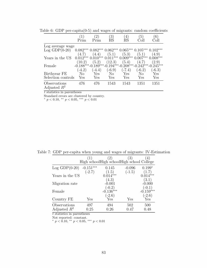
Table 6: GDP per-capita(0-5) and wages of migrants: random coefficients
(1) (2) (3) (4) (5) (6)Prim Prim HS HS Coll Coll
Log average wageLog GDP(0-20) 0.082∗∗∗ 0.082∗∗∗ 0.062∗∗∗ 0.065∗∗∗ 0.105∗∗∗ 0.102∗∗∗
(4.7) (4.4) (5.1) (5.3) (5.1) (4.9)Years in the US 0.012∗∗∗ 0.010∗∗∗ 0.011∗∗∗ 0.009∗∗∗ 0.007∗∗∗ 0.008∗∗∗
(10.2) (5.2) (12.3) (5.4) (4.7) (2.9)Female -0.188∗∗∗-0.189∗∗∗-0.194∗∗∗-0.208∗∗∗-0.242∗∗∗-0.245∗∗∗
(-4.2) (-4.4) (-6.9) (-7.4) (-6.2) (-6.3)Birthyear FE No Yes No Yes No YesSelection controls Yes Yes Yes Yes Yes Yes
Observations 476 476 1543 1543 1351 1351Adjusted R2
t statistics in parenthesesStandard errors are clustered by country.∗ p < 0.10, ∗∗ p < 0.05, ∗∗∗ p < 0.01
Table 7: GDP per-capita when young and wages of migrants: IV-Estimation
(1) (2) (3) (4)High schoolHigh schoolHigh school College
Log GDP(0-20) -0.151∗∗∗ 0.145 -0.096 0.199∗
(-2.7) (1.5) (-1.5) (1.7)Years in the US 0.014∗∗∗ 0.014∗∗∗
(4.3) (3.1)Migration rate -0.001 -0.000
(-0.2) (-0.1)Female -0.136∗∗∗ -0.159∗∗∗
(-2.6) (-2.6)Country FE Yes Yes Yes Yes
Observations 497 494 502 500Adjusted R2 0.25 0.26 0.47 0.48t statistics in parenthesesNot reported: constant.∗ p < 0.10, ∗∗ p < 0.05, ∗∗∗ p < 0.01
83

Table 8: International scores vs returns to schooling, FE
(1) (2) (3)All PrimarySecondary
Aggreg. score .0518∗∗
(2.6)Aggreg. primary .0282
(0.5)Aggreg. secondary .0876∗∗∗
(2.8)Constant .0633∗∗∗ .0743∗∗∗ .0486∗∗∗
(6.4) (3.1) (3.0)Observations 68 39 56Adjusted R2 -0.47 -2.38 -0.42t statistics in parentheses∗ p < 0.10, ∗∗ p < 0.05, ∗∗∗ p < 0.01
84

Chapter 3: Technology Spillovers and Suboptimal Rent Sharing
1 Abstract
The paper studies the effects of technology spillovers through the employee mobility
on technology adoption. It challenges the theoretical result of Franco and Filson (2006) by
assuming that the workers are risk averse and that the number of competitors is finite. I find
that for realistic parameter values the high-technology firm operates in an almost socially
optimal way by employing and training large number of workers immediately after starting
production. However, technology spillovers can significantly affect the high-technology firm’s
decision to enter the market. For realistic parameter values, the presence of the technology
spillovers can reduce the value function of the high-technology firm by 50-80% as compared to
the no spillovers case if the gap between current technology and new technology is very high.
For smaller productivity gaps technology spillovers can be beneficial for high-technology
firms. These effects of technology spillover can skew technology transfer towards more
developed regions with better local technologies.
2 Introduction
In 1977, Daewoo company established the joint venture in Pakistan to produce textile.
The company planned to use Korean technology and cheap Pakistan labor to produce
garments and simultaneously to evade quotas, imposed on the Korean exports. Daewoo
provided free training to 130 managers and supervisors from Pakistan. But in one year
only 15 workers from those 130 trained professionals continued to work in the joint venture.
Other 115 left to work in their own companies, profiting from the comprehensive technical
education provided by Daewoo. Many of them established their own factories or joined
other export-oriented enterprises, reducing the market share for Daewoo’s joint enterprise
(Easterly, 2000).
The example above illustrates the possible negative effect of spillovers on the returns
85

to investment in advanced technology. In contrast, the theoretical literature supports a
view that spillovers in general do not harm high-tech firms. Pakes and Nitzan (1983)
construct a two-period model of innovative firm, which is hiring a researcher to develop
a new technology. The firm has to deal with possibility of researchers leaving to create their
own spin-off companies. They show that if a spinoff company is harming the innovative firm
more than it benefits the researcher, the optimal contract will always prevent the researcher
from leaving. Moreover in the first period the researcher will accept lower wages in order to
fully compensate the innovative company for higher wage in the second period.
Franco and Filson (2006) propose a general equilibrium model of technology spillovers
with a continuum of competitive firms. In this environment, technology spillovers do not
harm innovative companies because the spinoffs of any particular company have negligible
impact on the market price. As a result, innovative firms do not prevent researchers
from leaving. Workers accept lower wages at higher technology firms and thus completely
compensate innovative firms for opportunity to learn. The equilibrium is shown to be Pareto
optimal. It means that the gains from the investment in new technology are higher than the
gains without spillovers, as new technology increases the productivity of other enterprises.
Both theoretical models predict the labor market outcomes which are inconsistent with
the recent empirical literature. First, it is generally found that workers in firms with higher
productivity earn higher wages, while in the Franco-Filson model wages decrease with the
productivity level. Empirical studies indeed demonstrate that foreign companies pay higher
wages on average. This effect was observed in numerous studies for both developed and
developing countries (Aitken, Harrison and Lipken, 1996, Martins, 2008). The similar wage
premium is observed not only for foreign-owned employers, but also for big or exporting firms.
Empirical evidence suggests that all of these traits are strongly associated with productivity
differences, implying that high-productive firms pay higher wages. Second, both papers
predict that workers fully compensate the high-technology firm for learning opportunities by
accepting lower wages. Empirical studies suggests, that it is happening on a very limited
86

scale. For example, in Pesola (2007) the firm’s wage premium paid by foreign-owned firms
is found to be insignificant and the tenure premium is only slightly higher than in domestic
firms.
In this paper, I show that the presence of spillovers in many realistic cases can lower
the sum of discounted profits for a high-technology firm. Two crucial deviations from the
Franco-Filson assumptions are responsible for this result. First, in my model the workers are
unable to accept very low wages, either because of the risk aversion or liability constraints.
Second, in my framework the number of firms is finite and outflow of workers from one firm
has a significant effect on market prices. High technology firms then can manipulate prices
by controlling the outflow of experienced workers and average productivity of the competitive
environment and pay higher wages to the experienced workers in equilibrium.
The model predicts that for plausible parameter values a high-technology firm would
choose high employment and high outflow in first periods. The choices would be close to
socially optimal choices and the welfare losses as compared to the social planner solution
would be also very low. The model also predicts low wages for new workers and much
higher wages for workers with experience in high-technology firm. The wedge between wages
of experienced and inexperienced workers incentivizes the high-technology firm to choose
higher employment of inexperienced workers in first periods and to let experienced workers
move to local firms with lower technology.
I also find that technology spillovers can significantly reduce high-technology firm’s
benefits from investing in a low-technology country. If the gap between local and new
technologies is very high, the high-technology firm extracts only a small part of benefits of
technology spillovers with larger decrease in the market price. This finding can help to ex-
plain the phenomenon of slow adoption of modern technologies in developing countries. As it
was pointed out in Keller (2004), the slow diffusion of technology is largely responsible for the
existing gap in TFP between developed and developing countries. My paper suggests that the
technology spillovers through the employee mobility can negatively affect technology transfer
87

by preventing high technology companies from directly investing in developing countries.
Other explanations in the literature include contractual incompleteness (Acemoglu, Antras
and Helpman, 2007) and high monitoring and law enforcement costs (Cole, Greenwood and
Sanchez, 2012).
This paper is also related to the labor literature on employee training. In case of
technology spillovers a worker obtains useful knowledge and applies it in another firm,
increasing its productivity. In case of training, the worker increases his own productivity and
applies it in another firm. It is a well known fact that in the competitive labor market firms
have no incentives to pay for general skills training (Becker, 1964) as increase in productivity
will be matched by increase in the labor compensation. On the contrary, papers of Acemoglu
and Pischke (1999, 2000) argue that firms will be able to appropriate part of the training
benefits and so will invest in training if the labor market is not competitive or if firms have
imperfect information about the workers’ abilities.
In this paper, worker also shares benefits of learning with a firm. One crucial difference
here is that firms do not bear any direct costs of training and knowledge accumulation occurs
only through the learning-by-doing. In my model there is also no asymmetric information
on the labor market and there exists a perfect competition for workers on the demand
side. As a result, the wage structure in equilibrium is not compressed as in Acemoglu
and Pischke. Moreover, firms compete on the product market, which influences their labor
market decisions. Firms in my model are still not able to obtain full gains of the costless
training, because workers are risk-averse.
The paper is organized as follows. In Section 3, I describe my model of industry with
technology spillovers and explain the intuition behind it. Section 4 contains most of the
results in my paper. It starts by explaining the numerical algorithm I use to solve the model
and assumptions on parameter values. Next, in 4.2 I describe the choices of high-technology
firms with respect to employment and outflow of workers for baseline parameter values. In
subsection 4.3, I compare the social benefits of profit-maximizing technology firm with the
88

social planner’s benefits. Then I proceed to discuss policy implications in 4.5 and 4.6 both
for the location choice for high-technology firms and for the benefits of non-compete clauses.
Section 5 concludes the paper.
3 Model
In the example of Daewoo in the introduction, the company investing in advanced
technology experiences costs of technology spillovers to competitors. There are at least two
channels for negative effects of technology spillovers both of which are absent in perfect
competition models. First, an increase in the productivity of competing firms can increase
the total output and lower market prices, reducing the profit of high-technology company.
Second, a higher productivity of competitors can raise the wages if other companies possess
market power on the labor market. The model includes the first channel, but ignores the
second one to keep the model tractable.
In this model, I consider the case of high-technology company producing a product
with a competitive fringe, which can copy its technology by hiring its former employees.
Firms compete on the product market with high-technology firm possessing some market
power. Firms can still hire as many workers as needed from the outside sector at a fixed
wage. Hence my model incorporates the first channel (product market competition), but not
the second one.
Another crucial fact I want to incorporate into my model is that more productive
firms pay higher wages. Empirical research (Abowd, Kramarz and Margolis, 2001; Song et
al, 2018) indicates that at least part of this difference comes from differences in effective
prices of labor. In order to incorporate this feature, the model uses discrete timing with
infinite horizon t = 1, 2, ... Infinite horizon allows for stationary solutions in which more
productive companies retain their workers and pay higher wages. In contrast, in finite time
horizon technology spillovers would involve zero costs for high-technology firms and so the
stationary solution is impossible.
89

3.1 Competitive Environment
In this partial equilibrium model I consider one economy, producing the good C and the
numeraire composite good y. The market of good C is small enough to neglect its effects on
income21, so the consumers’ preferences can be fully summarized by the demand function:
P = P (Q), Q =
∫qidi (18)
Where price P is expressed in units of the good y and Q refers to the total quantity of good
C produced and consumed and qi to the output of the particular firm.
There are two types of firms in the industry C. There is a continuum of local firms of
measure M and one non-local firm, which I call MNC (short of multinational corporation)
throughout the paper. This structure is an approximation to the industry with M + 1 firms,
where M is large enough22. I refer to a continuum to postulate no market power for any of
M local firm. The MNC firm is different, because in the model it has market power both in
the product and the labor market.
All firms in the industry C produce perfect substitutes according to technology f(·)
with decreasing returns to scale. The following formula describes output qi of any firm:
qi = Aif(ni), f() ∈ C2, f ′ > 0, f ′′ < 0 (19)
Productivity parameter Ai differs between firms. At period t = 0 the MNC has a higher
productivity Ah and all other firms have productivity A0 < Ah . I call all other firms with
initial productivity A0 ”local firms” or ”environment”.
21Alternatively, one can make an assumption, that all product C is exported.22In calibration I assume M=20,50 or 100
90

3.2 Workers
Workers are risk neutral and do not value leisure. The utility of a worker for any consumption
sequence {wi}∞i=1 is a discounted sum of future utilities:
U({wi}∞i=1) =∞∑i=1
βi−1u(wi), 0 < β < 1 (20)
Utility u(·) is a strictly increasing function of consumption. I consider both risk-neutral
u(c) = c and risk-averse workers in the paper. There is no saving or borrowing in the model.
This assumption is innocuous in the case of risk-neutral workers, but less so in case of
risk-averse workers. However, allowing borrowing and saving results in overly complicated
problem with a much larger state space in quantitative analysis.
Workers can always find work in the outside sector, producing the numeraire good y.
Firms in the outside sector pay constant wage w. As the labor demand in the industry C is
negligible compared to employment in the numeraire sector y, we can think that there is an
infinite supply of workers by wage w for the sector C. The only difference between workers
is their level of industry-specific knowledge, which does not affect their own productivity,
but can influence the productivity of their employer.
3.3 Technology Spillovers
The standard assumption in the theoretical technology spillover literature is that former
workers create new spin-off firms (Pakes and Nitzan, 1983; Franco and Filson, 2006; Das-
gupta, 2012). This assumption makes the analysis easier in the perfectly competitive envi-
ronment by avoiding the need to assume the specific functional form of the spillover function.
I study a different market structure, where one company holds a market power both on the
product and labor markets, and spin-offs in this setup eliminate the market power starting
from the next period. Instead of considering spin-off companies, I assume that hiring workers
from more productive companies can directly increase the productivity. This approach
91

to technology spillovers is consistent with the recent empirical literature, which suggests
that hiring workers from more productive firms tends to increase productivity (Poole, 2008;
Stoyanov and Zubanov, 2012; Serafinelli, 2014).23
Workers employed at the MNC learns industry-specific knowledge on the job. The
learning occurs with certainty after one period of employment. The knowledge is any infor-
mation allowing to increase worker’s productivity which is also transferable between firms
and workers. Potentially this definition of knowledge includes not only production know-how,
but also management, marketing or even personal time-management and discipline. I will
call workers with recent experience in MNC ”experienced” workers throughout the rest of
the paper.
This knowledge of experienced workers may be used by local firms to increase the
productivity. Namely, by hiring in total ne workers with at least one period of experience
with firm j and productivity Aj > Ai a local firm i increases its productivity Ai to:
A′i = G(Ai, Aj, le) = (1− exp(−ρle))Aj + exp(−ρle)Ai(0) (21)
This spillover function G(·, ·) is strictly increasing and concave in the third argument (le
here), approaching Aj, when le goes to infinity. Note that future productivity A′i in this
formula depends on the total number of workers hired and on the initial productivity Ai(0)
before hiring any workers with experience in j. The effect of hiring one additional experienced
worker is:
dAi(t+ 1)
dle= ρ(Aj − Ai(t)) (22)
Less is the difference between the current productivity Ai(t) and Aj, less is the effect
of hiring additional experienced workers. It happens because the know-how of firm’s j is
already partially absorbed by firm i. Therefore additional workers bring less new knowledge.
23Some theoretical papers (Cooper, 2001; Fosfuri et al, 2001) also assume that firms acquire technology byhiring workers from other companies , but they concentrate on highly stylized setups with only one worker.
92

I assume that workers can transmit knowledge only once. All the knowledge transferred
to any of the local companies becomes a common knowledge in the next period. Hence
hiring the same experienced worker consecutively by several local companies increases the
productivity only for the first employer.
All workers in the outside sector do not possess any knowledge specific for the industry
C. This assumption will hold if, for example, all the workers leaving at the same period
carry the identical knowledge and so in the next period their know how becomes a common
knowledge.
3.4 Contracting Environment
The MNC and the local firms post state-contingent employment contracts to workers, con-
ditional on full employment history. The contracts specify both the payments in each state
w(·) and the promised value Vw(·), starting from the current period.
In the model workers can walk out of the contract at any moment. I will argue, that
labor market institutions are less developed in poor countries, which are the focus of this
model. Also non-compete agreements are not enforceable24.
Labor contracts are subject to limited liability constraints. Namely the contracts do not
allow for negative wages in any period. This assumption prevents workers from paying MNC
for learning if the present discounted benefit of learning is higher than the worker’s marginal
product. Contracts involving workers paying to firms seem to be extremely rare based on the
anecdotal evidence. Both legal constraints such as minimum wage and borrowing constraints
can hinder implementation of negative wages in practice.
24The non-compete clause can be also implemented as a voluntary agreement, in which workers are paidin each period if they do not work for competing firms. In this contract, the former employer still bearssome costs to verify the employment state of the worker. My assumption of no non-compete agreements isthen equivalent to stating that the verification costs are too high.
93

3.5 Equilibrium Definition
In the subsequent analysis I concentrate on the Markov perfect equilibrium by limiting the
set of possible contracts and strategies to depend only on payoff-relevant variables. This
assumption eliminates the plausible possibility that MNC commits to the certain strategy
in period 0. By doing so the MNC, in general, can achieve a higher payoff, but this strategy
will require some commitment mechanism, which is not always available.
Later I demonstrate that the Markov perfect equilibrium remains an equilibrium even
if history-dependent contracts are allowed. It is harder to justify the absence of history-
dependent contracts if workers are strictly risk averse. Risk aversion, for example, will allow
for wage smoothing contracts which depend on the state at the moment the contract is
signed. In this case, the Markov perfect equilibrium remains an equilibrium only under the
additional assumption that firms can renege on the contract.
In the Markov perfect equilibrium the aggregate state Z is described by only two
variables: the employment level of the MNC lm and the current productivity level of the
local firms Af . Employment level of the MNC matters because it equals to the future measure
of experienced workers and thus limits the increase in productivity in the next period.
The current productivity level of local firms Af describes the distribution of local firms
productivities. Local firms have identical strictly concave value functions in equilibrium,
and so they choose the same productivity level. The productivity level of local firms affects
both the equilibrium price and the future productivity through the spillover function.
The worker’s promised value Vw(a,Ah, Z) depends on his knowledge level a, the pro-
ductivity level of the employer Ah and the aggregate state Z = [lm, Af ]. The knowledge
level a equals Ah if in the previous period the worker was employed at MNC and 0 otherwise
(workers do not learn anything in local firms).25 It is equal to the sum of the current period
wage plus the discounted future value under the assumption of optimal choice of subsequent
25In equilibrium local firms will have identical productivity levels, so the knowledge transfer from onelocal firm to another is excluded.
94

employment.
Vw(a,A, Z) = w(a,A, Z) + βmaxA′
Vw(a′, A′, Z ′) (23)
a′ =
Ah, A = Ah
0, A < Ah
The wage w(a,Ah, Z) also depends on the productivity of the current employer and on
the knowledge level. In each state Z the economy has four different wage levels:
1. wage of inexperienced workers employed outside of the MNC w = w(0, A, Z), A < Ah
2. wage of inexperienced workers employed in MNC wu(Z) = w(0, Ah, Z)
3. wage of experienced workers employed in local firms We(Z) = w(Ah, A, Z), A < Ah
4. wage of experienced workers employed in the MNC we(Z) = w(Ah, Ah, Z)
Because the worker is choosing the employer in each period, the promised values have
to satisfy several participation constraints. First, the promised values of experienced workers
at MNC and at local companies should be equal to make workers indifferent Vw(a,A, Z) =
Vw(a,Ah, Z). This is necessary if both the local firms and the MNC employ some experienced
workers. This assumption can be also supported without loss of generality even if workers
concentrate in only one sector, because the MNC can never lose by matching the promised
value of local firms. Next, the promised values for the inexperienced worker employed at
the MNC should be higher or equal to the discounted sum of utilities from staying in the
outside sector Vw(0, Ah, Z) ≥ w/(1 − β). I describe two other constraints while discussing
the problem of local firms next.
The value function of the MNC satisfies the following Bellman equation:
Vm(Af , lm) = maxl′m,A
′f
[AhP (Af , l′m)f(l′m)−we[l′m−Ne]−wu[l′m− lm +Ne] + βVm(A′f , l
′m)] (24)
95

we = we(Af , l′m), wu = wu(Af , l
′m)
subject to: lm −Ne(Af , A′f ) ≥ 0, l′m − l +Ne(Af , A
′f ) ≥ 0
Here lm is the starting employment of the MNC, Af is the current productivity level
of followers, P (Af , lm) is the equilibrium price of the product, Ne - the total measure of
experienced workers, leaving the MNC in this period, we - compensation of experienced
workers in MNC. The expression in the right hand side of the equation is the revenue minus
costs of experienced workers and inexperienced workers plus the discounted future value.
The value function of a local firm is:
Vf (Af , lm, Ai) = maxlf ,le
[AiP (Af , l′m)f(lf )−Wele − w(lf − le) + βVf (A
′f , l′m, A
′i)] (25)
subject to A′i = G(Ah, Ai, le) = (1− exp(−ρle))Ah + exp(−ρle)Ai, 0 ≤ le ≤ lf
In this function Ai is the current productivity of firm i, le - total employment of the
local firm, , le - employment level of experienced workers. Next period productivity depends
on the current productivity and employment of experienced workers according to the spillover
function G(·).
Local firms can always hire inexperienced workers from the outside sector. Hence, the
promised value for inexperienced workers in local firms should be equal to the discounted
sum of wages outside Vw(0, A, Z) = u(w)1−β . The promised value for experienced workers in
local firms is then equal to:
Vw(Ah, A, Z) = w(Ah, A, Z) + βVw(0, A, Z ′) = We(Z) + βw
1− β(26)
The MNC chooses the inexperienced workers wage to be as small as possible without
96

breaking the worker’s participation constraint and the limited liability constraint:
wu(Z) = min[0, u−1(w
1− β− βVw(Ah, Ah, Z
′))] (27)
Local firms compete on the labor market and so the promised value of experienced workers
in local firms is equal to the marginal gains from hiring a worker. I will specify the marginal
gains when discussing the first-order conditions for the firm’s problem.
Equilibrium Definition. The Markov perfect equilibrium is a combination of wage
functions w(·), value functions V mt (·), V f
t (·), Vw(·), decision rules for the future productivity
A′i = A(Ai(t), Z) and employment l′m(Ai, Z), le = le(Ai, Z) as well as the law of motion for
A′f = Γ(Z), such that the following conditions are satisfied:
� The value functions V mt (·), V f
t (·), Vw(·) satisfy the Bellman equations (23)-(25) and the
decision rules A(·), l′(·), le(·) represent the solutions to the equations.
� The law of motion for Af is consistent with the decision rules.
� The market of experienced labor force is cleared in each state Ne = Mle(Af , Z) (M is
the measure of local firms).
� Wages satisfy the conditions for the optimal contract (26)-(27).
In this equilibrium, the MNC chooses the path of productivities of local companies by varying
the measure of leaving workers and the path of employment. The chosen path maximizes the
value of the MNC, taking into account the effect of productivities on prices. Productivity of
local firms negatively affects both the price of the product C and the wage of experienced
workers at MNC. Because of it, the MNC has the incentives to increase the productivity of
environment, despite the negative effect on the product market.
This equilibrium here is essentially a subgame perfect Nash equilibrium. The MNC’s
chosen path is optimal for each level of local firms productivity AF and for each employment
level lm. Local firms take this into account while chosing employment of experienced workers.
97

Hence my concept of equilibrium differs from the dynamic Stackelberg problem (Miller and
Salmon, 1985), in which the MNC would commit to a certain path of productivities and
employment.
3.6 Social Planner’s Problem
First, I would like to start my analysis from finding the socially optimum paths of employ-
ment and productivity. In this subsection, I consider a social planner who maximizes the
discounted sum of the social surplus. The social surplus equals to the difference between
consumers surplus at the market-clearing price minus production costs. The planner chooses
sequences of MNC’s employment lm(t), local firms employment lf (t) and experienced workers
hired by local firms le(t) to maximize the discounted sum of social surplus:
maxlm,lf ,le
∞∑t=0
βt
(∫ Q(t)
0
P (q)dq − (lm +Mlf )w)
)(28)
subject to: Q(t) = Ahf(lm) +MAff(lf ) (29)
Af (t+ 1) = Ah + (Af (t)− Ah) exp(−(ρ/M)le(t− 1)) (30)
Af (t) = Ah + (A0 − Ah) exp(−(ρ/M)t−1∑i=1
le(i)) (31)
lm(t− 1) ≥ le(t), lf (t) ≥ le(t)
In this equation, le is the number of experienced workers hired out by local firms which
determines their future productivity and lm is the employment of the MNC. Equations (30)
and (31) are algebraically equivalent.
I start with two obvious observations about the socially optimal path. First, on
the socially optimal path all local firms should have the same employment and the same
productivity due to a strict concavity of both the production function and the spillover
function. In formulating the equations (28)-(31), I already take this into account. Second,
98

the MNC should not employ any experienced workers, because while experienced workers
bring no additional benefits to the MNC, they increase future productivity of local firms.
To find first-order conditions, I substitute equations (29) and (31) directly into the
objective. The first-order conditions are:
PtAhf′(lm(t)) + λt+1 = w (32)
ρ(Ah − A0)∞∑
k=t+1
βk−tPkf(lf ) exp[−(ρ/M)k−1∑i=1
le(i)]− λt − µt = 0 (33)
PtAff′(lf ) + µt = w (34)
λt(le(t)− lm(t)) = 0, µt((1/M)le(t)− lf (t)) = 0 (35)
The first equation (32) equalizes the social benefits of workers in the MNC with social
costs. Social benefits have two components. The first component PtAhf′(lm) corresponds to
an increase in social surplus achieved due to higher MNC’s output. The second component
λt+1 is the shadow price of experienced workers given their use for technology transfer in the
next period. The actual benefit of experienced workers moving to local companies is a sum
in the second equation (33):
B = ρ(Ah − A0)∞∑
k=t+1
βk−tPkf(lf ) exp[−(ρ/M)k−1∑i=1
le(i)]
The future marginal benefits B of experienced workers joining local firms are equal
to the discounted sum of changes in local firms’ revenues due to an increase in future
productivity from spillovers. Social benefits depend both on past and future transfer of
experienced workers le.
The multiplier µt corresponds to the benefit of increasing employment in local com-
panies beyond employment equalizing MPL with wage w. The multiplier is zero if the
employment of experienced workers in the representative local firm is less than the total
99

employment in the firm (1/M)le < lf . Because future benefits B > 0, the multiplier
λt > 0 whenever µt = 0. Hence, as long as local firms also hire some inexperienced workers
((1/M)le < lf ), the marginal product of labor in the MNC is less than the wage w and all
MNC’s former workers get jobs in local firms lm = le.
Let’s consider the solution path with moderate spillovers such that (1/M)le < lf . This
path exists for zero spillovers ρ = 0 or Af = Ah. The solution with moderate spillovers
should exist in some neighborhood of zero spillovers by the continuity argument as long as
the spillovers coefficient ρ is low enough or the productivity gap is small.
As follows from the discussion above, on the path with moderate spillovers µt = 0 and
lm = le. Hence, the first-order condition for the monopoly’s employment on this path takes
the following form:
PtAhf′(lm(t)) +B = w (36)
Equation (36) states that on the path with moderate spillovers the optimal employment
of the MNC lm should equalize the sum of marginal product of labor and future marginal
benefits of local firms with the wage in the outside sector w. It implies that in the social
planner’s solution the MNC should hire more workers compared to the MNC in case with
no spillovers. Next, we compare this solution with the case of the MNC with spillovers.
3.7 Markov Perfect Equilibrium Analysis
Next, I proceed to the analysis of the equilibrium problem in the Markov perfect equilibrium
with profit-maximizing MNC and local firms. I start with a simpler analysis of local
firms. The representative local firm’s problem is to choose employment of experienced and
100

inexperienced workers in order to maximize the discounted sum of future profits26:
maxlf (t),le(t)
∞∑t=0
βt[Af (t)P (Af , lm(t))f(lf (t))−W et le(t)− w(lf (t)− le(t))]
Af (t) = Ah + (A0 − Ah) exp[−ρt−1∑i=1
le(i)]
le(t) ≥ 0, lf (t)− le(t) ≥ 0
Due to their size, local firms consider the market price to be constant P (Af , lm) = Pt.
The Lagrangean of a representative local firm is:
L(Af , le, lf ) =
∞∑t=0
βtG[t−1∑i=1
Lei ]P (t)f(lf (t))−Wele(t)−w(lf (t)−le(t))+λtle(t)+µt(lf (t)−le(t))]
In the equation above the functionG(·) is the function mapping cumulative employment
of experienced workers to productivity (technology spillovers function). The first-order
conditions are:
Af (t)P (t)f ′(lf (t)) = w − µt (37)
−W et + w − ρ
∞∑i=t+1
βi−t(Af (i)− Ah)P (i)f(lf (i))− µt = 0 (38)
I substitute the (37) into the condition (38) and take into account that the non-
negativity constraint on experienced workers employment never binds (because experienced
workers always increase productivity). Then the wage of experienced workers at local firms
26Here I abuse the notation by using le to refer to the measure of experienced workers hired by therepresentative firm instead of the total amount of experienced workers hired by the local firms.
101

is:
W et = Af (t)P (t)f ′(lf (t)) + ρ
∞∑i=t+1
βi−t(Ah − Af (t))P (i)f(lf (i)) = Af (t)P (t)f ′(lf (t)) +B
Hence the current wage of experienced workers equals to the marginal product of labor
in the current period plus the share of expected difference in future output achieved by hiring
an additional experienced worker. The second component equals to the future benefits of
spillovers in the social planner’s problem B as long as productivity and price paths coincide.
This expression () maps the future outflow of experienced workers from the MNC to the
current wages of experienced workers in local firms. In future I will also use the recursive
representation of wages which directly follows from the equation above:
W et = A(t)P (t)f ′(lf (t))− βA(t+ 1)P (t+ 1)f ′(lf (t+ 1))+
+ρβ(Ah − Af (t+ 1))P (t+ 1)f(lf (t+ 1)) + βW et+1
(39)
Now consider the problem of the MNC. The MNC chooses the current period employ-
ment lm in each period as well as the outflow of experienced workers le. The choice is going
to affect both the current price and the future sequence of wages and productivities. The
problem of the MNC is:
maxlm,le
∞∑t=0
βt[AhP (Af , lm)f(lm)− we(lm(t− 1)−Mle(t))− wu(t)(lm(t)− lm(t− 1) +Mle(t))]
Subject to the equations for equilibrium wage paths and productivities of local firms:
We(t) = AiPf′(lf (t)) + ρ
∞∑i=t+2
βi−t(Ah − A(i))P (i)f(lf (i))
102

A(t) = Ah + (A0 − Ah) exp[−ρt−2∑i=1
(1/M)le(i)]
we(t) = min[0,We(t)− βWe(t+ 1) + βw]
wu(t) = min[0, w(1 + β)− βWe(t+ 1)]
le ≥ 0, lm ≥ 0, lm(t)− lm(t− 1) +Mle(t) ≥ 0
I consider analytically only the path with moderate spillovers in which local firms still
hire some inexperienced workers le < lf . First, we can substitute the expression for the
productivity of local firms directly into other constraints and the objective. On the path
with moderate spillovers the recursive representation of wages of experienced workers at local
firms (39) yields the following expression for wages of experienced workers at the MNC:
we(t) = w + ρβ(Ah − Af (t+ 1))Pt+1f(Lt+1) > 0 (40)
wu(t) = min[0, w − ρ(Ah − A0)∞∑
k=t+1
βk−tP (k)f(Lk) exp[−(ρ/M)k−2∑i=1
lm(i)]] (41)
The equilibrium employment and price paths of MNC in general differ
from the socially optimal solution. This is not surprising given its market power,
but the market power is not the only driver of suboptimal decisions. Another reason for
this suboptimality is the inability to completely internalize the benefits of worker’s learning.
As soon as wages of inexperienced workers hit the zero threschold, an additional increase in
future benefits of local companies produces zero benefits for labor costs of the MNC.
Consider the case when the MNC employs no experienced workers lm(t−1)−Mle(t) = 0
and always employs some inexperienced workers lm(t) > 0 as in the socially optimal solution.
If the MNC’s solution is socially optimal then it is also socially optimal for the constrained
problem with lm(t)− lm(t− 1) +Mle(t) = 0 and lm > 0. The Lagrangean of the constrained
103

problem is:
L(Af , lm) =∞∑t=0
βt[AhP (Af , lm)f(lm)− wulm(t)
]I calculate the first-order condition with respect to employment lm and take into
account the dependency of wages of inexperienced wu on future productivity and product
prices. The first-order condition is the most similar to the first-order condition of the social
planner when wages of inexperienced workers wu are non-zero:
AhPtf′(lm)︸ ︷︷ ︸
MPL
+P ′2Ahf(lm)︸ ︷︷ ︸Price effect
+∞∑
k=t+1
βk−tχkAhP′1f(lm)︸ ︷︷ ︸
Future price effect
+ ρ
∞∑k=t+1
βk−tlm(k)χkP (k)f(lf (k)))︸ ︷︷ ︸Lower wage due to higher future productivity
+
+ ρ∞∑
k=t+1
βk−tlm(k)χkP′1f(lf (k))(Ah − Af )︸ ︷︷ ︸
Future wage effect from prices
= wu
Where χt = ρ(Ah − Af )/M and P ′1 = P ′1(Af , lm) is the first derivative of market price
with respect to productivity of local firms and P ′2 is the first derivative of market price with
respect to MNC’s employment lm. After substituting the expression for positive wu (41) into
the equation above and rearranging terms I obtain:
AhPtf′(lm) + AhP
′2f(lm) +
∞∑k=t+1
βk−tχkAhP′1f(lm)+
+ρ∞∑
k=t+1
βk−tlm(k)χkf(lf (k))(P ′1(Ah − Af ) + P (k)) = w − ρ∞∑
k=t+1
βk−tP (k)f(Lk)(Ah − Af )
There is at least one clear case in which the MNC’s equilibrium path is socially sub-
optimal. Consider the case of perfect elasticity of demand P = const. In this case, the
consumer surplus and the social surplus are still well defined. However, in the MNC’s
104
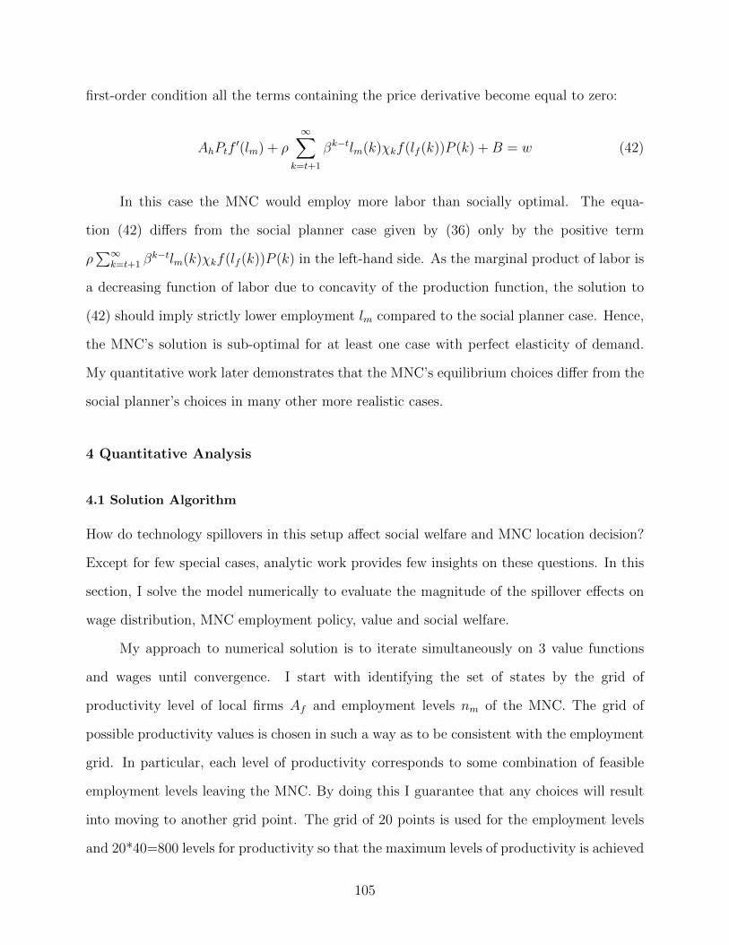
first-order condition all the terms containing the price derivative become equal to zero:
AhPtf′(lm) + ρ
∞∑k=t+1
βk−tlm(k)χkf(lf (k))P (k) +B = w (42)
In this case the MNC would employ more labor than socially optimal. The equa-
tion (42) differs from the social planner case given by (36) only by the positive term
ρ∑∞
k=t+1 βk−tlm(k)χkf(lf (k))P (k) in the left-hand side. As the marginal product of labor is
a decreasing function of labor due to concavity of the production function, the solution to
(42) should imply strictly lower employment lm compared to the social planner case. Hence,
the MNC’s solution is sub-optimal for at least one case with perfect elasticity of demand.
My quantitative work later demonstrates that the MNC’s equilibrium choices differ from the
social planner’s choices in many other more realistic cases.
4 Quantitative Analysis
4.1 Solution Algorithm
How do technology spillovers in this setup affect social welfare and MNC location decision?
Except for few special cases, analytic work provides few insights on these questions. In this
section, I solve the model numerically to evaluate the magnitude of the spillover effects on
wage distribution, MNC employment policy, value and social welfare.
My approach to numerical solution is to iterate simultaneously on 3 value functions
and wages until convergence. I start with identifying the set of states by the grid of
productivity level of local firms Af and employment levels nm of the MNC. The grid of
possible productivity values is chosen in such a way as to be consistent with the employment
grid. In particular, each level of productivity corresponds to some combination of feasible
employment levels leaving the MNC. By doing this I guarantee that any choices will result
into moving to another grid point. The grid of 20 points is used for the employment levels
and 20*40=800 levels for productivity so that the maximum levels of productivity is achieved
105

only if all the workers at the maximum employment levels leave the MNC in each period for
40 periods. On this grid, I choose some starting value matrix of the MNC Vm(0) and the
value matrix of experienced worker dV f(0), showing the increase in value of local firm from
hiring one additional experienced worker. I also calculate the matrix of equilibrium prices
P (), so that at each grid point P (Af , Lm) is equal to the price which clears the product
market for productivity of local firms Af and employment of the MNC lm.
After obtaining the equilibrium price matrix, I iterate on the value functions of MNC
and local firms by using the following algorithm:27
1. Calculate we, wu,We as described in Appendix 2.
2. For each starting level of MNC employment lm and each starting level of productivity
of local firms Af :
� Calculate the new value matrix of MNC as:
V (Af , lm)(t+1) = maxA′f ,l
′[AhP (Af , l
′m)f(lm)−we(le)(lm−Mle)−wu(le)(l′m−lm+Mle)+
+βV (A′f , l′m)(t)]
,where Mle is the outflow of experienced workers from the MNC. This variable is
calculated as a function of both current and future productivity levels.
� Calculate the change in the local firm value dV f by using the decision rules
obtained from the optimization problem above:
dV f(Af , l)(t+ 1) = ρ(Ah− Af )P (Af , l′m)f(l) + βdV f(A′f , l
′m)(t)
where l is an optimal employment of local firm for a price P (Af , l′m) and produc-
tivity Af .
27For the used range of parameters these iterations always converge to the stable combination of valuefunctions.
106

� Calculate the value of experienced worker at MNC:
Vw(Af , lm)(t+ 1) = we(A′f , l′m) + βVw(A′f , l
′m)(t)
3. Stop if the sum of absolute differences between the value functions Vw()(t + 1) and
Vw()(t) is small enough, otherwise go to Step 1.28
Additionally, I also iterate on the social value function which is equal to the sum of
discounted social surplus to calculate the maximum attainable social welfare. The social
planner’s value function is:
Vs(Af , lm) = maxl′m,le,lf
CS(P (Af , l′m, le, lf ))− w(l′m +Mlf )] + βVs(A
′f , l′m)
s.t.A′f = Ah + (Af − Ah) exp[−(ρ/M)le]
le ≤ lm, (1/M)le ≤ lf
In this system of equations, CS(·) is a consumer surplus which depends on price
P (Af , l′m, le, lf ) and the inverse demand function P (·) and Vs(·) is the social planner’s value
function. The social planner chooses current MNC’s employment, employment of experienced
workers in local firms and local firm’s employment to maximize the sum of current surplus
and discounted future value. This recursive representation is equivalent to the sequential
representation in Section 2. The iteration on the social value function proceeds independently
from the iteration on the MNC’s problem above.
In the numerical solutions, I use the Cobb-Douglas production function f(l) = lα. The
worker’s utility function is linear u(C) = C if not specified otherwise. I also study CRRA
utility with different levels of relative risk aversion to explore the robustness of results. For
the demand function the simple constant elasticity function is used P = P0
Qγ.
28In the calculations the convergence of value functions always led to the convergence of wages.
107

There are 10 constants in the model: elasticity of demand 1γ, discounting factor β,
production function parameter α, demand shifter P0, starting productivity of local firms
A0 ≡ Af (0), measure of local companies M , wage in the outside sector w and the spillover
function parameter ρ. Wage in the outside sector w and the initial productivity A0 in the
sector C are normalized to 1. The choices for β = 0.95 and α = 0.7 are based on accepted
standards in literature.
For the spillover speed parameter I rely on empirical findings from Serafinelli(2013).
Serafinelli studies small firms in Veneto region of Italy and finds that hiring one worker
with experience in high-wage firm increases the productivity of hiring firm by approximately
1.8-3%. I choose my ρ so that for the same average employment of hiring firm around 30
workers, hiring one experienced workers increases future productivity by 2.4% which is the
mid-point of the Serafinelli’s range. This translates into the spillover parameter ρ = 0.13. I
calibrate the parameter P0 so that in each simulation the employment of local firms matched
the median employment in the Serafinelli’s sample or approximately 30 workers.
I do not have a way to impose any discipline on the choice of γ, because price elasticities
of demand vary between markets. My baseline value of γ = 0.7 should lie within the
reasonable range for many industries. The chosen measure of local firms M = 50 corresponds
to the industry with relatively low level of concentration.
4.2 Solutions: Infinite Horizon
The calculation proceeds independently for different values of starting local firms’ produc-
tivity A0 in the range from 1.2 to 5.0. In all of my calculations the productivity of MNC is
equal to Ah = 5. For each starting productivity value A0 I calculate the value function of the
MNC with spillovers, the value function of MNC without spillovers, the social welfare under
the path chosen by MNC and the social value function to show the maximum attainable
108

welfare. The value function of MNC without spillovers is given by the following expression:
Vm(Ah) = maxlm
∞∑t=1
[βt−1AhP (A0, lm)lαm − wlm] (43)
The value function Vm(Ah) without spillovers the maximum value the MNC can achieve
if local companies cannot improve productivity by hiring experienced workers. Besides
describing a case with no transferable know-how, equation (43) also correspond to a situation
with strictly enforced non-compete agreement. The problem of MNC without spillovers
is essentially a static problem, because in absence of spillovers the productivity of local
companies stays constant Af (t) = A0. This value function is equal to the discounted sum of
monopolistic profits.
The typical solution for the specific value A0 = 2.1 is presented on Figure 1. Four
different graph present the dynamics of MNC’s employment, outflow of experienced workers,
market price P and the profit in first 10 periods. The simulation of the optimal path starts
from the zero employment and zero cumulative outflow of experienced workers Af (0) = A0.
I compare optimal choices of the MNC with the social planner (red) and with the monopoly
without spillovers.
The simulation demonstrates that MNC achieves high employment early on and de-
creases it later. High employment in early periods serves two purposes. First, it allows to
profit from relatively high market prices due to low productivity of competitors. Second,
high employment exploits lower wages of inexperienced workers faced by the MNC. Because
the local firm’s benefits B from hiring experienced workers positively depend on market price
and negatively depend on cumulative number of workers hired, local firms are willing to pay
the highest premium to experienced workers in first periods. It translates to lower wages of
inexperienced workers paid by MNC, incentivizing MNC to increase employment.
Market prices decline over time due to an increase in productivity of local companies.
Prices already start at the lower level due to higher starting employment of the MNC in case
109

of spillovers and decline further after local firms absorb more and more experienced workers.
Market prices by the MNC are almost indifferent from market-clearing prices chosen by the
social planner.
MNC derives high profits in first two periods due to high prices and low wages of
inexperienced workers. Afterwards, the profits decline below the level of profits without
spillovers. This finding implies that both the speed of learning and knowledge transfer
and/or discount rate would affect the optimal dynamics of employment and experienced
workers’ outflow.
Figure 2 supports my explanation that low wages of inexperienced workers drive the
dynamics of employment. On Figure 2, the wages we and wu are plotted as functions of
local firms’ productivity Af . For low levels of Af local firms can get large productivity
gains by attracting experienced workers and so they pay high wage premiums. High wage
premiums for experienced workers imply lower initial wages for inexperienced workers. As
the productivity gap closes the difference in wages for experienced and inexperienced workers
also shrinks.
By paying lower wages in the first period of employment workers partially compensates
MNC for learning. In case of risk averse workers the decrease in wages is lower than the
gain in future wages. Limited liability restriction with risk neutral workers leads to the
same result if the future discounted gain is higher than the worker’s reservation wage w. It
happens for large productivity gaps between the local companies and MNC. At the same
time, MNC needs to pay higher wages to the experienced workers to reduce the outflow of
workers. Because the learning speed slows down as Af approaches Ah, the gap between the
two wages decreases with productivity of environment Af .
The difference between wages of inexperienced and experienced workers at the MNC
is very high as long as there is a substantial gap in productivities. For example, when the
productivity of environment is A0 = 1.2 and the productivity of MNC is Ah = 5, MNC pays
less zero wages to inexperienced workers until the productivity of environment goes up to
110

more than Af = 4. On another hand, the wage premium for experienced workers exceeds
1000%. The MNC, however, retains no experienced workers for chosen parameter values
and so it receives most of the technology-generated rent. If the starting productivity of local
firms is much close to the MNC productivity (A0 = 4.5, Ah = 5), experienced workers receive
very small wage premium of no more than 20% compared to the outside wage w.
4.3 Social and Private Benefits of FDI
Dynamics of MNC’s employment (Figure 3) shows that the employment policy of the MNC
is close to the socially optimal policy for all values of starting productivity A0 except
cases of very high and very low productivity gap. Typically, the social planner chooses
higher employment compared both to the MNC with and without spillovers. For very high
productivity gaps, the social planner chooses significantly higher employment in all the
periods except the second one. It should be noted, that my limited grid size could cause this
discrepancy in the second period. For lower productivity gap (A0 = 4), the social planner
again consistently chooses higher employment.
While there is a small difference in employment level chosen by the MNC and by the
social planner, there is no difference in their policy towards experienced workers. The social
planner let all the experienced workers go in order to increase the productivity of local firms
and increase the social surplus. The MNC also lets all the experienced workers go for all the
starting levels of productivity A0 as keeping them is both extremely costly as compared to
inexperienced.
Given the small difference in employment policies, it comes as no surprise that the MNC
achieves almost the same level of welfare as the social planner (Figure 4). The difference in
surplus is the highest for a higher productivity gap (A0 = 1.2). For these parameter values,
MNC produces deadweight losses of just about 3% of the maximum attainable cumulative
social surplus. The gap in surplus converges to about 0.5% when the gap disappears (A0 =
Ah = 5).
111

Figure 5 demonstrates that local workers derive a significant portion of gains from
having MNC in the economy. The worker’s rent Rw is equal to the discounted sum of
differences between actual wages and their outside option w multiplied by a number of
workers in each wage level:
Rw =∞∑t=0
βt[(we(t)−w)(lm(t−1)−Mle(t)))+(wu(t)−w)(lm(t)−lm(t−1)+Mle(t))+(We(t)−w)Mle(t)]
Workers receive the highest rent when the productivity of local firms is in the middle
range (2-4). The rent disappears whenever the gap disappears, because the zero-wage bound
becomes non-binding.
The MNC is also able to obtain large rents from hiring cheap inexperienced labor and
training it. Let R(t) denote the difference between the costs of labor, paid by the MNC
in period t in case of spillovers and the costs of the same quantity of labor at the outside
sector’s wage w:
R(t) =∞∑t=0
βt[(we(t)− w)(lm(t)−Mle(t))− (wu(t)− w(t))(lm(t+ 1)− lm(t) +Ne(t))]
This discounted sum R(t) represents the MNC’s wage savings from spillovers. It does
not include the additional payments received at local companies. The change in labor costs
due to spillovers is rather drastic, but surprisingly MNC bears no losses in labor costs.
The MNC’s rent is positively and relatively large (Figure 5), meaning that MNC is able to
significantly reduce labor costs by using cheaper labor.
Summing up, the MNC’s policy in presence of spillovers is very close to the socially
optimal policy and the deadweight losses are small. The possibility to extract benefits from
technology spillovers by employing and training cheap labor incentivizes MNC to choose high
employment and high speed of technology transfer. It means that, at least for my parameter
112

values, there is a very limited room for welfare-enhancing policies as long as a high-technology
firm chooses to operate in the location. However, a policy to attract high-technology firms
to particular location can have much more impact on social welfare.
The presence of spillovers leads the MNC to charge lower prices, employ less workers
and pay higher wages to experienced workers. I explore the contribution of each of the
factors in MNC value by studying three effects separately:
� Effect of wages, taking into account that the liability constraints can prevent full rent
extraction from workers
� Prices go down due to higher productivity of local firms
� Employment of MNC goes down to reduce the spillovers and to raise prices while facing
stronger competition
The calculations show that higher wages of experienced workers do not directly decrease
the value, as MNC in equilibrium bears less labor costs per unit of labor resulting in a
positive rent extracted from workers (Figure 3.5). But change in labor prices have indirect
effect on value, forcing the MNC to fire some experienced workers in order to reduce the
wage premium. It leads to higher productivity of environment and lower equilibrium prices.
On Figure 3.6 I plot the value of MNC (Price effect, dotted line), which can be obtained
if the MNC without spillovers faces the same path of local productivities as the MNC with
spillovers. This value differs from the MNC value in no spillovers case only by the market
price dynamics. The effect of price is very strong as it drops the MNC value below the value
with spillovers. The ”Employment Effect” (dark blue dash-dot line) plots the value of MNC
under the assumption that MNC in the economy without spillovers chooses the employment
levels, which are optimal for the economy with spillovers. The effect is also strong, but
smaller than the effect of lower prices29.
29Note, that the difference can’t be completely separated into the effects of price, employment and wagesdue to non-linearity
113

4.5 Why Don’t Technologies Flow from Rich to Poor Countries?
The slow technology transfer between rich and poor countries is a long-standing puzzling
fact in macroeconomic development literature (Cole, Greenwood and Sanchez, 2016). While
poor countries tend to have much lower input prices and hence higher potential profit given
the same technology, most foreign direct investment still flow from developed to developed
countries. According to the 2017 UNCTAD report, developed countries in 2017 accounted
both for most outflows and for most inflows, while more than 70% of outflows from developing
countries went to other developing countries. Producers in developing countries tend to use
obsolete technologies and have low total factor productivity.
Technology spillovers through employee mobility can provide one potential explanation
for slow technology adoption in developing countries. In this subsection, I construct a
quantitative example in which the MNC finds it more profitable to invest into a country
with a higher level of local technology.
Figure 6 already demonstrates that MNC receives very small benefit from investing
in countries with low initial productivity. This figure shows the value of the MNC with
spillovers and the value without spillovers for different levels of starting productivity of local
firms A0 = 1.2, .., 5.0. While the value of the MNC without spillovers starts at very high
level and quickly falls with the productivity of the environment, the value with spillovers
follows much more gradual decline. It suggest that for a particular choice of parameters
investing in less developed country (with lower A0) may actually bring lower value to the
MNC. I explore this possibility in my next quantitative example.
I consider two locations (North and South) with different starting productivity of local
firms AN0 > AS0 and different wages in the outside sector wN > wS. Wages in the outside
sector are equal to productivities of local firms wN = AN0 , wS = AS0 and so the North is
more productive in all sectors of the economy30. Both locations have certain measures of
30Note that when the North has the same wages in the outside sector, investing in North location becomesonly more attractive.
114

local firms producing good C with MN firms in the North and MS firms in the South. Both
Northern and Southern firms supply goods to the same market and face the same market
price P . All other assumptions of the model in this example are the same as before.
MNC chooses between the two locations to maximize the discounted sum of future
profits. Technology spillovers occur only to local firms at the chosen location. Hence, the
MNC faces the trade-off between low input prices w,wu but higher negative effect of spillovers
on market prices and higher input prices with lower spillovers.
I solve the model for values of AS = wS = 1.2 and AN = wN = 4 and Ah = 5. I
calibrate the scale of the demand function P0 in order to receive employment level of about
30 workers in local companies which is consistent with my previous analysis. Except for the
calculation of equilibrium prices the solution algorithm is exactly the same.
My calculation demonstrates that if the technology transfer is fast/discount rate is low
(β = 0.97) and if the North has less more local firms (MN = 20,MS = 200), the MNC derives
significantly higher value from investing in the North than from investing in the South. I
calculate the value from investing to South to be 41% smaller. In this scenario, investing in
the South allows for higher rent extraction from local workers due to non-binding liability
constraint (zero wage bound). Investing in the North also has a lower negative effect on the
market price due to a smaller number of potential competitors. Note, that the number of
potential competitors would not matter in the absence of spillovers, because the choice of
the location would not affect neither the number nor the productivity of competitors in both
scenarios.
In this somewhat extreme example, a high-technology firm (MNC) optimally chooses to
invest in North location despite lower labor costs in location South. While this exact scenario
seems unlikely, this finding still suggests another potential barrier for technology transfer
into least-developed countries. According to my calculations both here and for baseline
parameter values,the benefits of location with lower input costs become much smaller when
accounting for value-destroying effects of technology spillovers. Hence even relatively minor
115

transportation, communication and protection costs can shift the choice of location towards
a country with a higher level of local technology.
4.6 Benefits of Non-Compete Clauses
Non-compete clauses or non-compete agreements are terms in employment contracts which
prevent employees from seeking employment in competing firms for some fixed period of
time. In many cases, these contracts or clauses also prevent former employees from starting
competing businesses. Companies often use non-compete agreements in order to reduce
negative effects of technology spillovers.
The existing literature (Cooper, 2001; Franco and Mitchell, 2008) suggests that non-
compete agreements can have both positive and negative effects on productivity. The positive
effect comes from greater protection of intellectual property and hence higher potential
rewards from inventing. The negative effects are the decrease in technology transfer and
lower mobility and higher risks of employees. For these reasons, many regions do not allow
non-compete agreements. For example, the state of California considers any non-compete
agreements void, while in Massachusetts non-compete clauses are still legal.
In the language of this model, the presence of non-compete agreements transforms my
model with spillovers to the model without technology spillovers. As experienced workers
cannot take jobs in local firms in the same sector C, the MNC does not need to retain
them in order to prevent spillovers. On another hand, with enforced non-compete agreement
inexperienced workers become less motivated to join the MNC and do not want to accept
wage discounts wu < w.
The comparison of value functions with and without spillovers in Figure 6 suggest
that non-compete agreements are not always beneficial to the MNC. For low levels of local
productivity A0 < 2.5, Ah = 5) or high productivity gap the value of MNC without spillovers
is higher than the value with spillovers. In this case, enforcing non-compete agreements would
be beneficial for the MNC. However, when the productivity of local firms becomes closer to
116

the level of high-technology firms, the value of MNC with spillovers becomes higher. In this
case, non-compete agreement would not be optimally enforced by the high-technology firm
(MNC) even if allowed by local legal environment.
This analysis suggests that allowing and enforcing non-compete agreements would be
helpful for very poor countries facing difficulties in attracting foreign direct investment.
While non-compete agreement would make the employment policy of the high-technology
sub-optimal, they would be beneficial for investor. Non-compete agreement laws would have
no effect if the difference in productivity levels between local and new technology is small or
moderate.
5 Conclusion
Empirical evidence provides three important observations about the technology spillovers
between firms. First observation is that at least in some circumstances workers transfer the
knowledge of production technologies between firms. Second observation is that employees
with previous experience in more productive companies receive higher wages. The third
important empirical finding is that workers in general do not compensate more productive
employers with lower initial wages.
The paper incorporates these facts into a theoretical model. The model considers one
competitive industry, producing the homogeneous good. The industry contains two types
of firms: local firms with low initial productivity and one firm with higher productivity.
Workers may transfer technical knowledge between firms while moving between employers.
The theoretical model adds two novel elements into existing theory of technology
spillovers. First, it imposes lower limits on workers wages through liability constraints or risk
aversion assumptions. These limits reduce the potential benefits from technology spillovers
to high-technology firms whenever the potential for spillovers is particularly large. Second,
workers knowledge increases the productivity of local firms instead of creating new spin-out.
This assumption allows me to study infinite horizon behavior.
117

If find that even for plausibly high levels of technology spillovers, the profit-maximizing
high-technology firms chooses almost socially optimal policies. The deadweight losses of
technology spillovers vary from 0.5% to 5% of the total social surplus depending on the
gap between low and high technology and the price elasticity of demand. High-technology
firm in my setup chooses high employment, high speed of technology transfer through
employee mobility and low prices because of the low wages of new workers and high wages
of experienced workers.
On another hand, I find that the presence of technology spillovers can play an important
role in the choice of location for a high-technology firm. Technology spillovers significantly
reduce the gains from investing in advanced technology if the gap between the current
technology and the new technology is too large. For plausible values of parameters the
decrease in value of the firm with higher productivity (MNC) may constitute more than 70%
of the value, calculated for the economy without spillovers. The gap persists for the economy
with lower number of competitors and lower elasticity of demand though the decrease in
elasticity of demand makes the problem less pronounced. In one of the examples I find that
the negative effect of spillovers becomes so large that the value from investing in a location
with higher level of technology is higher than a value from investing in location with the
lowest level of technology.
At the same time, spillovers is not a concern for gradual advances in technology. When
the gap between the current productivity of the industry and the productivity of the new
enterprise is less than 100%, the firm with advanced technology extracts most gains from
technology spillovers by reducing the wages of new employees. As a result, the value of
high-technology firm in the spillovers environment exceeds the value in the economy without
spillovers. This finding also implies that non-compete clauses can help to attract new high-
technology firms to least developed countries at the cost of increasing deadweight losses of
already existing high-technology firms.
118

6 Bibliography
[1] Abowd J., F. Kramarz and D. Margolis (1999) ”High Wage Workers and High WageFirms,” Econometrica, Vol. 67(2), pp. 251-333.
[2] Acemoglu P, P. Antras and E. Helpman (2007) ”Contracts and Technology Adoption,”American Economic Review, vol. 97(3), pp. 916-943.
[3] Aitken B., A. Harrison and R. Lipsey (1996) ”Wages and Foreign Ownership (A Com-parative Study of Mexico, Venezuela and the United States”,Journal of InternationalEconomics, vol. 40(3-4), pp. 345-371.
[4] Balsvik R. (2011) ”Is Labor Mobility a Channel for Spillovers fom Multinationals?Evidence from Norwegian Manufacturing,”Review of Economics and Statistics, Vol.93(1), pp. 285-297.
[5] Becker G. (1964) ”Human Capital: A Theoretical and Empirical Analysis, with SpecialReference to Education” Chicago, University of Chicago Press.
[6] Cole H., Greenwood J and J. Sanchez (2012) ”Why Doesn’t Technology Flow from Richto Poor Countries?” Federal Reserve St. Louis working paper 2012-042.
[7] Cooper, D. P. (2001) ”Innovation and reciprocal externalities: information transmissionvia job mobility.” Journal of Economic Behavior & Organization 45, no. 4, 403-425.
[8] Dasgupta, K. (2012). ”Learning and knowledge diffusion in a global economy.” Journalof International Economics, 87(2), 323-336.
[9] Easterly W., 2002 ”The Elusive Quest for Growth: Economists Adventures and Mis-adventures in Tropics,” MIT Press Books.
[10] Erikkson T., Pytlikova M. (2011) ”Foreign Ownership Wage Premium in EmergingEconomies,” Economics of Transition, vol. 19(2).
[11] Fosfuri, A., Motta, M., & Ronde, T. (2001). Foreign direct investment and spilloversthrough workers mobility. Journal of International Economics, 53(1), 205-222.
[12] Franco A. and Filson D. (2006) ”Spin-Outs: Knwoledge Diffusion through EmployeeMobility,” RAND Journal of Economics, vol. 37(4), pp. 841-860.
[13] Gorg H. and Strobl E.(2005) ”Spillovers from Foreign Firms through Worker Mobility:An Empirical Investigation,” Scandinavian Journal of Economics, vol. 107(4), pp.693-709.
[14] Hsieh C, and P. Klenow (2009) ”Misallocation and Manufacturing TFP in China andIndia,” Quarterly Journal of Economics, vol. 124(4), pp. 1403-1448.
[15] Keller W. (2004) ”International Technology Diffusion,” Journal of Economic Literature,vol. XLII (Sept. 2004), pp. 752-782.
119

[16] Martins P. (2005) ”Inter-Firm Employee Mobility, Displacement and Foreign DirectInvestment Spillovers”.
[17] Martins P. (2008) ”Paying More to Hire the Best? Foreign Firms, Wages and WorkerMobility,” IZA Discussion Paper No. 3607.
[18] Miller, M., & Salmon, M. (1985). Dynamic games and the time inconsistency of optimalpolicy in open economies. Economic Journal, 95(Supplement), 124-137.
[19] Pakes A. and S. Nitzan (1983) ”Optimum Contracts for Research Personnel, Researchemployment, and the Establishment of “Rival” Enterprises” Journal of Labor Eco-nomics, vol.1(4), pp. 345-365.
[20] Pesola H. (2007) ”Foreign Ownership, Labour Mobility and Wages,” Helsinki DiscussionPaper No. 175, Helsinki School of Economics and HECEP.
[21] Poole, J. P. (2008). Multinational spillovers through worker turnover. UC Santa Cruz.
[22] Serafinelli M. (2013), ”Good Firms, Worker Flows and Productivity,” Job MarketPaper, Berkeley, 2013.
[23] Song J., D. Price, F. Guvenen, N. Bloom and T. Warner (2018) ”Firming Up Inequal-ity,” Quarterly Journal of Economics, 134(1), pp. 1-50.
[24] Stoyanov, A., & Zubanov, N. (2012). Productivity spillovers across firms throughworker mobility. American Economic Journal: Applied Economics, 4(2), 168-98.
120
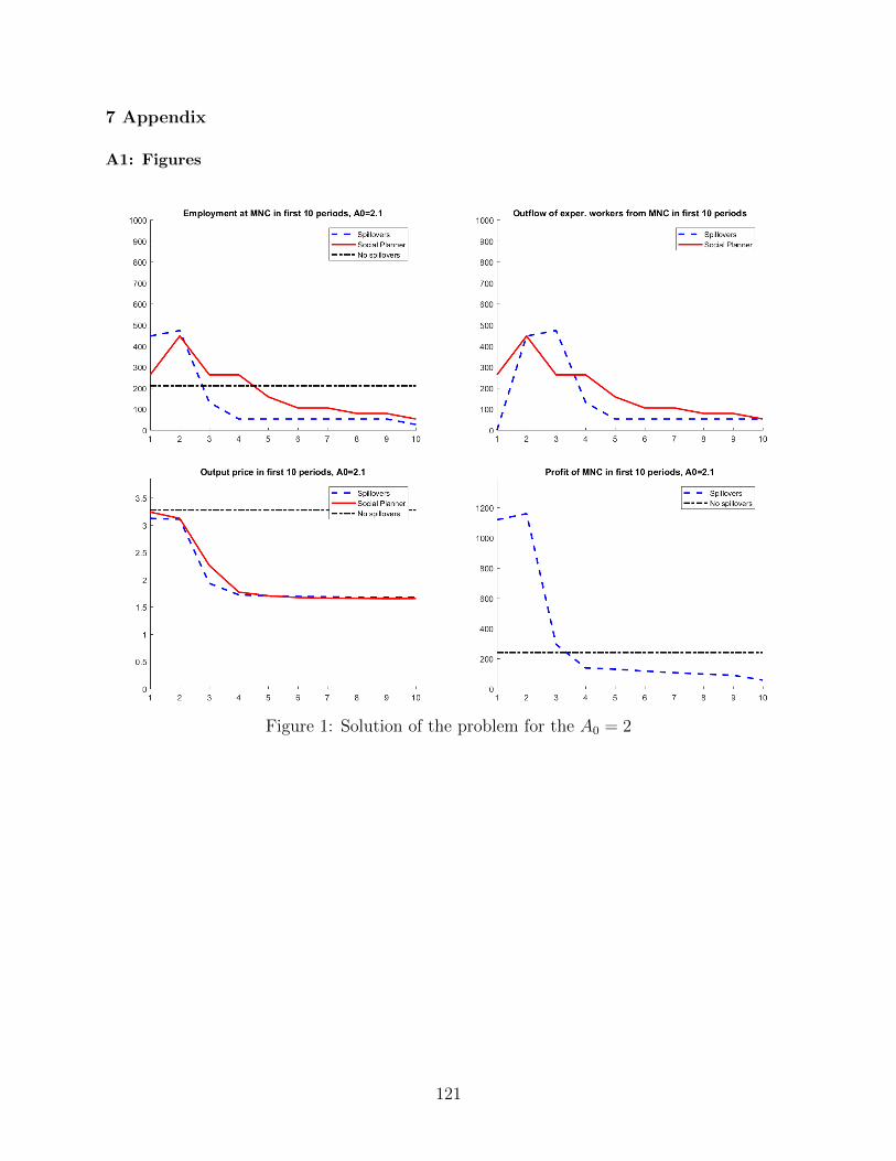
7 Appendix
A1: Figures
Figure 1: Solution of the problem for the A0 = 2
121

Figure 2: Wages of the MNC workers
122

Figure 3: Employment Policy of MNC for Different Productivity Levels
Figure 4: Wages of the MNC workers
123

Figure 5: Cumulative social surplus: Social Planner vs Profit-Maximizing MNC
Figure 6: Workers Rent
124

Figure 7: Value of the MNC V (Ah)
Figure 8: Separating Price and Employment Contribution in MNC Value
125

A2: Equilibrium Robustness
The Markov perfect equilibrium makes strict assumptions on possible contracts. In this
section I show that these assumptions are not very restrictive in the sense that the Markov
perfect equilibrium remains the equilibrium even if more complicated history-dependent
contracts are available. In other words, no firm will find it beneficial to deviate from the
equilibrium Markovian contract by offering an alternative history-dependent contract. This
statement also holds true when the alternative set of assumptions is used with strictly risk
averse workers.
Firms in this extended contracting environment observe the worker’s history and con-
dition their contracts on the observed history. They can also condition the contract on their
own history and their own workers composition.31 I use two variables to describe the history
of any worker. First variable a will denote the knowledge level of the worker. It will equal Ah
if in the previous period the worker was employed at MNC and 0 otherwise (it is assumed,
that workers do not learn anything in local firms).32 All other information about the worker’s
history will go into the second variable S. To allow for conditioning on the firm history, I
add the third variable Hi for a firm i. I will show that there is an equilibrium in which
the contracts do not depend on the knowledge-irrelevant history S and the composition of
workers H.
The employment contract specifies the payment in each state w(A, a, S,H, Z) and the
value Vw(A, a, S,H, Z), promised to the worker. The first variable in each of these functions
denotes the productivity level of the current employer and the the second variable denotes
the knowledge level of the worker. The value functions also depend on the aggregate state
variable Z, which include the distribution of firms by productivity and employment levels.
31To avoid the infinite increase in the dimensionality of the contract I assume that firms cannot observethe histories of workers employed in other firms. It implies that the firms cannot condition the contract onworkers’ composition in firms where worker was employed before.
32In equilibrium, which I will consider, local firms will have identical productivity levels, so the knowledgetransfer from one local firm to another is excluded.
126

The value of a worker equals to the discounted sum of future utility values:
Vw(A, a, S,H, Z) =∞∑t=0
βtu(w(A, a, S(t), H(t), Z(t)))
Here A is the current productivity of a firm with A = Ah referring to the MNC and
A = Af for the followers, a ∈ {0, Ah} - is the productivity level of the worker’s knowledge
(a = Ah if a worker has a recent experience in MNC, 0 - otherwise), S - all other components
of worker’s/firm’s employment history, not reflected in a. The sequence of histories and
productivities levels in the value function above is assumed to be internally consistent and
optimal for the worker in the sense, that it maximizes his next period value, and the current
choice is fixed in the definition. The contract will be over, if the worker or the firm walks
out. There is no uncertainty or information asymmetry in these environment, and so there
is no incentive constraints and the promise keeping constraint is trivial.
The participation constraints for workers in MNC and local firms should be satisfied.
If the worker is employed in MNC at t, he should be at least indifferent between staying
there or joining the local company:
Vw(Ah, 0, S,H, Z) ≥ Vw(Af , 0, S,H′, Z),∀Z, S,H,H ′, such S that he chooses MNC (44)
Vw(Ah, Ah, S,H, Z) ≥ Vw(Af , Ah, S,H′, Z),∀Z, S,H,H ′, such S that he chooses MNC
(45)
The opposite should be true, if a worker is employed at a local firm:
Vw(Ah, 0, S, Z) ≤ Vw(Af , 0, S, Z),∀Z, S, such S that he chooses local (46)
Vw(Ah, Ah, S, Z) ≤ Vw(Af , Ah, S, Z),∀Z, S, such S that he chooses local (47)
127

Second, workers should prefer being employed in the industry, rather than leaving for
the outside sector:
Vw(A, a, S,H, Z) ≥ u(w)
1− β,∀Z, S,A,H, such S that he chooses local or MNC (48)
At last, the limited liability constraint excludes any payments from workers to the firm
(negative wages):
w(A, a, S,H, Z) ≥ 0,∀A, a, S,H, Z
Firms may vary the menu of contracts. Let Vf (A,H,Λ, Z) denote the discounted sum
of firm’s profits, where Λ denotes the current composition of the labor force at moment t:
Vf (A,H,Λ, Z) =∞∑i=0
βt(P (i)An(Λ(i))α −
∫w(A, a, S,H, i)dΛ(i)
)(49)
Here n(Λ) denotes the measure of the workforce employed, and the integral in the RHS
is taken with respect to workers distribution by a, S. Alternatively I will call Vf (A,H,Λ, Z)
a value function of the firm with productivity A, history H and current composition of the
labor force Λ. Again these histories are taken to be consistent and profit-maximizing for a
firm.
If some contract modification increases the firm’s value, then the firm should be
interested in applying this deviation. In equilibrium no such deviation can exist. I will
call it an optimization condition.
The next restriction on the equilibrium menu of contracts follows from the fact, that
the firms in the model can choose the optimal amount of new hires, similar to the competitive
labor market. I will call it a firm’s participation constraint. The participation constraint
says that the firm cannot improve its value by hiring any different composition of workers
Λ′′ 6= Λ:
Vf (A,H,Λ, Z) ≥ Vf (A,H,Λ′′, Z) (50)
128

The equilibrium is a combination of the menu of workers’ contracts (w(), Vw()), value
function of a firm Vf () and a decision rule for a labor force composition by firm Λ(H,Z),
such that:
� Participation and non-negativity constraints for workers are satisfied
� No profitable deviations in menu of contracts and workers composition for a firm exist
(optimization condition)
� Value functions Vw(), Vf () satisfy the corresponding Bellman equations
� The price clears the product market.
� The laws of motion for local firms productivity and employment distribution are
consistent with the decision rule Λ(H,Z)
The following Proposition states that the Markov perfect equilibrium if it exists still
remains an equilibrium in the environment with history-dependent contracts.
Proposition 1. If the economy satisfies one of the following:
� Workers are risk neutral.
� Workers are risk averse, no borrowing/saving is allowed, firms cannot commit to
contracts.
Then any Markov perfect equilibrium is an equilibrium in environment with history-dependent
contracts.
Proof. Suppose, that there is an alternative contract Vw(A, a, S,H, Z) with higher or equal
expected firm value Vf (A,H,Λ, Z) > Vf (A,Z) for some unilaterally deviating firm with
history H and workforce composition Λ in the equilibrium environment. I am going to show,
that this contract is going to be the same as the equilibrium menu of contracts and so the
unilateral deviation to more complicated contracts is not beneficial to the deviator.
129

First, suppose that the deviator is a local firm. By worker’s participation constraint
the new contract Vw(A, a, S,H, Z) should offer to any worker at local companies at least the
same utility as the equilibrium contract Vw(A, a, Z). Suppose that there exist a history (S,H)
that for this history the alternative menu gives a higher promised utility Vw(A, 0, S,H, Z) >
Vw(A, a, Z) . It implies that for the set of periods when the workers are employed by the
deviating local company, the discounted sum of utilities for each worker is no less than the
discounted sum of utilities of market wages with strict inequality for at least one worker (as
any local company can not affect the wages a worker receives in other companies). On other
hand, the alternative contract should achieve higher or equal value to the deviating firm,
implying that the discounted sum of wages in the alternative contract is lower or equal than
the discounted sum of market wages.
If workers are risk neutral, it automatically implies that such a contract is impossible. If
workers are strictly risk averse then the alternative contract can achieve the lower discounted
sum of wages only if wages paid by the deviating firm are less risky. It is impossible given that
the market wages are constant for inexperienced workers and higher only in the first period
of employment for experienced worker. Hence the only way to decrease the risk will be to
decrease the wage offered to an experienced worker with raising the wage for inexperienced
worker. In absence of contract enforcement the firm cannot make a credible promise to pay
higher wages to inexperienced workers, because these workers will be more costly for a firm
than the workers hired by using the equilibrium contract menu.
Next, suppose that the MNC deviates from the equilibrium contract. The alternative
contract has to offer at least the same promised utility to all the employed workers as the
equilibrium contract: Vw(Ah, Ah, S,H, Z) ≥ Vw(Af , Ah, Z). More specifically, it implies
that the experienced workers at MNC have the same or higher promised value than the
experienced workers in local companies Vw(Ah, Ah, S,H, Z) > Vw(Af , Ah, Z) . If workers are
risk neutral then only the equilibrium contract can satisfy this condition and achieve the
same of higher value for the MNC. If workers are strictly risk averse, then all the workers
130

with higher promised utility at some state will have a higher cost for a firm, making it to
renege on the contract.
131

A3: Calculation of Equilibrium Wages
I reformulate the value function of local firm in terms of cumulative number of experienced
workers hired to date (which corresponds one-to-one to the productivity of the firm):
Vf (Le, Af , lm) = maxL′e≥Le,l≥L′e−Le
[Ai(Le)P ()lα−We(L′e−Le)−w(l−L′e+Le)+βVf (L′e, A′f (Af , lm), l′m(Af , lm)]
This value function Vf (·) depends both on the number of experienced workers hired to date
Le by a representative firm and the market-wide productivity level of local firms Af and
employment of the MNC lm. Both Af and lm are aggregate states and evolve according to
the MNC’s decision rules.
I assume that the equilibrium path of productivities Af exists and the productivities
are bounded by the model assumptions. I also assume that the differentiable value function
exist Vf (·) solving the equation above exists for each optimal path of Af and lm.
The first-order condition with respect to future number of experienced workers hired
to date L′e:
−We − w + β∂Vf (t+ 1)
∂L′e+ λt − µt = 0
Where λt = 0 if the constraint L′e ≥ Le is non-binding and λt > 0 otherwise. The constraint
µt = 0 if the constraint l ≥ L′e − Le is non-binding.
The first-order condition with respect to total employment of a local firm l:
αAi(Le)P ()lα−1 − w + µt = 0
Then:
µt = w − αAi(Le)P ()lα−1
From this we can get the expression for the wage of experienced workers at local firms
132

We:
We = w + β∂Vf (Le(t+ 1), Af (t+ 1), lm(t+ 1))
∂L′e+ λt − µt
The constraint L′e ≥ Le should never bind for any equilibrium policy of the MNC.
Otherwise the MNC can always reduce the wage paid to its own experienced workers in
order to make the local firms indifferent for attracting the marginal experienced worker
given the outflow at Mle. Then after substituting the expression for µt I obtain:
We = αAi(Le)P ()lα−1 + β∂Vf (t+ 1)
∂L′e
Then I need to calculate the derivative of future value function with respect to L′e,
which by the envelope theorem equals:
∂Vf (t+ 1)
∂L′e= P ()lα
∂Ai∂Le
+We(t+ 1)− w − λt+1 + µt+1
From the FOC for Le above follows that (where L′′e corresponds to the choice of cumulative
experienced labor at period t+ 2):
−λt+1 + µt+1 = w −We(t+ 1) + β∂Vf (t+ 2)
∂L′′e
By substituting it into the expression for∂Vf (t+1)
∂L′eI get:
∂Vf (Le, Af , lm)
∂Le= P ()lα
∂Ai∂Le
+ β∂Vf (Le, A
′f (Af , lm), l′m(Af , lm))
∂L′′e(51)
As derived in Section 2 (22), the partial derivative of follower’s productivity with
respect to Le is just:
∂A
∂Le= ρ(Ah − A)
After substituting this formula to the equation (51) I obtain the following recursive
133

formula to use in my simulations:
∂Vf (Le, Af , lm)
∂Le= P ()lαρ(Ah − A) + β
∂Vf (Le, A′f (Af , lm), l′m(Af , lm))
∂Le(52)
We = αAi(Le)P ()lα−1 + β∂Vf (t+ 1)
∂L′e
134

Conclusion
Three chapters of my dissertation study different aspects of human capital accumula-
tion. My first chapter studies the potential inefficiencies of human capital allocation, their
effects on human capital accumulation and their productivity implications. The second
chapter of the dissertation studies determinants of education quality. My final third chapter
studies the knowledge transfer through foreign direct investment in a presence of technology
spillovers through employee mobility.
Findings of all the chapters in my dissertation directly or indirectly explain the puzzle
of low productivity in developing countries. In the fist chapter of this dissertation, I find
that the cross-country differences in occupational sorting contribute about 10-20% to the
aggregate productivity variation, which is a sizeable effect on its own but far from explaining
the cross-country productivity variation. The second chapter of my dissertation studies the
difference in education quality which explains a large portion of cross-country productivity
differences. My second chapter demonstrates that economic growth positively and consis-
tently correlates with the education quality as predicted by several existing theories. This
observation indicates that growing incomes can help in closing the gap in education quality
and productivity between developed and developing countries. Finally, in the last chapter of
my dissertation, I find that human capital accumulation can be postponed if employees can
transfer know-how between firms and the difference in technology level is high enough. This
finding helps to explain slow transfer of technologies between countries thus also contributing
to the explanation of the productivity puzzle.
135
Related Documents