Essays on Energy Economics – Empirical Analyses Based on German Household Data Inaugural-Dissertation zur Erlangung des akademischen Grades eines Doktors der Wirtschafts- und Sozialwissenschaften der Wirtschafts- und Sozialwissenschaftlichen Fakultät der Christian-Albrechts-Universität zu Kiel vorgelegt von MA Dragana Nikodinoska aus Ohrid Kiel, Januar 2017

Welcome message from author
This document is posted to help you gain knowledge. Please leave a comment to let me know what you think about it! Share it to your friends and learn new things together.
Transcript

Essays on Energy Economics
–
Empirical Analyses Based on German Household Data
Inaugural-Dissertation
zur Erlangung des akademischen Grades eines Doktors
der Wirtschafts- und Sozialwissenschaften
der Wirtschafts- und Sozialwissenschaftlichen Fakultät
der Christian-Albrechts-Universität zu Kiel
vorgelegt von
MA Dragana Nikodinoska
aus Ohrid
Kiel, Januar 2017

Gedruckt mit Genemigung der
Wirtschafts- und Sozialwissenschaftlichen Fakultät
der Christian-Albrechts-Universität zu Kiel
Dekan:
Prof. Dr. Till Requate
Erstberichterstattender:
Prof. Dr. Carsten Schröder
Freie Universität Berlin und Deutsches Institute für Wirtschaftsforschung (DIW)
Zweitberichterstattender:
Prof. Dr. Katrin Rehdanz
Christian-Albrechts-Universität zu Kiel und Institute für Weltwirtchaft (IfW)
Tag der Abgabe der Arbeit:
18. Januar 2017
Tag der mündlichen Prüfung:
28. Juni 2017
Christian-Albrechts-Universität zu Kiel
Wilhelm-Seelig Platz 1
24118 Kiel


i
Acknowledgements
I am eternally thankful to my parents, Biljana and Dragan, and my brother, Mirko, whose
love and continuous support enabled me to work while being far away from all of them.
I am very grateful to my supervisor, Prof. Dr. Carsten Schröder, for his many insightful ideas,
comments, and remarks as well as for his continuous devotion and support throughout the
research and writing stages of my PhD.
I would like to thank the Doctoral Program Quantitative Economics and the Gesellschaft für
Energie und Klimaschutz Schleswig-Holstein GmbH (EKSH) for financial support of my PhD
studies, research, and dissertation writing.
I would also like to thank our Associate Editor of Resource and Energy Economics and two
anonymous referees for many helpful comments on the first chapter of this thesis.

ii
Contents
Acknowledgements .................................................................................................................... i
Contents ...................................................................................................................................... ii
List of Abbreviations ................................................................................................................. iv
List of Tables ............................................................................................................................. vi
List of Figures ......................................................................................................................... viii
Motivation and contribution to literature .................................................................................. 1
Chapter 1 On the Emissions–Inequality and Emissions–Welfare Trade-offs in Energy Taxation: Evidence on the German Car Fuels Tax .................................................................... 7
1.1 Introduction ................................................................................................................. 7
1.2 Literature review .............................................................................................................. 9
1.3 Data and data preparation ............................................................................................... 11
1.3.1 German Income and Expenditure Survey ............................................................... 11
1.3.2 Consumer prices ...................................................................................................... 13
1.4 Estimation strategy and policy evaluation criteria ......................................................... 16
1.4.1 Demographically-Scaled Quadratic Almost Ideal Demand System ....................... 16
1.4.2 The car fuels tax ...................................................................................................... 18
1.4.3 Policy evaluation criteria ......................................................................................... 19
1.5 Demand System Estimates ............................................................................................. 22
1.6 Policy analyses ............................................................................................................... 24
1.7 Sensitivity analyses ........................................................................................................ 29
1.8 Interim Conclusion ......................................................................................................... 31
1.9 Appendix ........................................................................................................................ 33
1.9.1 Data tables ............................................................................................................... 33
1.9.2 Estimation details .................................................................................................... 38
1.9.2.1 Technical details concerning the methodology .................................................... 38
1.9.2.2 Correcting for endogeneity ................................................................................... 39
1.9.2.3 Calculation of income and price elasticities of demand ....................................... 40
1.9.3 Estimation Tables and Figures ................................................................................ 42
Chapter 2 How Electricity Prices Alter Poverty and CO2 Emissions ‒ The Case of Germany 50
2.1 Introduction .................................................................................................................... 50
2.2 Literature review ............................................................................................................ 53
2.3 Data description .............................................................................................................. 55
2.3.1 Income concepts for the poverty analyses ............................................................... 55
2.3.2 Variables for the demand system ............................................................................ 56
2.4 Estimation techniques: A Demographically-Scaled Quadratic Almost Ideal Demand System (DQUIDS), price elasticites, and scenarios analyses .............................................. 57
2.5 Empirical evidence ......................................................................................................... 61
2.5.1 Development of income and energy poverty ...................................................... 61
2.5.2 On the relationship between income poverty and energy poverty .......................... 65
2.5.3 Differences in poverty levels across household types ............................................. 67

iii
2.5.4 Price and expenditure elasticites of energy demand ............................................... 68
2.6 Scenarios design and results ........................................................................................... 69
2.6.1 Scenarios with marginal changes in EEG surcharge ............................................... 71
2.6.2 Other potential scenarios ......................................................................................... 71
2.6.3 The relationship between poverty and energy taxes ......................................... 76
2.7 Interim conclusion .......................................................................................................... 78
2.8 Appendix ........................................................................................................................ 80
2.8.1 Tables ...................................................................................................................... 80
2.8.2 Figures ..................................................................................................................... 94
Chapter 3 Inter- and Intra-generational Emissions Inequality in Germany: Empirical Analyses .................................................................................................................................................. 98
3.1 Introduction .................................................................................................................... 98
3.2 Literature review .......................................................................................................... 100
3.3 Methodology ................................................................................................................ 103
3.4 Data and descriptive evidence ...................................................................................... 106
3.5 Empirical results ........................................................................................................... 114
3.51. Total energy related emissions .............................................................................. 114
3.5.2 Emissions from the separate sources: electricity, gas, and car fuels ..................... 118
3.6 Consistency checks and methodological issues ........................................................... 120
3.7 Interim conclusion ........................................................................................................ 123
3.8 Appendix ...................................................................................................................... 126
Concluding Remarks .......................................................................................................... 144
Appendix A: Separate Analyses for Schleswig-Holstein ................................................... 148
A1 Car fuels tax .............................................................................................................. 150
A2 EEG surcharge .......................................................................................................... 154
A3 Emissions inequalities .............................................................................................. 157
Bibliography ........................................................................................................................... 164
Declaration ............................................................................................................................. 177

iv
List of Abbreviations
2M – twice median
ACER – Agency for the Cooperation of Energy Regulators
AIC – Akaike Information Criterion
AIDS – Almost Ideal Demand System
APC – Age Period Cohort
APCD – De-trended Age Period Cohort
APC-IE – Age Period Cohort Intrinsic Estimator
BIC – Bayesian Information Criterion
CFT – Car Fuels Tax
CO2 – Carbon Dioxide
CV – Compensating Variation
DAIDS – Demographically-scaled Almost Ideal Demand System
DQUAIDS – Demographically-scaled Quadratic Almost Ideal Demand System
EEA – European Environment Agency
EEG – Renewable Energy Act
EKC – Environmental Kuznets Curve
ETR – Environmental Tax Reform
E.U. – European Union
EUR – euro
EV – Equivalent Variation
FIT – Feed-In-Tariffs
FGT – Foster, Greer, and Thorbecke
G.B. – Great Britain
HC – Head Count
IEA – International Energy Agency
IES – Income and Expenditure Survey

v
kWh – kilowatt hour
l – liter
LIHC – Low Income High Costs
MIS – Minimum Income Standard
NOx – Nitrogen Oxides
OECD – Organization for Economic Co-operation and Development
PIGLOG – Price-Independent Generalized Logarithmic
POTP – Post-Tax Total Prices
QUAIDS – Quadratic Almost Ideal Demand System
RES – Renewable Energy Sources
S – Scenario
S0 – Status quo/Initial scenario
SPI – Stone Price Indices
SH – Schleswig-Holstein
SO2 – Sulfur Dioxide
t – ton
TPR – Ten Percent Rule
U.K. – United Kingdom
U.S. – United States
VAT – Value Added Tax

vi
List of Tables
Table 1. 1 Pre-tax and final consumer prices of car fuels ........................................................ 19
Table 1. 2 Income and price elasticities (uncompensated) ....................................................... 23
Table 1. 3 Status quo ................................................................................................................ 25
Table 1. 4 Tax simulations with 50 and 25 percent tax decrease, and 25 and 50 percent tax increase ..................................................................................................................................... 26
Table 1. 5 Elasticities by equivalent income classes ................................................................ 31
Table 1. 6 Identifiers of the underlying original IES variables ................................................ 33
Table 1. 7 Descriptive statistics for 1993 ................................................................................. 34
Table 1. 8 Descriptive statistics for 1998 ................................................................................. 35
Table 1. 9 Descriptive statistics for 2003 ................................................................................. 36
Table 1. 10 Descriptive statistics for 2008 ............................................................................... 37
Table 1. 11 The augmented equation for ln (m) ....................................................................... 42
Table 1. 12 Coefficient estimates of the demand systems ....................................................... 43
Table 1. 13 Comparison of Base and Demographic QUAIDS elasticities ............................... 44
Table 1. 14 Comparison of rural and urban households’ elasticities ....................................... 44
Table 1. 15 Comparison with previous literature estimates ..................................................... 45
Table 1. 16 Compensating variation with 50 and 25 percent tax decrease, and 25 and 50 percent tax increase .................................................................................................................. 45
Table 2. 1 Development of variables relevant for measuring poverty ..................................... 56
Table 2. 2 The overlap between income poverty and energy poverty ..................................... 66
Table 2. 3 Income and energy poverty by household types ..................................................... 67
Table 2. 4 Elasticities and expenditure shares according to disposable equivalent income deciles ....................................................................................................................................... 70
Table 2. 5 Scenarios with marginal changes ............................................................................ 72
Table 2. 6 Scenario 5 (doubling of the EEG surcharge) results across income deciles and household types ........................................................................................................................ 74
Table 2. 7 Scenario 6 (abolishing the EEG surcharge) results across income deciles and household types ........................................................................................................................ 75
Table 2. 8 Relevant household level studies and their contribution to literature ..................... 80
Table 2. 9 Descriptive statistics of the variables included in the demand system ................... 83
Table 2. 10 Summary statistics by household type .................................................................. 84
Table 2. 11 Comparison with previous studies on income and energy poverty ....................... 85
Table 2. 12 Income and energy poverty according to working status and area of residence ... 86
Table 2. 13 Results of the probit model: probability to be energy poor................................... 86
Table 2. 14 Elasticities for the different household types ........................................................ 87
Table 2. 15 DQUAIDS and QUAIDS Coefficient Estimates .................................................. 88
Table 2. 16 Comparison of demographic and base (QU)AIDS elasticities ............................. 90
Table 2. 17 Comparison with electricity demand elasticities from existing literature ............. 90
Table 2. 18 Scenario 7 (doubling of the EEG surcharge and CFT) results across income deciles and household types ..................................................................................................... 91
Table 2. 19 Scenario 8 (abolishing the EEG surcharge and CFT) results across income deciles and household types ................................................................................................................. 92
Table 2. 20 Results of Scenario 9 and Scenario 10 .................................................................. 93
Table 3. 1 Descriptive statistics .............................................................................................. 108
Table 3. 2 Relevant studies and their contribution to literature ............................................. 126

vii
Table 3. 3 Summary statistics of rural and urban households ................................................ 128
Table 3. 4 Total energy related emissions across the deciles ................................................. 128
Table 3. 5 Summary statistics of households according to birth cohort of household’s leader ................................................................................................................................................ 129
Table 3. 6 Coefficient estimates of the APCD model ............................................................ 131
Table 3. 7 Estimates from APCD with additional controls for electricity, gas, and car fuels 133
Table 3. 8 Consistency check: Estimates from the APC-IE model ........................................ 138
Table A. 1 Income and price elasticities (uncompensated) in Schleswig-Holstein ............... 152
Table A. 2 Results of policy change scenarios in Schleswig-Holstein .................................. 153
Table A. 3 Elasticities and expenditure shares Schleswig-Holstein versus Germany ........... 156
Table A. 4 Scenarios S5-S8 results Schleswig-Holstein versus Germany ............................. 156
Table A. 5 Summary statistics of rural and urban households in Schleswig-Holstein versus Germany ................................................................................................................................. 159
Table A. 6 Total energy related emissions in Schleswig-Holstein across the deciles............ 160
Table A. 7 Coefficient estimates of the APCD model for Schleswig-Holstein versus Germany ................................................................................................................................................ 161

viii
List of Figures
Figure 1. 1 Development of expenditure shares over time....................................................... 14
Figure 1. 2 Expenditure shares and income ............................................................................. 15
Figure 1. 3 Four tax scenarios: effects of tax change on emissions, tax burdens, and EV across the equivalent income deciles................................................................................................... 28
Figure 1. 4 The relationship between tax rate, emissions, tax burden, Gini index, and EV .... 30
Figure 1. 5 Density functions for the expenditure shares ......................................................... 46
Figure 1. 6 Four scenarios: effects on compensating variation ................................................ 47
Figure 1. 7 The relationship between tax rate, emissions, Theil index, and CV ...................... 48
Figure 2. 1 Headcount ratio over time ...................................................................................... 62
Figure 2. 2 Poverty gap over time ............................................................................................ 63
Figure 2. 3 Energy poverty over time ...................................................................................... 65
Figure 2. 4 The relationship between energy taxes and income poverty and energy poverty . 77
Figure 2. 5 HC ratio on equivalent expenditures and equivalent expenditures after energy taxes .......................................................................................................................................... 94
Figure 2. 6 Poverty gap on equivalent expenditures and equivalent expenditures after energy taxes .......................................................................................................................................... 95
Figure 2. 7 Kernel density functions of energy expenditure share in income by years ........... 96
Figure 3. 1 Development of total CO2 emissions for the first, fifth and tenth equivalent income decile over time ...................................................................................................................... 111
Figure 3. 2 Differences in emissions levels between rural and urban households ................. 112
Figure 3. 3 Birth cohorts and total emissions ......................................................................... 113
Figure 3. 4 Cohort effects of household’s leader on total energy CO2 emissions without controls ................................................................................................................................... 115
Figure 3. 5 Cohort effects of household’s leader on total energy CO2 emissions with control variables and other cohorts effects ......................................................................................... 117
Figure 3. 6 Cohort effects of household leader on different energy CO2 emissions sources, with additional control variables and other cohorts effects .................................................... 119
Figure 3. 7 Cohort effects of household’s leader from the APC-IE model without controls . 121
Figure 3. 8 Cohort effects of household’s leader from the APC-IE model with additional controls and other cohorts effects ........................................................................................... 122
Figure 3. 9 Cohorts effects of other household members on total energy CO2 emissions with control variables ..................................................................................................................... 140
Figure 3. 10 Cohort effects of the household leader on different energy CO2 emissions sources, without controls ........................................................................................................ 141
Figure 3. 11 Other household members’ cohort effects from the APC-IE model.................. 142
Figure A. 1 Birth cohorts and total emissions in Schleswig-Holstein.................................... 160


1
Motivation and contribution to literature
Recent literature in the field of energy economics has returned to investigating the
household or the individual by implementing household’s decision models. Household’s
decision models are useful for studying the effectiveness of energy and environmental
policies. In particular, energy demand systems include behavioral responses of households
and allow for welfare and environmental analyses of energy policy reforms. Such frameworks
can help to find the groups which are overconsuming energy relative to the population as a
whole so that they can be targeted with various policy measures in order to change their
consumer behavior.
Demand systems have been widely applied in the context of residential energy demand in
several countries and to explore different energy policy changes. Several studies have
explored the effects of gasoline or electricity taxes using demand models. Namely, Dumagan
and Mount (1992) were among the first to apply such framework and to show that carbon tax
has regressive effect in the US i.e. the tax burden as share of income is larger proportion for
the poor than for the rich households. Some years later, West and Williams III (2004) find
gasoline tax to be regressive in the U.S., and Brännlund and Nordström (2004) also find
carbon tax (on gasoline and electricity) to be regressive in Sweden. Tiezzi (2005) finds that
carbon tax burden is progressively distributed across Italian households, but she uses total
expenditures instead of income as the ordering criterion. Beznoska (2014) considers an eco-
tax on gasoline and diesel, and finds that the regressively of the gasoline tax to be lower than
the regressively of taxes on electricity in Germany. Gahvari and Tsang (2011) study the
effects of electricity taxes in the U.S. and prove that an energy tax on electricity is
detrimental for consumer welfare, despite its environmental benefits. While many papers have
considered the distribution or welfare impacts, only few papers have dealt with the
environmental effects of energy taxes (for example: Brännlund and Nordström (2007)),even
fewer that deal with the effects of energy taxes on poverty, and almost none which have
considered all of those effects in a consistent framework. The paper of Klauss (2016) is
unique in the sense that it estimates how an energy price change influences poverty. The
author finds that gas price increase leads to higher poverty levels among Armenian
households but he does not consider the separate effects of energy taxes on poverty nor does
he consider behavioral responses. Other studies have applied demand system to estimate price
and income elasticities without conducting tax simulations (see for instance Filipinni (1995),
Kohn and Missong (2003), and Kratena and Wüger (2009) among others). None of these

Motivation and contribution to literature 2
studies have addressed the trade-offs between emissions and inequality, and emissions and
consumer welfare. Nor have they studied energy poverty or the effects of energy taxes or
surcharges on income poverty and energz poverty.
The year of birth can influence life opportunities and also consumer or environmental
habits of the individual. However, the role of birth cohorts in explaining energy consumption
and energy related residential emissions has not been widely researched. The few studies
which have addressed this question include Chancel (2014), Segall (2013), Sànchez-Peña
(2013), and Aguiar and Hurst (2013). Chancel (2014) finds that the French households with
leaders born between 1930 and 1955 are the highest CO2 emitters. The results of Sànchez-
Peña (2013) confirm that the cohorts born 1923–1968 consume more energy (and emit more
CO2) than the average household in Mexico. Both Aguiar and Hurst (2013) and Segall (2013)
find significant cohort effects in explaining utilities consumption or energy budget allocation
in the U.S. However, all of those studies have only considered the cohort effects of the
household’s leader and none has examined the birth cohort effects of other household’s
members.
The dissertation contributes to the existing literature in several ways. To begin with,
Germany is at the center of the analyses of this dissertation. Germany is particularly
interesting case to analyse since it is one of the EU countries which prioritize both distributive
justice and environmental protection in their policy agenda. In this country, energy taxes and
surcharges are imposed with the goal to restrict energy consumption and to finance green
energy, and energy prices are among the highest in the EU. Secondly, this dissertation uses
very recent and very detailed data on energy expenditures of German households. The dataset
preparation was complex task since demand systems impose strict requirements for the data:
waves must be comparable, consistent, of high quality, and randomly drawn. The final dataset
is very extensive and covers around 170,000 (220,000) German households in 4 (5) cross
sections between 1993 and 2008 (2013). Most importantly, I provide a consistent framework
in which consumer welfare, income distribution, environmental, and poverty effects of
different energy policy reforms can be measured. The demand system itself is quadratic,
demographically scaled, corrects for potential endogeneity, and encompasses improved price
variation. The tax simulations allow for studying the effects of changes in car fuels and (or)
electricity price on the dimensions mentioned above. In addition, energy related emissions
are calculated and the following emissions’ determinants are considered: income, area of
residence, age, and birth cohort. A significant gap in the literature is filled by considering the
birth cohort effects of other household’s members in addition to the households’ leader.

Motivation and contribution to literature 3
As mentioned, German households are faced with relatively high energy prices, which are
mainly caused by increasing taxes and surcharges. The Ecological Tax Reform-ETR in
Germany (1998–2003) led to increases in the existing taxes on fossil fuels and an introduction
of tax on electricity. Moreover, in 2007 the value-added tax rate was increased from 16 to 19
percent. By 2008, energy and other taxes constituted 59 percent of the price of car fuels
(gasoline and diesel). Furthermore, the electricity price has been also growing due to increases
in the yearly adjusted surcharge for renewable energy (Renewable Energy Act surcharge or
EEG-Umlage1), which has grown from 0.2 euro cents per kWh in 2000 to 6.35 euro cents per
kWh of electricity in 2016. In 2013 energy and other taxes and surcharges were amounting to
45 percent of the electricity price in Germany and it was the second highest in Europe.
Three essays which deal with households’ energy demand and CO2 emissions are part of
the dissertation. The first paper examines the environmental, distributive, and welfare effects
of the car fuels tax. Higher car fuels taxes could potentially lead to lower car fuels’
consumption and lower CO2 emissions but can increase inequality in the post-tax income
distribution and decrease consumer welfare. The second paper scrutinizes the effects of the
EEG surcharge, which was introduced in Germany as means to finance renewable energy
production, on energy poverty, income poverty, and CO2 emissions. Abolishing of the EEG
surcharge is expected to lower the tax burdens of the low income households and hence
decrease both income poverty and energy poverty. Both chapters can provide policy makers
with empirical evidence about how to weight environmental and inequality/poverty concerns,
and point out potential targets groups (of households) that can lead to largest energy
consumption savings or largest energy poverty decreases. The third paper investigates the
determinant of energy related emissions’ inequalities among three dimensions: income, area
of residence, and birth cohort. Again, this kind of analyses will help to find the determinants
of CO2 emissions, and to identify the groups of the population that should be targeted in order
to decrease the inequalities and emissions altogether.
The first paper is titled “On the Emissions–Inequality and Emissions–Welfare Trade-offs
in Energy Taxation: Evidence on the German Car Fuels Tax” and examines how changes in
the car fuels tax affect households in Germany. The price elasticity of demand for car fuels is
critical for the size of the environmental effect and the shape of the Engel curve is crucial for
the welfare and distributive effects. Moreover, analyzing the determinants of demand for
energy goods is important especially since residential energy consumption has recently
increased in Europe despite higher energy taxes (The World Bank, 2013). For that purpose, a
1 I refer to it as the EEG surcharge throughout the dissertation.

Motivation and contribution to literature 4
Demographically-scaled Quadratic Almost Ideal Demand System (DQUAIDS) is estimated
using German household level data for the years 1993–2008 (Ray (1983), Banks et al. (1997),
and Blacklow et al. (2010)). The parameter estimates are consistent, statistically significant,
and allow for calculation of income and price elasticities: car fuels are necessity good and
demand is price inelastic (–0.203). The several tax simulations reveal the existence of the
emissions inequality and emissions welfare trade-offs in energy taxation: if the car fuels tax
increases, the CO2 emissions decrease but the income inequality and the welfare loss both
increase.
Even though many papers have investigated the impact of energy taxes on the income
distribution or on the energy related emissions, this study builds on those results in a number
of dimensions. First of all, the study provides a consistent framework (which updates previous
ones because it includes corrections for endogeneity and increased price variation) in which
welfare, environmental, and inequality effects of an energy tax change can be measured.
Secondly, the paper graphically scrutinizes the trade-offs between emissions, inequality, and
welfare which most papers have overlooked. By addressing those trade-offs, we ensure that
no groups in the German population will be harmed more than others due to a policy reform.
My contributions to this co-authored paper are described as follows. I have assembled
and prepared all the relevant data: household income and expenditure micro data (Income and
Expenditure Survey); time series of commodity prices; information on changes in energy and
environmental policies. Moreover, I coded the STATA program files necessary for the
econometric analyses (estimation of demographically scaled quadratic demand systems).
Furthermore, I compiled the programs for executing the tax simulations (using the demand
system estimates) in order to evaluate the effect of different levels of the car fuels tax on the
three dimensions investigated in the study: (1) energy consumption; (2) CO2 emissions levels;
(3) distributional effects-consumer welfare and income inequality.
The second paper, entitled “How Electricity Prices Alter Poverty and CO2 Emissions ‒
The Case of Germany” deals with the effects of changes in the Renewable Energy Act
Surcharge (EEG-Umlage) on energy poverty and residential electricity related emissions. By
examining energy poverty, how it evolved over time, how it is related with income poverty,
which are its determinants, and how energy taxes influence it, I have tackled a crucial topic in
the face of growing energy costs and income poverty. Energy poverty (the lack of adequate
energy services) represents a growing concern in developed countries with colder climates
since can lead to health problems and rationing of other household budgets. Energy poverty is
found to have increased in Germany between 1993 and 2013, and is higher among single

Motivation and contribution to literature 5
parents, unemployed, and households living in rural areas. Income poverty is found to be
significant factor behind of the probability of being energy poor. Electricity demand is found
to be price inelastic and a decrease in the electricity price (abolishing of the EEG surcharge
and slight increase in the car fuels tax) is expected to be beneficial for households – by
lowering energy poverty and electricity tax/surcharge burdens – while increasing emissions
by a small amount and keeping government tax revenues almost constant.
This second paper addresses the gap in the literature by using a very recent data from
2013 for Germany. Moreover, it captures energy poverty in this country and analyses in detail
the determinants of energy poverty. In addition, the effects of changes in the EEG surcharge
on income and energy poverty, and also CO2 emissions are investigated, which has not been
done before. Furthermore, I identify a positive relationship between higher EEG surcharge
and energy poverty indicating that an increase in the surcharge will always increase poverty
and hurt the most vulnerable groups of households/individuals, such as low income
households or single parents.
The third paper has the following title: “Inter- and Intra-generational Emissions
Inequality in Germany: Empirical Analyses”. The main research question is to investigate the
effect of income, area of residence, and birth cohort on residential energy related emissions. I
identify: a) income related emissions inequalities, with low income households emitting much
less CO2 than high income households; b) area of residence emissions inequalities, with rural
households having much higher emissions than urban households; and c) birth cohort
emissions inequalities, with cohorts 1933–1963 being the highest CO2 emitters. A De-trended
Age Period Cohort (APCD) model allows for separation of the effects of birth cohort from the
effects of age, income, and other explanatory variables, while it solves the identification
problems inherent to Age Period Cohort (APC) models. The results from the APCD confirm
that having either a household’s leader or household’s member from the cohorts 1943–1968
increases energy related emissions by more than the cohorts born before 1943 or after 1968.
The last paper has several contributions to the existing literature on residential energy
related emissions. To start with, it calculates electricity, gas, and car fuels related emissions of
German households using expenditure data, prices, and emissions factors. Second of all, the
paper investigates the descriptive evidence of birth cohort related inequalities by carefully
analyzing the demographic and economic characteristics of households according to the birth
cohort of the household’s leader. Crucially, the APCD model examines the effects of birth
cohorts of other household’s members on CO2 emissions, which none of the previous studies
have considered.


7
Chapter 1
On the Emissions–Inequality and Emissions–Welfare
Trade-offs in Energy Taxation: Evidence on the German
Car Fuels Tax
1.1 Introduction
Faced with climate change and threats to environmental sustainability, many countries,
particularly those in Europe, are redesigning and enhancing their environmental policies to
reduce anthropogenic carbon dioxide emissions (World Nuclear Association, 2011). The
introduction and increase of energy taxes has the aim to limit energy consumption, and special
focus has been put on the households sector. Despite these changes, fossil fuels consumption,
an important determining factor of CO2 emissions, has increased in recent years (The World
Bank, 2015). This apparently paradoxical situation calls for thorough investigation of the
determinants of demand for car fuels and other energy goods by the households.
Our study deals with the environmental, distributive, and welfare effects of the car fuels
tax in Germany, a country that places high priority on both environmental protection
(International Energy Agency, 2007) and distributive justice. The car fuels tax is charged as a
fixed monetary amount per liter and serves as an instrument to reduce households’ vehicle
emissions, the largest source of CO2 emissions after the industrial sector (International Energy
Agency, 2007). Crucial for the size of the environmental effect is the price elasticity of
demand for car fuels: The more elastic the demand, the larger the environmental effect in
terms of CO2 emissions reductions. Crucial for the distributive and welfare effects is the shape
of the Engel curve: If the expenditure (share) for fuels decreases in income, then households
with a greater ability to pay will pay lower taxes relative to income and also incur a smaller
relative reduction in welfare.
This chapter is based on joint work with Prof. Dr. Carsten Schröder from DIW Berlin, see Nikodinoska and
Schröder (2016) https://doi.org/10.1016/j.reseneeco.2016.03.001.

Chapter 1.On the Emissions–Inequality and Emissions–Welfare Trade-offs in Energy Taxation: Evidence on the
German Car Fuels Tax 8
The potential emissions–inequality and emissions–welfare trade-offs in energy tax policy
have become an important issue in political and academic debate.2 As pointed out by Baumol
and Oates (1988), by ignoring these trade-offs, “we may either unintentionally harm certain
groups in society or, alternatively, undermine the program politically” (p. 235). Most studies
investigate the trade-offs in a traditional tax incidence framework, i.e., by quantifying average
tax burdens at different points of the income distributions. Only a few studies, among them
Jorgenson et al. (1992), Oladosu and Rose (2007), Araar et al. (2011), and Grösche and
Schröder (2014a), 3
provide a detailed examination of the redistributive or welfare effects.
We suggest and implement a two-step procedure for a systematic assessment of the
potential emissions–inequality and emissions–welfare trade-offs using the German car fuels
tax as an example. First, we estimate a demographic specification of the Quadratic Almost
Ideal Demand System, which describes how household demands respond to price and income
changes. The estimated price elasticities reveal how household demands respond to variations
of the car fuels tax. Second, based on the demand system estimates we quantify the following
three outcomes of interest for various tax levels: (a) emissions; (b) inequality, by means of a
comprehensive set of inequality indices; and (c) household welfare, by means of
equivalent/compensating variations and tax burdens over the quantiles of the income
distribution. In sum, the proposed two-step procedure gives answers to the following type of
question: “Suppose the car fuels tax increases by five percent: How does the tax increase
change emissions, inequality, and households’ economic welfare?” The answers are
visualized by means of trade-off curves that depict how the three outcomes vary with the tax
rate.
Each separate ingredient of the proposed procedure is well-known. However, the
combination of the tools provides a comprehensive picture of the intensity of emissions–
inequality and emissions–welfare trade-offs that most previous literature has been lacking and
that can be applied fruitfully in many other settings. The procedure can also be embedded in a
broader framework that combines the household-micro level perspective with multisector
general equilibrium techniques as presented in Araar et al. (2011).
To our knowledge, we are the first to implement such a detailed trade-off analyses. This
study focuses on Germany, a country where environmental sustainability is highly prioritized
on the policy agenda. Our estimates indicate the presence of an emissions–inequality trade-
2 See Pearson and Smith (1991), Wier et al. (2005), Scott and Eakins (2004), Oladosu and Rose (2007), Callan et
al. (2008), Fullerton (2009), Grainger and Kolstad (2009), Jacobsen et al. (2003), or Grösche and Schröder
(2014a). 3 Other studies for Germany include Bach et al. (2002) and Sterner (2012), but they provide less detailed
analyses.

Chapter 1.On the Emissions–Inequality and Emissions–Welfare Trade-offs in Energy Taxation: Evidence on the
German Car Fuels Tax 9
off: As an example, increasing the original tax rate by 50 percent (from 0.606 euros/liter to
0.909 euros/liter) reduces CO2 emissions by about 8.2 percent, and increases the Gini index
from the distribution of equivalent disposable income by about 0.2 percent. This is because
the associated tax burden relative to disposable income decreases in household needs-adjusted
(equivalent) income.4
At first glance, the redistributive effect and the intensity of the emissions–inequality
trade-off may appear small. The key reason for the small magnitude of the effect is the small
share of car-fuel expenditures in household budgets, about 3.75 percent. Our basic interest,
however, is in the sign of the redistributive effect, which turns out to be regressive: Several of
the environmental taxes in Germany (electricity taxes or taxes on heating fuels) work in a
comparable manner to the car fuels tax and thus add to the regressive effect.5 According to a
simulation analyses for various OECD countries, Flues and Thomas (2015) conclude that also
taxes on heating fuels and, particularly, electricity are “clearly regressive” (p. 40). These
environmental taxes thus add to the regressive effect of fuels taxes measured in the present
study. Our analyses also reveals an emissions–welfare trade-off. A 50 percent tax increase
amounts to an annual welfare loss in terms of equivalent variation by 283 euros on average,
and by 148 euros for the first decile, a sizeable amount for low-income households.
The paper is structured as follows. Section 1.2 provides a literature review. Section 1.3
describes the data and Section 1.4 the quantitative methods. Section 1.5 provides the demand
system estimates and Section 1.6 the results from the policy analyses. Section 1.7 provides
sensitivity analyses, and Section 1.8 presents the concluding remarks.
1.2 Literature review
Several studies have investigated environmental taxes and their impact on households’
energy consumption, welfare or emissions levels. From a technical perspective, the studies
can be classified according to three criteria: (a) static one-period vs. dynamic multi-period
framework; (b) partial analyses of a single sector vs. total analyses with inter-sector linkages;
(c) abstraction from or explicit modeling of behavioral responses.
Because the international literature is so extensive, we confine our review to selected
works with a framework similar to ours: a one-period partial analyses of the household sector
4 Equivalent income is derived by dividing household income by the modified OECD equivalence scale (see
Section 1.4.3 for details). 5 For an assessment of the feed-in tariff induced redistributive effects in Germany’s electricity sector, see
Grösche and Schröder (2014a).

Chapter 1.On the Emissions–Inequality and Emissions–Welfare Trade-offs in Energy Taxation: Evidence on the
German Car Fuels Tax 10
with consideration of behavioral responses. One such study is Brännlund and Nordström
(2004) using Swedish data. They use the Quadratic Almost Ideal Demand System (QUAIDS)
and tax simulations to analyse the consumer responses and welfare effects of a CO2 tax. The
authors find that doubling of the CO2 tax lowers petrol demand by ten percent.6 Further, using
the compensating variation as assessment criterion, the authors show that low-income
households carry a larger share of the tax burden relative to their income (0.55 percent) in
comparison to high-income households (0.33 percent), meaning that the tax is regressive.
Studies for the US include Dumagan and Mount (1992) and West and Williams III
(2004). Using a generalized logit demand system, Dumagan and Mount (1992) investigate the
welfare effect of carbon tax in the US and find evidence of a regressive effect. West and
Williams III (2004) use a general demand system to quantify welfare changes and
redistributive effects (but not the environmental effect) of the US gasoline tax. They find a
regressive effect of the carbon tax (except in the case when the revenue is used to fund lump-
sum transfers).
Tiezzi (2005) estimates an AIDS for Italy in order to explore the distributional and
welfare effects of a carbon tax. She finds that the welfare loss from an introduction of the
carbon tax is non-negligible: 2.32 billion euros over four years. Contrary to many other
studies, she finds that the tax burden is progressively distributed across Italian households, but
she uses total monthly expenditures as opposed to income as the ordering criterion.
Kohn and Missong (2003) and Beznoska (2014) have estimated demand systems for
West Germany and Germany, respectively. Kohn and Missong (2003) estimate both linear
and quadratic expenditure systems (both exclude demographic scaling) composed of several
nondurables categories. Their estimates for the income elasticities reveal that food and shelter
(which includes energy) are necessity goods while mobility (which includes car fuels) is a
luxury good. Price elasticities reveal that food, shelter, and mobility are relatively price
inelastic. Their study does not investigate the effects on any potential tax policy changes.
Beznoska (2014) estimates a demand system of energy, mobility, and leisure using a non-
scaled AIDS. His results demonstrate substitutional character between mobility (consisting of
diesel, gasoline, and public transport) and heating and between mobility and leisure. The
author conducts welfare and distributional analyses of an eco-tax on gasoline and diesel and
finds that the regressively of the gasoline tax appears to be lower than the regressively of
other indirect taxes, including energy goods like electricity. His results show that static tax cut
6 In a later study, Brännlund et al. (2007) find that in order to keep CO2 emissions at their initial levels (to
neutralize the rebound effect), CO2 tax should be raised by 130 percent.

Chapter 1.On the Emissions–Inequality and Emissions–Welfare Trade-offs in Energy Taxation: Evidence on the
German Car Fuels Tax 11
of 15 cents per liter shows a progressive effect up to the third decile of income (seventh decile
of expenditures),which is followed by a regressive effect.
This study contributes to the existing literature in several ways. Most importantly, we
suggest a coherent framework to study how a car fuels tax affects a set of outcomes: (a)
environmental effects – evaluated by CO2 emissions; (b) redistributive effects – by a
comprehensive set of inequality indices; (c) welfare implications – by means of the
compensating and equivalent variation and also tax burdens over the deciles of the income
distribution. In particular, this framework allows a systematic assessment of the potential
trade-offs between emission reductions and inequality increases, and between emissions
reductions and welfare. Further, our analyses relies on thorough demand estimations: We
have estimated a demographic specification of the quadratic demand system, which takes into
account differences in households’ size and behavioral responses and corrects for the potential
endogeneity of total expenditures. Finally, we are the first to present such a detailed analyses
for Germany, a country which is in the focus of large number of studies in the area of
environmental economics.
1.3 Data and data preparation
We use two data sources provided by the German Federal Statistical Office. The first
is the German Income and Expenditure Survey (IES), i.e., representative micro-level
household income and expenditure data. The second source is consumer price data for various
expenditure categories.
1.3.1 German Income and Expenditure Survey
The German IES is a cross-sectional household micro database, collected once every
five years. Each wave includes a quota sample of about 60,000 German households, for which
frequency weights are provided to ensure representativeness (for further information on the
data, see Bönke et al., 2013, and references therein). The variable spectrum of the data is
broad, including socio-economic and demographic characteristics, income and other revenues,
paid taxes and contributions, inventories, wealth (accumulation), et cetera. Most importantly
for our purposes, IES is the single German database providing in-depth information on all
kinds of household expenditures – from food and electrical appliances to cars and car fuels.

Chapter 1.On the Emissions–Inequality and Emissions–Welfare Trade-offs in Energy Taxation: Evidence on the
German Car Fuels Tax 12
From the most recent IES waves 1993 to 2008, we have generated a pooled database
with time-consistent information. Details on the pooling strategy can be found in Bönke et al.
(2013). Most importantly, we have converted all expenditures to yearly amounts in euros and
implemented a symmetric trimming of disposable incomes (lowest and highest percentile of
the distribution). Furthermore, households with extreme ratios of total expenditures relative to
disposable income are not included in the sample.7
The final working sample includes 169,486 households in four cross-sections. The
following IES variables are used in the empirical analyses: total expenditures; expenditures
for food, electricity, other fuels, and car fuels;8 disposable income; number and age of
household members; population size of the place of residence; and frequency weights.
The core variable for the analyses that follows is expenditure on car fuels. It can be
derived from the original IES waves by combining a set of variables, identified by a uniform
short notation “ef” (German abbreviation for an identifier) and a serial number. For 1993,
expenditure on car fuels is the sum of ef761, ef762, and ef763. For 1998–2008, it is ef810,
ef299, and ef300 respectively.9 Unfortunately, separate data on gasoline and diesel fuel is
available only for 1993, making it impossible to separate the two fuels in the empirical
analyses. For this reason we cannot control for substitutability between gasoline and diesel,
which is taxed-favored by many governments in Europe (exceptions are Switzerland and the
United Kingdom). Hence, we also cannot distinguish emissions of carbon and harmful air
pollutants from using gasoline and diesel, 10
although emission costs are known to be higher
for diesel (see Harding, 2014). For the inequality analyses the inability to distinguish gasoline
and diesel means that we cannot separate the distributional effects of taxes on gasoline and
diesel.11
Table 1.6 in the Appendix provides details on the construction of all the expenditure
variables used in our empirical analyses. Summary statistics of these variables as well as
others are provided in Tables 1.7–1.10 in the Appendix.
Figure 1.1 represents the development of the expenditure shares between 1993 and
2008. The expenditure share of a good is its related expenditure divided by total household
expenditures. Each panel in Figure 1.1 shows the tenth, fiftieth (median), and ninetieth
percentile of the expenditure share for each good. The expenditure share of car fuels increased
7 Households belonging to the lowest and highest percentiles of the distribution of total expenditures relative to
disposable income were excluded from the sample. 8 The choice of the expenditure categories follows Brännlund et al. (2007).
9 For further details about the original IES variables, please refer to Table 1.6 in the Appendix.
10 In this study, the emissions per liter of car fuels are also derived by weighting the carbon emissions content of
gasoline and diesel. 11
According to Flues and Thomas (2015, p. 25) taxing diesel higher usually hits high-income households harder
than low-income households.

Chapter 1.On the Emissions–Inequality and Emissions–Welfare Trade-offs in Energy Taxation: Evidence on the
German Car Fuels Tax 13
steadily over the period under consideration. The increasing expenditure share of car fuels
reflects the increasing fuel prices during the period and less changes in demand.12
The price
increases are due to both increasing energy taxes on car fuels (see Section 1.4.2 for details)
and prices of crude oil. The question of whether increases in oil prices are immediately and
fully passed-through to retail fuel prices in Germany has been widely researched. E.g., the
German Federal Statistical Office in their 2015 report on “Prices- Data on Energy Price
Trends” conclude that the development of both gasoline and diesel price strongly depends on
the dynamics of crude oil price on the world markets. The second driver in Germany is energy
taxes (see Table 1.1 in Section 1.4.2 for further details).
Figure 1.2 shows the relationship between the expenditure shares and disposable
income. The expenditure share of car fuels displays a nonlinear relationship with income: For
the households in the first income decile it is 0.023; it increases to around 0.045 for the sixth
and seventh deciles; and then decreases slightly to 0.041 for the tenth decile. The expenditure
share of other fuels is also decreasing with disposable income. The share of food in total
expenditures is highest (0.171) for the households belonging to the lowest disposable income
deciles and decreases with income; for the richest households it is 0.125. While for the
poorest households, electricity makes up 3.5 percent of their total expenditures, for the richest
households it is only 2.2 percent. In contrast to all the other expenditure shares, the share of
other goods is increasing with disposable income, indicating that as households become
richer, they can afford more leisure, travel, culture, education, et cetera.
Figure 1.5 in the Appendix provides the kernel density functions for the expenditure
shares by household type for 2008. For other fuels and car fuels, a substantial fraction of
households do not seem to consume the goods as they have no related expenditures. The
densities also indicate some marked differences across household types: In particular, the
expenditure shares for food and car fuels increase with household size, whereas the opposite
holds for other goods. Densities for food and electricity indicate that both goods have
characteristics of basic goods: Basically all households report positive expenditure shares.13
1.3.2 Consumer prices
12
Between 1993 and 1998, demand increased by around 13.5 percent for the average German household,
decreased by about 7 percent up to 2003,0 and by another 12.4 percent up to 2008. 13
The small fraction of households with expenditure shares of zero for electricity can be explained by particular
social security instruments that step in once households cannot afford to pay their electricity bills.

Chapter 1.On the Emissions–Inequality and Emissions–Welfare Trade-offs in Energy Taxation: Evidence on the German Car Fuels Tax 14
Figure 1. 1 Development of expenditure shares over time
Note. Median values (dashed line) of expenditure shares and tenth (solid line) and ninetieth (dotted line) percentile are given. Database is IES, 1993–2008.

Chapter 1.On the Emissions–Inequality and Emissions–Welfare Trade-offs in Energy Taxation: Evidence on the German Car Fuels Tax 15
Figure 1. 2 Expenditure shares and income
Note. Average values of variables and lower and upper bound of 95 percent confidence intervals are presented. Database is IES 2008.

Chapter 1.On the Emissions–Inequality and Emissions–Welfare Trade-offs in Energy Taxation: Evidence on the
German Car Fuels Tax 16
Because the German Federal Statistical Office is responsible for collecting the IES
data and computing consumer prices for various goods, we find the same categorization of
consumption aggregates in both data sources. From the consumer prices and household
expenditure data, we derive Stone Price Indices (SPI) for three aggregated expenditure
categories: food, other fuels, and other goods. As car fuels and electricity are not composed of
any subcategories, we take the price indices as provided by the statistical office. The SPIs
reflect differences in consumption patterns across household units. To derive the SPIs, we
follow the approach outlined in Hoderlein and Mihaleva (2008). Let 𝑎 = 1, … , 𝐴 denote the
different expenditure categories. An expenditure category can encompass several sub-
categories of expenditures, 𝑎1, … , 𝑎𝑆. The corresponding prices are 𝑝𝑎1, … , 𝑝𝑎𝑆
. The
expenditure share of an expenditure category 𝑎 for household ℎ in period 𝑡, 𝑤𝑎,ℎ,𝑡, is defined
as, 𝑤𝑎,ℎ,𝑡 = 𝑥𝑎,ℎ,𝑡 ∑ 𝑥𝑎,ℎ,𝑡𝑎⁄ , with 𝑥𝑎,ℎ,𝑡 denoting nominal expenditures. The SPI for category
𝑎 is:
𝑃𝑎,ℎ,𝑡 =1
𝑘 ∏ (
𝑝𝑎𝑠
𝑤𝑎𝑠,ℎ,𝑡)𝑤𝑎𝑠,ℎ,𝑡
𝑎𝑠
(1.1)
with 𝑘 = ∏ (𝑤𝑎𝑠,𝑡)−𝑤𝑎𝑠,𝑡𝑎𝑠
, and with �̅�𝑎𝑠,𝑡 denoting the expenditure share of the reference
household in period 𝑡. A household with average budget shares is taken as the reference
household. Finally, the prices for each category are divided by the lowest price in the base
period (1993).
Summary statistics of prices are provided in Tables 1.7–1.10 in the Appendix. The
price of car fuels increased over time during the period under observation; the mean price
index was 1.552 in 2008, which represents 83 percent increase from the price in 1993. Thus,
the increase in car fuel expenditures over the period can be attributed largely to price
increases but also to changes in the quantity of fuels consumed.
1.4 Estimation strategy and policy evaluation criteria
1.4.1 Demographically-Scaled Quadratic Almost Ideal Demand System
There exists a wide range of demand systems. Our analyses builds on a Quadratic
Almost Ideal Demand System (DQUAIDS). It allows for the modelling of household
demographics within the QAIDS framework, and incorporates the well-known AIDS as a

Chapter 1.On the Emissions–Inequality and Emissions–Welfare Trade-offs in Energy Taxation: Evidence on the
German Car Fuels Tax 17
nested model.14
Demand systems are an exceptionally useful tool for (ex-ante) evaluation of
policy reforms as they describe consumer choices in a consistent framework that secures basic
economic assumptions. That is, estimates are consistent with the household budget
constraints, satisfy the axioms of order, and aggregate over consumers (see Banks et al.,
1997). Most importantly, the demand system estimation takes into account behavioral
responses of the households, and should, in practice, match the patterns of observed consumer
behavior and at the same time be consistent with consumer theory (see Banks et al., 1997).
The motivation for applying the DQUAIDS is threefold. First, compared to the linear,
the quadratic specification allows for more flexibility and budget shares which are non-linear
in log of total expenditures. The QUAIDS model was proven to be more flexible and superior
to the AIDS in several empirical cases.15
Secondly, the QUAIDS is shown to provide more
precise valuations of welfare changes in comparison to the AIDS.16
Third, the quadratic
expenditure term allow for goods to be necessities at specific expenditure levels and luxuries
at others. Finally, like the AIDS, the demographic version of QUAIDS allows the
incorporation of demographic variables.17
A detailed description of the DQUAIDS used in the present study can be found in
Banks et al. (1997), Ray (1983), Blacklow et al. (2010), and Poi (2012). Here we focus on the
central equations. In order to ease notation, household and time period subscripts are
suppressed. The estimable demand system takes the following form:
𝑤𝑖 = 𝛼𝑖 + ∑ 𝛾𝑖𝑗ln (𝑝𝑗 )
𝑛
𝑗=1
+ (𝛽𝑖 + ∑ 𝜃𝑖s𝑧s
𝑡
𝑠=1 )
∗ (ln(𝑚) − ln(𝑎(𝑝)) − ln (1 + ∑ 𝜌𝑠𝑧s
𝑡
𝑠=1)) + (
𝜆𝑖
(𝑏(𝑝)𝑐(𝑝, 𝑧)))
∗ {(ln(𝑚) − ln(𝑎(𝑝)) − ln (1 + ∑ 𝜌𝑠𝑧s
𝑡
𝑠=1))}
2
+ 𝑢𝑖
(1.2)
with 𝑤𝑖 denoting the expenditure share of commodity 𝑖 = 1, … , 𝑛 in total expenditures 𝑚. The
variable 𝑝𝑗 denotes the price of good 𝑗, and 𝑎(𝑝) the subsistence level. The variable zs
14
See Deaton and Muellbauer (1980). 15
See Banks et al. (1997) for the UK, Kohn and Missong (2003) for Germany, and Betti (2000) for Italy. 16
Gahvari and Tsang (2011) find AIDS to overestimate welfare losses (𝐸𝑉), and the bias increases with income. 17
Blow (2003) argues that household’s composition affects expenditures allocation due to different needs of
members and economies of scale.

Chapter 1.On the Emissions–Inequality and Emissions–Welfare Trade-offs in Energy Taxation: Evidence on the
German Car Fuels Tax 18
describes the demographic characteristic, 𝑠,18 with 𝑠 = 1, … , 𝑡. The bliss level is 𝑏(𝑝), and
𝑐(𝑝, 𝑧) is a Cobb-Douglas price aggregator.19
Accordingly, the parameters to be estimated are 𝛼𝑖, 𝛽𝑖, 𝛾𝑖𝑗, 𝜌𝑖 , 𝜃𝑖 , 𝜆𝑖, with 𝛼0 set at the
lowest level of natural logarithm of total expenditures in the base year (1993). Several
restrictions are imposed on the parameters in order to ensure adding up of the budget
constraint, homogeneity of degree zero, and Slutsky symmetry, summarized in equation (1.3):
∑ 𝛼𝑖 = 1 ;
𝑖
∑ 𝛽𝑖 = 0 ;
𝑖
∑ 𝜆𝑖 = 0 ;
𝑖
∑ 𝛾𝑘𝑗 = 0
𝑘
; ∑ 𝜃𝑖1 = ∑ 𝜃𝑖2 = 0
𝑖
.
𝑖
(1.3)
The DQUAIDS can be tested against nested models including the QUAIDS and the AIDS. All
results are provided in Section 1.5.
1.4.2 The car fuels tax
In Germany, two taxes are levied on top of the producer price of car fuels: the car
fuels tax and the value-added tax. The car fuels tax is a quantity tax charged per liter and it
differs between gasoline and diesel fuel. The tax base of the value-added tax is the fuel price
per liter including the car fuels taxes. Hence, for our period of investigation, 2008, the end
consumer price of car fuels takes the form: 20
𝑝𝑓 = (𝑝𝑖𝑚,𝑓 + 𝐶𝑀𝑓 + 𝑇𝑓) ∗ (1 + 𝑉𝐴𝑇) (1.4)
where 𝑝𝑓 denotes the consumer price for fuel of type 𝑓, gasoline or diesel. The import price is
𝑝𝑖𝑚,𝑓 (in 2008: 0.525 euros/liter gasoline and 0.650 euros/liter diesel); 𝐶𝑀𝑓 denotes the
contribution margins (this part covers the expenses of mineral-oil companies and their profits
plus costs of the emergency storage fund); 𝑇𝑓 is the car fuels tax, and VAT the value-added
tax.21
Because we cannot distinguish between diesel and gasoline after 1993 in our household
18
The number of adults and number of children in the household are included as demographics. When the
difference between rural and urban households is considered, a variable for city size is also included. 19
Details on subsistence and bliss levels, cost and indirect utility functions are provided in Section 1.9.2.1 in the
Appendix. Section 1.9.2.2 in the Appendix outlines the method for correcting for potential endogeneity. 20
See Federal Ministry of Finance, 2014. 21
Value-added tax is imposed on the basis of the Value Added Tax Act of 15 July 2006. See Federal Ministry of
Justice and Consumer Protection, 2014d.

Chapter 1.On the Emissions–Inequality and Emissions–Welfare Trade-offs in Energy Taxation: Evidence on the
German Car Fuels Tax 19
micro data, we have constructed a weighted average for the end user price on car fuels using
the consumption shares of gasoline and diesel in total car fuel consumption in 2008 as weights
(0.73 and 0.27, respectively22
). A weighted average was constructed in the same way for the
car fuels tax.
Table 1.1 provides a summary of pre-tax prices,23
car fuels taxes,24
and final consumer
prices of car fuels in Germany during the investigation period 1993–2008. During the period,
the car fuels tax was increased several times. For example, the tax on gasoline (diesel)
increased from 0.4193 (0.2812) to 0.5011 (0.3170) euros per liter between 1993 and 1994.
Since 2003 it has averaged 0.6545 (0.4704) euros per liter. Also in 2007 the value-added tax
was increased from 16 to 19 percent, leading to a further increase in the consumer price of car
fuels. The tax and import-price increases are the key drivers of the rise in car fuel
expenditures shares documented in Figure 1.1 in Section 1.3.1.
Table 1. 1 Pre-tax and final consumer prices of car fuels
Diesel (EUR/liter) Gasoline (EUR/liter)
Period Pre-tax price Car fuels tax
Total
price Pre-tax price Car fuels tax
Total
price
01.01.93–31.12.93 0.195 0.281 0.548 0.199 0.419 0.712
01.01.94–31.12.94 0.191 0.317 0.584 0.192 0.419 0.797
01.01.95–31.12.95 0.181 0.317 0.573 0.188 0.501 0.793
01.01.96–31.12.96 0.224 0.317 0.622 0.218 0.501 0.827
01.01.97–31.12.97 0.234 0.317 0.634 0.242 0.501 0.854
01.01.98–31.12.98 0.186 0.317 0.582 0.202 0.501 0.814
01.01.99–31.12.99 0.210 0.348 0.638 0.229 0.532 0.874
01.01.00–31.12.00 0.312 0.378 0.801 0.312 0.562 1.015
01.01.01–31.12.01 0.300 0.409 0.822 0.289 0.593 1.024
01.01.02–31.12.02 0.284 0.440 0.840 0.279 0.624 1.048
01.01.03–31.12.03 0.294 0.470 0.886 0.287 0.655 1.093
01.01.04–31.12.04 0.338 0.470 0.937 0.324 0.655 1.136
01.01.05–31.12.05 0.448 0.470 1.065 0.399 0.655 1.223
01.01.06–31.12.06 0.492 0.470 1.116 0.456 0.655 1.289
01.01.07–31.12.07 0.512 0.470 1.169 0.472 0.655 1.341
01.01.08–31.12.08 0.650 0.470 1.333 0.525 0.655 1.403
Note. Source: International Energy Agency (2008). All numbers are in nominal terms.
1.4.3 Policy evaluation criteria
22 See Statista, 2014. 23
The question of the extent to which changes in oil prices are passed through to retail fuel prices in Germany
has been widely researched. For example, the German Federal Statistical Office (2015) concludes that the
development of both gasoline and diesel prices depends heavily on the dynamics of crude oil prices on world
markets. 24
The car fuels tax replaced the mineral oil tax in 2006. It is imposed on the basis of the Energy Tax Act of 15
July 2006. See Energy Tax Act, Federal Ministry of Justice and Consumer Protection, 2014a.

Chapter 1.On the Emissions–Inequality and Emissions–Welfare Trade-offs in Energy Taxation: Evidence on the
German Car Fuels Tax 20
Our central aim is the quantification of the potential trade-offs between emissions and
inequality as well as emissions and households’ material welfare. To achieve this goal, we
take the DQUAIDS estimates and derive household expenditures and demands in year 2008
for various levels of the tax on car fuels (including its actual value in 2008 as a benchmark).
Then we derive the outcomes of interest: aggregate car-related CO2 emissions, inequality in
the post-tax income distribution, and household material welfare.
Our assessment of the responsiveness of aggregate car-related CO2 emissions of the
household sector to car fuel taxes follows Brännlund et al. (2007). The percentage change in
CO2 emissions (𝛥𝐸) for a particular change in the car fuels tax is:
𝛥𝐸 =( 𝜃𝑞1 − 𝜃𝑞0 )
𝜃𝑞0 (1.5)
with 𝜃 denoting the carbon factor of car fuels in tons per liter, and 𝑞0 (𝑞1) denoting average
fuel demand in the status quo (after the tax variation).
Our assessment of the distributional effects relies on two standard inequality
measures: the Gini and the Theil index. Let �̅� denote the mean equivalent income of the
population and 𝐹(𝑦) the proportion of the population with income less than or equal to 𝑦, or:
Φ(𝑦) =1
𝑦∫ 𝑧𝑑𝐹(𝑧).
𝑦
0
(1.6)
The term Φ(𝑦) gives the proportion of total income received by individuals with income less
than 𝑦 and 𝑧 is the integration variable, income. Then the Gini index (𝐺) is defined as:
𝐺 = 1 – 2 ∫ Φ𝑑𝐹.1
0
(1.7)
It is thus defined as twice the area between the line of perfect equality (everyone has
the same income) and the Lorenz curve (𝐹, Φ), the graphical representation of population
proportion 𝐹 versus the income proportion Φ.25
A Gini index of 0 means perfect equality and
index of 1 means perfect inequality. The Gini index puts a great deal of weight to the middle
25
See The World Bank, 2014.

Chapter 1.On the Emissions–Inequality and Emissions–Welfare Trade-offs in Energy Taxation: Evidence on the
German Car Fuels Tax 21
of the income distribution. As an alternative measure, we consider the Theil entropy index, 𝑇 ,
defined as:
𝑇 =1
𝑛∑
𝑦𝑖
�̅�
𝑛
𝑖=1log (
𝑦𝑖
�̅�) . (1.8)
If the Gini or the Theil index increases (decreases) with the tax rate, the tax is
regressive (progressive), increasing (decreasing) inequality. Both indices are derived from the
distribution of equivalent disposable income after car fuels taxes. Equivalent disposable
income is the household’s disposable income adjusted by the household’s equivalence scale.
Equivalences scales adjust for differences in needs of households of different composition
(number of adults and children). Here we use the OECD modified equivalence scale (𝐸𝑆),
𝐸𝑆 = 1 + 0.5 ∗ (𝑛𝑎𝑑𝑢𝑙𝑡𝑠 − 1) + 0.3 ∗ 𝑛𝑐ℎ𝑖𝑙𝑑𝑟𝑒𝑛, (1.9)
with 𝑛𝑎𝑑𝑢𝑙𝑡𝑠 (𝑛𝑐ℎ𝑖𝑙𝑑𝑟𝑒𝑛) denoting the number of adults (children) in the household.
Our assessment of the welfare changes relies on three indicators. The first indicator is
the change in tax burden (𝛥𝑡) due to a change in the tax rate,
𝛥𝑡 = 𝐸𝑇1𝑞1 − 𝐸𝑇0𝑞0, (1.10)
with 𝐸𝑇0 and 𝐸𝑇1 and denoting the tax burden in the status quo and in another tax regime.
Further we make use of two standard measures from welfare analyses: equivalent and
compensating variations. The equivalent variation (𝐸𝑉), the amount of money that a
household is willing to give up in order to avert the price change, is:
𝐸𝑉 = 𝑒 (𝑝1, 𝑉1) – 𝑒 (𝑝0, 𝑉1), (1.11)
with 𝑒 (𝑝1, 𝑉1) denoting the expenditure function at new prices and utility levels and
𝑒 (𝑝0, 𝑉1) representing the expenditure at old prices and utility after the tax change. Positive
value for the equivalent variation indicates a welfare loss due to a tax change while the
negative value indicates a welfare gain. The compensating variation (𝐶𝑉) measures how much

Chapter 1.On the Emissions–Inequality and Emissions–Welfare Trade-offs in Energy Taxation: Evidence on the
German Car Fuels Tax 22
money each household should be given in order to maintain their old utility levels after the
price change:
𝐶𝑉 = 𝑒 (𝑝1, 𝑉0) – 𝑒 (𝑝0, 𝑉0). (1.12)
To gain a more detailed picture of the welfare changes, we further derive the welfare
indicators for different quantiles of the distribution of equivalent disposable income. The
emissions–inequality and emissions–welfare trade-offs are visualized graphically by the
combinations of the three outcomes for different levels of the car fuels tax. For example, the
emissions–inequality trade-off is visualized by all potential combinations of CO2 emissions
and the Gini index.
1.5 Demand System Estimates
In the DQUAIDS estimation, we have considered five commodities: car fuels, food,26
electricity, other fuels, and an aggregate of other goods. A demographically scaled version is
estimated using the numbers of adults and children as explanatory variables.27
The estimated
coefficients do not have direct economic interpretations and hence we have shifted them to
Table 1.12 in the Appendix. The table also provides the results from the non-scaled
AIDS/QUAIDS and the analogous DAIDS specification. The results confirm the DQUAIDS
as the appropriate specification.
Table 1.2 summarizes all mean income and uncompensated price elasticities together
with the lower and upper bounds of 95 percent confidence intervals.28
Following Banks et al.
(1997), a weighted average elasticity is constructed with the household’s share of total sample
expenditure for the relevant good as weight. The income elasticities show that car fuels, food,
electricity, and other fuels are normal and necessity goods: That is, a one percent income
increase raises the demand for car fuels by 0.832 percent. The aggregate of other goods is
normal but a luxury good (income elasticity above one).
The price elasticities for car fuels indicate that the demand is highly price-inelastic.
According to our estimates, a one percent price increase lowers the demand by only 0.084
percent. Gicheva et al. (2007, 2010) find a similar result for households in California. There
26
Food includes food away from home and non-alcoholic beverages. 27
Children are household members below age 15. 28
Section 1.9.2 in the Appendix explains the calculation of own-price, cross-price, and income elasticities.

Chapter 1.On the Emissions–Inequality and Emissions–Welfare Trade-offs in Energy Taxation: Evidence on the
German Car Fuels Tax 23
are at least two explanations for the inelastic demand. First, many households rely on
automobiles on a daily basis (i.e., commuters) and they have trouble reducing their
consumption of car fuels ‒ at least in the short run ‒ particularly because purchasing a new car
is a costly investment. Second, many people perceive cars as status symbols or prefer driving
to public transportation ‒ even in the presence of a good public transport system. Indeed, we
find low price elasticities for residents of both rural and urban areas,29
with the latter having
presumably better public transport systems and shorter commuting distances. Cross-price
elasticities reveal that car fuels are a complementary good to food and other goods.30
Car fuels
are found to be substitutes for electricity and other fuels, but all of these cross- price
elasticities are rather low.
Interestingly, we find a rather high price elasticity for food (– 0.972). However, this is
the uncompensated elasticity, and compensated elasticities are usually lower in absolute
terms. Other studies find estimates of similar sizes.31
Another interesting result pertains to
food and electricity, which appear to be substitute goods. One explanation is that the IES food
aggregate includes food at home and food at restaurants. It might be that as restaurant food
becomes increasingly expensive people start to cook more at home, hence using more
electricity. Indeed, Gicheva et al. (2007, 2010) find that as gasoline prices increase, people in
California shift from eating out to buying groceries and cooking at home. This result is not at
odds with our finding of complementarity between food and car fuels, as our food aggregate
also covers food away from home.32
Table 1. 2 Income and price elasticities (uncompensated)
Income
elasticities Price elasticities
Food Electricity Other fuels Car fuels Other goods
29
See Table 1.14 in the Appendix. 30
Gicheva et al. (2007) also find that as gasoline prices rise, households in California reduce their food
expenditures. 31
Banks et al. (1997) obtain an elasticity of –0.959 and Bränlund et al. (2004) of –0.840. Andreyeva et al.
(2010) review 160 studies on the price elasticity of food demand and concluded that the elasticity ranged from
0.27 to 0.81 (absolute values). They argue that “food away from home, soft drinks, juice, and meats being most
responsive” (p. 216), components that are also included in the food aggregate in the German Income and
Expenditure Survey underlying our estimations. 32
Our elasticities estimates are comparable to the estimates from previous studies for other countries as well to
estimates for Germany of Kohn and Missong (2003) and Beznoska (2014). Kohn and Missong (2003) estimate a
non-demographic QUAIDS for broad number of goods categories in Germany for the years 1988–1993, while
Beznoska (2014) estimates a non-demographic AIDS for Germany for energy, mobility and leisure for the years
1998–2008. Both of those studies include the category mobility, which includes car fuels as well as expenditures
on public transport. See Table 1.15 in the Appendix for comparison of our results with those studies as well as
others.

Chapter 1.On the Emissions–Inequality and Emissions–Welfare Trade-offs in Energy Taxation: Evidence on the
German Car Fuels Tax 24
Table 1. 2 (continued)
Income
elasticities Price elasticities
Food Electricity Other fuels Car fuels Other goods
Food 0.415 –0.972 0.030 -0.041 –0.041 0.608
[0.376;
0.445]
[–0.975;
–0.969]
[0.027;
0.032]
[-0.042;
-0.040]
[–0.042;
–0.040]
[0.600;
0.616]
Electricity 0.507 0.140 –0.811 0.216 0.083 –0.135
[0.505;
0.509]
[0.139;
0.141]
[–0.813;
–0.810]
[0.214;
0.216]
[0.082;
0.084]
[–0.136;
–0.134]
Other fuels 0.724 –0.171 0.153 -0.559 0.152 –0.299
[0.723;
0.725]
[–0.173;
–0.168]
[0.151;
0.155]
[-0.560;
-0.558]
[0.150;
0.154]
[–0.301;
–0.298]
Car fuels 0.832 –0.180 0.046 0.134 –0.084 –0.747
[0.831;
0.833]
[–0.182;
–0.178]
[0.044;
0.048]
[0.133;
0.135]
[–0.085;
–0.083]
[–0.745;
–0.749]
Other goods 1.136 0.007 –0.021 –0.028 –0.050 –1.044
[1.133;
1.139]
[0.006;
0.005]
[–0.022;
–0.020]
[–0.029;
–0.027]
[–0.052;
–0.048]
[–1.045;
–1.043]
Note. Average values of the coefficient estimates and lower and upper bound of 95 percent confidence intervals
are provided. Database is IES, 1993–2008.
1.6 Policy analyses
To assess the effects of the car fuels tax on emissions, inequality, and household
welfare, we proceed as follows. We start with a summary of indicators for the three outcome
domains in the status quo ‒ 2008, the last year observed in the data. That is, we provide the
level of emissions together with the set of inequality and welfare indices explained in Section
1.4.3. We proceed with a simulation of a 1 percent variation of the tax on car fuels to derive
the marginal effects on the indicators from all outcome domains. We conduct the same
exercise but for four “sizeable” tax reforms, i.e., an increase and decrease of 25 and 50
percent in the car fuels tax. This exercise adds to the marginal analyses as our simulations rely
on a quadratic demand system, meaning that the results from the marginal tax variation cannot
be extrapolated in a linear manner. Finally, we provide the emissions–inequality and
emissions–welfare trade-offs by means of the graphical devices detailed in Section 1.4.3. For
example, one graph shows the emissions–inequality trade-off by providing, for a wide range
of tax rates, potential combinations of CO2 emissions and the Gini index, while another shows
the emissions–welfare trade-off by presenting potential combinations of emissions and
equivalent variation (Figure 1.4).
We first characterize the status quo, that is, the situation in 2008. In that year, the car
fuels tax amounted to 0.606 euros per liter of car fuel. Table 1.3 presents the corresponding

Chapter 1.On the Emissions–Inequality and Emissions–Welfare Trade-offs in Energy Taxation: Evidence on the
German Car Fuels Tax 25
key figures on emissions, tax burdens, and inequality indices for the post-tax distributions. All
the numbers relate to the average German household for a period of one year. The average
household produces car fuels-related emissions of 2.065 tons of CO2 and pays 622 euros for
car fuels tax. The level of inequality in the post-tax equivalent income distribution, as
captured by the Gini index (Theil index), is 0.266 (0.112). We take the 2008 situation as a
benchmark and now simulate a marginal 1 percent tax variation in the car fuels tax. If the tax
is reduced by one percent, emissions increase by 0.003 tons (0.15 percent) while the tax
burden decreases by 6.4 euros (1.03 percent). Because the additional tax burden is small
compared to household incomes, the Gini index and Theil index remain basically unchanged.
If the tax is increased by one percent, emissions decrease by 0.003 tons (0.15 percent) and the
tax burden increases by 3.9 euros (0.627 percent).
Table 1. 3 Status quo
Tax rate
(in EUR/liter)
Emissions
(in tons)
Tax burden
(in EUR) Gini index Theil index
Status quo 0.606 2.065 621. 675 0.266 0.114
[2.055; 2.075] [617.639; 623.712] [0.265; 0.267] [0.112; 0.116]
1 percent tax
decrease
0.600 2.068 615.309 0.266 0.114
[2.058; 2.079] [612.299; 618.318] [0.265; 0.267] [0.112; 0.116]
1percent tax
increase
0.612 2.062 625.631 0.266 0.114
[2.051; 2.072] [622.569; 628.693] [0.265; 0.267] [0.112; 0.116]
Note. Average values of the variables and 95 percent lower and upper confidence intervals are provided.
Database is IES, 2008.
Departing from the status quo, we assess four alternative scenarios: tax reductions and
increases of 25 and 50 percent. The results of the four tax scenarios are summarized in Table
1.4. For the 50 (25) percent reduction of the tax, the tax burden is 46 (22) percent lower than
in the status quo and the welfare gain amounts to 307 (150) euros for the average German
household as measured by the 𝐸𝑉.33 The average emissions increase to 2.22 (2.15) tons per
household or by 7.99 (4.11) percent in comparison to the status quo. The Gini and the Theil
indices indicate a moderate reduction of inequality (by about 0.001 (0.0007) points). The
small change in the inequality can be attributed to the fact that the poorer households spend a
much smaller proportion of their total expenditures on car fuels (2.95 percent in the status
quo) in comparison to the richer households (4.98 percent in the status quo). Car fuels
expenditures relative to income in the status quo is 2.75 percent for low-income (equivalent
33
All the welfare results derived from the EV are reconfirmed by the CV. The respective results are provided in
the Appendix (see Table 1.16 and Figure 1.6).

Chapter 1.On the Emissions–Inequality and Emissions–Welfare Trade-offs in Energy Taxation: Evidence on the
German Car Fuels Tax 26
income below 12,221 euros), 3.70 percent for middle-income (equivalent income between
23,528 and 26,412 euros), and 2.39 percent for high-income households (equivalent income
above 42,419 euros). Further, the mean tax burden paid for car fuels in the status quo
represents 1.96 percent of the disposable income of the average household. For the 50 (25)
percent tax increases, the tax burden increases by 37 (19) percent and the households suffer a
welfare loss of 284 (146) euros. The inequality in the post-tax distribution is 0.005 (0.0001)
percentage points higher, while emissions drop by 8.2 (4.3) percent relative to the status
quo.34
Table 1. 4 Tax simulations with 50 and 25 percent tax decrease, and 25 and 50 percent
tax increase
Tax rate
(in EUR/liter)
Emissions
(in tons)
Tax
burden
(in EUR)
EV
(in EUR)
Gini
index
Theil
index
50 percent tax reduction
0.303 2.223 334.027 –306.556 0.2649 0.1123
[2.213;
2.234]
[332.412;
335.643]
[–307.892;
–305.220]
[0.2648;
0.2650]
[0.1122;
0.1124]
25 percent tax reduction
0.455 2.150 484.536 –149.958 0.2653 0.1137
[2.140;
2.161]
[482.180;
486.892]
[–150.620;
–149.300]
[0.2652;
0.2654]
[0.1136;
0.1138]
25 percent tax increase
0.758 1.979 743.138 145.898 0.2661 0.1144
[1.969;
1.988]
[739.478;
746.798]
[145.244;
146.552]
[0.2660;
0.2662]
[0.1143;
0.1145]
50 percent tax increase
0.909 1.895 854.230 284.318 0.2665 0.1147
[1.886;
1.905]
[849.995;
858.464]
[283.033;
285.603]
[0.2664;
0.2666]
[0.1146;
0.1148]
Note. Average values of the variables and lower and upper bound of 95 percent confidence intervals are
provided. Database is IES, 2008.
To better understand how changes in the car fuels tax rate impact “rich” and “poor”
households, Figure 1.3 provides, for each of the four different scenarios, the decile-specific35
averages of the following outcomes: changes in CO2 emissions, changes in tax burdens, and
equivalent variations. Hence, there is a set of three graphs per scenario, one graph per
outcome. In each graph, the abscissa indicates the deciles. The left (right) ordinate depicts the
average (percentage) change of the outcome within a decile. Solid (dashed) lines indicate the
total (percentage) changes.
We first comment on the two scenarios of tax reductions. The first row of graphs
provides the decile-specific changes in emissions. If the tax is decreased by 50 (25) percent,
34
Austin and Dinan (2005) find the gasoline tax to be an efficient policy instrument for achieving great
immediate gasoline and emissions savings by encouraging people to drive less and eventually to buy more fuel-
efficient cars. 35
The deciles are identified based on equivalent disposable income in the status quo.

Chapter 1.On the Emissions–Inequality and Emissions–Welfare Trade-offs in Energy Taxation: Evidence on the
German Car Fuels Tax 27
emissions increase for all the deciles and exhibit an inverse u-shaped relationship. The
percentage increase in CO2 emissions is about 6.3 (3.7) percent for the lowest deciles, grows
to 8.6 (4.5) percent for the households in the fourth decile, and declines thereafter. Thus, CO2
emissions reductions are largest for the middle part of the equivalent income distribution
under both scenarios. The second row gives the decile-specific average changes in tax burden.
A tax reduction of 50 percent implies an average nominal tax relief of 143 euros for the
bottom and of 466 euros for the top decile. While the tax relief, in absolute terms, increases
over the deciles, the opposite holds for the relative relief as percentage of income: it is highest
for the lowest decile ‒ 1.1 (0.5) percent ‒ and lowest for the richest households ‒ 0.6 (0.3)
percent. The third row gives the welfare changes, expressed by the equivalent variation (𝐸𝑉).
The 𝐸𝑉, as proportion of income, is highest for the poorest households, 1.2 (0.6) percent, and
decreases with income, indicating that the monetary welfare gain is highest for the bottom of
the equivalent income distribution.
We now comment on the two scenarios of tax increases. If the tax is increased by 50
(25) percent, the emissions decrease over the deciles, with the decline exhibiting an inverse-u
shape. For the lowest decile, emissions decline by about 7.8 (3.9) percent for the poorest, by
about 8.5 (3.5) percent for the third to fifth decile, and by around 6.0 (2.9) percent for the
richest households. In absolute (relative) terms, the change in the average tax burden is
increasing (decreasing) over the deciles. The pattern is very similar for the average decile-
specific 𝐸𝑉. The monetary loss, in terms of equivalent variation, for the poorest households
amounts to 150 (76) euros and for the richest to around 440 (225) euros.36
In a final step, we derive the functional relationships between emissions, inequality,
and welfare by systematically varying the tax rate: the emissions–inequality and emissions–
welfare trade-offs. The results are summarized in Figure 1.4, which provides six graphs in
total. The three graphs in the upper row and the first graph in the lower row give the
relationships between nominal car fuel tax rates (in EUR/liter) and the following four
outcomes at the household-sector level: CO2 emissions, car fuels tax burden, welfare
(equivalent variation), and inequality (Gini index). The last two graphs in the lower row give
the corresponding emissions–inequality and emissions–welfare trade-offs.
36
The tax simulations of Brännlund and Nordström (2004) involve a doubling of the CO2 tax and reduction of
the general VAT in Sweden, which meant higher prices of petrol and oil and lower price of electricity. They find
on 10.8 percent reduction in the consumption of petrol and CV of around 105 euros (0.47 percent of income). If
car fuels tax is doubled in Germany and revenue is not recycled, our results demonstrate that consumption
decreases by around 15.6 percent and the CV is found to be 555 euros (1.8 percent of income).

Chapter 1.On the Emissions–Inequality and Emissions–Welfare Trade-offs in Energy Taxation: Evidence on the German Car Fuels Tax 28
Figure 1. 3 Four tax scenarios: effects of tax change on emissions, tax burdens, and EV across the equivalent income deciles
Note. Average values of variables and lower and upper bound of 95 percent confidence intervals are presented. In the first row of the graph, solids line stands for emissions
changes in tons and the size can be read from the left y axis while the dashed line stands for percentage change and the size can be read from the right y axis. Similarly in the
second (third) row solid line represents the change in tax burden (EV) in euros and the dashed line represents the change in tax burden (EV) as percentage of income. Database is
IES 2008.

Chapter 1.On the Emissions–Inequality and Emissions–Welfare Trade-offs in Energy Taxation: Evidence on the
German Car Fuels Tax 29
While the relationship between CO2 emissions and tax rate is negative and almost
linear, the relationship between the tax rate and the other three outcomes (tax burden, welfare,
and inequality) is positive, suggesting the presence of systematic emissions – inequality and
emissions – welfare trade-offs. As an example, in the status quo, the total car fuels-related
emissions of German households are 77.6 megatons (Mt), and the inequality in the post-tax
income distribution is 0.266 percent (Gini index).37
Increasing (lowering) the tax by 50
percent lowers (increases) emissions by 8.25 percent (7.63 percent) but increases (decreases)
the Gini index by 0.27 percent (0.34 percent). The figure also indicates the trade-off between
emissions and households welfare. Increasing (lowering) the tax by 50 percent decreases
(increases) monetary welfare by a total of 11.51 (10.7) billion euros as measured by the sum
of the equivalent variation over all households, but nevertheless lowers (increases) emissions
by 8.25 percent (7.63 percent). Policy makers are yet to decide how to weigh environmental
goals against equality and welfare concerns to determine an optimal tax level.
At first glance, the small changes in the Gini coefficient might suggest that one need
not worry about the redistribute effects of the car fuels tax. However, one should keep in mind
that the moderate changes in inequality are due to the small expenditure share of car fuels in
households’ overall budgets. Accordingly, the nominal tax burden is relatively small, and so
is the change in the inequality measures. Our basic interest should thus be in the sign of the
effect, which turned out to be regressive. The sign matters because the car fuel tax is not the
only environmental tax in Germany that taxes households’ demands as a basis. Another such
tax is the electricity tax, which has also been shown to be regressive (Grösche and Schröder,
2014a). Flues and Thomas (2015) show that also taxes on heating fuels are “clearly
regressive” (p. 40). Both thus add to the regressive effect of fuels taxes measured here.
Finally, the associated welfare losses are sizeable, especially for poor households.
1.7 Sensitivity analyses
In Sections 1.4.1 and 1.9.3 we have shown the advantages of the DQAIDS model
specification over nested models like QAIDS38
or (D)AIDS. Also, we already addressed the
potential differences in demand patterns between residents of rural and urban areas. As
another robustness check, we have re-estimated the original DQAIDS specification separately
by quartiles of the equivalent disposable income distribution. Table 1.5 shows the elasticities
37
The relationship between the Theil index (𝐶𝑉) and the tax rate and the Theil index (𝐶𝑉) and emissions is
depicted in Figure 1.7 in the Appendix, and the patterns are the same as with the Gini index and 𝐸𝑉. 38
See Tables 1.12 and 1.13.

Chapter 1.On the Emissions–Inequality and Emissions–Welfare Trade-offs in Energy Taxation: Evidence on the German Car Fuels Tax 30
Figure 1. 4 The relationship between tax rate, emissions, tax burden, Gini index, and EV
Note. Average values of total emissions (and Gini index) and lower and upper bound of 95 percent confidence intervals are presented. Database is IES 2008.

Chapter 1.On the Emissions–Inequality and Emissions–Welfare Trade-offs in Energy Taxation: Evidence on the
German Car Fuels Tax 31
for each quartile of the equivalent income distribution. Overall, the estimated income
elasticities do not differ substantially across quartiles. Critical for our policy analyses is the
price elasticity of demand for car fuels. The results are that households at the top of the
distribution respond to an increase in the price of car fuels with a stronger reduction in fuel
demand than households at the bottom of the distribution. Using the quartile-specific
elasticities would therefore imply an intensification of the estimated emissions–inequality
trade-off.
Table 1. 5 Elasticities by equivalent income classes
Equivalent income quartiles 0–25 percent 25–50 percent 50–75 percent 75–100 percent
Income elasticities
Food 1.034 1.116 1.128 0.667
[1.033; 1.035] [1.113; 1.119] [1.127; 1.129] [0.665; 0.669]
Electricity 0.771 0.862 0.861 0.392
[0.769; 0.773] [0.861; 0.863] [0.860; 0.862] [0.390; 0.394]
Other fuels 0.657 0.677 0.656 0.521
[0.655; 0.659] [0.675; 0.679] [0.654; 0.658] [0.520; 0.522]
Car fuels 1.336 1.022 0.937 0.355
[1.334; 1.338] [1.021; 1.023] [0.935; 0.939] [0.354; 0.356]
Other goods 1.007 0.992 0.996 1.121
[1.005; 1.009] [0.990; 0.994] [0.993; 0.999] [1.120; 1.122]
Price elasticities
Food –1.175 –1.205 –1.206 –1.036
[–1.176: –1.174] [–1.207; –1.203] [–1.208; –1.204] [–1.038; –1.034]
Electricity -0.822 –0.749 –0.885 -0.523
[–0.824; –0.820] [–0.751; –0.747] [–0.886; –0.884] [–0.525; –0.521]
Other fuels –0.659 –0.790 –0.776 –0.621
[–0.661; –0.657] [–0.792: –0.788] [–0.778; –0.774] [–0.623; –0.619]
Car fuels –0.064 –0.240 –0.244 –0.404
[–0.065; –0.063] [–0.242; –0.238] [–0.246; –0.242] [–0.406; –0.402]
Other goods –0.914 –0.904 –0.900 –1.028
[–0.916; –0.912] [–0.905; –0.903] [–0.901; –0.899] [–2.030; –1.026]
Note. Average values of the variables and lower and upper bound of 95 percent confidence intervals are
provided. Database is IES, 1993–2008.
1.8 Interim Conclusion
In many countries, policies have been implemented that tackle the issues of climate
change and environmental pollution. Environmental and energy taxes are important

Chapter 1.On the Emissions–Inequality and Emissions–Welfare Trade-offs in Energy Taxation: Evidence on the
German Car Fuels Tax 32
components of these policies. These taxes are intended to promote environmentally friendly
activities by means of economic incentives. The German car fuels tax is a prototypical
example: for every purchased liter of gasoline, 0.525 euros (which represents 38 percent of
the price) are levied on the consumers, increasing the relative consumer price of gasoline. The
quantitative effect on the demand for car fuels and thus the potential emissions reduction
hinges on the price elasticity of this demand.
Environmental taxes not only alter demands, they also affect households’ budgets
(income after taxes), implying distributional and welfare effects. As the tax base is
consumption of particular commodities rather than economic capability, regressive effects
cannot be excluded. If the effect is regressive, environmental taxes might counteract efforts at
reducing inequality and poverty.
Here we have suggested and implemented a framework to systematically investigate
the potential trade-offs between emission, distribution, and welfare targets that builds on a
demographically-scaled Quadratic Almost Ideal Demand System. Our estimates indicate the
presence of an emissions–inequality and an emissions–welfare trade-off: Increasing the 2008
car fuels tax by 5 percent implies an emissions reduction of 0.9 percent, an increase in
inequality of 0.04 percent (according to the Gini coefficient), and a considerable welfare
reduction (according to the equivalent variation) for low-income households of 17 euros (0.12
percent of income).
A partial equilibrium framework such as ours has been adopted in many studies
worldwide (e.g., West and Williams III, 2004, and Bento et al., 2009). Such a framework
ignores possible general equilibrium effects. While such effects are possibly small for small-
scale policy changes, they might invalidate the conclusions from partial equilibrium analyses
for major policy reforms (see Goulder and Williams III, 2003, Böhringer and Rutherford,
1997, Fullerton and Heutel, 2010, Bhattacharyya, 1996, or Araar et al., 2011). Future work
could incorporate our household-sector analyses into a computable general equilibrium
framework to study the role of general equilibrium effects for tax variations of different
magnitudes.

Chapter 1.On the Emissions–Inequality and Emissions–Welfare Trade-offs in Energy Taxation: Evidence on the
German Car Fuels Tax 33
1.9 Appendix
1.9.1 Data tables
Table 1. 6 Identifiers of the underlying original IES variables
Original IES variables in each
category
Content
1993 1998 2003 2008
Food and beverages
expenditures (no alcohol, no
tobacco)
ef109 ef125 ef51 ef61 Food, beverages and tobacco
ef644 ef740 Other beverages, tobacco
Electricity expenditures
ef705 ef770 ef258 ef251 Electricity (including solar from 2003 on)
ef771
ef772
Other fuels expenditures
ef707
ef773;
ef774;
ef775
ef259 ef252
Gas
ef709
ef776;
ef777;
ef778
ef260 ef253
Liquid fuels
ef711;
ef713;
ef715
ef779;
ef780;
ef781
ef261 ef254 Solid fuels: including hard coal, coke,
wood, lignite, etc.
ef718 ef782; ef262 ef255 District heating, hot water
ef783;
ef784
Car fuels expenditures
ef761
ef810 ef299 ef300
Gasoline
ef762 Diesel
ef763 Consumables for motor vehicles and
bicycles
Note. Database is IES 1993–2008.

Chapter 1.On the Emissions–Inequality and Emissions–Welfare Trade-offs in Energy Taxation: Evidence on the
German Car Fuels Tax 34
Table 1. 7 Descriptive statistics for 1993
Variable Obs Mean Std. Dev. Min Max
𝑦 38378 33630.450 17749.480 7016.458 105893.200
𝑒𝑡𝑜𝑡𝑎𝑙 38378 26732.410 13139.430 3488.475 138006.000
𝑒𝑓𝑜𝑜𝑑 38378 4338.383 2399.318 2556.453 47433.570
𝑒𝑒𝑙𝑒𝑐𝑡𝑟𝑖𝑐𝑖𝑡𝑦 38378 601.557 4356.844 0.000 8141.812
𝑒𝑜𝑡ℎ𝑒𝑟 𝑓𝑢𝑒𝑙𝑠 38378 701.997 5169.145 0.000 13367.220
𝑒𝑐𝑎𝑟 𝑓𝑢𝑒𝑙𝑠 38378 698.220 5816.776 0.000 6959.194
𝑒𝑜𝑡ℎ𝑒𝑟 𝑔𝑜𝑜𝑑𝑠 38378 20392.250 11219.500 1221.674 126590.700
𝑠𝑓𝑜𝑜𝑑 38378 0.172 0.066 0.000 0.616
𝑠𝑒𝑙𝑒𝑐𝑡𝑟𝑖𝑐𝑖𝑡𝑦 38378 0.026 0.018 0.000 0.286
𝑠𝑜𝑡ℎ𝑒𝑟 𝑓𝑢𝑒𝑙𝑠 38378 0.033 0.026 0.000 0.349
𝑠𝑐𝑎𝑟 𝑓𝑢𝑒𝑙𝑠 38378 0.025 0.023 0.000 0.230
𝑠𝑜𝑡ℎ𝑒𝑟 𝑔𝑜𝑜𝑑𝑠 38378 0.744 0.076 0.317 0.978
𝑙𝑛(𝑝𝑓𝑜𝑜𝑑) 38378 1.285 0.115 0.993 1.681
𝑙𝑛(𝑝𝑒𝑙𝑒𝑐𝑡𝑟𝑖𝑐𝑖𝑡𝑦) 38378 1.201 0.000 1.201 1.201
𝑙𝑛(𝑝𝑜𝑡ℎ𝑒𝑟 𝑓𝑢𝑒𝑙𝑠) 38378 0.945 0.129 0.384 1.222
𝑙𝑛(𝑝𝑐𝑎𝑟 𝑓𝑢𝑒𝑙𝑠) 38378 0.848 0.000 0.848 0.848
𝑙𝑛(𝑝𝑜𝑡ℎ𝑒𝑟 𝑔𝑜𝑜𝑑𝑠) 38378 1.212 0.087 0.049 1.640
𝑛𝑎𝑑𝑢𝑙𝑡𝑠 38378 2.036 0.831 1.000 8.000
𝑛𝑐ℎ𝑖𝑙𝑑𝑟𝑒𝑛 38378 0.595 0.960 0.000 6.000
𝑟𝑢𝑟𝑎𝑙 38378 0.637 0.481 0 1
Note. Database is IES 1993.

Chapter 1.On the Emissions–Inequality and Emissions–Welfare Trade-offs in Energy Taxation: Evidence on the
German Car Fuels Tax 35
Table 1. 8 Descriptive statistics for 1998
Variable Obs Mean Std. Dev. Min Max
𝑦 47747 38462.200 20493.800 7454.636 124794.100
𝑒𝑡𝑜𝑡𝑎𝑙 47747 29171.110 17187.370 3675.714 215394.200
𝑒𝑓𝑜𝑜𝑑 47747 4087.903 2.067.809 4090.335 23813.930
𝑒𝑒𝑙𝑒𝑐𝑡𝑟𝑖𝑐𝑖𝑡𝑦 47747 570.083 4.102.481 0.000 7415.777
𝑒𝑜𝑡ℎ𝑒𝑟 𝑓𝑢𝑒𝑙𝑠 47747 691.718 7.366.757 0.000 16563.810
𝑒𝑐𝑎𝑟 𝑓𝑢𝑒𝑙𝑠 47747 940.144 7.681.655 0.000 10872.110
𝑒𝑜𝑡ℎ𝑒𝑟 𝑔𝑜𝑜𝑑𝑠 47747 22881.260 15783.510 2164.336 207614.400
𝑠𝑓𝑜𝑜𝑑 47747 0.155 0.069 0.000 0.525
𝑠𝑒𝑙𝑒𝑐𝑡𝑟𝑖𝑐𝑖𝑡𝑦 47747 0.024 0.017 0.000 0.283
𝑠𝑜𝑡ℎ𝑒𝑟 𝑓𝑢𝑒𝑙𝑠 47747 0.030 0.029 0.000 0.383
𝑠𝑐𝑎𝑟 𝑓𝑢𝑒𝑙𝑠 47747 0.031 0.029 0.000 0.353
𝑠𝑜𝑡ℎ𝑒𝑟 𝑔𝑜𝑜𝑑𝑠 47747 0.760 0.085 0.347 0.983
𝑙𝑛(𝑝𝑓𝑜𝑜𝑑) 47747 1.347 0.004 1.062 1.755
𝑙𝑛(𝑝𝑒𝑙𝑒𝑐𝑡𝑟𝑖𝑐𝑖𝑡𝑦) 47747 1.193 0.000 1.193 1.193
𝑙𝑛(𝑝𝑜𝑡ℎ𝑒𝑟 𝑓𝑢𝑒𝑙𝑠) 47747 0.951 0.122 0.527 1.304
𝑙𝑛(𝑝𝑐𝑎𝑟 𝑓𝑢𝑒𝑙𝑠) 47747 0.960 0.000 0.960 0.960
𝑙𝑛(𝑝𝑜𝑡ℎ𝑒𝑟 𝑔𝑜𝑜𝑑𝑠) 47747 1.343 0.098 0.153 1.713
𝑛𝑎𝑑𝑢𝑙𝑡𝑠 47747 2.021 0.815 1.000 8.000
𝑛𝑐ℎ𝑖𝑙𝑑𝑟𝑒𝑛 47747 0.568 0.912 0.000 6.000
𝑟𝑢𝑟𝑎𝑙 47748 0.646 0.478 0 1
Note. Database is IES 1998.

Chapter 1.On the Emissions–Inequality and Emissions–Welfare Trade-offs in Energy Taxation: Evidence on the
German Car Fuels Tax 36
Table 1. 9 Descriptive statistics for 2003
Variable Obs Mean Std. Dev. Min Max
𝑦 41046 41307.400 22416.890 7612.000 131484.000
𝑒𝑡𝑜𝑡𝑎𝑙 41046 27869.260 16098.570 3206.515 232843.300
𝑒𝑓𝑜𝑜𝑑 41046 3650.286 1909.102 32.000 21440.000
𝑒𝑒𝑙𝑒𝑐𝑡𝑟𝑖𝑐𝑖𝑡𝑦 41046 662.423 4840.913 0.000 10064.000
𝑒𝑜𝑡ℎ𝑒𝑟 𝑓𝑢𝑒𝑙𝑠 41046 930.854 1082.000 0.000 23628.000
𝑒𝑐𝑎𝑟 𝑓𝑢𝑒𝑙𝑠 41046 1201.276 9895.956 0.000 11424.000
𝑒𝑜𝑡ℎ𝑒𝑟 𝑔𝑜𝑜𝑑𝑠 41046 21424.420 14489.550 2470.718 225339.300
𝑠𝑓𝑜𝑜𝑑 41046 0.144 0.061 0.001 0.571
𝑠𝑒𝑙𝑒𝑐𝑡𝑟𝑖𝑐𝑖𝑡𝑦 41046 0.028 0.019 0.000 0.350
𝑠𝑜𝑡ℎ𝑒𝑟 𝑓𝑢𝑒𝑙𝑠 41046 0.038 0.038 0.000 0.518
𝑠𝑐𝑎𝑟 𝑓𝑢𝑒𝑙𝑠 41046 0.041 0.037 0.000 0.360
𝑠𝑜𝑡ℎ𝑒𝑟 𝑔𝑜𝑜𝑑𝑠 41046 0.749 0.083 0.319 0.982
𝑙𝑛(𝑝𝑓𝑜𝑜𝑑) 41046 1.386 0.122 1.081 1.756
𝑙𝑛(𝑝𝑒𝑙𝑒𝑐𝑡𝑟𝑖𝑐𝑖𝑡𝑦) 41046 1.312 0.000 1.313 1.312
𝑙𝑛(𝑝𝑜𝑡ℎ𝑒𝑟 𝑓𝑢𝑒𝑙𝑠) 41046 1.238 0.065 0.931 1.378
𝑙𝑛(𝑝𝑐𝑎𝑟 𝑓𝑢𝑒𝑙𝑠) 41046 1.276 0.000 1.276 1.276
𝑙𝑛(𝑝𝑜𝑡ℎ𝑒𝑟 𝑔𝑜𝑜𝑑𝑠) 41046 1.373 0.074 0.084 1.708
𝑛𝑎𝑑𝑢𝑙𝑡𝑠 41046 1.997 0.824 1.000 8.000
𝑛𝑐ℎ𝑖𝑙𝑑𝑟𝑒𝑛 41046 0.440 0.826 0.000 6.000
𝑟𝑢𝑟𝑎𝑙 41046 0.706 0.456 0 1
Note. Database is IES 2003.

Chapter 1.On the Emissions–Inequality and Emissions–Welfare Trade-offs in Energy Taxation: Evidence on the
German Car Fuels Tax 37
Table 1. 10 Descriptive statistics for 2008
Variable Obs Mean Std. Dev. Min Max
𝑦 42315 40989.970 22710.660 7504.000 129240.000
𝑒𝑡𝑜𝑡𝑎𝑙 42315 26306.320 14525.560 3111.000 213739.000
𝑒𝑓𝑜𝑜𝑑 42315 3847.322 2037.563 28.000 21924.000
𝑒𝑒𝑙𝑒𝑐𝑡𝑟𝑖𝑐𝑖𝑡𝑦 42315 755.444 5664.706 0.000 11620.000
𝑒𝑜𝑡ℎ𝑒𝑟 𝑓𝑢𝑒𝑙𝑠 42315 1203.773 1716.214 255.000 29391.000
𝑒𝑐𝑎𝑟 𝑓𝑢𝑒𝑙𝑠 42315 1398.887 1223.770 0.000 13376.000
𝑒𝑜𝑡ℎ𝑒𝑟 𝑔𝑜𝑜𝑑𝑠 42315 19100.890 12446.150 1812.000 201304.000
𝑠𝑓𝑜𝑜𝑑 42315 0.158 0.066 0.001 0.595
𝑠𝑒𝑙𝑒𝑐𝑡𝑟𝑖𝑐𝑖𝑡𝑦 42315 0.034 0.023 0.000 0.372
𝑠𝑜𝑡ℎ𝑒𝑟 𝑓𝑢𝑒𝑙𝑠 42315 0.049 0.052 0.001 0.634
𝑠𝑐𝑎𝑟 𝑓𝑢𝑒𝑙𝑠 42315 0.049 0.045 0.000 0.531
𝑠𝑜𝑡ℎ𝑒𝑟 𝑔𝑜𝑜𝑑𝑠 42315 0.710 0.094 0.100 0.975
𝑙𝑛(𝑝𝑓𝑜𝑜𝑑) 42315 1.512 0.172 1.195 1.868
𝑙𝑛(𝑝𝑒𝑙𝑒𝑐𝑡𝑟𝑖𝑐𝑖𝑡𝑦) 42315 1.566 0.000 1.566 1.566
𝑙𝑛(𝑝𝑜𝑡ℎ𝑒𝑟 𝑓𝑢𝑒𝑙𝑠) 42315 1.662 0.044 1.134 1.907
𝑙𝑛(𝑝𝑐𝑎𝑟 𝑓𝑢𝑒𝑙𝑠) 42315 1.552 0.000 1.553 1.553
𝑙𝑛(𝑝𝑜𝑡ℎ𝑒𝑟 𝑔𝑜𝑜𝑑𝑠) 42315 1.389 0.063 0.181 1.751
𝑛𝑎𝑑𝑢𝑙𝑡𝑠 42315 1.933 0.807 1.000 8.000
𝑛𝑐ℎ𝑖𝑙𝑑𝑟𝑒𝑛 42315 0.358 0.749 0.000 6.000
𝑟𝑢𝑟𝑎𝑙 42316 0.689 0.463 0 1
Note. Database is IES 2008.

Chapter 1.On the Emissions–Inequality and Emissions–Welfare Trade-offs in Energy Taxation: Evidence on the
German Car Fuels Tax 38
1.9.2 Estimation details 1.9.2.1 Technical details concerning the methodology
The first step for obtaining the demand equations is the specification of a function,
which is general enough to be a second-order approximation of the utility or cost function.
Banks et al. (1997) rely on the Price-Independent Generalized Logarithmic (PIGLOG)
preferences, with demands having expenditure shares linear in logarithm of total expenditures.
These demands arise from indirect utility functions (𝑉), which are linear in logarithm of total
expenditures, but also include an extra term, 𝜆(𝑝), which allows for non-linearity:
ln(𝑉) = [ (ln(𝑚)−ln(𝑎(𝑝))
𝑏(𝑝))
(−1)
+ 𝜆(𝑝) ](−1). (1.13)
In equation (1.13), ln (𝑎(𝑝)) represents the cost of subsistence, which takes a translog form:
ln (𝑎 (𝑝)) = 𝛼0 + ∑ 𝛼𝑖ln (𝑝𝑖)𝑛𝑖=1 + 0.5 ∑ ∑ 𝛾𝑖𝑗ln (𝑝𝑖)
𝑛𝑗=1
𝑛𝑖=1 ln (𝑝𝑗). (1.14)
Moreover, 𝑏(𝑝) represents the cost of bliss, and is a simple Cobb-Douglass price aggregator:
𝑏(𝑝) = ∏ 𝑝𝑖𝛽𝑖 𝑛
𝑖=1 . (1.15)
𝑐(𝑝, 𝑧) is also a price aggregator, dependent on the demographics:
𝑐(𝑝, 𝑧) = ∏ 𝑝𝑗∑ 𝜃𝑗s𝑧s
𝑡𝑠=1
𝑘
𝑗=1 (1.16)
And 𝜆 represents the nonlinear specification of the Engel curves; it is a differentiable,
homogeneous function of degree zero in prices:

Chapter 1.On the Emissions–Inequality and Emissions–Welfare Trade-offs in Energy Taxation: Evidence on the
German Car Fuels Tax 39
𝜆(𝑝) = ∑ 𝜆𝑖𝑙𝑛𝑝𝑖𝑛𝑖=1 . (1.17)
Cost function, which defines the minimum expenditure necessary to attain specific
utility level given the prices, can also be used to represent the PIGLOG preferences. Such a
cost function takes the following form:
ln (𝐶(𝑉, 𝑝)) = ln (𝑎(𝑝)) + 𝑏(𝑝)(𝑙𝑛𝑉 −1
𝜆(𝑝)).
(1.18)
By price differentiation of equation (1.18), the demand functions can be derived:
𝜕ln (𝐶)
𝜕ln (𝑝𝑖)=
𝑝𝑖𝑞𝑖
𝐶= 𝑤𝑖. (1.19)
1.9.2.2 Correcting for endogeneity
Exogeneity is necessary in the estimation of demand systems in order to have
consistent and unbiased estimates. As LaFrance (1991) claims, it is almost impossible for
expenditures to be exogenous in a set of demand functions and he presents evidence that the
endogeneity significantly impacts the demand parameter estimates. According to Dhar et al.
(2003), any inference based on endogenous estimates would be invalid.
The exogeneity assumption is likely to be violated as the budget shares of the
commodities are likely to be jointly determined with total expenditures, which makes total
expenditures endogenous in the budget equations. Let us rewrite equation (1) as
𝑤𝑖𝑗 = 𝑔𝑗(ln(𝑚)) + 휀𝑖𝑗. Then endogeneity implies that 𝐸(휀𝑗| ln (𝑚)) ≠ 0. We follow the
augmented regression technique of Blundell et al. (1998) to correct for the potential
endogeneity. Let us suppose there exists a variable 𝑦 such that ln(𝑚) = 𝜋 ∗ 𝑦 + 𝜗 with
𝐸(𝜗 | 𝑦) = 0. Then assume the following model holds true:
𝑤𝑗 = 𝑔𝑗(ln(𝑚)) + 𝜗 ∗ 𝜌𝑗 + 휀𝑗 𝑤𝑖𝑡ℎ 𝐸(휀𝑗| ln(𝑚)) = 0, (1.20)

Chapter 1.On the Emissions–Inequality and Emissions–Welfare Trade-offs in Energy Taxation: Evidence on the
German Car Fuels Tax 40
which implies that 𝑤𝑗 − 𝐸(𝑤𝑗| ln(𝑚)) = (𝜗 − 𝐸(𝜗| ln(𝑚)))𝜌𝑗 + 휀𝑗. The estimator of
𝑔𝑗(ln(𝑚)) is given by:
𝑔𝑗ℎ̂(ln(𝑚)) = 𝑡𝑗ℎ�̂� (ln(𝑚)) + 𝑡𝑗ℎ
�̂� (ln(𝑚))𝜌�̂� (1.21)
And in place of the unobservable error component, the first stage residuals are used:
�̂� = 𝑚 − 𝑦�̂�, (1.22)
where �̂� is the least squares estimator of 𝜋. All the variables included in the augmented
equation are statistically significant (see Table 1.11).
1.9.2.3 Calculation of income and price elasticities of demand
We differentiate equation (1.2) from Section 1.4.1 with respect to ln(𝑚) to obtain the
income elasticity, and with respect to ln (𝑝𝑗), to derive the price elasticity.
휀𝑖 =𝜇𝑖
𝑤𝑖+ 1 (1.23)
where
𝜇𝑖 ≡𝜕𝑤𝑖
𝜕 ln(𝑚)= 𝛽𝑖
+ ∑ 𝜃𝑖𝑠𝑧𝑠
t
𝑠=1
+ {2𝜆𝑖
𝑏(𝑝)𝑐(𝑝, 𝑧)} {𝑙𝑛𝑚 − ln (𝑎(𝑝)) − ln (1 + ∑ 𝜌𝑠𝑧s
𝑡
𝑠=1)}
(1.24)
Equation (1.23) represents the income elasticity of demand. Income elasticity lower
than one indicates necessities, while elasticity greater than one indicates luxury goods.

Chapter 1.On the Emissions–Inequality and Emissions–Welfare Trade-offs in Energy Taxation: Evidence on the
German Car Fuels Tax 41
Positive income elasticity is associated with normal goods whereas negative income elasticity
is associated with Giffen goods.
The uncompensated price elasticity is calculated in the following manner:
휀𝑖𝑗𝑢 =
𝜇𝑖𝑗
𝑤𝑖− 𝛿𝑖𝑗 (1.25)
where
𝜇𝑖𝑗 ≡ 𝜕𝑤𝑖
𝜕ln (𝑝𝑗)= 𝛾𝑖𝑗 − 𝜇𝑖(𝛼𝑗 + ∑ 𝛾𝑗𝑘ln (𝑝𝑘
𝑛
𝑘=1))
− {(𝜆𝑖(𝛽𝑗 + ∑ 𝜃𝑖s𝑧s
𝑡𝑠=1 )
𝑏(𝑝)𝑐(𝑝, 𝑧)} {(ln(𝑚) − ln (𝑎))
− ln (1 + ∑ 𝜌𝑠𝑧s
𝑡
𝑠=1)}2
(1.26)
and 𝛿𝑖𝑗 is the Kroneker delta, 𝛿𝑖𝑗 = 1 for 𝑖 = 𝑗 and 0 otherwise.
The compensated price elasticity is derived from the following equation:
휀𝑖𝑗𝑐 = 휀𝑖𝑗
𝑢 + 휀𝑖𝑤𝑗 (1.27)
Own-price elasticity should be negative; 휀𝑖𝑗𝑐 lower than one is a sign of inelastic
demand; 휀𝑖𝑗𝑐 higher than one is a sign of price-elastic demand. Substitute goods are associated
with positive cross-price elasticity whereas complementary goods are associated with negative
cross-price elasticity. For instance, if a price of a certain good goes up, the demand for the
complementary good will go down.

Chapter 1.On the Emissions–Inequality and Emissions–Welfare Trade-offs in Energy Taxation: Evidence on the
German Car Fuels Tax 42
1.9.3 Estimation Tables and Figures
Table 1. 11 The augmented equation for ln (m)
Variable Coefficient
𝑦𝑒𝑎𝑟 0.175***
ln (𝑦) 1.131***
𝑙𝑛 ((𝑦)2) –0.024***
𝑙𝑛(𝑝𝑓𝑜𝑜𝑑) –0.024***
𝑙𝑛(𝑝𝑒𝑙𝑒𝑐𝑡𝑟𝑖𝑐𝑖𝑡𝑦) 0.102***
𝑙𝑛(𝑝𝑜𝑡ℎ𝑒𝑟 𝑓𝑢𝑒𝑙𝑠) –0.075***
𝑙𝑛(𝑝𝑐𝑎𝑟 𝑓𝑢𝑒𝑙𝑠) –0.675***
𝑙𝑛(𝑝𝑜𝑡ℎ𝑒𝑟 𝑔𝑜𝑜𝑑𝑠) –0.836***
𝑛𝑎𝑑𝑢𝑙𝑡𝑠 0.083***
𝑛𝑐ℎ𝑖𝑙𝑑𝑟𝑒𝑛 0.044***
𝑐𝑜𝑛𝑠𝑡𝑎𝑛𝑡 2.216***
Note. Authors’ calculations; Database is IES 1993–2008. *** Significant at 1 percent.

Chapter 1.On the Emissions–Inequality and Emissions–Welfare Trade-offs in Energy Taxation: Evidence on the
German Car Fuels Tax 43
Table 1. 12 Coefficient estimates of the demand systems
Coefficient AIDS QUAIDS DAIDS DQUAIDS
𝛼1 0.173*** 0.169*** 0.147*** 0.147***
𝛼2 0.034*** 0.033*** 0.026*** 0.026***
𝛼3 0.048*** 0.047*** 0.038*** 0.039***
𝛼4 0.044*** 0.039*** 0.045*** 0.047***
𝛽1 –0.027*** –0.002*** –0.068*** –0.069***
𝛽2 –0.009*** –0.008*** –0.012*** –0.013***
𝛽3 –0.014*** –0.009*** –0.013*** –0.011***
𝛽4 0.004*** 0.026*** –0.001*** 0.006***
𝛾11 –0.027*** –0.014*** –0.004*** –0.007***
𝛾12 0.000 0.001* 0.003*** 0.002***
𝛾13 –0.001*** –0.004*** –0.007*** –0.007***
𝛾14 –0.015*** –0.006*** –0.011*** –0.008***
𝛾22 0.008*** 0.007*** 0.005*** 0.004***
𝛾23 0.005*** 0.004*** 0.005*** 0.005***
𝛾24 –0.001*** 0.001*** 0.002*** 0.002***
𝛾33 0.008*** 0.011*** 0.014*** 0.015***
𝛾34 0.009*** 0.007*** 0.005*** 0.005***
𝛾44 0.030*** 0.035*** 0.032*** 0.035***
𝜌1 0.964*** –0.002***
𝜌2 0.410*** 0.001***
𝜃11 –0.003*** 0.001***
𝜃21 0.001* –0.009***
𝜃31 0.002*** 0.010***
𝜃41 –0.006*** –0.006***
𝜃21 –0.006*** 0.001***
𝜃22 0.001 –0.005**
𝜃32 0.002*** 0.010***
𝜃42 –0.004*** 0.942***
𝜆1 –0.017*** 0.004***
𝜆2 –0.001*** 0.001***
𝜆3 –0.003*** –0.003***
𝜆4 –0.014*** –0.011***
𝜈1 –0.012*** –0.011*** 0.010*** 0.008***
𝜈2 –0.003*** –0.004*** –0.003*** –0.003***
𝜈3 0.006*** 0.005*** 0.002*** 0.003***
𝜈4 –0.014*** –0.015*** –0.005*** –0.008***
Note. Authors’ calculations; Database is IES 1993–2008. * Significant at 10 percent, ** Significant at 5 percent,
*** Significant at 1 percent.

Chapter 1.On the Emissions–Inequality and Emissions–Welfare Trade-offs in Energy Taxation: Evidence on the
German Car Fuels Tax 44
Table 1. 13 Comparison of Base and Demographic QUAIDS elasticities
Income elasticities Price elasticities
Base Demographic Base Demographic
Food 0.991 0.415 –1.083 –0.972
[0.990; 0.992] [0.376; 0.445] [–1.085; –1.081] [–0.975; –0.969]
Electricity 0.703 0.507 –0.714 –0.811
[0.701; 0.705] [0.505; 0.509] [–0.715; –0.713] [–0.813; –0.810]
Other fuels 0.749 0.724 –0.686 –0.559
[0.748; 0.750] [0.723; 0.725] [–0.690; –0.680] [–0.560; –0.558]
Car fuels 1.520 0.832 –0.305 –0.084
[1.518; 1.522] [0.831; 0.833] [–0.307; –0.303] [–0.085; –0.083]
Other goods 0.991 1.136 –0.930 –1.044
[0.990; 0.992] [1.133; 1.139] [–0.935; –0.925] [–1.045; –1.043]
Note. Average values of the variables and lower and upper bound of 95 percent confidence intervals are
provided. Database is IES, 1993–2008.
Table 1. 14 Comparison of rural and urban households’ elasticities
Income elasticities Price elasticities
Rural Urban Rural Urban
Food 0.611 0.519 –1.004 –0.995
[0.601; 0.621] [0.515; 0.523] [–1.010; –0.980] [–0.998; –0.992]
Electricity 0.445 0.486 –0.788 –0.766
[0.436; 0.454] [0.482; 0.490] [–0.792; –0.784] [–0.768; –0.764]
Other fuels 0.793 0.701 –0.582 –0.556
[0.783; 0.803] [0.699; 0.703] [–0.587; –0.573] [–0.558; –0.554]
Car fuels 0.549 0.868 –0.146 –0.068
[0.542; 0.556] [0.866; 0.870] [–0.150; –0.142] [–0.070; –0.066]
Other goods 1.138 1.131 –1.047 –1.043
[1.135; 1.141] [1.130; 1.132] [–1.050; –1.044] [–1.045; –1.041]
Note. Average values of the variables and lower and upper bound of 95 percent confidence intervals are
provided. Rural dummy is included as a demographic variable in the demand system estimation. Rural
households are those living in areas with fewer than 20,000 inhabitants. Database is IES, 1993–2008.

Chapter 1.On the Emissions–Inequality and Emissions–Welfare Trade-offs in Energy Taxation: Evidence on the
German Car Fuels Tax 45
Table 1. 15 Comparison with previous literature estimates
Studies DQUAIDS 5
Germany
Bränlund et al.
(2004)
Banks et al.
(1997)
Kohn and
Missong
(2003)
Labandeira et al.
(2006)
Beznoska
(2014)
Income elasticities
Food 0.415 0.770 0.568 0.684 0.600 -
Electricity 0.507 0.830 - - 0.811 0.840
Other fuels 0.724 1.290 - - 0.621 1.230
Car fuels 0.832 1.060 0.475 1.236 1.790 0.810
Other goods 1.136 1.490 1.261 1.532 - 1.010
Price elasticities
Food –0.972 –0.840 –0.959 –0.326 –0.422 -
Electricity –0.811 –0.710 - - –0.797 –0.680
Other fuels –0.559 –0.610 - - –0.207 –0.910
Car fuels –0.084 –0.920 –0.804 –0.385 –0.110 –0.500
Other goods –1.044 –0.860 –0.683 –0.465 - –1.080
Note. Elasticities estimates are taken from the relevant studies.
Table 1. 16 Compensating variation with 50 and 25 percent tax decrease, and 25 and 50
percent tax increase
Note. Average values of the variables and lower and upper bound of 95 percent confidence intervals are
provided. Database is IES, 2008.
Tax rate
(in EUR/l) CV (in EUR)
50 percent tax reduction 0.303 –303.014
[–304.347; –301.680]
25 percent tax reduction 0.455 –149.102
[–149.761; –148.443]
25 percent tax increase 0.758 146.727
[146.072; 147.382]
50 percent tax increase 0.909 287.494
[286.204; 288.784]

Chapter 1.On the Emissions–Inequality and Emissions–Welfare Trade-offs in Energy Taxation: Evidence on the German Car Fuels Tax 46
Figure 1. 5 Density functions for the expenditure shares
Note. Database is IES, 2008. Solid line: household type 1– single adults; dashed line: household type 2 – single parents; dotted line: household type 3
– two adults with no children; dashed and dotted line: household type 4 – two or more adults with children.

Chapter 1.On the Emissions–Inequality and Emissions–Welfare Trade-offs in Energy Taxation: Evidence on the German Car Fuels Tax 47
Figure 1. 6 Four scenarios: effects on compensating variation
Note. Average values of CV and lower and upper bound of 95 percent confidence intervals are provided. Solids line stands for CV in euros and the size can be read from the left y
axis while the dashed line stands for CV as percentage of income, and the size can be read from the right y axis. Database is IES 2008.

Chapter 1.On the Emissions–Inequality and Emissions–Welfare Trade-offs in Energy Taxation: Evidence on the German Car Fuels Tax 48
Figure 1. 7 The relationship between tax rate, emissions, Theil index, and CV
Note. Average values of the inequality index and total emissions; as well as lower and upper bound of 95 percent confidence intervals are provided. Database is IES, 2008.


50
Chapter 2
How Electricity Prices Alter Poverty and CO2 Emissions ‒
The Case of Germany
2.1 Introduction
Energy poverty, defined as lack of (adequate) energy services, is present and growing
concern both in developing and developed countries in cold climate regions. In Darby (2013),
the definition of energy poverty is the inability to heat the home up to a socially and
materially necessitated level. Energy poverty can have severe consequences, ranging from
rationing of energy consumption and cold homes (affecting human health and quality of life)
to potential energy debts and reduction of other budgets like food (Dubois, 2012). In
particular, Murray (2012) finds evidence of the heat or eat behavior among poor U.S.
households.
Growing energy prices and low incomes are usually found to be associated with
energy poverty. Those factors have been present even in developed countries such as the U.K.
and Germany. The results of Palmer et al. (2008) confirm that high fuel prices and income
poverty, as well as poor energy efficiency of dwellings are major factors behind energy
poverty in England. In Germany, the electricity prices have been constantly growing in recent
years and are among the highest in Europe nowadays. The International Energy Agency (IEA,
2013) warns that between 2007 and 2011 the constant and the nominal electricity prices in
Germany increased by 40 and 60 percent respectively. Neuhoff et al. (2013) find that poor
German households suffer the most from the increase in the electricity price, which is caused
by increases in the Renewable Energy Act Surcharge (EEG-Umlage), which is part of the
electricity bill. 39
Taxes and surcharges constituted 45 percent of the final consumer price for
electricity in 2013 (IEA, 2013). Schumacher et al. (2015) discern that an increasing number of
39
For details on the composition of households’ electricity price in Germany, refer to Section 2.4.

Chapter 2. How Electricity Prices Alter Poverty and CO2 Emissions ‒ The Case of Germany 51
German households cannot afford to pay their energy bills due to increasing prices of
necessities like electricity40
and housing, and stagnating incomes. In addition, the risk of
income poverty in Germany has increased by 12.1 percent: from 14 percent in 2006 to 15.7
percent in 2015 (Statista (2016)). Up-to-date, most of the studies for Germany measure
poverty based on disposable equivalent income, i.e. income after income taxes plus transfers,
adjusted for household size. Grabka et al. (2015) find that the risk of poverty among the
German population grew considerably between 2000 and 2009 but stagnated between 2010
and 2012. The results of Grabka et al. (2012) show that young adults among the age groups
and single adults and single parents among the household types are at highest poverty risk.
However, none of those studies have considered the potential effect of energy taxes or energy
expenditures on poverty in Germany.
Energy and (or) environmental taxes and surcharges have been introduced in many
European countries, with the aim to reduce energy consumption and to finance a greener
energy production. In Germany, one of the pioneer countries when it comes to renewable
energy, the Renewable Energy Act Surcharge (EEG Umlage) 41
is implemented since 2000 as
means to finance the production of electricity from Renewable Energy Sources (RES). The
EEG surcharge is calculated as the difference between the Feed-in-Tariffs (FITs) paid by
utilities for renewable energy and the revenues from sales of that energy. This surcharge is
also the main driver of the electricity price increase in Germany (the EEG surcharge has
increased by 80 percent increase since 2001 while the before tax electricity price only by 2
percent). Neuhoff et al. (2013) find that because of the raising surcharge, electricity share in
spending will increase to 2.5 percent in 2013, 0.5 percent of which is the surcharge.
This paper contributes to the existing literature in several ways. First of all, income
poverty is measured by taking energy taxes and surcharges into consideration. Secondly, the
development of energy poverty among German households is analysed. In addition, the
impact of income poverty on energy poverty is studied with a probit model. Third of all, the
impact of energy taxes on income poverty and energy poverty is further scrutinized with the
help of tax simulations, which rely on estimates from an energy demand system. Furthermore,
the paper uses a very recent data set and focuses on measuring energy poverty in Germany
unlike the previous studies which just compared a set of indicators, without providing a
concrete conclusion. Last but not least, the relationship between poverty and energy taxes is
40
The study states that in 2011 alone, 322,000 cases of disconnection from the electricity grid have been
reported and this number might be even higher in reality. 41
The Renewable Energy Act (EEG) was introduced to ensure sustainable energy supply for the future and
development of technologies for the generation of electricity from renewable energy sources (RES). For more
details see Federal Ministry of Justice and Consumer Protection, 2016.

Chapter 2. How Electricity Prices Alter Poverty and CO2 Emissions ‒ The Case of Germany 52
graphically analysed by considering the trade-offs between poverty and energy surcharges or
taxes.
The descriptive evidence reveals that income poverty, measured at the individual
level, has increased by around 31.6 percent between 1993 and 2013. That is, if the headcount
ratio is calculated using disposable equivalent income and 60 percent of the median
disposable equivalent income is used as the poverty line. Once the headcount ratio is
calculated on disposable equivalent income after electricity taxes and car fuels taxes, income
poverty is higher for all years.42
On top of less income available to meet the needs for
necessities, the price of electricity for households increased from 0.143 euros/kWh in 1993 to
0.268 euros/kWh in 2013 (87 percent price growth over 20 years period). So the increasing
prices of electricity, other energy goods, and housing, made it gradually more difficult for
low-income households to afford their energy bills, which in turn led to growing energy
poverty among German households. Energy poverty, using the ten percent rule (TPR) of
energy expenditures share in income, has more than tripled in the period 1993–2013. Energy
poverty is particularly pronounced among single parent households, households with
unemployed or self-employed leaders, and households in rural areas. Probability of becoming
energy poor is confirmed to be higher for the aforementioned categories of households as well
as for households which are income poor. The elasticites obtained from the energy demand
system indicate that electricity is a necessity good in Germany, with moderately low price
elasticity (–0.235) that is especially low among high income households (–0.174).
The paper investigates four alternative policy scenarios: doubling of the EEG
surcharge, abolishing of the EEG surcharge, doubling or abolishing of the car fuels tax (CFT)
accompanied by equivalent change in EEG. Doubling of the surcharge increases the
electricity tax burden for all income deciles but the increase is highest percentage of income
for the poorest households. Both income and energy poverty would increase by 1.4 and 13.3
percent respectively while CO2 emissions coming from electricity decrease by around 9
percent. Doubling of both the CFT and the EEG surcharge, leads to 5.1 percent increase in
income poverty and 55.1 percent increase in energy poverty. Under such reform, CO2
emissions would be 9.1 percent lower than in the status quo. If on the contrary the EEG is
abolished, electricity related emissions would increase by around 6 percent. Energy poverty
will decrease by 10.4 percent and income poverty will be 1.8 percent lower. The poorest
households would benefit from elimination of the electricity tax also by having lower energy
42
The poverty lines are defined to be 60 percent of the median disposable equivalent income and 60 percent of
the median disposable equivalent income after energy taxes respectively.

Chapter 2. How Electricity Prices Alter Poverty and CO2 Emissions ‒ The Case of Germany 53
tax burdens. When the CFT is also abolished, income poverty and energy poverty decrease by
7.2 and 48.7 percent respectively and electricity related emissions increase by 12.3 percent.
The rest of the study is structured as follows: Section 2.2 provides an overview of the
existing literature while Section 2.3 describes the data. Section 2.4 outlines the estimation
methods and Section 2.5 provides an overview of the empirical evidence. The scenarios’
design and results are outlined in Section 2.6 and Section 2.7 concludes the paper.
2.2 Literature review
There is a substantial set of international literature on energy poverty, the impacts of
energy taxes (or surcharges) on the income distribution or on the environmental deterioration.
Table 2.8 in the Appendix provides an overview of all the relevant household level studies,
which deal with energy demand, distributive effects, energy poverty, or emissions analyses.
It is often argued that poor households spend a larger share of their income on energy
taxes than rich households implying that energy taxes have regressive effects. According to
this argument, higher energy taxes would affect the lower income households particularly
hard (Flues and Thomas (2015)). One stream of the literature relies on the development of
electricity tax burden across income deciles to investigate its impact on the income
distribution, while ignoring the behavioral responses of the households. For instance,
Jacobsen et al. (2003) find that taxing electricity as a necessity good harms the lowest income
groups more than the richer ones in Denmark. Flues and Thomas (2015) also provide
evidence that electricity taxes are regressive in Germany. Withana et al. 2013 finds that in
terms of distributional impacts, the electricity tax in Germany (as part of the Environmental
Tax Reform-ETR) has demonstrated elements of regressivity.43
Other studies44
investigate the impact of electricity taxes or surcharges by employing
demand systems with the aim to include behavioral reactions while providing partial
equilibrium analyses (restricted to the household sector only). Two such papers have
considered the effects of electricity tax changes. Combining energy demand system and tax
simulations, Brännlund and Nordström (2004) find evidence that a CO2 tax on electricity is
regressive in Sweden. Gahvari and Tsang (2011) prove that an energy tax (on electricity) is
43
ETR schemes in Denmark, Finland, Ireland and British Colombia were also found to be regressive. 44
Studies that deal with demand systems (including behavioral reponses) and impact of energy taxes on the
income distribution include West and Williams III (2004), Beznoska (2014), Tiezzi (2005), Dumagan and Mount
(1992), et cetera. Filipinni (1995) and Kohn and Missong (2003) estimate energy demand systems but refrain
from distributional or poverty analyses.

Chapter 2. How Electricity Prices Alter Poverty and CO2 Emissions ‒ The Case of Germany 54
detrimental for consumer welfare in the U.S., in spite of its environmental benefits. Neither of
those studies have conducted detailed poverty analyses.
Even though many studies45
have investigated the impact of energy taxes (including
but not limited to electricity tax) on the income distribution, the effects of taxes or surcharges
on poverty has barely received any attention in the existing literature. The only study I came
across is the one of Klauss (2016), which by means of partial equilibrium model estimates
how an energy price change influences poverty. Using Armenian data, the author finds that 40
percent increase in the gas price leads to 2.8 percent higher poverty among households and 8
percent of households shifting away from gas. Still, he does not consider the separate effects
of energy taxes on poverty nor does he consider the behavioral responses of households.
Meyer and Sullivan (2009) have analysed the impact of income taxes on poverty in the U.S.
Their results confirm that poverty has declined due to changes in the income tax policy,
particularly for families with children.
Fourth set of research deals with the determinants of energy poverty and the role of
energy expenditures (including taxes and surcharges) in pushing individuals or households
below the poverty line. Legendre and Ricci (2015) propose a fuel vulnerability definition:
households are fuel vulnerable if they are pushed into income poverty because of their
domestic (heating) energy expenses. The authors estimate a logit model on the probability of
being fuel poor in France and find evidence that the probability is higher for retired people,
single adult households, tenants, and households with low energy performance of their
dwelling. Having higher education and using district heating systems are associated with
lower chance of becoming fuel poor.
A fifth stream of literature investigates the overlap between income poverty and
energy poverty, as well as the other determinants of energy poverty in partial equilibrium
settings. Gonzales-Eguino (2015) claims that energy poverty is a reflection of both income
inequality and income poverty. Households with low income have lower or inadequate energy
consumption and are unable to invest in electric appliances and housing improvements, which
is then manifested as energy poverty. Energy poverty could create a poverty trap and hence,
the author recommends that energy poverty should be reduced by reducing absolute (income)
poverty. Palmer et al. (2008) shown that in 2005, 75 percent of the fuel poor in England were
also income poor. The authors find descriptive evidence that being a single adult (both
working age and pensioners) or being a rural poor household is a big factor behind fuel
45
Other studies which deal with the distributive effects of energy taxes include: Araar et al. (2014), Oladsu and
Rose (2007), Grösche and Schröder (2014), and many others.

Chapter 2. How Electricity Prices Alter Poverty and CO2 Emissions ‒ The Case of Germany 55
poverty in England. A significant relationship between energy poverty and income poverty is
also found in Papada and Kaliampakos (2016) for Greek households. Households under the
income poverty threshold are much more likely to be energy poor (9 out of 10 households)
than households above the threshold (4 out of 10 households). Heindl (2014) finds that half
of the German households which are identified as fuel poor are pushed below the poverty line
after expenditures on energy.
2.3 Data description
2.3.1 Income concepts for the poverty analyses
The Income and Expenditure Survey (IES) represents a comprehensive cross-sectional
dataset, containing in-depth information on income, expenditures and characteristics of
households in Germany. The households are asked to record their disposable income and
wealth accumulation during the whole year. In addition, since 1998 they report expenditures
on non-durables such as food during a four week period, while for some durable commodities
or fuels they report their annual expenditures.
The focus is put on the most recent waves after the reunification of Germany, namely
1993, 1998, 2003, 2008, and 2013. The 2013 wave of the IES has become available only
recently and this study is among the first ones to use it in such detailed poverty and energy
demand analyses. As there are differences in the classification of the goods and also in the
households characteristics between the five surveys, achieving comparability and including
the 2013 data wave was a complex assignment. The data waves must be high quality,
comparable, and random so that to ensure that the requirements for an estimation of the
energy demand system are met. Expenditures categories were carefully aggregated by
following the original survey definitions and the same procedure was applied for the
demographic characteristics across all five waves. After the data cleaning, 219,826
households, across five time periods, are incorporated in the empirical analyses.46
Several
household types are formed according to the number and age of household members:
household type 1 – single adults; household type 2 – single parents; household type 3 – two
adults no children; household type 4 – two and more adults with children.
Before calculating the poverty indicators, the development of income, energy tax
burdens, and energy expenditures should be considered (see Table 2.1). Energy expenditures
46
Please refer to Section 1.3.1 in Chapter 1 for the specificities of the IES data preparation.

Chapter 2. How Electricity Prices Alter Poverty and CO2 Emissions ‒ The Case of Germany 56
are important for the calculation of the income poverty and energy poverty indicators.
Disposable income has been steadily increasing (in nominal terms) between 1993 and 2008
but between 2008 and 2013 it stagnated. Disposable equivalent income (disposable income
adjusted according to the modified OECD equivalence scale) has also been steadily increasing
due to growing income but also to decreasing household size. While income grew by around
37 percent, electricity expenditures electricity expenditures increased on average by 52
percent; car fuels expenditures more than doubled during the twenty years period. Total
energy expenditures (including electricity, car fuels, gas and central heating) increased by 64
percent by 2013 relative to 1993. The tax burden for car fuels was around 330 euros in 1993
and reached 571 euros in 2013 and the electricity tax and surcharge burden was around 42
euros in 1993 but reached 274 euros in 2013, demonstrating that the average German
household has been faced with constantly increasing burdens for energy goods.
Table 2. 1 Development of variables relevant for measuring poverty
1993 1998 2003 2008 2013
Variable Mean
𝑦𝑑𝑖𝑠𝑝 28708.220 31426.280 33898.480 34692.720 36805.630
𝑦𝑑𝑖𝑠𝑝𝑒𝑞 18210.710 20479.610 22324.790 23233.660 24929.150
𝑒𝑒𝑙𝑒𝑐𝑡𝑟𝑖𝑐𝑖𝑡𝑦 554.758 521.153 601.535 694.849 840.644
𝑒𝑐𝑎𝑟 𝑓𝑢𝑒𝑙𝑠 661.077 639.048 836.839 1089.509 920.666
𝑒𝑒𝑛𝑒𝑟𝑔𝑦
604.102 771.925 990.534 1174.111 1229.165
𝑡𝑒𝑙𝑒𝑐𝑡𝑟𝑖𝑐𝑖𝑡𝑦 41.549 29.014 76.795 119.111 273.607
𝑡𝑐𝑎𝑟 𝑓𝑢𝑒𝑙𝑠 329.308 456.179 698.937 611.335 570.766
Note. Dataset is IES 1993–2013. 𝑦𝑑𝑖𝑠𝑝 is disposable income, 𝑒 and 𝑡 stand for expenditures and tax burden.
Weighted to assure representativeness of the German population.
2.3.2 Variables for the demand system
The following IES variables are needed for the demand system estimation:
expenditures shares of food (food at home and food at restaurants) and nonalcoholic drinks;
expenditures shares of electricity; expenditures shares of other fuels (gas, district heating,
liquid and fossil fuels); expenditures shares of car fuels (gasoline and diesel); expenditures
shares of residual expenditures (including education, leisure, furniture, hygiene products,
communication, and housing); total expenditures (the sum of all expenditures); number and
age of household members; place of residence; and frequency weights. 47
Then the IES data
47
For descriptive statistics of the variables necessary for the demand system, refer to Table 2.9 in the Appendix.
Table 2.10 includes the same variables across the different household types.

Chapter 2. How Electricity Prices Alter Poverty and CO2 Emissions ‒ The Case of Germany 57
has to be combined with consumer prices, and in particular Stone Price Indices (SPIs) for the
specific expenditures categories. 48
2.4 Estimation techniques: A Demographically-Scaled Quadratic Almost Ideal
Demand System (DQUIDS), price elasticites, and scenarios analyses
In order to assess the effects of a policy change, a reliable framework is provided by a
demand system because it allows for consumer behavior responses while it satisfies some
necessary economic assumptions. Out of the many different types of demand systems, a
Demographically-Scaled Quadratic Almost Ideal Demand System (DQUAIDS)49
is chosen
for the analyses because of its desirable empirical properties outlined in Section 1.4.1 of
Chapter 1.
As mentioned earlier, it is crucial to obtain price elasticities for the scenario analyses.
The own and cross price elasticities are useful because they express the effect of price or tax
change i.e. the percentage change in energy consumption that would result from one percent
change in the price of specific good. Here, the elasticities from a DQUAIDS were obtained. 50
Namely, the uncompensated price elasticity is calculated in the following manner:
휀𝑖𝑗𝑢 =
𝜇𝑖𝑗
𝑤𝑖− 𝛿𝑖𝑗 (2.1)
where,
𝜇𝑖𝑗 ≡
𝜕𝑤𝑖
𝜕ln (𝑝𝑗)= 𝛾𝑖𝑗 − 𝜇𝑖(𝛼𝑗 + ∑ 𝛾𝑗𝑘ln (𝑝𝑘
𝑛𝑘=1 )) − {
(𝜆𝑖(𝛽𝑗+∑ 𝜃𝑖s𝑧s𝑡𝑠=1 )
𝑏(𝑝)𝑐(𝑝,𝑧)} {(ln(𝑚) −
ln (𝑎)) − ln(1 + ∑ 𝜌𝑠𝑧s𝑡𝑠=1 )}2,
(2.2)
and 𝑤𝑖 is the expenditure share of good 𝑖 in total expenditures 𝑚; 𝑝𝑗 stands for the price of the
good 𝑗; 𝑎(𝑝) is the subsistence level; 𝑧s stands for the demographic variables; 𝑠 = 1, … , 𝑡
denotes the number of demographic variables; 𝑏(𝑝) represents the bliss level; 𝑐(𝑝, 𝑧) is a
48
Table 2.9 in the Appendix provides summary statistics of the logarithm of prices for the years 1993–2013. 49
For details on methodology, please refer to the Sections 1.4.1 and 1.9.2 of Chapter 1. 50
The paper closely follows Banks et al. (1997), Ray (1983), Blacklow et al. (2010), and Poi (2012) estimation
techniques while it corrects for potential endogeneity (see Section 1.9.2.2 of the Appendix in Chapter 1). In order
to ease notation, household and time period subscripts are suppressed.

Chapter 2. How Electricity Prices Alter Poverty and CO2 Emissions ‒ The Case of Germany 58
simple Coubb-Douglas price aggregator; 51
𝛼𝑖 , 𝛽𝑖, 𝛾𝑖𝑗, 𝜌𝑖 , 𝜃𝑖 , 𝜆𝑖 are the parameters estimated
from the demand system, and 𝛿𝑖𝑗 is the Kroneker delta, 𝛿𝑖𝑗 = 1 for 𝑖 = 𝑗 and 0 otherwise.
Once the demand system estimates and the elasticities are obtained, scenarios
involving different electricity price change reforms are considered. Before that the breakdown
of the final electricity price for households is considered. The Agency for the Cooperation of
Energy Regulators (ACER) defines post-tax total prices (POTP) as the sum of the commodity
price, regulated transmission and distribution charges, and retail components (billing,
metering, customer services, and a fair margin on such services) plus value-added tax, levies
(local, national, and environmental), and any other surcharges. 52
The following equation illustrates the breakdown of electricity price for German households
in 2013:
𝑝𝑒 = (𝑝𝑝 + 𝐸𝐷𝑒 + 𝐸𝐸𝐺𝑒 + 𝐶𝐹𝑒) ∗ (1 + 𝑉𝐴𝑇) (2.3)
where 𝑝𝑝 represents the producer price, it was 0.143 euros per kWh (which included the costs
of energy procurement and sales, network charges, measurement and billing; 𝐸𝐷𝑒 denotes the
electricity tax or duty, 53
which amounted to 0.0205 euros per kWh; 𝐸𝐸𝐺𝑒 stands for the
Renweable Energy Act Surcharge, which amounted to 0.0528 euros per kWh; 𝐶𝐹𝑒 denotes the
concession fee, which was 0.0179 euros per kWh; 𝑉𝐴𝑇 denotes the value added tax. 54
The
final consumer price, 𝑝𝑒, was 0.268 euros per kWh in 2013, which is among the highest
electricity prices in Europe.
To explore the effects of electricity price change through changes in the German EEG
surcharge, the approach of Banks et al. (1997) is used. The amount of the EEG surcharge is
changed upwards or downwards, and then the after-price change expenditure functions,
indirect utility function, subsistence, and bliss levels are derived (all of these functions are
available in the Appendix of Chapter 1: Section 1.9.2.1). The effects of the price change on
income poverty, energy poverty, energy tax burdens, and CO2 emissions are considered. In
several scenarios, the price of car fuels is also changed together with the electricity price.
51
For details concerning the subsistence and bliss levels, cost function, indirect utility function, please refer to
Section 1.9.2.1 in the Appendix of Chapter 1. 52
See International Energy Agency (2013). 53
The electricity duty, as part of the Germany’s Ecological Tax Reform, is imposed on the basis of the
Electricity Duty Act of 24 March 1999 and the Electricity Duty Implementing Ordinance of 31 May 2000. See
Federal Ministry of Justice and Consumer Protection, 2014b and 2014c. 54
The Value Added Tax is imposed on the basis of the Value Added Tax Act of 15 July 2006. See Value Added
Tax Act, Federal Ministry of Justice and Consumer Protection, 2014. See Federal Ministry of Justice and
Consumer Protection, 2014d.

Chapter 2. How Electricity Prices Alter Poverty and CO2 Emissions ‒ The Case of Germany 59
In order to measure income poverty, the paper implements the Foster, Greer, and
Thorbecke (FGT) indicator. The general formula of the FGT indicator takes the following
form: 55
𝐹𝐺𝑇𝛼 =1
𝑛∑ (
𝑧 − 𝑦𝑖
𝑧)
𝛼𝑞
𝑖=1
(2.4)
𝑛 is the population size, 𝑞 represents the number of poor (households with income below the
poverty line 𝑧), 𝑦𝑖 is the household income and 𝛼 represents the sensitivity parameter. If 𝛼 is
set at zero, one obtains measure of the headcount ratio (proportion of households which fall
below the poverty line). If 𝛼 is set to one, the poverty gap is obtained and if it set at two, the
squared poverty gap is computed. The poverty gap indicator shows how far below the poverty
line households are affected and indicates whether the situation has improved i.e. if the poor
move closer to the poverty line. The squared poverty gap indicator considers both the
distance separating the poor from the poverty line and the inequality among the poor (higher
burden is put on households far away from the poverty threshold). The depth and severity of
poverty are hence measured with the poverty gap and squared poverty gap indicators. To see
the effect of changes in the price of electricity on poverty, the change in the poverty measure
on disposable equivalent income net of energy taxes is computed before and after the price
change.
The paper goes one step further by incorporating energy taxes in the poverty analyses.
Both 𝑧 and 𝑦𝑖 from equation (2.4) are assumed to be affected by energy taxes. The poverty
line, 𝑧, is chosen to be 60 percent of the median disposable equivalent income56
after energy
taxes. 𝑦𝑖 is also lower by the amount of energy taxes (including electricity and car fuels
taxes). In the tax simulation scenarios, the poverty line remains unaffected by a change in a
specific energy tax. The amount of disposable equivalent income changes with the tax
change. The poverty levels before the tax change (status quo) are calculated in the following
manner:
55
See Foster et al. (1984). 56
Disposable equivalent income is disposable income divided by modified OECD equivalence scale (1 + 0.5 ∗(𝑛𝑎𝑑𝑢𝑙𝑡𝑠 − 1) + 0.3 ∗ 𝑛𝑐ℎ𝑖𝑙𝑑𝑟𝑒𝑛).

Chapter 2. How Electricity Prices Alter Poverty and CO2 Emissions ‒ The Case of Germany 60
𝐹𝐺𝑇𝛼0 =
1
𝑛∑ (
(0.6 ∗ 𝑟50(𝑦𝑑𝑖𝑠𝑝0 − 𝑡𝑒𝑛𝑒𝑟𝑔𝑦
0
𝑠𝑐𝑎𝑙𝑒) − (
𝑦𝑑𝑖𝑠𝑝0 − 𝑡𝑒𝑛𝑒𝑟𝑔𝑦0
𝑠𝑐𝑎𝑙𝑒)
(0.6 ∗ 𝑟50(𝑦𝑑𝑖𝑠𝑝0 − 𝑡𝑒𝑛𝑒𝑟𝑔𝑦
0
𝑠𝑐𝑎𝑙𝑒)
)
𝛼𝑞
𝑖=1
. (2.5)
The poverty levels after the tax change are calculated in the following manner:
𝐹𝐺𝑇𝛼1 =
1
𝑛∑ (
(0.6 ∗ 𝑟50(𝑦𝑑𝑖𝑠𝑝0 − 𝑡𝑒𝑛𝑒𝑟𝑔𝑦
0
𝑠𝑐𝑎𝑙𝑒) − (
𝑦𝑑𝑖𝑠𝑝0 − 𝑡𝑒𝑛𝑒𝑟𝑔𝑦1
𝑠𝑐𝑎𝑙𝑒)
(0.6 ∗ 𝑟50(𝑦𝑑𝑖𝑠𝑝0 − 𝑡𝑒𝑛𝑒𝑟𝑔𝑦
0
𝑠𝑐𝑎𝑙𝑒)
)
𝛼
,
𝑞
𝑖=1
(2.6)
where 𝑟50 indicates the median value, 𝑠𝑐𝑎𝑙𝑒 stands for the modified OECD equivalence
scale, superscript zero means before the tax change (status quo) and superscript one indicates
after the tax change.
Households that live with inadequate amount of energy services are defined as energy
poor. Any energy poverty definition should take into account equalized incomes, housing
cost, fuels costs, and minimum income standards (MIS). Following Heindl (2014) and sources
therein, I use two alternative measures of energy poverty (the ten percent rule (TRP) and the
twice median expenditure share (2M) rule) that have been proven to have the desirable
properties. First, the total energy expenditure share in income is derived:
𝑠𝑒𝑛𝑒𝑟𝑔𝑦 =𝑒𝑒𝑙𝑒𝑐𝑡𝑟𝑖𝑐𝑖𝑡𝑦 + 𝑒𝑔𝑎𝑠 + 𝑒𝑐𝑎𝑟 𝑓𝑢𝑒𝑙𝑠
𝑦𝑑𝑖𝑠𝑝 . (2.7)
The ten percent rule (TRP) classifies households that spend more than ten percent of
their income on energy services as energy poor. The twice median (2M) rule classifies
households as energy poor if their energy expenditures share in income exceed twice the
median energy expenditures share of the population. Heindl and Schüster (2015) find that the
TPR and the MIS fare well from a dynamic perspective, i.e. they properly measure changes in
energy poverty over time. Moore (2012) on the other hand favors relative poverty measures
(using multiples of the median energy expenditures) to absolute fuel poverty (using the ten
percent of income cutoff).
Following Legendre and Ricci (2015), a probit model could be estimated to
empirically test for the factors explaining energy or fuel poverty. The general probit model
can be defined as:

Chapter 2. How Electricity Prices Alter Poverty and CO2 Emissions ‒ The Case of Germany 61
Pr(Y = 1|𝑋1, 𝑋2, … , 𝑋𝑘) = Ф(𝛽0 + 𝛽1𝑋1 + 𝛽2𝑋2 + ⋯ + 𝛽𝑘𝑋𝑘) (2.8)
where Pr(Y = 1) in this case stands for the probability of being energy poor to be equal to
one, Φ() is the standard normal cumulative distribution function (cdf) and 𝑋𝑖 are the
explanatory variables.57
The marginal effects from the probit model are not constant (they
depends on the position in the distribution) and cannot be directly interpreted.
The environmental criterion involves comparisons of the direct electricity related as
well as the direct car fuels related CO2 emissions for the status quo and the alternative
scenarios. The change in tax burdens should measure the impact of the price change on the
income distribution.58
Finally, the relationship between income poverty, energy poverty, and
energy taxes is then analysed by means of graphical representations.
2.5 Empirical evidence
2.5.1 Development of income and energy poverty
When measuring income poverty, Heindl (2014) recommends to use equivalent
income as welfare measure, 60 percent of median income as poverty line and to estimate
several poverty indicators. As a next step, poverty in Germany is calculated on disposable
equivalent income and disposable equivalent income after energy taxes (electricity and car
fuels taxes) using three poverty indices: the headcount ratio, poverty gap, and squared poverty
gap. For comparison purposes, poverty is also calculated on equivalent expenditures and
equivalent expenditures after energy taxes. Sixty percent of the median of the respective
variable (equivalent disposable income or equivalent expenditures) is used as poverty line in
both cases.
Figure 2.1 presents the patterns of income poverty over time and it shows an overall
upward trend. The headcount ratio (alpha is set to zero in equation (2.4)) indicates that 10.35
percent of individuals were in income poverty in 1993 while the percentage increased to
13.62 in 2013 (solid line). But between 2008 and 2013 poverty did not increase but rather
decreased by 0.5 percent. For comparison of those results with other studies on poverty in
Germany see Table 2.11 in the Appendix. So, the calculations show that income poverty has
grown by 31.59 percent during the past twenty years. The income poverty is higher in every
57
See Wooldridge (2010), pages 387–388. 58
See Section 1.4.3 in Chapter 1 for details on how CO2 emissions and tax burdens are calculated.

Chapter 2. How Electricity Prices Alter Poverty and CO2 Emissions ‒ The Case of Germany 62
following period if income after energy taxes59
is considered and the gap between poverty
measured on income and poverty measured on income after energy taxes widens over time.
The headcount ratio calculated on disposable equivalent income after energy taxes is almost
ten percent higher than the headcount ratio calculated on disposable equivalent income in
2013. But the overall increase in poverty between 1993 and 2013 is almost the same: 31.27
percent increase (from 11.11 percent in 1993 to 14.91 percent in 2013 (dashed line in Figure
2.1)). The data tables of Statista (2016) also show a slight upward trend for income poverty in
Germany in the past ten years. For the U.S., Meyer and Sullivan (2009) find that relative
income poverty rose in the early 1980s, but since 1990 the changes in relative poverty have
been small.
Figure 2. 1 Headcount ratio over time
Note. Own calculations. Dataset is IES 1993–2013. Solid line stands for poverty calculated on disposable
equivalent income while dashed line stands for poverty calculated on disposable equivalent income minus
energy taxes. Line segments indicate the 95 percent confidence intervals.
59
The paper only considers electricity and car fuels taxes. Taxes on gas or district heating are not considered but
it is expected that poverty will be even higher if these energy taxes are taken into consideration.

Chapter 2. How Electricity Prices Alter Poverty and CO2 Emissions ‒ The Case of Germany 63
The poverty gap (alpha is set to one in equation (2.4)) and the squared poverty gap
(alpha is set to two in equation (2.4)) demonstrate that income poverty in Germany has
deepened after 1993. Figure 2.2 shows the upward trend in the poverty gap as indicator of
income poverty. While the poverty gap of income after energy taxes is 0.0296 in 2013, it is
almost half of that or 0.0172 in 1993. The poor individuals have moved further away from
the poverty line in the period between 1993 and 2013. In both cases, poverty is significantly
higher when energy taxes are taken into account.
Figure 2. 2 Poverty gap over time
Note. Own calculations. Dataset is IES 1993–2013. Solid line stands for poverty calculated on disposable
equivalent income while dashed line stands for poverty calculated on equivalent income minus energy taxes.
Line segments indicate the 95 percent confidence intervals.
Total household’s expenditures should be a proper measure of permanent income.
Poverty measured on equivalent expenditures60
is lower than poverty measured on equivalent
income for all three poverty indices. The HC ratio shows percentage of people below the
poverty line is 9.31 in 1993, drops to 7.03 percent by 2003 and increases afterwards. If one
looks at the expenditures after energy taxes, 10.41 percent of the German population were
60
Please refer to Figures 2.5 and 2.6 in the Appendix.
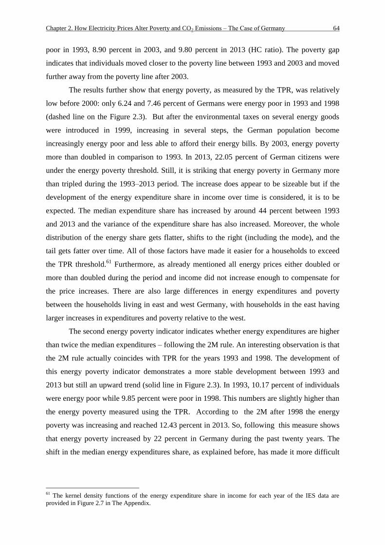
Chapter 2. How Electricity Prices Alter Poverty and CO2 Emissions ‒ The Case of Germany 64
poor in 1993, 8.90 percent in 2003, and 9.80 percent in 2013 (HC ratio). The poverty gap
indicates that individuals moved closer to the poverty line between 1993 and 2003 and moved
further away from the poverty line after 2003.
The results further show that energy poverty, as measured by the TPR, was relatively
low before 2000: only 6.24 and 7.46 percent of Germans were energy poor in 1993 and 1998
(dashed line on the Figure 2.3). But after the environmental taxes on several energy goods
were introduced in 1999, increasing in several steps, the German population become
increasingly energy poor and less able to afford their energy bills. By 2003, energy poverty
more than doubled in comparison to 1993. In 2013, 22.05 percent of German citizens were
under the energy poverty threshold. Still, it is striking that energy poverty in Germany more
than tripled during the 1993–2013 period. The increase does appear to be sizeable but if the
development of the energy expenditure share in income over time is considered, it is to be
expected. The median expenditure share has increased by around 44 percent between 1993
and 2013 and the variance of the expenditure share has also increased. Moreover, the whole
distribution of the energy share gets flatter, shifts to the right (including the mode), and the
tail gets fatter over time. All of those factors have made it easier for a households to exceed
the TPR threshold.61
Furthermore, as already mentioned all energy prices either doubled or
more than doubled during the period and income did not increase enough to compensate for
the price increases. There are also large differences in energy expenditures and poverty
between the households living in east and west Germany, with households in the east having
larger increases in expenditures and poverty relative to the west.
The second energy poverty indicator indicates whether energy expenditures are higher
than twice the median expenditures – following the 2M rule. An interesting observation is that
the 2M rule actually coincides with TPR for the years 1993 and 1998. The development of
this energy poverty indicator demonstrates a more stable development between 1993 and
2013 but still an upward trend (solid line in Figure 2.3). In 1993, 10.17 percent of individuals
were energy poor while 9.85 percent were poor in 1998. This numbers are slightly higher than
the energy poverty measured using the TPR. According to the 2M after 1998 the energy
poverty was increasing and reached 12.43 percent in 2013. So, following this measure shows
that energy poverty increased by 22 percent in Germany during the past twenty years. The
shift in the median energy expenditures share, as explained before, has made it more difficult
61
The kernel density functions of the energy expenditure share in income for each year of the IES data are
provided in Figure 2.7 in The Appendix.

Chapter 2. How Electricity Prices Alter Poverty and CO2 Emissions ‒ The Case of Germany 65
for households to exceed the 2M threshold and be qualified as energy poor according to this
indicator.
Figure 2. 3 Energy poverty over time
Note. Own calculations. Dataset is IES 1993–2013.Dash and dotted line indicates energy poverty calculated
using the ten percent rule (TPR) while solid line indicate energy poverty calculated using the twice median
expenditures (2M) rule. Line segments indicate the 95 percent confidence intervals.
2.5.2 On the relationship between income poverty and energy poverty
In order for income poverty policies to have impact on energy poverty as well, there
has to be an overlap between income poverty and energy poverty. The results in Table 2.2
indicate that around one quarter of the households that are energy poor are also income poor
throughout the 1993–2013 period. The proportion of energy poor households, which are also
income poor, reached 5.7 percent in 2013, almost four times larger than the proportion in
1993. This could indicate that income poverty is rather an important determinant of energy
poverty. The share of energy poor households, which do not fall under income poverty, also
increased by more than four times during this period. Similarly, the proportion of income poor
households that are not energy poor has grown by around 55 percent.

Chapter 2. How Electricity Prices Alter Poverty and CO2 Emissions ‒ The Case of Germany 66
Income poverty and energy poverty can be related to the type of employment status of the
household’s leader. German households with an unemployed leader are at highest risk of
income poverty and households with a retired leader are at second highest risk, both of which
show an upward trend since 1993 (refer to Table 2.12 in the Appendix). Urban households are
more likely to become income poor than rural ones. The risk of energy poverty is again
highest among the unemployed and second highest for the self-employed. A household with
unemployed leader is twice as likely to be energy poor as a household with employed leader.
The rural households are more prone to energy poverty in comparison to the urban households
(in 2013 the percentage energy poor among rural was around twice the one of the urban).
Palmer (2008) also found that energy poverty is higher among rural households in the U.K.
Table 2. 2 The overlap between income poverty and energy poverty
Income poor
Income poor not
energy poor
Both income and
energy poor
Energy poor not
income poor
Energy poor
(percent of all households)
1993 7.504 6.282 1.390 4.408 5.680
1998 7.034 5.698 1.501 4.961 6.318
2003 9.108 6.638 2.829 9.842 12.148
2008 12.176 8.165 4.738 17.866 21.090
2013 14.485 9.848 5.673 18.173 22.011
Note. Own calculations. Dataset is IES 1993–2013. Weighted to assure representativeness of the German
population.
Using the probit model from equation (2.8), I empirically investigate the effect of
income poverty on the probability of becoming energy poor. Several variables are included as
controls in the different probit specifications: binary indicator for income poverty, household
size, working status, education, and binary indicator for rural area of residence.62
Correlations of the variables included in the different probit model specifications are low to
moderate in order to avoid multicollinearity. The estimates from the first probit specification
(see Table 2.13 in the Appendix) do indeed prove that being income poor has positive and
significant impact on energy poverty in Germany. An income poor household has a 29.1
percent chance to be energy poor.63
Households which are not income poor are three times
less likely to become energy poor (10.6 percent probability) in comparison to income poor
households. Living in rural area leads to higher probability of being energy poor (12.5
62
The choice of controls follows Palmer (2008), and Legendare and Ricci (2015). 63
The marginal effect is calculated from the first specification without including any additional controls. The
probability measured at the mean values of the variables in the third specification indicates 29.1 percent chance
for poor household to become energy poor.

Chapter 2. How Electricity Prices Alter Poverty and CO2 Emissions ‒ The Case of Germany 67
percent) than living in urban area (7.4 percent).64
A household with unemployed leader has a
14.7 percent chance of becoming energy poor. Being self-employed increases the probability
of energy poverty and being retired or living in bigger household reduces it. Those results are
in line with the descriptive evidence of Table 2.12 in the Appendix. The fourth probit
specification demonstrates that households with more income and more educated leaders tend
to be less likely to be energy poor.
2.5.3 Differences in poverty levels across household types
Income poverty levels are different across the different household types in Germany.
The most vulnerable category appears to be single parents and single adults are the second
most vulnerable category. If disposable equivalent income is used to calculate the head count
ratio, 29 percent of all single parent households are poor in 1993 and 34 percent in 2013. If
disposable equivalent income after energy tax burdens is considered, 30 percent of all single
parent households are poor in 1993 and 36 percent in 2013.
As before, energy poverty is measured using two different indicators. Table 2.3
indicates that single parent households have the highest energy poverty levels under the TPR
but the 2M shows that households with two adults and children are most energy poor (this is
also due to the fact that the second indicator does not take household size into account).
During the period between 1993 and 2013, the TPR points out that energy poverty increased
among all the household types, with the number of energy poor single parent households
increasing by 188 percent. The second indicator of energy poverty shows that poverty among
two adult households with children increased by around 73 percent.
Table 2. 3 Income and energy poverty by household types
1993 1998 2003 2008 2013
𝐻𝐶 𝑟𝑎𝑡𝑖𝑜 (𝐷𝑖𝑠𝑝𝑜𝑠𝑎𝑏𝑙𝑒 𝑒𝑞𝑢𝑖𝑣𝑎𝑙𝑒𝑛𝑡 𝑖𝑛𝑐𝑜𝑚𝑒)
ℎℎ𝑡𝑦𝑝𝑒 1 16.071 17.751 19.946 24.330 26.343
ℎℎ𝑡𝑦𝑝𝑒 2 27.712 31.894 28.831 32.149 28.343
ℎℎ𝑡𝑦𝑝𝑒 3 7.394 7.403 8.017 9.669 9.556
ℎℎ𝑡𝑦𝑝𝑒 4 8.496 8.987 6.496 8.964 7.790
𝐻𝐶 𝑟𝑎𝑡𝑖𝑜 (𝐷𝑖𝑠𝑝𝑜𝑠𝑎𝑏𝑙𝑒 𝑒𝑞𝑢𝑖𝑣𝑎𝑙𝑒𝑛𝑡 𝑖𝑛𝑐𝑜𝑚𝑒 𝑚𝑖𝑛𝑢𝑠 𝑒𝑛𝑒𝑟𝑔𝑦 𝑡𝑎𝑥 𝑏𝑢𝑟𝑑𝑒𝑛𝑠)
ℎℎ𝑡𝑦𝑝𝑒 1 16.680 18.294 21.285 25.510 27.694
ℎℎ𝑡𝑦𝑝𝑒 2 29.593 33.084 32.043 34.341 31.530
ℎℎ𝑡𝑦𝑝𝑒 3 7.802 7.939 9.088 10.534 10.544
ℎℎ𝑡𝑦𝑝𝑒 4 9.563 9.868 7.720 10.041 8.910
64
All the other variables are considered to be at their mean values.

Chapter 2. How Electricity Prices Alter Poverty and CO2 Emissions ‒ The Case of Germany 68
Table 2. 4 (Continued)
1993 1998 2003 2008 2013
𝐸𝑛𝑒𝑟𝑔𝑦 𝑝𝑜𝑣𝑒𝑟𝑡𝑦 (𝑇𝑃𝑅)
ℎℎ𝑡𝑦𝑝𝑒 1 7.762 8.366 13.887 20.609 20.394
ℎℎ𝑡𝑦𝑝𝑒 2 9.057 9.125 16.636 27.016 26.534
ℎℎ𝑡𝑦𝑝𝑒 3 4.759 4.883 10.105 18.917 20.181
ℎℎ𝑡𝑦𝑝𝑒 4 4.126 5.109 10.140 18.259 18.135
𝐸𝑛𝑒𝑟𝑔𝑦 𝑝𝑜𝑣𝑒𝑟𝑡𝑦 (2𝑀)
ℎℎ𝑡𝑦𝑝𝑒 1 0.961 0.953 0.760 1.110 1.452
ℎℎ𝑡𝑦𝑝𝑒 2 4.848 3.797 4.187 3.959 5.484
ℎℎ𝑡𝑦𝑝𝑒 3 6.044 5.894 6.483 8.300 11.037
ℎℎ𝑡𝑦𝑝𝑒 4 15.879 15.257 17.125 20.776 26.967
Note. ℎℎ𝑡𝑦𝑝𝑒 1 – single adult; ℎℎ𝑡𝑦𝑝𝑒 2 – single parent; ℎℎ𝑡𝑦𝑝𝑒 3 –two adults with no children; ℎℎ𝑡𝑦𝑝𝑒 4 –
two or more adults with children. Weighted to assure representativeness of the German population.
2.5.4 Price and expenditure elasticites of energy demand
The demand system estimates65
allow for calculation of the price and expenditure
elasticities of the energy goods. The elasticies obtained from the demand system are included
in Table 2.4. Electricity is found to have rather low own price elasticity throughout
Germany: for 1 percent increase in the price of electricity, demand would decrease by 0.235
percent, holding everything else constant. So, price change policies are not expected to be
very efficient in reducing electricity consumption. The expenditure elasticity of electricity
demand is 0.496, which shows that electricity is a necessity and normal good among German
households: given 1 percent increase in expenditures will lead to 0.496 percent higher demand
for electricity.66
Car fuels are also a necessity good (elasticity is 0.994) and demand for fuels
is price inelastic in Germany: for 1 percent price increase consumption would go down by
0.316 percent.
The elasticities in Table 2.4 also reveal that there are differences in price responses
according to the level of income. Low income households have highest price elasticity of
demand for electricity (–0.478) while high income households have lowest elasticity (–0.173)
in absolute terms. Poor households in Germany are three times more responsive to electricity
price changes in comparison to rich households. Murray (2012) finds higher elasticity for
electricity among poor than among rich U.S. households. Car fuels demand is again most
elastic for the poor income households and least elastic for high income households. Car fuels
65
For details on the demand system coefficient estimates, please refer to Table 2.15 in the Appendix. Table 2.16
compares the elasticities obtained from demographic and base (QU) AIDS. 66
Table 2.17 in the Appendix provides comparison of price and expenditure elasticites with similar papers from
the existing literature.

Chapter 2. How Electricity Prices Alter Poverty and CO2 Emissions ‒ The Case of Germany 69
are also found to be luxury good for the first six deciles of disposable equivalent income. Poor
and rich German households also differ by the amount of their total expenditures devoted on
energy goods. Low income households pay 4.024 percent of their total expenditures on
electricity while for high income households the share is only 2.415 percent (almost 40
percent lower share than the poor). The reverse holds for car fuels: while the poor devote
2.968 percent of total expenditures to car fuels the rich devote 4.551 percent.
The price and income elasticities by household type are summarized in Table 2.14 in
the Appendix. The table indicates that there are differences as well as similarities in demand
responses of the various households’ types. The price elasticities show that single parent
households are most responsive to electricity price changes while single adults are least
responsive. If the demand for car fuels is considered, single parents have highest price
elasticity and couples without children have lowest price elasticity.
Low income households can ration their energy expenditures and also ration the food
budget when faced with higher energy prices. The cross price elasticitis reveal that food is
complementary with electricity and other fuels among German households: as prices of
energy goods would go up, food demand will tend to decrease, indicating a heat or eat
behavior. Food demand will decrease by 0.097 if price of other fuels increases by 1 percent
and will decrease by 0.003 percent if electricity price increases by 1 percent. Murray (2012)
also finds that U.S. households consider food and energy to be complements, but the effects
are larger. A one percent increase in natural gas price causes 0.47 percent reductions in the
food at home expenditures and a one percent increase in electricity price causes reductions in
the food at home by 0.14 percent.
2.6 Scenarios design and results
First of all, marginal (1 percent) changes in the EEG surcharge for 2013 are
considered. Secondly, marginal changes of the car fuels tax67
in addition to the EEG
surcharge are studied. Then varying between 100 percent reduction and 100 percent increase
in EEG only and both EEG and car fuels tax so overall four main scenarios are scrutinized.
Moreover, the impact of such changes on income and energy poverty, and the environment is
analysed in detail.
67
For details on the disaggregation and development of the car fuels tax and price, please refer to Section 1.4.2.

Chapter 2. How Electricity Prices Alter Poverty and CO2 Emissions ‒ The Case of Germany 70
Table 2. 5 Elasticities and expenditure shares according to disposable equivalent income deciles
Disposable
equivalent
income
deciles
Price elasticities Expenditure elasticities Expenditure shares (percent of total expenditures)
Food Electricity
Other
fuels
Car
fuels
Other
goods Food Electricity
Other
fuels
Car
fuels
Other
goods Food Electricity
Other
fuels
Car
fuels
Other
goods
1 –1.006 –0.478 –0.718 –0.327 –1.130 0.560 0.581 0.776 1.550 1.140 21.381 4.024 4.691 2.968 66.936
2 –1.006 –0.430 –0.704 –0.402 –1.133 0.525 0.576 0.783 1.301 1.145 20.189 3.449 4.169 3.938 68.255
3 –1.008 –0.395 –0.695 –0.421 –1.134 0.498 0.571 0.782 1.189 1.147 18.927 3.232 3.912 4.313 69.616
4 –1.009 –0.373 –0.688 –0.429 –1.134 0.477 0.570 0.783 1.119 1.148 17.935 3.095 3.779 4.529 70.662
5 –1.010 –0.352 –0.683 –0.431 –1.135 0.456 0.568 0.784 1.060 1.149 17.102 3.027 3.705 4.694 71.472
6 –1.011 –0.332 –0.677 –0.431 –1.134 0.440 0.564 0.778 1.022 1.148 16.336 2.964 3.660 4.823 72.217
7 –1.012 –0.317 –0.672 –0.427 –1.134 0.422 0.563 0.776 0.979 1.148 15.616 2.839 3.611 4.906 73.028
8 –1.014 –0.291 –0.665 –0.407 –1.133 0.392 0.558 0.770 0.914 1.148 21.381 2.761 3.561 4.929 73.946
9 –1.017 –0.263 –0.658 –0.379 –1.132 0.344 0.551 0.759 0.842 1.146 20.189 2.642 3.501 4.843 75.142
10 –1.028 –0.174 –0.617 –0.123 –1.128 0.239 0.526 0.705 0.371 1.142 18.927 2.415 3.342 4.551 77.671
Germany –1.003 –0.235 –0.657 –0.316 –1.136 0.488 0.496 0.770 0.994 1.149 17.044 3.231 4.030 4.183 71.513
SE 0.001 0.008 0.001 0.005 0.000 0.005 0.003 0.001 0.008 0.000 0.075 0.023 0.043 0.039 0.095
Note. Own calculations. Dataset is IES 1993–2013.

Chapter 2. How Electricity Prices Alter Poverty and CO2 Emissions ‒ The Case of Germany 71
2.6.1 Scenarios with marginal changes in EEG surcharge
Table 2.5 summarizes the results from the four marginal tax scenarios (S1–S4) and
identifies the baseline scenario or the status quo (S0). The situation in 2013 is taken as the
status quo: the electricity tax amounts to 0.0201 euros/kWh, the EEG surcharge amounts to
0.0528 euros/kWh, and the energy tax on car fuels amounts to 0.606 euros/liter. The average
German household pays 186 euros for the EEG surcharge, 72 euros for electricity tax, and
575 euros for car fuels taxes (CFT) annually. The energy tax burdens for electricity and CFT
represent 0.870 percent and 1.674 percent of income respectively. However, the tax payments
in euros and as percentage of income differ largely between the poor and the rich families and
also according to household type. In the status quo, the average household emits 1.649 tons of
CO2 related to electricity and 1.912 tons of CO2 related to car fuels. Around 16 percent of the
German households live in energy poverty and around 19 percent live in income poverty. All
variables are predicted using the expenditures weights obtained from the demand system
rather than using the actual expenditure shares.
Under the first scenario (S1), the EEG surcharge is one percent higher than under the
baseline. Electricity related emissions would go down by 0.12 percent while income poverty
as measured by the headcount ratio would increase by 0.04 percent and energy poverty would
increase by 0.63 percent. Tax burden of electricity is around 0.12 percent lower than the
status quo. If in addition to the EEG surcharge, the car fuels tax is increased by one percent
(S3), income poverty is 0.05 percent higher than the baseline and energy poverty is 1.27
percent higher. S2 considers one percent decrease in the EEG surcharge and S4 considers one
percent decrease in both the EEG surcharge and in the CFT. Under S2, electricity related
emissions remain same as under the baseline (price change is too small), income poverty goes
down by 0.05 percent, and energy poverty goes up by 0.63 percent. In the fourth scenario
(S4), energy poverty is 1.27 percent lower and income poverty is 0.10 percent lower than
under the baseline.
2.6.2 Other potential scenarios
Departing once again from the status quo, the changes in tax burdens, emissions,
energy poverty, and income poverty are analysed for another four scenarios (S5–S8) across
disposable equivalent income deciles and household types. Tables 2.6 and 2.7 include the

Chapter 2. How Electricity Prices Alter Poverty and CO2 Emissions ‒ The Case of Germany 72
Table 2. 6 Scenarios with marginal changes
S0
S1:
𝐸𝐸𝐺 + 1%
S2:
𝐸𝐸𝐺 − 1%
S3:
𝐸𝐸𝐺 + 1%; 𝐶𝐹𝑇 + 1%
S4:
𝐸𝐸𝐺 − 1%; 𝐶𝐹𝑇 − 1%
Variable Mean
Std.
Err. Mean
Std.
Err. Mean
Std.
Err. Mean
Std.
Err. Mean
Std.
Err.
Emissions electricity (t) 1.649 0.003 1.647 0.003 1.649 0.003 1.646 0.003 1.650 0.004
Emissions car fuels (t) 1.912 0.005 1.911 0.005 1.911 0.005 1.907 0.005 1.915 0.005
EEG surcharge (euros) 185.667 0.379 187.298 0.382 183.856 0.375 187.246 0.382 183.907 0.400
Tax burden electricity (euros) 72.087 0.147 72.000 0.147 72.105 0.147 71.980 0.147 72.124 0.156
Tax burden car fuels (euros) 574.607 1.362 574.150 1.361 574.290 1.361 578.802 1.372 569.618 1.347
Income povery (𝐻𝐶 𝑟𝑎𝑡𝑖𝑜) 18.785 0.002 18.792 0.000 18.775 0.000 18.796 0.000 18.767 0.000
Income poverty
(𝐴𝑣𝑒𝑟𝑎𝑔𝑒 𝑛𝑜𝑟𝑚𝑎𝑙𝑖𝑧𝑒𝑑 𝑝𝑜𝑣𝑒𝑟𝑡𝑦 𝑔𝑎𝑝) 0.041 0.001 0.041 0.000 0.041 0.000 0.041 0.000 0.041 0.000
Income poverty
(𝐴𝑣𝑒𝑟𝑎𝑔𝑒 𝑠𝑞𝑢𝑎𝑟𝑒𝑑 𝑛𝑜𝑟𝑚𝑎𝑙𝑖𝑧𝑒𝑑 𝑝𝑜𝑣𝑒𝑟𝑡𝑦 𝑔𝑎𝑝) 0.013 0.000 0.013 0.000 0.013 0.000 0.013 0.000 0.013 0.000
Energy poverty (𝑇𝑃𝑅) 0.369 0.002 0.370 0.002 0.368 0.002 0.372 0.002 0.367 0.002
Note. 𝐸𝐸𝐺 is the renewable energy surcharge and 𝐶𝐹𝑇 is the car fuels tax. All poverty indices are calculated on disposable equivalent income after energy taxes.

Chapter 2. How Electricity Prices Alter Poverty and CO2 Emissions ‒ The Case of Germany 73
results of S5: doubling of the EEG surcharge and S6: abolishing the EEG surcharge
respectively. Tables 2.18 and 2.19 in the Appendix include the results from S7: doubling of
both the EEG surcharge and the CFT and S8: abolishing both the EEG surcharge and the
CFT.
Under S5, the electricity tax burden (the sum of EEG surcharge and electricity tax)
increases for all income deciles but the increase is highest percentage for the low income
households (0.69 percent of income). Withana et al. (2013) finds that the electricity tax is
mainly born by low income households in Germany. The households in the first decile have
also the largest percentage decrease in electricity related emissions (9.47 percent) while the
households in the tenth decile will have smallest emissions reductions (4.32 percent) as they
have the lowest price elasticity. The households in the top income deciles experience largest
increase in energy poverty68
of above 20 percent relative to the baseline. If the effects across
the different household types are analysed, it appears that single parents have largest increase
in electricity tax burden and largest emissions decrease if the EEG is doubled. Single adult
households are least responsive to the change in the EEG surcharge so they would have
smallest consumption and emissions reductions. Income poverty increases the most among
two adults’ households without children and energy poverty among two adults’ households
with children.
Abolishment of the EEG surcharge makes the electricity price 22 percent price lower,
leads to 109 euros lower energy tax burden for the low income households and 250 euros
lower burden for the high income households. The decrease in tax burden as percent of
income is largest for low income German households and also among the single parents. The
poorest households have largest emissions increase of 11.41 percent and the single parent’s
households also emit 8.90 percent more CO2 emissions than under the baseline scenario.
In spite of largest tax burdens decreases among poor and single parents households, it
is the households in the tenth decile that experience largest decrease in energy poverty of
around 30 percent relative to S0. Among the different household types, the two adults’
households with children will have largest income poverty decrease (3.25 percent) and
largest energy poverty decrease (17.3 percent). Overall, income poverty is 2 percent lower
and energy poverty almost 14 percent lower. Aasnesss et al. (2002) also find evidence that
reduced electricity tax increase equality in the income distribution and improves consumer
welfare.
68
By using the TPR.

Chapter 2. How Electricity Prices Alter Poverty and CO2 Emissions ‒ The Case of Germany 74
Table 2. 7 Scenario 5 (doubling of the EEG surcharge) results across income deciles and household types
Electricity tax burden Electricity emissions
Income poverty
(HC ratio)
Energy poverty
(TPR)
euros % of income tons % change before after before after
𝐷𝑖𝑠𝑝𝑜𝑠𝑎𝑏𝑙𝑒 𝑒𝑞𝑢𝑖𝑣𝑎𝑙𝑒𝑛𝑡 𝑖𝑛𝑐𝑜𝑚𝑒 𝑑𝑒𝑐𝑖𝑙𝑒𝑠 Mean
Std.
Dev. Mean
Std.
Dev. Mean
Std.
Dev. Mean
Std.
Dev. Mean
Mean
Mean
Mean
1 88.054 32.951 0.688 0.117 –0.095 0.034 –9.473 1.006 1.000 1.000 33.356 36.664
2 114.153 43.711 0.579 0.093 –0.110 0.043 –8.660 1.181 0.659 0.685 26.973 29.620
3 132.124 49.812 0.524 0.089 –0.118 0.047 –8.085 1.373 0.000 0.000 21.655 24.306
4 147.610 57.179 0.482 0.086 –0.124 0.053 –7.713 1.565 0.000 0.000 17.757 20.538
5 162.140 63.028 0.451 0.081 –0.130 0.057 –7.394 1.650 0.000 0.000 13.270 15.625
6 170.999 66.950 0.422 0.082 –0.130 0.061 –7.051 1.885 0.000 0.000 8.986 10.627
7 181.561 70.580 0.391 0.075 –0.133 0.061 –6.846 1.844 0.000 0.000 6.805 8.161
8 193.635 78.055 0.368 0.082 –0.130 0.066 –6.399 2.208 0.000 0.000 3.794 4.635
9 206.947 82.302 0.334 0.076 –0.128 0.069 –5.970 2.466 0.000 0.000 2.305 2.921
10 226.009 93.571 0.286 0.084 –0.096 0.096 –4.322 4.433 0.000 0.000 1.353 1.623
ℎℎ𝑡𝑦𝑝𝑒
1 95.392 28.289 0.494 0.151 –0.066 0.030 –7.052 3.017 0.329 0.332 17.158 19.165
2 144.640 46.685 0.539 0.137 –0.125 0.033 –8.170 1.630 0.398 0.402 23.482 26.297
3 172.756 54.869 0.461 0.152 –0.129 0.034 –7.495 2.217 0.138 0.140 15.272 17.281
4 234.379 75.164 0.448 0.136 –0.190 0.040 –7.803 1.575 0.116 0.119 12.052 13.988
Overall change 154.009 75.477 0.476 0.150 –0.118 0.060 –7.451 2.459 1.629 0.000 13.333 0.000
Note. Own calculations. Dataset is IES 2013. ℎℎ𝑡𝑦𝑝𝑒 1 – single adult; ℎℎ𝑡𝑦𝑝𝑒 2 – single parent; ℎℎ𝑡𝑦𝑝𝑒 3 – two adults with no children; ℎℎ𝑡𝑦𝑝𝑒 4 – two or more adults with
children.

Chapter 2. How Electricity Prices Alter Poverty and CO2 Emissions ‒ The Case of Germany 75
Table 2. 8 Scenario 6 (abolishing the EEG surcharge) results across income deciles and household types
Electricity tax burden Electricity emissions Income poverty
(HC ratio)
Energy poverty
(TPR)
euros % of income tons % change before after before after
𝐷𝑖𝑠𝑝𝑜𝑠𝑎𝑏𝑙𝑒 𝑒𝑞𝑢𝑖𝑣𝑎𝑙𝑒𝑛𝑡 𝑖𝑛𝑐𝑜𝑚𝑒 𝑑𝑒𝑐𝑖𝑙𝑒𝑠 Mean Std.
Dev. Mean
Std.
Dev. Mean
Std.
Dev. Mean
Std.
Dev. Mean Mean Mean Mean
1 –108.590 39.826 –0.849 0.132 0.114 0.042 11.406 1.931 1.000 1.000 33.356 29.925
2 –138.328 52.197 –0.701 0.097 0.125 0.053 9.842 2.266 0.659 0.629 26.973 23.975
3 –158.184 58.970 –0.625 0.092 0.127 0.060 8.737 2.635 0.000 0.000 21.655 18.806
4 –175.355 67.117 –0.570 0.085 0.129 0.068 8.021 3.003 0.000 0.000 17.757 14.526
5 –191.351 73.577 –0.530 0.081 0.130 0.073 7.408 3.167 0.000 0.000 13.270 11.710
6 –200.443 77.617 –0.492 0.081 0.125 0.082 6.748 3.617 0.000 0.000 8.986 7.078
7 –211.880 81.503 –0.455 0.074 0.124 0.081 6.354 3.539 0.000 0.000 6.805 5.538
8 –223.728 88.230 –0.423 0.079 0.112 0.096 5.495 4.240 0.000 0.000 3.794 2.944
9 –236.962 91.431 –0.381 0.072 0.100 0.106 4.670 4.735 0.000 0.000 2.305 1.641
10 –250.494 97.705 –0.316 0.081 0.033 0.176 1.516 8.354 0.000 0.000 1.353 1.084
ℎℎ𝑡𝑦𝑝𝑒
1 –110.486 25.225 –0.584 0.189 0.058 0.065 6.761 5.745 0.329 0.325 17.158 15.064
2 –172.548 51.087 –0.649 0.169 0.133 0.051 8.899 3.131 0.398 0.388 23.482 20.841
3 –202.118 52.975 –0.547 0.185 0.123 0.083 7.600 4.262 0.138 0.135 15.272 13.248
4 –276.997 79.687 –0.533 0.163 0.192 0.072 8.183 3.028 0.116 0.113 12.052 9.964
Overall change –180.681 84.038 –0.566 0.184 0.114 0.089 7.518 4.698 –2.123 0.000 –13.291 0.000
Note. Own calculations. Dataset is IES 2013. ℎℎ𝑡𝑦𝑝𝑒 1 – single adult; ℎℎ𝑡𝑦𝑝𝑒 2 – single parent; ℎℎ𝑡𝑦𝑝𝑒 3 – two adults with no children; ℎℎ𝑡𝑦𝑝𝑒 4 – two or more adults with
children.

Chapter 2. How Electricity Prices Alter Poverty and CO2 Emissions ‒ The Case of Germany 76
Doubling of the CFT, accompanied by doubling of the EEG surcharge (S7), increases
both income poverty and energy poverty by 5.1 and 55.1 percent. Emissions among German
households would decrease by 9.1 percent. When the CFT is abolished together with the EEG
surcharge (S8), income poverty and energy poverty are 7.2 percent and 48.7 percent lower
respectively, and emissions are 12.3 percent higher than under S0. Since the two goods are
found to be complementary, having both goods cheaper also activates the income effect.
Alternatively, I have constructed a scenario in which total energy related emissions for
the average German household would increase by only 0.03 tons while energy tax burden is
around 65 euros lower than the status quo and the welfare loss is only 4.8 euros.69
At the same
time, income poverty is 0.79 percent lower and energy poverty is 5.3 percent lower. The
above mentioned effects would follow from a scenario in which the EEG surcharge is
abolished while the CFT is increased by 25 percent (S9). If the EEG surcharge is abolished
and the CFT is increased by 50 percent (S10), emissions would go down by 0.7 tons, tax
burden will be 46 euro higher, and welfare loss is 140 euros (0.34 percent of income). Income
poverty and energy poverty would both increase under S10. On the other hand, S9 will be
very beneficial for the German households while assuring minimal environmental damage
and revenue loss for the government. Such policy would allow for large reduction in energy
costs for the households and reductions in energy poverty and income poverty, and should
definitely be considered by policy makers as a potential alternative for reducing electricity
prices while assuring adequate revenues for financing the green energy.
2.6.3 The relationship between poverty and energy taxes
Figure 2.4 includes a total of 6 graphs: the upper three graphs include the relationship
between the EEG surcharge rate and the income poverty indicators (HC ratio and poverty
gap) and between the EEG surcharge and the energy poverty indicator (TPR) and the lower
three graphs include the relationship between the car fuels tax rate (CFT) and the income
poverty indicators (HC ratio and poverty gap) and between the CFT and the energy poverty
indicator (TPR). Both income poverty indicators show a positive relationship between
poverty and the surcharge: income poverty increases with higher levels of EEG surcharge.
Energy poverty is also growing in the EEG surcharge, with more pronounced effects than
income poverty. As an example, by changing the EEG surcharge from 0.026 to 0.0317 euros
per kWh, energy poverty would shift from 14.8 to 15.0 percent while income poverty would
69
See Table 2.20 in the Appendix.

Chapter 2. How Electricity Prices Alter Poverty and CO2 Emissions ‒ The Case of Germany 77
Figure 2. 4 The relationship between energy taxes and income poverty and energy
poverty
Note. Own calculations. Dataset is IES 2013. Line segments indicate the 95 percent confidence intervals.
shift from 18.58 to 18.63 percent. Increases in the CFT will potentially also lead to higher
levels of income poverty and energy poverty among German households. For instance,
increasing the CFT from 0.303 to 0.363 euros per liter, would change income poverty from
18.28 to 18.36 percent and energy poverty from 12.7 to 13.3 percent. The effect of changes in
the CFT on both income poverty and energy poverty is more pronounced than the effect of the
EEG surcharge changes. That might be a consequence of the price elasticities of demand as
well as of proportion that each tax/surcharge represents in the respective energy price. In
monetary terms, CFT is ten times higher than the EEG, and as percentage of prices they
represent 0.390 and 0.197 percent of car fuels and electricity price respectively. Both car fuels
and electricity are necessity goods among German households, and price elasticities are 0.316
and 0.235 respectively. The trade-offs between EEG surcharge, CFT, and poverty levels are
hence confirmed by the graph and should be considered and addressed in policy design.

Chapter 2. How Electricity Prices Alter Poverty and CO2 Emissions ‒ The Case of Germany 78
2.7 Interim conclusion
Reduction of both income poverty and energy poverty reduction are given high
priority in the EU policy agenda. In Germany, income poverty has increased by around one
third between 1993 and 2013. During the same time, the price of electricity for households
increased by around 90 percent. Accordingly, the growing poverty together with the
increasing electricity prices
made it more difficult for households to afford their energy bills which in turn led to more
than tripling of energy poverty among German households. I find empirical evidence that
being income poor, unemployed, or living in rural residential area are all associated with
higher probability of falling under energy poverty.
The results from the energy demand system indicate that electricity is a necessity
good, with relatively low elasticity of demand, demonstrating that price change polices will
not be very efficient in reducing electricity consumption. The paper investigates the effect of
change in the electricity price (though changing the EEG surcharge) on income poverty,
energy poverty, and CO2 emissions. Four rather extreme scenarios are scrutinized; doubling
or eliminating of the EEG surcharge, doubling or eliminating of both the EEG surcharge and
the car fuels tax (CFT).
Doubling of the EEG surcharge brings highest increase in the tax burden as percentage
of income for the poorest households. Income poverty and energy poverty both increase while
electricity related CO2 emissions decrease. If in contrast, the EEG is abolished electricity
related emissions would grow, which is not a desirable environmental result. However,
energy poverty will decrease by around 13 percent and income poverty will decrease by
around 2 percent. The low income and the single parent households would benefit from
elimination of the EEG surcharge also by having lower energy tax burdens. Doubling of the
CFT, accompanied by doubling of the EEG surcharge, leads to 5.1 percent increase in income
poverty and 55.1 percent increase in energy poverty. Electricity related CO2 emissions would
decrease by 9.1 percent. When the CFT is abolished simultaneously with the EEG surcharge,
income poverty and energy poverty are 7.2 percent and 48.7 percent lower respectively, and
emissions are 12.3 percent higher.
Hence, I identify a positive relationship between poverty and energy surcharges or
taxes is i.e. higher levels of EEG surcharge or CFT are associated with higher levels of
income poverty and energy poverty in Germany. My results indicate a possibility of
abolishing the EEG surcharge while increasing the CFT by one quarter. Overall energy tax

Chapter 2. How Electricity Prices Alter Poverty and CO2 Emissions ‒ The Case of Germany 79
burden is slightly lower and energy related emissions increase by a very small amount while
income poverty and energy poverty both decrease (Scenario 9). The higher CFT is expected
to encourage switch towards more efficient vehicles or electric means of transportation. Such
policy reform should definitely be scrutinized by energy policy makers as it is promising
minimal revenue loss for the government and minimal environmental damage while reducing
energy poverty and income poverty levels. Especially unemployed people, households in rural
areas (as they already have higher poverty levels), single parent households (due to lower tax
burdens), and larger families (due to lower poverty levels) are likely to benefit the most from
lower electricity prices.
Alternatively, an energy solidarity payment could be introduced, as suggested by
Grösche and Schröder (2014b). According to the authors, such payment will generate the
same amount of revenues as the EEG surcharge but will assure more fair and proportional
distribution of payments (as it will be calculated proportionally to income tax contributions
and hence will be independent of consumption). Generating an adequate amount of revenues
through solidarity payment will make room for abolishing either the EEG surcharge or the
electricity tax. Renewable energy production could be sponsored through the solidarity
payment and will lead to further shifting the electricity mix towards higher proportion of
RES (and less carbon) so in the long run electricity emissions will go down, despite the lower
electricity price. Income poverty and energy poverty will also decrease once the electricity
price is reduced. Cheaper and cleaner electricity could also further motivate the use of electric
cars, which would lead to even lower CO2 emissions levels.

Chapter 2. How Electricity Prices Alter Poverty and CO2 Emissions ‒ The Case of Germany 80
2.8 Appendix 2.8.1 Tables
Table 2. 9 Relevant household level studies and their contribution to literature
Study Country, and time period Energy goods Behavioral
responses
Scenarios with
policy change
Income poverty
/Energy poverty
analyses
Emissions
analyses
Distributional
analyses
West and Williams III (2004) U.S., 1996–1998 Gasoline Yes Yes No/No No Yes
Tiezzi (2005) Italy, 1985–1996 Domestic fuels, transport
fuels, public transport
Yes Yes No/No No
Tiezzi and Verde (2016) U.S., 2007–2009 Gasoline Yes Yes No/No No No
Dumagan and Mount (1992) U.S., 1960–1987 Electricity, natural gas, oil Yes No No/No No Yes
Beznoska (2014) Germany, 1998–2008 Heating, electricity, mobility Yes Yes No/No No Yes
Filipinni (1995) Switzerland, 1991 Electricity Yes No No/No No No
Kohn and Missong (2003) Germany, 1988–1993 Energy and shelter aggregate Yes No No/No No No
Gahvari and Tsang (2011) U.S., 1996–1999 Energy aggregate good Yes Yes No/No No No
Brännlund and Nordström
(2004)
Sweden, 1985–1992 Petrol, public transport, other
transport, heating
Yes Yes No/No No Yes
Brännlund et al. (2007) Sweden, 1980–1997 Electricity, district heating,
oil, car, public and other
transport
Yes Yes No/No Yes No
Berkhout et al. (2004) Netherlands, 1992–1999 Electricity, gas Yes Yes No/No No Yes
Miniaci et al. (2014) Italy, 1998–2011 Electricity, gas No No No/Yes No No
Withana et al. (2013) Australia, British Columbia,
Denmark, Finland, Germany,
Ireland, Netherlands, Norway,
Sweden, and U.K.; (2010)
Natural gas, solid fuels,
electricity, mineral oils
No Yes No/No No Yes
Flues and Thomas (2015) 21 OECD countries, 2008–2012 Transport fuels, heating
fuels, electricity
No No No/No No Yes
Jacobsen et al. (2003) Denmark, 1997 Heating, transport fuels,
electricity
No No No/No No Yes
Klauss (2016) Armenia, 2009–2011 Natural gas, biomass No Yes Yes/No No No
Palmer et al. (2008) U.K., 2005–2007 Heating fuels, electricity No No Yes/Yes No No
Legendre and Ricci (2015) France, 2006 Electricity, gas, heating No No No/Yes No No

Chapter 2. How Electricity Prices Alter Poverty and CO2 Emissions ‒ The Case of Germany 81
Table 2. 8 (Continued)
Study Country, and time period Energy goods Behavioral
responses
Scenarios with
policy change
Income poverty
/Energy poverty
analyses
Emissions
analyses
Distributional
analyses
Papada and Kaliampakos
(2016)
Greece, 2015 Electricity, space heating No No No/Yes No No
Sterner (2012) France, Germany, Italy, and
Spain (2006), Serbia (2007),
Sweden (2004–2006)
Transport fuels No No No/No No Yes
Labandeira et al. (2006) Spain, 1973–1995 Electricity, natural gas, LPG,
car fuels, public transport
Yes No No/No No No
Labandeira et al. (2009) Spain, 1973–1995 Electricity, natural gas, LPG,
car fuels, public transport
Yes Yes No/No No Yes
Ekins et al. (2011)
Czech Republic, Germany,
Spain, Sweden, U.K.; (2005)
Electricity, heating fuels, car
fuels
No Yes No/No No Yes
Scarpellini et al. (2015) Spain (reg. Aragon), 2011–2015 Electricity, heating No No No/Yes No No Faik (2012) Germany, 2002–2010 - No No Yes/No No Yes Meyer and Sullivan (2009) US, 1960–2005 - No No Yes/No No No
Grabka et al. (2015) Germany, 2000–2012 - No No Yes/No No Yes Grabka et al. (2012) Germany, 2005–2010 - No No Yes/No No Yes Heindl (2014) Germany, 2011 Electricity, heating No No No/Yes No No Moore (2012) U.K., 2008 Heating fuels No No No/Yes No No Aasness et al. (2002) Norway, 2000 Electricity No Yes No/No No Yes Alberini et al. (2011) US, 1997–2007 Electricity, gas Yes No No/No No No
Halvorsen and Nesbakken
(2002)
Norway, 1993–1994 Electricity No Yes No/No No Yes
Kratena and Wüger (2009) Austria 1990–2006 Gasoline/diesel, heating,
electricity
Yes Yes No/No No
Kratena and Wüger (2010) Austria, 1972–2005 Gasoline, heating, electricity Yes Yes No/No No No
Ghalwash (2007) Sweden, 1980–2002 Petrol, public and other
transport, electricity, district
heating, oil
Yes No No/No No No
Blacklow et al. (2010) Australia, 1988–2004 Electricity and housing fuels Yes No No/No No Yes
Betti (2000) Italy, 1985–1994 Fuel and heating, transport Yes No No/No No No
Romero-Jordán et al. (2016) Spain, 2006–2012 Electricity No No No/No No Yes
Neuhoff et al. (2013) Germany, 1998–2008 Electricity No No No/No No Yes
Murray (2012) U.S., 1999–2009 Natural gas, electricity Yes No Yes/Yes No No

Chapter 2. How Electricity Prices Alter Poverty and CO2 Emissions ‒ The Case of Germany 82
Table 2. 8 (Continued)
Study Country, and time period Energy goods Behavioral
responses
Scenarios with
policy change
Income poverty
/Energy poverty
analyses
Emissions
analyses
Distributional
analyses
Grösche and Schröder (2014a) Germany, 2010 Electricity No Yes No No Yes
Nikodinoska and Schröder
(2016)
Germany, 1993–2008 Electricity, other fuels, car
fuels
Yes Yes No Yes Yes
Schumacher et al. (2015) Bulgaria , France, Germany,
Greece, Ireland, Italy, Poland,
Spain, U.K., E.U.; (2013)
Electricity, gas No No No/Yes No No
Frondel et al. (2015) Germany, 2006–2012 Electricity No Yes No/No No Yes
Boonekamp (2007) Netherlands, 1990–2000 Electricity No Yes No/No No No
Nygård (2013) Norway, 1978–2010 Electricity, fuels and district
heating, coal, coke, peat and
wood
Yes Yes No/No No No
Hills (2012) England, 2009 Electricity, gas No No No/Yes No No
Note. All necessary information is taken from the respective studies.

Chapter 2. How Electricity Prices Alter Poverty and CO2 Emissions ‒ The Case of Germany 83
Table 2. 10 Descriptive statistics of the variables included in the demand system
1993 1998 2003 2008 2013
Variable Mean
𝑙𝑛(𝑒𝑡𝑜𝑡𝑎𝑙) 9.723 9.834 9.871 9.900 9.965
𝑠𝑓𝑜𝑜𝑑 0.214 0.177 0.153 0.158 0.155
𝑠𝑒𝑙𝑒𝑐𝑡𝑟𝑖𝑐𝑖𝑡𝑦 0.032 0.027 0.030 0.034 0.038
𝑠𝑜𝑡ℎ𝑒𝑟 𝑓𝑢𝑒𝑙𝑠 0.040 0.034 0.041 0.049 0.037
𝑠𝑐𝑎𝑟 𝑓𝑢𝑒𝑙𝑠 0.031 0.036 0.044 0.049 0.048
𝑠𝑜𝑡ℎ𝑒𝑟 𝑔𝑜𝑜𝑑𝑠 0.683 0.726 0.732 0.710 0.722
𝑙𝑛(𝑝𝑓𝑜𝑜𝑑) 1.581 1.644 1.684 1.805 1.885
𝑙𝑛(𝑝𝑒𝑙𝑒𝑐𝑡𝑟𝑖𝑐𝑖𝑡𝑦) 1.497 1.488 1.608 1.861 2.163
𝑙𝑛(𝑝𝑜𝑡ℎ𝑒𝑟 𝑓𝑢𝑒𝑙𝑠) 1.245 1.247 1.533 1.957 2.026
𝑙𝑛(𝑝𝑐𝑎𝑟 𝑓𝑢𝑒𝑙𝑠) 1.143 1.255 1.571 1.848 1.954
𝑙𝑛(𝑝𝑜𝑡ℎ𝑒𝑟 𝑔𝑜𝑜𝑑𝑠) 1.539 1.655 1.681 1.691 1.777
𝑛𝑎𝑑𝑢𝑙𝑡𝑠 1.887 1.834 1.804 1.758 1.727
𝑛𝑐ℎ𝑖𝑙𝑑𝑟𝑒𝑛 0.424 0.359 0.334 0.298 0.281
Note. Dataset is IES 1993–2013. 𝑒 stands for expenditures, 𝑠 stands for expenditures share, 𝑝 is price and 𝑛 is
number.

Chapter 2. How Electricity Prices Alter Poverty and CO2 Emissions ‒ The Case of Germany 84
Table 2. 11 Summary statistics by household type
ℎℎ𝑡𝑦𝑝𝑒 1 2 3 4
Variable Mean
𝑦𝑑𝑖𝑠𝑝 20132.800 25713.360 37193.620 47140.910
𝑒𝑡𝑜𝑡𝑎𝑙 14233.230 19321.400 24450.130 30586.120
𝑒𝑓𝑜𝑜𝑑 1951.818 3294.660 3790.314 5237.592
𝑒𝑒𝑙𝑒𝑐𝑡𝑟𝑖𝑐𝑖𝑡𝑦 433.663 640.870 695.769 852.427
𝑒𝑜𝑡ℎ𝑒𝑟 𝑓𝑢𝑒𝑙𝑠 601.943 785.250 952.226 998.902
𝑒𝑐𝑎𝑟 𝑓𝑢𝑒𝑙𝑠 503.110 777.413 1045.769 1507.134
𝑒𝑜𝑡ℎ𝑒𝑟 𝑔𝑜𝑜𝑑𝑠 10742.700 13823.210 17966.050 21990.070
𝑠𝑓𝑜𝑜𝑑 0.152 0.184 0.174 0.188
𝑠𝑒𝑙𝑒𝑐𝑡𝑟𝑖𝑐𝑖𝑡𝑦 0.034 0.036 0.032 0.030
𝑠𝑜𝑡ℎ𝑒𝑟 𝑓𝑢𝑒𝑙𝑠 0.044 0.043 0.041 0.034
𝑠𝑐𝑎𝑟 𝑓𝑢𝑒𝑙𝑠 0.034 0.039 0.044 0.051
𝑠𝑜𝑡ℎ𝑒𝑟 𝑔𝑜𝑜𝑑𝑠 0.736 0.698 0.710 0.696
Note. ℎℎ𝑡𝑦𝑝𝑒 1 – single adult; ℎℎ𝑡𝑦𝑝𝑒 2 – single parent; ℎℎ𝑡𝑦𝑝𝑒 3 – two adults with no children; ℎℎ𝑡𝑦𝑝𝑒 4 –
two or more adults with children. Weighted to assure representativeness of the German population.

Chapter 2. How Electricity Prices Alter Poverty and CO2 Emissions ‒ The Case of Germany 85
Table 2. 12 Comparison with previous studies on income and energy poverty
Income poverty - Head Count ratio (equivalent disposable income)
Variable This study
(2016)
EU-SILC
(2014)
Faik
(2012)
Grabka et
al.
(2015)
Grabka et
al. (2012)
4th Poverty
report
(2013)
Statista
(2016)
Germany
1993 10.4
11.5
1998 11.1
10.8 10.4
2003 10.9
16.8 13.0 14.2 13.2
2008 13.7 15.3 17.0 14.4 14.6 14.3 14.4
2013 13.6 16.2
15.5
Energy poverty (TPR/LIHC)
This study
(2016) Palmer et al. (2008)
Legendre
and Ricci
(2015)
Hills (2012)
Germany England Scotland Wales Northern
Ireland France England
1993 5.3
1998 6.0
2003 11.4 6.0
(2004)
23.0
(2005-6)
11.0
(2004)
23.0
(2004)
16.6
(2006)
2008 19.7 7.0
(2005)
15.0
(2009)
2013 20.3
Note. Faik (2012) uses 50 percent of mean single person household's net income as poverty line while all the
other studies use 60 percent of median disposable equivalent income (according to OECD modified scale). HC
ratio indicates the percent of poor within the whole population on. TRP stands for the ten percent rule, as
described earlier and LIHC stands for Low Income High Costs, a measure used in Hills (2012).

Chapter 2. How Electricity Prices Alter Poverty and CO2 Emissions ‒ The Case of Germany 86
Table 2. 13 Income and energy poverty according to working status and area of
residence
Self-
employed
Employed Unemployed Retired Rural Urban
Income poverty (proportion poor)
1993 0.056 0.032 0.361 0.095 0.065 0.085
1998 0.044 0.033 0.386 0.078 0.055 0.089
2003 0.060 0.035 0.454 0.091 0.074 0.105
2008 0.076 0.039 0.719 0.109 0.086 0.138
2013 0.125 0.045 0.734 0.148 0.102 0.165
Energy poverty (proportion poor)
1993 0.041 0.043 0.148 0.055 0.057 0.048
1998 0.058 0.057 0.144 0.048 0.063 0.054
2003 0.119 0.107 0.233 0.097 0.125 0.088
2008 0.220 0.186 0.363 0.186 0.222 0.143
2013 0.279 0.185 0.353 0.209 0.233 0.136
Note. Own calculations. Dataset is IES 1993–2013.
Table 2. 14 Results of the probit model: probability to be energy poor
𝑃𝑟𝑜𝑏(𝑒𝑛𝑒𝑟𝑔𝑦 𝑝𝑜𝑜𝑟) Coef. Std. Err. Coef. Std. Err. Coef. Std. Err. Coef. Std. Err.
𝑖𝑛𝑐𝑜𝑚𝑒 𝑝𝑜𝑜𝑟 0.679 0.010
0.612 0.011
𝑙𝑛 (𝑦𝑑𝑖𝑠𝑝)
–0.546 0.006 –0.644 0.008
ℎℎ𝑠𝑖𝑧𝑒
–0.086 0.003 0.044 0.004
𝑟𝑢𝑟𝑎𝑙
0.327 0.008 0.375 0.008
𝑒𝑑𝑢𝑐2
–0.198 0.011 –0.080 0.011
𝑒𝑑𝑢𝑐3
–0.276 0.011 –0.144 0.011
𝑠𝑒𝑙𝑓𝑒𝑚𝑝𝑙𝑜𝑦𝑒𝑑
0.103 0.017 0.121 0.017
𝑢𝑛𝑒𝑚𝑝𝑙𝑜𝑦𝑒𝑑
0.174 0.017 0.089 0.016
𝑟𝑒𝑡𝑖𝑟𝑒𝑑
–0.077 0.008 –0.119 0.009
𝑐𝑜𝑛𝑠𝑡𝑎𝑛𝑡 –1.218 0.004 4.504 0.064 –1.166 0.011 5.196 0.079
𝑃𝑠𝑒𝑢𝑑𝑜 𝑅2 0.026 0.048 0.047 0.068
Note. Own calculations. Dataset is IES 1993–2013.

Chapter 2. How Electricity Prices Alter Poverty and CO2 Emissions ‒ The Case of Germany 87
Table 2. 15 Elasticities for the different household types
ℎℎ𝑡𝑦𝑝𝑒 1 2 3 4
Mean SE Mean SE Mean SE Mean SE
Price elasticities
Food –1.0156 0.0192 –1.0051 0.0065 –1.0133 0.1051 –1.0024 0.0412
Electricity –0.3284 0.1853 –0.3971 0.1004 –0.3555 0.1364 –0.3743 0.0970
Other fuels –0.6746 0.3353 –0.6931 0.0263 –0.6871 0.0424 –0.6828 0.0233
Car fuels –0.3814 0.5549 –0.3925 0.1878 –0.3638 0.2212 –0.3880 0.2723
Other goods –1.1212 0.0012 –1.1371 0.0083 –1.1310 0.0023 –1.1512 0.0112
Expenditure elasticities
Food 0.4561 0.2002 0.4830 0.0909 0.4532 0.1102 0.4250 0.7033
Electricity 0.5104 0.0620 0.5770 0.0387 0.5710 0.0346 0.6287 0.0341
Other fuels 0.6962 0.3328 0.7985 0.0435 0.7690 0.0341 0.8785 0.0546
Car fuels 1.3018 0.8325 1.1830 0.4012 1.0320 0.3956 0.7944 0.4706
Other goods 1.1306 0.0013 1.1506 0.0106 1.1436 0.0016 1.1698 0.0141
Note. Own calculations. Dataset is IES 1993–2013.

Chapter 2. How Electricity Prices Alter Poverty and CO2 Emissions ‒ The Case of Germany 88
Table 2. 16 DQUAIDS and QUAIDS Coefficient Estimates
DQUAIDS
QUAIDS
DAIDS
AIDS
Mean SE Mean SE Mean SE Mean SE
𝛼1 0.1456 0.0002 0.1809 0.0002 0.1452 0.0002 0.1788 0.0003
𝛼2 0.0250 0.0001 0.0331 0.0001 0.0252 0.0001 0.0329 0.0001
𝛼3 0.0383 0.0001 0.0446 0.0001 0.0381 0.0001 0.0443 0.0001
𝛼4 0.0492 0.0001 0.0464 0.0001 0.0470 0.0001 0.0450 0.0001
𝛼5 0.7419 0.0000 0.6951 0.0000 0.7445 0.0000 0.6991 0.0000
𝛽1 –0.0772 0.0006 –0.0162 0.0005 –0.0776 0.0006 –0.0303 0.0004
𝛽2 –0.0164 0.0002 –0.0094 0.0002 –0.0163 0.0002 –0.0102 0.0002
𝛽3 –0.0123 0.0004 –0.0092 0.0003 –0.0123 0.0004 –0.0105 0.0003
𝛽4 0.0090 0.0003 0.0218 0.0003 0.0084 0.0003 0.0093 0.0003
𝛽5 0.0969 0.0000 0.0130 0.0000 0.0979 0.0000 0.0418 0.0000
𝛾11 –0.0129 0.0011 –0.0209 0.0012 –0.0099 0.0011 –0.0321 0.0011
𝛾12 –0.0028 0.0004 –0.0043 0.0004 –0.0013 0.0003 –0.0042 0.0006
𝛾13 –0.0190 0.0005 –0.0216 0.0005 –0.0168 0.0005 –0.0177 0.0005
𝛾14 –0.0102 0.0006 –0.0133 0.0006 –0.0152 0.0006 –0.0216 0.0006
𝛾22 0.0225 0.0005 0.0207 0.0005 0.0229 0.0005 0.0210 0.0003
𝛾23 –0.0018 0.0003 –0.0029 0.0003 –0.0017 0.0003 –0.0027 0.0003
𝛾24 –0.0029 0.0004 –0.0017 0.0004 –0.0033 0.0004 –0.0025 0.0004
𝛾33 0.0126 0.0007 0.0106 0.0007 0.0120 0.0007 0.0086 0.0007
𝛾34 0.0017 0.0006 0.0043 0.0006 0.0019 0.0006 0.0055 0.0006
𝛾44 0.0300 0.0007 0.0264 0.0007 0.0297 0.0007 0.0247 0.0008
𝛾43 0.0017 0.0000 0.0043 0.0000 0.0019 0.0000 0.0055 0.0000
𝛾42 –0.0029 0.0000 –0.0017 0.0000 –0.0033 0.0000 –0.0025 0.0000
𝛾41 –0.0102 0.0000 –0.0133 0.0000 –0.0152 0.0000 –0.0216 0.0000
𝛾32 –0.0018 0.0000 –0.0029 0.0000 –0.0017 0.0000 –0.0027 0.0000
𝛾31 –0.0190 0.0000 –0.0216 0.0000 –0.0168 0.0000 –0.0177 0.0000
𝛾21 –0.0028 0.0000 –0.0043 0.0000 –0.0013 0.0000 –0.0042 0.0000
𝛾15 0.0449 0.0000 0.0601 0.0000 0.0432 0.0000 0.0756 0.0000
𝛾25 –0.0152 0.0000 –0.0118 0.0000 –0.0167 0.0000 –0.0115 0.0000
𝛾35 0.0065 0.0000 0.0096 0.0000 0.0046 0.0000 0.0063 0.0000
𝛾45 –0.0185 0.0000 –0.0157 0.0000 –0.0130 0.0000 –0.0062 0.0000
𝛾54 –0.0185 0.0000 –0.0157 0.0000 –0.0130 0.0000 –0.0062 0.0000
𝛾53 0.0065 0.0000 0.0096 0.0000 0.0046 0.0000 0.0063 0.0000
𝛾52 –0.0152 0.0000 –0.0118 0.0000 –0.0167 0.0000 –0.0115 0.0000
𝛾51 0.0449 0.0000 0.0601 0.0000 0.0432 0.0000 0.0756 0.0000
𝛾55 –0.0178 0.0000 –0.0423 0.0000 –0.0181 0.0000 –0.0642 0.0000
𝜆1 0.0046 0.0004 –0.0177 0.0003
𝜆2 0.0022 0.0001 –0.0010 0.0001
𝜆3 –0.0001 0.0002 –0.0015 0.0002
𝜆4 –0.0131 0.0002 –0.0156 0.0002
𝜆5 0.0064 0.0000 0.0358 0.0000
𝜃11 –0.0020 0.0004
–0.0023 0.0003
𝜃21 –0.0079 0.0001
–0.0080 0.0001
𝜃31 0.0019 0.0002
0.0015 0.0002

Chapter 2. How Electricity Prices Alter Poverty and CO2 Emissions ‒ The Case of Germany 89
Table 2. 15 (Continued)
DQUAIDS QUAIDS DAIDS AIDS
Mean SE Mean SE Mean SE Mean SE
𝜃41 0.0011 0.0002
0.0009 0.0002
𝜃21 0.0026 0.0004
0.0027 0.0004
𝜃22 0.0027 0.0001
0.0028 0.0001
𝜃32 –0.0112 0.0002
–0.0087 0.0002
𝜃42 –0.0064 0.0002
–0.0053 0.0002
𝜃51 0.0087 0.0000
0.0068 0.0000
𝜃52 0.0105 0.0000
0.0097 0.0000
𝜌1 0.9308 0.0057
0.9490 0.0059
𝜌2 0.3674 0.0044
0.3713 0.0045
𝜈1 0.0121 0.0006 –0.0103 0.0006 0.0122 0.0006 –0.0127 0.0005
𝜈2 –0.0025 0.0002 –0.0033 0.0002 –0.0025 0.0002 –0.0034 0.0002
𝜈3 0.0044 0.0004 0.0061 0.0004 0.0044 0.0004 0.0061 0.0005
𝜈4 –0.0146 0.0004 –0.0179 0.0003 –0.0145 0.0004 –0.0199 0.0003
𝜈5 0.0006 0.0000 0.0254 0.0000 0.0004 0.0000 0.0299 0.0000
Note. Own calculations. Dataset is IES 1993–2013.

Chapter 2. How Electricity Prices Alter Poverty and CO2 Emissions ‒ The Case of Germany 90
Table 2. 17 Comparison of demographic and base (QU)AIDS elasticities
DQUAIDS
QUAIDS DAIDS AIDS
Mean SE Mean SE Mean SE Mean SE
Price
elasticities
Food –1.0026 0.0005 –1.1020 0.0000 –0.9858 0.0000 –1.1585 0.0003
Electricity –0.2346 0.0079 –0.3164 0.0004 –0.2163 0.0043 –0.2975 0.0003
Other fuels –0.6569 0.0005 –0.7126 0.0002 –0.6740 0.0003 –0.7599 0.0001
Car fuels –0.3164 0.0048 –0.4973 0.0003 –0.3274 0.0005 –0.4508 0.0002
Other goods –1.1357 0.0000 –1.0730 0.0000 –1.1381 0.0000 –1.1299 0.0000
Expenditure
elasticities
Food 0.4876 0.0051 0.9080 0.0000 0.4989 0.0007 0.8196 0.0003
Electricity 0.4955 0.0032 0.6935 0.0002 0.5116 0.0029 0.6626 0.0002
Other fuels 0.7701 0.0005 0.7616 0.0002 0.7696 0.0003 0.7190 0.0002
Car fuels 0.9942 0.0076 1.4295 0.0003 0.9327 0.0005 1.2095 0.0001
Other goods 1.1491 0.0000 1.0185 0.0000 1.1512 0.0000 1.0581 0.0000
Note. Own calculations. Dataset is IES 1993–2013.
Table 2. 18 Comparison with electricity demand elasticities from existing literature
Studies
This
study
(2016)
Ghalwash
(2007)
Kratena
and
Wüger
(2010)
Dumagan
and
Mount
(1992)
Labandeira
et al.
(2006)
Kratena
and
Wüger
(2009)
Blacklow et
al. (2010)
Nygård
(2013)
Price elasticity –0.235 –0.140 –0.179 –0.067 –0.447 –0.124 –0.331 –0.140
Expenditure
elasticity 0.496 0.460 4.466 0.723 0.739 0.334 0.132 0.59
Note. Elasticities estimates are taken from the relevant studies.

Chapter 2. How Electricity Prices Alter Poverty and CO2 Emissions ‒ The Case of Germany 91
Table 2. 19 Scenario 7 (doubling of the EEG surcharge and CFT) results across income deciles and household types
Electricity tax burden Electricity emissions
Income poverty
(HC ratio)
Energy poverty
(TPR)
euros % of income tons % change before after before after
𝐷𝑖𝑠𝑝𝑜𝑠𝑎𝑏𝑙𝑒 𝑒𝑞𝑢𝑖𝑣𝑎𝑙𝑒𝑛𝑡 𝑖𝑛𝑐𝑜𝑚𝑒 𝑑𝑒𝑐𝑖𝑙𝑒𝑠 Mean
Std.
Dev. Mean
Std.
Dev. Mean
Std.
Dev. Mean
Std.
Dev. Mean
Mean
Mean
Mean
1 84.636 31.368 0.662 0.110 –0.108 0.039 –10.707 0.819 1.000 1.000 33.356 48.356
2 109.220 41.406 0.554 0.086 –0.129 0.049 –10.069 0.962 0.659 0.740 26.973 38.217
3 126.026 47.043 0.500 0.082 –0.140 0.055 –9.620 1.121 0.000 0.000 21.655 33.559
4 140.479 53.830 0.458 0.078 –0.151 0.062 –9.336 1.275 0.000 0.000 17.757 28.070
5 154.018 59.223 0.428 0.074 –0.160 0.066 –9.093 1.344 0.000 0.000 13.270 22.244
6 162.160 62.773 0.400 0.075 –0.163 0.070 –8.825 1.533 0.000 0.000 8.986 16.998
7 171.957 66.081 0.371 0.068 –0.169 0.072 –8.671 1.499 0.000 0.000 6.805 12.583
8 182.944 72.685 0.347 0.074 –0.170 0.076 –8.322 1.783 0.000 0.000 3.794 8.134
9 195.106 76.349 0.315 0.068 –0.172 0.076 –7.988 1.983 0.000 0.000 2.305 4.654
10 211.653 85.791 0.268 0.076 –0.150 0.089 –6.674 3.525 0.000 0.000 1.353 2.353
ℎℎ𝑡𝑦𝑝𝑒
1 90.558 25.431 0.471 0.146 –0.083 0.021 –8.737 2.405 0.329 0.341 17.158 0.261
2 137.799 43.383 0.515 0.132 –0.151 0.037 –9.715 1.293 0.398 0.414 23.482 0.349
3 163.884 49.824 0.439 0.146 –0.162 0.025 –9.180 1.746 0.138 0.147 15.272 0.235
4 222.078 69.101 0.425 0.129 –0.235 0.048 –9.527 1.221 0.116 0.123 12.052 0.204
Overall 146.118 70.284 0.454 0.144 –0.147 0.068 –9.132 1.960 5.117 0.000 55.063 0.000
Note. Own calculations. Dataset is IES 2013. ℎℎ𝑡𝑦𝑝𝑒 1 – single adult; ℎℎ𝑡𝑦𝑝𝑒 2 – single parent; ℎℎ𝑡𝑦𝑝𝑒 3 – two adults with no children; ℎℎ𝑡𝑦𝑝𝑒 4 – two or more adults with
children.

Chapter 2. How Electricity Prices Alter Poverty and CO2 Emissions ‒ The Case of Germany 92
Table 2. 20 Scenario 8 (abolishing the EEG surcharge and CFT) results across income deciles and household types
Electricity tax burden Electricity emissions
Income poverty
(HC ratio)
Energy poverty
(TPR)
euros % of income tons % change before after before after
𝐷𝑖𝑠𝑝𝑜𝑠𝑎𝑏𝑙𝑒 𝑒𝑞𝑢𝑖𝑣𝑎𝑙𝑒𝑛𝑡 𝑖𝑛𝑐𝑜𝑚𝑒 𝑑𝑒𝑐𝑖𝑙𝑒𝑠 Mean
Std.
Dev. Mean
Std.
Dev. Mean
Std.
Dev. Mean
Std.
Dev. Mean
Mean
Mean
Mean
1 –106.967 39.119 –0.836 0.130 0.151 0.055 15.025 1.422 1.000 1.000 33.356 20.417
2 –136.019 51.184 –0.689 0.094 0.178 0.070 13.921 1.671 0.659 0.551 26.973 14.821
3 –155.352 57.767 –0.614 0.089 0.192 0.078 13.144 1.946 0.000 0.000 21.655 10.390
4 –172.064 65.677 –0.559 0.082 0.205 0.087 12.654 2.213 0.000 0.000 17.757 7.601
5 –187.620 71.948 –0.520 0.078 0.216 0.094 12.235 2.332 0.000 0.000 13.270 5.820
6 –196.396 75.848 –0.482 0.077 0.218 0.099 11.771 2.661 0.000 0.000 8.986 3.154
7 –207.497 79.609 –0.445 0.071 0.224 0.101 11.505 2.602 0.000 0.000 6.805 2.848
8 –218.876 86.027 –0.414 0.075 0.223 0.107 10.899 3.096 0.000 0.000 3.794 1.445
9 –231.610 89.020 –0.372 0.069 0.222 0.110 10.319 3.450 0.000 0.000 2.305 0.887
10 –244.081 94.766 –0.308 0.078 0.180 0.141 8.025 6.136 0.000 0.000 1.353 0.609
ℎℎ𝑡𝑦𝑝𝑒
1 –108.237 24.032 –0.573 0.186 0.109 0.039 11.607 4.166 0.329 0.313 17.158 9.720
2 –169.383 49.691 –0.638 0.167 0.206 0.052 13.314 2.241 0.398 0.374 23.482 12.110
3 –198.051 50.862 –0.537 0.182 0.216 0.045 12.380 3.044 0.138 0.126 15.272 7.535
4 –271.444 77.183 –0.523 0.160 0.319 0.066 12.998 2.134 0.116 0.106 12.052 4.857
Overall –177.068 81.872 –0.555 0.181 0.197 0.096 12.299 3.404 –7.165 0.000 –48.734 0.000
Note. Own calculations. Dataset is IES 2013. ℎℎ𝑡𝑦𝑝𝑒 1 – single adult; ℎℎ𝑡𝑦𝑝𝑒 2 – single parent; ℎℎ𝑡𝑦𝑝𝑒 3 – two adults with no children; ℎℎ𝑡𝑦𝑝𝑒 4 – two or more adults with
children.

Chapter 2. How Electricity Prices Alter Poverty and CO2 Emissions ‒ The Case of Germany 93
Table 2. 21 Results of Scenario 9 and Scenario 10
S9:
𝐸𝐸𝐺 − 100%; 𝐶𝐹𝑇 + 25%
S10:
𝐸𝐸𝐺 − 100%; 𝐶𝐹𝑇 + 50%
Change in variables Mean
Std.
Dev. Mean
Std.
Dev.
Emissions electricity (t) 0.102 0.095 0.089 0.098
Emissions electricity (%) 6.340 4.933 5.641 5.124
Emissions car fuels (t) -0.071 0.058 –0.161 0.109
Emissions car fuels (%) –3.368 0.000 –7.690 0.000
Tax burden electricity (euros) –194.851 84.627 –195.420 84.964
Tax burden electricity (% of income) –0.539 0.176 –0.540 0.176
Tax burden car fuels (euros) 130.353 63.594 241.355 119.380
Tax burden car fuels (% of income) 0.343 0.098 0.633 0.181
Income povery (𝐻𝐶 𝑟𝑎𝑡𝑖𝑜) –0.793 0.000 0.144 0.000
Energy poverty (𝑇𝑃𝑅) –5.300 0.000 3.165 0.000
Compensating variation (euros) 4.827 48.156 139.618 115.710
Compensating variation (% of income) 0.062 0.183 0.338 0.239
Note. Own calculations. Dataset is IES 2013.

Chapter 2. How Electricity Prices Alter Poverty and CO2 Emissions ‒ The Case of Germany 94
2.8.2 Figures
Figure 2. 5 HC ratio on equivalent expenditures and equivalent expenditures after
energy taxes
Note. Own calculations. Dataset is IES 1993–2013. Solid line stands for poverty calculated on disposable
equivalent expenditures while dashed line stands for poverty calculated on disposable equivalent expenditures
minus energy taxes. Line segments indicate the 95 percent confidence intervals.

Chapter 2. How Electricity Prices Alter Poverty and CO2 Emissions ‒ The Case of Germany 95
Figure 2. 6 Poverty gap on equivalent expenditures and equivalent expenditures after
energy taxes
Note. Own calculations. Dataset is IES 1993–2013. Solid line stands for poverty calculated on disposable
equivalent expenditures while dashed line stands for poverty calculated on disposable equivalent expenditures
minus energy taxes. Line segments indicate the 95 percent confidence intervals.

Chapter 2. How Electricity Prices Alter Poverty and CO2 Emissions ‒ The Case of Germany 96
Figure 2. 7 Kernel density functions of energy expenditure share in income by years
Note. Vertical lines stand for twice the median energy expenditure share (2M).


98
Chapter 3
Inter- and Intra-generational Emissions Inequality in
Germany: Empirical Analyses
3.1 Introduction
Several countries in Europe have experienced growing demand for residential energy
and hence increasing anthropogenic carbon dioxide (CO2) emissions from the household
sector (European Environment Agency, 2015). However, the increase in energy consumption
and emissions has not been equally distributed among all households and it seems to be
highly dependent on the level of income. Even in developed countries such as Germany,
U.K., Sweden, France, U.S., and others there exists a wide gap in energy consumption and
emissions (pollution) between rich (high income) and the poor (low income) households.70
Chancel and Piketty (2015) find that global CO2 emissions remain concentrated: the top 10
percent of emitters are responsible for 45 percent of the emissions and the bottom 50 percent
are responsible for only 13 percent of global emissions. To address the challenge of
increasing and unequally distributed emissions, the interactions between environmental
degradation and economic inequalities in specific countries should be explored.
The differences in the levels of emissions/pollution among households are known as
impact inequalities (Chancel (2014)). In this study, I distinguish between three types of
impact inequalities: a) income – poor versus rich; b) place of residence – urban versus rural
households; and c)year of birth – earlier (older) versus later cohorts (younger); the first two
70
Rehdanz (2007) finds that income is an important determinant of heating costs and heating expenditures
increase with income in Germany. Jamasb and Meier (2010) find that total energy expenditures increase with
income in the U.K. Räty and Carlsson-Kanyama (2009) find that in Sweden and Germany CO2 emissions
intensity increases with income.

Chapter 3. Inter- and Intra-generational Emissions Inequality in Germany: Empirical Analyses 99
being intra-temporal and the latter being inter-temporal inequalities. Understanding the
impact inequalities and their causes among households will provide a better understanding of
inequalities in climate change and will contribute in creating public policies that aim at
reduction of these inequalities possibly through changes in lifestyles. In addition, information
about households’ emissions distributions can prove useful in designing improved mitigation
policies.
The results of this study should present evidence on the importance of birth cohorts in
determining residential energy consumption and the related pollution in Germany. As the date
of birth shapes lifestyle chances (access to education or employment, level of income,
housing, et cetera.), it can also influence consumer behavior and the environmental footprint
(see Chancel, 2014). If the cohort compositional differences are significant, this can provide
an understanding about the creation and durability of energy and environmental practices
among households. According to Mannheim (1952), cohort effects refer to how formative
experiences are shaping individuals’ behavior and values.
This study contributes to the existing literature in several ways. Initially, I quantify
residential energy related CO2 emissions in Germany by their source. Moreover, I investigate
both intra-generational (by income and by place of residence) and inter-generational (by year
of birth) emissions inequalities and their underlying causes. Furthermore, I scrutinize the
differences between households according to the birth cohort of their household leader. Most
importantly, I study the birth cohort effects of not only the household leader but also of the
other household members on emissions (the presence of other birth cohorts in the household).
First of all, this study analyses the descriptive evidence on emissions inequalities, from
a German micro data (Income and Expenditure Survey, 1993–2013), along the 3 dimensions
mentioned above. I find that the richest German households emitted around 70 percent more
CO2 than the poorest households in 1993 and the gap has almost tripled by 2013.71
The
existence of emissions inequalities related to residence place is also confirmed: the rural
households emitted around 11 percent more emissions than the urban households in 1993 and
around 40 percent more in 2013. An inverted u-shaped relationship is found between total
energy related emissions and the birth cohort of the household’s leader. The emissions are
highest for the households that have a leader born between 1933 and 1963, and these
households are found to emit around 9 percent more CO2 than the average German household
71
In 2013, the households in the tenth equivalent income decile emitted almost 200 percent more CO2 than
households in the first income decile. Chancel (2014) also finds that the rich households in France emit 3.2 times
more CO2 than the poor while in the U.S. the rich emit 3 times more CO2 than the poor between 1980 and 2000,
and the gaps have remained almost constant over time.

Chapter 3. Inter- and Intra-generational Emissions Inequality in Germany: Empirical Analyses 100
regardless of the age of the leader or the period in which the data was collected. The cohorts
with leaders from the birth cohorts 1908–1928 and 1968–1993 have lower CO2 emissions
than the average level.
Next, this paper focuses on the effects of date of birth, age, and education of the
household leader, income, and household size (or number of household members belonging to
a specific birth cohort) on households’ direct energy related CO2 emissions in Germany.
Special emphasis is put on the impact of year of birth of the household’s leader and other
household members (cohort effects). For that purpose, a de-trended Age Period Cohort
(APCD) model is applied on German household data. The data set contains detailed
information on energy expenditures, income, age, education, and many other characteristics of
the households.
My estimates show that households with leaders born in 1933, 1938, 1943, 1948,
1953, 1958, 1963, 1968, and 1973 emit more CO2 than the average German household and
the cohort pure effects are statistically significant. The birth cohort effects of the household’s
leader are still present and significant once I control for all the relevant variables. The
magnitude of the cohorts’ effects is larger and they are positive for the cohorts born 1943–
1973, indicating that these cohorts have a stronger tendency to emit more CO2 than their
predecessors or followers. Having an additional household member, who belongs to the
cohorts 1923, 1928, 1933, 1938, 1943, 1948, 1953, 1958, 1963, and 1968 leads to higher
emissions on average. The APCD model for total emissions as well as for the emissions
coming from the separate energy sources also confirms the presence of income- and place of
residence-related emissions inequalities.
The structure of the paper is the following: Section 3.2 provides a literature review;
Section 3.3 describes the quantitative methods; Section 3.4 provides overview of the dataset
and some descriptive evidence; Section 3.5 presents the empirical results; Section 3.6 outlines
the results from the consistency check and Section 3.7 provides the concluding remarks.
3.2 Literature review
Table 3.2 in the Appendix lists all the relevant studies which deal with the
determinants energy related emissions or energy consumption and hence points out the gaps
in the literature. The table includes both household level analyses as well as analyses of

Chapter 3. Inter- and Intra-generational Emissions Inequality in Germany: Empirical Analyses 101
aggregate data across countries.72
Larger emphasis is put on the residential level studies,
which focus on one or few (mostly developed) countries and are more relevant for the
analyses here. Among the studies which investigate the determinants of energy related
emissions, very few consider birth cohorts as important factors. Even fewer studies have
adressed cohort effects in an age period cohort (APC) framework and none have adressed the
effects of birth cohorths of other members of the household. This review first scrutinizes
papers with determining factors of energy and emissions, then describes in detail the papers
involving APC models in their household level analyses, and finally presents evidence from
cross-countries analyses dealing with cohort effects.
A number of factors such as income and income inequality are found to be important
determinants of energy consumption and intra-generational gaps in energy related emissions
levels. Hargreaves et al. (2013) find that emissions of U.K. households are strongly correlated
with income: the richest ten percent emit three times more than the poorest ten percent of
households. The results of Weber and Matthews (2008) demonstrate that the total US
household CO2 footprint is best predicted by total household’s income and expenditures. The
authors also find that households differ considerably in their CO2 responsibilities, with at least
a factor of ten difference between low- and high-impact households. Fahmy et al. (2011)
show that income inequalities are determining factors in explaining emissions and energy
consumption of U.K. households. Räty and Carlsson-Kanyama (2009) find that energy
consumption of households increases almost linearly with income in Germany, Greece,
Norway, and Sweden.
Brännlund and Ghalwash (2008) also provide evidence that residential CO2 emissions
in Sweden are increasing in income (at a decreasing rate) and are decreasing in income
inequality. Moreover, Ghalwash (2007) finds evidence in support of the Environmental
Kuznets Curve hypothesis (EKC – humped shaped relationship between emissions and per
capita income73
) in Sweden. According to his results, expenditure on environmental services
increases with higher income. The results of Papathanasopoulou and Jackson (2009) confirm
that fossil resources consumption inequality between rich and poor U.K. households grew by
24 percent while the inequality in the total expenditures rose by 13 percent between 1968 and
2000.
Area of residence, age, and household size are found to be the additional factors
behind explaining emissions’ levels. Hargreaves et al. (2013) find the following
72
For studies which conduct cross-countries analyses on the determinants of emissions, please refer to Lenzen et
al. (2006), Grunewald et al. (2016), Ravallion et al. (2000), Heerink et al. (2001), Ajmi et al. (2015), et cetera. 73
See Kuznets (1955).

Chapter 3. Inter- and Intra-generational Emissions Inequality in Germany: Empirical Analyses 102
characteristics of U.K. households to be associated with higher emissions: multi-adults
households and couples, middle aged households (35–60 years), households containing
multiple workers, households that use oil for heating, and properties in rural areas. Büchs and
Schnepf (2013) show that elderly, low income, and jobless households in the U.K. are more
likely to have high emissions from home energy than from other domains, which could
indicate that they may be less affected by carbon taxes on transport or on total emissions.
Energy consumed in housing increased with age in Norway, Sweden, Greece, and Germany
(Räty and Carlsson-Kanyama (2009)).
Several studies have focused their analyses on German households. Weber and Perrels
(2000) find that home energy emissions in West Germany are negatively related with income
and positively related with age and household size. Transport related emissions are found to
be positively related with income and negatively related with age and household size. The
results of Rehdanz (2007) demonstrate that heating expenditures are lower among German
households that own the dwelling where they live in comparison to households which rent
their dwellings. Deutsch and Timpe (2013) provide evidence of clear age related effects
(separate from overlaps with housing condition, household size, and economies of scale) in
energy consumption in Germany. Similarly, Nikodinoska and Schröder (2016) find evidence
of a trade-off between residential CO2 emissions and income inequality in Germany. Räty and
Carlsson-Kanyama (2009) find gender related consumption inequalities in Germany: men are
higher energy consumers than women, and this is especially pronounced among older people
(the generation born before 1945).
A number of articles in the field of economics have used Age Period Cohort (APC)
models to explain inter-generational differences in residential energy consumption and
emissions. For instance, Chancel (2014) applies a De-trended Age Period Cohort (APCD)
model on direct CO2 emissions of French and American households for the period 1980–
2005. He finds no evidence of the effect of year of birth of the household leader on emissions
in the USA, but in France strong birth cohort effects are present. The French households with
leaders born between 1930 and 1955 are the highest CO2 emitters compared to cohorts born
before 1930 or after 1955 (even after introducing other control variables in the model). He
concludes that the generational impact might be a consequence of progressive economic
marginalization of younger generations as well as carbon intensive dwellings used by the
older generations.
Moreover, using an APC model, Sànchez-Peña (2013) finds proof that cohort
compositional differences are relevant in explaining residential energy consumption patterns

Chapter 3. Inter- and Intra-generational Emissions Inequality in Germany: Empirical Analyses 103
in Mexico. The results of the paper further show that for the cohorts that came to age during
economic expansion there is a cohort pure effect i.e. they have higher consumption above and
beyond their other characteristics. Pampel and Hunter (2012) use multi-level APC model to
investigate the role of birth cohorts and socio economic status in explaining support for
environmental spending in the U.S. They find that birth cohorts play an important role in
explaining willingness to pay for environmental protection, with younger generations having
higher willingness to pay (but they do not exhibit lower CO2 emissions in comparison to other
cohorts).
Furthermore, Segall (2013) integrates an APC model into Almost Ideal Demand
System (AIDS) framework in order to test the existence of generational or cohort effect in the
U.S. spending behavior. The model is then tested on consumer expenditure survey data and
the results indicate that household budget allocations (including the budget for energy) show
statistically significant cohort effects. Moreover, her results demonstrate that adding cohort
effects improves demand models that only take age into account. Similarly, Aguiar and Hurst
(2013) integrate cohort effects in demand system with the goal to deconstruct lifecycle
expenditures of U.S. households. They find evidence of cohort and family compositional
effects in explaining utilities consumption, which displays no decline after middle age but
rather an increase.
Evidence from cross sectional analyses of OECD countries about cohorts effects in
explaining emissions is mixed. Menz and Welsch (2012) have found that cohort composition
has contributed to increasing carbon emissions. Their results clearly show robust cohort
effects, with the people born after 1960 being found as relatively emissions intensive. The
authors also found that higher per capita income raises carbon emissions, which is in contrast
to the EKC. Menz and Küling (2011) do similar analyses of sulfur dioxide (SO2) emissions
and find that people born before1960 emit more SO2 than their followers.
3.3 Methodology
Age Period Cohort (APC) models have been extensively applied in social, behavioral,
and human health sciences (see for instance Chauvel and Schröder (2014, and 2015), Yang et
al. (2004, and 2008), Yang and Land (2006), Carstensen (2005), et cetera). Those studies have
shown that generational factors can be important determinants of observed differences among
households or individuals. According to Chauvel and Schröder (2015), an APC model can
identify how an outcome (in this study CO2 emissions) is explained by the position in the life

Chapter 3. Inter- and Intra-generational Emissions Inequality in Germany: Empirical Analyses 104
cycle (the effect of age), the time of measurement (the effect of the period), and year of birth
(the effect of the cohort). The general APC model can be described as,
𝑦𝑎𝑝𝑐 = 𝑓(𝑎) + 𝑔(𝑝) + ℎ(𝑐) (3.1)
where 𝑦𝑎𝑝𝑐 can stand for the logged-CO2 emissions (the variable of intereset here), 𝑎 is age,
𝑝 refers to the period variable, 𝑐 refers to the cohort variable, and 𝑓(), 𝑔(), and ℎ() are
functions. The empirical identification of age, period and cohort effects is difficult due to the
linear relationship between the explanatory variables, namely 𝑐 = 𝑝 − 𝑎. In order to assure
identification, the model needs to be constrained. One such model is a de-trended Age Period
Cohort (APCD) model (Chauvel, 2012). One of the main goals of the APCD model is the
detection of “intrinsic” cohort effects, and according to Chancel (2014), the APCD cohort
estimates are most reliable in comparison to other APC models. The main focus of the APCD
model are the cohortal fluctuations, i.e. the non-linearities that cannot be represented by a
combination of age and period variables. This model considers how the effects of age, period,
and cohort fluctuate around a linear trend, which it absorbs. According to Chauvel (2012),
and Chauvel and Schröder (2014, 2015), the APCD model can be defined as,
𝑦𝑎𝑝𝑐 = 𝛼𝑎 + 𝜋𝑝 + 𝛾𝑐 + 𝛼0𝑟𝑒𝑠𝑐𝑎𝑙𝑒(𝑎) + 𝛾0𝑟𝑒𝑠𝑐𝑎𝑙𝑒(𝑐) + 𝛽0 + ∑ 𝛽𝑗𝑋𝑗 + 휀𝑖
𝑗
(3.2)
where 𝛼𝑎 is the vector of age effect; 𝜋𝑝 is the vector of period effect; 𝛾𝑐 is the vector of cohort
effect (all those vectors reflect exclusively the nonlinear effects of age, period and cohort); the
terms 𝛼0𝑟𝑒𝑠𝑐𝑎𝑙𝑒(𝑎), and 𝛾0𝑟𝑒𝑠𝑐𝑎𝑙𝑒(𝑐) absorb the linear trends; 𝑟𝑒𝑠𝑐𝑎𝑙𝑒 is a transformation
that standardizes the coefficients 𝛼0 and 𝛾0 i.e. it transforms age (𝑎) from the initial code
𝑎𝑚𝑖𝑛 to 𝑎𝑚𝑎𝑥 to the interval –1 to +1; 74
𝛽0 is the general intercept; 𝑋𝑗 represent the
additional control variables.
The constraints under (3.3) – (3.6) allow for unique estimates of the de-trended cohort
effect and solve the identification problem:
𝑝 = 𝑎 + 𝑐 (3.3)
74
For instance, if 𝑎 is 45, 𝑎𝑚𝑖𝑛 is 25 and 𝑎𝑚𝑎𝑥 is 85, then 𝑟𝑒𝑠𝑐𝑎𝑙𝑒(𝑎) = 2 ∗(𝑎−𝑎𝑚𝑖𝑛)
(𝑎𝑚𝑎𝑥−𝑎𝑚𝑖𝑛)− 1 or –0.33. Cohort is
similarly rescaled.

Chapter 3. Inter- and Intra-generational Emissions Inequality in Germany: Empirical Analyses 105
∑ 𝛼𝑎 = ∑ 𝜋𝑝
𝑝𝑎
= ∑ 𝛾𝑐
𝑐
= 0 (3.4)
𝑠𝑙𝑜𝑝𝑒𝑎(𝛼𝑎) = 𝑠𝑙𝑜𝑝𝑒𝑝(𝜋𝑝) = 𝑠𝑙𝑜𝑝𝑒𝑐(𝛾𝑐) = 0 (3.5)
min(𝑐) < 𝑐 < max (𝑐). (3.6)
Restrictions (3.4) and (3.5) indicate that each vector sums up to zero, and its slope is also zero
(the orthogonality assumption, for details see Cartensen (2007), p. 3029 and Deaton (1997), p.
108). Restriction (3.6) indicates that the first and last cohorts, which appear just once in the
model, are excluded.
Alternatively, the constrained generalized linear models (CGLIM) with equality
constraints on age-period-cohort effects use a single equality constraint on the coefficients so
that to solve the identification problem in APC models (see Chancel, 2014). This method
includes an indicator variable for each unique value of age, period, and cohort as independent
variable, uses a constraint to these indicator variables, and then completes the generalized
linear model. According to the author, the CGLIM estimates are expected to have some bias
since the cohort effects estimates assume that there is no time variation.
Yet another solution for the identification problem of age period cohort models has
been suggested by Yang et al. (2004 and 2008); it is called the Age Period Cohort Intrinsic
Estimator (APC-IE). As the authors infer, the numbers of age groups and time periods (the
design matrix) may affect the estimates obtained from conventional CGLIM estimators.
Hence, the APC-IE employs a special principal components regression that removes the
influence of the null (column) space of the design matrix on the estimator. The APC-IE adds
an indicator variable for each unique value of age, period, and cohort as independent variable,
but omits one category for each of age, period, and cohort. Once the principal components
regression has been estimated, the zero-sum constraints are used to obtain estimates for the
deleted age, period, and cohort categories. In summary, the APC-IE tries to isolate a linear
trend specific to cohorts. Chancel (2014) claims the results from the APC-IE should be
interpreted with caution, but comparison of the APC-IE and APCD estimates should provide
insight about the robustness of the cohort effect estimates.

Chapter 3. Inter- and Intra-generational Emissions Inequality in Germany: Empirical Analyses 106
3.4 Data and descriptive evidence
The main data source for this paper is the Income and Expenditure Survey (IES), an
extensive micro data survey conducted by the German Federal Statistical Office. This survey
represents a cross-sectional household data set, which is collected once in every five years
since 1973. 75
The IES includes detailed information on various household’s characteristics
such as age, residential location, households size; as well as expenditures and incomes. The
analyses here use the data from 1993 to 2013. In comparison to the dataset in Section 1.3.1
(Chapter 1), this paper includes the last available IES wave for 2013 and focuses only on the
energy expenditures.
I use the following IES variables in the estimations: disposable income; education, and
age of the household’s leader; total expenditures; expenditures on electricity, gas, and car
fuels; number and age of household members; dwelling size; type of heating system installed;
number of electric appliances and cars; region (state); and frequency weights at the state
level.76
The final data comprises around 220,000 German households, across five cross-
sections.
Since only household’s expenditures information is available in the data, I have used
the average commodity specific prices to calculate the consumed quantities of electricity and
gas in kWh and car fuels (both diesel and gasoline) in liters. Then, the quantities are used so
that to derive the household’s direct energy related CO2 emissions. The direct emissions from
electricity (𝐸𝑒), gas (𝐸𝑔), and car fuels (𝐸𝑐𝑓) are calculated as the product of the carbon
factor of the respective energy good (𝜃𝑖) and the quantity of that energy good 𝑞𝑖:
𝐸𝑖 = 𝜃𝑖𝑞𝑖 (3.7)
where 𝑖 stands for 𝑒, 𝑔 or 𝑐𝑓.77
Total energy emissions (𝐸𝑡) are calculated as the sum of the
three. The estimable APCD equation for emissions then takes the following form,
ln(𝐸𝑖)𝑎𝑝𝑐 = 𝛼𝑎𝑖 + 𝜋𝑝𝑖 + 𝛾𝑐𝑖 + 𝛼0𝑖𝑟𝑒𝑠𝑐𝑎𝑙𝑒(𝑎) + 𝛾0𝑖𝑟𝑒𝑠𝑐𝑎𝑙𝑒(𝑐) + 𝛽0𝑖 +
𝛽1𝑖ℎℎ𝑠𝑖𝑧𝑒 + 𝛽2𝑖 𝑒𝑑𝑢𝑐2 + 𝛽3𝑖𝑒𝑑𝑢𝑐3 + 𝛽4𝑖ln (𝑦𝑑𝑖𝑠𝑝) + 𝛽5𝑖𝑟𝑢𝑟𝑎𝑙 + 휀𝑖,
(3.8)
75
For more detailed information on the dataset and pooling strategies, see Section 1.3.1 in Chapter 1 and Section
2.3.1 in Chapter 2. 76
Frequency weights at the state level are used to ensure that the data is representative of the whole German
population. 77
For simplicity, household, age, period, and cohort sub-indices are omitted.

Chapter 3. Inter- and Intra-generational Emissions Inequality in Germany: Empirical Analyses 107
where ℎℎ𝑠𝑖𝑧𝑒 stands for household size (number of adults plus children), 𝑒𝑑𝑢𝑐2 is a binary
variable indicating whether the household’s leader78
has completed high school or other
specialized school, 𝑒𝑑𝑢𝑐3 similarly indicates if the household’s leader has university or
higher education , 𝑦𝑑𝑖𝑠𝑝 is the disposable income of the household, and 𝑟𝑢𝑟𝑎𝑙 is a binary
variable indicating if the household liver in rural residential area. 79 Dwelling size, number of
electric appliances, and type of heating system are used as additional control variables in the
equations for electricity and gas emissions. Numbers of old and new cars are used as controls
in the equation for car fuels emissions.
One relevant issue is addressed in this paper: the cohort effects of other household
members (not just the household leader) are analysed. There can be persons from different
cohorts living in the same household and the energy consumption (and emissions) is then
blurred by the consumption activities of several birth cohorts. Previous literature has totally
disregarded the presence of other birth cohorts in the household and focused only on the
effect of the leader’s birth cohort on emissions. Therefore, instead of household size, I include
the number of household members belonging to a specific birth cohort are as controls,
ln(𝐸𝑖)𝑎𝑝𝑐 = 𝛼𝑎𝑖 + 𝜋𝑝𝑖 + 𝛾𝑐𝑖 + 𝛼0𝑖𝑟𝑒𝑠𝑐𝑎𝑙𝑒(𝑎) + 𝛾0𝑖𝑟𝑒𝑠𝑐𝑎𝑙𝑒(𝑐) + 𝛽0𝑖 +
∑ 𝜇𝑐𝑖𝑛𝑐1988𝑐=1908 + 𝛽2𝑖 𝑒𝑑𝑢𝑐2 + 𝛽3𝑖𝑒𝑑𝑢𝑐3 + 𝛽4𝑖 ln(𝑦𝑑𝑖𝑠𝑝) + 𝛽5𝑖𝑟𝑢𝑟𝑎𝑙 + 휀𝑖,
(3.9)
where 𝑛𝑐 stands for the number of household members belonging to particular cohort 𝑐 and
𝜇𝑐𝑖 is the cohort effect, coming from that particular household member, on emissions.
To examine the changes in characteristics and energy consumption of the average German
household, Table 3.1 includes the summary statistics of the main variables of interest,
weighted for the whole German population. The average German household got smaller,
older, and richer between 1993 and 2013. The leaders of the households tend to be more
educated: while in 1993 only 8.3 percent had completed high school or other specialized
education in 2013 this number is up to 11.1 percent (𝑒𝑑𝑢𝑐2); the proportion of leaders with
university or higher education also increased (𝑒𝑑𝑢𝑐3). The average household tend to own
more electric appliance and to live in bigger dwellings in 2013 in comparison to earlier
78
Date of birth (birth cohort), age, and education are defined for the leader of the household, who is the main
income earner in the family. Many studies that investigate cohort effects among households make such an
assumption (Chancel (2014), Sànchez-Peña (2013), and Segal (2013)). 79
Some variables are logged and others are binary indicators so that to make the interpretation of the coefficients
easier. Chancel (2014) also measures income in logs so that to obtain the income elasticity of emissions.

Chapter 3. Inter- and Intra-generational Emissions Inequality in Germany: Empirical Analyses 108
Table 3. 1 Descriptive statistics
1993 1998 2003 2008 2013
Variable Mean Std. Dev. Mean Std. Dev. Mean Std. Dev. Mean Std. Dev. Mean Std. Dev.
𝑎𝑑𝑢𝑙𝑡𝑠 1.887 0.820 1.834 0.802 1.804 0.804 1.758 0.789 1.727 0.778
𝑐ℎ𝑖𝑙𝑑𝑟𝑒𝑛 0.424 0.819 0.359 0.757 0.334 0.734 0.298 0.692 0.281 0.682
𝑎𝑔𝑒 50.479 16.297 51.267 16.447 51.650 16.627 51.693 16.516 52.464 17.145
𝑦𝑑𝑖𝑠𝑝 28708.220 16807.470 31426.280 18937.680 33898.480 20528.100 34692.720 21922.690 36805.630 22777.440
𝑒𝑑𝑢𝑐1 0.649 0.477 0.700 0.458 0.684 0.465 0.647 0.478 0.653 0.476
𝑒𝑑𝑢𝑐2 0.083 0.275 0.108 0.310 0.118 0.322 0.122 0.327 0.111 0.314
𝑒𝑑𝑢𝑐3 0.114 0.318 0.127 0.333 0.142 0.349 0.131 0.337 0.150 0.357
𝑇𝑉𝑠 1.227 0.641 1.419 0.751 1.474 0.843 1.483 0.869 1.675 0.964
𝑃𝐶𝑠 𝑎𝑛𝑑 𝑛𝑜𝑡𝑒𝑏𝑜𝑜𝑘𝑠 0.249 0.498 0.463 0.656 0.866 0.893 1.224 1.080 1.810 1.342
𝑟𝑒𝑓𝑟𝑖𝑔𝑒𝑟𝑎𝑡𝑜𝑟𝑠 𝑎𝑛𝑑 𝑓𝑟𝑒𝑒𝑧𝑒𝑟𝑠 1.717 0.755 1.994 0.739 1.917 0.831 1.796 0.888 1.269 0.535
𝑑𝑖𝑠ℎ𝑤𝑎𝑠ℎ𝑒𝑟𝑠 0.313 0.466 0.461 0.505 0.583 0.507 0.643 0.497 0.752 0.465
𝑤𝑎𝑠ℎ𝑖𝑛𝑔 𝑚𝑎𝑐ℎ𝑖𝑛𝑒𝑠 𝑎𝑛𝑑 𝑑𝑟𝑖𝑒𝑟𝑠 1.112 0.537 1.236 0.582 1.322 0.608 0.386 0.491 1.441 0.627
𝑑𝑤𝑒𝑙𝑙𝑖𝑛𝑔 𝑠𝑖𝑧𝑒 85.808 38.192 89.785 40.927 92.665 42.002 92.316 41.748 92.809 42.366
𝑐𝑎𝑟𝑠 𝑛𝑒𝑤 0.446 0.586 0.432 0.587 0.410 0.578 0.367 0.561 0.431 0.607
𝑐𝑎𝑟𝑠 𝑜𝑙𝑑 0.478 0.641 0.535 0.677 0.605 0.710 0.625 0.716 0.669 0.758
𝑑𝑖𝑠𝑡𝑎𝑛𝑡 ℎ𝑒𝑎𝑡𝑖𝑛𝑔 0.179 0.384 0.154 0.361 0.153 0.360 0.163 0.369 0.168 0.374
𝑐𝑒𝑛𝑡𝑟𝑎𝑙 ℎ𝑒𝑎𝑡𝑖𝑛𝑔 0.636 0.481 0.740 0.439 0.776 0.417 0.771 0.420 0.773 0.419
𝑞𝑢𝑎𝑛𝑡𝑖𝑡𝑦 𝑜𝑓 𝑒𝑙𝑒𝑐𝑡𝑟𝑖𝑐𝑖𝑡𝑦 3879.428 2876.294 3644.427 2734.130 3880.870 2898.537 3144.112 2462.313 3136.729 2534.392
𝑞𝑢𝑎𝑛𝑡𝑖𝑡𝑦 𝑜𝑓 𝑔𝑎𝑠 21325.060 16043.200 20614.440 22579.500 17434.150 20917.880 15345.200 22644.410 12967.130 22570.810
𝑞𝑢𝑎𝑛𝑡𝑖𝑡𝑦 𝑜𝑓 𝑐𝑎𝑟 𝑓𝑢𝑒𝑙𝑠 904.344 855.088 1047.388 1000.752 958.891 901.726 847.734 842.634 792.499 787.780

Chapter 3. Inter- and Intra-generational Emissions Inequality in Germany: Empirical Analyses 109
Table 3. 1 (Continued)
1993 1998 2003 2008 2013
Variable Mean Std. Dev. Mean Std. Dev. Mean Std. Dev. Mean Std. Dev. Mean Std. Dev.
𝑒𝑙𝑒𝑐𝑡𝑟𝑖𝑐𝑖𝑡𝑦 𝑟𝑒𝑙𝑎𝑡𝑒𝑑 𝑒𝑚𝑖𝑠𝑠𝑖𝑜𝑛𝑠 2.165 1.605 2.034 1.526 2.166 1.617 1.754 1.374 1.750 1.414
𝑔𝑎𝑠 𝑟𝑒𝑙𝑎𝑡𝑒𝑑 𝑒𝑚𝑖𝑠𝑠𝑖𝑜𝑛𝑠 8.935 6.722 8.637 9.461 7.305 8.765 6.430 9.488 5.433 9.457
𝑐𝑎𝑟 𝑓𝑢𝑒𝑙𝑠 𝑟𝑒𝑙𝑎𝑡𝑒𝑑 𝑒𝑚𝑖𝑠𝑠𝑖𝑜𝑛𝑠 2.170 2.052 2.514 2.402 2.301 2.164 2.035 2.022 1.902 1.891
𝑡𝑜𝑡𝑎𝑙 𝑒𝑛𝑒𝑟𝑔𝑦 𝑒𝑚𝑖𝑠𝑠𝑖𝑜𝑛𝑠 13.270 7.561 13.185 10.342 11.772 9.749 10.219 10.345 9.086 10.255
𝑒𝑙𝑒𝑐𝑡𝑟𝑖𝑐𝑖𝑡𝑦 𝑝𝑟𝑖𝑐𝑒 0.143 0 0.143 0 0.155 0 0.221 2.78E-17 0.268 0
𝑔𝑎𝑠 𝑝𝑟𝑖𝑐𝑒 0.031 0 0.031 0 0.048 0 0.071 0 0.071 0
𝑐𝑎𝑟 𝑓𝑢𝑒𝑙𝑠 𝑝𝑟𝑖𝑐𝑒 0.668 0 0.737 0 1.033 0 1.385 0 1.551 0
𝑜𝑏𝑠𝑒𝑟𝑣𝑎𝑡𝑖𝑜𝑛𝑠 38376 47747 41046 42315 50342
Note. Database is IES 1993–2013. Weights used to assure representativeness of the German population. 𝑦𝑑𝑖𝑠𝑝 stands for disposable income, 𝑒𝑑𝑢𝑐2 indicates whether the
household’s leader has completed high school or other specialized school, e𝑑𝑢𝑐3 if she or he has a university or higher education.

Chapter 3. Inter- and Intra-generational Emissions Inequality in Germany: Empirical Analyses 110
periods, which consequently requires more electricity and space heating. Germans also own a
higher proportion of older cars in comparison to new, which adds to the consumption of car
fuels because the older cars are less energy efficient. The data shows that households that own
old cars have on average six percent higher consumption of car fuels than households that
own new cars.
Table 3.1 reveals no clear trend in the consumption of electricity and the related
emissions, but it appears that consumption is much lower in 2013 than it was in 1993
(consumption decreased by 19.2 percent). The decrease in electricity consumption is mainly
due to higher electricity prices (which almost doubled during the period) and partially due to
more energy efficient electric appliances (which is difficult to measure given the dataset).
Concerning heating of their homes, the German households rely increasingly on central
heating, which is usually gas operated. But gas consumption has also decreased by around
39.2 percent during the period whereas the gas price has more than doubled. Similarly, the
consumption of car fuels and the related emissions have decreased by 12.4 percent. So, also
the total direct energy related CO2 emissions for the average German household have declined
during the last twenty years of the IES data. The drop could be a consequence of the decrease
in the average household size and the increase of energy prices but potentially also due to the
economic crisis.
In order to investigate the emissions inequality between the poor ‒ low income and the
rich ‒ high income households in Germany (determined by the level of equivalent income:
disposable income divided by modified OECD scale), the emissions for each equivalent
income decile are computed separately. The development of total energy related CO2
emissions over time for the first (empty triangles), fifth (empty circles), and tenth decile
(empty diamonds) of equivalent disposable income is provided in Figure 3.1.80
The figure
also includes the upper and lower 95 percent confidence intervals. The low income
households emitted 10.6 tons of CO2 in 1993 and only 4.4 tons of CO2 in 2013. The CO2
emissions of the high income German households have increased slightly from 1993 to
1998, then declined to 17.0 tons in 2003 and further to 13.1 tons of CO2 in 2013 (overall they
decreased by 26.7 percent). The fifth (middle) decile exhibits similar pattern to the tenth
decile, only with smaller magnitude. The emissions inequality according to income levels is
quite evident in Germany. Figure 3.1 further shows that in 1993 the rich emitted 68.9 percent
80
Table 3.4 in the Appendix includes the total energy related CO2 emissions for each year and each decile
separately.

Chapter 3. Inter- and Intra-generational Emissions Inequality in Germany: Empirical Analyses 111
more emissions than the poor while in 2013 even 196.8 percent more emissions81
. Thus, the
income emissions inequality has further widened during the period 1993–2013 but one has to
be cautious since this evidence comes from raw data without controlling for any other
relevant variables which might partly explain the difference. Rich and poor households differ
in household size, age, and education levels. Richer households are likely to be older (age is
usually related to higher energy consumption) and more educated while poorer households are
likely to be bigger in size, all of which could partly explain the emissions inequalities between
the two groups. Moreover, low income households are also less likely to own a car or electric
home appliances and are more likely limit their consumption of other energy goods due to
budget limitations.
Figure 3. 1 Development of total CO2 emissions for the first, fifth and tenth equivalent
income decile over time
Note. Database is IES 1993–2013. Empty triangles denote the first, empty circles denote the fifth decile, and
empty diamonds denote the tenth equivalent income decile. Line segments indicate the 95 percent confidence
intervals.
81
As mentioned in the literature review, rich households in the U.S., France (Chancel (2014)), and U.K.
(Hargreaves et al. (2013)) are also found to emit around three times more CO2 than the poor households.

Chapter 3. Inter- and Intra-generational Emissions Inequality in Germany: Empirical Analyses 112
Figure 3.2 presents the total energy related emissions of rural (empty circles) and
urban (empty diamonds) households during the period 1993‒2013. Rural households are
defined as households living in areas with less than 100,000 inhabitants.82
The gap between
the rural and urban households’ emissions has widened during the period, despite the
decreasing trend in direct CO2 emissions (for the rural households this trend starts only after
1998). In 1993, the average urban household emitted 13.2 tons while the rural emitted 14.9
tons total direct energy related CO2 emissions; the difference was 12.9 percent. However, by
2008 the gap widened further to 27.7 percent and by 2013 to 39.1 percent with urban and
rural households emitting 6.9 and 9.6 tons of CO2 respectively. Other differences between the
rural and urban households, which might clarify the place of residence emissions inequalities,
include household size, age, income, and education (see Table 3.3 in the Appendix). Rural
households are found to be bigger, older and richer while urban households are found to be
more educated ‒ higher education is usually associated with higher environmental
consciousness and thus lower emissions.
Figure 3. 2 Differences in emissions levels between rural and urban households
Note. Database is IES 1993–2013. Empty circles denote the urban and empty diamonds denote the rural
households. Line segments indicate the 95 percent confidence intervals.
82
Using an alternative specification of rural as households living in areas with below 50,000 inhabitants,
demonstrates that the gap between urban and rural households is even wider.

Chapter 3. Inter- and Intra-generational Emissions Inequality in Germany: Empirical Analyses 113
For the emissions inequality according to year of birth (birth cohort), I have prepared
Figure 3.3. The figure shows sort of an inverted u-shaped relationship between total energy
related emissions and the birth cohort of the household leader. It can be seen in Figure 3.3 that
the households which have a household leader born between 1933 and 1963 emit around 8.8
percent more CO2 than the average German household. The highest emitters appear to be the
cohort born in 1953, with 16.1 percent higher than average emissions. The households with
leaders born 1908–1923 and 1968–1993 have lower than average emissions. As extreme
cases, the cohorts born 1993 and 1995 have 44.8 percent and 58.1 percent lower emissions
than the average German household.
Figure 3. 3 Birth cohorts and total emissions
Note. Database is IES 1993-2013. Line segments indicate the 95 percent confidence intervals.
Once again, other household’s characteristics could also explain such large differences
in emissions levels. 83
Namely, household size is 5.9 percent larger than average among the
households with leaders born 1953–1978. Moreover, households with leaders from birth
83
Table 3.5 in the Appendix summarizes the variables of interest according to birth cohort of the household’s
leader.

Chapter 3. Inter- and Intra-generational Emissions Inequality in Germany: Empirical Analyses 114
cohorts 1933–1963 live in 6.4 percent larger dwellings. Furthermore, if the households has a
leader born between 1948 and 1978, income tends to be 6.7 percent higher. Hence, overall
energy consumption appears to be highest among cohorts 1933–1963. Energy taxes on
electricity would be more effective in reducing emissions if imposed on the generations
1933–1988 and energy taxes on gas should be imposed on the generations 1913-1963. Also,
households with leaders from certain birth cohorts tend to have larger number of household
appliances: cohorts 1943–1963 own 7.2 percent higher number of TVs, cohorts 1948–1993
own 12.6 percent higher number of PCs and notebooks, cohorts 1928–1958 own 6.5 percent
higher number of refrigerators and freezers, cohorts 1943–1993 own 11.2 percent higher
number of dishwashers, and cohorts 1943–1963 own 6.1 percent higher number of washing
machines and driers. In addition, the cohorts 1948-1993 possess 10.8 percent larger than
average number old cars, and the cohorts 1928–1958 possess 7.1 percent larger than average
number of new cars. Increasing car fuels tax for the cohorts born before 1953 would affect
emissions by less than if imposed on the cohorts born after 1953.
3.5 Empirical results
3.51. Total energy related emissions
The results from the APCD specification, where only age, period, and cohort are
included as explanatory variables, show that the households with leaders born between 1933
and 1973 have a stronger tendency to emit CO2 than the households with leaders born before
1933 and after 1973 (see Figure 3.4). All the cohort effects are statistically significant84
indicating that birth cohorts are important determinant of energy related emissions in
Germany. So, the total energy emissions of German households exhibit sort of an inverted u-
shaped relationship with the birth cohort of the household’s leader. The cohorts born 1933–
1973 emit more CO2 than the average German household, holding everything else constant.
Figure 3.4 also shows that the households whose leader is born in 1913, 1918 or 1983 emit
less emissions than the average household probably due to lower demand for energy goods
(for instance demand for car fuels among the earlier generations). The existence of strong
generational emissions inequalities in Germany could be explained by the fact that baby
boomers are wealthier, live in energy inefficient dwellings, and have certain types of habits
84
With exception of the cohorts 1923 and 1973. Table 3.6 in the Appendix shows the details on the estimated
coefficients of the model without additional controls, with controls, and with other cohorts’ effects.

Chapter 3. Inter- and Intra-generational Emissions Inequality in Germany: Empirical Analyses 115
and life styles. The estimates from the APCD model overlap with the descriptive evidence
(see Figure 3.3 in Section 3.4), which shows the households with leaders born 1933–1963 to
be the highest emitters (irrespective of age, period, and other characteristics). So, controlling
for age, period, and cohort effects helped to explain part of of the inter-generational emissions
gap found in the data.
The generational effect is still present once income, education, other socioeconomic,
demographic, and life style variables are included in the model. Figure 3.5 shows the effect of
birth cohort of household’s leader on CO2 emissions with additional explanatory variables and
number of household members of certain cohorts (except of the household’s leader), as
described by equation (3.9). 85
This specification significantly improved the model fit and
Figure 3. 4 Cohort effects of household’s leader on total energy CO2 emissions without
controls
Note. Database is IES 1993–2013. Line segments indicate the 95 percent confidence intervals.
also allowed for analyses of the influence of household’s members (potentially belonging to a
different birth cohort from the leader ) on emissions. The results reveal that generations born
between 1943 and 1973 have higher CO2 emissions than the average German household and
85
Household size (number of adults and children) as control is included in the second specification (equation
(3.8)). See the third column in Table 3.6 in the Appendix for the results.

Chapter 3. Inter- and Intra-generational Emissions Inequality in Germany: Empirical Analyses 116
most of the cohort effects are statistically significant. 86
Households whose leader belongs to
the 1963 birth cohort are the highest CO2 emitters. It seems that the 1943–1973 cohorts have
difficulties in adapting to more energy efficient consumption patterns and lifestyles. The
households’ leader belonging to the generations born before 1943 and after 1973 have lower
tendency to emit CO2. Chancel (2014) claims that the sign of the cohort effects is more
important than the actual magnitude. The cohort effects for Germany are comparable to the
results of Chancel (2014) for France, where the cohorts born between 1930 and 1955 are the
highest CO2 emissions emitters (using data for the period 1980–2000), and overlap also with
the results of Menz and Küling (2011) for OECD countries (using data for the period 1970–
2000), where people born before1960 are found to have lower SO2 emissions). Sànchez-Peña
(2013) finds that in Mexico, the cohorts born between 1923 and 1968 consume more energy
(and therefore emit more CO2 emissions) than the average household. The results of Menz
and Welsch (2012) demonstrate that people born 1920 and earlier, and between 1941 and
1960 emit significantly less CO2 than people born after 1960. 87
As explained before, including the number of other household members belonging to a
certain birth cohort (see equation (3.9)) as control variables, allowed for the examination of
the impact of the birth cohorts of other household members on energy emissions, which has
not been done in earlier studies. The cohort effect of the household members born between
1918 and 1988 is positive and statistically significant. Only the cohort effect of the household
members born in 1908 is negative but insignificant (Figure 3.9 and Table 3.5 in the
Appendix). Having an additional household member, who belongs to the birth cohorts 1923,
1928, 1933, 1938, 1943, 1948, 1953, 1958, 1963 or 1968, increases energy related CO2
emissions. Additional members from the cohort 1943 have highest effect on emissions.
Interestingly enough, the results indicate that having either a households leader or at least one
household member from the birth cohorts 1943–196888
leads to higher energy consumption
and tendency to emit more CO2.
The results of the APCD model with controls and other household members cohorts’
controls provide several further details about the determinants of energy related emissions,
besides the birth cohorts of the leader and other members. The effect of dwelling size on total
energy emissions is positive and statistically significant. High school or university education
86
For details on the estimated coefficients and their standard errors, please refer to Table 3.6 in the Appendix.
The cohort effects of household’s leader on emissions are insignificant only for the cohorts born 1913, 1938, and
1973. 87
The data used in Sànchez-Peña (2013), and Menz and Welsch (2012) cover the period 1992–2008 (in 4 years
gaps) 1960–2005 respectively. 88
This is the overlap of the results of Figures 3.6 and 3.11.

Chapter 3. Inter- and Intra-generational Emissions Inequality in Germany: Empirical Analyses 117
of the household’s leader appears to have small but negative effect on total emissions.
Households which have a leader aged between 50 and 75 are found to emit more CO2 than the
average German household. In France, households with leaders aged above 60 emit more CO2
than the average household (Chancel (2014)). The age of the household’s leader has been
associated with the life cycle of the household. Households that are at later stages of their life
cycle usually increase their consumption net of other effects (Pachauri, 2004). Indeed in some
developed countries, age is found to be positively related with higher residential energy
consumption (see for instance Rehdanz (2007), Liddle and Lund (2010), and O’Neill and
Chen (2002)).
Figure 3. 5 Cohort effects of household’s leader on total energy CO2 emissions with
control variables and other cohorts effects
Note. Database is IES 1993–2013. Line segments indicate the 95 percent confidence intervals.
To examine the effect of income on emissions and to confirm the oresence of income
emissions inequalities among German households, the sign and statistical significance of the
coefficient of income in equation (3.9) are important. The results demonstrate that income has
positive and significant effect on emissions – comparing two households with same
characteristics but with different income levels, the households with higher income is

Chapter 3. Inter- and Intra-generational Emissions Inequality in Germany: Empirical Analyses 118
expected to have higher energy related emissions. Weber and Matthews (2008), find that 10
percent increase in the income of US households leads to 3.5 to 5.2 percent increase in the
carbon footprint.89
Similarly, to confirm the presence of place of living inequalities, the
coefficient on the rural variable should be significant.90
A household living in rural area in
Germany is expected to have higher total energy related emissions than a household living in
urban residential area, holding everything else constant.
3.5.2 Emissions from the separate sources: electricity, gas, and car fuels
The cohort effects for the separate energy related emissions91
(electricity, gas, and car
fuels) are displayed in Figure 3.6. The effects represented on the graph are coming from the
model with additional control variables and other cohorts’ effects.92
For electricity related
emissions, the households with leaders born between 1948 and 1978 are highest CO2 emitters.
Having an additional household member from the cohorts 1933–1953 increases electricity
related emissions (see Table 3.7 in the Appendix). The household with leader born between
1928 and 1968 are responsible for more gas related CO2 emissions than the average
household. Gas related emissions are higher if the household has an additional member from
the cohorts 1928–1953. The cohort effects of the household’s leader for car fuels related
emissions demonstrate that the cohorts 1958–1973 are the highest emissions emitters. Having
an additional household member from the cohorts 1938–1963 leads to higher than average car
fuels related emissions. Households with either a household’s leader or member from birth
cohorts 1948–1953, 1928–1953, and 1938–1963 have propensity to emit more electricity, gas,
or car fuels related emissions respectively.
The outcomes from the APCD further provide evidence of income related emissions
inequalities for electricity, gas, and car fuels related emissions.93
So, a positive relationship
between income and total energy related CO2 emissions is reconfirmed for the emissions
coming from separate energy sources, as was also found in Brännlund and Ghalwash (2008).
Table 3.7 in the Appendix also presents evidence of area of residence emissions inequalities
for CO2 emissions coming from gas and car fuels. Rural households are expected to have
89
The authors consider the carbon footprint across all goods categories (not just energy) and consider both
domestic and emissions included in imported goods and services. 90
See Table 3.5 in the Appendix for details on estimated coefficients for income and rural place of residence.
The descriptive evidence from Figures 3.1 and 3.2 is in line with the empirical results included in Table 3.5. 91
For details on the estimates, please refer to Table 3.7 in the Appendix. 92
For the pure cohort effects, without controls, please check Figure 3.10 in the Appendix. They are comparable
to Figure 3.6 but slightly larger in absolute value. 93
Please refer to Table 3.7 in the Appendix.

Chapter 3. Inter- and Intra-generational Emissions Inequality in Germany: Empirical Analyses 119
higher gas related emissions and higher car fuels related emissions, probably due to more
travel necessary for everyday life. As expected, there is no difference between rural and urban
households in CO2 emissions related to electricity.
Figure 3. 6 Cohort effects of household leader on different energy CO2 emissions
sources, with additional control variables and other cohorts effects
Note. Database is IES 1993–2013. Years 13–83 stand for 1913–1983. Line segments indicate the 95 percent
confidence intervals.
The results have several policy implication concerning which groups of the population
should be targeted in order to achieve highest CO2 emissions savings. In Germany, rural and
high income households have higher electricity, gas, and car fuels related emissions. Carbon
taxes would decrease emissions more for the rural and rich than for the urban and poor
households.94
Energy taxes on gas would be more effective in reducing emissions if imposed
on the generations 1928-1968, and energy taxes on electricity should be imposed on the
generations 1948-1973. Increasing car fuels tax for the cohorts 1953-1973 would affect
emissions more than if imposed on the cohorts born before 1953 or after 1973. So for the
94
This also depends on the price elasticites of demand of the respective groups, and for instance in Chapter 2, I
have shown that low income households have higher elasticity for electricity demand than the high income
households.

Chapter 3. Inter- and Intra-generational Emissions Inequality in Germany: Empirical Analyses 120
earlier cohorts, energy taxes on domestic energy would be more efficient than taxes on
transport. Having higher emissions from gas or electricity than from car fuels can indicate that
taxes on car fuels will not be as effective in reducing emissions for that part of the population.
Hence, mitigation policies need to be scrutinized for the separate emission domains in order
to assure fairness. Moreover changes in lifestyles can also contribute to lowering residential
energy related emissions in Germany. Living in bigger household size and smaller (energy
efficient) dwellings, lower number or more efficient electric appliances and cars can all bring
CO2 savings.
3.6 Consistency checks and methodological issues
The Age Period Cohort Intrinsic Estimator (APC-IE) model95
is estimated to check the
robustness of the APCD results. The estimates from the APC-IE reconfirm the inverted u-
shape of residential energy emissions in Germany but as the estimates are expected to include
some bias, the predicted coefficients should be interpreted with caution. Figure 3.7 includes
the cohorts’ effects of the household’s leader on total energy emissions as predicted by the
APC-IE model without controls. The figure demonstrates that households with leader from
the birth cohorts 1923–1973 have higher emissions whereas the 1943 and 1948 cohorts are
found to have highest tendency to emit CO2. This was also the case in the APCD model
without controls: 1948 cohort is the highest emitter, and the cohorts 1933–1973 emitting more
CO2 than the average household.
Figure 3.8 shows the birth cohort effects from the APC-IE model with controls and
other household members cohorts’ effects. On this figure, it can be seen that the households
with leaders belonging to birth cohorts 1933–1973 emit more CO2, and the leaders belonging
to 1963 cohort emit more CO2 than the average household. APCD also predicted households
with leaders from the 1963 birth cohort as highest emitters and positive and significant cohort
effect on emissions if the leader is from the birth cohorts 1943–1973. The APC-IE cohort
effects of other household’s members indicate that household’s members belonging to cohorts
1928–1963 raise energy consumption and CO2 emissions.96
95
For details on model specifications, please refer to Yang et al. (2004 and 2008), Yang and Land (2006),
Rutherford et al. (2010), Sasieni (2012), and Schulhofer-Wohl and Yang (2006). Detailed results from the
German data are provided in Table 3.8 and Figure 3.11 in the Appendix. 96
The cohorts’ effects of other household members from APC-IE are very similar to APCD estimates (compare
Figures 3.10 and 3.11 in Appendix).
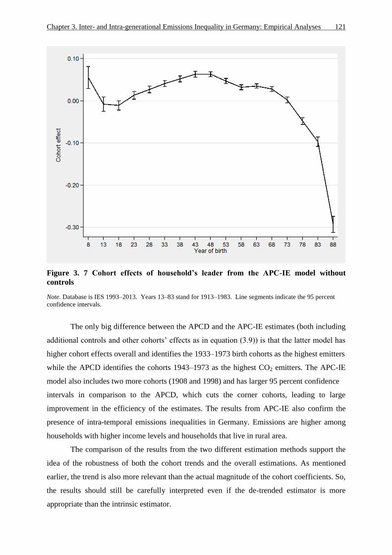
Chapter 3. Inter- and Intra-generational Emissions Inequality in Germany: Empirical Analyses 121
Figure 3. 7 Cohort effects of household’s leader from the APC-IE model without
controls
Note. Database is IES 1993–2013. Years 13–83 stand for 1913–1983. Line segments indicate the 95 percent
confidence intervals.
The only big difference between the APCD and the APC-IE estimates (both including
additional controls and other cohorts’ effects as in equation (3.9)) is that the latter model has
higher cohort effects overall and identifies the 1933–1973 birth cohorts as the highest emitters
while the APCD identifies the cohorts 1943–1973 as the highest CO2 emitters. The APC-IE
model also includes two more cohorts (1908 and 1998) and has larger 95 percent confidence
intervals in comparison to the APCD, which cuts the corner cohorts, leading to large
improvement in the efficiency of the estimates. The results from APC-IE also confirm the
presence of intra-temporal emissions inequalities in Germany. Emissions are higher among
households with higher income levels and households that live in rural area.
The comparison of the results from the two different estimation methods support the
idea of the robustness of both the cohort trends and the overall estimations. As mentioned
earlier, the trend is also more relevant than the actual magnitude of the cohort coefficients. So,
the results should still be carefully interpreted even if the de-trended estimator is more
appropriate than the intrinsic estimator.

Chapter 3. Inter- and Intra-generational Emissions Inequality in Germany: Empirical Analyses 122
Figure 3. 8 Cohort effects of household’s leader from the APC-IE model with additional
controls and other cohorts effects
Note. Database is IES 1993–2013. Years 13–83 stand for 1913–1983. Line segments indicate the 95 percent
confidence intervals.
There can be potentially other factors, such as behavioral, housing, and income,
behind the cohort trends.97
The number and type of household appliances, or the number and
type of cars, and the frequency of their usage could be interpreted as behavioral as well as
income determined factors. The cohorts 1933–1963 own larger than average number of
household appliances, the cohorts 1948–1993 own larger than average number of old cars,
and the cohorts 1928–1958 own larger than average number of new cars. Some of the electric
appliances owned by generations born after 1973 might be more energy efficient but it also
might be the case that the latter generations use the appliances less frequently due to
environmental concerns or different habits.98
Similarly, newer cars could be more energy
97
The issue of inter-generational emissions gaps was already touched upon at the end of Section 3.4 (and Table
3.5 in the Appendix). 98
Lighting and heating requirements are also very different for a retired person who spends significant amount
of time at home and a student who spends significant amount of time at the university buildings.

Chapter 3. Inter- and Intra-generational Emissions Inequality in Germany: Empirical Analyses 123
efficient and different birth cohorts could have different behavioral patterns. 99
Households
with leaders born between 1933 and 1963 live in larger dwellings, which requires more
lighting and heating and represents the housing factor. Unfortunately, data on type of
dwelling and year of construction was not available for all the waves of the IES data.
The household size and type of heating system are also determined by both behavior
and income. For example, household size is higher than average among the households with
leader born 1953–1978. Households with leaders born 1958–1993 rely more on central
heating, which is usually gas operated. The income factor is clearly present and income is
higher than average among the households with leader born 1948–1978. This could indicate
that the younger generations as well as pensioners are more resources restricted, which in turn
is reflected in lower energy consumption and emissions. It is worth to note that all three
factors overlap for the generations 1953 and 1958, which are also identified as higher emitters
by the APCD.
An additional concern might be that the only direct energy emissions of households
are included in the analyses. According to some studies, the indirect energy emissions (which
are incorporated in the goods and services purchased by the households) account for 40-50
percent of total households’ emissions (see Chancel, 2014). In addition, the emissions levels
in this paper are measured based on energy expenditures, assuming that all households pay
the same price for specific energy good in a given year. Consequently, higher energy
consumption levels might be assigned to a household that pays higher energy price per unit of
energy good, hence overstating their emissions. So, surveys that collect data on both energy
quantity (consumption) and price might be more suitable for analyses in the future. Another
potential reason for caution with the results’ interpretation is that the APCD requires that age
and cohort variables to be equality spaced with the frequency of the data collection ( which in
the case of the German IES is five years). So actual age and year of births were converted to
an interval: for instance if the leader was born in 1976 and was aged 38 in 2013, he or she will
be assigned to the birth cohort 1973–1978 and age of 40. This might slightly alter the
predictions on the size of cohorts and age effects.
3.7 Interim conclusion
99
For instance, the student might opt out for using a bicycle or public transport whereas a pensioner might
choose to drive the car.

Chapter 3. Inter- and Intra-generational Emissions Inequality in Germany: Empirical Analyses 124
The goal of this paper is to investigate energy related emissions inequalities and their
underlying causes. For that purpose, first the direct residential CO2 emissions are derived
from German households data. Secondly, two types of emissions inequalities among German
households are identified: i) intra-generational – a) poor versus rich and b) rural versus urban
inequalities, and ii) intergenerational – birth cohort inequalities. The descriptive evidence
demonstrates that the high income German households emit around 200 percent more CO2
than low income households in 2013. Also the gap between the rural and poor households’
emissions is large, with rural emitting 40 percent more CO2 than urban households in 2013.
Some of the intra-generational emissions inequalities could be potentially explained by
differences in household size and composition, age, education, income, and area of residence.
An inverted u-shaped relationship is found between total energy related emissions and the
birth cohort of the household’s leader. The emissions are highest for the households that have
a leader born between 1933 and 1963. The cohorts born 1908–1928 and 1968–1993 have
lower than the average emissions. The younger (later) German generations appear to be more
environmentally conscious as well as resources restricted and this could partly explain the
intergenerational CO2 emissions inequality.
Thirdly, the analyses focuses the role of year of birth in driving emissions by applying
a De-trended Age Period Cohort (APCD) model. The estimates indicate the presence of clear
cohort effects on residential energy related CO2 emissions. The households with leaders born
1933–1973 (in 5 years gaps) are found to be the highest CO2 emitters. Adding additional
controls to the model demonstrates that the generational effect is still present, statistically
significant, and might be a reflection of both large and energy inefficient infrastructures as
well as higher number of motor vehicles used by earlier generations. The German households
with leaders born 1943–1973 emit more CO2 than their predecessors or followers. The
estimates confirm the presence of intra-temporal, namely income- and area of residence-
related emissions inequalities in Germany. Households in rural areas and richer households
have higher energy related emissions.
This paper tackles a crucial issue: estimating the birth cohort effects of additional
household members on emissions. The cohort effects of other household members prove that
additional household members born between 1913 and 1988 have positive and statistically
significant effect on emissions. Household’s members belonging to the birth cohorts 1923,
1928, 1933, 1938, 1943, 1948, 1953, 1958, 1963 or 1968 add more to emissions than the
average household member.

Chapter 3. Inter- and Intra-generational Emissions Inequality in Germany: Empirical Analyses 125
The results demonstrate solid evidence that birth cohort effects (both of household’s
leader and household’s members) are significant in explaining residential energy related
pollution in Germany. The cohort compositional differences provide knowledge about the
creation of environmental practices of households and can be useful in creating improved
environmental policies, which would target specific birth cohorts in the population. The
cohort effects partly explain the durability of energy practices of German households and
maybe in the future lower pollution levels will be achieved by cohort replacement.
The empirical outcomes have several policy implications on how to reduce emissions
and to overcome emissions inequalities. Carbon or energy taxes would decrease emissions
more if imposed/increased for the rural and the high income households. Taxes could reduce
emissions by larger amounts if imposed on the households leaders or members from the
generations 1943–1968. Also for the earlier (older) cohorts taxes on domestic energy would
be more effective than taxes on car fuels. Fahmy et al. (2011) also recommend policies which
aim at reduction of energy consumption among the groups which are “overconsuming”
relative to the population (for instance taxing private vehicle and aviation transport among the
rich households). Last but not least, changes in lifestyles such as smaller (energy efficient)
dwellings, bigger household size, less or more efficient cars, and electric appliances can play
an important role in lowering residential energy related emissions in Germany.
There are several possibilities for future research. The empirical analyses could be
repeated for actual consumption (including other domestic fuels besides gas) or emissions
data when such dataset becomes available for an extended period of time. The analyses can be
conducted for other pollutants like sulfur dioxide (SO2) or nitrogen oxides (NOx). Similarly,
the examination of the presence of cohort effects of the household’s leader and other
household’s members in other countries of the European Union (E.U.) might be worthwhile to
identify potential target groups for more effective mitigation policies.

Chapter 3. Inter- and Intra-generational Emissions Inequality in Germany: Empirical Analyses 126
3.8 Appendix
Table 3. 2 Relevant studies and their contribution to literature
Study Country, and time
period
Energy/
Resources
inequalitiy
Determinants of
energy consumption/
emissions
Age-Period-
Cohort model
Cohort effects of
household‘s
leader/members
Age
effects
Income
effects
Rural
(Urbanization
effects)
Ghalwash (2007) Sweden, 1984–1996 Yes No No No/No No Yes No
Aguiar and Hurst (2013) U.S., 1980–2003 No Yes (with behavioral
responses)
No Yes/No Yes Yes No
Segall (2013) U.S., 1980–2003 Yes Yes (with behavioral
responses)
Yes Yes/No Yes Yes No
Deutsch and Timpe
(2012)
Germany, 2008 Yes Yes No No/No Yes No No
Sànchez-Peña (2013) Mexico, 1992–2008 Yes Yes Yes Yes/No Yes Yes No
Chancel (2014) France, US, 1980–
2000
Yes Yes Yes Yes/No Yes Yes No
Papathanasopoulou and
Jackson (2009)
U.K., 1968–2000 Yes No No No/No No Yes No
Papathanasopoulou (2007) Greece, 1990–2006 Yes Yes No No/No No No No
Fahmy et al. (2011) U.K., 2002–2008 Yes Yes No No/No Yes Yes Yes
Hargreaves et al. (2013) G.B., 2004–2007 Yes Yes No No/No Yes Yes Yes
Büchs and Schnepf (2013) U.K., 2006 –2009 Yes Yes No No/No Yes Yes Yes
Pampel and Hunter (2012) U.S., 1973–2008 No Yes (environmental
spending)
Yes Yes/No Yes Yes No
Weber and Matthews
(2008)
U.S., 2004 Yes Yes No No/No No Yes No
Weber and Perrels (2000) West Germany,
Netherlands, and
France, 1990
No Yes No No/No Yes Yes No
Rehdanz (2007) Germany, 1998–2003 No Yes No No/No Yes Yes No
Jamasb and Meier (2010) U.K., 1991–2007 No Yes No No/No No Yes Yes
Meier and Rehdanz
(2010)
U.K., 1991–2005 No Yes No No/No Yes Yes No

Chapter 3. Inter- and Intra-generational Emissions Inequality in Germany: Empirical Analyses 127
Table 3. 2 (Continued)
Study Country, and time
period
Energy/
Resources
inequalitiy
Determinants of
energy consumption/
emissions
Age-Period-
Cohort model
Cohort effects of
household‘s
leader/members
Age
effects
Income
effects
Rural
(Urbanization
effects)
Bin and Dowlatabadi
(2005)
U.S., 1997 No Yes No No/No No No No
Xu et al. (2016)
China, 2011 Yes Yes No No/No Yes Yes Yes
O’Neill and Chen (2002) U.S., 1993–1994 No Yes No No/No Yes Yes Yes
Räty and Carlsson-
Kanyama (2009)
Germany, 2003;
Norway, 2001–2003;
Greece, 2004–2005;
Sweden, 2003–2005
Yes Yes No No/No Yes Yes No
Chancel and Piketty
(2015)
Worldwide, 1998–
2013
Yes No No/No No Yes No
Grunewald et al. (2016) 158 countries, 1980–
2008
Yes (income
inequality)
Yes No No/No No Yes No
Menz and Küling (2011) 25 OECD countries,
1970–2000
Yes Yes No Yes/No Yes Yes Yes
Menz and Welsch (2012) 26 OECD countries,
1960–2005
Yes Yes No Yes/No Yes Yes Yes
Ravallion et al. (2000) 42 countries, 1975–
1992
Yes (income
inequality)
Yes No No/No No Yes Yes
Note. All necessary information is taken from the respective studies.

Chapter 3. Inter- and Intra-generational Emissions Inequality in Germany: Empirical Analyses 128
Table 3. 3 Summary statistics of rural and urban households
Rural Urban All
Variable Mean Std.Dev. Mean Std.Dev. Mean Std.Dev.
𝑎𝑑𝑢𝑙𝑡𝑠 1.886 0.822 1.638 0.730 1.955 0.811
𝑐ℎ𝑖𝑙𝑑𝑟𝑒𝑛 0.388 0.789 0.239 0.620 0.447 0.836
𝑎𝑔𝑒 51.699 16.251 51.296 17.338 52.470 15.019
𝑦𝑑𝑖𝑠𝑝 35182 20845 29762 19703 39184 21647
𝑒𝑑𝑢𝑐1 0.700 0.458 0.606 0.489 0.615 0.487
𝑒𝑑𝑢𝑐2 0.106 0.308 0.114 0.317 0.145 0.352
𝑒𝑑𝑢𝑐3 0.111 0.314 0.175 0.380 0.171 0.376
𝑇𝑉𝑠 1.500 0.851 1.405 0.816 1.548 0.874
𝑃𝐶𝑠 𝑎𝑛𝑑 𝑛𝑜𝑡𝑒𝑏𝑜𝑜𝑘𝑠 0.980 1.133 0.912 1.082 1.075 1.135
𝑟𝑒𝑓𝑟𝑖𝑔𝑒𝑟𝑎𝑡𝑜𝑟𝑠 𝑎𝑛𝑑 𝑓𝑟𝑒𝑒𝑧𝑒𝑟𝑠 1.803 0.821 1.587 0.730 1.797 0.828
𝑑𝑖𝑠ℎ𝑤𝑎𝑠ℎ𝑒𝑟𝑠 0.600 0.506 0.486 0.511 0.636 0.499
𝑤𝑎𝑠ℎ𝑖𝑛𝑔 𝑚𝑎𝑐ℎ𝑖𝑛𝑒𝑠 𝑎𝑛𝑑 𝑑𝑟𝑖𝑒𝑟𝑠 1.158 0.681 1.033 0.681 1.174 0.678
𝑑𝑤𝑒𝑙𝑙𝑖𝑛𝑔 𝑠𝑖𝑧𝑒 99.274 43.061 75.220 32.307 98.509 42.263
𝑐𝑎𝑟𝑠 𝑛𝑒𝑤 0.448 0.604 0.361 0.545 0.479 0.615
𝑐𝑎𝑟𝑠 𝑜𝑙𝑑 0.653 0.735 0.462 0.634 0.634 0.729
𝑑𝑖𝑠𝑡𝑎𝑛𝑡 ℎ𝑒𝑎𝑡𝑖𝑛𝑔 0.109 0.312 0.263 0.440 0.150 0.357
𝑐𝑒𝑛𝑡𝑟𝑎𝑙 ℎ𝑒𝑎𝑡𝑖𝑛𝑔 0.793 0.405 0.647 0.478 0.742 0.438
𝑞𝑢𝑎𝑛𝑡𝑖𝑡𝑦 𝑜𝑓𝑒𝑙𝑒𝑐𝑡𝑟𝑖𝑐𝑖𝑡𝑦 3778 2895 3036 2280 3801 2844
𝑞𝑢𝑎𝑛𝑡𝑖𝑡𝑦 𝑜𝑓 𝑔𝑎𝑠 18603 24021 15126 15659 18780 22650
𝑞𝑢𝑎𝑛𝑡𝑖𝑡𝑦 𝑜𝑓 𝑐𝑎𝑟 𝑓𝑢𝑒𝑙𝑠 1038 914 672 777 1073 923
𝑡𝑜𝑡𝑎𝑙 𝑒𝑛𝑒𝑟𝑔𝑦 𝑒𝑚𝑖𝑠𝑠𝑖𝑜𝑛𝑠 12.394 10.888 9.644 7.522 2.121 1.587
𝑜𝑏𝑠𝑒𝑟𝑣𝑎𝑡𝑖𝑜𝑛𝑠 147922 71904 219826
Note. Database is IES 1993–2013. Weights used to assure representativeness of the German population. 𝑦𝑑𝑖𝑠𝑝
stands for disposable income, 𝑒𝑑𝑢𝑐2 indicates whether the household’s leader has completed high school or
other specialized school, e𝑑𝑢𝑐3 if she or he has a university or higher education.
Table 3. 4 Total energy related emissions across the deciles
Decile/ 1 2 3 4 5 6 7 8 9 10
Year Mean CO2 emissions (in tons)
Germany
1993 10.562 12.258 13.086 13.793 14.312 14.878 15.598 16.032 17.940 17.346
1998 9.311 11.241 12.311 13.089 14.025 14.833 15.676 16.351 18.083 16.682
2003 7.393 9.150 10.373 11.122 12.032 12.810 13.710 14.301 17.029 15.160
2008 5.496 7.294 8.360 9.552 10.463 11.427 11.919 12.948 14.922 13.708
2013 4.415 5.996 6.914 8.079 8.746 9.645 10.585 11.116 13.120 11.824
Note. Database is IES 1993–2013. Weights used to assure representativeness of the German population.

Chapter 3. Inter- and Intra-generational Emissions Inequality in Germany: Empirical Analyses 129
Table 3. 5 Summary statistics of households according to birth cohort of household’s leader
Cohorts All
cohorts 1908 1913 1918 1923 1928 1933 1938 1943 1948 1953 1958 1963 1968 1973 1978 1983 1988 1993
Variable Mean
𝑎𝑑𝑢𝑙𝑡𝑠 1.798 1.272 1.329 1.389 1.431 1.565 1.722 1.735 1.808 1.992 2.094 2.039 1.942 1.805 1.711 1.601 1.562 1.535 1.487
𝑐ℎ𝑖𝑙𝑑𝑟𝑒𝑛 0.336 0.000 0.001 0.004 0.004 0.008 0.009 0.015 0.042 0.134 0.320 0.535 0.684 0.719 0.696 0.573 0.360 0.153 0.070
𝑎𝑔𝑒 51.557 85.000 82.898 80.134 76.318 73.679 70.572 66.902 62.571 56.458 51.614 47.032 42.207 38.017 35.246 31.735 28.604 25.359 22.477
𝑦𝑑𝑖𝑠𝑝 33274 16809 17935 21025 22560 25457 28512 30133 32864 36178 37838 38071 37337 36486 36362 34200 30863 26327 21403
𝑒𝑑𝑢𝑐1 0.667 0.626 0.683 0.686 0.674 0.663 0.652 0.672 0.687 0.680 0.671 0.671 0.688 0.686 0.681 0.621 0.584 0.587 0.473
𝑒𝑑𝑢𝑐2 0.109 0.026 0.049 0.050 0.071 0.099 0.104 0.117 0.118 0.119 0.114 0.114 0.110 0.114 0.110 0.121 0.113 0.088 0.037
𝑒𝑑𝑢𝑐3 0.134 0.053 0.045 0.069 0.083 0.110 0.132 0.121 0.125 0.142 0.156 0.155 0.142 0.135 0.131 0.155 0.165 0.141 0.046
𝑇𝑉𝑠 1.467 0.979 1.048 1.096 1.194 1.265 1.406 1.457 1.541 1.633 1.636 1.577 1.491 1.418 1.410 1.390 1.450 1.452 1.643
𝑃𝐶𝑠 𝑎𝑛𝑑 𝑛𝑜𝑡𝑒𝑏𝑜𝑜𝑘𝑠 0.956 0.002 0.010 0.054 0.091 0.233 0.456 0.661 0.895 0.982 1.075 1.143 1.126 1.162 1.262 1.354 1.516 1.646 1.736
𝑟𝑒𝑓𝑟𝑖𝑔𝑒𝑟𝑎𝑡𝑜𝑟𝑠 𝑎𝑛𝑑 𝑓𝑟𝑒𝑒𝑧𝑒𝑟𝑠 1.727 1.413 1.517 1.651 1.770 1.854 1.888 1.842 1.821 1.902 1.876 1.808 1.726 1.642 1.524 1.406 1.351 1.276 1.256
𝑑𝑖𝑠ℎ𝑤𝑎𝑠ℎ𝑒𝑟𝑠 0.560 0.070 0.098 0.166 0.229 0.341 0.457 0.526 0.587 0.630 0.633 0.637 0.626 0.618 0.612 0.586 0.580 0.597 0.740
𝑤𝑎𝑠ℎ𝑖𝑛𝑔 𝑚𝑎𝑐ℎ𝑖𝑛𝑒𝑠 𝑎𝑛𝑑 𝑑𝑟𝑖𝑒𝑟𝑠 1.114 0.782 0.868 0.988 1.029 1.068 1.096 1.080 1.180 1.234 1.204 1.189 1.175 1.066 1.036 0.956 0.985 0.953 1.443
𝑑𝑤𝑒𝑙𝑙𝑖𝑛𝑔 𝑠𝑖𝑧𝑒 90.808 71.976 73.115 77.047 82.304 86.627 91.596 92.699 94.662 97.167 98.587 97.955 94.849 90.789 89.398 82.942 75.328 65.578 58.137
𝑐𝑎𝑟𝑠 𝑛𝑒𝑤 0.418 0.144 0.161 0.251 0.336 0.425 0.486 0.512 0.504 0.523 0.489 0.447 0.384 0.348 0.328 0.293 0.297 0.312 0.428
𝑐𝑎𝑟𝑠 𝑜𝑙𝑑 0.586 0.079 0.110 0.136 0.183 0.257 0.366 0.441 0.557 0.629 0.696 0.695 0.705 0.725 0.724 0.710 0.698 0.635 0.668
𝑑𝑖𝑠𝑡𝑎𝑛𝑡 ℎ𝑒𝑎𝑡𝑖𝑛𝑔 0.163 0.212 0.159 0.182 0.175 0.181 0.186 0.195 0.185 0.170 0.171 0.157 0.144 0.131 0.128 0.140 0.170 0.180 0.165
𝑐𝑒𝑛𝑡𝑟𝑎𝑙 ℎ𝑒𝑎𝑡𝑖𝑛𝑔 0.742 0.521 0.638 0.654 0.665 0.697 0.706 0.715 0.727 0.749 0.741 0.750 0.757 0.773 0.793 0.783 0.772 0.763 0.767
𝑞𝑢𝑎𝑛𝑡𝑖𝑡𝑦 𝑜𝑓 𝑒𝑙𝑒𝑐𝑡𝑟𝑖𝑐𝑖𝑡𝑦 3517 3039 2926 3083 3231 3380 3545 3552 3662 3955 4092 3963 3747 3462 3201 2925 2579 2125 1885
𝑞𝑢𝑎𝑛𝑡𝑖𝑡𝑦 𝑜𝑓 𝑔𝑎𝑠 17379 19527 18224 19436 19224 19354 19678 19152 19369 20155 19829 18975 17821 15950 13804 11126 9595 7983 5730
𝑞𝑢𝑎𝑛𝑡𝑖𝑡𝑦 𝑜𝑓 𝑐𝑎𝑟 𝑓𝑢𝑒𝑙𝑠 909 108 156 239 316 450 610 686 824 1020 1116 1130 1151 1123 1120 1038 897 743 559

Chapter 3. Inter- and Intra-generational Emissions Inequality in Germany: Empirical Analyses 130
Table 3. 5 (Continued)
Cohorts All
cohorts 1908 1913 1918 1923 1928 1933 1938 1943 1948 1953 1958 1963 1968 1973 1978 1983 1988 1993
Variable Mean
𝑒𝑙𝑒𝑐𝑡𝑟𝑖𝑐𝑖𝑡𝑦 𝑒𝑚𝑖𝑠𝑠𝑖𝑜𝑛𝑠 1.963 1.696 1.633 1.720 1.803 1.886 1.978 1.982 2.043 2.207 2.283 2.211 2.091 1.932 1.786 1.632 1.439 1.186 1.052
𝑔𝑎𝑠 𝑒𝑚𝑖𝑠𝑠𝑖𝑜𝑛𝑠 7.282 8.182 7.636 8.144 8.055 8.109 8.245 8.025 8.116 8.445 8.308 7.950 7.467 6.683 5.784 4.662 4.020 3.345 2.401
𝑐𝑎𝑟 𝑓𝑢𝑒𝑙𝑠 𝑒𝑚𝑖𝑠𝑠𝑖𝑜𝑛𝑠 2.182 0.259 0.374 0.574 0.757 1.079 1.465 1.647 1.977 2.447 2.678 2.712 2.762 2.695 2.688 2.490 2.152 1.783 1.341
𝑡𝑜𝑡𝑎𝑙 𝑒𝑚𝑖𝑠𝑠𝑖𝑜𝑛𝑠 11.426 10.137 9.643 10.438 10.615 11.075 11.689 11.654 12.136 13.099 13.269 12.873 12.320 11.309 10.258 8.784 7.612 6.314 4.794
Note. Database is IES 1993–2013. Weights used to assure representativeness of the German population. 𝑦𝑑𝑖𝑠𝑝 stands for disposable income, 𝑒𝑑𝑢𝑐2 indicates whether the
household’s leader has completed high school or other specialized school, 𝑒𝑑𝑢𝑐3 if she or he has a university or higher education.

Chapter 3. Inter- and Intra-generational Emissions Inequality in Germany: Empirical Analyses 131
Table 3. 6 Coefficient estimates of the APCD model
Without additional
controls
With additional
controls
and ℎℎ𝑠𝑖𝑧𝑒
With controls and
other
cohorts effects
ln(𝐸𝑡𝑜𝑡𝑎𝑙) Coef. Std. Err. Coef. Std. Err. Coef. Std. Err.
𝑐𝑜ℎ𝑜𝑟𝑡 1913 –0.047 0.015 –0.026 0.014 –0.015 0.014
𝑐𝑜ℎ𝑜𝑟𝑡 1918 –0.047 0.010 –0.033 0.009 –0.026 0.010
𝑐𝑜ℎ𝑜𝑟𝑡 1923 –0.020 0.008 –0.028 0.008 –0.026 0.008
𝑐𝑜ℎ𝑜𝑟𝑡 1928 –0.003 0.007 –0.012 0.007 –0.021 0.007
𝑐𝑜ℎ𝑜𝑟𝑡 1933 0.015 0.006 0.001 0.006 –0.012 0.006
𝑐𝑜ℎ𝑜𝑟𝑡 1938 0.029 0.006 0.004 0.006 –0.006 0.006
𝑐𝑜ℎ𝑜𝑟𝑡 1943 0.043 0.006 0.021 0.006 0.013 0.006
𝑐𝑜ℎ𝑜𝑟𝑡 1948 0.046 0.006 0.031 0.005 0.032 0.006
𝑐𝑜ℎ𝑜𝑟𝑡 1953 0.034 0.005 0.048 0.005 0.051 0.006
𝑐𝑜ℎ𝑜𝑟𝑡 1958 0.023 0.005 0.050 0.005 0.055 0.005
𝑐𝑜ℎ𝑜𝑟𝑡 1963 0.029 0.005 0.051 0.005 0.059 0.005
𝑐𝑜ℎ𝑜𝑟𝑡 1968 0.026 0.006 0.039 0.005 0.052 0.005
𝑐𝑜ℎ𝑜𝑟𝑡 1973 0.004 0.007 0.007 0.007 0.005 0.007
𝑐𝑜ℎ𝑜𝑟𝑡 1978 –0.042 0.008 –0.045 0.007 –0.052 0.008
𝑐𝑜ℎ𝑜𝑟𝑡 1983 –0.088 0.010 –0.107 0.009 –0.111 0.010
𝑎𝑔𝑒 25 –0.214 0.009 0.023 0.009 0.013 0.009
𝑎𝑔𝑒 30 –0.143 0.006 –0.012 0.006 0.000 0.006
𝑎𝑔𝑒 35 0.015 0.005 –0.035 0.005 –0.012 0.005
𝑎𝑔𝑒 40 0.087 0.005 –0.064 0.005 –0.045 0.005
𝑎𝑔𝑒 45 0.141 0.005 –0.037 0.005 –0.033 0.005
𝑎𝑔𝑒 50 0.150 0.005 0.010 0.005 –0.002 0.005
𝑎𝑔𝑒 55 0.141 0.005 0.049 0.005 0.027 0.005
𝑎𝑔𝑒 60 0.086 0.006 0.067 0.005 0.042 0.005
𝑎𝑔𝑒 65 –0.008 0.006 0.058 0.005 0.038 0.005
𝑎𝑔𝑒 70 –0.042 0.006 0.044 0.005 0.034 0.005
𝑎𝑔𝑒 75 –0.012 0.006 0.016 0.006 0.019 0.006
𝑎𝑔𝑒 80 –0.059 0.008 –0.023 0.007 –0.008 0.007
𝑎𝑔𝑒 85 –0.141 0.010 –0.097 0.009 –0.072 0.009
𝑝𝑒𝑟𝑖𝑜𝑑 1993 –0.046 0.002 –0.021 0.002 –0.024 0.002
𝑝𝑒𝑟𝑖𝑜𝑑 1998 0.013 0.003 –0.001 0.003 0.000 0.003
𝑝𝑒𝑟𝑖𝑜𝑑 2003 0.060 0.003 0.032 0.003 0.033 0.003
𝑝𝑒𝑟𝑖𝑜𝑑 2008 0.025 0.003 0.025 0.003 0.029 0.003
𝑝𝑒𝑟𝑖𝑜𝑑 2013 –0.052 0.002 –0.034 0.002 –0.038 0.002

Chapter 3. Inter- and Intra-generational Emissions Inequality in Germany: Empirical Analyses 132
Table 3.6 (Continued)
Without additional
controls
With additional
controls
and ℎℎ𝑠𝑖𝑧𝑒
With controls and
other
cohorts effects
ln(𝐸𝑡𝑜𝑡𝑎𝑙) Coef. Std. Err. Coef. Std. Err. Coef. Std. Err.
𝑟𝑒𝑠𝑐𝑎𝑐𝑜ℎ –1.766 0.014 –1.905 0.013 –2.002 0.016
𝑟𝑒𝑠𝑐𝑎𝑎𝑔𝑒 –0.870 0.007 –0.949 0.007 –1.016 0.008
ln(𝑦𝑑𝑖𝑠𝑝) 0.303 0.004 0.277 0.004
ℎℎ𝑠𝑖𝑧𝑒 0.066 0.002
𝑛1908 –0.050 0.046
𝑛1913 0.017 0.031
𝑛1918 0.046 0.017
𝑛1923 0.076 0.012
𝑛1928 0.116 0.010
𝑛1933 0.149 0.008
𝑛1938 0.150 0.007
𝑛1943 0.192 0.007
𝑛1948 0.178 0.006
𝑛1953 0.171 0.006
𝑛1958 0.141 0.006
𝑛1963 0.104 0.006
𝑛1968 0.015 0.003
𝑛1973 0.029 0.003
𝑛1978 0.050 0.003
𝑛1983 0.069 0.004
𝑛1988 0.117 0.004
ln(ℎ_𝑞𝑚) 0.358 0.005 0.356 0.005
𝑒𝑑𝑢𝑐2 –0.010 0.004 –0.008 0.004
𝑒𝑑𝑢𝑐3 –0.024 0.004 –0.019 0.004
𝑟𝑢𝑟𝑎𝑙 0.048 0.003 0.047 0.003
𝑤𝑒𝑖𝑔ℎ𝑡 –0.189 0.002 –0.014 0.002 –0.015 0.002
𝑐𝑜𝑛𝑠𝑡𝑎𝑛𝑡 2.402 0.003 –2.685 0.033 –2.380 0.035
𝐴𝐼𝐶 2.177 1.978 1.972
𝐵𝐼𝐶 –2548613 –2568754 –2569055
𝑜𝑏𝑠𝑒𝑟𝑣𝑎𝑡𝑖𝑜𝑛𝑠 216578 216578 216578
Note. Database is IES 1993–2013. Weights used to assure representativeness of the German population. 𝑦𝑑𝑖𝑠𝑝
stands for disposable income, 𝑒𝑑𝑢𝑐2 indicates whether the household’s leader has completed high school or
other specialized school, 𝑒𝑑𝑢𝑐3 if she or he has a university or higher education. 𝑛1908 − 𝑛1988 indicate
number of household members from these birth cohorts. ℎ_𝑞𝑚 is dwelling size. 𝐴𝐼𝐶 and 𝐵𝐼𝐶 stand for Akaike
and Bayesian Information Criterion.

Chapter 3. Inter- and Intra-generational Emissions Inequality in Germany: Empirical Analyses 133
Table 3. 7 Estimates from APCD with additional controls for electricity, gas, and car fuels
Electricity Gas Car fuels
With controls
and ℎℎ𝑠𝑖𝑧𝑒
With controls and
other
cohorts effects
With controls
and ℎℎ𝑠𝑖𝑧𝑒
With controls and
other
cohorts effects
With controls
and ℎℎ𝑠𝑖𝑧𝑒
With controls and
other
cohorts effects
ln(𝐸𝑖) Coef. Std. Err. Coef. Std. Err. Coef. Std. Err. Coef. Std. Err. Coef. Std. Err. Coef. Std. Err.
𝑐𝑜ℎ𝑜𝑟𝑡 1913 –0.001 0.010 0.014 0.011 –0.067 0.018 –0.066 0.019 0.006 0.020 0.066 0.021
𝑐𝑜ℎ𝑜𝑟𝑡 1918 –0.007 0.007 0.004 0.007 –0.039 0.012 –0.040 0.013 –0.035 0.012 –0.005 0.013
𝑐𝑜ℎ𝑜𝑟𝑡 1923 –0.006 0.006 0.003 0.006 –0.034 0.010 –0.034 0.010 –0.026 0.010 –0.012 0.010
𝑐𝑜ℎ𝑜𝑟𝑡 1928 –0.016 0.005 –0.018 0.005 0.010 0.009 0.005 0.009 0.000 0.008 –0.003 0.009
𝑐𝑜ℎ𝑜𝑟𝑡 1933 –0.003 0.004 –0.016 0.005 0.029 0.008 0.022 0.008 0.001 0.007 –0.022 0.008
𝑐𝑜ℎ𝑜𝑟𝑡 1938 0.001 0.004 –0.017 0.005 0.033 0.007 0.028 0.008 –0.012 0.006 –0.050 0.007
𝑐𝑜ℎ𝑜𝑟𝑡 1943 0.013 0.004 –0.005 0.005 0.047 0.007 0.044 0.008 0.013 0.006 –0.029 0.007
𝑐𝑜ℎ𝑜𝑟𝑡 1948 0.023 0.004 0.011 0.004 0.050 0.007 0.053 0.008 0.017 0.006 –0.020 0.007
𝑐𝑜ℎ𝑜𝑟𝑡 1953 0.014 0.004 0.009 0.004 0.047 0.006 0.054 0.007 0.026 0.005 –0.005 0.006
𝑐𝑜ℎ𝑜𝑟𝑡 1958 0.007 0.003 0.010 0.004 0.041 0.006 0.050 0.007 0.030 0.005 0.008 0.006
𝑐𝑜ℎ𝑜𝑟𝑡 1963 0.002 0.003 0.012 0.004 0.029 0.006 0.040 0.006 0.022 0.005 0.018 0.005
𝑐𝑜ℎ𝑜𝑟𝑡 1968 –0.005 0.004 0.009 0.004 –0.007 0.007 0.002 0.007 0.039 0.006 0.058 0.006
𝑐𝑜ℎ𝑜𝑟𝑡 1973 0.003 0.005 0.007 0.005 –0.040 0.009 –0.041 0.009 0.045 0.007 0.067 0.008
𝑐𝑜ℎ𝑜𝑟𝑡 1978 0.001 0.006 0.001 0.006 –0.054 0.010 –0.063 0.010 –0.032 0.008 –0.007 0.009
𝑐𝑜ℎ𝑜𝑟𝑡 1983 –0.025 0.007 –0.024 0.007 –0.044 0.013 –0.055 0.013 –0.093 0.011 –0.062 0.011
𝑎𝑔𝑒 25 0.021 0.006 0.004 0.007 0.059 0.011 0.052 0.011 –0.017 0.010 –0.041 0.010
𝑎𝑔𝑒 30 –0.021 0.004 –0.018 0.004 0.004 0.008 0.009 0.008 –0.021 0.006 –0.020 0.006

Chapter 3. Inter- and Intra-generational Emissions Inequality in Germany: Empirical Analyses 134
Table 3. 7 (Continued)
Electricity Gas Car fuels
With controls
and ℎℎ𝑠𝑖𝑧𝑒
With controls and
other
cohorts effects
With controls
and ℎℎ𝑠𝑖𝑧𝑒
With controls and
other
cohorts effects
With controls
and ℎℎ𝑠𝑖𝑧𝑒
With controls and
other
cohorts effects
ln(𝐸𝑖) Coef. Std. Err. Coef. Std. Err. Coef. Std. Err. Coef. Std. Err. Coef. Std. Err. Coef. Std. Err.
𝑎𝑔𝑒 35 –0.033 0.004 –0.020 0.004 –0.015 0.006 –0.005 0.007 –0.052 0.005 –0.040 0.005
𝑎𝑔𝑒 40 –0.036 0.004 –0.021 0.004 –0.031 0.006 –0.022 0.006 –0.079 0.005 –0.064 0.005
𝑎𝑔𝑒 45 –0.014 0.003 –0.006 0.004 –0.022 0.006 –0.018 0.006 –0.026 0.005 –0.016 0.005
𝑎𝑔𝑒 50 0.018 0.004 0.018 0.004 –0.015 0.006 –0.018 0.006 0.039 0.005 0.042 0.005
𝑎𝑔𝑒 55 0.031 0.004 0.024 0.004 –0.002 0.006 –0.010 0.007 0.090 0.005 0.087 0.006
𝑎𝑔𝑒 60 0.048 0.004 0.038 0.004 0.004 0.007 –0.007 0.007 0.108 0.006 0.101 0.006
𝑎𝑔𝑒 65 0.040 0.004 0.031 0.004 –0.012 0.007 –0.021 0.007 0.093 0.006 0.086 0.006
𝑎𝑔𝑒 70 0.023 0.004 0.017 0.004 –0.003 0.007 –0.008 0.007 0.063 0.006 0.058 0.006
𝑎𝑔𝑒 75 –0.006 0.004 –0.007 0.004 –0.009 0.008 –0.011 0.008 0.019 0.007 0.020 0.007
𝑎𝑔𝑒 80 –0.021 0.005 –0.018 0.005 0.010 0.009 0.015 0.009 –0.065 0.009 –0.060 0.009
𝑎𝑔𝑒 85 –0.050 0.007 –0.041 0.007 0.030 0.012 0.043 0.012 –0.151 0.012 –0.152 0.012
𝑝𝑒𝑟𝑖𝑜𝑑 1993 0.021 0.002 0.019 0.002 –0.054 0.003 –0.048 0.003 –0.078 0.002 –0.088 0.003
𝑝𝑒𝑟𝑖𝑜𝑑 1998 –0.062 0.002 –0.066 0.002 0.156 0.003 0.152 0.004 0.100 0.003 0.106 0.004
𝑝𝑒𝑟𝑖𝑜𝑑 2003 0.057 0.002 0.064 0.003 0.051 0.004 0.044 0.004 0.022 0.003 0.030 0.004
𝑝𝑒𝑟𝑖𝑜𝑑 2008 –0.012 0.002 –0.006 0.003 –0.354 0.003 –0.353 0.004 –0.032 0.003 –0.027 0.003
𝑝𝑒𝑟𝑖𝑜𝑑 2013 –0.004 0.002 –0.011 0.002 0.201 0.003 0.204 0.003 –0.012 0.002 –0.021 0.003
𝑟𝑒𝑠𝑐𝑎𝑐𝑜ℎ –0.568 0.012 –0.571 0.014 –2.224 0.017 –2.223 0.021 –0.701 0.016 –0.777 0.019
𝑟𝑒𝑠𝑐𝑎𝑎𝑔𝑒 –0.207 0.006 –0.230 0.007 –0.986 0.009 –1.007 0.011 –0.708 0.008 –0.738 0.009

Chapter 3. Inter- and Intra-generational Emissions Inequality in Germany: Empirical Analyses 135
Table 3. 7 (Continued)
Electricity Gas Car fuels
With controls
and ℎℎ𝑠𝑖𝑧𝑒
With controls and
other
cohorts effects
With controls
and ℎℎ𝑠𝑖𝑧𝑒
With controls and
other
cohorts effects
With controls
and ℎℎ𝑠𝑖𝑧𝑒
With controls and
other
cohorts effects
ln(𝐸𝑖) Coef. Std. Err. Coef. Std. Err. Coef. Std. Err. Coef. Std. Err. Coef. Std. Err. Coef. Std. Err.
ln(𝑦𝑑𝑖𝑠𝑝) 0.144 0.003 0.124 0.003 0.109 0.005 0.097 0.005 0.445 0.004 0.423 0.004
ℎℎ𝑠𝑖𝑧𝑒 0.111 0.001 0.035 0.002 0.052 0.002
𝑛1908 0.165 0.034 –0.051 0.060 –0.103 0.049
𝑛1913 0.129 0.023 0.051 0.040 –0.121 0.036
𝑛1918 0.171 0.013 0.106 0.023 –0.036 0.020
𝑛1923 0.147 0.009 0.089 0.015 0.003 0.014
𝑛1928 0.163 0.007 0.082 0.012 0.045 0.011
𝑛1933 0.186 0.006 0.104 0.010 0.074 0.008
𝑛1938 0.202 0.005 0.094 0.009 0.122 0.007
𝑛1943 0.220 0.005 0.113 0.009 0.161 0.007
𝑛1948 0.209 0.005 0.093 0.008 0.161 0.007
𝑛1953 0.198 0.005 0.080 0.008 0.158 0.006
𝑛1958 0.167 0.004 0.062 0.008 0.146 0.006
𝑛1963 0.138 0.004 0.037 0.007 0.119 0.006
𝑛1968 0.085 0.002 0.009 0.004 0.030 0.003
𝑛1973 0.096 0.002 0.026 0.004 0.023 0.003
𝑛1978 0.089 0.002 0.039 0.004 0.029 0.003
𝑛1983 0.102 0.003 0.036 0.004 0.042 0.004

Chapter 3. Inter- and Intra-generational Emissions Inequality in Germany: Empirical Analyses 136
Table 3. 7 (Continued)
Electricity Gas Car fuels
With controls
and ℎℎ𝑠𝑖𝑧𝑒
With controls and
other
cohorts effects
With controls
and ℎℎ𝑠𝑖𝑧𝑒
With controls and
other
cohorts effects
With controls
and ℎℎ𝑠𝑖𝑧𝑒
With controls and
other
cohorts effects
ln(𝐸𝑖) Coef. Std. Err. Coef. Std. Err. Coef. Std. Err. Coef. Std. Err. Coef. Std. Err. Coef. Std. Err.
𝑛1988 0.133 0.003 0.043 0.005 0.081 0.004
𝑒𝑑𝑢𝑐2 –0.055 0.003 –0.053 0.003 –0.017 0.005 –0.015 0.005 –0.007 0.004 –0.003 0.004
𝑒𝑑𝑢𝑐3 –0.089 0.003 –0.085 0.003 –0.001 0.005 0.002 0.005 –0.035 0.004 –0.030 0.004
ln(ℎ_𝑞𝑚) 0.363 0.004 0.362 0.004 0.486 0.006 0.485 0.006
𝑑𝑖𝑠𝑡𝑎𝑛𝑡 –0.446 0.005 –0.444 0.005 0.296 0.008 0.298 0.008
𝑐𝑒𝑛𝑡𝑟𝑎𝑙 –0.345 0.004 –0.342 0.004 0.406 0.008 0.409 0.008
𝑇𝑉𝑠 0.019 0.001 0.017 0.001
𝑃𝐶𝑠 𝑎𝑛𝑑 𝑛𝑜𝑡𝑒𝑏𝑜𝑜𝑘𝑠 0.008 0.001 0.010 0.001
𝑟𝑒𝑓𝑟𝑖𝑔𝑒𝑟𝑎𝑡𝑜𝑟𝑠 𝑎𝑛𝑑 𝑓𝑟𝑒𝑒𝑧𝑒𝑟𝑠 0.049 0.002 0.046 0.002
𝑑𝑖𝑠ℎ𝑤𝑎𝑠ℎ𝑒𝑟𝑠 0.064 0.003 0.066 0.003
𝑤𝑎𝑠ℎ𝑖𝑛𝑔 𝑚𝑎𝑐ℎ𝑖𝑛𝑒𝑠 𝑎𝑛𝑑 𝑑𝑟𝑖𝑒𝑟𝑠 0.062 0.002 0.064 0.002
𝑐𝑎𝑟𝑠 𝑛𝑒𝑤 0.203 0.003 0.198 0.003
𝑐𝑎𝑟𝑠 𝑜𝑙𝑑 0.228 0.003 0.225 0.003
𝑟𝑢𝑟𝑎𝑙 –0.001 0.002 –0.002 0.002 0.055 0.004 0.054 0.004 0.145 0.003 0.145 0.003
𝑤𝑒𝑖𝑔ℎ𝑡 0.015 0.002 0.017 0.002 0.003 0.003 0.005 0.003 –0.016 0.003 –0.017 0.003
𝑐𝑜𝑛𝑠𝑡𝑎𝑛𝑡 –2.722 0.026 –2.423 0.027 –1.871 0.044 –1.727 0.046 –4.372 0.039 –4.107 0.040
𝐴𝐼𝐶 1.376 1.371 2.289 2.288 1.991 1.987
𝐵𝐼𝐶 –2569152 –2569226 –2035358 –2035278 –2166322 –2166480

Chapter 3. Inter- and Intra-generational Emissions Inequality in Germany: Empirical Analyses 137
Table 3. 7 (Continued)
Electricity
Gas
Car fuels
With controls
and ℎℎ𝑠𝑖𝑧𝑒
With controls and
other
cohorts effects
With controls
and ℎℎ𝑠𝑖𝑧𝑒
With controls and
other
cohorts effects
With controls
and ℎℎ𝑠𝑖𝑧𝑒
With controls and
other
cohorts effects
𝑜𝑏𝑠𝑒𝑟𝑣𝑎𝑡𝑖𝑜𝑛𝑠 213440 213440 176933 176933 185188 185188
Note. Database is IES 1993–2013. Weights used to assure representativeness of the German population. 𝑦𝑑𝑖𝑠𝑝 stands for disposable income, 𝑒𝑑𝑢𝑐2 indicates whether the
household’s leader has completed high school or other specialized school, 𝑒𝑑𝑢𝑐3 if she or he has a university or higher education. 𝑛1908 − 𝑛1988 indicate number of household
members from these birth cohorts. ℎ_𝑞𝑚 is dwelling size. 𝐴𝐼𝐶 and 𝐵𝐼𝐶 stand for Akaike and Bayesian Information Criterion.

Chapter 3. Inter- and Intra-generational Emissions Inequality in Germany: Empirical Analyses 138
Table 3. 8 Consistency check: Estimates from the APC-IE model
Without additional
controls With controls and ℎℎ𝑠𝑖𝑧𝑒
With controls and other cohorts
effects
ln(𝐸𝑡𝑜𝑡𝑎𝑙) Coef. Std. Err. Coef. Std. Err. Coef. Std. Err.
ln (𝑦𝑑𝑖𝑠𝑝) 0.305 0.004 0.280 0.004
ℎℎ𝑠𝑖𝑧𝑒 0.066 0.002
𝑛1908 –0.039 0.042
𝑛1913 0.030 0.028
𝑛1918 0.044 0.017
𝑛1923 0.076 0.012
𝑛1928 0.116 0.010
𝑛1933 0.149 0.008
𝑛1938 0.150 0.007
𝑛1943 0.191 0.007
𝑛1948 0.178 0.006
𝑛1953 0.171 0.006
𝑛1958 0.142 0.006
𝑛1963 0.105 0.006
𝑛1968 0.015 0.003
𝑛1973 0.028 0.003
𝑛1978 0.050 0.003
𝑛1983 0.070 0.004
𝑛1988 0.118 0.004
ln (ℎ𝑞𝑚) 0.359 0.005 0.358 0.005
𝑒𝑑𝑢𝑐2 –0.010 0.004 –0.008 0.004
𝑒𝑑𝑢𝑐3 –0.025 0.004 –0.020 0.004
𝑟𝑢𝑟𝑎𝑙 0.049 0.003 0.048 0.003
𝑤𝑒𝑖𝑔ℎ𝑡 –0.187 0.002 –0.012 0.002 –0.013 0.002
𝑎𝑔𝑒 25 –0.207 0.011 0.032 0.010 0.033 0.010
𝑎𝑔𝑒 30 –0.136 0.007 –0.005 0.006 0.017 0.006
𝑎𝑔𝑒 35 0.021 0.006 –0.030 0.005 0.001 0.005
𝑎𝑔𝑒 40 0.091 0.005 –0.061 0.005 –0.036 0.005
𝑎𝑔𝑒 45 0.144 0.005 –0.036 0.005 –0.028 0.005
𝑎𝑔𝑒 50 0.152 0.005 0.010 0.005 –0.001 0.005
𝑎𝑔𝑒 55 0.141 0.005 0.048 0.005 0.026 0.005
𝑎𝑔𝑒 60 0.085 0.006 0.066 0.005 0.039 0.005
𝑎𝑔𝑒 65 –0.011 0.006 0.056 0.005 0.032 0.006

Chapter 3. Inter- and Intra-generational Emissions Inequality in Germany: Empirical Analyses 139
Table 3.8 (Continued)
Without additional
controls With controls and ℎℎ𝑠𝑖𝑧𝑒
With controls and other cohorts
effects
ln(𝐸𝑡𝑜𝑡𝑎𝑙) Coef. Std. Err. Coef. Std. Err. Coef. Std. Err.
𝑎𝑔𝑒 70 –0.045 0.006 0.041 0.006 0.025 0.006
𝑎𝑔𝑒 75 –0.018 0.007 0.011 0.006 0.007 0.006
𝑎𝑔𝑒 80 –0.067 0.008 –0.029 0.007 –0.023 0.007
𝑎𝑔𝑒 85 –0.150 0.011 –0.104 0.010 –0.090 0.010
𝑝𝑒𝑟𝑖𝑜𝑑 1993 0.241 0.003 0.293 0.003 0.309 0.004
𝑝𝑒𝑟𝑖𝑜𝑑 1998 0.157 0.003 0.156 0.003 0.167 0.003
𝑝𝑒𝑟𝑖𝑜𝑑 2003 0.060 0.003 0.032 0.003 0.033 0.003
𝑝𝑒𝑟𝑖𝑜𝑑 2008 –0.119 0.003 –0.132 0.003 –0.138 0.003
𝑝𝑒𝑟𝑖𝑜𝑑 2013 –0.339 0.003 –0.348 0.003 –0.372 0.003
𝑐𝑜ℎ𝑜𝑟𝑡 1908 0.055 0.026 0.095 0.023 0.092 0.024
𝑐𝑜ℎ𝑜𝑟𝑡 1913 –0.008 0.017 –0.002 0.015 –0.002 0.016
𝑐𝑜ℎ𝑜𝑟𝑡 1918 –0.011 0.011 –0.010 0.010 –0.012 0.011
𝑐𝑜ℎ𝑜𝑟𝑡 1923 0.013 0.009 –0.007 0.008 –0.013 0.009
𝑐𝑜ℎ𝑜𝑟𝑡 1928 0.027 0.008 0.007 0.007 –0.007 0.008
𝑐𝑜ℎ𝑜𝑟𝑡 1933 0.041 0.007 0.018 0.007 0.002 0.007
𝑐𝑜ℎ𝑜𝑟𝑡 1938 0.052 0.007 0.019 0.006 0.007 0.007
𝑐𝑜ℎ𝑜𝑟𝑡 1943 0.063 0.007 0.035 0.006 0.026 0.007
𝑐𝑜ℎ𝑜𝑟𝑡 1948 0.063 0.006 0.043 0.006 0.044 0.007
𝑐𝑜ℎ𝑜𝑟𝑡 1953 0.047 0.006 0.058 0.005 0.063 0.006
𝑐𝑜ℎ𝑜𝑟𝑡 1958 0.032 0.006 0.058 0.005 0.065 0.006
𝑐𝑜ℎ𝑜𝑟𝑡 1963 0.035 0.005 0.057 0.005 0.069 0.005
𝑐𝑜ℎ𝑜𝑟𝑡 1968 0.028 0.006 0.043 0.005 0.060 0.005
𝑐𝑜ℎ𝑜𝑟𝑡 1973 0.002 0.007 0.009 0.007 0.013 0.007
𝑐𝑜ℎ𝑜𝑟𝑡 1978 –0.048 0.008 –0.044 0.008 –0.045 0.008
𝑐𝑜ℎ𝑜𝑟𝑡 1983 –0.097 0.011 –0.109 0.010 –0.104 0.010
𝑐𝑜ℎ𝑜𝑟𝑡 1988 –0.293 0.019 –0.270 0.017 –0.257 0.017
𝑐𝑜𝑛𝑠𝑡𝑎𝑛𝑡 2.383 0.004 –2.735 0.033 –2.428 0.034
𝐴𝐼𝐶 2.183 1.982 1.977
𝐵𝐼𝐶 –2578843 –2599493 –2599803
𝑂𝑏𝑠𝑒𝑟𝑣𝑎𝑡𝑖𝑜𝑛𝑠 218998 218998 218998
Note. Database is IES 1993–2013. Weights used to assure representativeness of the German population. 𝑦𝑑𝑖𝑠𝑝
stands for disposable income, e𝑑𝑢𝑐2 indicates whether the household’s leader has completed high school or
other specialized school, 𝑒𝑑𝑢𝑐3 if she or he has a university or higher education. 𝑛1908 − 𝑛1988 indicate
number of household members from these birth cohorts. ℎ_𝑞𝑚 is dwelling size. 𝐴𝐼𝐶 and 𝐵𝐼𝐶 stand for Akaike
and Bayesian Information Criterion.

Chapter 3. Inter- and Intra-generational Emissions Inequality in Germany: Empirical Analyses 140
Figure 3. 9 Cohorts effects of other household members on total energy CO2 emissions
with control variables
Note. Database is IES 1993–2013. Line segments indicate the 95 percent confidence intervals.

Chapter 3. Inter- and Intra-generational Emissions Inequality in Germany: Empirical Analyses 141
Figure 3. 10 Cohort effects of the household leader on different energy CO2 emissions
sources, without controls
Note. Database is IES 1993–2013. Years 13–83 stand for 1913–1983. Line segments indicate the 95 percent
confidence intervals.

Chapter 3. Inter- and Intra-generational Emissions Inequality in Germany: Empirical Analyses 142
Figure 3. 11 Other household members’ cohort effects from the APC-IE model
Note. Database is IES 1993–2013. Line segments indicate the 95 percent confidence intervals.


144
Concluding Remarks
Environmental and energy taxes are crucial components behind the policies aiming at
pollution reduction from the residential sector. As in many other E.U. countries, the car fuels
tax in Germany is imposed with the goal to limit energy consumption: 0.53 euros are levied
on the final consumers for every purchased liter of gasoline, leading to around 40 percent
higher relative consumer prices. The price elasticity of gasoline demand determines the
potential for reductions in consumption and CO2 emissions. Despite their desirable
environmental effects, those taxes usually also influence households’ budgets (after-tax
income), and hence both the consumer welfare and the income distribution. Since the
consumption of particular energy good serves as the tax base, the tax can have regressive
effects, which might offset any policy efforts to reduce income inequality.
The first paper proposed and employed a framework which relies on estimates from
Demographically-scaled Quadratic Almost Ideal Demand System (DQUAIDS). Such
framework has allowed for thorough investigation of the potential trade-offs between CO2
emissions, income distribution, and welfare targets. Clear emissions–inequality and
emissions–welfare trade-offs are identified. If the car fuels tax is increased by 5 percent, this
indicates emissions reduction of 0.9 percent, inequality increase of 0.04 percent, and welfare
reduction of 35 euros (0.24 percent of income).
Similarly, the EEG surcharge as part of the electricity price, is imposed in Germany
with the goal to finance electricity production from renewable energy sources. The EEG
surcharge has led to substantial electricity price increases, which affect certain types of
households more than others. In particular, higher energy prices are expected to hurt poor
households, making them to restrict their heating consumption (leading to health problems) or
to ration their other budgets (like food). The above mentioned factors have led to tripling of
energy poverty (inadequate amount of energy services) among German households between
1993 and 2013. Being income poor, unemployed, or living in rural residential area are all
associated with higher probability of being energy poor.
The estimates show that electricity is a necessity good in Germany, with relatively low
elasticity of demand (-0.235), demonstrating that price change polices will not be very
effective tools in managing electricity consumption. Also electricity and other fuels are found
to be complementary goods with food, indicating a heat or eat behavior. Abolishing the EEG

Concluding Remarks 145
surcharge would make electricity related emissions higher but still energy poverty will
decrease by around 10 percent and income poverty will decrease by around 2 percent. Such
policy reform would help the poorest and single parent household by lowering their energy
tax burdens. Abolishing both the CFT and the EEG surcharge, increases emissions by 12.3
percent while income and energy poverty are 7.2 percent and 65 percent lower respectively.
Hence, I identify a positive link between poverty and energy taxes is i.e. higher levels of EEG
surcharge or CFT are associated with higher levels of income and energy poverty in Germany.
My results indicate a potential policy reform which would decrease energy poverty
while increasing energy related emissions only slightly. The EEG surcharge could be
abolished and the CFT could be increased by 25 percent. This change in energy policy is
expected to bring limited environmental damage and minimal revenue loss for the
government. The groups of people expected to have highest benefit are: unemployed people,
single parent households, and larger families.
The final paper investigated the sources of residential energy related emissions
inequalities. Two types of emissions inequalities are identified among German households: i)
intra-generational – a) poor versus rich and b) rural versus urban inequalities, and ii)
intergenerational – birth cohort inequalities. I find that high income (rich) households emitted
around 200 percent more CO2 than low income (poor) households; and rural emitted 40
percent more CO2 than urban households in 2013. An inverted u-shaped relationship is found
between total energy related emissions and the birth cohort of the household’s leader. The
estimates from a De-trended Age Period Cohort (APCD) model demonstrate the presence of
clear birth cohort effects in explaining emissions. The German households with leaders born
between 1943 and 1973 emit more CO2 than their predecessors or followers. The results
confirm the presence of intra-temporal, namely income- and area of residence-related
emissions inequalities in Germany. Households in rural areas of residence have 5 percent
higher emissions while each additional percentage of income adds 0.3 percent to energy
related emissions.
This paper investigates an imperative question which was disregarded by previous
studies: the effect of the presence of other persons, potentially from different birth cohorts, on
carbon emissions. The estimates reveal that each additional household member who belongs
to the birth cohorts 1923 to 1968 increases emissions by more than the average member, who
increases emissions by 7 percent. The results confirm the significance of birth cohort effects
in explaining energy related CO2 emissions of German households and provide potential
sources on how to reduce emissions and to overcome emissions inequalities. The evidence

Concluding Remarks 146
presented in this paper can be used in creating birth cohort specific (targeted) environmental
policies. For instance, carbon or energy taxes would be more effective in reducing emissions
if imposed on the household’s leaders or members from the generations 1943–1968. Also for
the earlier cohorts taxes on domestic energy would be more effective than taxes on car fuels.
Such taxes could lead to larger emissions’s reductions if imposed on the rural and the high
income households. In addition, changes in habits and lifestyles such as bigger household
size, smaller dwellings, lower number of cars and electric appliances, can lead to lower
emissions inequality and lower energy related CO2 emissions in Germany.


148
Appendix A: Separate Analyses for Schleswig-Holstein
As mentioned already, Germany is a leader in Europe when it comes to energy
production from Renewable Energy Sources (RES). In particular, the federal state Schleswig-
Holstein (SH) has been a pioneer in harnessing renewable energy, especially on- and off-shore
wind energy. It is expected that in the foreseeable future electricity consumption could be
covered by generation from wind turbines, but grid stability could be compromised with the
decommissioning of the three nuclear power plants in the region. As SH supplies energy for
other states in Germany, demand will play a big role both in SH as well as throughout the
country. Hence, it is crucial to understand the residential energy demand for better and
sustainable energy policy design. On the demand side, the costs for the household of supporting
the financing of RES (through the Renewable Energy Act surcharge-EEG Umlage) can possibly
impacts the public acceptance of certain policies. Similarly, the households in this region can be
affected by increased environmental taxes (such as the car fuels tax) and determining the tax
burden and the tax effects on income inequality and poverty is essential.
Predicting the household energy consumption in this federal state could help in designing
better energy and environmental policies, with the aim of decreasing carbon dioxide (CO2)
emissions, and circumventing usage of fossil fuels in power generation. The vast possibilities of
biofuels, given that a large share of the industry in Schleswig-Holstein is agriculture, need to be
incorporated in power and heat generation both on a large and small scale which also leads to
unification of policies for household energy usage as well as industry. Adjustment of household
energy consumption models will keep SH on the path to meeting the emissions requirements
beyond the Kyoto protocol and set an example for the rest of the German federal states.
Data from the German Income and Expenditure Survey for the federal state of Schleswig-
Holstein is used to analyse energy demand and energy related emissions. IES data is combined
with data of consumer prices, also provided by the German Federal Statistical Office. For
detailed data description, please refer to Section 1.3 in Chapter 1. Around 6,664 (8,697)
households are observed in Schleswig-Holstein during the years 1993–2008 (1993–2013).
Using IES data for SH for the period between 1993 and 2008, I find electricity, car fuels,
and other fuels to be necessity goods and price inelastic in the federal state Schleswig-Holstein.

Appendix A: Separate Analyses for Schleswig-Holstein 149
The existence of emissions–inequality and emissions–welfare trade-offs is also confirmed for SH.
The higher is the car fuels tax, the lower are the emissions, but the higher is the welfare loss and
inequality in the post-tax income distribution.
The results from the energy demand system for the period 1993–2013 indicate that
electricity has a relatively low elasticity of demand in the federal state Schleswig-Holstein.
Households in Schleswig Holstein are least vulnerable to price increases in electricity (and have
lower than average increases in income poverty and energy poverty) so in this federal state it
might be a good idea to enforce higher prices so that to generate more tax revenues.
The factors behind inter- and inter-generational emissions inequalities are also
investigated for the federal state of Schleswig-Holstein. Birth cohort of the household’s leader is
not significant in explaining energy related CO2 emissions for Schleswig-Holstein. However,
birth cohorts of the other household’s members are important determinants of emissions’ levels.
So, inter-generational emissions inequalities are confirmed by the results. Income- and rural-
related emissions inequalities (both being intra-generational) are also established for SH.

Appendix A: Separate Analyses for Schleswig-Holstein 150
A1 Car fuels tax
Using the estimates from a Demographically-scaled Almost Ideal Demand System
(DAIDS) on data from the Income and Expenditure Survey (IES) for Schleswig-Holstein for the
period 1993–2008, the price and income elasticities of demand are obtained for this federal state.
Table A1 summarizes those elasticities. It appears that car fuels are necessary good among
households in Schleswig-Holstein: for one percent increase in income, demand for car fuels will
decrease by 0.795 percent. Food, electricity, and other fuels are also necessary goods. Demand
for car fuels is also price inelastic: for one percent increase in the price, demand will go down by
0.261 percent. Electricity demand is also relatively price inelastic, with elasticity of –0.104.
Throughout Germany, electricity demand is more price elastic (–0.787) and car fuels demand is
less price elastic (–0.165). This is indicative that price instruments (through managing the energy
tax) will be more effective in managing electricity demand in Germany and car fuels demand in
Schleswig-Holstein. The cross price elasticities show that car fuels are complementary goods
with food and electricity, demonstrating the “drive or eat behavior” and the “heat or eat
behavior” where consumers are rationing their other budgets (like food) due to increase in energy
price.
Two different policy change scenarios are considered for Schleswig-Holstein: doubling
of the car fuels tax (CFT) and abolishing of the CFT, leading to 52 percent increase and decrease
in the car fuels price respectively (see Table A2). Under the first scenario, car fuels related
emissions will be 18.9 percent lower and electricity related emissions will be 5.7 percent lower,
or total energy related emissions will be 24.5 percent lower than the status quo: the situation as it
was in 2008. The compensating variation and equivalent variation, as measures of consumer
welfare, indicate a welfare loss of 656 euros and 642 euros (both representing around 1.7 percent
of income). Tax burden is 382 euros higher than under the status quo and represents 0.987
percent of income and the inequality in the post-tax income distribution increases, as measured
by the Gini index. If the CFT is abolished, total energy related emissions will be 35.6 percent
higher than under the status quo. The equivalent and compensating variation both show welfare
gain, which is approximately 2 percent of income. The tax burden in this case is 604 euros lower
and the inequality in the post-tax income distribution decreases by 0.666 percent. The results
indicate the presence of the emissions–inequality and emissions–welfare trade-offs in SH. Those

Appendix A: Separate Analyses for Schleswig-Holstein 151
trade-offs provide evidence for policy makers about balancing environmental with income
inequality and consumer welfare concerns.

Appendix A: Separate Analyses for Schleswig-Holstein 152
Table A. 1 Income and price elasticities (uncompensated) in Schleswig-Holstein
Income
elasticities SE Price elasticities
Food SE Electricity SE Other fuels SE Car fuels SE Other goods SE
Food 0.5043 0.0027 –0.9175 0.0004 0.0851 0.0007 –0.1397 0.0001 –0.1671 0.0001 –0.0044 0.0000
Electricity 0.5244 0.0038 0.0150 0.0001 –0.1043 0.0067 –0.0002 0.0000 –0.1193 0.0001 –0.0284 0.0000
Other fuels 0.8213 0.0001 –0.0216 0.0001 0.0107 0.0001 –0.6936 0.0002 0.3061 0.0002 –0.0273 0.0000
Car fuels 0.7947 0.0004 –0.0313 0.0001 –0.1686 0.0013 0.3230 0.0002 –0.2614 0.0006 –0.0427 0.0000
Other goods 1.1399 0.0000 0.4512 0.0024 –0.3473 0.0024 –0.3108 0.0002 –0.5530 0.0005 –1.0371 0.0000
Note. Database is IES, 1993-2008.

Appendix A: Separate Analyses for Schleswig-Holstein 153
Table A. 2 Results of policy change scenarios in Schleswig-Holstein
Doubling of CFT Abolishing of CFT
Mean Std. Dev. Mean Std. Dev.
Electricity emissions (% change) –0.0565 0.0209 0.1144 0.0530
Car fuels emissions (% change) –0.1886 0.0260 0.2411 0.0520
Total emissions (% change) –0.2450 0.0444 0.3555 0.0723
CV 656.5212 327.8904 –804.0259 403.0891
CV (% of income) 1.7019 0.5558 –2.0836 0.6859
EV 642.6838 321.5386 –824.4658 412.3253
EV(% of income) 1.6652 0.5436 –2.1385 0.7047
Tax burden (% change) 381.6311 203.7450 –604.0883 291.2950
Tax burden change (% of income) 0.9872 0.3565 –1.5672 0.4830
Gini index (% change) 0.3858 0.0000 –0.6661 0.0000
Note. Database is IES, 2008.

Appendix A: Separate Analyses for Schleswig-Holstein 154
A2 EEG surcharge
Applying the separate IES data for Schleswig-Holstein for the period 1993–2013, I was
able to obtain estimates from the Demographically-scaled Quadratic Almost Ideal Demand
System (DQUAIDS). The elasticies obtained from this demand system are included in Table A3.
The expenditure elasticities indicate that electricity is a necessity good and the households in SH
are extremely unresponsive (almost price inelastic) to electricity price changes: for 1 percent
price increase, demand will decrease by only 0.021 percent. This indicates that as electricity
price goes up or down, the quantity demanded will change by very little amounts, proving that
energy or environmental policies (which are price related) will not be very effective in SH.
The expenditure elasticity of electricity shows that electricity is normal good among households
in Schleswig-Holstein: for 1 percent increase in expenditures, households would increase their
electricity consumption by 0.766. Car fuels are found to be a luxury good within this federal state
(expenditure elasticity is 1.298). Demand for other fuels is also price inelastic: for 1 percent price
increase consumption would go down by 0.316 percent and by 0.377 in Germany and Schleswig-
Holstein respectively.
Several scenarios with changes in the Renewable Energy Act Surcharge (EEG surcharge)
are considered for SH – S5: the EEG is doubled; S6: abolishing of the EEG; S7: doubling of both
the EEG and the Car Fuels Tax (CFT); and S8: abolishing of both the EEG and the CFT. The
results are summarized in Table A4. I compare all relevant variables with their values in the
status quo (the situation in 2013) in order to calculate the percentage change in tax burdens,
emissions or poverty. If the EEG surcharge is doubled, the electricity tax burden will be 184
euros lower in Schleswig-Holstein, which represents almost 0.5 percent of average income.
Income and energy poverty will increase by 1.2 and 11.3 percent respectively. Electricity related
emissions will be 4.5 percent lower than under the status quo. Under this scenario, the emissions’
reduction in Schleswig-Holstein is much smaller than in Germany (7.5 percent), and the increase
in poverty is also smaller. Under S6, tax burden is 203 euros lower in SH and energy poverty
will decrease by 14.2 percent. Households in SH increase their electricity’s consumption (and
emissions) by much less than households in Germany when the EEG surcharge is abolished.
They also experience much smaller reduction in income poverty due to such policy reform (0.6
percent in SH versus 2.1 percent in Germany).

Appendix A: Separate Analyses for Schleswig-Holstein 155
If both the EEG surcharge and the CFT are doubled (S7), the electricity tax burden for
households in Schleswig-Holstein will be 148 euros (0.4 percent of income) higher than the
status quo. The tax burden change is lower under S7 than under S5 due to the fact that electricity
and car fuels are found to be complementary goods: as price of electricity increases demand for
car fuels goes down and also as car fuels price goes up demand for electricity goes down.
Residential CO2 emissions in SH will decrease by 11.8 percent but income and energy poverty
will increase by 4.3 and 45.9 percent respectively. The emissions reductions in SH are more
pronounced in SH than in Germany while the poverty indicators are more responsive in Germany
than in SH alone. Under S8, the reduction in electricity tax burden and increase in electricity
related emissions is more pronounced in SH than in Germany. Income poverty and energy
poverty will decrease by 5.8 and 67.3 percent in SH respectively. Throughout Germany, income
and energy poverty decrease by 7.2 and 65 percent. Scenarios 5 and 7 are efficient in reducing
emissions while scenarios 6 and 8 are effective in reducing income poverty and energy poverty
in Schleswig Holstein.
Alternatively, a ninth scenario (S9) leads to lower income and energy poverty while
energy related CO2 emissions (both from electricity and car fuels) are only slightly increased.
Those effects would occur if the EEG surcharge is abolished whereas the car fuels tax is
increased by 25 percent. Such policy reform should be considered by policy makers in Germany,
and hence be implemented at the federal level, not just in Schleswig-Holstein.

Appendix A: Separate Analyses for Schleswig-Holstein 156
Table A. 3 Elasticities and expenditure shares Schleswig-Holstein versus Germany
Price elasticities Expenditure elasticities Expenditure shares (% of total expenditures)
Food Electricity
Other
fuels
Car
fuels
Other
goods Food Electricity
Other
fuels
Car
fuels
Other
goods Food Electricity
Other
fuels
Car
fuels
Other
goods
Schleswig-
Holstein –1.004 –0.021 –0.822 –0.377 –1.024 0.899 0.766 0.762 1.298 1.039 17.048 3.060 4.058 4.396 71.438
SE 0.002 0.015 0.004 0.019 0.001 0.013 0.012 0.013 0.047 0.001 0.069 0.020 0.040 0.036 0.088
Germany –1.003 –0.235 –0.657 –0.316 –1.136 0.488 0.496 0.770 0.994 1.149 17.044 3.231 4.030 4.183 71.513
SE 0.001 0.008 0.001 0.005 0.000 0.005 0.003 0.001 0.008 0.000 0.075 0.023 0.043 0.039 0.095
Note. Own calculations. Dataset is IES 1993–2013.
Table A. 4 Scenarios S5-S8 results Schleswig-Holstein versus Germany
Electricity tax burden Electricity emissions
Income poverty
(HC ratio)
Energy poverty
(TPR)
change in euros % of income change in tons % change % change % change
Scenarios Mean
Std.
Dev. Mean
Std.
Dev. Mean
Std.
Dev. Mean
Std.
Dev. Mean
Std.
Dev. Mean
Std.
Dev.
S5–doubling of 𝐸𝐸𝐺
Schleswig-Holstein 184.117 75.060 0.488 0.144 –0.072 0.078 –4.451 5.098 1.223 0.000 11.321 0.000
Germany 154.009 75.477 0.476 0.150 –0.118 0.060 –7.451 2.459 1.629 0.000 11.111 0.000
S6–abolishing of 𝐸𝐸𝐺
Schleswig-Holstein –202.791 74.551 –0.545 0.160 0.014 0.145 1.763 7.615 –0.612 0.000 –14.151 0.000
Germany –180.681 84.038 –0.566 0.184 0.114 0.089 7.518 4.698 –2.123 0.000 –13.890 0.000
S7–doubling of 𝐸𝐸𝐺and 𝐶𝐹𝑇
Schleswig-Holstein 147.488 57.568 0.393 0.114 –0.208 0.074 –11.789 2.871 4.281 0.000 45.912 0.000
Germany 146.118 70.284 0.454 0.144 –0.147 0.068 –9.132 1.960 5.117 0.000 48.700 0.000
S8–abolishing of 𝐸𝐸𝐺and 𝐶𝐹𝑇
Schleswig-Holstein –187.584 67.730 –0.506 0.149 0.362 0.124 20.431 3.958 –5.810 0.000 –67.296 0.000
Germany –177.068 81.872 –0.555 0.181 0.197 0.096 12.299 3.404 –7.165 0.000 –65.050 0.000
Note. Own calculations. Dataset is IES 2013. 𝐸𝐸𝐺 stands for the Renewable Energy Act Surcharge and 𝐶𝐹𝑇 is the Car Fuels Tax.

Appendix A: Separate Analyses for Schleswig-Holstein 157
A3 Emissions inequalities
The socioeconomic and demographic characteristics of households are relevant factors in
explaining residential energy consumption and energy related emissions. The characteristics of
the households in Schleswig-Holstein (SH) differ slightly than the ones from the rest of the
country. Around 9,000 observations are available for SH from the IES database, across five time
periods (1993–2013). Households in SH tend to be slightly larger in size, older, wealthier, and
more educated (see Table A5). They also possess larger number of electric appliances, old cars,
and live in larger dwellings. Households in this state consume larger amounts of energy in
comparison to the other states: electricity consumption is 4.7 percent larger, gas consumption is
10 percent larger, and car fuels consumption is 3.2 percent larger.
Both the emissions of the low and high income households in Schleswig-Holstein are
larger than the German averages. Low income (first equivalent income decile) households
emitted around 11 tons of CO2 in 1993 and around 5 tons in 2013. High income (tenth equivalent
income decile) households emitted 19.6 in 1993 and 12.5 tons of CO2 in 2013. Hence, the gap
between low and high income households has widened in SH, where high income households
emitted 78 percent more CO2 than the low income households in 1993 and 146.9 percent more
by 2013 (Table A6). Hence, income-related emissions inequalities are confirmed by the data.
Rural households in SH are also found to be higher emitters than urban households. While
households in rural areas emitted 14.6 tons of CO2, households in urban areas emitted 11 tons of
CO2. Area of residence-related emissions inequalities exist also in SH.
Inter-generational emissions inequalities are also investigated for households in SH. An
inverted u-shaped relationship between the emissions and the birth cohort of the household
leader is also identified for Schleswig-Holstein.100
Similarly to the whole country, households in
SH with a leader from the birth cohorts 1933–1963 have higher CO2 emissions (7.6 percent
higher). The cohort 1943 emits even 14.4 percent more CO2 that the average household in
Schleswig-Holstein.
A de-trended age period cohort (APCD) model is employed to separate the effects of
birth cohort, age, and period on energy related CO2 emissions. No birth cohort effects of the
household’s leader are identified for Schleswig-Holstein (they are statistically insignificant).101
100
See Figure A1. 101
See Table A7 for the estimates of the APCD model for Schleswig-Holstein and Germany.

Appendix A: Separate Analyses for Schleswig-Holstein 158
This has been also the case for households in the US, where cohort effects were also statistically
insignificant (see Chancel, 2014). Birth cohorts of the other household members are important
determinants of emissions’ levels. Namely, additional household members belonging to 1918–
1958 birth cohorts increase emissions by more than the average household member. Income- and
rural-related emissions inequalities are confirmed by the APCD model for Schleswig-Holstein,
with higher income and rural households emitting more CO2. Also households with leaders aged
65–75 are found to be higher emitters.

Appendix A: Separate Analyses for Schleswig-Holstein 159
Table A. 5 Summary statistics of rural and urban households in Schleswig-Holstein versus Germany
Schleswig-Holstein Germany
Rural Urban All All
Variable Mean Std.Dev. Mean Std.Dev. Mean Std.Dev. Mean Std.Dev.
𝑎𝑑𝑢𝑙𝑡𝑠 2.006 0.796 1.727 0.745 1.933 0.793 1.955 0.811
𝑐ℎ𝑖𝑙𝑑𝑟𝑒𝑛 0.543 0.934 0.344 0.742 0.491 0.892 0.447 0.836
𝑎𝑔𝑒 53.451 14.913 51.034 16.666 52.818 15.427 52.470 15.019
𝑦𝑑𝑖𝑠𝑝 42235 20515 33581 19787 39969 20679 39184 21647
𝑒𝑑𝑢𝑐2 0.168 0.374 0.145 0.352 0.162 0.368 0.145 0.352
𝑒𝑑𝑢𝑐3 0.130 0.337 0.172 0.378 0.141 0.348 0.171 0.376
𝑇𝑉𝑠 1.715 0.958 1.531 0.900 1.667 0.946 1.548 0.874
𝑃𝐶𝑠 𝑎𝑛𝑑 𝑛𝑜𝑡𝑒𝑏𝑜𝑜𝑘𝑠 1.088 1.153 1.034 1.096 1.074 1.139 1.075 1.135
𝑟𝑒𝑓𝑟𝑖𝑔𝑒𝑟𝑎𝑡𝑜𝑟𝑠 𝑎𝑛𝑑 𝑓𝑟𝑒𝑒𝑧𝑒𝑟𝑠 1.900 0.856 1.618 0.758 1.826 0.841 1.797 0.828
𝑑𝑖𝑠ℎ𝑤𝑎𝑠ℎ𝑒𝑟𝑠 0.698 0.477 0.537 0.508 0.656 0.490 0.636 0.499
𝑤𝑎𝑠ℎ𝑖𝑛𝑔 𝑚𝑎𝑐ℎ𝑖𝑛𝑒𝑠 𝑎𝑛𝑑 𝑑𝑟𝑖𝑒𝑟𝑠 1.250 0.675 1.094 0.692 1.209 0.683 1.174 0.678
𝑑𝑤𝑒𝑙𝑙𝑖𝑛𝑔 𝑠𝑖𝑧𝑒 107.853 41.142 80.460 34.680 100.681 41.343 98.509 42.263
𝑐𝑎𝑟𝑠 𝑛𝑒𝑤 0.459 0.590 0.375 0.537 0.437 0.578 0.479 0.615
𝑐𝑎𝑟𝑠 𝑜𝑙𝑑 0.675 0.739 0.544 0.672 0.640 0.724 0.634 0.729
𝑑𝑖𝑠𝑡𝑎𝑛𝑡 ℎ𝑒𝑎𝑡𝑖𝑛𝑔 0.147 0.354 0.400 0.490 0.214 0.410 0.150 0.357
𝑐𝑒𝑛𝑡𝑟𝑎𝑙 ℎ𝑒𝑎𝑡𝑖𝑛𝑔 0.824 0.381 0.573 0.495 0.758 0.428 0.742 0.438
𝑞𝑢𝑎𝑛𝑡𝑖𝑡𝑦 𝑜𝑓𝑒𝑙𝑒𝑐𝑡𝑟𝑖𝑐𝑖𝑡𝑦 4253 2976 3241 2676 3988 2934 3801 2844
𝑞𝑢𝑎𝑛𝑡𝑖𝑡𝑦 𝑜𝑓 𝑔𝑎𝑠 22100 22972 17389 17018 20867 21671 18780 22650
𝑞𝑢𝑎𝑛𝑡𝑖𝑡𝑦 𝑜𝑓 𝑐𝑎𝑟 𝑓𝑢𝑒𝑙𝑠 1219 956 794 794 1108 938 1073 923
𝑡𝑜𝑡𝑎𝑙 𝑒𝑛𝑒𝑟𝑔𝑦 𝑒𝑚𝑖𝑠𝑠𝑖𝑜𝑛𝑠 14.559 10.635 11.000 8.239 2.225 1.637 2.121 1.587
𝑜𝑏𝑠𝑒𝑟𝑣𝑎𝑡𝑖𝑜𝑛𝑠 6420 2277 8697 219826
Note. Database is IES 1993–2013. Weights used to assure representativeness of the German population. 𝑒𝑑𝑢𝑐2 indicates whether the household’s leader has
completed high school or other specialized school, e𝑑𝑢𝑐3 if she or he has a university or higher education.

Appendix A: Separate Analyses for Schleswig-Holstein 160
Table A. 6 Total energy related emissions in Schleswig-Holstein across the deciles
Decile/ 1 2 3 4 5 6 7 8 9 10
Year Mean CO2 emissions (in tons)
1993 10.979 12.382 14.376 15.263 16.715 16.196 17.387 17.821 18.493 19.631
1998 8.531 10.792 13.961 12.343 16.348 15.425 15.544 18.592 18.023 18.074
2003 7.602 10.143 12.416 12.162 12.903 15.559 15.675 14.556 18.581 20.377
2008 5.395 7.901 9.077 10.380 11.044 10.869 12.927 13.174 15.335 14.983
2013 5.066 7.503 8.498 8.223 10.554 9.712 13.073 12.470 12.710 12.506
Note. Database is IES 1993–2013. Weights used to assure representativeness of the German population.
Figure A. 1 Birth cohorts and total emissions in Schleswig-Holstein
Note. Database is IES 1993–2013. Line segments indicate the 95 percent confidence intervals.

Appendix A: Separate Analyses for Schleswig-Holstein 161
Table A. 7 Coefficient estimates of the APCD model for Schleswig-Holstein versus
Germany
Schleswig-Holstein Germany
With controls and other cohorts effects
ln(𝐸𝑡𝑜𝑡𝑎𝑙) Coef. Std. Err. Coef. Std. Err.
𝑐𝑜ℎ𝑜𝑟𝑡 1913 0.112 0.061 –0.015 0.014
𝑐𝑜ℎ𝑜𝑟𝑡 1918 –0.038 0.043 –0.026 0.010
𝑐𝑜ℎ𝑜𝑟𝑡 1923 –0.083 0.038 –0.026 0.008
𝑐𝑜ℎ𝑜𝑟𝑡 1928 –0.067 0.034 –0.021 0.007
𝑐𝑜ℎ𝑜𝑟𝑡 1933 –0.053 0.031 –0.012 0.006
𝑐𝑜ℎ𝑜𝑟𝑡 1938 0.020 0.029 –0.006 0.006
𝑐𝑜ℎ𝑜𝑟𝑡 1943 –0.011 0.029 0.013 0.006
𝑐𝑜ℎ𝑜𝑟𝑡 1948 –0.011 0.029 0.032 0.006
𝑐𝑜ℎ𝑜𝑟𝑡 1953 0.058 0.027 0.051 0.006
𝑐𝑜ℎ𝑜𝑟𝑡 1958 0.077 0.025 0.055 0.005
𝑐𝑜ℎ𝑜𝑟𝑡 1963 0.090 0.023 0.059 0.005
𝑐𝑜ℎ𝑜𝑟𝑡 1968 0.062 0.025 0.052 0.005
𝑐𝑜ℎ𝑜𝑟𝑡 1973 –0.013 0.033 0.005 0.007
𝑐𝑜ℎ𝑜𝑟𝑡 1978 –0.062 0.041 –0.052 0.008
𝑐𝑜ℎ𝑜𝑟𝑡 1983 –0.080 0.049 –0.111 0.010
𝑎𝑔𝑒 25 0.019 0.040 0.013 0.009
𝑎𝑔𝑒 30 0.061 0.028 0.000 0.006
𝑎𝑔𝑒 35 –0.001 0.024 –0.012 0.005
𝑎𝑔𝑒 40 –0.069 0.022 –0.045 0.005
𝑎𝑔𝑒 45 –0.042 0.022 –0.033 0.005
𝑎𝑔𝑒 50 –0.019 0.023 –0.002 0.005
𝑎𝑔𝑒 55 –0.017 0.024 0.027 0.005
𝑎𝑔𝑒 60 0.000 0.026 0.042 0.005
𝑎𝑔𝑒 65 0.042 0.026 0.038 0.005
𝑎𝑔𝑒 70 0.029 0.025 0.034 0.005
𝑎𝑔𝑒 75 0.035 0.027 0.019 0.006
𝑎𝑔𝑒 80 –0.022 0.032 –0.008 0.007
𝑎𝑔𝑒 85 –0.016 0.041 –0.072 0.009
𝑝𝑒𝑟𝑖𝑜𝑑 1993 –0.015 0.012 –0.024 0.002
𝑝𝑒𝑟𝑖𝑜𝑑 1998 –0.023 0.015 0.000 0.003
𝑝𝑒𝑟𝑖𝑜𝑑 2003 0.079 0.016 0.033 0.003
𝑝𝑒𝑟𝑖𝑜𝑑 2008 –0.029 0.015 0.029 0.003

Appendix A: Separate Analyses for Schleswig-Holstein 162
Table A. 7 (Continued)
Schleswig-Holstein Germany
With controls and other cohorts effects
ln(𝐸𝑡𝑜𝑡𝑎𝑙) Coef. Std. Err. Coef. Std. Err.
𝑝𝑒𝑟𝑖𝑜𝑑 2013 –0.012 0.011 –0.038 0.002
𝑟𝑒𝑠𝑐𝑎𝑐𝑜ℎ –1.956 0.075 –2.002 0.016
𝑟𝑒𝑠𝑐𝑎𝑎𝑔𝑒 –0.986 0.038 –1.016 0.008
ln(𝑦𝑑𝑖𝑠𝑝) 0.309 0.018 0.277 0.004
𝑛1908 –0.126 0.279 –0.050 0.046
𝑛1913 0.142 0.135 0.017 0.031
𝑛1918 0.130 0.083 0.046 0.017
𝑛1923 0.124 0.057 0.076 0.012
𝑛1928 0.102 0.051 0.116 0.010
𝑛1933 0.156 0.037 0.149 0.008
𝑛1938 0.099 0.034 0.150 0.007
𝑛1943 0.177 0.032 0.192 0.007
𝑛1948 0.165 0.032 0.178 0.006
𝑛1953 0.127 0.031 0.171 0.006
𝑛1958 0.110 0.028 0.141 0.006
𝑛1963 0.049 0.027 0.104 0.006
𝑛1968 0.017 0.013 0.015 0.003
𝑛1973 0.041 0.013 0.029 0.003
𝑛1978 0.024 0.015 0.050 0.003
𝑛1983 0.029 0.018 0.069 0.004
𝑛1988 0.089 0.017 0.117 0.004
ln(ℎ_𝑞𝑚) 0.427 0.024 0.356 0.005
𝑒𝑑𝑢𝑐2 –0.004 0.019 –0.008 0.004
𝑒𝑑𝑢𝑐3 –0.029 0.020 –0.019 0.004
𝑟𝑢𝑟𝑎𝑙 0.038 0.016 0.047 0.003
𝑐𝑜𝑛𝑠𝑡𝑎𝑛𝑡 –2.935 0.161 –2.380 0.035
𝐴𝐼𝐶 1.867 1.972
𝐵𝐼𝐶 –73576 –2569055
𝑜𝑏𝑠𝑒𝑟𝑣𝑎𝑡𝑖𝑜𝑛𝑠 8533 216578
Note. Database is IES 1993–2013.𝑒𝑑𝑢𝑐2 indicates whether the household’s leader has completed high school or
other specialized school, 𝑒𝑑𝑢𝑐3 if she or he has a university or higher education. 𝑛1908 − 𝑛1988 indicate
number of household members from these birth cohorts. ℎ_𝑞𝑚 is dwelling size. 𝐴𝐼𝐶 and 𝐵𝐼𝐶 stand for Akaike
and Bayesian Information Criterion.


Bibliography
Aasness, J., Benedictow, A., Hussein, M., 2002. Distributional Efficiency of Direct and Indirect
Taxes. Economic Research Program on Taxation, Report 69.
Aguiar, M., Hurst, E., 2013. Deconstructing Life Cycle Expenditure. Journal of Political
Economy, 121 (3), 437–492.
Ajmi, A.N., Hammoudeh, S., Nguyen, D. K., Sato, J.R., 2015. On the Relationships Between
CO2 Emissions, Energy Consumption and Income: The Importance of Time Variation. Energy
Economics, 49,629–638.
Alberini, A., Gans, W., Velez-Lopez, D., 2011. Residential Consumption of Gas and Electricity
in the U.S.: The Role of Prices and Income. Energy Economics, 33, 870–881.
Andreyeva, T., Long, M.W., Brownell, K., 2010. The Impact of Food Prices on Consumption: A
Systematic Review of Research on the Price Elasticity of Demand for Food. American Journal
of Public Health, 100, 216–222.
Araar, A., Dissou, Y, Duclos, J.-Y., 2011. Household Incidence of Pollution Control Policies: A
Robust Welfare Analysis Using General Equilibrium Effects. Journal of Environmental
Economics and Management, 61(2), 227–243.
Austin, D., Dinan, T., 2005. Clearing the Air: The Costs and Consequences of Higher CAFE
Standards and Increased Gasoline Taxes. Journal of Environmental Economics and
Management, 50, 562–582.
Bach, S., Kohlhaas, M., Meyer, B., Praetorius, B., Welsch, H., 2002. The Effects of
Environmental Fiscal Reform in Germany: A Simulation Study. Energy Policy, 30, 803–811.
Banks, J., Blundell, R., Lewbel, A., 1997. Quadratic Engel Curves and Consumer Demand. The
Review of Economics and Statistics, 79, 527–539.
Baumol, W.J., Oates, W.E., 1988. The Theory of Environmental Policy. New York: Cambridge
University Press, 2nd
Edition.
Bento, A.M., Goulder, L.H., Jacobsen, M.R., von Haefen R.H., 2009. Distributional and
Efficiency Impacts of Increased US Gasoline Taxes. American Economic Review, 99 (3),
667–699.
Berkhout, P.H.G., Ferre-i-Carbonell, A., Muskens, J.C., 2004. The Ex Post Impact of an Energy
Tax on Household Energy Demand. Energy Economics, 26, 297–317.

Betti, G., 2000. Quadratic Engel Curves and Household Equivalence Scales: the Case of Italy
1985–1994. MIMEO. Department of Statistics, London School of Economics.
Beznoska, M., 2014. Estimating a Consumer Demand System of Energy, Mobility and Leisure.
A Microdata Approach for Germany. Free University Berlin Discussion Paper 08/2014.
Bhattacharyya, S.C., 1996. Applied General Equilibrium Models for Energy Studies: A Survey.
Energy Economics, 18, 145–164.
Bin, S. Dowlatabadi, H., 2005. Consumer Lifestyle Approach To US Energy Use and the
Related CO2 Emissions. Energy Policy, 33, 197–208.
Blacklow, P., Nicholas, A., Ray, R., 2010. Demographic Demand Systems with Application to
Equivalence Scales Estimation and Inequality Analysis: The Australian Evidence. Australian
Economic Papers, 49, 161–179.
Blow, L., 2003. Demographics in Demand Systems. Institute for Fiscal Studies: London, UK.
IFS Working Papers W03/18.
Blundell, R., Duncan, A., Pendakur, K., 1998. Semiparametric Estimation and Consumer
Demand. Journal of Applied Econometrics, 13, 435–461.
Boonekamp, P. G.M., 2007. Price Elasticities, Policy Measures and Actual Developments in
Household Energy Consumption – A Bottom up Analysis for The Netherlands. Energy
Economics, 29, 133–157.
Böhringer, C., Rutherford, T.F., 1997. Carbon Taxes with Exemptions in an Open Economy: A
General Equilibrium Analysis of the German Tax Initiative. Journal of Environmental
Economics and Management, 32, 189–203.
Bönke, T., Schröder, C., Werdt, C., 2013. Compiling a Harmonized Database from Germany’s
1978 to 2003 Sample Surveys of Income and Expenditure. Wirtschafts- und
Sozialstatistisches Archiv, 7, 135–168.
Brännlund, R., Ghalwash, T., 2008. The Income-Pollution Relationship and the Role of Income
Distribution. Resource and Energy Economics, 30, 369–387.
Brännlund, R., Ghalwash, T., Nordström, J., 2007. Increased Energy Efficiency and the Rebound
Effect: Effects on Consumption and Emissions. Energy Economics, 29, 1–17.
Brännlund, R., Nordström, J., 2004. Carbon Tax Simulations Using a Household Demand
Model. European Economic Review, 48, 211–233.

Büchs, M., Schnepf, S. V., 2013. Who emits most? Associations between Socio-Economic
Factors and UK Households' Home Energy, Transport, Indirect and Total CO2 Emissions.
Ecological Economics, 90, 114–123.
Callan, T., Lyons, S., Scott, S., Tol, R.S.J., Verde, S., 2009. The Distributional Implications of a
Carbon Tax in Ireland. Energy Policy, 37, 407–412.
Carstensen, B., 2007. Age–Period–Cohort Models for the Lexis diagram. Statistics in Medicine,
26, 3018–3045.
Chancel, L., 2014. Are Younger Generations Higher Carbon Emiters than Their Elders?
Inequalities, Generations and CO2 Emissions in France and in the USA. Ecological
Economics, 100, 195–207.
Chancel, L., Piketty, T., 2015. Carbon and Inequality: From Kyoto to Paris. Trends in the Global
Inequality of Carbon Emissions (1998–2013) and Prospects for An Equitable Adaptaion Fund.
Paris School of Economics.
Chauvel, L., 2012. APCD: Stata Module for Estimating Age Period Cohort Effects with
Detrended Coefficients, Age-Period-Cohort Detrended APC-D Model. Statistical
Software Components, Boston College Department of Economics.
Chauvel, L., Schröder, M., 2014. Generational Inequalities and Welfare Regimes. Social Forces,
92 (4), 1259–1283.
Chauvel, L., Schröder, M., 2015. The Impact of Cohort Membership on Disposable Incomes in
West Germany, France, and the United States. European Sociological Review, 1–14.
Darby, S. J., 2012. Metering: EU Policy and Implications for Fuel Poor Households. Energy
Policy, 49, 98–106.
Deaton, A., 1997. The Analysis of Household Surveys. A Microeconometric Approach to
Development Policy. Published for the World Bank: The Johns Hopkins University Press,
Baltimore and London.
Deaton, A., Muellbauer, J., 1980. An Almost Ideal Demand System. The American Economic
Review, 70, 312–326.
Deutsch, M., Timpe, P., 2013. The Effect of Age on Residential Energy Demand. ECEEE 2013
Summer Study Proceedings.

Dhar, T., Chavas, J.P., Gould, B.W., 2003. An Empirical Assessment of Endogeneity Issues in
Demand Analysis for Differentiated Products. American Journal of Agricultural Economics,
85, 605–617.
Dubois, U., 2012. From Targeting to Implementation: The Role of Identification of Fuel Poor
Households. Energy Policy, 49, 107–115.
Dumagan, J.C., Mount, T.D., 1992. Measuring the Consumer Welfare Effects of Carbon
Penalties. Energy Economics, 14, 82–93.
Ekins, P., Pollitt, H., Barton, J., Blobel, D., 2011. The implications for Households of the
Environmental Tax Reform in Europe. Ecological Economics, 70, 2772–2485.
European Environment Agency, 2015. Final Energy Consumption by Sector and Fuel between
1990 and 2013. Indicator Assessment – Data and Maps. Available online:
http://www.eea.europa.eu/data-and-maps/indicators/final-energy-consumption-by-sector-
9/assessment
Faik, J., 2012. Income Inequality and Poverty in Front of and During the Economics Crisis – An
Empirical Investigation for Germany 2002–2010. SOEP Papers on Multidisciplinary Panel
Data Research, 2012/450.
Fahmy, E., Thumim, J., White, V., 2011. The Distribution of UK Household CO2 Emissions:
Interim Report. JRF Programme Paper: Climate Change and Social Justice.
Federal Ministry of Finance, 2014. [Basic Knowledge of the Price of Gasoline and its
Development]. Available online:
http://www.bundesfinanzministerium.de/Content/DE/Standardartikel/Themen/Steuern/Steuera
rten/spritpreis.html (in German).
Federal Ministry of Justice and Consumer Protection, 2014a. [Energy Tax Act]. Available
online: http://www.gesetze-im-internet.de/energiestg/index.html (in German).
Federal Ministry of Justice and Consumer Protection, 2014b. [Electricity Duty Act]. Available
online: http://www.gesetze-im-internet.de/stromstg/index.html (in German).
Federal Ministry of Justice and Consumer Protection, 2014c. [Electricity Duty Implementing
Ordinance]. Available online: http://www.gesetze-im-internet.de/stromstv/index.html(in
German).
Federal Ministry of Justice and Consumer Protection, 2014d. [Value Added Tax Act]. Available
online: http://www.gesetze-im-internet.de/ustg_1980/index.html (in German).

Federal Ministry of Justice and Consumer Protection, 2016. [Renewable Energy Sources Act].
Available online: http://www.gesetze-im-internet.de/eeg_2014/index.html (in German).
Federal Ministry of Labor and Social Security, 2014. [The Fourth Poverty and Wealth Report].
Available online: http://www.bmas.de/DE/Service/Medien/Publikationen/a334-4-armuts-
reichtumsbericht-2013.html (in German).
Filippini, M., 1995. Electricity Demand by Time of Use. An Application of the Household AIDS
Model. Energy Economics, 17, 197–204.
Flues, F., Thomas, A. 2015. The Distributional Effects of Energy Taxes, OECD Taxation
Working Papers, No. 23, OECD Publishing, Paris. Available online:
http://dx.doi.org/10.1787/5js1qwkqqrbv-en.
Foster, J., Greer, J., Thorbecke, E., 1984. A Class of Decomposable Poverty Measures.
Econometrica, 52 (3), 761–765.
Frondel, M., Sommer, S., Vance, C., 2015. The Burden of Germany’s Energy Transition: An
Empirical Analysis of Distributional Effects. Economic Analysis and Policy, 45, 89–99.
Fullerton, D., 2009. Distributional Effects of Environmental and Energy Policy: An Introduction.
Distributional Effects of Environmental and Energy Policy. Ed. Don Fullerton. Aldershot,
UK: Ashgate.
Fullerton, D., Heutel, G., 2010. Analytical General Equilibrium Effects of Energy Policy on
Output and Factor Prices. National Bureau of Economic Research, Working Paper No. 15788.
Gahvari, F., Tsang, H., 2011. Incidence of Environmental Taxes under Quadratic Almost Ideal
Demand System. University of North Dakota, Department of Economics Working Paper.
German Federal Statistical Office, 2015. Prices – Data on Energy Price Trends: Long-time Series
from January 2000 to July 2015. Available online:
https://www.destatis.de/DE/Publikationen/Thematisch/Preise/Energiepreise/EnergyPriceTren
dsPDF_5619002.pdf?__blob=publicationFile
Ghalwash, T., 2007. Demand for Environmental Quality: An Empirical Analysis of Consumer
Behavior in Sweden. Environmental and Resource Economics, 41, 71–87.
Ghalwash, T., 2007. Energy Taxes as a Signaling Device: An Empirical Analysis of Consumer
Preferences. Energy Policy, 35, 29–38.
Gicheva, D., Hastings, J., Villas-Boas, S., 2007. Revisiting the Income Effect: Gasoline Prices
and Grocery Purchases. NBER Working Paper No. 13614.

Gicheva, D., Hastings, J., Villas-Boas, S., 2010. Investigating Income Effects in Scanner Data:
Do Gasoline Prices Affect Grocery Purchases? American Economic Review, 100, 480–84.
Gonzales-Eguino, M, 2015. Energy Poverty: An Overview. Renewable and Sustainable Energy
Reviews, 47, 377–385.
Goulder, L.H., Williams III, R.C., 2003. The Substantial Bias from Ignoring General
Equilibrium Effects in Estimating Excess Burden, and a Practical Solution. Journal of
Political Economy, 111, 898–927.
Grabka, M., Goebel, J., Schröder, C., 2015. Income Inequality Remains High in Germany-
Young Singles and Career Entrants Increasingly at Risk of Poverty. DIW Economic Bulletin,
25.
Grabka, M., Goebel, J., Schupp, J., 2012. Has Income Inequality Spiked in Germany? DIW
Economic Bulletin, 12.
Grainger, C.A., Kolstad, C.D., 2009. Who Pays a Price on Carbon?. Environmental and Resource
Economics, 46, 359–376.
Grösche, P., Schröder, C., 2014a. On the Redistributive Effects of Germany’s Feed-In Tariff.
Empirical Economics, 46, 1339–1383.
Grösche, P., Schröder, C., 2014b. [Plea for Energy Solidarity] Plädoyer für Einen Energiesoli.
Perspektiven der Wirtschaftspolitik, 16 (4), 367–378. (in German).
Grunewald, N., Klasen, S., Martínez-Zarzoso, I., Muris, C., 2016. The Trade-off Between
Income Inequality and Carbon Dioxide Emissions. Working Paper. Available online:
https://chrismuris.github.io/GKMM2016-emissions.pdf
Halvorsen, B., Nesbakken, R., 2002. Distributional Effects of Household Electricity Taxation.
Statistics Norway. Research Department, Documents 2002/12.
Harding, M., 2014. Personal Tax Treatment of Company Cars and Commuting Expenses:
Estimating the Fiscal and Environmental Costs, OECD Taxation Working Paper, No. 20.
Hargreaves, K., Preston, I., White, V., Thumim, J., 2013. The Distribution of Household CO2
Emissions in Great Britain. Supplementary Project Paper No. 1, JRF Programme Paper:
Climate Change and Social Justice.
Heerink, N., Mulatu, A., Bulte, E., 2001. Income Inequality and The Environment: Aggregation
Bias in Environmental Kuznets Curves. Ecological Economics, 38, 359–367.

Heindl, P., 2014. Measuring Fuel Poverty: General Considerations and Application to German
Household Data. SOEP Papers on Multidisciplinary Panel Data Research, 32.
Heindl, P., Schüssler, R., 2015. Dynamic Properties of Energy Affordability Measures. SOEP
Papers on Multidisciplinary Panel Data Research, 746.
Hills, J., 2012. Getting the Measure of Fuel Poverty. Final Report of the Fuel Poverty Review.
CASE Report, 72.
Hoderlein, S., Mihaleva, S., 2008. Increasing the Price Variation in a Repeated Cross Section.
Journal of Econometrics, 147, 316–325.
Holford, T.R., 1983. The Estimation Of Age, Period And Cohort Effects For Vital Rates.
Biometrics, 39, 311–324.
International Energy Agency, 2007. Energy Policy of Germany. Available online:
http://www.iea.org/Textbase/npsum/Germany2007SUM.pdf
International Energy Agency, 2008. Energy Prices and Taxes, 4th
Quarter 2008 − Energy End-
Use Prices in OECD Countries. Available online:
http://www.oecd-
ilibrary.org/docserver/download/6208041e.pdf?expires=1441803809&id=id&accname=oci
d41022529&checksum=14545E205AF4398024DCEFEBEA67B68B.
International Energy Agency (IEA), 2013. Energy Polices of IEA Countries: Germany, 2013
Review.https://www.iea.org/publications/freepublications/publication/Germany2013_free.pdf
Jacobsen, H.K., Birr-Pedersen, K., Wier, M., 2003. Distributional Implications of Environmental
Taxation in Denmark. Fiscal Studies, 24, 477–499.
Jamasb, T., Meier, H., 2010. Household Energy Expenditure and Income Groups: Evidence
from Great Britain. EPRG Working Paper, 1003. Cambridge Working Paper in Economics,
1011.
Jorgenson, D.W., Slesnik, D.T., Wilcoxen, P.J., 1992. Carbon Taxes and Economic Welfare.
Brookings Papers on Economic Activity, Microeconomics, 393–431.
Klauss, A., 2016. How Natural Gas Tariff Increases Can Influence Poverty: Results,
Measurement, Constraints and Bias. Energy Economics, doi:10.1016/j.eneco.2016.09.010.
Kratena, K., Wüger, M., 2009. The Impact of Technological Change and Lifestyles on the
Energy Demand of Households. WIFO Working Papers No. 334.

Kratena, K., Wüger, M., 2010. The Full Impact of Energy Efficiency on Households' Energy
Demand. WIFO Working Papers No. 356.
Kohn, K., Missong, M., 2003. Estimation of Quadratic Expenditure Systems Using German
Household Budget Data. Jahrbücher für Nationaloekonomie und Statistik, 4, 422–448.
Kuznets, S., 1955. Economic Growth and Income Inequality. American Economic Review,
45(1), 1–28.
Labandeira, X., Labeaga, J., Rodriguez, M., 2006. A Residential Energy Demand System for
Spain. The Energy Journal, 27, 87–111.
Labandeira, X., Labeaga, J., Rodriguez, M., 2009. An Integrated Economic and Distributional
Analyses of Energy Policies. Energy Policy, 37, 5776–5786.
LaFrance, J., 1991. When is Expenditure “Exogeneous” in Separable Demand Models. Western
Journal of Agricultural Economics, 16, 49–62.
Legendre, B., Ricci, O., 2015. Measuring Fuel Poverty in France: Which Households Are the
Most Fuel Vulnerable? Energy Economics 49, 620–628.
Lenzen, M., Wier, M., Cohen, C., Hayami, H., Pachauri, S., Schaeffer, R., 2006. A Comparative
Multivariate Analysis of Household Energy Requirements in Australia, Brazil, Denmark,
India and Japan. Energy, 31, 181–207.
Liddle, B., Lund, S., 2010. Age Structure, Urbanization and Climate Change in Developed
Countries: Revisiting STRIPAT for Disaggregated Population and Consumption Related
Environmental Impacts. Population and Environment, 31, 317–343.
Mannheim, K. 1952. The Problem of Generations in Mannheim, K., Essays on the Sociology of
Knowledge, London: RKP.
Meier, H. and Rehdanz, K., 2010. Determinants of Residential Space Heating Expenditures in
Great Britain, Energy Economics, 32, 949–959.
Menz, T., Küling, J., 2011. Population Aging and Environmental Quality in OECD Countries:
Evidence From Sulphur Dioxide Emissions Data. Population and Environment, 33, 55–79.
Menz, T., Welsch, H., 2012. Population Aging and Carbon Emissions in OECD Countries:
Accounting for Life Cycle and Cohort Effects. Energy Economics, 34, 842–849.
Meyer, B. D., Sullivan, J. X., 2009. Five Decades of Consumption and Income Poverty, NBER
Working Paper, 14827.

Miniaci, R., Scarpa, C., Valbonesi, P., 2014. Energy Affordability and the Benefits System in
Italy. Energy Policy, 75, 289–300.
Moore, R., 2012. Definitions of Fuel Poverty: Implications for Policy. Energy Policy, 49, 19–26.
Murray, A. G., 2012. Three Essays Examining Household Energy Demand and Behavior.
Doctoral Dissertation, Faculty of the Virginia Polytechnic Institute and State University.
Neuhoff, K., Bach, S., Diekmann, J., Beznoska, M., El-Laboudy, T., 2013. Distributional Effects
of Energy Transition: Impacts of Renewable Electricity Support in Germany, Economics of
Energy and Environmental Policy, 2 (1), 41–54.
Nikodinoska, D., Schröder, C., 2016. On the Emissions–Inequality and Emissions–Welfare
Trade-Offs in Energy Taxation: Evidence on the German Car Fuels Tax. Resource and Energy
Economics, 44, 206–233.
Nygård, V. M., 2013. An Almost Ideal Demand System Analysis of Non-Durable Consumption
Categories. Statistics Norway, Report 01/2013.
Oladosu, G., Rose, A., 2007. Income Distribution Impacts of Climate Change Mitigation Policy
in the Susquehanna River Basin Economy. Energy Economics, 29, 520–544.
O’Neill, B.C., Chen, B., 2002. Demographic Determinants of Household Energy Use in the
United States. Population and Development Review, 28, 53–88.
Pachauri, S., 2004. An Analysis of Cross-Sectional Variation in Total Household Energy
Consumption Requirements in India using Micro Survey Data. Energy Policy, 32, 1732–1735.
Palmer, G., Maclnnes, T., Kenway, P., 2008. Cold and Poor: An Analysis of the Link between
Fuel Poverty and Low Income. Report, New Policy Institute.
Pampel, F., Hunter, L., 2012. Cohort Change, Diffusion, and Support for Environmental
Spending. American Journal of Sociology, 118(2), 420–448.
Papada, L., Kaliampakos, D., 2016. Measuring Energy Poverty in Greece. Energy Policy, 94,
157–165.
Papathanasopoulou, E., 2010. Household Consumption, Associated Fossil Fuel Demand and
Carbon Dioxide Emissions: The Case of Greece between 1990 and 2006. Energy Policy, 38,
4152–4162.
Papathanasopoulou, E., Jackson, T., 2009. Measuring Fossil Resource Inequality‒A Case Study
for the UK between 1968 and 2000. Ecological Economics, 68, 1213–1225.

Pearson, M., Smith, S., 1991. Open Access Publications from University College London,
University College London. Available online: http://discovery.ucl.ac.uk
Poi, B.P., 2012. Easy Demand-System Estimation with QUAIDS. The Stata Journal, 3, 433–446.
Ray, R., 1983. Measuring the Cost of Children: An Alternative Approach. Journal of Public
Economics, 22, 89–102.
Ravallion, M., Heil, M., Jalan, J., 2000. Carbon Emissions and Income Inequality. Oxford
Economic Papers, 52, 651–669.
Räty, R., Carlsson-Kanyama, A., 2009. Comparing Energy Use by Gender, Age and Income in
Some European Countries. Swedish Defense Research Agency: Base Data Report.
Rehdanz, K., 2007. Determinants of Residential Space Heating Expenditures in Germany.
Energy Economics, 29 (2), 167–182.
Romero-Jordán, D., del Rio, P., Peñasco, C., 2016. An Analysis of the Welfare and Distributive
Factors Influencing Household Electricity Consumption. Energy Policy, 88, 361–370.
Rutherford, M.J, Lambert, P.C., Thompson, J.R., 2010. Age-Period-Cohort Modeling. The Stata
Journal, 10 (4), 606–627.
Sànchez-Peña, L., 2013. Understanding Energy Consumption in Mexico: An Age Period Cohort
Analysis. Presented at XXVII IUSSP International Population Conference, Busan, Korea.
Sasieni, P.D., 2012. Age-Period-Cohort Models in Stata. The Stata Journal, 12 (1), 45–60.
Scarpellini, S., Rivera-Torres, P., Suárez-Perales, I., Aranda-Usón, A., 2015. Analyses of Energy
Poverty Intensity from the Perspective of the Regional Administration: Empirical Evidence
from the Households in Southern Europe. Energy Policy, 86, 729–738.
Schulhofer-Wohl, S., Yang, Y., 2006. APC: Stata Module for Estimating Age-Period-Cohort
Effects. Statistical Software Components, Boston College Department of Economics.
Schumacher, K., Cludius, J., Förster, H., Greiner, B., Hünecke, K., Kenkmann, T., Van Nuffel,
L., 2015. How to End Energy Poverty? Scrutiny of Current EU and Member States
Instruments. Policy Department A: Economic and Scientific Policy. European Parliament:
Directorate General for Internal Policies.
Schüssler, R., 2014. Energy Poverty Indicators – Conceptual Issues. ZEW Discussion Paper, 14-
037, Mannheim.

Scott, S., Eakins, J., 2004. Carbon Taxes: Which Households Gain or Lose? ERTDI Report
Series No.20, Environmental Protection Agency, Johnstown Castle.
Segall, E., 2013. Three Dimensions of Time: An Age Period Cohort Analysis of U.S. Spending
Patterns. The Yale Journal of Economics - Fall 2013 (2), 59–86.
Statista, 2014. [Car fuels Consumption of German Private Households in the Period from 2000 to
2008]. Available online: http://de.statista.com/statistik/daten/studie/73902/umfrage/pkw---
kraftstoffverbrauch-der-privaten-haushalte-in-deutschland (in German)
Statista, 2016. [Wealth, Risk of Poverty and Minimum Income Security in Germany 2006–
2015]. Available online:
https://de.statista.com/statistik/daten/studie/164822/umfrage/einkommensreichtum-und-
armut-in-deutschland-quoten/ (in German)
Sterner. T., 2012. Distributional Effects of Taxing Transport Fuel. Energy Policy, 41, 75–83.
Tiezzi, S., 2005. The Welfare Effects and the Distributive Impact of Carbon Taxation on Italian
Households. Energy Policy, 33, 1597–1612.
Tiezzi, S., Verde, S. F., 2016. Differential demand response to gasoline taxes and gasoline prices
in the U.S. Resource and Energy Economics 44, 71–91.
The World Bank, 2015. Fossil Fuels (Coal, Oil, Petroleum, and Natural Gas) Energy
Consumption. Available online:
http://data.worldbank.org/indicator/EG.USE.COMM.FO.ZS
The World Bank, 2014. Gini index. Available online:
http://data.worldbank.org/indicator/SI.POV.GINI
Weber, C., Matthews, H. 2008. Quantifying the Global and Distributional Aspects of American
Household Carbon Footprint. Ecological Economics, 66, 379–391.
Weber, C., Perrels, A., 2000. Modelling Impacts of Lifestyle on Energy Demand and Related
Emissions. Energy Policy, 28, 549–566.
West, S., Williams III, R., 2004. Estimates from a Consumer Demand System: Implications for
the Incidence of Environmental Taxes. Journal of Environmental Economics and
Management, 47, 535–558.
Wier, M., Birr-Pedersen, K., Jacobsen, H.K., Klok, J., 2005. Are CO2 Taxes Regressive?
Evidence from the Danish Experience. Ecological Economics, 52, 239–251.

Withana, S., Ten Brink, P., Kretschmer, B., Mazza, L., Hjerp, P., Sauter, R., 2013. Evaluation of
Environmental Tax Reforms: International Experiences, A Report by the Institute for
European Environmental Policy (IEEP) for the State Secretariat for Economic Affairs
(SECO) and the Federal Finance Administration (FFA) of Switzerland. Final Report.
Brussels.
Wooldridge, J. M., 2010. Econometric Analysis of Cross Section and Panel Data. The MIT Press
(Second Edition). Cambridge, Massachusetts. London, England.
World Nuclear Association, 2011. Policy Responses to Climate Change. Available online:
http://www.world-nuclear.org/info/Energy-and-Environment/Policy-Responses-to-Climate-
Change/
Xu, X., a, Han, L., Lv, X., 2016. Household Carbon Inequality in Urban China, its Sources
and Determinants. Ecological Economics, 128, 77–86.
Yang, Y., Fu, W. J., Land, K.C., 2004. A Methodological Comparison of Age-Period-Cohort
Models: Intrinsic Estimator and Conventional Generalized Linear Models. Sociological
Methodology, 34, 75–110.
Yang, Y., Schulhofer-Wohl, S., Fu, W.J., Land, K. C., 2008. The Intrinsic Estimator for Age-
Period-Cohort Analysis: What It Is and How To Use It. American Journal of Sociology, 113
(6), 1697–1736.
Yang, Y., Land, K. C., 2006. A Mixed Models Approach to the Age-Period-Cohort Analysis of
Repeated Cross-Section Surveys, with an Application to Data on Trends in Verbal Test
Scores. Sociological Methodology, 36, 75–97.


Declaration
I hereby declare that I have produced my doctoral thesis " Essays on Energy Economics –
Empirical Analyses Based on German Household Data" independently and without external
assistance, and that I have made a significant contribution as co-author to other scientific
articles. I have identified all word-for-word quotations of other authors, as well as comments
based closely on other authors’ ideas, and I have cited the sources according to the guidelines
I received.
18 January 2017
Dragana Nikodinoska
Related Documents