repper SCHOOL OF BUSINESS DISSERTATION Submitted in partial fulfillment of the requirements for the degree of DOCTOR OF PHILOSOPHY INDUSTRIAL ADMINISTRATION (OPERATIONS MANAGEMENT AND MANUFACTURING) Titled "ESSAYS IN SERVICE OPERATIONS MANAGEMENT" + Presented by Michele Dufalla Accepted by- --.- Chair: Prof. Alan Scheller- w: Approved by The Dean ;24r/??< Dean Robert M. Dammon Date , .

Welcome message from author
This document is posted to help you gain knowledge. Please leave a comment to let me know what you think about it! Share it to your friends and learn new things together.
Transcript
repper SCHOOL OF BUSINESS
DISSERTATION
Submitted in partial fulfillment ofthe requirements for the degree of
DOCTOR OF PHILOSOPHY INDUSTRIAL ADMINISTRATION
(OPERATIONS MANAGEMENT AND MANUFACTURING)
Titled
"ESSAYS IN SERVICE OPERATIONS MANAGEMENT"
+ Presented by
Michele Dufalla
Accepted by---.
Chair: Prof. Alan Scheller-w:
Approved by The Dean
;24r/??< j)~ Dean Robert M. Dammon Date
, .
'., "
Essays in Service OperationsManagement
by
Michele Dufalla
Submitted to the Tepper School of Business
in Partial Fulfillment of the Requirements for the Degree of
Doctor of PhilosophyOperations Management & Manufacturing
at
Carnegie Mellon University
May 1, 2014
Dissertation Committee
Professor Sunder Kekre
Professor Alan Scheller-Wolf (Chair)
Associate Professor Nicola Secomandi
Associate Professor Rein Vesilo
Associate Professor Param Vir Singh
i
AbstractIn this dissertation, I discuss three problems within service operations management: iden-tifying situational attributes that lead to positive customer outcomes under a Twitter-based customer service framework; the conditions for finite delay of first-in-first-out mul-tiserver systems when confronted with integral loads; and the relative performance ofdifferent bargaining mechanisms for a seller of finite perishable inventory, with a furtherinvestigation of the consequences of modeling private information.
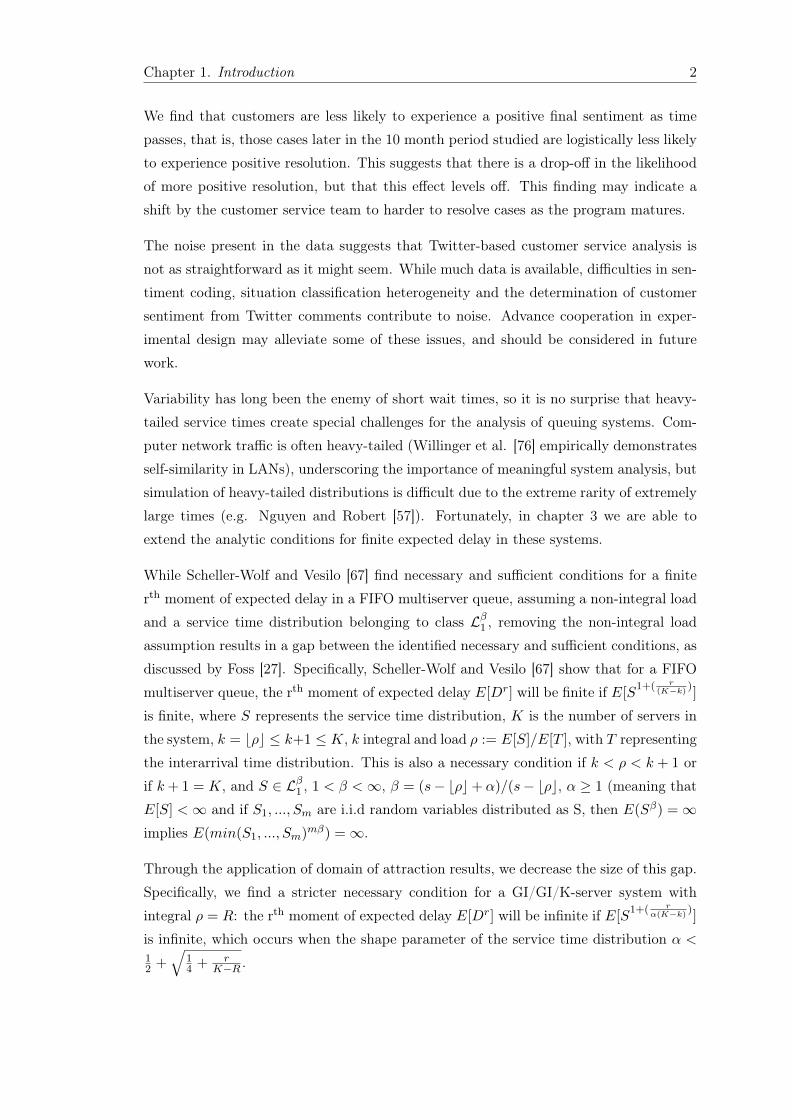
First, we consider a large telecommunications company that provides customer supportover Twitter. Using 10 months of service data, we apply model selection techniquesto develop an ordinal logistic regression model assessing the probability that a givencustomer service interaction will result in a positive, neutral or negative resolution asdetermined by the customer’s sentiment expression. Our model incorporates customer,service and network explanatory attributes. We find that customers are less likely toexperience a positive final sentiment as time passes, that is, those cases later in the 10month period studied are less likely to experience positive resolution. This suggests thatthere is a drop-off in the likelihood of more positive resolution, but that this effect levelsoff. This finding may indicate a shift by the customer service team to harder to resolvecases as the program matures.
Next, we consider conditions for finite expected delay in FIFO multiserver queues withintegral loads. Scheller-Wolf and Vesilo (2006) find necessary and sufficient conditionsfor a finite rth moment of expected delay in a FIFO multiserver queue, assuming a non-integral load and a service time distribution belonging to class L�1 . Removing the non-integral load assumption results in a gap between the identified necessary and sufficientconditions, as discussed by Foss (2009). We decrease the size of this gap through theapplication of domain of attraction results. Specifically, we find a stricter necessarycondition for a GI/GI/K-server system with integral ⇢ that is more restrictive thanthose in the literature.
Finally, we consider the problem of a seller with a finite supply of perishable inventory.We consider four price setting mechanisms: seller posted price, buyer posted price, split-the-difference, and the neutral bargaining solution. We rank the value of these differentmechanisms analytically and numerically in the context of the symmetric uniform trad-ing problem from the perspective of the seller. While the ordering of the mechanismsremains the same as compared to the infinite horizon case studied in the literature, we usea model analogous to the infinite horizon case to find numerically that the relative valueof the split-the-difference mechanism increases when the seller ultimately faces a dead-line to complete the sales. The split-the-difference mechanism becomes more valuable as
ii
the ratio of available inventory to time remaining increases because it is more likely toresult in a sale than the seller posted price mechanism. In general, modeling private in-formation is more challenging for the split-the-difference and neutral bargaining solutionmechanisms than for the two posted price mechanisms. To assess the importance of thisadded complication, we quantify the effect of modeling private information when com-puting the seller’s opportunity cost and find that while private information makes onlya small difference in the neutral bargaining solution case, this modeling choice makes alarge difference in the split-the-difference case when the seller is weak.

iii
AcknowledgmentsFirstly and foremostly, I thank my dissertation committee: a group characterized bysuperhuman patience, generosity of time and unvarying kindness. Specifically, thanks toAlan Scheller-Wolf, for chairing and for years of careful, clear and complete explanations;to Sunder Kekre, for always knowing what to try next and for his insights into practice;to Nicola Secomandi, for his extensive modeling knowledge and steadfast attention todetail; to Rein Vesilo, for demystifying large deviations and effective comments; and toParam Vir Singh, for his helpful suggestions and outside viewpoint.
For the second chapter, I thank Baohung Sun for her excellent choice modeling courseand advice, Liye Ma for his advice, Swapneel Desai for data acquisition, Yingda Lu forhis modeling ideas, and Bo Lin for his programming skills. Additionally, I am grateful toMaria Ferreyra, Peter Boatwright, Mark Schervish, Howard Seltman, and Patrick Foleyfor their generous help and perspectives in detangling a few thorny statistical issues. Forthe third chapter, I remain in awe of Mor Harchol-Balter’s Performance Modeling courseand book.
The formatting for this document was provided by a template by Steven Gunn and SunilPatel from http://www.latextemplates.com.
For years of fun and help in many different ways, I thank my friends Yangfang Zhou,Tinglong Dai, Emre Nadar, Aabha Verma, Elvin Çoban, Masha Shunko, Paul Enders,John Turner, Alp Akçay, Xin Fang, Canan Güneş, Erkut Sönmez, Xin Wang, Ying Xu,Vince Slaugh and Gaoqing Zhang. A very special thanks to Lawrence Rapp, who ensuredthat every administrative aspect of my time at Tepper ran perfectly smoothly!
I’m forever indebted to my parents for their limitless patience and generosity, specificallyto my father Michael Dufalla for his infinite support in all matters and to my motherPenny Suwak for her willingness to listen and unwillingness to sugarcoat the truth.Finally, my thanks to my sister Nicole Dufalla for her unflinching honesty and cartoonishhijinks, to my sister Jacqueline Dufalla for her fathomless calm and rapier wit, and toMahdi Cheraghchi for his unwavering support and much-needed perspective.

Contents
Abstract i
Contents iv
List of Figures viii
List of Tables xi
1 Introduction 1
2 Selecting a Model for Twitter-Based Customer Service Quality Metrics 42.1 Introduction . . . . . . . . . . . . . . . . . . . . . . . . . . . . . . . . . . . 42.2 Literature . . . . . . . . . . . . . . . . . . . . . . . . . . . . . . . . . . . . 52.3 Data . . . . . . . . . . . . . . . . . . . . . . . . . . . . . . . . . . . . . . . 8
2.3.1 Case Selection . . . . . . . . . . . . . . . . . . . . . . . . . . . . . 82.3.2 Sentiment Recoding . . . . . . . . . . . . . . . . . . . . . . . . . . 92.3.3 Network Effects - User Friends . . . . . . . . . . . . . . . . . . . . 10
2.4 Model . . . . . . . . . . . . . . . . . . . . . . . . . . . . . . . . . . . . . . 112.4.1 Model Selection . . . . . . . . . . . . . . . . . . . . . . . . . . . . . 13
2.4.1.1 Model Selection Procedure . . . . . . . . . . . . . . . . . 142.4.1.2 Model Selection Procedure Results . . . . . . . . . . . . . 14
2.4.2 Variables . . . . . . . . . . . . . . . . . . . . . . . . . . . . . . . . 152.4.2.1 Service/Customer Attribute - Ratio of company to total
messages . . . . . . . . . . . . . . . . . . . . . . . . . . . 162.4.2.2 Service Attribute - Company response time . . . . . . . . 162.4.2.3 Service Attribute - Date . . . . . . . . . . . . . . . . . . . 162.4.2.4 Customer Attribute - Customer response time . . . . . . 162.4.2.5 Network Attribute - Number of company related mes-
sages in network . . . . . . . . . . . . . . . . . . . . . . . 162.4.2.6 Network Attribute - Ratio of positive to total network
messages . . . . . . . . . . . . . . . . . . . . . . . . . . . 162.4.2.7 Network Attribute - Ratio of negative to total network
messages . . . . . . . . . . . . . . . . . . . . . . . . . . . 172.4.2.8 Service Attribute - Date of initial message . . . . . . . . . 17
2.4.3 Hypotheses . . . . . . . . . . . . . . . . . . . . . . . . . . . . . . . 172.4.3.1 Ratio of company to total messages . . . . . . . . . . . . 172.4.3.2 Ratio of positive to total network messages . . . . . . . . 18
iv

Contents v
2.4.3.3 Date of initial message . . . . . . . . . . . . . . . . . . . . 182.5 Results and Analysis . . . . . . . . . . . . . . . . . . . . . . . . . . . . . . 18
2.5.1 Evaluation of Hypothesis 3 . . . . . . . . . . . . . . . . . . . . . . 192.5.2 Service time variables . . . . . . . . . . . . . . . . . . . . . . . . . 21
2.6 Conclusion . . . . . . . . . . . . . . . . . . . . . . . . . . . . . . . . . . . . 222.6.1 Limitations . . . . . . . . . . . . . . . . . . . . . . . . . . . . . . . 222.6.2 Implications for Future Research . . . . . . . . . . . . . . . . . . . 23
2.7 Caveat . . . . . . . . . . . . . . . . . . . . . . . . . . . . . . . . . . . . . . 24
3 Necessary Condition for Finite Delay Moments for FIFO GI/GI/KQueues with Integral Load 253.1 Introduction . . . . . . . . . . . . . . . . . . . . . . . . . . . . . . . . . . . 253.2 GI/GI/K, ⇢ = 1 . . . . . . . . . . . . . . . . . . . . . . . . . . . . . . . . . 26
3.2.1 Bounding Delay . . . . . . . . . . . . . . . . . . . . . . . . . . . . . 273.2.1.1 t = �M . . . . . . . . . . . . . . . . . . . . . . . . . . . . 273.2.1.2 t = 0 . . . . . . . . . . . . . . . . . . . . . . . . . . . . . 273.2.1.3 t = x, x > 0 . . . . . . . . . . . . . . . . . . . . . . . . . 28
3.2.2 Delay in the (K-1)-server system . . . . . . . . . . . . . . . . . . . 303.2.3 Conditions for infinite E[S
1+ r
↵(K�1)] . . . . . . . . . . . . . . . . . 31
3.3 GI/GI/K, ⇢ = R, R � 2, R < K, R 2 N . . . . . . . . . . . . . . . . . . . 323.3.1 Bounding Delay . . . . . . . . . . . . . . . . . . . . . . . . . . . . . 32
3.3.1.1 t = �M . . . . . . . . . . . . . . . . . . . . . . . . . . . . 323.3.1.2 t = 0 . . . . . . . . . . . . . . . . . . . . . . . . . . . . . 323.3.1.3 t =
⌥2 x, x > 0 . . . . . . . . . . . . . . . . . . . . . . . . 33
3.3.1.4 t =
⌥2 x+
x
1↵
R
, x > 0 . . . . . . . . . . . . . . . . . . . . . 34
3.3.1.5 t =
⌥2 x+
x
1↵
R
+
x
1↵
R
2 , x > 0 . . . . . . . . . . . . . . . . . . 35
3.3.1.6 t =
⌥2 x+
x
1↵
R
+
x
1↵
R
2 + ...+
x
1↵
R
R�i
, x > 0 . . . . . . . . . . . 37
3.3.1.7 t =
⌥2 x+
PR�2n=1
x
1↵
R
n
, x > 0 . . . . . . . . . . . . . . . . . 37
3.3.1.8 t =
⌥2 x+
PR�1n=1
x
1↵
R
n
, x > 0 . . . . . . . . . . . . . . . . . 383.3.2 Delay in the (K-R)-server system . . . . . . . . . . . . . . . . . . . 403.3.3 Conditions for infinite E[S
1+ r
↵(K�R)] . . . . . . . . . . . . . . . . . 40
3.4 Conclusion . . . . . . . . . . . . . . . . . . . . . . . . . . . . . . . . . . . . 41
4 Revenue Management with Bargaining and a Finite Horizon 434.1 Introduction . . . . . . . . . . . . . . . . . . . . . . . . . . . . . . . . . . . 434.2 Model . . . . . . . . . . . . . . . . . . . . . . . . . . . . . . . . . . . . . . 46
4.2.1 Static Bargaining Model . . . . . . . . . . . . . . . . . . . . . . . . 464.2.2 Mechanisms . . . . . . . . . . . . . . . . . . . . . . . . . . . . . . . 464.2.3 Stochastic and Dynamic Model . . . . . . . . . . . . . . . . . . . . 48
4.3 Structural Analysis . . . . . . . . . . . . . . . . . . . . . . . . . . . . . . . 504.4 Assessing the Relevance of Modeling Private Information Under the STD
and NBS Mechanisms . . . . . . . . . . . . . . . . . . . . . . . . . . . . . 554.5 Numerical Results . . . . . . . . . . . . . . . . . . . . . . . . . . . . . . . 56
4.5.1 Optimal Value Function Comparison by Mechanism . . . . . . . . 574.5.2 Effects of Modeling Private Information . . . . . . . . . . . . . . . 59
Contents vi
4.6 Conclusion . . . . . . . . . . . . . . . . . . . . . . . . . . . . . . . . . . . . 61
5 Conclusion 64
A Appendix A: Selecting a Model for Twitter-Based Customer ServiceQuality Metrics 66A.1 Transitions . . . . . . . . . . . . . . . . . . . . . . . . . . . . . . . . . . . 66A.2 Descriptives . . . . . . . . . . . . . . . . . . . . . . . . . . . . . . . . . . . 67A.3 Variables Considered for Model Inclusion . . . . . . . . . . . . . . . . . . . 67
A.3.1 Customer Attribute - Initial Mention . . . . . . . . . . . . . . . . . 67A.3.2 Customer Attribute - Weekend . . . . . . . . . . . . . . . . . . . . 67A.3.3 Customer Attribute - Business Hours . . . . . . . . . . . . . . . . . 67A.3.4 Customer Attribute - Initial Sentiment . . . . . . . . . . . . . . . . 68A.3.5 Customer Attribute - Number of customer messages . . . . . . . . 68A.3.6 Service Attribute - Number of company messages . . . . . . . . . . 68A.3.7 Service Attribute - Company response time . . . . . . . . . . . . . 68A.3.8 Service/Customer Attribute - Average Time . . . . . . . . . . . . . 68A.3.9 Service/Customer Attribute - Ratio of company to total messages . 68A.3.10 Service/Customer Attribute - Ratio of customer to company mes-
sages . . . . . . . . . . . . . . . . . . . . . . . . . . . . . . . . . . . 68A.3.11 Service/Customer Attribute - Number of messages . . . . . . . . . 69A.3.12 Service Attribute - Priority . . . . . . . . . . . . . . . . . . . . . . 69A.3.13 Service Attribute - Elapsed Time . . . . . . . . . . . . . . . . . . . 69A.3.14 Service Attribute - Initial Response Time . . . . . . . . . . . . . . 69A.3.15 Service Attribute - Date of initial message . . . . . . . . . . . . . . 69A.3.16 Customer Attribute - Customer response time . . . . . . . . . . . . 69A.3.17 Customer Attribute - Number of followers . . . . . . . . . . . . . . 69A.3.18 Customer Attribute - Number of friends . . . . . . . . . . . . . . . 70A.3.19 Customer Network Attributes - Number of positive network mes-
sages from friend-followers . . . . . . . . . . . . . . . . . . . . . . . 70A.3.20 Customer Network Attributes - Number of neutral network mes-
sages from friend-followers . . . . . . . . . . . . . . . . . . . . . . . 70A.3.21 Customer Network Attributes - Number of negative network mes-
sages from friend-followers . . . . . . . . . . . . . . . . . . . . . . . 70A.3.22 Customer Network Attributes - Number of positive network mes-
sages from friend-but-not-followers . . . . . . . . . . . . . . . . . . 70A.3.23 Customer Network Attributes - Number of neutral network mes-
sages from friend-but-not-followers . . . . . . . . . . . . . . . . . . 71A.3.24 Customer Network Attributes - Number of negative network mes-
sages from friend-but-not-followers . . . . . . . . . . . . . . . . . . 71A.3.25 Customer Network Attributes - Number of positive network messages 71A.3.26 Customer Network Attributes - Number of neutral network messages 71A.3.27 Customer Network Attributes - Number of negative network mes-
sages . . . . . . . . . . . . . . . . . . . . . . . . . . . . . . . . . . . 71A.3.28 Network Attribute - Number of company related messages in network 72A.3.29 Network Attribute - Ratio of positive to total network messages . . 72
Contents vii
A.3.30 Network Attribute - Ratio of negative to total network messages . 72A.3.31 Customer Network Attribute - Number of promotional messages . 72A.3.32 Variable notes . . . . . . . . . . . . . . . . . . . . . . . . . . . . . . 72
A.4 Additional Results . . . . . . . . . . . . . . . . . . . . . . . . . . . . . . . 73A.4.1 Evaluation of Hypothesis 1 . . . . . . . . . . . . . . . . . . . . . . 73A.4.2 Evaluation of Hypothesis 2 . . . . . . . . . . . . . . . . . . . . . . 74
A.5 Extra References . . . . . . . . . . . . . . . . . . . . . . . . . . . . . . . . 74
B Appendix B: Necessary Condition for Finite Delay Moments for FIFOGI/GI/K Queues with Integral Load 75B.1 Proof of Lemma 3.4 . . . . . . . . . . . . . . . . . . . . . . . . . . . . . . 75B.2 Asymptotic convergence of bounds . . . . . . . . . . . . . . . . . . . . . . 78B.3 Workloads are greater than C
0x
1↵ . . . . . . . . . . . . . . . . . . . . . . . 79
C Appendix: Revenue Management with Bargaining and a Finite Horizon- Additional Numerical Results 82C.1 Results for � = 0.6, r = 0.05 (Figures C.1 to C.6) . . . . . . . . . . . . . . 83C.2 Results for � = 0.9, r = 0.05 (Figures C.7 to C.12) . . . . . . . . . . . . . 87C.3 Results for � = 0.3, r = 0.10 (Figures C.13 to C.18) . . . . . . . . . . . . . 91C.4 Results for � = 0.6, r = 0.10 (Figures C.19 to C.24) . . . . . . . . . . . . . 95C.5 Results for � = 0.9, r = 0.10 (Figures C.25 to C.30) . . . . . . . . . . . . . 99
References 103

List of Figures
2.1 John’s Twitter network. Messages posted by John’s friends are collectedfor him to read. John’s followers read messages posted by John. . . . . . . 5
2.2 Service, customer and network attributes included in the model. . . . . . . 62.3 Probability of positive, negative or neutral final resolution for each day of
the study period (February 22 is day 1). . . . . . . . . . . . . . . . . . . . 202.4 Percentage of messages sent by friends of the customers in the data set
classified as positive, negative and neutral during each week studied. . . . 20
4.1 Optimal value function ratio (V k
t
(y)/V
j
t
(y)) for different times-to-go, withr = 0.05 and � = 0.30 . . . . . . . . . . . . . . . . . . . . . . . . . . . . . 58
4.2 Optimal value function ratio (V k
t
(y)/V
j
t
(y)), with r = 0.05 and � = 0.30 . 584.3 Expected quantity sold under the four mechanisms for different times-to-
go, with r = 0.05 and � = 0.30 . . . . . . . . . . . . . . . . . . . . . . . . 594.4 Average price per unit expected to be received under the four mechanisms
for different times-to-go, with r = 0.05 and � = 0.30 . . . . . . . . . . . . 604.5 Ratio of approximate optimal value function to optimal value function
under the NBS mechanism, with r = 0.05 and � = 0.30 . . . . . . . . . . . 604.6 Ratio of approximate optimal value function to optimal value function
under the STD mechanism, with r = 0.05 and � = 0.30 . . . . . . . . . . . 614.7 Expected quantities sold and average price per unit expected to be received
under Model (4.2) specified for the STD mechanism and Model (4.10), fordifferent times-to-go, with r = 0.05 and � = 0.30 . . . . . . . . . . . . . . 62
C.1 Optimal value function ratio (V k
t
(y)/V
j
t
(y)) for different times-to-go, withr = 0.05 and � = 0.60 . . . . . . . . . . . . . . . . . . . . . . . . . . . . . 83
C.2 Expected quantity sold under the four mechanisms for different times-to-go, with r = 0.05 and � = 0.60 . . . . . . . . . . . . . . . . . . . . . . . . 84
C.3 Average price per unit expected to be received under the four mechanismsfor different times-to-go, with r = 0.05 and � = 0.60 . . . . . . . . . . . . 84
C.4 Ratio of approximate optimal value function to optimal value functionunder the NBS mechanism, with r = 0.05 and � = 0.60 . . . . . . . . . . . 85
C.5 Ratio of approximate optimal value function to optimal value functionunder the STD mechanism, with r = 0.05 and � = 0.60 . . . . . . . . . . . 85
C.6 Expected quantities sold and average price per unit expected to be receivedunder Model (4.2) specified for the STD mechanism and Model (4.10), fordifferent times-to-go, with r = 0.05 and � = 0.60 . . . . . . . . . . . . . . 86
C.7 Optimal value function ratio (V k
t
(y)/V
j
t
(y)) for different times-to-go, withr = 0.05 and � = 0.90 . . . . . . . . . . . . . . . . . . . . . . . . . . . . . 87
viii
List of Figures ix
C.8 Expected quantity sold under the four mechanisms for different times-to-go, with r = 0.05 and � = 0.90 . . . . . . . . . . . . . . . . . . . . . . . . 88
C.9 Average price per unit expected to be received under the four mechanismsfor different times-to-go, with r = 0.05 and � = 0.90 . . . . . . . . . . . . 88
C.10 Ratio of approximate optimal value function to optimal value functionunder the NBS mechanism, with r = 0.05 and � = 0.90 . . . . . . . . . . . 89
C.11 Ratio of approximate optimal value function to optimal value functionunder the STD mechanism, with r = 0.05 and � = 0.90 . . . . . . . . . . . 89
C.12 Expected quantities sold and average price per unit expected to be receivedunder Model (4.2) specified for the STD mechanism and Model (4.10), fordifferent times-to-go, with r = 0.05 and � = 0.90 . . . . . . . . . . . . . . 90
C.13 Optimal value function ratio (V k
t
(y)/V
j
t
(y)) for different times-to-go, withr = 0.10 and � = 0.30 . . . . . . . . . . . . . . . . . . . . . . . . . . . . . 91
C.14 Expected quantity sold under the four mechanisms for different times-to-go, with r = 0.10 and � = 0.30 . . . . . . . . . . . . . . . . . . . . . . . . 92
C.15 Average price per unit expected to be received under the four mechanismsfor different times-to-go, with r = 0.10 and � = 0.30 . . . . . . . . . . . . 92
C.16 Ratio of approximate optimal value function to optimal value functionunder the NBS mechanism, with r = 0.10 and � = 0.30 . . . . . . . . . . . 93
C.17 Ratio of approximate optimal value function to optimal value functionunder the STD mechanism, with r = 0.10 and � = 0.30 . . . . . . . . . . . 93
C.18 Expected quantities sold and average price per unit expected to be receivedunder Model (4.2) specified for the STD mechanism and Model (4.10), fordifferent times-to-go, with r = 0.10 and � = 0.30 . . . . . . . . . . . . . . 94
C.19 Optimal value function ratio (V k
t
(y)/V
j
t
(y)) for different times-to-go, withr = 0.10 and � = 0.60 . . . . . . . . . . . . . . . . . . . . . . . . . . . . . 95
C.20 Expected quantity sold under the four mechanisms for different times-to-go, with r = 0.10 and � = 0.60 . . . . . . . . . . . . . . . . . . . . . . . . 96
C.21 Average price per unit expected to be received under the four mechanismsfor different times-to-go, with r = 0.10 and � = 0.60 . . . . . . . . . . . . 96
C.22 Ratio of approximate optimal value function to optimal value functionunder the NBS mechanism, with r = 0.10 and � = 0.60 . . . . . . . . . . . 97
C.23 Ratio of approximate optimal value function to optimal value functionunder the STD mechanism, with r = 0.10 and � = 0.60 . . . . . . . . . . . 97
C.24 Expected quantities sold and average price per unit expected to be receivedunder Model (4.2) specified for the STD mechanism and Model (4.10), fordifferent times-to-go, with r = 0.10 and � = 0.60 . . . . . . . . . . . . . . 98
C.25 Optimal value function ratio (V k
t
(y)/V
j
t
(y)) for different times-to-go, withr = 0.10 and � = 0.90 . . . . . . . . . . . . . . . . . . . . . . . . . . . . . 99
C.26 Expected quantity sold under the four mechanisms for different times-to-go, with r = 0.10 and � = 0.90 . . . . . . . . . . . . . . . . . . . . . . . . 100
C.27 Average price per unit expected to be received under the four mechanismsfor different times-to-go, with r = 0.10 and � = 0.90 . . . . . . . . . . . . 100
C.28 Ratio of approximate optimal value function to optimal value functionunder the NBS mechanism, with r = 0.10 and � = 0.90 . . . . . . . . . . . 101
C.29 Ratio of approximate optimal value function to optimal value functionunder the STD mechanism, with r = 0.10 and � = 0.90 . . . . . . . . . . . 101

List of Figures x
C.30 Expected quantities sold and average price per unit expected to be receivedunder Model (4.2) specified for the STD mechanism and Model (4.10), fordifferent times-to-go, with r = 0.10 and � = 0.90 . . . . . . . . . . . . . . 102

List of Tables
2.1 Ordinal Logistic Regression Results for Exploratory Data . . . . . . . . . 152.2 Ordinal Logistic Regression Results for Test Data . . . . . . . . . . . . . . 19
3.1 Old and new lower bounds for ↵ for different numbers of servers K, with⇢ = 1 . . . . . . . . . . . . . . . . . . . . . . . . . . . . . . . . . . . . . . . 32
3.2 Old and new lower bounds for ↵ for different numbers of servers K, anddifferent loads ⇢ = R . . . . . . . . . . . . . . . . . . . . . . . . . . . . . . 41
A.1 Transition Table - Model Selection Data . . . . . . . . . . . . . . . . . . . 66A.2 Transition Table - Test Data . . . . . . . . . . . . . . . . . . . . . . . . . . 66A.3 Full Data Set - Descriptives . . . . . . . . . . . . . . . . . . . . . . . . . . 67A.4 Chosen model - full data set . . . . . . . . . . . . . . . . . . . . . . . . . . 73
xi

For my father:
Nie poddawaj się!
xii

Chapter 1
Introduction
Service operations management is a broad subfield incorporating many different man-agement problems. In this dissertation, I focus on three: identifying situational at-tributes that lead to positive customer outcomes under a Twitter-based customer serviceframework, the conditions for finite delay of first-in-first-out multiserver systems whenconfronted with heavy-tailed service times, and the relative performance of different bar-gaining mechanisms for a seller of finite perishable inventory, with a further investigationof the consequences of modeling private information.
Social media sites, including Twitter, provide companies with a unique window into theminds of their customers, as well as a way to monitor (and influence) their reputationin real-time. While social media has obvious marketing and brand management applica-tions, many companies are now branching out into providing customer service directlythrough the venues where customers complain. This has the dual advantages of provid-ing customer service in a customer-chosen outlet while potentially allowing the companyto protect its reputation. However, while elements of traditional customer service havebeen studied extensively, the applicability of these elements to new, social media basedforms of customer service is unclear.
In chapter 2, we consider a large telecommunications company that provides customersupport over Twitter. In order to identify which factors are most important for customersatisfaction when administering customer support over Twitter, we use model selectiontechniques on 10 months of service data to develop an ordinal logistic regression modelassessing the probability that a given customer service interaction will result in a positive,neutral or negative resolution as determined by the customer’s sentiment expression. Ourmodel incorporates customer, service and network attributes.
1
Chapter 1. Introduction 2
We find that customers are less likely to experience a positive final sentiment as timepasses, that is, those cases later in the 10 month period studied are logistically less likelyto experience positive resolution. This suggests that there is a drop-off in the likelihoodof more positive resolution, but that this effect levels off. This finding may indicate ashift by the customer service team to harder to resolve cases as the program matures.
The noise present in the data suggests that Twitter-based customer service analysis isnot as straightforward as it might seem. While much data is available, difficulties in sen-timent coding, situation classification heterogeneity and the determination of customersentiment from Twitter comments contribute to noise. Advance cooperation in exper-imental design may alleviate some of these issues, and should be considered in futurework.
Variability has long been the enemy of short wait times, so it is no surprise that heavy-tailed service times create special challenges for the analysis of queuing systems. Com-puter network traffic is often heavy-tailed (Willinger et al. [76] empirically demonstratesself-similarity in LANs), underscoring the importance of meaningful system analysis, butsimulation of heavy-tailed distributions is difficult due to the extreme rarity of extremelylarge times (e.g. Nguyen and Robert [57]). Fortunately, in chapter 3 we are able toextend the analytic conditions for finite expected delay in these systems.
While Scheller-Wolf and Vesilo [67] find necessary and sufficient conditions for a finiterth moment of expected delay in a FIFO multiserver queue, assuming a non-integral loadand a service time distribution belonging to class L�1 , removing the non-integral loadassumption results in a gap between the identified necessary and sufficient conditions, asdiscussed by Foss [27]. Specifically, Scheller-Wolf and Vesilo [67] show that for a FIFOmultiserver queue, the rth moment of expected delay E[D
r
] will be finite if E[S
1+( r
(K�k) )]
is finite, where S represents the service time distribution, K is the number of servers inthe system, k = b⇢c k+1 K, k integral and load ⇢ := E[S]/E[T ], with T representingthe interarrival time distribution. This is also a necessary condition if k < ⇢ < k + 1 orif k + 1 = K, and S 2 L�1 , 1 < � < 1, � = (s� b⇢c+ ↵)/(s� b⇢c, ↵ � 1 (meaning thatE[S] < 1 and if S1, ..., Sm
are i.i.d random variables distributed as S, then E(S
�
) = 1implies E(min(S1, ..., Sm
)
m�
) = 1.
Through the application of domain of attraction results, we decrease the size of this gap.Specifically, we find a stricter necessary condition for a GI/GI/K-server system withintegral ⇢ = R: the rth moment of expected delay E[D
r
] will be infinite if E[S
1+( r
↵(K�k) )]
is infinite, which occurs when the shape parameter of the service time distribution ↵ <
12 +
q14 +
r
K�R
.

Chapter 1. Introduction 3
Negotiation is important for both business to business and business to customer sales.Consider a seller with a finite inventory of perishable goods being visited by a seriesof potential buyers. The seller could propose a take-it-or-leave-it price for a unit ofinventory. Alternately, the buyer could propose a take-it-or-leave-it price. Both buyerand seller could state prices, then “split-the-difference". Finally, the buyer and sellercould engage in a face-to-face negotiation, the result of which can be represented byMyerson’s [53] neutral bargaining solution (NBS).
In chapter 4, we rank the value of these four different mechanisms analytically andnumerically in the context of Chatterjee and Samuelson’s [15] symmetric uniform tradingproblem, from the perspective of the seller. We demonstrate that a seller posted pricealways performs at least as well for the seller as the neutral bargaining solution, whichalways performs at least as well as a buyer posted price, and that splitting-the-differencealways performs at least as well as a buyer posted price. While this ordering of themechanisms remains the same as compared to the infinite horizon case studied in theliterature, we find numerically, in an analogous model, that the relative value of thesplit-the-difference (STD) mechanism increases as we move to a situation where theseller faces a deadline to complete the sales. The higher the ratio of available inventoryto time remaining becomes, the more valuable the STD mechanism becomes, because it ismore likely to result in a sale. While STD lacks the simplicity of a buyer or seller postedprice, it is a relatively easy to implement method for automated bargaining, making thisa practical option for a seller.
Incorporating private information into the model adds an additional layer of complexity.We quantify the importance of modeling private information when computing the seller’sopportunity cost under the STD and NBS mechanisms. While using a simplified modelthat calculates the seller’s opportunity cost using public information may be an accept-able approximation for the NBS mechanism, it produces substantially different resultsthan the private information case when STD mechanism is used by a strong seller.
We proceed first by identifying situational attributes that lead to positive customeroutcomes under a Twitter-based customer service framework in Chapter 2. In Chapter 3,we find conditions for finite delay of first-in-first-out multiserver systems when confrontedwith heavy-tailed service times. In Chapter 4, we assess the relative performance ofdifferent bargaining mechanisms for a seller of finite perishable inventory, with a furtherinvestigation of the consequences of modeling private information. Finally, in Chapter5, we summarize our findings and avenues for future work.

Chapter 2
Selecting a Model for Twitter-BasedCustomer Service Quality Metrics
2.1 Introduction
While elements of traditional customer complaint management have been studied exten-sively, the applicability of these elements to new, social media based forms of customerservice is still being examined. Many companies monitor social networking sites, includ-ing Twitter, to gauge public opinion and to identify problems. Other companies, such asDell, Whole Foods Market and Jet Blue Airways, go further and use social media basedcustomer support teams to attempt to assist customers over these media [41]. Advice forsuch uses is given in the popular press (for examples please see [34] [31]), but have notbeen exhaustively studied. In this work, we hope to identify the driving factors behindsuccessful Twitter-based customer complaint remediation.
The public nature of social media adds an interesting complication to the conventionalservice interaction. Within Twitter, a user has “friends” and “followers.” When a user’sfriend writes a tweet, that user will be able to see the tweet on his homepage. While allpublic tweets are viewable by all Twitter users, a user will select friends to assemble acurated page of tweets that interest him. Similarly, a “follower” is a user that subscribesto the tweets of another user. Consider figure 2.1. John likes to read the tweets hisfriends, Samantha, Nancy and Lady GaGa. Nancy and Ted like to read John’s tweets.Notice that Nancy is both John’s friend and follower, while other users may be only afriend or only a follower of a user. Please note that despite the terminology used byTwitter, a “friend” is not necessarily a mutual designation or indicative of any otherrelationship between users.
This chapter is joint work with Sunder Kekre.
4

Chapter 2. Selecting a Model for Twitter-Based Customer Service Quality Metrics 5
Figure 2.1: John’s Twitter network. Messages posted by John’s friends are collectedfor him to read. John’s followers read messages posted by John.
This public interaction results in the need for the company to consider its brand image.Online complaint resolution becomes both necessary and extremely important. Kapland[41] and Griffin [34] both emphasize the need to respond quickly and appropriately toboth positive and negative comments.
We consider one large telecommunications company. This company has a staff dedicatedto monitoring tweets containing the names of the company or its products. Those tweetsare evaluated and responded to when appropriate. Basic support advice can be providedthis way. For more complicated problems, the support staff can refer a customer toa URL where they can access additional service assistance. To address the problemof which metrics are important under this new service regime, we analyzed Twittercustomer service interactions from a period of 10 months. Using half the data set, amodel incorporating customer, service and network attributes was built. The relevantvariables are summarized in Figure 2.2. A test of this new model on the second halfof the data set suggests that cases later in the data set are less likely to have a morepositive resolution, but that this effect levels off. This may be the result of an expansionof the social media customer service group addressing more complicated cases as timeprogresses.
The difficulty in obtaining significant parameter values may stem from experiment design,but we propose several changes that could be made in future research to ameliorate thisproblem.
2.2 Literature
There is a large and varied literature on customer complaint management. One excel-lent general resource is the book “Complaint Management: The Heart of CRM.” [70]

Chapter 2. Selecting a Model for Twitter-Based Customer Service Quality Metrics 6
Figure 2.2: Service, customer and network attributes included in the model.
While this book does not discuss social media, it does detail most important elements ofcomplaint resolution, including techniques, analysis and firm improvement.
Before progressing farther, it would be appropriate to consider the numerous benefits ofcomplaint resolution, beyond merely solving one particular customer’s problem. Adam-son [2], and Fundin and Bergman [30] discuss the usage of complaint information forthe improvement of company products and services. Complaints offer a window intocustomer perception, and insights derived from the valuable feedback can be used tomake the firm more competitive. Berry and Parasuraman [7], Bosch and Enriquez [10],and Faed [23] each discuss possible systems for the appropriate collection, managementand analysis of the necessary data for this task. One financial consideration is the valueof customer retention. In a pair of papers, Fornell and Wernerfelt [25] [26] model thecustomer complaint process and consider the cost of lost customers due to unvoiced com-plaints. Also within the realm of defensive marketing, Ruyter and Brack [21] note thelegal ramifications of appropriate complaint management for the reduction of liability.
Despite these benefits, not all firms make customer complaint management a priority.In one study, Gulas and Larsen [35] found that 29.2% of communications (a mixtureof complaints and compliments) sent to a variety of companies were left unanswered.However, the same study found that this response rate was unrelated to the companies’returns on investment.
One large opportunity and possible pitfall related to complaint management is the roleof customer word of mouth. Chelminski and Coulter [16] find that customers are morelikely to complain to their friends rather than the company. To make matters worse,
Chapter 2. Selecting a Model for Twitter-Based Customer Service Quality Metrics 7
Casado et al. [11] find that customers who complain to the company and then receiveinadequate service are more likely to both leave the company and complain to friends.
Given the consequences of ignoring or mismanaging customer complaints, many studiestry to identify the characteristics of “good” customer complaint management. Blodgettand Anderson [9] use survey data from dissatisfied retail customers to explore a customercomplaint Bayesian network model. This model incorporated store loyalty, store type,a customer’s attitude towards complaining, a customer’s belief about the controllabilityof the problem to determine how likely a customer would be to complain, and then howsatisfied the customer would be in his or her problem resolution, and then considered theword of mouth and future loyalty effects of the result. Interestingly, after successful com-plaint resolution, newly happy customers exhibited a 46% probability of positive wordof mouth. This result certainly suggests that for our paper, the company faces a greatopportunity to convert Twitter complainers into Twitter promoters. A simpler loyaltyfocused model (without WOM effects) is provided by Andreassen [4]. Another loyalty fo-cused model (also without WOM effects) now incorporating overall customer satisfactionis provided by McQuilken et al. [51]. Focusing on a deeper level, Davidow [20] provides aframework clarifying both the current state and proposed future directions of research fo-cused on the actual mechanics of customer complaint response in the areas of timeliness,facilitation, redress, apology, credibility, attentiveness and interaction. Chan and Ngai[14] also focus on the mechanics of the company’s complaint response, although fromthe perspective of justice and fairness theory. Finally, reaching into electronic customerservice, Murphy et al. [52] examine company emails used for hotel customer service,categorizing each e-mail in dimensions of personalization, responsiveness, reliability andtangibility.
Extending into the online realm, several studies examine how companies should manageonline customer complaints posted in forum-type environments (as opposed to microblog-ging arenas like Twitter - for an overview of Twitter network characteristics, see Javaet al. [40]). Cho and Fjermestad [17] provide a brief overview of the scant literaturesurrounding online complaint management. Cho et al. [18] characterize the nature ofcomplaints in a variety of online complaint forums. Harrison-Walker [36] performs a sim-ilar analysis and also considers the customer experience that led to the online posting of acomplaint, with an excellent series of managerial recommendations. Lee and Lee [45] ap-proach the online forum feedback response issue from a customer trust perspective. Leeand Song [46] consider the word of mouth implications of customer feedback and com-pany response on online forums, investigating the risks of defensive, accomodative and noaction strategies by the company. Bach and Kim [6] also look at company response andmanagement of customer word of mouth in an online forum using a case study compar-ing one company’s “proactive” approach with another’s “defensive” approach. Branching
Chapter 2. Selecting a Model for Twitter-Based Customer Service Quality Metrics 8
from online forums into social media, Jansen et al. [39] consider WOM implications ofTwitter.
This chapter attempts to span these areas by again examining the actual mechanicsof customer complaint response (as in, which attributes lead to a positive complaintresolution experience), but within a Twitter-based WOM regime. Ma et al. [48] examinesentiment change for customers using the same data set as this work. However, whilethis chapter focuses on customer, service and network attributes that result in sentimentchange during a firm intervention using ordinal logistic regression, Ma et al. [48] use adynamic choice model to consider a customer’s sentiment change over time, influencedby the sentiments in that customer’s network, with firm intervention as an exogenousfactor. The two approaches use different modeling strategies and different granularitiesto answer different questions.
2.3 Data
The complete data set includes 1,149,851 Twitter messages (tweets) collected by a largetelecommunications company between February 13 and December 22, 2010. The tweetsincluded in the set are all public messages, not private “direct messages”, mentioningthe company or its products by name. The company organized these messages into12,625 cases. Some tweets were responded to by customer service representatives offeringassistance. Not all tweets were assigned a case, and many cases contain multiple tweets.
2.3.1 Case Selection
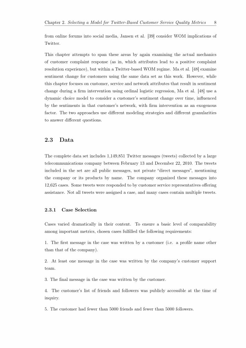
Cases varied dramatically in their content. To ensure a basic level of comparabilityamong important metrics, chosen cases fulfilled the following requirements:
1. The first message in the case was written by a customer (i.e. a profile name otherthan that of the company).
2. At least one message in the case was written by the company’s customer supportteam.
3. The final message in the case was written by the customer.
4. The customer’s list of friends and followers was publicly accessible at the time ofinquiry.
5. The customer had fewer than 5000 friends and fewer than 5000 followers.

Chapter 2. Selecting a Model for Twitter-Based Customer Service Quality Metrics 9
6. The initial message was posted after the first week of data collection (so that a fullweek of background network information is available).
7. The two sentiment coding tools discussed in Section 2.3.2 did not disagree on theinitial and final sentiments expressed by the customer (i.e. one tool did not code theinitial sentiment as “positive” while the other indicated that it was “negative”)
8. The company responded to each customer message in the case within one week, onaverage.
The first two conditions make sure that the examined cases follow a pattern of customercomplaint then customer service response. These conditions are necessary, as many in-cluded cases either do not include a customer service exchange, or include an exchangein a format impractical to analyze (such as an exchange initiated by customer service).The third condition is necessary to allow us to determine the ultimate outcome of theexchange. We are interested in the ultimate outcome of the interaction, so this finalcustomer sentiment is needed. The fourth, fifth and sixth conditions allow us to examinethe effects of comments within a customer’s network of friends (see Section 2.3.3). Theseventh condition allows us to exclude cases that were likely to have misclassified senti-ments. The eighth condition is intended to identify and remove atypical cases where thecompany and customer do not seem to have an interactive experience.
706 cases fulfilled these requirements. The breakdown of these 706 cases by initial andfinal sentiments for the model selection and test data partitions can be found in AppendixA.1 in Tables A.1 and A.2. Descriptives for the variables ultimately included in the modelcan be found in Appendix A.2.
2.3.2 Sentiment Recoding
The company used an automated coding system to classify the content of messages as pos-itive, negative or neutral. Not all messages were classified. For consistency, we initiallyused the Stanford Twitter Sentiment Classification API bulk classification service (previ-ously available at http://twittersentiment.appspot.com/api/bulkClassify, now availableat http://help.sentiment140.com/api) to categorize messages in the data set (includingmessages not included in any case, for use in determining network effects in Section 2.3.3)into positive, negative and neutral sentiment. Most messages are assigned a “neutral”coding. It appears that only very positive and very negative messages are coded as such.Manual inspection reveals that the categorization is far from perfect, however the sizeof the data set renders other methods of categorization impractical. For a discussion ofhow this tool works and its advantages, please see Go et al. [33].
Chapter 2. Selecting a Model for Twitter-Based Customer Service Quality Metrics 10
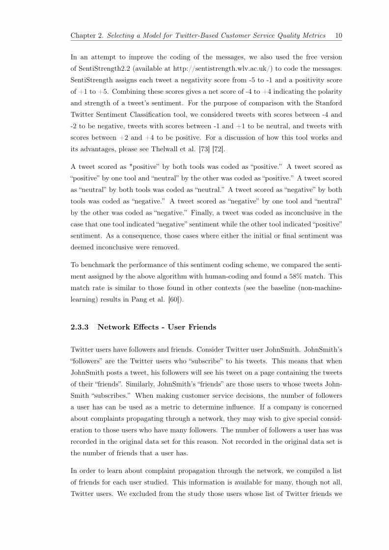
In an attempt to improve the coding of the messages, we also used the free versionof SentiStrength2.2 (available at http://sentistrength.wlv.ac.uk/) to code the messages.SentiStrength assigns each tweet a negativity score from -5 to -1 and a positivity scoreof +1 to +5. Combining these scores gives a net score of -4 to +4 indicating the polarityand strength of a tweet’s sentiment. For the purpose of comparison with the StanfordTwitter Sentiment Classification tool, we considered tweets with scores between -4 and-2 to be negative, tweets with scores between -1 and +1 to be neutral, and tweets withscores between +2 and +4 to be positive. For a discussion of how this tool works andits advantages, please see Thelwall et al. [73] [72].
A tweet scored as "positive” by both tools was coded as “positive.” A tweet scored as“positive” by one tool and “neutral” by the other was coded as “positive.” A tweet scoredas “neutral” by both tools was coded as “neutral.” A tweet scored as “negative” by bothtools was coded as “negative.” A tweet scored as “negative” by one tool and “neutral”by the other was coded as “negative.” Finally, a tweet was coded as inconclusive in thecase that one tool indicated “negative” sentiment while the other tool indicated “positive”sentiment. As a consequence, those cases where either the initial or final sentiment wasdeemed inconclusive were removed.
To benchmark the performance of this sentiment coding scheme, we compared the senti-ment assigned by the above algorithm with human-coding and found a 58% match. Thismatch rate is similar to those found in other contexts (see the baseline (non-machine-learning) results in Pang et al. [60]).
2.3.3 Network Effects - User Friends
Twitter users have followers and friends. Consider Twitter user JohnSmith. JohnSmith’s“followers” are the Twitter users who “subscribe” to his tweets. This means that whenJohnSmith posts a tweet, his followers will see his tweet on a page containing the tweetsof their “friends”. Similarly, JohnSmith’s “friends” are those users to whose tweets John-Smith “subscribes.” When making customer service decisions, the number of followersa user has can be used as a metric to determine influence. If a company is concernedabout complaints propagating through a network, they may wish to give special consid-eration to those users who have many followers. The number of followers a user has wasrecorded in the original data set for this reason. Not recorded in the original data set isthe number of friends that a user has.
In order to learn about complaint propagation through the network, we compiled a listof friends for each user studied. This information is available for many, though not all,Twitter users. We excluded from the study those users whose list of Twitter friends we

Chapter 2. Selecting a Model for Twitter-Based Customer Service Quality Metrics 11
were unable to access. In addition to those with private information, this includes thoseusers whose profile names include spaces, which interfered with the script we used toretrieve the friend lists. Additionally, the API for friend retrieval limits returns to 5000results so we removed cases with users with exceptionally high friend or follower counts.
After retrieving a list of user friends, we were able to find instances of users being exposedto the company related comments of others. To incorporate this effect into our model,we added a variable counting the number of positive tweets about the company a userwould have seen in the week before his initial complaint and during the period of thecase. Similar variables were created for neutral and negative tweets. An additionalvariable was created to indicated the sum of positive, neutral, negative and inconclusivemessages seen during this time period. Lu et al. [47] find that recent posting activity isan important component in opinion leadership in the context of online forums, so it is notunreasonable to believe that those tweets sent most recently would be more influential inthe current context. In addition to these magnitude measures, variables were created forthe proportion of positive and negative messages in a customers network. Tweets writtenby the customer support team were ignored, as it seems likely a customer only added thecompany’s customer support team as a friend once the customer service interaction wasunderway. Promotional tweets by the company were also ignored for the same reason.
Huberman et al. [37] show that while users have many friends, they interact with rela-tively few. (Also of interest is a study by Cha et al. [13] showing that a high followercount may not be an indicator of influence.) To account for different levels of Twitterattention, we established a new set of variables. First, we counted the number of posi-tive comments about the company made by those who were both friends and followersof a user in the week before the customer’s initial message and during the period of thecase. For the previous example in Figure 2.1, we would only consider Nancy’s commentswhen assessing John’s exposure. Similar variables were created for neutral and negativemessages. In addition, we counted the number of positive comments about the companymade by those who were friends but not followers for a user in the previous week. Similarvariables were created for neutral and negative messages. In addition to these magnitudemeasures, variables were created for the proportion of positive and negative messages ina customers network.
2.4 Model
Our model examines the importance of several operations metrics in the context of tweetbased customer support. We attempt to identify the driving factors behind customersentiment change. To do this, we consider the following basic interaction:

Chapter 2. Selecting a Model for Twitter-Based Customer Service Quality Metrics 12
1. A customer is exposed to the messages sent by his or her Twitter friends. Thecomments of the customer’s Twitter friends may affect the customer’s future sentimentexpression.
2. A customer tweets comments about the company’s services or products. This tweetmay be positive, neutral or negative in sentiment.
3. A customer service representative replies with assistance. The quality of this inter-vention may affect the customer’s final sentiment.
4. Additional messages may be exchanged as the issue is resolved. The customer maystill be influenced by comments within his or her network.
5. The customer tweets a last time, revealing a final sentiment of positive, neutral ornegative.
We hope to determine the probabilities of different final sentiment states, given the ser-vice, customer and customer network attributes described in Section 2.4.2. To determinethese probabilities, we use an ordinal logistic regression.
In SPSS, we used the ordinal logistic regression function to fit the following model:
⇡
i,positive
= (
1
1 + exp(↵
positive
� (x
0i
�))
)
⇡
i,neutral
= (
1
1 + exp((↵
neutral
� (x
0i
�))
)� ⇡
i,positive
(2.1)
⇡
i,negative
= 1� ⇡
i,positive
� ⇡
i,neutral
where ⇡i,j
is the probability of a final sentiment j (either positive, negative or neutral)for a customer i, with attributes x
i
and parameters ↵j
and �. SPSS maximizes thelog-likelihood function (plus a constant):
l =
mX
i=1
J�1X
j=1
jX
k=1
nklog
�
i,j
�
i,j+1 � �i, j
!!�
j+1X
k=1
nklog
�
i,j+1
�
i,j+1 � �i, j
!!(2.2)
where �i,j
is “the cumulative response probability up to and including Y=j at subpopula-tion i”, n is “the sum of all frequency weights” and m is “the number of subpopulations”.[1]
Chapter 2. Selecting a Model for Twitter-Based Customer Service Quality Metrics 13
For this model to be valid, the “proportional odds” assumption must hold. We usedthe parallel line test to confirm the validity of this assumption in our data. (UCLAInstitute for Digital Research and Education [58]) As a clarification, we considered “initialsentiment” as a variable, but it was insignificant and left out of the final model. We arenot modeling transitions, just the probability of a customer ending the interaction in apositive state.
To summarize, we are trying to discover which attributes change the probability thata given customer service interaction will result in a positive (or neutral or negative)final message sent by the customer. The ordinal logistic regression model allows us tocalculate the probability of a positive (or negative or neutral) final sentiment, given alist of attributes of the interaction (for example, number of messages or elapsed time).
2.4.1 Model Selection
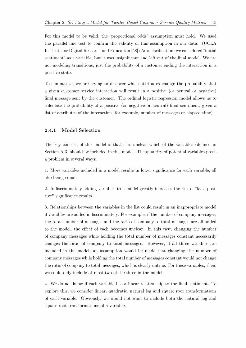
The key concern of this model is that it is unclear which of the variables (defined inSection A.3) should be included in this model. The quantity of potential variables posesa problem in several ways:
1. More variables included in a model results in lower significance for each variable, allelse being equal.
2. Indiscriminately adding variables to a model greatly increases the risk of “false posi-tive" significance results.
3. Relationships between the variables in the list could result in an inappropriate modelif variables are added indiscriminately. For example, if the number of company messages,the total number of messages and the ratio of company to total messages are all addedto the model, the effect of each becomes unclear. In this case, changing the numberof company messages while holding the total number of messages constant necessarilychanges the ratio of company to total messages. However, if all three variables areincluded in the model, an assumption would be made that changing the number ofcompany messages while holding the total number of messages constant would not changethe ratio of company to total messages, which is clearly untrue. For these variables, then,we could only include at most two of the three in the model.
4. We do not know if each variable has a linear relationship to the final sentiment. Toexplore this, we consider linear, quadratic, natural log and square root transformationsof each variable. Obviously, we would not want to include both the natural log andsquare root transformations of a variable.

Chapter 2. Selecting a Model for Twitter-Based Customer Service Quality Metrics 14
2.4.1.1 Model Selection Procedure
In order to address the above issues, we used the following procedure to move from theextended list of variables in Section A.3 to an appropriate model for analysis.
1. Randomly divided the data set into two parts. Part 1 is used for model selection (334cases). Part 2 is saved for model testing (372 cases).
2. Using only part 1 of the data, each variable in the complete variable list is regressedalone against the dependent variable. Additionally, quadratic, square root and naturallog transformations of these variables were also considered, where appropriate. (In thecase where the variable may have a value of 0 (number of friends, number of followers,number of a certain type of network message, etc.), the natural log of the value of thevariable plus one was taken.) Again, each model was run separately. Consequently, withthe exception of the dummy variables, each variable had four possible models (linear,quadratic, natural log and square root). The linear model was assumed to be the bestrepresentation, unless one of the alternate models had an Akaike Information Criterion(AIC) value that was a least 2 less than the linear model [3]. In that case, the modelwith the lowest AIC was viewed to be the best representation of that variable.
3. Still using only part 1 of the data, the best representation of each variable in thelist of complete variables (Appendix A.3) was considered for inclusion into a new model.Vincent Calcagno’s ‘glmulti’ package for R was used to search through candidate modelsusing a genetic algorithm, with the minimization of AICc as the goal [38]. Both the CLMand MASS packages were used. Due to redundant variables, some manual perturbationwas used to ensure that the model was consistent with theory and not suffering frommulticollinearity. These results are shown in Section 2.4.1.2.
4. A new regression was performed using the chosen model and the untouched half ofthe data (part 2) to obtain true significance values for the parameters and to validatethe model selection. These results are shown in Section 2.5.
5. For comparison, we also ran a regression using the chosen model and the full dataset (both the exploration half and the untouched test half). These results are shown inAppendix A.4.
2.4.1.2 Model Selection Procedure Results
Using R’s glmulti and manual adjustment, the lowest AICc obtained was for a modelincluding the variables for the ratio of company to customer messages, the average cus-tomer response time, the ratio of positive to total messages in the customer’s network,
Chapter 2. Selecting a Model for Twitter-Based Customer Service Quality Metrics 15
Table 2.1: Ordinal Logistic Regression Results for Exploratory Data
Parameter Value Std. Error Sig.↵
neutral
-1.721 .653 .008↵
positive
.645 .646 .318� Ratio of company to total messages 2.434 1.083 .025� Company response time .010 .076 .892� Customer response time -.115 .079 .144� Number of company related messages in net-work
-.011 .010 .267
� Ratio of positive to total network messages 5.006 1.521 .001� Ratio of positive to total network messagessquared
-5.100 1.650 .002
� Ratio of negative to total network messages -.614 .567 .278� LN(Date of initial message) -.245 .115 .034
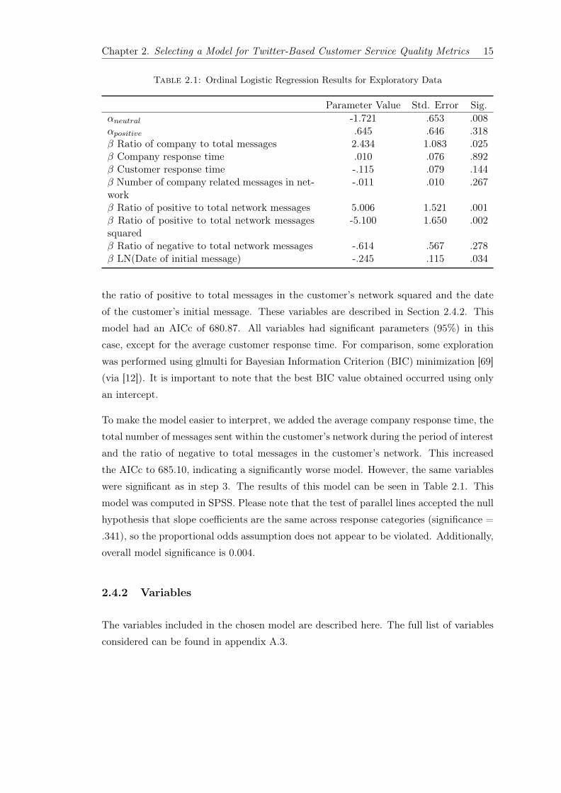
the ratio of positive to total messages in the customer’s network squared and the dateof the customer’s initial message. These variables are described in Section 2.4.2. Thismodel had an AICc of 680.87. All variables had significant parameters (95%) in thiscase, except for the average customer response time. For comparison, some explorationwas performed using glmulti for Bayesian Information Criterion (BIC) minimization [69](via [12]). It is important to note that the best BIC value obtained occurred using onlyan intercept.
To make the model easier to interpret, we added the average company response time, thetotal number of messages sent within the customer’s network during the period of interestand the ratio of negative to total messages in the customer’s network. This increasedthe AICc to 685.10, indicating a significantly worse model. However, the same variableswere significant as in step 3. The results of this model can be seen in Table 2.1. Thismodel was computed in SPSS. Please note that the test of parallel lines accepted the nullhypothesis that slope coefficients are the same across response categories (significance =.341), so the proportional odds assumption does not appear to be violated. Additionally,overall model significance is 0.004.
2.4.2 Variables
The variables included in the chosen model are described here. The full list of variablesconsidered can be found in appendix A.3.

Chapter 2. Selecting a Model for Twitter-Based Customer Service Quality Metrics 16
2.4.2.1 Service/Customer Attribute - Ratio of company to total messages
This variable divides the number of company messages by the total number of messagesin a case (that is, the number of company messages plus the number of customer messagesin a case).
2.4.2.2 Service Attribute - Company response time
This variable is the average time between a given customer message and the company’sresponse in a case.
2.4.2.3 Service Attribute - Date
This variable indicates the date of the customer’s first message.
2.4.2.4 Customer Attribute - Customer response time
This variable is the average time between a company message and the customer’s responsein a case.
2.4.2.5 Network Attribute - Number of company related messages in net-work
This variable is the total number of positive, negative, neutral and indeterminate mes-sages involving the company or its products sent during the case, as well as in the weekprior to the customer’s first message, by the customer’s friends.
2.4.2.6 Network Attribute - Ratio of positive to total network messages
This variable is the number of positive messages involving the company or its productssent during the case, as well as in the week prior to the customer’s first message, bythe customer’s friends, divided by the number of company related messages in networkvariable. In the event that the number of company related messages in network variablehad a value of 0, this variable was also coded as 0.
Chapter 2. Selecting a Model for Twitter-Based Customer Service Quality Metrics 17
2.4.2.7 Network Attribute - Ratio of negative to total network messages
This variable is the number of negative messages involving the company or its productssent during the case, as well as in the week prior to the customer’s first message, bythe customer’s friends, divided by the number of company related messages in networkvariable. In the event that the number of company related messages in network variablehad a value of 0, this variable was also coded as 0.
2.4.2.8 Service Attribute - Date of initial message
This variable indicates the date of the customer’s first message, where “1” indicates thefirst day in the data set (February 22). This value is subsequently incremented (e.g.Februrary 25 is “4”).
2.4.3 Hypotheses
Based on our exploration of part 1 of the data set, we developed some hypotheses to teston part 2 of the data set.
2.4.3.1 Ratio of company to total messages
Hypothesis 1. A higher ratio of company to total case messages increases the probabilityof a more positive case resolution (holding the date, company response time, customerresponse time, number of network messages and the percentage of positive and negativenetwork messages constant).
A higher company to total case message ratio indicates a higher service level. For eachpiece of information the customer sends to the company, he or she receives more informa-tion back. A lower company to total case message ratio would indicate that the companywas providing less information to the customer. A higher service level would result inhigher customer satisfaction. As an aside, because the first and last messages are alwayscustomer messages due to our case selection criteria, an otherwise 1:1 exchange (that is,the customer is always responded to by one company message, which is responded toby one customer message, etc.) would see a higher ratio of company to total messagesas the total number of messages in the case increased. This could be a marker of casedifficulty or complexity.
Chapter 2. Selecting a Model for Twitter-Based Customer Service Quality Metrics 18
2.4.3.2 Ratio of positive to total network messages
Hypothesis 2. A higher ratio of positive to total network messages in the period betweenone week prior to the customer’s first message and the customer’s last message initiallyincreases the probability of a more positive case resolution, but ultimately a quadraticrelationship results in a penalty for a high positive ratio (holding the date, ratio ofcompany to total messages, company response time, customer response time, number ofnetwork messages and the percentage of negative network messages constant).
Ma et al [48] found that positive sentiment expression in a customer’s network led tomore positive sentiment expression if the customer was already in a positive state andmore negative sentiment expression if the customer was already in a negative state.Our initial analysis suggests that the effect during a customer service intervention isquadratic. During a customer service event, the customer’s state is in flux. Initially, thecustomer had some complaint, but now resolution is possible. As the customer’s networkbecomes more positive, the customer may absorb some of this enthusiasm. However, ifthe network becomes too positive, the customer’s expectations may increase, resultingin a lower final sentiment when these expectations are not met.
2.4.3.3 Date of initial message
Hypothesis 3. A later chronological date decreases the probability of a more positivecase resolution, although the effect stabilizes (holding the ratio of company to total casemessages, company response time, customer response time, number of network messagesand the percentage of positive and negative network messages constant).
Our initial analysis suggests the counter intuitive result that cases handled later in thedata set are less likely to have a positive resolution. Please see Section 2.5.1 for details.
2.5 Results and Analysis
Using the untouched half of the data, the model selected in Section 2.4.1.2 produced theresults shown in Table 2.2. Overall model significance is 0.066, so the model is significantat 90%. The test of parallel lines resulted in a significance of .170, indicating the theproportional odds assumption is not rejected, so ordinal regression remains appropriate.Unfortunately (but foreshadowed by the poor BIC results in Section 2.4.1.2), the param-eters for the ratio of company to total messages and the ratio of positive to total networkmessages (and its quadratic term) are not significant in this independent sample. As

Chapter 2. Selecting a Model for Twitter-Based Customer Service Quality Metrics 19
Table 2.2: Ordinal Logistic Regression Results for Test Data
Parameter Value Std. Error Sig.↵
neutral
-2.522 .570 .000↵
positive
-.322 .555 .561� Ratio of company to total messages 1.270 1.003 .205� Company response time .067 .069 .322� Customer response time -.050 .089 .576� Number of company related messages in net-work
.009 .010 .378
� Ratio of positive to total network messages -.526 1.338 .695� Ratio of positive to total network messagessquared
.755 1.570 .631
� Ratio of negative to total network messages -.080 .508 .875� LN(Date of initial message) -.355 .104 .001
such, we are unable to address Hypotheses 1 and 2. The parameter for the natural log ofthe date of the initial message is significant, however, so Hypothesis 3 can be addressed.
2.5.1 Evaluation of Hypothesis 3
We find that the natural log of the date of the initial message has a parameter value of-0.355 with significance of 0.001 when the model was applied to the test data. This resultconfirms our hypothesis that a later chronological date decreases the probability of a morepositive case resolution, although the effect stabilizes (holding the ratio of company tototal case messages, company response time, customer response time, number of networkmessages and the percentage of positive and negative network messages constant). Thiseffect is demonstrated in Figure 2.3, using the mean values recorded in Table A.3.
One may expect the probability of positive resolution to improve over time, as the com-pany refines its customer service strategy. We propose three possible explanations forthis counter intuitive result.
1. Brand perception may have changed over time and made customers harder to please,either through a general increase in negative sentiments, or through a general increasein positive sentiments resulting in harder to satisfy higher expectations. Although wecontrol for the influence of positive and negative sentiments in a customer’s network inthe period immediately preceding (and during) a case, perhaps a long term effect is inplay. To explore this possibility, the sentiments of all of the company related messagessent by the friends of the customers in the data set were analyzed. Figure 2.4 shows thepercentage of the messages sent by these users classified as positive, negative and neutralduring each week studied. (Percentages do not add to 1 because of a small number ofmessages coded as “inconclusive”.) A linear regression suggests that the trends in positive

Chapter 2. Selecting a Model for Twitter-Based Customer Service Quality Metrics 20
Figure 2.3: Probability of positive, negative or neutral final resolution for each dayof the study period (February 22 is day 1).
and negative message percentages are not significant in this time period. These resultsseem to indicate that a general company related sentiment trend is not a driver of thisresult.
Figure 2.4: Percentage of messages sent by friends of the customers in the data setclassified as positive, negative and neutral during each week studied.
2. The customer service group may have initially been staffed by higher quality agents,who were then replaced by a new set of lower quality agents. However, if this is the case,

Chapter 2. Selecting a Model for Twitter-Based Customer Service Quality Metrics 21
we would expect to see an a reversal of this trend eventually as the new agents improved,while our model does not suggest improvement over a ten month period.
3. The customer service group may have changed its case selection methodology. Notall tweets are addressed, and the service representatives make the decision of which cus-tomers to contact. As time goes on, the customer service group becomes more confidentand established. They attempt to solve harder cases, resulting in a drop off in serviceoutcomes, but this drop off stabilizes after the transition is complete. We do not haveany metrics controlling for case complexity or the nature of the problem being addressed.As such, we cannot test this hypothesis. However, this explanation would account forthe decrease in the probability of more positive resolutions, as well as the leveling offperiod that follows.
2.5.2 Service time variables
It is of interest to note that none of the service time variables (average company responsetime, the company’s response time to a customer’s first message and the total elapsedtime of a case) were selected by AIC (or BIC) to be included in the model, despitethe well-known importance of wait time and customer satisfaction (please see Durrande-Moreau’s [22] survey of empirical research in this area, as well as Taylor’s [71] explorationof these effects). Average company response time was added manually for completeness,but was insignificant in both the model selection and hold out data regressions. Twopossible explanations are immediately apparent:
1. Signal-to-noise ratio may be too high to detect these effects in our data set. Mattilaand Mount [50] conducted an examination of the effect of company response times on e-mail-based complaint resolution. Unsurprisingly, they found that long company responsetimes resulted in decreased customer satisfaction. It would be plausible to see a similareffect in social media based customer complaint situations as well.
2. Traditional service time metrics may not be important for Twitter-based customerservice. Maister [49] notes that customers find waits to be shorter when they are occu-pied. Customers seeking resolution over Twitter do not have to wait in the same way ascustomers waiting for service over the phone or in person, so perhaps they are not con-cerned about wait time. However, a similar argument could be made for e-mail, whereresponse times are significant. A possible difference could lie in the fact that customerswho seek assistance over e-mail are actively awaiting a response, while those who areserved using Twitter may or may not have initially been expecting a response. However,this would only affect the initial response time sensitivity, and not the average companyresponse time sensitivity as once the service interaction has begun and customer would
Chapter 2. Selecting a Model for Twitter-Based Customer Service Quality Metrics 22
naturally be expecting a response. Additionally, controlling for those customers whoinitially sought out assistance (by “mentioning” (using the “@” symbol) the company orits customer service profile) does not seem to result in significant service time metricparameters in our data set. It seems necessary to mention that Maister also indicatesthat wait times of uncertain duration seem longer than those of known duration, whichwould seem to indicate that wait time could be important in Twitter-based customerservice, as there is no way for a customer to know what his or her wait might be. Forcompleteness, it is important to note that even for traditional customer service Davidow[20] suggests that wait time may not be that significant, as long as it is “reasonable”according to the situation.
2.6 Conclusion
2.6.1 Limitations
Several limitations should be acknowledged. First, the coding of the data was imperfect.That is, even under the best of conditions categorizing messages as “positive,” “negative,”and “neutral” lacks nuance. In this case, the automatic coding was not perfect, often con-flicting with manual coding, even under these rough categories. Combining the results oftwo different coding methodologies provided an important control, but the classificationwas still problematic. Unfortunately, the scale of data required precludes manual coding.However, the science of sentiment analysis continues to improve and this may not be aslarge an issue in the future.
Second, the data was extremely heterogeneous. Different products and problems werebeing discussed. For instance, one customer might have a small question about theoperation of her phone, while another customer cannot access the internet at all. Someproblems were trivial and some were serious. Additionally, the company’s response typewas also varied. In some cases, customers were simply referred to a URL for furtherassistance. Other cases involved detailed back and forth discussion between the customerand the customer support team. Again, the scale of the data causes difficulty for thecategorization and control of these issues. Further research could prove illuminating here.
Third, in order to have a “final sentiment,” only those cases where the customer sent afinal message were considered. This decision adds a bias toward gregarious customers,and it is not hard to imagine that gregariousness would be influenced by the actual finalsentiment state. Further study on this matter is required.

Chapter 2. Selecting a Model for Twitter-Based Customer Service Quality Metrics 23
Fourth, in order to consider network effects, only those cases where the customer hadcomplete network information available were considered. Hence, a few extreme customerswith more than 5000 friends or followers were excluded from the analysis, as well as thosewith screen names containing spaces. More worrisome was the exclusion of customerswith private follower lists.
Fifth, friend and follower information was time-delayed. While the company collected thenumber of followers at the time of service, the lists of customer friends and followers wereobtained well after the end of service. Because of the dynamic nature of a customer’snetwork, the list of friends and followers that were used to determine a customer’s influ-ence at time of service may not actually be the same friends and followers the customerhad at the time of service.
Sixth, the analysis considered only a customer’s first and last sentiment but not theintermediary states. Further analysis on these transitory states would be useful bothfor understanding the evolution of a customer’s sentiment change as well as seeing thesentiment effects of different firm, customer and company attributes at a higher level ofgranularity.
Finally, customer satisfaction was only measured indirectly by Twitter sentiment analysis,instead of directly by survey. We have no information about the customer (due to theanonymity of Twitter), but many demographic and experience related questions couldbe asked in a survey. More troubling, we can only guess at a customer’s customer serviceexperience quality. For example, a polite customer’s reaction may mask a substandardexperience when scanning tweets, while a direct discussion with the customer couldreveal his or her dissatisfaction. The opposite could also easily occur. Actual customerperception is completely ignored by our model.
The difference in granularity between this paper and that of Ma et al. may explainthe difference in the quality of results between the two papers. Ma et al. [48] followscustomers from message to message, only considering whether or not an interventionhappens, while this paper considers an entire customer service interaction as one case.This aggregation may be responsible for the loss of explanatory power experienced.
2.6.2 Implications for Future Research
The limitations of post-hoc Twitter-based customer service analysis are severe. Whilesentiment coding and case classification may improve with technology, there is no fix fornetwork data collection delays and the unavailability of customer perception informationbeyond better experimental design require the advance cooperation of a host company.

Chapter 2. Selecting a Model for Twitter-Based Customer Service Quality Metrics 24
By planning data collection with the company before the service interactions take place,several limitations could be removed. Additionally, the framework provided by Froehleand Roth [29] could be an excellent starting point for developing a system to determinecustomer perceptions.
1. While sentiment coding of a customer’s network may still be required, the actualcustomer sentiments could be determined by actually asking the customer, rather thaninference.
2. Through consultation with the company, a list of common problem types could bedeveloped. Going forward, the CSR who manages a case could code that case as a certainsituation, avoiding difficult post-hoc decisions and classification difficulties.
3. Through cooperation with the company, customer friend and follower informationcould be collected at the time of service, rather than months later.
The problems ingrained in post-hoc Twitter customer service analysis are difficult tosolve, but easy to bypass through advance planning and experimental design in conjunc-tion with a company. Unfortunately, the information availability problems of after thefact analysis seem to proclude simple model building.
2.7 Caveat
Initial analysis was performed on the entire data set and a multinomial logistic modelwas developed, incorporating the ratio of company to total messages, the natural logof the number of messages sent by the company during the case, the natural log of theaverage company response time, the natural log of the average customer response time,the natural log of the number of followers a customer had, the natural log of the numberof friends a customer had, the natural logs of the number of positive, neutral and negativemessages written by a customer’s friends who were also the customer’s followers in theweek before the initial message (but not during the period of case), the natural logs ofthe number of positive, neutral and negative messages written by a customer’s friendswho were not also the customer’s followers in the week before the initial message (butnot during the period of case), and the initial sentiment of the customer. All sentimentswere coded using only one coding methodology (Sentiment140).
Chapter 3
Necessary Condition for FiniteDelay Moments for FIFO GI/GI/KQueues with Integral Load
3.1 Introduction
Sufficient conditions for delay moments in stable GI/GI/K FIFO queuing systems, whichare also necessary conditions for GI/GI/1 queues, were first established by Kiefer andWolfowitz [42] [43]. Scheller-Wolf and Sigman [66], and later Scheller-Wolf [64], establishthat these conditions are not necessary for multi-server GI/GI/K queues. By adding thecondition that service times belong to class L� , as well as a requirement that traffic inten-sity is non-integer, Scheller-Wolf [65] was able to find necessary and sufficient conditionsfor GI/GI/K queues. Using methods developed by Whitt [75] and Foss and Korshunov[28], Scheller-Wolf and Vesilo [67] extended this result to service times in class L�1 , andthen to the workload at different servers within a GI/GI/K system (as opposed to onlydelay) [68].
As mentioned above, Scheller-Wolf and Vesilo [67] show that for a FIFO multiserverqueue, the rth moment of expected delay E[D
r
] will be finite if E[S
1+( r
(K�k) )] is finite,
where S represents the service time distribution, K is the number of servers in thesystem, k = b⇢c k + 1 K, k integral and load ⇢ := E[S]/E[T ], with T representingthe interarrival time distribution. This is also a necessary condition if k < ⇢ < k + 1
or if k + 1 = K, and S 2 L�1 , 1 < � < 1, � = (s � b⇢c + ↵)/(s � b⇢c), ↵ � 1.S 2 L�1 means that E[S] < 1 and if S1, ..., Sm
are i.i.d random variables distributed
This chapter is joint work with Alan Scheller-Wolf and Rein Vesilo.
25

Chapter 3. Necessary Condition for Finite Delay Moments for FIFO GI/GI/K Queueswith Integral Load 26
as S, then E(S
�
) = 1 implies E(min(S1, ..., Sm
)
m�
) = 1. Note that L�1 includes thePareto distribution. Consequently, there is a gap between the identified necessary andsufficient conditions for integral ⇢, as noted by Foss [27].
Using domain of attraction results from Feller [24], as well as results from Scheller-Wolf[65], Scheller-Wolf and Vesilo [67], Foss and Korshunov [28] and the additional assumptionthat the service time distribution S has P (X > u) ⇠ u
�↵, such as with a Paretodistribution, we find a stricter necessary condition for a GI/GI/K-server system withintegral ⇢ = R: the rth moment of expected delay E[D
r
] will be infinite if E[S
1+( r
↵(K�R) )]
is infinite, which occurs when the shape parameter of the service time distribution ↵ <
12 +
q14 +
r
K�R
. Please note that we are using R to denote integer values of ⇢, todistinguish from the notation of k used with non-integer loads. To prove this, we firstconsider the case of ⇢ = 1 (Section 3.2) then generalize to higher integral ⇢ values (Section3.3).
Theorem 3.1. For a FIFO GI/GI/K queue with integral ⇢ K, where K 2 N andS 2 L↵+1
1 and S has P (X > u) ⇠ u
�↵, with 1 ↵ 2 (such as with a Paretodistribution):
E[S
1+ r
↵(K�R)] = 1 ) E[D
r
] = 1
3.2 GI/GI/K, ⇢ = 1
We begin by characterizing a FIFO GI/GI/K queue with ⇢ = 1. The work at serveri at time n in a k-server system is denoted W
{k}n,i
. By definition, servers will not havenegative work, accordingly W
{k}n,1 ,W
{k}n,2 , ...,W
{k}n,K
� 0. Servers are periodically reorderedso that W
n,i
W
n,i+18i = 1...K � 1 . Consider a netput process Y , defined to be theamount of work accumulated by the system by job i. That is, Y
i
= (S
i
� T
i
)
+.
We will consider lower bounds of the workload at each server in this system as timeprogresses. We will show that, with some probability, the delay of the system will beproportional to x
1↵ in a deterministic arrival system (without loss of generality, as per
Lemma 3.3). We can bound this probability by comparing with a system with K � 1
servers and ⇢ =
12 . Finally, we find conditions on S that ensure an infinite expected
delay.

Chapter 3. Necessary Condition for Finite Delay Moments for FIFO GI/GI/K Queueswith Integral Load 27
3.2.1 Bounding Delay
3.2.1.1 t = �M
At time �M , we assume the system is empty. Time period M is sufficiently large thatthere is a probability P1(x) that the second server will accumulate more than C
2 x workduring this time period.
3.2.1.2 t = 0
We assume, for a given x, that by time 0, server 2 contains more than C
2 x work, where C
is chosen to be large enough to insure that C > 2 + 2✏E[S]
� 1↵ for ✏ > 0. This will occur
with some probability P1(x). Consequently, servers 2 through K must each contain morethan C
2 x work. The lower bounds on the work at each server are thus as follows.
W
{K}0,1 � 0
W
{K}0,2 >
C
2 x
...
W
{K}0,K >
C
2 x
Now, we can find bounds for P1(x), the probability that server 2 contains more than C
2 x
work using a result from Scheller-Wolf [65] .
Lemma 3.2. (Lemma 4.3, Scheller-Wolf [65]) If two initially empty FIFO queues havingK-1 and K servers, respectively, are fed by two identical interarrival and service timesequences and in addition, the queue with K-1 servers serves customers twice as fast asthe queue with K servers, then for all 1 l K � 1 and all [arrivals] n, it holds almostsurely that:
W
{K�1}n,i�1 W
{K}n,1 +W
{K}n,i
. (3.1)
Applying Lemma 3.2 to our system with i = 2, we see that W
{K�1}n,1 W
{K}n,1 +W
{K}n,2
almost surely. Because W {K}n,1 W
{K}n,2 by definition, we can see that W {K�1})
n,1 2W
{K}n,2 .
Therefore P (W
{K�1}n,1 > Cx) P (2W
{K}n,2 > Cx). By rearranging and recognizing that
the work at server 1 is equivalent to the delay of a system, we find P (D
{K�1}> Cx)
P (W
{K}n,2 >
C
2 x): the probability that the work at the second server of the K-serversystem with ⇢ = 1 exceeds C
2 x is greater than or equal to the probability that the delayof a (K-1)-server system with ⇢ =
12 exceeds Cx.

Chapter 3. Necessary Condition for Finite Delay Moments for FIFO GI/GI/K Queueswith Integral Load 28
3.2.1.3 t = x, x > 0
Because x time has passed, x work has been processed at servers 2 through K since time0. We consider x = nE[S]. However, during this same period of time, additional workmay have arrived and been sent to server 1. There is thus a possibility that work hasaccumulated at server 1. To bound this possibility, we consider additional lemmas.
We are interested in activity over a time period of x. We assume that arrival times aredeterministic with T ⌘ E[S]. However, the following analysis will still hold for generalinterarrival times, due to the following result from Foss and Korshunov [28].
Lemma 3.3. Consider a GI/GI/s system with stationary waiting time W. Now consideran auxiliary D/GI/s system with the same service times and deterministic arrival timeswith stationary waiting time W’.
If P{W 0> x} � ¯
G(x) for some long-tailed distribution G, then
lim inf
x!1
P{W > x}¯
G(x)
� 1 (3.2)
(Foss and Korshunov Lemma 2 [28])
Now, we consider the behavior of the sum of the netput process in the GI/GI/K systemwith with W
{K}0,2 � C
2 x and ⇢ = 1. Work on the order of x1↵ will accumulate at the server
with some probability, bounded by the following Lemma.
Lemma 3.4. Let Y
i
= S
i
� T , where T is deterministic and equal to E[S], and S hasP (X > u) ⇠ u
�↵ with 1 < ↵ < 2. Then,
P (
⌃Y
i
n
1↵
> ✏) ⇠ U
↵
(✏) (3.3)
where U is the stable distribution determined (including centering) by the characteristicfunction
(⇣) = |⇣|↵C �(3� ↵)
↵(↵� 1)
[cos
⇡↵
2
⌥ i(p� q)sin
⇡↵
2
]. (3.4)
Proof. Follows from Feller [24]. (Although we followed Feller, similar results are discussedin Omey and Van Gulck [59] and Petrov [61] (found via [59]).) Please see AppendixB.1.
Because interarrival time is equal to E[S], n is the number of arrivals and we are con-sidering the time period between 0 and x, we will set n =
x
E[S] in Lemma 3.4.

Chapter 3. Necessary Condition for Finite Delay Moments for FIFO GI/GI/K Queueswith Integral Load 29
P (
⌃Y
i
(x/E[S])
1↵
> ✏) ⇠ U
↵
(✏) (3.5)
To lower bound the delay in the system, we will assume W
{K}0,1 = 0. Therefore, because
servers 2 through K have a large amount of work, this new accumulated work is assignedto server 1. (If some of this work would have been assigned to server 2 we discard it,again yielding a lower bound.) Using equation (3.5), we see that this accumulated workis greater than ✏E[S]
� 1↵
x
1↵ with some probability P2(✏) = U
↵
(✏) > 0. Consequently, theupdated workload at time x is as follows.
W
{K}x,1 � ✏E[S]
� 1↵
x
1↵
W
{K}x,2 > (
C
2 � 1)x
...
W
{K}x,Q
> (
C
2 � 1)x
Recall that C > 2 + 2✏E[S]
� 1↵ and ✏ > 0. Coupled with the fact that ↵ must be greater
than 1 because of the finite mean of the service time distribution, this choice ensuresthat (
C
2 � 1)x > ✏E[S]
� 1↵
x
1↵ , which guarantees that ✏E[S]
� 1↵
x
1↵ will lower bound the
smallest workload, and therefore, the delay of the system.
To summarize our findings so far, delay in a K-server system with ⇢ = 1 will be at least✏E[S]
� 1↵
x
1↵ with some probability P2(✏) if the work at the second server exceeds C
2 , whichwill happen with probability P1(x) which is greater than or equal to the probability thatthe delay of a (K-1)-server system with ⇢ =
12 exceeds Cx:
P (D
{K}> ✏E[S]
� 1↵
x
1↵
) � P1(x)P2(✏)
� P2(✏)P (W
{K}n,2 >
C
2
x)
� P2(✏)P (D
{K�1}> Cx)
Changing variables (y = x
1↵ ):
P (D
{K}> ✏E[S]
� 1↵
y) � P2(✏)P (D
{K�1}> Cy
↵
)
Multiplying by ry
r�1:

Chapter 3. Necessary Condition for Finite Delay Moments for FIFO GI/GI/K Queueswith Integral Load 30
ry
r�1P (D
{K}> ✏E[S]
� 1↵
y) � ry
r�1P2(✏)P (D
{K�1}> Cy
↵
)
Z 1
0ry
r�1P (
D
{K}
✏E[S]
� 1↵
> y)dy �Z 1
0ry
r�1P2(✏)P (
D
{K�1}
C
> y
↵
)dy
E[S]
1↵
✏
E[D
{K}r] �
Z 1
0ry
r�1P2(✏)P (
D
{K�1}
C
> y
↵
)dy
For the next step, we use the follow result:
Lemma 3.5. Wolff [77], page 37, for � > 0
E[X
�
] =
Z 1
0�u
��1P (X > u)du
Substituting z = y
↵ then applying Lemma 3.5:
E[S]
1↵
✏
E[D
{K}r] �
Z 1
0rz
r�1↵
P2(✏)P (
D
{K�1}
C
> z)
z
1↵
�1
↵
dz
E[S]
1↵
✏
E[D
{K}r] � P2(✏)E[(
D
{K�1}
C
)
r
↵
]
E[S]
1↵
✏
E[D
{K}r] � P2(✏)C
�r
↵
E[(D
{K�1})
r
↵
]
E[D
{K}r] � ✏
E[S]
1↵
P2(✏)C�r
↵
E[(D
{K�1})
r
↵
]
So now we turn to E[(D
{K�1})
r
↵
], a value for which results already exist.
3.2.2 Delay in the (K-1)-server system
For information about the delay of this (K-1)-server system, we consider results fromScheller-Wolf [65].
Lemma 3.6. (Lemma 6.6, Scheller-Wolf [65]) For a FIFO GI/GI/K queue with k <
⇢ < k + 1 K, where k 2 N and S 2 L�+1 for � > 0:
E[S
1+ �
K�k
] = 1 ) E[D
�
] = 1
As a reminder, while the K-server system has ⇢ = 1, the (K-1)-server system has ⇢ =
12 .
Additionally, recall that we are assuming that S 2 L↵+11 . Applying Lemma 3.6 with
k = 0, K � 1 servers and � = r/↵, we see that E[S
1+ r
↵(K�1)] = 1 ) E[D
{K�1} r
↵
] = 1.

Chapter 3. Necessary Condition for Finite Delay Moments for FIFO GI/GI/K Queueswith Integral Load 31
E[D
{K}r] � ✏
E[S]
1↵
P2(✏)C�r
↵
E[D
{K�1} r
↵
]
E[S
1+ r
↵(K�1)] = 1 ) E[D
{K�1} r
↵
] = 1
E[S
1+ r
↵(K�1)] = 1 ) E[D
{K}r] = 1
3.2.3 Conditions for infinite E[S1+ r
↵(K�1) ]
Using Lemma 3.5 with � = 1 +
r
↵(K�1) and assuming P (X > u) ⇠ u
�↵:
E[X
�
] =
Z 1
0�u
��1P (X > u)du
E[S
1+ r
↵(K�1)] =
Z 1
0(1 +
r
↵(K � 1)
)u
r
↵(K�1)P (S > u)du
= (1 +
r
↵(K � 1)
)
Z 1
0u
r
↵(K�1)u
�↵du
= (1 +
r
↵(K � 1)
)
Z 1
0u
r
↵(K�1)�↵du
We see that that the limit is infinite when r
↵(K�1) � ↵ > �1.
r
↵(K � 1)
� ↵ > �1
r
↵(K � 1)
� ↵+ 1 > 0
r � ↵
2(K � 1) + ↵(K � 1) > 0
(K � 1)↵
2 � (K � 1)↵� r < 0
So E[S
1+ r
↵(K�1)] and consequently E[D
{K}r] is infinite when (K�1)↵
2�(K�1)↵�r < 0,or when ↵ <
12 +
q14 +
r
K�1 . These fall above Scheller-Wolf and Vesilo’s [67] previouslyestablished lower bounds of K+r
K
when r = 1 as shown in the table below. This is truefor all K > 2 and 0 < ⇢ < K, although the difference between the old and new boundsdecreases to 0 asymptotically. [Shown in Appendix B.2, using R = 1.] (When r >
K
K�1 ,the new bounds are still valid, but fall below the previously established bounds.)

Chapter 3. Necessary Condition for Finite Delay Moments for FIFO GI/GI/K Queueswith Integral Load 32
K Previous Lower Bound New Lower Bound2 1.500 1.6183 1.333 1.3664 1.250 1.2645 1.200 1.207
Table 3.1: Old and new lower bounds for ↵ for different numbers of servers K, with⇢ = 1
3.3 GI/GI/K, ⇢ = R, R � 2, R < K, R 2 N
Now we extend the above results to FIFO GI/GI/K queues with integral ⇢ � 2. Asbefore, we will consider the lower bounds of the workload at each server in this systemas time progresses. We will show that, with positive probability, the delay of the systemwill be proportional to x
1↵ in a deterministic arrival system (without loss of generality, as
per Lemma 3.3). We can bound this probability by comparing with a system with K�1
servers and ⇢ =
R
2 . Finally, we find conditions on S that ensure an infinite expecteddelay.
3.3.1 Bounding Delay
3.3.1.1 t = �M
At time �M , we assume the system is empty. Time period M is sufficiently large thatthere is a probability P1 that the R+1
th server will accumulate more than C
2Rx work dur-
ing this time period (where C is chosen to be large enough that C >
⇣R
R�1�1✏R
R�2(R�1)
⌘↵
(2
R+1RE[S])
and ✏ > 0, for reasoning explained in Section 3.3.1.8).
3.3.1.2 t = 0
We assume, for a given x, that server R+1 contains more than C
2Rx work. This will
occur with probability P1(x). For clarity of exposition, we will designate ⌥ =
C
2R.
Consequently, servers R+2 through K must each contain more than ⌥x work. The lowerbounds on the work at each server are thus as follows.
W
{K}0,1 � 0
W
{K}0,2 � 0
...

Chapter 3. Necessary Condition for Finite Delay Moments for FIFO GI/GI/K Queueswith Integral Load 33
W
{K}0,R � 0
W
{K}0,R+1 > ⌥x
W
{K}0,R+2 > ⌥x
...
W
{K}0,K > ⌥x
Now, we can find bounds for P1(x), the probability that server R+1 contains more than⌥x work.
Applying Lemma 3.2 to our system with s = K and i = R + 1, we see that W
{K�1}n,R
W
{K}n,1 + W
{K}n,R+1. Because W
{K}n,1 W
{K}n,R+1 by definition, we can see that W
{K�1}n,R
2W
{K}n,R+1. Therefore P (W
{K�1}n,R
> Cx) P (2W
{K}n,R+1 > Cx). Proceeding iteratively, we
find W
{K�R}n,1 2W
{K�R+1}n,2 4W
{K�R+2}n,3 ... 2
R
W
{K}n,R+1. Therefore P (W
{K�R}n,1 >
Cx) P (2
R
W
{K}n,R+1 > Cx). Please note that while the K-server system has ⇢ = R, the
(K-R)-server system has ⇢ =
R
2R.
P (W
{K�R}n,1 > Cx) P (2
R
W
{K}n,R+1 > Cx)
P (W
{K}n,R+1 >
C
2
R
x)
orP (D
{K�R}> Cx) P (W
{K}n,R+1 >
C
2
R
x)
3.3.1.3 t =
⌥2 x, x > 0
We are interested in activity over a time period of ⌥2 x, ⌥
2 x = nRE[S]. We assume thatarrival times are deterministic with T ⌘ RE[S]. These bounds will still hold for generalinterarrival times, as per Lemma 3.3. Because interarrival time is equal to RE[S], n isthe number of arrivals and we are considering the time period between 0 and ⌥
2 x, wewill set n =
⌥2RE[S]x in Lemma 3.4. (Please note that since ⇢ = R and E[S] = RT , so
E[Y ] = 0 and Lemma 3.4 is still valid.)
Because server R+1 is occupied by a large job, this new accumulated work is distributedbetween servers 1 through R. (The event of an extremely large job, i.e. larger than theworkload at server R+1, will give similar results. The reasoning for this is describedat the end of this section.) Using equation (3.5), we see that this accumulated work

Chapter 3. Necessary Condition for Finite Delay Moments for FIFO GI/GI/K Queueswith Integral Load 34
is greater than ✏(
⌥2RE[S]x)
1↵ with some probability P2(✏) = ⌦
↵
(✏) > 0. The updatedworkload is then as follows:
W
{K}⌥2 x,1
+W
{K}⌥2 x,2
+ ...+W
{K}⌥2 x,R
> ✏(
⌥2RE[S]x)
1↵
W
{K}⌥2 x,R+1
>
12⌥x
W
{K}⌥2 x,R+2
>
12⌥x
...
W
{K}⌥2 x,K
>
12⌥x
This new work could be one large job, located at server R, or it could be a series ofsmaller jobs, exactly and evenly divisible between servers 1 through R, or the divisioncould fall somewhere between these two extremes. In any case, W {K}
0,R � 1R
✏(
12RE[S]⌥x)
1↵ ,
so the updated workload is no smaller than
W
{K}⌥2 x,1
� 0
W
{K}⌥2 x,2
� 0
...
W
{K}⌥2 x,R
� 1R
✏(
⌥2RE[S]x)
1↵
W
{K}⌥2 x,R+1
>
12⌥x
W
{K}⌥2 x,R+2
>
12⌥x
...
W
{K}⌥2 x,K
>
12⌥x
In the event of an extremely large job (i.e. larger than the workload at server R+1), thisjob will cause a reordering that results in the server R+1 becoming server R. In this case,the workload at server R will be greater than 1
2⌥x, which is greater than ✏(1
2RE[S]⌥
2 x)
1↵ .
Similar reasoning holds for the time periods to follow.
3.3.1.4 t =
⌥2 x+
x
1↵
R
, x > 0
At this point, the load remains R, but at most R-1 servers are free. Consequently, workbegins accumulating linearly. This new work could be one large job, located at server

Chapter 3. Necessary Condition for Finite Delay Moments for FIFO GI/GI/K Queueswith Integral Load 35
R-1, or it could be a series of smaller jobs, exactly and evenly divisible between servers1 through R-1, or the division could fall somewhere between these two extremes. Inthe “worst” case for accumulation, work has been flowing into the system at a steadypace since time t =
⌥2 x, in very small jobs. In this event, the work will be evenly
distributed among servers 1 through R-1, which will process the work as it arrives (butnot completely, because there is 1 “extra” server’s work arriving). At time t =
⌥2 x+
x
1↵
R
we know that even in this most distributed of cases, W
{K}⌥2 x+x
1↵
R
,R�1
� 1R�1
x
1↵
R
, so the
updated workload is lower bounded by
W
{K}⌥2 x+x
1↵
R
,1
� 0
W
{K}⌥2 x+x
1↵
R
,2
� 0
...
W
{K}⌥2 x+x
1↵
R
,R�1
� 1R�1
x
1↵
R
W
{K}⌥2 x+x
1↵
R
,R
� 1R
✏(
⌥2RE[S]x)
1↵ � x
1↵
R
W
{K}⌥2 x+x
1↵
R
,R+1
>
12⌥x� x
1↵
R
W
{K}⌥2 x+x
1↵
R
,R+2
>
12⌥x� x
1↵
R
...
W
{K}⌥2 x+x
1↵
R
,K
>
12⌥x� x
1↵
R
As before, this remains true even in the event of an extremely large job.
3.3.1.5 t =
⌥2 x+
x
1↵
R
+
x
1↵
R
2 , x > 0
At this point, the load remains R, but at most only R-2 servers are free. Work continuesaccumulating linearly. This new work could be one large job, located at server R-2,or it could be a series of smaller jobs, exactly and evenly divisible between servers 1through R-2, or the division could fall somewhere between these two extremes. In anycase, W {K}
⌥2 x+x
1↵
R
+x
1↵
R
2 ],R�2
� 2R�2
x
1↵
R
2 , so the updated workload is lower bounded by
W
{K}⌥2 x+x
1↵
R
+x
1↵
R
2 ,1
� 0
W
{K}⌥2 x+x
1↵
R
+x
1↵
R
2 ,2
� 0

Chapter 3. Necessary Condition for Finite Delay Moments for FIFO GI/GI/K Queueswith Integral Load 36
...
W
{K}⌥2 x+x
1↵
R
+x
1↵
R
2 ,R�2
� 2R�2
x
1↵
R
2
W
{K}⌥2 x+x
1↵
R
+x
1↵
R
2 ,R�1
� 1R�1
x
1↵
R
� x
1↵
R
2
W
{K}⌥2 x+x
1↵
R
+x
1↵
R
2 ,R
� 1R
✏(
⌥2RE[S]x)
1↵ � x
1↵
R
� x
1↵
R
2
W
{K}⌥2 x+x
1↵
R
+x
1↵
R
2 ,R+1
>
12⌥x� x
1↵
R
� x
1↵
R
2
W
{K}⌥2 x+x
1↵
R
+x
1↵
R
2 ,R+2
>
12⌥x� x
1↵
R
� x
1↵
R
2
...
W
{K}⌥2 x+x
1↵
R
+x
1↵
R
2 ,K
>
12⌥x� x
1↵
R
� x
1↵
R
2
At this point, we suspend the reordering of servers based on workload. Note that theworkload at server R-1 is smaller than the workload at server R-2. This discrepancy is notimportant for the arguments to follow. The key is that there are a series of servers filledwith large jobs (those labeled R+1 and higher), those filled with workloads proportionalto x
1↵ (those labeled R, R-1 and R-2), and those that may be empty (servers labeled 1
through R-3).
We will show that after sufficient time passes, you may have a situation where serversR+1 through K are filled with larger workloads than servers 1 through R (we ensure thisthrough our choice of C). Servers 1 through R will have smaller workloads than serversR+1 through K, but their workloads will be lighter (due to the choice of C), greater than0 (proven in Section 3.3.1.8), and proportional to x
1↵ . The precise ordering of servers
1 through R is not important, as we only need to show that one of these servers willhave the smallest load, and therefore, indicates the delay of the system. As mentionedbefore, the arrival of a particularly large job does not change this reasoning. In the mostextreme case, we would see a series of extremely large jobs, resulting in all servers beingblocked except for that currently labeled R. This would then be the lightest workloadserver, and it is proportional to x
1↵ .
We will continue moving forward by time steps of x
1↵
R
R�i
, where i indicates the next “free”server to be considered.

Chapter 3. Necessary Condition for Finite Delay Moments for FIFO GI/GI/K Queueswith Integral Load 37
3.3.1.6 t =
⌥2 x+
x
1↵
R
+
x
1↵
R
2 + ...+
x
1↵
R
R�i
, x > 0
At this point, the load remains R, but only i servers are free, where i 2 [1, R� 1]. Workcontinues linear accumulation. This new work could be one large job, located at serveri, or it could be a series of smaller jobs, exactly and evenly divisible between servers 1through i, or the division could fall somewhere between these two extremes. In any case,W
{K}⌥2 x+x
1↵
R
+x
1↵
R
2 +...+ x
1↵
R
R�i
,i
� R�i
i
x
1↵
R
R�i
, so the updated workload is lower bounded by
W
{K}⌥2 x+x
1↵
R
+x
1↵
R
2 +...+ x
1↵
R
R�i
,1
� 0
W
{K}⌥2 x+x
1↵
R
+x
1↵
R
2 +...+ x
1↵
R
R�i
,2
� 0
...
W
{K}⌥2 x+x
1↵
R
+x
1↵
R
2 +...+ x
1↵
R
R�i
,i
� R�i
i
x
1↵
R
R�i
...
W
{K}⌥2 x+x
1↵
R
+x
1↵
R
2 +...+ x
1↵
R
R�i
,R�2
� 2R�2
x
1↵
R
2 � ...� x
1↵
R
R�i
W
{K}⌥2 x+x
1↵
R
+x
1↵
R
2 +...+ x
1↵
R
R�i
,R�1
� 1R�1
x
1↵
R
� x
1↵
R
2 � ...� x
1↵
R
R�i
W
{K}⌥2 x+x
1↵
R
+x
1↵
R
2 +...+ x
1↵
R
R�i
,R
� 1R
✏(
⌥2RE[S]x)
1↵ � x
1↵
R
� x
1↵
R
2 � ...� x
1↵
R
R�i
W
{K}⌥2 x+x
1↵
R
+x
1↵
R
2 +...+ x
1↵
R
R�i
,R+1
>
12⌥x� x
1↵
R
� x
1↵
R
2 � ...� x
1↵
R
R�i
W
{K}⌥2 x+x
1↵
R
+x
1↵
R
2 +...+ x
1↵
R
R�i
,R+2
>
12⌥x� x
1↵
R
� x
1↵
R
2 � ...� x
1↵
R
R�i
...
W
{K}⌥2 x+x
1↵
R
+x
1↵
R
2 +...+ x
1↵
R
R�i
,K
>
12⌥x� x
1↵
R
� x
1↵
R
2 � ...� x
1↵
R
R�i
We can follow this reasoning until we reach time t = ⌥2 x+
x
1↵
R
+
x
1↵
R
2 +...+
x
1↵
R
R�i
+...+
x
1↵
R
R�2 ,at which point servers 2 through K will all be busy.
3.3.1.7 t =
⌥2 x+
PR�2n=1
x
1↵
R
n
, x > 0
The updated workload is lower bounded by
W
{K}⌥2 x+
PR�2n=1
x
1↵
R
n
,1
� 0
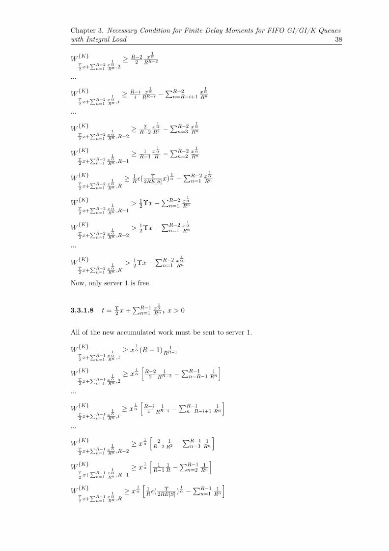
Chapter 3. Necessary Condition for Finite Delay Moments for FIFO GI/GI/K Queueswith Integral Load 38
W
{K}⌥2 x+
PR�2n=1
x
1↵
R
n
,2
� R�22
x
1↵
R
R�2
...
W
{K}⌥2 x+
PR�2n=1
x
1↵
R
n
,i
� R�i
i
x
1↵
R
R�i
�P
R�2n=R�i+1
x
1↵
R
n
...
W
{K}⌥2 x+
PR�2n=1
x
1↵
R
n
,R�2
� 2R�2
x
1↵
R
2 �P
R�2n=3
x
1↵
R
n
W
{K}⌥2 x+
PR�2n=1
x
1↵
R
n
,R�1
� 1R�1
x
1↵
R
�P
R�2n=2
x
1↵
R
n
W
{K}⌥2 x+
PR�2n=1
x
1↵
R
n
,R
� 1R
✏(
⌥2RE[S]x)
1↵ �
PR�2n=1
x
1↵
R
n
W
{K}⌥2 x+
PR�2n=1
x
1↵
R
n
,R+1
>
12⌥x�
PR�2n=1
x
1↵
R
n
W
{K}⌥2 x+
PR�2n=1
x
1↵
R
n
,R+2
>
12⌥x�
PR�2n=1
x
1↵
R
n
...
W
{K}⌥2 x+
PR�2n=1
x
1↵
R
n
,K
>
12⌥x�
PR�2n=1
x
1↵
R
n
Now, only server 1 is free.
3.3.1.8 t =
⌥2 x+
PR�1n=1
x
1↵
R
n
, x > 0
All of the new accumulated work must be sent to server 1.
W
{K}⌥2 x+
PR�1n=1
x
1↵
R
n
,1
� x
1↵
(R� 1)
1R
R�1
W
{K}⌥2 x+
PR�1n=1
x
1↵
R
n
,2
� x
1↵
hR�22
1R
R�2 �P
R�1n=R�1
1R
n
i
...
W
{K}⌥2 x+
PR�1n=1
x
1↵
R
n
,i
� x
1↵
hR�i
i
1R
R�i
�P
R�1n=R�i+1
1R
n
i
...
W
{K}⌥2 x+
PR�1n=1
x
1↵
R
n
,R�2
� x
1↵
h2
R�21R
2 �P
R�1n=3
1R
n
i
W
{K}⌥2 x+
PR�1n=1
x
1↵
R
n
,R�1
� x
1↵
h1
R�11R
�P
R�1n=2
1R
n
i
W
{K}⌥2 x+
PR�1n=1
x
1↵
R
n
,R
� x
1↵
h1R
✏(
⌥2RE[S])
1↵ �
PR�1n=1
1R
n
i

Chapter 3. Necessary Condition for Finite Delay Moments for FIFO GI/GI/K Queueswith Integral Load 39
W
{K}⌥2 x+
PR�1n=1
x
1↵
R
n
,R+1
>
12⌥x�
PR�1n=1
x
1↵
R
n
W
{K}⌥2 x+
PR�1n=1
x
1↵
R
n
,R+2
>
12⌥x�
PR�1n=1
x
1↵
R
n
...
W
{K}⌥2 x+
PR�1n=1
x
1↵
R
n
,K
>
12⌥x�
PR�1n=1
x
1↵
R
n
Remember that C >
⇣R
R�1�1✏R
R�2(R�1)
⌘↵
(2
R+1RE[S]) and ✏ > 0. Coupled with the fact that
↵ must be greater than 1 because of the finite mean of the service time distribution, thischoice ensures that the workload at server R is greater than C
0x
1↵ , where C
0 is a positiveconstant. This is proved in Appendix B.3.
To summarize our findings so far, the workload at servers 1 through R is C
0x
1↵ , where
C
0 is a constant that differs by server. Likewise servers R+1 through K have workloadsno smaller than C
0x
1↵ , because the workload at servers R+1 through K will be greater
than that at server R. That is, 12⌥x is greater than ✏
R
(
⌥x
2RE[S])1↵ . Consequently, we know
that one of the servers 1 through R must have the smallest workload. As mentionedabove, server R has a workload greater than C
0x
1↵ . Servers 1 through R-1 will also have
workloads greater than C
0x
1↵ . Please see Appendix B.3 for a proof of this. As mentioned
before, we do not establish an ordering for the workloads of servers 1 through R, exceptto say that all are of the format C
0x
1↵
> 0. Consequently, delay in a K-server systemwith integral ⇢ = R > 1 will be at least C 0
x
1↵ with some probability P2(✏) if the work at
the R+1 server exceeds ⌥x, which will happen with probability P1(x) which is greaterthan or equal to the probability that the delay of a (K-R)-server system with ⇢ =
R
2R
exceeds C
2Rx.
P (D
{K}> C
0x
1↵
) � P1(x)P2(✏)
� P2(✏)P (W
{K}n,R+1 >
C
2
R
x)
� P2(✏)P (D
{K�R}> Cx)
or taking y = x
1↵
P (D
{K}> C
0y) � P2(✏)P (D
{K�R}> Cy
↵
)
Multiplying by ry
r�1 and integrating:

Chapter 3. Necessary Condition for Finite Delay Moments for FIFO GI/GI/K Queueswith Integral Load 40
Z 1
0ry
r�1P (
1
C
0D{K}
> y)dy �Z 1
0ry
r�1P2(✏)P (
D
{K�R}
C
> y
↵
)dy
1
C
0E[D
{K}r] �
Z 1
0ry
r�1P2(✏)P (
D
{K�R}
C
> y
↵
)dy
Substituting z = y
↵:
1
C
0E[D
r{K}] �
Z 1
0rz
r�1↵
P2(✏)P (
D
{K�R}
C
> z)
z
1↵
�1
↵
dz
�Z 1
0
r
↵
z
r
↵
�1P2(✏)P (
D
{K�R}
C
> z)dz
� P2(✏)
↵
E[(
D
{K�R}
C
)
r
↵
]
� P2(✏)
↵
C
�r
↵
E[(D
{K�R})
r
↵
]
Therefore
E[D
{K}r] � C
0P2(✏)
↵
C
�r
↵
E[(D
{K�R})
r
↵
]
3.3.2 Delay in the (K-R)-server system
As a reminder, while the K-server system has ⇢ = R, the (K-R)-server system has⇢ =
R
2R. Additionally, recall that we are assuming that S 2 L↵+1. Applying Lemma 3.6
with k = 0 [because 0 <
R
2R< 1 for R � 2], K � R servers and � = r/↵, we see that
E[S
1+ r
↵(K�R)] = 1 ) E[D
{K�R} r
↵
] = 1.
Summarizing:
E[D
{K}r] � C
0P2(✏)C
�r
↵
E[D
{K�R} r
↵
].
AndE[S
1+ r
↵(K�R)] = 1 ) E[D
{K�R} r
↵
] = 1.
SoE[S
1+ r
↵(K�R)] = 1 ) E[D
{K}r] = 1.
3.3.3 Conditions for infinite E[S1+ r
↵(K�R) ]
Using Lemma 3.5 With � = 1 +
r
↵(K�R) and assuming P (X > u) ⇠ u
�↵

Chapter 3. Necessary Condition for Finite Delay Moments for FIFO GI/GI/K Queueswith Integral Load 41
E[X
�
] =
Z 1
0�u
��1P (S > u)du
E[S
1+ r
↵(K�R)] =
Z 1
0(1 +
r
↵(K �R)
)u
r
↵(K�R)P (X > u)du
= (1 +
r
↵(K �R)
)
Z 1
0u
r
↵(K�R)u
�↵du
= (1 +
r
↵(K �R)
)
Z 1
0u
r
↵(K�R)�↵du
We see that that the limit is infinite when r
↵(K�R) � ↵ � �1.
r
↵(K �R)
� ↵ � �1
r
↵(K �R)
� ↵+ 1 � 0
r � ↵
2(K �R) + ↵(K �R) � 0
(K �R)↵
2 � (K �R)↵� r � 0
So E[S
1+ r
↵(K�R)] and consequently E[D
{K}r] is infinite when (K�R)↵
2�(K�R)↵�r <
0, or when ↵ <
12 +
q14 +
r
K�R
. These fall above above Scheller-Wolf and Vesilo’s [67]previously established lower bounds of K�R+1+r
K�R+1 when r = 1 as shown in the table below,for all K > 2 and 0 < R < K, although the difference between the old and new boundsdecreases to 0 asymptotically. [Shown in Appendix B.2.] (When r >
K�R+1K�R
, the newbounds fall below the previously established bounds.)
R Previous Lower Bound New Lower BoundK-1 1.500 1.618K-2 1.333 1.366K-3 1.250 1.264K-4 1.200 1.207
Table 3.2: Old and new lower bounds for ↵ for different numbers of servers K, anddifferent loads ⇢ = R
3.4 Conclusion
We have successfully extended the Scheller-Wolf and Vesilo [68] necessary conditionsfor finite mean delay with integral load for FIFO GI/GI/K queues, with service times

Chapter 3. Necessary Condition for Finite Delay Moments for FIFO GI/GI/K Queueswith Integral Load 42
belonging to class L1+↵1 and service time distributions S such that P (X > u) ⇠ u
�↵
(such as Pareto), for those moments r < 1 +
1K�R
, under certain conditions. Previouswork established that the finite delay conditions of a system with integral ⇢ would beno worse than a system with ⇢ + ✏ and no better than a system with ⇢ � ✏. This workshows that the finite delay conditions will be strictly worse than a system with ⇢ � ✏,but whether more lenient conditions than those found for ⇢+ ✏ are available remains anopen question.

Chapter 4
Revenue Management withBargaining and a Finite Horizon
4.1 Introduction
Negotiation is commonplace in both business to business (B2B) and business to customer(B2C) interactions. Consider the situation of an airline. For each flight, the airline holdsan inventory of seats that can only be sold before the plane takes off. They must decidehow they will approach pricing, with the hope of obtaining the maximum payment fortheir inventory. Myerson [54] details four different price-deciding mechanisms. Appliedto this example, the airline could set a price and let the buyer decide if it is acceptable(seller posted price, SPP), the airline could allow the buyer to set a price and then decidefor itself if it is acceptable (buyer posted price, BPP), the airline and the buyer couldeach choose a price and then split-the-difference (STD), or the airline could conduct anegotiation with the buyer (represented by the neutral bargaining solution, NBS, devel-oped by Myerson [53]). The seller must determine which of these options is expectedto provide the greatest return. In this paper, we investigate the relative performance ofthese approaches from the seller’s perspective.
Bhandari and Secomandi [8] consider the problem of a seller selling an inventory item-by-item to multiple, stochastically-arriving, non-strategic buyers over an infinite horizonsales period. The distributions of the seller’s and buyer’s valuations are known to bothparties, but the actual valuations remain private. To model this situation, they developa Markov decision process based on Myerson and Satterthwaite’s [55] model. However,while Myerson and Satterthwaite consider a seller who has an exogenous valuation fora unit of inventory, Bhandari and Secomandi endogenously model the seller’s remaining
This chapter is joint work with Nicola Secomandi.
43
Chapter 4. Revenue Management with Bargaining and a Finite Horizon 44
inventory valuation as the (optimal) opportunity cost of that unit of inventory, gener-alizing the SPP-specific model of Das Varma and Vettas [19]. We extend the Bhandariand Secomandi [8] model to the more realistic finite horizon case. While our model isanalogous, a different strategy is required for proving the structural results.
An important caveat is that in our model, the time remaining to sell the inventory isthe private information of the seller. Consequently, the buyers do not have the necessaryinformation to strategically exploit the seller’s limited time. This assumption makes ourmodel internally consistent, as each period is the same to the buyer, but is not veryrealistic--one possible scenario would be a seller of expiring printer ink, who would havea secret, but binding, sell-by date for the ink inventory. On a related note, the seller’sinventory level is also the private information of the seller, but this situation occursfrequently in practice.
Analytically, we demonstrate that SPP always performs at least as well for the selleras NBS, which always performs at least as well as BPP, and that STD always per-forms at least as well as BPP. Compactly, SPP � NBS � BPP and STD � BPP .More generally, we demonstrate that a mechanism with a higher interim expected util-ity will produce a higher value for the seller at a given time-to-go and inventory level,extending the analytical findings of Bhandari and Secomandi [8] to a finite-horizon case.Numerically, we find that the quantitative differences between the seller’s optimal valuefunction under the four considered mechanisms in Chatterjee and Samuelson’s [15] sym-metric uniform trading problem (SUTP) change when moving from an infinite to a finitetime horizon. While in the infinite horizon case the STD mechanism can dominate theother mechanisms under extreme parameter values, we show that this same dominanceoccurs in the finite horizon case using much more plausible parameter values. This isan important finding because, although not as simple to use as SPP or BPP, STD is aneasy to implement mechanism that can be used in a variety of practical settings. Forinstance, a buyer and seller could simply report their valuations to a webpage whichcould then return the negotiated price. The evenness of the split can even be adjusted toaccommodate varying degrees of bargaining power, although we do not investigate thisfeature. From a broader perspective, while the NBS mechanism provides a normativerepresentation of the outcome of face-to-face negotiation, the STD mechanism could beimplemented as an automated negotiation.
Because modeling private information is more challenging for the STD and NBS mecha-nisms than for the SPP and BPP mechanisms, we quantify the importance of modelingprivate information when computing the seller’s opportunity cost under the STD andNBS mechanisms. We find that modeling private information has only a small effect inthe evaluation of the seller’s value function in the NBS case, but has a substantial effect

Chapter 4. Revenue Management with Bargaining and a Finite Horizon 45
in STD cases where there is relatively high time-to-go and relatively little inventory.Consequently, it may be acceptable to use a simplified model that assumes voluntarydisclosure of both the seller’s and the buyers’ valuations to compute the seller’s oppor-tunity cost under the NBS mechanism. This simplified model may also be acceptableunder the STD mechanism, but only in cases where there is relatively high inventory andrelatively little time-to-go.
Kuo, Ahn and Aydin [44] consider a similar problem, with a finite time horizon, but usinga generalized Nash bargaining solution requiring the true valuations of both parties to bevoluntarily revealed without the need to model incentive compatibility issues (completeinformation). They find that allowing negotiation (via the generalized Nash bargainingsolution) can result in more favorable outcomes for the seller than a posted price, dueto the advantage of price discrimination. Ayvaz-Cavdaroglu et al. [5] also build a modelto study SPP and BPP within a finite horizon and private information setting, with theaddition of unknown, non-stationary buyer and seller distributions. However, they focusonly on posted pricing mechanisms.
Within the realm of mechanism comparison, Riley and Zeckhauser [62] consider the saleof a single unit of inventory and find SPP to be the best possible mechanism for the seller.Gallien [32] considers the sale of multiple units of inventory, and also finds SPP to be thebest possible mechanism for the seller. However, both Riley and Zeckhauser and Gallienuse a dominant equilibrium framework, which assesses a mechanism against all potentialchoices made by buyers, as opposed to a Bayesian Nash equilibrium framework, whichassesses a mechanism against the beliefs the seller holds about the likely choices of thebuyers. Significantly, STD is incompatible with the dominant equilibrium framework,and our (Bayesian Nash equilbrium based) findings suggest that STD can outperformSPP when the seller is weak. Also challenging the superiority of SPP are Wang [74] andRoth et al. [63] who demonstrate the advantages of the Nash bargaining solution (whichsignificantly does not allow for private information).
In Section 4.2, we detail our model, which includes both a finite horizon and privateinformation, then structurally analyze this model in Section 4.3. We discuss the relevanceof modeling private information in Section 4.4. Numerical results are presented in Section4.5. Finally, Section 4.6 includes a summary and thoughts on future work. Additionalnumerical results are included in Appendix C.

Chapter 4. Revenue Management with Bargaining and a Finite Horizon 46
4.2 Model
In this section, we first consider Myerson and Satterthwaite’s one-period static bargainingmodel [55] in Subsection 4.2.1. In Subsection 4.2.2, we discuss the application of thismodel to the SUTP. We then consider the different properties of mechanisms, as well asthe application of Myerson’s [54] four mechanisms to the SUTP. Finally, we extend thesemodels into a new multi-period stochastic dynamic model in Subsection 4.2.3.
4.2.1 Static Bargaining Model
First, consider a static bargaining model by Myerson and Satterthwaite [55] and describedby Bhandari and Secomandi [8], but with valuations scaled to [0,1], rather than the moregeneral [a, b]. A risk neutral seller with one unit of inventory holds a valuation for theunit of v1 2 V1 = [0, 1]. (Throughout this paper, we will use subscripts of 1 to referto the seller, consistent with the notation in the literature.) A risk neutral buyer’svaluation for the unit of inventory is v2 2 V2 = [0, 1]. (We will use subscripts of 2 torefer to the buyer.) Each party knows his own valuation, but not the valuation of theother party. The buyer believes the seller’s valuation to be drawn from a cumulativedistribution function F1(v1). Similarly, the seller believes the buyer’s valuation to bedrawn from distribution F2(v2). F1(v1) and F2(v2) both have support [0, 1], and bothare public knowledge. An intermediary will confidentially request valuations from boththe seller and buyer, and then apply some bilateral bargaining mechanism j to determinea candidate sale price. If this price is mutually acceptable, a sale will occur. Otherwise,the buyer will leave without a sale. We use s
j
(v1, v2) 2 {0, 1} to indicate whether asale occurs given that a buyer with valuation v2 arrives, the seller has valuation v1 andmechanism j is applied. We let sj(v1, v2) = 1 if the sale occurs and 0 otherwise. Similarly,x
j
(v1, v2) will be the price paid under the same conditions. (If a sale does not occur,x
j
(v1, v2) = 0.) The transfer probability under mechanism j for valuations v1 and v2 isp
j
(v1, v2) 2 [0, 1]. That is, sj(v1, v2) = 1 with probability p
j
(v1, v2), and s
j
(v1, v2) = 0
with probability 1� p
j
(v1, v2).
4.2.2 Mechanisms
The SUTP proposed by Chatterjee and Samuelson [15] follows the static bargainingmodel described above with F1(v1) = v1 and F2(v2) = v2. The following summaryof four mechanisms, as well as their characteristic prices and transfer probabilities, wasoriginally presented by Myerson [54] and Bhandari and Secomandi [8]. First, a seller maypost a price that the buyer may accept or reject. In the SUTP, the corresponding transfer
Chapter 4. Revenue Management with Bargaining and a Finite Horizon 47
probability p
SPP
(v1, v2) will be equal to the probability that v2 � 1+v12 , and the price
paid will be x
SPP
(v1, v2) = p
SPP
(v1, v2)1+v12 . Analogously, a buyer may post a price
that the seller may accept or reject. In the SUTP, in this case the transfer probabilityp
BPP
(v1, v2) will be equal to the probability that v22 � v1, and the price paid will be
x
BPP
(v1, v2) = p
BPP
(v1, v2)v22 . The buyer and seller may both propose prices which
would then be averaged (possibly weighted by bargaining power, however in the SUTPthe two parties have equal bargaining power) to split-the-difference with a proposed“compromise” price, which the buyer and seller would then accept or reject. In the SUTP,the transfer probability p
STD
(v1, v2) will be equal to the probability that v2 � v1 +14
and the price paid will be x
STD
(v1, v2) = p
STD
(v1, v2)v1+v2+
12
3 . Finally, the neutralbargaining solution (Myerson [53]) corresponds to a seller posted price outcome whenthe seller has higher bargaining power, and a buyer posted price outcome when the buyerhas higher bargaining power. In the SUTP, the transfer probability p
NBS
(v1, v2) will beequal to the probability that either v2 � 3v1 or 3v2�2 � v1. The corresponding price paidwill be xNBS
(v1, v2) = p
NBS
(v1, v2)v22 if v2 1�v1 and x
NBS
(v1, v2) = p
NBS
(v1, v2)1+v12
otherwise.
All four of the mechanisms described above are direct mechanisms, meaning that anintermediary produces price and transfer decisions for a buyer and seller who concurrentlyand confidentially report their valuations [54]. To formally understand the properties ofthese and other mechanisms, we can consider the interim expected utility of the sellerand buyer, or the expected gap between the price and valuation of one unit for that partywhen negotiating with the other party. As before, the following is a summary of Myerson[54], using notation from Bhandari and Secomandi [8]. For the seller, this utility will bethe expected price received less the valuation of the seller times the probability of thesale. For the buyer, it will be the valuation of the buyer times the probability of the saleminus the price paid. For ease of exposition, we define
x
j
1(v1) :=
Z
v22V2
x
j
(v1, v2)dF2(v2),
x
j
2(v2) :=
Z
v12V1
x
j
(v1, v2)dF1(v1),
p
j
1(v1) :=
Z
v22V2
p
j
(v1, v2)dF2(v2),
p
j
2(v2) :=
Z
v12V1
p
j
(v1, v2)dF1(v1).
The term x
j
1(v1) is the expected price from the seller’s perspective, that is, with knownseller’s valuation v1. Similarly, xj2(v2) is the expected price from the buyer’s perspective,with known buyer’s valuation v2. Similarly, pj1(v1) and p
j
2(v2) are the expected transferprobabilities for the seller and buyer, respectively. Using this notation, the interim

Chapter 4. Revenue Management with Bargaining and a Finite Horizon 48
expected utility for the seller is u
j
1(v1) := x
j
1(v1) � v1pj
1(v1), and the interim expectedutility for the buyer u
j
2(v2) := v2pj
2(v2)� x
j
2(v2).
A direct mechanism is incentive compatible when the buyer and seller expect their high-est utility outcomes from “reporting [their] true valuations” [54] to the intermediary,assuming truthful reporting by the other party. Formally, u
j
1(v1) � x
j
1(v1) � v1pj
1(v1)
8v1, v1 2 V1 and u
j
2(v2) � v2pj
2(v2)� x
j
2(v2) 8v2, v2 2 V2 [8].
A mechanism is individually rational when neither the buyer nor seller expect negativeutility outcomes from the negotiation [54]. Formally, uj1(v1) � 0 8v1 2 V1 and u
j
2(v2) � 0
8v2 2 V2 [8].
Mechanisms that are “both individually rational and incentive compatible” are calledfeasible [54]. All four of the mechanisms described above are both direct and feasible,and our analytical results will focus on mechanisms with these properties. The Bayesianequilibrium of any mechanism can be represented using a direct and incentive compatiblemechanism via the revelation principle, so this restriction is without loss of generality[54].
4.2.3 Stochastic and Dynamic Model
Now we extend the static case to a dynamic case. Consider a risk neutral seller withy 2 Y = {1, ..., Y } units of inventory (where Y is the starting inventory), and t 2 T =
{0, ..., T} time periods in which that inventory may be sold, or “time-to-go” (where T isthe first sale period). With 0 time-to-go, the value of the inventory is 0. Additionally,� 2 (0, 1] is the discount factor for the seller for one period. For each time period, theprobability that a customer arrives is � 2 (0, 1]. That is, at most one customer mayarrive per period. If either � or � is zero, the problem becomes trivial. The quantities Y ,y, T , � and � are known only to the seller. While many realistic scenarios could feature aseller’s private starting inventory, current inventory, discount factor and customer arrivalrate, a private deadline T is rather rare. However, this assumption is required for theinternal consistency of our model, which does not include buyers strategically exploitingthe information of an impending sell-by date. The seller has a valuation for one unit ofinventory v1, but this valuation now depends on the amount of inventory remaining andtime-to-go. Each buyer has a valuation for a unit of inventory v2 2 V2 = [0, 1]. Eachparty knows his own valuation, but not the valuation of the other party. Each buyerbelieves the seller’s valuation to be drawn from distribution F1(v1). Similarly, the sellerbelieves each buyer’s valuation to be drawn from distribution F2(v2). F1(v1) and F2(v2)
both have support [0, 1], and both are public knowledge. During each time period, if abuyer arrives, the seller and buyer will confidentially report their valuations to a mediator

Chapter 4. Revenue Management with Bargaining and a Finite Horizon 49
who will apply some direct and feasible mechanism j to determine a candidate sale price.If this price is mutually acceptable, a sale will occur. Otherwise, the buyer will leavewithout a sale. As before, we use s
j
(v1, v2) to indicate whether a sale occurs, xj(v1, v2)for the price paid, and p
j
(v1, v2) for the transfer probability.
To study this dynamic case, we develop a stochastic dynamic programming model. Ourmodel is comparable to that of Bhandari and Secomandi [8], with the added complicationof a finite horizon. We want to develop a model for V
j
t
(y), the optimal expected valueof the y units of inventory remaining, given that we have t time periods left in which tosell the units.
At time t, a customer will not arrive with probability (1� �). In this case, the value tothe seller of y units of inventory at time t is simply the value of y units of inventory attime t � 1 discounted by �. The seller has no opportunity for action. A customer willarrive at time period t with probability �. In this case, a price x
j
(v1, v2) is paid frombuyer to seller (again, this price will be 0 if no sale occurs). Remember that while theseller must decide v1, he only knows the distribution of v2, hence we will use a tilde toindicate that v2 is a random variable. If the sale occurs, the seller also has the discountedvalue of his remaining y � 1 units to sell over t � 1 more periods. If the sale does notoccur, the seller has the discounted value of the full y units to sell over t�1 more periods.This result is the following stochastic dynamic programming model:
V
j
t
(y) = (1� �)�V
j
t�1(y)
+� max
v12V1
E[x
j
(v1, v2) + �V
j
t�1(y � 1)1{sj(v1, v2) = 1}
+�V
j
t�1(y)1{sj
(v1, v2) = 0}]. (4.1)
Because the seller will obtain nothing more if he has sold all of his inventory, we defineV
j
t
(0) := 0. Similarly, if the seller runs out of time, his inventory is valueless. Conse-quently, V j
0 (y) := 0. Model (4.1) can be rearranged as
V
j
t
(y) = (1� �)�V
j
t�1(y) + � max
v12V1
[x
j
1(v1) + �V
j
t�1(y � 1)p
j
1(v1) + �V
j
t�1(y)(1� p
j
1(v1))]
= �V
j
t�1(y) + � max
v12V1
[x
j
1(v1) + �V
j
t�1(y � 1)p
j
1(v1)� �V
j
t�1(y)pj
1(v1)]. (4.2)
Finally, we will use the notation �V
j
t
(y) := V
j
t
(y)� V
j
t
(y � 1) to condense model (4.2):
V
j
t
(y) = �V
j
t�1(y) + � max
v12V1
[x
j
1(v1)� ��V
j
t�1(y)pj
1(v1)]. (4.3)
Chapter 4. Revenue Management with Bargaining and a Finite Horizon 50
The opportunity cost to the seller for the sale of the y
th unit of inventory at time t isequal to ��V
j
t�1(y). By the feasibility of mechanism j, this quantity will then be theoptimal reported valuation of the seller, assuming that the opportunity cost lies withinthe support of F1(v1), or ��V
j
t�1(y) 2 V1 = [0, 1]. We prove that this is the case inLemma 4.1.
4.3 Structural Analysis
In this section we demonstrate the ordering of value functions of the four mechanismsof interest. In order to show this, we first establish that the opportunity cost of theseller ��V
j
t�1(y) 2 V1 ⌘ [0, 1] (Lemma 4.1), and is consequently the optimal choicefor v1 in model (4.3) (Proposition 1). Next, we demonstrate that the ordering of theseller’s interim expected utilities between mechanisms corresponds to the ordering ofvalue functions (Theorem 1). That is, a mechanism j with a higher interim expectedutility than mechanism k will also have a higher value function value, for a given t andy. Combining this result with the ordering of interim expected utilities for the fourmechanisms under study given by Bhandari and Secomandi [8] allows us to establish theordering of the value functions of these mechanisms when each transaction opportunityis modeled consistently with the SUTP, for a given y and t (Proposition 2).
Lemma 4.1. (a) Given direct and feasible mechanism j, the optimal value function V
j
t
(y)
is weakly increasing at a non-increasing rate in inventory 8y 2 Y [ {0}. Equivalently,the function ��V
j
t
(y) is nonnegative and weakly decreases in inventory 8y 2 Y. (b)Moreover, it holds that ��V
j
t
(y) 1, 8y 2 Y.
Lemma 4.1 is analogous to Lemma 2 in Bhandari and Secomandi [8], with the exceptionthat our Lemma 4.1 does not require u
j
1(1) = 0. The proof that follows, however, isnecessarily different.
Proof. (a) First, we show that V
j
t
(y) is weakly increasing in inventory, using analogousreasoning to Bhandari and Secomandi [8].
As defined, V j
0 (y) ⌘ 0 for all y 2 Y [ {0}. Consequently, �V
j
0 (y) ⌘ 0 for all y � 1.

Chapter 4. Revenue Management with Bargaining and a Finite Horizon 51
We make the induction hypothesis �V
j
t
(y) � 0 for steps 1, ..., t � 1 and all y 2 Y.Consider time t. We define v
⇤1,t(y) 2 argmax
v12V1 [xj
1(v1)� ��V
j
t�1(y)pj
1(v1)]. We have
�V
j
t
(y) = V
j
t
(y)� V
j
t
(y � 1)
= �V
j
t�1(y) + � max
v12V1
[x
j
1(v1)� ��V
j
t�1(y)pj
1(v1)]
��V j
t�1(y � 1)� � max
v12V1
[x
j
1(v1)� ��V
j
t�1(y � 1)p
j
1(v1)]
= ��V
j
t�1(y) + �x
j
1(v⇤1,t(y))� ���V
j
t�1(y)pj
1(v⇤1,t(y))
��xj1(v⇤1,t(y � 1)) + ���V
j
t�1(y � 1)p
j
1(v⇤1,t(y � 1))
� ��V
j
t�1(y) + �x
j
1(v⇤1,t(y � 1))� ���V
j
t�1(y)pj
1(v⇤1,t(y � 1))
��xj1(v⇤1,t(y � 1)) + ���V
j
t�1(y � 1)p
j
1(v⇤1,t(y � 1))
= �[(1� �p
j
1(v⇤1,t(y � 1)))�V
j
t�1(y) + �p
j
1(v⇤1,t(y � 1))�V
j
t�1(y � 1)]
� 0,
where the first inequality follows from the optimality of v⇤1,t(y) in stage t and state y,and the second inequality from the observation that 0 ��p
j
1(v⇤1,t(y � 1)) 1 and the
application of the induction hypothesis.
Consequently, �V
j
t
(y) � 0 for all t 2 T , and all y 2 Y by the principle of mathematicalinduction.
Next, we show that V j
t
(y) increases at a non-increasing rate in inventory. This propertyis trivially true in stage 0 because V
j
0 (y) ⌘ 0 for all y 2 Y [ {0}.
We make the induction hypothesis �V
j
t
(y) �V
j
t
(y�1) for steps 1, ..., t�1 and 8y 2 Y.Consider time t. Proceeding as in the proof of part (a), but with respect to �V
j
t
(y � 1)
yields
�V
j
t
(y � 1) � �[(1� �p
j
1(v⇤1,t(y � 2)))�V
j
t�1(y � 1) + �p
j
1(v⇤1,t(y � 2))�V
j
t�1(y � 2)]
= ��V
j
t�1(y � 1) + ��p
j
1(v⇤1,t(y � 2))[�V
j
t�1(y � 2)��V
j
t�1(y � 1)]
� ��V
j
t�1(y � 1), (4.4)
Chapter 4. Revenue Management with Bargaining and a Finite Horizon 52
where the last inequality follows from the induction hypothesis and ��pj1(v⇤1,t(y � 1)) 2[0, 1]. We also have
�V
j
t
(y) = V
j
t
(y)� V
j
t
(y � 1)
= �V
j
t�1(y) + � max
v12V1
[x
j
1(v1)� ��V
j
t�1(y)pj
1(v1)]
��V j
t�1(y � 1)� � max
v12V1
[x
j
1(v1) + ��V
j
t�1(y � 1)p
j
1(v1)]
= �V
j
t�1(y) + �x
j
1(v⇤1,t(y))� ���V
j
t�1(y)pj
1(v⇤1,t(y))
��V j
t�1(y � 1)� �x
j
1(v⇤1,t(y � 1)) + ���V
j
t�1(y � 1)p
j
1(v⇤1,t(y � 1))
��V
j
t�1(y) + �x
j
1(v⇤1,t(y))� ���V
j
t�1(y)pj
1(v⇤1,t(y))
��xj1(v⇤1,t(y)) + ���V
j
t�1(y � 1)p
j
1(v⇤1,t(y))
= �[(1� �p
j
1(v⇤1,t(y)))�V
j
t�1(y) + �p
j
1(v⇤1,t(y))�V
j
t�1(y � 1)]
�[(1� �p
j
1(v⇤1,t(y)))�V
j
t�1(y � 1) + �p
j
1(v⇤1,t(y))�V
j
t�1(y � 1)]
= ��V
j
t�1(y � 1), (4.5)
where the first inequality follows from the optimality of v⇤1,t(y�1) in stage t and state y�1
and the second inequality follows from the induction hypothesis and �p
j
1(v⇤1,t(y � 1)) 2
[0, 1].
Now we apply (4.4) and (4.5) to bound from above the difference between �V
j
t
(y) and�V
j
t
(y � 1):
�V
j
t
(y)��V
j
t
(y � 1) ��V
j
t�1(y � 1)��V
j
t
(y � 1)
��V
j
t�1(y � 1)� ��V
j
t�1(y � 1)
= 0,
where the first inequality follows from inequality (4.5), and the second inequality frominequality (4.4). Consequently, �V
j
t
(y) ��V
j
t
(y � 1) 0 for all t 2 T , and all y 2 Yby the principle of mathematical induction.

Chapter 4. Revenue Management with Bargaining and a Finite Horizon 53
(b) We trivially have �V
j
0 (y) = 0 1 for all y 2 Y . We make the induction hypothesisthat �V
j
t
(y) 1 for all t = 1, ..., t� 1 and all y 2 Y. In stage t we obtain
�V
j
t
(y) = V
j
t
(y)� V
j
t
(y � 1)
= �V
j
t�1(y) + � max
v12V1
[x
j
1(v1)� ��V
j
t�1(y)pj
1(v1)]
��V j
t�1(y � 1)� � max
v12V1
[x
j
1(v1)� ��V
j
t�1(y � 1)p
j
1(v1)]
= �V
j
t�1(y) + �x
j
1(v⇤1,t(y))� ���V
j
t�1(y)pj
1(v⇤1,t(y))
��V j
t�1(y � 1)� �x
j
1(v⇤1,t�1(y � 1)) + ���V
j
t�1(y � 1)p
j
1(v⇤1,t�1(y � 1))
�[1� �p
j
1(v⇤1,t(y))]�V
j
t�1(y) + ���V
j
t�1(y � 1)p
j
1(v⇤1,t(y))
+�[x
j
1(v⇤1,t(y))� x
j
1(v⇤1,t(y)]
= �{�V
j
t�1(y) + �p
j
1(v⇤1,t(y))[�V
j
t�1(y � 1)��V
j
t�1(y)]}
�V
j
t�1(y) +�V
j
t�1(y � 1)��V
j
t�1(y)
= �V
j
t�1(y � 1)
1, (4.6)
where the first inequality follows from the optimality of v⇤1,t(y � 1) at stage t and statey � 1 and rearranging, the second inequality from part (a) and �pj1(v⇤1,t(y)) 2 [0, 1], andthe final inequality from the induction hypothesis.
As in Bhandari and Secomandi [8], Lemma 4.1 and the incentive compatibility of mech-anism j imply the following proposition, analogous to Proposition 1 in that paper.
Proposition 4.2. If direct mechanism j is feasible then the seller’s optimal value functionsatisfies the following conditions, for all t and y:
V
j
t
(y) = �V
j
t�1(y) + �[x
j
1(��V
j
t�1(y))� ��V
j
t�1(y)pj
1(��V
j
t�1(y))].
Proposition 4.2 combines our new stochastic dynamic program model with the interpre-tation of the seller’s valuation v1 as the seller’s opportunity cost of one unit of inventory��V
j
t�1(y) (incentive compatibility). The results of Lemma 4.1 demonstrate that this isacceptable, by showing that 0 ��V
j
t�1(y) 1.
Now that we have resolved the nature of our model, we can consider the circumstancesunder which different mechanisms can be compared. The following theorem (which isanalogous to Theorem 1 in Bhandari and Secomandi [8]) relates the ordering of theseller’s interim expected utilities for different mechanisms to the ordering of the valuefunctions for those mechanisms (defined by Proposition 4.2).

Chapter 4. Revenue Management with Bargaining and a Finite Horizon 54
Theorem 4.3. Suppose that direct and feasible mechanisms j and k are defined on setV1 ⇥ V2 ⌘ [0, 1]
2, and are such that the seller’s interim expected utilities are ordered asu
j
1(v1) � u
k
1(v1), 8v1 2 V1. Then it holds that V j
t
(y) � V
k
t
(y), 8y 2 Y [ {0} and 8t 2 T .
Proof. We have V
j
0 (y) ⌘ V
k
0 (y) ⌘ 0, 8y 2 Y [ {0}. Thus the property trivially holdsin stage 0. Make the induction hypothesis that V
j
t
(y) � V
k
t
(y) for steps 1, ..., t � 1 and8y 2 Y. Consider stage t. Lemma 4.1 combined with the assumption on the interimexpected utilities of mechanisms j and k implies
V
k
t
(y) = �V
k
t�1(y) + �[x
k
1(��V
k
t�1(y))� ��V
k
t�1(y)pk
1(��V
k
t�1(y))]
�V
k
t�1(y) + �[x
j
1(��V
k
t�1(y))� ��V
k
t�1(y)pj
1(��V
k
t�1(y))],
which can be rearranged as
�x
j
1(��V
k
t�1(y)) � V
k
t
(y)� �V
k
t�1(y) + ���V
k
t�1(y)pj
1(��V
k
t�1(y)). (4.7)
Using Lemma 4.1 and the feasibility of mechanism j, we obtain
V
j
t
(y) = �V
j
t�1(y) + �[x
j
1(��V
j
t�1(y))� ��V
j
t�1(y)pj
1(��V
j
t�1(y))]
� �V
j
t�1(y) + �[x
j
1(��V
k
t�1(y))� ��V
j
t�1(y)pj
1(��V
k
t�1(y))],
which rearranged is
�x
j
1(��V
k
t�1(y)) V
j
t
(y)� �V
j
t�1(y) + ���V
j
t�1(y)pj
1(��V
k
t�1(y)). (4.8)
Using inequalities (4.7) and (4.8) yields
V
j
t
(y)��V j
t�1(y)+���V
j
t�1(y)pj
1(��V
k
t�1(y)) � V
k
t
(y)��V k
t�1(y)+���V
k
t�1(y)pj
1(��V
k
t�1(y)).
This inequality can be rearranged as
V
j
t
(y)� V
k
t
(y) � �[(1� �p
j
1(��V
k
t�1(y)))(Vj
t�1(y)� V
k
t�1(y))
+�p
j
1(��V
k
t�1(y))(Vj
t�1(y � 1)� V
k
t�1(y � 1))]
� 0,
where the second inequality follows from the induction hypothesis and �pj1(��V
k
t�1(y)) 2[0, 1]. By the principle of mathematical induction the property is true in all stages andstates.
Chapter 4. Revenue Management with Bargaining and a Finite Horizon 55
Now that we have a theorem to order the seller’s value function under different mech-anisms based on the ordering of the interim expected utilities of the seller under thosemechanisms, we need to know the ordering of the mechanisms under consideration, sum-marized in Lemma 4.4.
Lemma 4.4. (Bhandari and Secomandi [8] Lemma 1) For SUTP it holds that uSPP
1 (v1) �u
NBS
1 (v1) � u
BPP
1 (v1) and u
STD
1 (v1) � u
BPP
1 (v1), 8 v1 2 V1
As in the infinite horizon case, we can use Theorem 1 and Lemma 4.4 to establish valuefunction comparisons between the four mechanisms under consideration (as done byMyerson [54]). These are the same comparisons established in the infinite horizon casein Proposition 2 of Bhandari and Secomandi [8].
Proposition 4.5. Suppose that Vi
⌘ [0, 1], 8i 2 {1, 2} and F
i
(v
i
) ⌘ v
i
, 8i 2 {1, 2}. Thenit holds that V SPP
t
(y) � V
NBS
t
(y) � V
BPP
t
(y) and V
STD
t
(y) � V
BPP
t
(y), 8y 2 Y [ {0}and 8t 2 T .
4.4 Assessing the Relevance of Modeling Private Informa-
tion Under the STD and NBS Mechanisms
In our model the buyers and seller have private information about their respectivemarginal inventory valuations. In this private information setting, it is generally (that is,beyond the SUTP case) more challenging to obtain the STD and NBS mechanisms whileit is simpler to derive the SPP and BPP mechanisms. However, these constraints maybe important when calculating the seller’s opportunity cost under the STD and NBSmechanisms. It is thus of interest to assess the relevance of modeling private informationwhen computing the seller’s opportunity costs under the STD and NBS mechanisms.
If the seller’s and buyers’ marginal inventory valuations were public knowledge, then theSTD and NBS mechanisms would reduce to the Nash bargaining solution, a mechanismdeveloped by Nash [56] to resolve a complete information, two-player, risk-neutral bar-gaining game. In the static case, a sale will occur under the Nash bargaining solutioniff v1 v2 at price v1+v2
2 . Myerson [53] generalized the Nash bargaining solution toan incomplete information case to develop the NBS mechanism. Consequently, the NBSmechanism reduces to the Nash bargaining solution in the absence of private information.The STD obviously reduces to the Nash bargaining solution in the public informationcase (assuming an even split of the seller’s and buyers’ respective valuations).
For the SUTP, assuming no private information and that the Nash bargaining solution isused to model each negotiation, the resulting stochastic dynamic program for the seller

Chapter 4. Revenue Management with Bargaining and a Finite Horizon 56
is
V
Nash
t
(y) = (1� �)�V
Nash
t�1 (y)
+ �
Z 1
0
⇢I{v2 � ��V
Nash
t�1 (y)}hv2 + ��V
Nash
t�1 (y)
2
+ �V
Nash
t�1 (y � 1)
i
+ I{v2 < ��V
Nash
t�1 (y)}�V Nash
t�1 (y)
�dv2. (4.9)
where I{A} is an indicator function that equals 1 if A evaluates as true and 0 if A evalu-ates as false. Model (4.9) is simpler than Model (4.2) because of its simpler transactionalsetting.
We can use the opportunity cost ��V
Nash
t�1 (y) based on the Nash bargaining solutionmodel (4.9) in the presence of private information when using the STD and NBS mech-anisms to obtain approximate value functions U
STD
t
(y) and U
NBS
t
(y) for these mecha-nisms as follows:
U
STD
t
(y) = �U
STD
t�1 (y) + �[x
STD
1 (��V
Nash
t�1 (y))� ��U
STD
t�1 (y)p
STD
1 (��V
Nash
t�1 (y))],
(4.10)
U
NBS
t
(y) = �U
NBS
t�1 (y) + �[x
NBS
1 (��V
Nash
t�1 (y))� ��U
NBS
t�1 (y)p
NBS
1 (��V
Nash
t�1 (y))].
(4.11)
By comparing the value functions calculated for the SUTP under both the private andpublic information regimes, that is, under Model (4.9) specified with j equal to STDand NBS and Models (4.10) and (4.11), we can establish the importance of modelingprivate information when computing the seller’s opportunity cost in the SUTP case.We demonstrate these results numerically in Section 4.5.2. This analysis might provideinsights into the relevance of modeling private information beyond the SUTP case.
4.5 Numerical Results
In order to determine the significance of the comparison results in Proposition 4.5, inSubsection 4.5.1 we analyze numerical SUTP examples. Using a period length of oneday, we consider a variety of parameter values: annual interest rate r 2 {0.05, 0.1},with discount factor � = 1/(1+r/365); arrival probability � 2 {0.3, 0.6, 0.9}--this is theprobability that a customer will arrive on a given day. In Subsection 4.5.2, we investigatethe importance of modeling private information when computing the seller’s opportunitycost under the STD and NBS mechanisms numerically within the SUTP. Our results aresimilar in all parameter combination cases, so only the r = 0.05 and � = 0.3 case is
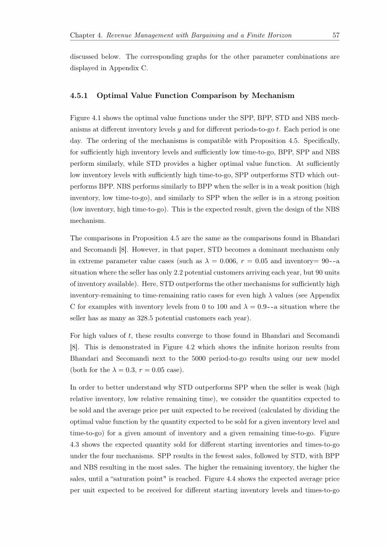
Chapter 4. Revenue Management with Bargaining and a Finite Horizon 57
discussed below. The corresponding graphs for the other parameter combinations aredisplayed in Appendix C.
4.5.1 Optimal Value Function Comparison by Mechanism
Figure 4.1 shows the optimal value functions under the SPP, BPP, STD and NBS mech-anisms at different inventory levels y and for different periods-to-go t. Each period is oneday. The ordering of the mechanisms is compatible with Proposition 4.5. Specifically,for sufficiently high inventory levels and sufficiently low time-to-go, BPP, SPP and NBSperform similarly, while STD provides a higher optimal value function. At sufficientlylow inventory levels with sufficiently high time-to-go, SPP outperforms STD which out-performs BPP. NBS performs similarly to BPP when the seller is in a weak position (highinventory, low time-to-go), and similarly to SPP when the seller is in a strong position(low inventory, high time-to-go). This is the expected result, given the design of the NBSmechanism.
The comparisons in Proposition 4.5 are the same as the comparisons found in Bhandariand Secomandi [8]. However, in that paper, STD becomes a dominant mechanism onlyin extreme parameter value cases (such as � = 0.006, r = 0.05 and inventory= 90--asituation where the seller has only 2.2 potential customers arriving each year, but 90 unitsof inventory available). Here, STD outperforms the other mechanisms for sufficiently highinventory-remaining to time-remaining ratio cases for even high � values (see AppendixC for examples with inventory levels from 0 to 100 and � = 0.9--a situation where theseller has as many as 328.5 potential customers each year).
For high values of t, these results converge to those found in Bhandari and Secomandi[8]. This is demonstrated in Figure 4.2 which shows the infinite horizon results fromBhandari and Secomandi next to the 5000 period-to-go results using our new model(both for the � = 0.3, r = 0.05 case).
In order to better understand why STD outperforms SPP when the seller is weak (highrelative inventory, low relative remaining time), we consider the quantities expected tobe sold and the average price per unit expected to be received (calculated by dividing theoptimal value function by the quantity expected to be sold for a given inventory level andtime-to-go) for a given amount of inventory and a given remaining time-to-go. Figure4.3 shows the expected quantity sold for different starting inventories and times-to-gounder the four mechanisms. SPP results in the fewest sales, followed by STD, with BPPand NBS resulting in the most sales. The higher the remaining inventory, the higher thesales, until a “saturation point" is reached. Figure 4.4 shows the expected average priceper unit expected to be received for different starting inventory levels and times-to-go

Chapter 4. Revenue Management with Bargaining and a Finite Horizon 58
10 periods to go 100 periods to go
500 periods to go 1000 periods to go
Figure 4.1: Optimal value function ratio (V kt (y)/V
jt (y)) for different times-to-go, with
r = 0.05 and � = 0.30
Bhandari and Secomandi [8] (Fig-ure 1)
Our model, with t = 5000
Figure 4.2: Optimal value function ratio (V kt (y)/V
jt (y)), with r = 0.05 and � = 0.30
under the four mechanisms. BPP results in the lowest average price, followed by STD,with SPP resulting in the highest price. The average price of NBS is close to that ofSPP when the seller is strong, and close to that of BPP when the seller is weak (whichis expected, given the design of the NBS mechanism).
If we consider the case of a weak seller (with high inventory and low time-to-go) we seethat while SPP has a higher average price than STD, STD has a higher quantity soldthan SPP. It appears that STD outperforms SPP for a weak seller due to quantity, ratherthan price, effects. By “splitting-the-difference” with the buyer, the seller receives a lowerprice, but has a higher likelihood of making a sale. When the seller is weak, it seems to
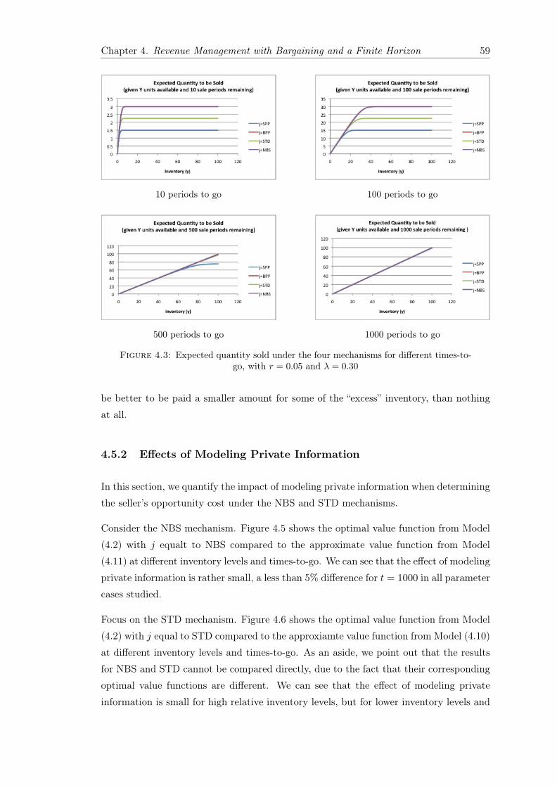
Chapter 4. Revenue Management with Bargaining and a Finite Horizon 59
10 periods to go 100 periods to go
500 periods to go 1000 periods to go
Figure 4.3: Expected quantity sold under the four mechanisms for different times-to-go, with r = 0.05 and � = 0.30
be better to be paid a smaller amount for some of the “excess” inventory, than nothingat all.
4.5.2 Effects of Modeling Private Information
In this section, we quantify the impact of modeling private information when determiningthe seller’s opportunity cost under the NBS and STD mechanisms.
Consider the NBS mechanism. Figure 4.5 shows the optimal value function from Model(4.2) with j equalt to NBS compared to the approximate value function from Model(4.11) at different inventory levels and times-to-go. We can see that the effect of modelingprivate information is rather small, a less than 5% difference for t = 1000 in all parametercases studied.
Focus on the STD mechanism. Figure 4.6 shows the optimal value function from Model(4.2) with j equal to STD compared to the approxiamte value function from Model (4.10)at different inventory levels and times-to-go. As an aside, we point out that the resultsfor NBS and STD cannot be compared directly, due to the fact that their correspondingoptimal value functions are different. We can see that the effect of modeling privateinformation is small for high relative inventory levels, but for lower inventory levels and

Chapter 4. Revenue Management with Bargaining and a Finite Horizon 60
10 periods to go 100 periods to go
500 periods to go 1000 periods to go
Figure 4.4: Average price per unit expected to be received under the four mechanismsfor different times-to-go, with r = 0.05 and � = 0.30
Figure 4.5: Ratio of approximate optimal value function to optimal value functionunder the NBS mechanism, with r = 0.05 and � = 0.30

Chapter 4. Revenue Management with Bargaining and a Finite Horizon 61
Figure 4.6: Ratio of approximate optimal value function to optimal value functionunder the STD mechanism, with r = 0.05 and � = 0.30
higher times-to-go, this effect approaches a nearly 40% difference in value functions whent = 1000 (the results are similar in other parameter cases). In other words, it seems thatthe impact of modeling private information is more pronounced when the seller is strong.
In order to develop some intuition for this finding, Figure 4.7 plots the expected quantitysold as well as the average price per unit expected to be received for Model (4.2) withj =STD and Model (4.10).
While the expected quantity sold is similar in both Models (4.3) and (4.10), the averageprice per unit expected to be received is higher in the Model (4.3) case. When the seller isstrong, the seller’s valuation for a unit of inventory is correspondingly high. In a privateinformation setting, the seller can optimally increase his reported valuation above histrue marginal valuation (this is what happens in equilibrium in the STD case; the STDmechanism considered here is the equivalent direct and feasible mechanism version ofthis equilibrium), leading to a higher average sales price, with less concern for lost salesdue to his strong position.
To summarize, modeling private information does not appear critical when using theNBS mechanism, or when a weak seller uses the STD mechanism. However, neglectingto model private information is not a reasonable approximation when considering a strongseller under the STD mechanism.
4.6 Conclusion
In this paper, we have extended the revenue management bargaining model developedby Bhandari and Secomandi [8] to a finite horizon setting, obtaining both structural
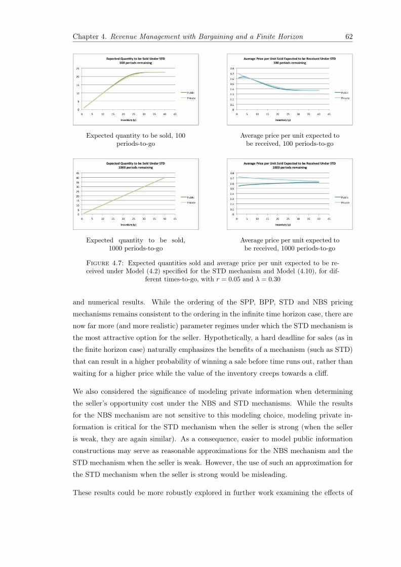
Chapter 4. Revenue Management with Bargaining and a Finite Horizon 62
Expected quantity to be sold, 100periods-to-go
Average price per unit expected tobe received, 100 periods-to-go
Expected quantity to be sold,1000 periods-to-go
Average price per unit expected tobe received, 1000 periods-to-go
Figure 4.7: Expected quantities sold and average price per unit expected to be re-ceived under Model (4.2) specified for the STD mechanism and Model (4.10), for dif-
ferent times-to-go, with r = 0.05 and � = 0.30
and numerical results. While the ordering of the SPP, BPP, STD and NBS pricingmechanisms remains consistent to the ordering in the infinite time horizon case, there arenow far more (and more realistic) parameter regimes under which the STD mechanism isthe most attractive option for the seller. Hypothetically, a hard deadline for sales (as inthe finite horizon case) naturally emphasizes the benefits of a mechanism (such as STD)that can result in a higher probability of winning a sale before time runs out, rather thanwaiting for a higher price while the value of the inventory creeps towards a cliff.
We also considered the significance of modeling private information when determiningthe seller’s opportunity cost under the NBS and STD mechanisms. While the resultsfor the NBS mechanism are not sensitive to this modeling choice, modeling private in-formation is critical for the STD mechanism when the seller is strong (when the selleris weak, they are again similar). As a consequence, easier to model public informationconstructions may serve as reasonable approximations for the NBS mechanism and theSTD mechanism when the seller is weak. However, the use of such an approximation forthe STD mechanism when the seller is strong would be misleading.
These results could be more robustly explored in further work examining the effects of

Chapter 4. Revenue Management with Bargaining and a Finite Horizon 63
a public deadline T, strategic buyers and non-stationary or unknown valuation distribu-tions, as well as through numerical examples in situations beyond the SUTP, as notedin Secomandi and Bhandari [8].

Chapter 5
Conclusion
In this dissertation, we examined three different service operations problems. First, weempirically examined the provision of customer service on Twitter. Using an ordinallogistic regression model, we found that customers are less likely to experience a positivefinal sentiment as time passes. This finding may indicate a shift by the customer serviceteam to harder to resolve cases as the program matures. Due to the noise in the data,future work could focus on better methods to reduce noise in data scraped from Twitter,such as better sentiment coding algorithms. Direct collaboration with a company duringthe data collection stage may be most rewarding, however. By obtaining direct customersatisfaction reports, as well as detailed customer and complaint information, noise wouldbe reduced and additional important variables could be included in the analysis, leadingto a better understanding of customer reactions to different Twitter-based customerservice metrics.
Next, we partially extended Scheller-Wolf and Vesilo’s [67] results for necessary andsufficient conditions for a finite rth moment of expected delay in a FIFO multiserverqueue, assuming a non-integral load and a service time distribution belonging to classL�1 , to the non-integral load case: we find a stricter necessary condition for a GI/GI/K-server system with integral ⇢ = R: the rth moment of expected delay E[D
r
] will beinfinite if E[S
1+( r
↵(K�k) )] is infinite, which occurs when the shape parameter of the service
time distribution ↵ <
12 +
q14 +
r
K�R
. Future work could include stricter necessary orsufficient conditions until the gap is closed, as well as further investigation of highermoment results. These results would provide further insight into the question of whetherintegral load systems in this class behave more like a system with slightly more or lesswork, or some combination thereof.
Finally, we ranked the value of four different bargaining mechanisms analytically and nu-merically in the context of the symmetric uniform trading problem, from the perspective
64

Chapter 5. Conclusion 65
of a seller of a finite inventory of perishable goods. While this ordering of the mechanismsremains the same as compared to the infinite horizon case studied in the literature, wefind numerically, in an analogous model, that the relative value of the split-the-difference(STD) mechanism increases as we move to a situation where the seller faces a deadlineto complete the sales. Additionally, we show that while using a simplified model thatcalculates the seller’s opportunity cost using public information may be an acceptable ap-proximation for the NBS mechanism, it produces substantially different results than theprivate information case when STD mechanism is used by a strong seller. Consequently,care must be taken when simplifying the model in this way.

Appendix A
Appendix A: Selecting a Model forTwitter-Based Customer ServiceQuality Metrics
A.1 Transitions
Table A.1: Transition Table - Model Selection Data
FinalSentiment
Negative Neutral Positive Total
Initial SentimentNegative 33 88 45 166Neutral 31 69 48 148Positive 3 11 6 20Total 67 168 99 334
Table A.2: Transition Table - Test Data
FinalSentiment
Negative Neutral Positive Total
Initial SentimentNegative 44 83 54 181Neutral 27 88 59 174Positive 3 7 7 17Total 74 178 120 372
66

Appendix A. Selecting a Model for Twitter-Based Customer Service Quality Metrics 67
A.2 Descriptives
Table A.3: Full Data Set - Descriptives
N Minimum Maximum Mean Std. Dev.Ratio of company to total mes-sages
706 .01 .71 .3321 .09899
Company response time 706 .00 6.99 1.0651 1.43519Customer response time 706 .00 14.00 .4699 1.24833Number of company related mes-sages in network
706 .00 147.00 5.0722 11.81532
Ratio of positive to total networkmessages
706 .00 1.00 .1115 .22997
Ratio of positive to total networkmessages squared
706 .00 1.00 .0652 .20284
Ratio of negative to total networkmessages
706 .00 1.00 .0897 .19468
LN(Date of initial message) 706 .00 5.71 4.5326 .97564
A.3 Variables Considered for Model Inclusion
A.3.1 Customer Attribute - Initial Mention
This variable is 1 if the customer’s initial message included "@company" or "@compa-nysupport," and 0 otherwise.
A.3.2 Customer Attribute - Weekend
This variable is 1 if the customer’s initial message occured during a weekend and 0otherwise.
A.3.3 Customer Attribute - Business Hours
This variable is 1 if the customer’s initial message occured during business hours and 0otherwise.

Appendix A. Selecting a Model for Twitter-Based Customer Service Quality Metrics 68
A.3.4 Customer Attribute - Initial Sentiment
This variable indicates the sentiment (positive, negative or neutral) of the customer’sinitial message.
A.3.5 Customer Attribute - Number of customer messages
This variable measures the total number of messages sent by the customer in a case.
A.3.6 Service Attribute - Number of company messages
This variable measures the total number of messages sent by the company’s companysupport team in a case.
A.3.7 Service Attribute - Company response time
This variable is the average time between a customer message and the company’s responsein a case.
A.3.8 Service/Customer Attribute - Average Time
This variable is calculated by dividing elapsed time by the total number of messages ina case.
A.3.9 Service/Customer Attribute - Ratio of company to total mes-sages
This variable divides the number of company messages by the total number of messagesin a case (that is, the number of company messages plus the number of customer messagesin a case).
A.3.10 Service/Customer Attribute - Ratio of customer to companymessages
This variable divides the number of customer messages by the number of company mes-sages.
Appendix A. Selecting a Model for Twitter-Based Customer Service Quality Metrics 69
A.3.11 Service/Customer Attribute - Number of messages
This variable measures the total number of messages sent by the company and thecustomer in a case.
A.3.12 Service Attribute - Priority
This variable is the priority (high-medium-low) assigned to a case by the company.
A.3.13 Service Attribute - Elapsed Time
This variable measures the time elapsed between the customer’s first message and thecompany’s final message in a case.
A.3.14 Service Attribute - Initial Response Time
This variable measures the time elapsed between the customer’s first message and thecompany’s first message in a case.
A.3.15 Service Attribute - Date of initial message
This variable indicates the date of the customer’s first message, where “1" indicates thefirst day in the data set (February 22). This value is subsequently incremented (e.g.Februrary 25 is “4").
A.3.16 Customer Attribute - Customer response time
This variable is the average time between a company message and the customer’s responsein a case.
A.3.17 Customer Attribute - Number of followers
This variable is the number of Twitter followers a customer had at the time of the serverinteraction.

Appendix A. Selecting a Model for Twitter-Based Customer Service Quality Metrics 70
A.3.18 Customer Attribute - Number of friends
This variable is the number of Twitter friends a customer had at the time of inquiry(after the server interaction).
A.3.19 Customer Network Attributes - Number of positive networkmessages from friend-followers
This variable is the number of messages involving the company or its products withpositive sentiment sent in the week prior to the customer’s first message by those friendswho are also followers.
A.3.20 Customer Network Attributes - Number of neutral networkmessages from friend-followers
This variable is the number of messages involving the company or its products withneutral sentiment sent during the case, as well as in the week prior to the customer’sfirst message by those friends who are also followers.
A.3.21 Customer Network Attributes - Number of negative networkmessages from friend-followers
This variable is the number of messages involving the company or its products withnegative sentiment sent during the case, as well as in the week prior to the customer’sfirst message by those friends who are also followers.
A.3.22 Customer Network Attributes - Number of positive networkmessages from friend-but-not-followers
This variable is the number of messages involving the company or its products withpositive sentiment sent during the case, as well as in the week prior to the customer’sfirst message by those friends who are not also followers.

Appendix A. Selecting a Model for Twitter-Based Customer Service Quality Metrics 71
A.3.23 Customer Network Attributes - Number of neutral networkmessages from friend-but-not-followers
This variable is the number of messages involving the company or its products withneutral sentiment sent during the case, as well as in the week prior to the customer’sfirst message by those friends who are not also followers.
A.3.24 Customer Network Attributes - Number of negative networkmessages from friend-but-not-followers
This variable is the number of messages involving the company or its products withnegative sentiment sent during the case, as well as in the week prior to the customer’sfirst message by those friends who are not also followers.
A.3.25 Customer Network Attributes - Number of positive networkmessages
This variable is the total number of messages involving the company or its products withpositive sentiment sent during the case, as well as in the week prior to the customer’sfirst message by the customer’s friends.
A.3.26 Customer Network Attributes - Number of neutral networkmessages
This variable is the total number of messages involving the company or its products withneutral sentiment sent during the case, as well as in the week prior to the customer’sfirst message by the customer’s friends.
A.3.27 Customer Network Attributes - Number of negative networkmessages
This variable is the total number of messages involving the company or its products withnegative sentiment sent during the case, as well as in the week prior to the customer’sfirst message by the customer’s friends.
Appendix A. Selecting a Model for Twitter-Based Customer Service Quality Metrics 72
A.3.28 Network Attribute - Number of company related messages innetwork
This variable is the total number of positive, negative, neutral and indeterminate mes-sages involving the company or its products sent during the case, as well as in the weekprior to the customer’s first message, by the customer’s friends.
A.3.29 Network Attribute - Ratio of positive to total network mes-sages
This variable is the number of positive messages involving the company or its productssent during the case, as well as in the week prior to the customer’s first message, bythe customer’s friends, divided by the number of company related messages in networkvariable. In the event that the number of company related messages in network variablehad a value of 0, this variable was also coded as 0.
A.3.30 Network Attribute - Ratio of negative to total network mes-sages
This variable is the number of negative messages involving the company or its productssent during the case, as well as in the week prior to the customer’s first message, bythe customer’s friends, divided by the number of company related messages in networkvariable. In the event that the number of company related messages in network variablehad a value of 0, this variable was also coded as 0.
A.3.31 Customer Network Attribute - Number of promotional mes-sages
This variable is the number of messages sent during the case, as well as in the weekprior to the customer’s first message through one of the company’s non-support Twitteraccounts.
A.3.32 Variable notes
Some of these variables are redundant. Additionally, quadratic, square root and naturallog transformations of these variables were also considered, where appropriate. In thecase where the variable may have a value of 0 (number of friends, number of followers,

Appendix A. Selecting a Model for Twitter-Based Customer Service Quality Metrics 73
number of a certain type of network message, etc.), the natural log of the value of thevariable plus one was taken.
A.4 Additional Results
Using the chosen model on the entire data set, we find the results given in table A.4. Itis important to note that this test uses some data that was used to chose the variablesin the model, so significance is overstated and unreliable. Overall model significanceis 0.001. The test of parallel lines resulted in a significance of .776, indicating the theproportional odds assumption is not rejected, so ordinal regression remains appropriate.In contrast to the test data only results, the parameters for the ratio of company to totalmessages and the ratio of positive to total network messages are significant, so we cannow address hypotheses 1 and 2. The parameter for the natural log of the date of theinitial message is also significant, as it was before, so the comments in 2.5.1 still apply.As before, the service time variables are insignificant, so the comments in section 2.5.2still apply.
Table A.4: Chosen model - full data set
Parameter Value Std. Error Sig.↵
neutral
-2.202 .427 .000↵
positive
.052 .418 .900� Ratio of company to total messages 1.673 .728 .022� Company response time .039 .051 .444� Customer response time -.091 .058 .116� Number of company related messages in net-work
.000 .007 .986
� Ratio of positive to total network messages 1.944 .988 .049� Ratio of positive to total network messagessquared
-1.908 1.110 .086
� Ratio of negative to total network messages -.281 .375 .454� LN(Date of initial message) -.308 .077 .000
A.4.1 Evaluation of Hypothesis 1
We find that the ratio of company to total messages has a parameter value of 1.673with significance of 0.022 when the model was applied to the full data set. This resultconfirms our hypothesis that a higher ratio of company to total case messages increasesthe probability of a more positive case resolution (holding the date, company responsetime, customer response time, number of network messages and the percentage of positiveand negative network messages constant). As discussed before, this may indicate that

Appendix A. Selecting a Model for Twitter-Based Customer Service Quality Metrics 74
a higher number of messages provided for the same amount of customer informationprovided implies higher service level which results in higher customer satisfaction.
A.4.2 Evaluation of Hypothesis 2
We find that the ratio of positive to total network messages has a parameter value of1.944 with significance of 0.049 when the model was applied to the full data set. However,the quadratic term is not significant. While this result does not confirm the quadraticnature of our hypothesis, it does correspond with the idea that a higher ratio of positiveto total network messages in the period between one week prior to the customer’s firstmessage and the customer’s last message increases the probability of a more positive caseresolution (holding the date, ratio of company to total messages, company response time,customer response time, number of network messages and the percentage of negativenetwork messages constant). As discussed before, this may related to the findings of Maet al [48] who found that positive sentiment expression in a customer’s network led tomore positive sentiment expression if the customer was already in a positive state, andmore negative sentiment expression if the customer was already in a negative state.
A.5 Extra References
’ordinal’ by Rune Haubo B Christensen
’glmulti’ by Vincent Calcagno
’vgam’ by Thomas Yee
’reshape2’ by Hadley Wickham
Wikipedia “AIC"
http://www.ats.ucla.edu/stat/spss/output/ologit.htm
http://www.ats.ucla.edu/stat/spss/dae/ologit.htm
http://www.ats.ucla.edu/stat/r/dae/ologit.htm
http://research.cs.tamu.edu/prism/lectures/iss/iss l13.pdf
http://www.stanford.edu/ hastie/Papers/ESLII.pdf
Appendix B
Appendix B: Necessary Conditionfor Finite Delay Moments for FIFOGI/GI/K Queues with Integral Load
B.1 Proof of Lemma 3.4
Lemma. Let Y
i
= S
i
� T , where T is deterministic and equal to E[S], and S has P (X >
u) ⇠ u
�↵ with 1 < ↵ < 2. Then,
P (
⌃Y
i
n
1↵
> ✏) ⇠ U
↵
(✏) (B.1)
where U is the stable distribution determined (including centering) by the characteristicfunction
(⇣) = |⇣|↵C �(3� ↵)
↵(↵� 1)
[cos
⇡↵
2
⌥ i(p� q)sin
⇡↵
2
]. (B.2)
Proof.
Definition B.1. Feller [24], page 172
“F belongs to the domain of attraction of U iff there exist constants a
n
> 0 and b
n
suchthat the distribution of a�1
n
S
n
� nb
n
tends to U."
Let ' be the characteristic function of F, and ! be the characteristic function of U. an
and b
n
are scaling parameters.
75

Appendix B. Necessary Condition for Finite Delay Moments for FIFO GI/GI/KQueues with Integral Load 76
In other words, Lemma 3.4 states that our netput process Y belongs to a domain ofattraction, allowing us to characterize the behavior of the accumulation of work in asystem with a load exactly equal to the number of servers available.
Feller [24] provides the two lemmas needed to prove Lemma 3.4: the first (Lemma B.2)presents the requirements needed for a distribution to belong to a domain of attraction,the second (Lemma B.3) presents the necessary scaling parameters a
n
and b
n
to ensurethe domain of attraction to be that described in equation B.2. After stating these lemmas,we show that the the sum of service times S will belong to the domain of attraction ofU when scaling parameters a
n
= n
1↵ and b
n
= T = E[S] are used.
Lemma B.2. Theorem 2 from Feller [24] section XVII.5
“(a) In order that a distribution F belong to some domain of attraction it is necessarythat the truncated moment function µ varies regularly with an exponent 2-↵ (0 < ↵ 2).
(b) If ↵ = 2, this condition is also sufficient provided F is not concentrated at one point.
(c) If µ(x) s x
2�↵L(x), x ! 1 holds with 0 < ↵ 2 then F belongs to some domain of
attraction iff the tails are balanced so that as x ! 1
1� F (x)
1� F (x) + F (�x)
! p (B.3)
F (�x)
1� F (x) + F (�x)
! q (B.4)
where L varies slowly.”
Lemma B.3. Theorem 3 from Feller [24] section XVII.5
“Let U be the stable distribution determined (including centering) by the characteristicfunction
(⇣) = |⇣|↵C �(3� ↵)
↵(↵� 1)
[cos
⇡↵
2
⌥ i(p� q)sin
⇡↵
2
] (B.5)
if ↵ 6= 1 or (⇣) = �|⇣| · C[
1
2
⇡ ± i(p� q)log|⇣|] (B.6)
if ↵ = 1.
Let the distribution F satisfy the conditions of [Lemma B.2], and let an
satisfy
n
a
2n
µ(a
n
) ! C
.

Appendix B. Necessary Condition for Finite Delay Moments for FIFO GI/GI/KQueues with Integral Load 77
(i) If 0 < ↵ < 1 then '
n
(⇣/a
n
) ! !(⇣) = e
(⇣).
(ii) If 1 < ↵ 2 and µ(1) = 1 the same is true provided F is centered to zeroexpectation.
(iii) If ↵ = 1 then('(⇣/a
n
)e
�ib
n
⇣
)
n ! !(⇣) = e
(⇣),
whereb
n
=
Z +1
�1sin
x
a
n
F{dx}.00
To summarize the application of Lemmas B.2 and B.3, Lemma 3.4 will be true if thefollowing four conditions are met:
1) the truncated moment function of S varies regularly with an exponent 2 � ↵, with0 < ↵ 2
2) the tails of S are balanced so that as x ! 1
1� F (x)
1� F (x) + F (�x)
! p
F (�x)
1� F (x) + F (�x)
! q
3) a
n
satisfiesn
a
2n
µ(a
n
) ! C
4) S is centered to 0 expectation.
We will demonstrate point-by-point that these conditions are met.
1) the truncated moment function of S varies regularly with an exponent 2 � ↵, with0 < ↵ 2:
The truncated moment function is defined as µ(x) =
Rx
�x
y
2f(y)dy. For S with P (X >
u) ⇠ u
�↵ and 1 < ↵ < 2, we find µ(x) =
Rx
0 y
2 ↵
y
↵+1dy ⇠ x
2�↵, so this condition isfulfilled.
2) the tails of S are balanced so that as x ! 1
1� F (x)
1� F (x) + F (�x)
! p

Appendix B. Necessary Condition for Finite Delay Moments for FIFO GI/GI/KQueues with Integral Load 78
F (�x)
1� F (x) + F (�x)
! q
We have S with P (X > u) ⇠ u
�↵, with F (�x) = 0:
1� F (x)
1� F (x) + F (�x)
=
x
�↵
x
�↵+ 0
! 1
0
x
�↵+ 0
! 0
,
so this condition is fulfilled.
3) a
n
satisfiesn
a
2n
µ(a
n
) ! C
Equation B.1 implies that a
n
= n
1↵ . With µ(a
n
) ⇠ a
2�↵n
, we see
n
a
2n
µ(a
n
) ⇠ n
(n
1↵
)
2(n
1↵
)
2�↵= 1 ! C
4) S is centered to 0 in expectation, which is fulfilled by using b
n
= T = E[S]
B.2 Asymptotic convergence of bounds
Here, we consider the limit of the ratio of the previous bounds to the new bounds forthe GI/GI/K case as the number of servers K approaches infinity.
Lemma B.4. The newly established necessary conditions for finite mean delay withintegral load for FIFO GI/GI/K queues, with service times both belonging to class L↵+1
with dF (x) ⇠ x
�↵ approach the previously established lower bounds of K�R+1+r
K�R+1 as thenumber of servers K approaches infinity.

Appendix B. Necessary Condition for Finite Delay Moments for FIFO GI/GI/KQueues with Integral Load 79
Proof.
lim
K!1
K�R+1+r
K�R+1
12 +
q14 +
r
K�R
= lim
K!1
K�R+1+r
K�R+1
12 +
qK�R+4r4(K�R)
= lim
K!1
K�R+1+r
K�R+1
12 +
pK�R+4rp4(K�R)
= lim
K!1
K�R+1+r
K�R+1
12 +
pK�R+4r2pK�R
= lim
K!1
2(
K�R+1+r
K�R+1 )
1 +
pK�R+4rpK�R
=
lim
K!1 2(
K�R+1+r
K�R+1 )
lim
K!1 1 +
qlim
K!1K�R+4rK�R
=
lim
K!1 2(
11)
lim
K!1 1 +
qlim
K!111
=
2
2
= 1
L’Hôpital’s Rule is used for the penultimate step. As the number of servers approachesinfinity, the ratio of the value of the new bounds to the value of the old bounds approaches1.
B.3 Workloads are greater than C
0x
1↵
The workload at server R will be greater than C
0x
1↵ , given that we have
C >
⇣R
R�1�1✏R
R�2(R�1)
⌘↵
(2
R+1RE[S]).
Lemma B.5. 1R
✏(
⌥2RE[S]x)
1↵ �
PR�1n=1
x
1↵
R
n
> C
0x
1↵ for R � 2 where C
0 is a positive
constant, if C >
⇣R
R�1�1✏R
R�2(R�1)
⌘↵
(2
R+1RE[S]).
Proof. We will solve backwards to find the values of C that will result in 1R
✏(
⌥2RE[S]x)
1↵ �
PR�1n=1
x
1↵
R
n
> C
0x
1↵ .
1
R
✏(
⌥
2RE[S]
x)
1↵ �
R�1X
n=1
x
1↵
R
n
> C
0x
1↵
1
R
✏(
⌥
2RE[S]
)
1↵ �
R�1X
n=1
1
R
n
!x
1↵
> C
0x
1↵

Appendix B. Necessary Condition for Finite Delay Moments for FIFO GI/GI/KQueues with Integral Load 80
So 1R
✏(
⌥2RE[S]x)
1↵ �
PR�1n=1
x
1↵
R
n
> C
0x
1↵ if
⇣1R
✏(
⌥2RE[S])
1↵ �
PR�1n=1
1R
n
⌘> 0
1
R
✏(
C/2
R
2RE[S]
)
1↵ �
R�1X
n=1
1
R
n
> 0
1
R
✏(
C/2
R
2RE[S]
)
1↵
>
R�1X
n=1
1
R
n
C
1↵
✏
R
(
1
2
R
2RE[S]
)
1↵
>
R�1X
n=1
1
R
n
Recognizing the summation term as a geometric series
C
1↵
✏
R
(
1
2
R
2RE[S]
)
1↵
>
R�1X
n=0
1
R
n
� 1
C
1↵
✏
R
(
1
2
R+1RE[S]
)
1↵
>
1� (1/R)
R
1� (1/R)
� 1
C
1↵
✏
R
(
1
2
R+1RE[S]
)
1↵
>
R
R�1 � 1
R
R�1(R� 1)
C
1↵
>
R
✏
(2
R+1RE[S])
1↵
R
R�1 � 1
R
R�1(R� 1)
C
1↵
>
R(R
R�1 � 1)(2
R+1RE[S])
1↵
✏R
R�1(R� 1)
C >
✓R
R�1 � 1
✏R
R�2(R� 1)
◆↵
(2
R+1RE[S])
So 1R
✏(
⌥2RE[S]x)
1↵ �
PR�1n=1
x
1↵
R
n
> C
0x
1↵ when C >
⇣R
R�1�1✏R
R�2(R�1)
⌘↵
(2
R+1RE[S]).
At time t =
⌥2 x +
PR�1n=1
x
1↵
R
n
, the workload at each server i in the group of servers 1
through R-1 will have a workload equal to R�i
i
x
1↵
R
R�i
�P
R�1n=R�i+1
x
1↵
R
n
.
Lemma B.6. R�i
i
x
1↵
R
R�i
�P
R�1n=R�i+1
x
1↵
R
n
> C
0x
1↵ where C
0 is a positive constant, for1 i R� 1 and R � 2.
Proof.
R� i
i
x
1↵
R
R�i
�R�1X
n=R�i+1
x
1↵
R
n
= x
1↵
[
R� i
i
1
R
R�i
�R�1X
n=R�i+1
1
R
n
]
= x
1↵
[
R� i
i
1
R
R�i
� (
R�2X
n=0
1
R
(
1
R
)
n �R�i�1X
n=0
1
R
(
1
R
)
n
)]
If [R�i
i
1R
R�i
� (
PR�2n=0
1R
(
1R
)
n �P
R�i�1n=0
1R
(
1R
)
n
)] > 0, then R�i
i
x
1↵
R
R�i
�P
R�1n=R�i+1
x
1↵
R
n
>
C
0x
1↵ . Now we can recognize the terms
PR�2n=0
1R
(
1R
)
n andP
R�i�1n=0
1R
(
1R
)
n as geometric

Appendix B. Necessary Condition for Finite Delay Moments for FIFO GI/GI/KQueues with Integral Load 81
series.
x
1↵
[
R� i
i
1
R
R�i
� (
R�2X
n=0
1
R
(
1
R
)
n �R�i�1X
n=0
1
R
(
1
R
)
n
)]
= x
1↵
[
R� i
i
1
R
R�i
� (
1
R
1� (
1R
)
R�1
1� 1R
� 1
R
1� (
1R
)
R�i
1� 1R
)]
= x
1↵
[
R� i
iR
R�i
�1� (
1R
)
R�1
R� 1
+
1� (
1R
)
R�i
R� 1
]
= x
1↵
[
R� i
iR
R�i
+
1� (
1R
)
R�i � 1 + (
1R
)
R�1
R� 1
]
= x
1↵
[
R� i
iR
R�i
+
(
1R
)
R�1 � (
1R
)
R�i
R� 1
]
= x
1↵
[
(R� i)(R� 1) + (
1R
)
R�1iR
R�i � (
1R
)
R�i
iR
R�i
iR
R�i
(R� 1)
]
=
x
1↵
iR
R�i
(R� 1)
[(R� i)(R� 1) + iR
1�i � i]
The smallest possible value for (R� i)(R�1) given 1 i R�1 occurs when i = R�1.Similarly, the largest possible value for i occurs when i = R�1. We can incorporate thisinformation into an inequality:
x
1↵
iR
R�i
(R� 1)
[(R� i)(R� 1) + iR
1�i � i] >
x
1↵
iR
R�i
(R� 1)
[(R� 1) + iR
1�i � (R� 1)]
=
x
1↵
iR
R�i
(R� 1)
[iR
1�i
]
> C
0x
1↵
because 1iR
R�i(R�1)> 0 and iR
1�i
> 0, the entire expression is greater than C
0x
1↵ .

Appendix C
Appendix: Revenue Managementwith Bargaining and a FiniteHorizon - Additional NumericalResults
In this Appendix, we summarize numerical results for parameter value combinationsother than � = 0.3, r = 0.05. Results for � = 0.6, r = 0.05 are displayed in SectionC.1 as Figures C.1 to C.6. Results for � = 0.9, r = 0.05 are displayed in Section C.2 asFigures C.7 to C.12. Results for � = 0.3, r = 0.10 are displayed in Section C.3 as FiguresC.13 to C.18. Results for � = 0.6, r = 0.10 are displayed in Section C.4 as Figures C.19to C.24. Finally, results for � = 0.9, r = 0.10 are displayed in Section C.5 as FiguresC.25 to C.30.
82

Appendix C. Revenue Management with Bargaining and a Finite Horizon 83
C.1 Results for � = 0.6, r = 0.05 (Figures C.1 to C.6)
10 periods to go 100 periods to go
500 periods to go 1000 periods to go
Figure C.1: Optimal value function ratio (V kt (y)/V
jt (y)) for different times-to-go,
with r = 0.05 and � = 0.60

Appendix C. Revenue Management with Bargaining and a Finite Horizon 84
10 periods to go 100 periods to go
500 periods to go 1000 periods to go
Figure C.2: Expected quantity sold under the four mechanisms for different times-to-go, with r = 0.05 and � = 0.60
10 periods to go 100 periods to go
500 periods to go 1000 periods to go
Figure C.3: Average price per unit expected to be received under the four mechanismsfor different times-to-go, with r = 0.05 and � = 0.60

Appendix C. Revenue Management with Bargaining and a Finite Horizon 85
Figure C.4: Ratio of approximate optimal value function to optimal value functionunder the NBS mechanism, with r = 0.05 and � = 0.60
Figure C.5: Ratio of approximate optimal value function to optimal value functionunder the STD mechanism, with r = 0.05 and � = 0.60

Appendix C. Revenue Management with Bargaining and a Finite Horizon 86
Expected quantity to be sold, 100periods-to-go
Average price per unit expected tobe received, 100 periods-to-go
Expected quantity to be sold,1000 periods-to-go
Average price per unit expected tobe received, 1000 periods-to-go
Figure C.6: Expected quantities sold and average price per unit expected to bereceived under Model (4.2) specified for the STD mechanism and Model (4.10), for
different times-to-go, with r = 0.05 and � = 0.60
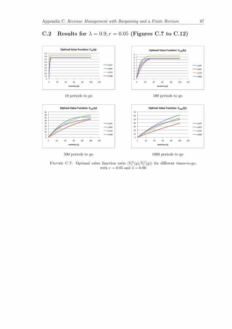
Appendix C. Revenue Management with Bargaining and a Finite Horizon 87
C.2 Results for � = 0.9, r = 0.05 (Figures C.7 to C.12)
10 periods to go 100 periods to go
500 periods to go 1000 periods to go
Figure C.7: Optimal value function ratio (V kt (y)/V
jt (y)) for different times-to-go,
with r = 0.05 and � = 0.90
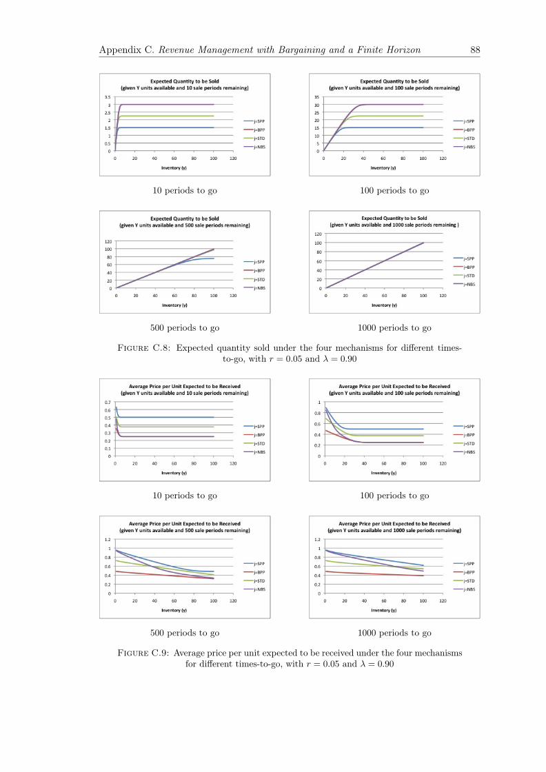
Appendix C. Revenue Management with Bargaining and a Finite Horizon 88
10 periods to go 100 periods to go
500 periods to go 1000 periods to go
Figure C.8: Expected quantity sold under the four mechanisms for different times-to-go, with r = 0.05 and � = 0.90
10 periods to go 100 periods to go
500 periods to go 1000 periods to go
Figure C.9: Average price per unit expected to be received under the four mechanismsfor different times-to-go, with r = 0.05 and � = 0.90
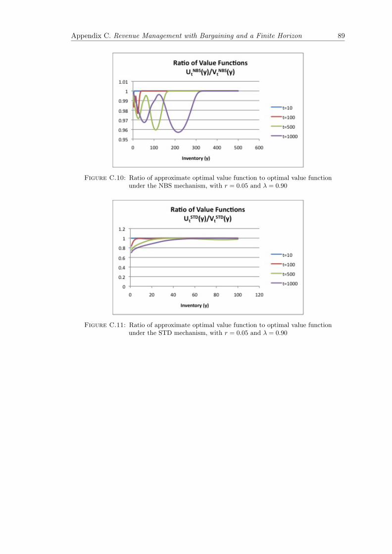
Appendix C. Revenue Management with Bargaining and a Finite Horizon 89
Figure C.10: Ratio of approximate optimal value function to optimal value functionunder the NBS mechanism, with r = 0.05 and � = 0.90
Figure C.11: Ratio of approximate optimal value function to optimal value functionunder the STD mechanism, with r = 0.05 and � = 0.90
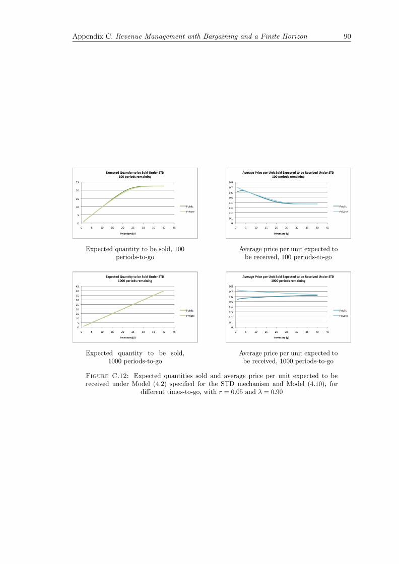
Appendix C. Revenue Management with Bargaining and a Finite Horizon 90
Expected quantity to be sold, 100periods-to-go
Average price per unit expected tobe received, 100 periods-to-go
Expected quantity to be sold,1000 periods-to-go
Average price per unit expected tobe received, 1000 periods-to-go
Figure C.12: Expected quantities sold and average price per unit expected to bereceived under Model (4.2) specified for the STD mechanism and Model (4.10), for
different times-to-go, with r = 0.05 and � = 0.90

Appendix C. Revenue Management with Bargaining and a Finite Horizon 91
C.3 Results for � = 0.3, r = 0.10 (Figures C.13 to C.18)
10 periods to go 100 periods to go
500 periods to go 1000 periods to go
Figure C.13: Optimal value function ratio (V kt (y)/V
jt (y)) for different times-to-go,
with r = 0.10 and � = 0.30
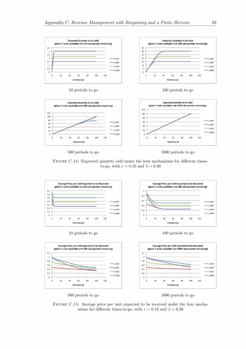
Appendix C. Revenue Management with Bargaining and a Finite Horizon 92
10 periods to go 100 periods to go
500 periods to go 1000 periods to go
Figure C.14: Expected quantity sold under the four mechanisms for different times-to-go, with r = 0.10 and � = 0.30
10 periods to go 100 periods to go
500 periods to go 1000 periods to go
Figure C.15: Average price per unit expected to be received under the four mecha-nisms for different times-to-go, with r = 0.10 and � = 0.30

Appendix C. Revenue Management with Bargaining and a Finite Horizon 93
Figure C.16: Ratio of approximate optimal value function to optimal value functionunder the NBS mechanism, with r = 0.10 and � = 0.30
Figure C.17: Ratio of approximate optimal value function to optimal value functionunder the STD mechanism, with r = 0.10 and � = 0.30

Appendix C. Revenue Management with Bargaining and a Finite Horizon 94
Expected quantity to be sold, 100periods-to-go
Average price per unit expected tobe received, 100 periods-to-go
Expected quantity to be sold,1000 periods-to-go
Average price per unit expected tobe received, 1000 periods-to-go
Figure C.18: Expected quantities sold and average price per unit expected to bereceived under Model (4.2) specified for the STD mechanism and Model (4.10), for
different times-to-go, with r = 0.10 and � = 0.30

Appendix C. Revenue Management with Bargaining and a Finite Horizon 95
C.4 Results for � = 0.6, r = 0.10 (Figures C.19 to C.24)
10 periods to go 100 periods to go
500 periods to go 1000 periods to go
Figure C.19: Optimal value function ratio (V kt (y)/V
jt (y)) for different times-to-go,
with r = 0.10 and � = 0.60

Appendix C. Revenue Management with Bargaining and a Finite Horizon 96
10 periods to go 100 periods to go
500 periods to go 1000 periods to go
Figure C.20: Expected quantity sold under the four mechanisms for different times-to-go, with r = 0.10 and � = 0.60
10 periods to go 100 periods to go
500 periods to go 1000 periods to go
Figure C.21: Average price per unit expected to be received under the four mecha-nisms for different times-to-go, with r = 0.10 and � = 0.60
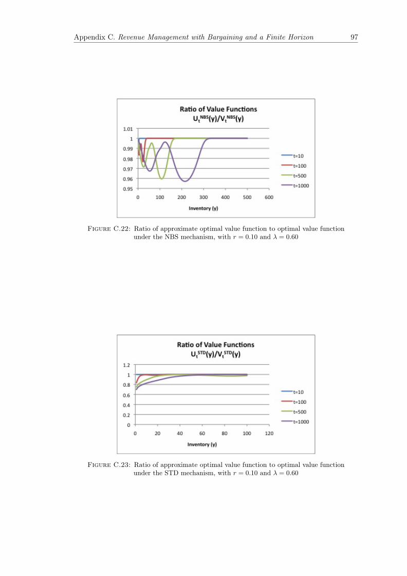
Appendix C. Revenue Management with Bargaining and a Finite Horizon 97
Figure C.22: Ratio of approximate optimal value function to optimal value functionunder the NBS mechanism, with r = 0.10 and � = 0.60
Figure C.23: Ratio of approximate optimal value function to optimal value functionunder the STD mechanism, with r = 0.10 and � = 0.60

Appendix C. Revenue Management with Bargaining and a Finite Horizon 98
Expected quantity to be sold, 100periods-to-go
Average price per unit expected tobe received, 100 periods-to-go
Expected quantity to be sold,1000 periods-to-go
Average price per unit expected tobe received, 1000 periods-to-go
Figure C.24: Expected quantities sold and average price per unit expected to bereceived under Model (4.2) specified for the STD mechanism and Model (4.10), for
different times-to-go, with r = 0.10 and � = 0.60

Appendix C. Revenue Management with Bargaining and a Finite Horizon 99
C.5 Results for � = 0.9, r = 0.10 (Figures C.25 to C.30)
10 periods to go 100 periods to go
500 periods to go 1000 periods to go
Figure C.25: Optimal value function ratio (V kt (y)/V
jt (y)) for different times-to-go,
with r = 0.10 and � = 0.90

Appendix C. Revenue Management with Bargaining and a Finite Horizon 100
10 periods to go 100 periods to go
500 periods to go 1000 periods to go
Figure C.26: Expected quantity sold under the four mechanisms for different times-to-go, with r = 0.10 and � = 0.90
10 periods to go 100 periods to go
500 periods to go 1000 periods to go
Figure C.27: Average price per unit expected to be received under the four mecha-nisms for different times-to-go, with r = 0.10 and � = 0.90

Appendix C. Revenue Management with Bargaining and a Finite Horizon 101
Figure C.28: Ratio of approximate optimal value function to optimal value functionunder the NBS mechanism, with r = 0.10 and � = 0.90
Figure C.29: Ratio of approximate optimal value function to optimal value functionunder the STD mechanism, with r = 0.10 and � = 0.90

Appendix C. Revenue Management with Bargaining and a Finite Horizon 102
Expected quantity to be sold, 100periods-to-go
Average price per unit expected tobe received, 100 periods-to-go
Expected quantity to be sold,1000 periods-to-go
Average price per unit expected tobe received, 1000 periods-to-go
Figure C.30: Expected quantities sold and average price per unit expected to bereceived under Model (4.2) specified for the STD mechanism and Model (4.10), for
different times-to-go, with r = 0.10 and � = 0.90
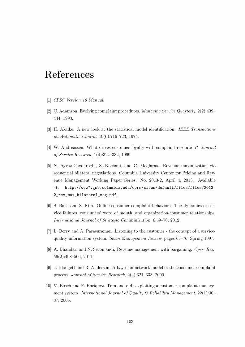
References
[1] SPSS Version 19 Manual.
[2] C. Adamson. Evolving complaint procedures. Managing Service Quarterly, 2(2):439–444, 1993.
[3] H. Akaike. A new look at the statistical model identification. IEEE Transactionson Automatic Control, 19(6):716–723, 1974.
[4] W. Andreassen. What drives customer loyalty with complaint resolution? Journalof Service Research, 1(4):324–332, 1999.
[5] N. Ayvaz-Cavdaroglu, S. Kachani, and C. Maglaras. Revenue maximization viasequential bilateral negotiations. Columbia University Center for Pricing and Rev-enue Management Working Paper Series: No. 2013-2, April 4, 2013. Availableat: http://www7.gsb.columbia.edu/cprm/sites/default/files/files/2013_
2_rev_max_bilateral_neg.pdf.
[6] S. Bach and S. Kim. Online consumer complaint behaviors: The dynamics of ser-vice failures, consumers’ word of mouth, and organization-consumer relationships.International Journal of Strategic Comminication, 6:59–76, 2012.
[7] L. Berry and A. Parasuraman. Listening to the customer - the concept of a service-quality information system. Sloan Management Review, pages 65–76, Spring 1997.
[8] A. Bhandari and N. Secomandi. Revenue management with bargaining. Oper. Res.,59(2):498–506, 2011.
[9] J. Blodgett and R. Anderson. A bayesian network model of the consumer complaintprocess. Journal of Service Research, 2(4):321–338, 2000.
[10] V. Bosch and F. Enriquez. Tqm and qfd: exploiting a customer complaint manage-ment system. International Journal of Quality & Reliability Management, 22(1):30–37, 2005.
103
References 104
[11] A. B. Casado, J. L. Nicolau, and F. Mas Ruiz. The negative effects of failed ser-vice recoveries. Working papers. serie ec, Instituto Valenciano de InvestigacionesEconómicas, S.A. (Ivie), 2008.
[12] J. Cavanaugh. 171:290 model selection - lecture vi: The bayesian information crite-rion. Available at: http://myweb.uiowa.edu/cavaaugh/ms lec 6 ho.pdf, 2009.
[13] M. Cha, H. Haddadi, F. Benevenuto, and K. Gummadi. Measuring user influencein twitter: The million follower fallacy. In Proceedings of the Fourth InternationalAAAI Conference on Weblogs and Social Media, 2010.
[14] H. C. Y. Chan and E. W. T. Ngai. What makes customer discontent with serviceproviders? an empirical analysis of complaint handling in information and commu-nication technology services. Journal of Business Ethics, 91:73–110, 2010.
[15] K. Chatterjee and W. Samuelson. Bargaining under incomplete information. Oper.Res., 31(5):835–851, 1983.
[16] P. Chelminski and R. Coulter. An examination of consumer advocacy and com-plaining behavior in the context of service failure. Journal of Services Marketing,25(5):361–370, 2012.
[17] Y. Cho and J. Fjermestad. Electronic Customer Relationship Management, chapter3: Using Electronic Customer Relationship Management to Maximize/MinimizeCustomer Satisfaction/Dissatisfaction, pages 34–50. M.E. Sharpe, 2006.
[18] Y. Cho, I. Im, R. Hiltz, and J. Fjermestad. An analysis of online customer com-plaints: Implications for web complaint management, 2002.
[19] G. Das Varma and N. Vettas. Optimal dynamic pricing with inventories. Econom.Lett., 72(3):335–340, 2001.
[20] M. Davidow. Organizational responses to customer complaints: What works andwhat doesn’t. Journal of Service Research, 5(3):225–250, 2003.
[21] K. de Ruyter and A. Brack. European legal developments in product safety andliability: The role of customer complaint management as a defensive marketing tool.Intern. J. of Research in Marketing, 10:153–164, 1993.
[22] A. Durrande-Moreau. Waiting for service: ten years of empirical research. Interna-tional Journal of Service Industry Management, 10(2):171–194, 1999.
[23] A. Faed. Handling e-complaints in customer complaint management system usingfmea as a qualitative system. In 2010 6th International Conference on Advanced In-formation Management and Service (IMS), pages 205–209, Perth, Australia, Novem-ber 30 - December 2 2010.

References 105
[24] W. Feller. An Introduction to Probability Theory and Its Applications, Vol. 2. Wiley,1971.
[25] C. Fornell and B. Wernerfelt. Defensive marketing strategy by customer complaintmanagement: A theoretical analysis. Journal of Marketing Research, 24(4):337–346,1987.
[26] C. Fornell and B. Wernerfelt. A model for customer complaint management. Mar-keting Science, 7(3):287–298, 1988.
[27] S. Foss. Some open problems related to stability. Invited Talk at Erlang CentennialConference, Copenhagen, 1-3 April, 2009, April 2009. arXiv:0909.0462v1.
[28] S. Foss and D. Korshunov. Heavy tails in multi-server queues. Queueing Systems,52:31–48, 2006.
[29] C. Froehle and A. Roth. New measurement scales for evaluating perceptions of thetechnology-mediated customer service experience. Journal of Operations Manage-ment, 22:1–21, 2004.
[30] A. Fundin and B. Bergman. Exploring the customer feedback process. MeasuringBusiness Excellence, 7(2):55–65, 2003.
[31] D. Fuscaldo. How to effectively handle customer complaints online,April 8 2011. Available at: http://smallbusiness.foxbusiness.com/technology-web/2011/04/08/effectively-handle-customer-complaints-online/.
[32] J. Gallien. Dynamic mechanism design for online commerce. Oper. Res., 54(2):291–310, 2006.
[33] A. Go, R. Bhayani, and L. Huang. Twitter senti-ment classification using distant supervision. Available at:http://cs.stanford.edu/people/alecmgo/papers/TwitterDistantSupervision09.pdf.
[34] J. Griffin. Double edged sword of communicating via social media. Keeping goodcompanies, pages 659–663, December 2011.
[35] C. Gulas and J. Larsen. Silence is not golden: Firm response and nonresponse toconsumer correspondence. Services Marketing Quarterly, 33:261–275, 2012.
[36] L. Harrison-Walker. E-complaining: a content analysis of an internet complaintforum. Journal of Services Marketing, 15(5):397–412, 2001.
[37] B. D. R. Huberman and F. Wu. Social networks that matter: Twitter under themicroscope. First Monday, 14(1-5), 2009.

References 106
[38] C. M. Hurvich and C. L. Tsai. Regression and time series model selection in smallsamples. Biometrika, 76:297–307.
[39] B. Jansen, M. Zhang, K. Sobel, and A. Chowdury. Twitter power: Tweets aselectronic word of mouth. Journal of the American Society for Information Scienceand Technology, 60(11):2169–2188, 2009.
[40] A. Java, T. Finin, X. Song, and B. Tseng. Why we twitter: Understanding mi-croblogging usage and communities. In Joint 9th WEBKDD and 1st SNA-KDDWorkshop ’07, San Jose, CA USA, August 12 2007.
[41] A. Kaplan and M. Haenlein. The early bird catches the news: Nine things youshould know about micro-blogging. Business Horizons, 54:105–113, 2011.
[42] J. Kiefer and J. Wolfowitz. On the theory of queues with many servers. Trans.Amer. Math. Soc., 78:1–18, 1955.
[43] J. Kiefer and J. Wolfowitz. On the characteristics of the general queueing processwith applications to random walk. Ann. Math. Statist., 27:147–161, 1956.
[44] C.-W. Kuo, H.-S. Ahn, and G. Aydin. Dynamic pricing of limited inventories whencustomers negotiate. Oper. Res., 59(4):882–897, 2011.
[45] S. Lee and Z. Lee. An experimental study of online complaint management inthe online feedback forum. Journal of Organizational Computing and ElectronicCommerce, 16(1):65–85, 2006.
[46] Y. Lee and S. Song. An empirical investigation of electronic word-of-mouth: Infor-mational motive and corporate response strategy. Computer in Human Behavior,26:1073–1080, 2010.
[47] Y. Lu, K. Jerath, and P. Singh. The emergence of opinion leaders in a networkedonline community: A dyadic model with time dynamics and a heuristic for fastestimation. Management Science. Forthcoming.
[48] L. Ma, S. Kekre, and B. Sun. Squeaky wheel gets the grease - an empirical analysisof customer voice and firm intervention on twitter. 2012.
[49] D. Maister. The psychology of waiting lines. In M. S. Czepiel, J. and C. Suprenant,editors, The Service Encounter.
[50] A. Mattila and D. Mount. The impact of selected customer characteristics and re-sponse time on e-complaint satisfaction and return intent. Hospitality Management,22:135–145, 2003.
References 107
[51] L. McQuilken, R. Breth, and R. Shaw. Satisfaction, complaining behaviour andrepurchase: an empirical study of a subscription service, December 2001.
[52] J. Murphy, R. Schegg, D. Olaru, and C. Hofacker. Information and CommunicationTechnologies in Tourism 2007, chapter Exploring Email Service Quality (EMSQ)Factors, pages 425–434. Springer Vienna, 2007. Editors: Sigala, M., L. Mich and J.Murphy.
[53] R. Myerson. Two-person bargaining problems with incomplete information. Econo-metrica, 52(2):461–487, 1984.
[54] R. Myerson. Analysis of two bargaining problems with incomplete information. InA. Roth, editor, Game-Theoretic Models of Bargaining, pages 115–147. CambridgeUniversity Press, 1985.
[55] R. Myerson and M. Satterthwaite. Efficient mechanisms for bilateral trading. J.Econom. Theory, 29(2):265–281, 1983.
[56] J. Nash. The bargaining problem. Econometrica, 18(2):155–162, 1950.
[57] Q. H. Nguyen and C. Y. Robert. New efficient estimators in rare event simulationwith heavy tails. Journal of Computational and Applied Mathematics, 261(0):39 –47, 2014.
[58] U. of California Los Angeles Institute for Digital Research and Education. Anno-tated spss output ordered logistic regression, Accessed 2014-05-08. Available at:http://www.ats.ucla.edu/stat/spss/output/ologit.htm.
[59] E. Omey and S. Van Gulck. Domains of attraction of the real random vector (x,x2)and applications. HUB Research Paper 2008/02, January 2008.
[60] B. Pang, L. Lee, and S. Vaithyanathan. Thumbs up? sentiment classification usingmachine learning techniques. In Proceedings of EMNLP, pages 79–86, 2002.
[61] V. Petrov. Limit Theorems of Probability Theory. Clarendon Press, 1995.
[62] J. Riley and R. Zeckhauser. Optimal selling strategies: When to haggle, when tohold firm. Quart. J. Econom., 98(2):267–289, 1983.
[63] S. Roth, H. Woratschek, and S. Pastowski. Negotiating prices for customized ser-vices. J. Service Res., 8(4):316–329, 2006.
[64] A. Scheller-Wolf. Further delay moment results for fifo multiserver queues. QueueingSystems, 34:387–400, 2000.
References 108
[65] A. Scheller-Wolf. Necessary and sufficient conditions for delay moments in fifo mul-tiserver queues with an application comparing s slow servers with one fast one. Oper.Res., 51(5):748–758, 2003.
[66] A. Scheller-Wolf and K. Sigman. Delay moments for fifo gi/gi/c queues. QueueingSystems, 25:77–95, 1997.
[67] A. Scheller-Wolf and R. Vesilo. Structural interpretation and derivation of necessaryand sufficient conditions for delay moments in fifo multiserver queues. QueueingSystems, 54:221–232, 2006.
[68] A. Scheller-Wolf and R. Vesilo. Sink or swim together: necessary and sufficientconditions for finite moments of workload components in fifo multiserver queues.Queueing Systems, 67:47–61, 2011.
[69] G. Schwarz. Estimating the dimension of a model. The Annals of Statistics,6(2):461–464, 1978.
[70] B. Stauss and W. Seidel. Complaint Management: The Heart of CRM. Thomson,2004.
[71] S. Taylor. Waiting for service: The relationship between delays and evaluations ofservice. The Journal of Marketing, 58(2):56–69, 1994.
[72] M. Thelwall, K. Buckley, and G. Paltoglou. Sentiment strength detection for thesocial web. Journal of the American Society for Information Science and Technology,63(1):163–173, 2012.
[73] M. Thelwall, K. Buckley, G. Paltoglou, D. Ca, and A. Kappasi. Sentiment strengthdetection in short informal text. Journal of the American Society for InformationScience and Technology, 61(12):2544–2558, 2010.
[74] R. Wang. Bargaining versus posted-price selling. Eur. Econom. Rev., 39(9):1747–1764, 1995.
[75] W. Whitt. The impact of a heavy-tailed service-time distribution upon the m/gi/swaiting-time distribution. Queueing Systems, 36:71–87, 2000.
[76] W. Willinger, M. Taqqu, W. Leland, and W. D. Self-similarity in high-speed packettraffic: Analysis and modeling of ethernet traffic measurements. Statistical Science,10(1):67–85, 1995.
[77] R. Wolff. Stochastic Modeling and the Theory of Queues. Prentice-Hall, 1989.
Related Documents


![Influence of Strain on Space Charge Distribution at ...cally treated ferroelectrics as insulators [Che02,SB01,ZB05,DB07,YD11c,LYSL10,LLSL11]. How-lunyang@cmu.edu ykaushik@cmu.edu](https://static.cupdf.com/doc/110x72/60c543017628cc6bf71fe2ad/iniuence-of-strain-on-space-charge-distribution-at-cally-treated-ferroelectrics.jpg)

