Essays in Health Economics A Thesis Submitted to the Faculty of the University of Minnesota by Keyvan Eslami in Partial Fulfillment of the Requirements for the Degree of Doctor of Philosophy Varadarajan V. Chari, Larry E. Jones July 2019

Welcome message from author
This document is posted to help you gain knowledge. Please leave a comment to let me know what you think about it! Share it to your friends and learn new things together.
Transcript

Essays in Health Economics
A Thesis Submitted to the Faculty of the
University of Minnesota
by
Keyvan Eslami
in
Partial Fulfillment of the Requirements
for the Degree of Doctor of Philosophy
Varadarajan V. Chari, Larry E. Jones
July 2019

Copyright© 2019
Keyvan Eslami, All Rights Reserved

i
All chapters of this thesis were completed in close collaboration with Seyed M. Karimi
and have benefited greatly from his help. Thomas Selden’s comments have helped to re-
structure and improve the material in Chapter 1.
In addition, I am grateful to V. V. Chari, Larry E. Jones, and Christopher Phelan, without
whose help this project could not exist. Anmol Bhandari and Ellen McGrattan deserve
special thanks for their feedback and support. I am also grateful to Mariacristina De Nardi,
Thomas J. Holmes, Naoki Aizawa, Elena Pastorino, Eric French, Brian Albrecht, Maziar
Moradi-Lakeh, and the participants of the Public Workshop at the University of Minnesota.
The author acknowledges the Minnesota Supercomputing Institute (MSI) at the University
of Minnesota for providing resources that contributed to the results reported within this
thesis.

ii
To Ghazal . . .
Ziba, Zahra, Asad, and Mohammad.

Contents
Contents iii
List of Tables v
List of Figures vi
Introduction 1
1 Health Care Utilization: Evidence from the MEPS 3
1.1 Introduction . . . . . . . . . . . . . . . . . . . . . . . . . . . . . . . . . . 3
1.2 Study Data and Methods . . . . . . . . . . . . . . . . . . . . . . . . . . . 4
1.3 Study Results . . . . . . . . . . . . . . . . . . . . . . . . . . . . . . . . . 8
1.4 Discussion . . . . . . . . . . . . . . . . . . . . . . . . . . . . . . . . . . . 14
1.5 Conclusion . . . . . . . . . . . . . . . . . . . . . . . . . . . . . . . . . . 17
2 Health Spending: Luxury or Necessity 18
2.1 Introduction . . . . . . . . . . . . . . . . . . . . . . . . . . . . . . . . . . 18
2.2 The Full Model . . . . . . . . . . . . . . . . . . . . . . . . . . . . . . . . 24
2.3 A Simplified Economy . . . . . . . . . . . . . . . . . . . . . . . . . . . . 36
2.4 The Quantitative Analysis . . . . . . . . . . . . . . . . . . . . . . . . . . 46
iii

CONTENTS iv
2.4.1 Data . . . . . . . . . . . . . . . . . . . . . . . . . . . . . . . . . . 53
2.4.2 Estimation Strategy . . . . . . . . . . . . . . . . . . . . . . . . . . 60
2.4.3 Remarks on the Computational Approach . . . . . . . . . . . . . . 75
2.5 The Results . . . . . . . . . . . . . . . . . . . . . . . . . . . . . . . . . . 77
2.5.1 Marginal Cost of Saving a Life . . . . . . . . . . . . . . . . . . . . 82
2.5.2 Revisiting Identification . . . . . . . . . . . . . . . . . . . . . . . 85
2.6 Implications for Policy . . . . . . . . . . . . . . . . . . . . . . . . . . . . 88
2.6.1 Medicare for All vs Medicaid Expansion . . . . . . . . . . . . . . 90
2.7 Concluding Remarks . . . . . . . . . . . . . . . . . . . . . . . . . . . . . 96
3 Productivity of Health Spending: RAND HIE 99
3.1 Introduction . . . . . . . . . . . . . . . . . . . . . . . . . . . . . . . . . . 99
3.2 Health Production Function and Its Estimation . . . . . . . . . . . . . . . . 104
3.3 Results of Estimating the Health Production Function . . . . . . . . . . . . 109
3.3.1 Health Outcome-Specific Results . . . . . . . . . . . . . . . . . . 109
3.3.2 The Effect on the Burden of Diseases . . . . . . . . . . . . . . . . 111
3.4 Implications for the Patterns of Medical Spending . . . . . . . . . . . . . . 117
3.4.1 The Model . . . . . . . . . . . . . . . . . . . . . . . . . . . . . . 119
3.4.2 Health Production as the Determinant of DALYs . . . . . . . . . . 120
3.4.3 Quantitative Analysis . . . . . . . . . . . . . . . . . . . . . . . . . 122
3.5 Conclusion . . . . . . . . . . . . . . . . . . . . . . . . . . . . . . . . . . 126
Bibliography 128

List of Tables
2.1 Summary of the Medical Expenditure Panel Survey Data, 1996–2015 . . . 57
2.2 Preset Parameters . . . . . . . . . . . . . . . . . . . . . . . . . . . . . . . 66
2.3 Estimation Results . . . . . . . . . . . . . . . . . . . . . . . . . . . . . . 78
2.4 Cost of Saving a Statistical Life . . . . . . . . . . . . . . . . . . . . . . . 84
3.1 Measures of Health . . . . . . . . . . . . . . . . . . . . . . . . . . . . . . 110
3.2 Estimations of Health Production Function for Different Measures of Cur-
rent Health . . . . . . . . . . . . . . . . . . . . . . . . . . . . . . . . . . 112
3.3 Estimations of Health Production Function for Different Measures of Bur-
den of Disease . . . . . . . . . . . . . . . . . . . . . . . . . . . . . . . . . 116
3.4 Health Spending to Income in the Cross-Section: RAND vs Model . . . . . 124
v

List of Figures
1.1 Average Inflation- and Payment-Adjusted Health Expenditures by Income
Group (1996–2015) . . . . . . . . . . . . . . . . . . . . . . . . . . . . . . 10
1.2 Annual Office-Based Visits, Dental Care Visits, and Prescribed Medicine
by Income Group (1998–2015) . . . . . . . . . . . . . . . . . . . . . . . . 12
1.3 Annual Emergency Room Visits, Hospital Discharges, and Hospital Out-
patient Visits by Income Group (1998–2015) . . . . . . . . . . . . . . . . 15
2.1 Gompertz Approximations in the 5th and 95th Income Percentiles . . . . . 60
2.2 Model Fit: Health Spending Relative to Income . . . . . . . . . . . . . . . 80
2.3 Model Fit: Average Health Spending over Time . . . . . . . . . . . . . . . 81
2.4 Evolution of Initial Health Status . . . . . . . . . . . . . . . . . . . . . . . 82
2.5 Health Spending over Time: Model vs Data . . . . . . . . . . . . . . . . . 86
2.6 Health Spending in the Cross Section: Model vs Data (40–49 year olds in
1996–2005) . . . . . . . . . . . . . . . . . . . . . . . . . . . . . . . . . . 87
2.7 Health Spending in the Cross Section: the Role of Policy (40–49 year olds
in 1996–2005) . . . . . . . . . . . . . . . . . . . . . . . . . . . . . . . . . 89
2.8 Medicaid Expansion vs Medicare for All: Health Spending Subsidy by
Income . . . . . . . . . . . . . . . . . . . . . . . . . . . . . . . . . . . . 92
vi

LIST OF FIGURES vii
2.9 Medicaid Expansion vs Medicare for All: Effect on Health Spending by
Income (40–49 year-olds in 1996–2005) . . . . . . . . . . . . . . . . . . . 92
2.10 Medicaid Expansion vs Medicare for All: Welfare Effects by Income . . . . 93
2.11 Pareto Weights . . . . . . . . . . . . . . . . . . . . . . . . . . . . . . . . 96
3.1 Rising Share of Health Spending: Data vs Model . . . . . . . . . . . . . . 125

Introduction
Total health care expenditures have risen from 5 percent of the GDP in 1960 to more than 18
percent in 2019, effectively comprising the world’s fifth largest economy. This constitutes a
4 percent average annual growth rate, which is far greater than that of the per capita income
in the United States over the same period—a trend that does not seem to be slowing down
anytime soon.
As such, the the trends of health care expenditures in the United States call for far more
attention from economists than what it has received so far. This thesis is an attempt to
contribute to this literature from a macroeconomist’s perspective, by carefully inspecting
the time series and cross-sectional patterns of health care spending in the Unites States over
the past half a century, trying to reconcile these patterns within a theoretical framework,
and examining the implications of this framework for the health care policy in the United
States.
In Chapter 1, by examining the data from the Medical Expenditure Panel Surveys
(MEPS), I identify two seemingly contradictory patterns in the health care spending in the
United States: while health care spending has risen faster than income over the past fifty
years, health care expenditures appear to be roughly the same across households regardless
of their income in any cross section in the past two decades. These observations pose a
potential puzzle from a macroeconomics viewpoint because, in the prominent macroeco-
nomic models of health care spending, income elasticity of health care spending is the same
in the cross section and time series.
1

LIST OF FIGURES 2
While Chapter 1 refrains from putting forth positive accounts for such observed pat-
terns, in Chapter 2, I use a theoretical framework that can potentially reconcile these pat-
terns. In this framework, a luxury-good mechanism accounts for the rapid rise in health
spending with income in the time series. On the other hand, heterogeneity in individuals’
underlying state of health—namely, health status—a strong correlation between agents’
income and health status, and a rapid decline in the marginal value of health care spending
with a betterment of health status lead to a flat Engel curve in the cross section.
Two major contributions of this chapter, beside its theoretical value, are (i) a novel
numerical methodology to solve a rather complex problem arising from the theoretical
model, and (ii) utilizing this solution in an indirect inference approach toward quantifying
the theoretical framework using the MEPS data. This quantified model, then, is used to
evaluate the welfare effects of two popular health care policy reforms: Medicare for all and
Medicaid expansion. My simulations strongly reject Egalitarian health care reforms, such
as Medicare for all, in favor of more targeted policies, such as Medicaid expansion.
Chapter 3 builds on the intuition from Chapter 2 to directly estimate the relation be-
tween different measures of health outcome and health spending using instrumental vari-
able techniques and the data from the seminal RAND Health Insurance Experiment (RAND
HIE). The novelty of this study is its attempt to quantify the effects of individuals’ under-
lying health on the marginal product of health spending—in effect, confirming the claims
of Chapter 2 through a different approach.
At the end, it is worth mentioning that, while these three chapters can be viewed as com-
plimenting each other in a unified line of thought, they have been written as independent
essays. As a result, an interested reader can refer to each of them as separate studies.

Chapter 1
Health Care Utilization by Income, Age,
and Service: Evidence from the MEPS
1.1 Introduction
The US per capita inflation-adjusted (or, real) national health care expenditures (HCE,
henceforth) grew from $1,059 in 1960 to $9,042 in 2015, representing a 4.0 percent av-
erage annual growth rate.1 Driving forces of this remarkable growth in HCE have been
extensively investigated. The major reasons proposed by researchers are development and
introduction of new medical technologies (Newhouse 1992; Cutler 1995; Smith, Heffler,
and Freeland 2000), increase in health insurance coverage (Finkelstein 2007; Feldstein and
Friedman 1977; Jones 2003; Hall and Jones 2007; Smith, Newhouse, and Freeland 2009),
and overall growth in income (Hall and Jones 2007; Smith, Newhouse, and Freeland 2009;
Dranove, Garthwaite, and Ody 2014).
1. National health expenditures information is from the US. Centers for Medicare & Medicaid Services,NHE Fact Sheets. GDP data is from the US Bureau of Economic Analysis. CPI data is from the Bureau ofLabor Statistics.
3

CHAPTER 1. HEALTH CARE UTILIZATION: EVIDENCE FROM THE MEPS 4
While income is considered among the key determinants of the over time growth in
HCE, income-based HCE differentials at any given point in time have been fairly small
(Dickman et al. 2016; Dickman, Himmelstein, and Woolhandler 2017). Nonetheless, in-
come has remained a strong predictor of health outcomes (Chetty et al. 2016; National
Academies of Sciences and Medicine 2015). For example, in the last fifteen years in the
US, an average person in the bottom income quartile has lived about ten years shorter than
an average person in the top income quartile (Chetty et al. 2016). The preceding obser-
vations pose a potential puzzle: despite their rather equal expenditures on health, why do
individuals from different income groups have notably different health outcomes?
To shed light on the puzzle, I adjusted HCE for utilization and estimated a dollar-valued
measure of health care utilization (HCU, henceforth). Then, using the measure, I extracted
the age profile of HCU by income group. Further, I compared income groups in terms of
their uses of different types of care at different ages.
For the internal consistency of my analyses, I focused on the period 1996–2015, a
period during which the Medical Expenditure Panel Surveys (MEPS, henceforth) were
continually conducted on an annual basis.2
1.2 Study Data and Methods
Data I use household component of the MEPS from 1996 to 2015 in my individual-level
data analyses (N = 21,257–37,418). The MEPS, a set of nationally representative surveys
conducted annually by the Agency for Healthcare Research and Quality (AHRQ) and the
National Center for Health Statistics (NCHS), provides detailed information on health care
2. From 1996 to 2015, per capita real HCE grew from 5,493 to 9,042 dollars, corresponding to an av-erage annual growth rate of 2.7 percent—again, almost double the growth rate for per capita real nationalexpenditures, resulting in an about 5 percent increase in the share of HCE in GDP.

CHAPTER 1. HEALTH CARE UTILIZATION: EVIDENCE FROM THE MEPS 5
utilization and expenditures of the US civilian, non-institutionalized population. Reported
expenditures are based on individuals’ self-reports, but they are verified and supplemented
with medical providers, insurers, and employers. Therefore, the MEPS provides a reliable
source of information on “total” HCE for surveyed individuals. Since the MEPS collects
ample individual and family background information, it is also suitable for studying the
distribution of HCE by demographic and socioeconomic characteristics.
Analysis I grouped individuals based on their family income and estimated the income
groups’ mean expenditures and utilization in every year by age and health service type.
HCE may be a distorted indicator of HCU of different income groups, as payment per use
can be different for different income groups because private and public payers may pay
different amounts for a specific service; on the other hand, utilization numbers cannot be
easily aggregated because they are of different units, e.g., number of visits, numbers of
discharges, and number of days. To address the former and to generate an overall indicator
of utilization, using the extracted expenditures and utilization information, I constructed
dollar-valued measures of utilization in which payments are set at the private insurance
levels. The specificities of my analyses are laid out in the followings.
I defined five income groups based on individuals’ family income as a percentage of
federal poverty line in the survey year: the high income (400% or greater than poverty
line), the middle income (200% to less than 400%), the low income (125% to less than
200%), the near poor (100% to less than 125%), and the poor (less than 100%). The
MEPS family income includes family members income from all sources such as wages
and compensations, business incomes, pensions, benefits, rents, interests, dividends, and
private cash transfers, excluding tax refunds and capital gains.
I considered six age groups: 0–4 years (infancy and early childhood), 5–17 years (pre-
school and school age), 18–24 years (college age), 25–44 years (prime working age), 45–64
years (middle age), and 65–90 years (retirement age).

CHAPTER 1. HEALTH CARE UTILIZATION: EVIDENCE FROM THE MEPS 6
To construct my dollar-denominated measures of use, first, I estimated total HCE on all
services as a linear function of total numbers of uses of different types of care—namely,
total number of office-based visits, total number of outpatient hospital visits, total number
of emergency room visits, total number of hospital discharges, total number of dental care
visits, total number of days of home care, total number of prescribed medicine (including
refills), a proxy for number of vision aid visits (namely, glasses and contact lenses charges),
and a proxy for medical equipment use (namely, medical equipment and supply charges). I
did an estimation for each age group of the privately insured, including only those who had
private insurance in all 12 months of the survey year. Next, I used the estimated models to
predict HCE for the corresponding age group in the whole sample. The predicted HCE are
my overall indices of consumption of health care because they hold payments per use or
per event constant at private insurance level.
I applied individual-level weights to all my estimates. Therefore, they represent the
corresponding values for the US non-institutionalized population. I also adjusted all dollar
values for inflation, using the personal health care (PHC) index. For expenditures on com-
ponents of medical services, I used the corresponding PHC components such as PHC for
hospital care, for physician and clinical services, and for dental services. I chose 2009 as
the base year for the inflation adjustments.
Limitations Total HCE calculated from the MEPS data are significantly different from
the estimates provided by the National Health Expenditures Accounts (NHEA), which
mainly use aggregate providers’ revenue data. The disparity does not originate from differ-
ent estimations of expenditures on comparable services but from differences in inclusion of
services and in covered populations. For example, expenditures on over-the-counter drugs,
longer than 45-day stays in hospitals, and for institutionalized individuals are out of the
MEPS’ scope (Selden et al. 2001; Sing et al. 2006). Once aggregate estimates from the
MEPS and NHEA are adjusted for services and population, and measurement methods are

CHAPTER 1. HEALTH CARE UTILIZATION: EVIDENCE FROM THE MEPS 7
made compatible, they tend to converge (Sing et al. 2006; Bernard et al. 2012). In effect, the
average growth rates of per person HCE, driven from MEPS and NHEA, are very similar.
For example, the per capita real national health expenditure grew at a 2.2 percent average
annual rate in 1996–2015, a rate very close to the 2.1 percent rate found in the MEPS data.
A potentially major limitation of my index of HCU is the implicit assumption that there
is no difference in the content of a visit across income groups for a given age group. The
MEPS does not specify the contents of a visit. Nonetheless, we can specify aggregated
HCU numbers in more details. Hence, as an alternative method and a robustness test, I
specified expenditures on each of the nine types of care as a linear function of numbers
of different kinds of visits under that specific care—for example, total office-based ex-
penditures as a function of numbers of six kinds of visits: physician, physician assistant,
chiropractor, optometrist, nurse/practitioner, and therapist visits. I estimated each of the
nine functions separately for age groups of the privately insured. Then, I used the esti-
mated models to predict expenditures on the nine types of care for the corresponding age
groups in the whole sample. Finally, I added up predicted expenditures on different types
of care to obtain the predicted total HCE by age group. The results of this alternative index
of use were very similar to the those of less detailed models.
Also, because of year-to-year changes in randomly selected MEPS samples and the
presence of large numbers of no use cases, zeros, for some types of care, there are year-to-
year, sometimes irregular, fluctuations in health care expenditure and utilization estimates,
especially when income groups are further divided into age groups then into medical ser-
vice groups. Therefore, I did not use direct estimates in most of my graphical illustrations.
Instead, I calculated three year moving averages to smooth out such fluctuations and over-
come high standard deviations for some estimations.

CHAPTER 1. HEALTH CARE UTILIZATION: EVIDENCE FROM THE MEPS 8
1.3 Study Results
Health Care Expenditures over Time Mean per capita real HCE, according to the
MEPS data, increased from $2,949 in 1996 to $4,484 in 2015, growing at a 2.2 percent
average annual rate. The rate of growth, however, varied noticeably during the period such
that, after a period of relative stability during 1996–2000, it grew at a 5.4 percent rate on
average during, entered a period of fluctuations from 2005 to 2009—before and during the
Great Recession—stabilized from 2010 to 2012, then grew at a 3.7 percent average annual
rate from 2012. During 1996–2015, average annual growth rate of total HCE was 0.9, 1.7,
2.8, 2.3, and 2.5 percent for individuals in poor, near poor, low income, middle income and
high income families, respectively.
Health Care Expenditures in Cross-Section In most years during 1996–2015, HCE
levels only moderately varied across the income groups. In fact, the differences in per per-
son real HCE across income groups were rarely statistically significant, as their 95 percent
confidence intervals almost always overlapped, even when the mean HCE in the highest
and lowest income groups were considered; whereas, family income gaps among the indi-
viduals were wide and persistent.3
Health Care Utilization, in Dollars, by Income and Time The analysis of HCE by
income, showing little statistically significant difference in HCE by income in the cross-
section, does not account for the possibility that payments per use can considerably vary
across income groups. Subsequently, trends in HCU may not necessarily be the same as
3. Differentials in HCE by income are modest in comparison to similar differentials in other major house-hold purchases. For example, in 2014, the high income spent 3.3, 4.7, and 4.4 times more than the pooron housing, transportation, and food on average, respectively. See Table 1101, Quintiles of income beforetaxes: annual expenditure means, shares, standard errors, and coefficient of variation. Consumer ExpenditureSurvey.

CHAPTER 1. HEALTH CARE UTILIZATION: EVIDENCE FROM THE MEPS 9
trends in HCE. To address this concern, I fixed payments per use at the private health
insurance levels and estimated payment-adjusted HCE, my dollar-valued measure of uti-
lization. Unlike the payment-unadjusted HCE, payment-adjusted HCE showed a greater
cross-sectional correlation with income. As a result, the differences in per person payment-
adjusted real HCE across income groups, especially when income gaps were larger, were
statistically significant.
Health Care Utilization, in Dollar, by Income and Age I pooled all years of MEPS
data, used my dollar-valued measure of utilization, and extracted the age profile of HCU
by income, as shown in Figure 1.1. During the first 5 years of life, utilization of health
care did not differ by income. From age 5 and during school ages, HCU was positively
correlated with income: although the differences in HCU across income groups were not
large but were statistically significant. From age 18 years old, however, HCU was nega-
tively correlated with income, also, differences in HCU widened between income groups.
The evidence—also documented for any 5 year subset of the 20 year period—suggests that
the lower income people used less health care earlier, when they were children and ado-
lescents, but much more later in life, when they were adults; higher income people did the
opposite.4
Health Care Utilization, in Actual Numbers, by Income and Age Next, I asked what
types of care people in different income groups used as children, adolescents, and adults—
demonstrating different age profiles of utilization, which was measured in aggregated,
dollar-valued terms. To this end, I used the MEPS direct information on utilization, namely,
the information on the numbers of office-based visits, outpatient hospital visits, emergency
4. Using an alternative method to estimate the dollar-valued measure of utilization—where expenditureon each type of care was predicted by numbers of different kinds of visits under that specific care at privateinsurance prices then the results were added up—I found patterns similar to presented in Figure 1.1.

FIGURE 1.1. Average Inflation- and Payment-Adjusted HCE by IncomeGroup (1996–2015)
Source: Author’s analysis of MEPS data.
10

CHAPTER 1. HEALTH CARE UTILIZATION: EVIDENCE FROM THE MEPS 11
room visits, hospital discharges, dental care visits, days of home care, and prescribed
medicine.5 This time, to test whether HCU patterns changed over time, I did not pool
individuals surveyed in different years.
Children and adolescents in higher income families receive more office visits and dental
care and use more prescribed medicine than those in lower income families. Specifically,
under 5 year old, children from poor and near poor families received fewer than 3 office
visits per year on average. The average annual number of office visits for under 5 year old
children from low income, middle income, and high income families were slightly more
than 3, between 3.5 and 4, and about 5 visits, respectively. The income-based differences in
under 5 year old children’s office visits were largely persistent over time, although indica-
tions of convergence is apparent from 2012. Similar persistent income-based differences in
office visits existed for 5–17 year old individuals: before 2009, the average annual number
of office visits were about 2.0 for those in poor, near poor, and low income families, about
2.5 for those in middle income families, and about 3.3 for those in high income families;
from 2009, the number of visits continuously increased for those in all income groups, but
the income based differences remained persistent, as illustrated in Figure 1.2.
Although constantly decreasing, the income-based gaps in the numbers of children’s
and adolescents’ dental care visits were statistically significant for most of the time pe-
riod. The gaps almost disappeared from 2010 for under 5 year old children and shrank,
but remained statistically significant, to about 1 between the poor and the high income
adolescents in 2015 (Figure 1.2).
In terms of the use of prescribe medicine, differences among children and adolescents
from the poor, the near poor, the low income, and the middle income families were rarely
statistically significant; nevertheless, those from high income families usually used more
prescribed medicine than others. High income children’s and adolescents’ use of prescribed
5. Numbers of vision care visits or medical equipment used are not reported in the MEPS data.

FIGURE 1.2. Average Annual Office-Based Visits, Dental Care Visits, andPrescribed Medicine by Income Group (3-year moving averages over
1998–2015)
Source: Author’s analysis of MEPS data.
12

CHAPTER 1. HEALTH CARE UTILIZATION: EVIDENCE FROM THE MEPS 13
medicine approached that of the others’ in recent years (Figure 1.2).
Apart from the use of office-based care among the elderly, the consumption of almost all
types of health services was negatively correlated with income. For instance, depending on
age, every year, the poor, the near poor, and the low income used almost the same amount
of dental care; the middle income and the high income used almost twice and thrice as
much as them, respectively (Figure 1.2). In terms of the use of prescribed medicine, at
ages 18–24 years, there was no clear income gradient; at ages 25–44, the low income, the
middle income, and the high income were not statistically different, but the poor and near
poor used much more; at ages 45–64, there was a monotonic negative relationship between
income and use, a relationship that was largely preserved at Medicare ages, 65 or more
(Figure 1.2).
The starkest income-based differences in HCU were in the use of more urgent, more
expensive care: regardless of age and survey years, there were strong negative relationships
between the numbers of emergency room visits and hospital discharges and income, rela-
tionships that were monotonic and became stronger by age after early childhood, as shown
in Figure 1.3). For instance, during the period, the average number of emergency room vis-
its for a typical 5–17, 18–24, 25–44, and 45–64 year old poor individual was around 0.15,
0.30, 0.35, and 0.37, respectively; for typical middle income and high income individuals,
the average numbers of emergency room visits were around 0.15 and 0.10, respectively,
regardless of age (Figure 1.3). Also, during the period, the average number of hospital dis-
charges for a typical 5–17, 18–24, 25–44, and 45–64 year old poor individual was usually
around 0.025, 0.15, 0.15, and 0.20, respectively; for a typical middle income individual,
the corresponding numbers were around 0.02, 0.05, 0.07, and 0.10, respectively; for a typi-
cal high income individual, the corresponding numbers were around 0.015, 0.03, 0.06, and
0.08, respectively (Figure 1.3). Finally, except for ages 45–64 years, there was no income
gradient in the number hospital outpatient visits (Figure 1.3). At ages 45–64 years, the poor
and near poor received more hospital outpatient cares than others, while the trends for all

CHAPTER 1. HEALTH CARE UTILIZATION: EVIDENCE FROM THE MEPS 14
income groups converged by 2012 from which started to diverge.
1.4 Discussion
There has been some research into the cross-sectional variations in HCE by age and gen-
der(Meara, White, and Cutler 2004; Lassman et al. 2014), but its variations by income have
received little attention until recently (Dickman et al. 2016; Dickman, Himmelstein, and
Woolhandler 2017; Pashchenko and Porapakkarm 2016; Ales, Hosseini, and Jones 2014). I
extracted the income-based variations in HCE both in specific years and over time, adjusted
them for payment levels to generate a dollar-dominated measure of utilization, then used
it to assess variations in the consumption of health care across income groups by age and
type of care.
I found that while there was no statistically significant income-gradient in expenditures
on health in most years during 1996–2015, there were statistically significant differences
in the overall use of health care, especially when the poor are compared to the others. Most
interestingly, I discerned a distinct age-related pattern in HCU by income: for children and
adolescents, HCU positively correlated with family income, but for adults, it negatively
and monotonically correlated with family income. Breaking down the overall utilization
to its components showed that rich people used more office-based and dental care when
they were children and adolescents, but poor people went with significantly less care until
curative care became a necessity, hence they ended up in emergency rooms or in hospitals.6
If one wishes to go beyond unidirectional relationships from socioeconomic status to
health (J. P. Smith 1999), then it can be argued that health is self-productive, in the sense
that investments in health capital not only determine health status but health-related ex-
6. These findings are in line with those of few studies that look at the types of HCU by income. Forexample, see Ozkan (2014) and Sherman et al. (2017).

FIGURE 1.3. Average Annual Emergency Room Visits, Hospital Discharges,and Hospital Outpatient Visits by Income Group (3-year moving averages
over 1998–2015)
Source: Author’s analysis of MEPS data.
15

CHAPTER 1. HEALTH CARE UTILIZATION: EVIDENCE FROM THE MEPS 16
penses in the future. In fact, a long tradition in health economics models health as a stock
variable that accumulates and deteriorates much like physical or human capital (Grossman
1972; Cunha and Heckman 2007; Heckman 2007). Accordingly, since most children from
any given income group remain in the same group or drop or jump only by one group as
they age,7 the distinctive age-specific differences in HCU by family income may explain
the large and expanding gap in health outcomes, in general, and in life-expectancy in par-
ticular (Chetty et al. 2016; National Academies of Sciences and Medicine 2015; Case and
Deaton 2015). Knowing the crucial importance of access to health care at earlier ages, it is
necessary to discuss a realignment of public health policy. Such realignments can include
encouraging the states to design incentive mechanisms that result in a reallocation of their
Medicaid funds from curative services to more extensive childhood diagnostic and preven-
tive services and providing special health insurance subsidies to near poor and low income
families with children. My analysis suggests that such policy proposals can be budgetary
neutral in the long run. The growing disparity in health outcomes among different income
groups indicate that such policy shifts could have significant impacts on the well-being of
the society, for instance, in the form of longer longevity for individuals from lower income
families.
While most income-based differences in the use of health care persisted over time, I
found evidence of convergence in the use of some types of care. The most notable cases
of convergence were found in the numbers of dental care visits by and prescribed medicine
7. In fact, the existing evidence shows a rather stagnant lifetime earning mobility in the US. Carr andWiemers (2016), for example, linked the Survey of Income and Program Participation (SIPP) to administra-tive data for 25–59 year old individuals and estimated detailed decile transition matrices. According to theirestimates, for a person ranked in the top decile of income distribution in 1993, the probability of staying inthe top three income deciles by 2008 was about 83 percent. On the other hand, for a person ranked in thebottom income decile in 1993, the probability of staying in the bottom three deciles by 2008 was about 64percent. More relevant to my study, Urahn et al. (2012) show that about 70 percent of children raised infamilies that were in the bottom income quintile, stayed in the bottom two income quintiles as adults. On theother hand, there was about 63 percent chance that children raised in the top income quintile remained in thetop two income quintiles as adults.

CHAPTER 1. HEALTH CARE UTILIZATION: EVIDENCE FROM THE MEPS 17
for the children under 5 year old, in the number of dental care visits by the 5–17 year olds,
and in the number of hospital stays by the 18–24 year olds.8
1.5 Conclusion
Total HCE does not account for utilization and averages over ages and services and, thus,
masks important variations in its components. Higher income families spend much more
than lower income families on their children’s non-emergency health care, whereas lower
income families’ use of inpatients and curative care at older ages are much more than those
in higher income families. The age-specific pattern of spending and utilization could have
contributed to the growing gap in morbidity and mortality rates in late middle and old ages
among income groups. Children’s health has received more attention from a welfare per-
spective by policymakers, and several health care provision programs that target children
have been lunched in the past two decades. Nevertheless, my findings suggest that there
are still significant disparities in HCU in childhood across income groups.
8. One would suspect if the fairly steady decrease in the number of hospital discharges for the 18–24year olds was influenced by the crack epidemics winding down or inner-city violence reductions. Suchspeculations need specific attention in independent research project, though this age group are hard to analyzebecause their parents’ income is not necessarily available in the data, their current income possibilities are farfrom their permanent incomes, and impatient stays are fairly rare in the MEPS.
Chapter 2
Health Spending: Luxury or Necessity
2.1 Introduction
The rising share of health spending relative to income in the past half century in the US—
and in other developed countries—has led many economists to assert that health care is
a luxury good, with an income elasticity well above one. However, in any cross section
during this period, the income elasticity of health spending has been roughly zero, with no
statistically significant difference between different income groups in health spending.
I develop a life-cycle model to reconcile these two patterns. In my framework, individ-
uals are heterogeneous in their income and underlying health status (or health capital), and
must allocate resources between health and non-health consumption. While consumption
directly determines individuals’ utility, health spending and health status have an indirect
effect on lifetime utility. In particular, health expenditures and health status determine
individuals’ chance of mortality: higher health spending or health status means that the
individual can enjoy consumption over a longer life span.
For a given health status, the growth in income leads to increases in health spending and
consumption over time. In my framework, under standard functional forms, the increase in
18

CHAPTER 2. HEALTH SPENDING: LUXURY OR NECESSITY 19
consumption implies a decline in marginal utility when normalized by average utility. The
simultaneous rise in health spending also increases the marginal product of health spending
relative to its average product. The resulting fall in the elasticity of utility with respect to
consumption relative to the elasticity of extending life with respect to health expenditures
leads to an income elasticity of health care that is well above one in the time series.
In spite of the evidence supporting the cross-effects between underlying health and
the productivity of health care, these effects have been largely ignored in the empirical
and theoretical literature. By incorporating this consideration into my framework, I show
that a strong correlation between health status and market productivity—an assumption
that is supported by extensive literature—leads high-income individuals to allocate fewer
resources to health care. This occurs because, in the presence of substitutability between
health spending and health status, health expenditures are less effective in extending the
life of healthier and wealthier people.
By addressing the patterns of health spending over time and in the cross section, my
framework is consistent with the luxury-good channel that has been proposed as a cause for
the rise in health spending over time. However, it also indicates that this channel is effective
only to the extent that the pace of technological and income growth in the economy exceeds
the growth rate of underlying health status of an average individual.
In addition, my framework has important insights for the literature that emphasizes the
role of health technology as the main reason for the rise in health share. While I incorporate
technological innovations as a contributing factor, my model implies that they cannot be the
only cause for the rise in health spending. The reason is—at least from the perspective of a
standard macroeconomic model—technological change entails a relative price change. The
inelasticity of health spending in the cross section with respect to income suggests that the
income effects of technological change are far more significant to allow for the observed

CHAPTER 2. HEALTH SPENDING: LUXURY OR NECESSITY 20
dramatic rise in health spending over time, solely because of substitution effects.1
Many attempts have been made to estimate the relation between various measures of
health outcome and health care utilization. Most of these attempts, however, ignore the
possibility of cross-effects between the underlying health status and health spending. Even
if that were not the case, one obstacle is finding an accurate measure of health status that
can convincingly address endogeneity.
To quantify the model, I take another approach to estimate this relationship. Instead
of constructing a measure of health status, I use the insights from the model to infer the
structural parameters of the model from variations in income over time and across individ-
uals. This is done using the Medical Expenditure Panel Survey (MEPS) data, by adopting
a simulation-based estimation method, and by employing a novel computational technique
to solve the model—namely, the Markov chain approximation method.
My results suggest that health status and health spending are relatively strong substi-
tutes, though this substitutability declines with age. I use these results to compute the cost
of saving a statistical life. While these costs are comparable to the estimated values of
statistical life in the literature for a median agent at different ages, they are considerably
higher for the top earners in my sample.
My findings have important implications for health care policy. To show this, I use my
estimates to compute the welfare implications of two policy proposals for different income
groups: (i) an extension of the post-retirement US health care policy—which subsidizes
health spending at all income levels, though at different rates—to all ages; and, (ii) an
expansion of the pre-retirement policy—which targets and subsidizes lower-income indi-
viduals—to deliver the same level of welfare to the low-income households as the first
1. A similar argument applies to the role of health care policy over time. In the cross section, at least beforeretirement and except for the very bottom of the income distribution, the US health care policy encouragesmore spending by higher-income individuals.

CHAPTER 2. HEALTH SPENDING: LUXURY OR NECESSITY 21
policy reform, leaving the high-income households as before. With a slight abuse of termi-
nology, and for lack of better terms, I will refer to these proposals as Medicare for all and
Medicaid expansion, respectively.2 Each policy is financed through an increased income
tax rate.
My simulations show that Medicare for all has a large and positive welfare impact at the
bottom of the income distribution. Nonetheless, the welfare gains diminish quickly because
of the increased income tax rate, disappearing entirely at the 17th income percentile. The
impact is negative and considerable at the top of the income distribution. In comparison,
the positive impact of Medicaid expansion become zero at the 14th percentile.
Importantly, the negative impact of Medicaid expansion is significantly smaller for the
top income groups, compared to Medicare for all. The intuition, based on my model, is
that, while Medicare for all subsidizes the health expenditures of high-income individuals
when they are young, it does so at the expense of considerably higher income taxes: a 6
percentage point increase in income tax rate for Medicare for all compared to 0.8 percent-
age points for Medicaid expansion. The increased health spending, however, does little to
increase the probability of survival for this group, as suggested by the considerable cost of
saving a life for them: individuals in this group are healthy, especially when young, and
have no urgent needs for health care. Nevertheless, the increased income tax causes them
to allocate fewer resources to health spending when they are older and have more health
care needs. My simulations show that, in total, life expectancy declines for this group of
people after the policy implementation.
In what follows, after providing a brief literature review, in Section 2.2, I lay out the
full economy and characterize its equilibrium. This is the model that I will eventually bring
to the data under standard assumptions for the functional forms. Using a simplified version
2. After all, neither Medicaid nor Medicare are the only government insurance programs in the US. Nev-ertheless, they are the largest of their kind, before and after retirement, respectively.
CHAPTER 2. HEALTH SPENDING: LUXURY OR NECESSITY 22
of this economy, I discuss the primary mechanisms that enable the model to account for the
different patterns of health spending in the cross section and over time in Section 2.3, and
how these mechanisms can be used to infer the structural parameters of the full model. In
Section 2.4, I explain the details of my quantitative method, before presenting my results
in Section 2.5. I discuss the implications of these results for health care policy in the US in
Section 2.6. Section 2.7 concludes.
A Review of the Literature
The rapid rise in the share of health expenditures relative to income and the downward-
sloping Engel curve in the cross section in the past five decades have separately been doc-
umented by many researchers before me, both in the US and in other developed countries.
Examples include Hall and Jones (2007), Ales, Hosseini, and Jones (2014), Ozkan (2014),
French and Kelly (2016), Dickman et al. (2016), and Dickman, Himmelstein, and Wool-
handler (2017), among others.3 However, this study is the first attempt to address both
observations simultaneously.
From a modeling perspective, this chapter is another step in a long line of literature
going back to Grossman (1972)’s seminal work in introducing health capital as an impor-
tant determinant in individuals’ utility. It is closely related to papers such as Ehrlich and
Chuma (1990), Fonseca et al. (2009), Scholz and Seshadri (2011), Hugonnier, Pelgrin, and
St-Amour (2013), Ozkan (2014), and Ales, Hosseini, and Jones (2014), who model individ-
uals’ life-cycle health spending. Foremost, this chapter builds on Hall and Jones (2007)’s
idea that changes in individuals’ valuations of the quality versus quantity of life is an impor-
tant driving force in the observed rise in health expenditures over time. My study extends
this framework to address a flat Engel curve in the cross section, in addition to a rising share
3. In Chapter 1, I document the cross sectional differences in health care spending among different incomegroups based on the type of services.

CHAPTER 2. HEALTH SPENDING: LUXURY OR NECESSITY 23
of health spending over time. It does so by introducing heterogeneity into a decentralized
economy and by relaxing Hall and Jones’s assumption that the cross-elasticity of health
outcomes with respect to health spending and health status—that is, “other factors” in Hall
and Jones—is zero.
From an empirical standpoint, Chapter 2 is related to a vast literature that measures
the relation between various measures of health outcome and health care utilization—
namely, a health production function—such as Newhouse and Friedlander (1980), Brook
et al. (1983), Finkelstein et al. (2012), and Baicker et al. (2013).4 Nevertheless, it departs
from this strand of literature in two important ways. First, I explicitly allow for the cross-
elasticity of health outcomes with respect to health spending and underlying health to be
non-zero. Brook et al. (1983) is among the very few papers in this literature that consider
such possibilities.5 Second, while most of this literature uses standard estimation tech-
niques to measure the impact of health care on outcomes, I take an indirect approach. I use
a structural model to estimate the health production function through the use of the indirect
inference method and an auxiliary model.
From the standpoint of its empirical methodology, this study uses the structural estima-
tion method proposed by A. A. Smith J. (1990, 1993) and developed further by Gourieroux,
Monfort, and Renault (1993). It is closely but indirectly related to studies such as Guvenen
and Smith (2010) that, instead of using simplifying assumptions for the sake of empirical
tractability, take an indirect approach toward statistical inference.
Finally, this chapter of the thesis is indirectly related to a literature that studies the re-
lationship between health outcomes—such as self-reported health status or longevity—and
income and other socio-economic factors. Some of the important works in this literature
4. See Freeman et al. (2008) and Levy and Meltzer (2008) for excellent reviews.
5. See Chapter 3 for an example in which these cross-effects are explicitly incorporated into an instrumen-tal variable (IV) estimation.

CHAPTER 2. HEALTH SPENDING: LUXURY OR NECESSITY 24
are Adler et al. (1994), Backlund, Sorlie, and Johnson (1996), Ettner (1996), Deaton and
Paxson (1998), Adler and Ostrove (1999), and Kawachi and Kennedy (1999).6 As noted
by J. P. Smith (1999), this relationship is complex and multilateral, and its study calls for
the use of theoretic models. This chapter is an example of such models.
2.2 The Full Model
Time is continuous and infinite, denoted by t. At each date t, a new cohort of individuals
enters the economy. The individuals’ age, denoted by a, is a =¯a upon entry.7 Agents are
identified by their entry cohort and live up to a =¯a+T .8
Individuals of a single cohort are heterogeneous in terms of their initial health status,
h0 ∈H ⊂ R+.9 I will denote the initial distribution of health status in cohort t0 by the
measure Γ(·, t0) over H .10 An individual’s health status at time t evolves according to a
geometric Brownian motion, as
d ln(h(t)) = g(h(t) ,a) ·dt +σh ·dωh (t) , (2.1)
6. See Mellor and Milyo (2002) for a review.
7. I allow¯a to be non-zero mainly to be consistent with the existing literature on mortality at certain ages
in my quantitative exercise.
8. At each date t, the individual’s age and cohort of entry are related according to t0 = t− (a−¯a).
9. In an extension of this model, I allow individuals of a cohort t0 to be heterogeneous in terms of anidiosyncratic productivity shock, ν0 := ν (t0), distributed according to Φ(·, t0). These shocks are assumed toaffect income, as will be discussed later on. While this extension is conceptually important, especially toexamine the predictions of the model for temporary income shocks, the inclusion of ν is extremely costlyfrom a numerical perspective. In addition, I lack reliable data to discipline these shocks. As a result, inmy quantitative exercise, I limit myself to a reasonable range for θν and σν . My estimates do not reflectsignificant changes as a consequence of their addition to the model. As a result, instead of modifying thebenchmark model to incorporate them, I will only briefly mention, in the footnotes that follow, the majormodifications that are needed to incorporate ν .
10. Note that Γ(·) need not be a probability measure. If so, it implicitly incorporates the variations in thebirthrate over time.

CHAPTER 2. HEALTH SPENDING: LUXURY OR NECESSITY 25
where ωh (·) is a Brownian motion.11,12 I will refer to g(·) in (2.1) as the depreciation
function, even though there is no assumption in (2.1) to indicate that health status cannot
accumulate over time.
Individuals retire at age aR ∈ (¯a, a). Before retirement and at time t, an individual with
health status h(t) earns a flow of income given by y(h(t) ,a, t). After retirement, income is
a constant function of income at the age of retirement,
φ(y(h(tR) ,aR, tR) , tR) ,
where tR := t −(a−aR) is the time of retirement (following Guvenen and Smith 2010).
With a slight abuse of notation, I summarize these by an income equation of the following
form:13
y(h(t) ,hR (t) ,a, t
)=
y(h(t) ,a, t) if a ∈[¯a,aR) ,
φ(y(hR (t) ,aR, tR) , tR) if a ∈
[aR, a
],
(2.3)
where hR (t) is the health status at the time of retirement. I will say more about this in the
sections that follow. Importantly, this formulation allows for individuals’ income profiles
to change over time.
Individuals can save their income or allocate it between health and non-health spending—
11. Let’s assume that (Ω,F ,P) is a probability space with a filtration Ft , t ∈ [0,∞) defined on it. Forthe sake of consistency, by a stochastic process I henceforth mean a set of random variables, x : [0,∞)→ Rk,defined over this probability space, such that for each t ∈ [0,∞), x(t) is Ft -measurable.
By a Brownian motion ω (·) I refer to a Ft -Wiener process. Naturally, a Wiener process is assumed to havecontinuous sample paths; that is for each outcome in Ω, ω (t) is a continuous function of t, for all t ∈ [0,∞).
12. This formulation of health shocks is consistent with Deaton and Paxson (1998).
13. With idiosyncratic productivity shocks, pre-retirement income is assumed to be a function of ν (t),besides health status. Productivity shocks are assumed to evolve according to an Ornstein-Uhlenbeck processof the form
dν (t) =−θν ·ν (t) ·dt +σν ·dων (t) , (2.2)
where ων (·) is a Brownian motion.

CHAPTER 2. HEALTH SPENDING: LUXURY OR NECESSITY 26
m and c, respectively. Individuals’ flow utility from consumption c is specified by the utility
function u(c). Agents discount the future at rate ρ , and I normalize their utility upon death
to zero, V d = 0.
At each age, individuals face an endogenous chance of mortality. I model mortality
as the first jump of a Poisson process with intensity 1/χ . (See Hugonnier, Pelgrin, and
St-Amour 2013 for a detailed discussion.) The variable χ depends on individuals’ health
status and health spending. Specifically, at any date t, given agents’ health status, h(t), and
health spending, m, χ at age a is characterized by a health production function as
χ = f (m,h(t) ,a, t) .14 (2.4)
Note that the production of health at any age can change with technological innovations.
Markets are incomplete in the sense that individuals can only save in a risk-free saving
technology with a fixed rate of return r. No borrowing is allowed, and upon death, individ-
uals’ savings are destroyed.15 I will denote individuals’ asset (physical capital) holdings
by k (·) and assume that the initial asset holdings are zero for all the individuals of each
cohort, k0 = 0.16
Policy in this economy is characterized by an income tax and a subsidy on health ex-
penditures. In particular, at each date t, the government is assumed to tax income at the
14. As I will discuss in the next section, this interpretation of the health production function is very narrow.While, in theory, one can interpret f (·) as a determinant of the marginal utility of consumption and its level,in practice I need an interpretation that allows for the quantitative identification of f (·). That is why I restrictmyself to the current definition of the health production function as the determinant of the survival rate.
15. We can think of this environment as an economy with international lenders who confiscate agents’deposits upon death. Without altruistic motives, neither of these settings has an impact on my results.
Alternatively, one can assume that international capital markets are competitive. As a result, the equilib-rium rate of return is the break-even rate, determined endogenously as a function of the distribution of themortality rate. An endogenous rate of return ensures that the capital accounts will balance in the equilibrium.
16. This assumption is consistent with the no-bequest assumption made earlier.

CHAPTER 2. HEALTH SPENDING: LUXURY OR NECESSITY 27
fixed rate τ (t). Depending on their income level and age, individuals face a subsidy rate of
s(y,a) on their health spending. Consolidating policy as a single rate of subsidy—which
depends on income and age—allows us to capture in a stylized way the relatively compli-
cated and segmented health care policy in the US.17,18
Individual’s Problem At any given time t, besides her age a, an individual’s state con-
sists of her health status, h(t), health status at retirement, hR (t), asset holdings, k (t), and
mortality, ι (t) ∈ 0,1—where ι (t) = 1 indicates death.19
It is worth emphasizing that individuals’ income after retirement is a function of their
health status at the age of retirement. To be able to restrict our attention to feedback control
rules (to be discussed in a moment), including health status at retirement as an individual
state is best. Of course, for the individual state to be adapted to the same filtration as ωh (·),
hR (·) cannot be anticipative. To avoid this, I will assume hR (t) = h(t) when t < tR, and
hR (t) = h(tR) when t ≥ tR.20 Formally,
d ln(h(t)) = gR (h(t) ,a) ·dt +σRh (a) ·dωh (t) , (2.5)
17. The health care policy in the Unites States is complicated, and a discussion of all of its different facetscalls for a separate study. However, as I will discuss in more detail later on, a single rate of subsidy on healthexpenditures does a relatively good job in consolidating this complicated system for my purposes.
18. An important provision in the US tax code—that is missing from my model—is the deductibility ofemployer provided health insurance from income tax. This policy encourages higher income individualsto spend more on health (Chari and Eslami 2016), and its absence in my model potentially leads to anunderestimation of the substitutability of health spending and health status.
19. I find it constructive to think of t as an aggregate state variable and a as an individual state. In addition,this distinction helps with the notational brevity. In practice, I use cohort of entry and age as the aggregatestates for a cohort of individuals.

CHAPTER 2. HEALTH SPENDING: LUXURY OR NECESSITY 28
where
gR (h(t) ,a) =
g(h(t) ,a) if a ∈[¯a,aR) ,
0 if a ∈[aR, a
],
(2.6)
and
σRh (a) =
σh if a ∈[¯a,aR) ,
0 if a ∈[aR, a
].
(2.7)
At each date t, I am going to summarize the individual’s states in an individual state
vector of the form
x(t) :=[a,k (t) ,h(t) ,hR (t) , ι (t)
]′,
and denote the domain of x by X . I will reserve x0 for the individual’s initial state:
x0 := [¯a,k0 = 0,h0,h0, ι = 0]′ .
Then, for individuals of cohort t0, x(t0) = x0 almost surely.
If we let U := R2+ 3 (c,m), an individual control u(·) = (c(·) ,m(·)) is a U -valued
stochastic process that is admissible with respect to ωh.21 In this chapter, I am going to
20. In my numerical exercise, I divide the individual’s problem into two periods: before and after retire-ment. This eliminates one of the state variables (namely, hR) before the age of retirement, decreasing thecomputational burden to some extent.
21. The stochastic process u(·) is said to be admissible with respect to ωh (·) if there exists a filtration,Ft , t ≥ 0, defined over the probability space (Ω,F ,P) such that u(·) is Ft -adapted and ωh (·) is an Ft -Wiener process. If so, u(·) is called non-anticipative with respect to ωh (·).
Adapting this definition to incorporate a vector-valued Wiener process (for when productivity shocks arepresent) is straightforward.

CHAPTER 2. HEALTH SPENDING: LUXURY OR NECESSITY 29
focus on pure Markov controls22 of the form
u : X × [0,∞)→U .23
Then, at any given date t, the law of motion of k under a feedback rule u = (c,m) is
k (t) = r · k (t)+ [1− τ (t)] · y(h(t) ,hR (t) ,a, t
)− c(x(t) , t)−
[1− s
(y(h(t) ,hR (t) ,a, t
),a)]
m(x(t) , t)
=: q(x(t) , t,u) . (2.8)
No-borrowing constrained is modeled as a reflecting barrier at k = 0.
For an individual of cohort t0, given the initial state x0, the evolution of individual
state x, under an admissible control u is given by the following controlled jump-diffusion
22. Pure Markov or feedback controls are the controls that are only functions of the current state and time.It is easy to see that such controls are admissible with respect to any Wiener process. One can show thatrestricting attention to the feedback class of controls is without any loss of generality for the problem at hand.
23. While u maps X ×R+ to U , in practice only the fraction of the control process over individual’slifetime is of interest to us.

CHAPTER 2. HEALTH SPENDING: LUXURY OR NECESSITY 30
process:
dx(t) =
1
q(x(t) , t,u)
g(h(t) ,a)
gR (h(t) ,a)
0
dt +
[0 0 σh σR
h (a) 0]′
dωh (t)
+[
0 0 0 0 1]′
dJ (x, t,u)
=: b(x, t,u)da+Σ(a)dw(t)+ΠdJ(x, t,u) , (2.9)
subject to x(t0) = x0 almost surely. In this equation, J (·) is a jump process whose inten-
sity 1/χ is defined by (2.4).24 I will refer to b(·) in (2.9) as the drift vector. D(x) :=
Σ(a)Σ′ (a)/2 is known as the diffusion tensor.25
Given an admissible control u, let ρut1 be the random variable characterizing the first
24. More precisely, J (·) is characterized by a Poisson random measure adapted to the same filtration as ωh(and ων , when present).
25. In the presence of productivity shocks, x(·) has an additional term:
x(t) =[a,k (t) ,h(t) ,hR (t) ,ν (t) , ι (t)
]′.
Then, we need to modify the drift vector, diffusion tensor, and the vector of Brownian shocks as follows:
b(x, t,u) =
1
q(x(t) , t,u)g(h(t) ,a)
gR (h(t) ,a)−θν ν (t)
0
, (2.10)
Σ(a) =[
0 0 σh σRh (a) 0 0
0 0 0 0 1 0
]′, and w(t) =
[ωh (t)ων (t)
]. (2.11)

CHAPTER 2. HEALTH SPENDING: LUXURY OR NECESSITY 31
jump of J (x, t,u), conditioned on no jumps before time t1:
ρut1 := inft : ι (t) = 1 | ι (t1) = 0 . (2.12)
At age a1 and starting from the state
x1 := x(t1) =[a1,k1,h1,hR
1 , ι (t1) = 0]′,
an individual’s expected discounted utility, under the admissible control u, is given by
W (x1, t1,u) := Eux1
[∫ t∧ρut1
t1e−ρ(t−t1) ·u(c(x(t) , t)) ·dt + e−ρ
(t∧ρu
t1−t1)·V d], (2.13)
where t := t1 +T − (a1− ¯a) and Eu
x1[·] represents the expectations with respect to the pro-
cess governing x (Equation (2.9)) under the feedback control u, assuming x(t1) = x1.
Under the assumption that J (·) is governed by a Poisson random measure whose in-
tensity is given by 1/χ , the random variable ρut1 has exponential distribution with density
exp(−ρ/χ)/χ . When V d = 0, Equation (2.13) can be simplified as
W (x1, t1,u) = Eux1
[∫ t
t1e−ρ(t−t1) · e−
∫ tt1
1χ(`)
d` ·u(c(x(t) , t)) ·dt], (2.14)
where
χ (t) = f (m(x(t) , t) ,h(t) ,a, t) .
Starting from any individual state x1 at time t1, an individual chooses an admissible
control u to maximize her expected discounted utility, given by (2.14). If we denote the
individual’s value at x1 by V (x1, t1), this value is given by
V (x1, t1) = supu
W (x1, t1,u) , (2.15)

CHAPTER 2. HEALTH SPENDING: LUXURY OR NECESSITY 32
where the optimization is over the set of all feedback control rules.
Writing an individual’s lifetime utility as in Equation (2.14) allows us to dispense with
ι as an individual state.26 With some abuse of notation, I will use x to denote the individ-
ual’s state vector, absent mortality, and let X denote the corresponding (new) state-space.
Then, under the assumption that the function V (·) is smooth enough, one can show that the
individual’s value function satisfies the partial differential equation known as Hamilton-
Jacobi-Bellman (HJB) equation.27
PROPOSITION 2.1 For any individual state x ∈X at date t, the individual’s value func-
tion solves the Hamilton-Jacobi-Bellman equation,
− ∂V (x(t) , t)∂ t
= sup(c,m)∈U
u(c)−
[ρ +
1f (m,h(t) ,a, t)
]V (x(t) , t)
+∂V (x(t) , t)
∂a+
[rk (t)+ [1− τ (t)]y
(h(t) ,hR (t) ,a, t
)− c−
[1− s
(y(h(t) ,hR (t) ,a, t
),a)]
m]
∂V (x(t) , t)∂k
+g(h(t) ,a)∂V (x(t) , t)
∂ ln(h)+gR (h(t) ,a)
∂V (x(t) , t)∂ ln(hR)
+12
σ2h
∂ 2V (x(t) , t)[∂ ln(h)]2
+12[σ
Rh (a)
]2 ∂ 2V (x(t) , t)[∂ ln(hR)]2
, (2.16)
26. This also means we can think of health spending and health status, more broadly, as determinants oflifetime utility. Equation (2.13) does not allow for such broad interpretation. I will talk more about this in thefollowing sections.
27. Even under standard functional forms for the utility and health production functions, we cannot be surethat the optimization problem on the right hand side of the HJB equation is concave. Nevertheless, in mynumerical results of Section 2.4, the problem always seems to have an interior solution and the resulting valuefunction is concave and differentiable everywhere. Even in the absence of such well behaved solutions, onecan argue that the individual’s value is the viscosity solution of Equation (2.16).

CHAPTER 2. HEALTH SPENDING: LUXURY OR NECESSITY 33
subject to the boundary value V (x, t) =V d when a≥ a and the smooth pasting condition,
∂V (x, t)∂k
∣∣∣∣k=0
= 0. (2.17)
In addition, under the assumption that an optimal admissible control exists such that
V (x, t) =W (x, t, u) , (2.18)
then u(t) = (c, m) is a solution to the optimization problem on the right hand side of (2.16).
To characterize the distribution of individual states, let p(x, t,u) denote the probability
of being alive and in state x at time t, under the admissible control u. The dynamic of
p(·) is determined by the stochastic process governing the individual state, Equation (2.9),
under the feedback rule u. One can show p(·) evolves according to a partial differential
equation known as the Kolmogorov’s forward (KF) equation (or Fokker-Plank equation),
as stated in the following proposition.28
PROPOSITION 2.2 Given the diffusion process governing x—Equation (2.9)—starting
from any initial distribution of individual states at time t1, namely p1 (·) over X , the prob-
ability of being alive and in state x at time t is a solution to the Kolmogorov’s forward
28. Except for the probability of jumps, Equation (2.19) is a standard Fokker-Plank equation. Heuristically,given the Poisson random measure governing the jumps, the probability of mortality in each infinitesimalinterval of length dt is given by
dt/ f (m(x(t) , t) ,h(t) ,a, t)+o(dt) .
When dt → 0, the change in the measure of individuals who are alive and in state x in t + dt should beadjusted to incorporate the fraction of people who die during dt. This is the intuition behind the last termin (2.19). The rigorous derivation, however, is rather cumbersome. Interested reader can refer to Hanson(2007).

CHAPTER 2. HEALTH SPENDING: LUXURY OR NECESSITY 34
equation, given by
∂ p(x, t,u)∂ t
=−4
∑i=1
∂
∂xi[bi (x, t,u) · p(x, t,u)]
+4
∑i=1
4
∑j=1
∂ 2
∂xi∂x j
[Di, j (x) · p(x, t,u)
]− 1
f (m(x(t) , t) ,h(t) ,a, t)· p(x, t,u) , (2.19)
subject to the boundary condition
p(x1, t1,u) = p1 (x1) , ∀x1 ∈X . (2.20)
In Equation (2.9), bi and Di, j’s are the components of the drift vector and diffusion tensor
associated with x.29
Using Proposition 2.2, one can derive the probability of moving from state x1 at date t1
to x2 at t2—under the feedback rule u—by finding the solution to KF equation subject to
the boundary condition p1 (x) = δ (x1) at time t1, where δ (x1) is the Dirac delta function
with unit point mass at x1. For the future use, let’s denote this transition probability by
ϑ (x1, t1,x2, t2,u).
The Evolution of Physical Capital The distribution of states among individuals of each
cohort, together with the feedback rule u(·) = (c(·) ,m(·)), determine the evolution of
29. It is implicitly assumed x is such that a≤ a.

CHAPTER 2. HEALTH SPENDING: LUXURY OR NECESSITY 35
aggregate (average) physical capital in the economy as follows:
K (t) =∫ t
t−T
∫H
∫X
[rk+[1− τ (t)]y
(h,hR,a, t
)− c(x, t)
−[1− s
(y(h,hR,a, t
),a)]
m(x, t)]
×ϑ (x0, `,dx, t,u)Γ(dh0, `)d`, (2.21)
where x0 = [¯a,0,h0,h0]
′ and x =[a,k,h,hR].
Government’s Budget Government is assumed to run a period-by-period balanced bud-
get. For a given feedback rule, I can write government’s budget constraint in date t as
∫ t
t−T
∫H
∫X
[s(y(h,hR,a, t
),a)·m(x, t)− τ (t) · y
(h,hR,a, t
)]×ϑ (x0, `,dx, t,u)Γ(dh0, `)d`= 0. (2.22)
Recursive Equilibrium Without a supply sector and with an exogenous rate of return,
the notion of equilibrium in this economy is rather mechanical. Nevertheless, I formalize
this notion in Definition 2.2 for the sake of completeness.
DEFINITION A recursive equilibrium of the economy of Section 2.2 consists of a value
functions V , a corresponding admissible control u, and a probability kernel ϑ , such that,
given the policies τ and s,
(i) for each x ∈X and t ∈ [0,∞), V (x, t) solves the Hamilton-Jacobi-Bellman equation
and u is the corresponding optimal feedback rule;
(ii) for any x1,x2 ∈X and t1, t2 ∈ [0,∞), ϑ (x1, t1,x2, t2, u) is the solution to Kolmogorov’s
forward equation under the boundary condition p1 (x) = δ (x1) at date t1;
(iii) average physical capital, evolving according to (2.21) under the admissible control,

CHAPTER 2. HEALTH SPENDING: LUXURY OR NECESSITY 36
satisfies K (t)≥ 0, for all t; and
(iv) government runs a balanced budget under the admissible control.
If it exists, the recursive equilibrium of this economy is fully characterized by the HJB
and KF equations.30 Nevertheless, the partial differential equation governing individuals’
value functions and optimal controls is too complicated to be solved analytically. For this
reason, I propose a quantitative method to solve the HJB and KF equations numerically.
These solutions, then, can be used to make inferences about the important structural pa-
rameters of the economy.
Before doing so, I find it useful to discuss the mechanisms in this economy that will
deliver a declining schedule for health spending among income groups in the cross section,
while implying a sharply upward sloping Engel curve in the time series. To do so, in the
next section, I will simplify the full model by abstracting from the aging of the agents.
This simplification will help me write the individuals’ problem as a stationary one whose
solution is considerably easier to find. I will use this simplified model to discuss the main
mechanisms of the model and how they will help me identify the parameters of interest in
my estimation exercise.
2.3 A Simplified Economy
Consider the economy of Section 2.2 and assume individuals of a given cohort t0 can
live forever without retiring—that is aR,T → ∞. In addition, suppose individuals’ initial
health status remains constant while alive—so that σh = 0, g(·) = 0—and, for simplic-
ity, they weight the future the same way they value today, ρ = 0. Also, to abstract from
the saving decisions, let’s assume r→ −∞. Moreover, suppose y(h,a, t0) = y(h, t0) and
30. One can come up with government policies under which no such equilibria exist.

CHAPTER 2. HEALTH SPENDING: LUXURY OR NECESSITY 37
f (m,h,a, t0) = f (m,h) for all a, so that the income equation and production of health are
independent of age.31 To be able to focus only on the important mechanisms of the model,
let’s simplify the economy even more by abstracting from the effects of policy and assum-
ing τ (t) = s(y,a) = 0.
Under these assumptions, the individual’s state—absent her state of mortality, as as-
sumed in Section 2.2—is going to remain constant over time. As a result, the problem of
an individual of cohort t0 with health status h0 can be written simply as
maxc(·),m(·)
∫∞
t=t0e−∫ t
t01
f(m(`),h0)d`
u(c(t))dt (2.23)
s.t. c(t)+m(t) = y(h0, t0) .
It is easy to see that, with a constant state vector, the individual chooses the same level
of consumption and health spending at all dates (assuming such an optimum is unique).
Hence, the solution to (2.23) coincides with that of the following static problem:
maxc,m
f (m,h0)u(c) s.t. c+m = y(h0, t0) . (2.24)
By writing the individual’s problem as (2.24), we can see that health production has a
broader interpretation than the determinant of longevity. While one certainly can construe
the first term in the objective function of Problem 2.24 as individual’s quantity of life (as
Hall and Jones 2007 note, in contrast to the quality of life, determined by the second term
in (2.24)), Problem (2.24) allows for a broader interpretation of health as a factor deter-
mining the marginal utility of consumption. These readings include the standard argument
regarding the dependency of utility on the state of health (see Finkelstein, Luttmer, and
31. The assumption that the health production function is independent of time eliminates the possibility oftechnological progress. In this section, I can dispense with this simplification. However, it is an importantpart of the full model.

CHAPTER 2. HEALTH SPENDING: LUXURY OR NECESSITY 38
Notowidigdo 2013, as an example) and health as a determinant of life-years adjusted for
the burden of diseases (see Chapter 3 for a discussion).
In addition to shedding light on the meaning of health and health production, an ad-
vantage of writing the individual’s problem as a static one is that it allows for comparative
static exercises that can clarify the channels through which health spending displays the
characteristics of a luxury good over time and an absolute necessity in the cross section.
A Luxury over Time Note that the optimal share of health spending in income in Prob-
lem (2.24) is given by the following condition:(s∗
1− s∗
)=
∂ f (m∗,h0)/∂m∂u(c∗)/∂c
m∗
c∗, (2.25)
where asterisks specify the optimal values. If I denote the elasticity of utility function with
respect to consumption at the optimum by εuc and elasticity of health production function
with respect to health spending at the optimum by εf
m, the following lemma formalizes the
conditions under which s increases with income, all else equal.
LEMMA 2.3 For a fixed level of health status and for large enough income, the optimal
share of health spending in income increases if, and only if, εf
m/εuc falls with income in the
optimum.
If we think of (2.24) as the problem of an individual allocating resources between health
and non-health consumption in a given period, Lemma 2.3 characterizes a standard luxury-
good channel for health spending: As income increases (say, between two periods), if
the marginal utility of consumption normalized by its average utility, falls relative to the
marginal product of health spending normalized by its average product, the individual is
better off dedicating more resources to health spending.32
32. Replacing the objective function in (2.24) by a function of the form U (c1,c2) does not change this

CHAPTER 2. HEALTH SPENDING: LUXURY OR NECESSITY 39
Under the condition of Lemma 2.3, assuming ∂y(h, t)/∂ t > 0 and Γ(h, t) = Γ(h) for
all h ∈H , as time passes and new cohorts enter the economy, the share of average health
spending in average income increases:
∫H m∗ (h0, t1)Γ(dh0)∫H y(h0, t1)Γ(dh0)
<
∫H m∗ (h0, t2)Γ(dh0)∫H y(h0, t2)Γ(dh0)
, (2.26)
if t1 < t2.33
A Necessity in the Cross Section Among the individuals of a single cohort, however,
income and health status move simultaneously. In general, I am inclined to believe that
an individual with a higher initial health status, h0, has higher income than an individual
with a low level of health status,¯h0.34 Under the assumption of Lemma 2.3, as a result of
this income differential, a high-income individual tends to dedicate a higher share of her
income to health spending.
Beside this indirect effect of health status on health spending through income, differ-
ences in health status have a direct impact on health spending through their effect on the
marginal product of health spending: If marginal product of health spending in extending
life falls as a result of an increase in health status, individuals with better health tend to
allocate less resources to health spending.
The total effect of an increase in health status on health spending depends on the relative
importance of the direct and indirect effects, as formalized by the following lemma. εfm
h and
argument by much: For c1 to be a luxury good, the marginal utility of c2 must fall rapidly, compared to themarginal utility of c1.
33. As I am going to discuss, the assumption that Γ(·, t) remains constant over time is not pivotal to thisresult: As long as the increase in the average health status in the economy does not dominate the increase inaverage income, Inequality (2.26) will hold.
34. See Section 2.1 for a brief review of the literature that documents this relationship for different indicesof health status.

CHAPTER 2. HEALTH SPENDING: LUXURY OR NECESSITY 40
εucc in Lemma 2.4 are the elasticity of marginal product of m with respect to health status
and the elasticity of marginal utility of consumption with respect to c, at the optimum.35
LEMMA 2.4 In a given cohort t0, ∂m∗ (h, t0)/∂h > 0 if, and only if,
[∂y(h, t0)
∂h
][εu
c − εucc
c∗ (h, t0)
]−
(ε
fh − ε
fmh
h
)> 0. (2.27)
The first term on the left hand side of Inequality (2.27) captures the indirect effect of
health status on health spending through income, whereas the second term characterizes its
direct effect through its impact on health production function.
Note that the direct effect of health status on spending depends directly on the cross-
elasticity of the health production function with respect to health spending and health status:
The higher (and more positive) this cross-elasticity, the higher the chance that the second
term in (2.27) dominates the first term, leading to a declining schedule of health spending
as a function of income, in the cross section.
Moreover, if a small difference in income among the individuals of a single cohort is
associated with a large difference in health status (that is there exists a strong correlation
between income and health status in the cross section), the probability that the first term on
the left-hand side of (2.27) is dominated by the second term is higher.
Lemmas 2.3 and 2.4 illustrate the main mechanisms behind a steep and upward sloping
Engel curve over time and a downward sloping curve in the cross section: In the cross
section, if an observed increase in income in the data is associated with a large increase
in individuals’ underlying health, under the condition of Lemma 2.4, we can expect the
health spending to decline. On the other hand, as long as the rise in income over time is
not dominated by an improvement in the general health status in the economy, a standard
35. The proof of Lemma 2.4 calls for differentiating the first order conditions of Problem (2.24) and rear-ranging the resulting equation.

CHAPTER 2. HEALTH SPENDING: LUXURY OR NECESSITY 41
luxury-good argument implies that we can expect the share of health spending to rise.36
Before summarizing these arguments for two standard functional forms of particular
interest for the utility and health production, I am going to briefly explain the relation
between the simplified model of this section and the full economy of Section 2.2.
Relation to the Full Model Even though it is hard to extend Lemmas 2.3 and 2.4 ana-
lytically to the full model, their logic still applies to the complete economy of Section 2.2.
This can be seen by comparing the optimality condition of Problem (2.24),
∂ f (m,h0)/∂mf (m,h0)
=u′ (c)u(c)
, (2.28)
to that for the optimal feedback rule, which given the value function V (·), the state vector
x, and time t, can be written as
∂ f (m,h,a, t)/∂mf (m,h,a, t)
=[1− s
(y(h,hR,a, t
),a)] u′ (c)
V (x, t)/ f (m,h,a, t). (2.29)
If we could approximate V (x, t)/ f (m,h,a, t) by u(c), then the same logic as the simplified
model would directly carry over to the full model. Though such an approximation is not
accurate, mostly due to the depreciation of health status through life, my numerical results
suggest that it is valid, especially earlier in life, up to a linear transformation.37
36. Lemma 2.4 clarifies what I mean by “domination” in this context: As long as the income growth overtime is not accompanied with an increase in health status that violates Inequality (2.27), it leads to an increasein health spending. In the next section, I will specify the conditions under which this increase actually leadsto a rise in the health spending as a share of income, for the functional forms of interest.
37. Given a smooth stream of consumption—which is a rather accurate approximation under the optimalcontrol according to my simulations of the full economy—if f (·) was equal to the life-expectancy, thenV (x, t)/ f (m,h,a, t) ≈ u(c) would be an accurate approximation. However, in the full model, f (·) is notexactly equal to the life-expectancy, but only a rough approximation, up to a linear transformation.

CHAPTER 2. HEALTH SPENDING: LUXURY OR NECESSITY 42
A CRRA Utility and a CES Health Production Consider the following constant rela-
tive risk aversion (CRRA) flow utility function with an additive term to which, following
Hall and Jones (2007) and Ales, Hosseini, and Jones (2014), I will refer as the value of
being alive:
u(c) = b+c1−σ
(1−σ). (2.30)
The parameter σ in (2.30) is the degree of relative risk aversion. It determines the elasticity
of intertemporal substitution.
Assume the health production function is given by the following constant elasticity of
substitution (CES) form:
f (m,h) = A[α (z ·m)γ +(1−α)hγ
] β
γ , (2.31)
where z > 0 is a measure of technological progress, α ∈ (0,1) is the share parameter, and
A > 0 is the total factor productivity. The other two parameters of interest in (2.31) are
γ ∈ (−∞,1] and β ∈ (0,1], which determine the elasticity of substitution between m and h,
and the elasticity of scale of inputs, respectively.38
The CRRA utility function is widely used in macroeconomic literature due to the fact
that it implies a constant elasticity of marginal utility, a constant degree of relative risk
aversion, and a declining degree of absolute risk aversion. However, the constant term b
also plays a crucial role when it comes to the effects of health and health spending, because
it determines the level of utility and, consequently, the value of being alive in comparison
to the utility at death.39
38. Kmenta (1967) was the first paper that added the parameter β to Arrow et al. (1961)’s constant returnsto scale CES production function. The addition of this term allows me to nest Hall and Jones (2007), Ales,Hosseini, and Jones (2014), and many others’ health production functions, as special cases.
39. One should also note that, for the standard range of values for σ in the macroeconomic literature, thelevel of utility in (2.30) becomes negative when b = 0. As a result, with V d normalized to zero, “mortalitybecomes a good, rather than a bad” (Hall and Jones 2007). This implies, in the absence of the additive term,

CHAPTER 2. HEALTH SPENDING: LUXURY OR NECESSITY 43
A CES health production function, on the other hand, is a novelty of this study. In par-
ticular, before this study, researchers have ignored the significance of the effect of underly-
ing health on the marginal product of health spending as captured by the cross-elasticity of
health production with respect to health status and health spending. For instance, Hall and
Jones (and many others) restrict their attention to a case where the elasticity of substation
is equal to one, by assuming a health production function in which health spending and
“other factors” enter multiplicatively.40
While the introduction of the elasticity of scale, β , in (2.31) allows me to capture the
possibility of diminishing returns as in Hall and Jones, I do not limit myself to a Cobb-
Douglas functional form. This, as I am going to discuss, makes it possible for the elastic-
ity of health production with respect to health spending to fall rapidly with health status.
Consequently, high income individuals have less incentives to allocate resources to health
spending, as long as their are “healthy enough.”
In the rest of this chapter, I am going to focus on the two functional forms in (2.30)
and (2.31). My main quantitative challenge is the estimation of the parameters of these
functions. To see how these two functional forms help me account for the observed patterns
of health spending in the time series and cross section, and how I can use these observations
to discipline the structural parameters of interest, let’s consider the implications of (2.30)
and (2.31) for Lemmas 2.3 and 2.4.
With the CRRA utility form of Equation (2.30), the elasticity of utility with respect to
individuals would rush to their death!
40. In addition, by assuming that the elasticity of scale is similar for both factor inputs, Hall and Jonesare implicitly assuming that the two factors have equal shares in the production (that is α = 0.5 in (2.31)).Considering the fact that both in Hall and Jones and this study, health status is a “latent variable,” this is onlya matter of normalization.

CHAPTER 2. HEALTH SPENDING: LUXURY OR NECESSITY 44
consumption is given by
εuc =
[1
bcσ−1−( 1
σ−1
)] . (2.32)
On the other hand, for the elasticity of health production with respect to health spending
when health production function is given by (2.31), I have
εf
m =β
1+(1−α
α
)( hzm
)γ . (2.33)
When b > 0, for a degree of relative risk aversion that is greater than unity (as broadly
accepted in the macroeconomics and finance literature), εuc declines rapidly with income
(assuming non-health consumption is a normal good). When γ = 0 in (2.33)—as assumed
previously in the literature—the ratio of elasticities in Lemma 2.3 rises rapidly with in-
come.41 On the other hand, when health status and health spending are stronger substi-
tutes, that is for elasticities of substitution greater than one (γ > 0 in (2.30)), εf
m no longer
remains constant with changes in income. Specifically, if health status is held fixed (as
assumed in Lemma 2.3), εf
m increases with rises in income. This, in turn, implies that the
ratio εf
m/εuc increases more rapidly with income, leading to a rapid rise in the share of health
spending.42
In summary, in addition to Hall and Jones’s channel where the rise in the share of
health spending is attributable to the rapid decline of the value of consumption relative to
the value of being alive, my health production function allows for a new channel for the
rise of health spending as a share of income: The rise in the share of health spending in
41. When the elasticity of substitution between health spending and health status is fixed at unity, εf
m re-mains constant regardless of how the underlying distribution of health status changes. This observation isscrutinized in Chapter 3.
42. As noted earlier, the assumption that health status remains fixed does not play a pivotal role in the aboveargument: As long as the rise in health status does not dominate the rise in income, this argument remainsvalid. Equation (2.33) makes this notion of domination precise for a CES production function.

CHAPTER 2. HEALTH SPENDING: LUXURY OR NECESSITY 45
life expectancy—or, more broadly, in marginal utility—compared to the share of health
status.43
For the CRRA utility function of Equation (2.30), the first term in Equality (2.27) be-
comes∂y(h, t)
∂h
(1
bcσ + c1−σ
+σ
c
). (2.34)
When σ > 1 and b> 0, for large enough values of consumption, the term in the parentheses
is positive and declining in consumption.
On the other hand, for the general CES production function in Equation (2.31), the
second term in (2.27) can be written as
γ
h[1−α +α
(mh
)γ] . (2.35)
A comparison of (2.34) and (2.35) reveals that, when γ = 0, the model of Section 2.2
(and, as discussed in the previous subsection, my full model) has no hope in accounting for
a downward sloping schedule for health spending in the income cross section. On the other
hand, when health status and health spending are strong compliments in the production of
health—that is, when γ 0—the model implies an increasing Engel curve in the cross
section. Only for values of γ which are above zero, the model can deliver a downward-
sloping spending curve. If we assume that Inequality (2.27) holds and h is sufficiently large
in Equation (2.35), a higher substitutability between health spending and health status—as
captured by a larger γ—implies a steeper Engel curve in the cross section.
The following proposition summarizes the preceding arguments on how each of the
parameters of the functions in (2.30) and (2.31) help us capture an aspect of the health
43. It is worth noting that the “utility channel” allows for the share of health spending to tend to oneasymptotically. However, the “health production channel” is limited in its capacity to explain the ever-growing rise in the share of health spending in the last five decades.

CHAPTER 2. HEALTH SPENDING: LUXURY OR NECESSITY 46
spending patterns in the data.44
PROPOSITION 2.5 With the constant relative risk aversion utility form of Equation (2.30)
and the constant elasticity of substitution health production function of Equation (2.31):
(i) for any 0 < γ < 1, there exists some Bt0 > 0 such that, 0 < ∂y(h, t0)/∂ t < Bt0 for all
h0 ∈H implies ∂m∗ (h0, t0)/∂h < 0; and
(ii) when ∂y(·, t)/∂ t > 0, then
∫H m∗ (h0, t1)Γ(dh0)∫H y(h0, t1)Γ(dh0)
<
∫H m∗ (h0, t2)Γ(dh0)∫H y(h0, t2)Γ(dh0)
, t1 < t2,
if either (1) b > 0 and σ > 1, (2) γ > 0, or both.
In the next section, I am going to use Proposition 2.5 to make inference about the
structural parameters of the model—importantly, the value of being alive and the elasticity
of substitution between health spending and health status.45
2.4 The Quantitative Analysis
The estimation of health production functions has been historically challenging primarily
because of the lack of reliable measures for health status. A straightforward way to see this
44. This proposition is a direct corollary of Lemmas 2.3 and 2.4.
45. At the end of this section, it is worth mentioning that this simple model can be used to study therole of technological progress—that is changes in z—on health spending. Under my formulation of healthproduction function, Equation (2.31), the role of health care technology is to determine the relative priceof the two commodities in the economy (as it is the case in many standard macroeconomic models). As aresult, a change in z entails a substitution and an income effect. The total impact of the growth in technology,therefore, depends on the magnitude of each of these effects. When γ = 0, for instance, these two effectscancel out, leaving technological innovations neutral with regard to the level of health spending. With γ > 0,however, technological improvements lead to an increase in the share of health spending relative to income.This channel is present in my quantitative exercise in the next section.

CHAPTER 2. HEALTH SPENDING: LUXURY OR NECESSITY 47
is in the context of the full model in Section 2.2. As assumed in my model, an unobserved
shock to health status (as captured by the Brownian process governing ωh) simultaneously
affects the individual’s income (through the income equation). Income, in turn, is a main
determinant of health spending (as discussed in the previous section). Any examination
of the relation between health outcomes (such as mortality, physiological outcomes, or
measures of the burden of diseases) that cannot capture these shocks in a health capital
index runs into the possibility of endogeneity and, consequently, biased estimates.46
A large literature in health economics is dedicated to this topic, suggesting a multitude
of instrumental variables to address the problems arising due to the endogeneity. However,
almost all of this literature ignores the possibility of cross-effects between the underlying
health status and health care spending—specifically, the effect of underlying health on
the marginal product of health spending, despite the early evidence on the importance of
these cross-effects going as far back as the RAND’s seminal health insurance experiment:47
Using data from the RAND HIE, Brook et al. (1983) show that the effect of health care
utilization on health outcomes can be significantly different across different income groups
and across groups with different risk factors.48,49
46. The above argument ignores the effect of idiosyncratic productivity shocks which can exacerbate theendogeneity issue.
47. RAND Health Insurance Experiment (RAND HIE) was a multimillion-dollar randomized controlledtrial conducted between 1971 and 1986, founded by the Department of Health, Education, and Welfare,which, to this day, remains the largest health policy study in the US history.
The study randomly assigned families across different health insurance plans with different levels of costsharing. One of the main findings of the study was that the health care utilization was significantly differentacross different plans. (Newhouse et al. 1981’s findings remain one of the main references for the priceelasticity of health spending, both in macroeconomics and health economics literature, to this day.) Due to itsrandom nature, RAND HIE also provided an excellent instrument to study the effects of health care utilizationon health outcomes, including the self-assessed health and detailed physiological outcomes measured by theRAND investigators.
48. For instance, as Phelps (2016) notes, “[f]or persons with relatively high health risks (e.g., from obesity,smoking, high blood pressure), the risk of dying was reduced by about 10 percent in the full-coverage group[. . . ].”
49. Chapter 3 uses the RAND HIE data to estimate an approximated version of (2.31) using instrumental

CHAPTER 2. HEALTH SPENDING: LUXURY OR NECESSITY 48
Instead of instrumenting for health spending (or health capital)—as most of the studies
before them do—Hall and Jones (2007) and Ales, Hosseini, and Jones (2014) estimate a
restricted form of the health production function in Equation (2.31) using a time trend as
an instrument (in a Generalized Method of Moments (GMM) estimation procedure). The
logic of this approach is as follows: Restricting the elasticity of substitution between health
spending and “other underlying factors” to one implies that technological innovations, the
rise in health spending, and the increase in these underlying factors each captures a constant
fraction of the improvement in health outcomes over time. If we consider mortality rate
(at different ages) as the main indicator of health outcomes and assume that technology
in the health sector grows at the same rate as the non-health sector, the only remaining
unknown is the growth rate of the underlying factors. In their benchmark analysis, both
studies assume that the growth rate of these factors pertains to one third of the total decline
of mortality in the US. This enables them to estimate the elasticity of scale—that is β in
(2.31)—by imposing two moment conditions on the detrended rates of morality in the past
five decades: they have zero mean and are uncorrelated with a time trend.
My discussions in the previous section deem the constraint γ = 0 on the health produc-
tion function as “too restrictive.” In this study, I relax the restriction on the cross-elasticity
of health production with respect to health status and health spending. The parameters of
the resulting relaxed functional form, however, can no longer be estimated using Hall and
Jones’s suggested approach.
variable techniques. To this end, they construct an index of health capital as the common component ofsocioeconomic correlates of health and use it to estimate the relation between several measures of health out-come, health spending, health capital, and their cross-product, instrumenting for the health care utilization.Their estimates indicate a significant cross-effect between health capital and health spending on most mea-sures of health outcomes. The limited sample size of the RAND HIE data, however, keeps me in Chapter 3from estimating these cross-effects for different age groups.

CHAPTER 2. HEALTH SPENDING: LUXURY OR NECESSITY 49
Identification Strategy: a Case for Indirect Inference Instead of directly estimating the
effects of health spending and health status on health outcomes (mortality, specifically), I
take an indirect approach: I use the patterns of health spending in the cross section and over
time to make inferences about the parameters of the health production function (beside the
value of being alive) using the results of the previous section.
To demonstrate the underlying logic, for the sake of argument, let’s assume that we
know the relation between health status and income within and across cohorts—as specified
by the functional form y(h, t0) in (2.3). Moreover, let’s focus our attention on the elasticity
of substitution and the elasticity of scale parameters by assuming the share parameter α
and the growth rate of z in (2.31) are known.
In the absence of any uncertainty (as in the simplified model of (2.24)), starting from
any initial cohort t0 and income level y(h0, t0), two instances of income change suffice to
infer all the (remaining) parameters of interest: a change in cohorts, which corresponds
to an increase in income not associated with an increase in health status; and a change in
health status in a given cohort.50
The arguments leading to Proposition 2.5 reveal that these two variations in income,
together with the level of spending at the initial sate, enable us to deduce γ , β , and b in
Equations (2.30) and (2.31). Specifically, an increase in the share of health spending across
two cohorts reveals the ratio of the elasticity of utility with respect to consumption relative
to the elasticity of health production with respect to health spending. On the other hand,
the slope of health spending with respect to income among the individuals of single cohorts
contain valuable information regarding the cross elasticity of health production with respect
to health status and health spending. These two pieces of information, when combined
with the information contained in the level of spending, suffice to infer all the parameters
50. The total factor productivity, A in Equation (2.31), has no bearing on the level or the slope of the healthspending schedule in the simplified model of Section 2.3. However, given the share parameter α , it hasimportant implications for the distribution of the health outcomes.
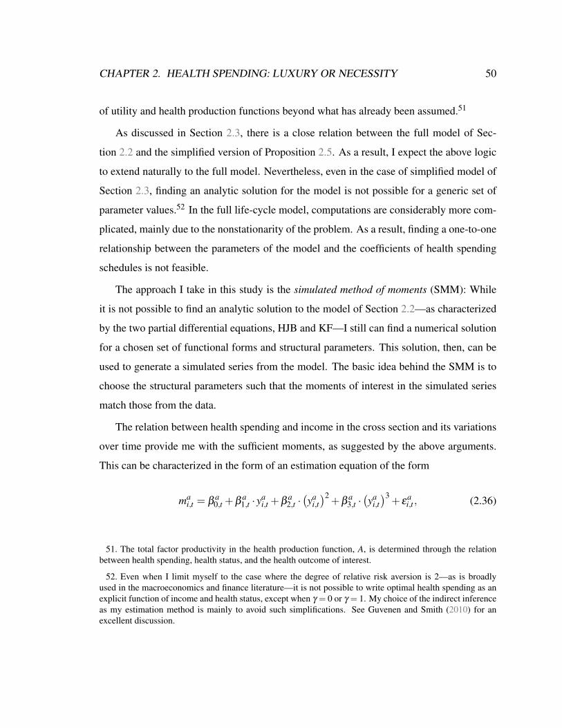
CHAPTER 2. HEALTH SPENDING: LUXURY OR NECESSITY 50
of utility and health production functions beyond what has already been assumed.51
As discussed in Section 2.3, there is a close relation between the full model of Sec-
tion 2.2 and the simplified version of Proposition 2.5. As a result, I expect the above logic
to extend naturally to the full model. Nevertheless, even in the case of simplified model of
Section 2.3, finding an analytic solution for the model is not possible for a generic set of
parameter values.52 In the full life-cycle model, computations are considerably more com-
plicated, mainly due to the nonstationarity of the problem. As a result, finding a one-to-one
relationship between the parameters of the model and the coefficients of health spending
schedules is not feasible.
The approach I take in this study is the simulated method of moments (SMM): While
it is not possible to find an analytic solution to the model of Section 2.2—as characterized
by the two partial differential equations, HJB and KF—I still can find a numerical solution
for a chosen set of functional forms and structural parameters. This solution, then, can be
used to generate a simulated series from the model. The basic idea behind the SMM is to
choose the structural parameters such that the moments of interest in the simulated series
match those from the data.
The relation between health spending and income in the cross section and its variations
over time provide me with the sufficient moments, as suggested by the above arguments.
This can be characterized in the form of an estimation equation of the form
mai,t = β
a0,t +β
a1,t · ya
i,t +βa2,t ·(ya
i,t)2
+βa3,t ·(ya
i,t)3
+ εai,t , (2.36)
51. The total factor productivity in the health production function, A, is determined through the relationbetween health spending, health status, and the health outcome of interest.
52. Even when I limit myself to the case where the degree of relative risk aversion is 2—as is broadlyused in the macroeconomics and finance literature—it is not possible to write optimal health spending as anexplicit function of income and health status, except when γ = 0 or γ = 1. My choice of the indirect inferenceas my estimation method is mainly to avoid such simplifications. See Guvenen and Smith (2010) for anexcellent discussion.

CHAPTER 2. HEALTH SPENDING: LUXURY OR NECESSITY 51
known as the auxiliary model. The variables mai,t and ya
i,t in Equation (2.36) are health
spending and income at time t for individual i in the data, respectively, who has age a.
For a given time t, the coefficients of Equation (2.36) (β ai,t’s) capture the relation between
income and health spending in the cross section for individuals of different ages at time t.
Estimating this equation for different t’s, then, characterize the variations of this relation
over time. The higher order terms on the right hand side of the auxiliary model capture
the fact that the relation between income and health spending is far from being linear, as
suggested by my model.53
My objective is to choose the structural parameters of the model so that the series
generated by the model (under these parameters) look as close as possible to the actual
data, as represented by the coefficients of the auxiliary model. This is the basic idea behind
the indirect inference approach.
The indirect inference method, first proposed by A. A. Smith J. (1990, 1993) and further
developed by Gourieroux, Monfort, and Renault (1993), provides a criterion—through the
use of an auxiliary model—to infer the structural parameters of interest in the model. In
effect, the indirect inference approach provides an answer to a key issue in the SMM,
through the use of an auxiliary model, and that is which moments to match (Qu 2012). As
Guvenen and Smith (2010) write,
“the indirect inference estimator is obtained by choosing the values of the
structural parameters so that the estimated model and the US data look as sim-
53. If my model is to represent the important mechanisms present in the “real world,” we can expect anestimation of Equation (2.36) to result in higher order coefficients that are statistically significant; after all, ahighly non-linear relationship between income and health spending, as suggested by the model, means thatthe several initial terms of a Taylor approximation of the “actual” relationship are significant.
One can expect the lagged income to also have an effect on the health spending because of its effecton savings, according to the model. These terms become important specially in the presence of stationaryidiosyncratic productivity shocks. Unfortunately, the limitations in MEPS’ panel features prevent me fromusing these moments.

CHAPTER 2. HEALTH SPENDING: LUXURY OR NECESSITY 52
ilar as possible when viewed through the lens of the auxiliary model.”
The Income Equation The above discussion forms the basis of our quantitative analysis
with a not-so-trivial shortcoming: The relation between health status and income is not
known. Without the knowledge of such a relationship, the identification of the parameters
of the health production function is not possible.54 Importantly, in my analysis, I want to
remain faithful to the notion of health status as a latent variable. This prevents me from
using an index of observed characteristics as a measure of underlying health status (as is a
standard practice in the literature).55
To overcome this difficulty, I use another source of variations in the data to make in-
ference about the income equation. I take advantage of the relation between the rate of
mortality at different ages—as a measure of health outcome—and income, as well as the
variations of this relationship over time, to deduce how income and health status are related
to each other.56
These two steps, that is comparing model’s simulations regarding the joint distributions
of income and health spending and income and life expectancy to the data, can be combined
in the form of two auxiliary equations: in practice, one can choose the parameters of an
income equation (that is the parameters of a functional form of choice for Equation (2.3))
and those of the utility and health production functions simultaneously such that model’s
simulations are “as close as possible” to the actual data. Closeness, in this context, is
determined by estimates of Equation (2.36) and an equation relating life expectancy to
54. Without an income equation, for any given set of parameter values, one can “choose” a level of individ-ual health status such that the model matches the data perfectly.
55. As my discussions at the start of Section 2.4 suggest, in the absence of reliable instruments, using suchmeasures of health status is prone to an endogeneity problem.
56. Limiting myself to the notion of health production as a determinant of longevity—at least in thissection—enables me to compare the resulting relation between income and longevity with the actual data,and to make further inference about the parameters of the income equation.

CHAPTER 2. HEALTH SPENDING: LUXURY OR NECESSITY 53
income.
In my estimation procedure, however, I am going to perform these two comparisons se-
quentially: In the first step, for a given set of parameters of the health production function,
I choose the parameters of an income equation. This is done such that, should the model
mimic the relationship between income and health spending in the data as closely as pos-
sible, the resulting joint distribution of income and life expectancy also matches that in the
data. This leads to an estimate of the income equation that is conditional on the parameters
of the health production function being equal to the SMM estimates. In the second step, the
conditional estimate of the income equation and the choice of parameters of the health pro-
duction function are used to compare the moments of the auxiliary equation (2.36) between
the data and the model. I repeat these steps until the moments of interest in the model are
close to those in the data.
In Section 2.4.2, I am going to explain this procedure in more detail in the context of
an estimation algorithm. As discussed above, this procedure uses the joint distributions
of income and health spending, and income and mortality rate, at different ages, and their
changes over time. In Section 2.4.1, I will briefly explain the data used for this purpose.
2.4.1 Data
The data on the joint distribution of income and health spending as a function of age and
cohort is taken from the household component of the Medical Expenditures Panel Survey
(MEPS). Annually conducted by the Agency for Healthcare Research and Quality (AHRQ)
and the National Center for Health Statistics (NCHS) form 1996, the MEPS includes na-
tionally representative surveys of detailed health care utilization and expenditures for the
US’ civilian, non-institutionalized population.
Health care expenditures are based on individuals’ self-reports, but they are verified
by and supplemented with reports from medical providers and employers. Therefore,the

CHAPTER 2. HEALTH SPENDING: LUXURY OR NECESSITY 54
MEPS provides a reliable source of information on health care expenditures for surveyed
individuals. Since it collects ample individual and family background information, it is
also suitable for studying the distribution of health care expenditures by demographic and
socioeconomic characteristics.
Total health care expenditures in the MEPS consist of expenditures, regardless of the
payer, on most medical services. Health care expenditures are paid out-of-pocket or by
private insurance, Medicaid, Medicare, or other local, state, and federal sources. Medical
services in MEPS are categorized into nine groups: medical provider visits, hospital out-
patient, inpatient and emergency room visits, dental visits, home health care, vision aids,
prescribed medicines, and other medical equipment and services.57
MEPS also gathers detailed information on respondents’ family income. Family in-
come is the summation of all family members’ income. An individual’s income includes
money made from all sources such as wages and compensations, business incomes, pen-
sions, benefits, rents, interests, dividends, and private cash transfers, excluding tax refunds
and capital gains.58
A central objective of this chapter is to study the effect of the evolution of income
on health spending. Therefore, as discuss in more detail in what follows, I use Center
on Budget and Policy Priorities (CBPP)’s estimates and projections of the growth rate of
57. Total health care expenditures calculated from the MEPS data are significantly different from theestimates provided by the National Health Expenditures Accounts (NHEA), which mainly use aggregateproviders’ revenue data. The disparity does not originate from different estimations of expenditures on com-parable services but from differences in inclusion of services and in covered populations. For example,expenditures on over-the-counter drugs, longer than 45-day stays in hospitals, and for institutionalized indi-viduals are out of the MEPS’ scope. Once aggregate estimations are adjusted for service and population, andmeasurement methods are made compatible, they tend to converge. In effect, the average growth rates of perperson health care expenditures, driven from MEPS and NHEA, are very similar. (See Chapter 1.)
58. The exclusion of capital gains from income is consistent with the definition of income in my model.However, I believe that my lack of access to tax refunds and transfers in the MEPS data—specifically for thelower income groups—does affect my results, as the Congressional Budget Office (CBO)’s comprehensiveincome measures paint a drastically different account of the growth rate of income at the bottom of the incomedistribution.

CHAPTER 2. HEALTH SPENDING: LUXURY OR NECESSITY 55
income at different parts of the income distribution to approximate the evolution of this
distribution before and after the MEPS’ time span (Stone et al. 2015).
Data on the relation between income and life expectancy is taken from Chetty et al. (2016)’s
seminal work on the association between the life expectancy and income in the US. Chetty
et al.’s analysis uses a database of federal income tax and Social Security records that in-
cludes all individuals with a valid Social Security Number between 1999 and 2014. Chetty
et al. construct the period life expectancy conditional on income percentile by (i) estimating
mortality rates for the ages of 40 to 76 years; (ii) extrapolating mortality rates beyond the
age of 76 years and calculating the life expectancy; and (iii) adjusting for differences in the
proportion of racial and ethnic groups across percentiles. Using the Social Security Ad-
ministration (SSA)’s death records, these steps lead to estimates for period life expectancy
at 40 for men and women at different levels of income over the period 2001–2014. (See
Figures 2 and 3 in Chetty et al. 2016.)
To compute the variance of health shocks, I use information from Ales, Hosseini, and
Jones (2014): the variance of log income at different ages. Ales, Hosseini, and Jones use
the data from the Panel Study of Income Dynamics (PSID) to construct this measure. (See
Figure 4 in Ales, Hosseini, and Jones 2014.)
Data Preliminaries
I use the disposable family income in the MEPS—by the Current Population Survey (CPS)’s
definition of family—as individuals’ income.59 At every stage of my estimations, I use
family-level weights provided by the MEPS, so that the survey samples provide as close
a representation to the US’ non-institutionalized population as possible. All dollar values
are adjusted for inflation, using the personal consumption expenditure (PCE) index. For
59. This is consistent with Chetty et al. (2016)’s measure of income.

CHAPTER 2. HEALTH SPENDING: LUXURY OR NECESSITY 56
expenditures on components of medical services, I use the corresponding personal health
care (PHC) components such as PHC for hospital care, for physician and clinical services,
and for dental services. All real values are in 2009 dollars. In addition, all individuals with
zero income in a given year are dropped from the sample.60,61 This leaves me with a total
of 639,649 individual-year observations in the period 1996–2015.
To use the variations of income over time in the estimation of the structural parame-
ters of the model, I divide the MEPS’ sample period into two sub-periods: 1996–2005 and
2006–2015—consistent with my assumption that each period in my model is equivalent to
an interval of ten years in the data, as discussed later on.62 The resulting two sub-periods
include 300,610 and 339,039 individual-year observations, respectively. I also group indi-
viduals in each sub-period into four age groups of ten-year intervals, from 40 to 70, and an
age group of individuals older than 80 years old.63,64 Table 2.1 provides a summary of the
MEPS data in each age group and across the two sub-samples.
Using the MEPS data, structured as described in Table 2.1, I construct the empirical
60. I drop zero-income individuals for two reasons. First, my model does not allow for consumption to fallbelow a certain level—because the utility must remain positive at all dates. Second, the SSA records do notprovide reliable data for such individuals.
61. Dropping the top and bottom 2.5% of the income distribution in each time period in a robustnessexercise does not alter my results significantly.
62. Hall and Jones (2007) consider five-year periods.
63. Individuals below the age of 40 are dropped to remain consistent with Chetty et al. (2016)’s estimates.
64. There are two main reasons for choosing ten-year time periods as the length of one period in the model:First, due to year-to-year changes in the randomly selected MEPS’ samples, there are year-to-year (sometimesirregular) fluctuations in health care expenditure estimates, especially when sub-groups are identified by morethan one characteristic. However, using time intervals of length five years show that the patterns of changesin income and health spending are remarkably similar to those between the two periods, 1996–2005 and2006–2015.
The second—and more important—reason is that this rough temporal grid leads to far fewer structuralparameters of the health production function. This smaller set of unknowns, in turn, eases the computationburden of the estimation procedure significantly. The author has implemented a version of the numericalmethod that uses intervals of length five years. However, at the time of writing this draft, the results of thisimplementation are not reliable.

TABLE 2.1. Summary of the Medical Expenditure Panel Survey Data,1996–2015
1996–2015 2005–2015 1996–2015
Age Group Obs.Percentage
of Males
Avg.
AgeObs.
Percentage
of Males
Avg.
AgeObs.
Percentage
of Males
Avg.
Age
40–49 42,417 49 44.36 44,149 48 44.61 86,566 48 44.48
(0.02) (0.03) (0.02)
50–59 32,078 48 54.14 42,227 49 54.30 74,305 48 54.23
(0.02) (0.02) (0.02)
60–69 20,384 47 64.22 28,797 47 64.11 49,181 47 64.15
(0.03) (0.03) (0.02)
70–79 15,509 43 74.19 15,771 45 74.12 31,280 44 74.15
(0.03) (0.04) (0.02)
≥ 80 8,158 36 83.65 9,581 39 83.33 17,739 38 83.47
(0.04) (0.04) (0.03)
≥ 40 118,546 46 57.13 140,525 47 58.174 259,071 47 57.70
(0.08) (0.11) (0.08)
Source: Medical Expenditure Panel Survey (1996–2015). Note: Observations with zero income have been dropped
from the sample. For the percentage of males and average age in each age group, personal weights, provided by the
MEPS are used. The total number of observations do not take survey weights into account.
57

CHAPTER 2. HEALTH SPENDING: LUXURY OR NECESSITY 58
distributions of income for different age groups in each of the sub-periods. As noted before,
one of the central objectives of this study is to use the variations in income over time to
make statistical inferences about the production of health. To address the fact that, at any
given age and year, rational agents also take these variations—both in the past and future—
into account, I need to extend the age-specific distributions of income to time periods before
and after the MEPS’ relatively short time span.65
To this end, I use the CBPP’s estimates—using the CBO’s data—to extrapolate the
age-specific distributions of income in the first time period. This gives me the age-specific
distributions of income down to the year 1980. For the years before 1980, I assume a
unified growth rate (equal to the growth rate of GDP per capita) for income at all income
percentiles. The CBPP’s projections are used in a similar procedure to extrapolate the
65. An important decision in the quantitative studies of life-cycle phenomena is how to deal with cohorteffects. In particular, as noted, I assume that each time interval of unit length in my model corresponds to aperiod of ten years in the MEPS data. This means that, in each of the sub-periods, I have individuals whohave entered the economy before the start of the sample’s time span and who will leave the economy afterthe sample’s end date.
A rather standard approach in the quantitative literature is to ignore these effects. For example, by poolingthe MEPS’s data, Ales, Hosseini, and Jones (2014) assume that individuals of age a in the model are goingto face the same income as the individuals of age a+ 1 in the sample, when they become a′ = a+ 1. Thisapproach obviates the need to make additional assumptions regarding the evolution of variables outside thesample. However, a more important advantage of it is to eliminate an aggregate state from the problem—thatis time—which has a considerable impact on the computational burden.
In practice, this is the same approach used in many longevity studies, including Chetty et al. (2016), tocalculate the life expectancy from the period life tables. (And, as I am going to talk about in Section 2.4.3,I start my numerical search for the model parameters by assuming this is the case.) Due to the nature of myclaims, however, I find it hard to justify that individuals in my economy do not take into account the evolutionof their income—and also technological innovations in the health sector—when making decisions.
With regard to the future evolution of income, using a projection seems justifiable (e.g., Arnold and Plotin-sky 2018). For the evolution of a cohort’s income distribution over its lifetime, what matters, from theperspective of my model, is the distribution of asset holdings. The MEPS, however, does not provide in-formation on this variable. My use of the CBPP’s estimates for the evolution of income before the MEPS’sample, in effect, serves as a tool to construct this distribution for individuals of different ages who, at thebeginning of the MEPS sample, are older than
¯a.
Another possibility is using other data sources to impute asset holdings at different income percentiles. Atthe time of writing this draft, the author is exploring this possibility using PSID.

CHAPTER 2. HEALTH SPENDING: LUXURY OR NECESSITY 59
income distributions up to 2035.66 I use these in the estimation of the parameters of the
income equation in periods that fall outside the MEPS’s time span.
I use the MEPS data to estimate the joint distribution of health spending and income
for each age group, in each of the time periods. This distribution, then, is used to compute
the average level of health spending in each income ventile, for each age group and time
period.
To calculate health status as a function of age and income for any given set of parameter
values, I need to have the survival rate at each age among different income groups in each
of the sub periods. To this end, I reconstruct the mortality rate at different ages, at each
point in Chetty et al.’s sample period, from the reported life expectancies at 40. I do this
by inverting the procedure used to construct the average life expectancy from the period
life tables, as follows:67 I start by extrapolating Chetty et al.’s estimates to the years in the
MEPS that are missing from Chetty et al.’s sample period. Next, I compute the average life
expectancy at 40 across the income groups in each time period of interest, 1996–2005 and
2006–2015, using the MEPS’ distribution of individuals by their gender in each period.
The Gompertz equation defines the rate of mortality as a function of age as
ln(mortality at age a) = g1 +g2 ln(a) .68 (GL)
Assuming that the Gompertz law provides an accurate description of the morality as a
66. This is the year at which individuals who are 40 at 2010 retire.
67. This is the procedure used by Chetty et al. to compute life expectancy from mortality rates at differentages, as discussed previously.
68. Chetty et al. show that the Gomperz equation provides a remarkably good description of the rate ofmorality as a function of age, at different levels of income, up to a certain age. (See Figure 1 in Chettyet al. 2016.) In their estimates of the life expectancy, they use this equation to extrapolate the mortality ratebeyond the age of 76.
It should be noted that the fit of the Gompertz model declines drastically after the age of 90.

CHAPTER 2. HEALTH SPENDING: LUXURY OR NECESSITY 60
FIGURE 2.1. Gompertz Approximations in the 5th and 95th IncomePercentiles
Source: Author’s calculations based on Chetty et al. (2016).
function of age at each level of income and each time period, I estimate g1 and g2 in
Equation (GL) for each time period and each income ventile. I do this such that the resulting
life expectancy at 40 matches those reported by Chetty et al., under the assumption that
a = 100. Figure 2.1 illustrates an example of the resulting mortality and survival rates for
the bottom and top income ventiles, in the first time period.
2.4.2 Estimation Strategy
I start the discussion of my estimation algorithm by choosing the specific functional forms
whose parameters, beside those of the CRRA and CES utility and health production func-

CHAPTER 2. HEALTH SPENDING: LUXURY OR NECESSITY 61
tions of Section 2.3, are going to be directly or indirectly targeted in the SMM method.
These include the depreciation function, the income equation, and the subsidy function.69
The depreciation of health status, at each given age a, is assumed to be an affine func-
tion of the natural logarithm of health status at that age. Formally, I assume that g(·) in
Equation (2.1) takes the form
g(h,a) =− [aδ (a)+bδ (a) · ln(h)] . (2.37)
I assume that at each age a, a linear function relates the natural logarithm of income to
the logarithm of health status, as
ln(y(h,a, t)) = y(a, t)+ϕ (a, t) · ln(h) . (2.38)
The term y(a, t) in this equation captures the common component of income among the in-
dividuals of cohort t−(a−¯a) at age a, whereas ϕ (a, t) characterizes the income variations
arising due to the heterogeneity in health.70
Following Guvenen and Smith (2010), after retirement, income is a function of the level
69. This is mainly due to the fact that I find having these relationships at hand helpful to the flow of thediscussions. Nevertheless, my methodology can be generalized to other assumed functions.
70. In the presence of productivity shocks, I modify Equation (2.38) as
ln(y(h,ν ,a, t)) = y(a, t)+ϕ (a, t) · ln(h)+ν . (2.39)
This is similar to the functional form considered by many in the literature for earnings and labor income,modified to include the impact of health status. Examples are Guvenen (2007, 2009), who instead of allowingy(·) to change freely with age, assume that the life-cycle profile of income is given by a quadratic functionof age. In the health economics literature, Scholz and Seshadri (2011) consider the same functional form butabstract from the effects of health status on income.
Equation (2.39) is similar to the functional form considered by Fonseca et al. (2009), with the considerationthat “health status” in Fonseca et al. is assumed to take discrete values. They, however, assume y(·) is aquadratic function of age.

CHAPTER 2. HEALTH SPENDING: LUXURY OR NECESSITY 62
of income at the age of retirement and the average income in the economy Y :
φ(yR, t
)= ay
[yR
Y (t)
]+by
[yR
Y (t)
]·[
yR
Y (t)
]. (2.40)
As discussed in Section 2.3, the flow utility is assumed to take the CRRA form with a
constant term—the value of being alive:
u(c) = b+c1−σ
(1−σ). (2.41)
For the health production function, I modify the CES functional form of Section 2.3 to
allow for individuals’ age to have an effect on the probability of survival:
f (h,m,a, t) = A(a)[α [z(t) ·m]γ(a)+(1−α)hγ(a)
] β (a)γ(a)
. (2.42)
This form allows my model to nest the health production functions of Hall and Jones (2007)
and Ales, Hosseini, and Jones (2014) as special cases. I will denote the growth rate of health
technology z(·) by gz.
Finally, I consider the following functional forms for the rate of subsidy, before and
after the retirement:
s(y,a) =
[as · exp(bs · y)]−1 if a ∈[¯a,aR) ,(
aRs +bR
s · y)−1 if a ∈
[aR, a
].71
(2.43)
71. As mentioned before, Equation (2.43) summarizes many different government health programs in theUS which include, but are not limited to, Medicaid, Medicare, State Children’s Health Insurance Program(SCHIP), the Department of Defense TRICARE and TRICARE for Life programs (DOD TRICARE), theVeterans Health Administration (VHA) program, the Indian Health Service (IHS) program.
Before retirement, Medicaid is the dominant provider among these government programs. Because ofMedicaid’s means-tested nature, its share in the total health spending declines rapidly by income, justifying

CHAPTER 2. HEALTH SPENDING: LUXURY OR NECESSITY 63
To estimate the parameters of these functional forms, I use an iterative procedure that
follows the logic discussed at the beginning of Section 2.4: to search for a set of parameters
under which the simulated data generated by the model looks as close as possible to the ac-
tual data, when viewed through the lens of an auxiliary model. To this end, I keep updating
the values of the unknown parameters of the model until no further improvements can be
achieved upon a “closeness” criterion. Some of the parameters of the model, however, are
estimated or calibrated outside this iterative loop. I will explain these variables first.
Preset Parameters
As noted earlier, I assume that an interval of unit length in my model corresponds to a
period of ten years in the data. Therefore, the two time periods under consideration in
the MEPS data, 1996–2005 and 2006–2015, correspond to a time interval of length two
in my model. For the sake of consistency (and convenience), I am going to denote the
approximate midpoints of the two time periods by t1 and t2, in what follows: t1 = 2000 and
t2 = 2010.
I set¯a = 40. This value is consistent with the initial age in Chetty et al. (2016)’s
sample. I assume individuals live up to a = 100 years (Hall and Jones 2007).72 For the
the exponential form of subsidies in Equation (2.43). My estimations show that this functional form in factdoes an excellent job in representing Unites States health care subsidization programs before retirement.
After retirement, Medicare replaces Medicaid as the major public provider of health care services. WhileMedicare is not means-tested, two factors seem to be responsible for the share of total health expenditurespaid by government entities to be declining in income. First, despite the dominant role of Medicare, Med-icaid remains as a complimentary provider of services that are not covered by Medicare for lower incomeindividuals. Second, Medicare’s provisions are not similar for all medical services. Therefore, the differ-ences in the type of health services that are consumed by each income group result in the rate of subsidy to benon-homogeneous in income. (My model does not capture these differences in the type of services that aredemanded by each income group. See Ozkan 2014 for an example where this consideration is explicitly mod-eled.) Equation (2.43) does a good job in consolidating these factors up to a certain threshold (specifically,up to 400% of the federal poverty line). After this threshold, however, the model fit declines.
72. This number seems to be consistent with Chetty et al. (2016)’s upper bounds using Gompertz extrapo-lation for the 99% income percentile of their sample.

CHAPTER 2. HEALTH SPENDING: LUXURY OR NECESSITY 64
age of retirement, I choose aR = 65. While, in my sample, there is a lot of variation in
the age of retirement, this value ensures that the individual is eligible to receive Medicare
compensations if a > aR.
The degree of risk aversion, σ in Equation (2.41), is set to 2.0, as it is the gold standard
in the macroeconomics and finance literature. This is the value that has been widely used
in the literature after Mehra and Prescott (1985)’s seminal work, and the parameter used by
Ales, Hosseini, and Jones (2014). In their benchmark quantitative analysis, Hall and Jones
use the same value. The value of ρ is chosen so that the annual discount rate is 0.98. r is
set to match the average long-term rate of return on the US treasury bills (that is 3.3%).73
A consequence of the insistence on treating the health status as a latent variable is
that my estimation strategy cannot identify the initial level of health status from the share
parameter, α in Equation (2.42), in the first time period. In addition, the growth rate of
average health status cannot be identified from the growth rate of health technology, pa-
rameter z in Equation (2.42). One can see this by noticing that none of these parameters are
invariant to the normalizations of health status: should the measurement unit of h change in
Equation (2.42), these variables change as well. Therefore, in my simulations, I normalize
α to 0.1 and z(t1) to 0.25. Following Hall and Jones, I assume z(·) grows at the same an-
nual rate as the long-run growth rate of GDP per capita in the US economy (1960–2016);
2.03%.74,75
73. Note that, unlike most of the macroeconomic literature, the gross rate of return is not equal to the inverseof discount rate in my calibrations, as dictated by the Euler equation. This assumption, besides the fact thatindividuals are not infinitely lived in my economy, is mainly justified by the endogenous chance of mortality.
74. My results do not show any change as a result of a change in z(t1) or any significant change as a resultof a change in α , confirming my claim that they act as normalization parameters.
75. This means gz, the growth rate of z(·) in the model is chosen such that
gz
10= ln
(z(t1 +0.1)
z(t1)
)= 0.0203.
This is because of the assumption that an interval of length ∆t = 1 in my model corresponds to ten years in

CHAPTER 2. HEALTH SPENDING: LUXURY OR NECESSITY 65
The parameters ay and by in Equation (2.40) are borrowed from Guvenen and Smith
(2010), so that
φ(yR, t
)= Y (t)×
0.9× y, if y≤ 0.3,
2.27+0.32× (y−0.3) , if 0.3 < y≤ 0.2,
0.81+0.15× (y−2.0) , if 2.0 < y≤ 4.1,
1.13, if 4.1≤ y,
(2.44)
where y := yR/Y (t). The MEPS data is used to estimate Y (t) for t = t1 and t = t2. Outside
the MEPS sample, Y (·) is assumed to grow at the same rate as the GDP per capita.
Finally, the parameters of the policy function, as, bs, aRs , and bR
s , are estimated so that
the resulting subsidy schedule matches the average share of total expenses that are paid
by government entities in the MEPS data as a function of income, before and after retire-
ment.The tax rate τ (·) is calibrated so that the government’s budget in Equation (2.22) is
balanced in each period.
Table 2.2 summarizes the parameters that are estimated or calibrated outside the main
SMM loop.
Simulated Method of Moments
The remaining structural parameters of the model consist of b, A(a)a, γ (a)a, β (a)a,
aδ (a)a, bδ (a), σh, y(a, t)a,t , and ϕ (a, t)a,t . In the continuous time model of Sec-
tion 2.2, t and a can take on all the values on the real line and in the interval [¯a, a], respec-
tively. Since it is not feasible to estimate the parameters that are functions of age and/or time
over their entire domain, I have to restrict my estimates to certain cross sections. As my dis-
the data.

TABLE 2.2. Preset Parameters
Parameter Value Source
σ 2.0Mehra and Prescott (1985), Ales, Hosseini, and Jones
(2014), Hall and Jones (2007)
ρ 0.2
r 0.32 US’ Department of Treasury
z(t1) 0.25
α 0.1
gz 0.20Hall and Jones (2007), National Income and Product
Accounts
Y (t1) 77,475Medical Expenditure Panel Survey
Y (t2) 77,876
gY 0.20 National Income and Product Accounts
aτ 1.660
Medical Expenditure Panel Surveybτ 0.069
aRτ 1.384
bRτ 0.013
Source: Author’s calibrations. Note: α and z(t1) are normalization parameters.
Values of r, ρ , gz, and gY are calibrated noting that one year in the data corresponds to
a period of length 0.1 in the model. Parameters of the policy function are estimated by
fitting the functional forms in Equation (2.43) to the share of total health expenditures
that are paid by government entities, before and after the age 65, over the entire
MEPS sample period, 1996–2015.
66

CHAPTER 2. HEALTH SPENDING: LUXURY OR NECESSITY 67
cussions of Section 2.4.1 suggest, for the time sections, I am going to estimate the parame-
ters for t ∈ t1, t2 in the MEPS sample and t ∈ 1950,1960,1970,1980,1990,2020,2030
outside the MEPS time span. For the variables that are functions of age, I limit my estima-
tions to the average ages in each of the five age groups (as given in Table 2.1).76,77
One can choose the parameters of the health production function, the utility function,
and the income equation so that the moments generated through the model match those of
two sets of auxiliary models: One characterized by Equation (2.36); and one relating the
life expectancy to income, at different ages. But, this means that my estimator will be a
vector of intractable dimensions, making the search for the global optima unfeasible.
To overcome this difficulty, as suggested before, I take another route and divide the
set of structural parameters of the model into two subsets: The first set consists of param-
eters that are “estimated directly” to “target” the moments of the auxiliary model, Equa-
tion (2.36). I denote this set by Λ:
Λ :=
b,A(a) ,γ (a) ,β (a)a
. (2.48)
76. To summarize, for the parameters that depend on t and a, the estimations are limited to
(t,a) ∈(t,44.36) ,(t,54.14) ,(t,64.22) ,(t,74.19) ,(t,83.65) ; t ∈ 1950, . . . ,2000
(2.45)
and
(t,a) ∈(t,44.61) ,(t,54.30) ,(t,64.11) ,(t,74.12) ,(t,83.33) ; t ∈ 2010,2020,2030
. (2.46)
For the parameters which are assumed to remain the same over the two periods, I limit my estimators to
a ∈ 44.48,54.23,64.15,74.15,83.47 . (2.47)
77. In my simulations, when a and t fall between two sections a1 and a2, and ta and tb, I use a bi-linearinterpolation of the parameter values at (a1, ta), (a1, tb), (a2, ta), and (a2, tb).

CHAPTER 2. HEALTH SPENDING: LUXURY OR NECESSITY 68
The second set of parameters are estimated indirectly, conditioned on Λ. This set includes
Θ :=
σh,aδ (a) ,bδ (a)a ,y(a, t) ,ϕ (a, t)a,t
. (2.49)
The logic behind the estimation of Θ conditioned on a set Λ is as follows: If we knew
the values of the parameters in Λ for the “true” underlying data-generating model, finding
the values in Θ would boil down to several ordinary least squares (OLS) regressions. The
reason is that, given Λ, we could use the joint distribution of health spending, income, and
mortality rates to deduce the joint distribution of health status and income, using the health
production function. This distribution (at different ages), in turn, could be used to estimate
aδ (·) and bδ (·), at different ages which, itself, determines the evolution of the distribution
of health status during the life-cycle of individuals. This distribution, together with the
evolution of the distribution of income for each cohort, enable me to estimate y(·) and ϕ (·)
at different ages and different dates. The variance σh, then, could be chosen so that the
variance of income as a function of age matches that in the data as closely as possible.
When Λ is not known, for a given guess Λ, should the moments of the simulated data
match those of the actual data as close as possible, we expect the joint distribution of
income and health spending to be similar between the generated and actual data. Therefore,
for the model to be able to also predict the joint distribution of income and life expectancy
as it prevails in the actual data, aδ (·), bδ (·), y(·) and ϕ (·) must take certain values. The
same is true for the parameter σh.
This enables me to estimate Θ conditioned on a given guess for Λ. If Λ does in fact
result in a data generating machine that closely resembles the actual data generation process
(as seen through the lens of the auxiliary model), we can rest assured that we have the
“right” estimate for Θ as well.
What makes this “sequential” estimation procedure possible is the fact that, under the
assumed functional forms, there is a direct correspondence between some moments in the

CHAPTER 2. HEALTH SPENDING: LUXURY OR NECESSITY 69
data and some of the parameters of the model (namely Θ). Hence, given an estimate of the
health status, it is easy to estimate the parameters in Θ using the conventional techniques.
This logic reduces the number of unknowns that are directly chosen in the indirect inference
method to 16. These are the parameters in Λ which are chosen to target the 50 reduced form
data moments that are derived from the auxiliary equations, Equation (2.36).
Estimating this over-identified set of moments requires the use of an efficient weighting
matrix. However, as we will discuss in more details in the steps that follow, instead of trying
to reduce the distance between the data and model moments using a weighting matrix, I
minimize a Gaussian objective function, as suggested by Guvenen and Smith (2010).
STEP 1: Generating the Shocks The starting period of the economy in my simulations
is when the cohort of individuals who are 90 at t1 enter the economy.78 I denote this starting
point by¯t := t1−50. The final period of the simulations is denoted t = t2 +60; the date at
which the cohort t2 reaches the age of a.
In the first step, I generate a set of random shocks corresponding to each individual in
my sample: For each individual in the sample, i∈I , I generate a Wiener process of length
t−¯t. I repeat this simulation N number of times. (I pick N = 10.) This leads to N sets of
random shocks, each of size |I |. I denote this set by N ,
N := (i,n) ; i ∈I ,n ∈ 1,2, . . . ,N ,
and the corresponding Wiener process by ωh (·; i,n). For each (i,n) ∈N , ωh (·; i,n) is the
path of health shocks that affects individual i during her lifetime. These simulated health
shocks are going to remain fixed throughout my simulations.
78. The number of individuals with non-zero income who are above 90 in the MEPS data is virtually zero.

CHAPTER 2. HEALTH SPENDING: LUXURY OR NECESSITY 70
STEP 2: An Initial Guess for Λ I make an initial guess for the set of parameters that
are estimated directly by targeting the moments of interest through the indirect inference
approach. Let’s denote this initial guess by Λ0.
STEP 3: Computing the Health status Health spending for each age group and each
time period t1 and t2 is given by the MEPS data at different income levels, m(a,y, t).
Given Λ0 and the log mortality rate at different ages in t1 and t2 in each income ventile,
log(χ (a,y, t)), I can compute the average health status in each income ventile and for dif-
ferent ages using Kmenta (1967)’s approximation of the health production function:79
log(χ (a,y, t)) = log(A(a))+αβ (a) log(z(t) ·m(a,y, t))
+(1−α)β (a) log(h(a,y, t))
+12
α (1−α)β (a)γ (a) [log(z(t) ·m(a,y, t))− log(h(a,y, t))]2 . (2.50)
STEP 4: Estimating the Depreciation Function Assuming that, after the age of 40,
there are no systematic movements between different percentiles of the log income during
the course of individuals’ life,80 I use the average health status of individuals in a given
income ventile who are a-years old in t1 and the same variable for individuals who are
a+1 in t2 to find an approximation for the depreciation function, aδ (·) and bδ (·) in Equa-
79. The use of Kmenta (1967)’s translog approximation of the health production function is to emphasizethat all variables are in natural logarithms, and has no real bearing on my simulations.
80. This assumption is different from saying there are no movements between the different percentiles oflog income. In fact, as Guvenen and Smith (2010) argue, there are differences in the growth rate of logincome during the life-cycle. But, as long as these differences are not in a way that, on average, individualsof a given income ventile end up in a higher ventile in the next decade of their life, my assumption is valid. Itis worth mentioning that this is the same assumption that Chetty et al. (2016) make, when using the mortalityrate of an individual of age a+1 in a given income percentile, as the future mortality rate of an individual inthe same income percentile, but at age a. Chetty et al. (2016) argue that this is a reasonable assumption.

CHAPTER 2. HEALTH SPENDING: LUXURY OR NECESSITY 71
tion (2.37).81,82
STEP 5: Computing the Evolution of Health Status Using my estimates for the depre-
ciation function and the distribution of health status for individuals of different cohorts in
t1 and t2, I can use the law of motion of health status to construct the initial distribution of
health status for each of the cohorts between¯t and t2, together with its evolution.83
STEP 6: Estimating the Income Equation The average log health status in each income
ventile, at different dates and for different age groups, can be used in conjunction with
the evolution of income distribution to estimate the parameters of the income equation,
Equation (2.38).
STEP 7: Estimating the Variance of Health Shocks Given ϕ (·) at different dates and
ages, I estimate the variance of health shocks σh such that the variance of log income in the
81. More precisely, the law of motion of health status implies that
Eh(t1) [log(h(t2))] =∫ 1
0[−aδ (a+ t)−bδ (a+ t) ln(h)]dt. (2.51)
Given E [log(h(t1))] = log(h(a,yv, t1)) at different income ventiles (yv’s), one can find aδ (·) and bδ (·) suchthat E [log(h(t2))] = log(h(a+1,yv, t2)) in Equation (2.51). Under the assumption that aδ (a) and bδ (a)remain constant for a ∈ [a,a+1], finding these parameters is rather easy. However, the assumption that fora ∈ (a,a+1), aδ (a) and bδ (a) are interpolations of their values at a and a+1 makes the calculations morecumbersome.
82. A more accurate approach to the estimation of the depreciation function is to use Kolmogorov’s back-ward equation to write the empirical distribution of health status in t1 and age a− 1 as a function of itsdistribution at t2 and age a, the depreciation function, and σh. Starting from an initial guess for σh, one caniterate on Steps 4 through 7 to pin down aδ (a), bδ (b), and σh.
This adds another estimation loop to an already numerically expensive problem that I want to avoid. Par-ticularly, when σh is small (and the curvature of the distribution of health status is not large), I do not expectthis step to add much to my estimations.
One should note that neither of these approaches takes into account the attrition due to mortality which wecan expect to be higher at lower levels of health status.
83. Cohort t2 is the last cohort that enters the economy.

CHAPTER 2. HEALTH SPENDING: LUXURY OR NECESSITY 72
model, on average, has the same age profile as the one estimated by Ales, Hosseini, and
Jones (2014) during the MEPS’ time period.84
This step concludes the estimation of Θ conditioned on Λ0, if the model is to generate
the joint distribution of income and mortality at different ages as observed in the data in t1
and t2.
STEP 8: Computing the Path of Health Status for Each Individual I can, now, use
the income equation to deduce the health status of each individual i ∈ I . For any n ∈
1,2, . . . ,N, the income equation and the law of motion of health status can be used to
construct the path of health status for individual i, under ωh(·; i, m
):
h(·; i, n
): [
¯a, a]→ R+. (2.53)
This is done for all the simulated Wiener processes in N .
STEP 9: Finding the Optimal Markov Control Given the functional forms and the
support of the distribution of health status, I can now solve the individual’s problem ,
Problem (2.15), by finding the solution to the HJB equation. This, in turn, gives me the
optimal feedback rule under Λ0: uΛ0 .
The computational approach that I take to solve the HJB equation is the Markov chain
approximation method. I discuss this method briefly in Section 2.4.3. (Interested reader
84. Note that, for a diffusion process, the variance of the sample path at any future date is equal to theproduct of the elapsed time and the variance of the underlying Wiener process. With a standard Wienerprocess, given the income equation and the law of motion of log health status (Equation (2.1)), the varianceof income at age a for individuals of cohort t0 is given by
Var [log(y(a)) | y(¯a)] =
∫ t0+a−¯a
t0ϕ (
¯a+ t− t0, t) ·σh ·dt. (2.52)

CHAPTER 2. HEALTH SPENDING: LUXURY OR NECESSITY 73
can refer to Kushner and Dupuis 2014 or Eslami 2017.)
STEP 10: Simulating the Path of Individual’s Health Expenditures For each individ-
ual observation i ∈ I in the MEPS data, let’s denote by ti and ai the corresponding year
(of the observation) and age (of the individual), respectively. For any(i, n)∈ N , I use
uΛ0 , together with h(0; i, n
)and individual’s cohort of entry ti− (ai− ¯
a), to construct the
sample path of optimal health spending under ωh(·; i, t
):
m(·; i, n
): [
¯a, a]→ R+. (2.54)
STEP 11: Consolidating the Simulated Data For any n∈1,2, . . . ,N, I can use h(·; i, n)
in (2.53) (with the income equation) and m(·; i, n) in (2.54) to construct the simulated pair
of health spending and income at age ai, for individual i, under the shock process n:
(y(ai; i, n
),m(ai; i, n
)).
I do this for all i ∈I to consolidate the simulated data, given n, in a set simΛ0 (n). Then,
simΛ0 :=
simΛ0 (n) ;n ∈ 1,2, . . . ,n.
In the next step, I use this simulated set to estimate the coefficients of the auxiliary
model.
STEP 12: The Auxiliary Model Now, I can estimate the coefficients of the auxiliary
model using each of the simulated data sets: simΛ0 (n), for n ∈ 1,2, . . . ,N. I do this
separately for each age group and time period of Table 2.1, using the OLS method and will

CHAPTER 2. HEALTH SPENDING: LUXURY OR NECESSITY 74
denote the resulting parameters by
βββ(simΛ0 (n)
):=(
βa0,t(simΛ0 (n)
), β a
1,t(simΛ0 (n)
), β a
2,t(simΛ0 (n)
), β a
3,t(simΛ0 (n)
))a,t
and σ(simΛ0 (n)
). I denote the average values of these estimates for different n’s by
βββ(simΛ0
)and σ
(simΛ0
):
βββ(simΛ0
)=
1N
N
∑n=1
βββ(simΛ0 (n)
)and σ
(simΛ0
)=
1N
N
∑n=1
σ(simΛ0 (n)
).
The same equation is estimated using the “actual data” from the MEPS in the two time
periods and for different age groups to yield the set of reduced form parameters βββ (data)
and σ (data).
STEP 13: The Gaussian Objective Function My indirect inference estimator is the
one suggested by Guvenen and Smith (2010). Following their notation, given the set of
parameters βββ and σ , define ε (·) as
εai,t
(βββ ,data
):= ma
i,t− βa0,t− β
a1,t · ya
i,t− βa2,t ·(ya
i,t)2− β
a3,t ·(ya
i,t)3, (2.55)
where mai,t and ya
i,t’s are from the MEPS data. (That is what data in this definition stands
for.) These residuals are used to compute the following Gaussian objective function:
L(
βββ , σ ,data)=
(1
2πσ2
) |I |2
exp
(− 1
2σ2 ∑i∈I
[ε
ai,t
(βββ ,data
)]2). (2.56)
Given these definitions, my indirect inference objective function is give by
GΛ0 := L(
βββ (data) , σ (data) ,data)−L
(βββ(simΛ0
), σ(simΛ0
),data
). (2.57)

CHAPTER 2. HEALTH SPENDING: LUXURY OR NECESSITY 75
STEP 14: The Closeness Criterion Our goal is to find the value of Γ (and corresponding
ΘΓ) to minimize GΓ. That is, our indirect inference estimator is given by
Γ := argminΛGΛ .85 (2.58)
To find the estimates of the parameters in Λ and Θ, I need to repeat this procedure, starting
from Step 2, until my “closeness criterion” is met. This criterion is provided by the opti-
mization algorithm of choice. I use a simulated annealing approach, for the reasons that
are going to be discussed briefly in the next section.
2.4.3 Remarks on the Computational Approach
In practice, finding the indirect inference estimates of the model parameters using the SMM
procedure of Section 2.4.2 boils down to choosing an optimization algorithm. Starting from
an initial guess for Λ, such an algorithm recommends a direction of movement in each
iteration of the above procedure, together with a closeness criterion.
With a control vector of length 16 and an objective function that is not very well-
behaved, standard optimization algorithms (like Newton-Raphson, adapted for a multi-
dimensional control space) do not, by themselves, guarantee a global optimum.
To ensure a global optimum, I use the simulated annealing method. In this algorithm,
in each iteration of the SMM, conditioned on the value of the objective function GΛ, there
is a chance of an “uphill movement. This probability, however, depends on the system’s
85. As Guvenen and Smith argue, using (2.57) as the objective function “obviates the need to estimatean efficient weighting matrix.” Estimating this matrix, in our problem, is rather hard and time-consuming,making Guvenen and Smith’s approach very appealing.
Nevertheless, testing an objective function that simply minimizes the Euclidean distance between the pa-rameters of the auxiliary model estimated separately using the actual and simulated data leads to the sameresults.

CHAPTER 2. HEALTH SPENDING: LUXURY OR NECESSITY 76
“temperature,” which asymptotically tends to zero.86 Starting from any feasible initial
guess Λ0, with a large number of repetitions of the SMM procedure from Λ0, I am more
confident that my results are, in fact, close to the global optimum of Problem (2.58).
From a computational standpoint, almost all of the numerical burden of the simulation
procedure is on the HJB equation, Equation (2.16): This is a PDE in four individual and
one aggregate states, making it extremely costly to solve. Even though the assumption that
x is governed by a diffusion process simplifies the first order conditions on the right hand
side of the equation to some extent, it should not be forgotten that the “actual” underlying
state is still a jump-diffusion with controlled jumps.87 This results in highly non-linear
optimality conditions and, consequently, adding to the numerical intensity of the problem.
To alleviate these difficulties, I start my global search by assuming no cohort effects:
that is, in each time interval ti, I assume that the economy is in a stationary equilibrium. In
addition, I assume σh = 0 in the benchmark model. This, in turn, eliminates the need to
keep track of hR (·) as an state variable after retirement. With two fewer states, I can find
the solution to the HJB equation rather quickly.
After a very thorough global search for the best candidates for Λ, under these sim-
plifying assumptions, I initiate several local searches starting from the global candidates.
The local searches are performed under the complete set of assumptions until no further
improvement seems feasible.88
86. In my numerical simulations, the temperature of the system is assumed to follow a simple reciprocalform. In each iteration, the probability of an uphill movement is proportional to exp
(−Gλ j/temp
).
87. The intensity of the mortality rate is still controlled by the health spending.
88. For the full economy, a complete cycle of the SMM procedure takes approximately twenty minutes ona workstation (with twelve cores working in parallel under OpenMP directives). Simplifying the economy, asexplained above, reduces this time to less than two minutes. Starting from the simplified economy allows meto pin down the optimum—from a relevant initial guess—in about three months on the same station. Usingthe Minnesota Supercomputer Institute (MSI)’s Linux cluster, I do this in less than two weeks using ten nodesworking under MPI directives.

CHAPTER 2. HEALTH SPENDING: LUXURY OR NECESSITY 77
An extensively used method for solving the HJB equation is the finite difference (FD)
method. In this approach, the PDE in (2.16) is approximated by a discrete equation.89 In
this study, however, I take a novel approach, known as the Markov chain approximation
method. In this method, which is developed by Kushner and Dupuis (2014), instead of
approximating the PDE itself, I approximate the underlying state vector x by a Markov
chain. Then, the individual’s problem is written for this approximating chain. This problem
is a functional equation (known as the Bellman equation) that can be solved iteratively.
Importantly, unlike the FD method, under some regulatory conditions on the approximating
chain—called the local consistency conditions—the solution to the Bellman equation is
guaranteed to converge to the solution to the HJB equation.90
2.5 The Results
Table 2.3 summarizes my estimation results for two of the parameters of interest: the elas-
ticity of scale and the cross elasticity of health outcomes with respect to health spending
and health status. My estimate for the value of being alive b is 110 (with a 95% confidence
interval of (97.68,122.32)).91
89. See Achdou et al. (2014) and Tourin (2010) for excellent discussions.
90. Approximating a diffusion process by a discrete Markov chain is not, by any means, equivalent tostarting from a general Markovian process. As Dixit (1993) notes, a discrete representation of a diffusionprocess is a random walk that satisfies ∆h = σ
√∆t, where ∆h is the size of the spacial jumps and ∆t is the
size of the temporal grid.The fact that the discretization takes the form of a random walk, however, has strict implications for the
controls: They can only change the probability of upward or downward movements, but cannot affect the sizeof the jumps. Consequently, the first order conditions would, in general, be considerably simpler than thoseof a discrete-time economy in which the states can, in theory, move freely.
However, in the presence of controlled jumps, these approximations loose their attraction, at least to someextent.
91. At the time of writing this draft, the standard errors are computed using the bootstrap method with onlyten re-samplings. However, in each of the re-samplings, the SMM procedure is restricted to a local searcharound the “true” candidate to avoid the extremely costly global search. See Footnote 88 for more details.

CHAPTER 2. HEALTH SPENDING: LUXURY OR NECESSITY 78
TABLE 2.3. Estimation Results
Age Group
40–49 50–59 60–69 70–79 80–89
Elasticity of Scale, β (a) 0.40*** 0.22** 0.11* 0.10 0.10***
(0.09) (0.10) (0.06) (0.08) (0.03)
Cross Elasticity, γ (a) 0.375*** 0.21*** 0.16 0.20*** 0.20***
(0.08) (0.08) (0.13) (0.03) (0.07)
Source: Author’s SMM estimates. Note: The elasticity of scale and the cross elasticity of health
production with respect to health spending and health status are estimated, together with the
value of being alive and the factor productivities, using the SMM. The targeted moments are
those of the auxiliary equation, Equation (2.36). See Section 2.4.2 for a detailed explanation.
The standard errors are computed using the bootstrap method with ten re-samplings of the data.
See Footnote 91 for more details.
Except two instances, all the estimates are statistically significant. These two are the
elasticity of scale for 70–79 year-old individuals and the cross elasticity for the age group
60–69. Moreover, except for the 40–49 age group, my estimates of the elasticity of scale
are close to Hall and Jones (2007)’s estimates. This parameter follows the same declining
trend as their results after the age of 40 suggest.
Importantly, my estimates of the elasticity of substitution are above one, ranging from
1.60 to 1.25, depending on age.92 This implies that health status and health spending are
relatively strong substitutes. In turn, this means that the effectiveness of health spending,
92. I believe that the decline in the substitutability of health spending and health status is rather intuitive.Specifically, at lower ages, the medical services that an individual receives tend to be closer in nature to areplacement for the underlying health: a heart valve surgery, an insulin injection, or an artificial limb, areall substitutes for a functioning organ. While these health services remain a major determinant of healthspending as individual ages, they tend to become effective only if the underlying health has not deterioratedgreatly.

CHAPTER 2. HEALTH SPENDING: LUXURY OR NECESSITY 79
in extending life, is relatively low at higher levels of health status.93
Therefore, as my discussions of Section 2.3 and, in particular, Proposition 2.5 suggest,
if health status and income are strongly correlated among the individuals of a given cohort,
high-income agents tend to have lower health spending (even in absolute terms) than low-
income individuals.
This is best shown in Figure 2.2, which depicts the model’s fit in the two time periods
of interest relative to the data. The model performs relatively well among the individuals of
the depicted cohorts. In particular, my estimates can capture the declining share of health
spending in the cross section and its increasing share in the time series: a necessity in the
cross section and a luxury over time.
An interesting observation is that, while income has not increased by much between the
two time periods in my data among the individuals of ages 40 to 49, the model suggests
that they still increase their spending by a relatively large margin (as it does in the data).
This can be attributed to two factors: an increase in z which, in effect, leads to a decline in
the relative price of health spending; and individuals’ expectations of higher future income
levels (as the average income depicts a significant increase at older ages in the sample).
As a result of this expected rise, individuals suppress their savings early in life—to some
extend—which frees up resources to be allocated to health care.
After the age 70, the model fit starts to diminish. In particular, my model predicts very
large levels of spending at ages over 80. The deterioration of model fit after the age of
80 can be attributed to several factors: First and foremost, the Gompertz equation used to
infer the mortality rates at different ages looses its predictive power at old ages. Second,
the variations in mortality rates among different income groups vanishes after a certain age,
93. Results of Table 2.3 suggest that, after the age of 60, the absolute value of the marginal product ofhealth spending declines with health status. This is beside the decline in the marginal product relative to theaverage product (which is the main determinant of health spending).

FIGURE 2.2. Model Fit: Health Spending Relative to Income
Source: Author’s simulations & MEPS.
80

CHAPTER 2. HEALTH SPENDING: LUXURY OR NECESSITY 81
FIGURE 2.3. Model Fit: Average Health Spending over Time
5.0
5.5
6.0
6.5
7.0
7.5
8.0
8.5
9.0
9.5
10.8 10.8 10.9 10.9 10.9 10.9 10.9 11.0 11.0 11.0
Log
Real
Hea
lth S
pend
ing
Log Real Income
Model: 𝑦𝑦 = 2.97 𝑥𝑥
MEPS: 𝑦𝑦 = 2.39 𝑥𝑥
Source: Author’s simulations & MEPS.
making my inferences on the health status at older ages even more inaccurate. Finally, my
sample sizes decline considerably for the last two age groups (as Table 2.1 suggests).
Figure 2.3 illustrates the predictive power of the model in the time series. Each point
on the figure illustrates the average log health spending in a given year during the MEPS
sample, versus the average log income in the same year. While the model can match the
rising share of health spending over time (through the slope of the fitted line, which is
significantly greater than one), it misses the level of spending. This, as I mentioned above,
is mainly because of the prediction of very high levels of spending at older ages (and among
the bottom 2% of the population).
My results suggest that initial health status has, in general, improved between the two
time periods, as depicted in Figure 2.4. In spite of an increase in general underlying health,
this rise has not been large enough to dominate the growth in income (or, at least, the
expectations thereof) or technology. Otherwise, as my discussions in Section 2.3 suggest,
I should have observed a decline in the share of health spending between the two periods.

CHAPTER 2. HEALTH SPENDING: LUXURY OR NECESSITY 82
FIGURE 2.4. Evolution of Initial Health Status
0
0.01
0.02
0.03
0.04
0.05
0.06
0.07
0.08
0.09
20 25 30 35 40 45 50
Den
sity
Log Health Capital
1996–2005
2006–2015
Source: Author’s estimates.
Finally, even though the general health status has improved across the two cohorts in t1 and
t2, this increase has not been the same for all income groups, as the distribution in Figure 2.4
has become significantly more skewed to the left. Such an increase in the variance of initial
health status is responsible for the rising gap of longevity across the income groups, as
documented by Chetty et al. (2016).
2.5.1 Marginal Cost of Saving a Life
Table 2.4 depicts the marginal cost of saving a statistical life for different age groups and
at the two time periods. The cost of saving a statistical life, at a given age (and time), is the
total amount of resources that are required to reduce the average number of deaths, at that
age, by one.
If we assume ς denotes the marginal effect of health spending on the rate of mortality
(at a given age), the resources required to prevent one death among the whole population—

CHAPTER 2. HEALTH SPENDING: LUXURY OR NECESSITY 83
that is to save one statistical life—is exactly 1/ς . In the context of my model, this is given
byf 2 (m,h,a, t)
∂ f (m,h,a, t)/∂m, (2.59)
for a given age and at a given time.
To compute this value for a given age group, I calculate (2.59) using my estimates of
the health production function and constructed health status, under the “actual” level of
health spending, at different ages within an age group. These are compounded to compute
the cost of saving a statistical life, as in Table 2.4.
Table 2.4 demonstrates these results at four different income levels: bottom and top
5%, median, and top 20%. The last two rows of the table provides a rough estimate for the
values of statistical life (VSL) that are widely used in the literature, as function of age and
time.94
Some remarks are in order. First, the general trend of marginal cost of saving a life,
over the life-cycle, is what one expects: as individuals get older, it becomes significantly
more expensive to save one statistical life. Aldy and Viscusi (2008)’s results show the same
trend: while estimated using a different approach, the trend of VSL after the age of 40 is
similar to ours. In addition, the marginal cost of saving a life has increased dramatically
across the two periods (except for the bottom 5% of income distribution). The same trend
is apparent in Hall and Jones (2007) and Aldy and Viscusi (2008)’s estimates.
Third, except within the first age group in which my results are significantly larger
than the conventional estimates of the VSL, my estimates of the cost of saving a life for
the median agent in my sample is comparable to the VSLs that prevails in the literature.
94. The values for the year 2000 are from Aldy and Viscusi (2008)’s VSL estimates at different ages. (Allof Aldy and Viscusi’s estimates seem to fall around the midpoints of the estimates in the literature, as reportedby Viscusi 2003.) For the year 2010, the growth rate of total VSL, estimated by Felder and Werblow (2009)for Switzerland, was applied to the values in the US to provide a rough picture.

TABLE 2.4. Cost of Saving a StatisticalLife (thousands USD)
Age Group
40–49 50–59 60–69
1996–2005:
Bottom 5% 6,570 2,487 919
Median 22,737 9,347 2,660
80th Percentile 247,836 52,484 17,786
Top 5% 754,643 122,555 33,733
2006–2015:
Bottom 5% 5,566 2,415 809
Median 67,778 18,608 6,555
80th Percentile 1,843,551 290,139 82,398
Top 5% 7,205,732 856,369 190,652
Value of
Statistical Life:
2000 11,800 9,900 4,200
2010 20,400 16,400 7,600
Source: Author’s calculations. Note: The cost of saving a statistical life at
age a is given by Equation (2.59). The cost, in each age group, is computed
as the compounded cost of saving a statistical life at different ages in the age
interval, using the indirect inference estimates. For each time period, the ac-
tual health spending and the constructed health status in each of the income
groups are used. The value of a statistical life is provided for comparison.
The values are from Aldy and Viscusi (2008) for 2000, and adjusted by the
growth rate estimates of Felder and Werblow (2009) for 2010. VSLs are
adjusted by the GDP deflator.
84

CHAPTER 2. HEALTH SPENDING: LUXURY OR NECESSITY 85
If we assume that the VSL is an index for the social value of life, this implies that health
expenditures have been—and still are—in their “efficient” range. In particular, if we accept
the trend of the marginal costs in Table 2.4, then, it appears that the average American is
spending more than what is efficient at early ages and less than the efficient levels when
she gets older.
Four, the cost of saving a statistical life is dramatically different across different in-
come groups. This observation, which goes to the root of this study, results from the claim
that, at any given level of technology, the effectiveness of health spending declines dra-
matically with underlying health; an observation that has been extensively ignored so far
in the literature. With a strong correlation between income and health status, this means
that a considerably larger sum of resources are required to save an individual at the top of
the income distribution compared to one at the bottom. This observation is going to play a
central role in the policy analysis of the next section.95
Finally, the value of statistical life has not, in general, risen in the bottom of the income
distribution. This is despite the fact that both health spending and health status have grown
among this group (though not by much). The main reason is that the rise in spending and
health status have fallen behind the technological innovations over this period. This has led
to a rise in the marginal product of health spending and, consequently, not a major shift in
the marginal cost of saving a life within this group.
2.5.2 Revisiting Identification
As I discussed in detail in Section 2.3, the growth of income over time translates to a
rise in the share of health spending through its effect on the elasticity of utility relative to
95. This statement, by no means, should be taken to imply that the resources allocated to health at the topof the income distribution are extensive and inefficient: without a comparable study that investigates the VSLat different levels of income, such conclusions can be greatly misleading.
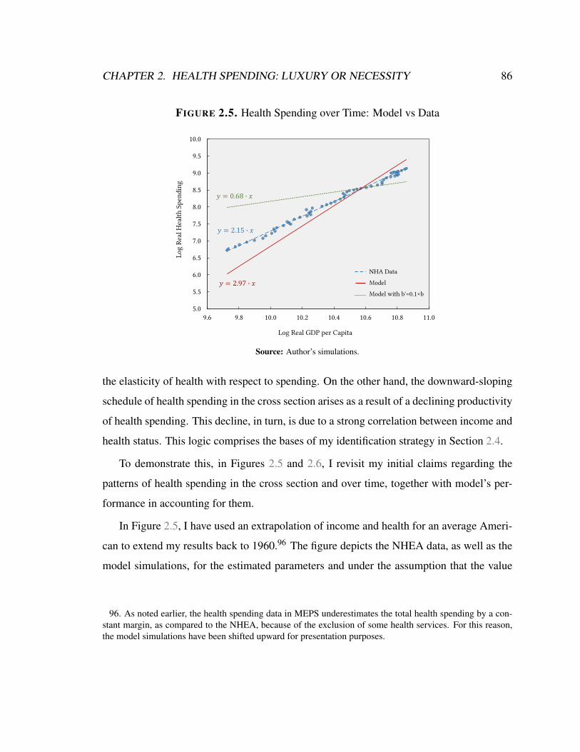
CHAPTER 2. HEALTH SPENDING: LUXURY OR NECESSITY 86
FIGURE 2.5. Health Spending over Time: Model vs Data
5.0
5.5
6.0
6.5
7.0
7.5
8.0
8.5
9.0
9.5
10.0
9.6 9.8 10.0 10.2 10.4 10.6 10.8 11.0
Log
Real
Hea
lth S
pend
ing
Log Real GDP per Capita
𝑦𝑦 = 2.97 𝑥𝑥
𝑦𝑦 = 0.68 𝑥𝑥
NHA Data
Model
Model with b'=0.1×b
𝑦𝑦 = 2.15 𝑥𝑥
Source: Author’s simulations.
the elasticity of health with respect to spending. On the other hand, the downward-sloping
schedule of health spending in the cross section arises as a result of a declining productivity
of health spending. This decline, in turn, is due to a strong correlation between income and
health status. This logic comprises the bases of my identification strategy in Section 2.4.
To demonstrate this, in Figures 2.5 and 2.6, I revisit my initial claims regarding the
patterns of health spending in the cross section and over time, together with model’s per-
formance in accounting for them.
In Figure 2.5, I have used an extrapolation of income and health for an average Ameri-
can to extend my results back to 1960.96 The figure depicts the NHEA data, as well as the
model simulations, for the estimated parameters and under the assumption that the value
96. As noted earlier, the health spending data in MEPS underestimates the total health spending by a con-stant margin, as compared to the NHEA, because of the exclusion of some health services. For this reason,the model simulations have been shifted upward for presentation purposes.

CHAPTER 2. HEALTH SPENDING: LUXURY OR NECESSITY 87
FIGURE 2.6. Health Spending in the Cross Section: Model vs Data(40–49 year olds in 1996–2005)
7.5
8.0
8.5
9.0
9.5
10.0
10.5
11.0
11.5
9.5 10.0 10.5 11.0 11.5 12.0 12.5
Log
Real
Hea
lth S
pend
ing
Log Real Income
𝑦𝑦 = −0.25 𝑥𝑥
𝑦𝑦 = 0.84 𝑥𝑥
𝑦𝑦 = −0.12 𝑥𝑥
MEPS Data
Model
Model with γ'=0.1×γ
Source: Author’s estimates.
of being alive is underestimated by 90%. As my previous discussions suggest, the value of
being alive plays a crucial role in determining the trend of health spending over time. This
point, which is one of Hall and Jones (2007)’s important contributions, is best understood
through Equation (2.32).
Figure 2.6 compares the model’s performance in the cross section, for the 40–49 year
old individuals in the first time period, to the MEPS data. As the figure suggests, an un-
derestimation of the elasticity parameter, γ by 90% (at all ages) leads to an upward sloping
spending schedule in the cross section: an observation that is in stark contrast with the data.
At the end, it is worth mentioning that none of my main parameters have an isolated
effect on the cross sectional or time series trends in my simulations. Nevertheless, one can
conceivably argue that the effect of each of these parameters is more pronounced on one
aspect of the results.

CHAPTER 2. HEALTH SPENDING: LUXURY OR NECESSITY 88
2.6 Implications for Policy
To the extent that a downward sloping health spending curve in the cross section is caused
by a declining productivity of health care, my results have clear implications for health care
policy. Importantly, the interaction between health status and productivity of health care
expenditures has been largely ignored in the public finance literature on the consequences
of health care reforms.
To separate the role of productivity differentials in the cross section, in Figure 2.7, I
compare the share of health spending (relative to income) in the model to that in the data,
for four income quartiles of the sample after eliminating the subsidies on health spending
during the entire life-cycle (s(y,a) = 0). (Only the initial age group, 40–49, is illustrated
for the sake of presentation.) As the figure suggests, to the extent that my model is a
relevant description of the underlying mechanisms, policy plays an important role in the
relatively high levels of health spending in the first income quartile.97 However, this role
diminishes quickly with income. All of slight changes in the spending at the top median
are virtually because of the elimination of Medicare subsidies after the retirement which
forces individuals to increase their saving when they are young.
Figure 2.7 ascertains my claim that most of the decline in the level of health spending
in the cross section is because of a decline in the marginal productivity of health spending
in extending life. If this effect of health status on the marginal product of health spending
is ignored, any policy evaluation exercise results in an overestimation of the favorable im-
plications of the policy for “wealthy and healthy” individuals. If, for instance, it is assumed
that health status has no effect on the marginal product of spending (as is the case under
the assumption that γ = 0 in Equation (2.31)), starting from the status quo, an increase
in the health care subsidies at all levels of income would be viewed as having the same
97. If my model does not capture the important aspects of the actual world, Figure 2.7 is simply the corollaryof a proposition regarding a statement whose inaccuracy forms the bases of the mentioned proposition!
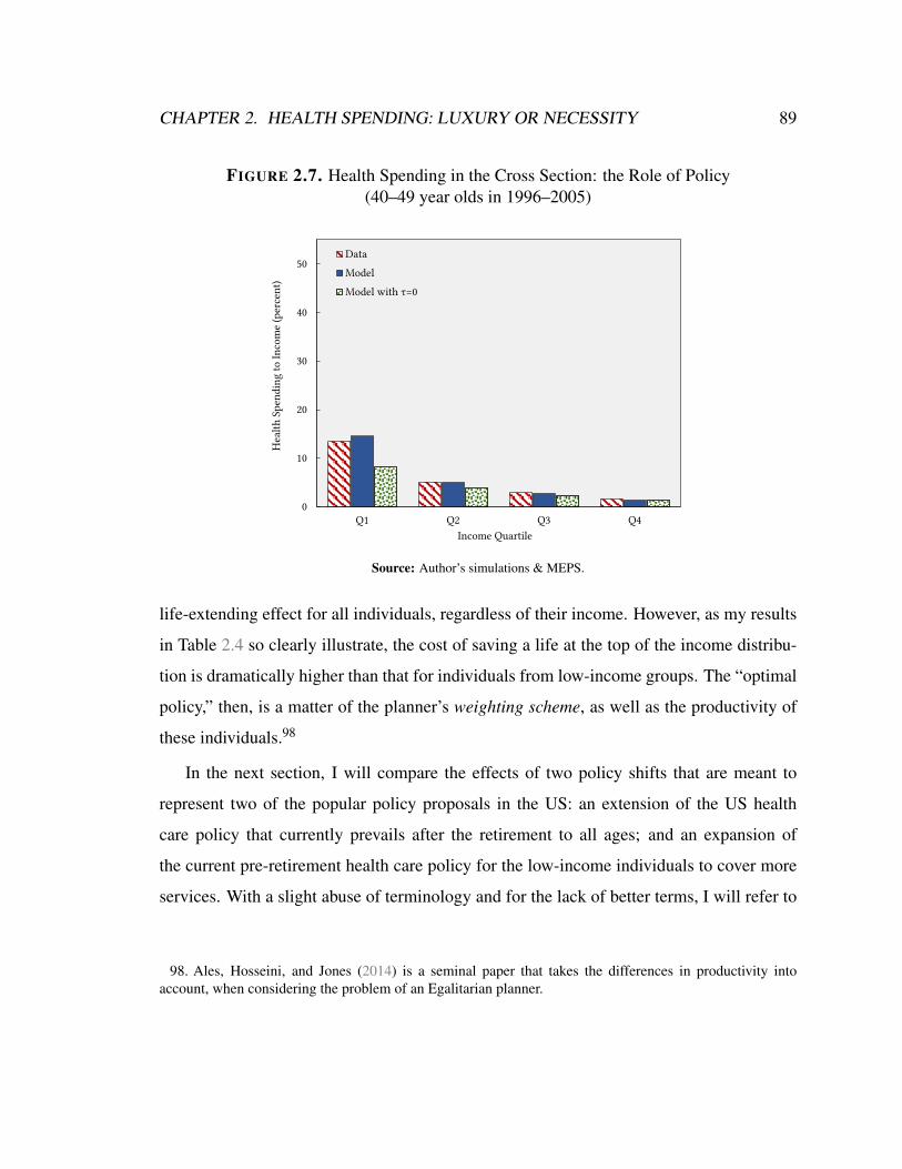
CHAPTER 2. HEALTH SPENDING: LUXURY OR NECESSITY 89
FIGURE 2.7. Health Spending in the Cross Section: the Role of Policy(40–49 year olds in 1996–2005)
0
10
20
30
40
50
Q1 Q2 Q3 Q4
Hea
lth S
pend
ing
to In
com
e (p
erce
nt)
Income Quartile
Data
Model
Model with τ=0
Source: Author’s simulations & MEPS.
life-extending effect for all individuals, regardless of their income. However, as my results
in Table 2.4 so clearly illustrate, the cost of saving a life at the top of the income distribu-
tion is dramatically higher than that for individuals from low-income groups. The “optimal
policy,” then, is a matter of the planner’s weighting scheme, as well as the productivity of
these individuals.98
In the next section, I will compare the effects of two policy shifts that are meant to
represent two of the popular policy proposals in the US: an extension of the US health
care policy that currently prevails after the retirement to all ages; and an expansion of
the current pre-retirement health care policy for the low-income individuals to cover more
services. With a slight abuse of terminology and for the lack of better terms, I will refer to
98. Ales, Hosseini, and Jones (2014) is a seminal paper that takes the differences in productivity intoaccount, when considering the problem of an Egalitarian planner.

CHAPTER 2. HEALTH SPENDING: LUXURY OR NECESSITY 90
these policy proposals as “Medicare for all” and “Medicaid expansion,” respectively.99 Not
to draw normative judgments about the Pareto weights that a planner might assign to each
individual in the economy, I will discuss the effects of each of these proposals on different
parts of the income distribution.100
2.6.1 Medicare for All vs Medicaid Expansion
Starting from the status quo policy, τ (·) and s(·), consider two policy shifts: (i) Medicare
for all, which is an extension of the post-retirement health policy to all ages, denoted by
s1 (·); (ii) and Medicaid expansion, s2 (·), under which the rate of subsidy for low-income
families is increased (in a way that it delivers the same level of welfare to the lowest income
individual in the sample as under Medicare for all, considering the required income tax),
while keeping the rate of subsidy for the top-earners unchanged. Formally,
s1 (y) =(aR
s +bRs · y)−1
(2.60)
and
s2 (y,a) =
[a′s exp(b′sy)]−1 if a ∈
[¯a,aR) ,(
aRs +bR
s · y)−1 if a ∈
[aR, a
],
(2.61)
99. I should emphasize that neither Medicare nor Medicaid comprise “all” of US post- or pre-retirementhealth care policies. However, as mentioned before, they are the most important public providers after andbefore the age of retirement, respectively. Refer to Footnote 71 for a more detailed explanation.
100. This does not mean that a policy can only be justified from a redistributive standpoint in my economy.In the presence of incomplete markets and, in particular, uninsured health shocks, there might exist a policyintervention that is Pareto improving from an ex ante sense: Even if income was fully insured against id-iosyncratic shocks, when the cross-elasticity of health outcomes with respect to health spending and healthstatus is non-zero, an individual might be willing to enter into a contract to transfer resources from one stateof the world to the other. Full characterization of such a policy, however, is outside the scope of this chapter.
CHAPTER 2. HEALTH SPENDING: LUXURY OR NECESSITY 91
where aRs and bR
s represent the status quo—given in Table 2.2. Both policies are assumed
to be financed through an increased tax on income so that the government’s budget, Equa-
tion (2.22), is balanced. I denote the resulting tax rates by τ1 (·) and τ2 (·), so that
τi (t) = τ (t)+∆τi (t) .
For the estimated parameters of the model, the coefficients of the policy functions in
Table 2.2, and a′s = 1.35 and b′s = 0.07, these policy shifts entail an increase in the income
tax rate of 5.8 and 0.8 percentage points, respectively, in the first decade (1996–2005):
∆τ1 (t1) = 5.8% and ∆τ2 (t1) = 1.0%. The resulting subsidy schedules are depicted in Fig-
ure 2.8. The solid green line in this figure illustrates the rate of pre-retirement subsidy on
health care—as a function of income—under the current health care policy in the US. The
red dashed line, on the other hand, is the rate of subsidy on health services that is only
applicable after the age of retirement. The blue dotted line depicts the proposed increase in
the subsidy rates before retirement.101
Figure 2.9 shows the effect of these policy changes on the health spending of each of
the income groups during the first decade of life. Both policies lead to an increase in the
share of spending in income because of their price effects. As one would expect, Medicare
for all has a larger impact on spending than Medicaid expansion.
However, the increased health spending does not necessarily result in improved welfare
for all income groups as Figure 2.10 illustrates. This figure shows the percentage change
in the lifetime stream of consumption (relative to the status quo) that results in the same
change in expected lifetime utility for the individuals that enter the economy in t1. As
the figure suggests, both policies entail a large and positive welfare impact on low-income
101. The Medicaid expansion is calibrated so that the rate of subsidy received by the lowest-income familyin the sample is equal to that under Medicare for all, but the high-income families receive the same rate beforeand after its implementation.

FIGURE 2.8. Medicaid Expansion vs Medicare for All:Health Spending Subsidy by Income
0
10
20
30
40
50
60
70
80
7.4 8.4 9.4 10.4 11.4
Rate
of S
ubsi
dy (p
erce
nt)
Log Real Income
Status Quo
Medicare for All
Medicaid Expansion
Source: Author’s simulations.
FIGURE 2.9. Medicaid Expansion vs Medicare for All:Effect on Health Spending by Income
(40–49 year-olds in 1996–2005)
0
5
10
15
20
25
30
35
40
Q1 Q2 Q3 Q4
Hea
lth S
pend
ing
to In
com
e (p
erce
nt)
Income Quartile
DataModelMedicare for AllMedicaid Expansion
Source: Author’s simulations & MEPS.
92

CHAPTER 2. HEALTH SPENDING: LUXURY OR NECESSITY 93
FIGURE 2.10. Medicaid Expansion vs Medicare for All:Welfare Effects by Income
-15
-10
-5
0
5
10
15
20
25
7.4 8.4 9.4 10.4 11.4
Chan
ge in
Initi
al E
xp. W
elfa
re(p
erce
nt c
hang
e in
con
sum
ptio
n)
Log Initial Income
Medicare for AllMedicaid Expansion
Source: Author’s simulations.
families. The reason for this large improvement in welfare is the relatively large impact
of increased spending on the probability of survival for these groups.102 Consequently,
despite the after-tax decline in income, low-income individuals are significantly better off.
Even though both policies have a similar positive impact on the lower tail of the income
distribution, these welfare gains diminish quickly. Under Medicaid expansion, welfare
effects become negative after the 12th percentile of income, while under Medicare for all
this happens at the 17th percentile.
The dissipation of the positive welfare effects under Medicare for all can be understood
in light of my results for the cost of saving a life, Table 2.2: As the underlying health
improves with income, the effectiveness of health spending in expanding life diminishes.
102. My simulations show that both policies are associated with a 50-day increase in the life expectancy ofan individual at the very bottom of the income distribution.

CHAPTER 2. HEALTH SPENDING: LUXURY OR NECESSITY 94
This is most felt at younger ages when high-income individuals enjoy a considerably better
health. Importantly, these are the exact same age groups that the proposed policy targets.
As a result, high-income individuals gain very little in terms of reduced chance of mortality
following the policy’s implementation.
However, the increased income tax means that, not only they can not spend as much as
before on consumption, but also they have to give up part of their savings which constitute
the source of most of their health spending at old ages when health status has depreciated
by a great deal. The total effect is a decline in life expectancy, rather than an increase, for
the high-income groups.103
For the very wealthy individuals, it is hard to replace this loss in expected life-years by
consumption. As a result, I observe a surprising decline in welfare that, for the top-earners,
surpasses the income loss due to taxes. A quote from Hall and Jones (2007) provides a nice
intuition for this:
“As we get older and richer, which is more valuable: a third car, yet another
television, more clothing—or an extra year of life?”
The intuition for the effects of Medicaid expansion is, more or less, the same: Even
the middle income individuals who do receive some of the fruits of health care reform (in
terms of increased subsidies), do not gain much due to the lower productivity of health care
for them. The welfare losses, however, at the top of the income distribution are dwarfed by
those under Medicare for all because of considerably lower tax rates that are required by
Medicaid expansion.104
103. Based on my calculations, the life expectancy of an individual at the 99th percentile of income decreasesby 5 days, after implementing Medicare for all.
104. It is important to remember that there are two sources of overestimation of (favorable) welfare effectsin my calculations which stem from the inelastic supply of labor in my model: First, an increase in thelabor income tax would have an additional negative income effect due to its impact on the supply of labor.

CHAPTER 2. HEALTH SPENDING: LUXURY OR NECESSITY 95
The punchline in my arguments in this section is that the key contributor to the mecha-
nism that delivers the flat cross sectional Engel curve in my model, that is the substitutabil-
ity between health status and health spending, also plays a crucial role in determining the
optimal direction that health care policy should take. In the absence of cross-effects be-
tween health status and health spending—when the marginal cost of saving the life of a
high income individual is similar to that of a low income person—health spending is more
valuable to a high income, high productivity individual. This is true from the perspective of
both an individual and a planner.105As a result, any policy evaluation that fails to account
for such differences can lead to misleading conclusions.106
Second, the increases in the income tax rates that are required to support the proposed policies are likelyunderestimated because of the fact that they do not take the resulting price effects into account. These twoeffects are likely more important in the first policy shift, Medicare for all, since it is more resource intensive.
105. To see how adding cross-elasticity considerations to Ales, Hosseini, and Jones (2014) can alter thedirection of optimal health spending from the perspective of an Egalitarian planner, consider the simplifiedeconomy of Section 2.3. Suppose the initial distribution of health status is given by a two-point distributionof the form Γ(h0) = 1/2 if h0 ∈
¯h, h
and Γ(h0) = 0 otherwise, where¯h < h. Then, the problem of an
Egalitarian planner, when r = 0, is given by
maxc(h0),m(h0)
∑h0
12
f (h0,m(h0)) ·u(c(h0)) (2.62)
s.t. ∑h0
12
f (h0,m(h0)) [y(h0)− c(h0)−m(h0)]≥ 0.
The first order conditions to this problem imply that, in the optimum, c(h0) = c∗ for all h0 (as in Ales,Hosseini, and Jones) and the planner equalizes
f (h0,m(h0))
fm (h0,m(h0))+ c∗+m(h0)− y(h0) (2.63)
across all individuals.Assuming a CES form for the health production function, when γ = 0, these conditions imply that the
optimal health spending is proportional to the individuals’ income, as claimed by Ales, Hosseini, and Jones.However, for large enough γ and a strong enough correlation between income and health status, this result nolonger holds.
106. In a simulation exercise, I examine the effect of the mis-estimation of parameter γ on the results ofthis section. My findings confirm the importance of considering the cross-elasticity of health outcomes withrespect to health status and health care spending. For instance, a 20% underestimation of the parameter γ atall ages leads to about 20% underestimation of the welfare effects of Medicare for all for the lowest-income

CHAPTER 2. HEALTH SPENDING: LUXURY OR NECESSITY 96
FIGURE 2.11. Pareto Weights
0.00
0.02
0.04
0.06
0.08
0.10
0.12
0.14
0.16
0.18
0.20
7.4 8.4 9.4 10.4 11.4
Inve
rse
of M
argi
nal U
tility
of I
nitia
l Con
sum
ptio
n
Log Initial Income
Source: Author’s simulations.
Finally, Figure 2.11 illustrates the inverse of the marginal utility at age¯a under the
status quo policies. This variable can be interpreted as a rough estimate for the Pareto
weights that are required for a planner to deliver the observed level of consumption under
the current system—if everything was observable. The author believes, without having to
draw normative conclusions, thinking about the political aspects of implementing each of
these policies will be misleading if one does not take such weighting schemes into account.
2.7 Concluding Remarks
I develop a life-cycle model with heterogeneity in income and health status, where individ-
uals allocate their income between consumption and health spending. While consumption
individuals.

CHAPTER 2. HEALTH SPENDING: LUXURY OR NECESSITY 97
determines the flow of utility through a standard utility function that incorporates the value
of being alive, health spending and health status enter a health production function to de-
termine individuals’ longevity.
In my framework, for a given level of health status, the growth of income over time
leads to a decline in the value of consumption relative to the value of being alive. This
relative change creates a luxury-good channel that causes the share of health spending in
income to increase over time. On the other hand, a strong correlation between income and
health status leads high-income individuals to devote fewer resources to health spending.
The reason is that, if health status and health care are substitutable, the marginal effect of
one dollar health spending on lifetime utility is smaller for wealthier and healthier agents.
These two channels enable my model to account for the conflicting patterns of health
spending in the cross section and time series. I take advantage of the distinct implications
of each channel for the cross section and time series to estimate the structural parameters
of the model. I use this insight to estimate the parameters of a health production function
using income variations in the cross section and over time in the US. My estimation results
confirm that the elasticity of substitution between health spending and health status is sig-
nificantly above one at all ages under consideration—an observation that has been largely
neglected in the literature.
Substitutability of health status and health expenditures has important implications for
the effects of health care policy. I show this by comparing the welfare consequences of
two popular policy proposals: an expansion in the pre-retirement health spending subsidies
for low-income families—Medicaid expansion—and an extension of the post-retirement
US health care policy to all ages—Medicare for all. Both of these policies entail positive
and comparable welfare effects for the lower income individuals. However, my finding
that the value of health care is low for high-health status individuals implies that wealthy
individuals have little to gain from increased subsidies on health expenditures under Medi-
care for all. Therefore, the much larger tax increments required to finance Medicare for all

CHAPTER 2. HEALTH SPENDING: LUXURY OR NECESSITY 98
lead to greater welfare losses at the top of the income distribution, compared to Medicaid
expansion.
Finally, two components missing from my framework are an endogenous process for
the accumulation of health status and a mechanism accounting for the initial differences
in health status. A vast literature in health economics relates the health differences among
individuals later in life to the early-life environment suggesting that, to account for initial
heterogeneity in health, one has to incorporate intergenerational links and altruistic motives
into the model. A seminal paper that models the life-cycle investment in health capital is
Ozkan (2014). In his framework, preventive health capital plays the role of health status,
and individuals decide to invest in preventive health to avoid unfavorable health outcomes
in the future.
Central to these endogenous channels of health capital variations is an investment func-
tion. I believe my approach in using various patterns of health expenditures and health
outcomes in the data to quantify a life-cycle model can be generalized and applied in these
frameworks to discipline such investment functions.107
107. For instance, in Ozkan’s model, if individuals are only heterogeneous regarding their initial incomeand the marginal product of investment in health capital is large enough, we should expect a rapid rise inthe preventive care utilization by lower-income individuals as their income grows over time. Similarly, ifinvestment in children’s future health has diminishing returns, we should expect a regression to the mean forthe health outcomes of different income groups (an implication that is rejected, partly, by rising gap in thelife expectancy in the US).

Chapter 3
Health Capital and the Productivity of
Health Spending: Evidence from the
RAND Health Insurance Experiment
3.1 Introduction
Health spending in the US has been continuously rising while its differentials across income
groups have remained insignificant (see Dickman et al. 2016 and Chapter 1). Nonetheless,
health outcome differentials—e.g., differences in life-expectancy—by income have been
considerable, and the gap appears to be widening in recent years (Chetty et al. 2016). The
existing income gradient in health outcomes calls attention to other determinants of health
and their likely interplay with health expenditures. Accordingly, the effectiveness of health
care policy would rely on identifying the influence of those “other determinants” of health
on the marginal productivity of medical spending.
Isolating the effect of health spending on health outcomes from other determinants of
health such as income and education, however, is challenging because these variables often
99

CHAPTER 3. PRODUCTIVITY OF HEALTH SPENDING: RAND HIE 100
move together and interact (Phelps 2016). In this study, I use a framework that allows for
the interaction of medical expenditures and a measure of other determinants of health—
which I, interchangeably, refer to as underlying health, health stock, or health capital.
Also, I address the endogeneity problem, arising from the simultaneity of health outcomes
and their determinants, by using data from a randomized controlled trial.
In effect, this chapter is most closely related to the branch of health economics that
attempts to estimate the health production function, a process that relates a health outcome
to health spending and other detriments of health. In Grossman (1972)’s seminal paper,
for example, the health outcome of interest is healthy time, defined as a function of health
spending, time spent on health, and a variable that represents education and knowledge.
As another example, in Hall and Jones (2007)’s influential work, the health outcome of
interest, namely the life-expectancy, is a function of health spending and a variable that
represents education and pollution, beside other factors.
The functional form that has been extensively used in the literature for the health pro-
duction function is Cobb-Douglas.1 The assumption of zero cross-elasticity of health pro-
duction with respect to its inputs, however, appears to be a strong one since it implies that
one dollar spent on health care has the same marginal effect on health outcomes of the
individual, regardless of her underlying health.
In this study, instead of limiting my functional form to one where the elasticity of
substitution between health spending and health capital is set to one, I start from a more
general form. My functional form explicitly allows for the level of health capital to affect
1. Since Grossman (1972) does not attempt to estimate his health production function, he does not spec-ify it with a functional form. Studies that use his theoretical framework, such as Wagstaff (1986), Wagstaff(1993), and Grossman (2000), assume a Cobb-Douglas process; Hall and Jones (2007), however, specify aCobb-Douglas process for their health production function. Ales, Hosseini, and Jones (2014) follow in Halland Jones’s steps by presuming a functional form in which health spending and other factors enter multiplica-tively. Ozkan (2014)’s interpretation of the health production function is in line with my broad description.In his framework, the probability of diseases is a health outcome, while curative health expenditures andpreventive health capital are the inputs.

CHAPTER 3. PRODUCTIVITY OF HEALTH SPENDING: RAND HIE 101
the marginal product of health expenditures. I estimate this health production function
using the results of medical screening exams of the RAND Health Insurance Experiment.
My measure of health capital is the common component of a series of socioeconomic
characteristics—including age, sex, race, ethnicity, marital status, employment status, in-
come, and education—at the beginning of the experiment. Each of the characteristics is
correlated with health outcomes, i.e., direct results of medical screening exams at the exit
from the experiment, controlled for medical spending during the experiment.2 Among the
results of medical examinations, I am specially interested in three major metabolic risk
factors: high blood pressure, high glucose level, and high cholesterol level. I estimate the
health production function for the all-cause burden of diseases attributable to the risk fac-
tors, before incorporating it into a theoretical framework, developed in Chapter 2, to test
how my estimates replicate the US health care expenditures trends at the aggregate level.3
My estimations of the health production function show that medical spending and health
capital have differential effects on the number of ECG abnormalities, glucose level, systolic
blood pressure, average hearing thresholds, and indicators of respiratory health. All the
differential effects point towards a single direction: the effect of health spending on health
outcomes is greater at lower levels of health capital. Specifically, the effect of a percentage
increase in medical spending on glucose, blood pressure, average hearing thresholds, and
forced vital capacity for an individual at the 25th percentile of health capital distribution
is about 1.4, 1.4–1.7, 2.7–3.5, and 12.2 times the effect for an individual at the 75th per-
centile, respectively. Also, the health capital adjusted marginal effect of health spending
on the number of ECG abnormalities is almost zero for the top half of health capital distri-
2. To the best of my knowledge, this is one of the rare studies that consider the interaction between medicalspending and health capital. Nevertheless, the evidence for the existence of such interactions goes as far backas the RAND HIE itself: Brook et al. (1983), using the RAND experiment data, show the productivity ofmedical spending in terms of decreasing the diastolic blood pressure is higher among low-income individuals.
3. Burden of diseases are measured by the rates of deaths, years of life lost (YLLs), years lived withdisability (YLDs), and disability-adjusted life years (DALYs).

CHAPTER 3. PRODUCTIVITY OF HEALTH SPENDING: RAND HIE 102
bution. I find similar results from the estimation of the health production functions for the
all-cause burden of diseases attributable to the metabolic risk factors: an increase in medi-
cal spending decreases the rates of deaths and disability, but at lower rates for individuals
with higher health capital.
In the next step, I incorporate the health production function for the burden of diseases,
together with my estimates of health capital, in a simple model of health spending where
individuals are heterogeneous in their income and health capital and can allocate resources
across health and non-health spending. The key trade-off that an individual faces in this
economy is between maximizing consumption and minimizing the burden of diseases.
The primary mechanisms at play in my model are those proposed in Chapter 2: First,
when the marginal product of health spending, normalized by it average product, falls
rapidly with health capital, individuals with better underlying health have little incentives
to spend on health.4 Under the assumption that health capital and income are strongly
correlated—as my results indicate—health spending is lower for higher income individuals,
leading to a negatively sloping schedule for the health spending as a function of income in
the cross-section.
Second, a relative change in the marginal utility of consumption and the marginal
product of health spending—when normalized by their average products—can lead to
an increase in the share of health spending over time: With a standard constant relative
risk aversion (CRRA) utility form with a constant additive term5, the marginal utility of
consumption—when normalized by average utility—falls rapidly. On the other hand, un-
der the assumed functional form for the production of health, the elasticity of health pro-
duction with respect to health spending rises. This relative change leads to an increase in
4. As discussed in Chapter 2, this is equivalent to health spending and health capital being strong substi-tutes in the health production function.
5. I will refer to this additive term as the value of life-years.

CHAPTER 3. PRODUCTIVITY OF HEALTH SPENDING: RAND HIE 103
the share of health spending over time. However, this argument, as noted in Chapter 2, is
true as long as the growth of average health capital does not dominate the rise in income. If
health capital rises more than income, a rapid fall in the marginal value of health spending
in decreasing the burden of decease implies a decline in the share of health spending.
After calibrating the value of individual’s life-years—to account for the level of health
spending at different income levels—the model is capable of predicting a downward slop-
ing health spending schedule in the cross-section that matches RAND HIE’s health spend-
ing data (specially for individuals with income above 200% of the federal poverty line at
the time of the experiment).
Next, using the calibrated model, I examine its predictions regarding the average health
spending over time, under different assumptions for the growth rate of average health cap-
ital in the US economy. My results indicate that, if the model is to account for the rapid
increase in the share of health spending in the past five decades, the rise in the average
health status should be considerably smaller than the rise in income. In particular, if I fol-
low Hall and Jones (2007)’s suggestion regarding the share of “other underlying factors” in
the total decline of mortality in the US, my model predicts that the share of health spend-
ing should have fallen in the past half a century.6 This is due to Hall and Jones (2007)’s
assumption that the cross elasticity of health outcomes with respect to health spending and
health capital is zero. My estimates, however, suggest that this assumption is not accurate.7
My simulations suggest that the growth rate of health capital has been almost zero in this
period. Therefore, while I agree with Hall and Jones (2007) that the rise of health spending
6. In Chapter 2, I argue that “other factors” in Hall and Jones (2007)’s health production function, cor-respond to underlying health in my model in this chapter. The fact that these underlying factors enter mul-tiplicatively in the production of health, however, implies that the cross elasticity of health production withrespect to health capital and health spending is zero.
7. For instance, when the health outcome of interest is the life years lost to disability, this cross elasticityis 0.075. See the second row of Table 3.3 for values when health outcomes are probability of death, YLL, orYLD.

CHAPTER 3. PRODUCTIVITY OF HEALTH SPENDING: RAND HIE 104
in the US in the past five decades has been efficient—in the Pareto sense—my results have
an important message for health economists and policymakers: The continually increasing
share of health care expenditures in GDP is not necessarily a good sign; it indicates that the
health status of an average American may not have improved even remotely as fast as her
income.
The rest of this chapter is organized as follows. In the following section, I introduce
my health production function, discuss the methodological details for its estimation, and
describe the data. In Section 3.3, I present the results of my estimations of the health
production functions and interpret them. 3.4 presents the individual health spending model
and describe the quantitative methods used to calibrate it. The last section concludes.
3.2 Health Production Function and Its Estimation
For simplicity, I choose a translog health production function, without its quadratic terms:
ln(xi) = α +βm ln(mi)+β
h ln(hi)+βm,h ln(mi) ln(hi)+ εi. (3.1)
i, in (3.1) represents an individual, with a stock of health capital hi at the beginning of
the period of interest. mi is the health spending during the period regardless of payer, and
variable x is a health outcome, that can be as specific as blood pressure or cholesterol level
and as general as the chance of survival, at the end of the period. εi is the error term.
In Equation (3.1), coefficient β m,h represents the differential effect of health capital on
the marginal productivity of medical spending. If higher values of x indicate better health,
then positive values for β m and negative values for β m,h imply the marginal effect of health
spending on health decreases as health capital increases (or, equivalently, the marginal
effect of an increase in medical spending on health is greater at lower health capital levels).
A similar interpretation applies to the case where smaller values of x indicate worse health,

CHAPTER 3. PRODUCTIVITY OF HEALTH SPENDING: RAND HIE 105
β m is negative, and β m,h is positive.8
Since health outcomes, health spending, and measures of health capital are simulta-
neously determined, any estimation of the marginal productivity of medical spending that
uses observational data is potentially biased. Using data from a relevant randomized con-
trolled trial (RCT) is ideal to address the problem. One of the prime examples of RCTs that
induced random variation in medical spending in the US is the RAND Health Insurance
Experiment (RAND HIE), conducted during 1974–1982. During the experiment, about
four thousand individuals were randomly assigned to health insurance plans that differed
in their level of cost-sharing. I use the health insurance plans assigned in the RAND HIE as
an instrument for health spending, as an individual’s decision on medical spending depends
on her access to health care.
In practice, twenty different health insurance plans were assigned to the experiment’s
participants: nineteen of them were fee-for-service (FFS) policies that varied in deductible,
coinsurance rate, and out-of-pocket maximum; one was a Health Maintenance Organization
(HMO) plan that used primary care physicians as gatekeepers, offered a limited network
on provider, and installed utilization reviews. To ensure consistency of comparisons, I
drop the HMO plan. Then, to have enough observations for each plan, I categorize the
FFS plans into six groups a la Aron-Dine, Einav, and Finkelstein (2013): free care, 25%
coinsurance, mixed 25% and 50% coinsurance, 50% coinsurance, individual deductible,
8. In Chapter 2, I suggest a constant elasticity of substitution (CES) function for the health production ofthe form:
xi = f (mi,hi) = γ
[δm−ρ
i +(1−δ )h−ρ
i
]− νρ
γ,ρ > 0. (3.2)
There, I argue that this is a flexible functional form that captures Hall and Jones (2007) (among many others’)assumptions on the health production) as a special case.
However, Equation (3.2) is closely related to my functional form in (3.1). To see this, using Kmenta(1967)’s second-order Taylor approximation of the function, we can write (3.2) as a translog function of theform:
ln(x) = ln(γ)+νδ ln(m)+ν (1−δ ) ln(h)− 12
ρνδ (1−δ ) [ln(m)− ln(h)]2 . (3.3)
Equation (3.1) is in fact (3.3) without the quadratic terms.

CHAPTER 3. PRODUCTIVITY OF HEALTH SPENDING: RAND HIE 106
and 95% coinsurance.9 In addition to the type of health insurance plan, I include other
factors that affected the random assignment of the plans by the experiment’s design—
namely, site, year and month of enrollment—in my list of medical spending instruments.
My first stage estimates show that there are statistically significant correlations between the
six health plans and average annual inflation-adjusted total health spending:10,11 In general,
medical spending increases as insurance plan’s cost-sharing decreases. For example, those
with 25% co-insurance plans spend about $1,226 (st. dev. 322) less than those with free
plans; whereas, those with 95% co-insurance plans spend about $1,713 (st. dev. 248) less
than those with free plans.12
To construct my measures of health outcome (x), health spending (m), and health capital
(h), I match four datasets from the RAND HIE at individual level: (1) the Full Demographic
Sample (FDS) containing background socioeconomic information on all participants at the
beginning of the experiment and on the health insurance plans’ assignment; (2) the An-
nual Expenditure and Visit Counts (AEVC) containing total—regardless of payer—annual
expenditures on inpatient, outpatient, and dental care, drugs, medical equipment, and psy-
chotherapy; (3) the Health Status and Attitude (HSA) containing 29 self-reported measures
of physical, physiological, mental, and social health, 14 self-reported health habits, anthro-
pometrics, and 24 measures of health care delivery satisfaction; and (4) the Adults Medical
9. The insurance plans under each category usually differ in out-of-pocket maximum.
10. I regress average annual inflation adjusted total health care expenditures on plan type, site, enrollmentyear, and enrollment month.
11. This finding is consistent with those of both RAND’s original investigators, Newhouse et al. (1981),and also Aron-Dine, Einav, and Finkelstein (2013).
12. Although instrumental variable method has been routinely used for variables that are linearly inserted inregressions, its application on nonlinear variables, such as interaction terms, is less straightforward. I followWooldridge (2010)’s suggestion and implement the following two-stage procedure. First, I regress ln(m)on the four instrumental variables (plan, site, year and month of enrollment) and all their interactions andcalculate the fitted values, ln(m)
∧
. Second, I instrument ln(m) and ln(m) · ln(h) with ln(m)∧
and ln(m)∧
· ln(h),respectively, and estimate the coefficients in (3.1).

CHAPTER 3. PRODUCTIVITY OF HEALTH SPENDING: RAND HIE 107
Disorder Files (AMDF) containing detailed information on 17 categories of medical dis-
order: acne, anemia, angina, chronic obstructive airway disease, congestive heart failure
tracer condition, diabetes, hay fever, hearing loss condition, hypercholesterolemia, hyper-
tension, joint disorders, kidney problems, peptic ulcer disease, sleeping pills and tranquiliz-
ers, surgical conditions, thyroid condition, and vision. The information, either self-reported
or the result of medical screening tests, is provided for most individuals at both enrollment
in and exit from the experiment.
My measure of health outcome, x, can either be a health status or habit, or an indi-
cator of a medical disorder evaluated at the exit from the experiment. My estimations of
Equation (3.1) that used the HSA’s self-reported health status variables indicate unexpected
results: I find adverse effects of medical spending on health status with and without the in-
teraction term in Equation (3.1). Such unexpected results, however, are also reported in
other research that uses “self-reported” measures of health.13 Hence, I turn my focus to
specific medical disorders, reported in the AMDF. For each of the 17 medical disorders, a
series of variables is provided that contain information either from medical history ques-
tionnaires filled by participants or from medical screening exams performed on participants
at the end of the experiment. I, however, only focus on the results of the medical screening
exams to avoid inaccuracies implemented by subjective self-evaluations. Further, I prefer
direct results of the screening exams, which provide continuous variables. Specifically, I
examine variables listed in Table 3.1 as x.
I construct my measure of health spending, m, by adding expenditures on all different
health services, regardless of payer, to calculate the total health spending. Then, using
13. E.g., using data from the Oregon Health Insurance Experiment, Baicker et al. (2013) show that receivingMedicaid coverage increases the chance of receiving medical screening. However, as Finkelstein et al. (2012)argue, this can lead to the diagnoses of diseases that were previously undiagnosed among Medicaid recipients,leading to a decline in self-assessed health status. As a result, all the studies that use self-assessed health asthe measure of health outcome are subject to the risk of biased estimates in measuring the relation betweenthe utilization and health outcomes.

CHAPTER 3. PRODUCTIVITY OF HEALTH SPENDING: RAND HIE 108
the consumer price index, I adjust it for the inflation. Since participants were enrolled in
the experiment for either 3 or 5 years, I calculate average annual inflation-adjusted total
medical spending and use it as m in my analyses.
Measuring health capital (h), however, is less straightforward since individuals arrive in
the RAND HIE with different levels of health capital formed by many factors such as ge-
netics, early-life environment and nutritional intake, and previous health and human capital
investments. In the reduced-form representations of his model, Grossman (2000) measures
health capital with individuals’ self-reported health status and relates it to the wage, years
of schooling, age, and the price of medical care. As explained above, I do not use self-
assessed measures of health status as health capital; I, instead, use the principal component
of a set of socioeconomic correlates of health at enrollment in the experiment as my mea-
sure of health capital.14 Specifically, I transform categorical variables to the corresponding
sets of binary variables and use them alongside the numerical variables in a principal com-
ponent analysis to compute health capital scores, a la Vyas and Kumaranayake (2006).
In practice, I try different combinations of the socioeconomic variables, comparing
their principal components’ internal in-coherency, which occurs when their distributions
have clumps or clusters (Filmer and Pritchett 2001). To examine internal coherency, I com-
pare general health, general functioning, and mental health at enrollment for quintiles of
the distribution of principal component scores.15 My best-performing principal component
includes logarithm of age, if male, if white, if currently married, if never married, if living
in a large or medium city, if living in a suburb, if living in a small town, if received health
insurance through employer, if received health insurance from government, if in the labor
14. The full set of socioeconomic variables, reported at enrollment in the FDS dataset, are sex, age, race,ethnicity, marital status, education, city size, employment status, full/part time working status, self-employedor waged job, occupation, industry, months of work experience, hourly wage rate, income, if received differ-ent types of public aid, and the type of health insurance prior to the experiment.
15. Indices of general health, general functioning, and mental health are coded as GHIDX, PFI, and MHIin the HSA dataset, respectively.

CHAPTER 3. PRODUCTIVITY OF HEALTH SPENDING: RAND HIE 109
force, if homemaker, if employed full-time, logarithm of real family income during the year
before enrollment, logarithm of months of work experience, logarithm of years of educa-
tion, if a professional or technical worker, if a manager or administrator, if a clerical worker,
if a craftsman, if an operative or a farmer, if a service worker, if working in construction,
agriculture, or mining industry, if working in manufacturing, if working in transportation,
communication, or other public utilities, if working in wholesale or retail trade, if work-
ing in finance, insurance, real estate, or business services, if working in entertainment and
recreation, and if working in the public sector.
Finally, I focus on 20 year or older individuals: although the AMDF dataset includes
14–65 year old individuals, values of most labor market related variables are missing for
most under 20 year old individuals. I cannot further limit the age range since I will lose
significant statistical power.
3.3 Results of Estimating the Health Production Function
3.3.1 Health Outcome-Specific Results
Table 3.2 presents the results of estimating Equation (3.1) for the health outcomes listed
in Table 3.1. According to these results, the effect of an increase in health spending or in
health capital, if statistically significant, leads to an improvement in health. Specifically,
a 10 percent increase in medical spending leads to a 1.2 percent increase in forced vital
capacity but to an about 0.5 , 1.7−2.3, and 0.4 percent decrease in glucose level, average
hearing threshold, and blood pressure (diastolic or systolic), respectively.16
When the effect of medical spending on a health outcome is significant, the effect of
16. It is hard to interpret the estimated coefficients for health capital since it is a linear combination of alarge number of socioeconomic variables. Also, I cannot compare the sizes of the effect on health outcomeof health spending and health capital because the ranges of their distributions is very different.

TABLE 3.1. Direct Results of the RAND HIE Medical Screening Exam atExit from the Experiment Used as Measure of Health, x
Correlation Variable NameVariable Description
with Health in Data
(+) ANEMHGBX Hemoglobin value
(-) ECGSUMX Number of electrocardiographic abnormalities
(-) MINNECGX Number of electrocardiographic abnormalities,
Minnesota criteria
(+) BSTFEV1X Highest of three FEVls
(+) BESTFVCX Highest of three FVCs
(-) GLUCOSEX Blood glucose results
(-) HEARAVLX Average hearing threshold for left ear
(-) HEARAVRX Average hearing threshold for right ear
(-) CHOLESTX Blood cholesterol measurement
(-) DIASTOLX Diastolic blood pressure
(-) SYSTOLX Systolic blood pressure
(-) URICACDX Serum uric acid
(-) KIDNBUNX Blood urea nitrogen (BUN)
(+) THYR T4X Total serum thyroxine (T4) measure
(-) VISNATFX Best natural far vision
(-) VISNATNX Best natural near vision
Note: (+) indicates an increase in the measure of health is generally associated with better
health; (-) indicates an increase in the measure of health is generally associated with worse
health. FEV1, forced expiratory volume, measures the amount of air in liters expelled in
the first second of exhalation after taking a deep breath. The reported value is the highest
of three FEV1s at exit. FVC, forced vital capacity, measures of the total amount of air in
liters expelled after taking a deep breath. The reported value is the highest of three FVCs
at exit.
110

CHAPTER 3. PRODUCTIVITY OF HEALTH SPENDING: RAND HIE 111
its interaction with health capital on health outcome is also statistically significant. More
important are the signs of the statistically significant interaction terms, all pointing at one
direction: the effect on health of medical spending is greater when health capital is lower.
Specifically, for example, the negative effect of a percentage point increase in health spend-
ing on in glucose level for an individual at the 25th percentile of the distribution of health
capital is about 1.4 times the effect for an individual at the 75th percentile. The ratios of
the effects on diastolic and systolic blood pressure levels for the same individuals are about
1.4 and 1.7, respectively. The ratios of the effects on hearing thresholds’ improvement are
between 2.7 to 3.5 and for the forced vital capacity is about 12.2. If the heart health is
considered, although an increase in the health capital adjusted medical spending decreases
the number of ECG abnormalities for the bottom half of the health capital distribution, it
has no effect for the top half.
My results show that there is a very high degree of substitutability between health
spending and health capital in determining heart and respiratory health such that the marginal
effect of health spending becomes almost zero at very high (top 10 percent) levels health
capital. There is a lesser, still noticeable, degree of substitutability between health spending
and health capital in determining key risk factors such as glucose and blood pressure levels.
3.3.2 The Effect on the Burden of Diseases
In this section, I estimate Equation (3.1) for measures of attributable burden of diseases—
namely, for deaths, years of life lost (YLLs), years lived with disability (YLDs), and
disability-adjusted life years (DALYs). In effect, I separately calculate the attributable
burdens of three major metabolic risk factors—high glucose, high cholesterol, high blood
pressure—add them up and use them as x. I justify my focus on the three metabolic risks
factors by the fact that they either have large, direct effects on all-cause mortality or are
mediators of other major metabolic risk factors, i.e., high BMI and of behavioral risks

TABLE 3.2. Estimations of Equation (3.1) for Different Measures of CurrentHealth
ln(x)→Hemoglobin
Level
Num. of
ECG
Abnorm.
Num. of
ECG
Abnorm.
2
Forced
Expira-
tory
Volume
in 1st
second
Forced
Vital
Capacity
Glucose
Level
Average
Hearing
Thresh-
old, Left
Ear
Average
Hearing
Thresh-
old,
Right Ear
Direction of x (+) (-) (-) (+) (+) (-) (-) (-)
ln(m) 0.024 -0.148*** -0.161*** 0.077 0.121*** -0.050*** -0.230*** -0.175**
(0.018) (0.049) (0.047) (0.050) (0.061) (0.015) (0.078) (0.079)
ln(m) ln(h) -0.013 0.085*** 0.088*** -0.046 -0.062* 0.014* 0.106** 0.0762*
(0.011) (0.027) (0.026) (0.030) (0.038) (0.009) (0.047) (0.046)
ln(h) 0.155** -0.545*** -0.580*** 0.451** 0.577** -0.077 -0.672** -0.515*
(0.070) (0.172) (0.163) (0.196) (0.241) (0.055) (0.298) (0.294)
constant 2.407*** 1.094*** 1.165*** 4.945*** 4.835*** 4.825*** 3.753*** 3.413***
(0.115) (0.319) (0.306) (0.323) (0.396) (0.099) (0.500) (0.510)
Observations 2,553 1,794 1,794 2,428 2,428 2,556 2,457 2,454
Endog Test 1 0.12 0.06 0.02 0.05 0.01 0.00 0.00 0.01
Endog Test 2 0.00 0.04 0.01 0.00 0.00 0.00 0.00 0.01
Source: Author’s estimates. Note: m is average annual real medical spending. h is a measure of health capital: the
principal component of a series of socioeconomic characteristics, excluding the measure of current health x at enrollment.
The variables are estimated using the instrumental variable method where ln(m) is instrumented with health insurance
plan, enrollment site, year, and month, and all their interactions. (+) indicates an increase in the measure of health is
generally associated with better health; (-) indicates an increase in the measure of health is generally associated with
worse health. The endogeneity tests examine if the presumed endogenous variable, health care expenditures, is really
endogenous and if instrumental variable is needed. Endogeneity is rejected at 95% is the reported p-values are greater
than 0.05. Endog Test 1 is based on Durbin Chi2 score; Endog Test 2 is based on Wu-Hausman F-test.
112

TABLE 3.2 (continued). Estimations of Equation (3.1) for Different Measuresof Current Health
ln(x)→Cholesterol
Level
Diastolic
Blood
Pressure
Systolic
Blood
Pressure
Uric
Acid
Level
Blood
Urea
Nitrogen
T4 Total
Serum
Thyrox-
ine
Best
Natural
Far
Vision
Best
Natural
Near
Vision
Direction of x (-) (-) (-) (-) (-) (+) (-) (-)
ln(m) 0.005 -0.038** -0.043*** -0.028 0.039 -0.022 -0.008 -0.038
(0.018) (0.016) (0.015) (0.036) (0.040) (0.023) (0.084) (0.082)
ln(m) ln(h) -0.001 0.012 0.015* 0.006 0.006 0.016 0.017 0.036
(0.011) (0.010) (0.009) (0.022) (0.024) (0.014) (0.051) (0.049)
ln(h) 0.043 -0.04 -0.051 0.139 0.119 -0.131 -0.13 -0.138
(0.067) (0.060) (0.055) (0.133) (0.149) (0.084) (0.313) (0.310)
constant 5.232*** 4.550*** 5.004*** 1.549*** 2.141*** 2.311*** 3.757*** 3.880***
(0.113) (0.101) (0.094) (0.221) (0.256) (0.142) (0.530) (0.522)
Observations 2,551 2,624 2,624 2,541 2,553 2,540 2,593 2,576
Endog Test 1 0.01 0.02 0.01 0.11 0.02 0 0 0.01
Endog Test 2 0.53 0.01 0.02 0.98 0 0.31 0.77 0.55
Source: Author’s estimates. Note: m is average annual real medical spending. h is a measure of health capital: the
principal component of a series of socioeconomic characteristics, excluding the measure of current health x at enrollment.
The variables are estimated using the instrumental variable method where ln(m) is instrumented with health insurance
plan, enrollment site, year, and month, and all their interactions. (+) indicates an increase in the measure of health is
generally associated with better health; (-) indicates an increase in the measure of health is generally associated with
worse health. The endogeneity tests examine if the presumed endogenous variable, health care expenditures, is really
endogenous and if instrumental variable is needed. Endogeneity is rejected at 95% is the reported p-values are greater
than 0.05. Endog Test 1 is based on Durbin Chi2 score; Endog Test 2 is based on Wu-Hausman F-test.
113
CHAPTER 3. PRODUCTIVITY OF HEALTH SPENDING: RAND HIE 114
(Collaborators 2017).17
More specifically, I take the following steps. First, assuming that the burden of diseases,
d, is linearly correlated with each of the risk factors, I write the following equation for the
risk factor, r:
dr(exit)i = δ
r1 +δ
r2 · x
r(exit)i (3.4)
where variable dr(exit)i is the burden of diseases (either Deaths, YLLs, YLDs, or DALYs)
attributable to the metabolic risk factor r (high glucose, high cholesterol, high blood pres-
sure) at exit from the RAND HIE for individual i, and variable xr(exit)i is the individual’s
level of metabolic risk factor r at exit. Next, I calculate an individual’s total attributable
burden, D, by adding the three values calculated for dr(exit)i ’s in the previous step:
Dr(exit)i = ∑
rdr(exit)
i (3.5)
where d and D are the same measures of attributable burden: either Deaths, YLLs, YLDs,
or DALYs. Finally, Dr(exit)i ’s are plugged in Equation (3.1) for x.18
I calibrate Equation (3.4), a line, for each pair of attributable burden measure and risk
17. According to Collaborators 2017, about 10, 52, and 33 percent of all-cause deaths in the US adultpopulation are attributable to environmental and occupational, behavioral, and metabolic risks, respectively.Components of behavioral risk are tobacco, alcohol and drugs, and dietary risk with about 26, 10, and 21percent of all-cause attributable deaths. Components of metabolic risks are high glucose, high cholesterol,high blood pressure, high BMI, low bone density, and impaired kidney with about 13, 9, 14, 19, 0.0, and 4percent of all-cause attributable deaths, respectively. The provision of health insurance under the RAND HIEdid not relate to environmental and occupational risks.
18. Adding up the attributable burden of the risk factors, I basically assume that they are not correlated.The research, however, shows that they are correlated (Hjermann et al. 1978; Stamler et al. 2002; Sakuraiet al. 2011), but the correlations between them are not strong. Hjermann et al. (1978), for example, reportsa 14 percent correlation between systolic blood pressure and cholesterol level; Sakurai et al. (2011), also,reports a low-order relationship between them. The correlation between blood pressure and blood sugar isalso not strong, except in the presence of diabetes: Hjermann et al. (1978), for example, reports an about10 percent correlation between them. There is an even weaker association between glucose and cholesterollevels (Zavaroni et al. 1985). Therefore, I do not expect a large overestimation in my calculation of the totalburden attributable to the risk factors.

CHAPTER 3. PRODUCTIVITY OF HEALTH SPENDING: RAND HIE 115
factor using the GBD (2016) Results Tool. Two points are needed to perform the cal-
ibration: I choose the average levels of each risk factor below and above the abnormal
threshold as two points for xr(exit); I assume the corresponding values for dr(exit) are zero
and the values reported by the GBD (2016) Results Tool.
The estimation results are presented in Table 3.3. The point estimates of the coefficients
for different measures of all-cause burden of diseases are very similar. On average, a 10
percent increase in medical spending leads to an about 2.5 percent decrease in the burden
of diseases associated with the risks of high blood pressure, high cholesterol, and high
glucose levels. The effect of health capital on the measures of burden of diseases, however,
cannot be distinguished from zero.
Again, I find strong evidence for the high degree of of substitutability between health
spending and health capital, as the coefficients of the interaction terms in Table 3.3 are
positive and statistically significant. Specifically, the effect on the burden diseases (through
the risk factors) of an increase in medical spending is smaller at high levels of health capital
but greater at low health capital levels. Specifically, the effect of an increase in medical
spending on DALYs rate in individuals at the 25th percentile of the distribution of health
capital is about 1.5 times the effect in individuals at the 75th percentile. When the effect
on DALYs of a medical spending on individuals at the 5th and 95th of the distribution of
health capital are compared, the ratio amounts to 2.1.
There is a 60 percent correlation between health capital and income (both evaluated at
enrollment in the experiment) in the sample of my burdens of diseases estimations. The
correlation consistently becomes stronger by age such that it amounts to about 80 percent
for 50 year or older individuals. Therefore, the implications of the measured differential
effects on health of medical spending by health capital are mostly applicable to differential
effects on health of medical spending by income.

TABLE 3.3. Estimations of Equation (3.1) for Measures ofBurden of Disease Attributable to High Blood Pressure, High
Cholesterol, and High Glucose Levels
Death YLLs YLDs DALYs
ln(m) -0.248*** -0.248*** -0.226*** -0.240**
(0.076) (0.076) (0.083) (0.076)
ln(m) ln(h) 0.081* 0.081* 0.062 0.075*
(0.0452) (0.0452) (0.0491) (0.0450)
ln(h) -0.342 -0.343 -0.304 -0.330
(0.283) (0.283) (0.310) (0.283)
constant 3.332*** 7.020*** 6.176*** 7.389***
(0.484) (0.484) (0.532) (0.485)
Observations 2,553 2,553 2,553 2,553
Endog Test 1 0.00 0.00 0.00 0.00
Endog Test 2 0.00 0.00 0.00 0.00
Source: Author’s estimates. Note: m is average annual real medical spend-
ing. h is a measure of health capital: the principal component of a series
of socioeconomic characteristics, excluding the measure of current health x
at enrollment. The variables are estimated using the instrumental variable
method where ln(s) is instrumented with health insurance plan, enrollment
site, year, and month, and all their interactions. The endogeneity tests exam-
ine if the presumed endogenous variable, health care expenditures, is really
endogenous and if instrumental variable is needed. Endogeneity is rejected at
95% is the reported p-values are greater than 0.05. Endog Test 1 is based on
Durbin Chi2 score; Endog Test 2 is based on Wu-Hausman F-test.
116

CHAPTER 3. PRODUCTIVITY OF HEALTH SPENDING: RAND HIE 117
3.4 Implications for the Patterns of Medical Spending
In this section, I use the estimates of the parameters of the health production function in
Equation (3.1) from RAND HIE (Table 3.3) in the context of a model of health spending to
test the claims in Chapter 2; that is the elasticity of substitution between medical spending
and health capital plays a crucial role in explaining the pattern of medical spending, both in
the cross section and the time series. To this end, unlike in Chapter 2 where I consider a full
life-cycle model, I assume that individuals are homogeneous in their age. The main reason
for this simplification is the RAND HIE’s small sample size, making the estimation of the
parameters of the health production function for different age groups impractical. As a
result, I assume that individuals of different ages face the same health production function.
Admittedly, this is an unrealistic assumption. Nevertheless, because individuals in my
sample have ages between 20 and 65, and that the depreciation of health capital accelerates
only after the age of 70, this simplification can still help me test the implications of my
estimates regarding the pattern of health expenditures among different income groups in
the 1980’s. In addition, as I show, this helps me deliver the central message of this section,
that the effect of health capital on the marginal productivity of medical spending cannot and
should not be neglected when arguing the causes of rapid increase in the share of health
care expenditures over the past five decades in the US.
I have adopted the model of this section from the simplified economy of Chapter 2.
As argued there—and as was argued by Hall and Jones (2007), before—focusing on this
simple economy helps writing an individual’s problem as a static one. This simplification,
in turns, allows for simple comparative static arguments.
Despite its simplicity, using a standard CRRA utility form with an additive term captur-
ing the value of life years, my model captures the fundamental mechanisms that are present
in Chapter 2: a standard luxury-good channel that allows for the share of health spending
to increase over time; and a marginal product of health spending that is declining in health

CHAPTER 3. PRODUCTIVITY OF HEALTH SPENDING: RAND HIE 118
capital in the cross-section.
When health capital and health spending are strong substitutes, as suggested in Chap-
ter 2 and as my results in Section 3.3 indicate, a rise in health capital implies a decline in
the marginal product of health spending.19 This means, when health capital and income
are strongly correlated—as my estimates of the health capital index point to—the marginal
productivity of one dollar spent on health is relatively low for an individual with higher
income than that for a low-income individual. As a result, health spending is a declining
function of income among the individuals of a given cohort.
In the time-series, a rise in income that is not followed by a substantial rise in health
capital implies a rapid rise in the ratio of the elasticity of health production with respect
to health spending relative to the elasticity of utility with respect to consumption. This
increase, in turn, leads to a rapid increase in the share of health spending over time.
The critical assumption in the preceding argument is that health capital does not rise at
the same (or a higher) rate than income. Otherwise, the increase in health capital leads to
a decline in the marginal product of health spending, offsetting the decline in the marginal
utility of consumption.
This last channel is absent in models like Hall and Jones (2007) where the elasticity of
substitution between health spending and health capital are exogenously set to unity. As
my calibration results reveal, this can lead to misleading conclusions regarding the general
betterment of health status in the US in recent years.
19. This is true as long as the health production function is given by Equation (3.1). With a CES healthproduction function, however, what matters is the marginal product of health spending normalized by itsaverage product.

CHAPTER 3. PRODUCTIVITY OF HEALTH SPENDING: RAND HIE 119
3.4.1 The Model
Time, t, is discrete and infinite. An individual i is born into a cohort t0 with a fixed level of
health capital, hi. In each period, she earns an income of y(hi; t0
), given by the following
income equation:20
ln(y(hi; t0
))= yt0 +ϕt0 ln
(hi) (3.6)
Income can be allocated between medical and non-medical spending—m and c, respec-
tively.21 An individual with health capital h and medical spending m faces a chance of
mortality of π (m,h), at the end of each period.22 Upon death, utility is normalized to zero.
To consolidate the segmented health care policy in the US in an stylized fashion, I
assume that individuals receive a subsidy on their medical spending. I assume the rate of
subsidy is a function of individual’s income and denote it by s(y). Specifically, I assume
s(y) is governed by the following functional form
s(y) =1
as · exp(bs · y).23 (3.7)
If, for the sake of simplicity in notation, I normalize the discount rate to zero, then the
expected life-time utility of individual i, under a sequence of consumption and medical
20. This functional form is the same as the one used in Chapter 2. Fonseca et al. (2009), also, use a similarequation for income.
21. While I do not allow for saving in this economy, one can consider an economy with an endogenous rateof return in which individuals “choose” not to save.
22. Note that mortality is independent of cohort. Under the assumption that hi is fixed for an individual i,this implies that individual can, potentially, live infinitely.
23. This is the functional form suggested in Chapter 2, before the age of retirement. Note that my samplehere is limited to individuals of age 62 and younger.

CHAPTER 3. PRODUCTIVITY OF HEALTH SPENDING: RAND HIE 120
spending of(
cit ,m
it)
t≥t0, is given by
∞
∑t=t0
[t
∏τ=t0
[1−π
(mi
τ ,hi)]]u
(ci
t). (3.8)
Individual i’s problem, then, is to maximize (3.8), subject to the period-by-period budget
constraint:
maxct ,mt
∞
∑t=t0
[t
∏τ=t0
[1−π
(mτ ,hi)]]u(ct) (3.9)
s.t. ct +[1− s(y)]mt = y, ∀t ≥ t0,
y = y(hi, t0
).
It is straightforward to show that the solution to this problem coincides with that of the
following static one:
maxc,m
u(c)π (m,hi)
(3.10)
s.t. c+[1− s
(y(hi, t0
))]m = y
(hi, t0
).
3.4.2 Health Production as the Determinant of DALYs
Following Hall and Jones (2007), Ales, Hosseini, and Jones (2014), and my practice in
Chapter 2, I will refer to 1/π(m,hi) as the health production function, denoting it by
f(m,hi). This provides an interesting interpretation for the production of health that is
in line with my interpretation in the previous sections. To see this, let’s rewrite (3.10) as:
maxc,m
f(m,hi) ·u(c) s.t. c+
[1− s
(y(hi, t0
))]m = y
(hi, t0
). (3.11)

CHAPTER 3. PRODUCTIVITY OF HEALTH SPENDING: RAND HIE 121
The first term in the objective function of Problem (3.11), then, is any determinant of
utility and marginal utility of consumption. This includes longevity—as is done in Hall and
Jones (2007) and Ales, Hosseini, and Jones (2014)—and state of health—as in Finkelstein,
Luttmer, and Notowidigdo (2013).
In this study, I assume that health is produced according to Equation (3.1),
ln(xi) = α +βm ln(z ·mi)+β
h ln(hi)+βm,h ln(z ·mi) ln(hi) , (3.12)
where z is a normalization parameter, capturing the productivity of medical spending. The
output of health production, x, is assumed to determine individual’s DALYs, as discussed in
Section 3.3. While this is a special case of the CES functional form considered in Chapter 2,
it captures its main idea—that is, the cross-elasticity of health production with respect to
m and h is crucial in determining the pattern of medical spending across income groups in
the cross section.
Using (3.12) as the health production function, optimal medical spending for individual
i is the solution to
β m +β m,h ln(hi)
m=[1− s
(y(hi, t0
))] u′(y(hi, t0
)−[1− s
(y(hi, t0
))]m)
u(y(hi, t0)− [1− s(y(hi, t0))]m). (3.13)
As Equation (3.13) illustrates, using (3.1) as the health production function enables me to
directly use my estimates from Table 3.3 to characterize medical spending as a function of
income.24 In the next section, I use these estimates, together with Medical Expenditures
Panel Survey data and National Health Expenditures Accounts to test the quantitative im-
plications of this simple model with respect to patterns of medical spending in the cross
24. Note that the only parameters of interest are β m and β m,h, both of which are significant, when DALYis the outcome of interest. In addition, as noted before, z does not affect optimum health spending. Anotherpossibility is to use the estimates from Table 3.3 to infer the parameters of a CES production function, usingKmenta (1967)’s approximation.

CHAPTER 3. PRODUCTIVITY OF HEALTH SPENDING: RAND HIE 122
section and time series.
3.4.3 Quantitative Analysis
I assume a CRRA utility for consumption of the form
u(c) = b+c1−σ
(1−σ). (3.14)
b is referred to as the value of being alive in the literature. As Hall and Jones (2007) note, b
is to ensure that utility remains non-negative while alive, when the intertemporal elasticity
of substitution is above one. Note that, since utility upon death is normalized to zero, when
b = 0, “mortality becomes a good rather than a bad.” In my quantitative analysis, I will
choose Hall and Jones (2007)’s midpoint for the intertemporal elasticity of substitution and
set σ = 1.5.25
I use my estimates of health capital in the RAND data to directly estimate the income
equation for the cohort of participating individuals. 26 My estimates for the parameters of
Equation (3.6) are yRAND = 8.87 and ϕRAND = 0.59.
For the subsidy on medical spending, I use the Medical Expenditures Panel Surveys’
(MEPS) initial waves to compute the share of total medical spending that is paid by gov-
ernment, as a function of income. This share is, then, used to estimate the policy in Equa-
tion (3.7).
25. Results are relatively robust to the choice of σ below this mid value. For values above 1.5, however,model fit becomes unacceptable for lower tail of the income distribution, unless b is made excessively small.While not necessarily a problem from a theoretical standpoint, this entails relatively large numerical errors.
26. Of course, since I do not separate individuals into different age groups, this cohort includes all theparticipants between the ages of 20 to 65.

CHAPTER 3. PRODUCTIVITY OF HEALTH SPENDING: RAND HIE 123
The Model Predictions for the Cross-Section
I use my estimation results from the last column of Table 3.3 for β m, β h, and β m,s to solve
the model (in particular, Equation (3.13)) for each individual in the RAND HIE data.27 z
and α are, then, calibrated so that model predictions are consistent with the joint distri-
bution of total life years and income in the 1980’s. Also, I calibrate b so that the level of
medical spending is comparable between the data and model.
Table 3.4 compares the share of medical spending across five income groups in the
RAND HIE data with those predicted by the model. Following Dickman et al. (2016),
these five income groups are characterized by four thresholds relative to the federal poverty
line in 1985: 100%, 125%, 230%, and 351%.
As is evident from the table, the model fit is not particularly good for the lowest income
group. I believe this is partly due to my estimates of the policy function, and the fact that
extrapolating these estimates from the 1990’s to early 1980’s does a poor job in mimicking
the actual health policy at the time. I, however, can attribute the low level of spending
among the individuals in the second income group to the small number of observations in
this group.
The Rise in Health Care Expenditures Over Time
Using my calibration results from the previous section, now I test the model’s predictions
regarding the rise of medical spending over time in the past decades in the US. To this end, I
use GDP per capita in the period 1970–2016, from National Income and Product Accounts,
as individual’s income. While the productivity growth, as captured by parameter z in (3.13)
does not play any role in the growth of medical spending in my economy, the growth rate
27. Following the standard practice in the literature of productivity and health, I eliminate the lower 2% ofthe income distribution to compensate for the possibility of individuals who are “too sick” to work.

CHAPTER 3. PRODUCTIVITY OF HEALTH SPENDING: RAND HIE 124
TABLE 3.4. Health Spending to Income in theCross-Section: RAND vs Model
Q1 Q2 Q3 Q4 Q5
Data 39.03 9.12 22.41 14.44 4.02
Model 18.62 22.26 21.49 16.10 4.56
Note: Model predictions are computed using Equation (3.13), when β m,
β h, and β m,s are chosen from last column of Table 3.3. Four income
thresholds are 100%, 125%, 230%, and 351% of the federal poverty line
in 1985.
of health capital, γh (i.e., the general level of well-being) does have a significant impact.28
This is illustrated in Figure 3.1, where the black dashed trend line depicts the growth rate
of health care expenditures, extracted from the National Health Expenditure Accounts.
The other lines in Figure 3.1 are the model’s predictions under four different scenarios
growth in health capital.29 The red square dotted trend line is the model’s predictions when
γh is chosen to match Hall and Jones (2007)’s assumption regarding the role of other-than-
medical-spending factors in the reduction of mortality. Hall and Jones, in their baseline
analysis, assume that one-third of the total mortality decline is attributable to these “other
factors.” The other factors, in the previous chapter’s framework and this, pertain to the
28. Note that, even though the growth rate of technology affects Hall and Jones (2007)’s estimates forthe parameters of the health production function through their GMM estimates, it virtually has no role inthe expansion of medical spending in their model, due to the specific functional form chosen for the healthproduction function. One can see the intuition behind this by solving individual’s problem in (3.10) whenf (m,h) = A(z ·m ·h)β .
29. The model misses the level of medical spending in 1985—my reference year—regardless of the choiceof γh. This poor fit is because medical spending among the participants of RAND HIE was generally higherthan the general population, due to the assignment of generous health insurance plans.

CHAPTER 3. PRODUCTIVITY OF HEALTH SPENDING: RAND HIE 125
FIGURE 3.1. Rising Share of Health Spending: Data vs Model
0
5
10
15
20
25
30
35
1969 1979 1989 1999 2009
Hea
lth S
pend
ing
to In
com
e (p
erce
nt)
γʰ = 2.97% (Hall & Jones) γʰ = γʸ (= 1.9%)γʰ = ⅟₂ γʸ (= 0.9%) γʰ = 0.0
general underlying health. Hence, using Equation (29) in Hall and Jones, this assumption
implies that health capital has been growing at a higher rate than income in the US in the
past five decades—namely, at a soaring rate of 2.97%, whereas average income growth
rate has been 1.9% in the same period. The intuition behind the declining share of medical
spending is clear: When we take the effect of health capital on the marginal product of
medical spending into account, a growth rate of health capital that dominates that of income
implies a rapidly declining marginal product of medical spending, relative to the marginal
utility of consumption. This consideration, in turn, implies a declining share of medical
spending.

CHAPTER 3. PRODUCTIVITY OF HEALTH SPENDING: RAND HIE 126
I generate the other three trends assuming the growth rate of health capital is equal to
or half the growth rate of income, or zero. The predicted trends suggest that the growth rate
of health capital has been near zero in this period, implying that the rapidly rising share of
medical spending in GDP—though through a mechanism that makes medical spending a
luxury, relative to non-medical spending—is alarming: it indicates that the health status of
an average American has not been improving as fast as her income!
3.5 Conclusion
In this study, I examine the effect of accounting for factors other than medical care on the
measurement of the marginal productivity of health spending. Labeling these other fac-
tors as health capital—as done by strand of literature initiated by Grossman (1972)—and
approximating it with the common component of an array of socioeconomic correlates of
health, such as age, sex, marriage status, education, income, job characteristics, I estimate
an array of production functions for different health outcomes from the RAND HIE’s med-
ical examination results. Importantly, I allow for the interaction of health spending and
health capital in my empirical model.
I find that, when statistically significant, an increase in health spending improves health.
However, the marginal effect is a diminishing function of health capital. In other words,
the effect of medical spending on health outcomes is smaller at higher levels of health
capital. I detect such a differential effect on the number of ECG abnormalities, indicators
of respiratory health, indicators of hearing health, glucose level, and blood pressure. For
example, the effect of an increase in medical spending on the blood pressure level of an
individual at the 25th percentile of health capital distribution is about 1.7 times the effect
for of an individual at the 75th percentile. The same ratio for glucose level is about 1.4. I
also estimate the differential effect of medical spending and health capital on the all-cause
burden of diseases attributable to three major metabolic risk factors: high blood pressure,

CHAPTER 3. PRODUCTIVITY OF HEALTH SPENDING: RAND HIE 127
high glucose, and high cholesterol levels. In this case, the ratio of the differential effect of
medical spending for 25th and 75th percentiles of health capital is about 1.5.
Using my burden of diseases health production function in a medical spending model,
calibrated for the US economy, I show that taking into account the interaction between
health spending and health capital is vital to understand the cross-sectional and time-series
patterns of health care expenditures in the US. My quantitative analysis leads me to con-
clude that the growth in health capital has been significantly less than that of income in the
past decades, when the cross effect of health capital on productivity of health spending is
taken into account.

Bibliography
Achdou, Yves, Francisco J. Buera, Jean-Michel Lasry, Pierre-Louis Lions, and Benjamin
Moll. 2014. “Partial Differential Equation Models in Macroeconomics.” Philosophical
Transactions of the Royal Society 372 (2028).
Adler, Nancy E., Thomas Boyce, Margaret A. Chesney, Sheldon Cohen, Susan Folkman,
Robert L. Kahn, and S. Leonard Syme. 1994. “Socioeconomic Status and Health: the
Challenge of the Gradient.” American Psychologist 49 (1): 15.
Adler, Nancy E., and Joan M. Ostrove. 1999. “Socioeconomic Status and Health: What We
Know and What We Don’t.” Annals of the New York Academy of Sciences 896 (1):
3–15.
Aldy, Joseph E., and W. Kip Viscusi. 2008. “Adjusting the Value of a Statistical Life for
Age and Cohort Effects.” Review of Economics and Statistics 90, number 3 (): 573–
581.
Ales, Laurence, Roozbeh Hosseini, and Larry E. Jones. 2014. Is There “Too Much” In-
equality in Health Spending Across Income Groups?, National Bureau of Economic
Research Working Paper.
Arnold, Robert, and Benjamin Plotinsky. 2018. The Budget and Economic Outlook: 2018
to 2028. Technical report. Congressional Budget Office, Washington, United States.
128

BIBLIOGRAPHY 129
Aron-Dine, Aviva, Liran Einav, and Amy Finkelstein. 2013. “The RAND Health Insurance
Experiment, Three Decades Later.” Journal of Economic Perspectives 27, number 1
(): 197–222. ISSN: 0895-3309.
Arrow, Kenneth J, Hollis B Chenery, Bagicha S Minhas, and Robert M Solow. 1961.
“Capital-labor substitution and economic efficiency.” The review of Economics and
Statistics: 225–250.
Backlund, Eric, Paul D. Sorlie, and Norman J. Johnson. 1996. “The Shape of the Relation-
ship between Income and Mortality in the United States: Evidence from the National
Longitudinal Mortality Study.” Annals of Epidemiology 6 (1): 12–20.
Baicker, Katherine, Sarah L. Taubman, Heidi L. Allen, Mira Bernstein, Jonathan H. Gru-
ber, Joseph P. Newhouse, Eric C. Schneider, Bill J. Wright, Alan M. Zaslavsky, and
Amy N. Finkelstein. 2013. “The Oregon Experiment—Effects of Medicaid on Clinical
Outcomes.” New England Journal of Medicine 368, number 18 (): 1713–1722.
Bernard, Didem, Cathy Cowan, Thomas Selden, Liming Cai, Aaron Catlin, and Stephen
Heffler. 2012. “Reconciling Medical Expenditure Estimates from the MEPS and NHEA,
2007.” Medicare & Medicaid Research Review 2 (4).
Brook, Robert H., John E. Ware Jr., William H. Rogers, Emmett B. Keeler, Allyson R.
Davies, Cathy A. Donald, George A. Goldberg, Kathleen N. Lohr, Patricia C. Masthay,
and Joseph P. Newhouse. 1983. “Does Free Care Improve Adults’ Health? Results
from a Randomized Controlled Trial.” New England Journal of Medicine 309 (23):
1426–1434.
Carr, Michael, and Emily E. Wiemers. 2016. The Decline in Lifetime Earnings Mobility in
the US: Evidence from Survey-Linked Administrative Data. Technical report. Wash-
ington, DC: Washington Center for Equitable Growth.

BIBLIOGRAPHY 130
Case, Anne, and Angus Deaton. 2015. “Rising Morbidity and Mortality in Midlife among
White Non-Hispanic Americans in the 21st Century.” Proceedings of the National
Academy of Sciences 112 (49): 15078–15083.
Chari, Varadarajan V., and Keyvan Eslami. 2016. “Evaluating Phelps-Parente Policy Pro-
posal: Macroeconomic Effects of Eliminating Tax Exemption of Employer Provided
Health Insurance.” Working Paper.
Chetty, Raj, Michael Stepner, Sarah Abraham, Shelby Lin, Benjamin Scuderi, Nicholas
Turner, Augustin Bergeron, and David Cutler. 2016. “The Association between In-
come and Life Expectancy in the United States, 2001–2014.” American Medical As-
sociation 315 (16): 1750–1766.
Collaborators, GBD 2016 Risk Factor. 2017. “Global, Regional, and National Comparative
Risk Assessment of 84 Behavioural, Environmental and Occupational, and Metabolic
Risks or Clusters of Risks, 1990–2016: a Systematic Analysis for the Global Burden
of Disease Study 2016.” Lancet 390 (10100): 1345–1422.
Cunha, Flavio, and James J. Heckman. 2007. “The Technology of Skill Formation.” Amer-
ican Economic Review 97 (2): 31–47.
Cutler, David M. 1995. Technology, Health costs, and the NIH. Harvard University / the
National Bureau of Economic Research.
Deaton, Angus S., and Christina H. Paxson. 1998. “Aging and Inequality in Income and
Health.” American Economic Review 88 (2): 248–253.
Dickman, Samuel L., David U. Himmelstein, and Steffie Woolhandler. 2017. “Inequality
and the Health-Care System in the USA.” Lancet 389 (10077): 1431–1441.
Dickman, Samuel L., Steffie Woolhandler, Jacob Bor, Danny McCormick, David H. Bor,
and David U. Himmelstein. 2016. “Health Spending for Low-, Middle-, and High-
Income Americans, 1963–2012.” Health Affairs 35 (7): 1189–1196.

BIBLIOGRAPHY 131
Dixit, Avinash K. 1993. The Art of Smooth Pasting. Volume 55. Taylor & Francis.
Dranove, David, Craig Garthwaite, and Christopher Ody. 2014. “Health Spending Slow-
down Is Mostly Due to Economic Factors, Not Structural Change in the Health Care
Sector.” Health Affairs 33 (8): 1399–1406.
Ehrlich, Isaac, and Hiroyuki Chuma. 1990. “A Model of the Demand for Longevity and the
Value of Life Extension.” Journal of Political economy 98 (4): 761–782.
Eslami, Keyvan. 2017. “Markov Chain Approximation and Its Applications to Heteroge-
nous Agent Models.” Technical Report.
Ettner, Susan L. 1996. “New Evidence on the Relationship between Income and Health.”
Journal of Health Economics 15 (1): 67–85.
Felder, Stefan, and Andreas Werblow. 2009. “The Marginal Cost of Saving a Life in Health
Care: Age, Gender and Regional Differences in Switzerland.” Swiss Journal of Eco-
nomics and Statistics 145, number 2 (): 137–153.
Feldstein, Martin, and Bernard Friedman. 1977. “Tax Subsidies, the Rational Demand for
Insurance and the Health Care Crisis.” Journal of Public Economics 7 (2): 155–178.
Filmer, Deon, and Lant Pritchett. 2001. “Estimating Wealth Effects without Expenditure
Data—Or Tears: an Application to Educational Enrollments in States of India.” De-
mography 38 (1): 115–132.
Finkelstein, Amy. 2007. “The Aggregate Effects of Health Insurance: Evidence from the
Introduction of Medicare.” Quarterly Journal of Economics 122 (1): 1–37.
Finkelstein, Amy, Erzo F. P. Luttmer, and Matthew J. Notowidigdo. 2013. “What Good Is
Wealth without Health? The Effect of Health on the Marginal Utility of Consumption.”
Journal of the European Economic Association 11 (suppl 1): 221–258. ISSN: 1542-
4766.

BIBLIOGRAPHY 132
Finkelstein, Amy, Sarah Taubman, Bill Wright, Mira Bernstein, Jonathan Gruber, Joseph
P. Newhouse, Heidi Allen, Katherine Baicker, and Oregon Health Study Group. 2012.
“The Oregon Health Insurance Experiment: Evidence from the First Year.” Quarterly
Journal of Economics 127, number 3 (): 1057–1106. ISSN: 0033-5533, 1531-4650.
Fonseca, Raquel, Pierre-Carl Michaud, Titus Galama, and Arie Kapteyn. 2009. On The
Rise of Health Spending and Longevity. Working Paper WR-722. RAND.
Freeman, Joseph D., Srikanth Kadiyala, Janice F. Bell, and Diane P. Martin. 2008. “The
Causal Effect of Health Insurance on Utilization and Outcomes in Adults: a Systematic
Review of US Studies.” Medical Care 46, number 10 (): 1023–1032.
French, Eric, and Elaine Kelly. 2016. “Medical Spendign around the Developed World.”
Fiscal Studies 37 (3–4): 327–344.
Gourieroux, Christian, Alain Monfort, and Eric Renault. 1993. “Indirect Inference.” Jour-
nal of Applied Econometrics 8 (S1): S85–S118. ISSN: 1099-1255.
Grossman, Michael. 1972. “On the Concept of Health Capital and the Demand for Health.”
Journal of Political Economy 80 (2): 223–255.
. 2000. “The Human Capital Model.” In Handbook of Health Economics, 1:347–
408. Elsevier.
Guvenen, Fatih. 2007. “Learning Your Earning: Are Labor Income Shocks Really Very
Persistent?” American Economic Review 97 (3): 687–712.
. 2009. “An Empirical Investigation of Labor Income Processes.” Review of Eco-
nomic dynamics 12 (1): 58–79.
Guvenen, Fatih, and Anthony A. Smith Jr. 2010. Inferring Labor Income Risk from Eco-
nomic Choices: An Indirect Inference Approach. Working Paper 16327. National Bu-
reau of Economic Research.

BIBLIOGRAPHY 133
Hall, Robert E., and Charles I. Jones. 2007. “The Value of Life and the Rise in Health
Spending.” Quarterly Journal of Economics 122 (1).
Hanson, Floyd B. 2007. “Applied Stochastic Processes and Control for Jump-Diffusions:
Modeling, Analysis and Computation”: 29.
Heckman, James J. 2007. “The Economics, Technology, and Neuroscience of Human Ca-
pability Formation.” Proceedings of the National Academy of Sciences 104 (33): 13250–
13255.
Hjermann, I., A. Helgeland, I. Holme, P. G. Lund-Larsen, and P. Leren. 1978. “The As-
sociation between Blood Pressure and Serum Cholesterol in Healthy Men: The Oslo
Study.” Journal of Epidemiology and Community Health 32 (2): 117–123.
Hugonnier, Julien, Florian Pelgrin, and Pascal St-Amour. 2013. “Health and (Other) Asset
Holdings.” Review of Economic Studies 80, number 2 (): 663–710. ISSN: 0034-6527.
Jones, Charles E. 2003. “Why Have Health Expenditures as a Share of GDP Risen So
Much?” NBER Working Paper, number 9325.
Kawachi, Ichiro, and Bruce P. Kennedy. 1999. “Income Inequality and Health: Pathways
and Mechanisms.” Health Services Research 34 (1): 215.
Kmenta, Jan. 1967. “On Estimation of the CES Production Function.” International Eco-
nomic Review 8, number 2 (): 180. ISSN: 00206598.
Kushner, Harold, and Paul G. Dupuis. 2014. Numerical Methods for Stochastic Control
Problems in Continuous Time. Volume 24. Springer Science & Business Media.
Lassman, David, Micah Hartman, Benjamin Washington, Kimberly Andrews, and Aaron
Catlin. 2014. “US Health Spending Trends by Age and Gender: Selected Years 2002-
–10.” Health Affairs 33 (5): 815–822.

BIBLIOGRAPHY 134
Levy, Helen, and David Meltzer. 2008. “The Impact of Health Insurance on Health.” An-
nual Review of Public Health 29, number 1 (): 399–409.
Meara, Ellen, Chapin White, and David M. Cutler. 2004. “Trends in Medical Spending by
Age, 1963–2000.” Health Affairs 23 (4): 176–183.
Mehra, Rajnish, and Edward C. Prescott. 1985. “The Equity Premium: a Puzzle.” Journal
of Monetary Economics 15 (2): 145–161.
Mellor, Jennifer M., and Jeffrey Milyo. 2002. “Income Inequality and Health Status in
the United States: Evidence from the Current Population Survey.” Journal of Human
Resources: 510–539.
National Academies of Sciences, Engineering, and Medicine. 2015. The Growing Gap in
Life Expectancy by Income: Implications for Federal Programs and Policy Responses.
National Academies Press.
Newhouse, Joseph P. 1992. “Medical Care Costs: How Much Welfare Loss?” Journal of
Economic Perspectives 6 (3): 3–21.
Newhouse, Joseph P., and Lindy J. Friedlander. 1980. “The Relationship between Medical
Resources and Measures of Health: Some Additional Evidence.” Journal of Human
Resources 15 (2): 200. ISSN: 0022166X. doi:10.2307/145331.
Newhouse, Joseph P., Willard G. Manning, Carl N. Morris, Larry L. Orr, Naihua Duan,
Emmett B. Keeler, Arleen Leibowitz, et al. 1981. “Some Interim Results from a Con-
trolled Trial of Cost Sharing in Health Insurance.” New England Journal of Medicine
305 (25): 7.
Ozkan, Serdar. 2014. “Preventive vs Curative Medicine: a Macroeconomic Analysis of
Health Care over the Life Cycle.”

BIBLIOGRAPHY 135
Pashchenko, Svetlana, and Ponpoje Porapakkarm. 2016. “Medical Spending in the US:
Facts from the Medical Expenditure Panel Survey Data Set.” Fiscal Studies 37 (3–4):
689–716.
Phelps, Charles E. 2016. Health Economics. Routledge.
Qu, Zhongjun. 2012. Advanced Econometrics. Lecture Notes. Boston University.
Sakurai, Masaru, Jeremiah Stamler, Katsuyuki Miura, Ian J. Brown, Hideaki Nakagawa,
Paul Elliott, Hirotsugu Ueshima, et al. 2011. “Relationship of Dietary Cholesterol to
Blood Pressure: The INTERMAP Study.” Journal of Hypertension 29 (2): 222–228.
Scholz, John K., and Ananth Seshadri. 2011. Health and Wealth in a Life Cycle Model.
Working Paper WP 2010-224. Ann Arbor, MI: Michigan Retirement Research Center.
Selden, Thomas M., Katharine R. Levit, Joel W. Cohen, Samuel H. Zuvekas, John F.
Moeller, David McKusick, and Ross H. Arnett III. 2001. “Reconciling Medical Ex-
penditure Estimates from the MEPS and the NHA, 1996.” Health Care Financing
Review 23 (1): 161.
Sherman, Bruce W., Teresa B. Gibson, Wendy D. Lynch, and Carol Addy. 2017. “Health
Care Use and Spending Patterns Vary by Wage Level in Employer-Sponsored Plans.”
Health Affairs 36 (2): 250–257.
Sing, Merrile, Jessica S. Banthin, Thomas M. Selden, Cathy A. Cowan, and Sean P. Kee-
han. 2006. “Reconciling Medical Expenditure Estimates from the MEPS and NHEA,
2002.” Health Care Financing Review 28 (1): 25.
Smith, Anthony A., Jr. 1990. “Three Essays on the Solution and Estimation of Dynamic
Macroeconomic Models.” Doctoral dissertation, Duke University.
. 1993. “Estimating Nonlinear Time-Series Models Using Simulated Vector Autore-
gressions.” Journal of Applied Econometrics 8 (S1).

BIBLIOGRAPHY 136
Smith, James P. 1999. “Healthy Bodies and Thick Wallets: the Dual Relation between
Health and Economic Status.” Journal of Economic Perspectives 13 (2): 144.
Smith, Sheila D., Stephen K. Heffler, and Mark S. Freeland. 2000. The Impact of Thech-
nological Change on Health Care Cost Spending: an Evaluation of the Literature.
19.
Smith, Sheila, Joseph P. Newhouse, and Mark S. Freeland. 2009. “Income, Insurance, and
Technology: Why Does Health Spending Outpace Economic Growth?” Health Affairs
28 (5): 1276–1284.
Stamler, Jeremiah, Kiang Liu, Karen Ruth, Jane Pryer, and Philip Greenland. 2002. “Eight-
Year Blood Pressure Change in Middle-Aged Men: Relationship to Multiple Nutri-
ents.” Hypertension 39 (5): 1000–1006.
Stone, Chad, Danilo Trisi, Arloc Sherman, and Brandon Debot. 2015. “A Guide to Statistics
on Historical Trends in Income Inequality.” Center on Budget and Policy Priorities 26.
Tourin, Agnes. 2010. An Introduction to Finite Difference Methods for PDEs in Finance.
Urahn, Susan K., Erin Currier, Dana Elliott, Lauren Wechsler, Denise Wilson, and Daniel
Colbert. 2012. Pursuing the American Dream: Economic Mobility across Genera-
tions. Technical report. The PEW Charitable Trusts.
Viscusi, W. Kip. 2003. “The Value of a Statistical Life: A Critical Review of Market Esti-
mates Throughout the World”: 72.
Vyas, Seema, and Lilani Kumaranayake. 2006. “Constructing Socio-economic Status In-
dices: How to Use Principal Components Analysis.” Health Policy and Planning 21
(6): 459–468.
Wagstaff, Adam. 1986. “The Demand for Health: Some New Empirical Evidence.” Journal
of Health Economics 2 (2): 189–198.

BIBLIOGRAPHY 137
Wagstaff, Adam. 1993. “The Demand for Health: an Empirical Reformulation of the Gross-
man Model.” Health Economics 5 (3): 189–198.
Wooldridge, Jeffrey M. 2010. Econometric Analysis of Cross-Section and Panel Data. MIT
Press.
Zavaroni, I., E. Dall’Aglio, O. Alpi, F. Bruschi, E. Bonora, A. Pezzarossa, and U. Butturini.
1985. “Evidence for an Independent Relationship between Plasma Insulin and Con-
centration of High Density Lipoprotein Cholesterol and Triglyceride.” Atherosclerosis
55 (3): 259–266.
Related Documents