Error analysis of sequence modeling for projecting cyber ...

Rochester Institute of Technology Rochester Institute of Technology

RIT Scholar Works RIT Scholar Works

Theses

5-1-2012

Error analysis of sequence modeling for projecting cyber attacks Error analysis of sequence modeling for projecting cyber attacks

Venkata Mudireddy

Follow this and additional works at: https://scholarworks.rit.edu/theses

Recommended Citation Recommended Citation Mudireddy, Venkata, "Error analysis of sequence modeling for projecting cyber attacks" (2012). Thesis. Rochester Institute of Technology. Accessed from

This Thesis is brought to you for free and open access by RIT Scholar Works. It has been accepted for inclusion in Theses by an authorized administrator of RIT Scholar Works. For more information, please contact [email protected].

Error Analysis of Sequence Modelingfor Projecting Cyber Attacks

by

Venkata Prasanth K R Mudireddy

A Thesis Submitted in Partial Fulfillment of the Requirements for the Degree ofMaster of Science in Computer Engineering

Supervised by

Dr. Shanchieh Jay Yang, Associate Professor and Department Head, Department ofComputer Engineering

Kate Gleason College of EngineeringRochester Institute of Technology

Rochester, New YorkMay 2012

Approved By:

Dr. Shanchieh Jay YangAssociate Professor and Department Head, Department of Computer EngineeringPrimary Adviser

Dr. Dhireesha KudithipudiAssistant Professor, Department of Computer Engineering

Dr. Amlan GangulyAssistant Professor, Department of Computer Engineering

Dedication

This work is dedicated to my parents Rama Devi and Bhaskara Reddy and to my brother

Kalyan.

ii

Acknowledgments

First and foremost, I would like to express my sincere gratitude to Dr. Shanchieh Jay Yang

as my primary adviser for his continuous support and patience throughout my thesis, and

for his immense knowledge. I would also like to thank Dr. Dhireesha Kudithipudi and Dr.

Amlan Ganguly for serving on my committee and for their encouragement.

Special thanks to Daniel Fava and Stephen Byers for their research work which devel-

oped the model that my research is based on. I would also like to thank all my friends and

colleagues from the RIT Computer Engineering Department.

iii

Abstract

Intrusion Detection System (IDS) has become an integral component in the field of network

security. Prior research has focused on developing efficient IDSs and correlating attacks as

Attack Tracks. To enhance the network analyst’s situational awareness, sequence modeling

techniques like Variable Length Markov Models (VLMM) have been used to project likely

future attacks. However, such projections are made assuming that the IDSs detect each

and every attack action, which is not viable in reality. An IDS could miss an attack due

to loss of packets or improper traffic analysis, or when an attacker evades detection by

employing obfuscation techniques. Such missed detections, could negatively affect the

prediction model, resulting in erroneous estimations.

This thesis investigates the prediction performance as an error analysis of VLMM when

used for projecting cyber attacks. This analysis is based on the impact of missed alerts,

representing undetected attack actions. The analysis begins with an analytical study of a

state-based Markov model, called Causal-State Splitting Reconstruction (CSSR), to con-

trast the context-based VLMM. Simulation results show that VLMM and CSSR perform

comparably, with VLMM being a simpler model without the need to maintain and train the

state space. A thorough design of experiments studies the effects of missing IDS alerts, by

having missed alerts at different locations of the attack sequence with different rates. The

experimental results suggested that the change in prediction accuracy is low when there

are missed alerts in one part of the sequence and higher if they are throughout the entire

sequence. Also, the prediction accuracy increases when there are rare alerts missing, and

it decreases when there are common alerts missing. In addition, change in the prediction

accuracy is relatively less for sequences with smaller symbol space compared to sequences

iv

with larger symbol space. Overall, the results demonstrate the robustness and limitations

of VLMM when used for cyber attack prediction. The insights derived in this analysis

will be beneficial to the security analyst in assessing the model in terms of its predictive

performance when there are missed alerts.

v

Contents

Dedication . . . . . . . . . . . . . . . . . . . . . . . . . . . . . . . . . . . . . . ii

Acknowledgments . . . . . . . . . . . . . . . . . . . . . . . . . . . . . . . . . iii

Abstract . . . . . . . . . . . . . . . . . . . . . . . . . . . . . . . . . . . . . . . iv

1 Introduction . . . . . . . . . . . . . . . . . . . . . . . . . . . . . . . . . . . 1

2 Related Work . . . . . . . . . . . . . . . . . . . . . . . . . . . . . . . . . . 62.1 Markov and Hidden-Markov Models . . . . . . . . . . . . . . . . . . . . . 62.2 Intrusion Detection System and events happening beyond detection . . . . . 92.3 Sequence Modeling and Prediction using Context-based Algorithm (VLMM) 12

3 Sequence Modeling and Prediction using State-based Algorithm (CSSR) . . 193.1 Methodology . . . . . . . . . . . . . . . . . . . . . . . . . . . . . . . . . 203.2 Comparison of CSSR with other state-based algorithms . . . . . . . . . . . 243.3 Comparison of CSSR with context-based algorithms . . . . . . . . . . . . 25

4 Error Analysis . . . . . . . . . . . . . . . . . . . . . . . . . . . . . . . . . 274.1 Possible Errors and their Significance . . . . . . . . . . . . . . . . . . . . 274.2 VLMM . . . . . . . . . . . . . . . . . . . . . . . . . . . . . . . . . . . . 294.3 CSSR . . . . . . . . . . . . . . . . . . . . . . . . . . . . . . . . . . . . . 30

5 Results and Discussion . . . . . . . . . . . . . . . . . . . . . . . . . . . . . 335.1 VLMM and CSSR on True Data . . . . . . . . . . . . . . . . . . . . . . . 33

5.1.1 Experiment Design . . . . . . . . . . . . . . . . . . . . . . . . . . 335.1.2 Results and Discussion . . . . . . . . . . . . . . . . . . . . . . . . 35

5.2 VLMM in presence of Missed Alerts . . . . . . . . . . . . . . . . . . . . . 375.2.1 Analysis based on Position . . . . . . . . . . . . . . . . . . . . . . 38

5.2.1.1 Experiment Design . . . . . . . . . . . . . . . . . . . . 38

vi

5.2.1.2 Results and Discussion . . . . . . . . . . . . . . . . . . 395.2.2 Analysis based on Occurrence . . . . . . . . . . . . . . . . . . . . 43

5.2.2.1 Experiment Design . . . . . . . . . . . . . . . . . . . . 435.2.2.2 Results and Discussion . . . . . . . . . . . . . . . . . . 44

5.3 Summary of results . . . . . . . . . . . . . . . . . . . . . . . . . . . . . . 515.4 Error Analysis on CSSR . . . . . . . . . . . . . . . . . . . . . . . . . . . 52

6 Conclusion and Future Work . . . . . . . . . . . . . . . . . . . . . . . . . 546.1 Conclusions . . . . . . . . . . . . . . . . . . . . . . . . . . . . . . . . . . 546.2 Future Work . . . . . . . . . . . . . . . . . . . . . . . . . . . . . . . . . . 55

Bibliography . . . . . . . . . . . . . . . . . . . . . . . . . . . . . . . . . . . . 57

vii

List of Figures

1.1 Components of Intrusion Detection System . . . . . . . . . . . . . . . . . 2

2.1 Markov Process . . . . . . . . . . . . . . . . . . . . . . . . . . . . . . . . 72.2 Hidden-Markov Process . . . . . . . . . . . . . . . . . . . . . . . . . . . 82.3 Overview of IDS and events happening beyond IDS . . . . . . . . . . . . . 102.4 Attack Track Example . . . . . . . . . . . . . . . . . . . . . . . . . . . . 132.5 Suffix Tree for sequence: +ABACBAC- . . . . . . . . . . . . . . . . . . . 142.6 Real-time Suffix Tree for sequence: +ABACBAC . . . . . . . . . . . . . . 152.7 GUI used for projection system [8] . . . . . . . . . . . . . . . . . . . . . . 18

3.1 Flow chart of CSSR [40] . . . . . . . . . . . . . . . . . . . . . . . . . . . 213.2 Even process used to illustrate CSSR [42] . . . . . . . . . . . . . . . . . . 223.3 The full ε-machine reconstructed from 10,000 samples of the even process

before the determinization procedure [42] . . . . . . . . . . . . . . . . . . 233.4 The final ε-machine by CSSR . . . . . . . . . . . . . . . . . . . . . . . . . 24

4.1 Example showing the change in order of probabilities of two symbols . . . 30

5.1 Interface used to generate a simulated network [28] . . . . . . . . . . . . . 345.2 VLMM vs. CSSR for true data . . . . . . . . . . . . . . . . . . . . . . . . 365.3 VLMM vs. CSSR for average of all data sets . . . . . . . . . . . . . . . . 375.4 Change in Prediction Accuracy for data sets with 376 alerts . . . . . . . . . 395.5 Change in Prediction Accuracy for ’Description’ data sets . . . . . . . . . . 405.6 Change in Prediction Accuracy for ’Destination’ data sets . . . . . . . . . . 405.7 Change in Prediction Accuracy for ’Category’ data sets . . . . . . . . . . . 405.8 Change in Prediction Accuracy for ’Description’ data sets based on posi-

tion for different trials . . . . . . . . . . . . . . . . . . . . . . . . . . . . . 415.9 Change in Prediction Accuracy for ’Destination IP’ data sets based on po-

sition for different trials . . . . . . . . . . . . . . . . . . . . . . . . . . . . 425.10 Change in Prediction Accuracy for ’Category’ data sets based on position

for different trials . . . . . . . . . . . . . . . . . . . . . . . . . . . . . . . 43

viii

5.11 Change in Prediction Accuracy for data sets with 376 alerts . . . . . . . . . 455.12 Change in Prediction Accuracy for ’Description’ data sets . . . . . . . . . . 455.13 Change in Prediction Accuracy for ’Destination IP’ data sets . . . . . . . . 455.14 Change in Prediction Accuracy for ’Category’ data sets . . . . . . . . . . . 465.15 Change in Prediction Accuracy for ’Description’ data sets based on occur-

rence for different trials . . . . . . . . . . . . . . . . . . . . . . . . . . . . 475.16 Change in Prediction Accuracy for ’Destination IP’ data sets based on oc-

currence for different trials . . . . . . . . . . . . . . . . . . . . . . . . . . 485.17 Change in Prediction Accuracy for ’Category’ data sets based on occur-

rence for different trials . . . . . . . . . . . . . . . . . . . . . . . . . . . . 495.18 Change in Prediction Accuracy for data sets with different symbol spaces . 50

ix

List of Tables

2.1 Probabilities of predicted symbols given observed sequence ’A, B’ . . . . . 17

3.1 Count statistics for words of length 4 and shorter from 104 samples of theeven process [42] . . . . . . . . . . . . . . . . . . . . . . . . . . . . . . . 22

4.1 CSSR variables description . . . . . . . . . . . . . . . . . . . . . . . . . . 31

5.1 Data Sets used to compare VLMM and CSSR . . . . . . . . . . . . . . . . 355.2 Prediction Accuracy of VLMM and CSSR for true data . . . . . . . . . . . 365.3 Data Sets used for error analysis of VLMM based on position . . . . . . . . 395.4 Data Sets used for error analysis of VLMM based on occurrence . . . . . . 44

x

Glossary

CSSR Causal-State Splitting Reconstruction. iv, xi

FN False Negative. xi, 27

FP False Positive. xi, 27

GUI Graphical User Interface. xi, 17

HMM Hidden-Markov Models. xi, 3

IDS Intrusion Detection System. iv, xi

IP Internet Protocol. xi, 13

KS test Kolmogorov-Smirnov test. xi, 32

VLMM Variable Length Markov Model. iv, xi

XML Extensible Markup Language. xi, 12

xi

Chapter 1

Introduction

In this Internet era, organizational dependence on networked information technology and

its underlying infrastructure has grown explosively. In conjunction with this growth, the

frequency and severity of network-based attacks have also drastically increased. At the

same time, there is an inverse relationship between the decreasing expertise required to

execute attacks and the increasing sophistication of those attacks. In other words, less skill

is needed to do more damage. Security has evolved over the years due to an increasing

dependence on public networks to disclose various restricted information. Security gained

prominence in the 1990’s when a hacker named Kevin Mitnick committed one of the largest

computer-related crimes in the U.S history. The losses were reported to be around eighty

million dollars [14]. Many incidents have taken place in the past where some prominent

organizations including eBay, CNN, Yahoo were successfully attacked. Recently, on Feb 3,

2012 it was reported that a hacking group who claim themselves as Anonymous have hacked

into a phone call between FBI and Scotland Yard. It was also reported earlier on Jan 19,

2012 that the same group have successfully taken down some prominent websites including

those of the US Department of Justice and US copyright office. On any given day, there are

around 225 major incidences of security breach reported to the CERT Coordination Center

at Carnegie Mellon University [14]. The worldwide economic impact of the three most

dangerous Internet Viruses of the last three years was estimated at 13.2 billion dollars [14].

Many such incidents reflect the fact that even the most secure networks are vulnerable and it

requires a lot of skill to protect them. This has prompted various organizations across many

1

Figure 1.1: Components of Intrusion Detection System

industries to rethink the ways of improving network security. In addition to traditional

Firewalls, Intrusion Detection Systems that monitor network events for signs of malicious

activity have become an integral component of security. To effectively protect the network

from the increasing number of intrusions and reduce their impact on the network, there is

an indispensable need for efficient Intrusion Detection Systems.

An Intrusion Detection System (IDS) monitors network traffic for suspicious activity

and alerts the network administrator. An IDS, as shown in Figure 1.1, is composed of

several components. Sensors are used to generate security events and a console is used to

monitor events and to control the sensors. It also has a central engine that records events

logged by the sensors in a database and uses a system of rules to generate alerts from

security events received. The two common types of IDS are based on pattern recognition

or anomaly detection techniques. The pattern recognition based IDS monitors packets on

the network and compares them against a database of signatures from known malicious

activities. It raises an alert when there is a match. On the other hand, anomaly detection

2

based IDS works by establishing a profile for the system’s normal activity. It raises an alert

when there is a conflict between observed activities and the normal profile.

To reduce the complexity of the overwhelming alerts generated by the IDSs, new tech-

niques called Alert Tracking have been proposed to create comprehensive alert reports.

Here the alerts that are related to each other would be grouped together as Attack Tracks.

Previous works have concentrated on developing efficient IDSs and correlating the gener-

ated alerts. But the concept of projecting future attacks, which happens beyond IDS and

attack tracking, hasn’t been completely explored by the researchers. Projection of likely

future attacks is a crucial aspect in the field of network security, because providing informa-

tion on the future alerts will assist the network analyst in taking necessary steps to protect

the network.

Attack tracks can be converted into sequences of symbols and then sequence modeling

schemes can be used to capture the properties of these sequences. The two main classes

of existing techniques for sequence characterization are Context-based Markov models and

State-based Hidden-Markov Models (HMM). Markov chains are most prominently used

probabilistic techniques in the field of intrusion detection because of their better perfor-

mance in terms of hit rate and false alarm rates [52]. Markov or finite-context models have

been used by Daniel Fava in [19] to capture the ordering properties of sequence symbols.

Different order Markov models have been implemented using a suffix tree, and then com-

bined into a Variable Length Markov Model (VLMM). Fava inferred the attackers proba-

ble future attack steps and behavior from the VLMM, created from several representative

attack tracks that have been previously observed. In [8], Byers has proposed a real-time

continually learning system capable of projecting attack tracks that does not require a priori

knowledge about network architecture.

In this thesis we propose to use a state-based model in place of a context-based model in

the field of cyber attack projection. An algorithm called Causal-State Splitting Reconstruc-

tion (CSSR) for discovering patterns in data, proposed in [41], is used. CSSR algorithm is

3

preferred over conventional methods like subtree-merging algorithm introduced by Crutch-

field and Young [10] or topological merging procedure of Perry and Binder [36]. This is

because the conventional methods fit hidden Markov models to data, but CSSR makes no

assumptions about the process’s causal architecture and actually infers it from the data.

And the causal states it infers have important predictive properties that the states inferred

by other techniques lack. It builds a minimal set of hidden, markovian states that are sta-

tistically capable of producing the behavior exhibited in the data. Also the set of processes

that it can represent are more than the set of processes that a VLMM can represent. CSSR

algorithm is tested with the data sets from a simulation model used in [8] for VLMM. The

performance of both these algorithms is compared for the various data sets.

It should be noted that the mentioned models calculate the probabilities of the future

attacks assuming that the IDS has detected all attacks without any missed alerts. But in

reality, even the most efficient IDS is not perfect and will likely miss some attacks. As

the calculated predictions are based on the counts of past attacks (symbols), a change in

the count would result in erroneous probabilities. An important part of this research is to

study the effect of missed alerts on the VLMM model and its estimated predictions. In

practice, a false negative is much more serious and critical than a false positive because

of the damage caused by that missed intrusion. Based on the analysis of the results, the

network analyst can infer the predictive performance of VLMM algorithm when IDS has

missing alerts. This research basically takes one more step in creating a comprehensive

report to help the analyst in assessing the model. This work uses the real-time VLMM

model in [8] for gathering the results.

Chapter 2 gives a brief overview of Markov Models and Hidden-Markov Models. It

then discusses the suffix tree model and the VLMM algorithm used to predict future actions

with some examples. It also covers the modified real-time version proposed by Byers [8].

It should be noted that the model in [19] required pre-training of data, whereas the new

real-time model in [8] is more like a self-learning system that does not require any pre-

training. Chapter 3 discusses in detail about the CSSR algorithm and its methodology with

4

an example. We then compare CSSR with other state-based models and also with context-

based models like VLMM. Chapter 4 covers the error analysis of the algorithms. We also

discuss about the different possible errors and their significance. Chapter 5 has the results

and their discussion, including the design of experiments. Chapter 6 has conclusions and

possible extensions of this work.

5

Chapter 2

Related Work

2.1 Markov and Hidden-Markov Models

A Markov Model is basically a probabilistic process over a finite set, (S1...Sk), usually

called its States. It is a simple stochastic process in which the distributions of the future

states depend only on the present state, and is independent of the path in which it arrived to

the present state. According to [34], a stochastic process x(t) is called Markov if for every

n and t1 < t2 < .... < tn, we have equation 2.1.

P (x(tn ≤ xn|x(t)∀t ≤ tn−1) = P (x(tn) ≤ xn|x(tn−1)) (2.1)

An order ’0’ Markov model is equivalent to a multinomial probability distribution. An

order ’1’ (first-order) Markov model has a memory of size ’1’. The order of a Markov

model of fixed order is the length of the history or context upon which the probabilities of

the possible values of the next state depend. For example, the next state of an order ’2’

(second-order) Markov model depends upon the two previous states. In a Markov process,

the current state of a system depends on the previous states. Finite context models are also

known as Markov models. They assign a probability to a symbol based on the context in

which the symbol appears. In an nth order finite-context model, an event depends on n pre-

vious observations. The simplest Markov Model is the Markov Chain, in which the states

are discrete and directly observable. The other forms of Markov process include hidden-

Markov process and semi-hidden Markov process. Markov chains have wide applications

6

in various fields of engineering, physics and biology. As a practical example, any board

game whose moves are determined by a dice is a Markov Chain. Because in such board

games, the next state of the board depends only on the current state and the next roll of dice

but not on how things got to the current state. Figure 2.1 can be considered as a Markov

process. It has two states and their corresponding transitions are shown with arrows. Given

an observed symbol, we can infer the next possible symbol based on the conditional proba-

bilities. For example, if the observed symbol is A, the probability that the next symbol will

be B is 0.7 and the probability that the next symbol will again be A is 0.3.

Figure 2.1: Markov Process

On the other hand, finite-state models, also known as Hidden Markov Models (HMMs),

are composed of an observable part (events), and a hidden part (states). Events are observed

with different probability distributions depending on the state of the system. A Hidden

Markov Process (HMP) is a special type of Markov process in which the generation of

observation symbols depends on the emission properties of the states. Therefore a state

can usually generate more than one symbol and we cannot directly observe the state se-

quence from the observation sequence. A simple HMP can be explained with an example

as follows. Suppose we have three boxes and each box contains balls of three different col-

ors namely red, green, and blue. We randomly select a box according to some probability

distribution and pick a ball from that box. After noting the color of the ball, we place the

ball back in the same box and then select another box. This newly selected box can be the

same box or a different box. We now pick a ball from the newly selected box and note its

7

color. If we repeat this process, we have a sequence of balls that we picked from the boxes.

Note that looking at a particular ball does not identify the box from which it was taken. We

can observe that there is an underlying hidden process, which is the selection of box. This

hidden process is not directly observable when we look at the sequence of balls. To build

a HMM to capture any process, there are three important factors to consider [31]. The first

one is to determine how many states are really needed to include the properties of the pro-

cess. The second factor is to choose the model parameters like state transition probabilities.

The third factor is the size of the observed sequence. Because if we are restricted to a small

observed sequence, we may not be able to reliably estimate the optimal model parameters.

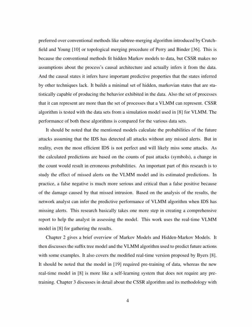
Figure 2.2: Hidden-Markov Process

For example, Figure 2.2 can be considered as a Hidden-Markov process. The circles

A and B represent the states. The arrows connecting them represent the transitions of the

model from one state to another and the labels shown indicate what symbol is emitted and

its prediction to go to a particular state. For example the label at the left side 1 | 0.5 implies

that the model can emit symbol 1 with a probability of 0.5 and remain in state A. Observe

that in this process, just by knowing the last observed symbol, one cannot always determine

the current state. If a 0 has been observed as last symbol, we can say that the current state of

the process is A but if a 1 was observed, we cannot determine which state the process is in.

Though we can infer the conditional distribution on the future based on the last observed

symbol, we cannot deduce the state the model is in. Since it has hidden states, this process

is an example of a hidden Markov process. Hidden Markov models have wide range of

applications in various fields including ecology, cryptanalysis and speech recognition.

8

Usage of Markov chains in the field of intrusion detection has given better performance

in terms of hit rate and false alarm rates compared to Hotelling’s T-square test and chi-

square multivariate test. These results have been proved by applying same testing set of

audit data on all the models in [52]. The hit rate is computed by dividing the total number

of hits with the total number of intrusive events in the testing data. The false alarm rate

is computed by dividing the total number of false alarms with the total number of normal

events in the testing data. 100% hit rate and 0% false alarm rate is ideal, which is the best

detection performance by the intrusion detection technique.

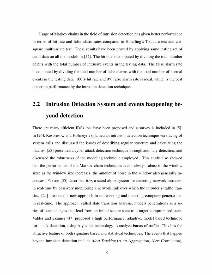
2.2 Intrusion Detection System and events happening be-

yond detection

There are many efficient IDSs that have been proposed and a survey is included in [5].

In [26], Kosoresow and Hofmeyr explained an intrusion detection technique via tracing of

system calls and discussed the issues of describing regular structure and calculating the

macros. [53] presented a cyber-attack detection technique through anomaly-detection, and

discussed the robustness of the modeling technique employed. This study also showed

that the performance of the Markov chain techniques is not always robust to the window

size: as the window size increases, the amount of noise in the window also generally in-

creases. Paxson [35] described Bro, a stand-alone system for detecting network intruders

in real-time by passively monitoring a network link over which the intruder’s traffic tran-

sits. [24] presented a new approach in representing and detecting computer penetrations

in real-time. The approach, called state transition analysis, models penetrations as a se-

ries of state changes that lead from an initial secure state to a target compromised state.

Valdes and Skinner [47] proposed a high performance, adaptive, model based technique

for attack detection, using bayes net technology to analyze bursts of traffic. This has the

attractive feature of both signature based and statistical techniques. The events that happen

beyond intrusion detection include Alert Tracking (Alert Aggregation, Alert Correlation),

9

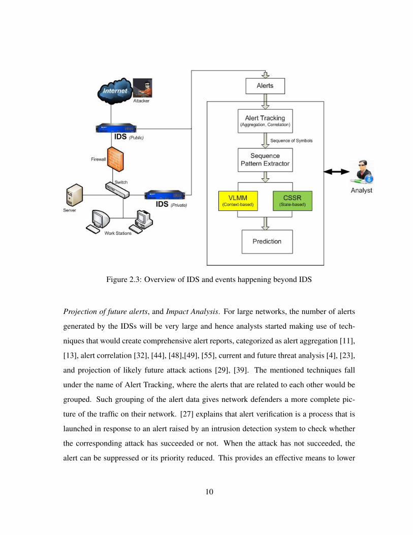
Figure 2.3: Overview of IDS and events happening beyond IDS

Projection of future alerts, and Impact Analysis. For large networks, the number of alerts

generated by the IDSs will be very large and hence analysts started making use of tech-

niques that would create comprehensive alert reports, categorized as alert aggregation [11],

[13], alert correlation [32], [44], [48],[49], [55], current and future threat analysis [4], [23],

and projection of likely future attack actions [29], [39]. The mentioned techniques fall

under the name of Alert Tracking, where the alerts that are related to each other would be

grouped. Such grouping of the alert data gives network defenders a more complete pic-

ture of the traffic on their network. [27] explains that alert verification is a process that is

launched in response to an alert raised by an intrusion detection system to check whether

the corresponding attack has succeeded or not. When the attack has not succeeded, the

alert can be suppressed or its priority reduced. This provides an effective means to lower

10

the number of false alarms that an administrator has to deal with. It also improves the re-

sults of alert correlation systems by cleaning their input data from spurious attacks. The

proposed approach in [33] constructs attack scenarios by correlating alerts on the basis

of prerequisites and consequences of intrusions. Based on the prerequisites and conse-

quences of different types of attacks, the proposed approach correlates alerts by (partially)

matching the consequence of some previous alerts and the prerequisite of some later ones.

[54] describes an intrusion alert management system called TRINETR. The architecture is

composed of three parts: Alert Aggregation, Knowledge-based Alert Evaluation and Alert

Correlation. The architecture is aimed at reducing the alert overload by aggregating alerts

from multiple sensors to generate condensed views, reducing false positives by integrating

network and host system information into alert evaluation process and correlating events

based on logical relations to generate global and synthesized alert report. The definition of

attack correlation is extended in [12] to correlate attacks with intrusion objectives and to

introduce the notion of anti correlation. This approach provides the security administrator

with a global view of what happens in the system. It controls unobserved actions through

hypothesis generation, clusters repeated actions in a single scenario, recognizes intruders

that are changing their intrusion objectives and is efficient to detect variations of an intru-

sion scenario. This approach can also be used to eliminate a category of false positives.

A novel threat assessment scheme called TANDI was proposed in [23] to predict future

attacker actions. TANDI predicts future attack actions accurately as long as the attack is

not part of a coordinated attack and contains no insider threats. Even in the presence of ab-

normal attack events, TANDI will alarm the network analyst for further analysis. A novel

approach to assess the threat of network intrusions was proposed in [29]. This approach

assesses the attack threat from a forwarding perspective. To every attack type and some

attack scenarios, their Probabilities of having Following Attacks (PFAs) are calculated by

a data mining algorithm and then the threats of real time intrusions are assessed by these

probabilities. A graph-based approach to network vulnerability analysis was proposed in

[37]. This method allowed analysis of attacks from both outside and inside the network.

11

It can analyze risks to a specific network asset, or examine the universe of possible con-

sequences following a successful attack. This method is based on the idea of an attack

graph which represents attack states and the transitions between them. The attack graph

can be used to identify attack paths that are most likely to succeed, or to simulate various

attacks. The major advantage of this method over other computer security risk methods is

that it considers the physical network topology in conjunction with the set of attacks. The

report in [50] examines the applicability of current risk assessment techniques to assess

modern electronic threats. It also analyses the concepts of risk, vulnerability, threat agent

and threat, and examine threat statistics from around the world and from various sources,

and the state of the art on the various risk and threat analysis techniques.

2.3 Sequence Modeling and Prediction using Context-based

Algorithm (VLMM)

The problem of projecting cyber attacks by looking at the sequential properties of corre-

lated IDS alerts belonging to multi-stage attack tracks was addressed by Fava [19]. The

basic methodology includes attack track pre-processing, sequence modeling and predic-

tion. Attack tracks consist of ordered collections of alerts belonging to a single multi-stage

attack. Sequence modeling techniques used in the fields like DNA analysis have been ap-

plied in the context of cyber attack projection by interpreting attack tracks as a sequence

of symbols. Finite-context models or Markov models have been used to characterize their

corresponding sequences of malicious actions.

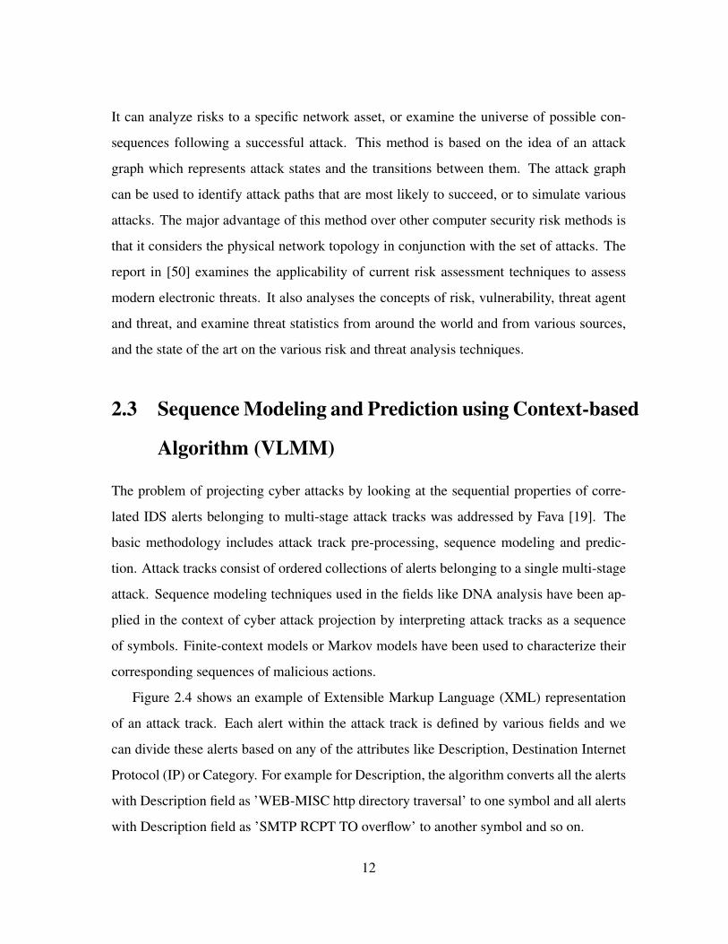
Figure 2.4 shows an example of Extensible Markup Language (XML) representation

of an attack track. Each alert within the attack track is defined by various fields and we

can divide these alerts based on any of the attributes like Description, Destination Internet

Protocol (IP) or Category. For example for Description, the algorithm converts all the alerts

with Description field as ’WEB-MISC http directory traversal’ to one symbol and all alerts

with Description field as ’SMTP RCPT TO overflow’ to another symbol and so on.

12

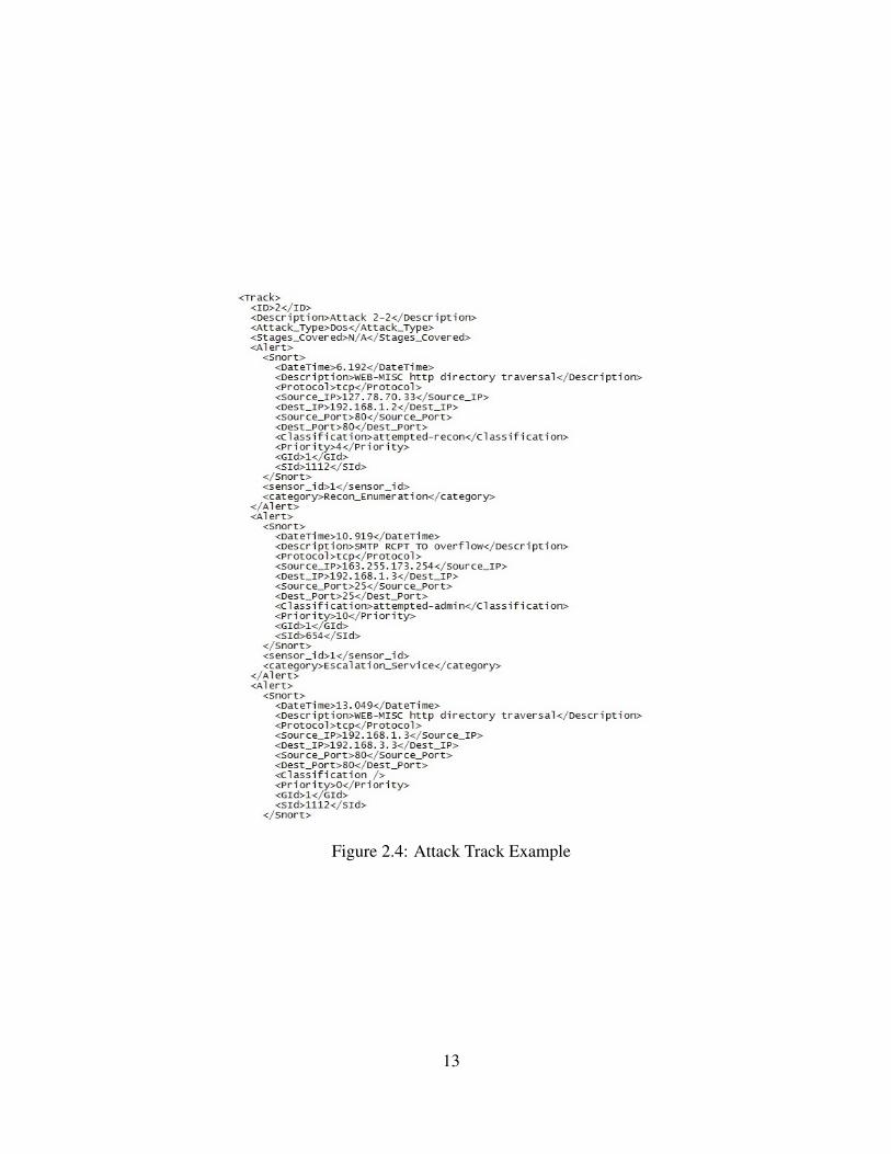
Figure 2.4: Attack Track Example

13

Suffix Tree :

Different order Markov models can be implemented using a Suffix Tree. The actual

suffix tree training algorithm was originally motivated by the work of Begleiter, El-Yaniv

and Yona [7]. It was modified by Fava [19] to take a set of finite length sequences in-

stead of a single long sequence of observations. For example, let us consider the se-

quence ’+,A,B,A,C,B,A,C,-’, where + and − represent the start and end of the sequence,

A and B may represent any alert descriptions. Edges are weighted with the number of

times the suffix tree has traversed through that branch. The suffix tree for the sequence

’+,A,B,A,C,B,A,C,-’ is shown in Figure 2.5.

Figure 2.5: Suffix Tree for sequence: +ABACBAC-

We can observe that Fava’s work [19] defines the start and end of sequence characters,

however the real-time algorithm proposed by Byers [8] trains the suffix tree with partial

sequences instead of finite completed sequence. Basically Byers algorithm [8] is more

like a self-learning system without the need for any pre-training. Now consider the same

sequence and consider the construction of tree one symbol at a time, where the end of

14

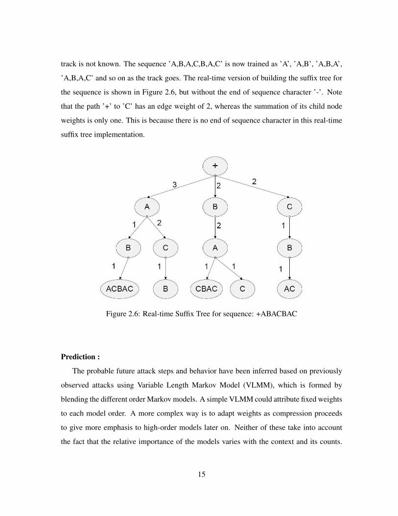
track is not known. The sequence ’A,B,A,C,B,A,C’ is now trained as ’A’, ’A,B’, ’A,B,A’,

’A,B,A,C’ and so on as the track goes. The real-time version of building the suffix tree for

the sequence is shown in Figure 2.6, but without the end of sequence character ’-’. Note

that the path ’+’ to ’C’ has an edge weight of 2, whereas the summation of its child node

weights is only one. This is because there is no end of sequence character in this real-time

suffix tree implementation.

Figure 2.6: Real-time Suffix Tree for sequence: +ABACBAC

Prediction :

The probable future attack steps and behavior have been inferred based on previously

observed attacks using Variable Length Markov Model (VLMM), which is formed by

blending the different order Markov models. A simple VLMM could attribute fixed weights

to each model order. A more complex way is to adapt weights as compression proceeds

to give more emphasis to high-order models later on. Neither of these take into account

the fact that the relative importance of the models varies with the context and its counts.

15

The weights in [19] have been derived from escape probabilities. The probability of en-

countering a previously unseen character is called the Escape Probability. Denoting the

probability of an escape at level j by ej , equivalent weights can be calculated from the

escape probabilities by:

Wj = (1− ej)×l∏

k=j+1

ek,−1 ≤ j ≤ l (2.2)

where l is the highest order context making a non-null prediction. In this formula, the

weight of each successively lower order is reduced by the escape probability from one

order to the next. The weights will be plausible provided that the escape probabilities

are between 0 and 1 and it is not possible to escape below order -1; hence e−1 = 0. The

advantage of expressing things in terms of escape probabilities is that they tend to be more

easily visualized and understood than the weights themselves, which can become small

very rapidly. Several methods have been proposed but Fava’s work [19] was not able to

identify any particular method to be better than others. One of the methods allocates one

additional count over and above the number of times the context has been seen to allow for

the occurrence of new characters. This was chosen as the default value in Byers work [8].

e0 =1

C0 + 1(2.3)

Using the equations of escape probabilities and weights, VLMM estimates the probabilities

using the following equation:

P (A) =l∑

j=−1

Wj × Pj(A) (2.4)

According to the results gathered by Fava [19], the first order model performs better than

0, or second or higher order models, because any next event has a strong correlation with

the immediate previous event. It was also shown that VLMM has the best prediction rate

due to the reason that an nth order model introduces more information that is not captured

by the (n− 1)th order model.

16

For example, with the sequence ’A,B,A,C,A,B,C’ trained using the real-time algorithm

[8], Table 2.1 shows the probabilities of the next occurring symbol given, let’s say, an

observed sequence of ’A,B’.

P(X) P(X given A) P(X given A,B)X=A 3/7 0 1/2X=B 2/7 2/3 0X=C 2/7 1/3 1/2

Table 2.1: Probabilities of predicted symbols given observed sequence ’A, B’

Another interesting concept to notice is that this real-time algorithm [8] also predicts

the occurrence of new symbols. When a new symbol occurs, the suffix tree is first trained

as normal and then trained again with the suffix history added with the special new symbol

definition.

Graphical User Interface and Metrics used :

A Graphical User Interface (GUI) was designed in [8], that displays real-time visu-

alization of suffix tree. This GUI, as shown in Figure 2.7, has various options including

threshold options and various metrics like prediction accuracy and number of total pre-

dictions. This real-time system tracks only overall metrics for each alphabet and tracks

detailed metrics if requested by the user via the GUI. Whether a particular prediction is

correct or in-correct is determined by a set of predictions against the next event. This set of

predictions is determined by a threshold number. Traditionally top-3 predictions are con-

sidered relevant and are used in our analysis. The XML files that contain the alert tracks

can be loaded into the GUI from File menu. It also has the option to use only the ground

truth instead of the entire file. Once a file is loaded, we can inject the alerts inside it by

clicking Inject Next Alert or Inject All Remaining Alerts buttons. After all the alerts are

injected, we can observe the metrics in the GUI. Under the settings menu, we can select the

prediction threshold like top-1, top-2 or top-3 and so on. In this research, we use this GUI

to collect results related to various performance metrics.

17

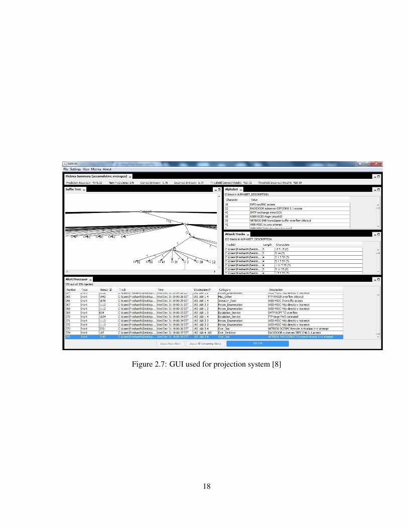
Figure 2.7: GUI used for projection system [8]

18

Chapter 3

Sequence Modeling and Prediction us-

ing State-based Algorithm (CSSR)

A new algorithm for discovering patterns in data, called Causal-State Splitting Reconstruc-

tion (CSSR), was proposed in [41]. It builds a minimal set of hidden, markovian states that

are statistically capable of producing the underlying process’s causal states.

Below are some properties related to Causal states that have been proved in [40]:

• Causal states are the minimal sufficient statistics needed for predicting futures of all

lengths.

• Causal states are not only minimum sufficient but also unique.

• Causal states are prescient. The causal states themselves form a Markov process.

• The causal states of a process are the members of the range of the function that maps

from histories to sets of histories.

• Each causal state has a unique associated distribution of outputs, called its morph. In

general every state has a morph, but two states in the same state class may have the

same morph.

• Causal states have the important property that all of their parts have the same morph.

19

• However each causal state has a unique morph, which means no two causal states

will have the same conditional distribution of the future.

• The past and the future of a process are independent, conditioning on the causal

states.

• A process’s causal states are the largest subsets of histories that are all strictly homo-

geneous with respect to futures of all lengths.

The current causal state and the next value of observed process will determine the next

causal state. These possible next symbols have well defined conditional probabilities. The

Transition Probability can be defined as the probability of making a transition from one

state to another while emitting a symbol. The combination of the function ε from histories

to causal states with the labeled transition probabilities is called the ε-machine of the pro-

cess [10]. ε-machines are deterministic and Markovian in nature, which means that given

a causal state at time t, the causal state at time t + 1 is independent of the causal states at

earlier times. ε-machine reconstruction is any procedure that given a process produces the

process’s ε-machine. An algorithm was developed for ε-machine reconstruction [10] [9],

which merged distinct histories together into states when their morphs seemed close. Be-

cause it works by merging, it effectively makes the most complicated model of the process

it can. Though the causal states are deterministic, the states it returns often aren’t. A new

ε-machine reconstruction algorithm called CSSR, which improves on the old algorithm,

was proposed in [41]. It operates on the opposite principle, by creating or splitting new

states only when absolutely forced to. The operation of CSSR is summarized in Figure 3.1.

3.1 Methodology

There are three procedures in CSSR: Initialize, Homogenize, and Determinize.

1. Initialize: The initial model is that the process is a sequence of independent, identically-

distributed random variables. Initially, it contains only the null sequence.

20

Figure 3.1: Flow chart of CSSR [40]

21

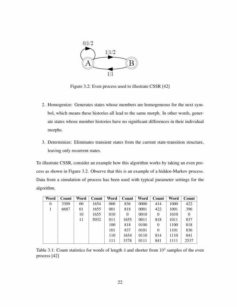
Figure 3.2: Even process used to illustrate CSSR [42]

2. Homogenize: Generates states whose members are homogeneous for the next sym-

bol, which means these histories all lead to the same morph. In other words, gener-

ate states whose member histories have no significant differences in their individual

morphs.

3. Determinize: Eliminates transient states from the current state-transition structure,

leaving only recurrent states.

To illustrate CSSR, consider an example how this algorithm works by taking an even pro-

cess as shown in Figure 3.2. Observe that this is an example of a hidden-Markov process.

Data from a simulation of process has been used with typical parameter settings for the

algorithm.

Word Count Word Count Word Count Word Count Word Count0 3309 00 1654 000 836 0000 414 1000 4221 6687 01 1655 001 818 0001 422 1001 396

10 1655 010 0 0010 0 1010 011 5032 011 1655 0011 818 1011 837

100 818 0100 0 1100 818101 837 0101 0 1101 836110 1654 0110 814 1110 841111 3378 0111 841 1111 2537

Table 3.1: Count statistics for words of length 4 and shorter from 104 samples of the evenprocess [42]

22

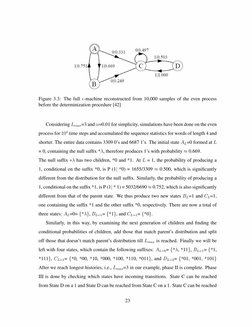
Figure 3.3: The full ε-machine reconstructed from 10,000 samples of the even processbefore the determinization procedure [42]

Considering Lmax=3 and α=0.01 for simplicity, simulations have been done on the even

process for 104 time steps and accumulated the sequence statistics for words of length 4 and

shorter. The entire data contains 3309 0’s and 6687 1’s. The initial state AL=0 formed at L

= 0, containing the null suffix *λ, therefore produces 1’s with probability ≈ 0.669.

The null suffix ∗λ has two children, *0 and *1. At L = 1, the probability of producing a

1, conditional on the suffix *0, is P (1| *0) = 1655/3309 ≈ 0.500, which is significantly

different from the distribution for the null suffix. Similarly, the probability of producing a

1, conditional on the suffix *1, is P (1| * 1) = 5032/6690≈ 0.752, which is also significantly

different from that of the parent state. We thus produce two new states BL=1 and CL=1,

one containing the suffix *1 and the other suffix *0, respectively. There are now a total of

three states: AL=0= {*λ}, BL=1= {*1}, and CL=1= {*0}.

Similarly, in this way, by examining the next generation of children and finding the

conditional probabilities of children, add those that match parent’s distribution and split

off those that doesn’t match parent’s distribution till Lmax is reached. Finally we will be

left with four states, which contain the following suffixes: AL=0= {*λ, *11}, BL=1= {*1,

*111}, CL=1= {*0, *00, *10, *000, *100, *110, *011}, and DL=2= {*01, *001, *101}

After we reach longest histories, i.e., Lmax=3 in our example, phase II is complete. Phase

III is done by checking which states have incoming transitions. State C can be reached

from State D on a 1 and State D can be reached from State C on a 1. State C can be reached

23

Figure 3.4: The final ε-machine by CSSR

from itself or from States A or B on a 0. Observe that State A can only be reached from

State B on a 1 and State B can only be reached from State A on a 1.

Continuing the process of determinization, we eliminate the two transient states A and

B. Since every suffix in State C goes to one in State C by adding a 0 and to State D by

adding a 1, we do not split C. Similarly we do not change State D because every suffix in

State D goes to one in State C by adding a 1. The process of determinization ends here.

The final result is an ε-machine with two states C and D as shown in Figure 5. These are

the causal states sufficient to capture the behavior exhibited in the data.

3.2 Comparison of CSSR with other state-based algorithms

The ε-machine captures all patterns in the process which have any predictive power. An

algorithm was initially developed for ε-machine reconstruction by Crutchfield and Young

in [10], [9]. Their default assumption is that each history that we come across in the data is

a causal state. The merging procedure can be explained as follows. Consider all the nodes

with subtrees of depth L, and take any two of them. If all the probability distributions at-

tached to the length-L path in their subtrees are within some constant, then the two nodes

are equivalent and will be merged. This procedure is repeated until no merging is possible.

All other ε-machine reconstruction methods are also based on merging. For example in the

’topological’ merging procedure of Perry and Binder [36], they consider the relationship

between histories and futures. Two histories are assigned to a same state, if sets of futures

24

they yield are identical. Then they estimate the distribution for each state, not for each

history. The problem with state-merging methods lies in their default assumption that each

history is its own state. Because of this assumption, the state-merging methods start by pro-

ducing the most complex possible null model of the process, given the length of histories,

and then trim it by merging.

Instead of using state-merging methods, a new reconstruction algorithm based on state-

splitting (CSSR) was proposed. CSSR starts off with a zero-complexity null model by

putting every history in one state and then adds states only if the current set of states are not

sufficient according to the statistical tests. Unlike conventional algorithms, which tune the

parameters in a fixed architecture, CSSR is capable of inferring the appropriate architecture

as well. The causal states it infers have important predictive optimality properties. These

predictors take the form of minimum sufficient statistics, arranged into a hidden Markov

model (HMM). Hence they preserve the features of HMMs without making any assump-

tions about the nature of the process. Also as explained in [42], CSSR must estimate 2k

probabilities for each history, one for each member of the power set of the alphabet, but

the state-merging algorithm must estimate the probability of each member of the power set

of future sequences which is 2kL probabilities. In [41], CSSR is compared to the use of

cross-validation to select an HMM architecture, and the results imply that CSSR’s predic-

tive performance is at least comparable to cross-validated expected-maximization, but it is

constructive and faster.

Though CSSR does not require any prior knowledge about system dynamics, it cannot

exploit such information when it exists.

3.3 Comparison of CSSR with context-based algorithms

Context-based algorithms construct so called Variable Length Markov Models from se-

quence data. Contexts are considered to be the suffixes of history and the algorithms work

by examining the long histories, creating new contexts by splitting existing ones based on

25

a threshold. VLMMs, similar to CSSR, do not rely on domain specific information. Each

state in a VLMM is represented by a single suffix, and consists of all and only the histories

ending in that suffix. For many processes, where the causal states contain multiple suffixes,

multiple contexts are needed to represent a single causal state, so VLMMs are generally

more complicated than the HMMs build in CSSR. The causal state model is the same as

the minimal VLMM if and only if every causal state contains a single suffix.

For the even process in Figure 3 that is used to illustrate CSSR, clearly A and B both

contain infinitely many suffixes, and so correspond to an infinite number of contexts. If we

let the length of histories grow, a VLMM algorithm will increase the number of contexts

it finds without bound. VLMM algorithms are incapable of capturing such even processes.

Hence the class of processes that CSSR can represent is larger than those that a VLMM can

represent. However the process involved in CSSR is a lot more complicated than VLMM,

which is far simpler. And also for CSSR to perform better with less error probability, we

need to have infinitely long sequences.

26

Chapter 4

Error Analysis

4.1 Possible Errors and their Significance

In the field of statistics, to describe particular flaws in any process, there are two major

kinds of possible errors:

• Type I error: It is the wrong decision that is made when a test rejects a true null

hypothesis. False Positive (FP) comes under this kind.

• Type II error: It is the wrong decision that is made when a test fails to reject a false

null hypothesis. False Negative (FN) comes under this kind.

The definitions of these two kinds of errors change depending on the application. In the

field of Intrusion Detection, they can be defined as follows:

• A False Positive is raising an alarm for a non-malicious activity.

• A False Negative is failing to identify an attack and not raising an alarm for a mali-

cious activity.

False Positives and False Negatives can happen to any Intrusion Detection System, no mat-

ter how efficient it is. Both types of errors cause various problems to the network security.

A false positive of the IDS will not result in an intrusion and it may be caused because

of two reasons: the detection mechanism of the IDS is faulty or the IDS has detected an

27

anomaly that turns out to be benign. Therefore, the false positives may cause security ana-

lysts to expend unnecessary effort. On the other hand, a false negative is a missed attack,

which may put networks or computer systems in danger. Clearly these are undesirable,

and every organization strives to avoid them. However, no detection system detects all the

attacks. Hence, the goal is to provide good coverage against high priority attacks. Sev-

eral other reasons may also cause a false negative. For example, in order to elude the IDS,

the attack may incorporate obfuscation techniques. Another possibility is to overwhelm the

IDS with traffic beyond its processing capacity, so that the IDS will drop the packets needed

to detect the attack. If an IDS raises an alert that did not happen, the worse that can happen

would be wastage of resources and time till the network administrator realizes that it is a

false alarm. But if an IDS fails to identify an alert, that alert might be malicious enough

to damage the whole network and hence risking the security. A mechanism proposed in

[21] collected more than two thousand FPs and FNs during sixteen months. It reported that

92.85% of false cases were FPs and 7.15% were FNs. Out of all the FPs, about 91% of

FP alerts occur because of IDS’s policy or company management policies, but not due to

security issues. Hence in practice, a false negative is much more serious and critical than

a false positive because of the negative effects it has and because of the damage caused by

that missed intrusion. Therefore it is necessary to analyze the effect of the false negatives in

detail to improve the network security. If reported data from IDS has some false negatives,

it impacts both the sequence model (suffix tree of VLMM or ε-machine of CSSR) that is

build and also the estimated probabilities that are calculated based on the model. This re-

search studies the effects of false negatives/missing alerts on the predictive performance of

the model being used. This would help the analyst in assessing the model (VLMM in our

case) in terms of its predictive performance in the presence of missed alerts.

28

4.2 VLMM

In case of a model like VLMM, the amount of effect a missing alert would have on the

suffix tree or the probability estimations would depend on many factors including:

• the occurrence rate of missing alert and its estimated probability

• the position of the missing alert in the sequence

• length of the sequence

• symbol space within the sequence

The future alerts are predicted based on weights and escape probabilities, which depend

on the occurrence rates of the symbols in the sequence. Hence missing alerts would result

in erroneous probability calculations. This change could be positive or negative depending

on the mentioned factors.

In order to have a comprehensive analysis, we will study the effect in two ways: one

with respect to the position of the missing alert and another with respect to the occurrence

of the missing alert. We will randomly remove alerts while doing the analysis. This random

removal in the design is based to reflect the scenarios where the attacker uses obfuscation

techniques to confuse the system by attacking at different positions at different times. We

will study the effect in terms of occurrence of missing alerts by defining the common and

rare alerts and compare it against the results based on position.

In addition to various factors like occurrence, position, length of sequence and symbol

space, the prediction accuracy of a model like VLMM will also be affected when missing

alerts cause a change in the order of probability within the threshold predictions. Depend-

ing on the occurrence rate of missing symbols and their probabilities, missing alerts can

result in change of the order of symbol probabilities. However, it does not mean a change

in the order of probabilities will always affect the prediction performance. If the estimated

probabilities of two symbols are close enough, it is likely that they will have a change in

their ranking due to the effect of missing alerts. Figure 4.1 shows a simple example of such

29

Figure 4.1: Example showing the change in order of probabilities of two symbols

scenario, where Pe refers to erroneous probability, P refers to actual true probability and

dP/dx refers to the differential probability.

4.3 CSSR

Error analysis of CSSR is done in [41] by considering the statistical errors that each of

the algorithm’s three procedures can produce. Since it merely sets up parameters and data

structures, nothing goes wrong in ’Initialize’ step. ’Homogenize’ step can make two kinds

of errors. First, it can group together histories with different distributions for the next

symbol. Second, it can fail to group together histories that have the same distribution.

Let Si and Sj are suffixes in the same state, with counts ni and nj . There is always the

variational distance t such that the significance test will not separate estimated distributions

differing by t or less. If we make ni large enough, then with probability arbitrarily close

to one, the estimated distribution for i is within t/2 of the true morph, and similarly for

j. Hence, the estimated morphs for the two suffixes are within t of each other and will be

merged. If any state contains any finite number of suffixes, by obtaining a sufficiently large

sample of each, we can ensure that they are all within t/2 of the true morph and so within

t of each other and thus merged. In this way, the probability of inappropriate splitting can

be made arbitrarily small. If each suffix’s conditional distribution is sufficiently close to its

30

true morph, then the test will eventually separate suffixes belonging to different morphs.

Since the step ’Determinization’ always refines the partition with which it starts, there is

no chance of merging histories that do not belong together. In summary, if the number of

causal states is finite and Lmax is sufficiently large, the probability that the states estimated

are not the causal states becomes arbitrarily small, for sufficiently large N.

To analyze the bounds of the error probability, CSSR used the chernoff’s inequality

[51], which states that:

P (|An − µ| ≥ t) ≤ 2e−2nt2 (4.1)

where An is the mean of the first n of the Xi (X1, X2, · · · , Xn are Bernoulli random vari-

ables), with probability µ of success.

The convergence of CSSR algorithm was shown in [41] based on Kolmogorov-Smirnov

test (KS test) [22], and Chernoff’s inequality [51], as follows:

P (d(Pn(S→1|S←L = s←L), P (S→1|S←L)) ≥ t) ≤∑A∈2A

2e−8nt2 = 2k+1e−8nt2 (4.2)

Two kinds of errors are possible in CSSR algorithm:

• It can group together histories with different distributions for the next symbol.

• It can fail to group together histories that have the same distribution.

Variable Name Description Values accordingto Table 2.1

n suffix count -N length of the sequence 1000L length of histories considered 3p∗ probability of the most improbable string 396/9996 ≈ 0.039k constant 2t difference between suffix and it’s true morph 0.461 (0.5-0.039)

(magnitude of the prediction error)q(t) probability of seeing an error of size t or larger ≈ 0

Table 4.1: CSSR variables description

Probability that one or more suffixes differ from its true morph by t:

31

q(t, n) ≤s∑

i=1

2e−8nit2

= 2k+1se−8mt2 (4.3)

wherem is the least of the ni and s is the number of histories actually seen or as the number

of histories needed to infer the true states. We can upper bound s by the maximum number

of morphs possible as:

s ≤ (kL+1 − 1)

(k − 1)(4.4)

=⇒ q(t, n) ≤ 2k+1 (kL+1 − 1)

(k − 1)e−8Np∗t2 (4.5)

The equation 4.5 approaches zero for large values of N .

We have applied the CSSR convergence formula for the data given in Table 3.1. An

example is shown in Table 4.1, where the error probability was almost zero. Hence by

obtaining a sufficiently large sample of each suffix, the error probability of CSSR can be

made small.

32

Chapter 5

Results and Discussion

In this research, we will run two sets of simulations. One is by using the true data sets

assuming that they do not have any missing alerts and another is by removing the alerts

from those true data sets. We will compare the performance of VLMM and CSSR in terms

of prediction accuracy for the true data sets. Prediction Accuracy is the percentage of

symbols occurring within a set based on a threshold, consisting of symbols with highest

probabilities according to the chosen model. Hence if an observed symbol was one of

the top three predictions with the highest probability, that would be included in the Top-3

prediction accuracy section. The prediction accuracy is calculated by dividing the number

of correct predictions to the total number of predictions made by the model used. The

choice of ’three’ is arbitrary and can be changed to any reasonable number. Traditionally

top-3 predictions are considered relevant and so we have used it in our error analysis.

5.1 VLMM and CSSR on True Data

5.1.1 Experiment Design

In previous work [19], the experimental dataset of attacks was randomly split into two

halves. One-half of the tracks were used to pre-train the model, and the other half to

test the algorithm’s predictive performance. But this research is based on the real-time

implementation done in [8], which processes one alert at a time. This system generates

33

symbols, dynamically trains models for each alphabet definition in parallel, and generates

next-step prediction sets for each attack track based on those changing models as events

unfold. This approach facilitates investigation into the adaptive qualities of the system to

new attack scenarios. For the first set of simulations, we will run the true data sets on two

different algorithms - VLMM and CSSR, and will compare their performance in terms of

prediction accuracy.

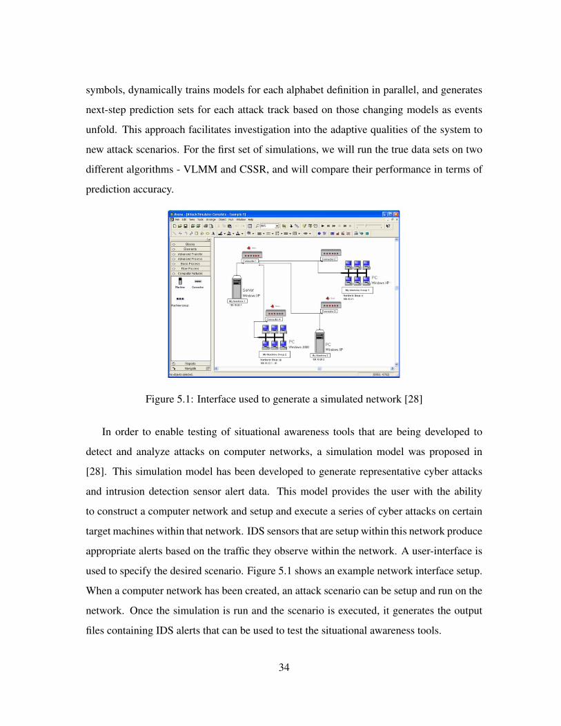
Figure 5.1: Interface used to generate a simulated network [28]

In order to enable testing of situational awareness tools that are being developed to

detect and analyze attacks on computer networks, a simulation model was proposed in

[28]. This simulation model has been developed to generate representative cyber attacks

and intrusion detection sensor alert data. This model provides the user with the ability

to construct a computer network and setup and execute a series of cyber attacks on certain

target machines within that network. IDS sensors that are setup within this network produce

appropriate alerts based on the traffic they observe within the network. A user-interface is

used to specify the desired scenario. Figure 5.1 shows an example network interface setup.

When a computer network has been created, an attack scenario can be setup and run on the

network. Once the simulation is run and the scenario is executed, it generates the output

files containing IDS alerts that can be used to test the situational awareness tools.

34

The outcome of this simulation model is a set of IDS alerts that can be used to test and

evaluate the various cyber security tools. Taking into account the need for ground truth (list

of actions executed during each attack), this research utilizes experimental datasets gener-

ated by the simulation model, implemented by RIT’s Industrial and Systems Engineering.

We have used five sets of data, containing ground truth without any noise, to test VLMM

and CSSR algorithms. The data sets used along with the length of the sequence and the

number of symbols in the sequence is shown in Table 5.1.

Data Set Alerts SymbolsBVT-2A 376 61BVT-2B 336 57BVT-2F 378 55BVT-2H 293 52BVT-2I 496 60

Table 5.1: Data Sets used to compare VLMM and CSSR

5.1.2 Results and Discussion

Table 5.2 shows the prediction accuracies for the data sets without considering any repe-

titions. Here the data sets used are assumed to be true data sets, which do not have any

missed alerts. The accuracies achieved by both VLMM and CSSR are encouraging given

the relatively large number of symbols in the corresponding symbol spaces. Consider for

BVT-2A, where a blind guess of 3 out of 61 would give a prediction rate of around 4.9%

which is much smaller than 41.30% by VLMM and 51.91% by CSSR.

If we consider the average values of all data sets as shown in Figure 5.3, we can observe

that in terms of top-3, top-2, and top-1 prediction accuracies, both VLMM and CSSR give

very similar results. However we can observe from Figure 5.2 that for some cases, there is

some significant difference in top-1 accuracies of VLMM and CSSR. For example for data

set BVT-2B the top-1 accuracy by VLMM is 23.83% whereas CSSR has only 11.59%.

This is likely because the symbol CSSR assigned highest probability most of times, has

occurred less frequently whereas the symbol that VLMM assigned highest probability has

35

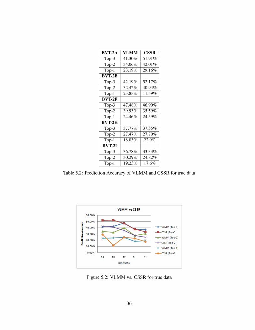
BVT-2A VLMM CSSRTop-3 41.30% 51.91%Top-2 34.06% 42.01%Top-1 23.19% 29.16%

BVT-2BTop-3 42.19% 52.17%Top-2 32.42% 40.94%Top-1 23.83% 11.59%

BVT-2FTop-3 47.48% 46.90%Top-2 39.93% 35.59%Top-1 24.46% 24.59%

BVT-2HTop-3 37.77% 37.55%Top-2 27.47% 27.70%Top-1 18.03% 22.9%

BVT-2ITop-3 36.78% 33.33%Top-2 30.29% 24.82%Top-1 19.23% 17.6%

Table 5.2: Prediction Accuracy of VLMM and CSSR for true data

Figure 5.2: VLMM vs. CSSR for true data

36

Figure 5.3: VLMM vs. CSSR for average of all data sets

occurred more frequently.

Because of the nature of different data sets, the results by VLMM and CSSR may not

always be consistent. From the results gathered, we can observe that CSSR does not give

any superior results in terms of predictive performance. Since we need to have infinitely

long sequences for CSSR to perform better and VLMM being a simpler process, we have

used VLMM for the error analysis of missed alerts.

5.2 VLMM in presence of Missed Alerts

For the second set of simulations, we analyze the effect of missing alerts using VLMM

by observing the change in prediction accuracies. One way to study the effect of missing

alerts using a particular algorithm is by adding alerts to data, where we assume that the data

gathered from the simulation model is as a result of IDS failing to identify alerts. However

this method is unclear and complicated because lot of factors need to be considered like

the various attributes of the alert and whether to introduce new alert or one of the already

occurred alerts. An easier way is by removing alerts from the data sequence, where we

assume that the data from simulation model is a result of IDS identifying each and every

alert without missing any attack. In order to have a more comprehensive analysis, we study

the effect of missing alerts both in terms of the position and in terms of the occurrence. In

37

the process, we repeat this analysis for sequences of different lengths and different symbol

spaces, as they would also influence the prediction accuracies.

5.2.1 Analysis based on Position

5.2.1.1 Experiment Design

Since position of the alert is one of the factors that can influence the prediction accuracy, we

first study the effect of missing alerts based on its position. For this, we have chosen to split

the entire sequence into 3 parts (3 is arbitrary), referring them as Beginning, Middle and

End of sequence. Then we have randomly selected the positions within those 3 parts and

removed alerts. In order to have a complete analysis, we will also remove alerts randomly

from the whole sequence. Although any data set contains multiple tracks, while removing

alerts we look at the total data set as a single sequence generated by VLMM after combining

all the multiple tracks in an order. This random removal in the design is based to reflect

some real world scenarios where the attacker, in order to elude the IDS, may incorporate

obfuscation techniques and confuse the system by sometimes attacking at the beginning and

sometimes at the middle or at the end. We have run simulations by varying the percentage

of missing alerts: 5%, 15%, 25%, 40%. In this work, the Beginning of any sequence is

defined as a set ranging from start to 40%, the Middle of the sequence is defined to range

from 30%-70% and the End of the sequence is defined to range from 60%-100%. The

overlap is to allow us to remove more percentage of alerts. These percentages are calculated

with respect to the total length of the sequence. We know that, because of missing alerts,

each symbol’s prediction accuracy will either increase or decrease or remain the same. We

will then calculate the change in prediction accuracies to make observations. The data sets

used and their true prediction accuracies are shown in Figure 5.3.

38

Data Set Alerts Symbols True Top-3 True Top-1Description-1 376 63 41.30% 23.19%

Destination IP-1 376 9 87.32% 58.70%Category-1 376 12 61.23% 28.99%

Description-2 478 77 36.24% 19.58%Destination IP-2 478 9 91.53% 56.61%

Category-2 478 12 56.61% 25.13%Description-3 599 69 39.88% 19.24%

Destination IP-3 599 9 95.19% 71.94%Category-3 599 11 57.52% 24.25%

Table 5.3: Data Sets used for error analysis of VLMM based on position

5.2.1.2 Results and Discussion

After different percentages of alerts are removed from the sequence, we first gather the

results of new prediction accuracies. Figure 5.4 shows the change in prediction accuracies

for ten trials in each case for various percentages of missed alerts at different positions in

the sequence.

Figure 5.4: Change in Prediction Accuracy for data sets with 376 alerts

We have calculated the difference between the new prediction accuracy and the true

prediction accuracy, to know by how much the value got deviated (could be positive or

negative). For this, we use the metric ’Change in Prediction Accuracy’, which is the differ-

ence in prediction accuracies with and without missed alerts for different test cases.

The change in prediction accuracy can be positive or negative. In other words, the

prediction accuracy can decrease or increase due to the missed alerts. It can be observed

39

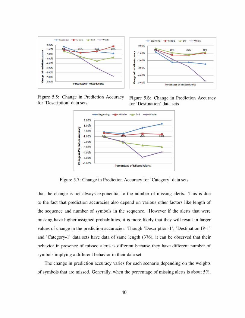
Figure 5.5: Change in Prediction Accuracyfor ’Description’ data sets

Figure 5.6: Change in Prediction Accuracyfor ’Destination’ data sets

Figure 5.7: Change in Prediction Accuracy for ’Category’ data sets

that the change is not always exponential to the number of missing alerts. This is due

to the fact that prediction accuracies also depend on various other factors like length of

the sequence and number of symbols in the sequence. However if the alerts that were

missing have higher assigned probabilities, it is more likely that they will result in larger

values of change in the prediction accuracies. Though ’Description-1’, ’Destination IP-1’

and ’Category-1’ data sets have data of same length (376), it can be observed that their

behavior in presence of missed alerts is different because they have different number of

symbols implying a different behavior in their data set.

The change in prediction accuracy varies for each scenario depending on the weights

of symbols that are missed. Generally, when the percentage of missing alerts is about 5%,

40

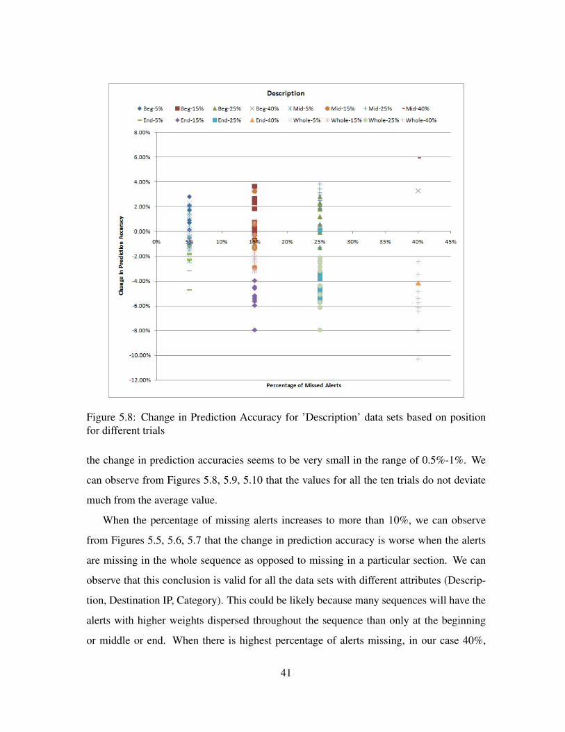
Figure 5.8: Change in Prediction Accuracy for ’Description’ data sets based on positionfor different trials

the change in prediction accuracies seems to be very small in the range of 0.5%-1%. We

can observe from Figures 5.8, 5.9, 5.10 that the values for all the ten trials do not deviate

much from the average value.

When the percentage of missing alerts increases to more than 10%, we can observe

from Figures 5.5, 5.6, 5.7 that the change in prediction accuracy is worse when the alerts

are missing in the whole sequence as opposed to missing in a particular section. We can

observe that this conclusion is valid for all the data sets with different attributes (Descrip-

tion, Destination IP, Category). This could be likely because many sequences will have the

alerts with higher weights dispersed throughout the sequence than only at the beginning

or middle or end. When there is highest percentage of alerts missing, in our case 40%,

41

Figure 5.9: Change in Prediction Accuracy for ’Destination IP’ data sets based on positionfor different trials

the performance is affected the most if they were missing throughout the entire sequence.

The next badly affected case is if they were missing at the beginning of the sequence. The

change in prediction accuracy is in the range of 4%-7% when the alerts are missing in the

whole sequence and 0-2% when alerts are missing at the beginning or middle or end of

the sequence. From Figures 5.8, 5.9, 5.10, we can also observe that this observation is

consistent across different trials, datasets and attributes. For example, in all the Figures

5.8, 5.9, 5.10, for the case when 25% alerts are missing, the change in prediction accuracy

is more for the case when alerts are missing throughout the sequence (circular dots high-

lighted in light green) as opposed to when alerts are missing at the beginning (triangle dots

highlighted in dark green) or at the middle (plus sign dots highlighted in blue) or at the end

42

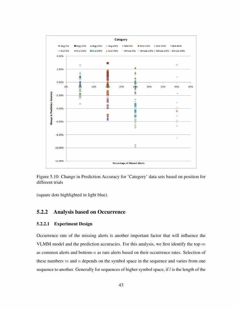
Figure 5.10: Change in Prediction Accuracy for ’Category’ data sets based on position fordifferent trials

(square dots highlighted in light blue).

5.2.2 Analysis based on Occurrence

5.2.2.1 Experiment Design

Occurrence rate of the missing alerts is another important factor that will influence the

VLMM model and the prediction accuracies. For this analysis, we first identify the top-m

as common alerts and bottom-n as rare alerts based on their occurrence rates. Selection of

these numbers m and n depends on the symbol space in the sequence and varies from one

sequence to another. Generally for sequences of higher symbol space, if l is the length of the

43

sequence, we can consider top-5 as common alerts and remaining (l− 5) as the rare alerts.

Since we have chosen top-3 in our results as the threshold for prediction accuracy values, it

is sufficient if we define the top-5 alerts as common alerts, because a change in the order of

symbols will also change the prediction accuracy. So if the 4th or 5th ranked symbols are

close enough to the 3rd ranked symbol, the order of these symbols might change because

of the missing symbols and cause a change in their ranking, which in turn will change the

prediction accuracy. And it is less probable for a symbol beyond 5th rank to change the

order with the 3rd or lesser ranked symbol. Hence 5 is a reasonable number to choose

for those sequences with larger symbol space. However for sequences with relatively less

number of symbols, the numbers will change and we can probably choose top-3 as the

common alerts and the remaining as rare alerts. This is because, for sequences with less

number of symbols, the sequence is usually dominated by the top-3 ranked symbols, and

hence higher prediction accuracies for such cases. The data sets used for this analysis are

shown in Figure 5.4 along with their true prediction accuracies.

Data Set Alerts Symbols True Top-3 True Top-1Description-1 376 63 41.30% 23.19%

Destination IP-1 376 9 87.32% 58.70%Category-1 376 12 61.23% 28.99%

Description-2 478 77 36.24% 19.58%Destination IP-2 478 9 91.53% 56.61%

Category-2 478 12 56.61% 25.13%Description-3 599 69 39.88% 19.24%

Destination IP-3 599 9 95.19% 71.94%Category-3 599 11 57.52% 24.25%

Table 5.4: Data Sets used for error analysis of VLMM based on occurrence

5.2.2.2 Results and Discussion

After identifying the common and rare alerts, we have randomly removed the alerts from

the entire sequence for ten trials. After observing the new prediction accuracy, we use

the same metric ’Change in Prediction Accuracy’, which is the difference in prediction

44

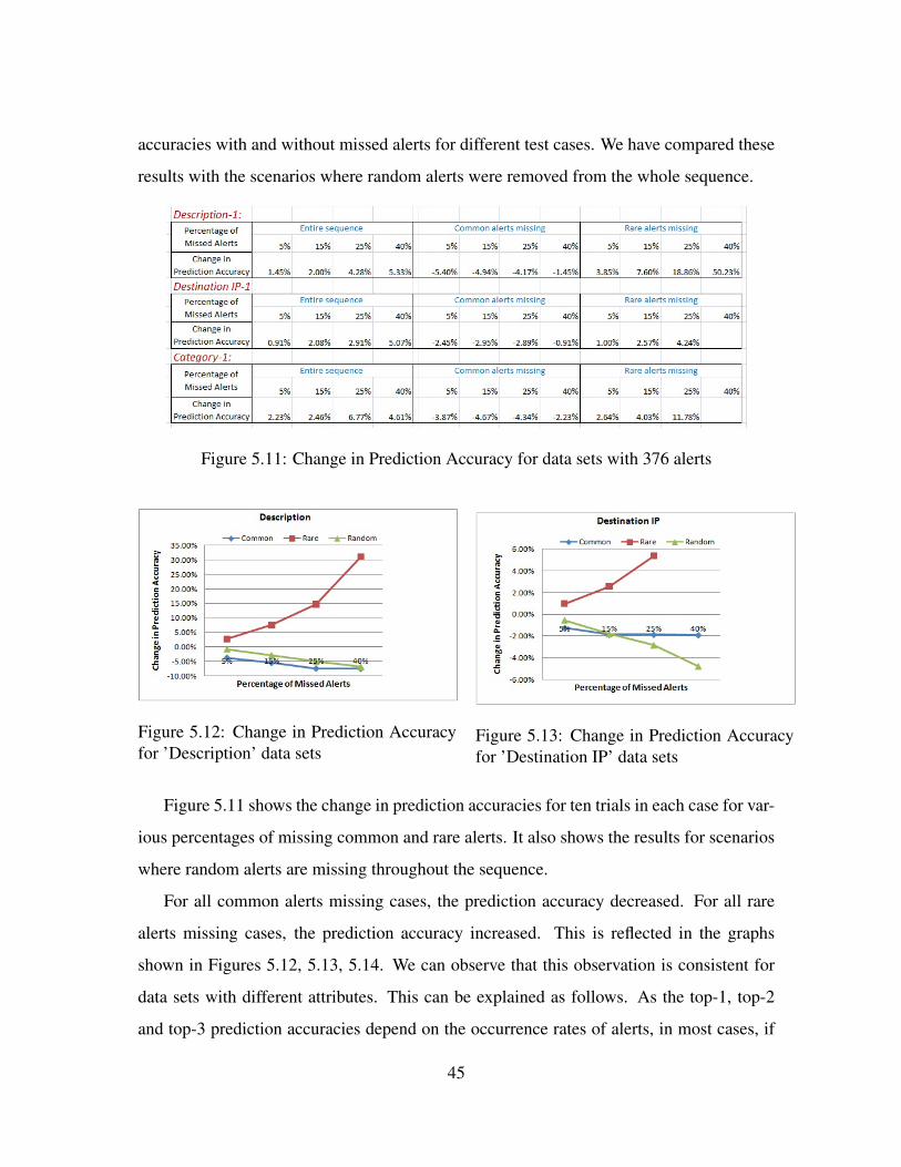
accuracies with and without missed alerts for different test cases. We have compared these

results with the scenarios where random alerts were removed from the whole sequence.

Figure 5.11: Change in Prediction Accuracy for data sets with 376 alerts

Figure 5.12: Change in Prediction Accuracyfor ’Description’ data sets

Figure 5.13: Change in Prediction Accuracyfor ’Destination IP’ data sets

Figure 5.11 shows the change in prediction accuracies for ten trials in each case for var-

ious percentages of missing common and rare alerts. It also shows the results for scenarios

where random alerts are missing throughout the sequence.

For all common alerts missing cases, the prediction accuracy decreased. For all rare

alerts missing cases, the prediction accuracy increased. This is reflected in the graphs

shown in Figures 5.12, 5.13, 5.14. We can observe that this observation is consistent for

data sets with different attributes. This can be explained as follows. As the top-1, top-2

and top-3 prediction accuracies depend on the occurrence rates of alerts, in most cases, if

45

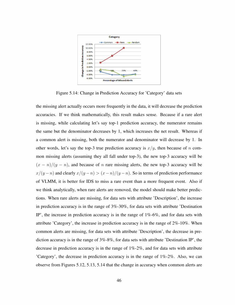
Figure 5.14: Change in Prediction Accuracy for ’Category’ data sets

the missing alert actually occurs more frequently in the data, it will decrease the prediction

accuracies. If we think mathematically, this result makes sense. Because if a rare alert

is missing, while calculating let’s say top-1 prediction accuracy, the numerator remains

the same but the denominator decreases by 1, which increases the net result. Whereas if

a common alert is missing, both the numerator and denominator will decrease by 1. In

other words, let’s say the top-3 true prediction accuracy is x/y, then because of n com-

mon missing alerts (assuming they all fall under top-3), the new top-3 accuracy will be

(x − n)/(y − n), and because of n rare missing alerts, the new top-3 accuracy will be

x/(y−n) and clearly x/(y−n) > (x−n)/(y−n). So in terms of prediction performance

of VLMM, it is better for IDS to miss a rare event than a more frequent event. Also if

we think analytically, when rare alerts are removed, the model should make better predic-

tions. When rare alerts are missing, for data sets with attribute ’Description’, the increase

in prediction accuracy is in the range of 3%-30%, for data sets with attribute ’Destination

IP’, the increase in prediction accuracy is in the range of 1%-6%, and for data sets with

attribute ’Category’, the increase in prediction accuracy is in the range of 2%-10%. When

common alerts are missing, for data sets with attribute ’Description’, the decrease in pre-

diction accuracy is in the range of 3%-8%, for data sets with attribute ’Destination IP’, the

decrease in prediction accuracy is in the range of 1%-2%, and for data sets with attribute

’Category’, the decrease in prediction accuracy is in the range of 1%-2%. Also, we can

observe from Figures 5.12, 5.13, 5.14 that the change in accuracy when common alerts are

46

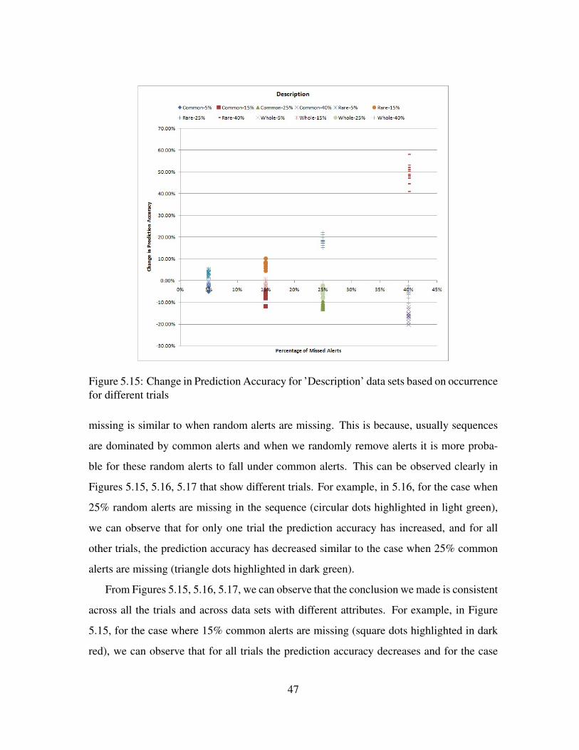
Figure 5.15: Change in Prediction Accuracy for ’Description’ data sets based on occurrencefor different trials

missing is similar to when random alerts are missing. This is because, usually sequences

are dominated by common alerts and when we randomly remove alerts it is more proba-

ble for these random alerts to fall under common alerts. This can be observed clearly in

Figures 5.15, 5.16, 5.17 that show different trials. For example, in 5.16, for the case when

25% random alerts are missing in the sequence (circular dots highlighted in light green),

we can observe that for only one trial the prediction accuracy has increased, and for all

other trials, the prediction accuracy has decreased similar to the case when 25% common

alerts are missing (triangle dots highlighted in dark green).

From Figures 5.15, 5.16, 5.17, we can observe that the conclusion we made is consistent

across all the trials and across data sets with different attributes. For example, in Figure

5.15, for the case where 15% common alerts are missing (square dots highlighted in dark

red), we can observe that for all trials the prediction accuracy decreases and for the case

47

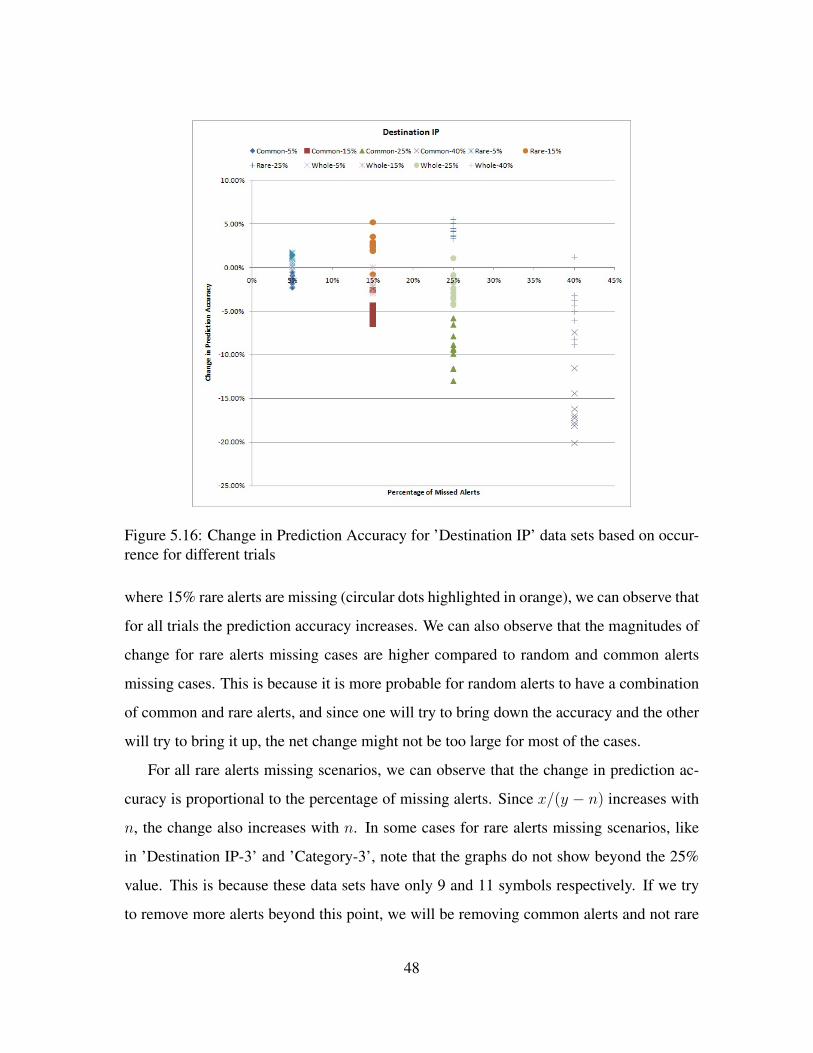
Figure 5.16: Change in Prediction Accuracy for ’Destination IP’ data sets based on occur-rence for different trials

where 15% rare alerts are missing (circular dots highlighted in orange), we can observe that

for all trials the prediction accuracy increases. We can also observe that the magnitudes of

change for rare alerts missing cases are higher compared to random and common alerts

missing cases. This is because it is more probable for random alerts to have a combination

of common and rare alerts, and since one will try to bring down the accuracy and the other

will try to bring it up, the net change might not be too large for most of the cases.

For all rare alerts missing scenarios, we can observe that the change in prediction ac-

curacy is proportional to the percentage of missing alerts. Since x/(y − n) increases with

n, the change also increases with n. In some cases for rare alerts missing scenarios, like

in ’Destination IP-3’ and ’Category-3’, note that the graphs do not show beyond the 25%

value. This is because these data sets have only 9 and 11 symbols respectively. If we try

to remove more alerts beyond this point, we will be removing common alerts and not rare

48

Figure 5.17: Change in Prediction Accuracy for ’Category’ data sets based on occurrencefor different trials

alerts.

We can observe from Figure 5.18 that usually the change in prediction accuracy for

rare alerts missing scenarios is less for sequences with less symbol space and more for

sequences with more symbols space. In our case, ’Destination IP’ and ’Category’ data

sets have smaller change in prediction accuracy than that of ’Description’ data sets. This

is because of their higher true prediction accuracies. For example ’Destination IP-1’ data

set has a top-3 true prediction accuracy of 87.2%, whereas ’Description-1’ has a top-3 true

prediction accuracy of 41.3%. It is obvious that no matter what the percentage of missing

alerts is, ’Destination IP-1’ cannot result in a change of more than 12.8%. However for

one data set that has 69 symbols (Description-3), the change is comparable to the data set

with 12 symbols (Category-1). For sequences with symbol space of around 9-12 symbols,

the increase in prediction accuracy is in the range of 1%-11%, and for sequences with

49

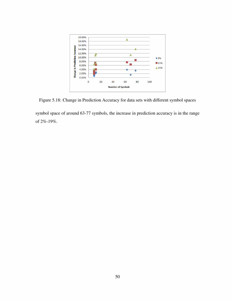
Figure 5.18: Change in Prediction Accuracy for data sets with different symbol spaces

symbol space of around 63-77 symbols, the increase in prediction accuracy is in the range

of 2%-19%.

50

5.3 Summary of results

• For true data (without any missing alerts), VLMM and CSSR give comparable re-

sults, with VLMM being a simpler process.

• For analysis based on position, for small percentages of missed alerts (about 5%-

10%), the decrease in prediction accuracy is very small in the range of 0.5%-1%,

irrespective of whether the alerts are missing at the beginning or middle or end or in

the whole sequence.

• When the percentage of missing alerts increases to more than 10%, the prediction

accuracy is worse (reduction is in the range of 4%-7%) when the alerts are missing

in the whole sequence as opposed to missing at the beginning or middle or end of

the sequence (reduction is in the range of 0-3%). This could be likely because many

sequences will have the alerts with higher weights dispersed throughout the sequence

than only at the beginning or middle or end.

• When there are common alerts missing, the prediction accuracy decreases and when

there are rare alerts missing, the prediction accuracy increases. When rare alerts are

missing, for data sets with attribute ’Description’, the increase in prediction accuracy

is in the range of 3%-30%, for data sets with attribute ’Destination IP’, the increase

in prediction accuracy is in the range of 1%-6%, and for data sets with attribute

’Category’, the increase in prediction accuracy is in the range of 2%-10%. When

common alerts are missing, for data sets with attribute ’Description’, the decrease in

prediction accuracy is in the range of 3%-8%, for data sets with attribute ’Destination

IP’, the decrease in prediction accuracy is in the range of 1%-2%, and for data sets

with attribute ’Category’, the decrease in prediction accuracy is in the range of 1%-

2%.

• The magnitude of change in prediction accuracy is more when rare alerts are missing

than when common or random alerts are missing in the sequence.

51

• The change in prediction accuracy is less for sequences with small symbol space

and more for sequences with large symbols space. For sequences with symbol space

of around 9-12 symbols, the increase in prediction accuracy is in the range of 1%-

11%, and for sequences with symbol space of around 63-77 symbols, the increase in

prediction accuracy is in the range of 2%-19%.

5.4 Error Analysis on CSSR

In this research, error analysis is done using VLMM. This work can be expanded to do a

similar analysis using CSSR algorithm.

As mentioned earlier in 4.5, the error probability of CSSR can be defined as:

q(t, n) ≤ 2k+1 (kL+1 − 1)

(k − 1)e−8Np∗t2 (5.1)

This equation approaches to zero for large values of N , the length of the sequence. In

other words, by taking N large enough, the probability that the correct states are inferred

becomes arbitrarily close to 1. According to [41], if the number of causal states is finite

and Lmax is sufficiently large, the probability that the states estimated are not the causal

states becomes arbitrarily small, for sufficiently large N .

Because CSSR’s performance depends on so many parameters, a similar analysis on

CSSR will yield different results as compared to VLMM based on the settings. Because

ε machine and suffix tree are two different types of models, the effect of missed alerts on

these will be different and accordingly, the change in prediction accuracies will be different.

For example, if Lmax is too large relative to N , the probabilities of long strings will not be

consistently estimated, so CSSR tends to produce too many states, which might result in

erroneous prediction accuracies. Since CSSR relies heavily on the length of the sequence,

the change in prediction accuracies might be worse for higher percentages of missed alerts

compared to VLMM. The percentage of the missing alerts and the parameters selected

52

might result in CSSR not having enough data, in which case CSSR will not reconstruct the

true model.

53

Chapter 6

Conclusion and Future Work

6.1 Conclusions

One of the contributions of this thesis is the use of a state-based model called Causal-State

Splitting Reconstruction (CSSR) in the context of projecting cyber attacks and its com-

parison against a context-based model called Variable Length Markov Model (VLMM).

Because other state-based models start by producing the most complex possible null model

of the process, and then trim it by merging, whereas CSSR starts off with a zero-complexity

null model by putting every history in one state and then adds states only if the current set

of states are not sufficient. And the causal states it produces have important predictive

properties. Hence CSSR is chosen over other state-based methods like state-merging algo-

rithms. Although CSSR, similar to VLMM, does not make any priori assumptions about

the architecture of the system, it cannot exploit such information when it exists.

An important contribution of this research is the study of the effect of missed alerts on

the model (VLMM) used for projecting cyber attacks, and its predictive performance. Since

VLMM is simpler in terms of building the model and it does not need to have infinitely

long sequences, this research used VLMM for the error analysis. With a thorough design

of experiments, we have studied the effects of missing IDS alerts, by having missed alerts

at different locations of the attack sequence with different rates. The experimental results

suggested that the change in prediction accuracy is low when there are missed alerts in

one part of sequence and higher if they are throughout the entire sequence. Also, the

54

prediction accuracy increases when there are rare alerts missing, and it decreases when

there are common alerts missing. In addition, change in the prediction accuracy is less

when the sequence has a smaller symbol space and relatively more if it has a larger symbol

space. Overall, the results demonstrate the robustness and limitations of VLMM when used

for cyber attack prediction. Based on such error analysis, the network analyst can infer and

assess the predictive performance of VLMM model when there are missed alerts.

This research basically provides one more significant step in creating a comprehen-

sive report to help the security analyst. This will also compliment the related work and

contribute to the overall architecture of network security.

6.2 Future Work

• This research focused on studying the error analysis of missed alerts using VLMM

model, but a similar analysis could also be done on any other model.

• The problem of selecting the data sets is always a major factor in testing any sit-

uational awareness tool. This could be done in two ways: testing on data from a

simulated network and testing on data from a physical network. Both approaches

have their own capabilities and limitations. In this work, we have used data gathered

from a simulation model consisting of a simulated network. Similarly we can test on

the data gathered from a real physical network as opposed to an abstract representa-

tion.

• Because of a limitation in the CSSR implementation, we have only run CSSR on

data sets with less symbol space (62) for comparing it against VLMM. It would be

interesting to observe its performance when there are more symbols.

• In previous works and in this work related to the field of projecting cyber attacks, a

prediction is considered correct if it occurs as the next event irrespective of the time

window in the future. In other words, an attack that is predicted to occur in the next

55

two or three events could in reality occur within the next second, or within the next

hour, depending on the attacker behavior. The determination of this window could

be investigated to have a better analysis report to the network analyst.

• In this analysis, we have removed the alerts assuming that the data sets from simula-

tion model are true without any missed alerts. A similar analysis could also be done

by adding alerts, assuming that the data sets from simulation model are not true.

56

Bibliography

[1] Ihsan A. Akbar. Statistical Analysis of Wireless Systems Using Markov Models. PhDthesis, Virginia Polytechnic Institute and State University, 2007.

[2] D. Andersson, M. Fong, and A. Valdes. Heterogeneous sensor correlation: A casestudy of live traffic analysis. IEEE Assurance and Security Workshop, June 2002.

[3] Andre Arnes, Karin Sallhammar, Kjetil Haslum, Tonnes Brekne, Marie Elisa-beth Gaup Moe, and Svein Johan Knapskog. Real-time risk assessment with networksensors and intrusion detection systems. In Proceedings of the 2005 internationalconference on Computational Intelligence and Security - Volume Part II, pages 388–397. Springer-Verlag, Dec 2005.

[4] Andre Arnes, Frederik Valeur, and Richard Kemmerer. Using hidden markov modelsto evaluate the risk of intrusions. In Proceedings of the 9th international conferenceon Recent Advances in Intrusion Detection, RAID’06, pages 145–164, Hamburg, Ger-many, 2006. Springer-Verlag.

[5] S. Axelsson. Intrusion detection systems: A survey and taxonomy. Technical report,Chalmers University, 2000.

[6] Tim Bass. Intrusion detection systems and multisensor data fusion. Communicationsof the ACM, 43(4):99–105, Apr 2000.

[7] Ron Begleiter, Ran El-Yaniv, and Golan Yona. On prediction using variable ordermarkov models. Journal of Artificial Intelligence, 22(1):385–421, Dec 2004.

[8] Stephen Reed Byers. Real-time fusion and projection of network intrusion activity.Master’s thesis, Rochester Institute of Technology, 2008.

[9] James P. Crutchfield and Karl Young. Computation at the onset of chaos. In TheSanta Fe Institute, Westview, pages 223–269. Press, 1988.

57

[10] James P. Crutchfield and Karl Young. Inferring statistical complexity. Phys. Rev. Lett.,63:105–108, July 1989.

[11] F. Cuppens. Managing alerts in a multi-intrusion detection environment. In Proceed-ings of the 17th Annual Computer Security Applications Conference, ACSAC ’01,pages 22–31, Washington, DC, USA, 2001. IEEE Computer Society.

[12] Frederic Cuppens, Fabien Autrel, Alexandre Miege, and Salem Benferhat. Correla-tion in an intrusion detection process. Proceedings of the SECI02 Workshop, 2002.

[13] O. Dain and R. Cunningham. Fusing a heterogeneous alert stream into scenarios. InProceedings of ACM Workshop on data mining for security applications, 2001.

[14] Bhavya Daya. Network security: History, importance, and future. Technical report,University of Florida.

[15] H. Debar, M. Dacier, and A. Wespi. Towards a taxonomy of intrusion-detection sys-tems. The International Journal of Computer and Telecommunications Networking,31(9):805–822, Apr 1999.

[16] G. Eschelbeck and M. Krieger. Eliminating noise from intrusion detection systems.Technical report, Information Security Technical Report, 2003.

[17] D. Fava, S. R. Byers, and S. J. Yang. Projecting cyber attacks through variablelength markov models. Information Forensics and Security, IEEE Transactions on,3(3):359–369, Sept 2008.

[18] D. Fava, J. Holsopple, S. J. Yang, and B. Argauer. Terrain and behavior modeling forprojecting multistage cyber attacks. In Proceedings of the ISIF/IEEE 10th Interna-tional on Information Fusion, pages 1–7, July 2007.

[19] Daniel S. Fava. Characterization of cyber attacks through variable length markovmodels. Master’s thesis, Rochester Insitute of Technology, 2007.

[20] J. Goodall, W. Lutters, and A. Komlodi. The work of intrusion detection: rethinkingthe role of security analysts. In Proceedings of the Americas Conference on Informa-tion Systems, 2004.

[21] Cheng-Yuan Ho, Yuan-Cheng Lai, I-Wei Chen, Fu-Yu Wang, and Wei-Hsuan Tai.Statistical analysis of false positives and false negatives from real traffic with intrusion

58

detection/prevention systems. IEEE Communications Magazine, 50:146–154, March2012.

[22] Myles Hollander and Douglas A. Wolfe. Nonparametric Statistical Methods (WileySeries in Probability and Statistics: Applied Probability and Statistic). 1999.

[23] Jared Holsopple, Shanchieh Jay Yang, and Moises Sudit. TANDI: Threat assessmentfor networked data and information. In Proceedings of SPIE, Defense and SecuritySymposium, volume 6242, April 2006.

[24] Ilgun K., Kemmerer R.A., and Porras P.A. State transition analysis: A rule-basedintrusion detection approach. IEEE Transactions on Software Engineering, 21:181–199, 1995.

[25] Kristopher Kendall. A database of computer attacks for the evaluation of intrusiondetection systems. Master’s thesis, Massachusetts Institute of Technology, 1999.

[26] Andrew Kosoresow and Steven Hofmeyr. Intrusion detection via system call traces.IEEE Software, 14(5):35–42, Sep/Oct 1997.

[27] Christopher Kruegel and William Robertson. Alert verification: Determining the suc-cess of intrusion attempts. In Proc. First Workshop the Detection of Intrusions andMalware and Vulnerability Assessment, pages 1–14, 2004.

[28] M.E. Kuhl, J. Kistner, K. Costantini, and M. Sudit. Cyber attack modeling and simu-lation for network security analysis. In Proceedings of the 39th conference on Wintersimulation, WSC ’07, pages 1180–1188, Piscataway, NJ, USA, 2007. IEEE Press.

[29] Zhitang Li, Jie Lei, Li Wang, and Dong Li. Assessing attack threat by the probabilityof following attacks. In Proceedings of the International Conference on Networking,Architecture, & Storage, pages 91–100, July 2007.

[30] L.R.Rabiner. A tutorial on hidden markov models and selected applications in speechrecognition. Proceedings of the IEEE, 77(2):257–286, Feb 1989.

[31] L.R.Rabiner and B.H.Juang. An introduction to hidden markov models. ASSP Mag-azine, IEEE, 3(1):4 –16, Jan 1986.

[32] P. Ning, Y. Cui, D. Reeves, and D. Xu. Techniques and tools for analyzing intrusionalerts. ACM Trans. Inf. Syst. Secur., 7(2):274–318, May 2004.

59

[33] P. Ning, Y. Cui, and D.S. reeves. Constructing attack scenarios through correlationof intrusion alerts. In Proceedings of the 9th ACM conference on Computer andcommunications security, CCS ’02, pages 245–254. ACM, 2002.

[34] Papoulis.A. Probability, Random Variables and Stochastic Processes. 1984.

[35] V. Paxson. Bro: A system for detecting network intruders in real-time. In ComputerNetworks, pages 2435–2463, 1999.

[36] N. Perry and P. M. Binder. Finite statistical complexity for sofic systems. Phys. Rev.E, 60:459–463, July 1999.

[37] C. Phillips and L. P. Swiler. A graph-based system for network-vulnerability analysis.In Proceedings of the 1998 workshop on New security paradigms, NSPW ’98, pages71–79. ACM, 1998.

[38] N. Puketza, K. Zhang, M. Chung, B. Mukherjee, and R. Olsson. A methodology fortesting intrusion detection systems. Technical report, University of California, 1995.

[39] Xinzhou Qin and Wenke Lee. Attack plan recognition and prediction using causalnetworks. In Proceedings of the 20th Annual Computer Security Applications Con-ference, ACSAC ’04, pages 370–379. IEEE Computer Society, 2004.

[40] Cosma Rohilla Shalizi. Causal Architecture, Complexity and Self-Organization inTime Series and Cellular Automata. PhD thesis, University of Wisconsin, 2001.

[41] Cosma Rohilla Shalizi and Kristina Lisa Klinkner. Blind construction of optimalnonlinear recursive predictors for discrete sequences. In Proceedings of the 20th con-ference on Uncertainty in artificial intelligence, UAI ’04, pages 504–511, Arlington,Virginia, United States, 2004. AUAI Press.

[42] Cosma Rohilla Shalizi, Kristina Lisa Shalizi, and James P. Crutchfield. An algorithmfor pattern discovery in time series. Technical report, Santa Fe Institute, 2003.

[43] Sourcefire. Snort: an open source network intrusion prevention and detection system.2008.

[44] Adam Stotz and Moises Sudit. INformation Fusion Engine for Real-time Decisionmaking (INFERD): A perceptual system for cyber attack tracking. In InformationFusion, 2007 10th International Conference on, pages 1–8, July 2007.

60

[45] T.Weissman and N.Merhav. Universal prediction of individual binary sequences inthe presence of noise. IEEE Transactions on Information Theory, 47(6):2151–2173,Sep 2001.

[46] Daniel R. Upper. Theory and Algorithms for Hidden Markov Models and GeneralizedHidden Markov Models. PhD thesis, University of California, Berkeley, 1997.

[47] Valdes and K. Skinner. Adaptive, model-based monitoring for cyber attack detection.In Recent Advances in Intrusion Detection (RAID 2000), number 1907, pages 80–92.Springer-Verlag, October 2000.

[48] A. Valdes and K. Skinner. Probabilistic alert correlation. In Proceedings of the 4th In-ternational Symposium on Recent Advances in Intrusion Detection, RAID ’00, pages54–68. Springer-Verlag, 2001.

[49] Frederik Valeur, Giovanni Vigna, Christopher Kruegel, and Richard A. Kemmerer. Acomprehensive approach to intrusion detection alert correlation. IEEE Transactionson Dependable and Secure Computing, 1(3):146–169, July-Sept 2004.

[50] S. Vidalis. A critical discussion of risk and threat analysis methods and methodolo-gies. Technical report, University of Glamorgan, 2004.

[51] Mathukumalli Vidyasagar. A Theory of Learning and Generalization: With Applica-tions to Neural Networks and Control Systems. 1997.

[52] N. Ye, X. Li, Q. Chen S. M. Emran, and M. Xu. Probabilistic techniques for intrusiondetection based on computer audit data. IEEE Transactions on Systems, Man, andCybernetics, 31:266–274, July 2001.

[53] Nong Ye, Yebin Zhang, and Connie M. Borror. Robustness of the markov-chainmodel for cyber-attack detection. IEEE Transactions on Reliability, 53(1):116–123,March 2004.

[54] Jinqiao Yu, Y. V. Ramana Reddy, Sentil Selliah, Srinivas Kankanahalli, SumitraReddy, and Vijayanand Bharadwaj. Trinetr: An intrusion detection alert managementsystem. In Proceedings of the 13th IEEE International Workshops on Enabling Tech-nologies: Infrastructure for Collaborative Enterprises, WETICE ’04, pages 235–240,Washington, DC, USA, 2004. IEEE Computer Society.

61

[55] Bin Zhu and Ali A. Ghorbani. Alert correlation for extracting attack strategies. Inter-national Journal of Network Security, pages 244–258, 2006.

62