Error Analysis of Satellite Precipitation Products in Mountainous Basins

Error Analysis of Satellite Precipitation Products in Mountainous Basins

YIWEN MEI AND EMMANOUIL N. ANAGNOSTOU

Civil and Environmental Engineering, University of Connecticut, Storrs, Connecticut

EFTHYMIOS I. NIKOLOPOULOS AND MARCO BORGA

Department of Land, Environment, Agriculture and Forestry, University of Padova, Legnaro, Padua, Italy

(Manuscript received 22 November 2013, in final form 17 April 2014)

ABSTRACT

Accurate quantitative precipitation estimation overmountainous basins is of great importance because of

their susceptibility to hazards such as flash floods, shallow landslides, and debris flows, triggered by heavy

precipitation events (HPEs). In situ observations over mountainous areas are limited, but currently

available satellite precipitation products can potentially provide the precipitation estimation needed for

hydrological applications. In this study, four widely used satellite-based precipitation products [Tropical

Rainfall MeasuringMission (TRMM)Multisatellite Precipitation Analysis (TMPA) 3B42, version 7 (3B42-

V7), and in near–real time (3B42-RT); Climate Prediction Center (CPC) morphing technique (CMORPH);

and Precipitation Estimation fromRemotely Sensed Imagery UsingArtificial Neural Networks (PERSIANN)]

are evaluated with respect to their performance in capturing the properties of HPEs over different basin scales.

Evaluation is carried out over the upper Adige River basin (eastern Italian Alps) for an 8-yr period (2003–10).

Basin-averaged rainfall derived from a dense rain gauge network in the region is used as a reference. Satellite

precipitation error analysis is performed for warm (May–August) and cold (September–December) season

months as well as for different quantile ranges of basin-averaged precipitation accumulations. Three error

metrics and a score system are introduced to quantify the performances of the various satellite products.

Overall, no single precipitation product can be considered ideal for detecting and quantifying HPE. Results

show better consistency between gauges and the two 3B42 products, particularly during warm season

months that are associated with high-intensity convective events. All satellite products are shown to have

a magnitude-dependent error ranging from overestimation at low precipitation regimes to underestimation

at high precipitation accumulations; this effect is more pronounced in the CMORPH and PERSIANN

products.

1. Introduction

Measuring surface rainfall is of great importance;

particularly for the heavy precipitation events (HPEs)

occurring over mountainous regions that often act

as flash flood–triggering storms (Borga et al. 2010).

Methods for quantifying precipitation include ground

observations from rain gauge and weather radar net-

works, estimates inferred from satellite observations,

outputs from numerical weather prediction models, and

estimates produced by a combination of all these dif-

ferent products (Michaelides et al. 2009). Each of these

is associated with specific rainfall estimation un-

certainties. Rain gauge networks are the most common

estimation method. These networks can provide accu-

rate pointwise precipitation measurements, but the

spatial representativeness is limited (Anagnostou et al.

2010; Sapiano andArkin 2009).Weather radar networks

provide precipitation estimates with high spatial and

temporal resolutions (i.e., 1–4 km and 5–15 min) but

with variable accuracy. Moreover, mountainous terrain

tends to degrade the accuracy of radar-derived rainfall

estimates because of observational limitations (beam

blockages and ground clutter) and their interaction

with precipitation vertical structure (Ciach et al. 2007;

Germann et al. 2006; Piccolo andChirico 2005;Anagnostou

et al. 2004; Sharif et al. 2002). In addition, radar observa-

tions have limited utility in cold weather, when the beam

detects primarily snow, which complicates the assessment

Corresponding author address: Emmanouil N. Anagnostou,

CEE, University of Connecticut, 261 Glenbrook Rd., Unit 3037,

Storrs, CT 06269.

E-mail: [email protected]

1778 JOURNAL OF HYDROMETEOROLOGY VOLUME 15

DOI: 10.1175/JHM-D-13-0194.1

� 2014 American Meteorological Society

of surface precipitation (Schneebeli et al. 2013). Com-

bining rain gauges with weather radar gives a partial so-

lution to the accuracy issues, but it is not a viable solution

for cases with large radar beam blockages due to orog-

raphy or in areas where those systems are not widely

available.

Satellite-based estimates of precipitation can poten-

tially provide a solution to the spatial sampling limita-

tions of ground-based sensors. Satellite sensors are

uninhibited by mountains and provide global coverage

without spatial inconsistencies (Sapiano andArkin 2009;

Kidd et al. 2003; Scofield and Kuligowski 2003; Arkin

and Ardanuy 1989). Several of the current global-scale

satellite precipitation retrieval algorithms are based on

the combination of high-spatiotemporal-resolution ob-

servations in the visible–infrared (VIS–IR) spectrum

from geostationary (GEO) satellites and the less fre-

quent but more direct precipitation observations from

active and passive microwave (MW) sensors deployed

on low-Earth-orbiting (LEO) satellites. The VIS–IR

techniques relate surface precipitation to cloud-top in-

formation (brightness temperatures) with a high sam-

pling frequency (15-min/3–4-km resolution, 1-km VIS).

However, these measurements cannot directly retrieve

surface precipitation from the inferred cloud-top prop-

erties, implying a weak link between cloud-top in-

formation and surface precipitation estimation (Sapiano

andArkin 2009). On the other hand,MW techniques are

more accurate than the VIS–IR because they physically

link the signal received by the satellite sensors to the size

and phase of the hydrometeors present within the ob-

served atmospheric column. Nonetheless, MW obser-

vations are associated with a large degree of sampling

error, particularly in dealing with short rain events be-

cause of their low observational frequency and large-

sensor field-of-view areas (Ebert et al. 2007; Kidd et al.

2003).

It is deemed by many studies that rainfall retrieved

from either VIS–IR or MW sensors, or the combination

of both sensor observations, suffers from noticeable

deficiencies compared to ground-based measurements

(Stampoulis and Anagnostou 2012; AghaKouchak et al.

2011; Fleming et al. 2011; Yong et al. 2010; Su et al. 2008;

Dinku et al. 2007; Ali et al. 2005). Stampoulis and

Anagnostou (2012) conducted an analysis for Tropical

Rainfall Measuring Mission (TRMM) Multisatellite

Precipitation Analysis (TMPA) 3B42 product, version 6

(3B42-V6), and the Climate Prediction Center (CPC)

morphing technique (CMORPH) over continental Eu-

rope and found that correlations of the two rainfall

products to the gauge-interpolated rainfall are magnitude

dependent in terms of daily rainfall accumulation;

moreover, the products exhibited more pronounced

seasonal dependency over high-elevation regions com-

pared to the low-elevation areas. Anagnostou et al.

(2010) evaluated two satellite products (CMORPH and

3B42-V6) over the Oklahoma region in the midwestern

United States. The study pointed out that CMORPH

tended to overestimate the precipitation volume more

prominently than 3B42-V6 during the warm season while

the bias of both satellite products was lower than 20%

during the cold season. Yong et al. (2010) highlighted the

geography-dependent (latitude and elevation) roles of

the TMPA 3B42 product in near–real time (3B42-RT)

and 3B42-V6 over the Laohahe basin in northeastern

China. Meanwhile, better agreement with gauge obser-

vations was found for 3B42-V6 at both daily andmonthly

scales. Su et al. (2008) focused on the performance of

3B42-V6 over the La Plata basin in the Amazon. They

concluded that the satellite estimates are slightly higher

than the gridded gauge data at both monthly and daily

time scales, with a higher degree of agreement for the

monthly time scales. Other satellite error studies are

those of Ali et al. (2005) and Dinku et al. (2007), who

investigated the error structures of four satellite products

over the Sahara and nine satellite products over the

complex terrain of East Africa, respectively. They

showed that the products are consistent with rainfall es-

timated from the ground-based gauge networks at

a coarse resolution (i.e., 2.58 3 2.58 grid cell at monthly

interval).

Although the topic of satellite rainfall error analysis

has been investigated globally for more than two decades

(Anagnostou et al. 2010; Anagnostou 2004; Petty and

Krajewski 1996; Arkin and Ardanuy 1989), only a small

portion of these studies have focused on the error struc-

ture of satellite products on the event basis (Nikolopoulos

et al. 2013; Mishra 2012; AghaKouchak et al. 2010); even

fewer of them have attempted to decipher the error

structure based on a large number of storm events

(Stampoulis and Anagnostou 2012). Furthermore, the

majority of the literature on this topic is generally focused

on the error analysis at the satellite products’ spatial

(typically ranging between 0.048 and 0.58) and temporal

scales (ranging between 15 min and daily). While using

a regular space–time scale has allowed consistency in the

evaluation of results from different error studies, it does

not allow a direct interpretation of the satellite rainfall

error in terms of hydrologic applications. In hydrologic

modeling, particularly the basin flood response to pre-

cipitation, spatial and temporal scales are dictated by the

basin’s drainage area and duration of storm causing the

flood event. Therefore, the current literature lacks com-

prehensive hydrologically driven satellite rainfall error

studies that depict the error structure of basin-averaged

satellite rainfall on the basis of long-term records of storm

OCTOBER 2014 ME I ET AL . 1779

events. Understanding and improving satellite rainfall

error characteristics at the basin scale, and on an event

basis, will improveuses of satellite rainfall data in regional

water budget analyses and for monitoring or forecasting

of hydrologic extremes (flash floods and droughts).

This study attempts to evaluate the error characteristics

of four quasi-global satellite precipitation algorithms (see

section 2b for the descriptions) over a mountainous area

in the eastern Italian Alps. The surface rainfall data are

derived from a dense rain gauge network over the study

area. This error analysis is expected to give supplemen-

tary information and guidance to relevant studies re-

garding the uncertainties of satellite-derived precipitation

estimates over complex mountainous regions and for

heavy precipitation events. It is noted that, given the

mountainous setting of the study domain, precipitation,

particularly during cold months, could be in the form of

snow or mixed phase, which is not discriminated in this

study. In the next section, we describe the study area and

data used. Section 3 introduces the error metrics and the

score system. Results are reviewed in section 4, and

conclusions are drawn in section 5.

2. Study area and data

a. Study area

This study focuses over the eastern part of the upper

Adige River basin, a mountainous region located in the

eastern Italian Alps (Fig. 1), particularly the Isarco

basin (4166 km2) and the upper Passirio basin (427 km2).

The basins have amean elevation of 1736mMSLwith the

highest (lowest) elevation at about 3700 (220)m MSL.

The region is influenced by western Atlantic airflows and

meridional circulation patterns (Frei and Schär 1998)causingHPEs and associated flash floods and debris flows

in the summer and fall seasons. The dominant climate

pattern in the region is continental, with the precipitation

monthly distribution exhibiting two maxima, during

August and October. The mean (maximum/minimum)

annual precipitation accumulations in the 2003–10 period

for the Isarco and Passirio basins were 651mm (987 /480)

and 637mm (865 /482), respectively. The October–April

period is typically dominated by snow and widespread

type precipitation, while in the May–September period

precipitation is mainly characterized by mesoscale con-

vective systems and localized thunderstorms (Norbiato

et al. 2009; Frei and Schär 1998).

b. Rainfall data

The study area is covered by a dense rain gauge net-

work (87 gauges) with densities of contributing gauges

per basin ranging between one station per 16 km2 (for

the various analyzed subbasins) and 53 km2 (average

gauge density for the entire area). The gauge rainfall

record is hourly with an 8-yr temporal coverage span

(2003–10). Hourly gauge precipitation time series av-

eraged over the study basins were generated using the

nearest neighbor interpolation technique.

Four near-global satellite products are used in this

study. The 3B42-RT product, which is corrected by

monthly climatological gauge rainfall, and available in

post-processing (version 7; hereafter named 3B42-V7)

using current month gauge adjustments (Huffman et al.

2007), are from the National Aeronautics and Space

Administration (NASA). Another IR-based precipita-

tion product is the Precipitation Estimation from Re-

motely Sensed Information Using Artificial Neural

Networks (PERSIANN), which uses a coincident MW

calibrated neural network technique to relate IR obser-

vations to rainfall estimates (Sorooshian et al. 2000). The

fourth product is theNationalOceanic andAtmospheric

Administration (NOAA) CMORPH, which uses

multisatellite-based MW rain estimates integrated in

space and time using motion vectors derived from IR

images (Joyce et al. 2004). The spatial and temporal

resolutions of the satellite rainfall products used in this

study are 0.258 at 3-hourly time intervals covering the

same period as the gauge rainfall product. As with the

rain gauges, all four satellite products were spatially

interpolated to derive basin-averaged precipitation, us-

ing the nearest neighbor approach (taking the center of

satellite pixel as the equivalent station location).

Since satellite products represent 3-hourly rainfall

values, hourly rain gauge basin-averaged rainfall time

series were averaged every three consecutive time steps

(i.e., 0000, 0300, 0600, etc., UTC) so as to match the

CMORPH and PERSIANN products. Since the two

3B42 products represent MW or IR rainfall estimates

within 61.5 h of the synoptic hours, we have taken

a different approach of matching gauges to this product.

Namely, hourly basin-averaged rain gauge rainfall

values were temporally averaged within 62 h around

each synoptic hour to represent the 3-hourly temporal

intervals of the 3B42 product.

3. Methodology

A large number of precipitation events (3249) based on

the 8-yr (2003–10) rain gauge record was grouped into

warm (May–August) and cold (September–December)

seasonmonths (the terms warm seasonmonths andMay–

August, as well as cold season months and September–

December, are used interchangeably in the text). These

events were used to evaluate systematic and random

error metrics of the three satellite products and their

1780 JOURNAL OF HYDROMETEOROLOGY VOLUME 15

dependency on seasonal characteristics of storms, basin

scale, and event severity. Analysis was based on basin-

averaged precipitation rather than the usual pixel-based

comparison. This approach allows us a more direct in-

ference on the hydrological impact of the satellite pre-

cipitation estimation error. In this study, thirteen basins

with an area greater than 200 km2 were considered and

summarized in Table 1. Basins with an area less than

530 km2 (namely, the approximate mean area of satellite

pixels over the study area) are classified here as small-

sized basins, while basins with area greater than this

threshold are classified as medium sized.

a. Event identification and matching

Basin precipitation events were extracted from the

rain gauge and satellite rainfall records for two distinct

periods (May–August and September–December) using

an ad hoc 9-h zero-rainfall time window to represent

interstorm periods. The sensitivity of the results on the

selected time window was investigated (not shown here)

and found to be low for values in the range of 9–16 h.

Our choice to use the lower value was to allow the

capture of the shorter-duration storms in our database.

Precipitation events identified on the basis of the rain

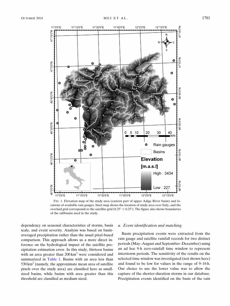
FIG. 1. Elevation map of the study area (eastern part of upper Adige River basin) and lo-

cations of available rain gauges. Inset map shows the location of study area over Italy, and the

overlaid grid corresponds to the satellite grid (0.258 3 0.258). The figure also shows boundaries

of the subbasins used in the study.

OCTOBER 2014 ME I ET AL . 1781

gauge (i.e., reference) and satellite basin-averaged pre-

cipitation time series were matched according to their

centroid differences as follows:

jtc,s 2 tc,gj#R , (1)

where tc,s and tc,g are the centroids of the satellite and

gauge precipitation events defined as

tc5

�T

s

t51

t[p(t)]

�T

s

t51

p(t)

, (2)

where p(t) is the basin-averaged precipitation rate

(mmh21) at each time step t (3 h) of the event duration

TS. The variable R is defined based on the reference

data as

R5max(tc 2 tb, te 2 tc) , (3)

where tb and te are the beginning and ending time of the

gauge-defined precipitation events, respectively. It is

possible that for a given gauge-defined precipitation

event with tc,g there is more than one eligible satellite-

defined precipitation event. In those cases, the satellite

precipitation events were merged into one event. Pre-

cipitation events with cumulative basin-averaged refer-

ence precipitation greater than 3mmwere considered in

this study to eliminate minor events with negligible hy-

drologic response.

Table 2 lists the properties of the selected events.

As noted from the table, the May–August period has

a larger number of precipitation events (nearly twice as

much as the September–December period), but events

in the September–December period have longer dura-

tions and higher rainfall accumulations due to the distinct

meteorological patterns in these two periods. It is also

noted that the basin-averaged precipitation accumula-

tions RV for the May–August period events are lower

than those of the September–December period events

for the small-scale basins, while for the medium-scale

basins the RV values tend to be similar in the two pe-

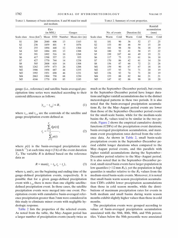
riods. Figure 2 shows the empirical cumulative density

functions (CDFs) of the precipitation event durations,

basin-averaged precipitation accumulation, and maxi-

mum event precipitation rates derived from the refer-

ence data. As shown in Table 2, small basin-scale

precipitation events in the September–December pe-

riod exhibit longer durations when compared to the

May–August period events, and this parallels with

higher rainfall accumulations during the September–

December period relative to the May–August period.

It is also noted that in the September–December pe-

riod, small-sized basin events have larger population in

low quantiles (,12mm RV), yet the population in high

quantiles is smaller relative to the RV values from the

medium-sized basin-scale events. Moreover, it is noted

that small-basin warm season precipitation accumula-

tion CDFs exhibit lower precipitation accumulations

than those in cold season months, while the distri-

butions of maximum precipitation rates for events in

both medium and small basins during warm season

months exhibit slightly higher values than those in cold

months.

The precipitation events were grouped according to

values of basin-averaged precipitation accumulation

associated with the 50th, 80th, 90th, and 95th percen-

tiles. Values below the 50th percentile were associated

TABLE 1. Summary of basin information. S and M stand for small

and medium.

Scale class Area (km2)

Elev

(m MSL) Gauges

Mean STD Number Mean elev (m)

S1 208 2040 606 13 1163

S2 236 1859 401 9 1076

S3 255 1894 448 12 1304

S4 345 1884 691 13 1388

S5 391 1892 516 10 1268

S6 417 1598 557 13 935

S7 427 1770 744 14 1258

S8 505 2008 618 16 1308

M1 1262 1979 673 26 1206

M2 1906 1958 687 44 1255

M3 1992 1951 690 46 1231

M4 2863 1904 758 68 1230

M5 4166 1770 838 85 1185

TABLE 2. Summary of event properties.

No. of events Duration (h)

Rainfall

accumulation

(mm)

Scale class Warm Cold Warm Cold Warm Cold

S1 181 90 36 52 17 25

S2 153 80 46 59 15 20

S3 161 98 58 56 18 19

S4 180 92 41 58 15 22

S5 199 107 44 49 19 21

S6 117 75 53 61 16 18

S7 170 86 42 61 14 20

S8 156 87 66 72 21 26

M1 159 90 67 67 18 18

M2 157 93 74 71 20 19

M3 156 92 74 71 20 19

M4 153 88 82 84 21 21

M5 147 82 86 90 18 20

1782 JOURNAL OF HYDROMETEOROLOGY VOLUME 15

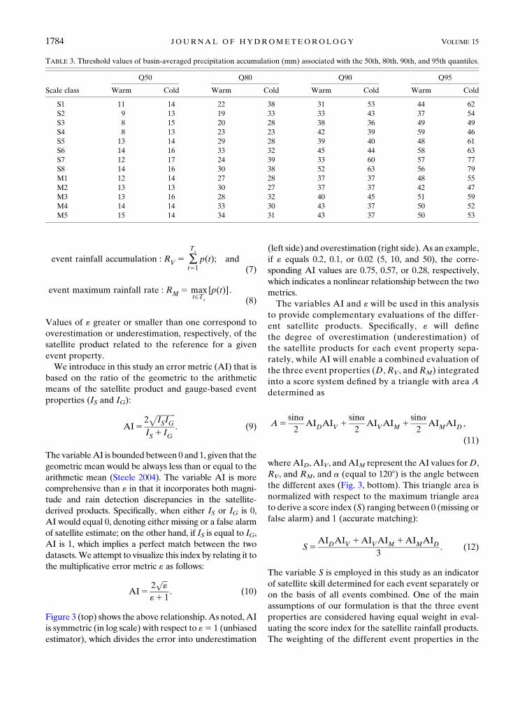
with low rainfall accumulation (,10mm; see Table 3)

and are excluded from this analysis since our interest is

toward moderate to heavy precipitation events. The

quantile values for the different basin scales and periods

are summarized in Table 3. It is noted that the quantile

values are greater in the September–December months

than those for the May–August months, which is con-

sistent with the cumulative distributions shown in Fig. 2

and points to the contrasting precipitation properties in

these two periods.

b. Evaluating metrics

Three evaluation metrics termed as relative centroid

displacement dc, multiplicative error «, and a herein

established accuracy index AI are selected to describe

the degree of disagreement between reference (i.e.,

gauge precipitation) data and the four satellite-derived

precipitation products.

A number of studies have shown that temporal error

characteristics in precipitation estimates may propagate

to the simulated hydrograph-producing timing errors

(Mei et al. 2014; Nikolopoulos et al. 2013; Zoccatelli

et al. 2011; Yong et al. 2010; Su et al. 2008; Sharif et al.

2002). However, to the best of our knowledge, these

error characteristics have not been exploited to develop

a metric for the evaluation of satellite precipitation es-

timates. The relative centroid displacement, Eq. (4), is

therefore proposed herein as a metric to depict the error

in estimating from satellite observations the time of ar-

rival of the event temporal center of mass:

dc 5tc,s 2 tc,g

Dg

, (4)

where Dg stands for the duration of gauge precipitation

event defined in Eq. (6). The numerator in Eq. (4) rep-

resents the centroid displacement. Since we have shown

that the durations of events in September–December

are generally shorter than those in May–August, we

normalized the net centroid displacements to the cor-

responding gauge-derived event durations. By the defi-

nition of tc from Eq. (2), tc,s/tc,g represents the temporal

centroid location in terms of satellite- or gauge-retrieved

basin-averaged precipitation rate for matching event

pairs; thus, positive and negative dc values represent de-

lay and advance in arrivals of storm center of mass, cor-

respondingly. In practice, dc reflects the situation of either

early or delayed detection of storm events, which could

be an important property when dealing with prediction of

a basin’s hydrologic response.

The multiplicative error «, defined as the ratio be-

tween gauge-event properties to the corresponding

satellite-event property, is one of the classical error

metrics used in satellite precipitation error studies (e.g.,

Hossain and Anagnostou 2006):

«5ISIG

, (5)

where IS and IG are the basin-averaged rainfall proper-

ties derived from satellite products and gauges. The

event properties are defined as follows:

event duration : D5 te 2 tb ; (6)

FIG. 2. Event-based empirical CDFs of (top) event duration

D, (middle) basin-averaged rainfall accumulation RV, and (bottom)

max rain rate RM; all derived from reference rainfall.

OCTOBER 2014 ME I ET AL . 1783

event rainfall accumulation : RV 5 �T

s

t51

p(t); and(7)

event maximum rainfall rate : RM 5 maxt2T

s

[p(t)] .(8)

Values of « greater or smaller than one correspond to

overestimation or underestimation, respectively, of the

satellite product related to the reference for a given

event property.

We introduce in this study an error metric (AI) that is

based on the ratio of the geometric to the arithmetic

means of the satellite product and gauge-based event

properties (IS and IG):

AI52

ffiffiffiffiffiffiffiffiffiffiISIG

p

IS1 IG. (9)

The variableAI is bounded between 0 and 1, given that the

geometric mean would be always less than or equal to the

arithmetic mean (Steele 2004). The variable AI is more

comprehensive than « in that it incorporates both magni-

tude and rain detection discrepancies in the satellite-

derived products. Specifically, when either IS or IG is 0,

AI would equal 0, denoting either missing or a false alarm

of satellite estimate; on the other hand, if IS is equal to IG,

AI is 1, which implies a perfect match between the two

datasets.We attempt to visualize this index by relating it to

the multiplicative error metric « as follows:

AI52

ffiffiffi«

p«1 1

. (10)

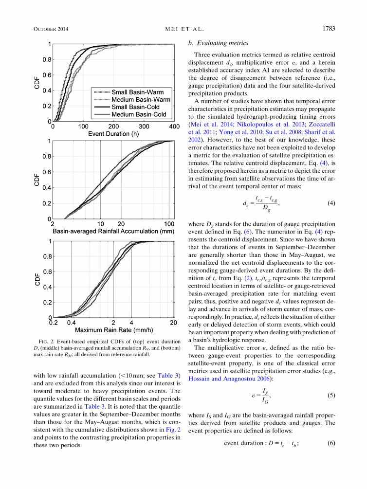
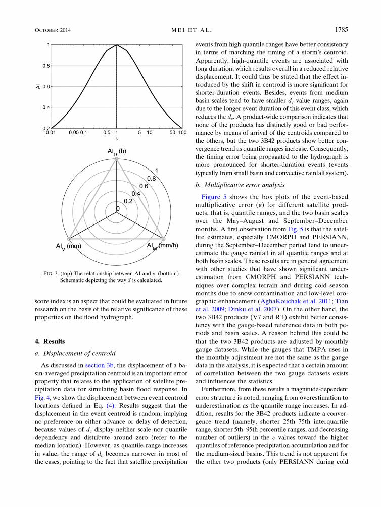
Figure 3 (top) shows the above relationship.As noted, AI

is symmetric (in log scale) with respect to «5 1 (unbiased

estimator), which divides the error into underestimation

(left side) and overestimation (right side). As an example,

if « equals 0.2, 0.1, or 0.02 (5, 10, and 50), the corre-

sponding AI values are 0.75, 0.57, or 0.28, respectively,

which indicates a nonlinear relationship between the two

metrics.

The variables AI and « will be used in this analysis

to provide complementary evaluations of the differ-

ent satellite products. Specifically, « will define

the degree of overestimation (underestimation) of

the satellite products for each event property sepa-

rately, while AI will enable a combined evaluation of

the three event properties (D, RV, andRM) integrated

into a score system defined by a triangle with area A

determined as

A5sina

2AIDAIV 1

sina

2AIVAIM 1

sina

2AIMAID ,

(11)

whereAID, AIV, andAIM represent theAI values forD,

RV, and RM, and a (equal to 1208) is the angle between

the different axes (Fig. 3, bottom). This triangle area is

normalized with respect to the maximum triangle area

to derive a score index (S) ranging between 0 (missing or

false alarm) and 1 (accurate matching):

S5AIDAIV 1AIVAIM 1AIMAID

3. (12)

The variable S is employed in this study as an indicator

of satellite skill determined for each event separately or

on the basis of all events combined. One of the main

assumptions of our formulation is that the three event

properties are considered having equal weight in eval-

uating the score index for the satellite rainfall products.

The weighting of the different event properties in the

TABLE 3. Threshold values of basin-averaged precipitation accumulation (mm) associated with the 50th, 80th, 90th, and 95th quantiles.

Scale class

Q50 Q80 Q90 Q95

Warm Cold Warm Cold Warm Cold Warm Cold

S1 11 14 22 38 31 53 44 62

S2 9 13 19 33 33 43 37 54

S3 8 15 20 28 38 36 49 49

S4 8 13 23 23 42 39 59 46

S5 13 14 29 28 39 40 48 61

S6 14 16 33 32 45 44 58 63

S7 12 17 24 39 33 60 57 77

S8 14 16 30 38 52 63 56 79

M1 12 14 27 28 37 37 48 55

M2 13 13 30 27 37 37 42 47

M3 13 16 28 32 40 45 51 59

M4 14 14 33 30 43 37 50 52

M5 15 14 34 31 43 37 50 53

1784 JOURNAL OF HYDROMETEOROLOGY VOLUME 15

score index is an aspect that could be evaluated in future

research on the basis of the relative significance of these

properties on the flood hydrograph.

4. Results

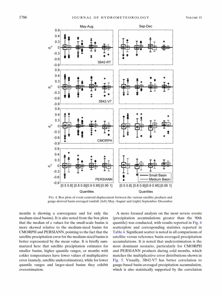
a. Displacement of centroid

As discussed in section 3b, the displacement of a ba-

sin-averaged precipitation centroid is an important error

property that relates to the application of satellite pre-

cipitation data for simulating basin flood response. In

Fig. 4, we show the displacement between event centroid

locations defined in Eq. (4). Results suggest that the

displacement in the event centroid is random, implying

no preference on either advance or delay of detection,

because values of dc display neither scale nor quantile

dependency and distribute around zero (refer to the

median location). However, as quantile range increases

in value, the range of dc becomes narrower in most of

the cases, pointing to the fact that satellite precipitation

events from high quantile ranges have better consistency

in terms of matching the timing of a storm’s centroid.

Apparently, high-quantile events are associated with

long duration, which results overall in a reduced relative

displacement. It could thus be stated that the effect in-

troduced by the shift in centroid is more significant for

shorter-duration events. Besides, events from medium

basin scales tend to have smaller dc value ranges, again

due to the longer event duration of this event class, which

reduces the dc. A product-wide comparison indicates that

none of the products has distinctly good or bad perfor-

mance by means of arrival of the centroids compared to

the others, but the two 3B42 products show better con-

vergence trend as quantile ranges increase. Consequently,

the timing error being propagated to the hydrograph is

more pronounced for shorter-duration events (events

typically from small basin and convective rainfall system).

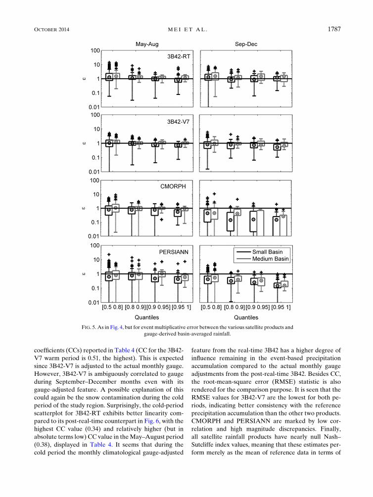
b. Multiplicative error analysis

Figure 5 shows the box plots of the event-based

multiplicative error («) for different satellite prod-

ucts, that is, quantile ranges, and the two basin scales

over the May–August and September–December

months. A first observation from Fig. 5 is that the satel-

lite estimates, especially CMORPH and PERSIANN,

during the September–December period tend to under-

estimate the gauge rainfall in all quantile ranges and at

both basin scales. These results are in general agreement

with other studies that have shown significant under-

estimation from CMORPH and PERSIANN tech-

niques over complex terrain and during cold season

months due to snow contamination and low-level oro-

graphic enhancement (AghaKouchak et al. 2011; Tian

et al. 2009; Dinku et al. 2007). On the other hand, the

two 3B42 products (V7 and RT) exhibit better consis-

tency with the gauge-based reference data in both pe-

riods and basin scales. A reason behind this could be

that the two 3B42 products are adjusted by monthly

gauge datasets. While the gauges that TMPA uses in

the monthly adjustment are not the same as the gauge

data in the analysis, it is expected that a certain amount

of correlation between the two gauge datasets exists

and influences the statistics.

Furthermore, from these results a magnitude-dependent

error structure is noted, ranging from overestimation to

underestimation as the quantile range increases. In ad-

dition, results for the 3B42 products indicate a conver-

gence trend (namely, shorter 25th–75th interquartile

range, shorter 5th–95th percentile ranges, and decreasing

number of outliers) in the « values toward the higher

quantiles of reference precipitation accumulation and for

the medium-sized basins. This trend is not apparent for

the other two products (only PERSIANN during cold

FIG. 3. (top) The relationship between AI and «. (bottom)

Schematic depicting the way S is calculated.

OCTOBER 2014 ME I ET AL . 1785

months is showing a convergence and for only the

medium-sized basins). It is also noted from the box plots

that the median of « values for the small-scale basins is

more skewed relative to the medium-sized basins for

CMORPH and PERSIANN, pointing to the fact that the

satellite precipitation error for themedium-sized basins is

better represented by the mean value. It is briefly sum-

marized here that satellite precipitation estimates for

smaller basins, higher quantile ranges, or months with

colder temperatures have lower values of multiplicative

error (namely, satellite underestimation), while for lower

quantile ranges and larger-sized basins they exhibit

overestimation.

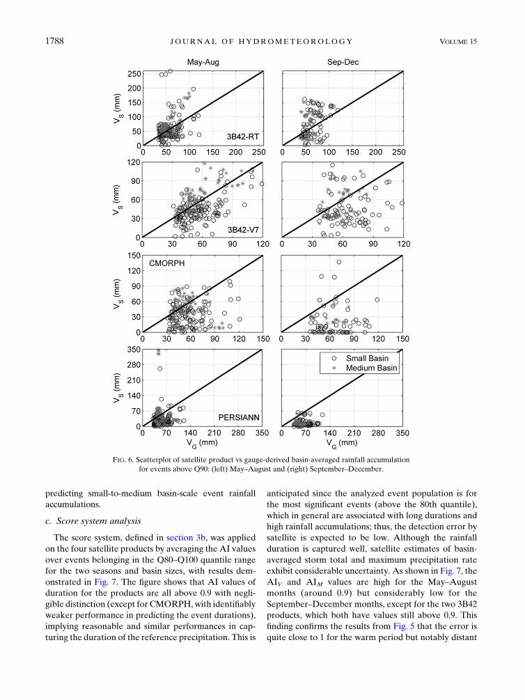
A more focused analysis on the most severe events

(precipitation accumulations greater than the 90th

quantile) was conducted, with results reported in Fig. 6

scatterplots and corresponding statistics reported in

Table 4. Significant scatter is noted in all comparisons of

satellite versus reference basin-averaged precipitation

accumulations. It is noted that underestimation is the

most dominant scenario, particularly for CMORPH

and PERSIANN products during cold months, which

matches the multiplicative error distributions shown in

Fig. 5. Visually, 3B42-V7 has better correlation to

gauge-based basin-averaged precipitation accumulation,

which is also statistically supported by the correlation

FIG. 4. Box plots of event centroid displacement between the various satellite products and

gauge-derived basin-averaged rainfall: (left) May–August and (right) September–December.

1786 JOURNAL OF HYDROMETEOROLOGY VOLUME 15

coefficients (CCs) reported in Table 4 (CC for the 3B42-

V7 warm period is 0.51, the highest). This is expected

since 3B42-V7 is adjusted to the actual monthly gauge.

However, 3B42-V7 is ambiguously correlated to gauge

during September–December months even with its

gauge-adjusted feature. A possible explanation of this

could again be the snow contamination during the cold

period of the study region. Surprisingly, the cold-period

scatterplot for 3B42-RT exhibits better linearity com-

pared to its post-real-time counterpart in Fig. 6, with the

highest CC value (0.34) and relatively higher (but in

absolute terms low) CC value in theMay–August period

(0.38), displayed in Table 4. It seems that during the

cold period the monthly climatological gauge-adjusted

feature from the real-time 3B42 has a higher degree of

influence remaining in the event-based precipitation

accumulation compared to the actual monthly gauge

adjustments from the post-real-time 3B42. Besides CC,

the root-mean-square error (RMSE) statistic is also

rendered for the comparison purpose. It is seen that the

RMSE values for 3B42-V7 are the lowest for both pe-

riods, indicating better consistency with the reference

precipitation accumulation than the other two products.

CMORPH and PERSIANN are marked by low cor-

relation and high magnitude discrepancies. Finally,

all satellite rainfall products have nearly null Nash–

Sutcliffe index values, meaning that these estimates per-

form merely as the mean of reference data in terms of

FIG. 5. As in Fig. 4, but for event multiplicative error between the various satellite products and

gauge-derived basin-averaged rainfall.

OCTOBER 2014 ME I ET AL . 1787

predicting small-to-medium basin-scale event rainfall

accumulations.

c. Score system analysis

The score system, defined in section 3b, was applied

on the four satellite products by averaging the AI values

over events belonging in the Q80–Q100 quantile range

for the two seasons and basin sizes, with results dem-

onstrated in Fig. 7. The figure shows that AI values of

duration for the products are all above 0.9 with negli-

gible distinction (except for CMORPH,with identifiably

weaker performance in predicting the event durations),

implying reasonable and similar performances in cap-

turing the duration of the reference precipitation. This is

anticipated since the analyzed event population is for

the most significant events (above the 80th quantile),

which in general are associated with long durations and

high rainfall accumulations; thus, the detection error by

satellite is expected to be low. Although the rainfall

duration is captured well, satellite estimates of basin-

averaged storm total and maximum precipitation rate

exhibit considerable uncertainty. As shown in Fig. 7, the

AIV and AIM values are high for the May–August

months (around 0.9) but considerably low for the

September–December months, except for the two 3B42

products, which both have values still above 0.9. This

finding confirms the results from Fig. 5 that the error is

quite close to 1 for the warm period but notably distant

FIG. 6. Scatterplot of satellite product vs gauge-derived basin-averaged rainfall accumulation

for events above Q90: (left) May–August and (right) September–December.

1788 JOURNAL OF HYDROMETEOROLOGY VOLUME 15

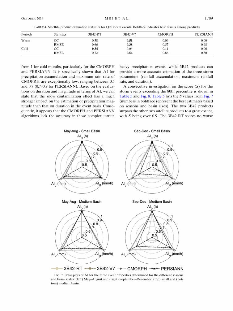
from 1 for cold months, particularly for the CMORPH

and PERSIANN. It is specifically shown that AI for

precipitation accumulation and maximum rain rate of

CMOPRH are exceptionally low, ranging between 0.5

and 0.7 (0.7–0.9 for PERSIANN). Based on the evalua-

tions on duration and magnitude in terms of AI, we can

state that the snow contamination effect has a much

stronger impact on the estimation of precipitation mag-

nitude than that on duration in the event basis. Conse-

quently, it appears that the CMORPH and PERSIANN

algorithms lack the accuracy in those complex terrain

heavy precipitation events, while 3B42 products can

provide a more accurate estimation of the three storm

parameters (rainfall accumulation, maximum rainfall

rate, and duration).

A consecutive investigation on the score (S) for the

storm events exceeding the 80th percentile is shown in

Table 5 and Fig. 8. Table 5 lists the S values from Fig. 7

(numbers in boldface represent the best estimates based

on seasons and basin sizes). The two 3B42 products

surpass the other two satellite products to a great extent,

with S being over 0.9. The 3B42-RT scores no worse

TABLE 4. Satellite product evaluation statistics for Q90 storm events. Boldface indicates best results among products.

Periods Statistics 3B42-RT 3B42-V7 CMORPH PERSIANN

Warm CC 0.38 0.51 0.06 0.00

RMSE 0.66 0.38 0.57 0.98

Cold CC 0.34 0.04 0.11 0.06

RMSE 0.72 0.54 0.86 0.80

FIG. 7. Polar plots of AI for the three event properties determined for the different seasons

and basin scales: (left) May–August and (right) September–December; (top) small and (bot-

tom) medium basin.

OCTOBER 2014 ME I ET AL . 1789

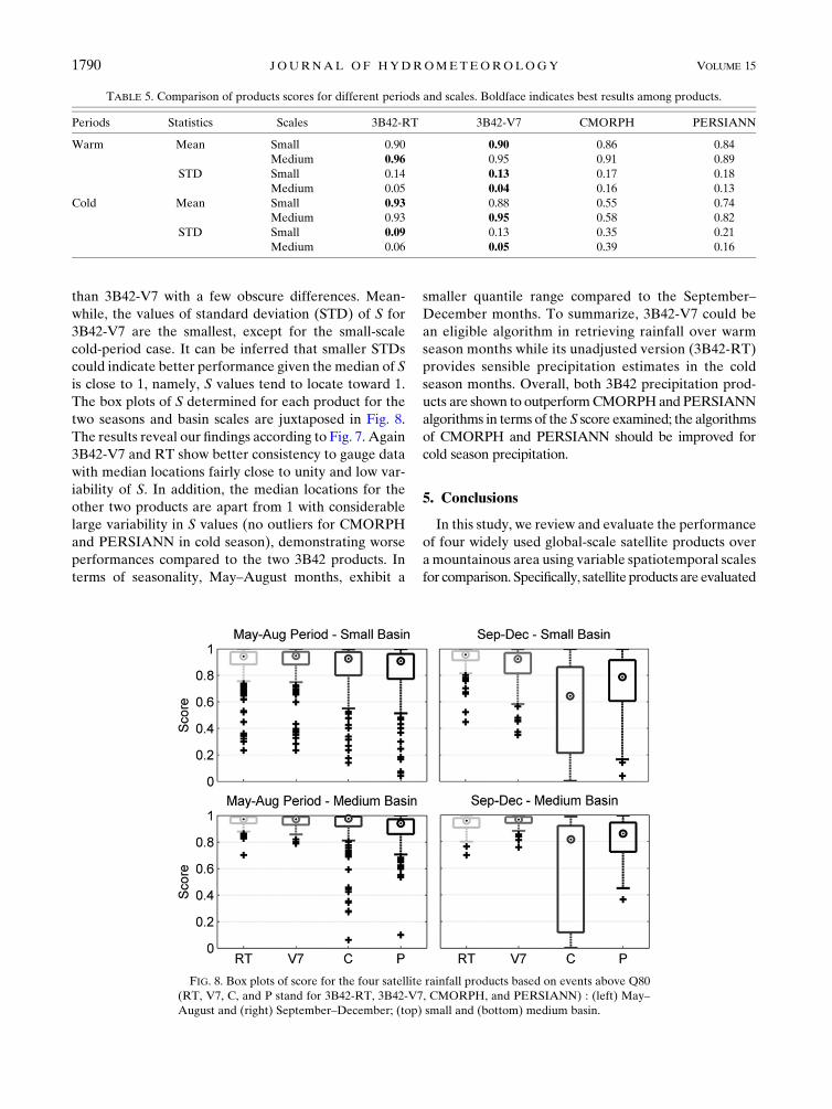
than 3B42-V7 with a few obscure differences. Mean-

while, the values of standard deviation (STD) of S for

3B42-V7 are the smallest, except for the small-scale

cold-period case. It can be inferred that smaller STDs

could indicate better performance given the median of S

is close to 1, namely, S values tend to locate toward 1.

The box plots of S determined for each product for the

two seasons and basin scales are juxtaposed in Fig. 8.

The results reveal our findings according to Fig. 7. Again

3B42-V7 and RT show better consistency to gauge data

with median locations fairly close to unity and low var-

iability of S. In addition, the median locations for the

other two products are apart from 1 with considerable

large variability in S values (no outliers for CMORPH

and PERSIANN in cold season), demonstrating worse

performances compared to the two 3B42 products. In

terms of seasonality, May–August months, exhibit a

smaller quantile range compared to the September–

December months. To summarize, 3B42-V7 could be

an eligible algorithm in retrieving rainfall over warm

season months while its unadjusted version (3B42-RT)

provides sensible precipitation estimates in the cold

season months. Overall, both 3B42 precipitation prod-

ucts are shown to outperformCMORPHand PERSIANN

algorithms in terms of the S score examined; the algorithms

of CMORPH and PERSIANN should be improved for

cold season precipitation.

5. Conclusions

In this study, we review and evaluate the performance

of four widely used global-scale satellite products over

amountainous area using variable spatiotemporal scales

for comparison. Specifically, satellite products are evaluated

TABLE 5. Comparison of products scores for different periods and scales. Boldface indicates best results among products.

Periods Statistics Scales 3B42-RT 3B42-V7 CMORPH PERSIANN

Warm Mean Small 0.90 0.90 0.86 0.84

Medium 0.96 0.95 0.91 0.89

STD Small 0.14 0.13 0.17 0.18

Medium 0.05 0.04 0.16 0.13

Cold Mean Small 0.93 0.88 0.55 0.74

Medium 0.93 0.95 0.58 0.82

STD Small 0.09 0.13 0.35 0.21

Medium 0.06 0.05 0.39 0.16

FIG. 8. Box plots of score for the four satellite rainfall products based on events above Q80

(RT, V7, C, and P stand for 3B42-RT, 3B42-V7, CMORPH, and PERSIANN) : (left) May–

August and (right) September–December; (top) small and (bottom) medium basin.

1790 JOURNAL OF HYDROMETEOROLOGY VOLUME 15

for separate storm events and different basin areas.

Three evaluating metrics, namely, relative centroid

displacement (dc), multiplicative error («), and a score

index (S), are used to quantify the satellite precipitation

estimation performance. The dc is a metric for depicting

the timing error of the precipitation event; « represents

the multiplicative error (i.e., bias ratio) in the event

basin-averaged precipitation accumulation; and S ac-

counts for the errors in three different properties of the

storm events: the event duration, basin-averaged pre-

cipitation accumulation, and event maximum rainfall

rate. The variable S is an error metric newly defined in

this study, based on an accuracy index (AI) metric that

was shown to be nonlinearly related to «. Although AI

cannot display the direction of error, it has the virtue of

value unity (possible value space is bounded between

0 and 1), which allows a universal comparison of different

precipitation, or hydrologic properties, in event scale.

It was shown that there is no clear trend in either the

delay, or advance, in detection over different event pre-

cipitation accumulation quantiles, seasons (summer ver-

sus fall), or basin scales for the different satellite products.

The variability of disagreement in the event-based basin-

averaged precipitation centroid was shown to be more

prominent for short-duration events over small-scale ba-

sins and low event-precipitation accumulations regardless

of the satellite precipitation product. This implies that we

cannot discriminate between satellite products in terms of

timing error for hydrologic simulations.

On the other hand, all satellite products were shown

to exhibit significant uncertainty in the estimation of

basin-averaged precipitation accumulation at the event

basis as indicated by «. The degree of discrepancy is

shown to vary between summer and fall months, basin

scale, and event severity (surrogated by basin-averaged

precipitation accumulation in this paper). A trend of

overestimation to underestimation with increasing the

quantile ranges of basin-averaged precipitation accu-

mulation was shown and was particularly apparent for

the CMORPH and PERSIANN products. The un-

certainty of this trend, visualized as the value range of «,

generally decreases with increasing precipitation accu-

mulation quantile values and basin scale (CMORPH in

cold season was an exception). For heavy precipitation

events, the results demonstrated that the two 3B42

products exhibit better correlation as well as a lower

degree of disagreement (quantified by RMSE) to the

gauges, while CMORPH and PERSIANN significantly

underestimated the reference data (particularly in the

fall to early winter months period).

Similar results are established from the AI-based S in-

dex. The predictive accuracy of satellite products for the

selected event properties (event duration, basin-averaged

storm total, and maximum precipitation rate) in heavy

precipitation events during the summer months is ac-

ceptable (S greater than 0.9), especially in estimating the

storm duration. A reasonable prediction (AI for dura-

tion above 0.9) for the duration is also shown during the

fall to early winter months. However, the retrieved basin

storm accumulation and maximum precipitation rates

are inaccurate for CMORPH and PERSIANN for the

September–December months. A slight decrease of the

AI for basin-averaged precipitation accumulation and

max rate is also observed for the 3B42-RT and 3B42-V7

products. Overall, the S index for 3B42-V7 and its real-

time version (3B42-RT) are concentrated near unity

with a higher degree of centralization for the medium-

sized basins during summer months. Product 3B42-V7 is

shown to be the best product for predicting event pre-

cipitation associated with convective systems during

summer months, while 3B42-RT outperformed 3B42-

V7 in the estimation of the cold-period precipitation

events occurring over small-scale basins. The evaluation

of cold-period precipitation events over medium-sized

basins was equally satisfactory by the two 3B42 prod-

ucts, while the usage of CMORPH or PERSIANN es-

timates exhibited low S indices.

Although the study is based on a long data record

(8 yr), it represents a limited hydroclimatic and geo-

morphologic regime, and results can only be generalized

for similar mountainous regions and orographic-driven

precipitation events. Furthermore, given the moun-

tainous setting and the early winter cold months con-

sidered in the study, we note the varying effects that

snow-covered surfaces and mixed-phase precipitation

can have on the satellite retrievals examined herein.

Specifically, CMORPH is particularly prone to the ef-

fect of snow screening on MW rainfall estimates, typi-

cally assigned zero rainfall values, which are propagated

through the morphing technique, thus introducing

strong underestimations of precipitation accumulations.

Future extensions of this study should focus on evalu-

ating these surface effects using in situ meteorological

and snow cover datasets. Furthermore, the value of

higher-spatial-resolution satellite rainfall products (e.g.,

PERSIANN at;0.048 and CMORPH at;0.088) shouldbe examined, particularly during the warm season con-

vective events, and evaluated in terms of their error

propagation in simulating the hydrologic response of

mountainous basins.

Acknowledgments. This work was supported by

NASA Precipitation Measurement Mission Award

NNX07AE31G. Efthymios Nikolopoulos was sup-

ported by EU FP7 Marie Curie Actions IEF (Project

PIEF-GA-2011-302720). We acknowledge and appreciate

OCTOBER 2014 ME I ET AL . 1791

Roberto Dinale from the Province of Bolzano for

making the gauge data available in this study.

REFERENCES

AghaKouchak, A., E. Habib, and A. Bárdossy, 2010: Modeling radar

rainfall estimation uncertainties: Random error model. J. Hydrol.

Eng., 15, 265–274, doi:10.1061/(ASCE)HE.1943-5584.0000185.

——, A. Behrangi, S. Sorooshian, K. Hsu, and E. Amitai, 2011:

Evaluation of satellite-retrieved extreme precipitation rates

across the central United States. J. Geophys. Res., 116,

D02115, doi:10.1029/2010JD014741.

Ali, A., A. Amani, and T. Lebel, 2005: Rainfall estimation in the

Sahel. Part II: Evaluation of rain gauge networks in the CILSS

countries and objective intercomparison of rainfall products.

J. Appl. Meteor., 44, 1707–1722, doi:10.1175/JAM2305.1.

Anagnostou, E. N., 2004: Overview of overland satellite rainfall

estimation for hydro-meteorological applications. Surv. Geo-

phys., 25, 511–537, doi:10.1007/s10712-004-5724-6.

——, M. N. Anagnostou, W. F. Krajewski, A. Kruger, and B. J.

Miriovsky, 2004: High-resolution rainfall estimation from

X-band polarimetric radar measurements. J. Hydrome-

teor., 5, 110–128, doi:10.1175/1525-7541(2004)005,0110:

HREFXP.2.0.CO;2.

——, V. Maggioni, E. I. Nikolopoulos, T. Meskele, F. Hossain, and

A. Papadopoulos, 2010: Benchmarking high-resolution global

satellite rainfall products to radar and rain-gauge rainfall es-

timates. IEEE Trans. Geosci. Remote Sens., 48, 1667–1683,

doi:10.1109/TGRS.2009.2034736.

Arkin, P. A., and P. E. Ardanuy, 1989: Estimating climatic-scale

precipitation from space: A review. J. Climate, 2, 1229–1238,

doi:10.1175/1520-0442(1989)002,1229:ECSPFS.2.0.CO;2.

Borga, M., E. N. Anagnostou, G. Blöschl, and J.-D. Creutin,

2010: Flash floods: Observations and analysis of hydro-

meteorological controls. J. Hydrol., 394, 1–3, doi:10.1016/

j.jhydrol.2010.07.048.

Ciach, G. J.,W. F. Krajewski, andG. Villarini, 2007: Product-error-

driven uncertainty model for probabilistic quantitative pre-

cipitation estimation with NEXRADdata. J. Hydrometeor., 8,

1325–1347, doi:10.1175/2007JHM814.1.

Dinku, T., P. Ceccato, E. Grover-Kopec, M. Lemma, S. J. Connor,

and C. F. Ropelewski, 2007: Validation of satellite rainfall

products over East Africa’s complex topography. Int. J. Re-

mote Sens., 28, 1503–1526, doi:10.1080/01431160600954688.

Ebert, E. E., J. E. Janowiak, and C. Kidd, 2007: Comparison of

near-real-time precipitation estimates from satellite observa-

tions and numerical models. Bull. Amer. Meteor. Soc., 88, 47–

64, doi:10.1175/BAMS-88-1-47.

Fleming, K., J. Awange, M. Kuhn, and W. Featherstone, 2011:

Evaluating the TRMM 3B43 monthly precipitation product

using gridded raingauge data over Australia. Aust. Meteor.

Oceanogr. J., 61, 171–184. [Available online at www.bom.gov.

au/amoj/docs/2011/fleming.pdf.]

Frei, C., and C. Schär, 1998: A precipitation climatology of the Alps

from high-resolution rain-gauge observations. Int. J. Climatol.,

18, 873–900, doi:10.1002/(SICI)1097-0088(19980630)18:8,873::

AID-JOC255.3.0.CO;2-9.

Germann, U., G. Galli, M. Boscacci, and M. Bolliger, 2006: Radar

precipitation measurement in a mountainous region. Quart.

J. Roy. Meteor. Soc., 132, 1669–1692, doi:10.1256/qj.05.190.

Hossain, F., and E. N. Anagnostou, 2006: Assessment of a multi-

dimensional satellite rainfall errormodel for ensemble generation

of satellite rainfall data. IEEE Geosci. Remote S., 3, 419–423,

doi:10.1109/LGRS.2006.873686.

Huffman, G. J., and Coauthors, 2007: The TRMM Multisatellite

Precipitation Analysis (TMPA): Quasi-global, multiyear,

combined-sensor precipitation estimates at fine scales. J. Hy-

drometeor., 8, 38–55, doi:10.1175/JHM560.1.

Joyce, R. J., J. E. Janowiak, P. A. Arkin, and P. Xie, 2004:

CMORPH: A method that produces global precipitation es-

timates from passive microwave and infrared data at high

spatial and temporal resolution. J. Hydrometeor., 5, 487–503,

doi:10.1175/1525-7541(2004)005,0487:CAMTPG.2.0.CO;2.

Kidd, C., D. R. Kniveton, M. C. Todd, and T. J. Bellerby, 2003: Sat-

ellite rainfall estimation using combined passive microwave and

infrared algorithms. J. Hydrometeor., 4, 1088–1104, doi:10.1175/

1525-7541(2003)004,1088:SREUCP.2.0.CO;2.

Mei, Y., E. N. Anagnostou, D. Stampoulis, E. I. Nikolopoulos,

M. Borga, and H. J. Vegara, 2014: Rainfall organization con-

trol on the flood response of mild-slope basins. J. Hydrol., 510,

565–577, doi:10.1016/j.jhydrol.2013.12.013.

Michaelides, S., V. Levizzani, E. N. Anagnostou, P. Bauer,

T. Kasparis, and J. E. Lane, 2009: Precipitation science:

Measurement, remote sensing, climatology and modeling.

Atmos. Res., 94, 512–533, doi:10.1016/j.atmosres.2009.08.017.

Mishra, A. K., 2012: Application of merged precipitation estima-

tion technique to study intense rainfall events over India and

associated oceanic region. Atmos. Climate Sci., 2, 222–229,

doi:10.4236/acs.2012.22023.

Nikolopoulos, E. I., E. N. Anagnostou, and M. Borga, 2013: Using

high-resolution satellite rainfall products to simulate a major

flash flood event in northern Italy. J. Hydrometeor., 14, 171–

185, doi:10.1175/JHM-D-12-09.1.

Norbiato, D., M. Borga, R. Merz, G. Blöschl, and A. Carton, 2009:

Controls on event runoff coefficients in the eastern ItalianAlps.

J. Hydrol., 375, 312–325, doi:10.1016/j.jhydrol.2009.06.044.

Petty, G. W., and W. F. Krajewski, 1996: Satellite estimation of

precipitation over land. Hydrol. Sci. J., 41, 433–451,

doi:10.1080/02626669609491519.

Piccolo, F., and G. B. Chirico, 2005: Sampling errors in rainfall

measurements by weather radar. Adv. Geosci., 2, 151–155,

doi:10.5194/adgeo-2-151-2005.

Sapiano, M. R., and P. A. Arkin, 2009: An intercomparison and

validation of high-resolution satellite precipitation estimates

with 3-hourly gauge data. J. Hydrometeor., 10, 149–166,

doi:10.1175/2008JHM1052.1.

Schneebeli, M., D. Nicholas, M. Lehning, and A. Berne, 2013:

High-resolution vertical profiles of X-band polarimetric radar

observables during snowfall in the Swiss Alps. J. Appl.Meteor.

Climatol., 52, 378–394, doi:10.1175/JAMC-D-12-015.1.

Scofield, R. A., and R. J. Kuligowski, 2003: Status and outlook of

operational satellite precipitation algorithms for extreme-

precipitation events. Wea. Forecasting, 18, 1037–1051,

doi:10.1175/1520-0434(2003)018,1037:SAOOOS.2.0.CO;2.

Sharif, H. O., F. L. Ogden, W. F. Krajewski, and M. Xue, 2002:

Numerical simulations of radar rainfall error propagation.

Water Resour. Res., 38, 1140, doi:10.1029/2001WR000525.

Sorooshian, S., K.-L. Hsu, X. Gao, H. V. Gupta, B. Imam, and

D. Braithwaite, 2000: Evaluation of PERSIANN system

satellite–based estimates of tropical rainfall.Bull.Amer.Meteor.

Soc., 81, 2035–2046, doi:10.1175/1520-0477(2000)081,2035:

EOPSSE.2.3.CO;2.

Stampoulis, D., and E. N. Anagnostou, 2012: Evaluation of global

satellite rainfall products over continental Europe. J. Hydro-

meteor., 13, 588–603, doi:10.1175/JHM-D-11-086.1.

1792 JOURNAL OF HYDROMETEOROLOGY VOLUME 15

Steele, J. M., 2004: The Cauchy-Schwarz Master Class: An In-

troduction to the Art of Mathematical Inequalities. Cambridge

University Press, 306 pp.

Su, F., Y. Hong, and D. P. Lettenmaier, 2008: Evaluation of

TRMM Multisatellite Precipitation Analysis (TMPA) and its

utility in hydrologic prediction in the La Plata basin. J. Hy-

drometeor., 9, 622–640, doi:10.1175/2007JHM944.1.

Tian, Y., and Coauthors, 2009: Component analysis of errors in

satellite-based precipitation estimates. J. Geophys. Res., 114,

D24101, doi:10.1029/2009JD011949.

Yong, B., L.-L. Ren, Y. Hong, J.-H. Wang, J. J. Gourley, S.-H.

Jiang, X. Chen, and W. Wang, 2010: Hydrologic evaluation of

Multisatellite Precipitation Analysis standard precipitation

products in basins beyond its inclined latitude band: A case

study in Laohahe basin, China. Water Resour. Res., 46,

W07542, doi:10.1029/2009WR008965.

Zoccatelli, D., M. Borga, A. Viglione, G. B. Chirico, andG. Blöschl,2011: Spatial moments of catchment rainfall: Rainfall spatial

organisation, basin morphology, and flood response. Hydrol.

Earth Syst. Sci., 15, 3767–3783, doi:10.5194/hess-15-3767-2011.

OCTOBER 2014 ME I ET AL . 1793

Copyright of Journal of Hydrometeorology is the property of American MeteorologicalSociety and its content may not be copied or emailed to multiple sites or posted to a listservwithout the copyright holder's express written permission. However, users may print,download, or email articles for individual use.