ERCOT MARKET EDUCATION Basic Training Program

Welcome message from author
This document is posted to help you gain knowledge. Please leave a comment to let me know what you think about it! Share it to your friends and learn new things together.
Transcript

ERCOT MARKET EDUCATION
Basic Training Program

Module 6: Real-Time Operations
Slide 3
Module 6: Objectives
Upon completion of this module, you will be able to:
• Identify the timeline and processes of the Operating Period.
• Describe the inputs, process, and outputs relating to Real-Time Energy Dispatch
• Real-Time Network Security Analysis
• Security Constrained Economic Dispatch (SCED)
• Describe the Load Frequency Control process.
• Illustrate the primary financial impacts associated with the Operating Period.

Slide 4
Course Agenda

Slide 5
Real-Time Operations
The Operating Period Activity Timeline

Slide 6
Real-Time Operations
Goals of Real-Time Operations
• Manage reliability • Match generation with demand • Operate transmission system
within established limits • Operate the system at least cost
ERCOT finds the balance between Reliability
and Economics.
Slide 7
Real-Time Operations
Constraints • Power Balance (Generation = Demand) • Transmission constraints • Resource constraints
Contributing Factors • Weather conditions • Planned and unplanned
Outages

Slide 8
Real-Time Operations
Real Time Processes • Energy Dispatch
• Achieve Power Balance • Manage Congestion • Least Cost Dispatch
• Load Frequency Control
• Maintain Power Balance
Slide 9
Real-Time Operations
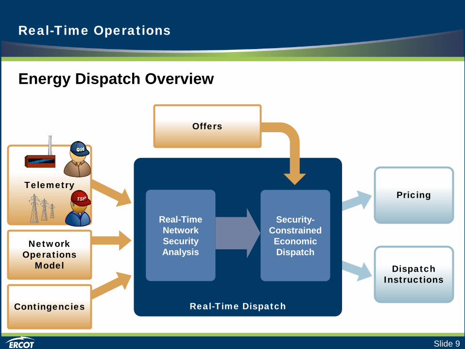
Energy Dispatch Overview
Offers
Telemetry
Network Operations
Model
Contingencies
Real-Time Network Security Analysis
Security-Constrained Economic Dispatch
Pricing
Dispatch Instructions
Real-Time Dispatch

Slide 10
Offers
Telemetry
Network Operations
Model
Contingencies
Real-Time Network Security Analysis
Security-Constrained Economic Dispatch
Pricing
Dispatch Instructions
Real-Time Dispatch
Energy Dispatch Process
Gather Real-Time System Data

Slide 11
QSE Data to ERCOT Telemetered Data includes:
• Resource Status • Generation Resource
• Power output (MW and MVAR) • High and Low Sustained Limits
• Load Resource • Real power consumption • Low and maximum power consumption limits
Real-Time System Data

Slide 12
QSE Data to ERCOT Telemetered Data (continued):
• Resource breaker & switch status • Resource Ramp Rates • Ancillary Service Resource
Responsibility • Ancillary Service Schedule • Current configuration of
combined-cycle Resources
Real-Time System Data

Slide 13
TSP Data to ERCOT Telemetered Data:
• Breaker and Switch Status • Bus Voltage • Line Flows (MW and MVAR) • Transformer Flows (MW and MVAR) • Dynamic Ratings
Real-Time System Data

Slide 14
Real-Time System Data
Resource Decommitments in the Operating Period
A QSE may decommit a Resource for intervals that were not RUC-Committed
• A QSE may decommit a Quick Start Generation Resource (QSGR) without request
• For all other Resources, the QSE must verbally request permission from ERCOT

Slide 15
Communicating Forced Outages In the event of an outage, the telemetered status of the Resource automatically notifies ERCOT of a Forced Outage. Additionally, the QSE provides ERCOT with:
• Nature of Forced Outage • Actual Start time of the Forced Outage or De-rating • Planned End time of the Forced Outage or De-rating • Revised HSL and/or LSL
Real-Time System Data

Slide 16
Offers
Telemetry
Network Operations
Model
Contingencies
Real-Time Network Security Analysis
Security-Constrained Economic Dispatch
Pricing
Dispatch Instructions
Energy Dispatch Process
Real-Time Network Security Analysis
Real-Time Dispatch

Slide 17
Offers
Telemetry
Network Operations
Model
Contingencies
Real-Time Network Security Analysis
Security-Constrained Economic Dispatch
Pricing
Dispatch Instructions
Energy Dispatch Process
Real-Time Network Security Analysis
Real-Time Network Security Analysis
State Estimator
Real-Time Dispatch

Slide 18
Offers
Telemetry
Network Operations
Model
Contingencies
Real-Time Network Security Analysis
Security-Constrained Economic Dispatch
Pricing
Dispatch Instructions
Energy Dispatch Process
Real-Time Network Security Analysis
State Estimator
Contingency Analysis
Real-Time Dispatch

Slide 19
Offers
Telemetry
Network Operations
Model
Contingencies
Real-Time Network Security Analysis
Security-Constrained Economic Dispatch
Pricing
Dispatch Instructions
Energy Dispatch Process
Real-Time Network Security Analysis
State Estimator
Contingency Analysis
Constraint Management
Real-Time Dispatch

Slide 20
Offers
Telemetry
Network Operations
Model
Contingencies
Real-Time Network Security Analysis
Security-Constrained Economic Dispatch
Pricing
Dispatch Instructions
Energy Dispatch Process
Real-Time Network Security Analysis
Constraints & Shift Factors
Real-Time Dispatch

Slide 21
Offers
Telemetry
Network Operations
Model
Contingencies
Real-Time Network Security Analysis
Security-Constrained Economic Dispatch
Pricing
Dispatch Instructions
Energy Dispatch Process
Security Constrained Economic Dispatch
Real-Time Dispatch

Slide 22
SCED
Balancing Reliability and Economics
SCED
Energy Offer
Curves
Network Security Analysis

Slide 23
SCED
Balancing Reliability and Economics
SCED
Energy Offer
Curves Network Security Analysis
Slide 24
SCED
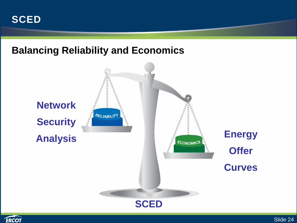
Balancing Reliability and Economics
SCED
Energy Offer
Curves
Network Security Analysis

Slide 25
SCED
Balancing Reliability and Economics
SCED
Energy Offer
Curves
Network Security Analysis

Slide 26
SCED
Energy Offer
Curves
Network Security Analysis
SCED
Balancing Reliability and Economics Security Constrained Economic Dispatch (SCED) evaluates Energy Offer Curves to produce a least cost dispatch of On-Line Resources while respecting transmission and generation constraints.

Slide 27
The Texas Two Step
SCED
SCED
SCED executes twice each cycle
• Ensures competition
• Reduces Market Power
• Allows high prices under “the right circumstances”

Slide 28
The Texas Two Step
SCED
SCED
Circumstances for high prices
• All generation is expensive
• Expensive generation needed to resolve constraints
• Scarcity

Slide 29
SCED
The Texas Two Step
Constraints are classified as: • Competitive • Non-Competitive
SCED

Slide 30
SCED
The Texas Two Step Step One • Uses Energy Offer Curves
for all On-Line Generation Resources
• Observes the limits of Competitive Constraints only
• Determines “Reference LMPs”
SCED
Energy Offer Curve
$ / MWh
Reference LMP
MW

Slide 31
SCED
Energy Offer Curve
The Texas Two Step Step Two • Observes limits of all Constraints
$ / MWh
Reference LMP
MW SCED

Slide 32
SCED
Mitigated Offer cap
The Texas Two Step Step Two • Observes limits of all Constraints
• Energy Offer Curve for on-line Resource capped at Reference LMP or Mitigated Offer Cap (whichever is greater)
Energy Offer Curve
$ / MWh
Reference LMP
MW SCED

Slide 33
SCED Scenarios
Texas Two Step

Slide 34
Energy Offer Curve
$ / MWh
MW
Reference LMP
Mitigated Offer cap
SCED has completed Step 1 and determined Reference LMPs.
How will this Energy Offer Curve look in STEP 2?
SCED
Energy Offer Curve
$ / MWh
MW
Reference LMP
Mitigated Offer cap

Slide 35
Energy Offer Curve
$ / MWh
MW
Reference LMP
Mitigated Offer cap
SCED
SCED has completed Step 1 and determined Reference LMPs.
1. How will this Energy Offer Curve look in STEP 2?
2. What will it take for this scenario to occur?
Energy Offer Curve
$ / MWh
MW
Reference LMP
Mitigated Offer cap

Slide 36
Offers
Telemetry
Network Operations
Model
Contingencies
Security-Constrained Economic Dispatch
Pricing
Dispatch Instructions
Energy Dispatch Process
The SCED Process
Constraints & Shift Factors
Real-Time Network Security Analysis
Real-Time Dispatch

Slide 37
Offers
Telemetry
Network Operations
Model
Contingencies
Security-Constrained Economic Dispatch
Pricing
Dispatch Instructions
Energy Dispatch Process
The SCED Process
Resource Limit Calculator
Constraints & Shift Factors
Real-Time Dispatch

Slide 38
Resource Limit Calculator
Telemetered by the QSE every few seconds
HSL
LSL
Operating Point
High Sustained Limit
Low Sustained Limit

Slide 39
Resource Limit Calculator
HSL
HASL
LASL
LSL
Reg-Up, RRS & Non-Spin
Reg-Down
Operating Point
Also telemetered by QSE • AS Schedule (RRS & Non-Spin) • AS Resource Responsibility (Reg)
High Ancillary Service Limit
Low Ancillary Service Limit
Slide 40
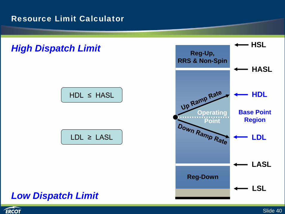
Resource Limit Calculator
Base Point Region
HASL
LASL
HDL
LDL
Reg-Up, RRS & Non-Spin
Reg-Down
LSL
Operating Point
HDL ≤ HASL
LDL ≥ LASL
High Dispatch Limit
Low Dispatch Limit
HSL

Slide 41
Offers
Telemetry
Network Operations
Model
Contingencies
Security-Constrained Economic Dispatch
Pricing
Dispatch Instructions
Real-Time Operations
The SCED Process
Resource Limit Calculator
Generation to be dispatched
Constraints & Shift Factors
Real-Time Dispatch

Slide 42
The SCED Process
Offers
Telemetry
Network Operations
Model
Contingencies
Security-Constrained Economic Dispatch
Pricing
Dispatch Instructions
Energy Dispatch Process
Resource Limit Calculator
Generation to be dispatched
Constraints & Shift Factors
Real-Time Dispatch
Slide 43
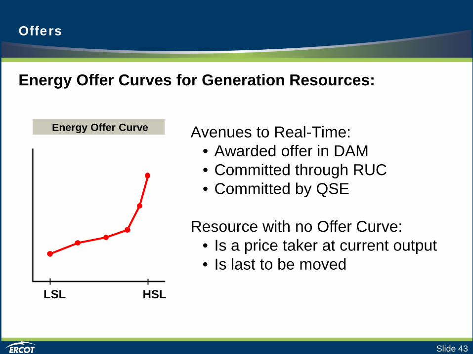
Avenues to Real-Time: • Awarded offer in DAM • Committed through RUC • Committed by QSE
Resource with no Offer Curve:
• Is a price taker at current output • Is last to be moved
Energy Offer Curves for Generation Resources:
Offers
Energy Offer Curve
LSL HSL
Slide 44
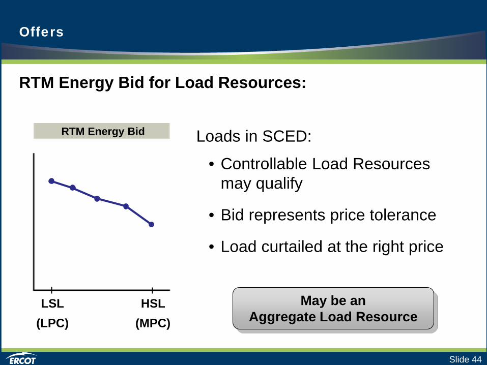
RTM Energy Bid for Load Resources:
Offers
Loads in SCED:
• Controllable Load Resources may qualify
• Bid represents price tolerance
• Load curtailed at the right price
RTM Energy Bid
LSL HSL (LPC) (MPC)
May be an Aggregate Load Resource

Slide 45
SCED Timeline SCED is executed:
• Every five minutes (at a minimum)
• More often as needed by ERCOT operators or other ERCOT systems.
Energy Dispatch Process Timing
SCED executed by schedule
SCED executed by schedule
SCED executed by schedule
Operator Initiated

Slide 46
Offers
Telemetry
Network Operations
Model
Contingencies
Security-Constrained Economic Dispatch
Pricing
Dispatch Instructions
Energy Dispatch Process
The SCED Process
Resource Limit Calculator
Generation to be dispatched
Constraints & Shift Factors
Real-Time Dispatch

Slide 47
Energy Dispatch Outputs
Locational Marginal Prices (LMPs)
• Offer-based marginal cost of serving the next increment of Load at an Electrical Bus
• Used to calculate Settlement Point Prices • Resource Nodes • Load Zones • Hubs
Resource Nodes
Load Zones
Hubs

Slide 48
Determining Locational Marginal Price
-- Warning --
Greek Letters Ahead!
Χ = Σ (Α + Ω)
Energy Dispatch Outputs
∑−=c
ccbusbus SPSFLMP ,, *λ
Shadow Price for Transmission Constraint “c”
Shift Factor of the bus on Transmission Constraint “c”
System Lambda (Price for Power Balance)

Slide 49
Resource-Specific Base Points When SCED issues Base Point Dispatch instructions to QSEs, the information will include:
• Resource Identifier • Desired MW output level • Time of the Dispatch Instruction
Energy Dispatch Outputs

Slide 50
Communication of Dispatch Instructions • ERCOT sends dispatch instructions to QSEs
• QSEs are responsible for communicating the instructions to the appropriate Resources
Energy Dispatch Outputs

Slide 51
Communication of Dispatch Instructions When they receive dispatch instructions from ERCOT, QSEs must verify receipt.
Energy Dispatch Outputs
Electronic Dispatch Instructions (ICCP) Receiving systems acknowledge receipt
to ERCOT within one minute.
For Verbal Dispatch Instructions Recipient orally repeats the instructions back to ERCOT.
Slide 52
Energy Dispatch Outputs
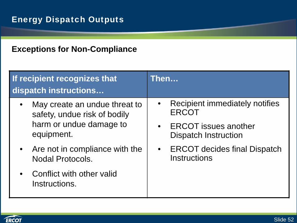
Exceptions for Non-Compliance
If recipient recognizes that dispatch instructions…
Then…
• May create an undue threat to safety, undue risk of bodily harm or undue damage to equipment.
• Are not in compliance with the Nodal Protocols.
• Conflict with other valid Instructions.
• Recipient immediately notifies ERCOT
• ERCOT issues another Dispatch Instruction
• ERCOT decides final Dispatch Instructions

Slide 53
Energy Dispatch Outputs
Non-Compliance Liability after Final Dispatch Instructions:
QSEs • Liable for failure as indicated in the Protocols • May be charged for the non-compliance
TSPs • Liable for failure as indicated in the Protocols and
the TSP’s Agreement with ERCOT
Slide 54
Energy Dispatch Outputs
MIS Hourly Postings
At the beginning of each hour, ERCOT will post: • Changes in ERCOT system conditions • Updated system load forecasts and distribution factors • Total ERCOT System Demand for each Settlement Interval

Slide 55
Energy Dispatch Outputs
MIS Postings After SCED
Upon completion of an execution of SCED, ERCOT posts: • LMPs for each Electrical Bus • SCED Shadow Prices • Settlement Point Prices for each Settlement Point
immediately following the end of each Settlement Interval • Active Binding Transmission Constraint and Contingency
pairs

Slide 56
Energy Dispatch Process
Energy Dispatch Summary
Offers
Telemetry
Network Operations
Model
Contingencies
Real-Time Network Security Analysis
Security-Constrained Economic Dispatch
Pricing
Dispatch Instructions
Real-Time Dispatch

Slide 57
Load Frequency Control
Load Frequency Control Overview
SCED is scheduled to execute every 5 minutes.
SCED executed by schedule
SCED executed by schedule
SCED executed by schedule

Slide 58
Load Frequency Control
Load Frequency Control Overview
SCED is scheduled to execute every 5 minutes.
In that same 5-minute interval, LFC runs 75 times.
SCED executed by schedule
LFC SCED executed by schedule
SCED executed by schedule
Slide 59
Load Frequency Control
Load Frequency Control Overview
The purpose of Load Frequency Control (LFC) is to maintain system frequency.
• Responds to frequency deviations
• Control signal to QSEs

Slide 60
Load Frequency Control
Load Frequency Control Outputs
Load Frequency Control produces several critical outputs.
• MW correction to restore system frequency
• Deployment of Resources providing:
• Up Regulation (Reg-Up)
• Down Regulation (Reg-Down)
• Responsive Reserve
• Updated Desired Base Point

Slide 61
Load Frequency Control Outputs
Posted on MIS Secure Area:.
• Total amount of deployed Reg-Up and Reg-Down energy in each Settlement Interval from the previous day.
Settlement:
• Net energy for a 15-min. settlement interval is captured in the Resource’s metered generation
• QSE paid at the Real-Time Settlement Point Price.
Load Frequency Control

Slide 62
Regulation Service Deployment
Regulation Service • An Ancillary Service that provides capacity that can
respond to control signals from ERCOT within three to five seconds to respond to changes in system frequency.
Two Types of Regulation Service • Regulation Up (Reg Up)
• Regulation Down (Reg Down)

Slide 63
Regulation Service Deployment
Deployment of Generation Resource Regulation Service
Service Generation Resource Load Resource
Reg-Up
• Amount available above any Base Point, and below the High Sustained Limit (HSL)
• Above the Low Power Consumption limit
Reg-Down
• Amount available below any Base Point , and above the Low Sustained Limit (LSL)
• Below the Load Resource’s Maximum Power Consumption limit

Slide 64
Regulation Service Deployment
Deployment of Load Resource Regulation Service
Service Generation Resource Load Resource
Reg-Up
• Amount available above any Base Point, and below the High Sustained Limit (HSL)
• Above the Low Power Consumption limit
Reg-Down
• Amount available below any Base Point , and above the Low Sustained Limit (LSL)
• Below the Load Resource’s Maximum Power Consumption limit

Slide 65
Regulation Service Deployment
Regulation Service Communications
QSEs to ERCOT: • AS Resource Responsibility • Status indicators for Regulation • Participation Factors
ERCOT to QSEs providing Regulation: • Control Signals • Every 4 seconds • ICCP data link
Slide 66
Responsive Reserve Service Deployment
Responsive Reserve Overview Responsive Reserve is an Ancillary Service that provides operating reserves intended to:
• Help restore system frequency within the first few seconds of a significant frequency deviation.
• Provide energy or Load interruption during the implementation of the Energy Emergency Alert (EEA)

Slide 67
Responsive Reserve Service Deployment
Responsive Reserve Overview ERCOT may also deploy Responsive Reserve when:
• Power requirement to restore frequency within 10 minutes exceeds the Reg-Up ramping capability.
• Responding to system disturbances if SCED does not have sufficient capacity available to dispatch
ERCOT will use Non-Spin to alleviate Responsive Reserve as soon as possible.

Slide 68
Responsive Reserve Deployment
Responsive Reserve Communications
QSEs to ERCOT: • AS Resource Responsibility • AS Schedule by Resource
ERCOT to QSEs with Responsive Reserve: • Control Signals (4 seconds) • ICCP data link • XML for non-Controllable Load Resources
For Responsive Reserve: AS Schedule = AS Resource Responsibility – AS Deployment
Slide 69
Responsive Reserve Deployment
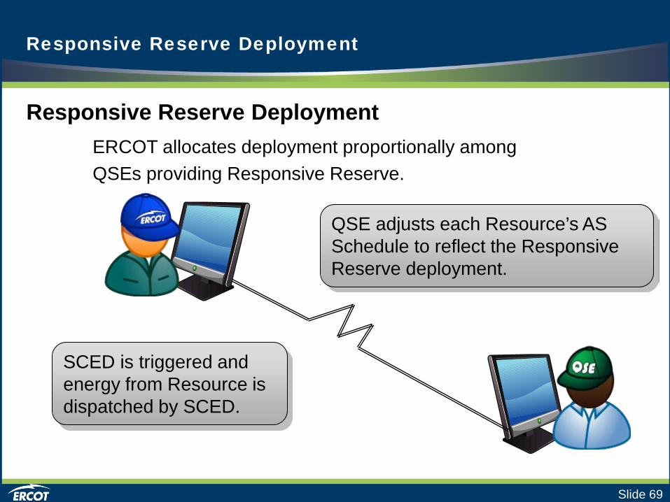
Responsive Reserve Deployment ERCOT allocates deployment proportionally among QSEs providing Responsive Reserve.
QSE adjusts each Resource’s AS Schedule to reflect the Responsive Reserve deployment.
SCED is triggered and energy from Resource is dispatched by SCED.

Slide 70
Non-Spinning Reserve
Non-Spinning Reserve
Non-Spinning Reserve is another ancillary service that provides reserve capacity, but with a longer response time than Responsive Reserve.
• Generally 30 minute response • Actual requirements vary by Resource type • May be used for system-wide or local needs

Slide 71
Resource Deployment Requirements Notes
Off-Line Generation Resource
Operator Dispatch
Instruction
Capable of reaching Non-Spin Resource Responsibility within 30 minutes of Dispatch Instruction.
Energy is dispatched by SCED
On-Line Generation Resource
Standing Deployment
QSE Reduces Non-Spin Schedule to zero at top of the hour
Energy is dispatched by SCED
Controllable Load
Resource
Operator Dispatch
Instruction
Provide the requested deployment energy within 30 minutes of Dispatch Instruction
Energy is dispatched by SCED
Non-Spinning Reserve
Non-Spinning Reserve Deployment

Slide 72
Load Frequency Control
Load Frequency Control Inputs
Input Location
Actual System Frequency Real-Time Telemetry
Scheduled System Frequency Operator Input in EMS
ERCOT System Frequency Bias Calculation in EMS
Resource Limits Resource Limit Calculator
Resource Output QSE Real-Time Telemetry
Participation Factor (Reg-up & Reg-Down) QSE Real-Time Telemetry
Raise Block Status and Lower Block Status indicators QSE Real-Time Telemetry

Slide 73
Load Frequency Control
Load Frequency Control Inputs
Input Location
Actual System Frequency Real-Time Telemetry
Scheduled System Frequency Operator Input in EMS
ERCOT System Frequency Bias Calculation in EMS
Resource Limits Resource Limit Calculator
Resource Output QSE Real-Time Telemetry
Participation Factor (Reg-up & Reg-Down) QSE Real-Time Telemetry
Raise Block Status and Lower Block Status indicators QSE Real-Time Telemetry

Slide 74
Load Frequency Control
The ACE Algorithm ERCOT ACE (Area Control Error) is the MW-equivalent correction needed to control the actual system frequency to the scheduled system frequency value.
The Equation
ERCOT ACE = 10ß (FS – FA)
Legend
F Frequency
Sub A Actual
Sub S Scheduled
Beta (ß)
System Frequency bias

Slide 75
ACE Algorithm inputs: • Scheduled frequency is 60 Hz
• Actual frequency is 59.8 Hz
• System frequency bias of -100
Load Frequency Control
Legend F Frequency
Sub A Actual 59.8 Hz
Sub S Scheduled 60 Hz
Beta (ß)
System Frequency
bias
-100
ERCOT ACE Algorithm:
ERCOT ACE = 10ß (FS – FA)
ERCOT ACE = 10(-100) * (60 - 59.8)
ERCOT ACE = -1000 * (0.2)
ERCOT ACE = -200

Slide 76
Load Frequency Control
Calculation informs ERCOT: • Short 200 MW
• Need to deploy 200 MW of Reg Up to restore system frequency to 60 Hz
Legend F Frequency
Sub A Actual 59.8 Hz
Sub S Scheduled 60 Hz
Beta (ß)
System Frequency
bias
-100
ERCOT ACE Algorithm:
ERCOT ACE = 10ß (FS – FA)
ERCOT ACE = 10(-100) * (60 - 59.8)
ERCOT ACE = -1000 * (0.2)
ERCOT ACE = -200

Slide 77
Load Frequency Control
Normal ACE Algorithm
14:00 14:05 14:10 14:15 14:20 14:25 14:30 14:35 14:40
200
150
100
50
0
-50
-100
-150
-200
ACE normally hovers around zero

Slide 78
Load Frequency Control
Normal ACE Algorithm
14:00 14:05 14:10 14:15 14:20 14:25 14:30 14:35 14:40
200
150
100
50
0
-50
-100
-150
-200
When system frequency drifts away from 60 Hz, ERCOT deploys Regulation to correct it

Slide 79
Load Frequency Control
Trend over time
14:00
200
150
100
50
0
-50
-100
-150
-200
14:01 14:02 14:03 14:04 14:05
What happens if system demand is increasing so quickly that ERCOT exhausts all Up-Regulation reserves before the next scheduled SCED run?

Slide 80
Real-Time Operations
Scenario Details: • At 0900, SCED runs & issues
Base Points
• Demand rises rapidly in next few minutes
• By 0905, Reg-Up will be exhausted
What options does the ERCOT Operator have for managing this situation?

Slide 81
Real-Time Operations
How does ERCOT know what Real-time reserves are available? Ancillary Services Capacity Monitor
• Calculates available levels of Resource capacity as per Real-time telemetry
• Calculated every 10 seconds
• Posted on MIS
• Streamed over ICCP
http://www.ercot.com/content/cdr/html/as_capacity_monitor.html

Slide 82
Real-Time Operations
Scenario Details: • At 0900, SCED runs and issues a
set of Base Points • Large Generation Resource trips • ERCOT System Frequency drops • Loss is detected through Real-
Time telemetry • ERCOT operators notified by alarm
What happens next?

Slide 83
Real-Time Operations
Real-Time Operations Timeline

Real-Time Financial Impacts
Slide 85
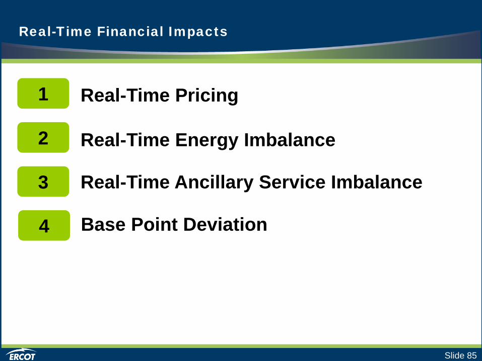
Real-Time Financial Impacts
Real-Time Energy Imbalance
Real-Time Ancillary Service Imbalance
Real-Time Pricing 1
2
3
4 Base Point Deviation

Slide 86
Real-Time Financial Impacts
Real-Time Energy Imbalance
Real-Time Ancillary Service Imbalance
Real-Time Pricing 1
2
3
4 Base Point Deviation

Slide 87
Real-Time Pricing Methodology
Locational Marginal Prices (LMPs)
• Produced by SCED
• Combined with Reserve Price Adders to form Real-Time Settlement Point Prices
LMPs are location-specific. Reserve Price Adders represent the value of
reserves ERCOT-wide.
Resource Nodes
Load Zones
Hubs

Slide 88
Real-Time Pricing Methodology
Time
Pric
e of
Ene
rgy
($ M
Wh)
SWCAP
SCED can set Scarcity Pricing
under the right conditions
Slide 89
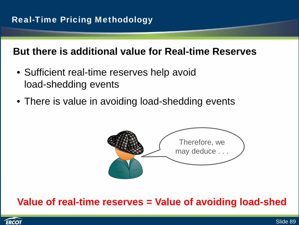
Real-Time Pricing Methodology
But there is additional value for Real-time Reserves
• Sufficient real-time reserves help avoid load-shedding events
• There is value in avoiding load-shedding events
Value of real-time reserves = Value of avoiding load-shed
Therefore, we may deduce . . .
Slide 90
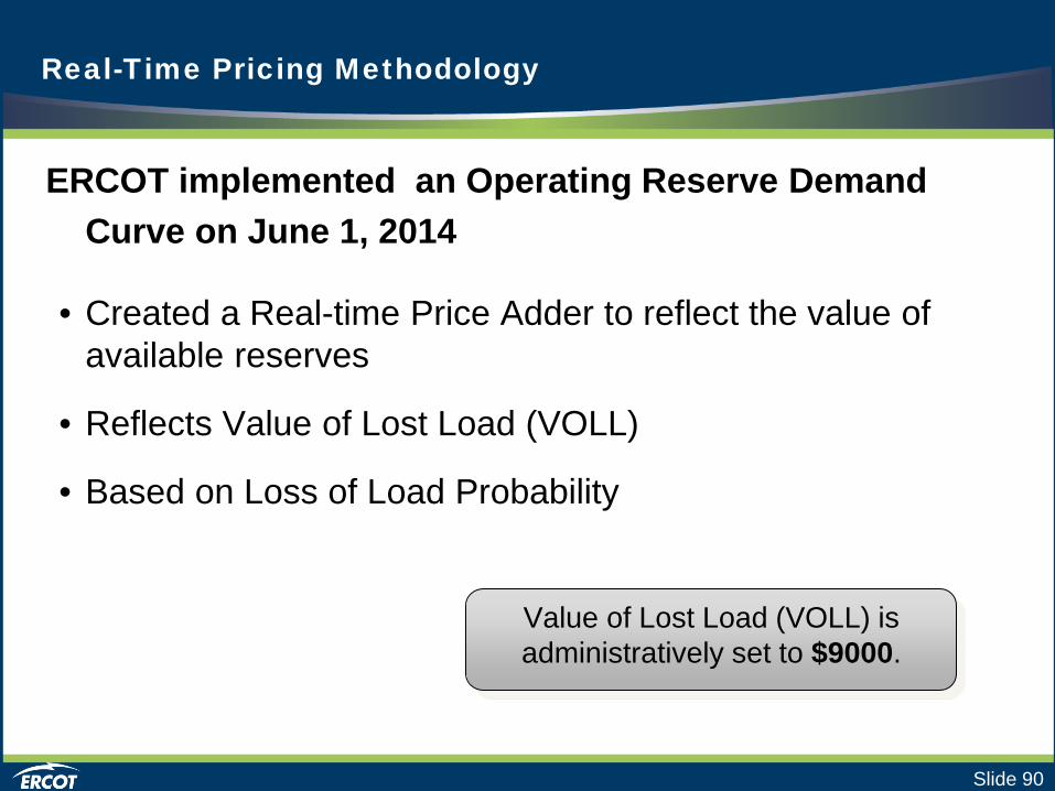
Real-Time Pricing Methodology
ERCOT implemented an Operating Reserve Demand Curve on June 1, 2014
• Created a Real-time Price Adder to reflect the value of available reserves
• Reflects Value of Lost Load (VOLL)
• Based on Loss of Load Probability
Value of Lost Load (VOLL) is administratively set to $9000.
Slide 91
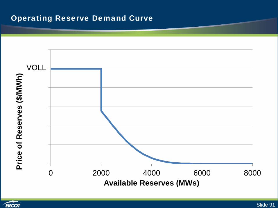
Operating Reserve Demand Curve
0 2000 4000 6000 8000
Pric
e of
Res
erve
s ($
/MW
h)
Available Reserves (MWs)
VOLL

Slide 92
Calculating Reserve Price Adders from ORDC
Overall goal is to improve scarcity pricing • SCED itself may produce scarcity pricing • Outside of any congestion impacts, energy pricing
should not exceed VOLL
Reserve Price Adders calculated based on
(VOLL – System Lambda) * Loss of Load Probability
Price of Power Balance in SCED

Slide 93
Real-Time Pricing Methodology
Time
Pric
e of
Ene
rgy
($ M
Wh)
SWCAP
VOLL
SCED can set Scarcity Pricing
under the right conditions
Reserve Price Adder improves Scarcity
Pricing
Slide 94
Real-Time Pricing Methodology
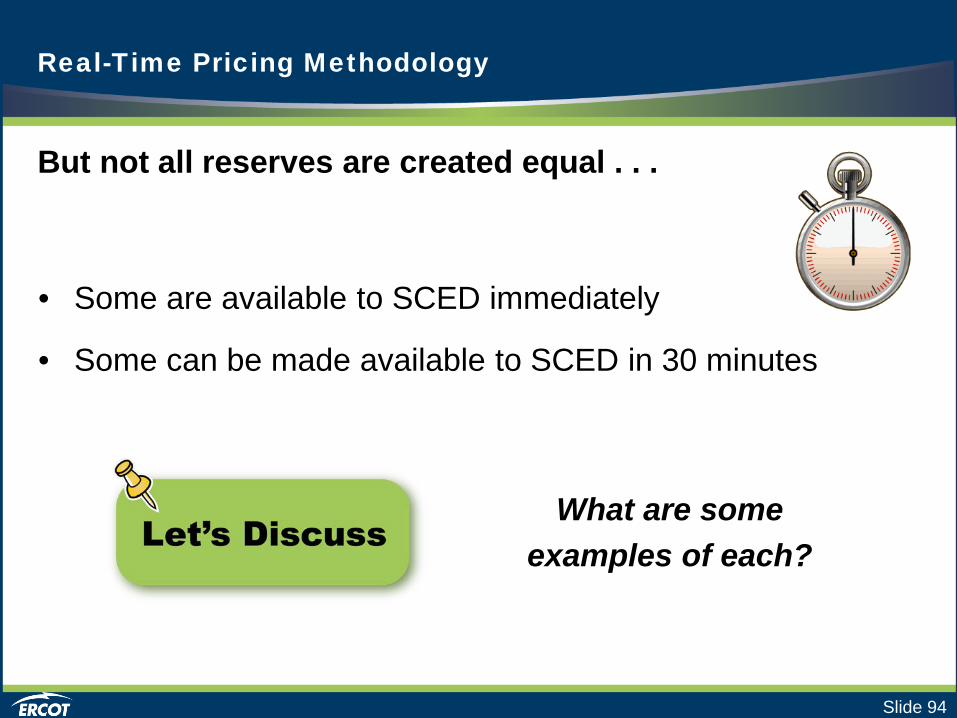
But not all reserves are created equal . . .
• Some are available to SCED immediately
• Some can be made available to SCED in 30 minutes
What are some examples of each?

Slide 95
Real-Time Pricing Methodology
Real-Time Reserve Price Adders
RTORPA – Available during the next 30 minutes
RTOFFPA – Available during the next 60 minutes ERCOT System
RTORPA Real-Time On-Line Reserve Price Adder RTOFFPA Real-Time Off-Line Reserve Price Adder
… calculated each SCED interval

Slide 96
Real-Time Pricing Methodology
Real-Time Reserve Price Adders
RTRSVPOR =
RTRSVPOFF =
ERCOT System
RTRSVPOR Real-Time Reserve Price for On-Line Reserves RTRSVPOFF Real-Time Reserve Price for Off-Line Reserves
Time-Weighted Average RTORPAs
Time-Weighted Average RTOFFPAs
… for each 15-minute interval

Slide 97
Resource Nodes
Load Zones
Hubs
Real-Time Pricing Methodology
Settlement Point Prices
= RTRSVPOR + Ave (LMPs)
… for each 15-minute interval
The way the LMPs are averaged varies by Settlement Point

Slide 98
Real-Time Financial Impacts
Real-Time Energy Imbalance
Real-Time Ancillary Service Imbalance
Real-Time Pricing 1
2
3
4 Base Point Deviation

Slide 99
Real-Time Energy Settlement In Real-time, energy sales and purchases are settled at each of the three Settlement Points:
• Resource Node • Load Zone • Hub
The Real-time Energy Imbalance Charge Type is used for this purpose.
Real-Time Energy Imbalance

Slide 100
Real-Time Energy Imbalance
The Basic Idea at any Settlement Point:
SUPPLIES ( ) OBLIGATIONS
( ) _ x RTSPP ($/MWh) Real-Time Settlement
Point Price
Now, we simply fill in the appropriate elements for each Settlement Point

Slide 101
Real-Time Energy Imbalance
Real-Time Energy Imbalance at a Load Zone Looking at a Load Zone, the calculation looks like this:
Notice that adjusted metered load is part of the equation.
Energy Bids Cleared in the DAM
+ Energy trades where
QSE is the buyer ( ) x RTSPP ($/MWh) Real-Time Settlement Point Price
Energy Offers Cleared
in the DAM +
Energy trades where QSE is the seller
+ Adjusted Metered
Load
( ) (-1) _

Slide 102
_
Real-Time Energy Imbalance
Real-Time Energy Imbalance at a Resource Node Looking at a Resource Node, the calculation looks like this:
For Resource Nodes, metered generation is included in the equation.
Metered Generation +
Energy Bids Cleared in the DAM
+ Energy trades where
QSE is the buyer ( ) x
RTSPP ($/MWh) Real-Time Settlement Point Price
( ) (-1) Energy Offers Cleared
in the DAM +
Energy trades where QSE is the seller
Slide 103
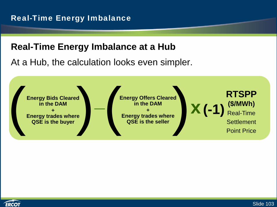
Real-Time Energy Imbalance
Real-Time Energy Imbalance at a Hub At a Hub, the calculation looks even simpler.
x RTSPP ($/MWh) Real-Time Settlement Point Price
( ) (-1) _ Energy Bids Cleared in the DAM
+ Energy trades where
QSE is the buyer ( ) Energy Offers Cleared in the DAM
+ Energy trades where
QSE is the seller
Slide 104
Real-Time Energy Imbalance
Converting DAM Transactions & Trades
• DAM transactions & Trades are conducted hourly
• Real-Time is settled in 15 minute intervals
• For Real-Time Settlements, DAM transactions and Trades must be converted to 15 minute intervals
Slide 105
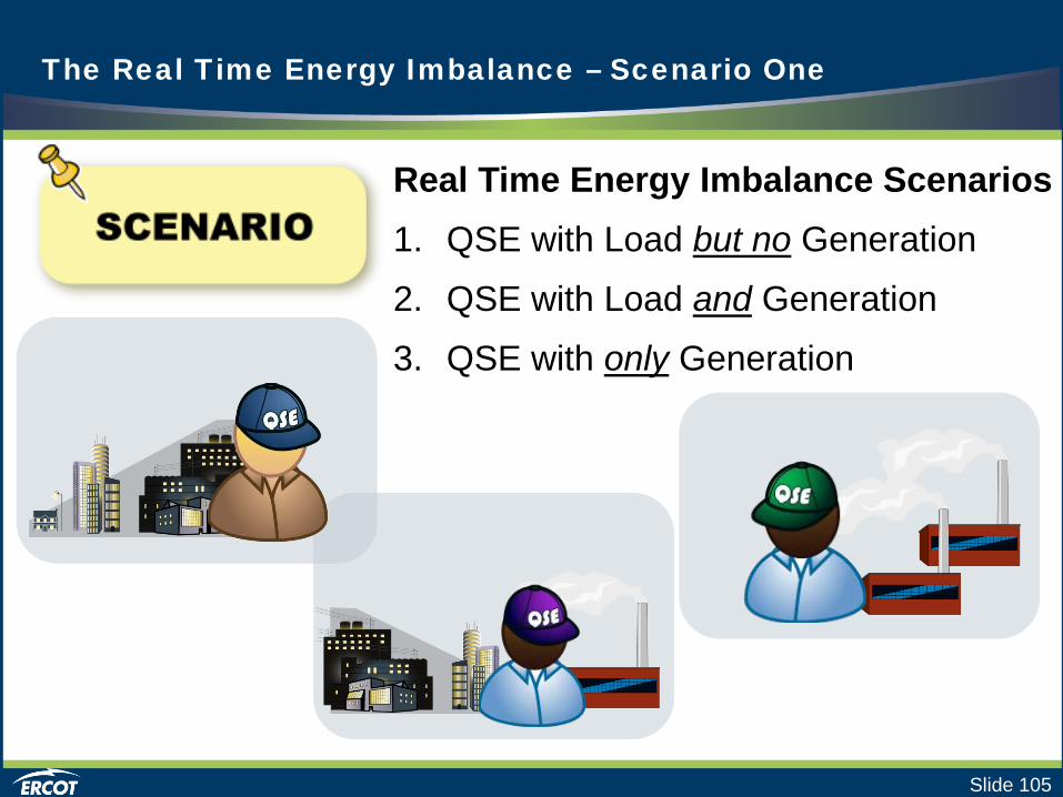
The Real Time Energy Imbalance – Scenario One
Real Time Energy Imbalance Scenarios 1. QSE with Load but no Generation
2. QSE with Load and Generation
3. QSE with only Generation

Slide 106
Real-Time Energy Imbalance – Scenario One
Scenario One: QSE with Load
Three ways QSE can choose to fulfill
it’s obligations:
No DAM Purchase, No Trades
DAM Purchase
Trade
2
3
1

Slide 107
Real-Time Energy Imbalance – Scenario One
Scenario One (Example 1):
• QSE does not participate in DAM
• No trades
• Load is 5 MWh for interval 0900
Energy Bids Cleared in the DAM
+ Energy trades where
QSE is the buyer ( ) x RTSPP ($/MWh) Real-Time Settlement Point Price
( ) (-1) _
Energy Offers Cleared in the DAM
+ Energy trades where
QSE is the seller +
Adjusted Metered Load
Slide 108
Real-Time Energy Imbalance – Scenario One
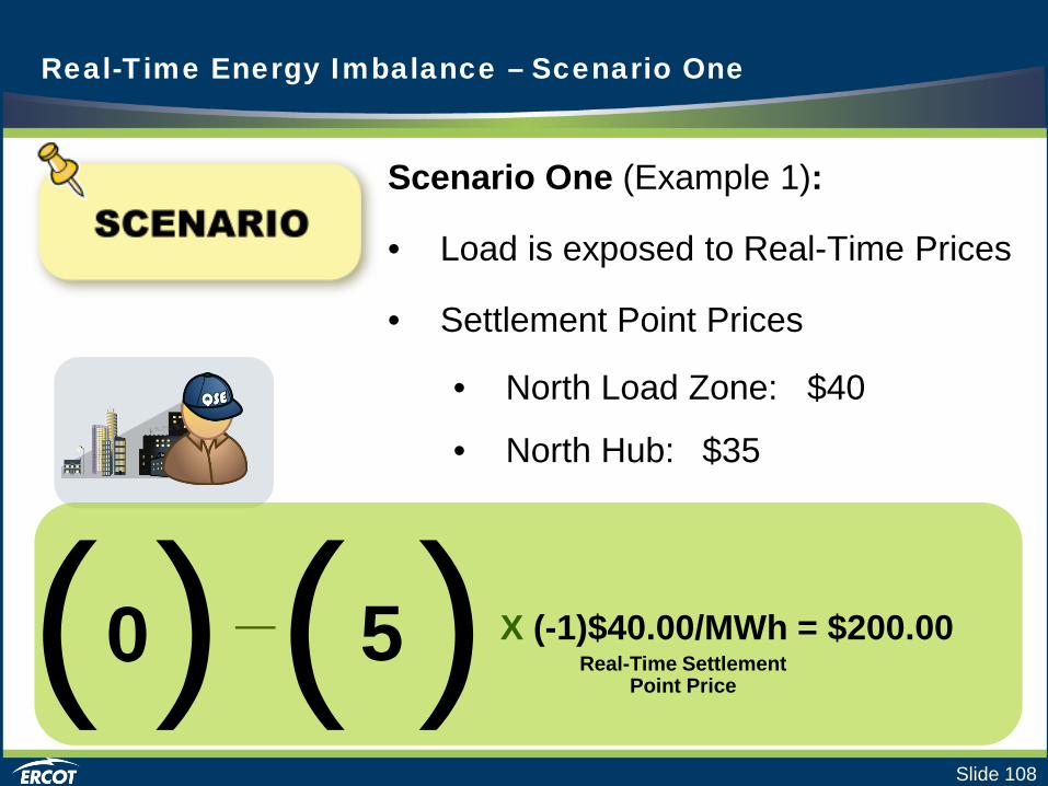
Scenario One (Example 1):
• Load is exposed to Real-Time Prices
• Settlement Point Prices
• North Load Zone: $40
• North Hub: $35
_
( ) ( ) X (-1)$40.00/MWh = $200.00 Real-Time Settlement
Point Price 0 5

Slide 109
Real-Time Energy Imbalance – Scenario One
( ) x RTSPP ($/MWh) Real-Time Settlement Point Price
( ) (-1)
Scenario One (Example 2): • QSE bought Day-Ahead Market
• No Trades
• Load is 5 MWh for interval 0900
_ Energy Bids Cleared in the DAM
+ Energy trades where
QSE is the buyer
Energy Offers Cleared
in the DAM +
Energy trades where QSE is the seller
+ Adjusted Metered
Load

Slide 110
Real-Time Energy Imbalance – Scenario One
Scenario One (Example 2):
• QSE bought 28 MW in Day-Ahead Market for Hour Ending 0900
• QSE gets credit for 28 MW in Real-Time (7 MWh per 15 minute interval)
_
( ) ( ) X (-1)$40.00/MWh = -$80.00 Real-Time Settlement
Point Price 7 5

Slide 111
Real-Time Energy Imbalance – Scenario One
Scenario One (Example 3):
• QSE bought 28 MW for Hour Ending 0900 through a trade at the North Hub.
• Load is 5 MWh for interval 0900

Slide 112
Real-Time Energy Imbalance – Scenario One
Real-Time Energy Imbalance at Hub
Real-Time Energy Imbalance at Load Zone
Scenario One (Example 3): • Imbalance calculated at both
Settlement Points (Hub & Load Zone)
Slide 113
Real-Time Energy Imbalance – Scenario One
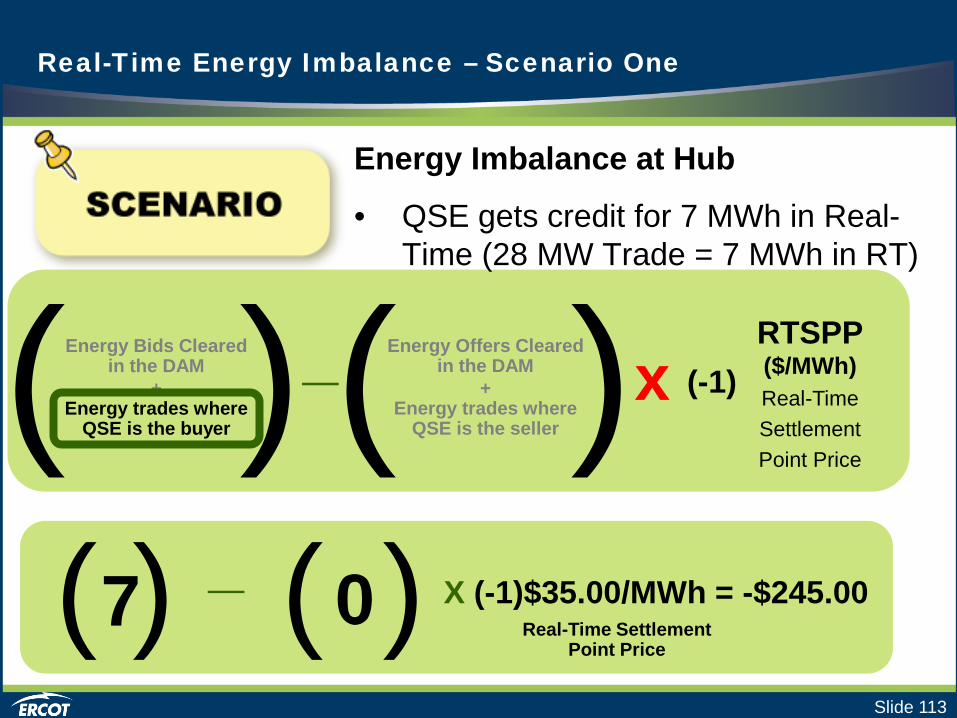
_ ( ) ( ) X (-1)$35.00/MWh = -$245.00 Real-Time Settlement
Point Price 7 0
Energy Imbalance at Hub
• QSE gets credit for 7 MWh in Real-Time (28 MW Trade = 7 MWh in RT)
Energy Bids Cleared
in the DAM +
Energy trades where QSE is the buyer ( ) _ ( ) RTSPP
($/MWh) Real-Time Settlement Point Price
(-1) Energy Offers Cleared
in the DAM +
Energy trades where QSE is the seller
x

Slide 114
Energy Imbalance at Load Zone
• QSE Load is still 5 MWh
Real-Time Energy Imbalance – Scenario One
( ) ( ) X (-1)$40.00/MWh = $200.00 Real-Time Settlement
Point Price 0 5
( ) RTSPP ($/MWh) Real-Time Settlement Point Price
( ) (-1)
_
x _
Energy Offers Cleared in the DAM
+ Energy trades where
QSE is the seller +
Adjusted Metered Load
Energy Bids Cleared in the DAM
+ Energy trades where
QSE is the buyer

Slide 115
Real-Time Energy Imbalance – Scenario One
QSE’s net settlement in Real-Time
• Paid $245 at the North Hub
• Charged $200 at the North Load Zone
• QSE is paid $45
Net = -$245 + 200 = -$45

Slide 116
The Real Time Energy Imbalance – Scenario Two
Real Time Energy Imbalance Scenarios 1. QSE with Load but no Generation
2. QSE with Load and Generation
3. QSE with only Generation

Slide 117
Real-Time Energy Imbalance – Scenario Two
Scenario Two: QSE with Load & Generation
• Load is still 5 MWh • QSE is dispatched to 20 MW • Settlement Point Prices
• North Load Zone: $40 • Old North Tap (ONTap)
Resource Node: $30

Slide 118
Scenario Two: • Imbalance calculated at Settlement
Points (Resource Node & Load Zone)
Real-Time Energy Imbalance – Scenario Two
Real-Time Energy Imbalance at Resource Node
Real-Time Energy Imbalance at Load Zone

Slide 119
Real-Time Energy Imbalance – Scenario Two
( ) ( ) X (-1)$30.00/MWh = -$150.00 Real-Time Settlement
Point Price
5 0
Energy Imbalance at Resource Node
Metered Generation +
Energy Bids Cleared in the DAM
+ Energy trades where
QSE is the buyer ( ) ( ) (-1) x _
_
RTSPP ($/MWh) Real-Time Settlement Point Price
Energy Offers Cleared in the DAM
+ Energy trades where
QSE is the seller
Slide 120
Real-Time Energy Imbalance – Scenario Two
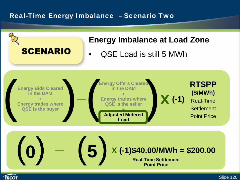
Energy Imbalance at Load Zone
• QSE Load is still 5 MWh
Energy Bids Cleared in the DAM
+ Energy trades where
QSE is the buyer ( ) RTSPP ($/MWh) Real-Time Settlement Point Price
Energy Offers Cleared
in the DAM +
Energy trades where QSE is the seller
+ Adjusted Metered
Load
( )
( ) ( ) X (-1)$40.00/MWh = $200.00 Real-Time Settlement
Point Price
0 5 _
(-1) x _

Slide 121
Real-Time Energy Imbalance – Scenario Two
What is the QSE’s net settlement in Real-Time?
• Paid $150 at the ONTap Resource Node
• Charged $200 at the North Load Zone
• QSE must pay $50
Net= -$150 + 200 = $50

Slide 122
The Real Time Energy Imbalance – Scenario Three
Real Time Energy Imbalance Scenarios 1. QSE with Load but no Generation
2. QSE with Load and Generation
3. QSE with only Generation

Slide 123
Real-Time Energy Imbalance – Scenario Three
Scenario One: QSE with Generation
Two Examples
QSE sells energy in DAM and produces it in Real-Time.
QSE sells energy in DAM and produces part of it in Real-Time.
2
1

Slide 124
Real-Time Energy Imbalance – Scenario Three
Relevant Facts: • QSE is dispatched to 20 MW during
interval Ending 0900 • Settlement Point Prices
• ONTap Resource Node: $30 • North Hub: $35

Slide 125
Real-Time Energy Imbalance – Scenario Three
Scenario Three (Example One): • QSE sells energy in DAM and
produces it in Real-Time.
• QSE’s metered generation is 5 MWh • QSE sold 12 MW in Day-Ahead
Market for Hour Ending 0900. • 12 MW in DAM = 3 MWh in Real-
Time
Slide 126
Real-Time Energy Imbalance – Scenario Three
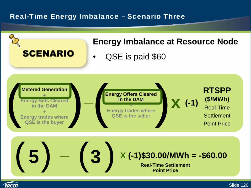
( ) X (-1)$30.00/MWh = -$60.00 Real-Time Settlement
Point Price
5 3
Energy Imbalance at Resource Node
• QSE is paid $60
_
( ) RTSPP ($/MWh) Real-Time Settlement Point Price
( ) (-1)
_
x
( )
Metered Generation +
Energy Bids Cleared in the DAM
+ Energy trades where
QSE is the buyer
Energy Offers Cleared in the DAM
+ Energy trades where
QSE is the seller

Slide 127
Real-Time Energy Imbalance – Scenario Three
Scenario Three (Example Two): • QSE sells energy in the DAM and
produces part of it in Real-Time. • Sold 28 MW in DAM for 0900 • Obligation to provide 7 MWh in Real-
Time (28 MW in DAM = 7 MWh in RT) • QSE’s metered generation is 5 MWh

Slide 128
Real-Time Energy Imbalance – Scenario Three
Energy Imbalance at Resource Node
• QSE is charged $60
( ) Real-Time Settlement Point Price
5 7 _ ( ) X (-1)$30.00/MWh = $60.00
_
( ) RTSPP ($/MWh) Real-Time Settlement Point Price
( ) (-1) x Metered Generation
+ Energy Bids Cleared
in the DAM +
Energy trades where QSE is the buyer
Energy Offers Cleared in the DAM
+ Energy trades where
QSE is the seller

Slide 129
Real-Time Energy Imbalance – Scenario Three
What is the QSE’s net settlement in Real-Time?
• Paid $150 at the ONTap Resource Node.
• Charged $175 at the North Hub.
• QSE must pay $25
Net= -$150 + 175 = $25

Slide 130
Real-Time Financial Impacts
Real-Time Energy Imbalance
Real-Time Ancillary Service Imbalance
Real-Time Pricing 1
2
3
4 Base Point Deviation

Slide 131
AS Capacity
Real-Time Ancillary Service Imbalance
Base Point
Base Point
$30.00 $34.50 $46.25 $67.80 $93.96 $131.16 $174.87 $227.12 $255.67
Base Point
Base Point
Gen 1 Gen 2
What if . . .
• we could keep on producing Energy from Gen 1?
• we could shift the AS from Gen 1 to Gen 2?

Slide 132
Real-Time Ancillary Service Imbalance
What would Real-Time Co-optimization Look Like?
AS Capacity
Available for
Energy Dispatch
DAM Co-opt.
Gen 1
Energy Produced
RT Co-opt.
QSE Real-Time Settlement:
• Paid RTSPP for energy produced in Real-Time
• Buy back AS Capacity at Real-Time AS Price

Slide 133
Real-Time Ancillary Service Imbalance
What would Real-Time Co-optimization Look Like?
AS Capacity
Available for
Energy Dispatch
DAM Co-opt.
Gen 2
Energy Produced
RT Co-opt.
QSE Real-Time Settlement:
• Paid RTSPP for energy produced in Real-Time
• Paid for AS Capacity at Real-Time AS Price

Slide 134
Real-Time Ancillary Service Imbalance
What would Real-Time Co-optimization Look Like?
AS Capacity
Available for
Energy Dispatch
DAM Co-opt.
Gen 2
Energy Produced
RT Co-opt.
QSE Real-Time Settlement:
• Paid RTSPP for energy produced in Real-Time
• Paid for AS Capacity at Real-Time AS Price
Currently, • No Real-Time Co-optimization • No Real-Time AS Prices
But we do have
Real-Time Reserve Prices

Slide 135
Real-Time Ancillary Service Imbalance
Real-Time Ancillary Service Imbalance Ancillary service reserves are settled at one of the Real-Time Reserve Prices.
• Approximates settlement impacts of Real-Time Co-optimization
• Provides payment for all capacity reserves
AS Capacity
System Capacity

Slide 136
Real-Time Ancillary Service Imbalance
The Basic Idea:
( ) On-line Reserve
Price * (-1) – On-Line Reserve SUPPLIES
On-Line Reserve OBLIGATIONS
( ) Off-line Reserve
Price * – Off-Line Reserve SUPPLIES
Off-Line Reserve OBLIGATIONS +
Calculated ERCOT-wide per QSE

Slide 137
Real-Time Ancillary Service Imbalance
Reserve Supplies and Obligations
Name some examples:
• On-Line Reserve Supplies
• On-Line Reserve Obligations
• Off-Line Reserve Supplies
• Off-Line Reserve Obligations

Slide 138
Real-Time Ancillary Service Imbalance
How’s it settled?
Energy Produced
Real-Time Generator
Paid in Real-Time Energy Imbalance Price: RTSPP
?
HSL
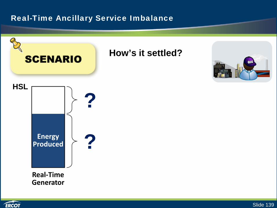
Slide 139
Real-Time Ancillary Service Imbalance
How’s it settled?
Energy Produced
Real-Time Generator
Paid in Real-Time Energy Imbalance Price: RTSPP
?
HSL Paid in Real-Time AS Imbalance Price: On-line Reserve Price ?

Slide 140
AS Capacity
Real-Time Ancillary Service Imbalance
How’s it settled?
Energy Produced
Real-Time Generator
Paid in Real-Time Energy Imbalance Price: RTSPP ?
HSL Paid in DAM or SASM Price: MCPC ?

Slide 141
AS Capacity
AS Deployed
Real-Time Ancillary Service Imbalance
How’s it settled?
Energy Produced
Real-Time Generator
Paid in Real-Time Energy Imbalance Price: RTSPP ?
HSL Charged in Real-Time AS Imbalance Price: On-line Reserve Price ?
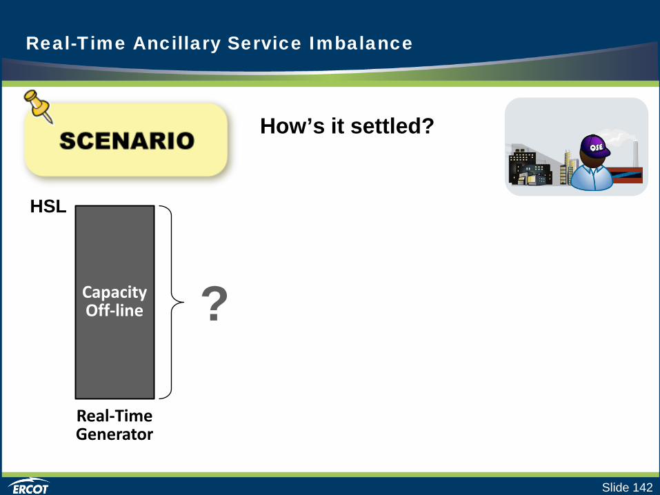
Slide 142
Real-Time Ancillary Service Imbalance
How’s it settled?
Capacity Off-line
Real-Time Generator
If available in 30 minutes, Paid in Real-Time AS Imbalance Price: Off-line Reserve Price
It depends . . . ?
HSL

Slide 143
Real-Time Ancillary Service Imbalance
How’s it settled?
Energy Consumed
Real-Time Load
Resource
Charged in Real-Time Energy
Imbalance
Price: RTSPP
?
HSL
LSL
Paid in Real-Time AS Imbalance
Price: On-line Reserve Price

Slide 144
Real-Time Ancillary Service Imbalance
How’s it settled?
Energy Consumed
AS Capacity
Real-Time Load
Resource
Charged in Real-Time Energy
Imbalance
Price: RTSPP
?
HSL
LSL
Paid in Real-Time AS Imbalance
Price: On-line Reserve Price
?
Paid in DAM or SASM Price: MCPC ?

Slide 145
Real-Time Financial Impacts
Real-Time Energy Imbalance
Real-Time Ancillary Service Imbalance
Real-Time Pricing 1
2
3
4 Base Point Deviation

Slide 146
Base Point Deviation
Real Time Energy Settlement QSE is paid for energy supplies and charged for energy obligations at a settlement point.
But what if a QSE with a Resource: • Generates more than instructed? • Generates less than instructed?
In other words, what happens if a QSE operates a Resource off of its Base Point?

Slide 147
Base Point Deviation
Base Point Deviation Charges Overview A QSE for a Generation Resource shall pay a base point deviation charge if the Resource did not follow Dispatch Instructions and Ancillary Services deployments within defined tolerances.

Slide 148
Base Point Deviation
Base Point Deviation Charges Overview A QSE for a Generation Resource shall pay a base point deviation charge if the Resource did not follow Dispatch Instructions and Ancillary Services deployments within defined tolerances. The NODAL Protocols define the tolerances as:
• ± 5% or ± 5MW, whichever is greater • + 10% for Intermittent Renewable Resources (IRR’s)

Slide 149
Base Point Deviation
Base Point Deviation Charge Exclusions • No charge during a frequency deviation greater than 0.05
Hz if the QSE’s deviation contributes to frequency correction
• No charge for intervals during which Responsive Reserve is deployed
Slide 150
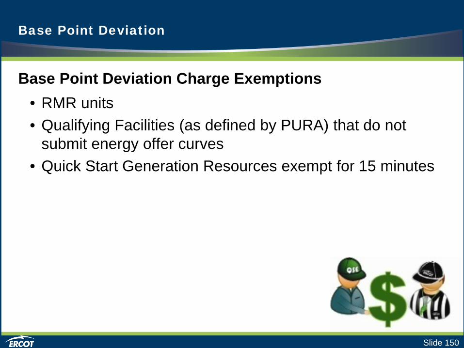
Base Point Deviation
Base Point Deviation Charge Exemptions • RMR units • Qualifying Facilities (as defined by PURA) that do not
submit energy offer curves • Quick Start Generation Resources exempt for 15 minutes

Slide 151
Base Point Deviation
Base Point Deviation Charges
Scenarios are as follows:
1. QSE has a single generator in ERCOT system.
2. Resource is not a QSGR
3. QSE does not provide Ancillary Services.
4. QSE receives base point dispatches from ERCOT to operate at 40 MW during Interval Ending 0900.

Slide 152
Base Point Deviation
Base Point Deviation Charge • Resource output exceeds Dispatch
Instructions by 8MW
• System Frequency at Max Deviation is 59.9400.
Frequency at max deviation during interval
5 9. 9 4 0 0 40 MW
48 MW

Slide 153
Does the QSE pay the base point deviation charge? No. System Frequency at Max Deviation exceeds the .05 threshold identified in the Protocols.
Base Point Deviation
Frequency at max deviation during interval
5 9. 9 4 0 0
-.06
40 MW
48 MW

Slide 154
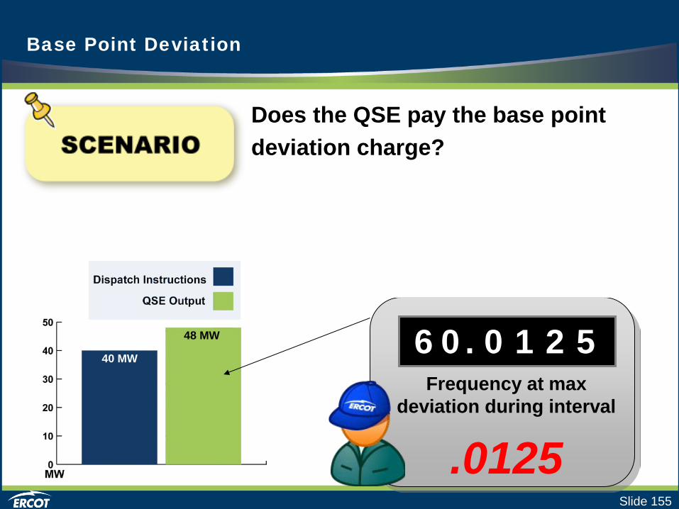
Base Point Deviation
Base Point Deviation Charge • Resource output exceeds Dispatch
Instructions by 8MW
• System Frequency at Max Deviation is 60.0125.
Frequency at max deviation during interval
6 0. 0 1 2 5 40 MW
48 MW
Slide 155
Base Point Deviation
Does the QSE pay the base point deviation charge? Yes. Resource output exceeds Dispatch Instructions beyond tolerances, and Frequency at Max Deviation is within Protocol allowances.
Frequency at max deviation during interval
6 0. 0 1 2 5
.0125
40 MW
48 MW

Slide 156
Base Point Deviation
Base Point Deviation Charge • Resource output falls short of
Dispatch Instructions by 6MW
• System Frequency at Max Deviation is 60.0125.
Frequency at max deviation during interval
6 0. 0 1 2 5 40 MW
34 MW

Slide 157
Base Point Deviation
Does the QSE pay the base point deviation charge? Yes. Resource output exceeds Dispatch Instructions beyond tolerances, and Frequency at Max Deviation is within Protocol allowances.
Frequency at max deviation during interval
6 0. 0 1 2 5
.0125
40 MW
34 MW

Slide 158
Base Point Deviation
Base Point Deviation Charge • Resource output falls short of
Dispatch Instructions by 6MW
• System Frequency at Max Deviation is 60.0525.
Frequency at max deviation during interval
6 0. 0 5 2 5 40 MW
34 MW
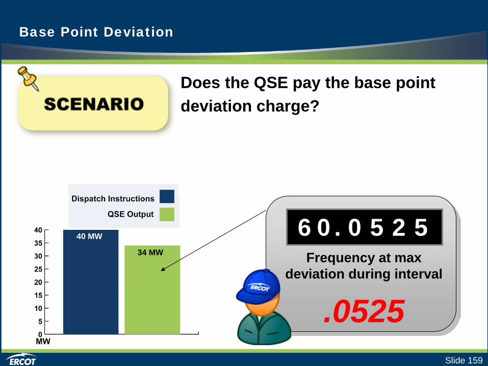
Slide 159
Base Point Deviation
Does the QSE pay the base point deviation charge? No. Resource output exceeds Dispatch Instructions tolerances, but Frequency Deviation is greater than .05 Hertz.
Frequency at max deviation during interval
6 0. 0 5 2 5
.0525
40 MW
34 MW

Slide 160
Determining Base Point Deviation Charges
ERCOT compares Adjusted Aggregated Base Points to the Time-Weighted Telemetered Generation.
Adjusted Aggregated Base Point
Time-Weighted Telemetered Generation
Base Point Deviation

Slide 161
Base Point Deviation
Calculating Adjusted Aggregated Base Point
Average Base Point
Adjusted Aggregated Base Point
Average Regulation = +
Considers Ramping
15 Minute Value

Slide 162
Base Point Deviation
Base Point Deviation for QSE with Regulation
• QSE receives Base Point dispatches during Interval Ending 0900
• QSE also receives Regulation deployments
Frequency at max deviation during interval
6 0. 0 7 8 6

Slide 163
Base Point Deviation
Base Point Deviation for QSE with Regulation
• Not following Reg-down instructions looks like over-generating.
• Not following Reg-up instructions looks like under-generating.
Frequency at max deviation during interval
6 0. 0 7 8 6

Slide 164
Module 6: Summary
You have learned: • Activities of ERCOT, TSPs, and QSEs in
Real-Time Operations
• Impact of ERCOT, TSPs and QSEs on the processes that occur in Real-Time Operations
• Purpose of the Real-Time processes
• The financial impact of the activities in Real-Time Operations

Module Conclusion
Related Documents