1 EQUIVALENT STATIC LOADS FOR RANDOM VIBRATION Revision N By Tom Irvine Email: [email protected] October 4, 2012 _____________________________________________________________________________________________ The following approach in the main text is intended primarily for single-degree-of-freedom systems. Some consideration is also given for multi-degree-of-freedom systems. Introduction A particular engineering design problem is to determine the equivalent static load for equipment subjected to base excitation random vibration. The goal is to determine peak response values. The resulting peak values may be used in a quasi-static analysis, or perhaps in a fatigue calculation. The response levels could be used to analyze the stress in brackets and mounting hardware, for example. Limitations Limitations of this approach are discussed in Appendices F through K. A particular concern for either a multi-degree-of-freedom system or a continuous system is that the static deflection shape may not properly simulate the predominant dynamic mode shape. In this case, the equivalent static load may be as much as one order of magnitude more conservative than the true dynamic load in terms of the resulting stress levels. Load Specification Ideally, the dynamics engineer and the static stress engineer would mutually understand, agree upon, and document the following parameters for the given component. 1. Mass, center-of-gravity, and inertia properties 2. Effective modal mass and participation factors 3. Stiffness 4. Damping 5. Natural frequencies 6. Dynamic mode shapes 7. Static deflection shape 8. Response acceleration 9. Modal velocity 10. Relative displacement

Welcome message from author
This document is posted to help you gain knowledge. Please leave a comment to let me know what you think about it! Share it to your friends and learn new things together.
Transcript
1
EQUIVALENT STATIC LOADS FOR RANDOM VIBRATION
Revision N
By Tom Irvine
Email: [email protected]
October 4, 2012
_____________________________________________________________________________________________
The following approach in the main text is intended primarily for single-degree-of-freedom
systems. Some consideration is also given for multi-degree-of-freedom systems.
Introduction
A particular engineering design problem is to determine the equivalent static load for equipment
subjected to base excitation random vibration. The goal is to determine peak response values.
The resulting peak values may be used in a quasi-static analysis, or perhaps in a fatigue
calculation. The response levels could be used to analyze the stress in brackets and mounting
hardware, for example.
Limitations
Limitations of this approach are discussed in Appendices F through K.
A particular concern for either a multi-degree-of-freedom system or a continuous system is that
the static deflection shape may not properly simulate the predominant dynamic mode shape. In
this case, the equivalent static load may be as much as one order of magnitude more conservative
than the true dynamic load in terms of the resulting stress levels.
Load Specification
Ideally, the dynamics engineer and the static stress engineer would mutually understand, agree
upon, and document the following parameters for the given component.
1. Mass, center-of-gravity, and inertia properties
2. Effective modal mass and participation factors
3. Stiffness
4. Damping
5. Natural frequencies
6. Dynamic mode shapes
7. Static deflection shape
8. Response acceleration
9. Modal velocity
10. Relative displacement

2
11. Transmitted force from the base to the component in each
of three axes
12. Bending moment at the base interface about each of three
axes
13. The manner in which the equivalent static loads and
moments will be applied to the component, such as point
load, body load, distributed load, etc.
14. Dynamic stress and strain at critical locations if the
component is best represented as a continuous system
15. Response limit criteria, such as yield stress, ultimate stress,
fatigue, or loss of clearance
Each of the response parameters should be given in terms of frequency response function, power
spectral density, and an overall response level.
Furthermore, assumptions must be documented, including a discussion of conservatism.
Again, this list is very idealistic.
Importance of Modal Velocity
Bateman wrote in Reference 24:
Of the three motion parameters (displacement, velocity, and acceleration) describing a
shock spectrum, velocity is the parameter of greatest interest from the viewpoint of
damage potential. This is because the maximum stresses in a structure subjected to a
dynamic load typically are due to the responses of the normal modes of the structure,
that is, the responses at natural frequencies. At any given natural frequency, stress is
proportional to the modal (relative) response velocity. Specifically,
EVC maxmax (1)
where
max = Maximum modal stress in the structure
maxV = Maximum modal velocity of the structural response
E = Elastic modulus
= Mass density of the structural material
C = Constant of proportionality dependent upon the geometry of
the structure (often assumed for complex equipment to be
4 < C < 8 )
Some additional research is needed to further develop equation 1 so that it can be used for
3
equivalent quasi-static loads for random vibration. Its fundamental principle is valid, however.
Further information on the relationship between stress and velocity is given in Reference 25.
Importance of Relative Displacement
Relative displacement is needed for the spring force calculation. Note that the transmitted force
for an SDOF system is simply the mass times the response acceleration.
Specifying the relative displacement for an SDOF system may seem redundant because the
relative displacement can be calculated from the response acceleration and the natural frequency
per equation (7) given later in this paper.
But specifying the relative displacement for an SDOF system is a good habit.
The reason is that the relationship between the relative displacement and the response
acceleration for a multi-degree-of-freedom (MDOF) or continuous system is complex. Any
offset of the component’s center-of-gravity (CG) further complicates the calculation due to
coupling between translational and rotational motion in the modal responses.
The relative displacement calculation for an MDOF system is beyond the scope of a hand
calculation, but the calculation can be made via a suitable Matlab script. A dynamic model is
required as shown in Appendices H and I.
Furthermore, examples of continuous structures are shown in Appendices J & K. The structures
are beams. The bending stress for the equivalent static analysis of each beam correlates better
with relative displacement than with response acceleration.
Model
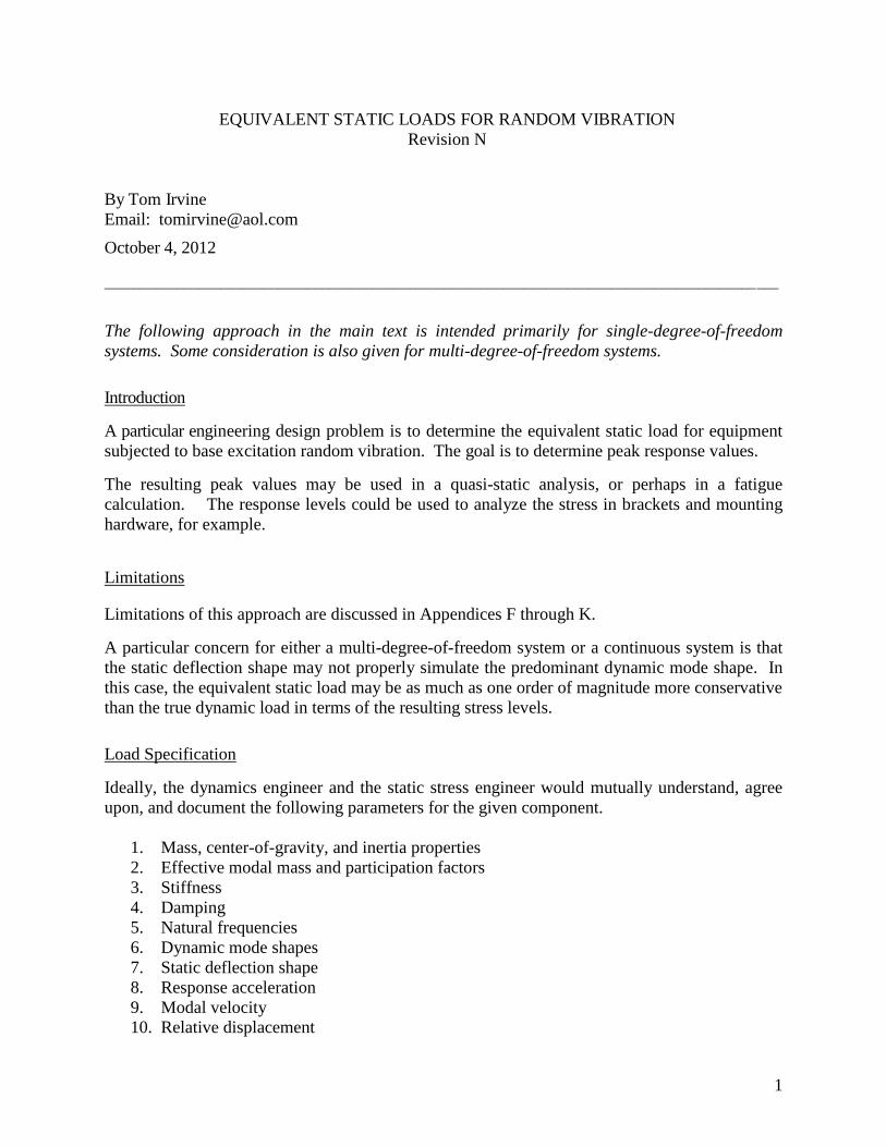
The first step is to determine the acceleration response of the component. Model the component as an SDOF system, if appropriate, as shown in Figure 1.
Figure 1.
m
k c
x
y

4
where
M is the mass
C is the viscous damping coefficient
K is the stiffness
X is the absolute displacement of the mass
Y is the base input displacement
Furthermore, the relative displacement z is
z = x – y (2)
The natural frequency of the system fn is
1 kfn
2 m
(3)
Acceleration Response
The Miles’ equation is a simplified method of calculating the response of a single-degree-of-
freedom system to a random vibration base input, where the input is in the form of a power
spectral density.
The overall acceleration response GRMSx is
fn
x f , PGRMS n2 2
(4)
where
Fn is the natural frequency
P is the base input acceleration power spectral density at the natural frequency
is the damping ratio

5
Note that the damping is often represented in terms of the quality factor Q.
1Q
2
(5)
Equation (4), or an equivalent form, is given in numerous references, including those listed in
Table 1.
Table 1. Miles’ equation References
Reference Author Equation Page
1 Himelblau (10.3) 246
2 Fackler (4-7) 76
3 Steinberg (8-36) 225
4 Luhrs - 59
5 Mil-Std-810G - 516.6-12
6 Caruso (1) 28
Furthermore, the Miles’ equation is an approximate formula that assumes a flat power spectral
density from zero to infinity Hz. As a rule-of-thumb, it may be used if the power spectral density
is flat over at least two octaves centered at the natural frequency.
An alternate response equation that allows for a shaped power spectral density input is given in
Appendix A.
Relative Displacement & Spring Force Consider a single-degree-of-freedom (SDOF) system subject to a white noise base input and with
constant damping. The Miles’ equation set shows the following with respect to the natural
frequency fn:
Response Acceleration nf (6)
Relative Displacement 5.1nf/1 (7)
Relative Displacement = Response Acceleration 2
n/ (8)

6
where nn f2
Equation (8) is derived in Reference 18.
Consider that the stress is proportional to the force transmitted through the mounting spring. The
spring force F is equal to the stiffness k times the relative displacement z.
F = k z (9)
RMS and Standard Deviation
The RMS value is related the mean and standard deviation values as follows:
RMS2 = mean
2 +
2 (10)
Note that the RMS value is equal to the 1 value assuming a zero mean.
A 3 value is thus three times the RMS value for a zero mean.
Peak Acceleration
There is no method to predict the exact peak acceleration value for a random time history.
An instantaneous peak value of 3 is often taken as the peak equivalent static acceleration. A
higher or lower value may be appropriate for given situation.
Some sample guidelines for peak acceleration are given in Table 2. Some of the authors have
intended their respective equations for design purposes. Others have intended their equations for
“Test Damage Potential.”
Table 2.
Sample Design Guidelines for Peak Response Acceleration or Transmitted Force
Refer. Author Design or Test
Equation Page Qualifying Statements
1 Himelblau,
et al 3 190
However, the response may
be non-linear and
non-Gaussian
2 Fackler 3 76 3 is the usual assumption
for the equivalent peak
sinusoidal level.
4 Luhrs 3 59 Theoretically, any large
acceleration may occur.

7
Table 2.
Sample Design Guidelines for Peak Response Acceleration or Transmitted Force
(continued)
Refer. Author Design or Test
Equation Page Qualifying Statements
7 NASA
3 for
STS Payloads
2 for
ELV Payloads
2.4-3 Minimum Probability Level
Requirements
8 McDonnell
Douglas 4 4-16 Equivalent Static Load
10 Scharton &
Pankow 5 - See Appendix C.
11 DiMaggio,
Sako, Rubin n Eq (22)
See Appendices B and D for
the equation to calculate n via
the Rayleigh distribution.
12 Ahlin Cn - See Appendix E for equation
to calculate Cn.
Furthermore, some references are concerned with fatigue rather than peak acceleration, as shown
in Table 3.
Table 3. Design Guidelines for Fatigue based on
Miner’s Cumulative Damage Index
Reference Author Page
3 Steinberg 229
6 Caruso 29
Note that the Miner’s Index considers the number of stress cycles at the 1, 2, and 3levels.
Modal Transient Analysis
The input acceleration may be available as a measured time history. If so, a modal transient
analysis can be performed. The numerical engine may be the same as that used in the shock
response spectrum calculation. The advantage of this approach is that it accounts for the
response peaks that are potentially above 3It is also useful when the base input is non-
stationary or when its histogram deviates from the normal ideal.
The modal transient approach can still be used if a power spectral density function is given
without a corresponding time history. In this case a time history can be synthesized to meet the

8
power spectral density, as shown in Appendix B. This approach effectively requires the time
history to be stationary with a normal distribution.
Furthermore, a time domain analysis would be useful if fatigue is a concern. In this case, the
rainflow cycle counting method could be used.
Special Case
Consider a system that has a natural frequency that is much higher than the maximum base input
frequency. An example would be a very stiff bar that was subjected to a low frequency base
excitation in the bar’s longitudinal axis.
This case is beyond the scope of Miles’ equation, since the Miles’ equation takes the input power
spectral density at the natural frequency. The formula in Appendix A can handle this case,
however.
As the natural frequency becomes increasingly higher than the maximum frequency of the input
acceleration, the following responses occur:
1. The response acceleration converges to the input acceleration.
2. The relative displacement approaches zero.
Furthermore, the following rule-of-thumb is given in Reference 24:
Quasi-static acceleration includes pure static acceleration as well as low-frequency
excitations. The range of frequencies that can be considered quasi-static is a function
of the first normal mode of vibration of the equipment. Any dynamic excitation at a
frequency less than about 20 percent of the lowest normal mode (natural) frequency of
the equipment can be considered quasi-static. For example, an earthquake excitation
that could cause severe damage to a building could be considered quasi-static to an
automobile radio.
Case History
A case history for random load factor derivation for a NASA programs is given in Reference 22.
Error Source Summary
Here is a list of error sources discussed in this paper, including the appendices.
1. An SDOF system may be an inadequate model for a component or
structure.
2. An SDOF model cannot account for spatial variation in either the input or
the response.
3. A CG offset leads to coupling between translational and rotational modes,
thus causing the transmitted forces to vary between the mounting springs.

9
4. Instantaneous peak values can occur in the time domain as high as
5depending on the duration and natural frequency.
5. The static deflection shape is not the same as the dynamic mode shape, thus
affecting the strain calculations.
Base Input & Component Response Concerns
The derivation of the base input level is beyond the scope of this paper, but a few points
are mentioned here as an aside.
1. The base input time history may have a histogram which departs from the
Gaussian ideal, with a kurtosis value > 3. A solution for this problem is
given in Reference 19.
2. Consider a component in its field or flight environment. The base excitation
at the component’s respective input points may vary by location in terms of
amplitude and phase. As a first approximation, the field response of the
component would be less than if the loads were uniform and in phase at the
input points, which would be the case during a shaker table test. On the other
hand, consider a beam simply-supported at each end. A uniform base input
would not excite the beam’s second bending mode. However, this mode
could be excited in a field environment where the inputs were non-uniform.
3. The base input level might not account for any force-limiting or mass-loading
effects from the component.
4. A structure or component may have a nonlinear response. Consider a
component mounted to a plate or shell, where the mounting structure is
excited by acoustical energy on the opposite side. At higher acoustic levels,
the structure will undergo membrane effects which limit its vibration
response, thus limiting the base input to the attached component.
5. Component damping tends to be non-linear. The damping tends to increase
as the input level increases. This increase can be due to joint slipping for
example. This should be considered in the context of adding margin to the
input levels.
6. Conservative enveloping may have been used to derive the component base
input level. In some case, the input level may be the maximum of all three
axes.
Conclusion
The task of deriving an accurate equivalent static load for a component or secondary structure is
very challenging.
There are numerous error sources. Some of the sources in this paper could lead to an under-
10
prediction of the load, such as omitting potential peaks > 3. Other sources could result in an
over-prediction, as shown for the cantilever beam example in Appendix J.
Ideally, these issues could be resolved by thorough testing and analysis.
Components could be instrumented with both accelerometers and strain gages and then exposed
to shaker table testing. This would allow a correlation between strain and acceleration response.
The input level should be varied to evaluate potential non-linearity. The resulting stress can then
be calculated from the strain.
Component modal testing would also useful to identify natural frequencies, mode shapes, and
modal damping values. This can be achieved to some extent by taking transmissibility
measurements during a shaker table test.
The test results could then be used to calibrate a finite element model. The calibration could be
as simple as a uniform scaling of the stiffness so that the model fundamental frequency matches
the measured natural frequency.
The test results would also provide the needed modal damping. Note that damping cannot be
calculated from theory. It can only be measured.
Cost and schedule often limit the amount of analysis which can be performed. But ideally, the
calibrated finite element model could be used for the dynamic stress calculation via a modal
transient or frequency response function approach. Note that the analyst may choose to perform
the post-processing via Matlab scripts using the frequency response functions from the finite
element analysis.
Otherwise, the calibrated finite element model could be used for a static analysis.
The proper approach for a given component must be considered on a case-by-case basis.
Engineering judgment is required.
Future Research
Further research is needed in terms of base input derivation, response analysis, and testing.
Another concern is material response. There are some references that report that steel and other
materials are able to withstand higher stresses than their respective ultimate limits if the time
history peak duration is of the order of 1 millisecond or less. See Appendix K.

11
Appendices
Table 4. Appendix Organization
Appendix Title
A SDOF Acceleration Response
B Normal Probability Values & Rayleigh Distribution
C Excerpt from Reference 10
D Excerpt from Reference 11
E Excerpt from Reference 12
F Excerpt from Reference 14
G Excerpts from References 15 & 16
H Two-degree-of-freedom System, Example 1
I Two-degree-of-freedom System, Example 2
J Cantilever Beam Example
K Beam Simply-supported at each End Example
L Material Stress Limits
References
1. H. Himelblau et al, NASA-HDBK-7005, Dynamic Environmental Criteria, Jet Propulsion
Laboratory, California Institute of Technology, 2001.
2. W. Fackler, Equivalence Techniques for Vibration Testing, SVM-9, The Shock and
Vibration Information Center, Naval Research Laboratory, United States Department of
Defense, Washington D.C., 1972.
3. Dave Steinberg, Vibration Analysis for Electronic Equipment, Wiley-Interscience, New
York, 1988.
4. H. Luhrs, Random Vibration Effects on Piece Part Applications, Proceedings of the
Institute of Environmental Sciences, Los Angeles, California, 1982.
5. MIL-STD-810G, “Environmental Test Methods and Engineering Guidelines,” United
States Department of Defense, Washington D.C., October 2008.
6. H. Caruso and E. Szymkowiak, A Clarification of the Shock/Vibration Equivalence in
Mil-Std-180D/E, Journal of Environmental Sciences, 1989.

12
7. General Environmental Verification Specification for STS & ELV Payloads, Subsystems,
and Components, NASA Goddard Space Flight Center, 1996.
8. Vibration, Shock, and Acoustics; McDonnell Douglas Astronautics Company, Western
Division, 1971.
9. W. Thomson, Theory of Vibration with Applications, Second Edition, Prentice- Hall,
New Jersey, 1981.
10. T. Scharton & D. Pankow, Extreme Peaks in Random Vibration Testing, Spacecraft and
Launch Vehicle Dynamic Environments Workshop, Aerospace/JPL, Hawthorne,
California, 2006.
11. DiMaggio, S. J., Sako, B. H., and Rubin, S., Analysis of Nonstationary Vibroacoustic
Flight Data Using a Damage-Potential Basis, AIAA Dynamic Specialists Conference,
2003 (also, Aerospace Report No. TOR-2002(1413)-1838, 1 August 2002).
12. K. Ahlin, Comparison of Test Specifications and Measured Field Data, Sound &
Vibration, September 2006.
13. T. Irvine, An Introduction to the Vibration Response Spectrum, Vibrationdata
Publications, 2000.
14. R. Simmons, S. Gordon, B. Coladonato; Miles’ Equation, NASA Goddard Space Flight
Center, May 2001.
15. H. Lee, Testing for Random Limit Load Versus Static Limit Load, NASA TM-108542,
1997.
16. H. Lee, A Simplistic Look at Limit Stresses from Random Loading, NASA TM-108427,
1993.
17. T. Irvine, The Steady-State Frequency Response Function of a Multi-degree-of-freedom
System to Harmonic Base Excitation, Rev C, Vibrationdata, 2010.
18. T. Irvine, Derivation of Miles’ equation for Relative Displacement Response to Base
Excitation, Vibrationdata, 2008.
19. T. Irvine, Deriving a Random Vibration Maximum Expected Level with Consideration
for Kurtosis, Vibrationdata, 2010.
20. T. Irvine, Steady-State Vibration Response of a Cantilever Beam Subjected to Base
Excitation, Rev A, 2009.
21. W. Young, Roark's Formulas for Stress & Strain, 6th edition, McGraw-Hill, New York,
1989.
22. Robert L. Towner, Practical Approaches for Random Load Factors, PowerPoint
Presentation, Mentors-Peers, Jacobs ESTS Group, November 21, 2008.

13
23. C. Lalanne, Sinusoidal Vibration (Mechanical Vibration and Shock), Taylor & Francis,
New York, 1999.
24. A. Piersol and T. Paez, eds., Harris’ Shock and Vibration Handbook, 6th Edition, NY,
McGraw-Hill, 2010.
25. T. Irvine, Shock & Vibration Stress as a Function of Velocity, Vibrationdata, 2010.
26. R. Huston and H. Josephs, Practical Stress Analysis in Engineering Design, Dekker,
CRC Press, 2008. See Table 13.1.

14
APPENDIX A
SDOF Acceleration Response
The acceleration response x GRMS of a single-degree-of-freedom system to a base input power
spectral density is
2i
2 22i i
N 1 (2 )ˆx f , Y (f ) f , f / fGRMS n A PSD i i i i n
1 2i 1
(A-1)
where
fn is the natural frequency
Y (f )A PSD n is the base input acceleration power spectral density
The corresponding relative displacement is
21
Z XRMS GRMS2 fn
(A-2)
Equation (A-1) allows for a shaped base input power spectral density, defined over a finite
frequency domain. It is thus less restrictive than the Miles’ equation. Equation (A-1) is derived
in Reference 13.
Note that equation (A-1) is the usual method for the vibration response spectrum calculation,
where the natural frequency is an independent variable.

15
APPENDIX B
Normal Probability Values
Note that the RMS value is equal to the 1 value assuming a zero mean. The 1 value is the
standard deviation.
Consider a broadband random vibration time history x(t), which has a normal distribution.
The precise amplitude x(t) cannot be calculated for a given time. Nevertheless, the probability
that x(t) is inside or outside of certain limits can be expressed in terms of statistical theory.
The probability values for the instantaneous amplitude are given in Tables B-1 and B-2 for
selected levels in terms of the standard deviation or value.
Table B-1.
Probability for a Random Signal with Normal Distribution and Zero Mean
Statement Probability Ratio Percent Probability
- < x < + 0.6827 68.27%
-2 < x < +2 0.9545 95.45%
-3 < x < +3 0.9973 99.73%
-4 < x < +4 0.99994 99.994%
Table B-2.
Probability for a Random Signal with Normal Distribution and Zero Mean
Statement Probability Ratio Percent Probability
| x | > 0.3173 31.73%
| x | > 2 0.0455 4.55%
| x | > 3 0.0027 0.27%
| x | > 4 6e-005 0.006%
Furthermore, the probability that an instantaneous amplitude is less than +3is P = 0.99865.
This is equivalent to saying that 1 out of every 741 points will exceed +3

16
Rayleigh Distribution
The following section is based on Reference 9.
Consider the response of single-degree-of-freedom distribution to a broadband time history. The
response is approximately a constant frequency oscillation with a slowly varying amplitude and
phase.
The probability distribution of the instantaneous acceleration is the same as that for the
broadband random function.
The absolute values of the response peaks, however, will have a Rayleigh distribution, as shown
in Table B-3.
Table B-3. Rayleigh Distribution Probability
Prob [ A > ]
0.5 88.25 %
1.0 60.65 %
1.5 32.47 %
2.0 13.53 %
2.5 4.39 %
3.0 1.11 %
3.5 0.22 %
4.0 0.034 %
4.5 4.0e-03 %
5.0 3.7e-04 %
5.5 2.7e-05 %
6.0 1.5e-06 %
The values in Table B-3 are calculated from
2
2
1expAP (B-1)
17
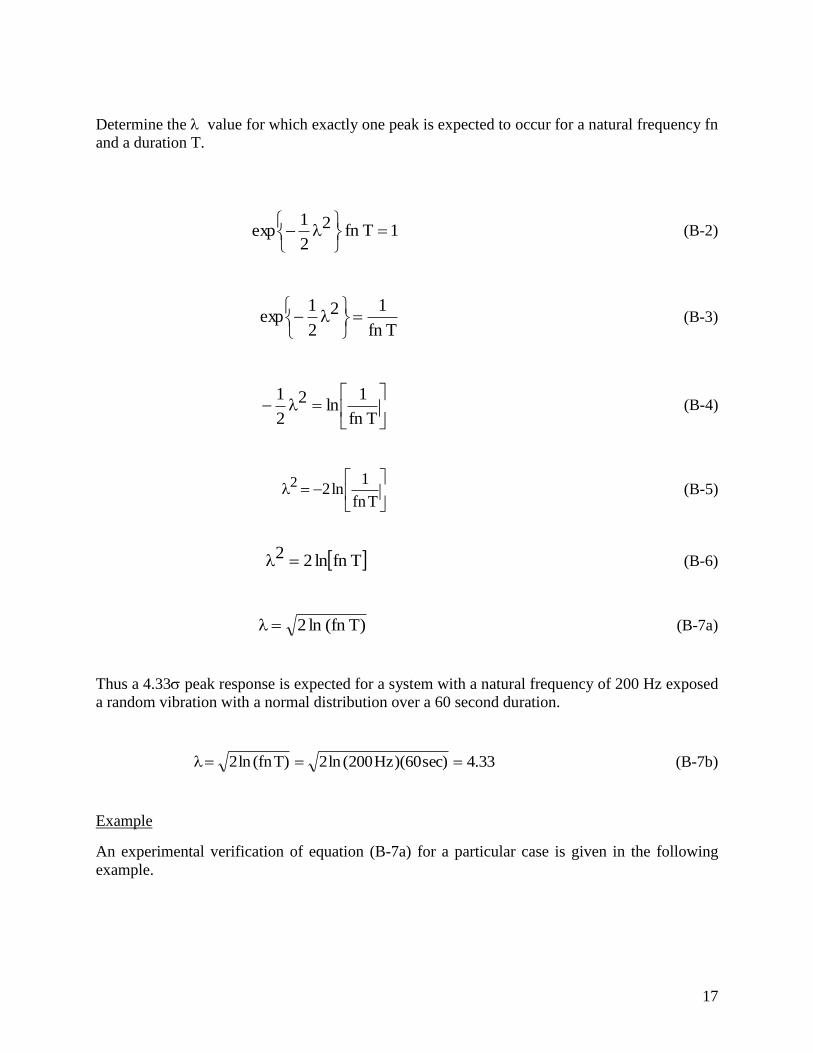
Determine the value for which exactly one peak is expected to occur for a natural frequency fn
and a duration T.
1Tfn2
2
1exp
(B-2)
Tfn
12
2
1exp
(B-3)
Tfn
1ln2
2
1 (B-4)
Tfn
1ln22
(B-5)
Tfnln22 (B-6)
)Tfn(ln2 (B-7a)
Thus a 4.33 peak response is expected for a system with a natural frequency of 200 Hz exposed
a random vibration with a normal distribution over a 60 second duration.
33.4sec)60)(Hz200(ln2)Tfn(ln2 (B-7b)
Example
An experimental verification of equation (B-7a) for a particular case is given in the following
example.

18
0.001
0.01
0.1
100 100020 2000
Synthesis, 6.06 GRMSSpecification, 6.06 GRMS
FREQUENCY (Hz)
AC
CE
L (
G2/H
z)
POWER SPECTRAL DENSITY
Figure B-1.
The synthesis curve agrees well with the specification, although it has a drop-out near 20 Hz.
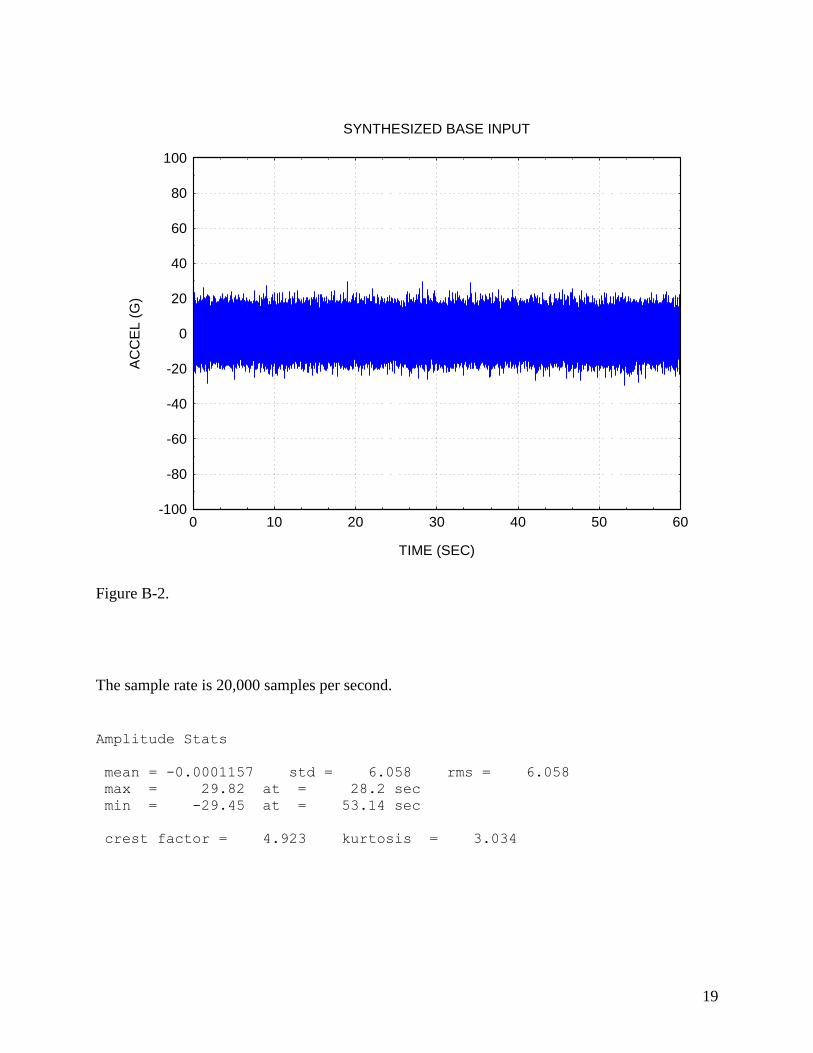
The actual synthesized time history is shown in Figure B-2.
19
-100
-80
-60
-40
-20
0
20
40
60
80
100
0 10 20 30 40 50 60
TIME (SEC)
AC
CE
L (
G)
SYNTHESIZED BASE INPUT
Figure B-2.
The sample rate is 20,000 samples per second.
Amplitude Stats
mean = -0.0001157 std = 6.058 rms = 6.058
max = 29.82 at = 28.2 sec
min = -29.45 at = 53.14 sec
crest factor = 4.923 kurtosis = 3.034

20
Figure B-3.
The histogram of the base input has a normal distribution.
21
-200
-150
-100
-50
0
50
100
150
200
0 10 20 30 40 50 60
TIME (SEC)
AC
CE
L (
G)
RESPONSE TIME HISTORY
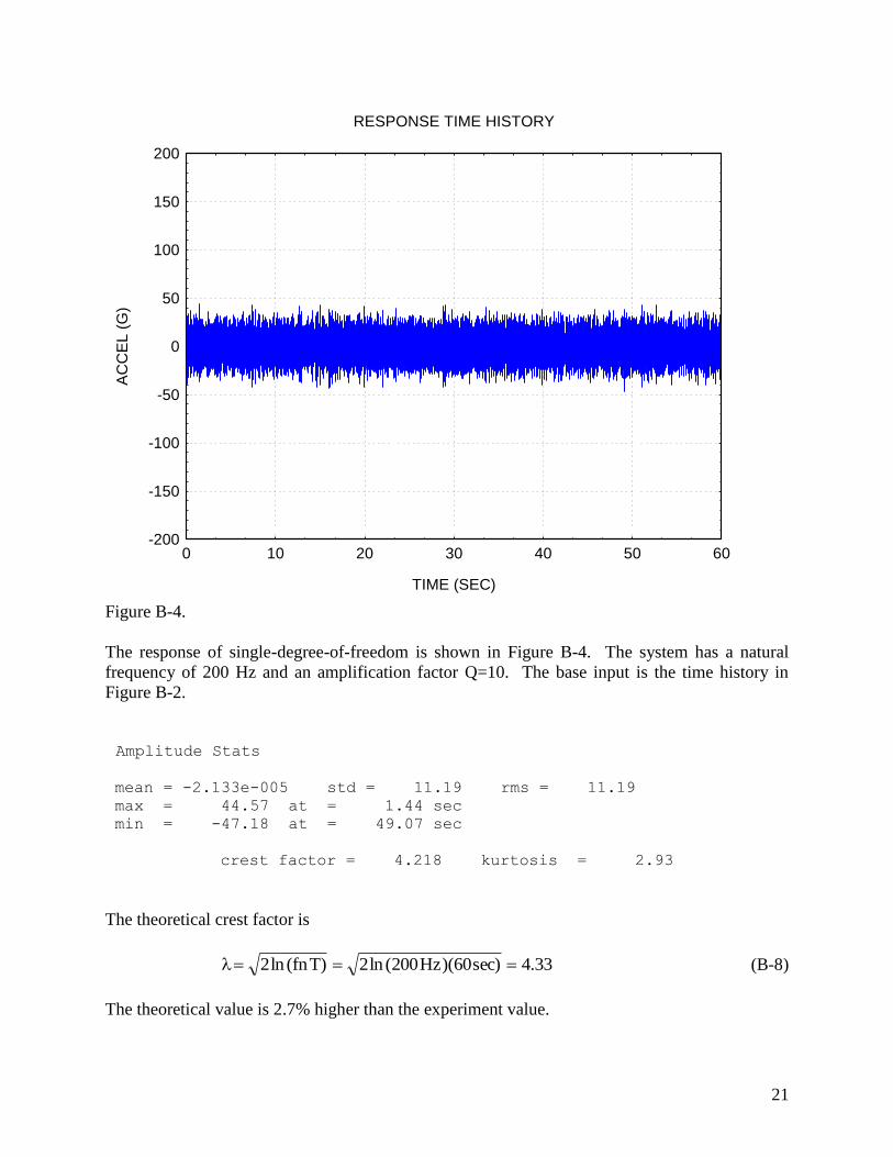
Figure B-4.
The response of single-degree-of-freedom is shown in Figure B-4. The system has a natural
frequency of 200 Hz and an amplification factor Q=10. The base input is the time history in
Figure B-2.
Amplitude Stats
mean = -2.133e-005 std = 11.19 rms = 11.19
max = 44.57 at = 1.44 sec
min = -47.18 at = 49.07 sec
crest factor = 4.218 kurtosis = 2.93
The theoretical crest factor is
33.4sec)60)(Hz200(ln2)Tfn(ln2 (B-8)
The theoretical value is 2.7% higher than the experiment value.

22
Figure B-5.
The histogram follows a normal distribution.

23
Figure B-6.
The histogram of the absolute peak from the response time history follows a Rayleigh
distribution.

24
APPENDIX C
Excerpt from Reference 10
Test data shows that occurrence of extreme peaks exceeds that predicted by Rayleigh
distribution.
For a Gaussian probability distribution, the probability of | x | > 5 is 6E-7.
If one has 60 seconds of white noise digitized at 20,000 points per seconds, the probability of a
peak exceeding 5 is 60 *20,000*6E-7=0.73
This may explain why one sees more extreme peaks than predicted by a Rayleigh distribution.
Extreme single peaks in the input acceleration are less of a concern because they do not appear to
produce near-resonant amplification of the response.
Extreme peaks in the base force and acceleration responses are a very real threat.
A simple experiment indicted that the strength of hard steel and carbon rods, and presumably of
other brittle materials, does not increase with frequencies up to 500 Hz.
Data in the literature indicate that the increase in strength of aluminum and many other materials
is small even at considerably higher frequencies.
Given the frequent observance of five sigma test peaks in time histories of responses in random
vibration tests, three sigma design strength requirements, such as those in NASA-STD-5002,
appear inconsistent.
The options are to increase mission limit loads, or to decrease test margins.

25
APPENDIX D
Excerpt from Reference 11
Reference 11 uses the Rayleigh distribution.
Equation (22) from this reference is
)fnT(ln22
2maxA
This equation is equivalent to equations (B-6) and (B-7) in Appendix B of this paper.

26
APPENDIX E
Excerpt from Reference 12
The following formula is intended for comparing random vibration to shock. It is not a design
level per se, but may be used as such.
Consider a single-degree-of-freedom system with the index n. The maximum response
nmax can be estimated by the following equations.
Tfnln2nc (E-1)
nc
5772.0ncnC (E-2)
nnCnmax (E-3)
where
fn is the natural frequency
T is the duration
ln is the natural logarithm function
n is the standard deviation of the oscillator response
27
APPENDIX F
Excerpt from Reference 14
The authors of Reference 14 give the following warning:
MILES’ EQUATION DOES NOT GIVE AN EQUIVALENT STATIC LOAD –
Calculating the GRMS value at a resonant peak after a random vibration test and
multiplying it by the test article mass does not mean that the test article was subjected to
that same, equivalent static load. It simply provides a statistical calculation of the peak
load for a SDOF system. The actual loading on a multiple DOF system due to random
input depends on the response of multiple modes, the mode shapes and the amount of
effective mass participating in each mode. Static testing must still be done.
28
APPENDIX G
Excerpt from References 15 & 16
NASA engineers performed experimental static and vibration testing an “AEPI fiberglass
pedestal” structure.
The following conclusions were made:
1. Strain, in general, is lower during random testing than during an equivalent static
loading as predicted by Miles’ equation.
2. The Miles’ equation equivalent static loading clearly develops stresses an order of
magnitude above those created by the random environments.
The reference also noted:
A study completed in 1993 by the Marshall Space Flight Center (MSFC) Random
Loads/Criteria Issues Team concluded, after an extensive literature search, that almost
no analytical or empirical documentation exists on the subject of the relationship
between random limit load (stress) and static limit load (stress). The consensus of the
team was that it is a complex subject and requires a carefully planned effort to produce
and effective, yet practical solution.
29
APPENDIX H
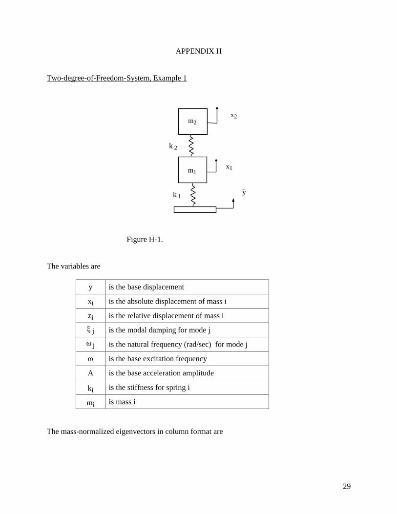
Two-degree-of-Freedom-System, Example 1
Figure H-1.
The variables are
y is the base displacement
xi is the absolute displacement of mass i
zi is the relative displacement of mass i
j is the modal damping for mode j
j is the natural frequency (rad/sec) for mode j
is the base excitation frequency
A is the base acceleration amplitude
ki is the stiffness for spring i
mi is mass i
The mass-normalized eigenvectors in column format are
m1
k 1
m2
k 2
k 3
x1
x2
y
30
2221
1211
The equation of motion from Reference 17 is
ym
ym
z
z
kk
kkk
z
z
m0
0m
2
1
2
1
22
221
2
1
2
1
(H-1)
Define participation factors 1 and 2 .
2211111 mqmq (H-2)
2221122 mqmq (H-3)
The relative displacement transfer functions are
2222
2
212
1122
1
1111
2j][
q
2j][
qA/(f)Z
(H-4)
2222
2
222
1122
1
1212
2j][
q
2j][
qA/(f)Z
(H-5)
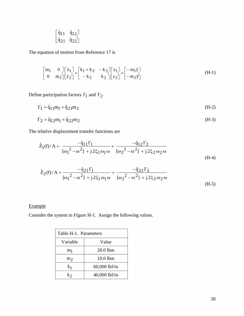
Example
Consider the system in Figure H-1. Assign the following values.
Table H-1. Parameters
Variable Value
1m 20.0 lbm
2m 10.0 lbm
1k 60,000 lbf/in
2k 40,000 lbf/in

31
Furthermore, assume that each mode has a damping value of 5%.
The following parameters were calculated for the sample system via a Matlab script.
Natural Frequencies =
126.2 Hz
268.5 Hz
Modes Shapes (column format) =
-2.823 -3.366
-4.76 3.993
Participation Factors =
-0.2696
-0.07097
Effective Modal Mass =
28.06 lbm
1.944 lbm
Total Modal Mass = 30.0000 lbm
32
0.01
0.1
1
10
100
10 100 1000
Mass 2Mass 1
FREQUENCY (Hz)
TR
AN
S (
G/G
)
ACCELERATION RESPONSE TRANSFER FUNCTION MAGNITUDE
Figure H-1.
The resulting transfer functions were also calculated via a Matlab script.

33
0.00001
0.0001
0.001
0.01
0.1
1 10 100 1000
Mass 1 - Mass 2Mass 2Mass 1
FREQUENCY (Hz)
TR
AN
S (
inch
/G)
RELATIVE DISPLACEMENT TRANSFER FUNCTION MAGNITUDE
Figure H-2.
Table H-2.
Magnitude Values at Fundamental Mode, Frequency = 126.2 Hz
Magnitude Parameter Mass 1 Mass 2
Acceleration Response (G/G) 7.7 12.8
Relative Displacement (inch/G) 0.0047 0.0079
Note that:
Relative Displacement = Acceleration Response / 2
1
This equation is true for the transfer function values, at least for a two-degree-of-freedom system
with well-separated modal frequencies. It will have some error, however, for the response
acceleration and relative displacement overall RMS values, as shown later in this appendix.
34
0.001
0.01
0.1
1
10
100
10 100 1000
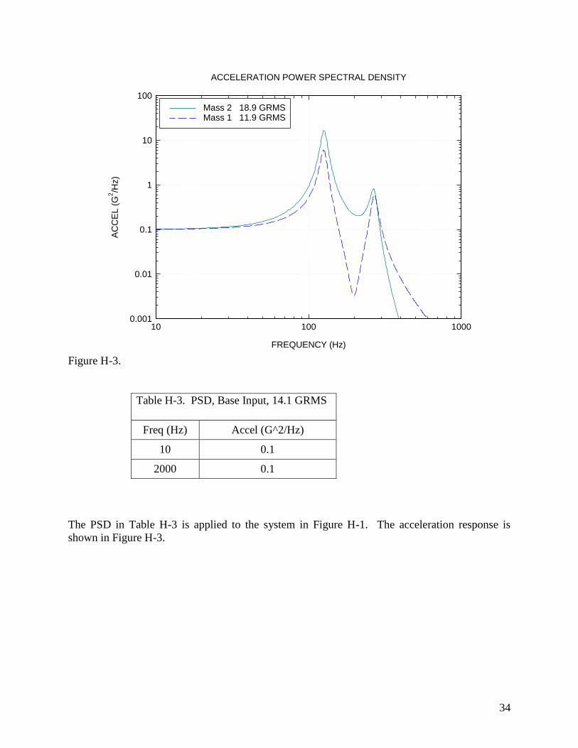
Mass 2 18.9 GRMSMass 1 11.9 GRMS
FREQUENCY (Hz)
AC
CE
L (
G2/H
z)
ACCELERATION POWER SPECTRAL DENSITY
Figure H-3.
Table H-3. PSD, Base Input, 14.1 GRMS
Freq (Hz) Accel (G^2/Hz)
10 0.1
2000 0.1
The PSD in Table H-3 is applied to the system in Figure H-1. The acceleration response is
shown in Figure H-3.
35
10-10
10-9
10-8
10-7
10-6
10-5
10 100 1000
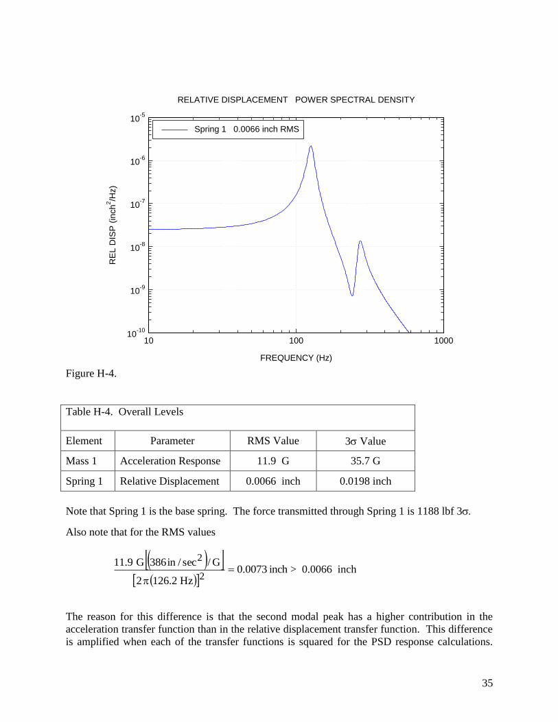
Spring 1 0.0066 inch RMS
FREQUENCY (Hz)
RE
L D
ISP
(in
ch
2/H
z)
RELATIVE DISPLACEMENT POWER SPECTRAL DENSITY
Figure H-4.
Table H-4. Overall Levels
Element Parameter RMS Value 3 Value
Mass 1 Acceleration Response 11.9 G 35.7 G
Spring 1 Relative Displacement 0.0066 inch 0.0198 inch
Note that Spring 1 is the base spring. The force transmitted through Spring 1 is 1188 lbf 3
Also note that for the RMS values
inch0073.0Hz2.1262
G/sec/in386G9.11
2
2
> 0.0066 inch
The reason for this difference is that the second modal peak has a higher contribution in the
acceleration transfer function than in the relative displacement transfer function. This difference
is amplified when each of the transfer functions is squared for the PSD response calculations.
36
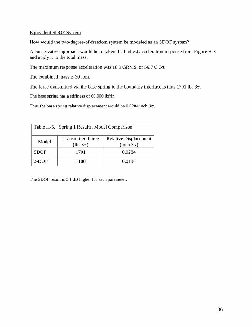
Equivalent SDOF System
How would the two-degree-of-freedom system be modeled as an SDOF system?
A conservative approach would be to taken the highest acceleration response from Figure H-3
and apply it to the total mass.
The maximum response acceleration was 18.9 GRMS, or 56.7 G 3
The combined mass is 30 lbm.
The force transmitted via the base spring to the boundary interface is thus 1701 lbf 3
The base spring has a stiffness of 60,000 lbf/in
Thus the base spring relative displacement would be 0.0284 inch 3.
Table H-5. Spring 1 Results, Model Comparison
Model Transmitted Force
(lbf 3
Relative Displacement
(inch 3
SDOF 1701 0.0284
2-DOF 1188 0.0198
The SDOF result is 3.1 dB higher for each parameter.

37
APPENDIX I
Two-degree-of-Freedom-System, Example 2
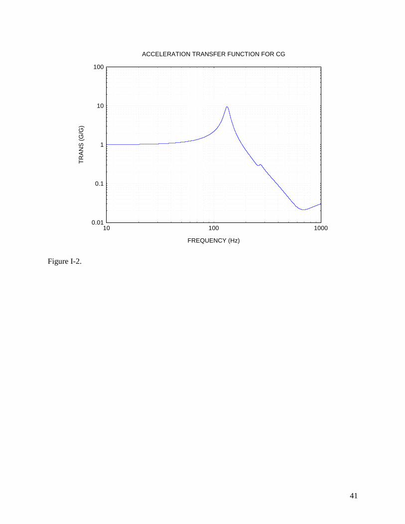
Figure I-1.
The system has a CG offset if 21 LL .
The system is statically coupled if 2211 Lk Lk .
The rotation is positive in the clockwise direction.
k 1 k 2
L1
y
L2
x
k 1 ( y - x - L1 )
) k 2 ( y - x + L2 )
)

38
The variables are
y is the base displacement
x is the translation of the CG
is the rotation about the CG
m is the mass
J is the polar mass moment of inertia
k i is the stiffness for spring i
z i is the relative displacement for spring i
j is the modal damping for mode j
j is the natural frequency (rad/sec) for mode j
is the base excitation frequency
A is the base acceleration amplitude
The mass-normalized eigenvectors in column format are
2221
1211
The equation of motion are taken from Reference 17.
yLk Lk
k k x
Lk Lk Lk Lk
Lk Lk k k x
J0
0m
2211
212
222
112211
221121
(I-1)
The relative displacement for spring 1 is
z1 = z + L1 (I-2)

39
The Fourier transform for the relative displacement in spring 1 is
2222
2
2211221
1122
1
21111111
2j][
qL qq
2j][
qL qqAmZ (I-3)
The relative displacement for spring 2 is
z2 = z - L2 (I-4)
The Fourier transform for the relative displacement in spring 2 is
2222
2
2221221
1122
1
21211112
2j][
qL qq
2j][
qL qqAmZ (I-5)
The Fourier transform for the translational acceleration at the CG is
2222
2
2112
1122
1
2112
a2j][
2j][
qm1AX (I-6)
The Fourier transform for the rotational acceleration is
2222
2
2122
1122
1
21111
2j][
2j][
qqAm (I-7)
40
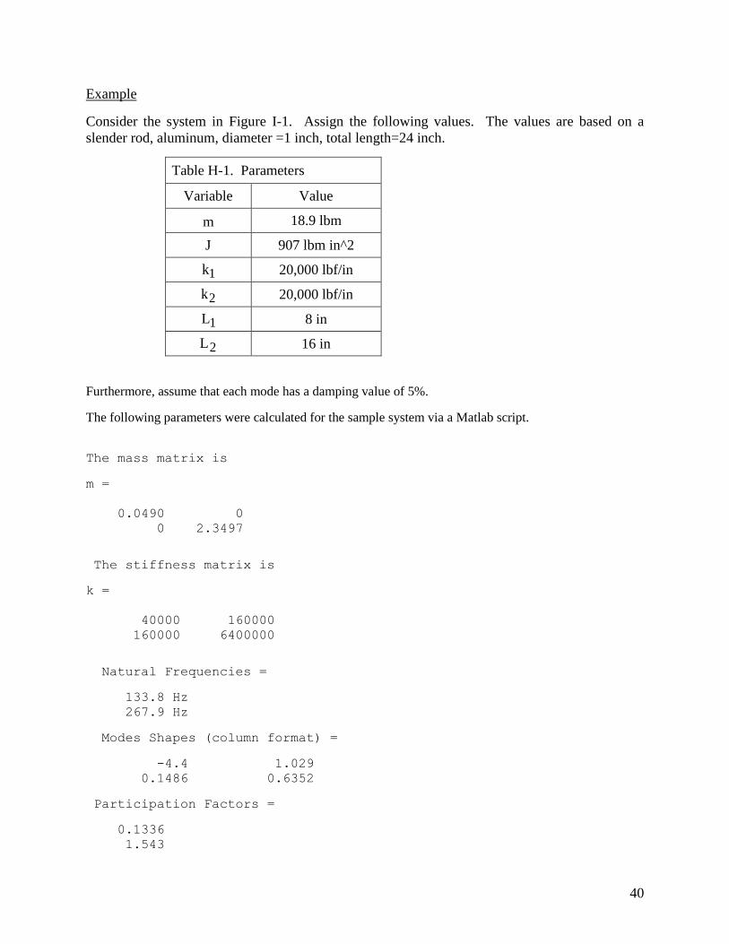
Example
Consider the system in Figure I-1. Assign the following values. The values are based on a
slender rod, aluminum, diameter =1 inch, total length=24 inch.
Table H-1. Parameters
Variable Value
m 18.9 lbm
J 907 lbm in^2
1k 20,000 lbf/in
2k 20,000 lbf/in
1L 8 in
2L 16 in
Furthermore, assume that each mode has a damping value of 5%.
The following parameters were calculated for the sample system via a Matlab script.
The mass matrix is
m =
0.0490 0
0 2.3497
The stiffness matrix is
k =
40000 160000
160000 6400000
Natural Frequencies =
133.8 Hz
267.9 Hz
Modes Shapes (column format) =
-4.4 1.029
0.1486 0.6352
Participation Factors =
0.1336
1.543
41
0.01
0.1
1
10
100
10 100 1000
FREQUENCY (Hz)
TR
AN
S (
G/G
)
ACCELERATION TRANSFER FUNCTION FOR CG
Figure I-2.

42
10-10
10-9
10-8
10-7
10-6
10-5
10 100 1000
Spring 2 0.0095 inch RMSSpring 1 0.0035 inch RMS
FREQUENCY (Hz)
RE
L D
ISP
(in
ch
2/H
z)
RELATIVE DISPLACEMENT POWER SPECTRAL DENSITY
Figure I-3.
43
0.001
0.01
0.1
1
10
10 100 1000
FREQUENCY (Hz)
AC
CE
L (
G2/H
z)
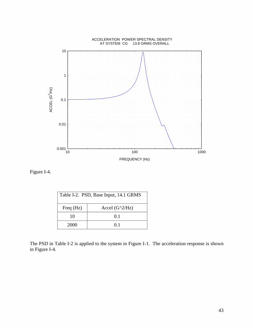
ACCELERATION POWER SPECTRAL DENSITY AT SYSTEM CG 13.8 GRMS OVERALL
Figure I-4.
Table I-2. PSD, Base Input, 14.1 GRMS
Freq (Hz) Accel (G^2/Hz)
10 0.1
2000 0.1
The PSD in Table I-2 is applied to the system in Figure I-1. The acceleration response is shown
in Figure I-4.

44
0.00001
0.0001
0.001
0.01
10 100 1000
Spring 2Spring 1
FREQUENCY (Hz)
TR
AN
S (
inch
/G)
RELATIVE DISPLACEMENT TRANSFER FUNCTIONS
Figure I-5.
Table I-3. Overall Levels, Two-degree-of-freedom Model
Element Parameter RMS Value 3 Value
Mass Acceleration Response 13.8 G 41.4 G
Spring 1 Relative Displacement 0.0035 inch 0.0105 inch
Spring 2 Relative Displacement 0.0095 inch 0.0285 inch
The results in Table I-3 show an error that would occur if the system had been modeled as an
SDOF system with translation only. The spring displacement in this case would have been
0.0065 inches. This would be 3.3 dB less that the Spring 1 displacement in Table I-3.
45
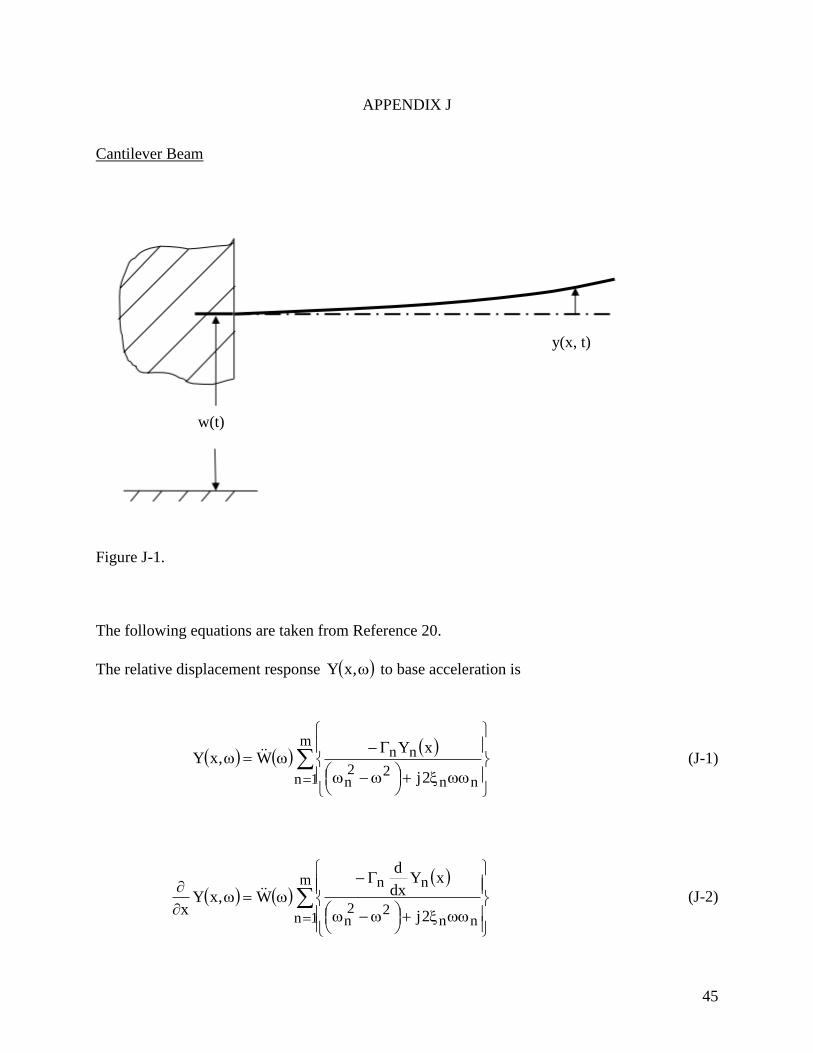
APPENDIX J
Cantilever Beam
Figure J-1.
The following equations are taken from Reference 20.
The relative displacement response ,xY to base acceleration is
m
1n nn22
n
nn
2j
xYW,xY (J-1)
m
1n nn22
n
nn
2j
xYdx
d
W,xYx
(J-2)
y(x, t)
w(t)
46
m
1n nn22
n
n2
2
n
2
2
2j
xYdx
d
W,xYx
(J-3)
The bending moment is
,xY
xEI,xM
2
2
(J-4)
The bending stress is
I
Mc (J-5)
,xY
xcE,x
2
2
(J-6)
m
1n nn22
n
n2
2
n
2j
xYdx
d
WcE,x (J-7)
m
1n nn22
n
n2
2
n
2ff2jff
xYdx
d
4
1fW2cEf,x (J-8)

47
m
1n nn22
n
n2
2
n
ff2jff
xYdx
d
fWcE2
1f,x (J-9)
The bending stress transfer function is
m
1n nn22
n
n2
2
n
sff2jff
xYdx
d
cE2
1
fW
f,x)f,x(H
(J-10)
The eigenvalue roots for the cantilever beam are
Table J-1. Roots
Index n Ln
1 1.875104
2 4.694091
3 7.854575
4 10.99554
The first mode shape and its derivatives are
xsinxsinh73410.0xcosxcoshL
1)x(Y 11111
(J-11)
xcosxcosh73410.0xsinxsinhL
)x(Ydx
d1111
11
(J-12)
xsinxsinh73410.0xcosxcoshL
)x(Ydx
d1111
21
12
2
(J-13)

48
The second mode shape and its derivatives are
xsinxsinh1.01847xcosxcoshL
1)x(Y 22222
(J-14)
xcosxcosh1.01847xsinxsinhL
)x(Ydx
d2222
22
(J-15)
xsinxsinh1.01847xcosxcoshL
)x(Ydx
d2222
22
22
2
(J-16)
The third mode shape and its derivatives are
xsinxsinh0.99922xcosxcoshL
1)x(Y 33333
(J-17)
xcosxcosh0.99922xsinxsinhL
)x(Ydx
d3333
33
(J-18)
xsinxsinh0.99922xcosxcoshL
)x(Ydx
d3333
23
32
2
(J-19)
The fourth mode shape and its derivatives are
xsinxsinh1.00003xcosxcoshL
1)x(Y 44444
(J-20)
xcosxcosh1.00003xsinxsinhL
)x(Ydx
d4444
44
(J-21)
xsinxsinh1.00003xcosxcoshL
)x(Ydx
d4444
24
42
2
(J-22)

49
Example
Consider a beam with the following properties:
Cross-Section Circular
Boundary Conditions Fixed-Free
Material Aluminum
Diameter D = 0.5 inch
Cross-Section Area A = 0.1963 in^2
Length L = 24 inch
Area Moment of Inertia I = 0.003068 in^4
Elastic Modulus E = 1.0e+07 lbf/in^2
Stiffness EI = 30680 lbf in^2
Mass per Volume v = 0.1 lbm / in^3 ( 0.000259 lbf sec^2/in^4 )
Mass per Length = 0.01963 lbm/in (5.08e-05 lbf sec^2/in^2)
Mass L = 0.471 lbm (1.22E-03 lbf sec^2/in)
Viscous Damping Ratio = 0.05
The normal modes and frequency response function analysis are performed via Matlab script:
continuous_base_base_accel.m. The normal modes results are:
Table J-2. Natural Frequency Results, Cantilever Beam
Mode
fn (Hz)
Participation
Factor
Effective
Modal Mass
( lbf sec^2/in )
Effective
Modal Mass
(lbm)
1 23.86 0.02736 0.000748 0.289
2 149.53 0.01516 0.00023 0.089
3 418.69 0.00889 7.90E-05 0.031
4 820.47 0.00635 4.04E-05 0.016
Note that the mode shape and participation factors are considered as dimensionless, but they
must be consistent with respect to one another.

50
0.1
1
10
100
10 100 1000 2000
FREQUENCY (Hz)
[RE
SP
ON
SE
AC
CE
L /
BA
SE
AC
CE
L]
( G
/ G
)
ACCELERATION TRANSFER FUNCTION AT FREE END
Figure J-2.
51
0.00001
0.0001
0.001
0.01
0.1
1
1 10 100 1000 2000
FREQUENCY (Hz)
[ R
EL
DIS
P
/ B
AS
E A
CC
EL
]
( in
ch
/ G
)
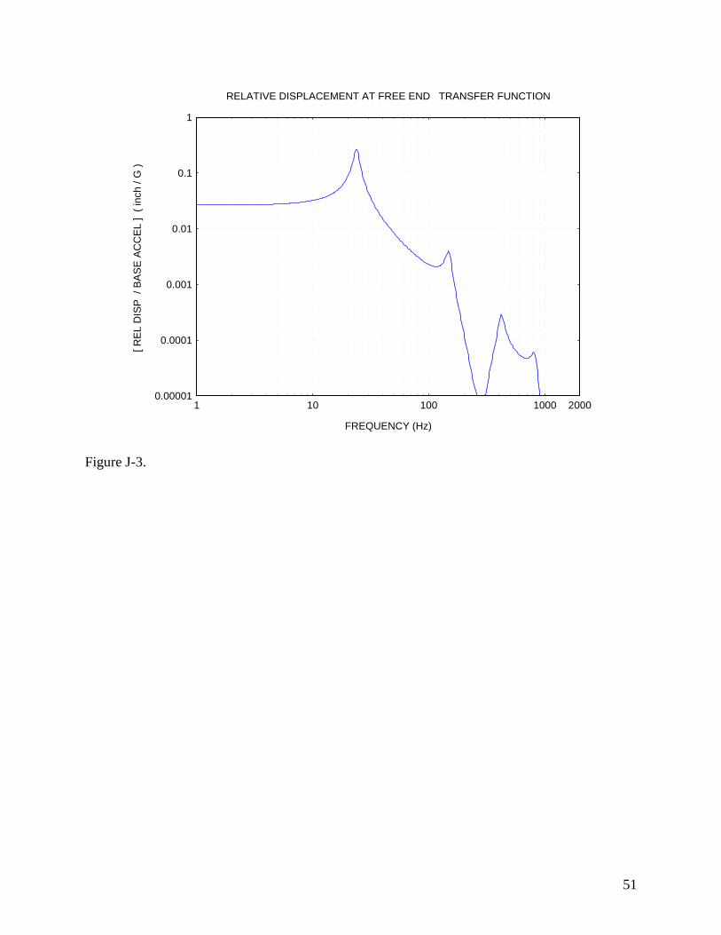
RELATIVE DISPLACEMENT AT FREE END TRANSFER FUNCTION
Figure J-3.
52
0.01
0.1
1
10
100
1 10 100 1000 2000
FREQUENCY (Hz)
[ B
EN
DIN
G M
OM
EN
T /
BA
SE
AC
CE
L ]
(
in lb
f /
G )
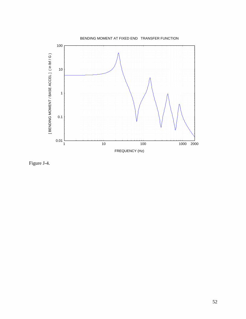
BENDING MOMENT AT FIXED END TRANSFER FUNCTION
Figure J-4.

53
0.001
0.01
0.1
1
10
100
10 100 1000 2000
FREQUENCY (Hz)
AC
CE
L (
G2/H
z)
ACCELERATION PSD AT FREE ENDOverall Level = 24.5 GRMS
Figure J-5.
Table J-3. PSD, Base Input, 14.1 GRMS
Freq (Hz) Accel (G^2/Hz)
10 0.1
2000 0.1
The cantilever beam is subjected to the base input PSD in Table J-3. The resulting response PSD
curves are shown in Figures J-5 through J-7 for selected parameters and locations.

54
10-7
10-6
10-5
10-4
10-3
10-2
10 100 1000 2000
FREQUENCY (Hz)
RE
LA
TIV
E D
ISP
(in
ch
2/H
z)
RELATIVE DISPLACEMENT PSD AT FREE ENDOverall Level = 0.162 inch RMS
Figure J-6.

55
0.00001
0.0001
0.001
0.01
0.1
1
1 10 100 1000 2000
FREQUENCY (Hz)
MO
ME
NT
(i
n lb
f)2/H
z
BENDING MOMENT PSD AT FIXED END Overall Level = 31.1 inch lbf RMS
Figure J-7.
Stress Calculation
Ignore stress concentration factors. Neglect shear stress.
The stress results are given in Table J-4.
Table J-4. Stress and Strain Results at Fixed End
Parameter RMS 3
Bending Moment (in lbf) 31.1 93.3
Bending stress (psi) 2551 7653
micro Strain 255 765
The bending stress is the peak fiber stress for the cross-section at the fixed interface.
56
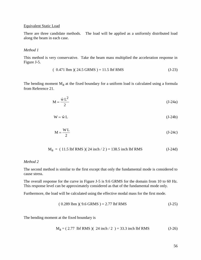
Equivalent Static Load
There are three candidate methods. The load will be applied as a uniformly distributed load
along the beam in each case.
Method 1
This method is very conservative. Take the beam mass multiplied the acceleration response in
Figure J-5.
( 0.471 lbm )( 24.5 GRMS ) = 11.5 lbf RMS (J-23)
The bending moment Ma at the fixed boundary for a uniform load is calculated using a formula
from Reference 21.
2
LwM
2
(J-24a)
LwW (J-24b)
2
LWM (J-24c)
Ma = ( 11.5 lbf RMS )( 24 inch / 2 ) = 138.5 inch lbf RMS (J-24d)
Method 2
The second method is similar to the first except that only the fundamental mode is considered to
cause stress.
The overall response for the curve in Figure J-5 is 9.6 GRMS for the domain from 10 to 60 Hz.
This response level can be approximately considered as that of the fundamental mode only.
Furthermore, the load will be calculated using the effective modal mass for the first mode.
( 0.289 lbm )( 9.6 GRMS ) = 2.77 lbf RMS (J-25)
The bending moment at the fixed boundary is
Ma = ( 2.77 lbf RMS )( 24 inch / 2 ) = 33.3 inch lbf RMS (J-26)

57
Method 3
The third method finds an equivalent load so that the static and dynamic relative displacements
match at the free end. The dynamic relative displacement is taken from Figure J-6.
Let Y be the relative displacement. The distributed load W per Reference 21 is
RMS)in/lbf(120.0
)in24(
RMSin162.0in^2 lbf 306808
L
YEI8W
44 (J-27)
The corresponding bending moment at the fixed boundary is
Ma = [ RMS)in/lbf(120.0 ] [ 24 inch]^2 / 2 = 34.5 inch lbf RMS (J-28)
Summary
Table J-5. Results Comparison RMS Values, Fixed End
Parameter
Modes
Included
Bending
Moment
(in lbf)
Bending
Stress
(lbf/in^2)
micro
Strain
Static Method 1, Accel 4 138.5 11,284 1128
Static Method 2, Accel 1 33.3 2713 271
Static Method 3, Relative Disp. 4 34.5 2811 281
Dynamic Analysis 4 31.1 2551 255
Methods 2 and 3 agree reasonably well with the dynamic results for each of the respective
parameters.
58
APPENDIX K
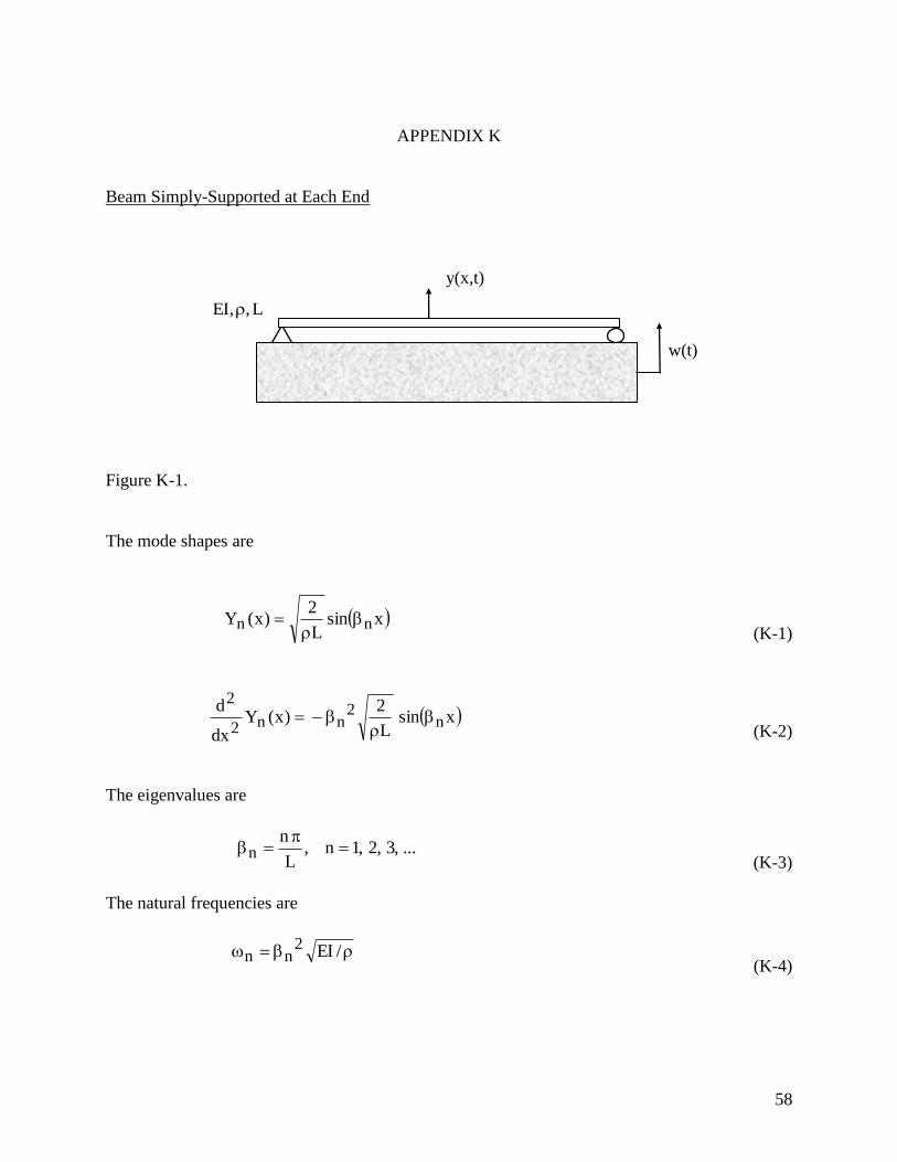
Beam Simply-Supported at Each End
Figure K-1.
The mode shapes are
xsinL
2)x(Y nn
(K-1)
xsinL
2)x(Y
dx
dn
2nn2
2
(K-2)
The eigenvalues are
...,3,2,1n,L
nn
(K-3)
The natural frequencies are
/EI2nn
(K-4)
L,,EI
w(t)
y(x,t)
59
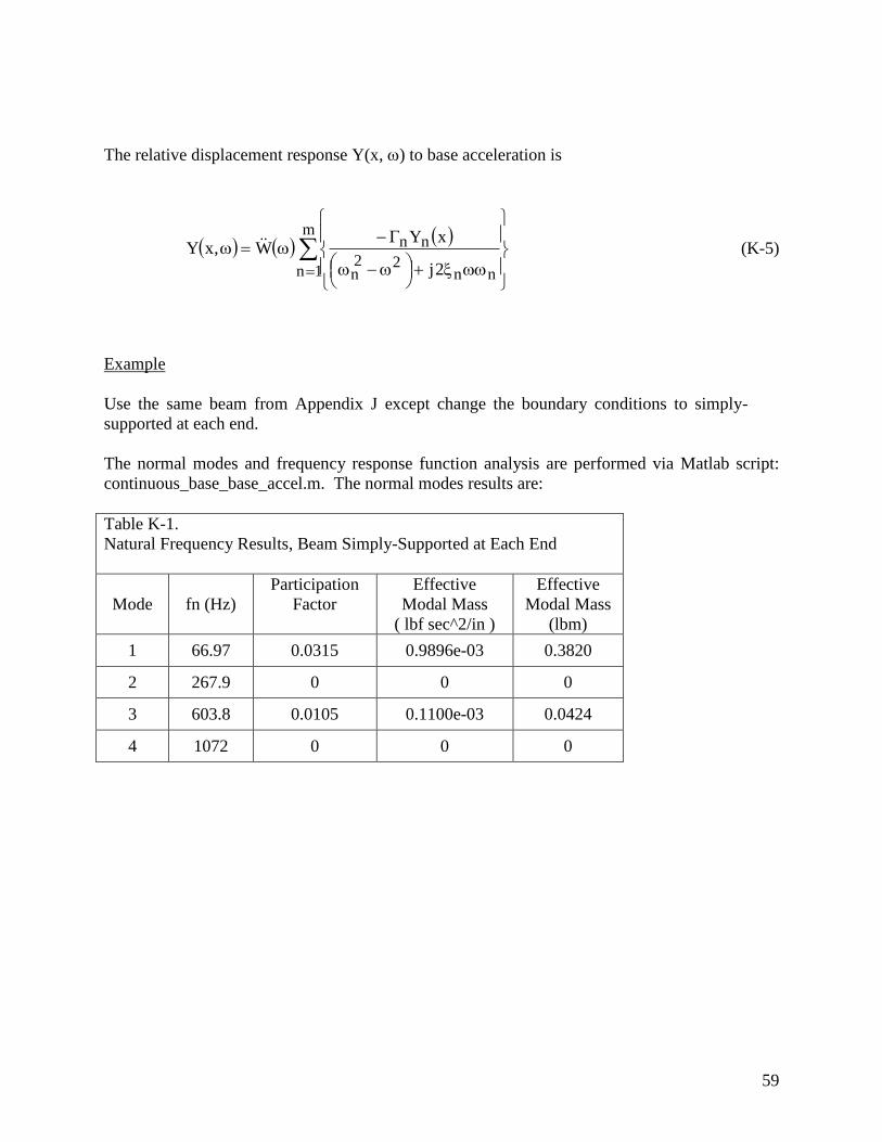
The relative displacement response Y(x, ) to base acceleration is
m
1n nn22
n
nn
2j
xYW,xY (K-5)
Example
Use the same beam from Appendix J except change the boundary conditions to simply-
supported at each end.
The normal modes and frequency response function analysis are performed via Matlab script:
continuous_base_base_accel.m. The normal modes results are:
Table K-1.
Natural Frequency Results, Beam Simply-Supported at Each End
Mode
fn (Hz)
Participation
Factor
Effective
Modal Mass
( lbf sec^2/in )
Effective
Modal Mass
(lbm)
1 66.97 0.0315 0.9896e-03 0.3820
2 267.9 0 0 0
3 603.8 0.0105 0.1100e-03 0.0424
4 1072 0 0 0

60
0.01
0.1
1
10
100
1 10 100 1000 2000
FREQUENCY (Hz)
[ B
EN
DIN
G M
OM
EN
T /
BA
SE
AC
CE
L ]
(
in lb
f /
G )
BENDING MOMENT AT x = 0.5 L TRANSFER FUNCTION
Figure K-2.

61
0.1
1
10
100
1 10 100 1000 2000
FREQUENCY (Hz)
[ R
ES
PO
NS
E A
CC
EL
/ B
AS
E A
CC
EL
] (
G/G
)
ACCELERATION at x=0.5 L TRANSFER FUNCTION
Figure K-3.

62
0.00001
0.0001
0.001
0.01
0.1
1 10 100 1000 2000
FREQUENCY (Hz)
[ R
EL
DIS
P
/ B
AS
E A
CC
EL
]
( in
ch
/ G
)
RELATIVE DISPLACEMENT AT x = 0.5 L TRANSFER FUNCTION
Figure K-4.
63
0.001
0.01
0.1
1
10
100
10 100 1000 2000
FREQUENCY (Hz)
AC
CE
L (
G2/H
z)
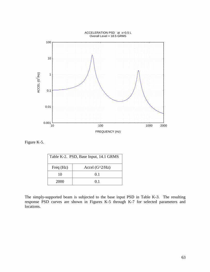
ACCELERATION PSD at x=0.5 LOverall Level = 18.5 GRMS
Figure K-5.
Table K-2. PSD, Base Input, 14.1 GRMS
Freq (Hz) Accel (G^2/Hz)
10 0.1
2000 0.1
The simply-supported beam is subjected to the base input PSD in Table K-3. The resulting
response PSD curves are shown in Figures K-5 through K-7 for selected parameters and
locations.

64
10-9
10-8
10-7
10-6
10-5
10-4
10 100 1000 2000
FREQUENCY (Hz)
RE
L D
ISP
(i
nch
2/H
z)
RELATIVE DISPLACEMENT PSD AT x = 0.5 L Overall Level = 0.028 inch RMS
Figure K-6.

65
0.001
0.01
0.1
1
10
100
10 100 1000 2000
FREQUENCY (Hz)
MO
ME
NT
(i
n lb
f)2/H
z
BENDING MOMENT PSD AT x = 0.5 L Overall Level = 14.9 inch lbf RMS
Figure K-7.
66
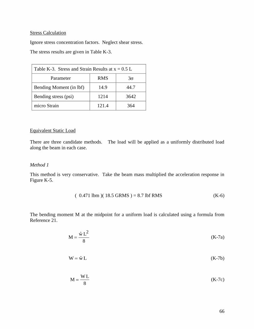
Stress Calculation
Ignore stress concentration factors. Neglect shear stress.
The stress results are given in Table K-3.
Table K-3. Stress and Strain Results at x = 0.5 L
Parameter RMS 3
Bending Moment (in lbf) 14.9 44.7
Bending stress (psi) 1214 3642
micro Strain 121.4 364
Equivalent Static Load
There are three candidate methods. The load will be applied as a uniformly distributed load
along the beam in each case.
Method 1
This method is very conservative. Take the beam mass multiplied the acceleration response in
Figure K-5.
( 0.471 lbm )( 18.5 GRMS ) = 8.7 lbf RMS (K-6)
The bending moment M at the midpoint for a uniform load is calculated using a formula from
Reference 21.
8
LwM
2
(K-7a)
LwW (K-7b)
8
LWM (K-7c)

67
inch24RMSlbf 8.78
1M
= 26.1 inch lbf RMS (K-7d)
Method 2
The second method is similar to the first except that only the fundamental mode is considered to
cause stress.
The overall response for the curve in Figure K-5 is 13.0 GRMS for the domain from 10 to 200
Hz. This response level can be approximately considered as that of the fundamental mode only.
Furthermore, the load will be calculated using the effective modal mass for the first mode.
( 0.382 lbm )( 13.0 GRMS ) = 5.0 lbf RMS (K-8)
The bending moment for a uniform load at the midpoint is
inch24RMS0.58
1
8
LWM
= 15 inch lbf RMS (K-9)
Method 3
The third method finds an equivalent load so that the static and dynamic relative displacements
match at the free end. The dynamic relative displacement is taken from Figure K-6.
Let Y be the relative displacement. The distributed load w per Reference 21 is
RMS)in/lbf(199.0
)in24(5
RMSin028.0in^2 lbf 30680384
L5
YEI384w
44 (K-10)
The corresponding bending moment at the midpoint is
22
inch24RMS)in/lbf(199.08
1
8
LwM
(K-11a)
lbfin3.14M (K-11b)

68
Summary
Table K-4. Results Comparison RMS Values, at x = 0.5 L
Parameter
Modes
Included
Bending
Moment
(in lbf)
Bending
Stress
(lbf/in^2)
micro
Strain
Static Method 1, Accel 4 26.1 2130 213.0
Static Method 2, Accel 1 15.0 1222 122.2
Static Method 3, Relative Disp. 4 14.3 1165 116.5
Dynamic Analysis 4 14.9 1214 121.4
Again, Methods 2 and 3 agree reasonably well with the dynamic results for each of the
respective parameters.
69
APPENDIX L
Material Stress Limits
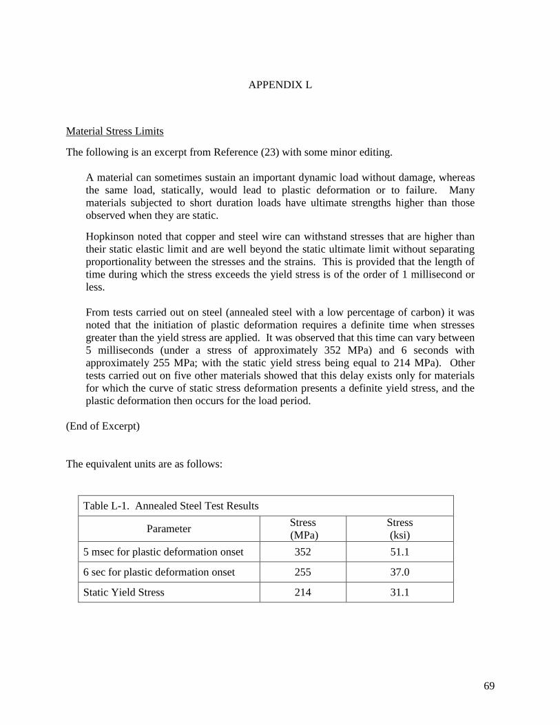
The following is an excerpt from Reference (23) with some minor editing.
A material can sometimes sustain an important dynamic load without damage, whereas
the same load, statically, would lead to plastic deformation or to failure. Many
materials subjected to short duration loads have ultimate strengths higher than those
observed when they are static.
Hopkinson noted that copper and steel wire can withstand stresses that are higher than
their static elastic limit and are well beyond the static ultimate limit without separating
proportionality between the stresses and the strains. This is provided that the length of
time during which the stress exceeds the yield stress is of the order of 1 millisecond or
less.
From tests carried out on steel (annealed steel with a low percentage of carbon) it was
noted that the initiation of plastic deformation requires a definite time when stresses
greater than the yield stress are applied. It was observed that this time can vary between
5 milliseconds (under a stress of approximately 352 MPa) and 6 seconds with
approximately 255 MPa; with the static yield stress being equal to 214 MPa). Other
tests carried out on five other materials showed that this delay exists only for materials
for which the curve of static stress deformation presents a definite yield stress, and the
plastic deformation then occurs for the load period.
(End of Excerpt)
The equivalent units are as follows:
Table L-1. Annealed Steel Test Results
Parameter Stress
(MPa)
Stress
(ksi)
5 msec for plastic deformation onset 352 51.1
6 sec for plastic deformation onset 255 37.0
Static Yield Stress 214 31.1

70
Dynamic Strength
Reference 26 notes:
As far as steels and other metals are concerned, those with lower yield strength are
usually more ductile than higher strength materials. That is, high yield strength
materials tend to be brittle. Ductile (lower yield strength) materials are better able to
withstand rapid dynamic loading than brittle (high yield strength) materials.
Interestingly, during repeated dynamic loadings low yield strength ductile materials
tend to increase their yield strength, whereas high yield strength brittle materials tend to
fracture and shatter under rapid loading.
Reference 26 includes the following table where the data was obtained for uniaxial testing using
an impact method.
Dynamic Strengthening of Materials
Material Static Strength
(psi)
Dynamic Strength
(psi)
Impact Speed
(ft/sec)
2024 Al (annealed) 65,200 68,600 >200
Magnesium Alloy 43,800 51,400 >200
Annealed Copper 29,900 36,700 >200
302 Stainless Steel 93,300 110,800 >200
SAE 4140 Steel 134,800 151,000 175
SAE 4130 Steel 80,000 440,000 235
Brass 39,000 310,000 216
Related Documents


![EQUIVALENT STATIC WIND LOADS ON TALL BUILDINGSbbaa6.mecc.polimi.it/uploads/validati/eb09.pdf · to each floor as proposed in Ref. [2], [3] and [4]. The equivalent static wind loads](https://static.cupdf.com/doc/110x72/5f0543a07e708231d4121947/equivalent-static-wind-loads-on-tall-to-each-ioor-as-proposed-in-ref-2-3.jpg)