EquityGiltStudy 2012 onebrandlwmconsultants.com/wp-content/uploads/2013/09/20130221-Barclays... · We have calculated three indices: changes in the capital value of each asset class;

PLEASE SEE ANALYST CERTIFICATION(S) AND IMPORTANT DISCLOSURES ON THE LAST PAGE.

Cover

“Without a measureless and perpetual uncertainty, thedrama of human life would be destroyed”Winston Churchill

“Reform is China’s second revolution”Deng Xiaoping

“Investing should be more like watching paint dry orwatching grass grow. If you want excitement, take $800and go to Las Vegas”Paul Samuelson

“All progress is based upon a universal innate desire on thepart of every living organism to live beyond its income”Samuel Butler

“I am not worried about the deficit. It is big enough to takecare of itself”Ronald Reagan

“Things do not happen. Things are made to happen”John F. Kennedy

“How much easier it is to be critical than to be correct”Benjamin Disraeli

Published by Barclays21 February 2013ISBN 978-0-9570088-1-6£100

Inside front cover

Barclays | Equity Gilt Study

21 February 2013 1

EQUITY GILT STUDY 2013

58th Edition The Equity Gilt Study has been published continuously since 1956, providing data, analysis and commentary on long-term asset returns in the UK and US. This publication provides a uniquely long and consistent database: the UK data go back to 1899, while the US data – provided by the Centre for Research in Security Prices at the University of Chicago – begin in 1925. We have also used the Equity Gilt Study as an opportunity to analyze medium- to long-term market trends.

Chapter 1 revisits the analysis of investment returns that appeared in last year's edition to account for the huge (roughly 20%) rally in global equities that has occurred since then. This performance can be attributed at least in part to the reduction in negative tail risks left over from the last crisis. With lower volatility having already been priced in, equity returns over the next five years are also expected to be lower – in the 3-4% range – than we had been anticipating previously and well below historic norms. Even so, returns on equities are likely to easily beat those on cash and bonds, both of which we expect to be negative in inflation-adjusted terms. The continuation of extraordinarily easy monetary policy should keep nominal returns on cash negligible, and the eventual normalization of monetary policy is expected to render returns on bonds even lower than cash.

Chapter 2 revisits last year’s theme that the prices of safe haven assets have been elevated because of the structural decrease in their supply. This time, we look at the structural demand for these assets, and find that it is likely to remain strong, reflecting banks' adjustments to new regulations and the behavior of investors in countries with ageing populations. As a result, the so-called “Great Rotation” out of bonds into equities is not likely to be as dramatic as many people think, and bond yields should remain low relative to historic norms.

Chapter 3 asks whether China can sustain economic growth and avoid the “middle income trap” that occurs when a developing country reaches middle income but is thwarted by rising wages and falling cost competitiveness on the one hand, and a lack of skills and innovation on the other. We argue that it can: the Chinese economy is in the middle of a major and broad-based structural transformation that will lead the country to slower but more sustainable growth. While the path is not without significant risks, our base case is that China will reach high-income status over the next decade or so.

Chapter 4 focuses on the risks associated with the extraordinary loose monetary policies of the major central banks since the onset of the financial crisis. Beyond the risk of high inflation, asset price bubbles and stagnant productivity resulting from the propping up of “zombie” companies could also emerge if extreme monetary accommodation is maintained for too long. The authorities will have to act deftly to ensure these risks from QE are contained.

Chapter 5 considers the portfolio implications of the new bond regime discussed in Chapters 1 and 2, taking as a starting point the assumption that the strong bond returns of the past 30 years are probably behind us.

We sincerely hope that you find the data and the essays interesting and enlightening, as well as useful inputs to your investment decisions.

Larry Kantor Head of Research, Barclays

Website: Equity Gilt Study on www.barclays.com E-mail: [email protected]

Barclays | Equity Gilt Study

21 February 2013 2

CONTENTS

Chapter 1 Low risk, low return 4 Although we cannot be sure that another financial crisis is not lurking around the corner, we think the ‘tail risks’ associated with the last crisis are probably behind us. When thinking about medium-term valuations and formulating expectations of investment returns, we think investors should, for now, work with a low-volatility base case, analogous to the 2003-07 ‘inter-crisis’ period of low volatility. In the next five years, we think the investment environment will be driven by two transitions. The eventual normalization of monetary conditions and China’s transition from economic ‘miracle’ to normal development could put downward pressure on equity returns. With valuations supported by a lower-risk environment and interest rates still at rock bottom, investors should expect lower returns. Over the next five years, we expect cash to provide inflation-adjusted returns of about -1.5% pa, ‘safe haven’ government bonds about -2%, and equities 3-4%. The implied equity risk premium remains in a historically normal 500-600bp range. Equities remain the most promising option for investors seeking positive, inflation-adjusted returns, and the main market risk seems to be that a migration to equities causes valuations to outrun fundamentals. But we are not there yet.

Chapter 2 Demand for safe havens to remain robust 16 Following on from the Equity Gilt Study 2012, in which we argued that conventional measures of the equity risk premium appeared elevated mainly because the structural decrease in the supply of risk-free assets had resulted in unusually low risk-free bond yields, we turn to the role of demand for safe-haven assets. We examine three sources of demand for such assets: official-sector demand via the investment of international reserve portfolios; institutional demand in a post-crisis era of tighter bank regulation; and private demand, particularly from an aging population across the developed world. We look for US institutional demand and the rotation of boomer investors into bonds to make up for some of the relative decline in demand from official sources, including our expectation of diminishing reserve accumulation in China. We conclude that structural demand for safe havens is likely to remain high and, when combined with the structural scarcity of such assets, is likely to keep interest rates on safe assets low by comparison with historical norms and conventional measures of the equity risk premium elevated.

Chapter 3 Can China avoid the middle-income trap? 35 Can China continue to grow while avoiding the ‘middle-income trap’ that occurs when a developing country fails to upgrade to high income status as a result of a lack of competitiveness and innovation? We believe that China should be able to reach high-income status over the next decade or so by narrowing its technological gap with advanced economies. Long-awaited structural improvements, including a narrowing of the current account surplus, a growing contribution of consumption to GDP and declining inequality, are already under way, but may be underappreciated by investors. In our view, political reform will be necessary to sustain economic growth in China, but we do not think current political institutions have exhausted the country’s growth potential yet. Science and technology have taken off much earlier in China relative to the experience of other emerging Asia economies. Although China’s economy faces many risks, we believe that it is unlikely to collapse, even though it may continue to look different from western advanced economies.

Barclays | Equity Gilt Study

21 February 2013 3

Chapter 4 QE carries risks beyond inflation 54 To a large extent, QE is a symptom rather than a cause of the economy’s underlying woes. Although it need not lead to high inflation, the latter may result from an increased tolerance of inflation in the face of stagnant real economic growth. The US and the UK appear most vulnerable to these pressures. Extraordinarily low yields on government bonds might push investors into riskier assets, but widespread uncertainty and strong savings intentions have so far prevented bubbles from arising. However, it remains to be seen whether the new macroprudential policy frameworks will be effective enough to stop damaging distortions from developing. Accommodative monetary policy and excessive forbearance by banks enable the survival of relatively weak companies that would otherwise be forced out of business, resulting in impaired productivity growth. We see the risk of structural degeneration as higher in Europe than in the US.

Chapter 5 Scenarios for a shifting bond landscape 67 Financial markets appear to be at a transitional point. Following on from the “Great Moderation” and the “Great Recession”, there now seems to be a debate over the next “Great” theme. The strong bond returns of the past 30 years are likely over. Against this backdrop, we analyse various financial scenarios and examine the implications for different investors.

Chapter 6 UK asset returns since 1899 75 We analyse returns on equities, gilts and cash from end-1899 to end-2012. Equity markets performed well in 2012, rallying by 13.4%, despite turbulent market conditions. Nominal and inflation-linked gilt yields were much weaker relative to 2011. Gilts, along with Bunds and Treasuries, had benefited from the flight-to-quality flows during 2011 and the first half of 2012. However, the introduction of the OMT helped to reduce the tail risks associated with Europe and encouraged investors to move out of safe havens into riskier assets. Corporate bonds benefited from this trend last year and generated a 12% real return, compared with just 1.6% in 2011.

Chapter 7 US asset returns since 1925 80 Equities were the best-performing assets of 2012, producing a 14.1% real total return, despite following a turbulent path similar to that of UK and European markets. Treasury returns were weaker in 2012, just 2%, compared with 22.5% in 2011. TIPS outperformed Treasuries by 8% as inflation expectations rose. Breakevens widened against the backdrop of dovish monetary policy and improved market liquidity. Corporate bonds also performed well as investors moved out of safe havens, increasing their risk exposure.

Chapter 8 Barclays indices 84 We have calculated three indices: changes in the capital value of each asset class; changes to income from these investments; and a combined measure of the overall return, on the assumption that all income is reinvested.

Chapter 9 Total investment returns 107 We present a series of tables showing the performance of equity and fixed-interest investments over any period of years since December 1899.

Barclays | Equity Gilt Study

21 February 2013 4

CHAPTER 1

Low risk, low return • Although we cannot be sure that another financial crisis is not lurking around the

corner, we think the ‘tail risks’ associated with the last crisis are probably behind us. When thinking about medium-term valuations and formulating expectations of investment returns, we think investors should, for now, work with a low-volatility base case, analogous to the 2003-07 ‘inter-crisis’ period of low volatility.

• In the next five years, we think the investment environment will be driven by two transitions. The eventual normalization of monetary conditions and China’s transition from economic ‘miracle’ to normal development could put downward pressure on equity returns.

• With valuations supported by a lower-risk environment and interest rates still at rock bottom, investors should expect lower returns. Over the next five years, we expect cash to provide inflation-adjusted returns of about -1.5% pa, ‘safe haven’ government bonds about -2%, and equities 3-4%. We see no reason to believe that high-grade credit will outperform.

• The implied equity risk premium remains in a historically normal 500-600bp range. Equities remain the most promising option for investors seeking positive, inflation-adjusted returns, and the main market risk seems to be that a migration to equities causes valuations to outrun fundamentals. But we are not there yet.

Diminished ‘tail risks’: A double-edged sword The collapse in asset-market volatility is a double-edged sword. On the one hand, it signals a genuine reduction in the tail risks of a globally destabilizing economic/financial event. This is a great relief for investors who have had to endure the anxiety created by such risks for several years. On the other hand, investors are ultimately paid to take risk, and without the wall of worry, what kind of rewards can they expect risky assets to yield? In this chapter, we offer some thoughts on the returns that may be on offer in the main asset classes, in the more tranquil financial environment that investors are likely to face in the immediate future. We extend previous work (including, in particular, “The equity risk premium: Cheap equity or expensive bonds?” Equity Gilt Study 2012) in the following ways.

Michael Gavin +1 212 412 5915 [email protected]

Piero Ghezzi +44 (0)20 3134 2190

[email protected]

FIGURE 1 A less volatile world

FIGURE 2 Equity returns tend to be low when interest rates are low

0

10

20

30

40

50

60

70

80

90

100

Dec-01 Dec-03 Dec-05 Dec-07 Dec-09 Dec-11

VIX V2X

0.0

1.0

2.0

3.0

4.0

5.0

6.0

7.0

8.0

-4.0 -3.0 -2.0 -1.0 0.0 1.0 2.0

Average real interest rate (% pa)

Long-term real equity return (% pa)

Source: Bloomberg Source: Elroy Dimson, Paul Marsh, and Mike Staunton, “Equity Premia around

the World”, manuscript, London School of Business, Oct 2011.

Barclays | Equity Gilt Study

21 February 2013 5

• We update our assessment of the outlook for investment returns to account for the substantial rally in global equities and the (more modest and more recent) selloff in ‘safe haven’ bond markets that market participants have enjoyed since early 2012. The roughly 18% rally in global equity prices that has occurred since the early days of 2012 amounts to a few years of the ‘steady-state’ equity appreciation that we deemed plausible in our assessment last year. It would be surprising if a forward-looking assessment of investment returns were untouched by a rally of this magnitude.

• We focus on a more concrete five-year investment horizon, rather than the less well defined ‘long run’ focus that we adopted last year.

• Finally, we embed in our thinking the assumption that the next five years are likely to be an ‘inter-crisis’ interlude, analogous in some ways to the 2003-07 period of low volatility between the collapse of the global equity bubble and the (even) more damaging collapse of the subsequent housing and credit bubble. Of course, five years is a long time and we cannot pretend to know that the coming half-decade will be untouched by economic or financial crisis. The spirit of our assumption is that a new crisis is far enough off that, for the next couple of years, investors will be able to make decisions mainly on the basis of considerations other than whether one ‘tail risk’ or another may be about to materialize.

Even if the next five years will be tranquil, they will be far from uneventful. We highlight two transitions that that we expect to be powerful drivers of asset markets over the next five years or so. The first is a likely normalization of monetary conditions, which should be reasonably far along, although most likely not complete, five years from now. The second is China’s transition to a new and qualitatively different development trajectory. This transition has been under way for some time, but has mainly been discussed within a Chinese national context (see Chapter 3, “Can China avoid the middle-income trap?” in this publication). We think that the integration of emerging market workers (including, most notably, Chinese workers) into the global labor force has been an extraordinarily powerful driver of employment, earnings, and asset prices around the world. It stands to reason that the transformation of the Chinese development trajectory could have equally powerful effects.

Can bonds earn more than cash? The 30-year bull market in what we now consider ‘safe haven’ government bonds probably reached a high-water mark in 2012, and investors in those bond markets are unlikely to continue to enjoy the combination of equity-like returns and bond-market volatility that they enjoyed during the boom. We agree with this consensus view, but also believe that the bull market in bonds is much more likely to end in a drawn-out whimper than in a 1994-style bond-market ‘bang’. There is nothing in the existing market context comparable to the leverage that contributed to the turmoil in 1994. Monetary authorities in the systemically important currencies are likely to keep the monetary floodgates open for many months to come and would likely use all the considerable means at their disposal to fend off any bond market selloff large enough to threaten the still-lacklustre economic recovery. Moreover, the global shortage of safe assets is unlikely to be materially narrowed in the coming decade, which does not mean that yields will never rise from current levels, but does mean that a persistent bid is likely to keep ‘safe haven’ bond prices elevated relative to historical norms (see “The equity risk premium: Cheap equities or expensive bonds?”, Equity Gilt Study 2012, and “Demand for safe havens to remain robust”, Chapter 2 in this publication).

Cash is likely to remain a value destroyer, in real terms If we want an estimate of the equity risk premium, we need a more quantitative assessment of the return on cash and bonds over our five-year investment horizon. The logical starting point is the yield curve. In the US, UK and euro area, government bond markets are pointing to a gradual normalization of monetary conditions over the coming years (Figure 3), but in all cases the normalization is expected to be incomplete

The 30-year bull market in ‘safe haven’ government bonds probably reached a high-water mark in 2012

Government bond markets point to a gradual normalization of monetary conditions over the coming years

Barclays | Equity Gilt Study

21 February 2013 6

by the end of our five-year investment horizon. In the US, for example, the 5y forward 1y interest rate (the yield curve’s interest-rate ‘forecast’ for 2018) is less than 2.5%, and the inflation-protected (TIPs) forward curve remains negative through 2018.

Figure 4 puts these forward rates into a US historical perspective and Figure 5 provides similar computations for GBP, EUR, and JPY interest rates. For our present purpose (which does not include a detailed analysis of relative value among these markets), the USD, GBP and EUR curves tell essentially the same story as in the US. Japan, where forward interest rates remain low for years to come and where the bond market outlook mainly reflects questions surrounding the recent turn toward more stimulative fiscal and monetary policies, is a case apart.

These forward rates are (by definition) the sum of the expected future rate and the term risk premium that the market attaches to owning bond duration rather than holding cash. For reasons discussed below, we believe that the term premium is low for short-duration bonds and that the expected return on cash over our five-year investment horizon is close to the average of the forward rates. The latter is (by construction) equivalent to the return on a 5y bond, which is on the order of 0.5-1% in the US, UK and euro area. After adjusting for expected inflation, a plausible value for the expected return on cash is thus something like -1.5%, though arguably lower in the UK and higher in the euro area.

FIGURE 3 The US yield curve implies a very gradual normalization…

FIGURE 4 …but real rates are projected to stay negative for 5 more yrs

0.0%

0.5%

1.0%

1.5%

2.0%

2.5%

3.0%

3.5%

4.0%

4.5%

2013 2015 2017 2019 2021

UST forward 1y interest rates

-10

-5

0

5

10

15

20

Apr-53 Apr-63 Apr-73 Apr-83 Apr-93 Apr-03 Apr-13

Nominal Real rate Note: Forward curve as of 2/15/2013. Source: Bloomberg, Barclays Research

Note: 1y US Treasury rates. Forecasts are from the UST nominal and TIPs curves. Source: Haver Analytics, Bloomberg, Barclays Research

FIGURE 5 Forward interest rates in the main reserve currencies

US UK Germany Japan

1y rates

Spot 0.15% 0.31% 0.06% 0.07%

1y forward 0.39% 0.32% 0.32% -0.02%

2y forward 0.70% 0.44% 0.44% 0.10%

3y forward 1.31% 1.28% 1.01% 0.23%

4y forward 1.76% 2.52% 1.47% 0.34%

5y forward 2.38% 2.54% 1.56% 0.67%

5y rates

spot 0.86% 0.97% 0.66% 0.14%

5y forward 3.16% 3.43% 2.66% 1.37%

10y forward 3.77% 3.96% 2.97% 2.25%

Source: Bloomberg, Barclays Research

Barclays | Equity Gilt Study

21 February 2013 7

Bond duration unlikely to provide an escape from low rates Except in the extremely unlikely event of a default, a 10y government bond will yield exactly 2.00%, 2.19%, and 1.65% if issued (in their own currency) by the US, UK and German government, respectively, and if the bond is held a full 10 years to maturity. But the hold-to-maturity thought experiment implicit in these yield-to-maturity calculations is not useful for most investors. More relevant is the return on bond duration over a given investment horizon. For the sake of concreteness, we ask what return to expect from maintaining exposure to bond duration for the coming five years equivalent to the duration embedded in the current 10y bond.

When interest rates are trending (lower in the past 30 years and likely higher in the next five), the holding period return is unlikely to match the yield to maturity. Even over long periods, this is no footnote. From 1982 to 2012, for example, continued exposure to the current 10y US Treasury bond would have yielded an investor 8.5% pa, more than 200bp above the average yield to maturity (6.4%) for those 10 years. This excess return was largely a windfall created by a decline in market interest rates beyond the wildest dreams of a typical bond investor circa 1982. Looking ahead, the problem is an anticipated increase in market rates.

Conceptually, the expected return on bonds can be expressed as the expected return on cash, plus the term risk premium that investors require as payment to own duration, which comes with mark-to-market volatility, rather than cash, which does not. This does not get us as far as we would like, because there is no consensus on the size or the term risk premium or even on whether it is positive or negative. Academic research has used a wide variety of economically-based and non-structural models to compute estimates of the yield curve, but there remains room for disagreement.

One prominent model of the term risk premium shows a strong decline since the early 1990s and a negative premium in the past couple of years (Figure 6). These estimates are based upon a purely statistical approach that does not embed specific financial-economic assumptions. But the decline of the estimated term risk premium coincides with a strong decline in the correlation between market returns on government bonds and equity risk, which turned negative around the year 2000, a ‘safe haven’ correlation that has been particularly prominent in the past couple of years (Figure 7). Figure 8 compares the ‘safe haven’ properties of safe EUR, GBP and JPY-denominated government bonds to those of the US. German and UK government bonds display strong ‘safe haven’ properties, although not as strong as US Treasuries. Japanese government bonds display a smaller ‘safe haven’ correlation. Figure 8 also shows that longer-duration bonds have had stronger ‘safe haven’ properties than shorter duration bonds.

In 1982-2012, continued exposure to the current 10y US Treasury bond would have yielded an investor 8.5% pa, more than 200bp higher than the average yield to maturity (6.4%) for those 10 years

FIGURE 6 Kim-Wright model of the US term risk premium

FIGURE 7 US Treasury beta to S&P 500

-1.5

-1.0

-0.5

0.0

0.5

1.0

1.5

2.0

2.5

3.0

3.5

Jul-90 Jul-94 Jul-98 Jul-02 Jul-06 Jul-10

10-year UST term risk premium (Kim-Wright)

-0.5-0.4-0.3-0.2-0.10.00.10.20.30.40.50.6

Jan-91 Jan-94 Jan-97 Jan-00 Jan-03 Jan-06 Jan-09 Jan-12

5-yr 10-yr Source: Board of Governors of the Federal Reserve System Note: Rolling beta of UST return to the S&P 500, using 36 months of data.

Source: Barclays research

The decline of the estimated term risk premium coincides with a strong decline in the correlation between market returns on government bonds and equity risk

Barclays | Equity Gilt Study

21 February 2013 8

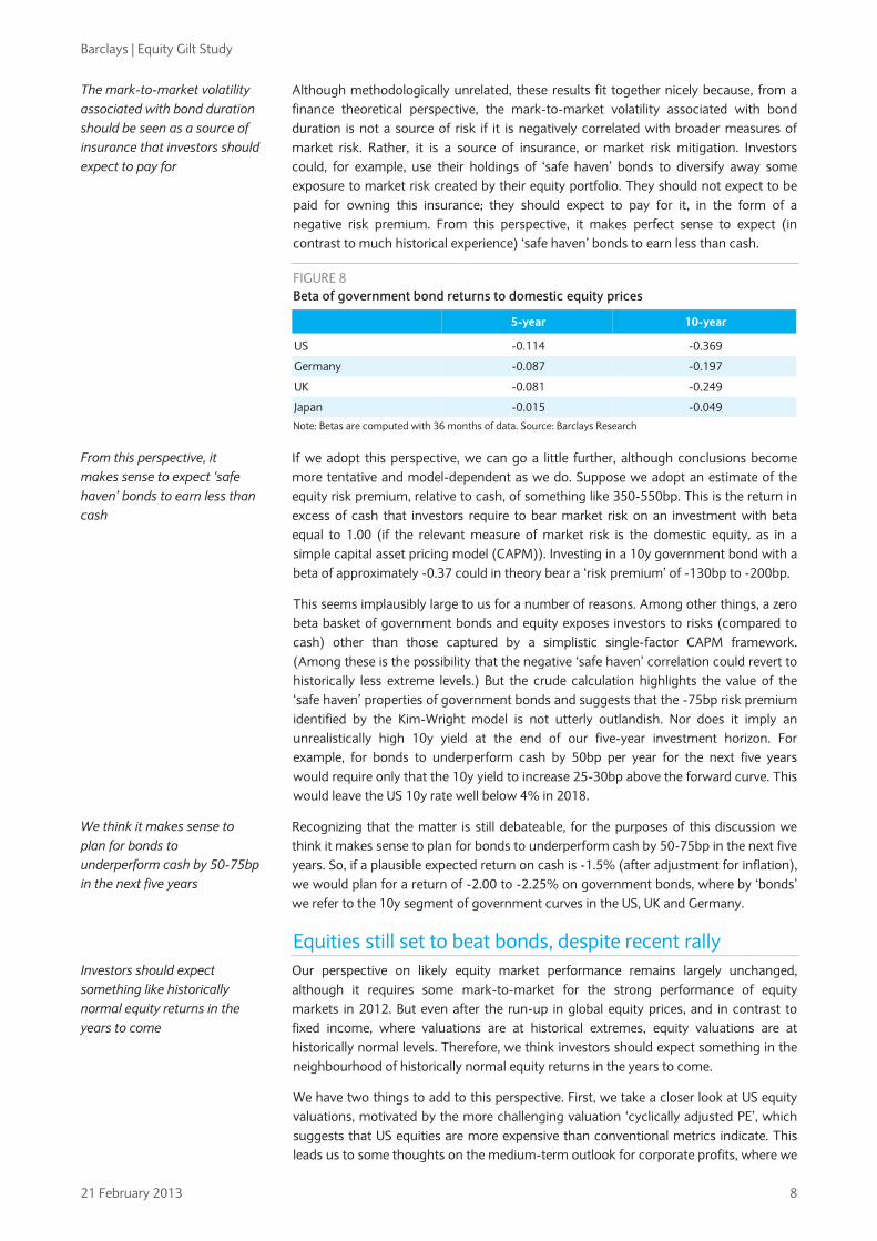
Although methodologically unrelated, these results fit together nicely because, from a finance theoretical perspective, the mark-to-market volatility associated with bond duration is not a source of risk if it is negatively correlated with broader measures of market risk. Rather, it is a source of insurance, or market risk mitigation. Investors could, for example, use their holdings of ‘safe haven’ bonds to diversify away some exposure to market risk created by their equity portfolio. They should not expect to be paid for owning this insurance; they should expect to pay for it, in the form of a negative risk premium. From this perspective, it makes perfect sense to expect (in contrast to much historical experience) ‘safe haven’ bonds to earn less than cash.

FIGURE 8 Beta of government bond returns to domestic equity prices

5-year 10-year

US -0.114 -0.369

Germany -0.087 -0.197

UK -0.081 -0.249

Japan -0.015 -0.049

Note: Betas are computed with 36 months of data. Source: Barclays Research

If we adopt this perspective, we can go a little further, although conclusions become more tentative and model-dependent as we do. Suppose we adopt an estimate of the equity risk premium, relative to cash, of something like 350-550bp. This is the return in excess of cash that investors require to bear market risk on an investment with beta equal to 1.00 (if the relevant measure of market risk is the domestic equity, as in a simple capital asset pricing model (CAPM)). Investing in a 10y government bond with a beta of approximately -0.37 could in theory bear a ‘risk premium’ of -130bp to -200bp.

This seems implausibly large to us for a number of reasons. Among other things, a zero beta basket of government bonds and equity exposes investors to risks (compared to cash) other than those captured by a simplistic single-factor CAPM framework. (Among these is the possibility that the negative ‘safe haven’ correlation could revert to historically less extreme levels.) But the crude calculation highlights the value of the ‘safe haven’ properties of government bonds and suggests that the -75bp risk premium identified by the Kim-Wright model is not utterly outlandish. Nor does it imply an unrealistically high 10y yield at the end of our five-year investment horizon. For example, for bonds to underperform cash by 50bp per year for the next five years would require only that the 10y yield to increase 25-30bp above the forward curve. This would leave the US 10y rate well below 4% in 2018.

Recognizing that the matter is still debateable, for the purposes of this discussion we think it makes sense to plan for bonds to underperform cash by 50-75bp in the next five years. So, if a plausible expected return on cash is -1.5% (after adjustment for inflation), we would plan for a return of -2.00 to -2.25% on government bonds, where by ‘bonds’ we refer to the 10y segment of government curves in the US, UK and Germany.

Equities still set to beat bonds, despite recent rally Our perspective on likely equity market performance remains largely unchanged, although it requires some mark-to-market for the strong performance of equity markets in 2012. But even after the run-up in global equity prices, and in contrast to fixed income, where valuations are at historical extremes, equity valuations are at historically normal levels. Therefore, we think investors should expect something in the neighbourhood of historically normal equity returns in the years to come.

We have two things to add to this perspective. First, we take a closer look at US equity valuations, motivated by the more challenging valuation ‘cyclically adjusted PE’, which suggests that US equities are more expensive than conventional metrics indicate. This leads us to some thoughts on the medium-term outlook for corporate profits, where we

The mark-to-market volatility associated with bond duration should be seen as a source of insurance that investors should expect to pay for

From this perspective, it makes sense to expect ‘safe haven’ bonds to earn less than cash

We think it makes sense to plan for bonds to underperform cash by 50-75bp in the next five years

Investors should expect something like historically normal equity returns in the years to come

Barclays | Equity Gilt Study

21 February 2013 9

see some downside risks from the exchange rate (in the US) and the prospective evolution of the Chinese growth model from one based upon super-abundant labor and inexpensive production inputs of all kinds, to a more balanced model.

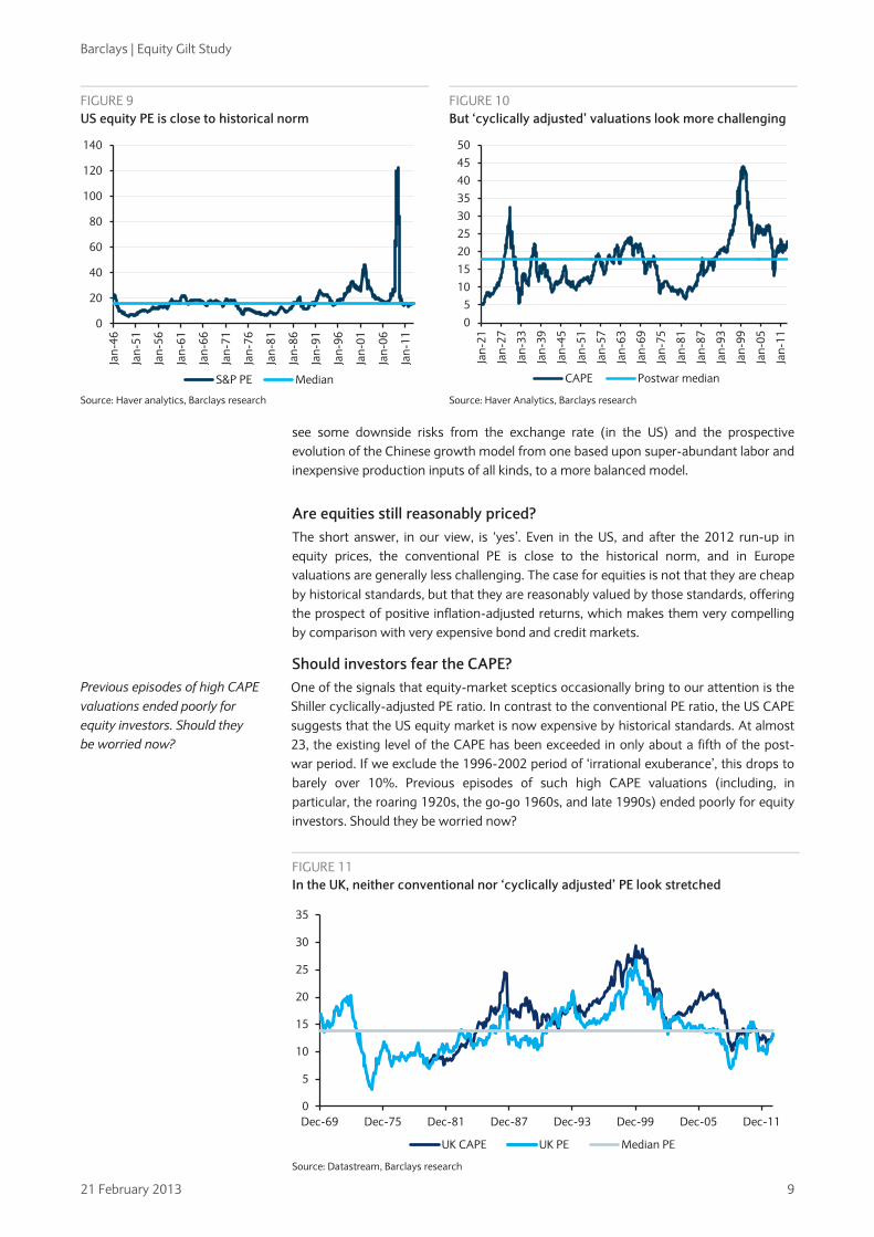
Are equities still reasonably priced? The short answer, in our view, is ‘yes’. Even in the US, and after the 2012 run-up in equity prices, the conventional PE is close to the historical norm, and in Europe valuations are generally less challenging. The case for equities is not that they are cheap by historical standards, but that they are reasonably valued by those standards, offering the prospect of positive inflation-adjusted returns, which makes them very compelling by comparison with very expensive bond and credit markets.

Should investors fear the CAPE? One of the signals that equity-market sceptics occasionally bring to our attention is the Shiller cyclically-adjusted PE ratio. In contrast to the conventional PE ratio, the US CAPE suggests that the US equity market is now expensive by historical standards. At almost 23, the existing level of the CAPE has been exceeded in only about a fifth of the post-war period. If we exclude the 1996-2002 period of ‘irrational exuberance’, this drops to barely over 10%. Previous episodes of such high CAPE valuations (including, in particular, the roaring 1920s, the go-go 1960s, and late 1990s) ended poorly for equity investors. Should they be worried now?

FIGURE 9 US equity PE is close to historical norm

FIGURE 10 But ‘cyclically adjusted’ valuations look more challenging

0

20

40

60

80

100

120

140

Jan-

46

Jan-

51

Jan-

56

Jan-

61

Jan-

66

Jan-

71

Jan-

76

Jan-

81

Jan-

86

Jan-

91

Jan-

96

Jan-

01

Jan-

06

Jan-

11

S&P PE Median

05

101520253035404550

Jan-

21

Jan-

27

Jan-

33

Jan-

39

Jan-

45

Jan-

51

Jan-

57

Jan-

63

Jan-

69

Jan-

75

Jan-

81

Jan-

87

Jan-

93

Jan-

99

Jan-

05

Jan-

11

CAPE Postwar median Source: Haver analytics, Barclays research Source: Haver Analytics, Barclays research

FIGURE 11 In the UK, neither conventional nor ‘cyclically adjusted’ PE look stretched

0

5

10

15

20

25

30

35

Dec-69 Dec-75 Dec-81 Dec-87 Dec-93 Dec-99 Dec-05 Dec-11

UK CAPE UK PE Median PE

Source: Datastream, Barclays research

Previous episodes of high CAPE valuations ended poorly for equity investors. Should they be worried now?

Barclays | Equity Gilt Study

21 February 2013 10

We think the answer is ‘no’, but not because signals delivered by the CAPE ought to be discounted as a matter of principle. Corporate earnings are heavily influenced by cyclical and other transitory factors, and some form of adjustment for spikes and temporary wiggles in earnings is valuable in principle, and in practice. Under some circumstances, the Shiller CAPE does a good job of this. But as most readers are aware, the ‘cyclical adjustment’ in the CAPE does not attempt to identify ‘cyclical’ influences and remove them from the earnings data, it merely smoothes (inflation-adjusted) earnings by taking a 10-year average. This makes sense for short-lived spikes such as the 2008 earnings downdraft, but it introduces a misleading lag in the response to more long-lived shifts in the level or growth rate of corporate earnings.

In the event of a long-lived upward shift in earnings, the CAPE will eventually normalize, but as a result of the gradual (specifically, 10-year) response of ‘cyclically adjusted’ earnings rather than a correction in equity prices. Even under reasonably cautious assumptions about future corporate earnings, this looks like the more probable scenario for the US. But before we get there, we should acknowledge that this discussion applies primarily to the US, and not more generally. In Europe, for example, earnings are (unsurprisingly) depressed relative to ‘cyclically adjusted’ earnings.

In the US, on the other hand, earnings are now very high relative to ‘cyclically adjusted’ earnings, as measured by the usual 10-year average. The question is whether this gap reflects mainly transitory factors, or a more enduring upward shift in earnings that the 10-year average has been slow to reflect.

To answer this question, it helps to consider some concrete scenarios. Suppose that the CAPE eventually normalizes at its historical average of just under 18, and we define ‘eventually’ as 10 years from now. This assumption, along with various assumptions about the trajectory of future earnings, determines the future equity price (inflation-adjusted, along with all the other numbers in these scenarios).

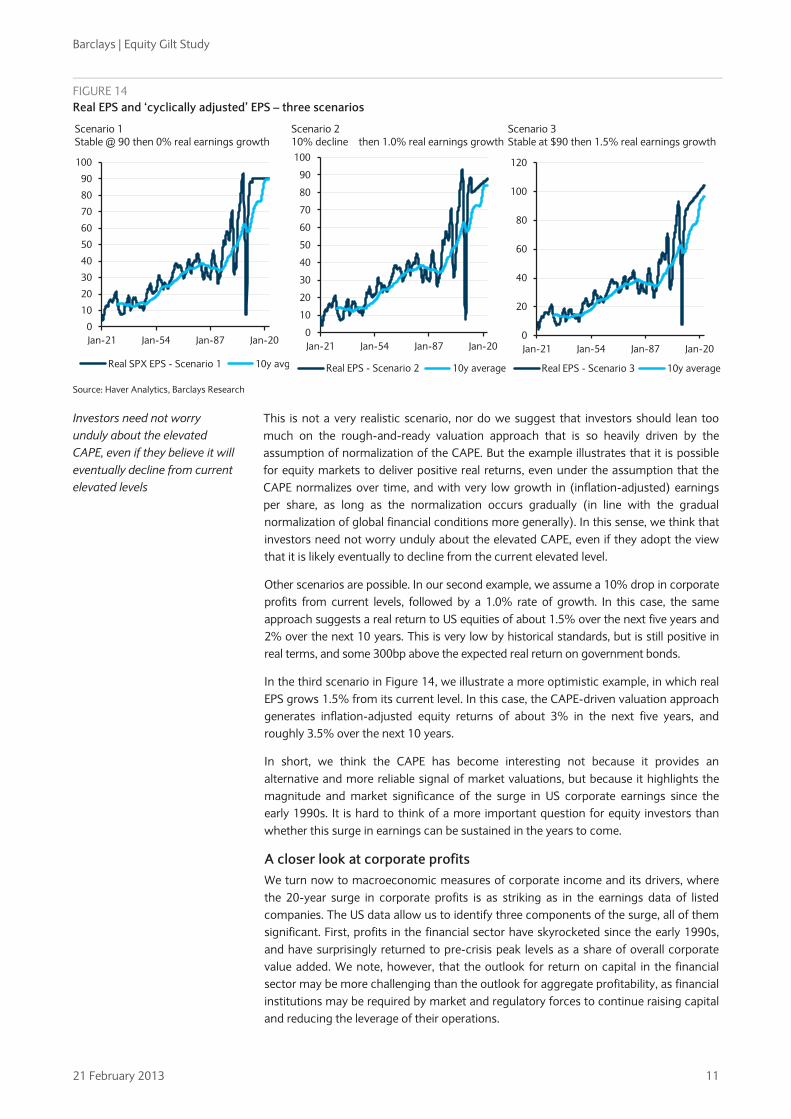
We consider three scenarios, which are more in the nature of plausible base cases, not risk cases that might arise (for example) in the event of a major recession. In the first, we assume that the EPS reaches $90 at end-2012 and remains constant at that level (again, in inflation-adjusted terms) for the next 10 years. As the first chart in Figure 14 illustrates, ‘cyclically adjusted’ EPS would gradually rise to $90, as a mechanical result of the 10-year averaging process. Under the assumption that the CAPE falls to its historical median of 17.8, real equity prices would end the 10-year period about 5% above their current level (1520), for a total inflation-adjusted return of about 2.5% pa, assuming a dividend yield of roughly 2%.

We think the answer is ‘no’

In the US, earnings are now very high relative to ‘cyclically adjusted’ earnings

FIGURE 12 UK real EPS is close to 10y average

FIGURE 13 US EPS is much higher than 10y average

0

100

200

300

400

500

600

Dec

-69

Jul-

72

Feb-

75

Sep-

77

Apr

-80

Nov

-82

Jun-

85

Jan-

88

Aug

-90

Mar

-93

Oct

-95

May

-98

Dec

-00

Jul-

03

Feb-

06

Sep-

08

Apr

-11

UK Real EPS 10y average

0102030405060708090

100

Jan-

21Ju

n-26

Nov

-31

Apr

-37

Sep-

42Fe

b-48

Jul-

53D

ec-5

8M

ay-6

4O

ct-6

9M

ar-7

5A

ug-8

0Ja

n-86

Jun-

91N

ov-9

6A

pr-0

2Se

p-07

Real SPX EPS 10y average Source: Datastream Source: Haver Analytics, Barclays research

Barclays | Equity Gilt Study

21 February 2013 11

FIGURE 14 Real EPS and ‘cyclically adjusted’ EPS – three scenarios

Scenario 1 Stable @ 90 then 0% real earnings growth

0

10

20

30

40

50

60

70

80

90

100

Jan-21 Jan-54 Jan-87 Jan-20

Real SPX EPS - Scenario 1 10y avg

Scenario 2 10% decline then 1.0% real earnings growth

0

10

20

30

40

50

60

70

80

90

100

Jan-21 Jan-54 Jan-87 Jan-20

Real EPS - Scenario 2 10y average

Scenario 3 Stable at $90 then 1.5% real earnings growth

0

20

40

60

80

100

120

Jan-21 Jan-54 Jan-87 Jan-20

Real EPS - Scenario 3 10y average

Source: Haver Analytics, Barclays Research

This is not a very realistic scenario, nor do we suggest that investors should lean too much on the rough-and-ready valuation approach that is so heavily driven by the assumption of normalization of the CAPE. But the example illustrates that it is possible for equity markets to deliver positive real returns, even under the assumption that the CAPE normalizes over time, and with very low growth in (inflation-adjusted) earnings per share, as long as the normalization occurs gradually (in line with the gradual normalization of global financial conditions more generally). In this sense, we think that investors need not worry unduly about the elevated CAPE, even if they adopt the view that it is likely eventually to decline from the current elevated level.

Other scenarios are possible. In our second example, we assume a 10% drop in corporate profits from current levels, followed by a 1.0% rate of growth. In this case, the same approach suggests a real return to US equities of about 1.5% over the next five years and 2% over the next 10 years. This is very low by historical standards, but is still positive in real terms, and some 300bp above the expected real return on government bonds.

In the third scenario in Figure 14, we illustrate a more optimistic example, in which real EPS grows 1.5% from its current level. In this case, the CAPE-driven valuation approach generates inflation-adjusted equity returns of about 3% in the next five years, and roughly 3.5% over the next 10 years.

In short, we think the CAPE has become interesting not because it provides an alternative and more reliable signal of market valuations, but because it highlights the magnitude and market significance of the surge in US corporate earnings since the early 1990s. It is hard to think of a more important question for equity investors than whether this surge in earnings can be sustained in the years to come.

A closer look at corporate profits We turn now to macroeconomic measures of corporate income and its drivers, where the 20-year surge in corporate profits is as striking as in the earnings data of listed companies. The US data allow us to identify three components of the surge, all of them significant. First, profits in the financial sector have skyrocketed since the early 1990s, and have surprisingly returned to pre-crisis peak levels as a share of overall corporate value added. We note, however, that the outlook for return on capital in the financial sector may be more challenging than the outlook for aggregate profitability, as financial institutions may be required by market and regulatory forces to continue raising capital and reducing the leverage of their operations.

Investors need not worry unduly about the elevated CAPE, even if they believe it will eventually decline from current elevated levels

Barclays | Equity Gilt Study

21 February 2013 12

The second component is profits generated by international operations, which skyrocketed from roughly 2.5% of corporate value added before the early 1990s, to roughly 5.5% now. The third component is profit generated by domestic operations of nonfinancial corporations. This remains the largest component of profits, and also the biggest contributor of the three to the growth in aggregate profits between the early 1990s and now.

FIGURE 15 US corporate profits as a share of value added by the corporate sector

0%

5%

10%

15%

20%

25%

30%

Q1 48 Q1 55 Q1 62 Q1 69 Q1 76 Q1 83 Q1 90 Q1 97 Q1 04 Q1 11

Domestic non-financial sector Financial sector Rest of world Source: Haver Analytics

In preparation for this chapter, we searched for academic research on the topic, expecting that a sea change of this magnitude would be the object of study by academic economists. We were disappointed to find little since the mid-1990s. Nevertheless, some stylized facts are easy to draw out of the data. In a statistical explanation of nonfinancial domestic profits as a share of corporate value added, we identified three powerful drivers:

• The first is the business cycle, represented by the rate of capacity utilization. This exerts a powerful influence, but is volatile and is not a major factor in the 20-year trend rise in corporate profitability.

• The second is the real exchange rate where, consistent with a number of academic studies from the early 1990s, we found that a weaker currency is associated with a higher rate of profits in the US. The estimated effect is powerful; all else equal, a 10% real exchange rate depreciation is estimated to increase the rate of profit by nearly a percentage point (from about 10% in the early 1990s). But the real exchange rate was almost exactly as weak in the early 1990s as it is now, so this factor explains little of the rise in the past 20 years.

• The third is the cost of labor, as measured by the ratio of unit labor costs to the price of private-sector output. This measure of labor compensation fluctuated in a narrow range until the early 1990s, then began to fall steadily, registering a cumulative fall of nearly 10% (Figure 16), which implies that labor compensation fell far short of the cumulative growth in productivity during the 20 years. Our statistical analysis suggests that the decline in this measure of labor compensation fully explains the rise in the rate of nonfinancial corporate profit from the early 1990s to the present.

At one level, it is unsurprising that the 20-year surge in corporate profits has been associated with a gap between growth in productivity and labor compensation. Still, other explanations are conceivable, and it concentrates the mind to see the expected association borne out in the data. The relevant question for us is what this might suggest about the outlook for profitability in the years to come.

The 20-year surge in corporate profits has been associated with a gap between growth in productivity and labor compensation

Barclays | Equity Gilt Study

21 February 2013 13

The impact of the real exchange rate is relatively clear. For the past couple of years, the US real exchange rate has flirted with historical lows, largely because US monetary policy has been more aggressively expansionary than policy in most of the rest of the world. It seems likely that the US will, eventually, lead the rest of the world out of this extreme monetary stance; as it does, it seems likely that the real exchange rate will tend to strengthen toward a historically more normal level. This will likely create headwinds for corporate earnings growth.

The bigger question is whether the gradual but cumulatively significant erosion of US workers’ compensation will remain in place or whether the terms of trade may shift in labor’s favor. Opinions are necessarily tentative and speculative. We do not have a full explanation for what happened in the past 20 years; we should certainly not pretend to know what will happen in the next 5-10 years.

Still, if we ever do reach a full understanding of what happened in the past 20 years, it will be surprising to us if the globalization of production and, in particular, the associated integration of hundreds of millions of low-wage workers into the global labor market, does not play a prominent role. And although globalization is highly unlikely to be reversed in the years to come, it is changing, above all in China, where a growth strategy predicated on the underpricing of labor, energy, capital, and environmental factors of production is being replaced with a more balanced approach that will involve, among other things, a substantial rise in returns to labor and other factors of production.

The question that arises in our mind is the extent to which the rise in the labor and other costs of production in China and other rapidly-developing emerging market economies – combined with a demographically-driven decline in the supply of labor – will shift the terms of trade in labor’s favour, as globalization arguably shifted them to labor’s detriment in its early stage starting in the 1990s. We do not pretend to have a complete answer, but think that investors should be aware of downside risks that the Chinese transition may pose for corporate earnings generated both abroad and at home.

A more subdued outlook for returns, but equities still beat bonds Returning to the question of equity market performance, we see the outlook for equity returns during the next 5-10 years as qualitatively similar to our assessment of a year ago, although the substantial equity market rally since then means even more limited room for gains due to the re-rating of equity risk, leaving investors with dividends and earnings growth as the plausible drivers of equity returns.

FIGURE 16 Real labor compensation has been falling since the 1990s

FIGURE 17 Share of EM exports in world total

0.85

0.90

0.95

1.00

1.05

1.10

1.15

Q1

48

Q1

53

Q1

58

Q1

63

Q1

68

Q1

73

Q1

78

Q1

83

Q1

88

Q1

93

Q1

98

Q1

03

Q1

08

Nonfarm ULC / P

0%

5%

10%

15%

20%

25%

30%

35%

40%

45%

1970

1972

1974

1976

1978

1980

1982

1984

1986

1988

1990

1992

1994

1996

1998

2000

2002

2004

2006

2008

2010

Emerging markets EM Asia Source: Haver Analytics, Barclays Research Source: IMF

The erosion of workers’ compensation is linked to the globalization of production and the integration of hundreds of millions of low-wage workers into the global labor market

The Chinese transition may pose downside risks for corporate earnings generated abroad and at home

The substantial equity market rally since last year means more limited room for gains due to re-rating of equity risk

Barclays | Equity Gilt Study

21 February 2013 14

In the US, where the ‘cyclical’ rebound in earnings seems largely complete, and secular drivers of earnings seem marked by at least as much downside risk as upside potential, we think it would be optimistic to assume more than 1.5-2.0% growth in real EPS for the next half decade of so, consistent with an expected real return of something like 3.5-4.0%. This is low by historical standards, but the implied risk premium vs government bonds of 550-600bp is at the high end of historical experience. In Europe, where a cyclical rebound in earnings is more plausible, valuations are less challenging, and dividend payouts higher, equities are likely to offer expected returns 100-150bp higher than in the US in the next half decade or so.

Credit can earn more than bonds, but not much As heavily influenced as credit markets are by developments in both government bond and equity markets, we require a benchmark against which to evaluate over- or underperformance compared with those markets. We adopt an empirical approach based on the idea that returns on corporate credit can be expressed as the sum of the return on government bonds, a beta to the equity market, and what is left unexplained. In our empirical formulation, the government bond markets are both intermediate and long-duration bonds, and we allow the data to determine the appropriate weight (which turns out to be about 75% to intermediate bonds and 25% to long bonds).

Using monthly data from 1973, roughly 75% of the variation in returns on US investment-grade corporate credit can be explained by statistical correlations with government bonds and equity markets. The remaining 25%, though not the largest part of the asset class’s total return, is nevertheless interesting. Figure 18 shows the cumulative ‘outperformance’, as measured by the idiosyncratic component of this statistical decomposition, since the early 1970s.

Simplistic though the approach may be, it highlights the relative performance of credit during key episodes of recent financial history. The underperformance of credit during the 1996-2002 equity-market bubble stands out clearly, and the underperformance of credit during the 2008-09 collapse is even more striking. The results also highlight the rapid recovery of credit from the recent collapse, and the substantial cumulative outperformance by credit since the immediate pre-crisis years. The strong performance of high-grade credit is also evident in valuations. Credit spreads are still above their pre-crisis lows, but they are below historically normal levels, and we think it would be optimistic to project a substantial decline in spreads during the coming five years. If spreads remain constant (at, for example, just under 140bp for corporate bonds in the Barclays US Aggregate index), then credit will outperform ‘safe haven’ bonds, but not by enough to avoid negative inflation-adjusted returns during the next five years.

Equities are likely to offer expected returns that are higher in Europe than in the US

FIGURE 18 Cumulative outperformance of investment-grade corporate credit in the US

-0.30

-0.25

-0.20

-0.15

-0.10

-0.05

0.00

0.05

0.10

Jan-73 Jan-77 Jan-81 Jan-85 Jan-89 Jan-93 Jan-97 Jan-01 Jan-05 Jan-09 Jan-13

Cumulative outperformance of high-grade credit Source: Barclays Research

Barclays | Equity Gilt Study

21 February 2013 15

Conclusion As the economic and financial tails risks that loomed so large in the aftermath of the 2008-09 financial collapse recede, investors confront a more tranquil environment, but one in which valuations are far more challenging, and prospective investment returns correspondingly diminished. In the next half-decade, investors also face the probable need to navigate an eventual sea change in the global financial environment, as the extraordinarily expansionary monetary stances of central banks around the world give way to a gradual normalization of financial conditions. Precisely how this will play out will depend upon valuations, positioning, and economic developments in the months and years to come. But the present reality of extraordinarily loose monetary policy suggests to us that real returns on cash will remain low during the next five years, when we think investors should be prepared to lose about 1.5% after adjustment for inflation in the US, with returns a little lower in the UK and higher in the euro area.

The pending normalization of financial conditions, although likely to be delayed and gradual, is likely to result in particularly low returns in ‘safe haven’ bond markets. We think that investors should be prepared to lose 50-75bp more on long-term ‘safe haven’ bonds than the 1.5% pa that they are likely to lose in cash (after adjustment for inflation). These low returns on government bonds are an artefact of the five-year time horizon that is our focus. After that period, market yields will likely have risen to levels that offer investors modestly positive returns on their ‘safe haven’ bond investments.

With credit spreads above their historical lows, but somewhat lower than historical normal levels, we think it would be overly optimistic for investors to expect a further decline in spreads during the next half decade. It seems reasonable to assume that investors will collect the credit spread, roughly 135bp for investment grade corporates, which would be enough to mitigate but not to eliminate the probable loss of real value created by the exposure to interest-rate duration associated with (unhedged) exposure to credit markets.

Our estimate of expected returns to equity is lower than published in last year’s Equity Gilt Study. This reflects, in part, our present focus on a five-year investment horizon, during which we expect the yield structure of global asset markets to be depressed by the extremely expansionary monetary policy likely to prevail, even if the gradual normalization of financial conditions begins during that period, as we expect. The lower estimate of prospective equity returns also reflects the 18% rise in global equity prices since the beginning of 2012, which brought forward capital gains that might otherwise have contributed to returns in coming years.

Despite our reduced estimate of the return on equities, the estimated equity risk premium remains in the 500-600bp range, broadly consistent with historical experience. Although absolute returns are likely to be lower than long historical experience, equities have become the only real option for investors seeking positive inflation-adjusted returns. Especially if the low-volatility environment persists, as now seems to be the relevant base case, the risk (not so unpleasant to contemplate) now seems to be that the search for return will push investors more forcefully into equities, causing yet more challenging valuations and eventually undermining the investment case for equities. But we do not think that we are there yet; in the absence of an economic or financial shock to our reasonably benign case, we think that for equity investors, things are likely to get better before they get worse.

Investors should be prepared to lose 50-75bp more on long-term ‘safe haven’ bonds than the 1.5% pa that they are likely to lose in cash

For equity investors, things are likely to get better before they get worse

Barclays | Equity Gilt Study

21 February 2013 16

CHAPTER 2

Demand for safe havens to remain robust • Following on from the Equity Gilt Study 2012, in which we argued that

conventional measures of the equity risk premium appeared elevated mainly because the structural decrease in the supply of risk-free assets had resulted in unusually low risk-free bond yields, we turn to the role of demand for safe-haven assets.

• We examine three sources of demand for such assets: official-sector demand via the investment of international reserve portfolios; institutional demand in a post-crisis era of tighter bank regulation; and private demand, particularly from an aging population across the developed world.

• We look for US institutional demand and the rotation of boomer investors into bonds to make up for some of the relative decline in demand from official sources, including our expectation of diminishing reserve accumulation in China.

• We conclude that structural demand for safe havens is likely to remain high and, when combined with the structural scarcity of such assets, is likely to keep interest rates on safe assets low by comparison with historical norms and conventional measures of the equity risk premium elevated.

The abrupt and radical change in the valuation of high-quality, liquid government bonds, or ‘safe havens’, following the onset of the Great Recession is now entering its fifth calendar year. The rich valuation environment for safe havens has frequently been described as an artifact of the financial crisis: demand from private investors seeking insurance in stormy financial markets combined with asset purchases from systemically important central banks engaged in quantitative easing to produce rock-bottom interest rates across most developed government bond markets. There is little doubt that cyclical factors following the deepest global recession since the Great Depression have been important factors in the low interest rate environment.

In “The equity risk premium: Cheap equities or expensive bonds?”, 2012 Equity Gilt Study, 8 February 2012, we outlined our view that low interest rates on safe assets were driven by more than cyclical factors alone. In our view, the relative scarcity of high-quality, liquid government bonds was among the more convincing structural explanations for low interest rates on safe assets. We used the safe-asset shortage argument to buttress our view that conventional measures of the equity risk premium were elevated mainly because the valuation of safe assets had changed radically and abruptly, not because equity investors had become significantly more intolerant of holding equity risk.

We still agree with this but acknowledge that our analysis was based primarily on the supply of safe havens and did not examine fully their demand, which is the focus here. After all, the supply of safe havens will likely be held in equilibrium, but the obvious question is at what price (and yield). To understand this fully requires knowing more about the objectives of the myriad of investors who include such assets in their portfolio decisions. We examine three components of safe asset demand: official-sector demand via the investment of international reserve portfolios; institutional demand in a post-crisis era of tighter bank regulation; and private demand, particularly from an aging population across the developed world.

We find that structural demand for safe havens is likely to remain high and, when combined with the structural scarcity of such assets, to keep interest rates on safe assets low and conventional measures of the equity risk premium elevated. The rebalancing of the global economy following the crisis should slow the growth of international reserve portfolios, particularly in China, where we see the country in the

Michael Gapen

+1 212 526 8536 [email protected]

The rich valuation environment for safe havens has frequently been described as an artifact of the financial crisis

But low rates on safe assets are driven by more than cyclical factors: they result from the relative scarcity of high-quality, liquid government bonds

The supply of safe havens will likely be held in equilibrium, but the question is at what price (and yield)

A much tighter regulatory landscape and an aging population will result in lasting demand for safe assets

Barclays | Equity Gilt Study

21 February 2013 17

early stages of breaking away from its old growth model (see Chapter 3, “Can China avoid the middle-income trap?”) but we find that demand for safe havens from official sources will remain important and their investment mandates make them fairly price- insensitive. We expect official demand for such assets to be complemented by two important shifts in the coming years. First is a much tighter regulatory landscape, where we see Basel III recommendations for higher capital and stronger liquidity coverage ratios as generating a structural increase in demand for safe havens, particularly from US financial institutions. Second, the aging population in the developed world should provide lasting demand for dollar- and euro-denominated safe havens due to shortened investment horizons and the need to fund current consumption during retirement years. We highlight the US, where the aging of the baby boom generation means almost half of US households will have a head of household aged 55 or older by the end of the decade. This investor class controls nearly two-thirds of household net worth and total financial assets in the US, and their portfolio decisions will carry proportionately larger weight.1

The main conclusions of this chapter are in concert with our findings elsewhere in the Equity Gilt Study 2013. Conventional wisdom suggests the current low interest rate environment cannot last. Some proponents of this view believe the combination of rock-bottom yields and high equity risk premium will produce a herd effect, or “great rotation,” as investors abandon fixed income investments in favour of equities, decimating investor portfolios with high exposure to fixed income. Other proponents of this view cite bloated central bank balance sheets as leading to rising inflation and higher nominal yields.

We find ourselves in partial agreement. We agree that low yields on safe haven assets and wide equity risk premiums will ultimately reward those investors willing to move out the risk spectrum (see Chapter 1, “Low risk, low return”). However, our view that equities remain attractive for those with a medium-term or longer horizon is partly dependent on structural shifts in the supply and demand for safe havens that are likely to keep the existing risk-reward structure in place. We would have less conviction about the relative attractiveness of equities at current valuations if our views on safe havens were influenced by cyclical factors alone. In addition, we are inclined to discount the risks of inflation associated with quantitative easing and the unprecedented expansion of central bank balance sheets (see Chapter 4, “QE carries risks beyond inflation”). None of this is to say that yields cannot rise; they undoubtedly will to some degree, as markets and policy normalize and economies continue to heal and cleanse the imbalances of the previous decade. However, structural factors limiting safe haven supply and supporting demand suggest to us that low real and nominal yields on safe havens will be more the norm than the exception in the years ahead.

The supply of safe assets: Where are we? We begin with a brief review of our findings on the safe asset shortage. To illustrate our view that the relative scarcity of high-quality, liquid government bonds was among the more convincing structural explanations for low interest rates on safe assets, we defined the safe asset universe at the onset of the Great Recession and plotted the outstanding stock of these assets as a percentage of world GDP over time (see “The equity risk premium: Cheap equities or expensive bonds?”, Equity Gilt Study 2012, 8 February 2012). The precise definition of a safe asset can vary depending on context, but we assume that it is reasonable to expect such assets to deliver very low default risk, high liquidity, and low currency risk. In applying this screen, we viewed the safe asset universe as including US government debt (excluding that held by the Federal

1 Outside of official demand from international reserve portfolios, we focus our analysis on US institutions and households since outstanding US Treasuries and US GSE debt accounts for more than 75% of the safe haven universe at present (Figure 1). US institutions and households are likely to exhibit a high degree of “home bias” in their portfolio decisions since financial institutions are subject to regulatory requirements to hold a sufficient liquidity backstop against local currency deposits and US households nearing retirement have a US dollar-denominated consumption basket. We leave non-US institutional and private sector demand for safe havens for future work.

Our view on the relative attractiveness of equities is predicated on structural factors that will keep yields on safe assets low

Barclays | Equity Gilt Study

21 February 2013 18

Reserve), direct debt and asset-backed securities issued by US government-sponsored agencies, privately issued mortgage-backed securities, and public debt of large European governments.2

A safe asset squeeze was already affecting markets before the financial crisis that erupted in 2008 (Figure 1). The only category in our safe asset universe to show an increase as a percentage of world GDP between 2000 and 2007 was US mortgage-related assets. Indeed, the growth of this category may have been, in part, fuelled by an increase in demand for safe assets against a relatively short supply, particularly by global central banks with rapidly expanding international reserves. In 2008, when the crisis intensified and any US housing-related asset was viewed as highly toxic, the supply of safe assets was abruptly curtailed. The subsequent downgrading of Spanish government debt in 2010 and of Italian government debt in 2011 compounded the problem. The return of US GSE debt to safe haven status in 2011 alleviated the shortfall only somewhat, but the stock of safe assets as a share of global GDP was still 11 percentage points below its 2003 peak. We then formed assumptions about the US debt profile and which assets returned to safe-haven status (and when), concluding that the safe asset shortage would be alleviated, but not overturned.

3

FIGURE 1 The safe-asset shortage

05

1015202530354045

00 01 02 03 04 05 06 07 08 09 10 11 12F 16F 21F

US gov debt Germany and FranceItaly and Spain US GSE debtGSE and private ABS International reserve assets

% of world GDP

Source: Banco de España, Banque de France, Bundesbank, Federal Reserve, IMF, INS, US Treasury, Haver Analytics, Barclays Research

Demand from official sources: The ‘Great Rebalancing’ and the end to the structural rise in international reserves The growth in international reserves has been a stylized fact of the global economy for more than a decade, and its origins date to the Asian financial crisis of 1997 and 1998. Prior to that, total global reserves (minus gold) amounted to $1,398bn at the end of 1995, according to the IMF database on the currency composition of official foreign exchange reserves (COFER). Advanced economies held two-thirds of this total ($932bn), while emerging and developing economies held only $457bn.

The post-Asian financial crisis period was a turning point in reserve management policies, as many emerging and developing economies chose to self-insure against modern balance of payments crises arising from the widespread liberalization of the capital accounts in many countries. At end-2007, on the eve of the global financial crisis, total global reserves had risen almost five-fold, to $6,704bn, or 12.0% of world GDP

2 We exclude the JGB market since it is primarily locally held. We also exclude UK public debt, which has traded like a safe haven asset, mainly on the grounds that sterling, like the yen, is a reserve currency of modest significance relative to the dollar and euro. Including UK public debt in the analysis would not alter the main thrust of the results. 3 In particular, we assumed the US debt-to-GDP ratio rose to 80% by 2016 and remained there throughout the end of the forecast horizon. We also assumed US agency debt returned to safe haven status, but other mortgage- and asset-backed bonds did not. Finally, we assumed Germany and France remained on safe haven status and were joined by Italy in 2021.

A safe asset squeeze was already affecting markets before the financial crisis that erupted in 2008

The past two decades have had a structural increase in reserve accumulation by many emerging and developing economies

Barclays | Equity Gilt Study

21 February 2013 19

(Figure 2). Emerging and developing economies accounted for much of the rise, with reserves climbing from $475bn in 1995 to $4,272bn in 2007, for a 64% share of total global reserves (Figure 3). In just 12 years, emerging/developing economies had become the dominant holders of international reserves.

The precautionary motive The level of accumulated reserves in many countries was generally viewed as far exceeding the amount needed to protect against conditional access to capital markets and adjustment costs. Studies that estimated the optimal level of precautionary reserves conditioned reserve balances on the level of government expenditures, level of debt, cost of adjustment, size of international transactions, economic variability, and exchange rate regime (fixed versus floating), among other factors.4

Competitiveness, terms of trade, and export promotion

These concluded that precautionary demand for international reserves, while an important contributing factor, was insufficient to explain fully the structural shift in reserve demand that began in the late 1990s.

In the years following the Asian financial crisis, many of the affected economies were subject to substantial real exchange rate depreciations, which enhanced competitiveness and terms of trade and, ultimately, led to improved trade balances. For example, real effective exchange rates at the end of 2004 in many of the affected economies were substantially below their pre-crisis levels (Figure 4). The combination of exchange rate regimes, controls and taxes on capital inflows and exchange market interventions allowed trade surpluses to persist and prevented currency appreciation. The widespread adoption of these policies by Asian countries, particularly China, led some to frame the issue of reserve accumulation as a normal evolution of the international monetary system.5

4 For an analysis of the determinants of reserve accumulation in emerging and developing economies, see Michael Gapen and Michael Papaioannou, 2008, “Reserve accumulation: Macroeconomics and management issues,” in Y. Kurihari, S. Takaya, H. Harui, and H. Kamae, editors, Information Technology and Economic Development, IGI Global: Hershey, PA; Olivier Jeanne and Romain Ranciere, 2006, “The Optimal Level of international reserves for emerging market countries: Formulas and applications, IMF Working Paper 06/229; and J. Aizenman and N. Marion, 2002, “The high demand for international reserves in the Far East: What’s going on? NBER Working Paper No. 9266, Cambridge: NBER.

Proponents of this view argued that the emergence of a fixed exchange rate periphery in Asia re-established the US as the center of a new Bretton-Woods-style international monetary order. In this scenario, Asia’s economic growth would ultimately require financial liberalization and floating exchange rates. In the meantime, however, the system of undervalued exchange rates and capital controls led to official capital outflows and the accumulation of reserve asset claims on the US.

5 See Michael Dooley, David Folkerts-Landau, and Peter Garber, 2003, “An essay on the revived Breton Woods system, NBER Working Paper No. 9971, Cambridge: NBER.

FIGURE 2 The desire to self-insure prompted a sharp growth in the reserve portfolios of many emerging economies

FIGURE 3 The share of total reserves held by emerging and developing economies rose steadily

0

2

4

6

8

10

12

14

16

95 96 97 98 99 00 01 02 03 04 05 06 07 08 09 10 11

Total international reserves

Emerging and developing economies

Advanced economies

% of world GDP

20

25

30

35

40

45

50

55

60

65

70

95 96 97 98 99 00 01 02 03 04 05 06 07 08 09 10 11

Emerging and developing economies

Advanced economies

% Share of total foreign exchange holdings

Source: IMF Statistics Department COFER database and International Financial Statistics

Source: IMF Statistics Department COFER database and International Financial Statistics

Precautionary demand for international reserves is insufficient to explain the structural increase in reserve demand

Undervalued exchange rates and capital controls in Asian countries led to official capital outflows and the accumulation of reserve asset claims on the US

Barclays | Equity Gilt Study

21 February 2013 20

FIGURE 4 Real effective exchange rates: 1996-2012

50

60

70

80

90

100

110

120

130

96 98 00 02 04 06 08 10 12

USD EUR PHP MYR SGD THB

12/31/96 = 100

Real effective exchange rate

Source: Barclays Research

The Great Rebalancing The prolonged accumulation of reserves from persistent structural imbalances had a deleterious effect on global financial stability and was unwound in a disorderly manner. There had been a vigorous debate about how long the arrangement could persist, given the mutually reinforcing policies of the public sectors in Asia and the US, and the degree to which these policies were beyond the reach of the private sector and market forces. The answer came in 2008, when market forces overwhelmed the system. The substantial and immediate adjustment seems to have brought an end to the period of aggressive reserve accumulation by official sources. The current account surpluses of major Asian economies have fallen, while the large current account deficits of the US and other developed economies have narrowed (Figures 5 and 6). Real exchange rate misalignment has also been reduced (Figure 4). The rebalancing of the global economies has been substantial and was achieved in fairly short order, but not without significant economic disruption to global markets along the way.

In retrospect, the marked growth in seemingly safe asset-backed securities was largely an endogenous response to the fact that the bulk of the current account surpluses was held and managed by risk-averse public sector institutions. These surpluses, accumulated in the form of foreign exchange reserves to reduce risks of future balance of payments crises, needed somewhere to go. The burgeoning securitized market substituted for high-quality, liquid government securities, which were becoming increasingly scarce. Excluding

The crisis of 2008 brought an end to the period of aggressive reserve accumulation by official sources

FIGURE 5 The current account surpluses of major Asian economies have fallen…

FIGURE 6 …and current account deficits mean global imbalances have been reduced

0

2

4

6

8

10

12

95 96 97 98 99 00 01 02 03 04 05 06 07 08 09 10 11 12

China Japan

Current account balance, % of GDP

-12

-10

-8

-6

-4

-2

0

2

4

95 96 97 98 99 00 01 02 03 04 05 06 07 08 09 10 11 12

US UK Spain Italy

Current account balance, % of GDP

Note: 2012 data are Barclays’ forecast. Source: SAFE, BOJ, Barclays Research Source: BDE, BdIt, BEA, BoJ, Bundesbank, ECB, ONS, Haver Analytics

Barclays | Equity Gilt Study

21 February 2013 21

the asset-backed securities category from Figure 1, the remaining supply of safe assets shrunk from 27.6% of world GDP in 2003 to 20.6% in 2008. The sharp increase in US Treasury debt in response to the economic contraction and financial instability that followed has not been enough to offset the loss of the GSEs, the asset-backed mortgage market and, later, the sovereign debt of Italy and Spain.

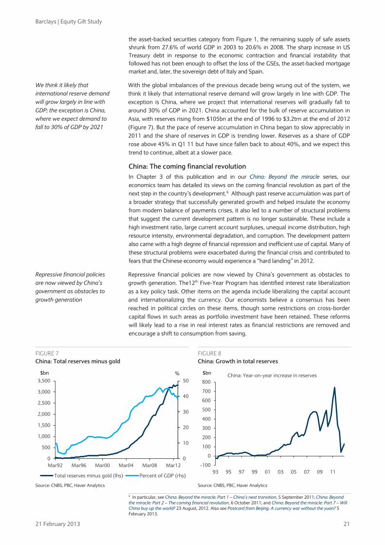
With the global imbalances of the previous decade being wrung out of the system, we think it likely that international reserve demand will grow largely in line with GDP. The exception is China, where we project that international reserves will gradually fall to around 30% of GDP in 2021. China accounted for the bulk of reserve accumulation in Asia, with reserves rising from $105bn at the end of 1996 to $3.2trn at the end of 2012 (Figure 7). But the pace of reserve accumulation in China began to slow appreciably in 2011 and the share of reserves in GDP is trending lower. Reserves as a share of GDP rose above 45% in Q1 11 but have since fallen back to about 40%, and we expect this trend to continue, albeit at a slower pace.

China: The coming financial revolution In Chapter 3 of this publication and in our China: Beyond the miracle series, our economics team has detailed its views on the coming financial revolution as part of the next step in the country’s development.6

Repressive financial policies are now viewed by China’s government as obstacles to growth generation. The12th Five-Year Program has identified interest rate liberalization as a key policy task. Other items on the agenda include liberalizing the capital account and internationalizing the currency. Our economists believe a consensus has been reached in political circles on these items, though some restrictions on cross-border capital flows in such areas as portfolio investment have been retained. These reforms will likely lead to a rise in real interest rates as financial restrictions are removed and encourage a shift to consumption from saving.

Although past reserve accumulation was part of a broader strategy that successfully generated growth and helped insulate the economy from modern balance of payments crises, it also led to a number of structural problems that suggest the current development pattern is no longer sustainable. These include a high investment ratio, large current account surpluses, unequal income distribution, high resource intensity, environmental degradation, and corruption. The development pattern also came with a high degree of financial repression and inefficient use of capital. Many of these structural problems were exacerbated during the financial crisis and contributed to fears that the Chinese economy would experience a “hard landing” in 2012.

6 In particular, see China: Beyond the miracle: Part 1 – China’s next transition, 5 September 2011; China: Beyond the miracle: Part 2 – The coming financial revolution, 6 October 2011; and China: Beyond the miracle: Part 7 – Will China buy up the world? 23 August, 2012. Also see Postcard from Beijing: A currency war without the yuan? 5 February 2013.

We think it likely that international reserve demand will grow largely in line with GDP; the exception is China, where we expect demand to fall to 30% of GDP by 2021

FIGURE 7 China: Total reserves minus gold

FIGURE 8 China: Growth in total reserves

0

10

20

30

40

50

0

500

1,000

1,500

2,000

2,500

3,000

3,500

Mar92 Mar96 Mar00 Mar04 Mar08 Mar12

Total reserves minus gold (lhs) Percent of GDP (rhs)

$bn %

-100

0

100

200

300

400

500

600

700

800

93 95 97 99 01 03 05 07 09 11

China: Year-on-year increase in reserves$bn

Source: CNBS, PBC, Haver Analytics Source: CNBS, PBC, Haver Analytics

Repressive financial policies are now viewed by China’s government as obstacles to growth generation

Barclays | Equity Gilt Study

21 February 2013 22

If the liberalization of financial markets in China follows the pattern in other countries at similar stages of development, it should increase gross capital flows, deepen financial integration, bolster GDP growth, and lower inflation. History also suggests that the liberalization of capital flows is associated with higher equity returns and lower bank capital adequacy ratios, the latter of which raises the potential for financial instability. However, the evidence is mixed when it comes to the relationship between liberalization and net flows, given that these are influenced by the measures enacted, the sequencing of reforms, and the extent of liberalization applied to inflows versus outflows. One IMF study that applies the average of previous cases of liberalization elsewhere to China’s economy suggests that gross inflows and outflows may increase by 3.3pp and 2.1pp, respectively, in 2016, representing net increases of US$380bn and US$240bn.7

We expect growth in outflows from China to be heavily concentrated in direct investment. Outward direct investment could grow steadily over the coming decade by at least $100bn per year even according to conservative estimates. We expect retaining restrictions on cross-border capital flows to mean net portfolio investment will remain of secondary consideration.

If implemented, the financial revolution in China will likely mean further economic adjustment, smaller current account surpluses, and less reserve accumulation. How much less is an open question, yet of great importance when attempting to gauge demand for “safe havens.” Here, we attempt to estimate the magnitude of the adjustment that might reasonably be expected. The IMF’s illustrative medium-term scenario in its 2012 Article IV Report for China is a good starting point, in our view.8

7 Saadi Sedik, Tahsin and Tao Sun, Effects of capital flow liberalization—What is the evidence from recent experiences of emerging market economies? IMF Working Paper 12/275, November 2012.

Its longstanding convention is to perform a medium-term scenario analysis that assumes a constant real exchange rate and a continuation of the current policy framework. This environment, which assumes no liberalization of capital markets and exchange markets, can be viewed as an upper bound on the pace of reserve accumulation and, in turn, the demand for safe haven assets if no reforms are undertaken. Under current policies, the IMF projected that the current account would slowly begin to widen in 2013, reaching 4.3% of GDP by 2017 (Figure 9). This, plus persistent capital inflows and exchange market intervention, would imply reserve accumulation of $400-600bn per year, or growth exceeding 11% per year (Figure 10). Gross reserves would exceed $6trn in 2017, or nearly twice current levels.

8 People’s Republic of China: Staff Report for the 2012 Article IV Consultation, IMF Country Report no. 12/195, July 2012.

We expect growth in outflows from China to be heavily concentrated in outward direct investment

FIGURE 9 Financial reform would lower current account imbalances…

FIGURE 10 …and slow reserve accumulation in China

0

1

2

3

4

5

2014 2015 2016 2017

Unchanged policies Financial liberalization

% of GDPChina: Current account surplus under:

0

100

200

300

400

500

600

700

800

2014 2015 2016 2017

Unchanged policies Financial liberalization

$bnChina: Annual reserve accumulation under:

Source: IMF, Barclays Research Source: IMF, Barclays Research

The financial revolution in China will likely mean further economic adjustment, smaller current account surpluses, and less reserve accumulation

Barclays | Equity Gilt Study

21 February 2013 23

However, assuming that liberalization does occur, we estimate that the current account could gradually fall to 1-2% of GDP by 2017 and further exchange rate appreciation would limit net direct investment inflows. In this case, we estimate that annual reserve accumulation would slow to $200-300bn per year, or annual growth of about 5%. This puts reserve growth in China in line with forecasts of global nominal GDP growth and would be consistent with reserves as a percentage of Chinese GDP declining toward 30% in the coming decade.

Even smaller reserve accumulation is possible under several scenarios. One possibility is that demographics result in even lower saving rates and, ultimately, toward the end of the decade, current account deficits. A second scenario would involve a different sequencing of financial reforms that permitted greater freedom of outward portfolio flows, which could spur residents to move capital abroad. Finally, structural imbalances could result in a financial crisis and declines in net capital flows. Each of these scenarios would result in slower reserve accumulation, or even reserve outflows.

Official institutions: A significant source of demand for safe havens The structural increase in reserve accumulation by many emerging and developing economies in the past two decades has been among the most striking features of global capital markets. The coming decade should feature smaller current account surpluses, smaller current account deficits, and reduced global imbalances. If our expectation on this front is met, it seems unlikely that official demand for high-quality, liquid assets will be as important a driver of safe haven price dynamics and cross-border capital flows as it has been in the past. Though we do not expect it to grow in relative importance as it did previously, the fact that we expect reserves to remain stable at 14-15% of world GDP suggests that official sources will be an important source of demand for safe havens in the years ahead.

The outcome of financial reform and long-run demographic trends in China is likely to mean significantly less reserve accumulation, which has led some to speculate that yields on US Treasury securities could move higher on this factor alone. We disagree with this conclusion, in part since the decline in demand for US Treasuries is expected to result from a smaller current account surplus, not an arbitrary decision to rebalance away from US dollars in reserve holdings while the gross financing needs of the US economy remain excessively large. As long as the reduction in the current account surplus in China and other Asian economies is mirrored by a similar-sized decline in the current account deficit in the United States, we see the effect on Treasury, agency, and agency MBS yields as limited. We also look for US institutional demand and the rotation of boomer investors into bonds potentially to offset our expectation of diminishing reserve accumulation in China.

FIGURE 11 Loans and securities in US bank credit

FIGURE 12 Growth of loans and securities in US bank credit

0

200

400

600

800

1000

1200

1400

1600

1800

2000

2,000

3,000

4,000

5,000

6,000

7,000

8,000

9,000

90 92 94 96 98 00 02 04 06 08 10 12

US bank credit (lhs)

US government securities in US bank credit (rhs)

$bn

-20

-15

-10

-5

0

5

10

15

20

25

30

90 92 94 96 98 00 02 04 06 08 10 12

US bank holdings of Treasury and agency securitiesUS bank credit

12m % chg, sa

Note: All FDIC-insured commercial banks, domestically chartered plus foreign-related institutions. Source: Federal Reserve, Haver Analytics

Note: All FDIC-insured commercial banks, domestically chartered plus foreign-related institutions. Source: Federal Reserve, Haver Analytics

The coming decade should feature smaller current account surpluses, smaller current account deficits, and reduced global imbalances

As long as the reduction in the current account surplus in China is mirrored by a similar-sized decline in the current account deficit in the US, we see the effect on risk-free bond yields as limited

Barclays | Equity Gilt Study

21 February 2013 24

Basel III: Shadow institutional demand for safe havens Although we believe the structural increase in official demand for safe assets has largely run its course, a structural rise in demand for safe assets by US financial institutions looks to be in its early stages. US banks suffered capital losses as a result of the crisis and now face a more stringent regulatory environment. The US banking sector has generally refrained from extending credit in recent years, hindering the effectiveness of monetary policy to generate a stronger recovery. Instead, banks have sought to increase capital and adjust the composition of risk-weighted assets in favor of high-quality securities. An increased willingness among banks to tighten credit standards also coincided with lower demand from households already burdened by high debt levels. Figures 11 and 12 show that growth in holdings of Treasury and agency securities has outpaced growth in bank credit on the balance sheets of FDIC-insured commercial banks since early 2008. This is consistent with the trend observed in the previous two recessionary periods, in which Basel capital standards (introduced in 1989) have been in place, but the recent contraction in real bank credit was much deeper and long-lasting.

We think the preference for government securities in bank credit will endure well beyond the recent crisis. US bank regulators have been tasked with redesigning rules to ensure the capital and liquidity adequacy of large institutions as part of the Dodd-Frank legislation in 2010 and Basel III capital accord.9

Loss-absorbing common equity

The latter introduces new metrics for capital adequacy, including loss-absorbing common equity, which specifies that regulatory capital must take into account unrealized gains and losses on securities that are marked to market and liquidity coverage ratios, which require that banks hold sufficient liquid assets. Both of these features suggest regulatory-driven demand for low-volatility instruments that are also effective liquidity buffers.

The Basel committee on Banking Supervision has recommended accounting for unrealized gains and losses on “available for sale” (AFS) securities in the computation of the Tier 1 common equity ratio. This feature of the post-crisis regulatory landscape will likely introduce volatility into regulatory capital, particularly in rising interest rate environments, given the high degree of correlation between changes in interest rates and unrealized gains and losses on AFS securities (Figures 13 and 14). Although the introduction of loss-absorbing common equity will likely encourage banks to take less

9 This section draws heavily on the analysis in Basel III: A shadow tightening of policy, 17 May 2012, which examines the effect of Basel III regulations on banking system costs, potential loan growth, and economic activity.

FIGURE 13 Net unrealized gains/losses on AFS portfolios and US Treasury yields

FIGURE 14 Volatility in regulatory capital correlates with interest rate changes

1

2

3

4

5

6

7

-80

-60

-40

-20

0

20

40

96 98 00 02 04 06 08 10 12Net unrealized gains/loss on AFS securities (lhs)

10y US Treasury yield (rhs)

$bn %

-1.2

-1.0

-0.8

-0.6

-0.4

-0.2

0.0

0.2

0.4

0.6

0.8

-20 -15 -10 -5 0 5 10 15

Monthly change in unrealized gain/loss in AFS securities ($bn)

Monthly change in 10y UST yield(bps)

Note: Large domestic commercial banks. Source: Federal Reserve, Haver Analytics

Note: Large domestic commercial banks. Source: Federal Reserve, Haver Analytics

We think the preference for government securities in bank credit will endure well beyond the recent crisis

Banks will increasingly prefer low-risk, low-duration instruments to minimize the volatility of regulatory capital

Barclays | Equity Gilt Study

21 February 2013 25

risk by narrowing any duration gaps or increasing hedging practices, we believe it also means that they will increasingly prefer low-risk, low-duration instruments to minimize the volatility of capital from this provision.

Liquidity coverage ratios The introduction of the liquidity coverage ratio (LCR) requires banks to hold enough liquid assets to meet a 30-day run on insured retail deposits of 3%. The final liquidity rule, announced on 7 January 2013, after the Committee’s endorsement a day earlier, extended the deadline for compliance to 2019 from 2015 and expanded the pool of eligible securities. Assets that qualify for the LCR based on this rule are divided into two categories: Level 1 and Level 2. Level 1 assets include cash, central bank reserves, domestic sovereign bonds, and zero risk-weight assets with sufficiently deep repo and cash markets. Level 2A assets include government guaranteed debt and corporate or covered bonds rated above AA-. Level 2B includes corporate debt securities rated A+ to BBB-, certain unencumbered equities, and certain residential mortgage-backed securities. The minimum LCR in 2015 is 60% and rises 10pp per year, to reach 100% in 2019. The final classifications may change based on the Federal Reserve’s interpretation, with the conclusion for now being that the presence of an LCR will mean US banks will need to hold sufficient amounts of safe assets – as we have defined them in Figure 1 – to meet regulatory liquidity targets.

Assessing compliance and regulatory demand for safe havens Our analysts envision that the new Basel III guidelines will be applied to the majority of US banking system assets. The Financial Stability Oversight Council has designated eight US institutions as global systemically important financial institutions (GSIFI), making them subject to Basel III and the additional GSIFI surcharge. At the end of 2011, these institutions accounted for 62% of total assets and 51% of total bank lending. We expect the Basel III framework also to apply to institutions with greater than $50bn in assets, which means that capital adequacy and liquidity coverage guidelines would apply to 84% of total banking assets and 80% of loans. Our rates team also expects smaller institutions to increase their capital and liquidity positions as a competitive response. Historically, smaller banks have had to fund higher capital positions to overcome the perception that larger banks were safer. To raise deposits on a competitive basis, we expect smaller institutions to build capital and liquidity thresholds in excess of regulatory thresholds. Thus, tougher regulatory standards for the larger banks should trickle down throughout the financial system, with important implications for securities demand.

FIGURE 15 Concentration of the US banking industry

FIGURE 16 Basel III Tier 1 common capital ratios: Large banks

Total assets Total loans

All US Bank holding companies 13,683 6,600

Designated as SIFI 8,464 3,388

%, Designated as SIFI 62% 51%

Banks with assets > $50bn 11,543 5,282

%, Banks with Assets > $50bn 84% 80%

Remaining bank holding companies 2,140 1,318

%, Remaining bank holding companies 16% 20%

As of Q4 11, $bn

Basel III Tier 1 Common ratio,

Q3 12 (%)

Increase in Q3 12

(%)

Contribution of Tier 1 common

equity (%)

JPMorgan Chase & Co 8.40 0.5 0.4

Bank of America 8.97 1.0 0.6

Citigroup 8.60 0.7 0.6

Wells Fargo & Co 8.02 0.2 0.4

US Bancorp 8.20 0.3 0.3

BNY Mellon 9.30 0.6 0.8

Note: Goldman Sachs, Morgan Stanley and MetLife have been excluded. Source: SNL Financial, Barclays Research

Note: The rest of the increase in Basel III Tier 1 capital in Q3 is derived from the net reduction in risk-weighted assets. Source: Company filings, Barclays Research

Tougher regulatory standards for the larger banks should trickle down throughout the financial system

Barclays | Equity Gilt Study

21 February 2013 26

Large US banks have made significant progress in shoring up their capital and liquidity profiles in recent years, but remain short of the final minimum requirements. The cumulative Tier 1 common Basel III capital ratio for the largest banks had improved to 8.5% through Q3 12, up from 7.9% in Q2, but is still short of the minimum 9.5% requirement including the GSIFI surcharge (Figure 15). Much of the capital increase was driven by a higher contribution from Tier 1 common equity, with the rest coming from a reduction in risk-weighted assets. On the liquidity side, the average LCR for large banks has risen from 54% in Q4 09 to 69% in Q4 11 (Figure 16). Over this period, holdings of zero risk-weighted securities and cash rose more than 3pp, to 13%, while real estate loans fell 3pp. Whereas large banks are somewhat short on their capital ratios and flush with liquidity, smaller institutions have stronger capital ratios, but need to bolster their liquidity positions.

Assessing US financial institution demand for liquid assets To examine various scenarios on the relative importance of loan growth and securities purchases in the coming years under the new regulatory environment, we refer to an exercise performed by our rates analysts that maximized return on equity subject to becoming Basel III compliant in three years, limits on deposit and loan growth based on historical experience, an unchanged cash position in the system until the Fed begins to drain reserves, and no increase interest rate risk, among other constraints. The results of the simulation are shown in Figure 19 and indicate the following:

• Bank balance sheets are expanding by about 2% per year, or about a third of the pre-crisis trend, with large banks fairly static and mid-sized banks growing 5-6% per year. This is consistent with a regulatory environment tilted in favor of smaller institutions and against large, systemically important ones. Overall growth could accelerate in outer years as the scope of regulations becomes clear. Moreover, if investors are willing to accept lower ROE, balance sheets could expand slightly faster.

• Loan portfolios grow about 3% per year, mainly as a result of the constraints faced by the largest banks in terms of balance sheet expansion. In addition, loan growth is slow because of the need of mid-sized institutions to improve their liquidity coverage ratios through securities purchases. If they were not subject to LCR requirements, demand for securities could decline in favor of stronger loan growth.

• Banks end up buying approximately $100bn per year of liquid securities, while letting illiquid securities continue to roll off. The bulk of this demand comes from smaller institutions that are short on LCR. The $100bn per year estimate is about 35% below the realized $155bn per annum increase in securities purchases in 2011, due to the four largest banks having already met or exceeded LCR requirements (Figure 17).

FIGURE 17 Mid-sized institutions need to improve their liquidity profiles

FIGURE 18 Fed asset purchases boost cash on bank balance sheets

0%

20%

40%

60%

80%

100%

120%

>$50bn in assets Largest 4 banks Rest

Weighted average Simple average

Liquidity coverage ratio, Q4 11

0

2

4

6

8

10

12

02 03 04 05 06 07 08 09 10 11 12

US Domestically chartered commercial banks

Cash as a percent of total assets

%

Source: SNL Financial, Barclays Research Source: Federal Reserve, Haver Analytics

Whereas large US banks are somewhat short on their capital ratios and flush with liquidity, smaller institutions have stronger capital ratios, but need to bolster their liquidity positions

Barclays | Equity Gilt Study

21 February 2013 27

Risks to the central scenario We believe risks are skewed in the direction of lower loan growth and higher securities demand versus the baseline described above. We consider three alternative scenarios:

• Scenario 1: If unrealized gains/losses are included in regulatory capital computations, banks may choose to operate above the minimum requirements to ensure compliance in an environment of mark-to-market losses. This would imply slower loan growth and stronger securities accumulation, of $200bn or more per annum.

• Scenario 2: This includes scenario 1 plus an assumption that mid-sized banks will voluntarily elect to operate at comparable or higher capital ratios than their larger counterparts. This would also lead banks to favor securities purchases over loans, but loan growth in this scenario could ultimately turn negative for a time, meaning that the absolute level of securities purchases in scenario 2 is less than in scenario 1.

• Scenario 3: In addition to scenario 2, the eventual tightening cycle of monetary policy means that Federal Reserve policymakers could drain more than $500bn from the system by the end of 2015.10

An upward shift in institutional demand for safe havens

This number is somewhat arbitrary and is only an example of how the system might react. Cash as a percentage of total assets on bank balance sheets had risen from 2-3% prior to the crisis to more than 8% by end-2012 (Figure 18). When the Federal Reserve drains excess reserves, demand for securities should increase if liquidity ratios worsen.

In sum, the new bank regulatory environment, with its focus on higher capital ratios and the introduction of liquidity coverage ratios, is set to lead to higher structural demand for safe haven assets by US banks in the years ahead. Based on scenario analysis and assumptions about the overall level of adoption of the Basel Committee guidelines within the US financial system, it seems reasonable to expect holdings of liquid securities by US banks to increase $100-200bn per annum, even when accounting for the dilution of the liquidity rules by the Basel Committee in January. As a result, we look for institutional demand to offset some of the relative decline in demand from official sources discussed in the previous section (Figure 20). If US institutions do indeed increase purchases of liquid assets at this rate in the coming years, it would be an important offset to our expectation of diminishing reserve accumulation in a post-financial reform landscape in China.

10 At the time of this report, policy rate guidance by the Federal Reserve indicated the funds rate would move off the zero-lower bound in mid-2015. Based on previous FOMC communications, a period of reserve draining would occur prior to raising the funds rate, either by shrinking the Fed’s securities holdings or using reverse repos and short-term time deposits to withdraw excess reserves from the financial system. See Basel III: The Liquidity Coverage Ratio and liquidity risk monitoring tools, Basel Committee on Banking Supervision, January 2013.

FIGURE 19 Risks to US liquid securities growth skewed to the upside

Annual change $bnBasic

Regulation

Scenario 1: Include

unrealized gain/loss

Scenario 2: Scenario 1 plus mid-size bank

compliance

Scenario 3: Scenario 2 plus

Fed exit strategy in mid-2015

Loan growth 150 50 -40 -40

Securities growth 70 210 180 300

Liquid securities 100 240 210 330

Other securities -30 -30 -30 -30

Cash 0 0 0 -160

Total assets 210 260 140 100

Risk weighted assets 140 60 -20 -30

Annual asset growth 1.8% 2.2% 1.3% 0.9%

Note: Amounts rounded to nearest $10bn for simplicity. Source: SNL Financial, Barclays Research

Holdings of liquid securities by US banks could increase $100-200bn per annum

Barclays | Equity Gilt Study

21 February 2013 28

FIGURE 20 Projected government securities holdings of US commercial banks

1

2

3

4

00 01 02 03 04 05 06 07 08 09 10 11 12 16E 21E

Scenario 1 Scenario 2 Scenario 3

% of world GDP

US Commercial banks: Treasury and Agency securities in bank credit

Note: All FDIC-insured commercial banks, domestically chartered plus foreign-related institutions. Scenario 1 assumes unrealized gains and losses are included in the calculation of required capital. Scenario 2 further assumes that mid-sized banks adopt standards imposed on their larger counterparts. Scenario 3 includes these assumptions plus an exit of the highly accommodative policy stance of the Federal Reserve beginning in mid-2015. Source: Federal Reserve, IMF, Haver Analytics, Barclays Research

Private portfolio demand: An aging developed world To round out our analysis of demand for safe havens, we examine the decisions of private investors. In many ways, this is more complicated than evaluating the behavior of official and institutional behavior since private investors are solving a different problem. The objectives of international reserve managers have traditionally focused on security and liquidity first, with total return a secondary consideration.11

Stated more formally, the decision problem for the private investor is to choose portfolio weights in available assets to maximize expected future return. The problem is straightforward to describe, but more complex to evaluate in practice. Assets are called

The same is true for financial institutions, where the regulatory environment plays a pivotal role in determining capital and liquidity requirements and permissible securities holdings. Private investors, however, tend to approach the problem from the other direction, examining how to trade off expected return and risk adequately. In addition, households are willing to invest across a variety of assets and generally see high quality government bonds as only one option on a wider menu.

11 For an extensive examination of the guidelines for foreign exchange reserve management and case studies, see “Guidelines for foreign exchange reserve management: Accompanying document and case studies,” IMF, 1 April, 2005.

The decision problem for the private investor is to choose portfolio weights in available assets to maximize expected future return

FIGURE 21 A higher median age of the population…

FIGURE 22 …and a rapid rise in the number of persons over 65

15

20

25

30

35

40

45

1950 1960 1970 1980 1990 2000 2010 2020

Industrial economies China

India Other Emerging

Median age of the population

0

2

4

6

8

10

12

14

16

1950 1960 1970 1980 1990 2000 2010 2020

Industrial economies China World

Percent of the population age 65 and older

Source: U.N. Population Statistics, Haver Analytics Source: U.N. Population Statistics, Haver Analytics

Barclays | Equity Gilt Study

21 February 2013 29

“risky” for a reason; their return is determined by a variety of factors unknown to the investor when forming a portfolio today. Understanding the uncertainty embedded in these factors and how the state of the world may unfold is what complicates the problem. In addition, investors are not homogeneous in their preferences and characteristics. Whereas some have a high tolerance for volatility, others do not, and the age and time horizon of investors can alter the composition of equities, bonds, and other alternative investments in their portfolios.

Demographics and asset markets: The developed world is set to age further Financial economists use a common set of assumptions and techniques to understand portfolio decisions and asset pricing problems.12

In the US, the main stylized demographic fact is the aging of the “baby boomers,” those born between 1946 and 1964 during the surge in the birth rate that followed the Second World War.

We apply these methods to understand how the aging of the population in the developed world, particularly in the US, alters the portfolio decision and the demand for safe havens. The populations of most developed economies are set to age further in the coming decades. Figures 21 and 22 show that the median age of the population in industrial economies is projected by the UN to rise to nearly 43 years in the next 10 years from 40 years today, with the fraction of the population aged 65 and older set to rise 3pp. These trends are also prevalent in emerging and developing economies, but to a lesser degree. The exception is China, however, where population controls are expected to lead to rapid population aging.

13 Individuals born in 1946 turned 55 at the start of the last decade and are now 67 years old. The percentage of the population age 55 and older rose to 26% in 2012 from 21% in 2000 (Figures 23 and 24). The percentage of US households with a head of household aged 55 and older has risen by a similar amount, to 41% in 2012 from 34% 10 years ago. The aging of the baby boom generation in the US is a contributing factor to structurally lower labor force participation rates,14

the growth in entitlement spending and concerns about the medium-term US debt profile, and, as we examine here, the allocation of assets in investor portfolios.

12 For an overview of the computational methods for portfolio decision and asset pricing problems, see Yu Chen, Thomas F. Cosimano, and Alex A. Himonas, “On Formulating and Solving Portfolio Decision and Asset Pricing Problems,” forthcoming in Handbook of Computational Economics Volume 3. Karl Schmedders and Kenneth Judd, editors, North Holland. 13 The older population: 2010, US Census Bureau, November 2011. 14 For further analysis on the aging of the US population and labor force participation rates, see Dispelling an urban legend: US labor force participation will not stop the unemployment rate decline, 1 March 2012. Also see Beyond the cycle: Weaker growth, higher unemployment, 15 December 2010, for a discussion of demographics, labor markets, and potential US GDP growth.

In the US, the main stylized demographic fact is the aging of the “baby boomers”

FIGURE 23 The percentage of US households with a head of household older than 55 has risen

FIGURE 24 US population aging has accelerated in the past decade

15

20

25

30

35

40

45

80 84 88 92 96 00 04 08 12

< 35yrs 35-54yrs 55 and older

%Percentage of US households with head age:

-6

-4

-2

0

2

4

6

8

< 35yrs 35-54yrs 55 and older

1992-2002 2002-2012

%Change in percentate of total households

Source: Census Bureau, Haver Analytics

Source: Census Bureau, Haver Analytics

Barclays | Equity Gilt Study

21 February 2013 30

A framework for households with different investment horizons To understand the implication of an aging population on safe haven demand, we modify the standard portfolio problem to account for heterogeneity of the investor’s age and the time horizon over which the problem is solved.15

We included equities and three bonds in the analysis. The bonds are 2y, 5y, and 10y US Treasury coupon bonds of constant maturity and are priced by a no-arbitrage term structure model.

Older investors generally have shorter time horizons before accumulated wealth will be needed to support consumption, while younger cohorts are making portfolio decisions with a longer horizon. To account for heterogeneity in investor age and investment horizon, we assume the population can be divided into three categories: “young”, “middle-aged”, and “older”. We assume the “young” household has a head of household under the age of 35, the “middle-aged” household has a head of household aged 35-54, and the “older” household has a head of household age 55 and older. We assume each age group has the same objective – to maximize end-of-horizon wealth – with identical preferences toward risk and identical investment opportunity sets.

16 The holding period return on the bonds is a function of the changes in the state variables, or factors, that influence the level, slope, and curvature of the yield curve. The framework estimates the elasticity between changes in these factors and the prices of the bonds. The expected return on equities is estimated using the value-weighted average of all stocks in the US from the Center for Research in Security Prices (CRSP), NYSE, AMEX, and NASDAQ stocks. The data are monthly from 1990 to 2012. The expected holding period return on equities is based on the observed price-dividend ratio.17 Use of the price-dividend ratio means the expected return process on equity is fairly persistent since the price-dividend ratio is typically persistent. Finally, we form expectations of future inflation using current information.18

On the assumption that the “young” household has an investment horizon of 30 years, the “middle-aged” household an investment horizon of 20 years, and the “older” household an investment horizon of 10 years, we can compute the equilibrium. For example, the equilibrium for the 2y government bond is defined as:

OID2yr + (wyoung,2yr*Wyoung) + (wmiddle,2yr*Wmiddle) + (wold,2yr*Wold) = S2yr

where OID2yr is the official and institutional demand for 2y bonds, wyoung,2yr is the weight that “young” households with a 30-year investment horizon place in 2y bonds, and

15 I thank Thomas Cosimano, Jun Ma, and Mark Wohar for their work in developing this framework. 16 Specifically, the affine term structure model of Scott Joslin, Kenneth J. Singleton, and Haoxiang Zhu, “A new perspective on Gaussian dynamic term structure models,” Review of Financial Studies, 2011 No. 24, vol. 3: 926-970. 17 See Jun Ma and Mark Wohar, “Expected returns and expected dividend growth: Time to rethink an established empirical literature,” for an example of this procedure. 18 For details, see Don H. Kim, “Challenges in macro-finance modeling,” Federal Reserve Bank of St. Louis Review, September/October 2009, No. 91, Vol. 5 Part 2: 519-44.

FIGURE 25 Older US households have a larger share of net worth…

FIGURE 26 …and financial assets than do younger US households

0

10

20

30

40

50

60

70

89 92 95 98 01 04 07 10

< 35yrs 35-54yrs 55 and older

% Percent of net worth of US households with head age:

0

10

20

30

40

50

60

70

89 92 95 98 01 04 07 10

< 35yrs 35-54yrs 55 and older

%Percent of financial assets of US households with head age:

Source: Census Bureau, Federal Reserve, Haver Analytics, Barclays Research Source: Census Bureau, Federal Reserve, Haver Analytics, Barclays Research

Barclays | Equity Gilt Study

21 February 2013 31

Wyoung is the total wealth of “young” households. These sources of demand, plus the demand from “middle-aged” and “older” households must equal the total supply of 2y bonds, S2yr. Summing across all bonds, equities, households, and official and institutional sources, the equilibrium return is estimated as:

( ) ( )[ ]⎥⎥⎦

⎤

⎢⎢⎣

⎡ββ⎟⎟

⎠

⎞⎜⎜⎝

⎛=ι−μ π X,,,

WW

,W

W,

W

W,

WS

,W

OIDFtrt X

oldmiddleyoung

The solution to this problem has several useful attributes. First, the left-hand side is the expected excess return across asset classes, with ι denoting a vector of ones, indicating that the optimal portfolio is a function of the Sharpe ratio. Optimal portfolio weights are positively related to expected return and negatively related to variance. The Sharpe ratio and its relationship to the portfolio problem has been a staple of financial economics since its introduction four decades ago.19

Second, the right-hand side of the above equation indicates that excess return is a function of official and institutional demand, total asset supply, the distribution of wealth across “young”, “middle-aged”, and “older” households, the elasticity between asset returns and inflation, and elasticity between the investment horizon of the investor and changes in the model factors (the level, slope, and curvature of the yield curve, equity returns, and expected inflation), and the factors themselves. In the above, W represents the total wealth of households, or W=Wyoung+ Wmiddle+ Wold. Assets that have returns that are positively correlated with inflation (eg, a positive “inflation beta”) will receive higher weights in the portfolio. The framework allows us to complement what we know about official and institutional demand for safe havens, which we detailed above, with demand from private sources.

Distribution of household wealth Our estimates of the distribution of US household wealth come from the Federal Reserve’s Survey of Consumer Finances. The survey has been conducted regularly since 1989, with the most recent published in June 2012 and containing information through 2010. Between 2007 and 2010, net worth – the difference between families’ gross assets and liabilities – fell sharply. The mean net worth of “young” households with head of household under 35 years of age fell 41%, to $65.3k in 2010 from $111.1k in 2007. “Middle-aged” households with heads of household age 35-44 years had a similar decline of 36% (to $217.4k from $341.9k). “Older” households fared better, losing only 15% of net worth following the financial crisis.

The decline in net worth was amplified by the collapse of the US housing sector since homes are frequently mortgaged. Net equity positions that are often smaller than the value of the property mean changes in housing values have an amplified effect on changes in net worth. The sharp decline in home prices beginning in 2006 meant that the decline in net worth across US households was disproportionately larger in younger households, which typically have larger mortgages and smaller net equity positions. It also meant the decline in net worth was about twice the decline in total assets. Looking only at financial assets of US households, “young” and “middle-aged” households saw total financial assets decline 9.9% and 10.9%, respectively, in the three years ending 2010. “Older” households actually had a small increase in total financial assets of about 3%, reflecting the recovery in equity values and falling yields on total returns in fixed income instruments.

19 Willilam F. Sharpe, “Mutual fund performance,” Journal of Business, January 1966: 119-138. The portfolio problem for finite and infinite horizons was formulated and solved in Robert Merton, 1969, “Lifetime portfolio selection under uncertainty: The continuous time case,” Review of Economics and Statistics, Vol. 51: 247-257. Jessica A Wachter, “Asset Allocation,” Annual Review of Financial Economics 2010, vol. 2: 175-206. provides a summary of the current research on the portfolio problem.

Barclays | Equity Gilt Study

21 February 2013 32

Nevertheless, whether viewed in terms of net worth or total financial assets, “older” households now hold a larger share of US wealth than they have at any point since the survey began in 1989. This has to do with the rise in the number of older households stemming from the aging of the baby boomers and the effects of the financial crisis, which mainly hit younger households with larger net exposure to the housing sector. In 2010, “older” households held 64.4% of total household net worth in the US and 64.8% of total financial assets. “Middle-aged” households held about 32.7% and 32.4%, respectively, while “young” households held the remainder. This suggests that the portfolio decisions of older households, who hold nearly two-thirds of US household wealth and have shorter investment horizons, are set to be a prime driver of pricing and expected returns across asset classes.

The Great Rotation into bonds? Conventional wisdom claims that the current low interest rate environment and high equity risk premium will produce a herd effect, or “great rotation,” as investors rotate out of fixed income investments into equities in the coming years. Proponents of this view have further argued that such a rotation will result in sharply higher yields on safe havens and decimate the performance of investor portfolios with high exposure to fixed income. While we have not gone so far as to claim that such a rotation will materialize, we continue to believe that moderate global growth, highly accommodative monetary policy, low yields on safe haven assets, and wide equity risk premiums will ultimately reward those investors willing to move out the risk spectrum. We have been frequent advocates of a more aggressive asset allocation to those with the appropriate investment mandates and tolerance for risk.

That said, we have been careful to qualify our recommendations. The advice to move out the risk spectrum is not suitable for every investor; risk tolerance, time horizon, and investment mandates remain important qualifiers. In addition, our view that equities remain attractive for those with a medium-term or longer horizon partly encompasses the view that yields on safe havens are unlikely to spike sharply and persistently as a result, thereby keeping the existing risk-reward structure in place.

Our portfolio framework outlined above suggests that the demographic trends in the United States and the higher concentration of wealth in the hands of older investors will, all else equal, lead to a higher allocation to bonds relative to stocks. Younger investors can be characterized as having a lower beginning level of wealth, longer investment horizon, and little need to consume from accumulated wealth in interim years. Our framework, which is a generalization of modern portfolio analysis, indicates investors with these characteristics will favor assets with higher expected return even if

The portfolio decisions of older households are set to be a prime driver of pricing and expected returns across asset classes

Moderate global growth, accommodative monetary policy, low yields on safe assets, and wide equity risk premiums should ultimately reward those investors willing to move out the risk spectrum

But the recommendation to move out the risk spectrum is not suitable for every investor

The demographic trends in the US should, all else equal, lead to a higher allocation to bonds relative to stocks

FIGURE 27 Optimal allocation to stocks

High dividend yieldAvg. dividend yield, no intermediate consumptionAvg. dividend yield, intermediate consumptionLow dividend yield

Allocation to stocks

0 TInvestment horizon (years)

Note: Stylized representation of our findings. Similar to the results in Jessica A Wachter, “Asset Allocation,” Annual Review of Financial Economics 2010, vol. 2: 175-206. Source: Barclays Research

Barclays | Equity Gilt Study

21 February 2013 33

that return comes with higher volatility (eg, equities). The long investment horizon means young investors can be more indifferent to when uncertainty is resolved or, put differently, can accept several years of underperformance with the expectation that “time is on their side”.

Older investors, however, are not likely to be indifferent about the timing of resolution of uncertainty since they have shorter investment horizons and a greater propensity to consume from accumulated wealth, particularly during retirement. Our framework points toward a higher relative bond allocation from this group, which is expected to grow as a proportion of total US households. Figure 27 shows the stylized results of our framework in terms of optimal allocation and investment horizon, which are similar to those found in academic studies on asset allocation. The figure plots the optimal allocation to equities as a function of investor time horizon, where T can be viewed as the terminal point in the portfolio problem.

The solid dark line in the figure corresponds to the optimal allocation to equities when the dividend yield is at its long-run average. The price-dividend ratio is one of our model factors that inform investor expectations about expected returns on equities. A higher dividend yield, the dashed line above, or a low dividend yield, the dashed line below, causes investor demand for equities to shift up or down, respectively, independent of any remaining factors. Changes in equity fundamentals, while holding remaining factors constant, cause parallel shifts in the allocation line in the figure. As we discuss in depth in Chapter 1, “Low risk, low return,” price-earnings ratios of most developed equity markets, when evaluated using trailing earnings, are near historical post-war norms. The US equity market stands out as being somewhat more expensive, but we characterize the range of price-earnings ratios as near historical averages and do not look for any dramatic shift in the years ahead.

The upward slope to the solid dark allocation line indicates that the optimal allocation to equities rises in line with investment horizon. As the time horizon shortens, the amount of wealth allocated to equities declines and the allocation to bonds increases. The light blue solid line in the figure reflects optimal demand for equities once we account for the notion that older investors also have intermediate consumption needs. The need to consume out of wealth sooner than later, regardless of the time horizon remaining, leads investors to favor bonds over equities. This is depicted by the rotation of the line towards the horizontal axis. Overall, the results of our analysis lead us to believe that the gradual aging of the US population, and the distribution of wealth that leaves most of household net worth in the hands of this growing older generation, will create a structural increase in demand for fixed income instruments relative to equities, will likely include holdings of safe havens.

Demand for safe haven assets set to remain robust The scarcity of high-quality, liquid securities has been a main factor behind the radical and abrupt change in the valuation of safe assets. However, the restricted supply of safe havens is only one side of the story. The abrupt and persistent move toward a high price/low yield environment for safe havens has also been underpinned by official and institutional investors that are less sensitive to traditional risk-return incentives and by an aging population in many developed nations. Although international reserve portfolios of central banks are unlikely to grow as sharply in the decade ahead as they have in the past, official institutions are likely to remain an important source of demand for short-term, high-quality, liquid government securities, particularly those denominated in the two principal international reserve currencies: the US dollar and the euro. Furthermore, the push by the Basel committee for higher capital ratios, loss-absorbing common equity, and stronger liquidity coverage ratios is likely to lead to higher structural demand for safe haven assets by US banks in the years ahead. Demand for safe havens from these official and institutional sources will likely be relatively inelastic in nature, as investment preferences of these institutions are primarily a derivative of political and regulatory objectives.

Barclays | Equity Gilt Study

21 February 2013 34

Demand for safe havens from official and institutional sources will, in our view, be complemented by private demand from an aging population in the US and other developed nations. The aging of the baby boomers means that nearly half of the households in the US will be headed by someone aged 55 and older by the end of the decade. Portfolio decisions by this investor class, who control nearly two-thirds of household net worth and total financial assets in the US, will carry proportionately larger weight. Our asset allocation framework indicates that the combination of a shorter investment horizon, the need to transform wealth into consumption, and a preference for early resolution to uncertainty are likely to mean that demand for safe havens will remain robust, even in an environment of low to negative inflation-adjusted returns on bonds and elevated equity risk premiums.

Demand for safe havens from official and institutional sources will likely be complemented by private demand from an aging population in the US and other developed nations

Barclays | Equity Gilt Study

21 February 2013 35

CHAPTER 3

Can China avoid the middle-income trap? • Can China continue to grow while avoiding the ‘middle-income trap’ that occurs

when a developing country fails to upgrade to high-income status as a result of a lack of competitiveness and innovation? We believe that China should be able to reach high-income status over the next decade or so by narrowing its technological gap with advanced economies.

• China is breaking away from its old growth model. Long-awaited structural improvements, including a narrowing of the current account surplus, a growing contribution of consumption to GDP and declining inequality, are already under way, but may be underappreciated by investors.

• While institutions matter for long-run growth, optimal institutions may be different for economies at different stages of development. In our view, political reform will be necessary to sustain economic growth in China, but we do not think current political institutions have exhausted the country’s growth potential yet.

• Science and technology have taken off much earlier in China relative to the experience of other emerging Asia economies. Moreover, the diffusion of existing technology should remain a powerful economic driver for some time to come. As China moves up the value chain, we think it will probably shed labour-intensive industries faster than most expect.

• Although China’s economy faces many risks, including pollution, corruption, monopoly and disparity, we believe that China is unlikely to collapse, even though it may continue to look different from western advanced economies. As the economy grows and rebalances, consumption should show secular improvement, the currency would exhibit a strengthening trend and heavy industries may experience consolidation.

China’s new growth challenge In 2012, Chinese economic growth decelerated by more than many government officials and market participants had anticipated at the start of the year. Although the government set the official growth target at 7.5%, most officials forecast annual growth in the 8.0-8.5% range. Year-on-year growth ended at 7.8%, bottoming at 7.4% during the third quarter. However, the slowdown did not cause a major disruption to the economy and revealed at least two important changes: first, China’s growth potential has probably come down to 7-8% from 10%; second, below-8% growth might not cause the much-feared unemployment problem.

The growth slowdown also suggests that the Chinese economy is in the middle of a major and broad-based structural transformation, as we argued in our China: Beyond the Miracle series. In those reports, we forecast that the economy was about to shift from economic ‘miracle’ to normal development1

1 “China’s next transition”, Part 1 of China: Beyond the Miracle report series, September 2011, Barclays, Hong Kong.

and anticipated that rapidly rising wages, resource-pricing reforms and other factors would lead to fundamental shifts in the economy, including slower growth, higher inflation pressure, improved income distribution, more balanced economic structure, accelerated industrial upgrading and more distinct economic cycles.

Yiping Huang +852 2903 3291 [email protected]

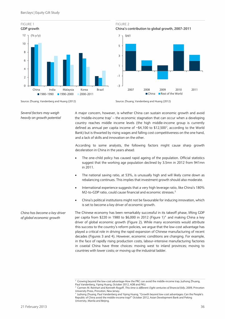
Barclays | Equity Gilt Study

21 February 2013 36

A major concern, however, is whether China can sustain economic growth and avoid the ‘middle-income trap’ – the economic stagnation that can occur when a developing country reaches middle income levels (the high middle-income group is currently defined as annual per capita income of ~$4,100 to $12,5002

According to some analysts, the following factors might cause sharp growth deceleration in China in the years ahead:

, according to the World Bank) but is thwarted by rising wages and falling cost competitiveness on the one hand, and a lack of skills and innovation on the other.

• The one-child policy has caused rapid ageing of the population. Official statistics suggest that the working age population declined by 3.5mn in 2012 from 941mn in 2011.

• The national saving ratio, at 53%, is unusually high and will likely come down as rebalancing continues. This implies that investment growth should also moderate.

• International experience suggests that a very high leverage ratio, like China’s 180% M2-to-GDP ratio, could cause financial and economic stresses.3

• China’s political institutions might not be favourable for inducing innovation, which is set to become a key driver of economic growth.

The Chinese economy has been remarkably successful in its takeoff phase, lifting GDP per capita from $220 in 1980 to $6,000 in 2012 (Figure 1)4

2 Growing beyond the low-cost advantage-How the PRC can avoid the middle-income trap, Juzhong Zhuang, Paul Vandenberg, Yiping Huang, October 2012, ADB and PKU.

and making China a key driver of global economic growth (Figure 2). While many economists would attribute this success to the country’s reform policies, we argue that the low-cost advantage has played a critical role in driving the rapid expansion of Chinese manufacturing of recent decades (Figures 3 and 4). However, economic conditions are changing. For example, in the face of rapidly rising production costs, labour-intensive manufacturing factories in coastal China have three choices: moving west to inland provinces; moving to countries with lower costs; or moving up the industrial ladder.

3 Carmen M. Reinhart and Kenneth Rogoff, This time is different: Eight centuries of financial folly, 2009, Princeton University Press, Princeton, New Jersey. 4 Juzhong Zhuang, Paul Vandenberg and Yiping Huang, “Growth beyond low-cost advantages: Can the People’s Republic of China avoid the middle-income trap?” October 2012, Asian Development Bank and Peking University, Manila and Beijing.

FIGURE 1 GDP growth

FIGURE 2 China’s contribution to global growth, 2007-2011

0

2

4

6

8

10

12

China India Malaysia Korea Brazil

(% y/y)

1980-1990 1990-2000 2000-2011

-3

-1

1

3

5

7

2007 2008 2009 2010 2011

(pp)

China Rest of the World

Source: Zhuang, Vandenberg and Huang (2012) Source: Zhuang, Vandenberg and Huang (2012)

Several factors may weigh heavily on growth potential

China has become a key driver of global economic growth

Barclays | Equity Gilt Study

21 February 2013 37

In a way, what is occurring in China’s coastal area now is a repeat of what happened in Hong Kong, Korea and Taiwan (HKT) 30 years ago. All three economies later became high-income economies.

International experience, however, suggests that the success rate of overcoming the middle-income trap is quite low. According to the World Bank and the Development Research Centre of the State Council (DRC), of 101 middle-income economies in 1960 (based on GDP per capita relative to the US) only 13 had become high-income economies by 2008, including HKT, Japan and Singapore in Asia.5

Whether China will graduate to high-income status will depend critically on its ability to graduate from low value-added manufacturing and move into high value-added manufacturing and services. This requires changes in two interrelated areas: one is to alleviate structural risks, such as imbalances, inefficiency and inequality; the other is to encourage technological innovation and industrial upgrading.

The remaining 88, including Malaysia, the Philippines and Thailand (MPT) in Asia, failed to do so (Figure 5).

FIGURE 5 Income per person relative to the US, 1960 and 2008 (log of %)

0.0

1.0

2.0

3.0

4.0

5.0

0 1 2 3 4 5 6

Income per person relative to the

United States, log of %

1960

Low-income to middle-

Low-income "trap"

Becoming poor

Middle-income

Staying rich

Middle-income to high-

Botswana

Burundi

China

Oman MalaysiaS. Korea

Taiwan

Brazil

United StatesSwitzerlan

Kuwait

GreeceIsreal

Becoming poor

Middle-income

Staying rich

Middle-income to high-

Botswana

Burundi

China

Oman MalaysiaS. Korea

Taiwan

Brazil

Niger

N. Korea

United StatesSwitzerland

KuwaitArgentina

Greece

2008

Source: World Bank, Barclays Research

5 China: 2030 – Building a modern, harmonious, and creative high-income society, The World Bank and Development Research Center of the State Council, the People’s Republic of China, March 2012, Washington D.C.

FIGURE 3 Index of hourly manufacturing labor compensation costs, 2010 (US=100)

FIGURE 4 Annual average real interest rates (lending), 1990-2010 (% pa)

0

10

20

30

40

50

60

70

80

90

100

US

Sing

apor

e

Kore

a

Braz

il

Taiw

an

Mex

ico

Phili

ppin

es

Chin

a

Indi

a

0

3

6

9

12

15

Chin

a

Mal

aysi

a

Phili

ppin

es

Indo

nesi

a

Thai

land

Chile

Arg

entin

a

UK

Japa

n

Kore

a

US

Ger

man

y

Middle income countries High income countries

Source: Zhuang, Vandenberg and Huang (2012) Source: Zhuang, Vandenberg and Huang (2012)

Will China graduate from low value-added manufacturing and move into high value-added manufacturing and services?

Barclays | Equity Gilt Study

21 February 2013 38

Lessons from the other countries The term “middle-income trap” was originally coined by the World Bank to describe growth stagnation in Latin America. Most low-income countries are agrarian. Economic development often involves the migration of farmers into the urban sector, generating significant productivity gain while labour costs remain very low given virtually unlimited supply. Therefore, by developing labour-intensive and low value-added urban sectors, the economy can grow rapidly. This process can continue until the countryside runs out of surplus labour (as happened in Japan in the early 1960s, in Korea and Taiwan in the early 1980s and in China right now). At that point, labour costs start to rise sharply and the country quickly loses competitiveness in labour-intensive industries.

The key factor determining whether a country can escape this trap lies in its ability to achieve technological progress and industrial upgrading. If it can climb up the value chain, its new industries should be competitive, even with higher labour costs, allowing it to graduate into the high-income group. If it fails to progress in these areas, it will be unable to compete with either low-income or high-income economies, remaining stuck in the middle-income range.

According to a report by Zhuang, Vandenberg and Huang (2012), 28 of 125 countries globally have been at middle-income levels since 1987.6

Of these, 18 were middle-income economies as early as 1962, meaning that they have been stuck at the middle-income level for at least 50 years (Figure 6). Of these 18 countries, 12 are in Latin America, three in Africa and the Middle East, and three – Malaysia, Philippines and Thailand (MPT) – in Asia.

FIGURE 6 High and middle income country groups

High income Middle income

Group 1 Group 2 Group 3 HI before/in 1965 HI after 1965 MI continuously 1987-2009 n=17 n=14 n=28 Europe Europe Europe Latin America Austria Croatia Belarus Argentina Belgium Czech Republic Lithuania Bolivia Denmark Hungary Romania Brazil Finland Poland Russia Chile France Slovakia Colombia Germany Asia Costa Rica Italy Greece Malaysia Dominican Republic Netherlands Ireland Philippines El Salvador Norway Portugal Thailand Guatemala Sweden Spain Mexico Switzerland Africa/Near East Panama United Kingdom Asia Jordan Paraguay Hong Kong Lebanon Peru N. America/Oceania Japan Morocco Uruguay Australia Korea South Africa Canada Singapore Syria New Zealand Taiwan Tunisia United States Turkey Near East Israel

Note: Includes only countries with populations exceeding 3mn; excludes members of the Organization of the Petroleum Exporting Countries. Source: P Vandenberg, L. Poot and J. Zhuang, “The middle-income trap: Characteristics, policies and lessons for the People’s Republic of China”, 2011, Asian Development Bank, Manila.

6 Some materials presented in this subsection are adapted or drawn from Juzhong Zhuang, Paul Vandenberg and Yiping Huang, “Growing beyond the low-cost advantage: Can the People’s Republic of China avoid the middle income trap?”, Asian Development Bank and Peking University, 2012, Manila and Beijing.

If a country can climb up the value chain, its new industries should be competitive, even with higher labour costs

Barclays | Equity Gilt Study

21 February 2013 39

Currently, there are about 31 high-income economies worldwide. Of these, 14 moved from middle- to high-income levels after 1965. Nine of these are in the European periphery, with the remaining five from East Asia: Hong Kong, Japan, Korea, Singapore and Taiwan. Japan emerged from the devastation of World War II to reach high-income status in 1968 – a period of just 23 years. Korea reached the middle-income level in 1962 and became a high-income economy 32 years later, in 1994. Taiwan, Hong Kong and Singapore were firmly middle-income in 1962 and became high-income economies in the 1970s and 1980s.

For decades, Malaysia, Philippines and Thailand have failed to move up the value chain. This could simply be because they have not focused on innovation. In 2006, R&D expenditure accounted for 0.63% of GDP in Malaysia, 0.11% in the Philippines and 0.25% in Thailand. By contrast, the ratio was 3.4% in Japan, 3.0% in Korea and 2.2% in Singapore. But the causes of low R&D can be wide-ranging, including insufficient government input, lack of human capital, lack of intellectual property protection, macroeconomic instability and social and political chaos.

The experiences of successful economies suggest that several key ingredients are required to support innovation, upgrading, and the transition to a high-value economy.7

Second, the government needs to invest in physical infrastructure, the social environment and human capital. Industrial upgrading requires human capital for research, development, production and management, which calls for a strong education system. Infrastructure, including transport, communication and power, is also vital for firms to boost productivity and compete globally. Sound legal and regulatory systems are needed to protect intellectual property rights and encourage technological innovation. Most of these tasks cannot be accomplished by the private sector alone and require significant government effort.

First, macroeconomic, political and social stability are necessary for an economy to overcome the middle-income trap, as instability will disrupt investment decisions, production planning, and market demand. Indeed, many Latin American countries that have failed to move beyond the middle-income development stage have suffered from hyperinflation, macroeconomic instability, debt crises, high income equality, and political instability.

Third, a well functioning market system is necessary to allocate resources efficiently, organize production and trade, and provide price signals and incentives for producers and consumers. While the government has many roles to play, international experience suggests that resource allocation and other economic decisions are best left to the market and the private sector. An efficient financial system is needed to facilitate investment, production and trade. More important, R&D activities require financial services that differ from those needed for low value-added manufacturers. Financing channels need to be diversified to better manage risk and support investment in innovation.

Finally, a focused industrial policy may be helpful. This remains a contentious issue but an increasing number of economists recognize that industrial policy has an important role to play in successfully transforming an economy and avoiding the middle-income trap. Such policies may involve sector- and industry-specific interventions to support innovation and upgrading. Varied industrial policy measures have been used in developing economies, including targeting priority industries, providing subsidized credit, trade policy, support for R&D, state ownership, and information sharing.

In our view, the experience of recent decades calls for a reassessment of the Washington Consensus (on the basis of which Washington-based institutions often provided policy advice to developing countries). Key elements of the Washington Consensus include privatisation, liberalisation, free markets, fiscal discipline and minimal state intervention. Yet most economies overcoming the middle-income trap have not rigorously followed these policy prescriptions. East Asia’s economic success also shows that government can play an important role, especially in urging structural transformation where markets alone are insufficient.8

7 Zhuang, Vandenberg and Huang (2012).

8 Daniel Rodrik, “Industrial policy for the twenty-first century”, 2004, John F. Kennedy School of Government, Harvard University, Massachusetts.

Macroeconomic, political and social stability are necessary for an economy to overcome the middle-income trap

The government also needs to invest in physical infrastructure, the social environment and human capital

Financing channels need to be diversified to better manage risk and support investment in innovation

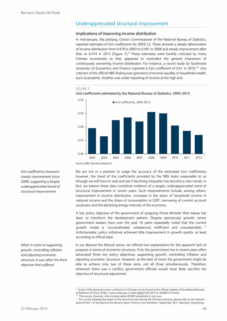
Barclays | Equity Gilt Study

21 February 2013 40

Underappreciated structural improvement

Implications of improving income distribution In mid-January, Ma Jiantang, China’s Commissioner of the National Bureau of Statistics, reported estimates of Gini coefficients for 2003-12. These showed a steady deterioration of income distribution from 0.479 in 2003 to 0.491 in 2008 and steady improvement after that, to 0.474 in 2012 (Figure 7).9 These estimates were harshly criticised by many Chinese economists as they appeared to contradict the general impression of continuously worsening income distribution. For instance, a recent study by Southwest University of Economics and Finance reported a Gini coefficient of 0.61 in 2010.10

One criticism of the official NBS finding was ignorance of income equality in household wealth, such as property. Another was under-reporting of income at the high end.

FIGURE 7 Gini coefficients estimated by the National Bureau of Statistics, 2003-2012

0.46

0.47

0.48

0.49

0.50

2003 2004 2005 2006 2007 2008 2009 2010 2011 2012

Gini coefficients, 2003-2012

Source: NBS, Barclays Research

We are not in a position to judge the accuracy of the estimated Gini coefficients; however, the trend of the coefficients provided by the NBS looks reasonable to us (though we will have to wait and see if declining inequality has become a new trend). In fact, we believe these data constitute evidence of a largely underappreciated trend of structural improvement in recent years. Such improvements include, among others, improvement in income distribution, increases in the share of household income in national income and the share of consumption in GDP, narrowing of current account surpluses, and the declining energy intensity of the economy.

A key policy objective of the government of outgoing Prime Minister Wen Jiabao has been to transform the development pattern. Despite spectacular growth, senior government leaders have over the past 10 years repeatedly noted that the current growth model is ‘uncoordinated, unbalanced, inefficient and unsustainable’. 11

In our Beyond the Miracle series, we offered two explanations for the apparent lack of progress in terms of economic structure. First, the government has in recent years often advocated three key policy objectives: supporting growth, controlling inflation and adjusting economic structure. However, at the best of times the government might be able to achieve only two of these aims, not all three simultaneously. Therefore, whenever there was a conflict, government officials would most likely sacrifice the objective of structural adjustment.

Unfortunately, policy initiatives achieved little improvement in growth quality, at least according to official data.

9 Script of Ma Jiantang’s press conference in Chinese can be found at the official website of the National Bureau of Statistics of China: (http://www.stats.gov.cn/tjdt/gjtjjdt/t20130118_402867315.htm). 10 This survey, however, only includes about 8,000 households in one year. 11 For a more detailed discussion of the structural risks facing the Chinese economy, please refer to the relevant parts of Part 1 of the Beyond the Miracle report ‘China’s next transition’, September 2011, Barclays, Hong Kong.

Gini coefficients showed a steady improvement since 2008, suggesting a largely underappreciated trend of structural improvement

When it came to supporting growth, controlling inflation and adjusting economic structure, it was often the third objective that suffered

Barclays | Equity Gilt Study

21 February 2013 41

Second, distortions in factor costs are at least partly responsible for extraordinary growth performance and a deteriorating economic structure. Correction of these structural problems also requires changes to factor costs to alter the behaviour of economic agencies. In our view, Wen Jiabao’s policy initiatives have achieved limited results, primarily because he focused mainly on administrative measures, not incentive structures, such as input costs. For example, the government tried to control the overinvestment problem by approving fewer projects. This did not work because incentives for investment remained very strong.

Our latest analysis, however, suggests that structural improvement has begun, albeit not as a result of policy initiatives. The main trigger of the improvement has been change in factor markets, including rapid wage growth stemming from increasing labour shortages, and de facto interest rate liberalization as a result of growing shadow banking businesses. These change incentive structures for corporations and households and income distributions at different levels, leading, in turn, to improvements in economic structure.

Consumption recovery and structural rebalancing Important structural changes are happening. For instance, household income as a share of GDP has started to pick up mainly because of rapid wage growth. The current account surplus narrowed from 10.8% of GDP in 2007 to 2.6% in 2012. Mainly because of this, PBoC Deputy Governor Yi Gang argued that the yuan exchange rate was near equilibrium, while US President Obama’s former top economic advisor, Lawrence Summers, noted in January 2013 that the yuan was not as undervalued as it was five years earlier.12

Official data also suggest that the contribution of consumption to GDP growth increased from about one-third in 2009 to 51% in 2012. Two Chinese economists, Tian Zhu and Jun Zhang of Shanghai, have gone further, arguing that China’s consumption share is grossly underestimated as a result of underreported residential spending, consumption covered by institutional spending and technical issues in the household survey method. They note that the consumption share estimated by the Penn World Table was 60.9% in 2010, compared with the official figure of 47.4% and 58.9% in the Penn World Table in 1990.

Another rebalancing in recent years relates to regional disparity, with the rural-urban income gap narrowing notably (Figure 8). In addition, China’s reform success was until recently a story of the coastal regions. However, inland economies are now growing faster than the coastal economies, thanks to the government’s ‘go west’ policy, the migration of manufacturing industries, and rich resource endowments in western China (Figure 9).

12 “Yi warns of currency wars as yuan close to ‘equilibrium’”, 28 January 2013, Bloomberg, http://www.bloomberg.com/news/2013-01-26/china-s-yi-warns-on-currency-wars-as-yuan-in-equilibrium-.html.

Distortions in factor costs were behind the observed rapid increase in corporate profits

Structural improvement has begun as a result of changes in factor markets

Another rebalancing in recent years relates to regional disparity, with the rural-urban income gap narrowing notably

FIGURE 8 Rural – urban income gap narrowed

FIGURE 9 Growth in Eastern, Central and Western China

1.

2.

2.

3.

3.

4.

0

5

10

15

20

25

1987 1992 1997 2002 2007 2012

Income per capita: Urban (CNY th)

Income per capita: Rural (CNY th)

Urban-Rural Ratio (%, RHS)

0

2

4

6

8

10

12

14

16

Beiji

ng

Shan

ghai

Zhej

iang

Jiang

su

Jiang

xi

Anh

ui

Hub

ei

Cho

ngqi

ng

Sich

uan

Xin

jiang

2012 China GDP growth (%y/y)

Eastern Central Western

Source: CEIC, Barclays Research Source: CEIC, Barclays Research

Barclays | Equity Gilt Study

21 February 2013 42

Our research finds that the consumption share of GDP began to rise after 2008, although this is not yet fully reflected in official statistics.13

Our analysis encountered widespread scepticism after its initial dissemination. Some commentators found it difficult to accept our finding given their strong impression of sharply worsened structural problems following the CNY 4trn stimulus package adopted in late 2008. Others argued that structural improvement was impossible since the government had not undertaken more decisive reforms. However, five months later, David Li, a former member of the PBoC’s Monetary Policy Committee, published a similar study applying a different approach. By recalculating Chinese household consumption expenditure, he concluded that household consumption share rebounded from 36% in 2007 to 38.5% in 2011 (Figure 11).

By comparing three sets of consumption data collected and compiled by the NBS, we find significant gaps between retail sales and national account consumption data. Although the latter are derived mainly from household survey data, some previous studies pointed to possible underreporting of both household income and consumption. By assuming new growth rates for consumption (a weighted average of consumption-related retail sales growth and service sales growth), we find that the consumption share of GDP fell during much of the past decade, as suggested by official data, but rebounded from 48% in 2008 to 52% in 2010 (Figure 10).

Causes of rebalancing in China Both our study and that of David Li point to recent wage increases as the main trigger of an increase in the consumption share of GDP. According to the study by Li and Xu, alongside a rebound of the consumption share of GDP, labour income also picked up from 41% in 2007 to 47.1% in 2009 (Figure 12). One special mechanism is the change in labour market conditions. When an ‘unlimited labour supply’ exists, rapid industrialisation is accompanied by a stable wage rate and, therefore, a declining share of wage income in GDP. This is reversed when a labour shortage emerges: wages rise rapidly and the share of wage income in GDP starts to grow.

In fact, this was exactly what happened in Korea and Taiwan in the mid-1980s, when their consumption shares started to recover. That was also when those two economies experienced the so-called Lewis turning point, when labour markets shift from surplus to shortage (Figure 13). The same has happened in recent years in China, with the labour shortage problem intensifying since mid-2009. Rapid wage growth increased the share of household income in the economy and contributed to a rebound in the consumption share of GDP, although this rebalancing is only at the beginning.

13 China: Beyond the Miracle: Great wave of consumption upgrading, Yiping Huang, Jian Chang, Lingxiu Yang, January 2012.

The consumption share of GDP started to rise after 2008, although this is not yet fully reflected in official statistics

FIGURE 10 Consumption share of GDP by estimate by Barclays

FIGURE 11 Household consumption share estimate by former PBoC MPC member, David Li

40

45

50

55

60

65

70

2000 2002 2004 2006 2008 2010

Official consumption share (%)

Estimated consumption share (%)

30

35

40

45

50

55

1990 1993 1996 1999 2002 2005 2008 2011

Reconstructed consumption share (%)

Official consumption share (%)

Source: Barclays Research

Source: Li & Xu study

A labour shortage causes wages to rise rapidly and the share of wage income in GDP starts to grow

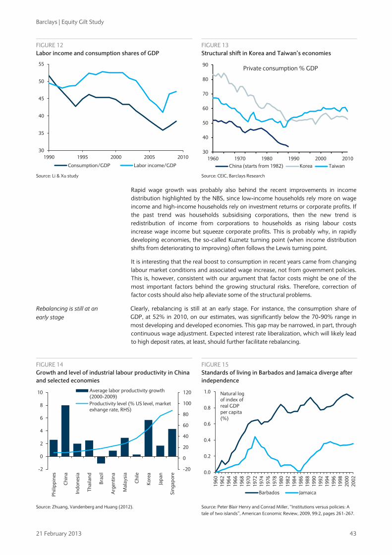
Barclays | Equity Gilt Study

21 February 2013 43

Rapid wage growth was probably also behind the recent improvements in income distribution highlighted by the NBS, since low-income households rely more on wage income and high-income households rely on investment returns or corporate profits. If the past trend was households subsidising corporations, then the new trend is redistribution of income from corporations to households as rising labour costs increase wage income but squeeze corporate profits. This is probably why, in rapidly developing economies, the so-called Kuznetz turning point (when income distribution shifts from deteriorating to improving) often follows the Lewis turning point.

It is interesting that the real boost to consumption in recent years came from changing labour market conditions and associated wage increase, not from government policies. This is, however, consistent with our argument that factor costs might be one of the most important factors behind the growing structural risks. Therefore, correction of factor costs should also help alleviate some of the structural problems.

Clearly, rebalancing is still at an early stage. For instance, the consumption share of GDP, at 52% in 2010, on our estimates, was significantly below the 70-90% range in most developing and developed economies. This gap may be narrowed, in part, through continuous wage adjustment. Expected interest rate liberalization, which will likely lead to high deposit rates, at least, should further facilitate rebalancing.

FIGURE 12 Labor income and consumption shares of GDP

FIGURE 13 Structural shift in Korea and Taiwan’s economies

30

35

40

45

50

55

1990 1995 2000 2005 2010

Consumption/GDP Labor income/GDP

30

40

50

60

70

80

90

1960 1970 1980 1990 2000 2010

Private consumption % GDP

China (starts from 1982) Korea Taiwan Source: Li & Xu study Source: CEIC, Barclays Research

FIGURE 14 Growth and level of industrial labour productivity in China and selected economies

FIGURE 15 Standards of living in Barbados and Jamaica diverge after independence

-20

0

20

40

60

80

100

120

-2

0

2

4

6

8

10

Phili

ppin

es

Chin

a

Indo

nesi

a

Thai

land

Braz

il

Arg

entin

a

Mal

aysi

a

Chile

Kore

a

Japa

n

Sing

apor

e

Average labor productivity growth (2000-2009)Productivity level (% US level, market exhange rate, RHS)

0.0

0.2

0.4

0.6

0.8

1.0

1960

1962

1964

1966

1968

1970

1972

1974

1976

1978

1980

1982

1984

1986

1988

1990

1992

1994

1996

1998

2000

2002

Natural log of index of real GDP per capita (%)

Barbados Jamaica

Source: Zhuang, Vandenberg and Huang (2012). Source: Peter Blair Henry and Conrad Miller, “Institutions versus policies: A tale of two islands”, American Economic Review, 2009, 99:2, pages 261-267.

Rebalancing is still at an early stage

Barclays | Equity Gilt Study

21 February 2013 44

Further changes may also be required to transform the development pattern completely. This could involve measures to improve income equality beyond the primary round of income distribution, development of social welfare systems such as pension, medical insurance and education, and financial and capital account liberalization.

Rebalancing and reduction of other structural risks are only the first steps toward sustainable growth. If China relied mainly on increasing factor inputs to rise to a high middle-income economy, at GDP $6,000 per capita in 2012, it now has to depend more on productivity growth to double the current income level and graduate to high-income status. On a positive note, as Justin Lin has noted, China still has huge potential to grow.14

Political and economic reforms

Its current level of industrial labour productivity is only about 10% that of the US and still below the levels of Malaysia, Argentina, Brazil, Thailand and Indonesia (Figure 14). Realizing that potential, however, could be a very arduous task.

For some scholars and policymakers, the Chinese economic experience of the past three decades provides an alternative model to the Washington Consensus. Joshua Cooper Ramo, for instance, published The Beijing Consensus in 2004.15

Will China fail?

Although there is no precise definition of the Beijing Consensus, it has evolved to mean alternative plans for economic development in emerging markets. Critics, however, often argue that the so-called important features of the Beijing Consensus are simply problems yet to be addressed in a half-reformed economy.

In Why nations fail, Daron Acemoglu and James A. Robinson (AR) argued that “growth under extractive political institutions, as in China, will not bring sustained growth, and is likely to run out of steam.”16

Perhaps the most important contribution of AR’s analytical framework is the distinction between inclusive and extractive institutions. Inclusive economic institutions are those that allow and encourage participation by the great mass of people in economic activities that make best use of their talents and skills and that enable individuals to make the choices they wish.

Their central thesis is that institutions influence behaviour and incentives in real life and forge the success or failure of nations.

17

Politics, in the meantime, is the process by which a society chooses the rules it lives by. AR refer to political institutions that are sufficiently centralized and pluralistic as inclusive political institutions, and refer to the institutions as extractive political institutions when either of the above conditions fails.

Inclusive economic institutions are good for growth because they give people the freedom to choose what they do best and also promote education and technological progress, two important engines of growth. In contrast, extractive economic institutions are designed to extract income and wealth from one subset of society to benefit a different subset.

AR conclude that nations fail when they have extractive economic institutions, supported by extractive political institutions that impede and even block economic growth. Why don't all societies create economic institutions that bring prosperity? The answer lies in the fact that different institutions have different consequences not only for the prosperity of a nation, but also for how that prosperity is distributed and who has power. Economic growth creates both winners and losers. Therefore, powerful groups often stand against economic progress and against the engines of prosperity.

14 Justin Yifu Lin, Demystifying the Chinese Economy, 2011, Cambridge University Press, New York. 15 Joshua Cooper Ramo, The Beijing Consensus, 2004, The Foreign Policy Centre, London. 16 AR’s theory that institutions determine long-run growth runs right into the heart of the popular institutional economics. Acemoglu received the John Bates Clark Medal in 2006 for his work on institutions and growth, which is awarded to economists under forty judged to have made the most significant contribution to economic thought and knowledge. He is widely speculated in the economist community as a potential candidate for the Nobel Prize in Economics. 17 Furthermore, to be inclusive, economic institutions must feature secure private property, an unbiased system of law, and a provision of public services that provides a level playing field in which people can exchange and contract; it also must permit the entry of new businesses and allow people to choose their careers.

China now has to depend more on productivity growth to double its current income level and graduate to high-income status

Barclays | Equity Gilt Study

21 February 2013 45

AR argue that rapid growth is possible in China because of a significant move away from the most extractive economic institutions, even without transformation of the political institutions. But in AR’s view, this growth will not be sustained, for two reasons. First, sustained economic growth requires innovation, and innovation cannot be decoupled from creative destruction. Second, the ability of those who dominate extractive institutions to benefit greatly at the expense of the rest of society implies that political power under extractive institutions is highly coveted, making many groups and individuals fight to obtain it.

We think AR makes an important point that political reform needs to eradicate problems such as corruption, monopoly and disparity and to sustain rapid economic growth. But we also believe that AR’s analytical framework may be too simplistic and their overall assessment of the Chinese growth outlook too pessimistic. First, there could be more than one form of ‘good’ institution supporting long-run growth, especially at different stages of development. For example, Hong Kong, Korea, Singapore and Taiwan did not have inclusive political institutions when they were about to graduate into high-income status. We are also unsure whether Britain’s institutions at the time of the industrial revolution were more inclusive than the institutions in many Asian countries today.

In our view, what China needs to undertake in the next stage of economic development is technological diffusion, not original innovation. As Jeffrey Sachs has noted, innovation and diffusion require different types of institutions.18

Second, while institutions are undoubtedly important, macroeconomic policies may exert just as much influence on economic performance. In an interesting study, Peter Blair Henry and Conrad Miller compared economic performance between two Caribbean islands.

Original research and innovation are highly uncertain, so the only way to succeed is to encourage large-scale experimentation. Meanwhile, technological diffusion has a clear target: comprehension, replication and adaption. Therefore, the state may be able to play a greater role in directly supporting technological diffusion. In other words, while institutions matter, optimal institutions may be different for economies at different stages of development.

19

A quick examination of economic performance of the transitional economies during the last two decades may push the above argument even further. Many of the transitional economies in Central and Eastern Europe clearly have more ‘inclusive’ economic and political institutions than those in the transitional economies in Asia, according to AR’s definitions. The former group, however, had consistently weaker growth performance than the latter group, especially China.

Barbados and Jamaica are both former British colonies, gaining independence in 1966 and 1962, respectively. Both inherited almost identical economic and political institutions: Westminster Parliamentary democracy, constitutional protection of property rights, and English Common Law. In the 40 years after independence, the standard of living in the two countries diverged (Figure 15). Jamaica recorded average real income growth of 0.8% per year during the entire sample period, while Barbados achieved 2.2%. The difference, according to Henry and Miller, stemmed almost entirely from differences in macroeconomic policies, not institutions.

Third, we think AR’s analytical framework has a major shortcoming, ie, the one-directional causation from politics to economic institutions to growth performance. There is no feedback from economics to politics. And this is probably why they often fail to explain how political changes take place. For instance, in the book, AR described at length how Deng Xiaoping engineered a political ‘revolution’ in the late 1970s before introducing economic reforms. But they do not address why Deng Xiaoping started economic reform. We think the reason behind Deng Xiaoping’s reforms was that the

18 Jeffrey D. Sachs, “Government, geography and growth: The true driver of economic development”, Foreign Affairs, September/October 2012. 19 Peter Blair Henry and Conrad Miller, “Institutions versus policies: A tale of two islands”, American Economic Review, 2009, 99:2, pages 261-267.

In Why nations fail, the authors may have overestimated the role of ‘good’ institutions

In the next stage of economic development, China needs to undertake technological diffusion, not original innovation

While institutions matter, macroeconomic policies may exert just as much influence on economic performance

We disagree with the one-directional causation from politics to economic institutions to growth performance

Barclays | Equity Gilt Study

21 February 2013 46

economy was on the verge of collapse and he saw no alternative. The Chinese political system has evolved for the same reason. For example, the Communist Party now actively recruits members from among private entrepreneurs, conducts direct elections at the village level and allows a certain degree of monitoring by social media.

Re-defining the role of the government in the economy Our overall take is that political reforms are important for maintaining social and political stability, but economic policy choices can still play a major role in facilitating economic growth.

To that end, both the World Bank and the Asian Development Bank, in collaboration with some Chinese institutions, made important policy recommendations in 2012 (Figure 16). The two sets of recommendations have significant overlaps. Both highlight the importance of supporting innovation and industrial upgrading. They also focus on structural reforms to improve the functioning of markets, macroeconomic policy reforms, the greening of the economy and maintaining good relations with the rest of the world. The World Bank also singles out social security for all, while the Asian Development Bank emphasises the importance of services, urbanization and equality.

Incoming Premier Li Keqiang has set urbanization as a key policy theme for the next 10 years. This essentially means giving 200-300mn migrant workers official urban resident status and bringing even more rural residents into the cities. This should support economic growth by increasing consumer spending, growing the service sector, etc. But it will also require substantial reforms and investment, including in urban infrastructure, housing and social security systems.

One option for organizing the reform agenda is to redefine the relationship between the government and market, as suggested by the Central Committee’s Political Report to the 18th Party Congress last October. The relationship between the government and the market has been a hot topic since the beginning of economic reform. Essentially, economic reform is about the government making room for the market to play a greater role in allocating resources, products and income. However, the Chinese reform approach has been gradual. The state continues to play an active role in economic activities. That approach has generated good results in terms of achieving economic growth but also created problems that could hinder future economic growth.

We expect the government to redefine the relationship between the government and market in the coming years at three levels. The first is to liberalise the factor markets and complete the transition to a market economy. During the past three decades, the government has completely abandoned restrictions on product markets but intervened in factor markets. Distortions to factor markets, including subsidies to corporations and taxes on households, boosted economic growth but also led to various imbalances,

FIGURE 16 Some policy prescriptions for avoiding the middle-income trap in China

World Bank & Development Research Center Asian Development Bank & Peking University

Accelerating the pace of innovation and creating an open innovation system

Stepping up innovation and industrial upgrading

Implementing structural reforms to strengthen the foundations for market-based economy

Deepening structural reform, especially reforms of enterprises, labour and land markets

Developing services and scaling up urbanization

Reducing income inequality

Expanding opportunities and promoting social security for all

Strengthening the fiscal system Maintaining macroeconomic and financial stability

Seizing the opportunity to “go green” Promoting green growth to conserve resources and protect the environment

Seeking mutually beneficial relations with the world Strengthening international and regional economic cooperation

Source: “China 2030: Building a modern, harmonious and creative high-income society”, the World Bank and the Development Research Center, 2012, Washington DC and Beijing; “Growing beyond the low-cost advantage: Can the People’s Republic of China avoid the middle income trap?” Asian Development Bank and Peking University, 2012, Manila and Beijing

Distortions to factor markets boosted economic growth but also led to various imbalances

Barclays | Equity Gilt Study

21 February 2013 47

inefficiency and inequality problems. If China had a no-market economy during the pre-reform period and a half-market economy during the past three decades, it is now, in our view, time for China to move to a full-market economy.

We believe the transition to a full-market economy will require the scrapping of the household registration system, a major obstacle to labour mobility. Financial liberalisation is also critical for efficient allocation of financial resources. This may involve interest rate liberalisation, exchange rate reform, reform of financial institutions’ corporate governance and liberalisation of the capital account. Given the political reality, we do not anticipate a major wave of privatisation of state-owned enterprises (SOEs) any time soon. Instead, the government will probably try to create a level-playing field for SOEs and non-SOEs by focusing on reforms in two areas: input cost distortions and monopoly power.

The second task will be to establish a new macroeconomic regulatory system, including a professional monetary policy-making mechanism and accountable budgetary systems for government at all levels. This is crucial not only to facilitate the transition to the full-market economy but also to control some growing macroeconomic risks. For instance, in retrospect, the stimulus package introduced in late 2008 was quite successful in boosting economic growth in 2009. But it also created fiscal, credit and inflation risks. One of the reasons for this was that the authorities mobilised SOEs, financial institutions and local governments to achieve macroeconomic policy objectives. But many of these institutions did not have hard budget constraints. Therefore, we believe it is important to make SOEs, financial institutions and local governments accountable for their own decisions. It is also necessary to divorce macroeconomic policies from these institutions.

The third plank is to change the way the government intervenes in economic activities, from directly supporting production and investment to promoting technological innovation and industrial upgrading. In the past, the government’s active role in mobilizing resources for economic activities was a positive factor for economic growth, especially at the early stage of economic liberalisation and market development. However, as economic development moves to the next stage, technological innovation and industrial upgrading will require more decentralised efforts. By definition, innovation is a risky business. Unlike manufacturing production, it is difficult to plan. This does not mean there is no room for the government to play a role, however. The government could focus more on supporting infrastructure development, promoting education and research, facilitating financial services and enforcing protection of intellectual property rights. Again, the government may still design industrial policies to support industrial upgrading.

Early takeoff of science & technology Although future growth will have to rely more on productivity growth and industrial upgrading, China still enjoys a hefty backwardness ‘advantage’. That is to say, it can probably count on technological diffusion to drive economic growth for a long time to come. Unlike pushing the world technological frontier, diffusion is about learning existing technologies from others, which requires different skills and institutions.

The government should move away from directly supporting production and investment and promote technological innovation and industrial upgrading instead

China still enjoys a hefty backwardness ‘advantage’

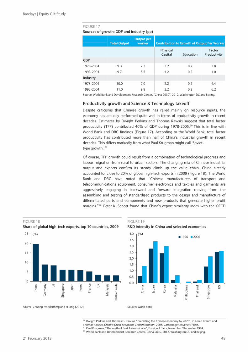
Barclays | Equity Gilt Study

21 February 2013 48

FIGURE 17 Sources of growth: GDP and industry (pp)

Total Output

Output per worker Contribution to Growth of Output Per Worker

Physical Capital Education

Factor Productivity

GDP

1978-2004 9.3 7.3 3.2 0.2 3.8

1993-2004 9.7 8.5 4.2 0.2 4.0

Industry

1978-2004 10.0 7.0 2.2 0.2 4.4

1993-2004 11.0 9.8 3.2 0.2 6.2

Source: World Bank and Development Research Center, “China 2030”, 2012, Washington DC and Beijing.

Productivity growth and Science & Technology takeoff Despite criticisms that Chinese growth has relied mainly on resource inputs, the economy has actually performed quite well in terms of productivity growth in recent decades. Estimates by Dwight Perkins and Thomas Rawski suggest that total factor productivity (TFP) contributed 40% of GDP during 1978-2005.20 This is in line with World Bank and DRC findings (Figure 17). According to the World Bank, total factor productivity has contributed more than half of China’s industrial growth in recent decades. This differs markedly from what Paul Krugman might call ‘Soviet- type growth’.21

Of course, TFP growth could result from a combination of technological progress and labour migration from rural to urban sectors. The changing mix of Chinese industrial output and exports confirm its steady climb up the value chain. China already accounted for close to 20% of global high-tech exports in 2009 (Figure 18). The World Bank and DRC have noted that “Chinese manufacturers of transport and telecommunications equipment, consumer electronics and textiles and garments are aggressively engaging in backward and forward integration moving from the assembling and testing of standardised products to the design and manufacture of differentiated parts and components and new products that generate higher profit margins.”

22

20 Dwight Perkins and Thomas G. Rawski, “Predicting the Chinese economy by 2025”, in Loren Brandt and Thomas Rawski, China’s Great Economic Transformation, 2008, Cambridge University Press.

Peter K. Schott found that China’s export similarity index with the OECD

21 Paul Krugman, “The myth of East Asian miracle”, Foreign Affairs, November/December 1994. 22 World Bank and Development Research Center, China 2030, 2012, Washington DC and Beijing.

FIGURE 18 Share of global high-tech exports, top 10 countries, 2009

FIGURE 19 R&D intensity in China and selected economies

0

5

10

15

20

25

Chin

a

Ger

man

y

US

Sing

apor

e

Japa

n

Kore

a

Fran

ce UK

Mal

aysi

a

Net

herla

nds

(%)

0.0

0.5

1.0

1.5

2.0

2.5

3.0

3.5

4.0

Chin

a

Japa

n

Kore

a

Mal

aysi

a

Phili

ppin

es

Thai

land

Sing

apor

e

US

1996 2006(%)

Source: Zhuang, Vandenberg and Huang (2012)

Source: World Bank

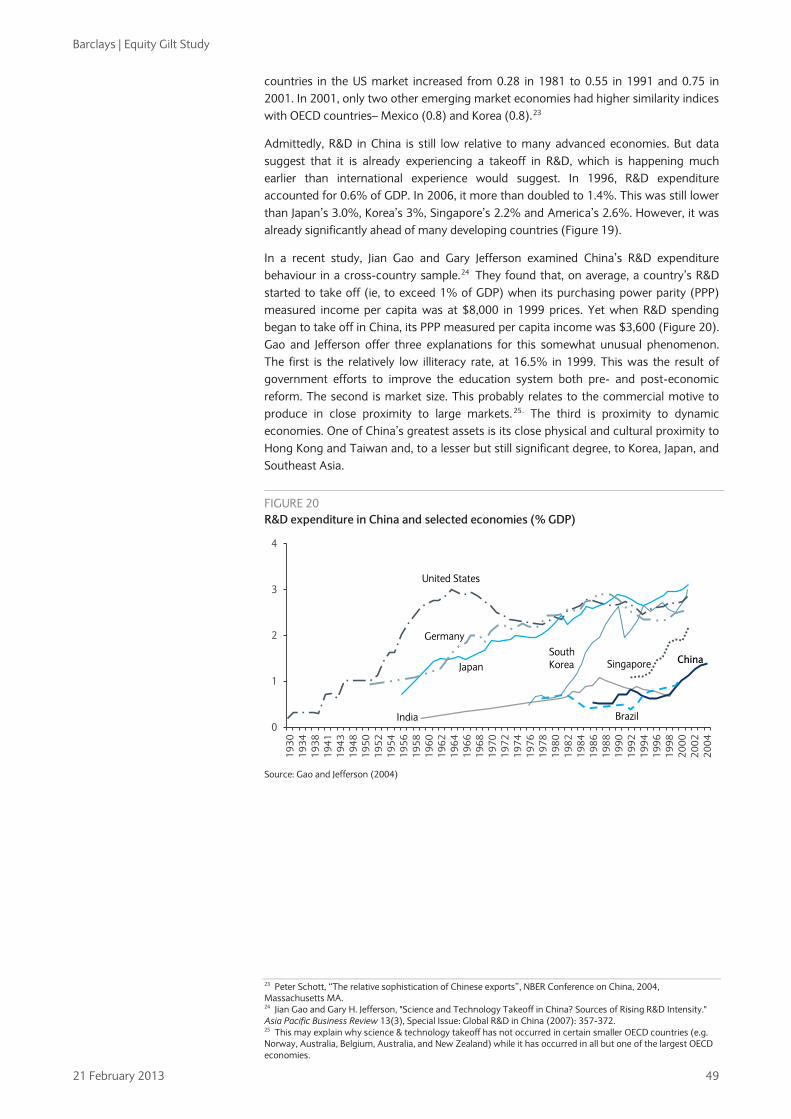
Barclays | Equity Gilt Study

21 February 2013 49

countries in the US market increased from 0.28 in 1981 to 0.55 in 1991 and 0.75 in 2001. In 2001, only two other emerging market economies had higher similarity indices with OECD countries– Mexico (0.8) and Korea (0.8).23

Admittedly, R&D in China is still low relative to many advanced economies. But data suggest that it is already experiencing a takeoff in R&D, which is happening much earlier than international experience would suggest. In 1996, R&D expenditure accounted for 0.6% of GDP. In 2006, it more than doubled to 1.4%. This was still lower than Japan’s 3.0%, Korea’s 3%, Singapore’s 2.2% and America’s 2.6%. However, it was already significantly ahead of many developing countries (Figure 19).

In a recent study, Jian Gao and Gary Jefferson examined China’s R&D expenditure behaviour in a cross-country sample.24 They found that, on average, a country’s R&D started to take off (ie, to exceed 1% of GDP) when its purchasing power parity (PPP) measured income per capita was at $8,000 in 1999 prices. Yet when R&D spending began to take off in China, its PPP measured per capita income was $3,600 (Figure 20). Gao and Jefferson offer three explanations for this somewhat unusual phenomenon. The first is the relatively low illiteracy rate, at 16.5% in 1999. This was the result of government efforts to improve the education system both pre- and post-economic reform. The second is market size. This probably relates to the commercial motive to produce in close proximity to large markets. 25

. The third is proximity to dynamic economies. One of China’s greatest assets is its close physical and cultural proximity to Hong Kong and Taiwan and, to a lesser but still significant degree, to Korea, Japan, and Southeast Asia.

FIGURE 20 R&D expenditure in China and selected economies (% GDP)

0

1

2

3

4

1930

1934

1938

1941

1943

1948

1950

1952

1954

1956

1958

1960

1962

1964

1966

1968

1970

1972

1974

1976

1978

1980

1982

1984

1986

1988

1990

1992

1994

1996

1998

2000

2002

2004

China

India Brazil

SingaporeSouthKorea

United States

Germany

Japan

Source: Gao and Jefferson (2004)

23 Peter Schott, “The relative sophistication of Chinese exports”, NBER Conference on China, 2004, Massachusetts MA. 24 Jian Gao and Gary H. Jefferson, "Science and Technology Takeoff in China? Sources of Rising R&D Intensity." Asia Pacific Business Review 13(3), Special Issue: Global R&D in China (2007): 357-372. 25 This may explain why science & technology takeoff has not occurred in certain smaller OECD countries (e.g. Norway, Australia, Belgium, Australia, and New Zealand) while it has occurred in all but one of the largest OECD economies.

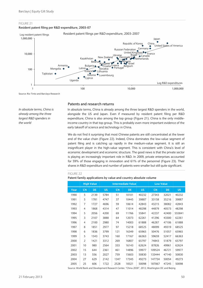
Barclays | Equity Gilt Study

21 February 2013 50

Patents and research returns In absolute terms, China is already among the three largest R&D spenders in the world, alongside the US and Japan. Even if measured by resident patent filing per R&D expenditure, China is also among the top group (Figure 21). China is the only middle-income country in that top group. This is probably even more important evidence of the early takeoff of science and technology in China.

We do not find it surprising that most Chinese patents are still concentrated at the lower end of the value chain (Figure 22). Indeed, China dominates the low-value segment of patent filing and is catching up rapidly in the medium-value segment. It is still an insignificant player in the high-value segment. This is consistent with China’s level of economic development and economic structure. The good news is that the private sector is playing an increasingly important role in R&D. In 2009, private enterprises accounted for 59% of those engaging in innovation and 61% of the personnel (Figure 23). Their shares in R&D expenditure and number of patents were smaller but still quite significant.

FIGURE 22 Patent family applications by value and country absolute volume

High Value

Intermediate Value

Low Value

Year CN DE US CN DE US CN DE US

1990 5 2139 5784 51 10101 40232 27343 32021 40232

1991 5 1781 4747 37 10445 39887 33158 35216 39887

1992 7 1727 4696 59 10614 42843 43215 38082 42843

1993 4 1868 4314 47 11014 48298 44879 40573 48298

1994 5 2056 4200 69 11766 55841 42237 42400 555841

1995 3 2107 3888 64 12073 62261 41296 43300 62261

1996 4 2100 2980 74 14003 61888 46287 47106 61888

1997 8 1851 2977 97 15218 68525 48099 49319 68525

1998 6 1836 3799 121 16349 65965 50476 51057 65965

1999 5 1543 3743 160 17167 66363 59659 52417 66363

2000 2 1421 3312 269 16807 65797 74843 51879 65797

2001 10 980 2564 333 16143 62624 87826 49961 62624

2002 15 644 2361 461 14896 59977 109524 46721 59977

2003 13 556 2027 759 15603 50830 133444 47140 50830

2004 27 629 2142 1347 17345 49273 147734 50054 49273

2005 25 606 1722 2528 18321 50098 187067 47245 50098 Source: World Bank and Development Research Center, “China 2030”, 2012, Washington DC and Beijing

FIGURE 21 Resident patent filing per R&D expenditure, 2003-07

Tajikistan

MongoliaArmenia

LatviaBulgaria

BelarusRomania

Kazakhstan New ZealandUkraine

Russian Federation Germany

ChinaRepublic of KoreaUnited States of America

Japan

UgandaCyprus

LuxembourgEstoniaIceland Lithuania

Slovakia PortugalCroatia Belgium

IsraelNorway

Denmark NetherlandsBrazil Canada

FranceUnited Kingdom

Greece

Log resident patent filings

Log R&D expenditures

Resident patent filings per R&D expenditure, 2003-20071,000,000

10,000

100

11 100 10,000 1,000,000

Source: Rio Tinto and Barclays Research

In absolute terms, China is already among the three largest R&D spenders in the world

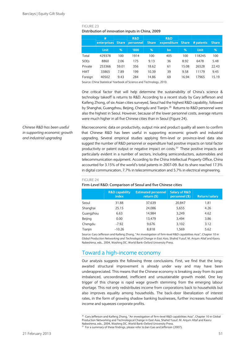
Barclays | Equity Gilt Study

21 February 2013 51

FIGURE 23 Distribution of innovation inputs in China, 2009

#

enterprises Share R&D

personnel Share R&D

expenditure Share # patents Share

Unit % ‘000 % bn % Unit %

Total 429378 100 1914 100 405 100 118245 100

SOEs 8860 2.06 175 9.13 36 8.92 6478 5.48

Private 253366 59.01 356 18.62 61 15.08 26528 22.43

HMT 33865 7.89 199 10.39 39 9.58 11179 9.45

Foreign 40502 9.43 284 14.86 69 16.94 17965 15.19 Source: China Statistical Yearbook of Science and Technology, 2010.

One critical factor that will help determine the sustainability of China’s science & technology takeoff is returns to R&D. According to a recent study by Gary Jefferson and Kaifeng Zhong, of six Asian cities surveyed, Seoul had the highest R&D capability, followed by Shanghai, Guangzhou, Beijing, Chengdu and Tianjin.26

Macroeconomic data on productivity, output mix and product quality all seem to confirm that Chinese R&D has been useful in supporting economic growth and industrial upgrading. Several empirical studies applying firm-level or province-level data also suggest the number of R&D personnel or expenditure had positive impacts on total factor productivity or patent output or negative impact on costs.

Returns to R&D personnel were also the highest in Seoul. However, because of the lower personnel costs, average returns were much higher in all five Chinese cities than in Seoul (Figure 24).

27

FIGURE 24

These positive impacts are particularly evident in a number of sectors, including semiconductors, automobiles and telecommunication equipment. According to the China Intellectual Property Office, China accounted for 3.15% of the world’s total patents in 2007-09. But its share reached 17.3% in digital communication, 7.7% in telecommunication and 5.7% in electrical engineering.

Firm-Level R&D: Comparison of Seoul and five Chinese cities

R&D capability

index Estimated personnel

return ($) Salary of R&D personnel ($) Return/salary

Seoul 31.88 37,639 20,847 1.81

Shanghai 25.15 24,086 5,655 4.26

Guangzhou 6.63 14,984 3,249 4.62

Beijing 0.00 13,479 3,494 3.86

Chengdu -7.92 9,676 3,102 3.12

Tianjin -10.26 8,818 1,569 5.62 Source: Gary Jefferson and Kaifeng Zhong, “An investigation of firm-level R&D capabilities Asia”, Chapter 10 in Global Production Networking and Technological Change in East Asia, Shahid Yusuf, M. Anjum Altaf and Kaoru Nabeshima, eds., 2004, Washing DC, World Bank-Oxford University Press.

Toward a high-income economy Our analysis suggests the following three conclusions. First, we find that the long-awaited structural improvement is already under way and may have been underappreciated. This means that the Chinese economy is breaking away from its past imbalanced, uncoordinated, inefficient and unsustainable growth model. One key trigger of this change is rapid wage growth stemming from the emerging labour shortage. This not only redistributes income from corporations back to households but also improves equality among households. The back-door liberalization of interest rates, in the form of growing shadow banking businesses, further increases household income and squeezes corporate profits.

26 Gary Jefferson and Kaifeng Zhong, “An investigation of firm-level R&D capabilities Asia”, Chapter 10 in Global Production Networking and Technological Change in East Asia, Shahid Yusuf, M. Anjum Altaf and Kaoru Nabeshima, eds., 2004, Washing DC, World Bank-Oxford University Press. 27 For a summary of these findings, please refer to Jian Gao and Jefferson (2007).

Chinese R&D has been useful in supporting economic growth and industrial upgrading

Barclays | Equity Gilt Study

21 February 2013 52

Although rebalancing has so far been driven mainly by changes in factor markets, economic reforms will be critical for furthering structural improvement. These should include removing remaining factor cost distortions, liberalising the financial sector and improving social security systems. We do not think outright privatisation of SOE is feasible in the near term. But the government likely will move steadily toward the creation of a level-playing field by removing input cost subsidy and reducing the monopoly power.

Second, although it is unlikely that China will adopt Western-style democracy any time soon, we expect its leaders to implement some political reforms in the years ahead. Such steps may be necessary to ease social economic tensions and facilitate continuous economic growth and could include the gradual extension of direct election to higher levels of government, having more candidates than posts in high-level internal elections, increased tolerance of social media, stepped-up efforts against corruption, and improvements in the transparency of budgetary and other decision processes.

We do not think Chinese political institutions have already exhausted their potential to foster growth. The experiences of East Asia suggest that more than one form of political institution can support long-run growth. This is particularly true if the economy is still in the technological catch-up stage. Moreover, although institutions are very important, economic policies under the same institutions can still make a big difference in terms of economic growth, as illustrated by the comparison of historical macroeconomic performance between Jamaica and Barbados. And while politics determine economic institutions, which, in turn, affect growth, economic activity may also influence politics. This is why we think political reforms are likely in the coming years.

Finally, the takeoff of science and technology in China has occurred much earlier than international experience would suggest. This is probably because of China’s high literacy rate, large market size and proximity to dynamic economies. In fact, China is already among the world’s leaders in R&D expenditure and research productivity, despite its middle-income status. Its patent-filing activity dominates that of the US and Germany in the low-value segment and is catching up rapidly in the medium-value segment. Most important, private enterprises are playing an increasingly important role in China’s R&D activities.

It is also important to recognise that China can still rely on technological diffusion to climb the value chain. This may require different sets of skills and institutions from pure innovation. Still, China needs to overcome a few hurdles in order to support technological diffusion (innovation) and industrial upgrading. These include better protection of intellectual property rights, more diversified financial services, more government supports to education and basic research. In his book New Structural Economics, Justin Lin proposed that the government play an active role in guiding industrial upgrading by providing hard and soft infrastructure for enterprises based on comparative advantages.28

Currently, China’s GDP per capita is $6,000. If we apply the World Bank’s criterion of slightly above $12,000 as the entry level to high-income status, then China needs to double its real per capita income. We think this could happen before 2020 if we assume growth potential at 7-8% and modest currency appreciation of, say, 3% a year. By then, the Chinese economy would be at least as large as that of the United States. In our view, the favourable factors set out in this report could easily carry the Chinese economy through 2030, when growth potential should fall to 5-6% but per capita income should rise to $22,000, similar to Korea’s current income level.

28 Justin Yifu Lin, The Quest for Prosperity: How developing economies can takeoff? 2012, Princeton University Press, Princeton.

Economic reforms will be critical for furthering structural improvement

We expect China’s leaders to implement some political reforms in the years ahead

We do not think Chinese political institutions have already exhausted their potential to foster growth

The takeoff of science and technology in China has occurred much earlier than international experience would suggest

China can still rely on technological diffusion to climb the value chain

Barclays | Equity Gilt Study

21 February 2013 53

Implications for investors In our view, the key takeaway of our research is that China is unlikely to collapse, even though it may continue to look different from western advanced economies. The experiences of many East Asian economies in the post-war period already demonstrate that there may be more than just one workable route to sustainable economic growth, especially when the economy is still at the catch-up stage. The global financial crisis also indicates that western institutions may themselves have defects. Most important, Chinese institutions, including political institutions, have been dynamic and flexible in responding to the changing conditions, at least since the late 1970s.

One strong argument for a collapse of China or Chinese growth is its high leverage ratio, illustrated by its M2/GDP ratio at 180.1% in 2011. This might be a potential risk, but to show that it is not a sufficient condition for collapse one need look only at the same ratio for Germany: 179.8% in 2011 and 167.7% in 1999. In fact, a high M2/GDP ratio often reflects a financial system dominated by banks not markets.

Meanwhile, continued (albeit slower) economic growth and structural rebalancing should support secular improvement in consumption. Continued wage growth, interest rate liberalisation and the government’s policy on income distribution should support continued rapid growth of household income. In the near term, the luxury sector will likely be dented by income redistribution away from corporate profits as a result of rising production costs and the government’s anti-corruption drive. The medium to high sectors of consumer goods should benefit more as household income rises. Our earlier analyses reveal that when household incomes rise, they spend disproportionately more on appliances, communication and transportation, education, culture and tourism, and financial services. Over time, however, as income levels approach the $10,000 threshold, the consumer base for luxury goods could expand markedly.

China’s strong ability to innovate and upgrade imply that it could lose low-end manufacturing relatively quickly. Although many labour-intensive factories have been moving to inland provinces, this may not last for long as costs are rising across the country. But China will probably not lose its manufacturing altogether. Instead, we expect it to move up the value chain quickly to supply more sophisticated products. Relatively speaking, China is already doing well in patents filing in digital communication, telecommunication and electrical engineering. If current trends continue, China’s technology may also advance rapidly in some other areas, such as automobiles. Thus, if US manufacturers regain competitiveness, the main worry might not stem from China but from those economies stuck between China and the US on the value chain.

Finally, as the economy continues to grow and upgrade, the currency should appreciate steadily. Its current account may stay close to balance, although we think surpluses are more likely than deficits in most years. Outward direct investment (ODI) should rise quickly, probably surpassing inward foreign direct investment (FDI) sometime during the next five years, as the government liberalises the capital account, labour-intensive manufacturers migrate to low-cost destinations and other Chinese companies seek resources, markets and technology. Following financial liberalisation, further growth should emerge in capital markets and direct financing. Banks’ relative importance could decline and the cost of capital in the formal sector should rise. The latter may lead to financial pressure on and consolidation among the mostly state-owned capital-intensive and highly leveraged heavy industries.

China is unlikely to collapse, even though it may continue to look different from western advanced economies

The medium to high sectors of consumer goods should benefit more as household income rises

As the economy continues to grow and upgrade, the currency should appreciate steadily

Barclays | Equity Gilt Study

21 February 2013 54

CHAPTER 4

QE carries risks beyond inflation • The unconventional monetary policies of the major central banks since the onset of

the financial crisis carry the risks of creating excessive inflation, asset price bubbles and stagnant productivity resulting from the propping up of “zombie” companies.

• To a large extent, QE is a symptom rather than a cause of the economy’s underlying woes. Although it need not lead to high inflation, the latter may result from an increased tolerance of inflation in the face of stagnant real economic growth. The US and the UK appear most vulnerable to these pressures.

• Extraordinarily low yields on government bonds might push investors into riskier assets, but widespread uncertainty and strong savings intentions have so far prevented bubbles from arising. However, it remains to be seen whether the new macroprudential policy frameworks will be effective enough to stop damaging distortions from developing if interest rates are held low for too long.

• Accommodative monetary policy and excessive forbearance by banks enable the survival of relatively weak companies that would otherwise be forced out of business, resulting in impaired productivity growth. We see the risk of structural degeneration as higher in Europe than in the US.

In standard models of the economy, the long-run path of output is driven by “real” factors: the size of the labour force, the stock of capital and the effectiveness with which the two are combined (ie, productivity). Monetary policy plays a purely counter-cyclical role, nudging demand back toward sustainable levels when things risk getting too hot or too cold.

It would be a stretch, however, to describe the current loose monetary stance in the major advanced economies as a “nudge”. Policy rates were cut close to zero in the US, UK and euro area in 2008-09 and have remained exceptionally low ever since. The Bank of Japan has been targeting minimal overnight rates since 1998. At the same time, the central banks in these economies have boosted the size of their balance sheets many times over, injecting unprecedented amounts of base money into the economy through various asset purchase operations that we group under the umbrella term “quantitative easing” (QE). One effect of QE is to convey the central banks’ view that interest rates are unlikely to rise for a long time. Thus, although ultra-loose monetary conditions may not be permanent, there is a widespread expectation that they will be very long-lived.

With monetary policy so loose for so long, we ask whether it is still reasonable to assume that it has no lasting effect on economic performance. One clear concern is that ultra-loose monetary policy could lead to high inflation. Keeping interest rates below market levels for a long period might also encourage over-investment and asset price bubbles, posing risks to financial stability. On top of this, the forestalling of the “creative destruction” process could impede productivity growth.

In our view, all three concerns have some legitimacy. Although QE may have helped stave off outright deflation – undoubtedly a substantial benefit – it comes with associated costs. Whether the policy is ultimately deemed successful will depend in part on the authorities acting deftly to ensure these costs are contained.

The risk of excessive inflation

A waning commitment to low inflation? In normal times, there is general agreement that central banks should aim for a low and stable rate of inflation, and 2% has emerged as a common benchmark. However, when unemployment is high, policymakers’ appetite for a single-minded focus on inflation

Simon Hayes +44 (0)20 7773 4637 [email protected]

Paul Robinson +44 (0)20 7773 0903

[email protected]

One effect of QE is to convey the central banks’ view that interest rates are unlikely to rise for a long time

High inflation might be tolerated when unemployment is also high

Barclays | Equity Gilt Study

21 February 2013 55

control may wane. This is especially likely when the economy is de-leveraging, as inflation is viewed as a useful way to erode debt overhangs. History reveals a preference for high rather than low inflation: there have been many examples of relatively high inflation, including in economies such as the US, UK and parts of the eurozone. Though far from ideal, many of these episodes have been successfully dealt with.

Modern economies have had much less experience of dealing with persistently low inflation. Only Japan has had prolonged negative inflation, with deflation apparently the result of endemic weak demand and low inflation expectations (Figure 1). The Japanese experience has troubled many observers because it has been coupled with weak growth. And, unlike those economies in the 1970s where inflation became uncomfortably high, the Japanese authorities have yet to introduce policies that have convincingly stopped the deflation malaise.

No major central bank has jettisoned inflation targeting, nor does this seem likely, but some softening stances on inflation have emerged. The BoJ has adopted an inflation target of 2%, replacing its previous “goal” of 1%, under pressure from the government, a move that should create room for a sizable fiscal expansion to raise activity and employment. The yen has fallen sharply, which should stoke both activity and inflation.

The Fed has increased the emphasis on the unemployment dimension of its dual mandate by specifying an explicit threshold for the unemployment rate above which policy will continue to be held extraordinarily accommodative, as long as inflation remains contained. The “longer-run goal” of 2% inflation has been retained, but somewhat higher inflation will be tolerated if unemployment remains high.

The UK MPC has arguably shown the most tolerance for high inflation, which rose above 5% in 2011 and has been continuously above the 2% target for more than three years. Since the start of the UK recession in 2008, the Governor of the BoE has written 13 letters to the Chancellor of the Exchequer explaining why inflation has been so far above target. Although the inflation target is notionally symmetrical, no letters have ever been written to explain why inflation has been too low. The committee has said that running a tighter monetary policy to bring inflation back to target quickly would worsen unemployment and would not be in the country’s overall economic interests. Incoming BoE Governor Mark Carney has emphasised the importance of economies achieving “escape velocity”, even if this means tolerating above-target inflation for a period.

The ECB stands out as an exception to this drift toward a reduced emphasis on inflation and has shown little appetite for forbearance in the face of inflationary shocks. The ECB’s mandate is similar to that of the BoE – the primacy of the inflation target is tempered somewhat by a requirement for policy to support objectives such as full

FIGURE 1 Deflation has been the norm in Japan in recent decades

FIGURE 2 Inflation swaps suggest few concerns about inflation

0%

10%

20%

30%

40%

50%

60%

Italy

Net

h

U.K

.

Ger

Can Fr

a

Spai

n

Aus

t

U.S

.

Swed

Swit

Japa

n

Proportion of quarters with negative inflation since 1990

-3

-2

-1

0

1

2

3

4

5

Feb-08 Feb-09 Feb-10 Feb-11 Feb-12

%

US Euro area UK Japan Source: Haver Analytics Source: Barclays Research

No major central bank has jettisoned inflation targeting, but some softening stances on inflation have emerged in Japan and the US

The Bank of England has arguably shown the most tolerance for high inflation, which has been above the 2% target for more than three years

The ECB stands out as an exception to the drift toward a reduced emphasis on inflation

Barclays | Equity Gilt Study

21 February 2013 56

employment and balanced growth. However, it has held inflation much closer to its goal than has the BoE, tolerating instead a sharp rise in the euro area unemployment rate, which is now close to 12% compared with the UK rate of below 8%.

Inflation expectations and forecasts Despite these developments, financial markets have so far shown little concern about heightened inflation risks. For example, implied medium-term inflation expectations from inflation-linked swaps differ little from what they were before the global financial crisis (Figure 2). Investors have adjusted inflation expectations in response to changes in the monetary policy framework – notice, for instance, the rise in the Japanese implied inflation expectation following recent policy developments – but such changes have been small in the broad sweep of history.

Our own medium-term inflation forecasts reflect our perception of likely biases across the major economies. In the US and UK, our forecasts are above the central banks’ targets, as we believe that so long as activity growth remains lacklustre, a degree of forbearance will be shown. In the US, we forecast CPI inflation at about 2.75% five years ahead and 2.5% on the PCE measure; in the UK we expect CPI inflation to be closer to 2.5% than to the 2% target.

We think it much less likely that the ECB will tolerate above-target inflation, although history shows that the ECB has tended to struggle to hold HICP inflation below 2% for an extended period. We therefore expect euro area inflation to settle close to 2% in the medium term. Finally, we remain sceptical about the BoJ’s ability to achieve its new target, and expect CPI inflation to settle at around 0.4% in the medium term.

What are the inflation risks from QE? In the four years since the global financial crisis, the US, the euro area, Japan and the UK have seen an extraordinary expansion in base money.1

Central to this question is the concept of the “velocity of circulation of money”, which is the speed with which money changes hands in the economy. When firms and households want to economise on their money holdings – eg, because the expected returns on other assets such as bonds and equities are especially high – we would expect velocity to be high. By contrast, if firms and households wished to operate with large buffers of liquidity – perhaps because they were worried about their ability to access emergency credit – velocity would tend to be low. Similar considerations apply to banks: the more banks are concerned about liquidity risks the more likely they are to operate with sizable quantities of reserves, and the lower the velocity of circulation of money is likely to be.

Between Q3 08 and Q4 12, the monetary base of the UK rose by 321%, the US by 204%, the euro area by 87% and Japan by 43%. How feasible is it that such large expansions would not lead to a surge in inflation?

2

The natural starting point for analysing the link between money growth and inflation is the Quantity Theory of Money (QTM), which implies a one-for-one relationship between the money stock and the aggregate price level. Viewed through this prism, the increases in base money that have arisen as a result of QE should be a major concern.

The QTM begins with an identity. Denoting the growth rates of money, velocity, the aggregate price level and the number of transactions undertaken in the economy as m, v, p and t respectively, it is identically true that:

p = m + v - t

1 The monetary base is defined as notes and coin plus the reserve balances of commercial banks, which are readily transformable into notes and coin. 2 When liquidity concerns reside predominantly in the banking system, we would expect to see both a low level of velocity and a low value for the money multiplier, as the stock of narrow money would tend to be large relative to the stock of broad money. This has been a common feature of the recent crisis.

Financial markets have so far shown little concern about heightened inflation risks

The US, the euro area, Japan and the UK have seen an extraordinary expansion in base money since the onset of the financial crisis

Barclays | Equity Gilt Study

21 February 2013 57

Thus, the growth in the aggregate price level (ie, inflation) is identical to the growth in the money stock plus the growth in velocity minus the growth in transactions. This equation might seem to imply an automatic one-for-one relationship between money growth and inflation – double m and p will double, too – but that is only true if changes in money growth do not automatically imply concomitant changes in velocity or the number of transactions. What makes the QTM a theory is the assumption that these restrictions hold. However, if this assumption is wrong, changes in money growth may be associated with larger or smaller changes in inflation even though the inflation identity holds.

What does the empirical evidence tell us about these relationships? In a study spanning more than 100 countries, De Grauwe and Polan (2005)3

The evidence implies there are systematic links between money growth and velocity and/or money growth and output. The latter does not seem to be the issue: generally speaking, money growth and output are found to be independent in the long run (the so-called “neutrality of money”). Instead, it appears that there is a systematic relation between money growth and velocity, although one that switches sign depending on the economic backdrop. In low-inflation economies, money growth moves in the opposite direction to shocks to velocity, keeping the overall inflation rate stable. But when money growth becomes very high, hyperinflationary dynamics can take hold. In this situation, higher money growth leads to a rise in velocity as people attempt to reduce their money holdings in the (self-fulfilling) expectation that higher inflation will erode its purchasing power.

found that the strength of the relationship between money growth and inflation was greater for countries with high rates of money growth. In such countries, the coefficient on money growth was significantly higher than 1, whereas for countries with low rates of money growth the relation was weak and not statistically significant, even at a 30-year frequency.

On the face of it, this evidence is not reassuring. Inflation rates may currently be low, and the feed-through from money growth to inflation may be slow, but the sheer size of expansion of central banks’ balance sheets would seem to pose a hyperinflationary risk.

This is not our interpretation, however. What the theory and evidence highlight is the importance of the joint behaviour of money and velocity. A positive correlation between the two can produce unstable inflation dynamics but a negative correlation means the inflationary consequences of a monetary expansion are dampened. What is the relationship likely to be at present? The key feature of the current circumstances is that QE was enacted precisely because central banks expected a large drop in velocity. The financial crisis impaired the flow of credit, especially within the banking system but also, by extension, from the banking system to non-financial firms and households. This would be expected to lead to a large drop in velocity as banks, non-financial firms and households sought to self-insure themselves against sudden demands on their liquidity. The large expansion of central banks’ balance sheets can be seen as a response to this jump in liquidity demand, with the aim of ensuring that the drop in velocity did not cause deflationary dynamics to take hold.

Although this interpretation is more benign, it does not give the all-clear on inflation risks. What it highlights is the importance of central bank deftness in identifying shifts in velocity and varying the money stock appropriately. If they can do this, there is no reason why a period of rapid money growth should imply a worrying inflation outlook. As velocity rises to more normal levels, central banks need to withdraw the exceptional liquidity provision.

3 “Is inflation always and everywhere a monetary phenomenon?”, Scandinavian Journal of Economics 107(2), 239-259, 2005.

The strength of the relationship between money growth and inflation is greater for countries with high rates of money growth

In high inflation economies, higher money growth leads to a rise in velocity as people attempt to economise on their money holdings

During the current financial crisis, QE was enacted precisely because central banks expected a large drop in velocity

Barclays | Equity Gilt Study

21 February 2013 58

How easy is this likely to be? The withdrawal of QE itself should not be problematic given that the central banks’ interventions have been designed to allow for a clear exit path. (The emphasis on ease-of-unwind is what distinguishes this form of QE from the more corrosive outright monetisation of government deficits or other forms of currency debasement.) In the US, the UK and Japan, this has been achieved by purchasing only highly liquid assets – mostly government bonds – that can be readily sold into deep markets. In the case of the ECB, its liquidity operations are time limited and therefore need regular refreshing.

More difficult is likely to be the judgement of when to unwind QE and at what pace. The profound shocks to the financial system, and associated harm to confidence and the real economy, make it more difficult than usual to gauge the appropriate policy stance. There are bigger questions than usual about economies’ underlying productive capacities and therefore about the amount of growth that can be accommodated without stoking inflation. There is also much uncertainty about how firms and households will react to monetary tightening, given what still seem like stretched balance sheet positions. Financial markets’ reaction to the unwinding of QE asset purchases is another source of uncertainty.

In this thorny environment, policymakers are likely to fear tightening “too soon” and de-railing a nascent recovery; but the upshot could well be that policy is kept too loose for too long, with inflation rising to higher-than-intended levels. As such, although we do not believe that QE is dangerous per se, the attendant economic circumstances point to risks that inflation will be higher than past policy pledges might suggest. If inflation expectation were to rise while unemployment remained high this would present a major test of the commitment to current inflation targets. Political pressure to focus on growth at the expense of inflation control might become irresistible.

The threat of asset bubbles and resource misallocation Another concern raised by a long period of ultra-loose monetary policy is that it can lead to financial profligacy. Unprofitable investments may be undertaken and investors may be induced to under-price risk, increasing the threat of financial instability. In either case, this would be to the detriment of the long-run health of the economy.

A useful economic shorthand for thinking about the monetary policy setting is the “natural” rate of interest (sometimes called the “Wicksellian” interest rate, after its inventor, Knut Wicksell). The natural interest rate is that which equates savings and investment, with the result that inflationary pressures in the economy are stable. The market interest rate may differ from the natural rate, causing inflationary pressures to build if it is below the natural

The central banks’ interventions have been designed to allow for a clear exit path

But it will be difficult to decide when to unwind QE and at what pace

A long period of ultra-loose monetary policy can lead to financial profligacy

FIGURE 3 UK 10y government bond yields are 1se below our model-based estimate of fair value

FIGURE 4 A wide range of bond yields are far below historical norms, in contrast to equity yields

0

2

4

6

8

10

12

Feb-92 Feb-96 Feb-00 Feb-04 Feb-08 Feb-12

10yrmodel 10yr-1SE+1SE

0.0

0.5

1.0

1.5

2.0

2.5

Euro

equ

ities

US

equi

ties

Euro

hig

h yl

d

US

high

yld

Emg

mkt

bon

ds

US

inv

grd

Euro

inv

grd

Fran

ce 1

0yr

US

10yr

UK

10yr

Ger

man

10y

r

Expensiveness (standard deviation of yields versus history)

Risk assets priced at extreme levels

Traditional safe havens

Fairly valued assets

Source: Barclays Research Source: Barclays Research

Barclays | Equity Gilt Study

21 February 2013 59

rate, and to abate if it is higher than the natural rate. From this viewpoint, monetary policy operates by the central bank forcing market rates temporarily higher or lower than the natural rate to generate the desired inflationary dynamics.

The key word here, again, is “temporarily”. These actions are seen as “fine tuning” operations that are not designed to influence the long-run path of the economy. Clearly, however, the longer market interest rates are held at a level different from the natural rate, the greater the chance that damaging distortions arise.

To illustrate this effect, Figure 3 shows our fixed-income strategists’ estimate of the fair value of the UK 10y gilt yield. It is currently close to 1pp above its actual yield. Their model uses macroeconomic variables, but another way of measuring fair value is to observe where yields are relative to the past. In principle, risk-free rates should be stationary – they are tied down by economic agents’ underlying rate of time preference, which is generally assumed to be stable, at least in the long run. At present, a wide range of fixed income classes have very low yields relative to the past (Figure 4) – although some of these high valuations can be explained by the existence of fewer risky assets than has been the case historically (see “The equity risk premium: Cheap equities or expensive bonds?” Equity Gilt Study 2012).

What might be the consequences of holding market rates below the prevailing natural rate for a long period? The first concern would be that investors would undertake unprofitable investments because hurdle rates would come to be seen to be permanently lower. This risk applies at least as much to public investment as to private investment. In the former case, QE that involves purchases of government debt might be viewed as a form of financial repression. Artificially low interest rates on government borrowing may lead the authorities to undertake infrastructure investments with little real economic value.

The second concern would be that investors, seeking higher yields, would put undue weight on riskier investments. This danger is perhaps particularly likely for investors such as pension funds that may hold long-term liabilities that imply much higher nominal rates of return than safer assets are now likely to deliver. If risk is underpriced, this increases the probability that unexpected losses will at some point cause serious economic dislocation.

Are there reasons to be concerned about these potentially adverse consequences? We think it is important to monitor such factors as credit flows, commodity prices and investment intentions for signs of exuberance. However, there are no signs of over-investment at present: in both nominal and real terms, investment as a share of GDP is

Artificially low interest rates may lead to investments with little real economic value

FIGURE 5 Investment to GDP ratios remain low

FIGURE 6 Credit gaps are low or negative

12

14

16

18

20

22

24

26

28

30

95 96 97 98 99 00 01 02 03 04 05 06 07 08 09 10 11 12

%

UK US Euro area Japan

-20

-15

-10

-5

0

5

10

15

20

25

52 57 62 67 72 77 82 87 92 97 02 07 12

pp

UK US Japan Euro area Source: Haver Analytics, Barclays Research Note: The chart shows the percentage point gap between actual credit to the

private non-financial sector and its estimated trend, based on the proposed Basel III methodology. Source: Barclays Research

It may also lead to investors putting undue weight on riskier investments

We see no signs of over-investment at present in the G4

Barclays | Equity Gilt Study

21 February 2013 60

low across the G4 (Figure 5). Moreover, relative to the real economy, if warning lights are flashing it is because the flow of credit is too weak rather than too strong (Figure 6). Indeed, viewed in this way, it seems likely that, despite ultra-low policy rates supported by QE, the authorities have been unable to cut market interest rates much below the natural rate, which is itself likely to have fallen in an environment of low business, consumer and investor confidence.

The weakness of investor confidence can be seen in the amount of risk to which they are willing to be exposed. A consistent pattern in our Global Macro Surveys over recent years has been that risk appetite has remained relatively weak (Figure 7).

The “search for yield” dimension is probably more worthy of concern. Risk mispricing cannot be healthy, and nobody needs reminding of the high costs of financial instability caused by sudden and steep declines in asset prices. The new macro-prudential frameworks that are being developed are intended to spot and act against the build-up of these risks and imbalances, and help minimise the potentially damaging side-effects of a protracted, ultra-loose monetary stance. However, such frameworks are in their infancy, and history suggests the authorities’ ability to prevent the build-up of imbalances is highly limited (see This Time Is Different: Eight Centuries of Financial Folly, by Carmen Reinhart and Kenneth Rogoff).

Widespread uncertainty and strong savings intentions mean that bubbles driven by excessive confidence have not yet arisen. But there is another cause for concern: if assets are mispriced then resources are unlikely to be allocated optimally – whatever direction the mispricing is in. We see two reasons to worry that this might be the case at present.

First, central banks and other public sector institutions have become extremely important investors in certain key markets, notably government bonds. They are not doing this for conventional investment reasons and their purchases are also affecting all other asset markets (by design – this is the main way that QE affects the economy). The price mechanism may still work efficiently, and the counterfactual of them not investing in these assets could be even more distorting, but there is room to be concerned that some asset prices are not currently consistent with the underlying fundamentals.

Second, all asset prices are a function of the underlying risk-free rate. Together with asset-specific risk premia, this rate is used to discount future income flows. In practical terms, the yield on high-quality government bonds is taken as the normal proxy for the unobservable underlying risk-free rate in economies. This is problematic when bond purchases are a key policy tool and the ‘safeness’ of government bonds has been questioned to an unprecedented extent. Even US Treasuries, for decades almost the definition of global risk-free assets, are no longer rated triple A. This makes it difficult to

FIGURE 7 For the past two years, investors have consistently run less risk than usual, according to our quarterly global survey

0

10

20

30

40

50

60

Mar-11 Jun-11 Sep-11 Dec-11 Mar-12 Jun-12 Sep-12 Dec-12

Lighter than average Average Heavier than average

Source: Barclays Research

The “search for yield” is more worthy of concern

Barclays | Equity Gilt Study

21 February 2013 61

judge the fair value of all asset classes. The earnings yield for equities is close to the long-run average but if they are being priced off bond yields that are artificially low, they may also be vulnerable in absolute terms to a bond market sell-off, even though they should outperform bonds.

Even if widespread bubbles in risky asset prices do not emerge as a result of QE – and this remains to be seen – government bonds may be over-priced, impairing the ‘price discovery’ mechanism. At least some misallocation of resources is therefore likely.

The risks of “zombification” Deflation in Japan began when the 1980s bubble burst, with many asset prices far above their equilibrium level and a severely undercapitalised banking sector. There were, therefore, many similarities between the situation in Japan in the 1990s and in many of the world’s largest economies following the 2008-09 global financial crisis. Japan’s experience raises important questions for policymakers and financial markets in other developed economies recovering from the bursting of the bubbles built up prior to the financial crisis.

The Japanese experience Although there remains some disagreement over the causes of Japan’s economic stagnation, one view is that attempts to limit the costs of the recession prolonged it. Policymakers, banks and effectively insolvent companies and households had a mutual incentive to limit the number of bankruptcies, resulting in excessive forbearance by banks.

Policymakers wished to reduce the severity of the economic downturn and the rise of unemployment. Banks did not want to appear even more under-capitalised by acknowledging bad loans, and may have faced moral suasion to support companies in difficulty and the wider economy at a time of stress.

On a micro level, companies (the ‘zombies’) entered into agreements with banks that allowed them to continue to exist even though they were effectively bankrupt. It is difficult to know for sure how widespread the problem was, but an influential paper by Caballero, Hoshi and Kashyap (2008) included estimates that the proportion of zombies was somewhere between 10.65% and 28.2%, weighted by total assets, in 2002. And on a macro level, resources that would otherwise have been redeployed remained in less efficient parts of the economy. In short, ‘creative destruction’ did not take place to the extent that would have occurred in the absence of this mechanism.

Where do zombies come from? What led to such a high proportion of zombie companies? In our view, a combination of factors was necessary.

Monetary policy Very low interest rates are likely to be part of the mechanism. Low nominal rates reduce the cash flow required to service debt, and low real interest rates generally increase the importance to the lender of the principal repayment relative to the interest payments. Banks might thus be more willing to forego short-term income if this boosts the probability of the original loan eventually being repaid. Very accommodative monetary policy enables the survival of some companies that would otherwise be forced out of business.

Low interest rates do not seem to be sufficient, though. They mean that weak companies are more likely to survive in the short run, but banks should still find it in their interest to stop extending loans to companies unlikely ever to repay them. Something else needs to give banks an incentive to make decisions that, in isolation, do not offer good risk/reward.

Bank capital requirements A second contributing factor in Japan was a banking sector with a significant capital shortfall. Banks with capital problems have an incentive not to write off non-performing loans because it might make raising new capital both easier and cheaper, and, if the

The ‘price discovery’ mechanism may have been impaired as a result of QE, leading to some misallocation of resources

Attempts to limit the costs of the recession in Japan may have prolonged it

Resources that would otherwise have been redeployed remained in less efficient parts of the economy

Accommodative monetary policy enables the survival of some companies that would otherwise be forced out of business

Banks with capital problems have an incentive not to write off non-performing loans

Barclays | Equity Gilt Study

21 February 2013 62

non-performing loans are not appropriately provisioned for, it reduces the apparent capital shortfall. In the meantime, before the principal is due something might change for the better: for example, the loan will start to perform better or the government might offer support. In effect, the banks were ‘gambling for resurrection’.

The need for capital will typically be increased if bank capital requirements are being tightened. The regulatory environment often becomes more stringent during a period of weak growth (ie, at the same time as market conditions typically make raising capital relatively difficult and bad loans are increasing). During such a period, crystallising bad loans before it is absolutely necessary may become unattractive to banks, and to regulators, because of its potentially destabilising effect. A bank going under may have very different systemic implications during a period of general fragility than during a relatively stable period. The objectives of short-term stability and long-term economic efficiency may clash.

The public policy environment Third, banks do not exist in a vacuum. If they are under pressure to support lending and not force companies out of business, this may increase the likelihood of forbearance. Their reputation has a value. This is likely to be particularly important if the general political mood is critical of past bank decisions and the difficulties facing the distressed companies are associated with those perceived errors.

Do these conditions hold in other economies? In our view, the current environment in the US, eurozone and UK has some similarities to Japan in the 1990s – but also some important differences.

Low interest rates Policy interest rates have never been lower in nominal terms, and real rates across all maturities are very low and below those that prevailed in Japan during the 1990s. Credit risk premia have increased, but not enough to stop interest rates facing the economy as a whole being very low (Figure 8).

The picture varies across economies. The situation in the eurozone is more complex than in the US and UK because private and public borrowers in its different constituent economies face very different interest rates, despite the common policy rate. Perhaps more important still, the ECB has become the source of short-term financing to a very important sector of the economy – the banking system itself – and has done so at well below market rates.

Bank capital requirements The focus on bank capital has increased sharply over recent years in the face of large write-downs of assets and a realisation that the risks facing the banking system, and

FIGURE 8 Borrowing costs facing the corporate sector have fallen, despite increasing credit spreads

0

2

4

6

8

10

12

Jan-06 Apr-07 Jun-08 Aug-09 Oct-10 Dec-11 Jan-13

US AA US A EA AA EA A UK AA UK A Source: Barclays Research

Barclays | Equity Gilt Study

21 February 2013 63

therefore individual banks, were far higher than previously thought. Banks needed to increase their equity buffers both because their capital positions had deteriorated and because regulatory requirements had tightened. In some cases, it was effectively impossible for them to raise capital privately or by retaining earnings, so governments injected equity into many banks directly, either wholly or partly nationalising them.

There are different ways of judging whether banks are sufficiently capitalised. Broadly speaking, the US has generally used total equity relative to the absolute size of the balance sheet, whereas in Europe capital has been measured relative to risk-weighted assets. Using the US convention, the American banking system seems to be significantly better capitalised than is the case in Europe, but this overstates the difference because US banks generally have riskier assets. The problem with risk weights is that they tend to be subjective, as our bank equity strategists have written about at length (European banks: eight key questions for 2013, 7 January 2013). Overall, our judgment is that the need to increase capital was a very important issue during the crisis, but that the shortfall has largely been rectified. However, some individual banks are likely to require more capital given expected losses. These are concentrated in the weakest economies, in particular in parts of southern Europe. The need to raise capital may therefore have been a potential reason for excessive forbearance, but this has now become much less important.

The public policy environment The close relationship between the banking crisis and the deepest recession since the Great Depression means that banks have come under pressure to continue to lend to companies that might otherwise have gone out of business. Comments from the media and politicians reflect the wider public mood that has been very critical of the part that banks played in the run-up to the financial crisis. In such an environment, a relatively lax approach to forbearance might be the path of least resistance.

The pressure from financial regulators has been mixed, however, and the Japanese experience is not being ignored. For example, the European Banking Authority commented that “higher provisioning levels are being demanded and some supervisors and banks are strengthening their loan-modification and arrears management monitoring capacity to help identify inflection points where forbearance on potentially problematic loans moves from being a risk mitigant to being a risk in its own right4

Essentially, the message has been that forbearance in itself is a good thing but that it should be done only if appropriately provisioned. The incentive for banks to keep companies afloat to avoid the need to raise further capital is therefore lessened. But from the perspective of longer-term growth, the possibility of too much forbearance remains.

.” Similarly, the Bank of England’s interim Financial Stability Committee has stressed that banks should provision adequately for any forbearance and recommended that the FSA review the amount of forbearance being given by banks both domestically and internationally. Yet it has also “advised the FSA to encourage banks, via its supervisory dialogue, to manage their balance sheets in such a way that would not exacerbate market or economic fragility”.

Direct government ownership of parts of the banking sector has increased significantly, and, especially in the eurozone, public policy institutions have become very important suppliers of loans to banks. Neither factor necessarily implies that the banks have to follow government strictures in terms of keeping companies afloat, but it would appear likely to add pressure on them to carry on lending to some companies that appear to be only marginally viable in the long run. Consistent with that, UK banks have had target amounts to lend to UK companies, and there has been some “Balkanization” of banking (that is, banks preferring to reduce exposures to other economies than to their home economies), especially in the eurozone (Balkanisation?: The fragmentation of Europe’s banks, 3 September 2012).

4 “Report on Risks and Vulnerabilities of the European Banking System”, July 2012

The message has been that forbearance is a good thing but that it should be done only if appropriately provisioned

Barclays | Equity Gilt Study

21 February 2013 64

Evidence of zombies and their economic consequences The underlying economic and financial conditions appear conducive to the excessive forbearance by banks that may have occurred in Japan, but to a much more limited extent. Is there evidence that this is happening?

Direct evidence of the problem There are no official estimates of the proportion of ‘zombie’ firms or whether there has been excessive forbearance. There are some signs of potential problems, though, particularly with regard to the situation in Europe. In November 2012, R3, the insolvency industry trade body, estimated that nearly 10% of UK firms would have been unable to repay their debts but were able to cover their interest payments. Insolvency rates across Europe also suggest problems because the lowest insolvency rates in 2011 were in the weakest economies (Figure 9). Insolvency law varies among economies, but in our view it is very difficult to account for this pattern in any way other than that companies are being kept afloat artificially.

Associated economic developments: Theory Perhaps more important from an investor perspective is whether there are associated wider macroeconomic effects. In assessing this, it is worth thinking about the likely macroeconomic consequences from a theoretical perspective. Caballero, Hoshi and Kashyap (2008) outline a ‘creative destruction’ model of the implications of a rise in the number of zombies.

In the face of a negative aggregate profit shock, the natural economic balancing mechanism is for the least efficient companies to go out of business. That reduces congestion and competition, thus increasing the profitability of surviving firms and of potential new entrants. This continues until the net flow out of the economy stops and it is once again in a steady state. Excessive forbearance disrupts this natural equilibrating mechanism. Companies that would have otherwise gone out of business continue to operate. But the profitability shock has still taken place, so the economy still needs to adjust. The only way this can happen is for company creation to be even weaker than would otherwise be the case.

This leads to several outcomes. First, for a given level of growth there are fewer insolvencies and company births than would otherwise be the case. Second, productivity growth is lowered. That is both because the average level of efficiency of the remaining firms is lower than if the least profitable had gone out of business, and, in their model, the existence of the zombies also reduces the profitability of the non-zombie firms. Third, those sectors which have more zombies have particularly weak productivity growth.

FIGURE 9 In Europe, solvency rates are lowest where macroeconomic weakness is most extreme

0

20

40

60

80

100

120

140

Gre

ece

Spai

n

Italy

Port

Swe

UK

Net

h

Irel

and

Ger

Fran

ce

Switz

Insolvency rates per 10,000 companies in 2011 Source: Creditreform

Under excessive forbearance, company creation is even weaker than would otherwise be the case

And productivity growth is also lowered

Barclays | Equity Gilt Study

21 February 2013 65

Associated economic developments: Evidence Among the more striking aspects of different economies’ recoveries since the crisis have been labour market developments. Productivity growth has been far stronger in the US than in Europe. And while the gap between the UK and eurozone is less pronounced, relative to the pre-crisis trends, productivity growth has been particularly weak in the UK (Figure 10).

The corollary of weak productivity growth in the UK has been a more modest pick-up in the unemployment rate. Indeed, using the difference between the size of the economy and the pre-crisis trend projected forward as a measure of the output gap, the relationship between the amount of spare capacity and the increase in the unemployment rate in the eurozone and US is very similar. In the UK, by contrast, the pick-up in the unemployment rate for a given amount of economic slack has been weaker (Figure 11). The combination of sluggish growth and a relatively modest unemployment rate increases echoes of Japan in the 1990s. Excessive forbearance may be part of the explanation. Indeed, it was discussed as a relevant factor behind the weak productivity growth in the MPC’s November 2012 Inflation Report.

Asset market implications Macroeconomic developments over the past few years are consistent with “zombification” of the economy being much more of a problem in Europe than in the US. If this is the case, what does it imply for future asset market returns? There have been two major trends in Japanese asset prices relative to the rest of the world over the past two decades. First, those asset classes most associated with the 1980s bubble – property and equities – have performed very poorly (Figure 12). Second, bond prices have remained extraordinarily high for a prolonged period (Figure 13).

The combination of asset price moves appears consistent with what economic theory would suggest. Resources being trapped in inefficient production units will tend to lower both the level of output in the economy and, because this reduces the inflow of more productive companies, its growth rate. This has two effects. First, the real interest rate in the long run is closely related to trend growth: the weaker growth is, the lower the real interest rate will be. In Japan’s case, though, a more important factor is the combination of persistently high desired savings rates and very low inflation.

Second, there are two offsetting effects on equity (and property) prices. Lower real interest rates will increase the present value of future earnings, but those earnings will generally be lower. The effect on the level of equity prices is therefore ambiguous. But lower real interest rates will tend to depress future expected returns on equities. In the Japanese case, the fall after the bubble burst stemmed from the correction of the mispricing inherent in the bubble. Since then, returns have been persistently very weak (Figure 12).

The corollary of weak productivity growth in the UK has been a more modest pick-up in the unemployment rate

FIGURE 10 UK productivity growth has been weak in both relative and absolute terms since the crisis

FIGURE 11 The rise in unemployment has been weaker in the UK given the pattern of growth relative to the pre-crisis trend

80

85

90

95

100

105

110

00 01 02 03 04 05 06 07 08 09 10 11 12

Eurozone UK US

Q4 07 = 100

-1

0

1

2

3

4

5

6

-20 -15 -10 -5 0

US

UK

Eurozone

Source: Barclays Research Source: Barclays Research

“Zombification” of the economy is much more of a problem in Europe than in the US

Barclays | Equity Gilt Study

21 February 2013 66

FIGURE 12 Japanese equities have underperformed significantly in common currency terms since the Japanese bubble burst…

FIGURE 13 …while bond yields have been persistently extremely low

0

100

200

300

400

500

600

700

800

Dec-86 May-91 Sep-95 Jan-00 May-04 Sep-08

Topix S&P500

FTSE100 EuroStoxx

0

1

2

3

4

5

6

7

8

9

Jan-90 Jan-94 Jan-98 Jan-02 Jan-06 Jan-10Benchmark 10y JGB yield (%)

Source: Bloomberg Source: Bloomberg

Barclays | Equity Gilt Study

21 February 2013 67

CHAPTER 5

Scenarios for a shifting bond landscape • Financial markets appear to be at a transitional point. Following on from the

“Great Moderation” and the “Great Recession”, there now seems to be a debate over the next “Great” theme.

• As discussed in previous chapters, the strong bond returns of the past 30 years are likely over. History tells us that the portfolio implications of the new bond regime will depend on investor expectations as well as the economic and policy backdrop.

• We analyse various financial scenarios and examine the implications for different investors. Identifying just how these scenarios affect market returns may make it easier to identify hedging strategies tailored to specific portfolios, thereby providing a more effective way to navigate the changing financial landscape.

Financial markets appear to be at transitional point. Following the remarkable returns seen during the “Great Moderation”, (1985-2008) and the turbulence of the “Great Recession”, (2008-09) there now seems to be a divergence of views over the next “Great” theme. As discussed in previous chapters, we believe the strong bond returns of the past 30 years are probably behind us, yet the transition to higher bond yields is likely to be very gradual as the demand for safe havens will probably remain strong (see Chapter 2, “Demand for safe havens to remain robust”). We do not believe that QE necessarily leads to inflation, but if monetary policy is held too loose for too long, inflation may rise to higher-than-expected levels (see Chapter 4, “QE carries risk beyond inflation”). In this chapter, we analyse various scenarios and examine their potential impact on different investors. These scenarios are of particular concern for pension funds, as changes in interest rates and inflation can significantly affect both their liabilities and assets. We use regression analysis to test how different scenarios might affect asset returns and compare implications for a long-only portfolio as well as a typical pension fund following a liability-driven investment strategy (LDI). Identifying exactly how these scenarios affect market returns might make it easier to identify hedging strategies tailored to specific portfolios, thereby providing a more effective way to navigate the changing financial landscape.

History suggests that perception is key The potential for a “Great Rotation”, ie, a shift out of safe havens into risk assets, has been heavily debated recently, raising questions about the potential implications for other assets. Although the extent of current global monetary easing has no precedent, history reminds us of the importance of the economic backdrop when considering the impact of a fixed income sell-off. Using US data since 1925, Figure 1 shows the years in which US Treasuries sold off by more than 5% in one year. The results across assets are mixed, with equity returns ranging almost plus/minus 50%, and no consistent pattern in credit spread changes. 1

FIGURE 1

Annual nominal returns during years when bonds sell-off more than 5%

Equity Bonds T-Bills Inflation Nominal

GDP Credit

Spreads Change in credit

spreads

2009 32.20% -13.20% 0.10% 2.72% -2.22% 1.73% -4.02%

1999 25.62% -7.76% 4.56% 2.68% 6.37% 1.71% -0.43%

1994 -0.84% -6.12% 3.88% 2.67% 6.27% 1.22% -0.13%

1956 8.65% -6.01% 2.42% 2.98% 5.47% 0.97% 0.26%

1969 -11.20% -6.01% 6.59% 6.20% 8.20% 1.84% 0.26%

1967 29.52% -5.63% 4.15% 3.04% 5.67% 1.57% 0.04%

1931 -45.93% -5.14% 1.02% -9.32% -16.12% 6.49% 3.00%

1958 47.00% -5.02% 1.42% 1.76% 1.32% 1.05% -0.68% Source: Barclays Research

1For further historical analysis on credit spreads see The Great Rotation: Myth or Reality?

Sreekala Kochugovindan

+44 (0)20 7773 2234 sreekala.kochugovindan@ barclays.com

Simon Polbennikov +44 (0)20 3134 0752

[email protected] Anando Maitra

+44 (0)20 3134 0091 [email protected]

History reminds us of the importance of the economic and monetary policy backdrop in determining the impact of shifting bond yields

Barclays | Equity Gilt Study

21 February 2013 68

Three extreme examples stand out. The first is 2009, where the combination of coordinated global monetary easing, normalising credit conditions and the subsequent improvement in growth expectations led to a sharp sell-off in bonds accompanied by a very strong rally in equities. In contrast, even though 1994 exhibited strong growth and stable inflation, US equities sold off alongside Treasuries. In both cases, bond yields rose, yet the equity market response and the overall portfolio implications were very different. One reason for this difference may have been simultaneous monetary policy easing by the Fed, BoE, Bundesbank and BoJ between 1989 and 1993. This was accompanied by a global bond rally and mini-bubbles in some EM equity markets. During 1993 alone, the US Treasury curve bull-flattened by 55bp, while bond yields in the other three regions declined by an average of 190bp. This global injection of liquidity may have helped to fuel risk extension in 1993. However, by 1994, policy normalisation by the Fed led to sharp corrections across many EM equity markets, while US equities experienced a mild sell-off.

Going further back, 1931 also provides an extreme example: equities sold off 46% that year, while bonds sold off 5%. Despite the backdrop of bank failures, a liquidity crisis and the sharp decline in industrial production, the Fed actually raised policy rates in 1931 to avoid an exit from the gold standard (as had occurred in the UK earlier that year). By raising rates, the Fed aimed to stabilise the dollar without leaving the gold standard. It was only in 1932 that QE was introduced and bond yields steadily declined.

The three episodes above emphasise the importance of the economic and monetary policy backdrop in determining the impact of shifting bond yields. It’s the difference in the drivers behind changing bond yields that matter. Economic expectations are also key. Figures 2 and 3 illustrate the relationship between equity returns and one-year forward consensus forecasts for US GDP and inflation. We find a particularly strong correlation between the six-month change in GDP forecasts and the six-month return in the S&P500. A beta of 6.5 since 1991 suggests that a 1% downgrade in growth expectations leads to a 6.5% sell-off in equities over a six-month period. Figure 3 provides regime analysis based on these economic expectations for the US. The average cross-asset returns during four regimes are considered: 1) rising growth and inflation expectations; 2) rising growth, falling inflation; 3) falling growth, rising inflation; and 4) falling growth and inflation expectations.

Generally, an environment of rising bond yields occurs when growth and inflation expectations are rising, while bond yields fall on average across all other regimes. The best equity performance is seen during periods of rising growth and falling inflation expectations. Copper performs best when both growth and inflation expectations rise. The average returns for Brent are positive across all four regimes. However, in the sample, 1992-to-date is dominated by the great bull-run in energy prices and, with the exception of the sell-off and rebound of 2008-09, there was little deviation in the price trend over that period. Gold posts its best performance in a falling growth outlook and rising inflation expectations, supporting the metal’s reputation as an inflation hedge as well as its occasional safe-haven status.

2009, 1994 and 1931 stand out as extreme examples of bond sell offs accompanied by very diverse equity market reactions

FIGURE 2 Consensus forecasts 1y ahead and S&P500 expectations

FIGURE 3 The importance of expectations

0

200

400

600

800

1,000

1,200

1,400

1,600

1,800

-2

-1

0

1

2

3

4

5

May 90 May 97 May 04 May 11

GDP 1y forecast Inflation 1y forecast

S&P 500 (RHS)

-50%

-40%

-30%

-20%

-10%

0%

10%

20%

30%

40%

50%

-4%

-3%

-2%

-1%

0%

1%

2%

3%

4%

May-90 Dec-94 Jul-99 Feb-04 Sep-08

GDP 1y forecast (6m chg )

S&P 500 6m return (RHS)

Source: Consensus Economics, Bloomberg Source: Consensus Economics, Bloomberg

Equity returns have a particularly strong correlation with economic expectations. Regime analysis based on expectations suggests the best equity performance coincides with rising growth and falling inflation expectations

Barclays | Equity Gilt Study

21 February 2013 69

FIGURE 4 Average six-month returns under various economic expectations (1992 to 2012)

GDP Inflation SPX UST 10y yield change

MSCI world MSCI EM Gold Copper Brent

GDP and inflation forecasts rising 0.8% 0.5% 6.3% 0.17% 7.5% 11.0% 4.7% 14.1% 6.0%

Rising growth, falling inflation 0.5% -0.2% 11.1% -0.04% 9.0% 11.2% 1.5% 6.2% 1.9%

Falling growth, rising inflation -0.4% 0.3% -0.3% -0.13% -0.1% 2.3% 6.9% 9.6% 6.6%

GDP and inflation forecasts falling -0.7% -0.6% 0.4% -0.47% -1.2% -2.1% 4.0% -5.2% 3.8%

Source: Consensus Economics, Barclays Research

The regime analysis above confirms that the worst scenario for pension funds is most likely to be that of falling growth and rising inflation expectations. On average, this scenario produces weaker equity performance, eroding portfolio returns, and falling bond yields, as investors downgrade the growth outlook and may even discount further monetary easing. Falling bond yields lower the discount rate for pension liabilities, thus increasing those liabilities. Furthermore, a large proportion of these liabilities is inflation-linked; thus, an increase in inflation would also boost liabilities. In the next section, we use a maximum likelihood estimation to model the impact of interest rate and inflation changes on two types of portfolios: 1) a long-only investor; and b) a pension fund following a liability-driven investment strategy.

Modelling the portfolio impact The technical details of the maximum likelihood estimation are provided in the appendix. We use data since 1999 to model the scenarios in order to capture the two financial boom-bust cycles of the dotcom crash (2000-02) and the credit crunch (2007-09). We do not use a longer history given that the correlation structure between assets was quite different during the 1970s, or even during the early 1990s. Regressions over longer time horizons weaken the relationship between assets, making it difficult to ascertain the portfolio impact of regime changes. Instead, we impose economic and yield assumptions, based upon the historical analysis conducted above and examine the portfolio impact of a regime change over a one-year horizon. To translate economic and financial shocks into the model, we use financial variables to represent the shock. So a 1% decline in growth expectations translates into a 6.5% decline in equities. Thus, we “shock” the model by 6.5% and see how that influences other asset returns, as well as the overall portfolio impact. Inflation expectations are captured by changes in inflation-linked bond breakevens, while rate changes are captured by the relevant bond index.

The historical analysis regime analysis conducted earlier was for US growth and inflation expectations, where a long history of consensus forecast data was available. We assume that results of the historical analysis for US markets apply to UK markets as well.2

The average UK defined-benefit pension fund asset allocation has shifted substantially since 2006, from 60% equity, 30% fixed income, 10% cash and alternative to a 40:40:20 distribution across equities, bonds and cash/alternatives, respectively (Figure 5). The post crisis reallocation has benefited not only the safe havens of Gilts, but also corporate bonds and alternatives, such as hedge funds. In the example that follows, we use the 40:40:20 allocation to represent a typical pension fund portfolio. We compare a long-only version of this portfolio with a liability-driven investment (LDI) strategy to represent a UK pension fund. We assume a liability duration of 16 years, 80% of which is inflation-linked. The liabilities of a typical LDI mandate result in a net short duration and inflation exposure, Figure 6 provides our exposure assumptions for the long-only and LDI investor in our example below. The long-only investor exposures are represented in the asset column, while LDI is represented in the net of liabilities exposures in the final column.

2 The correlation between UK and US real GDP over the past 20 years is around 80%. The correlation between US and UK growth expectations since 2003 is 91%, while the correlation between the UK and US equity markets has been 80% since 1999.

We model the impact of interest rate and inflation changes on two types of portfolios: 1) Long-only investor; 2) a pension fund following a liability-driven investment strategy

The average UK defined-benefit scheme holds a 40:40:20 distribution across equities, bonds and cash/alternatives. We compare a typical LDI pension fund strategy with a long-only investor

Barclays | Equity Gilt Study

21 February 2013 70

FIGURE 5 Average UK defined benefit asset allocation in total assets

2006 2007 2008 2009 2010 2011 2012

Equities 61.1% 59.5% 53.6% 46.4% 42.0% 41.1% 38.5%

Gilts and fixed interest 28.3% 29.6% 32.9% 37.1% 40.4% 40.1% 43.2%

Cash & deposits 2.3% 2.3% 3.0% 3.9% 3.9% 4.1% 5.1%

Property 4.3% 5.2% 5.6% 5.2% 4.6% 4.4% 4.9%

Other 4.0% 3.3% 4.9% 5.9% 6.8% 7.9% 3.8%

Hedge funds n/a n/a n/a 1.5% 2.2% 2.4% 4.5% Source: PPF/The Pension Regulator

FIGURE 6 Portfolio exposures for a typical LDI investor

Assets Liabilities Net

Rate Duration 6.34 15.81 -9.5

DTS* (Spread Exposure) 2.54 0.00 2.5

BE Inflation Duration 2.76 12.55 -9.8

Equity (%) 45% 0% 45%

Note: * DTS is the product of spread duration and spread, Source: Barclays Research

Scenario definitions Our base case scenario draws on the analysis in Chapters 1 (“Low risk, low return”) and 2 (“Demand for safe havens to remain robust”) of this publication. The strong bond returns of the past 30 years are probably behind us, but the transition to higher bond yields is likely to be very gradual. The supply and demand backdrop for safe-haven assets suggests that the low interest rate environment is likely to persist, although the next five years are most likely to produce negative real returns for safe-haven bonds.

Scenario 1: Rotation to riskier assets: Steady portfolio rebalancing leads to a shift out of safe havens into riskier assets and a gradual shift higher in yields. We assume the 10y yields rise by 40bp a year. Growth and inflation expectations are assumed to be stable and provide a mildly supportive backdrop for equities. We assume a 6% annual rally in UK equities to capture the backdrop of a mild rise in growth expectations over the next 12 months.

Scenario 2: Recession fears: This scenario captures the portfolio impact of a recession. During the second half of 2008, growth expectations fell 3%, 10y gilt yields fell 215bp, and the FTSE100 fell 23%, an extremely harsh combination for LDI portfolios. We do not expect a repeat of that scenario over the coming years; instead, we model a milder recession that incorporates a 40bp fall in yields and a 10% fall in equities.

Scenario 3 Inflationary slowdown: As outlined in Chapter 4, we do not believe that QE necessarily leads to inflation, but in the event that monetary policy is held too loose for too long, inflation may rise to higher-than-expected levels. We do not expect a repeat of 1970s style stagflation; however, to stress the potential portfolio impact of higher-than-expected inflation, we assume a rise in breakeven inflation of 50bp and a 15% sell-off in equities. This implies a combination of rising inflation expectations yet sluggish growth, which may prevent policymakers from removing stimulus. Thus, nominal bond yields may oscillate in a narrow range during the year.

The results of our analysis are presented in Figures 7 and 8.

We consider three scenarios: rotation into riskier assets; recession fears; and inflationary slowdown

Barclays | Equity Gilt Study

21 February 2013 71

FIGURE 7 Expected price returns

Unweighted return Scenario 1

Rotation to riskier assets

Scenario 2 Recession fears

Scenario 3 Inflation & growth

slowdown

Rates -4.16 3.92 -2.93

Spread 1.44 -2.09 -1.14

Inflation 3.02 -3.77 11.62

Equities 6.75 -10.96 -14.02

US 6.22 -10.01 -10.97

EMU 7.48 -11.78 -14.91

UK 6.00 -10.00 -15.00

EM 8.28 -13.42 -14.11

Alternatives 1.98 -3.02 -1.81

PE 8.87 -13.49 -8.62

Property 0.78 -0.99 0.60

Hedge Funds 0.42 -0.85 -1.51

Source: Barclays indices, Bloomberg, Barclays Research

In Figure 8, the portfolio returns for each scenario are provided in the first row. The rest of the table and Figure 7 indicate the returns attributable to each risk factor. For example, the “Rates” row provides the returns from the change in yields across all fixed income instruments, while “Spread” captures the pure spread contribution from investment grade corporate bonds and “Inflation” captures the pure breakeven contribution. While returns attributable to each risk factor are fixed for a given scenario, the exposures to each risk factor would vary by investor type. The exposure (weight) times the factor returns would provide us with returns contributed by each factor in the portfolio. Here we look at two types of portfolios, indicating a long-only investor and a LDI investor. The long-only investor would be long duration and exposure, while the typical LDI manager would be short duration and short breakeven.

FIGURE 8 Portfolio expected price returns and factor contributions

Long-only investor

Scenario 1 Rotation to

riskier assets

Scenario 2 Recession

fears

Scenario 3 Inflation &

growth slowdown

LDI investor

Scenario 1 Rotation to

riskier assets

Scenario 2 Recession

fears

Scenario 3 Inflation &

growth slowdown

Portfolio return 2.11 -4.44 -7.33 Portfolio return 4.96 -6.64 -8.61

Factor contributions (Source of portfolio returns) Factor contributions (Source of portfolio returns)

Rates -1.79 1.69 -0.03 Rates 2.57 -2.40 0.13

Spread 0.29 -0.42 -0.41 Spread 0.29 -0.42 -0.41

Inflation 0.33 -0.41 0.32 Inflation -1.18 1.47 -1.12

Equities 3.04 -4.93 -6.83 Equities 3.04 -4.93 -6.83

US 0.56 -0.90 -1.17 US 0.56 -0.90 -1.17

EMU 0.67 -1.06 -1.44 EMU 0.67 -1.06 -1.44

UK 1.14 -1.90 -2.85 UK 1.14 -1.90 -2.85

EM 0.66 -1.07 -1.37 EM 0.66 -1.07 -1.37

Alternatives 0.24 -0.36 -0.38 Alternatives 0.24 -0.36 -0.38

Private equity 0.18 -0.27 -0.28 Private equity 0.18 -0.27 -0.28

Property 0.04 -0.05 -0.02 Property 0.04 -0.05 -0.02

Hedge Funds 0.02 -0.04 -0.07 Hedge Funds 0.02 -0.04 -0.07

Source: Barclays Research, Barclays indices, Bloomberg

The maximum likelihood estimation process provides a flexible tool to investigate potential portfolio returns

Barclays | Equity Gilt Study

21 February 2013 72

To explain this further we can start by looking at the results of the long-only investor. In scenario 1, we assumed two model inputs, a 40bp rise in 10y gilt yields and a 6% rally in equities. As Figure 8 shows, the impact of the 40bp rise in gilt yields contributed a -1.79% drag on portfolio returns as fixed income assets sold off. However, “spread” contributed +0.29% due to corporate spread compression during the stable growth and inflation environment. The inflation component provides a marginal positive contribution due to a mild rise in breakevens. Equities and other risk assets provide positive contributions in this scenario. In scenario 2, we assumed a 40bp fall in yields and a 10% sell-off in equities; naturally, we see a positive contribution only from the rates component of the portfolio while the rest is negative. In scenario 3, we see the impact of low growth and rising inflation expectations as quite detrimental to the overall portfolio returns, at -7.33%; in this case the only positive contribution comes from the inflation breakeven component of the portfolio.

Turning to a pension fund following an LDI strategy, we see that the portfolio returns in scenario 1 are more than double that of the long-only investor, while the returns are much worse in the other two scenarios. The factor contributions from equities, alternatives and spread contribution are exactly the same as the long-only investor in each case. The key difference is in the rates and inflation contributions. So, in scenario 1 the impact of a 40bp rise in gilt yields has helped to reduce the pension fund liabilities and is now an additional positive contribution to portfolio return. Inflation, on the other hand, provides a negative contribution, but the mild inflation outlook in this scenario has not been enough to outweigh the positive contribution of rising bond yields. In scenario 2, we see the opposite effect: the negative contribution of rising bond yields outweighs the positive contribution of falling inflation expectations. Finally, in scenario 3, we see that rising inflation expectations produce a 1% drag on portfolio returns, as the inflation-linked liabilities rise.

Conclusion As discussed in previous chapters, a number of long-run financial themes are likely to influence asset returns over the coming years. These have led investors to debate a range of potential scenarios. In this chapter we have used the maximum likelihood estimation process to provide a flexible tool to investigate potential portfolio returns. Having presented just three stylised scenarios we can see the range of potential returns for different types of investors. By investigating exactly how these scenarios affect portfolio factor contributions, it may become easier to identify appropriate hedging strategies to navigate a changing financial landscape.

Appendix: Scenario Forecasts – Methodology Scenario analysis helps to translate discrete forecast of economic and market outcomes into projected asset returns. This is particularly useful in risk management as scenario analysis can complement conventional estimates of risk based on the analysis of historical data, such as factor risk models or Monte Carlo simulations calibrated to historical distributions of asset returns. Investors can formulate scenarios that do not necessarily have to be linked to historical data, but rather are forward-looking in nature. Scenario analysis can lead to various portfolio applications such as hedging of scenario-specific risks and portfolio rebalancing.

Estimating scenario returns across different asset classes can, however, be challenging in many respects. Besides the fact that scenarios may relate to outcomes that were not observed in the past, scenario formulation is most often based on a very small number of qualitative projections. In practice, we proceed by steps. First, judgemental macro-economic analysis provides scenario projections for a small set of risk factors or asset classes. In our study, this analysis relies on analysis of comparable historical events. Second, these projections are propagated to a broader investment universe based on a quantitative framework. This approach relies on a multi-factor risk model calibrated from historical data and takes fundamental scenario projections as inputs. Quantitative projections are obtained from the following process.

Investigating how economic scenarios affect portfolio factor contributions may make it easier to identify appropriate hedging strategies

Barclays | Equity Gilt Study

21 February 2013 73

FIGURE 9 Approach to scenario analysis

Step 1: Fundamental Analysis Step 2: Quantitative Analysis

Methodology Forward-looking analysis of a few key macro variables

Take step 1 output as input Use historical relationships between market factors to propagate shocks on key variables Relies on multifactor risk model

Output Expected sequence of events Projected levels or changes in key market variables

Expected scenario returns for various asset classes

Source: Barclays Research

First, the scenario is defined in terms of shocks to appropriate risk factors (e.g. rates, equities or break-even inflation). Second, empirical relationships between scenario and non-scenario factors are established. These relationships can be derived from the estimated factor covariance matrix calculated from historical data. Finally, projected realizations of non-scenario factors or asset returns are obtained using a maximum likelihood approach meaning that the derived scenario projections have the highest probability to occur in the specified scenario given estimated relationships between risk factors.

Appendix: Factor description We use a multi-factor model to explain returns of individual assets. Asset returns are represented as the product of factor realizations and factor exposures.

∑ ×= ExposureFactorturnRe

The factor realizations and factor exposures for the various asset classes are as follows:

Equities, Commodities & FX – Factor realizations are monthly index returns. Factor exposures are ‘1’. We use FTSE 100 for UK equities and MSCI Index data for other equity markets. Equity Indices used are total return indices. We use local currency returns for developed market indices and USD returns for emerging market indices. We use WMR Reuters FX data sourced from Bloomberg. Commodity returns use S&P commodity total returns indices from Bloomberg.

“Safe haven” bond indices (US, UK, Germany) – Factor realization are monthly total returns of bond market returns normalized by duration for various maturity buckets. This is similar to taking yield changes at various maturities. Factor exposures are the current durations of the bond indices. We use Barclays bond indices in this analysis.

Credit and other government bond indices – Markets that are exposed to significant spread risk (this includes European sovereign debt markets, except Germany) map to both a treasury factor and a spread factor. Each spread sector (Investment Grade, High Yield, Peripheral sovereign) would have its own spread factor relative to its reference risk free curve. We use Barclays bond indices in this analysis. The treasury factor realization is the realization of the relevant duration matched risk free (Safe haven) treasury curve, with exposures being the duration of the bond index.

The spread factor is defined as proportional changes in spreads over the corresponding treasury curve and accordingly, we take DTS (Duration Times Spread) as a measure of spread exposure

Appendix: Maximum Likelihood estimation Scenarios are expressed as shocks to a typically small selection of risk factors.

We use a maximum likelihood approach to estimate the effect of these shocks on a broad universe of risk factors. This relies on a covariance matrix between risk factors.

Barclays | Equity Gilt Study

21 February 2013 74

The maximum likelihood estimate for non scenario factors ‘x’ conditional on shocks ‘s’ is the following:

)( 21,,1 µµ −ΣΣ+= − sx sssx ,

μ1 and μ2 are the unconditional means of the non-scenario and scenario factors

respectively. sx,Σ are the covariances between scenario and non-scenario variables.

ss,Σ are the covariances between scenario variables.

If we assume an unconditional mean of zero, the expression reduces to the following:

)(1,, sx sssx−ΣΣ=

which is identical to the formulation of an OLS regression.

Since price returns can be projected as products of factor exposures and factor realizations, we can express scenario returns as:

)(* 1,, sFa sssx−ΣΣ=

This is an estimate of the mark-to-market returns of assets given scenario shocks. For an estimate of total return we can add a measure of carry such as yields or long run equity risk premia. The contribution of carry to total return depends on for the scenario horizon. If the scenario occurs over a protracted period, the carry may add a substantial component to total returns. However, in the case of a sudden shock, the contribution of carry will be marginal.

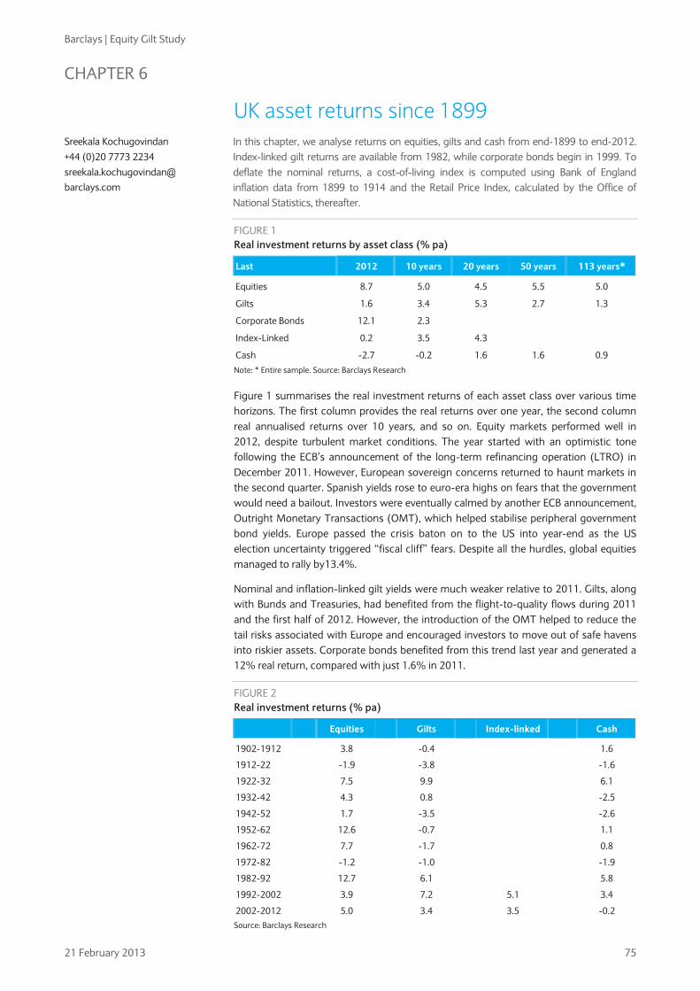
Barclays | Equity Gilt Study

21 February 2013 75

CHAPTER 6

UK asset returns since 1899 In this chapter, we analyse returns on equities, gilts and cash from end-1899 to end-2012. Index-linked gilt returns are available from 1982, while corporate bonds begin in 1999. To deflate the nominal returns, a cost-of-living index is computed using Bank of England inflation data from 1899 to 1914 and the Retail Price Index, calculated by the Office of National Statistics, thereafter.

FIGURE 1 Real investment returns by asset class (% pa)

Last 2012 10 years 20 years 50 years 113 years*

Equities 8.7 5.0 4.5 5.5 5.0

Gilts 1.6 3.4 5.3 2.7 1.3

Corporate Bonds 12.1 2.3

Index-Linked 0.2 3.5 4.3

Cash -2.7 -0.2 1.6 1.6 0.9

Note: * Entire sample. Source: Barclays Research

Figure 1 summarises the real investment returns of each asset class over various time horizons. The first column provides the real returns over one year, the second column real annualised returns over 10 years, and so on. Equity markets performed well in 2012, despite turbulent market conditions. The year started with an optimistic tone following the ECB’s announcement of the long-term refinancing operation (LTRO) in December 2011. However, European sovereign concerns returned to haunt markets in the second quarter. Spanish yields rose to euro-era highs on fears that the government would need a bailout. Investors were eventually calmed by another ECB announcement, Outright Monetary Transactions (OMT), which helped stabilise peripheral government bond yields. Europe passed the crisis baton on to the US into year-end as the US election uncertainty triggered “fiscal cliff” fears. Despite all the hurdles, global equities managed to rally by13.4%.

Nominal and inflation-linked gilt yields were much weaker relative to 2011. Gilts, along with Bunds and Treasuries, had benefited from the flight-to-quality flows during 2011 and the first half of 2012. However, the introduction of the OMT helped to reduce the tail risks associated with Europe and encouraged investors to move out of safe havens into riskier assets. Corporate bonds benefited from this trend last year and generated a 12% real return, compared with just 1.6% in 2011.

FIGURE 2 Real investment returns (% pa)

Equities

Gilts

Index-linked

Cash

1902-1912 3.8

-0.4

1.6

1912-22 -1.9

-3.8

-1.6

1922-32 7.5

9.9

6.1

1932-42 4.3

0.8

-2.5

1942-52 1.7

-3.5

-2.6

1952-62 12.6

-0.7

1.1

1962-72 7.7

-1.7

0.8

1972-82 -1.2

-1.0

-1.9

1982-92 12.7

6.1

5.8

1992-2002 3.9

7.2

5.1

3.4

2002-2012 5.0

3.4

3.5

-0.2 Source: Barclays Research

Sreekala Kochugovindan

+44 (0)20 7773 2234 sreekala.kochugovindan@ barclays.com

Barclays | Equity Gilt Study

21 February 2013 76

Figure 2 decomposes real asset returns for consecutive 10-year intervals. Equities have produced the best returns over the past decade, with an average annualised return of 5% since 2002. Cash, on the other hand, has delivered the worst returns since the stagflationary 1970s. Ranking the annual returns and placing them into deciles provides a clearer illustration of their historical significance. The results for 2012 are shown in Figure 7. The equity portfolio is ranked in the fifth best decile since 1899, an improvement from the eighth decile in 2011. Gilts also ranked in the fifth decile, while linkers fell from the first decile in 2011 to the eighth last year. Cash remained in the ninth best decile, as yields were held near zero.

FIGURE 3 Distribution of real annual equity returns

FIGURE 4 Distribution of real annual gilt returns

0

1

2

3

4

5

6

7

8

9

-50 -42 -34 -26 -18 -10 -2 6 14 22 30 38 46 54

0

2

4

6

8

10

12

14

-50 -42 -34 -26 -18 -10 -2 6 14 22 30 38 46 54

Source: Barclays Research Source: Barclays Research

FIGURE 5 Distribution of real annual cash returns

FIGURE 6 Maximum and minimum real returns over various periods

0

5

10

15

20

25

30

-50 -42 -34 -26 -18 -10 -2 6 14 22 30 38 46 54

-60%-40%-20% 0% 20% 40% 60% 80% 100%

1 year

5 year

10 year

20 year

23 year

Cash

Gilts

Equities

Source: Barclays Research Source: Barclays Research

FIGURE 7 2012 performance ranked by decile (1899-2012)

Decile

Equities 5

Gilts 5

Index-Linked 8

Cash 9

Notes: Deciles ranking: 1 signifies the best 10% of the history, 10 the worst 10%. Source: Barclays Research

Barclays | Equity Gilt Study

21 February 2013 77

Figures 3-5 illustrate the distribution of returns over the past 113 years. They show that equity returns have the widest dispersion, followed by gilts and then cash. The observed distributions are in accordance with financial theory; from an ex-ante perspective, we would apply the highest risk premium to equities, given their perpetual nature and our uncertainty over future growth in corporate profits and changes in the rate of inflation. For gilts, the uncertainty with respect to inflation remains, but the risk from the perspective of coupon and principal is reduced, given their government guarantee. Over the past 30 years, the dispersion of annual gilt returns has widened significantly; in the 1970s and 1980s, an unexpected increase in the inflation rate led to significant negative real returns, while in the 1990s, an unanticipated fall in inflation, in conjunction with lower government deficits, facilitated above-average real returns. The cash return index has the lowest dispersion. In recent years, the real returns to cash have been relatively stable, with the move toward inflation-targeting by the Bank of England stabilising the short-term real interest rate.

Performance over time Having analysed annual real returns since 1899, we now examine returns over various holding periods. Figure 6 compares the annualised returns when the holding period is extended to 5, 10 or 20 years, or beyond.

The most striking feature of the chart is the change in the volatility of returns as the investments are held for longer periods. The variance of equity returns falls significantly in relation to the other assets as the holding period is extended. When equities are held for as long as 20 years, the minimum return is actually greater than for either gilts or cash. However, as discussed in previous issues of this study, we do not believe that this fall in volatility should be interpreted as an indication of mean reversion in the returns. The series used are of rolling returns; hence, there is an overlap in the data. For example, in the 10-year holding period, nine of the annual returns will be the same in any consecutive period; thus, the observations cannot be considered to be independently drawn.

Figure 8 illustrates the performance of equities against gilts and cash for various holding periods. The first column shows that over a holding period of two years, equities outperformed cash in 75 out of 112 years; thus, the sample-based probability of equity outperformance is 67%. Extending the holding period out to 10 years, this rises to 90%.

FIGURE 8 Equity performance

Holding period (years)

2 3 4 5 10 18

Outperform cash 75 77 79 81 94 95

Underperform cash 37 34 31 28 10 1

Total number of years 112 111 110 109 104 96

Probability of Equity Outperformance 67% 69% 72% 74% 90% 99%

Outperform Gilts 76 82 83 80 82 84

Underperform Gilts 36 29 27 29 22 12

Total number of years 112 111 110 109 104 96

Probability of Equity Outperformance 68% 74% 75% 73% 79% 88%

Source: Barclays Research

Barclays | Equity Gilt Study

21 February 2013 78

FIGURE 9 Today’s value of £100 invested at the end of 1899 without reinvesting income

Nominal Real

Equities £12,782 £168

Gilts £58 £1

Source: Barclays Research

FIGURE 10 Today’s value of £100 invested at the end of 1899, income reinvested gross

Nominal Real

Equities £1,837,824 £24,184

Gilts £32,961 £434

Cash £20,294 £267

Source: Barclays Research

FIGURE 11 Five-year average dividend growth rates

-5%

0%

5%

10%

15%

20%

1945 1950 1955 1960 1965 1970 1975 1980 1985 1990 1995 2000 2005 2010

Source: Barclays Research

The importance of reinvestment Figures 9 and 10 show how reinvestment of income affects the performance of the various asset classes. The first table shows £100 invested at the end of 1899 without reinvesting income; the second is with reinvestment. One hundred pounds invested in equities at the end of 1899 would be worth just £168 in real terms without the reinvestment of dividend income, but with reinvestment the portfolio would have grown to £24,184. The effect upon the gilt portfolio is less in absolute terms, but the ratio of the reinvested to non-reinvested portfolio exceeds 400 in real terms.

Turning to the dividend growth ratio, the FTSE all-share dividend rose 10% in 2012, following 14% in 2011. Figure 11 shows that the five-year average growth rate stabilised following the steady declines of recent years after corporates began cutting dividends in 2008. In 1997-2001, dividend income had fallen by a cumulative 15% as companies cut dividends on the basis that funds would be put to better use by corporates than by shareholders. In the wake of the dotcom crash, investors actively sought income-yielding stocks as a way to lower risk.

Figures 12 and 13 illustrate the time series of price indices and total return indices for equities, gilts and cash over the entire series. These returns are in nominal terms and are shown with the use of a logarithmic scale.

Barclays | Equity Gilt Study

21 February 2013 79

FIGURE 12 Barclays price indices – Nominal terms

FIGURE 13 Barclays total return indices – Nominal terms, gross income reinvested

1

10

100

1000

10000

100000

1899 1914 1929 1944 1959 1974 1989 2004

Equities Gilts Retail Prices

10

10,000

10,000,000

1899 1914 1929 1944 1959 1974 1989 2004

Equities Gilts T-Bills

Source: Barclays Research Source: Barclays Research

FIGURE 14 Today’s value of £100 invested at the end of 1945 without reinvesting income

Nominal Real

Equities £8,011 £238

Gilts £63 £2

Source: Barclays Research

FIGURE 15 Today’s value of £100 invested at the end of 1945, gross income reinvested

Nominal Real

Equities £147,384 £4,379

Gilts £7,078 £210

Cash £6,215 £185

Source: Barclays Research

FIGURE 16 Today’s value of £100 invested at the end of 1990, gross income reinvested

Nominal Real

Equities £615 £324

Gilts £696 £366

Index-Linked Gilts £504 £266

Treasury Bills £298 £157

Source: Barclays Research

Barclays | Equity Gilt Study

21 February 2013 80

CHAPTER 7

US asset returns since 1925 The first holding period covered in this analysis is the calendar year 1926, which would represent money invested at the end of 1925 and its value at the end of 1926. The total sample includes 86 annual return observations for equities, government bonds, and cash. The construction of the series is explained in more detail in the indices in Chapter 8, (“Barclays Indices”). The corporate bond performance is captured using the Barclays Investment Grade Corporate Long Index, which incorporates bonds with a maturity of 10 years or more. The Barclays US Inflation Linked 15-year Plus Index is used to represent the performance of TIPS. The nominal return series are deflated by the change in the consumer price index, which is calculated by the Bureau of Labor Statistics.

FIGURE 1 Real investment returns (% pa)

Last 2012 10 years 20 years 50 years 87 years*

Equities 14.1 5.8 6.0 5.7 6.7

Government Bond 2.1 5.0 5.9 3.2 2.6

TIPS 10.1 6.5

Corporate Bond 10.5 5.6 5.6

Cash -1.7 -0.8 0.5 1.0 0.5 *Note: Entire sample. Source: Centre for Research into Security Prices (CRSP) provided US asset return data for the past 13 years, Barclays Research

Figure 1 provides real annualised returns over various time horizons. The table illustrates that US asset returns followed a similar trend to those of the UK, set out in Chapter 6 (“UK asset returns since 1899”). Equities were the best-performing assets of 2012, producing a 14.1% real total return, despite following a turbulent path similar to that of UK and European markets.

Treasury returns were weaker last year, just 2%, compared with 22.5% in 2011. TIPS outperformed Treasuries by 8% as inflation expectations rose. Breakevens widened against the backdrop of dovish monetary policy and improved market liquidity. Corporate bonds also performed well as investors moved out of safe havens and steadily increased their risk exposure. Figure 2 breaks the study period down into consecutive decades.

FIGURE 2 Real investment returns (% pa)

Equities Government Bond Corporate Bond Cash

1932-42 7.6 1.7

-2.4

1942-52 11.9 -2.6

-3.7

1952-62 12.2 1.1

0.8

1962-72 6.7 -0.8

1.1

1972-82 -0.9 -2.8

-0.1

1982-92 11.2 8.4 9.3 3.0

1992-2002 6.1 6.8 5.7 1.8

2002-2012 5.8 5.0 5.6 -0.8 Source: CRSP, Barclays Research

Equities marginally outperformed Treasuries and corporate bonds in the most recent decade. A total real return of 5.8% is in line with the average returns of the past 50 years, but below the average performance since 1925. Equities’ best decades were in the immediate aftermath of WWII and in the 1990s. Bonds have enjoyed the strongest performance over the past three decades. Strong real bond returns are largely explained by continued disinflation since the late 1970s.

Sreekala Kochugovindan

+44 (0)20 7773 2234 sreekala.kochugovindan@ barclays.com

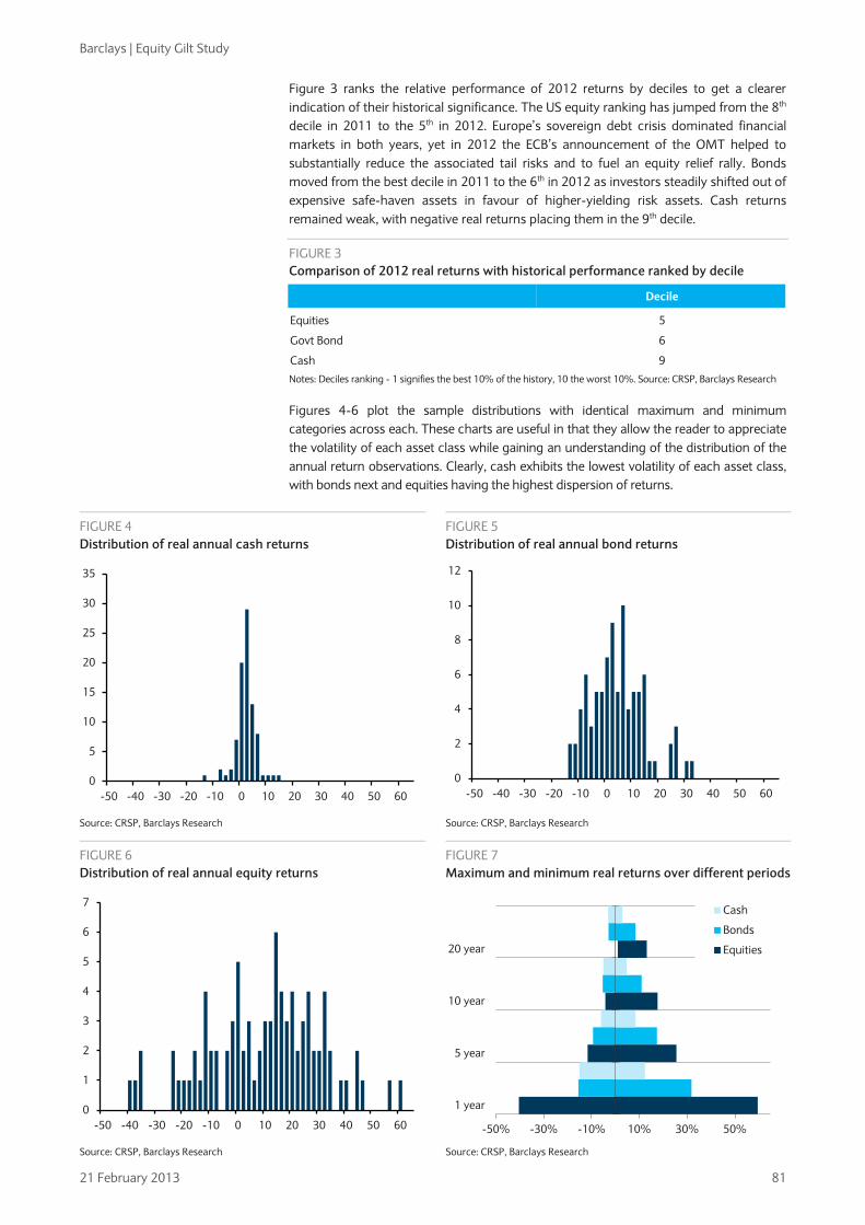
Barclays | Equity Gilt Study

21 February 2013 81

Figure 3 ranks the relative performance of 2012 returns by deciles to get a clearer indication of their historical significance. The US equity ranking has jumped from the 8th decile in 2011 to the 5th in 2012. Europe’s sovereign debt crisis dominated financial markets in both years, yet in 2012 the ECB’s announcement of the OMT helped to substantially reduce the associated tail risks and to fuel an equity relief rally. Bonds moved from the best decile in 2011 to the 6th in 2012 as investors steadily shifted out of expensive safe-haven assets in favour of higher-yielding risk assets. Cash returns remained weak, with negative real returns placing them in the 9th decile.

FIGURE 3 Comparison of 2012 real returns with historical performance ranked by decile

Decile

Equities 5

Govt Bond 6

Cash 9

Notes: Deciles ranking - 1 signifies the best 10% of the history, 10 the worst 10%. Source: CRSP, Barclays Research

Figures 4-6 plot the sample distributions with identical maximum and minimum categories across each. These charts are useful in that they allow the reader to appreciate the volatility of each asset class while gaining an understanding of the distribution of the annual return observations. Clearly, cash exhibits the lowest volatility of each asset class, with bonds next and equities having the highest dispersion of returns.

FIGURE 4 Distribution of real annual cash returns

FIGURE 5 Distribution of real annual bond returns

0

5

10

15

20

25

30

35

-50 -40 -30 -20 -10 0 10 20 30 40 50 60

0

2

4

6

8

10

12

-50 -40 -30 -20 -10 0 10 20 30 40 50 60

Source: CRSP, Barclays Research Source: CRSP, Barclays Research

FIGURE 6 Distribution of real annual equity returns

FIGURE 7 Maximum and minimum real returns over different periods

0

1

2

3

4

5

6

7

-50 -40 -30 -20 -10 0 10 20 30 40 50 60

-50% -30% -10% 10% 30% 50%

1 year

5 year

10 year

20 year

Cash

Bonds

Equities

Source: CRSP, Barclays Research Source: CRSP, Barclays Research

Barclays | Equity Gilt Study

21 February 2013 82

Figure 7 shows the extremes of the return distribution for various holding periods. The volatility of equities over very short horizons is clearly demonstrated in the maximum and minimum distribution of one-year returns. As we extend the holding period, the distribution begins to narrow. Over the past 87 years, the worst average annualised 20-year return for equities was 0.96%, while the best was 13.2%. However, this is not to say that it is impossible to lose money by holding equities over a 20-year period, as the analysis is conducted on an ex-post basis. The figure merely highlights that such an occurrence seems unlikely, given equities’ performance over the past 87 years.

In addition, over the long term, we would expect the ex-ante equity risk premium to provide a cushion against uncertainty. Bonds and cash have experienced negative returns over a 20-year horizon, reflecting unexpected jumps in inflation at various points in the past century.

Figure 8 plots the US equity risk premium and shows that the 10-year annualised excess return of equities over bonds has bounced back from the lows of 2008 and edged into positive territory.

FIGURE 8 Equity-risk premium – excess return of equities relative to bonds (10y annualised)

-10%

-5%

0%

5%

10%

15%

20%

1935 1946 1957 1968 1979 1990 2001 2012

Source: CRSP, Barclays Research

Barclays | Equity Gilt Study

21 February 2013 83

The importance of reinvestment Figures 9 and 10 show the importance of reinvestment of income in the form of dividends on equity investments and coupons on government bonds.

FIGURE 11 Value of $100 invested at the end of 1925 without reinvesting income

Nominal Real

Equities $10,414 $812

Bonds $138 $11

Source: CRSP, Barclays Research

FIGURE 12 Value of $100 invested at the end of 1925 with income reinvested gross

Nominal Real

Equities $347,460 $27,088

Bonds $12,179 $949

Cash $2,041 $159

Source for both tables: CRSP, Barclays Research

FIGURE 9 Barclays US price indices in nominal terms

FIGURE 10 Barclays US total return indices in nominal terms with gross income reinvested

1

100

10,000

1,000,000

1925 1935 1945 1955 1965 1975 1985 1995 2005

Equities Bonds Consumer Prices

1

1,000

1,000,000

1925 1935 1945 1955 1965 1975 1985 1995 2005

Equity Bonds Cash

Source: CRSP, Barclays Research Source: CRSP, Barclays Research

Barclays | Equity Gilt Study

21 February 2013 84

CHAPTER 8

Barclays indices We have calculated three indices: changes in the capital value of each asset class; changes to income from these investments; and a combined measure of the overall return, on the assumption that all income is reinvested.

Additional series allow for the effects of inflation. The data for cash include building society deposit rates and Treasury bills. The series on index-linked securities is based at December 1982 and the corporate bond index starts at the end of 1990.

Barclays Equity Index The Barclays Equity Index is designed to give as accurate a measure as possible of the performance of a representative portfolio of equities. Three main types of index can be used. The FT Index, which for years was the most widely used in the UK, is geometric, meaning that the price changes of the 30 shares it comprises are multiplied together to produce the change in the index. We believe that this is a fair basis for indicating short-term market behaviour, but that over long periods it imparts a downward bias. The second type of index uses the Dow formula, in which the prices of a number of shares are added together. This does not have the distorting effect of a geometric index, but the weighting of the various shares is arbitrary and varies with changes in capitalisation.

We think the most accurate and representative indices are arithmetic and weighted by the number of shares in issue by each company. These indices include virtually all of the large quoted companies, and thus we believe they accurately reflect the behaviour of an equity market. The Standard & Poor’s Indices are of this type, and they date back to the 1920s. The FT Actuaries Indices, introduced in the 1960s, were the first of this type in the UK. Subsequently, a number of weighted arithmetic international indices, such as those calculated by Morgan Stanley Capital International and Datastream, have been introduced. More recently, the FTSE 100 Index, which uses the same construction but incorporates only the 100 leading shares, has been introduced and, generally, is now used as the main market indicator because it is calculated on a real-time basis throughout the day.

The Barclays Equity Index, which is used in this study, is a weighted arithmetic index, and is available for the period since 1899, with a dividend yield and an income index. The original Barclays Equity Index, used in editions of this study until 1999, was first calculated retrospectively in 1956 and included 30 shares chosen because of their similarities to the FT 30 Index, which covers the 1935 to 1962 period. For the 2000 edition of this study, we compiled a new index for 1899-1935, based on the 30 largest shares by market capitalisation in each year. From 1962, the Barclays Equity Index is based on the FTSE Actuaries All-Share Index because, with its broader coverage, it gives a more accurate picture of market movements. The indices are calculated only annually, at year-end.

The equity returns between 1899 and 1935 are therefore calculated from a new Equity Index, consisting of the 30 largest shares by market capitalisation in each year; between 1935 and 1962 they are calculated from the FT 30 Index and from 1962 onward they are derived from the FTSE Actuaries All-Share Index.

Sreekala Kochugovindan

+44 (0)20 7773 2234 sreekala.kochugovindan@ barclays.com

Barclays | Equity Gilt Study

21 February 2013 85

FIGURE 1 Equity Index constituents

Constituents at December 1899 Constituents at December 1934 Constituents at December 1962

De Beers Consolidated Mines Rio Tinto Ltd Armstrong Whitworth Consolidated Gold Fields London and County Bank

Woolworth Ltd Imperial Chemical Industries Shell' Transport & Trading Ltd Courtaulds Ltd Royal Insurance Co

Associated Portland Cement Bass Mitchells & Butlers British Motor Coats Patons Cory (William)

London City & Midland Bank Ltd Lloyds Bank Ltd London & Westminster Bank Ltd Vickers, Sons & Maxim Ltd Imperial Ottoman Bank

Barclay & Company Lloyds Bank Prudential Assurance Co Ltd Westminster Bank Ltd Midland Bank Ltd

Courtaulds Distillers Dunlop EMI Fine Spinners & Doublers

Parrs Bank Ltd Royal Insurance Co Tharsis Sulphur & Copper Ltd Great Northern of Copenhagen Simmer & Jack PropietaryMines Ltd

London & Lancashire Fire Ins. Co North British & Mercantile In. Co Ltd Reckitt & Sons Ltd County of London Electric Supply Co Unilever Ltd

General Electric Guest Keen Hawker Siddeley House of Fraser ICI

North British & Mercantile Insurance Consett Iron Ltd Eastern Extension Australasia * China Ltd Nobel Dynamite TstLtd Mysore Gold Mining Ltd

Tate & Lyle Ltd Alliance Assurance Company Boots Pure Drug Co Ltd Pearl Assurance Co Marks & Spencer Ltd

Imperial Tobacco International Stores Leyland Motors London Brick Murex

Exploration Co Alliance Assurance Co Aerated Bread Ltd Howard & Bullough Ltd Sun Insurance Office

Cory (WM.) & Son National Bank Of Egypt Consolidated Gold Fields Of South Africa Bass, Ratcliff & Gretton Ltd GeduldProp Mines Ltd

P&O Steam Navigation Rolls-Royce Swan Hunter Tate & Lyle Tube Investments

New JagersfonteinMining & Expl Ltd Champion Reef Gold Mining National Telephone Ltd Northern Assurance Phoenix Assurance Co

Sun Insurance Office Bank Of Australasia British South Africa Co Chartered Bank Of India, Australia & China North Eastern Elec Supply Co

Turner & Newall United Steel Vickers WatneyMann Woolworth

Source: Barclays Research

The Equity Index is a weighted arithmetic average. In the Equity Index, the weights of the 30 constituent companies for each year are proportional to their market capitalisation at the beginning of the year. Each year a fund was constructed. The number of shares in the fund for each company was calculated so that its market value at the beginning of the year was equal to the company’s index weighting. The value of the fund was calculated annually at the end of the year.

For 1899-1962, the Equity Income Index is based on the Barclays Equity Fund. The Income Index relates to the dividend income actually received in the 12 months prior to the date of the index. It is calculated by totalling the dividends paid on the shares in the fund. We believe that it is the only published index based on actual income receipts.

From 1963 the Income Index is derived from the yield on the FTSE All-Share Index. Despite a minimal discontinuity in the yield, in our view, this is the most representative method of evaluating equity performance over the period. The dividend yield is quoted net from 1998, with non-taxpayers no longer able to reclaim ACT.

Barclays Gilt Index The Gilt Index measures the performance of long-dated gilts. From 1899 to 1962 the index is based on the prices of undated British funds. During this period the undated stocks were a major part of the gilt market, but over the years the effect of high interest rates on their prices, together with the growing number of conventional long-dated issues, meant that undated stocks became less and less representative of the market as a whole.

Barclays | Equity Gilt Study

21 February 2013 86

Since 1962, the Barclays Gilt Index has been based on a portfolio of long-dated stocks, selected on 1 January each year. The portfolio was chosen to represent as closely as possible a 20-year security on a par yield, and contains a weighted combination of four long-dated stocks with a mean life of 20½ years (so that the average life of the stocks for the year in which they are in the portfolio was 20 years). The combination and weightings of the four stocks are chosen to have the minimum possible deviation from a par yield. Small issues (less than £1bn) are excluded and in any year none of the four stocks has been allocated a weight of more than 40%, or less than 5% of the index.

During the late 1980s there was a steady contraction in the number of issues that satisfied the criteria for inclusion in the Gilt Index. As a result of the lack of issues of new long-dated stocks and the fall in the remaining life of existing stocks, the universe of eligible stocks narrowed sharply. By the end of 1989 there were four stocks with a life of more than 20 years, and only two of these were over £1bn nominal.

Thus from the beginning of 1990 the index has been constructed to represent a portfolio of 15-year par yielding gilts.

Barclays Inflation-linked Index The index-linked market has now been established for almost three decades and is capitalised at £354bn (compared with the £1.1trn capitalisation of the conventional market). The index has been constructed to mirror as closely as possible the rules of the conventional gilt index. An average life of 20 years was used up until 1990, and 15 years thereafter. Again, stocks have been chosen to be as close to par as possible, although of course in this case par means “indexed par”.

Barclays Corporate Bond Index The UK corporate bond market has expanded markedly since the beginning of 1999. The index and returns are based on the Barclays Sterling Aggregate Corporate Index. Clearly, we are unable to select individual stocks for this index in the way we do for the gilt indices because such a small sample of stocks cannot be representative of the market.

Barclays Building Society Fund In previous editions of this study we have included indices of the value of £100 invested in a building society at the end of 1945. We originally used the average interest rate on an ordinary share account. In the mid-1980s many building societies introduced new tiered interest rate accounts, which provided a higher rate of interest while still allowing instant access. In response to this we have been tracking both types of account, but as time progressed the old style “ordinary share accounts” became less and less representative and by the mid-1990s had been completely superseded by the new accounts. From 1986 the Barclays Index follows the Halifax Liquid Gold Account (formerly called the Halifax Instant Xtra) as a representative of the newer tiered interest rate-style accounts. The Halifax is no longer a building society, having converted to a bank, so from 1998 we follow the Nationwide Invest Direct Account. This is the closest equivalent account offered by the Nationwide Building Society (which is now the largest remaining building society in the UK); the difference is that it is operated by post. We consider this type of postal account to be more representative of building society returns than the branch operated passbook accounts, which are more in the nature of a cash-based transaction account.

US asset returns The US indices used in this study were provided by the Center for Research in Security Prices (CRSP) at the Graduate School of Business in the University of Chicago. The value-weighted equity index covers all common stocks trading on the New York, American and Nasdaq Stock Exchanges, excluding ADRs. For the bond index, the CRSP has used software which selects the bond that is closest to a 20-year bond in each month. The same methodology has been employed for the 30-day T-Bill.

Barclays | Equity Gilt Study

21 February 2013 87

Total returns In this study, we have shown the performance of representative investments in UK equities and long gilts, with additional analysis of equivalent US returns in both monetary and real (inflation adjusted) terms. The total returns to the investor, however, also include the income on the investment. This is important throughout the study for comparability between asset classes. For example, when constructing an index for a cash investment such as the UK Treasury Bill Index, the £100 invested at the end of 1899 grew to approximately £104 by the end of the following year. This full amount is reinvested and by the end of 1920 the value of this investment had grown to about £190. In contrast, equity and bond market returns can be split into two components: capital appreciation; and dividend income. The most commonly quoted stock market indices usually include only the capital component of the return. In order to calculate returns on a comparable basis, we need to include the returns obtained by reinvesting this income. This is particularly important in looking at bonds where the scope for capital appreciation is small, so almost all of the return will be from income. In this study, total returns are calculated assuming income is reinvested at the end of the year.

Taxation The total return to an investor depends crucially on the tax regime. The largest long-term investors in the British equity and gilt markets are pension funds and similar institutions that (until the abolition of the advance corporation tax (ACT) credit) have not suffered tax on their income or capital; our main tables therefore make no allowance for tax until 1998, which was the first full year that non-taxpayers were unable to reclaim the ACT credit. This effectively reduced the dividend yield to non-taxpayers, and is reflected in our main tables and gross total return series.

The personal investor must suffer tax. The net return to a building society account is straightforward to compute. However, changes in the tax regime in recent years make the net return to equity and gilt investment less straightforward to calculate on a consistent basis. For example, the change to total return taxation for gilts means that it is inappropriate to calculate a net total return on the basis of taxing income alone. Thus returns are quoted gross throughout, but for reference we also quote basic tax rates.

Arithmetic and geometric averages Our analysis of past data usually relies on calculations of the geometric mean for each series. Arithmetic averages can provide a misleading picture. For example, suppose equities rose from a base of 100 to 200 over one year and then fell back to 100 over the next year. The return for year one would have been 100% and for year two minus 50%. The arithmetic average return would be 25% even though equities are actually unchanged in value over the two years.

The geometric average return in this example would be zero. This method of calculation is therefore preferable. Over long periods, the geometric average for total returns is the rate at which a sum invested at the beginning of the period will grow to by the end of the period, assuming all income is reinvested. The calculation of geometric averages depends only on the initial and final values for the investment, not particular values at any other point in time.

For periods of one year, arithmetic and geometric averages will be the same. But over longer periods the geometric average is always less than the arithmetic average, except when all the individual yearly returns are the same. For the mathematically minded, the geometric return is approximately equal to the arithmetic return minus one-half the variance of the arithmetic return.

Although geometric returns are appropriate to analyse the past, arithmetic returns should be used to provide forecasts. Arithmetic averages provide the better unbiased estimator of returns (for a statistical proof of this see Ian Cooper’s paper Arithmetic vs

Barclays | Equity Gilt Study

21 February 2013 88

Geometric Premium: setting discount rates for capital budgeting calculations, IFA Working Paper 174-93, April 1993).

Capital value indices The indices in Figure 2 show the nominal capital value of £100 invested in equities and gilts at the end of 1899. The chart also plots the Barclays Cost of Living Index. Note how the equity index has correlated with increases in the cost of living versus a similar investment in gilts. The index values at the end of 2012 were 12,782 for equities, 57.92 for gilts, and 7599 for the cost of living.

We then show the same capital indices adjusted for the increase in the cost of living since 1899. Figure 3 shows the end-2012 real equity price index at 168 with the real gilt price index at 0.76.

Total return indices The next two charts show the nominal and real value of the equity, gilt and cash funds with gross income received reinvested at the end of each year since 1899. Figure 4 shows that the nominal worth of £100 invested in equities at the end of 1899 was £1,837,824. The same investment in gilts was worth £32,960 and in T-Bills £20,294. When these values are adjusted for inflation, the equity fund is worth £24,184, the gilt £434 and the cash fund £267.

FIGURE 2 Barclays price indices in nominal terms

FIGURE 3 Barclays price indices in real terms

1

10

100

1000

10000

100000

1899 1914 1929 1944 1959 1974 1989 2004

Equities Gilts Retail Prices

0

50

100

150

200

250

300

1899 1914 1929 1944 1959 1974 1989 2004

Equities Gilts Source: Barclays Research Source: Barclays Research

FIGURE 4 Barclays total return indices in nominal terms with gross income reinvested

FIGURE 5 Barclays total return indices in real terms with gross income reinvested

10

10,000

10,000,000

1899 1914 1929 1944 1959 1974 1989 2004

Equities Gilts T-Bills

1

10

100

1,000

10,000

100,000

1899 1914 1929 1944 1959 1974 1989 2004

Equities Gilts T- Bills

Source: Barclays Research Source: Barclays Research

Barclays | Equity Gilt Study

21 February 2013 89

FIGURE 6 Barclays UK Cost of Living Index

Change % Change %

Year December

(1899=100) In year 5y average Year December In year 5y average 1900 103.3 3.3 1956 358.3 3.0 4.0 1901 103.3 0.0 1957 374.9 4.6 3.7 1902 106.7 3.2 1958 381.8 1.8 3.9 1903 106.7 0.0 1959 381.8 0.0 3.1 1904 106.7 0.0 1.3 1960 388.7 1.8 2.3 1905 106.7 0.0 0.6 1961 405.7 4.4 2.5 1906 100.0 -6.2 -0.7 1962 416.5 2.6 2.1 1907 110.0 10.0 0.6 1963 424.2 1.9 2.1 1908 113.3 3.0 1.2 1964 444.6 4.8 3.1 1909 113.3 0.0 1.2 1965 464.5 4.5 3.6 1910 113.3 0.0 1.2 1966 481.6 3.7 3.5 1911 116.7 2.9 3.1 1967 493.4 2.5 3.4 1912 120.0 2.9 1.8 1968 522.7 5.9 4.3 1913 120.0 0.0 1.1 1969 547.1 4.7 4.2 1914 120.0 0.0 1.1 1970 590.3 7.9 4.9 1915 148.3 23.6 5.5 1971 643.6 9.0 6.0 1916 175.8 18.5 8.6 1972 692.9 7.7 7.0 1917 212.5 20.9 12.1 1973 766.2 10.6 7.9 1918 244.7 15.2 15.3 1974 912.8 19.1 10.8 1919 250.3 2.3 15.8 1975 1140.0 24.9 14.1 1920 299.2 19.6 15.1 1976 1311.8 15.1 15.3 1921 221.4 -26.0 4.7 1977 1471.1 12.1 16.3 1922 200.2 -9.5 -1.2 1978 1594.4 8.4 15.8 1923 196.9 -1.7 -4.3 1979 1869.3 17.2 15.4 1924 201.3 2.3 -4.3 1980 2151.9 15.1 13.5 1925 196.9 -2.2 -8.0 1981 2411.2 12.0 12.9 1926 199.1 1.1 -2.1 1982 2541.6 5.4 11.6 1927 188.0 -5.6 -1.3 1983 2676.7 5.3 10.9 1928 186.9 -0.6 -1.0 1984 2799.3 4.6 8.4 1929 185.8 -0.6 -1.6 1985 2958.5 5.7 6.6 1930 172.4 -7.2 -2.6 1986 3068.6 3.7 4.9 1931 164.6 -4.5 -3.7 1987 3182.0 3.7 4.6 1932 159.1 -3.4 -3.3 1988 3397.6 6.8 4.9 1933 159.1 0.0 -3.2 1989 3659.5 7.7 5.5 1934 160.2 0.7 -2.9 1990 4001.4 9.3 6.2 1935 163.5 2.1 -1.1 1991 4180.0 4.5 6.4 1936 168.0 2.7 0.4 1992 4287.8 2.6 6.1 1937 178.0 6.0 2.3 1993 4369.3 1.9 5.2 1938 173.5 -2.5 1.8 1994 4495.6 2.9 4.2 1939 192.4 10.9 3.7 1995 4640.3 3.2 3.0 1940 216.9 12.7 5.8 1996 4754.2 2.5 2.6 1941 223.6 3.1 5.9 1997 4926.6 3.6 2.8 1942 222.5 -0.5 4.6 1998 5062.1 2.8 3.0 1943 221.4 -0.5 5.0 1999 5151.4 1.8 2.8 1944 223.6 1.0 3.0 2000 5302.3 2.9 2.7 1945 225.8 1.0 0.8 2001 5339.2 0.7 2.3 1946 226.9 0.5 0.3 2002 5496.3 2.9 2.2 1947 234.2 3.2 1.0 2003 5650.2 2.8 2.2 1948 245.7 4.9 2.1 2004 5847.3 3.5 2.6 1949 254.3 3.5 2.6 2005 5976.6 2.2 2.4 1950 262.4 3.2 3.0 2006 6241.4 4.4 3.2 1951 294.0 12.0 5.3 2007 6493.9 4.0 3.4 1952 312.7 6.3 6.0 2008 6561.7 1.0 3.0 1953 316.0 1.1 5.2 2009 6712.5 2.3 2.8 1954 328.5 4.0 5.3 2010 7032.8 4.8 3.3 1955 347.7 5.8 5.8 2011 7371.5 4.8 3.4

2012 7599.3 3.1 3.2

Barclays | Equity Gilt Study

21 February 2013 90

FIGURE 7 Barclays UK Equity Index

Year Equity Price Index

December Equity Income Index

December Income yield %

Equity Price Index adjusted for

Cost of Living

Equity Income Index adjusted for

Cost of Living

1899 100 100 1900 108 +8.3% 100 6.3 105 +4.8% 100 1901 100 -7.9% 69 -30.6% 4.8 97 -7.9% 69 -30.6% 1902 101 +1.3% 80 +15.6% 5.4 95 -1.9% 78 +11.9% 1903 98 -2.7% 66 -17.3% 4.6 92 -2.7% 64 -17.3% 1904 106 +8.0% 62 -6.1% 4.0 100 +8.0% 60 -6.1% 1905 105 -0.7% 71 +13.7% 4.6 99 -0.7% 69 +13.7% 1906 112 +6.1% 77 +8.5% 4.7 112 +13.2% 79 +15.7% 1907 107 -4.7% 79 +2.9% 5.1 97 -13.3% 74 -6.4% 1908 108 +1.3% 57 -27.4% 3.6 95 -1.7% 52 -29.5% 1909 115 +6.3% 73 +26.5% 4.3 101 +6.3% 66 +26.5% 1910 112 -2.1% 69 -4.5% 4.2 99 -2.1% 63 -4.5% 1911 109 -2.9% 71 +2.1% 4.4 94 -5.7% 63 -0.8% 1912 108 -1.4% 69 -3.2% 4.4 90 -4.2% 59 -5.8% 1913 100 -7.1% 57 -16.5% 3.9 83 -7.1% 49 -16.5% 1914 96 -4.4% 57 +0.1% 4.1 80 -4.4% 49 +0.1% 1915 96 0.0% 36 -37.8% 2.6 64 -19.1% 25 -49.7% 1916 89 -6.8% 67 +88.2% 5.2 51 -21.4% 39 +58.8% 1917 93 +4.2% 66 -2.2% 4.8 44 -13.8% 32 -19.1% 1918 108 +16.3% 63 -3.6% 4.0 44 +1.0% 27 -16.3% 1919 116 +7.7% 34 -47.0% 2.0 46 +5.3% 14 -48.2% 1920 86 -25.6% 77 +128.9% 6.1 29 -37.8% 26 +91.4% 1921 80 -7.1% 79 +2.7% 6.7 36 +25.5% 37 +38.8% 1922 96 +19.8% 73 -7.9% 5.2 48 +32.5% 37 +1.8% 1923 92 -4.0% 72 -0.8% 5.3 47 -2.4% 38 +0.9% 1924 106 +15.3% 67 -7.5% 4.3 53 +12.8% 34 -9.5% 1925 117 +9.9% 73 +10.3% 4.3 59 +12.4% 39 +12.7% 1926 119 +1.8% 83 +12.5% 4.8 60 +0.7% 43 +11.2% 1927 124 +4.0% 76 -8.2% 4.2 66 +10.1% 42 -2.8% 1928 139 +12.2% 79 +3.9% 3.9 74 +12.9% 44 +4.5% 1929 113 -19.1% 90 +14.9% 5.5 61 -18.6% 50 +15.6% 1930 102 -9.2% 80 -11.0% 5.4 59 -2.1% 48 -4.2% 1931 77 -24.3% 65 -18.7% 5.8 47 -20.8% 41 -14.8% 1932 99 +27.9% 64 -2.4% 4.4 62 +32.4% 41 +1.0% 1933 119 +20.6% 60 -5.6% 3.5 75 +20.6% 39 -5.6% 1934 131 +9.8% 70 +15.7% 3.6 82 +9.0% 45 +14.9% 1935 144 +9.9% 78 +11.5% 3.7 88 +7.7% 49 +9.2% 1936 166 +15.1% 82 +5.8% 3.4 99 +12.1% 51 +3.0% 1937 138 -16.7% 93 +12.7% 4.6 78 -21.4% 54 +6.4% 1938 118 -14.9% 94 +1.8% 5.5 68 -12.7% 56 +4.4% 1939 114 -3.1% 90 -4.8% 5.4 59 -12.6% 48 -14.2% 1940 102 -10.2% 94 +4.8% 6.3 47 -20.3% 45 -7.1% 1941 119 +16.8% 91 -3.6% 5.2 53 +13.3% 42 -6.5% 1942 135 +12.9% 86 -4.5% 4.4 61 +13.4% 40 -4.0% 1943 144 +7.1% 86 -0.2% 4.1 65 +7.7% 40 +0.3% 1944 156 +8.3% 87 +0.4% 3.8 70 +7.3% 40 -0.6% 1945 160 +2.0% 88 +2.0% 3.8 71 +1.0% 40 +1.0% 1946 182 +13.9% 93 +4.9% 3.5 80 +13.3% 42 +4.4% 1947 170 -6.3% 107 +15.1% 4.3 73 -9.2% 47 +11.6% 1948 157 -7.7% 98 -7.7% 4.3 64 -12.1% 41 -12.1% 1949 141 -10.3% 103 +4.4% 5.0 55 -13.3% 42 +0.8% 1950 149 +5.6% 109 +5.6% 5.0 57 +2.3% 43 +2.3% 1951 153 +3.0% 121 +11.2% 5.4 52 -8.1% 42 -0.7% 1952 144 -5.9% 128 +6.3% 6.1 46 -11.5% 42 -0.0% 1953 170 +17.8% 134 +4.3% 5.4 54 +16.6% 44 +3.2% 1954 242 +42.4% 155 +16.0% 4.4 74 +36.9% 49 +11.6% 1955 256 +5.8% 179 +15.4% 4.8 74 -0.0% 53 +9.1%

Barclays | Equity Gilt Study

21 February 2013 91

Year Equity Price Index

December Equity Income Index

December Income yield %

Equity Price Index adjusted for

Cost of Living

Equity Income Index adjusted for

Cost of Living

1956 220 -13.9% 183 +2.2% 5.7 62 -16.5% 53 -0.8% 1957 205 -7.0% 188 +2.8% 6.3 55 -11.1% 52 -1.7% 1958 289 +41.1% 202 +7.5% 4.8 76 +38.5% 55 +5.5% 1959 432 +49.5% 227 +12.1% 3.6 113 +49.5% 61 +12.1% 1960 421 -2.6% 276 +21.7% 4.5 108 -4.4% 73 +19.5% 1961 409 -3.0% 286 +3.5% 4.8 101 -7.0% 73 -0.8% 1962 391 -4.4% 285 -0.4% 5.0 94 -6.9% 71 -3.0% 1963 450 +15.2% 266 -6.5% 4.1 106 +13.1% 65 -8.2% 1964 405 -10.0% 303 +13.7% 5.1 91 -14.2% 70 +8.5% 1965 428 +5.9% 326 +7.7% 5.2 92 +1.3% 73 +3.1% 1966 389 -9.3% 328 +0.5% 5.8 81 -12.5% 70 -3.1% 1967 500 +28.7% 319 -2.5% 4.4 101 +25.6% 67 -4.8% 1968 718 +43.5% 339 +6.1% 3.2 137 +35.4% 67 +0.2% 1969 609 -15.2% 342 +0.8% 3.9 111 -19.0% 65 -3.7% 1970 563 -7.5% 360 +5.5% 4.4 95 -14.3% 63 -2.3% 1971 799 +41.9% 379 +5.1% 3.3 124 +30.2% 61 -3.6% 1972 901 +12.8% 414 +9.3% 3.2 130 +4.8% 62 +1.6% 1973 619 -31.4% 430 +3.9% 4.8 81 -37.9% 58 -6.0% 1974 276 -55.3% 472 +9.6% 11.7 30 -62.5% 53 -8.0% 1975 653 +136.3% 521 +10.4% 5.5 57 +89.2% 47 -11.6% 1976 628 -3.9% 588 +12.8% 6.4 48 -16.5% 46 -2.0% 1977 886 +41.2% 682 +16.1% 5.3 60 +25.9% 48 +3.5% 1978 910 +2.7% 768 +12.6% 5.8 57 -5.3% 50 +3.9% 1979 949 +4.3% 951 +23.8% 6.9 51 -11.0% 53 +5.6% 1980 1206 +27.1% 1073 +12.8% 6.1 56 +10.4% 52 -2.0% 1981 1294 +7.2% 1111 +3.5% 5.9 54 -4.3% 48 -7.6% 1982 1579 +22.1% 1211 +9.0% 5.3 62 +15.8% 49 +3.4% 1983 1944 +23.1% 1309 +8.1% 4.6 73 +16.9% 51 +2.7% 1984 2450 +26.0% 1578 +20.6% 4.4 88 +20.5% 58 +15.3% 1985 2822 +15.2% 1781 +12.8% 4.3 95 +9.0% 62 +6.8% 1986 3452 +22.3% 2033 +14.1% 4.0 112 +17.9% 68 +10.0% 1987 3596 +4.2% 2264 +11.4% 4.3 113 +0.4% 74 +7.4% 1988 3829 +6.5% 2628 +16.1% 4.7 113 -0.3% 80 +8.7% 1989 4978 +30.0% 3076 +17.0% 4.2 136 +20.7% 87 +8.7% 1990 4265 -14.3% 3401 +10.5% 5.5 107 -21.6% 88 +1.1% 1991 4907 +15.1% 3591 +5.6% 5.0 117 +10.1% 89 +1.1% 1992 5635 +14.8% 3573 -0.5% 4.4 131 +11.9% 86 -3.0% 1993 6951 +23.3% 3414 -4.4% 3.4 159 +21.0% 81 -6.2% 1994 6286 -9.6% 3684 +7.9% 4.0 140 -12.1% 85 +4.9% 1995 7450 +18.5% 4127 +12.0% 3.8 161 +14.8% 92 +8.5% 1996 8320 +11.7% 4536 +9.9% 3.7 175 +9.0% 99 +7.3% 1997 9962 +19.7% 4690 +3.4% 3.2 202 +15.5% 98 -0.2% 1998 11048 +10.9% 4026 -14.2% 2.5 218 +7.9% 82 -16.5% 1999 13396 +21.2% 4140 +2.8% 2.1 260 +19.1% 83 +1.0% 2000 12329 -8.0% 4007 -3.2% 2.2 233 -10.6% 78 -5.9% 2001 10428 -15.4% 3998 -0.2% 2.6 195 -16.0% 77 -0.9% 2002 7825 -25.0% 4049 +1.3% 3.6 142 -27.1% 76 -1.6% 2003 9121 +16.6% 4121 +1.8% 3.1 161 +13.4% 75 -1.0% 2004 9961 +9.2% 4428 +7.5% 3.1 170 +5.5% 78 +3.8% 2005 11764 +18.1% 5058 +14.2% 3.0 197 +15.5% 87 +11.8% 2006 13311 +13.2% 5549 +9.7% 2.9 213 +8.3% 92 +5.0% 2007 13580 +2.0% 5978 +7.7% 3.0 209 -1.9% 95 +3.5% 2008 9129 -32.8% 5974 -0.1% 4.5 139 -33.4% 94 -1.0% 2009 11407 +25.0% 5321 -10.9% 3.2 170 +22.0% 82 -13.0% 2010 12655 +10.9% 5331 +0.2% 2.9 180 +5.9% 78 -4.4% 2011 11808 -6.7% 6059 +13.6% 3.5 160 -11.0% 85 +8.4% 2012 12782 +8.2% 6651 +9.8% 3.6 168 +5.0% 90 +6.5%

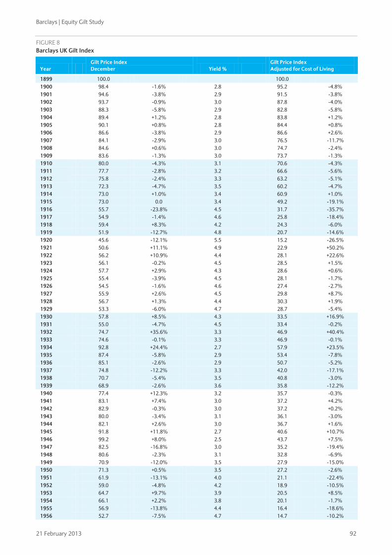
Barclays | Equity Gilt Study

21 February 2013 92

FIGURE 8 Barclays UK Gilt Index

Year Gilt Price Index December Yield %

Gilt Price Index Adjusted for Cost of Living

1899 100.0 100.0 1900 98.4 -1.6% 2.8 95.2 -4.8% 1901 94.6 -3.8% 2.9 91.5 -3.8% 1902 93.7 -0.9% 3.0 87.8 -4.0% 1903 88.3 -5.8% 2.9 82.8 -5.8% 1904 89.4 +1.2% 2.8 83.8 +1.2% 1905 90.1 +0.8% 2.8 84.4 +0.8% 1906 86.6 -3.8% 2.9 86.6 +2.6% 1907 84.1 -2.9% 3.0 76.5 -11.7% 1908 84.6 +0.6% 3.0 74.7 -2.4% 1909 83.6 -1.3% 3.0 73.7 -1.3% 1910 80.0 -4.3% 3.1 70.6 -4.3% 1911 77.7 -2.8% 3.2 66.6 -5.6% 1912 75.8 -2.4% 3.3 63.2 -5.1% 1913 72.3 -4.7% 3.5 60.2 -4.7% 1914 73.0 +1.0% 3.4 60.9 +1.0% 1915 73.0 0.0 3.4 49.2 -19.1% 1916 55.7 -23.8% 4.5 31.7 -35.7% 1917 54.9 -1.4% 4.6 25.8 -18.4% 1918 59.4 +8.3% 4.2 24.3 -6.0% 1919 51.9 -12.7% 4.8 20.7 -14.6% 1920 45.6 -12.1% 5.5 15.2 -26.5% 1921 50.6 +11.1% 4.9 22.9 +50.2% 1922 56.2 +10.9% 4.4 28.1 +22.6% 1923 56.1 -0.2% 4.5 28.5 +1.5% 1924 57.7 +2.9% 4.3 28.6 +0.6% 1925 55.4 -3.9% 4.5 28.1 -1.7% 1926 54.5 -1.6% 4.6 27.4 -2.7% 1927 55.9 +2.6% 4.5 29.8 +8.7% 1928 56.7 +1.3% 4.4 30.3 +1.9% 1929 53.3 -6.0% 4.7 28.7 -5.4% 1930 57.8 +8.5% 4.3 33.5 +16.9% 1931 55.0 -4.7% 4.5 33.4 -0.2% 1932 74.7 +35.6% 3.3 46.9 +40.4% 1933 74.6 -0.1% 3.3 46.9 -0.1% 1934 92.8 +24.4% 2.7 57.9 +23.5% 1935 87.4 -5.8% 2.9 53.4 -7.8% 1936 85.1 -2.6% 2.9 50.7 -5.2% 1937 74.8 -12.2% 3.3 42.0 -17.1% 1938 70.7 -5.4% 3.5 40.8 -3.0% 1939 68.9 -2.6% 3.6 35.8 -12.2% 1940 77.4 +12.3% 3.2 35.7 -0.3% 1941 83.1 +7.4% 3.0 37.2 +4.2% 1942 82.9 -0.3% 3.0 37.2 +0.2% 1943 80.0 -3.4% 3.1 36.1 -3.0% 1944 82.1 +2.6% 3.0 36.7 +1.6% 1945 91.8 +11.8% 2.7 40.6 +10.7% 1946 99.2 +8.0% 2.5 43.7 +7.5% 1947 82.5 -16.8% 3.0 35.2 -19.4% 1948 80.6 -2.3% 3.1 32.8 -6.9% 1949 70.9 -12.0% 3.5 27.9 -15.0% 1950 71.3 +0.5% 3.5 27.2 -2.6% 1951 61.9 -13.1% 4.0 21.1 -22.4% 1952 59.0 -4.8% 4.2 18.9 -10.5% 1953 64.7 +9.7% 3.9 20.5 +8.5% 1954 66.1 +2.2% 3.8 20.1 -1.7% 1955 56.9 -13.8% 4.4 16.4 -18.6% 1956 52.7 -7.5% 4.7 14.7 -10.2%

Barclays | Equity Gilt Study

21 February 2013 93

Year Gilt Price Index December Yield %

Gilt Price Index Adjusted for Cost of Living

1957 46.9 -10.9% 5.3 12.5 -14.9% 1958 52.4 +11.7% 4.8 13.7 +9.6% 1959 50.4 -3.9% 5.0 13.2 -3.9% 1960 44.3 -11.9% 5.6 11.4 -13.5% 1961 38.3 -13.7% 6.5 9.4 -17.3% 1962 45.3 +18.3% 5.4 10.9 +15.3% 1963 44.5 -1.7% 5.5 10.5 -3.5% 1964 41.0 -7.9% 6.1 9.2 -12.1% 1965 40.3 -1.7% 6.2 8.7 -6.0% 1966 39.5 -2.1% 6.4 8.2 -5.5% 1967 37.9 -4.1% 6.9 7.7 -6.4% 1968 34.4 -9.3% 7.6 6.6 -14.4% 1969 31.7 -7.6% 8.5 5.8 -11.7% 1970 30.1 -5.2% 9.3 5.1 -12.2% 1971 35.4 +17.6% 8.3 5.5 +7.8% 1972 31.0 -12.3% 9.6 4.5 -18.5% 1973 25.3 -18.6% 11.9 3.3 -26.4% 1974 18.3 -27.5% 17.0 2.0 -39.2% 1975 21.8 +19.2% 14.8 1.9 -4.6% 1976 21.6 -1.1% 15.0 1.6 -14.0% 1977 28.2 +30.6% 10.9 1.9 +16.4% 1978 24.4 -13.3% 13.2 1.5 -20.0% 1979 22.2 -9.2% 14.7 1.2 -22.6% 1980 23.5 +6.2% 13.9 1.1 -7.8% 1981 20.7 -12.1% 15.8 0.9 -21.6% 1982 28.2 +36.2% 11.1 1.1 +29.2% 1983 29.5 +4.9% 10.5 1.1 -0.4% 1984 28.5 -3.4% 10.6 1.0 -7.7% 1985 28.7 +0.4% 10.5 1.0 -5.0% 1986 28.8 +0.4% 10.5 0.9 -3.2% 1987 30.6 +6.2% 9.5 1.0 +2.4% 1988 30.6 +0.0% 9.3 0.9 -6.3% 1989 29.4 -3.7% 10.0 0.8 -10.6% 1990 28.1 -4.5% 10.6 0.7 -12.7% 1991 30.4 +8.0% 9.8 0.7 +3.4% 1992 33.0 +8.7% 8.7 0.8 +6.0% 1993 39.4 +19.3% 6.4 0.9 +17.1% 1994 32.2 -18.1% 8.6 0.7 -20.4% 1995 35.5 +10.3% 7.6 0.8 +6.8% 1996 35.7 +0.6% 7.6 0.8 -1.8% 1997 40.0 +11.8% 6.3 0.8 +7.9% 1998 47.4 +18.6% 4.4 0.9 +15.4% 1999 43.4 -8.4% 5.3 0.8 -10.0% 2000 45.2 +4.0% 4.7 0.9 +1.0% 2001 43.4 -3.8% 5.0 0.8 -4.5% 2002 45.5 +4.8% 4.4 0.8 +1.8% 2003 44.1 -3.2% 4.7 0.8 -5.8% 2004 45.2 +2.5% 4.5 0.8 -1.0% 2005 47.0 +3.9% 4.1 0.8 +1.7% 2006 44.8 -4.6% 4.7 0.7 -8.6% 2007 45.1 +0.6% 4.5 0.7 -3.3% 2008 48.8 +8.3% 3.4 0.7 +7.3% 2009 46.4 -5.0% 4.2 0.7 -7.3% 2010 48.7 +5.0% 3.6 0.7 +0.3% 2011 57.2 +17.4% 2.4 0.8 +12.0% 2012 57.9 +1.3% 2.2 0.8 -1.7%

Barclays | Equity Gilt Study

21 February 2013 94

FIGURE 9 Barclays UK Treasury Bill Index

Year Treasury Bill Index

December Treasury Bill Index

adjusted for cost of living

1899 100 100 1900 104 +4.0% 101 +0.6% 1901 107 +2.5% 103 +2.5% 1902 110 +3.0% 103 -0.3% 1903 114 +3.4% 106 +3.4% 1904 117 +2.9% 110 +2.9% 1905 119 +2.2% 112 +2.2% 1906 123 +3.0% 123 +9.9% 1907 128 +3.8% 116 -5.7% 1908 130 +2.2% 115 -0.8% 1909 133 +2.1% 118 +2.1% 1910 137 +3.1% 121 +3.1% 1911 141 +2.8% 121 -0.1% 1912 144 +2.0% 120 -0.8% 1913 148 +3.0% 124 +3.0% 1914 153 +3.0% 127 +3.0% 1915 158 +3.0% 106 -16.6% 1916 162 +3.0% 92 -13.1% 1917 167 +3.0% 79 -14.7% 1918 172 +3.0% 70 -10.5% 1919 179 +3.6% 71 +1.3% 1920 190 +6.5% 64 -11.0% 1921 199 +4.7% 90 +41.5% 1922 204 +2.6% 102 +13.4% 1923 210 +2.7% 107 +4.4% 1924 217 +3.5% 108 +1.2% 1925 226 +4.2% 115 +6.6% 1926 237 +4.6% 119 +3.5% 1927 247 +4.4% 131 +10.5% 1928 257 +4.3% 138 +4.9% 1929 271 +5.4% 146 +6.1% 1930 278 +2.5% 161 +10.5% 1931 289 +3.7% 175 +8.6% 1932 293 +1.5% 184 +5.0% 1933 295 +0.6% 185 +0.6% 1934 297 +0.7% 185 +0.0% 1935 298 +0.5% 182 -1.5% 1936 300 +0.6% 179 -2.1% 1937 302 +0.6% 170 -5.1% 1938 304 +0.6% 175 +3.2% 1939 308 +1.3% 160 -8.6% 1940 311 +1.0% 143 -10.4% 1941 314 +1.0% 140 -2.0% 1942 317 +2.0% 143 +1.5% 1943 320 +1.0% 145 +1.5% 1944 324 +1.0% 145 +0.0% 1945 327 +0.9% 145 -0.1% 1946 328 +0.5% 145 +0.0% 1947 330 +0.5% 141 -2.6% 1948 332 +0.5% 135 -4.2% 1949 333 +0.5% 131 -2.9% 1950 335 +0.5% 128 -2.6% 1951 337 +0.5% 115 -10.3% 1952 344 +2.1% 110 -4.0% 1953 352 +2.4% 111 +1.3% 1954 359 +1.9% 109 -2.0% 1955 371 +3.5% 107 -2.2% 1956 390 +5.0% 109 +1.9%

Barclays | Equity Gilt Study

21 February 2013 95

Year Treasury Bill Index

December Treasury Bill Index

adjusted for cost of living

1957 409 +5.0% 109 +0.4% 1958 430 +5.1% 113 +3.2% 1959 445 +3.4% 117 +3.4% 1960 467 +5.0% 120 +3.2% 1961 491 +5.1% 121 +0.7% 1962 513 +4.5% 123 +1.8% 1963 533 +3.8% 126 +1.9% 1964 556 +4.4% 125 -0.4% 1965 591 +6.3% 127 +1.7% 1966 627 +6.1% 130 +2.4% 1967 664 +5.9% 135 +3.4% 1968 714 +7.4% 137 +1.4% 1969 770 +7.9% 141 +3.1% 1970 828 +7.5% 140 -0.4% 1971 879 +6.2% 137 -2.6% 1972 927 +5.4% 134 -2.1% 1973 1010 +9.0% 132 -1.4% 1974 1137 +12.6% 125 -5.5% 1975 1259 +10.8% 110 -11.3% 1976 1402 +11.3% 107 -3.2% 1977 1534 +9.4% 104 -2.4% 1978 1658 +8.1% 104 -0.3% 1979 1881 +13.5% 101 -3.2% 1980 2204 +17.2% 102 +1.8% 1981 2507 +13.8% 104 +1.5% 1982 2817 +12.4% 111 +6.6% 1983 3103 +10.1% 116 +4.6% 1984 3399 +9.5% 121 +4.8% 1985 3803 +11.9% 129 +5.8% 1986 4219 +10.9% 137 +7.0% 1987 4624 +9.6% 145 +5.7% 1988 5133 +11.0% 151 +4.0% 1989 5880 +14.6% 161 +6.4% 1990 6812 +15.9% 170 +6.0% 1991 7602 +11.6% 182 +6.8% 1992 8322 +9.5% 194 +6.7% 1993 8810 +5.9% 202 +3.9% 1994 9286 +5.4% 207 +2.4% 1995 9911 +6.7% 214 +3.4% 1996 10522 +6.2% 221 +3.6% 1997 11246 +6.9% 228 +3.1% 1998 12137 +7.9% 240 +5.0% 1999 12805 +5.5% 249 +3.7% 2000 13601 +6.2% 257 +3.2% 2001 14349 +5.5% 269 +4.8% 2002 14939 +4.1% 272 +1.1% 2003 15500 +3.8% 274 +0.9% 2004 16211 +4.6% 277 +1.1% 2005 17022 +5.0% 285 +2.7% 2006 17856 +4.9% 286 +0.4% 2007 18903 +5.9% 291 +1.8% 2008 19891 +5.2% 303 +4.2% 2009 20026 +0.7% 298 -1.7% 2010 20126 +0.5% 286 -4.1% 2011 20228 +0.5% 274 -4.1% 2012 20294 +0.3% 267 -2.7%

Barclays | Equity Gilt Study

21 February 2013 96

FIGURE 10 Barclays UK Index-linked Gilt Index

Year Index Linked Gilt

Price Index December Real

yield % Money yield %

Index Linked Gilt Price Index adjusted for Cost of Living

1982 100 2.7 8.3 100

1983 98.1 -1.9% 3.2 8.7 93.2 -6.8%

1984 101.6 +3.6% 3.3 8.1 92.3 -1.0%

1985 98.5 -3.1% 3.9 9.8 84.6 -8.3%

1986 101.4 +3.0% 4.1 7.9 84.0 -0.7%

1987 105.1 +3.6% 4.0 7.9 84.0 -0.1%

1988 116.0 +10.4% 3.8 10.8 86.8 +3.3%

1989 129.1 +11.3% 3.5 11.5 89.7 +3.3%

1990 130.8 +1.3% 4.0 13.8 83.1 -7.4%

1991 133.2 +1.8% 4.5 9.2 81.0 -2.5%

1992 151.1 +13.4% 3.9 6.6 89.6 +10.6%

1993 177.1 +17.2% 2.9 4.9 103.0 +15.0%

1994 158.3 -10.6% 4.0 7.0 89.5 -13.1%

1995 171.1 +8.1% 3.6 6.9 93.7 +4.7%

1996 176.2 +3.0% 3.6 6.1 94.2 +0.5%

1997 193.4 +9.8% 3.1 6.9 99.8 +5.9%

1998 227.4 +17.6% 2.0 4.8 114.2 +14.4%

1999 233.7 +2.8% 2.2 4.0 115.3 +1.0%

2000 235.4 +0.8% 2.3 5.3 112.9 -2.1%

2001 227.7 -3.3% 2.7 3.4 108.4 -4.0%

2002 240.7 +5.7% 2.1 5.1 111.3 +2.7%

2003 251.9 +4.7% 1.7 4.5 113.3 +1.8%

2004 267.6 +6.3% 1.7 5.3 116.3 +2.7%

2005 286.7 +7.1% 1.5 3.8 121.9 +4.8%

2006 287.0 +0.1% 1.6 6.0 116.9 -4.1%

2007 297.9 +3.8% 1.4 5.5 116.6 -0.3%

2008 290.3 -2.5% 1.4 2.3 112.5 -3.5%

2009 302.5 +4.2% 0.8 3.2 114.5 +1.8%

2010 328.3 +8.5% 0.4 5.2 118.6 +3.6%

2011 369.5 +12.5% -0.5 4.2 127.4 +7.4%

2012 363.6 -1.6% -0.5 2.6 121.6 -4.5%

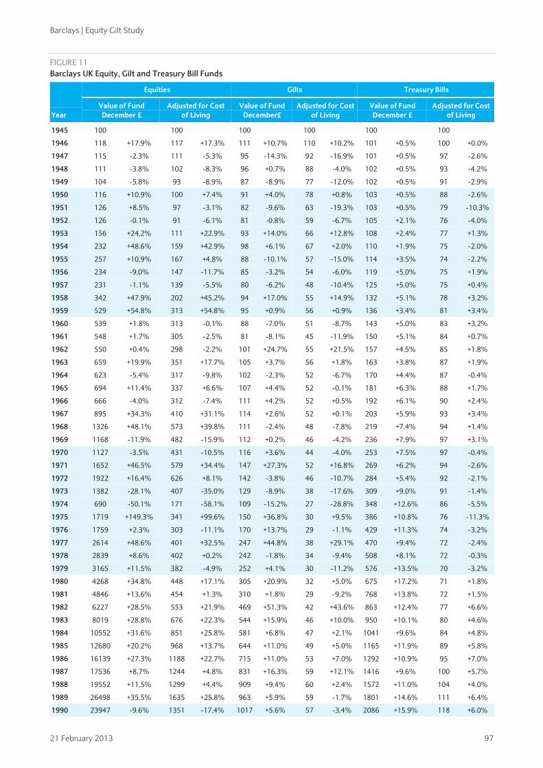
Barclays | Equity Gilt Study

21 February 2013 97

FIGURE 11 Barclays UK Equity, Gilt and Treasury Bill Funds

Year

Equities Gilts Treasury Bills

Value of Fund December £

Adjusted for Cost of Living

Value of Fund December£

Adjusted for Cost of Living

Value of Fund December £

Adjusted for Cost of Living

1945 100 100 100 100 100 100

1946 118 +17.9% 117 +17.3% 111 +10.7% 110 +10.2% 101 +0.5% 100 +0.0%

1947 115 -2.3% 111 -5.3% 95 -14.3% 92 -16.9% 101 +0.5% 97 -2.6%

1948 111 -3.8% 102 -8.3% 96 +0.7% 88 -4.0% 102 +0.5% 93 -4.2%

1949 104 -5.8% 93 -8.9% 87 -8.9% 77 -12.0% 102 +0.5% 91 -2.9%

1950 116 +10.9% 100 +7.4% 91 +4.0% 78 +0.8% 103 +0.5% 88 -2.6%

1951 126 +8.5% 97 -3.1% 82 -9.6% 63 -19.3% 103 +0.5% 79 -10.3%

1952 126 -0.1% 91 -6.1% 81 -0.8% 59 -6.7% 105 +2.1% 76 -4.0%

1953 156 +24.2% 111 +22.9% 93 +14.0% 66 +12.8% 108 +2.4% 77 +1.3%

1954 232 +48.6% 159 +42.9% 98 +6.1% 67 +2.0% 110 +1.9% 75 -2.0%

1955 257 +10.9% 167 +4.8% 88 -10.1% 57 -15.0% 114 +3.5% 74 -2.2%

1956 234 -9.0% 147 -11.7% 85 -3.2% 54 -6.0% 119 +5.0% 75 +1.9%

1957 231 -1.1% 139 -5.5% 80 -6.2% 48 -10.4% 125 +5.0% 75 +0.4%

1958 342 +47.9% 202 +45.2% 94 +17.0% 55 +14.9% 132 +5.1% 78 +3.2%

1959 529 +54.8% 313 +54.8% 95 +0.9% 56 +0.9% 136 +3.4% 81 +3.4%

1960 539 +1.8% 313 -0.1% 88 -7.0% 51 -8.7% 143 +5.0% 83 +3.2%

1961 548 +1.7% 305 -2.5% 81 -8.1% 45 -11.9% 150 +5.1% 84 +0.7%

1962 550 +0.4% 298 -2.2% 101 +24.7% 55 +21.5% 157 +4.5% 85 +1.8%

1963 659 +19.9% 351 +17.7% 105 +3.7% 56 +1.8% 163 +3.8% 87 +1.9%

1964 623 -5.4% 317 -9.8% 102 -2.3% 52 -6.7% 170 +4.4% 87 -0.4%

1965 694 +11.4% 337 +6.6% 107 +4.4% 52 -0.1% 181 +6.3% 88 +1.7%

1966 666 -4.0% 312 -7.4% 111 +4.2% 52 +0.5% 192 +6.1% 90 +2.4%

1967 895 +34.3% 410 +31.1% 114 +2.6% 52 +0.1% 203 +5.9% 93 +3.4%

1968 1326 +48.1% 573 +39.8% 111 -2.4% 48 -7.8% 219 +7.4% 94 +1.4%

1969 1168 -11.9% 482 -15.9% 112 +0.2% 46 -4.2% 236 +7.9% 97 +3.1%

1970 1127 -3.5% 431 -10.5% 116 +3.6% 44 -4.0% 253 +7.5% 97 -0.4%

1971 1652 +46.5% 579 +34.4% 147 +27.3% 52 +16.8% 269 +6.2% 94 -2.6%

1972 1922 +16.4% 626 +8.1% 142 -3.8% 46 -10.7% 284 +5.4% 92 -2.1%

1973 1382 -28.1% 407 -35.0% 129 -8.9% 38 -17.6% 309 +9.0% 91 -1.4%

1974 690 -50.1% 171 -58.1% 109 -15.2% 27 -28.8% 348 +12.6% 86 -5.5%

1975 1719 +149.3% 341 +99.6% 150 +36.8% 30 +9.5% 386 +10.8% 76 -11.3%

1976 1759 +2.3% 303 -11.1% 170 +13.7% 29 -1.1% 429 +11.3% 74 -3.2%

1977 2614 +48.6% 401 +32.5% 247 +44.8% 38 +29.1% 470 +9.4% 72 -2.4%

1978 2839 +8.6% 402 +0.2% 242 -1.8% 34 -9.4% 508 +8.1% 72 -0.3%

1979 3165 +11.5% 382 -4.9% 252 +4.1% 30 -11.2% 576 +13.5% 70 -3.2%

1980 4268 +34.8% 448 +17.1% 305 +20.9% 32 +5.0% 675 +17.2% 71 +1.8%

1981 4846 +13.6% 454 +1.3% 310 +1.8% 29 -9.2% 768 +13.8% 72 +1.5%

1982 6227 +28.5% 553 +21.9% 469 +51.3% 42 +43.6% 863 +12.4% 77 +6.6%

1983 8019 +28.8% 676 +22.3% 544 +15.9% 46 +10.0% 950 +10.1% 80 +4.6%

1984 10552 +31.6% 851 +25.8% 581 +6.8% 47 +2.1% 1041 +9.6% 84 +4.8%

1985 12680 +20.2% 968 +13.7% 644 +11.0% 49 +5.0% 1165 +11.9% 89 +5.8%

1986 16139 +27.3% 1188 +22.7% 715 +11.0% 53 +7.0% 1292 +10.9% 95 +7.0%

1987 17536 +8.7% 1244 +4.8% 831 +16.3% 59 +12.1% 1416 +9.6% 100 +5.7%

1988 19552 +11.5% 1299 +4.4% 909 +9.4% 60 +2.4% 1572 +11.0% 104 +4.0%

1989 26498 +35.5% 1635 +25.8% 963 +5.9% 59 -1.7% 1801 +14.6% 111 +6.4%

1990 23947 -9.6% 1351 -17.4% 1017 +5.6% 57 -3.4% 2086 +15.9% 118 +6.0%

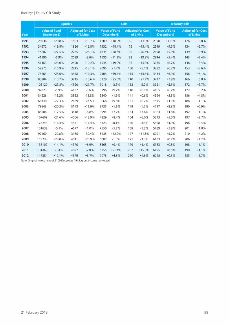
Barclays | Equity Gilt Study

21 February 2013 98

Year

Equities Gilts Treasury Bills

Value of Fund December £

Adjusted for Cost of Living

Value of Fund December£

Adjusted for Cost of Living

Value of Fund December £

Adjusted for Cost of Living

1991 28936 +20.8% 1563 +15.7% 1209 +18.9% 65 +13.8% 2328 +11.6% 126 +6.8%

1992 34672 +19.8% 1826 +16.8% 1432 +18.4% 75 +15.4% 2549 +9.5% 134 +6.7%

1993 44207 +27.5% 2285 +25.1% 1844 +28.8% 95 +26.4% 2698 +5.9% 139 +3.9%

1994 41590 -5.9% 2089 -8.6% 1635 -11.3% 82 -13.8% 2844 +5.4% 143 +2.4%

1995 51163 +23.0% 2490 +19.2% 1945 +19.0% 95 +15.3% 3035 +6.7% 148 +3.4%

1996 59275 +15.9% 2815 +13.1% 2095 +7.7% 100 +5.1% 3222 +6.2% 153 +3.6%

1997 73263 +23.6% 3358 +19.3% 2503 +19.4% 115 +15.3% 3444 +6.9% 158 +3.1%

1998 83284 +13.7% 3715 +10.6% 3129 +25.0% 140 +21.7% 3717 +7.9% 166 +5.0%

1999 103120 +23.8% 4520 +21.7% 3018 -3.5% 132 -5.2% 3921 +5.5% 172 +3.7%

2000 97023 -5.9% 4132 -8.6% 3296 +9.2% 140 +6.1% 4165 +6.2% 177 +3.2%

2001 84226 -13.2% 3562 -13.8% 3340 +1.3% 141 +0.6% 4394 +5.5% 186 +4.8%

2002 65440 -22.3% 2689 -24.5% 3668 +9.8% 151 +6.7% 4575 +4.1% 188 +1.1%

2003 78643 +20.2% 3143 +16.9% 3725 +1.6% 149 -1.2% 4747 +3.8% 190 +0.9%

2004 88508 +12.5% 3418 +8.8% 3994 +7.2% 154 +3.6% 4964 +4.6% 192 +1.1%

2005 107609 +21.6% 4066 +18.9% 4329 +8.4% 164 +6.0% 5213 +5.0% 197 +2.7%

2006 125243 +16.4% 4531 +11.4% 4323 -0.1% 156 -4.4% 5468 +4.9% 198 +0.4%

2007 131639 +5.1% 4577 +1.0% 4550 +5.2% 158 +1.2% 5789 +5.9% 201 +1.8%

2008 92460 -29.8% 3185 -30.4% 5135 +12.9% 177 +11.8% 6091 +5.2% 210 +4.2%

2009 119238 +29.0% 4011 +25.9% 5087 -1.0% 171 -3.3% 6133 +0.7% 206 -1.7%

2010 136107 +14.1% 4370 +8.9% 5565 +9.4% 179 +4.4% 6163 +0.5% 198 -4.1%

2011 131469 -3.4% 4027 -7.8% 6755 +21.4% 207 +15.8% 6195 +0.5% 190 -4.1%

2012 147384 +12.1% 4379 +8.7% 7078 +4.8% 210 +1.6% 6215 +0.3% 185 -2.7%

Note: Original Investment of £100 December 1945, gross income reinvested.

Barclays | Equity Gilt Study

21 February 2013 99

FIGURE 12 Barclays UK Treasury Bills and Building Society Accounts

Year

Treasury Bills Annual

Return %

Building Society Acc.

Annual Rate of Interest

Basic Rate Income Tax

Calendar Year Average Year

Treasury Bills Annual

Return %

Building Society Acc. Annual rate

of Interest

Basic Rate Income Tax

Calendar Year Average

1946 0.51 6.51 46.25

1947 0.51 6.36 45.00

1948 0.51 6.36 45.00

1949 0.52 6.36 45.00

1950 0.52 6.36 45.00 1990 15.86 12.04 25.00

1951 0.52 4.82 46.88 1991 11.59 9.32 25.00

1952 2.09 4.65 47.50 1992 9.47 9.59 24.68

1953 2.36 4.60 45.62 1993 5.86 4.12 24.50

1954 1.89 4.55 45.00 1994 5.40 3.69 20.00

1955 3.50 4.69 43.12 1995 6.74 3.93 20.00

1956 5.02 5.44 42.50 1996 6.16 2.61 20.00

1957 5.01 6.09 42.50 1997 6.88 3.06 20.00

1958 5.11 6.09 42.50 1998 7.92 7.06 20.00

1959 3.42 5.59 39.69 1999 5.51 5.11 23.00

1960 5.04 5.52 38.75 2000 6.22 5.50 22.00

1961 5.14 5.81 38.75 2001 5.50 4.70 22.00

1962 4.46 6.12 38.75 2002 4.12 3.40 22.00

1963 3.80 5.81 38.75 2003 3.75 3.33 22.00

1964 4.40 5.71 38.75 2004 4.59 4.21 22.00

1965 6.29 6.50 40.62 2005 5.00 3.95 22.00

1966 6.12 6.81 41.25 2006 4.90 4.36 22.00

1967 5.90 7.23 41.25 2007 5.87 4.77 22.00

1968 7.43 7.52 41.25 2008 5.23 0.85 20.00

1969 7.93 8.29 41.25 2009 0.68 0.25 20.00

1970 7.45 8.51 41.25 2010 0.50 0.20 20.00

1971 6.18 8.25 39.38 2011 0.51 0.20 20.00

1972 5.42 8.16 38.75 2012 0.32 0.20 20.00

1973 9.01 9.70 32.19

1974 12.56 11.07 32.25

1975 10.75 11.01 34.50

1976 11.34 10.65 35.00

1977 9.44 10.65 34.25

1978 8.06 9.42 33.25

1979 13.45 12.22 30.75

1980 17.17 15.00 30.00

1981 13.76 12.94 30.00

1982 12.38 12.19 30.00

1983 10.14 9.64 30.00

1984 9.55 9.99 30.00

1985 11.87 10.81 30.00

1986 10.95 10.55 29.26

1987 9.58 9.66 27.50

1988 11.01 8.26 25.50

1989 14.55 10.71 25.00

Note: 1. Annual returns on treasury bills are based on four consecutive investments in 91-day bills. 2. The building society rate of interest above is gross of tax.

Barclays | Equity Gilt Study

21 February 2013 100

FIGURE 13 Barclays Index-linked Funds

Index Linked gilts

Value of Fund December £ Adjusted for Cost of Living

1982 100 100

1983 101 +0.8% 96 -4.3%

1984 107 +6.6% 98 +1.9%

1985 107 -0.2% 92 -5.5%

1986 114 +6.1% 94 +2.3%

1987 122 +6.9% 97 +3.1%

1988 138 +13.7% 103 +6.5%

1989 158 +14.5% 110 +6.3%

1990 165 +4.4% 105 -4.5%

1991 174 +5.2% 106 +0.7%

1992 204 +17.1% 121 +14.1%

1993 247 +21.1% 144 +18.9%

1994 227 -7.9% 128 -10.5%

1995 254 +12.0% 139 +8.5%

1996 271 +6.5% 145 +4.0%

1997 307 +13.4% 158 +9.4%

1998 369 +20.3% 186 +17.1%

1999 388 +5.0% 191 +3.2%

2000 400 +3.1% 192 +0.1%

2001 396 -0.9% 189 -1.6%

2002 428 +8.2% 198 +5.1%

2003 457 +6.8% 206 +3.9%

2004 497 +8.6% 216 +4.9%

2005 542 +9.1% 231 +6.7%

2006 554 +2.3% 226 -2.1%

2007 585 +5.5% 229 +1.4%

2008 578 -1.2% 224 -2.1%

2009 610 +5.6% 231 +3.1%

2010 673 +10.3% 243 +5.3%

2011 808 +19.9% 278 +14.4%

2012 834 +3.3% 279 +0.2%

Barclays | Equity Gilt Study

21 February 2013 101

FIGURE 14 Barclays US Equity Index

Year Equity Price Index

December Equity Income Index

December Income Yield %

Equity Price Index Adjusted for Cost of

Living

Equity Income Index Adjusted for Cost of

Living

1925 100 100

1926 104 +4.2% 100 5.5 105 +5.4% 100

1927 133 +27.3% 143 +43.3% 6.2 137 +30.2% 147 +46.6%

1928 177 +33.7% 167 +16.4% 5.4 186 +35.2% 173 +17.8%

1929 145 -18.2% 79 -52.4% 3.1 151 -18.6% 82 -52.6%

1930 99 -32.1% 56 -29.3% 3.3 110 -27.4% 62 -24.4%

1931 52 -47.7% 30 -47.1% 3.3 63 -42.3% 36 -41.6%

1932 44 -14.5% 47 +56.7% 6.0 60 -4.7% 63 +74.6%

1933 67 +51.1% 75 +60.6% 6.4 90 +49.9% 100 +59.4%

1934 67 +0.1% 49 -34.7% 4.2 89 -1.4% 65 -35.7%

1935 93 +39.0% 95 +94.2% 5.9 120 +35.0% 122 +88.6%

1936 117 +26.5% 116 +21.8% 5.6 150 +24.7% 146 +20.1%

1937 73 -38.1% 44 -61.9% 3.5 90 -39.8% 54 -62.9%

1938 89 +22.7% 84 +91.5% 5.4 114 +26.2% 107 +97.0%

1939 87 -2.6% 72 -14.6% 4.8 111 -2.6% 91 -14.6%

1940 76 -12.7% 69 -3.8% 5.2 96 -13.3% 87 -4.5%

1941 64 -15.7% 68 -2.0% 6.1 74 -23.3% 78 -10.8%

1942 69 +8.7% 93 +36.3% 7.6 73 -0.3% 97 +25.0%

1943 84 +21.7% 94 +1.7% 6.4 87 +18.2% 96 -1.2%

1944 97 +15.5% 100 +6.3% 5.9 98 +12.9% 100 +3.9%

1945 129 +32.9% 125 +24.5% 5.5 127 +30.0% 121 +21.8%

1946 117 -9.7% 78 -37.4% 3.8 97 -23.6% 64 -47.0%

1947 114 -2.2% 112 +43.3% 5.6 87 -10.2% 85 +31.7%

1948 110 -3.9% 120 +7.1% 6.2 82 -6.7% 88 +4.0%

1949 123 +12.1% 172 +43.1% 8.0 93 +14.5% 129 +46.2%

1950 149 +21.3% 227 +32.3% 8.7 107 +14.5% 161 +24.9%

1951 171 +14.2% 199 -12.3% 6.7 115 +7.7% 133 -17.3%

1952 183 +7.4% 190 -4.6% 5.9 123 +6.6% 126 -5.3%

1953 174 -5.1% 165 -13.4% 5.4 116 -5.8% 108 -14.0%

1954 249 +43.1% 307 +86.4% 7.0 167 +44.2% 203 +87.8%

1955 299 +20.3% 263 -14.4% 5.0 200 +19.8% 173 -14.7%

1956 312 +4.3% 230 -12.5% 4.2 202 +1.2% 147 -15.0%

1957 268 -14.1% 175 -24.0% 3.7 169 -16.5% 109 -26.1%

1958 374 +39.3% 361 +106.4% 5.5 231 +36.9% 221 +102.9%

1959 407 +9.0% 255 -29.3% 3.6 248 +7.2% 154 -30.5%

1960 398 -2.2% 237 -7.2% 3.4 239 -3.6% 141 -8.5%

1961 491 +23.3% 313 +32.3% 3.6 293 +22.5% 185 +31.4%

1962 426 -13.3% 222 -29.2% 3.0 251 -14.4% 129 -30.1%

1963 499 +17.1% 330 +49.0% 3.8 289 +15.2% 189 +46.5%

1964 563 +12.8% 340 +2.9% 3.5 323 +11.8% 193 +1.9%

1965 624 +11.0% 370 +9.0% 3.4 351 +8.9% 206 +6.9%

1966 551 -11.7% 289 -22.1% 3.0 300 -14.6% 155 -24.7%

1967 688 +24.7% 462 +60.1% 3.8 363 +21.0% 241 +55.3%

1968 763 +10.9% 433 -6.2% 3.2 385 +5.9% 216 -10.4%

1969 660 -13.5% 309 -28.8% 2.7 313 -18.6% 145 -32.9%

Barclays | Equity Gilt Study

21 February 2013 102

Year Equity Price Index

December Equity Income Index

December Income Yield %

Equity Price Index Adjusted for Cost of

Living

Equity Income Index Adjusted for Cost of

Living

1970 637 -3.4% 388 +25.6% 3.5 287 -8.5% 173 +19.0%

1971 719 +12.8% 426 +9.7% 3.4 313 +9.2% 183 +6.3%

1972 822 +14.3% 443 +4.1% 3.1 346 +10.5% 185 +0.7%

1973 647 -21.2% 275 -38.0% 2.4 251 -27.5% 105 -43.0%

1974 446 -31.1% 244 -11.3% 3.1 154 -38.6% 83 -21.0%

1975 588 +31.8% 570 +134.1% 5.5 190 +23.3% 182 +118.9%

1976 717 +21.9% 609 +6.8% 4.9 221 +16.3% 185 +1.9%

1977 665 -7.3% 503 -17.5% 4.3 192 -13.1% 143 -22.6%

1978 687 +3.3% 631 +25.6% 5.3 182 -5.3% 165 +15.2%

1979 812 +18.3% 870 +37.8% 6.1 190 +4.4% 201 +21.7%

1980 1033 +27.1% 1104 +26.9% 6.1 214 +13.0% 226 +12.8%

1981 947 -8.4% 724 -34.5% 4.4 180 -15.9% 136 -39.8%

1982 1081 +14.2% 1168 +61.5% 6.2 198 +10.0% 212 +55.5%

1983 1275 +17.9% 1062 -9.1% 4.8 225 +13.6% 186 -12.4%

1984 1260 -1.1% 950 -10.5% 4.3 214 -4.9% 160 -13.9%

1985 1594 +26.5% 1380 +45.2% 4.9 261 +21.8% 223 +39.9%

1986 1781 +11.8% 1176 -14.8% 3.8 289 +10.6% 188 -15.7%

1987 1757 -1.4% 980 -16.7% 3.2 273 -5.5% 150 -20.2%

1988 1985 +13.0% 1589 +62.2% 4.6 295 +8.2% 233 +55.3%

1989 2462 +24.0% 1897 +19.4% 4.4 350 +18.5% 266 +14.1%

1990 2231 -9.4% 1291 -32.0% 3.3 298 -14.6% 171 -35.9%

1991 2892 +29.6% 2029 +57.1% 4.0 375 +25.8% 260 +52.5%

1992 3069 +6.1% 1583 -22.0% 2.9 387 +3.1% 197 -24.2%

1993 3339 +8.8% 1630 +3.0% 2.8 410 +5.9% 198 +0.2%

1994 3230 -3.3% 1427 -12.4% 2.5 386 -5.8% 169 -14.7%

1995 4279 +32.5% 2368 +66.0% 3.2 499 +29.2% 273 +61.9%

1996 5082 +18.8% 2142 -9.5% 2.4 574 +14.9% 239 -12.5%

1997 6513 +28.2% 2465 +15.1% 2.2 723 +26.0% 270 +13.1%

1998 7850 +20.5% 2413 -2.1% 1.8 857 +18.6% 261 -3.7%

1999 9707 +23.7% 2748 +13.9% 1.6 1032 +20.4% 289 +10.9%

2000 8536 -12.1% 1460 -46.9% 1.0 878 -14.9% 149 -48.6%

2001 7474 -12.4% 1538 +5.4% 1.2 757 -13.8% 154 +3.8%

2002 5821 -22.1% 1292 -16.0% 1.3 576 -23.9% 126 -18.0%

2003 7613 +30.8% 3140 +143.1% 2.4 739 +28.4% 302 +138.6%

2004 8439 +10.8% 3178 +1.2% 2.2 794 +7.4% 296 -2.0%

2005 8895 +5.4% 2999 -5.6% 1.9 809 +1.9% 270 -8.8%

2006 10145 +14.0% 3835 +27.9% 2.2 900 +11.2% 336 +24.7%

2007 10678 +5.3% 3772 -1.7% 2.0 910 +1.1% 318 -5.5%

2008 6443 -39.7% 1623 -56.98% 1.4 549 -39.7% 137 -57.0%

2009 8255 +28.1% 4631 +185.4% 3.2 684 +24.7% 380 +177.9%

2010 9524 +15.4% 4135 -10.7% 2.5 778 +13.7% 334 -12.0%

2011 9229 -3.1% 3287 -20.5% 2.0 732 -5.9% 258 -22.8%

2012 10414 12.9% 5173 57.4% 2.8 812 10.9% 399 +54.7%

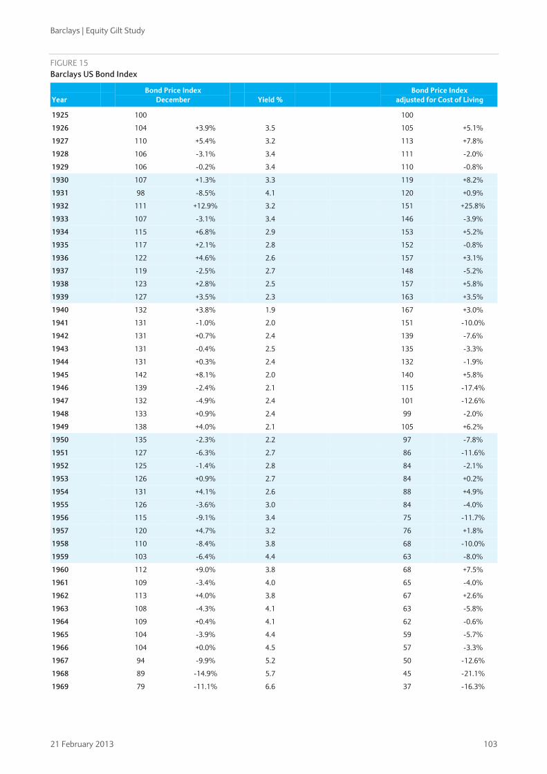
Barclays | Equity Gilt Study

21 February 2013 103

FIGURE 15 Barclays US Bond Index

Year Bond Price Index

December Yield % Bond Price Index

adjusted for Cost of Living

1925 100 100

1926 104 +3.9% 3.5 105 +5.1%

1927 110 +5.4% 3.2 113 +7.8%

1928 106 -3.1% 3.4 111 -2.0%

1929 106 -0.2% 3.4 110 -0.8%

1930 107 +1.3% 3.3 119 +8.2%

1931 98 -8.5% 4.1 120 +0.9%

1932 111 +12.9% 3.2 151 +25.8%

1933 107 -3.1% 3.4 146 -3.9%

1934 115 +6.8% 2.9 153 +5.2%

1935 117 +2.1% 2.8 152 -0.8%

1936 122 +4.6% 2.6 157 +3.1%

1937 119 -2.5% 2.7 148 -5.2%

1938 123 +2.8% 2.5 157 +5.8%

1939 127 +3.5% 2.3 163 +3.5%

1940 132 +3.8% 1.9 167 +3.0%

1941 131 -1.0% 2.0 151 -10.0%

1942 131 +0.7% 2.4 139 -7.6%

1943 131 -0.4% 2.5 135 -3.3%

1944 131 +0.3% 2.4 132 -1.9%

1945 142 +8.1% 2.0 140 +5.8%

1946 139 -2.4% 2.1 115 -17.4%

1947 132 -4.9% 2.4 101 -12.6%

1948 133 +0.9% 2.4 99 -2.0%

1949 138 +4.0% 2.1 105 +6.2%

1950 135 -2.3% 2.2 97 -7.8%

1951 127 -6.3% 2.7 86 -11.6%

1952 125 -1.4% 2.8 84 -2.1%

1953 126 +0.9% 2.7 84 +0.2%

1954 131 +4.1% 2.6 88 +4.9%

1955 126 -3.6% 3.0 84 -4.0%

1956 115 -9.1% 3.4 75 -11.7%

1957 120 +4.7% 3.2 76 +1.8%

1958 110 -8.4% 3.8 68 -10.0%

1959 103 -6.4% 4.4 63 -8.0%

1960 112 +9.0% 3.8 68 +7.5%

1961 109 -3.4% 4.0 65 -4.0%

1962 113 +4.0% 3.8 67 +2.6%

1963 108 -4.3% 4.1 63 -5.8%

1964 109 +0.4% 4.1 62 -0.6%

1965 104 -3.9% 4.4 59 -5.7%

1966 104 +0.0% 4.5 57 -3.3%

1967 94 -9.9% 5.2 50 -12.6%

1968 89 -14.9% 5.7 45 -21.1%

1969 79 -11.1% 6.6 37 -16.3%

Barclays | Equity Gilt Study

21 February 2013 104

Year Bond Price Index

December Yield % Bond Price Index

adjusted for Cost of Living

1970 85 +7.0% 6.2 38 +1.4%

1971 95 +12.2% 4.5 41 +8.6%

1972 96 +1.3% 4.5 40 -2.1%

1973 88 -8.8% 7.1 34 -16.1%

1974 84 -3.8% 7.7 29 -14.4%

1975 83 -1.7% 7.7 27 -8.0%

1976 91 +9.8% 6.9 28 +4.7%

1977 86 -6.0% 7.5 25 -11.9%

1978 77 -10.3% 8.8 20 -17.7%

1979 69 -10.0% 9.9 16 -20.5%

1980 60 -13.3% 11.6 12 -22.9%

1981 53 -11.5% 13.7 10 -18.7%

1982 65 +23.3% 10.5 12 +18.8%

1983 59 -9.4% 11.6 10 -12.7%

1984 61 +2.5% 11.3 10 -1.4%

1985 72 +18.7% 9.3 12 +14.3%

1986 84 +16.1% 7.6 14 +14.8%

1987 75 -11.0% 8.8 12 -14.8%

1988 74 -0.6% 8.8 11 -4.8%

1989 81 +9.5% 7.9 12 +4.6%

1990 79 -2.8% 8.2 11 -8.4%

1991 86 +9.1% 7.3 11 +5.9%

1992 86 -0.3% 7.3 11 -3.1%

1993 93 +8.8% 6.4 11 +5.9%

1994 80 -14.3% 7.9 10 -16.5%

1995 97 +21.1% 5.9 11 +18.1%

1996 90 -7.0% 6.6 10 -10.0%

1997 97 +7.7% 5.9 11 +5.9%

1998 103 +6.1% 5.3 11 +4.4%

1999 88 -14.5% 6.7 9 -16.8%

2000 100 +13.3% 5.5 10 +9.6%

2001 98 -2.1% 5.7 10 -3.6%

2002 108 +10.5% 4.8 11 +7.9%

2003 105 -2.9% 5.0 10 -4.7%

2004 107 +2.4% 4.8 10 -0.8%

2005 110 +2.2% 4.6 10 -1.2%

2006 105 -4.1% 4.8 9 -6.5%

2007 109 +4.1% 4.5 9 -0.0%

2008 131 +19.8% 3.1 11 +19.7%

2009 107 -17.9% 4.5 9 -20.1%

2010 113 +4.8% 4.1 9 +3.3%

2011 137 +21.7% 2.5 11 +18.2%

2012 138 +0.4% 2.7 11 -1.3%

Barclays | Equity Gilt Study

21 February 2013 105

FIGURE 16 Barclays US Treasury Bill Index

Year Treasury Bill Index

December Treasury Bill Index

adjusted for Cost of Living

1925 100 100

1926 103 +3.2% 104 +4.4%

1927 106 +3.1% 110 +5.5%

1928 110 +3.8% 116 +5.0%

1929 116 +4.7% 120 +4.1%

1930 118 +2.3% 132 +9.3%

1931 120 +1.0% 147 +11.4%

1932 121 +0.8% 165 +12.3%

1933 121 +0.3% 164 -0.5%

1934 121 +0.2% 162 -1.3%

1935 121 +0.2% 157 -2.7%

1936 122 +0.2% 155 -1.3%

1937 122 +0.3% 152 -2.5%

1938 122 +0.0% 156 +2.9%

1939 122 +0.0% 156 +0.0%

1940 122 -0.1% 155 -0.8%

1941 122 +0.0% 141 -9.0%

1942 122 +0.3% 130 -8.0%

1943 123 +0.3% 126 -2.5%

1944 123 +0.3% 124 -1.9%

1945 124 +0.3% 121 -1.9%

1946 124 +0.4% 103 -15.1%

1947 125 +0.5% 95 -7.7%

1948 126 +1.0% 93 -2.0%

1949 127 +1.1% 96 +3.2%

1950 129 +1.2% 92 -4.5%

1951 131 +1.5% 88 -4.3%

1952 133 +1.6% 89 +0.9%

1953 135 +1.8% 90 +1.0%

1954 136 +0.9% 91 +1.6%

1955 138 +1.6% 92 +1.2%

1956 142 +2.4% 92 -0.5%

1957 146 +3.1% 92 +0.2%

1958 148 +1.4% 92 -0.3%

1959 152 +2.8% 93 +1.1%

1960 156 +2.6% 94 +1.2%

1961 160 +2.2% 95 +1.5%

1962 164 +2.7% 97 +1.4%

1963 169 +3.2% 98 +1.5%

1964 175 +3.5% 101 +2.5%

1965 182 +4.0% 103 +2.0%

1966 191 +4.7% 104 +1.2%

1967 199 +4.1% 105 +1.1%

1968 209 +9.7% 105 +0.5%

1969 223 +6.6% 106 +0.4%

Barclays | Equity Gilt Study

21 February 2013 106

Year Treasury Bill Index

December Treasury Bill Index

adjusted for Cost of Living

1970 237 +6.4% 107 +0.8%

1971 247 +4.3% 108 +1.0%

1972 257 +3.9% 108 +0.5%

1973 275 +7.1% 107 -1.5%

1974 297 +8.1% 103 -3.8%

1975 315 +5.8% 102 -1.0%

1976 331 +5.2% 102 +0.3%

1977 348 +5.2% 100 -1.5%

1978 373 +7.3% 99 -1.6%

1979 413 +10.7% 96 -2.3%

1980 461 +11.5% 96 -0.9%

1981 529 +14.9% 101 +5.4%

1982 586 +10.7% 107 +6.6%

1983 638 +8.8% 113 +4.9%

1984 701 +10.0% 119 +5.8%

1985 755 +7.7% 124 +3.7%

1986 801 +6.1% 130 +4.9%

1987 844 +5.4% 131 +0.9%

1988 897 +6.3% 133 +1.8%

1989 971 +8.2% 138 +3.4%

1990 1046 +7.7% 140 +1.5%

1991 1103 +5.5% 143 +2.4%

1992 1141 +3.4% 144 +0.5%

1993 1174 +2.9% 144 +0.1%

1994 1219 +3.9% 146 +1.2%

1995 1287 +5.5% 150 +2.9%

1996 1353 +5.1% 153 +1.8%

1997 1422 +5.1% 158 +3.3%

1998 1490 +4.8% 163 +3.1%

1999 1558 +4.6% 166 +1.8%

2000 1647 +5.8% 169 +2.3%

2001 1710 +3.8% 173 +2.2%

2002 1738 +1.6% 172 -0.7%

2003 1755 +1.0% 170 -0.8%

2004 1776 +1.2% 167 -2.0%

2005 1829 +3.0% 166 -0.4%

2006 1916 +4.8% 170 +2.2%

2007 2006 +4.7% 171 +0.6%

2008 2036 +1.5% 173 +1.4%

2009 2038 +0.1% 169 -2.6%

2010 2040 +0.1% 167 -1.4%

2011 2041 +0.04% 162 -2.8%

2012 2041 +0.001% 159 -1.7%

Barclays | Equity Gilt Study

21 February 2013 107

CHAPTER 9

Total investment returns Our final chapter presents a series of tables showing the performance of equity and fixed-interest investments over any period of years since December 1899.

The first section reviews the performance of each asset class, taking inflation into account. The second section reviews the performance over the 52 years since December 1960. On each page we provide two tables illustrating the same information in alternative forms. The first table shows the average annual real rate of return; the second shows the real value of a portfolio at the end of each year, which includes reinvested income. This section provides data on equities and gilts, with dividend income reinvested gross. Finally, we provide figures for Treasury bills and building society shares.

The final pullout section provides the annual real rate of return on UK and US equities and bonds (with reinvestment of income for each year since 1899 for the UK, and since 1925 for the US). There is also a table showing the real capital value of equities for the UK. The sources for all data in this chapter are the Barclays indices, as outlined in Chapter 8.

• Equities – income gross

• Gilts – income gross

• Treasury Bills – income gross

• Building Society Shares – income gross

• Index-linked gilts

• Corporate bonds

• UK and US real bond returns – income gross

• UK and US real equities returns – income gross

• UK Equities – real capital value

Sreekala Kochugovindan

+44 (0)20 7773 2234 sreekala.kochugovindan@ barclays.com

1960-2012

UK: 1899-2012 US: 1925-2012

Barclays | Equity Gilt Study

21 February 2013 108

Real return on equities - gross income re-invested Average Annual Real Rate of Return

INV

ESTM

ENT

TO E

ND

YEA

R

INVESTMENT FROM END YEAR

1960 1961 1962 1963 1964 1965 1966 1967 1968 1969 1970 1971 1972 1973 1974 1975 1976 1977 1978 1979 1980 1981 1982 1983 1984 1985 1986 1987 1988 1989 1990 1991 1992 1993 1994 1995 1996 1997 1998 1999 2000 2001 2002 2003 2004 2005 2006 2007 2008 2009 2010 2011

1961 (2.5) 1962 (2.4) (2.2) 1963 3.9 7.3 17.7 1964 0.3 1.3 3.0 (9.8) 1965 1.5 2.6 4.2 (1.9) 6.6 1966 (0.0) 0.5 1.2 (3.8) (0.7) (7.4) The dates along the top (and bottom) are

those on which each portfolio starts. Those down the side are the dates to which the annual rate of return is calculated. Reading the top figure in each column diagonally down the table gives the real rate of return in each year since 1960. The table can be used to see the real rate of return over any period; thus a purchase made at the end of 1960 would have lost 2.5% (allowing for reinvestment of income) in one year but over the first three years (up to the end of 1963) would have given an average annual real return of 3.9%. Each figure on the bottom line of the table shows the real growth up to December 2012 from the year shown below the figure.

1967 3.9 5.0 6.6 3.9 9.0 10.2 31.1 1968 7.8 9.4 11.5 10.3 16.0 19.3 35.4 39.8 1969 4.9 5.9 7.1 5.4 8.8 9.3 15.5 8.5 (15.9) 1970 3.3 3.9 4.7 3.0 5.3 5.0 8.4 1.7 (13.2) (10.5) 1971 5.8 6.6 7.7 6.5 9.0 9.4 13.2 9.1 0.4 9.7 34.4 1972 6.0 6.8 7.7 6.7 8.9 9.2 12.3 8.9 2.3 9.1 20.5 8.1 1973 2.1 2.4 2.9 1.5 2.8 2.4 3.9 (0.1) (6.6) (4.1) (1.9) (16.2) (35.0) 1974 (4.2) (4.4) (4.5) (6.3) (6.0) (7.3) (7.3) (11.8) (18.3) (18.7) (20.7) (33.5) (47.8) (58.1) 1975 0.6 0.8 1.0 (0.2) 0.7 0.1 1.0 (2.3) (7.2) (5.6) (4.6) (12.4) (18.4) (8.6) 99.6 1976 (0.2) (0.0) 0.1 (1.1) (0.4) (1.0) (0.3) (3.3) (7.7) (6.4) (5.7) (12.2) (16.6) (9.4) 33.2 (11.1) 1977 1.5 1.7 2.0 1.0 1.8 1.5 2.3 (0.2) (3.9) (2.3) (1.0) (5.9) (8.5) (0.4) 33.0 8.5 32.5 1978 1.4 1.6 1.9 0.9 1.7 1.4 2.1 (0.2) (3.5) (2.0) (0.9) (5.1) (7.1) (0.3) 23.9 5.7 15.2 0.2 1979 1.1 1.3 1.5 0.5 1.3 0.9 1.6 (0.6) (3.6) (2.3) (1.3) (5.1) (6.8) (1.1) 17.5 2.9 8.1 (2.4) (4.9) 1980 1.8 2.0 2.3 1.4 2.2 1.9 2.6 0.7 (2.0) (0.7) 0.4 (2.8) (4.1) 1.4 17.4 5.6 10.3 3.7 5.5 17.1 1981 1.8 2.0 2.2 1.4 2.1 1.9 2.5 0.7 (1.8) (0.5) 0.5 (2.4) (3.5) 1.4 15.0 4.9 8.4 3.1 4.1 8.9 1.3 1982 2.6 2.9 3.1 2.4 3.2 3.0 3.6 2.0 (0.2) 1.1 2.1 (0.4) (1.2) 3.5 15.8 7.2 10.6 6.6 8.3 13.1 11.1 21.9 1983 3.4 3.7 4.0 3.3 4.1 3.9 4.6 3.2 1.1 2.5 3.5 1.3 0.7 5.2 16.5 9.0 12.2 9.1 11.0 15.3 14.7 22.1 22.3 1984 4.3 4.6 4.9 4.3 5.1 5.0 5.7 4.4 2.5 3.9 5.0 3.0 2.6 6.9 17.4 10.7 13.8 11.3 13.3 17.4 17.4 23.3 24.0 25.8 1985 4.6 4.9 5.3 4.7 5.5 5.4 6.1 4.9 3.1 4.5 5.5 3.7 3.4 7.5 17.1 11.0 13.8 11.6 13.4 16.7 16.7 20.8 20.5 19.6 13.7 1986 5.3 5.6 5.9 5.4 6.2 6.2 6.9 5.8 4.1 5.4 6.5 4.9 4.7 8.6 17.5 12.0 14.6 12.8 14.5 17.6 17.7 21.2 21.0 20.6 18.1 22.7 1987 5.2 5.6 5.9 5.4 6.1 6.1 6.8 5.7 4.2 5.4 6.4 4.9 4.7 8.3 16.5 11.4 13.7 12.0 13.4 15.9 15.7 18.3 17.6 16.5 13.5 13.4 4.8 1988 5.2 5.5 5.8 5.4 6.1 6.0 6.7 5.7 4.2 5.4 6.3 4.9 4.7 8.0 15.6 10.9 12.9 11.3 12.4 14.6 14.2 16.2 15.3 13.9 11.2 10.3 4.6 4.4 1989 5.9 6.2 6.5 6.1 6.8 6.8 7.5 6.5 5.1 6.3 7.3 5.9 5.8 9.1 16.3 11.9 13.9 12.4 13.6 15.6 15.5 17.4 16.7 15.8 13.9 14.0 11.2 14.6 25.8 1990 5.0 5.3 5.5 5.1 5.7 5.7 6.3 5.3 4.0 5.0 5.9 4.6 4.4 7.3 13.8 9.6 11.3 9.8 10.6 12.2 11.7 12.9 11.8 10.4 8.0 6.9 3.3 2.8 2.0 (17.4) 1991 5.3 5.6 5.9 5.5 6.1 6.1 6.7 5.7 4.5 5.5 6.3 5.1 4.9 7.8 13.9 10.0 11.6 10.2 11.0 12.4 12.0 13.2 12.2 11.0 9.1 8.3 5.6 5.9 6.4 (2.2) 15.7 1992 5.7 5.9 6.2 5.9 6.5 6.5 7.0 6.2 5.0 6.0 6.8 5.6 5.5 8.2 14.1 10.4 11.9 10.6 11.4 12.8 12.4 13.5 12.7 11.7 10.0 9.5 7.4 8.0 8.9 3.7 16.2 16.8 1993 6.2 6.5 6.8 6.4 7.1 7.1 7.6 6.8 5.7 6.7 7.5 6.4 6.4 9.0 14.6 11.2 12.6 11.5 12.3 13.6 13.4 14.4 13.8 12.9 11.6 11.3 9.8 10.7 11.9 8.7 19.1 20.9 25.1 1994 5.7 6.0 6.3 5.9 6.5 6.5 7.0 6.2 5.1 6.0 6.8 5.7 5.6 8.1 13.3 10.0 11.3 10.2 10.8 12.0 11.6 12.5 11.7 10.8 9.4 8.9 7.3 7.7 8.2 5.0 11.5 10.1 7.0 (8.6) 1995 6.1 6.4 6.6 6.3 6.9 6.9 7.4 6.7 5.6 6.5 7.3 6.3 6.2 8.6 13.6 10.5 11.7 10.7 11.3 12.4 12.1 12.9 12.3 11.5 10.2 9.9 8.6 9.1 9.7 7.3 13.0 12.3 10.9 4.4 19.2 1996 6.3 6.6 6.8 6.5 7.1 7.1 7.6 6.9 5.9 6.8 7.5 6.5 6.5 8.8 13.6 10.6 11.8 10.8 11.4 12.5 12.2 12.9 12.3 11.6 10.5 10.2 9.0 9.5 10.1 8.1 13.0 12.5 11.4 7.2 16.1 13.1 1997 6.6 6.9 7.2 6.9 7.4 7.4 8.0 7.3 6.3 7.2 7.9 7.0 6.9 9.2 13.8 11.0 12.1 11.2 11.8 12.8 12.6 13.3 12.8 12.1 11.1 10.9 9.9 10.4 11.1 9.4 13.9 13.6 13.0 10.1 17.1 16.1 19.3 1998 6.7 7.0 7.3 7.0 7.5 7.5 8.0 7.4 6.4 7.3 8.0 7.1 7.1 9.2 13.7 10.9 12.1 11.2 11.8 12.7 12.5 13.2 12.6 12.0 11.1 10.9 10.0 10.5 11.1 9.5 13.5 13.2 12.6 10.2 15.5 14.3 14.9 10.6 1999 7.1 7.4 7.6 7.4 7.9 7.9 8.4 7.8 6.9 7.7 8.4 7.6 7.6 9.7 14.0 11.4 12.5 11.6 12.2 13.1 12.9 13.6 13.2 12.6 11.8 11.6 10.8 11.3 12.0 10.7 14.4 14.2 13.8 12.0 16.7 16.1 17.1 16.0 21.7 2000 6.7 6.9 7.2 6.9 7.4 7.4 7.9 7.3 6.4 7.2 7.8 7.0 7.0 9.0 13.0 10.5 11.5 10.7 11.2 12.0 11.8 12.3 11.8 11.2 10.4 10.2 9.3 9.7 10.1 8.8 11.8 11.4 10.7 8.8 12.0 10.7 10.1 7.2 5.5 (8.6) 2001 6.1 6.3 6.6 6.3 6.8 6.8 7.2 6.6 5.7 6.5 7.0 6.2 6.2 8.1 11.9 9.4 10.4 9.5 9.9 10.7 10.4 10.9 10.3 9.7 8.8 8.5 7.6 7.8 8.1 6.7 9.2 8.6 7.7 5.7 7.9 6.2 4.8 1.5 (1.4) (11.2) (13.8) 2002 5.3 5.5 5.7 5.4 5.8 5.8 6.2 5.5 4.7 5.3 5.9 5.1 5.0 6.7 10.3 8.0 8.8 7.9 8.2 8.8 8.5 8.8 8.2 7.5 6.6 6.2 5.2 5.3 5.3 3.9 5.9 5.1 3.9 1.8 3.2 1.1 (0.8) (4.3) (7.8) (15.9) (19.3) (24.5) 2003 5.5 5.7 5.9 5.6 6.1 6.0 6.4 5.8 5.0 5.7 6.2 5.4 5.3 7.0 10.6 8.3 9.1 8.2 8.6 9.2 8.8 9.2 8.6 8.0 7.1 6.8 5.9 6.0 6.1 4.8 6.7 6.0 5.1 3.2 4.6 3.0 1.6 (1.1) (3.3) (8.7) (8.7) (6.1) 16.9 2004 5.6 5.8 6.0 5.7 6.1 6.1 6.5 5.9 5.1 5.8 6.3 5.5 5.4 7.1 10.5 8.3 9.0 8.3 8.6 9.2 8.8 9.2 8.6 8.0 7.2 6.9 6.0 6.1 6.2 5.0 6.9 6.2 5.4 3.7 5.0 3.6 2.5 0.3 (1.4) (5.4) (4.6) (1.4) 12.8 8.8 2005 5.9 6.1 6.3 6.0 6.4 6.4 6.8 6.2 5.4 6.1 6.6 5.9 5.8 7.5 10.8 8.6 9.4 8.6 8.9 9.5 9.2 9.6 9.1 8.5 7.7 7.4 6.7 6.8 6.9 5.9 7.6 7.1 6.4 4.9 6.2 5.0 4.2 2.4 1.3 (1.8) (0.3) 3.4 14.8 13.7 18.9 2006 6.0 6.2 6.4 6.1 6.5 6.5 6.9 6.4 5.6 6.2 6.8 6.1 6.0 7.6 10.8 8.7 9.4 8.7 9.0 9.6 9.3 9.6 9.2 8.6 7.9 7.6 6.9 7.0 7.2 6.2 7.9 7.4 6.7 5.4 6.7 5.6 4.9 3.4 2.5 0.0 1.5 4.9 13.9 13.0 15.1 11.4 2007 5.9 6.1 6.3 6.0 6.4 6.4 6.8 6.2 5.5 6.1 6.6 5.9 5.8 7.4 10.5 8.5 9.2 8.5 8.7 9.3 9.0 9.3 8.8 8.3 7.6 7.3 6.6 6.7 6.9 5.9 7.4 6.9 6.3 5.1 6.2 5.2 4.5 3.1 2.3 0.2 1.5 4.3 11.2 9.9 10.2 6.1 1.0 2008 5.0 5.1 5.3 5.0 5.4 5.4 5.7 5.1 4.4 5.0 5.4 4.7 4.6 6.1 9.0 7.0 7.6 6.9 7.1 7.6 7.3 7.5 7.0 6.4 5.7 5.3 4.6 4.6 4.6 3.6 4.9 4.3 3.5 2.2 3.1 1.9 1.0 (0.5) (1.5) (3.8) (3.2) (1.6) 2.9 0.3 (1.8) (7.8) (16.2) (30.4) 2009 5.3 5.5 5.7 5.4 5.8 5.8 6.1 5.6 4.9 5.4 5.9 5.2 5.1 6.6 9.4 7.5 8.1 7.5 7.7 8.1 7.9 8.1 7.6 7.1 6.4 6.1 5.4 5.5 5.5 4.6 5.9 5.4 4.7 3.6 4.4 3.5 2.8 1.5 0.7 (1.2) (0.3) 1.5 5.9 4.1 3.3 (0.3) (4.0) (6.4) 25.9 2010 5.4 5.6 5.8 5.5 5.9 5.9 6.2 5.7 5.0 5.5 6.0 5.3 5.2 6.6 9.4 7.6 8.2 7.5 7.7 8.2 7.9 8.1 7.7 7.2 6.5 6.2 5.6 5.6 5.7 4.8 6.0 5.6 5.0 3.9 4.7 3.8 3.2 2.0 1.4 (0.3) 0.6 2.3 6.3 4.8 4.2 1.5 (0.9) (1.5) 17.1 8.9 2011 5.1 5.3 5.5 5.2 5.6 5.5 5.8 5.3 4.6 5.2 5.6 5.0 4.9 6.2 8.9 7.1 7.7 7.0 7.2 7.6 7.3 7.5 7.1 6.6 5.9 5.6 5.0 5.0 5.0 4.2 5.3 4.8 4.3 3.2 3.9 3.1 2.4 1.3 0.6 (1.0) (0.2) 1.2 4.6 3.1 2.4 (0.2) (2.3) (3.2) 8.1 0.2 (7.8)

2012 5.2 5.4 5.5 5.3 5.6 5.6 5.9 5.4 4.7 5.3 5.7 5.1 5.0 6.3 8.9 7.1 7.7 7.1 7.3 7.7 7.4 7.6 7.1 6.7 6.0 5.8 5.1 5.2 5.2 4.4 5.5 5.0 4.5 3.5 4.2 3.4 2.8 1.8 1.2 (0.2) 0.5 1.9 5.0 3.8 3.1 1.1 (0.6) (0.9) 8.3 3.0 0.1 8.7

Barclays | Equity Gilt Study

21 February 2013 109

Real Value of £100 Invested IN

VES

TMEN

T TO

EN

D Y

EAR

INVESTMENT FROM END YEAR

1960 1961 1962 1963 1964 1965 1966 1967 1968 1969 1970 1971 1972 1973 1974 1975 1976 1977 1978 1979 1980 1981 1982 1983 1984 1985 1986 1987 1988 1989 1990 1991 1992 1993 1994 1995 1996 1997 1998 1999 2000 2001 2002 2003 2004 2005 2006 2007 2008 2009 2010 2011

1961 97

1962 95 98

1963 112 115 118

1964 101 104 106 90

1965 108 111 113 96 107

1966 100 102 105 89 99 93 The dates along the top (and bottom) are those on which each portfolio starts. Those down the side are the dates to which the change in real value is calculated. Reading the top figure in each column diagonally down the table gives the growth in each year since 1960. The table can be used to see the real growth over any period; thus an investment of £100 made at the end of 1960 would have fallen to £97 (allowing for reinvestment of income and the effect of inflation) in one year but after three years (up to the end of 1963) would have reached £112 in real terms. Each figure on the bottom line of the table shows the real growth up to December 2012 from the year shown below the figure.

1967 131 134 137 117 129 121 131

1968 183 188 192 163 181 170 183 140

1969 154 158 162 137 152 143 154 118 84

1970 138 141 145 123 136 128 138 105 75 89

1971 185 190 194 165 183 172 185 141 101 120 134

1972 200 205 210 179 198 186 201 153 109 130 145 108

1973 130 134 137 116 129 121 130 99 71 85 94 70 65

1974 55 56 57 49 54 51 55 42 30 35 40 29 27 42

1975 109 112 114 97 108 101 109 83 59 71 79 59 54 84 200

1976 97 99 102 86 96 90 97 74 53 63 70 52 48 74 177 89

1977 128 132 135 114 127 119 128 98 70 83 93 69 64 98 235 118 133

1978 128 132 135 115 127 119 129 98 70 83 93 69 64 99 236 118 133 100

1979 122 125 128 109 121 113 122 93 67 79 89 66 61 94 224 112 126 95 95

1980 143 147 150 128 141 133 143 109 78 93 104 77 71 110 262 132 148 112 111 117

1981 145 149 152 129 143 134 145 111 79 94 105 78 72 111 266 133 150 113 113 119 101

1982 177 181 186 158 175 164 177 135 97 115 128 95 88 136 324 162 183 138 138 145 124 122

1983 216 222 227 193 214 200 217 165 118 140 157 117 108 166 396 199 223 169 168 177 151 149 122

1984 272 279 286 243 269 252 272 208 149 177 197 147 136 209 499 250 281 212 212 223 190 188 154 126

1985 309 317 325 276 306 287 310 236 169 201 224 167 154 238 567 284 320 241 241 253 216 213 175 143 114

1986 380 390 398 339 375 352 380 290 207 246 275 205 190 292 696 349 392 296 295 311 265 262 215 176 140 123

1987 398 408 417 355 393 369 398 304 217 258 289 215 199 305 729 365 411 310 310 325 278 274 225 184 146 129 105

1988 415 426 436 370 411 385 416 317 227 270 301 224 207 319 762 382 429 324 323 340 290 286 235 192 153 134 109 104

1989 523 536 549 466 517 485 523 399 286 339 379 282 261 401 958 480 540 408 407 428 365 360 296 242 192 169 138 131 126

1990 432 443 453 385 427 400 433 330 236 280 313 233 216 332 792 397 446 337 336 353 302 298 244 200 159 140 114 109 104 83

1991 500 513 524 446 494 463 500 382 273 324 363 270 250 384 916 459 516 390 389 409 349 344 283 231 184 162 132 126 120 96 116

1992 584 599 613 521 577 541 584 446 319 379 423 315 291 448 1070 536 603 455 454 478 408 402 330 270 215 189 154 147 141 112 135 117

1993 730 749 766 651 722 677 731 558 399 474 530 394 365 561 1339 671 755 569 568 597 510 503 413 338 268 236 192 184 176 140 169 146 125

1994 668 685 701 596 660 619 669 510 365 434 485 361 333 513 1224 613 690 521 520 546 467 460 378 309 245 216 176 168 161 128 155 134 114 91

1995 796 817 835 710 787 738 797 608 435 517 577 430 397 611 1459 731 822 621 619 651 556 549 450 368 292 257 210 200 192 152 184 159 136 109 119

1996 900 923 944 803 889 834 901 687 492 584 653 486 449 691 1650 827 930 702 700 736 629 620 509 416 331 291 237 226 217 172 208 180 154 123 135 113

1997 1073 1101 1126 957 1061 995 1075 820 586 697 779 579 536 824 1968 986 1109 837 835 878 750 740 607 496 394 347 283 270 258 205 248 215 184 147 161 135 119

1998 1187 1218 1246 1059 1174 1101 1189 907 649 771 862 641 593 912 2177 1091 1227 926 924 972 830 819 672 549 436 384 313 299 286 227 275 238 203 163 178 149 132 111

1999 1445 1482 1516 1289 1428 1340 1447 1104 789 938 1048 780 722 1110 2649 1327 1493 1127 1124 1182 1009 996 817 668 531 467 381 363 348 276 334 289 248 198 216 182 161 135 122

2000 1321 1355 1386 1178 1305 1224 1323 1009 722 858 958 713 660 1014 2422 1213 1365 1030 1028 1081 923 910 747 611 485 427 348 332 318 253 306 264 226 181 198 166 147 123 111 91

2001 1138 1168 1195 1016 1125 1056 1140 870 622 739 826 615 569 874 2088 1046 1177 888 886 932 795 785 644 527 418 368 300 286 274 218 264 228 195 156 171 143 127 106 96 79 86

2002 859 882 902 766 849 797 861 656 470 558 624 464 429 660 1576 790 888 670 669 703 600 592 486 397 316 278 226 216 207 164 199 172 147 118 129 108 95 80 72 59 65 75

2003 1005 1031 1054 896 993 931 1006 767 549 652 729 542 502 771 1842 923 1038 783 782 822 702 693 568 465 369 325 265 253 242 192 233 201 172 138 150 126 112 94 85 70 76 88 117

2004 1092 1121 1147 974 1080 1013 1094 835 597 709 793 590 546 839 2003 1004 1129 852 850 894 763 753 618 505 402 353 288 275 263 209 253 219 187 150 164 137 121 102 92 76 83 96 127 109

2005 1299 1333 1364 1159 1284 1205 1301 993 710 844 943 702 649 998 2383 1194 1343 1013 1011 1063 908 896 735 601 478 420 342 327 313 249 301 260 223 178 195 163 144 121 109 90 98 114 151 129 119

2006 1448 1486 1520 1292 1432 1343 1450 1106 791 940 1051 782 723 1112 2656 1331 1497 1129 1127 1185 1012 998 819 670 532 468 382 364 349 277 335 290 248 198 217 182 161 135 122 100 110 127 169 144 133 111

2007 1463 1501 1536 1305 1446 1356 1465 1118 799 950 1062 790 731 1124 2683 1344 1512 1141 1139 1197 1022 1009 827 677 538 473 385 368 352 280 339 293 251 200 219 184 163 136 123 101 111 129 170 146 134 113 101

2008 1018 1045 1068 908 1006 944 1019 778 556 661 739 550 508 782 1867 935 1052 794 792 833 711 702 576 471 374 329 268 256 245 195 236 204 174 139 152 128 113 95 86 70 77 89 118 101 93 78 70 70

2009 1282 1316 1346 1144 1267 1189 1284 979 700 832 930 692 640 985 2351 1178 1325 1000 998 1049 896 884 725 593 471 414 338 322 309 245 297 257 220 176 192 161 142 119 108 89 97 113 149 128 117 99 89 88 126

2010 1397 1433 1466 1246 1381 1295 1399 1067 763 907 1014 754 698 1073 2561 1283 1444 1089 1087 1143 976 963 790 646 513 452 368 351 336 267 323 280 239 191 209 176 155 130 118 97 106 123 163 139 128 107 96 95 137 109 2011 1287 1321 1351 1148 1272 1193 1289 983 703 836 934 695 643 989 2360 1183 1330 1004 1002 1053 899 887 728 595 473 416 339 324 310 246 298 258 221 176 193 162 143 120 108 89 97 113 150 128 118 99 89 88 126 100 92

2012 1400 1436 1469 1249 1384 1298 1402 1069 765 909 1016 756 699 1075 2567 1286 1447 1091 1089 1145 978 965 792 647 514 453 369 352 337 268 324 280 240 192 210 176 156 130 118 97 106 123 163 139 128 108 97 96 138 109 100 109

Barclays | Equity Gilt Study

21 February 2013 110

Real return on gilts - gross income re-invested Average Annual Real Rate of Return

INV

ESTM

ENT

TO E

ND

YEA

R

INVESTMENT FROM END YEAR

1960 1961 1962 1963 1964 1965 1966 1967 1968 1969 1970 1971 1972 1973 1974 1975 1976 1977 1978 1979 1980 1981 1982 1983 1984 1985 1986 1987 1988 1989 1990 1991 1992 1993 1994 1995 1996 1997 1998 1999 2000 2001 2002 2003 2004 2005 2006 2007 2008 2009 2010 2011

1961 (11.9) 1962 3.5 21.5 1963 2.9 11.2 1.8 1964 0.4 4.9 (2.6) (6.7) 1965 0.3 3.6 (1.8) (3.5) (0.1) 1966 0.3 3.0 (1.2) (2.2) 0.2 0.5 The dates along the top (and bottom) are

those on which each portfolio starts. Those down the side are the dates to which the annual rate of return is calculated. Reading the top figure in each column diagonally down the table gives the real rate of return in each year since 1960. The table can be used to see the real rate of return over any period; thus a purchase made at the end of 1960 would have lost 11.9% (allowing for reinvestment of income) in one year but over the first three years (up to the end of 1963) would have given an average annual real return of 2.9%. Each figure on the bottom line of the table shows the real growth up to December 2012 from the year shown below the figure.

1967 0.3 2.5 (0.9) (1.6) 0.2 0.3 0.1 1968 (0.8) 0.9 (2.1) (2.9) (1.9) (2.5) (4.0) (7.8) 1969 (1.1) 0.3 (2.4) (3.1) (2.4) (2.9) (4.0) (6.1) (4.2) 1970 (1.4) (0.2) (2.6) (3.2) (2.6) (3.1) (4.0) (5.4) (4.1) (4.0) 1971 0.1 1.4 (0.6) (0.9) (0.1) (0.1) (0.2) (0.3) 2.4 5.9 16.8 1972 (0.9) 0.2 (1.7) (2.1) (1.5) (1.7) (2.0) (2.4) (1.0) 0.0 2.1 (10.7) 1973 (2.3) (1.4) (3.3) (3.7) (3.4) (3.8) (4.4) (5.1) (4.6) (4.7) (4.9) (14.2) (17.6) 1974 (4.4) (3.8) (5.7) (6.4) (6.3) (7.0) (7.9) (9.0) (9.1) (10.1) (11.6) (19.4) (23.4) (28.8) 1975 (3.6) (2.9) (4.6) (5.1) (5.0) (5.4) (6.1) (6.8) (6.7) (7.1) (7.7) (13.0) (13.7) (11.7) 9.5 1976 (3.4) (2.8) (4.4) (4.8) (4.7) (5.1) (5.6) (6.2) (6.0) (6.3) (6.6) (10.7) (10.7) (8.3) 4.1 (1.1) 1977 (1.8) (1.1) (2.4) (2.7) (2.4) (2.6) (2.9) (3.2) (2.6) (2.4) (2.2) (5.1) (3.9) (0.1) 11.8 13.0 29.1 1978 (2.2) (1.6) (2.9) (3.2) (2.9) (3.1) (3.4) (3.8) (3.3) (3.2) (3.1) (5.7) (4.8) (2.1) 6.1 5.0 8.1 (9.4) 1979 (2.7) (2.2) (3.4) (3.7) (3.5) (3.7) (4.1) (4.4) (4.1) (4.1) (4.1) (6.4) (5.8) (3.6) 2.4 0.7 1.3 (10.3) (11.2) 1980 (2.3) (1.8) (2.9) (3.2) (3.0) (3.2) (3.4) (3.7) (3.4) (3.3) (3.2) (5.2) (4.5) (2.5) 2.8 1.5 2.2 (5.5) (3.4) 5.0 1981 (2.7) (2.2) (3.3) (3.6) (3.4) (3.6) (3.8) (4.1) (3.8) (3.8) (3.8) (5.6) (5.0) (3.3) 1.0 (0.4) (0.2) (6.4) (5.4) (2.3) (9.2) 1982 (0.9) (0.4) (1.4) (1.5) (1.2) (1.3) (1.4) (1.5) (1.0) (0.8) (0.5) (1.9) (1.0) 1.0 5.5 5.0 6.0 1.9 5.0 11.1 14.2 43.6 1983 (0.5) 0.1 (0.8) (1.0) (0.7) (0.7) (0.8) (0.8) (0.3) (0.0) 0.3 (1.0) (0.1) 1.9 6.0 5.6 6.6 3.2 6.0 10.8 12.8 25.7 10.0 1984 (0.4) 0.2 (0.7) (0.8) (0.5) (0.5) (0.6) (0.6) (0.2) 0.1 0.4 (0.8) 0.1 1.9 5.6 5.2 6.0 3.1 5.3 9.0 10.0 17.3 6.0 2.1 1985 (0.2) 0.4 (0.5) (0.6) (0.3) (0.3) (0.3) (0.3) 0.1 0.4 0.7 (0.4) 0.5 2.2 5.6 5.2 5.9 3.3 5.3 8.3 9.0 14.1 5.7 3.6 5.0 1986 0.1 0.6 (0.2) (0.3) 0.1 0.1 0.0 0.0 0.5 0.8 1.1 0.1 0.9 2.5 5.7 5.3 6.0 3.7 5.5 8.1 8.7 12.6 6.0 4.7 6.0 7.0 1987 0.5 1.0 0.3 0.2 0.6 0.6 0.6 0.6 1.1 1.4 1.7 0.8 1.6 3.2 6.2 5.9 6.6 4.5 6.2 8.6 9.1 12.5 7.2 6.5 8.0 9.5 12.1 1988 0.6 1.1 0.4 0.3 0.6 0.7 0.7 0.7 1.1 1.4 1.7 0.9 1.7 3.1 5.9 5.6 6.2 4.3 5.8 7.9 8.3 11.0 6.4 5.7 6.6 7.1 7.2 2.4 1989 0.5 1.0 0.3 0.2 0.5 0.6 0.6 0.6 1.0 1.3 1.6 0.8 1.5 2.8 5.4 5.1 5.6 3.8 5.1 6.9 7.1 9.4 5.2 4.4 4.9 4.8 4.2 0.4 (1.7) 1990 0.4 0.8 0.2 0.1 0.4 0.4 0.4 0.4 0.8 1.0 1.3 0.6 1.2 2.5 4.8 4.5 4.9 3.3 4.4 5.9 6.0 7.9 4.1 3.3 3.4 3.1 2.2 (0.9) (2.5) (3.4) 1991 0.8 1.2 0.6 0.6 0.8 0.9 0.9 0.9 1.3 1.6 1.9 1.2 1.8 3.1 5.3 5.1 5.5 4.0 5.1 6.6 6.7 8.4 5.1 4.5 4.9 4.8 4.4 2.6 2.6 4.8 13.8 1992 1.2 1.7 1.1 1.0 1.3 1.4 1.4 1.5 1.9 2.2 2.5 1.8 2.5 3.7 5.9 5.6 6.1 4.7 5.8 7.2 7.4 9.1 6.1 5.7 6.1 6.3 6.2 5.0 5.7 8.3 14.6 15.4 1993 1.9 2.4 1.8 1.8 2.1 2.2 2.3 2.3 2.8 3.1 3.4 2.8 3.5 4.7 6.8 6.7 7.2 5.9 7.1 8.5 8.8 10.4 7.8 7.6 8.2 8.6 8.9 8.3 9.5 12.5 18.4 20.8 26.4 1994 1.4 1.8 1.3 1.3 1.5 1.6 1.6 1.7 2.1 2.3 2.6 2.0 2.7 3.7 5.7 5.5 5.9 4.7 5.6 6.8 7.0 8.3 5.8 5.4 5.8 5.9 5.7 4.8 5.2 6.7 9.4 7.9 4.4 (13.8) 1995 1.8 2.2 1.7 1.7 2.0 2.0 2.1 2.1 2.5 2.8 3.1 2.6 3.2 4.2 6.1 6.0 6.4 5.2 6.2 7.4 7.5 8.8 6.5 6.2 6.6 6.8 6.7 6.1 6.6 8.1 10.5 9.7 7.9 (0.3) 15.3 1996 1.9 2.3 1.8 1.8 2.1 2.1 2.2 2.2 2.6 2.9 3.2 2.7 3.3 4.3 6.1 5.9 6.3 5.2 6.1 7.2 7.4 8.6 6.4 6.1 6.5 6.6 6.6 6.0 6.4 7.6 9.6 8.8 7.2 1.5 10.1 5.1 1997 2.2 2.6 2.1 2.1 2.4 2.5 2.6 2.7 3.0 3.3 3.6 3.1 3.7 4.7 6.5 6.3 6.7 5.7 6.6 7.7 7.8 9.0 7.0 6.8 7.1 7.3 7.3 6.9 7.4 8.6 10.4 9.8 8.8 4.7 11.8 10.1 15.3 1998 2.7 3.1 2.6 2.7 2.9 3.0 3.1 3.2 3.6 3.9 4.2 3.7 4.3 5.3 7.1 7.0 7.4 6.4 7.3 8.3 8.5 9.7 7.8 7.7 8.1 8.4 8.5 8.1 8.7 10.0 11.7 11.5 10.8 7.9 14.2 13.8 18.4 21.7 1999 2.5 2.9 2.4 2.4 2.7 2.8 2.9 2.9 3.3 3.6 3.8 3.4 4.0 4.9 6.6 6.4 6.8 5.9 6.6 7.6 7.8 8.8 7.0 6.8 7.2 7.3 7.4 7.0 7.4 8.3 9.7 9.2 8.4 5.6 10.0 8.7 9.9 7.4 (5.2) 2000 2.6 3.0 2.5 2.5 2.8 2.9 3.0 3.0 3.4 3.7 3.9 3.5 4.1 5.0 6.5 6.4 6.7 5.9 6.6 7.6 7.7 8.6 7.0 6.8 7.1 7.2 7.3 6.9 7.3 8.1 9.4 8.9 8.1 5.7 9.3 8.2 9.0 7.0 0.3 6.1 2001 2.5 2.9 2.5 2.5 2.7 2.8 2.9 3.0 3.3 3.6 3.8 3.4 3.9 4.8 6.3 6.2 6.5 5.6 6.4 7.2 7.3 8.2 6.6 6.5 6.7 6.8 6.8 6.4 6.8 7.5 8.5 8.0 7.2 5.0 8.1 6.9 7.3 5.3 0.4 3.3 0.6 2002 2.6 3.0 2.6 2.6 2.8 2.9 3.0 3.1 3.4 3.7 3.9 3.5 4.0 4.9 6.3 6.2 6.5 5.7 6.4 7.2 7.3 8.2 6.6 6.5 6.7 6.8 6.8 6.5 6.7 7.4 8.4 7.9 7.2 5.2 7.9 6.9 7.2 5.6 1.9 4.4 3.6 6.7 2003 2.5 2.9 2.5 2.5 2.7 2.8 2.9 3.0 3.3 3.5 3.7 3.4 3.8 4.7 6.1 5.9 6.2 5.4 6.1 6.8 6.9 7.7 6.3 6.1 6.3 6.3 6.3 6.0 6.2 6.8 7.6 7.1 6.4 4.6 6.8 5.8 5.9 4.4 1.3 3.0 2.0 2.7 (1.2) 2004 2.5 2.9 2.5 2.5 2.8 2.8 2.9 3.0 3.3 3.5 3.7 3.4 3.8 4.6 6.0 5.9 6.1 5.3 6.0 6.7 6.8 7.5 6.1 5.9 6.1 6.2 6.2 5.8 6.0 6.6 7.3 6.8 6.1 4.5 6.5 5.6 5.6 4.3 1.7 3.1 2.4 3.0 1.2 3.6 2005 2.6 3.0 2.6 2.6 2.8 2.9 3.0 3.0 3.4 3.6 3.8 3.4 3.9 4.7 6.0 5.9 6.1 5.4 6.0 6.7 6.7 7.5 6.1 6.0 6.1 6.2 6.2 5.8 6.0 6.5 7.2 6.8 6.1 4.6 6.5 5.6 5.7 4.5 2.3 3.6 3.1 3.7 2.8 4.8 6.0 2006 2.5 2.8 2.4 2.4 2.7 2.7 2.8 2.9 3.1 3.4 3.6 3.2 3.7 4.4 5.6 5.5 5.7 5.0 5.6 6.3 6.3 7.0 5.7 5.5 5.6 5.7 5.6 5.3 5.4 5.9 6.5 6.0 5.4 3.9 5.5 4.7 4.6 3.5 1.4 2.4 1.8 2.1 0.9 1.7 0.7 (4.4) 2007 2.4 2.8 2.4 2.4 2.6 2.7 2.7 2.8 3.1 3.3 3.5 3.2 3.6 4.3 5.5 5.4 5.6 4.9 5.4 6.1 6.1 6.7 5.5 5.3 5.4 5.5 5.4 5.1 5.2 5.6 6.1 5.7 5.1 3.7 5.2 4.4 4.3 3.3 1.4 2.3 1.7 1.9 1.0 1.5 0.9 (1.7) 1.2 2008 2.6 3.0 2.6 2.6 2.8 2.9 2.9 3.0 3.3 3.5 3.7 3.4 3.8 4.5 5.7 5.6 5.8 5.1 5.6 6.3 6.3 6.9 5.7 5.5 5.7 5.7 5.7 5.4 5.5 5.9 6.5 6.0 5.5 4.2 5.6 4.9 4.9 4.0 2.4 3.3 2.9 3.3 2.7 3.5 3.5 2.6 6.4 11.8 2009 2.5 2.8 2.5 2.5 2.7 2.7 2.8 2.9 3.1 3.3 3.5 3.2 3.6 4.3 5.4 5.3 5.5 4.8 5.3 5.9 6.0 6.5 5.4 5.2 5.3 5.3 5.3 5.0 5.1 5.4 5.9 5.5 4.9 3.7 5.0 4.3 4.3 3.4 1.9 2.6 2.2 2.4 1.8 2.3 2.1 1.1 3.0 4.0 (3.3) 2010 2.5 2.9 2.5 2.5 2.7 2.8 2.8 2.9 3.2 3.4 3.6 3.2 3.6 4.3 5.4 5.3 5.5 4.8 5.3 5.9 5.9 6.5 5.3 5.2 5.3 5.3 5.2 4.9 5.1 5.4 5.8 5.4 4.9 3.8 5.0 4.3 4.3 3.5 2.1 2.8 2.4 2.6 2.2 2.6 2.5 1.8 3.4 4.1 0.5 4.4 2011 2.8 3.1 2.8 2.8 3.0 3.1 3.1 3.2 3.4 3.6 3.8 3.5 3.9 4.6 5.7 5.5 5.7 5.1 5.6 6.2 6.2 6.8 5.7 5.5 5.7 5.7 5.6 5.4 5.5 5.8 6.3 5.9 5.5 4.4 5.6 5.0 5.0 4.3 3.1 3.8 3.6 3.9 3.6 4.2 4.3 4.0 5.8 6.9 5.4 10.0 15.8

2012 2.8 3.1 2.7 2.7 3.0 3.0 3.1 3.1 3.4 3.6 3.8 3.5 3.9 4.5 5.5 5.4 5.6 5.0 5.5 6.0 6.1 6.6 5.5 5.4 5.5 5.5 5.5 5.2 5.3 5.6 6.1 5.7 5.3 4.3 5.4 4.8 4.8 4.1 3.0 3.6 3.4 3.7 3.4 3.9 4.0 3.7 5.1 5.9 4.4 7.1 8.5 1.6

Barclays | Equity Gilt Study

21 February 2013 111

Real Value of £100 Invested IN

VES

TMEN

T TO

EN

D Y

EAR

INVESTMENT FROM END YEAR

1960 1961 1962 1963 1964 1965 1966 1967 1968 1969 1970 1971 1972 1973 1974 1975 1976 1977 1978 1979 1980 1981 1982 1983 1984 1985 1986 1987 1988 1989 1990 1991 1992 1993 1994 1995 1996 1997 1998 1999 2000 2001 2002 2003 2004 2005 2006 2007 2008 2009 2010 2011

1961 88

1962 107 121

1963 109 124 102

1964 102 115 95 93

1965 101 115 95 93 100

1966 102 116 95 94 100 101 The dates along the top (and bottom) are those on which each portfolio starts. Those down the side are the dates to which the change in real value is calculated. Reading the top figure in each column diagonally down the table gives the growth in each year since 1960. The table can be used to see the real growth over any period; thus an investment of £100 made at the end of 1960 would have fallen to £88 (allowing for reinvestment of income and the effect of inflation) in one year but after three years (up to the end of 1963) would have reached £109 in real terms. Each figure on the bottom line of the table shows the real growth up to December 2012 from the year shown below the figure.

1967 102 116 95 94 100 101 100

1968 94 107 88 86 93 93 92 92

1969 90 102 84 83 89 89 88 88 96

1970 87 98 81 79 85 85 85 85 92 96

1971 101 115 94 93 99 100 99 99 107 112 117

1972 90 102 84 83 89 89 88 88 96 100 104 89

1973 74 84 69 68 73 73 73 73 79 83 86 74 82

1974 53 60 49 49 52 52 52 52 56 59 61 52 59 71

1975 58 66 54 53 57 57 57 57 62 64 67 57 64 78 110

1976 57 65 54 53 56 56 56 56 61 64 66 57 63 77 108 99

1977 74 84 69 68 73 73 73 72 79 82 86 73 82 100 140 128 129

1978 67 76 63 61 66 66 66 66 71 74 77 66 74 90 127 116 117 91

1979 59 68 56 55 59 59 58 58 63 66 69 59 66 80 112 103 104 80 89

1980 62 71 58 57 61 62 61 61 66 69 72 62 69 84 118 108 109 84 93 105

1981 57 64 53 52 56 56 56 56 60 63 66 56 63 76 107 98 99 77 85 95 91

1982 81 92 76 75 80 80 80 80 87 90 94 81 90 110 154 141 142 110 122 137 130 144

1983 90 102 84 82 88 88 88 88 95 99 104 89 99 121 169 155 156 121 134 151 143 158 110

1984 92 104 86 84 90 90 90 90 97 102 106 91 101 123 173 158 160 124 137 154 147 161 112 102

1985 96 109 90 88 95 95 94 94 102 107 111 95 107 129 182 166 168 130 143 162 154 169 118 107 105

1986 103 117 96 94 101 101 101 101 109 114 119 102 114 138 194 177 179 139 153 173 165 181 126 115 112 107

1987 115 131 108 106 113 114 113 113 123 128 133 114 128 155 218 199 201 156 172 194 185 203 142 129 126 120 112

1988 118 134 110 108 116 116 116 116 126 131 137 117 131 159 223 204 206 160 176 199 189 208 145 132 129 123 115 102

1989 116 132 109 107 114 114 114 114 123 129 134 115 129 156 220 200 203 157 173 195 186 205 143 130 127 121 113 101 98

1990 112 127 105 103 110 111 110 110 119 125 130 111 124 151 212 194 196 152 167 189 180 198 138 125 123 117 109 97 95 97

1991 128 145 119 117 126 126 125 125 136 142 148 126 142 172 241 220 223 173 191 215 204 225 157 142 139 133 124 111 108 110 114

1992 147 167 138 135 145 145 144 144 157 164 170 146 163 198 279 254 257 199 220 248 236 260 181 164 161 153 143 128 125 127 131 115

1993 186 211 174 171 183 184 183 182 198 207 215 184 206 251 352 321 325 252 278 313 298 328 229 208 203 194 181 162 158 160 166 146 126

1994 161 182 150 147 158 158 157 157 171 178 186 159 178 216 303 277 280 217 240 270 257 283 197 179 175 167 156 139 136 138 143 126 109 86

1995 185 210 173 170 182 182 181 181 197 205 214 183 205 249 350 319 323 250 276 311 296 326 227 206 202 193 180 160 157 159 165 145 126 99 115

1996 195 221 182 179 191 192 191 191 207 216 225 193 216 262 368 336 340 263 290 327 311 343 239 217 213 202 189 169 165 167 173 152 132 104 121 105

1997 224 255 210 206 221 221 220 220 238 249 259 222 248 302 424 387 391 303 335 377 359 395 275 250 245 233 218 194 190 193 200 176 152 120 140 121 115

1998 273 310 255 250 268 269 267 267 290 303 315 270 302 367 516 471 476 369 407 459 437 481 335 304 298 284 265 237 231 235 243 214 185 146 170 147 140 122

1999 259 294 242 237 254 255 254 253 275 287 299 256 287 348 489 446 451 350 386 435 414 456 317 288 282 269 251 224 219 223 230 202 175 139 161 140 133 115 95

2000 274 311 256 252 270 270 269 269 292 305 317 272 304 369 519 473 479 371 410 461 439 483 337 306 300 285 267 238 232 236 245 215 186 147 171 148 141 122 101 106

2001 276 314 258 253 272 272 271 270 293 306 319 273 306 371 522 476 482 373 412 464 442 487 339 308 302 287 269 239 234 238 246 216 187 148 172 149 142 123 101 107 101

2002 295 334 275 270 290 290 289 289 313 327 341 292 326 396 557 508 514 398 440 495 471 519 362 329 322 306 287 255 249 254 263 231 200 158 183 159 151 131 108 114 107 107

2003 291 330 272 267 286 287 285 285 309 323 336 288 322 391 550 502 508 393 434 489 466 513 357 325 318 303 283 252 246 251 259 228 197 156 181 157 150 130 107 113 106 105 99

2004 301 342 282 277 297 297 296 295 320 335 349 298 334 405 570 520 526 407 450 507 482 531 370 336 329 314 293 261 255 260 269 236 205 162 188 163 155 134 111 117 110 109 102 104

2005 320 363 299 293 315 315 313 313 340 355 370 316 354 430 604 552 558 432 477 537 512 563 392 357 349 333 311 277 271 275 285 250 217 172 199 173 164 143 117 124 117 116 109 110 106

2006 306 347 286 281 301 301 300 299 325 339 353 303 339 411 578 527 534 413 456 514 489 539 375 341 334 318 297 265 259 263 272 239 207 164 190 165 157 136 112 118 111 111 104 105 101 96

2007 309 351 289 284 304 305 303 303 329 343 357 306 343 416 584 534 540 418 462 520 495 545 380 345 338 322 301 268 262 266 276 242 210 166 193 167 159 138 113 120 113 112 105 106 103 97 101

2008 346 393 323 317 340 341 339 339 367 384 400 342 383 465 653 597 604 467 516 581 553 609 424 386 378 360 336 300 293 298 308 271 235 186 215 187 178 154 127 134 126 125 117 119 115 108 113 112

2009 335 380 313 307 329 330 328 328 355 371 387 331 371 450 632 577 584 452 499 562 535 589 411 373 365 348 325 290 283 288 298 262 227 180 208 181 172 149 123 129 122 121 114 115 111 105 109 108 97

2010 349 397 326 321 344 344 342 342 371 388 404 346 387 470 660 603 610 472 521 587 559 615 429 390 382 363 340 303 296 301 311 274 237 187 218 189 180 156 128 135 127 126 119 120 116 109 114 113 101 104

2011 405 459 378 371 398 399 397 396 430 449 468 400 448 544 764 698 706 547 604 680 647 713 496 451 442 421 393 351 342 348 360 317 274 217 252 219 208 180 148 156 147 146 137 139 134 127 132 131 117 121 116 2012 411 467 384 377 405 405 403 403 437 456 475 407 456 553 777 709 718 556 614 691 658 724 505 459 449 428 400 357 348 354 366 322 279 221 256 222 211 183 151 159 150 149 140 141 136 129 134 133 119 123 118 102

Barclays | Equity Gilt Study

21 February 2013 112

Real return on treasury bills - gross income re-invested Average Annual Real Rate of Return

INV

ESTM

ENT

TO E

ND

YEA

R

INVESTMENT FROM END YEAR

1960 1961 1962 1963 1964 1965 1966 1967 1968 1969 1970 1971 1972 1973 1974 1975 1976 1977 1978 1979 1980 1981 1982 1983 1984 1985 1986 1987 1988 1989 1990 1991 1992 1993 1994 1995 1996 1997 1998 1999 2000 2001 2002 2003 2004 2005 2006 2007 2008 2009 2010 2011

1961 0.7 1962 1.3 1.8 1963 1.5 1.8 1.9 1964 1.0 1.1 0.8 (0.4) 1965 1.1 1.2 1.1 0.7 1.7 1966 1.3 1.5 1.4 1.2 2.0 2.4 The dates along the top (and bottom) are

those on which each portfolio starts. Those down the side are the dates to which the annual rate of return is calculated. Reading the top figure in each column diagonally down the table gives the real rate of return in each year since 1960. The table can be used to see the real rate of return over any period; thus a purchase made at the end of 1963 would have lost 0.4% (allowing for reinvestment of income) in one year but over the first three years (up to the end of 1966) would have given an average annual real return of 1.2%. Each figure on the bottom line of the table shows the real growth up to December 2012 from the year shown below the figure.

1967 1.6 1.8 1.8 1.8 2.5 2.9 3.4 1968 1.6 1.7 1.7 1.7 2.2 2.4 2.4 1.4 1969 1.8 1.9 1.9 1.9 2.4 2.6 2.6 2.3 3.1 1970 1.6 1.6 1.6 1.6 1.9 2.0 1.9 1.4 1.3 (0.4) 1971 1.2 1.2 1.1 1.1 1.3 1.2 0.9 0.4 0.0 (1.5) (2.6) 1972 0.9 0.9 0.8 0.7 0.8 0.7 0.4 (0.1) (0.5) (1.7) (2.3) (2.1) 1973 0.7 0.7 0.6 0.5 0.6 0.4 0.2 (0.4) (0.7) (1.6) (2.0) (1.7) (1.4) 1974 0.3 0.2 0.1 (0.1) (0.0) (0.2) (0.6) (1.1) (1.5) (2.4) (2.9) (3.0) (3.5) (5.5) 1975 (0.6) (0.7) (0.8) (1.1) (1.1) (1.4) (1.8) (2.4) (3.0) (4.0) (4.7) (5.2) (6.2) (8.5) (11.3) 1976 (0.7) (0.8) (1.0) (1.2) (1.3) (1.6) (2.0) (2.5) (3.0) (3.9) (4.4) (4.8) (5.4) (6.8) (7.4) (3.2) 1977 (0.8) (0.9) (1.1) (1.3) (1.4) (1.6) (2.0) (2.5) (2.9) (3.7) (4.1) (4.4) (4.8) (5.7) (5.7) (2.8) (2.4) 1978 (0.8) (0.9) (1.1) (1.3) (1.3) (1.5) (1.9) (2.3) (2.7) (3.3) (3.7) (3.8) (4.1) (4.6) (4.4) (2.0) (1.4) (0.3) 1979 (0.9) (1.0) (1.2) (1.4) (1.4) (1.7) (2.0) (2.4) (2.7) (3.3) (3.6) (3.7) (4.0) (4.4) (4.2) (2.3) (2.0) (1.8) (3.2) 1980 (0.8) (0.9) (1.0) (1.2) (1.2) (1.4) (1.7) (2.1) (2.4) (2.9) (3.1) (3.1) (3.3) (3.5) (3.2) (1.5) (1.1) (0.6) (0.8) 1.8 1981 (0.7) (0.8) (0.9) (1.0) (1.1) (1.3) (1.5) (1.8) (2.1) (2.5) (2.7) (2.7) (2.8) (2.9) (2.5) (1.0) (0.5) (0.1) (0.0) 1.7 1.5 1982 (0.4) (0.4) (0.5) (0.7) (0.7) (0.8) (1.0) (1.3) (1.5) (1.8) (1.9) (1.9) (1.9) (1.9) (1.4) 0.1 0.6 1.2 1.6 3.3 4.0 6.6 1983 (0.2) (0.2) (0.3) (0.4) (0.4) (0.5) (0.7) (0.9) (1.1) (1.4) (1.5) (1.4) (1.3) (1.3) (0.8) 0.6 1.2 1.8 2.2 3.6 4.2 5.6 4.6 1984 0.0 0.0 (0.1) (0.2) (0.1) (0.2) (0.4) (0.6) (0.7) (1.0) (1.0) (0.9) (0.8) (0.7) (0.3) 1.1 1.6 2.2 2.6 3.8 4.4 5.3 4.7 4.8 1985 0.3 0.2 0.2 0.1 0.1 0.0 (0.1) (0.3) (0.4) (0.6) (0.6) (0.4) (0.3) (0.2) 0.3 1.5 2.1 2.6 3.1 4.2 4.7 5.4 5.1 5.3 5.8 1986 0.5 0.5 0.5 0.4 0.4 0.4 0.3 0.1 0.0 (0.1) (0.1) 0.0 0.2 0.3 0.8 2.0 2.6 3.1 3.6 4.6 5.0 5.7 5.5 5.9 6.4 7.0 1987 0.7 0.7 0.7 0.6 0.7 0.6 0.5 0.4 0.3 0.2 0.2 0.4 0.6 0.7 1.2 2.3 2.8 3.4 3.8 4.7 5.1 5.7 5.6 5.8 6.2 6.3 5.7 1988 0.8 0.8 0.8 0.7 0.8 0.7 0.7 0.5 0.5 0.4 0.4 0.6 0.8 0.9 1.4 2.4 2.9 3.4 3.8 4.6 5.0 5.5 5.3 5.4 5.6 5.5 4.8 4.0 1989 1.0 1.0 1.0 1.0 1.0 1.0 0.9 0.8 0.8 0.7 0.7 0.9 1.1 1.2 1.7 2.7 3.2 3.7 4.0 4.8 5.1 5.6 5.4 5.6 5.8 5.7 5.3 5.2 6.4 1990 1.2 1.2 1.2 1.1 1.2 1.2 1.1 1.0 1.0 0.9 1.0 1.2 1.4 1.5 2.0 2.9 3.4 3.8 4.2 4.9 5.2 5.6 5.5 5.6 5.8 5.8 5.5 5.4 6.2 6.0 1991 1.3 1.4 1.4 1.3 1.4 1.4 1.3 1.3 1.3 1.2 1.2 1.4 1.6 1.8 2.3 3.2 3.6 4.1 4.4 5.1 5.4 5.8 5.7 5.8 5.9 6.0 5.8 5.8 6.4 6.4 6.8 1992 1.5 1.5 1.5 1.5 1.6 1.6 1.5 1.5 1.5 1.4 1.5 1.7 1.9 2.1 2.5 3.4 3.8 4.2 4.6 5.2 5.5 5.8 5.8 5.9 6.0 6.1 5.9 6.0 6.5 6.5 6.8 6.7 1993 1.6 1.6 1.6 1.6 1.7 1.7 1.6 1.6 1.6 1.5 1.6 1.8 2.0 2.1 2.6 3.4 3.8 4.2 4.5 5.1 5.3 5.7 5.6 5.7 5.8 5.8 5.6 5.6 5.9 5.8 5.8 5.3 3.9 1994 1.6 1.6 1.6 1.6 1.7 1.7 1.7 1.6 1.6 1.5 1.6 1.8 2.0 2.2 2.6 3.3 3.7 4.1 4.4 4.9 5.1 5.4 5.3 5.4 5.5 5.4 5.2 5.2 5.4 5.2 5.0 4.3 3.2 2.4 1995 1.7 1.7 1.7 1.7 1.7 1.7 1.7 1.7 1.7 1.6 1.7 1.9 2.1 2.2 2.6 3.4 3.7 4.1 4.3 4.8 5.0 5.3 5.2 5.2 5.3 5.2 5.0 4.9 5.1 4.9 4.6 4.1 3.2 2.9 3.4 1996 1.7 1.7 1.7 1.7 1.8 1.8 1.8 1.7 1.7 1.7 1.8 2.0 2.1 2.3 2.6 3.4 3.7 4.0 4.3 4.7 4.9 5.2 5.1 5.1 5.1 5.1 4.9 4.8 4.9 4.7 4.5 4.0 3.3 3.2 3.5 3.6 1997 1.7 1.8 1.8 1.8 1.8 1.8 1.8 1.8 1.8 1.7 1.8 2.0 2.2 2.3 2.7 3.4 3.7 4.0 4.2 4.7 4.8 5.0 4.9 5.0 5.0 4.9 4.7 4.6 4.7 4.5 4.3 3.9 3.3 3.2 3.4 3.4 3.1 1998 1.8 1.9 1.9 1.9 1.9 1.9 1.9 1.9 1.9 1.9 1.9 2.1 2.3 2.4 2.8 3.4 3.7 4.0 4.3 4.7 4.8 5.0 4.9 5.0 5.0 4.9 4.7 4.7 4.7 4.5 4.4 4.0 3.6 3.5 3.8 3.9 4.1 5.0 1999 1.9 1.9 1.9 1.9 2.0 2.0 2.0 1.9 2.0 1.9 2.0 2.2 2.3 2.5 2.8 3.4 3.7 4.0 4.2 4.6 4.8 5.0 4.9 4.9 4.9 4.8 4.7 4.6 4.6 4.5 4.3 4.0 3.6 3.5 3.8 3.9 3.9 4.4 3.7 2000 1.9 1.9 1.9 1.9 2.0 2.0 2.0 2.0 2.0 2.0 2.0 2.2 2.4 2.5 2.8 3.4 3.7 4.0 4.2 4.6 4.7 4.9 4.8 4.8 4.8 4.7 4.6 4.5 4.5 4.3 4.2 3.9 3.5 3.5 3.7 3.7 3.8 4.0 3.4 3.2 2001 2.0 2.0 2.0 2.0 2.1 2.1 2.1 2.1 2.1 2.0 2.1 2.3 2.4 2.6 2.9 3.5 3.8 4.0 4.2 4.6 4.7 4.9 4.8 4.8 4.8 4.7 4.6 4.5 4.5 4.4 4.2 4.0 3.7 3.7 3.8 3.9 4.0 4.2 3.9 4.0 4.8 2002 2.0 2.0 2.0 2.0 2.1 2.1 2.1 2.0 2.0 2.0 2.1 2.2 2.4 2.5 2.8 3.4 3.7 3.9 4.1 4.4 4.5 4.7 4.6 4.6 4.6 4.5 4.4 4.3 4.3 4.1 4.0 3.7 3.4 3.4 3.5 3.5 3.5 3.6 3.2 3.0 2.9 1.1 2003 1.9 2.0 2.0 2.0 2.0 2.0 2.0 2.0 2.0 2.0 2.1 2.2 2.3 2.5 2.8 3.3 3.6 3.8 4.0 4.3 4.4 4.5 4.4 4.4 4.4 4.3 4.1 4.1 4.1 3.9 3.7 3.5 3.2 3.1 3.2 3.2 3.1 3.1 2.7 2.5 2.3 1.0 0.9 2004 1.9 1.9 1.9 2.0 2.0 2.0 2.0 2.0 2.0 2.0 2.0 2.2 2.3 2.4 2.7 3.2 3.5 3.7 3.8 4.1 4.2 4.4 4.3 4.2 4.2 4.1 4.0 3.9 3.9 3.7 3.5 3.3 3.0 2.9 3.0 2.9 2.9 2.8 2.5 2.2 2.0 1.0 1.0 1.1 2005 1.9 2.0 2.0 2.0 2.0 2.0 2.0 2.0 2.0 2.0 2.0 2.2 2.3 2.4 2.7 3.2 3.4 3.7 3.8 4.1 4.2 4.3 4.2 4.2 4.1 4.1 3.9 3.8 3.8 3.6 3.5 3.3 3.0 2.9 3.0 2.9 2.8 2.8 2.5 2.3 2.1 1.5 1.6 1.9 2.7 2006 1.9 1.9 1.9 1.9 2.0 2.0 2.0 2.0 2.0 1.9 2.0 2.1 2.3 2.4 2.6 3.1 3.3 3.5 3.7 3.9 4.0 4.1 4.0 4.0 4.0 3.9 3.7 3.6 3.6 3.5 3.3 3.1 2.8 2.7 2.8 2.7 2.6 2.5 2.2 2.0 1.8 1.3 1.3 1.4 1.6 0.4 2007 1.9 1.9 1.9 1.9 2.0 2.0 2.0 1.9 2.0 1.9 2.0 2.1 2.2 2.4 2.6 3.1 3.3 3.5 3.6 3.9 3.9 4.0 3.9 3.9 3.9 3.8 3.6 3.5 3.5 3.4 3.2 3.0 2.7 2.7 2.7 2.6 2.5 2.5 2.2 2.0 1.8 1.3 1.4 1.5 1.6 1.1 1.8 2008 1.9 2.0 2.0 2.0 2.0 2.0 2.0 2.0 2.0 2.0 2.1 2.2 2.3 2.4 2.7 3.1 3.3 3.5 3.6 3.9 4.0 4.0 3.9 3.9 3.9 3.8 3.7 3.6 3.5 3.4 3.3 3.1 2.8 2.8 2.8 2.7 2.7 2.6 2.4 2.2 2.1 1.7 1.9 2.0 2.3 2.1 3.0 4.2 2009 1.9 1.9 1.9 1.9 1.9 2.0 1.9 1.9 1.9 1.9 2.0 2.1 2.2 2.3 2.5 3.0 3.2 3.3 3.5 3.7 3.8 3.8 3.7 3.7 3.7 3.6 3.4 3.3 3.3 3.1 3.0 2.8 2.6 2.5 2.5 2.4 2.3 2.3 2.0 1.8 1.7 1.3 1.3 1.4 1.5 1.2 1.4 1.2 (1.7) 2010 1.7 1.8 1.8 1.8 1.8 1.8 1.8 1.8 1.8 1.7 1.8 1.9 2.0 2.1 2.3 2.8 2.9 3.1 3.2 3.4 3.5 3.6 3.4 3.4 3.4 3.3 3.1 3.0 2.9 2.8 2.6 2.4 2.2 2.1 2.1 2.0 1.9 1.8 1.5 1.3 1.1 0.7 0.6 0.6 0.5 0.1 0.0 (0.6) (2.9) (4.1) 2011 1.6 1.6 1.6 1.6 1.7 1.7 1.7 1.6 1.6 1.6 1.7 1.8 1.9 1.9 2.2 2.6 2.7 2.9 3.0 3.2 3.2 3.3 3.2 3.1 3.1 3.0 2.8 2.7 2.6 2.5 2.3 2.1 1.8 1.7 1.7 1.6 1.4 1.3 1.0 0.8 0.6 0.2 0.1 0.0 (0.1) (0.6) (0.8) (1.5) (3.3) (4.1) (4.1)

2012 1.5 1.6 1.6 1.6 1.6 1.6 1.6 1.5 1.5 1.5 1.5 1.6 1.7 1.8 2.0 2.4 2.6 2.7 2.8 3.0 3.0 3.1 3.0 2.9 2.9 2.7 2.6 2.5 2.4 2.2 2.1 1.8 1.6 1.5 1.4 1.3 1.2 1.1 0.8 0.6 0.3 (0.1) (0.2) (0.3) (0.5) (0.9) (1.1) (1.7) (3.1) (3.6) (3.4) (2.7)

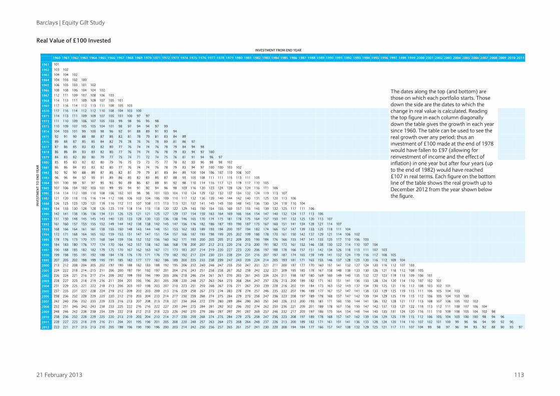
Barclays | Equity Gilt Study

21 February 2013 113

Real Value of £100 Invested IN

VES

TMEN

T TO

EN

D Y

EAR

INVESTMENT FROM END YEAR

1960 1961 1962 1963 1964 1965 1966 1967 1968 1969 1970 1971 1972 1973 1974 1975 1976 1977 1978 1979 1980 1981 1982 1983 1984 1985 1986 1987 1988 1989 1990 1991 1992 1993 1994 1995 1996 1997 1998 1999 2000 2001 2002 2003 2004 2005 2006 2007 2008 2009 2010 2011

1961 101

1962 103 102

1963 104 104 102

1964 104 103 102 100

1965 106 105 103 101 102

1966 108 108 106 104 104 102 The dates along the top (and bottom) are those on which each portfolio starts. Those down the side are the dates to which the change in real value is calculated. Reading the top figure in each column diagonally down the table gives the growth in each year since 1960. The table can be used to see the real growth over any period; thus an investment of £100 made at the end of 1978 would have fallen to £97 (allowing for reinvestment of income and the effect of inflation) in one year but after four years (up to the end of 1982) would have reached £107 in real terms. Each figure on the bottom line of the table shows the real growth up to December 2012 from the year shown below the figure.

1967 112 111 109 107 108 106 103

1968 114 113 111 109 109 107 105 101

1969 117 116 114 112 113 111 108 105 103

1970 117 116 114 112 112 110 108 104 103 100

1971 114 113 111 109 109 107 105 101 100 97 97

1972 111 110 109 106 107 105 103 99 98 95 95 98

1973 110 109 107 105 105 104 101 98 97 94 94 97 99

1974 104 103 101 99 100 98 96 92 91 88 89 91 93 94

1975 92 91 90 88 88 87 85 82 81 78 79 81 83 84 89

1976 89 88 87 85 85 84 82 79 78 76 76 78 80 81 86 97

1977 87 86 85 83 83 82 80 77 76 74 74 76 78 79 84 94 98

1978 86 86 84 83 83 82 80 77 76 74 74 76 78 79 83 94 97 100

1979 84 83 82 80 80 79 77 75 74 71 72 74 75 76 81 91 94 96 97

1980 85 85 83 82 82 80 79 76 75 73 73 75 77 78 82 93 96 98 98 102

1981 86 86 84 83 83 82 80 77 76 74 74 76 78 79 83 94 97 100 100 103 102

1982 92 92 90 88 89 87 85 82 81 79 79 81 83 84 89 100 104 106 107 110 108 107

1983 96 96 94 92 93 91 89 86 85 82 83 85 87 88 93 105 108 111 111 115 113 111 105

1984 101 100 99 97 97 95 93 90 89 86 87 89 91 92 98 110 114 116 117 121 119 117 110 105

1985 107 106 104 102 103 101 99 95 94 91 92 94 96 98 103 116 120 123 124 128 126 124 116 111 106

1986 114 114 112 109 110 108 106 102 101 98 98 101 103 104 110 124 129 132 132 137 134 132 124 119 113 107

1987 121 120 118 116 116 114 112 108 106 103 104 106 109 110 117 132 136 139 140 144 142 140 131 125 120 113 106

1988 126 125 123 120 121 119 116 112 111 107 108 111 113 115 121 137 141 145 145 150 148 145 136 130 124 118 110 104

1989 134 133 130 128 128 126 123 119 118 114 115 118 120 122 129 145 150 154 155 160 157 155 145 139 132 125 117 111 106

1990 142 141 138 136 136 134 131 126 125 121 121 125 127 129 137 154 159 163 164 169 166 164 154 147 140 132 124 117 113 106

1991 151 150 148 145 145 143 140 135 133 129 130 133 136 138 146 165 170 174 175 181 178 175 164 157 150 141 132 125 120 113 107

1992 161 160 157 155 155 152 149 144 142 138 138 142 145 147 156 176 182 186 187 193 190 187 175 167 160 151 141 134 128 121 114 107

1993 168 166 164 161 161 158 155 150 148 143 144 148 151 153 162 183 189 193 194 200 197 194 182 174 166 157 147 139 133 125 118 111 104

1994 172 171 168 164 165 162 159 153 151 147 147 151 154 157 166 187 193 198 199 205 202 199 186 178 170 161 150 142 137 129 121 114 106 102

1995 178 176 173 170 171 168 164 159 156 152 152 156 160 162 171 193 200 205 205 212 209 205 193 184 176 166 155 147 141 133 125 117 110 106 103

1996 184 183 180 176 177 174 170 164 162 157 158 162 166 168 178 200 207 212 213 220 216 213 200 191 182 172 161 152 146 138 130 122 114 110 107 104

1997 190 188 185 182 182 179 175 170 167 162 163 167 171 173 183 207 214 219 220 227 223 220 206 197 188 178 166 157 151 142 134 126 118 113 111 107 103

1998 199 198 195 191 192 188 184 178 176 170 171 176 179 182 192 217 224 230 231 238 234 231 216 207 197 187 174 165 159 149 141 132 124 119 116 112 108 105

1999 207 205 202 198 199 195 191 185 182 177 177 182 186 189 200 225 233 238 239 247 243 239 224 214 205 193 181 171 165 155 146 137 128 123 120 116 112 109 104

2000 213 212 208 204 205 202 197 190 188 182 183 188 192 195 206 232 240 246 247 255 250 247 231 221 211 200 187 177 170 160 151 141 132 127 124 120 116 112 107 103

2001 224 222 218 214 215 211 206 200 197 191 192 197 201 204 216 243 251 258 258 267 262 258 242 232 221 209 195 185 178 167 158 148 138 133 130 126 121 118 112 108 105

2002 226 224 221 216 217 214 209 202 199 193 194 199 203 206 218 246 254 261 261 270 265 261 245 234 224 211 198 187 180 169 160 149 140 135 132 127 123 119 113 109 106 101

2003 228 227 223 218 219 216 211 204 201 195 196 201 205 208 220 248 257 263 264 273 268 264 247 237 226 213 200 189 182 171 161 151 141 136 133 128 124 120 114 110 107 102 101

2004 231 229 225 221 222 218 213 206 203 197 198 203 207 210 223 251 259 266 267 276 271 267 250 239 228 216 202 191 184 173 163 152 143 137 134 130 125 121 116 112 108 103 102 101

2005 237 235 231 227 228 224 219 212 209 202 203 209 213 216 229 258 267 273 274 283 278 274 257 246 235 222 207 196 189 177 167 157 147 141 138 133 129 125 119 115 111 106 105 104 103

2006 238 236 232 228 229 225 220 212 210 203 204 210 214 217 230 259 268 274 275 284 279 275 258 247 236 223 208 197 189 178 168 157 147 142 139 134 129 125 119 115 112 106 105 104 103 100

2007 242 240 236 232 233 229 223 216 213 207 208 213 218 221 234 264 272 279 280 289 284 280 263 251 240 226 212 200 193 181 171 160 150 144 141 136 132 128 121 117 113 108 107 106 105 102 102

2008 252 251 246 242 243 238 233 225 222 216 216 222 227 230 244 275 284 291 292 302 296 292 274 262 250 236 221 209 201 189 178 167 156 150 147 142 137 133 127 122 118 113 112 111 109 107 106 104

2009 248 246 242 238 238 234 229 222 218 212 213 218 223 226 240 270 279 286 287 297 291 287 269 257 246 232 217 205 197 186 175 164 154 148 144 140 135 131 124 120 116 111 110 109 108 105 104 102 98

2010 238 236 232 228 229 225 220 213 210 203 204 210 214 217 230 259 268 274 275 284 279 275 258 247 236 223 208 197 189 178 168 157 147 142 139 134 129 125 119 115 112 106 105 104 103 100 100 98 94 96

2011 228 227 223 218 219 216 211 204 201 195 196 201 205 208 220 248 257 263 264 273 268 264 248 237 226 213 200 189 182 171 161 151 141 136 133 128 124 120 114 110 107 102 101 100 99 96 96 94 90 92 96 2012 222 221 217 213 213 210 205 198 196 190 190 196 200 203 214 242 250 256 257 265 261 257 241 230 220 208 194 184 177 166 157 147 138 132 129 125 121 117 111 107 104 99 98 97 96 94 93 92 88 90 93 97

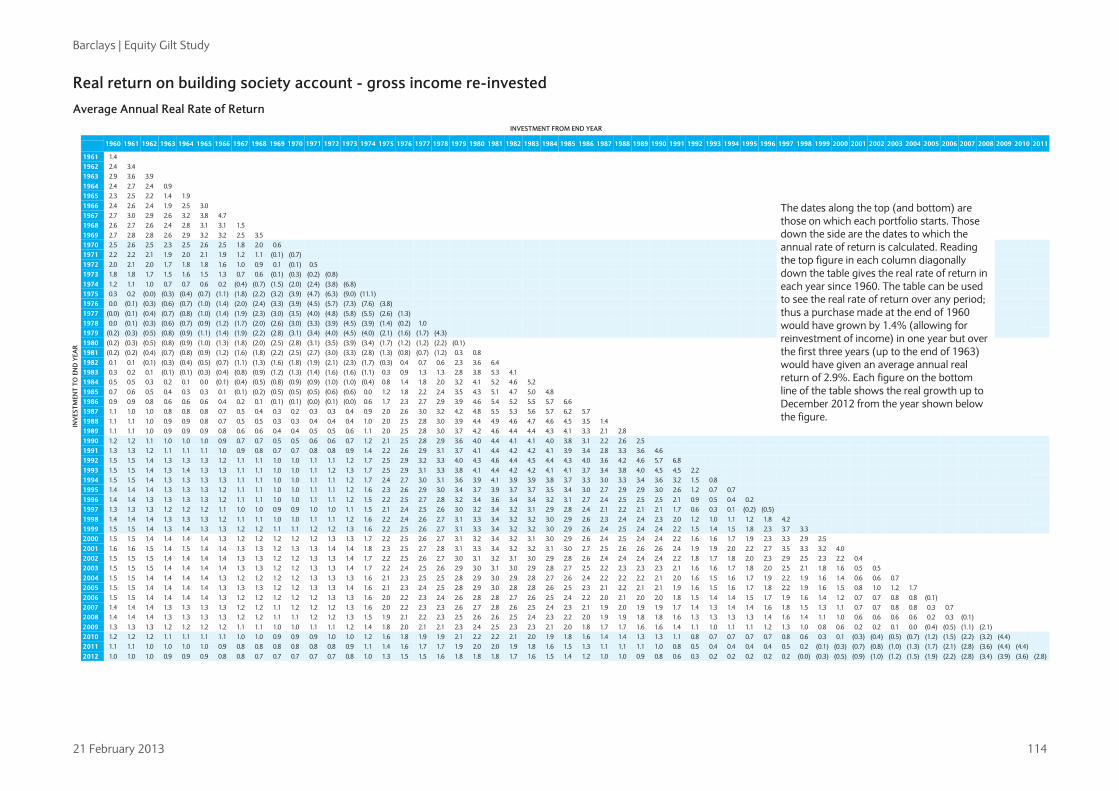
Barclays | Equity Gilt Study

21 February 2013 114

Real return on building society account - gross income re-invested Average Annual Real Rate of Return

INV

ESTM

ENT

TO E

ND

YEA

R

INVESTMENT FROM END YEAR

1960 1961 1962 1963 1964 1965 1966 1967 1968 1969 1970 1971 1972 1973 1974 1975 1976 1977 1978 1979 1980 1981 1982 1983 1984 1985 1986 1987 1988 1989 1990 1991 1992 1993 1994 1995 1996 1997 1998 1999 2000 2001 2002 2003 2004 2005 2006 2007 2008 2009 2010 2011

1961 1.4 1962 2.4 3.4 1963 2.9 3.6 3.9 1964 2.4 2.7 2.4 0.9 1965 2.3 2.5 2.2 1.4 1.9 1966 2.4 2.6 2.4 1.9 2.5 3.0 The dates along the top (and bottom) are

those on which each portfolio starts. Those down the side are the dates to which the annual rate of return is calculated. Reading the top figure in each column diagonally down the table gives the real rate of return in each year since 1960. The table can be used to see the real rate of return over any period; thus a purchase made at the end of 1960 would have grown by 1.4% (allowing for reinvestment of income) in one year but over the first three years (up to the end of 1963) would have given an average annual real return of 2.9%. Each figure on the bottom line of the table shows the real growth up to December 2012 from the year shown below the figure.

1967 2.7 3.0 2.9 2.6 3.2 3.8 4.7 1968 2.6 2.7 2.6 2.4 2.8 3.1 3.1 1.5 1969 2.7 2.8 2.8 2.6 2.9 3.2 3.2 2.5 3.5 1970 2.5 2.6 2.5 2.3 2.5 2.6 2.5 1.8 2.0 0.6 1971 2.2 2.2 2.1 1.9 2.0 2.1 1.9 1.2 1.1 (0.1) (0.7) 1972 2.0 2.1 2.0 1.7 1.8 1.8 1.6 1.0 0.9 0.1 (0.1) 0.5 1973 1.8 1.8 1.7 1.5 1.6 1.5 1.3 0.7 0.6 (0.1) (0.3) (0.2) (0.8) 1974 1.2 1.1 1.0 0.7 0.7 0.6 0.2 (0.4) (0.7) (1.5) (2.0) (2.4) (3.8) (6.8) 1975 0.3 0.2 (0.0) (0.3) (0.4) (0.7) (1.1) (1.8) (2.2) (3.2) (3.9) (4.7) (6.3) (9.0) (11.1) 1976 0.0 (0.1) (0.3) (0.6) (0.7) (1.0) (1.4) (2.0) (2.4) (3.3) (3.9) (4.5) (5.7) (7.3) (7.6) (3.8) 1977 (0.0) (0.1) (0.4) (0.7) (0.8) (1.0) (1.4) (1.9) (2.3) (3.0) (3.5) (4.0) (4.8) (5.8) (5.5) (2.6) (1.3) 1978 0.0 (0.1) (0.3) (0.6) (0.7) (0.9) (1.2) (1.7) (2.0) (2.6) (3.0) (3.3) (3.9) (4.5) (3.9) (1.4) (0.2) 1.0 1979 (0.2) (0.3) (0.5) (0.8) (0.9) (1.1) (1.4) (1.9) (2.2) (2.8) (3.1) (3.4) (4.0) (4.5) (4.0) (2.1) (1.6) (1.7) (4.3) 1980 (0.2) (0.3) (0.5) (0.8) (0.9) (1.0) (1.3) (1.8) (2.0) (2.5) (2.8) (3.1) (3.5) (3.9) (3.4) (1.7) (1.2) (1.2) (2.2) (0.1) 1981 (0.2) (0.2) (0.4) (0.7) (0.8) (0.9) (1.2) (1.6) (1.8) (2.2) (2.5) (2.7) (3.0) (3.3) (2.8) (1.3) (0.8) (0.7) (1.2) 0.3 0.8 1982 0.1 0.1 (0.1) (0.3) (0.4) (0.5) (0.7) (1.1) (1.3) (1.6) (1.8) (1.9) (2.1) (2.3) (1.7) (0.3) 0.4 0.7 0.6 2.3 3.6 6.4 1983 0.3 0.2 0.1 (0.1) (0.1) (0.3) (0.4) (0.8) (0.9) (1.2) (1.3) (1.4) (1.6) (1.6) (1.1) 0.3 0.9 1.3 1.3 2.8 3.8 5.3 4.1 1984 0.5 0.5 0.3 0.2 0.1 0.0 (0.1) (0.4) (0.5) (0.8) (0.9) (0.9) (1.0) (1.0) (0.4) 0.8 1.4 1.8 2.0 3.2 4.1 5.2 4.6 5.2 1985 0.7 0.6 0.5 0.4 0.3 0.3 0.1 (0.1) (0.2) (0.5) (0.5) (0.5) (0.6) (0.6) 0.0 1.2 1.8 2.2 2.4 3.5 4.3 5.1 4.7 5.0 4.8 1986 0.9 0.9 0.8 0.6 0.6 0.6 0.4 0.2 0.1 (0.1) (0.1) (0.0) (0.1) (0.0) 0.6 1.7 2.3 2.7 2.9 3.9 4.6 5.4 5.2 5.5 5.7 6.6 1987 1.1 1.0 1.0 0.8 0.8 0.8 0.7 0.5 0.4 0.3 0.2 0.3 0.3 0.4 0.9 2.0 2.6 3.0 3.2 4.2 4.8 5.5 5.3 5.6 5.7 6.2 5.7 1988 1.1 1.1 1.0 0.9 0.9 0.8 0.7 0.5 0.5 0.3 0.3 0.4 0.4 0.4 1.0 2.0 2.5 2.8 3.0 3.9 4.4 4.9 4.6 4.7 4.6 4.5 3.5 1.4 1989 1.1 1.1 1.0 0.9 0.9 0.9 0.8 0.6 0.6 0.4 0.4 0.5 0.5 0.6 1.1 2.0 2.5 2.8 3.0 3.7 4.2 4.6 4.4 4.4 4.3 4.1 3.3 2.1 2.8 1990 1.2 1.2 1.1 1.0 1.0 1.0 0.9 0.7 0.7 0.5 0.5 0.6 0.6 0.7 1.2 2.1 2.5 2.8 2.9 3.6 4.0 4.4 4.1 4.1 4.0 3.8 3.1 2.2 2.6 2.5 1991 1.3 1.3 1.2 1.1 1.1 1.1 1.0 0.9 0.8 0.7 0.7 0.8 0.8 0.9 1.4 2.2 2.6 2.9 3.1 3.7 4.1 4.4 4.2 4.2 4.1 3.9 3.4 2.8 3.3 3.6 4.6 1992 1.5 1.5 1.4 1.3 1.3 1.3 1.2 1.1 1.1 1.0 1.0 1.1 1.1 1.2 1.7 2.5 2.9 3.2 3.3 4.0 4.3 4.6 4.4 4.5 4.4 4.3 4.0 3.6 4.2 4.6 5.7 6.8 1993 1.5 1.5 1.4 1.3 1.4 1.3 1.3 1.1 1.1 1.0 1.0 1.1 1.2 1.3 1.7 2.5 2.9 3.1 3.3 3.8 4.1 4.4 4.2 4.2 4.1 4.1 3.7 3.4 3.8 4.0 4.5 4.5 2.2 1994 1.5 1.5 1.4 1.3 1.3 1.3 1.3 1.1 1.1 1.0 1.0 1.1 1.1 1.2 1.7 2.4 2.7 3.0 3.1 3.6 3.9 4.1 3.9 3.9 3.8 3.7 3.3 3.0 3.3 3.4 3.6 3.2 1.5 0.8 1995 1.4 1.4 1.4 1.3 1.3 1.3 1.2 1.1 1.1 1.0 1.0 1.1 1.1 1.2 1.6 2.3 2.6 2.9 3.0 3.4 3.7 3.9 3.7 3.7 3.5 3.4 3.0 2.7 2.9 2.9 3.0 2.6 1.2 0.7 0.7 1996 1.4 1.4 1.3 1.3 1.3 1.3 1.2 1.1 1.1 1.0 1.0 1.1 1.1 1.2 1.5 2.2 2.5 2.7 2.8 3.2 3.4 3.6 3.4 3.4 3.2 3.1 2.7 2.4 2.5 2.5 2.5 2.1 0.9 0.5 0.4 0.2 1997 1.3 1.3 1.3 1.2 1.2 1.2 1.1 1.0 1.0 0.9 0.9 1.0 1.0 1.1 1.5 2.1 2.4 2.5 2.6 3.0 3.2 3.4 3.2 3.1 2.9 2.8 2.4 2.1 2.2 2.1 2.1 1.7 0.6 0.3 0.1 (0.2) (0.5) 1998 1.4 1.4 1.4 1.3 1.3 1.3 1.2 1.1 1.1 1.0 1.0 1.1 1.1 1.2 1.6 2.2 2.4 2.6 2.7 3.1 3.3 3.4 3.2 3.2 3.0 2.9 2.6 2.3 2.4 2.4 2.3 2.0 1.2 1.0 1.1 1.2 1.8 4.2 1999 1.5 1.5 1.4 1.3 1.4 1.3 1.3 1.2 1.2 1.1 1.1 1.2 1.2 1.3 1.6 2.2 2.5 2.6 2.7 3.1 3.3 3.4 3.2 3.2 3.0 2.9 2.6 2.4 2.5 2.4 2.4 2.2 1.5 1.4 1.5 1.8 2.3 3.7 3.3 2000 1.5 1.5 1.4 1.4 1.4 1.4 1.3 1.2 1.2 1.2 1.2 1.2 1.3 1.3 1.7 2.2 2.5 2.6 2.7 3.1 3.2 3.4 3.2 3.1 3.0 2.9 2.6 2.4 2.5 2.4 2.4 2.2 1.6 1.6 1.7 1.9 2.3 3.3 2.9 2.5 2001 1.6 1.6 1.5 1.4 1.5 1.4 1.4 1.3 1.3 1.2 1.3 1.3 1.4 1.4 1.8 2.3 2.5 2.7 2.8 3.1 3.3 3.4 3.2 3.2 3.1 3.0 2.7 2.5 2.6 2.6 2.6 2.4 1.9 1.9 2.0 2.2 2.7 3.5 3.3 3.2 4.0 2002 1.5 1.5 1.5 1.4 1.4 1.4 1.4 1.3 1.3 1.2 1.2 1.3 1.3 1.4 1.7 2.2 2.5 2.6 2.7 3.0 3.1 3.2 3.1 3.0 2.9 2.8 2.6 2.4 2.4 2.4 2.4 2.2 1.8 1.7 1.8 2.0 2.3 2.9 2.5 2.3 2.2 0.4 2003 1.5 1.5 1.5 1.4 1.4 1.4 1.4 1.3 1.3 1.2 1.2 1.3 1.3 1.4 1.7 2.2 2.4 2.5 2.6 2.9 3.0 3.1 3.0 2.9 2.8 2.7 2.5 2.2 2.3 2.3 2.3 2.1 1.6 1.6 1.7 1.8 2.0 2.5 2.1 1.8 1.6 0.5 0.5 2004 1.5 1.5 1.4 1.4 1.4 1.4 1.3 1.2 1.2 1.2 1.2 1.3 1.3 1.3 1.6 2.1 2.3 2.5 2.5 2.8 2.9 3.0 2.9 2.8 2.7 2.6 2.4 2.2 2.2 2.2 2.1 2.0 1.6 1.5 1.6 1.7 1.9 2.2 1.9 1.6 1.4 0.6 0.6 0.7 2005 1.5 1.5 1.4 1.4 1.4 1.4 1.3 1.3 1.3 1.2 1.2 1.3 1.3 1.4 1.6 2.1 2.3 2.4 2.5 2.8 2.9 3.0 2.8 2.8 2.6 2.5 2.3 2.1 2.2 2.1 2.1 1.9 1.6 1.5 1.6 1.7 1.8 2.2 1.9 1.6 1.5 0.8 1.0 1.2 1.7 2006 1.5 1.5 1.4 1.4 1.4 1.4 1.3 1.2 1.2 1.2 1.2 1.2 1.3 1.3 1.6 2.0 2.2 2.3 2.4 2.6 2.8 2.8 2.7 2.6 2.5 2.4 2.2 2.0 2.1 2.0 2.0 1.8 1.5 1.4 1.4 1.5 1.7 1.9 1.6 1.4 1.2 0.7 0.7 0.8 0.8 (0.1) 2007 1.4 1.4 1.4 1.3 1.3 1.3 1.3 1.2 1.2 1.1 1.2 1.2 1.2 1.3 1.6 2.0 2.2 2.3 2.3 2.6 2.7 2.8 2.6 2.5 2.4 2.3 2.1 1.9 2.0 1.9 1.9 1.7 1.4 1.3 1.4 1.4 1.6 1.8 1.5 1.3 1.1 0.7 0.7 0.8 0.8 0.3 0.7 2008 1.4 1.4 1.4 1.3 1.3 1.3 1.3 1.2 1.2 1.1 1.1 1.2 1.2 1.3 1.5 1.9 2.1 2.2 2.3 2.5 2.6 2.6 2.5 2.4 2.3 2.2 2.0 1.9 1.9 1.8 1.8 1.6 1.3 1.3 1.3 1.3 1.4 1.6 1.4 1.1 1.0 0.6 0.6 0.6 0.6 0.2 0.3 (0.1) 2009 1.3 1.3 1.3 1.2 1.2 1.2 1.2 1.1 1.1 1.0 1.0 1.1 1.1 1.2 1.4 1.8 2.0 2.1 2.1 2.3 2.4 2.5 2.3 2.3 2.1 2.0 1.8 1.7 1.7 1.6 1.6 1.4 1.1 1.0 1.1 1.1 1.2 1.3 1.0 0.8 0.6 0.2 0.2 0.1 0.0 (0.4) (0.5) (1.1) (2.1) 2010 1.2 1.2 1.2 1.1 1.1 1.1 1.1 1.0 1.0 0.9 0.9 0.9 1.0 1.0 1.2 1.6 1.8 1.9 1.9 2.1 2.2 2.2 2.1 2.0 1.9 1.8 1.6 1.4 1.4 1.3 1.3 1.1 0.8 0.7 0.7 0.7 0.7 0.8 0.6 0.3 0.1 (0.3) (0.4) (0.5) (0.7) (1.2) (1.5) (2.2) (3.2) (4.4) 2011 1.1 1.1 1.0 1.0 1.0 1.0 0.9 0.8 0.8 0.8 0.8 0.8 0.8 0.9 1.1 1.4 1.6 1.7 1.7 1.9 2.0 2.0 1.9 1.8 1.6 1.5 1.3 1.1 1.1 1.1 1.0 0.8 0.5 0.4 0.4 0.4 0.4 0.5 0.2 (0.1) (0.3) (0.7) (0.8) (1.0) (1.3) (1.7) (2.1) (2.8) (3.6) (4.4) (4.4)

2012 1.0 1.0 1.0 0.9 0.9 0.9 0.8 0.8 0.7 0.7 0.7 0.7 0.7 0.8 1.0 1.3 1.5 1.5 1.6 1.8 1.8 1.8 1.7 1.6 1.5 1.4 1.2 1.0 1.0 0.9 0.8 0.6 0.3 0.2 0.2 0.2 0.2 0.2 (0.0) (0.3) (0.5) (0.9) (1.0) (1.2) (1.5) (1.9) (2.2) (2.8) (3.4) (3.9) (3.6) (2.8)

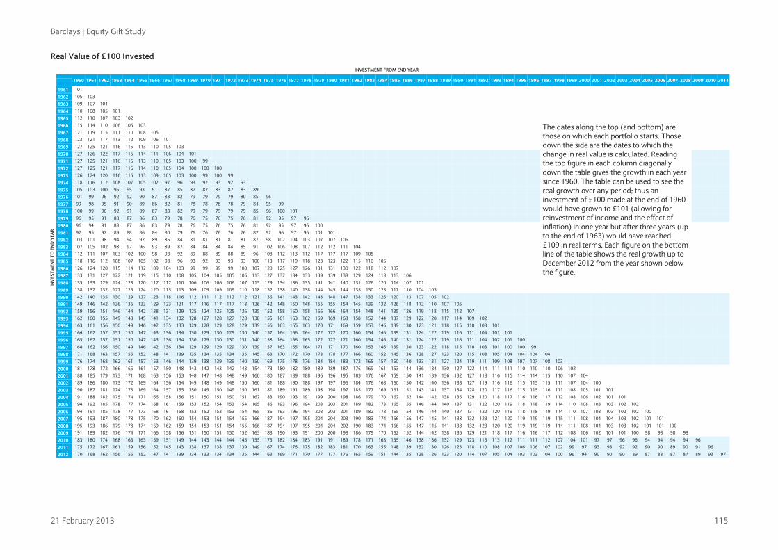
Barclays | Equity Gilt Study

21 February 2013 115

Real Value of £100 Invested IN

VES

TMEN

T TO

EN

D Y

EAR

INVESTMENT FROM END YEAR

1960 1961 1962 1963 1964 1965 1966 1967 1968 1969 1970 1971 1972 1973 1974 1975 1976 1977 1978 1979 1980 1981 1982 1983 1984 1985 1986 1987 1988 1989 1990 1991 1992 1993 1994 1995 1996 1997 1998 1999 2000 2001 2002 2003 2004 2005 2006 2007 2008 2009 2010 2011

1961 101

1962 105 103

1963 109 107 104

1964 110 108 105 101

1965 112 110 107 103 102

1966 115 114 110 106 105 103 The dates along the top (and bottom) are those on which each portfolio starts. Those down the side are the dates to which the change in real value is calculated. Reading the top figure in each column diagonally down the table gives the growth in each year since 1960. The table can be used to see the real growth over any period; thus an investment of £100 made at the end of 1960 would have grown to £101 (allowing for reinvestment of income and the effect of inflation) in one year but after three years (up to the end of 1963) would have reached £109 in real terms. Each figure on the bottom line of the table shows the real growth up to December 2012 from the year shown below the figure.

1967 121 119 115 111 110 108 105

1968 123 121 117 113 112 109 106 101

1969 127 125 121 116 115 113 110 105 103

1970 127 126 122 117 116 114 111 106 104 101

1971 127 125 121 116 115 113 110 105 103 100 99

1972 127 125 121 117 116 114 110 105 104 100 100 100

1973 126 124 120 116 115 113 109 105 103 100 99 100 99

1974 118 116 112 108 107 105 102 97 96 93 92 93 92 93

1975 105 103 100 96 95 93 91 87 85 82 82 83 82 83 89

1976 101 99 96 92 92 90 87 83 82 79 79 79 79 80 85 96

1977 99 98 95 91 90 89 86 82 81 78 78 78 78 79 84 95 99

1978 100 99 96 92 91 89 87 83 82 79 79 79 79 79 85 96 100 101

1979 96 95 91 88 87 86 83 79 78 76 75 76 75 76 81 92 95 97 96

1980 96 94 91 88 87 86 83 79 78 76 75 76 75 76 81 92 95 97 96 100

1981 97 95 92 89 88 86 84 80 79 76 76 76 76 76 82 92 96 97 96 101 101

1982 103 101 98 94 94 92 89 85 84 81 81 81 81 81 87 98 102 104 103 107 107 106

1983 107 105 102 98 97 96 93 89 87 84 84 84 84 85 91 102 106 108 107 112 112 111 104

1984 112 111 107 103 102 100 98 93 92 89 88 89 88 89 96 108 112 113 112 117 117 117 109 105

1985 118 116 112 108 107 105 102 98 96 93 92 93 93 93 100 113 117 119 118 123 123 122 115 110 105

1986 126 124 120 115 114 112 109 104 103 99 99 99 99 100 107 120 125 127 126 131 131 130 122 118 112 107

1987 133 131 127 122 121 119 115 110 108 105 104 105 105 105 113 127 132 134 133 139 139 138 129 124 118 113 106

1988 135 133 129 124 123 120 117 112 110 106 106 106 106 107 115 129 134 136 135 141 141 140 131 126 120 114 107 101

1989 138 137 132 127 126 124 120 115 113 109 109 109 109 110 118 132 138 140 138 144 145 144 135 130 123 117 110 104 103

1990 142 140 135 130 129 127 123 118 116 112 111 112 112 112 121 136 141 143 142 148 148 147 138 133 126 120 113 107 105 102

1991 149 146 142 136 135 133 129 123 121 117 116 117 117 118 126 142 148 150 148 155 155 154 145 139 132 126 118 112 110 107 105

1992 159 156 151 146 144 142 138 131 129 125 124 125 125 126 135 152 158 160 158 166 166 164 154 148 141 135 126 119 118 115 112 107

1993 162 160 155 149 148 145 141 134 132 128 127 128 127 128 138 155 161 163 162 169 169 168 158 152 144 137 129 122 120 117 114 109 102

1994 163 161 156 150 149 146 142 135 133 129 128 129 128 129 139 156 163 165 163 170 171 169 159 153 145 139 130 123 121 118 115 110 103 101

1995 164 162 157 151 150 147 143 136 134 130 129 130 129 130 140 157 164 166 164 172 172 170 160 154 146 139 131 124 122 119 116 111 104 101 101

1996 165 162 157 151 150 147 143 136 134 130 129 130 130 131 140 158 164 166 165 172 172 171 160 154 146 140 131 124 122 119 116 111 104 102 101 100

1997 164 162 156 150 149 146 142 136 134 129 129 129 129 130 139 157 163 165 164 171 171 170 160 153 146 139 130 123 122 118 115 110 103 101 100 100 99

1998 171 168 163 157 155 152 148 141 139 135 134 135 134 135 145 163 170 172 170 178 178 177 166 160 152 145 136 128 127 123 120 115 108 105 104 104 104 104

1999 176 174 168 162 161 157 153 146 144 139 138 139 139 140 150 169 175 178 176 184 184 183 172 165 157 150 140 133 131 127 124 119 111 109 108 107 107 108 103

2000 181 178 172 166 165 161 157 150 148 143 142 143 142 143 154 173 180 182 180 189 189 187 176 169 161 153 144 136 134 130 127 122 114 111 111 110 110 110 106 102

2001 188 185 179 173 171 168 163 156 153 148 147 148 148 149 160 180 187 189 188 196 196 195 183 176 167 159 150 141 139 136 132 127 118 116 115 114 114 115 110 107 104

2002 189 186 180 173 172 169 164 156 154 149 148 149 148 150 160 181 188 190 188 197 197 196 184 176 168 160 150 142 140 136 133 127 119 116 116 115 115 115 111 107 104 100

2003 190 187 181 174 173 169 164 157 155 150 149 150 149 150 161 181 189 191 189 198 198 197 185 177 169 161 151 143 141 137 134 128 120 117 116 115 115 116 111 108 105 101 101

2004 191 188 182 175 174 171 166 158 156 151 150 151 150 151 162 183 190 193 191 199 200 198 186 179 170 162 152 144 142 138 135 129 120 118 117 116 116 117 112 108 106 102 101 101

2005 194 192 185 178 177 174 168 161 159 153 152 154 153 154 165 186 193 196 194 203 203 201 189 182 173 165 155 146 144 140 137 131 122 120 119 118 118 119 114 110 108 103 103 102 102

2006 194 191 185 178 177 173 168 161 158 153 152 153 153 154 165 186 193 196 194 203 203 201 189 182 173 165 154 146 144 140 137 131 122 120 119 118 118 119 114 110 107 103 103 102 102 100

2007 195 193 187 180 178 175 170 162 160 154 153 154 154 155 166 187 194 197 195 204 204 203 190 183 174 166 156 147 145 141 138 132 123 121 120 119 119 119 115 111 108 104 104 103 102 101 101

2008 195 193 186 179 178 174 169 162 159 154 153 154 154 155 166 187 194 197 195 204 204 202 190 183 174 166 155 147 145 141 138 132 123 120 120 119 119 119 114 111 108 104 103 103 102 101 101 100

2009 191 189 182 176 174 171 166 158 156 151 150 151 150 152 163 183 190 193 191 200 200 198 186 179 170 162 152 144 142 138 135 129 121 118 117 116 116 117 112 108 106 102 101 101 100 98 98 98 98

2010 183 180 174 168 166 163 159 151 149 144 143 144 144 145 155 175 182 184 183 191 191 189 178 171 163 155 146 138 136 132 129 123 115 113 112 111 111 112 107 104 101 97 97 96 96 94 94 94 94 96

2011 175 172 167 161 159 156 152 145 143 138 137 138 137 139 149 167 174 176 175 182 183 181 170 163 155 148 139 132 130 126 123 118 110 108 107 106 106 107 102 99 97 93 93 92 92 90 90 89 90 91 96 2012 170 168 162 156 155 152 147 141 139 134 133 134 134 135 144 163 169 171 170 177 177 176 165 159 151 144 135 128 126 123 120 114 107 105 104 103 103 104 100 96 94 90 90 90 89 87 88 87 87 89 93 97

Barclays | Equity Gilt Study

21 February 2013 116

Real return on index-linked gilts Average Annual Real Rate of Return

GROSS INCOME RE-INVESTED

INV

ESTM

ENT

TO E

ND

YEA

R

1982 1983 1984 1985 1986 1987 1988 1989 1990 1991 1992 1993 1994 1995 1996 1997 1998 1999 2000 2001 2002 2003 2004 2005 2006 2007 2008 2009 2010 2011

1983 (4.3)

1984 (1.2) 1.9

1985 (2.7) (1.9) (5.5)

1986 (1.5) (0.5) (1.7) 2.3

1987 (0.6) 0.4 (0.1) 2.7 3.1

1988 0.6 1.6 1.5 3.9 4.8 6.5

1989 1.4 2.3 2.4 4.5 5.3 6.4 6.3

1990 0.6 1.3 1.2 2.7 2.7 2.6 0.8 (4.5)

1991 0.6 1.3 1.2 2.3 2.3 2.2 0.7 (1.9) 0.7

1992 1.9 2.6 2.7 3.9 4.2 4.4 3.9 3.2 7.2 14.1

1993 3.3 4.1 4.4 5.7 6.2 6.7 6.8 6.9 11.0 16.5 18.9

1994 2.1 2.7 2.8 3.8 3.9 4.1 3.7 3.1 5.2 6.7 3.1 (10.5)

1995 2.6 3.2 3.3 4.2 4.4 4.6 4.3 4.0 5.8 7.1 4.9 (1.5) 8.5

1996 2.7 3.2 3.3 4.2 4.4 4.5 4.3 4.0 5.5 6.5 4.6 0.3 6.2 4.0

1997 3.1 3.7 3.8 4.6 4.8 5.0 4.8 4.7 6.0 7.0 5.6 2.5 7.3 6.7 9.4

1998 3.9 4.5 4.7 5.5 5.8 6.1 6.0 6.0 7.4 8.3 7.4 5.3 9.6 10.0 13.2 17.1

1999 3.9 4.4 4.6 5.4 5.6 5.8 5.7 5.7 6.9 7.7 6.8 4.9 8.3 8.3 9.7 9.9 3.2

2000 3.7 4.2 4.3 5.0 5.2 5.4 5.3 5.2 6.2 6.8 5.9 4.2 6.9 6.6 7.2 6.5 1.6 0.1

2001 3.4 3.8 4.0 4.6 4.7 4.8 4.7 4.6 5.5 5.9 5.1 3.5 5.6 5.2 5.4 4.4 0.5 (0.7) (1.6)

2002 3.5 3.9 4.0 4.6 4.7 4.9 4.7 4.6 5.4 5.9 5.1 3.6 5.6 5.2 5.4 4.6 1.7 1.2 1.7 5.1

2003 3.5 3.9 4.0 4.6 4.7 4.8 4.7 4.6 5.3 5.7 5.0 3.7 5.4 5.0 5.1 4.4 2.1 1.8 2.4 4.5 3.9

2004 3.6 4.0 4.1 4.6 4.7 4.8 4.7 4.6 5.3 5.6 5.0 3.8 5.3 5.0 5.1 4.5 2.6 2.4 3.0 4.6 4.4 4.9

2005 3.7 4.1 4.2 4.7 4.8 4.9 4.8 4.7 5.4 5.7 5.1 4.0 5.5 5.2 5.3 4.8 3.2 3.2 3.8 5.2 5.2 5.8 6.7

2006 3.5 3.8 3.9 4.4 4.5 4.5 4.4 4.3 4.9 5.2 4.6 3.5 4.8 4.5 4.5 4.0 2.5 2.4 2.8 3.7 3.3 3.1 2.2 (2.1)

2007 3.4 3.7 3.8 4.2 4.3 4.4 4.3 4.2 4.7 4.9 4.4 3.4 4.5 4.2 4.3 3.7 2.4 2.3 2.6 3.3 2.9 2.7 2.0 (0.3) 1.4

2008 3.2 3.5 3.5 3.9 4.0 4.1 3.9 3.8 4.3 4.5 3.9 3.0 4.1 3.7 3.7 3.2 1.9 1.8 2.0 2.5 2.1 1.7 0.9 (0.9) (0.4) (2.1)

2009 3.2 3.4 3.5 3.9 4.0 4.0 3.9 3.8 4.2 4.4 3.9 3.0 4.0 3.7 3.7 3.2 2.0 1.9 2.1 2.6 2.2 2.0 1.4 0.1 0.8 0.5 3.1

2010 3.2 3.5 3.6 4.0 4.0 4.1 4.0 3.9 4.3 4.5 4.0 3.2 4.1 3.8 3.8 3.4 2.3 2.2 2.4 2.9 2.6 2.4 2.0 1.1 1.9 2.1 4.2 5.3

2011 3.6 3.9 4.0 4.3 4.4 4.5 4.4 4.3 4.8 5.0 4.5 3.8 4.7 4.4 4.5 4.1 3.2 3.2 3.5 4.0 3.9 3.9 3.7 3.2 4.3 5.0 7.5 9.8 14.4 2012 3.5 3.8 3.8 4.2 4.3 4.3 4.2 4.1 4.5 4.7 4.3 3.6 4.4 4.2 4.2 3.8 3.0 2.9 3.2 3.6 3.5 3.4 3.3 2.8 3.6 4.0 5.6 6.5 7.1 0.2

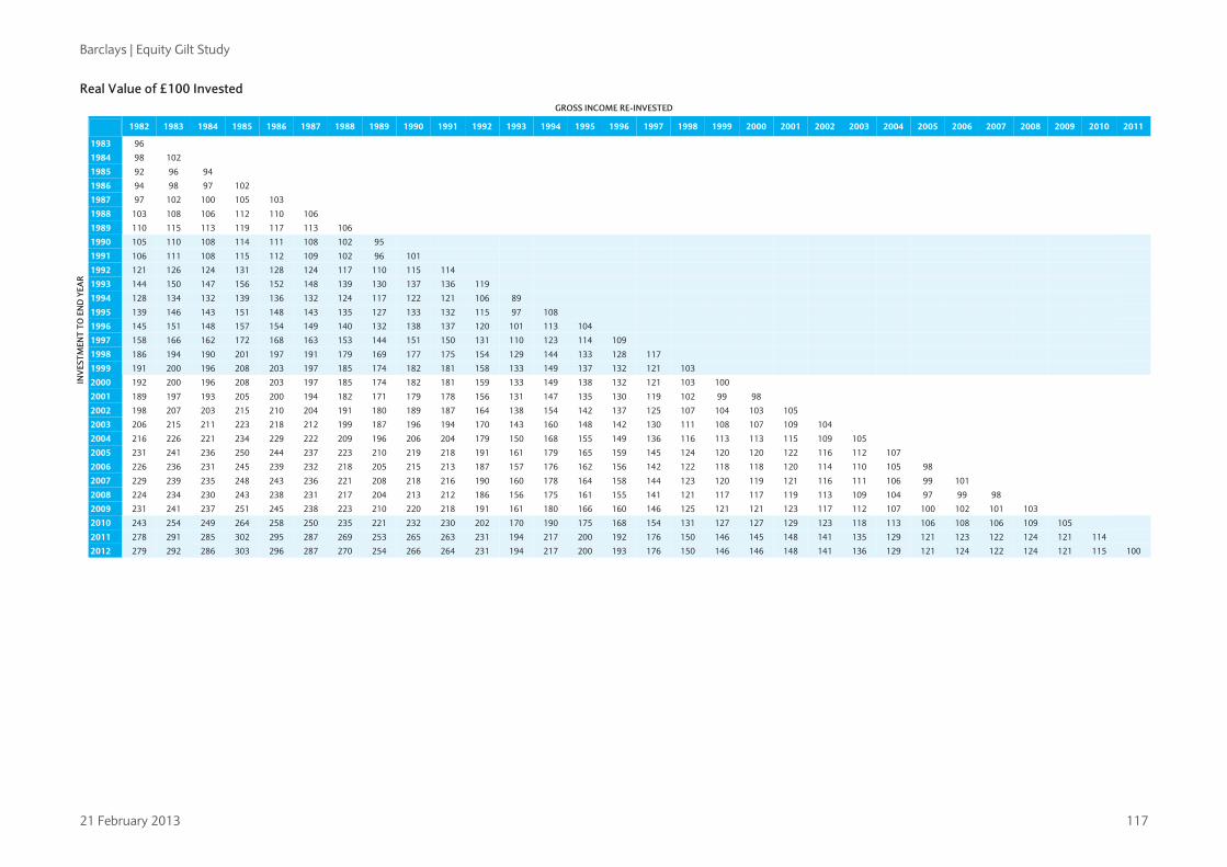
Barclays | Equity Gilt Study

21 February 2013 117

Real Value of £100 Invested GROSS INCOME RE-INVESTED

INV

ESTM

ENT

TO E

ND

YEA

R

1982 1983 1984 1985 1986 1987 1988 1989 1990 1991 1992 1993 1994 1995 1996 1997 1998 1999 2000 2001 2002 2003 2004 2005 2006 2007 2008 2009 2010 2011

1983 96

1984 98 102

1985 92 96 94

1986 94 98 97 102

1987 97 102 100 105 103

1988 103 108 106 112 110 106

1989 110 115 113 119 117 113 106

1990 105 110 108 114 111 108 102 95

1991 106 111 108 115 112 109 102 96 101

1992 121 126 124 131 128 124 117 110 115 114

1993 144 150 147 156 152 148 139 130 137 136 119

1994 128 134 132 139 136 132 124 117 122 121 106 89

1995 139 146 143 151 148 143 135 127 133 132 115 97 108

1996 145 151 148 157 154 149 140 132 138 137 120 101 113 104

1997 158 166 162 172 168 163 153 144 151 150 131 110 123 114 109

1998 186 194 190 201 197 191 179 169 177 175 154 129 144 133 128 117

1999 191 200 196 208 203 197 185 174 182 181 158 133 149 137 132 121 103

2000 192 200 196 208 203 197 185 174 182 181 159 133 149 138 132 121 103 100

2001 189 197 193 205 200 194 182 171 179 178 156 131 147 135 130 119 102 99 98

2002 198 207 203 215 210 204 191 180 189 187 164 138 154 142 137 125 107 104 103 105

2003 206 215 211 223 218 212 199 187 196 194 170 143 160 148 142 130 111 108 107 109 104

2004 216 226 221 234 229 222 209 196 206 204 179 150 168 155 149 136 116 113 113 115 109 105

2005 231 241 236 250 244 237 223 210 219 218 191 161 179 165 159 145 124 120 120 122 116 112 107

2006 226 236 231 245 239 232 218 205 215 213 187 157 176 162 156 142 122 118 118 120 114 110 105 98

2007 229 239 235 248 243 236 221 208 218 216 190 160 178 164 158 144 123 120 119 121 116 111 106 99 101

2008 224 234 230 243 238 231 217 204 213 212 186 156 175 161 155 141 121 117 117 119 113 109 104 97 99 98

2009 231 241 237 251 245 238 223 210 220 218 191 161 180 166 160 146 125 121 121 123 117 112 107 100 102 101 103

2010 243 254 249 264 258 250 235 221 232 230 202 170 190 175 168 154 131 127 127 129 123 118 113 106 108 106 109 105

2011 278 291 285 302 295 287 269 253 265 263 231 194 217 200 192 176 150 146 145 148 141 135 129 121 123 122 124 121 114 2012 279 292 286 303 296 287 270 254 266 264 231 194 217 200 193 176 150 146 146 148 141 136 129 121 124 122 124 121 115 100

UK real return on equities - gross income re-invested(annual average rates of return between year ends)

INVESTMENT FROM END YEAR INVESTMENT FROM END YEAR INVESTMENT FROM END YEAR INVESTMENT FROM END YEAR1899 1900 1901 1902 1903 1904 1905 1906 1907 1908 1909 1910 1911 1912 1913 1914 1915 1916 1917 1918 1919 1920 1921 1922 1923 1924 1925 1926 1927 1928 1929 1930 1931 1932 1933 1934 1935 1936 1937 1938 1939 1940 1941 1942 1943 1944 1945 1946 1947 1948 1949 1950 1951 1952 1953 1954 1955 1956 1957 1958 1959 1960 1961 1962 1963 1964 1965 1966 1967 1968 1969 1970 1971 1972 1973 1974 1975 1976 1977 1978 1979 1980 1981 1982 1983 1984 1985 1986 1987 1988 1989 1990 1991 1992 1993 1994 1995 1996 1997 1998 1999 2000 2001 2002 2003 2004 2005 2006 2007 2008 2009 2010 2011

1900 11.5 1900 1901 3.7 (3.5) 1901 1902 3.6 (0.1) 3.5 1902 1903 3.2 0.5 2.6 1.8 1903 1904 4.9 3.4 5.7 6.9 12.3 1904 1905 4.8 3.5 5.3 5.9 8.0 3.8 1905 1906 6.6 5.8 7.8 8.9 11.4 11.0 18.6 1906 1907 4.5 3.6 4.8 5.1 5.9 3.9 3.9 (8.9) 1907 1908 4.2 3.4 4.4 4.5 5.1 3.4 3.2 (3.7) 1.9 1908 1909 4.9 4.2 5.2 5.4 6.1 4.8 5.1 1.0 6.3 10.9 1909 1910 4.6 4.0 4.8 5.0 5.5 4.4 4.5 1.2 4.9 6.4 2.1 1910 1911 4.1 3.5 4.2 4.3 4.6 3.5 3.5 0.7 3.3 3.7 0.3 (1.5) 1911 1912 3.8 3.2 3.8 3.8 4.1 3.1 3.0 0.6 2.6 2.8 0.2 (0.7) 0.0 1912 1913 3.3 2.7 3.2 3.2 3.3 2.3 2.2 0.0 1.6 1.5 (0.7) (1.6) (1.7) (3.4) 1913 1914 3 0 2 4 2 9 2 8 2 9 2 1 1 9 (0 1) 1 3 1 2 (0 7) (1 3) (1 3) (2 0) (0 5) 1914

HOW TO USE TABLES OF TOTAL RETURNS

The dates along the top (and bottom) are those on which each portfolio starts; those down the side are the dates to which the annual rate of return is calculated. Thus the figure at the bottom right hand corner - 8.7 - shows that the real return on a portfolio bought at the end of December 2011 and held for one year to December 2012 was 8 7% Figures in brackets indicate negative returns1914 3.0 2.4 2.9 2.8 2.9 2.1 1.9 (0.1) 1.3 1.2 (0.7) (1.3) (1.3) (2.0) (0.5) 1914

1915 1.6 1.0 1.3 1.2 1.1 0.1 (0.2) (2.1) (1.2) (1.6) (3.6) (4.7) (5.5) (7.3) (9.1) (17.0) 1915 1916 0.4 (0.3) (0.0) (0.3) (0.4) (1.4) (1.9) (3.7) (3.2) (3.8) (5.7) (6.9) (8.0) (9.9) (11.9) (17.2) (17.3) 1916 1917 (0.2) (0.8) (0.7) (0.9) (1.1) (2.1) (2.6) (4.3) (3.8) (4.4) (6.2) (7.3) (8.3) (9.8) (11.4) (14.7) (13.5) (9.6) 1917 1918 0.1 (0.5) (0.3) (0.6) (0.7) (1.6) (2.0) (3.5) (3.0) (3.5) (5.0) (5.9) (6.5) (7.5) (8.3) (10.2) (7.7) (2.6) 5.0 1918 1919 0.4 (0.1) 0.1 (0.1) (0.2) (1.0) (1.4) (2.7) (2.2) (2.6) (3.8) (4.5) (4.8) (5.5) (5.9) (6.9) (4.2) 0.7 6.2 7.4 1919 1920 (1.6) (2.2) (2.1) (2.4) (2.6) (3.5) (4.0) (5.4) (5.1) (5.7) (7.1) (7.9) (8.6) (9.7) (10.5) (12.1) (11.1) (9.4) (9.4) (15.8) (34.0) 1920 1921 (0.2) (0.7) (0.5) (0.8) (0.9) (1.6) (2.0) (3.2) (2.8) (3.1) (4.2) (4.7) (5.1) (5.6) (5.9) (6.6) (4.8) (2.1) (0.1) (1.7) (6.0) 34.0 1921 1922 1.3 0.9 1.1 0.9 0.9 0.3 0.1 (1.0) (0.4) (0.6) (1.4) (1.7) (1.7) (1.9) (1.7) (1.8) 0.5 3.9 6.8 7.2 7.2 36.6 39.3 1922 1923 1.4 0.9 1.1 1.0 1.0 0.4 0.2 (0.7) (0.2) (0.3) (1.1) (1.3) (1.3) (1.4) (1.3) (1.3) 0.8 3.7 6.1 6.3 6.1 24.3 19.7 2.8 1923 1924 2.0 1.6 1.8 1.7 1.7 1.2 1.1 0.2 0.8 0.7 0.1 (0.1) 0.0 0.0 0.3 0.4 2.6 5.4 7.7 8.1 8.3 22.6 19.0 10.0 17.6 1924 1925 2.5 2.2 2.4 2.4 2.4 1.9 1.8 1.0 1.6 1.6 1.0 1.0 1.2 1.2 1.6 1.8 3.9 6.6 8.8 9.4 9.7 21.5 18.6 12.4 17.4 17.3 1925 1926 2.6 2.3 2.5 2.5 2.5 2.1 2.0 1.3 1.8 1.8 1.3 1.3 1.4 1.5 1.9 2.1 4.1 6.5 8.5 8.9 9.1 18.7 15.8 10.6 13.3 11.2 5.5 1926 1927 3.0 2.7 3.0 3.0 3.0 2.6 2.6 1.9 2.4 2.5 2.0 2.0 2.2 2.4 2.8 3.1 4.9 7.2 9.1 9.5 9.8 18.1 15.6 11.4 13.7 12.4 10.0 14.8 1927 1928 3.5 3.2 3.5 3.5 3.5 3.2 3.2 2.5 3.1 3.2 2.8 2.8 3.1 3.2 3.7 4.0 5.8 8.0 9.8 10.3 10.6 18.0 15.9 12.4 14.4 13.6 12.4 16.0 17.3 1928 1929 2.8 2.6 2.8 2.8 2.8 2.4 2.4 1.7 2.2 2.3 1.8 1.8 2.0 2.1 2.5 2.7 4.3 6.1 7.6 7.8 7.8 13.9 11.6 8.1 9.0 7.4 5.1 4.9 0.3 (14.1) 1929 1930 2.9 2.6 2.8 2.8 2.8 2.5 2.4 1.8 2.3 2.3 1.9 1.9 2.1 2.2 2.5 2.7 4.2 5.9 7.2 7.4 7.4 12.8 10.6 7.5 8.2 6.7 4.7 4.5 1.3 (5.9) 3.1 1930 1931 2.2 1.9 2.1 2.1 2.1 1.7 1.6 1.0 1.4 1.4 1.0 1.0 1.1 1.1 1.4 1.5 2.8 4.3 5.4 5.4 5.2 9.8 7.6 4.6 4.8 3.1 0.9 (0.0) (3.4) (9.5) (7.0) (16.2) 1931 1932 3.1 2.9 3.1 3.1 3.1 2.8 2.8 2.2 2.7 2.7 2.4 2.4 2.6 2.7 3.1 3.3 4.6 6.1 7.3 7.4 7.5 11.9 10.1 7.5 8.1 6.9 5.5 5.5 3.8 0.7 6.1 7.7 38.3 1932 1933 3.7 3.5 3.7 3.7 3.8 3.5 3.5 3.0 3.5 3.5 3.2 3.3 3.5 3.7 4.0 4.3 5.6 7.2 8.3 8.5 8.6 12.8 11.2 9.0 9.6 8.8 7.8 8.1 7.0 5.1 10.5 13.1 31.3 24.8 1933 1934 4.0 3.8 4.0 4.0 4.1 3.8 3.8 3.3 3.8 3.9 3.6 3.7 3.9 4.1 4.5 4.7 6.0 7.5 8.6 8.8 8.9 12.9 11.4 9.3 9.9 9.2 8.3 8.7 7.8 6.4 11.0 13.1 24.9 18.7 13.0 1934 1935 4.2 4.0 4.2 4.2 4.3 4.1 4.1 3.6 4.1 4.2 3.9 4.0 4.2 4.4 4.8 5.0 6.3 7.7 8.7 9.0 9.1 12.8 11.4 9.5 10.1 9.4 8.7 9.0 8.3 7.1 11.1 12.8 21.5 16.3 12.3 11.6 1935 1936 4.5 4.3 4.5 4.6 4.6 4.4 4.4 4.0 4.5 4.6 4.3 4.4 4.7 4.9 5.2 5.5 6.7 8.1 9.1 9.3 9.5 13.0 11.7 9.9 10.5 9.9 9.3 9.7 9.1 8.2 11.8 13.3 20.3 16.2 13.5 13.7 15.9 1936 1937 3.8 3.6 3.8 3.8 3.9 3.7 3.7 3.2 3.6 3.7 3.4 3.5 3.7 3.8 4.2 4.4 5.5 6.7 7.6 7.7 7.7 10.9 9.6 7.8 8.2 7.5 6.7 6.8 6.1 4.9 7.6 8.2 12.9 8.4 4.7 2.1 (2.4) (17.7) 1937 1938 3.5 3.3 3.5 3.5 3.5 3.3 3.3 2.8 3.2 3.3 3.0 3.1 3.2 3.4 3.6 3.8 4.8 6.0 6.8 6.9 6.8 9.7 8.5 6.8 7.0 6.3 5.5 5.5 4.7 3.6 5.7 6.1 9.7 5.5 2.1 (0.5) (4.2) (13.0) (7.9) 1938 1939 3.2 3.0 3.2 3.2 3.2 3.0 2.9 2.5 2.9 2.9 2.7 2.7 2.8 2.9 3.2 3.3 4.3 5.3 6.1 6.1 6.1 8.7 7.5 5.9 6.0 5.3 4.5 4.4 3.6 2.5 4.3 4.4 7.3 3.5 0.3 (2.0) (5.2) (11.3) (7.9) (7.9) 1939

end of December 2011 and held for one year to December 2012 was 8.7%. Figures in brackets indicate negative returns.

Each figure on the bottom line of the table shows the average annual return up to the end of December 2012 from the year shown below the figure. The first figure is 5.0, showing that the average annual rate of return over the whole period since 1899 has been 5.0%.

The top figure in each column is the rate of return in the first year, so that reading diagonally down the table gives the real rate of return in each year since 1899. The table can be used to see the rate of return over any period; thus a purchase made at the end of 1900 would have lost 3.5% of its value in one year (allowing for reinvestment of income) but, over the first five years (up to the end of 1905), would have given an average annual real return of 3.5%.

1939 3.2 3.0 3.2 3.2 3.2 3.0 2.9 2.5 2.9 2.9 2.7 2.7 2.8 2.9 3.2 3.3 4.3 5.3 6.1 6.1 6.1 8.7 7.5 5.9 6.0 5.3 4.5 4.4 3.6 2.5 4.3 4.4 7.3 3.5 0.3 (2.0) (5.2) (11.3) (7.9) (7.9) 1939 1940 2.7 2.5 2.7 2.6 2.7 2.4 2.4 1.9 2.3 2.3 2.0 2.0 2.1 2.2 2.4 2.5 3.4 4.4 5.0 5.0 4.9 7.4 6.1 4.6 4.7 3.9 3.1 2.9 2.0 0.8 2.3 2.3 4.5 0.9 (2.1) (4.4) (7.3) (12.3) (10.4) (11.7) (15.3) 1940 1941 3.1 2.9 3.0 3.0 3.1 2.8 2.8 2.4 2.7 2.8 2.5 2.5 2.7 2.8 3.0 3.1 4.0 4.9 5.6 5.6 5.5 7.9 6.8 5.3 5.4 4.7 4.0 3.9 3.2 2.2 3.6 3.7 5.9 2.8 0.4 (1.3) (3.3) (6.8) (3.8) (2.4) 0.5 19.2 1941 1942 3.4 3.2 3.4 3.4 3.4 3.2 3.2 2.8 3.1 3.2 3.0 3.0 3.1 3.2 3.5 3.6 4.5 5.4 6.1 6.1 6.1 8.4 7.3 5.9 6.1 5.4 4.8 4.7 4.1 3.2 4.7 4.8 7.0 4.3 2.2 1.0 (0.5) (3.0) 0.3 2.4 6.1 18.8 18.4 1942 1943 3.6 3.4 3.6 3.6 3.6 3.4 3.4 3.0 3.4 3.4 3.2 3.3 3.4 3.5 3.8 3.9 4.7 5.7 6.3 6.3 6.3 8.5 7.5 6.2 6.4 5.8 5.2 5.2 4.6 3.8 5.2 5.4 7.4 5.0 3.2 2.1 1.0 (1.0) 2.2 4.3 7.6 16.5 15.2 12.1 1943 1944 3.8 3.6 3.8 3.8 3.8 3.6 3.6 3.2 3.6 3.6 3.4 3.5 3.6 3.8 4.0 4.1 5.0 5.9 6.5 6.5 6.5 8.6 7.7 6.4 6.6 6.1 5.5 5.5 5.0 4.3 5.6 5.8 7.7 5.5 3.9 3.0 2.1 0.5 3.4 5.4 8.3 15.2 13.9 11.7 11.3 1944 1945 3.8 3.6 3.8 3.8 3.8 3.6 3.6 3.3 3.6 3.7 3.5 3.5 3.7 3.8 4.0 4.2 5.0 5.8 6.4 6.5 6.4 8.5 7.5 6.3 6.5 6.0 5.5 5.5 5.0 4.3 5.6 5.7 7.5 5.4 4.0 3.2 2.4 1.0 3.6 5.3 7.7 13.0 11.6 9.4 8.0 4.8 1945 1946 4.1 3.9 4.1 4.1 4.1 4.0 4.0 3.6 4.0 4.0 3.8 3.9 4.0 4.2 4.4 4.6 5.3 6.2 6.8 6.8 6.8 8.8 7.9 6.8 6.9 6.5 6.0 6.0 5.6 5.0 6.2 6.4 8.1 6.2 4.9 4.3 3.6 2.5 5.0 6.8 9.0 13.7 12.7 11.3 11.0 10.9 17.3 1946 1947 3.9 3.7 3.9 3.9 3.9 3.7 3.7 3.4 3.7 3.8 3.6 3.6 3.8 3.9 4.1 4.2 5.0 5.8 6.4 6.4 6.4 8.3 7.4 6.3 6.4 5.9 5.5 5.5 5.0 4.4 5.5 5.7 7.2 5.4 4.2 3.5 2.9 1.8 4.0 5.4 7.1 10.8 9.5 7.8 6.7 5.2 5.4 (5.3) 1947 1948 3.6 3.4 3.6 3.6 3.6 3.4 3.4 3.1 3.4 3.4 3.3 3.3 3.4 3.5 3.7 3.8 4.6 5.3 5.8 5.9 5.8 7.6 6.8 5.7 5.8 5.3 4.8 4.8 4.3 3.7 4.8 4.9 6.3 4.5 3.3 2.6 2.0 0.9 2.8 3.9 5.3 8.2 6.7 4.9 3.5 1.7 0.6 (6.8) (8.3) 1948 1949 3.3 3.2 3.3 3.3 3.3 3.1 3.1 2.8 3.1 3.1 2.9 3.0 3.1 3.2 3.3 3.5 4.1 4.9 5.3 5.4 5.3 7.0 6.1 5.1 5.2 4.7 4.2 4.2 3.7 3.1 4.0 4.1 5.3 3.7 2.5 1.8 1.1 0.1 1.7 2.7 3.8 6.2 4.6 2.8 1.3 (0.6) (1.9) (7.5) (8.6) (8.9) 1949 1950 3.4 3.2 3.4 3.4 3.4 3.2 3.2 2.9 3.2 3.2 3.0 3.1 3.2 3.3 3.5 3.6 4.2 4.9 5.4 5.4 5.4 7.0 6.2 5.2 5.3 4.8 4.3 4.3 3.9 3.3 4.2 4.2 5.5 3.9 2.8 2.2 1.6 0.6 2.2 3.1 4.1 6.3 4.9 3.4 2.2 0.7 (0.1) (4.0) (3.5) (1.1) 7.4 1950 1951 3.3 3.1 3.3 3.2 3.3 3.1 3.1 2.8 3.0 3.1 2.9 2.9 3.0 3.1 3.3 3.4 4.0 4.7 5.1 5.2 5.1 6.7 5.9 4.9 4.9 4.5 4.0 4.0 3.6 3.0 3.9 3.9 5.0 3.5 2.4 1.8 1.3 0.3 1.8 2.6 3.5 5.4 4.1 2.6 1.5 0.2 (0.6) (3.8) (3.4) (1.8) 2.0 (3.1) 1951 1952 3.1 2.9 3.1 3.1 3.1 2.9 2.9 2.6 2.8 2.9 2.7 2.7 2.8 2.9 3.0 3.1 3.7 4.4 4.8 4.8 4.7 6.3 5.5 4.5 4.5 4.1 3.6 3.6 3.1 2.6 3.4 3.4 4.4 3.0 2.0 1.4 0.8 (0.1) 1.2 1.9 2.7 4.4 3.1 1.7 0.6 (0.6) (1.4) (4.2) (4.0) (2.9) (0.8) (4.6) (6.1) 1952 1953 3.4 3.3 3.4 3.4 3.4 3.3 3.3 3.0 3.2 3.3 3.1 3.1 3.2 3.3 3.5 3.6 4.2 4.8 5.3 5.3 5.2 6.7 6.0 5.0 5.1 4.7 4.3 4.2 3.8 3.3 4.1 4.2 5.2 3.9 2.9 2.4 1.9 1.2 2.5 3.2 4.0 5.7 4.7 3.5 2.7 1.7 1.4 (0.7) 0.1 1.8 4.7 3.8 7.4 22.9 1953 1954 4.0 3.9 4.0 4.1 4.1 3.9 3.9 3.7 3.9 4.0 3.8 3.9 4.0 4.1 4.3 4.4 5.0 5.7 6.1 6.2 6.1 7.6 6.9 6.0 6.2 5.8 5.4 5.4 5.1 4.6 5.5 5.6 6.6 5.4 4.5 4.1 3.8 3.1 4.5 5.3 6.3 8.0 7.2 6.3 5.8 5.3 5.3 3.9 5.3 7.7 11.4 12.4 18.2 32.6 42.9 1954 1955 4.0 3.9 4.1 4.1 4.1 4.0 4.0 3.7 4.0 4.0 3.9 3.9 4.0 4.1 4.3 4.4 5.0 5.7 6.1 6.1 6.1 7.6 6.9 6.0 6.1 5.8 5.4 5.4 5.1 4.6 5.4 5.5 6.6 5.4 4.6 4.2 3.8 3.2 4.5 5.3 6.2 7.8 7.0 6.2 5.7 5.2 5.3 4.0 5.2 7.3 10.3 10.9 14.7 22.6 22.4 4.8 1955 1956 3.7 3.6 3.7 3.8 3.8 3.6 3.6 3.4 3.6 3.7 3.5 3.5 3.6 3.7 3.9 4.0 4.6 5.2 5.6 5.6 5.6 7.0 6.3 5.4 5.5 5.2 4.8 4.8 4.4 4.0 4.8 4.8 5.8 4.6 3.8 3.4 3.0 2.4 3.6 4.3 5.0 6.5 5.7 4.8 4.3 3.7 3.6 2.3 3.2 4.7 6.8 6.7 8.8 12.9 9.8 (3.8) (11.7) 1956 1957 3.6 3.4 3.6 3.6 3.6 3.5 3.4 3.2 3.4 3.5 3.3 3.3 3.4 3.5 3.7 3.8 4.3 4.9 5.3 5.3 5.3 6.6 5.9 5.1 5.2 4.8 4.5 4.4 4.1 3.7 4.4 4.4 5.3 4.2 3.4 3.0 2.6 2.0 3.1 3.7 4.4 5.7 4.9 4.1 3.5 3.0 2.8 1.6 2.3 3.5 5.2 4.9 6.3 9.0 5.7 (4.4) (8.7) (5.5) 1957 1958 4.2 4.1 4.2 4.2 4.2 4.1 4.1 3.8 4.1 4.2 4.0 4.1 4.2 4.3 4.5 4.6 5.1 5.7 6.1 6.2 6.1 7.5 6.8 6.1 6.2 5.8 5.5 5.5 5.2 4.8 5.6 5.7 6.6 5.5 4.8 4.5 4.2 3.7 4.8 5.5 6.2 7.6 6.9 6.3 5.9 5.5 5.6 4.6 5.6 7.1 9.0 9.2 11.1 14.3 12.6 6.1 6.6 17.1 45.2 1958 1959 4.9 4.8 4.9 4.9 5.0 4.9 4.9 4.6 4.9 5.0 4.9 4.9 5.1 5.2 5.4 5.5 6.1 6.7 7.1 7.2 7.2 8.5 7.9 7.1 7.3 7.0 6.7 6.7 6.5 6.2 6.9 7.1 8.0 7.0 6.4 6.1 5.9 5.5 6.7 7.4 8.3 9.7 9.2 8.6 8.4 8.2 8.5 7.8 9.0 10.7 12.9 13.6 15.8 19.4 18.8 14.5 17.0 28.6 49.9 54.8 1959 1960 4.8 4.7 4.8 4.8 4.9 4.8 4.8 4.5 4.8 4.9 4.8 4.8 4.9 5.1 5.2 5.4 5.9 6.5 6.9 7.0 7.0 8.3 7.7 7.0 7.1 6.8 6.5 6.5 6.3 6.0 6.7 6.8 7.7 6.7 6.1 5.9 5.7 5.2 6.4 7.1 7.9 9.2 8.7 8.1 7.9 7.7 7.9 7.3 8.3 9.8 11.7 12.1 14.0 16.7 15.9 11.9 13.4 20.7 31.0 24.4 (0.1) 1960 1961 4.7 4.6 4.7 4.7 4.8 4.6 4.6 4.4 4.7 4.7 4.6 4.7 4.8 4.9 5.1 5.2 5.7 6.3 6.7 6.7 6.7 8.0 7.4 6.7 6.8 6.5 6.2 6.3 6.0 5.7 6.4 6.5 7.3 6.4 5.8 5.6 5.3 4.9 6.0 6.6 7.4 8.6 8.1 7.6 7.3 7.1 7.2 6.6 7.5 8.8 10.4 10.7 12.2 14.4 13.4 9.7 10.6 15.7 21.6 14.7 (1.3) (2.5) 1961 1962 4.5 4.4 4.6 4.6 4.6 4.5 4.5 4.3 4.5 4.6 4.5 4.5 4.6 4.7 4.9 5.0 5.6 6.1 6.5 6.5 6.5 7.7 7.2 6.5 6.6 6.3 6.0 6.0 5.8 5.5 6.1 6.2 7.0 6.1 5.5 5.3 5.0 4.6 5.7 6.3 6.9 8.1 7.6 7.0 6.8 6.5 6.6 6.0 6.8 8.0 9.4 9.6 10.8 12.6 11.6 8.1 8.6 12.5 16.4 10.2 (1.6) (2.4) (2.2) 1962 1963 4.7 4.6 4.8 4.8 4.8 4.7 4.7 4.5 4.8 4.8 4.7 4.8 4.9 5.0 5.2 5.3 5.8 6.4 6.7 6.8 6.8 8.0 7.4 6.7 6.8 6.6 6.3 6.3 6.1 5.8 6.4 6.5 7.3 6.5 5.9 5.7 5.5 5.1 6.1 6.7 7.3 8.5 8.0 7.5 7.3 7.1 7.2 6.7 7.5 8.6 10.0 10.2 11.3 13.1 12.1 9.2 9.7 13.2 16.6 11.6 2.9 3.9 7.3 17.7 1963 1964 4.5 4.4 4.5 4.5 4.6 4.5 4.5 4.2 4.5 4.5 4.4 4.5 4.6 4.7 4.8 5.0 5.5 6.0 6.4 6.4 6.4 7.5 7.0 6.3 6.4 6.1 5.8 5.9 5.6 5.3 5.9 6.0 6.8 5.9 5.4 5.1 4.9 4.5 5.5 6.0 6.6 7.6 7.2 6.7 6.4 6.2 6.3 5.7 6.4 7.3 8.5 8.6 9.6 11.0 10.0 7.1 7.4 10.0 12.4 7.8 0.2 0.3 1.3 3.0 (9.8) 1964 1965 4 5 4 4 4 6 4 6 4 6 4 5 4 5 4 3 4 5 4 6 4 5 4 5 4 6 4 7 4 9 5 0 5 5 6 0 6 4 6 4 6 4 7 5 7 0 6 3 6 4 6 1 5 9 5 9 5 7 5 4 6 0 6 0 6 8 5 9 5 4 5 2 5 0 4 6 5 5 6 0 6 6 7 6 7 1 6 7 6 4 6 2 6 3 5 7 6 4 7 3 8 4 8 5 9 3 10 6 9 7 7 1 7 3 9 6 11 7 7 6 1 3 1 5 2 6 4 2 (1 9) 6 6 1965

INV

ESTM

ENT

TO E

ND

YEA

R INV

ESTMEN

T TO EN

D YEA

R

an average annual real return of 3.5%.

1965 4.5 4.4 4.6 4.6 4.6 4.5 4.5 4.3 4.5 4.6 4.5 4.5 4.6 4.7 4.9 5.0 5.5 6.0 6.4 6.4 6.4 7.5 7.0 6.3 6.4 6.1 5.9 5.9 5.7 5.4 6.0 6.0 6.8 5.9 5.4 5.2 5.0 4.6 5.5 6.0 6.6 7.6 7.1 6.7 6.4 6.2 6.3 5.7 6.4 7.3 8.4 8.5 9.3 10.6 9.7 7.1 7.3 9.6 11.7 7.6 1.3 1.5 2.6 4.2 (1.9) 6.6 1965 1966 4.3 4.2 4.4 4.4 4.4 4.3 4.3 4.1 4.3 4.4 4.2 4.3 4.4 4.5 4.6 4.7 5.2 5.7 6.1 6.1 6.1 7.2 6.6 6.0 6.0 5.8 5.5 5.5 5.3 5.0 5.6 5.6 6.3 5.5 5.0 4.7 4.5 4.2 5.0 5.5 6.0 7.0 6.5 6.0 5.8 5.5 5.6 5.0 5.6 6.4 7.4 7.4 8.1 9.2 8.3 5.8 5.9 7.8 9.4 5.6 (0.0) (0.0) 0.5 1.2 (3.8) (0.7) (7.4) 1966 1967 4.7 4.6 4.7 4.7 4.8 4.7 4.7 4.5 4.7 4.8 4.7 4.7 4.8 4.9 5.1 5.2 5.7 6.2 6.5 6.5 6.5 7.6 7.1 6.5 6.6 6.3 6.1 6.1 5.9 5.6 6.2 6.3 7.0 6.2 5.7 5.5 5.3 4.9 5.8 6.3 6.9 7.8 7.4 6.9 6.7 6.5 6.6 6.1 6.7 7.6 8.6 8.7 9.5 10.6 9.7 7.5 7.8 9.7 11.4 8.2 3.4 3.9 5.0 6.6 3.9 9.0 10.2 31.1 1967 1968 5.1 5.0 5.2 5.2 5.3 5.1 5.2 5.0 5.2 5.3 5.2 5.2 5.3 5.4 5.6 5.7 6.2 6.7 7.1 7.1 7.1 8.2 7.7 7.1 7.2 7.0 6.8 6.8 6.6 6.3 6.9 7.0 7.7 7.0 6.5 6.3 6.2 5.9 6.8 7.3 7.9 8.8 8.4 8.1 7.9 7.8 7.9 7.5 8.1 9.0 10.1 10.2 11.0 12.2 11.5 9.6 9.9 12.0 13.7 11.0 6.9 7.8 9.4 11.5 10.3 16.0 19.3 35.4 39.8 1968 1969 4.8 4.7 4.8 4.9 4.9 4.8 4.8 4.6 4.8 4.9 4.8 4.8 4.9 5.0 5.2 5.3 5.8 6.3 6.6 6.6 6.6 7.6 7.2 6.6 6.6 6.4 6.2 6.2 6.0 5.7 6.3 6.4 7.0 6.3 5.8 5.6 5.5 5.2 6.0 6.4 7.0 7.8 7.4 7.1 6.9 6.7 6.8 6.3 6.9 7.7 8.6 8.6 9.3 10.3 9.6 7.7 7.9 9.5 10.9 8.2 4.4 4.9 5.9 7.1 5.4 8.8 9.3 15.5 8.5 (15.9) 1969 1970 4.6 4.5 4.6 4.6 4.7 4.5 4.5 4.3 4.6 4.6 4.5 4.6 4.7 4.7 4.9 5.0 5.4 5.9 6.2 6.3 6.2 7.2 6.8 6.2 6.2 6.0 5.8 5.8 5.6 5.3 5.8 5.9 6.5 5.8 5.3 5.1 5.0 4.7 5.4 5.9 6.3 7.2 6.8 6.4 6.2 6.0 6.0 5.6 6.1 6.8 7.6 7.6 8.2 9.0 8.3 6.4 6.5 8.0 9.1 6.5 3.0 3.3 3.9 4.7 3.0 5.3 5.0 8.4 1.7 (13.2) (10.5) 1970 1971 4.9 4.8 5.0 5.0 5.0 4.9 4.9 4.8 5.0 5.0 4.9 5.0 5.1 5.2 5.3 5.4 5.9 6.4 6.7 6.7 6.7 7.7 7.3 6.7 6.8 6.5 6.3 6.3 6.2 5.9 6.4 6.5 7.2 6.5 6.0 5.8 5.7 5.4 6.2 6.6 7.1 7.9 7.6 7.2 7.1 6.9 7.0 6.6 7.1 7.9 8.7 8.7 9.4 10.3 9.6 7.9 8.1 9.6 10.7 8.4 5.3 5.8 6.6 7.7 6.5 9.0 9.4 13.2 9.1 0.4 9.7 34.4 1971 1972 5.0 4.9 5.0 5.0 5.1 5.0 5.0 4.8 5.0 5.1 5.0 5.0 5.1 5.2 5.4 5.5 5.9 6.4 6.7 6.8 6.7 7.7 7.3 6.7 6.8 6.6 6.4 6.4 6.2 6.0 6.5 6.6 7.2 6.5 6.1 5.9 5.8 5.5 6.2 6.7 7.2 7.9 7.6 7.3 7.1 7.0 7.0 6.7 7.2 7.9 8.7 8.7 9.3 10.1 9.5 7.9 8.1 9.5 10.5 8.4 5.5 6.0 6.8 7.7 6.7 8.9 9.2 12.3 8.9 2.3 9.1 20.5 8.1 1972 1973 4.3 4.2 4.3 4.3 4.4 4.3 4.3 4.1 4.3 4.3 4.2 4.2 4.3 4.4 4.5 4.6 5.0 5.5 5.8 5.8 5.8 6.7 6.2 5.7 5.7 5.5 5.3 5.3 5.1 4.8 5.3 5.3 5.9 5.2 4.8 4.6 4.4 4.1 4.8 5.2 5.6 6.3 5.9 5.5 5.3 5.1 5.1 4.7 5.1 5.7 6.4 6.3 6.8 7.4 6.7 5.1 5.1 6.2 6.9 4.8 1.9 2.1 2.4 2.9 1.5 2.8 2.4 3.9 (0.1) (6.6) (4.1) (1.9) (16.2) (35.0) 1973 1974 3.0 2.9 3.0 3.0 3.0 2.9 2.9 2.7 2.9 2.9 2.8 2.8 2.8 2.9 3.0 3.0 3.4 3.8 4.1 4.1 4.0 4.9 4.4 3.8 3.8 3.6 3.3 3.3 3.0 2.8 3.2 3.2 3.7 3.0 2.5 2.2 2.0 1.6 2.2 2.5 2.8 3.4 3.0 2.5 2.2 2.0 1.9 1.3 1.6 2.0 2.5 2.3 2.5 2.9 2.0 0.3 0.1 0.8 1.2 (1.1) (4.0) (4.2) (4.4) (4.5) (6.3) (6.0) (7.3) (7.3) (11.8) (18.3) (18.7) (20.7) (33.5) (47.8) (58.1) 1974 1975 3.9 3.8 3.9 3.9 4.0 3.9 3.9 3.7 3.9 3.9 3.8 3.8 3.9 4.0 4.1 4.2 4.6 5.0 5.2 5.3 5.2 6.1 5.7 5.1 5.1 4.9 4.7 4.7 4.5 4.2 4.7 4.7 5.2 4.5 4.1 3.9 3.7 3.4 4.0 4.4 4.8 5.4 5.0 4.6 4.4 4.2 4.2 3.7 4.1 4.6 5.1 5.0 5.4 5.9 5.2 3.7 3.6 4.5 5.1 3.1 0.5 0.6 0.8 1.0 (0.2) 0.7 0.1 1.0 (2.3) (7.2) (5.6) (4.6) (12.4) (18.4) (8.6) 99.6 1975 1976 3.7 3.6 3.7 3.7 3.8 3.6 3.6 3.4 3.6 3.7 3.6 3.6 3.7 3.7 3.8 3.9 4.3 4.7 4.9 4.9 4.9 5.8 5.3 4.8 4.8 4.6 4.4 4.3 4.1 3.9 4.3 4.3 4.8 4.2 3.7 3.5 3.3 3.0 3.6 4.0 4.3 4.9 4.5 4.1 3.9 3.7 3.6 3.2 3.5 4.0 4.5 4.4 4.7 5.2 4.4 3.0 2.9 3.7 4.2 2.3 (0.2) (0.2) (0.0) 0.1 (1.1) (0.4) (1.0) (0.3) (3.3) (7.7) (6.4) (5.7) (12.2) (16.6) (9.4) 33.2 (11.1) 1976 1977 4.1 4.0 4.1 4.1 4.1 4.0 4.0 3.8 4.0 4.0 3.9 4.0 4.0 4.1 4.2 4.3 4.7 5.1 5.4 5.4 5.3 6.2 5.8 5.2 5.3 5.1 4.8 4.8 4.6 4.4 4.8 4.8 5.4 4.7 4.3 4.1 3.9 3.7 4.3 4.6 5.0 5.6 5.2 4.9 4.6 4.4 4.4 4.0 4.4 4.8 5.4 5.3 5.6 6.1 5.5 4.1 4.1 4.9 5.4 3.7 1.4 1.5 1.7 2.0 1.0 1.8 1.5 2.3 (0.2) (3.9) (2.3) (1.0) (5.9) (8.5) (0.4) 33.0 8.5 32.5 1977 1978 4.0 3.9 4.0 4.0 4.0 3.9 3.9 3.8 3.9 4.0 3.9 3.9 4.0 4.0 4.2 4.2 4.6 5.0 5.3 5.3 5.2 6.1 5.7 5.1 5.2 5.0 4.7 4.7 4.5 4.3 4.7 4.7 5.2 4.6 4.2 4.0 3.9 3.6 4.2 4.5 4.8 5.4 5.1 4.7 4.5 4.3 4.3 3.9 4.2 4.7 5.2 5.1 5.4 5.9 5.3 3.9 3.9 4.7 5.2 3.5 1.3 1.4 1.6 1.9 0.9 1.7 1.4 2.1 (0.2) (3.5) (2.0) (0.9) (5.1) (7.1) (0.3) 23.9 5.7 15.2 0.2 1978 1979 3.9 3.8 3.9 3.9 3.9 3.8 3.8 3.6 3.8 3.8 3.7 3.8 3.8 3.9 4.0 4.1 4.5 4.8 5.1 5.1 5.1 5.9 5.5 5.0 5.0 4.8 4.6 4.5 4.4 4.1 4.5 4.5 5.0 4.4 4.0 3.8 3.6 3.4 3.9 4.2 4.6 5.1 4.8 4.4 4.2 4.0 4.0 3.6 3.9 4.4 4.8 4.7 5.0 5.5 4.9 3.6 3.5 4.2 4.7 3.1 1.0 1.1 1.3 1.5 0.5 1.3 0.9 1.6 (0.6) (3.6) (2.3) (1.3) (5.1) (6.8) (1.1) 17.5 2.9 8.1 (2.4) (4.9) 1979 1980 4.0 4.0 4.0 4.1 4.1 4.0 4.0 3.8 4.0 4.0 3.9 3.9 4.0 4.1 4.2 4.3 4.6 5.0 5.3 5.3 5.3 6.1 5.7 5.2 5.2 5.0 4.8 4.8 4.6 4.3 4.7 4.8 5.3 4.7 4.3 4.1 3.9 3.7 4.2 4.5 4.9 5.4 5.1 4.8 4.6 4.4 4.4 4.0 4.3 4.7 5.2 5.1 5.4 5.9 5.3 4.1 4.0 4.7 5.2 3.7 1.7 1.8 2.0 2.3 1.4 2.2 1.9 2.6 0.7 (2.0) (0.7) 0.4 (2.8) (4.1) 1.4 17.4 5.6 10.3 3.7 5.5 17.1 1980 1981 4.0 3.9 4.0 4.0 4.0 3.9 3.9 3.8 3.9 4.0 3.9 3.9 4.0 4.0 4.2 4.2 4.6 5.0 5.2 5.2 5.2 6.0 5.6 5.1 5.1 4.9 4.7 4.7 4.5 4.3 4.7 4.7 5.2 4.6 4.2 4.0 3.9 3.6 4.2 4.5 4.8 5.3 5.0 4.7 4.5 4.3 4.3 3.9 4.2 4.6 5.1 5.0 5.3 5.7 5.1 4.0 3.9 4.6 5.0 3.6 1.7 1.8 2.0 2.2 1.4 2.1 1.9 2.5 0.7 (1.8) (0.5) 0.5 (2.4) (3.5) 1.4 15.0 4.9 8.4 3.1 4.1 8.9 1.3 1981 1982 4.2 4.1 4.2 4.2 4.3 4.2 4.2 4.0 4.2 4.2 4.1 4.1 4.2 4.3 4.4 4.5 4.8 5.2 5.5 5.5 5.4 6.2 5.8 5.3 5.4 5.2 5.0 5.0 4.8 4.6 5.0 5.0 5.5 4.9 4.5 4.4 4.2 4.0 4.5 4.8 5.1 5.7 5.4 5.1 4.9 4.7 4.7 4.4 4.7 5.1 5.6 5.5 5.8 6.2 5.7 4.5 4.5 5.2 5.7 4.3 2.5 2.6 2.9 3.1 2.4 3.2 3.0 3.6 2.0 (0.2) 1.1 2.1 (0.4) (1.2) 3.5 15.8 7.2 10.6 6.6 8.3 13.1 11.1 21.9 1982 1983 4.4 4.3 4.4 4.4 4.5 4.4 4.4 4.2 4.4 4.4 4.3 4.4 4.5 4.5 4.6 4.7 5.1 5.4 5.7 5.7 5.7 6.5 6.1 5.6 5.6 5.5 5.3 5.3 5.1 4.9 5.3 5.3 5.8 5.2 4.9 4.7 4.6 4.3 4.9 5.2 5.5 6.0 5.8 5.5 5.3 5.2 5.2 4.9 5.1 5.6 6.0 6.0 6.3 6.7 6.2 5.1 5.1 5.8 6.3 4.9 3.3 3.4 3.7 4.0 3.3 4.1 3.9 4.6 3.2 1.1 2.5 3.5 1.3 0.7 5.2 16.5 9.0 12.2 9.1 11.0 15.3 14.7 22.1 22.3 1983 1984 4.6 4.6 4.7 4.7 4.7 4.6 4.6 4.5 4.6 4.7 4.6 4.6 4.7 4.8 4.9 5.0 5.3 5.7 6.0 6.0 6.0 6.7 6.4 5.9 6.0 5.8 5.6 5.6 5.4 5.2 5.6 5.7 6.1 5.6 5.2 5.1 5.0 4.8 5.3 5.6 5.9 6.5 6.2 5.9 5.8 5.6 5.6 5.4 5.7 6.1 6.5 6.5 6.8 7.2 6.8 5.7 5.8 6.5 6.9 5.7 4.1 4.3 4.6 4.9 4.3 5.1 5.0 5.7 4.4 2.5 3.9 5.0 3.0 2.6 6.9 17.4 10.7 13.8 11.3 13.3 17.4 17.4 23.3 24.0 25.8 1984 1985 4.7 4.7 4.8 4.8 4.8 4.7 4.7 4.6 4.8 4.8 4.7 4.8 4.8 4.9 5.0 5.1 5.5 5.8 6.1 6.1 6.1 6.9 6.5 6.0 6.1 5.9 5.7 5.7 5.6 5.4 5.8 5.8 6.3 5.7 5.4 5.3 5.1 4.9 5.5 5.8 6.1 6.6 6.3 6.1 5.9 5.8 5.8 5.6 5.9 6.3 6.7 6.7 7.0 7.4 7.0 6.0 6.0 6.7 7.2 6.0 4.4 4.6 4.9 5.3 4.7 5.5 5.4 6.1 4.9 3.1 4.5 5.5 3.7 3.4 7.5 17.1 11.0 13.8 11.6 13.4 16.7 16.7 20.8 20.5 19.6 13.7 1985 1986 4.9 4.9 5.0 5.0 5.0 4.9 4.9 4.8 5.0 5.0 4.9 5.0 5.1 5.1 5.2 5.3 5.7 6.1 6.3 6.3 6.3 7.1 6.7 6.3 6.3 6.1 6.0 6.0 5.8 5.7 6.0 6.1 6.5 6.0 5.7 5.6 5.5 5.3 5.8 6.1 6.4 6.9 6.7 6.4 6.3 6.2 6.2 6.0 6.3 6.7 7.1 7.1 7.4 7.9 7.4 6.5 6.5 7.2 7.7 6.5 5.1 5.3 5.6 5.9 5.4 6.2 6.2 6.9 5.8 4.1 5.4 6.5 4.9 4.7 8.6 17.5 12.0 14.6 12.8 14.5 17.6 17.7 21.2 21.0 20.6 18.1 22.7 1986 1987 4.9 4.9 5.0 5.0 5.0 4.9 4.9 4.8 5.0 5.0 4.9 5.0 5.1 5.1 5.2 5.3 5.7 6.0 6.3 6.3 6.3 7.0 6.7 6.2 6.3 6.1 6.0 6.0 5.8 5.6 6.0 6.1 6.5 6.0 5.7 5.6 5.4 5.2 5.8 6.1 6.4 6.9 6.6 6.4 6.3 6.2 6.2 5.9 6.2 6.6 7.1 7.1 7.4 7.8 7.4 6.4 6.5 7.1 7.6 6.5 5.1 5.2 5.6 5.9 5.4 6.1 6.1 6.8 5.7 4.2 5.4 6.4 4.9 4.7 8.3 16.5 11.4 13.7 12.0 13.4 15.9 15.7 18.3 17.6 16.5 13.5 13.4 4.8 1987 1988 4.9 4.8 4.9 5.0 5.0 4.9 4.9 4.8 5.0 5.0 4.9 5.0 5.0 5.1 5.2 5.3 5.7 6.0 6.3 6.3 6.3 7.0 6.6 6.2 6.3 6.1 5.9 5.9 5.8 5.6 6.0 6.0 6.5 6.0 5.7 5.5 5.4 5.2 5.7 6.0 6.3 6.8 6.6 6.4 6.2 6.1 6.1 5.9 6.2 6.6 7.0 7.0 7.3 7.7 7.3 6.4 6.4 7.0 7.5 6.4 5.0 5.2 5.5 5.8 5.4 6.1 6.0 6.7 5.7 4.2 5.4 6.3 4.9 4.7 8.0 15.6 10.9 12.9 11.3 12.4 14.6 14.2 16.2 15.3 13.9 11.2 10.3 4.6 4.4 1988 1989 5.1 5.1 5.2 5.2 5.2 5.1 5.2 5.0 5.2 5.2 5.2 5.2 5.3 5.4 5.5 5.6 5.9 6.3 6.5 6.5 6.5 7.3 6.9 6.5 6.5 6.4 6.2 6.2 6.1 5.9 6.3 6.3 6.8 6.3 6.0 5.9 5.8 5.6 6.1 6.4 6.7 7.2 7.0 6.7 6.6 6.5 6.6 6.3 6.6 7.0 7.4 7.4 7.7 8.1 7.7 6.9 6.9 7.6 8.0 7.0 5.7 5.9 6.2 6.5 6.1 6.8 6.8 7.5 6.5 5.1 6.3 7.3 5.9 5.8 9.1 16.3 11.9 13.9 12.4 13.6 15.6 15.5 17.4 16.7 15.8 13.9 14.0 11.2 14.6 25.8 1989 1990 4.9 4.8 4.9 4.9 4.9 4.8 4.9 4.7 4.9 4.9 4.8 4.9 5.0 5.0 5.1 5.2 5.6 5.9 6.1 6.1 6.1 6.9 6.5 6.1 6.1 6.0 5.8 5.8 5.7 5.5 5.9 5.9 6.3 5.8 5.5 5.4 5.3 5.1 5.6 5.9 6.2 6.6 6.4 6.2 6.0 5.9 6.0 5.7 6.0 6.3 6.8 6.7 7.0 7.4 7.0 6.1 6.2 6.7 7.1 6.1 4.8 5.0 5.3 5.5 5.1 5.7 5.7 6.3 5.3 4.0 5.0 5.9 4.6 4.4 7.3 13.8 9.6 11.3 9.8 10.6 12.2 11.7 12.9 11.8 10.4 8.0 6.9 3.3 2.8 2.0 (17.4) 1990 1990 4.9 4.8 4.9 4.9 4.9 4.8 4.9 4.7 4.9 4.9 4.8 4.9 5.0 5.0 5.1 5.2 5.6 5.9 6.1 6.1 6.1 6.9 6.5 6.1 6.1 6.0 5.8 5.8 5.7 5.5 5.9 5.9 6.3 5.8 5.5 5.4 5.3 5.1 5.6 5.9 6.2 6.6 6.4 6.2 6.0 5.9 6.0 5.7 6.0 6.3 6.8 6.7 7.0 7.4 7.0 6.1 6.2 6.7 7.1 6.1 4.8 5.0 5.3 5.5 5.1 5.7 5.7 6.3 5.3 4.0 5.0 5.9 4.6 4.4 7.3 13.8 9.6 11.3 9.8 10.6 12.2 11.7 12.9 11.8 10.4 8.0 6.9 3.3 2.8 2.0 (17.4) 1990 1991 5.0 4.9 5.0 5.0 5.0 5.0 5.0 4.8 5.0 5.0 5.0 5.0 5.1 5.2 5.3 5.4 5.7 6.0 6.3 6.3 6.3 7.0 6.6 6.2 6.3 6.1 5.9 6.0 5.8 5.7 6.0 6.1 6.5 6.0 5.7 5.6 5.5 5.3 5.8 6.1 6.3 6.8 6.6 6.4 6.2 6.1 6.2 5.9 6.2 6.6 7.0 6.9 7.2 7.6 7.2 6.4 6.4 7.0 7.4 6.4 5.2 5.3 5.6 5.9 5.5 6.1 6.1 6.7 5.7 4.5 5.5 6.3 5.1 4.9 7.8 13.9 10.0 11.6 10.2 11.0 12.4 12.0 13.2 12.2 11.0 9.1 8.3 5.6 5.9 6.4 (2.2) 15.7 1991 1992 5.1 5.0 5.1 5.1 5.2 5.1 5.1 5.0 5.1 5.2 5.1 5.1 5.2 5.3 5.4 5.5 5.8 6.2 6.4 6.4 6.4 7.1 6.8 6.4 6.4 6.3 6.1 6.1 6.0 5.8 6.2 6.2 6.6 6.2 5.9 5.8 5.7 5.5 6.0 6.2 6.5 7.0 6.8 6.6 6.4 6.3 6.4 6.1 6.4 6.8 7.2 7.2 7.4 7.8 7.4 6.6 6.7 7.2 7.6 6.7 5.5 5.7 5.9 6.2 5.9 6.5 6.5 7.0 6.2 5.0 6.0 6.8 5.6 5.5 8.2 14.1 10.4 11.9 10.6 11.4 12.8 12.4 13.5 12.7 11.7 10.0 9.5 7.4 8.0 8.9 3.7 16.2 16.8 1992 1993 5.3 5.2 5.3 5.3 5.4 5.3 5.3 5.2 5.4 5.4 5.3 5.4 5.5 5.5 5.6 5.7 6.0 6.4 6.6 6.6 6.6 7.3 7.0 6.6 6.7 6.5 6.4 6.4 6.3 6.1 6.4 6.5 6.9 6.5 6.2 6.1 6.0 5.8 6.3 6.6 6.8 7.3 7.1 6.9 6.8 6.7 6.7 6.5 6.8 7.2 7.6 7.6 7.8 8.2 7.8 7.1 7.1 7.7 8.1 7.2 6.0 6.2 6.5 6.8 6.4 7.1 7.1 7.6 6.8 5.7 6.7 7.5 6.4 6.4 9.0 14.6 11.2 12.6 11.5 12.3 13.6 13.4 14.4 13.8 12.9 11.6 11.3 9.8 10.7 11.9 8.7 19.1 20.9 25.1 1993 1994 5.1 5.1 5.2 5.2 5.2 5.1 5.2 5.0 5.2 5.2 5.2 5.2 5.3 5.3 5.5 5.5 5.8 6.2 6.4 6.4 6.4 7.1 6.8 6.4 6.4 6.3 6.1 6.1 6.0 5.9 6.2 6.2 6.6 6.2 5.9 5.8 5.7 5.5 6.0 6.3 6.5 7.0 6.8 6.6 6.5 6.4 6.4 6.2 6.4 6.8 7.2 7.2 7.4 7.8 7.4 6.6 6.7 7.2 7.6 6.7 5.6 5.7 6.0 6.3 5.9 6.5 6.5 7.0 6.2 5.1 6.0 6.8 5.7 5.6 8.1 13.3 10.0 11.3 10.2 10.8 12.0 11.6 12.5 11.7 10.8 9.4 8.9 7.3 7.7 8.2 5.0 11.5 10.1 7.0 (8.6) 1994 1995 5.3 5.2 5.3 5.3 5.4 5.3 5.3 5.2 5.3 5.4 5.3 5.3 5.4 5.5 5.6 5.7 6.0 6.3 6.6 6.6 6.6 7.3 6.9 6.5 6.6 6.5 6.3 6.3 6.2 6.0 6.4 6.4 6.8 6.4 6.1 6.0 5.9 5.8 6.2 6.5 6.8 7.2 7.0 6.8 6.7 6.6 6.6 6.4 6.7 7.0 7.4 7.4 7.7 8.0 7.7 6.9 7.0 7.5 7.9 7.0 5.9 6.1 6.4 6.6 6.3 6.9 6.9 7.4 6.7 5.6 6.5 7.3 6.3 6.2 8.6 13.6 10.5 11.7 10.7 11.3 12.4 12.1 12.9 12.3 11.5 10.2 9.9 8.6 9.1 9.7 7.3 13.0 12.3 10.9 4.4 19.2 1995 1996 5.3 5.3 5.4 5.4 5.4 5.4 5.4 5.2 5.4 5.5 5.4 5.4 5.5 5.6 5.7 5.8 6.1 6.4 6.6 6.7 6.7 7.3 7.0 6.6 6.7 6.5 6.4 6.4 6.3 6.1 6.5 6.5 6.9 6.5 6.2 6.1 6.0 5.9 6.3 6.6 6.9 7.3 7.1 6.9 6.8 6.7 6.8 6.6 6.8 7.2 7.5 7.5 7.8 8.1 7.8 7.1 7.1 7.7 8.0 7.2 6.1 6.3 6.6 6.8 6.5 7.1 7.1 7.6 6.9 5.9 6.8 7.5 6.5 6.5 8.8 13.6 10.6 11.8 10.8 11.4 12.5 12.2 12.9 12.3 11.6 10.5 10.2 9.0 9.5 10.1 8.1 13.0 12.5 11.4 7.2 16.1 13.1 1996 1997 5.5 5.4 5.5 5.5 5.6 5.5 5.5 5.4 5.6 5.6 5.5 5.6 5.7 5.7 5.8 5.9 6.2 6.6 6.8 6.8 6.8 7.5 7.2 6.8 6.8 6.7 6.6 6.6 6.5 6.3 6.7 6.7 7.1 6.7 6.4 6.3 6.2 6.1 6.5 6.8 7.1 7.5 7.3 7.1 7.0 6.9 7.0 6.8 7.1 7.4 7.8 7.8 8.0 8.4 8.0 7.3 7.4 7.9 8.3 7.5 6.4 6.6 6.9 7.2 6.9 7.4 7.4 8.0 7.3 6.3 7.2 7.9 7.0 6.9 9.2 13.8 11.0 12.1 11.2 11.8 12.8 12.6 13.3 12.8 12.1 11.1 10.9 9.9 10.4 11.1 9.4 13.9 13.6 13.0 10.1 17.1 16.1 19.3 1997 1998 5.5 5.5 5.6 5.6 5.6 5.6 5.6 5.4 5.6 5.7 5.6 5.6 5.7 5.8 5.9 6.0 6.3 6.6 6.8 6.9 6.9 7.5 7.2 6.8 6.9 6.8 6.6 6.6 6.5 6.4 6.7 6.8 7.1 6.7 6.5 6.4 6.3 6.2 6.6 6.9 7.1 7.6 7.4 7.2 7.1 7.0 7.1 6.9 7.1 7.5 7.8 7.8 8.1 8.4 8.1 7.4 7.5 8.0 8.3 7.5 6.5 6.7 7.0 7.3 7.0 7.5 7.5 8.0 7.4 6.4 7.3 8.0 7.1 7.1 9.2 13.7 10.9 12.1 11.2 11.8 12.7 12.5 13.2 12.6 12.0 11.1 10.9 10.0 10.5 11.1 9.5 13.5 13.2 12.6 10.2 15.5 14.3 14.9 10.6 1998 1999 5.7 5.6 5.7 5.7 5.8 5.7 5.7 5.6 5.8 5.8 5.8 5.8 5.9 6.0 6.1 6.2 6.5 6.8 7.0 7.0 7.0 7.7 7.4 7.0 7.1 6.9 6.8 6.8 6.7 6.6 6.9 7.0 7.4 6.9 6.7 6.6 6.5 6.4 6.8 7.1 7.4 7.8 7.6 7.4 7.3 7.3 7.3 7.1 7.4 7.7 8.1 8.1 8.3 8.7 8.4 7.7 7.8 8.3 8.6 7.9 6.9 7.1 7.4 7.6 7.4 7.9 7.9 8.4 7.8 6.9 7.7 8.4 7.6 7.6 9.7 14.0 11.4 12.5 11.6 12.2 13.1 12.9 13.6 13.2 12.6 11.8 11.6 10.8 11.3 12.0 10.7 14.4 14.2 13.8 12.0 16.7 16.1 17.1 16.0 21.7 1999 2000 5.5 5.5 5.6 5.6 5.6 5.6 5.6 5.4 5.6 5.6 5.6 5.6 5.7 5.8 5.9 6.0 6.3 6.6 6.8 6.8 6.8 7.5 7.2 6.8 6.9 6.7 6.6 6.6 6.5 6.4 6.7 6.7 7.1 6.7 6.5 6.4 6.3 6.1 6.6 6.8 7.1 7.5 7.3 7.1 7.0 7.0 7.0 6.8 7.1 7.4 7.7 7.7 8.0 8.3 8.0 7.3 7.4 7.9 8.2 7.4 6.5 6.7 6.9 7.2 6.9 7.4 7.4 7.9 7.3 6.4 7.2 7.8 7.0 7.0 9.0 13.0 10.5 11.5 10.7 11.2 12.0 11.8 12.3 11.8 11.2 10.4 10.2 9.3 9.7 10.1 8.8 11.8 11.4 10.7 8.8 12.0 10.7 10.1 7.2 5.5 (8.6) 2000 2001 5.3 5.3 5.3 5.4 5.4 5.3 5.3 5.2 5.4 5.4 5.4 5.4 5.5 5.5 5.6 5.7 6.0 6.3 6.5 6.6 6.5 7.2 6.9 6.5 6.6 6.4 6.3 6.3 6.2 6.0 6.4 6.4 6.8 6.4 6.1 6.0 5.9 5.8 6.2 6.4 6.7 7.1 6.9 6.7 6.6 6.6 6.6 6.4 6.6 6.9 7.3 7.3 7.5 7.8 7.5 6.8 6.9 7.3 7.6 6.9 6.0 6.1 6.3 6.6 6.3 6.8 6.8 7.2 6.6 5.7 6.5 7.0 6.2 6.2 8.1 11.9 9.4 10.4 9.5 9.9 10.7 10.4 10.9 10.3 9.7 8.8 8.5 7.6 7.8 8.1 6.7 9.2 8.6 7.7 5.7 7.9 6.2 4.8 1.5 (1.4) (11.2) (13.8) 2001 2002 5.0 4.9 5.0 5.0 5.0 5.0 5.0 4.9 5.0 5.0 5.0 5.0 5.1 5.1 5.2 5.3 5.6 5.9 6.1 6.1 6.1 6.7 6.4 6.1 6.1 6.0 5.8 5.8 5.7 5.6 5.9 5.9 6.2 5.8 5.6 5.5 5.4 5.3 5.7 5.9 6.1 6.5 6.3 6.1 6.0 5.9 5.9 5.8 6.0 6.2 6.6 6.5 6.7 7.0 6.7 6.1 6.1 6.5 6.8 6.1 5.1 5.3 5.5 5.7 5.4 5.8 5.8 6.2 5.5 4.7 5.3 5.9 5.1 5.0 6.7 10.3 8.0 8.8 7.9 8.2 8.8 8.5 8.8 8.2 7.5 6.6 6.2 5.2 5.3 5.3 3.9 5.9 5.1 3.9 1.8 3.2 1.1 (0.8) (4.3) (7.8) (15.9) (19.3) (24.5) 2002 2003 5.1 5.0 5.1 5.1 5.2 5.1 5.1 5.0 5.1 5.2 5.1 5.1 5.2 5.3 5.4 5.4 5.7 6.0 6.2 6.2 6.2 6.8 6.5 6.2 6.2 6.1 6.0 6.0 5.9 5.7 6.0 6.0 6.4 6.0 5.8 5.6 5.6 5.4 5.8 6.0 6.3 6.7 6.5 6.3 6.2 6.1 6.1 5.9 6.2 6.4 6.7 6.7 6.9 7.2 6.9 6.3 6.3 6.7 7.0 6.3 5.4 5.5 5.7 5.9 5.6 6.1 6.0 6.4 5.8 5.0 5.7 6.2 5.4 5.3 7.0 10.6 8.3 9.1 8.2 8.6 9.2 8.8 9.2 8.6 8.0 7.1 6.8 5.9 6.0 6.1 4.8 6.7 6.0 5.1 3.2 4.6 3.0 1.6 (1.1) (3.3) (8.7) (8.7) (6.1) 16.9 2003 2004 5.1 5.1 5.1 5.2 5.2 5.1 5.1 5.0 5.2 5.2 5.1 5.2 5.2 5.3 5.4 5.5 5.8 6.1 6.2 6.3 6.3 6.9 6.6 6.2 6.3 6.1 6.0 6.0 5.9 5.7 6.0 6.1 6.4 6.0 5.8 5.7 5.6 5.5 5.9 6.1 6.3 6.7 6.5 6.3 6.2 6.1 6.2 6.0 6.2 6.5 6.8 6.8 7.0 7.2 6.9 6.3 6.4 6.8 7.0 6.3 5.5 5.6 5.8 6.0 5.7 6.1 6.1 6.5 5.9 5.1 5.8 6.3 5.5 5.4 7.1 10.5 8.3 9.0 8.3 8.6 9.2 8.8 9.2 8.6 8.0 7.2 6.9 6.0 6.1 6.2 5.0 6.9 6.2 5.4 3.7 5.0 3.6 2.5 0.3 (1.4) (5.4) (4.6) (1.4) 12.8 8.8 2004 2005 5.2 5.2 5.3 5.3 5.3 5.3 5.3 5.1 5.3 5.3 5.3 5.3 5.4 5.4 5.5 5.6 5.9 6.2 6.4 6.4 6.4 7.0 6.7 6.4 6.4 6.3 6.1 6.2 6.0 5.9 6.2 6.2 6.6 6.2 6.0 5.9 5.8 5.6 6.0 6.3 6.5 6.9 6.7 6.5 6.4 6.3 6.4 6.2 6.4 6.7 7.0 7.0 7.2 7.4 7.2 6.6 6.6 7.0 7.3 6.6 5.7 5.9 6.1 6.3 6.0 6.4 6.4 6.8 6.2 5.4 6.1 6.6 5.9 5.8 7.5 10.8 8.6 9.4 8.6 8.9 9.5 9.2 9.6 9.1 8.5 7.7 7.4 6.7 6.8 6.9 5.9 7.6 7.1 6.4 4.9 6.2 5.0 4.2 2.4 1.3 (1.8) (0.3) 3.4 14.8 13.7 18.9 2005 2006 5.3 5.2 5.3 5.3 5.4 5.3 5.3 5.2 5.4 5.4 5.3 5.4 5.4 5.5 5.6 5.7 6.0 6.2 6.4 6.5 6.4 7.0 6.8 6.4 6.5 6.3 6.2 6.2 6.1 6.0 6.3 6.3 6.6 6.3 6.0 5.9 5.9 5.7 6.1 6.3 6.6 6.9 6.8 6.6 6.5 6.4 6.5 6.3 6.5 6.8 7.1 7.1 7.2 7.5 7.2 6.6 6.7 7.1 7.4 6.7 5.9 6.0 6.2 6.4 6.1 6.5 6.5 6.9 6.4 5.6 6.2 6.8 6.1 6.0 7.6 10.8 8.7 9.4 8.7 9.0 9.6 9.3 9.6 9.2 8.6 7.9 7.6 6.9 7.0 7.2 6.2 7.9 7.4 6.7 5.4 6.7 5.6 4.9 3.4 2.5 0.0 1.5 4.9 13.9 13.0 15.1 11.4 2006 2007 5.3 5.2 5.3 5.3 5.3 5.3 5.3 5.2 5.3 5.3 5.3 5.3 5.4 5.5 5.6 5.6 5.9 6.2 6.4 6.4 6.4 7.0 6.7 6.4 6.4 6.3 6.1 6.2 6.0 5.9 6.2 6.2 6.6 6.2 6.0 5.9 5.8 5.7 6.0 6.3 6.5 6.8 6.7 6.5 6.4 6.3 6.4 6.2 6.4 6.7 7.0 6.9 7.1 7.4 7.1 6.5 6.6 7.0 7.2 6.6 5.7 5.9 6.1 6.3 6.0 6.4 6.4 6.8 6.2 5.5 6.1 6.6 5.9 5.8 7.4 10.5 8.5 9.2 8.5 8.7 9.3 9.0 9.3 8.8 8.3 7.6 7.3 6.6 6.7 6.9 5.9 7.4 6.9 6.3 5.1 6.2 5.2 4.5 3.1 2.3 0.2 1.5 4.3 11.2 9.9 10.2 6.1 1.0 2007 2008 4.9 4.8 4.9 4.9 4.9 4.9 4.9 4.7 4.9 4.9 4.9 4.9 5.0 5.0 5.1 5.2 5.4 5.7 5.9 5.9 5.9 6.4 6.2 5.8 5.9 5.7 5.6 5.6 5.5 5.4 5.6 5.7 6.0 5.6 5.4 5.3 5.2 5.1 5.4 5.6 5.8 6.2 6.0 5.8 5.7 5.6 5.6 5.5 5.7 5.9 6.2 6.2 6.3 6.6 6.3 5.7 5.7 6.1 6.3 5.7 4.8 5.0 5.1 5.3 5.0 5.4 5.4 5.7 5.1 4.4 5.0 5.4 4.7 4.6 6.1 9.0 7.0 7.6 6.9 7.1 7.6 7.3 7.5 7.0 6.4 5.7 5.3 4.6 4.6 4.6 3.6 4.9 4.3 3.5 2.2 3.1 1.9 1.0 (0.5) (1.5) (3.8) (3.2) (1.6) 2.9 0.3 (1.8) (7.8) (16.2) (30.4) 2008 2009 5.0 5.0 5.1 5.1 5.1 5.0 5.0 4.9 5.1 5.1 5.0 5.1 5.1 5.2 5.3 5.4 5.6 5.9 6.1 6.1 6.1 6.6 6.4 6.0 6.1 6.0 5.8 5.8 5.7 5.6 5.9 5.9 6.2 5.9 5.6 5.5 5.4 5.3 5.7 5.9 6.1 6.4 6.3 6.1 6.0 5.9 5.9 5.8 6.0 6.2 6.5 6.5 6.6 6.9 6.6 6.0 6.1 6.4 6.7 6.0 5.2 5.3 5.5 5.7 5.4 5.8 5.8 6.1 5.6 4.9 5.4 5.9 5.2 5.1 6.6 9.4 7.5 8.1 7.5 7.7 8.1 7.9 8.1 7.6 7.1 6.4 6.1 5.4 5.5 5.5 4.6 5.9 5.4 4.7 3.6 4.4 3.5 2.8 1.5 0.7 (1.2) (0.3) 1.5 5.9 4.1 3.3 (0.3) (4.0) (6.4) 25.9 2009 2010 5.1 5.0 5.1 5.1 5.1 5.1 5.1 5.0 5.1 5.1 5.1 5.1 5.2 5.2 5.3 5.4 5.7 5.9 6.1 6.1 6.1 6.7 6.4 6.1 6.1 6.0 5.9 5.9 5.8 5.6 5.9 5.9 6.2 5.9 5.7 5.6 5.5 5.4 5.7 5.9 6.1 6.5 6.3 6.1 6.0 6.0 6.0 5.8 6.0 6.2 6.5 6.5 6.7 6.9 6.6 6.1 6.1 6.5 6.7 6.1 5.3 5.4 5.6 5.8 5.5 5.9 5.9 6.2 5.7 5.0 5.5 6.0 5.3 5.2 6.6 9.4 7.6 8.2 7.5 7.7 8.2 7.9 8.1 7.7 7.2 6.5 6.2 5.6 5.6 5.7 4.8 6.0 5.6 5.0 3.9 4.7 3.8 3.2 2.0 1.4 (0.3) 0.6 2.3 6.3 4.8 4.2 1.5 (0.9) (1.5) 17.1 8.9 2010 2011 4.9 4.9 5.0 5.0 5.0 4.9 5.0 4.8 5.0 5.0 4.9 5.0 5.0 5.1 5.2 5.2 5.5 5.8 6.0 6.0 6.0 6.5 6.2 5.9 5.9 5.8 5.7 5.7 5.6 5.5 5.7 5.8 6.1 5.7 5.5 5.4 5.3 5.2 5.5 5.7 5.9 6.3 6.1 5.9 5.8 5.7 5.8 5.6 5.8 6.0 6.3 6.3 6.4 6.6 6.4 5.8 5.8 6.2 6.4 5.8 5.0 5.1 5.3 5.5 5.2 5.6 5.5 5.8 5.3 4.6 5.2 5.6 5.0 4.9 6.2 8.9 7.1 7.7 7.0 7.2 7.6 7.3 7.5 7.1 6.6 5.9 5.6 5.0 5.0 5.0 4.2 5.3 4.8 4.3 3.2 3.9 3.1 2.4 1.3 0.6 (1.0) (0.2) 1.2 4.6 3.1 2.4 (0.2) (2.3) (3.2) 8.1 0.2 (7.8) 2011 2012 5.0 4.9 5.0 5.0 5.0 5.0 5.0 4.9 5.0 5.0 5.0 5.0 5.1 5.1 5.2 5.3 5.5 5.8 6.0 6.0 6.0 6.5 6.3 5.9 6.0 5.8 5.7 5.7 5.6 5.5 5.8 5.8 6.1 5.7 5.5 5.4 5.4 5.2 5.6 5.8 6.0 6.3 6.1 6.0 5.9 5.8 5.8 5.6 5.8 6.1 6.3 6.3 6.5 6.7 6.4 5.9 5.9 6.2 6.5 5.9 5.1 5.2 5.4 5.5 5.3 5.6 5.6 5.9 5.4 4.7 5.3 5.7 5.1 5.0 6.3 8.9 7.1 7.7 7.1 7.3 7.7 7.4 7.6 7.1 6.7 6.0 5.8 5.1 5.2 5.2 4.4 5.5 5.0 4.5 3.5 4.2 3.4 2.8 1.8 1.2 (0.2) 0.5 1.9 5.0 3.8 3.1 1.1 (0.6) (0.9) 8.3 3.0 0.1 8.7 2012

1899 1900 1901 1902 1903 1904 1905 1906 1907 1908 1909 1910 1911 1912 1913 1914 1915 1916 1917 1918 1919 1920 1921 1922 1923 1924 1925 1926 1927 1928 1929 1930 1931 1932 1933 1934 1935 1936 1937 1938 1939 1940 1941 1942 1943 1944 1945 1946 1947 1948 1949 1950 1951 1952 1953 1954 1955 1956 1957 1958 1959 1960 1961 1962 1963 1964 1965 1966 1967 1968 1969 1970 1971 1972 1973 1974 1975 1976 1977 1978 1979 1980 1981 1982 1983 1984 1985 1986 1987 1988 1989 1990 1991 1992 1993 1994 1995 1996 1997 1998 1999 2000 2001 2002 2003 2004 2005 2006 2007 2008 2009 2010 2011

INVESTMENT FROM END YEAR INVESTMENT FROM END YEAR INVESTMENT FROM END YEAR INVESTMENT FROM END YEARINVESTMENT FROM END YEAR INVESTMENT FROM END YEAR INVESTMENT FROM END YEAR INVESTMENT FROM END YEAR

UK real capital value of equities(annual average rates of return between year-ends)

INVESTMENT FROM END YEAR INVESTMENT FROM END YEAR INVESTMENT FROM END YEAR INVESTMENT FROM END YEAR1899 1900 1901 1902 1903 1904 1905 1906 1907 1908 1909 1910 1911 1912 1913 1914 1915 1916 1917 1918 1919 1920 1921 1922 1923 1924 1925 1926 1927 1928 1929 1930 1931 1932 1933 1934 1935 1936 1937 1938 1939 1940 1941 1942 1943 1944 1945 1946 1947 1948 1949 1950 1951 1952 1953 1954 1955 1956 1957 1958 1959 1960 1961 1962 1963 1964 1965 1966 1967 1968 1969 1970 1971 1972 1973 1974 1975 1976 1977 1978 1979 1980 1981 1982 1983 1984 1985 1986 1987 1988 1989 1990 1991 1992 1993 1994 1995 1996 1997 1998 1999 2000 2001 2002 2003 2004 2005 2006 2007 2008 2009 2010 2011

1900 105 1900 1901 97 92 1901 1902 95 90 98 1902 1903 92 88 95 97 1903 1904 100 95 103 105 108 1904 1905 99 94 102 104 107 99 1905 1906 112 107 116 118 121 112 113 1906 1907 97 92 100 102 105 97 98 87 1907 1908 95 91 99 101 103 96 96 85 98 1908 1909 101 97 105 107 110 102 103 91 104 106 1909 1910 99 95 103 105 108 100 100 89 102 104 98 1910 1911 94 89 97 99 102 94 95 84 97 98 92 94 1911 1912 90 86 93 95 97 90 91 80 93 94 89 90 96 1912 1913 83 79 86 88 90 84 84 75 86 87 82 84 89 93 1913 1914 80 76 82 84 86 80 81 71 82 84 79 80 85 89 96 1914

HOW TO USE TABLES OF RETURNS

The dates along the top (and bottom) are those on which each portfolio starts; those down the side are the dates to which the annual rate of return is calculated. Thus the figure at the bottom right hand corner - 105 - shows that the real capital value of a portfolio bought at the end of December 2011 and held for one year to December 2012 was £105.1914 80 76 82 84 86 80 81 71 82 84 79 80 85 89 96 1914

1915 64 61 67 68 70 65 65 58 66 68 64 65 69 72 77 81 1915 1916 51 48 52 53 55 51 51 45 52 53 50 51 54 57 61 64 79 1916 1917 44 42 45 46 47 44 44 39 45 46 43 44 47 49 52 55 68 86 1917 1918 44 42 46 47 48 44 45 39 46 46 44 44 47 49 53 55 68 87 101 1918 1919 46 44 48 49 50 47 47 42 48 49 46 47 50 52 56 58 72 92 106 105 1919 1920 29 28 30 30 31 29 29 26 30 30 29 29 31 32 35 36 45 57 66 65 62 1920 1921 36 35 38 38 39 36 37 32 37 38 36 37 39 40 44 46 56 72 83 82 78 126 1921 1922 48 46 50 51 52 48 49 43 50 50 47 48 51 54 58 60 75 95 110 109 103 166 132 1922 1923 47 45 49 49 51 47 47 42 48 49 46 47 50 52 56 59 73 93 107 106 101 162 129 98 1923 1924 53 50 55 56 57 53 54 47 55 56 52 53 57 59 63 66 82 104 121 120 114 183 146 110 113 1924 1925 59 57 62 63 65 60 60 53 61 62 59 60 64 66 71 75 92 117 136 135 128 206 164 124 127 112 1925 1926 60 57 62 63 65 60 61 54 62 63 59 60 64 67 72 75 93 118 137 136 129 207 165 125 128 113 101 1926 1927 66 63 68 70 72 66 67 59 68 69 65 66 70 74 79 83 102 130 151 150 142 228 182 137 141 125 111 110 1927 1928 74 71 77 79 81 75 75 67 77 78 74 75 80 83 89 93 116 147 170 169 160 258 205 155 159 141 125 124 113 1928 1929 61 58 63 64 66 61 61 54 63 64 60 61 65 68 73 76 94 120 139 137 130 210 167 126 129 115 102 101 92 81 1929 1930 59 57 61 63 64 60 60 53 61 62 59 60 63 66 71 74 92 117 136 134 128 205 163 123 126 112 100 99 90 80 98 1930 1931 47 45 49 50 51 47 48 42 48 49 46 47 50 52 56 59 73 93 108 106 101 163 130 98 100 89 79 78 71 63 78 79 1931 1932 62 59 64 66 67 63 63 56 64 65 61 63 66 69 75 78 97 123 142 141 134 215 172 129 133 118 105 104 94 84 103 105 132 1932 1933 75 72 78 79 81 75 76 67 77 79 74 76 80 84 90 94 116 148 172 170 161 260 207 156 160 142 126 125 114 101 124 127 160 121 1933 1934 82 78 85 86 89 82 83 73 84 86 81 82 87 91 98 103 127 161 187 185 176 283 225 170 174 155 137 137 124 110 135 138 174 131 109 1934 1935 88 84 91 93 96 88 89 79 91 92 87 89 94 98 106 110 137 174 201 200 189 305 243 183 188 166 148 147 133 118 145 148 187 142 117 108 1935 1936 99 94 102 104 107 99 100 88 102 104 97 99 105 110 118 124 153 195 226 224 212 341 272 205 210 186 166 165 150 133 163 166 210 159 132 121 112 1936 1937 78 74 80 82 84 78 79 69 80 81 77 78 83 87 93 97 120 153 178 176 167 269 214 161 165 147 130 130 118 104 128 131 165 125 103 95 88 79 1937 1938 68 65 70 71 73 68 69 61 70 71 67 68 72 76 81 85 105 134 155 154 146 234 187 141 144 128 114 113 103 91 112 114 144 109 90 83 77 69 87 1938 1939 59 56 61 62 64 59 60 53 61 62 58 60 63 66 71 74 92 117 135 134 127 205 163 123 126 112 100 99 90 80 98 100 126 95 79 72 67 60 76 87 1939

the end of December 2011 and held for one year to December 2012 was £105.

Each figure on the bottom line of the table shows the real capital value of £100 up to the end of December 2012 from the year shown below the figure. The first figure is 168, showing that the accumulated capital value of £100 for the whole period since 1899 is £168.

The top figure in each column is the capital value in the first year, so that reading diagonally down the table gives the capital value in each year since 1899. The table can be used to see the cumulative capital growth over any period; thus a £100 investment made at the end of 1900 would have fallen to £92 in one year but, over the first five years (up to the end of 1905), would have climbed back up to £94, £6 below the original investment.

1939 59 56 61 62 64 59 60 53 61 62 58 60 63 66 71 74 92 117 135 134 127 205 163 123 126 112 100 99 90 80 98 100 126 95 79 72 67 60 76 87 1939 1940 47 45 49 50 51 47 48 42 49 50 47 48 50 53 57 59 73 93 108 107 102 163 130 98 101 89 79 79 71 63 78 80 100 76 63 58 54 48 61 70 80 1940 1941 53 51 55 56 58 54 54 48 55 56 53 54 57 60 64 67 83 105 122 121 115 185 147 111 114 101 90 89 81 72 88 90 114 86 71 65 61 54 69 79 90 113 1941 1942 61 58 63 64 66 61 61 54 63 64 60 61 65 68 73 76 94 120 139 137 130 210 167 126 129 115 102 101 92 81 100 102 129 97 81 74 69 61 78 89 102 129 113 1942 1943 65 62 68 69 71 66 66 58 67 68 64 66 70 73 78 82 101 129 149 148 140 226 180 136 139 123 110 109 99 88 108 110 139 105 87 80 74 66 84 96 110 138 122 108 1943 1944 70 67 72 74 76 70 71 63 72 73 69 71 75 78 84 88 109 138 160 159 151 242 193 146 149 132 118 117 106 94 116 118 149 113 93 86 80 71 90 103 118 148 131 115 107 1944 1945 71 67 73 75 77 71 72 63 73 74 70 71 76 79 85 89 110 139 162 160 152 245 195 147 151 134 119 118 107 95 117 119 150 114 94 86 80 72 91 104 119 150 132 117 108 101 1945 1946 80 76 83 84 87 80 81 72 83 84 79 81 86 89 96 101 124 158 183 182 172 277 221 167 171 151 135 134 121 108 132 135 170 129 107 98 91 81 103 118 135 170 150 132 123 114 113 1946 1947 73 69 75 77 79 73 74 65 75 76 72 73 78 81 87 91 113 144 166 165 157 252 201 151 155 137 122 121 110 98 120 123 155 117 97 89 83 74 94 107 123 154 136 120 111 104 103 91 1947 1948 64 61 66 67 69 64 65 57 66 67 63 64 68 71 77 80 99 126 146 145 138 221 176 133 136 121 108 107 97 86 106 108 136 103 85 78 73 65 82 94 108 136 120 106 98 91 90 80 88 1948 1949 55 53 57 59 60 56 56 50 57 58 55 56 59 62 67 70 86 109 127 126 119 192 153 115 118 105 93 93 84 74 92 94 118 89 74 68 63 56 71 82 94 118 104 92 85 79 78 69 76 87 1949 1950 57 54 59 60 62 57 57 51 59 60 56 57 61 63 68 71 88 112 130 129 122 196 156 118 121 107 95 95 86 76 94 96 121 91 76 69 64 58 73 84 96 120 106 94 87 81 80 71 78 89 102 1950 1951 52 50 54 55 57 52 53 47 54 55 51 53 56 58 63 65 81 103 119 118 112 181 144 109 111 99 88 87 79 70 86 88 111 84 70 64 59 53 67 77 88 111 98 86 80 75 74 65 72 82 94 92 1951 1952 46 44 48 49 50 46 47 41 48 48 46 47 49 51 55 58 72 91 106 105 99 160 127 96 98 87 78 77 70 62 76 78 98 74 62 56 52 47 59 68 78 98 86 76 71 66 65 58 63 72 83 81 89 1952 1953 54 51 56 57 58 54 54 48 56 57 53 54 58 60 65 68 84 106 123 122 116 186 148 112 115 102 91 90 82 72 89 91 115 87 72 66 61 55 69 79 91 114 101 89 83 77 76 67 74 84 97 95 103 117 1953 1954 74 70 76 78 80 74 75 66 76 77 73 74 79 82 88 93 114 145 169 167 159 255 203 153 157 139 124 123 112 99 122 124 157 118 98 90 84 75 95 109 125 156 138 122 113 105 104 92 101 115 133 130 141 160 137 1954 1955 74 70 76 78 80 74 75 66 76 77 73 74 79 82 88 93 114 145 169 167 159 255 203 153 157 139 124 123 112 99 122 124 157 118 98 90 84 75 95 109 124 156 138 122 113 105 104 92 101 115 133 130 141 160 137 100 1955 1956 62 59 64 65 67 62 62 55 63 65 61 62 66 69 74 77 95 121 141 140 132 213 170 128 131 116 103 103 93 83 102 104 131 99 82 75 70 62 79 91 104 131 115 102 94 88 87 77 85 96 111 108 118 133 114 84 84 1956 1957 55 52 57 58 59 55 55 49 56 57 54 55 58 61 66 69 85 108 125 124 118 189 151 114 117 103 92 91 83 73 90 92 116 88 73 67 62 55 71 81 92 116 102 90 84 78 77 68 75 86 99 96 105 119 102 74 74 89 1957 1958 76 72 78 80 82 76 77 68 78 80 75 76 81 85 91 95 118 150 173 172 163 262 209 158 162 143 127 127 115 102 125 128 161 122 101 93 86 77 98 112 128 161 142 125 116 108 107 95 104 119 137 134 145 164 141 103 103 123 139 1958 1959 113 108 117 120 123 114 115 101 117 119 112 114 121 126 136 142 176 224 259 257 244 392 312 236 242 214 190 189 172 152 187 191 241 182 151 139 129 115 146 167 191 240 212 187 174 162 160 141 156 177 204 200 217 245 210 154 154 184 207 149 1959 1960 108 103 112 114 118 109 110 97 112 114 107 109 116 121 130 136 168 214 248 246 233 375 299 226 231 205 182 181 164 146 179 183 231 174 144 132 123 110 140 160 183 230 203 179 166 155 153 135 149 169 195 191 208 235 201 147 147 176 198 143 96 1960 1961 101 96 104 106 109 101 102 90 104 106 99 102 108 112 121 126 156 199 231 228 217 349 278 210 215 190 169 168 153 135 166 170 214 162 134 123 114 102 130 149 170 214 189 166 154 144 143 126 139 158 182 178 193 218 187 137 137 164 184 133 89 93 1961 1962 94 89 97 99 102 94 95 84 97 98 93 95 100 105 113 118 146 185 215 213 202 325 259 195 200 177 158 157 142 126 155 158 200 151 125 115 107 95 121 138 158 199 176 155 144 134 133 117 129 147 169 165 180 203 174 127 127 152 171 124 83 87 93 1962 1963 106 101 110 112 115 107 107 95 109 111 105 107 113 118 127 133 165 209 243 240 228 367 292 221 226 201 178 177 161 142 175 179 226 171 141 130 120 108 137 157 179 225 199 175 163 152 150 132 146 166 191 187 203 230 197 144 144 172 194 140 94 98 105 113 1963 1964 91 87 94 96 99 91 92 81 94 96 90 92 97 102 109 114 141 180 208 206 196 315 251 190 194 172 153 152 138 122 150 154 194 146 121 111 103 92 117 134 154 193 170 150 140 130 129 114 125 142 164 160 175 197 169 124 124 148 166 120 80 84 90 97 86 1964 1965 92 88 96 97 100 93 93 82 95 97 91 93 99 103 111 116 143 182 211 209 199 319 254 192 197 174 155 154 140 124 152 156 196 148 123 113 105 94 119 136 156 196 173 152 141 132 131 115 127 144 166 163 177 200 171 125 125 150 169 122 81 85 92 98 87 101 1965

INV

ESTM

ENT

TO E

ND

YEA

RIN

VESTM

ENT TO

END

YEAR

g

1965 92 88 96 97 100 93 93 82 95 97 91 93 99 103 111 116 143 182 211 209 199 319 254 192 197 174 155 154 140 124 152 156 196 148 123 113 105 94 119 136 156 196 173 152 141 132 131 115 127 144 166 163 177 200 171 125 125 150 169 122 81 85 92 98 87 101 1965 1966 81 77 84 85 88 81 82 72 83 85 80 81 86 90 97 101 125 159 185 183 174 279 223 168 172 153 136 135 122 108 133 136 172 130 108 99 92 82 104 119 136 171 151 133 124 115 114 101 111 126 146 142 155 175 150 110 110 131 148 107 71 75 80 86 76 89 88 1966 1967 101 97 105 107 110 102 103 91 105 106 100 102 108 113 122 127 157 200 232 230 218 351 280 211 216 192 171 169 154 136 167 171 216 163 135 124 115 103 131 150 171 215 190 167 155 145 143 127 139 159 183 179 194 220 188 138 138 165 185 134 90 94 101 108 96 111 110 126 1967 1968 137 131 142 145 149 138 139 123 142 144 136 138 147 153 165 172 213 271 314 311 296 475 379 286 293 260 231 229 208 184 227 232 292 221 183 168 156 139 177 203 232 291 257 227 210 196 194 172 189 215 248 242 263 298 255 186 186 223 251 181 121 127 136 146 129 151 149 170 135 1968 1969 111 106 115 117 121 112 113 99 115 117 110 112 119 124 134 140 173 220 255 252 240 385 307 232 237 210 187 186 169 149 184 188 237 179 148 136 126 113 143 164 188 236 208 184 171 159 157 139 153 174 201 196 213 241 207 151 151 181 203 147 98 103 110 119 105 122 121 138 110 81 1969 1970 95 91 99 101 103 96 97 85 98 100 94 96 102 106 114 120 148 188 218 216 205 330 263 199 203 180 160 159 145 128 157 161 203 153 127 117 108 97 123 141 161 202 179 157 146 136 135 119 131 149 172 168 183 207 177 129 129 155 174 126 84 88 95 102 90 105 103 118 94 69 86 1970 1971 124 118 129 131 135 125 126 111 128 130 123 125 133 138 149 156 193 245 284 281 267 430 342 258 265 235 209 207 188 167 205 209 264 200 166 152 141 126 160 183 210 263 232 205 190 177 176 155 171 194 224 219 238 269 231 168 168 202 227 164 110 115 123 132 117 136 135 154 122 90 112 130 1971 1972 130 124 135 137 141 131 132 116 134 137 128 131 139 145 156 163 202 257 298 295 280 450 359 271 277 246 219 217 197 175 215 219 277 209 173 159 148 132 168 192 220 276 244 215 199 186 184 162 179 203 235 229 249 282 242 177 177 211 238 172 115 120 129 139 123 143 141 161 128 95 117 136 105 1972 1973 81 77 84 85 88 81 82 72 83 85 80 81 86 90 97 101 125 159 185 183 174 280 223 168 172 153 136 135 122 108 133 136 172 130 108 99 92 82 104 119 136 171 151 133 124 115 114 101 111 126 146 142 155 175 150 110 110 131 148 107 71 75 80 86 76 89 88 100 80 59 73 85 65 62 1973 1974 30 29 31 32 33 30 31 27 31 32 30 31 32 34 36 38 47 60 69 69 65 105 83 63 65 57 51 51 46 41 50 51 64 49 40 37 34 31 39 45 51 64 57 50 46 43 43 38 42 47 55 53 58 66 56 41 41 49 55 40 27 28 30 32 29 33 33 38 30 22 27 32 24 23 37 1974 1975 57 55 59 60 62 58 58 51 59 60 57 58 61 64 69 72 89 113 131 130 123 198 158 119 122 108 96 96 87 77 95 97 122 92 76 70 65 58 74 85 97 122 107 95 88 82 81 72 79 90 103 101 110 124 106 78 78 93 105 76 51 53 57 61 54 63 62 71 57 42 51 60 46 44 71 189 1975 1976 48 46 50 51 52 48 48 43 49 50 47 48 51 53 57 60 74 94 110 109 103 166 132 100 102 90 80 80 73 64 79 81 102 77 64 59 54 49 62 71 81 102 90 79 73 68 68 60 66 75 86 84 92 104 89 65 65 78 87 63 42 44 48 51 45 53 52 59 47 35 43 50 39 37 59 158 84 1976 1977 60 57 62 64 65 61 61 54 62 63 60 61 64 67 72 76 94 119 138 137 130 209 166 125 128 114 101 101 91 81 99 102 128 97 80 74 68 61 78 89 102 128 113 99 92 86 85 75 83 94 109 106 116 131 112 82 82 98 110 80 53 56 60 64 57 66 65 75 59 44 54 63 49 46 75 199 105 126 1977 1978 57 54 59 60 62 57 58 51 59 60 56 58 61 64 68 72 89 113 131 129 123 198 157 119 122 108 96 95 87 77 94 96 121 92 76 70 65 58 74 84 96 121 107 94 87 82 81 71 78 89 103 101 109 124 106 77 77 93 104 75 50 53 57 61 54 63 62 71 56 42 51 60 46 44 71 188 100 119 95 1978 1979 51 48 53 54 55 51 51 45 52 53 50 51 54 57 61 64 79 100 116 115 109 176 140 106 108 96 85 85 77 68 84 86 108 82 68 62 58 51 65 75 86 108 95 84 78 73 72 63 70 79 92 90 97 110 94 69 69 83 93 67 45 47 50 54 48 56 55 63 50 37 46 53 41 39 63 168 89 106 84 89 1979 1980 56 53 58 59 61 56 57 50 58 59 55 57 60 63 67 70 87 111 128 127 121 194 155 117 120 106 94 94 85 75 93 95 119 90 75 69 64 57 72 83 95 119 105 93 86 80 79 70 77 88 101 99 108 121 104 76 76 91 102 74 49 52 56 60 53 62 61 69 55 41 50 59 45 43 69 185 98 117 93 98 110 1980 1981 54 51 56 57 58 54 54 48 55 56 53 54 57 60 64 67 83 106 123 122 116 186 148 112 114 101 90 90 81 72 89 91 114 86 72 66 61 54 69 79 91 114 100 89 82 77 76 67 74 84 97 95 103 116 100 73 73 87 98 71 47 50 53 57 51 59 58 66 53 39 48 56 43 41 66 177 94 112 89 94 106 96 1981 1982 62 59 64 66 67 62 63 56 64 65 61 63 66 69 75 78 96 123 142 141 134 215 171 129 133 117 104 104 94 83 103 105 132 100 83 76 71 63 80 92 105 132 116 103 95 89 88 78 85 97 112 110 119 135 115 84 84 101 114 82 55 57 62 66 59 68 67 77 61 45 56 65 50 48 77 205 108 130 103 109 122 111 116 1982 1983 73 69 75 77 79 73 74 65 75 76 72 73 78 81 87 91 113 143 166 165 156 251 200 151 155 137 122 121 110 98 120 123 155 117 97 89 83 74 94 107 123 154 136 120 111 104 103 91 100 114 131 128 139 157 135 99 99 118 133 96 64 67 72 77 68 80 79 90 72 53 65 76 59 56 90 240 127 152 121 127 143 130 135 117 1983 1984 88 83 91 92 95 88 89 78 90 92 86 88 94 98 105 110 136 173 200 198 188 303 241 182 187 165 147 146 133 118 144 148 186 141 117 107 99 89 113 129 148 186 164 144 134 125 124 109 120 137 158 154 168 190 163 119 119 142 160 115 77 81 87 93 83 96 95 108 86 64 79 92 70 67 108 289 153 183 145 153 172 156 163 141 121 1984 1985 95 91 99 101 103 96 97 85 98 100 94 96 102 106 114 120 148 188 218 216 205 330 263 199 203 180 160 159 145 128 157 161 203 153 127 117 108 97 123 141 161 202 179 157 146 136 135 119 131 149 172 168 183 207 177 129 129 155 174 126 84 88 95 102 90 105 103 118 94 69 86 100 77 73 118 315 166 199 158 167 188 170 178 153 131 109 1985 1986 112 107 116 119 122 113 114 101 116 118 111 113 120 125 135 141 175 222 257 255 242 389 310 234 240 213 189 188 171 151 186 190 239 181 150 138 128 114 145 166 190 239 211 186 172 161 159 141 155 176 203 198 216 244 209 153 153 183 206 148 99 104 112 120 106 124 122 139 111 82 101 118 91 86 139 372 196 235 187 197 221 201 210 181 155 129 118 1986 1987 113 108 117 119 123 114 114 101 117 119 112 114 121 126 136 142 175 223 259 256 243 391 312 235 241 214 190 189 171 152 187 191 241 182 151 138 128 115 146 167 191 240 212 186 173 161 160 141 155 177 204 199 217 245 210 153 153 184 207 149 100 104 112 120 107 124 123 140 111 82 102 118 91 87 140 373 197 236 188 198 222 202 211 182 156 129 118 100 1987 1988 113 107 117 119 122 113 114 101 116 118 111 114 120 126 135 141 175 222 258 255 243 390 311 235 240 213 189 188 171 151 186 190 240 181 150 138 128 114 145 166 190 239 211 186 173 161 159 141 155 176 203 199 216 244 209 153 153 183 206 149 99 104 112 120 106 124 122 140 111 82 101 118 91 87 140 372 197 235 187 197 222 201 210 181 155 129 118 100 100 1988 1989 136 130 141 144 148 137 138 122 140 143 134 137 145 152 163 171 211 268 311 308 293 471 375 283 290 257 229 227 206 183 225 229 290 219 181 166 155 138 175 201 230 288 255 224 208 194 193 170 187 213 245 240 261 295 253 185 185 221 249 179 120 126 135 145 128 149 147 168 134 99 122 143 110 105 168 449 237 284 226 238 268 243 254 219 187 155 143 121 120 121 1989 1990 107 102 110 112 116 107 108 95 110 112 105 107 114 119 128 134 165 210 244 242 229 369 294 222 227 202 179 178 162 143 176 180 227 171 142 130 121 108 137 157 180 226 200 176 163 152 151 133 147 167 192 188 204 231 198 145 145 173 195 141 94 98 106 114 100 117 116 132 105 78 96 112 86 82 132 352 186 223 177 187 210 190 199 172 147 122 112 95 94 95 78 1990 1990 107 102 110 112 116 107 108 95 110 112 105 107 114 119 128 134 165 210 244 242 229 369 294 222 227 202 179 178 162 143 176 180 227 171 142 130 121 108 137 157 180 226 200 176 163 152 151 133 147 167 192 188 204 231 198 145 145 173 195 141 94 98 106 114 100 117 116 132 105 78 96 112 86 82 132 352 186 223 177 187 210 190 199 172 147 122 112 95 94 95 78 1990 1991 117 112 122 124 127 118 119 105 121 123 116 118 125 131 141 147 182 232 269 266 253 406 324 244 250 222 197 196 178 158 194 198 250 189 157 144 133 119 151 173 198 249 220 194 180 168 166 147 161 184 212 207 225 254 218 159 159 191 215 155 104 108 117 125 111 129 127 145 116 85 106 123 95 90 145 388 205 245 195 206 231 209 219 189 162 134 123 104 104 104 86 110 1991 1992 131 125 136 139 143 132 133 118 136 138 130 132 140 147 158 165 204 259 301 298 283 455 362 274 280 248 221 219 199 177 217 222 280 211 175 161 149 133 169 194 222 279 246 217 201 188 186 164 181 206 237 232 252 285 244 178 178 214 240 173 116 121 130 140 124 144 142 163 130 96 118 138 106 101 163 434 229 275 218 230 259 234 245 211 181 150 138 117 116 117 97 123 112 1992 1993 159 152 165 168 173 160 161 142 164 167 157 160 170 177 191 200 247 314 364 361 342 551 439 331 339 301 268 266 241 214 263 268 339 256 212 195 181 161 205 235 269 337 298 263 244 227 225 199 219 249 287 280 305 345 296 216 216 259 291 210 140 147 158 170 150 175 172 197 157 116 143 167 128 122 197 525 278 332 264 279 313 284 296 256 219 182 167 141 141 141 117 149 135 121 1993 1994 140 133 145 148 152 141 142 125 144 147 138 141 149 156 168 176 217 276 320 317 301 484 386 291 298 264 235 234 212 188 231 236 298 225 186 171 159 142 180 206 236 297 262 231 214 200 198 175 192 219 252 246 268 303 260 190 190 227 256 185 123 129 139 149 132 154 152 173 138 102 126 147 113 107 173 462 244 292 232 245 275 249 261 225 193 160 147 124 124 124 103 131 119 106 88 1994 1995 161 153 166 169 174 161 163 144 166 169 159 162 172 179 193 202 249 317 367 364 346 556 443 334 342 304 270 268 243 216 265 271 342 258 214 196 182 163 207 237 271 340 301 265 246 229 227 201 221 251 290 283 308 348 298 218 218 261 293 212 142 148 159 171 151 176 174 199 158 117 144 168 129 123 199 530 280 335 266 281 316 286 299 258 221 183 168 143 142 142 118 151 137 122 101 115 1995 1996 175 167 181 185 190 176 177 156 181 184 173 176 187 195 210 220 272 345 401 397 377 606 483 364 373 331 294 292 265 235 289 295 373 281 233 214 199 177 226 258 296 371 328 289 268 250 248 219 241 274 316 308 336 379 325 237 237 284 320 231 154 162 174 187 165 192 190 217 173 127 157 183 141 135 217 578 305 366 290 307 345 312 326 282 241 200 183 156 155 155 129 164 149 133 110 125 109 1996 1997 202 193 209 213 219 203 205 181 209 212 200 204 216 226 243 254 314 399 463 458 435 700 558 421 431 382 340 338 307 272 334 341 430 325 270 247 230 205 261 299 342 429 378 334 310 289 286 253 278 316 365 356 388 438 376 274 274 329 370 267 179 187 201 216 191 222 219 250 199 147 182 212 163 155 250 668 353 422 336 354 398 361 377 325 278 231 212 180 179 179 149 190 172 154 127 145 126 116 1997 1998 218 208 226 230 237 219 221 195 225 229 216 220 233 243 262 274 339 431 500 495 470 755 602 454 465 413 367 364 331 293 360 368 465 351 291 267 248 221 281 322 369 463 409 360 335 312 309 273 300 341 394 385 419 473 405 296 296 355 399 288 193 201 217 233 206 240 237 270 215 159 196 229 176 168 270 721 381 456 362 382 430 389 407 351 301 249 229 194 193 194 160 205 186 166 137 156 136 125 108 1998 1999 260 248 269 274 282 261 263 233 268 273 257 262 278 290 312 326 404 513 595 590 560 900 717 541 555 492 437 434 394 349 429 439 554 418 347 318 295 264 335 384 439 551 487 429 399 372 368 325 358 407 469 458 499 563 483 353 353 423 475 343 230 240 258 277 245 286 282 322 256 189 234 273 209 200 322 859 454 543 432 456 512 464 485 418 358 297 273 231 230 231 191 244 221 198 163 186 162 149 129 119 1999 2000 233 222 241 245 252 234 235 208 240 244 230 234 248 259 279 292 361 459 532 527 501 805 641 484 496 440 391 388 353 312 384 392 495 374 310 284 264 236 300 343 393 493 435 384 356 332 329 290 320 364 419 410 446 504 432 316 316 378 425 307 205 215 231 248 219 255 252 288 229 169 209 244 187 179 288 768 406 486 386 407 458 415 433 374 320 266 244 207 206 206 171 218 198 177 146 166 145 133 115 107 89 2000 2001 195 186 202 206 212 196 198 175 202 205 193 197 209 218 234 245 303 386 447 443 420 676 539 407 417 369 328 326 296 262 322 329 416 314 260 239 222 198 252 288 330 414 366 322 299 279 276 244 269 305 352 344 375 423 363 265 265 317 357 258 172 180 194 208 184 215 212 242 193 142 176 205 157 150 242 645 341 408 324 342 385 348 364 314 269 223 205 174 173 173 144 183 166 149 123 140 122 112 97 89 75 84 2001 2002 142 136 147 150 154 143 144 127 147 149 141 144 152 159 171 179 221 281 326 323 306 493 393 296 304 269 239 238 216 191 235 240 303 229 190 174 162 144 184 210 241 302 266 235 218 203 201 178 196 223 257 251 273 308 264 193 193 231 260 188 126 131 141 152 134 156 154 176 140 104 128 149 115 109 176 470 248 297 236 249 280 254 265 229 196 163 149 127 126 126 105 134 121 108 89 102 89 81 70 65 55 61 73 2002 2003 161 154 167 170 175 162 163 144 167 169 159 163 173 180 194 203 250 319 369 366 347 559 445 336 344 305 271 270 245 217 266 272 344 260 215 197 183 164 208 238 273 342 302 266 247 231 228 202 222 252 291 284 310 350 300 219 219 262 295 213 143 149 160 172 152 177 175 200 159 118 145 169 130 124 200 533 282 337 268 283 318 288 301 260 222 184 169 143 143 143 119 151 137 123 101 115 101 92 80 74 62 69 83 113 20032004 170 162 176 180 185 171 172 152 176 179 168 172 182 190 204 214 264 336 390 386 367 590 470 355 363 322 286 284 258 229 281 287 363 274 227 208 194 173 220 252 288 361 319 281 261 243 241 213 234 266 307 300 327 369 316 231 231 277 311 225 150 157 169 182 161 187 185 211 168 124 153 179 137 131 211 563 297 356 283 299 335 304 317 274 235 195 179 151 151 151 125 160 145 130 107 122 106 97 84 78 66 73 87 120 106 20042005 197 188 204 208 214 198 199 176 203 207 194 198 210 220 236 247 305 388 450 446 424 681 543 410 420 372 331 329 298 264 325 332 419 316 262 241 224 200 254 291 333 417 368 325 302 281 279 246 271 308 355 347 377 426 366 267 267 320 360 260 174 182 195 210 186 216 213 244 194 143 177 206 159 151 244 650 344 411 327 345 388 351 367 317 271 225 206 175 174 175 145 185 168 150 124 141 123 112 97 90 76 85 101 138 122 116 20052006 213 203 221 225 231 214 216 191 220 224 211 215 228 238 256 268 331 421 488 483 459 738 588 444 455 403 359 356 323 286 352 360 454 343 284 261 242 216 275 315 360 452 399 352 327 305 302 266 293 333 385 376 409 462 396 289 289 347 390 281 188 197 212 227 201 234 231 264 210 155 192 224 172 164 264 704 372 446 354 374 420 380 397 343 294 244 224 190 189 189 157 200 182 162 134 153 133 122 105 98 82 92 109 150 132 125 108 20062007 209 199 217 221 227 210 212 187 216 220 206 211 223 233 251 263 325 413 479 474 450 724 577 435 446 395 352 349 317 281 345 353 445 336 279 256 238 212 270 309 353 443 391 345 321 299 296 261 288 327 377 369 401 453 389 284 284 340 382 276 185 193 208 223 197 230 227 259 206 152 188 219 168 161 259 691 365 437 347 366 412 373 390 337 288 239 219 186 185 186 154 196 178 159 131 150 130 119 103 96 80 90 107 147 130 123 106 98 2007 2008 139 133 144 147 151 140 141 125 144 146 138 140 149 155 167 175 216 275 319 316 300 482 384 290 297 263 234 233 211 187 230 235 296 224 186 170 158 141 180 206 235 295 261 230 213 199 197 174 191 218 251 245 267 302 259 189 189 226 255 184 123 129 138 148 131 153 151 172 137 101 125 146 112 107 172 460 243 291 231 244 274 248 260 224 192 159 146 124 123 124 102 131 119 106 88 100 87 80 69 64 54 60 71 98 86 82 71 65 67 2008 2009 170 162 176 179 184 171 172 152 175 178 168 171 182 190 204 213 264 335 389 385 366 588 469 354 362 321 286 284 258 228 281 287 362 273 227 208 193 172 219 251 287 360 318 280 260 243 241 212 234 266 306 299 326 368 316 231 231 276 311 224 150 157 169 181 160 187 184 210 168 124 153 178 137 131 210 561 297 355 282 298 335 303 317 273 234 194 178 151 150 151 125 159 145 129 107 122 106 97 84 78 65 73 87 119 105 100 86 80 81 122 2009 2010 180 172 186 190 195 181 182 161 186 189 178 181 192 201 216 226 279 355 412 408 387 623 496 375 384 340 303 300 273 242 297 304 383 289 240 220 204 182 232 266 304 382 337 297 276 257 255 225 247 281 324 317 345 390 334 244 244 292 329 237 159 166 179 192 170 198 195 223 177 131 162 189 145 138 223 594 314 376 299 315 354 321 335 290 248 206 189 160 159 160 132 169 153 137 113 129 112 103 89 82 69 77 92 126 111 106 91 84 86 129 106 2010 2011 160 153 166 169 174 161 162 143 165 168 158 161 171 179 192 201 249 316 367 363 345 554 442 333 342 303 269 268 243 215 264 270 341 258 214 196 182 162 206 237 271 340 300 264 246 229 227 200 220 251 289 282 307 347 298 217 217 260 293 211 141 148 159 171 151 176 174 198 158 117 144 168 129 123 198 529 280 335 266 281 315 286 299 258 221 183 168 142 142 142 118 150 136 122 101 115 100 92 79 73 62 69 82 113 99 94 81 75 77 115 94 89 2011 2012 168 160 174 177 182 169 170 150 174 177 166 170 180 188 202 211 261 332 385 381 362 582 464 350 359 318 283 281 255 226 278 284 358 270 224 206 191 171 217 248 284 357 315 278 258 240 238 210 231 263 303 296 323 364 312 228 228 273 307 222 148 155 167 179 159 185 182 208 166 122 151 176 135 129 208 555 294 351 279 295 331 300 313 271 232 192 176 150 149 149 124 158 143 128 106 120 105 96 83 77 65 72 86 118 104 99 85 79 80 121 99 93 105 2012

1899 1900 1901 1902 1903 1904 1905 1906 1907 1908 1909 1910 1911 1912 1913 1914 1915 1916 1917 1918 1919 1920 1921 1922 1923 1924 1925 1926 1927 1928 1929 1930 1931 1932 1933 1934 1935 1936 1937 1938 1939 1940 1941 1942 1943 1944 1945 1946 1947 1948 1949 1950 1951 1952 1953 1954 1955 1956 1957 1958 1959 1960 1961 1962 1963 1964 1965 1966 1967 1968 1969 1970 1971 1972 1973 1974 1975 1976 1977 1978 1979 1980 1981 1982 1983 1984 1985 1986 1987 1988 1989 1990 1991 1992 1993 1994 1995 1996 1997 1998 1999 2000 2001 2002 2003 2004 2005 2006 2007 2008 2009 2010 2011

INVESTMENT FROM END YEAR INVESTMENT FROM END YEAR INVESTMENT FROM END YEAR INVESTMENT FROM END YEARINVESTMENT FROM END YEAR INVESTMENT FROM END YEAR INVESTMENT FROM END YEAR INVESTMENT FROM END YEAR

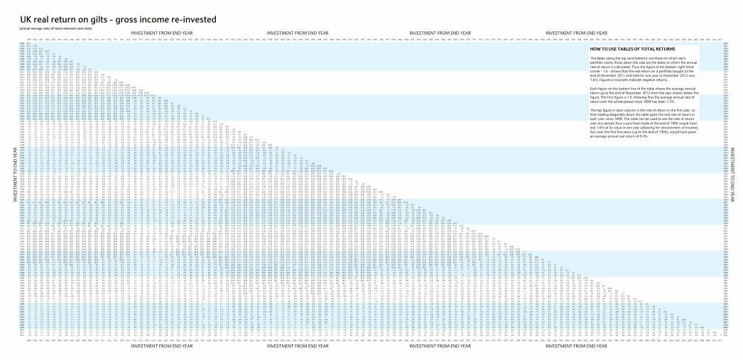
UK real return on gilts - gross income re-invested(annual average rates of return between year ends)

INVESTMENT FROM END YEAR INVESTMENT FROM END YEAR INVESTMENT FROM END YEAR INVESTMENT FROM END YEAR1899 1900 1901 1902 1903 1904 1905 1906 1907 1908 1909 1910 1911 1912 1913 1914 1915 1916 1917 1918 1919 1920 1921 1922 1923 1924 1925 1926 1927 1928 1929 1930 1931 1932 1933 1934 1935 1936 1937 1938 1939 1940 1941 1942 1943 1944 1945 1946 1947 1948 1949 1950 1951 1952 1953 1954 1955 1956 1957 1958 1959 1960 1961 1962 1963 1964 1965 1966 1967 1968 1969 1970 1971 1972 1973 1974 1975 1976 1977 1978 1979 1980 1981 1982 1983 1984 1985 1986 1987 1988 1989 1990 1991 1992 1993 1994 1995 1996 1997 1998 1999 2000 2001 2002 2003 2004 2005 2006 2007 2008 2009 2010 2011

1900 (2.1) 1900 1901 (1.6) (1.0) 1901 1902 (1.5) (1.1) (1.2) 1902 1903 (1.9) (1.8) (2.2) (3.1) 1903 1904 (0.7) (0.4) (0.1) 0.4 4.0 1904 1905 (0.0) 0.4 0.8 1.4 3.8 3.6 1905 1906 0.8 1.3 1.7 2.5 4.4 4.6 5.6 1906 1907 (0.5) (0.3) (0.2) 0.0 0.8 (0.2) (2.0) (9.1) 1907 1908 (0.4) (0.2) (0.1) 0.1 0.8 (0.0) (1.2) (4.4) 0.5 1908 1909 (0.2) 0.0 0.1 0.3 0.9 0.3 (0.5) (2.4) 1.1 1.7 1909 1910 (0.3) (0.1) (0.0) 0.1 0.6 0.0 (0.6) (2.1) 0.3 0.2 (1.3) 1910 1911 (0.5) (0.3) (0.3) (0.2) 0.2 (0.3) (1.0) (2.2) (0.4) (0.7) (1.9) (2.6) 1911 1912 (0.6) (0.5) (0.4) (0.4) (0.0) (0.5) (1.1) (2.2) (0.7) (1.1) (2.0) (2.3) (2.0) 1912 1913 (0.7) (0.6) (0.5) (0.4) (0.2) (0.6) (1.1) (2.1) (0.8) (1.1) (1.8) (2.0) (1.7) (1.4) 1913 1914 (0.3) (0.2) (0.1) (0.0) 0.2 (0.1) (0.5) (1.3) (0.1) (0.2) (0.6) (0.4) 0.3 1.5 4.5 1914 1915 (1.4) (1.4) (1.4) (1.4) (1.3) (1.7) (2.2) (3.1) (2.3) (2.7) (3.4) (3.8) (4.1) (4.8) (6.5) (16.3) 1915 1916 (3.6) (3.7) (3.9) (4.1) (4.1) (4.8) (5.5) (6.6) (6.3) (7.1) (8.3) (9.4) (10.7) (12.8) (16.3) (25.0) (32.8) 1916 1917 (4.3) (4.4) (4.6) (4.8) (4.9) (5.6) (6.3) (7.3) (7.2) (8.0) (9.1) (10.2) (11.4) (13.1) (15.9) (21.7) (24.3) (14.7) 1917 1918 (4.1) (4.3) (4.4) (4.6) (4.7) (5.3) (6.0) (6.9) (6.7) (7.4) (8.3) (9.2) (10.1) (11.4) (13.3) (17.2) (17.5) (8.6) (2.0) 1918 1919 (4.5) (4.6) (4.8) (5.0) (5.1) (5.7) (6.3) (7.2) (7.0) (7.7) (8.6) (9.3) (10.2) (11.3) (12.8) (15.9) (15.8) (9.2) (6.4) (10.5) 1919 1920 (5.4) (5.6) (5.8) (6.1) (6.2) (6.8) (7.5) (8.4) (8.3) (9.0) (9.9) (10.8) (11.6) (12.7) (14.3) (17.0) (17.2) (12.7) (12.1) (16.7) (22.5) 1920 1921 (3.2) (3.3) (3.4) (3.5) (3.5) (3.9) (4.4) (5.0) (4.7) (5.1) (5.6) (6.0) (6.4) (6.8) (7.5) (9.1) (7.8) (1.8) 1.7 3.0 10.5 57.5 1921 1922 (2.0) (2.0) (2.1) (2.1) (2.0) (2.4) (2.7) (3.2) (2.8) (3.0) (3.4) (3.6) (3.7) (3.8) (4.1) (5.1) (3.4) 2.6 6.5 8.7 16.1 42.0 28.0 1922 1923 (1.7) (1.7) (1.7) (1.7) (1.7) (2.0) (2.2) (2.7) (2.3) (2.5) (2.7) (2.9) (2.9) (3.0) (3.1) (3.9) (2.3) 3.1 6.4 8.2 13.5 28.8 16.5 6.0 1923 1924 (1.4) (1.4) (1.4) (1.4) (1.4) (1.6) (1.9) (2.3) (1.9) (2.0) (2.3) (2.3) (2.3) (2.3) (2.4) (3.1) (1.5) 3.3 6.2 7.6 11.7 22.4 12.5 5.5 4.9 1924 1925 (1.3) (1.3) (1.3) (1.3) (1.2) (1.4) (1.7) (2.0) (1.6) (1.7) (2.0) (2.0) (2.0) (2.0) (2.0) (2.6) (1.1) 3.3 5.8 6.9 10.1 18.2 10.0 4.5 3.8 2.7 1925 1926 (1.2) (1.1) (1.1) (1.1) (1.1) (1.3) (1.5) (1.8) (1.4) (1.6) (1.7) (1.8) (1.7) (1.7) (1.7) (2.2) (0.8) 3.1 5.3 6.3 8.9 15.3 8.3 3.8 3.1 2.2 1.8 1926 1927 (0.7) (0.6) (0.6) (0.6) (0.5) (0.7) (0.9) (1.2) (0.7) (0.8) (0.9) (0.9) (0.8) (0.7) (0.7) (1.1) 0.3 4.0 6.1 7.1 9.5 15.0 9.1 5.7 5.6 5.9 7.5 13.6 1927 1928 (0.4) (0.4) (0.4) (0.3) (0.2) (0.4) (0.6) (0.8) (0.4) (0.5) (0.6) (0.5) (0.4) (0.3) (0.2) (0.6) 0.8 4.2 6.1 7.0 9.1 13.9 8.7 5.8 5.8 6.0 7.1 9.9 6.4 1928 1929 (0.5) (0.4) (0.4) (0.4) (0.2) (0.4) (0.6) (0.8) (0.4) (0.5) (0.6) (0.6) (0.4) (0.4) (0.3) (0.6) 0.6 3.8 5.5 6.2 8.1 12.1 7.5 4.8 4.6 4.6 5.0 6.2 2.6 (1.0) 1929 1930 0.2 0.3 0.3 0.4 0.5 0.4 0.2 0.0 0.4 0.4 0.4 0.5 0.6 0.8 0.9 0.7 1.9 5.0 6.7 7.5 9.3 13.1 9.0 6.8 6.9 7.3 8.2 9.9 8.7 9.9 21.9 1930 1931 0.3 0.4 0.4 0.5 0.6 0.5 0.4 0.2 0.6 0.6 0.5 0.6 0.8 1.0 1.1 0.9 2.1 5.0 6.5 7.2 8.8 12.2 8.5 6.5 6.6 6.8 7.5 8.7 7.6 8.0 12.7 4.3 1931 1932 1.4 1.6 1.6 1.7 1.9 1.8 1.8 1.6 2.1 2.1 2.2 2.3 2.6 2.8 3.0 2.9 4.2 7.1 8.7 9.5 11.3 14.7 11.4 9.9 10.3 11.0 12.2 14.1 14.2 16.2 22.6 23.0 45.0 1932 1933 1.5 1.6 1.7 1.8 2.0 1.9 1.8 1.7 2.1 2.2 2.2 2.4 2.6 2.8 3.0 3.0 4.1 6.9 8.4 9.1 10.7 13.7 10.7 9.2 9.6 10.1 11.1 12.5 12.3 13.5 17.4 16.0 22.3 3.2 1933 1934 2.1 2.3 2.4 2.5 2.7 2.6 2.6 2.5 2.9 3.0 3.1 3.3 3.5 3.8 4.1 4.0 5.2 7.9 9.4 10.1 11.7 14.6 11.9 10.6 11.0 11.7 12.7 14.2 14.3 15.6 19.3 18.6 23.8 14.4 26.9 1934 1935 1.9 2.1 2.1 2.2 2.4 2.4 2.3 2.2 2.6 2.7 2.8 2.9 3.2 3.4 3.6 3.6 4.7 7.2 8.5 9.2 10.6 13.2 10.6 9.3 9.6 10.0 10.8 11.9 11.6 12.4 14.8 13.4 15.9 7.5 9.7 (5.1) 1935 1936 1.8 1.9 2.0 2.1 2.3 2.2 2.2 2.1 2.5 2.5 2.6 2.7 2.9 3.2 3.4 3.3 4.3 6.7 7.9 8.5 9.7 12.2 9.6 8.4 8.6 8.9 9.5 10.3 10.0 10.4 12.2 10.6 12.0 4.9 5.5 (3.8) (2.4) 1936 1937 1.4 1.4 1.5 1.6 1.7 1.7 1.6 1.5 1.9 1.9 1.9 2.0 2.2 2.4 2.5 2.5 3.4 5.6 6.7 7.2 8.2 10.4 8.0 6.7 6.8 6.9 7.3 7.8 7.3 7.4 8.5 6.7 7.1 0.8 0.2 (7.4) (8.6) (14.4) 1937 1938 1.3 1.4 1.5 1.6 1.7 1.6 1.6 1.5 1.8 1.9 1.9 2.0 2.1 2.3 2.5 2.4 3.3 5.3 6.4 6.8 7.8 9.8 7.5 6.3 6.4 6.5 6.8 7.2 6.6 6.7 7.5 5.9 6.1 0.7 0.2 (5.5) (5.7) (7.3) 0.4 1938 1939 1.1 1.1 1.2 1.3 1.4 1.3 1.2 1.1 1.5 1.5 1.5 1.6 1.7 1.9 2.0 1.9 2.7 4.6 5.6 6.0 6.9 8.7 6.5 5.4 5.3 5.4 5.5 5.8 5.2 5.1 5.8 4.1 4.1 (0.7) (1.4) (6.2) (6.5) (7.9) (4.4) (9.0) 1939 1940 1.1 1.2 1.2 1.3 1.4 1.4 1.3 1.2 1.5 1.5 1.5 1.6 1.8 1.9 2.0 1.9 2.7 4.6 5.5 5.9 6.7 8.4 6.3 5.2 5.2 5.2 5.4 5.6 5.0 4.9 5.5 4.0 3.9 (0.3) (0.8) (4.8) (4.7) (5.3) (2.1) (3.3) 2.9 1940 1941 1.2 1.3 1.4 1.5 1.6 1.5 1.5 1.3 1.7 1.7 1.7 1.8 1.9 2.1 2.2 2.1 2.9 4.7 5.6 5.9 6.7 8.4 6.4 5.3 5.3 5.3 5.5 5.7 5.2 5.1 5.6 4.3 4.3 0.5 0.2 (3.1) (2.8) (2.9) 0.2 0.1 5.0 7.3 1941 1942 1.3 1.4 1.4 1.5 1.6 1.6 1.5 1.4 1.7 1.7 1.7 1.8 2.0 2.1 2.2 2.2 2.9 4.6 5.5 5.8 6.6 8.1 6.2 5.2 5.2 5.2 5.4 5.6 5.1 5.0 5.4 4.2 4.2 0.8 0.5 (2.4) (2.0) (1.9) 0.8 0.9 4.4 5.2 3.2 1942 1943 1.3 1.3 1.4 1.5 1.6 1.5 1.5 1.4 1.7 1.7 1.7 1.8 1.9 2.1 2.2 2.1 2.8 4.5 5.3 5.6 6.3 7.8 5.9 5.0 4.9 4.9 5.0 5.2 4.7 4.6 5.1 3.9 3.8 0.7 0.5 (2.1) (1.7) (1.6) 0.7 0.7 3.3 3.5 1.6 0.1 1943 1944 1.3 1.4 1.5 1.5 1.7 1.6 1.5 1.4 1.7 1.8 1.8 1.9 2.0 2.1 2.2 2.2 2.9 4.5 5.2 5.5 6.2 7.6 5.9 5.0 4.9 4.9 5.0 5.2 4.7 4.6 5.0 3.9 3.9 1.0 0.8 (1.4) (1.0) (0.9) 1.2 1.4 3.6 3.8 2.6 2.3 4.6 1944 1945 1.6 1.7 1.7 1.8 1.9 1.9 1.8 1.7 2.0 2.1 2.1 2.2 2.3 2.5 2.6 2.5 3.2 4.8 5.5 5.8 6.5 7.9 6.2 5.3 5.3 5.3 5.4 5.6 5.2 5.1 5.5 4.5 4.6 2.0 1.9 (0.2) 0.3 0.7 2.7 3.0 5.2 5.7 5.3 6.0 9.1 13.7 1945 1946 1.8 1.8 1.9 2.0 2.1 2.1 2.0 1.9 2.2 2.3 2.3 2.4 2.5 2.7 2.8 2.8 3.4 4.9 5.7 6.0 6.6 8.0 6.3 5.5 5.5 5.5 5.7 5.9 5.5 5.4 5.8 4.9 4.9 2.5 2.5 0.7 1.2 1.6 3.5 3.9 5.9 6.4 6.2 7.0 9.4 11.9 10.2 1946 1947 1.3 1.4 1.5 1.5 1.6 1.6 1.5 1.4 1.7 1.7 1.7 1.8 1.9 2.1 2.2 2.1 2.7 4.2 4.8 5.1 5.7 6.9 5.3 4.5 4.5 4.4 4.5 4.6 4.2 4.1 4.4 3.5 3.4 1.1 0.9 (0.8) (0.4) (0.3) 1.3 1.4 2.7 2.7 2.0 1.7 2.1 1.3 (4.3) (16.9) 1947 1948 1.2 1.3 1.3 1.4 1.5 1.4 1.4 1.3 1.6 1.6 1.6 1.7 1.8 1.9 2.0 1.9 2.5 3.9 4.5 4.8 5.3 6.5 5.0 4.2 4.1 4.1 4.1 4.2 3.8 3.7 3.9 3.0 2.9 0.8 0.6 (1.0) (0.7) (0.6) 0.8 0.8 2.0 1.9 1.1 0.7 0.9 (0.0) (4.2) (10.7) (4.0) 1948 1949 0.9 1.0 1.0 1.1 1.2 1.1 1.1 1.0 1.2 1.2 1.2 1.3 1.4 1.5 1.6 1.5 2.1 3.4 4.0 4.2 4.7 5.8 4.3 3.5 3.4 3.4 3.4 3.5 3.0 2.9 3.1 2.2 2.1 (0.0) (0.2) (1.8) (1.6) (1.5) (0.4) (0.4) 0.5 0.2 (0.6) (1.2) (1.4) (2.5) (6.2) (11.1) (8.1) (12.0) 1949 1950 0.9 1.0 1.0 1.1 1.2 1.1 1.1 1.0 1.2 1.2 1.2 1.3 1.4 1.5 1.5 1.5 2.0 3.3 3.9 4.1 4.6 5.6 4.2 3.4 3.3 3.3 3.3 3.4 2.9 2.8 3.0 2.1 2.0 0.0 (0.2) (1.7) (1.4) (1.4) (0.3) (0.3) 0.5 0.3 (0.5) (0.9) (1.1) (2.0) (4.9) (8.3) (5.2) (5.8) 0.8 1950 1951 0.5 0.6 0.6 0.6 0.7 0.6 0.6 0.5 0.7 0.7 0.7 0.7 0.8 0.9 0.9 0.8 1.4 2.6 3.1 3.3 3.7 4.7 3.3 2.5 2.4 2.3 2.3 2.3 1.9 1.7 1.8 1.0 0.8 (1.1) (1.3) (2.8) (2.7) (2.7) (1.8) (1.9) (1.3) (1.7) (2.6) (3.2) (3.6) (4.7) (7.4) (10.6) (9.0) (10.6) (9.8) (19.3) 1951 1952 0.4 0.4 0.4 0.5 0.5 0.5 0.4 0.3 0.5 0.5 0.5 0.5 0.6 0.7 0.7 0.6 1.1 2.3 2.8 3.0 3.4 4.3 3.0 2.2 2.1 2.0 2.0 2.0 1.5 1.3 1.4 0.6 0.4 (1.4) (1.6) (3.0) (2.9) (2.9) (2.1) (2.3) (1.8) (2.1) (2.9) (3.5) (3.9) (4.9) (7.3) (10.0) (8.5) (9.6) (8.8) (13.3) (6.7) 1952 1953 0.6 0.6 0.7 0.7 0.8 0.7 0.7 0.5 0.8 0.8 0.8 0.8 0.9 1.0 1.0 0.9 1.4 2.6 3.1 3.2 3.7 4.6 3.3 2.5 2.4 2.3 2.3 2.4 1.9 1.8 1.9 1.1 1.0 (0.8) (1.0) (2.2) (2.1) (2.1) (1.2) (1.4) (0.8) (1.1) (1.7) (2.2) (2.4) (3.1) (5.0) (7.0) (5.3) (5.5) (3.8) (5.3) 2.6 12.8 1953 1954 0.6 0.7 0.7 0.7 0.8 0.7 0.7 0.6 0.8 0.8 0.8 0.8 0.9 1.0 1.0 1.0 1.4 2.5 3.1 3.2 3.6 4.5 3.2 2.5 2.4 2.3 2.3 2.3 2.0 1.8 1.9 1.1 1.0 (0.6) (0.8) (2.0) (1.9) (1.8) (1.1) (1.1) (0.6) (0.8) (1.4) (1.8) (2.0) (2.6) (4.3) (5.9) (4.3) (4.3) (2.7) (3.5) 2.4 7.3 2.0 1954 1955 0.3 0.3 0.4 0.4 0.5 0.4 0.3 0.2 0.4 0.4 0.4 0.4 0.5 0.6 0.6 0.5 1.0 2.1 2.5 2.7 3.1 3.9 2.6 1.9 1.8 1.7 1.7 1.7 1.3 1.1 1.2 0.4 0.3 (1.3) (1.5) (2.7) (2.6) (2.6) (1.9) (2.0) (1.6) (1.9) (2.5) (2.9) (3.1) (3.8) (5.4) (7.0) (5.7) (5.9) (4.9) (6.0) (2.3) (0.7) (6.9) (15.0) 1955 1956 0.2 0.2 0.3 0.3 0.3 0.3 0.2 0.1 0.3 0.3 0.3 0.3 0.4 0.4 0.5 0.4 0.8 1.8 2.3 2.4 2.8 3.6 2.4 1.7 1.6 1.5 1.4 1.4 1.0 0.8 0.9 0.2 0.0 (1.5) (1.7) (2.8) (2.7) (2.8) (2.1) (2.2) (1.8) (2.1) (2.7) (3.1) (3.4) (4.0) (5.5) (6.9) (5.7) (5.9) (5.0) (6.0) (3.0) (2.1) (6.6) (10.6) (6.0) 1956 1957 (0.0) 0.0 0.0 0.1 0.1 0.1 (0.0) (0.1) 0.1 0.1 0.0 0.1 0.1 0.2 0.2 0.1 0.5 1.5 2.0 2.1 2.4 3.2 2.0 1.3 1.2 1.1 1.0 1.0 0.6 0.4 0.5 (0.2) (0.4) (1.9) (2.1) (3.2) (3.1) (3.1) (2.5) (2.7) (2.3) (2.6) (3.2) (3.6) (3.9) (4.5) (5.9) (7.2) (6.2) (6.4) (5.7) (6.6) (4.3) (3.8) (7.6) (10.6) (8.2) (10.4) 1957 1958 0.2 0.3 0.3 0.3 0.4 0.3 0.3 0.2 0.3 0.3 0.3 0.4 0.4 0.5 0.5 0.4 0.8 1.8 2.3 2.4 2.7 3.5 2.3 1.7 1.6 1.5 1.4 1.4 1.1 0.9 0.9 0.3 0.1 (1.3) (1.5) (2.5) (2.4) (2.4) (1.8) (1.9) (1.5) (1.7) (2.2) (2.6) (2.7) (3.2) (4.4) (5.6) (4.4) (4.5) (3.6) (4.2) (1.8) (0.9) (3.5) (4.8) (1.1) 1.5 14.9 1958 1959 0.2 0.3 0.3 0.3 0.4 0.3 0.3 0.2 0.4 0.4 0.3 0.4 0.4 0.5 0.5 0.4 0.8 1.8 2.2 2.3 2.7 3.4 2.3 1.7 1.6 1.5 1.4 1.4 1.1 0.9 0.9 0.3 0.2 (1.2) (1.4) (2.4) (2.2) (2.2) (1.6) (1.7) (1.4) (1.6) (2.1) (2.4) (2.5) (3.0) (4.1) (5.1) (4.0) (4.0) (3.2) (3.6) (1.4) (0.7) (2.7) (3.7) (0.6) 1.3 7.7 0.9 1959 1960 0.1 0.1 0.1 0.2 0.2 0.2 0.1 0.0 0.2 0.2 0.1 0.2 0.2 0.3 0.3 0.2 0.6 1.6 2.0 2.1 2.4 3.1 2.0 1.4 1.3 1.2 1.1 1.1 0.7 0.6 0.6 (0.0) (0.2) (1.5) (1.7) (2.6) (2.5) (2.5) (2.0) (2.1) (1.7) (2.0) (2.4) (2.7) (2.9) (3.3) (4.4) (5.3) (4.4) (4.4) (3.7) (4.1) (2.3) (1.7) (3.6) (4.5) (2.3) (1.3) 1.9 (4.0) (8.7) 1960 1961 (0.1) (0.1) (0.1) (0.0) 0.0 (0.1) (0.1) (0.2) (0.1) (0.1) (0.1) (0.1) (0.0) 0.0 0.0 (0.1) 0.3 1.2 1.6 1.7 2.0 2.7 1.6 1.0 0.9 0.8 0.7 0.7 0.3 0.2 0.2 (0.4) (0.6) (1.9) (2.0) (3.0) (2.9) (2.9) (2.4) (2.5) (2.2) (2.5) (2.9) (3.2) (3.4) (3.9) (4.9) (5.8) (4.9) (5.0) (4.4) (4.9) (3.3) (2.9) (4.7) (5.6) (3.9) (3.5) (1.7) (6.7) (10.3) (11.9) 1961 1962 0.2 0.2 0.3 0.3 0.3 0.3 0.2 0.1 0.3 0.3 0.3 0.3 0.4 0.4 0.4 0.4 0.7 1.6 2.0 2.1 2.4 3.1 2.1 1.5 1.4 1.3 1.2 1.2 0.9 0.7 0.8 0.2 0.1 (1.2) (1.3) (2.2) (2.1) (2.1) (1.5) (1.6) (1.3) (1.5) (1.9) (2.1) (2.2) (2.6) (3.5) (4.3) (3.4) (3.3) (2.6) (2.9) (1.2) (0.7) (2.1) (2.6) (0.7) 0.3 2.5 (0.3) (0.7) 3.5 21.5 1962 1963 0.2 0.3 0.3 0.3 0.4 0.3 0.2 0.2 0.3 0.3 0.3 0.3 0.4 0.4 0.5 0.4 0.8 1.6 2.0 2.1 2.4 3.1 2.1 1.5 1.4 1.3 1.3 1.2 0.9 0.8 0.8 0.2 0.1 (1.1) (1.2) (2.1) (1.9) (1.9) (1.4) (1.5) (1.2) (1.3) (1.7) (1.9) (2.0) (2.4) (3.2) (3.9) (3.1) (3.0) (2.3) (2.5) (1.0) (0.5) (1.7) (2.1) (0.4) 0.5 2.4 0.1 (0.1) 2.9 11.2 1.8 1963 1964 0.1 0.1 0.2 0.2 0.2 0.2 0.1 0.0 0.2 0.2 0.2 0.2 0.2 0.3 0.3 0.2 0.6 1.5 1.8 1.9 2.2 2.9 1.8 1.3 1.2 1.1 1.0 1.0 0.7 0.6 0.6 0.0 (0.1) (1.2) (1.4) (2.2) (2.1) (2.1) (1.6) (1.7) (1.4) (1.6) (1.9) (2.2) (2.3) (2.6) (3.4) (4.1) (3.3) (3.2) (2.6) (2.8) (1.5) (1.0) (2.2) (2.6) (1.1) (0.4) 1.1 (1.1) (1.5) 0.4 4.9 (2.6) (6.7) 1964 1965 0.1 0.1 0.2 0.2 0.2 0.2 0.1 0.0 0.2 0.2 0.2 0.2 0.2 0.3 0.3 0.2 0.6 1.4 1.8 1.9 2.2 2.8 1.8 1.3 1.1 1.1 1.0 1.0 0.7 0.5 0.6 0.0 (0.1) (1.2) (1.4) (2.1) (2.0) (2.0) (1.6) (1.6) (1.3) (1.5) (1.9) (2.1) (2.2) (2.5) (3.2) (3.9) (3.1) (3.0) (2.5) (2.7) (1.4) (0.9) (2.0) (2.4) (1.0) (0.4) 0.9 (0.9) (1.3) 0.3 3.6 (1.8) (3.5) (0.1) 1965 1966 0.1 0.1 0.2 0.2 0.2 0.2 0.1 0.0 0.2 0.2 0.2 0.2 0.2 0.3 0.3 0.2 0.6 1.4 1.8 1.8 2.1 2.7 1.8 1.2 1.1 1.0 1.0 1.0 0.7 0.5 0.6 0.0 (0.1) (1.2) (1.3) (2.1) (2.0) (2.0) (1.5) (1.6) (1.3) (1.4) (1.8) (2.0) (2.1) (2.3) (3.1) (3.7) (2.9) (2.9) (2.3) (2.5) (1.2) (0.8) (1.8) (2.1) (0.9) (0.3) 0.9 (0.8) (1.0) 0.3 3.0 (1.2) (2.2) 0.2 0.5 1966 1967 0.1 0.1 0.2 0.2 0.2 0.2 0.1 0.0 0.2 0.2 0.2 0.2 0.2 0.3 0.3 0.2 0.6 1.4 1.7 1.8 2.1 2.7 1.7 1.2 1.1 1.0 1.0 1.0 0.7 0.5 0.6 0.0 (0.1) (1.1) (1.3) (2.0) (1.9) (1.9) (1.4) (1.5) (1.2) (1.4) (1.7) (1.9) (2.0) (2.2) (2.9) (3.5) (2.8) (2.7) (2.2) (2.3) (1.2) (0.8) (1.7) (1.9) (0.8) (0.3) 0.8 (0.7) (0.9) 0.3 2.5 (0.9) (1.6) 0.2 0.3 0.1 1967 1968 (0.0) 0.0 0.0 0.1 0.1 0.0 (0.0) (0.1) 0.1 0.0 0.0 0.0 0.1 0.1 0.2 0.1 0.4 1.2 1.5 1.6 1.9 2.5 1.5 1.0 0.9 0.8 0.8 0.7 0.5 0.3 0.3 (0.2) (0.3) (1.3) (1.4) (2.2) (2.1) (2.1) (1.7) (1.7) (1.5) (1.6) (1.9) (2.1) (2.2) (2.5) (3.1) (3.7) (3.0) (3.0) (2.5) (2.6) (1.6) (1.2) (2.1) (2.4) (1.3) (0.9) (0.0) (1.4) (1.7) (0.8) 0.9 (2.1) (2.9) (1.9) (2.5) (4.0) (7.8) 1968 1969 (0.1) (0.0) (0.0) (0.0) 0.0 (0.0) (0.1) (0.2) (0.0) (0.0) (0.1) (0.0) 0.0 0.1 0.1 (0.0) 0.3 1.1 1.4 1.5 1.7 2.3 1.4 0.9 0.8 0.7 0.7 0.6 0.3 0.2 0.2 (0.3) (0.4) (1.4) (1.5) (2.2) (2.2) (2.1) (1.7) (1.8) (1.6) (1.7) (2.0) (2.2) (2.3) (2.6) (3.2) (3.7) (3.1) (3.0) (2.6) (2.7) (1.7) (1.4) (2.2) (2.5) (1.5) (1.2) (0.4) (1.7) (1.9) (1.1) 0.3 (2.4) (3.1) (2.4) (2.9) (4.0) (6.1) (4.2) 1969 1970 (0.1) (0.1) (0.1) (0.1) (0.0) (0.1) (0.1) (0.2) (0.1) (0.1) (0.1) (0.1) (0.1) (0.0) 0.0 (0.1) 0.2 1.0 1.3 1.4 1.6 2.2 1.3 0.8 0.7 0.6 0.5 0.5 0.2 0.1 0.1 (0.4) (0.5) (1.5) (1.6) (2.3) (2.2) (2.2) (1.8) (1.9) (1.6) (1.8) (2.1) (2.3) (2.3) (2.6) (3.2) (3.7) (3.1) (3.1) (2.6) (2.8) (1.8) (1.6) (2.3) (2.6) (1.7) (1.4) (0.7) (1.9) (2.1) (1.4) (0.2) (2.6) (3.2) (2.6) (3.1) (4.0) (5.4) (4.1) (4.0) 1970 1971 0.1 0.1 0.1 0.2 0.2 0.1 0.1 0.0 0.2 0.2 0.1 0.2 0.2 0.2 0.3 0.2 0.5 1.3 1.6 1.7 1.9 2.5 1.6 1.1 1.0 0.9 0.9 0.9 0.6 0.5 0.5 0.0 (0.1) (1.0) (1.2) (1.8) (1.7) (1.7) (1.3) (1.4) (1.1) (1.2) (1.5) (1.7) (1.7) (1.9) (2.5) (3.0) (2.4) (2.3) (1.8) (1.9) (1.0) (0.7) (1.4) (1.6) (0.6) (0.3) 0.5 (0.5) (0.7) 0.1 1.4 (0.6) (0.9) (0.1) (0.1) (0.2) (0.3) 2.4 5.9 16.8 1971 1972 (0.1) (0.0) (0.0) (0.0) 0.0 (0.0) (0.1) (0.2) (0.0) (0.0) (0.0) (0.0) 0.0 0.1 0.1 0.0 0.3 1.0 1.3 1.4 1.6 2.2 1.3 0.8 0.7 0.7 0.6 0.6 0.3 0.2 0.2 (0.3) (0.4) (1.3) (1.4) (2.1) (2.0) (2.0) (1.6) (1.6) (1.4) (1.5) (1.8) (2.0) (2.0) (2.3) (2.8) (3.3) (2.7) (2.6) (2.2) (2.4) (1.5) (1.2) (1.9) (2.1) (1.3) (1.0) (0.3) (1.3) (1.5) (0.9) 0.2 (1.7) (2.1) (1.5) (1.7) (2.0) (2.4) (1.0) 0.0 2.1 (10.7) 1972 1973 (0.3) (0.3) (0.3) (0.3) (0.2) (0.3) (0.4) (0.4) (0.3) (0.3) (0.3) (0.3) (0.3) (0.3) (0.2) (0.3) (0.0) 0.7 1.0 1.0 1.3 1.8 0.9 0.4 0.3 0.2 0.2 0.2 (0.1) (0.3) (0.2) (0.7) (0.8) (1.7) (1.8) (2.5) (2.4) (2.4) (2.1) (2.1) (1.9) (2.1) (2.3) (2.5) (2.6) (2.8) (3.4) (3.9) (3.3) (3.3) (2.9) (3.1) (2.3) (2.0) (2.7) (3.0) (2.3) (2.0) (1.5) (2.5) (2.7) (2.3) (1.4) (3.3) (3.7) (3.4) (3.8) (4.4) (5.1) (4.6) (4.7) (4.9) (14.2) (17.6) 1973 1974 (0.8) (0.8) (0.8) (0.7) (0.7) (0.8) (0.8) (0.9) (0.8) (0.8) (0.9) (0.9) (0.8) (0.8) (0.8) (0.9) (0.6) 0.1 0.4 0.4 0.6 1.1 0.3 (0.2) (0.3) (0.4) (0.5) (0.5) (0.8) (1.0) (1.0) (1.4) (1.6) (2.5) (2.6) (3.3) (3.2) (3.2) (2.9) (3.0) (2.8) (3.0) (3.3) (3.5) (3.6) (3.9) (4.4) (4.9) (4.4) (4.4) (4.1) (4.3) (3.6) (3.5) (4.2) (4.5) (3.9) (3.8) (3.3) (4.4) (4.7) (4.4) (3.8) (5.7) (6.4) (6.3) (7.0) (7.9) (9.0) (9.1) (10.1) (11.6) (19.4) (23.4) (28.8) 1974 1975 (0.6) (0.6) (0.6) (0.6) (0.6) (0.6) (0.7) (0.8) (0.7) (0.7) (0.7) (0.7) (0.7) (0.7) (0.6) (0.7) (0.4) 0.2 0.5 0.6 0.8 1.2 0.4 (0.0) (0.2) (0.3) (0.3) (0.4) (0.6) (0.8) (0.8) (1.2) (1.3) (2.2) (2.3) (3.0) (2.9) (2.9) (2.6) (2.7) (2.5) (2.6) (2.9) (3.1) (3.2) (3.4) (4.0) (4.4) (3.9) (3.9) (3.6) (3.8) (3.1) (2.9) (3.6) (3.8) (3.2) (3.1) (2.7) (3.6) (3.9) (3.6) (2.9) (4.6) (5.1) (5.0) (5.4) (6.1) (6.8) (6.7) (7.1) (7.7) (13.0) (13.7) (11.7) 9.5 1975 1976 (0.7) (0.6) (0.6) (0.6) (0.6) (0.6) (0.7) (0.8) (0.7) (0.7) (0.7) (0.7) (0.7) (0.7) (0.6) (0.7) (0.5) 0.2 0.5 0.5 0.7 1.2 0.4 (0.1) (0.2) (0.3) (0.3) (0.4) (0.6) (0.8) (0.8) (1.2) (1.3) (2.2) (2.3) (2.9) (2.9) (2.9) (2.6) (2.6) (2.5) (2.6) (2.9) (3.1) (3.1) (3.4) (3.9) (4.3) (3.9) (3.8) (3.5) (3.7) (3.0) (2.8) (3.5) (3.7) (3.1) (3.0) (2.6) (3.5) (3.7) (3.4) (2.8) (4.4) (4.8) (4.7) (5.1) (5.6) (6.2) (6.0) (6.3) (6.6) (10.7) (10.7) (8.3) 4.1 (1.1) 1976 1977 (0.3) (0.3) (0.3) (0.3) (0.2) (0.3) (0.3) (0.4) (0.3) (0.3) (0.3) (0.3) (0.3) (0.3) (0.2) (0.3) (0.0) 0.6 0.9 0.9 1.2 1.6 0.8 0.4 0.3 0.2 0.2 0.1 (0.1) (0.2) (0.2) (0.6) (0.8) (1.6) (1.7) (2.3) (2.2) (2.2) (1.9) (1.9) (1.7) (1.9) (2.1) (2.3) (2.3) (2.5) (3.0) (3.4) (2.9) (2.9) (2.5) (2.6) (1.9) (1.7) (2.3) (2.5) (1.9) (1.7) (1.2) (2.0) (2.2) (1.8) (1.1) (2.4) (2.7) (2.4) (2.6) (2.9) (3.2) (2.6) (2.4) (2.2) (5.1) (3.9) (0.1) 11.8 13.0 29.1 1977 1978 (0.4) (0.4) (0.4) (0.4) (0.4) (0.4) (0.5) (0.6) (0.4) (0.4) (0.5) (0.5) (0.4) (0.4) (0.4) (0.5) (0.2) 0.5 0.7 0.8 1.0 1.4 0.7 0.2 0.1 0.0 (0.0) (0.1) (0.3) (0.4) (0.4) (0.8) (0.9) (1.8) (1.9) (2.4) (2.4) (2.4) (2.1) (2.1) (1.9) (2.1) (2.3) (2.5) (2.5) (2.7) (3.2) (3.6) (3.1) (3.1) (2.8) (2.9) (2.2) (2.0) (2.6) (2.8) (2.2) (2.0) (1.6) (2.4) (2.6) (2.2) (1.6) (2.9) (3.2) (2.9) (3.1) (3.4) (3.8) (3.3) (3.2) (3.1) (5.7) (4.8) (2.1) 6.1 5.0 8.1 (9.4) 1978 1979 (0.6) (0.6) (0.6) (0.5) (0.5) (0.6) (0.6) (0.7) (0.6) (0.6) (0.6) (0.6) (0.6) (0.6) (0.6) (0.6) (0.4) 0.3 0.5 0.6 0.8 1.2 0.4 0.0 (0.1) (0.2) (0.2) (0.3) (0.5) (0.7) (0.7) (1.1) (1.2) (2.0) (2.1) (2.6) (2.6) (2.6) (2.3) (2.4) (2.2) (2.3) (2.6) (2.7) (2.8) (3.0) (3.4) (3.8) (3.4) (3.4) (3.1) (3.2) (2.6) (2.4) (2.9) (3.1) (2.6) (2.5) (2.1) (2.8) (3.0) (2.7) (2.2) (3.4) (3.7) (3.5) (3.7) (4.1) (4.4) (4.1) (4.1) (4.1) (6.4) (5.8) (3.6) 2.4 0.7 1.3 (10.3) (11.2) 1979 1980 (0.5) (0.5) (0.5) (0.5) (0.4) (0.5) (0.6) (0.6) (0.5) (0.5) (0.6) (0.5) (0.5) (0.5) (0.5) (0.6) (0.3) 0.3 0.6 0.6 0.8 1.3 0.5 0.1 (0.0) (0.1) (0.1) (0.2) (0.4) (0.6) (0.5) (0.9) (1.0) (1.8) (1.9) (2.5) (2.4) (2.4) (2.1) (2.2) (2.0) (2.1) (2.4) (2.5) (2.6) (2.8) (3.2) (3.6) (3.1) (3.1) (2.8) (2.9) (2.3) (2.1) (2.7) (2.8) (2.3) (2.2) (1.8) (2.5) (2.6) (2.3) (1.8) (2.9) (3.2) (3.0) (3.2) (3.4) (3.7) (3.4) (3.3) (3.2) (5.2) (4.5) (2.5) 2.8 1.5 2.2 (5.5) (3.4) 5.0 1980 1981 (0.6) (0.6) (0.6) (0.6) (0.6) (0.6) (0.7) (0.8) (0.6) (0.6) (0.7) (0.7) (0.6) (0.6) (0.6) (0.7) (0.4) 0.2 0.4 0.5 0.7 1.1 0.3 (0.1) (0.2) (0.3) (0.3) (0.4) (0.6) (0.7) (0.7) (1.1) (1.2) (2.0) (2.1) (2.6) (2.6) (2.6) (2.3) (2.4) (2.2) (2.3) (2.5) (2.7) (2.8) (3.0) (3.4) (3.7) (3.3) (3.3) (3.0) (3.1) (2.5) (2.4) (2.9) (3.1) (2.6) (2.4) (2.1) (2.8) (2.9) (2.7) (2.2) (3.3) (3.6) (3.4) (3.6) (3.8) (4.1) (3.8) (3.8) (3.8) (5.6) (5.0) (3.3) 1.0 (0.4) (0.2) (6.4) (5.4) (2.3) (9.2) 1981 1982 (0.2) (0.2) (0.1) (0.1) (0.1) (0.1) (0.2) (0.3) (0.1) (0.2) (0.2) (0.2) (0.1) (0.1) (0.1) (0.1) 0.1 0.7 1.0 1.0 1.2 1.7 0.9 0.5 0.4 0.4 0.3 0.3 0.1 (0.0) (0.0) (0.4) (0.5) (1.2) (1.3) (1.8) (1.8) (1.8) (1.5) (1.5) (1.3) (1.4) (1.6) (1.7) (1.8) (1.9) (2.3) (2.7) (2.2) (2.2) (1.9) (1.9) (1.3) (1.1) (1.6) (1.7) (1.2) (1.0) (0.6) (1.2) (1.3) (0.9) (0.4) (1.4) (1.5) (1.2) (1.3) (1.4) (1.5) (1.0) (0.8) (0.5) (1.9) (1.0) 1.0 5.5 5.0 6.0 1.9 5.0 11.1 14.2 43.6 1982 1983 (0.1) (0.0) (0.0) (0.0) 0.0 (0.0) (0.1) (0.1) (0.0) (0.0) (0.0) (0.0) 0.0 0.0 0.1 (0.0) 0.3 0.9 1.1 1.2 1.4 1.8 1.1 0.7 0.6 0.5 0.5 0.5 0.2 0.1 0.2 (0.2) (0.3) (1.0) (1.1) (1.6) (1.5) (1.5) (1.2) (1.3) (1.1) (1.2) (1.4) (1.5) (1.5) (1.7) (2.0) (2.3) (1.9) (1.8) (1.5) (1.6) (1.0) (0.8) (1.2) (1.3) (0.8) (0.6) (0.2) (0.8) (0.8) (0.5) 0.1 (0.8) (1.0) (0.7) (0.7) (0.8) (0.8) (0.3) (0.0) 0.3 (1.0) (0.1) 1.9 6.0 5.6 6.6 3.2 6.0 10.8 12.8 25.7 10.0 1983 1984 (0.0) (0.0) (0.0) 0.0 0.1 0.0 (0.0) (0.1) 0.0 0.0 (0.0) (0.0) 0.0 0.1 0.1 0.0 0.3 0.9 1.1 1.2 1.4 1.8 1.1 0.7 0.6 0.5 0.5 0.5 0.3 0.2 0.2 (0.2) (0.3) (1.0) (1.0) (1.5) (1.5) (1.4) (1.2) (1.2) (1.0) (1.1) (1.3) (1.4) (1.4) (1.6) (1.9) (2.2) (1.8) (1.7) (1.4) (1.5) (0.9) (0.7) (1.1) (1.2) (0.7) (0.5) (0.1) (0.6) (0.7) (0.4) 0.2 (0.7) (0.8) (0.5) (0.5) (0.6) (0.6) (0.2) 0.1 0.4 (0.8) 0.1 1.9 5.6 5.2 6.0 3.1 5.3 9.0 10.0 17.3 6.0 2.1 1984 1985 0.0 0.0 0.1 0.1 0.1 0.1 0.0 (0.0) 0.1 0.1 0.0 0.1 0.1 0.1 0.1 0.1 0.3 0.9 1.2 1.2 1.4 1.8 1.1 0.8 0.7 0.6 0.6 0.6 0.4 0.3 0.3 (0.1) (0.2) (0.9) (0.9) (1.4) (1.3) (1.3) (1.0) (1.1) (0.9) (1.0) (1.1) (1.2) (1.3) (1.4) (1.8) (2.0) (1.6) (1.6) (1.2) (1.3) (0.7) (0.5) (0.9) (1.0) (0.5) (0.3) 0.1 (0.4) (0.5) (0.2) 0.4 (0.5) (0.6) (0.3) (0.3) (0.3) (0.3) 0.1 0.4 0.7 (0.4) 0.5 2.2 5.6 5.2 5.9 3.3 5.3 8.3 9.0 14.1 5.7 3.6 5.0 1985 1986 0 1 0 1 0 1 0 1 0 2 0 1 0 1 0 0 0 2 0 2 0 1 0 2 0 2 0 2 0 2 0 2 0 4 1 0 1 3 1 3 1 5 1 9 1 2 0 9 0 8 0 7 0 7 0 7 0 5 0 4 0 4 0 0 (0 0) (0 7) (0 8) (1 3) (1 2) (1 2) (0 9) (0 9) (0 7) (0 8) (1 0) (1 1) (1 1) (1 2) (1 6) (1 8) (1 4) (1 3) (1 0) (1 1) (0 5) (0 3) (0 7) (0 8) (0 3) (0 1) 0 3 (0 2) (0 2) 0 1 0 6 (0 2) (0 3) 0 1 0 1 0 0 0 0 0 5 0 8 1 1 0 1 0 9 2 5 5 7 5 3 6 0 3 7 5 5 8 1 8 7 12 6 6 0 4 7 6 0 7 0 1986

INV

ESTM

ENT

TO E

ND

YEA

R INV

ESTMEN

T TO EN

D YEA

R

HOW TO USE TABLES OF TOTAL RETURNS

The dates along the top (and bottom) are those on which each portfolio starts; those down the side are the dates to which the annual rate of return is calculated. Thus the figure at the bottom right hand corner - 1.6 - shows that the real return on a portfolio bought at the end of December 2011 and held for one year to December 2012 was 1.6%. Figures in brackets indicate negative returns.

Each figure on the bottom line of the table shows the average annual return up to the end of December 2012 from the year shown below the figure. The first figure is 1.3, showing that the average annual rate of return over the whole period since 1899 has been 1.3%.

The top figure in each column is the rate of return in the first year, so that reading diagonally down the table gives the real rate of return in each year since 1899. The table can be used to see the rate of return over any period; thus a purchase made at the end of 1900 would have lost 1.0% of its value in one year (allowing for reinvestment of income) but, over the first five years (up to the end of 1905), would have given an average annual real return of 0.4%.

1986 0.1 0.1 0.1 0.1 0.2 0.1 0.1 0.0 0.2 0.2 0.1 0.2 0.2 0.2 0.2 0.2 0.4 1.0 1.3 1.3 1.5 1.9 1.2 0.9 0.8 0.7 0.7 0.7 0.5 0.4 0.4 0.0 (0.0) (0.7) (0.8) (1.3) (1.2) (1.2) (0.9) (0.9) (0.7) (0.8) (1.0) (1.1) (1.1) (1.2) (1.6) (1.8) (1.4) (1.3) (1.0) (1.1) (0.5) (0.3) (0.7) (0.8) (0.3) (0.1) 0.3 (0.2) (0.2) 0.1 0.6 (0.2) (0.3) 0.1 0.1 0.0 0.0 0.5 0.8 1.1 0.1 0.9 2.5 5.7 5.3 6.0 3.7 5.5 8.1 8.7 12.6 6.0 4.7 6.0 7.0 1986 1987 0.2 0.3 0.3 0.3 0.3 0.3 0.2 0.2 0.3 0.3 0.3 0.3 0.3 0.4 0.4 0.3 0.6 1.2 1.4 1.5 1.6 2.1 1.4 1.0 1.0 0.9 0.9 0.8 0.6 0.6 0.6 0.2 0.2 (0.5) (0.6) (1.0) (0.9) (0.9) (0.6) (0.6) (0.5) (0.5) (0.7) (0.8) (0.8) (0.9) (1.2) (1.5) (1.1) (1.0) (0.7) (0.7) (0.2) 0.0 (0.3) (0.4) 0.1 0.3 0.7 0.2 0.2 0.5 1.0 0.3 0.2 0.6 0.6 0.6 0.6 1.1 1.4 1.7 0.8 1.6 3.2 6.2 5.9 6.6 4.5 6.2 8.6 9.1 12.5 7.2 6.5 8.0 9.5 12.1 1987 1988 0.2 0.3 0.3 0.3 0.3 0.3 0.3 0.2 0.3 0.3 0.3 0.3 0.4 0.4 0.4 0.4 0.6 1.2 1.4 1.5 1.7 2.1 1.4 1.1 1.0 0.9 0.9 0.9 0.7 0.6 0.6 0.3 0.2 (0.4) (0.5) (1.0) (0.9) (0.9) (0.6) (0.6) (0.4) (0.5) (0.6) (0.7) (0.7) (0.8) (1.2) (1.4) (1.0) (0.9) (0.6) (0.7) (0.1) 0.1 (0.3) (0.3) 0.2 0.4 0.7 0.3 0.3 0.6 1.1 0.4 0.3 0.6 0.7 0.7 0.7 1.1 1.4 1.7 0.9 1.7 3.1 5.9 5.6 6.2 4.3 5.8 7.9 8.3 11.0 6.4 5.7 6.6 7.1 7.2 2.4 1988 1989 0.2 0.3 0.3 0.3 0.3 0.3 0.2 0.2 0.3 0.3 0.3 0.3 0.3 0.4 0.4 0.3 0.6 1.1 1.4 1.4 1.6 2.0 1.4 1.0 0.9 0.9 0.8 0.8 0.6 0.5 0.6 0.2 0.2 (0.5) (0.5) (1.0) (0.9) (0.9) (0.6) (0.6) (0.4) (0.5) (0.7) (0.7) (0.8) (0.9) (1.2) (1.4) (1.0) (0.9) (0.7) (0.7) (0.1) 0.0 (0.3) (0.4) 0.1 0.3 0.7 0.2 0.2 0.5 1.0 0.3 0.2 0.5 0.6 0.6 0.6 1.0 1.3 1.6 0.8 1.5 2.8 5.4 5.1 5.6 3.8 5.1 6.9 7.1 9.4 5.2 4.4 4.9 4.8 4.2 0.4 (1.7) 1989 1990 0.2 0.2 0.2 0.2 0.3 0.2 0.2 0.1 0.3 0.3 0.2 0.3 0.3 0.3 0.3 0.3 0.5 1.1 1.3 1.4 1.5 1.9 1.3 0.9 0.9 0.8 0.8 0.8 0.6 0.5 0.5 0.2 0.1 (0.5) (0.6) (1.0) (0.9) (0.9) (0.6) (0.7) (0.5) (0.6) (0.7) (0.8) (0.8) (0.9) (1.2) (1.5) (1.1) (1.0) (0.7) (0.8) (0.2) (0.1) (0.4) (0.4) 0.0 0.2 0.5 0.1 0.1 0.4 0.8 0.2 0.1 0.4 0.4 0.4 0.4 0.8 1.0 1.3 0.6 1.2 2.5 4.8 4.5 4.9 3.3 4.4 5.9 6.0 7.9 4.1 3.3 3.4 3.1 2.2 (0.9) (2.5) (3.4) 1990 1991 0.3 0.4 0.4 0.4 0.4 0.4 0.3 0.3 0.4 0.4 0.4 0.4 0.4 0.5 0.5 0.5 0.7 1.2 1.5 1.5 1.7 2.1 1.5 1.1 1.0 1.0 1.0 1.0 0.8 0.7 0.7 0.4 0.3 (0.3) (0.4) (0.8) (0.7) (0.7) (0.4) (0.4) (0.2) (0.3) (0.4) (0.5) (0.5) (0.6) (0.9) (1.2) (0.8) (0.7) (0.4) (0.4) 0.1 0.3 (0.0) (0.1) 0.4 0.6 0.9 0.5 0.5 0.8 1.2 0.6 0.6 0.8 0.9 0.9 0.9 1.3 1.6 1.9 1.2 1.8 3.1 5.3 5.1 5.5 4.0 5.1 6.6 6.7 8.4 5.1 4.5 4.9 4.8 4.4 2.6 2.6 4.8 13.8 1991 1992 0.5 0.5 0.5 0.5 0.6 0.5 0.5 0.5 0.6 0.6 0.6 0.6 0.6 0.7 0.7 0.6 0.9 1.4 1.6 1.7 1.9 2.3 1.6 1.3 1.2 1.2 1.2 1.2 1.0 0.9 0.9 0.6 0.6 (0.1) (0.1) (0.5) (0.4) (0.4) (0.1) (0.1) 0.0 (0.0) (0.2) (0.2) (0.2) (0.3) (0.6) (0.8) (0.4) (0.3) (0.1) (0.1) 0.4 0.6 0.3 0.3 0.7 0.9 1.3 0.9 0.9 1.2 1.7 1.1 1.0 1.3 1.4 1.4 1.5 1.9 2.2 2.5 1.8 2.5 3.7 5.9 5.6 6.1 4.7 5.8 7.2 7.4 9.1 6.1 5.7 6.1 6.3 6.2 5.0 5.7 8.3 14.6 15.4 1992 1993 0.7 0.8 0.8 0.8 0.8 0.8 0.8 0.7 0.8 0.8 0.8 0.9 0.9 0.9 1.0 0.9 1.2 1.7 1.9 2.0 2.2 2.6 2.0 1.6 1.6 1.5 1.5 1.5 1.3 1.2 1.3 1.0 0.9 0.3 0.3 (0.1) (0.0) 0.0 0.3 0.3 0.5 0.4 0.3 0.2 0.3 0.2 (0.1) (0.3) 0.1 0.2 0.5 0.5 1.0 1.2 0.9 0.9 1.3 1.6 1.9 1.6 1.6 1.9 2.4 1.8 1.8 2.1 2.2 2.3 2.3 2.8 3.1 3.4 2.8 3.5 4.7 6.8 6.7 7.2 5.9 7.1 8.5 8.8 10.4 7.8 7.6 8.2 8.6 8.9 8.3 9.5 12.5 18.4 20.8 26.4 1993 1994 0.6 0.6 0.6 0.6 0.7 0.6 0.6 0.5 0.7 0.7 0.6 0.7 0.7 0.7 0.8 0.7 1.0 1.5 1.7 1.8 1.9 2.3 1.7 1.4 1.3 1.3 1.3 1.3 1.1 1.0 1.0 0.7 0.7 0.1 0.0 (0.4) (0.3) (0.2) 0.0 0.0 0.2 0.1 0.0 (0.0) (0.0) (0.1) (0.4) (0.6) (0.2) (0.1) 0.1 0.1 0.6 0.8 0.5 0.5 0.9 1.1 1.4 1.1 1.1 1.4 1.8 1.3 1.3 1.5 1.6 1.6 1.7 2.1 2.3 2.6 2.0 2.7 3.7 5.7 5.5 5.9 4.7 5.6 6.8 7.0 8.3 5.8 5.4 5.8 5.9 5.7 4.8 5.2 6.7 9.4 7.9 4.4 (13.8) 1994 1995 0.7 0.7 0.7 0.8 0.8 0.8 0.7 0.7 0.8 0.8 0.8 0.8 0.9 0.9 0.9 0.9 1.1 1.7 1.9 1.9 2.1 2.5 1.9 1.6 1.5 1.5 1.4 1.4 1.3 1.2 1.2 0.9 0.9 0.3 0.3 (0.1) (0.0) 0.0 0.3 0.3 0.4 0.4 0.3 0.2 0.2 0.1 (0.1) (0.3) 0.1 0.2 0.4 0.4 0.9 1.1 0.9 0.8 1.3 1.5 1.8 1.5 1.5 1.8 2.2 1.7 1.7 2.0 2.0 2.1 2.1 2.5 2.8 3.1 2.6 3.2 4.2 6.1 6.0 6.4 5.2 6.2 7.4 7.5 8.8 6.5 6.2 6.6 6.8 6.7 6.1 6.6 8.1 10.5 9.7 7.9 (0.3) 15.3 1995 1996 0.7 0.8 0.8 0.8 0.9 0.8 0.8 0.7 0.9 0.9 0.9 0.9 0.9 1.0 1.0 0.9 1.2 1.7 1.9 2.0 2.1 2.5 1.9 1.6 1.6 1.5 1.5 1.5 1.3 1.3 1.3 1.0 1.0 0.4 0.3 (0.0) 0.0 0.1 0.4 0.4 0.5 0.5 0.4 0.3 0.3 0.2 (0.0) (0.2) 0.2 0.3 0.5 0.5 1.0 1.2 1.0 0.9 1.4 1.5 1.9 1.6 1.6 1.9 2.3 1.8 1.8 2.1 2.1 2.2 2.2 2.6 2.9 3.2 2.7 3.3 4.3 6.1 5.9 6.3 5.2 6.1 7.2 7.4 8.6 6.4 6.1 6.5 6.6 6.6 6.0 6.4 7.6 9.6 8.8 7.2 1.5 10.1 5.1 1996 1997 0.9 0.9 0.9 1.0 1.0 1.0 0.9 0.9 1.0 1.0 1.0 1.0 1.1 1.1 1.1 1.1 1.3 1.9 2.1 2.1 2.3 2.7 2.1 1.8 1.7 1.7 1.7 1.7 1.5 1.4 1.5 1.2 1.2 0.6 0.6 0.2 0.3 0.3 0.6 0.6 0.8 0.7 0.6 0.6 0.6 0.5 0.3 0.1 0.5 0.5 0.8 0.8 1.3 1.5 1.3 1.2 1.7 1.9 2.2 1.9 1.9 2.2 2.6 2.1 2.1 2.4 2.5 2.6 2.7 3.0 3.3 3.6 3.1 3.7 4.7 6.5 6.3 6.7 5.7 6.6 7.7 7.8 9.0 7.0 6.8 7.1 7.3 7.3 6.9 7.4 8.6 10.4 9.8 8.8 4.7 11.8 10.1 15.3 1997 1998 1.1 1.1 1.1 1.2 1.2 1.2 1.1 1.1 1.2 1.2 1.2 1.2 1.3 1.3 1.4 1.3 1.6 2.1 2.3 2.4 2.5 2.9 2.3 2.0 2.0 1.9 1.9 1.9 1.8 1.7 1.7 1.5 1.4 0.9 0.9 0.5 0.6 0.6 0.9 0.9 1.1 1.1 1.0 0.9 0.9 0.9 0.6 0.5 0.8 0.9 1.2 1.2 1.7 1.9 1.7 1.7 2.1 2.3 2.6 2.3 2.4 2.7 3.1 2.6 2.7 2.9 3.0 3.1 3.2 3.6 3.9 4.2 3.7 4.3 5.3 7.1 7.0 7.4 6.4 7.3 8.3 8.5 9.7 7.8 7.7 8.1 8.4 8.5 8.1 8.7 10.0 11.7 11.5 10.8 7.9 14.2 13.8 18.4 21.7 1998 1999 1.0 1.0 1.1 1.1 1.1 1.1 1.1 1.0 1.1 1.2 1.1 1.2 1.2 1.3 1.3 1.2 1.5 2.0 2.2 2.3 2.4 2.8 2.2 1.9 1.9 1.8 1.8 1.8 1.7 1.6 1.6 1.4 1.3 0.8 0.8 0.4 0.5 0.5 0.8 0.8 1.0 0.9 0.8 0.8 0.8 0.7 0.5 0.3 0.7 0.8 1.1 1.1 1.6 1.7 1.5 1.5 1.9 2.1 2.4 2.1 2.2 2.5 2.9 2.4 2.4 2.7 2.8 2.9 2.9 3.3 3.6 3.8 3.4 4.0 4.9 6.6 6.4 6.8 5.9 6.6 7.6 7.8 8.8 7.0 6.8 7.2 7.3 7.4 7.0 7.4 8.3 9.7 9.2 8.4 5.6 10.0 8.7 9.9 7.4 (5.2) 1999 2000 1.1 1.1 1.1 1.1 1.2 1.2 1.1 1.1 1.2 1.2 1.2 1.2 1.3 1.3 1.3 1.3 1.5 2.0 2.3 2.3 2.5 2.8 2.3 2.0 1.9 1.9 1.9 1.9 1.7 1.7 1.7 1.4 1.4 0.9 0.8 0.5 0.6 0.6 0.9 0.9 1.1 1.0 0.9 0.9 0.9 0.8 0.6 0.4 0.8 0.9 1.2 1.2 1.7 1.8 1.6 1.6 2.0 2.2 2.5 2.2 2.3 2.6 3.0 2.5 2.5 2.8 2.9 3.0 3.0 3.4 3.7 3.9 3.5 4.1 5.0 6.5 6.4 6.7 5.9 6.6 7.6 7.7 8.6 7.0 6.8 7.1 7.2 7.3 6.9 7.3 8.1 9.4 8.9 8.1 5.7 9.3 8.2 9.0 7.0 0.3 6.1 2000 2001 1.1 1.1 1.1 1.1 1.2 1.1 1.1 1.1 1.2 1.2 1.2 1.2 1.3 1.3 1.3 1.3 1.5 2.0 2.2 2.3 2.5 2.8 2.3 2.0 1.9 1.9 1.9 1.9 1.7 1.7 1.7 1.4 1.4 0.9 0.8 0.5 0.6 0.6 0.9 0.9 1.1 1.0 0.9 0.9 0.9 0.8 0.6 0.5 0.8 0.9 1.2 1.2 1.6 1.8 1.6 1.6 2.0 2.2 2.5 2.2 2.2 2.5 2.9 2.5 2.5 2.7 2.8 2.9 3.0 3.3 3.6 3.8 3.4 3.9 4.8 6.3 6.2 6.5 5.6 6.4 7.2 7.3 8.2 6.6 6.5 6.7 6.8 6.8 6.4 6.8 7.5 8.5 8.0 7.2 5.0 8.1 6.9 7.3 5.3 0.4 3.3 0.6 2001 2002 1.1 1.1 1.2 1.2 1.2 1.2 1.2 1.1 1.2 1.3 1.2 1.3 1.3 1.4 1.4 1.4 1.6 2.1 2.3 2.3 2.5 2.9 2.3 2.0 2.0 1.9 1.9 1.9 1.8 1.7 1.8 1.5 1.5 1.0 0.9 0.6 0.7 0.7 1.0 1.0 1.1 1.1 1.0 1.0 1.0 0.9 0.7 0.6 0.9 1.0 1.3 1.3 1.7 1.9 1.7 1.7 2.1 2.3 2.6 2.3 2.3 2.6 3.0 2.6 2.6 2.8 2.9 3.0 3.1 3.4 3.7 3.9 3.5 4.0 4.9 6.3 6.2 6.5 5.7 6.4 7.2 7.3 8.2 6.6 6.5 6.7 6.8 6.8 6.5 6.7 7.4 8.4 7.9 7.2 5.2 7.9 6.9 7.2 5.6 1.9 4.4 3.6 6.7 2002 2003 1.1 1.1 1.1 1.2 1.2 1.2 1.2 1.1 1.2 1.2 1.2 1.2 1.3 1.3 1.4 1.3 1.5 2.0 2.2 2.3 2.5 2.8 2.3 2.0 1.9 1.9 1.9 1.9 1.7 1.7 1.7 1.5 1.4 0.9 0.9 0.6 0.6 0.7 0.9 0.9 1.1 1.1 1.0 0.9 1.0 0.9 0.7 0.5 0.9 1.0 1.2 1.2 1.7 1.8 1.6 1.6 2.0 2.2 2.5 2.2 2.2 2.5 2.9 2.5 2.5 2.7 2.8 2.9 3.0 3.3 3.5 3.7 3.4 3.8 4.7 6.1 5.9 6.2 5.4 6.1 6.8 6.9 7.7 6.3 6.1 6.3 6.3 6.3 6.0 6.2 6.8 7.6 7.1 6.4 4.6 6.8 5.8 5.9 4.4 1.3 3.0 2.0 2.7 (1.2) 2003 2004 1.1 1.1 1.2 1.2 1.2 1.2 1.2 1.1 1.2 1.3 1.2 1.3 1.3 1.4 1.4 1.3 1.6 2.0 2.3 2.3 2.5 2.8 2.3 2.0 2.0 1.9 1.9 1.9 1.8 1.7 1.7 1.5 1.5 1.0 0.9 0.6 0.7 0.7 1.0 1.0 1.1 1.1 1.0 1.0 1.0 0.9 0.7 0.6 0.9 1.0 1.3 1.3 1.7 1.9 1.7 1.7 2.0 2.2 2.5 2.2 2.3 2.5 2.9 2.5 2.5 2.8 2.8 2.9 3.0 3.3 3.5 3.7 3.4 3.8 4.6 6.0 5.9 6.1 5.3 6.0 6.7 6.8 7.5 6.1 5.9 6.1 6.2 6.2 5.8 6.0 6.6 7.3 6.8 6.1 4.5 6.5 5.6 5.6 4.3 1.7 3.1 2.4 3.0 1.2 3.6 2004 2005 1.2 1.2 1.2 1.2 1.3 1.2 1.2 1.2 1.3 1.3 1.3 1.3 1.4 1.4 1.4 1.4 1.6 2.1 2.3 2.3 2.5 2.8 2.3 2.1 2.0 2.0 2.0 2.0 1.8 1.8 1.8 1.6 1.5 1.0 1.0 0.7 0.8 0.8 1.0 1.1 1.2 1.2 1.1 1.1 1.1 1.0 0.8 0.7 1.0 1.1 1.3 1.4 1.8 2.0 1.8 1.8 2.1 2.3 2.6 2.3 2.4 2.6 3.0 2.6 2.6 2.8 2.9 3.0 3.0 3.4 3.6 3.8 3.4 3.9 4.7 6.0 5.9 6.1 5.4 6.0 6.7 6.7 7.5 6.1 6.0 6.1 6.2 6.2 5.8 6.0 6.5 7.2 6.8 6.1 4.6 6.5 5.6 5.7 4.5 2.3 3.6 3.1 3.7 2.8 4.8 6.0 2005 2006 1.1 1.1 1.2 1.2 1.2 1.2 1.2 1.1 1.2 1.2 1.2 1.3 1.3 1.3 1.4 1.3 1.5 2.0 2.2 2.3 2.4 2.8 2.2 2.0 1.9 1.9 1.9 1.9 1.7 1.7 1.7 1.5 1.4 0.9 0.9 0.6 0.7 0.7 1.0 1.0 1.1 1.1 1.0 1.0 1.0 0.9 0.7 0.6 0.9 1.0 1.2 1.3 1.7 1.8 1.6 1.6 2.0 2.2 2.4 2.2 2.2 2.5 2.8 2.4 2.4 2.7 2.7 2.8 2.9 3.1 3.4 3.6 3.2 3.7 4.4 5.6 5.5 5.7 5.0 5.6 6.3 6.3 7.0 5.7 5.5 5.6 5.7 5.6 5.3 5.4 5.9 6.5 6.0 5.4 3.9 5.5 4.7 4.6 3.5 1.4 2.4 1.8 2.1 0.9 1.7 0.7 (4.4) 2006 2007 1.1 1.1 1.2 1.2 1.2 1.2 1.2 1.1 1.2 1.2 1.2 1.3 1.3 1.3 1.4 1.3 1.5 2.0 2.2 2.3 2.4 2.7 2.2 2.0 1.9 1.9 1.9 1.9 1.7 1.7 1.7 1.5 1.4 1.0 0.9 0.6 0.7 0.7 1.0 1.0 1.1 1.1 1.0 1.0 1.0 0.9 0.7 0.6 0.9 1.0 1.2 1.3 1.7 1.8 1.6 1.6 2.0 2.1 2.4 2.2 2.2 2.4 2.8 2.4 2.4 2.6 2.7 2.7 2.8 3.1 3.3 3.5 3.2 3.6 4.3 5.5 5.4 5.6 4.9 5.4 6.1 6.1 6.7 5.5 5.3 5.4 5.5 5.4 5.1 5.2 5.6 6.1 5.7 5.1 3.7 5.2 4.4 4.3 3.3 1.4 2.3 1.7 1.9 1.0 1.5 0.9 (1.7) 1.2 2007 2008 1.2 1.2 1.2 1.3 1.3 1.3 1.3 1.2 1.3 1.3 1.3 1.4 1.4 1.4 1.5 1.4 1.7 2.1 2.3 2.4 2.5 2.8 2.3 2.1 2.0 2.0 2.0 2.0 1.9 1.8 1.8 1.6 1.6 1.1 1.1 0.7 0.8 0.9 1.1 1.1 1.3 1.3 1.2 1.1 1.2 1.1 0.9 0.8 1.1 1.2 1.4 1.4 1.8 2.0 1.8 1.8 2.1 2.3 2.6 2.3 2.4 2.6 3.0 2.6 2.6 2.8 2.9 2.9 3.0 3.3 3.5 3.7 3.4 3.8 4.5 5.7 5.6 5.8 5.1 5.6 6.3 6.3 6.9 5.7 5.5 5.7 5.7 5.7 5.4 5.5 5.9 6.5 6.0 5.5 4.2 5.6 4.9 4.9 4.0 2.4 3.3 2.9 3.3 2.7 3.5 3.5 2.6 6.4 11.8 2008 2009 1.2 1.2 1.2 1.2 1.3 1.2 1.2 1.2 1.3 1.3 1.3 1.3 1.4 1.4 1.4 1.4 1.6 2.0 2.2 2.3 2.4 2.8 2.3 2.0 2.0 1.9 1.9 1.9 1.8 1.7 1.8 1.5 1.5 1.0 1.0 0.7 0.8 0.8 1.0 1.1 1.2 1.2 1.1 1.1 1.1 1.0 0.8 0.7 1.0 1.1 1.3 1.3 1.7 1.9 1.7 1.7 2.0 2.2 2.5 2.2 2.3 2.5 2.8 2.5 2.5 2.7 2.7 2.8 2.9 3.1 3.3 3.5 3.2 3.6 4.3 5.4 5.3 5.5 4.8 5.3 5.9 6.0 6.5 5.4 5.2 5.3 5.3 5.3 5.0 5.1 5.4 5.9 5.5 4.9 3.7 5.0 4.3 4.3 3.4 1.9 2.6 2.2 2.4 1.8 2.3 2.1 1.1 3.0 4.0 (3.3) 2009 2010 1.2 1.2 1.2 1.3 1.3 1.3 1.3 1.2 1.3 1.3 1.3 1.3 1.4 1.4 1.5 1.4 1.6 2.1 2.3 2.3 2.5 2.8 2.3 2.0 2.0 2.0 1.9 2.0 1.8 1.8 1.8 1.6 1.5 1.1 1.0 0.7 0.8 0.9 1.1 1.1 1.3 1.2 1.1 1.1 1.1 1.1 0.9 0.8 1.1 1.2 1.4 1.4 1.8 1.9 1.8 1.8 2.1 2.2 2.5 2.3 2.3 2.5 2.9 2.5 2.5 2.7 2.8 2.8 2.9 3.2 3.4 3.6 3.2 3.6 4.3 5.4 5.3 5.5 4.8 5.3 5.9 5.9 6.5 5.3 5.2 5.3 5.3 5.2 4.9 5.1 5.4 5.8 5.4 4.9 3.8 5.0 4.3 4.3 3.5 2.1 2.8 2.4 2.6 2.2 2.6 2.5 1.8 3.4 4.1 0.5 4.4 2010 2011 1.3 1.3 1.4 1.4 1.4 1.4 1.4 1.3 1.4 1.5 1.5 1.5 1.5 1.6 1.6 1.6 1.8 2.2 2.4 2.5 2.6 2.9 2.4 2.2 2.1 2.1 2.1 2.1 2.0 1.9 2.0 1.7 1.7 1.2 1.2 0.9 1.0 1.1 1.3 1.3 1.4 1.4 1.3 1.3 1.3 1.3 1.1 1.0 1.3 1.4 1.6 1.6 2.0 2.2 2.0 2.0 2.3 2.5 2.7 2.5 2.5 2.8 3.1 2.8 2.8 3.0 3.1 3.1 3.2 3.4 3.6 3.8 3.5 3.9 4.6 5.7 5.5 5.7 5.1 5.6 6.2 6.2 6.8 5.7 5.5 5.7 5.7 5.6 5.4 5.5 5.8 6.3 5.9 5.5 4.4 5.6 5.0 5.0 4.3 3.1 3.8 3.6 3.9 3.6 4.2 4.3 4.0 5.8 6.9 5.4 10.0 15.8 2011 2012 1.3 1.3 1.4 1.4 1.4 1.4 1.4 1.3 1.4 1.5 1.5 1.5 1.5 1.6 1.6 1.6 1.8 2.2 2.4 2.4 2.6 2.9 2.4 2.2 2.1 2.1 2.1 2.1 2.0 1.9 2.0 1.7 1.7 1.3 1.2 0.9 1.0 1.1 1.3 1.3 1.4 1.4 1.3 1.3 1.3 1.3 1.1 1.0 1.3 1.4 1.6 1.6 2.0 2.2 2.0 2.0 2.3 2.5 2.7 2.5 2.5 2.8 3.1 2.7 2.7 3.0 3.0 3.1 3.1 3.4 3.6 3.8 3.5 3.9 4.5 5.5 5.4 5.6 5.0 5.5 6.0 6.1 6.6 5.5 5.4 5.5 5.5 5.5 5.2 5.3 5.6 6.1 5.7 5.3 4.3 5.4 4.8 4.8 4.1 3.0 3.6 3.4 3.7 3.4 3.9 4.0 3.7 5.1 5.9 4.4 7.1 8.5 1.6 2012

1899 1900 1901 1902 1903 1904 1905 1906 1907 1908 1909 1910 1911 1912 1913 1914 1915 1916 1917 1918 1919 1920 1921 1922 1923 1924 1925 1926 1927 1928 1929 1930 1931 1932 1933 1934 1935 1936 1937 1938 1939 1940 1941 1942 1943 1944 1945 1946 1947 1948 1949 1950 1951 1952 1953 1954 1955 1956 1957 1958 1959 1960 1961 1962 1963 1964 1965 1966 1967 1968 1969 1970 1971 1972 1973 1974 1975 1976 1977 1978 1979 1980 1981 1982 1983 1984 1985 1986 1987 1988 1989 1990 1991 1992 1993 1994 1995 1996 1997 1998 1999 2000 2001 2002 2003 2004 2005 2006 2007 2008 2009 2010 2011

INVESTMENT FROM END YEAR INVESTMENT FROM END YEAR INVESTMENT FROM END YEAR INVESTMENT FROM END YEAR

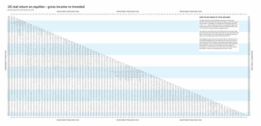
US real return on equities - gross income re-invested(annual average rates of return between year ends)

INVESTMENT FROM END YEAR INVESTMENT FROM END YEAR INVESTMENT FROM END YEAR1925 1926 1927 1928 1929 1930 1931 1932 1933 1934 1935 1936 1937 1938 1939 1940 1941 1942 1943 1944 1945 1946 1947 1948 1949 1950 1951 1952 1953 1954 1955 1956 1957 1958 1959 1960 1961 1962 1963 1964 1965 1966 1967 1968 1969 1970 1971 1972 1973 1974 1975 1976 1977 1978 1979 1980 1981 1982 1983 1984 1985 1986 1987 1988 1989 1990 1991 1992 1993 1994 1995 1996 1997 1998 1999 2000 2001 2002 2003 2004 2005 2006 2007 2008 2009 2010 2011

1926 11.2 1926 1927 24.0 38.2 1927 1928 29.9 40.4 42.5 1928 1929 16.4 18.2 9.4 (16.1) 1929 1930 6.6 5.5 (3.6) (20.7) (25.1) 1930 1931 (3.2) (5.9) (14.5) (27.9) (33.2) (40.4) 1931 1932 (2.6) (4.8) (11.6) (21.5) (23.3) (22.4) 1.0 1932 1933 3.6 2.5 (2.5) (9.6) (7.9) (1.3) 27.0 59.6 1933 1934 3.5 2.5 (1.7) (7.6) (5.8) (0.3) 18.3 28.0 2.7 1934 1935 6.9 6.4 3.0 (1.7) 0.9 7.1 24.0 32.8 21.1 42.9 1935 1936 8.9 8.7 5.8 2.0 4.8 10.9 25.5 32.5 24.6 37.2 31.7 1936 1937 4.0 3.3 0.4 (3.5) (1.8) 2.1 11.7 14.0 4.8 5.4 (9.4) (37.7) 1937 1938 6.0 5.5 3.0 (0.3) 1.6 5.5 14.5 16.9 9.9 11.8 3.0 (9.0) 33.1 1938 1939 5.7 5.3 2.9 (0.1) 1.6 5.1 12.9 14.7 8.5 9.7 2.7 (5.4) 16.5 2.0 1939 1940 4.6 4.2 1.9 (0.9) 0.7 3.7 10.2 11.4 5.9 6.4 0.3 (6.3) 7.4 (3.5) (8.8) 1940 1941 3.0 2.5 0.3 (2.4) (1.1) 1.4 6.9 7.6 2.4 2.4 (3.1) (8.9) 0.2 (8.9) (13.9) (18.7) 1941 1942 3.2 2.8 0.8 (1.7) (0.5) 1.9 7.0 7.6 3.0 3.0 (1.7) (6.4) 1.6 (5.1) (7.3) (6.6) 7.3 1942 1943 4.4 4.0 2.2 (0.1) 1.2 3.5 8.4 9.1 5.0 5.3 1.4 (2.4) 5.2 0.4 0.0 3.1 16.1 25.7 1943 1944 5.1 4.8 3.1 1.0 2.3 4.6 9.2 9.9 6.3 6.6 3.2 0.1 7.2 3.4 3.6 7.0 17.2 22.6 19.5 1944 1945 6.5 6.3 4.8 2.9 4.2 6.5 11.0 11.8 8.6 9.1 6.2 3.7 10.5 7.6 8.6 12.5 21.9 27.3 28.0 37.2 1945 1946 5.1 4.8 3.2 1.4 2.5 4.6 8.6 9.1 6.0 6.3 3.4 1.0 6.5 3.6 3.8 6.1 11.9 13.1 9.2 4.3 (20.7) 1946 1947 4.6 4.3 2.8 1.1 2.1 4.0 7.7 8.1 5.1 5.3 2.7 0.4 5.3 2.6 2.7 4.4 8.9 9.2 5.4 1.1 (13.2) (5.1) 1947 1948 4.3 4.0 2.6 1.0 1.9 3.7 7.1 7.5 4.7 4.9 2.4 0.3 4.7 2.2 2.3 3.7 7.4 7.4 4.1 0.6 (9.3) (3.0) (0.9) 1948 1949 5.1 4.8 3.5 1.9 2.9 4.7 8.0 8.4 5.8 6.0 3.8 1.9 6.2 4.0 4.2 5.8 9.3 9.6 7.1 4.8 (2.0) 5.2 10.7 23.6 1949 1950 5.8 5.6 4.3 2.9 3.9 5.6 8.8 9.2 6.8 7.1 5.1 3.4 7.5 5.6 5.9 7.5 10.9 11.4 9.5 7.9 2.8 9.7 15.1 24.1 24.5 1950 1951 6.1 5.9 4.8 3.4 4.3 6.0 9.1 9.5 7.3 7.5 5.7 4.1 8.0 6.3 6.6 8.2 11.3 11.8 10.1 8.8 4.7 10.7 15.1 20.9 19.6 14.9 1951 1952 6.4 6.2 5.1 3.7 4.7 6.3 9.3 9.7 7.6 7.8 6.1 4.6 8.3 6.7 7.1 8.6 11.4 11.9 10.4 9.3 5.9 11.1 14.6 18.9 17.3 13.9 12.9 1952 1953 6.1 5.9 4.8 3.6 4.5 6.0 8.8 9.2 7.1 7.4 5.7 4.3 7.7 6.2 6.5 7.8 10.4 10.7 9.3 8.2 5.0 9.3 11.9 14.7 12.5 8.8 5.9 (0.7) 1953 1954 7.5 7.4 6.4 5.2 6.1 7.7 10.5 10.9 9.0 9.3 7.8 6.6 10.0 8.7 9.2 10.6 13.3 13.8 12.8 12.1 9.6 14.1 17.2 20.5 19.9 18.7 20.1 23.8 54.4 1954 1955 8.0 7.9 7.0 5.9 6.8 8.3 11.1 11.5 9.7 10.1 8.6 7.6 10.9 9.7 10.2 11.6 14.1 14.7 13.8 13.3 11.1 15.4 18.2 21.2 20.9 20.1 21.5 24.5 39.4 25.8 1955 1956 8.0 7.9 6.9 5.9 6.8 8.2 10.8 11.3 9.5 9.9 8.5 7.4 10.6 9.4 9.9 11.2 13.5 14.0 13.1 12.6 10.6 14.3 16.7 19.2 18.5 17.6 18.1 19.5 27.0 15.2 5.5 1956 1957 7.2 7.1 6.2 5.1 6.0 7.3 9.8 10.2 8.5 8.7 7.4 6.3 9.2 8.1 8.5 9.6 11.6 11.9 11.0 10.4 8.4 11.5 13.3 15.0 14.0 12.5 12.2 12.0 15.4 4.8 (4.4) (13.4) 1957 1958 8.2 8.1 7.3 6.2 7.1 8.5 10.9 11.3 9.7 10.0 8.8 7.8 10.7 9.7 10.1 11.3 13.3 13.7 13.0 12.5 10.8 13.9 15.8 17.7 17.0 16.1 16.3 16.9 20.7 13.5 9.7 11.8 44.5 1958 1959 8.3 8.2 7.4 6.4 7.2 8.6 10.9 11.3 9.8 10.1 8.9 8.0 10.7 9.7 10.1 11.2 13.2 13.6 12.8 12.4 10.8 13.7 15.4 17.0 16.4 15.5 15.6 16.0 19.0 13.0 10.0 11.6 26.6 11.0 1959 1960 8.0 7.9 7.1 6.2 7.0 8.3 10.5 10.9 9.4 9.6 8.5 7.6 10.2 9.3 9.6 10.6 12.4 12.7 12.0 11.6 10.0 12.6 14.1 15.5 14.8 13.8 13.7 13.8 16.1 10.7 7.9 8.5 16.9 5.2 (0.3) 1960 1961 8.5 8.4 7.7 6.8 7.6 8.8 11.0 11.4 10.0 10.2 9.1 8.3 10.9 10.0 10.4 11.4 13.1 13.4 12.8 12.4 11.0 13.5 15.0 16.3 15.7 15.0 15.0 15.2 17.4 12.9 10.8 11.9 19.4 12.0 12.5 26.9 1961 1962 7.9 7.8 7.0 6.2 6.9 8.1 10.2 10.5 9.1 9.4 8.3 7.5 9.8 9.0 9.3 10.2 11.8 12.0 11.3 10.9 9.5 11.8 13.0 14.0 13.3 12.5 12.2 12.2 13.7 9.4 7.3 7.6 12.3 5.5 3.7 5.8 (11.9) 1962 1963 8.2 8.1 7.4 6.5 7.3 8.4 10.5 10.8 9.5 9.7 8.7 7.9 10.2 9.4 9.7 10.6 12.1 12.4 11.7 11.3 10.1 12.2 13.4 14.4 13.8 13.0 12.8 12.8 14.3 10.5 8.7 9.2 13.5 8.2 7.5 10.2 2.6 19.6 1963 1964 8.4 8.3 7.6 6.8 7.5 8.6 10.6 10.9 9.7 9.9 8.9 8.2 10.4 9.6 9.9 10.8 12.3 12.5 11.9 11.6 10.3 12.4 13.5 14.5 13.9 13.2 13.0 13.1 14.4 11.0 9.5 10.0 13.8 9.4 9.0 11.5 6.8 17.6 15.6 1964 1965 8.5 8.4 7.7 6.9 7.6 8.8 10.7 11.0 9.7 10.0 9.0 8.3 10.5 9.7 10.0 10.9 12.3 12.5 12.0 11.6 10.5 12.4 13.5 14.4 13.8 13.1 13.0 13.0 14.2 11.2 9.8 10.3 13.7 9.8 9.6 11.7 8.2 15.9 14.1 12.6 1965 1966 7.9 7.8 7.2 6.4 7.0 8.1 10.0 10.2 9.0 9.2 8.3 7.6 9.6 8.9 9.1 9.9 11.2 11.4 10.8 10.4 9.3 11.0 11.9 12.7 12.1 11.4 11.1 11.0 12.0 9.0 7.6 7.8 10.5 6.8 6.2 7.4 3.8 8.2 4.6 (0.5) (12.1) 1966 1967 8.3 8.2 7.6 6.8 7.5 8.6 10.4 10.7 9.5 9.7 8.8 8.1 10.1 9.4 9.7 10.4 11.7 11.9 11.4 11.0 10.0 11.7 12.6 13.4 12.8 12.2 12.0 11.9 12.9 10.2 9.0 9.3 11.9 8.8 8.5 9.8 7.2 11.5 9.5 7.6 5.1 25.7 1967 1968 8.3 8.3 7.6 6.9 7.5 8.6 10.3 10.6 9.5 9.7 8.8 8.1 10.1 9.4 9.7 10.4 11.6 11.8 11.3 11.0 9.9 11.6 12.4 13.2 12.6 12.0 11.8 11.8 12.7 10.1 9.0 9.3 11.7 8.8 8.6 9.7 7.5 11.1 9.5 8.0 6.5 17.2 9.4 1968 1969 7.7 7.6 7.0 6.2 6.9 7.8 9.5 9.8 8.6 8.8 8.0 7.3 9.1 8.4 8.7 9.3 10.5 10.6 10.1 9.7 8.7 10.2 10.9 11.5 11.0 10.3 10.0 9.9 10.6 8.1 7.0 7.1 9.0 6.2 5.8 6.5 4.2 6.7 4.7 2.6 0.3 4.8 (4.4) (16.4) 1969 1970 7.4 7.3 6.7 6.0 6.6 7.5 9.1 9.4 8.2 8.4 7.6 6.9 8.7 8.0 8.2 8.8 9.9 10.0 9.5 9.1 8.1 9.5 10.2 10.7 10.1 9.5 9.2 9.0 9.6 7.2 6.1 6.2 7.8 5.2 4.7 5.2 3.1 5.1 3.2 1.2 (0.9) 2.1 (4.7) (11.0) (5.3) 1970 1971 7.5 7.4 6.8 6.1 6.7 7.6 9.2 9.4 8.4 8.5 7.7 7.1 8.8 8.1 8.3 8.9 10.0 10.1 9.6 9.2 8.3 9.6 10.3 10.8 10.3 9.6 9.4 9.2 9.8 7.6 6.5 6.6 8.2 5.8 5.4 5.9 4.0 5.9 4.4 2.8 1.3 4.2 (0.6) (3.7) 3.4 12.9 1971 1972 7.6 7.6 7.0 6.3 6.9 7.8 9.3 9.6 8.5 8.7 7.9 7.3 8.9 8.3 8.5 9.1 10.1 10.2 9.7 9.4 8.5 9.8 10.4 10.9 10.4 9.8 9.6 9.4 10.0 7.9 6.9 7.0 8.6 6.4 6.0 6.6 4.9 6.7 5.4 4.2 3.0 5.8 2.2 0.5 6.8 13.4 13.9 1972 1973 6.8 6.7 6.1 5.4 6.0 6.8 8.3 8.5 7.5 7.6 6.8 6.2 7.8 7.1 7.3 7.8 8.8 8.8 8.3 7.9 7.0 8.2 8.8 9.2 8.6 8.0 7.7 7.4 7.8 5.8 4.8 4.8 6.0 3.8 3.4 3.6 1.9 3.3 1.8 0.3 (1.1) 0.6 (3.1) (5.4) (2.5) (1.5) (8.0) (25.7) 1973 1974 5.7 5.6 5.0 4.3 4.8 5.6 7.0 7.1 6.1 6.2 5.4 4.8 6.2 5.6 5.7 6.1 7.0 7.0 6.4 6.0 5.1 6.2 6.6 6.9 6.3 5.6 5.2 4.9 5.1 3.1 2.1 1.9 2.8 0.7 0.0 0.1 (1.8) (0.9) (2.5) (4.2) (5.9) (5.1) (8.8) (11.6) (10.6) (11.8) (18.8) (31.4) (36.7) 1974 1975 6.1 6.0 5.4 4.8 5.3 6.1 7.5 7.6 6.6 6.7 5.9 5.3 6.8 6.2 6.3 6.8 7.6 7.6 7.1 6.7 5.8 6.9 7.4 7.7 7.1 6.5 6.1 5.8 6.2 4.3 3.3 3.2 4.2 2.2 1.7 1.8 0.2 1.2 (0.2) (1.5) (2.8) (1.7) (4.7) (6.5) (4.8) (4.7) (8.6) (15.1) (9.3) 30.1 1975 1976 6.4 6.3 5.8 5.1 5.6 6.4 7.8 7.9 7.0 7.1 6.3 5.7 7.2 6.6 6.7 7.2 8.0 8.0 7.5 7.2 6.3 7.4 7.8 8.2 7.6 7.0 6.7 6.5 6.8 5.0 4.1 4.0 5.1 3.2 2.8 3.0 1.5 2.6 1.4 0.3 (0.8) 0.4 (2.0) (3.4) (1.4) (0.7) (3.2) (7.1) 0.1 25.9 21.9 1976 1977 6.1 6.0 5.4 4.8 5.3 6.0 7.4 7.5 6.5 6.6 5.9 5.3 6.7 6.1 6.2 6.7 7.5 7.5 7.0 6.6 5.8 6.8 7.2 7.5 7.0 6.4 6.1 5.8 6.1 4.3 3.5 3.4 4.3 2.5 2.1 2.2 0.8 1.7 0.6 (0.5) (1.5) (0.5) (2.8) (4.1) (2.4) (2.0) (4.3) (7.5) (2.3) 12.9 5.1 (9.4) 1977 1978 6.0 5.9 5.3 4.7 5.1 5.9 7.2 7.3 6.4 6.5 5.8 5.2 6.6 6.0 6.1 6.5 7.3 7.3 6.8 6.4 5.6 6.6 7.0 7.2 6.7 6.1 5.8 5.5 5.8 4.2 3.3 3.2 4.1 2.4 1.9 2.1 0.8 1.6 0.5 (0.5) (1.4) (0.5) (2.6) (3.7) (2.2) (1.8) (3.7) (6.4) (1.9) 9.4 3.3 (4.9) (0.3) 1978 1979 6.0 6.0 5.4 4.8 5.3 6.0 7.3 7.4 6.5 6.6 5.9 5.3 6.7 6.1 6.2 6.6 7.4 7.4 6.9 6.6 5.8 6.7 7.1 7.3 6.8 6.3 6.0 5.7 6.0 4.4 3.6 3.5 4.4 2.8 2.4 2.5 1.3 2.1 1.1 0.2 (0.6) 0.3 (1.5) (2.5) (0.9) (0.4) (2.0) (4.1) 0.1 9.7 5.1 0.0 5.1 10.8 1979 1980 6.3 6.2 5.7 5.1 5.5 6.3 7.5 7.7 6.8 6.8 6.2 5.6 6.9 6.4 6.5 6.9 7.7 7.7 7.2 6.9 6.1 7.1 7.4 7.7 7.2 6.7 6.4 6.2 6.5 5.0 4.2 4.2 5.0 3.5 3.1 3.3 2.2 3.0 2.1 1.4 0.6 1.6 (0.0) (0.8) 0.8 1.4 0.2 (1.4) 2.7 11.3 7.9 4.7 9.8 15.3 19.9 1980 1981 5.9 5.8 5.3 4.7 5.2 5.9 7.1 7.2 6.3 6.4 5.7 5.2 6.5 5.9 6.0 6.4 7.1 7.1 6.7 6.3 5.6 6.4 6.8 7.1 6.6 6.0 5.8 5.5 5.7 4.3 3.5 3.4 4.2 2.7 2.4 2.5 1.4 2.2 1.3 0.5 (0.2) 0.6 (0.9) (1.7) (0.4) 0.1 (1.1) (2.6) 0.7 7.6 4.3 1.1 3.9 5.3 2.6 (12.2) 1981 1982 6.1 6.0 5.5 4.9 5.4 6.1 7.3 7.4 6.5 6.6 5.9 5.4 6.7 6.2 6.2 6.6 7.3 7.3 6.9 6.6 5.9 6.7 7.1 7.3 6.9 6.4 6.1 5.9 6.1 4.7 4.0 3.9 4.7 3.3 3.0 3.1 2.1 2.9 2.1 1.3 0.7 1.6 0.1 (0.5) 0.9 1.4 0.4 (0.9) 2.4 8.7 6.0 3.5 6.3 8.0 7.1 1.3 16.8 1982 1983 6.3 6.2 5.7 5.2 5.6 6.3 7.5 7.6 6.8 6.8 6.2 5.7 6.9 6.4 6.5 6.9 7.6 7.6 7.2 6.9 6.2 7.0 7.4 7.6 7.2 6.7 6.5 6.3 6.5 5.2 4.5 4.5 5.2 3.9 3.6 3.8 2.8 3.6 2.8 2.2 1.7 2.5 1.2 0.7 2.1 2.7 1.8 0.8 3.9 9.8 7.5 5.6 8.3 10.2 10.0 6.9 17.9 19.0 1983 1984 6.2 6.1 5.6 5.1 5.5 6.2 7.3 7.4 6.6 6.7 6.1 5.6 6.8 6.3 6.4 6.7 7.4 7.4 7.0 6.7 6.0 6.8 7.2 7.4 7.0 6.5 6.2 6.0 6.3 5.0 4.3 4.3 5.0 3.7 3.4 3.6 2.7 3.4 2.7 2.1 1.5 2.3 1.1 0.6 1.9 2.4 1.6 0.7 3.5 8.7 6.6 4.8 7.0 8.2 7.7 4.9 11.3 8.6 (0.8) 1984 1985 6.5 6.4 6.0 5.4 5.8 6.5 7.7 7.8 7.0 7.1 6.5 6.0 7.2 6.7 6.8 7.2 7.8 7.8 7.4 7.2 6.5 7.3 7.7 7.9 7.5 7.1 6.8 6.7 6.9 5.6 5.0 5.0 5.7 4.5 4.3 4.5 3.6 4.3 3.7 3.2 2.7 3.5 2.4 2.0 3.3 3.9 3.3 2.5 5.3 10.3 8.5 7.1 9.4 10.9 10.9 9.1 15.2 14.7 12.6 27.9 1985 1986 6.7 6.6 6.1 5.6 6.0 6.7 7.8 7.9 7.1 7.2 6.6 6.2 7.3 6.8 6.9 7.3 8.0 8.0 7.6 7.3 6.7 7.5 7.8 8.1 7.7 7.3 7.0 6.9 7.1 5.9 5.3 5.3 6.0 4.9 4.6 4.8 4.0 4.8 4.2 3.7 3.2 4.1 3.1 2.7 4.0 4.6 4.0 3.4 6.0 10.7 9.1 7.9 10.0 11.3 11.4 10.1 15.1 14.7 13.3 21.1 14.7 1986 1987 6.5 6.4 6.0 5.4 5.8 6.5 7.6 7.7 6.9 7.0 6.4 6.0 7.1 6.6 6.7 7.1 7.7 7.7 7.4 7.1 6.5 7.2 7.6 7.8 7.4 7.0 6.8 6.6 6.8 5.6 5.1 5.0 5.7 4.6 4.4 4.5 3.8 4.4 3.9 3.4 3.0 3.8 2.8 2.4 3.6 4.1 3.6 3.0 5.4 9.6 8.1 6.9 8.7 9.7 9.6 8.2 12.0 11.0 9.1 12.7 5.8 (2.5) 1987 1988 6.6 6.5 6.1 5.6 6.0 6.6 7.7 7.8 7.0 7.1 6.5 6.1 7.2 6.8 6.9 7.2 7.9 7.9 7.5 7.2 6.6 7.4 7.7 7.9 7.6 7.1 6.9 6.8 7.0 5.8 5.3 5.3 6.0 4.9 4.7 4.8 4.1 4.8 4.2 3.8 3.4 4.2 3.2 2.9 4.1 4.6 4.2 3.6 5.9 9.9 8.4 7.4 9.1 10.0 10.0 8.8 12.1 11.4 9.9 12.8 8.2 5.0 13.1 1988 1989 6.8 6.8 6.3 5.8 6.2 6.9 7.9 8.1 7.3 7.4 6.8 6.4 7.5 7.1 7.2 7.5 8.2 8.2 7.8 7.6 7.0 7.7 8.1 8.3 7.9 7.5 7.3 7.2 7.4 6.3 5.8 5.8 6.5 5.4 5.2 5.4 4.7 5.4 4.9 4.5 4.2 4.9 4.1 3.8 5.0 5.6 5.2 4.7 6.9 10.7 9.5 8.6 10.2 11.2 11.3 10.3 13.5 13.1 12.1 14.9 11.9 10.9 18.3 23.7 1989 1990 6.5 6.5 6.0 5.5 5.9 6.5 7.6 7.7 7.0 7.0 6.5 6.1 7.1 6.7 6.8 7.1 7.7 7.7 7.4 7.1 6.5 7.2 7.6 7.8 7.4 7.0 6.8 6.7 6.9 5.8 5.2 5.2 5.9 4.8 4.6 4.8 4.1 4.8 4.2 3.8 3.5 4.2 3.3 3.1 4.1 4.6 4.2 3.7 5.7 9.2 7.9 7.0 8.3 9.1 8.9 7.9 10.4 9.6 8.3 9.9 6.7 4.7 7.3 4.5 (11.8) 1990 1991 6.9 6.8 6.4 5.9 6.3 6.9 7.9 8.1 7.3 7.4 6.9 6.5 7.5 7.1 7.2 7.5 8.1 8.1 7.8 7.6 7.0 7.7 8.0 8.2 7.9 7.5 7.4 7.2 7.4 6.4 5.9 5.9 6.5 5.5 5.4 5.6 4.9 5.6 5.1 4.7 4.4 5.1 4.4 4.2 5.2 5.7 5.4 4.9 7.0 10.3 9.2 8.4 9.8 10.6 10.6 9.8 12.3 11.8 10.9 12.7 10.4 9.5 12.7 12.6 7.4 30.8 1991 1992 6.9 6.8 6.4 5.9 6.3 6.9 7.9 8.0 7.3 7.4 6.9 6.5 7.5 7.1 7.2 7.5 8.1 8.1 7.8 7.5 7.0 7.7 8.0 8.2 7.9 7.5 7.3 7.2 7.4 6.4 5.9 5.9 6.5 5.6 5.4 5.6 5.0 5.6 5.1 4.8 4.5 5.2 4.4 4.2 5.2 5.7 5.4 5.0 6.9 10.1 9.0 8.3 9.6 10.3 10.3 9.5 11.7 11.2 10.4 11.9 9.8 8.9 11.4 11.0 7.0 17.9 6.2 1992 1993 6 9 6 8 6 4 5 9 6 3 6 9 7 9 8 0 7 3 7 4 6 9 6 5 7 5 7 1 7 2 7 5 8 1 8 1 7 8 7 6 7 0 7 7 8 0 8 2 7 9 7 5 7 4 7 2 7 4 6 4 6 0 6 0 6 6 5 7 5 5 5 7 5 1 5 7 5 2 4 9 4 6 5 3 4 6 4 4 5 4 5 9 5 6 5 2 7 0 10 0 9 0 8 3 9 5 10 2 10 2 9 4 11 5 11 0 10 2 11 5 9 6 8 9 11 0 10 5 7 5 14 8 7 5 8 8 1993

INV

ESTM

ENT

TO E

ND

YEA

R INV

ESTMEN

T TO EN

D YEA

R

HOW TO USE TABLES OF TOTAL RETURNS

The dates along the top (and bottom) are those on which each portfolio starts; those down the side are the dates to which the annual rate of return is calculated. Thus the figure at the bottom right hand corner - 14.1 - shows that the real return on a portfolio bought at the end of December 2011 and held for one year to December 2012 was 14.1%. Figures in brackets indicate negative returns.

Each figure on the bottom line of the table shows the average annual return up to the end of December 2012 from the year shown below the figure. The first figure is 6.7, showing that the average annual rate of return over the whole period since 1925 has been 6.7%.

The top figure in each column is the rate of return in the first year, so that reading diagonally down the table gives the real rate of return in each year since 1925. The table can be used to see the rate of return over any period; thus a purchase made at the end of 1926 would have gained 38.2% in value in one year (allowing for reinvestment of income) but, over the first five years (up to the end of 1931), would have fallen in value by an average annual real rate of -5.9%.

1993 6.9 6.8 6.4 5.9 6.3 6.9 7.9 8.0 7.3 7.4 6.9 6.5 7.5 7.1 7.2 7.5 8.1 8.1 7.8 7.6 7.0 7.7 8.0 8.2 7.9 7.5 7.4 7.2 7.4 6.4 6.0 6.0 6.6 5.7 5.5 5.7 5.1 5.7 5.2 4.9 4.6 5.3 4.6 4.4 5.4 5.9 5.6 5.2 7.0 10.0 9.0 8.3 9.5 10.2 10.2 9.4 11.5 11.0 10.2 11.5 9.6 8.9 11.0 10.5 7.5 14.8 7.5 8.8 1993 1994 6.7 6.7 6.2 5.8 6.2 6.7 7.7 7.8 7.1 7.2 6.7 6.3 7.3 6.9 7.0 7.3 7.9 7.9 7.6 7.3 6.8 7.5 7.8 7.9 7.6 7.3 7.1 7.0 7.2 6.2 5.7 5.7 6.3 5.4 5.2 5.4 4.8 5.4 5.0 4.6 4.4 5.0 4.3 4.1 5.0 5.5 5.2 4.8 6.5 9.3 8.3 7.6 8.7 9.3 9.2 8.5 10.3 9.7 8.9 9.9 8.1 7.3 8.8 8.1 5.2 9.9 3.7 2.5 (3.4) 1994 1995 7.1 7.0 6.6 6.1 6.5 7.1 8.1 8.2 7.5 7.6 7.1 6.7 7.7 7.3 7.4 7.7 8.3 8.3 8.0 7.8 7.3 7.9 8.2 8.4 8.1 7.8 7.6 7.5 7.7 6.8 6.3 6.4 6.9 6.1 5.9 6.1 5.6 6.1 5.7 5.4 5.2 5.9 5.2 5.1 6.0 6.5 6.2 5.9 7.6 10.4 9.5 8.8 9.9 10.6 10.6 10.0 11.8 11.4 10.8 11.9 10.4 9.9 11.6 11.4 9.4 14.2 10.4 11.9 13.5 33.3 1995 1996 7.2 7.2 6.8 6.3 6.7 7.3 8.2 8.3 7.7 7.8 7.3 6.9 7.9 7.5 7.6 7.9 8.5 8.5 8.2 8.0 7.5 8.1 8.4 8.6 8.3 8.0 7.8 7.7 7.9 7.0 6.6 6.6 7.2 6.4 6.2 6.4 5.9 6.5 6.1 5.8 5.6 6.2 5.6 5.5 6.4 6.9 6.6 6.4 8.0 10.7 9.8 9.3 10.3 11.0 11.0 10.4 12.1 11.8 11.3 12.4 11.0 10.7 12.3 12.1 10.6 14.8 11.9 13.3 14.9 25.3 17.7 1996 1997 7.5 7.4 7.0 6.6 7.0 7.5 8.5 8.6 8.0 8.1 7.6 7.2 8.2 7.8 7.9 8.2 8.8 8.8 8.5 8.3 7.8 8.5 8.8 9.0 8.7 8.4 8.3 8.2 8.4 7.5 7.1 7.1 7.7 6.9 6.8 7.0 6.5 7.0 6.7 6.4 6.2 6.9 6.3 6.2 7.1 7.6 7.4 7.2 8.8 11.4 10.6 10.1 11.2 11.8 11.9 11.4 13.1 12.9 12.4 13.5 12.4 12.2 13.8 13.9 12.7 16.7 14.5 16.3 18.2 26.4 23.1 28.8 1997 1998 7.7 7.6 7.2 6.8 7.2 7.7 8.7 8.8 8.2 8.3 7.8 7.4 8.4 8.0 8.1 8.4 9.0 9.0 8.7 8.6 8.1 8.7 9.0 9.2 8.9 8.6 8.5 8.4 8.6 7.8 7.4 7.4 8.0 7.2 7.1 7.3 6.8 7.4 7.1 6.8 6.7 7.3 6.8 6.7 7.6 8.1 7.9 7.7 9.3 11.8 11.1 10.6 11.6 12.3 12.3 11.9 13.5 13.3 13.0 14.0 13.0 12.9 14.4 14.5 13.6 17.2 15.4 17.0 18.7 25.0 22.3 24.7 20.7 1998 1999 7.8 7.8 7.4 7.0 7.4 7.9 8.9 9.0 8.4 8.5 8.0 7.7 8.6 8.2 8.4 8.7 9.2 9.2 9.0 8.8 8.3 9.0 9.3 9.5 9.2 8.9 8.8 8.7 8.9 8.1 7.7 7.7 8.3 7.6 7.5 7.7 7.2 7.8 7.5 7.2 7.1 7.7 7.2 7.1 8.0 8.5 8.4 8.2 9.7 12.2 11.5 11.1 12.1 12.7 12.8 12.5 14.0 13.9 13.5 14.6 13.7 13.6 15.1 15.2 14.4 17.8 16.2 17.7 19.3 24.4 22.3 23.9 21.5 22.4 1999 2000 7.5 7.5 7.1 6.7 7.0 7.6 8.5 8.6 8.0 8.1 7.6 7.3 8.2 7.8 7.9 8.2 8.8 8.8 8.5 8.3 7.9 8.5 8.8 9.0 8.7 8.4 8.3 8.2 8.4 7.5 7.2 7.2 7.7 7.0 6.9 7.1 6.6 7.1 6.8 6.6 6.4 7.0 6.5 6.4 7.2 7.7 7.5 7.3 8.8 11.0 10.3 9.9 10.8 11.3 11.4 11.0 12.3 12.1 11.7 12.5 11.6 11.3 12.5 12.4 11.5 14.1 12.4 13.2 13.8 17.0 14.0 13.0 8.3 2.5 (14.1) 2000 2001 7.2 7.2 6.8 6.4 6.7 7.3 8.2 8.3 7.7 7.7 7.3 6.9 7.8 7.5 7.6 7.9 8.4 8.4 8.1 7.9 7.5 8.1 8.3 8.5 8.2 7.9 7.8 7.7 7.9 7.1 6.7 6.7 7.2 6.5 6.4 6.5 6.1 6.6 6.2 6.0 5.8 6.4 5.9 5.8 6.5 7.0 6.8 6.5 7.9 10.1 9.4 8.9 9.7 10.2 10.1 9.7 10.9 10.6 10.2 10.9 9.9 9.6 10.5 10.3 9.2 11.4 9.6 10.0 10.1 12.2 9.0 7.3 2.6 (2.9) (13.4) (12.8) 2001 2002 6.8 6.7 6.3 5.9 6.3 6.8 7.6 7.7 7.1 7.2 6.7 6.4 7.3 6.9 7.0 7.3 7.8 7.8 7.5 7.3 6.8 7.4 7.6 7.8 7.5 7.2 7.1 7.0 7.1 6.3 5.9 6.0 6.4 5.7 5.6 5.7 5.2 5.7 5.4 5.1 4.9 5.4 4.9 4.8 5.5 5.9 5.6 5.4 6.7 8.7 7.9 7.4 8.2 8.5 8.4 7.9 9.0 8.6 8.1 8.6 7.6 7.2 7.8 7.5 6.3 8.0 6.1 6.1 5.8 7.0 3.7 1.6 (3.1) (8.3) (16.7) (18.0) (23.0) 2002 2003 7.0 7.0 6.6 6.2 6.6 7.1 7.9 8.0 7.4 7.5 7.1 6.7 7.6 7.3 7.3 7.6 8.1 8.1 7.9 7.7 7.2 7.8 8.0 8.2 7.9 7.6 7.5 7.4 7.6 6.8 6.4 6.4 6.9 6.2 6.1 6.2 5.8 6.3 6.0 5.7 5.5 6.1 5.6 5.5 6.2 6.6 6.4 6.1 7.4 9.4 8.7 8.2 9.0 9.4 9.3 8.9 9.9 9.6 9.2 9.7 8.8 8.5 9.2 8.9 7.9 9.6 8.0 8.2 8.1 9.5 6.8 5.4 1.9 (1.5) (6.7) (4.1) 0.6 31.4 2003 2004 7.1 7.0 6.7 6.3 6.6 7.1 8.0 8.1 7.5 7.5 7.1 6.8 7.6 7.3 7.4 7.7 8.1 8.1 7.9 7.7 7.3 7.8 8.1 8.2 8.0 7.7 7.5 7.4 7.6 6.8 6.5 6.5 7.0 6.3 6.2 6.3 5.9 6.4 6.0 5.8 5.7 6.2 5.7 5.6 6.3 6.6 6.5 6.2 7.5 9.4 8.7 8.3 9.0 9.4 9.3 8.9 9.9 9.6 9.2 9.7 8.8 8.5 9.2 9.0 8.1 9.6 8.2 8.3 8.3 9.5 7.2 5.9 3.0 0.3 (3.6) (0.8) 3.5 20.0 9.7 2004 2005 7.0 7.0 6.6 6.2 6.6 7.1 7.9 8.0 7.4 7.5 7.1 6.7 7.6 7.2 7.3 7.6 8.1 8.1 7.8 7.6 7.2 7.7 8.0 8.1 7.9 7.6 7.5 7.4 7.5 6.8 6.4 6.4 6.9 6.2 6.1 6.3 5.8 6.3 6.0 5.8 5.6 6.1 5.6 5.5 6.2 6.6 6.4 6.2 7.4 9.2 8.6 8.1 8.8 9.2 9.1 8.7 9.7 9.4 9.0 9.4 8.6 8.3 8.9 8.7 7.8 9.2 7.8 8.0 7.9 9.0 6.8 5.7 3.1 0.8 (2.4) 0.1 3.6 14.4 6.7 3.9 2005 2006 7.1 7.1 6.7 6.3 6.7 7.1 8.0 8.1 7.5 7.6 7.1 6.8 7.7 7.3 7.4 7.7 8.2 8.2 7.9 7.7 7.3 7.8 8.1 8.2 8.0 7.7 7.6 7.5 7.7 6.9 6.6 6.6 7.0 6.4 6.3 6.4 6.0 6.5 6.2 6.0 5.8 6.3 5.8 5.7 6.4 6.8 6.6 6.4 7.5 9.3 8.7 8.3 9.0 9.3 9.3 8.9 9.8 9.5 9.2 9.6 8.8 8.5 9.2 8.9 8.1 9.5 8.2 8.4 8.3 9.4 7.4 6.4 4.2 2.3 (0.3) 2.3 5.6 14.2 9.0 8.6 13.6 2006 2007 7.1 7.0 6.7 6.3 6.6 7.1 7.9 8.0 7.4 7.5 7.1 6.8 7.6 7.3 7.4 7.6 8.1 8.1 7.8 7.7 7.2 7.8 8.0 8.2 7.9 7.6 7.5 7.4 7.6 6.8 6.5 6.5 7.0 6.3 6.2 6.4 5.9 6.4 6.1 5.9 5.7 6.2 5.8 5.7 6.3 6.7 6.5 6.3 7.4 9.1 8.6 8.1 8.8 9.1 9.1 8.7 9.6 9.3 8.9 9.3 8.6 8.3 8.8 8.6 7.8 9.1 7.9 8.0 8.0 8.9 7.1 6.1 4.1 2.4 0.2 2.4 5.2 11.9 7.5 6.8 8.3 3.2 2007 2008 6.3 6.3 5.9 5.6 5.9 6.3 7.1 7.2 6.6 6.7 6.3 6.0 6.8 6.4 6.5 6.7 7.2 7.2 6.9 6.7 6.3 6.8 7.0 7.1 6.9 6.6 6.4 6.3 6.5 5.7 5.4 5.4 5.8 5.1 5.0 5.1 4.7 5.1 4.8 4.6 4.4 4.8 4.4 4.2 4.8 5.1 4.9 4.7 5.7 7.3 6.7 6.2 6.8 7.0 6.9 6.5 7.2 6.9 6.4 6.7 5.9 5.5 5.9 5.6 4.7 5.7 4.4 4.2 3.9 4.5 2.5 1.4 (0.8) (2.7) (5.2) (4.0) (2.7) 1.2 (4.0) (7.1) (10.5) (20.6) (38.9) 2008 2009 6.6 6.5 6.2 5.8 6.1 6.6 7.4 7.5 6.9 7.0 6.5 6.2 7.0 6.7 6.8 7.0 7.4 7.5 7.2 7.0 6.6 7.1 7.3 7.5 7.2 6.9 6.8 6.7 6.8 6.1 5.8 5.8 6.2 5.6 5.5 5.6 5.2 5.6 5.3 5.1 4.9 5.3 4.9 4.8 5.4 5.7 5.5 5.3 6.3 7.9 7.3 6.9 7.4 7.7 7.6 7.2 7.9 7.6 7.2 7.5 6.8 6.4 6.8 6.6 5.8 6.8 5.6 5.5 5.3 5.9 4.2 3.3 1.4 (0.2) (2.2) (0.8) 0.8 4.7 0.8 (0.8) (2.0) (6.7) (11.3) 28.7 2009 2010 6.7 6.6 6.3 5.9 6.2 6.7 7.5 7.6 7.0 7.1 6.7 6.4 7.2 6.8 6.9 7.1 7.6 7.6 7.3 7.2 6.7 7.2 7.5 7.6 7.3 7.1 7.0 6.9 7.0 6.3 6.0 6.0 6.4 5.8 5.7 5.8 5.4 5.8 5.5 5.3 5.1 5.6 5.1 5.0 5.6 5.9 5.7 5.5 6.5 8.1 7.5 7.1 7.7 7.9 7.8 7.5 8.2 7.9 7.5 7.9 7.1 6.8 7.2 7.0 6.2 7.2 6.1 6.1 6.0 6.6 5.0 4.1 2.5 1.1 (0.7) 0.8 2.4 6.1 2.9 1.9 1.5 (1.4) (2.8) 22.4 16.5 2010 2011 6.6 6.5 6.2 5.8 6.1 6.6 7.3 7.4 6.9 6.9 6.5 6.2 7.0 6.7 6.7 7.0 7.4 7.4 7.2 7.0 6.6 7.1 7.3 7.4 7.2 6.9 6.8 6.7 6.8 6.1 5.8 5.8 6.2 5.6 5.5 5.6 5.2 5.6 5.3 5.1 4.9 5.3 4.9 4.8 5.4 5.7 5.5 5.3 6.3 7.7 7.2 6.8 7.3 7.5 7.4 7.1 7.8 7.5 7.1 7.4 6.7 6.4 6.8 6.5 5.8 6.7 5.6 5.6 5.4 5.9 4.4 3.6 2.0 0.7 (0.9) 0.3 1.8 5.0 2.0 1.0 0.5 (1.9) (3.1) 12.9 5.8 (4.0) 2011 2012 6.7 6.6 6.3 5.9 6.2 6.7 7.4 7.5 7.0 7.0 6.6 6.3 7.1 6.8 6.8 7.1 7.5 7.5 7.2 7.1 6.7 7.2 7.4 7.5 7.3 7.0 6.9 6.8 6.9 6.2 5.9 5.9 6.3 5.7 5.6 5.7 5.4 5.7 5.5 5.3 5.1 5.5 5.1 5.0 5.6 5.9 5.7 5.5 6.4 7.9 7.4 7.0 7.5 7.7 7.6 7.3 8.0 7.7 7.3 7.6 6.9 6.7 7.0 6.8 6.1 7.0 6.0 6.0 5.8 6.4 5.0 4.2 2.8 1.6 0.1 1.4 2.8 5.8 3.3 2.5 2.4 0.6 0.1 13.2 8.5 4.7 14.1 2012

1925 1926 1927 1928 1929 1930 1931 1932 1933 1934 1935 1936 1937 1938 1939 1940 1941 1942 1943 1944 1945 1946 1947 1948 1949 1950 1951 1952 1953 1954 1955 1956 1957 1958 1959 1960 1961 1962 1963 1964 1965 1966 1967 1968 1969 1970 1971 1972 1973 1974 1975 1976 1977 1978 1979 1980 1981 1982 1983 1984 1985 1986 1987 1988 1989 1990 1991 1992 1993 1994 1995 1996 1997 1998 1999 2000 2001 2002 2003 2004 2005 2006 2007 2008 2009 2010 2011

INVESTMENT FROM END YEAR INVESTMENT FROM END YEAR INVESTMENT FROM END YEAR

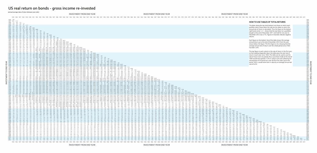
US real return on bonds - gross income re-invested(annual average rates of return between year ends)

INVESTMENT FROM END YEAR INVESTMENT FROM END YEAR INVESTMENT FROM END YEAR1925 1926 1927 1928 1929 1930 1931 1932 1933 1934 1935 1936 1937 1938 1939 1940 1941 1942 1943 1944 1945 1946 1947 1948 1949 1950 1951 1952 1953 1954 1955 1956 1957 1958 1959 1960 1961 1962 1963 1964 1965 1966 1967 1968 1969 1970 1971 1972 1973 1974 1975 1976 1977 1978 1979 1980 1981 1982 1983 1984 1985 1986 1987 1988 1989 1990 1991 1992 1993 1994 1995 1996 1997 1998 1999 2000 2001 2002 2003 2004 2005 2006 2007 2008 2009 2010 2011

1926 8.8 19261927 10.1 11.3 19271928 7.1 6.2 1.3 19281929 5.9 5.0 2.0 2.7 19291930 7.1 6.6 5.1 7.1 11.7 19301931 6.7 6.2 5.0 6.3 8.1 4.6 19311932 9.7 9.9 9.6 11.8 15.0 16.6 30.0 19321933 8.3 8.3 7.8 9.1 10.8 10.5 13.6 (0.8) 19331934 8.3 8.3 7.8 9.0 10.3 9.9 11.8 3.7 8.3 19341935 7.7 7.5 7.1 7.9 8.9 8.3 9.2 3.1 5.1 1.9 19351936 7.5 7.4 7.0 7.7 8.4 7.9 8.5 3.8 5.3 3.9 5.9 19361937 6.6 6.4 6.0 6.5 7.0 6.3 6.6 2.5 3.3 1.7 1.6 (2.6) 19371938 6.8 6.6 6.2 6.7 7.1 6.6 6.9 3.4 4.3 3.3 3.8 2.8 8.5 19381939 6.7 6.5 6.2 6.6 7.0 6.5 6.7 3.8 4.6 3.8 4.3 3.8 7.2 5.9 19391940 6.6 6.5 6.1 6.5 6.9 6.4 6.6 4.0 4.7 4.1 4.5 4.2 6.5 5.6 5.2 19401941 5.6 5.4 5.0 5.3 5.5 5.0 5.0 2.5 3.0 2.2 2.3 1.6 2.6 0.8 (1.7) (8.2) 19411942 4.9 4.7 4.3 4.5 4.6 4.1 4.0 1.7 2.0 1.2 1.2 0.4 1.0 (0.8) (2.9) (6.8) (5.3) 19421943 4.6 4.4 3.9 4.1 4.2 3.7 3.6 1.5 1.7 1.0 0.9 0.2 0.7 (0.8) (2.4) (4.8) (3.1) (0.8) 19431944 4.4 4.1 3.7 3.9 4.0 3.4 3.4 1.4 1.6 1.0 0.9 0.2 0.7 (0.6) (1.8) (3.5) (1.9) (0.2) 0.5 19441945 4.6 4.4 4.0 4.1 4.2 3.8 3.7 1.9 2.1 1.6 1.6 1.1 1.6 0.6 (0.2) (1.3) 0.5 2.5 4.2 8.1 19451946 3.5 3.3 2.9 2.9 3.0 2.4 2.3 0.6 0.7 0.1 (0.1) (0.7) (0.5) (1.5) (2.6) (3.8) (2.9) (2.3) (2.8) (4.4) (15.4) 19461947 2.8 2.6 2.1 2.2 2.2 1.6 1.4 (0.2) (0.2) (0.8) (1.0) (1.6) (1.5) (2.6) (3.6) (4.8) (4.2) (4.0) (4.7) (6.4) (12.9) (10.4) 19471948 2.7 2.5 2.1 2.1 2.1 1.6 1.4 (0.2) (0.1) (0.7) (0.9) (1.5) (1.4) (2.3) (3.2) (4.2) (3.6) (3.3) (3.7) (4.8) (8.7) (5.2) 0.4 19481949 3.0 2.7 2.4 2.4 2.4 1.9 1.8 0.3 0.4 (0.1) (0.3) (0.7) (0.6) (1.3) (2.0) (2.8) (2.1) (1.6) (1.8) (2.2) (4.7) (0.8) 4.4 8.6 19491950 2.6 2.4 2.0 2.0 2.0 1.5 1.4 (0.0) 0.0 (0.5) (0.6) (1.1) (0.9) (1.7) (2.4) (3.1) (2.5) (2.1) (2.3) (2.8) (4.8) (2.0) 1.0 1.3 (5.5) 19501951 2.1 1.9 1.5 1.5 1.5 1.0 0.8 (0.5) (0.5) (1.0) (1.2) (1.6) (1.6) (2.3) (2.9) (3.7) (3.2) (3.0) (3.2) (3.7) (5.6) (3.5) (1.7) (2.3) (7.4) (9.2) 19511952 2.1 1.8 1.5 1.5 1.4 1.0 0.8 (0.5) (0.5) (0.9) (1.1) (1.5) (1.4) (2.1) (2.7) (3.3) (2.9) (2.6) (2.8) (3.2) (4.7) (2.8) (1.2) (1.6) (4.9) (4.5) 0.4 19521953 2.1 1.9 1.5 1.5 1.5 1.1 0.9 (0.3) (0.3) (0.7) (0.9) (1.3) (1.2) (1.8) (2.3) (2.9) (2.4) (2.1) (2.3) (2.6) (3.8) (2.0) (0.6) (0.8) (3.0) (2.1) 1.6 2.8 19531954 2.3 2.1 1.7 1.8 1.7 1.3 1.2 0.0 0.1 (0.3) (0.4) (0.8) (0.7) (1.2) (1.7) (2.1) (1.7) (1.3) (1.4) (1.6) (2.6) (0.9) 0.6 0.6 (0.9) 0.3 3.7 5.3 7.9 19541955 2.2 2.0 1.6 1.7 1.6 1.2 1.1 (0.0) 0.0 (0.3) (0.5) (0.8) (0.7) (1.2) (1.6) (2.1) (1.6) (1.3) (1.3) (1.5) (2.4) (0.9) 0.4 0.4 (0.9) 0.0 2.5 3.2 3.4 (1.0) 19551956 1.8 1.6 1.3 1.3 1.2 0.8 0.7 (0.4) (0.4) (0.7) (0.9) (1.2) (1.1) (1.6) (2.0) (2.5) (2.1) (1.9) (1.9) (2.1) (3.0) (1.7) (0.7) (0.8) (2.1) (1.5) 0.1 0.1 (0.8) (4.9) (8.7) 19561957 1.9 1.7 1.4 1.4 1.3 1.0 0.8 (0.2) (0.1) (0.5) (0.6) (0.9) (0.8) (1.3) (1.7) (2.1) (1.7) (1.4) (1.5) (1.6) (2.4) (1.1) (0.1) (0.2) (1.2) (0.6) 0.9 1.0 0.6 (1.7) (2.1) 5.0 19571958 1.6 1.4 1.1 1.1 1.1 0.7 0.6 (0.4) (0.4) (0.8) (0.9) (1.2) (1.1) (1.6) (1.9) (2.3) (2.0) (1.8) (1.8) (2.0) (2.7) (1.6) (0.7) (0.8) (1.8) (1.4) (0.2) (0.3) (0.9) (3.0) (3.6) (1.0) (6.7) 19581959 1.5 1.3 1.0 0.9 0.9 0.5 0.4 (0.6) (0.6) (0.9) (1.0) (1.3) (1.2) (1.7) (2.0) (2.4) (2.1) (1.9) (1.9) (2.1) (2.8) (1.8) (1.0) (1.1) (2.0) (1.7) (0.7) (0.8) (1.4) (3.2) (3.7) (2.0) (5.3) (3.9) 19591960 1.7 1.5 1.3 1.3 1.2 0.9 0.8 (0.2) (0.1) (0.4) (0.5) (0.8) (0.7) (1.1) (1.4) (1.8) (1.4) (1.2) (1.2) (1.3) (1.9) (0.9) (0.1) (0.1) (0.9) (0.4) 0.6 0.6 0.3 (0.9) (0.9) 1.2 (0.0) 3.5 11.5 19601961 1.7 1.5 1.2 1.2 1.2 0.8 0.7 (0.2) (0.1) (0.4) (0.5) (0.8) (0.7) (1.1) (1.4) (1.7) (1.4) (1.1) (1.2) (1.3) (1.8) (0.8) (0.1) (0.1) (0.8) (0.4) 0.5 0.5 0.2 (0.8) (0.8) 0.9 (0.1) 2.2 5.4 (0.4) 19611962 1.8 1.6 1.4 1.4 1.3 1.0 0.9 0.0 0.1 (0.2) (0.3) (0.5) (0.4) (0.8) (1.1) (1.3) (1.0) (0.8) (0.8) (0.9) (1.4) (0.4) 0.3 0.3 (0.3) 0.1 1.0 1.1 0.9 0.1 0.2 1.8 1.1 3.2 5.7 2.9 6.2 19621963 1.7 1.5 1.3 1.3 1.2 0.9 0.8 (0.0) (0.0) (0.3) (0.4) (0.6) (0.5) (0.8) (1.1) (1.4) (1.1) (0.9) (0.9) (0.9) (1.4) (0.5) 0.1 0.1 (0.5) (0.1) 0.8 0.8 0.6 (0.2) (0.1) 1.2 0.6 2.1 3.6 1.1 1.9 (2.3) 19631964 1.7 1.6 1.3 1.3 1.3 1.0 0.9 0.1 0.1 (0.2) (0.2) (0.5) (0.4) (0.7) (1.0) (1.2) (0.9) (0.7) (0.7) (0.7) (1.2) (0.3) 0.3 0.3 (0.2) 0.2 0.9 1.0 0.8 0.1 0.2 1.4 0.9 2.2 3.5 1.6 2.3 0.4 3.1 19641965 1.6 1.5 1.2 1.2 1.2 0.9 0.8 0.0 0.0 (0.2) (0.3) (0.5) (0.4) (0.7) (1.0) (1.2) (0.9) (0.7) (0.7) (0.8) (1.2) (0.4) 0.2 0.2 (0.3) 0.0 0.7 0.7 0.6 (0.1) 0.0 1.0 0.5 1.6 2.6 0.9 1.2 (0.4) 0.5 (2.0) 19651966 1.6 1.4 1.2 1.2 1.2 0.9 0.8 0.0 0.0 (0.2) (0.3) (0.5) (0.4) (0.7) (0.9) (1.2) (0.9) (0.7) (0.7) (0.7) (1.1) (0.4) 0.2 0.2 (0.3) 0.0 0.7 0.7 0.6 (0.0) 0.1 1.0 0.5 1.5 2.3 0.8 1.1 (0.2) 0.5 (0.8) 0.5 19661967 1.4 1.2 0.9 0.9 0.9 0.6 0.5 (0.2) (0.2) (0.5) (0.5) (0.7) (0.7) (1.0) (1.2) (1.4) (1.2) (1.0) (1.0) (1.1) (1.5) (0.8) (0.3) (0.3) (0.8) (0.5) 0.1 0.1 (0.1) (0.7) (0.7) 0.1 (0.4) 0.3 0.9 (0.6) (0.6) (1.9) (1.8) (3.4) (4.1) (8.4) 19671968 1.2 1.0 0.8 0.8 0.7 0.4 0.3 (0.4) (0.4) (0.6) (0.7) (0.9) (0.8) (1.1) (1.4) (1.6) (1.3) (1.2) (1.2) (1.3) (1.7) (1.0) (0.5) (0.5) (1.0) (0.8) (0.2) (0.3) (0.5) (1.0) (1.1) (0.4) (0.9) (0.3) 0.2 (1.2) (1.3) (2.5) (2.5) (3.9) (4.5) (6.9) (5.4) 19681969 0.9 0.7 0.5 0.5 0.4 0.1 0.0 (0.7) (0.7) (0.9) (1.0) (1.2) (1.2) (1.5) (1.7) (2.0) (1.7) (1.6) (1.6) (1.7) (2.1) (1.5) (1.0) (1.1) (1.6) (1.3) (0.9) (1.0) (1.2) (1.8) (1.8) (1.3) (1.8) (1.3) (1.1) (2.4) (2.6) (3.8) (4.1) (5.5) (6.3) (8.5) (8.5) (11.5) 19691970 1.0 0.8 0.6 0.6 0.5 0.3 0.2 (0.5) (0.5) (0.7) (0.8) (1.0) (1.0) (1.2) (1.5) (1.7) (1.4) (1.3) (1.3) (1.4) (1.8) (1.1) (0.7) (0.8) (1.2) (1.0) (0.5) (0.6) (0.8) (1.3) (1.3) (0.8) (1.2) (0.7) (0.4) (1.5) (1.7) (2.6) (2.7) (3.6) (3.9) (5.0) (3.8) (2.9) 6.4 19701971 1.2 1.1 0.9 0.9 0.8 0.6 0.5 (0.2) (0.2) (0.4) (0.5) (0.6) (0.6) (0.9) (1.1) (1.3) (1.0) (0.9) (0.9) (0.9) (1.2) (0.6) (0.2) (0.2) (0.6) (0.4) 0.1 0.1 (0.1) (0.5) (0.5) 0.1 (0.3) 0.3 0.6 (0.3) (0.3) (1.0) (0.9) (1.4) (1.3) (1.7) 0.1 2.0 9.5 12.6 19711972 1.3 1.1 0.9 0.9 0.8 0.6 0.5 (0.2) (0.1) (0.4) (0.4) (0.6) (0.5) (0.8) (1.0) (1.2) (0.9) (0.8) (0.8) (0.8) (1.1) (0.5) (0.1) (0.1) (0.5) (0.3) 0.2 0.2 0.0 (0.4) (0.4) 0.2 (0.1) 0.3 0.7 (0.2) (0.1) (0.8) (0.6) (1.0) (0.9) (1.1) 0.4 1.9 6.8 7.0 1.6 19721973 1.0 0.9 0.6 0.6 0.6 0.3 0.2 (0.4) (0.4) (0.6) (0.7) (0.8) (0.8) (1.0) (1.2) (1.4) (1.2) (1.1) (1.1) (1.1) (1.5) (0.9) (0.5) (0.6) (0.9) (0.7) (0.3) (0.3) (0.5) (0.9) (0.9) (0.4) (0.8) (0.4) (0.1) (0.9) (1.0) (1.6) (1.6) (2.1) (2.1) (2.4) (1.4) (0.6) 2.4 1.1 (4.2) (9.8) 19731974 0.8 0.7 0.5 0.4 0.4 0.1 0.0 (0.6) (0.6) (0.8) (0.8) (1.0) (1.0) (1.2) (1.4) (1.6) (1.4) (1.3) (1.3) (1.4) (1.7) (1.1) (0.8) (0.8) (1.2) (1.0) (0.6) (0.7) (0.8) (1.2) (1.3) (0.8) (1.2) (0.8) (0.6) (1.4) (1.5) (2.1) (2.1) (2.6) (2.7) (3.0) (2.3) (1.7) 0.4 (1.1) (5.3) (8.5) (7.3) 19741975 0.8 0.6 0.4 0.4 0.4 0.1 0.0 (0.6) (0.6) (0.8) (0.8) (1.0) (1.0) (1.2) (1.4) (1.6) (1.4) (1.3) (1.3) (1.3) (1.6) (1.1) (0.8) (0.8) (1.2) (1.0) (0.6) (0.7) (0.8) (1.2) (1.2) (0.8) (1.1) (0.8) (0.6) (1.4) (1.4) (2.0) (2.0) (2.4) (2.5) (2.8) (2.1) (1.6) 0.2 (1.0) (4.1) (6.0) (4.0) (0.7) 19751976 1.0 0.9 0.7 0.6 0.6 0.4 0.3 (0.3) (0.3) (0.5) (0.5) (0.7) (0.7) (0.9) (1.1) (1.2) (1.0) (0.9) (0.9) (0.9) (1.2) (0.7) (0.4) (0.4) (0.7) (0.5) (0.1) (0.2) (0.3) (0.7) (0.6) (0.2) (0.5) (0.1) 0.1 (0.6) (0.6) (1.1) (1.0) (1.3) (1.2) (1.4) (0.6) 0.0 1.8 1.1 (1.1) (1.8) 1.1 5.5 12.0 19761977 0.9 0.7 0.5 0.5 0.5 0.3 0.2 (0.4) (0.4) (0.6) (0.7) (0.8) (0.8) (1.0) (1.2) (1.3) (1.1) (1.0) (1.0) (1.1) (1.3) (0.9) (0.5) (0.5) (0.9) (0.7) (0.3) (0.4) (0.5) (0.8) (0.8) (0.4) (0.7) (0.4) (0.2) (0.8) (0.9) (1.3) (1.3) (1.6) (1.5) (1.7) (1.0) (0.5) 0.9 0.2 (1.8) (2.4) (0.5) 1.9 3.1 (5.1) 19771978 0.7 0.5 0.3 0.3 0.3 0.0 (0.1) (0.6) (0.6) (0.8) (0.9) (1.0) (1.0) (1.2) (1.4) (1.6) (1.4) (1.3) (1.3) (1.3) (1.6) (1.2) (0.8) (0.9) (1.2) (1.0) (0.7) (0.8) (0.9) (1.3) (1.3) (0.9) (1.2) (0.9) (0.7) (1.4) (1.4) (1.9) (1.9) (2.2) (2.2) (2.5) (1.9) (1.6) (0.4) (1.2) (3.0) (3.8) (2.5) (1.3) (1.5) (7.7) (10.3) 19781979 0.4 0.3 0.1 0.0 (0.0) (0.2) (0.3) (0.9) (0.9) (1.1) (1.2) (1.3) (1.3) (1.5) (1.7) (1.9) (1.7) (1.6) (1.6) (1.7) (2.0) (1.5) (1.2) (1.3) (1.6) (1.5) (1.2) (1.2) (1.4) (1.7) (1.8) (1.4) (1.7) (1.5) (1.4) (2.0) (2.1) (2.6) (2.6) (2.9) (3.0) (3.3) (2.8) (2.6) (1.6) (2.5) (4.2) (5.1) (4.2) (3.6) (4.4) (9.3) (11.3) (12.3) 19791980 0.2 (0.0) (0.2) (0.2) (0.3) (0.5) (0.6) (1.2) (1.2) (1.4) (1.4) (1.6) (1.6) (1.8) (2.0) (2.2) (2.0) (1.9) (1.9) (2.0) (2.3) (1.9) (1.6) (1.7) (2.0) (1.9) (1.6) (1.7) (1.8) (2.2) (2.2) (2.0) (2.2) (2.0) (2.0) (2.6) (2.7) (3.2) (3.2) (3.6) (3.7) (4.0) (3.7) (3.5) (2.7) (3.6) (5.3) (6.1) (5.6) (5.3) (6.2) (10.2) (11.9) (12.7) (13.0) 19801981 0.0 (0.1) (0.3) (0.3) (0.4) (0.6) (0.7) (1.3) (1.3) (1.5) (1.5) (1.7) (1.7) (1.9) (2.1) (2.3) (2.1) (2.0) (2.1) (2.1) (2.4) (2.0) (1.7) (1.8) (2.1) (2.0) (1.7) (1.8) (2.0) (2.3) (2.4) (2.1) (2.4) (2.2) (2.1) (2.7) (2.8) (3.3) (3.4) (3.7) (3.8) (4.1) (3.8) (3.7) (3.0) (3.8) (5.3) (6.1) (5.6) (5.3) (6.1) (9.4) (10.4) (10.4) (9.5) (5.7) 19811982 0.5 0.4 0.2 0.2 0.1 (0.1) (0.2) (0.7) (0.7) (0.9) (0.9) (1.1) (1.0) (1.2) (1.4) (1.6) (1.4) (1.3) (1.3) (1.3) (1.6) (1.2) (0.9) (0.9) (1.2) (1.1) (0.8) (0.8) (1.0) (1.3) (1.3) (1.0) (1.2) (1.0) (0.9) (1.4) (1.4) (1.8) (1.8) (2.0) (2.0) (2.2) (1.8) (1.5) (0.7) (1.3) (2.4) (2.8) (2.0) (1.3) (1.4) (3.5) (3.2) (1.3) 2.6 11.5 31.8 19821983 0.5 0.4 0.2 0.1 0.1 (0.1) (0.2) (0.7) (0.7) (0.9) (0.9) (1.1) (1.0) (1.3) (1.4) (1.6) (1.4) (1.3) (1.3) (1.4) (1.6) (1.2) (0.9) (1.0) (1.2) (1.1) (0.8) (0.9) (1.0) (1.3) (1.3) (1.0) (1.2) (1.0) (0.9) (1.4) (1.4) (1.8) (1.8) (2.0) (2.0) (2.1) (1.7) (1.5) (0.7) (1.3) (2.3) (2.7) (2.0) (1.3) (1.4) (3.2) (2.9) (1.4) 1.6 7.0 14.0 (1.5) 19831984 0.7 0.5 0.3 0.3 0.3 0.1 0.0 (0.5) (0.5) (0.7) (0.7) (0.8) (0.8) (1.0) (1.1) (1.3) (1.1) (1.0) (1.0) (1.1) (1.3) (0.9) (0.6) (0.6) (0.9) (0.8) (0.5) (0.5) (0.6) (0.9) (0.9) (0.6) (0.8) (0.6) (0.4) (0.9) (0.9) (1.2) (1.2) (1.4) (1.4) (1.5) (1.0) (0.7) 0.0 (0.4) (1.4) (1.6) (0.8) (0.2) (0.1) (1.5) (1.0) 0.6 3.4 8.0 13.0 4.6 11.1 19841985 1.0 0.9 0.7 0.7 0.7 0.5 0.4 (0.1) (0.0) (0.2) (0.2) (0.4) (0.3) (0.5) (0.6) (0.8) (0.6) (0.5) (0.5) (0.5) (0.7) (0.3) (0.0) (0.0) (0.2) (0.1) 0.2 0.2 0.1 (0.1) (0.1) 0.2 0.0 0.3 0.5 0.0 0.1 (0.2) (0.1) (0.3) (0.2) (0.2) 0.3 0.6 1.4 1.1 0.3 0.2 1.1 1.9 2.2 1.1 1.9 3.8 6.8 11.3 16.0 11.1 18.0 25.3 19851986 1.4 1.2 1.1 1.1 1.0 0.9 0.8 0.3 0.3 0.2 0.2 0.1 0.1 (0.1) (0.2) (0.3) (0.1) 0.0 0.0 0.0 (0.2) 0.2 0.5 0.5 0.3 0.5 0.8 0.8 0.7 0.5 0.6 0.9 0.8 1.0 1.2 0.8 0.9 0.7 0.8 0.7 0.8 0.9 1.4 1.8 2.6 2.4 1.7 1.7 2.7 3.5 3.9 3.2 4.1 6.1 9.0 13.2 17.4 14.0 19.7 24.2 23.2 19861987 1.2 1.1 1.0 0.9 0.9 0.7 0.7 0.2 0.2 0.1 0.0 (0.1) (0.0) (0.2) (0.3) (0.4) (0.2) (0.1) (0.1) (0.1) (0.3) 0.1 0.4 0.4 0.2 0.3 0.6 0.6 0.5 0.3 0.4 0.7 0.5 0.8 0.9 0.6 0.6 0.4 0.5 0.4 0.5 0.5 1.0 1.3 2.1 1.8 1.2 1.2 2.0 2.8 3.0 2.3 3.0 4.6 7.0 10.2 13.1 9.7 12.6 13.1 7.5 (6.2) 19871988 1.3 1.2 1.0 1.0 1.0 0.8 0.7 0.3 0.3 0.1 0.1 0.0 0.1 (0.1) (0.2) (0.3) (0.2) (0.0) (0.0) (0.0) (0.2) 0.2 0.5 0.5 0.3 0.4 0.7 0.7 0.6 0.4 0.5 0.8 0.6 0.9 1.1 0.7 0.7 0.5 0.7 0.5 0.7 0.7 1.1 1.5 2.2 2.0 1.4 1.4 2.1 2.9 3.1 2.4 3.1 4.6 6.6 9.4 11.8 8.7 10.9 10.8 6.4 (1.1) 4.1 19881989 1.5 1.3 1.2 1.2 1.2 1.0 0.9 0.5 0.5 0.4 0.3 0.2 0.3 0.1 0.0 (0.1) 0.1 0.2 0.2 0.2 0.1 0.5 0.7 0.7 0.6 0.7 1.0 1.0 1.0 0.8 0.8 1.1 1.0 1.3 1.4 1.1 1.2 1.0 1.1 1.0 1.2 1.2 1.6 2.0 2.7 2.5 2.0 2.0 2.8 3.5 3.8 3.2 3.9 5.3 7.3 9.8 11.9 9.4 11.3 11.3 8.0 3.4 8.6 13.2 19891990 1.4 1.3 1.2 1.2 1.2 1.0 0.9 0.5 0.5 0.4 0.3 0.2 0.3 0.1 0.0 (0.1) 0.1 0.2 0.2 0.2 0.1 0.5 0.7 0.7 0.6 0.7 1.0 1.0 0.9 0.8 0.8 1.1 1.0 1.2 1.4 1.1 1.1 1.0 1.1 1.0 1.1 1.1 1.6 1.9 2.6 2.4 1.9 1.9 2.7 3.3 3.6 3.0 3.6 4.9 6.6 8.8 10.6 8.2 9.6 9.4 6.4 2.6 5.7 6.5 0.3 19901991 1.6 1.5 1.4 1.4 1.4 1.2 1.1 0.7 0.7 0.6 0.6 0.5 0.5 0.4 0.3 0.2 0.4 0.5 0.5 0.5 0.4 0.7 1.0 1.0 0.9 1.0 1.3 1.3 1.3 1.1 1.2 1.5 1.4 1.6 1.8 1.5 1.5 1.4 1.5 1.5 1.6 1.6 2.1 2.4 3.1 3.0 2.5 2.5 3.3 3.9 4.2 3.7 4.4 5.6 7.2 9.3 10.9 8.8 10.2 10.1 7.7 4.9 7.8 9.1 7.1 14.4 19911992 1.7 1.6 1.4 1.4 1.4 1.2 1.2 0.8 0.8 0.7 0.7 0.6 0.6 0.5 0.4 0.3 0.5 0.6 0.6 0.6 0.5 0.8 1.1 1.1 1.0 1.1 1.4 1.4 1.4 1.2 1.3 1.5 1.5 1.7 1.9 1.6 1.7 1.5 1.6 1.6 1.7 1.8 2.2 2.5 3.2 3.0 2.6 2.7 3.4 4.0 4.3 3.8 4.4 5.6 7.1 8.9 10.4 8.4 9.6 9.4 7.3 4.9 7.2 8.0 6.4 9.5 4.9 19921993 1.8 1.7 1.6 1.6 1.6 1.4 1.4 1.0 1.0 0.9 0.9 0.8 0.8 0.7 0.6 0.5 0.7 0.8 0.9 0.9 0.7 1.1 1.4 1.4 1.2 1.4 1.6 1.7 1.6 1.5 1.6 1.8 1.8 2.0 2.2 1.9 2.0 1.9 2.0 2.0 2.1 2.2 2.6 2.9 3.6 3.5 3.1 3.1 3.8 4.4 4.7 4.3 4.9 6.0 7.5 9.3 10.6 8.9 10.0 9.8 8.0 6.0 8.2 9.0 8.0 10.7 9.0 13.2 1993

INV

ESTM

ENT

TO E

ND

YEA

R INV

ESTMEN

T TO EN

D YEA

R

HOW TO USE TABLES OF TOTAL RETURNS

The dates along the top (and bottom) are those on which each portfolio starts; those down the side are the dates to which the annual rate of return is calculated. Thus the figure at the bottom right hand corner -2.1 - shows that the real return on a portfolio bought at the end of December 2011 and held for one year to December 2012 was 2.1%. Figures in brackets indicate negative returns.

Each figure on the bottom line of the table shows the average annual return up to the end of December 2012 from the year shown below the figure. The first figure is 2.6, showing that the average annual rate of return over the whole period since 1925 has been 2.6%.

The top figure in each column is the rate of return in the first year, so that reading diagonally down the table gives the real rate of return in each year since 1925. The table can be used to see the rate of return over any period; thus a purchase made at the end of 1926 would have gained 11.3% in value in one year (allowing for reinvestment of income) but, over the first five years (up to the end of 1931), would have risen in value by an average annual real rate of 6.2%.

1993 1.8 1.7 1.6 1.6 1.6 1.4 1.4 1.0 1.0 0.9 0.9 0.8 0.8 0.7 0.6 0.5 0.7 0.8 0.9 0.9 0.7 1.1 1.4 1.4 1.2 1.4 1.6 1.7 1.6 1.5 1.6 1.8 1.8 2.0 2.2 1.9 2.0 1.9 2.0 2.0 2.1 2.2 2.6 2.9 3.6 3.5 3.1 3.1 3.8 4.4 4.7 4.3 4.9 6.0 7.5 9.3 10.6 8.9 10.0 9.8 8.0 6.0 8.2 9.0 8.0 10.7 9.0 13.2 19931994 1.7 1.6 1.4 1.4 1.4 1.3 1.2 0.8 0.8 0.7 0.7 0.6 0.7 0.5 0.4 0.3 0.5 0.6 0.7 0.7 0.5 0.9 1.1 1.1 1.0 1.1 1.4 1.4 1.4 1.2 1.3 1.6 1.5 1.7 1.9 1.6 1.7 1.5 1.6 1.6 1.7 1.8 2.2 2.5 3.1 2.9 2.5 2.6 3.2 3.8 4.0 3.6 4.1 5.1 6.3 7.9 9.0 7.3 8.1 7.8 6.1 4.1 5.6 5.9 4.5 5.6 2.8 1.7 (8.6) 19941995 2.0 1.9 1.8 1.8 1.7 1.6 1.6 1.2 1.2 1.1 1.1 1.0 1.0 0.9 0.8 0.8 0.9 1.1 1.1 1.1 1.0 1.3 1.6 1.6 1.5 1.6 1.9 1.9 1.9 1.8 1.8 2.1 2.0 2.3 2.5 2.2 2.3 2.2 2.3 2.3 2.4 2.5 2.9 3.2 3.9 3.8 3.4 3.5 4.1 4.7 5.0 4.6 5.2 6.2 7.5 9.0 10.1 8.6 9.5 9.3 7.9 6.3 8.0 8.5 7.8 9.3 8.1 9.2 7.2 25.7 19951996 1.9 1.8 1.7 1.7 1.7 1.5 1.5 1.1 1.1 1.0 1.0 0.9 1.0 0.8 0.8 0.7 0.9 1.0 1.0 1.0 0.9 1.2 1.5 1.5 1.4 1.5 1.8 1.8 1.8 1.6 1.7 2.0 1.9 2.1 2.3 2.1 2.1 2.0 2.2 2.1 2.3 2.3 2.7 3.0 3.6 3.5 3.1 3.2 3.8 4.3 4.6 4.2 4.7 5.6 6.8 8.2 9.2 7.7 8.5 8.3 6.8 5.3 6.7 7.0 6.1 7.1 5.8 6.0 3.7 10.4 (3.1) 19961997 2.1 2.0 1.8 1.8 1.8 1.7 1.6 1.3 1.3 1.2 1.2 1.1 1.2 1.0 1.0 0.9 1.1 1.2 1.2 1.2 1.1 1.5 1.7 1.7 1.6 1.8 2.0 2.0 2.0 1.9 2.0 2.2 2.2 2.4 2.6 2.3 2.4 2.3 2.5 2.4 2.6 2.6 3.0 3.3 3.9 3.8 3.5 3.6 4.2 4.7 5.0 4.6 5.1 6.0 7.1 8.5 9.4 8.1 8.8 8.6 7.3 6.0 7.3 7.6 7.0 8.0 6.9 7.3 5.9 11.2 4.7 13.0 19971998 2.2 2.1 2.0 2.0 2.0 1.8 1.8 1.4 1.4 1.3 1.3 1.3 1.3 1.2 1.1 1.1 1.2 1.3 1.4 1.4 1.3 1.6 1.9 1.9 1.8 1.9 2.2 2.2 2.2 2.1 2.2 2.4 2.4 2.6 2.8 2.6 2.6 2.5 2.7 2.7 2.8 2.9 3.3 3.6 4.1 4.1 3.8 3.8 4.4 5.0 5.2 4.9 5.4 6.3 7.3 8.6 9.5 8.2 8.9 8.8 7.6 6.4 7.6 8.0 7.4 8.3 7.5 7.9 6.9 11.2 6.7 12.0 10.9 19981999 2.0 1.9 1.8 1.8 1.8 1.6 1.6 1.2 1.2 1.1 1.1 1.1 1.1 1.0 0.9 0.9 1.0 1.1 1.2 1.2 1.1 1.4 1.6 1.7 1.5 1.7 1.9 1.9 1.9 1.8 1.9 2.1 2.1 2.3 2.4 2.2 2.3 2.2 2.3 2.3 2.4 2.5 2.8 3.1 3.6 3.5 3.2 3.3 3.8 4.3 4.5 4.2 4.6 5.4 6.4 7.5 8.3 7.1 7.6 7.4 6.2 5.0 6.0 6.2 5.5 6.1 5.1 5.1 3.8 6.5 2.2 4.0 (0.2) (10.2) 19992000 2.2 2.1 2.0 2.0 2.0 1.8 1.8 1.4 1.5 1.4 1.3 1.3 1.3 1.2 1.2 1.1 1.3 1.4 1.4 1.4 1.3 1.6 1.9 1.9 1.8 1.9 2.2 2.2 2.2 2.1 2.2 2.4 2.4 2.6 2.8 2.5 2.6 2.5 2.7 2.6 2.8 2.9 3.2 3.5 4.0 3.9 3.7 3.7 4.3 4.7 5.0 4.7 5.1 5.9 6.8 7.9 8.7 7.6 8.1 7.9 6.9 5.8 6.8 7.0 6.4 7.1 6.3 6.5 5.5 8.1 4.9 6.9 5.0 2.2 16.2 20002001 2.2 2.1 2.0 2.0 2.0 1.8 1.8 1.4 1.5 1.4 1.4 1.3 1.4 1.3 1.2 1.1 1.3 1.4 1.4 1.4 1.3 1.7 1.9 1.9 1.8 2.0 2.2 2.2 2.2 2.1 2.2 2.4 2.4 2.6 2.8 2.5 2.6 2.5 2.7 2.6 2.8 2.8 3.2 3.5 4.0 3.9 3.6 3.7 4.2 4.7 4.9 4.6 5.0 5.7 6.6 7.7 8.4 7.3 7.8 7.6 6.6 5.6 6.5 6.6 6.1 6.7 5.9 6.0 5.2 7.3 4.5 6.1 4.4 2.3 9.2 2.6 20012002 2.3 2.2 2.1 2.1 2.1 2.0 2.0 1.6 1.6 1.6 1.5 1.5 1.5 1.4 1.4 1.3 1.5 1.6 1.6 1.7 1.5 1.9 2.1 2.1 2.0 2.2 2.4 2.5 2.4 2.3 2.4 2.7 2.6 2.8 3.0 2.8 2.9 2.8 2.9 2.9 3.1 3.1 3.5 3.8 4.3 4.2 3.9 4.0 4.5 5.0 5.2 4.9 5.4 6.1 6.9 8.0 8.7 7.6 8.1 7.9 7.0 6.1 6.9 7.1 6.7 7.2 6.6 6.8 6.1 8.1 5.8 7.3 6.2 5.1 10.7 8.1 13.9 20022003 2.3 2.2 2.1 2.1 2.1 2.0 1.9 1.6 1.6 1.5 1.5 1.5 1.5 1.4 1.4 1.3 1.5 1.6 1.6 1.6 1.5 1.9 2.1 2.1 2.0 2.1 2.4 2.4 2.4 2.3 2.4 2.6 2.6 2.8 2.9 2.8 2.8 2.7 2.9 2.9 3.0 3.1 3.4 3.7 4.2 4.1 3.8 3.9 4.4 4.8 5.0 4.8 5.2 5.8 6.7 7.6 8.3 7.3 7.7 7.6 6.6 5.7 6.5 6.7 6.2 6.7 6.1 6.2 5.5 7.2 5.1 6.4 5.3 4.2 8.1 5.6 7.1 0.7 20032004 2.3 2.3 2.1 2.1 2.1 2.0 2.0 1.6 1.7 1.6 1.6 1.5 1.6 1.5 1.4 1.4 1.5 1.6 1.7 1.7 1.6 1.9 2.1 2.2 2.1 2.2 2.4 2.5 2.5 2.4 2.4 2.7 2.6 2.8 3.0 2.8 2.9 2.8 2.9 2.9 3.0 3.1 3.4 3.7 4.2 4.1 3.9 3.9 4.4 4.8 5.0 4.8 5.2 5.8 6.6 7.5 8.1 7.2 7.6 7.4 6.5 5.7 6.4 6.6 6.1 6.6 6.0 6.1 5.5 7.0 5.1 6.2 5.2 4.3 7.5 5.4 6.3 2.7 4.7 20042005 2.4 2.3 2.2 2.2 2.2 2.0 2.0 1.7 1.7 1.6 1.6 1.6 1.6 1.5 1.5 1.4 1.6 1.7 1.7 1.7 1.6 1.9 2.2 2.2 2.1 2.2 2.5 2.5 2.5 2.4 2.5 2.7 2.6 2.9 3.0 2.8 2.9 2.8 2.9 2.9 3.1 3.1 3.5 3.7 4.2 4.1 3.9 3.9 4.4 4.8 5.0 4.7 5.1 5.7 6.5 7.4 8.0 7.0 7.4 7.2 6.4 5.6 6.3 6.4 6.0 6.4 5.9 5.9 5.3 6.7 5.0 5.9 5.1 4.3 6.9 5.1 5.7 3.1 4.4 4.0 20052006 2.3 2.2 2.1 2.1 2.1 2.0 2.0 1.6 1.7 1.6 1.6 1.5 1.6 1.5 1.4 1.4 1.5 1.6 1.7 1.7 1.6 1.9 2.1 2.1 2.0 2.2 2.4 2.4 2.4 2.3 2.4 2.6 2.6 2.8 2.9 2.7 2.8 2.7 2.8 2.8 3.0 3.0 3.3 3.6 4.0 4.0 3.7 3.8 4.2 4.6 4.8 4.5 4.9 5.5 6.2 7.0 7.6 6.7 7.0 6.8 6.0 5.2 5.9 6.0 5.6 5.9 5.4 5.4 4.8 6.0 4.4 5.2 4.4 3.6 5.7 4.0 4.3 2.0 2.5 1.4 (1.2) 20062007 2.3 2.3 2.2 2.2 2.2 2.0 2.0 1.7 1.7 1.6 1.6 1.6 1.6 1.5 1.5 1.4 1.6 1.7 1.7 1.7 1.6 1.9 2.2 2.2 2.1 2.2 2.4 2.5 2.5 2.4 2.4 2.7 2.6 2.8 3.0 2.8 2.9 2.8 2.9 2.9 3.0 3.1 3.4 3.6 4.1 4.0 3.8 3.8 4.3 4.6 4.8 4.6 4.9 5.5 6.2 7.0 7.5 6.6 7.0 6.8 6.0 5.2 5.9 5.9 5.6 5.9 5.4 5.4 4.9 6.0 4.5 5.2 4.4 3.7 5.6 4.2 4.5 2.7 3.2 2.7 2.0 5.2 20072008 2.6 2.5 2.4 2.4 2.4 2.3 2.3 2.0 2.0 1.9 1.9 1.9 1.9 1.8 1.8 1.7 1.9 2.0 2.0 2.1 2.0 2.3 2.5 2.5 2.4 2.6 2.8 2.8 2.8 2.7 2.8 3.0 3.0 3.2 3.4 3.2 3.3 3.2 3.3 3.3 3.5 3.5 3.9 4.1 4.5 4.5 4.3 4.4 4.8 5.2 5.3 5.1 5.5 6.1 6.8 7.5 8.1 7.2 7.6 7.5 6.8 6.1 6.7 6.8 6.5 6.8 6.4 6.5 6.1 7.2 5.9 6.7 6.1 5.7 7.6 6.6 7.1 6.0 7.1 7.7 9.0 14.5 24.6 20082009 2.3 2.3 2.2 2.2 2.2 2.1 2.0 1.7 1.7 1.7 1.6 1.6 1.7 1.6 1.5 1.4 1.6 1.7 1.7 1.8 1.7 2.0 2.2 2.2 2.1 2.2 2.4 2.5 2.5 2.4 2.4 2.7 2.6 2.8 2.9 2.8 2.8 2.8 2.9 2.9 3.0 3.1 3.3 3.6 4.0 3.9 3.7 3.8 4.2 4.5 4.7 4.4 4.8 5.3 5.9 6.7 7.1 6.3 6.6 6.4 5.7 5.0 5.6 5.6 5.3 5.5 5.1 5.1 4.6 5.5 4.2 4.8 4.1 3.5 5.0 3.8 4.0 2.7 3.0 2.6 2.3 3.5 2.6 (15.5) 20092010 2.4 2.3 2.2 2.2 2.2 2.1 2.1 1.8 1.8 1.7 1.7 1.7 1.7 1.6 1.6 1.5 1.7 1.8 1.8 1.9 1.8 2.1 2.3 2.3 2.2 2.3 2.5 2.6 2.6 2.5 2.5 2.8 2.7 2.9 3.0 2.9 3.0 2.9 3.0 3.0 3.1 3.2 3.5 3.7 4.1 4.0 3.8 3.9 4.3 4.6 4.8 4.5 4.9 5.4 6.0 6.7 7.2 6.4 6.7 6.5 5.8 5.1 5.7 5.7 5.4 5.6 5.2 5.2 4.8 5.7 4.5 5.0 4.4 3.9 5.3 4.2 4.4 3.3 3.7 3.5 3.4 4.6 4.4 (4.5) 8.0 20102011 2.6 2.6 2.5 2.5 2.5 2.4 2.3 2.0 2.1 2.0 2.0 1.9 2.0 1.9 1.9 1.8 2.0 2.1 2.1 2.1 2.0 2.3 2.6 2.6 2.5 2.6 2.8 2.9 2.9 2.8 2.9 3.1 3.1 3.2 3.4 3.2 3.3 3.3 3.4 3.4 3.5 3.6 3.9 4.1 4.5 4.4 4.2 4.3 4.7 5.0 5.2 5.0 5.3 5.8 6.5 7.2 7.6 6.9 7.2 7.0 6.4 5.8 6.3 6.4 6.1 6.4 6.0 6.1 5.7 6.6 5.5 6.1 5.6 5.2 6.6 5.8 6.1 5.3 5.9 6.0 6.4 7.9 8.6 3.8 15.0 22.5 20112012 2.6 2.6 2.5 2.5 2.5 2.4 2.3 2.0 2.1 2.0 2.0 1.9 2.0 1.9 1.9 1.8 2.0 2.1 2.1 2.1 2.0 2.3 2.5 2.6 2.5 2.6 2.8 2.9 2.9 2.8 2.9 3.1 3.0 3.2 3.4 3.2 3.3 3.2 3.3 3.3 3.5 3.5 3.8 4.0 4.4 4.4 4.2 4.2 4.6 5.0 5.1 4.9 5.2 5.7 6.3 7.0 7.4 6.7 7.0 6.9 6.2 5.6 6.1 6.2 5.9 6.2 5.8 5.9 5.5 6.3 5.3 5.8 5.4 5.0 6.3 5.5 5.7 5.0 5.4 5.5 5.7 6.9 7.3 3.3 10.5 11.8 2.1 2012

1925 1926 1927 1928 1929 1930 1931 1932 1933 1934 1935 1936 1937 1938 1939 1940 1941 1942 1943 1944 1945 1946 1947 1948 1949 1950 1951 1952 1953 1954 1955 1956 1957 1958 1959 1960 1961 1962 1963 1964 1965 1966 1967 1968 1969 1970 1971 1972 1973 1974 1975 1976 1977 1978 1979 1980 1981 1982 1983 1984 1985 1986 1987 1988 1989 1990 1991 1992 1993 1994 1995 1996 1997 1998 1999 2000 2001 2002 2003 2004 2005 2006 2007 2008 2009 2010 2011

INVESTMENT FROM END YEAR INVESTMENT FROM END YEAR INVESTMENT FROM END YEAR

Barclays | Equity Gilt Study

21 February 2013 LAST PAGE

Analyst Certification We, Michael Gavin, Piero Ghezzi, Michael Gapen, Yiping Huang, Simon Hayes, Paul Robinson, Sreekala Kochugovindan, Anando Maitra and Simon Polbennikov, hereby certify (1) that the views expressed in this research report accurately reflect our personal views about any or all of the subject securities or issuers referred to in this research report and (2) no part of our compensation was, is or will be directly or indirectly related to the specific recommendations or views expressed in this research report. Important Disclosures: Barclays Research is a part of the Corporate and Investment Banking division of Barclays Bank PLC and its affiliates (collectively and each individually, "Barclays"). For current important disclosures regarding companies that are the subject of this research report, please send a written request to: Barclays Research Compliance, 745 Seventh Avenue, 17th Floor, New York, NY 10019 or refer to http://publicresearch.barcap.com or call 212-526-1072. Barclays Capital Inc. and/or one of its affiliates does and seeks to do business with companies covered in its research reports. As a result, investors should be aware that Barclays may have a conflict of interest that could affect the objectivity of this report. Barclays Capital Inc. and/or one of its affiliates regularly trades, generally deals as principal and generally provides liquidity (as market maker or otherwise) in the debt securities that are the subject of this research report (and related derivatives thereof). Barclays trading desks may have either a long and / or short position in such securities and / or derivative instruments, which may pose a conflict with the interests of investing customers. Where permitted and subject to appropriate information barrier restrictions, Barclays fixed income research analyst(s) regularly interact with its trading desk personnel to determine current prices of fixed income securities. Barclays fixed income research analyst(s) receive compensation based on various factors including, but not limited to, the quality of their work, the overall performance of the firm (including the profitability of the investment banking department), the profitability and revenues of the Fixed Income, Currencies and Commodities Division ("FICC") and the outstanding principal amount and trading value of, the profitability of, and the potential interest of the firms investing clients in research with respect to, the asset class covered by the analyst. To the extent that any historical pricing information was obtained from Barclays trading desks, the firm makes no representation that it is accurate or complete. All levels, prices and spreads are historical and do not represent current market levels, prices or spreads, some or all of which may have changed since the publication of this document. The Corporate and Investment Banking division of Barclays produces a variety of research products including, but not limited to, fundamental analysis, equity-linked analysis, quantitative analysis, and trade ideas. Recommendations contained in one type of research product may differ from recommendations contained in other types of research products, whether as a result of differing time horizons, methodologies, or otherwise. In order to access Barclays Statement regarding Research Dissemination Policies and Procedures, please refer to https://live.barcap.com/publiccp/RSR/nyfipubs/disclaimer/disclaimer-research-dissemination.html.

Disclaimer: This publication has been prepared by the Corporate and Investment Banking division of Barclays Bank PLC and/or one or more of its affiliates (collectively and each individually, "Barclays"). It has been issued by one or more Barclays legal entities within its Corporate and Investment Banking division as provided below. It is provided to our clients for information purposes only, and Barclays makes no express or implied warranties, and expressly disclaims all warranties of merchantability or fitness for a particular purpose or use with respect to any data included in this publication. Barclays will not treat unauthorized recipients of this report as its clients. Prices shown are indicative and Barclays is not offering to buy or sell or soliciting offers to buy or sell any financial instrument. Without limiting any of the foregoing and to the extent permitted by law, in no event shall Barclays, nor any affiliate, nor any of their respective officers, directors, partners, or employees have any liability for (a) any special, punitive, indirect, or consequential damages; or (b) any lost profits, lost revenue, loss of anticipated savings or loss of opportunity or other financial loss, even if notified of the possibility of such damages, arising from any use of this publication or its contents. Other than disclosures relating to Barclays, the information contained in this publication has been obtained from sources that Barclays Research believes to be reliable, but Barclays does not represent or warrant that it is accurate or complete. Barclays is not responsible for, and makes no warranties whatsoever as to, the content of any third-party web site accessed via a hyperlink in this publication and such information is not incorporated by reference. The views in this publication are those of the author(s) and are subject to change, and Barclays has no obligation to update its opinions or the information in this publication. The analyst recommendations in this publication reflect solely and exclusively those of the author(s), and such opinions were prepared independently of any other interests, including those of Barclays and/or its affiliates. This publication does not constitute personal investment advice or take into account the individual financial circumstances or objectives of the clients who receive it. The securities discussed herein may not be suitable for all investors. Barclays recommends that investors independently evaluate each issuer, security or instrument discussed herein and consult any independent advisors they believe necessary. The value of and income from any investment may fluctuate from day to day as a result of changes in relevant economic markets (including changes in market liquidity). The information herein is not intended to predict actual results, which may differ substantially from those reflected. Past performance is not necessarily indicative of future results. This communication is being made available in the UK and Europe primarily to persons who are investment professionals as that term is defined in Article 19 of the Financial Services and Markets Act 2000 (Financial Promotion Order) 2005. It is directed at, and therefore should only be relied upon by, persons who have professional experience in matters relating to investments. The investments to which it relates are available only to such persons and will be entered into only with such persons. Barclays Bank PLC is authorised and regulated by the Financial Services Authority ("FSA") and a member of the London Stock Exchange. The Corporate and Investment Banking division of Barclays undertakes U.S. securities business in the name of its wholly owned subsidiary Barclays Capital Inc., a FINRA and SIPC member. Barclays Capital Inc., a U.S. registered broker/dealer, is distributing this material in the United States and, in connection therewith accepts responsibility for its contents. Any U.S. person wishing to effect a transaction in any security discussed herein should do so only by contacting a representative of Barclays Capital Inc. in the U.S. at 745 Seventh Avenue, New York, New York 10019. Non-U.S. persons should contact and execute transactions through a Barclays Bank PLC branch or affiliate in their home jurisdiction unless local regulations permit otherwise. Barclays Bank PLC, Paris Branch (registered in France under Paris RCS number 381 066 281) is regulated by the Autorité des marchés financiers and the Autorité de contrôle prudentiel. Registered office 34/36 Avenue de Friedland 75008 Paris. This material is distributed in Canada by Barclays Capital Canada Inc., a registered investment dealer and member of IIROC (www.iiroc.ca). Subject to the conditions of this publication as set out above, Absa Capital, the Investment Banking Division of Absa Bank Limited, an authorised financial services provider (Registration No.: 1986/004794/06. Registered Credit Provider Reg No NCRCP7), is distributing this material in South Africa. Absa Bank Limited is regulated by the South African Reserve Bank. This publication is not, nor is it intended to be, advice as defined and/or contemplated in the (South African) Financial Advisory and Intermediary Services Act, 37 of 2002, or any other financial, investment, trading, tax, legal, accounting, retirement, actuarial or other professional advice or service whatsoever. Any South African person or entity wishing to effect a

Barclays | Equity Gilt Study

21 February 2013 LAST PAGE

transaction in any security discussed herein should do so only by contacting a representative of Absa Capital in South Africa, 15 Alice Lane, Sandton, Johannesburg, Gauteng 2196. Absa Capital is an affiliate of Barclays. In Japan, foreign exchange research reports are prepared and distributed by Barclays Bank PLC Tokyo Branch. Other research reports are distributed to institutional investors in Japan by Barclays Securities Japan Limited. Barclays Securities Japan Limited is a joint-stock company incorporated in Japan with registered office of 6-10-1 Roppongi, Minato-ku, Tokyo 106-6131, Japan. It is a subsidiary of Barclays Bank PLC and a registered financial instruments firm regulated by the Financial Services Agency of Japan. Registered Number: Kanto Zaimukyokucho (kinsho) No. 143. Barclays Bank PLC, Hong Kong Branch is distributing this material in Hong Kong as an authorised institution regulated by the Hong Kong Monetary Authority. Registered Office: 41/F, Cheung Kong Center, 2 Queen's Road Central, Hong Kong. This material is issued in Taiwan by Barclays Capital Securities Taiwan Limited. This material on securities not traded in Taiwan is not to be construed as 'recommendation' in Taiwan. Barclays Capital Securities Taiwan Limited does not accept orders from clients to trade in such securities. This material may not be distributed to the public media or used by the public media without prior written consent of Barclays. This material is distributed in South Korea by Barclays Capital Securities Limited, Seoul Branch. All equity research material is distributed in India by Barclays Securities (India) Private Limited (SEBI Registration No: INB/INF 231292732 (NSE), INB/INF 011292738 (BSE), Registered Office: 208 | Ceejay House | Dr. Annie Besant Road | Shivsagar Estate | Worli | Mumbai - 400 018 | India, Phone: + 91 22 67196363). Other research reports are distributed in India by Barclays Bank PLC, India Branch. Barclays Bank PLC Frankfurt Branch distributes this material in Germany under the supervision of Bundesanstalt für Finanzdienstleistungsaufsicht (BaFin). This material is distributed in Malaysia by Barclays Capital Markets Malaysia Sdn Bhd. This material is distributed in Brazil by Banco Barclays S.A. This material is distributed in Mexico by Barclays Bank Mexico, S.A. Barclays Bank PLC in the Dubai International Financial Centre (Registered No. 0060) is regulated by the Dubai Financial Services Authority (DFSA). Principal place of business in the Dubai International Financial Centre: The Gate Village, Building 4, Level 4, PO Box 506504, Dubai, United Arab Emirates. Barclays Bank PLC-DIFC Branch, may only undertake the financial services activities that fall within the scope of its existing DFSA licence. Related financial products or services are only available to Professional Clients, as defined by the Dubai Financial Services Authority. Barclays Bank PLC in the UAE is regulated by the Central Bank of the UAE and is licensed to conduct business activities as a branch of a commercial bank incorporated outside the UAE in Dubai (Licence No.: 13/1844/2008, Registered Office: Building No. 6, Burj Dubai Business Hub, Sheikh Zayed Road, Dubai City) and Abu Dhabi (Licence No.: 13/952/2008, Registered Office: Al Jazira Towers, Hamdan Street, PO Box 2734, Abu Dhabi). Barclays Bank PLC in the Qatar Financial Centre (Registered No. 00018) is authorised by the Qatar Financial Centre Regulatory Authority (QFCRA). Barclays Bank PLC-QFC Branch may only undertake the regulated activities that fall within the scope of its existing QFCRA licence. Principal place of business in Qatar: Qatar Financial Centre, Office 1002, 10th Floor, QFC Tower, Diplomatic Area, West Bay, PO Box 15891, Doha, Qatar. Related financial products or services are only available to Business Customers as defined by the Qatar Financial Centre Regulatory Authority. This material is distributed in the UAE (including the Dubai International Financial Centre) and Qatar by Barclays Bank PLC. This material is distributed in Saudi Arabia by Barclays Saudi Arabia ('BSA'). It is not the intention of the publication to be used or deemed as recommendation, option or advice for any action (s) that may take place in future. Barclays Saudi Arabia is a Closed Joint Stock Company, (CMA License No. 09141-37). Registered office Al Faisaliah Tower, Level 18, Riyadh 11311, Kingdom of Saudi Arabia. Authorised and regulated by the Capital Market Authority, Commercial Registration Number: 1010283024. This material is distributed in Russia by OOO Barclays Capital, affiliated company of Barclays Bank PLC, registered and regulated in Russia by the FSFM. Broker License #177-11850-100000; Dealer License #177-11855-010000. Registered address in Russia: 125047 Moscow, 1st Tverskaya-Yamskaya str. 21. This material is distributed in Singapore by the Singapore branch of Barclays Bank PLC, a bank licensed in Singapore by the Monetary Authority of Singapore. For matters in connection with this report, recipients in Singapore may contact the Singapore branch of Barclays Bank PLC, whose registered address is One Raffles Quay Level 28, South Tower, Singapore 048583. Barclays Bank PLC, Australia Branch (ARBN 062 449 585, AFSL 246617) is distributing this material in Australia. It is directed at 'wholesale clients' as defined by Australian Corporations Act 2001. IRS Circular 230 Prepared Materials Disclaimer: Barclays does not provide tax advice and nothing contained herein should be construed to be tax advice. Please be advised that any discussion of U.S. tax matters contained herein (including any attachments) (i) is not intended or written to be used, and cannot be used, by you for the purpose of avoiding U.S. tax-related penalties; and (ii) was written to support the promotion or marketing of the transactions or other matters addressed herein. Accordingly, you should seek advice based on your particular circumstances from an independent tax advisor. © Copyright Barclays Bank PLC (2013). All rights reserved. No part of this publication may be reproduced in any manner without the prior written permission of Barclays. Barclays Bank PLC is registered in England No. 1026167. Registered office 1 Churchill Place, London, E14 5HP. Additional information regarding this publication will be furnished upon request.

Back cover