Equity and transport policy reform

Equity and transport policy reform1

by

Inge Mayeres2

Agora Jules Dupuit─Publication AJD-46

Université de Montréal

10 July 2001

1 The research reported in this paper was financed by the Fund for Scientific Research – Flanders (contract G.0263.95) and the Sustainable Mobility Programme of the Belgian Federal OSTC (contract MD/DD/008). The paper benefited from a research visit at the Agora Jules Dupuit (AJD), Université de Montréal. The comments and suggestions of T. Bayindir-Upmann, B. De Borger, S. Proost, E. Schokkaert, P. Van Cayseele, D. Van Regemorter, P. Van Rompuy and participants at various presentations are gratefully acknowledged. Any remaining errors are the author’s sole responsibility. 2 Postdoctoral researcher of the Fund for Scientific Research – Flanders, Center for Economic Studies, K.U.Leuven, Naamsestraat 69, 3000 Leuven, Belgium. E-mail: [email protected].

Abstract The paper assesses the marginal welfare and equity impacts of three transport instruments for a second-best economy in which the government has to use distortionary taxes for revenue-raising and distributional purposes. The assessment uses an applied general equilibrium model for Belgium. The model includes three types of external costs of transport: congestion, air pollution and accidents. The transport instruments are: peak road pricing, the fuel tax and subsidies to public transport. They are introduced in a revenue-neutral way with the labour income tax, the lump sum social security transfers and other transport instruments serving as revenue-preserving instruments. It is shown that the equity effects of the transport instruments depend to a large extent on how revenue-neutrality is ensured. The political acceptability of transport policy reforms can therefore be enhanced by a careful design of the revenue-preserving strategies. Moreover, it is argued that distributional considerations cannot be ignored in the double dividend discussion. Keywords: transport, externalities, tax reform, equity, applied general equilibrium JEL classification: H2, H23, R41, D58 Résumé Cet article considère les effets marginaux sur le bien-être et sa répartition de trois instruments de politique de transport lorsque le transport cause des effets externes négatifs. L’analyse est faite pour une économie second-best dans laquelle le gouvernment doit recourir à des taxes distortives pour générer des revenus et réaliser ses objectifs d’équité, à l’aide d’un modèle d’équilibre général pour la Belgique. Les trois instruments de politique de transport sont un péage routier en période de pointe, une taxe sur les carburants et une subvention pour les transports en commun. La neutralité budgétaire est assurée par, outre les instruments de transport, la taxe sur le revenu de travail et les tranferts de la sécurité sociale. Les simulations montrent que les effets sur la répartition dépendent largement de la manière dont la neutralité budgétaire est assurée. L’acceptabilité des réformes de politique de transport peut être améliorée par une stratégie judicieuse d’utilisation des revenus. En plus, les simulations indiquent que les effets redistributifs doivent être pris en compte dans la discussion sur le double dividende. Mots clés: transport, externalités, réforme fiscale, équité, modèle d’équilibre général appliqué Classification JEL: H2, H23, R41, D58

Samenvatting Het artikel bestudeert de marginale welvaarts- en verdelingseffecten van drie transport instrumenten. Het beschouwt een second best economie waarin de overheid gebruik moet maken van distortieve belastingen om inkomsten te verkrijgen en om de doelstellingen inzake verdeling te realiseren. De analyse gebruikt een toegepast algemeen evenwichtsmodel voor België. Het model beschouwt drie categorieën van externe kosten van transport, nl. congestie, luchtverontreiniging en ongevallen. De drie transport instrumenten zijn: rekeningrijden in de spits, de brandstofbelastingen en de subsidies aan het openbaar vervoer. Ze worden op een budgetneutrale wijze ingevoerd. Dit wordt verzekerd door middel van een aanpassing van de arbeidsbelasting, de sociale zekerheidstransfers en transport instrumenten. Er wordt aangetoond dat de verdelingseffecten in belangrijke mate afhangen van de wijze waarop de budgettaire neutraliteit verkregen wordt. Voor het transportbeleid heeft dit als implicatie dat een goed doordacht ontwerp van deze maatregelen de politieke aanvaardbaarheid van de beleidshervormingen kan verbeteren. De simulaties tonen eveneens aan dat verdelingsoverwegingen moeten opgenomen worden in de dubbel dividend discussie. Trefwoorden: transport, externe effecten, belastinghervorming, verdeling, toegepast algemeen evenwichtsmodel JEL classificatie: H2, H23, R41, D58

TABLE OF CONTENTS

1 INTRODUCTION................................................................................................................1

2 THE AGE MODEL AND ITS CALIBRATION...............................................................4 2.1 THE AGE MODEL.............................................................................................................4 2.2 THE BENCHMARK EQUILIBRIUM AND THE CALIBRATION OF THE AGE MODEL .................5

2.2.1 The quintiles' consumption and income ......................................................................................... 6 2.2.2 The demand and supply elasticities of the consumers and the firms.............................................. 7 2.2.3 The marginal external costs of transport use .................................................................................. 8

3 THE MARGINAL WELFARE EFFECT OF THREE TRANSPORT INSTRUMENTS WITH VARIOUS REVENUE-PRESERVING STRATEGIES......13 3.1 A DESCRIPTION OF THE REVENUE-NEUTRAL MARGINAL POLICY REFORMS .....................14 3.2 THE MEASUREMENT OF THE WELFARE IMPACTS .............................................................17 3.3 SIMULATION RESULTS ....................................................................................................18

3.3.1 The model without externalities ................................................................................................... 20 3.3.2 The model with externalities ........................................................................................................ 23

4 CONCLUSIONS ................................................................................................................31 Appendix A: The marginal welfare impacts for � = 0.25 and � = 1.5....................................32 References.................................................................................................................................33

LIST OF TABLES Table 1: The share of the quintiles in total household expenditures and income ..................6 Table 2: The average consumer demand elasticities in the benchmark equilibrium .............7 Table 3: The consumer’s value of a marginal time saving in transport in the benchmark

equilibrium ..........................................................................................................9 Table 4: The average elasticity of the VOT with respect to its main determinants in the

benchmark equilibrium .......................................................................................9 Table 5: The marginal external costs of air pollution ..........................................................10 Table 6: The quintiles’ marginal willingness to pay for a reduction in emissions...............11 Table 7: Road transport: the marginal external costs and the taxes in the benchmark

equilibrium ........................................................................................................13 Table 8: The government instruments in the benchmark equilibrium .................................16 Table 9: The marginal welfare impact of the three transport instruments with various revenue-

preserving strategies ..........................................................................................19 Table 10: An overview of terminology in the double dividend literature..............................21 Table 11: The percentage change in equivalent income caused by the individual policy

instruments (model with externalities)..............................................................27 Table 12: The marginal impact on inequality – model with externalities (� = 0.5) ...............30 LIST OF FIGURES Figure 1: The welfare impact on the quintiles (model with externalities).............................26 LIST OF ABBREVIATIONS AGE applied general equilibrium pkm passenger kilometre vkm vehicle kilometre VOT value of a marginal time saving WTP willingness-to-pay

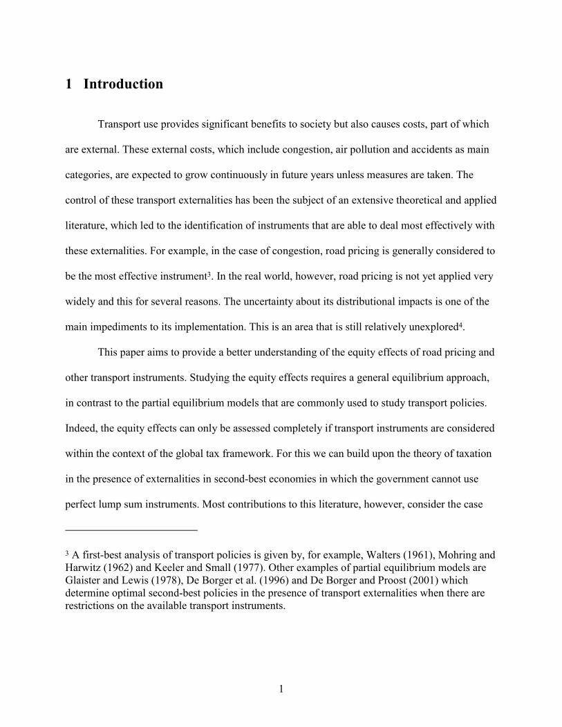
1 Introduction

Transport use provides significant benefits to society but also causes costs, part of which

are external. These external costs, which include congestion, air pollution and accidents as main

categories, are expected to grow continuously in future years unless measures are taken. The

control of these transport externalities has been the subject of an extensive theoretical and applied

literature, which led to the identification of instruments that are able to deal most effectively with

these externalities. For example, in the case of congestion, road pricing is generally considered to

be the most effective instrument3. In the real world, however, road pricing is not yet applied very

widely and this for several reasons. The uncertainty about its distributional impacts is one of the

main impediments to its implementation. This is an area that is still relatively unexplored4.

This paper aims to provide a better understanding of the equity effects of road pricing and

other transport instruments. Studying the equity effects requires a general equilibrium approach,

in contrast to the partial equilibrium models that are commonly used to study transport policies.

Indeed, the equity effects can only be assessed completely if transport instruments are considered

within the context of the global tax framework. For this we can build upon the theory of taxation

in the presence of externalities in second-best economies in which the government cannot use

perfect lump sum instruments. Most contributions to this literature, however, consider the case

3 A first-best analysis of transport policies is given by, for example, Walters (1961), Mohring and Harwitz (1962) and Keeler and Small (1977). Other examples of partial equilibrium models are Glaister and Lewis (1978), De Borger et al. (1996) and De Borger and Proost (2001) which determine optimal second-best policies in the presence of transport externalities when there are restrictions on the available transport instruments.

1

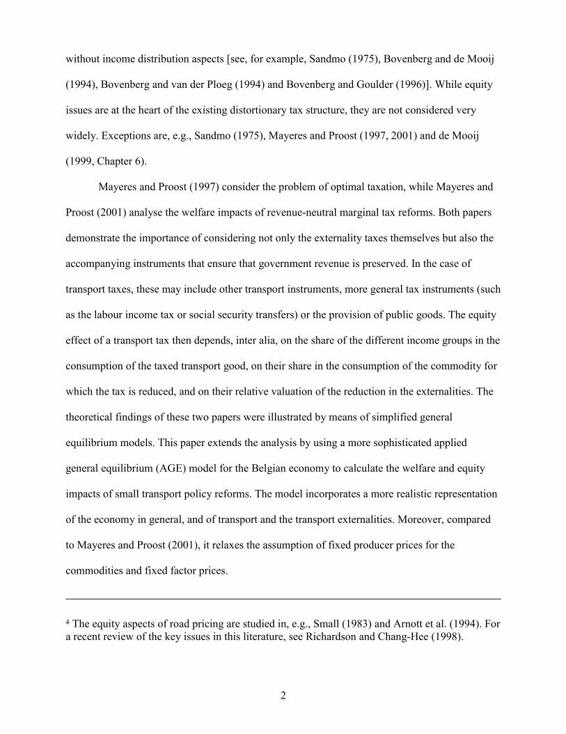
without income distribution aspects [see, for example, Sandmo (1975), Bovenberg and de Mooij

(1994), Bovenberg and van der Ploeg (1994) and Bovenberg and Goulder (1996)]. While equity

issues are at the heart of the existing distortionary tax structure, they are not considered very

widely. Exceptions are, e.g., Sandmo (1975), Mayeres and Proost (1997, 2001) and de Mooij

(1999, Chapter 6).

Mayeres and Proost (1997) consider the problem of optimal taxation, while Mayeres and

Proost (2001) analyse the welfare impacts of revenue-neutral marginal tax reforms. Both papers

demonstrate the importance of considering not only the externality taxes themselves but also the

accompanying instruments that ensure that government revenue is preserved. In the case of

transport taxes, these may include other transport instruments, more general tax instruments (such

as the labour income tax or social security transfers) or the provision of public goods. The equity

effect of a transport tax then depends, inter alia, on the share of the different income groups in the

consumption of the taxed transport good, on their share in the consumption of the commodity for

which the tax is reduced, and on their relative valuation of the reduction in the externalities. The

theoretical findings of these two papers were illustrated by means of simplified general

equilibrium models. This paper extends the analysis by using a more sophisticated applied

general equilibrium (AGE) model for the Belgian economy to calculate the welfare and equity

impacts of small transport policy reforms. The model incorporates a more realistic representation

of the economy in general, and of transport and the transport externalities. Moreover, compared

to Mayeres and Proost (2001), it relaxes the assumption of fixed producer prices for the

commodities and fixed factor prices.

4 The equity aspects of road pricing are studied in, e.g., Small (1983) and Arnott et al. (1994). For a recent review of the key issues in this literature, see Richardson and Chang-Hee (1998).

2

The approach taken here is similar to the one followed in Ballard and Medema (1993),

Brendemoen and Vennemo (1996), Bovenberg and Goulder (1997) and Mayeres (2000).

However, the analysis differs from the first three studies in three ways. First of all, it focuses on

the three main transport externalities: congestion, air pollution and accidents. Secondly, it

incorporates the feedback effect of congestion on the behaviour of producers and consumers.

Both features were already included in Mayeres (2000). The last difference, which is also an

extension of Mayeres (2000), is that the paper explicitly takes into account distributional

concerns.

The paper calculates the welfare impacts of small revenue-neutral policy reforms,

consisting of a change in a transport instrument and an accompanying change in a revenue-

preserving instrument, which may belong to two categories. The first category includes two

conventional tax instruments: the lump sum social security transfer and the labour-income tax.

The second category consists of transport instruments, which makes it possible to evaluate the

earmarking of transport tax revenue for use within the transport sector. The welfare impacts are

first computed for a constant level of the externalities. This allows us to explore the implications

of equity considerations for the double dividend argument, which claims that the budget-neutral

substitution of an externality tax for an existing distortionary tax might offer an extra dividend, in

addition to the benefits of the lower externality5. Next, we include the three main transport

externalities in the analysis. We consider the following questions: How are different income

groups affected by policy reforms? What is the impact on the level of inequality? What are the

implications of inequality aversion for the ranking of the transport instruments? Do the

5 Goulder (1995) presents an overview of the double dividend issue.

3

recommended revenue-recycling strategies change as a function of the attitude towards

inequality?

Section 2 briefly describes the AGE model and its calibration. Section 3 presents the

welfare and equity impacts of the revenue-neutral marginal policy reforms. Section 4 concludes

and discusses some extensions to the analysis.

2 The AGE model and its calibration

2.1 The AGE model

The AGE model is similar to the one presented in Mayeres (2000). The only differences

with that model arise from the fact that the AGE model now includes five consumer groups,

corresponding with the quintiles of the Belgian household budget survey, instead of one

representative consumer group. For a detailed description of the model, the reader is referred to

Mayeres (1999).

The AGE model is a static model for a small open economy, with a medium term time

horizon. Four types of economic agents are considered: five consumer groups, fourteen main

production sectors, the government and the foreign sector. Two individuals belonging to a

different consumer group are assumed to differ in terms of the following main characteristics:

their productivity, their tastes and their share in the total endowment of capital goods and the

government transfers. Individuals belonging to the same consumer group are however identical in

terms of their needs.

The model includes several transport commodities. It makes a distinction between

passenger and freight transport, between three transport modes (road, rail and inland navigation),

between vehicle types and between peak and off-peak transport (except for freight rail and inland

4

navigation). Three types of externalities are taken into account: congestion, air pollution

(including global warming) and accidents. Air pollution and accidents are assumed to have an

impact on the consumers’ welfare, but not on their behaviour6. The modeling of the impact of

congestion on the consumers is based on DeSerpa (1971) and Bruzelius (1979). Congestion does

not only affect the consumers’ welfare negatively, but also influences the transport choices of the

consumers. Moreover, the modeling approach implies that the value of a marginal time saving

(VOT) is determined endogenously in the model7. Congestion is also assumed to reduce the

productivity of transport labour in the production sectors.

2.2 The benchmark equilibrium and the calibration of the AGE model

The starting point of the exercises is the situation in Belgium in 1990, which represents

the benchmark equilibrium8. The calibration of the model consists of the selection of parameters

such that the behaviour of the economic agents around the benchmark equilibrium and their

valuation of the transport externalities corresponds with values given in the literature. This

section first presents the share of the quintiles in total household expenditures and receipts. Next,

it discusses some crucial demand and supply elasticities. Finally, it presents the marginal external

costs of transport in the benchmark equilibrium and compares them with taxes paid.

6 In reality air pollution and accident risks also affect the consumption choices. Such feedback effects are not yet included in the model. 7 This contrasts with the generalised cost approach often used in transport models. In that approach, the demand for a transport good depends, inter alia, on its generalised cost, which is the sum of its money price and the time requirement multiplied by an exogenous VOT. 8 For details on the data set and the calibration, the reader is referred to Mayeres (1999).

5

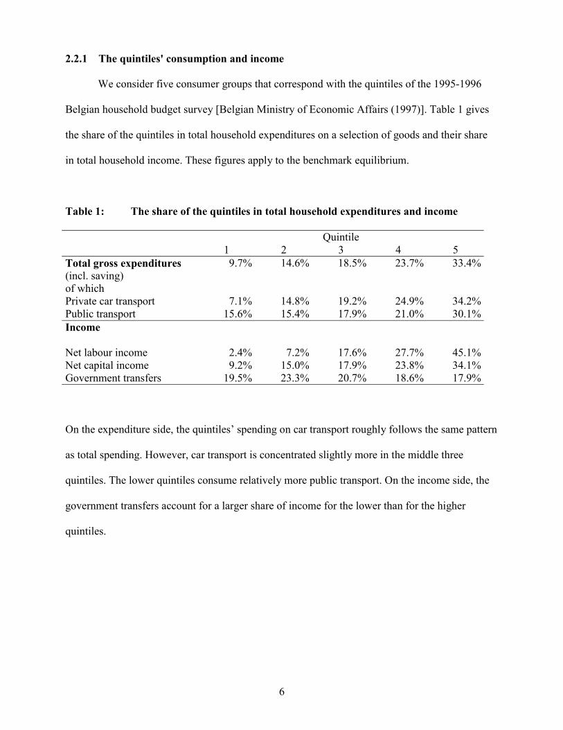
2.2.1 The quintiles' consumption and income

We consider five consumer groups that correspond with the quintiles of the 1995-1996

Belgian household budget survey [Belgian Ministry of Economic Affairs (1997)]. Table 1 gives

the share of the quintiles in total household expenditures on a selection of goods and their share

in total household income. These figures apply to the benchmark equilibrium.

Table 1: The share of the quintiles in total household expenditures and income Quintile 1 2 3 4 5 Total gross expenditures (incl. saving) of which Private car transport Public transport

9.7%

7.1%15.6%

14.6%

14.8%15.4%

18.5%

19.2%17.9%

23.7%

24.9% 21.0%

33.4%

34.2%30.1%

Income Net labour income Net capital income Government transfers

2.4%9.2%

19.5%

7.2%15.0%23.3%

17.6%17.9%20.7%

27.7% 23.8% 18.6%

45.1%34.1%17.9%

On the expenditure side, the quintiles’ spending on car transport roughly follows the same pattern

as total spending. However, car transport is concentrated slightly more in the middle three

quintiles. The lower quintiles consume relatively more public transport. On the income side, the

government transfers account for a larger share of income for the lower than for the higher

quintiles.

6

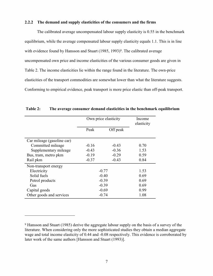
2.2.2 The demand and supply elasticities of the consumers and the firms

The calibrated average uncompensated labour supply elasticity is 0.55 in the benchmark

equilibrium, while the average compensated labour supply elasticity equals 1.1. This is in line

with evidence found by Hansson and Stuart (1985, 1993)9. The calibrated average

uncompensated own price and income elasticities of the various consumer goods are given in

Table 2. The income elasticities lie within the range found in the literature. The own-price

elasticities of the transport commodities are somewhat lower than what the literature suggests.

Conforming to empirical evidence, peak transport is more price elastic than off-peak transport.

Table 2: The average consumer demand elasticities in the benchmark equilibrium

Own price elasticity

Peak Off peak

Income elasticity

Car mileage (gasoline car) Committed mileage Supplementary mileage Bus, tram, metro pkm Rail pkm

-0.16 -0.43 -0.19 -0.37

-0.43 -0.36 -0.29 -0.43

0.70 1.53 0.59 0.84

Non-transport energy Electricity Solid fuels Petrol products Gas Capital goods Other goods and services

-0.77 -0.40 -0.39 -0.39 -0.69 -0.74

1.53 0.69 0.69 0.69 0.99 1.08

9 Hansson and Stuart (1985) derive the aggregate labour supply on the basis of a survey of the literature. When considering only the more sophisticated studies they obtain a median aggregate wage and total income elasticity of 0.44 and -0.08 respectively. This evidence is corroborated by later work of the same authors [Hansson and Stuart (1993)].

7

Capros et al. (1997) is the basis for most of the elasticities on the producer side. The

elasticities of substitution for freight transport are chosen in function of the elasticity estimates

presented in Oum et al. (1992).

2.2.3 The marginal external costs of transport use

The marginal external congestion costs

Congestion is taken to occur only on the road network. The road traffic flow determines

the minimum time needed per unit of motorized passenger and freight road transport10. The road

network is represented as a one-link system with homogeneous traffic conditions. An exponential

time-flow relationship, based on O’ Mahony et al. (1997), is used to calculate the impact of

traffic flow on the minimum time requirement per unit of road transport11.

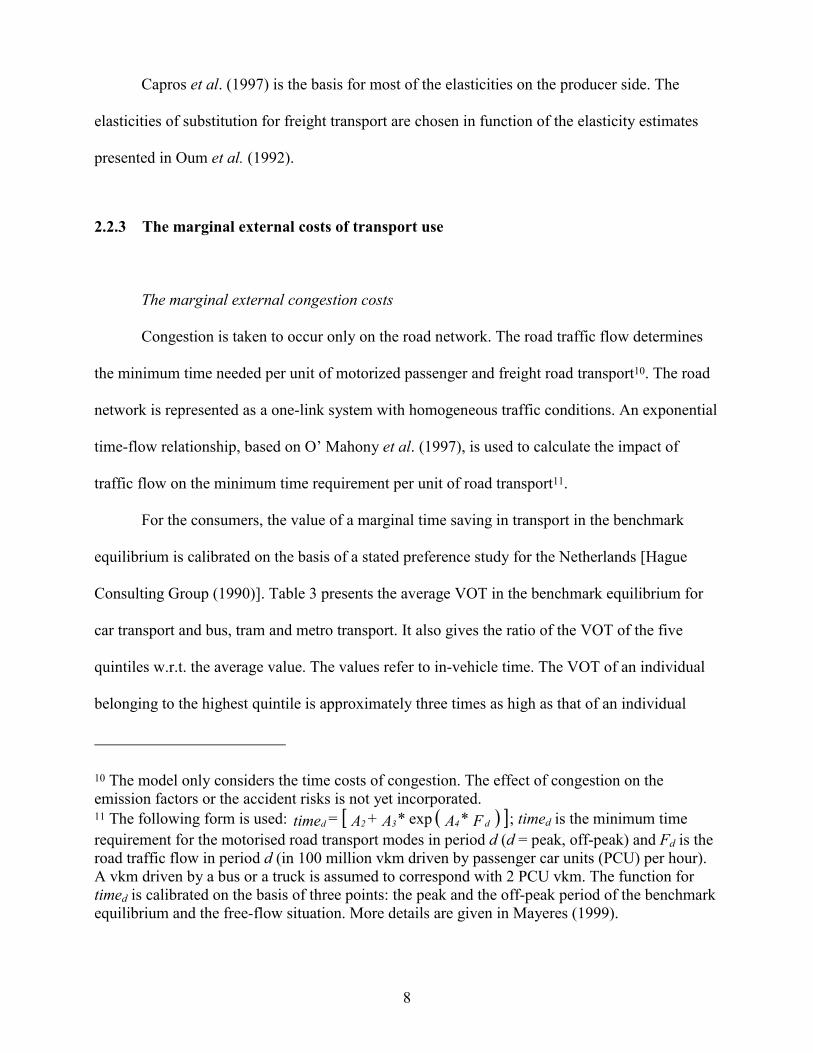
For the consumers, the value of a marginal time saving in transport in the benchmark

equilibrium is calibrated on the basis of a stated preference study for the Netherlands [Hague

Consulting Group (1990)]. Table 3 presents the average VOT in the benchmark equilibrium for

car transport and bus, tram and metro transport. It also gives the ratio of the VOT of the five

quintiles w.r.t. the average value. The values refer to in-vehicle time. The VOT of an individual

belonging to the highest quintile is approximately three times as high as that of an individual

� �

10 The model only considers the time costs of congestion. The effect of congestion on the emission factors or the accident risks is not yet incorporated. 11 The following form is used: time ; timed is the minimum time requirement for the motorised road transport modes in period d (d = peak, off-peak) and Fd is the road traffic flow in period d (in 100 million vkm driven by passenger car units (PCU) per hour). A vkm driven by a bus or a truck is assumed to correspond with 2 PCU vkm. The function for timed is calibrated on the basis of three points: the peak and the off-peak period of the benchmark equilibrium and the free-flow situation. More details are given in Mayeres (1999).

�� F* A * A + A = d432d exp

8

belonging to the lowest quintile. For the firms, the monetary value of a time saving is assumed to

be given by the before-tax wage rate.

Table 3: The consumers’ value of a marginal time saving in transport in the benchmark equilibrium

Car Bus, tram, metro

Average VOT (EURO(2000)/h) Peak Off-peak

6.43 5.72

5.11 4.16

Ratio of the quintile’s VOT w.r.t. the average VOT Quintile 1 Quintile 2 Quintile 3 Quintile 4 Quintile 5

0.49 0.55 0.75 0.98 1.46

0.48 0.58 0.69 0.97 1.44

Given the way in which congestion is modeled, the VOT is affected by the tax reforms.

Table 4 presents the calibrated average elasticity of the VOT w.r.t. its determinants in the

benchmark equilibrium.

Table 4: The average elasticity of the VOT with respect to its main determinants in the benchmark equilibrium

The elasticity of the VOT w.r.t.

Wage rate Money price of the transport good

Minimum time requirement

Peak car Off-peak car Peak bus, tram, metro Off-peak bus, tram, metro

1.08 1.18 1.15 1.32

-0.08 -0.17 0.02 0.08

0.11 0.19 0.33 0.50

9

It is related positively to the wage rate and to the minimum time requirement. An increase in the

consumer price reduces the VOT for car transport. This is in line with intuition: the willingness-

to-pay (WTP) for a time saving is higher the lower the monetary price one is already paying for

the transport good. For bus, tram and metro the relationship between the consumer price and the

VOT is a positive one. The consumer price has a direct and an indirect impact on the VOT. The

direct effect is always negative. But a higher consumer price also reduces the demand for the

transport good, which tends to increase the VOT. For bus, tram and metro transport, the indirect

effect dominates.

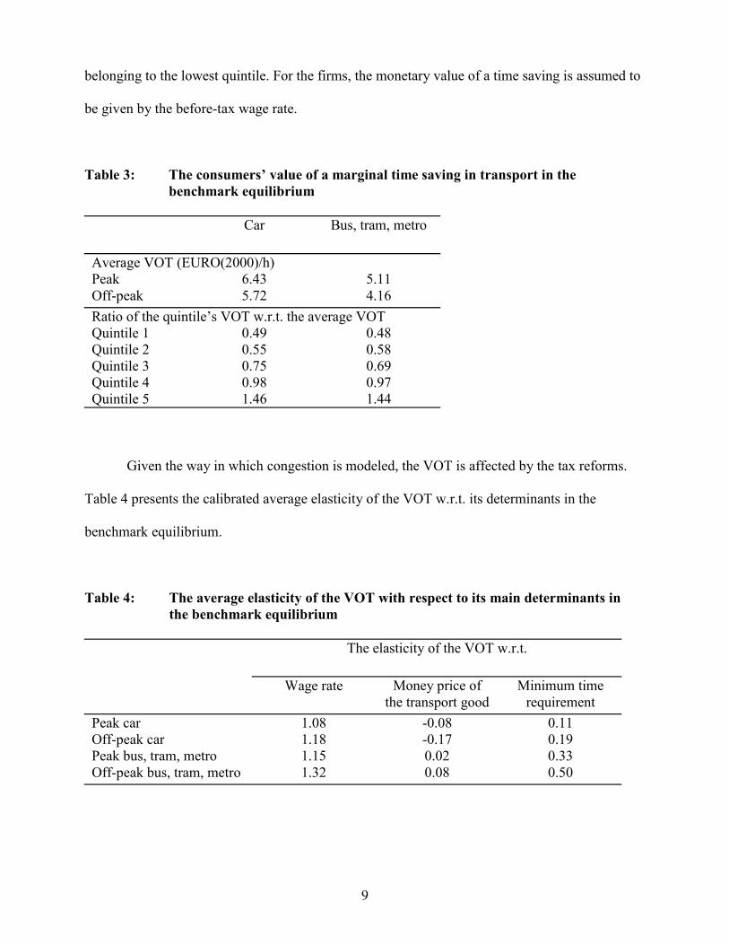
The marginal external air pollution costs

The model includes the following air pollutants: NOx, SO2, HC, CO, CO2 and particulate

matter with a diameter smaller than 10 and 2.5 microns (PM10 and PM2.5,

respectively). The emissions of these pollutants are a function of the use of energy for transport

and non-transport purposes. Table 5 presents the marginal social costs per unit of emissions in the

benchmark equilibrium. The cost calculations are based on Mayeres et al. (1996) and the Extern-

E project [Bickel et al. (1997)]. The marginal social air pollution costs consist mainly of health

damage costs.

Table 5: The marginal external costs of air pollution

NOx SOx HC PM10 PM2.5 CO CO2

EURO(2000)/kg EURO(2000)/metric tonne

The marginal external air pollution costs 2.52 7.20 0.31 26.57 280 2.79 15.86

10

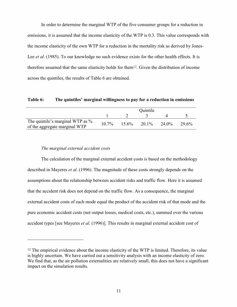
In order to determine the marginal WTP of the five consumer groups for a reduction in

emissions, it is assumed that the income elasticity of the WTP is 0.3. This value corresponds with

the income elasticity of the own WTP for a reduction in the mortality risk as derived by Jones-

Lee et al. (1985). To our knowledge no such evidence exists for the other health effects. It is

therefore assumed that the same elasticity holds for them12. Given the distribution of income

across the quintiles, the results of Table 6 are obtained.

Table 6: The quintiles’ marginal willingness to pay for a reduction in emissions

Quintile 1 2 3 4 5 The quintile’s marginal WTP as % of the aggregate marginal WTP 10.7% 15.6% 20.1% 24.0% 29.6%

The marginal external accident costs

The calculation of the marginal external accident costs is based on the methodology

described in Mayeres et al. (1996). The magnitude of these costs strongly depends on the

assumptions about the relationship between accident risks and traffic flow. Here it is assumed

that the accident risk does not depend on the traffic flow. As a consequence, the marginal

external accident costs of each mode equal the product of the accident risk of that mode and the

pure economic accident costs (net output losses, medical costs, etc.), summed over the various

accident types [see Mayeres et al. (1996)]. This results in marginal external accident cost of

12 The empirical evidence about the income elasticity of the WTP is limited. Therefore, its value is highly uncertain. We have carried out a sensitivity analysis with an income elasticity of zero. We find that, as the air pollution externalities are relatively small, this does not have a significant impact on the simulation results.

11

29.50 10-3 EURO(2000) per vehicle kilometer (vkm) for cars, 116.80 10-3 EURO/vkm for buses,

0.20 10-3 EURO/vkm for trams, 16.80 10-3 EURO/vkm for trucks and 226.80 10-3 EURO per

passenger km (pkm) for non-motorized transport. The high costs for non-motorized transport are

explained by the relatively high accident risks for this mode.

The marginal WTP for a reduction in accidents is assumed to be identical for all

individuals. As will be clear later, the marginal external accident costs are of relatively small

importance and therefore this assumption is not expected to affect the model’s results

significantly.

The marginal external costs of transport use

Table 7 presents the resulting marginal external costs of the various transport modes in the

benchmark equilibrium. It also compares the marginal external costs with the taxes paid. In the

case of public transport the subsidies related to the provision of the transport services are high,

which results in a negative tax. For peak road transport congestion accounts for the largest share

in the external costs. In the off-peak period air pollution is the most important external cost

category for diesel vehicles, while accident costs form the largest category for gasoline vehicles.

For all transport modes there is a large divergence between the tax and the marginal

external costs. Note, however, that we are in a second-best economy in which the government has

to use distortionary taxes in order to achieve three types of objectives: raising revenue,

controlling the externalities, and reaching its distributional goals. This implies that, unlike in a

first-best economy, the optimal tax on transport will in general be different from the marginal

external costs [see, for example, Mayeres and Proost (1997)].

12

Table 7: Road transport: the marginal external costs and the taxes in the benchmark equilibrium

Share in marginal external costs

Marginal external

costs (EURO (2000)/ vkm)

Congestion Air pollution

Accidents

Taxa

(EURO (2000) /vkm)

Passenger transport

Gasoline car – peak Gasoline car - off-peak Diesel car - peak Diesel car - off-peak

0.29 0.09 0.34 0.15

83% 48% 69% 30%

7% 21% 22% 50%

10% 31% 9%

20%

0.10 [0.04] 0.10 [0.04] 0.06 [0.02] 0.06 [0.02]

Tram, metro – peak Tram, metro - off-peak Bus - peak Bus - off-peak

0.47 0.09 1.16 0.78

100% 100% 41% 12%

0% 0%

49% 73%

0% 0%

10% 15%

-0.80 -0.93 -0.67 -0.77

Rail - electric Rail – diesel

0 0.26

0%

100%

0%

-1.63 [-2.25] -0.51 [-0.63]

Freight transport

Truck - peak Truck – off-peak

0.89 0.51

53% 18%

45% 79%

2% 3%

0.13 0.13

Rail - electric Rail – diesel

0 0.72

0%

100%

0%

0 0

Inland navigation 0.02 0% 100% 0% 0a The values between brackets refer to the tax on business car transport

3 The marginal welfare effect of three transport instruments with various revenue-preserving strategies

We now use the AGE model to calculate the marginal welfare effect of three transport

instruments: peak road pricing, the fuel tax and subsidies to public transport. As the term

“marginal” reflects, we consider small policy changes with respect to the benchmark equilibrium.

The results should be interpreted as such. Generally, the impacts of the tax reforms can be

13

expected not to be a linear function of the size of the reforms. In addition, the policy reforms are

taken to be revenue-neutral. In order to ensure this, the transport instruments are accompanied by

changes in other policy instruments.

3.1 A description of the revenue-neutral marginal policy reforms

For reasons of comparability we consider the same policy changes as in Mayeres (1999).

The three transport instruments correspond with the following policy reforms:

- Peak road pricing: a tax is levied on the vehicle km driven by motorized road transport in

the peak period. Both domestic and foreign transport users are subject to the tax. No

distinction is made between vehicle types.

- The fuel tax: the instrument consists of altering the excise on the fuels for road transport.

Table 8 presents the level of the excises in the benchmark equilibrium. It is assumed that

all fuel types are subject to the same change in the excise, expressed in percentage points.

Since the excise is altered, rather than the value added tax rate, the tax on the use of fuel

for road transport changes for both the consumers and the domestic producers. Foreign

road transport users do not face a tax change, since they are assumed to buy their fuel

abroad. The tax rate on fuel used by rail transport and inland navigation remains constant.

- The public transport subsidy: the subsidy rate for public passenger and freight transport is

changed. The benchmark level of the subsidy rates is summarized in Table 8. The

percentage change with respect to the benchmark equilibrium is taken to be the same for

all public transport modes.

14

The transport instruments are introduced in a revenue-neutral way. As revenue-preserving

instruments, we first consider two “conventional” instruments (that is, not aimed at the transport

sector):

- The lump sum tax: the instrument consists of a change in the lump sum social security

transfers received by the individuals. In the initial equilibrium the share of these transfers

in net money income ranges from 55% for the poorest quintile to 15% for the richest

quintile (see Table 8). The same percentage change in the real lump sum social security

transfers is assumed for all quintiles.

- The labour income tax: Table 8 presents the labour income tax rate for the quintiles in the

initial equilibrium. The labour income tax rate is changed in the same proportion for all

quintiles.

Secondly, we analyse the welfare effects of earmarking the transport tax revenues for use

within the transport sector.

In order to ensure comparability the changes in the three transport instruments imply an

equal absolute impact on government spending (0.20%), when abstraction is made of the

revenue-preserving changes in the other instruments.

15

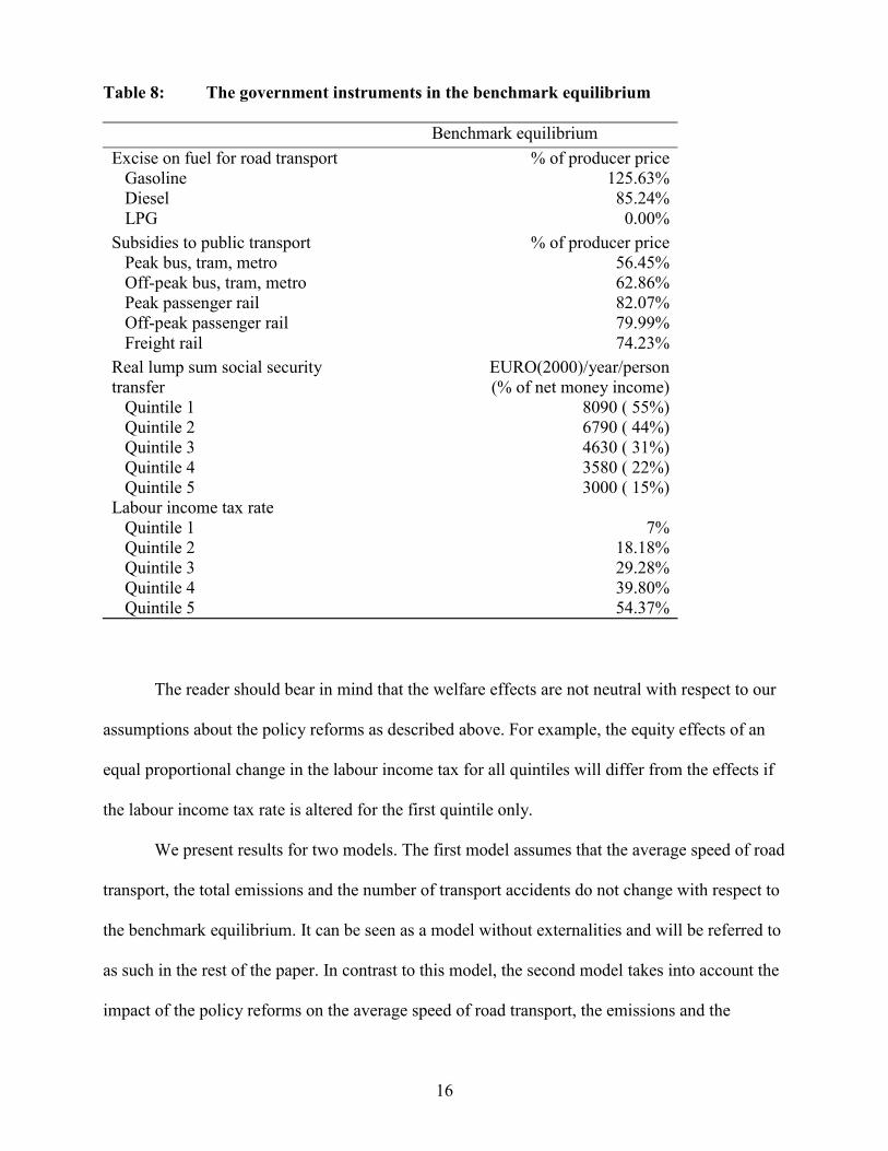
Table 8: The government instruments in the benchmark equilibrium Benchmark equilibrium Excise on fuel for road transport Gasoline Diesel LPG

% of producer price 125.63% 85.24% 0.00%

Subsidies to public transport Peak bus, tram, metro Off-peak bus, tram, metro Peak passenger rail Off-peak passenger rail Freight rail

% of producer price 56.45% 62.86% 82.07% 79.99% 74.23%

Real lump sum social security transfer Quintile 1 Quintile 2 Quintile 3 Quintile 4 Quintile 5

EURO(2000)/year/person (% of net money income)

8090 ( 55%) 6790 ( 44%) 4630 ( 31%) 3580 ( 22%) 3000 ( 15%)

Labour income tax rate Quintile 1 Quintile 2 Quintile 3 Quintile 4 Quintile 5

7%

18.18% 29.28% 39.80% 54.37%

The reader should bear in mind that the welfare effects are not neutral with respect to our

assumptions about the policy reforms as described above. For example, the equity effects of an

equal proportional change in the labour income tax for all quintiles will differ from the effects if

the labour income tax rate is altered for the first quintile only.

We present results for two models. The first model assumes that the average speed of road

transport, the total emissions and the number of transport accidents do not change with respect to

the benchmark equilibrium. It can be seen as a model without externalities and will be referred to

as such in the rest of the paper. In contrast to this model, the second model takes into account the

impact of the policy reforms on the average speed of road transport, the emissions and the

16

transport accidents. In the rest of the paper it is termed the model with externalities. Comparing

the results of these two models allows to determine how the policy conclusions are affected by

including the impact on the externalities and to link the discussion to the double dividend

literature.

3.2 The measurement of the welfare impacts

The marginal welfare impacts are presented in EURO per EURO of government revenue.

The monetary value of the change in social welfare is measured by the social equivalent gain of

the policy reform, summed over the individuals. This is defined as the increase in each

individual’s original equivalent income that would produce a social welfare level equal to the one

obtained in the post-reform equilibrium [King (1983)].

The following iso-elastic formulation is used for the social welfare function:

� �1

5

1 1

ii

i

EIW a

�

�

�

�

�

�

�

ai is the number of persons in quintile i. The welfare of an individual belonging to quintile i is

measured by means of his equivalent income EIi. That is the level of income which, at the

benchmark price vector and the benchmark levels of congestion, emissions and accidents, allows

one to reach the same level of utility as can be attained under the new price vector and level of

congestion, emissions and accidents. � is the degree of inequality aversion. We present results for

different degrees of inequality aversion in order to analyse the implications if society's attitude

towards inequality changes. A value of � equal to zero gives rise to a pure efficiency social

welfare function. This means that the social welfare function gives an equal marginal social

welfare weight to all individuals. As the value of � increases, society gives a relatively higher

marginal social welfare weight to individuals belonging to the poorer quintiles.

17

Given this definition of the social welfare function, the social equivalent gain (SGn(�)) of

a policy reform n can be derived from:

� �� � � �1 1,5 5

1 11 1

i ref in ni i

i i

EI SG EIa a

� �

�

� �

� �

� �

�

�

� �� �

with EIi,ref the equivalent income in the benchmark equilibrium. The value of SGn depends on the

degree of inequality aversion.

3.3 Simulation results

Table 9 summarizes the marginal welfare impacts of nine revenue-neutral policy reforms. The

results are presented as a function of two criteria:

�� the model used: the left-hand side of the table refers to the model without externalities,

while the right-hand side gives the results for the model with externalities.

�� the degree of inequality aversion: the upper part of the table assumes a pure efficiency

social welfare function (� = 0), while the lower part presents the results for a higher

degree of inequality aversion (� = 0.5).

Section 3.3.1 first discusses the results for the model without externalities. This gives us

an idea of the gross welfare costs of the instruments, i.e. the impact abstracting from their effect

on the externalities. Next, Section 3.3.2 turns to the model with externalities. Both sections first

present the efficiency case and then consider the implications of equity considerations.

18

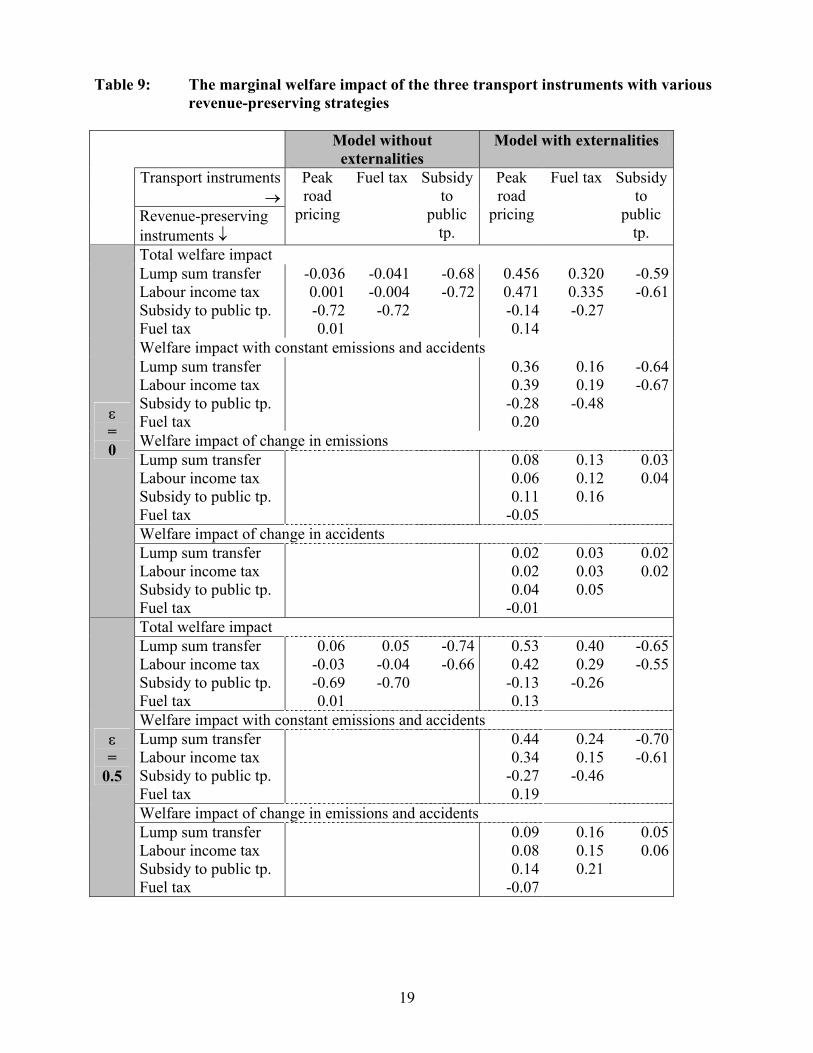
Table 9: The marginal welfare impact of the three transport instruments with various revenue-preserving strategies

Model without

externalities Model with externalities

Transport instruments �

Revenue-preserving instruments �

Peak road

pricing

Fuel tax Subsidy to

public tp.

Peak road

pricing

Fuel tax Subsidy to

public tp.

Total welfare impact Lump sum transfer Labour income tax Subsidy to public tp. Fuel tax

-0.0360.001-0.720.01

-0.041-0.004-0.72

-0.68-0.72

0.4560.471-0.140.14

0.320 0.335 -0.27

-0.59-0.61

Welfare impact with constant emissions and accidents Lump sum transfer Labour income tax Subsidy to public tp. Fuel tax

0.360.39

-0.280.20

0.16 0.19

-0.48

-0.64-0.67

Welfare impact of change in emissions Lump sum transfer Labour income tax Subsidy to public tp. Fuel tax

0.080.060.11

-0.05

0.13 0.12 0.16

0.030.04

Welfare impact of change in accidents

� = 0

Lump sum transfer Labour income tax Subsidy to public tp. Fuel tax

0.020.020.04

-0.01

0.03 0.03 0.05

0.020.02

Total welfare impact Lump sum transfer Labour income tax Subsidy to public tp. Fuel tax

0.06-0.03-0.690.01

0.05-0.04-0.70

-0.74-0.66

0.530.42

-0.130.13

0.40 0.29

-0.26

-0.65-0.55

Welfare impact with constant emissions and accidents Lump sum transfer Labour income tax Subsidy to public tp. Fuel tax

0.440.34

-0.270.19

0.24 0.15

-0.46

-0.70-0.61

Welfare impact of change in emissions and accidents

� =

0.5

Lump sum transfer Labour income tax Subsidy to public tp. Fuel tax

0.090.080.14

-0.07

0.16 0.15 0.21

0.050.06

19

3.3.1 The model without externalities

Efficiency

With a pure efficiency social welfare function (� = 0) the conclusions are similar as in

Mayeres (2000). When the impact on the externalities is ignored, the three transport instruments

give rise to a marginal welfare loss in most cases. The marginal welfare losses are the largest

(close to –0.70 in all cases) when the subsidies to public transport are raised. In the absence of

concerns about transport externalities or equity and under the assumption of a constant-returns-

to-scale technology for public transport, it is clearly not beneficial to increase these subsidies.

For the other policy packages the absolute value of the welfare impact is much smaller.

First, we consider the case of peak road pricing and the fuel tax, when the lump sum transfer is

used as the revenue-preserving instrument. They both result in a welfare loss. Therefore, in the

absence of externality considerations they are not socially worthwhile. However, the welfare loss

is relatively small, for which there are two reasons. First of all, the two transport instruments

cause a relatively small welfare loss. This is because both measures increase labour supply,

which somewhat limits the negative impact of the instruments on labour income tax revenue.

This is made possible by the fact that more expensive transport means that less time is devoted to

transport. Moreover, there is a shift from relatively less productive and lowly taxed labour

(supplied by the first two quintiles) to relatively highly productive and highly taxed labour.

Secondly, increasing the lump sum social security transfer is extra beneficial because it increases

the labour supply measured in efficiency hours and the share of heavily taxed labour, and

therefore the labour income tax revenue.

The marginal welfare loss of the fuel tax is larger than that of peak road pricing, although

the tax base of the former is broader than that of the latter. The fuel tax leads to a larger switch to

20

public transport and, consequently, to a larger increase in the total subsidies paid to this transport

mode. This also explains why the revenue-neutral substitution of peak road pricing for the fuel

tax leads to a small welfare gain.

How does the welfare impact of these two instruments change when the labour-income

tax is used as the revenue-preserving instrument instead of the lump sum transfers? Here we enter

the area of the double dividend literature. We use the classification of Goulder (1995) as

summarised in Table 10.

Table 10: An overview of terminology in the double dividend literature first dividend = the welfare gain associated with the lower externalities weak double dividend = a gross welfare gain is obtained by the replacement of the

lump sum transfer by the labour income tax to return the externality tax revenues

strong double dividend = a zero or positive gross welfare gain obtained by the revenue neutral substitution of the externality tax for a representative distortionary tax

based on Goulder (1995)

In the absence of equity concerns, the welfare gain with a lower labour-income tax is

larger than that of a lower lump sum tax. So a weak double dividend is present for peak road

pricing and the fuel tax. This is because, in contrast to the lump sum tax, which has only revenue

effects, the labour-income tax has distortionary effects as well, caused by substitution away from

the tax base. Note that similar reasons explain why the welfare loss of the public transport

subsidies is larger when the labour-income tax rather than the lump sum tax is used to finance

them.

When peak road pricing is combined with a lower labour income tax the net welfare effect

is non-negative, which means that there is some scope for a strong double dividend. However, its

size is very small. As was explained above, peak road pricing increases the labour supply and the

share of relatively highly productive and highly taxed labour. This dominates the distortions of

21

intermediate input choice and of the choice between consumer goods that peak road pricing

causes additionally in comparison with the labour income tax.

The implications of equity considerations

How do the findings change when equity considerations come into play? We consider

here the case of � = 0.513. This corresponds with a medium degree of inequality aversion14.

The main effect of the higher degree of inequality aversion is that the double dividend

results do not longer hold, be it in the weak or strong version. Indeed, for peak road pricing and

the fuel tax, the ranking between the lump sum tax and the labour income tax as a revenue-

recycling instrument is now reversed. The weak double dividend, that is generally considered to

be the least controversial form of the double dividend, is no longer evident when equity concerns

become more important. Moreover, the combination of peak road pricing and the labour income

tax now gives rise to a gross welfare loss. These findings illustrate the importance of introducing

distributional considerations in the double dividend discussion, an aspect was has been largely

ignored up to now [for exceptions, see Mayeres and Proost (1997, 2001) and de Mooij (1999)].

With � = 0.5 the beneficial effects of higher lump sum transfers turn out to be high

enough, so that is socially beneficial to finance them by the two transport taxes, even in the

absence of considerations about transport externalities. Note, however, that the welfare gain

would be larger if the higher lump sum transfers were financed by the labour income tax. This

13 We also considered two other degrees of inequality aversion (� = 0.25 and � = 1.5). For the interested reader the results for these two cases are presented in Appendix A. The main conclusions of this section continue to hold for these two other values of �. 14 With � = 0.5 the marginal social welfare weight of people belonging to the highest quintile is appr. 70% of those belonging to the lowest quintile.

22

would allow for gross welfare gain of 0.09 (= 0.06-(-0.03); instead of 0.06 in the case of peak

road pricing accompanied by a lower labour income tax).

A higher degree of inequality aversion does not change the conclusions about the

subsidies to public transport. The poorer quintiles consume a relatively larger share of public

transport than of car transport, which leads to a slight decrease in the gross welfare cost of public

transport subsidies (except when they are financed by lower lump sum transfers). However, the

distributional gains are outweighed by far by the efficiency costs of the subsidies, so that they

continue to be welfare reducing even with a higher degree of inequality aversion.

3.3.2 The model with externalities

We now consider how the introduction of the externalities changes the policy conclusions.

As can be expected, the impact is significant.

Efficiency

When only efficiency matters, the policy conclusions conform to those presented in

Mayeres (2000). Therefore, the discussion of the results will be brief. The right-hand side of

Table 9 first presents the total welfare impact of the reforms. This impact is split into three

components:

- The first component corresponds with the welfare effect when the emissions and the

transport accidents remain constant at their benchmark level. Given the way in which

congestion is modeled, this part includes the welfare effects of the change in road

congestion. For peak road pricing and the fuel tax the impact on congestion explains the

major part of the difference between the model with and without externalities. The

23

calculation of the change in congestion and its impact on welfare takes into account the

feedback effect and the impact of the policy packages on the VOT of transport.

- The second component presents the welfare impact associated with the change in

emissions.

- Finally, the last component gives the welfare effect of the change in the number of

accidents.

Which of the three transport instruments is to be preferred?

The choice among the three transport instruments depends on their effectiveness in

tackling the externalities and on the relative importance of the externalities. Table 9 shows that,

for a given revenue-preserving strategy, the highest welfare gains are realised with the

introduction of peak road pricing. Congestion is the most important externality in our model and

of the three transport instruments considered here, peak road pricing addresses congestion in the

most effective way. Indeed, it allows to treat peak and off-peak transport differently, while the

fuel tax15 and subsidies to public transport do not. A higher fuel tax leads to less car transport in

the peak and the off-peak period, with the highest reduction in the latter period, while congestion

is by definition a peak period phenomenon. Note that the fuel tax is more effective than peak road

pricing in tackling air pollution and accidents (cf. the welfare impact of the change in emissions

and accidents in Table 9), since it has the largest impact on total traffic volume, which is the main

15 The model does not yet include the choice between vehicles with different fuel efficiencies. Including the possibility to switch to more fuel-efficient vehicles would make the fuel tax even less appropriate for tackling congestion. Moreover, the tax should be set higher in order to finance the real increase in government spending, which would also reduce the welfare gain.

24

determinant of these externalities in the model. However, given the high relative weight given to

congestion it is ranked in second position.

How should the revenues of peak road pricing be used?

The welfare gain of peak road pricing is the highest when its revenue is recycled through

a lower labour income tax (0.471) rather than a higher lump sum transfer (0.456). This is in line

with the difference in gross welfare costs of the lump sum tax and the labour-income tax. The

difference between these two revenue-recycling instruments is small and also less pronounced

than in the model without externalities. This is because the cut in the labour income tax increases

the externalities more than the higher lump sum transfer.

Using the revenues of peak road pricing to finance higher subsidies to public transport

results in a welfare loss (-0.14), despite the fact that the higher subsidies reinforce the

instrument’s effect on the externalities. However, this beneficial effect only partly compensates

for the gross welfare costs of the subsidies.

Substituting road pricing for the fuel tax improves welfare. However, the resulting welfare

gain (0.14) is small compared to the case in which road pricing revenue substitutes for the labour-

income tax (0.471). This is because peak road pricing and the fuel tax have a similar gross

welfare effect. Moreover, the lower fuel tax undoes part of the beneficial effects of road pricing

on congestion and the combination of the two instruments leads to higher air pollution and

accident costs than in the benchmark.

The differential welfare impact on the quintiles

Figure 1 presents the impact of the nine policy packages on the equivalent income of the

quintiles. To facilitate the discussion of this figure, Table 11 presents the same information for

25

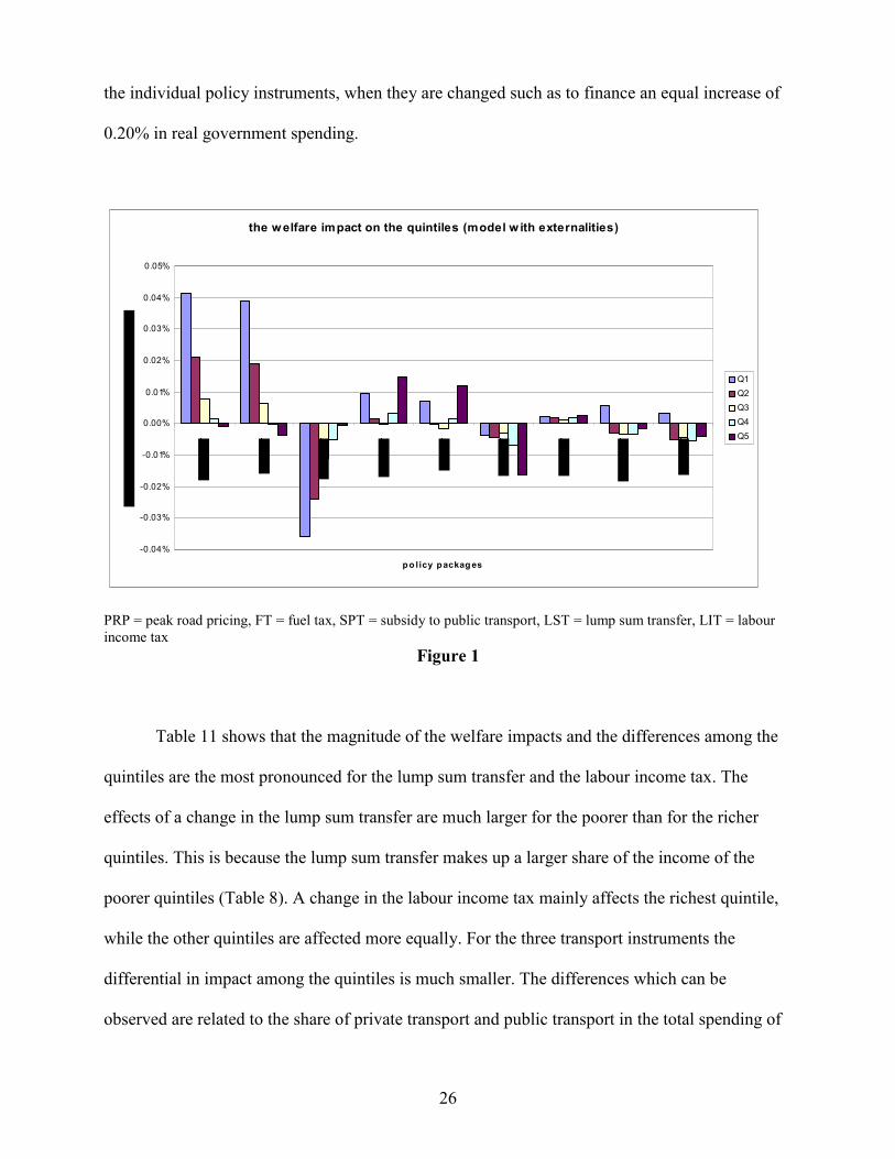
the individual policy instruments, when they are changed such as to finance an equal increase of

0.20% in real government spending.

the welfare impact on the quintiles (model w ith externalities)

-0.04%

-0.03%

-0.02%

-0.01%

0.00%

0.01%

0.02%

0.03%

0.04%

0.05%

po licy packag es

Q1Q2Q3Q4Q5

PRP = peak road pricing, FT = fuel tax, SPT = subsidy to public transport, LST = lump sum transfer, LIT = labour income tax

Figure 1

Table 11 shows that the magnitude of the welfare impacts and the differences among the

quintiles are the most pronounced for the lump sum transfer and the labour income tax. The

effects of a change in the lump sum transfer are much larger for the poorer than for the richer

quintiles. This is because the lump sum transfer makes up a larger share of the income of the

poorer quintiles (Table 8). A change in the labour income tax mainly affects the richest quintile,

while the other quintiles are affected more equally. For the three transport instruments the

differential in impact among the quintiles is much smaller. The differences which can be

observed are related to the share of private transport and public transport in the total spending of

26

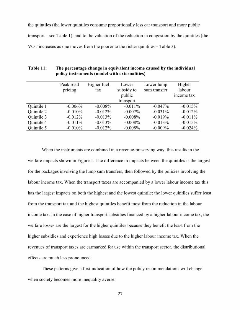
the quintiles (the lower quintiles consume proportionally less car transport and more public

transport – see Table 1), and to the valuation of the reduction in congestion by the quintiles (the

VOT increases as one moves from the poorer to the richer quintiles – Table 3).

Table 11: The percentage change in equivalent income caused by the individual policy instruments (model with externalities)

Peak road

pricing Higher fuel

tax

Lower subsidy to

public transport

Lower lump sum transfer

Higher labour

income tax

Quintile 1 Quintile 2 Quintile 3 Quintile 4 Quintile 5

-0.006% -0.010% -0.012% -0.011% -0.010%

-0.008%-0.012%-0.013%-0.013%-0.012%

-0.011%-0.007%-0.008%-0.008%-0.008%

-0.047% -0.031% -0.019% -0.013% -0.009%

-0.015%-0.012%-0.011%-0.015%-0.024%

When the instruments are combined in a revenue-preserving way, this results in the

welfare impacts shown in Figure 1. The difference in impacts between the quintiles is the largest

for the packages involving the lump sum transfers, then followed by the policies involving the

labour income tax. When the transport taxes are accompanied by a lower labour income tax this

has the largest impacts on both the highest and the lowest quintile: the lower quintiles suffer least

from the transport tax and the highest quintiles benefit most from the reduction in the labour

income tax. In the case of higher transport subsidies financed by a higher labour income tax, the

welfare losses are the largest for the higher quintiles because they benefit the least from the

higher subsidies and experience high losses due to the higher labour income tax. When the

revenues of transport taxes are earmarked for use within the transport sector, the distributional

effects are much less pronounced.

These patterns give a first indication of how the policy recommendations will change

when society becomes more inequality averse.

27

The implications of equity considerations

Which of the three transport instruments is to be preferred?

When a higher social welfare weight is given to the poorer quintiles (� = 0.5), the

reduction of the externalities becomes relatively less important, since the VOT and the WTP to

reduce air pollution is lower for the poorer quintiles (see Table 3 and 6). However, on the whole,

externality reduction still remains desirable and the relative weight given to the three externalities

does not change significantly when equity considerations come into play. Therefore, a higher

degree of inequality aversion does not affect the ranking between the three transport instruments

for a given revenue-preserving strategy. Peak road pricing remains the best instrument of the

three, followed by a higher fuel tax. The same conclusion holds for the two other degrees of

inequality aversion that we considered (� = 0.25 and � = 1.5).

How should the revenues of peak road pricing be used?

Whereas the degree of inequality aversion does not affect the choice between the three

transport instruments, it does influence the choice of the revenue-preserving strategy. When peak

road pricing is introduced, it is now preferred to use its revenues to increase the lump sum

transfer rather than to reduce the labour income tax. The impact of a higher degree of inequality

aversion is the same as in the model without externalities. It is mainly explained by the difference

in the gross welfare costs of the two instruments. Note that the case for using the lump sum

transfer rather than the labour income tax is slightly strengthened with respect to the model

without externalities. This is because the lump sum tax leads to a lower level of the externalities

than the labour income tax.

28

Changing the degree of inequality aversion changes the absolute values of the marginal

welfare impacts, but for the two other values of � that we considered, the main results continue to

hold (see Appendix A). All this leads us to the conclusion that equity considerations are more

important in determining how the revenue of the externality taxes should be used than in the

setting of the externality taxes themselves. This is a confirmation of results that obtained in

previous, more simplified, models [Small (1983), Mayeres and Proost (1997, 2001)]. It implies

that the importance of revenue recycling strategies should not be ignored when designing

transport policy reforms.

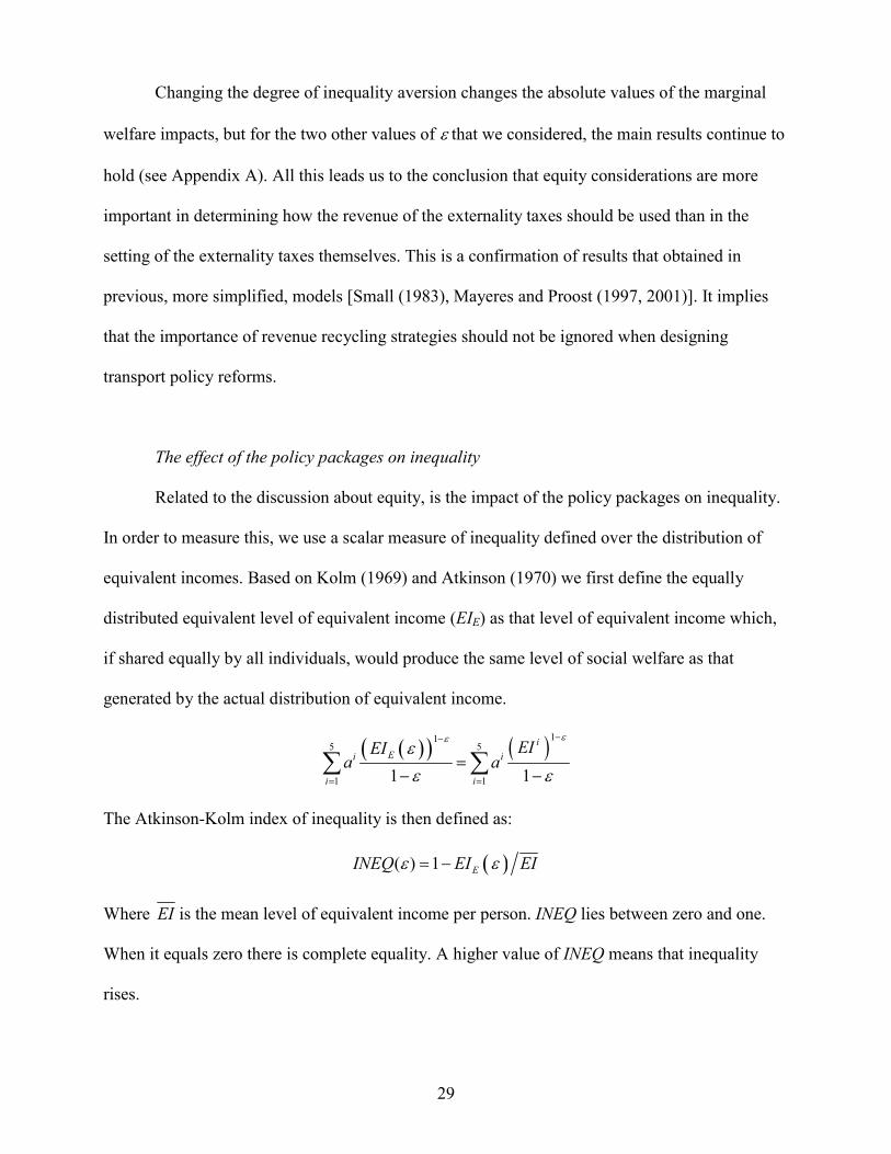
The effect of the policy packages on inequality

Related to the discussion about equity, is the impact of the policy packages on inequality.

In order to measure this, we use a scalar measure of inequality defined over the distribution of

equivalent incomes. Based on Kolm (1969) and Atkinson (1970) we first define the equally

distributed equivalent level of equivalent income (EIE) as that level of equivalent income which,

if shared equally by all individuals, would produce the same level of social welfare as that

generated by the actual distribution of equivalent income.

� �� � � �11

5 5

1 11 1

iEi i

i i

EIEIa a

��

�

� �

��

� �

�

� �

� �

The Atkinson-Kolm index of inequality is then defined as:

� �( ) 1 EINEQ EI EI� �� �

Where EI is the mean level of equivalent income per person. INEQ lies between zero and one.

When it equals zero there is complete equality. A higher value of INEQ means that inequality

rises.

29

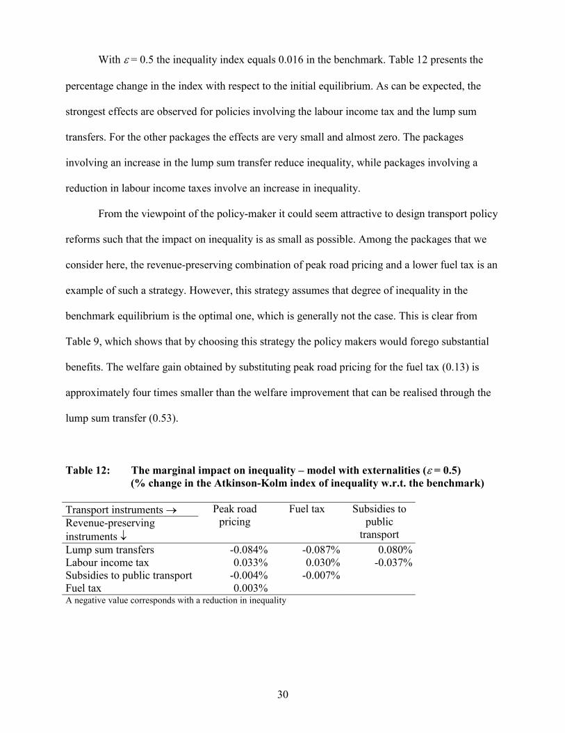
With � = 0.5 the inequality index equals 0.016 in the benchmark. Table 12 presents the

percentage change in the index with respect to the initial equilibrium. As can be expected, the

strongest effects are observed for policies involving the labour income tax and the lump sum

transfers. For the other packages the effects are very small and almost zero. The packages

involving an increase in the lump sum transfer reduce inequality, while packages involving a

reduction in labour income taxes involve an increase in inequality.

From the viewpoint of the policy-maker it could seem attractive to design transport policy

reforms such that the impact on inequality is as small as possible. Among the packages that we

consider here, the revenue-preserving combination of peak road pricing and a lower fuel tax is an

example of such a strategy. However, this strategy assumes that degree of inequality in the

benchmark equilibrium is the optimal one, which is generally not the case. This is clear from

Table 9, which shows that by choosing this strategy the policy makers would forego substantial

benefits. The welfare gain obtained by substituting peak road pricing for the fuel tax (0.13) is

approximately four times smaller than the welfare improvement that can be realised through the

lump sum transfer (0.53).

Table 12: The marginal impact on inequality – model with externalities (� = 0.5) (% change in the Atkinson-Kolm index of inequality w.r.t. the benchmark)

Transport instruments � Revenue-preserving instruments �

Peak road pricing

Fuel tax Subsidies to public

transport Lump sum transfers Labour income tax Subsidies to public transport Fuel tax

-0.084%0.033%

-0.004%0.003%

-0.087%0.030%

-0.007%

0.080% -0.037%

A negative value corresponds with a reduction in inequality

30

4 Conclusions

This paper adds to previous analyses by explicitly considering equity in the assessment of

transport instruments. A prerequisite for the evaluation of the equity impacts is that transport

instruments are not considered in isolation, but that the rest of the tax system is also taken into

account. This implies that the evaluation is done preferably in a general equilibrium, rather than a

partial equilibrium framework.

The simulation results show that equity considerations do not have a large impact on the

ranking of the three transport instruments that are evaluated in this paper. Peak road pricing

continues to be preferred to the fuel tax, and higher subsidies to public transport are found to

reduce rather than increase welfare. However, when society becomes more inequality averse, this

does have a significant impact on the ranking of the revenue-preserving strategies. While in the

pure efficiency case the revenues of peak road pricing are best used to reduce the labour income

tax, an increase in the lump sum transfers is preferred with higher degrees of inequality aversion.

An important implication of the analysis is that the revenue-preserving strategies cannot

be ignored in the design of transport policies, and that they can play a significant role in their

political acceptability.

Two qualifications apply. First of all, the equity effects depend on the assumptions made

about the policy instruments. A different design of these instruments will result in different equity

effects. Secondly, they are calculated by means of a particular AGE model that does not include

all possible effects. For example, it has a medium time horizon, in which the location decisions of

consumers and firms are not modeled. As a consequence, the equity effects of a change in land

use are not captured by our analysis.

31

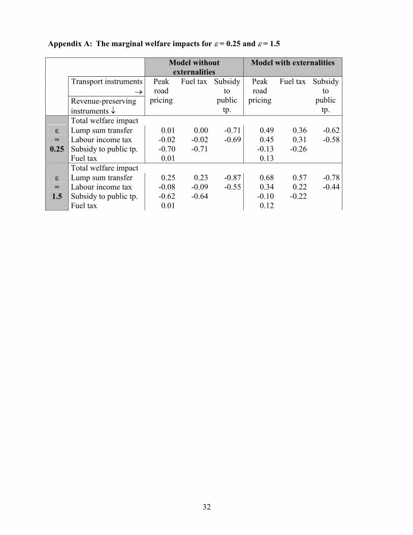
Appendix A: The marginal welfare impacts for � = 0.25 and � = 1.5

Model without externalities

Model with externalities

Transport instruments �

Revenue-preserving instruments �

Peak road

pricing

Fuel tax Subsidy to

public tp.

Peak road

pricing

Fuel tax Subsidy to

public tp.

Total welfare impact � =

0.25

Lump sum transfer Labour income tax Subsidy to public tp. Fuel tax

0.01-0.02-0.700.01

0.00-0.02-0.71

-0.71-0.69

0.490.45

-0.130.13

0.36 0.31

-0.26

-0.62-0.58

Total welfare impact � =

1.5

Lump sum transfer Labour income tax Subsidy to public tp. Fuel tax

0.25-0.08-0.620.01

0.23-0.09-0.64

-0.87-0.55

0.680.34

-0.100.12

0.57 0.22

-0.22

-0.78-0.44

32

References

Arnott, R., A. De Palma and R. Lindsey (1994): “The Welfare Effects of Congestion Tolls with Heterogeneous Commuters”. Journal of Transport Economics and Policy, 28, 139-161.

Atkinson, A.B. (1970): “On the Measurement of Inequality”. Journal of Economic Theory, 2, 244-263.

Ballard, C.L. and S.G. Medema (1993): “The Marginal Efficiency Effects of Taxes and Subsidies in the Presence of Externalities. A Computable General Equilibrium Model”. Journal of Public Economics, 52, 199-216.

Belgium, Ministry of Economic Affairs (1997): Huishoudbudgetonderzoek. Enquête gehouden van juni 1995 tot mei 1996. Ministry of Economic Affairs, NIS, Brussels.

Bickel, P., S. Schmid, W. Krewitt and R.E. Friedrich (1997): External Costs of Transport in ExternE. IER, Stuttgart.

Bovenberg, A. L. and R.A. de Mooij (1994): “Environmental Levies and Distortionary Taxation”. American Economic Review, 94, 1085-1089.

Bovenberg, A.L. and L.H. Goulder (1997): “Costs of Environmentally Motivated Taxes in the Presence of Other Taxes: General Equilibrium Analyses”. National Tax Journal, 50, 59-87.

Bovenberg, A.L. and L.H. Goulder (1996): “Optimal Environmental Taxation in the Presence of Other Taxes: General Equilibrium Analyses”. American Economic Review, 86, 985-1000.

Bovenberg, A.L. and F. van der Ploeg (1994): “Environmental Policy, Public Finance and the Labour Market in a Second-Best World”. Journal of Public Economics, 55, 349-390.

Brendemoen, A. and H. Vennemo (1996): “The Marginal Cost of Funds in the Presence of Environmental Externalities”. Scandinavian Journal of Economics, 98, 405-422.

Bruzelius, N. (1979): The Value of Travel Time. Theory and Measurement. London: Groom Helm.

Capros, P., T. Georgoakopoulos, D. Van Regemorter, S. Proost, T. Schmidt and K. Conrad (1997): The GEM-E3 Model. Reference Manual.

De Borger, B., I. Mayeres, S. Proost and S. Wouters (1996): “Optimal Pricing of Urban Passenger Transport - A Simulation Exercise for Belgium”. Journal of Transport Economics and Policy, 31-54.

De Borger, B. and S. Proost (eds.) (2001): Reforming Transport Pricing in the European Union. Edward Elgar, forthcoming.

de Mooij, R. (1999): Environmental Taxation and the Double Dividend. PhD. Dissertation, Erasmus University Rotterdam.

DeSerpa, A.C. (1971): “A Theory of the Economics of Time”. The Economic Journal, 81, 828-845.

Glaister, S. and D. Lewis (1978): “An Integrated Fares Policy for Transport in London”. Journal of Public Economics, 9, 341-355.

Goulder, L. H. (1995): “Environmental Taxation and the Double Dividend: A Reader's Guide”. International Tax and Public Finance, 2, 157-183.

Hague Consulting Group (1990): The Netherlands' 'Value of Time' Study: Final Report . Hague Consulting Group, The Hague.

Hansson, I. and C. Stuart (1993): “The Effects of Taxes on Aggregate Labor: A Cross-Country General-Equilibrium Study”. Scandinavian Journal of Economics, 95, 311-326.

Hansson, I. and C. Stuart (1985): “Tax Revenue and the Marginal Cost of Public Funds in Sweden”. Journal of Public Economics, 27, 331-353.

33

Jones-Lee, M., M. Hammerton and P.R. Philips (1985), “The Value of Safety: Results of a National Sample Survey”. The Economic Journal, 95, 49-72.

Keeler, T.E. and K.A. Small (1977): “Optimal Peak-Load Pricing, Investment, and Service Levels on Urban Expressways”. Journal of Political Economy, 85, 1-25.

King, M.A. (1983): “Welfare Analysis of Tax Reforms Using Household Data”. Journal of Public Economics, 21, 183-214.

Kolm, S.-C. (1969): “The Optimal Production of Social Justice”. in: J. Margolis and H. Guitton (eds.) Public Economics: An Analysis of Public Production and Consumption and their Relations to the Private Sector. Macmillan, London.

Mayeres, I. (2000): “The Efficiency Effects of Transport Policies in the Presence of Externalities and Distortionary Taxes”. Journal of Transport Economics and Policy, 32, 233-260.

Mayeres, I. (1999): The Control of Transport Externalities: A General Equilibrium Analysis. PhD Dissertation, Faculty of Economics and Applied Economics, K.U.Leuven, Leuven.

Mayeres, I., S. Ochelen and S. Proost (1996): “The Marginal External Costs of Urban Transport”. Transportation Research, 1D, 111-130.

Mayeres, I. and S. Proost (2001): “Marginal Tax Reform, Externalities and Income Distribution”. Journal of Public Economics, 79, 343-363.

Mayeres, I. and S. Proost (1997): “Optimal Tax and Public Investment Rules for Congestion Type of Externalities”. Scandinavian Journal of Economics, 99, 261-279.

Mohring, H. and M. Harwitz (1962): Highway Benefits: An Analytical Framework. Evanston: Northwestern University Press.

O' Mahony, M., K. Kirwan and S. McGrath (1997): “Modelling the Internalisation of External Costs of Transport”. Transportation Research Record, 1576, 93-98.

Oum, T.H., I.W.G. Waters and J.-S. Yong (1992): “Concepts of Price Elasticities of Transport Demand and Recent Empirical Estimates, An Interpretative Survey”. Journal of Transport Economics and Policy, 139-154.

Richardson, H.W. and C.B. Chang-Hee (1998): “The Equity Impacts of Road Congestion Pricing”, in: K.J. Button and E. Verhoef (eds.), Road Pricing, Traffic Congestion and the Environment, Issues of Efficiency and Social Feasibility. Edward Elgar, Cheltenham, 247-262.

Sandmo, A. (1975): “Optimal Taxation in the Presence of Externalities”. Swedish Journal of Economics, 77, 86-98.

Small, K. (1983): “The Incidence of Congestion Tolls on Urban Highways”. Journal of Urban Economics, 13, 90-111.

Walters, A.A. (1961): “The Theory and Measurement of Private and Social Cost of Highway Congestion”. Econometrica, 29, 676-699.

34