Equilibrium Search with Time-Varying Unemployment Bene fi

Equilibrium Search with Time-VaryingUnemployment Benefits∗

James Albrecht and Susan VromanDepartment of EconomicsGeorgetown UniversityWashington, D.C. 20057

June 2004

Abstract

In this paper we show how time-varying unemployment benefits cangenerate equilibrium wage dispersion in an economy in which identi-cal firms post wages and homogeneous risk-averse workers search foracceptable offers. We model a two-tier unemployment benefit systemthat is similar to real-world unemployment insurance programs. Weassume that the unemployed initially receive benefits at rate b. Even-tually, if a worker does not in the meantime find and accept a wageoffer, the benefit falls to a lower level, s. The duration of high-benefitreceipt is treated as an exponential random variable, so the model isstationary. We characterize the equilibrium, and we derive the com-parative statics effects of changes in the unemployment compensationsystem (i.e., in the two benefit levels and in the expected duration ofthe high-benefit state) on the equilibrium wage distribution and theunemployment rate.

1 Introduction

In this paper, we analyze the implications of time-varying unemploymentinsurance in an equilibrium search model. We consider a two-tier system,i.e., a system with a high and a low benefit level. This is the form taken by

∗We thank participants at the Tinbergen Institute’s Conference on Search and Assign-ment for useful comments. In particular, we thank Gerard van den Berg, who sharednotes with us on an alternative approach to the topic of this paper. We also thank LucasNavarro for valuable research assistance.

1

most real-world UI programs. Unemployed workers initially receive unem-ployment compensation, but eventually, if a worker does not find a job inthe meantime, this benefit is terminated. The worker then has access onlyto lower social assistance benefits or in some countries to no benefits at all.

Specifically, we consider an economy in which newly unemployed work-ers initially receive unemployment benefits at rate b. Eventually, if a workerdoes not find and accept a job in the meantime, the unemployment benefitfalls to a lower level, s. We assume the event that triggers the fall from b tos occurs at Poisson rate λ.1 This allows us to do our equilibrium analysisin a stationary framework while focusing on the most important aspect oftime-varying unemployment compensation, namely, that after some pointthe benefit falls. This representation of time-varying unemployment com-pensation enables us to derive a two-point equilibrium wage distribution ina simple stationary setting. We derive this equilibrium distribution using awage-posting model of sequential search. We allow for free entry and exitof jobs and for matching frictions in the sense that the rate at which un-employed workers and vacant jobs contact one another depends on overalllabor market tightness. The use of a matching function to determine the jobcontact rate for workers (and the worker contact rate for jobs) is relativelyunusual in wage-posting models, which typically assume a fixed contact rate.Our model can thus be viewed as a combination of the wage-posting andjob-matching (e.g, Pissarides 2000) traditions.

Equilibrium wage dispersion can arise in our model because time-varyingunemployment benefits lead to a distribution of worker reservation wages.2

Even though workers are identical ex ante, a worker who is receiving b canafford to be choosier about the jobs that he or she will accept (has a higher

1Our model can be interpreted as one in which the search activity of unemployedworkers is imperfectly monitored by a government agency. Suppose unemployed workersare punished by a reduction in their benefits from b to s when found to be putting forthless search effort than required and that detection of insufficient search effort occurs atPoisson rate λ. If all workers choose to put forth less than the required effort — and thisis a plausibe assumption, given that workers are homogeneous —, then this “sanctions”model is equivalent to our model with time-varying benefits. That is, our model can beinterpreted as a (simplified) equilibrium version of Abbring, van den Berg, and van Ours(2000).

2The insight that time-varying unemployment benefits generate a distribution of reser-vation wages is an old one. Mortensen (1977) and Burdett (1979) initially developed theidea that with a (deterministic) time limit on unemployment benefits, a worker’s reserva-tion wage falls as elapsed duration gets closer to the time limit. This individual problemof nonstationary search has now been analyzed in considerable generality, in particular,by van den Berg (1990). One contribution of our paper is to incorporate the basic insightfrom this literature into an equilibrium wage-posting model.

2

reservation wage) than can a worker who is receiving s. Time-varying unem-ployment compensation thus provides a new way to overcome the Diamond(1971) paradox, which suggests that in a wage-posting model with homo-geneous workers and firms, search costs, no matter how small, will leadto an equilibrium wage distribution that is degenerate at the monopsonywage. Other models have generated equilibrium wage dispersion from adistribution of reservation wages. Albrecht and Axell (1984) did this bysimply assuming that workers were ex ante heterogenous with respect tothe value of leisure and hence had differing reservation wages. Burdett andMortensen (1998) use on-the-job search to generate an endogenous distrib-ution of reservation wages for ex ante identical workers — an employed jobseeker’s reservation wage is his or her current wage. We also generate anendogenous distribution of reservation wages for ex ante identical workers.We use a real-world institution (time-varying unemployment benefits) togenerate an endogenous distribution of worker types and hence reservationwages. Unlike Burdett and Mortensen (1998), our model has a distribu-tion of reservation wages among unemployed workers. This can lead to jobrejection by some unemployed workers and to search unemployment.3

In addition to providing a new foundation for equilibrium wage disper-sion, the introduction of time-varying unemployment benefits into an equi-librium model leads to interesting comparative statics. The possibility offalling from the high-benefit to the low-benefit state creates an incentivefor workers to accept jobs in order to be reentitled to high benefits. Thisreentitlement incentive causes some comparative static effects to differ con-siderably from those that would be found in a model in which unemploymentbenefits do not vary over time. For example, an increase in the high ben-efit leads to a reduction in the reservation wage for high-benefit recipients.Absent time-varying unemployment compensation, the increased value ofbeing unemployed would increase the reservation wage, but with the chanceof falling into the low-benefit state, the increase in the high benefit raisesthe worker’s incentive for reentitlement and leads to a lower reservationwage. This captures the real-world phenomenon of workers who are aboutto lose unemployment compensation taking jobs in order to requalify forunemployment benefits.

The next section presents our model. Section 3 presents the special caseof worker risk neutrality. We present this case because with risk neutrality,

3Using a strategic bargaining approach, Coles and Masters (2003) also focus on theeffect of time-varying unemployment benefits on reservation wages. However, their modelis one with complete information, so no wages are rejected in equilibrium.

3

the model can be solved analytically and we can explicitly derive the com-parative statics results. In Section 4, we present a numerical example withlog utility. We show that the comparative static effects of the main policyvariables, b, s, and λ are virtually the same as in the case of risk neutrality.Section 5 considers an extension of the model to allow workers to quit thelow-wage job and receive the high unemployment benefit with some prob-ability. (In the basic model, this probability is implicitly set to zero.) InSection 6, we discuss the implications of our model for the optimality oftime-varying unemployment insurance. Section 7 contains conclusions.

2 The Model

We consider a continuous-time model in which ex ante homogeneous workersare infinitely-lived. The measure of workers is fixed and normalized to 1.The decision that workers make is whether or not to accept job offers. Jobsare likewise ex ante homogeneous. The decision that a firm (job owner)makes is whether the job should be in the market (entry/exit) and whatwage to post when the job is vacant. The measure of jobs in the market(vacancies plus filled jobs) is endogenous. Both workers and firms discountthe future at the rate r.

2.1 Workers

At any moment, a worker is either unemployed or employed. When unem-ployed, a worker receives the (income-equivalent) value of leisure or homeproduction, h, plus unemployment compensation. When initially unem-ployed, a worker receives b and then moves to the lower level s at Poissonrate λ. Thus, when unemployed, the worker’s income, y, can equal eitherb+h or s+h.When employed, a worker’s income is the wage that he or sheis paid; that is, y = w. The worker’s instantaneous utility function is ξ(y),which is common across workers. We assume that ξ0(y) > 0 and ξ00(y) ≤ 0.

Workers move from employment to unemployment (worker/job matchesbreak up) at an exogenous Poisson rate δ. The transition rate from un-employment to employment is endogenous and depends on labor markettightness and on worker choice. Specifically, we assume a constant returnsto scale contact function, M(u, v) = m(θ)u, where u is the unemploymentrate, v is the measure of vacant jobs, and θ = v/u represents labor markettightness. The Poisson rate at which an unemployed worker contacts a va-cant job is thus m(θ), and the rate at which a vacancy meets an unemployedworker is m(θ)/θ. The contact function is increasing in its arguments and

4

satisfies M(0, v) = M(u, 0) = 0. These assumptions imply m(0) = 0 and

limθ→0

m(θ)/θ = +∞, as well as m0(θ) > 0 andd[m(θ)/θ]

dθ< 0. Finally, the fact

that the offer arrival rate for workers is increasing in θ while the applicantarrival rate for vacancies is decreasing in θ implies the standard elasticitycondition, 0 < m0(θ)θ/m(θ) < 1.

Given any distribution of wage offers across vacancies, F (w), there willbe two reservation wages among the unemployed, one for those receiving band one for those receiving s. Firms have no incentive to offer a wage that isnot someone’s reservation wage; thus, in equilibrium, at most two wages willbe offered. We let wb denote the reservation wage for workers with unem-ployment benefit b, ws the reservation wage for workers with unemploymentbenefit s, and φ the fraction of offers at wb. Since workers receiving b willreject offers of ws, not all offers need be accepted in equilibrium.

The higher reservation wage is determined by equating the value of un-employment for those receiving b, U(b), to the value of employment at wb,N(wb). Similarly, the lower reservation wage is determined by equating thevalue of unemployment for those receiving s, U(s), to the value of employ-ment at ws, N(ws). The unemployment values are defined by

rU(b) = ξ(b+ h) + φm(θ)[N(wb)− U(b)] + λ[U(s)− U(b)] (1)

rU(s) = ξ(s+h)+φm(θ)[N(wb)−U(s)]+ (1−φ)m(θ)[N(ws)−U(s)]. (2)

The value for an unemployed worker who is receiving b reflects the fact thatonly the higher wage offer, wb, is acceptable. The value for an unemployedworker who is receiving s reflects the fact that such a worker will be less se-lective; that is, either wage offer will be accepted. Similarly, the employmentvalues are defined by

rN(wb) = ξ(wb) + δ[U(b)−N(wb)] (3)

rN(ws) = ξ(ws) + δ[U(b)−N(ws)]. (4)

Using the reservation wage property, that is,

U(b) = N(wb) and U(s) = N(ws),

and substituting in equation (3) yields

N(wb) =ξ(wb)

r= U(b).

5

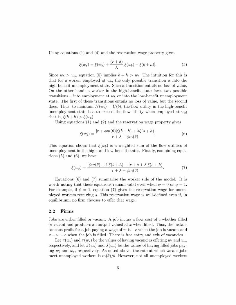
Using equations (1) and (4) and the reservation wage property gives

ξ(ws) = ξ(wb) +(r + δ)

λ[ξ(wb)− ξ(b+ h)]. (5)

Since wb > ws, equation (5) implies b + h > wb. The intuition for this isthat for a worker employed at wb, the only possible transition is into thehigh-benefit unemployment state. Such a transition entails no loss of value.On the other hand, a worker in the high-benefit state faces two possibletransitions — into employment at wb or into the low-benefit unemploymentstate. The first of these transitions entails no loss of value, but the seconddoes. Thus, to maintain N(wb) = U(b), the flow utility in the high-benefitunemployment state has to exceed the flow utility when employed at wb;that is, ξ(b+ h) > ξ(wb).

Using equations (1) and (2) and the reservation wage property gives

ξ(wb) =[r + φm(θ)]ξ(b+ h) + λξ(s+ h)

r + λ+ φm(θ). (6)

This equation shows that ξ(wb) is a weighted sum of the flow utilities ofunemployment in the high- and low-benefit states. Finally, combining equa-tions (5) and (6), we have

ξ(ws) =[φm(θ)− δ]ξ(b+ h) + [r + δ + λ]ξ(s+ h)

r + λ+ φm(θ). (7)

Equations (6) and (7) summarize the worker side of the model. It isworth noting that these equations remain valid even when φ = 0 or φ = 1.For example, if φ = 1, equation (7) gives the reservation wage for unem-ployed workers receiving s. This reservation wage is well-defined even if, inequilibrium, no firm chooses to offer that wage.

2.2 Firms

Jobs are either filled or vacant. A job incurs a flow cost of c whether filledor vacant and produces an output valued at x when filled. Thus, the instan-taneous profit for a job paying a wage of w is −c when the job is vacant andx−w − c when the job is filled. There is free entry and exit of vacancies.

Let π(wb) and π(ws) be the values of having vacancies offering wb and ws,respectively, and let J(wb) and J(ws) be the values of having filled jobs pay-ing wb and ws, respectively. As noted above, the rate at which vacant jobsmeet unemployed workers is m(θ)/θ. However, not all unemployed workers

6

will accept ws. Letting γ denote the fraction of unemployed with reservationwage wb, we have

rπ(wb) = −c+ m(θ)

θ[J(wb)− π(wb)]

rπ(ws) = −c+ m(θ)

θ(1− γ)[J(ws)− π(ws)]

rJ(wb) = x−wb − c+ δ[π(wb)− J(wb)]

rJ(ws) = x−ws − c+ δ[π(ws)− J(ws)].

Eliminating J(wb) and J(ws) gives

π(wb) = −c+ m(θ)

θ

x−wb − c

r + δ(8)

π(ws) = −c+ m(θ)

θ(1− γ)

x−ws − c

r + δ. (9)

If 0 < φ < 1, that is, if some firms post wb while others post ws, thenfree entry/exit requires that π(wb) = π(ws) = 0. If only ws is offered, thatis, if φ = 0, then free entry/exit requires π(ws) = 0 but only that π(wb) ≤ 0.Similarly, if only wb is offered, i.e., if φ = 1, then π(wb) = 0 and π(ws) ≤ 0must hold in equilibrium.

2.3 Steady-State Conditions

In steady state, the measures of workers in each possible state must be con-stant through time. We use two steady-state conditions to derive expressionsfor γ and u.

Workers can be classified into three categories — employed, unemployedand receiving b, and unemployed and receiving s. The measure of employedis 1 − u, the measure of unemployed receiving b is γu, and the measure ofunemployed receiving s is (1− γ)u. Since the measure of workers is normal-ized to one, we need only equate inflows and outflows for two of these states.We work with the two unemployment states.

The condition that equates the flows into and out of the high-benefitunemployment state is

δ(1− u) = [φm(θ) + λ]γu.

7

Workers flow into this state from employment at rate δ; workers flow outof this state either back into employment (at rate φm(θ)) or into the low-benefit unemployment state (at rate λ). The comparable equation for thelow-benefit unemployment state is

λγu = m(θ)(1− γ)u;

that is,λγ = m(θ)(1− γ).

These conditions imply that we can write γ and u in terms of the otherendogenous variables of the model, namely,

γ =m(θ)

λ+m(θ)(10)

u =δ

δ + γ(φm(θ) + λ). (11)

2.4 Equilibrium

A steady-state equilibrium is a vector {wb, ws, φ, θ, γ, u} such that(i) U(b) = N(wb) and U(s) = N(ws),(ii) No wage other than wb or ws is offered, and one of the following is

satisfied:(a) 0 < φ < 1 and π(wb) = π(ws) = 0(b) φ = 0 and π(ws) = 0 but π(wb) ≤ 0(c) φ = 1 and π(wb) = 0 but π(ws) ≤ 0

(iii) the steady-state conditions (10) and (11) hold.Condition (i) states that workers search optimally given the wage offer distri-bution, {wb, ws, φ}.4 Condition (ii) states that firms optimize with respectto their wage offers in the sense that no wage is offered that is not someworker’s reservation wage and with respect to their entry/exit decisions.

4Since all offers at wb are accepted, whereas only a fraction 1 − γ of offers at ws areaccepted, the equilibrium distributions of wages offered and of wages paid are not the same.The relationship between the two distributions can be derived from the condition that theflows of workers into and out of high-wage employment must be the same. (Equivalently,one can use the condition that the flows into and out of low-wage employment are thesame.) Let η denote the fraction of employed workers who are paid wb. The steady-statecondition is then φm(θ)u = δη(1− u). Using equations (10) and (11) to eliminate u, this

implies η = φ(λ+m(θ)

λ+ φm(θ)).

8

There are three types of equilibria to consider — equilibria in which onlythe low wage is offered (φ = 0), equilibria with wage dispersion (0 < φ < 1),and equilibria in which only the high wage is offered (φ = 1).

We want to know which parameter configurations are consistent with theexistence of a steady-state equilibrium and whether equilibrium is unique.Further, we want to know which parameter configurations imply φ = 0,which lead to wage dispersion, and which imply φ = 1. We can addressthese issues by considering the effects of varying a single parameter, holdingall others constant. The most intuitive parameter to vary is x, the flowoutput from filled jobs. Given any collection of fixed values for the otherparameters of the model (subject only to trivial restrictions such as b > s,r > 0, etc.), it is clear that for x sufficiently close to zero, no steady-stateequilibrium (with θ > 0) exists. For x sufficiently small, it is not worthposting a vacancy at the lower wage, even if that vacancy could be filledarbitrarily quickly.

For somewhat larger values of x, there is a unique equilibrium in whichφ = 0. To see this, suppose provisionally that φ = 0. With φ = 0, equations(6) and (7) show that neither wb nor ws vary with θ and that wb > ws.There are thus values of x such that x− ws − c > 0 > x− wb − c. At suchvalues, it is profitable for at least a small number of firms to create low-wage vacancies while at the same time it is unprofitable to create high-wagevacancies. That is, for sufficiently small values of x (but not so small thatx−ws− c < 0), there is a unique equilibrium in which only the low wage isposted.

As x increases further, eventually x−wb− c > 0. It becomes worthwhileat some point for a first (individually negligible) firm to post the higherwage. At this value of x, there is a corresponding value of θ such thatπ(wb) = π(ws) = 0. The assertion that there is an (x, θ) such that

−c+ m(θ)

θ

x−wb − c

r + δ= −c+ m(θ)

θ

λ

λ+m(θ)

x−ws − c

r + δ= 0

is easy to verify since we are still at the point (because the posting of thefirst high-wage vacancy does not measurably increase φ above zero) at whichwb and ws can be treated as constants. As x increases even further, morefirms have an incentive to post the higher wage. The situation becomesmore complicated because wb and ws are no longer constants.

To show the existence of a unique equilibrium when x is such that0 < φ < 1, we reduce the system of equations defining equilibrium to asingle equation in θ, show that equation has a unique solution, and thencheck that given θ, the other endogenous variables of the model are uniquely

9

determined. First, equation (5) gives ws as a function of wb and parameters;in particular, ws is an increasing function of wb. Next, from π(wb) = 0 (cf.equation (8)),

wb = x− c− c(r + δ)θ

m(θ).

Thus, wb is an decreasing function of θ, and so too is ws. Finally, π(ws) = 0(equation (9)) gives our equation for θ, namely,

c = (m(θ)

θ)(

λ

λ+m(θ))(x− c−ws

r + δ).

As θ → 0, the right-hand side of this equation goes to infinity; as θ → ∞,the right-hand side goes to zero; and the right-hand side is decreasing inθ so long as m(θ) ≥ r + δ. Thus, if the equilibrium θ is not too small, theequation has a unique solution in θ.

The last step is to check that the other endogenous variables are uniquelydetermined. We have already shown that the two wages are uniquely deter-mined by θ. Equation (6) can be rearranged to give:

φ =(r + λ)ξ(wb)− rξ(b+ h)− λξ(s+ h)

m(θ)[ξ(b+ h)− ξ(wb)],

so φ is also uniquely determined by labor market tightness. Finally, equation(10) gives γ as a function of θ, and equation (11), after substituting for γand φ, gives u as a function of γ.

Finally, for x sufficiently large, φ = 1, as it is no longer worthwhile toincur the “delay cost” implied by posting ws. Again, it is easy to see thatfor any x such that φ = 1, equilibrium is unique. To see this, note that withφ = 1, equation (6) gives

ξ(wb) =[r +m(θ)]ξ(b+ h) + λξ(s+ h)

r + λ+m(θ).

At the same time, π(wb) = 0 (equation (8)) implies

wb = x− c− c(r + δ)θ

m(θ);

thus in any equilibrium with φ = 1,

ξ(x− c− c(r + δ)θ

m(θ)) =

[r +m(θ)]ξ(b+ h) + λξ(s+ h)

r + λ+m(θ).

10

The right-hand side of this equation is monotonically increasing in θ, ranging

fromrξ(b+ h) + λξ(s+ h)

r + λto ξ(b+ h). The left-hand side is monotonically

decreasing in θ, starting from ξ(x − c) at θ = 0. So long as x > c + b + h,the above equation has a unique solution; that is, equilibrium with φ = 1 isunique.

We have thus shown that for any fixed values of the other parameters ofthe model, a range of equilibrium possibilities can be traced out as we varyx.

3 Risk Neutrality

We now consider the special case of risk neutrality. Risk neutrality allowsus to solve the model analytically and to derive qualitative comparativestatics results. In this case, the equations defining the equilibrium withwage dispersion are

γ =m(θ)

λ+m(θ)(10)

u =δ

δ + γ(φm(θ) + λ)(11)

ws = wb +(r + δ)

λ[wb − b− h] (50)

wb = b+ h− cθ (12)

φ =λ(b− s)− cθ(r + λ)

cθm(θ)(13)

cθm(θ)− (r + δ)cθ + (x− c− b− h)m(θ) = 0. (14)

Equations (10) and (11) are repeated from the last section. Equation (50)is equation (5) in the case of risk neutrality. The derivation of equations(12)-(14) is given in Appendix 1. Equation (14) has a unique solution forθ so long as x− c− b−h ≤ 0.5 Using equations (10)-(14) and (50) then gives

5To see this, rewrite equation (14) as

cm(θ)− (r + δ)c = −(x− c− b− h)m(θ)/θ.

The left-hand side, which is monotonically increasing in θ, equals −(r + δ)c when θ = 0and tends to infinity as θ → ∞. The right-hand side is monotonically decreasing in θ (ifand only if x − c − b − h < 0), tends to infinity as θ → 0 and tends to zero as θ → ∞.Thus, when x− c− b−h < 0, this equation has a unique solution.When x− c− b−h = 0,the unique solution is the θ that solves m(θ) = r + δ.

11

a unique solution for the other endogenous variables.

3.1 Comparative Statics

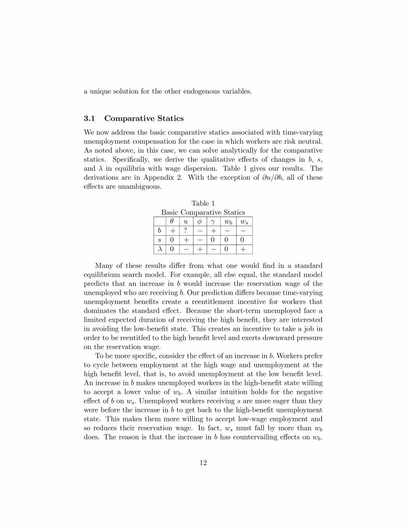
We now address the basic comparative statics associated with time-varyingunemployment compensation for the case in which workers are risk neutral.As noted above, in this case, we can solve analytically for the comparativestatics. Specifically, we derive the qualitative effects of changes in b, s,and λ in equilibria with wage dispersion. Table 1 gives our results. Thederivations are in Appendix 2. With the exception of ∂u/∂b, all of theseeffects are unambiguous.

Table 1Basic Comparative Statics

θ u φ γ wb ws

b + ? − + − −s 0 + − 0 0 0

λ 0 − + − 0 +

Many of these results differ from what one would find in a standardequilibrium search model. For example, all else equal, the standard modelpredicts that an increase in b would increase the reservation wage of theunemployed who are receiving b. Our prediction differs because time-varyingunemployment benefits create a reentitlement incentive for workers thatdominates the standard effect. Because the short-term unemployed face alimited expected duration of receiving the high benefit, they are interestedin avoiding the low-benefit state. This creates an incentive to take a job inorder to be reentitled to the high benefit level and exerts downward pressureon the reservation wage.

To be more specific, consider the effect of an increase in b.Workers preferto cycle between employment at the high wage and unemployment at thehigh benefit level, that is, to avoid unemployment at the low benefit level.An increase in b makes unemployed workers in the high-benefit state willingto accept a lower value of wb. A similar intuition holds for the negativeeffect of b on ws. Unemployed workers receiving s are more eager than theywere before the increase in b to get back to the high-benefit unemploymentstate. This makes them more willing to accept low-wage employment andso reduces their reservation wage. In fact, ws must fall by more than wb

does. The reason is that the increase in b has countervailing effects on wb.

12

On the one hand, the direct effect of the increase in b is to make high-benefit unemployment more attractive. If this were the only effect, as inthe standard model, wb would increase. On the other hand, as indicatedabove, the increase in b makes workers in the high-benefit unemploymentstate more eager to avoid the low-benefit unemployment state, so wb falls.The second effect dominates. The effect of an increase in b on ws is, however,unambiguously negative.

With the fall in both wb and ws, firms have an incentive to open morevacancies. Because ws falls by more than wb, entry at the low wage is par-ticularly attractive; thus, φ decreases. With a smaller fraction of vacanciesat the high wage, there is an increase in the fraction of unemployed whoare receiving b; that is, γ increases. The zero-value condition for high-wagejobs implies that the matching rate, m(θ)/θ, must fall (and, accordingly, θmust increase) to offset the decrease in wb. Finally, the ambiguous effect onunemployment is a result of two offsetting factors. Job offers arrive fasterthan they did before the increase in b (θ increases), but relatively fewer ofthese offers are acceptable (φ decreases).

Next, consider the effects of an increase in s. An unemployed workerreceiving b now has less incentive to avoid falling into the low-benefit state;all else equal, this places upward pressure on wb. For an unemployed workerreceiving s, matters are more complicated. On the one hand, an increase ins makes low-benefit unemployment more attractive, so there is a tendencyfor ws to rise. On the other hand, the high-benefit state has become moreattractive, so there is downward pressure on the reservation wage of workersreceiving s. In short, there is stronger pressure on wb to increase than thereis on ws. However, this pressure is counterbalanced by a change in vacancycomposition — it is now relatively less attractive for firms to open high-wagevacancies; that is, φ falls. This means that the low-benefit unemployed areless likely to find high-wage jobs and this causes the value of unemploymentat s to fall. These two effects on U(s) balance, so U(s) and ws remainunchanged. The reservation wage of the high-benefit unemployed, wb, alsodoes not change. This is because the only effect of s on U(b) is throughchanges in U(s). From the zero-value condition for the high-wage jobs, thefact that wb is unchanged requires that the matching rate for these firmsremains the same, i.e., θ is unchanged. Since neither ws nor θ are affectedby a change in s, zero value for low-wage vacancies implies that changes ins do not affect γ. Finally, the fall in φ, all else equal, implies relatively feweracceptable offers for unemployed workers at the high benefit level; that is,the average duration of unemployment rises and with it, u increases.

13

The final comparative statics effects are those for λ. Consider unem-ployed workers receiving s. When λ increases, the reentitlement incentivefor these workers is reduced, so their reservation wage rises. The reentitle-ment incentive for unemployed workers receiving b is also reduced, puttingupward pressure on wb, but this is counterbalanced by the first-order effectof the reduction in the value of unemployment at b. Since the upward pres-sure on ws is greater than on wb, φ rises. This further increases the upwardpressure on ws and wb. In equilibrium, this leaves ws higher and just offsetsthe first-order negative effect on wb, leaving it unchanged. As noted above,there is a direct link between wb and θ via the zero-value condition for high-wage vacancies. If wb is unaffected by the increase in λ, then θ is unchanged.An increase in λ, by reducing the expected duration of high-benefit unem-ployment, reduces γ, the fraction of unemployed who are in the high-benefitstate. In addition, since ws increases with λ while θ is unaffected, γ must fallin order to maintain zero value for low-wage vacancies. Finally, the increasein φ in conjunction with the increase in λ makes the unemployed accept joboffers more quickly, and that is why the unemployment rate falls with λ.

The next section provides a numerical example of the comparative staticsfor a case in which workers are risk averse. For comparison, we also presentthe example for the case of risk neutrality. The effects of changes in b ands are virtually the same in both cases, while the effect of changes in λ aresomewhat different. While this indicates that the comparative statics aresimilar when we allow for risk aversion, this is only a numerical example,which need not hold for all forms of risk aversion.

4 Numerical Example

In this section, we present a numerical example to illustrate the properties ofthe model in the case of risk aversion. We also present the numerical examplewith the same parameters for the case of risk-neutral workers. We do this toillustrate the effect of risk aversion. The example uses the contact function,m(θ) = 8

√θ, and in the baseline case, we assume that b = 1, s = 0, h = 1,

λ = 2, x = 2, δ = .2, c = .5, and r = .05. The baseline parameter values werechosen with two criteria in mind. First, the parameter values themselvesshould be reasonable. Second, the values of the endogenous variables thatfollow from these parameter values should also be reasonable. For the caseof risk aversion, we use the instantaneous utility function ξ(y) = ln y.

Table 2 presents the solution for our baseline case with worker risk aver-sion (in row 1) and the comparative statics of changes in b.

14

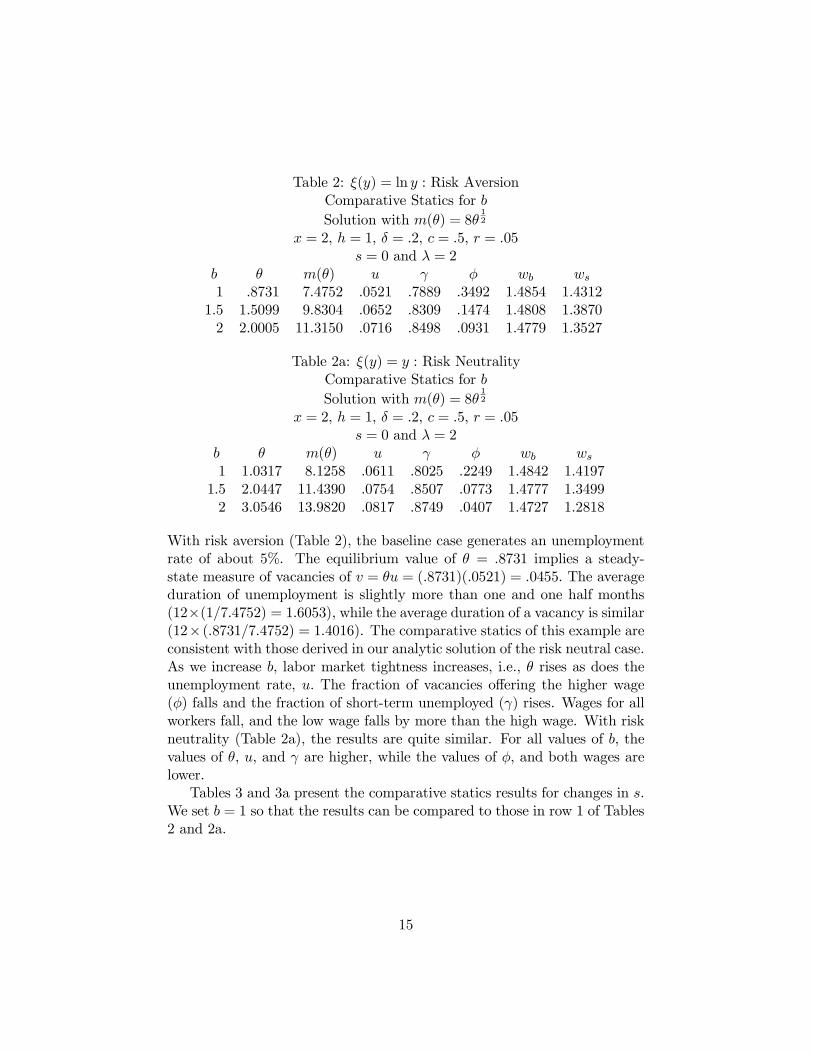
Table 2: ξ(y) = ln y : Risk AversionComparative Statics for bSolution with m(θ) = 8θ

12

x = 2, h = 1, δ = .2, c = .5, r = .05s = 0 and λ = 2

b θ m(θ) u γ φ wb ws

1 .8731 7.4752 .0521 .7889 .3492 1.4854 1.43121.5 1.5099 9.8304 .0652 .8309 .1474 1.4808 1.38702 2.0005 11.3150 .0716 .8498 .0931 1.4779 1.3527

Table 2a: ξ(y) = y : Risk NeutralityComparative Statics for bSolution with m(θ) = 8θ

12

x = 2, h = 1, δ = .2, c = .5, r = .05s = 0 and λ = 2

b θ m(θ) u γ φ wb ws

1 1.0317 8.1258 .0611 .8025 .2249 1.4842 1.41971.5 2.0447 11.4390 .0754 .8507 .0773 1.4777 1.34992 3.0546 13.9820 .0817 .8749 .0407 1.4727 1.2818

With risk aversion (Table 2), the baseline case generates an unemploymentrate of about 5%. The equilibrium value of θ = .8731 implies a steady-state measure of vacancies of v = θu = (.8731)(.0521) = .0455. The averageduration of unemployment is slightly more than one and one half months(12×(1/7.4752) = 1.6053), while the average duration of a vacancy is similar(12× (.8731/7.4752) = 1.4016). The comparative statics of this example areconsistent with those derived in our analytic solution of the risk neutral case.As we increase b, labor market tightness increases, i.e., θ rises as does theunemployment rate, u. The fraction of vacancies offering the higher wage(φ) falls and the fraction of short-term unemployed (γ) rises. Wages for allworkers fall, and the low wage falls by more than the high wage. With riskneutrality (Table 2a), the results are quite similar. For all values of b, thevalues of θ, u, and γ are higher, while the values of φ, and both wages arelower.

Tables 3 and 3a present the comparative statics results for changes in s.We set b = 1 so that the results can be compared to those in row 1 of Tables2 and 2a.

15

Table 3: ξ(y) = ln y : Risk AversionComparative Statics for sSolution with m(θ) = 8θ

12

x = 2, h = 1, δ = .2, c = .5, r = .05b = 1 and λ = 2

s θ m(θ) u γ φ wb ws

.1 .8731 7.4752 .0600 .7889 .2635 1.4854 1.4312

.2 .8731 7.4752 .0697 .7889 .1852 1.4854 1.4312

.3 .8731 7.4752 .0818 .7889 .1132 1.4854 1.4312

.4 .8731 7.4752 .0974 .7889 .0466 1.4854 1.4312

Table 3a: ξ(y) = y : Risk NeutralityComparative Statics for sSolution with m(θ) = 8θ

12

x = 2, h = 1, δ = .2, c = .5, r = .05b = 1 and λ = 2

s θ m(θ) u γ φ wb ws

.1 1.0317 8.1258 .0676 .8025 .1771 1.4842 1.4197

.2 1.0317 8.1258 .0755 .8025 .1294 1.4842 1.4197

.3 1.0317 8.1258 .0856 .8025 .0817 1.4842 1.4197

.4 1.0317 8.1258 .0968 .8025 .0340 1.4842 1.4197

As predicted by the analytic comparative statics in the risk neutralitycase, changing s has no effect on θ, γ, wb, or ws. As in Tables 2 and 2a, thevalues of θ and γ are higher with risk neutrality, while the values of wb andws are lower. In both Tables 3 and 3a, as s increases, the fraction of high-wage vacancies, φ, falls and the unemployment rate rises. Comparing theeffect of an increase in s from .1 to .2 with the increase in b from 1 to 1.5, onecan see that in this example the effect of increasing the low unemploymentbenefit on unemployment is greater than a comparable increase in the highbenefit.

Finally, Tables 4 and 4a present the comparative statics results forchanges in λ. The third row corresponds to the baseline case. Higher lev-els of λ correspond to steady states with shorter average durations of highunemployment benefit receipt. As λ increases, the fraction of unemployedreceiving b falls (i.e., γ decreases), unemployment falls, and the fraction ofvacancies offering the higher wage rises. As we argued above, this is becauseof the positive effect of an increase in λ on the lower wage, which is appar-ent in both Tables 4 and 4a. Unlike the case of changes in b and s, there

16

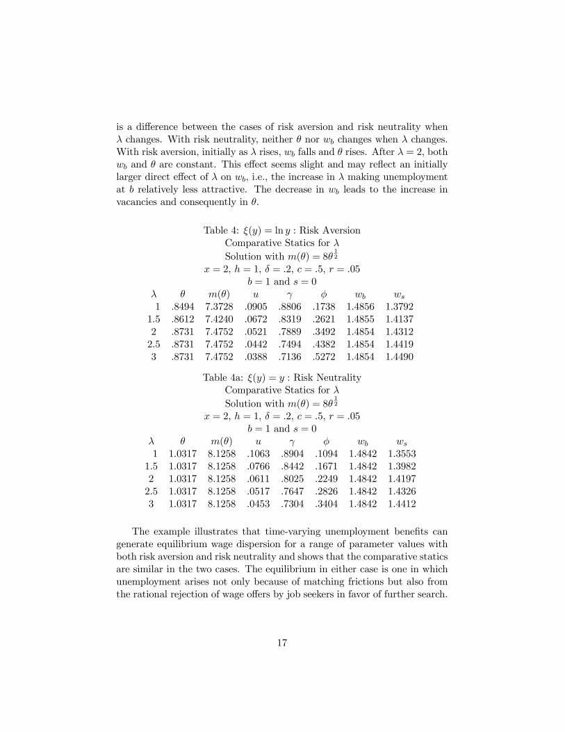
is a difference between the cases of risk aversion and risk neutrality whenλ changes. With risk neutrality, neither θ nor wb changes when λ changes.With risk aversion, initially as λ rises, wb falls and θ rises. After λ = 2, bothwb and θ are constant. This effect seems slight and may reflect an initiallylarger direct effect of λ on wb, i.e., the increase in λ making unemploymentat b relatively less attractive. The decrease in wb leads to the increase invacancies and consequently in θ.

Table 4: ξ(y) = ln y : Risk AversionComparative Statics for λSolution with m(θ) = 8θ

12

x = 2, h = 1, δ = .2, c = .5, r = .05b = 1 and s = 0

λ θ m(θ) u γ φ wb ws

1 .8494 7.3728 .0905 .8806 .1738 1.4856 1.37921.5 .8612 7.4240 .0672 .8319 .2621 1.4855 1.41372 .8731 7.4752 .0521 .7889 .3492 1.4854 1.43122.5 .8731 7.4752 .0442 .7494 .4382 1.4854 1.44193 .8731 7.4752 .0388 .7136 .5272 1.4854 1.4490

Table 4a: ξ(y) = y : Risk NeutralityComparative Statics for λSolution with m(θ) = 8θ

12

x = 2, h = 1, δ = .2, c = .5, r = .05b = 1 and s = 0

λ θ m(θ) u γ φ wb ws

1 1.0317 8.1258 .1063 .8904 .1094 1.4842 1.35531.5 1.0317 8.1258 .0766 .8442 .1671 1.4842 1.39822 1.0317 8.1258 .0611 .8025 .2249 1.4842 1.41972.5 1.0317 8.1258 .0517 .7647 .2826 1.4842 1.43263 1.0317 8.1258 .0453 .7304 .3404 1.4842 1.4412

The example illustrates that time-varying unemployment benefits cangenerate equilibrium wage dispersion for a range of parameter values withboth risk aversion and risk neutrality and shows that the comparative staticsare similar in the two cases. The equilibrium in either case is one in whichunemployment arises not only because of matching frictions but also fromthe rational rejection of wage offers by job seekers in favor of further search.

17

5 Quits into Unemployment

We have assumed up to now that a worker employed at the low wage cannotquit. There is, however, a clear incentive to do so since quitting a low-wagejob would imply an expected lifetime utility gain of U(b)−N(ws). In the realworld, workers who quit their jobs are typically not eligible for UI, but asthere is often ambiguity about whether a separation is a quit or a layoff, wenow consider a variation on our model in which a worker who quits receivesthe high level of unemployment compensation, b, with exogenous probabilityq and the low benefit, s, with probability 1− q. In this case, we interpret sas the level of minimum social benefits.6 The model we have considered upto this point corresponds to the special case of q = 0.

Let Q be the value of quitting. Then

Q = qU(b) + (1− q)U(s).

Workers are homogeneous, so if ws is to be offered in equilibrium, they mustchoose not to quit low-wage jobs. This implies a no-quit constraint of

N(ws) ≥ Q.

The no-quit constraint has an efficiency wage interpretation — ws has to behigh enough so that low-wage jobs can keep their workers. As Q > U(s)for q > 0, the reservation wage condition, N(ws) ≥ U(s), does not bind forlow-wage jobs, and ws is determined by the efficiency wage constraint.

Suppose the parameters of the model are such that both wages are of-fered. Substituting N(wb) = U(b) and N(ws) = Q into equations (1) and(2) and using the definition of Q gives

rU(b) = ξ(b+ h) + λ [U(s)− U(b)]

rU(s) = ξ(s+ h) + φm(θ) [U(b)− U(s)] + (1− φ)m(θ) [q(U(b)−U(s))] .

Solving simultaneously,

rU(b) =[r +m(θ)(φ+ q(1− φ))] ξ(b+ h) + λξ(s+ h)

r + λ+m(θ)(φ+ q(1− φ))

rU(s) =m(θ)(φ+ q(1− φ))ξ(b+ h) + (r + λ)ξ(s+ h)

r + λ+m(θ)(φ+ q(1− φ)).

6 It is straightforward to generalize to the case in which quitters who are detected receiveflow benefit z < s.

18

Using N(wb) = U(b) = ξ(wb)/r from equation (3) gives

ξ(wb) =[r +m(θ)(φ+ q(1− φ))] ξ(b+ h) + λξ(s+ h)

r + λ+m(θ)(φ+ q(1− φ)). (15)

Similarly, using N(ws) =ξ(ws) + δU(b)

r + δfrom equation (4) and N(ws) =

Q = qU(b) + (1− q)U(s) gives

ξ(ws) =[m(θ)(φ+ q(1− φ)) + (r + δ)q − δ] ξ(b+ h) [r + δ + λ− (r + δ)q] ξ(s+ h)

r + λ+m(θ)(φ+ q(1− φ)).

(16)Equations (15) and (16) are the generalizations of equations (6) and (7) toallow for quits.

The other equations of the model are as before. It is still the case thatπ(wb) ≤ 0 (= 0 if some high-wage vacancies are posted) and similarly forlow-wage vacancies. Likewise, the steady-state conditions still need to besatisfied in equilibrium.

Intuitively, the first-order effect of introducing the possibility of quittingis to increase ws. As q increases, all else equal, a higher wage is requiredto keep low-wage workers from quitting their jobs. Of course, as q changes,the other endogenous variables of the model are also affected. To get a feelfor the comparative static effects of increasing q, we have solved the modelnumerically using log utility and our baseline-case parameters. The resultsare shown in Table 5.

Table 5: ξ(y) = ln yComparative Statics for qSolution with m(θ) = 8θ

12

x = 2, h = 1, δ = .2, c = .5, r = .05b = 1 and s = 0

q θ m(θ) u γ φ wb ws

0 .8674 7.4508 .0522 .7884 .3504 1.4854 1.4312.1 .7812 7.0709 .0585 .7795 .3007 1.4862 1.4374.2 .6948 6.6686 .0671 .7693 .2425 1.4870 1.4436.3 .6083 6.2395 .0787 .7573 .1749 1.4878 1.4498.4 .5216 5.7779 .0953 .7429 .0964 1.4887 1.4561.5 .4348 5.2752 .1193 .7251 .0073 1.4897 1.4625

As suggested above, an increase in q leads to a corresponding increasein ws. Note that as ws increases so too must wb. This in turn leads to a

19

fall in vacancy creation so that θ falls, while u increases. The increase inunemployment makes posting a low-wage vacancy relatively more attractiveeven though the low wage rises more than the high wage.

6 Implications for Optimal Unemployment Insur-ance

Although the main purpose of our paper is to analyze the positive effectsof time-varying unemployment benefits, it is also interesting to speculate onthe implications of our model for optimal unemployment insurance. Thebasic issue in the optimal UI literature is how best to manage the tradeoffbetween the insurance benefit of unemployment compensation — presuming,of course, that workers are risk averse and unable to self-insure — and thecorresponding moral hazard cost, that is, the less-than-optimal job searchintensity, job acceptance decisions, and/or job retention effort that UI mayinduce. This insurance/moral hazard tradeoff is one that can be understoodat the level of the individual worker without worrying about equilibriumcomplications, and it is at this level that Shavell and Weiss (1979) make theargument for the optimality of an unemployment benefit that declines withelapsed duration of unemployment. In their model, the moral hazard prob-lem is one of insufficient search intensity among the unemployed. If UI weretime invariant, it would be possible to reduce the moral hazard cost of UIby shifting some benefits forward in time, that is, to move in the directionof a declining-benefit system. The reason is that unemployed job seekerswould have an incentive to increase their search intensities early on in orderto avoid low benefits later. This shift in benefits can be engineered in sucha way as to leave the insurance benefit of UI unchanged. If the distributionof unemployment durations were the same as in the time-invariant baseline,time-varying compensation would reduce the insurance benefit of UI. How-ever, since a declining-benefit system gives workers an incentive to increasetheir search intensities early on, unemployment durations are shorter onaverage.

Fredriksson and Holmlund (2001) show that the Shavell-Weiss resultholds in an equilibrium setting. Their approach to modeling time-varyingUI is the same as ours; namely, benefits switch from a high level to a lowlevel (zero in their model) at an exogenous Poisson rate. They use a stan-dard Pissarides (2000) framework to analyze the equilibrium effects of time-varying UI. A key feature of their model is that all workers are paid thesame wage. This results from their use of Nash bargaining and their strong

20

assumption that all workers have the same threat point. They justify thecommon threat point assumption by arguing that if employers were to try toexploit the weak bargaining position of the unemployed who are receivingthe low benefit by offering a correspondingly low wage, then these work-ers could threaten to respond by immediately quitting. This threat to quitimmediately has the effect of giving low-benefit job applicants the samebargaining position as their higher-benefit counterparts. When the discountrate goes to zero, Fredriksson and Holmlund (2001) show analytically thata time-varying UI system is preferable to a constant-rate system; numeri-cal calibrations indicate that a time-varying system is also preferable in aneconomy with a positive discount rate.

Our model suggests that these results should be viewed with caution. Ina wage-posting model — and in our view most of the workers who make useof real-world unemployment insurance take jobs for which wages are postedrather than bargained over — time-varying unemployment benefits can leadto inefficient job rejection. This occurs either if the parameters of the modelare such that there is wage dispersion or if only ws is offered in equilibrium.In either case, high-benefit recipients reject low-wage jobs. Such job rejectionis inefficient. There is a positive surplus created by a match between anyvacancy and any worker. Incomplete information, i.e., the fact that thepotential employer “guessed wrong” about the job applicant’s benefit status,is what keeps this surplus from being realized. In short, while time-varyingunemployment benefits may lessen the moral hazard problem associatedwith search effort, they may at the same time worsen the moral hazardproblem associated with the job acceptance decision.7

7 Concluding Remarks

We could extend our model in a number of ways, e.g., by introducing searchintensity or on-the-job search. While such extensions would be interesting,we feel that the basic model is sufficient for our purposes. That is, it allowsus to explore how time-varying unemployment compensation can generateequilibrium wage dispersion, even though both workers and firms are exante homogeneous. We have thus added to the equilibrium search literatureby demonstrating the implications of a new approach to overcoming the

7The third potential moral hazard problem, insufficient job retention effort, is analyzedin Wang and Williamson (1996). Considering this problem together with that of insuf-ficient search intensity, they find that the optimal UI profile initially increases but laterdecreases.

21

Diamond (1971) paradox.In addition to showing that time-varying unemployment benefits can lead

to equilibrium wage dispersion, we find that the time-varying benefit struc-ture leads to interesting comparative statics by introducing a role for benefitreentitlement effects. For example, an increase in the high benefit level leadsto a reduction in the reservation wages of high-benefit recipients. With con-stant unemployment benefits, the increase in the value of being unemployedwould increase workers’ reservation wages, but with time-varying benefits,the increase in the high benefit also raises the incentive for reentitlementand on net leads to lower reservation wages. This reflects the phenomenonof workers taking jobs primarily to requalify for unemployment benefits.

We present simulations of our model to show that the comparative stat-ics results that we derive in the risk-neutral case can hold when workers arerisk averse. These simulations suggest that changes in the level of the lowbenefit and in the duration of the high benefit can have larger effects thanchanges in the high benefit level on the equilibrium unemployment rate.We also allow for the possibility that workers can quit in order to collectunemployment benefits. So long as quits are detected with a high enoughprobability, our basic results continue to hold. Finally, we discuss the im-plications of our model for the optimality of time-varying unemploymentinsurance. While the literature emphasizes that declining unemploymentbenefits can have positive effects on search effort, our model indicates thattime-varying benefits can lead to wage dispersion and thus to inefficient jobrejection.

22

References

[1] Abbring, J., G. van den Berg, and J. van Ours, “The Effect of Unem-ployment Insurance Sanctions on the Transition Rate from Unemploy-ment to Employment,” mimeo, 2000.

[2] Albrecht, J. and B. Axell, “An Equilibrium Model of Search Unemploy-ment,” Journal of Political Economy, 92 (1984), 824-40.

[3] Burdett, K., “Search, Leisure, and Individual Labor Supply,” in Lipp-man, S. and J. McCall (eds.), Studies in the Economics of Search (1979)(Amsterdam: North Holland)

[4] Burdett, K. and D. Mortensen, “Wage Differentials, Unemployment,and Employer Size,” International Economic Review, 39 (1998), 257-273.

[5] Coles, M. and A. Masters, “Optimal Unemployment Insurance in aMatching Equlibrium,” mimeo, 2003.

[6] Diamond, P., “A Model of Price Adjustment,” Journal of EconomicTheory, 3 (1971), 156-68.

[7] Fredriksson, P. and B. Holmlund, “Optimal Unemployment Insurancein Search Equilibrium,” Journal of Labor Economics, 19 (2001), 370-99.

[8] Mortensen, D., “Unemployment Insurance and Job Search Decisions,”Industrial and Labor Relations Review, 30 (1977), 505-17.

[9] Pissarides, C., Equilibrium Unemployment Theory, 2nd edition (2000)(Basil Blackwell, Oxford).

[10] Shavell, S. and L. Weiss. ”The Optimal Payment of UnemploymentInsurance Benefits over Time,” Journal of Political Economy 87 (1979):1347-62.

[11] van den Berg, G., “Nonstationarity in Job Search Theory,” Review ofEconomic Studies, 57 (1990), 255-77.

[12] Wang, C. and S. Williamson, ”Unemployment Insurance with MoralHazard in a Dynamic Economy,” Carnegie-Rochester Conference Serieson Public Policy 44 (1996): 1-41.

23

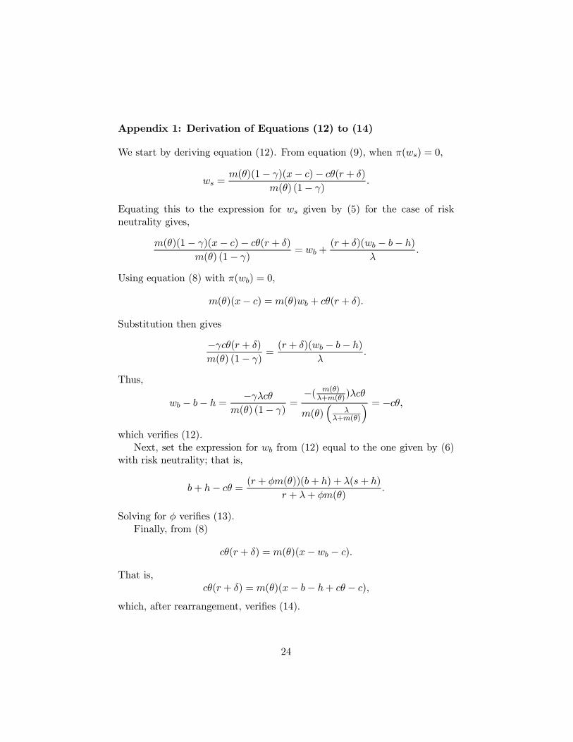
Appendix 1: Derivation of Equations (12) to (14)

We start by deriving equation (12). From equation (9), when π(ws) = 0,

ws =m(θ)(1− γ)(x− c)− cθ(r + δ)

m(θ) (1− γ).

Equating this to the expression for ws given by (5) for the case of riskneutrality gives,

m(θ)(1− γ)(x− c)− cθ(r + δ)

m(θ) (1− γ)= wb +

(r + δ)(wb − b− h)

λ.

Using equation (8) with π(wb) = 0,

m(θ)(x− c) = m(θ)wb + cθ(r + δ).

Substitution then gives

−γcθ(r + δ)

m(θ) (1− γ)=(r + δ)(wb − b− h)

λ.

Thus,

wb − b− h =−γλcθ

m(θ) (1− γ)=−( m(θ)

λ+m(θ))λcθ

m(θ)³

λλ+m(θ)

´ = −cθ,which verifies (12).

Next, set the expression for wb from (12) equal to the one given by (6)with risk neutrality; that is,

b+ h− cθ =(r + φm(θ))(b+ h) + λ(s+ h)

r + λ+ φm(θ).

Solving for φ verifies (13).Finally, from (8)

cθ(r + δ) = m(θ)(x−wb − c).

That is,cθ(r + δ) = m(θ)(x− b− h+ cθ − c),

which, after rearrangement, verifies (14).

24

Appendix 2: Comparative Statics Derivations

a. Comparative statics for θ: Using (14),

∂θ

∂b=

m(θ)

c[m(θ)− (r + δ)] +m0(θ)[cθ + (x− c− b− h)].

The denominator of this expression is positive since, from (14), we have

c[m(θ)− (r + δ)] = −[m(θ)/θ](x− c− b− h) > 0

andcθ + (x− c− b− h) = cθ(r + δ)/m(θ) > 0.

Thus, ∂θ/∂b > 0. Since neither s nor λ enters into (14), we have ∂θ/∂s =∂θ/∂λ = 0.

b. Comparative statics for wb: Using (12), ∂wb/∂b = 1−c(∂θ/∂b). Thatis,

∂wb

∂b=

−c(r + δ) +m0(θ)[cθ + (x− c− b− h)]

c[m(θ)− (r + δ)] +m0(θ)[cθ + (x− c− b− h)].

From (14), c(r + δ) =m(θ)

θ[cθ + (x− c− b− h)], so by substitution

∂wb

∂b=

[−m(θ)θ

+m0(θ)][cθ + (x− c− b− h)]

c[m(θ)− (r + δ)] +m0(θ)[cθ + (x− c− b− h)].

As m0(θ)θ < m(θ) and cθ+(x− c− b−h) > 0 we have ∂wb/∂b < 0. Since sand λ appear in neither (12) nor (14) it follows that ∂wb/∂s = ∂wb/∂λ = 0.

c. Comparative statics for ws: From (50),

∂ws

∂b= (

r + δ + λ

λ)∂wb

∂b− r + δ

λ< 0 and

∂ws

∂λ=(b+ h−wb)(r + δ)

λ2=

cθ(r + δ)

λ2> 0.

Finally, ∂ws/∂s = 0.

25

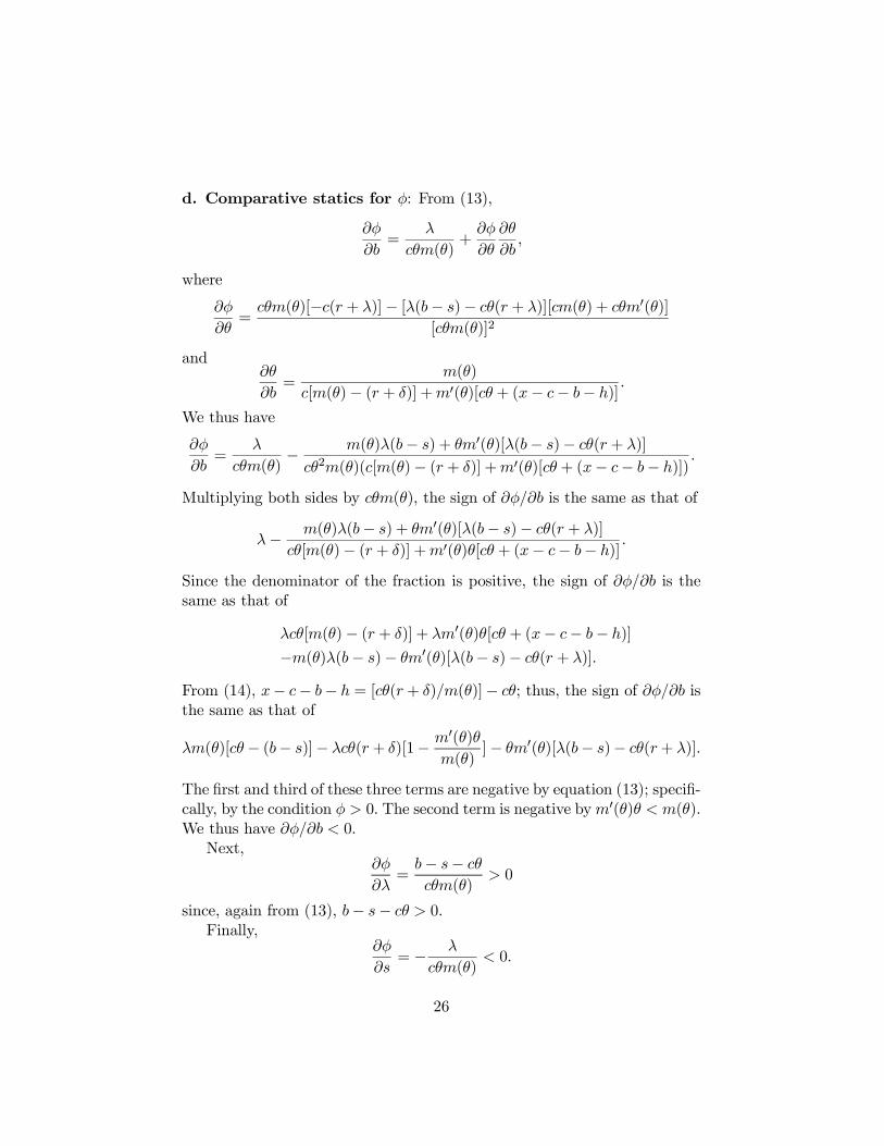
d. Comparative statics for φ: From (13),

∂φ

∂b=

λ

cθm(θ)+

∂φ

∂θ

∂θ

∂b,

where

∂φ

∂θ=

cθm(θ)[−c(r + λ)]− [λ(b− s)− cθ(r + λ)][cm(θ) + cθm0(θ)][cθm(θ)]2

and∂θ

∂b=

m(θ)

c[m(θ)− (r + δ)] +m0(θ)[cθ + (x− c− b− h)].

We thus have

∂φ

∂b=

λ

cθm(θ)− m(θ)λ(b− s) + θm0(θ)[λ(b− s)− cθ(r + λ)]

cθ2m(θ)(c[m(θ)− (r + δ)] +m0(θ)[cθ + (x− c− b− h)]).

Multiplying both sides by cθm(θ), the sign of ∂φ/∂b is the same as that of

λ− m(θ)λ(b− s) + θm0(θ)[λ(b− s)− cθ(r + λ)]

cθ[m(θ)− (r + δ)] +m0(θ)θ[cθ + (x− c− b− h)].

Since the denominator of the fraction is positive, the sign of ∂φ/∂b is thesame as that of

λcθ[m(θ)− (r + δ)] + λm0(θ)θ[cθ + (x− c− b− h)]

−m(θ)λ(b− s)− θm0(θ)[λ(b− s)− cθ(r + λ)].

From (14), x− c− b− h = [cθ(r + δ)/m(θ)]− cθ; thus, the sign of ∂φ/∂b isthe same as that of

λm(θ)[cθ− (b− s)]− λcθ(r + δ)[1− m0(θ)θm(θ)

]− θm0(θ)[λ(b− s)− cθ(r+ λ)].

The first and third of these three terms are negative by equation (13); specifi-cally, by the condition φ > 0. The second term is negative bym0(θ)θ < m(θ).We thus have ∂φ/∂b < 0.

Next,∂φ

∂λ=

b− s− cθ

cθm(θ)> 0

since, again from (13), b− s− cθ > 0.Finally,

∂φ

∂s= − λ

cθm(θ)< 0.

26

e. Comparative statics for γ: From (10),

∂γ

∂θ=

λm0(θ)(λ+m(θ))2

> 0.

Then ∂γ/∂λ = −m(θ)/[λ + m(θ)]2 < 0, and the rest of the derivativesof γ have the same signs as the partials of θ with respect to the variousparameters. Specifically, ∂γ/∂b > 0 and ∂γ/∂s = 0.

f. Comparative statics for u: From (11),

∂u

∂b=

∂u

∂φm(θ)

∂(φm(θ))

∂b+

∂u

∂γ

∂γ

∂b,

where∂u

∂φm(θ)=

−δγ(δ + γ[φm(θ) + λ])2

< 0

and∂u

∂γ=

−δ(φm(θ) + λ)

(δ + γ[φm(θ) + λ])2< 0.

Let Ψ =δ

(δ + γ[φm(θ) + λ])2> 0. Then, we have

∂u

∂b= −Ψ(γ∂φm(θ)

∂b+ (φm(θ) + λ)

∂γ

∂b).

Next from equation (13) we have

φm(θ) =λ(b− s)

cθ− (r + λ)

so∂φm(θ)

∂b=

λ

cθ− λ(b− s)

cθ2∂θ

∂b=

λ

cθ(1− (b− s)

θ

∂θ

∂b).

From above,∂γ

∂b=

λm0(θ)(λ+m(θ))2

∂θ

∂b> 0.

Thus,

∂u

∂b= −λΨ

µγ

cθ+

∂θ

∂b[m0(θ)(φm(θ) + λ)

(λ+m(θ))2− γ(b− s)

cθ2]

¶.

27

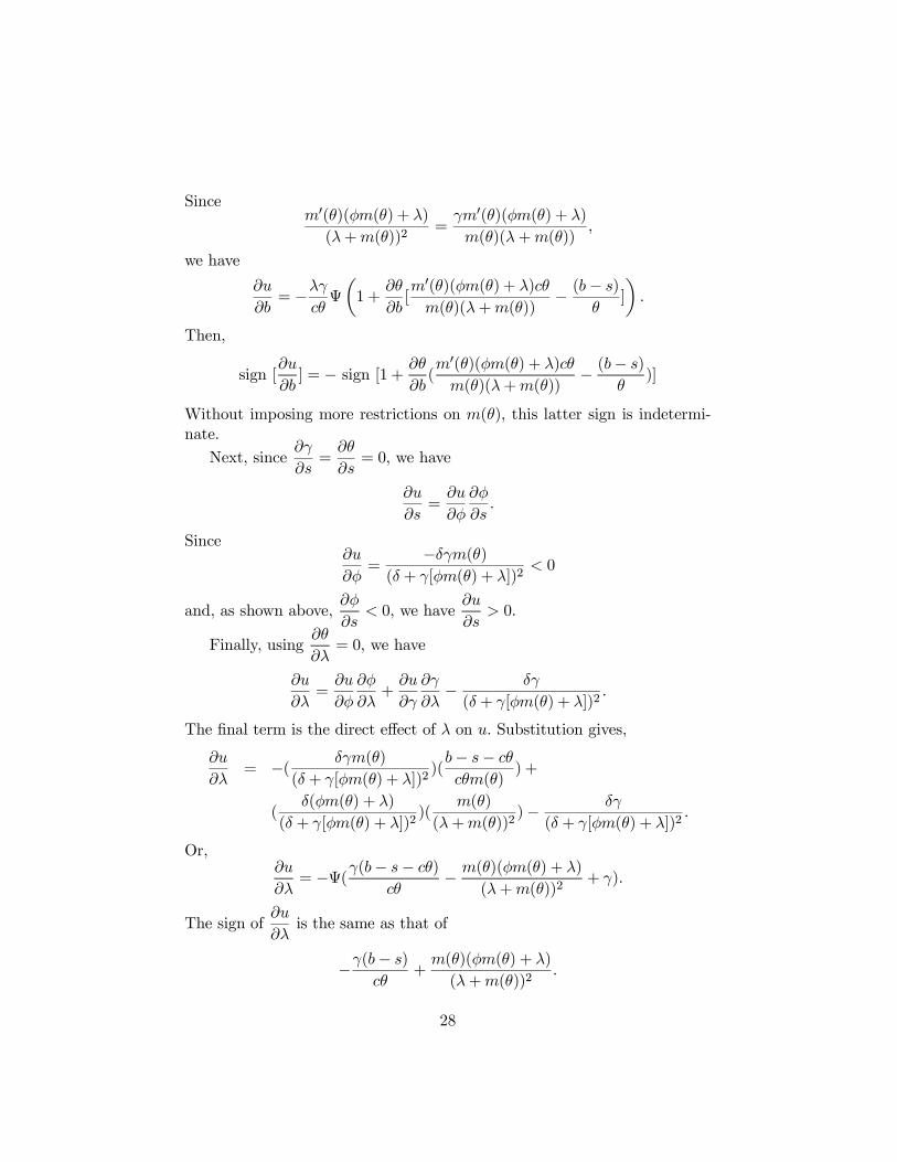
Sincem0(θ)(φm(θ) + λ)

(λ+m(θ))2=

γm0(θ)(φm(θ) + λ)

m(θ)(λ+m(θ)),

we have

∂u

∂b= −λγ

cθΨ

µ1 +

∂θ

∂b[m0(θ)(φm(θ) + λ)cθ

m(θ)(λ+m(θ))− (b− s)

θ]

¶.

Then,

sign [∂u

∂b] = − sign [1 + ∂θ

∂b(m0(θ)(φm(θ) + λ)cθ

m(θ)(λ+m(θ))− (b− s)

θ)]

Without imposing more restrictions on m(θ), this latter sign is indetermi-nate.

Next, since∂γ

∂s=

∂θ

∂s= 0, we have

∂u

∂s=

∂u

∂φ

∂φ

∂s.

Since∂u

∂φ=

−δγm(θ)(δ + γ[φm(θ) + λ])2

< 0

and, as shown above,∂φ

∂s< 0, we have

∂u

∂s> 0.

Finally, using∂θ

∂λ= 0, we have

∂u

∂λ=

∂u

∂φ

∂φ

∂λ+

∂u

∂γ

∂γ

∂λ− δγ

(δ + γ[φm(θ) + λ])2.

The final term is the direct effect of λ on u. Substitution gives,

∂u

∂λ= −( δγm(θ)

(δ + γ[φm(θ) + λ])2)(b− s− cθ

cθm(θ)) +

(δ(φm(θ) + λ)

(δ + γ[φm(θ) + λ])2)(

m(θ)

(λ+m(θ))2)− δγ

(δ + γ[φm(θ) + λ])2.

Or,∂u

∂λ= −Ψ(γ(b− s− cθ)

cθ− m(θ)(φm(θ) + λ)

(λ+m(θ))2+ γ).

The sign of∂u

∂λis the same as that of

−γ(b− s)

cθ+

m(θ)(φm(θ) + λ)

(λ+m(θ))2.

28

Using equations (10) and (13) for γ and φ, the sign of∂u

∂λis the same as

that of

− m(θ)

λ+m(θ)(b− s)

cθ+m(θ)[

λ(b− s)− cθ(r + λ)

cθ+ λ]

(λ+m(θ))2=−m(θ)[(b− s)m(θ) + cθr]

cθ(λ+m(θ))2< 0.

Thus,∂u

∂λ< 0.

29