Equilibrium and Stability Studies of Plasmas Confined in a Dipole Magnetic Field Using Magnetic Measurements by Ishtak Karim Submitted to the Department of Nuclear Science and Engineering in partial fulfillment of the requirements for the degree of Doctor of Science in Applied Plasma Physics at the MASSACHUSETTS INSTITUTE OF TECHNOLOGY February 2007 c Massachusetts Institute of Technology 2007. All rights reserved. Author .............................................................. Department of Nuclear Science and Engineering January 12, 2007 Certified by .......................................................... Jay Kesner Senior Research Scientist Thesis Supervisor Certified by .......................................................... Darren Garnier Research Scientist, Columbia University Thesis Cosupervisor Certified by .......................................................... Ron Parker Professor of Nuclear Engineering Thesis Reader Accepted by ......................................................... Jeffrey A. Coderre Chairman, Department Committee on Graduate Students

Welcome message from author
This document is posted to help you gain knowledge. Please leave a comment to let me know what you think about it! Share it to your friends and learn new things together.
Transcript
Equilibrium and Stability Studies of Plasmas
Confined in a Dipole Magnetic Field Using
Magnetic Measurementsby
Ishtak KarimSubmitted to the Department of Nuclear Science and Engineering
in partial fulfillment of the requirements for the degree of
Doctor of Science in Applied Plasma Physics
at the
MASSACHUSETTS INSTITUTE OF TECHNOLOGY
February 2007
c© Massachusetts Institute of Technology 2007. All rights reserved.
Author . . . . . . . . . . . . . . . . . . . . . . . . . . . . . . . . . . . . . . . . . . . . . . . . . . . . . . . . . . . . . .Department of Nuclear Science and Engineering
January 12, 2007
Certified by. . . . . . . . . . . . . . . . . . . . . . . . . . . . . . . . . . . . . . . . . . . . . . . . . . . . . . . . . .Jay Kesner
Senior Research ScientistThesis Supervisor
Certified by. . . . . . . . . . . . . . . . . . . . . . . . . . . . . . . . . . . . . . . . . . . . . . . . . . . . . . . . . .Darren Garnier
Research Scientist, Columbia UniversityThesis Cosupervisor
Certified by. . . . . . . . . . . . . . . . . . . . . . . . . . . . . . . . . . . . . . . . . . . . . . . . . . . . . . . . . .Ron Parker
Professor of Nuclear EngineeringThesis Reader
Accepted by . . . . . . . . . . . . . . . . . . . . . . . . . . . . . . . . . . . . . . . . . . . . . . . . . . . . . . . . .Jeffrey A. Coderre
Chairman, Department Committee on Graduate Students

2
Equilibrium and Stability Studies of Plasmas Confined in a
Dipole Magnetic Field Using Magnetic Measurements
by
Ishtak Karim
Submitted to the Department of Nuclear Science and Engineeringon January 12, 2007, in partial fulfillment of the
requirements for the degree ofDoctor of Science in Applied Plasma Physics
Abstract
The Levitated Dipole Experiment (LDX) is the first experiment of its kind to usea levitated current ring to confine a plasma in a dipole magnetic field. The plasmais stabilized by compressibility and can theoretically attain a peak beta on the or-der of unity. Various magnetic sensors have been designed, calibrated, installed,and operated to measure the plasma current, from which the pressure profile is de-duced through a mathematical process called reconstruction. Both isotropic andanisotropic models are introduced and used to obtain the equilibrium. The needfor an anisotropic pressure model is evident since electron cyclotron resonance heat-ing produces highly anisotropic plasmas in LDX. Compared to the isotropic pressuremodels, the anisotropic model predicts a larger peak beta for a given set of magneticmeasurements due to a modification in the current-pressure relationship. We haveachieved a peak beta in excess of 26 % using the anisotropic model.
One of the important results of this work involves characterizing the propertiesof reconstructing LDX plasmas. Because the floating coil is superconducting, it mustbe ensured that the flux linked to it is kept constant while deducing the plasmacurrent. A significant difficulty in reconstructing LDX plasmas is that the magneticsensors are sensitive mostly to the plasma dipole moment due to their large distancesfrom the plasma. This means that a family of current and pressure profiles with thesame dipole moment fits the magnetic measurements equally well. X-ray emissivitydata is used as a supplemental measurement to unequivocally determine the pressureprofile. Simulation results show that adding internal flux loops close to the plasmacan increase their sensitivity to higher order moments.
In addition to demonstrating the feasibility of achieving high beta, the magneticdiagnostics have decisively shown that LDX plasmas routinely have supercritical pres-sure profiles that exceed the MHD limit. The plasmas we have achieved to date havea significant fraction of hot electrons, which are susceptible to a kinetic analog of theMHD interchange mode called the hot electron interchange mode (HEI). Althoughthe MHD gradient limit is slightly increased by incorporating pressure anisotropy, thebest fit profile usually gives a pressure gradient that substantially exceeds even the
3
anisotropic limit. Magnetic measurements therefore confirm that the hot electronsare not subject to the MHD interchange mode, and the HEI is the relevant instabil-ity. The HEI’s have been measured by Mirnov coils, and their occurrences have beencorrelated to drops in flux measurements. Lastly, a stored energy-plasma currentrelationship has been derived, and its result has been used to estimate the energyconfinement time of LDX plasmas with different heating frequency compositions.
Thesis Supervisor: Jay KesnerTitle: Senior Research Scientist
4

Acknowledgments
I would hereby like to acknowledge the people in my group who have made this work
possible. Jay Kesner for being the laid back advisor who never breathed down behind
my neck and allowed me to do my research freely. Darren Garnier for leading the
way and advising me on both engineering and physics issues and giving me logistic
support when needed. Mike Mauel for always being keen on the details of what I did.
Alex Hansen for letting me use his credit card. Jennifer Ellsworth for supplementing
my below average computer skills. Eugene Ortiz for broaching all kinds of physics
questions related to my measurements and pushing me when necessary. Alex Boxer
for being more absent than I am and attending me for hours while I worked inside
the vessel and engaging me with interesting conversations from time to time. Austin
Roach and Daniel Benitez for allowing me to abuse you as UROPs. Rick Lations for
letting me use his tools and forgiving me when I drank his coffee. Lastly, but not
leastly, Don Strahan for welding many many studs for me inside the vessel wearing a
heat-maintaining bunny suit in the 110 chamber. Thank you all.
My thanks also go to my reader, Ron Parker, and the committee members for my
defense, Ian Hutchinson and Jeff Freidberg.
5

6
Contents
1 Introduction 19
1.1 Fusion as a Power Source . . . . . . . . . . . . . . . . . . . . . . . . . 19
1.2 LDX Hardware . . . . . . . . . . . . . . . . . . . . . . . . . . . . . . 20
1.3 Diagnostics . . . . . . . . . . . . . . . . . . . . . . . . . . . . . . . . 22
1.4 Experimental Goals, Procedures, and Accomplishments . . . . . . . . 27
1.5 Thesis Goals . . . . . . . . . . . . . . . . . . . . . . . . . . . . . . . . 29
2 Magnetic Diagnostics 31
2.1 Magnetic Diagnostics on LDX . . . . . . . . . . . . . . . . . . . . . . 33
2.1.1 Sensors for Equilibrium Measurement . . . . . . . . . . . . . . 34
2.1.2 Sensors for Fluctuation Measurement . . . . . . . . . . . . . . 40
2.2 Calibration of the Electronics and Diagnostics . . . . . . . . . . . . . 42
2.2.1 Electronics Calibration . . . . . . . . . . . . . . . . . . . . . . 42
2.2.2 Diagnostics Calibration . . . . . . . . . . . . . . . . . . . . . . 43
2.3 Future Improvements to the Magnetic Diagnostics System . . . . . . 45
3 Sensor location optimization 51
3.1 Mathematical formulation . . . . . . . . . . . . . . . . . . . . . . . . 51
3.2 Application to LDX Magnetic Diagnostics . . . . . . . . . . . . . . . 53
4 Error analysis 65
4.1 Precision errors . . . . . . . . . . . . . . . . . . . . . . . . . . . . . . 65
4.2 Random errors . . . . . . . . . . . . . . . . . . . . . . . . . . . . . . 66
7
4.2.1 Errors in the Bp coil and flux loop measurements . . . . . . . 66
4.2.2 Errors in the Hall probe measurements . . . . . . . . . . . . . 69
4.3 The effect of the sensor position error on the field / flux measurement
error . . . . . . . . . . . . . . . . . . . . . . . . . . . . . . . . . . . . 70
4.3.1 Comprehensive error in the Hall probe measurement . . . . . 70
4.3.2 Comprehensive errors in the Bp coil and flux loop measurements 71
4.4 Error in the determination of the floating coil current due to the errors
in the Hall probe measurements . . . . . . . . . . . . . . . . . . . . . 73
4.5 Equilibrium quantity errors due to the errors in the Bp coil and flux
loop measurements . . . . . . . . . . . . . . . . . . . . . . . . . . . . 76
5 Equilibrium and Stability of LDX Plasma 79
5.1 Plasma equilibrium in LDX . . . . . . . . . . . . . . . . . . . . . . . 80
5.2 Interchange instabilities . . . . . . . . . . . . . . . . . . . . . . . . . 82
5.2.1 MHD Pressure Driven Interchange . . . . . . . . . . . . . . . 82
5.2.2 Hot Electron Interchange . . . . . . . . . . . . . . . . . . . . . 90
5.3 Summary of LDX Equilibrium and Stability . . . . . . . . . . . . . . 91
6 Equilibrium Reconstruction 93
6.1 Reconstruction procedure . . . . . . . . . . . . . . . . . . . . . . . . 94
6.1.1 Conservation of the floating coil flux . . . . . . . . . . . . . . 94
6.1.2 DFIT: The Dipole Current Filament Code . . . . . . . . . . . 96
6.2 Reconstruction methods . . . . . . . . . . . . . . . . . . . . . . . . . 97
6.2.1 Full Reconstruction . . . . . . . . . . . . . . . . . . . . . . . . 97
6.2.2 Vacuum Reconstruction . . . . . . . . . . . . . . . . . . . . . 100
6.3 Pressure models . . . . . . . . . . . . . . . . . . . . . . . . . . . . . . 101
6.3.1 Isotropic models . . . . . . . . . . . . . . . . . . . . . . . . . . 102
6.3.2 An anisotropic model . . . . . . . . . . . . . . . . . . . . . . . 104
6.4 Sensitivity of the magnetic measurements to the lowest order moment 105
6.4.1 Evidence . . . . . . . . . . . . . . . . . . . . . . . . . . . . . . 105
6.4.2 Using x-ray data to help constrain the parameters . . . . . . . 109
8
7 Typical Shots 115
7.1 Characterization of the three regimes . . . . . . . . . . . . . . . . . . 115
7.1.1 Low density regime . . . . . . . . . . . . . . . . . . . . . . . . 117
7.1.2 High beta regime . . . . . . . . . . . . . . . . . . . . . . . . . 117
7.1.3 Afterglow regime . . . . . . . . . . . . . . . . . . . . . . . . . 121
7.2 Equilibrium reconstruction of the typical shot . . . . . . . . . . . . . 121
7.3 Comparison of the different pressure models . . . . . . . . . . . . . . 128
8 Special Shots 131
8.1 ECRH Control . . . . . . . . . . . . . . . . . . . . . . . . . . . . . . 131
8.2 Gas Fueling Control . . . . . . . . . . . . . . . . . . . . . . . . . . . 138
8.3 Vertical Field Control . . . . . . . . . . . . . . . . . . . . . . . . . . . 138
8.4 Comprehensive Plasma Control . . . . . . . . . . . . . . . . . . . . . 143
9 Analysis 145
9.1 High beta measurement . . . . . . . . . . . . . . . . . . . . . . . . . 145
9.2 Measurement of Supercritical Profiles . . . . . . . . . . . . . . . . . . 149
9.3 Magnetic detection of the HEI . . . . . . . . . . . . . . . . . . . . . . 152
9.4 Plasma current vs. Stored energy Relation . . . . . . . . . . . . . . . 157
9.5 Energy confinement time . . . . . . . . . . . . . . . . . . . . . . . . . 160
9.6 Analysis Summary . . . . . . . . . . . . . . . . . . . . . . . . . . . . 163
10 Conclusion 167
10.1 Main Results . . . . . . . . . . . . . . . . . . . . . . . . . . . . . . . 167
10.2 Summary . . . . . . . . . . . . . . . . . . . . . . . . . . . . . . . . . 168
10.3 Future Work and Levitation . . . . . . . . . . . . . . . . . . . . . . . 171
A Figures 173
B Reconstruction codes 175
9

10
List of Figures
1-1 A schematic view of the LDX apparatus. . . . . . . . . . . . . . . . . 21
1-2 The floating coil. . . . . . . . . . . . . . . . . . . . . . . . . . . . . . 23
1-3 The charging coil. . . . . . . . . . . . . . . . . . . . . . . . . . . . . . 24
1-4 The levitation coil. . . . . . . . . . . . . . . . . . . . . . . . . . . . . 25
1-5 The locations of different diagnostics. The initial sets of diagnostics
include magnetics, electric probes, x-ray detectors, and a single-chord
interferometer. . . . . . . . . . . . . . . . . . . . . . . . . . . . . . . . 27
2-1 A poloidal field coil. . . . . . . . . . . . . . . . . . . . . . . . . . . . 36
2-2 Flux loops at the bottom of the vessel. . . . . . . . . . . . . . . . . . 37
2-3 A Hall-probe attached to the top of a Bp coil. . . . . . . . . . . . . . 39
2-4 A Mirnov coil. . . . . . . . . . . . . . . . . . . . . . . . . . . . . . . . 41
2-5 (a) The transfer function (to within a multiplicative factor) of a Mirnov
coil as installed and (b) the transfer function multiplied by frequency. 49
3-1 Forty-three possible positions to install the sensors. . . . . . . . . . . 54
3-2 A histogram showing the most sensitive positions for normal Bp coils. 57
3-3 A histogram showing the most sensitive positions for tangential Bp coils. 58
3-4 A histogram showing the most sensitive positions for flux loops. . . . 59
3-5 A picture of where the different sensors should be placed. . . . . . . . 60
3-6 A schematic of the sensor locations as installed. The normal and par-
allel Bp coils are installed on the same poloidal plane although the
picture depicts otherwise for clarity. . . . . . . . . . . . . . . . . . . . 61
11
3-7 Actual pictures of the Bp coils and flux loops as installed at the top
(top right), side (left), and bottom (bottom right) of the vessel. . . . 64
5-1 Constant ψ contours for a typical LDX equilibrium (a) without the
levitation coil current and (b) with the levitation coil at its nominal
current. . . . . . . . . . . . . . . . . . . . . . . . . . . . . . . . . . . 81
5-2 A sample pressure profile with Pedge = 0.025 Pa and Rpeak = 0.76 m.
The marginal stability gradient of P ∼ R− 203 was used. . . . . . . . . 83
5-3 A particle picture of an interchange event. Different particle drifts
collude to drive the perturbation. . . . . . . . . . . . . . . . . . . . . 85
5-4 If the interchange of Region I and Region II results in a lower energy
state, then the plasma is unstable to this interchange. . . . . . . . . . 86
5-5 The plasma region outside of the pressure peak has the magnetic cur-
vature and pressure gradient pointing in the same direction and thus
can be unstable. . . . . . . . . . . . . . . . . . . . . . . . . . . . . . . 88
6-1 A flowchart of the reconstruction algorithm. The free parameters are
varied until the best fit, designated by the minimum χ2, is found.
The C and M in the superscript stands for calculated and measured,
respectively. The pressure model introduced in Ch. 3 is used as an
example. . . . . . . . . . . . . . . . . . . . . . . . . . . . . . . . . . . 98
6-2 A contour plot of chi-squared as the currents in the two filaments are
varied. The contour of minimum chi-squared is not shown but should
be where the black dot is. Instead, a contour of a fixed dipole moment
is shown in its place. The fact that the two contours roughly overlay
each other shows that the magnetic sensors are sensitive only to the
dipole moment. . . . . . . . . . . . . . . . . . . . . . . . . . . . . . . 107
6-3 Plots of chi-squared as a function of Pedge and g = 53fcrit with a fixed
ψpeak. For each Pedge, there is a g that minimizes chi-squared. Plotting
these minima vs. Pedge gives an absolute minimum of chi-squared as a
function of the two variables. . . . . . . . . . . . . . . . . . . . . . . . 108
12
6-4 Chi-squared contours in the (ψpeak, g) plane. The dotted lines are
the contours for the external sensors only, and the solid lines are the
contours for the external sensors plus internal flux loops. The x-axis
of the figure (R) designates the radius of the pressure peak, which is
qualitatively equivalent to the flux at the pressure peak (ψpeak). The
minimum is unambiguous only when the internal loops are present. . 110
6-5 Contours of the reconstructed pressure profiles superimposed onto the
x-ray images measured during (top) 2.45 GHz heating and (bottom)
6.4 GHz heating. . . . . . . . . . . . . . . . . . . . . . . . . . . . . . 111
6-6 An x-ray image for 2.45 GHz only heating (left), its line integrated
emissivity (right top), and its Abel inversion (right bottom). . . . . . 112
7-1 Signals from various diagnostics showing the evolution of a typical LDX
discharge (shot 50317014). The three plasma regimes are marked by
different colors. The pale yellow region is the low density regime, white
is the high beta regime, and the light blue region is the after-glow regime.116
7-2 A video image showing flying debris caused by energetic electrons hit-
ting solid structures during the low density regime. . . . . . . . . . . 118
7-3 The DFIT code result showing the current centroid moving outwards
as the plasma transitions from the low density to high beta regime. . 119
7-4 An increase in broad spectrum fluctuations can be seen on the Mirnov
and edge probe signals as the plasma enters the high beta regime. The
edge probe clearly acquires a positive current after the transition. . . 120
7-5 A video image of the high beta regime plasma. The plasma is much
more tranquil compared to that during the low density regime. . . . . 122
7-6 A video image of the afterglow regime. A bright halo of hot electrons
is clearly visible around the floating coil. . . . . . . . . . . . . . . . . 124
7-7 The best fit (a) current and (b) pressure profiles, and the resulting (c)
beta profile. . . . . . . . . . . . . . . . . . . . . . . . . . . . . . . . . 126
7-8 The equilibrium flux contours showing the shape of the plasma. . . . 127
13
7-9 Comparison of the equilibrium parameters from three different pressure
models. . . . . . . . . . . . . . . . . . . . . . . . . . . . . . . . . . . 129
8-1 The ECRH signals (top) and the corresponding signal from a flux loop
(bottom) for shot 50318009. The 2.45 GHz signal is shown in red and
the 6.4 GHz signal is shown in black. . . . . . . . . . . . . . . . . . . 133
8-2 The ECRH signals (top) and the corresponding signal from a flux loop
(bottom) for shot 50318010. The 2.45 GHz signal is shown in red and
the 6.4 GHz signal is shown in black. . . . . . . . . . . . . . . . . . . 134
8-3 The best fit pressure profiles for shots 50318009 (top) and 50318010
(bottom) at t = 2 sec (solid) and 8 sec (dotted). . . . . . . . . . . . . 135
8-4 The current magnitudes (top) and centroids (bottom) from DFIT for
shots 50318009 (black) and 50318010 (blue) as a function of time. . . 137
8-5 Plots of the ion gauge pressure (blue) and one of the flux loops (red).
The plasma oscillates between the low density and high beta regimes. 139
8-6 Plots of the ion gauge pressure (above) and one of the flux loops (below)
for shot 50513002. Excessive fueling causes the plasma to almost disrupt.140
8-7 Shape of the plasma at a Helmholtz coil current of (a) 0 kA, (b) 8 kA,
(c) 16 kA, and (d) 24 kA. . . . . . . . . . . . . . . . . . . . . . . . . 141
8-8 Current and pressure profiles for the four vertical field currents: 0 kA
(black), 8 kA (red), 16 kA (blue), and 24 kA (green). . . . . . . . . . 142
9-1 The reconstructed pressure and beta profiles of the DipoleEq model
(black), isotropic smooth adiabatic model (blue), and anisotropic smooth
adiabatic model with P⊥P‖
= 5 (red). The beta for the anisotropic case
is the perpendicular beta. . . . . . . . . . . . . . . . . . . . . . . . . 147
9-2 The reconstructed (a) pressure and (b) current contours using the
isotropic smooth adiabatic model and (c) pressure and (d) current con-
tours using the anisotropic model with p = 2. . . . . . . . . . . . . . 148
9-3 A plot of ten shots that have been reconstructed using the DipoleEq
model. Most shots have pressure profiles steeper than V − 53 . . . . . . 150
14
9-4 A plot of χ2 vs. gγ
for the highest beta shot using the DipoleEq model
(top) and plots of χ2 vs. g for the same shot using both the isotropic
and anisotropic smooth adiabatic models (bottom). The red curve is
the isotropic case, green is the anisotropic case with p = 1, and black
curve is the anisotropic case with p = 2. . . . . . . . . . . . . . . . . 151
9-5 A Mirnov signal overlaid on a flux loop signal for shot 50513024. An
HEI event occurs during the after-glow. . . . . . . . . . . . . . . . . . 153
9-6 A Mirnov signal overlaid on a flux loop signal for shots 50513027 (top)
and 50513028 (bottom). The two shots are identical except that shot
50513028 has an extra HEI event right before 1 sec. Both shots suffer
an HEI event around 4 and 6 seconds. . . . . . . . . . . . . . . . . . 154
9-7 A Mirnov signal overlaid on a flux loop signal for shots 50513033 (top)
and 50513032 (bottom). Shot 50513032 endures an HEI event the
moment the RF’s turn off. Otherwise, the two shots are identical. . . 155
9-8 A Mirnov signal overlaid on a flux loop signal for shots 50513040 (top)
and 50513041 (bottom). Again, the two shots are identical except for
an HEI event that occurs around 5 sec for shot 50513041. . . . . . . . 156
9-9 Shots 50318015 (top) and 50318016 (bottom) are identical, but shot
50318016 endures multiple relaxation events during the high beta regime.
A blowup of the relaxation events is shown to the right. . . . . . . . . 158
9-10 Plots of the two functions of γ and their product that appear in the
expression for WRc
Ip. The ψ values have been chosen for a floating coil
charge of 900 kA. . . . . . . . . . . . . . . . . . . . . . . . . . . . . . 161
9-11 Plots of W vs. IpRc
for nine 900 kA charge shots. The best fit line
predicts a WRc
Ipvalue of about 60 J·m·kA−1. Error bars have been
suppressed since they are smaller than the dots in the y direction and
on the order of their size in the x direction. . . . . . . . . . . . . . . . 162
15
9-12 Plots of energy confinement time vs. 2.45 GHz heating fraction. The
different colors represent the different floating coil currents, and the
spot sizes represent the total heating power. The stored energies have
been estimated using the current-energy relation of the previous section.164
A-1 Armadillo slaying lawyer. . . . . . . . . . . . . . . . . . . . . . . . . . 173
A-2 Armadillo eradicating national debt. . . . . . . . . . . . . . . . . . . 174
16

List of Tables
2.1 Calibration data for amplifier and integrator boards. . . . . . . . . . 44
2.2 Calibration data of Bp coils and Hall probes. . . . . . . . . . . . . . . 46
2.3 Calibration data of Mirnov coils. . . . . . . . . . . . . . . . . . . . . 47
3.1 The (X, Z, Θ) coordinates and their estimated errors of the Bp coils
and flux loops. The (X, Z) coordinates are measured from the center
of the vacuum vessel, and the angles are measured clockwise from the
vertical. In the above, N stands for “normal” (as in normal to the
vessel) and P stands for “parallel.” The flux loops are designated by F . 62
3.2 The (X, Z, Θ) coordinates and their estimated errors of the Hall probes. 63
4.1 The total measurement errors of the Hall probes and the measurement
and position errors that contribute to them. . . . . . . . . . . . . . . 72
4.2 The total measurement errors of the Bp coils and flux loops and the
measurement and position errors that contribute to them. . . . . . . 74
4.3 Variations of the best fit current due to random variations in the mea-
sured fields. . . . . . . . . . . . . . . . . . . . . . . . . . . . . . . . . 75
4.4 Variations of the equilibrium quantities due to random variations in
the measured diamagnetic fields and fluxes. . . . . . . . . . . . . . . . 76
7.1 Key equilibrium parameters during a typical high beta regime. . . . . 123
7.2 The equilibrium parameters of shot 50317014 calculated from the best
fit pressure profile. . . . . . . . . . . . . . . . . . . . . . . . . . . . . 125
17
8.1 The equilibrium parameters of shots 50318009 and 50318010 at t = 2,
8 sec calculated from the best fit pressure profiles. . . . . . . . . . . . 136
8.2 Equilibrium parameters for the four Helmholtz currents. . . . . . . . 143
9.1 Equilibrium parameters obtained from the two isotropic and the anisotropic
pressure models. . . . . . . . . . . . . . . . . . . . . . . . . . . . . . . 146
18
Chapter 1
Introduction
The Levitated Dipole Experiment (LDX) is a joint MIT-Columbia experiment that
studies the basic physics of a plasma confined in a dipole magnetic field [20]. Its
global goal is to demonstrate the feasibility of sustaining a stable, high-beta plasma in
this unique and simple magnetic configuration. LDX is first of its kind amongst other
dipole confinement experiments in terms of its large size. It is also the first experiment
to utilize plasma compressibility for its stability. LDX is a culmination of recent
advances made in superconductor technology along with a better understanding of
relevant plasma theory that predicts the possibility of a good dipolar confinement.
1.1 Fusion as a Power Source
Magnetic confinement of hot and dense plasmas may be the most viable method
for attaining controlled nuclear fusion, and it therefore plays an important role in
making cheap energy from fusion power a reality. Fusion energy production may
soon by approaching the break-even point (i.e. getting as much power out as putting
in), but its high cost of production prevents it from becoming an economically viable
alternative to coal, petroleum, and nuclear fission. Only when we nearly exhaust
our fossil fuel availability (in a few decades) may fusion become an economically
competitive source of energy. However, economics is not the sole arbiter of energy
choices, and increasing environmental awareness among the populous is driving the
19
need for clean energy sources. Because fusion is relatively clean and has a semi-infinite
source of fuel, it is unquestionably one of the most important energy sources of the
future.
The most extensively studied and tested device for doing plasma confinement is the
tokamak. Although the tokamak may be the most promising machine for becoming
the prototype of a future reactor, it is not without disadvantages, and numerous other
types of “alternate concept” machines have been studied. One of them derives from
the concept of confining a plasma in a dipolar magnetic field. The motivation for
using a dipole magnetic configuration for plasma confinement comes from numerous
observations made by astronomers and astrophysicists concerning planetary plasma
confinement. One of the important things learned from these observations is that one
of the planets, namely Jupiter, confines plasma very efficiently with a local maximum
β on the order of unity. Such a high β is unheard of in any conventional tokamak
(i.e. excluding spherical torii), and fusion scientists began to think about adopting
this confinement scheme to a laboratory setting to study its plasma physics. Akira
Hasegawa is credited for envisioning the use of a dipole field created by a levitated
ring to confine a hot plasma for fusion power generation [15, 16]. LDX has been
designed to test the feasibility of such a confinement scheme.
1.2 LDX Hardware
The Levitated Dipole Experiment roughly consists of a large vacuum vessel ( 80m3)
and three superconducting magnets [10] (Figure 1-1). The vacuum vessel is con-
structed of 3/4” thick stainless steel to maintain its structural integrity while minimiz-
ing eddy currents. Each of the three magnets plays an integral role in the operation
of the experiment. Additional components of the experiment consist of Helmholtz
shaping coils, diagnostic sensors, and various pumps to evacuate the vessel.
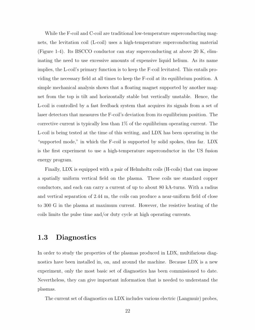
The floating coil (F-coil) is the magnet that produces the necessary dipole field to
confine the plasma (Figure 1-2). It consists of a central Nb3Sn conductor surrounded
by three concentric toroidal structures. The inner most torus is a helium pressure
20
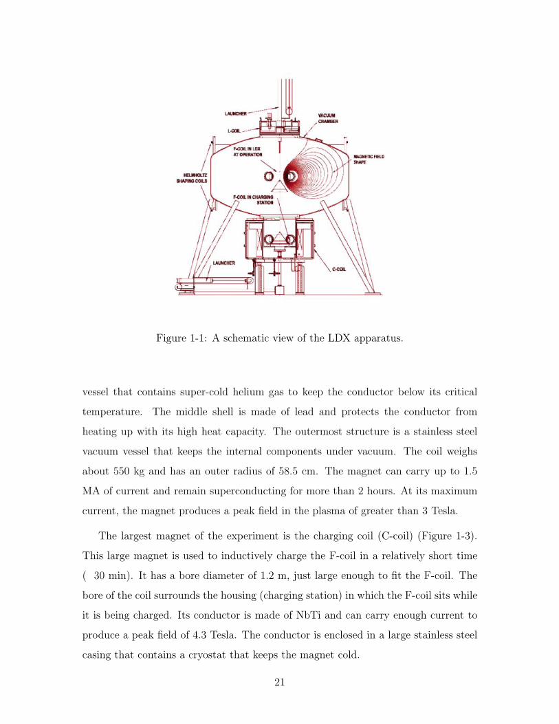
Figure 1-1: A schematic view of the LDX apparatus.
vessel that contains super-cold helium gas to keep the conductor below its critical
temperature. The middle shell is made of lead and protects the conductor from
heating up with its high heat capacity. The outermost structure is a stainless steel
vacuum vessel that keeps the internal components under vacuum. The coil weighs
about 550 kg and has an outer radius of 58.5 cm. The magnet can carry up to 1.5
MA of current and remain superconducting for more than 2 hours. At its maximum
current, the magnet produces a peak field in the plasma of greater than 3 Tesla.
The largest magnet of the experiment is the charging coil (C-coil) (Figure 1-3).
This large magnet is used to inductively charge the F-coil in a relatively short time
( 30 min). It has a bore diameter of 1.2 m, just large enough to fit the F-coil. The
bore of the coil surrounds the housing (charging station) in which the F-coil sits while
it is being charged. Its conductor is made of NbTi and can carry enough current to
produce a peak field of 4.3 Tesla. The conductor is enclosed in a large stainless steel
casing that contains a cryostat that keeps the magnet cold.
21
While the F-coil and C-coil are traditional low-temperature superconducting mag-
nets, the levitation coil (L-coil) uses a high-temperature superconducting material
(Figure 1-4). Its BSCCO conductor can stay superconducting at above 20 K, elim-
inating the need to use excessive amounts of expensive liquid helium. As its name
implies, the L-coil’s primary function is to keep the F-coil levitated. This entails pro-
viding the necessary field at all times to keep the F-coil at its equilibrium position. A
simple mechanical analysis shows that a floating magnet supported by another mag-
net from the top is tilt and horizontally stable but vertically unstable. Hence, the
L-coil is controlled by a fast feedback system that acquires its signals from a set of
laser detectors that measures the F-coil’s deviation from its equilibrium position. The
corrective current is typically less than 1% of the equilibrium operating current. The
L-coil is being tested at the time of this writing, and LDX has been operating in the
“supported mode,” in which the F-coil is supported by solid spokes, thus far. LDX
is the first experiment to use a high-temperature superconductor in the US fusion
energy program.
Finally, LDX is equipped with a pair of Helmholtz coils (H-coils) that can impose
a spatially uniform vertical field on the plasma. These coils use standard copper
conductors, and each can carry a current of up to about 80 kA-turns. With a radius
and vertical separation of 2.44 m, the coils can produce a near-uniform field of close
to 300 G in the plasma at maximum current. However, the resistive heating of the
coils limits the pulse time and/or duty cycle at high operating currents.
1.3 Diagnostics
In order to study the properties of the plasmas produced in LDX, multifarious diag-
nostics have been installed in, on, and around the machine. Because LDX is a new
experiment, only the most basic set of diagnostics has been commissioned to date.
Nevertheless, they can give important information that is needed to understand the
plasmas.
The current set of diagnostics on LDX includes various electric (Langmuir) probes,
22
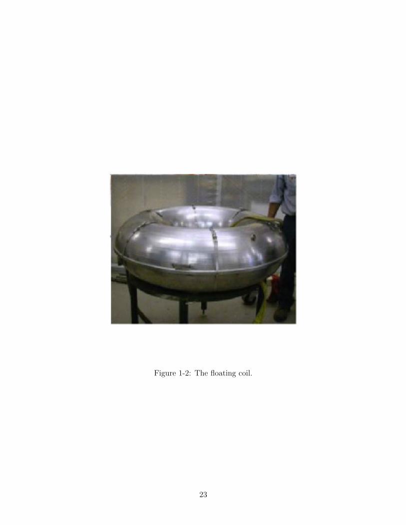
Figure 1-2: The floating coil.
23
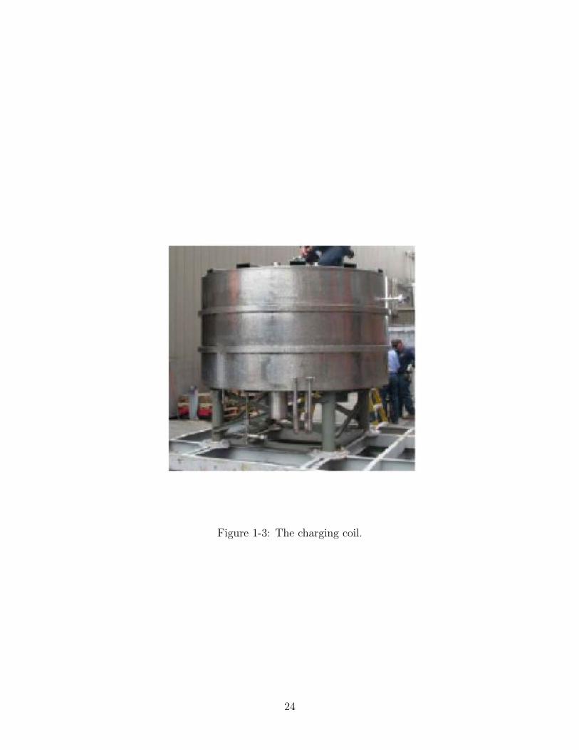
Figure 1-3: The charging coil.
24
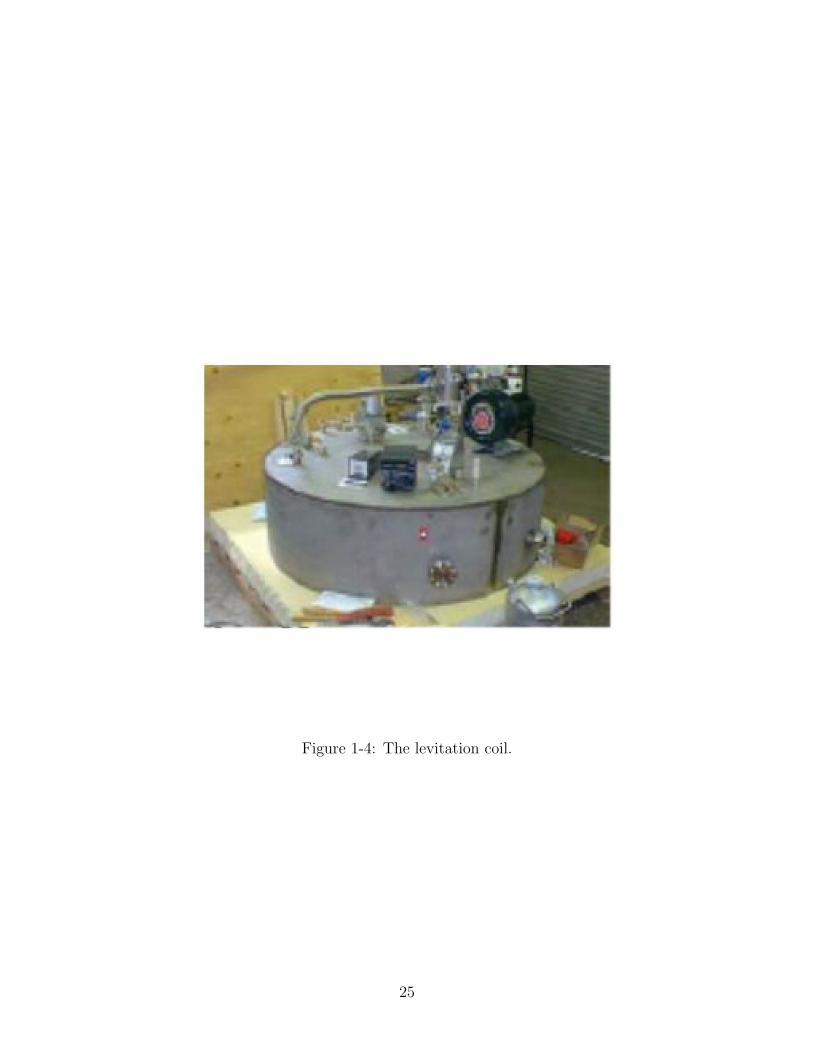
Figure 1-4: The levitation coil.
25
a four-channel x-ray pulse height analyzer, an x-ray camera, a photodiode array, a
single channel microwave interferometer, and an assortment of magnetic diagnostics.
Some of these sensors allow us to measure different plasma parameters while others
measure similar properties and serve as complimentary diagnostics. There are multi-
ple sets of moveable and fixed Langmuir probes that operate in different modes. Some
are biased at a fixed voltage while others are voltage swept to obtain current-voltage
characteristics. The probes that are kept at a fixed voltage allow us to measure and
characterize electrostatic fluctuations whereas those that are swept give density and
temperature measurements. Because the swept probes are voltage swept many times
over one shot, sufficient time resolution can be obtained for these measurements. Since
the probes can significantly perturb the plasma and cannot withstand too much heat
flux, probe measurements are limited to the plasma edge.
X-ray diagnostics are primarily used to measure the energy of the hot electron
species produced by electron cyclotron resonance heating (ECRH) of LDX plasma. A
4-channel pulse height analyzer gives the energy distribution of the collected electrons,
from which temperature information can be deduced. An x-ray camera converts
the x-ray intensity to a visible light intensity on a phosphor screen. Hence, a line
integrated x-ray intensity can be attained through proper calibration. Because both
of these measurements are line integrated measurements, a proper inversion scheme
(i.e. Abel inversion) must be employed in order to obtain any spatial resolution of
the data.
A heterodyne interferometer is used in LDX to measure its core plasma density.
As with the x-ray measurements, the interferometer measures a line integrated value
and hence requires more than one chord to get a spatial resolution. The interferometer
system has not been completed at this time and only uses a single chord. Although
the current system can only measure line integrated density values, it will be upgraded
in the near future to include multiple chords to allow for the measurement of density
profiles.
LDX has a sizable set of magnetic diagnostics for equilibrium and perturbation
measurements. Their details will be discussed in the next chapter and hence will
26
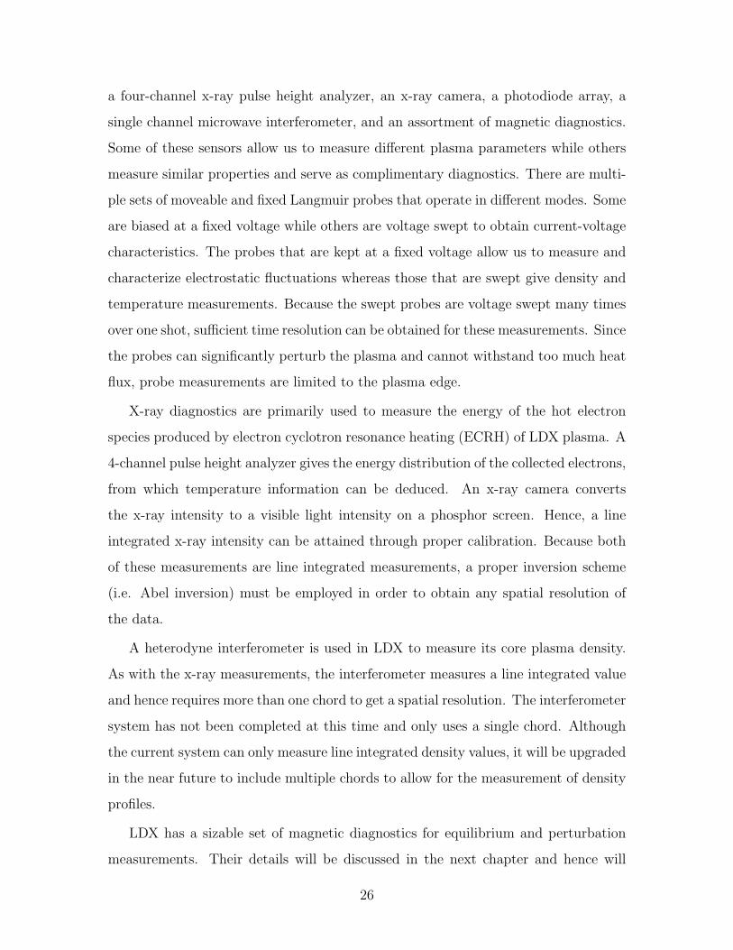
not be elaborated here. Figure 1-5 summarizes the locations of the diagnostics with
respect to the vacuum vessel.
Figure 1-5: The locations of different diagnostics. The initial sets of diagnostics
include magnetics, electric probes, x-ray detectors, and a single-chord interferometer.
1.4 Experimental Goals, Procedures, and Accom-
plishments
The Levitated Dipole Experiment is designed to test the feasibility of concept for
realizing a future levitated dipole fusion reactor. To this end, the experiment serves
as establishing the physics feasibility of heating, confining, and sustaining a high
beta plasma in the dipole magnetic configuration. LDX is not a proof of concept
experiment in the sense that it does not address the effects of a burning plasma on
the hardware or on the plasma itself. In addition to fulfilling its role as a fusion
experiment, LDX is an excellent testing bed to study the physics of planetary and
27
stellar plasmas. The magnetic field of LDX is designed to mimic that of planets and
stars as previously mentioned, hence it is only natural that LDX plasmas are relevant
for learning and understanding plasmas that occur naturally in space.
One of the key questions LDX must answer is whether it can sustain a high
beta plasma. The answer to this question has already been half-obtained. LDX has
attained a peak local beta in excess of 20%. However, attaining high beta by itself is
not sufficient; we need to understand the conditions that lead to the creation of high
beta plasmas and gain a physical insight into how these conditions facilitate such
creation. Only after understanding the physics of producing high beta plasmas can
one develop a relevant theory or connect current theories to experimental data. The
understanding and confirmation of such theories are essential to reproducing high
beta plasmas, not only in our experiment, but also in a scaled up version of LDX.
Another key question LDX is purposed to explore is the plasma confinement prop-
erties in a magnetic dipole. Specifically, we want to learn about the formation and
evolution of convective cells that may arise in this kind of plasma. Convective cells are
global convective motions of particles caused by exceeding the MHD stability limit.
It is of great interest to study how convective cells affect the energy and particle
transport. If convective cells only transport particles and not energy, it would be of
great consequence to solving the fueling and ash removal problems in a future reac-
tor. Because LDX plasmas are quasi-steady state (limited only by the RF source),
we would also like to study their long term evolution. This issue is related to the first
question; can we sustain a quiescent high-beta plasma for an indefinite time without
causing disruptions or otherwise violent instabilities? The longest shots we have had
so far were on the order of ten seconds, and we have been successful in sustaining a
high-beta 20% plasma for this length of time. The next obvious step would be to
lengthen our shots to demonstrate the true quasi-steadiness of our plasma.
In reaching the objectives of the experiment, LDX will be operated in three distinct
phases. Phase one is the current phase in which the dipole is supported during
operation. Although there are only three thin supports, they are enough to cause
end losses that limit the beta of the plasma. Plasma formation and profile control
28
by multi-frequency electron cyclotron resonance heating is being explored in this
phase. The measurement of beta and instabilities that limit it is crucial at this
stage. The next phase is the levitated dipole phase. The mechanical supports will
be gone, and the dipole will be supported by the levitation coil. The eradication of
the supports will eliminate end losses, and pitch angle scattered particles will survive,
leading to the attainment of higher beta. True confinement studies can be done in
this phase since most of the energy losses can be attributed to classical diffusion and
bremmstrahlung. In these first two phases of operation, there will be two marginally
interacting populations of electrons– hot and cold. The hot electrons are produced
by ECRH, and they eventually become cold electrons through collisions. However,
during ECRH there always will be a population of hot electrons that have not had
the time to cool down; in other words, the characteristic time of the creation of hot
electrons is much shorter than that of them cooling down through collisions. Hence,
the distribution function of electrons is never a maxwellian during the initial two
phases. The final phase of operation is intended to produce a maxwellian population
of electrons through gas puffs and pellet injections.
1.5 Thesis Goals
The purpose of this thesis is to answer and resolve some of the questions and issues
broached in the previous section. Of course, it is not the intent and would be inap-
propriate to cover the broad range of questions related to LDX as a whole in a single
thesis. Accordingly, this work focuses on the key results obtained from the magnetic
diagnostics that help elucidate the physics of LDX. The magnetic diagnostics alone
provide enough data to answer some of the most important questions about LDX
that need to be answered in its first phase of operation.
The outline of the thesis goes as follows: Ch. 2 introduces and discusses the
different types of magnetic diagnostics on LDX, Ch. 3 examines the mathematical
procedure used to optimize the sensor locations, Ch. 4 is devoted to error analysis,
equilibrium and stability of LDX are studied in Ch. 5, and the characteristics of
29
reconstructing LDX plasmas are explained in Ch. 6. Chapters 7-9 deal with the
interpretation of the magnetic data obtained from measuring LDX plasmas under
various experimental conditions. The main points of the thesis are summarized and
recommendations for future work are given in Ch. 10.
Amongst other notable achievements in the thesis, the two that clearly stand
out as most important are the measurement of high beta and the measurement of
supercritical pressure profiles. These two measurements are momentous not only
because they prove that LDX can do what it was designed to do, but also because
they show how MHD applies (or not apply) to LDX in a favorable way. It is generally
understood that the assumptions of MHD rarely, if ever, conform with the parameters
of a given plasma experiment. However, it often is the case that despite its fallacious
assumptions, MHD predictions prevail. MHD predictions usually give the worst case
scenarios and hence are inconvenient for the experimenters. Ironically in LDX, the
pressure gradient routinely exceeds the MHD limit. Although the pressure in LDX
plasmas is dominated by the contribution from the hot electrons that clearly violate
the MHD assumptions, the fact that it is not somehow bound by the MHD limit is
noteworthy. It is important to point out that the ability of LDX plasmas to attain
high betas does not depend on them exceeding the MHD gradient limit. Of course,
the steeper the pressure gradient can get, the higher the peak beta can be for a given
edge pressure. But the marginal gradient is still very steep, and large peak betas can
still be attained if there is sufficient edge pressure. In other words, MHD does not
inherently limit the peak beta; MHD limits the pressure gradient, which can affect
the peak beta. Hence, we can expect to achieve high betas even in the third phase of
the experiment, in which all the electrons are thermalized.
30
Chapter 2
Magnetic Diagnostics
One of the most important and basic diagnostics that LDX has is magnetic diagnos-
tics. The magnetic sensors are integral to achieving one of the goals of the experiment;
they allow us to deduce the pressure and beta profiles of the plasma, if not alone then
in conjunction with other diagnostics. Without magnetic sensors, it would be very
difficult to measure the beta of the plasma and hence gauge the performance of the
machine in attaining its goals.
The importance of the determination of the pressure profile extends well beyond
finding the peak beta. The pressure profile measurement is crucial to understand-
ing the nature of the instability that is most expected to occur in the dipole con-
figuration. Specifically, MHD pressure driven instabilities such as interchange and
ballooning modes depend on the steepness of the pressure profile, and we need to
be able to measure the marginal (maximum) pressure gradient we can have without
exciting them. With different magnetic sensors working synchronically, it is possible
to capture the maximum equilibrium pressure gradient the plasma can support and
the structure and dynamics of subsequent instabilities caused by exceeding the limit.
In the first phase of operation, however, we will not expect the stability property
of the plasma to be limited by the pressure gradient since most of the pressure is
carried by the hot electrons that do not adhere to the MHD stability theory. Instead,
the hot electrons are subject to a kinetic analog of the MHD interchange instability
called the hot electron interchange instability (HEI). The HEI is dependent on the
31
density gradient and the ratio of the hot electrons to cold electrons rather than on the
pressure gradient. Although the measurement of the pressure profile is less important
to characterizing the HEI than to characterizing MHD pressure driven modes, it is
nevertheless of great interest to know how much pressure gradient (beyond the MHD
marginal gradient) the hot electrons can sustain.
Another notable role that magnetic diagnostics play is in the determination of
the plasma shape and size. MHD theory predicts that the pressure profile of the
LDX plasma is a strong function of its shape and size. This is a result of the fact
that the LDX plasma is stabilized by plasma compressibility (as will be discussed
in Ch. 5). It goes without saying that simultaneous determination of the plasma
shape, size, and pressure profile is needed to test the compressibility theory. LDX
will be operated with different internal and external magnetic configurations, and it
is of great interest to learn how the plasma shape and size change as the currents in
the different magnets are varied. For example, in going from phase one of operation
to phase two, the L-coil will be activated and its field is predicted to change how
the plasma is limited at the edge, potentially altering the confinement properties.
Another example is the use of the Helmholtz coils to abruptly change the size of the
plasma to test for compressibility. These are just a few examples of why it is so vital
to know what the plasma looks like in the vacuum chamber.
As its name implies, a magnetic diagnostic is a sensor that measures magnetic
fields. Some sensors measure the time rate of change of the field while others measure
the absolute field. The field that these sensors measure is a combination of the field
from the magnets on (or floating within) the machine and that from plasma current.
Knowing the plasma current profile allows for determining the plasma pressure pro-
file through a mathematical process known as reconstruction. This process will be
discussed in detail in Ch. 6.
32
2.1 Magnetic Diagnostics on LDX
LDX is equipped with multifarious magnetic sensors. Most of the sensors are located
outside of the vacuum vessel (as opposed to inside) for several reasons. The most
obvious reason is for simplicity in their construction and installation. If a sensor were
to go inside the vessel, it would need to be constructed of high vacuum compatible
materials that could withstand sufficient heat flux from the plasma. Even if they meet
these requirements, it is generally bad practice to expose them directly to the plasma
and some kind of metal shielding is usually required. Another reason for putting the
sensors outside is to minimize their effect on the plasma. A solid object in the plasma
inevitably perturbs or limits it, hence changing the very property of the entity that
is being measured. The final reason the sensors are placed outside is because they
simply do not have to go inside. In saying this, we need to consider what effect the
vacuum vessel has on the magnetic measurements.
A change in the magnetic field propagates as an electromagnetic wave at the
speed of light in a given medium. If the change is produced in the vacuum vessel,
this information has to travel through the vessel wall to reach an external sensor.
Depending on the characteristic time (or frequency) of the changing field, the EM
wave will be attenuated when it travels through a conductive medium such as the
vessel wall. This attenuation is exponential for a plane wave and can be calculated
in a straight-forward manner. The result is usually written as the skin depth, or the
distance the wave has to travel in the material to become attenuated by a factor of e,
δskin =
√2
ωµ0σ. (2.1)
Assuming that an e-fold attenuation can be tolerated, the equation can be rewritten
to find the maximum frequency a given wall will transmit,
fmax =1
πµ0σd2, (2.2)
where d is the wall thickness.
The LDX vessel wall has a thickness of 3/4” and is made of type 302 stainless
steel. Plugging in the appropriate physical parameters, it is expected that the vessel
33
will significantly attenuate EM frequencies above 500 Hz. Frequencies below 500
Hz are not necessarily safe since there is another frequency limit below fmax that is
associated with the mode size and given by [18],
flimit =1
µ0σLw, (2.3)
where w is the wall thickness and L is the characteristic size of the mode. A large
mode in LDX may be on the order of a meter, and this would give a frequency
limit of 30 Hz. A typical shot on LDX lasts for multiple seconds, so the frequencies
associated with equilibrium measurements are much lower than 500 Hz and suffi-
ciently lower than 30 Hz. This means that all magnetic sensors associated with
equilibrium measurements can be placed outside the vacuum chamber without los-
ing pertinent information. On the other hand, magnetic fluctuations of the plasma
are typically of much higher frequency than 500 Hz, and it is imperative that the
sensors that detect them go inside the vessel. For example, a typical MHD fluc-
tuation has a characteristic frequency that goes like the Alfven speed divided by
the characteristic length ωMHD ∼ vA
L. Taking B ∼ 1 T, n ∼ 1017 m−3, and L ∼
1 m (order of magnitude of the machine dimension), we get ωMHD of more than 10
MHz. If the fluctuation sensors are placed outside the vessel, there is absolutely no
chance they will detect these fast activities. For this simple reason, all fluctuation
measuring detectors have been placed inside the vacuum chamber and made from
vacuum compatible and heat resistant materials.
2.1.1 Sensors for Equilibrium Measurement
There are three main types of magnetic sensors that measure the equilibrium fields
and fluxes. Poloidal field (Bp) coils and flux loops depend on Faraday’s Law for
their utility whereas Hall probes take advantage of the Hall effect. Because these
diagnostics are placed outside the vessel wall, they are relatively simple to build and
install.
Poloidal field coils are designed to measure the boundary magnetic fields of LDX
plasma. The field in LDX is only in the poloidal direction, so these coils are oriented
34
and named accordingly. As the name implies, these sensors are basically coils of thin
wire wound around a solid mandrel. Faraday’s Law says that a time rate of change
of field (dBdt
) produces a voltage at the ends of a coil,
V = NAdB
dt, (2.4)
where N is the number of turns and A is the cross-sectional area.
Since the quantity of interest is the ∆B produced by the plasma current, the
output voltage from a coil must be integrated over the time of plasma existence. For
this purpose, the outputs of all the coils are connected to analog integrator circuits
that have been specifically developed for Alcator C-Mod magnetic diagnostics. The
integrator circuits integrate the input voltage (output from a coil) over time and
divide the result by their respective RC time constants [27],
Vout =1
RC
∫ t2
t1
Vindt , (2.5)
where the integration starts at t1 and ends at t2.
Substituting in the output voltage from a coil for Vin, we get,
Vout =NA
τ∆B (τ ≡ RC) . (2.6)
Experimentally, it is ideal to get an output voltage on the order of a few volts for a
typically expected ∆B of LDX plasma. Through simulated equilibrium reconstruc-
tions with reasonable plasma parameters, it has been found that a typical ∆B at the
vessel wall is on the order of 10 G. Setting the ideal output voltage to be ∼ 5 V, a
requirement is imposed on the quantity NAτ
. Furthermore, all integrators are prone
to drift more with decreasing time constant, so τ should be kept above 1 ms to avoid
signal adulteration by wild drifts. With this additional constraint, the required con-
dition becomes NA > 5 m2. The question now is to choose the appropriate number
of turns and area to meet this condition. It is easy to see that increasing A entails
compromising the spatial resolution of the coil, so it may seem logical to minimize the
area and make enough turns as necessary. This is true as long as the LR0
time (where
R0 is the sum of the resistance of the coil, resistance of the transmission line, and the
35
integrator input impedance) is kept significantly shorter than the characteristic time
of equilibrium measurement. In lieu of the fact that the vessel wall cannot transmit
any signal much faster than 500 Hz, it is more than sufficient to keep LR0< 2 ms.
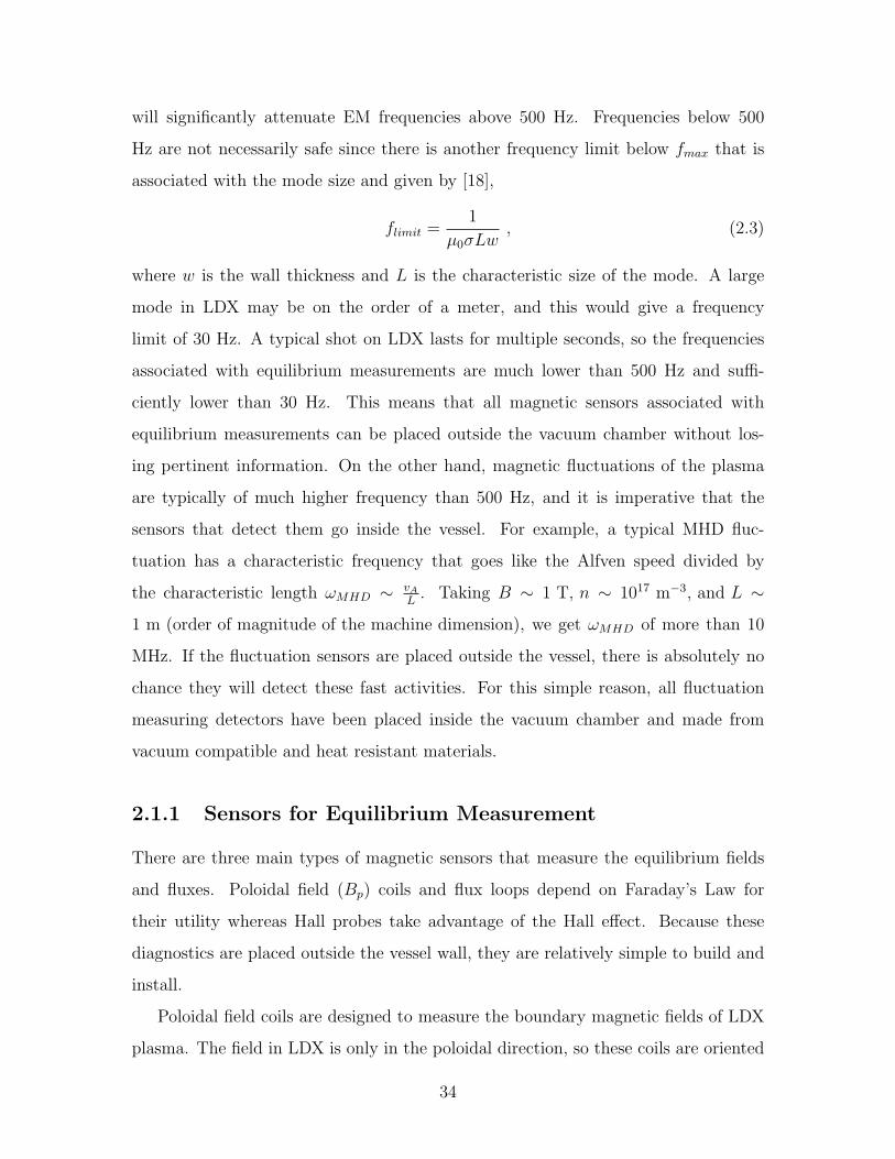
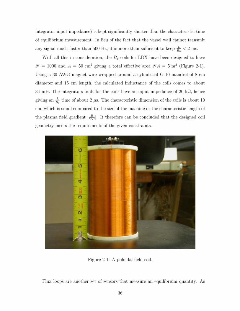
With all this in consideration, the Bp coils for LDX have been designed to have
N = 1000 and A = 50 cm2 giving a total effective area NA = 5 m2 (Figure 2-1).
Using a 30 AWG magnet wire wrapped around a cylindrical G-10 mandrel of 8 cm
diameter and 15 cm length, the calculated inductance of the coils comes to about
34 mH. The integrators built for the coils have an input impedance of 20 kΩ, hence
giving an LR0
time of about 2 µs. The characteristic dimension of the coils is about 10
cm, which is small compared to the size of the machine or the characteristic length of
the plasma field gradient | B∇B |. It therefore can be concluded that the designed coil
geometry meets the requirements of the given constraints.
Figure 2-1: A poloidal field coil.
Flux loops are another set of sensors that measure an equilibrium quantity. As
36
the name implies, they are basically loops of wire that measure the equilibrium flux.
These sensors are topologically equivalent to Bp coils, the only difference being that
the mandrel of the loops is the vacuum vessel itself. Just like for the Bp coils, flux loop
signals are derived from Faraday’s Law and must be integrated to get the equilibrium
flux. The calculation to obtain the integrated output voltage for these loops is exactly
the same as was done for the Bp coils (with the substitution NAB → ψ) and will not
be replicated. The result is,
Vout =∆ψ
τ. (2.7)
Notice that the number of turns has been constrained to one (as is for a typical flux
loop), but this need not be the case. If after calculating a typical ∆ψ at the vessel
wall and finding that the signal is too weak, more turns can be added as needed.
Simulated equilibrium reconstructions showed that a typical ∆ψ at the wall is on
the order of 10 mWb. Setting the integrator time constant to be 1 ms, this gives an
integrated output voltage of about 10 V, which is more than what is needed. It was
consequently determined that a single turn would be enough for all the flux loops
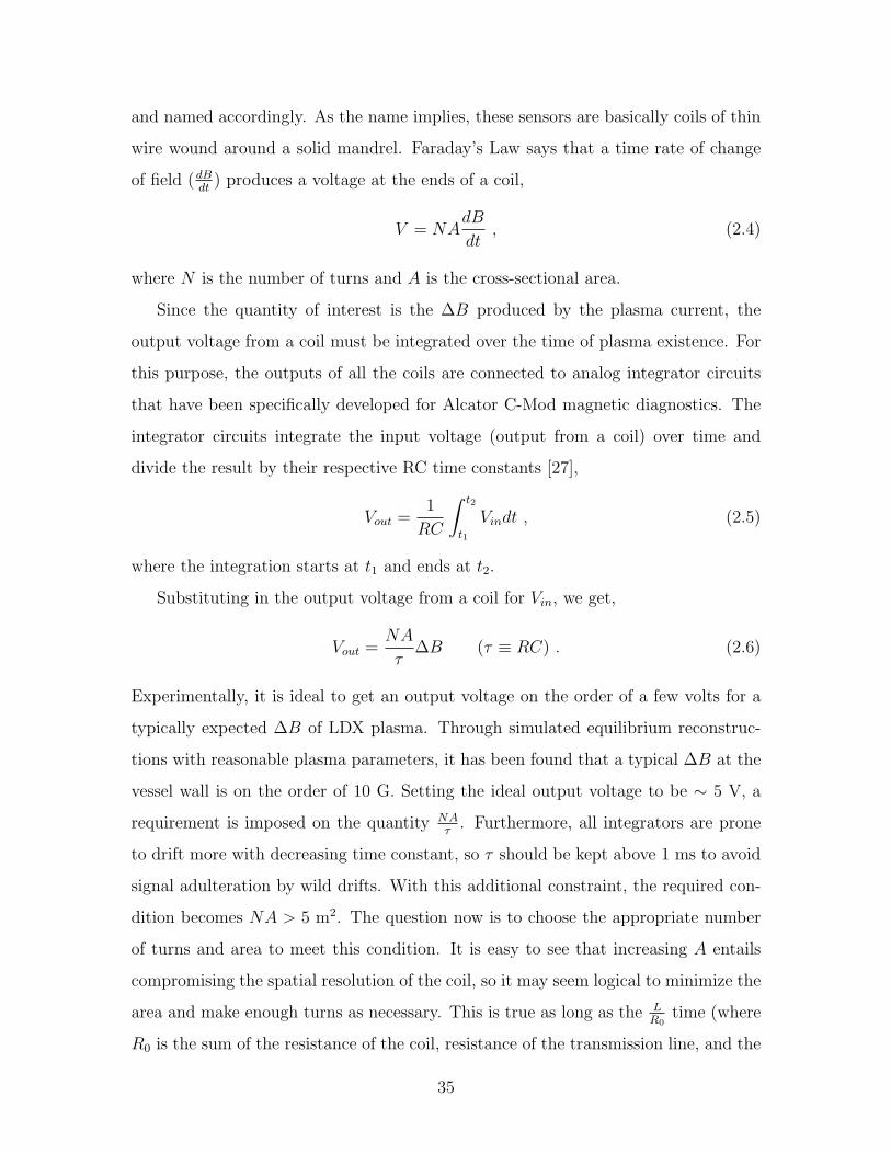
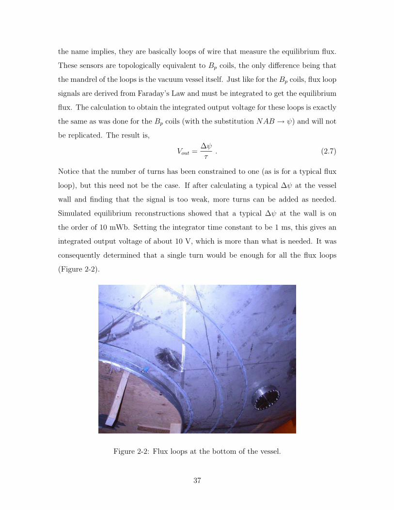
(Figure 2-2).
Figure 2-2: Flux loops at the bottom of the vessel.
37
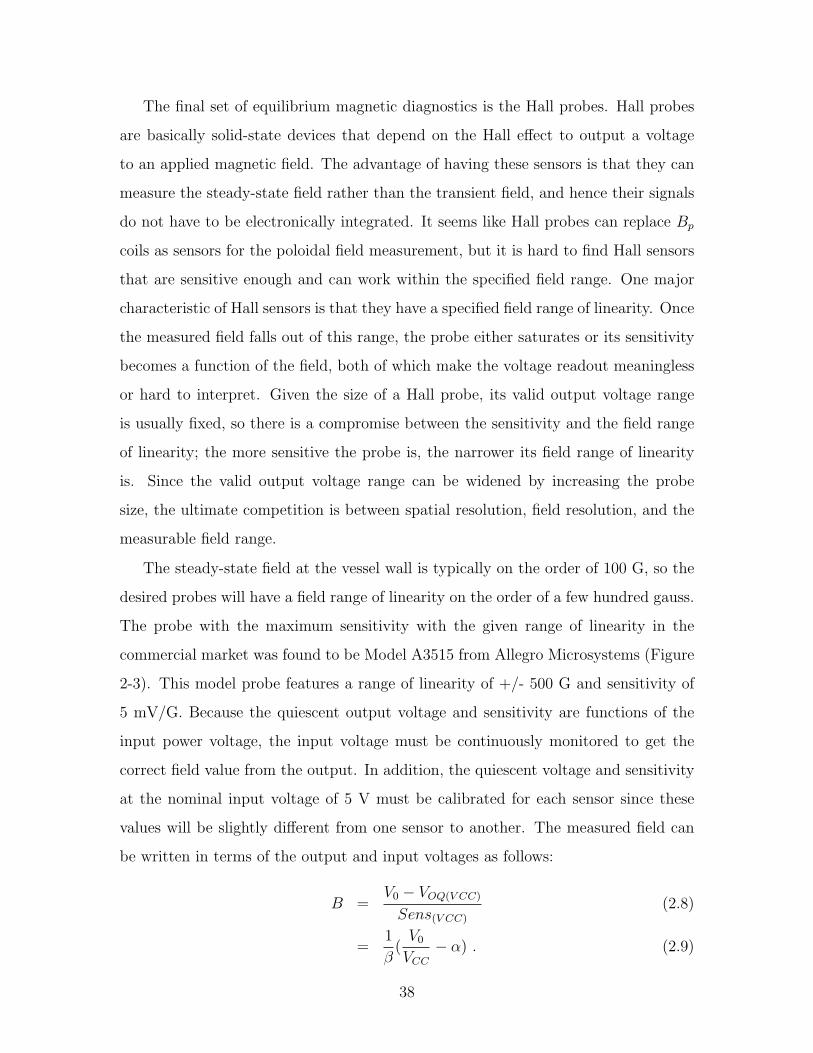
The final set of equilibrium magnetic diagnostics is the Hall probes. Hall probes
are basically solid-state devices that depend on the Hall effect to output a voltage
to an applied magnetic field. The advantage of having these sensors is that they can
measure the steady-state field rather than the transient field, and hence their signals
do not have to be electronically integrated. It seems like Hall probes can replace Bp
coils as sensors for the poloidal field measurement, but it is hard to find Hall sensors
that are sensitive enough and can work within the specified field range. One major
characteristic of Hall sensors is that they have a specified field range of linearity. Once
the measured field falls out of this range, the probe either saturates or its sensitivity
becomes a function of the field, both of which make the voltage readout meaningless
or hard to interpret. Given the size of a Hall probe, its valid output voltage range
is usually fixed, so there is a compromise between the sensitivity and the field range
of linearity; the more sensitive the probe is, the narrower its field range of linearity
is. Since the valid output voltage range can be widened by increasing the probe
size, the ultimate competition is between spatial resolution, field resolution, and the
measurable field range.
The steady-state field at the vessel wall is typically on the order of 100 G, so the
desired probes will have a field range of linearity on the order of a few hundred gauss.
The probe with the maximum sensitivity with the given range of linearity in the
commercial market was found to be Model A3515 from Allegro Microsystems (Figure
2-3). This model probe features a range of linearity of +/- 500 G and sensitivity of
5 mV/G. Because the quiescent output voltage and sensitivity are functions of the
input power voltage, the input voltage must be continuously monitored to get the
correct field value from the output. In addition, the quiescent voltage and sensitivity
at the nominal input voltage of 5 V must be calibrated for each sensor since these
values will be slightly different from one sensor to another. The measured field can
be written in terms of the output and input voltages as follows:
B =V0 − VOQ(V CC)
Sens(V CC)
(2.8)
=1
β(V0
VCC− α) . (2.9)
38
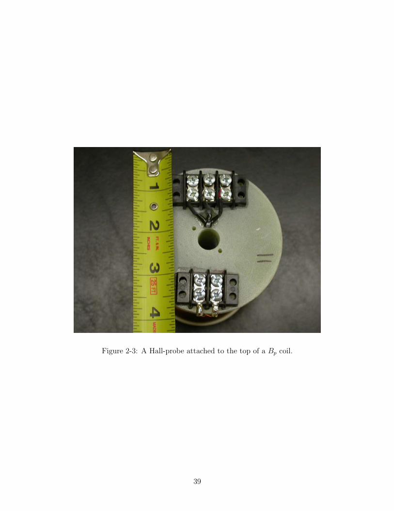
Figure 2-3: A Hall-probe attached to the top of a Bp coil.
39
In the above, V0 is the output voltage, VCC is the input voltage, and VOQ(V CC) and
Sens(V CC) are the quiescent output voltage and sensitivity, respectively, when the
input voltage is VCC . The parameters α and β are to be calibrated using the following
ratiometric relations:
α ≡VOQ(5V )
5V=VOQ(V CC)
VCC(2.10)
β ≡Sens(5V )
5V=Sens(V CC)
VCC. (2.11)
Hence, α and β can be deduced by measuring the quiescent output voltage and
sensitivity at a given input voltage VCC . In actuality, the sensitivity and quiescent
output voltage are also functions of the ambient temperature, but the effect is very
small for the ambient temperature range we expect in the experimental cell. The
details of the calibration procedure will be discussed in the next section.
2.1.2 Sensors for Fluctuation Measurement
The only set of magnetic sensors used for fluctuation measurements is Mirnov coils.
Mirnov coils are structurally identical to Bp coils, but there are some important
differences. As stated earlier, these sensors must go inside the vessel, so they need
to be made of appropriate materials. Also, the coils must be sufficiently small to
minimize their effect on the plasma. Although the physical principle of operation of
Mirnov coils is the same as that of Bp coils (i.e. Faraday’s Law), Mirnov signals are
not integrated and only amplified to preserve all the details of the fluctuations. As
such, an output from a Mirnov coil retains the time derivative factor,
V = GNAdB
dt, (2.12)
where N is the number of turns, A is the cross-sectional area, and G is the amplifier
gain.
Again, the goal is to design the coils to give an output on the order of a few
volts under typical plasma conditions. Unfortunately, an equilibrium reconstruction
program cannot predict the levels of magnetic fluctuations that can occur since fluctu-
ations are inherently transient events. However, data from another dipole confinement
40
experiment at Columbia called the Collisionless Terrella Experiment (CTX) helped
to estimate the expected fluctuation levels to be on the order of 100 µG/µs. Hence,
GNA must be on the order of 100. The effective area NA should be maximized
without making the probes too large or sacrificing their time resolution to maximize
their sensitivity. The recurring theme of the competition between the various merits
of the probes is once again apparent [28].
Figure 2-4: A Mirnov coil.
Without further analysis, the Mirnov coils have been designed with N = 200 and
A = 3 cm2 giving NA = 0.06 m2 (Figure 2-4). The coil mandrels are made of boron
nitride, which is both heat resistant and vacuum compatible, with 1.9 cm (0.75”)
diameter and 3.4 cm (1 1/3”) length. The same 30 AWG magnet wire is used as the
conductor, but its surface is coated with heat resistant boron nitride spray to protect
the insulation coating. These coils are connected to dual stage amplifier boards (also
from C-Mod) with the gains set at around 1600 to give ∼ 1 V level signals. The
41
calculated inductance of the coils is about 400 µH, and the corresponding LR0
time is
200 ps when connected to the amplifiers with a 2 MΩ input impedance. Of course,
200 ps is not the actual temporal resolution of the coils when they are wired to the
amplifiers through transmission lines, because capacitive effects of the whole system
must be considered. Nevertheless, it is enough to ensure that the coil inductance will
not be the limiting parameter in their time response. The coils are encased in tiny
stainless steel boxes to prevent direct contact with the plasma. This also ensures that
they do not pick up unwanted electrical noises on the probe leads. The stainless steel
shieldings are thin enough (0.01”) that signals slower than 3 MHz are not significantly
attenuated. The shielding boxes are also small enough to ensure minimal perturbation
of the plasma, but they can still limit the plasma at a maximum of 1” from the wall.
This is not expected to have much impact on the characteristics of the plasma.
2.2 Calibration of the Electronics and Diagnostics
2.2.1 Electronics Calibration
The integrator and amplifier boards have been tested and calibrated using a standard
signal generator and an oscilloscope. The parameter to be calibrated in both of these
electronics is their gain. The amplifier gain is just a unitless multiplicative factor,
but the integrator gain is the reciprocal of its RC time constant. Although the right
resistance and capacitance (only for the integrators) values have been selected to
produce the desired gain, the resistors and capacitors have a tolerance of 1 % and
10 %, respectively, and hence it is good practice to calibrate the gain using a known
input signal.
A 60 Hz sinusoidal signal is used as the input to measure the gain of the integrators
and amplifiers. Both the integrators and amplifiers output an amplified sinusoid at
the same frequency. Notice that the integral of a sinusoid is a phase shifted sinusoid
attenuated by its angular frequency. The integrators therefore output a sinusoid
that is amplified by a factor of 1ωτ
. The time constant can be found by inverting
42
the product of the angular frequency and the amplification factor. The gain of an
amplifier channel is simply its amplification factor. The calibration data for the
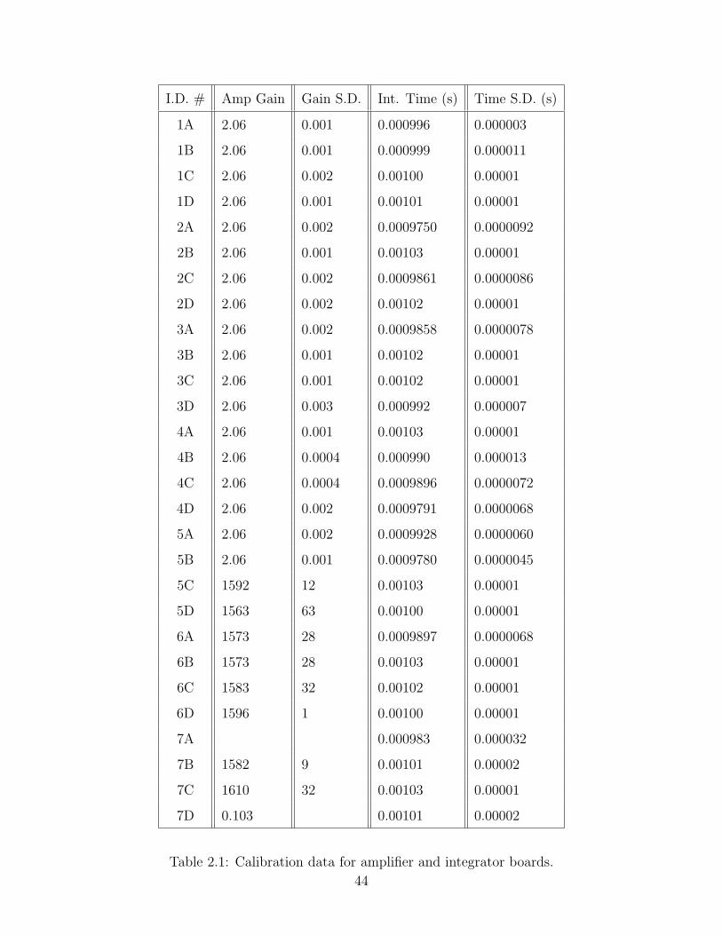
integrators and amplifiers is summarized in Table 2.1.
2.2.2 Diagnostics Calibration
Every magnetic diagnostic has been calibrated with a pair of Helmholtz coils. These
coils are different from and much smaller than the H-coils on the machine. The radius
of the coils is 30.5 cm, and each has 100 turns. It is straightforward to calculate the
field at the center of the pair for a given current and goes as follows:
B[G] = 2.95I[A] . (2.13)
To measure the NA values of the Bp and Mirnov coils, one only needs to measure
the RMS output voltage from the coils and the RMS of the time derivative of the
imposed field as calculated from the RMS current in the Helmholtz coils,
B = B0 sin(ωt) (2.14)
dB
dt= ωB0 cos(ωt) (2.15)
dB
dt
∣∣∣∣RMS
= ωBRMS = 2πfBRMS . (2.16)
Therefore,
V out = NAdB
dt(2.17)
NA =V outRMS
dBdt
∣∣RMS
=V outRMS
2πfBRMS
. (2.18)
The Bp and Mirnov coils have been calibrated at 500 Hz at 3 G and 980 Hz at 2
G, respectively. Because Mirnov coils have a small NA, the product fBRMS was
maximized for their calibration to get the maximum possible signal.
Hall probe calibration requires finding two independent parameters, α and β, that
have already been defined. Finding α is a simple matter of measuring the quiescent
output voltage (output voltage at zero field) at a given input power voltage. Finding
β involves measuring the output voltage at at least one field. The can be done with
43
I.D. # Amp Gain Gain S.D. Int. Time (s) Time S.D. (s)
1A 2.06 0.001 0.000996 0.000003
1B 2.06 0.001 0.000999 0.000011
1C 2.06 0.002 0.00100 0.00001
1D 2.06 0.001 0.00101 0.00001
2A 2.06 0.002 0.0009750 0.0000092
2B 2.06 0.001 0.00103 0.00001
2C 2.06 0.002 0.0009861 0.0000086
2D 2.06 0.002 0.00102 0.00001
3A 2.06 0.002 0.0009858 0.0000078
3B 2.06 0.001 0.00102 0.00001
3C 2.06 0.001 0.00102 0.00001
3D 2.06 0.003 0.000992 0.000007
4A 2.06 0.001 0.00103 0.00001
4B 2.06 0.0004 0.000990 0.000013
4C 2.06 0.0004 0.0009896 0.0000072
4D 2.06 0.002 0.0009791 0.0000068
5A 2.06 0.002 0.0009928 0.0000060
5B 2.06 0.001 0.0009780 0.0000045
5C 1592 12 0.00103 0.00001
5D 1563 63 0.00100 0.00001
6A 1573 28 0.0009897 0.0000068
6B 1573 28 0.00103 0.00001
6C 1583 32 0.00102 0.00001
6D 1596 1 0.00100 0.00001
7A 0.000983 0.000032
7B 1582 9 0.00101 0.00002
7C 1610 32 0.00103 0.00001
7D 0.103 0.00101 0.00002
Table 2.1: Calibration data for amplifier and integrator boards.
44

either AC or DC, but using an AC field is a bit easier since it does not require the
measurement of the quiescent voltage (i.e. AC quiescent voltage is zero). With these
measurements, α and β can easily be calculated through their definitions.
The β parameters have been calibrated at both 500 Hz at 3 G and 20 Hz at
9 G. Although only a single field measurement is necessary to find β, the two field
measurement allows to check for linearity, albeit in the small field range. The specced
bandwidth of the probes is 30 kHz, so measuring the sensitivity at the two frequencies
should not be an issue.
Lastly, since the output voltage from the flux loops depends only on the measured
flux and the integrator time constant, there is no calibration associated with the loops
themselves.
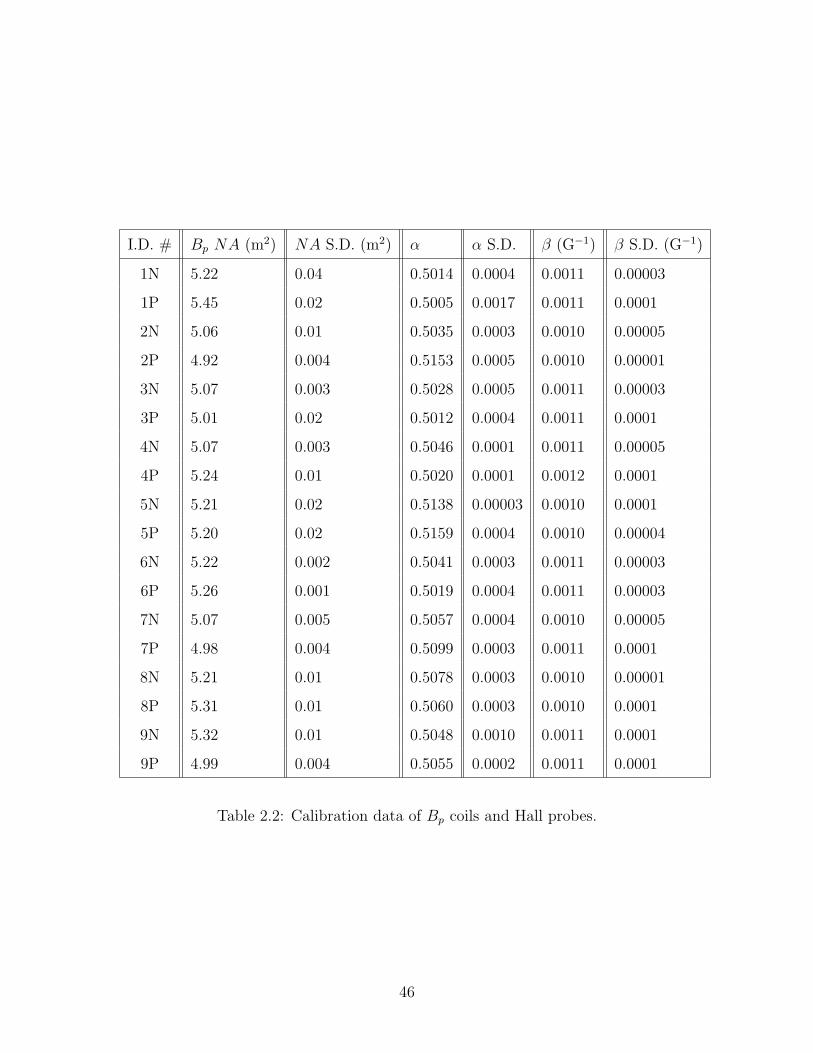
The diagnostics calibration results are shown in Tables 2.2 and 2.3.
2.3 Future Improvements to the Magnetic Diag-
nostics System
A lot has been accomplished in the development and installation of the magnetic
diagnostics on LDX. Needless to say, there are certain improvements and additions
that would doubtlessly further their utility. This section deals with some suggested
improvements to the magnetic diagnostics that can possibly be undertaken by a for-
tunate student who may happen to adopt them for his / her thesis work.
The Bp coils and flux loops are connected to integrator circuits that suffer from
signal drifts. The drift is aggravated as their gains increase. Currently, the gains
are set to a level that gives a typical output voltage of a less than a volt for typical
plasma shots. Ideally, we want to have an output voltage between 1 V and 10 V
to fully take advantage of the bit resolution of the digitizer. The integrator circuits
currently in use are of a relatively rudimentary design, and more sophisticated circuits
could possibly be used to ameliorate the drift. A typical LDX shot today is on the
order of ten seconds, but we may want to study much longer shots in the future.
45
I.D. # Bp NA (m2) NA S.D. (m2) α α S.D. β (G−1) β S.D. (G−1)
1N 5.22 0.04 0.5014 0.0004 0.0011 0.00003
1P 5.45 0.02 0.5005 0.0017 0.0011 0.0001
2N 5.06 0.01 0.5035 0.0003 0.0010 0.00005
2P 4.92 0.004 0.5153 0.0005 0.0010 0.00001
3N 5.07 0.003 0.5028 0.0005 0.0011 0.00003
3P 5.01 0.02 0.5012 0.0004 0.0011 0.0001
4N 5.07 0.003 0.5046 0.0001 0.0011 0.00005
4P 5.24 0.01 0.5020 0.0001 0.0012 0.0001
5N 5.21 0.02 0.5138 0.00003 0.0010 0.0001
5P 5.20 0.02 0.5159 0.0004 0.0010 0.00004
6N 5.22 0.002 0.5041 0.0003 0.0011 0.00003
6P 5.26 0.001 0.5019 0.0004 0.0011 0.00003
7N 5.07 0.005 0.5057 0.0004 0.0010 0.00005
7P 4.98 0.004 0.5099 0.0003 0.0011 0.0001
8N 5.21 0.01 0.5078 0.0003 0.0010 0.00001
8P 5.31 0.01 0.5060 0.0003 0.0010 0.0001
9N 5.32 0.01 0.5048 0.0010 0.0011 0.0001
9P 4.99 0.004 0.5055 0.0002 0.0011 0.0001
Table 2.2: Calibration data of Bp coils and Hall probes.
46
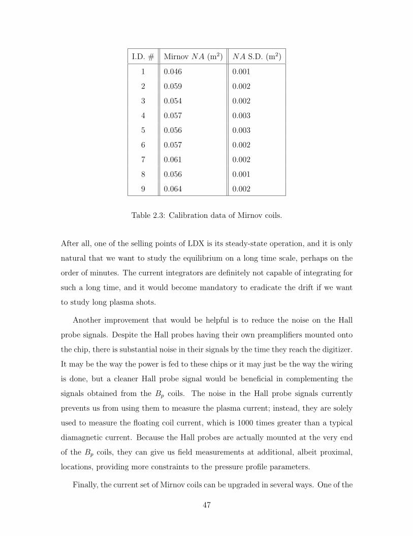
I.D. # Mirnov NA (m2) NA S.D. (m2)
1 0.046 0.001
2 0.059 0.002
3 0.054 0.002
4 0.057 0.003
5 0.056 0.003
6 0.057 0.002
7 0.061 0.002
8 0.056 0.001
9 0.064 0.002
Table 2.3: Calibration data of Mirnov coils.
After all, one of the selling points of LDX is its steady-state operation, and it is only
natural that we want to study the equilibrium on a long time scale, perhaps on the
order of minutes. The current integrators are definitely not capable of integrating for
such a long time, and it would become mandatory to eradicate the drift if we want
to study long plasma shots.
Another improvement that would be helpful is to reduce the noise on the Hall
probe signals. Despite the Hall probes having their own preamplifiers mounted onto
the chip, there is substantial noise in their signals by the time they reach the digitizer.
It may be the way the power is fed to these chips or it may just be the way the wiring
is done, but a cleaner Hall probe signal would be beneficial in complementing the
signals obtained from the Bp coils. The noise in the Hall probe signals currently
prevents us from using them to measure the plasma current; instead, they are solely
used to measure the floating coil current, which is 1000 times greater than a typical
diamagnetic current. Because the Hall probes are actually mounted at the very end
of the Bp coils, they can give us field measurements at additional, albeit proximal,
locations, providing more constraints to the pressure profile parameters.
Finally, the current set of Mirnov coils can be upgraded in several ways. One of the
47
chief concerns of the current system is the sensitivity to electrostatic noise. Although
the coils are well shielded, they may still be susceptible to high frequency noise that
can creep through the small openings. One remedy would be to completely rebuild
the coils to incorporate a center tap. This would preferentially block all electrostatic
signals while maintaining the magnetic signals. Another possible improvement would
be in the wiring of the transmission line and modifying the amplifier circuit. The
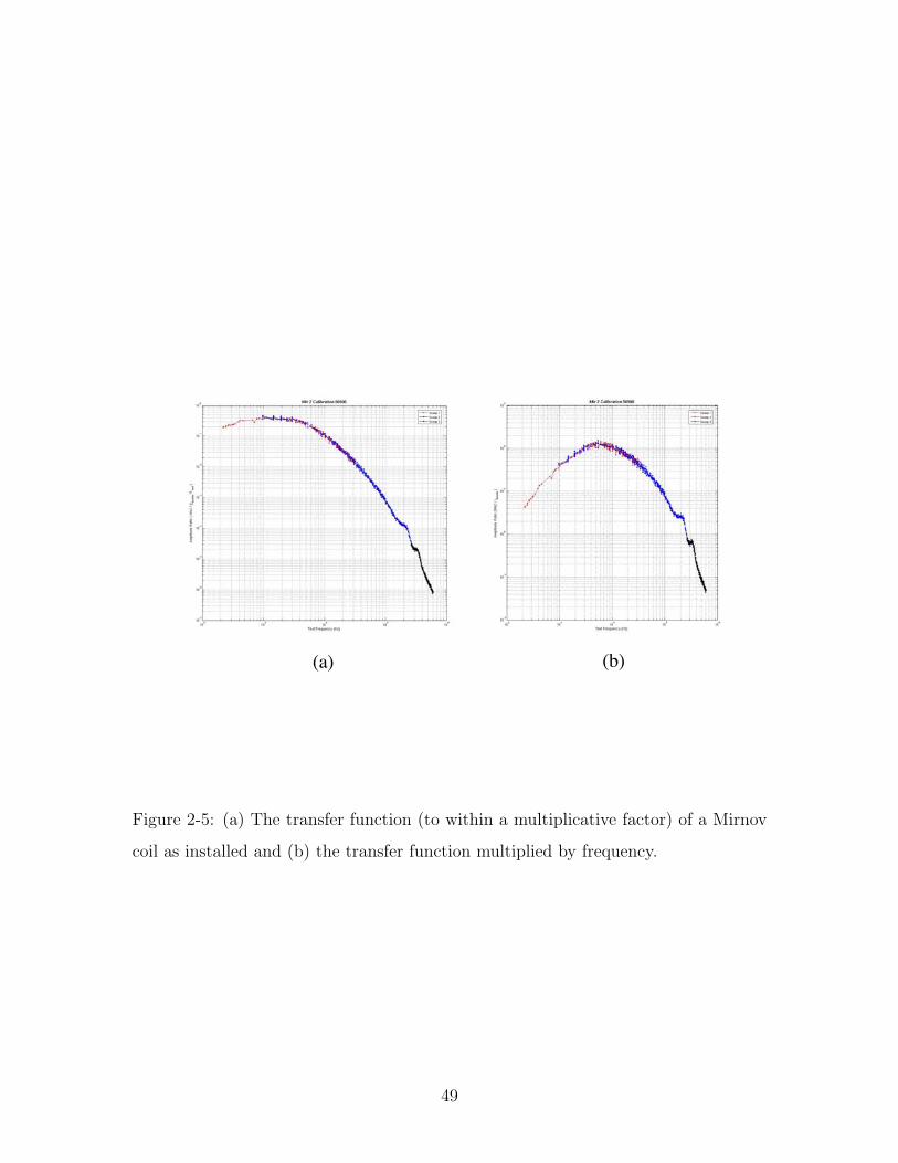
current system suffers from a low frequency roll-off that prevents us from measuring
the details of the evolution of high frequency signals (Figure 2-5). It may be good to
incorporate some or all of these improvements before we enter the third phase of the
experiment, in which the plasma is thermalized to study Maxwellian plasmas that
are susceptible to MHD modes.
48
(a) (b)
Figure 2-5: (a) The transfer function (to within a multiplicative factor) of a Mirnov
coil as installed and (b) the transfer function multiplied by frequency.
49

50
Chapter 3
Sensor location optimization
In conducting any kind of diagnostic measurements, an important question must be
answered. Where should the sensors be placed? The answer to the question may de-
pend on several factors, including available space, vacuum and plasma compatibility,
ease of access, and sensitivity. Since the LDX magnetic diagnostics for equilibrium
measurements are placed outside the vacuum vessel where space and ease of access
are not an issue, the real question boils down to where the sensors should be placed to
maximize their sensitivities to various plasma parameters. There are various ways to
address this question, and a particularly simple method that has been used to choose
the sensor positions in LDX will be discussed in this chapter.
3.1 Mathematical formulation
The optimization method presented here is inspired by B. J. Braams’ work on func-
tion parametrization [3] and is based on the establishment of a functional relationship
between measurements from different sensors at different locations and plasma pa-
rameters,
m = F (p) , (3.1)
where
m is an m-dimensional vector of different types of measurements
at different positions.
51
p is an n-dimensional vector of plasma parameters.
F : Rn → Rm is the response function.
The goal here is to find the response function so that the sensitivity matrix, (∇pF )T ≡
(dFdp
)T = (dmdp
)T , can be calculated. Notice that if we Taylor expand the response
function about some point p0 in the parameter space, the sensitivity matrix comes
out naturally in the first order term,
F (p) ≈ F (p0) + (∇pF )T |p=p0· (p− p0) ≡ k + R · p , (3.2)
where all the constant terms have been lumped into k, and R ≡ (∇pF )T |p=p0.
The sensitivity matrix R has elements of the form ∂mi
∂pjthat give the sensitivities of
measurements i to parameters j.
Because the sensitivity matrix has m× n independent elements and the constant
vector has m independent components, we need to have m(n+ 1) independent equa-
tions to specify them. By running the equilibrium code with p as the input and m
as the output, we can produce m independent equations in the elements and compo-
nents. Therefore, we need n + 1 different equilibria to produce n + 1 pairs (m, p)
and m(n + 1) independent equations. In other words, we need n + 1 equilibria to
completely determine R. It may be instructive to look at this problem from a math-
ematical perspective. The Taylor expansion of the response function F and keeping
up to the first order term is equivalent to approximating the m hypersurfaces of F
by m hyperplanes whose linear coefficients are rows of R in m (n + 1)-dimensional
spaces. Specifying the hyperplanes for a mapping from n dimensions to m dimensions
requires knowing n + 1 points on them, because if we know one point on the hyper-
planes, we also need to know the derivatives in each of the n directions to completely
specify them. This is precisely the reason we need to compute n+1 equilibria to find
R (and k).
There are two important points to be extracted from the mathematical picture
given above. The first is that the n + 1 equilibria needed to compute R must not
52
be too far apart in the parameter space. Mathematically, ||pi − pj|| < ε ∀ i, j ∈
1, 2, 3, ..., n+ 1. The value of ε depends on various factors, such as the values of
higher derivatives of F at the expansion point, but it usually suffices to keep it as
small as practically possible. The proximity condition of equilibrium points basically
says that the points used to define hyperplanes that are approximations to the hy-
persurfaces at p0 must be close to p0. Otherwise, the hyperplanes would not be good
approximations to the hypersurfaces at p0. A corollary to this is that hyperplanes are
good approximations to the hypersurfaces if we are concerned with points in small
neighborhoods of p0. The message here is that the sensitivity matrix R calculated
about a point p0 is valid only in a small neighborhood of the point. We therefore
need to calculate many sensitivity matrices corresponding to different regions in the
parameter space. In other words, we are approximating the response function with
many different sensitivity matrices (plus constant vectors) in a piecewise linear fash-
ion. The second point to be understood is that the n + 1 points needed to define
R in a particular region in the parameter space must reflect deviations in all the n
directions from a given point on the hyperplanes. After all, it would not be possible
to define a hyperplane without knowing its derivatives in all the directions. The n+1
points must be wisely chosen to ensure that the necessary information is contained
in them.
3.2 Application to LDX Magnetic Diagnostics
Now that the theoretical groundwork has been laid out, we can apply the concept
to determine where the magnetic diagnostics should be placed. The strategy goes as
follows:
1. Choose x possible locations on the vacuum vessel where the sensors can be
placed.
2. Define m by having as its components the measurements of the y different
sensors at x different locations. Hence, the dimension of m is m = xy.
53
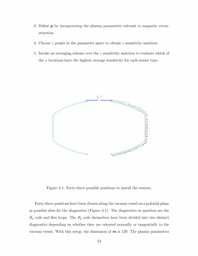
3. Define p by incorporating the plasma parameters relevant to magnetic recon-
struction.
4. Choose z points in the parameter space to obtain z sensitivity matrices.
5. Invoke an averaging scheme over the z sensitivity matrices to evaluate which of
the x locations have the highest average sensitivity for each sensor type.
1 2 3 4 5 67 8 9 10 11
1213
1415
1617
181920212223242526
2728
2930
31323334
353637383940414243
Figure 3-1: Forty-three possible positions to install the sensors.
Forty-three positions have been chosen along the vacuum vessel on a poloidal plane
as possible sites for the diagnostics (Figure 3-1). The diagnostics in question are the
Bp coils and flux loops. The Bp coils themselves have been divided into two distinct
diagnostics depending on whether they are oriented normally or tangentially to the
vacuum vessel. With this setup, the dimension of m is 129. The plasma parameters
54
have been chosen accordingly to the most likely pressure model to be used in the
reconstruction process. The pressure model has three free parameters and is of the
following form:
P (ψ;ψpeak, Pedge, g) =
Pedge[Vedge
V (ψ)]g for ψ > ψpeak
Pedge[Vedge
V (ψ)]g sin2[π
2( ψψpeak
)2] for ψ < ψpeak, (3.3)
where V ≡ dV oldψ
=∮
dlB
is the differential flux tube volume per differential flux. This
and other pressure models will be discussed in more detail in Chapter 6. For now it
suffices to understand that the model has the following three free parameters: ψpeak
(flux at the pressure peak), Pedge (pressure at the plasma edge), and g (the adiabatic
parameter that gives the slope of the pressure fall and is equal to 53
in a 3-D collisional
gas). The three parameters give three dimensions to p. When written out, Eq. 3.2
looks like the following:
mBN1
...
mBN43
mBT1
...
mBT43
mψ1
...
mψ43
=
k1
...
k129
+
∂BN1
∂Pedge
∂BN1
∂Rpeak
∂BN1
∂Fcrit
......
...
∂BN43
∂Pedge
∂BN43
∂Rpeak
∂BN43
∂Fcrit
∂BT1
∂Pedge
∂BT1
∂Rpeak
∂BT1
∂Fcrit
......
...
∂BT43
∂Pedge
∂BT43
∂Rpeak
∂BT43
∂Fcrit
∂ψ1
∂Pedge
∂ψ1
∂Rpeak
∂ψ1
∂Fcrit
......
...
∂ψ43
∂Pedge
∂ψ43
∂Rpeak
∂ψ43
∂Fcrit
·
Pedge
Rpeak
Fcrit
. (3.4)
The parameters ψpeak and g have been replaced by Rpeak (midplane radius at the
pressure peak) and Fcrit = 35g, respectively, so that their physical meanings are eluci-
dated. Following the specifications of m and p, a domain that covers the most likely
operational regime of LDX is defined. The domain is a cube in the parameter space
constructed as,
0.1 Pa ≤ Pedge ≤ 10.0 Pa
0.50 m ≤ Rpeak ≤ 0.90 m
0.5 ≤ Fcrit ≤ 3.0
55
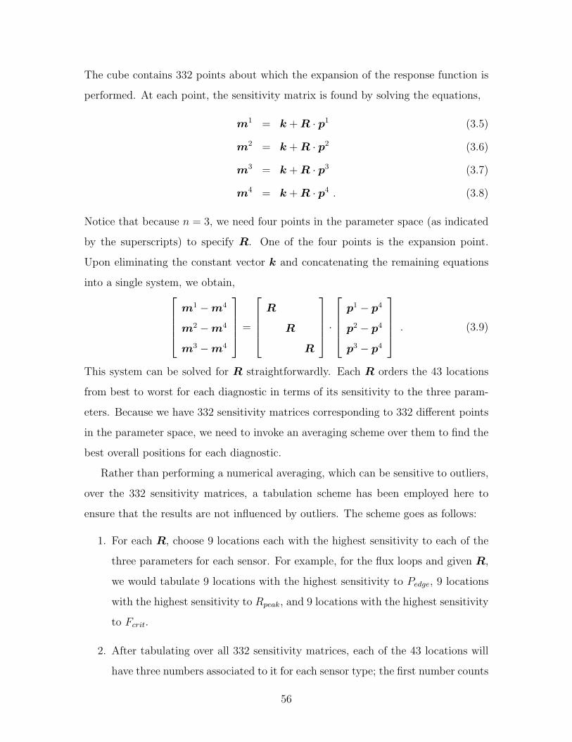
The cube contains 332 points about which the expansion of the response function is
performed. At each point, the sensitivity matrix is found by solving the equations,
m1 = k + R · p1 (3.5)
m2 = k + R · p2 (3.6)
m3 = k + R · p3 (3.7)
m4 = k + R · p4 . (3.8)
Notice that because n = 3, we need four points in the parameter space (as indicated
by the superscripts) to specify R. One of the four points is the expansion point.
Upon eliminating the constant vector k and concatenating the remaining equations
into a single system, we obtain,m1 −m4
m2 −m4
m3 −m4
=
R
R
R
·
p1 − p4
p2 − p4
p3 − p4
. (3.9)
This system can be solved for R straightforwardly. Each R orders the 43 locations
from best to worst for each diagnostic in terms of its sensitivity to the three param-
eters. Because we have 332 sensitivity matrices corresponding to 332 different points
in the parameter space, we need to invoke an averaging scheme over them to find the
best overall positions for each diagnostic.
Rather than performing a numerical averaging, which can be sensitive to outliers,
over the 332 sensitivity matrices, a tabulation scheme has been employed here to
ensure that the results are not influenced by outliers. The scheme goes as follows:
1. For each R, choose 9 locations each with the highest sensitivity to each of the
three parameters for each sensor. For example, for the flux loops and given R,
we would tabulate 9 locations with the highest sensitivity to Pedge, 9 locations
with the highest sensitivity to Rpeak, and 9 locations with the highest sensitivity
to Fcrit.
2. After tabulating over all 332 sensitivity matrices, each of the 43 locations will
have three numbers associated to it for each sensor type; the first number counts
56
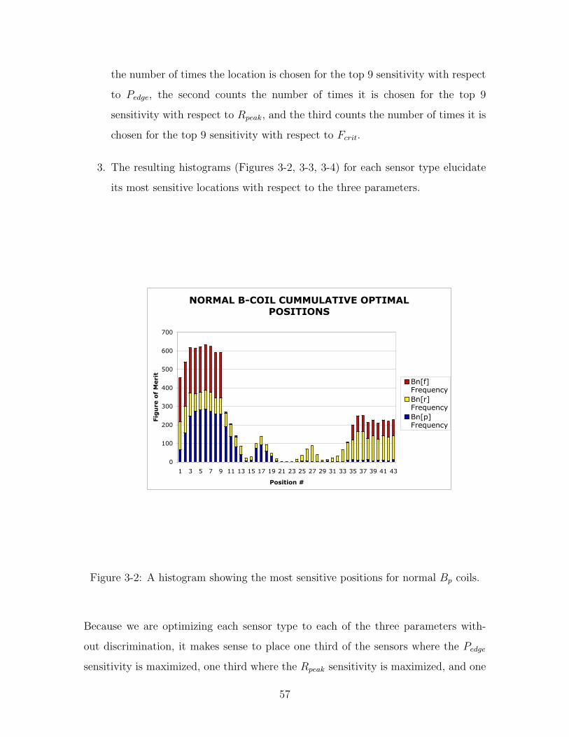
the number of times the location is chosen for the top 9 sensitivity with respect
to Pedge, the second counts the number of times it is chosen for the top 9
sensitivity with respect to Rpeak, and the third counts the number of times it is
chosen for the top 9 sensitivity with respect to Fcrit.
3. The resulting histograms (Figures 3-2, 3-3, 3-4) for each sensor type elucidate
its most sensitive locations with respect to the three parameters.
NORMAL B-COIL CUMMULATIVE OPTIMAL POSITIONS
0
100
200
300
400
500
600
700
1 3 5 7 9 11 13 15 17 19 21 23 25 27 29 31 33 35 37 39 41 43
Position #
Fig
ure
of
Meri
t
Bn[f]FrequencyBn[r]FrequencyBn[p]Frequency
Figure 3-2: A histogram showing the most sensitive positions for normal Bp coils.
Because we are optimizing each sensor type to each of the three parameters with-
out discrimination, it makes sense to place one third of the sensors where the Pedge
sensitivity is maximized, one third where the Rpeak sensitivity is maximized, and one
57
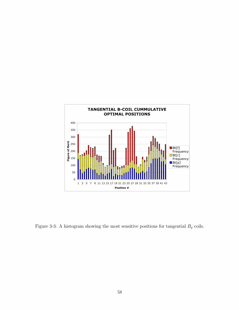
TANGENTIAL B-COIL CUMMULATIVE OPTIMAL POSITIONS
0
50
100
150
200
250
300
350
400
1 3 5 7 9 11 13 15 17 19 21 23 25 27 29 31 33 35 37 39 41 43
Position #
Fig
ure
of
Meri
t
Bt[f]FrequencyBt[r]FrequencyBt[p]Frequency
Figure 3-3: A histogram showing the most sensitive positions for tangential Bp coils.
58
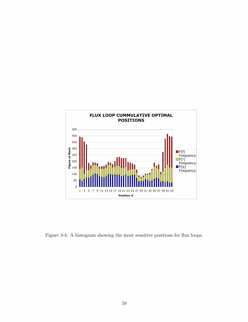
FLUX LOOP CUMMULATIVE OPTIMAL POSITIONS
0
50
100
150
200
250
300
350
400
450
1 3 5 7 9 11 13 15 17 19 21 23 25 27 29 31 33 35 37 39 41 43
Position #
Fig
ure
of
Meri
t
F[f]FrequencyF[r]FrequencyF[p]Frequency
Figure 3-4: A histogram showing the most sensitive positions for flux loops.
59
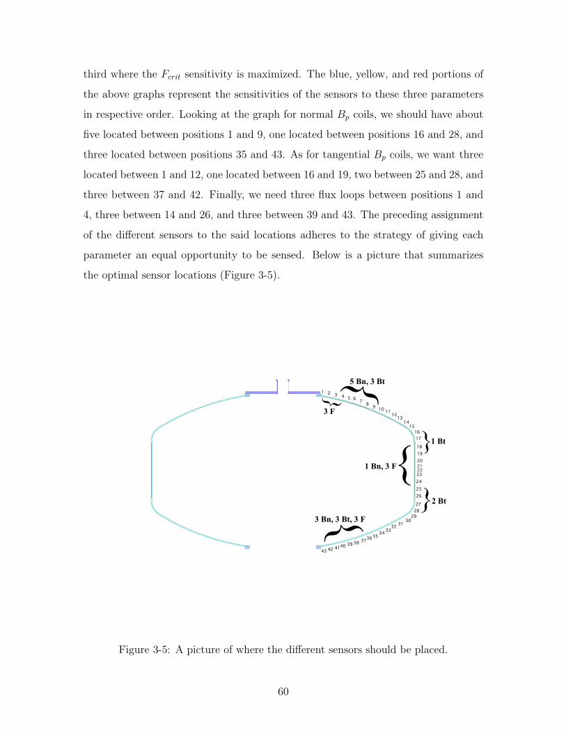
third where the Fcrit sensitivity is maximized. The blue, yellow, and red portions of
the above graphs represent the sensitivities of the sensors to these three parameters
in respective order. Looking at the graph for normal Bp coils, we should have about
five located between positions 1 and 9, one located between positions 16 and 28, and
three located between positions 35 and 43. As for tangential Bp coils, we want three
located between 1 and 12, one located between 16 and 19, two between 25 and 28, and
three between 37 and 42. Finally, we need three flux loops between positions 1 and
4, three between 14 and 26, and three between 39 and 43. The preceding assignment
of the different sensors to the said locations adheres to the strategy of giving each
parameter an equal opportunity to be sensed. Below is a picture that summarizes
the optimal sensor locations (Figure 3-5).
1 2 3 4 5 6 7 8 9 10 1112
1314
151617
181920212223242526
2728
2930
31323334
353637383940414243
5 Bn, 3 Bt
3 F
1 Bn, 3 F
1 Bt
2 Bt
3 Bn, 3 Bt, 3 F
Figure 3-5: A picture of where the different sensors should be placed.
60
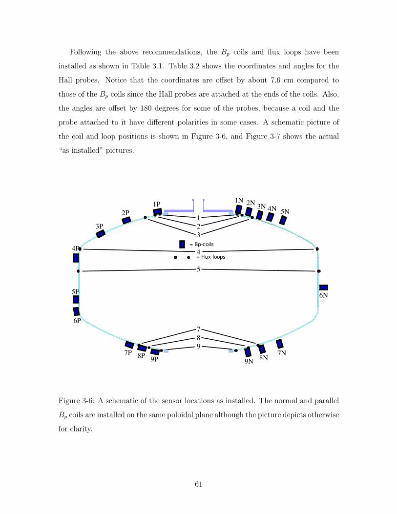
Following the above recommendations, the Bp coils and flux loops have been
installed as shown in Table 3.1. Table 3.2 shows the coordinates and angles for the
Hall probes. Notice that the coordinates are offset by about 7.6 cm compared to
those of the Bp coils since the Hall probes are attached at the ends of the coils. Also,
the angles are offset by 180 degrees for some of the probes, because a coil and the
probe attached to it have different polarities in some cases. A schematic picture of
the coil and loop positions is shown in Figure 3-6, and Figure 3-7 shows the actual
“as installed” pictures.
1N 2N 3N 4N 5N
6N
7N8N9N
1P2P
3P
4P
5P
6P
7P 8P 9P
123
5
789
= Bp-coils
= Flux loops4
Figure 3-6: A schematic of the sensor locations as installed. The normal and parallel
Bp coils are installed on the same poloidal plane although the picture depicts otherwise
for clarity.
61
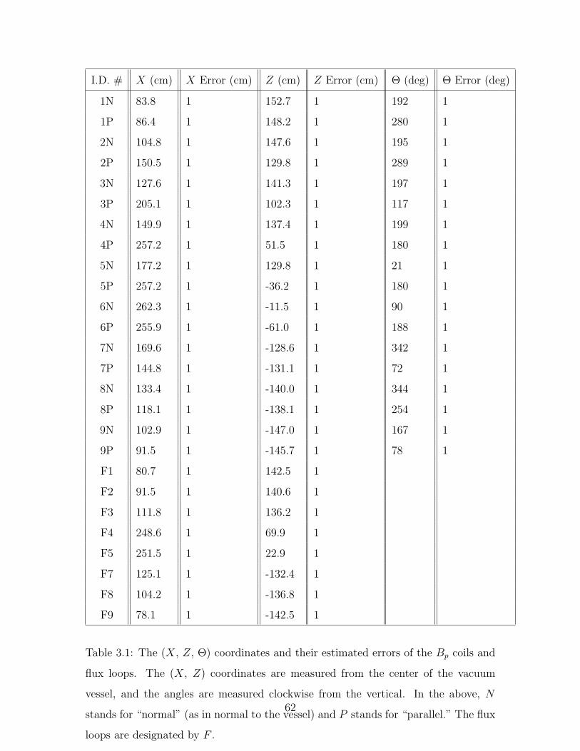
I.D. # X (cm) X Error (cm) Z (cm) Z Error (cm) Θ (deg) Θ Error (deg)
1N 83.8 1 152.7 1 192 1
1P 86.4 1 148.2 1 280 1
2N 104.8 1 147.6 1 195 1
2P 150.5 1 129.8 1 289 1
3N 127.6 1 141.3 1 197 1
3P 205.1 1 102.3 1 117 1
4N 149.9 1 137.4 1 199 1
4P 257.2 1 51.5 1 180 1
5N 177.2 1 129.8 1 21 1
5P 257.2 1 -36.2 1 180 1
6N 262.3 1 -11.5 1 90 1
6P 255.9 1 -61.0 1 188 1
7N 169.6 1 -128.6 1 342 1
7P 144.8 1 -131.1 1 72 1
8N 133.4 1 -140.0 1 344 1
8P 118.1 1 -138.1 1 254 1
9N 102.9 1 -147.0 1 167 1
9P 91.5 1 -145.7 1 78 1
F1 80.7 1 142.5 1
F2 91.5 1 140.6 1
F3 111.8 1 136.2 1
F4 248.6 1 69.9 1
F5 251.5 1 22.9 1
F7 125.1 1 -132.4 1
F8 104.2 1 -136.8 1
F9 78.1 1 -142.5 1
Table 3.1: The (X, Z, Θ) coordinates and their estimated errors of the Bp coils and
flux loops. The (X, Z) coordinates are measured from the center of the vacuum
vessel, and the angles are measured clockwise from the vertical. In the above, N
stands for “normal” (as in normal to the vessel) and P stands for “parallel.” The flux
loops are designated by F .
62
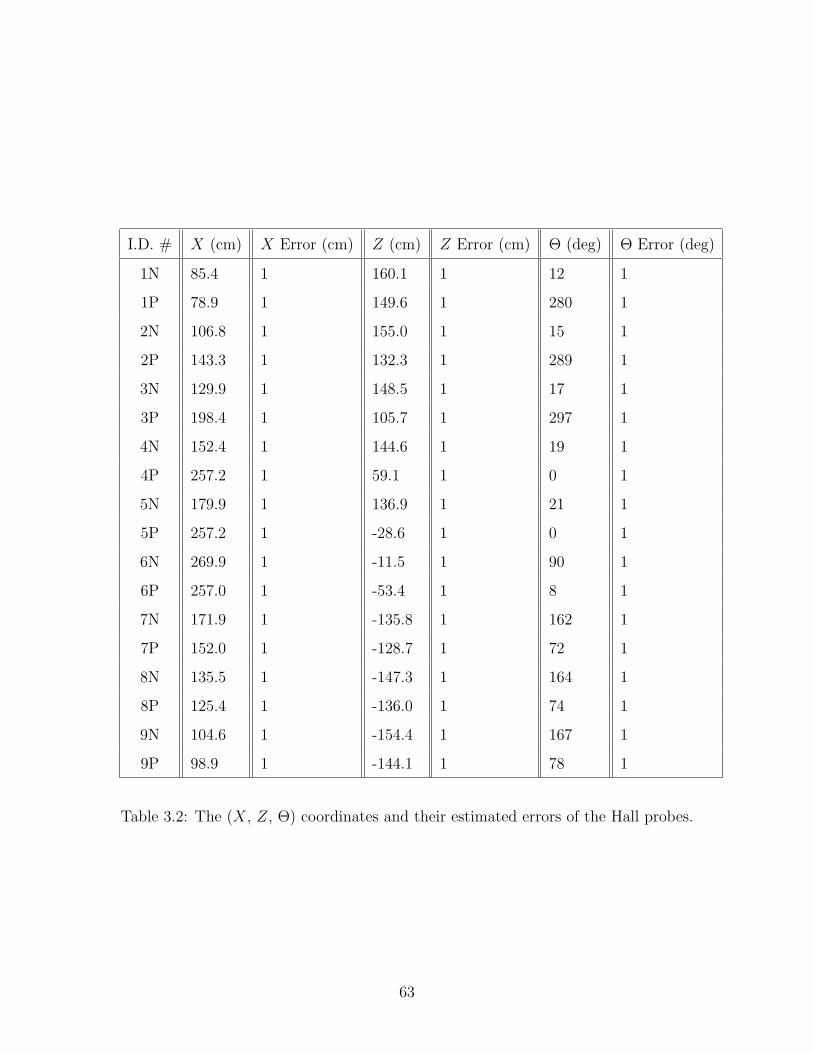
I.D. # X (cm) X Error (cm) Z (cm) Z Error (cm) Θ (deg) Θ Error (deg)
1N 85.4 1 160.1 1 12 1
1P 78.9 1 149.6 1 280 1
2N 106.8 1 155.0 1 15 1
2P 143.3 1 132.3 1 289 1
3N 129.9 1 148.5 1 17 1
3P 198.4 1 105.7 1 297 1
4N 152.4 1 144.6 1 19 1
4P 257.2 1 59.1 1 0 1
5N 179.9 1 136.9 1 21 1
5P 257.2 1 -28.6 1 0 1
6N 269.9 1 -11.5 1 90 1
6P 257.0 1 -53.4 1 8 1
7N 171.9 1 -135.8 1 162 1
7P 152.0 1 -128.7 1 72 1
8N 135.5 1 -147.3 1 164 1
8P 125.4 1 -136.0 1 74 1
9N 104.6 1 -154.4 1 167 1
9P 98.9 1 -144.1 1 78 1
Table 3.2: The (X, Z, Θ) coordinates and their estimated errors of the Hall probes.
63
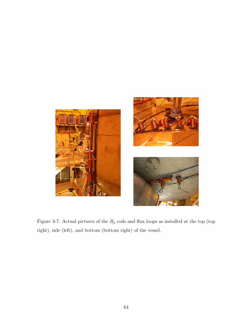
Figure 3-7: Actual pictures of the Bp coils and flux loops as installed at the top (top
right), side (left), and bottom (bottom right) of the vessel.
64
Chapter 4
Error analysis
Before proceeding to presenting experimental data, a thorough analysis of errors
associated with measured and calculated quantities is needed. Errors can come from
several sources and be of various types; there may be a precision error in measuring
the position of a sensor or a random error in its calibration, for example. Precision
and random errors are facts of experiments and cannot be eradicated. Another type of
error is systematic error, in which the error is not distributed symmetrically about the
“true” value and is biased in either direction. Systematic errors come from systemic
problems that somehow shift the measured value from the “true” value. Systematic
errors can often be calibrated away or eradicated by identifying the source of the bias.
A good experimenter would identify all causes of systematic errors and make sure that
they do not distort the measurements. Because all systematic errors can potentially
be isolated and eliminated, this chapter will focus on precision and random errors,
which are ubiquitous in all experiments.
4.1 Precision errors
Precision errors are not as prominent as random errors, because random errors often
dominate over precision errors. However, when a measurement is done using a very
simple instrument, like a ruler, then there is minimal source of random errors, and
precision errors become the main source of the total error.
65
In conducting magnetic measurements of plasmas, knowing the precise locations
and orientations of the sensors becomes very important. Magnetic sensors measure
the plasma current from which the pressure is deduced, so an inaccurate measurement
of the sensor locations or orientations could inevitably lead to an inaccurate pressure
profile. Once the locations and orientations are measured to the best of our abilities,
we need to know the accuracies to within which they are measured. These estimated
errors of the locations and orientations will be added to the field or flux measurement
error to estimate the errors in the parameters of the pressure profile and other derived
quantities such as plasma current and beta by propagating the total error through
the equilibrium program.
The locations of LDX magnetic sensors have been measured using a simple ruler.
Although the ruler is delineated to 116
”, the actual resolution of the measurements
was 14”, giving a uniformly distributed error of about ± 3 mm. However, taking into
account the accuracy of the placement of the ruler itself, the estimated error becomes
about 1 cm as noted in Table 3.1. Similarly, the angular orientations of the Bp coils
and Hall probes have been measured using a simple protractor. By using a liquid
level and a pair of eyes, the angles were measured to about a degree error.
4.2 Random errors
The calibrations of the sensors and their associated electronics have been done with
more complicated instruments than a ruler, and random errors consequently dominate
the total error. Chapter 2 described how the sensors and electronics were calibrated.
This section will discuss how the errors in each calibrated quantity combine to give a
comprehensive error in the field or flux measurement.
4.2.1 Errors in the Bp coil and flux loop measurements
Equations 2.6 and 2.7 describe the output voltages of a Bp coil and flux loop, respec-
tively, when they are connected to integrator circuits. The measured field and flux
66
values can be obtained by simply inverting these equations,
∆B =τ
NAVout (4.1)
∆ψ = τVout . (4.2)
Each term on the right hand side has an associated error, and we can write the errors
in ∆B and ∆ψ as functions of the errors on the right hand side,
σ∆B =
√V 2out
(NA)2σ2τ +
τ 2V 2out
(NA)4σ2NA +
τ 2
(NA)2σ2V out (4.3)
σ∆ψ =√V 2outσ
2τ + τ 2σ2
V out . (4.4)
The errors in τ and NA can be approximated by their standard deviations in the
calibration data, as shown in Tables 2.1 and 2.2. The error in Vout is the greater of
the bit noise or bit resolution. Everything else in the above equations is known from
the calibration data except for Vout itself. Since Vout is dependent on the actual shot,
the same goes for σ∆B and σ∆ψ. However, for the purpose of estimating σ∆B and
σ∆ψ, we can use a “typical shot” to get Vout for each sensor. Because calculating σ∆B
and σ∆ψ for every shot becomes cumbersome, we will use their “typical shot” values
for every shot unless we need to analyze the plasma at a time when the actual Vout is
significantly different from V typicalout for a given sensor.
The “typical” σ∆B and σ∆ψ are calculated using shot 50318014. Table 4.2.1 shows
the appropriately propagated errors. Because the errors in τ , NA, and V are mostly
less than a percent, the propagated errors in ∆B and ∆ψ are mostly within a percent
67
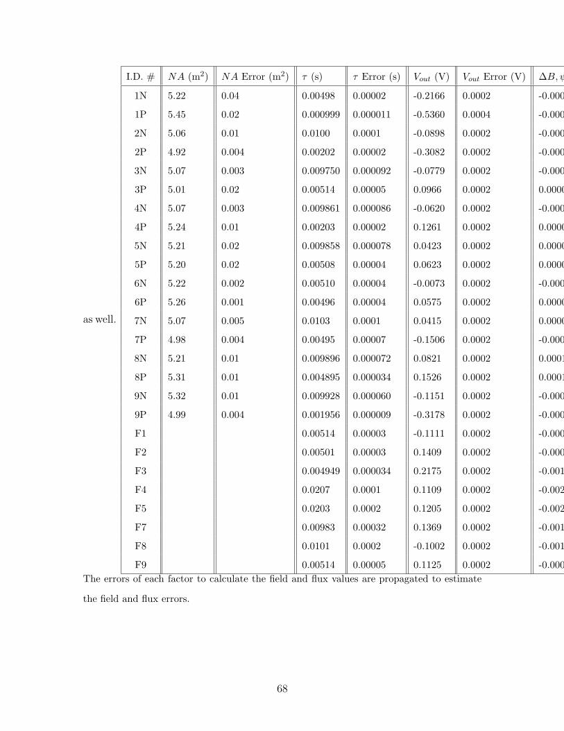
as well.
I.D. # NA (m2) NA Error (m2) τ (s) τ Error (s) Vout (V) Vout Error (V) ∆B,ψ (T, Wb) ∆B,ψ Error (T, Wb)
1N 5.22 0.04 0.00498 0.00002 -0.2166 0.0002 -0.000206 0.000002
1P 5.45 0.02 0.000999 0.000011 -0.5360 0.0004 -0.0000982 0.0000012
2N 5.06 0.01 0.0100 0.0001 -0.0898 0.0002 -0.000178 0.000002
2P 4.92 0.004 0.00202 0.00002 -0.3082 0.0002 -0.000126 0.000001
3N 5.07 0.003 0.009750 0.000092 -0.0779 0.0002 -0.000150 0.000001
3P 5.01 0.02 0.00514 0.00005 0.0966 0.0002 0.0000991 0.0000010
4N 5.07 0.003 0.009861 0.000086 -0.0620 0.0002 -0.000121 0.000001
4P 5.24 0.01 0.00203 0.00002 0.1261 0.0002 0.0000490 0.0000005
5N 5.21 0.02 0.009858 0.000078 0.0423 0.0002 0.0000800 0.0000007
5P 5.20 0.02 0.00508 0.00004 0.0623 0.0002 0.0000608 0.0000005
6N 5.22 0.002 0.00510 0.00004 -0.0073 0.0002 -0.0000071 0.0000002
6P 5.26 0.001 0.00496 0.00004 0.0575 0.0002 0.0000542 0.0000004
7N 5.07 0.005 0.0103 0.0001 0.0415 0.0002 0.0000842 0.0000007
7P 4.98 0.004 0.00495 0.00007 -0.1506 0.0002 -0.000150 0.000002
8N 5.21 0.01 0.009896 0.000072 0.0821 0.0002 0.000156 0.000001
8P 5.31 0.01 0.004895 0.000034 0.1526 0.0002 0.000141 0.000001
9N 5.32 0.01 0.009928 0.000060 -0.1151 0.0002 -0.000215 0.000001
9P 4.99 0.004 0.001956 0.000009 -0.3178 0.0002 -0.000125 0.000001
F1 0.00514 0.00003 -0.1111 0.0002 -0.000571 0.000004
F2 0.00501 0.00003 0.1409 0.0002 -0.000706 0.000005
F3 0.004949 0.000034 0.2175 0.0002 -0.001076 0.000007
F4 0.0207 0.0001 0.1109 0.0002 -0.00229 0.00002
F5 0.0203 0.0002 0.1205 0.0002 -0.00245 0.00002
F7 0.00983 0.00032 0.1369 0.0002 -0.00135 0.00004
F8 0.0101 0.0002 -0.1002 0.0002 -0.00102 0.00002
F9 0.00514 0.00005 0.1125 0.0002 -0.000578 0.000006The errors of each factor to calculate the field and flux values are propagated to estimate
the field and flux errors.
68
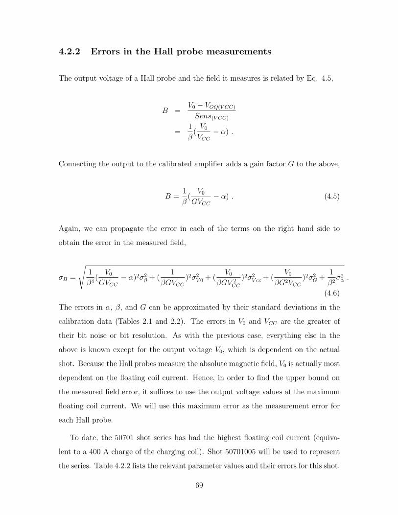
4.2.2 Errors in the Hall probe measurements
The output voltage of a Hall probe and the field it measures is related by Eq. 4.5,
B =V0 − VOQ(V CC)
Sens(V CC)
=1
β(V0
VCC− α) .
Connecting the output to the calibrated amplifier adds a gain factor G to the above,
B =1
β(V0
GVCC− α) . (4.5)
Again, we can propagate the error in each of the terms on the right hand side to
obtain the error in the measured field,
σB =
√1
β4(V0
GVCC− α)2σ2
β + (1
βGVCC)2σ2
V 0 + (V0
βGV 2CC
)2σ2V cc + (
V0
βG2VCC)2σ2
G +1
β2σ2α .
(4.6)
The errors in α, β, and G can be approximated by their standard deviations in the
calibration data (Tables 2.1 and 2.2). The errors in V0 and VCC are the greater of
their bit noise or bit resolution. As with the previous case, everything else in the
above is known except for the output voltage V0, which is dependent on the actual
shot. Because the Hall probes measure the absolute magnetic field, V0 is actually most
dependent on the floating coil current. Hence, in order to find the upper bound on
the measured field error, it suffices to use the output voltage values at the maximum
floating coil current. We will use this maximum error as the measurement error for
each Hall probe.
To date, the 50701 shot series has had the highest floating coil current (equiva-
lent to a 400 A charge of the charging coil). Shot 50701005 will be used to represent
the series. Table 4.2.2 lists the relevant parameter values and their errors for this shot.
69
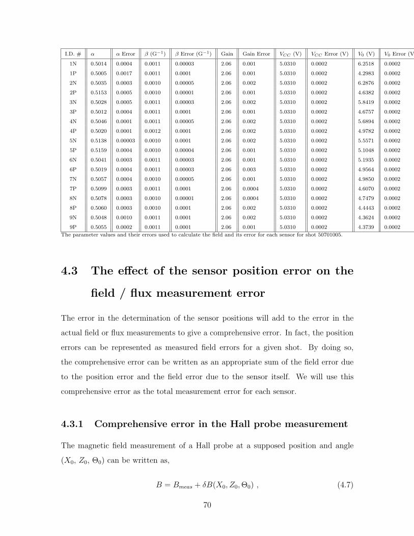
I.D. # α α Error β (G−1) β Error (G−1) Gain Gain Error VCC (V) VCC Error (V) V0 (V) V0 Error (V) B (G) B Error (G)
1N 0.5014 0.0004 0.0011 0.00003 2.06 0.001 5.0310 0.0002 6.2518 0.0002 93 3
1P 0.5005 0.0017 0.0011 0.0001 2.06 0.001 5.0310 0.0002 4.2983 0.0002 -75 7
2N 0.5035 0.0003 0.0010 0.00005 2.06 0.002 5.0310 0.0002 6.2876 0.0002 99 5
2P 0.5153 0.0005 0.0010 0.00001 2.06 0.001 5.0310 0.0002 4.6382 0.0002 -68 1
3N 0.5028 0.0005 0.0011 0.00003 2.06 0.002 5.0310 0.0002 5.8419 0.0002 56 2
3P 0.5012 0.0004 0.0011 0.0001 2.06 0.001 5.0310 0.0002 4.6757 0.0002 -43 3
4N 0.5046 0.0001 0.0011 0.00005 2.06 0.002 5.0310 0.0002 5.6894 0.0002 40 2
4P 0.5020 0.0001 0.0012 0.0001 2.06 0.002 5.0310 0.0002 4.9782 0.0002 -19 1
5N 0.5138 0.00003 0.0010 0.0001 2.06 0.002 5.0310 0.0002 5.5571 0.0002 23 1
5P 0.5159 0.0004 0.0010 0.00004 2.06 0.001 5.0310 0.0002 5.1048 0.0002 -23 1
6N 0.5041 0.0003 0.0011 0.00003 2.06 0.001 5.0310 0.0002 5.1935 0.0002 -2.9 0.4
6P 0.5019 0.0004 0.0011 0.00003 2.06 0.003 5.0310 0.0002 4.9564 0.0002 -21 1
7N 0.5057 0.0004 0.0010 0.00005 2.06 0.001 5.0310 0.0002 4.9850 0.0002 -24 1
7P 0.5099 0.0003 0.0011 0.0001 2.06 0.0004 5.0310 0.0002 4.6070 0.0002 -61 5
8N 0.5078 0.0003 0.0010 0.00001 2.06 0.0004 5.0310 0.0002 4.7479 0.0002 -50 1
8P 0.5060 0.0003 0.0010 0.0001 2.06 0.002 5.0310 0.0002 4.4443 0.0002 -76 5
9N 0.5048 0.0010 0.0011 0.0001 2.06 0.002 5.0310 0.0002 4.3624 0.0002 -79 7
9P 0.5055 0.0002 0.0011 0.0001 2.06 0.001 5.0310 0.0002 4.3739 0.0002 -78 7
The parameter values and their errors used to calculate the field and its error for each sensor for shot 50701005.
4.3 The effect of the sensor position error on the
field / flux measurement error
The error in the determination of the sensor positions will add to the error in the
actual field or flux measurements to give a comprehensive error. In fact, the position
errors can be represented as measured field errors for a given shot. By doing so,
the comprehensive error can be written as an appropriate sum of the field error due
to the position error and the field error due to the sensor itself. We will use this
comprehensive error as the total measurement error for each sensor.
4.3.1 Comprehensive error in the Hall probe measurement
The magnetic field measurement of a Hall probe at a supposed position and angle
(X0, Z0, Θ0) can be written as,
B = Bmeas + δB(X0, Z0,Θ0) , (4.7)
70

where δB(X,Z,Θ) = B(X,Z,Θ) − B(X0, Z0,Θ0). Although δB(X0, Z0,Θ0) itself is
zero, its error is nonzero for nonzero errors in X0, Z0, and/or Θ0. The error in δB,
which we will write as σpos, can be written as follows:
σpos =
√(∂B
∂X
)2
σ2X0 +
(∂B
∂Z
)2
σ2Z0 +
(∂B
∂Θ
)2
σ2Θ0 . (4.8)
The partial derivatives in the above expression can be found for a particular shot. For
the purpose of estimating σpos (and in keeping with the spirit of the previous section),
we will again use shot 50701005. Once σpos is found for each sensor, the total error
in the field measurement is easily calculated as follows:
σtot =√σ2meas + σ2
pos , (4.9)
where σmeas is the measurement error of the sensor itself, as given in Table 4.2.2.
Table 4.1 tabulates σmeas, σpos, and σtot for each sensor. The table shows that the
field measurement error due to the position error contributes minimally to the total
measurement error for most sensors. The total error ranges from a few percent to
about ten percent for all sensors except for sensor 6N, for which the error is about 20
%.
4.3.2 Comprehensive errors in the Bp coil and flux loop mea-
surements
Similarly to the Hall probes, the field and flux measurements of the coils and loops
at position and angle (for the Bp coils) (X0, Z0, Θ0) can be written as,
∆B = ∆Bmeas + δ∆B(X0, Z0,Θ0) (4.10)
∆ψ = ∆ψmeas + δ∆ψ(X0, Z0) , (4.11)
where δ∆B(X,Z,Θ) = ∆B(X,Z,Θ)−∆B(X0, Z0,Θ0) and δ∆ψ(X,Z) = ∆ψ(X,Z)−
∆ψ(X0, Z0). Just like for the Hall probes, we will call the error in δ∆B and δ∆ψ
71
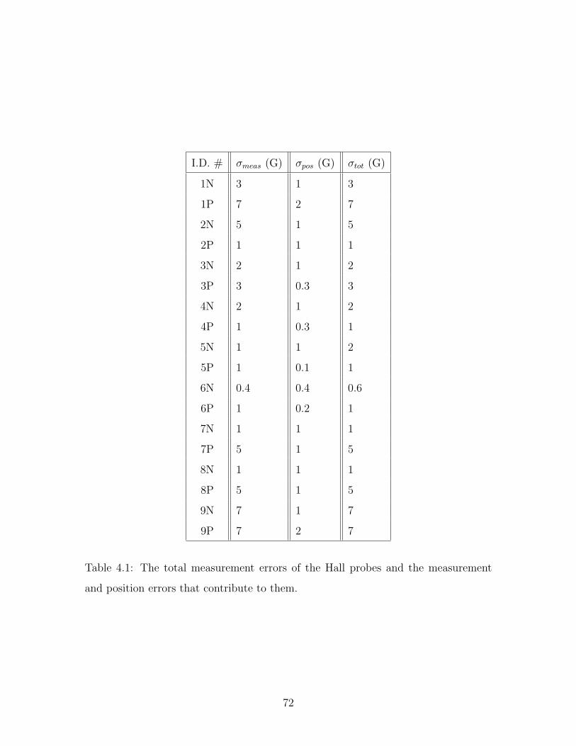
I.D. # σmeas (G) σpos (G) σtot (G)
1N 3 1 3
1P 7 2 7
2N 5 1 5
2P 1 1 1
3N 2 1 2
3P 3 0.3 3
4N 2 1 2
4P 1 0.3 1
5N 1 1 2
5P 1 0.1 1
6N 0.4 0.4 0.6
6P 1 0.2 1
7N 1 1 1
7P 5 1 5
8N 1 1 1
8P 5 1 5
9N 7 1 7
9P 7 2 7
Table 4.1: The total measurement errors of the Hall probes and the measurement
and position errors that contribute to them.
72
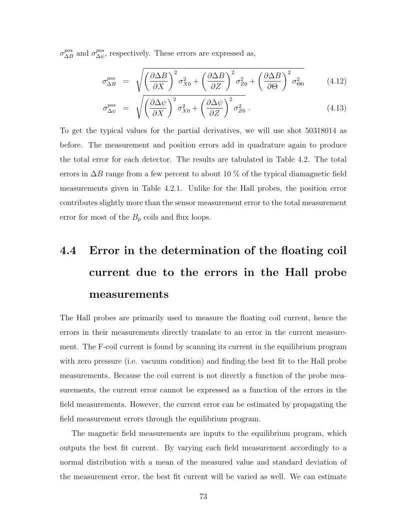
σpos∆B and σpos∆ψ, respectively. These errors are expressed as,
σpos∆B =
√(∂∆B
∂X
)2
σ2X0 +
(∂∆B
∂Z
)2
σ2Z0 +
(∂∆B
∂Θ
)2
σ2Θ0 (4.12)
σpos∆ψ =
√(∂∆ψ
∂X
)2
σ2X0 +
(∂∆ψ
∂Z
)2
σ2Z0 . (4.13)
To get the typical values for the partial derivatives, we will use shot 50318014 as
before. The measurement and position errors add in quadrature again to produce
the total error for each detector. The results are tabulated in Table 4.2. The total
errors in ∆B range from a few percent to about 10 % of the typical diamagnetic field
measurements given in Table 4.2.1. Unlike for the Hall probes, the position error
contributes slightly more than the sensor measurement error to the total measurement
error for most of the Bp coils and flux loops.
4.4 Error in the determination of the floating coil
current due to the errors in the Hall probe
measurements
The Hall probes are primarily used to measure the floating coil current, hence the
errors in their measurements directly translate to an error in the current measure-
ment. The F-coil current is found by scanning its current in the equilibrium program
with zero pressure (i.e. vacuum condition) and finding the best fit to the Hall probe
measurements. Because the coil current is not directly a function of the probe mea-
surements, the current error cannot be expressed as a function of the errors in the
field measurements. However, the current error can be estimated by propagating the
field measurement errors through the equilibrium program.
The magnetic field measurements are inputs to the equilibrium program, which
outputs the best fit current. By varying each field measurement accordingly to a
normal distribution with a mean of the measured value and standard deviation of
the measurement error, the best fit current will be varied as well. We can estimate
73
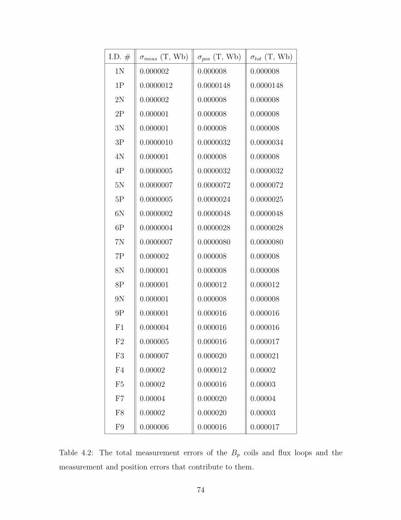
I.D. # σmeas (T, Wb) σpos (T, Wb) σtot (T, Wb)
1N 0.000002 0.000008 0.000008
1P 0.0000012 0.0000148 0.0000148
2N 0.000002 0.000008 0.000008
2P 0.000001 0.000008 0.000008
3N 0.000001 0.000008 0.000008
3P 0.0000010 0.0000032 0.0000034
4N 0.000001 0.000008 0.000008
4P 0.0000005 0.0000032 0.0000032
5N 0.0000007 0.0000072 0.0000072
5P 0.0000005 0.0000024 0.0000025
6N 0.0000002 0.0000048 0.0000048
6P 0.0000004 0.0000028 0.0000028
7N 0.0000007 0.0000080 0.0000080
7P 0.000002 0.000008 0.000008
8N 0.000001 0.000008 0.000008
8P 0.000001 0.000012 0.000012
9N 0.000001 0.000008 0.000008
9P 0.000001 0.000016 0.000016
F1 0.000004 0.000016 0.000016
F2 0.000005 0.000016 0.000017
F3 0.000007 0.000020 0.000021
F4 0.00002 0.000012 0.00002
F5 0.00002 0.000016 0.00003
F7 0.00004 0.000020 0.00004
F8 0.00002 0.000020 0.00003
F9 0.000006 0.000016 0.000017
Table 4.2: The total measurement errors of the Bp coils and flux loops and the
measurement and position errors that contribute to them.
74
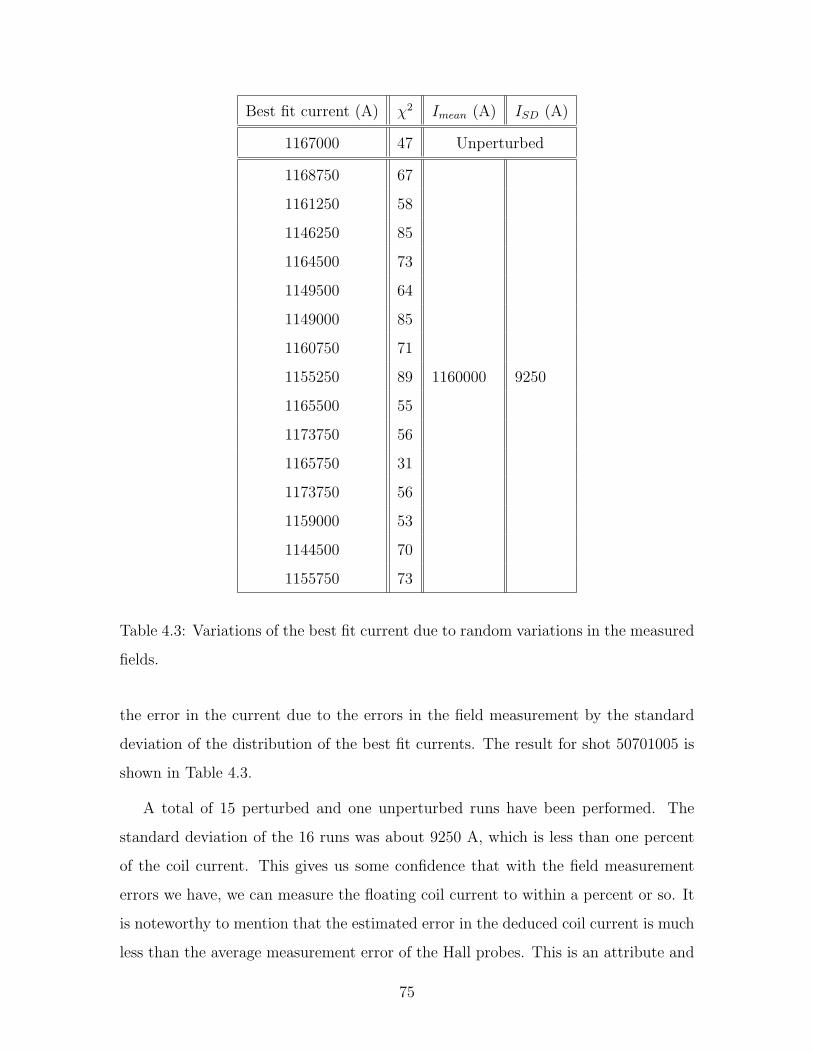
Best fit current (A) χ2 Imean (A) ISD (A)
1167000 47 Unperturbed
1168750 67
1161250 58
1146250 85
1164500 73
1149500 64
1149000 85
1160750 71
1155250 89 1160000 9250
1165500 55
1173750 56
1165750 31
1173750 56
1159000 53
1144500 70
1155750 73
Table 4.3: Variations of the best fit current due to random variations in the measured
fields.
the error in the current due to the errors in the field measurement by the standard
deviation of the distribution of the best fit currents. The result for shot 50701005 is
shown in Table 4.3.
A total of 15 perturbed and one unperturbed runs have been performed. The
standard deviation of the 16 runs was about 9250 A, which is less than one percent
of the coil current. This gives us some confidence that with the field measurement
errors we have, we can measure the floating coil current to within a percent or so. It
is noteworthy to mention that the estimated error in the deduced coil current is much
less than the average measurement error of the Hall probes. This is an attribute and
75
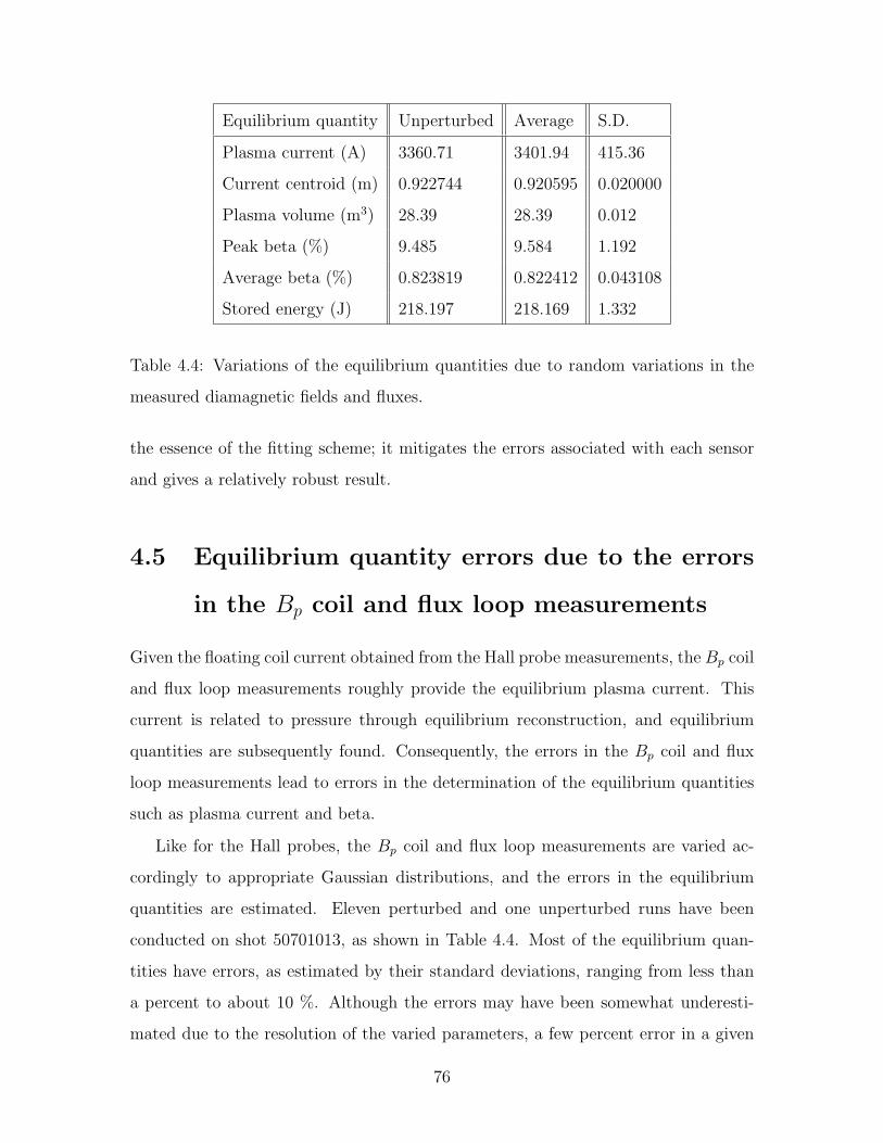
Equilibrium quantity Unperturbed Average S.D.
Plasma current (A) 3360.71 3401.94 415.36
Current centroid (m) 0.922744 0.920595 0.020000
Plasma volume (m3) 28.39 28.39 0.012
Peak beta (%) 9.485 9.584 1.192
Average beta (%) 0.823819 0.822412 0.043108
Stored energy (J) 218.197 218.169 1.332
Table 4.4: Variations of the equilibrium quantities due to random variations in the
measured diamagnetic fields and fluxes.
the essence of the fitting scheme; it mitigates the errors associated with each sensor
and gives a relatively robust result.
4.5 Equilibrium quantity errors due to the errors
in the Bp coil and flux loop measurements
Given the floating coil current obtained from the Hall probe measurements, the Bp coil
and flux loop measurements roughly provide the equilibrium plasma current. This
current is related to pressure through equilibrium reconstruction, and equilibrium
quantities are subsequently found. Consequently, the errors in the Bp coil and flux
loop measurements lead to errors in the determination of the equilibrium quantities
such as plasma current and beta.
Like for the Hall probes, the Bp coil and flux loop measurements are varied ac-
cordingly to appropriate Gaussian distributions, and the errors in the equilibrium
quantities are estimated. Eleven perturbed and one unperturbed runs have been
conducted on shot 50701013, as shown in Table 4.4. Most of the equilibrium quan-
tities have errors, as estimated by their standard deviations, ranging from less than
a percent to about 10 %. Although the errors may have been somewhat underesti-
mated due to the resolution of the varied parameters, a few percent error in a given
76

equilibrium quantity is definitely satisfactory.
77

78
Chapter 5
Equilibrium and Stability of LDX
Plasma
A plasma confined in a dipole magnetic geometry exhibits unique equilibrium and
stability properties that are not seen in tokamaks or other magnetic confinement
devices. However, the dipole geometry has certain similarities with hardcore z-pinches
and mirror machines, and there consequently is some overlap in the physics principles
of these apparatus. For example, the stability of a hardcore z-pinch greatly depends
on the plasma pressure gradient and the plasma pressure can be highly anisotropic in
a mirror machine, both properties of which are observed in LDX. In fact, a hardcore
z-pinch is approximately a very high aspect ratio LDX, in which the curvature of
the internal coil is taken to be zero, and its stability properties have been studied
extensively to give insight into the stability properties of LDX [23].
The Levitated Dipole Experiment is not the first experiment to study plasma con-
finement in a dipolar field. The Collisionless Terrella Experiment (CTX) at Columbia
University has been operating long before LDX to study plasma fluctuations and
transport in a supported dipole [26, 29, 30]. The University of Tokyo is a host to
several supported and levitated dipole experiments including Proto-RT (supported)
[42, 43], mini-RT (levitated), and RT-1 (levitated). RT-1, which has just recently
started operation earlier this year, is a larger version of mini-RT but still much smaller
than LDX. Before the existence of laboratory dipole confinement devices, much of the
79
experimental studies of dipolarly confined plasmas had been conducted on planetary
magnetospheres [13, 4]. Accordingly, basic equilibrium and stability properties of
plasmas in a dipole field had been developed long before the first laboratory appara-
tus was ever built.
5.1 Plasma equilibrium in LDX
The equilibrium of LDX plasma is described by the ideal MHD theory. Although the
equilibrium can also be described by kinetic or single particle theories, MHD provides
the essence of the macroscopic picture. The relevant equations are,
∇ ·B = 0 (5.1)
∇×B = µ0J (5.2)
∇P = J ×B . (5.3)
The first two equations are two of Maxwell’s equations, and the third is the MHD
momentum balance equation. The momentum balance equation in the above form
assumes an isotropic pressure, but it can be recast in an anisotropic form by substi-
tuting ∇ ·P for ∇P , where P is the pressure tensor. The above three equations can
be combined to derive the Grad-Shafranov equation [8],
∆∗ψ = −µ0R2dP
dψ− F
dF
dψ. (5.4)
In the above, ∆∗ ≡ R2∇ ·( ∇R2
)is an elliptic differential operator, and F ≡ RBφ is a
function of ψ. Because there is no toroidal field in LDX, the second term is identically
zero. The G-S equation without the second term is what the equilibrium program
solves to obtain P (ψ) given the external magnetic measurements.
The magnetic field in LDX is provided by the floating coil and plasma current.
Because the plasma current flows in the same direction as the floating coil current
and is typically less than 1% of the floating coil current, the equilibrium field is well
approximated by the vacuum field. The field of a dipole decreases as 1R3 on the
equatorial plane. Unlike in a tokamak, there is no driven plasma current in LDX;
80
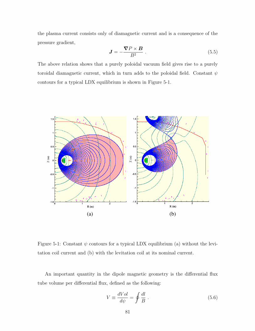
the plasma current consists only of diamagnetic current and is a consequence of the
pressure gradient,
J = −∇P ×B
B2. (5.5)
The above relation shows that a purely poloidal vacuum field gives rise to a purely
toroidal diamagnetic current, which in turn adds to the poloidal field. Constant ψ
contours for a typical LDX equilibrium is shown in Figure 5-1.
(a) (b)
Figure 5-1: Constant ψ contours for a typical LDX equilibrium (a) without the levi-
tation coil current and (b) with the levitation coil at its nominal current.
An important quantity in the dipole magnetic geometry is the differential flux
tube volume per differential flux, defined as the following:
V ≡ dV ol
dψ=
∮dl
B. (5.6)
81
The closed line integral on the right hand side is taken along a field line. Because B
decreases and∮dl increases as one moves away from the dipole, the flux tube volume
per unit flux increases rapidly as R increases. In fact, B ∼ R−3 and∮dl ∼ R, so
V ∼ RR−3 = R4. In the next section, we will see that the condition PV γ = const. is the
marginal stability criterion for MHD interchange modes. If we maximize the pressure
gradient at the marginal stability limit, the pressure dependence on the equatorial
radius can be found,
P ∼ V −γ ∼ R−4γ = R− 203 , (5.7)
where we have assumed a γ value of 53
for a 3-D collisional gas. Hence, at marginal
stability, the maximum attainable pressure is strongly dependent on the edge pres-
sure and and peak pressure position; the greater the edge pressure and closer the
peak position to the floating coil, the greater the peak pressure and beta. In other
words, the edge condition and the heating location will strongly influence the energy
characteristics of the plasma. Figure 5-2 shows a sample pressure profile.
5.2 Interchange instabilities
LDX plasmas are susceptible to two types of interchange instabilities, one driven by
the pressure gradient of the bulk electrons and the other driven by a population of
hot electrons. As mentioned in Ch. 1 and 2, the first phase of operation involves a
significant population of hot electrons that carry most of the pressure. Accordingly,
the interchange instability caused by hot electrons, or the hot electron interchange
instability (HEI), is the dominant instability in this phase of operation. By the third
phase of operation, when a more Maxwellian population of electrons is produced, the
dominant instability is expected to shift from HEI to the MHD interchange mode.
5.2.1 MHD Pressure Driven Interchange
MHD instabilities can be broadly classified into two categories. The first is the current
driven modes, and the second is the pressure driven modes. Current driven modes, or
82
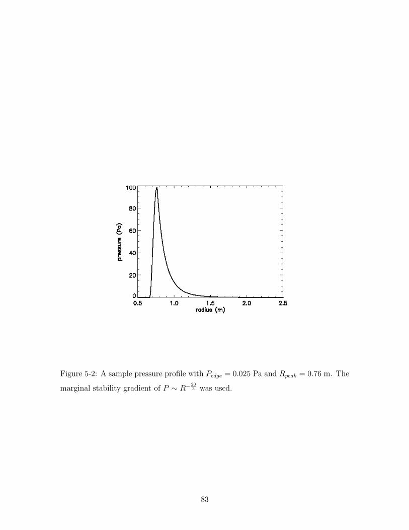
Figure 5-2: A sample pressure profile with Pedge = 0.025 Pa and Rpeak = 0.76 m. The
marginal stability gradient of P ∼ R− 203 was used.
83
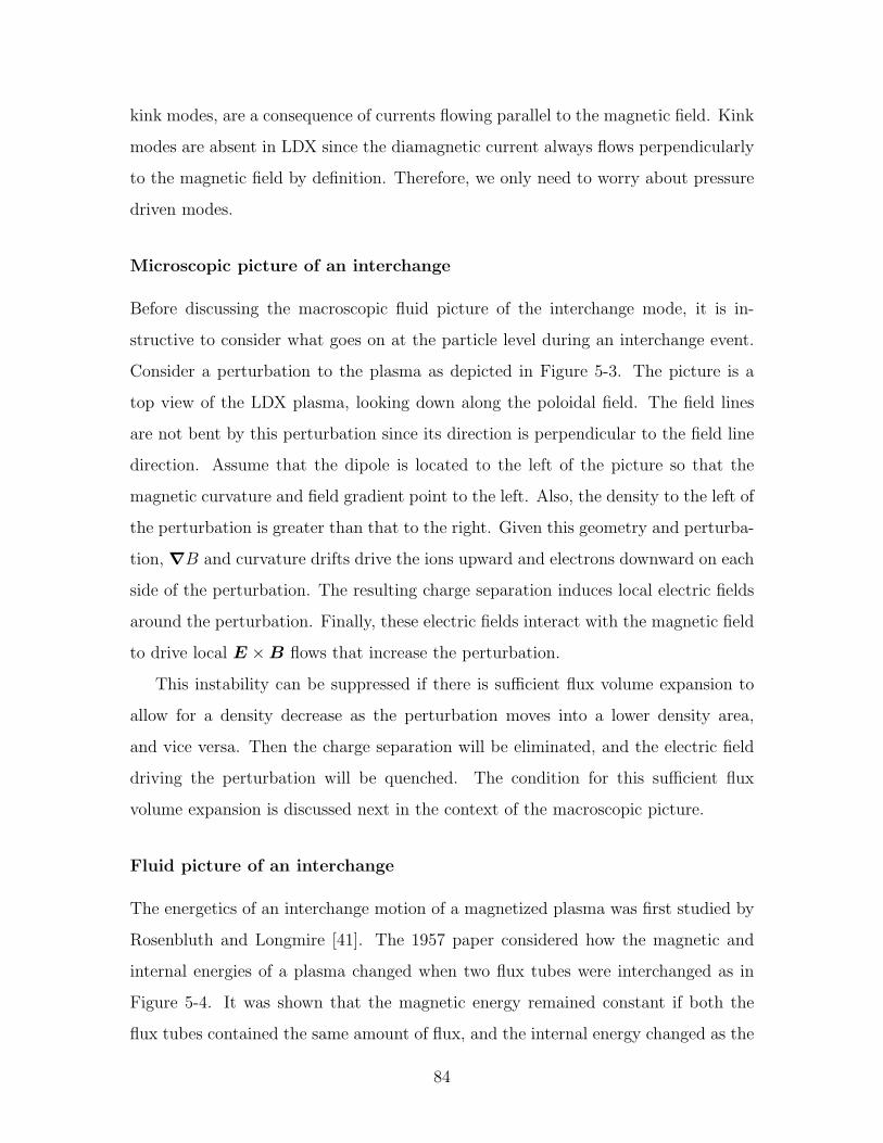
kink modes, are a consequence of currents flowing parallel to the magnetic field. Kink
modes are absent in LDX since the diamagnetic current always flows perpendicularly
to the magnetic field by definition. Therefore, we only need to worry about pressure
driven modes.
Microscopic picture of an interchange
Before discussing the macroscopic fluid picture of the interchange mode, it is in-
structive to consider what goes on at the particle level during an interchange event.
Consider a perturbation to the plasma as depicted in Figure 5-3. The picture is a
top view of the LDX plasma, looking down along the poloidal field. The field lines
are not bent by this perturbation since its direction is perpendicular to the field line
direction. Assume that the dipole is located to the left of the picture so that the
magnetic curvature and field gradient point to the left. Also, the density to the left of
the perturbation is greater than that to the right. Given this geometry and perturba-
tion, ∇B and curvature drifts drive the ions upward and electrons downward on each
side of the perturbation. The resulting charge separation induces local electric fields
around the perturbation. Finally, these electric fields interact with the magnetic field
to drive local E ×B flows that increase the perturbation.
This instability can be suppressed if there is sufficient flux volume expansion to
allow for a density decrease as the perturbation moves into a lower density area,
and vice versa. Then the charge separation will be eliminated, and the electric field
driving the perturbation will be quenched. The condition for this sufficient flux
volume expansion is discussed next in the context of the macroscopic picture.
Fluid picture of an interchange
The energetics of an interchange motion of a magnetized plasma was first studied by
Rosenbluth and Longmire [41]. The 1957 paper considered how the magnetic and
internal energies of a plasma changed when two flux tubes were interchanged as in
Figure 5-4. It was shown that the magnetic energy remained constant if both the
flux tubes contained the same amount of flux, and the internal energy changed as the
84
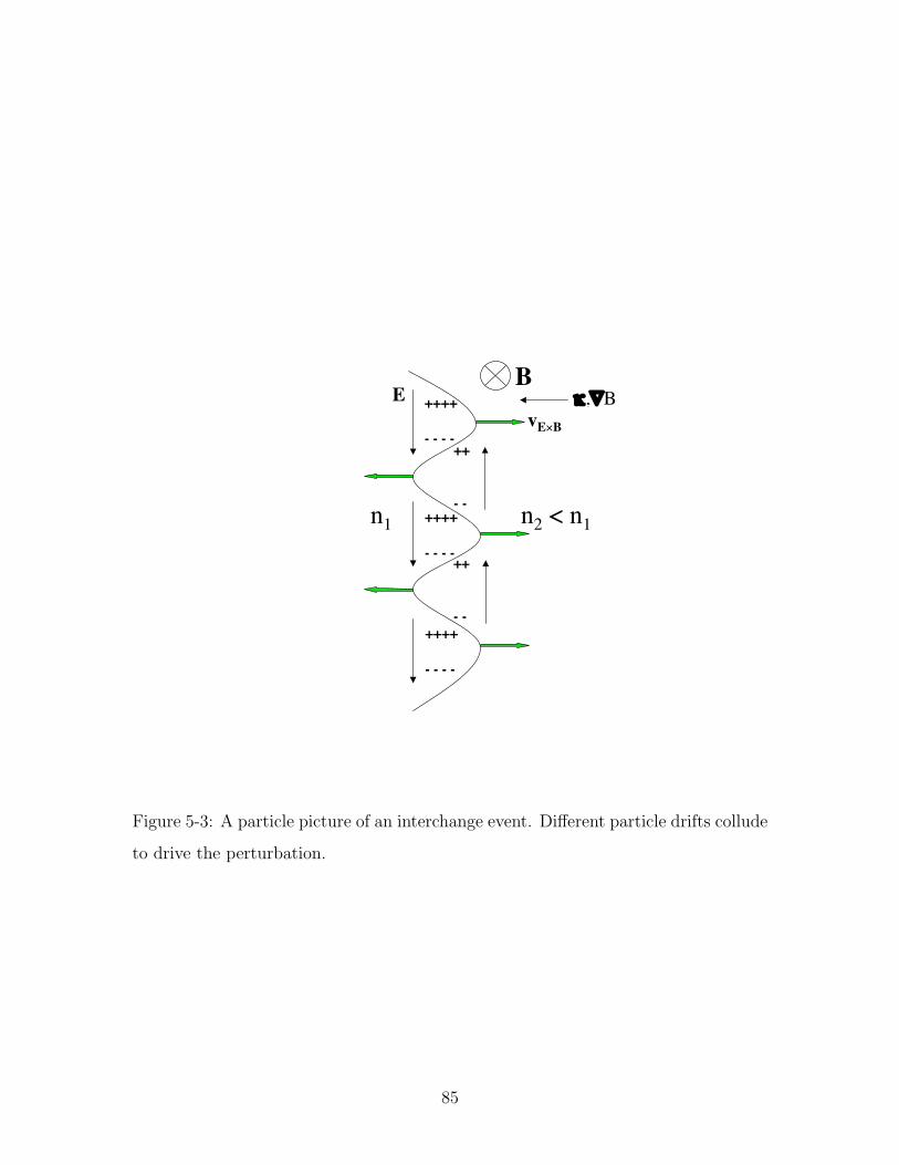
B
n1 n2 < n1
κ,∇B
++
- -
++
- -
++++
- - - -
++++
- - - -
E ++++
- - - -vE×B
Figure 5-3: A particle picture of an interchange event. Different particle drifts collude
to drive the perturbation.
85
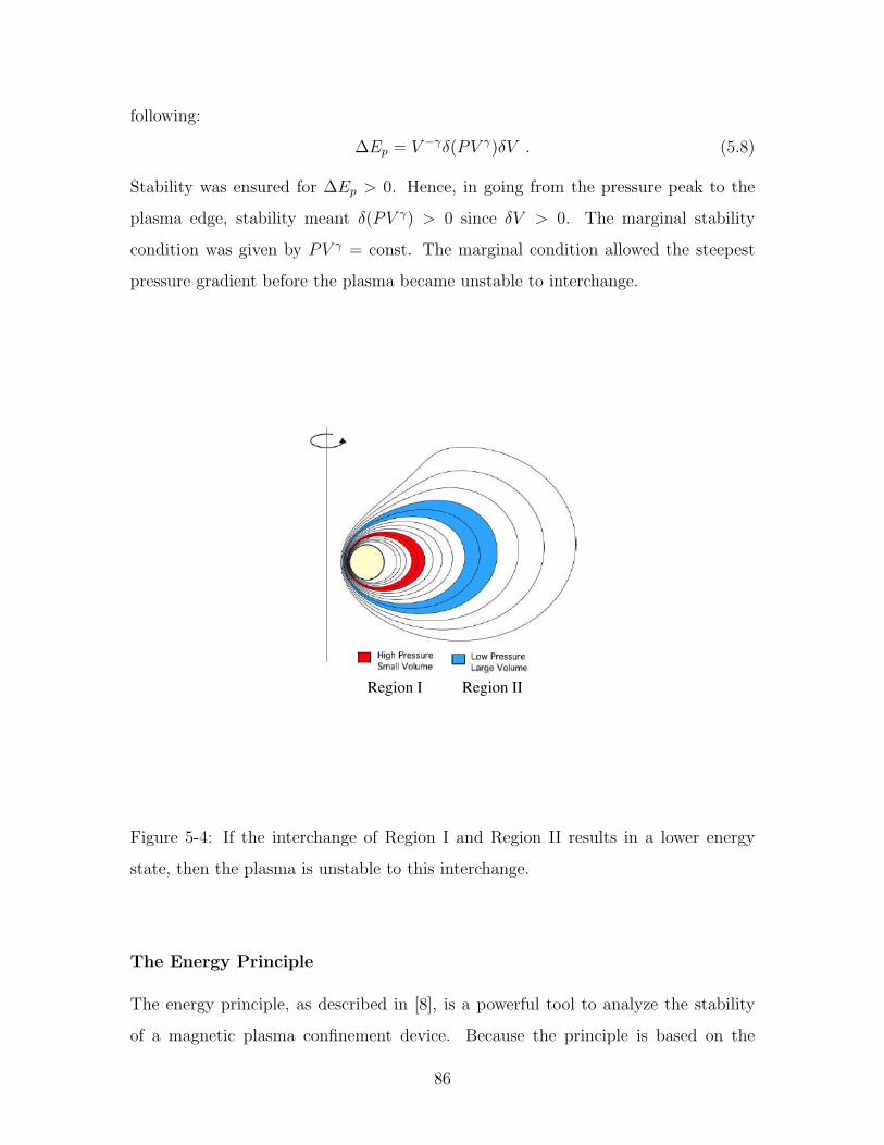
following:
∆Ep = V −γδ(PV γ)δV . (5.8)
Stability was ensured for ∆Ep > 0. Hence, in going from the pressure peak to the
plasma edge, stability meant δ(PV γ) > 0 since δV > 0. The marginal stability
condition was given by PV γ = const. The marginal condition allowed the steepest
pressure gradient before the plasma became unstable to interchange.
Region I Region II
Figure 5-4: If the interchange of Region I and Region II results in a lower energy
state, then the plasma is unstable to this interchange.
The Energy Principle
The energy principle, as described in [8], is a powerful tool to analyze the stability
of a magnetic plasma confinement device. Because the principle is based on the
86
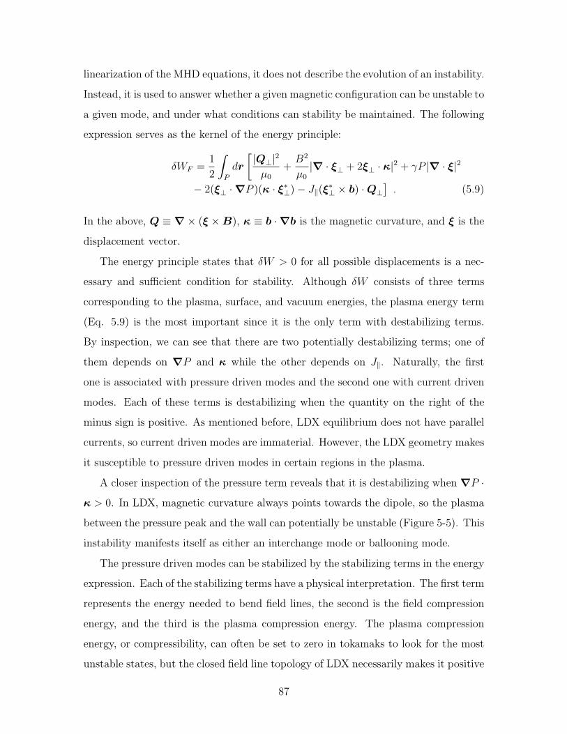
linearization of the MHD equations, it does not describe the evolution of an instability.
Instead, it is used to answer whether a given magnetic configuration can be unstable to
a given mode, and under what conditions can stability be maintained. The following
expression serves as the kernel of the energy principle:
δWF =1
2
∫P
dr
[|Q⊥|2
µ0
+B2
µ0
|∇ · ξ⊥ + 2ξ⊥ · κ|2 + γP |∇ · ξ|2
− 2(ξ⊥ ·∇P )(κ · ξ∗⊥)− J‖(ξ∗⊥ × b) ·Q⊥
]. (5.9)
In the above, Q ≡ ∇× (ξ ×B), κ ≡ b ·∇b is the magnetic curvature, and ξ is the
displacement vector.
The energy principle states that δW > 0 for all possible displacements is a nec-
essary and sufficient condition for stability. Although δW consists of three terms
corresponding to the plasma, surface, and vacuum energies, the plasma energy term
(Eq. 5.9) is the most important since it is the only term with destabilizing terms.
By inspection, we can see that there are two potentially destabilizing terms; one of
them depends on ∇P and κ while the other depends on J‖. Naturally, the first
one is associated with pressure driven modes and the second one with current driven
modes. Each of these terms is destabilizing when the quantity on the right of the
minus sign is positive. As mentioned before, LDX equilibrium does not have parallel
currents, so current driven modes are immaterial. However, the LDX geometry makes
it susceptible to pressure driven modes in certain regions in the plasma.
A closer inspection of the pressure term reveals that it is destabilizing when ∇P ·
κ > 0. In LDX, magnetic curvature always points towards the dipole, so the plasma
between the pressure peak and the wall can potentially be unstable (Figure 5-5). This
instability manifests itself as either an interchange mode or ballooning mode.
The pressure driven modes can be stabilized by the stabilizing terms in the energy
expression. Each of the stabilizing terms have a physical interpretation. The first term
represents the energy needed to bend field lines, the second is the field compression
energy, and the third is the plasma compression energy. The plasma compression
energy, or compressibility, can often be set to zero in tokamaks to look for the most
unstable states, but the closed field line topology of LDX necessarily makes it positive
87
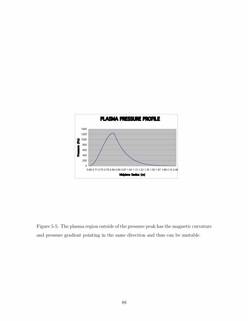
PLASMA PRESSURE PROFILE
0
200
400
600
800
1000
1200
1400
0.68 0.71 0.75 0.79 0.84 0.90 0.97 1.04 1.13 1.23 1.35 1.50 1.67 1.88 2.14 2.46
Midplane Radius (m)
Pres
sure
(Pa
)
Figure 5-5: The plasma region outside of the pressure peak has the magnetic curvature
and pressure gradient pointing in the same direction and thus can be unstable.
88
and stabilizing. The implication is that modes that do not bend or compress magnetic
field lines can be stabilized by this term. In fact, compressibility is the dominant
stabilizing term that stabilizes the pressure driven modes in LDX.
As discussed earlier, interchange modes in LDX are stabilized if δ(PV γ) > 0.
This condition is equivalent to the compressibility term overpowering the destabilizing
pressure driven term in the plasma region between the pressure peak and the wall
for all allowable interchange motions. However, for ballooning modes, the pressure
driven term can locally become very large, and the field line bending energy becomes
an important stabilizing term. Garnier shows in [11] that if an equilibrium is stable to
interchange modes, then it is also stable to high-n ballooning modes. Because high-n
modes are the most unstable of the ballooning modes, we can see that δ(PV γ) > 0 is
a necessary and sufficient condition for MHD stability.
Anisotropic Effect
The energy principle discussed above must be slightly altered when anisotropic pres-
sure effects are incorporated. In particular, the stabilizing plasma compressibility
term has to be derived using kinetic theory, resulting in the Krukal-Oberman form
of the energy principal. A rather simple expression, much like the expression in the
isotropic case, for interchange stability can be derived if we assume that the ratio of
P⊥ to P‖ is constant throughout the plasma, P⊥P‖
= 1 + 2p, where p is the anisotropy
parameter. When the appropriate minimizations are done via the energy principle,
the following criterion is obtained [45]:
γV ′
V+P ′
P< 0 , (5.10)
where γ ≡ γ(
1+ 45p
1+ 43p
), P ≡ P (ψ)
[B0(ψ)B∗
]2p
, and V ≡∮
dlB
(B∗
B
)2p. Also, B0 is the
magnetic field on the midplane, B∗ is a constant reference magnetic field, and ′ ≡ ddψ
.
As will be seen in the next chapter, pressure becomes a function of both ψ and B
when it is anisotropic; P is the part of pressure that is dependent only on ψ,
P‖(ψ,B) = P (ψ)
(B∗
B
)2p
. (5.11)
89
Also,
P‖(ψ,B0) = P (ψ) . (5.12)
The form of the stability criterion for anisotropic pressure is identical to that for
isotropic pressure, but now the quantities are dependent on the anisotropy parameter,
p. To see how anisotropy affects the pressure gradient limit, we need to isolate P ′
Pin
the above expression. After some algebra, the criterion becomes,
P ′
P
∣∣∣∣anisotropic
< − γV′
V− 2p
B′0
B0
. (5.13)
The criterion in the isotropic case is equivalent to the above with p = 0,
P ′
P
∣∣∣∣isotropic
< −γV′
V. (5.14)
The right hand side of the anisotropic criterion can be numerically evaluated and
compared to the right hand side of the isotropic criterion. The result shows that
adding anisotropy affects the gradient limit by a mere 4 %,
P ′
P
∣∣∣∣anisotropic
<∼ −1.04γV ′
V. (5.15)
5.2.2 Hot Electron Interchange
When there is a significant fraction of hot electrons in the plasma, such as in LDX,
hot electron interchange mode becomes a relevant potential instability. Because hot
electrons violate the high collisionality assumption of ideal MHD, they do not strictly
adhere to MHD stability laws. A kinetic analysis must be performed to characterize
interchange modes of hot electrons. The reader can refer to [21, 1, 9], for example, for
the derivation and observation of the hot electron interchange (HEI) mode. General
characteristics of the HEI are described here.
The stability condition for the HEI is given as follows:
−d ln nhd lnV
< 1 +m2
⊥24
ωdhωci
ninh
. (5.16)
In the above, m⊥ is the perpendicular wave number, nh is the flux-tube averaged
hot electron density, ni is the flux-tube averaged ion density, ωdh is the hot electron
90
curvature drift frequency, and ωci is the ion cyclotron frequency. Unlike the MHD
interchange mode, the HEI imposes a gradient limit on the density rather than on the
pressure. This means that the hot electron pressure gradient can exceed the MHD
limit without being unstable. The additional stability comes from the interaction
of the hot electrons with the background ions. Stability to the HEI is enhanced by
increasing the right hand side of the inequality. Because ωdh is proportional to the
hot electron energy, the hotter hot electrons can sustain a steeper density gradient
than the cooler ones. Also, too much hot electron in the plasma can seriously degrade
its stability by limiting the density gradient at a low level. This situation can arise
when there are not enough neutrals to collide with the hot electrons during plasma
startup in the presence of ECRH heating.
5.3 Summary of LDX Equilibrium and Stability
The equilibrium of LDX has a very simple configuration with a purely poloidal field
and a purely toroidal current. The current is naturally driven by the pressure gradient
(i.e. diamagnetic) and does not need an external driving source. It is interesting to
note that the cause and effect of the diamagnetic current and the pressure gradient is a
classical chicken or the egg conundrum. In the light of the MHD momentum balance,
we know that there needs to be a pressure gradient in order for the diamagnetic
current to exist, and vice versa. What is not obvious is whether one causes the other
or they come to coexist simultaneously.
The two relevant instabilities for LDX plasmas are the MHD and hot electron
interchange modes. The MHD interchange stability criterion can be derived by con-
sidering the energy involved in interchanging two flux tubes (fluid elements) in the
plasma. An equivalent, and perhaps more sophisticated, derivation is done by writing
down the different potential energy terms of the plasma as a function of a perturbation
and minimizing them. This so-called energy principle and the energy consideration of
exchanging two flux tubes give the marginal pressure gradient criterion, PV γ = const.
The effective value of γ slightly increases when pressure anisotropy is included. The
91
MHD interchange criterion roughly applies to the cold background electrons, but the
ECRH heated hot electrons follow a kinetic analog of the MHD interchange called
the hot electron interchange mode. The HEI puts a restriction on the hot electron
density gradient rather than on the pressure gradient. The hot electrons can therefore
attain pressure gradients that exceed the MHD limit.
92
Chapter 6
Equilibrium Reconstruction
Equilibrium reconstruction is a process by which magnetic and possibly other mea-
surements are used to find key equilibrium parameters. Because plasma equilibrium
is most often described by MHD, the physics that relates magnetic measurements to
equilibrium quantities is governed by MHD equations. The Grad-Shafranov equation
encompasses the key physics that plays a principal role in the reconstruction process.
However, the G-S equation, and MHD theory for that matter, lacks one physics detail
that is needed to carry out the reconstruction. The equation (Eq. 5.4) has a dPdψ
term
on the right hand side, and MHD indeed shows that pressure is a function of magnetic
flux. What MHD does not provide is the actual function P (ψ). Without knowing
the functional form of P , the G-S equation cannot be solved. Hence, some kind of
a pressure model must be developed to enable the process. The model will typically
have free parameters that get adjusted during reconstruction to fit the magnetic data.
While the quality, or validity, of the chosen model is given by the goodness of fit pa-
rameter χ2, its particular choice may have a significant effect on the reconstruction
result.
Reconstruction is a very machine dependent process, and different experimental
apparatus will have their own idiosyncrasies. LDX is no exception. The goal of
this chapter is to give an expose of some of the unique features of LDX equilibrium
reconstruction and provide potential solutions to overcome them if they happen to
be problems that impede the process.
93
6.1 Reconstruction procedure
The reconstruction procedure begins with determining the floating coil current using
the Hall probe measurements. The current is found by a least-squares fit method;
a parameter called χ2 that measures the deviation of the measured fields from the
fields calculated for a given current is minimized,
χ2 =18∑i=0
(Bmeasi −Bcalc
i )2
σ2i
, (6.1)
where σ2i is the total measurement error of the i-th probe. The minimum χ2 gives the
best fit current, which is subsequently used to calculate the vacuum field. The Hall
probe measurements are taken before the plasma is produced to isolate the vacuum
field.
The next step is to choose the time at which the plasma is to be reconstructed.
Once the time is chosen, the diamagnetic field and flux measurements from the Bp
coils and flux loops are obtained. The diamagnetic field and flux are added to the
vacuum field and flux at each sensor location to find the total field and flux in the
presence of the plasma. As simple as it seems, this step actually warrants a closer
inspection.
6.1.1 Conservation of the floating coil flux
Because the LDX floating coil is a superconductor, the flux linked to it must stay
constant. This implies that the floating coil current must decrease when the plasma
is created, because the plasma diamagnetic current is in the same direction as the
floating coil current and therefore adds to its flux. Now, the Bp coils and flux loops
measure the change in the fields and fluxes from the vacuum field to the plasma field.
This means that they measure the sum of the field and flux change due to the floating
coil current decrease and the field and flux change due to the production of the plasma
current,
∆B = ∆Bf−coil + ∆Bplasma (6.2)
∆ψ = ∆ψf−coil + ∆ψplasma . (6.3)
94
The total field and flux in the presence of the plasma is,
Btotal = Bvac + ∆Bf−coil + ∆Bplasma = Bvac + ∆B (6.4)
ψtotal = ψvac + ∆ψf−coil + ∆ψplasma = ψvac + ∆ψ . (6.5)
Hence, adding the field and flux values measured by the Bp coils and flux loops to
the vacuum field and flux values still give us the total field and flux with the plasma.
However, when the equilibrium code is run to reconstruct the plasma, the decrease
in the floating coil current must be taken into account. In other words, the current
we ascribe to the floating coil during plasma reconstruction is less than that found
via the best fit algorithm.
A potential problem arises here. We need to know the plasma current profile to
find the mutual inductance between the plasma and the floating coil and thus the
current decrease, but we also need to know the current decrease to find the correct
floating coil current to use in the reconstruction of the plasma current profile. This
circle must be broken somewhere to resolve the issue.
The flux conservation requirement is given as the following:
LfIf = Lf (If + ∆If ) +MfpIp (6.6)
⇒ ∆If = −Mfp
LfIp , (6.7)
where the f and p subscripts designate floating coil and plasma, respectively. The self-
inductance of the floating coil is known from its geometry, but the mutual inductance
between the floating coil and the plasma and the plasma current are unknown before
the reconstruction. The mutual inductance can be roughly estimated by calculating
the mutual between the floating coil and a current ring at a plausible radius, giving
Lf ∼ 3–5Mfp. With a typical diamagnetic current ∼ 2.5 kA and a typical floating
coil current ∼ 1 MA, we get∆IfIf∼ − 500 A
1 MA = −0.05 %. Although the floating coil
current decrease is a tiny fraction of the floating coil current, it can lead to ascribing
significantly more current to the plasma and therefore changing the reconstruction
results.
A more accurate calculation of the floating coil current decrease is done by defining
95
the mutual inductance between the coil and the plasma as [33, 34],
Mfp ≡1
Ip
N∑i=1
∫ ∫Mi(x, z)Jp(x, z)dxdz . (6.8)
Eq. 6.8 assumes that the floating coil consists of N current loops, and Mi(x, z) is
the mutual inductance between a current filament at (x, z) and the i-th loop of the
floating coil. As stated before, we do not know Jp(x, z) a priori, but we can find it
to within a given tolerance by iterating through the reconstruction procedure. First,
assume that the Bp coil and flux loop measurements are of the diamagnetic current
only (i.e. ∆If = 0). Next, carry out the reconstruction with this assumption to
find the diamagnetic current. Finally, use the obtained plasma current distribution
to find ∆If , and repeat until the desired tolerance is reached. The good news is
that this procedure converges quickly and can be accomplished without carrying out
the full plasma reconstruction. The problem is purely electromagnetic and involves
no plasma physics, so there is absolutely no need to waste time solving the Grad-
Shafranov equation. Instead of iterating through the full reconstruction procedure,
both the plasma current distribution and the decrease in the floating coil current
can be found by iterating through a current filament code much like MFIT used in
tokamaks.
6.1.2 DFIT: The Dipole Current Filament Code
A current filament code that allows for a fast reconstruction of the plasma current has
been developed by Prof. Mike Mauel of Columbia University [38]. The code is purely
electromagnetic and does not have the capability of reconstructing plasma parameters
besides the current distribution. Because the code does not have to solve a PDE like
the full reconstruction code, it is extremely fast and ideal for monitoring the plasma
current on a shot by shot basis. Part of its speed comes from using only two current
filaments to model the plasma; the obvious downside to the simplicity is that the
current profile it can deduce is very coarse. The code, however, does an excellent
job finding integrated quantities of the current profile such as the total current, its
96
centroid, its dipole moment, and the mutual inductance between the floating coil and
the plasma.
The DFIT code works by changing the magnitude and location of the two current
filaments and finding the best fit to the magnetic data. Technically, there are a
total of six free parameters (current magnitude, x position, and z position times two
filaments) to be adjusted, but the assumption of up-down symmetry allows us to
constrain the z positions to the midplane (i.e. z = 0). This, however, cannot be done
when the levitation coil is activated since the up-down symmetry will be broken.
The real merit of the DFIT code is that it has the capability of holding the
floating coil flux constant while the best fit is found. This allows us to forgo the
iterative process needed to find the floating coil current decrease and the diamagnetic
current. The floating coil current decrease obtained from DFIT can be used to find
the actual floating coil current in the presence of the plasma, which is a required
input to the reconstruction program.
6.2 Reconstruction methods
6.2.1 Full Reconstruction
The standard reconstruction method involves iteratively solving the Grad-Shafranov
equation to obtain the best fit equilibrium parameters for the chosen pressure model.
Different parameters may depend on the model to different degrees. The character-
istics of different pressure models will be discussed in the next section. The iterative
process actually consists of an inner loop, in which ψ is varied to solve the equation
for fixed parameter values, and an outer loop, in which the parameter values are
varied. The inner loop is solved by using the Green’s function approach along with
the Picard iteration scheme [25, 24]. The outer loop can be solved either by a brute
force method or by employing an intelligent minimization scheme. The G-S equation
can be written in the following form to designate the iterative process (showing only
97
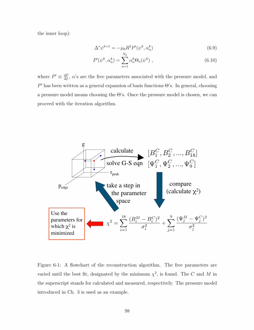
the inner loop):
∆∗ψk+1 = −µ0R2P ′(ψk, αkn) (6.9)
P ′(ψk, αkn) =
Np∑n=1
αknΘn(ψk) , (6.10)
where P ′ ≡ dPdψ
, α’s are the free parameters associated with the pressure model, and
P ′ has been written as a general expansion of basis functions Θ’s. In general, choosing
a pressure model means choosing the Θ’s. Once the pressure model is chosen, we can
proceed with the iteration algorithm.
pedge
rpeak
gcalculate
compare(calculate χ2)
take a step in the parameter space
solve G-S eqn
Use theparameters forwhich χ2 is minimized
Figure 6-1: A flowchart of the reconstruction algorithm. The free parameters are
varied until the best fit, designated by the minimum χ2, is found. The C and M in
the superscript stands for calculated and measured, respectively. The pressure model
introduced in Ch. 3 is used as an example.
98
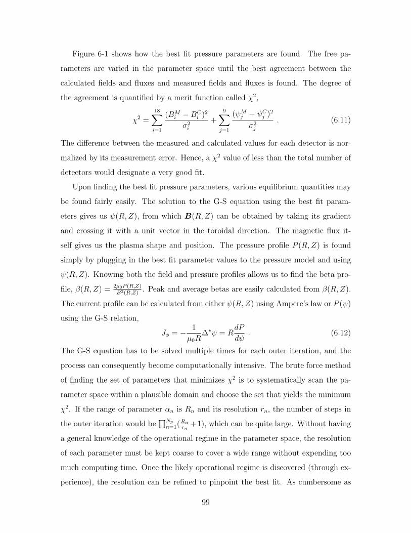
Figure 6-1 shows how the best fit pressure parameters are found. The free pa-
rameters are varied in the parameter space until the best agreement between the
calculated fields and fluxes and measured fields and fluxes is found. The degree of
the agreement is quantified by a merit function called χ2,
χ2 =18∑i=1
(BMi −BC
i )2
σ2i
+9∑j=1
(ψMj − ψCj )2
σ2j
. (6.11)
The difference between the measured and calculated values for each detector is nor-
malized by its measurement error. Hence, a χ2 value of less than the total number of
detectors would designate a very good fit.
Upon finding the best fit pressure parameters, various equilibrium quantities may
be found fairly easily. The solution to the G-S equation using the best fit param-
eters gives us ψ(R,Z), from which B(R,Z) can be obtained by taking its gradient
and crossing it with a unit vector in the toroidal direction. The magnetic flux it-
self gives us the plasma shape and position. The pressure profile P (R,Z) is found
simply by plugging in the best fit parameter values to the pressure model and using
ψ(R,Z). Knowing both the field and pressure profiles allows us to find the beta pro-
file, β(R,Z) = 2µ0P (R,Z)B2(R,Z)
. Peak and average betas are easily calculated from β(R,Z).
The current profile can be calculated from either ψ(R,Z) using Ampere’s law or P (ψ)
using the G-S relation,
Jφ = − 1
µ0R∆∗ψ = R
dP
dψ. (6.12)
The G-S equation has to be solved multiple times for each outer iteration, and the
process can consequently become computationally intensive. The brute force method
of finding the set of parameters that minimizes χ2 is to systematically scan the pa-
rameter space within a plausible domain and choose the set that yields the minimum
χ2. If the range of parameter αn is Rn and its resolution rn, the number of steps in
the outer iteration would be∏Np
n=1(Rn
rn+1), which can be quite large. Without having
a general knowledge of the operational regime in the parameter space, the resolution
of each parameter must be kept coarse to cover a wide range without expending too
much computing time. Once the likely operational regime is discovered (through ex-
perience), the resolution can be refined to pinpoint the best fit. As cumbersome as
99
this method is, it is very useful in grasping the trend of χ2 as different parameters
are varied. Because χ2 is evaluated at every point on the domain grid, defined by
the range and resolution of each parameter, the χ2 hypersurface is mapped out in
an (Np + 1)-dimensional space. This kind of mapping is very helpful in studying the
characteristics of a pressure model.
A more sophisticated approach to finding the minimum χ2 is to use some kind
of an intelligent minimization scheme. There are a myriad of such schemes, like the
singular value decomposition method [25, 40], grid search method, and gradient search
method [2], and each method has its advantages and disadvantages. A particularly
easy routine to implement with the existing reconstruction code is called the downhill
simplex method, otherwise known as the amoeba method [40]. The amoeba method
has the advantage that it does not require the computation of the derivatives, but
it requires more function evaluations than some of the other methods. As with all
intelligent minimization schemes, this method is susceptible to converging to a local
minimum. This is especially true if the initial starting point is chosen close to such
a minimum and the scope of the search is limited to a small neighborhood around
it. The problem can usually be overcome by widening the domain of the search. For
this and other reasons, it is a good idea to perform some reconstructions using the
brute force method to get a feel for the behavior of χ2, especially when a new pressure
model is used or when a different operational regime is reached.
6.2.2 Vacuum Reconstruction
As seen in the previous subsection, the full reconstruction method can become cum-
bersome and computationally demanding. LDX has a unique magnetic field structure
that allows us to forgo the proper computation and obtain accurate equilibrium results
using vacuum field calculations [32]. This fortuitous situation is a direct consequence
of the plasma current structure in the dipole geometry. Not only is the plasma current
in the same direction as the dipole current, its magnitude is typically less than 0.5 %
of the dipole current magnitude. Consequently, the magnetic flux in the presence of
the plasma closely resembles the vacuum flux. In fact, for a plasma current of about
100
3.5 kA with a reasonable distribution and a dipole current of about 1.2 MA, the dif-
ference between the plasma and vacuum fluxes is less than 3 % at every point. This
allows us to forgo the G-S equation and simply use the vacuum flux to calculate the
plasma current, from which the fields and fluxes at the sensor locations are calculated
to find the best fit,
Jφ = RdP
dψ≈ R
dP
dψvac. (6.13)
Although the vacuum approximation brings about a small inconsistency since ∆∗ψvac =
0, it is legitimate as long as the plasma current does not exceed about 1 % of the
dipole current.
The procedure to find the best fit pressure parameters now becomes very compu-
tationally facile, involving only integrals and derivatives. Once the vacuum field is
found and pressure model chosen, the free parameters are varied to find the minimum
χ2. The algorithm looks identical to Figure 6-1 except for substituting “solve G-S
eqn” with “evaluate R dPdψvac and use Ampere’s law to calculate B and ψ.” Being able
to use the vacuum approximation in reconstructing LDX plasmas gives us the ability
to reconstruct plasmas in real time without having to go through a fancy code like
rtEFIT [7, 12].
6.3 Pressure models
The pressure models are the crux of the reconstruction process. They incorporate
the physics of plasma transport and wave absorption. Although plausible forms of
pressure models for a given confinement device may be found by doing extensive
transport studies, more often than not some set of basis functions is just chosen .
By definition, basis functions span the function space, so any set of basis functions
can technically represent any pressure profile. What distinguishes a good choice of
basis functions from a bad choice is the number of terms required to adequately
represent the pressure profile. For example, if the pressure profile contains a decaying
asymptote, the set of polynomials would require more terms than the set of hyperbolic
functions. Amongst other reasons, having too many number of terms should be
101
avoided since it can under-constrain the minimization process to the point where
there will be multiple minima of which merit cannot be distinguished. It is therefore
wise to carefully choose the pressure model based on the expected shape and form of
the pressure profile.
6.3.1 Isotropic models
Pressure models can be isotropic or anisotropic. Obviously, isotropic models are
simpler because there is no distinction between P⊥ and P‖. Three isotropic models
that have been used in reconstructing LDX plasmas are discussed in this section.
The first model called the DipoleEq profile is the one that was introduced in Ch.
3 and is the most frequently used,
P (ψ;ψpeak, Pedge, g) =
Pedge
[Vedge
V (ψ)
]gfor ψ > ψpeak
Pedge
[Vedge
V (ψ)
]gsin2
[π2
(ψ
ψpeak
)2]
for ψ < ψpeak. (6.14)
Having discussed the marginal MHD stability criterion in Ch. 5, it is quite easy to
see why a pressure model in the above form is suitable to describe LDX plasmas.
The marginal criterion sets the maximum slope of the pressure profile according to
PV γ = PedgeVγedge between the pressure peak and the wall (ψ > ψpeak). If we assume
that the plasma is heated quickly enough that it is always in the vicinity of the
marginal limit, then the profile should fit the model quite well. Even if the plasma
is not close to the marginal limit, the slope parameter g is left free to be constrained
by magnetic measurements so that the profile can nevertheless be fitted to the model
satisfactorily. The region between the floating coil edge and the pressure peak is
modeled so that the profile rises sinusoidally from the coil edge to the peak and
continuously transitions to the profile on the other side of the peak. One noticeable
flaw of this model is that the first derivative of the profile is discontinuous at the
pressure peak. This makes the profile unrealistically cuspy at the peak, potentially
giving spurious peak and average beta values. However, the model correctly gives a
finite pressure at both the inner limiter (the floating coil) and outer limiter (the vessel
wall). In fact the MHD stability of LDX plasmas depends on the fact that there is
102
finite pressure at the outer wall.
One may ask if this pressure model based on the MHD stability criterion is still
suitable for LDX plasmas with a significant fraction of hot electrons. As was discussed
in Ch. 5, hot electrons are not subject to the MHD criterion. Hot electrons will still
adhere to profile shapes that are generally consistent with those given by the model.
It is also of interest to see by how much hot electrons can exceed the MHD gradient
limit by finding their best fit g parameter.
The second isotropic model, which we call the “no edge pressure profile,” is very
simple and has been used only once for comparison purposes,
P (ψ; a, b, g) =a
V g(ψmax − ψ)b(ψ − ψmin)
c . (6.15)
The model has the familiar V −g factor, but there also are two factors in the numerator
that make the pressure go to zero at the inner and outer limiters. A closer inspection of
the form of the model reveals that it is actually a polynomial model of degree 4g+b+c
with repeated free parameters (i.e. the coefficients of different terms depend on each
other). The coefficients of the polynomial are set up so that the pressure vanishes at
the limiters. The unphysicality of the vanishing pressure at the edges is somewhat
compensated by the more physically realistic continuity of the first derivative at the
pressure peak.
The third and final isotropic model that has been used is called the “smooth
adiabatic profile.” This model is an attempt to retain the stability dependent profile
of the first model while eradicating its unphysical cusp at the pressure peak,
P (ψ;ψpeak, Ppeak, g) = Ppeak
(ψ − ψf−coil
ψpeak − ψf−coil
)α (ψ
ψpeak
)4g
, (6.16)
where α ≡ 4g(|ψf−coil
ψpeak| − 1). The stability dependent V −g factor is hidden in the ψ4g
factor. Although this model still makes the pressure vanish at the inner limiter, the
smoothness of the pressure peak potentially makes us to believe it the most realistic
of all.
103
6.3.2 An anisotropic model
Plasmas in LDX are heated by electron cyclotron resonance heating (ECRH), as men-
tioned in Ch. 1. Because ECRH preferentially accelerates electrons in the direction
perpendicular to the field lines, they naturally gain more kinetic energy in the per-
pendicular direction than in the parallel direction. This leads to the plasma having
an anisotropic pressure with P⊥ > P‖. To capture the physics of the anisotropic
pressure, a pressure model that incorporates the anisotropy must be employed in the
reconstruction process. Before we can discuss a specific anisotropic pressure model,
MHD equilibrium must be revisited to understand how the current-pressure relation-
ship changes due to the anisotropy. The treatment of anisotropic equilibria is given
in many books, including the one by Hazeltine and Meiss [17].
The only relevant equation that is altered in the MHD model to account for the
anisotropy is the momentum equation,
∇P = J ×B =⇒ ∇ · P = J ×B , (6.17)
where P is the pressure tensor. With this modification, the current becomes,
J =B ×∇ · P
B2=
B ×∇P⊥B2
+B × κ
B2(P‖ − P⊥) , (6.18)
where κ = b · ∇b is the magnetic curvature. When compared to the isotropic case,
an extra term that depends on the anisotropy of the pressure is present. In the low
beta (or vacuum) approximation, Eq. 6.18 can be rewritten as [35],
Jφ = R∂P⊥∂ψ
+R(P‖ − P⊥)∂ lnB
∂ψ, (6.19)
where the chain rule ∂∂ψ≡ |∇ψ|−2∇ψ · ∇ and the vacuum curvature approximation
κ ≈ ∇⊥BB
have been used. Notice that P⊥ > P‖ everywhere in the ECRH heated
plasma and ∂ lnB∂ψ
> 0 outside the pressure peak. The second term of Jφ is therefore
negative. This is a significant result because for a given measurement of Jφ, the
anisotropic model predicts a larger ∂P⊥∂ψ
than the isotropic model. Accordingly, the
anisotropic model gives a higher beta for a given measured current. To find an
anisotropic equilibrium, one needs only to apply the desired pressure model to the
above equation.
104
The anisotropic model that has been developed for anisotropic pressure reconstruc-
tion is a modification of the “smooth adiabatic profile.”[36] Now that the pressure is
anisotropic, it is not only a function of ψ but is a function of B as well,
P⊥ = G(ψ;ψpeak, Ppeak, g)H[B(ψ, χ); p] (6.20)
G(ψ) ≡ Ppeak
(ψ − ψf−coil
ψpeak − ψf−coil
)α (ψ
ψpeak
)4g
(6.21)
H(B) ≡(B0
B
)2p
. (6.22)
This model was originally developed by Connor and Hastie [5, 22, 45] and incorpo-
rates the anisotropy parameter p ≡ P⊥−P‖2P‖
. In the model, χ is the magnetic scalar
potential (∇χ = B) which serves as the “angular” component of the magnetic coor-
dinate system, and B0 ≡ B(ψ, χ = 0) is the minimum field strength on a field-line.
The function G(ψ) is precisely the “smooth adiabatic profile,” and the anisotropy is
incorporated by multiplying this by a function H(B) that depends on B and p only.
The H function’s role is to progressively localize the pressure to the midplane as it
becomes more anisotropic. Physically, the electrons become more deeply trapped and
confined near the midplane as their pressure becomes more anisotropic and the ratio
v⊥v‖
increases. The anisotropy parameter p generally varies in space, but it is kept
spatially uniform in the Connor-Hastie model to make the analysis more tractable.
6.4 Sensitivity of the magnetic measurements to
the lowest order moment
6.4.1 Evidence
Magnetic field in a current-free region can be written as a gradient of the scalar
potential [38],
B = −∇η , (6.23)
where η is the magnetic scalar potential. Furthermore, the scalar potential can be
expanded as a sum of Legendre polynomials, or equivalently, spherical harmonics as
105
follows:
η =∑l
Alr−(l+1)Yl0(θ) . (6.24)
The 2l-pole moment is represented by Al, and r−(l+1) gives its radial dependence (in
spherical coordinates). It is evident that the higher order moments quickly vanish as
one moves away from the current source. Because A0 = 0 (no monopole), the dipole
moment dominates at large distances.
As mentioned earlier in the chapter, equilibrium reconstruction is heavily depen-
dent on the characteristics of the machine. One unwanted but inevitable feature of
the magnetic diagnostics in LDX is that the external sensors are located far away
from the plasma. The large vacuum chamber is designed to confine a relatively small
plasma, so the external sensors are necessarily distant from the current source. In the
context of the previous paragraph, this means that the sensors may not have sufficient
sensitivity to measure anything beyond the dipole moment of the plasma current.
In addition to the sensors being far from the plasma, the measurement of the next
lowest moment—the quadrupole moment—is dominated by the contribution from the
floating coil. As discussed earlier, the Bp coils and flux loops pick up the sum of the
plasma current and the floating coil current decrease. Because the plasma current
and the current decrease are in opposite directions, it contributes significantly to
the total quadrupole moment. In conjunction with the far distance of the detectors,
measuring the plasma quadrupole moment becomes an arduous, if not impossible,
task. Capturing the higher order moments is even more difficult.
One key evidence that the magnetic sensors are sensitive only to the plasma dipole
moment comes from studying the results from the DFIT code. Given a plasma shot,
DFIT finds the best fit magnitudes and locations of the two current filaments. Figure
6-2 shows a contour plot of chi-squared as a function of the current magnitudes of the
two filaments at fixed positions for shot 50318014. The black dot designates where
the minimum chi-squared contour (not shown) is. The blue line that intersects the
dot is a contour of a fixed dipole moment. The significance of this plot is that the
contour of the fixed dipole moment approximately overlays the contour of minimum
106
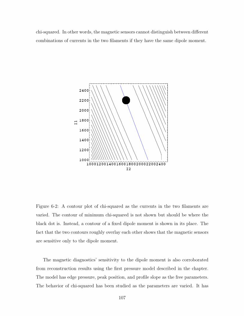
chi-squared. In other words, the magnetic sensors cannot distinguish between different
combinations of currents in the two filaments if they have the same dipole moment.
Figure 6-2: A contour plot of chi-squared as the currents in the two filaments are
varied. The contour of minimum chi-squared is not shown but should be where the
black dot is. Instead, a contour of a fixed dipole moment is shown in its place. The
fact that the two contours roughly overlay each other shows that the magnetic sensors
are sensitive only to the dipole moment.
The magnetic diagnostics’ sensitivity to the dipole moment is also corroborated
from reconstruction results using the first pressure model described in the chapter.
The model has edge pressure, peak position, and profile slope as the free parameters.
The behavior of chi-squared has been studied as the parameters are varied. It has
107
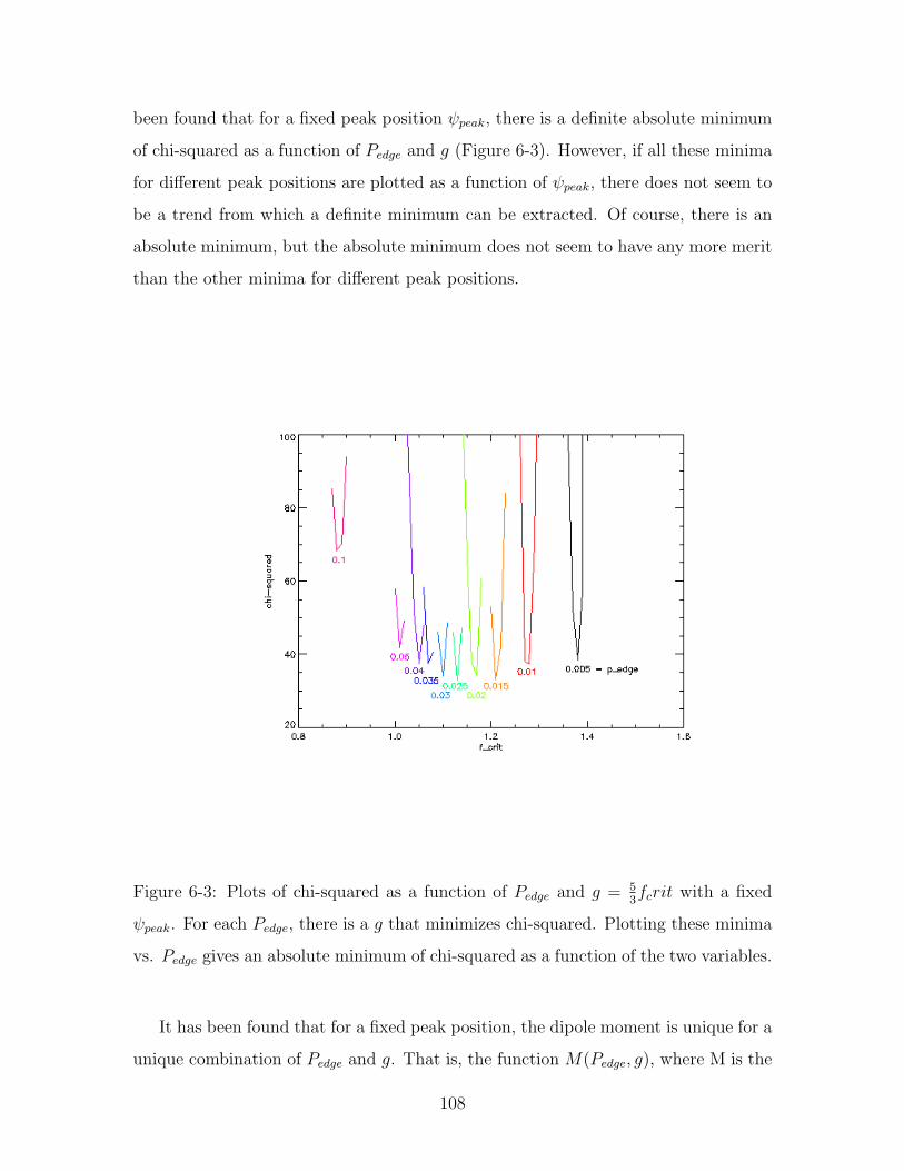
been found that for a fixed peak position ψpeak, there is a definite absolute minimum
of chi-squared as a function of Pedge and g (Figure 6-3). However, if all these minima
for different peak positions are plotted as a function of ψpeak, there does not seem to
be a trend from which a definite minimum can be extracted. Of course, there is an
absolute minimum, but the absolute minimum does not seem to have any more merit
than the other minima for different peak positions.
Figure 6-3: Plots of chi-squared as a function of Pedge and g = 53fcrit with a fixed
ψpeak. For each Pedge, there is a g that minimizes chi-squared. Plotting these minima
vs. Pedge gives an absolute minimum of chi-squared as a function of the two variables.
It has been found that for a fixed peak position, the dipole moment is unique for a
unique combination of Pedge and g. That is, the function M(Pedge, g), where M is the
108
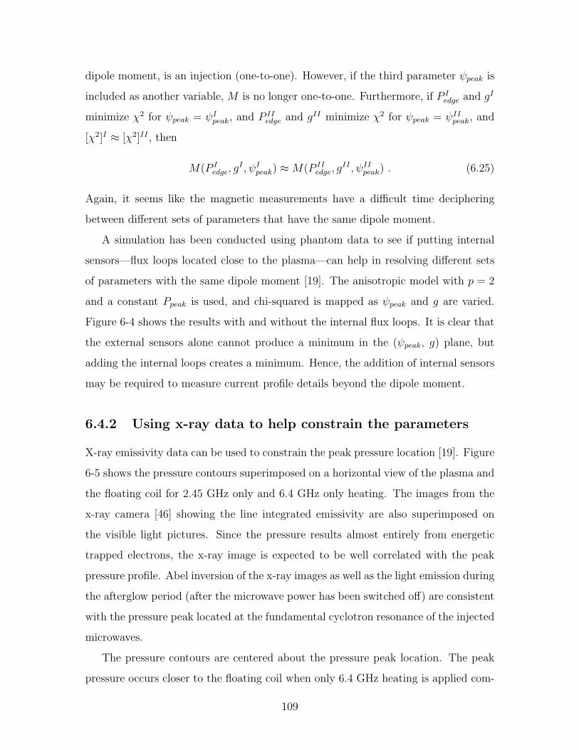
dipole moment, is an injection (one-to-one). However, if the third parameter ψpeak is
included as another variable, M is no longer one-to-one. Furthermore, if P Iedge and gI
minimize χ2 for ψpeak = ψIpeak, and P IIedge and gII minimize χ2 for ψpeak = ψIIpeak, and
[χ2]I ≈ [χ2]II , then
M(P Iedge, g
I , ψIpeak) ≈M(P IIedge, g
II , ψIIpeak) . (6.25)
Again, it seems like the magnetic measurements have a difficult time deciphering
between different sets of parameters that have the same dipole moment.
A simulation has been conducted using phantom data to see if putting internal
sensors—flux loops located close to the plasma—can help in resolving different sets
of parameters with the same dipole moment [19]. The anisotropic model with p = 2
and a constant Ppeak is used, and chi-squared is mapped as ψpeak and g are varied.
Figure 6-4 shows the results with and without the internal flux loops. It is clear that
the external sensors alone cannot produce a minimum in the (ψpeak, g) plane, but
adding the internal loops creates a minimum. Hence, the addition of internal sensors
may be required to measure current profile details beyond the dipole moment.
6.4.2 Using x-ray data to help constrain the parameters
X-ray emissivity data can be used to constrain the peak pressure location [19]. Figure
6-5 shows the pressure contours superimposed on a horizontal view of the plasma and
the floating coil for 2.45 GHz only and 6.4 GHz only heating. The images from the
x-ray camera [46] showing the line integrated emissivity are also superimposed on
the visible light pictures. Since the pressure results almost entirely from energetic
trapped electrons, the x-ray image is expected to be well correlated with the peak
pressure profile. Abel inversion of the x-ray images as well as the light emission during
the afterglow period (after the microwave power has been switched off) are consistent
with the pressure peak located at the fundamental cyclotron resonance of the injected
microwaves.
The pressure contours are centered about the pressure peak location. The peak
pressure occurs closer to the floating coil when only 6.4 GHz heating is applied com-
109
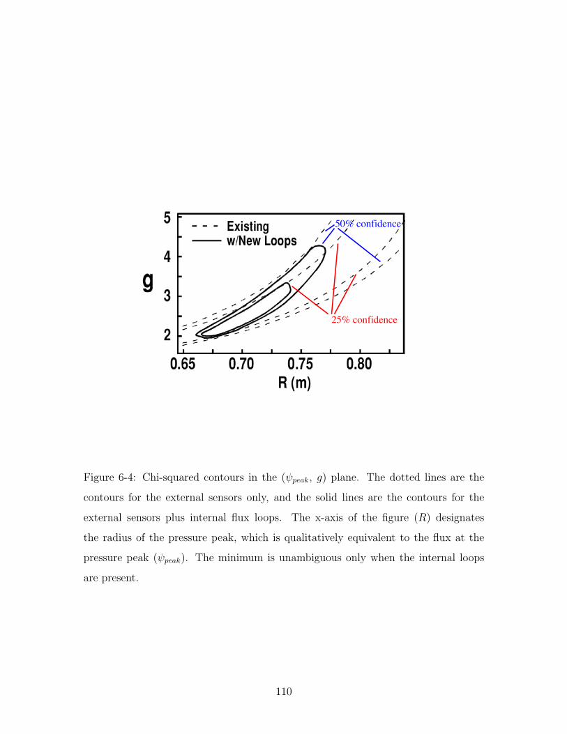
25% confidence
50% confidence
Figure 6-4: Chi-squared contours in the (ψpeak, g) plane. The dotted lines are the
contours for the external sensors only, and the solid lines are the contours for the
external sensors plus internal flux loops. The x-axis of the figure (R) designates
the radius of the pressure peak, which is qualitatively equivalent to the flux at the
pressure peak (ψpeak). The minimum is unambiguous only when the internal loops
are present.
110
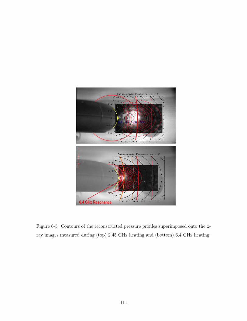
Figure 6-5: Contours of the reconstructed pressure profiles superimposed onto the x-
ray images measured during (top) 2.45 GHz heating and (bottom) 6.4 GHz heating.
111
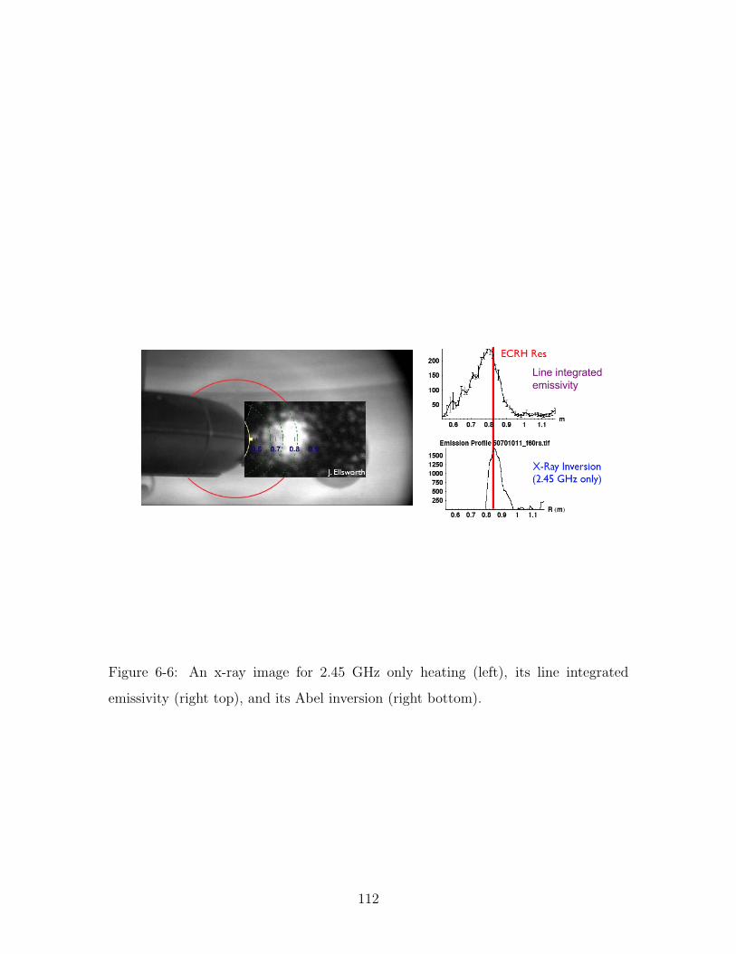
Line integratedemissivity
Figure 6-6: An x-ray image for 2.45 GHz only heating (left), its line integrated
emissivity (right top), and its Abel inversion (right bottom).
112
pared to when only 2.45 GHz is used (Figure 6-6). When the two frequencies are
combined, the pressure peaks in between the two fundamental resonance locations.
Since the pressure model constrains the plasma to have a single pressure peak, it is
unclear whether there is a single peak in between the two resonance locations or a
local peak at each location. It is interesting to note that χ2 for the combined heating
case is about twice that for the single frequency heating case. It may be that the
single peak model is inadequate for describing an LDX plasma heated by more than
one frequency.
The effect of anisotropic pressure is also evident in these contour pictures. The
pressure contours do not coincide with flux contours, and the pressure becomes more
localized to the midplane as it becomes more anisotropic. This is in stark contrast
to an isotropic pressure, whose magnitude is independent of the magnetic angular
coordinate χ.
Once the peak pressure location is constrained by the Abel inverted x-ray emissiv-
ity, chi-squared can be minimized without any equivocality. Equivalently, the plasma
current can be resolved beyond its dipole moment by deducing it from the pressure
using MHD relations. Using kinetic data, such as temperature and pressure measure-
ments, in conjunction with magnetic data is a common practice in better constraining
pressure parameters.
113

114
Chapter 7
Typical Shots
This chapter describes the typical LDX plasma shots. Although every shot is unique
to some degree, there are a lot of commonalities that are shared amongst all the shots.
Specifically, most of the shots have three distinct plasma regimes that are clearly
distinguished by the measurements from different diagnostics. The three regimes will
be described in detail throughout the chapter. Also, magnetic data will be used to
reconstruct some shots using the different pressure models described in the previous
chapter.
7.1 Characterization of the three regimes
A typical LDX discharge is shown in Figure 7-1. In this shot, 2.5 kW each of 2.45
and 6.4 GHz microwaves is used to heat the plasma. The figure shows measurements
from some of the key diagnostics installed on the machine. The discharge is divided
into three time intervals, each interval corresponding to a different plasma regime [9].
The first time period from 0 to about 0.25 sec is called the low density regime. The
middle interval from about 0.25 to 4 sec is referred to as the high beta regime. The
final interval from 4 sec to infinity is the after-glow regime. Each of these regimes
will be explained in the following subsections.
115
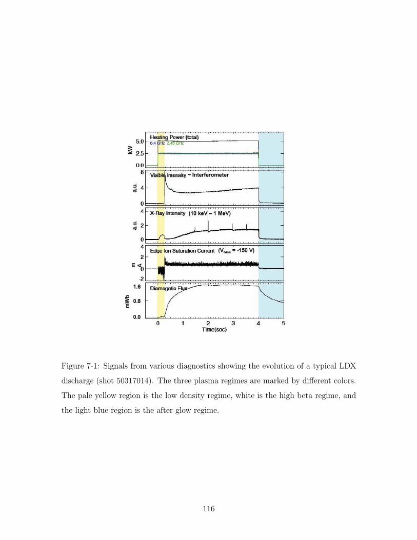
Figure 7-1: Signals from various diagnostics showing the evolution of a typical LDX
discharge (shot 50317014). The three plasma regimes are marked by different colors.
The pale yellow region is the low density regime, white is the high beta regime, and
the light blue region is the after-glow regime.
116
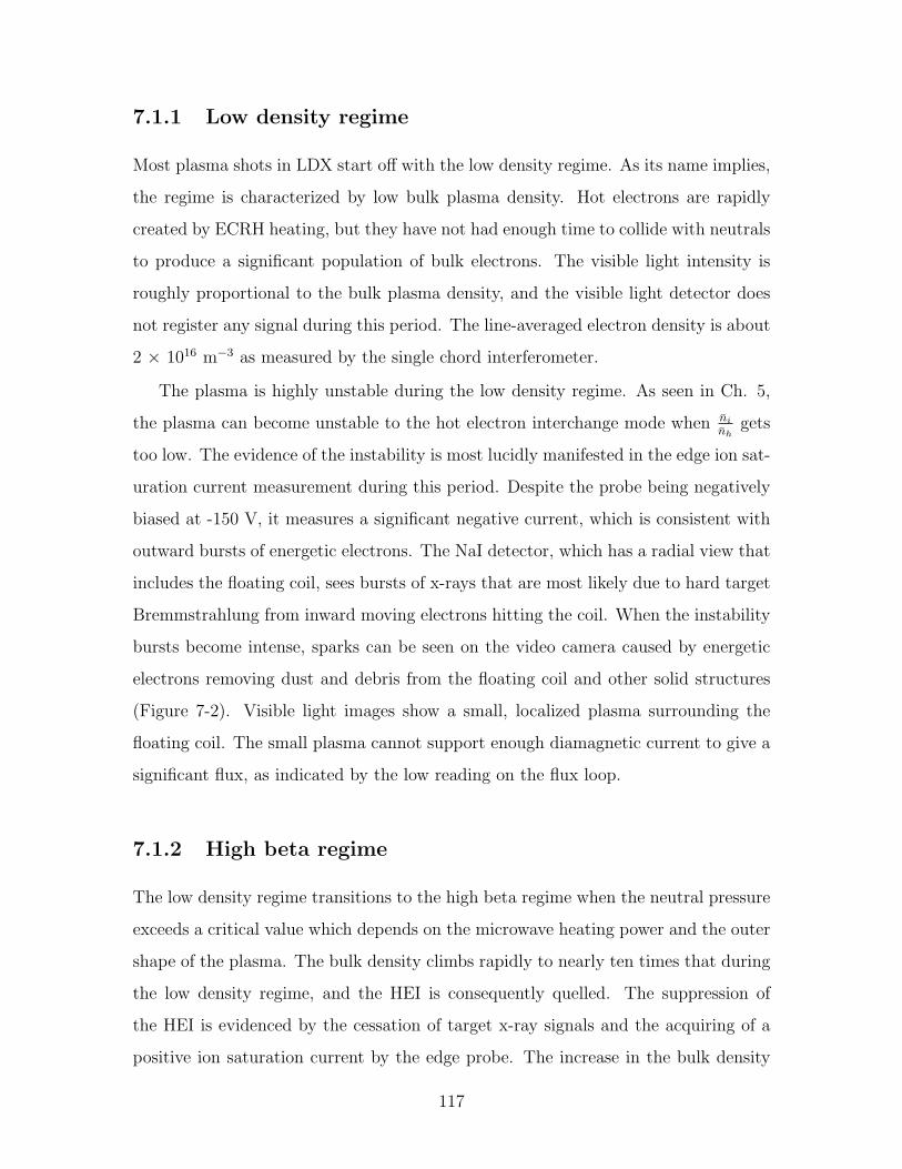
7.1.1 Low density regime
Most plasma shots in LDX start off with the low density regime. As its name implies,
the regime is characterized by low bulk plasma density. Hot electrons are rapidly
created by ECRH heating, but they have not had enough time to collide with neutrals
to produce a significant population of bulk electrons. The visible light intensity is
roughly proportional to the bulk plasma density, and the visible light detector does
not register any signal during this period. The line-averaged electron density is about
2 × 10¹⁶ m−3 as measured by the single chord interferometer.
The plasma is highly unstable during the low density regime. As seen in Ch. 5,
the plasma can become unstable to the hot electron interchange mode when ni
nhgets
too low. The evidence of the instability is most lucidly manifested in the edge ion sat-
uration current measurement during this period. Despite the probe being negatively
biased at -150 V, it measures a significant negative current, which is consistent with
outward bursts of energetic electrons. The NaI detector, which has a radial view that
includes the floating coil, sees bursts of x-rays that are most likely due to hard target
Bremmstrahlung from inward moving electrons hitting the coil. When the instability
bursts become intense, sparks can be seen on the video camera caused by energetic
electrons removing dust and debris from the floating coil and other solid structures
(Figure 7-2). Visible light images show a small, localized plasma surrounding the
floating coil. The small plasma cannot support enough diamagnetic current to give a
significant flux, as indicated by the low reading on the flux loop.
7.1.2 High beta regime
The low density regime transitions to the high beta regime when the neutral pressure
exceeds a critical value which depends on the microwave heating power and the outer
shape of the plasma. The bulk density climbs rapidly to nearly ten times that during
the low density regime, and the HEI is consequently quelled. The suppression of
the HEI is evidenced by the cessation of target x-ray signals and the acquiring of a
positive ion saturation current by the edge probe. The increase in the bulk density
117
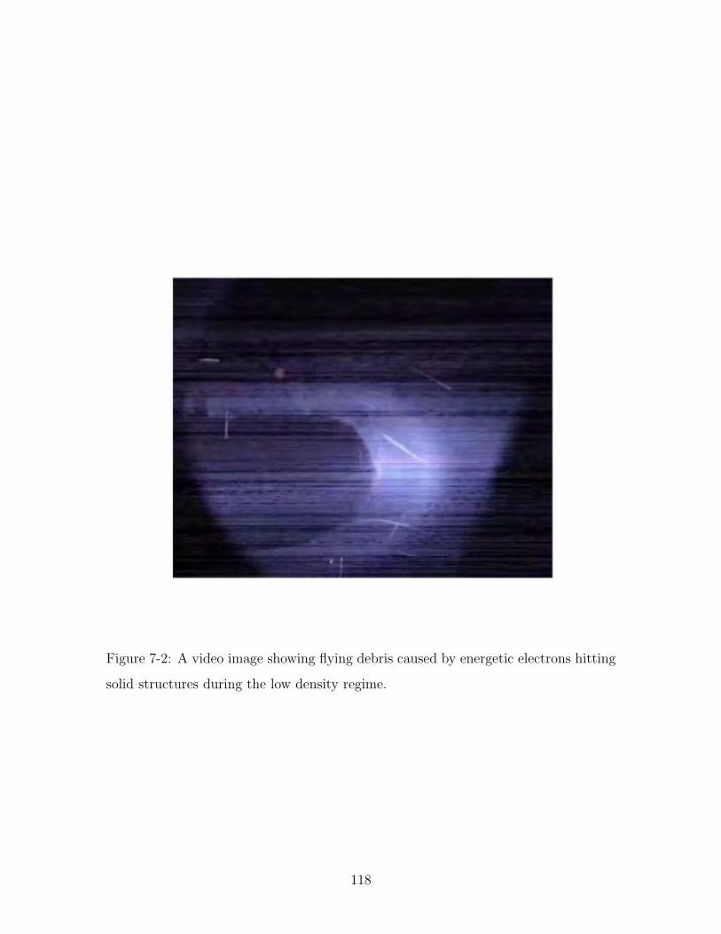
Figure 7-2: A video image showing flying debris caused by energetic electrons hitting
solid structures during the low density regime.
118
allows the hot electron population to build up as well. The DFIT reconstruction
shows that the current centroid moves outward (Figure 7-3) as the plasma transitions
from the low density to high beta regime, indicating a growth in the plasma volume.
As shown by the flux loop signal, there is a rapid increase in the diamagnetism, which
is a rough measure of the pressure and beta. Broad low frequency fluctuations can
be seen on the Mirnov and edge probes throughout the period indicating some sort
of MHD activities (Figure 7-4).
Figure 7-3: The DFIT code result showing the current centroid moving outwards as
the plasma transitions from the low density to high beta regime.
Although the high beta regime is relatively quiescent, periodic relaxation events
are observed a few times a second on the flux loop measurement. The relaxation
events consist of beta dumps accompanied by spikes in the x-ray signal. There usually
119
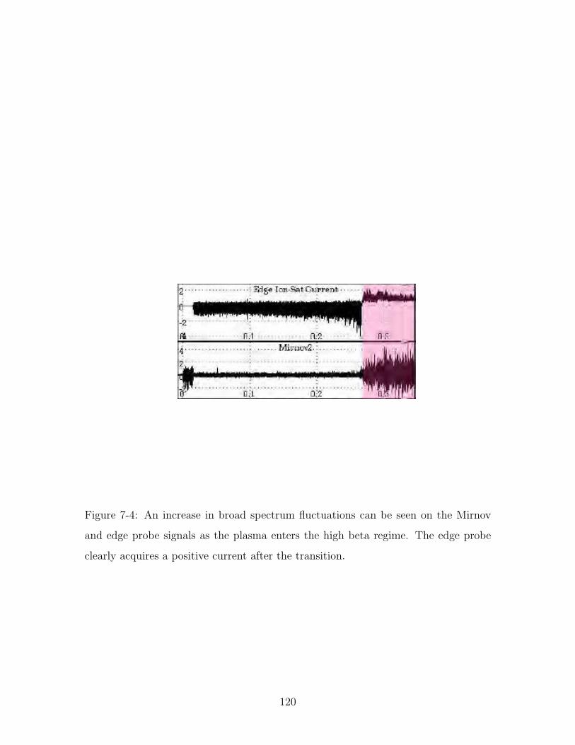
Figure 7-4: An increase in broad spectrum fluctuations can be seen on the Mirnov
and edge probe signals as the plasma enters the high beta regime. The edge probe
clearly acquires a positive current after the transition.
120
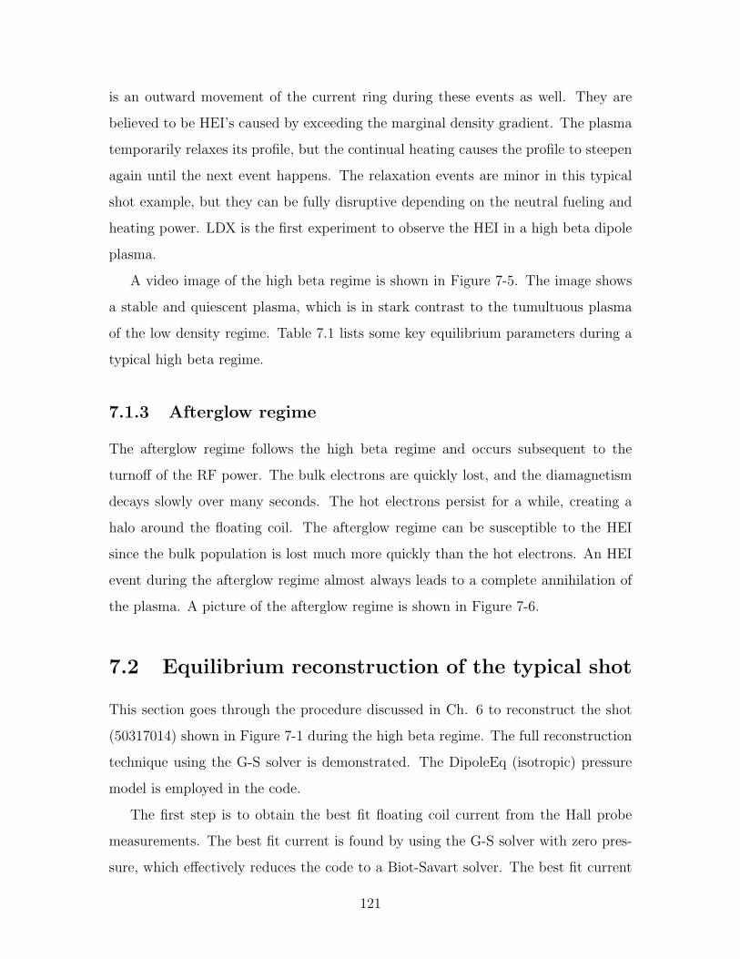
is an outward movement of the current ring during these events as well. They are
believed to be HEI’s caused by exceeding the marginal density gradient. The plasma
temporarily relaxes its profile, but the continual heating causes the profile to steepen
again until the next event happens. The relaxation events are minor in this typical
shot example, but they can be fully disruptive depending on the neutral fueling and
heating power. LDX is the first experiment to observe the HEI in a high beta dipole
plasma.
A video image of the high beta regime is shown in Figure 7-5. The image shows
a stable and quiescent plasma, which is in stark contrast to the tumultuous plasma
of the low density regime. Table 7.1 lists some key equilibrium parameters during a
typical high beta regime.
7.1.3 Afterglow regime
The afterglow regime follows the high beta regime and occurs subsequent to the
turnoff of the RF power. The bulk electrons are quickly lost, and the diamagnetism
decays slowly over many seconds. The hot electrons persist for a while, creating a
halo around the floating coil. The afterglow regime can be susceptible to the HEI
since the bulk population is lost much more quickly than the hot electrons. An HEI
event during the afterglow regime almost always leads to a complete annihilation of
the plasma. A picture of the afterglow regime is shown in Figure 7-6.
7.2 Equilibrium reconstruction of the typical shot
This section goes through the procedure discussed in Ch. 6 to reconstruct the shot
(50317014) shown in Figure 7-1 during the high beta regime. The full reconstruction
technique using the G-S solver is demonstrated. The DipoleEq (isotropic) pressure
model is employed in the code.
The first step is to obtain the best fit floating coil current from the Hall probe
measurements. The best fit current is found by using the G-S solver with zero pres-
sure, which effectively reduces the code to a Biot-Savart solver. The best fit current
121
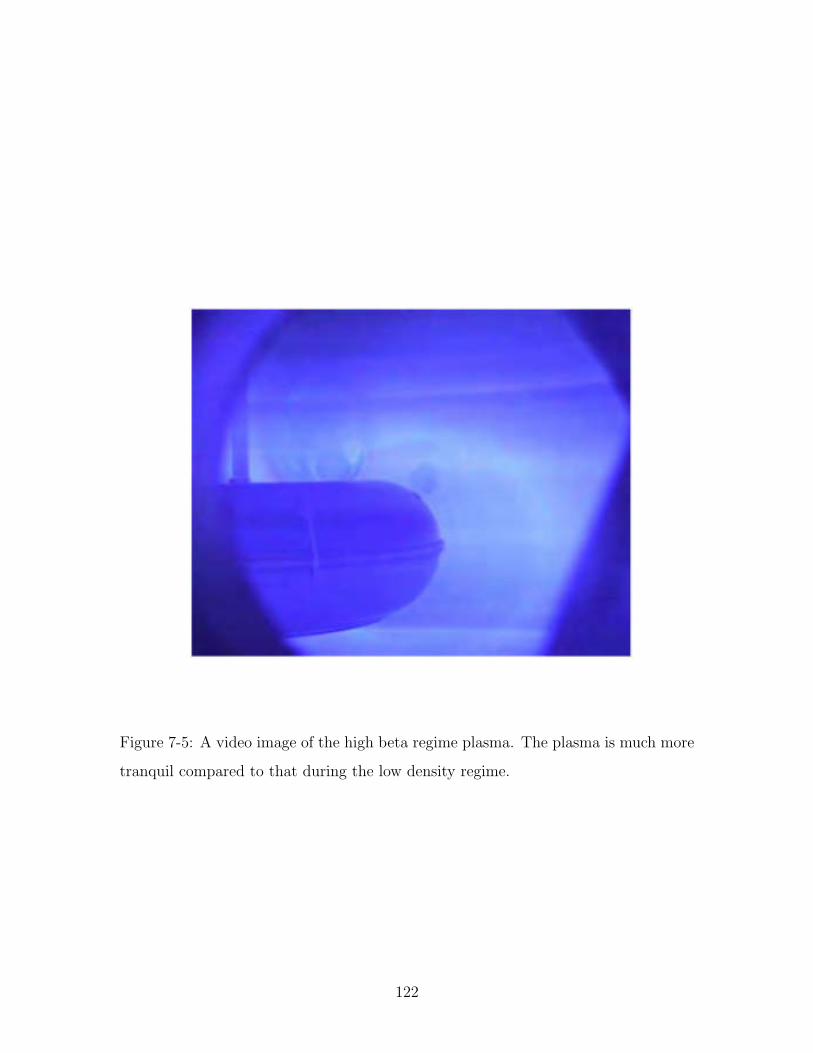
Figure 7-5: A video image of the high beta regime plasma. The plasma is much more
tranquil compared to that during the low density regime.
122
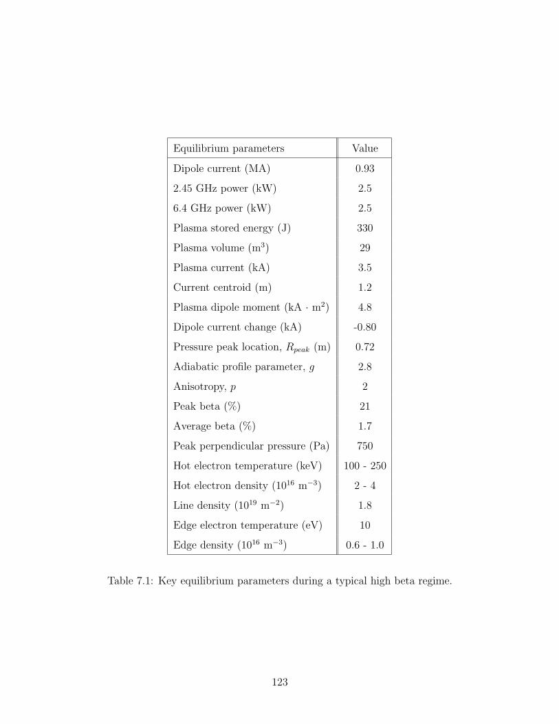
Equilibrium parameters Value
Dipole current (MA) 0.93
2.45 GHz power (kW) 2.5
6.4 GHz power (kW) 2.5
Plasma stored energy (J) 330
Plasma volume (m3) 29
Plasma current (kA) 3.5
Current centroid (m) 1.2
Plasma dipole moment (kA · m2) 4.8
Dipole current change (kA) -0.80
Pressure peak location, Rpeak (m) 0.72
Adiabatic profile parameter, g 2.8
Anisotropy, p 2
Peak beta (%) 21
Average beta (%) 1.7
Peak perpendicular pressure (Pa) 750
Hot electron temperature (keV) 100 - 250
Hot electron density (1016 m−3) 2 - 4
Line density (1019 m−2) 1.8
Edge electron temperature (eV) 10
Edge density (1016 m−3) 0.6 - 1.0
Table 7.1: Key equilibrium parameters during a typical high beta regime.
123
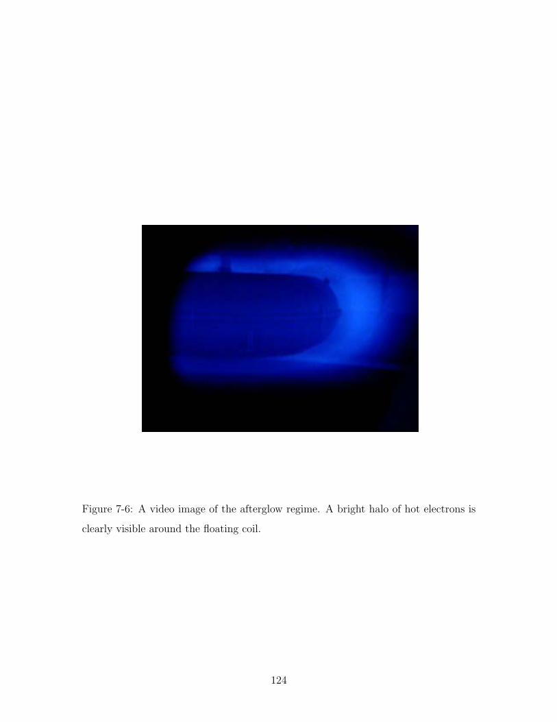
Figure 7-6: A video image of the afterglow regime. A bright halo of hot electrons is
clearly visible around the floating coil.
124
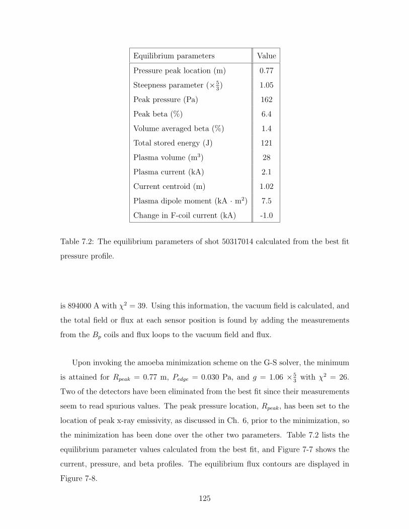
Equilibrium parameters Value
Pressure peak location (m) 0.77
Steepness parameter (×53) 1.05
Peak pressure (Pa) 162
Peak beta (%) 6.4
Volume averaged beta (%) 1.4
Total stored energy (J) 121
Plasma volume (m3) 28
Plasma current (kA) 2.1
Current centroid (m) 1.02
Plasma dipole moment (kA · m2) 7.5
Change in F-coil current (kA) -1.0
Table 7.2: The equilibrium parameters of shot 50317014 calculated from the best fit
pressure profile.
is 894000 A with χ2 = 39. Using this information, the vacuum field is calculated, and
the total field or flux at each sensor position is found by adding the measurements
from the Bp coils and flux loops to the vacuum field and flux.
Upon invoking the amoeba minimization scheme on the G-S solver, the minimum
is attained for Rpeak = 0.77 m, Pedge = 0.030 Pa, and g = 1.06 ×53
with χ2 = 26.
Two of the detectors have been eliminated from the best fit since their measurements
seem to read spurious values. The peak pressure location, Rpeak, has been set to the
location of peak x-ray emissivity, as discussed in Ch. 6, prior to the minimization, so
the minimization has been done over the other two parameters. Table 7.2 lists the
equilibrium parameter values calculated from the best fit, and Figure 7-7 shows the
current, pressure, and beta profiles. The equilibrium flux contours are displayed in
Figure 7-8.
125
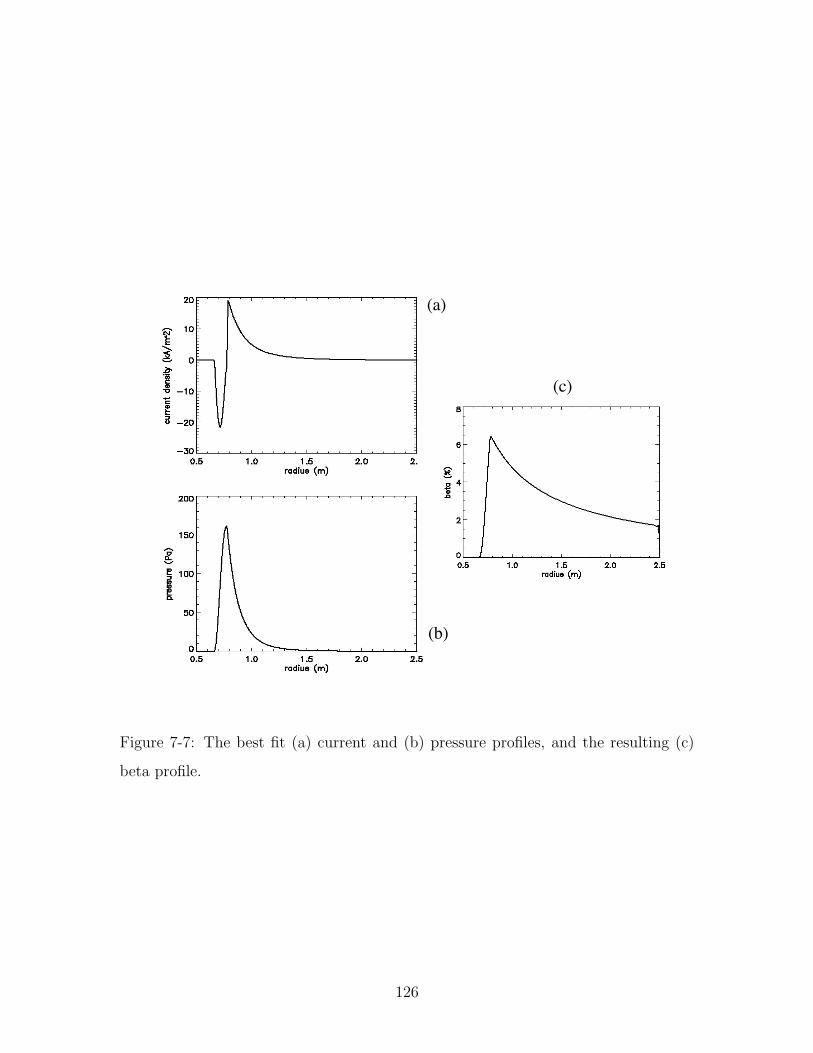
(a)
(b)
(c)
Figure 7-7: The best fit (a) current and (b) pressure profiles, and the resulting (c)
beta profile.
126
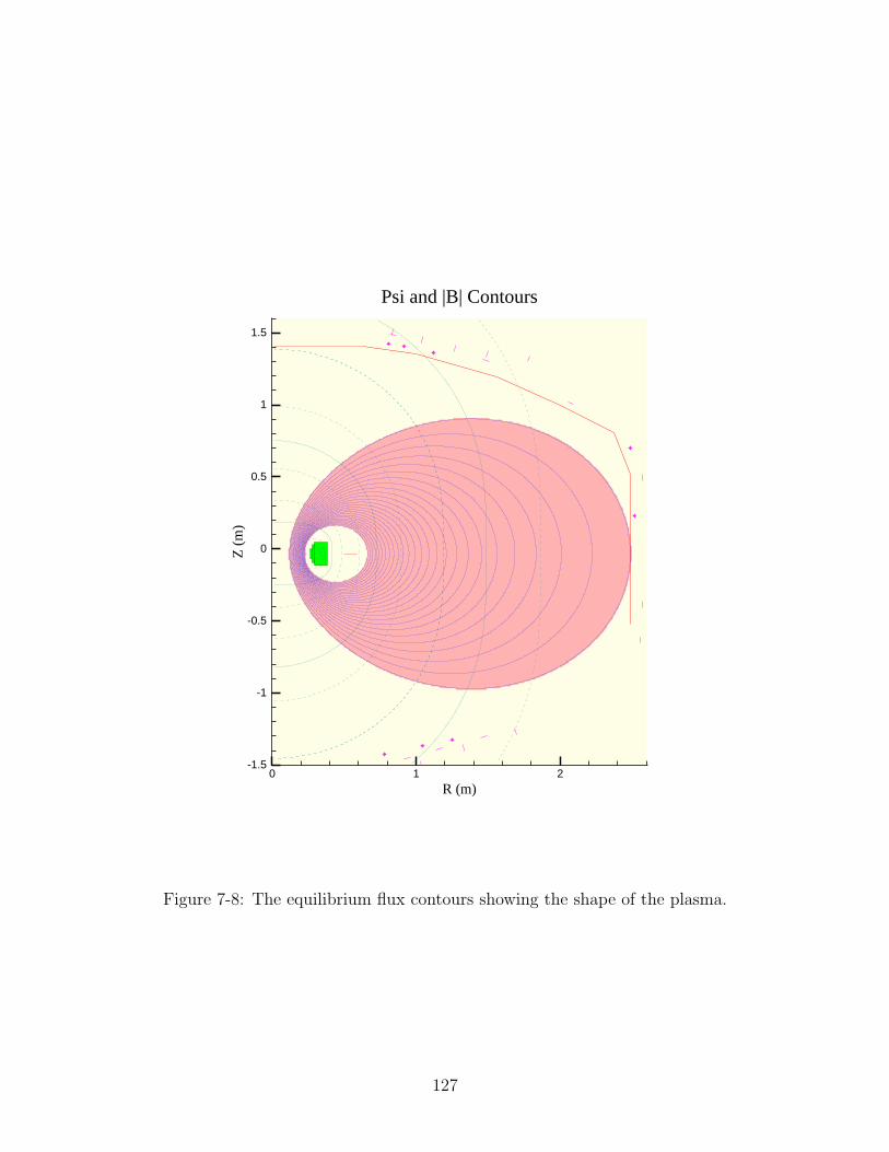
0 1 2
R (m)
-1.5
-1
-0.5
0
0.5
1
1.5
Z (
m)
Psi and |B| Contours
Figure 7-8: The equilibrium flux contours showing the shape of the plasma.
127
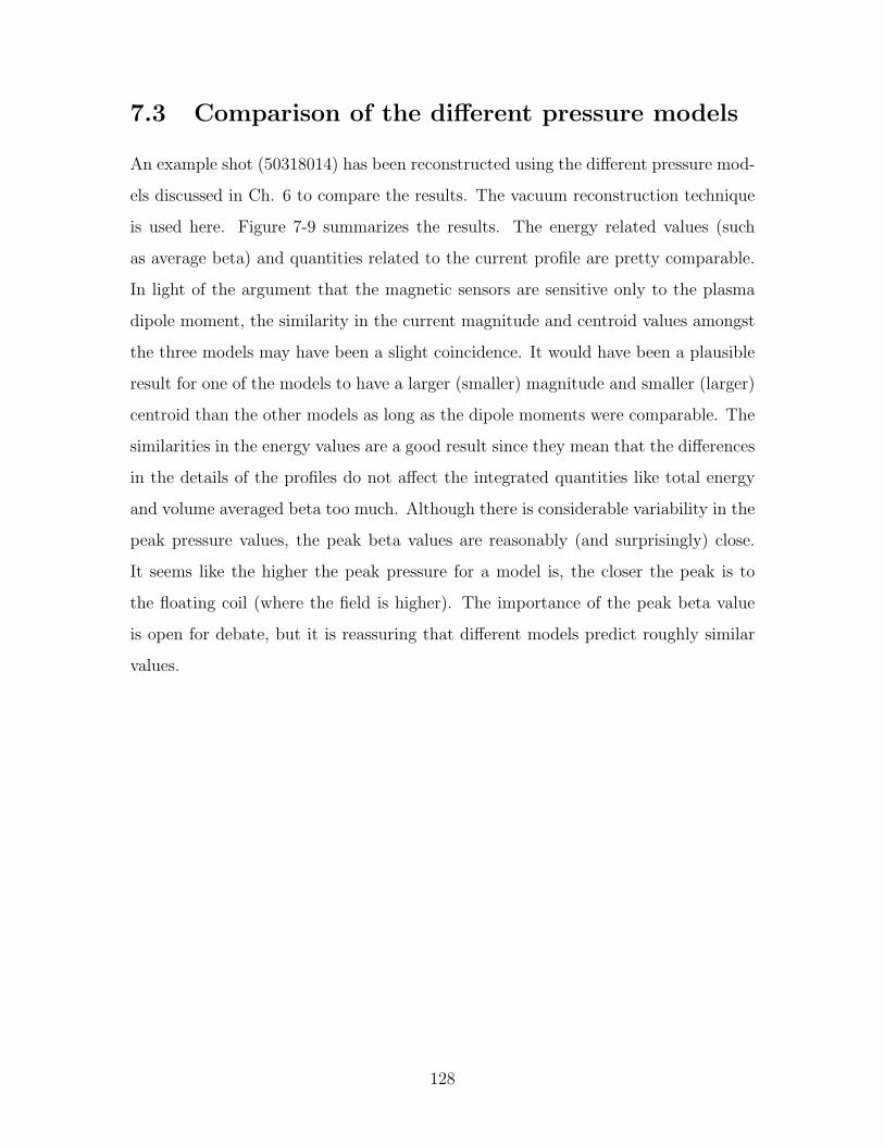
7.3 Comparison of the different pressure models
An example shot (50318014) has been reconstructed using the different pressure mod-
els discussed in Ch. 6 to compare the results. The vacuum reconstruction technique
is used here. Figure 7-9 summarizes the results. The energy related values (such
as average beta) and quantities related to the current profile are pretty comparable.
In light of the argument that the magnetic sensors are sensitive only to the plasma
dipole moment, the similarity in the current magnitude and centroid values amongst
the three models may have been a slight coincidence. It would have been a plausible
result for one of the models to have a larger (smaller) magnitude and smaller (larger)
centroid than the other models as long as the dipole moments were comparable. The
similarities in the energy values are a good result since they mean that the differences
in the details of the profiles do not affect the integrated quantities like total energy
and volume averaged beta too much. Although there is considerable variability in the
peak pressure values, the peak beta values are reasonably (and surprisingly) close.
It seems like the higher the peak pressure for a model is, the closer the peak is to
the floating coil (where the field is higher). The importance of the peak beta value
is open for debate, but it is reassuring that different models predict roughly similar
values.
128
-0.77-0.76-0.87Change in F-coil current (kA)
0.970.970.93Current centroid (m)
3.13.03.3Plasma current (kA)
247236290Total stored energy (J)
1.31.21.6Volume averaged beta (%)
8.49.511Peak beta (%)
162647310Peak pressure (Pa)
Smooth AdiabaticNo Edge PressureDipoleEqParameters \ Model Type
Figure 7-9: Comparison of the equilibrium parameters from three different pressure
models.
129

130
Chapter 8
Special Shots
LDX has three different types of ”knobs” that can alter the plasma in different ways.
The first knob is the control of the microwave sources [14]. LDX plasma is heated
by a 2.45 GHz magnetron and a 6.4 GHz klystron, and both of their powers can be
adjusted up to 3 kW. The second knob is the control of the gas fueling. Different
amounts of gas can be puffed into the chamber before and during plasma formation.
The third and the final knob is the pair of Helmholtz coils, described in Ch. 1. The
coils can impose different magnitudes of vertical field on the plasma and alter its size
and shape. This chapter deals with the different effects ”turning” these knobs have
on the properties of the plasma.
8.1 ECRH Control
Electron cyclotron heating provides an effective way to produce plasmas in a dipole
field. The microwaves are expected to be absorbed most strongly where the funda-
mental cyclotron frequency equals the wave frequency (ω = ωce) and |B| is tangent
to B, and there will be some absorption at the first harmonic (ω = 2ωce) location
as well. Consequently, microwaves at different frequencies will preferentially heat at
different locations, and there is a hope of achieving some degree of profile control by
using different heating frequencies.
LDX is equipped with the two aforementioned heating frequencies. The 2.45
131
GHz has the fundamental resonance at 0.088 T and the 6.4 GHz has it at 0.229 T,
neglecting relativistic effects. The corresponding locations on the midplane are 75
cm and 58 cm, respectively, at a floating coil current of about 900 kA. When the
floating coil current is about 1.17 MA, which is the highest current achieved to date,
the fundamental locations move outward to 81 cm and 62 cm, respectively. The first
harmonic locations are 93 cm and 69 cm at 900 kA and 101 cm and 75 cm at 1.17 MA.
The first harmonic locations of 6.4 GHz are always closer to the floating coil than the
fundamental locations of 2.45 GHz. The field line at the fundamental location of 6.4
GHz at either floating coil current is actually intercepted by the inner surface of the
floating coil, but the hot electrons are deeply mirror trapped and effective heating is
nevertheless possible at the fundamental location.
An obvious experiment to perform to study the effects of different heating frequen-
cies on the plasma is to modulate the power of one frequency while keeping the power
of the other fixed. By performing two shots in which one frequency is modulated in
the first and the other frequency is modulated in the second, all three possible scenar-
ios (2.45 GHz only, 6.4 GHz only, and combined) may be explored. Shots 50318009
and 50318010 have been reconstructed for this purpose. Figures 8-1 and 8-2 show
the ECRH powers and the signal from one of the flux loops for shots 50318009 and
50318010, respectively. The 6.4 GHz power is modulated in shot 50318009 whereas
the 2.45 GHz power is modulated in shot 50318010. Qualitative differences in the flux
loop response are evident for the two modulations. The 2.45 GHz power increases the
flux more quickly than 6.4 GHz, but it seems to saturate at a somewhat lower level
for 2.45 GHz. It is clear that the current for 2.45 GHz only (t = 0-2 sec) has saturated
by the time 6.4 GHz comes on in shot 50318009, but that for 6.4 GHz only (t = 0-2
sec) has not saturated by the time 2.45 GHz comes on in shot 50318010. Also, the
current quickly saturates when 2.45 GHz comes on (at t = 2 sec) in shot 50318010,
whereas it does not reach saturation when 6.4 GHz comes on (at t = 2 sec) in shot
50318009 before it is turned off at t = 4 sec. The difference in the rate of current rise
is evident for the two frequencies, but the difference in the flux saturation level may
be due to the difference in the current centroid locations rather than the difference
132
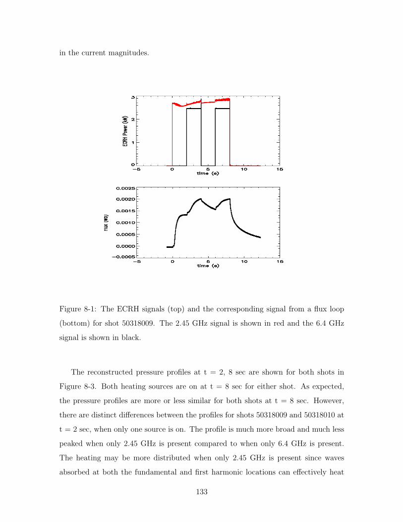
in the current magnitudes.
Figure 8-1: The ECRH signals (top) and the corresponding signal from a flux loop
(bottom) for shot 50318009. The 2.45 GHz signal is shown in red and the 6.4 GHz
signal is shown in black.
The reconstructed pressure profiles at t = 2, 8 sec are shown for both shots in
Figure 8-3. Both heating sources are on at t = 8 sec for either shot. As expected,
the pressure profiles are more or less similar for both shots at t = 8 sec. However,
there are distinct differences between the profiles for shots 50318009 and 50318010 at
t = 2 sec, when only one source is on. The profile is much more broad and much less
peaked when only 2.45 GHz is present compared to when only 6.4 GHz is present.
The heating may be more distributed when only 2.45 GHz is present since waves
absorbed at both the fundamental and first harmonic locations can effectively heat
133
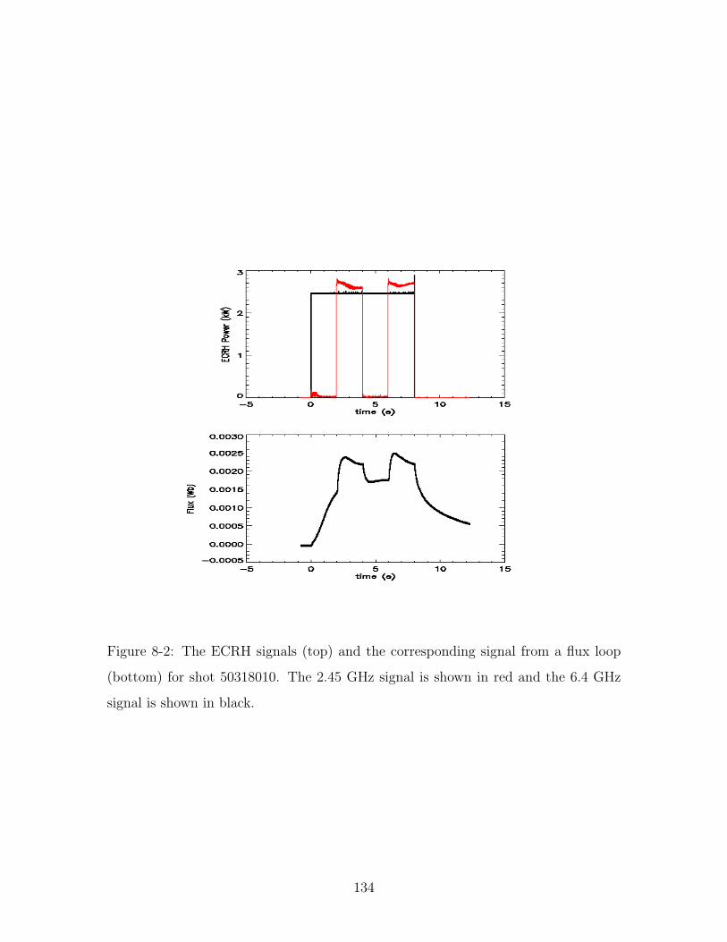
Figure 8-2: The ECRH signals (top) and the corresponding signal from a flux loop
(bottom) for shot 50318010. The 2.45 GHz signal is shown in red and the 6.4 GHz
signal is shown in black.
134
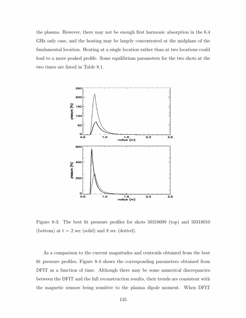
the plasma. However, there may not be enough first harmonic absorption in the 6.4
GHz only case, and the heating may be largely concentrated at the midplane of the
fundamental location. Heating at a single location rather than at two locations could
lead to a more peaked profile. Some equilibrium parameters for the two shots at the
two times are listed in Table 8.1.
Figure 8-3: The best fit pressure profiles for shots 50318009 (top) and 50318010
(bottom) at t = 2 sec (solid) and 8 sec (dotted).
As a comparison to the current magnitudes and centroids obtained from the best
fit pressure profiles, Figure 8-4 shows the corresponding parameters obtained from
DFIT as a function of time. Although there may be some numerical discrepancies
between the DFIT and the full reconstruction results, their trends are consistent with
the magnetic sensors being sensitive to the plasma dipole moment. When DFIT
135
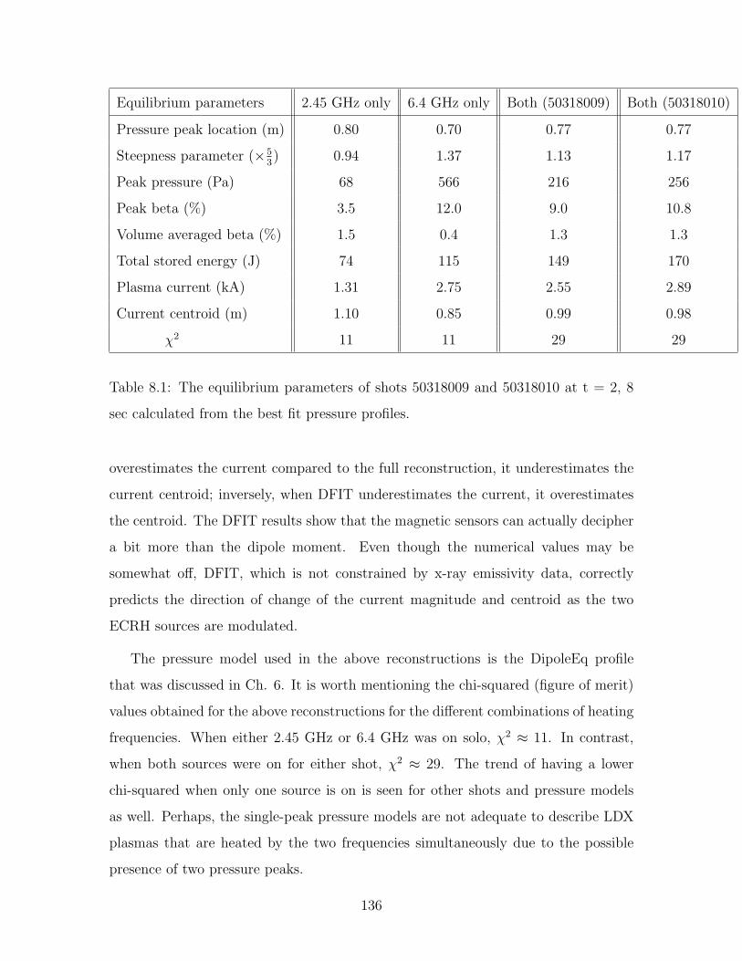
Equilibrium parameters 2.45 GHz only 6.4 GHz only Both (50318009) Both (50318010)
Pressure peak location (m) 0.80 0.70 0.77 0.77
Steepness parameter (×53) 0.94 1.37 1.13 1.17
Peak pressure (Pa) 68 566 216 256
Peak beta (%) 3.5 12.0 9.0 10.8
Volume averaged beta (%) 1.5 0.4 1.3 1.3
Total stored energy (J) 74 115 149 170
Plasma current (kA) 1.31 2.75 2.55 2.89
Current centroid (m) 1.10 0.85 0.99 0.98
χ2 11 11 29 29
Table 8.1: The equilibrium parameters of shots 50318009 and 50318010 at t = 2, 8
sec calculated from the best fit pressure profiles.
overestimates the current compared to the full reconstruction, it underestimates the
current centroid; inversely, when DFIT underestimates the current, it overestimates
the centroid. The DFIT results show that the magnetic sensors can actually decipher
a bit more than the dipole moment. Even though the numerical values may be
somewhat off, DFIT, which is not constrained by x-ray emissivity data, correctly
predicts the direction of change of the current magnitude and centroid as the two
ECRH sources are modulated.
The pressure model used in the above reconstructions is the DipoleEq profile
that was discussed in Ch. 6. It is worth mentioning the chi-squared (figure of merit)
values obtained for the above reconstructions for the different combinations of heating
frequencies. When either 2.45 GHz or 6.4 GHz was on solo, χ2 ≈ 11. In contrast,
when both sources were on for either shot, χ2 ≈ 29. The trend of having a lower
chi-squared when only one source is on is seen for other shots and pressure models
as well. Perhaps, the single-peak pressure models are not adequate to describe LDX
plasmas that are heated by the two frequencies simultaneously due to the possible
presence of two pressure peaks.
136
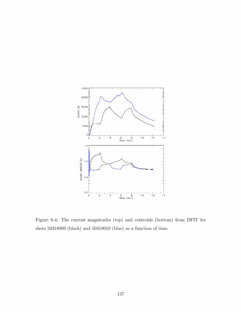
Figure 8-4: The current magnitudes (top) and centroids (bottom) from DFIT for
shots 50318009 (black) and 50318010 (blue) as a function of time.
137
8.2 Gas Fueling Control
The control of gas fueling in LDX is an important tool to study the properties of the
hot electron interchange mode. The initial amount of gas can determine the evolution
of the plasma throughout a shot. Successive puffing can control the plasma in real
time during the shot. The gas puffing example to be discussed in this section gives
an insight into the characteristics of the HEI.
Figure 8-5 shows the signals from the ion gauge and one of the flux loops for a
shot in which the gas is puffed periodically throughout the shot. The flux loop signal
shows the plasma vacillating between the low density regime (HEI unstable) and the
high beta regime (HEI stable). As discussed in Ch. 5, the plasma becomes susceptible
to the HEI when the neutral pressure falls below a critical value. The plots show that
this critical pressure is different from the critical pressure needed to go from the low
density regime to the high beta regime; the critical pressure in going from the low
density regime to the high beta regime is higher than that in going from the high
beta regime to the low density regime. Hence, there is a clear hysteresis in the gas
required to stabilize the HEI.
Although the previous example shows the need for maintaining sufficient neutral
pressure to keep the plasma in the high beta regime, excessive fueling can kill the
plasma. Figure 8-6 shows a shot in which the plasma is overfueled. The five large gas
puffs from 2.5 to 3.5 sec almost destroys the plasma. For optimal plasma performance,
the fueling must be sufficient to keep the plasma in the high beta regime but not
excessive such that the amount of neutral gas overwhelms the heating power.
8.3 Vertical Field Control
LDX is equipped with a pair of Helmholtz coils that can impose a semi-uniform ver-
tical field of up to 300 G in the plasma. This field is sufficient to substantially reduce
the size of the plasma. To study the effects of the vertical field on the plasma, equilib-
rium reconstructions have been performed at four different Helmholtz coil currents.
138
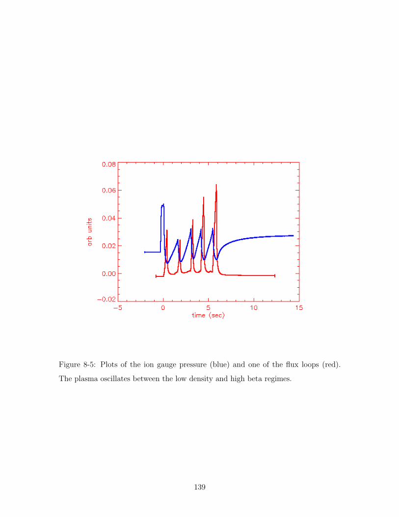
Figure 8-5: Plots of the ion gauge pressure (blue) and one of the flux loops (red).
The plasma oscillates between the low density and high beta regimes.
139
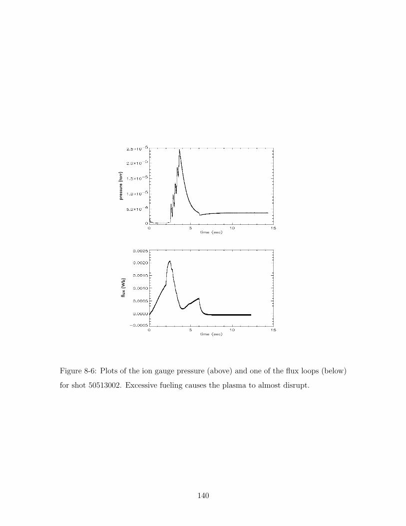
pres
sure
(to
rr)
flux
( Wb )
Figure 8-6: Plots of the ion gauge pressure (above) and one of the flux loops (below)
for shot 50513002. Excessive fueling causes the plasma to almost disrupt.
140
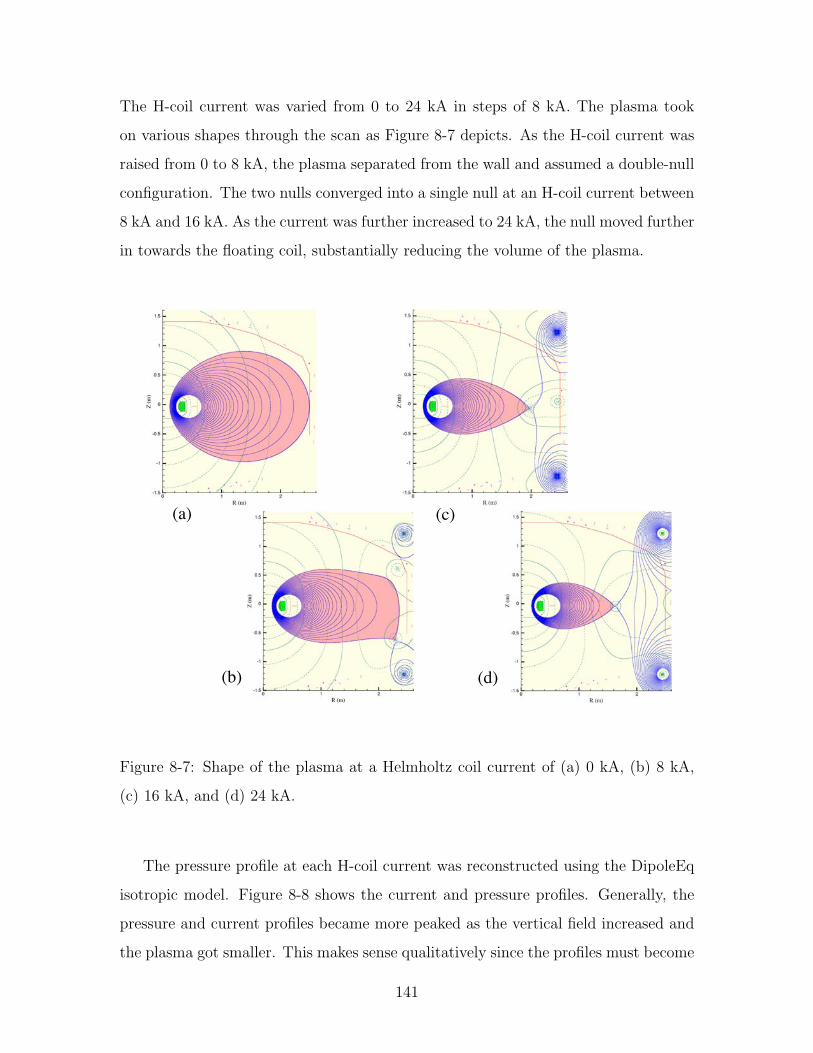
The H-coil current was varied from 0 to 24 kA in steps of 8 kA. The plasma took
on various shapes through the scan as Figure 8-7 depicts. As the H-coil current was
raised from 0 to 8 kA, the plasma separated from the wall and assumed a double-null
configuration. The two nulls converged into a single null at an H-coil current between
8 kA and 16 kA. As the current was further increased to 24 kA, the null moved further
in towards the floating coil, substantially reducing the volume of the plasma.
(a)
(b)
(c)
(d)
Figure 8-7: Shape of the plasma at a Helmholtz coil current of (a) 0 kA, (b) 8 kA,
(c) 16 kA, and (d) 24 kA.
The pressure profile at each H-coil current was reconstructed using the DipoleEq
isotropic model. Figure 8-8 shows the current and pressure profiles. Generally, the
pressure and current profiles became more peaked as the vertical field increased and
the plasma got smaller. This makes sense qualitatively since the profiles must become
141
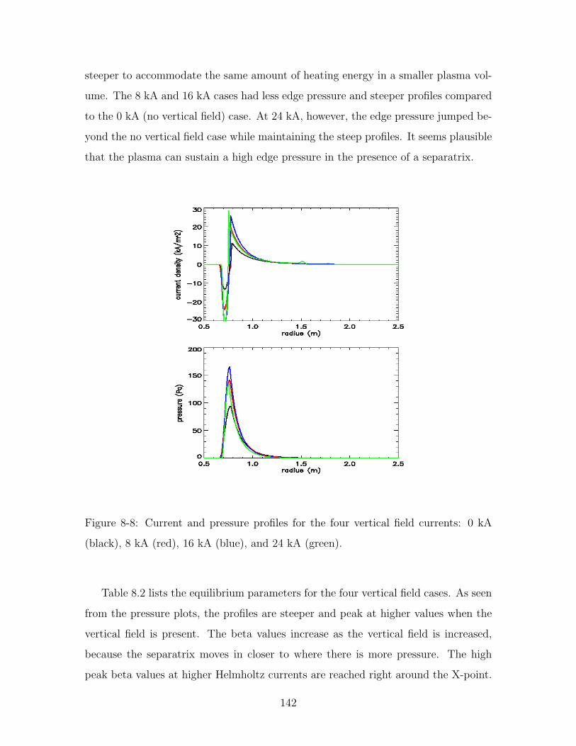
steeper to accommodate the same amount of heating energy in a smaller plasma vol-
ume. The 8 kA and 16 kA cases had less edge pressure and steeper profiles compared
to the 0 kA (no vertical field) case. At 24 kA, however, the edge pressure jumped be-
yond the no vertical field case while maintaining the steep profiles. It seems plausible
that the plasma can sustain a high edge pressure in the presence of a separatrix.
Figure 8-8: Current and pressure profiles for the four vertical field currents: 0 kA
(black), 8 kA (red), 16 kA (blue), and 24 kA (green).
Table 8.2 lists the equilibrium parameters for the four vertical field cases. As seen
from the pressure plots, the profiles are steeper and peak at higher values when the
vertical field is present. The beta values increase as the vertical field is increased,
because the separatrix moves in closer to where there is more pressure. The high
peak beta values at higher Helmholtz currents are reached right around the X-point.
142
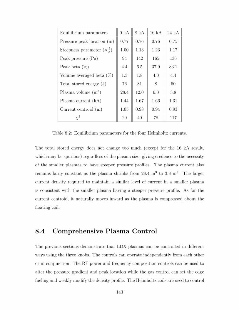
Equilibrium parameters 0 kA 8 kA 16 kA 24 kA
Pressure peak location (m) 0.77 0.76 0.76 0.75
Steepness parameter (×53) 1.00 1.13 1.23 1.17
Peak pressure (Pa) 94 142 165 136
Peak beta (%) 4.4 6.5 37.9 83.1
Volume averaged beta (%) 1.3 1.8 4.0 4.4
Total stored energy (J) 76 81 8 50
Plasma volume (m3) 28.4 12.0 6.0 3.8
Plasma current (kA) 1.44 1.67 1.66 1.31
Current centroid (m) 1.05 0.98 0.94 0.93
χ2 20 40 78 117
Table 8.2: Equilibrium parameters for the four Helmholtz currents.
The total stored energy does not change too much (except for the 16 kA result,
which may be spurious) regardless of the plasma size, giving credence to the necessity
of the smaller plasmas to have steeper pressure profiles. The plasma current also
remains fairly constant as the plasma shrinks from 28.4 m3 to 3.8 m3. The larger
current density required to maintain a similar level of current in a smaller plasma
is consistent with the smaller plasma having a steeper pressure profile. As for the
current centroid, it naturally moves inward as the plasma is compressed about the
floating coil.
8.4 Comprehensive Plasma Control
The previous sections demonstrate that LDX plasmas can be controlled in different
ways using the three knobs. The controls can operate independently from each other
or in conjunction. The RF power and frequency composition controls can be used to
alter the pressure gradient and peak location while the gas control can set the edge
fueling and weakly modify the density profile. The Helmholtz coils are used to control
143
the size and topology of the plasma. In terms of their utilities, the RF and gas controls
will be instrumental in suppressing the MHD and hot electron interchange modes,
respectively. For example, signals from the magnetic diagnostics and ion gauge can
be fed back to control these instruments. Although the effect of the plasma topology
on its stability properties is unclear at this point, we can envision a similar feedback
system to control the Helmholtz coils to suppress, for example, a parasitic mode with
certain spatial characteristics.
The RF, gas, and Helmholtz controls must be adjusted in unison on certain occa-
sions. In particular, there may be an interaction between the different controls, and
the effect of one must be taken into account when controlling another. For example,
the neutral pressure threshold against the HEI increases as the plasma volume de-
creases and heating power increases. Hence if the plasma is stable against the HEI
at a given gas fueling setting, it must be increased if the heating power is increased
or the plasma volume is decreased or both. It is important to always be aware of the
global effects of a control knob and its interactions with the other controls.
144
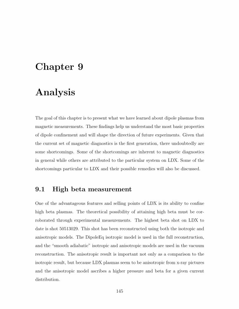
Chapter 9
Analysis
The goal of this chapter is to present what we have learned about dipole plasmas from
magnetic measurements. These findings help us understand the most basic properties
of dipole confinement and will shape the direction of future experiments. Given that
the current set of magnetic diagnostics is the first generation, there undoubtedly are
some shortcomings. Some of the shortcomings are inherent to magnetic diagnostics
in general while others are attributed to the particular system on LDX. Some of the
shortcomings particular to LDX and their possible remedies will also be discussed.
9.1 High beta measurement
One of the advantageous features and selling points of LDX is its ability to confine
high beta plasmas. The theoretical possibility of attaining high beta must be cor-
roborated through experimental measurements. The highest beta shot on LDX to
date is shot 50513029. This shot has been reconstructed using both the isotropic and
anisotropic models. The DipoleEq isotropic model is used in the full reconstruction,
and the “smooth adiabatic” isotropic and anisotropic models are used in the vacuum
reconstruction. The anisotropic result is important not only as a comparison to the
isotropic result, but because LDX plasmas seem to be anisotropic from x-ray pictures
and the anisotropic model ascribes a higher pressure and beta for a given current
distribution.
145
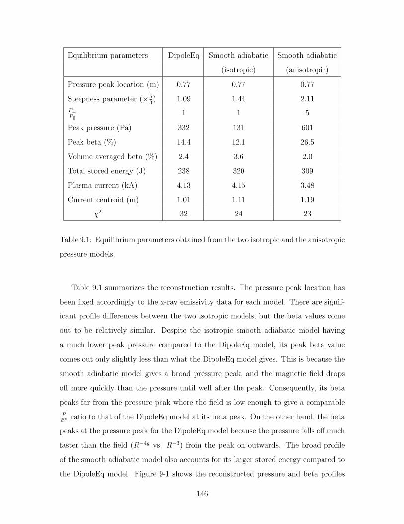
Equilibrium parameters DipoleEq Smooth adiabatic Smooth adiabatic
(isotropic) (anisotropic)
Pressure peak location (m) 0.77 0.77 0.77
Steepness parameter (×53) 1.09 1.44 2.11
P⊥P‖
1 1 5
Peak pressure (Pa) 332 131 601
Peak beta (%) 14.4 12.1 26.5
Volume averaged beta (%) 2.4 3.6 2.0
Total stored energy (J) 238 320 309
Plasma current (kA) 4.13 4.15 3.48
Current centroid (m) 1.01 1.11 1.19
χ2 32 24 23
Table 9.1: Equilibrium parameters obtained from the two isotropic and the anisotropic
pressure models.
Table 9.1 summarizes the reconstruction results. The pressure peak location has
been fixed accordingly to the x-ray emissivity data for each model. There are signif-
icant profile differences between the two isotropic models, but the beta values come
out to be relatively similar. Despite the isotropic smooth adiabatic model having
a much lower peak pressure compared to the DipoleEq model, its peak beta value
comes out only slightly less than what the DipoleEq model gives. This is because the
smooth adiabatic model gives a broad pressure peak, and the magnetic field drops
off more quickly than the pressure until well after the peak. Consequently, its beta
peaks far from the pressure peak where the field is low enough to give a comparable
PB2 ratio to that of the DipoleEq model at its beta peak. On the other hand, the beta
peaks at the pressure peak for the DipoleEq model because the pressure falls off much
faster than the field (R−4g vs. R−3) from the peak on outwards. The broad profile
of the smooth adiabatic model also accounts for its larger stored energy compared to
the DipoleEq model. Figure 9-1 shows the reconstructed pressure and beta profiles
146
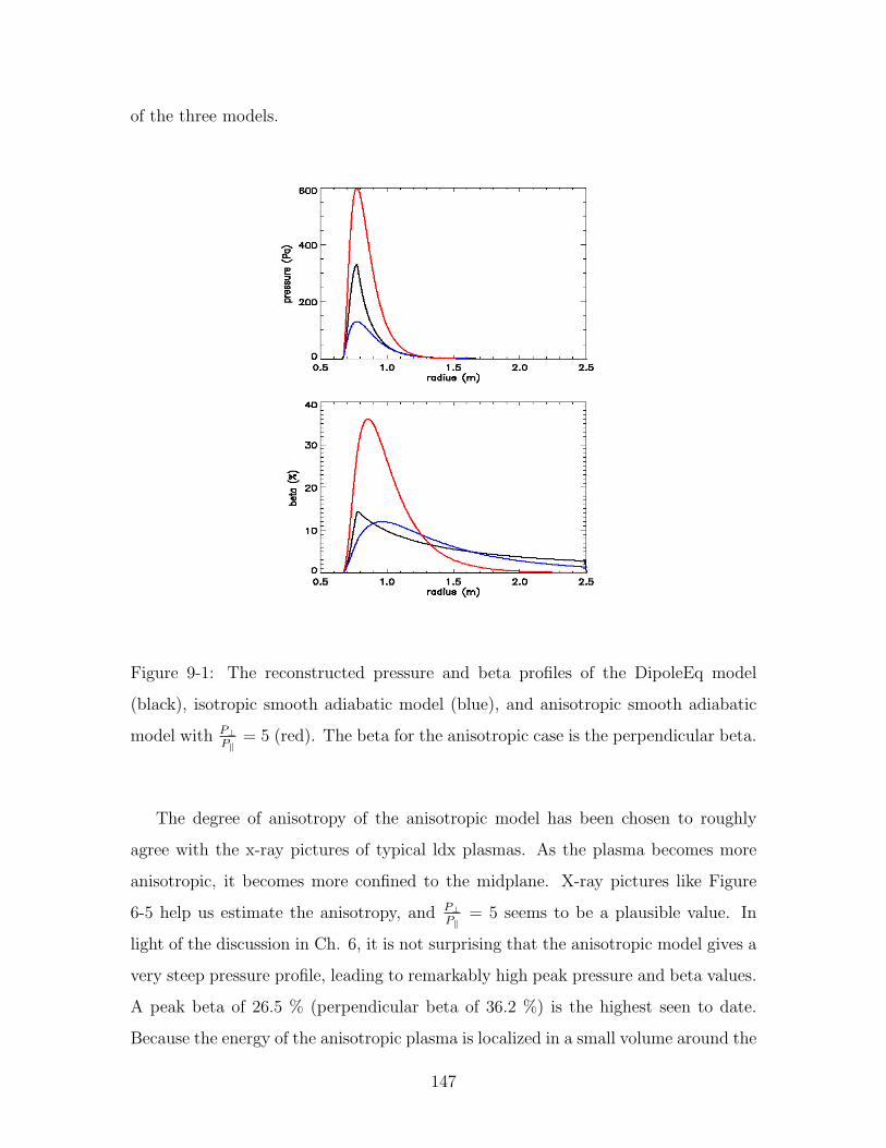
of the three models.
Figure 9-1: The reconstructed pressure and beta profiles of the DipoleEq model
(black), isotropic smooth adiabatic model (blue), and anisotropic smooth adiabatic
model with P⊥P‖
= 5 (red). The beta for the anisotropic case is the perpendicular beta.
The degree of anisotropy of the anisotropic model has been chosen to roughly
agree with the x-ray pictures of typical ldx plasmas. As the plasma becomes more
anisotropic, it becomes more confined to the midplane. X-ray pictures like Figure
6-5 help us estimate the anisotropy, and P⊥P‖
= 5 seems to be a plausible value. In
light of the discussion in Ch. 6, it is not surprising that the anisotropic model gives a
very steep pressure profile, leading to remarkably high peak pressure and beta values.
A peak beta of 26.5 % (perpendicular beta of 36.2 %) is the highest seen to date.
Because the energy of the anisotropic plasma is localized in a small volume around the
147
inner midplane, its volume averaged beta and total stored energy are comparable to
(if not lower than) the isotropic plasma despite the very high peaks the pressure and
beta attain. The contour plots of the pressure and current in Figure 9-2 demonstrate
how they become more localized as the plasma goes from isotropic to anisotropic with
p ≡ P⊥−P‖2P‖
= 2. Notice that the pressure contours no longer coincide with the flux
contours in the anisotropic case.
(a)
(b)
(c)
(d)
Figure 9-2: The reconstructed (a) pressure and (b) current contours using the
isotropic smooth adiabatic model and (c) pressure and (d) current contours using
the anisotropic model with p = 2.
The condition under which the high beta plasma was produced is worth noting.
Prior to shot 50513029, many long-pulse conditioning shots had been performed to
thoroughly clean the vessel and reach good vacuum status. Hence, shot 50513029
148
and its surrounding shots, which attained similar beta values, most likely produced
plasmas that were cleaner than average. Besides that, the shot was no different from
ordinary with both sources on at full power and sufficient fueling to avert HEI events
during the high beta phase.
Finally, the reconstruction results show that the magnetic diagnostics alone are
incapable of measuring the anisotropy of the plasma. The χ2 values for the isotropic
and anisotropic cases were virtually indistinguishable. But because the reconstructed
current distributions were sufficiently different between the isotropic and anisotropic
cases, there may be hope that additional well-placed sensors can acquire some infor-
mation about pressure anisotropy. For now, we must depend on x-ray camera data
to estimate the anisotropy of ldx plasmas.
9.2 Measurement of Supercritical Profiles
One of the key results of reconstructing LDX plasmas is the measurement of super-
critical pressure gradients. It has been alluded in Ch. 2 that because hot electrons are
subject to the HEI rather than the MHD criterion, they can exceed the MHD pressure
gradient limit, P ∼ V −γ. One of the main importance of the magnetic diagnostics
on LDX is their ability to verify whether hot electrons do indeed exceed the MHD
limit. Figure 9-3 gives a plot of ten shots that have been discussed thus far in the
R-g space, where R is the pressure peak location and g is the steepness parameter.
All these shots have been reconstructed using the DipoleEq model, and the pressure
peak has been constrained using x-ray emissivity data. The steepness parameter and
edge pressure are unambiguously constrained by magnetic data. The plot shows that
all but two of the ten shots give a best fit g that exceeds 53. It is therefore fair to say
that LDX plasmas routinely have pressure profiles that are steeper than what MHD
allows.
To really verify that the supercritical steepness parameters are the best fit to the
magnetics, plots of χ2 vs. g for the highest beta shot are shown in Figure 9-4. It is
clear that χ2 does indeed reach a minimum at a supercritical gγ
value of about 1.09
149
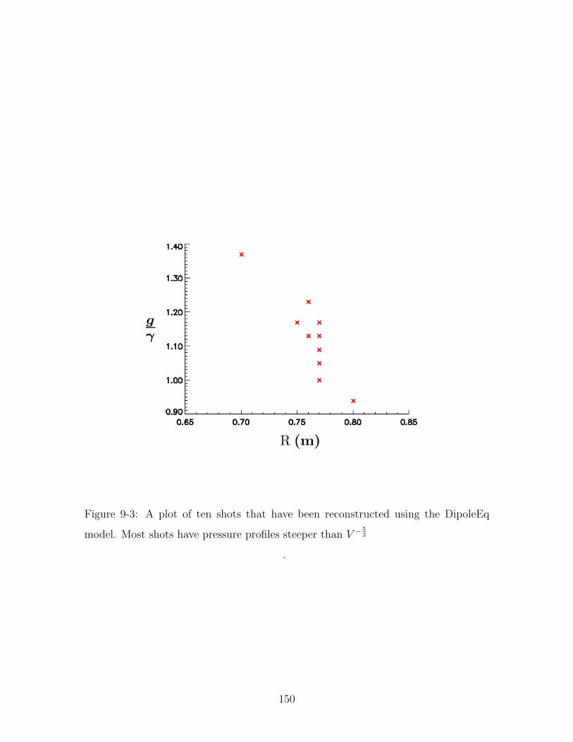
Figure 9-3: A plot of ten shots that have been reconstructed using the DipoleEq
model. Most shots have pressure profiles steeper than V − 53
.
150
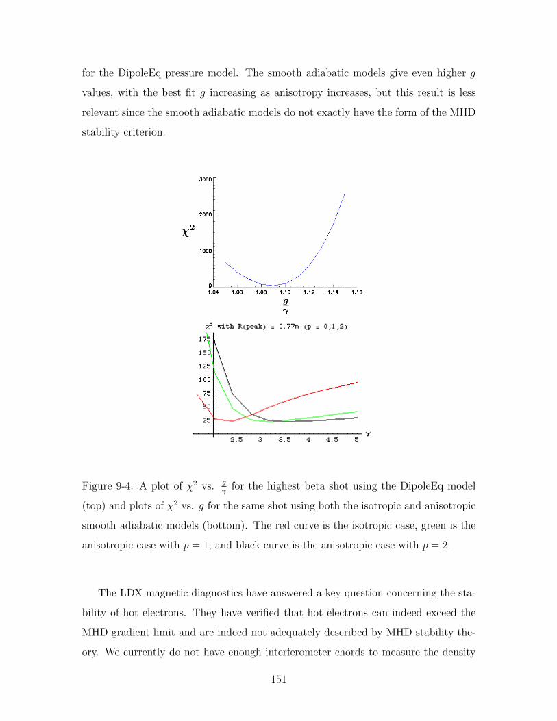
for the DipoleEq pressure model. The smooth adiabatic models give even higher g
values, with the best fit g increasing as anisotropy increases, but this result is less
relevant since the smooth adiabatic models do not exactly have the form of the MHD
stability criterion.
Figure 9-4: A plot of χ2 vs. gγ
for the highest beta shot using the DipoleEq model
(top) and plots of χ2 vs. g for the same shot using both the isotropic and anisotropic
smooth adiabatic models (bottom). The red curve is the isotropic case, green is the
anisotropic case with p = 1, and black curve is the anisotropic case with p = 2.
The LDX magnetic diagnostics have answered a key question concerning the sta-
bility of hot electrons. They have verified that hot electrons can indeed exceed the
MHD gradient limit and are indeed not adequately described by MHD stability the-
ory. We currently do not have enough interferometer chords to measure the density
151
profile, but it would be interesting to study how hot electrons are limited by their
density gradient and whether the limit, if any, is consistent with the theory of the
HEI.
9.3 Magnetic detection of the HEI
HEI events are most prominently detected by floating langmuir probes, but they
also possess magnetic signatures as well. Depending on the severity of the event,
a rapid fall of varying magnitudes in the diamagnetism can be seen on the Bp coil
and flux loop signals. Some events are severe enough to destroy the plasma, and
those are manifested as sharp spikes in Mirnov signals accompanied by a total loss
of diamagnetism. These spikes in the Mirnov signals have been correlated to spikes
in probe signals that have been extensively studied and characterized as HEI events
[39]. Some examples of near-catastrophic HEI events are shown in Figures 9-5 - 9-8.
Shot 50513024 shown in Figure 9-5 displays a situation in which the HEI occurs
seconds after all the RF is turned off. The after-glow regime is often susceptible to
an HEI because the bulk electrons are quickly lost, and the right hand side of Eq.
5.15 can become very small. As this particular shot shows, an HEI event during an
after-glow almost always leads to a quick and complete demise of what is left of the
decaying plasma.
Figures 9-6 - 9-8 each show two shots that are completely identical in terms of
the fueling, heating power, and heating frequencies. However, one sustains more HEI
events than the other. In Figure 9-6, both shots 50513027 and 50513028 suffer an
HEI event at the RF turnoff, but shot 50513028 has an extra HEI event during the
high beta regime. Shot 50513040 in Figure 9-8 does not have an HEI event, but shot
50513041 does during the high beta regime. In these shots, the neutral pressure is
near a critical level, and one shot happens to be on the “right” side of the stability
boundary while the other shot happens to be on the “wrong” side. Shots 50513033
and 50513032 in Figure 9-7 are in a similar situation; shot 50513032 has an HEI event
152
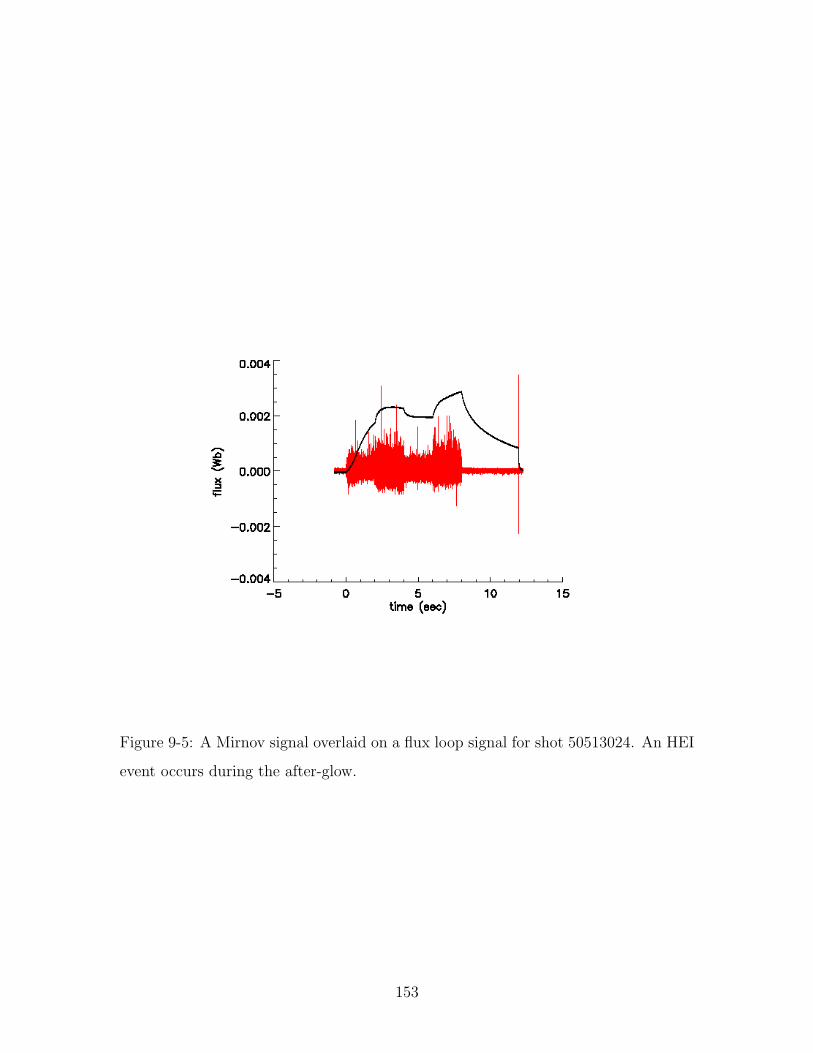
Figure 9-5: A Mirnov signal overlaid on a flux loop signal for shot 50513024. An HEI
event occurs during the after-glow.
153
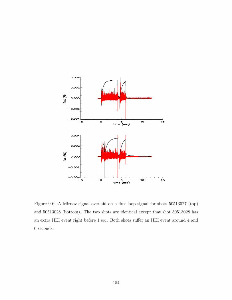
Figure 9-6: A Mirnov signal overlaid on a flux loop signal for shots 50513027 (top)
and 50513028 (bottom). The two shots are identical except that shot 50513028 has
an extra HEI event right before 1 sec. Both shots suffer an HEI event around 4 and
6 seconds.
154
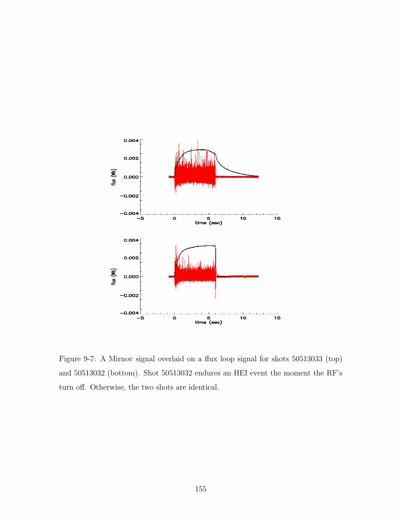
Figure 9-7: A Mirnov signal overlaid on a flux loop signal for shots 50513033 (top)
and 50513032 (bottom). Shot 50513032 endures an HEI event the moment the RF’s
turn off. Otherwise, the two shots are identical.
155
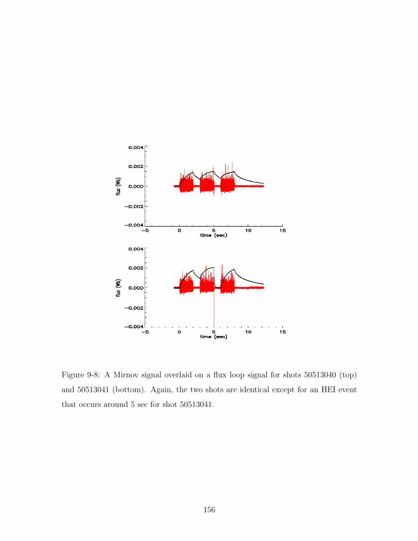
Figure 9-8: A Mirnov signal overlaid on a flux loop signal for shots 50513040 (top)
and 50513041 (bottom). Again, the two shots are identical except for an HEI event
that occurs around 5 sec for shot 50513041.
156
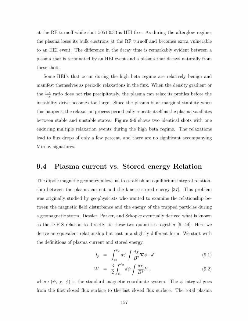
at the RF turnoff while shot 50513033 is HEI free. As during the afterglow regime,
the plasma loses its bulk electrons at the RF turnoff and becomes extra vulnerable
to an HEI event. The difference in the decay time is remarkably evident between a
plasma that is terminated by an HEI event and a plasma that decays naturally from
these shots.
Some HEI’s that occur during the high beta regime are relatively benign and
manifest themselves as periodic relaxations in the flux. When the density gradient or
the neh
nebratio does not rise precipitously, the plasma can relax its profiles before the
instability drive becomes too large. Since the plasma is at marginal stability when
this happens, the relaxation process periodically repeats itself as the plasma vacillates
between stable and unstable states. Figure 9-9 shows two identical shots with one
enduring multiple relaxation events during the high beta regime. The relaxations
lead to flux drops of only a few percent, and there are no significant accompanying
Mirnov signatures.
9.4 Plasma current vs. Stored energy Relation
The dipole magnetic geometry allows us to establish an equilibrium integral relation-
ship between the plasma current and the kinetic stored energy [37]. This problem
was originally studied by geophysicists who wanted to examine the relationship be-
tween the magnetic field disturbance and the energy of the trapped particles during
a geomagnetic storm. Dessler, Parker, and Sckopke eventually derived what is known
as the D-P-S relation to directly tie these two quantities together [6, 44]. Here we
derive an equivalent relationship but cast in a slightly different form. We start with
the definitions of plasma current and stored energy,
Ip =
∫ ψ2
ψ1
dψ
∫dχ
B2∇φ · J (9.1)
W =3
2
∫ ψ2
ψ1
dψ
∫dχ
B2P , (9.2)
where (ψ, χ, φ) is the standard magnetic coordinate system. The ψ integral goes
from the first closed flux surface to the last closed flux surface. The total plasma
157
Figure 9-9: Shots 50318015 (top) and 50318016 (bottom) are identical, but shot
50318016 endures multiple relaxation events during the high beta regime. A blowup
of the relaxation events is shown to the right.
158
volume is∫dψ
∫dχB2 , and the differential flux tube volume per differential flux, V , is∫
dχB2 .
The MHD momentum equation, ∇P = J ×B, can be used to eliminate J from
Eq. 9.2. After some simplification, the ratio of stored energy to plasma current can
be written as,W
Ip=
3
2
∫dψPV∫
dψP∂V/∂ψ. (9.3)
For a low beta plasma, the equilibrium flux is not much different from the vacuum
flux, in which V ∼ ψ−4, and Eq. 9.3 can be rewritten as,
W
Ip=
3
8
∫dψPV∫dψPV/ψ
. (9.4)
Hence, the stored energy to plasma current ratio can be calculated once P (ψ) is
specified.
We can specify the pressure function to be the marginally stable profile, which is
PV γ = const. and equivalent to the DipoleEq model profile. The energy to current
ratio then becomes,W
Ip=
3
8
∫dψV −γ+1∫dψV −γ+1/ψ
, (9.5)
and again by letting V ∼ ψ−4, it becomes,
W
Ip=
3
8
∫dψψ4γ−4∫dψψ4γ−5
. (9.6)
The above integrals can now be evaluated, and the result is the following:
W
Ip=
3
8
(4γ − 4
4γ − 3
) (ψ4γ−3
2 − ψ4γ−31
ψ4γ−42 − ψ4γ−4
1
). (9.7)
Now let us focus on the expression for the current centroid. We write the current
centroid as follows:
RcIpIp
=
∫dψ∂P/∂ψ
∫(dχ/B2)r sin θ∫
dψ∂P/∂ψ∫
(dχ/B2), (9.8)
where r and θ are the radial and polar angle coordinates in the standard spherical
coordinates. Upon computing r sin θ along the field lines by transforming the χ
integral into a ξ integral [31], with ξ ≡ sin2 θ, we get,
RcIpIp
≈ µ0M
2
∫dψPV/ψ2∫dψPV/ψ
, (9.9)
159
where M is the magnetic moment of the floating coil. The above integrals can be
evaluated as before using the marginally stable profile and by letting V ∼ ψ−4,
Rc ≈µ0M
2
(4γ − 4
4γ − 5
) (ψ4γ−5
2 − ψ4γ−51
ψ4γ−42 − ψ4γ−4
1
). (9.10)
The quantity of interest in the dipole equilibrium is WRc
Ip, because it is nearly a
constant as will be shown shortly. Multiplying the expressions for WIp
and Rc, we get,
WRc
Ip≈ 3
16µ0M
(4γ − 4)2
(4γ − 3)(4γ − 5)
(ψ4γ−32 − ψ4γ−3
1 )(ψ4γ−52 − ψ4γ−5
1 )
(ψ4γ−42 − ψ4γ−4
1 )2. (9.11)
The expression on the right of M in the above equation is nearly unity in the range
of γ we are interested in (Figure 9-10). For a floating coil charge of about 900 kA, its
magnetic moment is equal to about 300 kA·m2. Hence,
WRc
Ip≈ 3
16µ0M ≈ 70 J·m·kA−1 . (9.12)
The stored energy-current relationship is important, because it allows us to estimate
the plasma stored energy without fully reconstructing the equilibrium; we can instead
find the plasma current and its centroid using a current filament code like DFIT and
use the above relationship.
Plots of W vs. IpRc
is shown for all the 900 kA charge shots described in this thesis
in Figure 9-11. The best fit line through the nine data points has a slope of about 60
J·m·kA−1, which is about 14 % lower than the theoretical value. In the theoretical
derivation, we assumed the pressure to have the marginally stable profile from the
first closed flux surface to the last closed flux surface. In reality, the marginally
stable profile is valid from the pressure peak to the last closed flux surface, and the
profile should smoothly increase from the first closed flux surface to the peak. Hence,
we may have overestimated the integrals involved in the calculations, leading to an
overestimation of WRc
Ip.
9.5 Energy confinement time
The ECRH modulation shots discussed in the previous chapter are helpful to learn
about the effect of the heating frequency on the energy confinement time of the
160
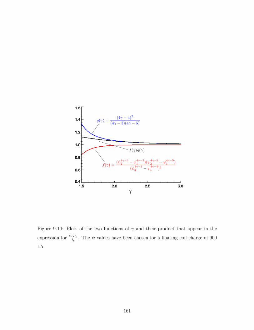
γ
Figure 9-10: Plots of the two functions of γ and their product that appear in the
expression for WRc
Ip. The ψ values have been chosen for a floating coil charge of 900
kA.
161
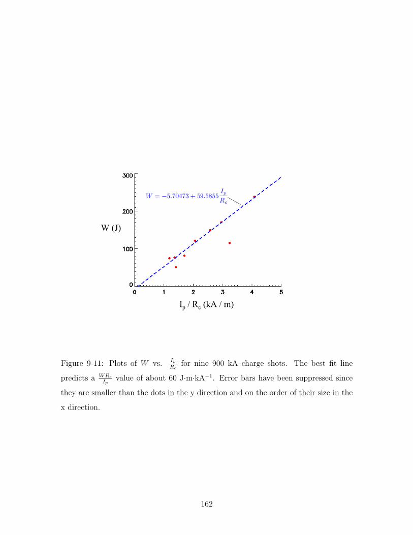
Ip / Rc (kA / m)
W (J)
Figure 9-11: Plots of W vs. IpRc
for nine 900 kA charge shots. The best fit line
predicts a WRc
Ipvalue of about 60 J·m·kA−1. Error bars have been suppressed since
they are smaller than the dots in the y direction and on the order of their size in the
x direction.
162
plasma. Simplistically, the energy confinement time can be found by dividing the
plasma stored energy by the total heating power. Doing so for shots 50318009 and
50318010, we find the energy confinement time for the 2.45 GHz only heating case
to be about 25 ms and that for the 6.4 GHz only heating case to be about 40 ms.
When both sources are on, the energy confinement time is about 30 ms. It seems like
6.4 GHz heating results in a higher energy confinement time than 2.45 GHz heating.
This trend is seen in a study of a larger number of shots with different heating powers
of the two frequencies (Figure 9-12). There is a general trend that shows the greater
the heating power fraction of 2.45 GHz, the worse the confinement time. Physically,
the 2.45 GHz microwave heats a larger plasma volume, thereby creating more bulk
species that are susceptible to parallel losses to the floating coil supports. It will be
interesting to see how the confinement times change when the floating coil is levitated.
9.6 Analysis Summary
This chapter discussed some of the most important results of the experiment to date.
By using the anisotropic pressure model, a peak beta of more than 26 % has been
measured. It should be reiterated that the use of an anisotropic model is not only
justified but absolutely required to obtain the correct beta values. For a given set of
magnetic measurements, the reconstructed beta increases as the anisotropy increases.
An anisotropy parameter value of 2 (P⊥P‖
= 5) is obtained for this reconstruction by
comparing the model pressure contours to the x-ray emissivity contours.
Figure 9-3 displays the reconstruction results of 10 LDX shots and convincingly
shows that supercritical pressure profiles are routinely obtained. As mentioned re-
peatedly before, the result is not surprising given that the hot electrons carry most of
the pressure, but the affirmation of the expected result unequivocally proves the case
that the MHD limit is irrelevant for the hot electrons. The next step is to test the
applicability of the HEI limit by measuring the density profile of the hot electrons
using a multi-chord interferometer. Also, it would be interesting to see if the MHD
163
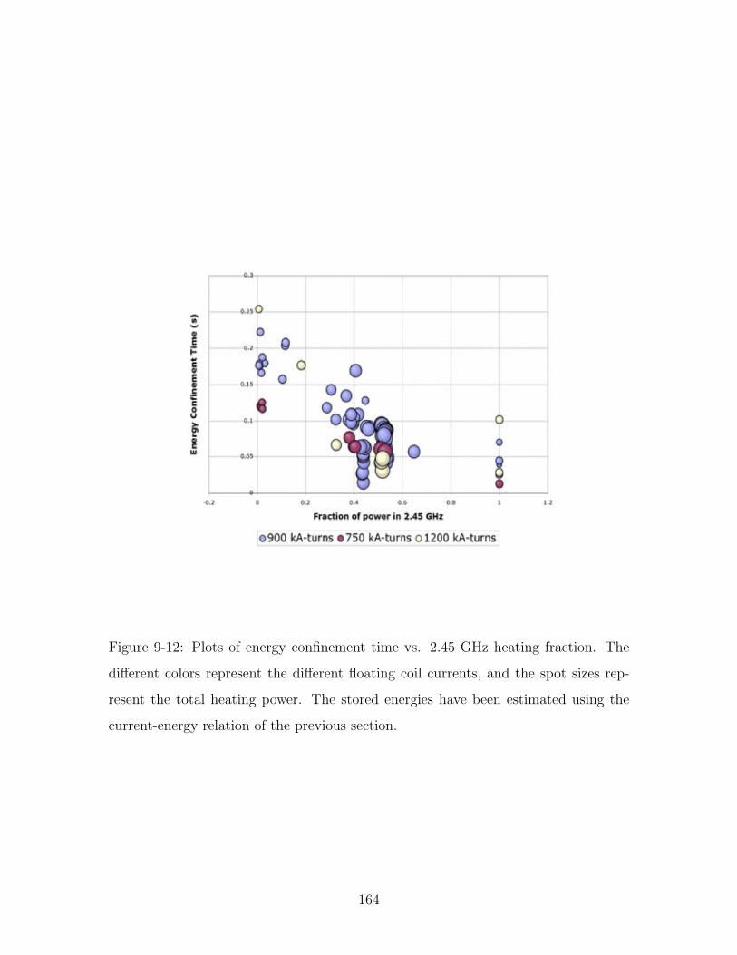
Figure 9-12: Plots of energy confinement time vs. 2.45 GHz heating fraction. The
different colors represent the different floating coil currents, and the spot sizes rep-
resent the total heating power. The stored energies have been estimated using the
current-energy relation of the previous section.
164
limit becomes relevant when the electrons are thermalized during the third phase of
the experiment.
Although the Mirnov coils were never designed to measure the HEI’s, their sig-
natures are clearly visible in the data. The details of their mode properties cannot
be extracted from the Mirnov signals, but their occurrences can be clearly correlated
temporally to drops in the flux signals. This observation is sufficient to surmise that
HEI events cause a global reorganization of the plasma current, possibly allowing for
the density profile to relax.
Finally, a theoretical relationship between the plasma current and stored energy,
much like the D-P-S relation, is derived and compared to empirical data. Perhaps
due to an inaccurate approximation in the derivation, the empirical data slightly
disagrees with the theoretical relation. Nevertheless, it is an important finding that
the empirical data is consistent with a linear relationship between the current and
stored energy. This relationship is very convenient since the plasma stored energy
can be estimated by merely knowing its current. The relationship has been used to
quickly estimate the energy confinement time of various LDX shots with different
heating frequency compositions. Although the reasons are yet unclear, 2.45 GHz
heating seems to be less efficient than 6.4 GHz heating.
165

166

Chapter 10
Conclusion
10.1 Main Results
The main results of the thesis clearly are the measurement of high beta and the
measurement of supercritical pressure profiles. These two measurements answer some
of the most basic questions regarding LDX physics. We have verified that LDX is
capable of sustaining stable, high beta plasmas for a prolonged period if there is
sufficient neutral fueling to suppress the hot electron interchange mode. Also, the
relative importance of the MHD interchange mode and the HEI is now understood,
at least as far as the hot electrons are concerned. In LDX the pressure is carried by
the hot electron species, and we have seen that the pressure profile can be measured
by the magnetics. Ideal MHD is not seen to play a role in determining the beta limit
for this hot electron plasma. MHD may still provide a limit to the pressure gradient
of the low beta background plasma, but the effect is difficult to measure since the
background plasma contributes negligibly to the total pressure. This will inevitably
change as we progress through the experimental phases and the electrons are made
to thermalize.
167
10.2 Summary
This thesis has described the basic properties of the Levitated Dipole Experiment
from a magnetic diagnostics standpoint. The work illuminates the basic physics
of dipole MHD equilibrium and stability. Because the current phase of operation
involves plasmas with a significant population of hot electrons, the basic properties of
the hot electron interchange mode have been touched as well. All the hardware that
makes this experiment possible, and the technological feat that had to be overcome
is described in the very first chapter.
The main players of this work have been the magnetic diagnostics. The description
and design of the different types of magnetic sensors are presented in Ch. 2, while
Ch. 3 tackles the mathematical problem of positioning the sensors where they are
most sensitive to changing plasma parameters. A comprehensive error analysis is
performed in Ch. 4 to relate the measured field errors to errors in the reconstructed
equilibrium parameters.
One of the main points of the thesis deals with the details of the reconstruction
process as applied to LDX plasmas in particular. The unique experimental configu-
ration of LDX brings about some difficulties in the reconstruction process. One such
difficulty is the requirement to keep the flux linked by the superconducting floating
coil constant while the plasma current ramps up. In theory, this requires an iterative
solution to get the right plasma current and floating coil current. In practice, the
current filament code, DFIT, helps estimate the change in the floating coil current,
thereby eliminating the need to iterate for a solution. Another more serious diffi-
culty is the inability of the magnetic sensors to decipher between different pressure
profiles with the same dipole moment. The reason for this shortcoming is the large
distance between the plasma and the magnetic sensors, hence making it difficult for
them to measure higher order moments. Simulations show that this problem could
be overcome by installing sensors closer to the plasma, but x-ray emissivity data is
used for now to constrain the radial location of the pressure profile peak and permit
the reconstruction of the constrained pressure profile.
168
The LDX configuration has its advantages as well. Unlike the tokamak, the LDX
vacuum field closely resembles the plasma field, and the vacuum field can conse-
quently be used to relate plasma pressure to plasma current without having to solve
the Grad-Shafranov equation. This approximation works well for our plasmas with
relatively low currents. The vacuum reconstruction technique gives us the potential
to quickly reconstruct the equilibrium in real time and may be used in the future to
provide input equilibrium parameters for feedback control of the plasma. The most
notable advantage of the dipole magnetic configuration comes from its simplicity.
From a reconstruction perspective, the lack of toroidal field in its equilibrium greatly
simplifies the fitting process since F ≡ RBφ need not be parameterized. This also
gives a direct relationship between the plasma current and dPdψ
, making the vacuum
reconstruction possible.
A fair number of shots has been reconstructed to find the plasma equilibrium
under various conditions. The plasma condition is varied using one of the three
experimental knobs, including ECRH control, fueling control, and application of dif-
ferent magnitudes of vertical field. The reconstructed pressure profiles (with the help
of x-ray data) clearly show that applying different heating frequencies can alter the
peak position and steepness of the profile. DFIT results show an appropriate change
in the current profile as the heating frequency is modulated. It is shown that suf-
ficient fueling is necessary to avert HEI events, which are prevented by maintaining
an adequate level of background plasma density, while too much fueling leads to a
beta collapse. Different strengths of vertical field have been applied to the plasma to
change its shape and size to different degrees. It is found that compressing the plasma
does not significantly change the amount of current it carries, and the pressure profile
is steepened accordingly to accommodate the current in a smaller volume.
The most important result in the thesis is the measurement of the high beta.
The highest beta shot to date, shot 50513029, has been reconstructed using both
an isotropic and anisotropic models. Although magnetic diagnostics cannot distin-
guish between an isotropic and anisotropic plasma, the physics of ECRH heating,
corroborated by x-ray pictures, serves as an evidence that our plasmas are highly
169
anisotropic with P⊥P‖∼ 5. As far as beta measurements go, using an anisotropic model
is imperative since, as discussed in Ch. 6, it gives a larger pressure gradient for a
given current density. The anisotropic reconstruction of shot 50513029 gives a peak
perpendicular beta of a whopping 36 %. The average beta and total stored energy
are not, however, significantly altered by the anisotropic model. It is important to
keep in mind that the excellent vacuum condition achieved prior to and during shot
50513029 undoubtedly helped achieve the high beta.
Another significant result is the measurement of supercritical pressure profiles of
hot electrons. The plots in Ch. 9 convincingly show that LDX plasmas routinely
exceed the MHD gradient limit and have a typical steepness parameter between 53
and 1.4× 53. This is evidence that hot electrons are not subject to the MHD criterion
and the MHD stability analysis is not adequate to describe them. The next step
would be to use density profile measurements to check the validity of the hot electron
interchange limit.
Other important results of the thesis include correlating HEI events to beta drops
and establishing a relationship between plasma current and stored energy. Chapter
9 shows a number of HEI events that cause substantial beta drops in the high-beta
and afterglow regimes. The beta drops are always coincident with sharp spikes in
the Mirnov data. Some HEI events that occur in the high-beta regime are more be-
nign with only a few percent drop in the flux. These events often occur periodically
throughout the high-beta regime and do not manifest themselves in the Mirnov sig-
nals. The relationship between plasma current and stored energy is derived assuming
a marginally stable pressure profile, PV γ = const., and predicts stored energy is re-
lated to plasma current through the relation, WRc
Ip≈ 70 J·m·kA−1. The reconstructed
empirical data, however, shows that WRc
Ip≈ 60 J·m·kA−1. The discrepancy may be
due to the simplification that the marginally stable profile extends from the first closed
flux surface to the last closed flux surface when it is valid only between the pressure
peak location and the last closed flux surface. Nevertheless, the reconstructed data
shows that there is a linear relationship between stored energy and plasma current
that can be used to estimate the stored energy without having to fully reconstruct
170
the plasma. The stored energy-current relationship is used to estimate the energy
confinement time of various shots with different compositions of heating frequencies.
The trend shows a lower confinement time for a greater fraction of 2.45 GHz heating
power. It is surmised that 2.45 GHz heating leads to the creation of more bulk elec-
trons that do not have enough energy to be mirror trapped and are therefore lost to
the floating coil supports through parallel transport. The eradication of the supports
in the next phase of operation may significantly alter the confinement time.
10.3 Future Work and Levitation
A lot has been accomplished in the course of this thesis work, but there is ample
future work to be pursued on the magnetic diagnostics and the Levitated Dipole
Experiment project. Some potential magnetics hardware improvements have already
been discussed at the conclusion of Ch. 2.
There can be several advances made in the reconstruction process discussed in Ch.
6. Although a lot of the procedures have been automated, they still rely too much on
human control. Further automation will not only free the person from tedious work,
but it will also allow the reconstructions to be done in an orderly manner. With
respect to the physics of reconstruction, additional pressure models may be devised
to describe the plasma more accurately. In particular, as mentioned in Ch. 8, there
may be two pressure peaks when both microwave frequencies are used to heat the
plasma. A two peak model may be developed and tested to check whether there
indeed are two peaks when both frequencies are used.
As for the LDX apparatus itself, the next step in its operation is the levitation of
the floating coil. As the name LDX implies, levitation is an important and necessary
part of the experiment. One of the main improvements levitation may bring is the
attainment of higher beta. Because of the elimination of parallel end losses, the energy
confinement time is expected to increase as well. It has been alluded, if not stated,
in Ch. 1 that the ultimate goal of LDX is to provide a physics basis for verifying the
feasibility of utilizing the levitated dipole concept in a reactor design. To this end,
171
the ability to levitate a massive superconducting magnet using a feedback control
system is in itself a momentous accomplishment. But more interesting is the unique
physics results that only a levitated dipole can bring. If we can show that a plasma
confined by a levitated dipole can support a higher beta and have a longer energy
confinement time, that would lend a lot of support to the feasibility of a levitated
dipole reactor. Magnetic diagnostics will continue to play a key role through this
phase of the experiment by measuring these key parameters. Levitation is truly the
next milestone in our experiment.
172

Appendix A
Figures
Figure A-1: Armadillo slaying lawyer.
173

Figure A-2: Armadillo eradicating national debt.
174

Appendix B
Reconstruction codes
This appendix describes some IDL codes involved in the reconstruction algorithm.
The first step in the reconstruction process is deducing the floating coil current
from Hall probe measurements. The following codes retrieve Hall probe data from
the mdsplus tree, use the calibrated magnetic field values to define a function of the
floating coil current, and use the amoeba minimization scheme to find the best fit
current:
function smoother_f, time, sensor
y = mdsvalue(sensor)
;str = ’dim_of(’ + ’\r’ + strmid(strtrim(sensor, 1), 2) + ’)’
str = ’dim_of(’ + strtrim(sensor, 1) + ’)’
x = mdsvalue(str)
i = (x[1048574] - x[0]) / 1048574 ; the sampling interval is found.
j = -long(x[0] / i) ; the index for time = 0 is found.
k = long(time / i) + j ; the index for the desired time is found.
yavg = mean(y[0:k])
print, yavg
return, yavg
end
function automatic_f, shot, time
175
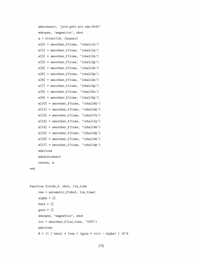
mdsconnect, ’jove.psfc.mit.edu:8100’
mdsopen, ’magnetics’, shot
m = fltarr(18, /nozero)
m[0] = smoother_f(time, ’\rhall1n’)
m[1] = smoother_f(time, ’\rhall1p’)
m[2] = smoother_f(time, ’\rhall2n’)
m[3] = smoother_f(time, ’\rhall2p’)
m[4] = smoother_f(time, ’\rhall3n’)
m[5] = smoother_f(time, ’\rhall3p’)
m[6] = smoother_f(time, ’\rhall4n’)
m[7] = smoother_f(time, ’\rhall4p’)
m[8] = smoother_f(time, ’\rhall5n’)
m[9] = smoother_f(time, ’\rhall5p’)
m[10] = smoother_f(time, ’\rhall6n’)
m[11] = smoother_f(time, ’\rhall6p’)
m[12] = smoother_f(time, ’\rhall7n’)
m[13] = smoother_f(time, ’\rhall7p’)
m[14] = smoother_f(time, ’\rhall8n’)
m[15] = smoother_f(time, ’\rhall8p’)
m[16] = smoother_f(time, ’\rhall9n’)
m[17] = smoother_f(time, ’\rhall9p’)
mdsclose
mdsdisconnect
return, m
end
function fields_f, shot, lin_time
raw = automatic_f(shot, lin_time)
alpha = []
beta = []
gain = []
mdsopen, ’magnetics’, shot
vcc = smoother_f(lin_time, ’\VCC’)
mdsclose
B = (1 / beta) * (raw / (gain * vcc) - alpha) / 10^4
176
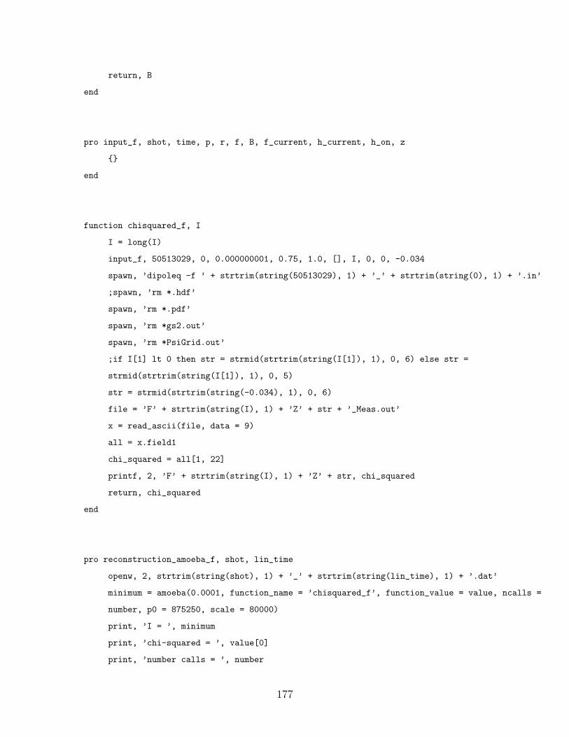
return, B
end
pro input_f, shot, time, p, r, f, B, f_current, h_current, h_on, z
end
function chisquared_f, I
I = long(I)
input_f, 50513029, 0, 0.000000001, 0.75, 1.0, [], I, 0, 0, -0.034
spawn, ’dipoleq -f ’ + strtrim(string(50513029), 1) + ’_’ + strtrim(string(0), 1) + ’.in’
;spawn, ’rm *.hdf’
spawn, ’rm *.pdf’
spawn, ’rm *gs2.out’
spawn, ’rm *PsiGrid.out’
;if I[1] lt 0 then str = strmid(strtrim(string(I[1]), 1), 0, 6) else str =
strmid(strtrim(string(I[1]), 1), 0, 5)
str = strmid(strtrim(string(-0.034), 1), 0, 6)
file = ’F’ + strtrim(string(I), 1) + ’Z’ + str + ’_Meas.out’
x = read_ascii(file, data = 9)
all = x.field1
chi_squared = all[1, 22]
printf, 2, ’F’ + strtrim(string(I), 1) + ’Z’ + str, chi_squared
return, chi_squared
end
pro reconstruction_amoeba_f, shot, lin_time
openw, 2, strtrim(string(shot), 1) + ’_’ + strtrim(string(lin_time), 1) + ’.dat’
minimum = amoeba(0.0001, function_name = ’chisquared_f’, function_value = value, ncalls =
number, p0 = 875250, scale = 80000)
print, ’I = ’, minimum
print, ’chi-squared = ’, value[0]
print, ’number calls = ’, number
177
printf, 2, ’I = ’, minimum
printf, 2, ’chi-squared = ’, value[0]
printf, 2, ’number calls = ’, number
close, 2
end
The body of input_f has been suppressed because of its length, but the subroutine
basically produces an input file that is read by the equilibrium code, DipolEq, which
is called by the chisquared_f function. The contents of some arrays have been
suppressed as well since they just contain numbers that take up space.
Upon obtaining the vacuum field corresponding to the best fit floating coil current,
the total field is calculated by adding the calibrated measurements from the Bp coils
and flux loops. The following codes subtract the integrator drift from Bp coil and
flux loop data, find the total field, use it to define a function of the pressure profile
parameters, and use the amoeba method to find the best fit parameter values:
function drift_helm, time, lin_time, ecrh_on, sensor
; this program attempts to eliminate the linear drift in the data caused by the integrator drift.
raw = ’\r’ + strmid(sensor, 2)
yr = mdsvalue(raw)
yr = abs(yr)
if max(yr) gt 9.8 then begin ; if the raw signal is ever greater than 9.8 then no further
print, 100 ; analysis is done.
return, 100
end
y = mdsvalue(sensor)
str = ’dim_of(’ + strtrim(sensor, 1) + ’)’
x = mdsvalue(str)
y = smooth(y, 400, /edge_truncate)
i = (x[1048574] - x[0]) / 1048574 ; the sampling interval is found.
j = -long(x[0] / i) ; the index for time = 0 is found.
m = long(lin_time / i) + j ; the index for the end/beginning time of the linear regime.
if lin_time le 0 then begin
ys = y[0:m] ; these new vectors are essentially truncated versions of x and y so that
xs = x[0:m] ; they only contain pre-trigger values.
178
endif else begin
ys = y[m:1048574] ; these vectors are also truncated versions of x and y so that
xs = x[m:1048574] ; they only contain the end values.
endelse
w = linfit(xs, ys) ; w contains the coefficients of the linear regression.
y = y - (w[0] + w[1] * x) ; the linear drift is subtracted here.
y = y - y[j] ; y @ t = 0 is zeroed.
plot, x, y
final = ’\f’ + strmid(sensor, 2) ; the final signal goes into this node.
expr = ’build_signal(build_with_units($, $), *, build_with_units(build_dim(*, $), $))’
if strmid(sensor, 2, 1) eq ’m’ then units = "Tesla" else units = "Weber"
;mdsput, final, expr, y, units, x, "sec"
k = long(time / i) + j ; the index for the desired time is found.
l = long(ecrh_on / i) + j ; the index for the ecrh turn on time.
print, y[k] - y[l]
return, y[k] - y[l]
end
function automatic, shot, time, lin_time, ecrh_on
;mdsconnect, ’jove.psfc.mit.edu:8100’
mdsopen, ’magnetics’, shot
diam = fltarr(26, /nozero)
diam[0] = drift_helm(time, lin_time, ecrh_on, ’\rmag1n’)
diam[1] = drift_helm(time, lin_time, ecrh_on, ’\rmag1p’)
diam[2] = drift_helm(time, lin_time, ecrh_on, ’\rmag2n’)
diam[3] = drift_helm(time, lin_time, ecrh_on, ’\rmag2p’)
diam[4] = drift_helm(time, lin_time, ecrh_on, ’\rmag3n’)
diam[5] = drift_helm(time, lin_time, ecrh_on, ’\rmag3p’)
diam[6] = drift_helm(time, lin_time, ecrh_on, ’\rmag4n’)
diam[7] = drift_helm(time, lin_time, ecrh_on, ’\rmag4p’)
diam[8] = drift_helm(time, lin_time, ecrh_on, ’\rmag5n’)
diam[9] = drift_helm(time, lin_time, ecrh_on, ’\rmag5p’)
diam[10] = drift_helm(time, lin_time, ecrh_on, ’\rmag6n’)
diam[11] = drift_helm(time, lin_time, ecrh_on, ’\rmag6p’)
diam[12] = drift_helm(time, lin_time, ecrh_on, ’\rmag7n’)
179
diam[13] = drift_helm(time, lin_time, ecrh_on, ’\rmag7p’)
diam[14] = drift_helm(time, lin_time, ecrh_on, ’\rmag8n’)
diam[15] = drift_helm(time, lin_time, ecrh_on, ’\rmag8p’)
diam[16] = drift_helm(time, lin_time, ecrh_on, ’\rmag9n’)
diam[17] = drift_helm(time, lin_time, ecrh_on, ’\rmag9p’)
diam[18] = drift_helm(time, lin_time, ecrh_on, ’\rflux1’)
diam[19] = -drift_helm(time, lin_time, ecrh_on, ’\rflux2’)
diam[20] = -drift_helm(time, lin_time, ecrh_on, ’\rflux3’)
diam[21] = -drift_helm(time, lin_time, ecrh_on, ’\rflux4’)
diam[22] = -drift_helm(time, lin_time, ecrh_on, ’\rflux5’)
diam[23] = -drift_helm(time, lin_time, ecrh_on, ’\rflux7’)
diam[24] = drift_helm(time, lin_time, ecrh_on, ’\rflux8’)
diam[25] = -drift_helm(time, lin_time, ecrh_on, ’\rflux9’)
smoother, ’\phall1n’
smoother, ’\phall1p’
smoother, ’\phall2n’
smoother, ’\phall2p’
smoother, ’\phall3n’
smoother, ’\phall3p’
smoother, ’\phall4n’
smoother, ’\phall4p’
smoother, ’\phall5n’
smoother, ’\phall5p’
smoother, ’\phall6n’
smoother, ’\phall6p’
smoother, ’\phall7n’
smoother, ’\phall7p’
smoother, ’\phall8n’
smoother, ’\phall8p’
smoother, ’\phall9n’
smoother, ’\phall9p’
fourier, ’\pmir2’
fourier, ’\pmir3’
;fourier, ’\pmir4’
;fourier, ’\pmir5’
;fourier, ’\pmir6’
180
;fourier, ’\pmir7’
;fourier, ’\pmir8’
;fourier, ’\pmir9’
mdsclose
;mdsdisconnect
return, diam
end
function fields, shot, time, lin_time, ecrh_on, vac
raw = automatic(shot, time, lin_time, ecrh_on)
NA = []
tau = []
B = (tau / NA) * raw
m = B + vac
return, m
end
pro input_r, shot, time, p, r, f, B, f_current, f_drop, h_current, h_on
end
function chisquared_r, p
input_r, 50513029, 5.95, p[0], 0.77, p[1], [] , 904000, 2005, 0, 0
spawn, ’dipoleq -f ’ + strtrim(string(50513029), 1) + ’_’ + strtrim(string(5.95), 1) + ’_’ +
’r’ + strmid(strtrim(string(0.77), 1), 0, 1) + strmid(strtrim(string(0.77), 1), 2, 2) + ’.in’
;spawn, ’rm *.hdf’
spawn, ’rm *.pdf’
spawn, ’rm *gs2.out’
spawn, ’rm *PsiGrid.out’
file = ’p’ + strmid(strtrim(string(p[0]), 1), 2, 3) + $
’r’ + strmid(strtrim(string(0.77), 1), 0, 1) + $
strmid(strtrim(string(0.77), 1), 2, 2) + $
’f’ + strmid(strtrim(string(p[1]), 1), 0, 1) + $
181
strmid(strtrim(string(p[1]), 1), 2, 2) + ’_Meas.out’
x = read_ascii(file, data = 9)
all = x.field1
chi_squared = all[1, 30]
printf, 2, ’p’ + strmid(strtrim(string(p[0]), 1), 2, 3) + $
’r’ + strmid(strtrim(string(0.77), 1), 0, 1) + $
strmid(strtrim(string(0.77), 1), 2, 2) + $
’f’ + strmid(strtrim(string(p[1]), 1), 0, 1) + $
strmid(strtrim(string(p[1]), 1), 2, 2), chi_squared
return, chi_squared
end
pro reconstruction_amoeba_r, shot, time, r
openw, 2, strtrim(string(shot), 1) + ’_’ + strtrim(string(time), 1) + ’_’ + ’r’ +
strmid(strtrim(string(r), 1), 0, 1) + strmid(strtrim(string(r), 1), 2, 2) + ’.dat’
minimum = amoeba(0.0001, function_name = ’chisquared_r’, function_value = value, ncalls =
number, p0 = [0.050, 1.10], scale = [0.010, 0.10])
print, ’p = ’, minimum[0], ’r = ’, r, ’f = ’, minimum[1]
print, ’chi-squared = ’, value[0]
print, ’number calls = ’, number
printf, 2, ’p = ’, minimum[0], ’r = ’, r, ’f = ’, minimum[1]
printf, 2, ’chi-squared = ’, value[0]
printf, 2, ’number calls = ’, number
close, 2
end
Most often, the amoeba minimization is used only after the approximate location of
the minimum is found through the brute force method. The brute force method is
carried out with the following code:
pro input, shot, time, p, r, f, B, f_current, f_drop, h_current, h_on
end
pro reconstruction, shot, time, lin_time, ecrh_on, f_current, f_drop, h_current, h_on, vac
182
;a = automatic(shot, time, lin_time, ecrh_on)
;NA = []
;tau = []
;B = (tau / NA) * a + vac
B = []
p = [0.005, 0.010, 0.020, 0.030, 0.040, 0.050, 0.060, 0.070]
;r = [0.67, 0.69, 0.71, 0.73, 0.75, 0.77, 0.79, 0.81, 0.83]
r = 0.77
f = [0.80, 0.90, 1.00, 1.10, 1.20, 1.30, 1.40, 1.50]
openw, 2, strtrim(string(shot), 1) + ’_’ + strtrim(string(time), 1) + ’.dat’
parameters = fltarr(3, 64, /nozero)
chi_squared = fltarr(64, /nozero)
for i = 0, 7 do begin
for j = 0, 0 do begin
for k = 0, 7 do begin
input, shot, time, p[i], r[j], f[k], B, f_current, f_drop, h_current, h_on
spawn, ’dipoleq -f ’ + strtrim(string(shot), 1) + ’_’ + strtrim(string(time), 1)
+ ’.in’
file = ’p’ + strmid(strtrim(string(p[i]), 1), 2, 3) + $
’r’ + strmid(strtrim(string(r[j]), 1), 0, 1) + $
strmid(strtrim(string(r[j]), 1), 2, 2) + $
’f’ + strmid(strtrim(string(f[k]), 1), 0, 1) + $
strmid(strtrim(string(f[k]), 1), 2, 2) + ’_Meas.out’
x = read_ascii(file, data = 9)
all = x.field1
printf, 2, ’p’ + strmid(strtrim(string(p[i]), 1), 2, 3) + $
’r’ + strmid(strtrim(string(r[j]), 1), 0, 1) + $
strmid(strtrim(string(r[j]), 1), 2, 2) + $
’f’ + strmid(strtrim(string(f[k]), 1), 0, 1) + $
strmid(strtrim(string(f[k]), 1), 2, 2), all[1, 30]
;n = 90 * i + 10 * j + k
;n = 10 * i + k
n = 8 * i + k
parameters[*, n] = [p[i], r[j], f[k]]
chi_squared[n] = all[1, 30]
endfor
183
endfor
endfor
chi_min = min(chi_squared, m)
printf, 2, parameters[*, m], chi_min
close, 2
end
The execution of the brute force method prior to running the amoeba scheme helps
prevent it from converging to a local minimum.
184

Bibliography
[1] H. L. Berk. Phys. Fluids, 19:1255, 1976.
[2] P. R. Bevington and D. K. Robinson. Data Reduction and Error Analysis for
the Physical Sciences. McGraw-Hill, 1992.
[3] B.J. Braams, W. Jilge, and K. Lackner. Nucl. Fusion, 26(6):699, 1986.
[4] A. Chan, M. Xia, and L. Chen. J. Geophys. Res., 99:17351, 1994.
[5] W. W. Connor and R. J. Hastie. Phys. Fluids, 19:1727, 1976.
[6] A. J. Dessler and E. N. Parker. J. Geophys. Res., 64:2239, 1959.
[7] J. R. Ferron, M. L. Walker, L. L. Lao, H. E. St. John, D. A. Humphreys, and
J. A. Leuer. Nucl. Fusion, 38:1055, 1998.
[8] J. P. Freidberg. Ideal Magnetohydrodynamics. Plenum Press, 1987.
[9] D. T. Garnier, A. Hansen, M. E. Mauel, E. Ortiz, A. C. Boxer, J. Ellsworth,
I. Karim, J. Kesner, S. Mahar, and A. Roach. Phys. Plasmas, 13:056111–1,
2006.
[10] D. T. Garnier, A. K. Hansen, J. Kesner, M. E. Mauel, P. C. Michael, J. V.
Minervini, A. Radovinsky, A. Zhukovsky, A. Boxer, J. Ellsworth, I. Karim, and
E. Ortiz. Design and initial operation of the ldx facility. Fusion Engineering and
Design, to be published, 2006.
[11] D. T. Garnier, J. Kesner, and M. E. Mauel. Phys. Plasmas, 6:3431, 1999.
185
[12] D. A. Gates, J. R. Ferron, M. Bell, T. Gibney, R. Johnson, R. J. Marsala, D. Mas-
trovito, J. E. Menard, D. Mueller, B. Penaflor, S. A. Sabbagh, and T. Stevenson.
Nucl. Fusion, 46:17, 2006.
[13] E. Hameiri, P. Laurence, and M. Mond. J. Geophys. Res., 96:1513, 1991.
[14] A. K. Hansen, A. C. Boxer, J. L. Ellsworth, D. T. Garnier, I. Karim, J. Kesner,
M. E. Mauel, and E. E. Ortiz. J. Fus. Energy, to be published, 2006.
[15] A. Hasegawa. Comm. Pl. Phys. & Cont. Fus., 1(147), 1987.
[16] A. Hasegawa, L. Chen, and M. E. Mauel. Nucl. Fusion, 30:2405, 1990.
[17] R. D. Hazeltine and J. D. Meiss. Plasma Confinement. Perseus Books, 1992.
[18] I. H. Hutchinson. Principles of Plasma Diagnostics. Cambridge University Press,
2002.
[19] I. Karim, M. E. Mauel, J. L. Ellsworth, A. C. Boxer, D. T. Garnier, A. K.
Hansen, J. Kesner, and E. E. Ortiz. J. Fus. Energy, to be published, 2006.
[20] J. Kesner, L. Bromberg, M. Mauel, D. Garnier, and J. M. Dawson. The dipole
fusion confinement concept. Technical report, 1998.
[21] N. A. Krall. Phys. Fluids, 9:820, 1966.
[22] S. I. Krasheninnikov and P. J. Catto. Phys. Plasmas, 7:626, 2000.
[23] N. S. Krasheninnikova and P. J. Catto. Phys. Plasmas, 12:032101, 2005.
[24] L. L. Lao, J. R. Ferron, R. J. Groebner, W. Howl, H. St. John, E. J. Strait, and
T. S. Taylor. Nucl. Fusion, 30:1035, 1990.
[25] L. L. Lao, H. St. John, R. D. Stambaugh, A. G. Kellman, and W. Pfeiffer. Nucl.
Fusion, 25:1611, 1985.
[26] B. Levitt, D. Maslovsky, and M. Mauel. Phys. Plasmas, 9, 2002.
186
[27] W. Lochte-Holtgreven. Plasma Diagnostics. American Institute of Physics, 1995.
[28] R. H. Lovberg. Plasma Diagnostic Techniques, chapter 3, pages 69–112. Aca-
demic Press, 1965.
[29] D. Maslovsky, B. Levitt, and M. Mauel. Phys. Rev. Lett., 10, 2003.
[30] D. Maslovsky, B. Levitt, and M. Mauel. Phys. Plasmas, 10, 2003.
[31] M. E. Mauel. J. Phys. IV, 7, 1997.
[32] M. E. Mauel. Another model pressure profile. Technical report, Columbia Uni-
versity, 2005.
[33] M. E. Mauel. Calculation of mutual inductance between f-coil and plasma. Tech-
nical report, Columbia University, 2005.
[34] M. E. Mauel. Calculation of mutual inductance between f-coil and plasma. Tech-
nical report, Columbia University, 2005.
[35] M. E. Mauel. Dipole equilibrium with anisotropic pressure. Technical report,
Columbia University, 2005.
[36] M. E. Mauel. Dipole equilibrium with anisotropic pressure (revised). Technical
report, Columbia University, 2005.
[37] M. E. Mauel. Equilibrium integral relations for dipole plasma. Technical report,
Columbia University, 2005.
[38] M. E. Mauel. Measuring the plasma current profile in ldx. Technical report,
Columbia University, 2005.
[39] E. E. Ortiz, A. C. Boxer, J. L. Ellsworth, D. T. Garnier, A. K. Hansen, I. Karim,
J. Kesner, and M. E. Mauel. J. Fus. Energy, to be published, 2006.
[40] W. H. Press, B. P. Flannery, S. A. Teukolsky, and W. T. Vetterling. Numerical
Recipes in C: The Art of Scientific Computing. Cambridge University Press,
1992.
187
[41] M. N. Rosenbluth and C. L. Longmire. Ann. Phys., 1:120, 1957.
[42] H. Saitoh, Z. Yoshida, H. Himura, J. Morikawa, and M. Fukao. Phys. Plasmas,
11:3331, 2004.
[43] H. Saitoh, Z. Yoshida, C. Nakashima, H. Himura, J. Morikawa, and M. Fukao.
Phys. Rev. Lett., 92:255005–1, 2004.
[44] N. Sckopke. J. Geophys. Res., 71:3125, 1966.
[45] A. N. Simakov, R. J. Hastie, and P. J. Catto. Phys. Plasmas, 7:3309, 2000.
[46] S. von Goeler, S. Jones, R. Kaita, S. Bernabei, W. Davis, H. Fishman, G. Get-
telfinger, D. Ignat, F. Paoletti, G. Petravich, F. Rimini, P. Roney, J. Stevens,
and W. Stodiek. Camera for imaging hard x rays from suprathermal electrons
during lower hybrid current drive on pbx-m. Rev. Sci. Instrum., 65:1621, May
1994.
188
Related Documents


