Equilibrium and (ir)reversibility in classical statistical mechanics

Equilibrium and (Ir)reversibility in Classical

Statistical Mechanics∗

D. A. LavisDepartment of Mathematics

King’s College, Strand, London WC2R 2LS - U.K.Email:[email protected]; Webpage:www.mth.kcl.ac.uk/∼dlavis

1 Introduction

The history of thermometry dates at least from the seventeenth century [1], but theadvent of thermodynamics proper can probably be set at the publication by Carnotof his Reflexions sur la puissance motrice du feu, et sur les machines propres adevelopper cette puissance. This work became well-known with its subsequent moreanalytic reformulation by Clapeyron [2] and inspired the work of Clausius andKelvin. In the case of each of these the development of thermodynamic conceptswas allied to a realization that heat has its origin in the motion of the constituentparticles of the system [3], and in the course of the next fifty years the foundationswere laid, by Maxwell and Boltzmann (among others), of kinetic theory leadingto statistical mechanics. So at least part of the role of statistical mechanics is toprovide the explanatory basis for thermodynamics. However, there are difficultieswith this, which were known to Maxwell and Boltzmann, and for which there areas yet no universally agreed resolution.

The temporal nature of events in the physical world can be divided into threetypes, distinguished by thinking of watching them on a film run in both directions.Some happenings appear possible (if eccentric) in both directions; others, like thepieces of a cup rising from the floor and reconstituting themselves into a whole cupstrike one as impossible. That leaves a third group of events for which the temporalordering is less clear. Suppose we have a cup of coffee into which we pour milk. Weexpect that the milk, starting in one region of the cup, will diffuse into the coffeeto form an apparently homogeneous mixture rather than the reverse process. Sincethere are no obvious forces leading to this outcome it needs an explanation. This isprovided by classical thermodynamics which orders equilibrium states according towhether one is adiabatically accessible from the other. The ordering of accessibilityof equilibrium states is defined in thermodynamics in terms of the entropy. For twoequilibrium states X and Y , X is adiabatically accessible from Y only if S(X) ≥S(Y ). For the coffee the final state will have larger entropy than the initial state(the increase being the entropy of mixing) and classical thermodynamics, in line

∗In ‘Frontiers in Fundamental Physics’,Vol. 3, Ed. B. G. Sidarth, Universities Press, India,2007.

1

with common-sense, will assert that the impossibility of the unmixing of the milkand coffee. So what is the problem? More precisely:

(i) What are the problems in using classical mechanics to produce a micro-scopic account of thermodynamics?

(ii) Do the mechanical systems which lead to thermodynamic behaviourhave any special features?

(iii) What are the competing programmes for solving this problem?

We shall describe below the structure of the dynamic models used to representthermodynamic systems. It is sufficient here to observe that they are normally (a)reversible and (b) volume-preserving. These two distinct properties each conflictwith the thermodynamic need for entropy to monotonically increase. The problemposed by having a reversible mechanical system was first noted by Maxwell [4], butbrought to Boltzmann’s attention in two papers published by Loschmidt [5, 6]. Thedifficulties posed by volume-preservation are a little more complicated. The mostwell-known is that the recurrence theorem of Poincare [7] applies [8, p. 214]. Poincare[9] drew attention to the problem that this posed for kinetic theory, although thiswas not considered by Boltzmann [10] until it was restated by Zermelo [11]. Lesswell-known is the problem of the meaning of equilibrium. The ‘equilibrium state’ ofa dynamic system is an attractor (stable equilibrium point, stable limit cycle, strangeattractor etc.). But volume-preserving systems do not have attractors [8, p. 210];so the concept of (mechanical) equilibrium does not apply to volume-preservingsystems. This means that, whatever mechanical description we try to give forthermodynamic equilibrium, it will not be related to the system being in dynamicequilibrium and there will be a need to define equilibrium.

Before outlining the different (and conflicting) attempts to resolve these prob-lems it is of interest to give some quotes which indicate where the difficulties lie.

The behaviour of thermodynamic systems, as embodied in the sec-ond law of thermodynamics, does not and cannot have an explana-tion in terms of the microscopic laws of physics as currently formulated.(Mackey [12].)

Either there is no temporal asymmetry at any stage, or it is there fromthe beginning. (Price [13, p. 43].)

Irreversibility is either true on all levels or on none; it cannot emergeas if out of nothing, on going from one level to another. (Prigogine andStengers [14, p. 285].)

Much of the history that Sklar recounts consists of physicists attemptingto continue the programme of deriving the thermodynamic laws from theunderlying dynamics even in the face of these objections. What seemsodd is the fairly manifest futility of these attempts. (Maudlin [15], inhis review of Physics and Chance by Sklar [16].)

Sklar [16] in his detailed survey of the foundations of statistical mechanics showsthat there is a variety of approaches which can be taken. However, if the dynamic

2

model is restricted in the way described below, they would seem to be of three maintypes:

The Weakened Second Law (Typical System) ApproachA vigorous defense of this view has been presented in a sequence of papers byLebowitz [17, 18, 19]. It can be summed up by the assertion that: “Having results fortypical microstates rather than averages is not just a mathematical nicety but at theheart of understanding the microscopic origin of observed macroscopic behaviour.We neither have nor do we need ensembles when we carry out observations . . . Whatwe do need and can expect is typical behaviour” [17, p. 38]. At the core of thisapproach is the willingness to accept the consequences of reversibility and recurrenceand to modify the weight of the thermodynamic second law to a high probabilityrather than a certainty. In his reply to Loschmidt [5], Boltzmann [20] argues forthis point of view and a similar point is made by Maxwell in his review of Tait’sThermodynamics. He asserts that the “truth of the second law”, as a statisticaltheorem, was “of the nature of a strong probability . . . not an absolute certainty”like dynamic laws, [4, p. 141]. More recently Griffths [21], Ruelle [22] and Bricmont[23] have supported this approach.

The Baysian (Subjectivist) ApproachJaynes [24, p. 416]1 asserts that statistical mechanics “is not a physical theory, but aform of statistical inference”. His maximum entropy method is based on a ‘rationalbelief’ interpretation of probability which allows the problems posed by reversibilityand recurrence to be resolved in a way not open to those who want to produce an‘objective’ theory. His aim “is not to ‘explain irreversibility’ [in thermodynamics],but to describe and predict the observed facts” [24, p. 416] and he is led to ask the“modest question: ‘Given the partial information that we do, in fact, have, whatare the best predictions we can make of observable phenomena?’ ” [24, p. 416].Whether one is inclined to accept the validity of this approach depends, to a largeextent, on being prepared to regard statistical mechanics as simply a procedurefor prediction, with the consequent information-related nature of thermodynamicquantities. In particular it means that: “Even at the purely phenomenological level,entropy is an anthropomorphic concept” [24, p. 86].

The Unstable System (Ensemble) ApproachThe use of ensembles in statistical mechanics can be traced to the work of Gibbs[26]. However, the reason for their use is not always clear except that they ‘work’.According to Tolman [27, p. 1] the “principles of statistical mechanics are to beregarded as permitting us to make reasonable predictions . . . expected to hold onaverage . . .”. In more recent times the use of ensembles has acquired, in the viewof their proponents, a more intrinsic role. According to Mackey [28, p. 984]: “Athermodynamic system is [my italics] a system that has, at any given time, statesdistributed throughout phase space . . ., and the distribution of these states is char-acterized by a density . . .”. The density referred to is the ensemble density and thusthe ensemble becomes the way that a thermodynamic system is defined. Accordingto Prigogine [29, p. 8] “it is at the level of ensembles that temporal evolution can bepredicted”. As we shall see the reason for making this assertion is that the subject

1For convenience references to Jaynes’ work are to his collected papers [24]. For an essay reviewof this collection see [25].

3

of statistical mechanics is taken to be unstable systems, for which, according to thethe Brussels–Austin School [29, 30, 31, 32, 33], it is necessary to develop a ‘com-plementary’ form of dynamics based on the evolution of a measure density, whichis reducible to a trajectory description only when the system is stable.

In the development of statistical mechanics it is customary to argue that the under-lying mechanical system has some further special properties beyond those describedin the next section. The purpose of these extra restrictions is, of course, to providea more or less plausible means of overcoming the problems cited above. As to whatthese extra special features are there is, however, some divergences of view, whichroughly divide into three positions, characterized by the following quotes:

(a) “The specific character of the systems studied in statistical mechanicsconsists mainly in the enormous number of degrees of freedom whichthese systems possess.” (Khinchin [34, p. 9].)

(b) The significant feature of a statistical mechanical system is that its “ini-tial state is incompletely specified”. (Tolman [27, p. 1].)

(c) Statistical mechanics is needed when the system is unstable and thereforechaotic. “For a stable system we can use a description in terms oftrajectories. We can also use a probabilistic description but this leadsto a description in terms of trajectories. The statistical description isreducible. On the other hand for chaotic systems the only descriptionwhich includes the approach to equilibrium is statistical.” (Prigogine[29, p. 60, my translation].)

Of these three propositions the contention that statistical mechanics is about sys-tems with a large number of particles (degrees of freedom) is that with the longestpedigree. It is frequently asserted at the beginning of undergraduate texts [35, p.140] and the thermodynamic limit, where the number of degrees of freedom N →∞,is fundamental to many of the exact results in statistical mechanics. A connectionbetween (a) and (b) is often made by the argument that it is the fact that N islarge which implies that we are unable to have complete knowledge of the system.While this is true it would go too far for Jaynes. The mere fact that we have in-complete knowledge of the system is sufficient justification for statistical mechanicsirrespective of whether N = 10 or 1023.2 If nevertheless we are interested in arguingthat statistical mechanics is a scientific theory (not just a procedure for inference)for incompletely specified systems, then we shall want to know why the system isincompletely specified? One possible answer is given by (c). Incomplete knowledgeis an intrinsic consequence of instability leading to chaos. In fact, as is clear fromthe passage from Les lois du chaos cited above, and in other places [36, p. 23], thisapproach by Prigogine and the Brussels–Austin group takes a more radical positionin asserting that in chaotic systems single trajectories do not exist.

Many of the fundamental disagreements about the foundations of statistical me-chanics can be related to three questions: (i) What does thermodynamics assert?

2For him probabilities, in statistical mechanics and elsewhere, “do not describe reality – onlyour information about reality” [24, p. 268], the reason for our ignorance about the system isirrelevant.

4

(ii) What is the meaning of probability? (iii) What kind of mechanics should beused? Their answers to (i) represent the main division between the typical systemand ensemble approaches and (ii) represents the main division between the subjec-tivist approach on the one hand and the typical system and ensemble approacheson the other [37]. The question of the nature of the mechanics used has two levels.The first is more-or-less benign in the sense that it would be common to all threeapproaches. The second represents the ‘heavier duty’ properties (ergodic, mixing,chaotic etc.) which are judged to be important by the Brussels–Austin Group,irrelevant by Jaynes’ group and of limited significance for the analysis of typicalsystems.3

1.1 The Dynamics

We now describe briefly the dynamic system assumed to be used for statisticalmechanics. We have a microstructure represented by an N -dimensional vector x ina phase space ΓN . Some dynamics x → φt x, (t ≥ 0) determines a flow in ΓN andthe set of points x(t) = φtx(0), parameterized by t ≥ 0, gives a trajectory.4 Thereis a measure on ΓN given by an L(1) density ρ(x; t). We suppose that the system is(a) classical, (b) finite, (c) deterministic,5 (d) autonomous. A consequence of (d) isthat the operators φtt≥0 form a semi-group. Let the time-evolution of the systembe determined by the equation of motion x(t) = F (x). Then a constant of motionf(x; t), and a measure density ρ(x; t), which yields an invariant measure on ΓN ,satisfy

∂f

∂t+ F · ∇(f) = 0 and

∂ρ

∂t+ ∇ · (ρF ) = 0, (1)

respectively, the latter being Liouville’s equation. The two remaining properties ofinterest will now be defined:

(e) The system is reversible if there exists an operator J on the points ofΓN , such that φtx = x′ implies J−1φtJ x′ = x. Then φ−t = J−1φtJand the set φtt∈< is a group.6

(f) Measure is preserved by the flow if ρ satisfies Liouville’s equation. Thisis a restriction on ρ not the system. A system is volume-preserving ifLiouville’s equation is satisfied by ρ = 1; then ∇ · F = 0. This is arestriction on the system.

Not all reversible systems are volume-preserving and not all volume-preserving sys-tems are reversible. For a volume-preserving system the equations (1) take the sameform; so an invariant measure density is a constant of motion.7

3Lebowitz seems to waver a little on the need for ergodicity.4We are primary interest in the case where both t and ΓN are continuous and our discussion

will be expressed in this form. However, it is often necessary for investigative purposes to useexamples where one or both of these is discrete [38].

5Although stochastic examples can often be heuristically useful [38].6For an ‘ordinary’ dynamic system, the variables x are divided into conjugate configuration q

and momentum p variables with J(q, p) = (q,−p).7An autonomous reversible Hamiltonian system is a special case of a volume-preserving system.

The Hamiltonian is a constant of motion and energy hyper-surfaces are invariant sets in ΓN .

5

Let Σ ⊂ ΓN be invariant with respect to the φt and let ρ(x; t) be normalizedover Σ. The functional

SG(ρ; t) = −kB

∫

Σ

ρ(x; t) lnρ(x; t) dNx, (2)

where kB is Boltzmann’s constant, is the Gibbs entropy.8 If ρ(x; t) satisfies Liou-ville’s equation then SG(ρ; t) is constant (with respect to time).9

We now define some of the more specialized properties of dynamic systems,which have been regarded as significant for statistical mechanics. Let Σ ⊂ ΓN beinvariant with respect to φt and 〈f〉σ denote the integral of f over σ ⊆ Σ. Thenthe system is:

Ergodic if Σ has no non-trivial invariant subsets. Then the following results canbe established:

(i) The time-independent solution ρ?(x) to Liouville’s equation, is uniqueto within normalization and an additive u such that 〈u〉Σ = 0. We shall,as a convenient name,10 call ρ?(x), with 〈ρ?〉Σ = 1, the equilibriumdensity function.

(ii) The infinite time average along a trajectory of a phase function f(x) isequal to its phase average 〈fρ?〉Σ.

(iii) With σ ⊂ Σ of non-zero measure, limτ→∞

T (σ; τ)τ

= 〈ρ?〉σ = M?(σ), where

T (σ; τ) is the time during the interval [0, τ ] in which the trajectory isin σ. This must, of course, be infinite as τ → ∞ for the limit to benon-zero.11

The simple harmonic oscillator is ergodic.

Mixing if the following condition holds. Let α, γ ⊂ Σ and let M? be an invariantequilibrium measure on Σ. If, in the infinite time limit, the part of the mapping ofγ which is in α is, in measure, proportional to the size of γ relative to the wholeof Σ then the system is mixing. A mixing flow is ergodic (but not the converse)and the equilibrium measure used in the definition is unique. The simple harmonicoscillator is not mixing.

Kolmogorov (a K-system) if it admits of a K-partition of Σ.12 K-systems aremixing. In 1963 Sinai proved that a system of more than two hard spheres in acube with perfectly reflecting walls is a K-system [41].

8At the moment this is just a convenient name without any physical baggage.9This result is not dependent on the system being volume-preserving.

10Without implying any specific meaning for the word ‘equilibrium’.11It follows from the Poincare recurrence theorem the trajectory must keep returning to points

arbitrarily close to x /∈ σ. It must therefore pass through σ an infinite number of times.12The rather technical definition of this is given in [39, p. 32] and [40, p. 80].

6

Bernoulli if there is a Bernoulli-partition Bn of Σ. This is defined in the followingway. Let Bn be a partition of Σ into n subsets. Label the members of Bn withthe integers [0, 1, . . . , n−1] and, for any trajectory and some ∆t, record the infinitesequence of numbers S = . . . , s−2, s−1, s0, s1, s2, . . ., where the trajectory is inthe set bsk

labelled sk at time k∆t. The partition is Bernoulli if all sequences S areuncorrelated and no two distinct trajectories have the same sequence. A Bernoullisystem is a K-system. The most celebrated example of a Bernoulli system is thebaker’s transformation (see below).

Exact if, for all σ ⊂ Σ, of non-zero measure, limt→∞

M?(φtσ) = 1. Such a systemcannot be reversible but it will be ergodic and mixing with a unique equilibriummeasure ρ?(x), and any invariant measure density ρ(x; t) satisfies

limt→∞

ρ(x; t) = ρ?(x). (3)

The missing member in this taxonomy is chaotic. This is rarely defined, even inbooks for which ‘chaos’ features in the title [8, 40]. A possible definition couldbe given in terms of the Lyapunov exponents of the flow [8, p. 129–138]. Roughlyspeaking a positive or negative Lyapunov exponent corresponds respectively to adilation or contraction of volume, with the flow, in that direction. A system ischaotic if it has at least one positive Lyapunov exponent and the sum of the expo-nents is not positive. For any system to have an attractor (probably strange in achaotic system) the sum of its Lyapunov exponents must be negative. As we havealready noted volume-preserving flows (including Hamiltonian systems) do not haveattractors and the sum of their Lyapunov exponents is zero. K-systems are chaotic;some mixing systems which are not K-systems are also chaotic.

2 The Weakened Second Law Approach

This approach is based on an explicit initial distinction between the micro andmacro levels. Consider a system, which at time t has microstate given by x(t) ∈ ΓN .Macrostates (observable states) are defined by a set Ξ of macroscopic variables.13

Let the set of macrostates be µΞ. They are so defined that every x ∈ ΓN is inexactly one macrostate denoted by µ(x) and the mapping x → µ(x) is many-one.Every macrostate µ is associated with its ‘volume’ V(µ) = Vµ in ΓN .14 We thushave the map x → µ(x) → Vµ(x) from ΓN to <+ or the positive integers. TheBoltzmann entropy is defined by

SB(x) = kB ln[Vµ(x)]. (4)

This is a phase function depending on the choice of macroscopic variables Ξ. How dowe expect that it will behave? The point of view of this approach can be expressedas follows:

13These may include some thermodynamic variables (volume, number of particles etc.) butthey can also include other variables, specifying, for example, the number of particles in a setof subvolumes. Ridderbos [42] denotes these by the collective name of supra-thermodynamicvariables.

14In the case where ΓN is continuous the volume of µ will normally be its Lebesque measure;when ΓN is discrete the volume will be the number of points in µ.

7

If the system starts at a phase point with low entropy then we expectthe entropy to increase. As it increases there will be fluctuations, whichcould be large. When the entropy gets near to its maximum value thenit will still fluctuate with possibly large fluctuations to small entropyvalues, but we don’t expect these to occur very often.

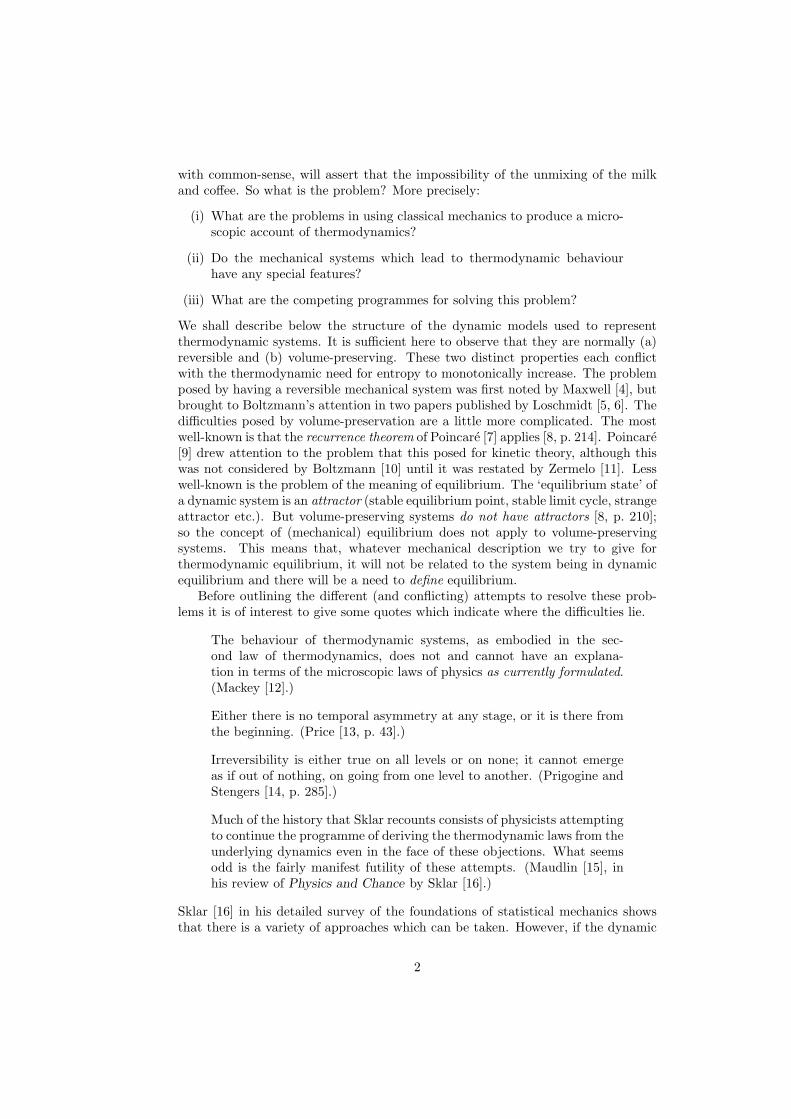
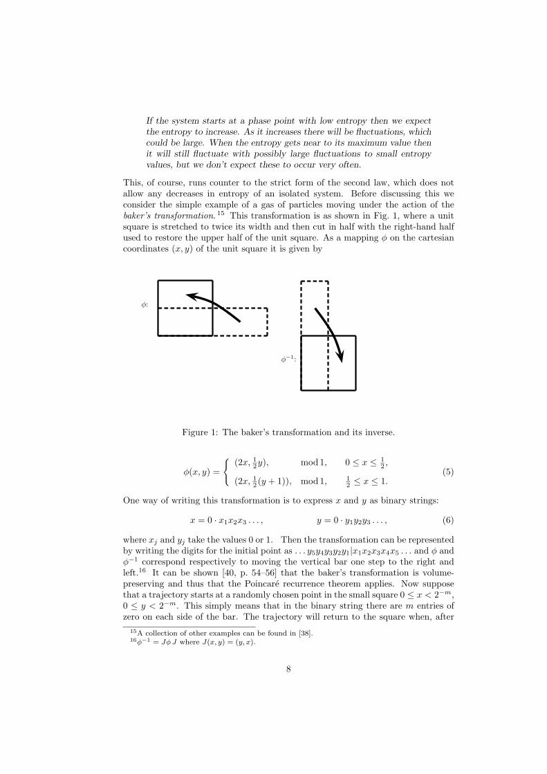
This, of course, runs counter to the strict form of the second law, which does notallow any decreases in entropy of an isolated system. Before discussing this weconsider the simple example of a gas of particles moving under the action of thebaker’s transformation. 15 This transformation is as shown in Fig. 1, where a unitsquare is stretched to twice its width and then cut in half with the right-hand halfused to restore the upper half of the unit square. As a mapping φ on the cartesiancoordinates (x, y) of the unit square it is given by

φ:

φ−1:

Figure 1: The baker’s transformation and its inverse.

φ(x, y) =

(2x, 1

2y), mod1, 0 ≤ x ≤ 12 ,

(2x, 12 (y + 1)), mod1, 1

2 ≤ x ≤ 1.(5)

One way of writing this transformation is to express x and y as binary strings:

x = 0 · x1x2x3 . . . , y = 0 · y1y2y3 . . . , (6)

where xj and yj take the values 0 or 1. Then the transformation can be representedby writing the digits for the initial point as . . . y5y4y3y2y1|x1x2x3x4x5 . . . and φ andφ−1 correspond respectively to moving the vertical bar one step to the right andleft.16 It can be shown [40, p. 54–56] that the baker’s transformation is volume-preserving and thus that the Poincare recurrence theorem applies. Now supposethat a trajectory starts at a randomly chosen point in the small square 0 ≤ x < 2−m,0 ≤ y < 2−m. This simply means that in the binary string there are m entries ofzero on each side of the bar. The trajectory will return to the square when, after

15A collection of other examples can be found in [38].16φ−1 = Jφ J where J(x, y) = (y, x).

8

t=0 t=2

t=4 t=6

t=8 t=10

t=12 t=14

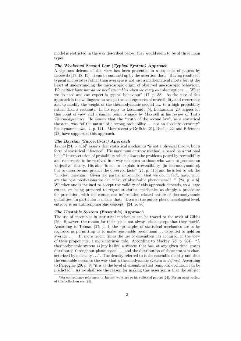
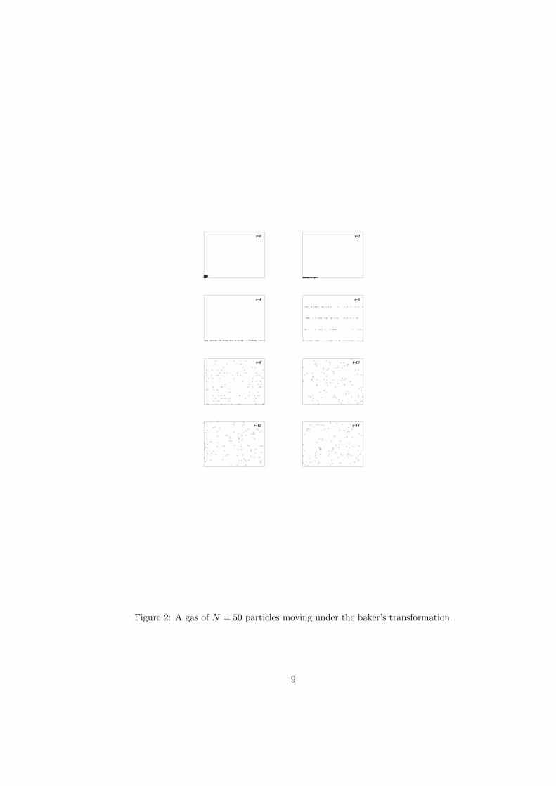
Figure 2: A gas of N = 50 particles moving under the baker’s transformation.

9

SB

t0

0.2

0.4

0.6

0.8

1

20 40 60 80 100

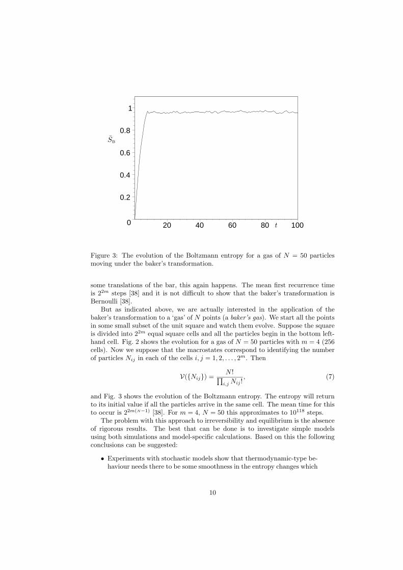
Figure 3: The evolution of the Boltzmann entropy for a gas of N = 50 particlesmoving under the baker’s transformation.

some translations of the bar, this again happens. The mean first recurrence timeis 22m steps [38] and it is not difficult to show that the baker’s transformation isBernoulli [38].

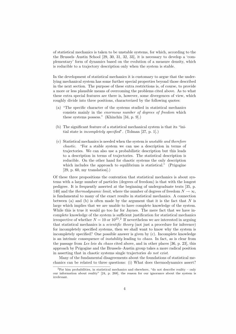
But as indicated above, we are actually interested in the application of thebaker’s transformation to a ‘gas’ of N points (a baker’s gas). We start all the pointsin some small subset of the unit square and watch them evolve. Suppose the squareis divided into 22m equal square cells and all the particles begin in the bottom left-hand cell. Fig. 2 shows the evolution for a gas of N = 50 particles with m = 4 (256cells). Now we suppose that the macrostates correspond to identifying the numberof particles Nij in each of the cells i, j = 1, 2, . . . , 2m. Then

V(Nij) =N !∏

i,j Nij !, (7)

and Fig. 3 shows the evolution of the Boltzmann entropy. The entropy will returnto its initial value if all the particles arrive in the same cell. The mean time for thisto occur is 22m(N−1) [38]. For m = 4, N = 50 this approximates to 10118 steps.

The problem with this approach to irreversibility and equilibrium is the absenceof rigorous results. The best that can be done is to investigate simple modelsusing both simulations and model-specific calculations. Based on this the followingconclusions can be suggested:

• Experiments with stochastic models show that thermodynamic-type be-haviour needs there to be some smoothness in the entropy changes which

10

occur as the trajectory passes from one macrostate to the next. This im-plies some restrictions of accessibility between macrostates. This is nor-mally achieved by the dynamics and a reasonable choice of macrostatestructure.

• Given a macrostate µ of volume V(µ), let v(±)(µ) be the proportionsin terms of total volume of the macrostates accessible from µ whichhave volumes [larger or equal]/[smaller] than V(µ). In models wherethe calculation can be made we have shown [38] that v(±)(µ) convergemonotonically above/below to 1

2 as V tends towards the macrostate oflargest volume Vmax.17 This suggests that when V(µ) ¿ Vmax a typicaltrajectory will pass into a macrostate of larger volume. Entropy willtypically increase. When V(µ) .= Vmax a typical trajectory will passinto macrostates of larger or smaller volume with almost equal proba-bilities. Entropy will fluctuate. Large fluctuations downwards from themaximum volume/entropy will be rare. To achieve a large reductionof entropy find a trajectory which has recently come from a state oflow entropy and reverse it. This will, if it can be done exactly, achieveuntypical behaviour.

3 The Baysian Approach

The argument from this standpoint which leads to an increasing entropy is givenby Jaynes [24, p. 27]. The basis of Jaynes’ method is to to ask what is the bestprobability distribution to use for the system given the information that we have.For Jaynes the key to the problem is the idea of uncertainty. Given an appropriatemeasure of uncertainty, if we choose the probability distribution which maximizesthe uncertainty relative to the available information then this will be the best prob-ability distribution because it assumes as little as possible. He shows the uniquemeasure of uncertainty, which satisfies some reasonable mathematical properties, isShannon’s information entropy which, for the dynamic system described in Sect. 1.1,is (to within a constant) the Gibbs entropy (2). Entropy is a measure of uncertaintyor lack of information. As time passes our information about the system becomesout-of-date. There is a loss of information, which is an increase in uncertainty (en-tropy). The way that this is realized is discussed in detail by Lavis and Milligan[25] and in the author’s contribution to the previous symposium in this series [37].A brief summary is as follows. Suppose we have the time-dependent observablesΩj(t) related to phase functions ωj(x; t) by Ωj(t) = 〈ωj(t)ρ(t)〉. Measurementsare made of these observables at the time t0 with the results Ωj(t0). The prob-ability density function ρ(x; t0) = ρ0(x; t0) is the one which maximizes SG(ρ; t0)subject to the constraints Ωj(t0) = 〈ωj(t0)ρ(t0)〉. The probability density func-tion evolves according to Liouville’s equation (1) and at a later time t is given byρ0(x; t). According to our state of knowledge our best predictions for the observ-ables at time t are now given by Ωj(t) = 〈ωj(t)ρ0(t)〉. Using these predicted valuesas new constraints we derive a new ρ(x; t) which maximizes SG(ρ; t). It is clearthat SG(ρ; t0) = SG(ρ0; t0) = SG(ρ0; t) ≤ SG(ρ; t). This approach highlights, even

17Of course, if µ is the unique macrostate of largest volume v(+)(µ) = 0, v(−)(µ) = 1.

11

more clearly that does Jaynes’ equilibrium treatment, the fact that entropy is tobe regarded, not as an objective property of the system but as dependent upon ourknowledge of the system. It is also somewhat more limited that the usual state-ment of the second law in that it does not establish that entropy is monotonicallyincreasing, but merely that it is larger at any time when it is recalculated.

4 The Unstable System Approach

For a reversible volume-preserving system, as described in Sect. 1.1, let Σ ⊂ ΓN

be invariant under the flow φt. Reversibility implies that the operators φtt∈<form a group and volume-preservation means that the Frobenius-Perron operatorsUtt∈<, given by

Utρ(x; 0) = ρ(φ−t(x); 0) = ρ(x; t), (8)

are unitary and also form a group with their inverses given by the correspondingKoopman operators [40].

In the ensemble approach equilibrium is defined to be the state described by atime-independent solution ρ?(x) of Liouville’s equation.18 As was indicated in Sect.1.1, for an ergodic system ρ?(x) exists and is unique. But for any arbitrary solutionρ(x; t) of Liouville’s equation to satisfy (3) and converge to the unique equilibriumsolution the system must be exact [40]. However, an exact system is not reversible,and this is the fundamental problem for which the Brussels–Austin group proposea solution. The evolution of their work from the late-sixties to the present has beendescribed in detail by Edens [43]. He divides the work into periods, the early years(1969–1985) and the later years (1988-present). In the former three strands canbe distinguished: (a) subdynamics, [30]; (b) Λ–transformations, [31, 36, 44]; (c)entropy as a selector of initial conditions, [45]. In our brief treatment of this workwe shall concentrate of the later part of this period.

Let $(x; γ; t) be the probability of a transition from x ∈ Σ to a point in γ ⊂ Σin time t and define the family of operators Wtt∈<+ by

Wtf(x) =∫

Σ

f(x′)$(x; dNx′; t), ∀ f ∈ L(2). (9)

It can be shown [31] that, if $(x; γ; t) is a Markov process, then Wtt∈<+ is a semi-group which preserves positivity and under which the uniform density is invariant.19

The next step is to find a non-unitary operator Λ so that

ΛUt = W †t Λ, and for which, we define ρ(x; t) = Λρ(x; t). (10)

Then it follows from (8) and (10) that

W †t ρ(x; 0) = ρ(x; t). (11)

Now it is necessary to determine the class of systems for which Λ exists, preservespositivity, the equilibrium density and the measure of any γ ⊂ Σ. We also want

18Hence the title ‘equilibrium density function’ coined on page 7.19Since the systems under consideration are at least ergodic the uniform density either is, or

induces, the unique equilbrium density.

12

||W †t ρ−ρ?||2 to decrease strictly monotonically to zero as t → +∞. However, when

this is true there is another subgroup W ′tt∈<− which shows the convergence when

t → −∞. So the problem is in two parts, first to find the non-unitary operator Λ andthen to give some principle which distinguishes between the realization which shows‘thermodynamic behaviour’ as t → +∞ and that for which this occurs as t → −∞.One possible approach, for a K-system, is to course-grain onto a K-partition [44].This means that Λ is a projection and does not have an inverse. The two repre-sentations are not complementary and there is a loss of information. The densityρ(x; t) cannot be reconstructed from the course-grained ρ(x; t). An alternative pro-cedure for K-systems can be developed [46, 47] in which Λ is invertible. However,“reconstruction is not possible for arbitrarily large time except if one assumes infi-nite accuracy in the observation of the physically evolving states” [46, p. 425]. Thequestion of distinguishing between thermodynamic and non-thermodynamic timeevolution is treated by Courbage [47]. The details are technical, but the idea is touse entropy as a measure of the information needed to construct the initial stateof the system. Non-thermodynamic behaviour needs the provision of an infiniteamount of information. This idea has a more than superficial similarity to thetrick, in the weakened second law approach, of achieving large Boltzmann entropydecreases in computer experiments by reversing the trajectory.

5 Conclusions

We have discussed three approaches20 to statistical mechanics which imply radicallydifferent meaning for irreversibility and equilibrium.

In the weakened second law approach the entropy is a phase function along atrajectory given by a combination of the dynamics and macrostate structure of thesystem. In consequence it fluctuates, but the dynamics and macrostate structurecombine to ensure that the fluctuations are typically small when the entropy is closeto its maximum. This entropy maximum is identified with the system being in itsmacrostate of maximum volume which is defined to be the equilibrium state. Asteep entropy increase occurs only when the system starts far from equilibrium ina macrostate of small volume.

In the baysian approach entropy is a measure of uncertainty about the system. Atany time it is calculated by finding the probability distribution which best representsour information about the system. Equilibrium is simply the state in which ourinformation is time-independent. If the information changes with time, and we makeno attempt to update it, it will necessarily become out-of-date, that is decrease, andthus entropy will be larger when it is recalculated using this information. This isan approach which is mathematically faultless, however, you must be prepared toaccept the anthropomorphic nature of entropy.

The unstable system approach takes as its starting point the supposition thatthermodynamic behaviour is an ensemble property. Classically this would have im-plied that we were dealing, not with a single system, but an average over a collection(ensemble) of systems. This would seem not to be the intention of Prigogine and

20There are other approaches (for a survey see e.g. Sklar [16]) which space does not allow us toconsider. In particular the deus ex machina approach in which irreversibility arises from outsideinterference is quite popular.

13

his group. Their aim is to develop a new form of dynamics which contains boththe usual dynamic description based on trajectories and a thermodynamic descrip-tion based on ensembles. These will be “complementary descriptions analogous tothe ‘complementarity’ encountered in quantum mechanics” [33]. The ensemble de-scription will be reducible to the trajectory description only when the system isnot chaotic. This project serves to support the contention of Mackey (quoted onpage 3) that a new form of mechanics is needed to produces a statistical mechanicswhich yields monotonic entropy increase. However, the conceptual content of theassertion that the sole description of a chaotic system is in terms of a distributionis less clear. The reference to an analogy with quantum mechanics might lead oneto suppose that some kind of ‘no-hidden-variable’ demonstration is necessary [48].The only form of this which is provided is the demonstration [49] that even whenρ(x; t) is localized in a region, however small, ρ(x; t) will be spread over all theaccessible set Σ ⊂ ΓN . This seems to be less that a proof of the non-existence oftrajectories.

References

[1] G. Emch and C. Liu. The logic of thermostatistical physics. Springer, 2002.

[2] B. P. Clapeyron. Memoire sur la puissance motrice de la chaleur. J. EcolePolytechnique, XIV, 23:153–190, 1834.

[3] R. Clausius. The nature of the motion which we call heat. Reprinted in Brush[50] Vol. 1, pages 111–134, 1857.

[4] P. M. Harman. The natural philosophy of James Clerk Maxwell. CambridgeU. P., 1998.

[5] J. Loschmidt. Wiener Beri., 73:139, 1876.

[6] J. Loschmidt. Wiener Beri., 75:67, 1877.

[7] H. Poincare. On the three-body problem and the equations of dynamics.Reprinted in Brush [50], Vol. 2, pages 194–202, 1890.

[8] E. Ott. Chaos in dynamical systems. Cambridge U. P., 1993.

[9] H. Poincare. Mechanism and experience. Reprinted in Brush [50], Vol. 2, pages203–207, 1893.

[10] L. Boltzmann. Reply to Zermelo’s remarks on the theory of heat. Reprintedin Brush [50], Vol. 2, pages 218–228, 1896.

[11] E. Zermelo. On a theorem of dynamics and the mechanical theory of heat.Reprinted in Brush [50], Vol. 2, pages 208–217, 1896.

[12] M. C. Mackey. Microscopic dynamics and the second law of thermodynamics. InC. Mugnai, A. Ranfagni, and L. S. Schulman, editors, Time’s arrows, quantummeasurement and superluminal behaviour, pages 49–65. Consignio NazionaleDell Ricerche, Roma, 2001.

14

[13] H. Price. Time’s arrow and Archimedes’ point: new directions for the physicsof time. Oxford U. P., 1996.

[14] I. Prigogine and I. Stengers. Order out of chaos. Heinemann, 1984.

[15] T. Maudlin. Review of Sklar [16]. Brit. J. Phil. Sci., 46:45–149, 1995.

[16] L. Sklar. Physics and chance. Cambridge U. P., 1993.

[17] J. L. Lebowitz. Boltzmann’s entropy and time’s arrow. Physics Today, 46:32–38, September 1993.

[18] J. L. Lebowitz. Time’s arrow and Boltzmann’s entropy. In J. J. Halliwell,J. Perez-Mercader, and W. H. Zurek, editors. Physical origins of time asym-metry. page 131, Cambridge U. P., 1994.

[19] J. L. Lebowitz. Statistical mechanics: A selective review of two central issues.Rev. Mod. Phys., 71:S386–S357, 1999.

[20] L. Boltzmann. On the relation of a general mechanical theorem to the secondlaw of thermodynamics. Reprinted in Brush [50], Vol. 2, pages 188–193, 1877.

[21] R. B. Griffiths. Statistical irreversibility: classical and quantum. In J. J.Halliwell, J. Perez-Mercader, and W. H. Zurek, editors. Physical origins oftime asymmetry. page 147, Cambridge U. P., 1994.

[22] D. Ruelle. Chance and chaos. Princeton U. P., 1991.

[23] J. Bricmont. Science of chaos or chaos in science? Physicalia, 17:159–208,1995.

[24] E. T. Jaynes. Papers on probability, statistics and statistical physics. Reidel,1983. Edited by Rosenkratz, R. D.

[25] D. A. Lavis and P. J. Milligan. The work of E. T. Jaynes on probability,statistics and statistical physics. Brit. J. Phil. Sci., 36:193–210, 1985.

[26] J. W. Gibbs. Elementary principles in statistical mechanics. Yale U. P., 1902.Reprinted by Dover Publications, 1960.

[27] R. C. Tolman. The principles of statistical mechanics. Oxford U. P., 1938.

[28] M. C. Mackey. The dynamic origin of increasing entropy. Rev. Mod. Phys.,61:981–1015, 1989.

[29] I. Prigogine. Les lois du chaos. Flammarion, 1994.

[30] R. Balescu. Equilibrium and non-equilibrium statistical mechanics. Wiley, 1975.

[31] B. Misra, I. Prigogine, and M. Courbage. From determininstic dynamics toprobabalistic descriptions. Physica A, 98:1–26, 1979.

[32] I. Prigogine. Laws of nature, probability and time symmetry breaking. PhysicaA, 263:528–539, 1999.

15

[33] B. Misra. Nonequilibrium entropy, Lyapounov variables and ergodic propertiesof classical systems. Proc. Natl. Acad. Sci. USA, 75:1627–1631, 1978.

[34] A. I. Khinchin. Mathematical foundations of statistical mechanics. Dover, 1949.

[35] K. Huang. Statistical mechanics. John Wiley, 1963.

[36] B. Misra and I. Prigogine. Time, probability and dynamics. In C.W. Horton,Reichl L. E., and V. G. Szebehely, editors, Proceedings of the workshop onlong-time predictions in nonlinear conservative dynamical systems, pages 21–43. Wiley, 1981.

[37] D. A. Lavis. The concept of probability in statistical mechanics. In B. G.Sidharth and M. V. Altaisky, editors, Frontiers of Fundamental Physics, 4,pages 293–308. Kluwer, 2001.

[38] D. A. Lavis. Some examples of simple systems. Available at:www.mth.kcl.ac.uk/∼dlavis/papers/examples.pdf, 2002.

[39] V. I. Arnold and A. Avez. Ergodic problems of classical mechanics. Benjamin,1968.

[40] A. L. Lasota and M. C. Mackey. Chaos, fractals and noise. Springer, 1994.

[41] Ja. G. Sinai. Ergodicity of Boltzmann’s gas model. In T. H. Bak, editor,Statistical mechanics: foundations and applications, pages 559–573. Benjamin,1967.

[42] K. Ridderbos. The course-graining approach to statistical mechanics: howblissful is our ignorance? Stud. Hist. Phil. Mod. Phys., 33:65–77, 2002.

[43] B. Edens. Semigroups and symmetry: an investigation of Prigogine’s theories.PhD thesis, Institute for History and Foundations of Science, Utrecht Univer-sity, 2001. Available at:http://philsci-archive.pitt.edu/documents/disk0/00/00/04/36/.

[44] B. Misra and I. Prigogine. On the foundations of kinetic theory. Sup. Prog.Theor. Phys., 69:101–110, 1980.

[45] M. Courbage and I. Prigogine. Intrinsic randomness and intrinsic irreversibilityin classical dynamical systems. Proc. Natl. Acad. Sci. USA, 80:2412–2416, 1983.

[46] B. Misra and I. Prigogine. Irreversibility and nonlocality. Let. Math. Phys.,7:421–429, 1983.

[47] M. Courbage. Intrinsic irreversibility of Kolmogorov dynamical systems. Phys-ica A, 122:459–482, 1983.

[48] R. W. Batterman. Randomness and probability in dynamical theories: on theproposals of the Prigogine school. Philosophy of Science, 58:241–262, 1991.

[49] S. Goldstein, B. Misra, and M. Courbage. On intrisic randomness of dynamicalsystems. J. Stat. Phys., 25:111–126, 1981.

[50] S. G. Brush. Kinetic theory, Vol. 1, Pergamon, 1965; Vol. 2, Pergamon, 1966.

16