Equating Test Scores (without IRT)

EQUATINGTESTSCORES(Without IRT)

Samuel A. Livingston

Listening.Learning.

Leading.72528189530-036492 • U54E6 • Printed in U.S.A.

036492_cover 5/13/04, 11:47 AM2-3

Equating Test Scores

(Without IRT)

Samuel A. Livingston

Copyright © 2004 Educational Testing Service. All rights reserved. Educational Testing Service, ETS, and the ETS logo are

registered trademarks of Educational Testing Service.

iii

i

Foreword This booklet is essentially a transcription of a half-day class on equating that I teach for new statistical staff at ETS. The class is a nonmathematical introduction to the topic, emphasizing conceptual understanding and practical applications. The topics include raw and scaled scores, linear and equipercentile equating, data collection designs for equating, selection of anchor items, and methods of anchor equating. I begin by assuming that the participants do not even know what equating is. By the end of the class, I explain why the Tucker method of equating is biased and under what conditions. In preparing this written version, I have tried to capture as much as possible of the conversational style of the class. I have included most of the displays projected onto the screen in the front of the classroom. I have also included the tests that the participants take during the class.

ii Acknowledgements The opinions expressed in this booklet are those of the author and do not necessarily represent the position of ETS or any of its clients. I thank Michael Kolen, Paul Holland, Alina von Davier, and Michael Zieky for their helpful comments on earlier drafts of this booklet. However, they should not be considered responsible in any way for any errors or misstatements in the booklet. (I didn’t even make all of the changes they suggested!) And I thank Kim Fryer for preparing the booklet for printing; without her expertise, the process would have been much slower and the product not as good.

iii

Objectives Here is a list of the instructional objectives of the class (and, therefore, of this booklet). If the class is completely successful, participants who have completed it will be able to... Explain why testing organizations report scaled scores instead of raw scores.

State two important considerations in choosing a score scale.

Explain how equating differs from statistical prediction.

Explain why equating for individual test-takers is impossible.

State the linear and equipercentile definitions of comparable scores and explain why they are meaningful only with reference to a population of test-takers.

Explain why linear equating leads to out-of-range scores and is heavily group-dependent and how equipercentile equating avoids these problems.

Explain why equipercentile equating requires “smoothing.”

Explain how the precision of equating (by any method) is limited by the discreteness of the score scale.

Describe five data collection designs for equating and state the main advantages and limitations of each.

Explain the problems of “scale drift” and “equating strains.”

State at least six practical guidelines for selecting common items for anchor equating.

Explain the fundamental assumption of anchor equating and explain how it differs for different equating methods.

Explain the logic of chained equating methods in an anchor equating design.

Explain the logic of equating methods that condition on anchor scores and the conditions under which these methods are biased.

iv Prerequisite Knowledge Although the class is nonmathematical, I assume that users are familiar with the following basic statistical concepts, at least to the extent of knowing and understanding the definitions given below. (These definitions are all expressed in the context of educational testing, although the statistical concepts are more general.) Score distribution: The number (or the percent) of test-takers at each score level.

Mean score: The average score, computed by summing the scores of all test-takers and dividing by the number of test-takers.

Standard deviation: A measure of the dispersion (spread, amount of variation) in a score distribution. It can be interpreted as the average distance of scores from the mean, where the average is a special kind of average called a “root mean square,” computed by squaring the distance of each score from the mean, then averaging the squared distances, and then taking the square root.

Correlation: A measure of the strength and direction of the relationship between the scores of the same people on two tests.

Percentile rank of a score: The percent of test-takers with lower scores, plus half the percent with exactly that score. (Sometimes it is defined simply as the percent with lower scores.)

Percentile of a distribution: The score having a given percentile rank. The 80th percentile of a score distribution is the score having a percentile rank of 80. (The 50th percentile is also called the median; the 25th and 75th percentiles are also called the 1st and 3rd quartiles.)

v

Table of Contents Why Not IRT?..................................................................................................................... 1

Teachers’ Salaries and Test Scores..................................................................................... 2

Scaled Scores ...................................................................................................................... 3

Choosing the Score Scale.................................................................................................... 5

Limitations of Equating ...................................................................................................... 7

Equating Terminology ........................................................................................................ 9

Equating Is Symmetric...................................................................................................... 10

A General Definition of Equating..................................................................................... 12

A Very Simple Type of Equating ..................................................................................... 12

Linear Equating................................................................................................................. 14

Problems with linear equating ...................................................................................... 16

Equipercentile Equating.................................................................................................... 17

A problem with equipercentile equating, and a solution .............................................. 19 A limitation of equipercentile equating ........................................................................ 23 Equipercentile equating and the discreteness problem ................................................. 23

Test: Linear and Equipercentile Equating......................................................................... 25

Equating Designs .............................................................................................................. 27

The single-group design................................................................................................ 27 The counterbalanced design.......................................................................................... 28 The equivalent-groups design ....................................................................................... 29 The internal-anchor design ........................................................................................... 30 The external-anchor design........................................................................................... 33

Test: Equating Designs ..................................................................................................... 36

Selecting “Common Items” for an Internal Anchor ......................................................... 38

Scale Drift ......................................................................................................................... 40

The Standard Error of Equating........................................................................................ 42

Equating Without an Anchor ............................................................................................ 43

Equating in an Anchor Design.......................................................................................... 44

Two ways to use the anchor scores............................................................................... 46

Chained Equating.............................................................................................................. 47

Conditioning on the Anchor: Frequency Estimation Equating......................................... 49

vi

Frequency estimation equating when the correlations are weak .................................. 52

Conditioning on the Anchor: Tucker Equating................................................................. 54

Tucker equating when the correlations are weak.......................................................... 57

Correcting for Imperfect Reliability: Levine Equating..................................................... 59

Choosing an Anchor Equating Method............................................................................. 59

Test: Anchor Equating ...................................................................................................... 61

References......................................................................................................................... 63

Answers to Tests ............................................................................................................... 64

Answers to test: Linear and equipercentile equating .................................................... 64 Answers to test: Equating designs ................................................................................ 66 Answers to test: Anchor equating................................................................................. 67

1

Why Not IRT? The subtitle of this booklet—“without IRT”—may require a bit of explanation. Item Response Theory (IRT) has become one of the most common approaches to equating test scores. Why is it specifically excluded from this booklet? The short answer is that IRT is outside the scope of the class on which this booklet is based and, therefore, outside the scope of this booklet. Many new statistical staff members come to ETS with considerable knowledge of IRT but no knowledge of any other type of equating. For those who need an introduction to IRT, there is a separate half-day class. But now that IRT equating is widely available, is there any reason to equate test scores any other way? Indeed, IRT equating has some important advantages. It offers tremendous flexibility in choosing a plan for linking test forms. It is especially useful for adaptive testing and other situations where each test-taker gets a custom-built test form. However, this flexibility comes at a price. IRT equating is complex, both conceptually and procedurally. Its definition of equated scores is based on an abstraction, rather than on statistics that can actually be computed. It is based on strong assumptions that often are not a good approximation of the reality of testing. Many equating situations don’t require the flexibility that IRT offers. In those cases, it is better to use other methods of equating—methods for which the procedure is simpler, the rationale is easier to explain, and the underlying assumptions are closer to reality.

2 Teachers’ Salaries and Test Scores I like to begin the class by talking not about testing but about teachers’ salaries. How did the average U.S. teacher’s salary in a recent year, such as 1998, compare with what it was 40 years earlier, in 1958? In 1998, it was about $39,000 a year; in 1958, it was only about $4,600 a year.1 But in 1958, you could buy a gallon of gasoline for 30¢; in 1998 it cost about $1.05, or 3 1/2 times as much. In 1958 you could mail a first-class letter for 4¢; in 1998, it cost 33¢, roughly eight times as much. A house that cost $20,000 in 1958 might have sold for $200,000 in 1998—ten times as much. So it’s clear that the numbers don’t mean the same thing. A dollar in 1958 bought more than a dollar in 1998. Prices in 1958 and prices in 1998 are not comparable. How can you meaningfully compare the price of something in one year with its price in another year? Economists use something called “constant dollars.” Each year the government’s economists calculate the cost of a particular selection of products that is intended to represent the things that a typical American family buys in a year. The economists call this mix of products the “market basket.” They choose one year as the “reference year.” Then they compare the cost of the “market basket” in each of the other years with its cost in the reference year. This analysis enables them to express wages and prices from each of the other years in terms of reference-year dollars. To compare the average teacher’s salary in 1958 with the average teacher’s salary in 1998, they would convert both those salaries into reference-year dollars. Now, what does all this have to do with educational testing? Most standardized tests exist in more than one edition. These different editions are called “forms” of the test. All the forms of the test are intended to test the same skills and types of knowledge, but each form contains a different set of questions. The test developers try to make the questions on different forms equally difficult, but more often than not, some forms of the test turn out to be harder than others. The simplest way to compute a test-taker’s score is to count the questions answered correctly. If the number of questions differs from form to form, you might want to convert that number to a percent-correct. We call number-correct and percent-correct scores “raw scores.” If the questions on one form are harder than the questions on another form, the raw scores on those two forms won’t mean the same thing. The same percent-correct score on the two different forms won’t indicate the same level of the knowledge or skill the test is intended to measure. The scores won’t be comparable. To treat them as if they were comparable would be misleading for the score users and unfair to the test-takers who took the form with the harder questions.

1 Source: www.aft.org/research/survey/tables (March 2003)

3

Scaled Scores Score users need to be able to compare the scores of test-takers who took different forms of the test. Therefore, testing agencies need to report scores that are comparable across different forms of the test. We need to make a given score indicate the same level of knowledge or skill, no matter which form of the test the test-taker took. Our solution to this problem is to report “scaled scores.” Those scaled scores are adjusted to compensate for differences in the difficulty of the questions. The easier the questions, the more questions you have to answer correctly to get a particular scaled score. Each form of the test has its own “raw-to-scale score conversion”—a formula or a table that gives the scaled score corresponding to each possible raw score. Table 1 shows the raw-to-scale conversions for the upper part of the score range on three forms of an actual test:

Table 1. Raw-to-Scale Conversion Table for Three Forms of a Test

Raw score Scaled score Form R Form T Form U

120 200 200 200 119 200 200 198 118 200 200 195 117 198 200 193 116 197 200 191 115 195 199 189 114 193 198 187 113 192 197 186 112 191 195 185 111 189 194 184 110 188 192 183 109 187 190 182 108 185 189 181 107 184 187 180 106 183 186 179 105 182 184 178 etc. etc. etc. etc.

4 Notice that on Form R to get the maximum possible scaled score of 200 you would need a raw score of 118. On Form T, which is somewhat harder, you would need a raw score of only 116. On Form U, which is somewhat easier, you would need a raw score of 120. Similarly, to get a scaled score of 187 on Form R, you would need a raw score of 109. On Form T, which is harder, you would need a raw score of only 107. On Form U, which is easier, you would need a raw score of 114. The raw-to-scale conversion for the first form of a test can be specified in a number of different ways. (I’ll say a bit more about this topic later.) The raw-to-scale conversion for the second form is determined by a statistical procedure called “equating.” The equating procedure determines the adjustment to the raw scores on the second form that will make them comparable to raw scores on the first form. That information enables us to determine the raw-to-scale conversion for the second form of the test. Now for some terminology. The form for which the raw-to-scale conversion is originally specified—usually the first form of the test—is called the “base form.” When we have determined the raw-to-scale conversion for a form of a test, we say that form is “on scale.” The raw-to-scale conversion for each form of the test other than the base form is determined by equating to a form that is already “on scale.” We refer to the form that is already on scale as the “reference form.” We refer to the form that is not yet on scale as the “new form.” Usually the “new form” is a form that is being used for the first time, while the “reference form” is a form that has been used previously. Occasionally we equate scores on two forms of the test that are both being used for the first time, but we still use the terms “new form” and “reference form” to indicate the direction of the equating. The equating process determines for each possible raw score on the new form the corresponding raw score on the reference form. This equating is called the “raw-to-raw” equating. But, because the reference form is already “on scale,” we can take the process one step further. We can translate any raw score on the new form into a corresponding raw score on the reference form and then translate that score to the corresponding scaled score. When we have translated each possible raw score on the new form into a scaled score, we have determined the raw-to-scale score conversion for the new form. Unfortunately, the process is not quite as simple as I have made it seem. A possible raw score on the new form almost never equates exactly to a possible score on the reference form. Instead, it equates to a point in between two raw scores that are possible on the reference form. So we have to interpolate. Consider the example in Table 2:

5

Table 2. New Form Raw Scores to Reference Form Raw Scores to Scaled Scores

New form raw-to-raw equating

Reference form raw-to-scale conversion

New form Reference form Reference form Raw score Raw score Raw score

Exact scaled score

... ... ... ... 59 60.39 59 178.65 58 59.62 58 176.71 57 58.75 57 174.77 56 57.88 56 172.83 ... ... ... ...

(In this example, I have used only two decimal places. Operationally we use a lot more than two.) Now suppose a test-taker had a raw score of 57 on the new form. That score equates to a raw score of 58.75 on the reference form, which is not a possible score. But it is 75 percent of the way from a raw score of 58 to a raw score of 59. So the test-taker’s exact scaled score will be the score that is 75 percent of the way from 176.71 to 178.65. That score is 178.14. In this way, we determine the exact scaled score for each raw score on the new form. We round the scaled scores to the nearest whole number before we report them to test-takers and test users, but we keep the exact scaled scores on record. We will need the exact scaled scores when this form becomes the reference form in a future equating.

Choosing the Score Scale Before we specify the raw-to-scale conversion for the base form, we have to decide what we want the range of scaled scores to be. Usually we try to choose a set of numbers that will not be confused with the raw scores. We want any test-taker or test user looking at a scaled score to know that the score could not reasonably be the number or the percent of questions answered correctly. That’s why scaled scores have possible score ranges like 200 to 800 or 100 to 200 or 150 to 190. Another thing we have to decide is how fine a score scale to use. For example, on most tests, the scaled scores are reported in one-point intervals (100, 101, 102, etc.). However, on some tests, they are reported in five-point intervals (100, 105, 110, etc.) or ten-point intervals (200, 210, 220, etc.). Usually we want each additional correct answer to make a difference in the test-taker’s scaled score, but not such a large difference that people exaggerate its importance. That is why the score interval on the SAT2 was changed. Many years ago, when the SAT was still called the “Scholastic Aptitude Test,” any whole

2 More precisely, the SAT® I: Reasoning Test.

6 number from 200 to 800 was a possible score. Test-takers could get scaled scores like 573 or 621. But this score scale led people to think the scores were more precise than they really were. One additional correct answer could raise a test-taker’s scaled score by eight or more points. Since 1970 the scaled scores on the SAT have been rounded to the nearest number divisible by 10. If a test-taker’s exact scaled score is 573.2794, that scaled score is reported as 570, not as 573. One additional correct answer will change the test-taker’s score by ten points (in most cases), but people realize that a ten-point difference is just one step on the score scale. One issue in defining a score scale is whether to “truncate” the scaled scores. Truncating the scaled scores means specifying a maximum value for the reported scaled scores that is less than the maximum value that you carry on the records. For example, we might use a raw-to-scale conversion for the base form that converts the maximum raw score to a scaled score of 207.1429, but truncate the scores at 200 so that no test-taker will have a reported scaled score higher than 200. (The raw-to-scale conversions shown in Table 1 are an example.) If we truncate the scores, we will award the maximum possible scaled score to test-takers who did not get the maximum possible raw score. We will disregard some of the information provided by the raw scores at the top end of the score scale. Why would we want to do such a thing? Here’s the answer. Suppose we decided not to truncate the scaled scores. Then the maximum reported scaled score would correspond to a perfect raw score on the base form—100 percent. Now suppose the next form of the test proves to be easier than the base form. The equating might indicate that a raw score of 100 percent on the second form corresponds to the same level of knowledge as a raw score of 96 percent on the base form. There will probably be test-takers with raw scores of 100 percent on the easier second form whose knowledge would be sufficient for a raw score of only 96 percent on the harder base form. Is it fair to give them the maximum possible scaled score? But there may be other test-takers with raw scores of 100 percent on the easier second form whose knowledge is sufficient for a raw score of 100 percent on the harder base form. Is it fair to give them anything less than the maximum possible scaled score? Truncating the scaled scores—awarding the maximum possible scaled score for a raw score less than 100 percent on the base form—helps us to avoid this dilemma. It is also common to truncate the scaled scores at the low end of the scale. In this case the reason is usually somewhat different—to avoid making meaningless distinctions. Most standardized tests are multiple-choice tests. On these tests, the lowest possible scores are below the “chance score.” That is, they are lower than the score a test-taker could expect to get by answering the questions without reading them. On most tests, if two scores are both below the chance score, the difference between those scores tells us very little about the differences between the test-takers who earn those scores.

7

There is more than one way to choose the raw-to-scale conversion for the base form of a test. One common way is to identify a group of test-takers and choose the conversion that will result in a particular mean and standard deviation for the scaled scores of that group. Another way is to choose two particular raw scores on the base form and specify the scaled score for each of those raw scores. Those two points will then determine a simple linear formula that transforms any raw score to a scaled score. For example, on the Praxis™ tests, we truncate the scaled scores at both ends. On the Praxis scale, the lowest scaled score is 100; the highest is 200. When we determine the raw-to-scale conversion for the first form of a new test, we typically make a scaled score of 100 correspond to the chance score on the base form. We make a scaled score of 200 correspond to a raw score of 95 percent correct on the base form. Some testing programs use a reporting scale that consists of a small number of broad categories. (The categories may be identified by labels, such as “advanced,” “proficient,” etc., or they may be identified only by numbers.) The smaller the number of categories, the greater the difference in meaning between any category and the next. But if each category corresponds to a wide range of raw scores, there will be test-takers in the same category whose raw scores differ by many points. To make matters worse, there will also be test-takers in different categories whose raw scores differ by only a single point. Reporting only the category for each test-taker will conceal some fairly large differences. At the same time, it will make small differences appear large. In my opinion, there is nothing wrong with grouping scores into broad categories and reporting the category for each test-taker if you also report a score that indicates the test-taker’s position within the category.

Limitations of Equating Let’s go back to the topic I started with—teachers’ salaries. The economists’ “constant dollars” don’t adjust correctly for the cost of each kind of thing a teacher might want to spend money on. From 1958 to 1998, the prices of housing, medical care, and college tuition went up much more than the prices of food and clothing. The prices of some things, like electronic equipment, actually went down. Constant dollars cannot possibly adjust correctly for the prices of all these different things. The adjustment is correct for a particular mix of products—the “market basket.” Similarly, if you were to compare two different test-takers taking the same test, one test-taker might know the answers to more of the questions on Form A than on Form B; the other might know the answers to more of the questions on Form B than on Form A. There is no possible score adjustment that will make Forms A and B equally difficult for these two test-takers. Equating cannot adjust scores correctly for every individual test-taker.

8 Equating can adjust scores correctly for a group of test-takers—but not for every possible group. One group may contain a high proportion of test-takers for whom Form A is easier than Form B. Another group may contain a high proportion of test-takers for whom Form B is easier than Form A. There is no possible score adjustment that will make Forms A and B equally difficult for these two groups of test-takers. For example, if one form of an achievement test happens to have several questions about points of knowledge that a particular teacher emphasizes, that teacher’s students are likely to find that test form easier than other forms of the same test. But the students of most other teachers will not find that form any easier than any other form. The adjustment that is correct for that particular teacher’s students will not be correct for students of the other teachers. Equating cannot adjust scores correctly for every possible group of test-takers. If you read some of the papers and articles that have been written about equating, you may see statements that equating must adjust scores correctly for every individual test-taker or that equating must adjust scores correctly for every possible group of test-takers. The examples I have just presented show clearly that no equating adjustment can possibly meet such a requirement.3 Fortunately, an equating adjustment that is correct for one group of test-takers is likely to be at least approximately correct for most other groups of test-takers. Note the wishy-washy language in that sentence: “likely to be at least approximately correct for most other groups of test-takers.” When we equate test scores, we identify a group of test-takers for whom we want the equating to be correct. We call this group the “target population.” It may be an actual group or a hypothetical group. We may identify it explicitly or only implicitly. But every test score equating is an attempt to determine the score adjustment that is correct for some target population. How well the results generalize to other groups of test-takers will depend on how similar the test forms are. The smaller the differences in the content and difficulty of the questions on the two forms of the test, the more accurately the equating results will generalize from the target population to other groups of test-takers. Another limitation of equating results from the discreteness of the scores. Typically the scaled scores that we report are whole numbers. When the equating adjustment is applied to a raw score on the new form, and the equated score is converted to a scaled score, the result is almost never a whole number. It is a fractional number—not actually a possible scaled score. Before reporting the scaled score, we round it to the nearest whole number. As a result, the scaled scores are affected by “rounding errors.”

3 Fred Lord proved this point more formally. He used the term “equity requirement” to mean a requirement that an equating adjustment be correct for every group of test-takers that can be specified on the basis of the ability measured by the test. This requirement is weaker than requiring the adjustment to be correct for every possible group of test-takers and far weaker than requiring it to be correct for every individual test-taker. Lord concluded that “... the equity requirement cannot hold for fallible tests unless x and y are parallel tests, in which case there is no need for any equating at all.” (Lord, 1980, pp. 195-196)

9

If the score scale is not too discrete—if there are lots of possible scaled scores and not too many test-takers with the same scaled score—rounding errors will not have an important effect on the scores. But on some tests the raw scores are highly discrete. There are just a few possible scores, with substantial percentages of the test-takers at some of the score levels. If we want the scaled scores to imply the same degree of precision as the raw scores, then the scaled scores will also have to be highly discrete: a small number of score levels with large proportions of the test-takers at some of those score levels. But with a highly discrete score scale, a tiny difference in the exact scaled score that causes it to round downward instead of upward can make a substantial difference in the way the score is interpreted. For a realistic example, suppose that the possible raw scores on an essay test range from 0 to 12, but nearly all the test-takers have scores between 3 and 10. On this test, a difference of one raw-score point may be considered meaningful and important. Now suppose the equating indicates that a raw score of 7 on Form B corresponds to a raw score of 6.48 on Form A. What can we conclude about the test-takers who took Form B and earned raw scores of 7? The equating results indicate that it would be a mistake to regard them as having done as well as the test-takers with scores of 7 on Form A. But it would be almost as large a mistake to regard them as having done no better than the test-takers who earned scores of 6 on Form A. One solution to this problem would be to use a finer score scale, so that these test-takers could receive a scaled score halfway between the scaled scores that correspond to raw scores of 6 and 7 on Form A. But then the scaled scores would imply finer distinctions than either form of the test is capable of making. In such a situation, there is no completely satisfactory solution.

Equating Terminology I have already introduced several terms that we in the testing profession use to talk about equating. Now I would like to introduce two more terms. Equating test scores is a statistical procedure; it is based on an analysis of data. Therefore, in order to equate test scores, we need (1) a plan for collecting the data and (2) a way to analyze the data. We call a plan for collecting the data an “equating design.” We call a way of analyzing the data an “equating method.” Here is a summary of the terms I have introduced: Raw score: An unadjusted score: number correct, sum of ratings, percent of maximum

possible score, “formula score” (number correct, minus a fraction of the number wrong), etc.

Scaled score: A score computed from the raw score; it usually includes an adjustment for difficulty. It is usually expressed on a different scale to avoid confusion with the raw score.

10 Base form: The form on which the raw-to-scale score conversion was originally

specified.

New form: The test form we are equating; the test form on which we need to adjust the scores.

Reference form: The test form to which we are equating the new form. Equating determines for each score on the new form the corresponding score on the reference form.

Target population: The group of test-takers for which we want the equating to be exactly correct.

Truncation: Assigning scaled scores in a way that does not discriminate among the very highest raw scores or among the very lowest raw scores.

Equating design: A plan for collecting data for equating.

Equating method: A way of analyzing data to determine an equating relationship.

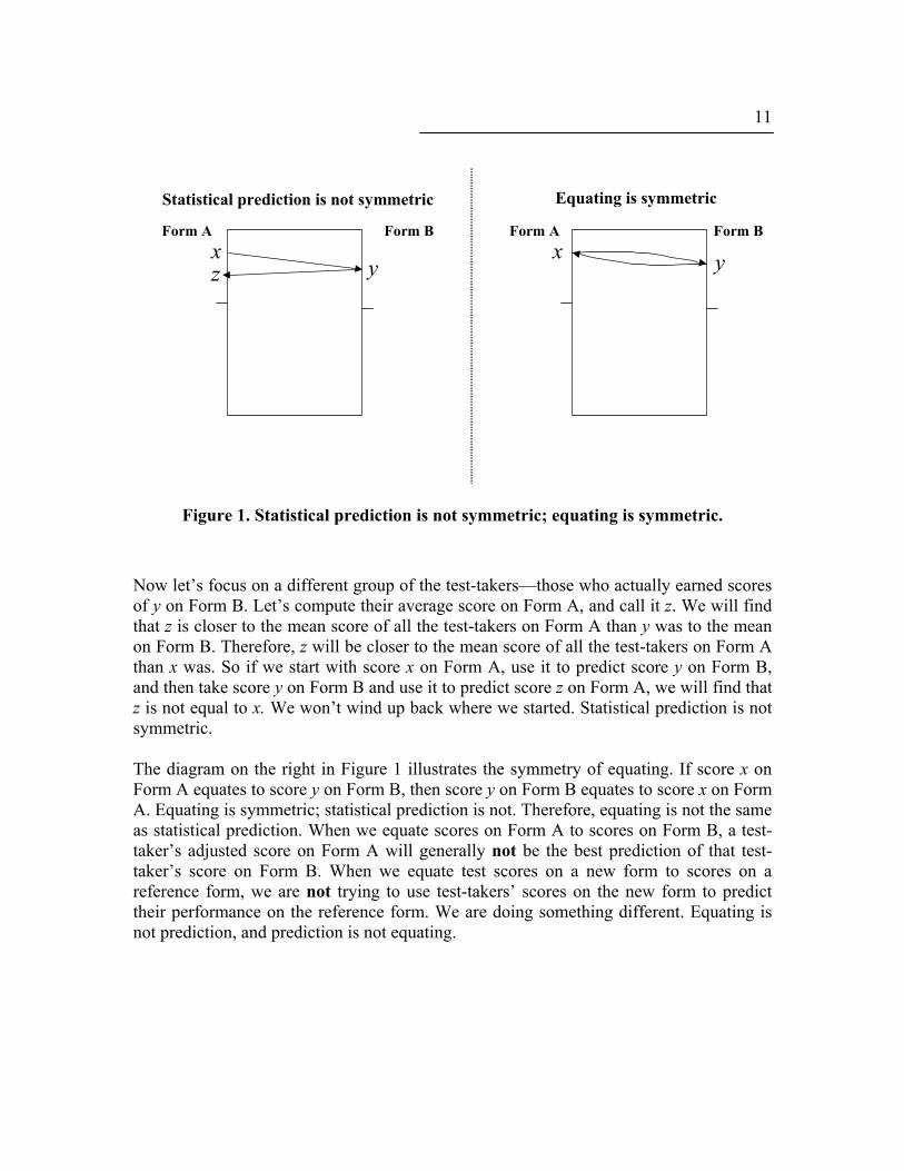
Equating Is Symmetric One important characteristic of an equating relationship is “symmetry.” An equating relationship is symmetric. That is, if score x on Form A equates to score y on Form B, then score y on Form B will equate to score x on Form A. You may wonder what’s remarkable about that. Aren’t all important statistical relationships symmetric? The answer is no. In particular, statistical prediction is not symmetric. Statistical prediction is affected by a phenomenon called “regression to the mean,” illustrated in the diagram on the left in Figure 1. Suppose a large group of test-takers took two forms of a test: Form A and Form B. Let’s choose a particular score on Form A. In Figure 1, I have chosen x to be a high score, far above the mean of the whole group. And let’s focus on just the test-takers with scores of x on Form A. Let’s look at those test-takers’ scores on Form B, and compute the average—call it y. Now, y is the average score on Form B for the group of test-takers with scores of x on Form A. We will find that y is closer to the mean score of all the test-takers on Form B than x was to the mean on Form A—closer in relation to the standard deviation of the scores of all the test-takers. (Incidentally, the weaker the correlation between the scores on Forms A and B, the stronger this effect will be. If the correlation were zero, the average score on Form B for the group of test-takers with scores of x on Form A would be the same as the mean score of all the test-takers.)

11

Statistical prediction is not symmetric

Form A Form B Form A Form B

Equating is symmetric

xz y

x y

Figure 1. Statistical prediction is not symmetric; equating is symmetric.

Now let’s focus on a different group of the test-takers—those who actually earned scores of y on Form B. Let’s compute their average score on Form A, and call it z. We will find that z is closer to the mean score of all the test-takers on Form A than y was to the mean on Form B. Therefore, z will be closer to the mean score of all the test-takers on Form A than x was. So if we start with score x on Form A, use it to predict score y on Form B, and then take score y on Form B and use it to predict score z on Form A, we will find that z is not equal to x. We won’t wind up back where we started. Statistical prediction is not symmetric. The diagram on the right in Figure 1 illustrates the symmetry of equating. If score x on Form A equates to score y on Form B, then score y on Form B equates to score x on Form A. Equating is symmetric; statistical prediction is not. Therefore, equating is not the same as statistical prediction. When we equate scores on Form A to scores on Form B, a test-taker’s adjusted score on Form A will generally not be the best prediction of that test-taker’s score on Form B. When we equate test scores on a new form to scores on a reference form, we are not trying to use test-takers’ scores on the new form to predict their performance on the reference form. We are doing something different. Equating is not prediction, and prediction is not equating.

12 A General Definition of Equating There is a single definition of equating that is general enough to include all of the types of equating I am going to describe. Here it is:

A score on the new form and a score on the reference form are equivalent in a group of test-takers if they represent the same relative position in the group.

You probably noticed that this definition states explicitly that the equating relationship is defined for a particular group of test-takers. What you might not notice is that it is missing an important detail. If you actually try to use this definition to determine a score adjustment, you will realize that you have to specify what you mean by “relative position.” You may also have noticed that this definition says nothing about the knowledge or skills measured by the new form and the reference form. If you simply applied this definition, you could equate scores on two tests that measure very different skills or types of knowledge. In practice we sometimes do apply procedures based on this definition to scores on tests that measure different things—but in that case we try to describe what we are doing by some term other than “equating.”

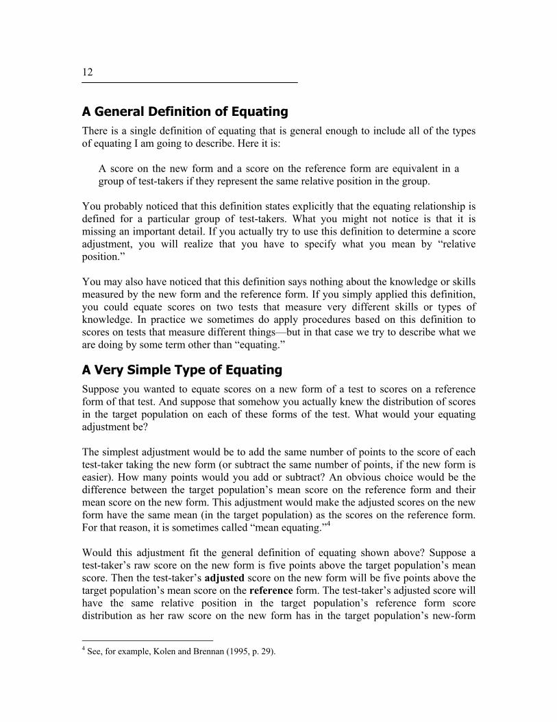
A Very Simple Type of Equating Suppose you wanted to equate scores on a new form of a test to scores on a reference form of that test. And suppose that somehow you actually knew the distribution of scores in the target population on each of these forms of the test. What would your equating adjustment be? The simplest adjustment would be to add the same number of points to the score of each test-taker taking the new form (or subtract the same number of points, if the new form is easier). How many points would you add or subtract? An obvious choice would be the difference between the target population’s mean score on the reference form and their mean score on the new form. This adjustment would make the adjusted scores on the new form have the same mean (in the target population) as the scores on the reference form. For that reason, it is sometimes called “mean equating.”4 Would this adjustment fit the general definition of equating shown above? Suppose a test-taker’s raw score on the new form is five points above the target population’s mean score. Then the test-taker’s adjusted score on the new form will be five points above the target population’s mean score on the reference form. The test-taker’s adjusted score will have the same relative position in the target population’s reference form score distribution as her raw score on the new form has in the target population’s new-form

4 See, for example, Kolen and Brennan (1995, p. 29).

13

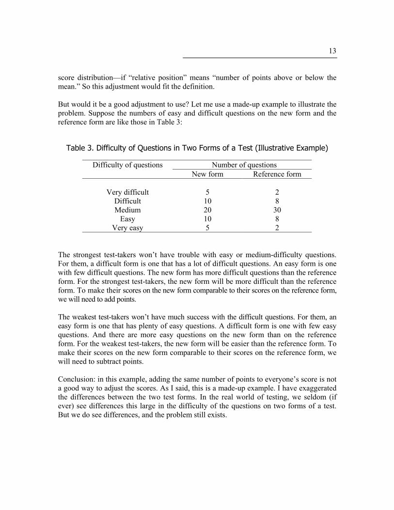
score distribution—if “relative position” means “number of points above or below the mean.” So this adjustment would fit the definition. But would it be a good adjustment to use? Let me use a made-up example to illustrate the problem. Suppose the numbers of easy and difficult questions on the new form and the reference form are like those in Table 3:

Table 3. Difficulty of Questions in Two Forms of a Test (Illustrative Example)

Difficulty of questions Number of questions New form Reference form

Very difficult 5 2 Difficult 10 8 Medium 20 30

Easy 10 8 Very easy 5 2

The strongest test-takers won’t have trouble with easy or medium-difficulty questions. For them, a difficult form is one that has a lot of difficult questions. An easy form is one with few difficult questions. The new form has more difficult questions than the reference form. For the strongest test-takers, the new form will be more difficult than the reference form. To make their scores on the new form comparable to their scores on the reference form, we will need to add points. The weakest test-takers won’t have much success with the difficult questions. For them, an easy form is one that has plenty of easy questions. A difficult form is one with few easy questions. And there are more easy questions on the new form than on the reference form. For the weakest test-takers, the new form will be easier than the reference form. To make their scores on the new form comparable to their scores on the reference form, we will need to subtract points. Conclusion: in this example, adding the same number of points to everyone’s score is not a good way to adjust the scores. As I said, this is a made-up example. I have exaggerated the differences between the two test forms. In the real world of testing, we seldom (if ever) see differences this large in the difficulty of the questions on two forms of a test. But we do see differences, and the problem still exists.

14 Linear Equating The previous example shows that we need an adjustment that depends on how high or low the test-taker’s score is. We can meet this requirement with an adjustment that defines “relative position” in terms of the mean and the standard deviation:

A score on the new form and a score on the reference form are equivalent in a group of test-takers if they are the same number of standard deviations above or below the mean of the group.

This definition implies the following procedure for adjusting the scores:

To equate scores on the new form to scores on the reference form in a group of test-takers, transform each score on the new form to the score on the reference form that is the same number of standard deviations above or below the mean of the group.

This type of equating is called “linear equating,” because the relationship between the raw scores and the adjusted scores appears on a graph as a straight line. The diagrams in Figure 2 illustrate linear equating in a situation where the new form is harder than the reference form.

-1 SD Mean +1 SD -1 SD Mean +1 SD

Raw score on ref. form

Raw score on new form

+1 SD

-1 SD

Mean

Adjusted score on new form

Raw score on new form

+1 SD

-1 SD

Mean

Figure 2. Linear equating; new form harder than reference form.

15

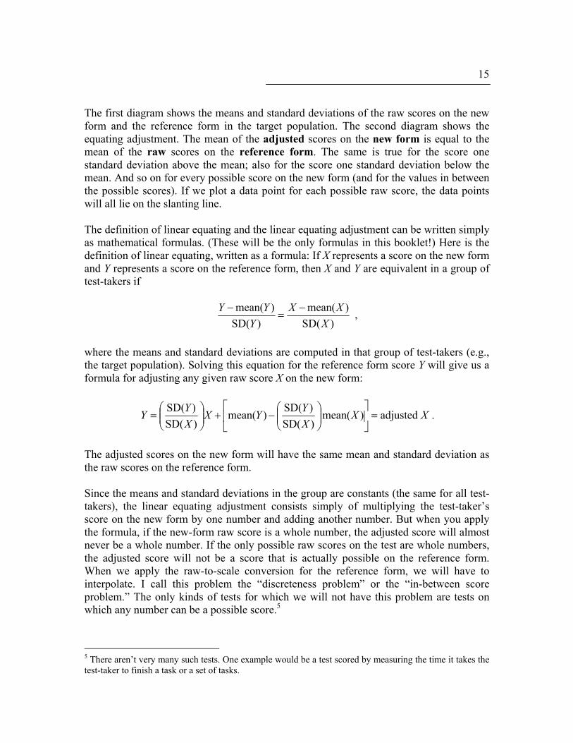
The first diagram shows the means and standard deviations of the raw scores on the new form and the reference form in the target population. The second diagram shows the equating adjustment. The mean of the adjusted scores on the new form is equal to the mean of the raw scores on the reference form. The same is true for the score one standard deviation above the mean; also for the score one standard deviation below the mean. And so on for every possible score on the new form (and for the values in between the possible scores). If we plot a data point for each possible raw score, the data points will all lie on the slanting line. The definition of linear equating and the linear equating adjustment can be written simply as mathematical formulas. (These will be the only formulas in this booklet!) Here is the definition of linear equating, written as a formula: If X represents a score on the new form and Y represents a score on the reference form, then X and Y are equivalent in a group of test-takers if

)SD()mean(

)SD()mean(

XXX

YYY −

=− ,

where the means and standard deviations are computed in that group of test-takers (e.g., the target population). Solving this equation for the reference form score Y will give us a formula for adjusting any given raw score X on the new form:

XXXY

YXXY

Y adjusted)mean()SD()SD(

)mean()SD()SD(

=

−+

= .

The adjusted scores on the new form will have the same mean and standard deviation as the raw scores on the reference form. Since the means and standard deviations in the group are constants (the same for all test-takers), the linear equating adjustment consists simply of multiplying the test-taker’s score on the new form by one number and adding another number. But when you apply the formula, if the new-form raw score is a whole number, the adjusted score will almost never be a whole number. If the only possible raw scores on the test are whole numbers, the adjusted score will not be a score that is actually possible on the reference form. When we apply the raw-to-scale conversion for the reference form, we will have to interpolate. I call this problem the “discreteness problem” or the “in-between score problem.” The only kinds of tests for which we will not have this problem are tests on which any number can be a possible score.5

5 There aren’t very many such tests. One example would be a test scored by measuring the time it takes the test-taker to finish a task or a set of tasks.

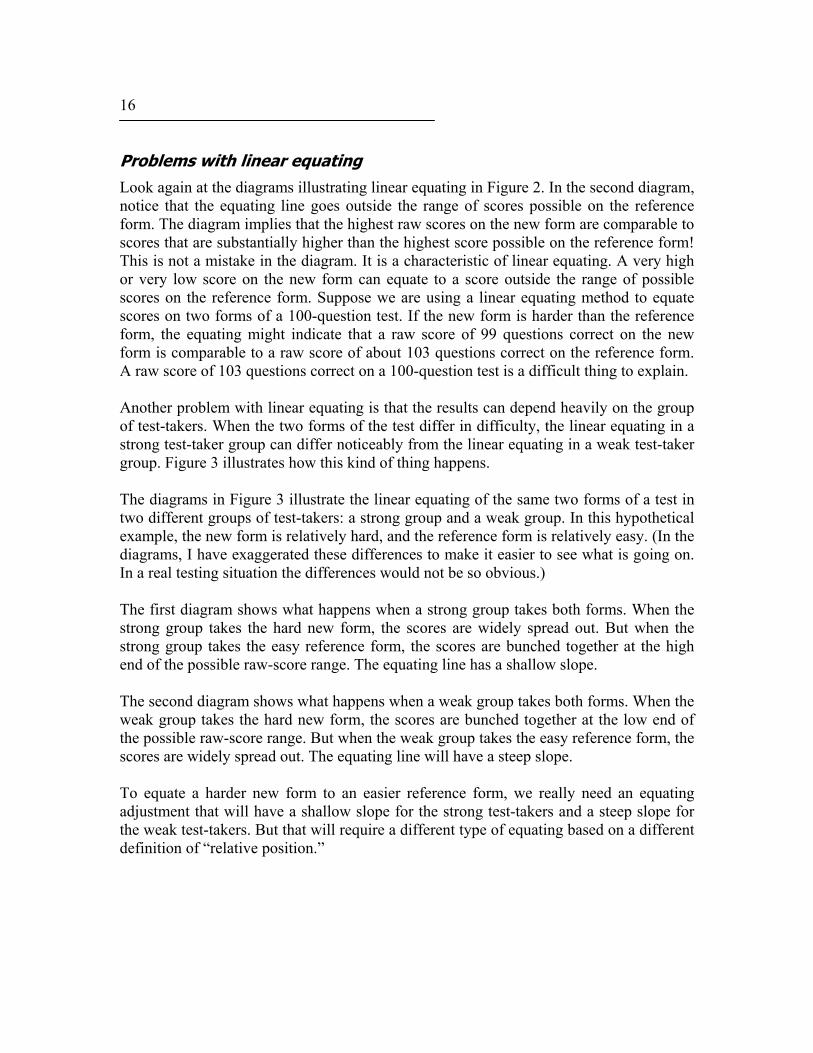
16 Problems with linear equating Look again at the diagrams illustrating linear equating in Figure 2. In the second diagram, notice that the equating line goes outside the range of scores possible on the reference form. The diagram implies that the highest raw scores on the new form are comparable to scores that are substantially higher than the highest score possible on the reference form! This is not a mistake in the diagram. It is a characteristic of linear equating. A very high or very low score on the new form can equate to a score outside the range of possible scores on the reference form. Suppose we are using a linear equating method to equate scores on two forms of a 100-question test. If the new form is harder than the reference form, the equating might indicate that a raw score of 99 questions correct on the new form is comparable to a raw score of about 103 questions correct on the reference form. A raw score of 103 questions correct on a 100-question test is a difficult thing to explain. Another problem with linear equating is that the results can depend heavily on the group of test-takers. When the two forms of the test differ in difficulty, the linear equating in a strong test-taker group can differ noticeably from the linear equating in a weak test-taker group. Figure 3 illustrates how this kind of thing happens. The diagrams in Figure 3 illustrate the linear equating of the same two forms of a test in two different groups of test-takers: a strong group and a weak group. In this hypothetical example, the new form is relatively hard, and the reference form is relatively easy. (In the diagrams, I have exaggerated these differences to make it easier to see what is going on. In a real testing situation the differences would not be so obvious.) The first diagram shows what happens when a strong group takes both forms. When the strong group takes the hard new form, the scores are widely spread out. But when the strong group takes the easy reference form, the scores are bunched together at the high end of the possible raw-score range. The equating line has a shallow slope. The second diagram shows what happens when a weak group takes both forms. When the weak group takes the hard new form, the scores are bunched together at the low end of the possible raw-score range. But when the weak group takes the easy reference form, the scores are widely spread out. The equating line will have a steep slope. To equate a harder new form to an easier reference form, we really need an equating adjustment that will have a shallow slope for the strong test-takers and a steep slope for the weak test-takers. But that will require a different type of equating based on a different definition of “relative position.”

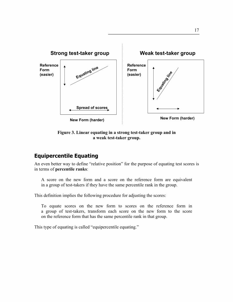
17

Strong test-taker group

ReferenceForm(easier)

New Form (harder)

Spread of scores

Weak test-taker group

ReferenceForm(easier)

New Form (harder)

Equating line

Equa

ting

line

Figure 3. Linear equating in a strong test-taker group and in

a weak test-taker group.

Equipercentile Equating An even better way to define “relative position” for the purpose of equating test scores is in terms of percentile ranks:

A score on the new form and a score on the reference form are equivalent in a group of test-takers if they have the same percentile rank in the group.

This definition implies the following procedure for adjusting the scores:

To equate scores on the new form to scores on the reference form in a group of test-takers, transform each score on the new form to the score on the reference form that has the same percentile rank in that group.

This type of equating is called “equipercentile equating.”

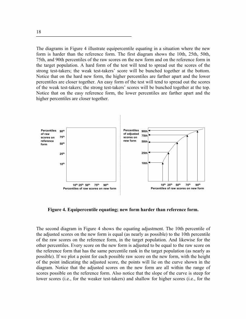
18 The diagrams in Figure 4 illustrate equipercentile equating in a situation where the new form is harder than the reference form. The first diagram shows the 10th, 25th, 50th, 75th, and 90th percentiles of the raw scores on the new form and on the reference form in the target population. A hard form of the test will tend to spread out the scores of the strong test-takers; the weak test-takers’ score will be bunched together at the bottom. Notice that on the hard new form, the higher percentiles are farther apart and the lower percentiles are closer together. An easy form of the test will tend to spread out the scores of the weak test-takers; the strong test-takers’ scores will be bunched together at the top. Notice that on the easy reference form, the lower percentiles are farther apart and the higher percentiles are closer together.

Percentiles of raw scores on new form

Percentiles of raw scores on reference form

10th 25th 50th 75th 90th

90th

50th

75th

25th

10th

Percentiles of raw scores on new form

Percentiles of adjusted scores on new form

10th 25th 50th 75th 90th

90th

50th

75th

25th

10th

Figure 4. Equipercentile equating; new form harder than reference form. The second diagram in Figure 4 shows the equating adjustment. The 10th percentile of the adjusted scores on the new form is equal (as nearly as possible) to the 10th percentile of the raw scores on the reference form, in the target population. And likewise for the other percentiles. Every score on the new form is adjusted to be equal to the raw score on the reference form that has the same percentile rank in the target population (as nearly as possible). If we plot a point for each possible raw score on the new form, with the height of the point indicating the adjusted score, the points will lie on the curve shown in the diagram. Notice that the adjusted scores on the new form are all within the range of scores possible on the reference form. Also notice that the slope of the curve is steep for lower scores (i.e., for the weaker test-takers) and shallow for higher scores (i.e., for the

19

stronger test-takers). These variations in the slope make it possible for the equating relationship to apply to the weaker test-takers and also to the stronger test-takers. Equipercentile equating will make the adjusted scores on the new form have very nearly the same distribution as the scores on the reference form in the target population. (I have to say “very nearly” because of the discreteness of the scores.) And, because the score distributions are very nearly the same, the means and the standard deviations in the target population will be very nearly the same for the adjusted scores on the new form as for the raw scores on the reference form. When will linear equating and equipercentile equating produce the same (or very nearly the same) results? When the distributions of scores on the new form and on the reference form in the target population have the same shape. In that case, a linear adjustment can make the adjusted scores on the new form have (very nearly) the same distribution as the raw scores on the reference form. And if the two distributions are the same, all their percentiles will be the same. Consequently, if the score distributions (in the target population) on the new form and the reference form have the same shape, the linear equating and the equipercentile equating will (very nearly) coincide. But if the score distributions for the new form and the reference form have different shapes, there is no linear adjustment to the scores on the new form that will make the distribution the same (or even nearly the same) as the distribution of scores on the reference form. The adjustment resulting from equipercentile equating will not be linear. There is no simple mathematical formula for the equipercentile equating adjustment.

A problem with equipercentile equating and a solution The main problem with equipercentile equating is that the score distributions we actually see on real tests taken by real test-takers are irregular. Figure 5 shows the distribution of the raw scores of 468 test-takers on a real test of 39 multiple-choice items. These 468 test-takers were selected at random from the 8,426 test-takers who took the test. Notice the irregularities in the score distribution. The percentage of the test-takers with a given score does not change gradually as the scores increase; it fluctuates. Irregularities in the score distributions cause problems for equipercentile equating. They produce irregularities in the equipercentile equating adjustment, and those irregularities do not generalize to other groups of test-takers. Figure 6 shows the distribution of the raw scores of 702 other test-takers on the same test, selected at random from the same large group of 8,426 who took the test. Notice that the distributions in Figures 5 and 6 are similar in some ways, but not in others. The overall level of the scores, the extent to which they are spread out, and the general shape of the distribution are similar in the two distributions. But the irregularities in Figure 5 do not correspond to those in Figure 6. In general, the location, the spread, and the general shape of a score distribution will tend to generalize to other groups of test-takers; the irregularities in the distribution will not.

20

0.0

1.0

2.0

3.0

4.0

5.0

6.0

7.0

8.0

9.0

10.0

1 2 3 4 5 6 7 8 9 10 11 12 13 14 15 16 17 18 19 20 21 22 23 24 25 26 27 28 29 30 31 32 33 34 35 36 37 38 39

Score

Perc

ent

Figure 5. Score distribution observed in a sample of 468 test-takers.

0.0

1.0

2.0

3.0

4.0

5.0

6.0

7.0

8.0

9.0

10.0

1 2 3 4 5 6 7 8 9 10 11 12 13 14 15 16 17 18 19 20 21 22 23 24 25 26 27 28 29 30 31 32 33 34 35 36 37 38 39

Score

Perc

ent

Figure 6. Score distribution observed in a sample of 702 test-takers.

21

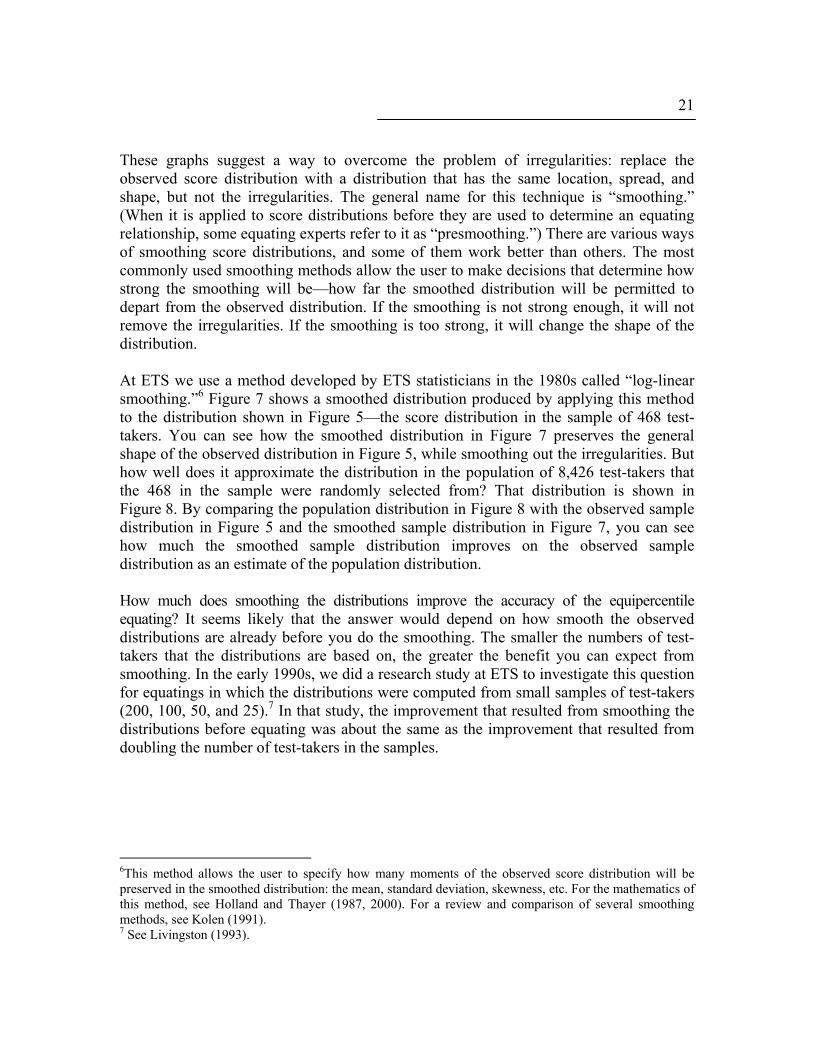
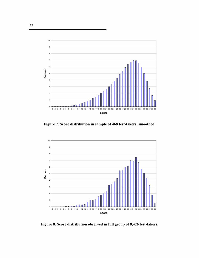
These graphs suggest a way to overcome the problem of irregularities: replace the observed score distribution with a distribution that has the same location, spread, and shape, but not the irregularities. The general name for this technique is “smoothing.” (When it is applied to score distributions before they are used to determine an equating relationship, some equating experts refer to it as “presmoothing.”) There are various ways of smoothing score distributions, and some of them work better than others. The most commonly used smoothing methods allow the user to make decisions that determine how strong the smoothing will be—how far the smoothed distribution will be permitted to depart from the observed distribution. If the smoothing is not strong enough, it will not remove the irregularities. If the smoothing is too strong, it will change the shape of the distribution. At ETS we use a method developed by ETS statisticians in the 1980s called “log-linear smoothing.”6 Figure 7 shows a smoothed distribution produced by applying this method to the distribution shown in Figure 5—the score distribution in the sample of 468 test-takers. You can see how the smoothed distribution in Figure 7 preserves the general shape of the observed distribution in Figure 5, while smoothing out the irregularities. But how well does it approximate the distribution in the population of 8,426 test-takers that the 468 in the sample were randomly selected from? That distribution is shown in Figure 8. By comparing the population distribution in Figure 8 with the observed sample distribution in Figure 5 and the smoothed sample distribution in Figure 7, you can see how much the smoothed sample distribution improves on the observed sample distribution as an estimate of the population distribution. How much does smoothing the distributions improve the accuracy of the equipercentile equating? It seems likely that the answer would depend on how smooth the observed distributions are already before you do the smoothing. The smaller the numbers of test-takers that the distributions are based on, the greater the benefit you can expect from smoothing. In the early 1990s, we did a research study at ETS to investigate this question for equatings in which the distributions were computed from small samples of test-takers (200, 100, 50, and 25).7 In that study, the improvement that resulted from smoothing the distributions before equating was about the same as the improvement that resulted from doubling the number of test-takers in the samples.

6This method allows the user to specify how many moments of the observed score distribution will be preserved in the smoothed distribution: the mean, standard deviation, skewness, etc. For the mathematics of this method, see Holland and Thayer (1987, 2000). For a review and comparison of several smoothing methods, see Kolen (1991). 7 See Livingston (1993).

22

0

1

2

3

4

5

6

7

8

9

10

1 2 3 4 5 6 7 8 9 10 11 12 13 14 15 16 17 18 19 20 21 22 23 24 25 26 27 28 29 30 31 32 33 34 35 36 37 38 39

Score

Perc

ent

Figure 7. Score distribution in sample of 468 test-takers, smoothed.

0

1

2

3

4

5

6

7

8

9

10

1 2 3 4 5 6 7 8 9 10 11 12 13 14 15 16 17 18 19 20 21 22 23 24 25 26 27 28 29 30 31 32 33 34 35 36 37 38 39

Score

Perc

ent

Figure 8. Score distribution observed in full group of 8,426 test-takers.

23

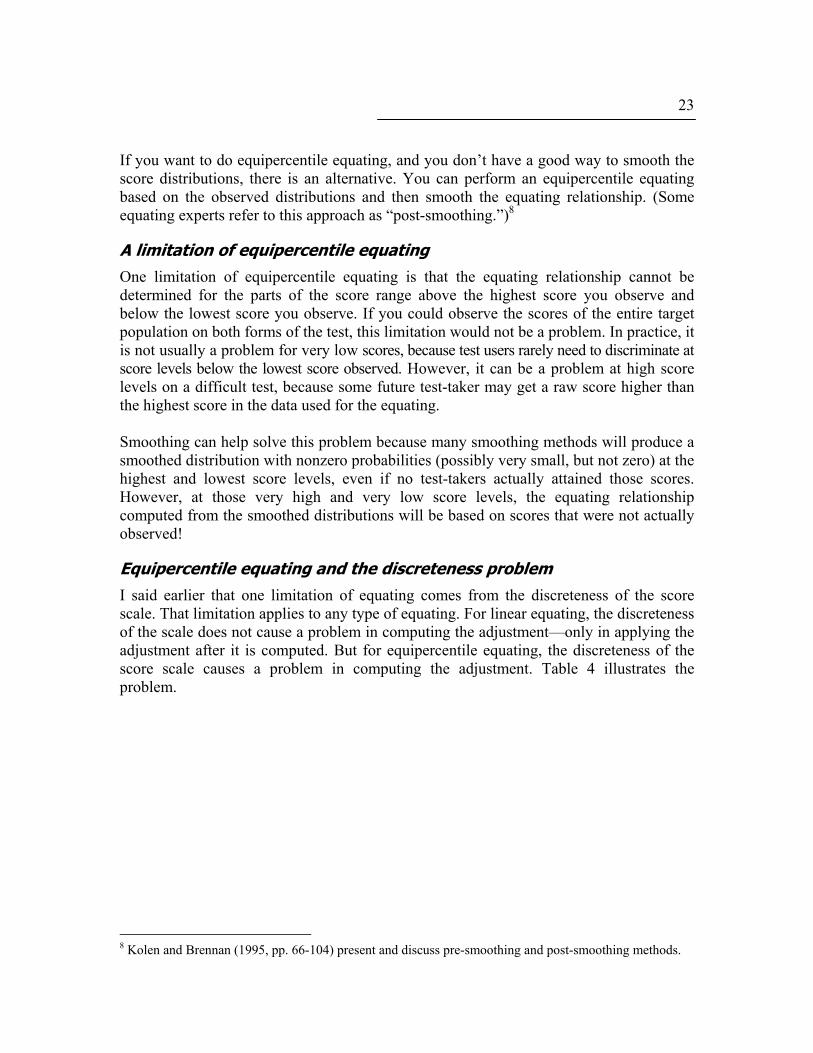
If you want to do equipercentile equating, and you don’t have a good way to smooth the score distributions, there is an alternative. You can perform an equipercentile equating based on the observed distributions and then smooth the equating relationship. (Some equating experts refer to this approach as “post-smoothing.”)8

A limitation of equipercentile equating One limitation of equipercentile equating is that the equating relationship cannot be determined for the parts of the score range above the highest score you observe and below the lowest score you observe. If you could observe the scores of the entire target population on both forms of the test, this limitation would not be a problem. In practice, it is not usually a problem for very low scores, because test users rarely need to discriminate at score levels below the lowest score observed. However, it can be a problem at high score levels on a difficult test, because some future test-taker may get a raw score higher than the highest score in the data used for the equating. Smoothing can help solve this problem because many smoothing methods will produce a smoothed distribution with nonzero probabilities (possibly very small, but not zero) at the highest and lowest score levels, even if no test-takers actually attained those scores. However, at those very high and very low score levels, the equating relationship computed from the smoothed distributions will be based on scores that were not actually observed!

Equipercentile equating and the discreteness problem I said earlier that one limitation of equating comes from the discreteness of the score scale. That limitation applies to any type of equating. For linear equating, the discreteness of the scale does not cause a problem in computing the adjustment—only in applying the adjustment after it is computed. But for equipercentile equating, the discreteness of the score scale causes a problem in computing the adjustment. Table 4 illustrates the problem.

8 Kolen and Brennan (1995, pp. 66-104) present and discuss pre-smoothing and post-smoothing methods.

24

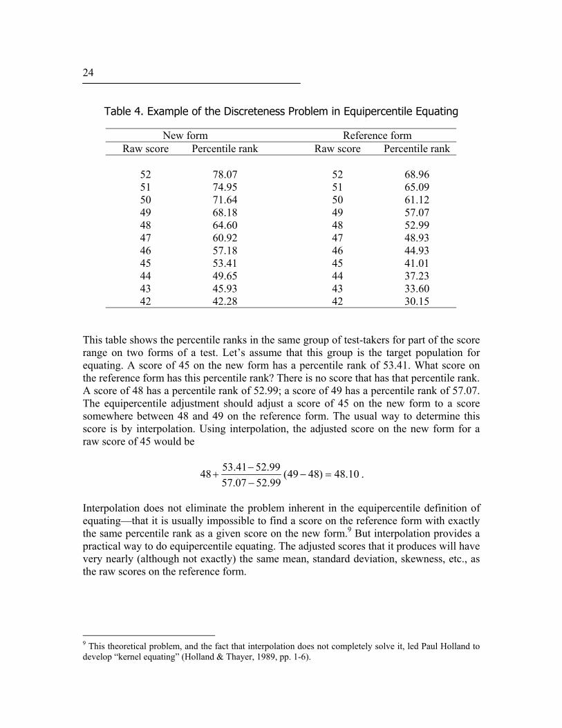
Table 4. Example of the Discreteness Problem in Equipercentile Equating

New form Reference form Raw score Percentile rank Raw score Percentile rank

52 78.07 52 68.96 51 74.95 51 65.09 50 71.64 50 61.12 49 68.18 49 57.07 48 64.60 48 52.99 47 60.92 47 48.93 46 57.18 46 44.93 45 53.41 45 41.01 44 49.65 44 37.23 43 45.93 43 33.60 42 42.28 42 30.15

This table shows the percentile ranks in the same group of test-takers for part of the score range on two forms of a test. Let’s assume that this group is the target population for equating. A score of 45 on the new form has a percentile rank of 53.41. What score on the reference form has this percentile rank? There is no score that has that percentile rank. A score of 48 has a percentile rank of 52.99; a score of 49 has a percentile rank of 57.07. The equipercentile adjustment should adjust a score of 45 on the new form to a score somewhere between 48 and 49 on the reference form. The usual way to determine this score is by interpolation. Using interpolation, the adjusted score on the new form for a raw score of 45 would be

10.48)4849(99.5207.5799.5241.5348 =−

−−

+ .

Interpolation does not eliminate the problem inherent in the equipercentile definition of equating—that it is usually impossible to find a score on the reference form with exactly the same percentile rank as a given score on the new form.9 But interpolation provides a practical way to do equipercentile equating. The adjusted scores that it produces will have very nearly (although not exactly) the same mean, standard deviation, skewness, etc., as the raw scores on the reference form.

9 This theoretical problem, and the fact that interpolation does not completely solve it, led Paul Holland to develop “kernel equating” (Holland & Thayer, 1989, pp. 1-6).

25

Test: Linear and Equipercentile Equating At this point in the class, the students take a short, self-administered test on linear and equipercentile equating. Then we discuss the answers to fill in any gaps in the instruction and to clear up any misunderstandings that may have occurred. Here is the test. The answers appear in a separate section in the back of this booklet. For each statement, check “yes” or “no” to indicate whether or not the statement applies to each of these two types of equating. Its purpose is to adjust the scores for differences in the difficulty of the questions on the test. True of linear equating? Yes No True of equipercentile equating? Yes No It requires data on the performance of people taking the test.

True of linear equating? Yes No True of equipercentile equating? Yes No It produces an adjustment that is correct for every person in the target population.

True of linear equating? Yes No True of equipercentile equating? Yes No The adjustment to the scores consists of multiplying by one number and then adding another.

True of linear equating? Yes No True of equipercentile equating? Yes No

26 The results can be improved by smoothing the score distributions before equating.

True of linear equating? Yes No True of equipercentile equating? Yes No The adjusted scores on the new form will generally fall in between the scores that are actually possible on the reference form.

True of linear equating? Yes No True of equipercentile equating? Yes No Some adjusted scores on the new form can be several points higher than the highest score possible on the reference form.

True of linear equating? Yes No True of equipercentile equating? Yes No The adjusted score on the new form is the best prediction of the score the test-taker would get on the reference form.

True of linear equating? Yes No True of equipercentile equating? Yes No

27

Equating Designs An equating design is a plan for collecting the data you need for equating. You can do either linear equating or equipercentile equating with the data from any equating design. Let’s indulge in a bit of wishful thinking. What information would we most like to have for equating the scores on two forms of a test? What we really want are two score distributions: the score distribution that would result if the entire target population took only the new form and the score distribution that would result if the entire target population took only the reference form. Now let’s get real. What kind of information can we get in the real world that will enable us to equate the scores on two forms of a test? We need some way to link the information about the new form to the information about the reference form. I know of three ways to get this kind of information. (1) We can get data on both forms from the same test-takers. (2) We can get data on the two forms from two groups of test-takers that we know to be equal in the skills measured by the test. (3) We can get some other relevant information about the test-takers taking the different forms—ideally, another measure of the same skills that the test measures—and use that information as the basis for the adjustment. These three ways to link the two forms lead to five different equating designs. Each design has its advantages and limitations. And each design requires an assumption about what statistical relationships (that we can observe in the scores we collect) will generalize to the target population.

The single-group design The simplest equating design is to have the same test-takers take both the new form and the reference form. This equating design is called the “single-group” design. The implicit assumption is that the equating relationship that we observe in this group of test-takers will generalize to the target population. It is not necessary that the group of test-takers be a representative sample of the target population. The group taking the test can be stronger than the target population, as long as the test-takers are stronger to the same degree on the new form as on the reference form. Similarly, the group taking the test can be weaker than the target population or more diverse or less diverse—as long as the test-takers differ from the target population in the same way on the new form as on the reference form. The main advantage of the single-group design is that, because the same test-takers take both forms of the test, it is statistically powerful. In comparison to most other equating designs, it offers a highly accurate equating in relation to the number of test-takers included in the design. Looking at it another way, it requires fewer test-takers for a given level of accuracy. The main disadvantage of the single-group design is that the test-takers’ performance on the second form they take is likely to be affected by the experience of taking the first

28 form. The single-group design is highly sensitive to order effects—practice effects or, in some cases, fatigue effects. Unless we are willing to assume that these effects are negligible, we can use the single-group design only if the test-takers take both forms at the same time. But how can we ever have test-takers take the new form and the reference form at the same time? One such situation occurs when we have to remove one or more questions from a test before reusing it. (That can happen for a number of different reasons, including new knowledge in the subject tested or changes in the way the subject is taught.) In this situation, the new form is simply the reference form minus the questions that are being deleted. For equating, we use the data from a group of test-takers who took the test before those questions were deleted. We compute two different scores for each test-taker: a reference form score that includes the deleted questions and a new form score that excludes them. These scores are the basis for the equating. We can also use the single-group design when one or more questions are being added to a test. For equating, we use the data from a group of test-takers who took the test with the new questions included. In this case, the new form score would include the new questions; the reference form score would exclude them. Another such situation occurs in constructed-response testing (essay tests, performance assessments, etc.). Sometimes the new form of the test contains exactly the same questions or problems as the reference form—the difference is in the scoring rules or procedure. In that case, we can equate the new-form scores to the reference form scores by having a group of test-takers’ responses scored twice. Since the questions are the same on both forms, these responses can come either from test-takers taking the new form or from test-takers taking the reference form (or both). The first scoring is done with the scoring rules and procedure used on the reference form; the second scoring is done with the scoring rules and procedure used on the new form. For each test-taker, we compute a new form score, based on the ratings assigned with the new form scoring rules and procedure, and a reference form score, based on the ratings assigned with the reference form scoring rules and procedure.

The counterbalanced design In the usual equating situation—two test forms that are really different forms, not just different versions of the same form—the problem of order effects makes the single-group equating design unsuitable. One way to overcome the problem is to divide the test-takers into two groups and “counterbalance” the order in which the groups take the two forms. One group takes the new form first and the reference form second; the other group takes the reference form first and the new form second. The test-takers have to take the two forms close together in time—close enough that there will be no real change in their level of the knowledge or the skills that the test measures. Ideally, the two groups of test-takers should be as similar as possible. In practice, this design usually produces good results

29

even if the groups differ somewhat. With this equating design, it is best that the two forms not have any questions in common. The key assumption of the counterbalanced design is that any order effects will balance out. When we use this design, we are assuming that the experience of taking the new form will affect performance on the reference form just as much as taking the reference form will affect performance on the new form. As in the single-group design, the groups don’t have to be representative of the target population. They can be somewhat stronger or weaker or more diverse or less diverse. The information that we assume will generalize from these groups of test-takers to the target population is the equating relationship between the two forms of the test. The main advantage of the counterbalanced design is the same as that of the single-group design: accurate results from a relatively small number of test-takers. Its main disadvantage is that it can almost never be designed into an operational administration of a test. Usually this equating design requires a special equating study for collecting the data.

The equivalent-groups design In most equating situations, there is no opportunity to have the same test-takers take two forms of the test. What can we do if each test-taker will take only one form of the test? The simplest solution is to have a separate group of test-takers take each form, making sure that the two groups are equal in the knowledge and skills that the test measures. But can we actually do that? We can never get the groups to be exactly equal, but if the number of test-takers is large, we can come close. The best way to do it is by “spiraling the books.” That term is testing jargon for packaging the two forms of the test in alternating sequence: new form, reference form, new form, reference form, etc. This way of assigning test forms to test-takers assures that the groups of test-takers taking the two forms will be similar in many ways: where they took the test, when they took the test, what part of the testing room they sat in, and so on. If any of these differences are associated with differences in the test-takers’ knowledge or skills, “spiraling the books” will tend to balance out the differences. For example, the test-takers at a particular testing site may be especially strong. “Spiraling the books” guarantees that the test-takers at that testing site will be divided equally between the new form and the reference form.10 The assumption of the equivalent-groups design is that the equating relationship observed between the two groups of test-takers will generalize to the target population. The two groups may differ from the target population as long as they both differ from the target population in the same way. If the group taking the new form is stronger than the

10 An additional benefit—one that has nothing to do with equating—is that alternating the test forms makes it hard for a test-taker to cheat by copying answers from the test-taker at the next desk.

30 target population, the group taking the reference form must also be stronger than the target population, to the same degree. The equivalent-groups design has some important practical advantages. It is fairly convenient to administer—provided that the people administering the test understand that they have to distribute the test booklets in the order in which they were packaged. This design can often be used in an operational test administration. It does not require the two forms of the test to have any questions in common, but it can be used even if they do. The equivalent-groups design also has some major limitations. Its main limitation is that in order to produce accurate equating results, it requires large numbers of test-takers. In comparison to the counterbalanced design, the equivalent-groups design could require from five to fifteen times as many test-takers for the same degree of accuracy.11 A second limitation has to do with test security. In most cases the reference form will have been administered previously. On some tests, there is a substantial risk that many test-takers will have seen (and even studied) the questions on a test form that has been used previously. On those tests, it may be impossible to get valid equating data from an equivalent-groups design.

The internal-anchor design In many large-scale testing programs, the testing is organized into “administrations.” Each administration is a short period of time (possibly a single day) in which a large number of test-takers take the same test. Typically, all the test-takers who take the test at a particular administration take the same form of the test. If that form of the test has not been given before, the scores will need to be equated to the scores on a form that was given at a previous administration. In this very common situation, we cannot assume that the groups of test-takers taking the new form and the reference form are equal in the skills the test measures. To equate the scores, we need a link between those groups—some kind of information that will show us how the groups differ in the skills the test measures. In testing jargon, this link is called an “anchor.” The best kind of an anchor for equating is a test of the same knowledge and skills that the test measures. The more similar the anchor is to the test, the better. The anchor can be either “internal” or “external.” An internal anchor is part of the test itself; an external anchor is not. An internal anchor consists of a set of questions from the reference form that have been included in the new form. These repeated questions are often called “common items,” and equating in an internal-anchor design is often called “common-

11 This comparison depends on the correlation between scores on the two test forms, because the accuracy of equating in a counterbalanced design depends on how strongly the two forms are correlated, while the accuracy of equating in an equivalent-groups design does not. The comparison is based on formulas from Angoff, 1984, pp. 97, 103. However, the formula for the equivalent-groups design (p. 97) assumes the groups to be independent random samples from the target population. Therefore, it somewhat overestimates the number of test-takers required when the groups are created by “spiraling” the test forms.

31

item” equating. Some other terms used to refer to the repeated questions are “anchor items” and “equating items.” Taken together, the repeated questions are sometimes referred to as the “equating set.” The main advantage of the internal-anchor design is that it does not complicate the administration of the test. However, it does complicate the test development process. It also requires a second exposure for the repeated questions, which can cause a security problem for some high-stakes tests. The key assumption of the internal-anchor design is that the meaning of the anchor score does not change. A given score on the anchor is assumed to indicate the same level of knowledge or skill for a test-taker taking the new form as for a test-taker taking the reference form. Therefore, the repeated questions must not change in difficulty. If the reference form has been released to test-takers or to their teachers, any questions repeated from that form are likely to have become easier. If there has been a security breach on the reference form, the questions repeated from that form are likely to have become easier for at least some of the test-takers. (In this case, it may be possible to identify the test-takers who are likely to have had prior knowledge of the repeated questions and to exclude their scores from the equating analysis.) Sometimes the difficulty of a repeated question can change as a result of circumstances.12 The knowledge needed to answer the question may become more commonly taught (or less commonly taught). Sometimes world events will bring the topic of a test question to the attention of the general public. For example, questions about the geography of Iraq would tend to be easier in 2003 than they were in previous years. How can we take these possibilities into account? We modify our assumption. We assume that most of the repeated questions have not changed systematically in difficulty. This assumption makes it possible to identify those questions that have changed in difficulty and remove them from the anchor by using “difficulty plots.” Figure 9 is an example of a difficulty plot. Each data point in the plot represents one of the repeated questions. The horizontal position of the data point represents the percent-correct on the question for the test-takers taking the new form. The vertical position of the point represents the percent-correct on the question for the test-takers taking the reference form. These two difficulty measures agree strongly, as is usually the case. But occasionally we find one or more data points that do not fit the pattern. These “outliers” are the data points for questions that have become easier or more difficult in the new form than they were in the reference form. Notice, in the upper right corner of Figure 9, one data point seems to stand out from the rest. This data point represents a question that was answered correctly by nearly all the test-takers taking the new form, but by only about three-quarters of those taking the reference form (even though the reference form 12 The difficulty of a question can also change if the position of the question in the test changes, e.g., from the end of the reference form to the middle of the new form. I’ll say more about this later.

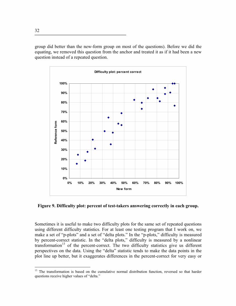
32 group did better than the new-form group on most of the questions). Before we did the equating, we removed this question from the anchor and treated it as if it had been a new question instead of a repeated question.

Difficulty plot: percent correct

0%

10%

20%

30%

40%

50%

60%

70%

80%

90%

100%

0% 10% 20% 30% 40% 50% 60% 70% 80% 90% 100%

New form

Ref

eren

ce fo

rm

Figure 9. Difficulty plot: percent of test-takers answering correctly in each group.

Sometimes it is useful to make two difficulty plots for the same set of repeated questions using different difficulty statistics. For at least one testing program that I work on, we make a set of “p-plots” and a set of “delta plots.” In the “p-plots,” difficulty is measured by percent-correct statistic. In the “delta plots,” difficulty is measured by a nonlinear transformation13 of the percent-correct. The two difficulty statistics give us different perspectives on the data. Using the “delta” statistic tends to make the data points in the plot line up better, but it exaggerates differences in the percent-correct for very easy or

13 The transformation is based on the cumulative normal distribution function, reversed so that harder questions receive higher values of “delta.”

33

very hard questions. The “p-plots” give us a better picture of the effect that removing a question from the anchor will have on the test-takers’ anchor scores. The two main limitations of the internal-anchor design have to do with the possibility that the repeated questions may change in difficulty. First, we have to be able to assume that most of the repeated questions will not change in difficulty from the reference form to the new form. Second, we need enough repeated questions that if some of them do change in difficulty, they can be identified and removed from the anchor. This second limitation makes the internal-anchor design unsuitable for equating a test that has only a small number of separate questions, problems, or tasks. Many essay tests and performance assessments fall into this category. For example, suppose that you needed to equate scores on a test consisting of only six separate problems. How many of those problems could you include in an internal anchor? Two or possibly three at most. A difficulty plot with only two or three data points would not be very useful for determining whether any of those repeated problems had changed in difficulty. Sometimes it is necessary to use an internal anchor that does not measure all the skills that the full test measures. Suppose, for example, that we want to use an internal-anchor design to equate scores on alternate forms of a test made up of fifty multiple-choice questions and one essay question. In this case, the internal anchor will consist entirely of multiple-choice questions. (The test developers will not want to use the same essay topic on all forms of the test!) Equating through the all-multiple-choice anchor requires the assumption that the groups taking the new form and the reference form differ just as much in the skills measured by the full test as in the skills measured by the multiple-choice portion alone. We make this assumption, not because we have a lot of confidence in it, but because the alternatives are worse. We have to report scores on the new form, one way or another. Whatever we do, we will be implicitly making an assumption about the skills of the test-takers taking the new form and of those who took the reference form. We can assume the two groups are equal in the skills that the full test measures. Alternatively, we can assume that the difference between the groups is shown by their unadjusted raw scores on the full test. Or we can assume that the difference between the groups is shown by their scores on an internal anchor consisting of repeated multiple-choice questions—the same questions for both groups. Given these three choices, we generally prefer to believe the information from the multiple-choice anchor.

The external-anchor design An external anchor is a common measure, separate from the test itself, that we can use to compare the group of test-takers taking the new form with the group taking the reference form. Ideally, the external anchor should measure the same knowledge and skills as the test to be equated, using questions or problems in the same format, administered under the same conditions. In reality we cannot often come close to this ideal. However, there is one well-known test on which the scores are equated through an external-anchor design that meets these ideal conditions—the SAT I.

34 The anchor for the SAT Verbal test is actually a short version of the full test with entirely different questions. Here is how the data collection plan works. Each form of the SAT includes an “equating” section that is different for different test-takers. There are several versions of the “equating” section, and these are spiraled among the test-takers, so that the group of test-takers taking each version is a representative sample of the full group of test-takers for that administration. Some test-takers get a short version of the Verbal test, while others get a short version of the Math test. For some of the test-takers, the equating section is an anchor that links the current form to a previous form. For others, the equating section is an anchor that will link the current form to a future form. Because the anchor is not taken by all the test-takers, the scores on the anchor are not included in computing the individual scores on the test. The anchor scores are used only for equating. An equating plan of this complexity would probably be impractical for most other tests. A more typical example of equating through an external-anchor equating design is the equating of an essay test intended to measure the test-takers’ writing skills. The anchor for equating scores on this test is a multiple-choice test, taken by the same test-takers, that requires the test-taker to distinguish between examples of well written and poorly written sentences. The scores on different forms of the multiple-choice test are equated through an internal anchor (“common items”), and then the adjusted scores on the multiple-choice test are used as an external anchor for equating scores on different forms of the essay test. More terminology. When we equate test scores, we often refer to the groups of test-takers as “equating samples.” We call the group that took the new form the “new form equating sample”; we call the group that took the reference form the “reference form equating sample.” Calling the groups “samples” reminds us that we want the equating results to generalize beyond the people whose test responses we are using. However, we have to remember that the equating samples often are not representative samples from the target population. The key assumption of the external-anchor design is that the groups of test-takers taking the two forms to be equated (the equating samples) will differ in the same way on the anchor as they do on the test to be equated. In the writing-test example, the assumption is that the two equating samples will differ just as much in their ability to write good essays as in their ability to distinguish between well written and poorly written sentences. We do not have the data to test this assumption, but we can get some related evidence. We can compute the correlation between the (essay) test scores and the (multiple-choice) anchor scores within each equating sample. If those correlations are strong, we will know that the anchor is a good indicator of the within-group differences between individual test-takers in the knowledge or skills that the test measures. In that case, we will be more inclined to trust the anchor as an indicator of the between-group differences, i.e., between the equating samples.

35

If the anchor for an external equating involves administering exactly the same questions to both equating samples, and if it includes enough questions, it may be wise to use a difficulty plot to identify and remove from the anchor score any questions that changed in difficulty. Probably the main advantage of the external-anchor design is that it can be used in situations where other equating designs cannot be used. It is often used to equate scores on different forms of an essay test or a performance assessment. In these cases, the external anchor is usually the test-taker’s equated score on a multiple-choice test measuring closely related knowledge and skills, as in the writing-test example described above. Another example, from the Praxis program, involves a constructed-response test in math. This test requires the test-taker to construct mathematical proofs and to solve mathematical problems, showing the reasoning behind the solution. The external anchor for equating scores on this test is the adjusted score on a multiple-choice test that the test-takers must also take, with questions drawn from the same areas of mathematics. The main disadvantage of the external-anchor design is the difficulty of finding a good external anchor. If the anchor measures different skills than the test to be equated, the equating samples may differ more in the skills measured by the anchor than they do in the skills measured by the test—or vice versa. In that case, the key assumption of the external-anchor design will be violated, and the equating will be inaccurate.

36 Test: Equating Designs At this point in the class, we pause while the students take a short, self-administered test on equating designs. Then we discuss the answers to identify and clear up any misunderstandings that may have occurred. Here is the test. The answers appear in a separate section in the back of this book. To answer the following questions, choose from the list of equating designs. Some questions have more than one answer. In some cases, the answer may be “none of these.”

Which equating designs require the same test-takers to take both forms of the test?

single-group equivalent-groups

counterbalanced internal-anchor

external-anchor none of these

Which one equating design requires the largest number of test-takers for an accurate equating?

single-group equivalent-groups

counterbalanced internal-anchor

external-anchor

Which two equating designs will produce accurate results with the smallest number of test-takers?

single-group equivalent-groups

counterbalanced internal-anchor

external-anchor

For which one equating design is it most useful to “spiral” (alternate) the test forms among test-takers?

single-group equivalent-groups

counterbalanced internal-anchor

external-anchor

37

Which one equating design does not work well if the test has very few questions?

single-group equivalent-groups

counterbalanced internal-anchor

external-anchor

Which one equating design is the best one to use when the two “forms” to be equated are just two different ways of scoring an essay test?

single-group equivalent-groups

counterbalanced internal-anchor

external-anchor

Which equating designs can be used for equipercentile equating?

single-group equivalent-groups

counterbalanced internal-anchor

external-anchor none of these

Which equating designs make it possible to compute a difficulty adjustment that will be correct for every test-taker taking the new form?

single-group equivalent-groups

counterbalanced internal-anchor

external-anchor none of these

38 Selecting “Common Items” for an Internal Anchor I said earlier that using an internal-anchor design for equating complicates the test development process. If a new form of a test is to be equated through an internal anchor, the test developers may have to decide which form to use as the reference form, and they will surely have to decide which questions from the reference form to include in the new form. If there is more than one previous form of the test that could possibly serve as the reference form, the test developers have to choose one. The first requirement is that the questions on the reference form must not have been made available to future test-takers—either officially or unofficially. If there have been changes in the content or format of the test, the reference form should be one that is as similar as possible to the new form. It should be a form that has been administered to a fairly large number of test-takers. The group of test-takers who took the reference form should be fairly typical of the target population, with respect to any characteristics that may affect their responses to the questions. For example, if the target population consists of students from many types of schools, the reference form should not be a form that was taken mainly by students at one particular type of school. Once the test developers have selected the reference form, they have to select the questions to include in the anchor—the “common items.” I have a list of guidelines that I give test developers to help them make these choices. The list begins with the guidelines that I consider most important: Include enough questions from the reference form. At ETS we like an internal anchor to include at least 20 common items—more, if the test is longer than 100 questions. But we’re not rigid about this number. If the test contains only 35 questions, we probably wouldn’t include 20 of them in an internal anchor. Choose a set of questions that resembles the full test in content and format. This guideline is important because the anchor is supposed to reflect differences between the groups taking the new form and the reference form in the knowledge and skills that the test measures. Ideally, the internal anchor should be a shorter version of the full test with the different types of content represented in the same proportion. Include questions that represent the full range of difficulty. If the anchor doesn’t include enough difficult questions, it won’t reflect the abilities of the strongest test-takers. The equating won’t be accurate at the high end of the score range. Similarly, if the anchor doesn’t include enough easy questions, it won’t reflect the abilities of the weakest test-takers. The equating won’t be accurate at the low end. Don’t include any questions that have been changed. A change in a test question is likely to make it easier or harder. Often a test developer will want to change a question to

39

prevent the test-takers from misinterpreting it. That kind of change is usually a good thing, but not if the question is intended to be part of the anchor. If fewer test-takers misinterpret the question, the question will become easier. It won’t accurately reflect the differences between the groups taking the reference form (containing the original version of the question) and the new form (containing the revised version). I tell the test developers, “If you have to change a question, take it out of the common-item equating set.” Try to avoid breaking up an “item set.” An “item set” is a group of questions based on a common stimulus: a reading passage, a description of an experiment, a picture, a graph, a map, a cartoon, or some such thing. If any items from an item set are going to be included in the common-item anchor, it is important to include the whole item set in the new form. The reason is that a test-taker’s response to a question can be affected by the questions that come shortly before it in the test. However, it is not necessary to include the whole item set in the common-item anchor. Sometimes a test developer wants to use an item set as part of the anchor but also wants to change one of the questions. In that case, I tell the test developer to put the entire item set into the new form, but to include only the unchanged questions in the common-item anchor. The remaining guidelines are not as important, but they are still worth considering: Don’t use questions at the end of the test as anchor items, unless the time limit is very generous. The problem here is that some of the test-takers will be under time pressure when they get to these questions. And that time pressure can be different for test-takers taking the new form than it was for those who took the reference form. For example, the new form may contain more time-consuming questions early in the test, leaving the test-takers less time for the questions at the end. (Even if nearly all the test-takers answer the last few questions on the test, their performance may be affected by the time limit. Many test-takers may answer the last few questions incorrectly because they don’t have time to reason carefully and to consider all the possibilities.) I consider this guideline less important than the previous ones because if this problem occurs, we can often see it in the difficulty plots. Still, it is better not to have to remove questions from the anchor. Put each anchor item in approximately the same position in the new form as it was in the reference form. It is not necessary to give each anchor item exactly the same position in the new form that it had in the reference form, but it is best to avoid moving an anchor item to a much later position or a much earlier position. The test-takers may respond differently to a question if it appears at a very different point in the test. Other things being equal, choose common items that correlate well with the total score. When our test developers select common items for an internal anchor, they look at statistics computed from the responses of the test-takers who took the reference form.

40 Questions that correlate more strongly with the total test score tend to provide more information about the relative strength of the groups taking the new form and the reference form. However, this is a low-priority guideline. It is not nearly as important as selecting a group of anchor items that represents the content and format of the full test.

Scale Drift As you know by now, in the real world of testing we don’t know the score distributions on both forms in the target population. We have to equate on the basis of the data we have, and the equating adjustments we compute from our data may not be quite correct for the target population. The difference between our equating results and the results we would get if we knew the distributions in the target population is called “equating error.”14 The equating error is usually not large enough to cause a problem. But even if the equating error is small, we could have a problem if it is repeatedly in the same direction. Suppose the equating of Form B to Form A makes the adjusted scores on Form B slightly too high. This small equating error may not matter—for comparing scores on Form B with scores on Form A. But suppose the equating of Form C to Form B also makes the adjusted scores on Form C slightly too high. Again, it may not matter—for comparing scores on Form C with scores on Form B. However, in a chain of several equatings, small equating errors in the same direction can accumulate so that (for example) scaled scores on Form F will not be comparable to scaled scores on Form A. This phenomenon is called “scale drift.” The way to find out whether scale drift has occurred (and, if so, how much the scale has drifted) is to equate a recent form—one that is already on scale—directly to a reference form that is several steps back in the chain of equatings. In the previous example, we might equate Form F directly to Form A. Sometimes the pattern of equatings is a single chain with each form equated to the one immediately before it. In this case, scale drift can affect comparisons over long time periods, but it will not be a problem for comparing the scores of test-takers who took the test fairly close together in time. However, sometimes the pattern of equating is a pair of parallel chains, as illustrated in Figure 10. In this case, the two chains of test forms are called “equating strains.” In Figure 10, Forms B, D, and F form one equating strain; Forms C and E are another. The danger is that there may be scale drift in only one of the two equating strains. Even worse, there could be scale drift in both equating strains in opposite directions. In that case, the scaled scores on two forms given close together in time (e.g., scaled scores on Forms E and F in Figure 10) may not be comparable.

14 The use of the word “error” in this phrase does not mean that someone has made a mistake in equating the test scores. It means only that the results are not exactly correct for the target population.

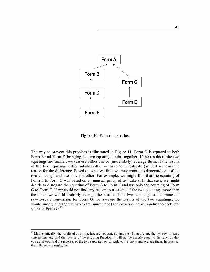
41

Form A

Form BForm C

Form DForm E

Form F

Figure 10. Equating strains. The way to prevent this problem is illustrated in Figure 11. Form G is equated to both Form E and Form F, bringing the two equating strains together. If the results of the two equatings are similar, we can use either one or (more likely) average them. If the results of the two equatings differ substantially, we have to investigate (as best we can) the reason for the difference. Based on what we find, we may choose to disregard one of the two equatings and use only the other. For example, we might find that the equating of Form E to Form C was based on an unusual group of test-takers. In that case, we might decide to disregard the equating of Form G to Form E and use only the equating of Form G to Form F. If we could not find any reason to trust one of the two equatings more than the other, we would probably average the results of the two equatings to determine the raw-to-scale conversion for Form G. To average the results of the two equatings, we would simply average the two exact (unrounded) scaled scores corresponding to each raw score on Form G.15

15 Mathematically, the results of this procedure are not quite symmetric. If you average the two raw-to-scale conversions and find the inverse of the resulting function, it will not be exactly equal to the function that you get if you find the inverses of the two separate raw-to-scale conversions and average them. In practice, the difference is negligible.

42

Form A

Form BForm C

Form DForm E

Form F

Form G

Figure 11. Equating strains brought together.

The Standard Error of Equating Unless we know the score distribution on both the new form and the reference form in the entire target population, our equating results will be affected by sampling variability. For any given raw score on the new form, the adjusted score is a statistic computed from a sample of test-takers. If it were computed from the scores of a different sample of test-takers, its value could be different. Suppose we could repeat the equating a very large number of times, each time with different test-takers taking the two forms—but the same numbers of test-takers each time. We could then choose a particular raw score on the new form and compare the equated scores that resulted from all those replications of the equating process. Those equated scores might be similar, but they would not all be exactly the same, so we could compute their distribution. This distribution would be the sampling distribution of a statistic: the equated score for that particular raw score. The standard deviation of this sampling distribution would show how much the equating results vary from one sample of test-takers to another. The standard deviation of the sampling distribution of the equated score has a name; we call it the “standard error of equating.” It is not a quantity that we can actually compute,

43

but sometimes we can estimate it.16 The larger the sample of test-takers whose scores are included in the equating analysis, the smaller the standard error of equating will be. To be more precise, we really should call it the “conditional standard error of equating” because the standard error of equating is different for different raw scores. In the middle of the score distribution, where most of the test-takers’ scores are located, the standard error of equating tends to be quite small. At the high and low ends of the score distribution, where the data are sparse, the standard error of equating tends to be larger.

Equating Without an Anchor When the equating data come from a single-group design, a counterbalanced design, or an equivalent-groups design (anything but an anchor design), equating is relatively simple. When you use one of these equating designs, you are assuming that the equating relationship you observe will generalize to the target population. If you are doing linear equating, you simply use the observed means and standard deviations to compute the equating relationship, just as you would if you knew the means and standard deviations in the target population. By using the means and standard deviations you observed in your data, you are not necessarily assuming that they are good estimates of the means and standard deviations in the target population. You are assuming only that the equating relationship that those means and standard deviations imply is a good estimate of the equating relationship in the target population. The means and standard deviations in your data can differ from those in the target population, as long as they differ from the target population in the same way (and to the same extent) on both forms of the test. For equipercentile equating, the procedure is a bit more complex. Unless your equating samples are extremely large, you will need to include a smoothing step. If you have a good way to presmooth the score distributions—one that preserves their shape while removing the irregularities—you should use it before you compute the equipercentile relationship. If you don’t have a good way to smooth the score distributions before equating, go ahead and compute the equipercentile equating from the observed score distributions, but then smooth the equating relationship that results. This procedure is often referred to as “postsmoothing.” What you want is a smoothing method that removes the irregularities, while preserving the shape and position of the equating curve. One problem that may arise with equipercentile equating is that of very sparse data—or no data at all—at the lower and upper ends of the score range. In this situation, linear equating will give you a set of equated scores (although they may well be the wrong ones!), but equipercentile equating will leave the equated scores undetermined. You may have to extrapolate the equating relationship beyond the range of the scores in your data.17

16 See Kolen and Brennan (1995), Angoff (1984, pp. 97, 103, 106), and Liou and Cheng (1995). 17 “Kernel equating” (Holland & Thayer, 1989) estimates equating relationships that extend beyond the observed data.

44 Equating in an Anchor Design Equating in an anchor design is more complex than equating in a single-group or equivalent-groups design. It is not simply a matter of equating two score distributions from the same group of test-takers or from groups that are assumed to be equal in the knowledge and skills measured by the test. We need the anchor because we cannot assume that the groups taking the two different forms are equal in their knowledge and skills. Somehow we have to use the information from the anchor score to adjust for the differences between the groups taking the new form and the reference form—the new form equating sample and the reference form equating sample. We have to assume that some kind of information we can compute in the equating samples will generalize to the target population. Figure 12 is an illustration of the anchor equating problem. The figure contains four boxes. Each box refers to a particular form of the test and a particular group of test-takers. The two boxes at the left refer to the new form; the two boxes at the right refer to the reference form. The box at the top refers to the new form equating sample; the box in the middle refers to the reference form equating sample; and the two boxes at the bottom refer to the target population. Each box represents the scatterplot of a two-way score distribution—a plot of the test-takers’ scores on the new form or the reference form and on the anchor. The horizontal axis represents the anchor score; the vertical axis represents the score on the new form or the reference form. If we had a large group of test-takers taking both the test and the anchor, and we plotted a data point for each test-taker, the data points would form a cloud with a roughly elliptical shape. That is what the ellipses shown in two of the boxes represent—the scatterplots of data that we can actually observe. The boxes representing the scatterplots for the target population are empty because in most equating situations we cannot observe the scores of the target population. In the situation pictured in Figure 12, the new form equating sample has high scores on the anchor. Those high anchor scores indicate that this group is a strong group. But the scores of this strong group on the new form are not particularly high. Therefore, we can infer that the new form is difficult. The reference form equating sample has much lower scores on the anchor. Those low anchor scores indicate that this group is a weak group. But the scores of this weak group on the reference form are not particularly low. Therefore, we can infer that the reference form is easy. An equating adjustment should compensate for the difference in the difficulty of the test forms by adjusting any given score on the new form to a higher score on the reference form. I will use this same situation to illustrate each of the anchor equating methods so you can see how each method leads to an adjustment in this direction.

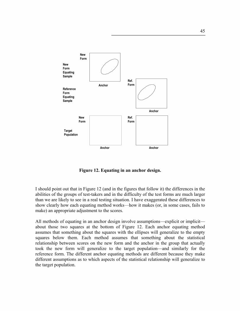
45

NewFormEquatingSample

ReferenceFormEquatingSample

TargetPopulation

Anchor

Anchor

AnchorAnchor

NewForm

NewForm

Ref.Form

Ref.Form

Figure 12. Equating in an anchor design.

I should point out that in Figure 12 (and in the figures that follow it) the differences in the abilities of the groups of test-takers and in the difficulty of the test forms are much larger than we are likely to see in a real testing situation. I have exaggerated these differences to show clearly how each equating method works—how it makes (or, in some cases, fails to make) an appropriate adjustment to the scores. All methods of equating in an anchor design involve assumptions—explicit or implicit—about those two squares at the bottom of Figure 12. Each anchor equating method assumes that something about the squares with the ellipses will generalize to the empty squares below them. Each method assumes that something about the statistical relationship between scores on the new form and the anchor in the group that actually took the new form will generalize to the target population—and similarly for the reference form. The different anchor equating methods are different because they make different assumptions as to which aspects of the statistical relationship will generalize to the target population.

46 Two ways to use the anchor scores Anchor equating methods can be classified into two types according to the way they use the information from the anchor. Each of these types includes at least one method for linear equating and at least one method for equipercentile equating. The first approach to using the anchor scores is “chained equating.” It consists of equating the scores on the new form to scores on the anchor and then equating the scores on the anchor to scores on the reference form. The “chain” formed by these two equatings links the scores on the new form to scores on the reference form. Chained equating assumes that the statistical relationship that generalizes from each equating sample to the target population is an equating relationship.18 The second approach to using the anchor scores is what I call “conditioning on the anchor.” (It is the same technique that many statisticians call “poststratification.”) In this approach, we use the anchor score as if it were a predictor variable. For each possible score on the anchor, we estimate the distribution (or possibly just the mean and standard deviation) of scores on the new form and on the reference form in the target population. These estimates are then used for equating as if they had actually been observed in the target population. This type of equating assumes that the relationship that generalizes from each equating sample to the target population is a conditional relationship. Table 5 illustrates this classification. We typically refer to the two chained equating methods simply as “chained linear” equating and “chained equipercentile” equating. The methods that condition on the anchor are “frequency estimation”—another descriptive term—and the “Tucker” and “Levine” methods. These two methods are named after the people who first proposed them, Ledyard Tucker and Richard Levine.19

18 Many testing experts would argue that the term “equating” is not appropriate here, unless the test and the anchor measure the same knowledge and skills and produce equally reliable scores (which never happens). Those experts would insist that this relationship between test scores and anchor scores be described only as a “symmetric linking” although, mathematically and operationally, it is indistinguishable from an equating relationship. 19 I have occasionally heard chained equipercentile equating referred to as “Lindquist” equating.

47

Table 5. Methods of Equating in an Anchor Design

Chained equating: equate new form to anchor;

equate anchor to reference form

Conditioning on the anchor: estimate score distributions or

means & SDs in target population

Linear equating

Chained linear method Tucker method, Levine method

Equipercentile

equating Chained equipercentile method Frequency estimation

equipercentile method

Chained Equating The logic of chained equipercentile equating is illustrated in Figure 13. It is fairly straightforward. The relationship that is assumed to generalize from each equating sample to the target population is an equipercentile equating relationship. In Figure 13, the curved line in the upper left box represents the equipercentile equating relationship between scores on the new form and scores on the anchor. That curve is copied into the lower left box because the equating relationship that it represents is assumed to generalize to the target population. Similarly, the curve in the middle right box represents the equipercentile equating relationship between scores on the reference form and on the anchor. That curve is copied into the lower right box because the relationship is assumed to generalize to the target population. The arrows in the bottom row of boxes illustrate the equating of a score on the new form to the corresponding score on the reference form. In the lower left box, we start with a given score on the new form and find the corresponding score on the anchor. We then find that score on the anchor in the lower right box and find the corresponding score on the reference form, completing the chain. In Figure 13, you can see how this process causes the selected score on the difficult new form to adjust to a higher score on the easy reference form.

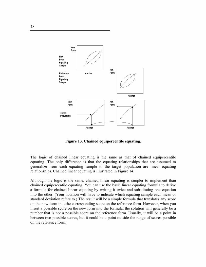
48

NewFormEquatingSample

ReferenceFormEquatingSample

TargetPopulation

Anchor

Anchor

AnchorAnchor

NewForm

NewForm

Ref.Form

Ref.Form

Figure 13. Chained equipercentile equating. The logic of chained linear equating is the same as that of chained equipercentile equating. The only difference is that the equating relationships that are assumed to generalize from each equating sample to the target population are linear equating relationships. Chained linear equating is illustrated in Figure 14. Although the logic is the same, chained linear equating is simpler to implement than chained equipercentile equating. You can use the basic linear equating formula to derive a formula for chained linear equating by writing it twice and substituting one equation into the other. (Your notation will have to indicate which equating sample each mean or standard deviation refers to.) The result will be a simple formula that translates any score on the new form into the corresponding score on the reference form. However, when you insert a possible score on the new form into the formula, the solution will generally be a number that is not a possible score on the reference form. Usually, it will be a point in between two possible scores, but it could be a point outside the range of scores possible on the reference form.

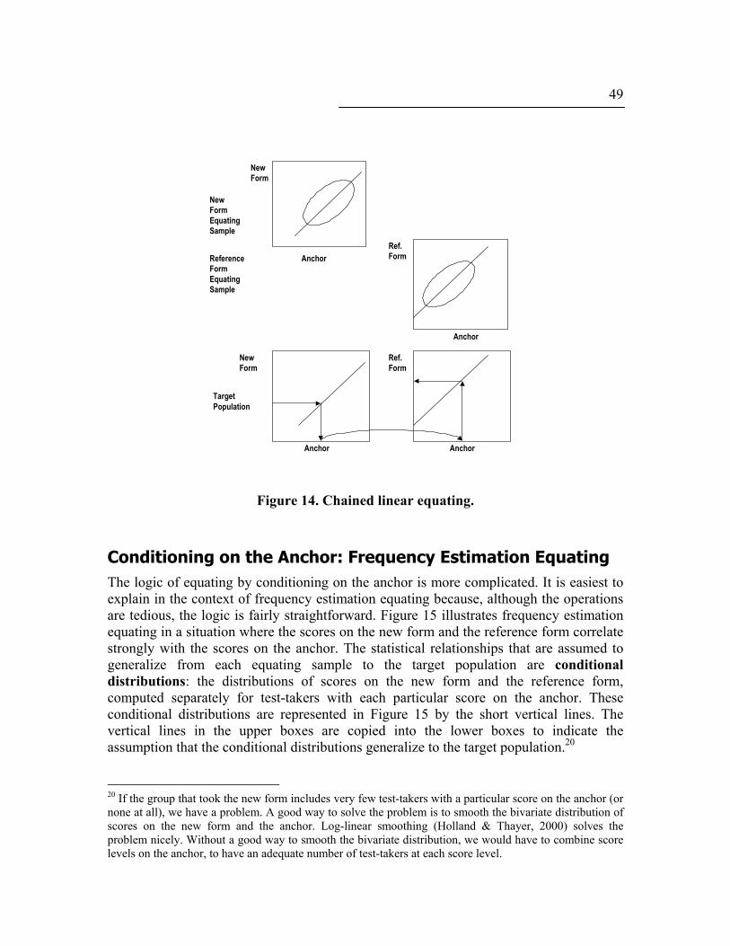
49

NewFormEquatingSample

ReferenceFormEquatingSample

TargetPopulation

Anchor

Anchor

AnchorAnchor

NewForm

NewForm

Ref.Form

Ref.Form

Figure 14. Chained linear equating.

Conditioning on the Anchor: Frequency Estimation Equating The logic of equating by conditioning on the anchor is more complicated. It is easiest to explain in the context of frequency estimation equating because, although the operations are tedious, the logic is fairly straightforward. Figure 15 illustrates frequency estimation equating in a situation where the scores on the new form and the reference form correlate strongly with the scores on the anchor. The statistical relationships that are assumed to generalize from each equating sample to the target population are conditional distributions: the distributions of scores on the new form and the reference form, computed separately for test-takers with each particular score on the anchor. These conditional distributions are represented in Figure 15 by the short vertical lines. The vertical lines in the upper boxes are copied into the lower boxes to indicate the assumption that the conditional distributions generalize to the target population.20

20 If the group that took the new form includes very few test-takers with a particular score on the anchor (or none at all), we have a problem. A good way to solve the problem is to smooth the bivariate distribution of scores on the new form and the anchor. Log-linear smoothing (Holland & Thayer, 2000) solves the problem nicely. Without a good way to smooth the bivariate distribution, we would have to combine score levels on the anchor, to have an adequate number of test-takers at each score level.

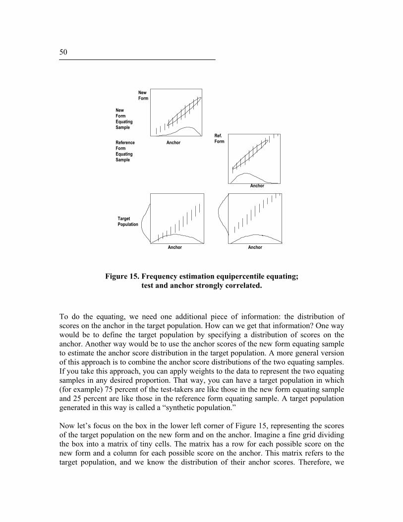
50

NewFormEquatingSample

ReferenceFormEquatingSample

TargetPopulation

Anchor

Anchor

AnchorAnchor

NewForm

Ref.Form

Figure 15. Frequency estimation equipercentile equating; test and anchor strongly correlated.

To do the equating, we need one additional piece of information: the distribution of scores on the anchor in the target population. How can we get that information? One way would be to define the target population by specifying a distribution of scores on the anchor. Another way would be to use the anchor scores of the new form equating sample to estimate the anchor score distribution in the target population. A more general version of this approach is to combine the anchor score distributions of the two equating samples. If you take this approach, you can apply weights to the data to represent the two equating samples in any desired proportion. That way, you can have a target population in which (for example) 75 percent of the test-takers are like those in the new form equating sample and 25 percent are like those in the reference form equating sample. A target population generated in this way is called a “synthetic population.” Now let’s focus on the box in the lower left corner of Figure 15, representing the scores of the target population on the new form and on the anchor. Imagine a fine grid dividing the box into a matrix of tiny cells. The matrix has a row for each possible score on the new form and a column for each possible score on the anchor. This matrix refers to the target population, and we know the distribution of their anchor scores. Therefore, we

51

know the proportion of the target population in each column of the matrix. We also know, for any column of the matrix, what proportion of the test-takers are in each cell. This information comes from the conditional distributions that we are assuming to be the same in the target population as they are in the new form equating sample. If we multiply these two proportions, we have an estimate of the proportion of the entire target population that is in the cell for that specific combination of scores on the anchor and the new form. We can write that proportion into the appropriate cell of the matrix. And we can do the same thing for all the other cells. When we have finished this operation, we will have a proportion written into each cell of the matrix. And these proportions, for the whole matrix, will sum to 1.00. Now we can specify a particular score on the new form and focus on its row of the matrix. If we sum the estimated proportions for all the cells in that row, we will have an estimate of the proportion of the target population who have that score on the new form. If we repeat this step for each score on the new form, we will have an estimate of the distribution of scores on the new form in the target population. We can then apply exactly the same procedure to estimate the distribution of scores on the reference form in the target population. And when we have estimated the score distributions on both the new form and the reference form, we can use those estimated distributions to do an equipercentile equating, as if we had actually observed the score distributions in the target population. I have tried to make the illustrations in Figure 15 show how frequency estimation equipercentile equating adjusts for the difference between the harder new form and the easier reference form. Looking at the lower left box of Figure 15, you can see that the test-takers with low anchor scores are estimated to get very low scores on the difficult new form. Even the test-takers with high scores on the anchor are estimated to get only moderately high scores on the new form. Therefore, the estimated distribution of scores on the new form in the target population will include lots of low scores and very few high scores. This distribution is shown at the left edge of the lower left box in Figure 15. Looking at the lower right box of Figure 15, you can see that the test-takers with low scores on the anchor are estimated to get only moderately low scores on the easy reference form. The test-takers with high scores on the anchor are estimated to get very high scores on the reference form. Therefore, the estimated distribution of scores on the reference form in the target population will include very few low scores and lots of high scores. This distribution is shown at the left edge of the lower right box in Figure 15.

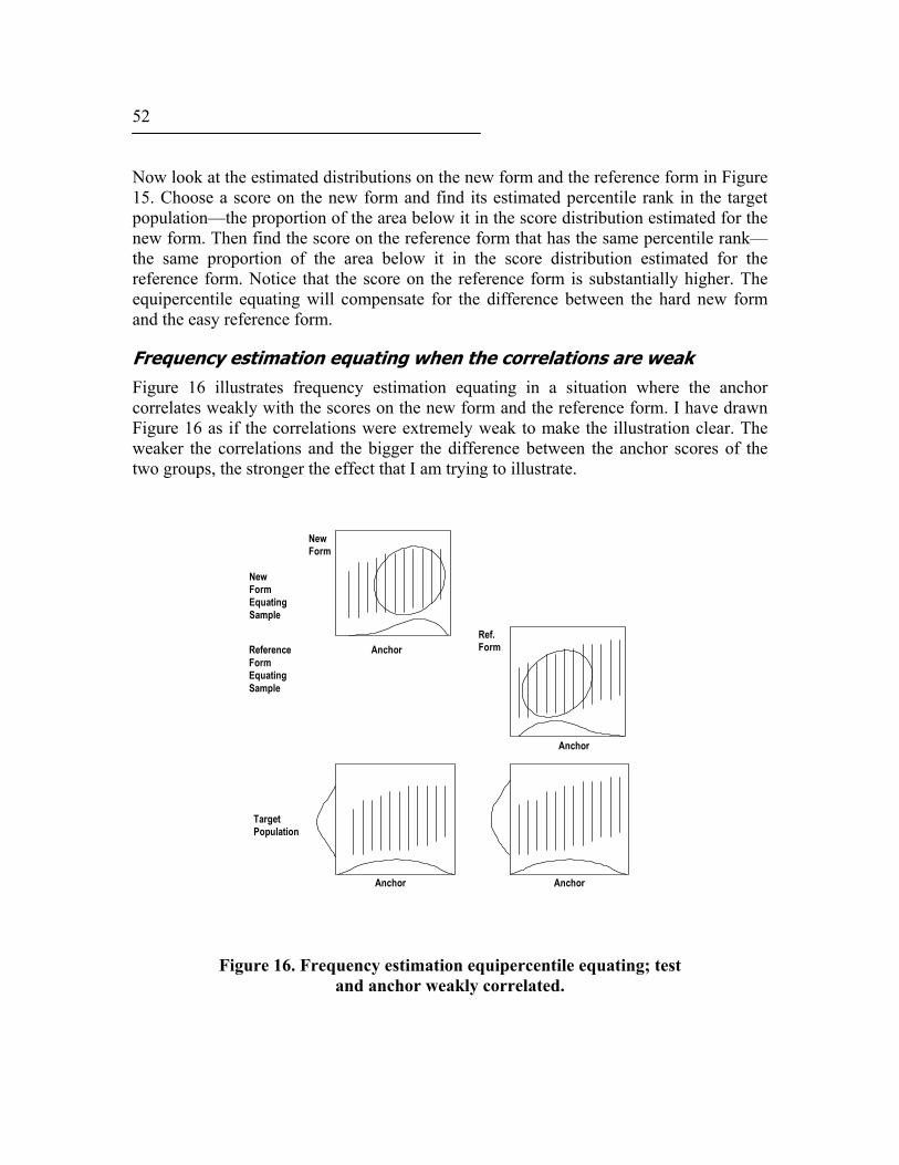
52 Now look at the estimated distributions on the new form and the reference form in Figure 15. Choose a score on the new form and find its estimated percentile rank in the target population—the proportion of the area below it in the score distribution estimated for the new form. Then find the score on the reference form that has the same percentile rank—the same proportion of the area below it in the score distribution estimated for the reference form. Notice that the score on the reference form is substantially higher. The equipercentile equating will compensate for the difference between the hard new form and the easy reference form.

Frequency estimation equating when the correlations are weak Figure 16 illustrates frequency estimation equating in a situation where the anchor correlates weakly with the scores on the new form and the reference form. I have drawn Figure 16 as if the correlations were extremely weak to make the illustration clear. The weaker the correlations and the bigger the difference between the anchor scores of the two groups, the stronger the effect that I am trying to illustrate.

NewFormEquatingSample

ReferenceFormEquatingSample

TargetPopulation

Anchor

Anchor

AnchorAnchor

NewForm

Ref.Form

Figure 16. Frequency estimation equipercentile equating; test and anchor weakly correlated.

53

As in all the previous examples, the new form equating sample is strong (their scores on the anchor are high), but the new form is difficult (the scores of this strong group on the new form are not particularly high). The reference form equating sample is weak (their scores on the anchor are low), but the reference form is easy (the scores of this weak group on the reference form are not particularly low). Because the new form is difficult and the reference form is easy, a given score on the new form should equate to a substantially higher score on the reference form. Now look at the vertical lines representing the conditional distributions in Figure 16. Because the correlations are weak, the vertical lines are longer than those in Figure 15, indicating that the conditional distributions are more spread out. And there is not as much difference between the conditional distributions for the test-takers with low anchor scores and those with high anchor scores. On the difficult new form, the few test-takers with low anchor scores do only slightly worse than those with high anchor scores. As a result, the new-form score distribution estimated for the target population is not much lower than that of the new form equating sample. On the easy reference form, the few test-takers with high anchor scores do only slightly better than those with low anchor scores. As a result, the reference form score distribution estimated for the target population is not much higher than that of the reference form equating sample. Because of the weak correlations in the equating samples, the score distributions estimated for the target population on the difficult new form and on the easy reference form are not very different. Therefore, the equipercentile equating based on these distributions will make only a small adjustment, even though the new form is much harder than the reference form. Frequency estimation equipercentile equating in this situation will not adequately compensate for the difference in difficulty. This problem with frequency estimation equating occurs, to some extent, whenever the two equating samples differ in their scores on the anchor and the correlations of the test scores with the anchor scores are less than perfect. To the extent that the correlations depart from 1.00, frequency estimation equating will adjust as if the equating samples were more similar in ability than the anchor scores indicate. The result will be a biased estimate of the equating adjustment in the target population.21 The size of the bias will depend on how much the two equating samples differ in ability and how weak the correlations are. If the anchor score distributions of the two equating samples are not very different or if the correlations between the test scores and the anchor scores are very high, the bias is small. In many cases, it is not large enough to worry about. But sometimes it is large enough to be cause for concern.

21 I am using the term “biased” the way statisticians use it, to mean that the expected value of an equated score estimated by this method differs systematically from the equated score in the target population.

54 This problem does not occur with chained equating because the statistical relationships that are assumed to generalize to the target population in chained equating are not affected by the size of the correlation between the test scores and the anchor scores.

Conditioning on the Anchor: Tucker Equating To do linear equating by conditioning on the anchor, it is not necessary to estimate the full distribution of scores on each form in the target population. All you need to estimate are the means and standard deviations in the target population. When you condition on the anchor for linear equating, you do not need to assume that the whole conditional distribution generalizes to the target population—only the conditional mean and standard deviation. And you can simplify the problem further by making some assumptions that are often made in other statistical applications. You can assume that in the target population

1. the conditional mean score on the new form (or the reference form) increases steadily (i.e., linearly) with scores on the anchor and

2. the conditional standard deviation is the same at all levels of the anchor score.

Assumption (1) implies that you can use a simple formula to estimate the conditional means in the target population. Assumption (2) implies that you can estimate a single value for the conditional standard deviation.22 Tucker equating assumes that what generalizes from the new form sample to the target population are (1) the linear equation for estimating the conditional mean on the new form for a given score on the anchor, and (2) the estimate of the conditional standard deviation of the scores on the new form for any given score on the anchor. And it makes the corresponding assumptions for the reference form. To estimate the mean and standard deviation of scores on the new form in the target population, you still need two more pieces of information: the mean and standard deviation of the anchor scores in the target population. As in frequency estimation, you can simply specify these values as a way of specifying the target population. Alternatively, you can assume that the new form equating sample is a representative sample of the target population. Under this assumption, the mean and standard deviation of the anchor scores in the new form equating sample will be estimates of those in the target population. Or you can specify a synthetic population that is a weighted combination of the equating samples. In this case, you can compute the mean and standard deviation of the anchor scores in the synthetic population from the means and standard deviations in the equating samples. When you have specified or estimated the mean and standard deviation of the anchor scores in the target population, you can derive formulas for estimating the mean and standard deviation of scores on the new form and on the reference form in the target population.

22 If you have studied regression analysis, you will recognize the estimation formula in assumption (1) as a linear regression equation and the estimated conditional standard deviation in assumption (2) as the residual standard deviation.

55

(It takes quite a bit of algebra, and I don’t intend to go into it here.)23 And when you have formulas for estimating the means and standard deviations in the target population for both the new form and the reference form, you can substitute the estimates into the basic formula for linear equating. The result will be a formula for Tucker equating. Tucker equating is difficult to illustrate in a diagram like the ones I have used for chained equating and for frequency estimation equating. I will try to show how Tucker equating works for a test-taker whose anchor score is at the mean of the target population. Figure 17 illustrates Tucker equating in a situation in which the anchor correlates strongly with the scores on the new form and the reference form. As in all the previous examples, the new form equating sample is a strong group (high scores on the anchor), but the new form is difficult (the scores of this strong group are not particularly high). The reference form equating sample is a weak group (low scores on the anchor), but the reference form is easy (the scores of this weak group are not particularly low). The equating should show a given score on the new form corresponding to a substantially higher score on the reference form.

NewFormEquatingSample

ReferenceFormEquatingSample

TargetPopulation

Anchor

Anchor

AnchorAnchor

NewForm

NewForm

Ref.Form

Ref.Form

Figure 17. Tucker equating; test and anchor strongly correlated.

23 See Kolen and Brennan (1995), pp. 105-111.

56 In the upper left box, the slanting line represents the equation for estimating the conditional mean on the new form conditioning on the anchor score. Notice that the slanting line extends beyond the ellipse, mostly at the left (low anchor scores). Even though the new form equating sample includes very few people with low anchor scores, the equation for estimating the conditional mean on the new form applies to the whole range of scores on the anchor. And notice that when the slanting line is extended into the range of low scores on the anchor, it gets quite low. Test-takers with low scores on the anchor are estimated to get very low scores on the new form. Similarly, in the upper right box, the slanting line represents the equation for estimating the conditional mean on the reference form, conditioning on the anchor score. Again, the slanting line extends beyond the ellipse, but now mostly at the right (high anchor scores). Even though the reference form equating sample includes very few people with high anchor scores, the equation for estimating the conditional mean on the reference form applies to the whole range of scores on the anchor. And when the slanting line is extended into the range of high scores on the anchor, it gets quite high. Test-takers with high scores on the anchor are estimated to get very high scores on the reference form. The equation for estimating the conditional mean score on the new form for any given anchor score is assumed to generalize to the target population. I have illustrated that assumption by copying the slanting line from the upper left box into the lower left box. In the lower left box, the vertical line indicates the mean anchor score of the target population. Look at the point where this vertical line intersects the slanting line. The height of that point indicates the conditional mean score on the new form estimated for test-takers whose anchor scores are at the mean of the target population. That new-form score is the estimated mean for the target population. Similarly, the slanting line from the middle right box (for the reference form equating sample) is copied into the lower right box (for the target population). In the lower right box, the vertical line indicates the mean anchor score of the target population. Look at the point where the vertical line intersects the slanting line. The height of that point indicates the conditional mean score on the reference form estimated for test-takers whose anchor scores are at the mean of the target population. That reference form score is the estimated mean for the target population. Comparing the two boxes in the bottom row, notice that the estimated mean score of the target population is much higher on the reference form than on the new form. A linear equating based on these estimated mean scores will show the lower mean score on the difficult new form as being comparable to the higher mean score on the easy reference form. In this way, Tucker equating compensates for the difference in the difficulty of the two forms.

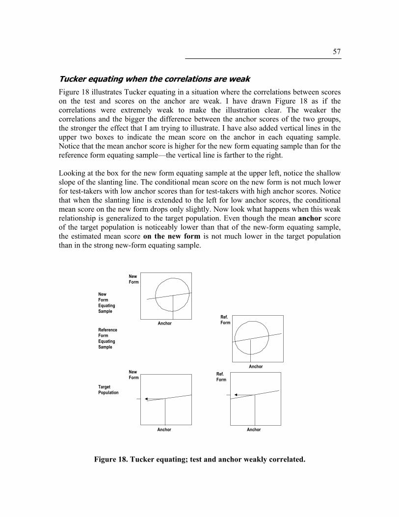
57

Tucker equating when the correlations are weak Figure 18 illustrates Tucker equating in a situation where the correlations between scores on the test and scores on the anchor are weak. I have drawn Figure 18 as if the correlations were extremely weak to make the illustration clear. The weaker the correlations and the bigger the difference between the anchor scores of the two groups, the stronger the effect that I am trying to illustrate. I have also added vertical lines in the upper two boxes to indicate the mean score on the anchor in each equating sample. Notice that the mean anchor score is higher for the new form equating sample than for the reference form equating sample—the vertical line is farther to the right. Looking at the box for the new form equating sample at the upper left, notice the shallow slope of the slanting line. The conditional mean score on the new form is not much lower for test-takers with low anchor scores than for test-takers with high anchor scores. Notice that when the slanting line is extended to the left for low anchor scores, the conditional mean score on the new form drops only slightly. Now look what happens when this weak relationship is generalized to the target population. Even though the mean anchor score of the target population is noticeably lower than that of the new-form equating sample, the estimated mean score on the new form is not much lower in the target population than in the strong new-form equating sample.

NewFormEquatingSample

ReferenceFormEquatingSample

TargetPopulation

Anchor

Anchor

AnchorAnchor

NewForm

NewForm

Ref.Form

Ref.Form

Figure 18. Tucker equating; test and anchor weakly correlated.

58 Similarly, in the box for the reference form equating sample, the line that estimates the conditional mean score on the reference form has a shallow slope. The conditional mean score on the reference form is not much higher for test-takers with high anchor scores than that for test-takers with low anchor scores. Notice that when the slanting line is extended to the right for high anchor scores, the conditional mean score on the reference form increases only slightly. Again, this weak relationship gets generalized to the target population. Even though the mean anchor score of the target population is noticeably higher than that of the reference form equating sample, the estimated mean score on the reference form is not much higher in the target population than in the weak reference form equating sample. You can see in the two boxes at the bottom of Figure 16 that in this situation, the estimated mean scores of the target population on the difficult new form and on the easy reference form do not differ very much. The equating adjustment will be small. It will not fully compensate for the difference in the difficulty of the two forms of the test. As with frequency estimation equating, this problem occurs, to some extent, whenever the anchor scores of the equating samples differ and the correlations of the test scores with the anchor scores are less than perfect. To the extent that the correlations depart from 1.00, Tucker equating will adjust as if the equating samples were more similar in ability than the anchor scores indicate. The result will be a biased estimate of the equating adjustment in the target population. The size of the bias will depend on how much the two equating samples differ in ability and how weak the correlations are. Notice that if the correlations were .00, the slanting lines that estimate the conditional mean scores on the new form and on the reference form would become horizontal. The estimated conditional mean on the new form for any possible anchor score would be the mean of the whole group taking the new form. Therefore, the target population’s estimated mean score on the new form would be the same as the mean score of the new form equating sample. Similarly, the target population’s estimated mean score on the reference form would be the same as the mean score of the reference form equating sample. In this situation—correlations of .00—Tucker equating would be the same as linear equating in an equivalent-groups design. Chained linear equating does not have this bias because in chained equating, the relationships that are assumed to generalize to the target population are symmetric relationships. The slopes of the lines are not affected by the size of the correlations between the scores on the test and on the anchor. Some people would argue that if the correlations between the test scores and anchor scores are weak, an equating adjustment should do what the Tucker equating method does—adjust as if the two equating samples were more similar in ability than the anchor

59

scores imply. In effect, the Tucker method is saying, “To the extent that the anchor correlates with the test scores, I will use it to adjust for differences between the equating samples. To the extent that it does not, I will assume the equating samples to be equal in the knowledge or skill the test measures.” You can think of Tucker equating as a compromise between chained linear equating and a linear equating that assumes the equating samples to be of equal ability. When the anchor scores correlate perfectly with the test scores, the Tucker method becomes identical to the chained linear method. When the anchor scores are uncorrelated with the test scores, the Tucker method becomes identical to a linear equating based on the assumption of equivalent groups. This rationale makes sense—if the two equating samples can be considered to be random samples from the same population of test-takers and if the reason for the imperfect correlations between the anchor scores and test scores is that the anchor and the test measure different knowledge or skills. However, there is another reason that correlations between test scores and anchor scores are less than perfect. The test scores and the anchor scores are not perfectly reliable. To the extent that the less-than-perfect correlations are caused by less-than-perfect reliability, the Tucker method will yield the wrong adjustment.

Correcting for Imperfect Reliability: Levine Equating One way to remove the bias from Tucker equating without abandoning the logic of the Tucker method is to base the equating on the statistical relationships of “true scores” on the new form, the reference form, and the anchor. A test-taker’s “true score” is the score the test-taker would earn if the test were perfectly reliable. No individual test-taker’s “true score” can ever be known, but it is possible to estimate statistical relationships involving “true scores” on the test and the anchor—the relationships that correspond to those used in Tucker equating. If you assume that these relationships of “true scores” generalize from the equating samples to the target population, you can get estimates of the means and standard deviations of scores on the new form and the reference form in the target population—estimates that are different from those in the Tucker method. This method based on “true scores” is called the Levine method. There are two versions of the Levine method, and a discussion of the difference between them is beyond the scope of this booklet.24 Both versions of the Levine method require good estimates of the reliability of the test scores and the anchor scores in the two equating samples. Choosing an Anchor Equating Method Which method of equating in an anchor design is best? Among people whose work includes the equating of test scores, there is not now (i.e., as of 2004) a consensus on this

24 See Kolen and Brennan (1995, pp. 111-120).

60 question. I tend to prefer chained equating. It avoids the bias that results from conditioning on the anchor when the equating samples differ in ability and the anchor scores are not highly reliable. Some research that my colleagues and I have done25 has convinced me that this bias is real, predictable, and explainable. I also prefer equipercentile equating over linear equating for three reasons:

1. I think equipercentile equating is based on a better definition of “relative position in the group.”

2. Equipercentile equating takes into account the possibility that the target population’s score distributions on the new form and on the reference form may have different shapes.

3. Equipercentile equating avoids (or at least minimizes) the problem of out-of-range adjusted scores.

For these reasons, I tend to prefer chained equipercentile equating. However, the chained equipercentile method does have some disadvantages and some limitations. It requires a good smoothing method. In the regions of the score scale where the data are sparse, one or two test-takers can have an exaggerated effect on the equating. In regions of the score scale where there are no data (e.g., if no test-takers have very high scores on the new form), the equating relationship cannot be determined. My colleagues and I often apply two or more equating methods to the same data and compare the results before deciding which method to use. Occasionally we will use the results of one method in some parts of the raw-score range and the results of another method in other parts of the raw-score range. Often the choice of an equating method comes down to a question of what is believable, given what we know about the test and the population of test-takers.

25 See Livingston, Dorans, and Wright (1990).

61

Test: Anchor Equating At this point, we end the class with a short, self-administered test on anchor equating. Here is the test. The answers appear in a separate section in the back of this book. Answer each question in a short phrase or sentence. A test developer is assembling a new form of a test that will be equated to a previous form by means of an internal anchor consisting of repeated questions (“common items”). The reference form included a set of four questions based on a particular reading passage, and the test developer wants to include those questions in the anchor. However, one of those questions has been changed. What should the statistician tell the test developer to do? In what part of the score distribution does the standard error of equating tend to be smallest? In chained equipercentile equating, what statistical relationship is assumed to generalize from the equating sample to the target population? In Tucker equating, what statistical relationship is assumed to generalize from the equating sample to the target population? Name an anchor equating method that equates the new form to the anchor in one group of test-takers and equates the anchor to the reference form in another group of test-takers.

62 Name an anchor equating method that uses data from the anchor test to estimate the mean and standard deviation of the scores on each form in the target population. Name an anchor equating method that tends to give better results if the score distributions are smoothed before the method is applied. Name an anchor equating method that requires reliability estimates for the full test and the anchor. Name an anchor equating method that produces an equating conversion that is correct for every examinee in the new form equating sample. Briefly describe the conditions under which the Tucker equating method is heavily biased.

63

References Angoff, W. H. (1984). Scales, norms, and equivalent scores. Princeton, NJ: Educational

Testing Service.

Holland, P. W., & Thayer, D. T. (1987). Notes on the use of log-linear models for fitting discrete probability distributions (Program Statistics Research Technical Report No. 87-79). Princeton, NJ: Educational Testing Service.

Holland, P. W., & Thayer, D. T. (1989). The kernel method of equating score distributions (Program Statistics Research Technical Report No. 89-84). Princeton, NJ: Educational Testing Service.

Holland, P. W., & Thayer, D. T. (2000). Univariate and bivariate loglinear models for discrete test score distributions. Journal of Educational and Behavioral Statistics, 25(2), 133-183.

Kolen, M. J. (1991). Smoothing methods for estimating test score distributions. Journal of Educational Measurement, 28, 257-282.

Kolen, M. J., & Brennan, R. L. (1995). Test equating. New York: Springer.

Liou, M., & Cheng, P. E. (1995). Asymptotic standard error of equipercentile equating. Journal of Educational and Behavioral Statistics, 20(3), 259-286.

Livingston, S. A. (1993). Small-sample equating with log-linear smoothing. Journal of Educational Measurement, 30, 23-39.

Livingston, S. A., Dorans, N. J., & Wright, N. K. (1990). What combination of sampling and equating methods works best? Applied Measurement in Education, 3(1), 73-95.

Lord, F. M. (1980). Applications of item response theory to practical testing problems. Hillsdale, NJ: Lawrence Erlbaum Associates.

64 Answers to Tests

Answers to test: Linear and equipercentile equating Its purpose is to adjust the scores for differences in the difficulty of the questions on the test.

True of linear equating? Yes. True of equipercentile equating? Yes. That’s what equating is all about.

It requires data on the performance of people taking the test.

True of linear equating? Yes. True of equipercentile equating? Yes. Like any other statistical procedure, equating requires relevant data.

It produces an adjustment that is correct for every person in the target population.

True of linear equating? No. True of equipercentile equating? No. It is not possible to make an adjustment that is correct for every individual.

The adjustment to the scores consists of multiplying by one number and then adding another.

True of linear equating? Yes. True of equipercentile equating? No. This is what makes linear equating linear.

The results can be improved by smoothing the score distributions before equating.

True of linear equating? No. True of equipercentile equating? Yes. There’s no need to smooth for linear equating, which uses only the means and standard deviations.

65

The adjusted scores on the new form will generally fall in between the scores that are actually possible on the reference form.

True of linear equating? Yes. True of equipercentile equating? Yes. True of any kind of equating.

Some adjusted scores on the new form can be several points higher than the highest score possible on the reference form.

True of linear equating? Yes. True of equipercentile equating? No. The100th percentile cannot be more than a fraction of a point higher than the highest possible score.

The adjusted score on the new form is the best prediction of the score the test-taker would get on the reference form.

True of linear equating? No. True of equipercentile equating? No. For a test-taker whose score is above the mean, the best prediction is somewhat lower than the adjusted score. For a test-taker whose score is below the mean, the best prediction is somewhat higher than the adjusted score. Equating is not the same as prediction. Prediction is not the same as equating.

66 Answers to test: Equating designs Which equating designs require the same test-takers to take both forms of the test?

Single-group and counterbalanced.

Which one equating design requires the largest number of test-takers for an accurate equating?

Equivalent-groups

Which two equating designs will produce accurate results with the smallest number of test-takers?

Single-group and counterbalanced. Having the same test-takers take both forms makes for a statistically powerful design.

For which one equating design is it most useful to “spiral” (alternate) the test forms among test-takers?

Equivalent-groups. This design won’t work unless the groups are equal in ability.

Which one equating design does not work well if the test has very few questions?

Internal-anchor. The anchor scores would not be very reliable, and you would not be able to determine whether the questions in the anchor had changed in difficulty.

Which one equating design is the best one to use when the two “forms” to be equated are just two different ways of scoring an essay test?

Single-group.

Which equating designs can be used for equipercentile equating?

All of them.

Which equating designs make it possible to compute a difficulty adjustment that will be correct for every test-taker taking the new form?

None of them. It is not possible to make such an adjustment.

67

Answers to test: Anchor equating A test developer is assembling a new form of a test that will be equated to a previous form by means of an internal anchor consisting of repeated questions (“common items”). The reference form included a set of four questions based on a particular reading passage, and the test developer wants to include those questions in the anchor. However, one of those questions has been changed. What should the statistician tell the test developer to do?

Include the whole item set in the new form, but include only the three unchanged items in the anchor score.

In what part of the score distribution does the standard error of equating tend to be smallest?

The middle of the distribution, where there are many test-takers.

In chained equipercentile equating, what statistical relationship is assumed to generalize from each equating sample to the target population?

The equipercentile equating of scores on the new form (or the reference form) and on the anchor.

In Tucker equating, what statistical relationship is assumed to generalize from each equating sample to the target population?

The equation that estimates the conditional mean score on the test (new form or reference form) for test-takers with a given anchor score. Give yourself a bonus point if you remembered that the value of the conditional standard deviation is also assumed to generalize to the target population.

Name an anchor equating method that equates the new form to the anchor in one group of test-takers and equates the anchor to the reference form in another group of test-takers.

Chained linear equating or chained equipercentile equating.

Name an anchor equating method that uses data from the anchor test to estimate the mean and standard deviation of the scores on the new form and the reference form in the target population.

Tucker equating or Levine equating. (Frequency estimation equipercentile equating estimates the entire score distribution in the target population, so it might possibly be considered a correct answer.)

Name an anchor equating method that tends to give better results if the score distributions are smoothed before the method is applied.

Chained equipercentile equating or frequency estimation equipercentile equating.

68 Name an anchor equating method that requires reliability estimates for the full test and the anchor.

Levine equating.

Name an anchor equating method that produces an equating conversion that is correct for every test-taker in the new form equating sample.

There is no such method.

Briefly describe the conditions under which the Tucker equating method is heavily biased.

The equating samples differ greatly on the anchor, and the correlations between the test and the anchor are weak. (Alternatively: The equating samples differ greatly on the anchor, and the scores on the anchor are unreliable.)

EQUATINGTESTSCORES(without IRT)

Samuel A. Livingston

Listening.Learning.

Leading.72528189530-036492 • U54E6 • Printed in U.S.A.

036492_cover 5/13/04, 11:47 AM2-3