Aspects of geophysical potential theory Joachim Vogt Jacobs University Bremen Course 210392 Earth and Planetary Physics Spring 2009 Joachim Vogt (Jacobs University B remen) Aspects of geophysical potential theory Cou rse 210 392 , S pr i n g 20 09 1 / 36 Motivation The Earth’s gravitational field and the geomagnetic fields are potential fields : they can be written as the gradient of a scalar potential Φ. Which differential equation is satisfied by the potential? What is a convenient mathematical representation (series expansion)? Geophysical fields are typically measured at the surface but we wish to know their values also in other regions. What is the relationship between potential values in different regions? Which infor mation is requi red to deter mine the potenti al uniquely? Geophysical fields are caused by source distributions. E.g., the Earth’s gravity field is generated by the mass density distribution in the interior. How does the potential depend on the source distr ibution ? What can surface measuremen ts tell us about the sources? Joachim Vogt (Jacobs Universit y Bremen) Aspects of geophysical potential theory Cou rse 210 392 , Sp rin g 20 09 2 / 36 Motivation (2) Earth’s gravity anomaly at the surface based on GRACE satellite data [(1) GRACE / GFZ Potsdam] Joachim Vogt (Jacobs University B remen) Aspects of geophysical potential theory Cou rse 210 392 , Sp rin g 20 09 3 / 36 Motivation (3) Gravity anomaly in the Earth’s mantle based on GRACE satellite data [(1) GRACE / GFZ Potsdam] Joachim Vogt (Jacobs Universit y Bremen) Aspects of geophysical potential theory Cou rse 210 392 , Sp rin g 20 09 4 / 36

Welcome message from author
This document is posted to help you gain knowledge. Please leave a comment to let me know what you think about it! Share it to your friends and learn new things together.
Transcript

7/29/2019 Epp Potential PV4
http://slidepdf.com/reader/full/epp-potential-pv4 1/9
Aspects of geophysical potential theory
Joachim Vogt
Jacobs University Bremen
Course 210392Earth and Planetary Physics
Spring 2009
Joachim Vogt (Jacobs University Bremen) Aspects of geophysical potential theory Course 210392, Spring 2009 1 / 36
Motivation
The Earth’s gravitational field and the geomagnetic fields are potential
fields : they can be written as the gradient of a scalar potential Φ.
Which differential equation is satisfied by the potential?
What is a convenient mathematical representation (series expansion) ?
Geophysical fields are typically measured at the surface but we wish to
know their values also in other regions.What is the relationship between potential values in different regions?
Which information is required to determine the potential uniquely?
Geophysical fields are caused by source distributions. E.g., the Earth’sgravity field is generated by the mass density distribution in the interior.
How does the potential depend on the source distribution ?
What can surface measurements tell us about the sources?
Joachim Vogt (Jacobs University Bremen) Aspects of geophysical potential theory Course 210392, Spring 2009 2 / 36
Motivation (2)
Earth’s gravity anomaly at the surface based on GRACE satellite data
[(1) GRACE / GFZ Potsdam]
Joachim Vogt (Jacobs University Bremen) Aspects of geophysical potential theory Course 210392, Spring 2009 3 / 36
Motivation (3)
Gravity anomaly in the Earth’s mantle based on GRACE satellite data
[(1) GRACE / GFZ Potsdam]
Joachim Vogt (Jacobs University Bremen) Aspects of geophysical potential theory Course 210392, Spring 2009 4 / 36

7/29/2019 Epp Potential PV4
http://slidepdf.com/reader/full/epp-potential-pv4 2/9
Motivation (4)
Geomagnetic field models based on data from the CHAMP satellite
Field intensity at the surface
[(2) CHAMP / S. Maus / NOAA-NGDC]
Vertical field component at . . .
. . . the Earth’s surface
. . . the core-mantle boundary
[(3) CHAMP / GFZ Potsdam]
Joachim Vogt (Jacobs University Bremen) Aspects of geophysical potential theory Course 210392, Spring 2009 5 / 36
Motivation (5)
Lithospheric magnetic field model (MF6): anomaly vertical component
[(4) CHAMP / S. Maus / GFZ Potsdam / NOAA-NGDC]
Joachim Vogt (Jacobs University Bremen) Aspects of geophysical potential theory Course 210392, Spring 2009 6 / 36
Motivation (6)
Lithospheric magnetic field model (MF4): anomaly total intensity . . .
. . . at 400 km altitude ...at 50 km altitude
[(4) CHAMP / S. Maus / GFZ Potsdam / NOAA-NGDC]
Joachim Vogt (Jacobs University Bremen) Aspects of geophysical potential theory Course 210392, Spring 2009 7 / 36
Overview
Part I: Vector field representations and potential equations
Potential representations of vector fields
The equations of Poisson and Laplace
Part II: Spherical harmonics
Solution of the Laplace equation in spherical coordinates
Properties of spherical harmonics
Part III: Earth’s global potential fields
Earth’s gravity field, Stokes coefficients
Geomagnetic field, Gauß coefficients
Joachim Vogt (Jacobs University Bremen) Aspects of geophysical potential theory Course 210392, Spring 2009 8 / 36

7/29/2019 Epp Potential PV4
http://slidepdf.com/reader/full/epp-potential-pv4 3/9
Aspects of geophysical potential theory – Part I
Vector field representations
and potential equations
Joachim Vogt (Jacobs University Bremen) Aspects of geophysical potential theory Course 210392, Spring 2009 9 / 36
Curl-free vector fields and scalar potentials
A vector field V is called
curl-free if ∇× V = 0,
a potential field (or gradient field ) if a scalar function Φ exists suchthat V = −∇Φ. Then the function Φ is the potential of V .
Note that
potential fields are always curl-free because ∇×∇Φ = 0,
the reverse holds for suitable definition domains (make sure thatsources are not enclosed ),
thus the term curl-free field is used usually as a synonym for potential field .
Examples:
Gravitational potential Φg, gravitational acceleration g = −∇Φg.
Electrostatic potential Φe, electric field E = −∇Φe.
Joachim Vogt (Jacobs University Bremen) Aspects of geophysical potential theory Course 210392, Spring 2009 10 / 36
Divergence-free vector fields and vector potentials
A vector field B is called divergence-free if ∇ ·B = 0. Such a field is thecurl of a vector potential A (suitable definition domain assumed):
B = ∇×A .
The vector potential is not uniquely defined, and additional constraints arerequired: gauge conditions , e.g.,
Coulomb gauge (magnetostatics): ∇ ·A = 0,
Lorentz gauge (electrodynamics): ∇ ·A = −∂ Φe/∂t,
A ·B = 0 (nonlinear gauge condition)→ Euler potentials α, β : B = ∇α ×∇β .
Special representations: toroidal and poloidal fields (dynamo theory).
Joachim Vogt (Jacobs University Bremen) Aspects of geophysical potential theory Course 210392, Spring 2009 11 / 36
Examples of potential equations (1)
Electrostatics : inserting E = −∇Φe into Gauß’ law yields
e = ∇ ·D = ε0∇ ·E = ε0∇ · (−∇Φe) = −ε0∇2Φe
(ε0: permittivity of free space, e: charge density), and we obtain
∇2Φe = −e/ε0
which is Poisson’s equation.
Magnetostatics I (magnetic fields due to magnetization): ∇×H = 0(zero currents), thus H = ∇Φm. B = µ0(H +M ), ∇ ·B = 0, thus
∇2Φm = −∇ ·M
(B: magnetic flux density [Vs/m2], H : magnetic field [A/m],M : magnetization [(A/m2)/m3], µ0: vaccum permeability).
Joachim Vogt (Jacobs University Bremen) Aspects of geophysical potential theory Course 210392, Spring 2009 12 / 36

7/29/2019 Epp Potential PV4
http://slidepdf.com/reader/full/epp-potential-pv4 4/9
Examples of potential equations (2)
Magnetostatics II (magnetic fields produced by stationary currents):zero magnetization, ∇ ·B = 0, thus B = ∇×A. From ∇×B = µ0 j
(Ampere’s law) we obtain
µ0 j = ∇×B = ∇×∇×A = ∇(∇ ·A)−∇2A .
Combine with Coulomb gauge ∇ ·A = 0 to get
∇2A = −µ0 j , ∇ ·A ,
i.e., a system of three Poisson-type equations (plus gauge condition).
Gravitational potential and mass density :
∇2Φg = 4πG
(: mass density, G: gravitational constant).
Joachim Vogt (Jacobs University Bremen) Aspects of geophysical potential theory Course 210392, Spring 2009 13 / 36
The equations of Poisson and Laplace
The potentials satisfy Poisson-type equations
∇2Φ = σ
where
Φ is the potential,
σ is the source term, and
∇2 is the Laplace operator.
In regions without sources: σ = 0. Poisson’s equation reduces to
∇2Φ = 0
This is the Laplace equation.
Solutions of the Laplace equations are called harmonic functions .
Joachim Vogt (Jacobs University Bremen) Aspects of geophysical potential theory Course 210392, Spring 2009 14 / 36
Boundary value problems
Poisson’s equation and the Laplace equation are elliptic PDEs that haveunique solutions if suitable boundary conditions are given.
Boundary value problem: Find the solution Φ of ∇2Φ = σ in a volume V for given values of the source function σ = σ(r) in V and additionalinformation on the boundary surface S = ∂ V .
(D) Dirichlet problem: Given on S = ∂ V are the values of the potential Φ.
(N) Von Neumann problem: Given on S = ∂ V are the values of thederivative of Φ in the direction n normal to the boundary surface:
∂ Φ
∂n= n · ∇Φ .
Both (D) and (N) have unique solutions under reasonable conditions.
Joachim Vogt (Jacobs University Bremen) Aspects of geophysical potential theory Course 210392, Spring 2009 15 / 36
Aspects of geophysical potential theory – Part II
Spherical harmonics
Joachim Vogt (Jacobs University Bremen) Aspects of geophysical potential theory Course 210392, Spring 2009 16 / 36

7/29/2019 Epp Potential PV4
http://slidepdf.com/reader/full/epp-potential-pv4 5/9
Laplace equation in spherical coordinates
Solutions of the Laplace equation ∇2Φ = 0 in spherical coordinates(r,ϑ,λ) are called (solid) spherical harmonics :
∇2Φ =1
r2
∂
∂r
r2 ∂ Φ
∂r
+
1
r2 sin ϑ
∂
∂ϑ
sin ϑ
∂ Φ
∂ϑ
+
1
r2 sin2 ϑ
∂ 2Φ
∂λ2= 0 .
We seek solutions through separation of variables which yields threeordinary differential equations (ODEs): write the potential Φ as a product
Φ(r,ϑ,λ) = R(r) · Ψ(ϑ, λ)
and insert this ansatz into the Laplace equation. Here
R = R(r) is called a radial function, and
Ψ = Ψ(ϑ, λ) is a surface spherical harmonic .
Joachim Vogt (Jacobs University Bremen) Aspects of geophysical potential theory Course 210392, Spring 2009 17 / 36
Separation of variables (1)
After multiplication with r2/Φ, we obtain
r2∇2Φ
Φ=
1
R
d
dr
„r2
dR
dr
« | z =const=n(n+1)
+1
Ψsin ϑ
∂
∂ϑ
„sin ϑ
∂ Ψ
∂ϑ
«+
1
Ψsin2 ϑ
∂ 2Ψ
∂λ2 | z =−n(n+1)
= 0 .
Note that the first underbraced expression depends only on the radial coordinate r, and thesecond one only shows angular dependences. This implies that each expression must be aconstant which is written as ±n(n + 1) for later convenience.
The equation for the radial function R reads
d
dr
„r2
dR
dr
«= n(n + 1) R
which can be solved by the ansatz R ∝ rα to yield two independent solutions rn and r−(n+1).
General solution for R = R(r) (radial function of degree n):
R(r) = A rn + B r−(n+1) .
Joachim Vogt (Jacobs University Bremen) Aspects of geophysical potential theory Course 210392, Spring 2009 18 / 36
Separation of variables (2)
We now separate the variables further and write Ψ as the product
Ψ(ϑ, λ) = Θ (ϑ) · Λ(λ) .
The differential equation for the function Ψ reads
1
sin ϑ
∂
∂ϑ
„sin ϑ
∂ Ψ
∂ϑ
«+
1
sin2 ϑ
∂ 2Ψ
∂λ2+ n(n + 1)Ψ = 0 ,
We insert the separation ansatz into this PDE and multiply by sin2 ϑ/Ψ to obtain
sin ϑ
ϑ
d
dϑ
„sin ϑ
dϑ
dϑ
«+ n(n + 1)sin2 ϑ | z
=const=m2
+1
Λ
d2Λ
dλ2 | z =−m2
= 0 .
Since the first term depends only on ϑ and the second one only on λ, we can conclude as beforethat each expression must be a constant. The azimuthal function Λ(λ) satisfies
d2Λ
dλ2+ m2Λ = 0 .
Joachim Vogt (Jacobs University Bremen) Aspects of geophysical potential theory Course 210392, Spring 2009 19 / 36
Separation of variables (3)
For the azimuthal dependence, the general solution can be written as
Λ(λ) = C cos mλ + D sin mλ .
Note that due to the uniqueness requirements Λ(λ) = Λ (λ + 2π) and Λ(λ) = Λ(λ + 2π),the number m must be a real integer and one can further assume that m is non-negative.
The ODE for Θ = Θ(ϑ) is more complicated than the previous ones:
1
sin ϑ
d
dϑ
„sin ϑ
dΘ
dϑ
«+˘
n(n + 1)sin2 ϑ− m2¯
Θ = 0 .
Substituting µ = cos ϑ and M (µ) = Θ(ϑ) yields
d
dµ
(1 − µ2)
dM
dµ
+
n(n + 1)sin2 ϑ −
m2
1 − µ2
M = 0
This ODE is solved by Legendre functions P mn (µ) .
Joachim Vogt (Jacobs University Bremen) Aspects of geophysical potential theory Course 210392, Spring 2009 20 / 36
7/29/2019 Epp Potential PV4
http://slidepdf.com/reader/full/epp-potential-pv4 6/9
Legendre functions (1)
Terminology:
m = 0: Legendre polynomials P n(µ),
m = 0: associated Legendre functions P mn (µ).
Rodriguez’ formula for Legendre polynomials:
P n(µ) = 12nn! dn
dµn
µ2 − 1
n
Associated Legendre functions:
P mn (µ) = pmn · (1− µ2)m/2 dm
dµmP n(µ)
Here pmn denotes a normalization factor.
Joachim Vogt (Jacobs University Bremen) Aspects of geophysical potential theory Course 210392, Spring 2009 21 / 36
Legendre functions (2)
Schmidt normalization: p0n = 1 (thus P n ≡ P 0n ), and
pmn =
2
(n− m)!
(n + m)!for m = 0 .
This is standard in geophysics and geomagnetism, and will also be used in
this course.
Other normalization conventions are given further below.The first four Legendre polynomials are
P 0 = 1 , P 1 = µ = cos ϑ ,
P 2 =1
2(3µ2 − 1) =
1
2(3cos2 ϑ− 1) ,
P 3 =1
2(5µ3 − 3µ) .
Associated Legendre functions
P 11 = (1− µ2)1/2 = sin ϑ ,
P 12 =√
3(1− µ2)1/2µ =√
3sin ϑ cos ϑ ,
P 22 =
√ 3
2(1− µ2) =
√ 3
2sin2 ϑ .
Joachim Vogt (Jacobs University Bremen) Aspects of geophysical potential theory Course 210392, Spring 2009 22 / 36
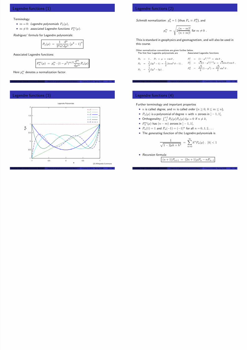
Legendre functions (3)
(5) Wikipedia Commons
Joachim Vogt (Jacobs University Bremen) Aspects of geophysical potential theory Course 210392, Spring 2009 23 / 36
Legendre functions (4)
Further terminology and important properties
n is called degree , and m is called order (n ≥ 0, 0 ≤ m ≤ n),
P n(µ) is a polynomial of degree n with n zeroes in ] − 1, 1[,
Orthogonality: +1−1 P k(µ)P n(µ) dµ = 0 if n = k,
P mn (µ) has (n− m) zeroes in ] − 1, 1[,
P n(1) = 1 and P n(−1) = (−1)n
for all n = 0, 1, 2, . . .The generating function of the Legendre polynomials is
1 1 − 2µh + h2
=
∞n=0
hnP n(µ) , |h| < 1
Recursion formula:
(n + 1)P n+1 = (2n + 1)µP n − nP n−1
Joachim Vogt (Jacobs University Bremen) Aspects of geophysical potential theory Course 210392, Spring 2009 24 / 36
7/29/2019 Epp Potential PV4
http://slidepdf.com/reader/full/epp-potential-pv4 7/9
Surface spherical harmonics (1)
The elementary surface spherical harmonics are given by
Ψmσn (ϑ, λ) = P mn (cos ϑ) ·
cos mλ , σ = c
sin mλ , σ = s
for 0 ≤ m ≤ n. Note that Ψ0sn ≡ 0.
Every function f (ϑ, λ) can be represented as a convergent series of
elementary surface spherical harmonics, i.e.,
f (ϑ, λ) =
∞n=0
nm=0
σ=c,s
Amσn Ψmσ
n (ϑ, λ)
with the coefficients (Ω is the unit sphere, and dΩ = sin ϑ dϑ dλ):
Amσn =
2n + 1
4π
Ω
f (ϑ, λ) Ψmσn (ϑ, λ) dΩ .
Joachim Vogt (Jacobs University Bremen) Aspects of geophysical potential theory Course 210392, Spring 2009 25 / 36
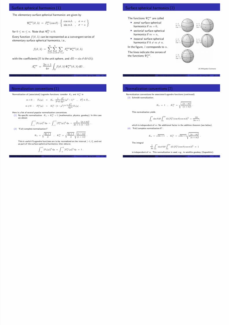
Surface spherical harmonics (2)
The functions Ψmσn are called
zonal surface sphericalharmonics if m = 0,
sectorial surface sphericalharmonics if m = n,
tesseral surface sphericalharmonics if 0 = m = n.
In the figure, l corresponds to n.
The lines indicate the zeroes of the functions Ψmσ
n .
(5) Wikipedia Commons
Joachim Vogt (Jacobs University Bremen) Aspects of geophysical potential theory Course 210392, Spring 2009 26 / 36
Normalization conventions (1)
Normalization of (associated) Legendre functions: consider K n and K mn in
m = 0 : P n(µ) = K n · 1
2nn!
dn
dµn(µ2 − 1)n , P 0n ≡ P n ,
m = 0 : P mn (µ) = K mn · (1− µ2)m/2dm
dµmP n(µ) .
Here is a list of several popular normalization conventions.
(1) No specific normalization: K n = K mn = 1 (mathematics, physics, geodesy). In this casewe obtain Z +1
−1[P n(µ)]2 dµ =
Z +1−1
[P mn (µ)]2 dµ =2
2n + 1
(n + m)!
(n− m)!.
(2) “Full/complete normalization I”:
K n =
r 2n + 1
2, K mn =
r 2n + 1
2
s (n − m)!
(n + m)!.
This is useful if Legendre functions are to be normalized on the interval [−1, 1], and notas part of the surface spherical harmonics. One obtainsZ +1
−1[P n(µ)]2 dµ =
Z +1−1
[P mn (µ)]2 dµ = 1 .
Joachim Vogt (Jacobs University Bremen) Aspects of geophysical potential theory Course 210392, Spring 2009 27 / 36
Normalization conventions (2)
Normalization conventions for associated Legendre functions (continued)
(3) Schmidt normalization:
K n = 1 , K mn =
s 2
(n− m)!
(n + m)!.
This normalization yields
Z π
0
sin ϑ dϑZ 2π
0
dλ [P mn (cos ϑ)cos mλ]2 =4π
2n + 1
which is independent of m. No additional factor in the addition theorem (see below).
(4) “Full/complete normalization II”:
K n =√
2n + 1 , K mn =√
2n + 1
s 2
(n − m)!
(n + m)!.
The integral1
4π
Z π0
sin ϑ dϑ
Z 2π0
dλ [P mn (cos ϑ)cos mλ]2 = 1
is independent of m. This normalization is used, e.g., in satellite geodesy (Gaposhkin).
Joachim Vogt (Jacobs University Bremen) Aspects of geophysical potential theory Course 210392, Spring 2009 28 / 36

7/29/2019 Epp Potential PV4
http://slidepdf.com/reader/full/epp-potential-pv4 8/9
Further identities for Legendre functions
Addition theorem:
ϑ and λ: co-latitude and the azimuth of a point P ,
ϑ and λ: co-latitude and the azimuth of a point P ,
both points lie on the unit sphere, and χ is the angle between P and P , then
cos χ = cos ϑ cos ϑ + sin ϑ sin ϑ cos(λ− λ) .
For Legendre functions in Schmidt normalization:
P n(cos χ) =nX
m=0
P mn (cos ϑ)P mn (cos ϑ)cos m(λ− λ)
Orthogonality of elementary surface spherical harmonics (in Schmidt normalization):
Z Ω
Ψmσn Ψmσ
n dΩ =
8<:
4π2n+1 : n = n, n = n, σ = σ =
s, c : m = 0 ,
c : m = 00 : else .
Joachim Vogt (Jacobs University Bremen) Aspects of geophysical potential theory Course 210392, Spring 2009 29 / 36
Aspects of geophysical potential theory – Part III
Earth’s global
potential fields
Joachim Vogt (Jacobs University Bremen) Aspects of geophysical potential theory Course 210392, Spring 2009 30 / 36
Gravitational potential
Consider a mass density distribution that is completely enclosed in asphere of radius a. Thus = 0 for r > a, the gravitational potential Φsatisfies ∇2Φ = 0, and can be written in terms of spherical harmonics:
Φ(r,ϑ,λ) =∞n=0
nm=0
rn P mn
(cos ϑ) [Amn
cos(mλ) + Bmn
sin(mλ)]
+∞
n=0
n
m=0
r−(n+1) P mn
(cos ϑ) [Amn
cos(mλ) + Bmn
sin(mλ)]
The potential must remain finite as r →∞, thus Amn = Bm
n = 0.
Earth: a = equatorial radius, and the largest term is A00/r = −GM E/r
(compare with spherical Earth model), thus A00 = −GM E and
Φ(r) = −GM E
r
1 −
∞n=1
nm=0
a
r
n
P mn
(cos ϑ) [C mn
cos(mλ) + S mn
sin(mλ)]
The parameters C mn and S mn are called Stokes coefficients .Joachim Vogt (Jacobs University Bremen) Aspects of geophysical potential theory Course 210392, Spring 2009 31 / 36
Stokes coefficients and density distribution (1)
The Earth’s gravitational potential at a point P in the exterior can b e written as follows:
Φ(r) = −G
Z Earth
(r)
|r− r|d3r = −G
Z Earth
(P )
D(P, P )dV
Primed variables refer to source (mass) distribution. Vectors r and r point from the origin to
P and P , respectively.
The distance D(P, P ) between P and P is expressed through
D2 = r2 + r2 − 2rr cos χ
where χ = ∠(r,r). The reciprocal distance 1/D = 1/|r− r| can be written using Legendrepolynomials as follows
1
D=
1
|r− r| =
1
r
∞Xn=0
„r
r
«nP n(cos χ) , r ≥ r ,
1
D=
1
r
∞Xn=0
“ r
r
”lP n(cos χ) , r ≤ r .
With this expansion, the gravitational potential reads
Φ(r) = −G
r
Z Earth
(r)Xn
„r
r
«nP n(cos χ) d3r .
Joachim Vogt (Jacobs University Bremen) Aspects of geophysical potential theory Course 210392, Spring 2009 32 / 36

7/29/2019 Epp Potential PV4
http://slidepdf.com/reader/full/epp-potential-pv4 9/9
Stokes coefficients and density distribution (2)
Inserting the addition theorem for spherical harmonics
P n(cos χ) =nX
m=0
P mn (cos ϑ) P mn (cos ϑ) cos(m(λ − λ))
then yields
Φ(r) = −∞Xn=0
G
rn+1
nXm=0
P mn (cos ϑ)
Z Earth
(r)rnP mn (cos ϑ)cos(m(λ − λ)) d3r
where cos(m(λ
− λ)) = cos(mλ) cos(mλ
) + sin(mλ) sin(mλ
) . The term−(G/r)R
Earth (r) d3r = −GM E/r is separated from the expansion for normalizationpurposes, and the series can now be written in the form
Φ(r) = −GM Er
(1 −
∞Xn=1
nXm=0
“a
r
”nP mn (cos ϑ) [C mn cos(mλ) + S mn sin(mλ)]
)
if we relate the Stokes coefficients to the mass density distribution as follows:C mnS mn
ff=
−1
anM E
Z V
(r,ϑ,λ) rn P mn (cos ϑ)
cos mλsin mλ
ffdV .
Note that dV = r2 sin ϑ dr dϑ dλ, and P mn are the Schmidt normalized Legendre functions.
Joachim Vogt (Jacobs University Bremen) Aspects of geophysical potential theory Course 210392, Spring 2009 33 / 36
Scalar potential of the geomagnetic field
In geomagnetism, the term magnetic field is mostly used for the fieldB = µ0H . The field B is measured in Tesla [T], and in other contexts itis called magnetic induction or magnetic flux density.
In the neutral atmosphere (between the ground and the ionosphere), thereare neither electrical currents nor magnetization, thus ∇×B = 0 and
B = −∇Φ .
Here Φ is the scalar magnetic potential, and (because of ∇ ·B = 0)
∇2Φ = 0 .
How to separate internal and external contributions to the geomagneticfield? Write the potential as a sum of two terms:
Φ = Φi + Φe .
Joachim Vogt (Jacobs University Bremen) Aspects of geophysical potential theory Course 210392, Spring 2009 34 / 36
Gauß coefficients
Decomposition according to C. F. Gauß
Φi = RE
∞n=1
RE
r
n+1 nm=0
(gmn cos mλ + hm
n sin mλ) P mn (cos ϑ) ,
Φe = RE
∞
n=1
r
REn n
m=0
gmn cos mλ + hm
n sin mλ P mn (cos ϑ)
The parameters gmn , hm
n , gmn , hm
n are called Gauß coefficients . Note thatthey have the same physical dimension as B and are usually given in nT.
Historically, the Gauß coefficients were determined from surfacemeasurements of the magnetic elements X (north), Y (east), and Z
(down). Nowadays they are determined from space (missions MAGSAT,CHAMP, Ørsted) and only supplemented by ground or aeromagneticmeasurements (mainly for regional field models).
Joachim Vogt (Jacobs University Bremen) Aspects of geophysical potential theory Course 210392, Spring 2009 35 / 36
Figure references
(1) Preliminary gravity anomaly maps based on data from the GRACE mission, see the websites hosted by the Geoforschungszentrum (GFZ) Potsdam athttp://op.gfz-potsdam.de/grace/results/grav/g001 eigen-grace01s.html (10April 2009). See also the GRACE web page at the University of Texas(http://www.csr.utexas.edu/grace/ ).
(2) Magnetic field intensity map based on the model POMME 3.0 by Stefan Maus, see theweb site http://www.geomag.us/info/mainfield.html hosted by the CooperativeInstitute for Research in Environmental Sciences (CIRES) and NOAA’s National
Geophysical Data Center (NGDC). See also the web site http://geomag.org/ (10 April2009).
(3) Maps of the vertical field component based on recent geomagnetic field models. Imagecredit: Geoforschungszentrum (GFZ) Potsdam, see http://www.gfz-potsdam.de/ (10April 2009).
(4) Lithospheric magnetic field maps based on the Magnetic Field Models MF4 and MF6developed at the Geoforschungszentrum (GFZ) Potsdam (http://www.gfz-potsdam.de/ )and at NOAA’s National Geophysical Data Center (NGDC). See the MF6 web site athttp://www.geomag.us/models/MF6.html by Stefan Maus at the NGDC (10 April 2009).
(5) Image files Harmoniques spheriques positif negatif.png and Legendre poly.svg fromWikipedia Commons http://en.wikipedia.org/wiki/ (10 April 2009).
Joachim Vogt (Jacobs University Bremen) Aspects of geophysical potential theory Course 210392, Spring 2009 36 / 36
Related Documents