Epikarst Hydrogeochemical Changes in Telogenetic Karst ...

Western Kentucky UniversityTopSCHOLAR®

Masters Theses & Specialist Projects Graduate School

Summer 2017

Epikarst Hydrogeochemical Changes inTelogenetic Karst Systems in South-centralKentuckyLeah JacksonWestern Kentucky University, [email protected]

Follow this and additional works at: http://digitalcommons.wku.edu/theses

Part of the Geology Commons, and the Speleology Commons

This Thesis is brought to you for free and open access by TopSCHOLAR®. It has been accepted for inclusion in Masters Theses & Specialist Projects byan authorized administrator of TopSCHOLAR®. For more information, please contact [email protected].

Recommended CitationJackson, Leah, "Epikarst Hydrogeochemical Changes in Telogenetic Karst Systems in South-central Kentucky" (2017). Masters Theses& Specialist Projects. Paper 2018.http://digitalcommons.wku.edu/theses/2018

EPIKARST HYDROGEOCHEMICAL PROCESSES IN TELOGENETIC KARST

SYSTEMS IN SOUTH-CENTRAL KENTUCKY

A Thesis

Presented to

The Faculty of the Department of Geography and Geology

Western Kentucky University

Bowling Green, Kentucky

In Partial Fulfillment

of the Requirements for the Degree

Master of Science

By

Leah E. Jackson

August 2017

iii

ACKNOWLEDGEMENTS

The decision to become a graduate student is not one made lightly. Graduate

student life is an arduous and grueling, demanding, yet exciting experience, riddled with

challenges that require dedication and fortitude to master.

I jumped into graduate school head first, with eyes open, eager, and ready and

willing to face whatever obstacles stood in my way. Like most other new recruits, I was

naive about the reality of graduate student life - a life that requires sacrifice, extreme hard

work, perseverance, and constant flexibility. Further, being a graduate student means

consistently stepping out of preconceived comfort zones, pushing personal limits, raising

the bar ever higher, and discovering one’s true potential. I owe my survival and

accomplishments to a great many people.

First and foremost, I want to thank my advisor Dr. Jason Polk. You ensured I

gained the most comprehensive, measurable, and thorough graduate school experience

possible. You pushed me consistently to work hard, taught me to reevaluate every aspect

from multiple angles, and trained me to be the best Earth Scientist I can be. To my

committee members, Dr. Leslie North and Dr. Pat Kambesis, I thank you for entertaining

my concerns and helping me celebrate my achievements. I thank you for supporting my

thesis topic switch at the 11th hour and working with me to ensure I completed my degree

on time.

To Dr. Margaret Crowder, I thank you for taking me under your wing to

demonstrate the finest methods toward delivering a university level education. I have

learned so much from you about what makes a great professor. Your unsurpassed advice

and ongoing support have helped me grow into a confident instructor.

iv

To Pauline Norris at AMI and Dr. Suvankar Chakraborty at SIRFER: thank you

for ensuring my samples were handled properly. Without your ongoing assistance, this

thesis wouldn’t exist.

To all the members at CHNGES: thank you for all your help conducting field

work, processing mountains of data, and aiding me in putting all the pieces together.

Without your assistance and guidance, I would not be writing this acknowledgements

section, much less a thesis. To one of my most favorite follow graduate students, Jason

Lively - I thank you for indulging my grievances and joining me on all those evening

stomping sessions through the mall. I never would have survived my first year without

your ear to bend.

To all the folks in the graduate student office: Autumn, Brita, CeCe, and the

international ladies Dolly, Indu, and Anisha; you showed me the world through a

universal lens, helping me to develop a deeper appreciation for cultures other than my

own, while simultaneously bringing levity and enjoyment to otherwise stress-laden

situations.

Last, but certainly not least, I thank my personal heroes: Mike and John. Mike, I

thank you for all those long, multi-hour-length, late-night phone sessions where you

helped me work out my concerns in a logical and rational manner. You offered sound

advice, an objective perspective, and a palette of humor I’ll never forget.

John, you have served as my best friend throughout this adventure. You have

counseled me through issues both professional and personal, but always doing it with a

witty style. Your words of encouragement, everlasting support, and eclectic humor have

v

reinvigorated this road-worn student to complete what seemed to be only a dream a mere

two years ago.

vi

TABLE OF CONTENTS

Chapter 1: Introduction ........................................................................................................1

Chapter 2: Literature Review ...............................................................................................4

2.1 Karst Landscapes ...............................................................................................4

2.2 Epikarst Theory ................................................................................................13

2.3 Carbon Processes in Karst ...............................................................................20

2.3.1 CO2 Dissolution Kinetics ..................................................................20

2.3.2 δ13CDIC Isotope Sourcing and Flux ...................................................26

Chapter 3: Study Area ........................................................................................................33

3.1 Crumps Cave at Smith’s Grove, KY................................................................34

3.2 Lost River Cave and Valley in Bowling Green, KY .......................................38

Chapter 4: Methods ............................................................................................................41

4.1 Site Selection and Instrument Installation .......................................................41

4.2 Field Data and Sample Collection ...................................................................44

4.3 Sample Analysis...............................................................................................47

4.4 Data Manipulation and Processing ..................................................................48

4.4.1 Hydrogeochemical Data Processing .................................................48

4.4.2 Carbon Isotope Sourcing ...................................................................51

4.4.3 LRS Hydrograph Generation ............................................................52

Chapter 5: Results ..............................................................................................................54

5.1 Epikarst Hydrogeochemistry ...........................................................................54

5.1.1 Site Geochemistry Results ................................................................54

5.1.2 δ13CDIC Isotopes Time Series Analysis .............................................58

5.1.3 Mixing Model Study Period and Seasonal Results ...........................61

Chapter 6: Discussion ........................................................................................................69

6.1 Epikarst Hydrogeochemistry ...........................................................................69

6.1.1 Site Geochemistry Discussion ..........................................................69

Precipitation ...............................................................................70

Surface and Water Temperature ................................................72

Specific Conductivity (SpC) ......................................................75

pH ...............................................................................................78

vii

Soil Temperature and Moisture Conditions ..............................84

Carbon Dioxide (CO2) ..............................................................87

Saturation Index (SIcalcite) ..........................................................94

Dissolved Inorganic Carbon (DIC) ...........................................99

6.1.2 Storm Event Hydrogeochemical Variability at WF1 and LRS .......102

STE 1: August 20-August 23, 2016 (JD233-236) ..................102

STE 2: November 28-December 1, 2016 (JD333-336) ..........109

6.1.3 Influences on Epikarst δ13CDIC ........................................................114

Soil Respiration .......................................................................116

Bedrock Dissolution................................................................116

δ13CDIC Sourcing at Crumps Cave (WF1 and SF) ...................117

δ13CDIC Sourcing at LRCV (LRS and LRWF) ........................119

6.1.4 Conduit Dissolution and DIC Flux .................................................121

6.1.5 Low-Resolution δ13CDIC, CO2, SIc, DIC Fluxes .............................126

6.2 Site Hydrogeochemical Comparisons ............................................................132

6.2.1 Regional Scope ...............................................................................132

Chapter 7: Conclusions ....................................................................................................140

References ........................................................................................................................146

Appendices .......................................................................................................................160

viii

LIST OF FIGURES

Figure 2.1 Conceptual model for a well-developed carbonate aquifer ................................8

Figure 2.2 Hydrologic features of epikarst zones ..............................................................14

Figure 2.3 Diagram expressing the global carbon cycle ....................................................26

Figure 3.1 Karst distribution in Kentucky .........................................................................33

Figure 3.2 GIS rendering of the study area in Warren County, Kentucky ........................35

Figure 4.1 Location of the study sites at Crumps Cave .....................................................42

Figure 4.2 Lost River Cave and Valley and the surrounding city of Bowling Green. .......43

Figure 4.3 Rating curve for Lost River Spring (LRS) discharge .......................................53

Figure 5.1 δ13CDIC Time Series Site Comparisons for CRUMPS-WF1 and SF .................59

Figure 5.2 δ13CDIC Time Series Site Comparisons for LRCV-LRS and LRWF ................60

Figure 5.3 Mean Contributions of Carbon Sourcing at CRUMPS-WF1 ...........................62

Figure 5.4 Mean Contributions of Carbon Sourcing at CRUMPS-SF...............................63

Figure 5.5 Mean Contributions of Carbon Sourcing at LRCV-LRS .................................66

Figure 5.6 Mean Contributions of Carbon Sourcing at LRCV-LRWF .............................67

Figure 6.1 Time series of hydrogeochemical changes at Crumps Cave-WF1 ..................71

Figure 6.2 Time series of hydrogeochemical changes at Crumps Cave-SF .....................74

Figure 6.3 Time series of hydrogeochemical changes at LRCV-LRS ..............................76

Figure 6.4 Time series of hydrogeochemical changes at LRCV-LRWF ..........................79

Figure 6.5 Surface and Soil Changes at Crumps Cave-WF1 ............................................82

Figure 6.6 Surface and Soil Changes at LRCV-LRS ........................................................83

Figure 6.7 DIC coefficient changes at Crumps Cave-WF1 ..............................................86

Figure 6.8 DIC coefficient changes at Crumps Cave-SF ..................................................89

ix

6igure 6.9 DIC coefficient changes at LRCV-LRS ..........................................................93

Figure 6.10 DIC coefficient changes at LRCV-LRWF ....................................................97

Figure 6.11 Crumps Cave-WF1 Storm Event JD233-236 ...............................................104

Figure 6.12 LRCV-LRS Storm Event JD233-236 ...........................................................106

Figure 6.13 Crumps Cave-WF1 Storm Event JD333-336 ...............................................110

Figure 6.14 LRCV-LRS Storm Event JD333-336 ...........................................................113

Figure 6.15 Time Series DIC Fluctuations at WF1 and LRS ..........................................123

Figure 6.16 Time series of CO2, DIC, and δ13CDIC at Crumps Cave-WF1 ......................127

Figure 6.17 Time series of CO2, DIC, and δ13CDIC at Crumps Cave-SF .........................129

Figure 6.18 Time series of CO2, DIC, and δ13CDIC at LRCV-LRS ..................................130

Figure 6.19 Time series of CO2, DIC, and δ13CDIC at LRCV-LRWF ..............................131

Figure 6.20 Illustration of CO2 exchange in the epikarst.................................................133

x

LIST OF TABLES

Table 5.1 Summary statistics of major hydrogeochemical and δ13CDIC parameters ..........56

Table 5.2 Seasonal trends of mixing model results for WF1 .............................................64

Table 5.3 Seasonal trends of mixing model results for SF ................................................65

Table 5.4 Seasonal trends of mixing model results for LRS .............................................68

Table 5.5 Seasonal trends of mixing model results for LRWF..........................................68

Table 6.1 Summary stats for DIC flux, conduit enlargement, and dissolution rates .......125

Table 6.2 Comparison of world epikarst and aquifer spring discharges to this

investigation .....................................................................................................................137

xi

LIST OF APPENDICES

Appendix 1 CRUMPS-WF1 Mixing Model Results .......................................................160

Appendix 2 CRUMPS-SF Mixing Model Results ...........................................................161

Appendix 3 LRCV-LRS Mixing Model Results .............................................................162

Appendix 4 LRCV-LRWF Mixing Model Results ..........................................................163

Appendix 5 Low Resolution Geochemical Time Series ..................................................164

Appendix 6 Recharge versus Discharge at Each Site ......................................................167

xii

EPIKARST HYDROGEOCHEMICAL PROCESSES IN TELOGENETIC KARST

SYSTEMS IN SOUTH-CENTRAL KENTUCKY

Leah E. Jackson August 2017 168 pages

Directed by: Jason S. Polk, Leslie North, Patricia Kambesis

Department of Geography and Geology Western Kentucky University

Telogenetic epikarst carbon sourcing and transport processes and the associated

hydrogeochemical responses are often complex and dynamic. Among the processes

involved in epikarst development is a highly variable storage and flow relationship that is

often influenced by the type, rate, and amount of dissolution kinetics involved. Diffusion

rates of CO2 in the epikarst zone may drive hydrogeochemical changes that influence

carbonate dissolution processes and conduit formation. Most epikarst examinations of

these defining factors ignore regional-scale investigations in favor of characterizing more

localized processes. This study aims to address that discrepancy through a comparative

analysis of two telogenetic epikarst systems under various land uses to delineate regional

epikarst behavior characteristics and mechanisms that influence carbon flux and

dissolution processes in south-central Kentucky. High-resolution hydrogeochemical and

discharge data from multiple data loggers and collected water samples serve to provide a

more holistic picture of the processes at work within these epikarst aquifers, which are

estimated to contribute significantly to carbonate rock dissolution processes and storage

of recharging groundwater reservoirs on the scale of regional aquifer rates. Data indicate

that, in agricultural settings, long-term variability is governed by seasonal availability of

CO2, while in urban environments extensive impermeable surfaces trap CO2 in the soil,

governing increased dissolution and conduit development in a heterogonous sense, which

is often observed in eogenetic karst development, as opposed to bedding plane derived

xiii

hydraulic conductivity usually observed in telogenetic settings. These results suggest

unique, site-specific responses, despite regional geologic similarities. Further, the results

suggest the necessity for additional comparative analyses between agricultural settings

and urban landscapes, as well as a focus on carbon sourcing in urban environments,

where increased urban sprawl could influence karst development.

1

Chapter 1: Introduction

Due to the complexity of karst systems, assessing the primary hydrogeochemical

processes involved in dissolution kinetics and aquifer storage and flow can be extremely

difficult. Hydrogeochemical processes that influence karst development and recharge and

discharge often begin in the epikarst zone, or “skin,” of the karst system, and result from

geochemical changes due to aggressive water-rock interactions (Bakalowicz 2004). The

extent of epikarst dissolution processes are highly influenced by surface conditions such

as soil and vegetation type and thickness, as well as storm event variability and

associated frequency of recharge intensity (Williams 2008). Excess atmospheric carbon

dioxide (CO2) derived from an increase in human industrialization over the past few

centuries has generated interest among scientists. It has been suggested that karst systems

can serve as an extensive carbon sink, due to their ability to absorb and utilize CO2 in

dissolution kinetics, which is the primary driver in karst development (Emblanch et al.

2003; Bakalowicz 2004; Palmer 2007a). Since the epikarst zone is where dissolution

initially occurs, and often is fastest, it is within this upper layer of the karst system where

special attention needs to be paid (Yang et al. 2012).

In the past, hydrogeochemical studies relied on low-resolution investigations to

account for changes in karst properties in relation to dissolution rates of limestone;

however, the need for higher-resolution examinations to capture speedy aquifer responses

has become vital to deriving a clearer and more thorough understanding of the connective

tissue which exists between the epikarst and the deeper-seated aquifer. One of the many

ways these high-resolution examinations have been achieved is through the deployment

of hydrogeochemical analyses in conjunction with current water monitoring technology.

2

Additionally, the sourcing of carbon by examination of carbon isotopes, as well as

assessing the concentrations of dissolved inorganic carbon, can shed light on the extent of

carbon dioxide’s role in karst systems and, in particular, the epikarst zone. The

employment of these types of investigations can further delineate the influence excess

atmospheric CO2 has on karst regions and their feasibility as carbon sinks (Zhang et al.

1995; Emblanch et al. 2003; Li et al. 2010; McClanahan et al. 2016; Huang et al. 2015).

In addition to carbon-based dissolution kinetics, understanding epikarst conduit

development can help infer the rate at which carbon is fluctuating within the system,

which can contribute to the karst system’s ability to serve as a carbon sink; therefore, it is

important to characterize epikarst storage and flow properties. Storage and flow rates

may be highly dependent on epikarst thickness, permeability and porosity, and the

existence of faults and fractures (Bakalowicz 2004). When recharge rates exceed

discharge rates, extensive storage may be actively occurring. In addition to high water

infiltration near the top of the epikarst zone, especially during storm inputs, a contrasting

property of water storage may exist near the base of the epikarst, allowing for longer

residence times and more extensive dissolution of the surrounding rock body (Aquilina et

al. 2004; Bakalowicz 2004; Chemseddine et al. 2015).

Regional examinations into karst landscape processes, such as the extent and rate

of water storage and flow velocities, and the evolution of karst conduit systems related to

dissolution kinetics, are prevalent for south-central Kentucky (Crawford 1984a; Crawford

1984b; Crawford 1989; Crawford 2003; Crawford 2005; Brewer and Crawford 2005;

Cesin and Crawford 2005; Nedvidek 2014); however, most of these investigations were

constrained to a single, specific cave system and fail to examine how epikarst processes

3

change over a regional scale. Additionally, where most studies in the past focused on the

primary underground rivers theorized to contain the majority of groundwater flow

(Palmer 2007a) at relatively low resolution (seasonal to bi-weekly), few studies quantify

the epikarst’s role in depth at a high resolution as a means to capture hydrogeochemical

variations with respect to carbon that occur in these systems, especially during storm

events (Lawhon 2014; Nedvidek 2014).

This study characterizes epikarst processes in a well-developed telogenetic karst

region at four individual epikarst-derived springs at two separate locations over the

course of nine months to capture seasonal changes, storm-event influences, and

hydrogeochemical responses. A combination of high-resolution hydrogeochemical

parameters, carbon isotope analysis, and hydrologic evaluations were employed. This

study addresses the following questions:

How does the sourcing and fluctuation of dissolved inorganic carbon change in

response to seasonal influences and storm events regionally in telogenetic epikarst

systems?

How do these fluctuations influence carbonate rock dissolution and carbon flux in

telogenetic epikarst systems?

The collected data from this investigation have illuminated the importance of

several key factors in karst processes, including a better understanding of the role of

carbon flux by karst systems, the extent to which that carbon is utilized within the

epikarst zone, and the feasibility of epikarst portions of karst systems to be referenced as

impactful carbon sinks.

4

Chapter 2: Literature Review

2.1 Karst Landscapes

Nearly 15% of all non-glaciated landscapes are karst landscapes and supply about

25% of the world’s fresh drinking water supply (Veni et al. 2001; De Waele et al. 2009;

Anaya et al. 2014). Karst is a term applied to any lithological landform that is capable of

producing conduits or caves through chemical dissolution (LeGrand 1983; Veni et al.

2001; White 2007; Mylroie 2013; Anaya et al. 2014). Karst environments are

characterized predominantly by limestones and dolomites, and less commonly by

gypsum, marble, and other evaporites (LeGrand 1983; Veni et al. 2001). The evolution of

a karst landscape is often governed by the interaction of five components: the type of

bedrock; the fluid involved in dissolution; the presence of structural influences such as

stratigraphic dip and tectonic deformation; the hydraulic gradient of subsurface flow; and

changes within local and regional climates over long periods of time (Palmer 1991; Ritter

et al. 2002; Palmer 2003a; Palmer 2003b; Palmer 2007a; Palmer 2007b). Since each karst

system is a unique combination of these elements, it can be difficult to categorize fully

the dominant processes within; often, individual case studies, where observations are

based on the interaction of one or more of these principles, are employed when

identifying aquifer properties and specific behaviors conducive to overall development.

Solution-derived karst systems can be divided into two main sections, with each

section governed by its own chemical and physical properties. The top layer, or “skin,” of

the karst system is known as the epikarst, which has been suggested also to include the

vadose or unsaturated zone (Bakalowicz 2004; Petrella et al. 2007; Trček 2007; Jacob et

al. 2009). Directly beneath the vadose zone is the phreatic or saturated zone. It is within

5

this zone that the main aquifer is located (Aquilina et al. 2004; Bakalowicz 2004; De

Waele et al. 2009). Because karst systems are governed by dissolution kinetics, which

happen to be at their most impactful within the epikarst, it is this top layer of a karst

system that requires special attention in research.

The epikarst can be thought of as a protective layer for the entirety of the karst

system. Previous investigations have shown that the majority of chemical changes within

the epikarst are driven by high concentrations of atmospheric and soil derived carbon

dioxide (CO2) (Zhongcheng and Daoxian 1999; Bakalowicz 2004; Palmer 2007a; Petrella

et al. 2007; Trček 2007; White 2007; Jacob et al. 2009; Liu et al. 2010; Yang et al. 2012;

Peyraube et al. 2014; Milanolo and Gabrovšek 2015; Zhang et al. 2016). This carbon

dioxide enters the karst system as dissolved CO2 in meteoric water or in antecedent

moisture in the topsoil.

The subsurface path that meteoric water follows is wrought with complexities

because of the heterogenetic nature of the epikarst, which is usually a result of several

processes including diagenesis, secondary and tertiary porosity and permeability, and

post-depositional structural deformation (LeGrand 1983; Aquilina et al. 2004; Palmer

2007a; De Waele et al. 2009; Pu et al. 2014a; Pu et al. 2014b). Diagenesis derived

variability originates from the unique mixture of deposited sediment before it undergoes

lithification. Depending on the orientation, shape, and size of each individual grain, small

gaps can form as the material is compressed. This is referred to as the rock’s porosity,

while frequency and proximity of void spaces, and thus the ability for the rock to transmit

fluid through those spaces, is considered the rock’s permeability. As the limestone

undergoes temporal diagenesis, permeability reduces due to overburden pressure from

6

overlying sediment deposition compressing the material and shrinking the size of the void

spaces within the matrix, reducing the rock’s ability to transmit fluid; however, as

temporal diagenesis serves to reduce primary porosity and permeability, it also allows

time for infiltrating water to dissolve along vertical fractures and horizontal bedding

planes, generating a condition known as secondary porosity resulting from dissolution

kinetics. Under these new conditions, the extent of water storage reduces as well, as pipe-

style conduits provide a means for secondary permeability and, thus, more efficient

hydraulic conductivity, unless the flow encounters a clog within the conduit system or it

enters the phreatic zone (Aquilina et al. 2004; Veni et al. 2001; Palmer 2007a;

Worthington 2007; De Waele et al. 2009; Anaya et al. 2014). The phreatic zone often

leads to springs and outlet systems, where discharge rates are governed by water table

fluctuations and the amount of recharge the system receives over time (Aquilina et al.

2004; Palmer 2007a).

Post-diagenetic structural deformation is usually a result of tectonic processes,

such as rifting or uplift. These processes can alter the stratigraphic dip of the region and

generate fractures and fissures, which then influence the hydraulic conductivity within

the system. Hydraulic conductivity is a more concise term applied to subsurface water

flow, such as slow percolation through a permeable medium, and the rapid drainage of

water through pipe-style conduits. Landscapes wrought with structural deformation will

aid in karst development and, thus, the transition between primary and secondary porosity

(Aquilina et al. 2004; Palmer 2007a). Hydraulic conductivity is also governed by the dip

of the landscape. As water infiltrates the bedrock, its ultimate goal is to reach local base

level; thus, water will follow the path of least resistance. Stratigraphic dip will serve to

7

govern the direction of water flow and the depth of conduit formation as surface rivers

simultaneous incise the landscape, dropping base level to a new position (Aquilina et al.

2004; Palmer 2007a).

The fluid involved in the dissolution of bedrock is dependent on several factors,

including the type of recharge (allogenic or autogenic), the amount of recharge (a

function of climate), and time (Palmer 2007a; Pu et al. 2014a; Pu et al. 2014b). In

epigenic cave development, the primary ingredients in soluble fluids are water and

carbon dioxide. The processes involved in dissolution from these soluble fluids are as

follows: water from precipitation absorbs carbon dioxide (CO2) from the atmosphere as it

falls onto the surface. The water becomes supersaturated with CO2 as it passes through

soil that is heavily laden with respiration-derived CO2 from vegetation, and infiltrates the

epikarst. This supersaturation of CO2 lowers the water’s pH to around 4.7, turning it into

carbonic acid (H2CO3). When the carbonic acid encounters calcium carbonate (CaCO3), it

will cause the calcium (Ca+) and carbonate (CO3) to disassociate (Veni et al. 2001; De

Waele et al. 2009). Furthermore, the additional hydrogen will join with the carbonate to

form bicarbonate (HCO3). The dissociation of CaCO3 into calcium and bicarbonate is

shown in the following reaction (White and White 1989; Palmer 2007a):

2H2O + CO2 + CaCO3 ↔ H2O + Ca2+ + 2HCO3− (Eq. 2.1)

The extent of dissolution is often contingent on recharge type, including allogenic

and autogenic (Palmer 1991; Palmer 2003a; Palmer 2003b; Palmer 2007a; Palmer

2007b). Allogenic recharge is derived from surface runoff that starts on non-karst

landscapes, but flows into karst landscapes. Allogenic recharge is often under-saturated

with respect to calcium and saturated with carbon dioxide by the time it enters the karst

8

system. As a result, its propensity for dissolution is much higher. In contrast, autogenic

recharge derived from runoff that immediately flows over a karst system, and is in

constant contact with soluble bedrock, may be heavily saturated with calcium and carbon

dioxide; however, its propensity for dissolution is much lower, due to its high calcium

saturation (Palmer 1991; Veni et al. 2001; Palmer 2003a; Palmer 2003b; Palmer 2007a;

De Waele et al. 2009; Mylroie 2013). In regions where the climate is more temperate or

tropical, karst development is more extensive due to higher annual precipitation rates.

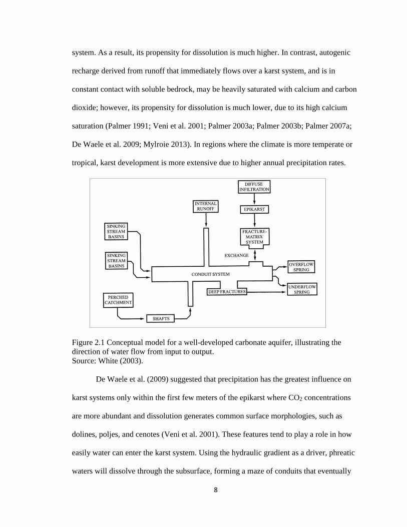
Figure 2.1 Conceptual model for a well-developed carbonate aquifer, illustrating the

direction of water flow from input to output.

Source: White (2003).

De Waele et al. (2009) suggested that precipitation has the greatest influence on

karst systems only within the first few meters of the epikarst where CO2 concentrations

are more abundant and dissolution generates common surface morphologies, such as

dolines, poljes, and cenotes (Veni et al. 2001). These features tend to play a role in how

easily water can enter the karst system. Using the hydraulic gradient as a driver, phreatic

waters will dissolve through the subsurface, forming a maze of conduits that eventually

9

meet the current level of the water table (Figure 2.1). As the water table rises, existing

caves and conduits will flood, and the processes will begin again at a different subsurface

elevation. When the water table drops, the phreatic zone will follow suit. Given enough

time, a series of intertwined conduits and caves develops in the subsurface, generating a

cave system, provided that surface erosion does not supersede the rate of cave formation

(Palmer 2007a; Palmer 2007b; De Waele et al. 2009).

Up to this point, the discussion of karst processes has been primarily through the

lens of telogenetic karst, or karst that has undergone temporal diagenesis, uplift, and

subsequent surface erosion; however, eogenetic karst has a hydraulic behavior and

geologic evolution unique to its environmental conditions as well. Although mostly

outside the scope of this study, it is important to touch on the primary differences

between these two karst landscapes, with a focus on hydraulic conductivity as it relates to

the storage and flow characteristics that are addressed in this study.

According to Worthington et al. (2000), Vacher and Mylroie (2002), and Florea

and Vacher (2006), there are three different types of karst defined by stages of deposition

influencing porosity of the limestone. Eogenetic karst is described as karst that has

undergone deposition and early exposure to surface processes; mesogenetic karst is that

which has experienced deep burial but not subsequent uplift; and telogenetic karst is karst

that has undergone deep burial, subsequent uplift, and surface erosion processes. It is

these three stages that result in telogenetic karst’s matrix permeability becoming heavily

altered. In eogenetic karst, permeable limestones having large volumes of interconnected

pore spaces, allowing for matrix-dominated, diffuse flow, dominate the bedrock. On the

other hand, deep burial of carbonates results in a reduction of porosity, due to

10

compression of overriding sediments, thus reducing permeability. Once the bedrock is

uplifted and exposed to surface erosions processes, hydraulic conductivity becomes

contingent on dissolution processes widening fractures and pore spaces between bedding

planes, eventually providing for pipe-style transmission of fluids. It is this shift in the

type of permeability, from matrix-dominated processes to conduit flow, which influences

subsequent dissolution processes, aquifer development, and overall residence times.

Florea and Vacher (2006) compiled examinations of spring hydrographs from a

variety of settings, including both eogenetic karst in Florida, and telogenetic karst in

Kentucky. They discovered that the responses to aquifer discharges varied greatly

depending on the type of karst, and attributed these varied responses to the type of flow

within the limestone. Martin and Dean (2001) found through a hydrogeochemical study

that the majority of flow within the Santa Fé River in Florida comes from matrix-

dominated flow during low-flow conditions, and this suggested that diffuse flow

processes are just as important to understanding karst landscape evolution as conduit-

flow processes. This statement is in direct conflict with White (1988), who suggested that

matrix permeability is negligible when examining spring response and, therefore, could

be easily dismissed as a major player, especially in high flow events. Despite the conflict

in the literature, Florea and Vacher (2006) submit that the type of karst will determine the

influences on aquifer processes by flow type, and that neither can be easily dismissed. In

fact, the authors suggested that matrix porosity cannot be dismissed as a significant

player in eogenetic karst, while secondary porosity generated by the growth of solution-

enlarged conduits in telogenetic karst plays a key role in hydraulic conductivity.

11

It is important to note, however, that White (1988) suggested that the primary

distinctive difference between diffuse flow in eogenetic karst and conduit flow in

telogenetic karst is in the spring response defined by a hydrograph. By using this tool,

one can infer the dominant processes within any karst system with respect to hydraulic

conductivity. According to Florea and Vacher (2006), White (1988) coined the term

“flashiness” when describing the responses to discharge observed in a hydrograph, and

describes this flashiness as a three-stage aquifer response: recharge, storage, and

transmission. Should residence time contribute to storage without ample recharge causing

a piston push effect, any rapid transmission of fluid discharged from the aquifer will be

reflected in a “flashy” hydrograph (White 1988; Worthington et al. 2000; Florea and

Vacher 2006; Worthington 2007). On the other hand, this flashiness could also be a

reflection of rapid recharge and rapid transmission (White 1988), especially in telogenetic

karst where water is easily transferred to the subsurface through sinking streams, with the

possibility of that same water being discharged through the aquifer provided extensive

storage is not taking place. The extent of storage in these cases, however, would need to

be delineated by examining the differences in base-flow discharge versus high-flow

discharge (Worthington et al. 2000; Worthington 2007). Additionally, Florea and Vacher

(2006) proposed that these types of spring responses are more likely to occur in well-

developed karst systems where flow has shifted from matrix-dominated diffuse flow to a

combination of matrix, conduit, and fracture flow, with dissolution conduits formed from

post uplift surface erosion and dissolution, leading to conduit flow becoming the

dominant flow regime.

12

These studies demonstrate that the setting in which the aquifer exists will often

determine the type of karst landscape, eogenetic versus telogenetic, which, in turn, will

usually describe the flow regime: diffuse flow versus conduit flow. These same flow

regimes are also observed in the epikarst (Petrella et al. 2007; Trček 2007; Williams

2008; Jacob et al. 2009); considering that the epikarst is more closely linked with surface

process, and thus higher rates of dissolution, examinations of epikarst discharge can shed

some light on just how different and unique are eogenetic and telogenetic karst,

especially with respect to hydraulic conductivity. By analyzing the hydrological factors

influencing subsurface geomorphology, an understanding of the timeline and key factors

for formation of a particular cave or aquifer system can be gained. This is achieved

through established methods, such as dye tracing, water sampling, and spatial and

temporal analysis of specific input and output locations; however, since passages may be

impassable for a variety of reasons, determining flow characteristics of an aquifer can be

complicated and time consuming (White 2007).

Investigations into the role of the epikarst, where dissolution is suggested to be

the most aggressive due to an open-system relationship with the surface, thus leading to a

mixture of conduit and diffuse flow regimes, is still not thoroughly understood. The

majority of investigations have shed some light on the abundant complexities of these

systems and the roles they play with respect to aquifer processes, but, to date, only

generalizations can be made about the influences that epikarst processes have on karst

systems. Often, location-specific research is necessary to delineate effectively the

epikarst’s role in karst landscape development.

13

2.2 Epikarst Theory

The epikarst is defined as highly weathered rock immediately underlying the soil

or present at the surface (Zhongcheng and Daoxian 1999; Aquilina et al. 2004;

Bakalowicz 2004; Klimchouk 2004; Groves et al. 2005; Jiang et al. 2007; Palmer 2007a;

Petrella et al. 2007; Trček 2007; White 2007; Williams 2008; Jacob et al. 2009; Liu et al.

2010; Yang et al. 2012; Peyraube et al. 2014; Milanolo and Gabrovšek 2015; Zhang et al.

2016). In the 1970s and 1980s, it was discovered that the uppermost layers of the karst

system played an important role in overall karst development, prompting deeper

investigations into the epikarst over the following decades (Williams 1983; Zhongcheng

and Daoxian 1999; Bakalowicz 2004; Klimchouk 2004; Cheng et al. 2005). According to

Klimchouk (2004), the term epikarst originated from the revelation that the upper part of

karst systems acted as a recharge zone for the entire system (Figure 2.2). This zone is

highly governed by the permeability and porosity of the bedrock, the type of recharge,

and the presence of structural deformation. The employment of hydrochemical and

isotopic analyses support the suggestion that these defining and governing characteristics

are the dominant drivers in epikarst processes (Zhongcheng and Daoxian 1999;

Bakalowicz 2004; Klimchouk 2004; Groves et al. 2005; Jiang et al. 2007; Petrella et al.

2007; Trček 2007; White 2007; Williams 2008; Jacob et al. 2009; Liu et al. 2010; Yang

et al. 2012; Peyraube et al. 2014; Milanolo and Gabrovšek 2015; Zhang et al. 2016).

Since the epikarst serves as a complex linkage with the surface and the deeply seated

saturated zone, and is sensitive to surface environmental changes, it could potentially

serve as a conduit for the percolation of polluted fluids as well as the transference of

meteoric water to the aquifer (Cheng et al. 2005; Williams 2008). Bakalowicz (2004)

14

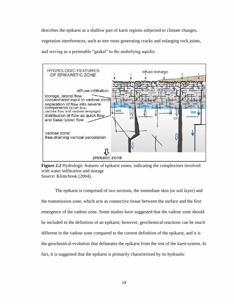
describes the epikarst as a shallow part of karst regions subjected to climate changes,

vegetation interferences, such as tree roots generating cracks and enlarging rock joints,

and serving as a permeable “gasket” to the underlying aquifer.

Figure 2.2 Hydrologic features of epikarst zones, indicating the complexities involved

with water infiltration and storage

Source: Klimchouk (2004).

The epikarst is comprised of two sections, the immediate skin (or soil layer) and

the transmission zone, which acts as connective tissue between the surface and the first

emergence of the vadose zone. Some studies have suggested that the vadose zone should

be included in the definition of an epikarst; however, geochemical reactions can be much

different in the vadose zone compared to the current definition of the epikarst, and it is

the geochemical evolution that delineates the epikarst from the rest of the karst system. In

fact, it is suggested that the epikarst is primarily characterized by its hydraulic

15

capabilities in relation to dissolution kinetics (Clemens et al. 1999; Bakalowicz 2004;

Klimchouk 2004; Groves et al. 2005; Jiang et al. 2007).

The epikarst can vary in thickness, depending on the particular region of karst

being investigated and, as a consequence, its characteristics will follow suit. Williams

(2008) suggested that the typical epikarst is between three and ten meters in depth and

exhibits contrasting porosity and permeability. For example, permeability can be much

greater near the surface of the epikarst, where the majority of fractures and faults have

been found. As a result, water infiltration may be greater in these areas. Porosity, on the

other hand, may be higher near the base of the epikarst where water is stored, forming

conduits and allowing for increased hydraulic conductivity (Palmer 2007a). Additionally,

if faults or fractures vertically transect part, or the entirety, of the epikarst, this can

provide a means for epikarst water to flush immediately through the system with minimal

to no storage time, generating high flow rates (Palmer 2007a; Williams 2008); however,

this particular characteristic may not be representative of the entirety of the epikarst.

Where water storage in the epikarst occurs, it is more likely to be found near the

base of the epikarst. In some respects, if the storage amount is great enough, it can be

thought of as an epikarst aquifer and serves as an aquitard to the vadose and phreatic

zones below (Clemens et al. 1999; Cheng et al. 2005; Groves et al. 2005; Aquilina et al.

2004; Jiang et al. 2007; Petrella et al. 2007; Trček 2007; Williams 2008; Jacob et al.

2009). As mentioned before, water storage in the epikarst is variable; therefore, it is also

highly influenced by seasonal changes and storm surges. Klimchouk (2004) found that

water within the epikarst could have various residence times, which are independent of

water stored in the deep-seated aquifer. In essence, it takes significant amounts of

16

recharge to push significant amounts of water through the system, reflected in high rates

of discharge. Due to the nature of water mixing within the solution-filled conduits, often

water that initially infiltrates the system is not directly observed as being the same water

that exits the system during the same storm event. In other words, freshly infiltrated water

often tends to replace older storage water (Palmer 2007a), instead of being immediately

discharged. In this respect, water storage in the epikarst allows time for limestone

dissolution and potential CO2 outgassing should that water enter the vadose zone, even in

the form of drip water that slowly percolates to the saturated zone.

Williams (2008) emphasized the importance of ensuring that the epikarst and its

functions are accurately identified as it may not always contain an active aquifer,

suggesting alternative storage properties are at work, or that storage only occurs at a

minimal level (Williams 2008); however, the presence of a perched aquifer in the epikarst

may exist when there is a well-defined network of fractures and faults that intersect, or

run perpendicular to bedding planes, thereby directly affecting water flow velocities and

direction (Williams 1983). Dissolution along these joints and fractures can actually

increase porosity and, thus, permeability as the rock undergoes temporal diagenesis. This

increase in permeability will cause a shift from lateral flow to a more vertical flow

direction; however, Williams (1983) noted that, with increasing depth, overburden

pressure will actually cause the aperture of these vertical shafts to reduce, forming a

cone-like shape near the base and creating a perched aquifer as water pools at these

narrow constrictions. Flow velocity will tend to reduce to a simple percolation as it

moves into the vadose zone. Consequently, water-flow direction may also shift to more

lateral flow as the water seeks a less restrictive route. Most often, epikarst derived

17

waterfalls are simply a single main vertical shaft to which the water has migrated due to a

reduction of flow-direction options. If the water cannot find its way toward these main

shafts, it will remain stored within that perched aquifer until there is sufficient hydraulic

head, often derived from storm events, to push it through the system (Williams 1983;

Williams 2008).

Worthington (2007) suggested that contrasting characteristics exist governing

mediums in which water will most likely be stored and/or transported. For example, in

older rocks, conduits only serve as a transportation network for groundwater flow, while

the majority of stored water occurs within the matrix, usually accompanied with long

residence times. This seems to support the theory that telogenetic karst systems, and

telogenetic epikarst specifically, are governed by a unique combination of matrix and

conduit style storage and flow parameters. Fractures serve as the connecting medium

between matrices and conduits, with low storage and moderate residence times. He also

suggested that it is possible to use environmental tracers to delineate the mediums in

which storage and residence times occur. For example, the author found that rapid flow

from injection points (sinking streams) to discharge points (springs) is an indication of

the presence of an extensive network of deep conduits with minimal storage and

residence times. On the other hand, samples from shallow depth conduits indicated long

residence times. Worthington (2007) also noted that the use of multiple environmental

and injection based tracers yielded conflicting residence times, possibly hinting toward

single, double, and triple porosity governing water flow and storage. He classified these

varying porosities as a function of conduit numbers and sizes within the aquifer.

Furthermore, it is possible these numbers will vary depending on the depth at which the

18

sample is collected. Epikarst permeability decreases with depth, according to Williams

(1983; 2008), but porosity increases with dissolution (Palmer 2007a; Worthington 2007);

therefore, storage, residence times, and flow rates will vary accordingly.

Williams (2008) suggested that dissolution propensity, which leads to this

increase in permeability along joints and fractures and bedding planes, is higher near the

surface, due to the abundant availability of atmospheric and soil derived CO2; thus,

hydro-geochemical processes and changes to the karst system are more aggressive in the

epikarst. This may not always be the case, as Chemseddine et al. (2015) claimed that

deep waters in the saturated zone are more active when rich with CO2. This saturation at

deep levels, however, may be a function of minimal epikarst thickness and/or storage,

high porosity, and the piezometric position of the water table being close to the surface.

In these cases, it may be that CO2-rich derived waters are immediately entering the

saturated zone, suggesting that no or very minimal storage in the epikarst exists.

Additionally, these phenomena may be local, in that this particular characteristic does not

necessarily represent the entirety of epikarst functions everywhere.

Attempting to resolve epikarst storage rates can be a difficult pursuit. Often, the

most common method is to calculate the difference between recharge and discharge rates

at epikarst springs; however, these values may not always be an accurate representation

of hydraulic conductivity, should the output exceed the input rate. To compensate for

such occurrences, additional dye tracing, geochemical, and isotopic data can be collected

at several points within a karst system to determine epikarst storage rates. Stable isotopes

can be used as tracers, especially when their values are examined with respect to the

fluctuation within different mediums as water moves from surface to subsurface.

19

Perrin et al. (2003) examined storage in a karst aquifer in the north of Switzerland

to determine the extent and type of storage. The authors compared stable isotopic data of

oxygen in spring discharge and underground river water samples to model the amount

and type of storage occurring in the epikarst. The authors found that in diffuse flow

environments, the epikarst exhibited the most dynamic storage properties, and that water

transferred to the saturated zone was immediately transported via a conduit network to

surface springs. They also identified two different types of water flow within the epikarst:

base flow and quick flow, which are dependent on storm surges and subsequent recharge

rates (Perrin et al. 2003).

The aforementioned studies highlight the importance of determining recharge and

discharge properties to infer water storage capabilities, flow dynamics, and subsequent

dissolution kinetics within the epikarst. It has been discovered that storage and flow,

though dependent on seasonal variations and storm surges, are mostly constrained by the

specifics of the locality of the karst system, such as lithology, geology, and latitude.

Hydrogeochemical data, such as pH, water temperature, specific conductivity, total

dissolved solids, alkalinity, and certain stable isotopes such as oxygen and carbon, can

provide proxy measurements for water transference through karst systems. Since

dissolution kinetics are most aggressive in the epikarst, and hydro-geochemical

parameters greatly reflect the extent of those kinetics, then hydro-geochemical

investigations are essential to delineating epikarst processes.

20

2.3 Carbon Processes in Karst

2.3.1 CO2 Dissolution Kinetics

Due to the ever-increasing concerns regarding excess atmospheric CO2 affecting

the environment, multiple studies have suggested that karst systems can serve as carbon

sinks (Li et al. 2008a; Cuezva et al. 2011; Gorka et al. 2011; Shin et al. 2011; White

2013; McClanahan et al. 2016; Jiang 2013; Zhang et al. 2015; Zeng et al. 2016). These

studies attempt to delineate carbon fluctuations within karst systems to better understand

carbon sequestration from the atmosphere. Additionally, as mentioned before, carbon is a

primary constituent in karst-dissolution kinetics and can serve as a practical tracer for

carbon flux. Therefore, by examining carbon isotope values with respect to carbon

sourcing, carbon fluctuations from surface to discharge point can be resolved. Further,

since the epikarst plays such a vital role in dissolution processes within karst systems, it

is within this zone that special attention to carbon processes is paid.

Karst dissolution processes are heavily dependent on the presence of dissolved

carbon dioxide in infiltrated waters. This CO2 is responsible for increasing the aggressive

nature of infiltrating waters, which, in turn, increases the rate by which carbonate bedrock

may be dissolved, and thus the rate at which water is either stored or discharged from the

system. Atmospheric CO2 is considered in equilibrium with precipitation and is usually

expressed as parts per million. According to the National Oceanic and Atmospheric

Administration (NOAA 2016), the rate of CO2 in the atmosphere, as of March 2017, was

roughly 409 parts per million, while the average global carbon dioxide level in soil is

significantly higher, at around 1,500 Pg (Hursh et al. 2017).

21

Most karst systems are considered open, wherein a continuous supply of CO2

from the surface dissolved within infiltrating meteoric waters contributes to ongoing

dissolution kinetics, even at great depths within the karst system. Several studies indicate

that epikarst heterogeneity, as well as the subsurface elevation of the saturated zone, can

greatly influence the point at which dissolution tends to cease (Hess and White 1992;

Baldini et al. 2006; Blecha and Faimon 2014a; Blecha and Faimon 2014b). Dissolution

kinetics lead to calcite and magnesium dominance in karst waters; therefore, karst water

is often considered to be in one of three states: under-saturated, or aggressive; saturated,

or chemically equilibrated; or supersaturated, at which point it is likely to precipitate the

dissolved minerals it carries. These values can be delineated mathematically and

expressed numerically, with any water value less than zero considered aggressive; any

water value at zero at equilibrium, and any water value greater than zero considered

supersaturated. In this sense, dissolution rates are considered a derivative of the saturation

index of water with respect to CaCO3 (Palmer 2007a).

In open systems, increased vegetation growth on the surface can contribute to a

rise in CO2 concentrations within the topsoil. This is primarily due to plant root

respiration and subsequent microbial activity converting organic matter into carbon

dioxide. Likewise, with increases in agriculturally based vegetation, soil CO2

concentrations can increase in response to the presence of agriculture. When those crops

are harvested, however, depletion in soil CO2 concentrations can occur, due to a severe

reduction in root respiration. Further, when natural vegetation shifts into the dormant

state during the winter months, an even greater depletion in soil CO2 can be observed;

thus, water containing reduced concentrations is transferred to the epikarst. Additionally,

22

these seasonal fluctuations in CO2 concentrations resulting from a change in vegetation

cover can have an impact on δ13C values, where depletion occurs resulting from

fractionation as plants utilize 12C. During the inert months, 13C enrichment occurs

because less 12C is utilized. Peyraube et al. (2014) suggests that equilibrium partial

pressure of CO2 can be used to account for the amount of dissolved CO2 in the system,

which, consequently, infers the extent of potential dissolution. To calculate the partial

pressures of CO2 (pCO2), the following equation (2.2) from Drever (1997) is used:

PCO2=

K1KCO2

10−pH[HCO31]

(Eq. 2.2)

where K1 is the temperature dependent dissociation constant of H2CO3 and KCO2 is the

solubility product of CO2 gas in water (Drever 1997; Lawhon 2014).

Studies on epikarst-dissolved CO2 concentrations, as well as the direct influence

from soils and in-cave air CO2 concentrations, have been conducted worldwide (Zaihua

et al. 1997; Baldini et al. 2006; Shen et al. 2013; Faimon et al. 2012a; Faimon et al.

2012b; Yang et al. 2012; Peyraube et al. 2013; Blecha and Faimon 2014a; Blecha and

Faimon 2014b). Baldini et al. (2006) examined potential sources of CO2 as it percolates

through the epikarst using drip water from two caves in Ireland. The authors found that,

in conjunction with soil CO2, seasonal fluctuations play a major role in total CO2

concentrations and variability. Peyraube et al. (2013) developed a methodology for

examining the concentrations of carbon and pCO2 in cave air after it infiltrates the

epikarst. They discovered that seasonal fluctuations are a key agent in pCO2 content.

Faimon et al. (2012a; 2012b) examined cave drip water for CO2 concentrations in a cave

in the Czech Republic. The authors found that their data correlated with previous

investigations of the same nature conducted in other parts of the world, which claim soil

23

CO2 rates and seasonal fluctuations are key agents in CO2 and HCO3 concentrations in

the epikarst and, subsequently, in the vadose and phreatic zone (Zeng et al. 2016). Zaihua

et al. (1997), Vesper and White (2004), Yang et al. (2012), and Blecha and Faimon

(2014a; 2014b) all had similar findings in their investigations; however, those

investigations examined the extent of dissolution resulting from influxes of CO2 content.

In fact, Peyraube et al. (2014) found that unsaturated zone CO2 baseline measurements

are extremely high and, thus, have a direct consequence on the CO2-saturation index

factors for calcium and magnesium. This discovery further supports the suggestion that

high concentrations of CO2 in the epikarst are directly responsible for increased rates of

dissolution during certain times.

Investigations conducted in Kentucky and Tennessee examined CO2 influences on

karst environments with the intent of determining the extent that CO2 concentration has

on dissolution kinetics (Hess and White 1992; Vesper and White 2004; Vanderhoff 2011;

Hatcher 2013; Lawhon 2014; Salley and Groves 2016). For example, Hatcher (2013)

investigated sources of CO2 controlling carbonate chemistry at Logsdon River at

Mammoth Cave. Three sites were chosen for that study: one feeding from the epikarst,

one with direct interaction from the vadose zone, and another from a spring. Hatcher

(2013) discovered that the vadose zone and spring exhibited minimal CO2 concentrations

with respect to the samples taken directly from the epikarst. This suggests that epikarstic

storage of CO2 is greater than in any other part of the karst system, furthering the

hypothesis that CO2 saturation is greatest where proximity or connection through

permeability to soils is highest.

24

Vesper and White (2004) examined CO2 from springs in a cave system near the

Kentucky/Tennessee border during storm events and found that changes in CO2 were a

direct result of flushing from the system associated with conduit-dominated karst

experiencing a pulse of water for the duration of the storm. The results suggest that CO2

levels in the karst system are higher during base flow, which allows the system time to

“compile” CO2 from various sources (Vesper and White 2004). One of the earliest studies

is by Hess and White (1992), who examined the hydrogeochemistry of several springs in

the Mammoth Cave region over one year during 1972. The authors suggested that

fluctuations in soil CO2 values, primarily due to seasonal changes, have the greatest

effect on the karst system. More localized and recent investigations of hydrogeochemical

influences were conducted in Bowling Green (Lawhon 2014) and Smith’s Grove,

Kentucky (Vanderhoff 2011), to ascertain the extent of storage and flow propensity,

especially with respect to storm events and contaminant transport. Both of these

investigations used CO2 concentrations as a proxy with respect to the nature of the

aquifers and their ability to transfer water from surface to spring. Although these

investigations did not directly ascertain sourcing of CO2 and direct effects of CO2 storage

and utilization, the work did reflect similar findings.

Dissolved CO2 concentrations in meteoric water are directly linked to bedrock

dissolution due to CO2’s ability to reduce pH to an acidic state (Zhongcheng and Daoxian

1999; Bakalowicz 2004; Palmer 2007a; Petrella et al. 2007; Trček 2007; White 2007;

Jacob et al. 2009; Liu et al. 2010; Yang et al. 2012; Peyraube et al. 2014; Milanolo and

Gabrovšek 2015; Zhang et al. 2016). The extent of dissolution from CO2 contributions

can be measured numerically by calculating the extent of water saturation, which is

25

referred to as the saturation index (SI) with respect to calcium and/or magnesium. In

terrestrial meteoric water, the saturation index of a particular mineral (Ca2+ or Mg2+) is

calculated by first determining the ion activity product (IAP). For example, the ion

activity product for calcite is:

(Ca2+)(CO32−) = KCalcite (Eq. 2.3)

where (Ca2+) equals the calcium ion activity, (CO32-) equals the carbonate ion activity,

and Kcalcite is the equilibrium constant for the reaction (a temperature dependent value).

Multiplying their values renders the IAP. If the IAP is less than K, then the solution is

considered under-saturated. If this is the case, dissolution of that particular mineral will

continue until the concentration of ions in solution supersaturates the solution. If the IAP

is greater than K, than the solution is considered oversaturated and dissolution of that

particular ion will cease and, in some cases, cause precipitation of that mineral (Palmer

2007a; Chemseddine et al. 2015). To determine the extent of solution saturation with

respect to a particular mineral, in this case calcite, the saturation index can be calculated

using the following formula from Palmer (2007a):

SIC = IAP/K (Eq. 2.4)

The extent of dissolution is a product of CO2 concentrations in infiltrated waters.

The CO2 is often derived from multiple sources, including atmospheric CO2, soil derived

CO2, and carbonate water-rock interactions. Determining the source of CO2 can delineate

which source is contributing the greatest amount of CO2 to the overall system, which, in

turn, can help better explain dissolution kinetics in epikarst systems, as well as the role

that anthropogenic forces play in natural systems.

26

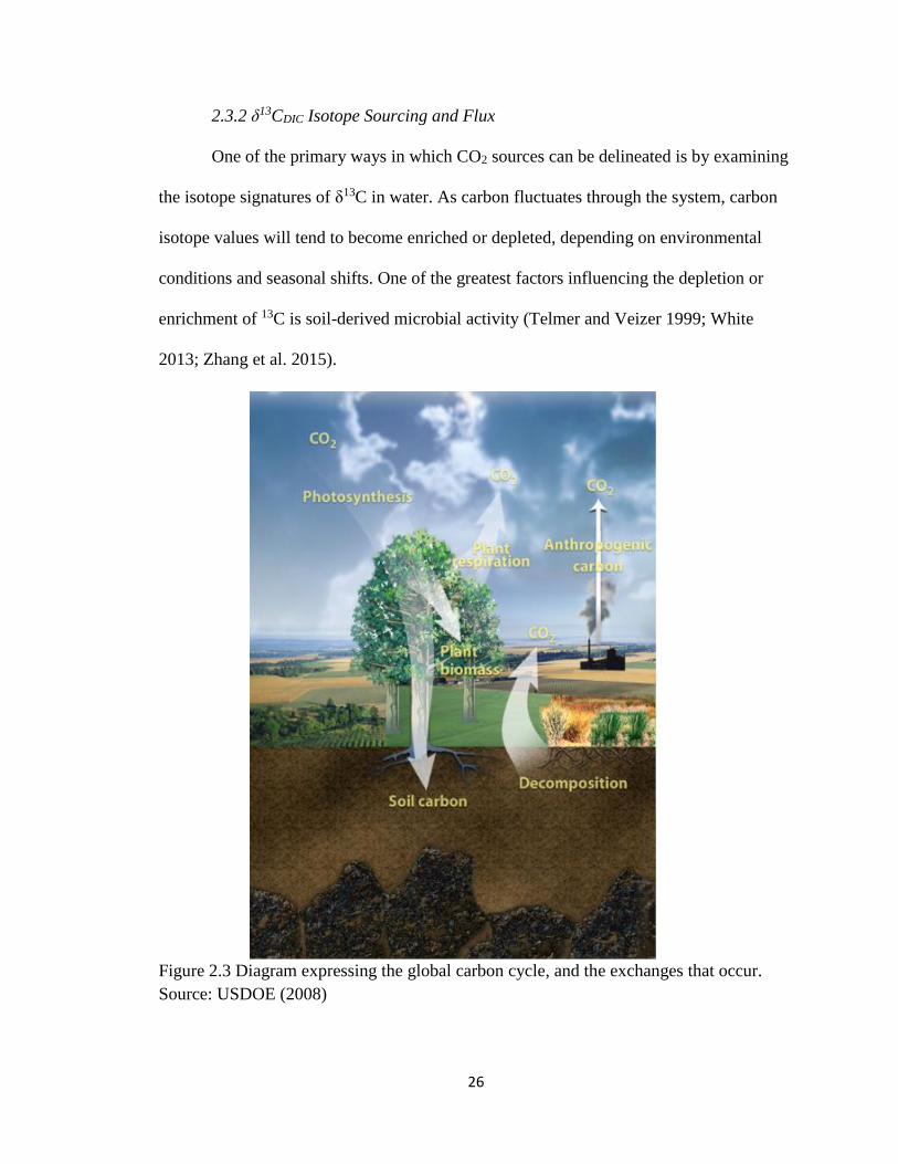
2.3.2 δ13CDIC Isotope Sourcing and Flux

One of the primary ways in which CO2 sources can be delineated is by examining

the isotope signatures of δ13C in water. As carbon fluctuates through the system, carbon

isotope values will tend to become enriched or depleted, depending on environmental

conditions and seasonal shifts. One of the greatest factors influencing the depletion or

enrichment of 13C is soil-derived microbial activity (Telmer and Veizer 1999; White

2013; Zhang et al. 2015).

Figure 2.3 Diagram expressing the global carbon cycle, and the exchanges that occur.

Source: USDOE (2008)

27

This variance is primarily due to the type of plant vegetation (C3 vs C4) that has a

direct bearing on the fractionation of carbon isotopes (12C vs 13C) being used by the

vegetation (Drever 1997; Li et al. 2008a; Hoefs 2010; Lambert and Aharon 2010; Gorka

et al. 2011; Shin et al. 2011; Florea 2013; White 2013; McClanahan et al. 2016).

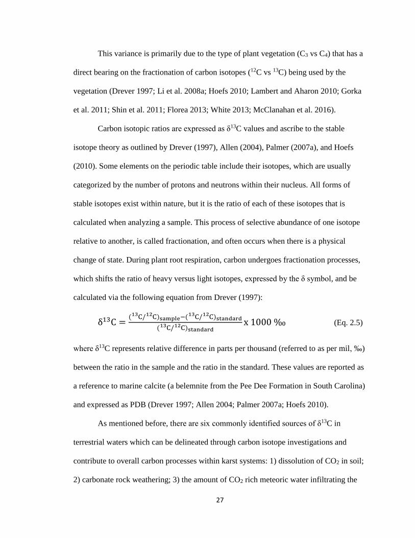
Carbon isotopic ratios are expressed as δ13C values and ascribe to the stable

isotope theory as outlined by Drever (1997), Allen (2004), Palmer (2007a), and Hoefs

(2010). Some elements on the periodic table include their isotopes, which are usually

categorized by the number of protons and neutrons within their nucleus. All forms of

stable isotopes exist within nature, but it is the ratio of each of these isotopes that is

calculated when analyzing a sample. This process of selective abundance of one isotope

relative to another, is called fractionation, and often occurs when there is a physical

change of state. During plant root respiration, carbon undergoes fractionation processes,

which shifts the ratio of heavy versus light isotopes, expressed by the δ symbol, and be

calculated via the following equation from Drever (1997):

δ13C =( C13 / C)12

sample−( C13 / C)12standard

( C13 / C)12standard

x 1000 ‰ (Eq. 2.5)

where δ13C represents relative difference in parts per thousand (referred to as per mil, ‰)

between the ratio in the sample and the ratio in the standard. These values are reported as

a reference to marine calcite (a belemnite from the Pee Dee Formation in South Carolina)

and expressed as PDB (Drever 1997; Allen 2004; Palmer 2007a; Hoefs 2010).

As mentioned before, there are six commonly identified sources of δ13C in

terrestrial waters which can be delineated through carbon isotope investigations and

contribute to overall carbon processes within karst systems: 1) dissolution of CO2 in soil;

2) carbonate rock weathering; 3) the amount of CO2 rich meteoric water infiltrating the

28

system; 4) exchange of bicarbonate and atmospheric CO2; 5) photosynthesis and

respiration of aquatic plants; and 6) silicate rock weathering (Li et al. 2008a; Li et al.

2008b; Li et al. 2010; Liu et al. 2007; Liu et al. 2010; Jiang 2013; Zhang et al. 2015).

In the case of one and three, the most influential parameters on δ13C values, the

concentration of dissolved CO2 in soil is often a product of the season in which it is

measured, the type of surface vegetation, and the amount and type of topsoil (permeable

soils will be more likely to transmit fluid containing dissolved gases such as CO2, while,

at the same time, soils high in microbial activity have higher concentrations of CO2

which provide for increased CO2 transmission). In the case of two, carbonate rock

weathering is highly governed by the rate in which solutionally aggressive water enters,

and is stored, in the system versus how often and how much water is immediately

discharged. Increased storage rates increase residence times and, thus, the ability for

dissolution to occur and remain ongoing until saturation is achieved. Four, five, and six

are often parameters heavily examined in riverine systems, which, while potentially

contributing to overall karst processes, are outside of the scope of this study and usually

indicative of minimal influences on carbon fluctuations compared to sources one and

three (Hess and White 1992; Drever 1997; Baldini et al. 2006; Li et al. 2008a; Hoefs

2010; Lambert and Aharon 2010; Gorka et al. 2011; Shin et al. 2011; Florea 2013; White

2013; Blecha and Faimon 2014a; Blecha and Faimon 2014b; McClanahan et al. 2016).

Since carbon isotopes (δ13C) are often used as tracers for both sourcing of carbon

in karst systems as well as assisting in delineation of the major hydrogeochemical players

influencing a specific karst system, understanding the relationship of CO2 and various

vegetation uptakes of CO2 can help delineate the impact that microbial activity within the

29

soil has on CO2 sourcing and, thus, 13C enrichment and/or depletion. For example, higher

CO2 concentrations provide for an increased uptake of 12C by plant roots, causing soil

waters transferred to the epikarst to become depleted with respect to 13C due to

fractionation. The ratio of 12C/13C is often expressed with a negative value, which

decreases as 13C depletion increases (Drever 1997; Amundson et al. 1998; Li et al. 2008a;

Hoefs 2010; Lambert and Aharon 2010; Gorka et al. 2011; Shin et al. 2011; Florea 2013;

Jiang 2013; White 2013; McClanahan et al. 2016). The uptake of CO2 by plant vegetation

is highly reliant on the pathway by which the plant chooses to metabolize the CO2. For

example, vegetation species characterized by C3 pathways and associated photosynthesis

are less efficient at metabolizing CO2, and, therefore, are often observed with more

enriched 13C values (closer to zero) as opposed to plants with C4 pathways, which are

known to metabolize CO2 more efficiently and produce more depleted carbon isotopic

values with respect to 13C (further from zero).

In addition to using δ13C to trace the route which the water has taken to enter the

system and its fluctuation through the system (Jiang 2013), δ13C can be useful in

understanding the role of the global carbon cycle in specific systems. Epikarst water often

is heavily laden with dissolved CO2, which is influenced by seasonal changes and storm

events, thus δ13C values are often reflective of these same principles (Hunkeler and

Mudry 2007; Knierim et al. 2015). Doctor et al. (2008) observed significant changes in

δ13C values at a spring discharge during seasonal changes from snowmelt in early spring

to summer rainfall. Their observations indicated changes related to both outgassing in the

unsaturated zone as well as recharge flushing the system of shallow water saturated with

CO2 from topsoil during high vegetation growth periods. Drever (1997) and Hoefs (2010)

30

suggested that carbon fractionation factors reach equilibrium within seconds, making

experimental determination rather challenging; thus, delineating sources of δ13C in

conjunction with derived values of total dissolved inorganic carbon (DIC) can provide

insight into how carbon is used by the system, as well as which source of carbon has the

most influence.

Dissolved inorganic carbon (DIC) is considered a primary product of carbonate

dissolution. This value is representative of several different carbon-based species

including H2CO3, CO2, HCO3-, or CO3

2- (Li et al. 2008a) found in karst waters, which are

fractionation factors of the dissolved carbon species; therefore, if the isotopic value of the

carbon (δ13CDIC) in the soils and the limestone is known, then the equilibrium isotopic

species of DIC currently dominating the system can be calculated (Zhang et al. 1995;

Zhongcheng and Daoxian 1999; Drever 1997; Palmer 2007a; Li et al. 2008a; Li et al.

2008b; Hoefs 2010; Lambert and Aharon 2010; Liu et al. 2010; Gorka et al. 2011; Shin et

al. 2011; Schulte et al. 2011; Faimon et al. 2012a; Faimon et al. 2012b; Singh et al. 2012;

Florea 2013; White, 2013; Peyraube et al. 2013; Peyraube et al. 2014; Pu et al. 2014a; Pu

et al. 2014b; McClanahan et al. 2016; Zhang et al. 2016).

According to Emblanch et al. (2003), δ13CDIC can be used as a tracer to determine

the extent of water mixing with respect to carbon sequestration within both the saturated

and unsaturated zones of a karst system. The authors suggested that soil influences will

be a primary adjuster to DIC content, since this relates to whether the DIC is being

measured from an open or closed system (Emblanch et al. 2003). The authors further

explained that exposure to soil compositions in open systems can heavily influence DIC

totals, as opposed to systems that have a limited amount of soil derived carbon. In the

31

case of epikarst environments, it is important to remember that direct influences from soil

derived carbon is common considering the type of infiltration and diffusion occurring

near the surface.

Despite what seems to be an extensive understanding of CO2 fluctuations and

subsequent carbon isotope variations in the epikarst, Gorka et al. (2011) and Faimon et al.

(2012a; 2012b) suggested that scientific understanding of epikarstic sources of CO2 and

changes with respect to δ13CDIC is still in its relative infancy. The quantitative

understanding of these processes increases with advances in monitoring technology. Liu

et al. (2007) suggested that better developed, high-resolution sampling studies can

potentially yield greater insight into the carbon uptake in epikarst systems. Zhang et al.

(2015) and Zeng et al. (2016) discovered that carbonate weathering and surface runoff

(river discharge versus subterranean sources) in karst catchments in China play vital roles

in carbon source flux. Further, Zeng et al. (2016) proposed that soil type, lithology, and

vegetation also play key roles in carbon fluxes. Due to the drastic need for quantitative

understanding of the effects of anthropogenic CO2 emissions on the environment,

recognizing the role karst landscapes play with respect to potential carbon sequestration

and utilization is imperative.

Ongoing examinations in the southcentral Kentucky region have been constrained

to individual caves, inadvertently overlooking the importance of understanding regional

CO2 uptake and, thus, storage and flow properties, which may be at work within multiple

cave systems. This research aims to fill a gap in the literature, with a comparative

assessment of epikarst hydrogeochemical influences on dissolution and storage and flow

dynamics, by examining the extent of carbon fluctuations with respect to CO2 and δ13C

32

variability through a nine-month, high-resolution study. It is hoped that this study will

further support the findings of previous investigations that suggest CO2 is one of the most

vital ingredients in epikarst dissolution kinetics, and that δ13C values can shed light on the

sourcing of this CO2.

33

Chapter 3: Study Area

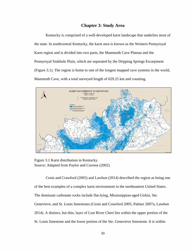
Kentucky is comprised of a well-developed karst landscape that underlies most of

the state. In southcentral Kentucky, the karst area is known as the Western Pennyroyal

Karst region and is divided into two parts, the Mammoth Cave Plateau and the

Pennyroyal Sinkhole Plain, which are separated by the Dripping Springs Escarpment

(Figure 3.1). The region is home to one of the longest mapped cave systems in the world,

Mammoth Cave, with a total surveyed length of 629.25 km and counting.

Figure 3.1 Karst distribution in Kentucky.

Source: Adapted from Paylor and Currens (2002).

Cesin and Crawford (2005) and Lawhon (2014) described the region as being one

of the best examples of a complex karst environment in the northeastern United States.

The dominant carbonate rocks include flat-lying, Mississippian-aged Girkin, Ste.

Genevieve, and St. Louis limestones (Cesin and Crawford 2005; Palmer 2007a; Lawhon

2014). A distinct, but thin, layer of Lost River Chert lies within the upper portion of the

St. Louis limestone and the lower portion of the Ste. Genevieve limestone. It is within

34

these lower bed layers (the St. Louis and the Ste. Genevieve) where the primary study

sites are located. Due to weathering and erosion processes, these limestones are covered

by thin, permeable clay soils in the sinkhole plain, while partially concealed beneath soils

and a sandstone cap within the Mammoth Cave Plateau.

Southcentral Kentucky exhibits the characteristics of a broad, low-relief sinkhole

plain and it is within this area that the primary study sites are situated (Figure 3.2). The

limestones in this area have undergone a long period of temporal diagenesis, trans-

forming the bed layers to telogenetic karst overlain by thin, clay rich soils. The sinkhole

plain lies atop a well-defined aquifer, recharged via autogenic recharge through numerous

sinkholes and sinking streams, as well as infiltration through fractures and matrix flow

(Palmer 2007a; Cesin and Crawford 2005; Lawhon 2014). Both study locations (Crumps

Cave and Lost River Cave and Valley) selected for this research are located within this

sinkhole plain and, as such, share similar geology, hydrology, and soil type. Additionally,

both systems eventually drain to the Barren River, with one draining from the north

(Crumps Cave) and the other from the south (Lost River Cave and Valley). The primary

differences between locations include surface land use (agricultural at Crumps Cave and

urbanization at Lost River Cave and Valley) and epikarst thickness (Crumps Cave

epikarst is roughly nine meters thicker than Lost River Cave and Valley). The study

locations are approximately 22 km apart.

3.1 Crumps Cave at Smith’s Grove, KY

Crumps Cave offers a unique study location suited to investigate epikarst

charcateristics. The cave is situated beneath agricultural lands, away from the

interference derived from large urban centers. Crumps Cave is located in Smith’s Grove,

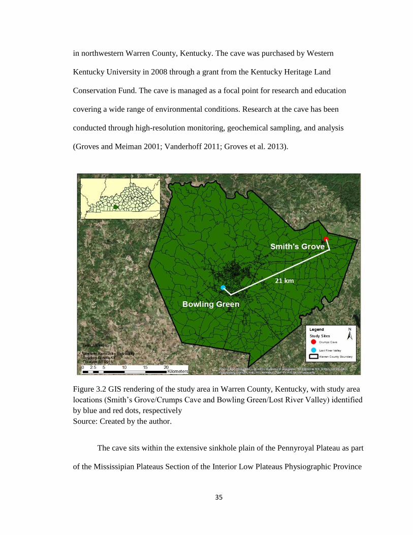
35

in northwestern Warren County, Kentucky. The cave was purchased by Western

Kentucky University in 2008 through a grant from the Kentucky Heritage Land

Conservation Fund. The cave is managed as a focal point for research and education

covering a wide range of environmental conditions. Research at the cave has been

conducted through high-resolution monitoring, geochemical sampling, and analysis

(Groves and Meiman 2001; Vanderhoff 2011; Groves et al. 2013).

Figure 3.2 GIS rendering of the study area in Warren County, Kentucky, with study area

locations (Smith’s Grove/Crumps Cave and Bowling Green/Lost River Valley) identified

by blue and red dots, respectively

Source: Created by the author.

The cave sits within the extensive sinkhole plain of the Pennyroyal Plateau as part

of the Mississipian Plateaus Section of the Interior Low Plateaus Physiographic Province

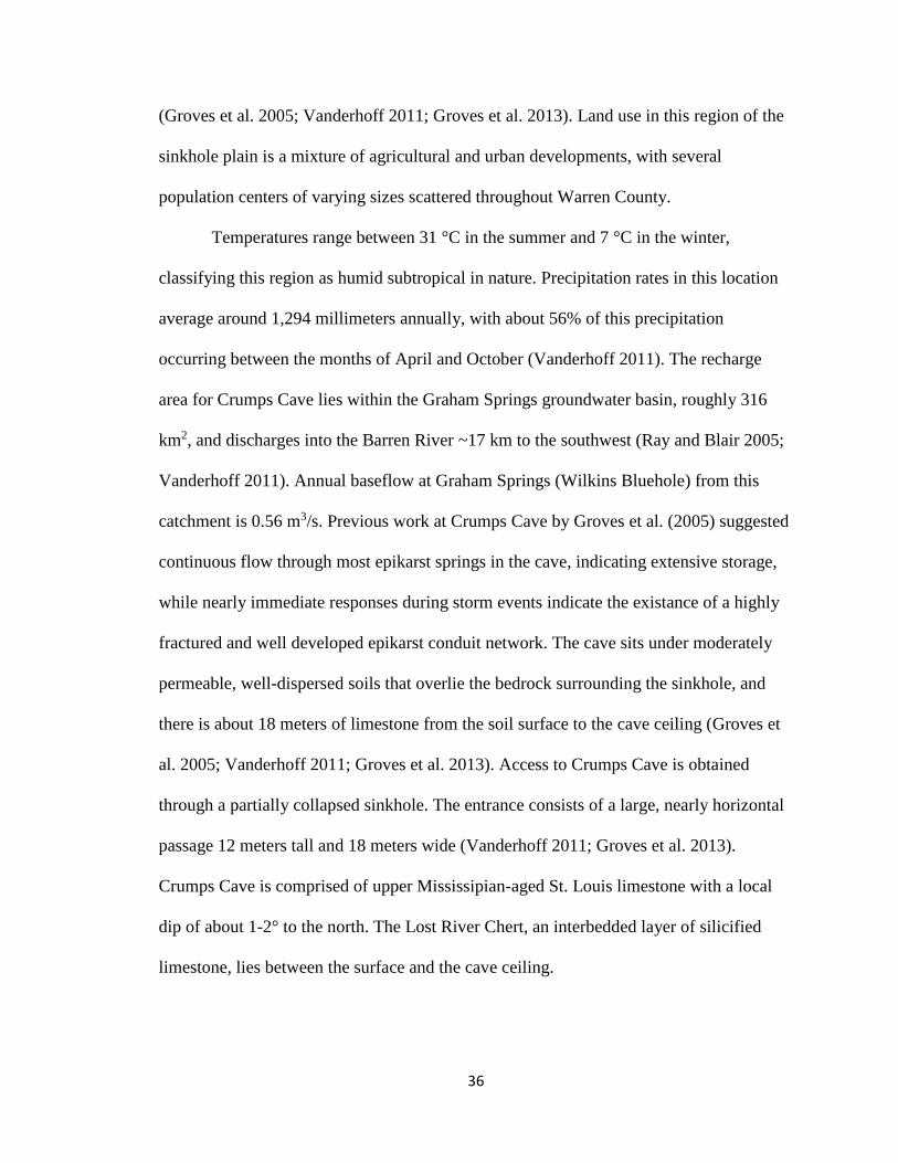
36

(Groves et al. 2005; Vanderhoff 2011; Groves et al. 2013). Land use in this region of the

sinkhole plain is a mixture of agricultural and urban developments, with several

population centers of varying sizes scattered throughout Warren County.

Temperatures range between 31 °C in the summer and 7 °C in the winter,

classifying this region as humid subtropical in nature. Precipitation rates in this location

average around 1,294 millimeters annually, with about 56% of this precipitation

occurring between the months of April and October (Vanderhoff 2011). The recharge

area for Crumps Cave lies within the Graham Springs groundwater basin, roughly 316

km2, and discharges into the Barren River ~17 km to the southwest (Ray and Blair 2005;

Vanderhoff 2011). Annual baseflow at Graham Springs (Wilkins Bluehole) from this

catchment is 0.56 m3/s. Previous work at Crumps Cave by Groves et al. (2005) suggested

continuous flow through most epikarst springs in the cave, indicating extensive storage,

while nearly immediate responses during storm events indicate the existance of a highly

fractured and well developed epikarst conduit network. The cave sits under moderately

permeable, well-dispersed soils that overlie the bedrock surrounding the sinkhole, and

there is about 18 meters of limestone from the soil surface to the cave ceiling (Groves et

al. 2005; Vanderhoff 2011; Groves et al. 2013). Access to Crumps Cave is obtained

through a partially collapsed sinkhole. The entrance consists of a large, nearly horizontal

passage 12 meters tall and 18 meters wide (Vanderhoff 2011; Groves et al. 2013).

Crumps Cave is comprised of upper Mississipian-aged St. Louis limestone with a local

dip of about 1-2° to the north. The Lost River Chert, an interbedded layer of silicified

limestone, lies between the surface and the cave ceiling.

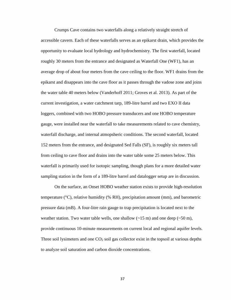
37

Crumps Cave contains two waterfalls along a relatively straight stretch of

accessible cavern. Each of these waterfalls serves as an epikarst drain, which provides the

opportunity to evaluate local hydrology and hydrochemistry. The first waterfall, located

roughly 30 meters from the entrance and designated as Waterfall One (WF1), has an

average drop of about four meters from the cave ceiling to the floor. WF1 drains from the

epikarst and disappears into the cave floor as it passes through the vadose zone and joins

the water table 40 meters below (Vanderhoff 2011; Groves et al. 2013). As part of the

current investigation, a water catchment tarp, 189-litre barrel and two EXO II data

loggers, combined with two HOBO pressure transducers and one HOBO temperature

gauge, were installed near the waterfall to take measurements related to cave chemistry,

waterfall discharge, and internal atmopsheric conditions. The second waterfall, located

152 meters from the entrance, and designated Sed Falls (SF), is roughly six meters tall

from ceiling to cave floor and drains into the water table some 25 meters below. This

waterfall is primarily used for isotopic sampling, though plans for a more detailed water

sampling station in the form of a 189-litre barrel and datalogger setup are in discussion.

On the surface, an Onset HOBO weather station exists to provide high-resolution

temperature (°C), relative humidity (% RH), precipitation amount (mm), and barometric

pressure data (mB). A four-litre rain gauge to trap precipitation is located next to the

weather station. Two water table wells, one shallow (~15 m) and one deep (~50 m),

provide continuous 10-minute measurements on current local and regional aquifer levels.

Three soil lysimeters and one CO2 soil gas collector exist in the topsoil at various depths

to analyze soil saturation and carbon dioxide concentrations.

38

3.2 Lost River Cave and Valley in Bowling Green

Lost River Cave and Valley (LRCV) represents the primary drainage system for

the Lost River Basin. The final discharge point, the Lost River Rise, represents roughly

152 km2 (Ray and Blair 2005) of urban and agricultural landscape runoff (Crawford

1984a; Crawford 1984b; Crawford 1989; Crawford 2003; Crawford 2005; Brewer and

Crawford 2005; Cesin and Crawford 2005; Palmer 2007a; Nedvidek 2014). The Lost

River basin is part of the Pennyroyal Sinkhole Plain and is comprised of Mississippian–

aged St. Louis and Ste. Genevieve limestones. Soils in the area cover 70% of the basin

and are permeable silt and clay type soils (Lawhon 2014). Bowling Green, Kentucky, is

built completely over the Lost River Cave system. Remediation efforts in the 1970s and

1980s to clean the cave environment after years of its use as a dump led to extensive

studies to understand the hydrology and spatial extent of the drainage basin (Lawhon

2014); however, because the catchment incorporates runoff from both agricultural and

urban activities, the possibility of having high major ionic concentrations is greater in this

watershed than at the Smith’s Grove Crumps Cave location.

One of the primary investigators to delineate the extent of the Lost River drainage

basin was Crawford (1984a; 1984b; 1989; 2003; 2005) with others (Crawford et al.1999;

Brewer and Crawford 2005; Cesin and Crawford 2005), who conducted a wide range of

dye tracing examinations to delineate the subsurface flow paths in relation to sinkhole

flooding and contaminant transport. Crawford (2005) also conducted electro-resistivity

and microgravity investigations in conjunction with cave mapping to determine the

overall length and extent of the Lost River. With these results, Crawford (1984a; 1989;

1999; 2003; 2005) generated reports for the City of Bowling Green to create new

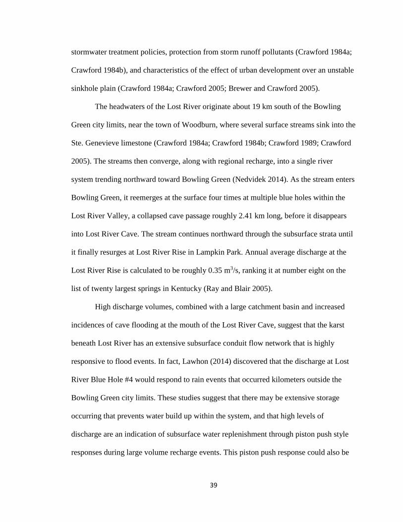
39

stormwater treatment policies, protection from storm runoff pollutants (Crawford 1984a;

Crawford 1984b), and characteristics of the effect of urban development over an unstable

sinkhole plain (Crawford 1984a; Crawford 2005; Brewer and Crawford 2005).

The headwaters of the Lost River originate about 19 km south of the Bowling

Green city limits, near the town of Woodburn, where several surface streams sink into the

Ste. Genevieve limestone (Crawford 1984a; Crawford 1984b; Crawford 1989; Crawford

2005). The streams then converge, along with regional recharge, into a single river

system trending northward toward Bowling Green (Nedvidek 2014). As the stream enters

Bowling Green, it reemerges at the surface four times at multiple blue holes within the

Lost River Valley, a collapsed cave passage roughly 2.41 km long, before it disappears

into Lost River Cave. The stream continues northward through the subsurface strata until

it finally resurges at Lost River Rise in Lampkin Park. Annual average discharge at the

Lost River Rise is calculated to be roughly 0.35 m3/s, ranking it at number eight on the

list of twenty largest springs in Kentucky (Ray and Blair 2005).

High discharge volumes, combined with a large catchment basin and increased

incidences of cave flooding at the mouth of the Lost River Cave, suggest that the karst

beneath Lost River has an extensive subsurface conduit flow network that is highly

responsive to flood events. In fact, Lawhon (2014) discovered that the discharge at Lost

River Blue Hole #4 would respond to rain events that occurred kilometers outside the

Bowling Green city limits. These studies suggest that there may be extensive storage

occurring that prevents water build up within the system, and that high levels of

discharge are an indication of subsurface water replenishment through piston push style

responses during large volume recharge events. This piston push response could also be

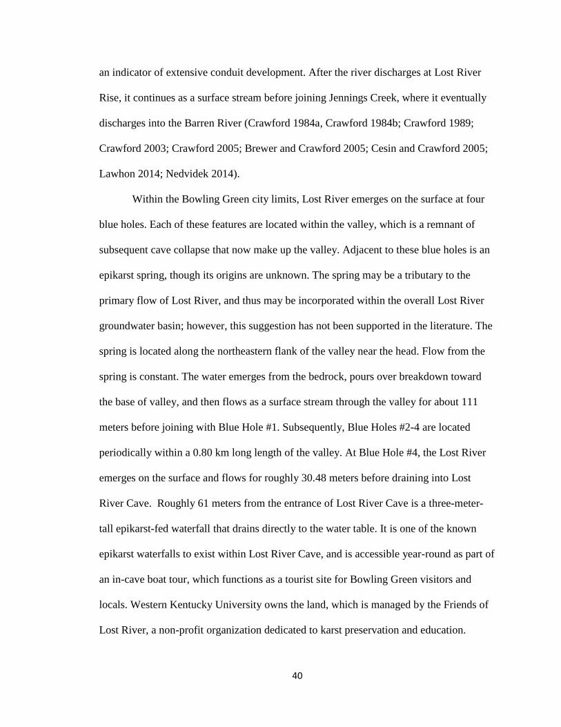
40

an indicator of extensive conduit development. After the river discharges at Lost River

Rise, it continues as a surface stream before joining Jennings Creek, where it eventually

discharges into the Barren River (Crawford 1984a, Crawford 1984b; Crawford 1989;

Crawford 2003; Crawford 2005; Brewer and Crawford 2005; Cesin and Crawford 2005;

Lawhon 2014; Nedvidek 2014).

Within the Bowling Green city limits, Lost River emerges on the surface at four

blue holes. Each of these features are located within the valley, which is a remnant of

subsequent cave collapse that now make up the valley. Adjacent to these blue holes is an

epikarst spring, though its origins are unknown. The spring may be a tributary to the

primary flow of Lost River, and thus may be incorporated within the overall Lost River

groundwater basin; however, this suggestion has not been supported in the literature. The

spring is located along the northeastern flank of the valley near the head. Flow from the

spring is constant. The water emerges from the bedrock, pours over breakdown toward

the base of valley, and then flows as a surface stream through the valley for about 111

meters before joining with Blue Hole #1. Subsequently, Blue Holes #2-4 are located

periodically within a 0.80 km long length of the valley. At Blue Hole #4, the Lost River

emerges on the surface and flows for roughly 30.48 meters before draining into Lost

River Cave. Roughly 61 meters from the entrance of Lost River Cave is a three-meter-

tall epikarst-fed waterfall that drains directly to the water table. It is one of the known

epikarst waterfalls to exist within Lost River Cave, and is accessible year-round as part of

an in-cave boat tour, which functions as a tourist site for Bowling Green visitors and

locals. Western Kentucky University owns the land, which is managed by the Friends of

Lost River, a non-profit organization dedicated to karst preservation and education.

41

Chapter 4: Methods

This study employed a wide variety of field, laboratory, and data processing and

analysis tools and methods. Field methods included automated data logging (YSI 2013),

metrological based recharge measurements, velocity and bucket based discharge

measurements, water sample collection for stable isotopes (Hess and White 1992; Wilde

et al. 2015) and cation/anions (Huang et al. 2015), and the collection of grab samples for

supplementary hydrogeochemical parameter analysis (Hunkeler and Mudry 2007).

Laboratory analysis included Cavity Ring-Down Mass Spectrometry for carbon isotope

ratio analysis (Godoy et al. 2012; Gebbinck et al. 2014), ion chromatography (IC)

analysis for major anion concentrations, inductively coupled plasma emission

spectroscopy (ICP-OES) for major cation concentrations, and manual titrations for

bicarbonate alkalinity. Data analyses were conducted using SigmaPlot and IsoSource

software, with Excel spreadsheets used to conduct simple calculations and for data

organization. SigmaPlot software was used to generate complicated data analyses and

graphical representation of all data. IsoSource software was used to determine carbon

isotope sourcing.

4.1 Site Selection and Instrument Installation

Two locations containing two sample sites each were chosen at both Crumps Cave

(WF1 and SF) and at Lost River Cave and Valley (LRWF and LRS) based on relatively

unrestricted access to epikarst derived water and the ability to install (or use existing)

scientific equipment.

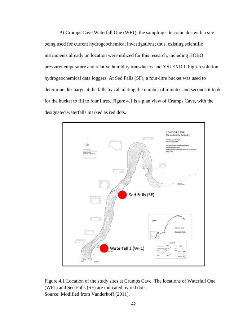
42

At Crumps Cave Waterfall One (WF1), the sampling site coincides with a site

being used for current hydrogeochemical investigations; thus, existing scientific

instruments already on location were utilized for this research, including HOBO

pressure/temperature and relative humidity transducers and YSI EXO II high-resolution

hydrogeochemical data loggers. At Sed Falls (SF), a four-litre bucket was used to

determine discharge at the falls by calculating the number of minutes and seconds it took

for the bucket to fill to four litres. Figure 4.1 is a plan view of Crumps Cave, with the

designated waterfalls marked as red dots.

Figure 4.1 Location of the study sites at Crumps Cave. The locations of Waterfall One

(WF1) and Sed Falls (SF) are indicated by red dots.

Source: Modified from Vanderhoff (2011).

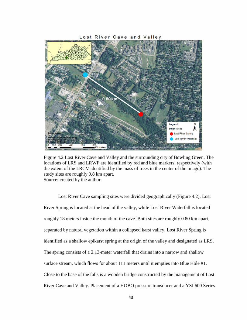
43

Figure 4.2 Lost River Cave and Valley and the surrounding city of Bowling Green. The

locations of LRS and LRWF are identified by red and blue markers, respectively (with

the extent of the LRCV identified by the mass of trees in the center of the image). The

study sites are roughly 0.8 km apart.

Source: created by the author.

Lost River Cave sampling sites were divided geographically (Figure 4.2). Lost

River Spring is located at the head of the valley, while Lost River Waterfall is located

roughly 18 meters inside the mouth of the cave. Both sites are roughly 0.80 km apart,

separated by natural vegetation within a collapsed karst valley. Lost River Spring is

identified as a shallow epikarst spring at the origin of the valley and designated as LRS.

The spring consists of a 2.13-meter waterfall that drains into a narrow and shallow

surface stream, which flows for about 111 meters until it empties into Blue Hole #1.

Close to the base of the falls is a wooden bridge constructed by the management of Lost

River Cave and Valley. Placement of a HOBO pressure transducer and a YSI 600 Series

44

high-resolution data-logging sonde was adjacent to the bridge and housed in 3.81-cm

diameter, 0.60-meter-long PVC stilling wells with fitted caps and secured with key locks

to avoid theft and/or vandalism. Small holes were drilled in the pipes at random spots

along their lengths to allow for water flow. A plastic screen was placed at the bottom of

the pipe to ensure that the logger and transducer placement inside the well did not vary.

Lost River Waterfall is located about 18 meters within the cave at an epikarst-

derived flowstone and is designated as LRWF. Access to the base of the flowstone is

through a narrow passage adjacent to the river and access to the waterfall portion of the

flowstone is up a set of manmade stairs carved into the limestone to a platform

overlooking the river. The falls is on the interior side of the flowstone, roughly three

meters above the river and about two meters above the base of the flowstone. A plastic

36-liter rectangular shaped tub and four-liter bucket were placed directly beneath the

point where the water emerges from the bedrock. The bin and bucket were used to

channel water flow to calculate discharge and collect water samples. A YSI 600 series

data-logging sonde was placed in a pool formed by a rimstone dam near the base of the

flowstone and programmed for high-resolution (10-minute interval) data collection. The

logger was secured to a nearby boulder with thick metal airline cable to prevent theft or

loss during flood events.

4.2 Field Data and Sample Collection

Beginning on May 24, 2016, weekly water sample collection occurred at each

site. A complete suite of water samples was collected in various-sized containers ranging

from 125 mL Nalgene bottles to 10 mL glass vials. Alkalinity samples were collected in

125 mL Nalgene bottles; cation samples were collected in 60 mL Nalgene bottles

45

containing seven drops of nitric acid for preservation; anion samples were collected in 60

mL Nalgene bottles; and carbon isotope samples were collected in 10 mL glass vials. All

water samples were filtered from 500 mL Nalgene bottles filled directly from the source

site, using a 0.45µm filter paper and 60 mL syringe. Distribution into all bottles ensured

zero headspace, and screw caps were covered with multiple layers of parafilm wax to

prevent outgassing and further fractionation. All water samples were collected following

guidelines in the USGS National Field Manual for the Collection of Water-Quality Data

(Wilde et al. 2015). All samples were refrigerated at 4 °C, until they could be delivered to

the proper facility for analysis (Hess and White 1992; Wilde et al. 2015).

In addition to water sampling, a YSI 556 Handheld Multiparameter Instrument

was used to perform grab sample analysis of standard geochemical parameters to support

logger results at all four sites. The handheld is equipped with probes designed to obtain

data regarding pH (±0.2 units), specific conductivity (±0.001 mS∙cm-1), temperature

(±0.15o C), dissolved oxygen (±1% saturation or ±0.1mg∙L-1), and turbidity (±0.3 NTU)

(YSI 2013). Grab samples were obtained at all four sites each week, except for during

times of high water, causing a lack of site access.

At WF1, high-resolution (10-minute) interval EXO II data logging collected

hydrogeochemical parameters, while one HOBO pressure transducer collected pressure

and temperature readings from inside the barrel. Additional HOBO barometric pressure

and relative humidity sensors were placed several meters away from the falls to

determine cave air conditions. Each of these sondes collected 10-minute resolution data

throughout the course of the study, except when briefly pulled for maintenance.

46

Beginning on August 21, 2016, an automated high-resolution YSI 600 Series data

logging sonde and a HOBO pressure/temperature transducer were installed at LRS. A

second automated high-resolution YSI 600 Series data logger was installed in a rimstone

dam pool one meter below LRWF. Each 600 Series sonde was programmed to record

geochemical parameters (pH, SpC, and water temperature) every ten minutes. Each 600

Series sondes is equipped with a probe for pH (±0.2 units), specific conductivity (±0.001

mS∙cm-1), and temperature (±0.15 ºC) (YSI 2013). The HOBO pressure transducer was

programmed for high-resolution 10-minute sampling of water temperature and pressure.

Volumetric discharge measurements were taken to gauge the amount of water

discharging from LRS using a wading rod and flow meter. The bucket and stopwatch

method was used to determine discharge at SF using a four-liter bucket (Michaud and

Wierenga 2005). The same bucket and stopwatch method was employed at LRWF, only

with the addition of a 36-liter tub to channelize flow in order to ensure full collection of

water. The amount of water being discharged at LRS, LRWF, and SF was measured once

a week and whenever flow conditions changed.

Meteorological data, including precipitation rates (mm/10 mins), relative

humidity (RH %), surface temperature (°C), barometric pressure (mB), and soil moisture

and temperature at three (10cm, 30cm, and 50cm) depths, were obtained from weather

monitoring stations located within 0.80 kilometers of Crumps Cave and Lost River Cave

and Valley. Soil temperature and moisture data at Lost River Cave and Valley were

obtained from the Kentucky Mesonet FARM monitoring station, and represented

conditions at three depths (8cm, 20cm, and 40cm).

47

4.3 Sample Analysis

Stable isotope concentrations of dissolved inorganic carbon (δ13CDIC) were

determined using a Cavity Ring-Down Mass Spectrometer as outlined in Godoy et al.

(2012) and Gebbinck et al. (2014) at the University of Utah’s Stable Isotope Ratio

Facility for Environmental Research (SIRFER) laboratory for each week samples were

collected at each site. Isotope ratios were calculated using the standard isotope ratio based

on the Vienna standard calculation for that element (Drever 1997; Allen 2004; Palmer

2007a; Hoefs 2010). Carbon isotopes ratios were reported using the standard δ notation

with a precision of ±0.3%. Results are referenced to the VPDB standard.

Anion concentrations of fluoride (F); chloride (Cl-); bromide (Br); nitrate (NO32−);

nitrite (NO2−); phosphate (PO4); sulfate (SO4

2−) were determined using Ion

Chromatography (IC) analysis conducted at WKU’s Advanced Materials Institute (AMI)

following EPA Method 9056 on a Dionex ICS-1500, and after Jackson (2000). Cation

concentrations of potassium (K+), sodium (Na+), magnesium (Mg2+), and calcium (Ca2+)

were determined using inductively coupled plasma emission spectroscopy (ICP-OES)

and were performed at AMI following EPA Method 200.8 using a Thermo Scientific

ICAP 6500 ICP-OES (Stefansson et al. 2007). These instruments provide concentrations

in parts per million (ppm) (equivalent to mg/L).

Manual titration of bicarbonate (HCO3−) alkalinity was conducted at the Center for

Human GeoEnvironmental Studies (CHNGES) laboratory at Western Kentucky

University (WKU). Samples were poured into 120 mL glass beakers and manually

titrated to a pH of ~4.5 using 0.205 N H2SO4 from May 24, 2016, to December 7, 2016.

A second 500 mL glass jar of 0.027 N H2SO4 was mixed at the HydroAnalytical

48

Laboratory at Bowling Green on December 7, 2016, and used to titrate samples manually

to a pH of ~4.5 from December 13, 2016, to March 14, 2017. The pH and temperature

were measured using the YSI 556 handheld probe. The total volume (mL) of H2SO4 used

to reduce the pH of a 50-mL sample to ~4.5 was recorded and used to calculate the total

carbonate alkalinity concentration in mg/L based on the methods outlined in Neal (2001).

4.4 Data Manipulation and Processing

All processed data were organized in SigmaPlot spreadsheet software for

convenient record keeping. Mastersheets were created for each site and included a

column for every measured parameter as well as those calculated as a function of other

measured parameters.

4.4.1 Hydrogeochemical Data Processing

Recorded high-resolution data from the EXO II, YSI 600 Series hydro-

geochemical loggers and HOBO pressure transducers were compiled into Sigma Plot

spreadsheet software for each week that data were collected. Calibration offsets for high-

resolution SpC and pH at WF1, LRS, and LRWF were corrected per the USGS method 1-

D3 (Wagner et al. 2006). Cation and anion concentrations in ppm, titrated alkalinity

concentrations in mg/L, water temperature values and pH values for all sites, were

inserted into a designated Excel spreadsheet to determine charge balances and calculate

bicarbonate concentrations in mg/L. Charge balances ranged between ±10-20% for all

sites, indicating raw data were good. Weekly HCO3 concentrations, SpC, pH, Ca2+, Mg2+

and water temperature values for all sites were then transferred into SigmaPlot to

calculate activity coefficients, including H2CO3, CO3, CO2, saturation index (SI) with

respect to CaCO3, and dissolved inorganic carbon (DIC), for each week at each site that

49

data were available. The equations used to execute these calculations included modified

versions of the following: partial pressure of CO2 as outlined in Drever (1997) and

expressed in Eq. 2.2, the Palmer equation to determine saturation index (Palmer 2007a)

and expressed in Eq. 2.4; and dissolved inorganic concentrations (DIC) as outlined in

White (1988) and expressed in Eq. 4.3. Concentrations of the partial pressure of CO2

were calculated by normalizing calculated PCO2 to atmospheric contributions, allowing to

express the final calculated values in the results and discussion as concentrations of CO2

in volumetric parts per million (ppmv).

Further, dissolution rates of limestone at varying timescales were calculated using

the equations found in White (1988) and Palmer (1991) and expressed as:

𝑅 = 𝑘1[𝐻+] + 𝑘2[𝐻2𝐶𝑂3] + 𝑘3[𝐻2𝑂] − 𝑘4[𝐶𝑎2+][𝐻𝐶𝑂3−] (Eq. 4.1)

where R is the rate of the dissolved calcite and expressed as millimoles per centimeter

square per second, k1-3 are temperature dependent forward rate constants that describe the

rate that calcite is dissolving, and k4 is the backwards rate constant dependent on

temperature and dissolution rates that describes the potential for precipitation of

dissolved calcite from solution. The rate of wall retreat in karst conduits can be calculated

using the equation from Palmer (1991) and expressed as:

𝑆 = 31.56 𝑘 (1−𝑆𝐼𝐶𝑎𝑙𝑐𝑖𝑡𝑒)𝑛

𝑃𝑟 (Eq. 4.2)

where S is the rate of conduit wall retreat in cm/year, k is the temperature dependent rate

constant, SICalcite is the saturation index of the mineral calcite (a ratio of the concentration

of calcite in solution to the saturation concentration of calcite in solution), n is the

reaction order of the dissolution reaction, and Pr is the density of the rock (2.7 g/cm3).

50

Dissolved inorganic carbon (DIC) concentrations in mg/L were derived from the

following formula from White (1988):

DIC = HCO3 + CO3 + H2CO3 (Eq. 4.3)

Mass flux of dissolved species, including DIC, at WF1 and LRS, were computed

by multiplying the concentration of the species of DIC by the discharge. Once a

continuous record of DIC fluctuations was generated, a mass flux of DIC in mg/9 months

for the study period was calculated by summing the total DIC concentrations. Likewise,

once high-resolution data were generated for dissolved calcite, an estimated volume of

rock dissolved at WF1 and LRS was determined by summation of the dissolution rate in

mg/L over the entirety of the study period.

Regression analyses were conducted on high-resolution SpC and weekly

Ca2+/Mg2+ and HCO3 for WF1, LRS, and LRWF to determine statistical robustness, as

well as their associated R2 values. As an additional statistical check, weekly resolution

hydrogeochemical samples for SpC and pH were plotted against high-resolution logger

data for the same date and time. No statistical difference was observed between both data

sets, indicating that field equipment was operating within specific parameters. Regression

equations from high resolution SpC, pH, and water temperature and weekly collected

Ca2+/Mg2+ and HCO3 concentrations were inserted into SigmaPlot to calculate high

resolution Ca2+/Mg2+ and HCO3 concentrations, and DIC activity coefficients of CO2,

Saturation indices, and DIC concentrations at WF1, LRS, and LRWF for the dates of

May 24, 2016, to March 13, 2017, for WF1, and August 18, 2016, to March 13, 2017, for

LRS and LRWF. Due to a logger malfunction at LRS, data are missing for a period of

three weeks (December 28, 2016, to January 11, 2017) at that site. The R2 values

51

representing the relationship between high-resolution measured variables and weekly

resolution ion constituents for WF1 and LRWF proved to be relatively robust, and thus

using the slope equation derived from regression analysis to extrapolate certain high

resolution was a simplified method to characterize shorter changes. This particular

method to extrapolate data is commonly used in other studies (Groves and Meiman 2001;

Groves et al. 2005; Liu et al. 2007; Groves et al. 2013; Pu et al. 2014a), but it is important

to note that it is not without some limitation of error, especially when R2 values aren’t as

strong as hoped for, as was the case at LRS. At that particular site, extrapolation

measures could potentially yield results subject to additional calculation error as

described in Osterhoudt (2014). To ensure robustness of the extrapolated data, despite the

low R2 value, weekly resolution data for LRS were compared with LRS high-resolution

data collected at the same date and times. No significant statistical difference exists.

4.4.2 Carbon Isotope Sourcing

Raw collected weekly carbon isotope data were organized in Excel spreadsheets

by site and date. A mixing model was run to determine exact source contributions

(atmosphere/soil/carbonates/etc.) over the entire course of the study and seasonally.

IsoSource software (v1.3) created by Don Phillips at the U.S. Environmental Protection

Agency was employed for this study (Phillips and Jillian 2003). Data for each week were

analyzed independently. The model was run with a 1.0% increment and mass balance

tolerance of 0.5% (Phillips and Jillian 2003). Data parameters covered one isotope system

with three possible isotopic end members (atmosphere, soil water, and carbonate

bedrock). Values for the mixture were input based on collected weekly waterfall samples.

The atmosphere value was assumed constant at -7‰ and based on established literature

52

(Clark and Fritz 1997; Shin et al. 2011; Zhang et al. 2015). Soil water values for Crumps

Cave (WF1 and SF) were obtained by analyzing soil water collected from three soil

lysimeters installed at varying depths (10cm, 30cm, and 50cm) to characterize soil CO2

inputs to the cave. The three lysimeters are located directly above WF1 and varied each

week they were available. During weeks that soil samples were not available at Crumps

Cave (WF1 and SF), a calculated value of -16‰ was obtained by averaging values for

soil carbon isotopes generated by Clark and Fritz (1997) for C3 vegetation (-23‰) and C4

vegetation (-9‰). Likewise, a soil sample value of -16‰ was used to process all

collected samples from Lost River Cave and Valley (LRS and LRWF) (Clark and Fritz

1997; Shin et al. 2011; Zhang et al. 2015). Carbonate bedrock values were derived from

powdered bedrock obtained from solid samples collected at each location (Crumps Cave

and Lost River Cave).

4.4.3 LRS Hydrograph Generation

Atmospheric pressure data collected from the LR HOBO weather station were

combined with the LRS HOBO pressure transducer data to determine high-resolution

water level in feet at the spring. Water level data were then transferred to a separate Excel

spreadsheet, which contained an embedded formula determined by regression analysis to

generate a rating curve. Units for water level were converted from feet to meters during

the rating curve generation phase of data processing. Average values calculated from

collected data from velocity Q discharge measurements conducted at LRS were compiled

in Excel spreadsheet software to generate a rating curve (Figure 4.3). Regression analysis

was conducted to determine an R2 value of 0.89 (p<0.001), which indicates a strong

statistical significance between the parameters.

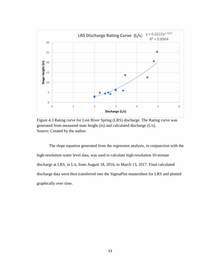
53

Figure 4.3 Rating curve for Lost River Spring (LRS) discharge. The Rating curve was

generated from measured state height (in) and calculated discharge (L/s).

Source: Created by the author.

The slope equation generated from the regression analysis, in conjunction with the

high-resolution water level data, was used to calculate high-resolution 10-minute

discharge at LRS, in L/s, from August 18, 2016, to March 13, 2017. Final calculated

discharge data were then transferred into the SigmaPlot mastersheet for LRS and plotted

graphically over time.

y = 0.0222x2.1627

R² = 0.8964

0

5

10

15

20

25

30

0 1 2 3 4 5 6

Stag

e H

eig

ht

(in

)

Discharge (L/s)

LRS Discharge Rating Curve (L/s)

54

Chapter 5: Results

The hydrogeochemistry and carbon flux of four epikarst-derived waterfalls within

the Pennyroyal Sinkhole Plain in southcentral Kentucky was examined from May 24,

2016, to March 13, 2017, to determine the impact of seasonal and storm event variability.

A multi-parameter approach was employed to collect 10-minute resolution data for pH,

SpC, water temperature, and meteorological changes, including precipitation, surface

temperature, and influences on soil moisture and temperature. Weekly sampling for

cations, anions, alkalinity, and carbon isotopes served to complete the study and address

carbon sourcing and fluctuations. These data show variations at each of the four sampling

sites (WF1, SF, LRS, and LRWF) with respect to the geochemistry and carbon

fluctuations, which can be attributed to epikarst development and surface input, while

carbon sourcing at each site seemed to show similar fluctuation responses. This suggested

that contributions from land use, vegetation cover, and soil microbial activity are present

and geochemical responses to these factors are relatively similar in a regional sense, yet

exhibit site specific differences.

5.1 Epikarst Hydrogeochemistry

5.1.1 Site Geochemistry Results

High-resolution hydrogeochemical basic statistical results for WF1, LRS, and

LRWF, and weekly resolution hydrogeochemical basic statistical results are presented in

Table 5.1. Study period precipitation at Crumps Cave (WF1 and SF) was 994.8 mm.

Crumps Cave-WF1 pH values range from 6.64 to 8.39, with an average of 7.43 (Table

5.1) during the study period. Specific conductivity values range from 144 µs/cm

(January) to 438 µs/cm (July), with an average of 305 µs/cm. Water temperature for WF1

55

range from 5.78 ºC in December to 15.5 ºC the following day in December. The average

water temperature at WF1 was 11.5 ºC. Discharge at WF1 is variable, but responds to

high precipitation events (Table 5.1). Baseflow at WF1 was recorded at 0.013 L/s during

the fall, while peak flow in discharge occurred in July and was recorded at 11.5 L/s.

Average discharge at WF1 was calculated to be 0.07 L/s. Concentrations of CO2 at

Crumps Cave-WF1 range from 0.67 ppmv during the winter and early spring to 147

ppmv during the month of September, with an average of 43.9 ppmv. SIc at WF1 shows

seasonal influences, with a minimal saturation index of –1.05 during the month of

September and a maximum saturation index of 0.33 during the month of November. The

average saturation index at WF1 was –0.31. DIC at WF1 showed similar seasonal

fluctuations, with high concentrations during the summer and low concentrations during

the winter. Minimum DIC in January was calculated at 127 mg/L while maximum DIC

was calculated at 1,455 mg/L during September, with an average value of 734 mg/L

(Table 5.1). DIC fluctuations varied during the study period, with a peak maximum

loading of 536 mg/L/s during the month of July and a minimum loading of 0.2110 mg/L/s

during the month of March.

Crumps Cave-SF (Table 5.1) collected geochemical and discharge data were at a

weekly resolution, and were plotted in conjunction with high-resolution precipitation and

surface temperature. Values for pH range between 6.12 and 7.81, with an average of 6.95.

Specific conductivity values range from 175 µs/cm (January) to 580 µs/cm (September),

with an average of 368 µs/cm. Water temperature for SF ranged from 8.52 ºC in

December to 17.5 ºC in July. The average water temperature at SF was 13.7 ºC.

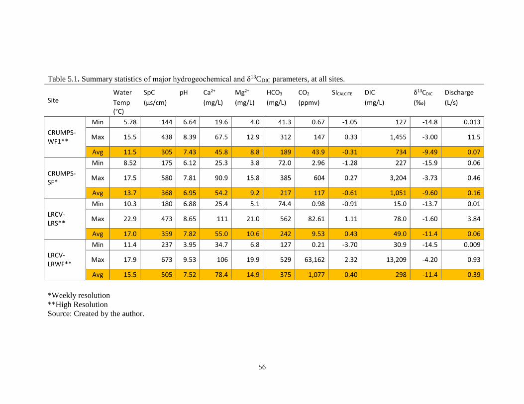
56

Table 5.1. Summary statistics of major hydrogeochemical and δ13CDIC parameters, at all sites.

Site Water SpC pH Ca2+ Mg2+ HCO3 CO2 SICALCITE DIC δ13CDIC Discharge

Temp (°C)

(µs/cm) (mg/L) (mg/L) (mg/L) (ppmv) (mg/L) (‰) (L/s)

Min 5.78 144 6.64 19.6 4.0 41.3 0.67 -1.05 127 -14.8 0.013

CRUMPS-WF1**

Max 15.5 438 8.39 67.5 12.9 312 147 0.33 1,455 -3.00 11.5

Avg 11.5 305 7.43 45.8 8.8 189 43.9 -0.31 734 -9.49 0.07

Min 8.52 175 6.12 25.3 3.8 72.0 2.96 -1.28 227 -15.9 0.06

CRUMPS-SF*

Max 17.5 580 7.81 90.9 15.8 385 604 0.27 3,204 -3.73 0.46

Avg 13.7 368 6.95 54.2 9.2 217 117 -0.61 1,051 -9.60 0.16

Min 10.3 180 6.88 25.4 5.1 74.4 0.98 -0.91 15.0 -13.7 0.01

LRCV-LRS**

Max 22.9 473 8.65 111 21.0 562 82.61 1.11 78.0 -1.60 3.84

Avg 17.0 359 7.82 55.0 10.6 242 9.53 0.43 49.0 -11.4 0.06

Min 11.4 237 3.95 34.7 6.8 127 0.21 -3.70 30.9 -14.5 0.009

LRCV-LRWF**

Max 17.9 673 9.53 106 19.9 529 63,162 2.32 13,209 -4.20 0.93

Avg 15.5 505 7.52 78.4 14.9 375 1,077 0.40 298 -11.4 0.39

*Weekly resolution

**High Resolution

Source: Created by the author.

57

Discharge at SF was calculated every week and ranged from 0.06 L/s in baseflow

conditions during November to peak flow conditions recorded at 0.46 L/s during August.

Average discharge at SF was calculated to be 0.16 L/s. At Crumps Cave-SF, CO2

concentrations ranged from 2.96 ppmv during February to 604 ppmv during the month of

October, with an average of 117 ppmv. SIc at SF shows seasonal influences, but with less

degree of variability than at WF1. Minimal saturation occurred during the month of May

at –1.28 and a maximum saturation of 0.27 during the month of November. The average

saturation index at SF was –0.61. DIC at SF showed similar responses, with a minimum

value of 227 mg/L during February and a maximum value of 3,204 mg/L during October,

with an average value of 1,051 mg/L (Table 5.1).

Study period precipitation at LRCV was 1019.6 mm. Lost River Cave and Valley-

LRS pH values range from 6.88 to 8.65, with an average of 7.82 (Table 5.1). Specific

conductivity values range from 180 µs/cm (August) to 473 µs/cm (December), with an

average of 359 µs/cm. Water temperatures for LRS ranged from 10.3 ºC in December to

22.9 ºC in September. The average water temperature at LRS was 17.0 ºC. Discharge at

LRS ranges from 0.01 L/s in baseflow conditions during the fall to peak flow conditions

recorded at 3.84 L/s in December. Average discharge at LRS was calculated to be 0.06

L/s. CO2 concentrations at LRS range from 0.98 ppmv during August and 82.61 ppmv

during the month of December, with an average of 9.53 ppmv. SIc values at LRS

fluctuated, with minimal saturation occurring during the month of August at –0.91 and a

maximum saturation of 1.11 during the month of November. The average saturation

index at LRS was 0.43. DIC at LRS show similar responses, with a minimum value of 15

mg/L during August and a maximum value of 78 mg/L during December, with an

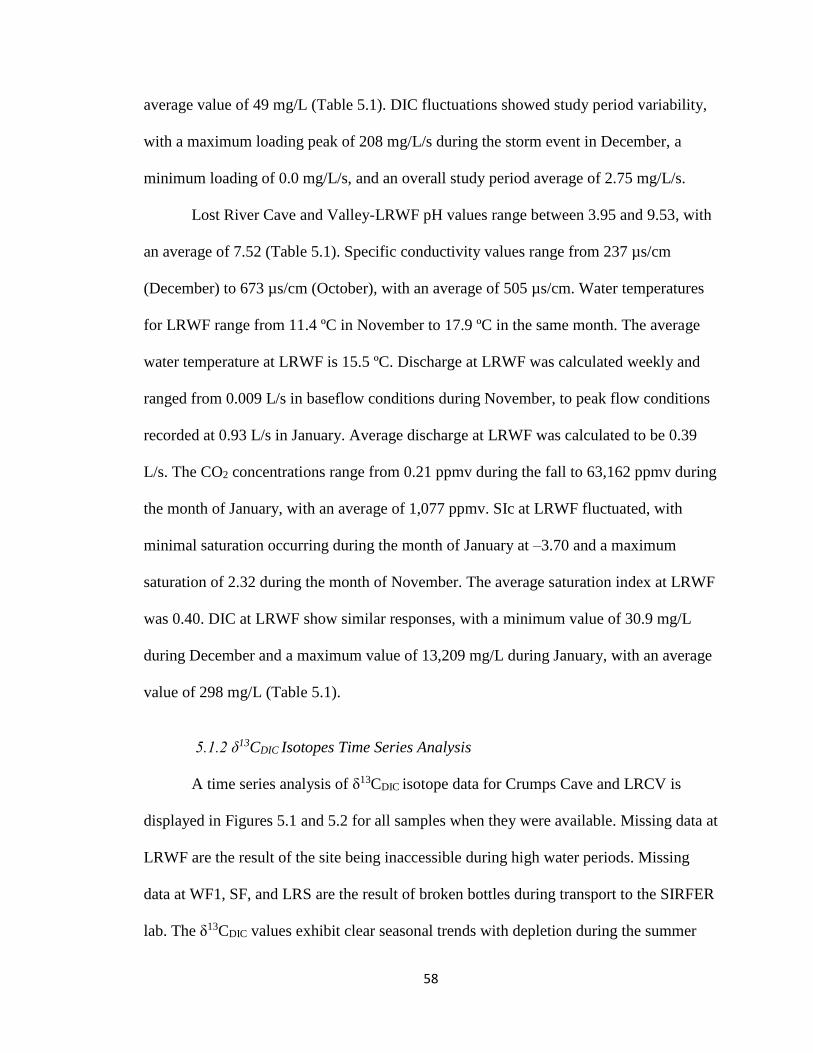
58

average value of 49 mg/L (Table 5.1). DIC fluctuations showed study period variability,

with a maximum loading peak of 208 mg/L/s during the storm event in December, a

minimum loading of 0.0 mg/L/s, and an overall study period average of 2.75 mg/L/s.

Lost River Cave and Valley-LRWF pH values range between 3.95 and 9.53, with

an average of 7.52 (Table 5.1). Specific conductivity values range from 237 µs/cm

(December) to 673 µs/cm (October), with an average of 505 µs/cm. Water temperatures

for LRWF range from 11.4 ºC in November to 17.9 ºC in the same month. The average

water temperature at LRWF is 15.5 ºC. Discharge at LRWF was calculated weekly and

ranged from 0.009 L/s in baseflow conditions during November, to peak flow conditions

recorded at 0.93 L/s in January. Average discharge at LRWF was calculated to be 0.39

L/s. The CO2 concentrations range from 0.21 ppmv during the fall to 63,162 ppmv during

the month of January, with an average of 1,077 ppmv. SIc at LRWF fluctuated, with

minimal saturation occurring during the month of January at –3.70 and a maximum

saturation of 2.32 during the month of November. The average saturation index at LRWF

was 0.40. DIC at LRWF show similar responses, with a minimum value of 30.9 mg/L

during December and a maximum value of 13,209 mg/L during January, with an average

value of 298 mg/L (Table 5.1).

5.1.2 δ13CDIC Isotopes Time Series Analysis

A time series analysis of δ13CDIC isotope data for Crumps Cave and LRCV is

displayed in Figures 5.1 and 5.2 for all samples when they were available. Missing data at

LRWF are the result of the site being inaccessible during high water periods. Missing

data at WF1, SF, and LRS are the result of broken bottles during transport to the SIRFER

lab. The δ13CDIC values exhibit clear seasonal trends with depletion during the summer

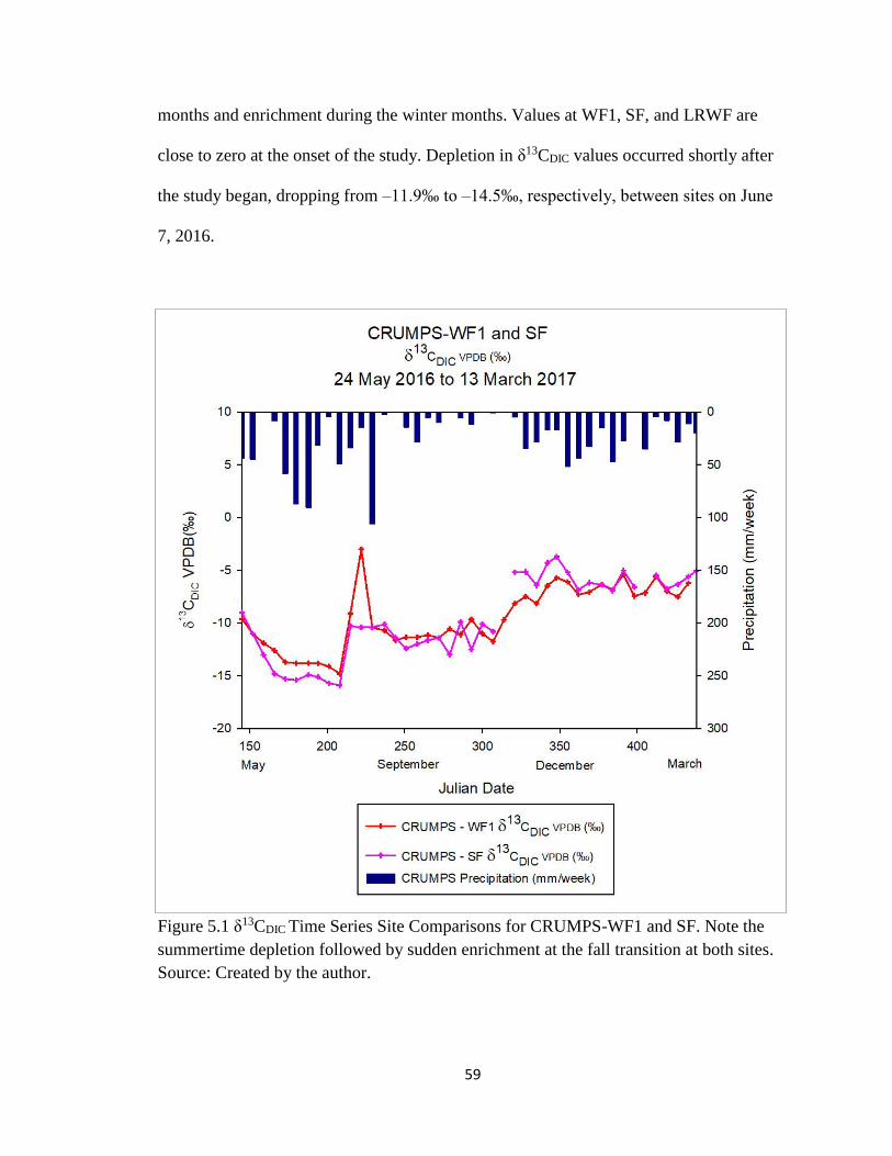
59

months and enrichment during the winter months. Values at WF1, SF, and LRWF are

close to zero at the onset of the study. Depletion in δ13CDIC values occurred shortly after

the study began, dropping from –11.9‰ to –14.5‰, respectively, between sites on June

7, 2016.

Figure 5.1 δ13CDIC Time Series Site Comparisons for CRUMPS-WF1 and SF. Note the

summertime depletion followed by sudden enrichment at the fall transition at both sites.

Source: Created by the author.

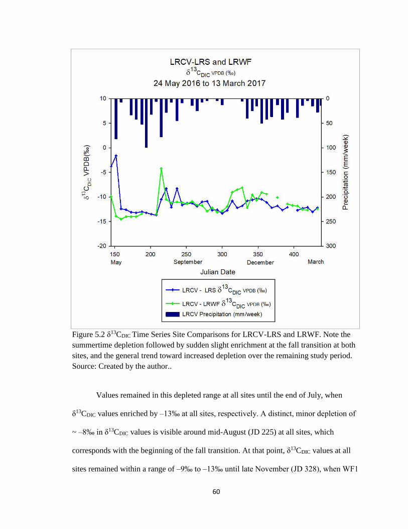
60

Figure 5.2 δ13CDIC Time Series Site Comparisons for LRCV-LRS and LRWF. Note the

summertime depletion followed by sudden slight enrichment at the fall transition at both

sites, and the general trend toward increased depletion over the remaining study period.

Source: Created by the author..

Values remained in this depleted range at all sites until the end of July, when

δ13CDIC values enriched by –13‰ at all sites, respectively. A distinct, minor depletion of

~ –8‰ in δ13CDIC values is visible around mid-August (JD 225) at all sites, which

corresponds with the beginning of the fall transition. At that point, δ13CDIC values at all

sites remained within a range of –9‰ to –13‰ until late November (JD 328), when WF1

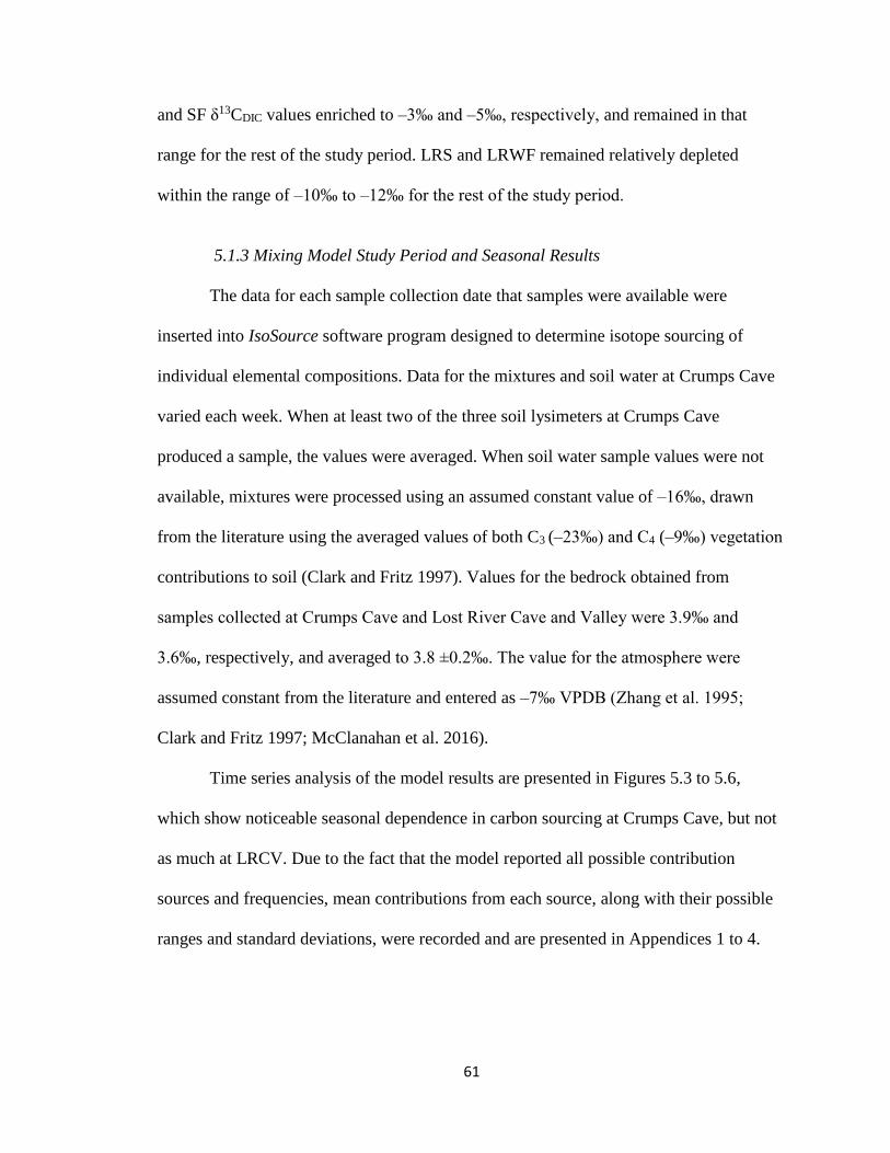
61

and SF δ13CDIC values enriched to –3‰ and –5‰, respectively, and remained in that

range for the rest of the study period. LRS and LRWF remained relatively depleted

within the range of –10‰ to –12‰ for the rest of the study period.

5.1.3 Mixing Model Study Period and Seasonal Results

The data for each sample collection date that samples were available were

inserted into IsoSource software program designed to determine isotope sourcing of

individual elemental compositions. Data for the mixtures and soil water at Crumps Cave

varied each week. When at least two of the three soil lysimeters at Crumps Cave

produced a sample, the values were averaged. When soil water sample values were not

available, mixtures were processed using an assumed constant value of –16‰, drawn

from the literature using the averaged values of both C3 (–23‰) and C4 (–9‰) vegetation

contributions to soil (Clark and Fritz 1997). Values for the bedrock obtained from

samples collected at Crumps Cave and Lost River Cave and Valley were 3.9‰ and

3.6‰, respectively, and averaged to 3.8 ±0.2‰. The value for the atmosphere were

assumed constant from the literature and entered as –7‰ VPDB (Zhang et al. 1995;

Clark and Fritz 1997; McClanahan et al. 2016).

Time series analysis of the model results are presented in Figures 5.3 to 5.6,

which show noticeable seasonal dependence in carbon sourcing at Crumps Cave, but not

as much at LRCV. Due to the fact that the model reported all possible contribution

sources and frequencies, mean contributions from each source, along with their possible

ranges and standard deviations, were recorded and are presented in Appendices 1 to 4.

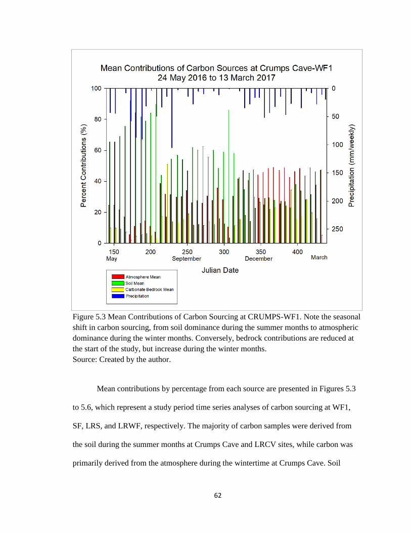
62

Figure 5.3 Mean Contributions of Carbon Sourcing at CRUMPS-WF1. Note the seasonal

shift in carbon sourcing, from soil dominance during the summer months to atmospheric

dominance during the winter months. Conversely, bedrock contributions are reduced at

the start of the study, but increase during the winter months.

Source: Created by the author.

Mean contributions by percentage from each source are presented in Figures 5.3

to 5.6, which represent a study period time series analyses of carbon sourcing at WF1,

SF, LRS, and LRWF, respectively. The majority of carbon samples were derived from

the soil during the summer months at Crumps Cave and LRCV sites, while carbon was

primarily derived from the atmosphere during the wintertime at Crumps Cave. Soil

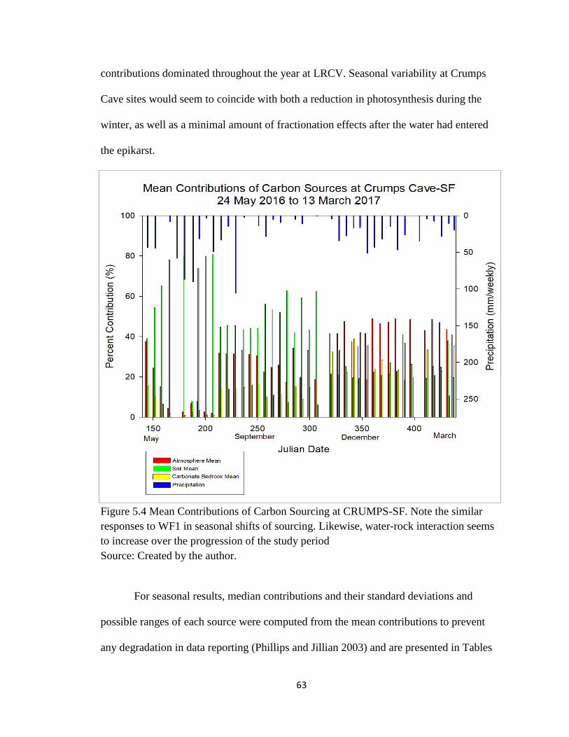
63

contributions dominated throughout the year at LRCV. Seasonal variability at Crumps

Cave sites would seem to coincide with both a reduction in photosynthesis during the

winter, as well as a minimal amount of fractionation effects after the water had entered

the epikarst.

Figure 5.4 Mean Contributions of Carbon Sourcing at CRUMPS-SF. Note the similar

responses to WF1 in seasonal shifts of sourcing. Likewise, water-rock interaction seems

to increase over the progression of the study period

Source: Created by the author.

For seasonal results, median contributions and their standard deviations and

possible ranges of each source were computed from the mean contributions to prevent

any degradation in data reporting (Phillips and Jillian 2003) and are presented in Tables

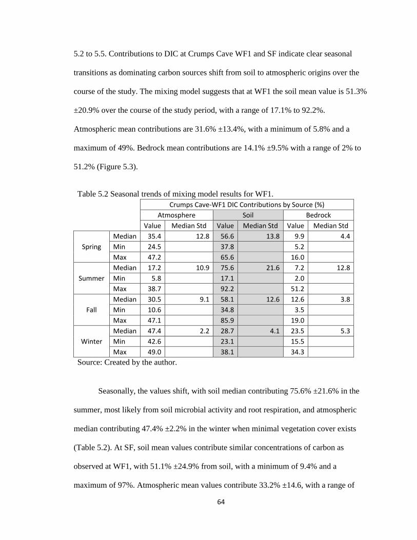
64

5.2 to 5.5. Contributions to DIC at Crumps Cave WF1 and SF indicate clear seasonal

transitions as dominating carbon sources shift from soil to atmospheric origins over the

course of the study. The mixing model suggests that at WF1 the soil mean value is 51.3%

±20.9% over the course of the study period, with a range of 17.1% to 92.2%.

Atmospheric mean contributions are 31.6% ±13.4%, with a minimum of 5.8% and a

maximum of 49%. Bedrock mean contributions are 14.1% ±9.5% with a range of 2% to

51.2% (Figure 5.3).

Seasonally, the values shift, with soil median contributing 75.6% ±21.6% in the

summer, most likely from soil microbial activity and root respiration, and atmospheric

median contributing 47.4% ±2.2% in the winter when minimal vegetation cover exists

(Table 5.2). At SF, soil mean values contribute similar concentrations of carbon as

observed at WF1, with 51.1% ±24.9% from soil, with a minimum of 9.4% and a

maximum of 97%. Atmospheric mean values contribute 33.2% ±14.6, with a range of

Table 5.2 Seasonal trends of mixing model results for WF1.

Crumps Cave-WF1 DIC Contributions by Source (%)

Atmosphere Soil Bedrock

Value Median Std Value Median Std Value Median Std

Spring

Median 35.4 12.8 56.6 13.8 9.9 4.4

Min 24.5

37.8

5.2 Max 47.2

65.6

16.0

Summer

Median 17.2 10.9 75.6 21.6 7.2 12.8

Min 5.8

17.1

2.0 Max 38.7

92.2

51.2

Fall

Median 30.5 9.1 58.1 12.6 12.6 3.8

Min 10.6

34.8

3.5 Max 47.1

85.9

19.0

Winter

Median 47.4 2.2 28.7 4.1 23.5 5.3

Min 42.6

23.1

15.5 Max 49.0

38.1

34.3

Source: Created by the author.

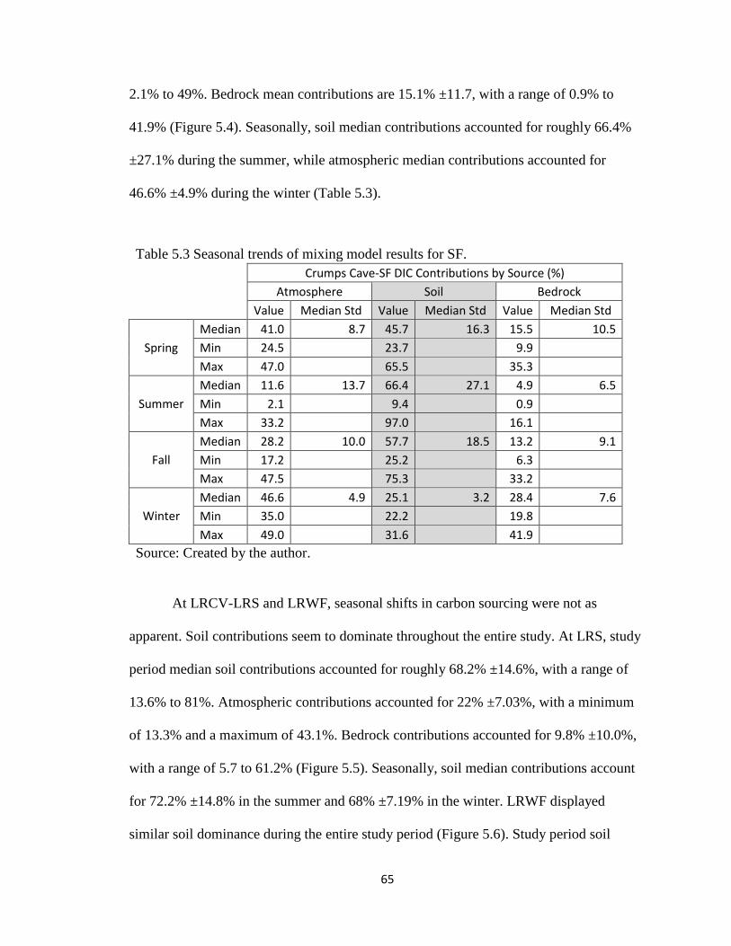
65

2.1% to 49%. Bedrock mean contributions are 15.1% ±11.7, with a range of 0.9% to

41.9% (Figure 5.4). Seasonally, soil median contributions accounted for roughly 66.4%

±27.1% during the summer, while atmospheric median contributions accounted for

46.6% ±4.9% during the winter (Table 5.3).

At LRCV-LRS and LRWF, seasonal shifts in carbon sourcing were not as

apparent. Soil contributions seem to dominate throughout the entire study. At LRS, study

period median soil contributions accounted for roughly 68.2% ±14.6%, with a range of

13.6% to 81%. Atmospheric contributions accounted for 22% ±7.03%, with a minimum

of 13.3% and a maximum of 43.1%. Bedrock contributions accounted for 9.8% ±10.0%,

with a range of 5.7 to 61.2% (Figure 5.5). Seasonally, soil median contributions account

for 72.2% ±14.8% in the summer and 68% ±7.19% in the winter. LRWF displayed

similar soil dominance during the entire study period (Figure 5.6). Study period soil

Table 5.3 Seasonal trends of mixing model results for SF.

Crumps Cave-SF DIC Contributions by Source (%)

Atmosphere Soil Bedrock

Value Median Std Value Median Std Value Median Std

Spring

Median 41.0 8.7 45.7 16.3 15.5 10.5

Min 24.5

23.7

9.9 Max 47.0

65.5

35.3

Summer

Median 11.6 13.7 66.4 27.1 4.9 6.5

Min 2.1

9.4

0.9 Max 33.2

97.0

16.1

Fall

Median 28.2 10.0 57.7 18.5 13.2 9.1

Min 17.2

25.2

6.3 Max 47.5

75.3

33.2

Winter

Median 46.6 4.9 25.1 3.2 28.4 7.6

Min 35.0

22.2

19.8 Max 49.0

31.6

41.9

Source: Created by the author.

66

contributions accounted for 65.1% ±15.3, with a range of 20.1% to 87.2%. Median

atmospheric contributions accounted for 24.2% ±9.52%, with a minimum of 9% and a

maximum median contribution of 44.3%. Bedrock contributions are 10.7% ± 6.69, with a

range of 3.8% to 42.6% (Figure 5.6). Seasonally, soil contributions dominated the system

throughout the entire study period, with median values of 59.7% ±10.6% during the

winter and 78.5% ±19.9% during the summer (Table 5.5).

Figure 5.5 Mean Contributions of Carbon Sourcing at LRCV-LRS. Note that soil

sourcing seems relatively uniform throughout the study.

Source: Created by the author.

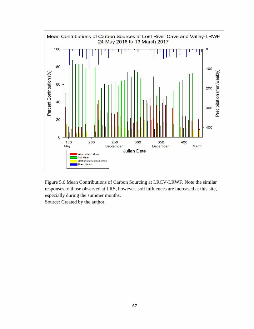
67

Figure 5.6 Mean Contributions of Carbon Sourcing at LRCV-LRWF. Note the similar

responses to those observed at LRS, however, soil influences are increased at this site,

especially during the summer months.

Source: Created by the author.

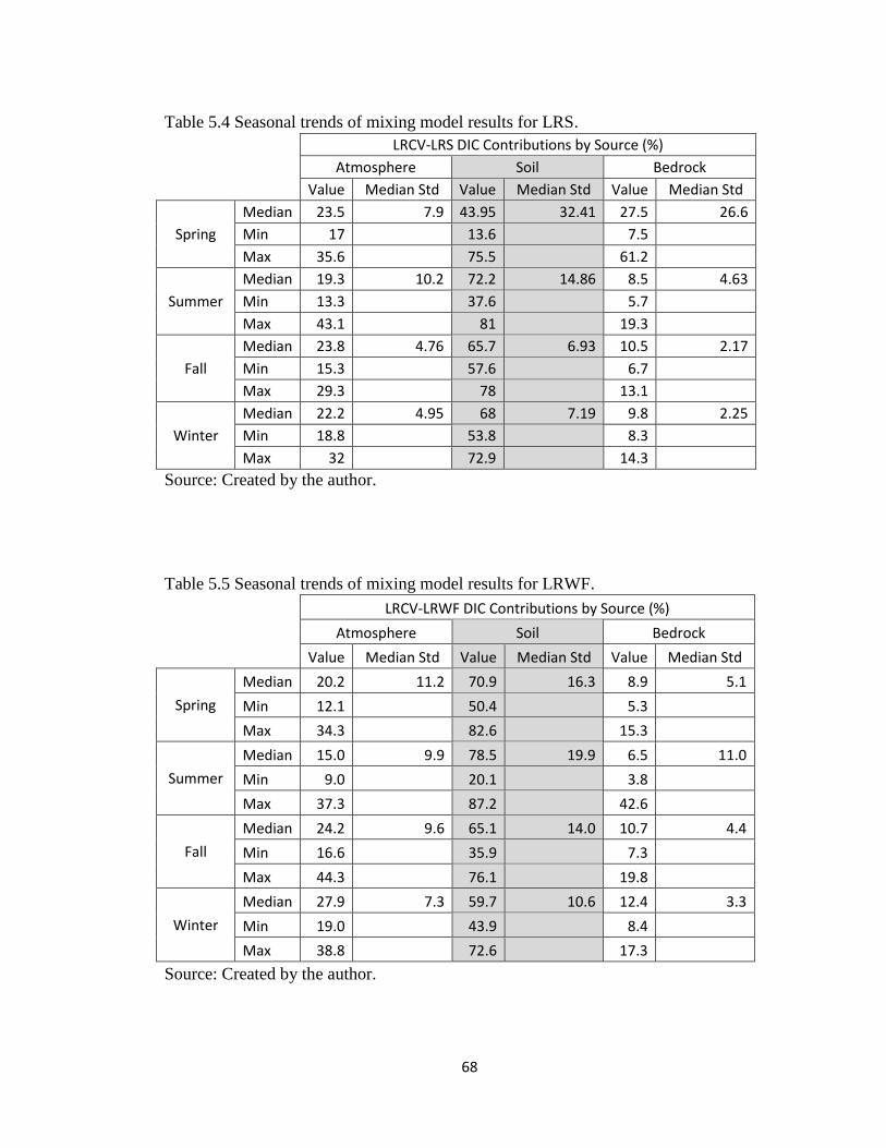
68

Table 5.5 Seasonal trends of mixing model results for LRWF.

LRCV-LRWF DIC Contributions by Source (%)

Atmosphere Soil Bedrock

Value Median Std Value Median Std Value Median Std

Spring

Median 20.2 11.2 70.9 16.3 8.9 5.1

Min 12.1

50.4

5.3 Max 34.3

82.6

15.3

Summer

Median 15.0 9.9 78.5 19.9 6.5 11.0

Min 9.0

20.1

3.8 Max 37.3

87.2

42.6

Fall

Median 24.2 9.6 65.1 14.0 10.7 4.4

Min 16.6

35.9

7.3 Max 44.3

76.1

19.8

Winter

Median 27.9 7.3 59.7 10.6 12.4 3.3

Min 19.0

43.9

8.4 Max 38.8

72.6

17.3

Source: Created by the author.

Table 5.4 Seasonal trends of mixing model results for LRS.

LRCV-LRS DIC Contributions by Source (%)

Atmosphere Soil Bedrock

Value Median Std Value Median Std Value Median Std

Spring

Median 23.5 7.9 43.95 32.41 27.5 26.6

Min 17

13.6

7.5 Max 35.6

75.5

61.2

Summer

Median 19.3 10.2 72.2 14.86 8.5 4.63

Min 13.3

37.6

5.7 Max 43.1

81

19.3

Fall

Median 23.8 4.76 65.7 6.93 10.5 2.17

Min 15.3

57.6

6.7 Max 29.3

78

13.1

Winter

Median 22.2 4.95 68 7.19 9.8 2.25

Min 18.8

53.8

8.3 Max 32

72.9

14.3

Source: Created by the author.

69

Chapter 6: Discussion

6.1 Epikarst Hydrogeochemistry

6.1.1 Site Geochemistry Discussion

The data presented from this investigation suggest that open system conditions are

present at both study locations (Williams 1983; White 1988; Palmer 1991; Clemens et al.

1999; Emblanch et al. 2003; Klimchouk 2004; Cheng et al. 2005; Palmer 2007a; Jiang et

al. 2007; Williams 2008; Faimon et al. 2012a). Higher precipitation rates and warm

surface temperatures during the summer months facilitate the interaction of CO2 with the

carbonate system by providing for surface conditions to encourage vegetation growth and

CO2 production in the soil at Crumps Cave sites, but less pronounced at Lost River Cave

and Valley sites due to an urban landscape potentially interfering with CO2 diffusion.

High precipitation events transport accumulated soil CO2 into the epikarst. During the

dry, relatively warm months, CO2 diffusion also occurs, but at a slower rate, because

precipitation events are lacking. In this case, while diffusion to the epikarst does occur,

CO2 concentrations appear to accumulate in the soil at increased concentrations. During

the colder, wet winter months, new soil CO2 production seems to decrease, along with

vegetation growth, while the remaining soil CO2, which has not diffused to the epikarst

during the warm, drought season, is then dissolved in rainwater and carried to the

bedrock below. Fluctuations in SpC and pH values throughout the study are

representative of dissolution and/or precipitation, and seem to coincide with surface

patterns. Likewise, CO2 concentrations, SIc, and DIC fluctuations also support surface

influences and, thus, open system conditions.

70

To delineate the extent of surface influences on epikarst responses, this study

focused on two levels of scrutiny: a multi-month time series analysis, which reflects the

seasonal changes occurring at each site (Figures 6.1 to 6.10), and two specific storm

events to characterize epikarst changes at extremely high-resolution at three different

intervals: baseflow conditions prior to the storm, storm responses at the site, and a return

to baseflow conditions (Figures 6.11 to 6.14). Both storm events (one in the summer and

one in the winter), spanned roughly three days and focus on the conditions at WF1 and

LRS to represent changes observed at each location as a regional comparison of site

responses. Due to the extremely large dataset, the most notable points within each time

series at every site are presented in the hydrogeochemical discussions.

Precipitation

Precipitation values at Crumps Cave (Figures 6.1 and 6.2) and LRCV (Figures 6.3

and 6.4) indicate wet and dry seasons. Distinctly higher precipitation rates and

frequencies occur during the summer months, followed by reduced precipitation events

during the fall, with increased precipitation events during the winter months and spring

transition. Summer precipitation frequencies and rates appear to be contributing to

epikarst water temperature, SpC, and pH conditions, reflecting distinct dilution effects as

precipitation filters through the topsoil and enters the epikarst (Figures 6.1 to 6.4). Study

period precipitation rates at Crumps Cave are higher than at LRCV (65% at Crumps Cave

versus 34% at LRCV); however, recorded precipitation at Crumps Cave and LRCV is

assumed the same for each study site within each location. Thus, the overall precipitation

rates at Crumps Cave are considered the same for WF1 and SF; likewise, the overall

precipitation rates at LRCV are assumed the same for LRS and LRWF.

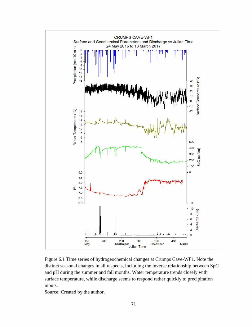
71

Figure 6.1 Time series of hydrogeochemical changes at Crumps Cave-WF1. Note the

distinct seasonal changes in all respects, including the inverse relationship between SpC

and pH during the summer and fall months. Water temperature trends closely with

surface temperature, while discharge seems to respond rather quickly to precipitation

inputs.

Source: Created by the author.

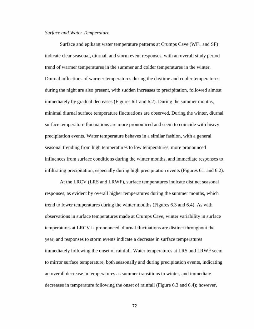
72

Surface and Water Temperature

Surface and epikarst water temperature patterns at Crumps Cave (WF1 and SF)

indicate clear seasonal, diurnal, and storm event responses, with an overall study period

trend of warmer temperatures in the summer and colder temperatures in the winter.

Diurnal inflections of warmer temperatures during the daytime and cooler temperatures

during the night are also present, with sudden increases to precipitation, followed almost

immediately by gradual decreases (Figures 6.1 and 6.2). During the summer months,

minimal diurnal surface temperature fluctuations are observed. During the winter, diurnal

surface temperature fluctuations are more pronounced and seem to coincide with heavy

precipitation events. Water temperature behaves in a similar fashion, with a general

seasonal trending from high temperatures to low temperatures, more pronounced

influences from surface conditions during the winter months, and immediate responses to

infiltrating precipitation, especially during high precipitation events (Figures 6.1 and 6.2).

At the LRCV (LRS and LRWF), surface temperatures indicate distinct seasonal

responses, as evident by overall higher temperatures during the summer months, which

trend to lower temperatures during the winter months (Figures 6.3 and 6.4). As with

observations in surface temperatures made at Crumps Cave, winter variability in surface

temperatures at LRCV is pronounced, diurnal fluctuations are distinct throughout the

year, and responses to storm events indicate a decrease in surface temperatures

immediately following the onset of rainfall. Water temperatures at LRS and LRWF seem

to mirror surface temperature, both seasonally and during precipitation events, indicating

an overall decrease in temperatures as summer transitions to winter, and immediate

decreases in temperature following the onset of rainfall (Figure 6.3 and 6.4); however,

73

some very distinct differences in temperature responses from both storm events and

seasonal variability occur at both sites. It is possible that these temperature differences

are also contributing to CO2 fluctuations, as increased water temperatures are less capable

of holding dissolved CO2, while decreased water temperatures are more capable of

holding higher concentrations of CO2, and thus, can contribute to ongoing dissolution.

While water temperatures at LRS (Figure 6.3) trend seasonally (highs in the

summer to lows in the winter) and responses to storm events are clearly present

(temperature dilutions at the onset of precipitation), the most pronounced effect is the

diurnal fluctuation in water temperature. These fluctuations are representative of

responses to water temperature, which is in relative equilibrium with surface temperature,

thus mirroring surface temperature behavior of day and night fluctuations. Increased

water temperature variability resulting from diurnal fluctuations in riverine systems have

been observed in hydrogeochemical studies conducted by Hess and White (1992),

Osterhoudt (2014), Pu et al. (2014a), McClanahan et al. (2016), and Salley (2016). At the

LRWF (Figure 6.4), these diurnal fluctuations are less pronounced, possibly due to the

water reaching equilibrium with cave temperature; thus, LRWF water temperature is

more heavily influenced by precipitation events and overall seasonal trending versus

daily cycles of day and night temperatures as observed at LRS.

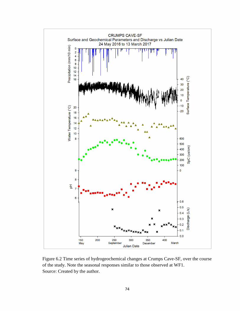
74

Figure 6.2 Time series of hydrogeochemical changes at Crumps Cave-SF, over the course

of the study. Note the seasonal responses similar to those observed at WF1.

Source: Created by the author.

75

Similar responses are observed at Crumps Cave and LRCV with respect to

seasonal, diurnal, and precipitation event temperature fluctuations and are common in

epikarst studies. Cheng et al. (2005); Jiang et al. (2007); Liu et al. (2010) and Pu et al.

(2014b) all found the same trends in karst regions in China. Likewise, investigations into

eogenetic karst systems in Florida by Gulley et al. (2015) found that surface temperature

and water temperature tend to mirror one another on all three scales. The studies suggest

that temperature fluctuations, both seasonally and diurnally, are a result of normal surface

influences on water temperature in open karst systems. Additionally, diurnal patterns are

a consequence of absorbed solar radiation influencing the water, which eventually drains

at the base of the epikarst. Lastly, during the summer months, solar output tends to heat

precipitation, driving the subsurface water temperature upward upon initial infiltration as

new water is mixed with older, more equilibrated water (Cheng et al. 2005; Liu et al.

2010; Yang et al. 2012; Pu et al. 2014a; Pu et al. 2014b; Gulley et al. 2015).

Specific Conductivity (SpC)

SpC values are an indicator of the number of free ions in water, usually caused by

dissolution (White 1988; Palmer 1991; Hess and White 1992; Drever 1997; Palmer

2007a). With higher values, the increased concentrations of free ions are assumed to

occupy the water. Since dissolution of limestone usually results in a combination of Ca2+

and Mg2+, (and less commonly K+ and Na+) and HCO3, then active dissolution, especially

during the summer months, is occurring at all sites, as evident by seasonal oscillations,

with higher values during the summer months and lower values during the winter months.

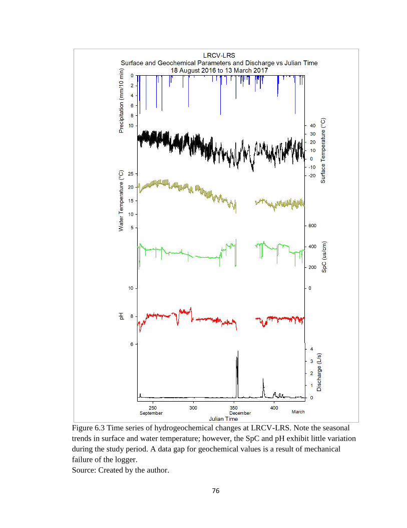
76

Figure 6.3 Time series of hydrogeochemical changes at LRCV-LRS. Note the seasonal

trends in surface and water temperature; however, the SpC and pH exhibit little variation

during the study period. A data gap for geochemical values is a result of mechanical

failure of the logger.

Source: Created by the author.

77

Most pronounced are the near immediate decreases in values following the onset

of precipitation events (Figures 6.1 to 6.4), which occur concurrently at all four sites with

seasonal trends (higher overall values in the summer and lower overall values in the

winter) (Cheng et al. 2005; Yang et al. 2012) (Figure 6.1 and Figure 6.2). Precipitation

responses create a near immediate decrease in values resulting from infiltrating water

with a low SpC, causing dilution effects resulting from the fast flush of fresh and storage

water through the system. Despite the difference in resolution at WF1 and SF, these

trends in both seasonal and storm event responses are very similar, suggesting that both

waterfalls are influenced by similar epikarst conduit networks, as was discovered by

studies conducted by Groves et al. (2005), Vanderhoff (2011), and Groves et al. (2013).

At the LRCV (LRS and LRWF), SpC values also show seasonal trends; however,

that trend is the least pronounced at LRS (Figure 6.3). This could be the result of surface

influences, such as exposure to the atmosphere, reducing the available CO2 for

dissolution reactions via degassing, causing precipitation of calcite and reduction of

dissolved ions (McClanahan et al. 2016; Osterhoudt 2014); however, SpC values still

show dilution responses to precipitation events, suggesting that SpC values in the spring

are severely affected by infiltrating rainwater.

The accounted difference in SpC values between locations (Figures 6.1 and 6.4)

could be a result of increased residence times at LRCV providing for additional water-

rock interaction, as suggested by Liu et al. (2010), which would cause higher SpC and pH

values, a higher saturation index, and lower CO2 values. At Crumps Cave, higher

volumes of discharge and near immediate responses to storm events in SpC values

indicate that shorter residence times are occurring in conjunction with rapid infiltration of

78

rainwater during certain events. Likewise, concentrations of Ca2+ and Mg2+, and HCO3

are greater at the LRCV sites versus the Crumps Cave sites, suggesting more dissolution

is occurring at the LRCV sites, which supports the increased SpC values recorded at LRS

and LRWF (Table 5.1; Figures 6.3 and 6.4).

pH

Values of pH are highly contingent on the concentrations of dissolved CO2 in

infiltrating waters (Palmer 2007a; Liu et al. 2010; Yang et al. 2012). Higher

concentrations of CO2 can drive pH toward more acidic values, causing an increase in the

aggressiveness of water and, thus, an increase in the extent and rate of dissolution. Over

time, prolonged water-rock interaction will buffer pH as CO2 concentrations reduce.

Concurrently, increased concentrations of dissolved CaCO3 may eventually increase pH

values as well. Fresh infiltrations of lower pH rainfall (~ 5.5), as suggested by White

(1988), Williams (1988), Palmer (1991), and Palmer (2007a), can serve to flush CO2

from the soil into the system and drive the pH lower (Liu et al. 2007; Li et al. 2008a; Li et

al. 2008b; Yang et al. 2012; Pu et al. 2014a; Pu et al. 2014b).

The pH values at WF1 and SF (Figures 6.1 and 6.2) trend similarly to one

another, indicating that differences in hydrogeochemical parameters are minimal between

sites with respect to pH. Seasonal trends, where values are lower in the summer and

higher in the winter, with a distinct increase around the beginning of the winter season, is

indicative of ongoing surface influences. Surface influences impacting pH, especially

during the winter months, can derive from several processes: a reduction in precipitation

and surface temperature causing of the reduction in root respiration from vegetation and

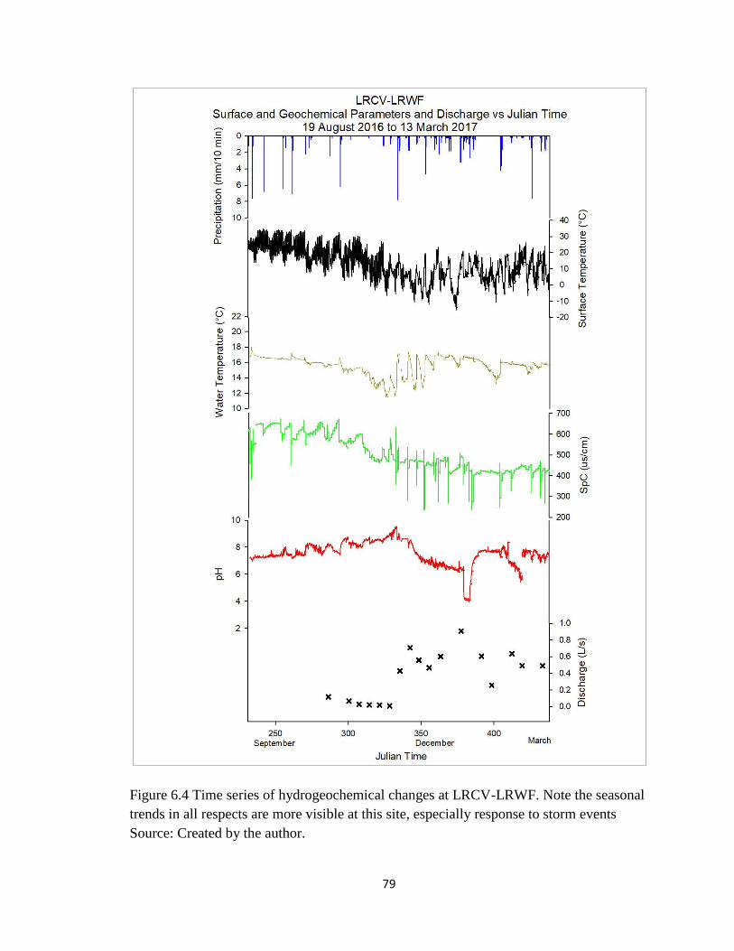
79

Figure 6.4 Time series of hydrogeochemical changes at LRCV-LRWF. Note the seasonal

trends in all respects are more visible at this site, especially response to storm events

Source: Created by the author.

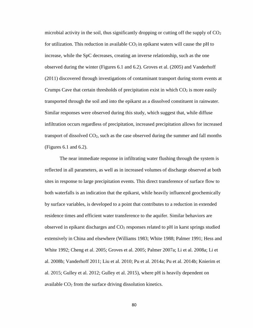
80

microbial activity in the soil, thus significantly dropping or cutting off the supply of CO2

for utilization. This reduction in available CO2 in epikarst waters will cause the pH to

increase, while the SpC decreases, creating an inverse relationship, such as the one

observed during the winter (Figures 6.1 and 6.2). Groves et al. (2005) and Vanderhoff

(2011) discovered through investigations of contaminant transport during storm events at

Crumps Cave that certain thresholds of precipitation exist in which CO2 is more easily

transported through the soil and into the epikarst as a dissolved constituent in rainwater.

Similar responses were observed during this study, which suggest that, while diffuse

infiltration occurs regardless of precipitation, increased precipitation allows for increased

transport of dissolved CO2, such as the case observed during the summer and fall months

(Figures 6.1 and 6.2).

The near immediate response in infiltrating water flushing through the system is

reflected in all parameters, as well as in increased volumes of discharge observed at both

sites in response to large precipitation events. This direct transference of surface flow to

both waterfalls is an indication that the epikarst, while heavily influenced geochemically

by surface variables, is developed to a point that contributes to a reduction in extended

residence times and efficient water transference to the aquifer. Similar behaviors are

observed in epikarst discharges and CO2 responses related to pH in karst springs studied

extensively in China and elsewhere (Williams 1983; White 1988; Palmer 1991; Hess and

White 1992; Cheng et al. 2005; Groves et al. 2005; Palmer 2007a; Li et al. 2008a; Li et

al. 2008b; Vanderhoff 2011; Liu et al. 2010; Pu et al. 2014a; Pu et al. 2014b; Knierim et

al. 2015; Gulley et al. 2012; Gulley et al. 2015), where pH is heavily dependent on

available CO2 from the surface driving dissolution kinetics.

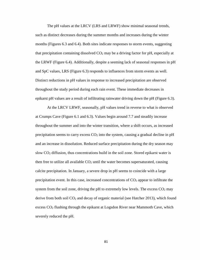
81

The pH values at the LRCV (LRS and LRWF) show minimal seasonal trends,

such as distinct decreases during the summer months and increases during the winter

months (Figures 6.3 and 6.4). Both sites indicate responses to storm events, suggesting

that precipitation containing dissolved CO2 may be a driving factor for pH, especially at

the LRWF (Figure 6.4). Additionally, despite a seeming lack of seasonal responses in pH

and SpC values, LRS (Figure 6.3) responds to influences from storm events as well.

Distinct reductions in pH values in response to increased precipitation are observed

throughout the study period during each rain event. These immediate decreases in

epikarst pH values are a result of infiltrating rainwater driving down the pH (Figure 6.3).

At the LRCV LRWF, seasonally, pH values trend in reverse to what is observed

at Crumps Cave (Figure 6.1 and 6.3). Values begin around 7.7 and steadily increase

throughout the summer and into the winter transition, where a shift occurs, as increased

precipitation seems to carry excess CO2 into the system, causing a gradual decline in pH

and an increase in dissolution. Reduced surface precipitation during the dry season may

slow CO2 diffusion, thus concentrations build in the soil zone. Stored epikarst water is

then free to utilize all available CO2 until the water becomes supersaturated, causing

calcite precipitation. In January, a severe drop in pH seems to coincide with a large

precipitation event. In this case, increased concentrations of CO2 appear to infiltrate the

system from the soil zone, driving the pH to extremely low levels. The excess CO2 may

derive from both soil CO2 and decay of organic material (see Hatcher 2013), which found

excess CO2 flushing through the epikarst at Logsdon River near Mammoth Cave, which

severely reduced the pH.

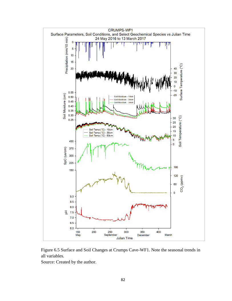
82

Figure 6.5 Surface and Soil Changes at Crumps Cave-WF1. Note the seasonal trends in

all variables.

Source: Created by the author.

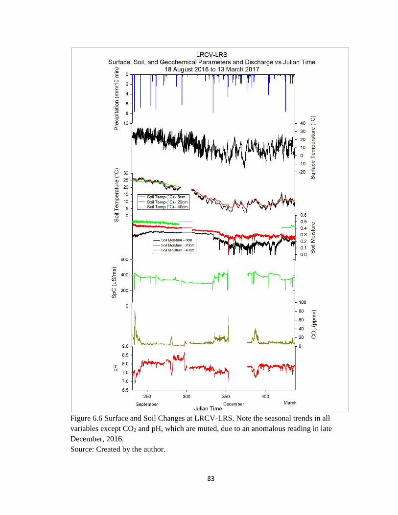
83

Figure 6.6 Surface and Soil Changes at LRCV-LRS. Note the seasonal trends in all

variables except CO2 and pH, which are muted, due to an anomalous reading in late

December, 2016.

Source: Created by the author.

84

It is possible that, at the LRWF, certain precipitation thresholds need to be met

before diffusion of CO2 in high concentrations can move swiftly to the epikarst and

transfer directly to the waterfall with minimal water-rock interaction. Responses in

discharge during large storm events seem to support the suggestion that a certain

threshold exists; however, when a threshold is not met, despite the continual flow of

water at LRWF, extremely low baseflow suggests that during dry periods extensive

water-rock interaction occurs. Increased SpC and Ca2+, Mg2+, and HCO3 concentrations,

as well as increased saturation index further support that concurrent ongoing dissolution

and precipitation is occurring at LRWF (Table 5.1 and Figure 6.4).

Soil Temperature and Moisture Conditions

According to Yang et al. (2012), soil CO2 originates from root respiration and

microbial decomposition and is a function of temperature and antecedent moisture. The

higher the temperature, the more root respiration and microbial activity observed, while,

conversely, drier, colder soils tend to produce less CO2 (Li et al. 2008a; Li et al. 2008b;

Liu et al. 2010; Yang et al. 2012). On diurnal scales, CO2 concentrations also fluctuate,

due to the day/night switch, as root respiration for most C3 and C4 plants (except for a

few row crop types) tends to slow during the night, with microbial activity in the soils

following suit (Clark and Fritz 1997). During the winter season, these diurnal fluctuations

are less pronounced, as most vegetation is dormant and, thus, microbial soil activity

slows or ceases depending on temperature (Yang et al. 2012). Excess soil CO2 is likely to

dissolve in antecedent moisture, which then slowly percolates into the epikarst. Likewise,

excess CO2 will also dissolve and transfer to the epikarst during increased precipitation;

however, if precipitation amounts supersede pre-existing antecedent moisture conditions,

85

it is possible that some soil CO2 may be exposed to the atmosphere and degas before it is

diffused to the epikarst. If antecedent moisture thresholds are not exceeded during

precipitation events, the infiltrating precipitation may transfer large concentrations of

dissolved CO2 to the epikarst more quickly than under normal, relatively dry conditions.

Soil conditions at Crumps Cave (Figures 6.5) indicate seasonal trends, with

increased temperatures during the summer months and decreased soil temperatures

during the winter months. Additionally, diurnal fluctuations are present, indicative of

solar radiation heating during the day and a reduction in solar radiation during the night.

At Crumps Cave (WF1 and SF), soil moisture conditions show significant increases

during large precipitation events, suggesting, especially during the summer months, that

antecedent moisture levels are consistently higher, possibly due to a lag time between

infiltration to the epikarst and the next storm event (Figure 6.5). A general decrease in

moisture conditions is visible during the fall drought, followed by an increase in

antecedent moisture during the winter storms (Figures 6.5). These distinct seasonal and

precipitation driven changes in temperature and soil moisture conditions are more likely

to produce CO2 during the spring-summer and into the fall months during the growing

period, while being less likely to produce soil CO2 during the late fall and winter months

due to vegetation loss and a reduction in soil microbial activity. More extreme

fluctuations in surface temperatures during the winter months are met with multiple

instances of fluctuations in both soil moisture and temperature, which suggest that soil

microbial activity may be switching on and off, thus producing, even in small increments,

higher concentrations of CO2.

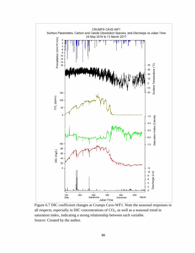
86

Figure 6.7 DIC coefficient changes at Crumps Cave-WF1. Note the seasonal responses in

all respects, especially in DIC concentrations of CO2, as well as a seasonal trend in

saturation index, indicating a strong relationship between each variable.

Source: Created by the author.

87

Similar soil responses in both temperature and moisture conditions, indicative of

vegetation and microbial activity and, thus, correlative fluctuations in soil CO2

concentrations, are observed in studies in China and elsewhere (Amundson et al. 1998;

Clemens et al. 1999; Bakalowicz 2004; Klimchouk 2004). The nearby Kentucky Mesonet

FARM Station recorded soil conditions for the LRCV, and the data were assumed to be

similar enough to apply to both study sites (LRS and LRWF) (Figure 6.6). Soil

temperature at the LRCV responds seasonally, with increased temperatures during the

summer months and decreased temperatures during the winter months (Figure 6.6). As

with observations made in soil temperature at Crumps Cave, LRCV soil temperature

indicates increased fluctuations on diurnal scales to winter surface temperatures. Soil

moisture conditions at the LRCV indicate more muted responses to seasonal changes,

especially the shallower readings, but distinct responses to precipitation events, especially

in the winter months (Figure 6.6). The difference in soil temperature and moisture

conditions between locations could be due to data collection resolution. Crumps Cave

collected data at ten-minute intervals while the FARM Station for LRCV collected data

every 30 minutes. Additionally, soil extent is heavily impacted by the presence of large

expanses of impermeable surfaces at LRCV, thus influencing the soil’s ability to respond

to seasonal changes (USDA 2017).

Carbon Dioxide (CO2)

Carbon dioxide in groundwater is a major geochemical driving factor in

dissolution kinetics (Williams 1983; White 1988; Palmer 1991; Drever 1997; Clemens et

al. 1998; Veni et al. 2001; Palmer 2007a; Li et al. 2008a; Yang et al. 2012; Gulley et al.

2015). As waters move from areas of low CO2 concentrations to high CO2

88

concentrations, pH levels decrease and dissolution occurs after the water becomes acidic.

This CO2 gradient is often spatially delineated (Gulley et al. 2012; Gulley et al. 2015) and

is identified to be heterogeneous in nature throughout the landscape. Likewise, an

investigation into the formation of phreatic caves in eogenetic karst by Gulley et al.

(2012), suggested that CO2 in a gaseous state may be responsible for increased cave

formation as opposed to the mixing of fresh and saltwater resulting from sea level rise,

which had been the assumed driver regarding eogenetic cave formation. Their study

found that the heterogenic distribution of CO2 is spatially dominant, in that cave

formation is a direct result of CO2-driven dissolution in a spatial context. In telogenetic

karst, dissolution is primarily a result of fluid dynamics and water-rock interaction, in

that water percolating through the matrix and along fractures and bedding planes tends to

form void spaces (Williams 1983; White 1988; Palmer 1991; Veni et al. 2001; Palmer

2007a). Further, CO2 exchange with the atmosphere and the epikarst is heavily contingent

on the presence of antecedent moisture in the topsoil and the surrounding temperature

(Cuezva et al. 2011).

The diffusion of CO2 at WF1 seems to occur in several ways. Firstly, as observed

in epikarst studies in other regions of the world, CO2 concentrations seem to vary

seasonally, with highs during the summer and lows during the winter (Liu et al. 2007; Li

et al. 2008a; Li et al. 2008b; Cuezva et al. 2011; Liu et al. 2010; Peyraube et al. 2012;

Yang et al. 2012; Peyraube et al. 2014; Pu et al. 2014b; Gulley et al. 2015), while storm

events result in high precipitation, which transports soil CO2 into the epikarst. Initially,

dilution effects are visible, followed by a relative lag before concentrations begin to rise.

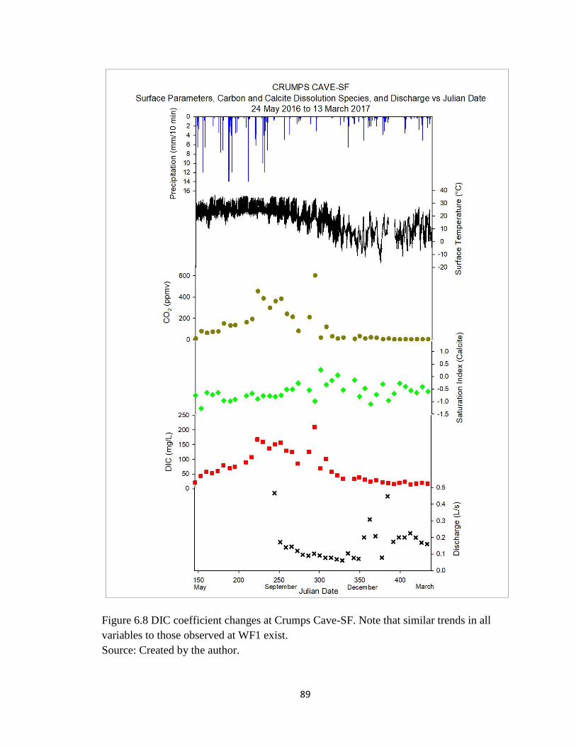
89

Figure 6.8 DIC coefficient changes at Crumps Cave-SF. Note that similar trends in all

variables to those observed at WF1 exist.

Source: Created by the author.

90

Likewise, peak CO2 concentrations during the months of September and October

are most likely due to the onset of the dry season combined with the maturation state of

surface vegetation, providing for the accumulation of increased soil CO2 concentrations.

At the onset of the late fall-early winter, when crops are harvested and natural vegetation

begins to wither, CO2 concentrations started to decrease to reach their lowest value (near

zero) and remained at that level for the rest of the study (Figure 6.7 and 6.8). Despite the

variability in precipitation, soil moisture, and soil temperature near the end of the winter

months and transitioning into the spring, little response is observed in CO2 concen-

trations. Minimal microbial activity and reduced root respiration may be the cause of

minimal CO2 concentrations in the epikarst, as no increases in CO2 concentrations were

observed in groundwater discharged from the spring. As a result of drastic diurnal surface

temperature fluctuations ranging above 20 ºC on some days during the winter, it is likely

that microbial activity may have shifted between dormant and non-dormant phases in

response. This shifting between phases generated higher concentrations of CO2 in the

soil. Studies regarding vegetation growth and microbial contributions to soil respiration

and CO2 production with respect to temperature and moisture fluctuations were

conducted by Zogg et al. (1995), Davidson et al. (1998), and Fierer et al (2003). Zogg et

al. (1995) found that fluctuations in soil temperatures can alter microbial communities in

the soil, thus dominant communities at higher temperatures can increase their ability to

metabolize nutrients more so than at lower temperatures.

Davidson et al. (1998) found that soil CO2 fluctuations are a result of variations in

soil temperature and moisture, especially over seasonal and diurnal scales. Fierer et al.

(2003) discovered that concentrations of CO2 from nutrient digestion by microbial

91

communities occurs at greater rates in the deeper substrate, influenced by a heightened

sensitivity to soil temperature and moisture changes versus the surface layer, which

appears less responsive. Despite these conditions, which should yield increased CO2

concentrations at the springs, WF1 and SF have low CO2 concentrations, which suggests

that any soil derived CO2 from the fluctuations in temperature was immediately utilized

in bedrock dissolution, as evident by minimal changes to pH at the spring, fluctuations of

SpC, and slight increases in DIC.

Trends of CO2 at SF mirror that of WF1 (Figure 6.8), suggesting that similar

influences in the epikarst are governing processes at both waterfalls. Seasonal responses

can be delineated, despite the weekly resolution; however, diurnal and storm event

variability at SF is not as easily identified and, in certain respects, impossible to

determine based on lower resolution. Seasonal trends indicate increases during the

growing season and decreases during the winter season. Additionally, SF exhibits overall

higher concentrations of CO2 relative to WF1. This difference in concentrations could be

due to the difference in resolution between sites. Likewise, the dominant processes at

each site, while similar, may be operating at different levels and intervals between sites.

Minimal seasonal variability is observed in CO2 concentrations at LRCV-LRS,

but increases in concentrations seem to coincide with storm events, suggesting that high

precipitation events breach the threshold required to facilitate the rapid movement of

dissolved CO2 (which had not degassed to the atmosphere) from the soil to the epikarst

(Figure 6.9). The lack of seasonal influence may be explained by land use in the region

adjacent to LRS. Vegetation and soil cover at LRS exist in pockets, due to residential and

commercial infrastructure and, thus, CO2 that normally contributes to seasonal increases

92

and decreases may be reduced to those pockets where vegetation exists and where CO2

production in the soil is still occurring. Likewise, any CO2 that would normally degas to

the atmosphere during the winter months under low antecedent moisture conditions could

potentially be trapped by the presence of extensive impermeable surfaces, preventing that

exchange with the atmosphere (Cuezva et al. 2011). Additionally, since CO2 values are

calculated from SpC and pH, which also indicate muted seasonal trends, it is likely that

CO2 measurements do the same. Lastly, discharge at LRS seems highly dependent on

increased precipitation rates at high frequencies. Thus, certain volumes of water in the

system must be met before any increase in discharge occurs, which suggests that longer

residence times are occurring at the site. Longer residence times would result in the

following conditions: reduction in CO2 due to the ongoing water-rock interaction driving

dissolution; an increase in pH due to a reduction in CO2 used in dissolution, and an

increase in SpC with high concentrations of calcium, magnesium, and bicarbonate, due to

an increase in dissolution. These conditions have been observed and described in

situations with similar soil and shallow epikarst springs in residential regions in other

parts of the world (Cheng et al. 2005; Liu et al. 2007; Li et al. 2008a; Li et al. 2008b;

Cuezva et al. 2011; Liu et al. 2010; Peyraube et al. 2012; Yang et al. 2012; Peyraube et

al. 2014; Pu et al. 2014a; Pu et al. 2014b).

The aforementioned conditions at LRS (Figure 6.9) could be considered baseline

conditions for this particular site; however, during high precipitation events, the

conditions shift. The CO2 spikes at the end of August, in October, December, and again

in January, all coinciding with high precipitation, which may flush whatever soil CO2

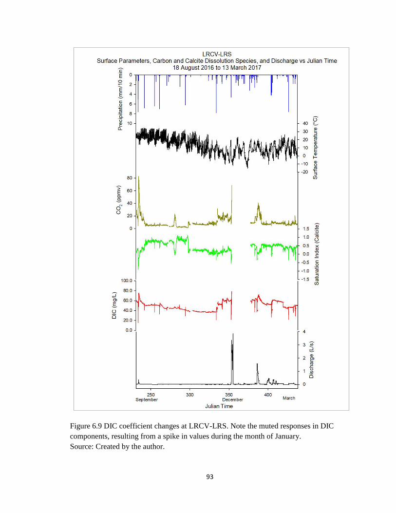
93

Figure 6.9 DIC coefficient changes at LRCV-LRS. Note the muted responses in DIC

components, resulting from a spike in values during the month of January.

Source: Created by the author.

94

exists in the epikarst and transfer it to the groundwater, causing spikes in CO2 readings at

the spring. A similar situation was observed at Maolon Spring in China, where rainfall

served to dissolve soil CO2 and transfer it to the epikarst (Liu et al. 2007) during high

precipitation events. Likewise, in a different study conducted by Liu et al. (2010), similar

behaviors in epikarst springs in China were recorded, driven by piston push effects,

which drained the soil of CO2 concentrations, transferring it to the epikarst, where it was

reflected at the spring and correlated with lower values of pH. Groundwater CO2

concentrations at LRWF are likely influenced from sources governed by an impermeable

urban landscape as well, as suggested by minimal seasonal influences on overall CO2

concentrations (Figure 6.10). Conversely, in areas where soil exists beneath these

impermeable surfaces near LRWF, soil microbial activity may be contributing to total

CO2 concentrations on an ongoing basis as opposed to seasonally.

Saturation Index (SIc)

Calculated values of SIc are proportional to pH values and are also a

representation of the saturation of the water with respect to calcite (Hess and White

19923; Drever 1997; Palmer 1991; Palmer 2007a; Yang et al. 2012). In saturated waters,

the value is usually zero, while under-saturated water is expressed as a negative number,

and supersaturated water is expressed as a positive number. Seasonally, during the

summer months, as CO2 concentrations increase in groundwater, so does dissolution, and,

thus, the saturation index should increase; however, because the concentration of CO2 is

often so high, the aggressiveness of the water reduces more slowly, thus, the saturation

index will remain below zero, especially if there is minimal water-rock interaction. If the

source of CO2 is either terminated or reduced, then the remaining CO2 in the system will

95

have a chance to react, thus causing the saturation index to rise. This is often what is

observed as the summer months transition into the winter, as described from studies in

Algeria (Chemseddine et al. 2015) and China (Cheng et al. 2005; Li et al. 2007a; Li et al

2007b; Liu et al. 2007; Yang et al. 2012; Knierim et al. 2015).

At Crumps Cave WF1, the saturation index of calcite mirrors that of pH values, as

a representation of the aggressiveness of water with respect to dissolution kinetics (Figure

6.7); thus, during the summer months, SIc values follow seasonal variability interspersed

with dilution effects from high precipitation events. The same under-saturated values in

the summer months, as well as close-to-saturation values in the winter months, were also

observed in studies elsewhere (Hess and White 1992; Liu et al. 2007; Yang et al. 2012).

During those studies, storm events resulting in severe dilution effects were observed, and

the saturation index decreased abruptly before recovering, as a result of high infiltration

of precipitation in conjunction with excess dissolved CO2 (Vesper and White 2004;

Cheng et al. 2005; Liu et al. 2007; Li et al. 2008a; Li et al. 2008b).

The seasonal variability, in conjunction with dilution effects during storm events

at Crumps Cave, is a product of both conduit flow and possible direct input from surface

infiltration, in conjunction with increased CO2 during the summer and reduced CO2

during the winter. During the winter transition, the saturation index breaches the zero

mark for a short time, indicating that the water was supersaturated. This spike in values is

due to the extended dry season extending water-rock interaction during minimal

precipitation events, which reduced the number of system flushes and increased the

residence time in the system. As the winter storm season set in, the saturation index

96

dropped below zero as storage water became diluted, system flush frequencies increased,

and water-rock interaction decreased, lowering the SIc values.

At Crumps Cave SF, the saturation index mirrors that of the saturation index at

WF1; however, values do not show as much seasonal trending nor as much storm event

influence (Figure 6.8). These differences could be a result of the lower resolution at SF.

Although minimal variability is observed during the summer months, significant

variability is observed in the winter months. This variability could be driven by dilution,

(low SIc concentrated, infiltrating precipitation, which serves to reduce storage water

concentrations), from storm events causing initial reductions in SIc concentrations. Once

this freshly diluted water exists the system, higher concentrated water with respect to SIc

is reflected in the data (Yang et al. 2012). Likewise, as saturation index values move

closer to zero during the winter months after storm events, dilution effects on epikarst

water can become more apparent, and thus, appear to have a greater impact on values.

At the LRCV-LRS, the saturation index fluctuates between under-saturated and

supersaturated throughout the course of the study, with the majority of the nine months

spent in a saturated or supersaturated state (Figure 6.9). During the storm event in

December 2016, seasonal variability is also masked; however, overall index values show

the water is consistently oversaturated. This response could be a result of extended

residence times allowing for prolonged water-rock interaction. Exact CO2 concentration

fluctuations are difficult to ascertain, but the observable responses and trends seem to

support the suggestion that supersaturation is a result of the utilization of available CO2 in

the system and, thus, explains the high values of pH in conjunction with the high values

of SIc. Similar behaviors were observed at Nongla Spring in China, where the water was

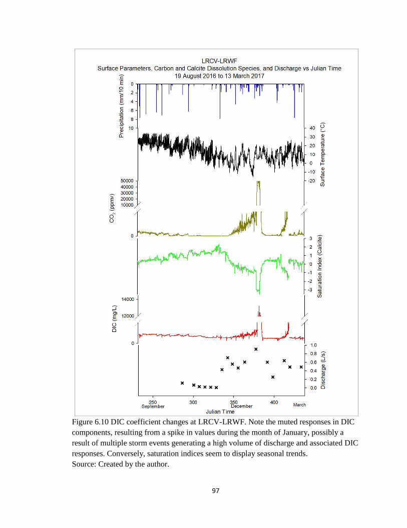
97

Figure 6.10 DIC coefficient changes at LRCV-LRWF. Note the muted responses in DIC

components, resulting from a spike in values during the month of January, possibly a

result of multiple storm events generating a high volume of discharge and associated DIC

responses. Conversely, saturation indices seem to display seasonal trends.

Source: Created by the author.

98

consistently saturated or supersaturated, while CO2 concentrations were consistently low.

The authors suggested this relationship was a result of the soil CO2 effect, where CO2

concentrations are reduced, due to a lag time in surface and soil temperature equilibrium

(Liu et al. 2007; Yang et al. 2012). Likewise, an examination into the behaviors of an

aquifer in Algeria suggested that calcite precipitation is a result of increased soil CO2

derived from open system conditions (Chemseddine et al. 2015).

At the LRCV-LRWF, values are the inverse of typical karst water behavior seen

at Crumps, suggesting that minimal dissolved CO2 exists in the system. This is most

likely due to available CO2 concentrations being used during dissolution until the water

was supersaturated (Figure 6.10). At the winter transition, pH values begin to decrease,

possibly in conjunction with a surge of CO2 carried into the epikarst during the winter

storms, allowing for dissolution and, thus, driving the saturation index below zero. The

process could be a result of two consecutive influences: 1) the dilution effect of excess

precipitation infiltrating the system, carrying with it soil derived CO2; and 2) that same

excess CO2 in the system reduced the pH and drove further dissolution, thereby causing

the saturation of the water to eventually increase as dissolution continues to saturate the

water with calcite and CO2 is used in the reaction.

Palmer (2007a) suggested that this process is ongoing, as dissolution kinetics are

a cyclical process that do not proceed to completion, due to open system conditions

providing a continuous supply of CO2. On the other hand, even if a finite supply of CO2

existed, dissolution kinetics will reduce or slow depending on the saturation level of the

water, which can only contain a certain concentration of calcite. Should levels of

saturation reach supersaturated, dissolution will temporarily cease until more water or

99

CO2 is added to the system, serving to dilute concentrations and allow dissolved CO2 to

react with the surrounding bedrock again (Palmer 2007a). Pu et al. (2014a) suggested a

similar explanation for processes observed in a karst aquifer in China. In that study,

dissolved CO2 in precipitation caused the saturation index to fluctuate between

supersaturated before the precipitation, to under-saturated after the precipitation as an

influx of fresh water containing highly concentrated CO2 provided for an increase in

dissolution kinetics. Li et al. (2008a) further supported these observations in a different

study, where a severe decrease in pH resulted from infiltrating excess CO2. That

investigation suggested precipitation not only contained excess dissolved CO2 from

microbial activity, but from atmospheric CO2 as well. Since microbial activity is

temperature dependent, and the winter months at both Crumps Cave and LRCV had odd

temperature fluctuations, a significant increase in microbial activity could have

contributed to the severe decrease in pH, thus showing a similar decline in SIc as well

(Telmer and Veizer 1999; Peyraube et al. 2014; Milanolo and Gabrovšek 2015; Zhang et

al. 2015; Zhao et al. 2015).

Dissolved Inorganic Carbon (DIC)

Dissolved inorganic carbon is expressed as a concentration, assigned to natural

waters, either surface or subsurface, and designed to identify the reaction constituents

and/or products within a given system (either CO2 or dissolved CaCO3, respectively)

(White 1988; Clark and Fritz 1997; Drever 1997; Palmer 2007a). Several studies have

explored the concentrations of DIC in surface and karst spring water (Emblanch et al.

2003; Liu et al. 2010; Shin et al. 2011; Charlier et al. 2012; Faimon et al. 2012a; Faimon

et al. 2012b; Yang et al. 2012; Knierim et al. 2013; Osterhoudt 2014; McClanahan 2016;

100

Salley 2016; Zhang et al. 2016) to determine the seasonal and storm event fluctuations.

Their results are mixed, with some karst landscapes showing the possibility of serving as

a carbon sink, while other studies show no real link to excess atmospheric CO2 and karst

landscape absorption (Liu et al. 2010). Since DIC is an important reaction product in

karst dissolution processes and, thus, karst landscape development, understanding the

relationship of DIC with seasonal and storm event variability, as well as the fluctuation of

carbon in relation to discharge, can aid in understanding the extent of dissolution at

Crumps Cave and LRCV.

At Crumps Cave WF1, DIC concentrations show distinct seasonal variability

(Figure 6.7). Generally, values increase during the summer months and decrease during

the winter months to coincide with dissolution reactions, with the overall trend mirroring

that of CO2 concentrations. This suggests that DIC values are heavily influenced by CO2

concentrations in groundwater (Emblanch et al. 2003; Shin et al. 2011; White 2013;

Knierim et al. 2015; Zhang et al. 2016) and can exhibit both seasonal and diel cycle

variability, as discovered by Gammons et al. (2011) and de Montety et al. (2011). Here,

accelerated photosynthetic uptake served to deplete CO2-DIC concentrations during the

day, while an increase in CO2-DIC concentrations occurred during the night from plant

respiration, indicating a reduction in 12C uptake. DIC concentrations at Crumps Cave

show responses to high precipitation events as well, with severe depletion as a result of

possible dilution effects. High-resolution DIC fluctuations were calculated against total

discharge and reflect variability both seasonally and volumetrically, due to high

precipitation events. The volume of DIC discharged from the system over the course of

101

the study period is presented in Table 6.1, along with the respective range of discharged

DIC during that time.

At Crumps Cave SF, seasonal variability in DIC concentrations is visible, with

highs in the summer and lows in the winter; however, due to weekly resolution,

influences from precipitation events are not as clearly defined (Figure 6.8). Overall,

concentrations of DIC are higher at SF than at WF1, and mirror higher concentrations of

CO2 observed at SF. The difference in concentrations could be a result of a difference in

resolution, as SF weekly resolution did not capture subtle changes to the system,

especially during high precipitation events, which can directly influence DIC

concentrations (Liu et al. 2010; Yang et al. 2012).

DIC concentrations at LRCV-LRS show minimal seasonal variability, possibly a

result of overall low concentrations of CO2 (Figure 6.9); however, numerous high

precipitation events flushed the system of concentrated SIc, but added increased

concentrations of CO2 and DIC. Similar peaks indicating piston effects were observed

during the onset of a storm event in China by Pu et al. (2014a; 2014b). They attributed

the increase in the values to highly concentrated storage water flushing from the system,

which had accumulated during a prior dry season. A similar pattern of precipitation and

epikarst responses is at work at the LRS (Li et al. 2008b; Li et al. 2010).

Overall DIC concentrations at LRCV-LRWF are also fairly masked in Figure 6.10

by a spike in concentration during two separate events associated with both a reduction in

pH and SIc, as well as an increase in CO2. This spike in concentrations, as noted by the

maximum value of 13,502 mg/L in Table 5.1 and illustrated in Figure 6.10, is due to an

intense flush of CO2 through the epikarst, caused by the aforementioned dual, high-

102

volume precipitation events. Although seasonal variability is relatively absent from the

data, concentrations of DIC show steep increases, due to increases in precipitation events

causing a surge of fresh water to flush storage water with highly concentrated DIC

through the system, before being replaced by water lower in DIC concentrations (Li et al.

2008b; Li et al. 2010). SpC and pH values show decreases during these precipitation

events, while CO2 concentrations show increases, suggesting that dissolution may have

occurred prior to the storm, leading to an increase in DIC as illustrated in Figure 6.10.

6.1.2 Storm Event Hydrogeochemical Variability at WF1 and LRS

Data for two separate storm events (August and November, 2016), are presented

in Figures 6.11 to 6.15, and illustrate changes in surface parameters associated with

geochemical responses. Data for Crumps Cave WF1 and LRCV-LRS are presented, as

they both contain high-resolution data in all respects, as well as a presumed accurate

geochemical depiction of their respective karst landscapes. Both events span a

period of three days, and the data presented are intended to characterize baseflow to

baseflow conditions, the changes within that timeframe, and highlight the importance of

geochemical relationships to surface influences in the epikarst.

STE 1: August 20-August 23, 2016 (JD233-236)

The first event chosen for deeper scrutiny occurred on August 20, 2016, and

lasted until August 23, 2016. Precipitation rates at Crumps Cave were slightly less than

precipitation rates at the LRCV, due to the fact that precipitation at the LRCV occurred in

two parts, as opposed to a single rainfall event recorded at Crumps Cave during the study

(Figures 6.11 and 6.12).

103

The surface temperature at Crumps Cave WF1 (Figure 6.11) showed distinct

diurnal fluctuations over the course of the storm event, with a ~5 ºC temperature decrease

immediately following the onset of the rainfall (Liu et al. 2007). A short lag time

occurred between the onset of the precipitation event and a sudden increase in water

temperature, suggesting that conduit flow dominates at WF1, facilitating the transference

of warm precipitation to the epikarst (Vanderhoff 2011; Groves et al. 2013).

Additionally, while surface temperature exhibited distinct diurnal fluctuations, water

temperature did not, suggesting that, during this particular storm, precipitation seems to

drive hydrogeochemical responses more so than surface temperature.

Water temperature gradually decreased over the course of the storm event, further

suggesting there is a lag time for warmer, infiltrating precipitation to reach equilibrium

with cooler, epikarst storage water. The SpC (Figure 6.11) also demonstrates a short lag

time between infiltrating precipitation and response in the epikarst, with a strong dilution

effect caused by the infiltrating precipitation, further supporting both direct conduit flow

and a piston effect, where storage water is sufficiently discharged from the system and

replaced with new precipitation (Li et al. 2008a; Li et al. 2008b). The pH values (Figure

6.11) respond minimally to precipitation moving through the system, suggesting that

infiltrating precipitation and karst water pH values were at or near equilibrium at the

onset of the storm, and, thus, minimally affected. Further, CO2 values decrease quite

steeply, shortly after the onset of precipitation, suggesting that fresh, infiltrating water

served to flush concentrated water from the system, before replacing it with diluted water

(Pu et al. 2014a; Pu et al. 2014b).

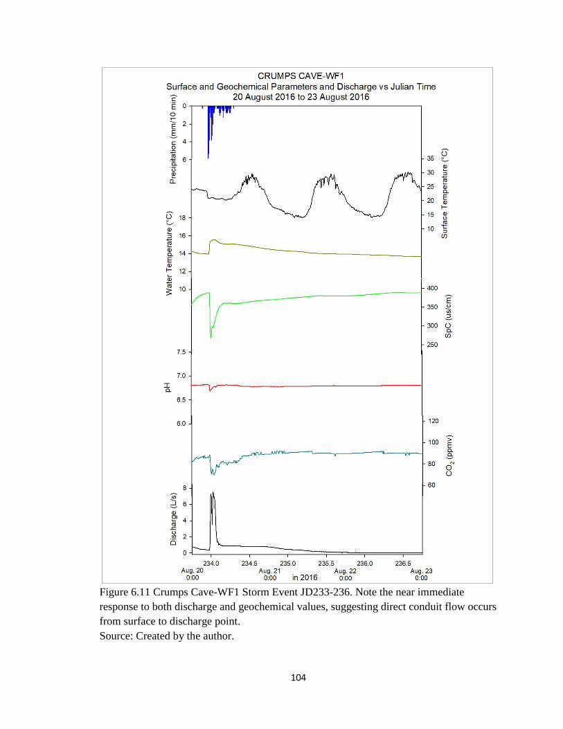
104

Figure 6.11 Crumps Cave-WF1 Storm Event JD233-236. Note the near immediate

response to both discharge and geochemical values, suggesting direct conduit flow occurs

from surface to discharge point.

Source: Created by the author.

105

Discharge at WF1 increased shortly after the onset of precipitation. This increase

in discharge is due to the well-developed epikarst facilitating transference of water from

the surface to the waterfall (Groves et al. 2005; Vanderhoff 2011; Groves et al. 2015).

Short lag times (~25-45 minutes) are observed between the onset of the precipitation, the

hydrogeochemical responses, and the return to normalized conditions, which suggest that

surface influences have a direct impact on epikarst process. These same behaviors were

observed at Crumps Cave in a previous study on contaminant transport through the

epikarst (Vanderhoff 2011). In that investigation, the author suggested conduit-dominated

flow as the primary facilitator of surface water transference to the aquifer and, thus, near

immediate responses in recorded hydrogeochemical parameters (Cheng et al. 2005; Liu et

al. 2007; Li et al. 2008a; Li et al. 2008b; Liu et al. 2010; Yang et al. 2012; Pu et al.

2014a; Pu et al. 2014b; Yang et al. 2012; Gulley et al. 2015).

At the LRS (Figure 6.12), precipitation occurred in two phases, with the first

event of short duration but high intensity, while the second phase included longer

duration rainfall with larger volume and intensity. This had minimal impact on surface

temperatures, which displayed diurnal responses following a small decrease after the

onset of the second phase of precipitation. As with responses at WF1, diurnal fluctuations

are not present in the water temperature, which exhibits distinct responses to infiltrating

precipitation, suggesting that, at both sites during intense storm events, surface

temperature has minimal impact on hydrogeochemical changes. Geochemical responses

to the first phase of precipitation are less pronounced than responses to the second phase

of precipitation, indicating a longer lag time between the onset of precipitation and the

responses in hydrogeochemical changes (Figure 6.12).

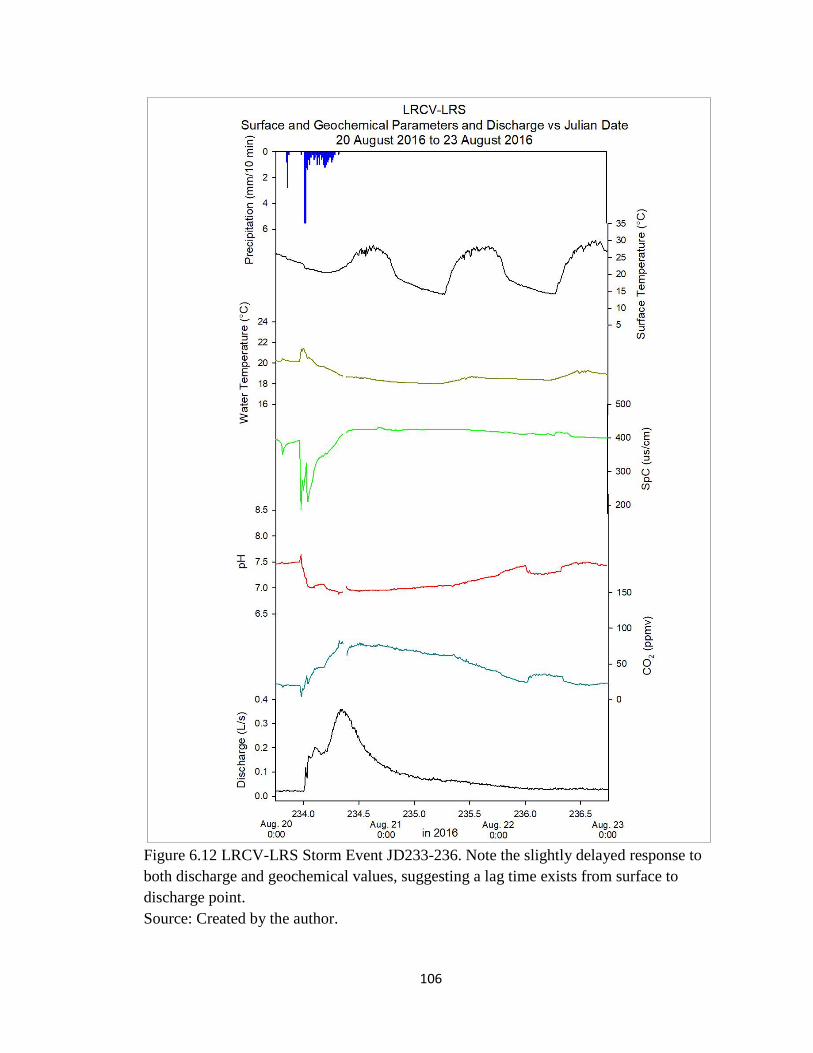
106

Figure 6.12 LRCV-LRS Storm Event JD233-236. Note the slightly delayed response to

both discharge and geochemical values, suggesting a lag time exists from surface to

discharge point.

Source: Created by the author.

107

All parameters respond to the second phase of precipitation, and to rather large

degrees, indicating subsequent timing of both precipitation events prevent sufficient

recovery period between them, compounding the responses following the second

precipitation phase. Water temperature increased slightly, followed by a gradual

decrease, which eventually reduced water temperature levels to several degrees cooler

than pre-storm levels (Cheng et al. 2005; Liu et al. 2007; Li et al. 2008a; Li et al. 2008b;

Liu et al. 2010; Yang et al. 2012; Pu et al. 2014a; Yang et al. 2012; Gulley et al. 2015).

SpC responded in two phases, potentially due to the two-phase precipitation, which

indicates that a lag time exists from the onset of precipitation to the point at which the

logger registers the infiltration of the fresh, less ion-rich water (Figure 6.12). The pH

values also decrease quite severely from infiltrating precipitation containing high

concentrations of dissolved CO2 (Figure 6.12) (Cheng et al. 2005; Liu et al. 2010; Yang

et al. 2012; Pu et al. 2014b). The pH values never fully recover, possibly due to a

substantial influx of CO2. CO2 concentrations increase significantly shortly following the

onset of precipitation, suggesting that either storage water with high concentrations of

CO2 was flushed from the system, or that precipitation infiltrating the system contained

large concentrations of dissolved CO2, from the topsoil (Liu et al. 2007; Liu et al. 2010;

Pu et al. 2014b). Discharge volumes demonstrated distinct lag times between the onset of

precipitation and the peak of discharge by about 12 hours, indicating that certain

thresholds of water volumes within the epikarst must be met before significant discharge

is registered at the spring (Figure 6.12). From the study period geochemical data,

specifically the calcium, magnesium, bicarbonate, CO2, and SIc data (Table 5.1), it would

appear that extensive storage is occurring at the LRS, while sufficient storage is occurring

108

even during drought conditions, at Crumps Cave to facilitate ongoing discharge at all

sites. At Crumps Cave, that storage is potentially governed by the presence of the chert

layer acting as a leaky perched aquifer. This perched aquifer is recharged during high

precipitation events, which also flushes increased concentrations of soil-derived CO2

through the system during the growing season, thus increasing the propensity for

dissolution from highly aggressive water, despite the fast transference. Similar behavior

was observed in storm event monitoring by Vesper and White (2004) during an

investigation into a Tennessee cave system. Likewise, large volumes of high rainfall

intensity over very short periods of time are required to flush the system at both locations.

At the LRCV, precipitation may not transfer to the epikarst as quickly, due to

impermeable surface layers derived from urbanization, combined with a general lack of

topsoil facilitating downward diffusion. In fact, flooding problems are a large concern for

Bowling Green residents, where the landscape has been modified to an extent that most

water is directed into the aquifer through injection wells instead of through the epikarst

(Crawford 1984a; Crawford 1984b; Crawford 1989; Crawford 2003; Crawford 2005;

Brewer and Crawford 2005; Cesin and Crawford 2005). Thus, precipitation diffusion into

the epikarst at the LRCV is more heterogeneous, and is influenced by a combination of

reduced soil extent and increased surrounding impermeable surfaces. As a consequence,

CO2 diffuses to the epikarst at a slower rate, allowing for study period concentrations of

soil CO2 to remain higher, relative to those concentrations observed at Crumps Cave,

where a more natural, less-anthropogenically influenced setting exists.

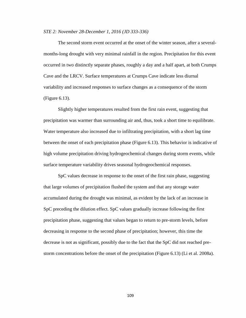
109

STE 2: November 28-December 1, 2016 (JD 333-336)

The second storm event occurred at the onset of the winter season, after a several-

months-long drought with very minimal rainfall in the region. Precipitation for this event

occurred in two distinctly separate phases, roughly a day and a half apart, at both Crumps

Cave and the LRCV. Surface temperatures at Crumps Cave indicate less diurnal

variability and increased responses to surface changes as a consequence of the storm

(Figure 6.13).

Slightly higher temperatures resulted from the first rain event, suggesting that

precipitation was warmer than surrounding air and, thus, took a short time to equilibrate.

Water temperature also increased due to infiltrating precipitation, with a short lag time

between the onset of each precipitation phase (Figure 6.13). This behavior is indicative of

high volume precipitation driving hydrogeochemical changes during storm events, while

surface temperature variability drives seasonal hydrogeochemical responses.

SpC values decrease in response to the onset of the first rain phase, suggesting

that large volumes of precipitation flushed the system and that any storage water

accumulated during the drought was minimal, as evident by the lack of an increase in

SpC preceding the dilution effect. SpC values gradually increase following the first

precipitation phase, suggesting that values began to return to pre-storm levels, before

decreasing in response to the second phase of precipitation; however, this time the

decrease is not as significant, possibly due to the fact that the SpC did not reached pre-

storm concentrations before the onset of the precipitation (Figure 6.13) (Li et al. 2008a).

110

Figure 6.13 Crumps Cave-WF1 Storm Event JD333-336. Note the increase in CO2 and

decrease in pH, opposite of the responses during the summer storm.

Source: Created by the author.

111

The pH values gradually decrease at the onset of the first precipitation phase, and

continue to decrease throughout the course of the storm event, suggesting that high

precipitation contained excess dissolved CO2 from the topsoil. During the August storm,

excess antecedent moisture and degassing may have served to reduce the available CO2

in the soil; however, due to drought conditions, CO2 buildup in the soil may have

occurred prior to this storm, providing an ample supply to diffuse to the epikarst as a

dissolved constituent within the precipitation (Figure 6.13) (Pu et al. 2014a; Pu et al.

2014b). Likewise, CO2 concentrations increased significantly over the course of the storm

event, with the shift occurring around the onset of the first precipitation phase, and

continuing to increase as the storm progressed. This suggests that, while conduit flow

likely dominates at Crumps Cave, a high concentration of CO2 from the topsoil was still

present, which was then transported by the infiltrating precipitation (Figure 6.13).

Discharge peaked twice, with very short lag times between the onset of precipitation and

peak volume. The first precipitation phase resulted in significant increase in discharge,

which gradually decreased following the end of the first precipitation phase. Discharge

eventually returned to baseflow before the onset of the second precipitation phase,

indicating that water transference at Crumps Cave is conduit dominated, as evidenced by

the near immediate response to increased precipitation flushing the system (Figure 6.13).

At the LRCV-LRS (Figure 6.14) precipitation occurred in two separate phases,

with the first phase delivering increased precipitation rates versus the second phase.

Surface temperature increased as a result of the onset of the first precipitation event, with

a significant increase in between rain phases. Shortly following the end of the second

precipitation phase, surface temperature began to reduce, indicating that warmer air in

112

conjunction with the storm may have equilibrated with pre-storm colder air (Figure 6.14).

SpC response occurred shortly, following a lag time from the onset of the first

precipitation phase. Significant decreases in SpC values at that time indicate that

infiltrating water flushed higher concentrated water from the system, followed by a

gradual increase to above pre-storm values, which eventually stabilized around 350

µs/cm until registering the second precipitation phase, where another reduction in SpC

occurred, although not as significant (Figure 6.14) (Yang et al. 2012).

The pH gradually decreased over the course of the storm event, but did not show

any significant responses to precipitation, suggesting that infiltrating water potentially

contained lower concentrations of CO2, as evident by the mirrored response to pH by

CO2 concentrations over the course the storm. The gradual decrease in pH and the

gradual increase in CO2, except for a brief instance immediately, following the start of the

November 29 (JD334), when a slight decrease in both pH and CO2 occur in response to

the onset of the first precipitation phase. Discharge responded quickly to the first

precipitation event, with the peak of discharge occurring shortly after the peak rainfall;

however, discharge did not respond to the second precipitation phase, possibly due to the

fact that the majority of stored water was flushed from the system in the first rain phase,

forcing the epikarst to recharge its volumetric water supply (Yang et al. 2012).

Discharge volumes also remained slightly above baseflow for the duration of the

storm indicating that large volumes of water from both storage and precipitation were

moving through the system, which further suggests that the threshold required for

significant discharge response was exceeded.

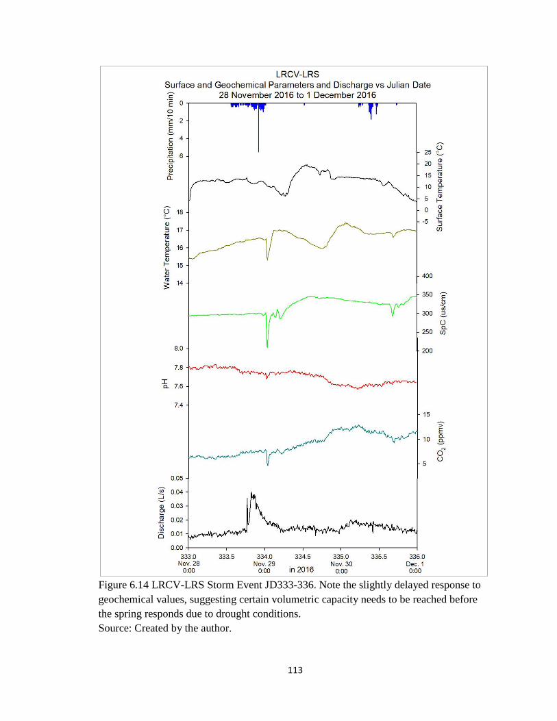
113

Figure 6.14 LRCV-LRS Storm Event JD333-336. Note the slightly delayed response to

geochemical values, suggesting certain volumetric capacity needs to be reached before

the spring responds due to drought conditions.

Source: Created by the author.

114

6.1.3 Influences on Epikarst δ13CDIC

The evolution of δ13CDIC in karst systems is influenced by external and internal

processes, including vegetation and soil respiration and bedrock dissolution, as discussed

and illustrated by Clark and Fritz (1997). Of these primary terrestrial sources, vegetation

and soil respiration seem to contribute the most (Li et al. 2010), especially on seasonal

scales. The data from this study suggest that seasonal influences from soil CO2 contribute

to dissolution processes at Crumps Cave, especially during the growing season, while soil

CO2 influences karst processes year-round at the LRCV. The primary difference between

the study sites, agricultural verses urban land use, provides a unique opportunity to

understand the sourcing and transport of δ13CDIC on a regional scale.

The δ13CDIC values at all four sites (Figures 5.1 and 5.2) indicate that seasonal

influences are having a great effect on the enrichment and depletion of δ13CDIC over the

entirety of the study period; however, that enrichment and depletion seem to be occurring

irrespective of precipitation, which in other studies is suggested to be a negligible

influence (Telmer and Veizer 1999; Lambert and Aharon 2010).

At Crumps Cave (WF1 and SF), seasonal variability is apparent, with values

showing greater depletion during the summer and greater enrichment during the

wintertime. Similar findings of δ13CDIC seasonal variability were found in other studies

(Telmer and Veizer 1999; Li et al. 2008a; Li et al. 2008b; Lambert and Aharon 2010; Li

et al. 2010; Zhao et al. 2015; Knierim et al. 2015; McClanahan et al. 2016), where it

appears that soil CO2 and vegetation cover contributed the most to δ13CDIC depletion,

especially due to fractionation effects within the topsoil from microbial activity being

more active during the summer months than during the winter. Over the course of the fall

115

months, δ13CDIC values enrich, with substantial enrichment occurring near the fall to

winter transition, and continuing until the end of the study. This increasing enrichment,

especially near the end of the study period and at the onset of the spring transition,

suggests that a certain lag time exists between vegetation root respiration and subsequent

microbial activity, depletion of δ13CDIC values, and registry of that depleted signal by

epikarst water (Li et al. 2010).

At the LRCV (LRS and LRWF), seasonal influences are slightly less apparent

than at Crumps Cave. While depletion of δ13CDIC values during the summer months

seems to trend similarly to the isotopic signatures at Crumps Cave, they diverge greatly at

the onset of the winter transition. The δ13CDIC values remain in a depleted state, which

could be a result of an urban environment masking the signal response (Li et al. 2010).

A substantial enrichment occurred at three of the four sites in the month of

September (JD 225) following a series of high precipitation events. Crumps Cave-WF1

and LRCV-LRWF showed higher enrichment compared to LRCV-LRS, while Crumps

Cave-SF showed the least enrichment. Knierim et al. (2015) suggested that, based on

similar findings in an investigation of Jack’s Cave in Arkansas, the magnitude of

different source inputs changes seasonally. For example, surface temperature is a proxy

for soil respiration (Clark and Fritz 1997; Knierim et al. 2015), and at lower temperatures

soil respiration rates are lower. For temperatures at or higher than 10 ºC, more microbial

activity is likely to occur, thus producing increased concentrations of soil CO2. Likewise,

more microbial activity is also responsible for the ongoing fractionation of 13C relative to

12C, causing increasingly depleted values of 13C (Clark and Fritz 1997; Knierim et al.

116

2015). The enrichment occurring at three of the four sites could be a result of a reduction

in fractionation effects derived from a reduction in plant root respiration.

Soil Respiration

Soil CO2 concentrations are a function of soil respiration, microbial activity, and

mineral weathering, and concentrations are partly contingent on soil thickness – thicker

soils equal increased concentrations of CO2 (Zhao et al. 2015). Thus, mineral weathering

is a product of soil CO2 concentrations after diffusion to the bedrock layer via infiltrating

precipitation and the presence of sufficient antecedent moisture, facilitates dissolution

(Pu et al. 2014a; Pu et al. 2014b; Knierim et al. 2015). Natural vegetation in temperate

and mid-latitude climate zones often operates using the C3 pathway, while certain

agricultural crops, such as corn and sugarcane, utilize the C4 pathway (Clark and Fritz

1997). As vegetation dies, microbial activity breaks down the decayed matter and

generates CO2; thus soil CO2 is higher in concentrations than the atmosphere on average

(Clark and Fritz 1997; Pu et al. 2014a; Pu et al. 2014b; Zhao et al. 2015).

Bedrock Dissolution

Carbonate rocks are generally derived from marine sediments and have a δ13C

value close to zero (Clark and Fritz 1997). Carbonate dissolution processes are heavily

dependent on the amount of CO2 available to react with the bedrock via carbonic acid,

which should yield a δ13CDIC value of –11.5‰ (Pu et al. 2014a; Pu et al. 2014b).

According to Clark and Fritz (1997), if completely open conditions exist, the δ13C value

will be controlled by the soil CO2, due to an ongoing replenishment interacting with the

bedrock. On the other hand, if the system is closed, then a finite supply of CO2 is

117

available, and eventually the δ13C will be diluted with DIC purely from carbonate

dissolution. Understanding the relationship values between pCO2, DIC, and δ13C can

provide insight into the conditions of the system, be it open or closed, or a combination of

both. Further, in open conditions, regardless of the type of vegetation (C3 or C4), final

groundwater values of δ13CDIC will be enriched by about 7‰ from the original soil CO2.

This enrichment is primarily due to the fact that CO2 and DIC have reached equilibrium

at increasing values of pH. In closed systems, similar enrichments occur; however, those

enrichments reflect a direct, linear one-to-one relationship between δ13CDIC and CO2

dissolved during recharge (Cerling 1984; Fritz et al. 1989; Cerling et al. 1991; Clark and

Fritz 1997; Cane and Clark 1999).

δ13CDIC Sourcing at Crumps Cave (WF1 and SF)

Results from carbon source identification using mixing model software with

inputs from the atmosphere, soil water, and carbonate bedrock were compared to identify

specific CO2 sources seasonally. At Crumps Cave WF1 and SF (Figure 5.3 and 5.4),

carbon isotopic sourcing indicates soil CO2 dominates during the summer months,

shifting to atmospheric CO2 dominating during the winter months. As vegetation cover

reduces and microbial activity turns dormant during the winter months, the majority of

CO2 in the system is derived from the atmosphere, simply due to the reduction in soil

derived CO2 signals.

The trends and seasonal shift of carbon sourcing align with isotopic trends of

δ13C, as illustrated in Figure 5.1. Seasonal shifts from soil CO2 to atmospheric CO2

coincides with the completion of the growing season, indicating that supplies of soil CO2

have significantly reduced, no longer contributing as greatly to epikarst waters (Knierim

118

et al. 2015) (Figures 5.3 and 5.4). Likewise, carbonate weathering sources during the

summer months were relatively low, suggesting that, while dissolution is occurring, an

increased soil CO2 signal is masking all other signals (Bakalowicz 2004; Klimchouk

2004) (Figures 5.3 And 5.4). However, atmospheric and carbonate bedrock weathering

sources increased during the winter months, while the soil CO2 signal was much weaker.

Atmospheric CO2 dominance versus carbonate weathering is a result of the overall

minimal residence times and less available CO2 to react with the bedrock (Figures 5.3

and 5.4; Figure 6.1).

In a study conducted by Li et al. (2010), seasonally fluctuating soil CO2 suggested

similar drivers are at work in karst landscapes in China. The authors found that this

increase in soil CO2 drives carbonate weathering and increases dissolution, and that the

shift in soil CO2 resulting from vegetation and microbial activity is responsible for the

evident seasonal pattern associated with carbonate sourcing. Likewise, Zhao et al. (2015)

found that an investigation into three catchment basins with varying soil thickness and

land uses rendered similar seasonal shifting in carbon sources. In that investigation, the

catchment used primarily for agricultural purposes and contained relatively thick soils;

however, bedrock dissolution was reduced, due to the fact that the groundwater flow path

was short and well developed, facilitating fairly easy transference to the aquifer with

minimal water-rock interaction. In both of those investigations, the reduction of soil CO2

contributions during the wintertime allowed for atmospheric and carbonate dissolution

signals to become more pronounced over time.

Similarly, an investigation into speleothem growth by Lambert and Aharon

(2010) suggested that, in karst landscapes with relatively quick water transport through

119

the epikarst, chemical equilibrium with 13C-depleted soil CO2 may retain a higher

atmospheric CO2 signal. This phenomenon would explain why atmospheric CO2

dominates during the wintertime, when depleted soil CO2 signals exist, due to the

reduction in vegetation cover and microbial activity combined with winter storms

facilitating the movement of water through the epikarst.

δ13CDIC Sourcing at LRCV (LRS and LRWF)

Carbon sourcing at LRS and LRWF (Figures 5.5 and 5.6) is dominated by soil

CO2 throughout the majority of the study period. Atmospheric contributions at both sites

are heavily masked by the strong soil CO2 signal, while the bedrock weathering signal

shows the least contributions over the course of the study period. Although residence

times at LRS and LRWF are significantly higher throughout the study period, allowing

for more soil CO2 equilibrium and water-rock interaction, certain high precipitation

events serve to flush the system with fresh meteoric water, mixing end members and

disrupting the signal (Lambert and Aharon 2010).

The masking of all other source signals could result from the fact that the LRCV

is located within Bowling Green, KY, a large urban environment (Figures 5.5 and 5.6).

Seasonal contributions from agricultural practices are relatively absent, which can

influence soil CO2 signals during the summer months. Cuezva et al. (2011) found,

through an investigation of both wet and dry periods, that soil moisture has a direct effect

on CO2 exchange between the atmosphere and the epikarst (Figure 6.20). They

discovered that increased moisture in the soil facilitates transference of CO2 into the

epikarst while preventing degassing to the atmosphere. Further, a lack of moisture during

the dry period actually allows for more atmospheric exchange of CO2 with the epikarst.

120

This is most likely the case during the dry season and in between rain events over the

winter months at Crumps Cave, where soil moisture is reduced or nearly absent, allowing

for facilitation of CO2 transference to the atmosphere and a greater atmospheric CO2

sourcing signal; however, despite similar seasonal soil conditions at the LRCV, this

atmospheric exchange may not be occurring, due to the presence of an impermeable

surface layer above the soil layer trapping CO2 in the soil throughout the study period.

This impermeable surface trapping of CO2 in the soil could also be responsible for

the dominant soil CO2 sourcing signal rendered in the IsoSource analysis. Likewise, Zhao

et al. (2015) discovered that agricultural land use practices continue to enhance signals

during the summer months and degrade signals during the winter months. Without this

contribution at LRCV, soil CO2 signal attenuation is less skewed. Lastly, due to the dual

porosity nature of the LRCV (Charlier et al. 2012), combined with more direct runoff

injection to the aquifer and less precipitation based soil CO2 transference to the epikarst,

CO2 signals experience a lag time in registry at the spring, as suggested by the overall

higher soil CO2 signal throughout the course of the study period at both sites.

Bedrock dissolution and atmospheric signals make up relatively small percentages

at both sites over the course of the study period and especially during the summer. At

LRWF (Figure 5.6) atmospheric contributions increase to over 40% at the onset of the

winter season for roughly the months of November and December, before decreasing

again in the month of February and March (Figures 5.5 and 5.6). The variability of

surface temperatures during the month of January, combined with a relatively warm

winter season, could result in a reactivation of soil microbial activity, despite an absence

of vegetation growth.

121

The increase in soil CO2 values in the month of February and March could be a

reflection of lag time between the generation of soil CO2 and its transference to the

spring, further supporting a slow diffusion through the epikarst. Precipitation appears as a

negligible influence on the transport of CO2, especially through the soil zone, similar to

studies that suggest precipitation can serve to generate disequilibrium between end

members (Lambert and Aharon 2010). Additionally, Knierim et al. (2015) found that

during the transition between dry and wet seasons, disequilibrium is greatest between

CO2 and DIC. The possibility of most precipitation being channeled through injection

wells in Bowling Green means it would bypass the soil zone; thus, soil CO2

concentrations would remain high even during the wintertime (Figures 5.5 and 5.6).

6.1.4 Conduit Dissolution and DIC Flux

Dissolution rates and individual conduit wall retreats were calculated (Eq. 4.1 and

4.2) to better determine the extent of epikarst development that may be occurring at all

four sites (Table 6.1). Likewise, mass DIC fluctuation over the study period was

calculated (Eq. 4.3) for WF1 and LRS utilizing high-resolution discharge (Table 6.1;

Figure 6.15). Wall retreats were calculated for each site to provide a general idea of the

extent of conduit growth; however, the results are limited by the fact that the Palmer

equation yields values referenced to a single conduit, not the extent of conduit

development throughout the entire epikarst. Since identifying specific conduits that may

or may not be growing is impossible without further geophysical investigations,

dissolution rates, which are expressed as a volume of material removed during a specific

time period, are more representative of the extent of epikarst development occurring at

each site during the study period.

122

Wall retreats at Crumps Cave (WF1 and SF) indicate that conduit growth rate is

greater at WF1, at 1,224.17 cm over the study period, and lower at SF at 1.36 cm over the

study period. Total dissolution, or volume of calcite material removed over the study

period, is higher at WF1 as well, with a total calculated volume of 0.18 kg/m3 over the

study period, while much lower at SF, at 0.000396 kg/m3 of total calculated volume over

the study period.

At the LRCV (LRS and LRWF), wall retreat values are significantly different

from one another, and considerably higher than at Crumps Cave, on average 841 cm over

the study period at LRS and 105,205 cm over the study period at the LRWF. Higher

saturation indexes at LRS and LRWF suggest that more precipitation is occurring than

dissolution, as evident by the presence of a flowstone and rimstone dam near LRWF, and

indicated by a negative value for the total calculated dissolution over the study period at

both sites. Conversely, since maximum calculated values of dissolution yielded positive

numbers, 0.00121 kg/m3 at LRS and 0.00274 kg/m3 at LRWF, respectively, at least some

dissolution of calcite is occurring at both sites. On the other hand, Covington et al.

(2015), found that dissolution rates are, at best, a rough estimate of conduit evolution,

primarily due to the suggestion that mechanical weathering has a greater impact on

material removal than chemical weathering. In that study, the PWP equation was applied

to over 59 surface stream study sites, where more variability from surface process were

observed, as opposed to dominant chemical weathering processes in the epikarst, which

can be partially buffered from surface influences by depth. Covington et al. (2015)

explained that low value variability of calcite dissolution can derive from several

influences, with low CO2 concentrations governing increased pH values as the primary

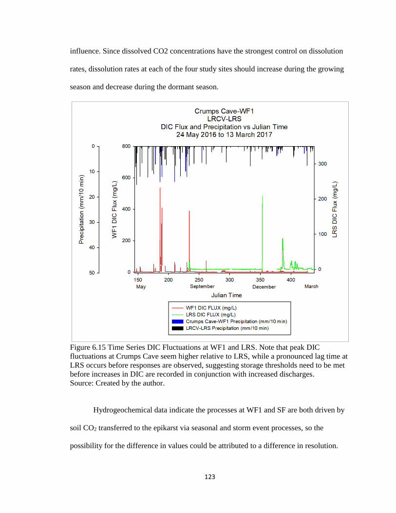
123

influence. Since dissolved CO2 concentrations have the strongest control on dissolution

rates, dissolution rates at each of the four study sites should increase during the growing

season and decrease during the dormant season.

Figure 6.15 Time Series DIC Fluctuations at WF1 and LRS. Note that peak DIC

fluctuations at Crumps Cave seem higher relative to LRS, while a pronounced lag time at

LRS occurs before responses are observed, suggesting storage thresholds need to be met

before increases in DIC are recorded in conjunction with increased discharges.

Source: Created by the author.

Hydrogeochemical data indicate the processes at WF1 and SF are both driven by

soil CO2 transferred to the epikarst via seasonal and storm event processes, so the

possibility for the difference in values could be attributed to a difference in resolution.

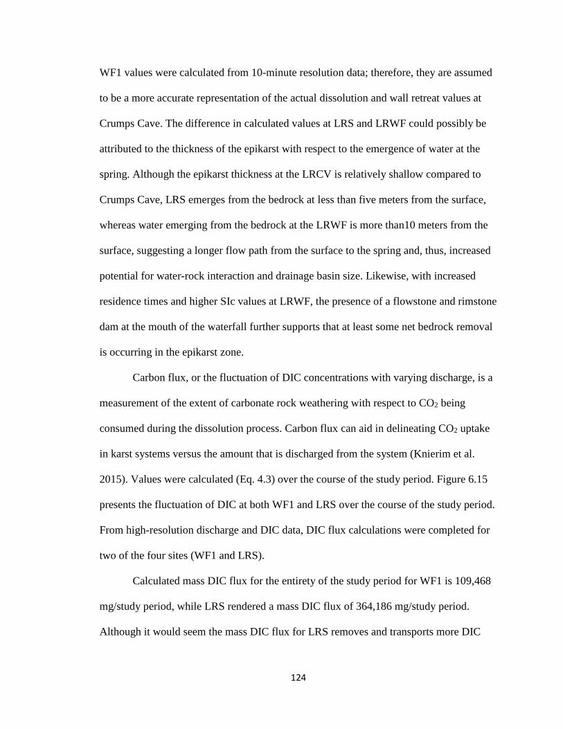
124

WF1 values were calculated from 10-minute resolution data; therefore, they are assumed

to be a more accurate representation of the actual dissolution and wall retreat values at

Crumps Cave. The difference in calculated values at LRS and LRWF could possibly be

attributed to the thickness of the epikarst with respect to the emergence of water at the

spring. Although the epikarst thickness at the LRCV is relatively shallow compared to

Crumps Cave, LRS emerges from the bedrock at less than five meters from the surface,

whereas water emerging from the bedrock at the LRWF is more than10 meters from the

surface, suggesting a longer flow path from the surface to the spring and, thus, increased

potential for water-rock interaction and drainage basin size. Likewise, with increased

residence times and higher SIc values at LRWF, the presence of a flowstone and rimstone

dam at the mouth of the waterfall further supports that at least some net bedrock removal

is occurring in the epikarst zone.

Carbon flux, or the fluctuation of DIC concentrations with varying discharge, is a

measurement of the extent of carbonate rock weathering with respect to CO2 being

consumed during the dissolution process. Carbon flux can aid in delineating CO2 uptake

in karst systems versus the amount that is discharged from the system (Knierim et al.

2015). Values were calculated (Eq. 4.3) over the course of the study period. Figure 6.15

presents the fluctuation of DIC at both WF1 and LRS over the course of the study period.

From high-resolution discharge and DIC data, DIC flux calculations were completed for

two of the four sites (WF1 and LRS).

Calculated mass DIC flux for the entirety of the study period for WF1 is 109,468

mg/study period, while LRS rendered a mass DIC flux of 364,186 mg/study period.

Although it would seem the mass DIC flux for LRS removes and transports more DIC

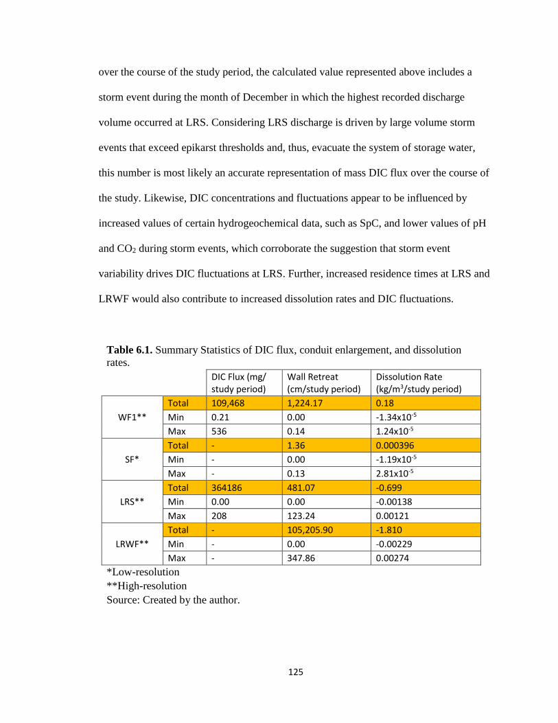
125

over the course of the study period, the calculated value represented above includes a

storm event during the month of December in which the highest recorded discharge

volume occurred at LRS. Considering LRS discharge is driven by large volume storm

events that exceed epikarst thresholds and, thus, evacuate the system of storage water,

this number is most likely an accurate representation of mass DIC flux over the course of

the study. Likewise, DIC concentrations and fluctuations appear to be influenced by

increased values of certain hydrogeochemical data, such as SpC, and lower values of pH

and CO2 during storm events, which corroborate the suggestion that storm event

variability drives DIC fluctuations at LRS. Further, increased residence times at LRS and

LRWF would also contribute to increased dissolution rates and DIC fluctuations.

Table 6.1. Summary Statistics of DIC flux, conduit enlargement, and dissolution

rates.

DIC Flux (mg/ study period)

Wall Retreat (cm/study period)

Dissolution Rate (kg/m3/study period)

WF1**

Total 109,468 1,224.17 0.18

Min 0.21 0.00 -1.34x10-5

Max 536 0.14 1.24x10-5

SF*

Total - 1.36 0.000396

Min - 0.00 -1.19x10-5

Max - 0.13 2.81x10-5

LRS**

Total 364186 481.07 -0.699

Min 0.00 0.00 -0.00138

Max 208 123.24 0.00121

LRWF**

Total - 105,205.90 -1.810

Min - 0.00 -0.00229

Max - 347.86 0.00274

*Low-resolution

**High-resolution

Source: Created by the author.

126

6.1.5 Low-Resolution δ13CDIC, CO2, SIc, DIC Site Comparisons

The data for low-resolution calculated CO2 and DIC versus δ13CDIC on a temporal

basis are presented in Figures 6.16 to 6.19 for both Crumps Cave (WF1 and SF) and

LRCV (LRS and LRWF). These data are presented to illustrate the statistical robustness

of both the measured weekly resolution of geochemical data and the calculated high-

resolution of geochemical data reported earlier in the thesis. Data illustrating individual

low-resolution versus time series for CO2, SIc, and DIC concentrations, and δ13CDIC

values, at each site, are in Appendix 5.

For Crumps Cave (WF1 and SF), both CO2 and DIC (Figures 6.16 and 6.17)

values track with δ13CDIC values during the summertime, indicating that ongoing root

respiration and soil CO2 production are causing a depletion in δ13CDIC values while

driving CO2 and DIC concentrations in the epikarst (Jiang 2013). During the wintertime,

as vegetation and microbial activity decreases, due to surface changes, the tracking of

CO2, DIC, and δ13CDIC diverge. The δ13CDIC values become more enriched as CO2

production and DIC concentrations severely reduce. This is indicative of the reduction in

fractionation of the 12/13C isotope caused by root respiration and microbial activity and

thus, a shifting in carbon sourcing from soil to atmosphere (Faimon et al. 2012a; 2012b).

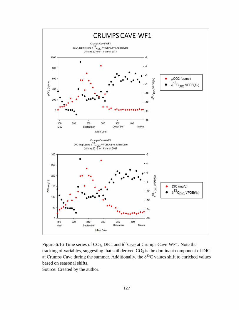
127

Figure 6.16 Time series of CO2, DIC, and δ13CDIC at Crumps Cave-WF1. Note the

tracking of variables, suggesting that soil derived CO2 is the dominant component of DIC

at Crumps Cave during the summer. Additionally, the δ13C values shift to enriched values

based on seasonal shifts.

Source: Created by the author.

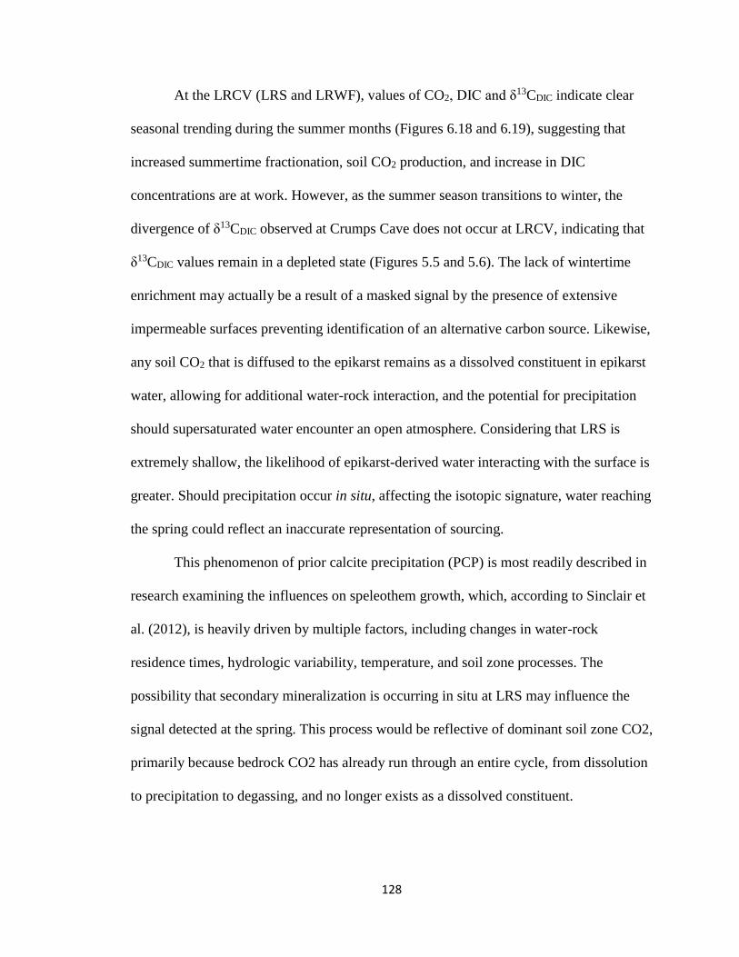
128

At the LRCV (LRS and LRWF), values of CO2, DIC and δ13CDIC indicate clear

seasonal trending during the summer months (Figures 6.18 and 6.19), suggesting that

increased summertime fractionation, soil CO2 production, and increase in DIC

concentrations are at work. However, as the summer season transitions to winter, the

divergence of δ13CDIC observed at Crumps Cave does not occur at LRCV, indicating that

δ13CDIC values remain in a depleted state (Figures 5.5 and 5.6). The lack of wintertime

enrichment may actually be a result of a masked signal by the presence of extensive

impermeable surfaces preventing identification of an alternative carbon source. Likewise,

any soil CO2 that is diffused to the epikarst remains as a dissolved constituent in epikarst

water, allowing for additional water-rock interaction, and the potential for precipitation

should supersaturated water encounter an open atmosphere. Considering that LRS is

extremely shallow, the likelihood of epikarst-derived water interacting with the surface is

greater. Should precipitation occur in situ, affecting the isotopic signature, water reaching

the spring could reflect an inaccurate representation of sourcing.

This phenomenon of prior calcite precipitation (PCP) is most readily described in

research examining the influences on speleothem growth, which, according to Sinclair et

al. (2012), is heavily driven by multiple factors, including changes in water-rock

residence times, hydrologic variability, temperature, and soil zone processes. The

possibility that secondary mineralization is occurring in situ at LRS may influence the

signal detected at the spring. This process would be reflective of dominant soil zone CO2,

primarily because bedrock CO2 has already run through an entire cycle, from dissolution

to precipitation to degassing, and no longer exists as a dissolved constituent.

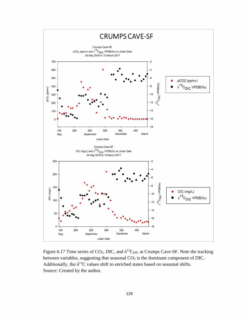
129

Figure 6.17 Time series of CO2, DIC, and δ13CDIC at Crumps Cave-SF. Note the tracking

between variables, suggesting that seasonal CO2 is the dominant component of DIC.

Additionally, the δ13C values shift to enriched states based on seasonal shifts.

Source: Created by the author.

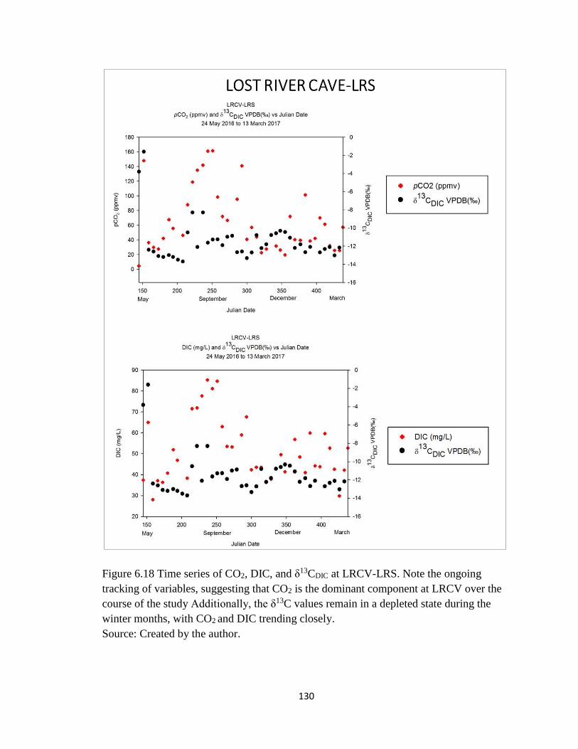
130

Figure 6.18 Time series of CO2, DIC, and δ13CDIC at LRCV-LRS. Note the ongoing

tracking of variables, suggesting that CO2 is the dominant component at LRCV over the

course of the study Additionally, the δ13C values remain in a depleted state during the

winter months, with CO2 and DIC trending closely.

Source: Created by the author.

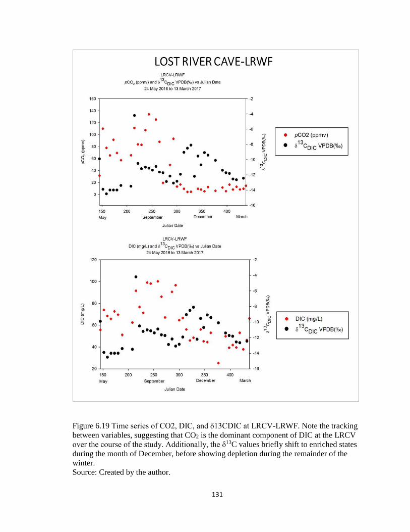
131

Figure 6.19 Time series of CO2, DIC, and δ13CDIC at LRCV-LRWF. Note the tracking

between variables, suggesting that CO2 is the dominant component of DIC at the LRCV

over the course of the study. Additionally, the δ13C values briefly shift to enriched states

during the month of December, before showing depletion during the remainder of the

winter.

Source: Created by the author.

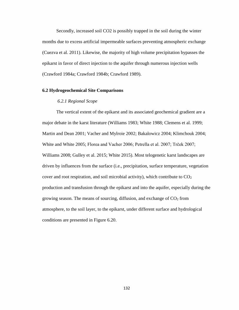
132

Secondly, increased soil CO2 is possibly trapped in the soil during the winter

months due to excess artificial impermeable surfaces preventing atmospheric exchange

(Cuezva et al. 2011). Likewise, the majority of high volume precipitation bypasses the

epikarst in favor of direct injection to the aquifer through numerous injection wells

(Crawford 1984a; Crawford 1984b; Crawford 1989).

6.2 Hydrogeochemical Site Comparisons

6.2.1 Regional Scope

The vertical extent of the epikarst and its associated geochemical gradient are a

major debate in the karst literature (Williams 1983; White 1988; Clemens et al. 1999;

Martin and Dean 2001; Vacher and Mylroie 2002; Bakalowicz 2004; Klimchouk 2004;

White and White 2005; Florea and Vacher 2006; Petrella et al. 2007; Trček 2007;

Williams 2008; Gulley et al. 2015; White 2015). Most telogenetic karst landscapes are

driven by influences from the surface (i.e., precipitation, surface temperature, vegetation

cover and root respiration, and soil microbial activity), which contribute to CO2

production and transfusion through the epikarst and into the aquifer, especially during the

growing season. The means of sourcing, diffusion, and exchange of CO2 from

atmosphere, to the soil layer, to the epikarst, under different surface and hydrological

conditions are presented in Figure 6.20.

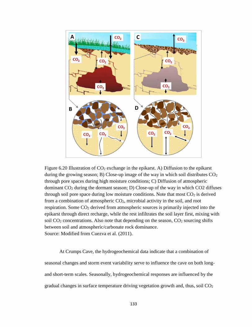
133

Figure 6.20 Illustration of CO2 exchange in the epikarst. A) Diffusion to the epikarst

during the growing season; B) Close-up image of the way in which soil distributes CO2

through pore spaces during high moisture conditions; C) Diffusion of atmospheric

dominant CO2 during the dormant season; D) Close-up of the way in which CO2 diffuses

through soil pore space during low moisture conditions. Note that most CO2 is derived

from a combination of atmospheric CO2, microbial activity in the soil, and root

respiration. Some CO2 derived from atmospheric sources is primarily injected into the

epikarst through direct recharge, while the rest infiltrates the soil layer first, mixing with

soil CO2 concentrations. Also note that depending on the season, CO2 sourcing shifts

between soil and atmospheric/carbonate rock dominance.

Source: Modified from Cuezva et al. (2011).

At Crumps Cave, the hydrogeochemical data indicate that a combination of

seasonal changes and storm event variability serve to influence the cave on both long-

and short-term scales. Seasonally, hydrogeochemical responses are influenced by the

gradual changes in surface temperature driving vegetation growth and, thus, soil CO2

134

production, especially during the summer months. Groves et al. (2005) found storage at

Crumps Cave exists within the epikarst, governed by the thin layer of chert, which

potentially creates a leaky, perched aquifer. This perched aquifer could partially inhibit

direct flow from the surface to the vadose zone, except during times of high precipitation

when the system is discharged of storage water. The near immediate responses in all

hydrogeochemical data at both WF1 and SF during storm events further indicate that

ongoing storage is occurring, which is then flushed through the system during those

storm events. Further, increased seasonal DIC fluctuations and dissolution rates, as well

as reduced overall wall retreat, suggest that conduit development in the epikarst has

reached a critical slow point during the winter months, as discussed in Palmer (1991;

2007a; 2007b), where development is relatively contingent on continuous aggressive

water-rock interaction in a dissolvable medium.

In this respect, dissolution rates are higher during the growing season, due to

increased water aggressiveness from an increased supply of soil CO2. Rates slow during

the dormant season as soil CO2 sourcing shifts to atmospheric CO2 sourcing. This shift in

CO2 sourcing serves to slowdown dissolution. Further, despite colder water being capable

of holding more dissolved CO2, the reduction in a highly concentrated supply of CO2

negates that capability, also providing for a reduction in dissolution kinetics. Likewise, as

calcite saturation approaches saturated to supersaturated levels, the rate of dissolution

slows further, even when increased water-rock interaction occurs during the dry season.

On the other hand, during the growing season, despite high volume precipitation events

transferring water quickly through the epikarst, thus reducing residence time, the water is

supersaturated with soil CO2 concentrations, driving aggressive dissolution.

135

The LRCV sites exhibit different responses than Crumps Cave sites, primarily due

to the urban environment governing soil and vegetation extent, CO2 sourcing and

diffusion in the epikarst, and seasonal variability in hydrogeochemical data. The presence

of a heavily paved (and rather impermeable) urban landscape on the surface, in

conjunction with an impermeable chert layer at the water table, contributes to a unique

development of the epikarst at both the LRS and LRWF. This unique situation is derived

from the potential trapping of soil CO2 in the soil layer beneath the paved surface layer,

which diffuses to the epikarst at a much slower rate overall, due to a reduction in

infiltrating precipitation and antecedent moisture conditions.

The hydrogeochemical data indicate that, while seasonal variability is less

apparent, responses to storm events drive the movement of epikarst water. It is during

these high precipitation events that soil CO2 diffusion to the epikarst increases. Further,

the presence of the chert layer at the water table (Groves 1987), which significantly slows

further reductions in the water table, may potentially contribute to an upward diffusion of

CO2 at LRS, generating heterogeneous pockets of increased CO2 concentrations (which

diffuse to areas of lower CO2 concentrations) providing for increased dissolution in a

lateral and vertical gradient, as observed in eogenetic karst systems by Gulley et al.

(2005). As a consequence, certain volumetric thresholds are required to be met before

increases in discharge are observed. The epikarst at LRCV behaves similarly to that of

eogenetic karst, as observed by Gulley et al. (2015), where heterogeneous CO2 diffusion

causes conduits to form independent of telogenetic governed hydraulic conductivity.

This unique combination of governing characteristics serves to increase dissolution rates

and wall retreats, as well as DIC fluxes, over the course of the study period; however,

136

calcite saturation at both LRCV sites is continuously high, as evident by the presence of a

growing flowstone at LRWF. This suggests that dissolution kinetics are governed by the

extent of saturation, as well as the contribution of CO2, and that CO2 sourcing is an

important driver of this process.

As mentioned earlier and shown in previous studies, the presence of a chert layer

at both locations may be governing water storage and transference and, thus, water-rock

interaction and residence times. A comparison of mean discharges and their respective

ranges at the four study sites in this investigation, as well as other springs around the

world, is presented in Table 6.2. Precipitation and recharge time series analysis for all

four sites are presented in graphical form in Appendix 6. The majority of aquifer

discharges at different sites around the world render slightly higher volumes in averages,

peak flows, and baseflows, compared to epikarst discharges, suggesting that the epikarst

can serve to store water, but volumetrically it does not equate to primary aquifer storage.

On the other hand, although discharge in the epikarst is reduced comparatively to the

main aquifer, CO2 flux and dissolution processes are greater in the epikarst, due to the

open system nature of most landscapes with surface influences. These processes drive

dissolution kinetics throughout the aquifer, with the majority of those processes occurring

at relatively shallow depths (between 10 to 30 meters) (Bakalowicz 2004; Klimchouk

2004). Thus, aquifer development and karst landscape evolution are highly contingent on

the status of dissolution kinetics and CO2 fluctuations in the epikarst.

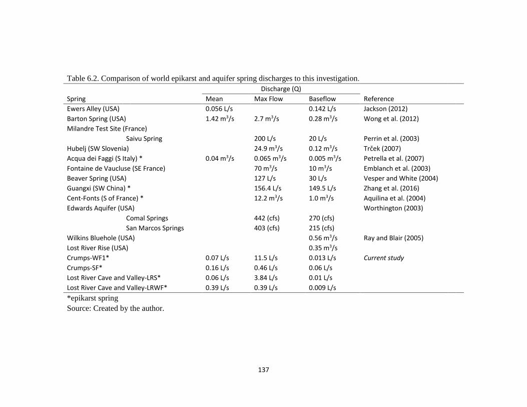
137

Table 6.2. Comparison of world epikarst and aquifer spring discharges to this investigation.

Discharge (Q) Spring

Mean Max Flow Baseflow Reference Ewers Alley (USA)

0.056 L/s

0.142 L/s Jackson (2012)

Barton Spring (USA)

1.42 m3/s 2.7 m3/s 0.28 m3/s Wong et al. (2012)

Milandre Test Site (France)

Saivu Spring

200 L/s 20 L/s Perrin et al. (2003)

Hubelj (SW Slovenia)

24.9 m3/s 0.12 m3/s Trček (2007)

Acqua dei Faggi (S Italy) * 0.04 m3/s 0.065 m3/s 0.005 m3/s Petrella et al. (2007)

Fontaine de Vaucluse (SE France)

70 m3/s 10 m3/s Emblanch et al. (2003)

Beaver Spring (USA)

127 L/s 30 L/s Vesper and White (2004)

Guangxi (SW China) *

156.4 L/s 149.5 L/s Zhang et al. (2016)

Cent-Fonts (S of France) *

12.2 m3/s 1.0 m3/s Aquilina et al. (2004)

Edwards Aquifer (USA)

Worthington (2003)

Comal Springs

442 (cfs) 270 (cfs)

San Marcos Springs

403 (cfs) 215 (cfs)

Wilkins Bluehole (USA)

0.56 m3/s Ray and Blair (2005)

Lost River Rise (USA)

0.35 m3/s

Crumps-WF1* 0.07 L/s 11.5 L/s 0.013 L/s Current study

Crumps-SF* 0.16 L/s 0.46 L/s 0.06 L/s

Lost River Cave and Valley-LRS* 0.06 L/s 3.84 L/s 0.01 L/s

Lost River Cave and Valley-LRWF* 0.39 L/s 0.39 L/s 0.009 L/s

*epikarst spring

Source: Created by the author.

138

Hydrogeochemical processes at Crumps Cave and at locations in China, Italy,

and France all exhibit certain responses to surface influences driving dissolution kinetics

governed by seasonal and storm event variability. At the LRCV, the presence of an urban

landscape plays a vital role on the development of the epikarst with respect to carbon

sourcing and diffusion, and dissolution kinetics and DIC fluctuations.

Previous karst investigations focused primarily on aquifer processes, where it is

assumed that the influences governing the majority of karst development are the greatest,

and thus require the most attention (Veni et al. 2001; Aquilina et al. 2004; Palmer 2007a;

Worthington 2007; De Waele et al. 2009; Anaya et al. 2014). As a consequence, the

epikarst is often overlooked as a large contributor to karst landscape development. Those

investigations that do focus on the epikarst suggest that the upper layer of the karst

system plays a vital role in geochemical influences (White 1988; Emblanch et al. 2003;

Bakalowicz 2004; Klimchouk 2004); however, the majority of those investigations are

limited to single cave systems under similar conditions such as land use, epikarst

thickness, and climate. Further, only a handful of those investigations have examined

epikarst processes in high resolution to characterize immediate changes as a way to

delineate the primary and secondary hydrogeochemical drivers to aquifer development

(Zhongcheng and Daoxian 1999; Bakalowicz 2004; Palmer 2007a; Petrella et al. 2007;

Trček 2007; White 2007; Jacob et al. 2009; Liu et al. 2010; Yang et al. 2012; Peyraube et

al. 2014; Milanolo and Gabrovšek 2015; Zhang et al. 2016). This investigation aimed to

combine those elements (epikarst hydrogeochemical high-resolution monitoring in

multiple karst systems under various land uses) to further delineate the influence of those

139

variables on epikarst processes and their extent of impact on aquifer evolution in

telogenetic karst systems.

The results of this investigation indicate that under natural and agricultural

settings, dissolution kinetics in the epikarst are driven by surface viability, such as

precipitation and temperature, which govern the availability of soil CO2 and its

subsequent diffusion to the epikarst. Seasonal changes are the most prominent driving

factor for increased production of CO2, while high-volume storm events facilitate the

diffusion of these large concentrations of CO2 to the epikarst where dissolution can

actually occur.

While concentrations of CO2 and DIC at Crumps Cave and the LRCV are

relatively similar, the methods by which they diffuse to the epikarst are different.

Likewise, the way the epikarst processes these constituents is also different. While a

natural landscape may seem more conducive to karst development, in this study the data

suggest that an urban environment can facilitate dissolution and supersaturation,

redistributing bedrock and possibly contributing to potential karst landscape hazards,

such as water containment storage and transport. Thus, urban landscapes, it would seem,

have relatively important impacts on hydrogeochemical processes in karst systems. Those

impacts can have negative effects on the human population as urban sprawl becomes

more and more of a contributor to the way that the epikarst responds and to any

subsequent influences on aquifer development and drinking water quality.

140

Chapter 7: Conclusions

Understanding the hydrogeochemical relationships with storage and flow

propensity in various karst settings is crucial to tying together certain fundamental

concepts about the primary functionality of the epikarst with respect to deeper

geochemical processes. Further, tracking carbon through the epikarst as a means to

understand dissolution kinetics and the propensity for karst systems to serve as carbon

sinks is extremely important, especially considering the growing concern over the

accumulation of atmospheric carbon dioxide released from anthropogenic activities.

Additionally, DIC fluctuations can illustrate how carbon is utilized by karst systems,

further illuminating the extent to which vast deposits of terrestrial limestone may serve as

carbon sinks (Zhang et al. 2015).

The Pennyroyal Sinkhole Plain in southcentral Kentucky has been the focus of

karst research for decades (Crawford 1984a; Crawford 1984b; Crawford 1989; Crawford

2003; Crawford 2005; Brewer and Crawford 2005; Cesin and Crawford 2005;

Vanderhoff 2011; Nedvidek 2014). Of those studies, the majority addressed cave

development and aquifer processes at varying resolutions (Palmer 2007a; Vanderhoff

2011; Lawhon 2014; Nedvidek 2014). Examinations into individual caves and their

hydrogeochemical processes have left a gap in the literature, allowing for a comparative

study with respect to multiple karst systems as a means to understand how those same

processes operate on a regional scale.

This investigation examined two cave systems under different land use

conditions, with a focus on epikarst hydrogeochemical processes and how those

processes serve to influence dissolution rates and conduit development in the epikarst.

141

Further, tracking carbon from inception to discharge can better infer both carbon uptake

in karst systems and a karst landscape’s role in the global carbon flux calculation. This

investigation yielded the following findings:

Seasonal, diurnal, and storm event variability serve to influence

hydrogeochemical dissolution processes through the diffusion of soil CO2.

Surface influences, such as temperature and precipitation, contribute to CO2

production and diffusion during the growing period; however, CO2 diffusion to

the epikarst is variable by location, with Crumps Cave sites experiencing

dominant seasonal diffusion, while the LRCV sites experienced dominant storm

event diffusion once certain antecedent moisture thresholds were met. The

dissimilarity in diffusion is due to land use differences, soil coverage, epikarst

thicknesses, and stages of epikarst development.

At Crumps Cave, storm event variability drives immediate hydrogeochemical

responses and facilitates movement of water through the epikarst, while seasonal

variability drives long-term changes, which influence dissolution processes via

the diffusion of CO2 as both a dissolved constituent in infiltrating, low-

precipitation events and antecedent moisture seepage.

At the LRCV, storm event variability is less pronounced, due to the urban

landscape interfering with natural recharge of the epikarst. This is in direct

contrast to the LRCV aquifer, which responds quite heavily to storm events

(Lawhon 2014). Seasonal changes are also less apparent, but longer residence

times and slower soil CO2 diffusion increase the rate of dissolution and

subsequent supersaturation.

142

Carbon uptake is heavily driven by soil CO2 in the summer months at both

locations, while primarily driven by atmospheric CO2 at Crumps Cave and soil

CO2 at the LRCV in the winter. This is primarily due to a difference in land use at

both locations, with Crumps Cave influenced by seasonal agricultural use and the

LRCV influenced by an urban setting, which aids in the reduction in the rate of

soil CO2 diffusion to the epikarst.

Telogenetic epikarst thickness and its internal conduit development are highly

contingent on the aforementioned dissolution rates. Crumps Cave epikarst appears

to be better developed than the LRCV, as evident by the near immediate response

to even minimal rainfall events, while LRCV sites require certain capacity

thresholds to be met before an increase in discharge is registered. This implies

that storage is occurring at both sites, with Crumps Cave’ capacity being greater

and able to transport more volume in shorter time periods, while the LRCV

experiences more matrix dominated flow. At the LRS, this matrix-dominated flow

could be a result of an extremely thin epikarst, while epikarst thickness at the

LRWF is less than that of Crumps Cave, but accommodating of water

transference at a volume greater than the LRS.

The differences in epikarst thickness and the presence of a rather impermeable

chert layer at both locations govern water residence times and, thus, the extent of

dissolution. As described by Williams (1983; 2008), Bakalowicz (2004), and

Klimchouk (2004), epikarst dissolution kinetics reduce and eventually cease at

depths between 10 to 30 meters, due to a shift from open system conditions to

closed system conditions. A shift from open system conditions to relatively closed

143

system conditions may be occurring at Crumps Cave, where 18 meters of epikarst

thickness exist between surface and epikarst drains. DIC concentrations and flux,

and saturation indexes, are lower at Crumps Cave versus the LRCV. Epikarst

thickness at the LRS is less than five meters and epikarst thickness at the LRWF

is roughly 13 meters. Likewise, isotopic soil signals at both LRCV sites are

stronger throughout the year, as well as increased dissolution rates, and greater

DIC fluctuations. DIC fluctuation calculations are a workable approach to

understanding how carbon sequestration and utilization in karst environments

operates, provided that similarities between examination sites exist, such as the

defining geology of the region. Conversely, even if land use and hydrological

differences are present (i.e. variability in storage and flow), the DIC fluctuation

calculations will illuminate the impact of these differences on overall carbon

utilization, further providing for insight into global carbon uptake in karst regions.

Generally, the investigation yielded many similarities between all sites, such as

hydrogeochemical responses driven primarily by soil CO2 seasonal influences and

secondarily by storm events; however, certain site specific characteristics, such as land

use cover and epikarst thickness, indicate that, indeed, the extent of epikarst development

and its associated hydrogeochemical processes are reliant on both geology and thickness

of the epikarst, for storage and flow variability were evident and unique to all sites

(Williams 1983; Worthington et al. 2000; Worthington 2003; Worthington 2007;

Bakalowicz 2004; Klimchouk 2004; Williams 2008).

Certain limitations of this project prohibit a more accurate representation of the

processes at work and, as such, assumptions were made, including the following:

144

Dissolution processes and carbon flux were contingent on discharge and

geochemical parameters. All values were calculated based on assumed sizes of

recharge basins, however, the exact area of recharge for all sites were unknown

for this study. Thus, it is important that future work address this issue to ensure an

exact quantitative assessment can be drawn with respect to the impact that the size

of the recharge basin has on each site’s DIC fluctuations and extent of storage.

At SF, low resolution of the collected data generated assumptions about responses

during events that occurred between collection dates.

At LRS, placement of the loggers was downstream from the sample collection

sitel; thus assumptions that the reach of the stream posed a negligible influence on

geochemical evolution were made.

At LRWF, failed access to the site on certain collection dates due to inclement

weather meant lost data, while low-resolution discharge required an assumption

regarding volumetric responses from precipitation influences. Lastly, the time

period for the study was short of a full year, primarily due to funding and

investigation timeline modifications due to extraneous circumstances. Thus, only

the onset of the spring transition was captured.

This investigation serves to contribute to the scientific understanding of epikarst

dissolution processes in mid-latitude regions, specifically southcentral Kentucky, with a

focus on hydrogeochemical and carbon isotope evolution. Further investigations along

similar lines could include continued high-resolution sample collection in all respects,

with an inclusion of technological monitoring at all sites. A closer examination of the

impact of an urban setting on carbon sourcing and transport at the LRCV, plus use of soil

145

CO2 utilization, with an emphasis on multi-year collection and monitoring, could increase

conceptual understanding on the processes at work in karst systems related to carbon flux

in varied land use settings around the world. Lastly, comparative analyses between

eogenetic karst systems and telogenetic epikarst systems are severely lacking in the

literature. The data from this investigation suggest that they exhibit similar behaviors and

thus, closer examinations are vital to understanding both epikarst and aquifer

development, especially in an ever-growing urban landscape.

146

References

Amundson, R., Stern, L., Baisden, T., Wang, Y. 1998. The isotopic composition of soil

and soil-respired CO2. Geoderma 82, 83-114.

Allen, D.M. 2004. Sources of groundwater salinity on islands using 18O, 2H, and 34S.

Groundwater 42(1), 17–31.

Anaya, A., Padilla, I., Macchiavelli, R., Vesper, D.J., Meeker, J.D., Alshawabkeh, A.N.

2014. Estimating preferential flow in karstic aquifers using statistical mixed

models. Groundwater 52(4), 584-596.

Aquilina, L., Ladouche, B., Dorfliger, N. 2004. Water storage and transfer in the epikarst

of karstic systems during high flow periods. Journal of Hydrology 327, 472-485.

Bakalowicz, M. 2004. The epikarst, the skin of karst. Karst Waters Institute Special

Publication 9, 16-22. Accessed on March 25, 2015 from:

https://www.researchgate.net/publication/267426221_THE_EPIKARST_THE_S

KIN_OF_KARST

Baldini, J.U.L., Baldini, L.M., McDermott, F., Clipson, N. 2006. Carbon dioxide sources,

sinks, and spatial variability in shallow temperate zone caves: Evidence from

Ballynamintra Cave, Ireland. Journal of Cave and Karst Studies 68(1), 4–11.

Blecha, M., Faimon, J. 2014a. Karst soils: dependence of CO2 concentrations on pore

dimension. Acta Carsologica 43(1), 55-64.

Blecha, M., Faimon, J. 2014b. Spatial and temporal variations in carbon dioxide (CO2)

concentrations in selected soils of the Moravian Karst (Czech Republic).

Carbonates Evaporites 29, 395-408.

Brewer, J., Crawford, N. 2005. Groundwater basin catchment delineation and

generalized flow routes through the karst aquifer beneath Bowling Green,

Kentucky, USA. Paper presented at the 14th International Congress of

Speleology, Athens, August 21-28. Hellenic Speleological Society P-15, 594-597.

Available online at:

http://www.ese.edu.gr/media/lipes_dimosiefsis/14isc_proceedings/p/15.pdf.

Cane, G., Clark, I.D. 1999. Tracing groundwater recharge in an agricultural watershed

with isotopes. Groundwater 37, 133-139.

147

Cerling, T.E. 1984. The stable isotope composition of soil carbonate and its relationship

to climate. Earth and Planetary Science Letters 71, 229-240.

Cerling, T.E., Solomon, D.K., Quade, J., Bowman, J.R. 1991. On the isotopic

composition of carbon in soil carbon dioxide. Geochimica et Cosmochimica Acta

55, 3403-3405.

Cesin, G.L., Crawford, N.C. 2005. Urban storm management for cities built upon karst:

Bowling Green, Kentucky, USA. Paper presented at the 14th International

Congress of Speleology, Athens, August 21-28. Hellenic Speleological Society O-

12, 66-70. Available online at:

http://www.ese.edu.gr/media/lipes_dimosiefsis/14isc_proceedings/o/012.pdf

Charlier J-B., Bertrand, C., Mudry, J. 2012. Conceptual hydrogeological model of flow

and transport of dissolved organic carbon in a small Jura karst system. Journal of

Hydrology 460-461, 52-64.

Chemseddine, F., Dalila, B., Fethi, B. 2015. Characterization of the main karst aquifers of

the Tezbent Plateau, Tebessa Region, Northeast of Algeria, based on

hydrochemical and isotopic data. Environmental Earth Science 74, 241-250.

Cheng, Z., Daoxian, Y., Jianhua, C. 2005. Analysis of the environmental sensitivities of a

typical dynamic epikarst system at the Nongla monitoring site, Guangxi, China.

Environmental Geology 47, 615-619.

Clark, I., Fritz, P. 1997. Environmental Isotopes in Hydrogeology, Boca Raton, FL:

CRC Press.

Clemens, T., Huckinghaus, D., Liedl, R., Sauter, M. 1999. Simulation of the development

of karst aquifers: role of epikarst. International Journal of Earth Sciences 88,

157-162.

Covington, M.D., Gulley, J.D., Gabrovšek, F. 2015. Natural variations in calcite

dissolution rates in streams: Controls, implications, and open questions.

Geophysical Research Letters 42, 2836-2843.

Crawford, N. 1984a. Sinkhole flooding associated with urban development upon karst

terrain: Bowling Green, Kentucky. In Balkema, A.A. (ed.) Proceedings of the

First Multidisciplinary Conference on Sinkholes, Orlando, Florida, October 15-

17, 283-292.

148

Crawford, N. 1984b. Toxic and explosive fumes rising from carbonate aquifers: A hazard

for residents of sinkhole plains. In Balkema, A.A. (ed.) Proceedings of the First

Multidisciplinary Conference on Sinkholes, Orlando, Florida, October 15-17,

297-304.

Crawford, N. 1989. The Karst Landscape of Warren County. Bowling Green, KY:

Technical Report 23, City-County Planning Commission of Warren County.

Crawford, N. 2003. Lazy Acres mobile home park ~ Lost River Cave dye tracing

investigation. Bowling Green, KY: Technical Report, Bowling Green–Warren

County Health Department.

Crawford, N. 2005. Ground-Water basin catchment delineation by dye tracing, water

table mapping, cave mapping, and geophysical techniques: Bowling Green,

Kentucky. In: Beck, B.F. (ed.), Proceedings of the Tenth Multidisciplinary

Conference on Sinkholes and the Engineering Impacts of Karst, San Antonio, TX,

September 24-28. 394-402.

Cuezva, S. Fernandez-Cortes, A., Benavente, D., Serrano-Ortiz, P., Kowalski, A.S.,

Sanchez-Moral, S. 2011. Short-term CO2(g) exchange between a shallow karstic

cavity and the external atmosphere during summer: Role of the surface soil layer.

Atmospheric Environment 45, 1418-1427.

Davidson, E.A., Belk, E., Boone, R.D. 1998. Soil water content and temperature as

independent or confounded factors controlling soil respiration in a temperate

mixed hardwood forest. Global Change Biology 4(2), 217-227.

de Montety, V., Martin, J.B., Cohen, M.J., Foster, C., Kurz, M.J. 2011. Influence of diel

biogeochemical cycles on carbonate equilibrium in a karst river. Chemical

Geology 283, 31-43.

De Waele, J., Plan, L., Audra, P. 2009. Recent developments in surface and subsurface

karst geomorphology: An introduction. Geomorphology 106(1-2), 1-8.

Doctor. D.H., Kendall. C., Sebestyen, S.D., Shanley, J.B., Ohte, N., Boyer, E.W. 2008.

Carbon Isotope Fractionation of Dissolved Inorganic Carbon (DIC) due to

Outgassing of Carbon Dioxide from a Headwater Stream. Hydrological Processes

22, 2410-2423.

149

Drever J.I. 1997. The Geochemistry of Natural Waters. Upper Saddle River, NJ: Pearson

Prentice Hall.

Emblanch, C., Zuppi, G.M., Mudry J., Blavoux, B., Batiot, C. 2003. Carbon 13 of TDIC to

quantify the role of the unsaturated zone: the example of the Vaucluse karst

systems (Southeastern France). Journal of Hydrology 279, 262-274.

Faimon, J., Licbinkska, M., Zajicek, P., Sracek, O. 2012a. Partial pressures of CO2 in

epikarstic zone deduced from hydrogeochemistry of permanent drips, the

Moravian Karst, Czech Republic. Acta Carsologica 41(1), 47-57.

Faimon, J., Licbinkska, M., Zajicek, P. 2012b. Relationship between carbon dioxide in

Balcarka Cave and adjacent soils in the Moravian Karst region of the Czech

Republic. International Journal of Speleology 41(1), 17-28.

Fierer, N., Allen, A.S., Schimel, J.P., Holden, P.A. 2003. Controls on microbial CO2

production: a comparison of surface and subsurface soil horizons. Global Change

Biology 9(9), 1322-1332.

Florea, L.J. 2013. Isotopes of carbon in a karst aquifer of the Cumberland Plateau of

Kentucky, USA. Acta Carsologica 42(2-3), 277-289.

Florea, L.J., Vacher, H.L. 2006. Springflow hydrographs: eogenetic vs telogenetic karst.

Groundwater 44(3), 352-361.

Fritz, P. Fontes, J.C., Frape, S.K., Louvant, D., Michelot J.L. 1989. The isotope

geochemistry of carbon in groundwater at Stripa. Geochimica et Cosmochimica

Acta 53, 1765-1775.

Gammons, C.H., Babcock, J.N., Parker, J.N., Poulson, S.R. 2011. Diel cycling and stable

isotopes of dissolved oxygen, dissolved inorganic carbon, and nitrogenous species

in a stream receiving treated municipal sewage. Chemical Geology 283, 44-55.

Gebbinck, C.D.K., Kim, S-T., Knyf, M., Wyman, J. 2014. A new online technique for the

simultaneous measurement of the δ13C value of dissolved inorganic carbon and

the δ18O value of water from a single solution sample using continuous-flow

isotope ratio mass spectrometry. Rapid Communications in Spectrometry 28, 553-

562.

150

Godoy, J.M., Godoy, M.L.D.P., Neto, A. 2012. Direct determination of δ(D) and δ(18O)

in water samples using cavity ring down spectrometry: Application to bottled

mineral water. Journal of Geochemical Exploration 119-120, 1-5.

Gorka, M. Sauer, P.E., Lewicka-Szczebak, D., Jedrysek, M-O. 2011. Carbon isotope

signature of dissolved inorganic carbon (DIC) in precipitation and atmospheric

CO2. Environmental Pollution 159, 294-301.

Groves, C. 1987. Lithologic controls on karst groundwater flow, Lost River groundwater

basin, Warren County, Kentucky. M.S. in Geography, Department of Geography

and Geology, Western Kentucky University, Bowling Green, KY. Accessed on

April 22, 2016, from http://digitalcommons.wku.edu/theses/1554/

Groves, C., Meiman, J. 2001. Inorganic carbon flux and aquifer evolution in the south-

central Kentucky karst. In Kuniansky, E.L. (ed), U.S. Geological Survey Interest

Group Proceedings, Water-Resources Investigations, Reston, VA: USGS Report

01-4011, 99-105.

Groves, C., Bolster, C., Meiman, J. 2005. Spatial and Temporal Variations in Epikarst

Storage and Flow in South Central Kentucky’s Pennyroyal Plateau Sinkhole

Plain. Reston, VA: U.S. Geological Survey Karst Interest Group Proceedings, 64-

73. Available online at http://digitalcommons.wku.edu/geog_fac_pub/28/.

Groves, C., Polk, J., Miller, B., Kambesis, P., Bolster, C., Vanderhoff, S., Tyrie, B., Ruth,

M., Ouellette, G., Osterhoudt, L., Nedvidek, D., McClanahan, K., Lawhon, N.,

Hall, H. 2013. The Western Kentucky University Crumps Cave Research and

Education Preserve. Paper presented at the 20th National Cave and Karst

Management Symposium, Carlsbad, NM, October 4-9, 105-110. Available online

at:

http://scholarcommons.usf.edu/nckms_2013/Proceedings/ShowCaves_Interpretati

on_and_Biology/7/

Gulley, J.D., Martin, J.B., Moore, P.J., Murphy, J. 2012. Formation of phreatic caves in

an eogenetic karst aquifer by CO2 enrichment at lower water tables and

subsequent flooding by sea level rise. Earth Surface Processes and Landforms

38(11), 1210-1224.

151

Gulley, J.D., Martin, J.B., Moore, P.J., Brown, A., Spellman, P.D., Ezell, J. 2015.

Heterogeneous distributions of CO2 may be more important for dissolution and

karstification in coastal eogenetic limestone than mixing dissolution. Earth

Surface Processes and Landforms 40, 1057-1071.

Hatcher, B.E. 2013. Sources of CO2 controlling the carbonate chemistry of the Logsdon

River, Mammoth Cave, Kentucky. M.S. Geoscience thesis, Department of

Geography and Geology, Western Kentucky University, Bowling Green, KY.

Accessed April 1, 2016, from http://digitalcommons.wku.edu/theses/1311/

Hess, J.W., White, W.B. 1992. Groundwater geochemistry of the carbonate karst aquifer,

southcentral Kentucky, U.S.A. Applied Geochemistry 8, 189-204.

Hoefs, J. 2010. Stable Isotope Geochemistry (6th Edn.). Berlin, Germany: Springer-

Verlag.

Huang, F., Zhang, C., Xie, Y., Li, L., Cao, J. 2015. Inorganic carbon flux and its source

in the karst catchment of Maocun, Guilin, China. Environmental Earth Science

74, 1079-1089.

Hunkeler, D. Mudry, J. 2007. Hydrochemical Methods. In Goldschieder, N., Drew, D.

(eds.) Methods in Karst Hydrogeology. London, U.K.: Taylor and Francis, 93-

122.

Hursh, A., Ballantyne, A., Cooper, L., Maneta, M., Kimball, J., Watts, J. 2017. The

sensitivity of soil respiration to soil temperature, moisture, and carbon supply at

the global scale. Global Change Biology 23, 2090-2103.

Jackson, P.E. 2000. Ion chromatography in Environmental Analysis. In Meyers, R.A.

(ed.) Encyclopedia of Analytical Chemistry. Chichester, U.K.: John Wiley and

Sons, 2779-2801

Jackson, D. 2012. An evaluation of physical and chemical discharge parameters at a

spring that drains the epikarst: Kentucky, USA. Carbonates and Evaporites 27,

173-184.

Jacob, T., Chery, J., Bayer, R., Le Moigne, N., Boy, J-P., Vernant., P., Boudin, F. 2009.

Time-lapse surface to depth gravity measurements on a karst system reveal the

dominant role of the epikarst as a water storage entity. Geophysical Journal

International 177, 347-360.

152

Jiang, Y. 2013. The contribution of human activities to dissolved inorganic carbon fluxes

in a karst underground river system: Evidence from major elements and δ13CDIC in

Nandong, Southwest China. Journal of Contaminant Hydrology 152, 1-11.

Jiang, G., Guo, F., Wu, J. 2007. The threshold value of epikarst runoff in forest karst

mountain area. Environmental Geology 55, 87-93.

Klimchouk, A. 2004. Towards defining, delimitating and classifying epikarst: Its origin,

processes and variants of geomorphic evolution. In: Jones, W.K., Culver, D.C.

Herman, J. (eds.) Karst Waters Institute Special Publication 9, 23-35.

Knierim, K.J., Pollock, E., Hays, P.D. 2013. Using isotopes of dissolved inorganic carbon

species and water to separate sources of recharge in a cave spring, northwestern

Arkansas, USA. Acta Carsologica 42(2-3), 261-276.

Knierim, K.J., Pollock, E., Hays, P.D., Khojasteh, J. 2015. Using stable isotopes of

carbon to investigate the seasonal variation of carbon transfer in a northwestern

Arkansas cave. Journal of Cave and Karst Studies 77(1), 12-27.

Lambert, W.J. Aharon, P. 2010. Controls on dissolved inorganic carbon and δ13C in cave

waters from DeSoto Caverns: Implications for speleothem δ13C assessments.

Geochimica et Cosmochimica Acta 75, 753-768.

Lawhon, N. 2014. Investigating telogenetic karst aquifer processes and evolution in

South-Central Kentucky, U.S., using high-resolution storm hydrology and

geochemistry monitoring. M.S. Geoscience thesis, Department of Geography and

Geology, Western Kentucky University, Bowling Green, KY. Accessed April 1,

2016, from http://digitalcommons.wku.edu/theses/1324/.

LeGrand, H. 1983. Perspective on karst hydrology. Journal of Hydrology 61(1-3), 343-

355.

Li, Q., Sun, H., Han, J., Liu, Z., Yu, L. 2008a. High resolution study on hydrochemical

variations caused by the dilution of precipitation in the epikarst spring: an

example spring in Landiantang at Nongla, Mashan, China. Environmental

Geology 54, 347-354.

Li, S-L., Liu, C-Q., Lang, Y-C., Tao, F., Zhao, Z., Zhou, Z. 2008b. Stable carbon isotope

biogeochemistry and anthropogenic impacts on karst ground water, Zunyi,

Southwest China. Aquatic Geochemical 14, 211-221.

153

Li, S-L., Liu, C-Q., Li, J., Lang, Y-C., Ding, H., Li, L. 2010. Geochemistry of dissolved

inorganic carbon and carbonate weathering in a small typical karstic catchment of

Southwest China: Isotopic and chemical constraints. Chemical Geology 277, 301-

309.

Liu, Z., Li, Q., Sun, H., Wang, J. 2007. Seasonal, diurnal and storm-scale hydrochemical

variations of typical epikarst springs in subtropical karst areas of SW China: Soil

CO2 and dilution effects. Journal of Hydrology 337, 207-223.

Liu, Z., Dreybrodt, W., Wang, H. 2010. A new direction in effective accounting for the

atmospheric CO2 budget: Considering the combined action of carbonate

dissolution, the global water cycle and photosynthetic uptake of DIC by aquatic

organisms. Earth-Science Reviews 99, 162-172.

Martin, J.B., Dean, R.W. 2001. Exchange of water between conduits and matrix in the

Floridan aquifer. Chemical Geology 179, 145-165.

McClanahan, K., Polk, J.S., Groves, C., Osterhoudt, L., Grubbs, S. 2016. Dissolved

Inorganic Carbon Sourcing using δ13CDIC from a Karst Influenced River System.

Earth Surface Processes and Landforms 41(3), 392-405.

Michaud, J.P., Wierenga, M. 2005. Estimating discharge and stream flows: a guide for

sand and gravel operations. Olympia, WA: Washington State Department of

Ecology 05-10-070. Accessed August 1, 2016, from:

fortress.wa.gov/ecy/publications/documents/0510070.pdf

Milanolo, S., Gabrovšek, F. 2015. Estimation of carbon dioxide flux degassing from

percolating waters in a karst cave: case study from Bijambare cave, Bosnia and

Herzegovina. Chemie der Erde 75, 465-474.

Mylroie, J.E. 2013. Coastal karst development in carbonate rocks. In: Lace, M.J.,

Mylroie, J.E. (eds.), Coastal Karst Landforms. New York, NY: Coastal Research

Library 5, Springer Science and Business Media, 77-109.

Neal, C. 2001. Alkalinity measurements within natural waters: towards a standardized

approach. The Science of the Total Environment 265, 99-113.

154

Nedvidek, D. 2014. Evaluating the effectiveness of regulatory stormwater monitoring

protocols on groundwater quality in urbanized karst regions. M.S. Geoscience

thesis, Department of Geography and Geology, Western Kentucky University,

Bowling Green, KY. Accessed April 1, 2016, from:

http://digitalcommons.wku.edu/theses/1407/.

NOAA (National Oceanic and Atmospheric Administration). 2016. Current rates of

atmospheric carbon dioxide in parts per million. Washington, D.C.: NOAA.

Accessed April 1, 2016, from www.esrl.noaa.gov/gmd/ccgg/trends/global.html

Osterhoudt, L.L. 2014. Impacts of carbonate mineral weathering on hydrochemistry of

the Upper Green River Basin, Kentucky. M.S. Geoscience thesis, Department of

Geography and Geology, Western Kentucky University, Bowling Green, KY.

Accessed April 26, 2016, from: http://digitalcommons.wku.edu/theses/1337/

Palmer, A.N. 1991. Origin and morphology of limestone caves. Geological Society of

America Bulletin 103, 1-21.

Palmer, A.N. 2003a. Speleogenesis in carbonate rocks. Speleogenesis and Evolution of

Karst Aquifers 1(1), 1-11 (republished article available online at:

http://www.speleogenesis.info/journal/issue/?issue=1).

Palmer, A.N. 2003b. Dynamics of cave development by allogenic water. Speleogenesis

and Evolution of Karst Aquifers 1(1), 1-11 (republished article available online at:

http://www.speleogenesis.info/journal/issue/?issue=1).

Palmer, A.N. 2007a. Cave Geology. Dayton, OH: Cave Books.

Palmer, A.N. 2007b. Variation in rates of karst processes. Acta Carsologica 36(1), 15-24.

Paylor, R.L., Currens, J.C. 2002. Karst Occurrence in Kentucky. Lexington, KY:

Kentucky Geological Survey, University of Kentucky, Map and Chart 33, Series

XII.

Perrin, J., Jeannin, P-Y., Zwahlen, F. 2003. Epikarst storage in a karst aquifer: a

conceptual model based on isotopic data, Milandre test site, Switzerland. Journal

of Hydrology 279, 106-124.

Petrella, E., Capuano, P., Celico, F. 2007. Unusual behavior of epikarst in the Acqua dei

Faggi carbonate aquifer (Southern Italy). Terra Nova 19, 82-88.

155

Peyraube, N., Lastennet, R., Denis, A. 2012. Geochemical evolution of groundwater in

the unsaturated zone of a karstic massif, using the PCO2-SIc relationship. Journal

of Hydrology 430-431, 13-24.

Peyraube, N., Lastennet, R., Denis, A., Malaurent, P. 2013. Estimation of epikarst air

PCO2 using measurements of water δ13CTDIC, cave air PCO2 and δ13CCO2.

Geochimica et Cosmochimica Acta 118, 1-17.

Peyraube, N., Lastennet, A., Denis, A., Malaurent, P., Villanueva, J.D. 2014. Interpreting

CO2-SIC relationship to estimate CO2 baseline in limestone aquifers.

Environmental Earth Science 72, 4207-4215.

Phillips D.L., Jillian W.G. 2003. Source partitioning using stable isotopes: coping with

too many sources. Oecologia 136, 261–269.

Pu, J., Cao, M., Zhang, Y., Yuan, D., Zhao, H. 2014a. Hydrochemical indications of

human impact on karst groundwater in a subtropical karst area, Chongqing,

China. Environmental Earth Science 72, 1683-1695.

Pu, J., Yuan, D., Zhao, H., Shen, L. 2014b. Hydrochemical and PCO2 variations of a cave

stream in a subtropical karst area, Chongqing, SW China: piston effects, dilution

effects, soil CO2 and buffer effects. Environmental Earth Science 71, 4039-4049.

Ray, J.A., Blair, R.J. 2005. Large perennial springs in Kentucky: Their identification,

base flow, catchment, and classification. In: Beck, B.F. (ed.) Sinkholes and the

Engineering and Environmental Impacts of Karst, Reston, VA: Geotechnical

Special Publication No. 144, American Society of Civil Engineers, 410-422.

Ritter, D.F., Kochel, R.C., Miller, J.R. 2002. Process Geomorphology (4th Edn.). Boston,

MA: McGraw Hill Higher Education.

Salley, C. Groves, C. 2016. Measurement of inorganic carbon fluxes from large river

basins in south-central Kentucky karst. In: Trimboli, S.R., Dodd, L.E., Young, D.

(eds.) Proceedings for Celebrating the Diversity of Research in the Mammoth,

Cave Region. Park City, KY: 11th Research Symposium at Mammoth Cave

National Park, 123-127.

Schulte, P., Geldern, R.V., Freitag, H., Karim, A., Negrel, P., Petelet-Giraud, E., Probst,

A., Probst, J., Telmer, K., Veizer, J., Barth., J.A.C. 2011. Applications of stable

water and carbon isotopes in watershed research: Weathering carbon cycling and

water balances. Earth Science Reviews 109, 20-31.

156

Shen, L., Deng, X., Jiang, Z., Li, T. 2013. Hydroecogeochemical effects of an epikarst

ecosystem: case study of the Nogla Landiantang Spring catchment.

Environmental Earth Science 68, 667-677.

Shin, W.J., Chung, G.S., Lee, D., Lee, K.S. 2011. Dissolved inorganic carbon export

from carbonate and silicate catchments estimated from carbonate chemistry and

δ13CDIC. Hydrology and Earth System Sciences 15, 2551-2560.

Sinclair, D.J., Banner, J.L., Taylor, F.W., Partin, J., Jenson, J., Mylroie, J., Goddard, E.,

Quinn, T., Jocson, J., Miklavič, B. 2012. Magnesium and strontium systematics in

tropical speleothems from the Western Pacific. Chemical Geology 294-295, 1-17.

Singh, V.B., Ramanathan, A., Pottakkal, J.G., Sharma, P., Linda, A., Azam, M.F.,

Chatterjee, C. 2012. Chemical characterization of meltwater draining from

Gangotri Glacier, Garhwal Himalaya, India. Journal of Earth System Science

121(3), 625-636.

Stefansson, A., Gunnarsson, I., Giroud, N. 2007. New methods for the direct

determination of dissolved inorganic carbon, organic and total carbon in natural

waters by Reagent-FreeTM Ion Chromatography and inductively coupled plasma

atomic emission spectrometry. Analytical Chimica Acta 582, 69-74.

Telmer, K., Veizer, J. 1999. Carbon fluxes, pCO2 and substrate weathering in a large

northern river basin, Canada: carbon isotope perspectives. Chemical Geology 159,

61-86.

Trček, B. 2007. How can the epikarst zone influence the karst aquifer hydraulic

behavior? Environmental Geology 51, 761-765.

USDA (United States Department of Agriculture). 2017. Custom soil resource report for

Warren County, Kentucky. Washington, D.C.: USDA, Natural Resources

Conservation. Accessed April 2, 2017, from:

websoilsurvey.sc.egov.usda.gov/App/HomePage.htm

USDOE (United States Department of Energy). 2008. The Carbon Cycle. Washington,

D.C. Office of Science. Accessed on June 30, 2017, from:

http://genomicscience.energy.gov/carboncycle/index.shtml

Vacher, H.L., Mylroie, J.E. 2002. Eogenetic karst from the perspective of an equivalent

porous medium. Carbonates and Evaporites 17(2), 182-196.

157

Vanderhoff, S. 2011. Multiple storm event impacts on epikarst storage and transport of

organic soil amendments in South-Central Kentucky. M.S. Geoscience thesis,

Department of Geography and Geology, Western Kentucky University, Bowling

Green, KY. Accessed April 1, 2016, from:

http://digitalcommons.wku.edu/theses/1128/

Veni, G., DuChene, H., Crawford, N., Groves, C., Huppert, G., Kastning, E., Olson, R.,

Wheeler, B. 2001. Living with Karst: A Fragile Foundation. Alexandria, VA:

American Geological Institute, AGI Environmental Awareness Series.

Vesper, D.J. White, W.B. 2004. Storm pulse chemographs of saturation index and carbon

dioxide pressure: implications for shifting recharge sources during storm events in

the karst aquifer at Fort Campbell, Kentucky/Tennessee, USA. Hydrogeology

Journal 12, 135-143.

Wagner, R.J., Boulger, R.W., Jr., Oblinger, C.J., Smith, B.A. 2006. Guidelines and

standard procedures for continuous water-quality monitors—Station operation,

record computation, and data reporting. Reston, VA: U.S. Geological Survey

Techniques and Methods 1–D3, 1-51. Accessed on March 18, 2017 from:

http://pubs.water.usgs.gov/tm1d3

White, W.B. 1988. Geomorphology and Hydrology of Karst Terrains. New York, NY:

Oxford University Press.

White, W.B. 2003. Conceptual models for karst aquifers. Speleogenesis and Evolution of

Karst Aquifers 1(1), 2. Re-published by permission from: Palmer, A.N., Palmer,

M.V., and Sasowsky, I.D. (eds.), Karst Modeling: Special Publication 5, The

Karst Waters Institute, Charles Town, West Virginia (USA), 11-16.

White, W.B. 2007. A brief history of karst hydrogeology: contributions of the NSS.

Journal of Cave and Karst Studies 69(1), 13-26.

White, W.B. 2013. Carbon fluxes in karst aquifers: sources, sinks, and the effect of storm

flow. Acta Carsologica 42(2-3), 177-186.

White, W.B. 2015. Carbon fluxes in karst aquifers: sources, sinks, and the effect of storm

flow. Acta Carsologica 42(2), 177-186.

White, W.B., White, E.L. 1989. Karst Hydrology: Concepts from the Mammoth Cave

Area. New York, NY: Van Nostrand Reinhold.

158

White, W.B., White, E.L. 2005. Groundwater flux distribution between matrix, fractures,

and conduits: constraints on modeling. Speleogenesis and Evolution of Karst

Aquifers 3(2), 2-6.

Wilde, F.D., Sandstrom, M.W., Skrobialowski, S.C. 2015. National field manual for the

collection of water-quality data. Reston, VA: U.S. Geological Survey, Techniques

of Water-Resources Investigations, Book 9. Accessed December 9, 2016, from:

water.usgs.gov/owq/FieldManual/

Williams, P.W. 1983. The role of the subcutaneous zone in karst hydrology. Journal of

Hydrology 61, 45-67.

Williams, P.W. 2008. The role of the epikarst in karst and cave hydrogeology: a review.

International Journal of Speleology 37(1), 1-10.

Wong, C.I., Mahler, B.J., Musgrove, M. Banner, J.L. 2012. Change sin sources and

storage in a karst aquifer during a transition from drought to wet conditions.

Journal of Hydrology 468-469, 159-172.

Worthington, S.R.H. 2003. Conduits and turbulent flow in the Edwards aquifer. San

Antonio, TX: Edwards Aquifer Authority.

Worthington, S.R.H. 2007. Groundwater residence times in unconfined carbonate

aquifers. Journal of Cave and Karst Studies 69(1), 94-102.

Worthington, S.R.H., Ford, D.C., Davis, G.J. 2000. Matrix, fracture and channel

components of storage and flow in a Paleozoic limestone aquifer. In Sasowsky,

I.D., Wicks, C.M. (eds.) Groundwater Flow and Contaminant Transport in

Carbonate Aquifers. New York, NY: Taylor and Francis, 113-128

Yang, R.Y., Liu, Z., Min Zhao, C.Z. 2012. Response of epikarst hydrochemical changes

to soil CO2 and weather conditions at Chenqi, Puding, SW China. Journal of

Hydrology 468-469, 151-158.

YSI (Yellow Springs Instrument). 2013. 6-Series Multi-Parameter Water Quality Sondes

User Manual. Yellow Springs, OH: YSI Incorporated. Accessed January 27,

2016, from: www.ysi.com/File%20Library/Documents/Manuals/069300-YSI-6-

Series-Manual-RevJ.pdf

159

Zaihua, L., Daoxian, Y., Shiyi, H. 1997. Stable carbon isotope geochemical and

hydrochemical features in the system of carbonate – H2O-CO2 and their

implications-evidence from several typical karst areas of China. Acta Geologica

Sinica 71(4), 446-454.

Zeng, C. Liu, A., Zhao, M., Yang, R. 2016. Hydrologically-driven variations in the karst-

related carbon sink fluxes: Insights from high-resolution monitoring of three karst

catchments in Southwest China. Journal of Hydrology 533, 74-90.

Zhang, J., Quay, P.D., Wilbour, D.O. 1995. Carbon isotope fractionation during gas-

water exchange and dissolution of CO2. Geochemica et Cosmochemica Acta 59,

107-114.

Zhang, L., Qin, X., Liu, P., Huang, Q., Lan, F., Ji, H. 2015. Estimation of carbon sink

fluxes in the Pearl River basin (China) based on a water-rock-gas-organism

interaction model. Environmental Earth Science 74, 945-952.

Zhang, C., Wang, J., Yan, J., Pei, J. 2016. Diel cycling and flux of HCO3 in a typical

karst spring-fed stream of southwestern China. Acta Carsologica 45(1), 107-122.

Zhao, M., Liu, Z., Li, H-C., Zeng, C., Yang, R., Chen, B., Yan, H. 2015. Response of

dissolved inorganic carbon (DIC) and δ13CDIC to changes in climate and land

cover in SW China karst catchments. Geochimica et Cosmochimica Acta 165,

123-136.

Zhongcheng, J., Daoxian, Y. 1999. CO2 source-sink in karst processes in karst areas of

China. Episodes 22(1), 33-35.

Zogg, G.P., Zak, D.R., Ringelberg, D.B., White, D.C., MacDonald, N.W., Pregitzer, K.S.

1995. Compositional and functional shifts in microbial communities due to soil

warming. Alliance of Crop, Soil, and Environmental Science Societies 61(2), 475-

481.

160

Appendix 1: Crumps-WF1 Mixing Model Results

161

Appendix 2: Crumps-SF Mixing Model Results

162

Appendix 3: LRCV-LRS Mixing Model Results

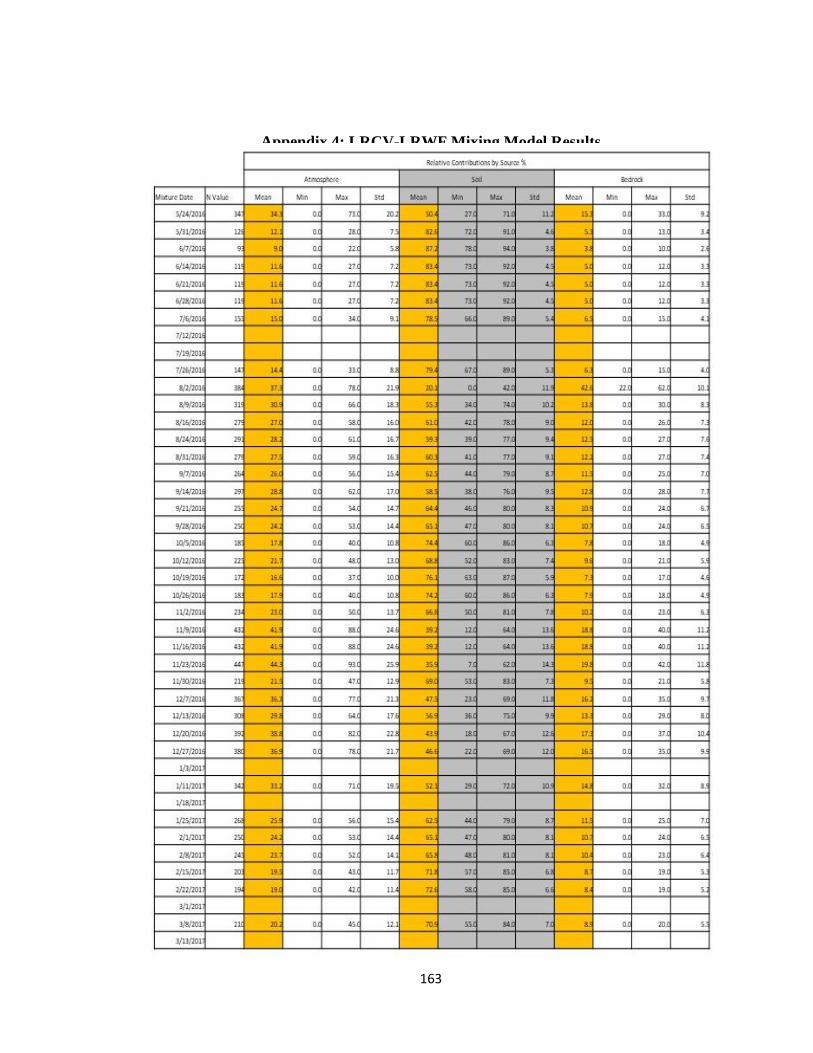
163

Appendix 4: LRCV-LRWF Mixing Model Results

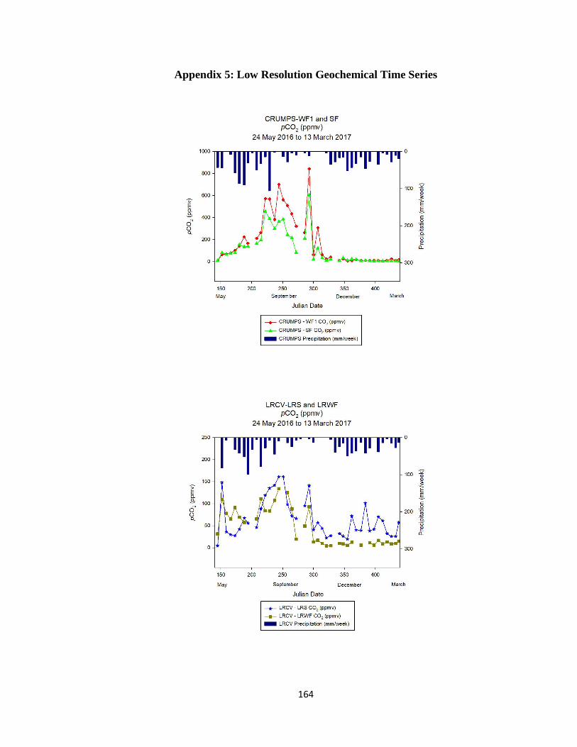
164

Appendix 5: Low Resolution Geochemical Time Series

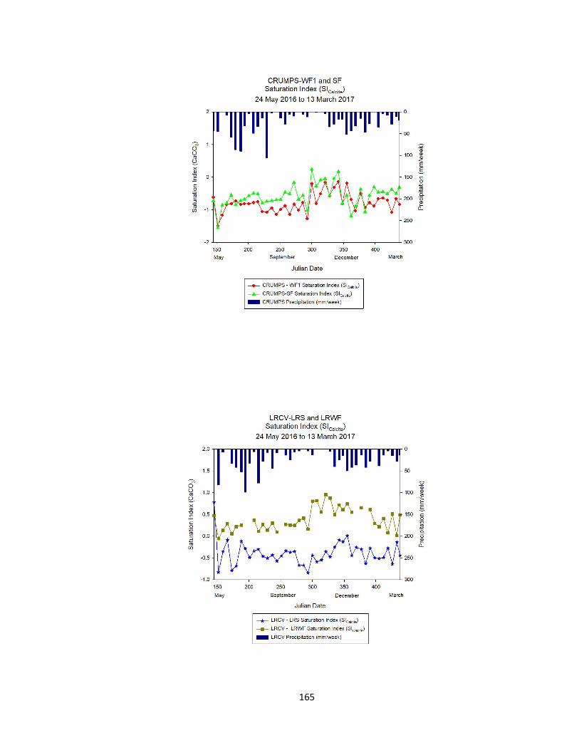
165

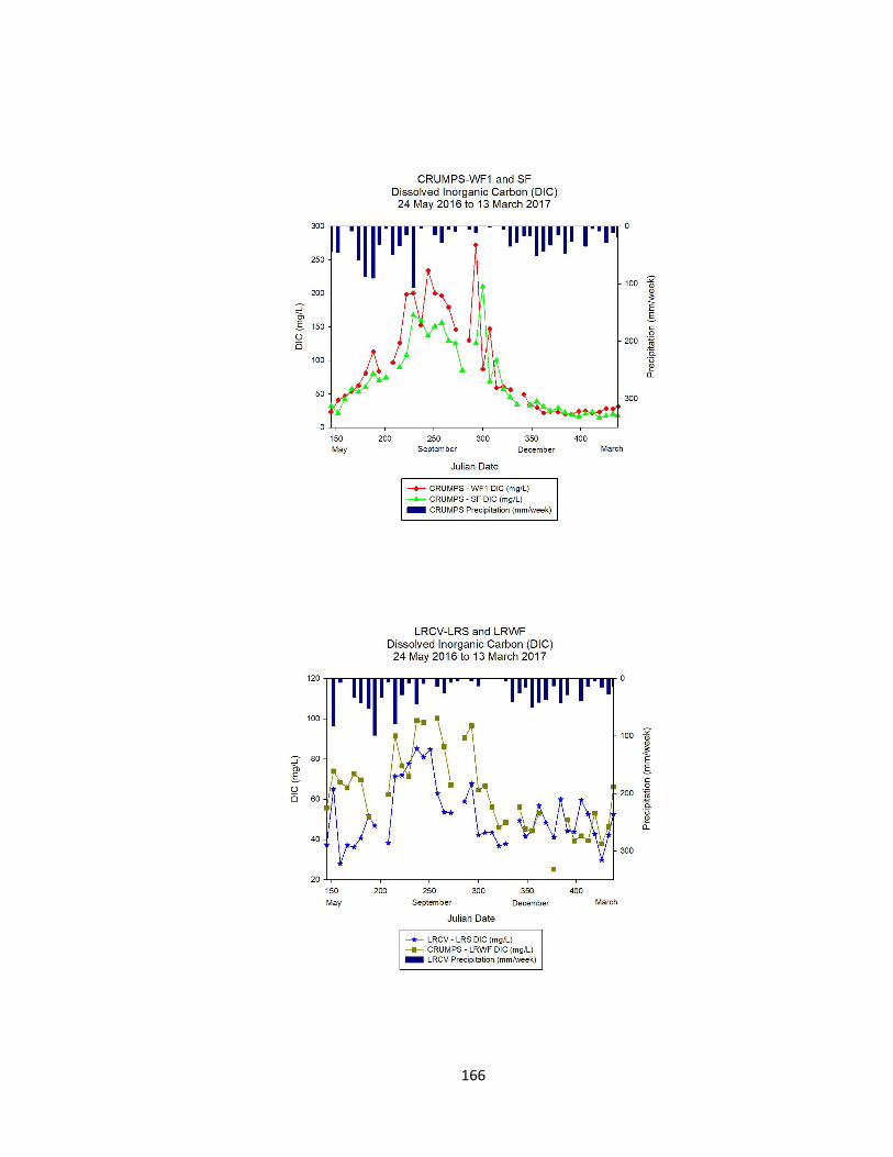
166

167

Appendix 6: Recharge versus Discharge at Each Site

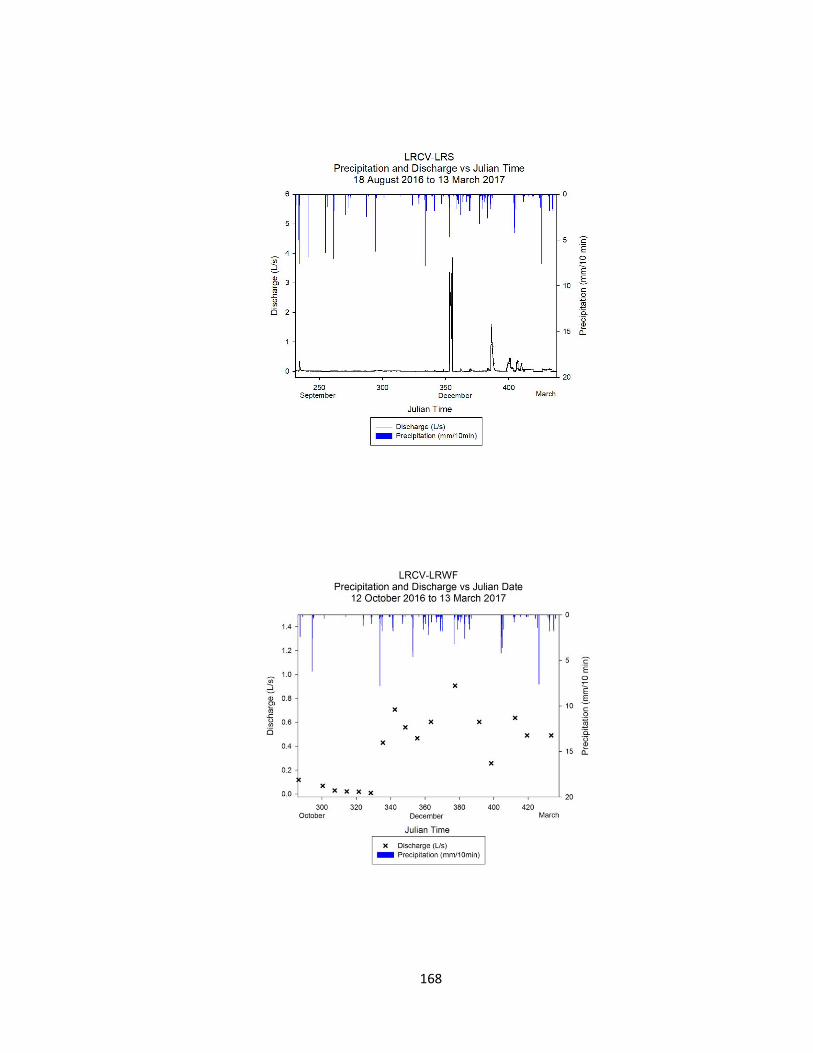
168