Epidemics and chaotic synchronization in recombining monogamous populations

arX

iv:1

004.

3509

v1 [

nlin

.AO

] 2

0 A

pr 2

010

Epidemics and chaotic synchronization in

recombining monogamous populations

Federico Vazquez

Max–Planck–Institut fur Physik Komplexer SystemeNothnitzer Str. 38, D–01187 Dresden, Germany

and Instituto de Fısica Interdisciplinar y Sistemas Complejos (CSIC-UIB)E-07122 Palma de Mallorca, Spain

Damian H. Zanette

Consejo Nacional de Investigaciones Cientıficas y TecnicasCentro Atomico Bariloche and Instituto Balseiro

8400 Bariloche, Rıo Negro, Argentina

Abstract

We analyze the critical transitions (a) to endemic states in an SIS epidemiologicalmodel, and (b) to full synchronization in an ensemble of coupled chaotic maps, onnetworks where, at any given time, each node is connected to just one neighbour. Inthese “monogamous” populations, the lack of connectivity in the instantaneous in-teraction pattern –that would prevent both the propagation of an infection and thecollective entrainment into synchronization– is compensated by occasional randomreconnections which recombine interacting couples by exchanging their partners.The transitions to endemic states and to synchronization are recovered if the re-combination rate is sufficiently large, thus giving rise to a bifurcation as this ratevaries. We study this new critical phenomenon both analytically and numerically.

Key words: Self–organization, network dynamics, epidemics, synchronizationPACS: 05.65.+b, 87.23.Ge, 89.75.-k

1 Introduction

The spontaneous emergence of different kinds of collective behaviour is themost paradigmatic phenomenon in natural and artificial systems formed bylarge ensembles of interacting dynamical elements. The interplay of individualdynamics and interactions entrains elements into coherent macroscopic evo-lution, which typically manifests itself in the form of spatial and/or temporal

Preprint submitted to Elsevier Science 21 April 2010

structures. Pattern formation and synchronization are widespread examples[1,2].

Self–organization into collective evolution requires that the information on thestate of any single element be able to spread all over the system, eventuallyreaching any other element in the ensemble. A crucial ingredient that controlssuch mutual influence of any pair of elements is the interaction pattern ofthe ensemble. In the case of binary interactions, this pattern is convenientlyrepresented as a network, whose links join pairs of elements which interactwith each other [3]. Coherent evolution of the whole ensemble is possible onlyif the interaction network is not disconnected.

It has recently been shown, in the context of epidemiological models, that dis-connection of the interaction network can however be compensated to someextent if the structure of the network itself varies with time, in such a waythat different parts of the ensemble are not continuously but occasionally in-terconnected [4,5,6,7]. Our aim in this paper is to analyze in depth the extremecase where, at any given time, each element is connected by the interactionnetwork to only one neighbour. Occasional random reconnections can how-ever make neighbour to be exchanged. As explained in detail in Section 2 thisscenario is motivated by the study of a sexually transmitted infection in amonogamous population, where each individual has just one sexual partnerat a time, but partners can change. Specifically, we focus on two critical phe-nomena that occur, upon variation of suitable control parameters, in a large,connected ensemble of interacting elements, but which are suppressed if theinteraction network only allows for monogamous static couples. We analyzethe reappearance of each critical phenomenon when random reconnections areallowed to happen.

In Section 2, we consider the critical transition to endemic states in an epidemi-ological model. In Section 3, we study the transition to full synchronizationin an ensemble of coupled chaotic maps. Both cases are, to a large extent,analytically tractable, so that exact results are obtained for the occurrence ofthese critical phenomena in time–varying, highly disconnected networks.

2 Endemic persistence of SIS epidemics

The SIS epidemiological model describes spreading of an infection by contagionbetween the members of a population. At any given time, each agent canbe either susceptible (S) or infectious (I). An S–agent becomes infectious bycontact with an I–agent, with probability α per time unit. An I–agent, in turn,spontaneously becomes susceptible with probability γ per time unit. Contactsbetween agents are represented by the links of a network. For a static random

2

network –provided that there are no disconnected components, i.e. no portionsof the population are separated from the rest– the evolution of the fraction nI

of I–agents in a large population is well described by the mean field equation[8]

nI = βnSnI − γnI, (1)

where nS = 1 − nI is the fraction of S–agents, and β = kα is the infectivity,with k the average number of links per agent in the contact network.

As a function of the infectivity β, the long–time asymptotic fraction of I–agents exhibits two distinct regimes. For β < γ, nI vanishes for long times,and the infection disappears from the population. For β > γ, on the otherhand, an endemic state with a non–vanishing infection level is reached. Theasymptotic fraction of infected agents in this state is

nI = 1− γ

β. (2)

The transition at the critical point where the infectivity β equals the recoveryprobability γ occurs through a transcritical bifurcation [9].

Let us now assume that we are dealing with a sexually transmitted infection,where contagion can only occur between sexual partners. Suppose also that thepopulation is monogamous so that, at any time, each agent has just one part-ner. For simplicity, we assume that all agents have partners. In this situation,the network of contacts is highly disconnected: for a population comprisingN agents, the network consists of N/2 isolated links defining agent couples.If at least one agent is initially infectious within a given couple, the infectioncan persist for some time as a result of repeated contagion between the twopartners. However, there is a finite probability that in any finite time inter-val both agents become susceptible. Assuming that no contacts are allowedwith other members of the population, the two recovered partners will neverbecome infectious again. If couples last forever, consequently, the fate of thesexually transmitted infection is to disappear from the population. Due toits lack of connectivity, the contact network is unable to sustain a long–timeendemic state.

If, on the other hand, sexual partners are allowed to change from time to time,even if at any instant the population is still monogamous, the infection mayspread over the population and, eventually, reach an endemic level. Specifically,let us consider that each couple (i, j) can exchange partners with anotherrandomly selected couple (h, l) at a given rate, creating new couples (i, h) and(j, l). Would it be possible that, if these recombination events are frequentenough, an endemic state is established in the monogamous population? To

3

investigate this question we adopt two different approaches, which can to alarge extent be dealt with analytically. In the first one [7], we compute thefraction of I–agents from the contribution of couples formed at different timesin the past. In the second approach, we study the evolution of the number ofcouples containing two, one, or no infectious partners.

2.1 Epidemiological dynamics within couples

Since the moment when two given agents become joined in a couple, theprobabilities of their being either susceptible or infectious evolve independentlyof the rest of the population. Let p0(t), p1(t), and p2(t) be the probabilitiesthat, at time t, the couple under study comprises zero, one, and two I–agents,respectively. These probabilities satisfy the equations

p0 = γp1,

p1 = 2γp2 − (γ + β)p1,

p2 = βp1 − 2γp2.

(3)

At all times, p0 + p1 + p2 = 1, so that the analysis can be restricted to thesystem formed by the two last lines of the above equations. As expected, theonly fixed point of this linear system, (p1, p2) = (0, 0), corresponds to thedisappearance of the infection. The eigenvalues around the fixed point are

µ± = −1

2(β + 3γ)± 1

2

√

β2 + 6βγ + γ2. (4)

Note that µ− < µ+ < 0. The inverse modulus of µ+ gives the typical durationtime of the infection within a couple, TI. For γ ≫ β and γ ≪ β we have,respectively, TI ∼ 1/γ and TI ∼ β/γ2. The general solution for p1 and p2 canbe written as (p1, p2) = A+e+ exp(µ+t) + A−e− exp(µ−t), with

e± =

(

1,β

2γ + µ±

)

, (5)

and where the coefficients A± are determined by the initial values of p1 andp2.

When a couple is formed, the initial values of p1 and p2 can be evaluated,on the basis of mean field–like arguments, from the fraction nI of I–agentsat that time: p1 = 2nI(1 − nI) and p2 = n2

I . Reversing the same arguments,the linear combination p1 + 2p2 gives the expected fraction of I–agents in the

4

same couple. With these elements, we can now write down an equation forthe evolution of nI(t) taking into account couple recombination events. Thefraction of I–agents at the present time t is given by the contributions of allthe present couples, formed at previous times t − s (0 ≤ s ≤ t). The initialprobabilities within each couple are determined by the fraction of I–agents atthe time of formation, nI(t− s), and the present probabilities are given by thesolution to Eqs. (3) discussed above. Summing up all the contributions, weget

nI(t) =

t∫

0

Π(t, s)

[

1

2

(

1 +2β

2γ + µ−

)

A−[nI(t− s)] exp(µ−s)

+1

2

(

1 +2β

2γ + µ+

)

A+[nI(t− s)] exp(µ+s)

]

ds. (6)

The coefficients A±(nI) are obtained from the evaluation of the initial proba-bilities in a couple in terms of the fraction of I–agents at that time:

(

2nI(1− nI), n2I

)

= A−(nI)e− + A+(nI)e+. (7)

In Eq. (6), the contribution to nI(t) of the couples formed at t−s is weighted byΠ(t, s), the probability that a couple present at time t has lasted for an intervalof length s. Since couple recombination occurs at random, this probabilitydistribution is a Poissonian function of s, specifically,

Π(t, s) =r exp(−rs)

1− exp(−rt), (8)

for 0 ≤ s ≤ t. Here, r is the recombination probability per couple per timeunit.

The rather involved form of our equation for nI(t), Eq. (6), is drasticallysimplified in the long–time limit. We find that for small values of the recom-bination rate r, the asymptotic fraction of I–agents vanishes –just as whenrecombination is absent and the infection, confined within couples, eventuallydisappears. There is however a critical value of the recombination rate abovewhich an endemic state is reached. The stationary fraction of I–agents is

nI = 1− γ

β

(

1 +2γ

r

)

. (9)

The appearance of the endemic state occurs here through a transcritical bi-furcation, like when the infectivity β is varied in the standard SIS model. The

5

critical value of the recombination rate is

rc =2γ

β/γ − 1. (10)

Note that Eq. (9) reduces to Eq. (2) in the limit r → ∞. For a given valueof the infectivity β, thus, infinitely frequent recombination in a monogamouscontact pattern sustains a stationary infection level equivalent to that of apopulation with a static, not disconnected pattern.

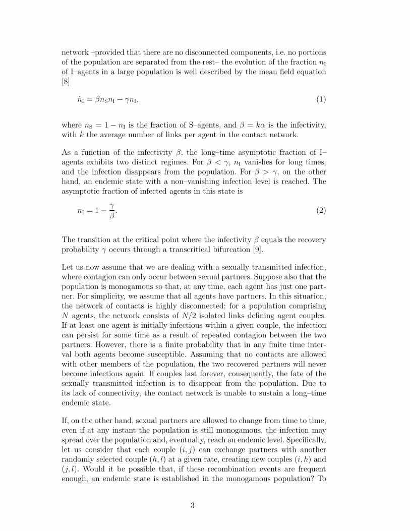
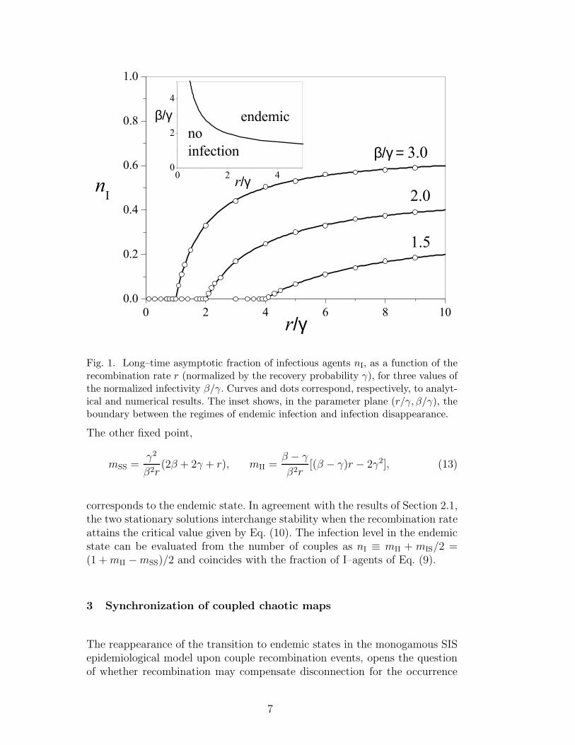
To validate the arguments used to derive Eqs. (6) and, in particular, theasymptotic result (9), we have performed numerical simulations of the epi-demiological model in a recombining monogamous population of N = 103

agents. Since two couples are involved in each recombination event, the prob-ability per time unit of each event in our numerical simulations equals r/2.Figure 1 compares analytical and numerical results, which turn out to showexcellent agreement. The inset shows the boundary between the regions ofparameter space where, for asymptotically long times, the infection persistsor disappears, as given by Eq. (10).

2.2 Evolution of the number of couples

Equivalent asymptotic results are obtained from mean field equations for thenumber of couples formed by agents with different epidemiological states. Notethat, in our problem, the dynamics of the number of couples of different kindscorresponds to the evolution of links in the contact network. Let mSS, mIS, andmII be the fraction of couples formed, respectively, by two S–agents, one I–agent and one S–agent, and two I–agents. Since at all timesmSS+mIS+mII = 1,it is enough to consider the evolution of only two of them, for instance, mSS

and mII. The mean field equations read

mSS = r4m2

IS − rmSSmII + γmIS,

mII = r4m2

IS − rmSSmII + βmIS − 2γmII,(11)

with mIS = 1 − mSS − mII. The first two terms in the right–hand side ofboth equations stand for the only recombination events that change the num-ber of couples of each kind, namely, (SS,II) ↔ (IS,IS). The remaining termscorrespond to the epidemiological events of contagion and recovery.

Equations (11) have two stationary solutions. One of them corresponds to thedisappearance of the infection:

mSS = 1, mII = 0. (12)

6

0 2 4 6 8 10

0.0

0.2

0.4

0.6

0.8

1.0

0

2

4

0 2 4

1.5

2.0nI

r/γ

β/γ = 3.0no

infection

β/γ

r/γ

endemic

Fig. 1. Long–time asymptotic fraction of infectious agents nI, as a function of therecombination rate r (normalized by the recovery probability γ), for three values ofthe normalized infectivity β/γ. Curves and dots correspond, respectively, to analyt-ical and numerical results. The inset shows, in the parameter plane (r/γ, β/γ), theboundary between the regimes of endemic infection and infection disappearance.

The other fixed point,

mSS =γ2

β2r(2β + 2γ + r), mII =

β − γ

β2r[(β − γ)r − 2γ2], (13)

corresponds to the endemic state. In agreement with the results of Section 2.1,the two stationary solutions interchange stability when the recombination rateattains the critical value given by Eq. (10). The infection level in the endemicstate can be evaluated from the number of couples as nI ≡ mII + mIS/2 =(1 +mII −mSS)/2 and coincides with the fraction of I–agents of Eq. (9).

3 Synchronization of coupled chaotic maps

The reappearance of the transition to endemic states in the monogamous SISepidemiological model upon couple recombination events, opens the questionof whether recombination may compensate disconnection for the occurrence

7

of similar critical phenomena in other ensembles of interacting dynamical ele-ments. In this section, we explore this question for the synchronization tran-sition of coupled chaotic maps.

Consider an ensemble of N identical chaotic maps whose individual statesxi (i = 1, . . . , N) evolve, in the absence of coupling, according to xi(t + 1) =f [xi(t)]. Let λ > 1 be the corresponding Lyapunov coefficient. On the average,the distance between two neighboring orbits of a map thus grows by a factorλ at each iteration. Global (all-to-all) coupling between maps is introducedfollowing the standard linear scheme [10,11]

xi(t+ 1) = (1− ε)f [xi(t)] +ε

N

N∑

j=1

f [xj(t)], (14)

where ε ∈ [0, 1] is the coupling intensity. It is well known that, if coupling isstrong enough, the ensemble undergoes a transition to full synchronization.Specifically, if

ε > εc = 1− 1

λ, (15)

coupling is able to overcome the exponential separation of chaotic orbits, andall the maps converge asymptotically to exactly the same trajectory: xi(t) =xj(t) for all i, j and t → ∞ [11]. This synchronized trajectory is still chaotic–in fact, it reproduces the orbit of a single map– but the motion of the mapswith respect to each other has been suppressed. Note that the threshold εc forthe synchronization transition does not depend on the ensemble size N .

Consider now a “monogamous” coupling pattern where, at any given time,each map is coupled to just one partner. Following the scheme of Eq. (14), ifmaps a and b form a couple, their states evolve according to

xa(t+ 1) = (1− ε)f [xa(t)] +ε2{f [xa(t)] + f [xb(t)]} ,

xb(t+ 1) = (1− ε)f [xb(t)] +ε2{f [xa(t)] + f [xb(t)]} .

(16)

If ε > εc, the two maps will synchronize, converging asymptotically to thesame chaotic orbit. Because of the nature of chaotic motion, however, theirsynchronized trajectory will differ from the orbits of other couples.

Would it be possible that, if couples of maps recombine exchanging partnersat random at a certain rate, full synchronization all over the ensemble is re-covered? By analogy with the occurrence of endemic states in SIS epidemicsover a recombining monogamous population, we may expect that synchroniza-tion spreads over the ensemble if recombination is faster enough, entraining

8

increasingly many maps towards the fully synchronized orbit. However, a dif-ference with the case of SIS epidemic is that, now, the recombination rate hasa limit: one random recombination per couple per iteration step produces themaximal possible rearrangement of the coupling pattern.

3.1 Synchronization dynamics within couples

To investigate whether full synchronization is possible in the monogamouscoupling pattern under the effects of recombination, we assume that the en-semble is symmetrically concentrated around a reference orbit x0(t) of themap f(x), so that the state of each map differs from x0(t) by a small amount:xi(t) = x0(t) + δi(t). If, as time elapses, the concentration around x0(t) growsin such a way that δi(t) → 0 for all i, full synchronization will be achieved.Equations (16) imply that the displacements of two coupled maps from thereference orbit x0(t) satisfy the linear equations

δa(t+ 1) = (1− ε2)f ′[x0(t)]δa(t) +

ε2f ′[x0(t)]δb(t),

δb(t + 1) = (1− ε2)f ′[x0(t)]δb(t) +

ε2f ′[x0(t)]δa(t),

(17)

where f ′(x) is the derivative of f(x).

Let us first study the simpler, extreme case where all couples recombine ateach iteration step. Since new partners are chosen at random, the displace-ments δa(t) and δb(t) of the two coupled maps are uncorrelated quantities. Inother words, the average ζ(t) = 〈δa(t)δb(t)〉, performed over all the couplesin the ensemble, vanishes. Consequently, from Eqs. (16), the variance of thedisplacement over the ensemble, σ2(t) = 〈δ2a(t)〉, is governed by

σ2(t+ 1) =

(

1− ε+ε2

2

)

f ′[x0(t)]2σ2(t). (18)

Taking into account that the long–time geometric mean value of f ′[x0(t)]2 is

limT→∞

t0+T∏

t=t0

f ′[x0(t)]2

1/T

= λ2, (19)

the variance σ2 will asymptotically vanish if (1 − ε + ε2/2)λ2 < 1 or, equiva-lently, if

ε > ε1 = 1−√2− λ2

λ. (20)

Thus, if the coupling intensity ε is larger than the critical value ε1, full synchro-nization is stable. Note that ε1 > εc for any λ & 1, so that full synchronizationfor maximal recombination rate requires stronger couplings than when the en-semble is globally coupled. Also, there is a critical limit λ1 =

√2 ≈ 1.41 for the

Lyapunov coefficient such that, if λ > λ1, full synchronization is impossibleeven under the maximal recombination rate.

When recombination does not occur for all couples at all times, the joint evolu-tion of two coupled maps introduces correlations between their displacementsfrom the reference orbit. In this case, Eqs. (16) imply that ζ(t) = 〈δa(t)δb(t)〉and σ2(t) = 〈δ2a(t)〉 are governed by

ζ(t+ 1) = (1− ε2)εf ′[x0(t)]

2σ2(t) + (1− ε+ ε2

2)f ′[x0(t)]

2ζ(t),

σ2(t + 1) = (1− ε+ ε2

2)f ′[x0(t)]

2σ2(t) + (1− ε2)εf ′[x0(t)]

2ζ(t).(21)

This linear system can be solved exactly. For the couples formed at a certaintime t0, we have ζ(t0) = 0 and σ2(t0) = σ2

0 . With such initial conditions, andtaking into account Eq. (19), the solution to Eqs. (21) for σ2 reads

σ2(t) =1

2λ2(t−t0)

[

1 + (1− ε)2(t−t0)]

σ20, (22)

for t ≫ t0. This quantity is the variance of the displacement from x0(t) ofthose maps whose present couples have formed at time t0 and lasted until thepresent time t.

Suppose now that, at a certain time τ , the ensemble around x0(τ) has varianceσ2τ . To evaluate the variance σ2

τ+1 at the next time step, we think of theensemble as made up of subensembles consisting of the maps whose presentcouples have formed at times τ , τ−1, τ−2, and so on. The fraction of maps inthe subensemble corresponding to couples formed at time τ−n (n = 0, 1, 2, . . .)is qn = r(1−r)n, where r is the probability that any couple forms at any giventime step (0 ≤ r ≤ 1). Using Eq. (22) with t ≡ τ and t0 ≡ τ − n, we find thatthe variance of this subensemble, which we denote σ2

n, changes from σ2n(τ) = σ2

τ

to

σ2n(τ + 1) = λ21 + (1− ε)2(n+1)

1 + (1− ε)2nσ2τ . (23)

Assuming that the ensemble has been evolving since an asymptotically longtime ago, its variance at time τ + 1 is given by

σ2τ+1 =

∞∑

n=0

qnσ2n(τ + 1) = rλ2

∞∑

n=0

(1− r)n1 + (1− ε)2(n+1)

1 + (1− ε)2nσ2τ . (24)

10

The synchronization threshold is therefore given by the condition

rλ2∞∑

n=0

(1− r)n1 + (1− εr)

2(n+1)

1 + (1− εr)2n= 1, (25)

where εr is the critical coupling intensity.

Note that, to obtain this result, we have used Eq. (22) for t−t0 = n = 0, 1, 2, . . .while, strictly, it holds for t ≫ t0 only. Consequently, the threshold condition(25) is just an approximation whose validity must be ascertained for eachspecific choice of the map f(x). Below, we present numerical results for a casewhere Eq. (22) holds at any time.

Whereas, in general, the summation in Eq. (25) cannot be exactly performed,two special cases are readily obtained. The first one corresponds to the max-imal recombination rate, r = 1, for which we reobtain the critical couplingintensity ε1 of Eq. (20). The second special case gives the recombination ratefor which the threshold coupling intensity is maximal, εr = 1, namely,

rmin = 2(

1− 1

λ2

)

. (26)

For recombination rates below rmin, synchronization is not possible even forthe strongest coupling.

3.2 Numerical simulations

To test the above results we have performed numerical simulations of recom-bining monogamous ensembles of N = 103 chaotic maps for the case of thetent map [9]:

f(x) =

px for 0 ≤ x ≤ 12,

p(1− x) for 12≤ x ≤ 1,

(27)

with x ∈ [0, 1] and p ∈ [0, 2]. The Lyapunov coefficient of the tent map isλ = p, which implies that the dynamics is chaotic for 1 < p ≤ 2. Moreover,f ′(x)2 = p2 = λ2 for all x, so that in Eq. (19) the limit of T → ∞ can bedropped, and Eq. (22) holds for any t.

In our simulations, after joint evolution of the coupled maps following Eq.(16), each one of the N/2 couples is allowed to recombine with probability ρ,

11

0.0

0.2

0.4

0.6

0.8

1.0

0.0 0.2 0.4 0.6 0.8 1.0

1.4

1.3

1.2

ρ

ε

p = 1.1

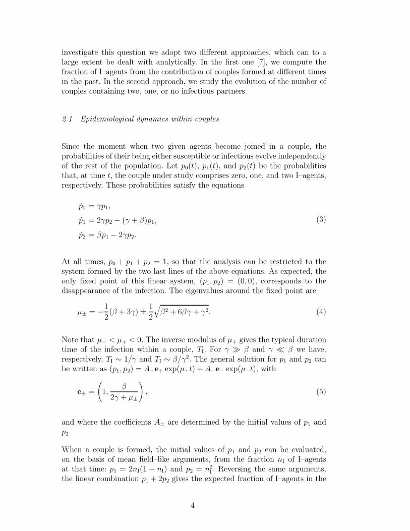
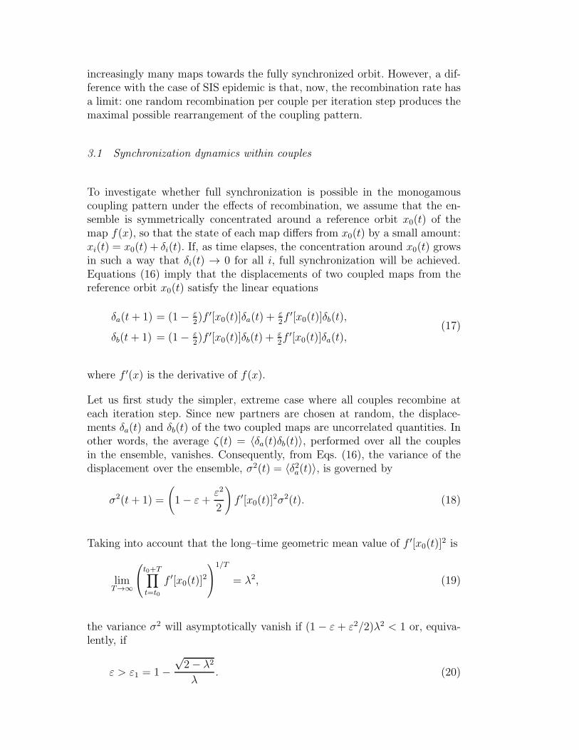
Fig. 2. Full-synchronization threshold for a recombining monogamous ensemble oftent maps, in the parameter plane (ρ, ε), for four values of the map parameter p. Fullsynchronization is stable above and to the right of each boundary. Dots and curvesstand, respectively, for numerical results on ensembles of 103 maps and the analyticalresult of Eq. (25). The numerical parameter ρ is related to the recombination rater through Eq. (28).

exchanging partners with another randomly selected couple. Since two cou-ples are involved at each recombination event, the resulting recombinationprobability per couple per time step is larger than ρ, and reads

r = 1− (1− ρ) exp(−ρ). (28)

Fully synchronized ensembles are detected by numerically measuring the vari-ance σ2

x(t) = N−1∑

i[xi(t) − x(t)]2 with respect to the average state x(t) =N−1∑

i xi(t). Realizations where σ2x(t) falls to the level of numerical round-off

errors are identified with full synchronization.

Figure 2 shows the boundary of full synchronization in the parameter space(ρ, ε) for four values of the tent map slope p. For each value of ρ, full synchro-nization is stable for coupling intensities ε above the boundary. Dots standfor the numerical determination of the synchronization threshold and curvescorrespond to the analytical prediction, Eq. (25). The agreement is very good.The systematic difference between numerical and analytical results, more vis-

0.0 0.2 0.4 0.6 0.810

-5

10-4

10-3

10-2

10-1

p = 1.2, ε = 0.6

p = 1.1, ε = 0.4

σx

ρ

p = 1.3, ε = 0.8

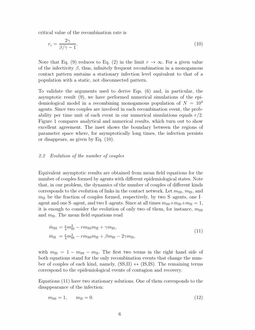
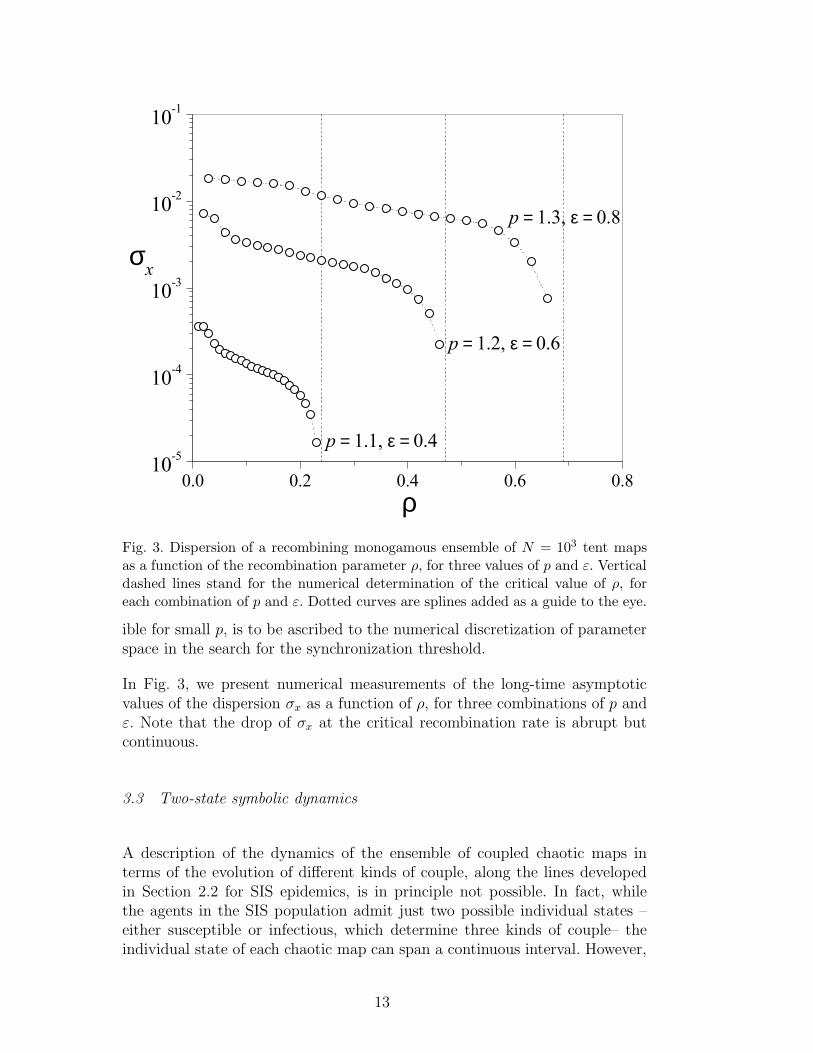
Fig. 3. Dispersion of a recombining monogamous ensemble of N = 103 tent mapsas a function of the recombination parameter ρ, for three values of p and ε. Verticaldashed lines stand for the numerical determination of the critical value of ρ, foreach combination of p and ε. Dotted curves are splines added as a guide to the eye.

ible for small p, is to be ascribed to the numerical discretization of parameterspace in the search for the synchronization threshold.

In Fig. 3, we present numerical measurements of the long-time asymptoticvalues of the dispersion σx as a function of ρ, for three combinations of p andε. Note that the drop of σx at the critical recombination rate is abrupt butcontinuous.

3.3 Two-state symbolic dynamics

A description of the dynamics of the ensemble of coupled chaotic maps interms of the evolution of different kinds of couple, along the lines developedin Section 2.2 for SIS epidemics, is in principle not possible. In fact, whilethe agents in the SIS population admit just two possible individual states –either susceptible or infectious, which determine three kinds of couple– theindividual state of each chaotic map can span a continuous interval. However,

13

as we show in this section, a symbolic representation of each map as a two-statevariable –either synchronized or unsynchronized– together with a reduced setof transition rules between the two states, is able to qualitatively reproducethe collective effects of recombination on the synchronization transition. Thisschematic approach has the virtue of capturing the essential mechanisms ofthe interplay between recombination and synchronization, and can also bereinterpreted in the context of the SIS epidemics model.

Let us thus assume that, at any given time, each chaotic map adopts one oftwo states, namely, unsynchronized (U) or synchronized (S). We stress thatsynchronization of an individual map i is here understood as defined withrespect to the ensemble, for instance, if the variable xi(t) is within a certainsmall distance from the average x(t) = N−1∑

j xj(t). In the spirit of Eqs. (11),we propose for the evolution of the fractions of couples mUU, mUS, and mSS

the Ansatz

mUU = r4m2

US − rmSSmUU + γmUS − η(r)mUU,

mSS = r4m2

US − rmSSmUU + β(r)mUS + η(r)mUU,(29)

with mUS = 1 − mSS − mUU, and where β(r), γ, and η(r) are non–negativequantities. The first two terms in the right–hand side of both equations de-scribe the effect of recombination at rate r per couple. They have exactlythe same origin as in Eqs. (11). The remaining terms, described in detail inthe following, stand for the transitions induced by the joint evolution of cou-pled maps. Note that we are assuming that all these transitions occur alwaystoward states where the two maps of a couple are either synchronized or un-synchronized. Also, we suppose that the two maps of an SS–couple, as long astheir link lasts, cannot become unsynchronized from the ensemble.

In the first place, as time elapses, a US–couple can become either an SS–couple or a UU–couple. This describes the tendency towards synchronizationwithin each couple. The rate for the transition US → SS, which we havecalled β in Eqs. (29), cannot however be a constant. If it were a constant, infact, all US–couples would become SS–couples for sufficiently long times, thussynchronizing with the ensemble even in the absence of recombination. This isnot the case, though: when recombination is infrequent, maps forming a long-lasting couple synchronize to each other, but are generally not synchronizedto the ensemble. We represent this effect phenomenologically, by ascribing toβ a dependence on r. The function β(r) increases as r grows, starting fromβ(0) = 0.

The transition US → UU, on the other hand, implies the desynchronizationof a map with respect to the ensemble by interaction with its already unsyn-chronized partner. This event does not require recombination: it is rather the

14

generally expected outcome within a US couple. We thus assume that its rate,γ, is constant.

Finally, Eqs. (29) include, in the last terms of their right–hand side, the tran-sition UU → SS. Because of the same reasons as in the case of the transitionUS → SS, which also involves the synchronization with the ensemble of previ-ously unsynchronized maps, we expect that the corresponding rate, η(r), is agrowing function of the recombination rate r. Possibly, however, η(r) is muchsmaller that γ(r), because becoming an SS–couple should occur less frequentlyfor a UU–couple than for a US–couple.

Equations (29) have two fixed points. One of them, mSS = 1, mUU = 0, corre-sponds to full synchronization of the ensemble of chaotic maps. For the otherfixed point, both mSS and mUU are different from zero, thus corresponding toa state of partial synchronization. There is a broad choice of functional formsfor β(r) and η(r) such that these stationary solutions have the expected be-haviour –namely, that full synchronization is unstable for small r and becomesstable above a critical value of the recombination rate, while the other fixedpoint exhibits opposite stability properties. For the sake of concreteness, letus assume the linear dependences β(r) = β0r and η(r) = η0r. Analysis of theeigenvalues of Eqs. (29) around the fixed points shows that, irrespectively ofthe values of β0 and γ, it is enough that η0 < 1 for the occurrence of a transi-tion to full synchronization as r grows. The critical value of the recombinationrate is

rc =γ

β0

1− η01 + η0

. (30)

Let us now attempt a semi–quantitative comparison of this result with ourresults for the synchronization transition in recombining monogamous ensem-bles of chaotic maps, for instance, those depicted in Fig. 2 for tent maps. Sinceγ is the rate for the transition US → UU –where, by interaction within its cou-ple, a map becomes desynchronized from the ensemble– it may be identifiedwith a measure of the rate at which chaotic orbits diverge from each other, i.e.of the Lyapunov coefficient λ. The factor β0, in turn, weights the rate of thetransition US → SS, where a map becomes synchronized to the ensemble byinteraction with its already synchronized partner. Thus, β0 is related to thestrength of the interaction between coupled maps, i.e. to the coupling intensityε. The factor η0 plays a similar role but, as mentioned above, its effect shouldbe quantitatively less important than that of β0. Figure 4 is a plot of thesynchronization threshold as given by Eq. (30). To stress the correspondencewith Fig. 2, we have plotted β0 (a measure of the coupling intensity ε) as afunction of the recombination rate r (directly related, through Eq. (28), tothe parameter ρ) for three values of γ (a measure of the Lyapunov coefficient,λ = p for the tent map), and fixed η0. The semi–quantitative analogy with our

15

0.0 0.2 0.4 0.6 0.8 1.0

0.0

0.2

0.4

0.6

0.8

1.0

0.5

0.25

γ = 0.1

β0

r

Fig. 4. Synchronization threshold in the parameter plane (r, β0) for the two–statemodel of coupled chaotic maps, corresponding to three values of the rate γ andη0 = 0.01. Full synchronization is stable in the region of large r and β0. Comparethis plot with Fig. 2.

numerical results for ensembles of tent maps, shown in Fig. 2, is apparent.

An analogy between this two–state approach to synchronization and the SISepidemiological model discussed in Section 2 can in turn be derived from theidentification of the unsynchronized state with the susceptible state on onehand, and of the synchronized state and the infectious state on the other.With this identification, the transitions US → SS and US → UU correspond,respectively, to contagion from the infectious partner and to the spontaneousrecovery of an infectious agent. The rates β and γ play the same role in bothdynamical models, with the difference that in the SIS model β does not dependon the recombination rate. Another difference is that the two–state approachto synchronization includes the transition UU → SS, which in the SIS modelwould correspond to simultaneous infection of two susceptible partners –aforbidden event. The SIS model, in turn, allows for the recovery of just oneamong two infectious partners, which would stand for the inexistent transitionSS → US. Notwithstanding these differences, we realize that the plot of Fig. 4is the equivalent in the two–state approach to synchronization as the endemicthreshold depicted in the insert of Fig. 1 –where both the infectivity β andthe recombination r are normalized by the recovery probability γ. The twothresholds have qualitatively the same functional dependence on the respectiveparameter. In addition, the transition to full synchronization in our two–state

16

formulation is a transcritical bifurcation, the same kind of critical phenomenonas in the SIS model.

4 Conclusion

We have here studied two critical phenomena in the collective behaviour oflarge ensembles of interacting dynamical elements –namely, the appearance ofendemic states in an SIS epidemiological model, and the stabilization of fullsynchronization of identical chaotic maps– when the corresponding interactionpatterns are highly disconnected and, concurrently, change with time. Specifi-cally, we have considered “‘monogamous” interaction patterns, represented bynetworks where each site is connected to only one neighbour at a time, butsuch that neighbours can be exchanged at random at a specified rate. While inthe absence of neighbour exchange –or, as we have called it, of recombination–the occurrence of endemic states and synchronization would be impossible dueto the lack of connectivity in the ensemble, sufficiently frequent recombinationevents make it possible that coherence is established all over the system, thusallowing for organized collective dynamics.

Recombination of interacting couples in a monogamous pattern introduces anew dynamical parameter –the recombination rate. The two critical phenom-ena studied here take now place upon variation of this parameter: endemicstates and full synchronization occur above a certain critical value of the re-combination rate. Moreover, for the SIS epidemiological model with a giveninfectivity, we have found that the limit of infinitely large recombination rateis equivalent to the situation where the interaction pattern is static but notdisconnected. For chaotic maps, on the other hand, the fact that time elapsesby discrete steps imposes a limit to the recombination rate: any interactingcouple can at most be recombined once per step. This establishes in turn anupper limit for the Lyapunov coefficient of individual maps such that they canbe synchronized by recombination. If the maps are “too chaotic”, synchroniza-tion is not possible even at the maximal rate of one recombination per coupleper time step.

The fact that, instantaneously, each dynamical element of the two ensemblesconsidered here has just only one interaction partner, makes the correspond-ing problems analytically tractable to a large extent. In particular, we haveobtained analytical approximations for the critical values of the recombina-tion rate which are in very good agreement with numerical results. For SISepidemics, the critical recombination rate was found both from the integra-tion over the whole population of the epidemiological dynamics within eachcouple, and from the dynamics of the number of couples in each epidemiolog-ical state. For the chaotic maps, we have replaced this latter approach by a

17

kind of symbolic schematic representation of the dynamics of couples. In thisrepresentation, which can also be adapted to the SIS model and qualitativelyreproduces the critical behaviour of the two systems, maps (or epidemiologicalagents) are though of as two–state elements. Their interactions induce transi-tions between the two states following a small set of intuitive rules. We con-jecture that this kind of representation is capturing the essential mechanismsthat govern the relative prevalence of unsynchronized/susceptible elements atone side of the critical point, and of synchronized/infectious elements at theother.

Collective dynamics on monogamous interaction patterns have the advantageof analytical tractability. It should however be borne in mind that these pat-terns represent a kind of extreme case among disconnected networks: they havethe minimal number of links that avoids isolated elements. Networks with lesssevere lack of connectivity should impose lower limitations to the developmentof collective self-organized behaviour. In these cases, therefore, we expect thatrecombination, even at lower rates, will also be able to compensate the lackof connectivity, triggering critical phenomena such as those studied here.

References

[1] A. S. Mikhailov, Foundations of Synergetics I. Distributed Active Systems, 2ndedition (Springer, Heidelberg, 1994).

[2] S. C. Manrubia, A. S. Mikhailov, and D. H. Zanette, Emergence of DynamicalOrder: Synchronization Phenomena in Complex Systems (World Scientific,Singapore, 2004).

[3] R. Pastor Satorras, J. Rubı and A. Dıaz Guilera, eds., Statistical Mechanics ofComplex Networks (Springer, Berlin, 2003).

[4] K. T. D. Eames and M. J. Keeling, Math. Biosc. 189, 115 (2004).

[5] M. J. Keeling and K. T. D. Eames, J. Royal Soc. Interface 2, 295 (2005).

[6] E. Volz and L.A. Meyers, Proc. R. Soc. B 274, 2925 (2007).

[7] S. Bouzat and D. H. Zanette, Eur. Phys. J. B 70, 557 (2009).

[8] J. D. Murray, Mathematical Biology (Springer, Berlin, 1993).

[9] S. H. Strogatz, Nonlinear Dynamics and Chaos (Westview, Cambridge, 2000).

[10] K. Kaneko, Phys. Rev. Lett 63, 219 (1989).

[11] K. Kaneko, Physica D 41, 137 (1990).

18