JSS Journal of Statistical Software MMMMMM YYYY, Volume VV, Issue II. http://www.jstatsoft.org/ envlp:A MATLAB Toolbox for Computing Envelope Estimators in Multivariate Analysis Dennis Cook University of Minnesota Zhihua Su University of Florida Yi Yang University of Minnesota Abstract Envelope models and methods represent new constructions that can lead to substantial increases in estimation efficiency in multivariate analyses. The envlp toolbox implements a variety of envelope estimators under the framework of multivariate linear regression, including the envelope model, partial envelope model, heteroscedastic envelope model, inner envelope model, scaled envelope model, and envelope model in the predictor space. The toolbox also implements the envelope model for estimating a multivariate mean. The capabilities of this toolbox include estimation of the model parameters, as well as performing standard multivariate inference in the context of envelope models; for example, prediction and prediction errors, F test for two nested models, the standard errors for contrasts or linear combinations of coefficients, and more. Examples and datasets are contained in the toolbox to illustrate the use of each model. All functions and datasets are documented. Keywords : multivariate linear regression, envelope models, dimension reduction, Grassmann manifold, MATLAB. 1. Introduction The envelope model is a new construction originally introduced by Cook, Li, and Chiaromonte (2010) in the context of multivariate linear regression Y = α + βX + ε, (1) where Y ∈ R r is the multivariate response vector, X ∈ R p is the non-stochastic predictor vector centered at 0 in the sample, the error vectors ε ∈ R r are identically and independently distributed across observations with mean 0 and positive definite covariance matrix Σ ∈ R r×r , and α ∈ R r is the unknown intercept. The key parameters are the elements of the coefficient

Welcome message from author
This document is posted to help you gain knowledge. Please leave a comment to let me know what you think about it! Share it to your friends and learn new things together.
Transcript
JSSJournal of Statistical SoftwareMMMMMM YYYY, Volume VV, Issue II. http://www.jstatsoft.org/
envlp: A MATLAB Toolbox for Computing Envelope
Estimators in Multivariate Analysis
Dennis CookUniversity of Minnesota
Zhihua SuUniversity of Florida
Yi YangUniversity of Minnesota
Abstract
Envelope models and methods represent new constructions that can lead to substantialincreases in estimation efficiency in multivariate analyses. The envlp toolbox implementsa variety of envelope estimators under the framework of multivariate linear regression,including the envelope model, partial envelope model, heteroscedastic envelope model,inner envelope model, scaled envelope model, and envelope model in the predictor space.The toolbox also implements the envelope model for estimating a multivariate mean.The capabilities of this toolbox include estimation of the model parameters, as well asperforming standard multivariate inference in the context of envelope models; for example,prediction and prediction errors, F test for two nested models, the standard errors forcontrasts or linear combinations of coefficients, and more. Examples and datasets arecontained in the toolbox to illustrate the use of each model. All functions and datasetsare documented.
Keywords: multivariate linear regression, envelope models, dimension reduction, Grassmannmanifold, MATLAB.
1. Introduction
The envelope model is a new construction originally introduced by Cook, Li, and Chiaromonte(2010) in the context of multivariate linear regression
Y = α+ βX + ε, (1)
where Y ∈ Rr is the multivariate response vector, X ∈ Rp is the non-stochastic predictorvector centered at 0 in the sample, the error vectors ε ∈ Rr are identically and independentlydistributed across observations with mean 0 and positive definite covariance matrix Σ ∈ Rr×r,and α ∈ Rr is the unknown intercept. The key parameters are the elements of the coefficient
2 envlp: A MATLAB Toolbox on Envelope Models
matrix β ∈ Rr×p. Compared to the standard ordinary least squares estimator βols, theenvelope estimator βem is potentially less variable and thus more efficient. This is achievedby allowing for the possibility that the distribution of some linear combinations of Y isinvariant to changes in X, and we call this the immaterial part of Y. The immaterial part ofY provides no worthwhile information on β, and yet it increases the variation in βols. Theenvelope model identifies and accounts for the immaterial information and therefore reducesthe variation in estimation. This reduction can be substantial, especially when the immaterialpart of Y introduces large variation.
Several extensions have been developed following Cook et al. (2010). The partial envelopemodel (Su and Cook 2011) focuses on the estimation of the coefficients for a selected subsetof the predictors, and is therefore more efficient in estimating those coefficients. The innerenvelope model (Su and Cook 2012) applies the enveloping idea in a novel way, which re-sults in new methodology that is able to gain efficiency even when there is no immaterialinformation in the data. The heteroscedastic envelope model (Su and Cook 2013) removesthe constant variance assumption in the envelope model, making it more flexible and morewidely applicable. The scaled envelope model (Cook and Su 2013) is a scale invariant versionof the envelope model, which can offer efficiency gains beyond those from the envelope modelitself. The envelope model in the predictor space (Cook, Helland, and Su 2013) focuses ondimension reduction for the predictors. It is equivalent to the partial least squares (PLS) inthe population and yet performs better than PLS with finite samples. The envelope modelthat estimates a multivariate mean can be viewed as an alternative to Stein estimation. Likethe other methods it is particularly effective and can perform better than Stein estimationwhen there is immaterial information present in the data.
The only software that now performs envelope estimation is MATLAB (The MathWorks, Inc.2012b) package LDR (Cook, Forzani, and Tomassi 2009). This package is mainly focusedon likelihood-based sufficient dimension reduction, not envelope estimation. It implementsthe basic envelope model in Cook et al. (2010), but not any of its extension or any inferencemethods in the envelope model context. This article describes the toolbox envlp, which im-plements all the existing envelope methods. It also contains functions for dimension selection,bootstrap estimation, prediction and hypothesis testing. Examples are provided to illustratethe use of the toolbox. All the documentation, as well as updates can be checked at thewebsite http://code.google.com/p/envlp/.
The rest of this paper is organized as follows. The envelope models are discussed in Section2. Section 3 is an overview of the toolbox. Section 4 provides some examples on using thepackage. Discussion on future developments is in Section 5.
2. Envelope models
2.1. The basic envelope model
Let (Γ,Γ0) ∈ Rr×r be an orthogonal matrix. If
Γ>0 Y | X ∼ Γ>0 Y, and Γ>Y Γ>0 Y | X,
then Γ>0 Y carries no information on β and it represents the immaterial part of Y, whileΓ>Y is the material part. Let B = span(β). Cook et al. (2010) showed that the previous two
Journal of Statistical Software 3
conditions are equivalent to the following two conditions
(2a) B ⊆ span(Γ), (2b) Σ = PΓΣPΓ + QΓΣQΓ, (2)
where P(·) is a projection matrix onto the subspace indicated by its argument and Q(·) =I − P(·). If we have (2b), span(Γ) is called a reducing subspace of Σ (Conway 1990). Anenvelope subspace is defined as the smallest reducing subspace of Σ containing B (Cook et al.2010), and is denoted by EΣ(B). In the context of (1), let Γ ∈ Rr×u span the envelopesubspace EΣ(B). The envelope model is then written as follows
Y = α+ ΓηX + ε, Σ = Σ1 + Σ2 = ΓΩΓ> + Γ0Ω0Γ>0 ,
where β = Γη, η ∈ Ru×p, Ω ∈ Ru×u and Ω0 ∈ R(r−u)×(r−u) are unknown positive definitematrices, u is the dimension of the envelope subspace. From this model, the two conditionsin (2) are satisfied: B is contained in span(Γ), and Σ is the sum of Σ1 = VAR(PΓY), thevariance related to the material part of Y, and Σ2 = VAR(QΓY), the variance related tothe immaterial part. It is seen from the envelope model that β and Σ are linked by Γ andit is this link that results in more efficient estimation of β. In effect, the estimation processaccounts for the variation in the immaterial information Γ>0 Y. Let ‖ · ‖ denote the spectralnorm of a matrix. When ‖Σ1‖ ‖Σ2‖, the immaterial part has relatively large variationand the envelope model will offer substantial efficiency gains over the standard model (1).
When u = r, there is no immaterial information in Y, and the envelope model is equivalentto the standard model (1). This will happen when the rank of β is equal to r.
2.2. Partial envelope model
The partial envelope model (Su and Cook 2011) is appropriate when part of the predictorsare of special interest. It is often more efficient than the envelope model for the purpose ofestimating the regression coefficients for those predictors.
Suppose we can partition X to (X>1 ,X>2 )>, where X1 ∈ Rp1 are the predictors of special
interest and X2 ∈ Rp2 are covariates, p1 + p2 = p. Then β can be partitioned accordinglyinto (β1,β2), and (1) can be written as
Y = α+ β1X1 + β2X2 + ε,
where β1 ∈ Rr×p1 is the key parameter.
The partial envelope model applies the enveloping idea on β1: Let B1 = span(β1). A partialΣ-envelope of B1, denoted by EΣ(B1), is the smallest reducing subspace of Σ containing B1.The coordinate form of the partial envelope model is
Y = α+ ΓηX1 + β2X2 + ε, Σ = Σ1 + Σ2 = ΓΩΓ> + Γ0Ω0Γ>0 ,
where Γ ∈ Rr×u1 spans EΣ(B1), Γ0 spans E⊥Σ(B1), the subspace orthogonal to EΣ(B1), u1 isthe dimension of EΣ(B1), η = Γ>β1 ∈ Ru1×p, Ω ∈ Ru1×u1 and Ω0 ∈ R(r−u1)×(r−u1) are bothpositive definite matrices. Compared to the envelope model, EΣ(B1) ⊆ EΣ(B) and u1 ≤ u.Intuitively, more information is immaterial relative to β1, so the partial envelope model istypically more efficient than the envelope model for the purpose of estimating β1.
The partial envelope model degenerates to the standard model when u1 = r, which meansno information is immaterial to β1. This happens when the rank of β1 is equal to r. So
4 envlp: A MATLAB Toolbox on Envelope Models
in a regression problem where rank(β) = r, the envelope model degenerates to the standardmodel; while as long as p1 < r, the partial envelope model is still applicable. In this sense,the partial envelope model is more flexible than the envelope model.
2.3. Heteroscedastic envelope model
The envelope model in Section 2.1 assumes homogeneity of the error variance. The het-eroscedastic envelope model (Su and Cook 2013) removes this assumption and allows fornon-constant covariance structure. The heteroscedastic envelope model was developed inthe context of estimating multivariate means for different populations. This problem can beformulated as
Y(i)j = µ+ β(i) + ε(i)j , i = 1, · · · , p, j = 1, · · · , n(i), (3)
where the subscripts with parentheses denote groups and subscripts without parentheses de-note observations within a group, Y(i)j ∈ Rr is the jth observation in the ith group, µ ∈ Rr
is the grand mean over all the observations, β(i) ∈ Rr is the main effect of the ith group andwe assume that
∑pi=1 n(i)β(i) = 0, n(i) is the sample size for the ith group, ε(i)j ∈ Rr follows
a distribution with mean 0 and covariance matrix Σ(i) ∈ Rr×r. From this formulation, theerrors have heteroscedastic covariance structure.
The heteroscedastic envelope model applies the enveloping idea on all the β(i)’s, and at thesame time accommodates the heteroscedastic covariance structure. Let M = Σ(i) : i =1, · · · , p be the collection of covariance matrices and let B = span(β(1), · · · ,β(p)). The M-envelope of B, denoted by EM(B), is the intersection of all subspaces that contain B andreduce each member of M. The coordinate form of this model is
Y(i)j = µ+ Γη(i) + ε(i)j , Σ(i) = Σ1(i) + Σ2 = ΓΩ1(i)Γ> + Γ0Ω0Γ
>0 ,
where β(i) = Γη(i), Γ ∈ Rr×u is a semi-orthogonal matrix that spans EM(B), Γ0 ∈ Rr×(r−u)
spans its orthogonal complement, η(i) = Γ>β(i) ∈ Ru, Ω1(i) ∈ Ru×u and Ω0 ∈ R(r−u)×(r−u)
are both positive definite matrices, and u is the dimension of EM(B). When u = r, theheteroscedastic envelope model degenerates to the standard model (3).
Compared with the envelope model in Section 2.1, recognizing the heteroscedastic error struc-ture leads to more reliable estimators and greater efficiency gains. To test homogeneity of thecovariance matrices, Box’s M test (Johnson and Wichern 2007) can be used.
2.4. Inner envelope model
The inner envelope model (Su and Cook 2012) provides an envelope method that can achieveefficiency gains even when all of Y is material. It has a different mechanism in utilizing thetool of reducing subspaces. Under the standard model (1), an inner Σ-envelope of B, denotedby IEΣ(B), is the reducing subspace of Σ with maximal dimension that is contained in B.Let Γ1 ∈ Rr×u be an orthogonal basis that spans IEΣ(B). The coordinate form of the innerenvelope model is then
Y = α+ (Γ1η>1 + Γ0Bη
>2 )X + ε, Σ = Γ1Ω1Γ
>1 + Γ0Ω0Γ
>0 ,
where β = Γ1η>1 +Γ0Bη
>2 , Γ0 ∈ Rr×(r−u) spans IEΣ(B)⊥, B ∈ R(r−u)×(p−u) is an orthogonal
matrix such that span(Γ1,Γ0B) = B, η1 ∈ Rp×u, η2 ∈ Rp×(p−u), Ω1 ∈ Ru×u and Ω0 ∈R(r−u)×(r−u) are positive definite matrices, u is the dimension of IEΣ(B).
Journal of Statistical Software 5
The inner envelope model divides β into two parts by IEΣ(B). If the part Γ1η>1 is estimated
with greater precision than the standard model (particularly when ‖Σ1‖ ‖Σ2‖), and thepart Γ0Bη
>2 is estimated with about the same precision, then overall we get better efficiency
in estimating β. The possible values of u are from 0 to p. When u = 0, the inner envelopemodel reduces to the standard model and when u = p, the inner envelope model is equivalentto the envelope model in Section 2.1.
2.5. Scaled envelope model
The scaled envelope model (Cook and Su 2013) is a scale invariant version of the envelopemodel in Section 2.1. It is invariant under scale transformation of the responses and canachieve efficiency gains beyond those offered by the envelope model. It is an alternativechoice to the envelope model especially when u = r is inferred via the envelope model.
Let Λ ∈ Rr×r be a diagonal matrix to represent the scale transformation of the responses. Itsdiagonal elements are λi > 0, i = 1, · · · , r, with λ1 = 1 and the rest to be estimated. Underthe framework of (1), the coordinate form of a scaled envelope model is
Y = α+ ΛΓηX + ε, Σ = ΛΓΩΓ>Λ + ΛΓ0Ω0Γ>0 Λ,
where Γ ∈ Rr×u is a semi-orthogonal matrix that spans the Λ−1ΣΛ−1-envelope of Λ−1B,Γ0 ∈ Rr×(r−u) is the completion of Γ, η ∈ Ru×p, Ω ∈ Ru×u and Ω0 ∈ R(r−u)×(r−u) arepositive definite matrices, and u is the dimension of the Λ−1ΣΛ−1-envelope of Λ−1B. Thescaled envelope model reduces to the standard model (1) when u = r. Like the other envelopemethods, the goal of the scaled envelope is to improve estimation efficiency in the estimationof β = ΛΓη. When u < r, the scaled envelope model is not nested within the standard modelor any scaled envelope model with a large dimension, so likelihood ratio testing cannot beapplied for selection of u.
2.6. Envelope model in the predictor space
The envelope model in the predictor space (Cook et al. 2013) is based on the possibilitythat the distribution of the full response vector Y is invariant to changes in some linearcombinations of the predictors X. It can be applied under the context of (1) with the responsebeing univariate or multivariate. In terms of prediction, the performance of this estimatoris asymptotically as good as or better than the least squares estimator. In population, itis equivalent to the partial least squares estimator obtained from the SIMPLS algorithm(de Jong 1993), but it typically has better performance with finite samples.
In contrast to the previous envelope models, we now assume that the predictors are randomso (Y,X) has a joint distribution. Let ΣX = VAR(X) and let B∗ = span(β>). Then the ΣX-envelope of B∗, denoted by EΣX
(B∗), is the smallest reducing subspace of ΣX that containsB∗. Letting Γ ∈ Rp×u be an orthogonal basis of EΣX
(B∗), the coordinate form of the envelopemodel in the predictor space is
Y = µ+ η>Ω−1Γ>X + ε, ΣX = ΓΩΓ> + Γ0Ω0Γ>0 , (4)
where β = η>Ω−1Γ>, Γ0 ∈ Rp×(p−u) is an orthogonal basis for E⊥ΣX(B∗), η ∈ Ru×r, Ω ∈
Ru×u, Ω0 ∈ R(p−u)×(p−u), and u is the dimension of the envelope EΣX(B∗). When u = p, this
envelope model reduces to the standard model (1).
6 envlp: A MATLAB Toolbox on Envelope Models
Under model (4), let E denote EΣX(B∗) for subscripts, then Y is conditionally uncorrelated
with QEX given PEX, and QEX is uncorrelated with PEX. Then QEX is immaterial to theregression. By recognizing and accounting for the immaterial part, the envelope model (4)has a better prediction performance than the standard model or even the partial least squaresestimator.
2.7. Envelope model with small sample size
When the sample size is smaller than r in the envelope model (Section 2.1) or p in the envelopemodel in the predictor space (Section 2.6), the usual envelope estimators cannot be computed.In these cases, a sequential algorithm (Cook 2012) can be used to obtain estimators that are(i) equivalent to the usual envelope estimators in the population, (ii) not generally as efficientwhen n > r or n > p, but (iii) can still provide useful results in small samples.
The usual estimators of an envelope subspace are obtained by optimizing an objective functionover a Grassmann manifold. For example, to estimate EΣ(B) (cf. Section 2.1), we minimizethe following objective function over a Grassmann manifold G(r, u):
Γ = arg minΓ∈G(r,u)
log |Γ>ΣresΓ|+ log |Γ>Σ−1Y Γ|,
where ΣY ∈ Rr×r is the sample covariance matrix of Y, Σres ∈ Rr×r is the sample covariancematrix of the residuals from the least squares regression of Y given X, and | · | is the determi-nant. The matrix ΣY is singular when the sample size is smaller than r and consequently theobjective fuction is not well-defined. However, a sequential algorithm can be used to obtainan alternative estimator of Γ. This estimator then allows straightforward computation of theother parameters in the envelope model, including β.
Let u ∈ Ra×b have rank(u) ≤ b, let S = span(u) ⊆ span(M), where M ∈ Ra×a is a semipositive-definite matrix. Suppose that the M-envelope of S, EM(S), has dimension d. Setw0 = 0, W = w0, and U = uu>. Then, for k = 0, 1, · · · , d− 1, construct
Ek = span(MWk)
wk+1 = l1(QEkUQEk)
Wk+1 = span(w0, · · · ,wk,wk+1),
where l1(A) means the eigenvector corresponding to the largest eigenvalue of A. At termi-nation, EM(S) = span(Wd). The sample version of this algorithm is obtained by simplysubstituting sample versions of U and M.
This sequential algorithm can be used for estimating a general envelope subspace. In thistoolbox, it is implemented for the envelope model and the envelope model in the predictorspace. With envelope model in the predictor space, Cook et al. (2013) showed that in thepopulation the envelope subspace provided by this algorithm is the same as that provided bythe SIMPLS algorithm.
The sequential algorithm described above can also be used for large sample size cases, andit is much faster than performing the Grassmann manifold optimization. It also providesa√n consistent estimator of the envelope subspace, although with large sample size, this
estimator’s performance may not be as good as that of the estimator based on Grassmannoptimization.
Journal of Statistical Software 7
2.8. Envelope estimator for multivariate mean
The context for the envelope methodology in this section is a bit different from that in previoussections, as now we consider estimating the multivariate mean, not fitting multivariate linearregression. Assuming that the sample Y1, · · · ,Yn is independent and identically distributedwith mean µ and covariance matrix Σ ∈ Rp×p, the sample mean Y =
∑ni=1 Yi is a natural
estimator of µ. James and Stein proved that this estimator is not admissible and is dominatedby the James-Stein estimator for p ≥ 3. Preliminary investigations have indicated that theenvelope estimator for multivariate mean has a smaller mean square error than Y, and itoften has a smaller mean square error than the James-Stein estimator.
The envelope estimator for the multivariate mean is based on the assumption that µ isorthogonal to some eigenvectors of Σ. Diaconis and Freedman (1984) showed that as thedimension tends to infinity, two random vectors are orthogonal to each other with probability1. In the envelope model for estimating the multivariate mean, it is assumed that µ lieswithin the space spanned by a subset of the eigenvectors of Σ, and we call the space S. Bya result in Cook et al. (2010), S is the Σ-envelope of M, where M = span(µ).
Let Γ ∈ Rp×u be a semi-orthogonal matrix that spans EΣ(M), then the envelope model is
µ = Γη, Σ = ΓΩΓ> + Γ0Ω0Γ>0 ,
where u is the dimension of EΣ(M), Γ0 ∈ Rp×(p−u) is the completion of Γ, η ∈ Ru, Ω ∈ Ru×u
and Ω0 ∈ R(p−u)×(p−u) carry the coordinates. The envelope estimator has the form µem =P
ΓY.
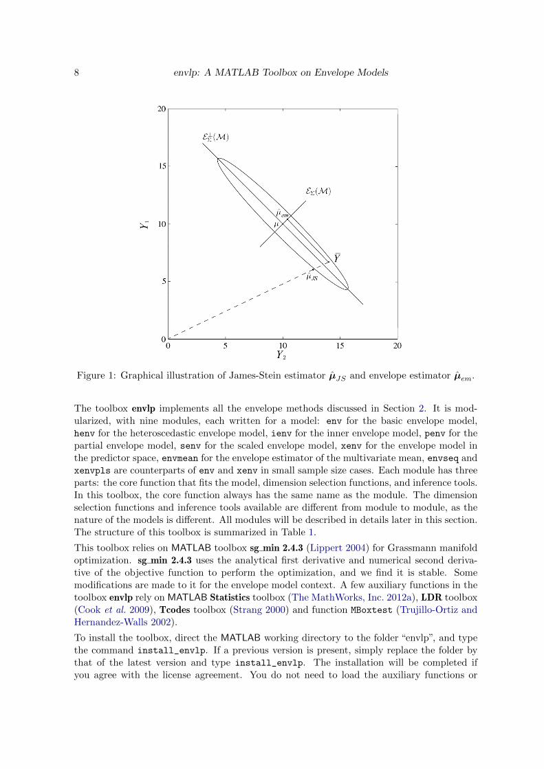
The difference between the James-Stein estimator and the envelope estimator can be visualizedin Figure 1. In the figure, the ellipse represents the distribution of Y. The James-Steinestimator of µ is denoted as µJS , and it shrinks Y towards the origin. In contrast to µJS ,the envelope estimator µem is the projection of Y onto the estimated envelope EΣ(M). Inthis figure, EΣ(M) aligns with the eigenvector corresponding to the smaller eigenvalue of Σ.Then the envelope estimator µem is much less variant than Y, and it is expected to have asmaller mean squared error than Y, or even µJS .
2.9. Role of normality
None of the envelope models discussed in Sections 2.1–2.8 require constraints on the distribu-tion of the errors ε beyond those listed previously. Adding the assumption that the errors arenormally distributed facilitates an analysis by providing a well-defined likelihood and asymp-totic standard errors. Excluding the sequential methods, all fitting in the envlp toolbox isbased on normal likelihoods, along with their corresponding inference methods. Those like-lihoods also provide
√n-consistent estimators without normality and experience has shown
that they perform well in non-normal settings. However, inference methods may be impactedby clear deviations from normality and then it is recommended that the bootstrap methodsavailable in the envlp toolbox be used for standard errors and inference. The bootstrap is theonly method provided for computing standard errors for the sequential estimators, as listedin Table 1.
3. Toolbox overview
8 envlp: A MATLAB Toolbox on Envelope Models
Figure 1: Graphical illustration of James-Stein estimator µJS and envelope estimator µem.
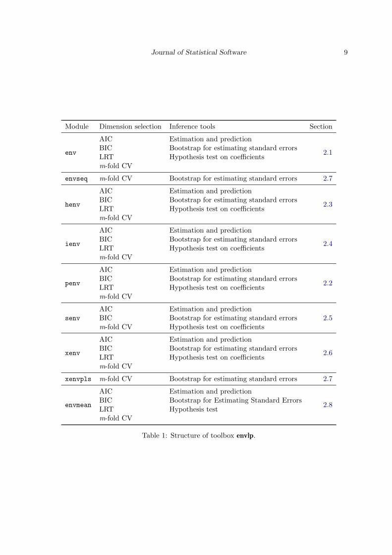
The toolbox envlp implements all the envelope methods discussed in Section 2. It is mod-ularized, with nine modules, each written for a model: env for the basic envelope model,henv for the heteroscedastic envelope model, ienv for the inner envelope model, penv for thepartial envelope model, senv for the scaled envelope model, xenv for the envelope model inthe predictor space, envmean for the envelope estimator of the multivariate mean, envseq andxenvpls are counterparts of env and xenv in small sample size cases. Each module has threeparts: the core function that fits the model, dimension selection functions, and inference tools.In this toolbox, the core function always has the same name as the module. The dimensionselection functions and inference tools available are different from module to module, as thenature of the models is different. All modules will be described in details later in this section.The structure of this toolbox is summarized in Table 1.
This toolbox relies on MATLAB toolbox sg min 2.4.3 (Lippert 2004) for Grassmann manifoldoptimization. sg min 2.4.3 uses the analytical first derivative and numerical second deriva-tive of the objective function to perform the optimization, and we find it is stable. Somemodifications are made to it for the envelope model context. A few auxiliary functions in thetoolbox envlp rely on MATLAB Statistics toolbox (The MathWorks, Inc. 2012a), LDR toolbox(Cook et al. 2009), Tcodes toolbox (Strang 2000) and function MBoxtest (Trujillo-Ortiz andHernandez-Walls 2002).
To install the toolbox, direct the MATLAB working directory to the folder “envlp”, and typethe command install_envlp. If a previous version is present, simply replace the folder bythat of the latest version and type install_envlp. The installation will be completed ifyou agree with the license agreement. You do not need to load the auxiliary functions or
Journal of Statistical Software 9
Module Dimension selection Inference tools Section
env
AIC Estimation and prediction
2.1BIC Bootstrap for estimating standard errorsLRT Hypothesis test on coefficientsm-fold CV
envseq m-fold CV Bootstrap for estimating standard errors 2.7
henv
AIC Estimation and prediction
2.3BIC Bootstrap for estimating standard errorsLRT Hypothesis test on coefficientsm-fold CV
ienv
AIC Estimation and prediction
2.4BIC Bootstrap for estimating standard errorsLRT Hypothesis test on coefficientsm-fold CV
penv
AIC Estimation and prediction
2.2BIC Bootstrap for estimating standard errorsLRT Hypothesis test on coefficientsm-fold CV
senv
AIC Estimation and prediction2.5BIC Bootstrap for estimating standard errors
m-fold CV Hypothesis test on coefficients
xenv
AIC Estimation and prediction
2.6BIC Bootstrap for estimating standard errorsLRT Hypothesis test on coefficientsm-fold CV
xenvpls m-fold CV Bootstrap for estimating standard errors 2.7
envmean
AIC Estimation and prediction
2.8BIC Bootstrap for Estimating Standard ErrorsLRT Hypothesis testm-fold CV
Table 1: Structure of toolbox envlp.
10 envlp: A MATLAB Toolbox on Envelope Models
toolboxes mentioned before. Once the toolbox is installed, you can call functions or datasetsin the toolbox from any current working directory.
The toolbox contains three types of functions: the core functions, functions for dimensionselection and functions for inference tools. Section 3.1 to 3.3 are devoted to the descriptionof these three types.
3.1. Core functions
The functions that fit the envelope models are the core functions of this package. There arenine of them, one in each module, and they share the same names as the module names.For example, the function env fits the envelope model, and the function envmean finds theenvelope estimator for the multivariate mean. The envelope models in the regression contextare env, henv, ienv, penv, senv, xenv, envseq and xenvpls. The inputs for these modelsare X, Y and u, where X and Y store the data matrices for the predictors and the responses,and u is the dimension of the envelope, which can be obtained by the functions discussed inSection 3.2. The inputs for envmean are the data matrix Y and the dimension of the envelopeu, as this context does not involve any predictors. The output of these nine functions is a listcontaining the envelope estimators of model parameters, and important statistics calculatedfrom the models like the value of the maximized log-likelihood function, asymptotic covariancematrix of the estimators, number of parameters in the model and many others.
We present an example by applying the envelope model to the wheat protein data in Cooket al. (2010). The wheat protein data contains seven variables, the logarithms of near infraredreflectance measured at six wavelengths and a group indictor taking value 0 or 1 for wheat withlow or high protein content. In multivariate linear regression (1), we take the group indicatoras the predictor and the spectral measurements as responses. The regression coefficients arethen the mean differences between the two groups. For demonstration purpose, we take onlythe third and fourth measurements as responses, so that we can visualize the data. First weload the data and assign the predictor and responses.
load wheatprotein.txt
X = wheatprotein(:, 8);
Y = wheatprotein(:, 3 : 4);
Figure 2 displays the data with two axis assigned to the two responses. For better visu-alization, we centered the data to have mean 0. Under the standard model, the estimatedcoefficients in β are 7.52 and −2.06, with the associated standard errors for these two elementsbeing 8.64 and 9.49. The standard errors returned by Out.asySE are asymptotic, for actualstandard errors, we need to multiply by 1/
√n, where n is the sample size.
Out1 = fit_OLS(X, Y);
Out1.betaOLS
ans =
7.5224
-2.0609
Journal of Statistical Software 11
-65 -20 25 70
-75
-25
2575
Y1 (1st response)
Y2
(2nd
resp
onse
)
A
-65 -20 25 70-75
-25
2575
Y1 (1st response)
Y2(2ndrespon
se)
B1
B2
EΣ(B)
E⊥Σ(B)
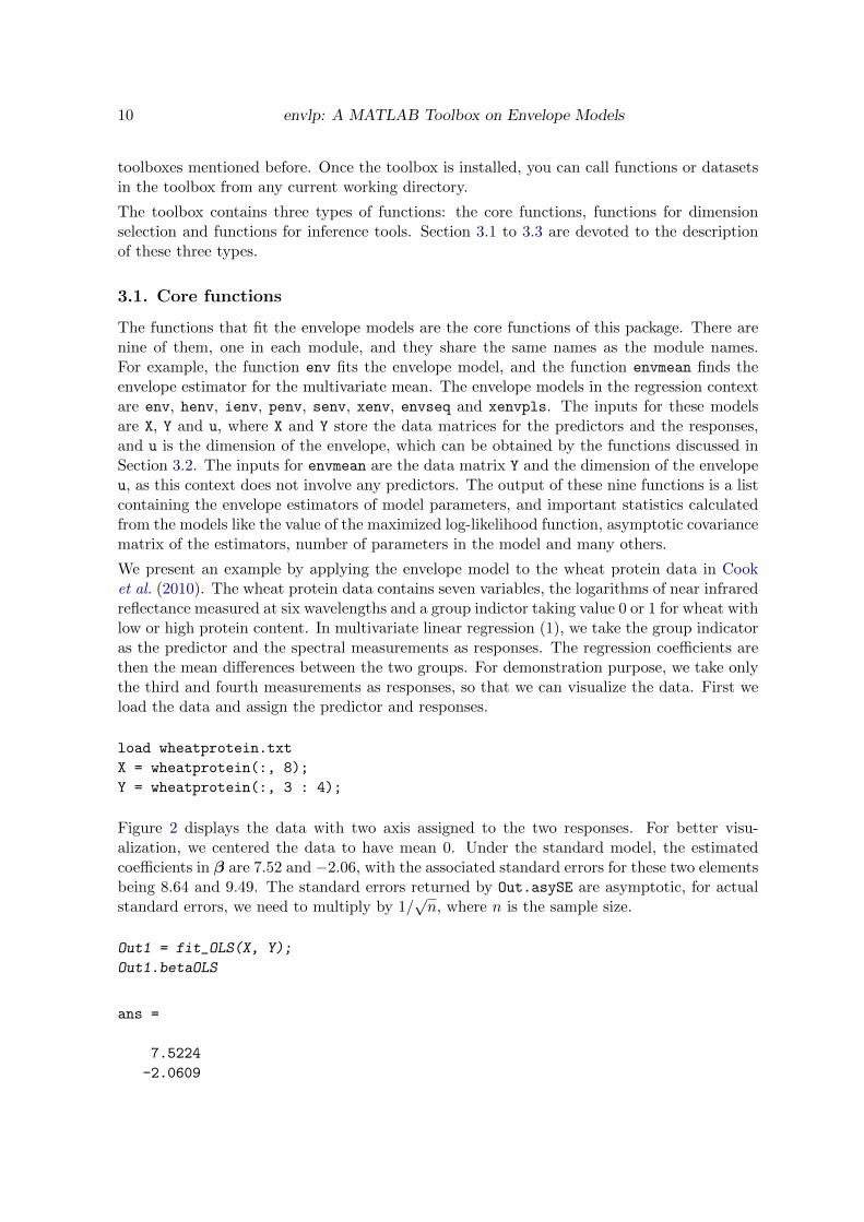
Figure 2: Graphical illustration of the working mechanism of the envelope model. The soliddots mark the wheat with high protein content and the open circles mark the wheat with lowprotein content.
n = 50;
Out1.asySE / sqrt(n)
ans =
8.6372
9.4852
The standard errors are large relative to the absolute value of elements in β, so it is hardto tell the difference between the two groups. The two curves in the left panel of Figure 2present the projection distribution of the two groups onto the Y1 axis, with the solid line forthe high protein group and the dashed line for the low protein group. The projection path fora sample point ‘x’ is marked as A in the plot. We notice that the two curves almost overlapwith each other, so it is hard to distinguish between the two groups. This is consistent withthe comparison of the absolute values of elements in β and their associated standard errors.
To fit the envelope model to this data, we need the dimension of the envelope. Dimensionselection will be discussed in Section 3.2, for now we just fixed the dimension of the envelopeat 1.
ModelOutput = env(X, Y, 1);
ModelOutput
ModelOutput =
12 envlp: A MATLAB Toolbox on Envelope Models
beta: [2x1 double]
Sigma: [2x2 double]
Gamma: [2x1 double]
Gamma0: [2x1 double]
eta: -6.9506
Omega: 6.0042
Omega0: 2.0510e+03
alpha: [2x1 double]
l: -377.3568
covMatrix: [2x2 double]
asyEnv: [2x1 double]
ratio: [2x1 double]
paramNum: 6
n: 50
After fitting the envelope model, the output is a list containing the estimates of regressioncoefficients β, error covariance matrix Σ, parameters in the envelope model including Γ, η,Ω, and Ω0, as well as important statistics like the value of the maximized log-likelihood l, theasymptotic covariance matrix of vectorized β, the asymptotic standard error for each elementin β, the number of parameters in the model and the sample size. To get the estimatedgroup difference, we call the respective component in the list ModelOutput.beta. Similarto the standard model, we can get the standard errors for elements in β by dividing theirasymptotic standard errors by
√n.
ModelOutput.beta
ans =
5.1405
-4.6782
ModelOutput.asySE / sqrt(n)
ans =
0.5142
0.4685
The envelope estimators of the two elements in β are 5.14 and −4.68, with standard errors0.51 and 0.47. Compared to the size of the elements in β, the standard errors are smalland it is easy to tell the difference between the two groups. The right panel of Figure 2illustrates the envelope analysis: The envelope model identifies the variation in the directionof E⊥Σ(B) as carrying no information on β, so a sample data point ‘x’ is projected first onto
the envelope subspace EΣ(B), and then onto the Y1 axis. The projection route is marked as B.The uniqueness of the envelope model is reflected on the first segment of B, which accountsfor the immaterial information in the data. The two curves on the Y1 axis are projectiondistributions of the two groups, with each data point following route similar to B. The two
Journal of Statistical Software 13
curves are well separated, indicating that we have obtained substantial efficiency gains. Toquantify the gains, we can compare the standard errors of the standard estimator and theenvelope estimator by taking their ratios. In this example, the ratios are 16.80 and 20.25 forthe two elements in β.
3.2. Dimension selection
Likelihood based methods including Akaike information criteria (AIC), Bayesian informationcriteria (BIC) and likelihood ratio testing (LRT) are implemented for selecting the dimensionof an envelope. In small sample size cases where the likelihood is not well-determined, weselect the dimension by m-fold cross validation.
The functions modelselectaic, modelselectbic and modelselectlrt choose the dimensionfor the envelope models in the regression context by AIC, BIC and LRT. The common inputsfor these three functions are data matrix X, Y, and modelType, while LRT has an additionalinput alpha indicating the significance level. The choices for modelType are ’env’, ’henv’,’ienv’, ’penv’, ’senv’ and ’xenv’.
The function mfoldcv chooses the dimension of the envelope models by m-fold cross validation.It divides the data into m folds of about equal size, and then uses one fold in turn as testingsamples and the rest as training samples. The function returns the dimension that minimizesthe average squared prediction errors using the identity inner product. The inputs for mfoldcvare data matrices X, Y, number of folds m and modelType. This method can be applied to anymodel, so the choices for modelType are ’env’, ’envseq’, ’henv’, ’ienv’, ’penv’, ’senv’,’xenv’, ’xenvpls’ and ’envmean’.
We write separate dimension selection functions for envelope estimator of multivariate means,as they have different input variables. The input variable of aic_envmean, bic_envmean andlrt_envmean is the data matrix Y only.
The output for all the dimension selection functions is an integer u for the dimension of theenvelope subspace.
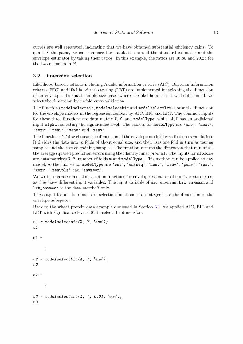
Back to the wheat protein data example discussed in Section 3.1, we applied AIC, BIC andLRT with significance level 0.01 to select the dimension.
u1 = modelselectaic(X, Y, 'env');u1
u1 =
1
u2 = modelselectbic(X, Y, 'env');u2
u2 =
1
u3 = modelselectlrt(X, Y, 0.01, 'env');u3
14 envlp: A MATLAB Toolbox on Envelope Models
u3 =
1
We notice that all three criteria agree that the dimension of the envelope subspace is 1.According to the right panel in Figure 2, u = 1 is well agreed by the data, and the estimatedenvelope subspace EΣ(B) is marked in the plot.
3.3. Inference tools
The inference tools provided by toolbox envlp include bootstrap estimation of standard errors,estimation and prediction at a new observation, and hypothesis testing.
The function bootstrapse computes the standard errors for elements in the estimated re-gression coefficients by bootstrapping the residuals. Its inputs are data matrices X, Y, thedimension of the envelope u, number of bootstrap sample B, and modelType, which can beenv, envseq, henv, ienv, penv, senv, xenv or xenvpls. The output bootse is a matrix hav-ing the same dimension as β with each element being the standard error of the correspondingelement in β. The function btrsp_envmean computes the standard errors for elements inµem. Its inputs and output are similar to bootstrapse, except that it does not need X andmodelType for input.
The function predict performs estimation or prediction for envelope models in the regressioncontext. It returns a list PredictOutput which includes the estimated or predicted value, itsstandard errors and covariance matrix. The input ModelOutput is the output list from thecore functions, Xnew is a column vector containing the value of X at which to estimate orpredict Y, infType can be chosen from ‘estimation’ or ‘prediction’, and modelType can beenv, henv, ienv, penv, senv or xenv. In the context of estimating a multivariate mean, theprediction function is called predict_envmean. It has similar structure as predict exceptthat it does not have inputs Xnew and modelType.
The function testcoefficient tests if certain linear combination of the rows or columns ofthe regression coefficients are equal to some pre-specified values. More specifically, lettingL, R and A be a × r, p × b and a × b matrices of constants, testcoefficient tests H0 :LβR = A versus Ha : LβR 6= A. The inputs are ModelOutput which is the output from thecore functions, TestInput which is a list that specifies L, R and A in the hypotheses andmodelType which can be chosen from env, henv, ienv, penv, senv and xenv. The outputTestOutput is a list that contains test statistic, degrees of freedom, p value and the covariancematrix of vectorized LβR. At the same time, a table is printed out to display the test results.The function testcoefficient_envmean is for testing H0 : Lµ = A versus Ha : Lµ 6= A,where µ is the multivariate mean, L is an a× r matrix and A is an a× 1 vector. The outputof testcoefficient_envmean has the same form as testcoefficient, but its input doesnot include modelType.
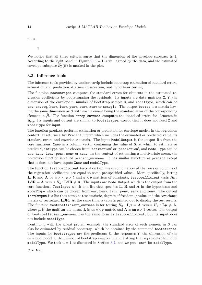
Continuing with the wheat protein example, the standard error of each element in β canalso be estimated by residual bootstrap, which be obtained by the command bootstrapse.The inputs for bootstrapse are the predictors X, the responses Y, the dimension of theenvelope model u, the number of bootstrap samples B, and a string that represents the modelmodelType. We took u = 1 as discussed in Section 3.2, and we put ’env’ for modelType.
B = 100;
Journal of Statistical Software 15
bootse = bootstrapse(X, Y, 1, B, 'env')
bootse =
0.5213
0.4767
Recall that the standard errors calculated using asymptotic standard errors are 0.5142 and0.4685, which are quite close to the bootstrap standard errors. We do not set seeds for thefunction bootstrapse, so the user can get different results each time he runs the function.But when B is large, the results should be close to each other.
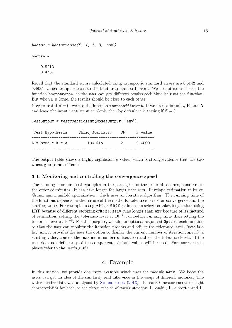
Now to test if β = 0, we use the function testcoefficient. If we do not input L, R and Aand leave the input TestInput as blank, then by default it is testing if β = 0.
TestOutput = testcoefficient(ModelOutput, 'env');
Test Hypothesis Chisq Statistic DF P-value
-------------------------------------------------------
L * beta * R = A 100.416 2 0.0000
-------------------------------------------------------
The output table shows a highly significant p value, which is strong evidence that the twowheat groups are different.
3.4. Monitoring and controlling the convergence speed
The running time for most examples in the package is in the order of seconds, some are inthe order of minutes. It can take longer for larger data sets. Envelope estimation relies onGrassmann manifold optimization, which uses an iterative algorithm. The running time ofthe functions depends on the nature of the methods, tolerance levels for convergence and thestarting value. For example, using AIC or BIC for dimension selection takes longer than usingLRT because of different stopping criteria; senv runs longer than env because of its methodof estimation; setting the tolerance level at 10−7 can reduce running time than setting thetolerance level at 10−9. For this purpose, we add an optional argument Opts to each functionso that the user can monitor the iteration process and adjust the tolerance level. Opts is alist, and it provides the user the option to display the current number of iteration, specify astarting value, control the maximum number of iteration and set the tolerance levels. If theuser does not define any of the components, default values will be used. For more details,please refer to the user’s guide.
4. Example
In this section, we provide one more example which uses the module henv. We hope theusers can get an idea of the similarity and difference in the usage of different modules. Thewater strider data was analyzed by Su and Cook (2013). It has 30 measurements of eightcharacteristics for each of the three species of water striders: L. esakii, L. dissortis and L.
16 envlp: A MATLAB Toolbox on Envelope Models
rufoscutellatus. In the datafile “waterstrider.mat”, X contains the two group indicators and Y
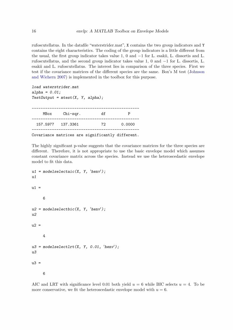
contains the eight characteristics. The coding of the group indicators is a little different fromthe usual, the first group indicator takes value 1, 0 and −1 for L. esakii, L. dissortis and L.rufoscutellatus, and the second group indicator takes value 1, 0 and −1 for L. dissortis, L.esakii and L. rufoscutellatus. The interest lies in comparison of the three species. First wetest if the covariance matrices of the different species are the same. Box’s M test (Johnsonand Wichern 2007) is implemented in the toolbox for this purpose.
load waterstrider.mat
alpha = 0.01;
TestOutput = mtest(X, Y, alpha);
------------------------------------------------
MBox Chi-sqr. df P
------------------------------------------------
157.5977 137.3361 72 0.0000
------------------------------------------------
Covariance matrices are significantly different.
The highly significant p-value suggests that the covariance matrices for the three species aredifferent. Therefore, it is not appropriate to use the basic envelope model which assumesconstant covariance matrix across the species. Instead we use the heteroscedastic envelopemodel to fit this data.
u1 = modelselectaic(X, Y, 'henv');u1
u1 =
6
u2 = modelselectbic(X, Y, 'henv');u2
u2 =
4
u3 = modelselectlrt(X, Y, 0.01, 'henv');u3
u3 =
6
AIC and LRT with significance level 0.01 both yield u = 6 while BIC selects u = 4. To bemore conservative, we fit the heteroscedastic envelope model with u = 6.
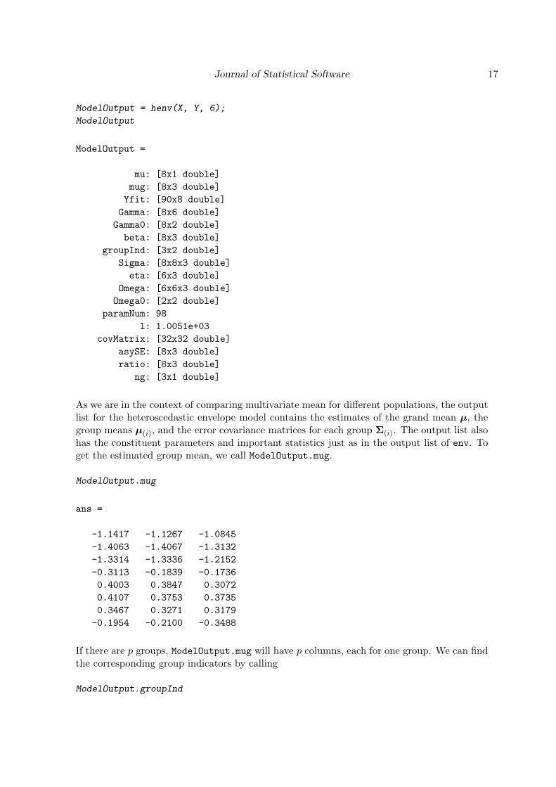
Journal of Statistical Software 17
ModelOutput = henv(X, Y, 6);
ModelOutput
ModelOutput =
mu: [8x1 double]
mug: [8x3 double]
Yfit: [90x8 double]
Gamma: [8x6 double]
Gamma0: [8x2 double]
beta: [8x3 double]
groupInd: [3x2 double]
Sigma: [8x8x3 double]
eta: [6x3 double]
Omega: [6x6x3 double]
Omega0: [2x2 double]
paramNum: 98
l: 1.0051e+03
covMatrix: [32x32 double]
asySE: [8x3 double]
ratio: [8x3 double]
ng: [3x1 double]
As we are in the context of comparing multivariate mean for different populations, the outputlist for the heteroscedastic envelope model contains the estimates of the grand mean µ, thegroup means µ(i), and the error covariance matrices for each group Σ(i). The output list alsohas the constituent parameters and important statistics just as in the output list of env. Toget the estimated group mean, we call ModelOutput.mug.
ModelOutput.mug
ans =
-1.1417 -1.1267 -1.0845
-1.4063 -1.4067 -1.3132
-1.3314 -1.3336 -1.2152
-0.3113 -0.1839 -0.1736
0.4003 0.3847 0.3072
0.4107 0.3753 0.3735
0.3467 0.3271 0.3179
-0.1954 -0.2100 -0.3488
If there are p groups, ModelOutput.mug will have p columns, each for one group. We can findthe corresponding group indicators by calling
ModelOutput.groupInd
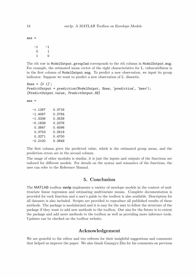
18 envlp: A MATLAB Toolbox on Envelope Models
ans =
-1 -1
0 1
1 0
The ith row in ModelOutput.groupInd corresponds to the ith column in ModelOutput.mug.For example, the estimated mean vector of the eight characteristics for L. rufoscutellatus isin the first column of ModelOutput.mug. To predict a new observation, we input its groupindicator. Suppose we want to predict a new observation of L. dissortis.
Xnew = [0 1]';PredictOutput = prediction(ModelOutput, Xnew, 'prediction', 'henv');[PredictOutput.value, PredictOutput.SE]
ans =
-1.1267 0.3716
-1.4067 0.3784
-1.3336 0.3539
-0.1839 0.2376
0.3847 0.4596
0.3753 0.3519
0.3271 0.4700
-0.2100 0.3849
The first column gives the predicted value, which is the estimated group mean, and theprediction errors are in the second column.
The usage of other modules is similar, it is just the inputs and outputs of the functions aretailored for different models. For details on the syntax and semantics of the functions, theuser can refer to the Reference Manual.
5. Conclusion
The MATLAB toolbox envlp implements a variety of envelope models in the context of mul-tivariate linear regression and estimating multivariate means. Complete documentation isprovided for each function and a user’s guide to the toolbox is also available. Description forall datasets is also included. Scripts are provided to reproduce all published results of thesemethods. The package is modularized and it is easy for the user to follow the structure of thepackage if they want to add new methods to the toolbox. Our aim for the future is to extentthe package and add more methods to the toolbox as well as providing more inference tools.Updates can be checked on the toolbox website.
Acknowledgement
We are grateful to the editor and two referees for their insightful suggestions and commentsthat helped us improve the paper. We also thank Guangyu Zhu for his comments on previous
Journal of Statistical Software 19
versions of the toolbox. The research in this article is supported in part by National ScienceFoundation Grants DMS-1007547 and SES-1156026.
References
Conway JB (1990). A Course in Functional Analysis. New York: Springer-Verlag.
Cook RD (2012). “Lecture Notes on Dimension Reduction.” School of Statistics, Universityof Minnesota, Minneapolis.
Cook RD, Forzani L, Tomassi D (2009). “LDR: A Package for Likelihood-based SufficientDimension Reduction.” Journal of Statistical Software, 39, 1–20.
Cook RD, Helland I, Su Z (2013). “Envelopes and Partial Least Squares Regression.” Journalof the Royal Statistical Society B, 75, 851–877.
Cook RD, Li B, Chiaromonte F (2010). “Envelope Models for Parsimonious and EfficientMultivariate Linear Regression (With Discussion).” Statistica Sinica, 20, 927–1010.
Cook RD, Su Z (2013). “Scaled Envelopes: Scale Invariant and Efficient Estimation in Mul-tivariate Linear Regression.” Biometrika, 100(4), 939–954.
de Jong S (1993). “SIMPLS: An Alternative Approach to Partial Least Squares Regression.”Chemometrics and Intelligent Laboratory Systems, 18(3), 251–263.
Diaconis P, Freedman D (1984). “Asymptotics of Graphical Projection Pursuit.” The Annalsof Statistics, pp. 793–815.
James W, Stein C (1961). “Estimation with Quadratic Loss.” In Proceedings of the FourthBerkeley Symposium on Mathematical Statistics and Probability, volume 1, pp. 361–379.
Johnson RA, Wichern DW (2007). Applied Multivariate Statistical Analysis. Upper SaddleRiver, NJ: Prentice Hall.
Lippert R (2004). sg min: Stiefel Grassmann Optimization. MATLAB package version 2.4.3.URL http://web.mit.edu/~ripper/www/sgmin.html.
Strang G (2000). Tcodes - MATLAB Teaching Codes. Massachusetts Institute of Technol-ogy, Cambridge, Massachusetts. URL http://web.mit.edu/18.06/www/Course-Info/
Tcodes.html.
Su Z, Cook RD (2011). “Partial Envelopes for Efficient Estimation in Multivariate LinearRegression.” Biometrika, 98(1), 133–146.
Su Z, Cook RD (2012). “Inner Envelopes: Efficient Estimation in Multivariate Linear Regres-sion.” Biometrika, 99(3), 687–702.
Su Z, Cook RD (2013). “Estimation of Multivariate Means with Heteroscedastic Errors UsingEnvelope Models.” Statistica Sinica, 23, 213–230.
20 envlp: A MATLAB Toolbox on Envelope Models
The MathWorks, Inc (2012a). Statistics Toolbox - MATLAB: Perform Statistical Modelingand Analysis. The MathWorks, Inc., Natick, Massachusetts. URL http://www.mathworks.
com/products/statistics/.
The MathWorks, Inc (2012b). MATLAB - The Language of Technical Computing, Ver-sion 8.0. The MathWorks, Inc., Natick, Massachusetts. URL http://www.mathworks.
com/products/matlab/.
Trujillo-Ortiz A, Hernandez-Walls R (2002). MBoxtest: Multivariate Statistical Testing forthe Homogeneity of Covariance Matrices by the Box’s M. A MATLAB file. URL http:
//www.mathworks.com/matlabcentral/fileexchange/2733.
Affiliation:
Dennis CookSchool of StatisticsUniversity of MinnesotaE-mail: [email protected]: http://users.stat.umn.edu/~rdcook
Zhihua SuDepartment of StatisticsUniversity of FloridaE-mail: [email protected]: http://www.stat.ufl.edu/~zhihuasu
Yi YangSchool of StatisticsUniversity of MinnesotaE-mail: [email protected]: http://users.stat.umn.edu/~yiyang
Journal of Statistical Software http://www.jstatsoft.org/
published by the American Statistical Association http://www.amstat.org/
Volume VV, Issue II Submitted: yyyy-mm-ddMMMMMM YYYY Accepted: yyyy-mm-dd
Related Documents