Environmental Statement Appendix 16.B (6.3.16.2) Hydrodynamic Modelling April 2016

Welcome message from author
This document is posted to help you gain knowledge. Please leave a comment to let me know what you think about it! Share it to your friends and learn new things together.
Transcript

Environmental Statement Appendix 16 .B (6.3.16.2)
Hydrodynamic Modelling
April 2016

Silvertown Tunnel
Appendix 16.B Hydrodynamic Modelling
Document Reference: 6.3.16.2
Page 2 of 80
THIS PAGE HAS INTENTIONALLY BEEN LEFT BLANK
Silvertown Tunnel
Appendix 16.B Hydrodynamic Modelling
Document Reference: 6.3.16.2
Page 3 of 80
Contents
List of Abbreviations ................................................................................................ 8
Glossary of Terms .................................................................................................... 9
Summary…………………………………………………………………...………………11
1. INTRODUCTION ......................................................................................... 13
1.1 Background ................................................................................................. 13
1.2 Study site .................................................................................................... 13
1.3 Scope of work ............................................................................................. 15
2. MODEL DATA ............................................................................................. 17
2.1 Bathymetry .................................................................................................. 17
2.2 Hydrodynamics ........................................................................................... 17
3. MODEL MESH MODELLING ...................................................................... 19
3.2 Silvertown Temporary jetty .......................................................................... 20
4. HYDRODYNAMIC SIMULATIONS ............................................................. 21
4.1 Simulations background .............................................................................. 21
4.2 Model validation .......................................................................................... 21
5. SEDIMENT SPILL SIMULATIONS ............................................................. 25
5.2 River bed surface sediment sampling ......................................................... 25
5.3 Vibracore Sediment Survey ........................................................................ 28
5.4 Dredging Instrument .................................................................................... 29
5.5 Dredging Log ............................................................................................... 29
5.6 Plume Modelling .......................................................................................... 31
6. MODEL RESULTS ...................................................................................... 35
6.1 Baseline hydrodynamics ............................................................................. 35
6.2 Current speed difference ............................................................................. 40
6.3 Sediment plume modelling .......................................................................... 44
6.4 Temporary jetty pile scour ........................................................................... 54
7. PROPELLER SCOUR ................................................................................. 61
8. CONCLUSION ............................................................................................ 63

Silvertown Tunnel
Appendix 16.B Hydrodynamic Modelling
Document Reference: 6.3.16.2
Page 4 of 80
Appendix A. Sediment particle size analysis .................................................. 65
Appendix B. Scour depth evolution ................................................................. 75

Silvertown Tunnel
Appendix 16.B Hydrodynamic Modelling
Document Reference: 6.3.16.2
Page 5 of 80
List of Tables
Table 4-1 Simulation matrix showing possible configurations for temporary jetty
structures, tidal conditions and river flow rates ......................................................... 21
Table 5-1 Cefas PSA statistics of the vibracore sediment sampling ........................ 29
Table 5-2 Sediment plume modelling scenarios ....................................................... 34
List of Figures
Figure 1-1 Silvertown temporary jetty design shown as the black outline with black
circular markers representing the temporary jetty piles ............................................ 14
Figure 3-1 Silvertown model mesh with bathymetry in mCD .................................... 19
Figure 3-2 Silvertown model mesh with bathymetry in mCD .................................... 20
Figure 4-1 Mean neap tide with mean river flow ....................................................... 22
Figure 4-2 Mean neap tide with high river flow conditions ........................................ 23
Figure 4-3 Mean spring tide with mean river flow conditions .................................... 23
Figure 4-4 Mean spring tide with high river flow conditions ...................................... 24
Figure 5-1 Location of intertidal and subtidal sample locations ................................ 26
Figure 5-2 Particle size analysis result of subtidal sample SU3 ............................... 27
Figure 5-3 Indicative location of proposed vibracore locations (1-6) and the location
of the moored barges in the centre of the site .......................................................... 28
Figure 5-4 Grain size and settling velocity ................................................................ 33
Figure 6-1 Baseline hydrodynamic flow conditions for mean neap tides and mean
river flow. .................................................................................................................. 36
Figure 6-2 Baseline hydrodynamic flow conditions for mean neap tides and high river
flow. .......................................................................................................................... 37
Figure 6-3 Baseline hydrodynamic flow conditions for mean spring tides and mean
river flow ................................................................................................................... 38
Figure 6-4 Baseline hydrodynamic flow conditions for mean spring tides and high
river flow. .................................................................................................................. 39
Figure 6-5 Difference in simulated current speed for mean spring and high flow
conditions. ................................................................................................................ 40
Figure 6-6 Current speed with and without the temporary jetty structure under mean
neap tide and mean flow conditions. ........................................................................ 41

Silvertown Tunnel
Appendix 16.B Hydrodynamic Modelling
Document Reference: 6.3.16.2
Page 6 of 80
Figure 6-7 Current speed with and without the temporary jetty structure under mean
neap tide and high flow conditions. .......................................................................... 42
Figure 6-8 Current speed with and without the temporary jetty structure under mean
spring tide and mean flow conditions ....................................................................... 43
Figure 6-9 Current speed with and without the temporary jetty structure under mean
spring tide and high flow conditions.......................................................................... 44
Figure 6-10 Map of maximum of Incremental SSC in mean neap tide and mean river
flow scenario ............................................................................................................ 46
Figure 6-11 Map of mean of Incremental SSC in mean neap tide and mean river flow
scenario .................................................................................................................... 46
Figure 6-12 Map of total bed mass change in mean neap tide and mean river flow
scenario .................................................................................................................... 47
Figure 6-13 Map of maximum of Incremental SSC in mean neap tide and high river
flow scenario ............................................................................................................ 47
Figure 6-14 Map of mean of Incremental SSC in mean neap tide and high river flow
scenario .................................................................................................................... 48
Figure 6-15 Map of total bed mass change in mean neap tide and high river flow
scenario .................................................................................................................... 48
Figure 6-16 Map of maximum of Incremental SSC in mean spring tide and mean
river flow scenario .................................................................................................... 49
Figure 6-17 Map of mean of Incremental SSC in mean spring tide and mean river
flow scenario ............................................................................................................ 49
Figure 6-18 Map of total bed mass change in mean spring tide and mean river flow
scenario .................................................................................................................... 50
Figure 6-19 Map of maximum of Incremental SSC in mean spring tide and high river
flow scenario ............................................................................................................ 50
Figure 6-20 Map of mean of Incremental SSC in mean spring tide and high river flow
scenario .................................................................................................................... 51
Figure 6-21 Map of total bed mass change in mean spring tide and high river flow
scenario .................................................................................................................... 51
Figure 6-22 Estimate of dry density of sea bed as a function of sand fraction and
consolidation ............................................................................................................ 52
Figure 6-23 Suspended sediment concentration (SSC) in 2006-2007 in the River
Thames. ................................................................................................................... 54
Figure 6-24 Typical flow structure around a pile structure. ....................................... 55

Silvertown Tunnel
Appendix 16.B Hydrodynamic Modelling
Document Reference: 6.3.16.2
Page 7 of 80
Figure 6-25 Location of current speed extraction (yellow markers) for jetty pile scour
depth calculations .................................................................................................... 57
Figure 6-26 Scour depth evolution over time for mean spring tide and high flow
conditions at the approach over two tidal cycles ...................................................... 59
Figure 6-27 Scour depth evolution over time for mean spring tide and high flow
conditions at the jetty head over two tidal cycles ...................................................... 60

Silvertown Tunnel
Appendix 16.B Hydrodynamic Modelling
Document Reference: 6.3.16.2
Page 8 of 80
List of Abbreviations
DCO Development Consent Order
ES Environmental Statement
FM Flow Model
kW Kilowatt
MT Mud Transport
PLA Port of London Authority
PSA Particle Size Analysis
SSC Suspended Sediment Concentration
STEP Scour Time Evolution Predictor
TfL Transport for London

Silvertown Tunnel
Appendix 16.B Hydrodynamic Modelling
Document Reference: 6.3.16.2
Page 9 of 80
Glossary of Terms
Bathymetry The study of underwater depth of lake
or ocean floors.
Blackwall Tunnel A pair of existing road tunnels under
the Thames at Blackwall in east
London
Dredging Dredging is the removal of sediments
and debris from the bottom of lakes,
rivers, harbours, and other water
bodies.
Hydrogeology Hydrogeology is the area of geology that deals with the distribution and movement of groundwater in the soil and rocks of the Earth's crust.
Silvertown Tunnel Proposed new twin-bore road tunnels
under the River Thames from the
A1020 in Silvertown to the A102 on
Greenwich Peninsula, East London.
Vibracore A technology and a technique for
collecting core samples of underwater
sediments and wetland soils.

Silvertown Tunnel
Appendix 16.B Hydrodynamic Modelling
Document Reference: 6.3.16.2
Page 10 of 80
THIS PAGE HAS INTENTIONALLY BEEN LEFT BLANK

Silvertown Tunnel
Appendix 16.B Hydrodynamic Modelling
Document Reference: 6.3.16.2
Page 11 of 80
SUMMARY
S.1.1 A hydrodynamic model of the River Thames between Greenwich and
Woolwich was created using MIKE21 Flow Model (FM). This model
includes tidal and river discharge boundary conditions. Four flow
scenarios were simulated: spring and neap tidal conditions with mean and
maximum river discharge. Simulated water elevations and current speeds
were validated against the HR Wallingford Thames Model and show good
agreement. A proposed Silvertown Tunnel jetty design is included in the
hydrodynamic model. Comparisons are made between simulations with
and without the jetty structure to show the impact of the jetty piles on flow
velocities. The construction of the jetty causes a reduction in flow velocity
around the jetty head and a slight increase on the approach jetty towards
the nearshore.
S.1.2 The MIKE21 Mud Transport (MT) module is used to assess the movement
of sediment caused by dredging the area around the jetty head.
Assessments are made of suspended and accumulated sediment as a
result of the dredging process. There is shown to be little impact on
suspended sediment concentration and sedimentation, particularly when
compared with background levels of suspended sediment concentration.
S.1.3 An assessment of scour around the jetty piles is made using the simulated
velocities around the jetty structure. The method of Whitehouse 1 was
applied which defines the scour depth as a function of time. An
adjustment factor is applied to account for cohesive sediments following
the method of HR Wallingford 2.A maximum scour depth of 0.46m is
calculated for the 1.016m diameter piles at the approach jetty and jetty
head.
S.1.4 Scour of the river bed due to propeller wash from ships berthed at the jetty
is also calculated. The depth of scour is directly related to the Froude
number, associated with the propeller flux velocity. The largest vessel to
be moored at the jetty is assumed to have a propeller diameter of 2.5m,
minimum height of propeller axis from the bed of 2.25m and engine power
1 Whitehouse, R. J. S. (1998). Scour at marine structures: A manual for practical applications. Thomas Telford, London, p198.
2 Harris J M., Whitehouse R. J. S., Benson T. (2012). The time evolution of scour around offshore structures – the scour time evolution predictor (STEP) model. HR Wallingford Ltd.

Silvertown Tunnel
Appendix 16.B Hydrodynamic Modelling
Document Reference: 6.3.16.2
Page 12 of 80
of 1500kW. These conditions give a maximum equilibrium scour depth
caused by propeller wash of 0.8m.

Silvertown Tunnel
Appendix 16.B Hydrodynamic Modelling
Document Reference: 6.3.16.2
Page 13 of 80
1. INTRODUCTION
1.1 Background
1.1.1 A new road tunnel has been proposed by Transport for London (TfL)
linking the areas of Greenwich Peninsula and Silvertown, on the banks of
the River Thames. As a part of this project a potential new temporary jetty
structure has been proposed on the northern bank of the River Thames,
to the east of the mouth of the River Lea, also known as Bow Creek. This
report investigates the impact of this structure on the local hydrodynamics
and determines the extent of any scour around the piles and alongside the
temporary jetty.
1.2 Study site
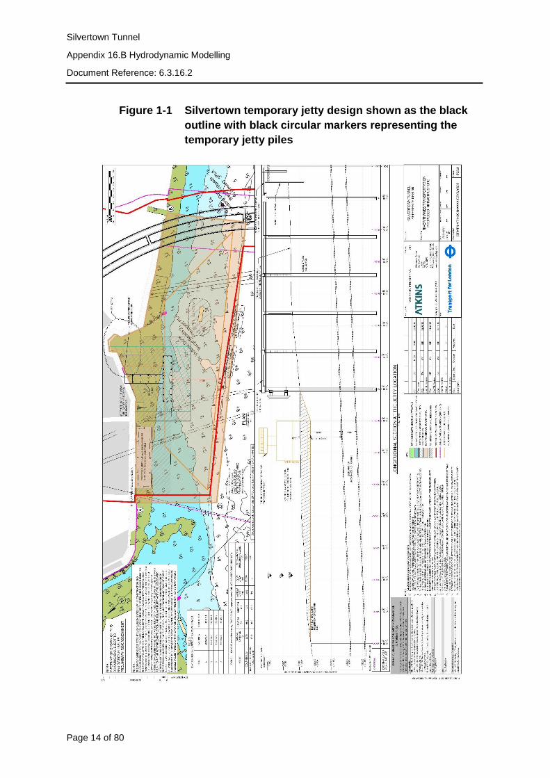
1.2.1 Figure 1-1 shows the indicative location of the temporary jetty structure on
the north bank of the River Thames, with Bow Creek to the west. The
proposed temporary jetty is a ‘T’ shaped structure, with a jetty head
attached to an approach jetty. Figure 1-1 shows the temporary jetty pile
alignments which consists of a total of 25 piles with a diameter of 1016
mm. The temporary jetty piles are indicated as black circular markers
within the T shaped jetty outline. A dredging area for vessels is shown as
the solid orange line polygon. The temporary jetty design shown in Figure
1-1 should not be viewed as the final design of the structure. The
hydrodynamic assessment present herein will assess the impact of the
structure and will therefore inform the final approval by the Port of London
Authority (PLA). Further to this, there will be a Development Consent
Order (DCO) requirement for the local authorities to approve the structure
design and external appearance. The orange trapezoid indicates an area
to be dredged, showing the area required to achieve a flat river bed for
jetty operations. Notwithstanding this, the Works Plans show a larger
dredge area for the Limits of Deviation of jetty operations which includes
the construction of the temporary jetty and the dredging works.
Silvertown Tunnel
Appendix 16.B Hydrodynamic Modelling
Document Reference: 6.3.16.2
Page 14 of 80
Figure 1-1 Silvertown temporary jetty design shown as the black
outline with black circular markers representing the
temporary jetty piles

Silvertown Tunnel
Appendix 16.B Hydrodynamic Modelling
Document Reference: 6.3.16.2
Page 15 of 80
1.3 Scope of work
1.3.1 The assessment of the impact of the temporary jetty structure will
investigate the change in local currents due to the movement of water
around the temporary jetty piles. The MIKE21FM hydrodynamic modelling
software is applied to simulate the tidal hydrodynamics, including the flow
of the River Thames and the River Lea. The model is developed on a
finite element flexible mesh of triangles, which allows for increased grid
resolution around complex areas of coastline and regions of interest, while
a coarser resolution can be applied to other regions, allowing for
increased model efficiency. MIKE21FM simulates the water level variation
and flow in response to a variety of forcing functions in coastal areas as
well as inshore waterbodies. The model can include the effects of
convective and cross momentum plus momentum dispersion, bottom and
surface (wind) shear stresses, coriolis and barometric pressure gradient
forcing, evaporation and precipitation, hydraulic structures and wave-
induced currents.
1.3.2 The simulated hydrodynamics around the temporary jetty piles will allow
for an estimate of the extent of river bed scour to be made. The scour
assessment will be made using the Scour Time Evolution Predictor
(STEP) model developed by HR Wallingford3 . The MIKE21 MT module is
used to assess the impact of sediments released into the water column
due to the dredging processes at the jetty head. The MIKE21 MT module
will account for sediment flocculation associated with cohesive sediments,
sediment settling and also resuspension. Regions of sediment
accumulation will show the deposition of sediments around the dredging
area. Suspended sediment concentrations will show the impact to the
water column due to the dredging works as assessed in Chapter 16 –
Water Quality and Flood Risk of the Environmental Statement (ES)
(Document Reference: 6.1.16).
3 Whitehouse, R. J. S. (1998). Scour at marine structures: A manual for practical applications. Thomas Telford, London, p198.

Silvertown Tunnel
Appendix 16.B Hydrodynamic Modelling
Document Reference: 6.3.16.2
Page 16 of 80
THIS PAGE HAS INTENTIONALLY BEEN LEFT BLANK

Silvertown Tunnel
Appendix 16.B Hydrodynamic Modelling
Document Reference: 6.3.16.2
Page 17 of 80
2. MODEL DATA
2.1 Bathymetry
2.1.1 Bathymetry data for the study site were supplied by the PLA at 10m
resolution and referenced to Chart Datum. These data were supplied on
29 May 2015. Regions of river bed dredging were manually included in
the model bathymetry in accordance with the indicative temporary jetty
specifications provided in the construction method statement Appendix
4.A (Document Reference: 6.3.4.1).
2.2 Hydrodynamics
2.2.1 Hydrodynamic boundary conditions for the Silvertown Tunnel tidal model,
simulated using MIKE21FM, were extracted from the HR Wallingford
River Thames model. Water level, both components of current velocity (u
and v) and river discharge were supplied at three locations: Greenwich
(538500, 178200), Silvertown (539500, 180400) and Woolwich (542000,
179600). A period of 48 hours was covered to allow for model spin up and
include a complete tidal cycle. Mean spring and neap tidal conditions were
included with mean and high river discharge rates to simulate low,
average and high flow conditions around the Silvertown Tunnel temporary
jetty structure. Discharge values were also supplied for River Lea (Bow
Creek), the river tributary to the immediate west of the temporary jetty
structure.

Silvertown Tunnel
Appendix 16.B Hydrodynamic Modelling
Document Reference: 6.3.16.2
Page 18 of 80
THIS PAGE HAS INTENTIONALLY BEEN LEFT BLANK

Silvertown Tunnel
Appendix 16.B Hydrodynamic Modelling
Document Reference: 6.3.16.2
Page 19 of 80
3. MODEL MESH MODELLING
3.1.1 The model domain was created to cover the region of the River Thames
between Greenwich and Woolwich. The mesh resolution varies from 50m
at the eastern and western boundaries to 7m around the Silvertown
Tunnel jetty structure. The finite element flexible mesh of triangles used
within the MIKE21 modelling software, allows for an efficient increase in
resolution around areas of interest while allowing for coarser resolution in
other regions of the model domain.
Figure 0-1 Silvertown model mesh with bathymetry in mCD

Silvertown Tunnel
Appendix 16.B Hydrodynamic Modelling
Document Reference: 6.3.16.2
Page 20 of 80
3.1.2 The mesh resolution can be seen to increase around the location of the
proposed temporary jetty (Figure 3-1).
3.2 Silvertown Temporary jetty
3.2.1 The temporary jetty structure configuration (Figure 1-1) is included in the
Silvertown model as a structure within MIKE21 FM mesh at a sub-grid
scale, with a diameter of 1016mm. This represents the likely development
that would be carried out, which is subject to detailed design and liaison
with the PLA. Location, width and shape of the piles is specified, for the
purpose of this assessment only, so that the effect on the flow can be
modelled by calculating the current induced drag force on each individual
pile. Jetty piles were included at a sub-grid scale where the mesh
resolution was chosen to be small enough to resolve the temporary jetty
but not excessive to reduce run times.
3.2.2 An area around the jetty head has been designated as a dredge area in
the initial design (Figure 1-1) and included in the model domain (Figure
0-2). This area is dredged to a depth of -5.3mCD to allow for vessels with
a draft of 4.642m.
Figure 0-2 Silvertown model mesh with bathymetry in mCD

Silvertown Tunnel
Appendix 16.B Hydrodynamic Modelling
Document Reference: 6.3.16.2
Page 21 of 80
4. HYDRODYNAMIC SIMULATIONS
4.1 Simulations background
4.1.1 The conditions simulated with the Silvertown Tunnel hydrodynamic model
include spring and neap tidal conditions with mean and high river flow
rates. Simulations were made with and without the jetty structure so that
the differences in current velocities due to the temporary jetty may be
examined. For the simulations with the temporary jetty structures the
modification to the bathymetry due to dredging for vessels, as shown in
Figure 0-2 Silvertown model mesh with bathymetry in mCD, is also
included. For the baseline simulations, without the temporary jetty
structures, the existing bathymetry was applied. Table 4-1 shows a
simulation matrix of the various jetty, tide and river flow conditions.
Table 4-1 Simulation matrix showing possible configurations for
temporary jetty structures, tidal conditions and river flow rates
Temporary jetty Option
Tide River flow
Without Neap Mean
Without Neap High
Without Spring Mean
Without Spring High
With Neap Mean
With Neap High
With Spring Mean
With Spring High
4.2 Model validation
4.2.1 The simulated hydrodynamic conditions listed in Table 4-1 Simulation
matrix showing possible configurations for temporary jetty structures, tidal
conditions and river flow rates are compared against the HR Wallingford
River Thames model results at a point close to the Silvertown Tunnel
temporary jetty (539500, 180400), using the baseline simulation without a
temporary jetty structure present. The HR Wallingford River Thames
model is validated against an estuary wide survey undertaken in 2004 as
a part of the Environment Agency TE2100 study, with further validation in

Silvertown Tunnel
Appendix 16.B Hydrodynamic Modelling
Document Reference: 6.3.16.2
Page 22 of 80
20094 . The Mean Absolute Errors for the validation of discharge rates are
between 5-10%, indicating a good performance in the HR Wallingford
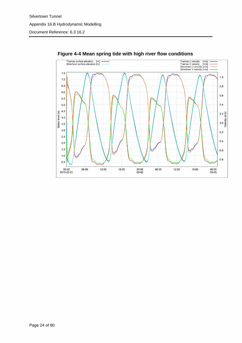
Thames model5. Figure 4-1 to Figure 4-4 shows the comparisons between
the Silvertown model and the HR Wallingford model simulated surface
elevation and both components of velocity (u and v). The comparisons in
Figure 4-1 to Figure 4-4 show very good agreement between simulated
hydrodynamics, with occasional differences for peak ood and peak ebb
velocity components. However, this is seen as an acceptable level of
model comparison and within the limits of the calibration.
Figure 4-1 Mean neap tide with mean river flow
4 HR Wallingford. (2015). LRS Central London Pier Extensions, hydrodynamic and scour assessment. HR Wallingford Ltd.
5 Baugh J.V., Littlewood M.A., “Development of a cohesive sediment transport model of the Thames Estuary”. Proceedings of the 9th International Conference on Estuarine and Coastal Modelling, 2005.

Silvertown Tunnel
Appendix 16.B Hydrodynamic Modelling
Document Reference: 6.3.16.2
Page 23 of 80
Figure 4-2 Mean neap tide with high river flow conditions
Figure 4-3 Mean spring tide with mean river flow conditions
Silvertown Tunnel
Appendix 16.B Hydrodynamic Modelling
Document Reference: 6.3.16.2
Page 24 of 80
Figure 4-4 Mean spring tide with high river flow conditions

Silvertown Tunnel
Appendix 16.B Hydrodynamic Modelling
Document Reference: 6.3.16.2
Page 25 of 80
5. SEDIMENT SPILL SIMULATIONS
5.1.1 The proposed temporary jetty development in Silvertown may require
dredging to maintain a minimum depth of -5.3 CD to manoeuvre the
vessels. To establish the possible sediment plume impact due to the
proposed dredging, sediment samples were collected. The results of
sediment sample analysis have provided an insight in to the local
sediment properties and also provided the data inputs for sediment plume
model.
5.2 River bed surface sediment sampling
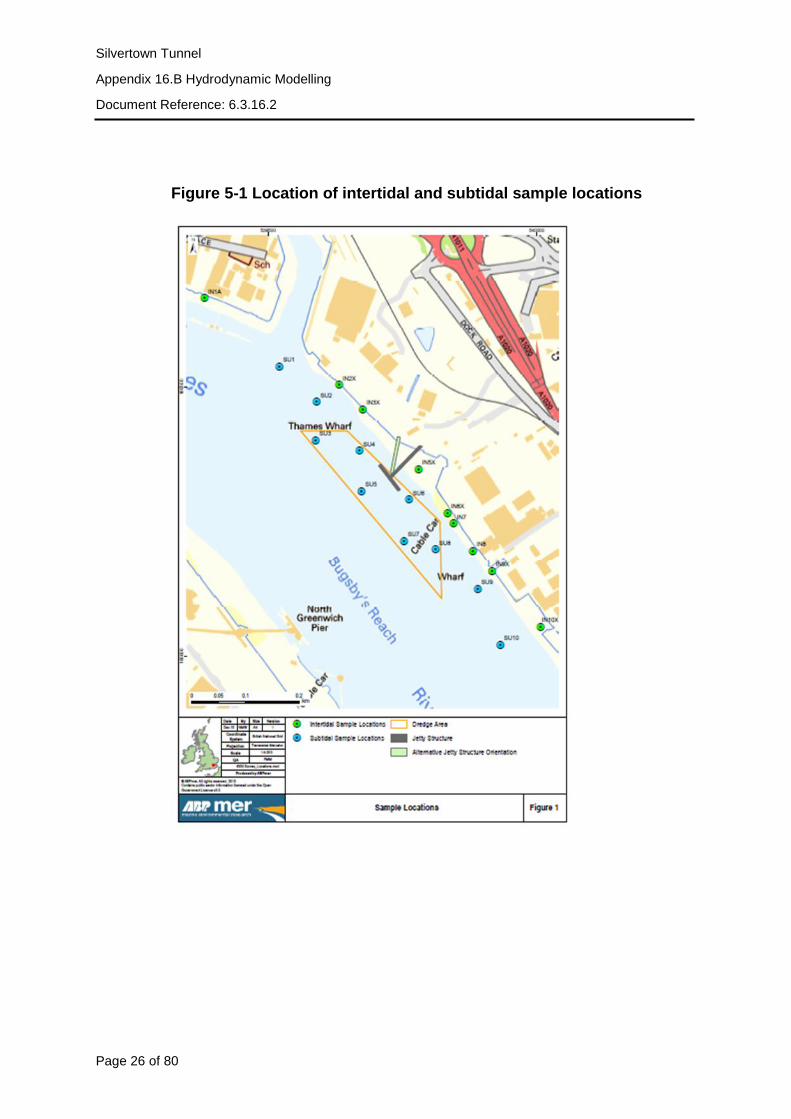
5.2.1 Surface sediment samples were collected by ABP Marine Environmental
Research Ltd at representative sample locations agreed with the Marine
Management Organisation in December 2015 in the vicinity of the
temporary jetty and dredge pocket and are shown in Figure 5-1. The
sediment samples were collected in both the intertidal and sub tidal
regime. The samples were analysed to obtain the particle size distribution
in the sediments to be dredged. Due to operational limitations only one
sub tidal sample result is available in the proposed dredging area i.e. SU3
(Figure 5-2). The sample proved to be composed of coarse-grained
material (gravel) on the river bed limiting the amount of sediment which
could be collected in the grab sampling. However, the results from all the
intertidal samples are presented in Appendix A. The sediment sample
analysis shows that, in the current dominated area (i.e. in the dredging
area and mid channel) the fraction of fine sediments is low, whereas in the
intertidal area, being a weak current area the fine material fractions are
high.
5.2.2 Since the current speed in the channel is in the order of 1-1.5 m/s the
deposition of fine material was ruled out. The sediment sample SU3
shows a silt content of only 1.5%. Considering the tidal current strength
and non-availability of the results of other subtidal sample, the sediment
sample SU3 is chosen as the representative sediment sample for the
dredging area. Hence it is established that percentage contribution of
fines in sediments to be dredged is 1.5-2%. The intertidal sediment
samples show a very high percentage of silt and clay. The high
concentration of fine sediments in intertidal sediment suggests that spilled
fine sediments mobilised due to the dredging would be deposited in the
intertidal area. The sediment sample results obtained from ABP Marine
Environmental Research Ltd can be found in Appendix A.
Silvertown Tunnel
Appendix 16.B Hydrodynamic Modelling
Document Reference: 6.3.16.2
Page 26 of 80
Figure 5-1 Location of intertidal and subtidal sample locations

Silvertown Tunnel
Appendix 16.B Hydrodynamic Modelling
Document Reference: 6.3.16.2
Page 27 of 80
.
Figure 5-2 Particle size analysis result of subtidal sample SU3
Silvertown Tunnel
Appendix 16.B Hydrodynamic Modelling
Document Reference: 6.3.16.2
Page 28 of 80
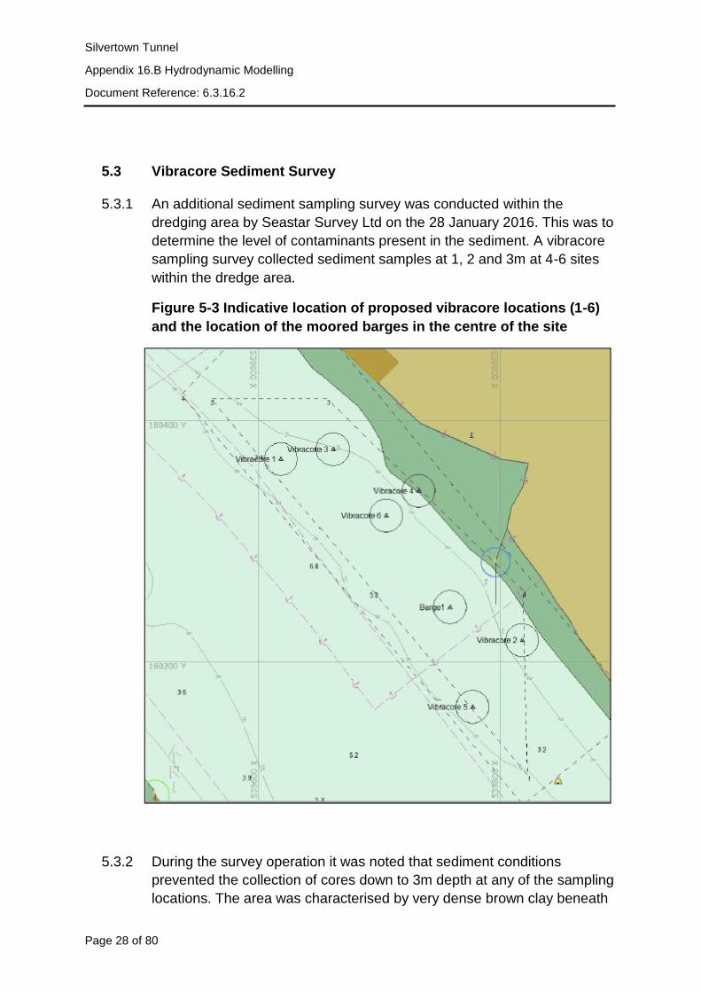
5.3 Vibracore Sediment Survey
5.3.1 An additional sediment sampling survey was conducted within the
dredging area by Seastar Survey Ltd on the 28 January 2016. This was to
determine the level of contaminants present in the sediment. A vibracore
sampling survey collected sediment samples at 1, 2 and 3m at 4-6 sites
within the dredge area.
Figure 5-3 Indicative location of proposed vibracore locations (1-6)
and the location of the moored barges in the centre of the site
5.3.2 During the survey operation it was noted that sediment conditions
prevented the collection of cores down to 3m depth at any of the sampling
locations. The area was characterised by very dense brown clay beneath

Silvertown Tunnel
Appendix 16.B Hydrodynamic Modelling
Document Reference: 6.3.16.2
Page 29 of 80
a surface of more mobile surface sediment, predominantly gravelly sand.
The clay plugged the vibracore barrel and prevented further sediment
from being collected. This limited the sub-sampling that was possible at
each site and reduced the number of samples for analysis. Particle size
analysis (PSA) conducted by Cefas (Table 5-1) shows the percentage of
clay for all samples to be within 71-89%. .
Table 5-1 Cefas PSA statistics of the vibracore sediment sampling
5.4 Dredging Instrument
5.4.1 The particle size analysis of the sediment sample in the dredging area
suggests that a mechanical dredger with a small draft would be required
to carry out the dredging work. A range of dredger types would be
available to the Contractor, with a backhoe dredger the most likely option
and probably represents the option with least headspill. As other dredging
options may be considered, this assessment assumes a grab dredger with
a capacity of 6m3. This represents intermediate worst case spill condition
of the dredging options available.
5.5 Dredging Log
5.5.1 The following dredge log calculations were completed using the sediment
sample, choice of dredging equipment and dredging volume. Total dredge
volume = 54,700m3.
5.5.2 It is a general practice to include over-dredge volume in the dredge log
calculation. It is required as the cut by grab dredger is not smooth, so, to
achieve the desired dredged depth, over-dredge is required. In this case
we assume the over dredged volume to be 10% of the total estimated
dredging volume.

Silvertown Tunnel
Appendix 16.B Hydrodynamic Modelling
Document Reference: 6.3.16.2
Page 30 of 80
5.5.3 Total volume to be dredged including over dredge volume is therefore
60,170 m3.
5.5.4 Bucket capacity of the grab dredger is 6 m3.
5.5.5 In general, there is slurry formation during the dredging process and lifting
the dredged material through the water column. Therefore each grab is
less than the bucket capacity. The Dredging handbook6 suggest a
reduction factor of 0.72 to be applied in case of sediments with silt and
sand content. The effective volume of sediment in each grab will be:
5.5.6 6 m3 * 0.72 = 4.32 m3.
5.5.7 The cycle time for each grab is assumed to be 210 seconds. The cycle
time includes the time required to lower the grab to the river bed, time
taken for dredging and lifting the dredged material through the water
column.
5.5.8 The grab dredger can work continuously, therefore continuous 24 hour
dredging operation is considered. This will lower the overall dredging cost
and it will also shorten the number of days required for the dredging.
5.5.9 The dredging rate is estimated to be 0.02m3⁄s.
5.5.10 The total time required to dredge the sediments is estimated as 34 days at
a dredging rate of 0.02m3⁄s. The total fine percentage in the dredged
sediment will be 2% (taken from subtidal sediment sample SU3). Since
the percentage of silt and clay in the sediment to be dredged is only 1.5%,
the dry density of the bed sediment is assumed to be 2,650 kg⁄m3
whereas the bulk density will be in the order of 2,000 kg⁄m3. The
percentage of fines spilled during the operation is assumed to be 7%.
Considering the above information, the spill flux is estimated to be 0.0576
kg/s. The formula used for spill flux is given below:
Spill volume (m3) = Volume of Dredged material (m3)*%fines*%spill of
fines
Spill flux= (Spill volume*Density of sediment)/Spill duration
6 R. N. Bray, J. M. Land, A. D. Bates. (1997). Dredging: A handbook for Engineers. Second Edition.

Silvertown Tunnel
Appendix 16.B Hydrodynamic Modelling
Document Reference: 6.3.16.2
Page 31 of 80
Volume of dredged material per grab= 4.32 𝑚3
Spill duration = Cycle time of per grab = 210 seconds
Percentage fines in dredged materials= 2%
Percentage spillage of fines during one dredge cycle= 7%
Wet density of the dredged materials= 2000 𝑘𝑔
𝑚3⁄
Spill volume per grab (𝑚3) = 4.32 (𝑚3) *2%*7% = 0.006 𝑚3
Spill flux = (0.006( 𝑚3)*2000(𝑘𝑔
𝑚3⁄ )/210 (s) = 0.0576 kg/s
5.6 Plume Modelling
5.6.1 The main objective of the dredging plume simulations is to identify areas
which are potentially exposed to higher concentrations of suspended
sediments and to siltation of dredged sediments. By knowing the extent
and magnitude of the dredging plumes, the construction method and
schedule can be optimised to reduce the environmental impact on
sensitive areas, if necessary. This is assessed in volume 1, Chapter 10 –
Marine Ecology of the Environmental Statement (Document Reference:
6.1.10).
5.6.2 The sediment transport/dredge plumes have been modelled by the MIKE
21 Mud Transport module (MIKE 21 MT). The MIKE 21 MT module
describes erosion, transport and deposition of mud or sand/mud mixtures
under the action of currents.
5.6.3 All dredging activities have been modelled by using the spill flux
calculated in the previous section. Based on the particle size analysis
result of sediment sample SU3, two fractions were considered for
suspended sediment. One fraction corresponds to the silt whereas the
other one is a representative of fine sand. No initial suspended sediment
concentrations are present in the model. Also the bed layer is defined as
hard rock without lose sediments, only settled sediment from the dredging
activities can re-suspend into the water column. The dispersion
coefficients are set proportional to the current. The water flowing through
the boundaries has no suspended sediment concentration. Applying a
value for the background would elevate suspended sediment levels
concentrations found in the receptor areas.

Silvertown Tunnel
Appendix 16.B Hydrodynamic Modelling
Document Reference: 6.3.16.2
Page 32 of 80
5.6.4 The settling velocity is dependent on the specific weight of the material,
kinematic viscosity and grain diameter. The settling velocities were
chosen from the chart given by USGS (Figure 5-4).

Silvertown Tunnel
Appendix 16.B Hydrodynamic Modelling
Document Reference: 6.3.16.2
Page 33 of 80
Figure 5-4 Grain size and settling velocity7
5.6.5 The settling velocity of silt fraction is chosen as 0.0005m/s whereas for
the fine sand the settling velocity is chosen as 0.0026m/s. The critical
7 U.S. Geological Survey Open file report 00-358

Silvertown Tunnel
Appendix 16.B Hydrodynamic Modelling
Document Reference: 6.3.16.2
Page 34 of 80
erosion shear stress is set to 0.15N/m2 whereas critical shear stress of
deposition is set to 0.07N/m2. The bed roughness is set to a Nikuradse
roughness of 0.001m.
5.6.6 The sediment plume modelling was carried out for four scenarios, similar
to the hydrodynamic modelling. The sediment plume modelling was
carried out for the baseline case which is does not contain the temporary
jetty structure. The scenarios considered for sediment plume modelling is
in Table 5-2. The simulations for each scenario were carried out for two
calendar days.
Table 5-2 Sediment plume modelling scenarios
Temporary jetty Option
Tide River flow
Without Neap Mean
Without Neap High
Without Spring Mean
Without Spring High

Silvertown Tunnel
Appendix 16.B Hydrodynamic Modelling
Document Reference: 6.3.16.2
Page 35 of 80
6. MODEL RESULTS
6.1 Baseline hydrodynamics
6.1.1 Figure 4-1 to Figure 4-4 shows the simulated U and V velocity
components at the Silvertown temporary jetty site, with a comparison
against the HR Wallingford Thames model. This shows the baseline
hydrodynamic conditions at the site of the proposed temporary jetty
structure. Figure 6-1 to Figure 6-4 shows simulated current speeds for
baseline model conditions, without the temporary jetty or dredge area, at
selected times of flood and ebb tides. Figure 4-4 and Figure 6-4 show that
under the worst case hydrodynamic conditions, mean spring tide with high
river flow, simulated current speeds are between 1-1.5m/s.

Silvertown Tunnel
Appendix 16.B Hydrodynamic Modelling
Document Reference: 6.3.16.2
Page 36 of 80
Figure 6-1 Baseline hydrodynamic flow conditions for mean neap
tides and mean river flow.

Silvertown Tunnel
Appendix 16.B Hydrodynamic Modelling
Document Reference: 6.3.16.2
Page 37 of 80
Figure 6-2 Baseline hydrodynamic flow conditions for mean neap
tides and high river flow.

Silvertown Tunnel
Appendix 16.B Hydrodynamic Modelling
Document Reference: 6.3.16.2
Page 38 of 80
Figure 6-3 Baseline hydrodynamic flow conditions for mean spring
tides and mean river flow

Silvertown Tunnel
Appendix 16.B Hydrodynamic Modelling
Document Reference: 6.3.16.2
Page 39 of 80
Figure 6-4 Baseline hydrodynamic flow conditions for mean spring
tides and high river flow.

Silvertown Tunnel
Appendix 16.B Hydrodynamic Modelling
Document Reference: 6.3.16.2
Page 40 of 80
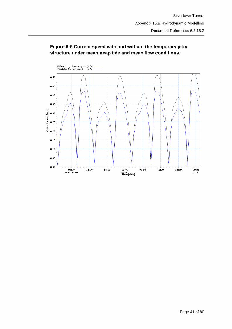
6.2 Current speed difference
6.2.1 To determine the effect of the temporary jetty structure on the
hydrodynamic flow, comparisons of simulated current speed with and
without the temporary jetty are calculated for all flow conditions. An initial
spatial comparison is made where the simulations without the temporary
jetty is subtracted from the simulations with the temporary jetty, so that
any increase in current speed is shown by positive values while negative
values represent a decrease in current speed. The difference between the
simulations is calculated at every time step, accounting for the initial
model spin up time of 1 hour. The statistical mean is then calculated.
Figure 6-5 shows the difference in current speed under spring tide and
high river flow conditions.
Figure 6-5 Difference in simulated current speed for mean spring and
high flow conditions.
Silvertown Tunnel
Appendix 16.B Hydrodynamic Modelling
Document Reference: 6.3.16.2
Page 41 of 80
Figure 6-6 Current speed with and without the temporary jetty
structure under mean neap tide and mean flow conditions.

Silvertown Tunnel
Appendix 16.B Hydrodynamic Modelling
Document Reference: 6.3.16.2
Page 42 of 80
Figure 6-7 Current speed with and without the temporary jetty
structure under mean neap tide and high flow conditions.

Silvertown Tunnel
Appendix 16.B Hydrodynamic Modelling
Document Reference: 6.3.16.2
Page 43 of 80
Figure 6-8 Current speed with and without the temporary jetty
structure under mean spring tide and mean flow conditions

Silvertown Tunnel
Appendix 16.B Hydrodynamic Modelling
Document Reference: 6.3.16.2
Page 44 of 80
Figure 6-9 Current speed with and without the temporary jetty
structure under mean spring tide and high flow conditions
6.2.2 Figure 6-5 shows that the temporary jetty would have a greatest impact on
the current speeds in the local area around the temporary jetty head. The
reduction in current speed around the temporary jetty head of the new
temporary jetty design is likely due to the drag influence caused by the
jetty head. Figure 6-5 also shows a slight increase in current speed
inshore of the temporary jetty due to the constriction of flow in this area
caused by the frictional influence of the jetty head and the constriction of
flow between the piles of the approach temporary jetty. Figure 6-6 to
Figure 6-9 shows the simulated current speeds with and without the
temporary jetty structure at the jetty head. A reduction in current speed
can be seen in all flow conditions and most pronounced around peak tidal
speeds. The reduction in current speed at peak ebb and flood tide is
within the range of 0.05m/s to 0.1m/s.
6.3 Sediment plume modelling
6.3.1 The results of the various plume modelling scenarios can be seen in
Figure 6-10 to Figure 6-21. The results of each scenario are presented as
a map of maximum and mean incremental increase in suspended

Silvertown Tunnel
Appendix 16.B Hydrodynamic Modelling
Document Reference: 6.3.16.2
Page 45 of 80
sediment concentration (SSC) and total bed mass change over the
simulation period (i.e. 2 calendar days). Figure 6-10 to Figure 6-21 shows
that the maximum concentration of suspended sediments over the
simulation influences the entire length of the model domain, primarily on
the northern river bank, with greatest concentrations around the dredge
site. The mean concentration of suspended sediments is much lower and
found in the dredge location. This suggests that, due to the relatively high
current velocities, suspended sediments from the dredging operation
would be transported away from the dredge site. Relatively low
concentrations of suspended sediments will remain around the dredge
and temporary jetty location. The faster flow conditions of spring tides and
high river flows shows lower mean concentrations of suspended
sediments around the dredge location, this shows how localised effects of
the dredging operation would change with the local flow conditions. It
should be noted that the concentration of suspended sediments simulated
from the dredging operation will be considerably lower than the
background level of suspended sediment concentration. Therefore, there
would be a negligible impact on the surrounding environment.
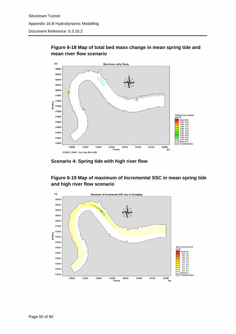
6.3.2 The total bed mass change represents accumulated sediments released
during the dredge operation. The simulated results show that there is not
significant accumulation of sediments around the temporary jetty
structure. Higher flow speeds associated with spring tides and high river
flows would transport the suspended sediments to further reaches in the
model domain.

Silvertown Tunnel
Appendix 16.B Hydrodynamic Modelling
Document Reference: 6.3.16.2
Page 46 of 80
Scenario 1: Neap tide with mean river flow
Figure 6-10 Map of maximum of Incremental SSC in mean neap tide
and mean river flow scenario
Figure 6-11 Map of mean of Incremental SSC in mean neap tide and
mean river flow scenario

Silvertown Tunnel
Appendix 16.B Hydrodynamic Modelling
Document Reference: 6.3.16.2
Page 47 of 80
Figure 6-12 Map of total bed mass change in mean neap tide and
mean river flow scenario
Scenario 2: Neap tide with high river flow
Figure 6-13 Map of maximum of Incremental SSC in mean neap tide
and high river flow scenario

Silvertown Tunnel
Appendix 16.B Hydrodynamic Modelling
Document Reference: 6.3.16.2
Page 48 of 80
Figure 6-14 Map of mean of Incremental SSC in mean neap tide and
high river flow scenario
Figure 6-15 Map of total bed mass change in mean neap tide and
high river flow scenario

Silvertown Tunnel
Appendix 16.B Hydrodynamic Modelling
Document Reference: 6.3.16.2
Page 49 of 80
Scenario 3: Spring tide with mean river flow
Figure 6-16 Map of maximum of Incremental SSC in mean spring tide
and mean river flow scenario
Figure 6-17 Map of mean of Incremental SSC in mean spring tide and
mean river flow scenario
Silvertown Tunnel
Appendix 16.B Hydrodynamic Modelling
Document Reference: 6.3.16.2
Page 50 of 80
Figure 6-18 Map of total bed mass change in mean spring tide and
mean river flow scenario
Scenario 4: Spring tide with high river flow
Figure 6-19 Map of maximum of Incremental SSC in mean spring tide
and high river flow scenario

Silvertown Tunnel
Appendix 16.B Hydrodynamic Modelling
Document Reference: 6.3.16.2
Page 51 of 80
Figure 6-20 Map of mean of Incremental SSC in mean spring tide and
high river flow scenario
Figure 6-21 Map of total bed mass change in mean spring tide and
high river flow scenario
6.3.3 The deposition of sediment is expressed as bed mass change which gives
the accumulated mass of sediment deposited per metre square area. The
simulation result shows that the deposition will be negligible except at
some locations. This is attributed to the fact that the current magnitude in
the domain is high, so deposition will be minimum and sediment will be

Silvertown Tunnel
Appendix 16.B Hydrodynamic Modelling
Document Reference: 6.3.16.2
Page 52 of 80
advected to distant sites. However, at a small number of locations, a
theoretical maximum deposition is seen in the domain where there is eddy
formation. In these locations the deposition is in the order of 1-4 kg/m2.
6.3.4 In order to convert the siltation rate into increase in depth it is required to
know the dry density of the sea bed. The dry density depends on the sand
fraction and degree of consolidation of the fine sediments.
6.3.5 An estimate of the dry density can be found by referring Figure 6-22. For
half consolidated sediment with a sand fraction between 0.2 to 0.4 the dry
density is in the range from 800 kg/m2 to 1000 kg/m2.
Figure 6-22 Estimate of dry density of sea bed as a function of sand
fraction and consolidation
6.3.6 𝑋 ((1 − 𝑛)𝑌)⁄ During the two day simulation period, the theoretical
deposition at a small number of sites is 1-4 kg/m2 at some locations in the
model domain as seen in the plots shown above. The increase in
sediment depth is calculated as:
6.3.7 Where X is the accumulation of sediment mass, n is the porosity (0.4) and
Y is the dry density of sediment. In these small “pockets” the theoretical
deposition of sediment may be in the order of 2x10⁻³m to 6x10⁻³m (2-
6mm) considering the dry density of 800kg/m3 over the complete dredge
duration. However, it should be noted that these areas of accumulation
are not in the immediate region of the temporary jetty structure.

Silvertown Tunnel
Appendix 16.B Hydrodynamic Modelling
Document Reference: 6.3.16.2
Page 53 of 80
6.3.8 Clearly this is a theoretic calculation at a small number of predicted sites
in the model domain. This has to be compared with the known natural
suspended sediment load which varies over the spring to neap tidal cycle
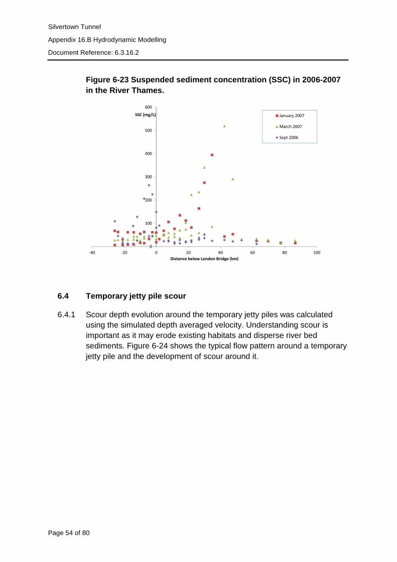
and on a seasonal basis with river flow and equinoctial tidal variation.
6.3.9 Previous studies of SSC in the River Thames have shown a seasonal
change with typical tide average values of 100 mg/l in summer, generally
low flow, and 50mg/l in winter, high flow, periods8. A study analysed two
years (2006-2007) of turbidity data to understand the turbidity maximum in
the Thames9 (Figure 6-23).The SSC sampling results for the 2006-2007
study show that for the Silvertown temporary jetty site (approximately
11km below London Bridge), concentration levels are within the range of
50-100 mg/l. Therefore the levels of SSC simulated from the dredge spill
modelling (Figure 6-10 to Figure 6-21) are negligible when compared with
the background levels.
8 Thames Tideway Tunnel. Application for Development Consent, Environmental Statement. Volume 3: Project-wide effects assessment appendices. Doc Red: 6.2.03 9 Mitchell S., Akesson L., Uncles R. (2012). Observations of turbidity in the Thames Estuary, United Kingdom. Water and Environment Journal.
Silvertown Tunnel
Appendix 16.B Hydrodynamic Modelling
Document Reference: 6.3.16.2
Page 54 of 80
Figure 6-23 Suspended sediment concentration (SSC) in 2006-2007
in the River Thames.
6.4 Temporary jetty pile scour
6.4.1 Scour depth evolution around the temporary jetty piles was calculated
using the simulated depth averaged velocity. Understanding scour is
important as it may erode existing habitats and disperse river bed
sediments. Figure 6-24 shows the typical flow pattern around a temporary
jetty pile and the development of scour around it.

Silvertown Tunnel
Appendix 16.B Hydrodynamic Modelling
Document Reference: 6.3.16.2
Page 55 of 80
Figure 6-24 Typical flow structure around a pile structure.
6.4.2 The sediment surveys have shown that the river bed is characterised by a
top layer of mobile sediment underlain by consolidated clay which is more
resistant to erosion. The method of Whitehouse10 was applied, which
defines the scour depth S(t) as a function of time using the following
equation:
𝑆(𝑡) = 𝑆𝑒 [1 − 𝑒𝑥𝑝 (−
𝑡
𝑇𝑠
)𝑛
] (1)
6.4.3 Where Ts is the time scale of the scour process given by equation 2, Se is
the equilibrium scour depth given by equation 4 and n is a power normally
assumed to be 1.
𝑇∗ =
[𝑔(𝑠 − 1)𝑑503 ]
12⁄
𝐷2𝑇𝑠
(2)
10 Whitehouse, R. J. S. (1998). Scour at marine structures: A manual for practical applications. Thomas Telford, London, p198.

Silvertown Tunnel
Appendix 16.B Hydrodynamic Modelling
Document Reference: 6.3.16.2
Page 56 of 80
6.4.4 Where d50 is the median grain size (m), g is the gravitational acceleration
(ms-2), D is the diameter of the pile (m) and T* is the dimensionless time
scale for currents given as:
𝑇∗ =
𝛿𝜃−2.2
2000𝐷
(3)
6.4.5 Where δ is the boundary layer thickness, assumed to be depth of flow for
tidal conditions and θ is the Shields parameter. The equation for the
equilibrium scour depth Se is given by:
𝑆𝑒 = 1.5𝐾1𝐾2𝐾3𝐾4𝐷 tanh (
ℎ
𝐷)
(4)
6.4.6 Where K1 is the correction factor for pile nose shape, K2 is the correction
factor for the angle of approach of the flow and K3 is the correction factor
for bed conditions, varying between 0 and 1 depending on flow conditions,
so that:
𝐾3 = 0 If 𝑈
𝑈𝑐𝑟< 0.5
𝐾3 = 2 (𝑈
𝑈𝑐𝑟
) − 1 If 0.5 ≤𝑈
𝑈𝑐𝑟< 1 (5)
𝐾3 = 1 If 𝑈
𝑈𝑐𝑟≥ 1
6.4.7 The parameter K4 is the correction factor for size of bed material, U is the
depth averaged current speed and Ucr is the threshold depth averaged
current speed. The scour depth methodology detailed so far has assumed
a gravely sand, non-cohesive sediment type. Previous studies have
shown that as the clay content of the sediment increases, the scour depth
ratio (St/D) decreases. The sediment clay content can be represented by
the use of a reduction factor multiplier on the scour depth. HR
Wallingford11 proposed a reduction factor Kcc, which represents the
fractional clay content C, with the expression:
11 Harris J M., Whitehouse R. J. S., Benson T. (2012). The time evolution of scour around offshore structures – the scour time evolution predictor (STEP) model. HR Wallingford Ltd.

Silvertown Tunnel
Appendix 16.B Hydrodynamic Modelling
Document Reference: 6.3.16.2
Page 57 of 80
𝐾𝑐𝑐 =1
(1 + 𝐶)2
(6)
6.4.8 This reduction factor reduces scour depth in a mixed sand-clay sediment
type by approximately 70%, assuming an 80% clay content, as seen in
the vibracore sediment samples. Simulated current speeds were extracted
from the Silvertown model at two locations on the temporary jetty
structure, at the jetty head and on the approach jetty (Figure 6-25).
Figure 6-25 Location of current speed extraction (yellow markers) for
jetty pile scour depth calculations
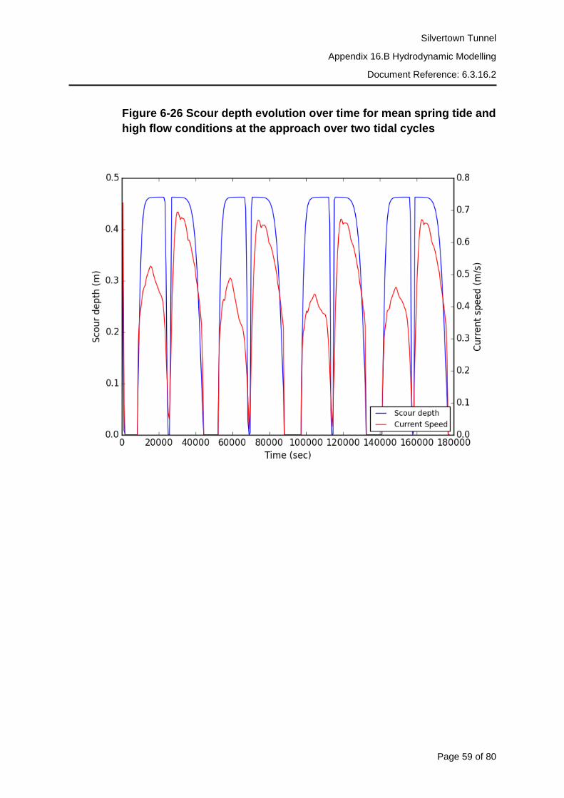
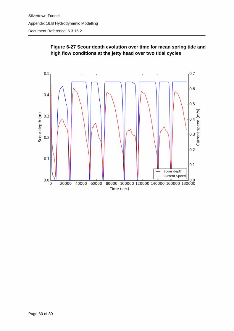
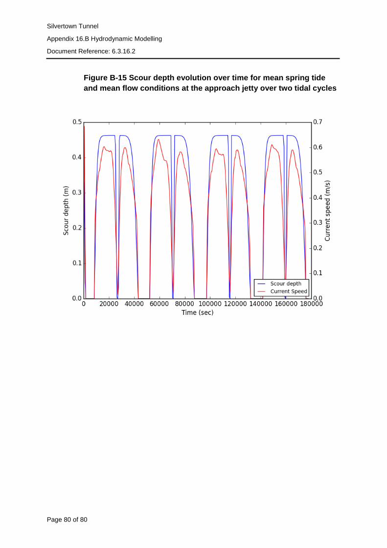
6.4.9 Figure 6-26 and Figure 6-27 shows the scour depth evolution over time for
mean spring tide and high river flow conditions at the jetty head and
approach pontoons. Scour depth evolution for all tidal and river flow
conditions can be found in Appendix B. This shows a maximum scour
depth of 0.46m around the temporary jetty piles, which is approximately
0.45 times the diameter of the pile (0.45D). This is less than the 1.3D
scour depth value of Harris et al.12, however this could be due to the
inclusion of the reduction factor due to a 80% clay sediment type.
12 Harris J M., Whitehouse R. J. S., Benson T. (2012). The time evolution of scour around offshore structures – the scour time evolution predictor (STEP) model. HR Wallingford Ltd.

Silvertown Tunnel
Appendix 16.B Hydrodynamic Modelling
Document Reference: 6.3.16.2
Page 58 of 80
6.4.10 The lateral extent of the scour around the temporary jetty piles is a
function of scour depth and the angle of repose of the sediment. A
laboratory study of tidal scour showed that lateral extents of 3.5 times the
predicted scour depth can be expected13. This method predicts a scour
width 1.61m scour width for the 1.016m piles. The slope of the upstream
and side edges of the scour hole will tend to be steeper than the
downstream edge (Figure 6-26). Therefore the extent of the lateral scour
will be greatest at the downstream edge of the temporary jetty structure,
and will therefore be less, parallel to the jetty head. The downstream edge
will also alternate with the flooding and ebbing tide. The lateral extent of
the scour will taper from the scour depth to the river bed. For cohesive
sediments, steeper slopes may be possible when compared with con-
cohesive sediments. Therefore the prediction of the lateral extent of scour
should be seen as a worst case scenario.
13 Escarameia M and May RWP (1999). Scour around structures in tidal flows. HR Wallingford report SR521
Silvertown Tunnel
Appendix 16.B Hydrodynamic Modelling
Document Reference: 6.3.16.2
Page 59 of 80
Figure 6-26 Scour depth evolution over time for mean spring tide and
high flow conditions at the approach over two tidal cycles
Silvertown Tunnel
Appendix 16.B Hydrodynamic Modelling
Document Reference: 6.3.16.2
Page 60 of 80
Figure 6-27 Scour depth evolution over time for mean spring tide and
high flow conditions at the jetty head over two tidal cycles
Silvertown Tunnel
Appendix 16.B Hydrodynamic Modelling
Document Reference: 6.3.16.2
Page 61 of 80
7. PROPELLER SCOUR
7.1.1 Ship propeller wash has the potential to cause erosion or scour of the sea
bed and therefore induce instability near to the jetty structure. Previous
studies have shown that the Froude F0 number influences scour depth,
given by:
𝐹0 =𝑈0
√(𝑔𝑑50 𝛿𝜌 𝜌⁄ )
(7)
7.1.2 Where U0 is the flux velocity of the propeller, g is acceleration due to
gravity, d50 is median grain size, δρ is the difference in density of
sediment and fluid and ρ is the density of the fluid. For berthing vessels
using propellers, maximum jet velocity generally occurs when the vessel
is stationary or slow moving (Hawkswood et al., 2014). The maximum jet
velocity U0 is given by:
𝑈0 = 1.48 (
𝑃𝑏
𝜌𝐷𝑝2
)
13⁄
(8)
7.1.3 Where Pb is the engine power and Dp is the propeller diameter. The
maximum equilibrium scour depth is then calculated using the non-
dimensional formula of Hong et al. (2012):
𝑑𝑠,𝑡
𝐷𝑝= 1.171𝐹0
0.872 (𝑦0
𝐷𝑝)
−0.761
(𝑑50
𝐷𝑝)
0.34
(9)
7.1.4 Where y0 is the height of the propeller axis from the bed. The largest
vessel proposed to be moored at the Silvertown jetty is the Dolphin HAV,
with a gross tonnage of 2075t, length of 88.3m and draft of 4.64m. The
propeller diameter is assumed to be 2.5m, the minimum height of the
propeller axis from the bed is 2.25m and the engine power is taken as
1500kW. It should be noted that this method so far is calculating propeller
scour depth for a sediment type of gravely sand. However, vibracore
sediment samples have shown a mobile layer of non-cohesive sediment
overlying consolidated clay. This clay layer will be harder to erode and will
therefore reduce scour depths. Applying a similar scour reduction factor to
that applied to the time evolving scour around the temporary jetty piles
(Eq 6) will allow for an estimate of the reduction in scour depth due to the
presence of clay. This reduction factor reduces the scour depth due to

Silvertown Tunnel
Appendix 16.B Hydrodynamic Modelling
Document Reference: 6.3.16.2
Page 62 of 80
propeller wash to 0.8m. It should be noted that this scour would be very
localised to the immediate area under the moored vessel’s propeller. This
section of the Thames is also subject to regular vessel movement e.g.
from the Thames clipper which docs just opposite the proposed
Silvertown temporary jetty.
7.1.5 The equation for maximum bottom velocity due to propeller wash is:
𝑉𝑏𝑚𝑎𝑥 = 𝐶1𝑈0𝐷𝑝 𝐻𝑝⁄ (12)
7.1.6 This generates a maximum bottom velocity Vbmax of 0.88m/s.
Silvertown Tunnel
Appendix 16.B Hydrodynamic Modelling
Document Reference: 6.3.16.2
Page 63 of 80
8. CONCLUSION
8.1.1 The hydrodynamic modelling for the Silvertown Temporary jetty model
has shown that the inclusion of the temporary jetty structure would reduce
velocities around the jetty head. The reduction in current speeds is due to
the increased drag forces generated by the series of temporary jetty piles
aligned with the direction of flow. The reduction in current speed is within
the range of 0.05-0.1 m/s and is most prominent at peak ebb and flood
velocities. The sediment plume modelling results for all scenarios
considered shows that there would be negligible incremental impact due
to the proposed dredging work. The current speed in the river is high (on
the order of 1-1.5 m/s) and the proposed dredging rate is too low to have
any significant increase in SSC or sedimentation. Simulated SSC levels
from the dredging works, of approximately 5mg/l, are seen to be much
lower than the naturally occurring background levels of SSC, typically in
the range of 50-100mg/l.
8.1.2 Scour depths for the temporary jetty piles were calculated using the
simulated current speeds under all tidal and river flow conditions. These
show that for the indicative 1016mm diameter D piles a maximum scour
depth of 0.46m occurs at the approach jetty and jetty head. This is
approximately 0.45D, which is less than the 1.3D scour depth value of
Harris et al.14 , potentially caused by the inclusion of the clay reduction
factor. The lateral extent of the scour around the temporary jetty piles was
found to be 1.61m. It should be noted that these scour calculations
represent a worst case scenario, as sediment surveys show that the area
consists of a mobile layer of non-cohesive sandy gravel which overlays
consolidated clay.
8.1.3 Scour depth was also calculated as a result of the propeller wash of
vessels moored at the Silvertown temporary jetty. Worst case scenario
conditions were applied, with water depths of 1m and the largest potential
moored vessel used. Some assumptions were made for vessel
specifications, with propeller diameter set to 2.5m and engine power at
1500kW. A maximum scour depth due to propeller wash with 1m
underkeel clearance would be in the region of 0.8m, caused by a
14 Harris J M., Whitehouse R. J. S., Benson T. (2012). The time evolution of scour around offshore structures – the scour time evolution predictor (STEP) model. HR Wallingford Ltd.

Silvertown Tunnel
Appendix 16.B Hydrodynamic Modelling
Document Reference: 6.3.16.2
Page 64 of 80
maximum near bed velocity of 0.89m/s. It should be noted that this scour
would be confined to the immediate area beneath the propeller.

Silvertown Tunnel
Appendix 16.B Hydrodynamic Modelling
Document Reference: 6.3.16.2
Page 65 of 80
Appendix A. Sediment particle size analysis
Figure A-1 Particle size analysis result of intertidal sample IN1a
Silvertown Tunnel
Appendix 16.B Hydrodynamic Modelling
Document Reference: 6.3.16.2
Page 66 of 80
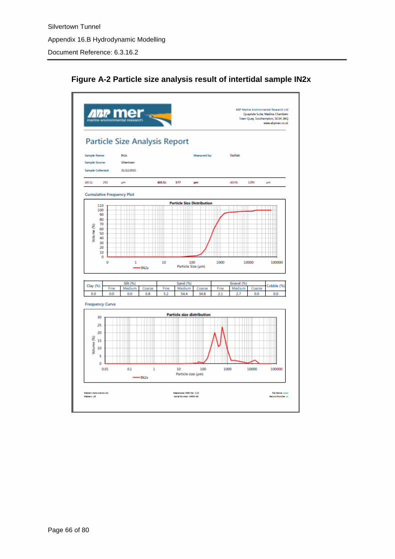
Figure A-2 Particle size analysis result of intertidal sample IN2x

Silvertown Tunnel
Appendix 16.B Hydrodynamic Modelling
Document Reference: 6.3.16.2
Page 67 of 80
Figure A-3 Particle size analysis result of intertidal sample IN3x

Silvertown Tunnel
Appendix 16.B Hydrodynamic Modelling
Document Reference: 6.3.16.2
Page 68 of 80
Figure A-4 Particle size analysis result of intertidal sample IN5

Silvertown Tunnel
Appendix 16.B Hydrodynamic Modelling
Document Reference: 6.3.16.2
Page 69 of 80
Figure A-5 Particle size analysis result of intertidal sample IN6x
Silvertown Tunnel
Appendix 16.B Hydrodynamic Modelling
Document Reference: 6.3.16.2
Page 70 of 80
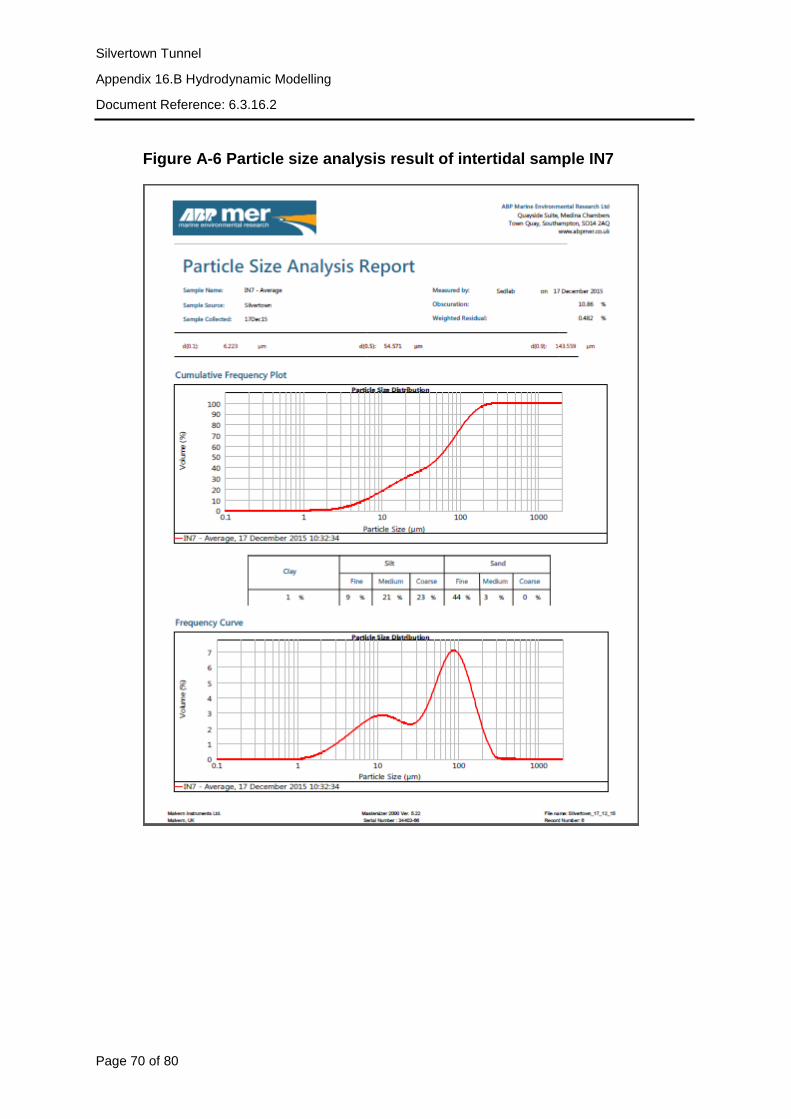
Figure A-6 Particle size analysis result of intertidal sample IN7

Silvertown Tunnel
Appendix 16.B Hydrodynamic Modelling
Document Reference: 6.3.16.2
Page 71 of 80
Figure A-7 Particle size analysis result of intertidal sample IN8

Silvertown Tunnel
Appendix 16.B Hydrodynamic Modelling
Document Reference: 6.3.16.2
Page 72 of 80
Figure A-8 Particle size analysis result of intertidal sample IN9x
Silvertown Tunnel
Appendix 16.B Hydrodynamic Modelling
Document Reference: 6.3.16.2
Page 73 of 80
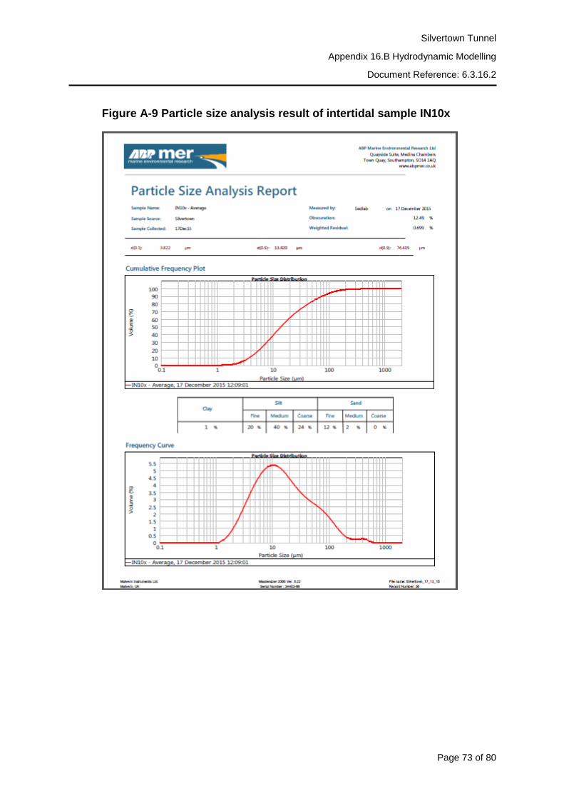
Figure A-9 Particle size analysis result of intertidal sample IN10x

Silvertown Tunnel
Appendix 16.B Hydrodynamic Modelling
Document Reference: 6.3.16.2
Page 74 of 80
THIS PAGE HAS INTENTIONALLY BEEN LEFT BLANK

Silvertown Tunnel
Appendix 16.B Hydrodynamic Modelling
Document Reference: 6.3.16.2
Page 75 of 80
Appendix B. Scour depth evolution
Figure B-10 Scour depth evolution over time for mean neap tide and
high flow conditions at the jetty head over two tidal cycles

Silvertown Tunnel
Appendix 16.B Hydrodynamic Modelling
Document Reference: 6.3.16.2
Page 76 of 80
Figure B-11 Scour depth evolution over time for mean neap tide and
high flow conditions at the approach jetty over two tidal cycles

Silvertown Tunnel
Appendix 16.B Hydrodynamic Modelling
Document Reference: 6.3.16.2
Page 77 of 80
Figure B-12 Scour depth evolution over time for mean neap tide and
mean flow conditions at the jetty head over two tidal cycles

Silvertown Tunnel
Appendix 16.B Hydrodynamic Modelling
Document Reference: 6.3.16.2
Page 78 of 80
Figure B-13 Scour depth evolution over time for mean neap tide and
mean flow conditions at the approach jetty orientation over two tidal
cycles

Silvertown Tunnel
Appendix 16.B Hydrodynamic Modelling
Document Reference: 6.3.16.2
Page 79 of 80
Figure B-14 Scour depth evolution over time for mean spring tide
and mean flow conditions at the jetty head over two tidal cycles
Silvertown Tunnel
Appendix 16.B Hydrodynamic Modelling
Document Reference: 6.3.16.2
Page 80 of 80
Figure B-15 Scour depth evolution over time for mean spring tide
and mean flow conditions at the approach jetty over two tidal cycles
Related Documents