1 Environmental Regulation and Green Skills: an empirical exploration Francesco Vona * Giovanni Marin † Davide Consoli ‡ David Popp § Abstract We present a data-driven methodology to identify occupational skills that are relevant for environmental sustainability. We find that these green skills are mostly engineering and technical know-how related to the design, production, management and monitoring of technology. We also evaluate the effect of environmental regulation on the demand of green skills exploiting exogenous geographical variation in regulatory stringency for a panel of US metropolitan and non-metropolitan areas over the period 2006-2014. Our results suggest that, while these recent changes in environmental regulation have no impact on overall employment, they create significant gaps in the demand for some green skills, especially those related to technical and engineering skills. Keywords: Green Skills, Environmental Regulation, Task Model, Workforce Composition. JEL codes: J24, Q52 Acknowledgements: We wish to thank Alex Bowen, Carmen Carrion-Flores, Mark Curtis, Olivier Deschenes, Ann Ferris, Jens Horbach, Karlygash Kuralbayeva, Maurizio Iacopetta, Leonard Lopoo, Stefania Lovo, Joelle Noailly, Edson Severnini and Elena Verdolini for useful comments and discussion. We also thank seminars participants at Maxwell School of Public Affairs (Syracuse), SKEMA Business School (Nice), the 3rd Annual Meeting of the Italian Association of Environmental and Resource Economists (Padova), University of Ferrara, 21st Annual Conference of the European Association of Environmental and Resource Economists (Helsinki), LSE conference on innovation and the environment (London) and 3rd IZA Workshop on Labor Market Effects of Environmental Policies (Berlin) for their comments. Francesco Vona and Giovanni Marin gratefully acknowledge the funding received from the European Union’s Seventh Framework Programme for research, technological development and demonstration under grant agreement no. 320278 (RASTANEWS). Francesco Vona wishes to thank Maxwell School of Citizenship and Public Affairs at Syracuse University for the kind hospitality during the initial writing of this paper. Davide Consoli acknowledges the financial support of the Spanish Ministerio de Economia y Competitividad (RYC-2011-07888). Davide Consoli would also like to thank Antonia Díaz, María Paz Espinosa and Sjaak Hurkens for setting an example of professional ethics. * OFCE SciencesPo and SKEMA Business School, France. [email protected] † IRCrES-CNR, Italy & OFCE-SciencesPo, France. [email protected] ‡ Ingenio CSIC-UPV, Spain. [email protected] § Department of Public Administration and International Affairs, The Maxwell School, Syracuse University, US, and National Bureau of Economic Research, US. [email protected]

Welcome message from author
This document is posted to help you gain knowledge. Please leave a comment to let me know what you think about it! Share it to your friends and learn new things together.
Transcript

1
Environmental Regulation and Green Skills: an
empirical exploration
Francesco Vona* Giovanni Marin† Davide Consoli‡ David Popp§
Abstract
We present a data-driven methodology to identify occupational skills that are relevant for
environmental sustainability. We find that these green skills are mostly engineering and
technical know-how related to the design, production, management and monitoring of
technology. We also evaluate the effect of environmental regulation on the demand of green
skills exploiting exogenous geographical variation in regulatory stringency for a panel of US
metropolitan and non-metropolitan areas over the period 2006-2014. Our results suggest that,
while these recent changes in environmental regulation have no impact on overall
employment, they create significant gaps in the demand for some green skills, especially those
related to technical and engineering skills.
Keywords: Green Skills, Environmental Regulation, Task Model, Workforce Composition.
JEL codes: J24, Q52
Acknowledgements: We wish to thank Alex Bowen, Carmen Carrion-Flores, Mark Curtis, Olivier
Deschenes, Ann Ferris, Jens Horbach, Karlygash Kuralbayeva, Maurizio Iacopetta, Leonard Lopoo,
Stefania Lovo, Joelle Noailly, Edson Severnini and Elena Verdolini for useful comments and discussion.
We also thank seminars participants at Maxwell School of Public Affairs (Syracuse), SKEMA Business
School (Nice), the 3rd Annual Meeting of the Italian Association of Environmental and Resource
Economists (Padova), University of Ferrara, 21st Annual Conference of the European Association of
Environmental and Resource Economists (Helsinki), LSE conference on innovation and the environment
(London) and 3rd IZA Workshop on Labor Market Effects of Environmental Policies (Berlin) for their
comments. Francesco Vona and Giovanni Marin gratefully acknowledge the funding received from the
European Union’s Seventh Framework Programme for research, technological development and
demonstration under grant agreement no. 320278 (RASTANEWS). Francesco Vona wishes to thank
Maxwell School of Citizenship and Public Affairs at Syracuse University for the kind hospitality during the
initial writing of this paper. Davide Consoli acknowledges the financial support of the Spanish Ministerio
de Economia y Competitividad (RYC-2011-07888). Davide Consoli would also like to thank Antonia Díaz,
María Paz Espinosa and Sjaak Hurkens for setting an example of professional ethics.
* OFCE SciencesPo and SKEMA Business School, France. [email protected] † IRCrES-CNR, Italy & OFCE-SciencesPo, France. [email protected] ‡ Ingenio CSIC-UPV, Spain. [email protected] § Department of Public Administration and International Affairs, The Maxwell School, Syracuse University, US, and
National Bureau of Economic Research, US. [email protected]
2
1 Introduction
The catchword ‘green skills’ has become common parlance in policy circles, exemplified by the Obama
stimulus package committing substantial resources, as much as $90 billion, to training programs for ‘green
jobs’. Yet in spite of a raging debate on the effectiveness of these actions, there is little systematic empirical
research to guide public intervention for meeting the demand for skills that will be needed to operate and
develop green technology.1 We argue that understanding the extent to which greening the economy can
induce significant changes in the demand for certain skills and, most cogently, which skills these might be,
is a crucial first step to inform the design of training and educational policies in the future. Using a new
data-driven methodology to identify green skills in the Occupational Information Network (O*NET)
dataset, we find that these skills are mostly engineering and technical know-how related to the design,
production, management and monitoring of technology. We evaluate the effect of environmental regulation
on the demand of green skills exploiting exogenous geographical variation in regulatory stringency for a
panel of US metropolitan and non-metropolitan areas over the period 2006-2014. Our findings suggest that,
while these recent changes in environmental regulation have no impact on overall employment, they create
significant gaps in the demand for some green skills, especially those related to technical and engineering
skills.
Environmental policy advocates often note that increased regulation will help the economy through the
creation of “green jobs.” For example, the summary for policymakers of the United Nations Environmental
Programme’s report on the green economy (UNEP 2011) touts the employment benefits of a greener
economy. At the same time, critics of climate policy often point to the job losses that they are sure will
follow.2 Empirical evidence of environmental regulation’s effect on employment is mixed. While many
studies present limited evidence of job losses from environmental regulations (e.g. Greenstone 2002), recent
studies such as Kahn and Mansur (2013) suggest the possibility of larger effects, particularly in energy-
intensive industries. One reason that studies often find limited effects is that there are reallocation effects
such that job losses due to a reduction in the scale of economic activity in one sector are offset by gains in
other sectors, including increased demand for pollution control equipment or of workers required to comply
with regulation and use new green technologies. At the same time, however, this research strand ignores
1 Further details on the Recovery Act at: http://www.whitehouse.gov/administration/eop/cea/factsheets-
reports/economic-impact-arra-4th-quarterly-report/section-4 For a review of studies on the effects of the package see:
http://www.washingtonpost.com/blogs/wonkblog/post/did-the-stimulus-work-a-review-of-the-nine-best-studies-on-
the-subject/2011/08/16/gIQAThbibJ_blog.html. For an assessment of the specific part of the program devoted to green
jobs see http://usatoday30.usatoday.com/news/washington/story/2012-01-30/obama-green-jobs-program-
failure/52895630/1 2 Bowen and Kuralbayeva (2015) provide a good summary of the policy debate surrounding green jobs.

3
important adjustment costs (Smith 2015). Job loss may entail other social costs, such as the stigma displaced
workers experience (Bartik 2015) or the need for workers to relocate (Kumioff et al. 2015). Even if workers
who lose their jobs in response to regulation are re-employed, higher unemployment spells mechanically
lead to long-run reduction in wages for these workers (Davis and von Watcher, 2011). Walker (2013) finds
that workers in sectors affected by the 1990 Clean Air Act lose 20% of their preregulatory earnings, with
most of the losses falling upon displaced workers. Moreover, workers displaced by environmental regulation
are more likely to take longer to find a new job and more likely to find their new job in a different industry.
While Walker notes that these costs are significantly lower than the aggregate benefits of the Clean Air Act,
they do suggest that the distributional effects of environmental regulation on workers may be significant.
Both the popularity of the “green jobs” concept within the environmental policy community and the
studies cited above suggest that consideration of green jobs and the possible adjustment costs of changes in
employment patterns in response to environmental regulation is important. The adjustment costs from job
losses can be exacerbated when the skill profile of expanding jobs does not match the skill profile of
contracting jobs. Labor research shows that workers’ relocation costs crucially depend on skill the similarity
between occupations, and that skill specificity is more tied to occupations than to a particular firm (Poletaev
and Robinson 2008; Kambourov and Manovskii 2009; Gathmann and Schönberg 2010). Consider an
economy reshaped by high carbon taxes to dramatically reduce carbon emissions from fossil fuel
consumption. An engineer who works drilling for petroleum may find his skills readily transferable to
similar drilling for carbon sequestration. In contrast, would a displaced coal miner find his skills easily
transferable to the manual labor used for installing new wind turbines or solar panels?
To understand the potential adjustment costs of greening the economy, we identify a set of skills that are
used more intensively in green occupations relative to non-green ones. Specifically, we obtain our green
skills constructs using a data-driven methodology that searches within the broad range of skills contained
in the O*NET dataset. For each occupation, the O*NET dataset allows distinguishing tasks specific to that
job from general skills that are used both in that occupation and elsewhere. Using this information we
identify, first, jobs having a significant share of green specific tasks over total tasks and, second, the sets of
general skills also associated with these jobs. We use these green general skills to compare the similarity of
workforce skills across occupations, with a particular interest in assessing whether these general skills are
substantially different from those of the particular workers that are displaced by environmental regulation.
To see how environmental regulation changes the demand for green skills, we use variations in
employment shares of occupations across US regions to construct aggregate skill measures for each US
metropolitan and non-metropolitan areas for 2006-2014. Adapting a standard empirical strategy to identify
the employment effect of environmental policies (e.g. Greenstone, 2002; Walker, 2011), we estimate the

4
effect of switches to nonattainment status on skill demand controlling for a host of observable and
unobservable regional characteristics. We argue that a positive net impact of environmental regulation on
any of these skill measures indicates the existence of gaps between the skills possessed by jobs that benefit
from regulation and those possessed by jobs that contract due to regulation. Identifying these gaps informs
the development of training and educational policies designed to mitigate the negative employment effects
that are traditionally associated to environmental regulation.
Empirical evidence on the labor market effects of environmental regulation provides mixed results. Some
studies predict job losses driven by reallocation of workers among industries rather than net job loss
economy-wide (Arrow et al, 1996; Henderson, 1996; Greenstone, 2002), while others find negligible
outcomes (e.g. Berman and Bui, 2001; Morgenstern et al, 2002; Cole and Elliott, 2007; Ferris et al., 2014).
Consistent with these findings, Mulatu et al. (2010) for European countries and Kahn and Mansur (2013)
for US states find that energy-intensive and polluting industries relocate in response to environmental
regulation. Other studies use plant-level data to understand the extent to which employment changes come
from higher layoff rates (job destruction) or decreasing hiring rates (job attrition). Walker (2011) finds that
a significant portion of employment adjustments are due to increases in job destruction, and that this effect
is stronger among newly regulated plants. Partially in contrast with these findings, Curtis (2014) shows that
incumbent workers are sheltered by the negative regulatory impact, and that the main driver is a slow-down
in hiring of young workers. Although recent analyses assess the cost of regulation for different experience
groups (Curtis 2014) or in terms of losses of industry-specific human capital (Walker 2013) , they do not
explore possible changes in the content of work and thus of the skills demanded from employers. These
occupational-specific features are particularly important in light of the documented importance of skill
similarity at the job rather than at industry level (Gathmann and Schönberg 2010).
To the best of our knowledge, only Becker and Shadbegian (2009) examine the relationship between
green productions and workforce skills. Their descriptive evidence shows that for a given level of output
and factor usage, plants producing green goods and services employ a lower share of production workers.
This finding lends support to a variant of the skill-bias technical change hypothesis postulating that at the
onset of a new wave of technological change the demand for high skilled workers increase and subsequently
dissipates inasmuch as codification facilitate the use of new technologies by the less talented workers
(Aghion et al, 2002; Vona and Consoli, 2015). By analogy, since most green technologies are still at an
early stage, we expect that their adoption will be associated with an increase in the demand of highly skilled
workers. However, since insights drawn from the skill-biased technical change literature can shape our
expectations only to a limited extent, in the remainder of the paper we rely on an empirical approach to

5
adapt more precisely the concept of ‘appropriate’ skills to the case of green technologies and production
methods.
This study contributes to the literature in three ways. First, we propose a new methodology to identify
the types of know-how that are important for certain occupations, green ones in our case. Our data-driven
measures build upon prior work on changes in the demand for skills (Autor, Levy and Murnarne, 2003) and
can be generalized to identify the skills relevant for any specific occupational group. Second, our paper is
the first to complement quantitative assessments of the effect of environmental regulation on employment
(e.g. Greenstone, 2002; Walker, 2013) with more qualitative aspects regarding the composition of workforce
skills. Third, we extend the literature on the effect of structural shocks, such as trade and technology (e.g.,
Autor and Dorn, 2013), on skill demand by focusing on a different driver, i.e. environmental regulation.
The remainder of the paper is organized as follows. Section 2 presents the methodology for the
construction of green skills measures. Sections 3 empirically assesses the effect of environmental regulation
on our newly created green skills indexes exploiting exogenous geographical variation in regulatory
stringency for a panel of US metropolitan and non-metropolitan areas. Section 4 provides additional
evidence that the effect of environmental regulation on the demand of green skills is mostly concentrated in
industries highly exposed to regulation. Section 5 concludes.
2 Identification and Measurement of Green Skills
This section is organized in four parts. The first briefly explains the data that we use to link green jobs
to green skills. The second subsection details a novel data-driven methodology for identifying green skills
within the US workforce. In the third part we provide descriptive evidence of our green skill measures vis-
à-vis other human capital measures, while the fourth part compares different skill measures for green and
brown jobs.
2.1 The Green Economy program of O*NET
In spite of much interest on green skills there is, to the best of our knowledge, no standard definition for
such a concept. Policy reports and an admittedly scant academic literature often conflate green skills with
‘green jobs’, namely the workforce of industries that produce environmentally friendly products and
services (see e.g. US Department of Commerce, 2010; Deitche, 2010; Deschenes, 2013). The ‘Green
Economy’ program maintained by the Occupational Information Network (O*NET) under the auspices of
the US Department of Labor is a notable exception in that it distinguishes between green jobs and green
skills, namely the skills that are used intensively in green jobs.

6
Green occupations are classified in three groups: (i) existing occupations that are expected to be in high
demand due to the greening of the economy; (ii) occupations that are expected to undergo significant
changes in task content due to the greening of the economy (green-enhanced, henceforth GE); and (iii) new
occupations in the green economy (new & emerging, henceforth NE) (see Dierdoff et al, 2009; 2011).
However, the involvement with environmental activities is more clearly identifiable in the last two groups
compared to the first one, which can be considered at best indirectly ‘green’ (see Consoli et al, 2015 for
details).
One important feature of the O*NET database is that it allows for a finer distinction of the importance
of green activities within an occupation. In particular, O*NET provides information on ‘general’ tasks,
which are common to all occupations, and tasks that are instead specific to each occupation.3 The Green
Task Development Project further enriches this distinction for ‘New & Emerging’ and ‘Green-Enhanced’
occupations by partitioning the set of specific tasks into green and non-green. For example, Sheet Metal
Workers perform both green tasks, such as 'constructing ducts for high efficiency heating systems or
components for wind turbines', and non-green tasks, such as 'developing patterns using computerized metal
working equipment'. Similarly, electrical engineers can 'plan layout of electric power generating plants or
distribution lines' and, at the same time, can 'design electrical components that minimize energy
requirements'. Unfortunately, different from general tasks whose importance is defined on a continuous
scale, these specific tasks are not comparable across occupations because specific tasks are binary
characteristics of any given occupation.
We exploit this complementary information to (1) define the greenness of an occupation based on the
number of specific green tasks required and (2) use this information to identify sets of green general skills
associated with greener occupations. Defining the greenness of an occupation based on the number of green
specific tasks allows for a more nuanced and accurate distinction of green and non-green jobs compared to
the O*NET classification, which identifies ‘full green’ jobs like Chemical Engineers, Electric Engineers,
Financial Analysis, Rail-track Operators or Sheet Metal Workers. On the other hand, the identification of
general skills used intensively in green occupations allows to address the key issue of the extent to which
current workforce skills can be easily transferred to green activities.
3 O*NET is a comprehensive database containing occupation-specific information on skill occupational requirements
and tasks performed on the job since the early 2000. These data provide detailed requirements for each occupation,
such as detailed tasks performed, skills, education and training requirements. Using questionnaire data from a
representative sample of US firms, expert evaluators and job incumbents assign importance scores to different task or
skill items, such as problem solving.

7
2.2 A methodology for the identification of Green Skills
Starting from the distinction between green and non-green specific tasks we compute the Greenness
measure, that is, the ratio between the number of green specific tasks and the total number of specific tasks
performed by an occupation k:
𝐺𝑟𝑒𝑒𝑛𝑛𝑒𝑠𝑠𝑘 =#𝑔𝑟𝑒𝑒𝑛 𝑠𝑝𝑒𝑐𝑖𝑓𝑖𝑐 𝑡𝑎𝑠𝑘𝑠𝑘
#𝑡𝑜𝑡𝑎𝑙 𝑠𝑝𝑒𝑐𝑖𝑓𝑖𝑐 𝑡𝑎𝑠𝑘𝑠𝑘. (1)
This indicator can be interpreted as a proxy of the relative importance of a particular class of job tasks
related, more or less directly, with environmental sustainability. The Greenness ratio allows an arguably
finer distinction between types of green job compared to the O*NET definition in that it captures well the
spectrum of greenness across various occupations, as shown by the examples in Table 1.4 As expected,
occupations like Environmental Engineers, Solar Photovoltaic Installers or Biomass Plant Technicians have
the highest Greenness score by virtue of the specificities of their job content to environmental activities.
Occupations that exhibit complementarity with environmental activities but that also include an ample
spectrum of non-green tasks have an intermediate score, such as Electrical Engineers, Sheet Metal Workers
or Roofers. At the bottom end of the greenness scale are occupations whose main activity occasionally
involves the execution of environmental tasks but that cannot be considered full-fledged green jobs, such as
traditional Engineering occupations, Marketing Managers or Construction Workers.
[Table 1 about here]
Using the Greenness indicator as a pure measure of skills has limitations for formulating policy
recommendations. Specifically, an indicator based on specific tasks is by definition not suitable to compare
the skill profiles of green and non-green occupations and, thus, limits our understanding of which non-green
skills can be successfully transferred to green activities and which green skills should be the target of
educational programs. Such a comparison is essential to estimate the cost of training programs considering
that workers’ relocation from brown to green jobs depends on the extent to which skills are portable and can
be reused in expanding jobs (e.g. Poletaev and Robinson, 2008). To overcome these limitations and broaden
the policy relevance of our study, we use the greenness indicator as a search criterion to create a Green
General Skills index (GGS henceforth). The identification is based on measures of general tasks retrieved
from the release 17.0 of the O*NET database. Importance scores for 108 general skills and tasks are reported
for 912 SOC 8-digit occupations.5 We use a two-step procedure. First, we regress the importance score of
4 The full list of green occupations and their greenness is reported in Table 12 in Appendix A. 5 We focus on ‘Knowledge’ (32 items), ‘Work activities’ (41 items) and ‘Skills’ (35 items), while we exclude ‘Work
context’ (57 items) because the items in it concern the characteristics of the workplace rather than actual know-how

8
each general task (or skill) l in occupation k on our greenness indicator plus a set of three-digit occupational
dummies:
𝑇𝑎𝑠𝑘_𝐼𝑚𝑝𝑘𝑙 = 𝛼 + 𝛽𝑙 × 𝐺𝑟𝑒𝑒𝑛𝑛𝑒𝑠𝑠𝑘 + 𝐷𝑘
𝑆𝑂𝐶_3𝑑 + 𝜀𝑘. (2)
Occupational dummies (𝐷𝑘𝑆𝑂𝐶_3𝑑
) are included to allow the comparability of the skill profiles of similar
occupations. In addition, we use only three digit SOC occupations containing at least one item with positive
greenness, thus eliminating occupations that bear no relevance on sustainability, such as Personal Care and
Service. Here, a positive (negative) and significant 𝛽𝑙 denotes that task l is used more (less) intensively in
greener occupations. We identify a general task as green when the estimated �̂�𝑙 is positive and statistically
significant at 99%. This generates a set of 16 GGS.
[Table 2 about here]
The second step is grouping these items into coherent macro-groups using principal component analysis
(PCA) and keeping only the selected green general tasks that load into principal components with eigenvalue
greater than 1.6 This leaves us with a list of 14 green task items that we group into 4 main skill types:
engineering and technical, science, operation management, and monitoring.7 Table 2 lists the task items in
each broader skill type. The principal component analysis yields Green General Skills constructs that
resonate with insights provided by policy reports and recent papers on organizational change and energy
efficiency.8
After having clustered items into coherent macro-groups by means of PCA, we build the final GGS skill
indices of occupation k for each of the four broad skill sets by taking the simple average of the importance
scores of each O*NET item belonging to a given macro-group. For instance, for the macro-group Science,
the GGS index for each occupation is the simple average between the importance score of ‘Biology’ and
applied in the workplace. O*NET data have been matched with BLS data using the 2010 SOC code. Details are
available in the data Appendix B. Importance scores in O*NET vary between 1 (low importance) and 5 (high
importance). We have rescaled the score to vary between 0 (low importance) and 1 (high importance). 6 In fact, we chose a slightly lower cut-off of 0.98 to include the GSS Science. Science appears together with
engineering a core GGS when using more demanding selection criteria. Note that the PCA analysis leads us to exclude
two task items: ‘Geography’ and ‘Operating Vehicles, Mechanized Devices, or Equipment.’ The reason is that the
loads of these two items is small on the four principal components selected by our analysis. In Appendix A we present
further robustness exercises with different approaches to select our set of green general skills. 7 The fifth component includes only one item, Geography, and was thereby excluded. Geographic skills pertain to
urban planning and analysis of emission dynamics (several profession intensive of Geography skills are green, such as
Environmental Restoration Planners, Landscape Architects and Atmospheric and Space Scientist). Due to the
specificity of this last component that only refers to one general skill we do not include it in the main analysis. Baseline
results for Geography and all single items are reported in 20 in Appendix D. 8 Martin et al (2012) find that energy managers have a positive impact on climate friendly innovation. Similarly,
Hottenrott and Rexshouser (2015) report productivity improvements due to complementarity between the
implementation of organizational practices and environmental technology adoption.
9
the importance score of ‘Physics’ (see Table 2). Thus, we can interpret the GGS for each skill type as the
importance of each GGS in a given occupation. Note that macro-group ‘Engineering and Technical’ is the
first principal component that accounts for the bulk of the difference in skill profiles between green and
non-green occupations.
2.3 A first take on Green Skills
Table 3 lists the GGS index for various 2-digit SOC occupations, sorted by each occupation’s greenness
index. The concentration of green jobs in high-level occupational groups explains in part the prevalence of
high skills in our selection of GGS. This is consistent with previous research showing that new occupations
such as several green ones are relatively more complex and exposed to new technologies than existing
occupations (Lin, 2011).
Table 3 also includes the average education and years of training for each occupation, as well as that
occupation’s Routine Task Index (RTI), which measures the extent to which a job performs routine tasks as
opposed to non-routine ones (Autor and Dorn, 2013).9 To better illustrate the relationship between education
and green skills, Figures 1 and 2 show the correlation between each individual GGS index and either the
RTI or educational requirement of each occupation. Note that the importance of both “Operation
Management” and “Monitoring” green general skills are higher in occupations that require more education
and that exhibit lower routine intensity. In contrast, green Engineering and Technical skills appear in both
high- and low-education occupations. We discuss the traits of each green general skill in more detail below.
[Figure 1 and Figure 2 about here]
The first GGS, Engineering and Technical (E&T henceforth) encompasses the whole spectrum of the
technology life cycle, namely: design, development and installation. Installation is the professional domain
of mid- and low-skill occupations with technical skills requiring vocational or associate degrees such as
Solar Installers, Roofers and Technicians. Conversely, technology development relies on ‘hard’ engineering
know-how possessed by green ‘Architecture and Engineering’ professions, such as Wind Energy or
Environmental Engineers. This heterogeneity is apparent in the first panel of Figure 1, which shows a high
GGS engineering index in both low-education occupations such as Construction & Extraction’ and
‘Installation & Maintenance’, as well as high-education occupations such as Architecture and Engineering.
Table 4 shows the education and training requirements for each of the six subcomponents of the Engineering
9 In this case a negative number implies a greater intensity of non-routine/complex tasks. The formula for the RTI
index is: RTI=log(1+4.5*RC+4.5*RM) – log(1+4.5*NRA+4.5*NRI), where NRI is non-routine interactive, NRA non-
routine analytical, RC routine cognitive and RM routine manual. Table 17 in Appendix B reports the O*NET task
items used to build NRI, NRA, RC and RM.

10
and Technical skill set. The first two subcomponents, ‘Engineering and Technology’ and ‘Design’ have a
significantly higher educational requirement than the remaining skills. As a result, in our analysis we
partition the E&T GGS into High and Low engineering, with High engineering representing the two skills
requiring higher educational attainment.
[Table 4 about here]
The second GGS construct, Science, is also related to innovation and technological development,
although in a more general way. Indeed, occupations with high scores in this skill can either possess specific
knowledge applicable to environmental issues, such as Environmental Scientists, Materials Scientists or
Hydrologists, or be more general-purpose occupations, such as Biochemists, Biophysicists and Biologist.
Not surprisingly, Figure 1 shows a positive correlation between occupations intensive in scientific GGS and
required education levels. Occupations with a high scientific GGS are also slightly less routine, although
the correlation there is weaker than for education (see Figure 2). Finally, note from Table 3 that even in
occupations with high greenness, the importance of science is generally lower than the other GGS.
The third GGS, Operation Management (O&M henceforth), captures skills related to the organization of
green activities and to managing the integration of various phases of the product cycle. Examples of
professions intensive in these skills are jobs that integrate green knowledge into organizational practices,
i.e., Climate Change Analysts and Sustainability Specialists, or jobs requiring adaptive management.
Adaptive management requires the capacity to identify environmental needs and to stir the dialogue across
different stakeholders’ groups, as is the case for Chief Sustainability Officers and Supply Chain Managers.
As these skills are concentrated in managerial, legal and mathematical occupations, this GGS is associated
with a high educational requirement and an extremely low routine intensity.
Finally, Monitoring GGS refers to legal, administrative and technical activities necessary to comply with
regulatory standards. Examples of such occupations include Environmental Compliance Inspectors,
Government Property Inspectors, Emergency and Management Directors and Legal Assistants. Monitoring
skills are similar to O&M skills as they are positively correlated with the educational requirement of
occupations and are less routine, although the correlation is partially driven by the outlier legal profession
(SOC-23, see bottom panel of Figure 1). Given that these pertain to different professional domains, in the
empirical analysis the two items, legal and technical, will be considered both together and separately.
2.4 Skill measures: green vs. brown jobs
The expected effect of environmental regulation on employment will depend on the skill distance
between occupations that may benefit and those that instead may be harmed by the implementation of new
environmental regulations. To compare the skill requirements in occupations likely to be harmed by
11
environmental regulation with those skills required in green jobs, we identify a set of brown occupations
that are prevalent in highly polluting industries. As in Curtis (2014), we first identify as 'pollution-intensive
industries' those manufacturing sectors with greater share of energy costs over total production.10 We then
define brown occupations as those with a share of employment in these polluting sector above 10%.11 Since
we are interested in the skills required to green our economies, we compare the skills required in brown jobs
to those in occupations with a greenness index greater than 0.1, using the metrics of GGS.
Brown jobs exist in 5 separate 2-digit SOC occupations. Interestingly, each of these five 2-digit
occupations also contain green jobs, permitting comparison the general skills required by green and brown
jobs under ceteris paribus conditions. Of these five macro professions only one is high skill, namely SOC-
17 ‘Architecture and Engineering’, while the remaining four are mostly low-medium skill jobs. This clearly
reflects the high share of low-skilled jobs in highly polluting sectors.
[Table 5 about here]
Table 5 presents the main results of this comparison. Looking at the total GGS for green and brown jobs
in these occupations, for each of our four GGS, the GGS index for brown jobs in these occupations falls
between that of green jobs and other types of jobs.12 This suggests that, in many cases, workers displaced
from brown jobs by environmental regulation may find re-employment in newly created green jobs easier
than other workers might. The education requirements for brown jobs also fall between that of green and
other jobs, but are much closer to the requirements for other jobs. However, both brown and other jobs are
less routine intensive than green jobs.
That said, there are important differences across occupations. For example, green E&T skills are more
important in green than brown jobs in both architecture (SOC 17) and construction and extraction (SOC
47). Note that the engineering GGS index for other jobs (those neither brown nor green) is similar to that of
green jobs in the construction and extraction industry, suggesting that workers in brown jobs displaced by
environmental regulation in this sector may face particular challenges finding new employment. A similar
10 In addition to the 'Mining, Quarrying, and Oil and Gas Extraction' (NAICS 21) and 'Electric Power Generation,
Transmission and Distribution' (NAICS 2211) industries, we identified as 'pollution-intensive industries' those
manufacturing sectors with greater share of energy costs over total production, similarly to Curtis (2014). We included
manufacturing industries (4-digit NAICS) in the top decile for this measures, that is: 3112, 3131, 3133, 3221, 3251,
3252, 3271, 3272, 3272, 3274, 3279, 3311, 3313, 3315 and 3328. Details are in Appendix B. 11 Notice that the employment shares in brown industries is only 1.75%. Thus, a 10% share to identify brown jobs is
remarkably greater than the share that would prevail if we randomly assign jobs to industries. Our results are however
robust to more or less strict definition of both brown and green jobs. Notice also that from this selection of brown
occupations we excluded those occupations related to renewable energy generation (e.g. Wind Turbine Service
Technicians) or nuclear power generation (e.g. Nuclear Power Reactor Operators) as most of them are employed in
the non-fossil part of the Electric power generation, transmission and distribution (NAICS 2211) industry. 12 The total is computed as the weighted mean of the GGS in all of the 2-digit occupations considered in Table 3.

12
pattern appears for the monitoring skill in SOC 47, although the magnitude of differences between green
and brown jobs is smaller. In contrast, within installation, maintenance and repair (SOC 49), production
(SOC 51) and transportation (SOC 53), the importance of GGS is rarely different between green and brown
jobs. Indeed, in some cases a GGS is more important in brown jobs than in green jobs, such as O&M in
production jobs. Also note that the difference between routine task intensity in green and brown jobs is
primarily driven by construction and installation jobs. Indeed, in architecture, green jobs are a bit less routine
intensive than brown jobs, although in all cases architecture is the least routine intensive of the five
occupations listed.
Taken together, these descriptive data highlight two facts relevant for the analysis of how environmental
regulation might affect the skill composition of the workforce. First, since environmental regulation will
mostly curb jobs in polluting industries where brown jobs are concentrated (Greenstone 2002; Kahn and
Mansur 2014), the low skill distance between green and brown jobs should translate into a small net effect
of regulation on workforce skills. The one exception to this is engineering and technical skills, particularly
in architecture and construction. Second, while green jobs are high skill jobs they are rarely more complex
(i.e. less routine intensive) than brown jobs. Thus, policies aimed at providing education and training for
green jobs should target an expansion of specific technical programs rather than the development of
advanced educational programs.
3 Effects of Regulation on Green General Skills: A Quasi-experimental
Approach
The descriptive analysis in the preceding section identifies skills likely to be of importance as
environmental regulation increases and suggests occupations where differences between the skills of green
and brown jobs are most likely to matter. However, environmental regulation may have additional effects
on the workplace. Environmental policies stimulate the adoption of technologies and organizational
practices that reduce the environmental burden of production processes, which in turn require specific
competences and skills needed to monitor environmental performance, evaluate compliance with regulatory
standard and even develop new production processes or, more generally, novel technical responses to
regulation. These may lead to increases or reductions in specific occupations, and thus changes in the mix
of skill levels observed within an economy. To assess the extent of these changes on the skill composition
of the workforce we analyse how changes in environmental regulation within US metropolitan and non-
metropolitan areas affect the importance of each of our green general skills. We argue that a positive net
impact of environmental regulation on any of these skill measures signals the existence of gaps between the
skills possessed by jobs that benefit from regulation and those possessed by jobs that instead contract due

13
to regulation. Ours is the first study that assesses the impact of a more stringent environmental regulation
on several skill measures, including our new GGS measures.
The main challenge is correctly identifying the effect of ER on green skills. Any positive shocks on GGS
may reduce the cost of hiring workers required to comply with regulation. If GGS abundance reduces the
burden of environmental regulation on exposed firms, one may find a positive effect of environmental
regulation on GGS demand simply because effective regulatory stringency depends on the availability of
the appropriate skills. In such a case, environmental regulation could be affected by unobserved shocks on
GGS supply that are independent of regulation, for example a new training program.
To identify the effect of environmental regulation, our main analysis uses a quasi-experimental research
design that exploits variation in regulatory stringency at the regional level due to approval of new emission
standards at the federal level.13 The US Clean Air Act (CAA) sets county-specific attainment standards for
the concentration of six criteria pollutants (National Ambient Air Quality Standards, or NAAQS). Counties
that fail to meet concentration levels for one or more of the six criteria pollutants are designated as
nonattainment areas for that pollutant, and the corresponding states are required to put in place
implementation plans to meet federal concentration standards within 5 years.14 We consider how changes
in attainment status affect our GGS measures using a panel of 537 metropolitan and non-metropolitan areas
over the period 2006-2014.
3.1 Data construction
During the time under analysis the Environmental Protection Agency (EPA) issued new environmental
standards for four criteria pollutants: PM (smaller than 2.5 micron), Ozone, Lead and SO2. Specifically,
new and more stringent concentration standards have been adopted in 2006 for PM 2.5, in 2008 for lead, in
2010 for SO2 and in 2008 for ozone. Effective designation of nonattainment areas for the new standards
took place with lags: in 2009 for PM 2.5, 2010 for Lead, 2011 for SO2, and 2012 for Ozone. Note that the
time window of the shocks, 2009-2012, lies exactly in the middle of the period under analysis, 2006-2014.
These new standards had a differential impact on regulatory stringency (as defined later in this section)
across counties, leading to a change in the attainment status for 81 counties that make up the 30.3% of US
13 Other papers using a similar strategy include Greenstone (2002), Walker (2011), and Kahn and Mansur (2014). 14 States may use a variety of policy tools to comply with concentration standards, such as creating a system of pollution
permits, mandating the adoption of specific technologies (reasonably available control measures, RACM, or best
available control measures, BACM, depending on the severity of the nonattainment status) or requiring that polluting
emissions from new establishments must be offset by corresponding reductions in emissions from existing
establishments.
14
population in 2014.15 Following previous literature, we exploit the fact that nonattainment counties
experience more stringent regulation (treated group) than counties that preserve their attainment designation
(control group). Figure 3 shows that new NA areas are mainly concentrated in densely populated areas in
the Ozone Transport Region (that includes 12 states in the North-East of the US) and in California.
[Figure 3 about here]
As a first step we compute a measure of green skill intensity for the local labor force in each region using
employment data by occupation at the metropolitan and nonmetropolitan area level of the Bureau of Labor
Statistics (Occupational Employment Statistics, OES). These data include the number of employees and
average wages in 822 6-digit Standard Occupational Classification occupations for 537 metropolitan and
non-metropolitan areas over the period 2006-2014 (see Appendix B for details). Metro and non-metro areas
are our units of analysis since detailed occupational data are not available at a finer regional level, i.e.
county. Pairing these data with our GGS index for each occupation, the intensity of each green general skill
in area j is:
𝐺𝐺𝑆𝑗𝑘 =
∑ 𝐺𝐺𝑆𝑘×𝐿𝑗𝑘
𝑘
𝐿𝑗 (3)
where 𝐺𝐺𝑆𝑘 is the skill intensity of occupation k at the US-level, 𝐿𝑗𝑘 is the number of employees in area j
and occupation k and 𝐿𝑗 is the total number of employees in area j.16
The second step is to develop an indicator of regulatory status for each region. To do so, we map county
NA status to larger metro and non-metro areas. An area, j, is categorized as nonattainment for a particular
pollutant in year t if: (1) it includes at least one county that has nonattainment status in year t for that
pollutant; (2) it was designated as attainment for the old standard of that pollutant in 2006. Regarding the
first condition, we follow the criterion of the Environmental Protection Agency of considering metropolitan
areas with at least one nonattainment county as nonattainment areas and extend it to non-metropolitan areas
(see Sheriff et al., 2015). Regarding the second condition, areas that were designated as nonattainment for
the old standard of a certain pollutant (i.e. Ozone-1997) should not experience a substantial change in
regulatory stringency if they continue to be designated as nonattainment for the new standard of the same
15 While our regression data are aggregated at the level of metropolitan and non-metropolitan areas as defined by the
U.S. Census Bureau, attainment status is defined by county. 16 As an alternative, we could have used data from the American Community Survey (ACS, available from the IPUMS
- Integrated Public Use Microdata Series). In the Appendix B we show that the within-area volatility in our skill
constructs is implausibly high when we use this data. Thus, we opt for BLS data as our identification strategy relies on
within-area variation only.
15
pollutant (i.e. Ozone-2012). In addition, although an area can be in principle nonattainment for more than
one pollutant, this is true only for seven of the areas under analysis. Accordingly, we simply set
nonattainment to one for these areas beginning in the year in which the area goes into nonattainment for any
of the regulated pollutants.17
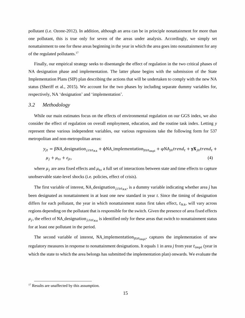
Finally, our empirical strategy seeks to disentangle the effect of regulation in the two critical phases of
NA designation phase and implementation. The latter phase begins with the submission of the State
Implementation Plans (SIP) plan describing the actions that will be undertaken to comply with the new NA
status (Sheriff et al., 2015). We account for the two phases by including separate dummy variables for,
respectively, NA ‘designation’ and ‘implementation’.
3.2 Methodology
While our main estimates focus on the effects of environmental regulation on our GGS index, we also
consider the effect of regulation on overall employment, education, and the routine task index. Letting y
represent these various independent variables, our various regressions take the following form for 537
metropolitan and non-metropolitan areas:
𝑦𝑗𝑡 = βNA_designation𝑗,𝑡≥𝑡𝑁𝐴+ ϕNA_implementationjt≥timpl
+ φNA𝑗0𝑡𝑟𝑒𝑛𝑑𝑡 + 𝛄𝐗𝑗0𝑡𝑟𝑒𝑛𝑑𝑡 +
𝜇𝑗 + 𝜇𝑡𝑠 + 𝜀𝑗𝑡 , (4)
where 𝜇𝑗 are area fixed effects and 𝜇𝑡𝑠 a full set of interactions between state and time effects to capture
unobservable state-level shocks (i.e. policies, effect of crisis).
The first variable of interest, NA_designation𝑗,𝑡≥𝑡𝑁𝐴, is a dummy variable indicating whether area j has
been designated as nonattainment in at least one new standard in year t. Since the timing of designation
differs for each pollutant, the year in which nonattainment status first takes effect, 𝑡𝑁𝐴, will vary across
regions depending on the pollutant that is responsible for the switch. Given the presence of area fixed effects
𝜇𝑗, the effect of NA_designation𝑗,𝑡≥𝑡𝑁𝐴 is identified only for these areas that switch to nonattainment status
for at least one pollutant in the period.
The second variable of interest, NA_implementationjt≥timpl, captures the implementation of new
regulatory measures in response to nonattainment designations. It equals 1 in area j from year 𝑡𝑖𝑚𝑝𝑙 (year in
which the state to which the area belongs has submitted the implementation plan) onwards. We evaluate the
17 Results are unaffected by this assumption.

16
combined effect of designation and implementation by testing the statistical significance of the sum of β̂
and ϕ̂.
The last variable of interest, NA𝑗0𝑡𝑟𝑒𝑛𝑑𝑡, gauges differential trends for areas that had nonattainment
status for at least one of the old standards in 2006. This term is important for comparisons across areas since
the implementation phase for old standards, such as Ozone-1997 and PM2.5-1997, were not completed
during the time span under analysis, and because areas in nonattainment status for both the old standard and
the new standard of the same pollutant are included in this group.
The set of covariates X facilitates a ceteris paribus comparison between treated and control group in
equation (4). Our vector of covariates includes the share of employment in manufacturing, utilities, primary
sector (extraction and agricultural sectors), construction, the log of population density, the log of the
establishment size and trade exposure, proxied by import penetration.18 Some of these control variables may
be themselves influenced by regulation. For example, several studies show that nonattainment status has an
impact on employment in industries highly exposed to regulation, i.e. part of manufacturing and utilities
(Ferris et al., 2014; Kahn and Mansur, 2013). If environmental regulation influences our control variables
which, in turn, are correlated with changes in GGS, the impact of regulation on GGS would be biased
because environmental regulation affect both the controls and our dependent variable. Angrist and Pischke
(2009) define such variables as ‘bad controls’. To allow for observable differences in regional characteristics
to affect the skill composition while avoiding the risk of including ‘bad controls’, we fix the vector of
controls X at levels observed at the beginning of the period (i.e. predetermined with respect to changes in
environmental regulation) and interact these variables with a time trend. While differences in levels of time-
invariant features are already captured by the area fixed effect, 𝜇𝑗, the interaction of our control variables
fixed at the beginning of the period with a linear trend allows the possibility of different patterns of average
growth in GGS for areas with different initial features.
Conditional on the controls, the estimated coefficients β̂ and ϕ̂ identify the differential change in GGS
induced by policy on the treated group compared to the change in GGS occurred in the control group. For
instance, the designation effect β̂ is:
β̂ = [𝐸(𝐺𝐺𝑆𝑡≥𝑡𝑁𝐴| 𝐗, NA_designation = 1) − 𝐸(𝐺𝐺𝑆𝑡<𝑡𝑁𝐴
| 𝐗, NA_designation = 1)] −
18 The economic justification for these controls is quite straightforward. The shares of employment by industry control
for the industrial structure and for the regional exposure to other shocks (i.e. construction for the financial crisis),
population density for agglomeration effects, establishment size for both economies of scale and mechanical
correlation between firm size and skill variety, import penetration for trade-induced compositional effects. Details on
data sources of these variables are reported in Appendix B.

17
[𝐸(𝐺𝐺𝑆𝑡≥𝑡𝑁𝐴| 𝐗, NA_designation = 0) − 𝐸(𝐺𝐺𝑆𝑡<𝑡𝑁𝐴
|𝐗 , NA_designation = 0)]. (5)
In this difference-in-difference setting (DID), the coefficient β̂ measures the treatment effect on the
treated under two conditions: (1) the two groups are similar in terms of observable and unobservable
characteristics (including pre-treatment dynamics); and (2) selection into treatment is random (Heckman et
al. 1997).
We address the first identification concern by testing for the existence of observable differences in the
covariates before the treatment occurs, i.e. E(𝐗𝑡<𝑡𝑁𝐴| NA_designation = 1) and
E(𝐗𝑡<𝑡𝑁𝐴| NA_designation = 0). Table 6 shows that only four covariates are unbalanced. Areas that will
switch were systematically more densely populated, with smaller share of employment in primary
(agriculture and mining) industries and more likely to be already nonattainment for at least one criteria
pollutant than areas for which no change in regulation will occur in later years. Switching areas were also
systematically more endowed with O&M green skills. Failing to consider pre-treatment differences in
nonattainment status for old regulatory standards is likely to influence the demand for GGS also during our
estimation period and may bias our estimates of β̂ and ϕ̂.
[Table 6 about here]
Besides evaluating systematic cross-sectional differences between areas, we also test for possible
differences in pre-treatment trends of GGS by means a series of fixed effect models with our indexes of
GGS as dependent variables and year dummies, also interacted with a time-invariant treatment dummy for
switching areas in pre-treatment years (2006-2008). Joint significance of the interaction between treatment
dummy and year dummies would indicate the existence of differences in pre-treatment trends. As shown in
Panel A of Table 7, we reject the null hypothesis of no common pre-treatment for Engineering and Technical
skills in a naïve model without controls. However, when control variables are added (equation 4) the null
hypothesis of common pre-treatment common trends cannot be rejected for all GGS. Thus, allowing
different trends for areas with different initial features is necessary to satisfy the assumption of pre-treatment
common trends.
[Table 7 about here]
The second identification issue concerns non-random selection into the treatment. A standard way to
address this is to approximate a randomized experiment by means of propensity score matching (Rubin,
2008). We use pre-treatment characteristics to estimate a probit model of the probability of being treated.
The propensity score allows measuring the similarity across units in a uni-dimensional fashion. The key

18
identifying assumption is that, conditional on the propensity score, the probability of being treated is
independent of observable area characteristics.
Once the propensity score is estimated, each treated unit is matched with one or more non-treated units.
Since our pool of potential control groups is rather limited in size (471 non-switching areas as opposed to
66 switching areas), we match non-switching areas with switching areas based on the kernel of the
propensity score. This method attributes decreasing weights (i.e. decreasing relative contribution to the
counterfactual) the farther away “control areas” are from the corresponding treated area in terms of
estimated propensity score. Weights, estimated for year 2006, are then employed as regression weights using
the same specification as in our baseline results.
Table 8 reports the probit estimates of the probability of switching. Not surprisingly, higher shares of
employment in utilities and manufacturing, higher population density and initial nonattainment increase the
probability of being treated. We also observe that areas that were initially more endowed with GGS are
more likely to be treated. On the other hand areas with higher average establishment size are less likely to
be treated while import penetration and the share of employment in primary (agriculture and mining) sector
play no role.
[Table 8 about here]
After matching and re-weighting the group of matched non-treated areas, the difference in average
observable features between treated and controls is never statistically different from zero (see Table 8).
Thus, matching on the propensity score balances the two groups in terms of observable pre-treatment
features. Therefore, following recent related papers by Ferris et al. (2014) and Curtis (2014), our preferred
specification of the effect of environmental regulation on GGS combines propensity score matching and
DID.
3.3 Results
The effects of a structural shock on workforce composition (e.g. the importance of a given GGS) will be
large if (1) there is substantial job turnover in the area and (2) if the skills of the jobs that have been created
do not match the skills of jobs that have been destroyed. Large contraction or expansion of employment
may generate short-term skill gaps due to frictions unrelated to structural differences in the skill portfolio
of expanding and contracting occupations. Thus, we begin by simply testing whether changes in
environmental regulation had substantial positive or negative employment effects by using the specification
described in equation 4 with the log of total employment (instead of the GGS index) as dependent variable.

19
Table 9 shows that the net employment effect of switching to NA status is near zero, and that this result
is robust. In Column 2, we estimate the same regression using the County Business Pattern (CBP) dataset
to construct the employment measure at regional level, as this dataset (that has been used by recent work on
the employment effect of environmental regulation, e.g. Kahn and Mansur, 2014) allows us to obtain
detailed estimates of employment by industry. Results are unaffected by the use of a different data source.
In Column 3, we estimate the effect of regulation on employment only for the industries more exposed to
regulation, i.e. manufacturing, construction and utilities. Again, the effects are not statistically different from
zero. It is worth noting that only areas that were NA for the old standards seem to experience a significant
decline in employment, i.e. φ is negative and significant in the model using total BLS employment, but such
a decline does not seem concentrated in the industries that are particularly exposed to regulation.
[
20
Table 9 about here]
In light of these results and of the ones pointing to a limited skill distance between green and brown jobs,
we should expect that the recent regulatory changes analysed by our study would have little or no effects on
workforce skills. Table 10 presents our estimates of equation (4) and, contrary to our expectation, suggests
that stricter environmental regulation does increase demand for our four general green skills plus the two
engineering & technical (low and high) and the two monitoring (law and compliance). However, the
magnitude of these effects is not large. Looking specifically at Panels A and B, the average treatment effect
on the treated, obtained by summing up the designation and the implementation effect, is statistically
significant for most GGS (although operations management and monitoring are only significant at the 10
percent level). Science and Law skills (a sub-component of the broad GGS Monitoring) are the only two
exceptions for which the joint effect of nonattainment designation and implementation are not statistically
significant. However, it is worth noting that the implementation stage does increase the importance of
Science GGS.
The nature of environmental technologies may explain the stronger effect of environmental regulation
on engineering and technical skills than on scientific skills. Rather than creating new basic knowledge, most
environmental technologies entail the application of general scientific knowledge to specific problems, i.e.
material science for renewable and transport technologies, or physics of conductors and insulators for energy
efficient solutions. Thus, rather than requiring purely scientific knowledge, these applications require
engineering to apply these technologies in new domains of use. Turning to monitoring, if we separate this
item into two components – compliance and law – nonattainment status increases the importance of
compliance skills but not of legal skills. It may be that while compliance activities must take place on-site,
legal activities associated with complying with environmental regulation take place elsewhere, such as in
state capitals.
[Table 10 about here]
Panel C of Table 10 contrasts the effect of environmental regulation on GGS to the effect on standard
human capital measures. We find no evidence that environmental regulation leads to an increase in the
demand of complex skills, measured by the RTI index, or in the share of workers with post-graduate
education. Combining these results with the increased demand for green general skills seen in panels A and
B lends support to the conjecture that the inducement effect of regulation is concentrated in a subset of
highly specific technical skills. This contrasts with the effect of other structural shocks such as trade and
technology (Autor, Levy and Murnarne, 2003; Ng and Lu, 2013), which mostly increase the demand of high
general skills required to perform non-routine tasks. While we caution that our results can only capture

21
short-run changes in demand, as a policy implication, this finding suggests that re-directing the educational
supply towards technical and engineering degrees is more important to support green economy activities
than merely increasing the level of education of the workforce.
To precisely quantify the effect of environmental regulation on green skills, note that the effective range
of variation of our skill indicators across regions is significantly smaller than the theoretical one (i.e. 0-1).
Within a given year, the largest range for any of our GGS indices is a gap of 0.239 for the GGS of High
Engineering & Technical skills in 2013.19 This helps explain the small absolute magnitude of our point
estimate of the treatment effect, which just increases the importance of green skills between 0.08% (for
O&M) and 0.21% (for Engineering high). To interpret the economic significance of these changes, we can
consider what such a change would mean to a community that was the median for each index in our initial
year of 2006. The largest increase in demand for green general skills occurs within Engineering.
Nonattainment status moves the median High-skilled Engineering community to the 58th percentile. The
median overall E&T community moves to the 56th percentile, and the median Low-skilled Engineering
community moves to the 54th percentile. The median Compliance community also moves up to the 54th
percentile after nonattainment status. In contrast, the effects are smaller for Operation Management and
Monitoring, where the median community moves up to just the 52nd or 53rd percentile. Recall that O&M
and Monitoring skills are usually less occupation-specific and require more general education than
engineering & technical skills (see Figures 1-2). In sum, the quantification of the effect of environmental
regulation on green skills corroborates our previous conclusion: training and educational support to green
activities should be specifically directed towards middle-high technical skills. Specifically, this result is
consistent with the fact that E&T skills explain the bulk of the difference between green and non-green jobs
and are the only occupations with significant differences in the GGS importance between green and brown
jobs (as shown previously in Table 5).
4 Industry-specific effects
While considering changes in nonattainment status provides a quasi-experimental research design, it also
limits the analysis to overall changes in workforce composition within a metro or non-metro area since
attainment status applies to an entire county. However, other studies find that the effects of environmental
regulation on labor can be concentrated in the most heavily regulated industries (Kahn and Mansur, 2014).
Unfortunately, the availability of region- (state) and sector-specific employment data broken down by
19 Table 18 in Appendix B shows the variation in our GGS measures across metro and non-metro areas.

22
occupations are only available for the years 2012 and 2013, preventing us from adopt a similar quasi-
experimental design on industry-level data.
In the face of such a shortcoming, we assess whether differential effects by industry matter using data
on the distribution of the workforce by both occupation, industry (using the 4-digit NAICS), and state for
the years 2012 and 2013.20 Instead of changes in nonattainment status we use the National Emission
Inventory (NEI) developed by the EPA to proxy for the stringency of environmental regulations across both
state and industry. According to Brunel and Levinson (2015), when the sectoral breakdown is sufficiently
narrow emissions are the best proxies of environmental regulatory and a higher emission level implies a
weaker regulation. While this allows us to focus on the effects of regulation on those industries most likely
to be affected, we acknowledge that the results in this section should not be interpreted causally, as we
cannot use a quasi-experimental design to distinguish between the causes of regulation and the composition
of the workforce.
To provide illustrative evidence on the positive effect of more stringent environmental regulation on
green general skills, following Brunel and Levinson (2015) we compute an index of environmental
regulation for each industry equal to the ratio between the state-level emissions per worker in industry i and
the federal level emissions per workers in the same industry i, and another index for GGS built in a similar
fashion.21 We then explore the relationship between environmental regulation and green skills at the sector-
state level by estimating the following equation:
log (𝐺𝐺𝑆𝑖𝑗
𝐺𝐺𝑆̅̅ ̅̅ ̅̅ 𝑖) = 𝛽log (
𝐸𝑅_𝑝𝑐𝑖𝑗
𝐸𝑅̅̅ ̅̅ _𝑝𝑐𝑖) + 𝜸𝐗ij + εij, (6)
where i indexes sector and j indexes states and 𝜀𝑖𝑗 is a conventional error term. The main variable of interest,
the ratio of state and national emissions per capita in sector i, is in logs as its distribution is highly right-
skewed. We transform the dependent variable in logs to interpret the results as elasticities. We also include
a set of parsimonious controls, 𝐗ij: state effects absorbing unobservable factors that affect both skill demand
and ER, such as subsidies to green investments; the log of the number of monitored facilities to control for
regulatory enforcement; and the 10-years log change in the level of employment to make sure that the
observed relationship between environmental regulation and workforce composition is not driven by strong
compositional effects. This empirical approach implicitly controls for sector fixed effects because the two
20 In principle, the annual ACS data have time-varying information on industry-region-occupation. However, as we
show in Appendix B, employment figures for each Census cells sector-state-occupation-time are not reliable and
implausibly volatile over time. 21 Details on the construction of these variables are in the data Appendix B.
23
variables of interests are measured in terms of deviation from the national mean for each industry, so that
the coefficients can be interpreted as percentage change deviations from the national mean.
[Table 11 about here]
Table 11 presents the results of this exercise.22 We focus on the two criteria pollutants that have been
most regulated in the last two decades, Ozone and PM2.5. Recall that a higher emission level implies a
weaker regulation which, in turn, leads us to expect a negative coefficient of ER on green skills. The results
in Table 11 are consistent with our previous findings. In particular, more stringent regulation is significantly
associated with a greater importance of GGS even though the degree of association is modest across the
board. To illustrate, a 10% reduction in PM2.5 emission intensity compared to the national mean leads only
to a 0.05 % increase in the sectoral use of O&M skills relative to the national average. The effect remains
small even if we take into account the extremely large degree of variability of environmental regulation
(𝐸𝑅𝑝𝑐𝑖𝑗/𝐸𝑅̅̅ ̅̅
𝑝𝑐𝑖). For example, in the case of PM2.5, even a one standard deviation decrease in emissions
would increase the importance of O&M skills by just 1.3% and high engineering and technical skills by just
1.8%. Also, and consistent with previous results, these associations are almost twice as large for engineering
high skills. The only notable differences is the large effect of regulation on science skills, which is now
similar to that of engineering high skills, and the non-significant effect of Ozone on engineering low skills.
In sum, the results of the industry-level analysis reinforce the point that educational and training support
should be especially directed towards high rather than middle technical skills. The emphasis on high
technical and scientific knowledge is also supported by the positive and significant correlation between
stringent regulation and the use of scientific skills. No doubt, these findings differ from those of previous
studies and offer food for thought. Two issues in particular are worth remarking.
First, the small effects in highly exposed industries observed here may conceal indirect effects from
inter-sectoral linkages between upstream equipment suppliers and downstream users. While the industries
that use pollution abatement equipment are emissions intensive, many of the key upstream suppliers of
pollution abatement equipment are in industries that are not emissions intensive. Therefore, our estimates
of the effect of environmental regulation on GGS demand in highly exposed sectors should be seen as a
lower bound of the overall effect of regulation on workforce composition, as green skills may also become
more important in industries that are not heavily regulated themselves, but that benefit from increased
demand under stricter environmental regulation. Indeed, as both Voigtlaender (2014) and Franco and Marin
22 Notice that these results are generally robust to richer empirical specifications (including for instance import
penetration and limit our analysis to the manufacturing sector) and to the use of an IV strategy to account for the
endogeneity in environmental regulation. The interested reader can find these results in a previous version of this work
(Vona et al., 2015).

24
(2015) recently remarked, inter-sectoral linkages should be analyzed more in detail to further disentangle
direct and indirect effects of environmental regulation on the demand of GGS. We leave such an
investigation here for future work.
Second, previous studies use data sources, such as the County Business Pattern dataset, that provide
richer sector-level detail but do not offer any details on employment changes at the occupation level, as we
require here. Normally in these studies environmental regulation is identified using a regulatory shock (such
as non-attainment status as in our section 4) that varies geographically, but not across sectors. That approach
is therefore intrinsically different from ours in which variation is truly sector-by-state. We believe that these
nuances and idiosyncrasies are especially enriching at this early stage of the debate on the labor market
effects of environmental regulation.
5 Conclusions
This paper takes a first step in filling a gap in our understanding of the incidence of environmental
regulation in the labor market. We first identify a set of general work skills that are associated with green
occupations. We then assess the effect of environmental regulation on the demand for these skills. The
contribution to the extant literature is twofold.
First, our empirically-driven selection of green skills allows the detection of skill gaps which can be used
to compute measures of skill transferability from brown to green occupations, or to specify in even greater
details the types of general skills in high demand in specific sectors or sub-groups of green jobs (e.g. those
related to renewable energy). Overall, we find that the skill gap between green jobs and high-polluting
“brown” jobs is small. Indeed, in most cases, the general skill requirements of brown jobs are closer to green
jobs than the general skill requirements of other jobs. Nonetheless, we find exceptions within specific
occupations, such as the importance of green engineering skills within the architecture and construction and
extraction fields. As energy extraction occupations, such as coal mining, are likely to be heavily impacted
by future climate policy regulations, this finding suggests paying attention to the adjustment costs of workers
in those sectors will be important. Combined with our finding that green jobs are rarely more complex than
brown jobs, this suggests that policies aimed at providing education and training for green jobs should target
an expansion of specific technical programs rather to a development of advanced educational programs.
Second, we use a quasi-experimental research design to assess the impact of increased environmental
regulation on both the importance of green general skills and on overall employment. Given the small skill
gap between green and brown jobs noted above, it is not surprising that the overall effect of environmental

25
regulation on employment is small. Similarly, we do observe some changes in the importance of green
general skills after regulation, but these are generally not large effects. Consistent with the gaps described
above, the largest effects are in the importance of high engineering skills. However, given the nature of our
research design, which uses county-level changes in Clean Air Act attainment status as a proxy for changes
in environmental regulation, we can say less about the employment and skill effects of environmental
regulation on specific occupations or industries. Such an investigation is left for future work.

26
Bibliographic references
Aghion, P., Howitt, P., and Violante, L. (2002), General purpose technology and within-group wage
inequality. Journal of Economic Growth 7, 315–345.
Angrist, J. and Pischke, S. (2009) Mostly Harmless Econometrics. Princeton University Press.
Arrow, K., Cropper, M., Eads, G., Hahn, R., Lave, L., Noll, R., and Stavins, R. (1996), Is There a Role for
Benefit-Cost Analysis in Environmental, Health, and Safety Regulation?. Science 272, 221.
Autor, D., and Dorn, D. (2013) The growth of low-skill service jobs and the polarization of the US labor
market. American Economic Review 103(5), 1553-1597.
Autor, D., Levy, F. and Murnane, R. (2003) The skill content of recent technological change: An empirical
exploration. Quarterly Journal of Economics 118 (4), 1279-1333.
Bartik, T. (2015) The social value of job loss and its effect on the costs of U.S. environmental regulations.
Review of Environmental Economics and Environmental Policy 9(2), 179-197.
Becker, R., and Shadbegian, R. (2009), Environmental products manufacturing: A look Inside the Green
Industry, The BE Journal of Economic Analysis and Policy, 9(1), 1935-1682.
Berman, E., and Bui, L. (2001), Environmental regulation and labor demand: Evidence from the south coast
air basin. Journal of Public Economics, 79(2), 265-295.
Bowen, A. and Kuralbayeva, K. (2015), Looking for green jobs: the impact of green growth on employment.
Grantham Research Institute on Climate Change and the Environment Policy Brief.
Brunel, C. and Levinson, A. (2015), Measuring Environmental Regulatory Stringency. Review of
Environmental Economics and Policy, forthcoming.
Cole, M., and Elliott, R. (2007) Do environmental regulations cost jobs? An industry-level analysis of the
UK. The BE Journal of Economic Analysis and Policy, 7(1).
Consoli, D., Marin, G., Marzucchi, A., and Vona, F., (2015). Do Green Jobs Differ from Non-Green Jobs
in Terms of Skills and Human Capital?. SPRU Working Paper Series 2015-16, University of Sussex.
Curtis, M. (2014), Who Loses under Power Plant Cap and Trade Programs? Estimating the Impact of the
NOx Budget Trading Program on Manufacturing Employment. NBER working paper no. 20808.
Davis, S. and von Watcher, T. (2011), Recessions and the costs of job loss. Brookings Papers on Economic
Activity, 1-55.
DeCanio, S. (1998), The efficiency paradox: bureaucratic and organizational barriers to profitable energy-
saving investments. Energy Policy, 21(26), 441–454.
Deitche, S. (2010) Green collar jobs: Environmental careers for the 21st century. ABC-CLIO.
Deschenes, O, (2013), Green Jobs, IZA Policy Paper No. 62.
Dierdorff, E., Norton, J., Drewes, D., Kroustalis, C., Rivkin, D., and Lewis, P. (2009), Greening of the
World of Work: Implications for O*NET-SOC and New and Emerging Occupations. National Center
for O*NET Development .
Dierdorff, E., Norton, J., Gregory, C., Rivkin, D., and Lewis, P. (2011), Greening of the World of Work:
Revisiting Occupational Consequences National Center for O*NET Development.
Ferris, A., R. Shadbegian, and Wolverton, A. (2014), The Effect of Environmental Regulation on Power
Sector Employment: Phase I of the Title IV SO2 Trading Program. Journal of the Association of
Environmental and Resource Economists, 1 (4), 521–553.
Franco, C. and Marin, G. (2015), The Effect of Within-Sector, Upstream and Downstream Energy Taxes on
Innovation and Productivity. Environmental and Resource Economics forthcoming.
Gathmann, C. and Schönberg, U. (2010), How General is Human Capital? A Task-Based Approach. Journal
of Labor Economics, 28( 1), 1-50.
Greenstone, M. (2002), The Impacts of Environmental Regulations on Industrial Activity: Evidence from
the 1970 and 1977 Clean Air Act Amendments and the Census of Manufactures. Journal of Political
Economy, 110(6), 1175-1219.
Heckman, J., Ichimura, H., and Todd, P. (1997), Matching as an econometric evaluation estimator: Evidence
from evaluating a job training programme. The review of economic studies, 64(4), 605-654.

27
Henderson, J. (1996) Effects of Air Quality Regulation. American Economic Review, 86(4), 789-813.
Hottenrott, H., and Rexhauser, S. (2015) Policy-induced environmental technology and inventive efforts: Is
there a crowding out?. Industry and Innovation, 22(5), 375-401.
Kahn, M., and Mansur, E. (2013) Do local energy prices and regulation affect the geographic concentration
of employment?. Journal of Public Economics 101, 105–114.
Kambourov, G., and Manovskii, I. (2009), Occupational specificity of human capital. International
Economic Review, 50 (1), 63–115.
Kuminoff, N., Schoellman, T., and Timmins, C. (2015), Environmental regulations and the welfare effects
of job layoffs in the United States: A spatial approach. Review of Environmental Economics and
Environmental Policy, 9(2), 198-218.
Lin, J. (2011) Technological Adaptation, Cities, and New Work, Review of Economics and Statistics, 93(2),
554-574.
Lu, Y. and Ng, T. (2013) Import Competition and Skill Content in U.S. Manufacturing Industries. Review
of Economics and Statistics, 95(4), 1404–1417.
Martin, R., Muûls, M., de Preux, L. B., and Wagner, U. J. (2012) Anatomy of a paradox: Management
practices, organizational structure and energy efficiency. Journal of Environmental Economics and
Management, 63(2), 208-223.
Morgenstern, R., Pizer, W. and Shih, J. (2002) Jobs versus the environment: an industry-level perspective.
Journal of Environmental Economics and Management, 43(3), 412-436.
Mulatu, A., Gerlagh, R., Rigby, D., and Wossink, A. (2010) Environmental regulation and industry location
in Europe. Environmental and Resource Economics, 45(4), 459-479.
Poletaev, M., and Robinson, C. (2008) Human capital specificity: evidence from the Dictionary of
Occupational Titles and Displaced Worker Surveys, 1984–2000. Journal of Labor Economics, 26(3),
387-420.
Rubin, D. (2008), For objective causal inference, design trumps analysis. The Annals of Applied Statistics,
2(3), 808-840.
Sheriff, G., Ferris, A., and Shadbegian, R. (2015), How did air quality standards affect employment and
generation at U.S. power plants? The importance of stringency, geography, and timing. NCEE
Working Paper Series Working Paper # 15-01.
Smith, V. (2015). Should benefit-cost methods take account of high unemployment? Symposium
introduction. Review of Environmental Economics and Environmental Policy 9(2), 165-178.
UNEP, (2011), Towards a Green Economy: Pathways to Sustainable Development and Poverty Eradication
- A Synthesis for Policy Makers. www.unep.org/greeneconomy
US Department of Commerce (2010), Measuring the Green Economy. Department of Commerce,
Economics and Statistics Administration.
Voigtlaender, N. (2014). Skill Bias Magnified: Intersectoral Linkages and White-Collar Labor Demand in
U.S. Manufacturing. Review of Economics and Statistics, 96(3): 495-513.
Vona, F., Marin, G., Consoli, D., and Popp, D., (2015), Green skills. NBER working paper no. 19951.
Vona, F., and Consoli, D. (2015), Innovation and skill dynamics: a life-cycle approach. Industrial and
Corporate Change, 24 (6): 1393-1415.
Walker, W. (2011), Environmental regulation and labor reallocation: Evidence from the Clean Air Act.
American Economic Review, 101(3), 442-447.
Walker, W. (2013), The Transitional Costs of Sectoral Reallocation: Evidence From the Clean Air Act and
the Workforce. Quarterly Journal of Economics, 128(4), 1787-1835.
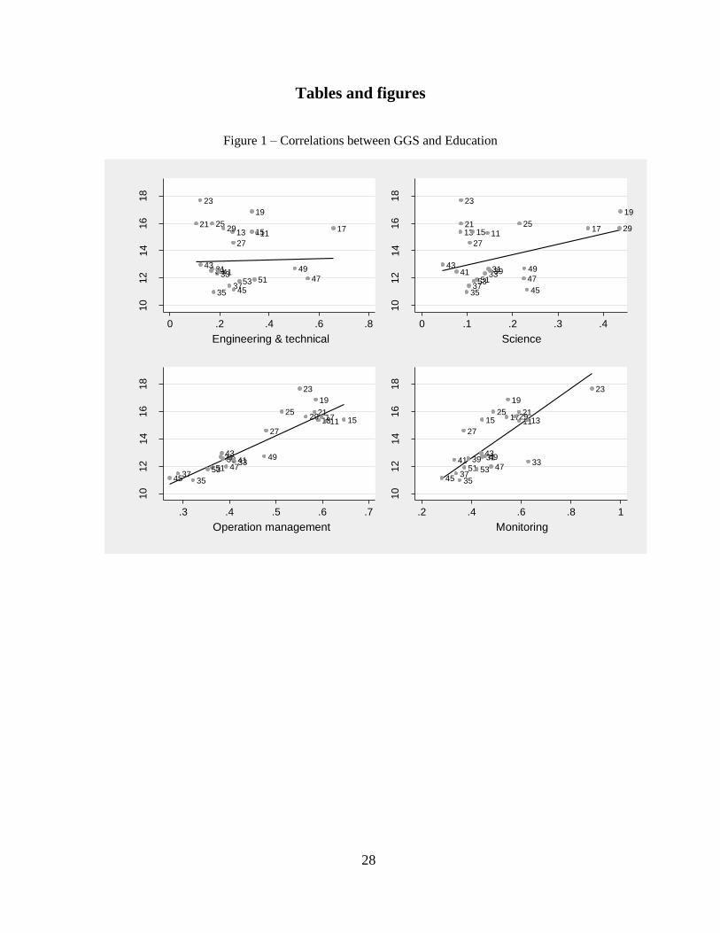
28
Tables and figures
Figure 1 – Correlations between GGS and Education
1113 15 17
19
21
23
25
27
29
3133
3537
394143
45
47
49
5153
10
12
14
16
18
0 .2 .4 .6 .8
Engineering & technical
1113 15 17
19
21
23
25
27
29
3133
3537
394143
45
47
49
5153
10
12
14
16
18
0 .1 .2 .3 .4
Science
1113 1517
19
21
23
25
27
29
3133
3537
39 4143
45
47
49
5153
10
12
14
16
18
.3 .4 .5 .6 .7
Operation management
111315 17
19
21
23
25
27
29
3133
3537
394143
45
47
49
51 53
10
12
14
16
18
.2 .4 .6 .8 1
Monitoring
Re
qu
ire
d y
ears
of
ed
uca
tion

29
Figure 2 – Correlations between GGS and RTI index
11
13
15 1719
21
23
25
2729
3133
3537
3941
43
45
4749
5153
-1.5
-1-.
50
.5
0 .2 .4 .6 .8
Engineering & technical
11
13
15 1719
21
23
25
2729
3133
3537
3941
43
45
4749
5153
-1.5
-1-.
50
.5
0 .1 .2 .3 .4
Science
11
13
151719
21
23
25
2729
3133
3537
39 41
43
45
4749
5153
-1.5
-1-.
50
.5
.3 .4 .5 .6 .7
Operation management
11
13
15 1719
21
23
25
2729
3133
3537
3941
43
45
4749
5153
-1.5
-1-.
50
.5
.2 .4 .6 .8 1
Monitoring
Ro
utin
e T
ask I
nte
nsity
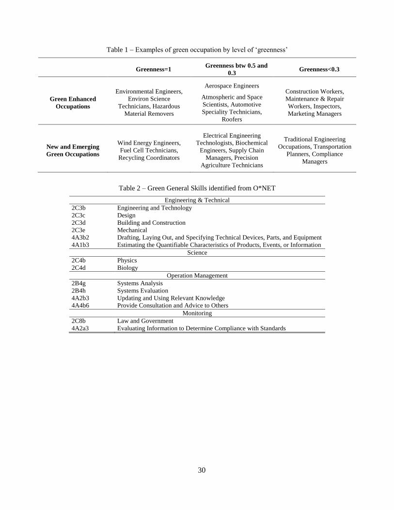
30
Table 1 – Examples of green occupation by level of ‘greenness’
Greenness=1
Greenness btw 0.5 and
0.3 Greenness<0.3
Green Enhanced
Occupations
Environmental Engineers,
Environ Science
Technicians, Hazardous
Material Removers
Aerospace Engineers
Atmospheric and Space
Scientists, Automotive
Speciality Technicians,
Roofers
Construction Workers,
Maintenance & Repair
Workers, Inspectors,
Marketing Managers
New and Emerging
Green Occupations
Wind Energy Engineers,
Fuel Cell Technicians,
Recycling Coordinators
Electrical Engineering
Technologists, Biochemical
Engineers, Supply Chain
Managers, Precision
Agriculture Technicians
Traditional Engineering
Occupations, Transportation
Planners, Compliance
Managers
Table 2 – Green General Skills identified from O*NET
Engineering & Technical
2C3b Engineering and Technology
2C3c Design
2C3d Building and Construction
2C3e Mechanical
4A3b2 Drafting, Laying Out, and Specifying Technical Devices, Parts, and Equipment
4A1b3 Estimating the Quantifiable Characteristics of Products, Events, or Information
Science
2C4b Physics
2C4d Biology
Operation Management
2B4g Systems Analysis
2B4h Systems Evaluation
4A2b3 Updating and Using Relevant Knowledge
4A4b6 Provide Consultation and Advice to Others
Monitoring
2C8b Law and Government
4A2a3 Evaluating Information to Determine Compliance with Standards
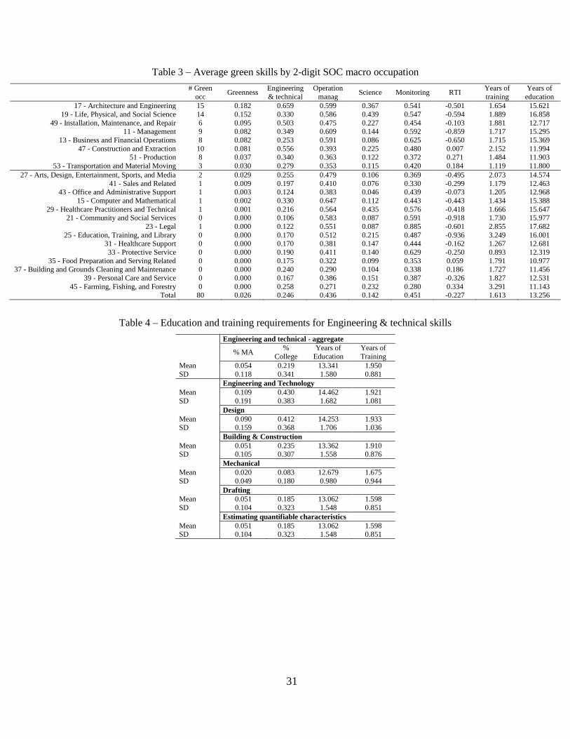
31
Table 3 – Average green skills by 2-digit SOC macro occupation
# Green
occ Greenness
Engineering
& technical
Operation
manag Science Monitoring RTI
Years of
training
Years of
education
17 - Architecture and Engineering 15 0.182 0.659 0.599 0.367 0.541 -0.501 1.654 15.621
19 - Life, Physical, and Social Science 14 0.152 0.330 0.586 0.439 0.547 -0.594 1.889 16.858
49 - Installation, Maintenance, and Repair 6 0.095 0.503 0.475 0.227 0.454 -0.103 1.881 12.717 11 - Management 9 0.082 0.349 0.609 0.144 0.592 -0.859 1.717 15.295
13 - Business and Financial Operations 8 0.082 0.253 0.591 0.086 0.625 -0.650 1.715 15.369
47 - Construction and Extraction 10 0.081 0.556 0.393 0.225 0.480 0.007 2.152 11.994 51 - Production 8 0.037 0.340 0.363 0.122 0.372 0.271 1.484 11.903
53 - Transportation and Material Moving 3 0.030 0.279 0.353 0.115 0.420 0.184 1.119 11.800
27 - Arts, Design, Entertainment, Sports, and Media 2 0.029 0.255 0.479 0.106 0.369 -0.495 2.073 14.574
41 - Sales and Related 1 0.009 0.197 0.410 0.076 0.330 -0.299 1.179 12.463 43 - Office and Administrative Support 1 0.003 0.124 0.383 0.046 0.439 -0.073 1.205 12.968
15 - Computer and Mathematical 1 0.002 0.330 0.647 0.112 0.443 -0.443 1.434 15.388
29 - Healthcare Practitioners and Technical 1 0.001 0.216 0.564 0.435 0.576 -0.418 1.666 15.647 21 - Community and Social Services 0 0.000 0.106 0.583 0.087 0.591 -0.918 1.730 15.977
23 - Legal 1 0.000 0.122 0.551 0.087 0.885 -0.601 2.855 17.682
25 - Education, Training, and Library 0 0.000 0.170 0.512 0.215 0.487 -0.936 3.249 16.001 31 - Healthcare Support 0 0.000 0.170 0.381 0.147 0.444 -0.162 1.267 12.681
33 - Protective Service 0 0.000 0.190 0.411 0.140 0.629 -0.250 0.893 12.319
35 - Food Preparation and Serving Related 0 0.000 0.175 0.322 0.099 0.353 0.059 1.791 10.977 37 - Building and Grounds Cleaning and Maintenance 0 0.000 0.240 0.290 0.104 0.338 0.186 1.727 11.456
39 - Personal Care and Service 0 0.000 0.167 0.386 0.151 0.387 -0.326 1.827 12.531
45 - Farming, Fishing, and Forestry 0 0.000 0.258 0.271 0.232 0.280 0.334 3.291 11.143 Total 80 0.026 0.246 0.436 0.142 0.451 -0.227 1.613 13.256
Table 4 – Education and training requirements for Engineering & technical skills
Engineering and technical - aggregate
% MA
%
College
Years of
Education
Years of
Training
Mean 0.054 0.219 13.341 1.950
SD 0.118 0.341 1.580 0.881
Engineering and Technology
Mean 0.109 0.430 14.462 1.921
SD 0.191 0.383 1.682 1.081
Design
Mean 0.090 0.412 14.253 1.933 SD 0.159 0.368 1.706 1.036
Building & Construction
Mean 0.051 0.235 13.362 1.910 SD 0.105 0.307 1.558 0.876
Mechanical
Mean 0.020 0.083 12.679 1.675
SD 0.049 0.180 0.980 0.944
Drafting
Mean 0.051 0.185 13.062 1.598
SD 0.104 0.323 1.548 0.851
Estimating quantifiable characteristics
Mean 0.051 0.185 13.062 1.598 SD 0.104 0.323 1.548 0.851

32
Table 5 - Green vs brown
Green Brown None Green Brown None
SOC 2 Engineering and Technical Science
17 - Architecture and Engineering 0.69 0.59 0.60 0.39 0.51 0.30 47 - Construction and Extraction 0.57 0.47 0.56 0.28 0.20 0.20
49 - Installation, Maintenance, and Repair 0.51 0.56 0.47 0.24 0.28 0.19
51 - Production 0.35 0.38 0.33 0.19 0.12 0.12 53 - Transportation and Material Moving 0.35 0.45 0.27 0.22 0.27 0.11
Total 0.56 0.44 0.36 0.28 0.19 0.14
SOC 2 Operation Management Monitoring
17 - Architecture and Engineering 0.61 0.68 0.56 0.56 0.55 0.51
47 - Construction and Extraction 0.37 0.37 0.41 0.48 0.44 0.49
49 - Installation, Maintenance, and Repair 0.46 0.46 0.49 0.44 0.44 0.47 51 - Production 0.31 0.43 0.34 0.39 0.39 0.36
53 - Transportation and Material Moving 0.36 0.34 0.35 0.50 0.46 0.42
Total 0.46 0.43 0.38 0.48 0.42 0.42
SOC 2 RTI Years of education
17 - Architecture and Engineering -0.54 -0.74 -0.40 15.79 16.39 15.13
47 - Construction and Extraction -0.01 0.20 -0.03 11.97 11.58 12.10 49 - Installation, Maintenance, and Repair -0.09 0.04 -0.17 12.85 12.54 12.61
51 - Production 0.24 0.16 0.31 12.76 12.24 11.75
53 - Transportation and Material Moving 0.35 0.36 0.18 11.66 12.06 11.80
Total -0.14 0.12 0.13 13.24 12.30 12.03
Skill intensity by macro-occupation weighted by employment (SOC 6-digit) in 2012 (BLS).
Figure 3 - Attainment status by metropolitan and non-metropolitan areas
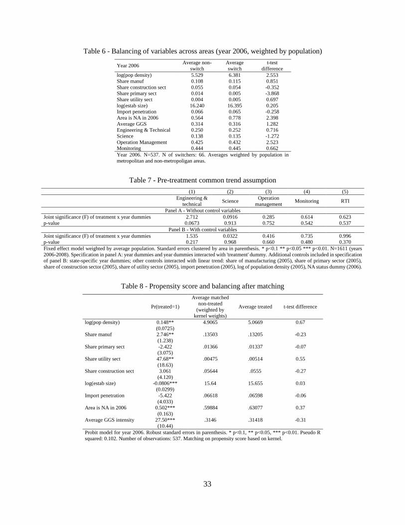
33
Table 6 - Balancing of variables across areas (year 2006, weighted by population)
Year 2006 Average non-
switch
Average
switch
t-test
difference
log(pop density) 5.529 6.381 2.553
Share manuf 0.108 0.115 0.851
Share construction sect 0.055 0.054 -0.352 Share primary sect 0.014 0.005 -3.868
Share utility sect 0.004 0.005 0.697
log(estab size) 16.240 16.395 0.205 Import penetration 0.066 0.065 -0.258
Area is NA in 2006 0.564 0.778 2.398
Average GGS 0.314 0.316 1.282 Engineering & Technical 0.250 0.252 0.716
Science 0.138 0.135 -1.272
Operation Management 0.425 0.432 2.523 Monitoring 0.444 0.445 0.662
Year 2006. N=537. N of switchers: 66. Averages weighted by population in
metropolitan and non-metropoligan areas.
Table 7 - Pre-treatment common trend assumption
(1) (2) (3) (4) (5)
Engineering &
technical Science
Operation
management Monitoring RTI
Panel A - Without control variables
Joint significance (F) of treatment x year dummies 2.712 0.0916 0.285 0.614 0.623
p-value 0.0673 0.913 0.752 0.542 0.537
Panel B - With control variables
Joint significance (F) of treatment x year dummies 1.535 0.0322 0.416 0.735 0.996 p-value 0.217 0.968 0.660 0.480 0.370
Fixed effect model weighted by average population. Standard errors clustered by area in parenthesis. * p<0.1 ** p<0.05 *** p<0.01. N=1611 (years
2006-2008). Specification in panel A: year dummies and year dummies interacted with 'treatment' dummy. Additional controls included in specification of panel B: state-specific year dummies; other controls interacted with linear trend: share of manufacturing (2005), share of primary sector (2005),
share of construction sector (2005), share of utility sector (2005), import penetration (2005), log of population density (2005), NA status dummy (2006).
Table 8 - Propensity score and balancing after matching
Pr(treated=1)
Average matched
non-treated
(weighted by kernel weights)
Average treated t-test difference
log(pop density) 0.148** 4.9065 5.0669 0.67
(0.0725) Share manuf 2.746** .13503 .13205 -0.23
(1.238)
Share primary sect -2.422 .01366 .01337 -0.07 (3.075)
Share utility sect 47.68** .00475 .00514 0.55
(18.63) Share construction sect 3.061 .05644 .0555 -0.27
(4.120)
log(estab size) -0.0806*** 15.64 15.655 0.03
(0.0299)
Import penetration -5.422 .06618 .06598 -0.06
(4.033) Area is NA in 2006 0.502*** .59884 .63077 0.37
(0.163)
Average GGS intensity 27.50*** .3146 .31418 -0.31 (10.44)
Probit model for year 2006. Robust standard errors in parenthesis. * p<0.1, ** p<0.05, *** p<0.01. Pseudo R
squared: 0.102. Number of observations: 537. Matching on propensity score based on kernel.

34
Table 9 - Baseline estimates for total employment
Tot employment (BLS) Tot employment (CBP) Empl in exposed
industries
NA in t=0 x trend -0.00333* -0.00181 -0.00311
(0.00172) (0.00123) (0.00321)
NA designation 0.00329 0.00472 0.0131 (0.00436) (0.00416) (0.00939)
NA implementation -0.0113 0.00293 -0.00336
(0.0101) (0.00532) (0.00989)
NA designation + NA implementation -0.00801 0.00765 0.00974 Test: NA design + NA implement=0 (p-value) 0.451 0.115 0.420
R sq 0.466 0.747 0.817
N 4806 4272 4806
Fixed effect model weighted by kernel-based weights based on propensity score. Other control variables: state-specific year dummies; other controls interacted with linear trend: share of manufacturing (2005), share of primary sector (2005), share of
construction sector (2005), share of utility sector (2005), import penetration (2005), log of population density (2005).
Table 10 - Baseline estimates for skill composition
Science Engineering &
technical Engineering 'high' Engineering 'low'
NA in t=0 x trend -0.0000286 -0.000140 -0.000221 -0.0000986 (0.0000817) (0.000141) (0.000162) (0.000138)
NA designation -0.000482 0.00104** 0.00130** 0.000909*
(0.000387) (0.000525) (0.000596) (0.000513) NA implementation 0.000719** 0.000524 0.000827 0.000373
(0.000337) (0.000592) (0.000684) (0.000566)
NA designation + NA implementation 0.000237 0.001564 0.002127 0.001282 Test: NA design + NA implement=0 (p-value) 0.443 0.0111 0.00222 0.0328
R sq 0.448 0.492 0.407 0.534
N 4806 4806 4806 4806
Operation
management Monitoring
Monitoring 'compliance'
Monitoring 'law'
NA in t=0 x trend -0.0000422 -0.0000603 -0.000161 0.0000400
(0.000102) (0.0000895) (0.0000984) (0.000115)
NA designation 0.0000538 0.000412 0.000948* -0.000124 (0.000413) (0.000436) (0.000511) (0.000549)
NA implementation 0.000725 0.000260 0.000138 0.000383
(0.000452) (0.000442) (0.000482) (0.000543)
NA designation + NA implementation 0.0007788 0.000672 0.001086 0.000259
Test: NA design + NA implement=0 (p-value) 0.0868 0.0814 0.0125 0.629
R sq 0.585 0.599 0.515 0.579 N 4806 4806 4806 4806
RTI log(training) log(education) Share requiring
master degree
NA in t=0 x trend -0.0000973 0.000571 -0.0000443 0.0000730 (0.000262) (0.000511) (0.000120) (0.000123)
NA designation 0.000828 -0.00217 -0.000280 -0.000964**
(0.00113) (0.00226) (0.000483) (0.000478) NA implementation -0.00172 0.00292 0.000992* 0.000860*
(0.00118) (0.00227) (0.000516) (0.000467)
NA designation + NA implementation -0.000892 0.00075 0.000712 -0.000104
Test: NA design + NA implement=0 (p-value) 0.497 0.719 0.179 0.822
R sq 0.591 0.295 0.576 0.611
N 4806 4806 4806 4806
Fixed effect model weighted by kernel-based weights based on propensity score. Other control variables: state-specific year dummies; other
controls interacted with linear trend: share of manufacturing (2005), share of primary sector (2005), share of construction sector (2005), share of utility sector (2005), import penetration (2005), log of population density (2005).
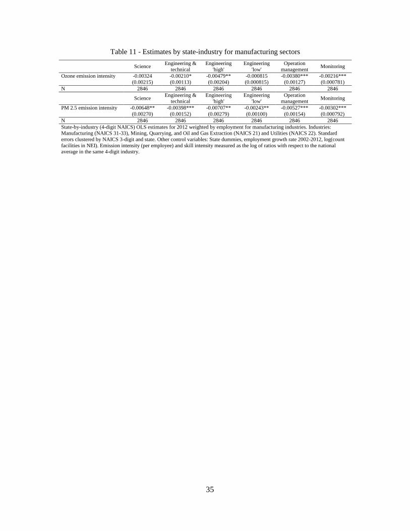
35
Table 11 - Estimates by state-industry for manufacturing sectors
Science Engineering &
technical
Engineering
'high'
Engineering
'low'
Operation
management Monitoring
Ozone emission intensity -0.00324 -0.00210* -0.00479** -0.000815 -0.00380*** -0.00216***
(0.00215) (0.00113) (0.00204) (0.000815) (0.00127) (0.000781)
N 2846 2846 2846 2846 2846 2846
Science Engineering &
technical Engineering
'high' Engineering
'low' Operation
management Monitoring
PM 2.5 emission intensity -0.00648** -0.00398*** -0.00707** -0.00243** -0.00527*** -0.00302***
(0.00270) (0.00152) (0.00279) (0.00100) (0.00154) (0.000792)
N 2846 2846 2846 2846 2846 2846
State-by-industry (4-digit NAICS) OLS estimates for 2012 weighted by employment for manufacturing industries. Industries: Manufacturing (NAICS 31-33), Mining, Quarrying, and Oil and Gas Extraction (NAICS 21) and Utilities (NAICS 22). Standard
errors clustered by NAICS 3-digit and state. Other control variables: State dummies, employment growth rate 2002-2012, log(count
facilities in NEI). Emission intensity (per employee) and skill intensity measured as the log of ratios with respect to the national average in the same 4-digit industry.

36
Appendix A: Green Skills
This appendix provides details of the data source and the procedure for the selection of GGS based on the
greenness of green occupations (the full list of green occupations and their level of greenness is reported
in Table 12).

37
Table 13 reports the estimated β of equation 2 for all general skills and tasks for which the beta was
significant at the 99 percent level or more. Recall that results are based on 921 occupations observed at the
8-digit SOC level for the year 2012 and regressions include 3-digit SOC dummies. Out of 108 general skills
and tasks, 16 have been selected as particularly relevant for green occupations.
[Table 12,

38
Table 13 and Table 14 about here]
As discussed in section 2.2, we perform a principal component analysis (PCA) on these 20 general skills
and tasks to generate more aggregate measures of GGS. As discussed in section 3.2, we retain five
components with respective Eigenvalues (unrotated components) of 5.58, 3.93, 1.34, 0.99 and 0.92, and a
cumulative explained variance of 79.72 percent. Table 14 shows the factor loadings of the 5 rotated
components (orthogonal VARIMAX rotation) that exceeded a 0.2 threshold. The first component groups
together “Engineering & Technical Skills”. The second component, labelled “Operation Management
Skills”, includes abilities that are relevant for management practices associated with new technology. The
third component is “Monitoring Skills”. Therein we observe that two general skills (Law and Government
and Evaluating Information to Determine Compliance with Standards) load much more than the third one
(Operating Vehicles, Mechanized Devices, or Equipment) which, instead, loads negatively on the second
component. A thorough reading of the description of these skills (from O*NET) reveals that only the first
two bear direct relevance for Monitoring activities, while the third one has to do with operating machineries,
vehicles and means of transport and thus not only with the use of monitoring devices. We therefore excluded
this third item from the construct. The fourth component clearly refers to Science Skills. Finally, the fifth
component is characterized by a large factor loading (Geography, 0.84) and a smaller loading one (Law and
Government which, however, was already assigned to component 3). Geographic skills capture activities
such as urban planning and analysis of emission dynamics (several profession intensive of Geography skills
are green, such as Environmental Restoration Planners, Landscape Architects and Atmospheric and Space
Scientist). Due to the specificity of this last component, which only refer to one general skill, we left it out
of the analysis. Results on the impact of environmental regulation for this GGS and for each single general
skill selected here (including "Geography" and "Operating Vehicles, Mechanized Devices, or Equipment",
which were excluded from the GGS constructs) are shown in the Appendix D.
[Table 15 and Table 16 about here]
We tried several alternative ways of selecting GGS to assess the robustness of our selection procedure and
to identify the GGS that are selected irrespective of the procedure. We present here two of these additional
exercises. First, we estimate equation 2 by weighting each occupation by the total of employees in year
201223. Note that this is not our favourite selection method because it assigns undue importance to
occupations that are highly present in the service sector and thus are not directly affected by the
23 Weights at the 6-digit SOC level for year 2012 are based on the Occupational Employment Statistics prepared by
the Bureau of Labor Statistics. It collects, among other things, aggregate employment measures by detailed occupation.
No information is available at the 8-digit SOC level. As discussed in Appendix B about state-industry measures, we
decide to weight equally each 8-digit occupation within its corresponding 6-digit macro-occupation.
39
sustainability issues. Results are reported in Table 15. This second method only retains general skills that
enter two of our Engineering & Technical and Science skills constructs, with the addition of Chemistry that
was not selected in our preferred approach. Engineering & Technical and Science skills encompass the core
technical and scientific know-how that is required in green occupations. Second, we decompose the
indicator of Greenness into its two components, that is, the count of green specific tasks and the count of
total specific tasks. In this specification we allow both components of the Greenness indicator to have an
independent effect on general skills. Results for the coefficients associated with green specific tasks and
total specific tasks are reported in Table 16. We observe a positive and significant (at the 99 percent level)
relationship between the number of green specific tasks for 13 general skills. Out of these 13 skills, just one
(Systems Evaluation) also shows a positive and significant correlation with the total number of specific
tasks. These 13 general skills represent a subset of our initial selection of 16 general skills. This second
criterion excludes two general skills that entered the Operation Management GGS (System Analysis and
Updating and Using Relevant Knowledge) and one Science skills (Biology).
Taking the cue from the polarization of occupations within engineering skills, in Table 4 we take a closer
look at the component parts of this construct: Engineering & Technology, Design, Building & Construction,
Mechanical, Drafting and Estimating quantifiable characteristics. The descriptions provided by O*NET
serve as first point of reference to detect functional commonalities and differences across these items.
Engineering & Technology and Design are areas of knowledge associated with the application of scientific
principles to practical problems. By contrast, Building & Construction, Mechanical, Drafting and Estimating
quantifiable characteristics pertain to areas of practical know-how of e.g. materials, machines, tools as well
as of the technical specifications that are necessary to operate them. In short, the first two items of Green
Engineering skills are about “Conceiving solutions” while the remaining three are about “Implementing
solutions”. This functional difference is reflected also in the educational levels associated with each of these
specific skills. The upper portion of Table 4 shows that an average 21% of workers in occupations with the
highest (top 10%) value of E&T skills possess a college degree, while only 5% have postgraduate education.
At the same time, the high standard deviation for college graduates suggests strong within group variability
which is confirmed by the mean values for each individual skill item. In particular, Engineering &
Technology and Design look rather similar since for both the average number of top occupations with at
least college degree is above 40%. This is not so for the other items, in particular for Mechanical and
Drafting skills where average values range between 8% and 18% respectively. Such a polarization in the
educational requirements of occupations with the highest intensity of green Engineering skills hints at
interesting heterogeneity in the type of knowledge possessed by these workers with vocational and technical
degrees more important for “low” engineering skills.

40

41
Appendix B: Data
B1. O*NET and BLS data
Our set of skill measures is built using occupation-MSA employment levels from BLS Occupational
Employment Statistics (BLS-OES) for 2006-2014 to weight O*NET data on occupational skills. We use the
release 17.0 (July 2012) of O*NET.
Importance scores of selected skill measures range from 1 (not important) to 5 (very important) and
measure how important is the general task for the occupation. Before computing GGSk, we rescale scores to
range between 0 and 1 (we subtract 1 and divide by 4 each item that enters GGSk). In addition to our GGS
indeces, we also build an index of Routine Task Intensity based on the items of O*NET identified by
Acemoglu and Autor (2010). The list of items is reported in Table 17.
[Table 17 about here]
BLS-OES data at the metropolitan area level are released yearly since 1999. However, prior to 2006
metropolitan areas boundaries were defined differently and cannot be easily harmonized with the new
delineation that has been adopted starting from 2006. Moreover, no information for non-metropolitan areas
was available before 2006. Employment by occupation and metropolitan and non-metropolitan areas is
reported if it is greater than 30 and if the cell occupation-area was 'sampled'. We filled missing values based
on employment observed in the same cell occupation area in adjacent years or, if no information available,
split employment in the cell macro-occupation (2-digit SOC) - area to 6-digit occupations based on federal-
level employment shares. Finally, we employed a weighted crosswalk between SOC2009 and SOC2010
classification to obtain data in terms of SOC2010 occupations also for the period 2006-2009.
It is worth recalling that the mismatch between the aggregation of the O*NET database and the
Occupational Employment Statistics is corrected by assuming that employees are uniformly distributed
across 8-digit SOC occupations within each 6-digit SOC occupation. 8-digit and 6-digit occupations
coincide for 678 occupations. For the remaining 97 6-digit occupations the average number of 8-digit
occupation is 3 and the median is 2, with a maximum of 12. The task constructs at 6-digit SOC are built as
the simple mean of the task constructs at 8-digit SOC. This is clearly a limitation of the combination of
O*NET with the BLS Occupational Employment Statistics Database but, in the absence of detailed
information on employment at the 8-digit SOC level, the aggregation of information of O*NET by means
of simple mean remains the most suitable options.
A possible alternative to BLS-OES data to evaluate the labour force composition of US regions would
be information from the American Community Survey (ACS) available at IPUMS (Integrated Public Use

42
Microdata Series). The time coverage of the ACS is 2005-2013 since no information on the PUMA (Public
Use Microdata Area) of work of workers is available prior of 2005 with the exception of decennial censuses.
However, the advantage of having additional information on some features of the labor force (e.g. industry,
earnings, educational attainment) comes at the cost of losing information about the detailed composition of
the local labor force. ACS classifies workers into occupations using the SOC (Standard Occupational
Classification) system, similarly to BLS data. Furthermore many occupations (including many green
occupations and occupations with high intensity of green skills) are classified in aggregate categories (e.g.
5-digit SOC or even 3-digit SOC) compared to the OES-BLS database. This implies that regional variation
in employment for the occupations that are relevant to our GGS constructs are measured less precisely. We
have computed the GGS by MSA using the ACS Census and find that these data are highly volatile.
[Figure 4 about here]
In Figure 4 we report standard deviation of yearly changes in our GGS measures at the metropolitan and
nonmetropolitan level for each year, estimated either using ACS or BLS. The volatility of these changes is
substantially larger for ACS than for BLS. Since workforce composition is long-term persistent feature of a
region, this large volatility of ACS data may indicate the lack of representativeness of the yearly
employment statistics at region-by-occupation level. In addition, this large volatility is worrisome as we use
variation within a region to identify the impact of environmental regulation on GGS.
[Figure 5 and Figure 6 about here]
In Figure 5 we also plot the GGS intensity by metropolitan and non-metropolitan areas using BLS and
ACS data respectively, using the average value for each area from 2006-2013. The two estimates look rather
similar overall, but some large deviations exist. The correlation between the two measures is 0.76 for
Science, 0.85 for Engineering and Technical, 0.93 for Operation Management and 0.83 for Monitoring.
However, when we look at the long run change in GGS in metropolitan and non-metropolitan areas (2005-
2013), reported in Figure 6, differences between the two data source become very relevant. The correlation
between the changes in the two estimates is very weak for Engineering and Technical (0.12) and Monitoring
(0.01) and even negative in some case (correlation for Science and Operation Management is, respectively,
-0.17 and -0.13).
In sum, BLS data seem much more reliable for our purposes than ACS data for at least two reasons. The
first regards the fact that the occupational level of aggregation in BLS is finer (6-digit SOC occupation) than
the one for ACS (occupations may be aggregated at the 5-digit or even 3-digit SOC level). Secondly,
samples of the ACS are not stratified by metropolitan and nonmetropolitan area: this means that they are

43
not necessarily representative of the population of workers in the area and thus displays significantly higher
volatility than BLS data.
B2. Environmental Regulation
Information on county-level nonattainment is retrieved from the 'Green Book Nonattainment Areas for
Criteria Pollutants' maintained by the Environment Protection Agency (EPA) and available here
http://www3.epa.gov/airquality/greenbook/. Attainment status by county is extended to the whole
metropolitan and non-metropolitan area sample as discussed in Section 3.1. Moreover, as discussed in Ferris
et al. (2014), all counties and areas in the states included in the Ozone Transport Region have to implement
regulatory actions equivalent to the ones mandated for nonattainment counties for the Ozone standards, even
though they comply with the standard.
B3. Data sources for control variables
Information on the distribution of employment by industry of metropolitan and non-metropolitan areas
comes from the BLS Quarterly Census of Employment and Wages (CEW). We aggregated county-level
figures to the metropolitan and non-metropolitan area level. Primary industries include NAICS codes 11
and 21, utilities NAICS codes 22 manufacturing industries NAICS codes 31-33. Also information on
average establishment size (average employees per establishment) is retrieved from the BLS-CEW.
Data on resident population comes from the US Census Bureau. Also in this case we retrieve information
at the county-level and the aggregate it at the metropolitan and non-metropolitan level.
Import penetration is measured as the ratio between import and 'domestic consumption' (import +
domestic production - export) at the 4-digit NAICS level for year 2006. Data on total import and export for
the US as a whole come from Schott (2009) and are available here
http://faculty.som.yale.edu/peterschott/sub_international.htm. Data on total production at the federal level
by 4-digit NAICS manufacturing industries come from the NBER-CES database. We compute import
penetration at the federal level and attribute it to metropolitan and non-metropolitan areas by multiplying
industry-level import penetration by area-level employment share by 4-digit NAICS industry. This latter
information, for year 2006, comes from the County Business Patterns database.
B5. State-industry data
Our set of skill measures is built using occupation-industry-state employment levels from BLS
(Occupational Employment Statistics, year 2012) weighted by O*NET data on occupational skills. Note
that occupation-industry-state cells with less than 30 employees are not reported. Out of 18,942,800
employees in NAICS industries 21, 22, 31, 32 and 33 in year 2012 (Occupational Employment Statistics,
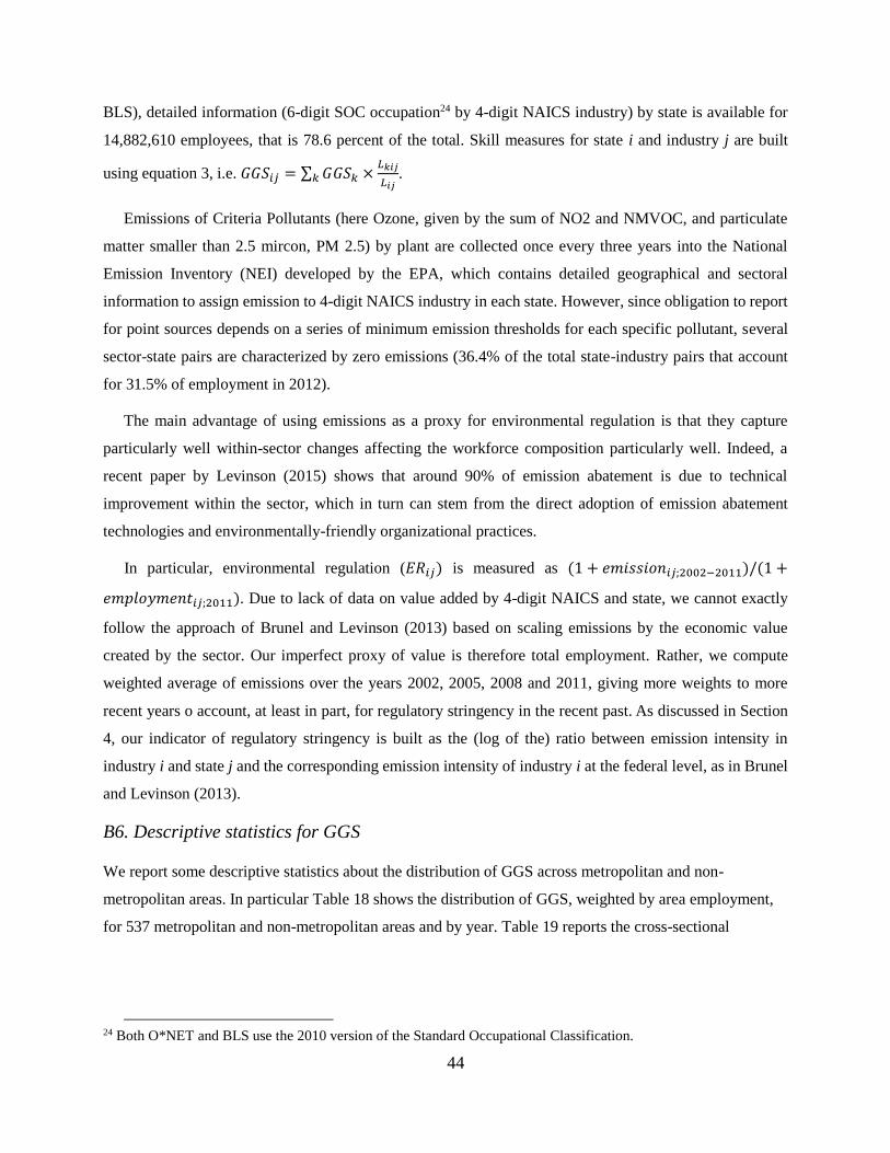
44
BLS), detailed information (6-digit SOC occupation24 by 4-digit NAICS industry) by state is available for
14,882,610 employees, that is 78.6 percent of the total. Skill measures for state i and industry j are built
using equation 3, i.e. 𝐺𝐺𝑆𝑖𝑗 = ∑ 𝐺𝐺𝑆𝑘𝑘 ×𝐿𝑘𝑖𝑗
𝐿𝑖𝑗.
Emissions of Criteria Pollutants (here Ozone, given by the sum of NO2 and NMVOC, and particulate
matter smaller than 2.5 mircon, PM 2.5) by plant are collected once every three years into the National
Emission Inventory (NEI) developed by the EPA, which contains detailed geographical and sectoral
information to assign emission to 4-digit NAICS industry in each state. However, since obligation to report
for point sources depends on a series of minimum emission thresholds for each specific pollutant, several
sector-state pairs are characterized by zero emissions (36.4% of the total state-industry pairs that account
for 31.5% of employment in 2012).
The main advantage of using emissions as a proxy for environmental regulation is that they capture
particularly well within-sector changes affecting the workforce composition particularly well. Indeed, a
recent paper by Levinson (2015) shows that around 90% of emission abatement is due to technical
improvement within the sector, which in turn can stem from the direct adoption of emission abatement
technologies and environmentally-friendly organizational practices.
In particular, environmental regulation (𝐸𝑅𝑖𝑗) is measured as (1 + 𝑒𝑚𝑖𝑠𝑠𝑖𝑜𝑛𝑖𝑗;2002−2011)/(1 +
𝑒𝑚𝑝𝑙𝑜𝑦𝑚𝑒𝑛𝑡𝑖𝑗;2011). Due to lack of data on value added by 4-digit NAICS and state, we cannot exactly
follow the approach of Brunel and Levinson (2013) based on scaling emissions by the economic value
created by the sector. Our imperfect proxy of value is therefore total employment. Rather, we compute
weighted average of emissions over the years 2002, 2005, 2008 and 2011, giving more weights to more
recent years o account, at least in part, for regulatory stringency in the recent past. As discussed in Section
4, our indicator of regulatory stringency is built as the (log of the) ratio between emission intensity in
industry i and state j and the corresponding emission intensity of industry i at the federal level, as in Brunel
and Levinson (2013).
B6. Descriptive statistics for GGS
We report some descriptive statistics about the distribution of GGS across metropolitan and non-
metropolitan areas. In particular Table 18 shows the distribution of GGS, weighted by area employment,
for 537 metropolitan and non-metropolitan areas and by year. Table 19 reports the cross-sectional
24 Both O*NET and BLS use the 2010 version of the Standard Occupational Classification.
45
correlation matrix across GGS at the metropolitan and non-metropolitan area level weighted by area
employment (average 2006-2014).
[Table 18 and Table 19 about here]
Finally, for illustrative purposes we report some descriptive statistics. Table 20 shows top 10 industries
in terms of emission intensity and GGS intensity by industry for year 2012.
[Table 18 about here]

46
Appendix C: Brown jobs
As discussed in Section 2.4, we define brown jobs (occupations) as the occupations for which more than
10 percent of the overall workforce is employed in energy intensive industries. These include the 'Mining,
Quarrying, and Oil and Gas Extraction' industry (NAICS 21) and 'Electric Power Generation, Transmission
and Distribution' (NAICS 2211) industry (for which, however, no direct information share of energy costs
over total costs) together with the top decile of manufacturing industries in terms of share of energy costs
over total production (source: NBER-CES database, year 2006). This resulted in the selection of the
following NAICS codes (4-digit): 3112, 3131, 3133, 3221, 3251, 3252, 3271, 3272, 3272, 3274, 3279, 3311,
3313, 3315 and 3328. As a second step we calculate for each 6-digit SOC occupations the share of total
employees of occupations that are employed in any of the brown industries using the BLS-OES estimates
of occupational employment by 4-digit NAICS industries for years 2006-2014. The list of 6-digit SOC
brown occupations is reported in Table 21.
[Table 21 about here]

47
Appendix C Robustness
Table 22 reports results on the impact of environmental regulation on the demand for green skills (as
described in Section 3.2) for each GGS item.
[Table 22 about here]
Results confirm our baseline results for GGS. However, for the two items that were not assigned to any
GGS group, we find a negative result for NA designation for Geography and no effect for implementation.
Similarly, we find no effect for Operating Vehicles, Mechanized Devices, or Equipment.
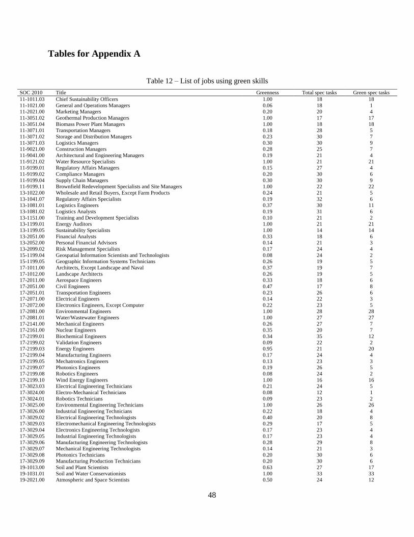
48
Tables for Appendix A
Table 12 – List of jobs using green skills
SOC 2010 Title Greenness Total spec tasks Green spec tasks
11-1011.03 Chief Sustainability Officers 1.00 18 18
11-1021.00 General and Operations Managers 0.06 18 1 11-2021.00 Marketing Managers 0.20 20 4
11-3051.02 Geothermal Production Managers 1.00 17 17
11-3051.04 Biomass Power Plant Managers 1.00 18 18 11-3071.01 Transportation Managers 0.18 28 5
11-3071.02 Storage and Distribution Managers 0.23 30 7
11-3071.03 Logistics Managers 0.30 30 9 11-9021.00 Construction Managers 0.28 25 7
11-9041.00 Architectural and Engineering Managers 0.19 21 4
11-9121.02 Water Resource Specialists 1.00 21 21 11-9199.01 Regulatory Affairs Managers 0.15 27 4
11-9199.02 Compliance Managers 0.20 30 6
11-9199.04 Supply Chain Managers 0.30 30 9 11-9199.11 Brownfield Redevelopment Specialists and Site Managers 1.00 22 22
13-1022.00 Wholesale and Retail Buyers, Except Farm Products 0.24 21 5
13-1041.07 Regulatory Affairs Specialists 0.19 32 6 13-1081.01 Logistics Engineers 0.37 30 11
13-1081.02 Logistics Analysts 0.19 31 6
13-1151.00 Training and Development Specialists 0.10 21 2 13-1199.01 Energy Auditors 1.00 21 21
13-1199.05 Sustainability Specialists 1.00 14 14
13-2051.00 Financial Analysts 0.33 18 6 13-2052.00 Personal Financial Advisors 0.14 21 3
13-2099.02 Risk Management Specialists 0.17 24 4
15-1199.04 Geospatial Information Scientists and Technologists 0.08 24 2 15-1199.05 Geographic Information Systems Technicians 0.26 19 5
17-1011.00 Architects, Except Landscape and Naval 0.37 19 7
17-1012.00 Landscape Architects 0.26 19 5 17-2011.00 Aerospace Engineers 0.33 18 6
17-2051.00 Civil Engineers 0.47 17 8
17-2051.01 Transportation Engineers 0.23 26 6 17-2071.00 Electrical Engineers 0.14 22 3
17-2072.00 Electronics Engineers, Except Computer 0.22 23 5 17-2081.00 Environmental Engineers 1.00 28 28
17-2081.01 Water/Wastewater Engineers 1.00 27 27
17-2141.00 Mechanical Engineers 0.26 27 7 17-2161.00 Nuclear Engineers 0.35 20 7
17-2199.01 Biochemical Engineers 0.34 35 12
17-2199.02 Validation Engineers 0.09 22 2 17-2199.03 Energy Engineers 0.95 21 20
17-2199.04 Manufacturing Engineers 0.17 24 4
17-2199.05 Mechatronics Engineers 0.13 23 3 17-2199.07 Photonics Engineers 0.19 26 5
17-2199.08 Robotics Engineers 0.08 24 2
17-2199.10 Wind Energy Engineers 1.00 16 16 17-3023.03 Electrical Engineering Technicians 0.21 24 5
17-3024.00 Electro-Mechanical Technicians 0.08 12 1
17-3024.01 Robotics Technicians 0.09 23 2 17-3025.00 Environmental Engineering Technicians 1.00 26 26
17-3026.00 Industrial Engineering Technicians 0.22 18 4
17-3029.02 Electrical Engineering Technologists 0.40 20 8 17-3029.03 Electromechanical Engineering Technologists 0.29 17 5
17-3029.04 Electronics Engineering Technologists 0.17 23 4
17-3029.05 Industrial Engineering Technologists 0.17 23 4 17-3029.06 Manufacturing Engineering Technologists 0.28 29 8
17-3029.07 Mechanical Engineering Technologists 0.14 21 3
17-3029.08 Photonics Technicians 0.20 30 6 17-3029.09 Manufacturing Production Technicians 0.20 30 6
19-1013.00 Soil and Plant Scientists 0.63 27 17
19-1031.01 Soil and Water Conservationists 1.00 33 33 19-2021.00 Atmospheric and Space Scientists 0.50 24 12

49
SOC 2010 Title Greenness Total spec tasks Green spec tasks
19-2041.01 Climate Change Analysts 1.00 14 14
19-2041.02 Environmental Restoration Planners 1.00 22 22
19-2042.00 Geoscientists, Except Hydrologists and Geographers 0.48 31 15 19-2099.01 Remote Sensing Scientists and Technologists 0.08 24 2
19-3011.01 Environmental Economists 1.00 19 19
19-3051.00 Urban and Regional Planners 0.37 19 7 19-3099.01 Transportation Planners 0.14 22 3
19-4011.01 Agricultural Technicians 0.12 25 3
19-4041.01 Geophysical Data Technicians 0.24 21 5 19-4041.02 Geological Sample Test Technicians 0.19 16 3
19-4051.01 Nuclear Equipment Operation Technicians 0.41 17 7
19-4091.00 Environmental Science and Protection Technicians, Including Health 1.00 25 25 19-4099.02 Precision Agriculture Technicians 0.30 23 7
19-4099.03 Remote Sensing Technicians 0.14 22 3 23-1022.00 Arbitrators, Mediators, and Conciliators 0.05 20 1
27-3022.00 Reporters and Correspondents 0.05 22 1
27-3031.00 Public Relations Specialists 0.24 17 4 29-9012.00 Occupational Health and Safety Technicians 0.35 26 9
41-4011.00 Sales Representatives, Wholesale and Manufacturing, Technical and Scientific
Products 0.11 38 4
41-4011.07 Solar Sales Representatives and Assessors 1.00 13 13
43-5071.00 Shipping, Receiving, and Traffic Clerks 0.09 11 1
47-2061.00 Construction Laborers 0.18 33 6 47-2152.01 Pipe Fitters and Steamfitters 0.15 20 3
47-2152.02 Plumbers 0.39 23 9
47-2181.00 Roofers 0.30 30 9 47-2211.00 Sheet Metal Workers 0.24 25 6
47-2231.00 Solar Photovoltaic Installers 1.00 26 26
47-4011.00 Construction and Building Inspectors 0.26 19 5 47-4041.00 Hazardous Materials Removal Workers 0.91 23 21
47-4099.03 Weatherization Installers and Technicians 1.00 18 18
47-5013.00 Service Unit Operators, Oil, Gas, and Mining 0.05 19 1 47-5041.00 Continuous Mining Machine Operators 0.17 12 2
49-3023.02 Automotive Specialty Technicians 0.40 25 10
49-3031.00 Bus and Truck Mechanics and Diesel Engine Specialists 0.16 25 4 49-9021.01 Heating and Air Conditioning Mechanics and Installers 0.23 30 7
49-9071.00 Maintenance and Repair Workers, General 0.13 31 4
49-9081.00 Wind Turbine Service Technicians 1.00 13 13 49-9099.01 Geothermal Technicians 1.00 24 24
51-2011.00 Aircraft Structure, Surfaces, Rigging, and Systems Assemblers 0.13 30 4
51-4041.00 Machinists 0.07 29 2 51-8011.00 Nuclear Power Reactor Operators 0.33 18 6
51-8013.00 Power Plant Operators 0.21 24 5
51-8099.03 Biomass Plant Technicians 1.00 16 16
51-9012.00 Separating, Filtering, Clarifying, Precipitating, and Still Machine Setters, Operators,
and Tenders 0.05 20 1
51-9061.00 Inspectors, Testers, Sorters, Samplers, and Weighers 0.06 32 2 51-9199.01 Recycling and Reclamation Workers 1.00 18 18
53-3032.00 Heavy and Tractor-Trailer Truck Drivers 0.09 33 3
53-6051.07 Transportation Vehicle, Equipment and Systems Inspectors, Except Aviation 0.41 22 9 53-7081.00 Refuse and Recyclable Material Collectors 1.00 16 16
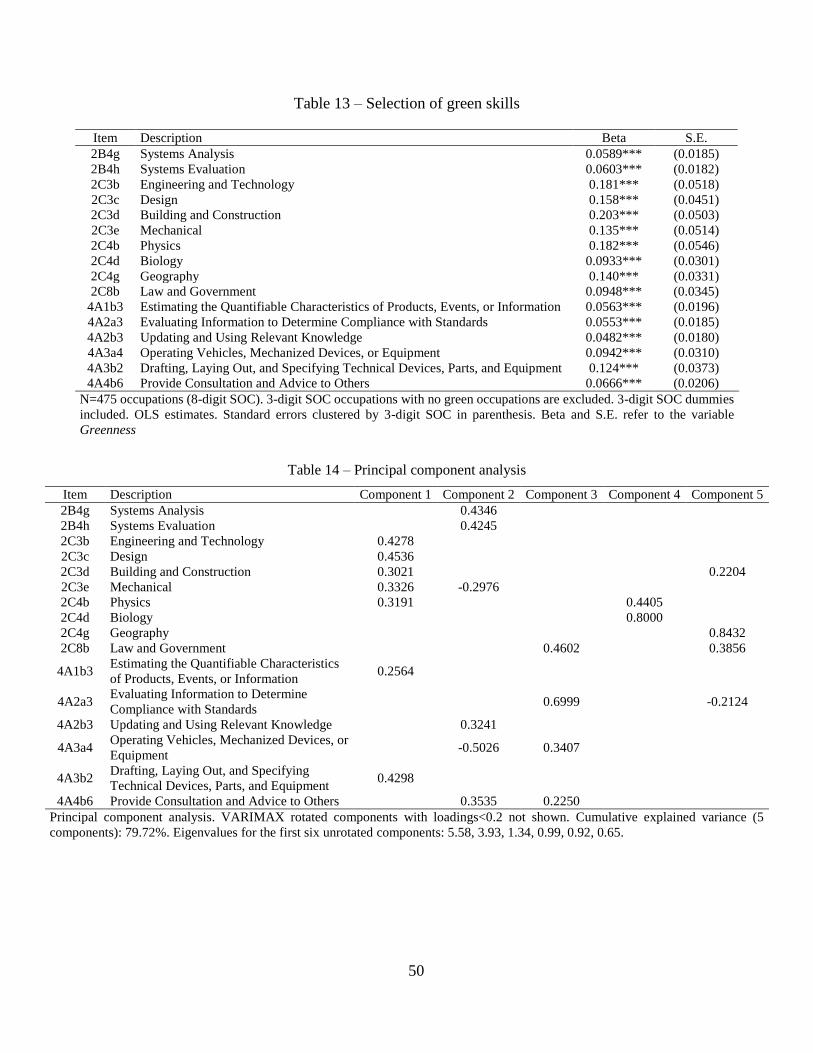
50
Table 13 – Selection of green skills
Item Description Beta S.E.
2B4g Systems Analysis 0.0589*** (0.0185)
2B4h Systems Evaluation 0.0603*** (0.0182)
2C3b Engineering and Technology 0.181*** (0.0518)
2C3c Design 0.158*** (0.0451)
2C3d Building and Construction 0.203*** (0.0503)
2C3e Mechanical 0.135*** (0.0514)
2C4b Physics 0.182*** (0.0546)
2C4d Biology 0.0933*** (0.0301)
2C4g Geography 0.140*** (0.0331)
2C8b Law and Government 0.0948*** (0.0345)
4A1b3 Estimating the Quantifiable Characteristics of Products, Events, or Information 0.0563*** (0.0196)
4A2a3 Evaluating Information to Determine Compliance with Standards 0.0553*** (0.0185)
4A2b3 Updating and Using Relevant Knowledge 0.0482*** (0.0180)
4A3a4 Operating Vehicles, Mechanized Devices, or Equipment 0.0942*** (0.0310)
4A3b2 Drafting, Laying Out, and Specifying Technical Devices, Parts, and Equipment 0.124*** (0.0373)
4A4b6 Provide Consultation and Advice to Others 0.0666*** (0.0206)
N=475 occupations (8-digit SOC). 3-digit SOC occupations with no green occupations are excluded. 3-digit SOC dummies
included. OLS estimates. Standard errors clustered by 3-digit SOC in parenthesis. Beta and S.E. refer to the variable
Greenness
Table 14 – Principal component analysis
Item Description Component 1 Component 2 Component 3 Component 4 Component 5
2B4g Systems Analysis 0.4346
2B4h Systems Evaluation 0.4245
2C3b Engineering and Technology 0.4278
2C3c Design 0.4536
2C3d Building and Construction 0.3021 0.2204
2C3e Mechanical 0.3326 -0.2976
2C4b Physics 0.3191 0.4405
2C4d Biology 0.8000
2C4g Geography 0.8432
2C8b Law and Government 0.4602 0.3856
4A1b3 Estimating the Quantifiable Characteristics
of Products, Events, or Information 0.2564
4A2a3 Evaluating Information to Determine
Compliance with Standards 0.6999 -0.2124
4A2b3 Updating and Using Relevant Knowledge 0.3241
4A3a4 Operating Vehicles, Mechanized Devices, or
Equipment -0.5026 0.3407
4A3b2 Drafting, Laying Out, and Specifying
Technical Devices, Parts, and Equipment 0.4298
4A4b6 Provide Consultation and Advice to Others 0.3535 0.2250
Principal component analysis. VARIMAX rotated components with loadings<0.2 not shown. Cumulative explained variance (5
components): 79.72%. Eigenvalues for the first six unrotated components: 5.58, 3.93, 1.34, 0.99, 0.92, 0.65.

51
Table 15 – Selection of green skills (with employment weights)
Item Description Beta S.E.
2C3b Engineering and Technology 0.244*** (0.0496)
2C3c Design 0.206*** (0.0638)
2C3d Building and Construction 0.303*** (0.0903)
2C3e Mechanical 0.221*** (0.0446)
2C4b Physics 0.246*** (0.0367)
2C4c Chemistry 0.140*** (0.0427)
2C4d Biology 0.124*** (0.0275)
2C4g Geography 0.153*** (0.0306)
N=475 occupations (8-digit SOC). 3-digit SOC occupations with no green
occupations are excluded. 3-digit SOC dummies included. OLS estimates
weighted by employment share. Standard errors clustered by 3-digit SOC in
parenthesis. Beta and S.E. refer to the variable Greenness.
Table 16 – Selection of green skills (count of specific tasks)
Item Description Green specific tasks Total specific tasks
Beta S.E. Beta S.E.
2B4h Systems Evaluation 0.00230** (0.000840) 0.00158** (0.000716)
2C3b Engineering and Technology 0.00836*** (0.00240) -0.000794 (0.00119)
2C3c Design 0.00718*** (0.00202) -0.000306 (0.00150)
2C3d Building and Construction 0.00931*** (0.00221) -0.00217 (0.00128)
2C3e Mechanical 0.00637** (0.00233) -0.00191 (0.00124)
2C4b Physics 0.00839*** (0.00244) -0.00134 (0.000823)
2C4g Geography 0.00681*** (0.00146) 0.000354 (0.00107)
2C8b Law and Government 0.00419*** (0.00150) 0.00102 (0.00129)
4A1b3 Estimating the Quantifiable Characteristics of
Products, Events, or Information 0.00266** (0.00103) -0.000312 (0.000760)
4A2a3 Evaluating Information to Determine Compliance with
Standards 0.00260*** (0.000854) 0.000859 (0.000728)
4A3a4 Operating Vehicles, Mechanized Devices, or
Equipment 0.00520*** (0.00149) -0.000908 (0.00124)
4A3b2 Drafting, Laying Out, and Specifying Technical
Devices, Parts, and Equipment 0.00570*** (0.00163) 0.0000792 (0.00117)
4A4b6 Provide Consultation and Advice to Others 0.00291*** (0.000798) 0.000844 (0.00123)
N=475 occupations (8-digit SOC). 3-digit SOC occupations with no green occupations are excluded. 3-digit SOC dummies
included. OLS estimates weighted. Standard errors clustered by 3-digit SOC in parenthesis. Beta and S.E. refer to the
variables Count of green specific tasks and Count of total specific tasks.

52
Tables for Appendix B
Table 17 - Items included in the Routine Task Intensity (RTI) index
Non-routine analytical (NRA)
4A2a4 Analyzing Data or Information
4A2b2 Thinking Creatively
4A4a1 Interpreting the Meaning of Information for Others
Non-routine interactive (NRI)
4A4a4 Establishing and Maintaining Interpersonal Relationships
4A4b4 Guiding, Directing, and Motivating Subordinates
4A4b5 Coaching and Developing Others
Routine cognitive (RC)
4C3b4 (cx) Importance of Being Exact or Accurate
4C3b7 (cx) Importance of Repeating Same Tasks
4C3b8 (cx) Structured versus Unstructured Work (reverse)
Routine manual (RM)
4A3a3 Controlling Machines and Processes
4C2d1i (cx) Spend Time Making Repetitive Motions
4C3d3 (cx) Pace Determined by Speed of Equipment
Figure 4 - Standard deviation of annual growth rate in GGS by metropolitan and nonmetropolitan areas
measured with ACS and BLS data
0
.002
.004
.006
.008
.01
SD
ann
ua
l o
f gro
wth
ra
te
2007 2008 2009 2010 2011 2012 2013
Science
ACS BLS
0
.005
.01
.015
SD
ann
ua
l o
f gro
wth
ra
te
2007 2008 2009 2010 2011 2012 2013
Engineering & Technical
ACS BLS
0
.005
.01
.015
SD
ann
ua
l o
f gro
wth
ra
te
2007 2008 2009 2010 2011 2012 2013
Operation management
ACS BLS
0
.005
.01
.015
SD
ann
ua
l o
f gro
wth
ra
te
2007 2008 2009 2010 2011 2012 2013
Monitoring
ACS BLS
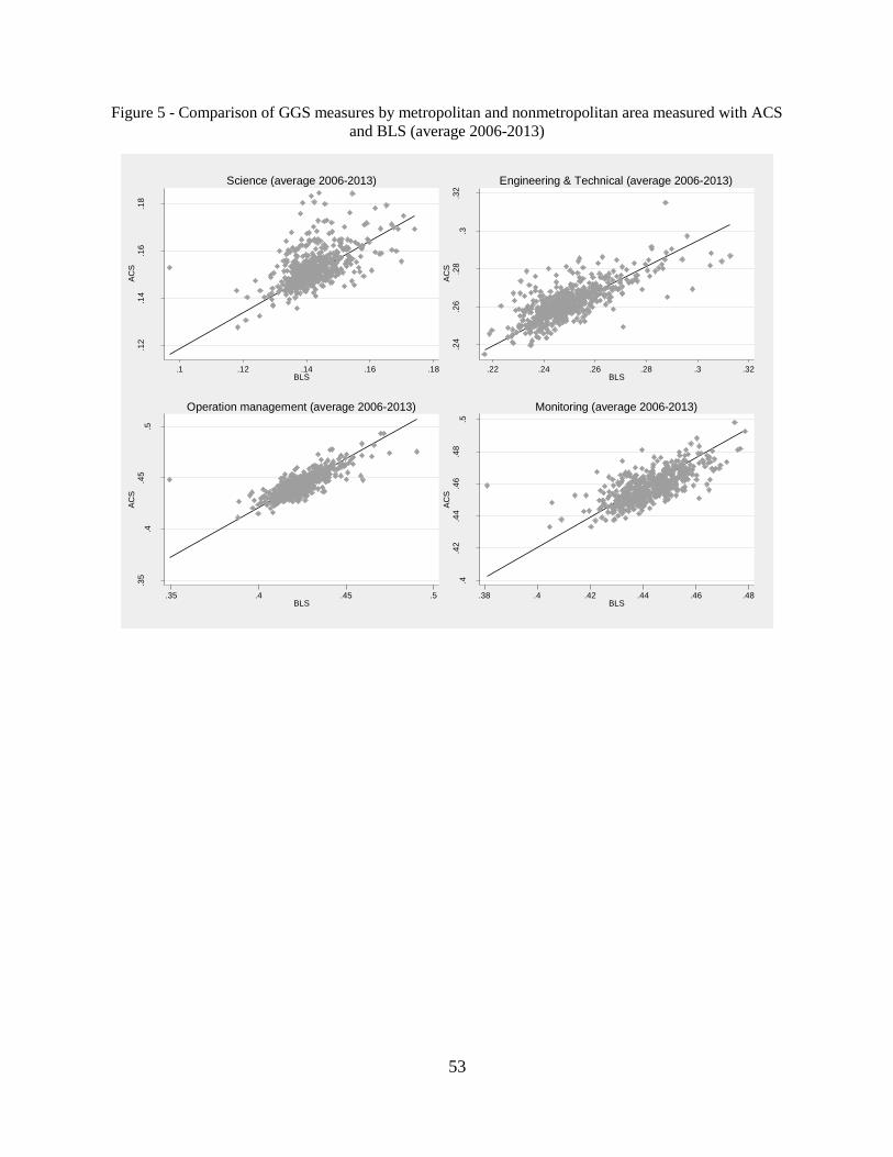
53
Figure 5 - Comparison of GGS measures by metropolitan and nonmetropolitan area measured with ACS
and BLS (average 2006-2013)
.12
.14
.16
.18
AC
S
.1 .12 .14 .16 .18BLS
Science (average 2006-2013)
.24
.26
.28
.3.3
2A
CS
.22 .24 .26 .28 .3 .32BLS
Engineering & Technical (average 2006-2013)
.35
.4.4
5.5
AC
S
.35 .4 .45 .5BLS
Operation management (average 2006-2013)
.4.4
2.4
4.4
6.4
8.5
AC
S
.38 .4 .42 .44 .46 .48BLS
Monitoring (average 2006-2013)

54
Figure 6 - Comparison of GGS measures by metropolitan and nonmetropolitan area measured with ACS
and BLS (change 2006-2013)
-.0
4-.
02
0
.02
.04
AC
S
-.02 -.01 0 .01 .02 .03BLS
Science (change 2006-2013)
-.0
4-.
02
0
.02
.04
AC
S
-.04 -.02 0 .02 .04BLS
Engineering & Technical (change 2006-2013)
-.0
4-.
02
0
.02
.04
AC
S
-.02 0 .02 .04BLS
Operation management (change 2006-2013)
-.0
4-.
02
0
.02
.04
.06
AC
S
-.01 0 .01 .02 .03 .04BLS
Monitoring (change 2006-2013)

55
Table 18 – Descriptive statistics of GGS by metropolitan and non-metropolitan area
Year Min Q1 Median Q3 Max Average SD IQR
Engineering and Technical
2006 0.221 0.244 0.251 0.257 0.307 0.251 0.011 0.013 2007 0.218 0.245 0.251 0.257 0.308 0.251 0.012 0.012
2008 0.217 0.243 0.250 0.256 0.316 0.250 0.012 0.013
2009 0.215 0.241 0.248 0.254 0.321 0.248 0.012 0.013 2010 0.212 0.239 0.245 0.251 0.320 0.245 0.011 0.012
2011 0.214 0.239 0.245 0.251 0.319 0.245 0.012 0.013
2012 0.214 0.239 0.245 0.252 0.324 0.246 0.012 0.012 2013 0.215 0.240 0.245 0.253 0.378 0.247 0.013 0.013
2014 0.215 0.240 0.246 0.253 0.361 0.247 0.013 0.013
Total 0.212 0.240 0.247 0.254 0.378 0.248 0.012 0.014
Science
2006 0.113 0.133 0.136 0.140 0.202 0.137 0.007 0.008
2007 0.101 0.133 0.137 0.141 0.185 0.138 0.007 0.008
2008 0.100 0.133 0.138 0.142 0.185 0.138 0.007 0.009 2009 0.091 0.135 0.140 0.144 0.180 0.140 0.007 0.008
2010 0.091 0.136 0.140 0.144 0.180 0.140 0.007 0.008
2011 0.088 0.137 0.141 0.144 0.179 0.141 0.007 0.007 2012 0.087 0.138 0.141 0.145 0.175 0.141 0.007 0.008
2013 0.092 0.136 0.142 0.145 0.215 0.141 0.008 0.009
2014 0.095 0.137 0.142 0.146 0.206 0.142 0.008 0.010
Total 0.087 0.135 0.139 0.144 0.215 0.140 0.008 0.009
Operation management
2006 0.343 0.420 0.429 0.438 0.485 0.429 0.014 0.019
2007 0.347 0.421 0.430 0.439 0.481 0.430 0.014 0.018 2008 0.348 0.422 0.432 0.440 0.480 0.431 0.014 0.018
2009 0.345 0.424 0.433 0.441 0.487 0.434 0.014 0.017
2010 0.352 0.425 0.435 0.441 0.494 0.434 0.015 0.016 2011 0.357 0.425 0.436 0.441 0.498 0.435 0.015 0.016
2012 0.349 0.426 0.438 0.442 0.498 0.435 0.015 0.016
2013 0.349 0.426 0.438 0.442 0.517 0.436 0.015 0.017 2014 0.348 0.426 0.438 0.443 0.506 0.436 0.015 0.016
Total 0.343 0.424 0.434 0.441 0.517 0.433 0.015 0.018
Monitoring
2006 0.375 0.439 0.446 0.452 0.477 0.445 0.010 0.013
2007 0.378 0.441 0.447 0.453 0.482 0.446 0.010 0.012 2008 0.379 0.441 0.447 0.454 0.478 0.446 0.010 0.013
2009 0.377 0.444 0.450 0.456 0.478 0.449 0.010 0.012
2010 0.384 0.445 0.451 0.456 0.479 0.450 0.010 0.011 2011 0.393 0.444 0.452 0.456 0.488 0.450 0.010 0.011
2012 0.382 0.445 0.452 0.457 0.497 0.451 0.010 0.012
2013 0.382 0.445 0.452 0.457 0.494 0.451 0.010 0.012 2014 0.372 0.445 0.452 0.458 0.498 0.451 0.010 0.013
Total 0.372 0.443 0.450 0.455 0.498 0.449 0.010 0.013
Statistics weighted by total employment. N=537 metropolitan and nonmetropolitan areas
Table 19 – Correlation between GGS measures at the metropolitan and non-metropolitan area level
Engineering
& Technical Science
Operation
management Monitoring
Engineering & Technical 1.000
Science 0.560 1.000
Operation management 0.065 0.091 1.000
Monitoring -0.076 0.091 0.833 1.000
N=537. Correlation on average 2006-2014 values weighted by average employment.

56
Table 20 - Top 10 industries (4-digit NAICS) in terms of emission intensity and GGS (year 2012)
NAICS Description PM2.5/empl NAICS Description Ozone/empl
2211 Electric Power Generation, Transmission and Distribution 0.919 2211 Electric Power Generation, Transmission and Distribution 5.941 3221 Pulp, Paper, and Paperboard Mills 0.592 3221 Pulp, Paper, and Paperboard Mills 2.640
3274 Lime and Gypsum Product Mfg 0.536 3274 Lime and Gypsum Product Mfg 2.387
3241 Petroleum and Coal Products Mfg 0.452 3241 Petroleum and Coal Products Mfg 2.000 3311 Iron and Steel Mills and Ferroalloy Mfg 0.398 2111 Oil and Gas Extraction 1.837
2122 Metal Ore Mining 0.339 3251 Basic Chemical Mfg 1.336
3113 Sugar and Confectionery Product Mfg 0.338 2122 Metal Ore Mining 1.025
3251 Basic Chemical Mfg 0.294 3273 Cement and Concrete Product Mfg 1.016
3212 Veneer, Plywood, and Engineered Wood Product Mfg 0.268 3112 Grain and Oilseed Milling 0.962
3313 Alumina and Aluminum Production and Processing 0.237 3272 Glass and Glass Product Mfg 0.827
NAICS Description Engineering
& Technical NAICS Description Science
2382 Building Equipment Contractors 0.528 6221 General Medical and Surgical Hospitals 0.305
5413 Architectural, Engineering, and Related Services 0.519 6215 Medical and Diagnostic Laboratories 0.299 2362 Nonresidential Building Construction 0.518 6223 Specialty (except Psychiatric and Substance Abuse) Hospitals 0.288
2381 Foundation, Structure, and Building Exterior Contractors 0.496 6219 Other Ambulatory Health Care Services 0.288
2373 Highway, Street, and Bridge Construction 0.488 5417 Scientific Research and Development Services 0.288 2379 Other Heavy and Civil Engineering Construction 0.482 4812 Nonscheduled Air Transportation 0.286
2361 Residential Building Construction 0.479 2213 Water, Sewage and Other Systems 0.280
2371 Utility System Construction 0.477 5413 Architectural, Engineering, and Related Services 0.266 2122 Metal Ore Mining 0.467 4879 Scenic and Sightseeing Transportation, Other 0.262
2389 Other Specialty Trade Contractors 0.462 6211 Offices of Physicians 0.255
NAICS Description Operation
Management NAICS Description Monitoring
5415 Computer Systems Design and Related Services 0.603 5411 Legal Services 0.731
5112 Software Publishers 0.597 4812 Nonscheduled Air Transportation 0.618
5417 Scientific Research and Development Services 0.571 4879 Scenic and Sightseeing Transportation, Other 0.596 3341 Computer and Peripheral Equipment Manufacturing 0.566 5221 Depository Credit Intermediation 0.591
5239 Other Financial Investment Activities 0.565 5239 Other Financial Investment Activities 0.588
5232 Securities and Commodity Exchanges 0.564 5259 Other Investment Pools and Funds 0.584 5211 Monetary Authorities-Central Bank 0.561 5231 Securities and Commodity Contracts Intermediation and Brokerage 0.581
5231 Securities and Commodity Contracts Intermediation and Brokerage 0.558 5251 Insurance and Employee Benefit Funds 0.570
5182 Data Processing, Hosting, and Related Services 0.557 5241 Insurance Carriers 0.563 5413 Architectural, Engineering, and Related Services 0.555 6219 Other Ambulatory Health Care Services 0.561

57
Tables for Appendix C
Table 21 - Brown occupations
SOC 2010 Title
11-3051 Industrial Production Managers 17-2041 Chemical Engineers
17-2071 Electrical Engineers
17-2131 Materials Engineers 17-2151 Mining and Geological Engineers, Including Mining Safety Engineers
17-2161 Nuclear Engineers
17-2171 Petroleum Engineers 19-2032 Materials Scientists
19-2042 Geoscientists, Except Hydrologists and Geographers
19-4031 Chemical Technicians 19-4041 Geological and Petroleum Technicians
19-4051 Nuclear Technicians
27-1012 Craft Artists 29-9011 Occupational Health and Safety Specialists
29-9012 Occupational Health and Safety Technicians
43-5041 Meter Readers, Utilities 47-2073 Operating Engineers and Other Construction Equipment Operators
47-5011 Derrick Operators, Oil and Gas
47-5012 Rotary Drill Operators, Oil and Gas 47-5013 Service Unit Operators, Oil, Gas, and Mining
47-5021 Earth Drillers, Except Oil and Gas
47-5031 Explosives Workers, Ordnance Handling Experts, and Blasters 47-5041 Continuous Mining Machine Operators
47-5042 Mine Cutting and Channeling Machine Operators
47-5051 Rock Splitters, Quarry 47-5061 Roof Bolters, Mining
47-5071 Roustabouts, Oil and Gas
47-5081 Helpers--Extraction Workers 49-2095 Electrical and Electronics Repairers, Powerhouse, Substation, and Relay
49-3042 Mobile Heavy Equipment Mechanics, Except Engines
49-9012 Control and Valve Installers and Repairers, Except Mechanical Door 49-9041 Industrial Machinery Mechanics
49-9043 Maintenance Workers, Machinery
49-9044 Millwrights 49-9045 Refractory Materials Repairers, Except Brickmasons
49-9051 Electrical Power-Line Installers and Repairers 49-9081 Wind Turbine Service Technicians
49-9096 Riggers
51-1011 First-Line Supervisors of Production and Operating Workers 51-4021 Extruding and Drawing Machine Setters, Operators, and Tenders, Metal and Plastic
51-4023 Rolling Machine Setters, Operators, and Tenders, Metal and Plastic
51-4032 Drilling and Boring Machine Tool Setters, Operators, and Tenders, Metal and Plastic 51-4033 Grinding, Lapping, Polishing, and Buffing Machine Tool Setters, Operators, and Tenders, Metal and Plastic
51-4051 Metal-Refining Furnace Operators and Tenders
51-4052 Pourers and Casters, Metal 51-4062 Patternmakers, Metal and Plastic
51-4071 Foundry Mold and Coremakers
51-4072 Molding, Coremaking, and Casting Machine Setters, Operators, and Tenders, Metal and Plastic
51-4191 Heat Treating Equipment Setters, Operators, and Tenders, Metal and Plastic
51-4193 Plating and Coating Machine Setters, Operators, and Tenders, Metal and Plastic
51-4194 Tool Grinders, Filers, and Sharpeners 51-6061 Textile Bleaching and Dyeing Machine Operators and Tenders
51-6064 Textile Winding, Twisting, and Drawing Out Machine Setters, Operators, and Tenders
51-6091 Extruding and Forming Machine Setters, Operators, and Tenders, Synthetic and Glass Fibers 51-8011 Nuclear Power Reactor Operators
51-8012 Power Distributors and Dispatchers
51-8013 Power Plant Operators 51-8021 Stationary Engineers and Boiler Operators
51-8091 Chemical Plant and System Operators
51-8092 Gas Plant Operators 51-8093 Petroleum Pump System Operators, Refinery Operators, and Gaugers
51-8099 Plant and System Operators, All Other

58
SOC 2010 Title
51-9011 Chemical Equipment Operators and Tenders
51-9012 Separating, Filtering, Clarifying, Precipitating, and Still Machine Setters, Operators, and Tenders
51-9021 Crushing, Grinding, and Polishing Machine Setters, Operators, and Tenders 51-9022 Grinding and Polishing Workers, Hand
51-9023 Mixing and Blending Machine Setters, Operators, and Tenders
51-9031 Cutters and Trimmers, Hand 51-9032 Cutting and Slicing Machine Setters, Operators, and Tenders
51-9041 Extruding, Forming, Pressing, and Compacting Machine Setters, Operators, and Tenders
51-9051 Furnace, Kiln, Oven, Drier, and Kettle Operators and Tenders 51-9121 Coating, Painting, and Spraying Machine Setters, Operators, and Tenders
51-9123 Painting, Coating, and Decorating Workers
51-9192 Cleaning, Washing, and Metal Pickling Equipment Operators and Tenders 51-9194 Etchers and Engravers
51-9195 Molders, Shapers, and Casters, Except Metal and Plastic 51-9196 Paper Goods Machine Setters, Operators, and Tenders
53-7011 Conveyor Operators and Tenders
53-7021 Crane and Tower Operators 53-7031 Dredge Operators
53-7032 Excavating and Loading Machine and Dragline Operators
53-7033 Loading Machine Operators, Underground Mining 53-7041 Hoist and Winch Operators
53-7071 Gas Compressor and Gas Pumping Station Operators
53-7072 Pump Operators, Except Wellhead Pumpers 53-7073 Wellhead Pumpers
53-7111 Mine Shuttle Car Operators

59
Tables for Appendix D
Table 22 – Item-by-item estimates of the impact of environmental regulation on green skills
NA in t=0 x
trend
NA
designation
NA
implement
Test: NA
design+NA
implement=0
(p-value)
R sq N
Science
Physics (2C4b) -0.0000908 0.000387 0.000616 0.0232 0.330 4806
(0.000101) (0.000433) (0.000441)
Biology (2C4d) 0.0000335 -0.00135** 0.000821* 0.262 0.599 4806
(0.000117) (0.000541) (0.000485)
Engineering and Technical - High
Engineering and Technology (2C3b) -0.000225 0.00136** 0.000729 0.00391 0.367 4806
(0.000156) (0.000617) (0.000719)
Design (2C3c) -0.000218 0.00125** 0.000926 0.00159 0.455 4806
(0.000171) (0.000592) (0.000666)
Engineering and Technical - Low
Building and Construction (2C3d) -0.0000207 0.000488 0.000623 0.109 0.629 4806
(0.000169) (0.000731) (0.000716)
Mechanical (2C3e) -0.000142 0.00126* 0.000505 0.0658 0.515 4806
(0.000199) (0.000744) (0.000848)
Estimating the Quantifiable Characteristics of
Products, Events, or Information (4A1b3)
-0.0000918 0.000798** 0.00000162 0.0435 0.377 4806
(0.0000992) (0.000365) (0.000391)
Drafting, Laying Out, and Specifying Technical
Devices, Parts, and Equipment (4A3b2)
-0.000140 0.00109** 0.000361 0.0236 0.479 4806
(0.000140) (0.000525) (0.000570)
Operation Management
Systems Analysis (2B4g) -0.000101 0.0000143 0.000781 0.119 0.550 4806
(0.000112) (0.000457) (0.000505)
Systems Evaluation (2B4h) -0.0000595 0.000126 0.000557 0.154 0.558 4806
(0.000105) (0.000456) (0.000499)
Updating and Using Relevant Knowledge
(4A2b3)
-0.000102 0.000113 0.000865 0.0687 0.477 4806
(0.000103) (0.000491) (0.000541)
Provide Consultation and Advice to Others
(4A4b6)
0.0000938 -0.0000380 0.000697* 0.129 0.651 4806
(0.000116) (0.000399) (0.000376)
Monitoring
Law and Government (2C8b) 0.0000400 -0.000124 0.000383 0.629 0.579 4806
(0.000115) (0.000549) (0.000543)
Evaluating Information to Determine
Compliance with Standards (4A2a3)
-0.000161 0.000948* 0.000138 0.0125 0.515 4806
(0.0000984) (0.000511) (0.000482)
Other
Geography (2C4g) 0.0000807 -0.000735** 0.000303 0.210 0.363 4806
(0.0000978) (0.000359) (0.000342)
Operating Vehicles, Mechanized Devices, or
Equipment (4A3a4)
0.0000443 0.000800 -0.000681 0.913 0.529 4806
(0.000197) (0.000768) (0.000923)
Fixed effect model weighted by kernel-based weights based on propensity score. Other control variables: state-specific year dummies; other
controls interacted with linear trend: share of manufacturing (2005), share of primary sector (2005), share of construction sector (2005), share
of utility sector (2005), import penetration (2005), log of population density (2005).
Related Documents