Environmental metabarcoding reveals heterogeneous drivers of microbial eukaryote diversity in contrasting estuarine ecosystems

OPEN

ORIGINAL ARTICLE

Environmental metabarcoding revealsheterogeneous drivers of microbial eukaryotediversity in contrasting estuarine ecosystems

Delphine Lallias1, Jan G Hiddink2, Vera G Fonseca3, John M Gaspar4, Way Sung5,Simon P Neill2, Natalie Barnes6, Tim Ferrero6, Neil Hall7, P John D Lambshead8,Margaret Packer6, W Kelley Thomas4 and Simon Creer1

1Molecular Ecology and Fisheries Genetics Laboratory, School of Biological Sciences, Environment CentreWales, Bangor University, Bangor, UK; 2School of Ocean Sciences, Bangor University, Anglesey, UK;3Zoological Research Museum Alexander Koenig (ZFMK), Centre for Molecular Biodiversity Research,Bonn, Germany; 4Hubbard Center for Genome Studies, University of New Hampshire, Durham, NH, USA;5Department of Biology, Indiana University, Bloomington, IN, USA; 6The Natural History Museum, ZoologyDepartment, London, UK; 7Advanced Genomics Facility, Institute of Integrative Biology, University ofLiverpool, Liverpool, UK and 8School of Ocean & Earth Science, University of Southampton, NationalOceanography Centre, Southampton, UK

Assessing how natural environmental drivers affect biodiversity underpins our understanding of therelationships between complex biotic and ecological factors in natural ecosystems. Of all ecosystems,anthropogenically important estuaries represent a ‘melting pot’ of environmental stressors, typified byextreme salinity variations and associated biological complexity. Although existing models attempt topredict macroorganismal diversity over estuarine salinity gradients, attempts to model microbialbiodiversity are limited for eukaryotes. Although diatoms commonly feature as bioindicator species,additional microbial eukaryotes represent a huge resource for assessing ecosystem health. Of these,meiofaunal communities may represent the optimal compromise between functional diversity that canbe assessed using morphology and phenotype–environment interactions as compared with smallerlife fractions. Here, using 454 Roche sequencing of the 18S nSSU barcode we investigate which of thelocal natural drivers are most strongly associated with microbial metazoan and sampled protistdiversity across the full salinity gradient of the estuarine ecosystem. In order to investigate potentialvariation at the ecosystem scale, we compare two geographically proximate estuaries (Thames andMersey, UK) with contrasting histories of anthropogenic stress. The data show that althoughcommunity turnover is likely to be predictable, taxa are likely to respond to different environmentaldrivers and, in particular, hydrodynamics, salinity range and granulometry, according to variedlife-history characteristics. At the ecosystem level, communities exhibited patterns of estuary-specificsimilarity within different salinity range habitats, highlighting the environmental sequencingbiomonitoring potential of meiofauna, dispersal effects or both.The ISME Journal advance online publication, 25 November 2014; doi:10.1038/ismej.2014.213

Introduction

Biodiversity contributes to ecosystem stability,resilience, function (Loreau et al., 2001; Wardleet al., 2004) and the continued provision ofecosystem services (Schroter et al., 2005), but issubject to a range of natural and anthropogenicforces. By understanding the natural processes thataffect different facets of biodiversity, the effect of

environmental change (Christensen et al., 2007) andstressors (Chariton et al., 2010) can then be disen-tangled from natural ecological processes in terres-trial and aquatic environments.

Estuaries are often centres of human habitation(Basset et al., 2012) and are therefore the focus ofintensive and costly biomonitoring programmes(Baird and Hajibabaei, 2012) designed for assessingecosystem health (Rosenberg et al., 2004). Estuariesare transitional habitats (Elliott and Whitfield, 2011)that are typified by diverse hydrodynamic flows,diurnal tidal cycles and radically different biologicalcommunities as the result of species adaptations tofreshwater, marine and intermediate salinityregimes (Attrill, 2002; Attrill and Rundle, 2002).In attempts to make predictions about the biodiversity

Correspondence: S Creer, Molecular Ecology and FisheriesGenetics Laboratory, Environment Centre Wales Building, Schoolof Biological Sciences, Bangor University, Bangor, Gwynedd LL572 UW, UK.E-mail: [email protected] 20 December 2013; revised 26 September 2014; accepted30 September 2014

The ISME Journal (2014), 1–14& 2014 International Society for Microbial Ecology All rights reserved 1751-7362/14

www.nature.com/ismej

of a typical estuary, many studies refer to thesomewhat arbitrary Remane model (based upon theBaltic Sea) that models species richness along asalinity continuum (Whitfield et al., 2012). TheRemane model and recent modifications refined byWhitfield et al. (2012) both predict the lowestspecies diversity between the oligohaline (0.5–5.0parts per thousand (p.p.t.)) and mesohaline(5–18 p.p.t.) zones, with peaks in euhaline(30–40 p.p.t.) and freshwater areas. Alternatively,Attrill (2002) proposes a different model thatpredicts a reduction of species richness withincreasing variation of local salinity.

Although diatoms and macroinvertebratescommonly feature as focal bioindicator species, thediversity of additional small organisms represent apotentially huge resource for assessing ecosystemhealth (Baird and Hajibabaei, 2012). Of the differentorganisms inhabiting benthic sediments, the meio-fauna (animals between 45 and 500 mm) (Giere,2009) might represent the optimal compromise forbiomonitoring potential between diversity in life-history characteristics, taxonomic tractability andtemporal stability as compared with bacteria andsmaller protist groups. Approximately 60% ofanimal phyla have meiofaunal representatives withcommunities being numerically dominated bynematodes (Giere, 2009). However, the potential ofusing such small organisms for assessing ecosystemhealth, as demonstrated by Chariton et al. (2010),has never been fully realised because of taxonomicand logistical limitations (Creer et al., 2010).

The synergies afforded by the advent of ‘second-generation sequencing’ platforms (Glenn, 2011) andnecessary taxonomic database reference libraries(Pruesse et al., 2007) present an unprecedentedopportunity to assess the biodiversity of previouslyintractable communities. In such studies, the DNAfrom entire communities are extracted en masse,and barcodes are amplified via PCR, sequenced,grouped into genetically similar units (operationaltaxonomic unit (OTU) clustering) and assigned tothe appropriate taxon using reference databases.Such en masse biodiversity assessments of micro-bial communities from environmental samples (Biket al., 2012) have been termed metabarcoding(Taberlet et al., 2012b), offering the potential for ananalytical framework referred to as Biomonitoring2.0 (Baird and Hajibabaei, 2012). This type ofmonitoring requires an effective understanding ofthe relationships between communities quantifiedusing monitoring and ecosystem-related effects. Forthe meiofaunal size fraction, many natural drivers ofbiodiversity have been proposed, but of these,sediment granulometry (Giere, 2009), salinity range(Attrill, 2002), hydrodynamic flows (Heip et al.,1985) and top-down processes such as bioturbation(Graf, 1992) have been hypothesised to stronglyaffect community diversity.

In this study, we adopt a metabarcoding approachto investigate whether sediment composition,

hydrodynamics, salinity range or levels of bioturba-tion have the largest effects on the biodiversity ofnumerous phyla at the estuarine ecosystem scale. Inorder to investigate potential variance at the ecosys-tem scale, we compare two contrasting UK estuarineecosystems: Thames and Mersey. Thames is con-sidered a ‘recovered’ estuary according to ecotox-icological history (Power et al., 1999; Matthiessenand Law, 2002), whereas Mersey, recognised in thepast as one of the most polluted estuaries in Europe(NRA, 1995), is now improving because of regula-tion and environmental campaigns (Struthers,1997). Such histories therefore are predicted toskew the relationships between the biodiversity ofdifferent phyla and environmental drivers accordingto ecosystem-specific effects.

Materials and methods

Sample collection and community decantationIn all, 104 benthic samples were collected fromThames (20 sampling stations) and Mersey (15sampling stations) estuaries (UK) in June–July2008. For both estuaries, benthic communities weresampled at the low-tide mark, accessed either onfoot (Thames) or by boat (Mersey) (SupplementaryTable S1 and Figure 1). At each station, 3 sedimentcore samples were collected using Perspex tubes(4.4 cm in diameter, 10 cm deep, B10 m apart) formetabarcoding analysis of meiofauna, each beingstored in 500 ml of DESS (20% dimethyl sulphoxideand 0.25 M disodium EDTA, saturated with NaCl, pH8.0, Yoder et al., 2006). A fourth core sample wascollected for granulometric analysis. In the labora-tory, the meiofaunal size fraction and organisms upto 1 mm in size were mechanically separated fromthe sediment and immobilised on a 45 mm filterbefore separation from fine silt using repetitivecentrifugations in 1.16 specific gravity LUDOXTM-40 solution (Sigma-Aldrich Company Ltd.,Gillingham, UK) (Fonseca et al., 2011). Followingthis step, each sample was retained on a distinctmesh sieve that was then folded, sliced, placed in a15 ml Falcon tube and kept at � 80 1C until DNAextraction. After overnight lysis at 55 1C, communityDNA was extracted with the QIAamp DNA BloodMaxi (Qiagen, Manchester, UK) according to iden-tical protocols set out in Fonseca et al. (2011).The highly conservative metabarcoding primersSSU_F_04 and SSU_R_22 (Blaxter et al., 1998;Fonseca et al., 2010) were used as they amplifybroadly throughout meiofaunal organisms (in addi-tion to protists and fungi) and they flank the mostvariable (in meiofaunal taxa) B450 bp nSSU generegion. The nSSU gene region was then PCRamplified in triplicates from community DNA usingPfu DNA polymerase (Promega, Southampton, UK)and forward and reverse MID-tagged fusion primers;visualised by gel electrophoresis and purifiedusing the QIAquick Gel Extraction Kit (Qiagen);

Environmental metabarcoding of microbial diversityD Lallias et al

2

The ISME Journal

quantified on an Agilent Bioanalyser 2100 (AgilentTechnologies, Stockport, UK) and pooled in equi-molar quantities. The purified amplicons pools werethen sequenced in a single direction (A-Amplicon)on four half plates using the 454 Roche GSFLX (454Life Sciences, Roche Applied Science, Branford, CT,USA) sequencing platform at Liverpool University’sCentre for Genomic Research (Liverpool, UK). Allprotocols were identical to those presented inFonseca et al. (2010).

Raw sequence reads were filtered and denoisedusing FlowClus (Gaspar and Thomas, submitted,freely available at GitHub (jsh58/FlowClus)).Criteria used for the filtering step were: minimumsequence length 150 bp; maximum sequence length500 bp; truncate reads before first N; truncate beforea window of 25 bp whose average quality score iso20; truncate before a set of four flows whosevalues are o0.40 (criteria recommended by Reederand Knight, 2010). The denoising step correctspyrosequencing errors by clustering the flowgramsand a constant denoising value of 0.50 was used.Then, the data were analysed using the QIIMEpipeline (Caporaso et al., 2010): (1) chimeras were

removed using UCHIME (Edgar et al., 2011), withthe abundance information generated by FlowClus;(2) OTUs were clustered at 96% sequence similarityusing UCLUST (Edgar, 2010), as 96% sequencesimilarity has most closely emulated species rich-ness via the analysis of control nematode commu-nities using nSSU (Fonseca et al., 2010); (3) arepresentative sequence was picked for each OTU;(4) taxonomy was assigned using the Silva 111database (Pruesse et al., 2007); and (5) an OTU tablewas generated. For direct ecological comparisonsamong samples that have different coverages (that is,number of reads), the percentage of reads in eachsample was used instead of read counts and down-stream analyses were focused on meiofauna anddominant protist groups occupying shallow sedi-ment habitats. Raw sequence reads were addition-ally analysed using the OCTUPUS pipeline (Fonsecaet al., 2010, available at http://octupus.sourcefor-ge.net/) and OTUs annotated against the down-loaded NCBI (National Center for BiotechnologyInformation) nucleotide database using the raw dataset and also a rarefied data set (1102 randomlypicked sequences from each sample).

Outer estuary Inner estuary

10 km

10 km

Oligohaline Oligo-mesohaline Poly-euhaline

Figure 1 Map of the sampling locations. (a) Mersey estuary. CM, Cuerdley Marsh; EB, Ellesmere Bank; EF, Eastham Ferry; EG, Egremont;EH, East Hale; FF, Fiddlers Ferry; FW, Forest Way; HH, Hale Head Shore; HW, Howley Weir; LA, Liverpool Airport; MT, Mersey Tunnel;RC, Runcorn; RF, Rock Ferry; SK, Speke; TN, The Narrows. (b) Thames estuary. AH, Allhallows; B, Beckton; CB, Cavney Island; CF,Coalhouse Fort; CP, Cadogan Pier; GV, Gravesend; GW, Greenwich; HB, Hammersmith Bridge; K, Kew; LB, London Bridge; OI, OldIsleworth; P, Purfleet; SBC, South Bank Centre; SE, Southend-on-Sea; SLH, Stanford Le Hope; SNE, Shoebury Ness; T, Teddington; WT,West Thurrock; WW, Woolwich; XN, Crossness. Salinity zones have been named according to the Venice salinity classification system:oligohaline (0.5–5%), mesohaline (5–18%), polyhaline (18–30%), euhaline (30–40%) and hyperhaline (440%).

Environmental metabarcoding of microbial diversityD Lallias et al

3

The ISME Journal

Environmental data and macrofaunal biodiversityKey environmental parameters, known to influencethe distribution of meiofaunal communities, weremeasured or modelled below.

Salinity range (the difference between meanlow-tide salinity and mean high-tide salinity) data(Attrill, 2002) were inferred from the EnvironmentAgency (EA, United Kingdom) salinity data, asexplained below. For Thames, mean salinity at eachsampling site was calculated from the EA spotsampling data (along the estuary from Teddington toBarrow No. 7 Buoy). Mean salinity range was theninferred from the equation established by Attrill(2002) between mean salinity and salinity range. Inthe Mersey estuary, salinity range at the EAsampling stations was inferred from monthly EAsalinity data. We constructed a model of the meansalinity range against the distance from HowleyWeir (from Monks Hall to Seacombe Ferry: 4.50 and41.67 km from Howley Weir, respectively) and fromthat relationship, salinity range was inferred at eachof our 15 sampling sites.

Longitudinal variations in the time-varying freesurface and current velocity were calculated using aone-dimensional sectional-averaged model (Neillet al., 2009) that discretely solves the continuityequation

@Z@t¼ � 1

B

@ðAUÞ@x

and the momentum equation

@U

@t¼ � g

@Z@x� CDU Uj jðhþ ZÞ4 = 3

where Z is the variation of the free surface frommean sea level, B is the channel width, A is thecross-sectional area of the channel, U is the depth-averaged velocity, CD is the bottom friction coeffi-cient, h is the mean water depth, r is water density,dx is the longitudinal grid spacing and g isgravitational acceleration. Cross-sectional areas foreach river/estuary system were digitised fromAdmiralty Charts to a longitudinal grid spacing ofdx = 500 m, and the amplitudes and phases of fourtidal constituents (including the dominant semi-diurnal constituents) were obtained from an analy-sis of tide gauge data to provide model boundaryconditions. The models were validated against tidegauge data along the length of each estuarine system.The models were run for the duration of a spring–neap cycle (B2 weeks), and statistics calculated ontidal range, velocities and bed shear stress at each ofthe sampling locations.

Two methods were used for the sediment particlesize analysis, depending on whether the sample wascomposed of predominantly fine or coarse material.Nine of the coarser samples were mechanicallysieved and for the 26 finer samples, particle sizeanalysis was carried out using a Malvern Mastersi-zer 2000 (Kenny and Sotheran, 2013). In contrast tomechanical sieving, the Mastersizer determines

particle size distribution by volume. However, ifwe assume that the density of individual particles isconstant, the results are directly comparable. Plotsof cumulative particle size distributions were usedto calculate the values of the particle diameter at50% (median grain size D50) and 10% (D10) in thecumulative distribution of grain sizes, and tocalculate the percentage of material containedwithin each size class.

Macrofaunal invertebrates were sampled at eachstation in the two estuaries by taking five 15 cmdiameter cores to a depth of 10 cm. The cores werepooled and sieved over 1 mm and preserved in 4%formalin. All invertebrates were identified to thehighest possible taxonomic resolution and their wetweight was measured after blotting. Macrofaunalspecies richness, abundance and biomass werecalculated. In the Thames estuary, no cores couldbe taken at London Bridge because of the rockysubstrate, and therefore only qualitative data wererecorded at this site; no cores could be taken atCadogan Pier and Kew because of a high fraction oflarge pebbles in the sediment.

Statistical analyses to identify the drivers ofmeiofaunal diversityIndependent samples t-tests (including Levene’s testfor equality of variances) were performed to testwhether there were significant differences in sampleOTU richness between the Thames and Merseyestuaries. Multivariate analyses were performed toinvestigate the similarity of meiofaunal commu-nities along the salinity gradient and to identifyenvironmental drivers of meiofaunal assemblages.Before multivariate analysis in PRIMER v6 (Clarkeand Gorley, 2006), the biotic data of meiofaunalOTUs were transformed into a presence/absencematrix of each OTU in each sample (only for OTUsannotated as Nematoda, Platyhelminthes (Turbel-laria), Arthropoda, Mollusca, Annelida, Gastrotri-cha, Tardigrada, Kinorhyncha, Rotifera, Cnidariaand Bryozoa). Analyses described below wereperformed for each estuary and for the two estuariescombined. First, the similarity between meiofaunalassemblages along the salinity gradient was ana-lysed by cluster analysis using group averageclustering and ordination by non-metric multidi-mensional scaling, using the Sørensen’s similaritycoefficient (Clarke, 1993). The SIMPROF procedure(or ‘similarity profile’ permutation tests) wasapplied to identify genuine clusters of samples, thatis, samples that were not significantly differentiatedfrom each other were grouped in the same cluster.Second, a BIOENV (‘biota-environment’) analysis(Clarke, 1993) was applied to investigate associa-tions between environmental variables to bioticcommunity composition using Spearman’s rankcorrelation method. Briefly, in the current example,BIOENV searches over subsets of the environmentalvariables for a combination that provides the best

Environmental metabarcoding of microbial diversityD Lallias et al

4

The ISME Journal

explanatory variables between meiofaunal commu-nity assemblages and environmental variables. Four-teen potential environmental drivers were includedfor both estuaries: spring tidal range, mean velocity,maximum velocity, mean bed shear stress, max-imum bed shear stress, D50, D10, % clay, % silt, %fine sand, % medium sand, % coarse sand, % graveland salinity range. In the Thames estuary, macro-fauna species richness, abundance and biomass datawere available for all sites except Cadogan Pier (CP),Kew (K) and London Bridge (LB). Therefore, for theThames estuary, the BIOENV procedure was per-formed on the 20 sampling sites without themacrofauna data, and on 17 sites (after exclusionof CP, K and LB sites) with the macrofauna data. Inthe Mersey estuary, because of the very lowabundance (three or less animals recorded at fivesites: TN, EG, RF, EF and SK) or absence (at six sites:EB, LA, HH, CM, FF and FW) of macrofauna species,in particular at sites with large mobile sand wavesconsisting of coarse sand, macrofauna speciesrichness, abundance and biomass were not includedin the BIOENV analyses. To complement theBIOENV analyses, we also performed a canonicalcorrespondence analysis (CCA) in the package‘vegan’ in R (Oksanen et al., 2013) to further testand visualise the relationships between the envir-onmental variables and community composition.Because correlated explanatory variables can makethe interpretation of CCA outputs difficult, expla-natory variables that had a correlation coefficient of40.7 were excluded from the analysis. After thisselection, only mean tidal velocity, the sedimentD50 and salinity range data were retained and thebest fitting model was selected by Akaike informa-tion criterion using a stepwise algorithm.

In order to investigate the geographical contribu-tion to the marine component of estuarine biodiver-sity, we subsampled UK-only sites from the recentlittoral beach data presented in Fonseca et al. (2014)and performed presence/absence Sørensen IndexMantel tests in PRIMER v6 to explore isolation byclosest coastal distance effects on communitycomposition.

Finally, we used partial least squares (PLS)regressions to assess which environmental variableswere the most important drivers of meiofaunaldiversity, with the PLS package in R (Mevik andWehrens, 2007). The PLS regressions have beendeveloped to deal with cases where there are manyexplanatory variables in relation to the number ofobservations and/or with cases of severe multi-collinearity (Carrascal et al., 2009) and are thereforeparticularly suited for this analysis. A PLS regres-sion is a linear regression of one or more responsevariables onto a number of components called latentvariables. The latent variables are linear combina-tions of the factors, also called predictor variables.They are constructed so that the original multi-collinearity is reduced to a lower number oforthogonal factors. The variable importance in

projection (VIP) approach (Chong and Jun, 2005)was used to order the pertinent original explanatoryvariables by rank importance, that is, responsevariables with VIP values 41 were consideredpertinent. Each PLS analysis generates the VIPvalues for each response variable, as well as thevariance (R2) explained by each of the two compo-nents. This analysis was performed within eachestuary for the meiofaunal phyla (whole data set andper phylum), protists (Alveolata and stramenopiles)and fungi.

Results

The raw sequencing data were analysed in threeways: (1) Octupus, non-rarefied, NCBI annotated; (2)Octupus, rarefied to the lowest number of reads,NCBI annotated and (3) FlowClus/QIIME, non-rarefied, Silva annotated. The diversity patternsand overlying conclusions were unaffected by thedifferent bioinformatic workflows, and hence belowwe present the results obtained with FlowClus/QIIME pipeline.

The 454 Roche sequencing yielded 957 216 reads,with each sample exhibiting between 1044 and30 786 sequence reads (Supplementary Table S2).The numbers of reads for the combined data set weredominated by Nematoda (55.38%) and Arthropoda(18.48%) (Supplementary Table S3). For the Thamesand Mersey estuaries, 1496 and 1131 OTUs wererecovered respectively (Supplementary Table S3).OTU richness was dominated by Nematoda (493OTUs across both estuaries, representing 22% of theOTUs in Thames and 31% in Mersey), followed bysubstantial contributions by Alveolata (173 OTUs),stramenopiles (146 OTUs), Arthropoda (138 OTUs),Platyhelminthes (89 OTUs) and a range of additionaltaxa from up to 27 separate phyla (Figure 2 andSupplementary Table S3). An analysis of variancealso revealed no significant difference in OTUrichness between 454 Roche plate gaskets (F = 2.24,P = 0.088).

Samples were taken over a distance of B46 kmfrom Mersey and 106 km from Thames, representingthe full spectrum of the salinity gradient in eachecosystem. The spring tidal range ranged from1.43 to 6.56 m in Thames and between 0 and8.64 m in Mersey, resulting in maximum flowvelocities of 0.68–2.07 and 0–1.70 m s� 1 and salinityranges of 0.89–14.16 and 0–18.97 p.p.t. respectively(Supplementary Tables S4 and S5).

A t-test revealed that richness between the twoestuaries was not significantly different for Nema-toda (t33 = � 1.107, P = 0.276), Platyhelminthes(t33 = � 0.746, P = 0.461), Arthropoda (t33 = 0.555,P = 0.582), Alveolata (t33 = 0.326, P = 0.747) and Rhi-zaria (t33 = 1.518, P = 0.139). However the Annelida(t33 = 3.014, P = 0.006), the stramenopiles (t33 = 2.350,P = 0.026) and Fungi (t33 = 4.009, P = 0.000) were allsignificantly richer in Thames as compared with

Environmental metabarcoding of microbial diversityD Lallias et al

5

The ISME Journal

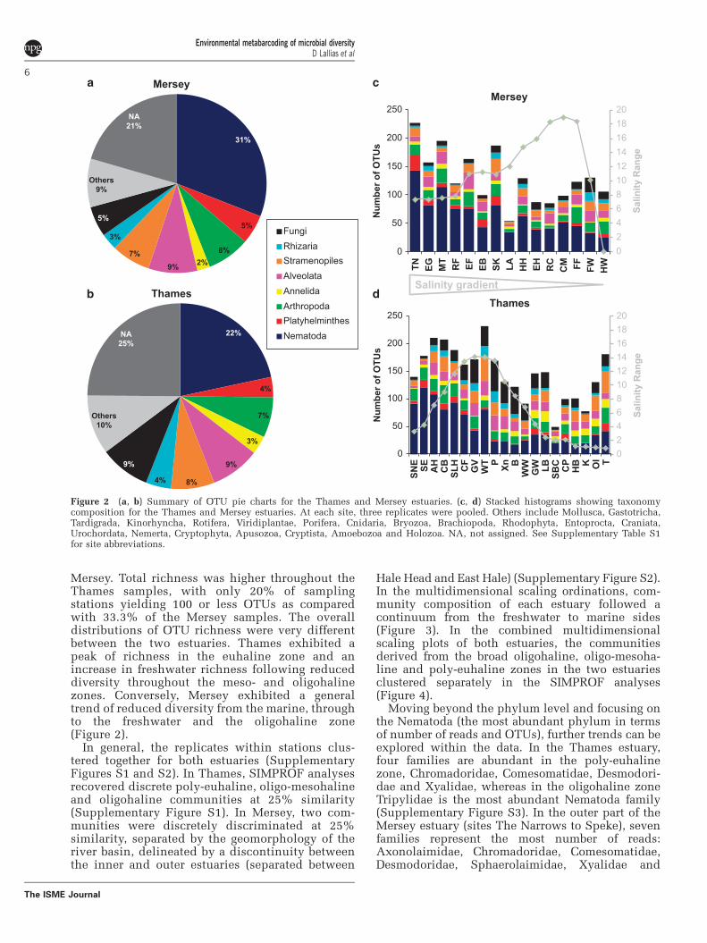
Mersey. Total richness was higher throughout theThames samples, with only 20% of samplingstations yielding 100 or less OTUs as comparedwith 33.3% of the Mersey samples. The overalldistributions of OTU richness were very differentbetween the two estuaries. Thames exhibited apeak of richness in the euhaline zone and anincrease in freshwater richness following reduceddiversity throughout the meso- and oligohalinezones. Conversely, Mersey exhibited a generaltrend of reduced diversity from the marine, throughto the freshwater and the oligohaline zone(Figure 2).

In general, the replicates within stations clus-tered together for both estuaries (SupplementaryFigures S1 and S2). In Thames, SIMPROF analysesrecovered discrete poly-euhaline, oligo-mesohalineand oligohaline communities at 25% similarity(Supplementary Figure S1). In Mersey, two com-munities were discretely discriminated at 25%similarity, separated by the geomorphology of theriver basin, delineated by a discontinuity betweenthe inner and outer estuaries (separated between

Hale Head and East Hale) (Supplementary Figure S2).In the multidimensional scaling ordinations, com-munity composition of each estuary followed acontinuum from the freshwater to marine sides(Figure 3). In the combined multidimensionalscaling plots of both estuaries, the communitiesderived from the broad oligohaline, oligo-mesoha-line and poly-euhaline zones in the two estuariesclustered separately in the SIMPROF analyses(Figure 4).

Moving beyond the phylum level and focusing onthe Nematoda (the most abundant phylum in termsof number of reads and OTUs), further trends can beexplored within the data. In the Thames estuary,four families are abundant in the poly-euhalinezone, Chromadoridae, Comesomatidae, Desmodori-dae and Xyalidae, whereas in the oligohaline zoneTripylidae is the most abundant Nematoda family(Supplementary Figure S3). In the outer part of theMersey estuary (sites The Narrows to Speke), sevenfamilies represent the most number of reads:Axonolaimidae, Chromadoridae, Comesomatidae,Desmodoridae, Sphaerolaimidae, Xyalidae and

Mersey

Thames

EG MT

RF

EF EB SK LA HH

EH RC

CM FF

FungiRhizariaStramenopilesAlveolataAnnelidaArthropodaPlatyhelminthesNematoda22%

4%

7%

3%

9%

8%4%

9%

Others10%

NA25%

31%

5%

8%2%9%

7%

3%

5%

Others9%

NA21%

02468101214161820

0

50

100

150

200

250

TN EG MT

RF EF EB SK LA HH EH RC

CM FF FW HW

Salin

ity R

ange

Num

ber o

f OTU

s

Mersey

02468101214161820

0

50

100

150

200

250

SNE SE AH

CB

SLH CF

GV

WT P Xn B

WW

GW LB

SBC CP

HB K OI T

Salin

ity R

ange

Num

ber o

f OTU

s

ThamesSalinity gradient

Figure 2 (a, b) Summary of OTU pie charts for the Thames and Mersey estuaries. (c, d) Stacked histograms showing taxonomycomposition for the Thames and Mersey estuaries. At each site, three replicates were pooled. Others include Mollusca, Gastotricha,Tardigrada, Kinorhyncha, Rotifera, Viridiplantae, Porifera, Cnidaria, Bryozoa, Brachiopoda, Rhodophyta, Entoprocta, Craniata,Urochordata, Nemerta, Cryptophyta, Apusozoa, Cryptista, Amoebozoa and Holozoa. NA, not assigned. See Supplementary Table S1for site abbreviations.

Environmental metabarcoding of microbial diversityD Lallias et al

6

The ISME Journal

Thoracostomopsidae. In the inner part of the Merseyestuary (sites Liverpool Airport to Howley Weir), thefamily Xyalidae is overwhelmingly dominant,whereas in the two extreme freshwater sites(Forest Way and Howley Weir) the Tripylidae andMonhysteridae additionally feature (SupplementaryFigure S4).

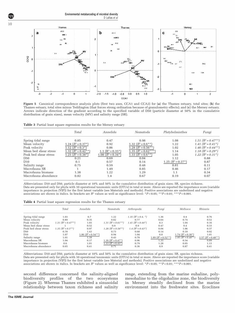
Considering meiofaunal community assemblages,the BIOENV analysis showed that both sedimentgranulometry and mean salinity range optimallyexplained differences in community composition ofthe sampled meiofauna in both estuaries (Tables 1and 2), with additional effects of hydrodynamicflow in Mersey (Table 1) and macrofauna speciesrichness in Thames (Table 2b). Similarly, Figure 5

summarises 74% and 78% of the total constrainedinertia of the final selected models of the CCAanalyses, with all three retained environmentalvariables showing highly significant associationswith community composition in Mersey (allP = 0.01) and Thames (all P = 0.005), respectively.The Mantel tests performed on the Sørensen Indexcommunity similarity measures from the UK-onlysites from Fonseca et al. (2014) showed no associa-tion with geographic distance.

For the PLS regression analyses, environmentalcharacters were ranked according to the strongestassociation between dependent and predictive vari-ables, regression plots assessed for spurious associa-tions and outlier effects. Data are presented only for

Thames estuary

Similarity204060

SNE1SNE2SNE3

SE1

SE2

SE3

AH1

AH2AH3

CB1CB2CB3

SLH1 SLH2

SLH3CF1

CF2CF3

GV1

GV2

GV3

WT2

WT3

P1 P2

P3XN1

XN2

XN3B1B2

B3

WW1

WW2

WW3

GW1

GW2GW3

LB1LB2

LB3

SBC2SBC3

CP1

CP2CP3

HB1

HB2HB3

K1

K2

K3

OI1

OI2

OI3

T1

T2

T3

WT1

2D Stress: 0.13

Mersey estuary

Similarity204060

TN1

TN2 TN3EG1 EG2

EG3

MT1MT2

MT3

RF1

RF2

RF3

EF1EF2

EF3

EB1

EB2

EB3

SK1

SK2

SK3

LA1LA2

LA3

HH1

HH2

HH3

EH1EH2

EH3

RC1RC2

RC3CM1

CM2

CM3

FF1

FF2

FF3

FW1

FW2

FW3

HW1

HW2

HW3

2D Stress: 0.15

Poly-euhaline

Oligo-mesohaline

Oligohaline

Salinity zones

Outer estuary

Inner estuary

Salinity zones

Figure 3 Multidimensional scaling (MDS) ordination for taxonomic patterns of meiofaunal communities based on Sørensen similaritiesof OTU presence/absence data for the Thames and Mersey estuaries analysed separately. Community-based similarity contours areshown (20%, 40%, and 60%). See Supplementary Table S1 for site abbreviations.

Environmental metabarcoding of microbial diversityD Lallias et al

7

The ISME Journal

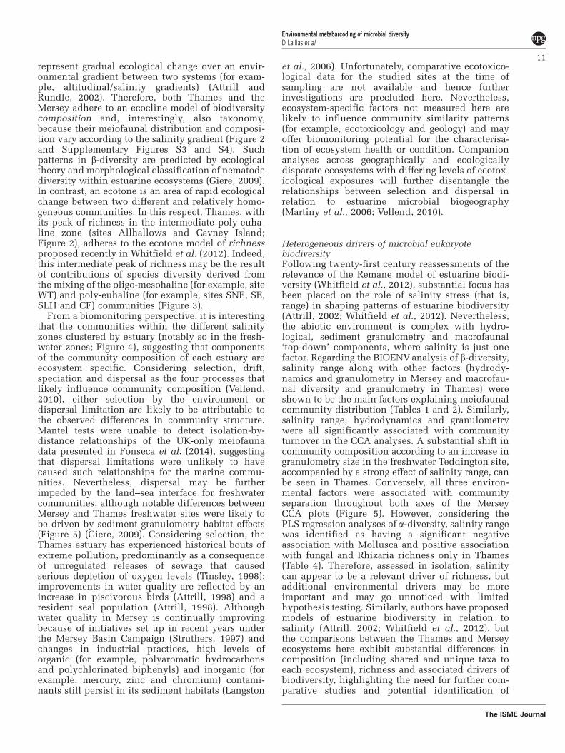
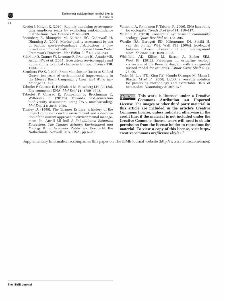
phyla with 10 OTUs in total or more. In Mersey,there were few clear associations with the environ-mental predictive variables. However, of these, therewere strong positive associations between hydro-dynamic flow and total biodiversity, Nematoda andAnnelida richness, and between small sedimentgranulometry (D10) and Platyhelminthes richness.There was also a negative association betweenhydrodynamic flow and Fungi richness (Table 3).Conversely, in Thames, all of the hydrodynamicassociations between the predictor variables andbiodiversity (all phyla, Nematoda and Arthropoda)exhibited a negative association. There was also anegative association between salinity range andMollusca richness. Positive associations wereobserved between granulometry and Annelida andMollusca richness. Additional positive associationswere observed between Nematoda richness andmacrofauna species richness and biomass, andbetween salinity range and the richness of Fungi/Rhizaria (Table 4).

Discussion

The metabarcoding approach and ecosystem diversityA number of recent reviews and studieshave highlighted the advantages of analysing envir-onmentally sourced community DNA as comparedwith using traditional taxonomical or ecologicalapproaches (Baird and Hajibabaei, 2012; Taberletet al., 2012a, b), and the present study supports thisview. Moreover, here we used community extrac-tions and longer PCR amplicons (ca. 450 bp) topreferentially amplify DNA from living commu-nities, as opposed to environmental DNA (Bohmannet al., 2014), that generally cannot be amplified fromdead organisms, or degraded environmental DNAusing longer PCR amplicons (Valentini et al., 2009).The use of a replicated sample design here showsthat replicate samples within a station were gen-erally not statistically different from each other,with the exception of SK, EG, RC, CM and FW inMersey and P, XN, CP, LB and HB in Thames (see

100

80

60

40

20

0S

imila

rity

Transform: Presence/absenceResemblance: S8 Sorensen

SNE1SNE2

SNE3

SE1SE2 SE3

AH1

AH2 AH3

CB1

CB2CB3

SLH1SLH2

SLH3

CF1

CF2CF3

GV1

GV2

GV3

WT1

WT3

P1

P2P3

XN1XN2

XN3 B1B2B3

WW1

WW2

WW3

GW1

GW2

GW3

LB1LB2

LB3SBC2

SBC3CP1

CP2CP3

HB1

HB2HB3

K1

K2

K3

OI1OI2OI3

T1T2

T3

TN1TN2

TN3

EG1

EG2EG3

MT1MT2

MT3

RF1RF2

RF3

EF1EF2EF3

EB1

EB2

EB3

SK1

SK2SK3

LA1LA2

LA3

HH1

HH2

HH3

EH1

EH2EH3

RC1RC2

RC3

CM1

CM2

CM3 FF1

FF2

FF3

FW1

FW2

FW3

HW1

HW2HW3

2D Stress: 0.18

SNE, SE, AH, CB RF, EG, MT, EF EH, RC, CM, FF, HH, LA, EB, SK, HW, FWWT, SLH, CF, K, SBC, HB, CP, OI, LB, T, GW, WW GV, B, XN, PTN, SK

Outer estuaryInner estuary

Poly-euhalineOligo-mesohalineOligohaline

MERSEY

THAMES

WT2

Figure 4 Cluster analysis and multidimensional scaling (MDS) ordination for taxonomic patterns of meiofaunal communities based onSørensen similarities of OTU presence/absence data for the combined estuaries. In the dendrogram, thick lines represent samples that aresignificantly differentiated based on a SIMPROF (‘similarity profile’ permutation tests) analysis. The two estuaries have been colourcoded (M, Mersey in blue; T, Thames in green). See Supplementary Table S1 for site abbreviations.

Environmental metabarcoding of microbial diversityD Lallias et al

8

The ISME Journal

Figure 3 and Supplementary Figures S1 and S2).However, in all these examples, clustering repre-sented geographically proximate sampled sites,likely representing ecologically distinct habitats.

Notably, and as for Fonseca et al. (2010), recov-ered estimates of Nematoda richness, using theQIIME pipeline at a 96% cutoff identity, weresimilar to those derived from traditional taxonomyfor the Thames estuary (Attrill, 1998; Ferrero et al.,2008) (for example, 209 spp. identified morphologi-cally at 8 sites by Ferrero et al., 2008; 324 OTUsfound at 20 sites (Supplementary Table S3 thisstudy); 199 OTUs found when restricting themolecular data to the same 8 sites than Ferreroet al., 2008). Moreover, the metabarcoding datayielded the same ecological pattern of communityturnover along the salinity gradient as traditionalanalyses based solely on nematode diversity(Ferrero et al., 2008) (Supplementary Figures S5and S6). Comparisons of the ecological signalbetween metabarcoding studies and traditionalecological surveys (Ji et al., 2013) will become anincreasingly important consideration by environ-mental agencies regarding the uptake of second-generation sequencing approaches to performroutine biomonitoring studies (Baird and Hajibabaei,2012).

Inter-ecosystem variability in richness and compositionThe first stark difference between the Thames andMersey ecosystems was that sufficient macroinver-tebrate taxa were manually recovered forhypothesis testing only in the Thames estuary. The

Table 1 Summary of results from the biota-environment(BIOENV) analysis in the Mersey estuary showing the 10 bestcombinations of environmental variables associated with thehighest correlation between the meiofaunal and environmentaldata matrices

No. ofvariables

Correlation Environmental variables

4 0.728 Spring tidal range, mean velocity, peakvelocity, mean salinity range

5 0.726 Spring tidal range, mean velocity, peakvelocity, % silt, mean salinity range

5 0.721 Spring tidal range, mean velocity, peakvelocity, % clay, mean salinity range

6 0.718 Spring tidal range, mean velocity, peakvelocity, mean bed shear stress, % clay,mean salinity range

3 0.716 Spring tidal range, mean velocity, meansalinity range

6 0.716 Spring tidal range, mean velocity, peakvelocity, mean bed shear stress, % silt,mean salinity range

3 0.716 Spring tidal range, mean velocity, peakvelocity

5 0.714 Spring tidal range, mean velocity, peakvelocity, mean bed shear stress, meansalinity range

5 0.714 Spring tidal range, mean velocity, meanbed shear stress, % clay, mean salinityrange

4 0.713 Spring tidal range, mean velocity, peakbed shear stress, mean salinity range

Correlation values correspond to Spearman’s rank correlationcoefficient (r).

Table 2 Summary of results from the biota-environment(BIOENV) analysis in the Thames estuary

No. ofvariables

Correlation Environmental variables

(a)

3 0.689 D10, % fine sand, mean salinity range2 0.672 % Fine sand, mean salinity range2 0.667 D10, % fine sand4 0.665 Peak velocity, D10, % fine sand, mean

salinity range3 0.659 % Fine sand, % coarse sand, mean

salinity range4 0.659 Peak bed shear stress, D10, % fine sand,

mean salinity range4 0.655 D10, % fine sand, % medium sand, mean

salinity range5 0.654 Peak velocity, D10, % fine sand, %

medium sand, mean salinity range5 0.649 D10, % fine sand, % medium sand, %

gravel, mean salinity range6 0.648 Peak velocity, D10, % fine sand, %

medium sand, % gravel, mean salinityrange

(b)

4 0.702 D10, % fine sand, mean salinity range,macrofauna species richness

5 0.697 D10, % fine sand, % medium sand, meansalinity range, macrofauna speciesrichness

6 0.685 Peak velocity, D10, % fine sand, %medium sand, mean salinity range,macrofauna species richness

6 0.683 D10, % fine sand, % medium sand, %coarse sand, mean salinity range, macro-fauna species richness

5 0.680 Peak velocity, D10, % fine sand, meansalinity range, macrofauna speciesrichness

5 0.677 D10, % fine sand, % coarse sand, meansalinity range, macrofauna speciesrichness

5 0.676 D50, % clay, % fine sand, % mediumsand, mean salinity range, macrofaunaspecies richness

3 0.676 D10, % fine sand, mean salinity range6 0.675 Peak bed shear stress, D10, % fine

sand, % medium sand, mean salinityrange, macrofauna species richness

5 0.675 Peak bed shear stress, D10, % fine sand,mean salinity range, macrofauna speciesrichness

Abbreviation: D10 and D50, particle diameter at 10% and 50% in thecumulative distribution of grain sizes.(a) All stations included, macrofauna data not included. (b) CadoganPier (CP), Kew (K) and London Bridge (LB) sites excluded,macrofauna data included.Correlation values correspond to Spearman’s rank correlationcoefficient (r).

Environmental metabarcoding of microbial diversityD Lallias et al

9

The ISME Journal

second difference concerned the salinity-alignedbiodiversity profiles of the two ecosystems(Figure 2). Whereas Thames exhibited a sinusoidalrelationship between taxon richness and salinity

range, extending from the marine euhaline, poly-mesohaline to the oligohaline zone, the biodiversityin Mersey steadily declined from the marineenvironment into the freshwater sites. Ecoclines

Table 3 Partial least square regression results for the Mersey estuary

Total Annelida Nematoda Platyhelminthes Fungi

Spring tidal range 0.85 0.47 0.98 1.08 1.51 (R2 = 0.47**)Mean velocity 1.24 (R2 = 0.37*) 0.92 1.32 (R2 = 0.6**) 1.22 1.41 (R2 = 0.41*)Peak velocity 1.12 (R2 = 0.3*) 0.86 1.28 (R2 = 0.56**) 1.02 1.46 (R2 = 0.44**)Mean bed shear stress 1.32 (R2 = 0.42**) 1.1 (R2 = 0.35*) 1.35 (R2 = 0.62***) 1.14 1.18 (R2 = 0.29*)Peak bed shear stress 1.25 (R2 = 0.38*) 1.08 (R2 = 0.34*) 1.33 (R2 = 0.6**) 1.05 1.22 (R2 = 0.31*)D50 0.21 0.69 0.04 1.12 0.88D10 0.1 0.57 0.14 1.25 (R2 = 0.27*) 0.87Salinity range 0.75 0.59 0.48 0.81 0.11Macrofauna SR 1 1.49 0.85 0.46 0.17Macrofauna biomass 1.38 1.22 1.29 1.1 0.34Macrofauna abundance 0.82 1.4 0.67 0.19 0.07

Abbreviations: D10 and D50, particle diameter at 10% and 50% in the cumulative distribution of grain sizes; SR, species richness.Data are presented only for phyla with 10 operational taxonomic units (OTUs) in total or more. Above are reported the importance score (variableimportance in projection (VIP)) for the first latent variable (see Materials and methods). Positive associations are underlined and negativeassociations are shown in italics. In brackets are R2 values as well as significance level: *Po0.05; **Po0.01; ***Po0.001.

Table 4 Partial least square regression results for the Thames estuary

Total Annelida Nematoda Arthropoda Fungi Mollusca Rhizaria

Spring tidal range 1.03 0.7 1.22 1.35 (R2 = 0.4, *) 1.36 0.4 0.76Mean velocity 0.89 0.35 0.82 0.77 0.64 0.74 0.52Peak velocity 1.31 (R2 = 0.47**) 1.03 1.31 (R2 = 0.61**) 1.41 (R2 = 0.44*) 0.3 1.04 0.16Mean bed shear stress 1 0.52 0.9 0.9 0.47 0.4 0.33Peak bed shear stress 1.35 (R2 = 0.5**) 0.97 1.26 (R2 = 0.56**) 1.4 (R2 = 0.43*) 0.04 1.06 0.37D50 0.78 1.43 0.73 0.68 0.14 0.18 0.02D10 1.07 1.86 (R2 = 0.54**) 0.94 1.04 0.8 1.74 (R2 = 0.38*) 1.01Salinity range 1.01 1.18 0.43 0.78 1.89 (R2 = 0.52**) 1.95 (R2 = 0.48**) 2.57 (R2 = 0.48**)Macrofauna SR 1.04 0.17 1.16 (R2 = 0.47*) 0.96 1.33 0.54 0.89Macrofauna biomass 0.6 1.01 1.13 (R2 = 0.45*) 0.79 1.28 0.05 1.13Macrofauna abundance 0.65 0.41 0.71 0.36 0.9 0.87 0.41

Abbreviations: D10 and D50, particle diameter at 10% and 50% in the cumulative distribution of grain sizes; SR, species richness.Data are presented only for phyla with 10 operational taxonomic units (OTUs) in total or more. Above are reported the importance score (variableimportance in projection (VIP)) for the first latent variable (see Material and methods). Positive associations are underlined and negativeassociations are shown in italics. In brackets are R2 values as well as significance level: *Po0.05; **Po0.01; ***Po0.001.

Figure 5 Canonical correspondence analysis plots (first two axes, CCA1 and CCA2) for (a) the Thames estuary, total sites; (b) theThames estuary, total sites minus Teddington (that forces strong ordination because of granulometry effects); and (c) the Mersey estuary.Arrows indicate direction of the gradient according to the specified variable of D50 (particle diameter at 50% in the cumulativedistribution of grain sizes), mean velocity (MV) and salinity range (SR).

Environmental metabarcoding of microbial diversityD Lallias et al

10

The ISME Journal

represent gradual ecological change over an envir-onmental gradient between two systems (for exam-ple, altitudinal/salinity gradients) (Attrill andRundle, 2002). Therefore, both Thames and theMersey adhere to an ecocline model of biodiversitycomposition and, interestingly, also taxonomy,because their meiofaunal distribution and composi-tion vary according to the salinity gradient (Figure 2and Supplementary Figures S3 and S4). Suchpatterns in b-diversity are predicted by ecologicaltheory and morphological classification of nematodediversity within estuarine ecosystems (Giere, 2009).In contrast, an ecotone is an area of rapid ecologicalchange between two different and relatively homo-geneous communities. In this respect, Thames, withits peak of richness in the intermediate poly-euha-line zone (sites Allhallows and Cavney Island;Figure 2), adheres to the ecotone model of richnessproposed recently in Whitfield et al. (2012). Indeed,this intermediate peak of richness may be the resultof contributions of species diversity derived fromthe mixing of the oligo-mesohaline (for example, siteWT) and poly-euhaline (for example, sites SNE, SE,SLH and CF) communities (Figure 3).

From a biomonitoring perspective, it is interestingthat the communities within the different salinityzones clustered by estuary (notably so in the fresh-water zones; Figure 4), suggesting that componentsof the community composition of each estuary areecosystem specific. Considering selection, drift,speciation and dispersal as the four processes thatlikely influence community composition (Vellend,2010), either selection by the environment ordispersal limitation are likely to be attributable tothe observed differences in community structure.Mantel tests were unable to detect isolation-by-distance relationships of the UK-only meiofaunadata presented in Fonseca et al. (2014), suggestingthat dispersal limitations were unlikely to havecaused such relationships for the marine commu-nities. Nevertheless, dispersal may be furtherimpeded by the land–sea interface for freshwatercommunities, although notable differences betweenMersey and Thames freshwater sites were likely tobe driven by sediment granulometry habitat effects(Figure 5) (Giere, 2009). Considering selection, theThames estuary has experienced historical bouts ofextreme pollution, predominantly as a consequenceof unregulated releases of sewage that causedserious depletion of oxygen levels (Tinsley, 1998);improvements in water quality are reflected by anincrease in piscivorous birds (Attrill, 1998) and aresident seal population (Attrill, 1998). Althoughwater quality in Mersey is continually improvingbecause of initiatives set up in recent years underthe Mersey Basin Campaign (Struthers, 1997) andchanges in industrial practices, high levels oforganic (for example, polyaromatic hydrocarbonsand polychlorinated biphenyls) and inorganic (forexample, mercury, zinc and chromium) contami-nants still persist in its sediment habitats (Langston

et al., 2006). Unfortunately, comparative ecotoxico-logical data for the studied sites at the time ofsampling are not available and hence furtherinvestigations are precluded here. Nevertheless,ecosystem-specific factors not measured here arelikely to influence community similarity patterns(for example, ecotoxicology and geology) and mayoffer biomonitoring potential for the characterisa-tion of ecosystem health or condition. Companionanalyses across geographically and ecologicallydisparate ecosystems with differing levels of ecotox-icological exposures will further disentangle therelationships between selection and dispersal inrelation to estuarine microbial biogeography(Martiny et al., 2006; Vellend, 2010).

Heterogeneous drivers of microbial eukaryotebiodiversityFollowing twenty-first century reassessments of therelevance of the Remane model of estuarine biodi-versity (Whitfield et al., 2012), substantial focus hasbeen placed on the role of salinity stress (that is,range) in shaping patterns of estuarine biodiversity(Attrill, 2002; Whitfield et al., 2012). Nevertheless,the abiotic environment is complex with hydro-logical, sediment granulometry and macrofaunal‘top-down’ components, where salinity is just onefactor. Regarding the BIOENV analysis of b-diversity,salinity range along with other factors (hydrody-namics and granulometry in Mersey and macrofau-nal diversity and granulometry in Thames) wereshown to be the main factors explaining meiofaunalcommunity distribution (Tables 1 and 2). Similarly,salinity range, hydrodynamics and granulometrywere all significantly associated with communityturnover in the CCA analyses. A substantial shift incommunity composition according to an increase ingranulometry size in the freshwater Teddington site,accompanied by a strong effect of salinity range, canbe seen in Thames. Conversely, all three environ-mental factors were associated with communityseparation throughout both axes of the MerseyCCA plots (Figure 5). However, considering thePLS regression analyses of a-diversity, salinity rangewas identified as having a significant negativeassociation with Mollusca and positive associationwith fungal and Rhizaria richness only in Thames(Table 4). Therefore, assessed in isolation, salinitycan appear to be a relevant driver of richness, butadditional environmental drivers may be moreimportant and may go unnoticed with limitedhypothesis testing. Similarly, authors have proposedmodels of estuarine biodiversity in relation tosalinity (Attrill, 2002; Whitfield et al., 2012), butthe comparisons between the Thames and Merseyecosystems here exhibit substantial differences incomposition (including shared and unique taxa toeach ecosystem), richness and associated drivers ofbiodiversity, highlighting the need for further com-parative studies and potential identification of

Environmental metabarcoding of microbial diversityD Lallias et al

11

The ISME Journal

ecologically representative taxa (Chariton et al.,2010).

Considering the top three meiofaunal phyla, theprevalence of the Nematoda and PlatyhelminthesOTUs seen in the present data have been observedin previous metabarcoding analyses of marinemeiofaunal biodiversity (Fonseca et al., 2010,2014), although the Arthropoda in the presentanalyses feature as the second most dominantphylum (Nematoda4Arthropoda4PlatyhelminthesOTUs). Despite both having a well-adapted vermi-form body for interstitial life (Giere, 2009), Nema-toda and Platyhelminthes responded to differentbiotic and abiotic drivers of richness. In Mersey,sediment granulometry was the most significantfactor affecting Platyhelminthes richness (Table 3),whereas hydrodynamics in Mersey (Table 3) andmetrics associated with hydrodynamics and macro-faunal bioturbation in Thames (Table 4) showed themost significant associations with Nematoda rich-ness. The positive associations with flatworm rich-ness could reflect a larger body size of turbellarianssampled in the study, accompanied by increasedhabitat diversity, and/or space associated with largersediment particles. The Nematoda in Thames likelybenefitted from the multiple side effects of the top-down processes of macrofaunal diversity and bio-turbation (for example, food, aeration, secondaryproduction, microbial activity and so on) (Branchand Pringle, 1987). Again, the comparisons betweenOTU richness and the various parameters of hydro-dynamic flows that we have modelled show thatbiodiversity trends in Thames and Mersey arediametrically opposed in relation to flow. For totalrichness, Nematoda and Annelida, there werepositive associations with flow in Mersey, butnegative associations for total richness, Nematodaand Arthropoda in Thames, respectively (Tables 3and 4), suggesting a depletion of biodiversity inareas of slow-flowing waters in Mersey. Therefore,either water quality or low oxygen levels in Merseymay have caused a reduction in microbial eukaryotebiodiversity immediately before sampling, notablyhighlighted by significantly higher numbers ofstramenopiles and Arthropoda OTUs in the Thames.Indeed, the geomorphology of Mersey presents achallenge for the exchange of water in and out of theecosystem (NRA 1995), via the retention of waterand increased residence times. Conversely, Thameshas experienced extensive bouts of canalisation andhydrodynamic measures that will increase flowsand decrease water residence times over short- andlong-term tidal cycles (Thames Estuary Partnership,personal communication).

Opportunities and limitations of environmentalmetabarcoding approachesThe present study showcases the scalable, objectiveand cost-effective benefits of metabarcoding com-pared with traditional taxonomy approaches. From

a quantitative perspective, the nSSU gene exhibitspronounced interspecific variation in copy number(Bik et al., 2013). Accordingly, interspecific biodi-versity metrics represent nSSU diversity, and notspecies diversity. Nevertheless, intraspecific nSSUcomparative measures are predicted to reflectmulticellular abundance, as for bacterial (cellular)abundance using 16S ribosomal RNA. In addition,typical second-generation sequencing nSSU taxon-omy gene loci do not resolve species in all cases(Creer et al., 2010). Nevertheless, by working inconjunction with taxonomists, molecular ecologistscan investigate reverse taxonomy approaches(Creer et al., 2010) to forge the necessary linksbetween metabarcoding data sets and morphology/functional ecology. In the future, the use of rapidlyevolving second-generation sequencing platformsand the incorporation of further environmentalfactors such as nutrients, physicochemical andecotoxicological data will only enhance this analy-tical power with the aim of constructing ecosystemscale models in order to understand not onlybaseline diversity of all kingdoms of life, but alsocommunity responses to further environmentalstressors and change.

Conflict of Interest

The authors declare no conflict of interest.

Acknowledgements

This work was funded by a NERC Post-Genomics andProteomics Grant (Ref NE/F001266/1) and New Investi-gator Grant NE/E001505/1 to SC. We also acknowledgesupport from The Thames Estuary partnership, TheMersey Basin Campaign, Dr Kerry Walsh and colleaguesat the UK Environment Agency and Bangor UniversitySchool of Ocean Sciences for boat support. Final thanksextend to Dr Margaret Hughes and Professor AndrewCossins at the Centre for Genomic Research (LiverpoolUniversity) for additional 454 Roche sequencing support.

References

Attrill MJ. (1998). A Rehabilitated Estuarine Ecosystem:The Environment and Ecology of the Thames Estuary.Springer: Dordrecht, the Netherlands.

Attrill MJ. (2002). A testable linear model for diversitytrends in estuaries. J Anim Ecol 71: 262–269.

Attrill MJ, Rundle SD. (2002). Ecotone of ecocline:ecological boundaries in estuaries. Estuar Coast ShelfS 55: 929–936.

Baird DJ, Hajibabaei M. (2012). Biomonitoring 2.0: a newparadigm in ecosystem assessment made possibleby next-generation DNA sequencing. Mol Ecol 21:2039–2044.

Basset A, Barbone E, Elliott M, Li B-L, Jorgensen SE,Lucena-Moya P et al. (2012). A unifying approachto understanding transitional waters: fundamental

Environmental metabarcoding of microbial diversityD Lallias et al

12

The ISME Journal

properties emerging from ecotone ecosystems.Estuar Coast Shelf S 132: 5–16.

Bik HM, Porazinska DL, Creer S, Caporaso JG, Knight R,Thomas WK. (2012). Sequencing our way towardsunderstanding global eukaryotic biodiversity. TrendsEcol Evol 27: 233–243.

Bik HM, Fournier D, Sung W, Bergeron RD, Thomas WK.(2013). Intra-genomic variation in the ribosomalrepeats of nematodes. PLoS One 8: e78230.

Blaxter ML, De Ley P, Garey JR, Liu LX, Scheldeman P,Vierstraete A et al. (1998). A molecular evolutionaryframework for the phylum Nematoda. Nature 392: 71–75.

Bohmann K, Evans A, Gilbert MT, Carvalho GR, Creer S,Knapp M et al. (2014). Environmental DNA forwildlife biology and biodiversity monitoring. TrendsEcol Evol 29: 358–367.

Branch GM, Pringle A. (1987). The impact of the sandprawn Callianassa kraussi Stebbing on sedimentturnover and on bacteria, meiofauna, and benthicmicroflora. J Exp Mar Biol Ecol 107: 219–235.

Caporaso JG, Kuczynski J, Stombaugh J, Bittinger K,Bushman FD, Costello EK et al. (2010). QIIME allowsanalysis of high-throughput community sequencingdata. Nat Methods 7: 335–336.

Carrascal LM, Galvan I, Gordo O. (2009). Partial leastsquares regression as an alternative to current regres-sion methods used in ecology. Oikos 118: 681–690.

Chariton AA, Court LN, Hartley DM, Colloff MJ,Hardy CM. (2010). Ecological assessment of estuarinesediments by pyrosequencing eukaryotic ribosomalDNA. Front Ecol Environ 8: 233–238.

Chong I-G, Jun C-H. (2005). Performance of some variableselection methods when multicollinearity is present.Chemometr Intell Lab Syst 78: 103–112.

Christensen J, Hewitson B, Busuioc A, Chen A, Gao X,Held I et al. (2007). Regional climate projections. In:Solomon SQD, Manning M, Chen Z, Marquis M,Averyt KB et al. (eds) Climate Change 2007: ThePhysical Science Basis. Contribution of WorkingGroup I to the Fourth Assessment Report of theIntergovernmental Panel on Climate Change.Cambridge University Press: Cambridge, UK andNew York, NY, USA. Chapter 11, pp 847-940.

Clarke KR. (1993). Non-parametric multivariate analysesof changes in community structure. Aust J Ecol 18:117–143.

Clarke KR, Gorley RN. (2006). PRIMER v6: User Manual/Tutorial PRIMER-E: Plymouth, UK.

Creer S, Fonseca VG, Porazinska DL, Giblin-Davis RM,Sung W, Power DM et al. (2010). Ultrasequencingof the meiofaunal biosphere: practice, pitfalls andpromises. Mol Ecol 19: 4–20.

Edgar RC. (2010). Search and clustering orders ofmagnitude faster than BLAST. Bioinformatics 26:2460–2461.

Edgar RC, Haas BJ, Clemente JC, Quince C, Knight R.(2011). UCHIME improves sensitivity and speed ofchimera detection. Bioinformatics 27: 2194–2200.

Elliott M, Whitfield AK. (2011). Challenging paradigms inestuarine ecology and management. Estuar Coast ShelfS 94: 306–314.

Ferrero TJ, Debenham NJ, Lambshead PJD. (2008).The nematodes of the Thames estuary: assemblagestructure and biodiversity, with a test of Attrill’s linearmodel. Estuar Coast Shelf S 79: 409–418.

Fonseca VG, Carvalho GR, Sung W, Johnson HF,Power DM, Neill SP et al. (2010). Second-generation

environmental sequencing unmasks marine metazoanbiodiversity. Nat Commun 1: 98.

Fonseca VG, Packer M, Carvalho GR, Power D, Lambshead J,Creer S. (2011). Isolation of marine meiofaunafrom sandy sediments: from decanting to DNAextraction. Nat Protoc Exchange. http://dx.doi.org/10.1038/nprot.2010.157.

Fonseca VG, Carvalho GR, Nichols B, Quince C,Johnson HF, Neill SP et al. (2014). Metageneticanalysis of patterns of distribution and diversityof marine meiobenthic eukaryotes. Global EcolBiogeogr 23: 1293–1302.

Giere O. (2009). Meiobenthology: The Microscopic MotileFauna of Aquatic Sediments. Springer-Verlag: Heidel-berg, Germany.

Glenn TC. (2011). Field guide to next generation sequen-cers. Mol Ecol Resour 11: 759–769.

Graf G. (1992). Benthic-pelagic coupling - a benthic view.Oceanogr Mar Biol 30: 149–190.

Heip C, Vincx M, Vranken G. (1985). The ecologyof marine nematodes. Oceanogr Mar Biol 23: 399–489.

Ji Y, Ashton L, Pedley SM, Edwards DP, Tang Y, Nakamura Aet al. (2013). Reliable, verifiable and efficient monitor-ing of biodiversity via metabarcoding. Ecol Lett 16:1245–1257.

Kenny AJ, Sotheran I. (2013). Characterising the physicalproperties of seabed habitats. In: Eleftheriou A (ed)Methods for the Study of Marine Benthos. John Wiley& Sons, Ltd, pp 47–95.

Langston WJ, Chesman BS, Burt GR. (2006). Characterisa-tion of European Marine Sites. Mersey EstuarySPA. Marine Biological Association of the UnitedKingdom: Plymouth, UK.

Loreau M, Naeem S, Inchausti P, Bengtsson J, Grime JP,Hector A et al. (2001). Ecology - biodiversity andecosystem functioning: current knowledge and futurechallenges. Science 294: 804–808.

Martiny JBH, Bohannan BJM, Brown JH, Colwell RK,Fuhrman JA, Green JL et al. (2006). Microbialbiogeography: putting microorganisms on the map.Nat Rev Microbiol 4: 102–112.

Matthiessen P, Law RJCPs. (2002). Contaminants and theireffects on estuarine and coastal organisms in theUnited Kingdom in the late twentieth century. EnvironPollut 120: 739–757.

Mevik BH, Wehrens R. (2007). The pls package: principalcomponent and partial least squares regression in R.J Stat Softw 18: 1–24.

Neill SP, Litt EJ, Couch SJ, Davies AG. (2009). The impactof tidal stream turbines on large-scale sedimentdynamics. Renew Energ 34: 2803–2812.

NRA (1995). The Mersey estuary: a report on environ-mental quality. Water Quality Series. Stationery OfficeBooks: London, UK.

Oksanen J, Blanchet FG, Kindt R, Legendre P, Minchin PR,O’Hara RB et al. (2013). vegan: Community EcologyPackage. R package version 2.0–10http://CRAN.R-project.org/package=vegan.

Power M, Attrill MJ, Thomas RM. (1999). Trends inagricultural pesticide (atrazine, lindane, simazine)concentrations in the Thames Estuary. Environ Pollut104: 31–39.

Pruesse E, Quast C, Knittel K, Fuchs B, Ludwig W, Peplies Jet al. (2007). SILVA: a comprehensive online resourcefor quality checked and aligned ribosomal RNAsequence data compatible with ARB. Nucl Acids Res35: 7188–7196.

Environmental metabarcoding of microbial diversityD Lallias et al

13

The ISME Journal

Reeder J, Knight R. (2010). Rapidly denoising pyrosequen-cing amplicon reads by exploiting rank-abundancedistributions. Nat Methods 7: 668–669.

Rosenberg R, Blomqvist M, Nilsson HC, Cederwall H,Dimming A. (2004). Marine quality assessment by useof benthic species-abundance distributions: a pro-posed new protocol within the European Union WaterFramework Directive. Mar Pollut Bull 49: 728–739.

Schroter D, Cramer W, Leemans R, Prentice IC, Araujo MB,Arnell NW et al. (2005). Ecosystem service supply andvulnerability to global change in Europe. Science 310:1333–1337.

Struthers WAK. (1997). From Manchester Docks to SalfordQuays: ten years of environmental improvements inthe Mersey Basin Campaign. J Chart Inst Water EnvManage 11: 1–7.

Taberlet P, Coissac E, Hajibabaei M, Rieseberg LH. (2012a).Environmental DNA. Mol Ecol 21: 1789–1793.

Taberlet P, Coissac E, Pompanon F, Brochmann C,Willerslev E. (2012b). Towards next-generationbiodiversity assessment using DNA metabarcoding.Mol Ecol 21: 2045–2050.

Tinsley D. (1998). The Thames Estuary: a history of theimpact of humans on the environment and a descrip-tion of the current approach to environmental manage-ment. In: Attrill MJ (ed) A Rehabilitated EstuarineEcosystem. The Thames Estuary: Environment andEcology. Kluer Academic Publishers: Dordrecht, theNetherlands; Norwell, MA, USA, pp 5–25.

Valentini A, Pompanon F, Taberlet P. (2009). DNA barcodingfor ecologists. Trends Ecol Evol 24: 110–117.

Vellend M. (2010). Conceptual synthesis in communityecology. Quart Rev Biol 85: 183–206.

Wardle DA, Bardgett RD, Klironomos JN, Setala H,van der Putten WH, Wall DH. (2004). Ecologicallinkages between aboveground and belowgroundbiota. Science 304: 1629–1633.

Whitfield AK, Elliott M, Basset A, Blaber SJM,West RJ. (2012). Paradigms in estuarine ecology- a review of the Remane diagram with a suggestedrevised model for estuaries. Estuar Coast Shelf S 97:78–90.

Yoder M, Ley ITD, King IW, Mundo-Ocampo M, Mann J,Blaxter M et al. (2006). DESS: a versatile solutionfor preserving morphology and extractable DNA ofnematodes. Nematology 8: 367–376.

This work is licensed under a CreativeCommons Attribution 3.0 Unported

License. The images or other third party material inthis article are included in the article’s CreativeCommons license, unless indicated otherwise in thecredit line; if the material is not included under theCreative Commons license, users will need to obtainpermission from the license holder to reproduce thematerial. To view a copy of this license, visit http://creativecommons.org/licenses/by/3.0/

Supplementary Information accompanies this paper on The ISME Journal website (http://www.nature.com/ismej)

Environmental metabarcoding of microbial diversityD Lallias et al

14

The ISME Journal