ENVIRONMENTAL AND INDUSTRIAL CFD SIMULATIONS Turbulence models in the environmental flow Zbyněk Jaňour Institute of Thermomechanics AS CR, Dolejškova 5 Prague 8, 182 00, Czech Republic,

ENVIRONMENTAL AND INDUSTRIAL CFD SIMULATIONS Turbulence models in the environmental flow Zbyn ě k Ja ň our Institute of Thermomechanics AS CR, Dolej š.
Jan 11, 2016
Welcome message from author
This document is posted to help you gain knowledge. Please leave a comment to let me know what you think about it! Share it to your friends and learn new things together.
Transcript
ENVIRONMENTAL AND INDUSTRIAL CFD SIMULATIONS
Turbulence models in the environmental flow
Zbyněk Jaňour Institute of Thermomechanics AS
CR, Dolejškova 5 Prague 8, 182 00, Czech Republic,
2
Overview• Introduction,• Equations,• Turbulence,• Atmospheric Boundary Layer,• Closure Problem,• Models,• Boundary Conditions,• Applications• Conclusion
3
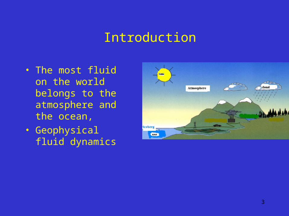
Introduction
• The most fluid on the world belongs to the atmosphere and the ocean,
• Geophysical fluid dynamics
4
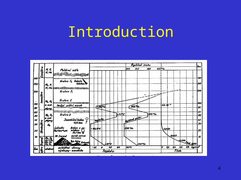
Introduction
5
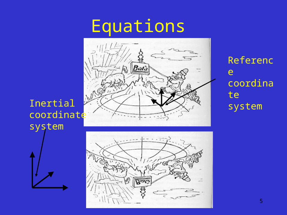
Equations
Inertial coordinate system
Reference coordinate system
6
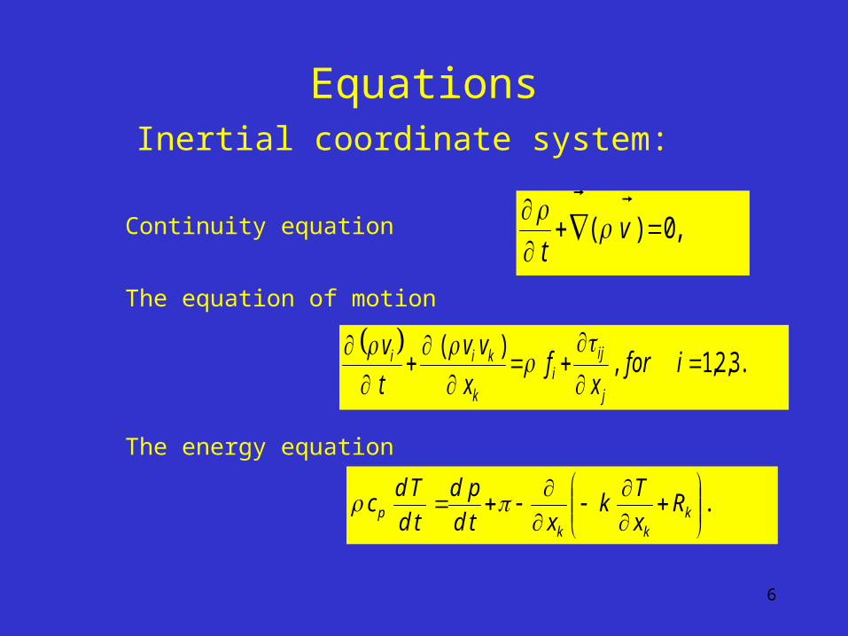
EquationsInertial coordinate system:
Continuity equation
The equation of motion
The energy equation
,0)(
vt
.3,2,1,
)(
iforx
fx
vv
t
v
j
iji
k
kii
.
kkk
p Rx
Tk
xtd
pd
td
Tdc
7
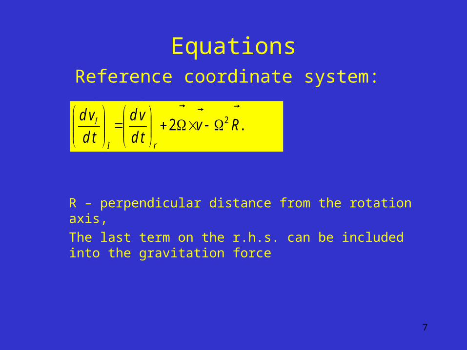
EquationsReference coordinate system:
R – perpendicular distance from the rotation axis,
The last term on the r.h.s. can be included into the gravitation force
.2 2 Rvtd
vd
td
vd
rI
I
8
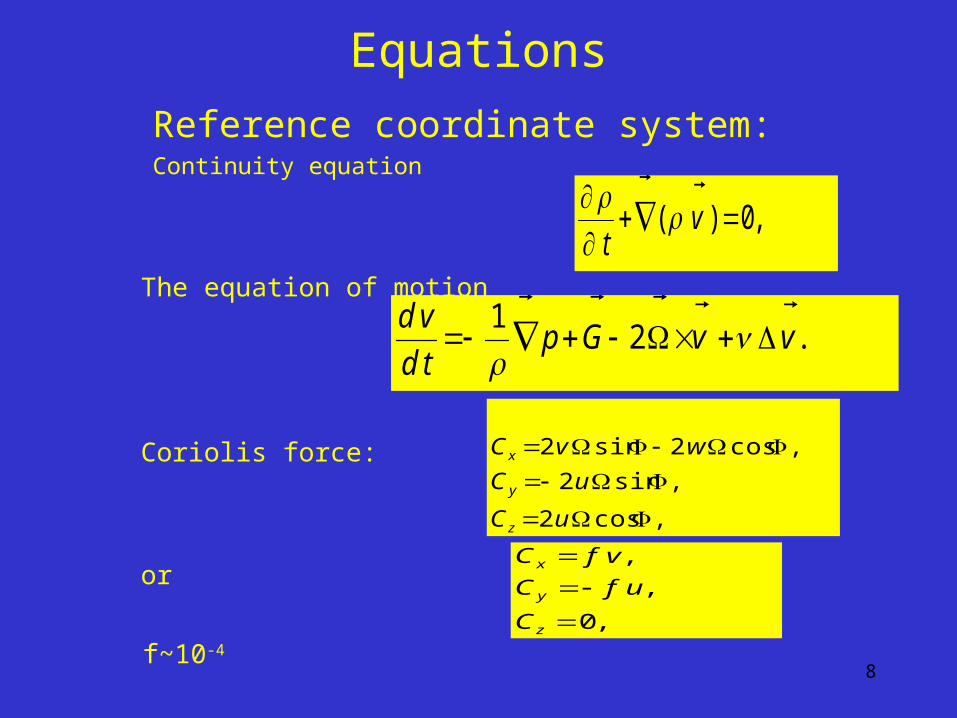
Equations
Reference coordinate system:Continuity equation
The equation of motion
Coriolis force:
or
,0)(
vt
.21
vvGptd
vd
,cos2
,sin2
,cos2sin2
uC
uC
wvC
z
y
x
,0
,
,
z
y
x
C
ufC
vfC
f~10-4
9
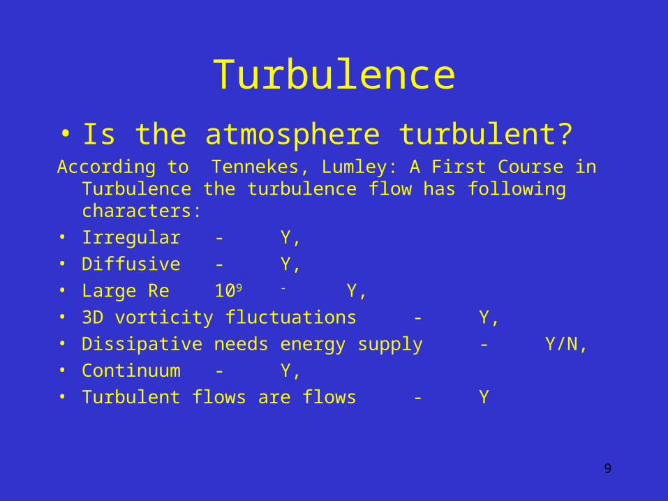
Turbulence• Is the atmosphere turbulent?According to Tennekes, Lumley: A First Course in Turbulence the
turbulence flow has following characters:
• Irregular - Y,
• Diffusive - Y,
• Large Re 109 - Y,
• 3D vorticity fluctuations - Y,
• Dissipative needs energy supply - Y/N,
• Continuum - Y,
• Turbulent flows are flows - Y
10
Turbulence
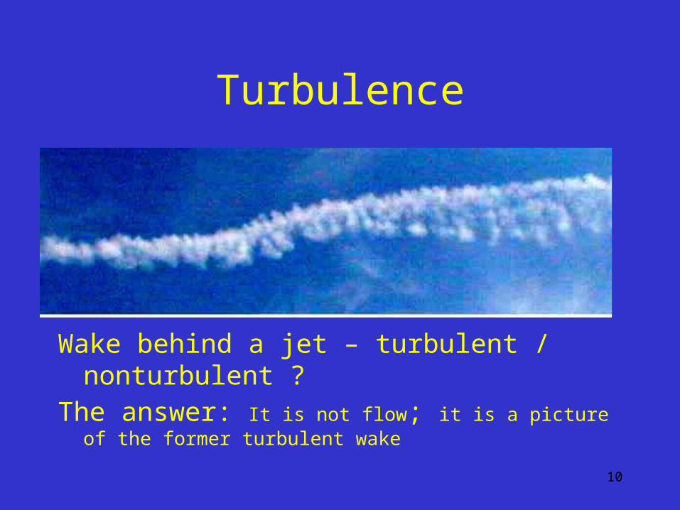
Wake behind a jet – turbulent / nonturbulent ?The answer: It is not flow; it is a picture of the former turbulent
wake
11
TurbulenceEnergy sources:
– Atmospheric Boundary Layer (ABL)– Free atmosphere:
• Clouds,
• Clear-Air Turbulence (CAT)
12
Turbulence
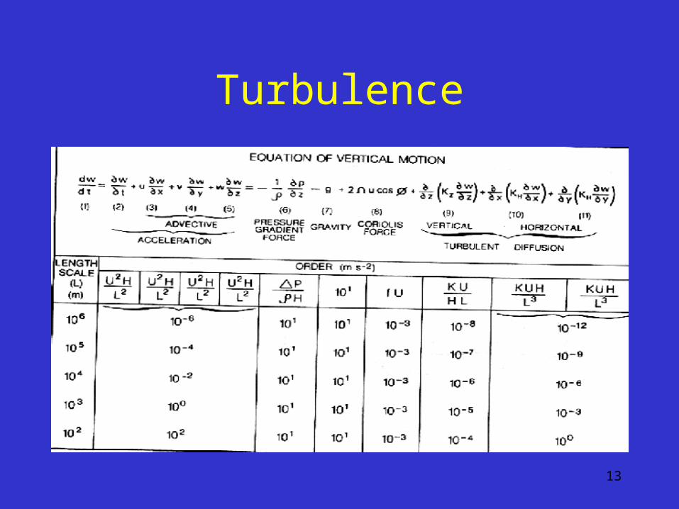
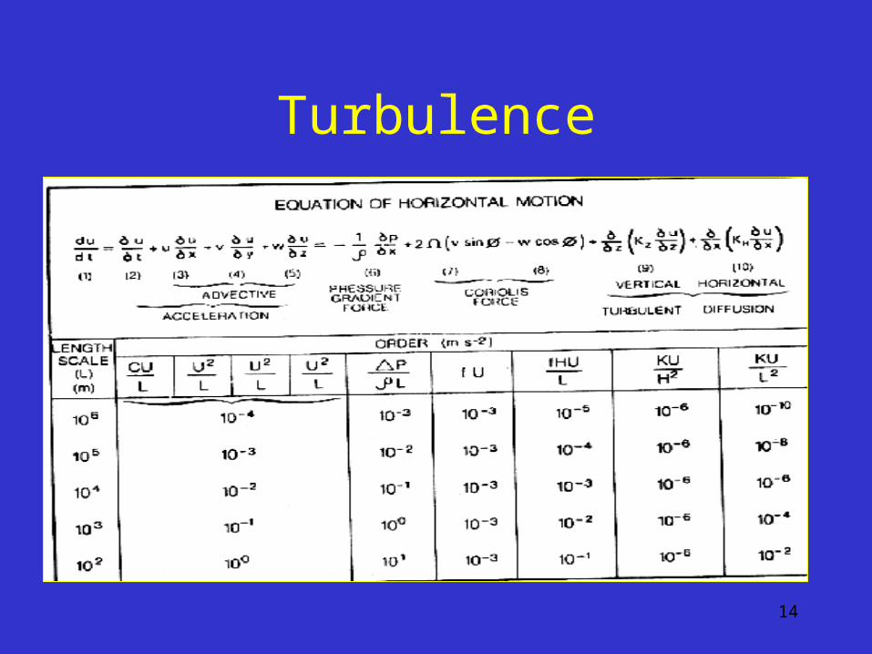
Characteristic scale:– Velocity U,– Length in horizontal direction L,– Length in vertical direction H,– -pressure P,
13
Turbulence
14
Turbulence
15
Turbulence
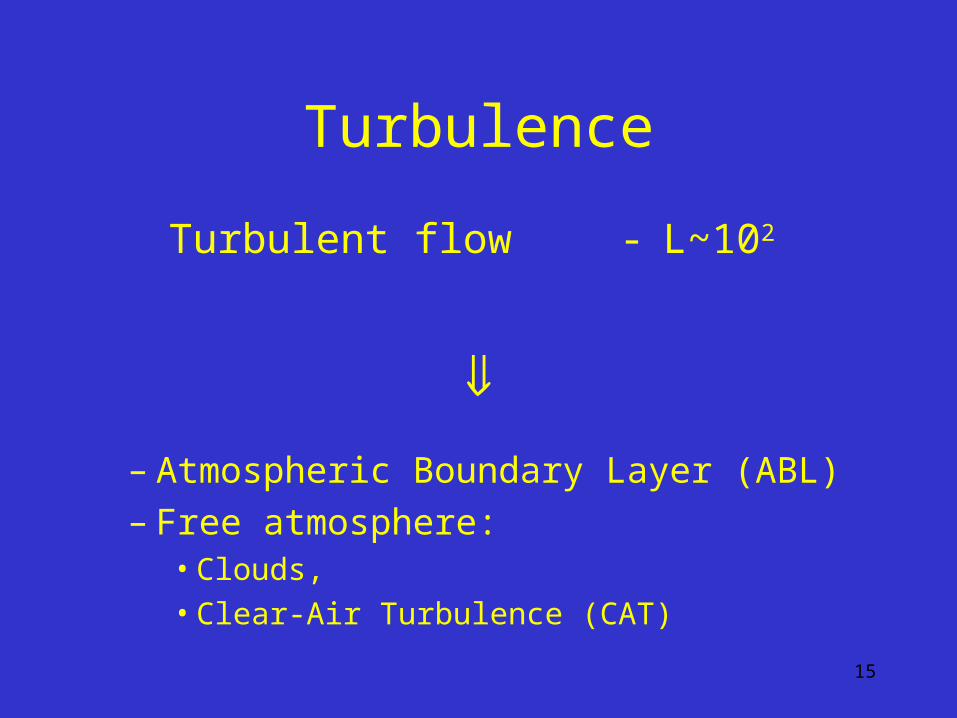
Turbulent flow - L~102
– Atmospheric Boundary Layer (ABL)– Free atmosphere:
• Clouds,
• Clear-Air Turbulence (CAT)
16
Turbulence
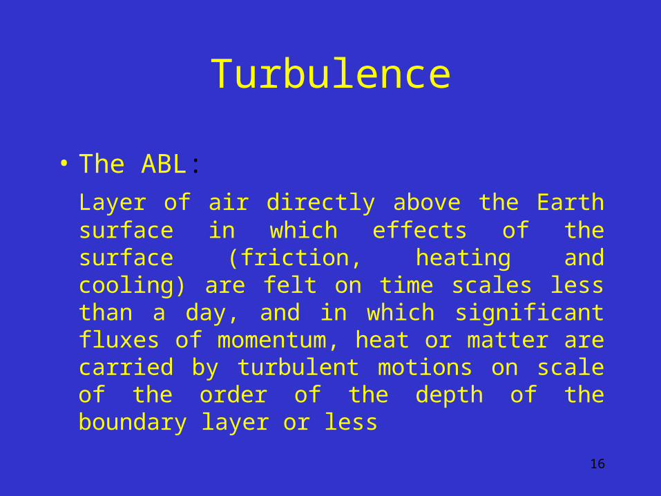
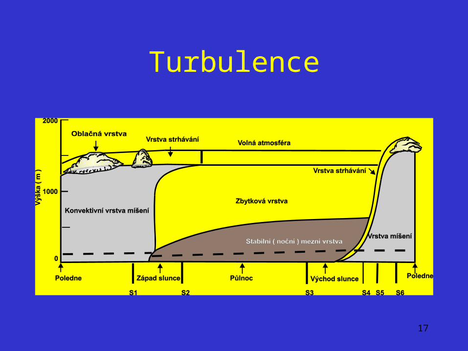
• The ABL:
Layer of air directly above the Earth surface in which effects of the surface (friction, heating and cooling) are felt on time scales less than a day, and in which significant fluxes of momentum, heat or matter are carried by turbulent motions on scale of the order of the depth of the boundary layer or less
17
Turbulence
18
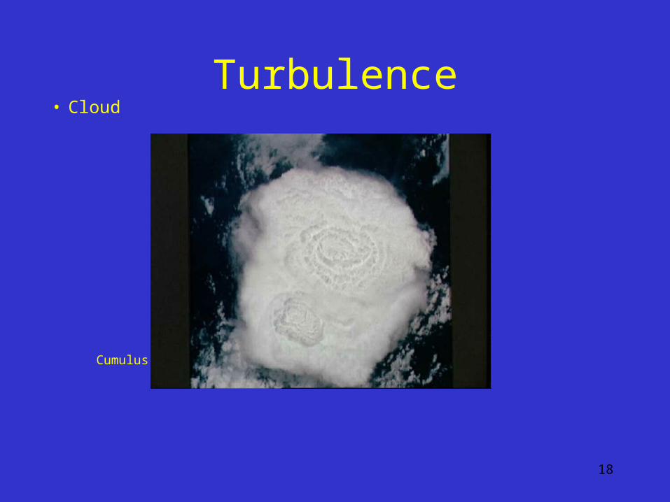
Turbulence• Cloud
Cumulus-type cloud associated with thunderstorm:
19
TurbulenceCAT• Shear turbulence without visible manifestations. • It occurs outside of clouds,• In only about 20% of the free atmosphere below 12 km,• is even less common above 12 km and occurs in only about 2% near 17 km,• It generally occurs in stable conditions, • It has not cased severe structure damage of aircraft.
20
Turbulence
Atmospheric turbulence differs from most
laboratory turbulence in:– Heat convection coexists with mechanical
turbulence,– The rotation of the earth becomes important for
many problems
21
Atmospheric Boundary Layer (ABL)
The ABL is the region in which the large-scale flow of the free atmosphere adjusts to the boundary condition imposed by the earth´s surface
22
ABL
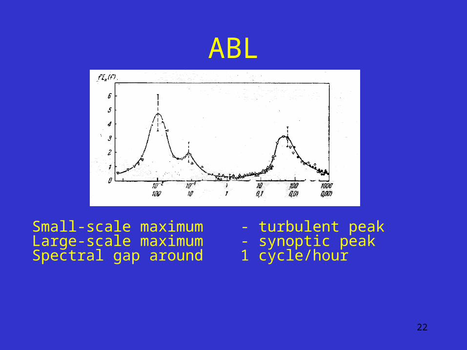
Small-scale maximum - turbulent peakLarge-scale maximum - synoptic peakSpectral gap around 1 cycle/hour
23
ABL
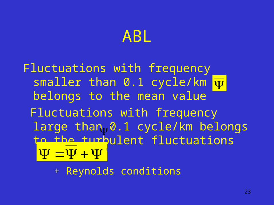
Fluctuations with frequency smaller than 0.1 cycle/km belongs to the mean value
Fluctuations with frequency large than 0.1 cycle/km belongs to the turbulent fluctuations
+ Reynolds conditions
´
'
24
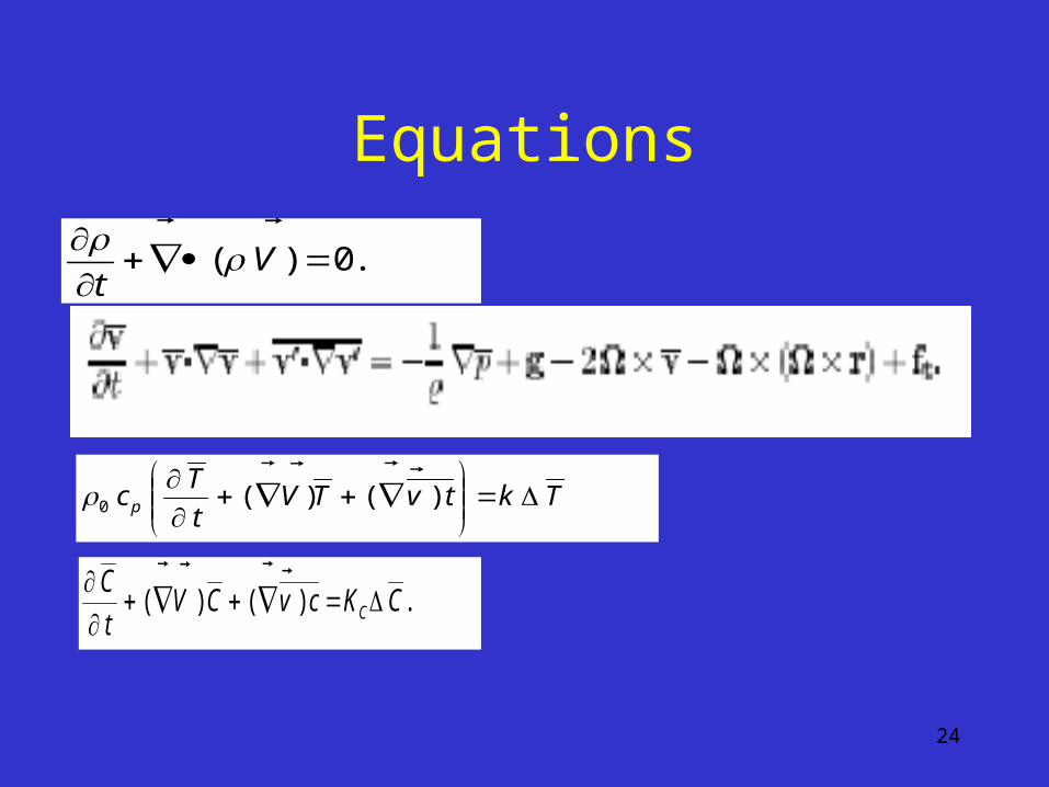
Equations
.0)(
Vt
TktvTVt
Tcp
)()(0
.)()( CKcvCVt
CC
25
Closure problem
),()(1
)(1
)(1
)(1
0
03
03
00
0
k
jkj
k
iki
k
ijk
k
jik
i
j
j
ij
ji
iikjjki
ikjjkikjikjik
ji
x
Uuu
x
Uuu
x
u
x
u
x
u
x
up
T
tug
T
tuguu
upupuuuUuuxt
uu
jiij uu0 ,0 ipi utcg .0 ii uch
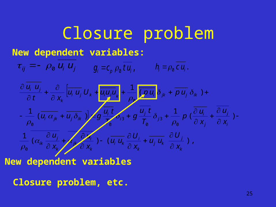
New dependent variables:
Closure problem, etc.
New dependent variables
26
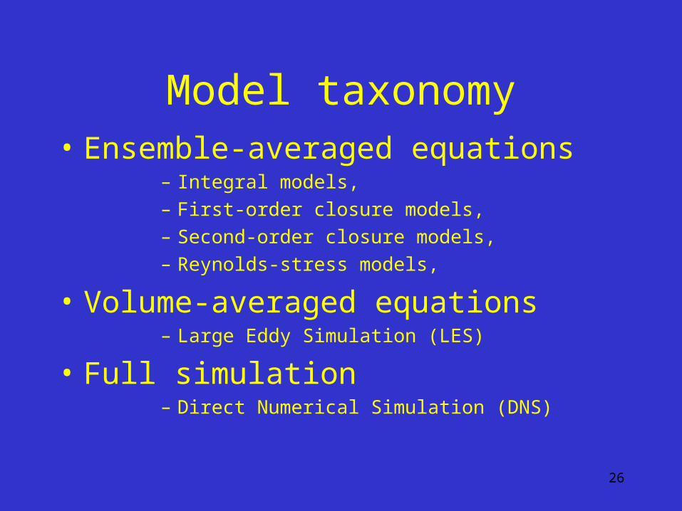
Model taxonomy• Ensemble-averaged equations
– Integral models,
– First-order closure models,
– Second-order closure models,
– Reynolds-stress models,
• Volume-averaged equations– Large Eddy Simulation (LES)
• Full simulation– Direct Numerical Simulation (DNS)
27
Integral models
Reynolds equations are integrated over at least one coordinate direction and the number of independent variables decreases
28
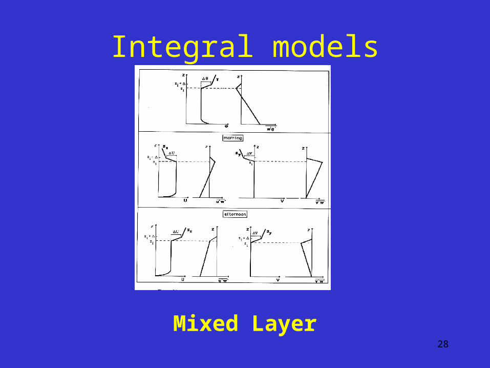
Integral models
Mixed Layer
29
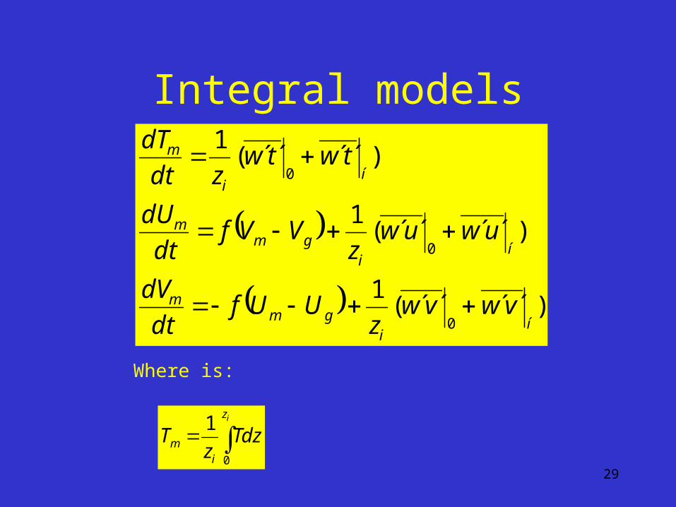
Integral models
)´´´´(1
)´´´´(1
)´´´´(1
0
0
0
íi
gmm
íi
gmm
íi
m
vwvwz
UUfdt
dV
uwuwz
VVfdt
dU
twtwzdt
dT
iz
im Tdz
zT
0
1
Where is:
30
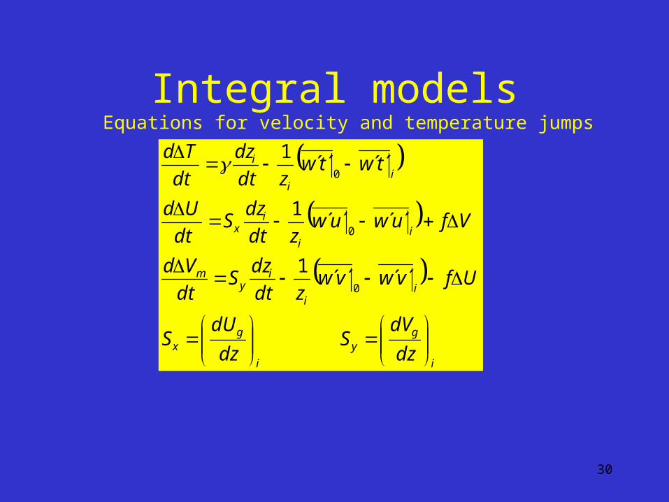
Integral models
i
gy
i
gx
ii
iy
m
ii
ix
ii
i
dz
dVS
dz
dUS
Ufvwvwzdt
dzS
dt
Vd
Vfuwuwzdt
dzS
dt
Ud
twtwzdt
dz
dt
Td
´´´´1
´´´´1
´´´´1
0
0
0
Equations for velocity and temperature jumps
31
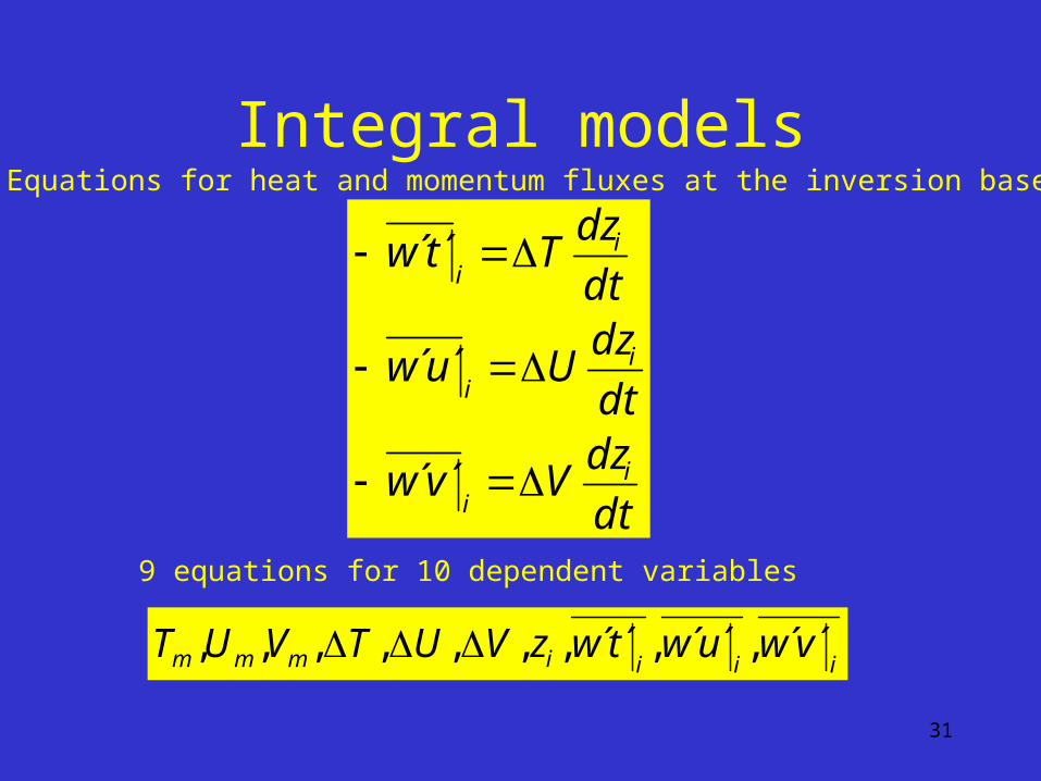
Integral models
dt
dzVvw
dt
dzUuw
dt
dzTtw
ii
ii
ii
´´
´´
´´
Equations for heat and momentum fluxes at the inversion base
9 equations for 10 dependent variables
iiiimmm vwuwtwzVUTVUT ´´,´´,´´,,,,,,,
32
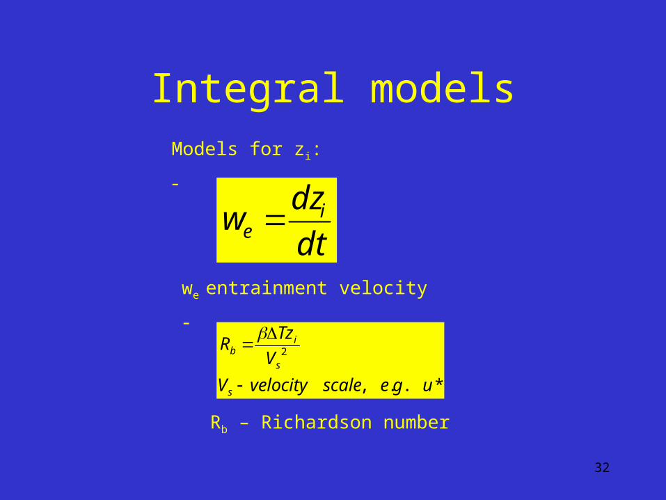
Integral models
dt
dzw i
e
Models for zi:
we entrainment velocity
-
-
*..,
2
ugescalevelocityV
V
TzR
s
s
ib
Rb – Richardson number
33
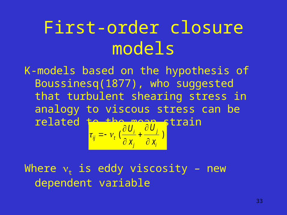
First-order closure models
K-models based on the hypothesis of Boussinesq(1877), who suggested that turbulent shearing stress in analogy to viscous stress can be related to the mean strain
Where t is eddy viscosity – new dependent variable
),(i
j
j
itij x
U
x
U
34
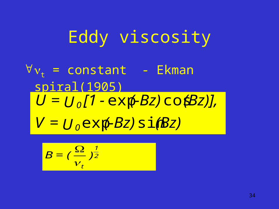
Eddy viscosity
t = constant - Ekman spiral(1905)
(Bz)(-Bz)U=V
(Bz)],(-Bz)-[1U=U
0
0
sinexp
cosexp
)(=B 2
1
t
35
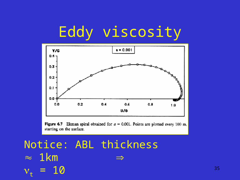
Eddy viscosity
Notice: ABL thickness 1km t = 10
36
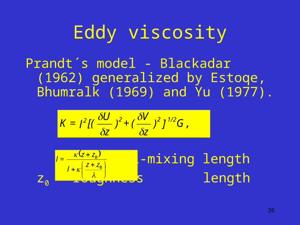
Eddy viscosity
Prandt´s model - Blackadar (1962) generalized by Estoqe, Bhumralk (1969) and Yu (1977).
l-mixing length
z0 – roughness length
,G])z
V(+)
z
U[(l=K 1/2222
0
0
zzl
zz=l
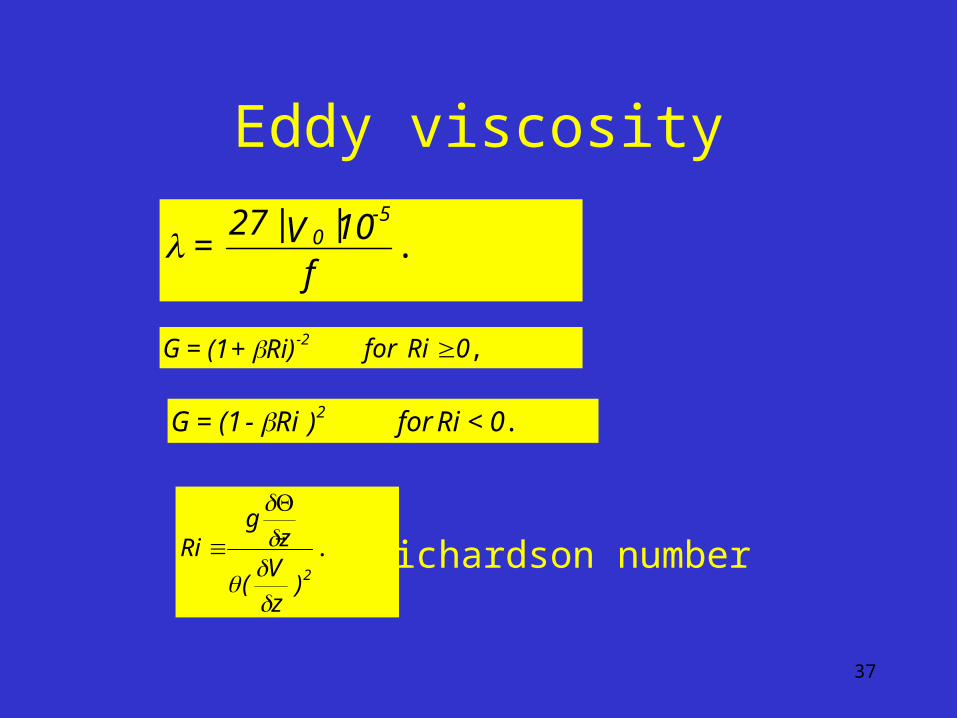
37
Eddy viscosity
.f
10|V|27=
-50
,0Rifor Ri)+(1=G -2
.0<Rifor )Ri-(1=G 2
.
)z
V(
zg
Ri2
Richardson number
38
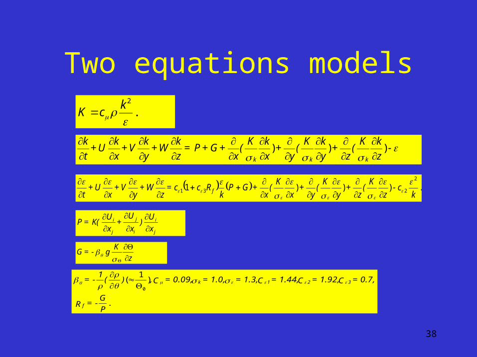
Two equations models
.2
kcK
-z
kK(
z+
y
kK(
y+
x
kK(
x+G+P=
z
kW+
y
kV+
x
kU+
t
k
kkk
)))
.)))12
231 kc-
z
K(
z+
y
K(
y+
x
K(
x+GP
kRcc=
zW+
yV+
xU+
t f
j
i
i
j
j
i
x
U)
x
U+
x
UK(=P
z
K g -=G
.
)1
(0
P
G-=R
0.7,=C 1.92,=C 1.44,=C 1.3,= 1.0,= 0.09,=C ,)(1
-=
f
321k
39
Large Eddy Simulation
• The first large-eddy simulations were performed by Deardorff (1972; 1973;1974), and were later investigated by e.g.,:
• Schemm and Lipps (1976),
• Sommeria (1976),
• Moeng (1984),
• Wyngaard and Brost (1984), Schmidt and Schumann (1989), Mason (1989). Much of the previous work
• LES has been focused on simulations of the convective boundary layers (Nieuwstadt et al., 1992).
• The cloudy boundary layers were simulated by e.g., Sommeria 1976; Deardorff 1980; Moeng 1986; Moeng et al. 1996; Lewellen and Lewellen 1996, Cuijpers and Duynkerke (1993).
40
Boundary Conditions
41
Boundary ConditionsThe equations of motion has to be supplemented with initial and boundary conditions – in many papers the conditions are not introduced
42
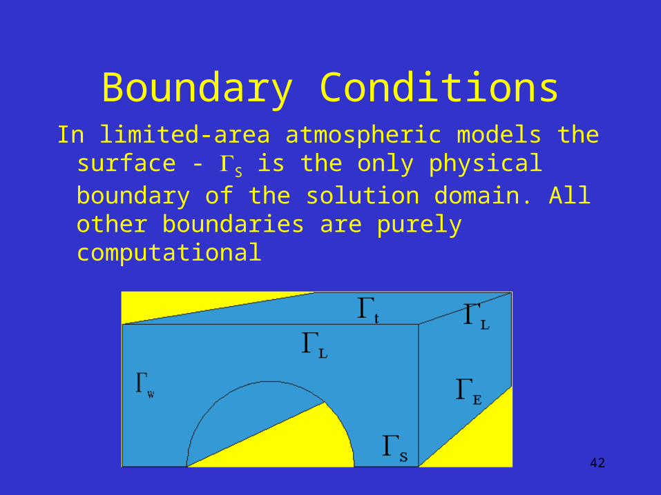
Boundary ConditionsIn limited-area atmospheric models the
surface - S is the only physical boundary of the solution domain. All other boundaries are purely computational
43
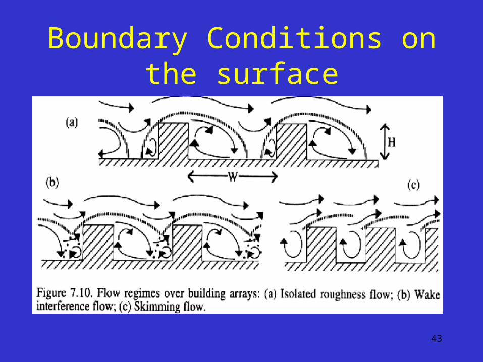
Boundary Conditions on the surface
44
Boundary Conditions on the surface
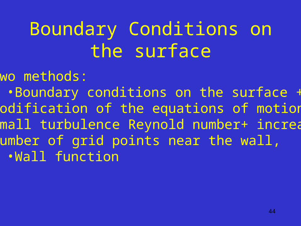
Two methods:•Boundary conditions on the surface +
modification of the equations of motion for small turbulence Reynold number+ increasing number of grid points near the wall,
•Wall function
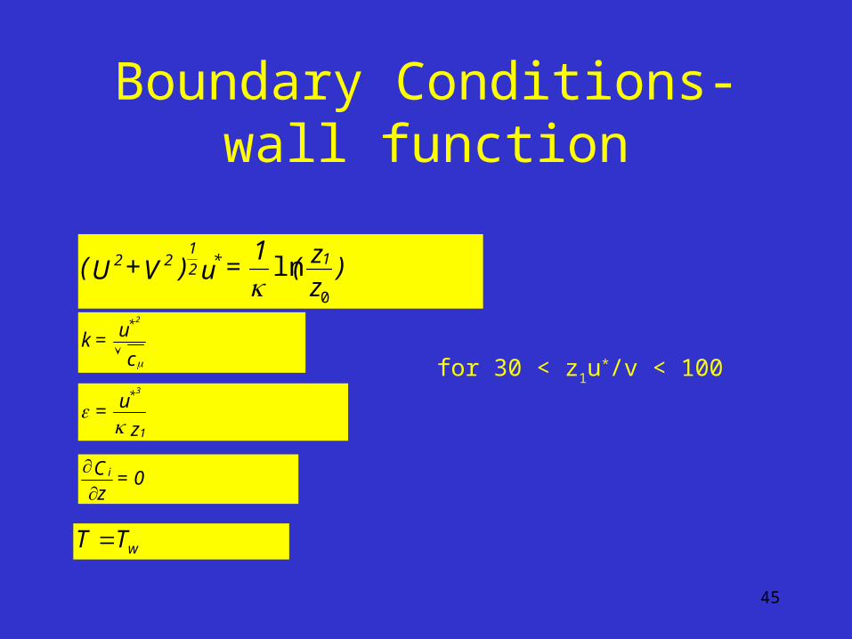
45
Boundary Conditions-wall function
)zz(
1=u)V+U( 1*
2
122
0
ln
for 30 < z1u*/v < 100 c
u=k* 2
z
u=1
* 3
0=zC i
wTT
46
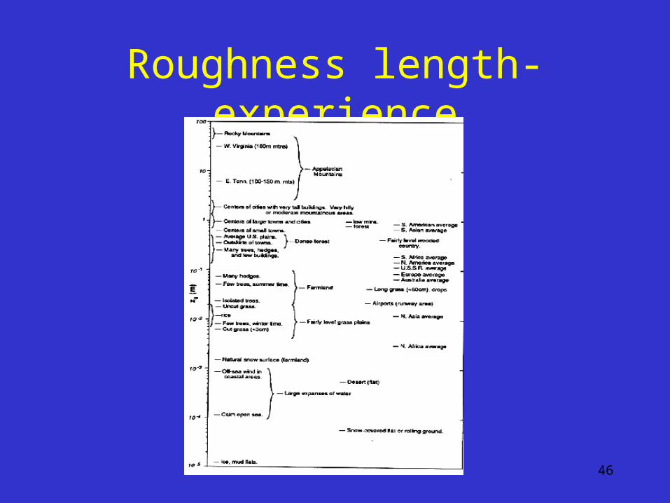
Roughness length- experience
47
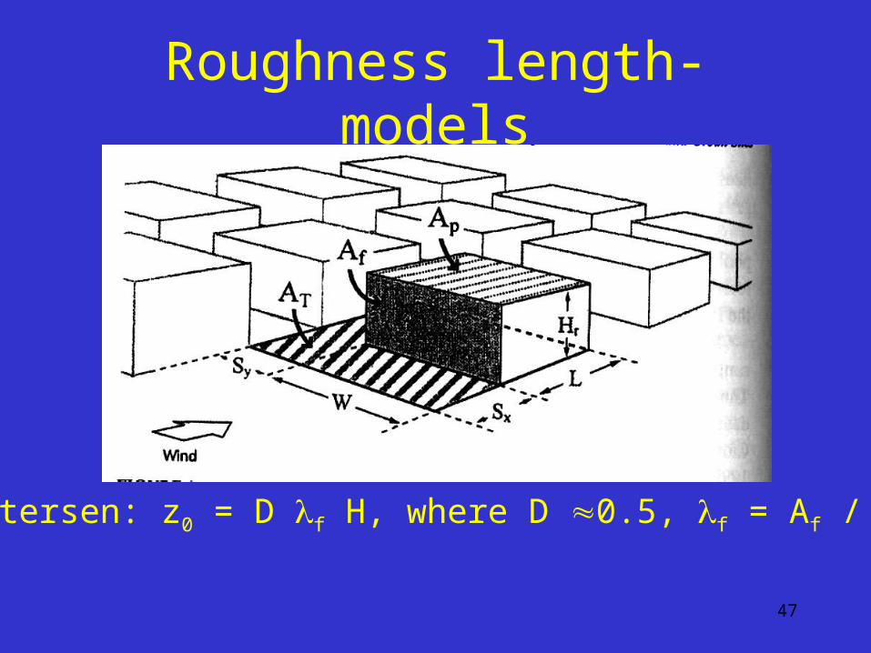
Roughness length-models
Petersen: z0 = D f H, where D 0.5, f = Af / AT
48
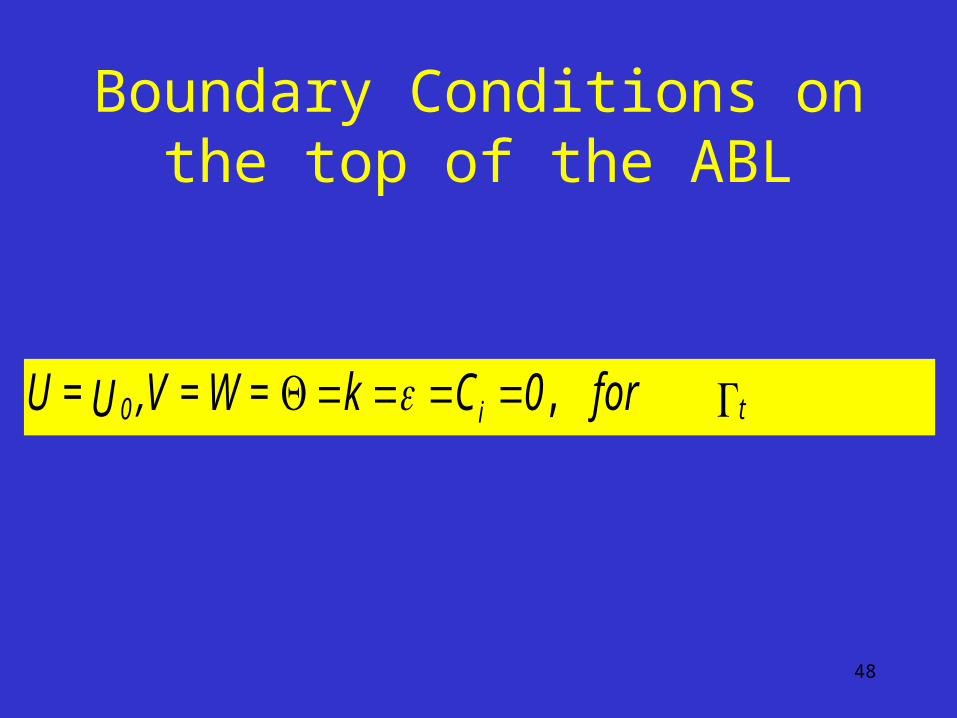
Boundary Conditions on the top of the ABL
ti0 for 0Ck=W=V ,U=U ,
49
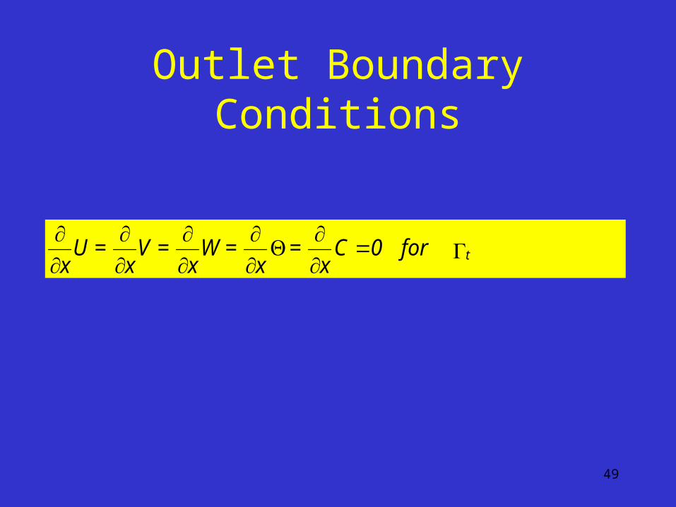
Outlet Boundary Conditions
t for 0Cx
=x
=Wx
=Vx
=Ux
50
Inlet Boundary Conditions
Dirichlet condition determined from:
• In-situ measurement – a very few data sets,
• Universal profiles:– Ekman spiral,– Power law,– ….
-mostly for horizontally homogeneous surface
51
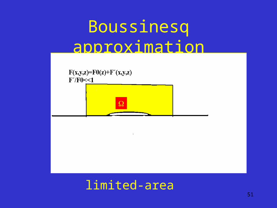
Boussinesq approximation
limited-area
52
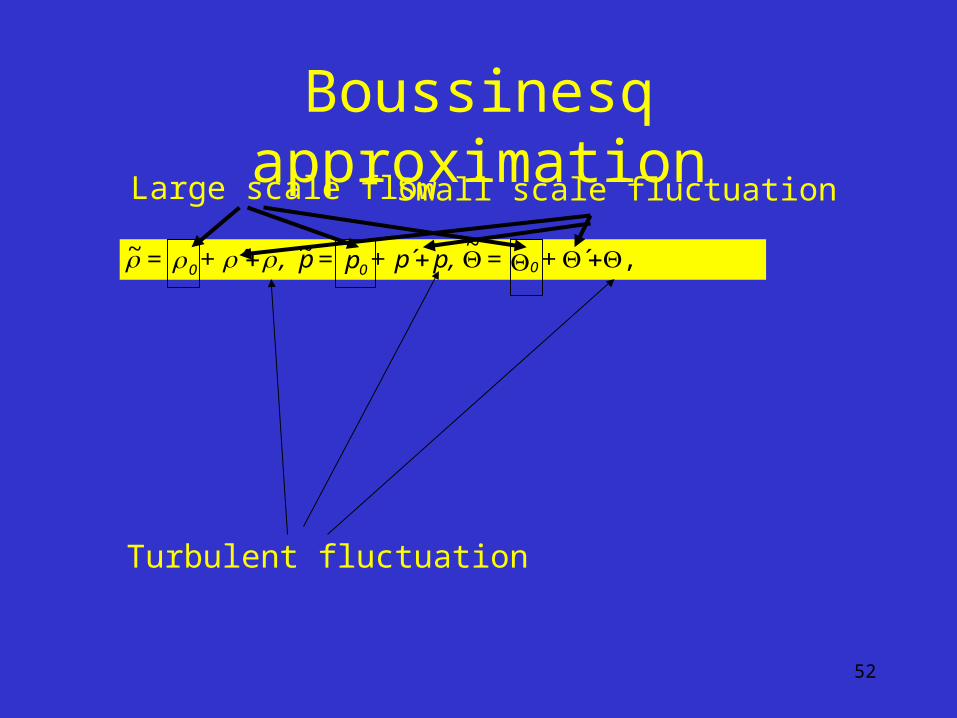
Boussinesq approximation
,´~
´~´~ += p,p+p=p ,+= 000
Large scale flow Small scale fluctuation
Turbulent fluctuation
53
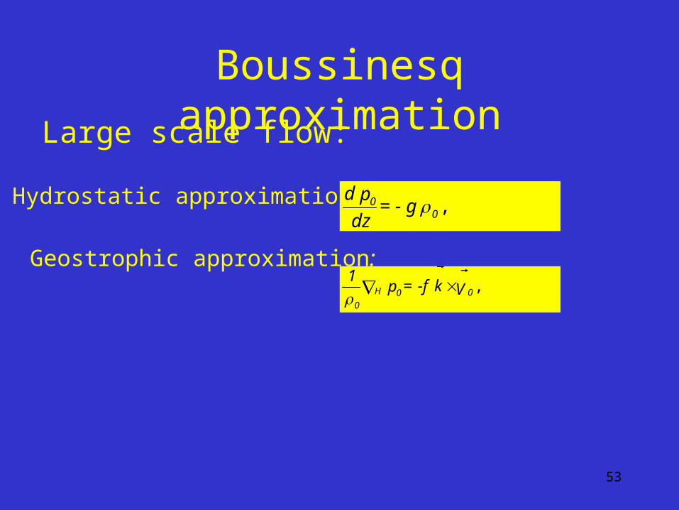
Boussinesq approximation
Hydrostatic approximation: , 00 g- =
dz
pd
Geostrophic approximation:,Vk -f= p
100H
0
Large scale flow:
54
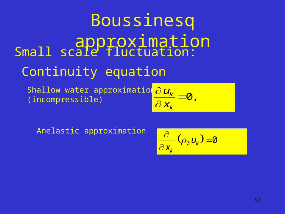
Boussinesq approximation
Shallow water approximation:(incompressible)
Continuity equation
,0
k
k
x
u
Anelastic approximation 00
kk
ux
Small scale fluctuation:
55
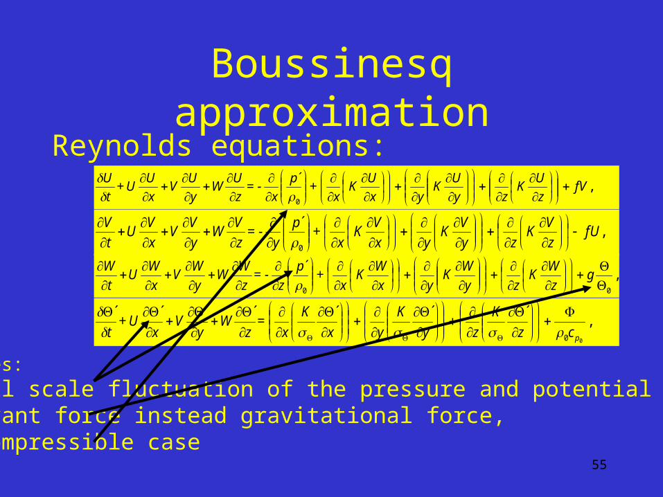
Boussinesq approximationReynolds equations:
,´
0
fVz
UK
zy
UK
yx
UK
x+
p
x- =
z
UW
y
UV
x
UU+
t
U
,´
0
fUz
VK
zy
VK
yx
VK
x+
p
y- =
z
VW
y
VV
x
VU
t
V
,´
00
gz
WK
zy
WK
yx
WK
x+
p
z- =
z
WW
y
WV
x
WU
t
W
,´´´´´´´
00 pcz
K
zy
K
yx
K
x =
zW
yV
xU+
t
Notices: •Small scale fluctuation of the pressure and potential temperature,•Buoyant force instead gravitational force,•Incompressible case
56
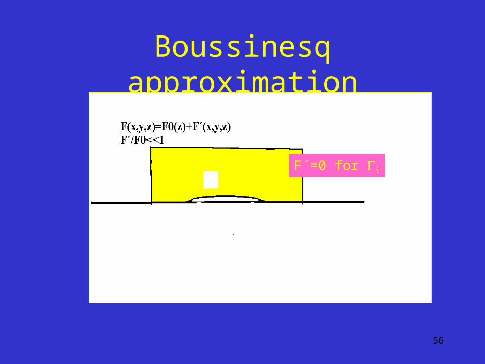
Boussinesq approximation
F´=0 for i
57
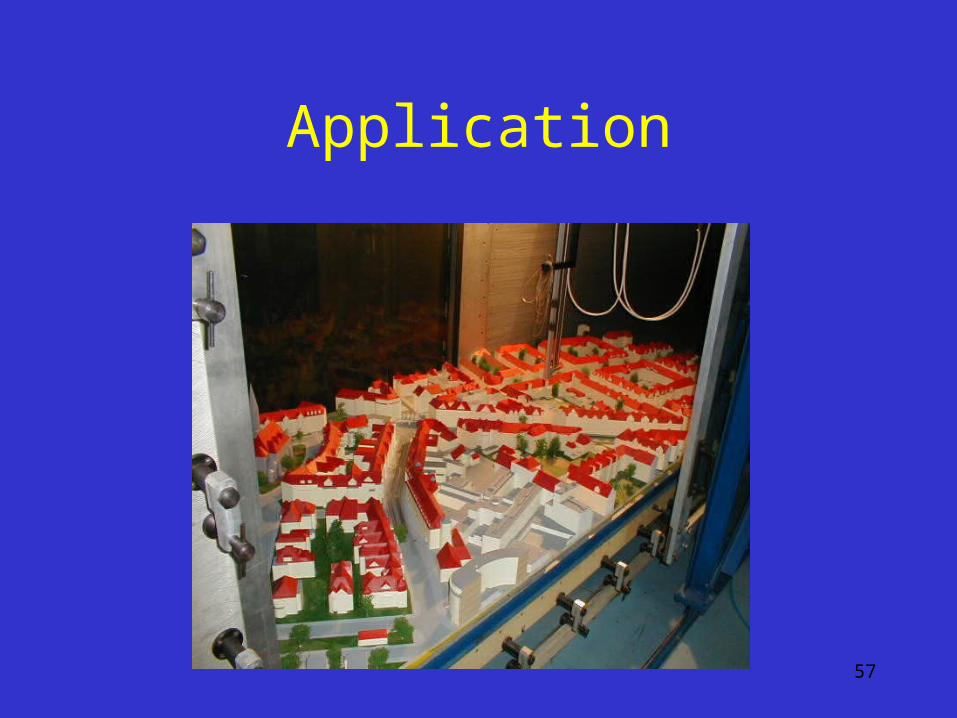
Application
58
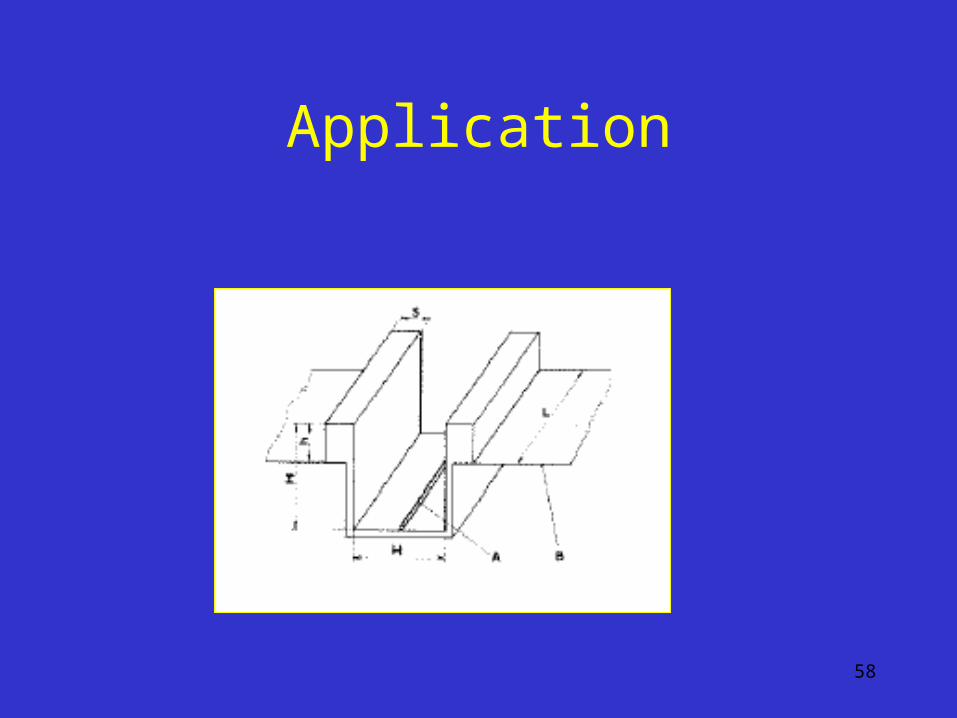
Application
59
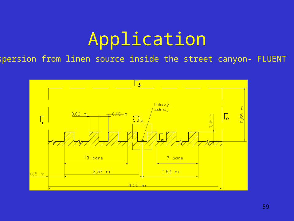
ApplicationDispersion from linen source inside the street canyon- FLUENT
60
Application
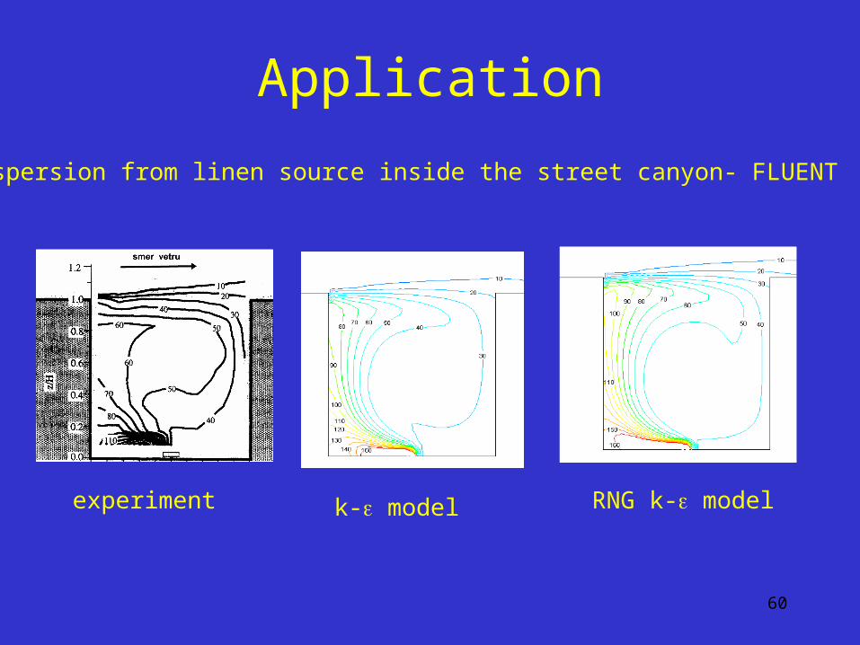
experiment k- model RNG k- model
Dispersion from linen source inside the street canyon- FLUENT
61
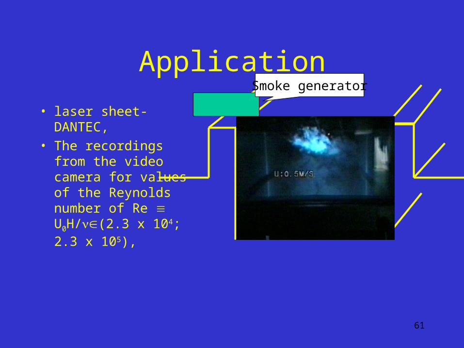
Application
• laser sheet- DANTEC,
• The recordings from the video camera for values of the Reynolds number of Re U0H/(2.3 x 104; 2.3 x 10⁵),
Smoke generator
62
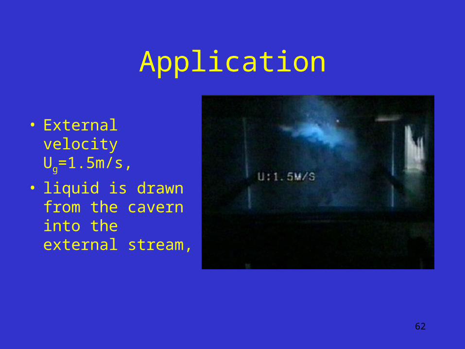
Application
• External velocity Ug=1.5m/s,
• liquid is drawn from the cavern into the external stream,

63
Application
• External velocity Ug=4.0m/s
64
Application
65
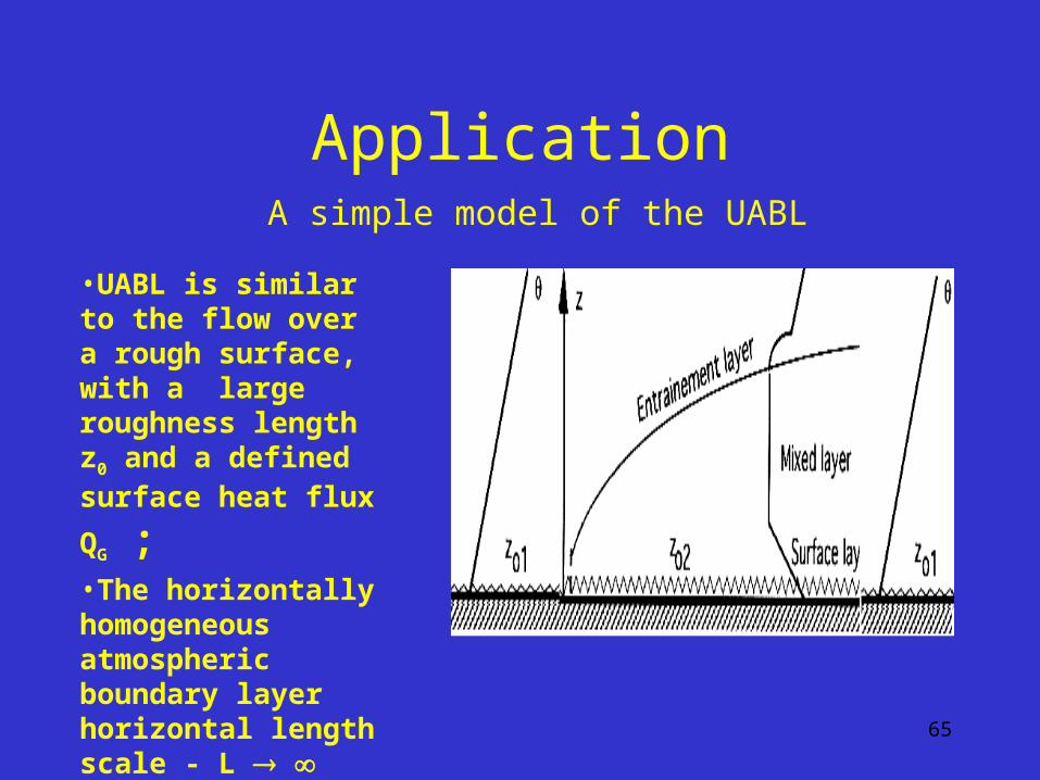
Application
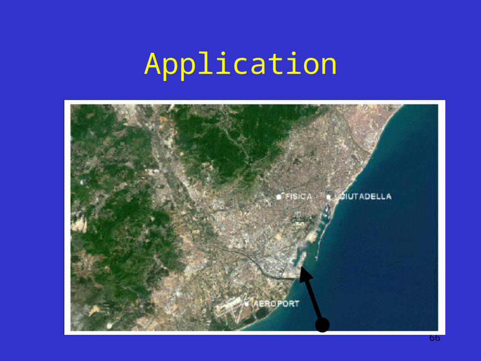
•UABL is similar to the flow over a rough surface, with a large roughness length z0 and a defined surface heat
flux QG ;•The horizontally homogeneous atmospheric boundary layer horizontal length scale - L
A simple model of the UABL
66
Application
67
Application
00,1
0,20,3
0,40,5
0,60,7
0,80,9
1
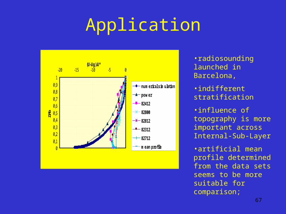
-20 -15 -10 -5 0(U-Ug)/U*
Z/Hb
numerical simulation
power
82412
82800
82812
82312
82712
mean profile
•radiosounding launched in Barcelona,
•indifferent stratification
•influence of topography is more important across Internal-Sub-Layer
•artificial mean profile determined from the data sets seems to be more suitable for comparison;
68
Application
00,1
0,20,3
0,40,50,6
0,70,8
0,91
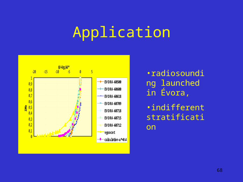
-20 -15 -10 -5 0 5(U-Ug)/U*
Z/Hb
EVORA-60500
EVORA-60600
EVORA-60618
EVORA-60709
EVORA-60718
EVORA-60715
EVORA-60712
vypocet
calculation-u*=0.4
•radiosounding launched in Évora,
•indifferent stratification
69
Application
00,1
0,20,30,40,5
0,60,70,8
0,91
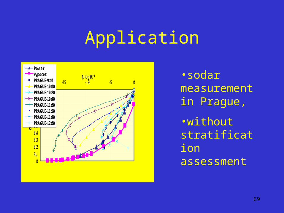
-20 -15 -10 -5 0(U-Ug)/U*
Z/Hb
PowervypocetPRAGUE-9:40PRAGUE-10:00PRAGUE-10:20PRAGUE-10:40PRAGUE-11:00PRAGUE-11:20PRAGUE-11:40PRAGUE-12:00
•sodar measurement in Prague,
•without stratification assessment
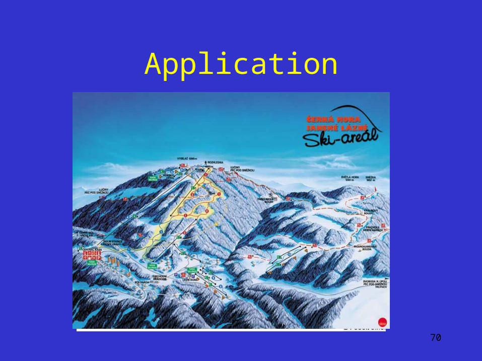
70
Application
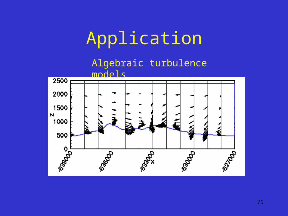
71
ApplicationAlgebraic turbulence models
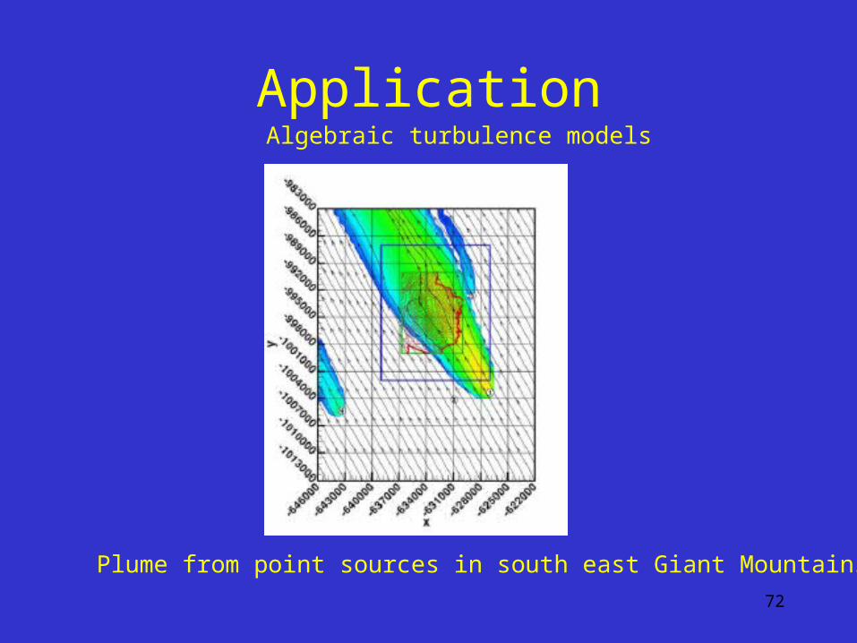
72
Application
Plume from point sources in south east Giant Mountains
Algebraic turbulence models
73
4. Conclusions
• Eddy viscosity models appears:– Quite satisfactory in neutral or stable ABL;– Fail in convective situations;
• Reynolds stress models are more suitable,
• Boundary Conditions are complicated and important task
Related Documents