Enumerative Combinatorics The LTCC lectures Combinatorics The LTCC lectures Peter J ... torics at the London Taught Course Centre in Autumn ... is the number of partitions of a set

Enumerative CombinatoricsThe LTCC lectures

Peter J. Cameron

Autumn 2013

Abstract

These are the notes of my lecture course on Enumerative Combina-torics at the London Taught Course Centre in Autumn 2013. Thanksto all who attended for their support. There are ten sections, as fol-lows:

• Subsets, partitions, permutations

• Formal power series

• Catalan numbers

• Unimodality

• q-analogues

• Symmetric polynomials

• Group actions

• Species

• Mobius inversion

• Cayley’s theorem

Exercises are included at the end of the sections.

1 Subsets, Partitions, Permutations

Enumerative combinatorics is concerned with counting discrete structures ofvarious types. There is a great deal of variation both in what we mean by“counting” and in the types of structures we count. Typically each structurehas a “size” measured by a non-negative integer n, and “counting” may mean

1

(a) finding an exact formula for the number f(n) of structures of size n;

(b) finding an approximate or asymptotic formula for f(n);

(c) finding an analytic expression for a generating function for f(n);

(d) finding an efficient algorithm for computing f(n) exactly or approxi-mately;

(e) finding an efficient algorithm for stepping from one of the counted ob-jects to the next (in some natural ordering).

In this course I will mostly be concerned with the first three goals; discussingalgorithms would lead too far afield. The exception to this is one particularlyimportant algorithm, a recurrence relation, in which the value of f(n) iscomputed from n and the earlier values f(0), . . . , f(n− 1).

An asymptotic formula for f(n) is an analytic function g(n) such thatf(n)/g(n) → 0 as n → ∞. There are several types of generating functions ;

the most important for us are the ordinary generating function∑n≥0

f(n)xn,

and the exponential generating function∑n≥0

f(n)xn

n!.

If you want to learn the state-of-the-art in combinatorial enumeration,I recommend the two volumes of Richard Stanley’s Enumerative Combina-torics, or the book Analytic Combinatorics by Philippe Flajolet and RobertSedgewick. The On-line Encyclopedia of Integer Sequences is another valu-able resource for combinatorial enumeration.

1.1 Subsets

The three most important objects in elementary combinatorics are subsets,partitions and permutations; we briefly discuss the counting functions forthese. First, subsets.

The total number of subsets of an n-element set is 2n. This can be usedby noting that this number f(n) satisfies the recurrence relation f(n) =2f(n− 1); this is proved by observing that any subset of {1, . . . , n− 1} canbe extended to a subset of {1, . . . , n} in two different ways, either includingthe element n or not.

2

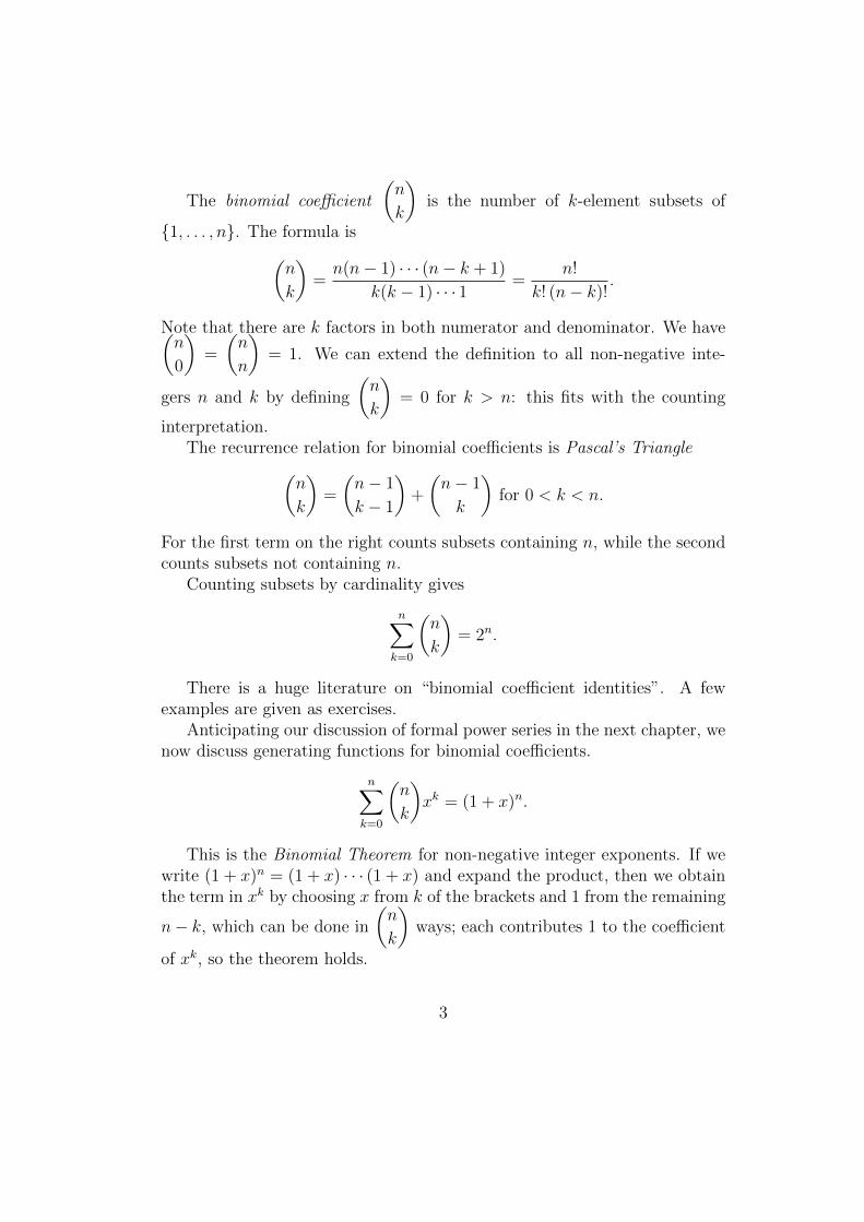
The binomial coefficient

(n

k

)is the number of k-element subsets of

{1, . . . , n}. The formula is(n

k

)=n(n− 1) · · · (n− k + 1)

k(k − 1) · · · 1=

n!

k! (n− k)!.

Note that there are k factors in both numerator and denominator. We have(n

0

)=

(n

n

)= 1. We can extend the definition to all non-negative inte-

gers n and k by defining

(n

k

)= 0 for k > n: this fits with the counting

interpretation.The recurrence relation for binomial coefficients is Pascal’s Triangle(

n

k

)=

(n− 1

k − 1

)+

(n− 1

k

)for 0 < k < n.

For the first term on the right counts subsets containing n, while the secondcounts subsets not containing n.

Counting subsets by cardinality gives

n∑k=0

(n

k

)= 2n.

There is a huge literature on “binomial coefficient identities”. A fewexamples are given as exercises.

Anticipating our discussion of formal power series in the next chapter, wenow discuss generating functions for binomial coefficients.

n∑k=0

(n

k

)xk = (1 + x)n.

This is the Binomial Theorem for non-negative integer exponents. If wewrite (1 + x)n = (1 + x) · · · (1 + x) and expand the product, then we obtainthe term in xk by choosing x from k of the brackets and 1 from the remaining

n− k, which can be done in

(n

k

)ways; each contributes 1 to the coefficient

of xk, so the theorem holds.

3

If we multiply this equation by yn and sum, we obtain the bivariategenerating function for the binomial coefficients:

∑n≥0

n∑k=0

(n

k

)xkyn =

∑n≥0

(1 + x)nyn

=1

1− (1 + x)y

=1

1− y· 1

1− xy/(1− y)

=∑k≥0

yk

(1− y)k+1xk,

so we obtain the other univariate generating function for binomial coefficients:∑n≥k

(n

k

)yn =

yk

(1− y)k+1.

This formula is actually a rearrangement of the Binomial Theorem for neg-ative integer exponents. The basis of this connection is the following evalu-ation, for positive integers m and k:(

−mk

)=−m(−m− 1) · · · (−m− k + 1

k!

= (−1)k(m+ k − 1) · · · (m+ 1)m

k!

= (−1)k(m+ k − 1

k

).

1.2 Partitions

In this case and the next, we are unable to write down a simple formulafor the counting numbers, and have to rely on recurrence relations or othertechniques.

The Bell number B(n) is the number of partitions of a set of cardinalityn. We refine this in the same way we did for subsets. The Stirling number ofthe second kind, S(n, k), is the number of partitions of an n-set into k parts.

4

Thus, S(0, 0) = 1 and S(0, k) = 0 for k > 0; and if n > 0, then S(n, 0) = 0,S(n, 1) = S(n, n) = 1, and S(n, k) = 0 for k > n. Clearly we have

n∑k=1

S(n, k) = B(n) for n > 0.

The recurrence relation replacing Pascal’s is:

S(n, k) = S(n− 1, k − 1) + kS(n− 1, k) for 1 ≤ k ≤ n.

It turns out that we can turn this into a statement about a generatingfunction, but with a twist. Let

(x)k = x(x− 1) · · · (x− k + 1) (k factors).

Then we have

xn =n∑k=1

S(n, k)(x)k for n > 0.

It is possible to find a traditional generating function for the index n:∑n≥k

S(n, k)yn =yk

(1− y)(1− 2y) · · · (1− ky).

Also, the exponential generating function for the index n is∑n≥k

S(n, k)xn

n!=

(exp(x)− 1)k

k!.

Summing over k gives the e.g.f. for the Bell numbers:∑n≥0

B(n)xn

n!= exp(exp(x)− 1).

1.3 Permutations

The number of permutations of an n-set (bijective functions from the set toitself) is the factorial function n! = n(n − 1) · · · 1 for n ≥ 0. The exponen-tial generating function for this sequence is 1/(1 − x), while the ordinarygenerating function has no analytic expression (it is divergent for all x 6= 0).

5

Any permutation can be decomposed uniquely into disjoint cycles. So werefine the count by letting u(n, k) be the number of permutations of an n-setwhich have exactly k cycles (including cycles of length 1). Thus,

n∑k=1

u(n, k) = n! for n > 0.

The numbers u(n, k) are the unsigned Stirling numbers of the first kind. Thereason for the name is that it is common to use a different count, where apermutation is counted with weight equal to its sign (as defined in elementaryalgebra, for example the theory of determinants). Let s(n, k) be the sum ofthe signs of the permutations of an n-set which have k cycles. Since the signof such a permutation is (−1)n−k, we have s(n, k) = (−1)n−ku(n, k). Thenumbers s(n, k) are the signed Stirling numbers of the first kind.

We haven∑k=1

s(n, k) = 0 for n > 1.

This is related to the algebraic fact that, for n > 1, the permutations withsign + form a subgroup of the symmetric group of index 2 (that is, containinghalf of all the permutations), called the alternating group.

We will mainly consider signed Stirling numbers below, though it is some-times convenient to prove a result first for the unsigned numbers.

As usual we take s(n, 0) = 0 for n > 0 and s(n, k) = 0 for k > n.We have s(n, n) = 1, s(n, 1) = (−1)n−1(n−1)!, and the recurrence relation

s(n, k) = s(n− 1, k − 1)− (n− 1)s(n− 1, k) for 1 ≤ k ≤ n.

From this, we find a generating function:

n∑k=1

s(n, k)xk = (x)n.

Putting x = 1 in this equation shows that indeed the sum of the signedStirling numbers is zero for n > 1.

Note that this is the inverse of the relation we found for the Stirlingnumbers of the second kind. So the matrices formed by the Stirling numbersof the first and second kind are inverses of each other.

6

Exercises

1. Let A be the matrix of binomial coefficients (with rows and columns

indexed by N, and (i, j) entry

(i

j

)), and B the matrix of “signed binomial

coefficients” (as before but with (i, j) entry (−1)i−j(i

j

)). Prove that A and

B are inverses of each other.

What are the entries of the matrix A2?

2. Prove thatn∑k=0

(n

k

)2

=

(2n

n

).

3. (a) Prove that the following are equivalent for sequences (a0.a1, . . .) and(b0, b1, . . .), with exponential generating functions A(x) and B(x) respec-tively:

(ii) b0 = a0 and bn =n∑k=1

S(n, k)ak for n ≥ 1;

(i) B(x) = A(exp(x)− 1).

(b) Prove that the following are equivalent for sequences (a0.a1, . . .) and(b0, b1, . . .), with exponential generating functions A(x) and B(x) respec-tively:

(i) b0 = a0 and bn =n∑k=1

s(n, k)ak for n ≥ 1;

(ii) B(x) = A(log(1 + x)).

4. Construct a bijection between the set of all k-element subsets of {1, 2, . . . , n}containing no two consecutive elements, and the set of all k-element subsetsof {1, 2, . . . , n − k + 1}. Hence show that the number of such subsets is(n−k+1

k

).

In the UK National Lottery, six numbers are chosen randomly (with-out replacement, order unimportant) from the set {1, . . . , 49}. What is theprobability that the selection contains no two consecutive numbers?

7

2 Formal power series

Probably you recognised in the last chapter a few things from analysis, suchas the exponential and geometric series; you may know from complex analysisthat convergent power series have all the nice properties one could wish. Butthere are reasons for considering non-convergent power series, as the followingexample shows.

Recall the generating function for the factorials:

F (x) =∑n≥0

n!xn,

which converges nowhere. Now consider the following problem. A permu-tation of {1, . . . , n} is said to be connected if there is no number m with1 ≤ m ≤ n− 1 such that the permutation maps {1, . . . ,m} to itself. Let Cnbe the number of connected permutations of {1, . . . , n}. Any permutation iscomposed of a connected permutation on an initial interval and an arbitrarypermutation of the remainder; so

n! =n∑

m=1

Cm(n−m)!.

Hence, if

G(x) = 1−∑n≥1

Cnxn,

we have F (x)G(x) = 1, and so G(x) = 1/F (x).Fortunately we can do everything that we require for combinatorics (ex-

cept some asymptotic analysis) without assuming any convergence proper-ties.

2.1 Formal power series

Let R be a commutative ring with identity. A formal power series over R is,formally, an infinite sequence (r0, r1, r2, . . .) of elements of R; but we alwaysrepresent it in the suggestive form

r0 + r1x+ r2x2 + · · · =

∑n≥0

rnxn.

8

We denote the set of all formal power series by R[[x]].The set R[[x]] has a lot of structure: there are many things we can do with

formal power series. All we require of any operations is that they only requireadding or multiplying finitely many elements of R. No analytic propertiessuch as convergence of infinite sums or products are required to hold in R.

(a) Addition: We add two formal power series term-by-term.

(b) Multiplication: The rule for multiplication of formal power series, likethat of matrices, looks unnatural but is really the obvious thing: wemultiply powers of x by adding the exponents, and then just gather upthe terms contributing to a fixed power. Thus(∑

anxn)·(∑

bnxn)

=∑

cnxn,

where

cn =n∑k=0

akbn−k.

Note that to produce a term of the product, only finitely many addi-tions and multiplications are required.

(c) Infinite sums and products: These are not always defined. Suppose, forexample, that A(i)(x) are formal power series for i = 0, 1, 2, . . .; assumethat the first non-zero coefficient in A(i)(x) is the coefficient of xni ,where ni → ∞ as i → ∞. Then, to work out the coefficient of xn inthe infinite sum, we only need the finitely many series A(i)(x) for whichni ≤ n. Similarly, the product of infinitely many series B(i) is definedprovided that B(i)(x) = 1 + A(i)(x), where A(i) satisfy the conditionjust described.

(d) Substitution: Let B(x) be a formal power series with constant termzero. Then, for any formal power series A(x), the series A(B(x)) ob-tained by substituting B(x) for x in A(x) is defined. For, if A(x) =∑anx

n, then A(B(x)) =∑anB(x)n, and B(x)n has no terms in xk

for k < n.

(e) Differentiation: of formal power series is always defined; no limitingprocess is required. The derivative of

∑anx

n is∑nanx

n−1, or alter-natively,

∑(n+ 1)an+1x

n.

9

(f) Negative powers: We can extend the notion of formal power series toformal Laurent series, which are allowed to have finitely many negativeterms: ∑

n≥−m

anxn.

Infinitely many negative terms would not work since multiplicationwould then require infintely many arithmetic operations in R.

(g) Multivariate formal power series: We do not have to start again fromscratch to define series in several variables. For R[[x]] is a commutativering with identity, and so R[[x, y]] can be defined as the set of formalpower series in y over R[[x]].

As hinted above, R[[x]] is indeed a commutative ring with identity: veri-fying the axioms is straightforward but tedious, and I will just assume this.With the operation of differentiation it is a differential ring.

Recall that a unit in a ring is an element with a multiplicative inverse.The units in R[[x]] are easy to describe:

Proposition 2.1 The formal power series∑rnx

n is a unit in R[[x]] if andonly if r0 is a unit in R.

Proof If (∑rnx

n) (∑snx

n) = 1, then looking at the constant term we seethat r0s0 = 1, so r0 is a unit.

Conversely, suppose that r0s0 = 1. Considering the coefficient of xn inthe above equation with n > 0, we see that

n∑k=0

rksn−k = 0,

so we can find the coefficients sn recursively:

sn = −s0

(n∑k=1

rksn−k

).

This argument shows the very close connection between finding inversesin R[[x]] and solving linear recurrence relations.

10

2.2 Example: partitions

We are considering partitions of a number n, rather than of a set, here. Apartition of n is an expression for n as a sum of positive integers arranged innon-increasing order; so the five partitions of 4 are

4 = 3 + 1 = 2 + 2 = 2 + 1 + 1 = 1 + 1 + 1 + 1.

Let p(n) be the number of partitions of n.

Theorem 2.2 (Euler’s Pentagonal Numbers Theorem)

p(n) =∑k≥1

(−1)k−1 (p(n− k(3k − 1)/2) + p(n− k(3k + 1)/2)) ,

where the sum contains all terms where the argument n − k(3k ± 1)/2 isnon-negative.

This is a very efficient recurrence relation for p(n), allowing it to becomputed with only about

√n arithmetic operations if smaller values are

known. For example, if we know

p(0) = 1, p91) = 1, p(2) = 2, p(3) = 3, p(4) = 5,

then we find p(5) = p(4) + p(3) − p(0) = 7, p(6) = p(5) + p(4) − p(1) = 11,and so on.

I will give a brief sketch of the proof.

Step 1: The generating function.∑n≥0

p(n)xn =∏k≥1

(1− xk)−1.

For on the right, we have the product of geometric series 1 + xk + x2k + · · ·,and the coefficient of xn is the number of ways of writing n =

∑kak, which

is just p(n).

11

Step 2: The inverse of the generating function. We need to find∏k≥1

(1− xk).

The coefficient of xn in this product is obtained from the expressions for n asa sum of distinct positive integers, where sums with an even number of termscontribute +1 and sums with an odd number contribute −1. For example,

9 = 8 + 1 = 7 + 2 = 6 + 3 = 5 + 4 = 6 + 2 + 1 = 5 + 3 + 1 = 4 + 3 + 2,

so there are four sums with an even number of terms and four with an oddnumber of terms, and so the coefficient is zero.

Step 3: Pentagonal numbers appear. It turns out that the following istrue:

The numbers of expressions for n as the sum of an even or anodd number of distinct positive integers are equal for all n exceptthose of the form k(3k ± 1)/2, for which the even expressionsexceed the odd ones by one if k is even, and vice versa if k is odd.

This requires some ingenuity, and I do not give the proof here.This shows that the expression in Step 2 is equal to

1 +∑k≥1

(−1)k(xk(3k+1)/2 + xk(3k−1)/2

),

and we immediately obtain the required recurrence relation.

Exercises

1. Suppose that R is a field. Show that R[[x]] has a unique maximal ideal,consisting of the formal power series with constant term zero. Describe allthe ideals of R[[x]].

2. Suppose that A(x), B(x) and C(x) are the exponential generating func-tions of sequences (an), (bn) and (cn) respectively. Show that A(x)B(x) =C(x) if and only if

cn =n∑k=0

(n

k

)akbn−k.

12

3. (a) Let (an) be a sequence of integers, and (bn) the sequence of partial sums

of (an) (in other words, bn =n∑i=0

ai). Suppose that the generating function

for (an) is A(x). Show that the generating function for (bn) is A(x)/(1− x).

(b) Let (an) be a sequence of integers, and let cn = nan for all n ≥0. Suppose that the generating function for (an) is A(x). Show that thegenerating function for (cn) is x(d/dx)A(x). What is the generating functionfor the sequence (n2an)?

(c) Use the preceding parts of this exercise to find the generating function

for the sequence whose nth term isn∑i=1

i2, and hence find a formula for the

sum of the first n squares.

3 Catalan numbers

In the last chapter, as in most of this course, we treated power series as formalobjects: even differentiation involves no limiting processes. However, if thecoefficients are complex numbers, and the series converge in some neighbour-hood of the origin, then analytic methods can be used. These methods canbe very powerful. We will see them at work in the derivation of a formula forthe Catalan numbers, and then give a few examples of combinatorial objectscounted by Catalan numbers.

3.1 Analysis

A complex function which is analytic in some neighbourhood of the originis represented by a convergent power series in a disc about the origin. Ifan analytic relation between functions holds in a suitable disc, then anyconnection between the coefficients which can be derived will also be true inthe world of formal power series.

The most important formal power series to which this principle can beapplied are

(a) The binomial series (1 + x)a =∑n≥0

(a

n

)xn, where a is any complex

13

number, and the binomial coefficient is defined as(a

n

)=a(a− 1) · · · (a− n+ 1)

n!.

(b) The exponential series exp(x) =∑n≥0

xn

n!..

(c) The logarithmic series log(1 + x) =∑n≥1

(−1)n−1xn

n.

Here is a simple example. The identity

(1 + x)a(1 + x)b = (1 + x)a+b,

valid for |x| < 1, gives rise to the Vandermonde convolution

n∑k=0

(a

k

)(b

n− k

)=

(a+ b

n

).

3.2 Example: Catalan numbers

The Catalan numbers are one of the most important sequences of combi-natorial numbers, with a large range of occurrences in apparently differentcounting problems. I will introduce them with one particular occurrence, andthen give a number of different places where they arise. The derivation ofthe formula for them is on the border between formal and analytic methods,and multivariate versions of this method are useful in areas such as latticepath problems.

Problem Given an algebraic structure with a (non-associative) binary op-eration ◦, in how many different ways can a product of n terms be evaluatedby inserting brackets?

For example, the product a ◦ b ◦ c ◦ d has five evaluations:

((a ◦ b) ◦ c) ◦ d, (a ◦ (b ◦ c)) ◦ d, (a ◦ b) ◦ (c ◦ d), a ◦ ((b ◦ c) ◦ d), a ◦ (b ◦ (c ◦ d)).

Let Cn be the number of evaluations of a product of n terms, for n ≥ 1,

so that C1 = C2 = 1, C3 = 2, C4 = 5. Let c(x) =∑n≥1

Cnxn be the generating

function.

14

In a bracketing of n terms, the last application of ◦ will combine someproduct of the first m terms with some product of the last n−m terms, forsome m with 1 ≤ m ≤ n− 1. So we have the recurrence relation

Cn =n−1∑m=1

CmCn−m for n > 1.

Combined with the initial condition C1 = 1, this determines the sequence.Now consider the product c(x)2. The recurrence relation shows that the

terms in xn in c(x)2 are the same as those in c(x) for n > 1; only the termsin x differ, with c(x) containing 1x and c(x)2 containing 0x. So we have

c(x) = x+ c(x)2.

We can rearrange this as a quadratic equation:

c(x)2 − c(x) + x = 0.

The solution of this equation is

c(x) = 12

(1±√

1− 4x).

The choice of sign in the square root is determined by the fact that c(0) = 0,so we must take the negative sign:

c(x) = 12

(1−√

1− 4x).

From this expression it is possible to extract the coefficient of xn. Ac-cording to the Binomial Theorem,

(1− 4x)1/2 =∑n≥0

(1/2

n

)(−4x)n,

and so

Cn = −12(−4)n

(1/2

n

).

Now (1/2

n

)=

(1/2)(−1/2) · · · (−(2n− 3)/2)

n!

15

=1

2n(−1)n−1

1 · 3 · (2n− 3)

n!

=1

2n(−1)n−1

1

n

(2n− 2)!

2n−1((n− 1)!)2

= −2(−14)n

1

n

(2n− 2

n− 1

),

so finally we obtain

Cn =1

n

(2n− 2

n− 1

).

The result and its proof call for a few remarks.First, are these manipulations really valid?

(a) We have used here the Binomial Theorem for exponent 1/2, which isproved analytically by observing that the function (1+x)1/2 is analyticin the interior of the unit disc (it has a branchpoint at x = −1), andthen using the formula for the coefficient of xn in the Taylor series(differentiate n times, put x = 0, divide by n!).

(b) It is clear, from back substitution, that the function c(x) = 12(1 −√

1− 4x) does indeed satisfy the equation c(x) = x + c(x)2; so itscoefficients satisfy the recurrence relation and initial condition for theCatalan numbers Cn. Since these data determine the numbers uniquely,our final formula is indeed valid.

Second, this is a case where, even once you know the formula for the Cata-lan numbers, it is difficult to show directly that they satisfy the recurrencerelation. (Spend a few moments trying; you will be convinced of this!)

And third, it is not at all obvious that n divides the binomial coeffi-

cient

(2n− 2

n− 1

); but since Cn counts something, it is an integer, and so this

divisibility is indeed true.

3.3 Other Catalan objects

Here are a small selection of the many objects counted by Catalan numbers.The obvious ways of verifying this for a class of objects are either

(a) to verify the Catalan recurrence and initial condition; or

16

(b) to find a bijection to a known class of Catalan objects.

There are sometimes other less obvious ways, as we will see in the case ofDyck paths.

Where possible I have given an illustration of the five Catalan objectscounted by C4.

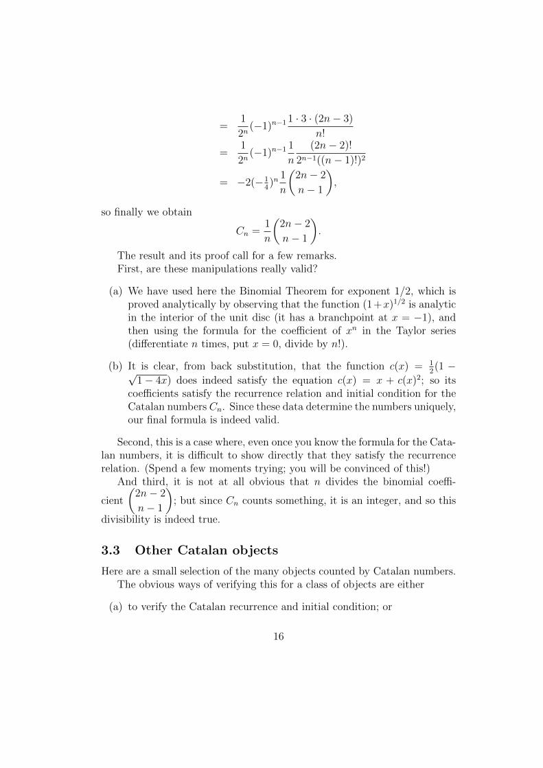
Binary treesA binary tree has a root of degree 2; the other vertices have degree 1 or

3. So every non-root vertex is either a leaf or has two descendants, which wespecify as left and right descendants.

The number of binary trees with n leaves is Cn. Figure 1 shows thecorrespondence with bracketed products: the tree is a “parse tree” for theproduct.

�����

r r r r\\\\\\r r r

(a ◦ (b ◦ (c ◦ d)))

���r r rr r rr

\\\\\ ��

(a ◦ ((b ◦ c) ◦ d))

��\\LL ��LL �� rr rr r r r

((a ◦ b) ◦ (c ◦ d))

\\\

�����\\

rrr rrr r

((a ◦ (b ◦ c)) ◦ d)

\\\\\

rrrr��

���� rrr

(((a ◦ b) ◦ c) ◦ d)

Figure 1: Binary trees and bracketed products

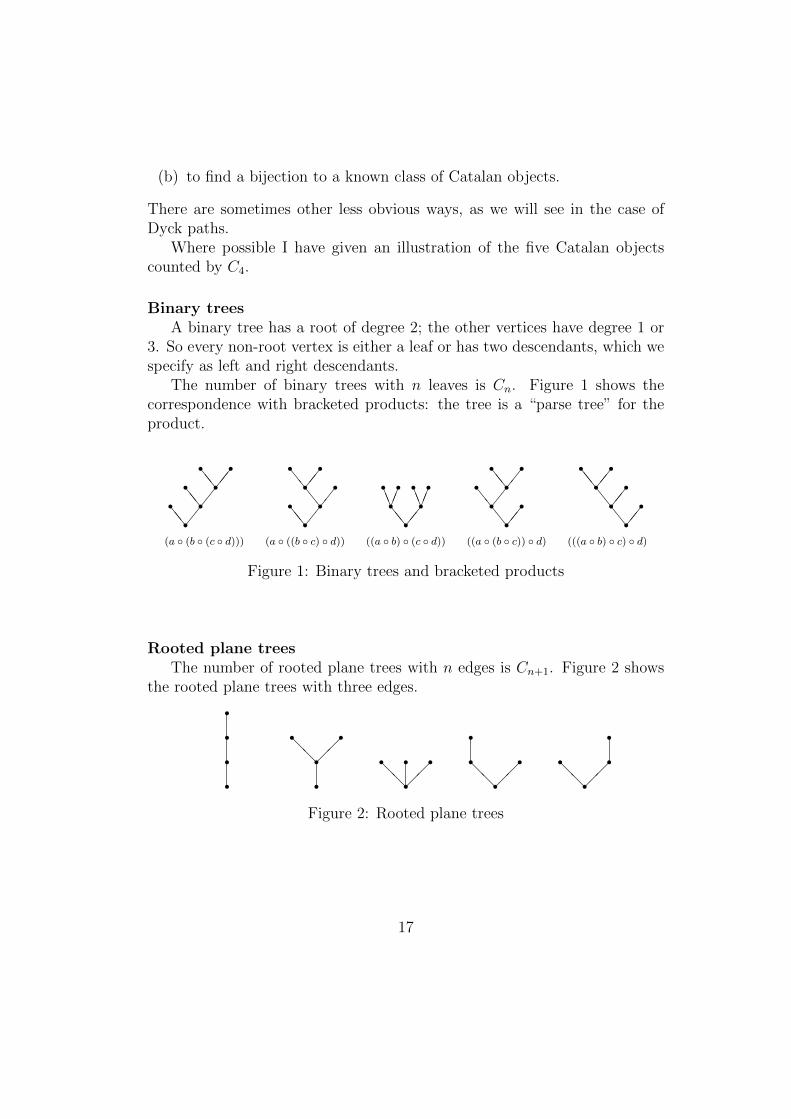
Rooted plane treesThe number of rooted plane trees with n edges is Cn+1. Figure 2 shows

the rooted plane trees with three edges.

rrrr

rr@@��

r rrrr r

@@�� r rrr

@@�� rr rr

@@��

Figure 2: Rooted plane trees

17

Dissections of polygonsAn n-gon can be dissected into triangles by drawing n − 2 non-crossing

diagonals. There are Cn−1 dissections of an n-gon. Figure 3 shows dissectionsof a pentagon.

BBB

���

��ZZ

q qq qq����

���

BBB

���

��ZZ

q qq qq

BBBB

ZZZ

BBB

���

��ZZ

q qq qq���

BBB

���

��ZZ

q qq qq����

BBBB

BBB

���

��ZZ

q qq qqZZZ

Figure 3: Dissections of a polygon

Dyck pathsA Dyck path starts at the origin and ends at (2n, 0), moving at each step

to the adjacent lattice point in either the north-easterly or south-easterlydirection and never going below the X-axis. (An even number of steps isrequired since each step either increases or decreases the Y-coordinate by 1.)

Figure 4 shows the Dyck paths with n = 3.

����

@@

@@q q q q q q qq q q q q q qq q q q q q qq q q q q q q���@@q��@

@@q q q q q q qq q q q q q qq q q q q q qq q q q q q q���@

@@��@@q q q q q q qq q q q q q qq q q q q q qq q q q q q q��@@�

��@

@@q q q q q q qq q q q q q qq q q q q q qq q q q q q q�� �� ��@@ @@ @@q q q q q q qq q q q q q qq q q q q q qq q q q q q q

Figure 4: Dyck paths

The number of Dyck paths is Cn+1, and of these, Cn never return to theX-axis before the end. I will indicate the proof since it illustrates anothertechnique.

Let Dn be the number of Dyck paths, and En the number which neverreturn to the axis. Now a Dyck path begins by moving from (0, 0) to (1, 1)and ends by moving from (2n − 1, 1) to (2n, 0); if it did not return to theaxis in between, then removing these “legs” gives a shorter Dyck path. So

En = Dn−1.

Suppose that a Dyck path first returns to the axis at (2k, 0). Then it is acomposite of a non-returning Dyck path of length 2k with an arbitrary Dyck

18

path of length 2(n− k); so

Dn =n∑k=1

EkDn−k.

Solving these simultaneous recurrences gives the result.

Ballot numbersAn election is held with two candidates A and B, each of whom receives

exactly n votes. In how many ways can the votes be counted so that A isnever behind in the count?

It is easy to match these ballot numbers with Dyck paths. For n = 3, thefive counts are AAABBB, AABABB, AABBAB, ABAABB, and ABABAB.

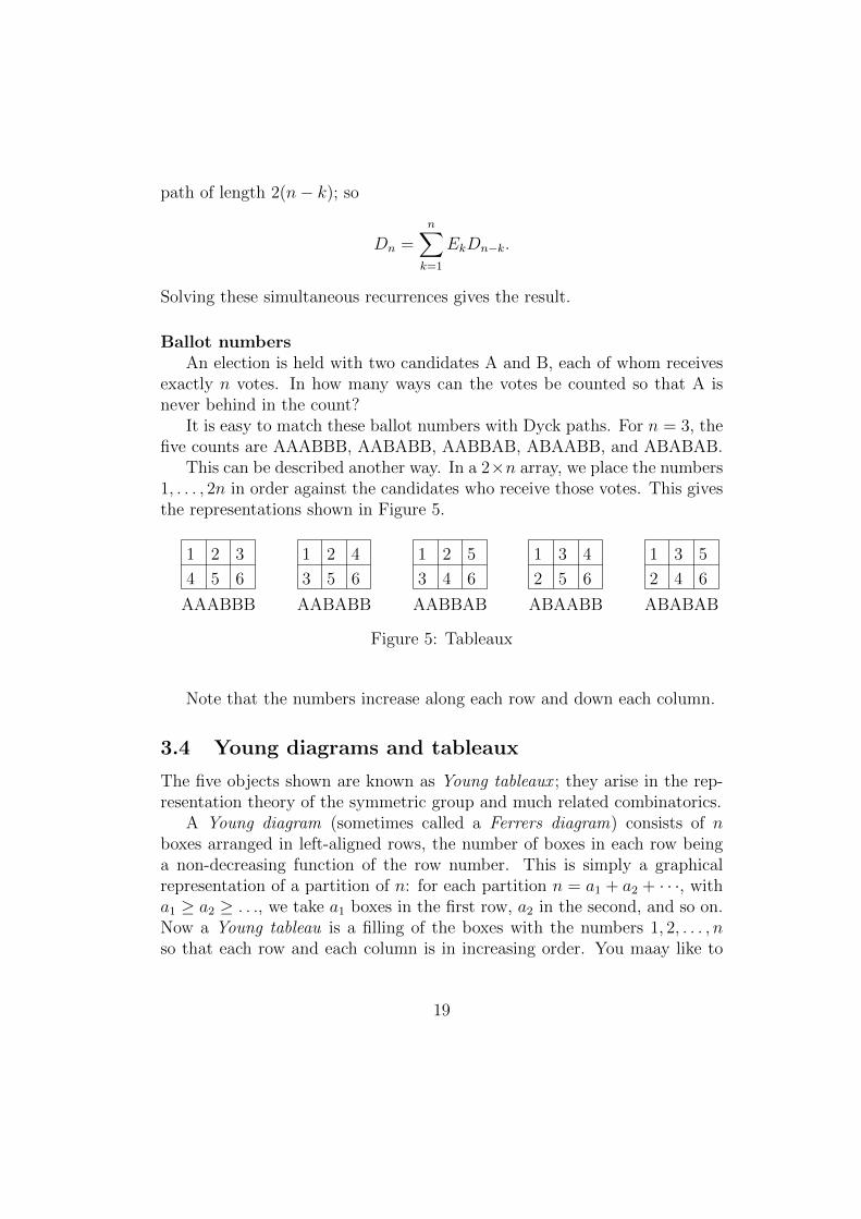
This can be described another way. In a 2×n array, we place the numbers1, . . . , 2n in order against the candidates who receive those votes. This givesthe representations shown in Figure 5.

1 2 3

4 5 6

1 2 4

3 5 6

1 2 5

3 4 6

1 3 4

2 5 6

1 3 5

2 4 6

AAABBB AABABB AABBAB ABAABB ABABAB

Figure 5: Tableaux

Note that the numbers increase along each row and down each column.

3.4 Young diagrams and tableaux

The five objects shown are known as Young tableaux ; they arise in the rep-resentation theory of the symmetric group and much related combinatorics.

A Young diagram (sometimes called a Ferrers diagram) consists of nboxes arranged in left-aligned rows, the number of boxes in each row beinga non-decreasing function of the row number. This is simply a graphicalrepresentation of a partition of n: for each partition n = a1 + a2 + · · ·, witha1 ≥ a2 ≥ . . ., we take a1 boxes in the first row, a2 in the second, and so on.Now a Young tableau is a filling of the boxes with the numbers 1, 2, . . . , nso that each row and each column is in increasing order. You maay like to

19

invent a ballot interpretation for the number of Young tableaux belonging toa given diagram.

This combinatorics is important in describing the representation theoryof the symmetric group Sn, the group of all permutations of {1, . . . , n}. Itis known that the irreducible matrix representations of Sn over the complexnumbers are in one-to-one correspondence with the partitions of n (that is, tothe Young diagrams); the degree of a representation is equal to the numberof Young tableaux belonging to the corresponding diagram. Thus, the fiveYoung tableaux shown in the preceding section correspond to an irreduciblerepresentation of degree 5 of the group S6.

There is a “hook length formula” for the number of Young tableaux cor-responding to a given diagram. The hook associated with a cell consists ofthat cell and all those to its right in the same row or below it in the samecolumn. The hook length of a cell is the number of cells in its hook. Now thenumber of Young tableaux associated with the diagram is equal to n! dividedby the product of the hook lengths of all its cells.

Thus for the diagram with two rows of length 3, the formula gives

6!

4 · 3 · 2 · 3 · 2 · 1= 5.

3.5 Wedderburn–Etherington numbers

What happens if we count binary trees without the left-right distinctionbetween the two children at each node? In other words, two binary trees willcount as “the same” if a sequence of reversals of subtrees above each pointconverts one to the other.

It can be shown that the recurrence relation for the number Wn of binarytrees with this convention (the Wedderburn–Etherington numbers is

Wn =

12

n−1∑i=1

WiWn−i if n is odd,

12

(n−1∑i=1

WiWn−i +Wn/2

)if n is even,

and that the generating function w(x) satisfies

w(x) = x+ 12(w(x)2 + w(x2)).

20

This is much more difficult to solve. Whereas Cn is roughly 4n (in the

sense that the limit of C1/nn as n→∞ is 4), Wn is roughly 2.483 . . .n in the

same sense.

Exercises

1 Give a counting proof of the Vandermonde convolution in the case wherea and b are natural numbers.

2 Verify some of the formulae for Catalan objects in the notes, either byderiving a recurrence, or by finding bijections between the objects counted.

3 In the analysis of Dyck paths, adopt the convention that D0 = 1 andE0 = 0. Prove that, if d(x) and e(x) are the generating functions, then

xd(x) = e(x), d(x) = 1 + e(x)d(x).

Hence derive formulae for Dn and En.

4 Use the hook length formula to derive the formula for the Catalan numberCn.

5 Prove the recurrence relation and the equation for the generating functionfor the Wedderburn–Etherington numbers.

4 Unimodality

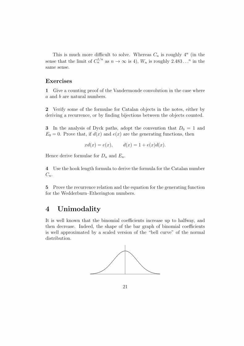
It is well known that the binomial coefficients increase up to halfway, andthen decrease. Indeed, the shape of the bar graph of binomial coefficientsis well approximated by a scaled version of the “bell curve” of the normaldistribution.

. .................. .................. .......... ......... .......... ......... ....................

...........................................................................................

..........................

..........................

.................................................................... .......... ......... ......... .......... .......... ........... ..........

.................. ...................

..........................

..........................

.........................

............

........... ........... ..........................

.........................

.......... .......... ......... .......... .................. ..................

21

This property of binomial coefficients is easily proved. Since(n

k + 1

)=n− kk + 1

(n

k

),

the binomial coefficient increases from k to k + 1, remains constant, or de-creases, according as n − k > k + 1, n − k = k + 1 or n − k < k + 1, thatis, as n is greater than, equal to, or less than 2k + 1. So, if n is even, thebinomial coefficients increase up to k = n/2 and then decrease; if n is odd,the two middle values (k = (n− 1)/2 and k = (n+ 1)/2) are equal, and theyincrease before this point and decrease after.

Other combinatorial numbers also show this unimodality property, butin cases where we don’t have a formula, we need general techniques.

4.1 Unimodality and log-concavity

Given a sequence of positive numbers, say a0, a1, a2, . . . , an, we say that thesequence is unimodal if there is an index m with 0 ≤ m ≤ n such that

a0 ≤ a1 ≤ · · · ≤ am ≥ am+1 ≥ · · · ≥ an.

The sequence a0, a1, a2, . . . , an of positive integers is said to be log-concaveif a2k ≥ ak−1ak+1 for 1 ≤ k ≤ n − 1. The reason for the name is thatthe logarithms of the as are concave: setting bk = log ak, we have 2bk ≤bk−1 + bk+1, or in other words, bk+1− bk ≤ bk − bk−1. So if we plot the points(k, bk) for 0 ≤ k ≤ n, then the slopes of the lines joining consecutive pointsdecrease as k increases, so that the figure they form is concave when viewedfrom above.

Now it is clear that a log-concave sequence is unimodal.A nice general result is:

Theorem 4.1 Let A(x) =n∑k=0

akxk be the generating polynomial for the

numbers a0, . . . , an. Suppose that all the roots of the equation A(x) = 0 arereal and negative. Then the sequence a0, . . . an is log-concave.

Before we begin the proof, we note that a polynomial with all coefficientspositive cannot have a real non-negative root, and a polynomial all of whoseroots are negative has all its coefficients positive.

22

The proof is by induction: there is nothing to prove when n = 1, sinceany sequence of two numbers is log-concave. For n = 2, the condition forthe polynomial a0 + a1x + a2x

2 to have real roots is a21 − 4a0a2 ≥ 0, whichis stronger than log-concavity; as remarked, if the roots are real, they arenegative.

Now we turn to the general case. Suppose that A(x) = (x+c)B(x), wherec > 0 and

B(x) = bn−1xn−1 + · · ·+ b1x+ b0.

Now the polynomial B(x) has all its roots real and negative, since they areall the roots of A(x) except for −c. So the coefficients are all positive, andby the inductive hypothesis, the sequence b0, . . . , bn−1 is log-concave; that is,

b2k ≥ bk−1bk+1

for k = 1, . . . , n − 2. Also, since A(x) = (x + c)B(x), we have a0 = cb0,an = bn−1, and ak = bk−1 + cbk for 1 ≤ k ≤ n− 1.

We first show that bkbk−1 ≥ bk+1bk−2 for 2 ≤ k ≤ n− 2. For we have

b2kbk−1 ≥ bk+1b2k−1 ≥ bk+1bkbk−2;

dividing by bk gives the result.Now for 2 ≤ k ≤ n− 2, we have

a2k − ak+1ak−1 = (bk−1 + cbk)2 − (bk + cbk+1)(bk−2 + cbk−1)

= (b2k−1 − bkbk−2) + c(bk−1bk − bk+1bk−2) + c2(b2k − bk+1bk−1);

and all three terms are non-negative since c > 0.The cases k = 1 and k = n− 1 are left to the reader.

4.2 Binomial coefficients and Stirling numbers

For the binomial coefficients, we have

n∑k=0

(n

k

)xk = (1 + x)n;

all its roots are −1, and so the theorem shows that the binomial coefficientsare log-concave, and hence unimodal.

23

For the unsigned Stirling numbers of the first kind, we have

n∑k=1

u(n, k)xk = x(x+ 1) · · · (x+ n− 1),

and the polynomial on the right has roots 0, −1, −2, . . . , −(n− 1). We canneglect the zero root: the Stirling numbers start at k = 1 rather than zero,and dividing by x simply changes the indexing so that they start at 0. Soagain the Stirling numbers are log-concave and hence unimodal.

The Stirling numbers of the second kind are more difficult, since thereis no convenient form for the generating polynomial. We start with therecurrence relation

S(n, 1) = S(n, n) = 1, S(n, k) = S(n−1, k−1)+kS(n−1, k) for 1 < k < n.

Let

An(x) =n∑k=0

S(n, k)xk.

We have A0(x) = 1. For n > 0, we have A(n, 0) = 0, so zero is a root ofAn(x) = 0. We have to show that the other roots are real and negative.We prove this by induction: P1(x) = x has a single root at x = 0, whileA2(x) = x+ x2 has roots at x = 0 and x = −1; so the induction begins.

From the recurrence relation, we have

An(x) =n∑k=1

S(n, k)xk

=n∑k=1

S(n− 1, k − 1)xk +n∑k=1

kS(n− 1, k)xk

= x (dAn−1(x)/dx+ An−1(x)) .

Putting Bn(x) = An(x)ex, we see that An(x) = 0 and Bn(x) = 0 havethe same roots. The identity above, multiplied by ex, gives

x dBn−1(x)/dx = Bn(x).

By Rolle’s Theorem, there is a root of Bn(x) between each pair of roots ofBn−1(x), and one to the left of the smallest root of Bn−1(x) (since Bn−1(x)→0 as x → −∞); and also a a root at 0. This accounts for (n − 2) + 1 + 1roots, that is, all the roots of Bn(x). So the induction step is complete.

24

Exercises

1 Let S be a fixed set of positive integers, and let rn be the number ofpartitions of n into distinct parts from the set S. What is the generatingpolynomial

∑rnx

n? Is the sequence (rn) unimodal?

2 Let (an) be an infinite sequence of positive numbers which is log-concave(that is, an−1an+1 ≤ a2n for all n ≥ 1). Show that the ratio an+1/an tends toa limit as n→∞.

5 q-analogues

In a sense, a q-analogue of a combinatorial formula is simply another formulainvolving a variable q which has the property that, as q → 1, the secondformula becomes the first. Of course there is more to it than that; someq-analogues are more important than others. What follows is nothing likea complete treatment; I will concentrate on a particularly important case,the Gaussian or q-binomial coefficients, which are, in the above sense, q-analogues of binomial coefficients.

5.1 Definition of Gaussian coefficients

The Gaussian (or q-binomial) coefficient is defined for non-negative integersn and k as [

n

k

]q

=(qn − 1)(qn−1 − 1) · · · (qn−k+1 − 1)

(qk − 1)(qk−1 − 1) · · · (q − 1).

In other words, in the formula for the binomial coefficient, we replace eachfactor r by qr − 1. Note that this is zero if k > n; so we may assume thatk ≤ n.

Now observe that limq→1

qr − 1

q − 1= r. This follows from l’Hopital’s rule: both

numerator and denominator tend to 0, and their derivatives are rqr−1 and 1,whose ratio tends to r. Alternatively, use the fact that

qr − 1

q − 1= 1 + q + · · ·+ qr−1,

and we can now harmlessly substitute q = 1 in the right-hand side; each ofthe r terms becomes 1.

25

Hence if we replace each factor (qr − 1) in the definition of the Gaussiancoefficient by (qr − 1)/(q − 1), then the factors (q − 1) in numerator anddenominator cancel, so the expression is unchanged; and now it is clear that

limq→1

[n

k

]q

=

(n

k

).

5.2 Interpretations

Quantum calculus The letter q stands for “quantum”, and the q-binomialcoefficients do play a role in “quantum calculus” similar to that of the ordi-nary binomial coefficients in ordinary calculus. I will not discuss this further;see the book Quantum Calculus, by V. Kac and P. Cheung, Springer, 2002,for further details.

Vector spaces over finite fields The letter q is also routinely used forthe number of elements in a finite field (which is necessarily a prime power,and indeed there is a unique finite field of any given prime power order q –a theorem of Galois).

Theorem 5.1 Let V be an n-dimensional vector space over a field with q

elements. Then the number of k-dimensional subspaces of v is

[n

k

]q

.

Proof The proof follows the standard proof for binomial coefficients count-ing subsets of a set.

A k-dimensional subspace of V is specified by choosing a basis, a sequenceof k linearly independent vectors. Now the number of choices of the firstvector is qn − 1 (since every vector except the zero vector is eligible); thesecond can be chosen in qn− q ways (since the q multiples of the first vectorare now ineligible); the third in qn−q2 ways (since the q2 linear combinationsof the first two are now ruled out); and so on. In total,

(qn − 1)(qn − q) · · · (qn − qk−1)

choices.We have to divide this by the number of k-tuples of vectors which form

a basis for a given k-dimensional subspace. This number is obtained by

26

replacing n by k in the above formula, that is,

(qk − 1)(qk − q) · · · (qk − qk−1).

Dividing, and cancelling the powers of q, gives the result.

Remark Let F denote a field of q elements. Then a set of k linearlyindependent vectors in F n can be represented as a k × n matrix of rankk. We may put it into reduced echelon form by elementary row operationswithout changing the subspace it spans; and, indeed, any subspace has aunique basis in reduced echelon form. So as a corollary we obtain

Corollary 5.2 The number of k×n matrices over a field of q elements which

are in reduced echelon form is

[n

k

]q

.

As a reminder, a matrix is in reduced echelon form if

(a) the first non-zero entry in any row is a 1 (a leading 1);

(b) the leading 1s occur further to the right in successive rows;

(c) all the other elements in the column of a leading 1 are 0.

This has two consequences. First, it gives us another way of calculatingthe Gaussian coefficients. For example, the 2×4 matrices in reduced echelonform are as follows, where ∗ denotes any element of the field:[

1 0 ∗ ∗0 1 ∗ ∗

],

[1 ∗ 0 ∗0 0 1 ∗

],

[1 ∗ ∗ 00 0 0 1

],[

0 1 0 ∗0 0 1 ∗

],

[0 1 ∗ 00 0 0 1

],

[0 0 1 00 0 0 1

].

So we have[4

2

]q

= q4 + q3 + q2 + q2 + q + 1 = (q2 + 1)(q2 + q + 1).

This expression, and the definition, are polynomials in q, which agree for ev-ery prime power q; so they coincide. In a similar way, any Gaussian coefficientcan be written out as a polynomial.

27

The other consequence is that algebra is not required here. Over anyalphabet of size q, containing two distinguished elements 0 and 1, the numberof k × n matrices in “reduced echelon form” (satisfying (a)–(c) above) with

no zero rows is

[n

k

]q

.

Lattice paths How many lattice paths are there from the origin to thepoint (m,n), where each step in the path moves one unit either north oreast?

Clearly the number is

(m+ n

m

), since we must take m+n steps of which

m are north and n are east, and the northward steps may occur in any m ofthe m+ n positions.

Suppose we want to count the paths by the area under the path (that is,bounded by the X-axis, the line x = m, and the path). We use a generatingfunction approach, so that a path enclosing an area of a units contributesqa to the overall generating function. Here q is simply a formal variable; theanswer is obviously a polynomial in q.

Theorem 5.3 The generating function for lattice paths from (0, 0) to (m,n)

by area under the path is

[m+ n

m

]q

.

We will see why in the next section. Note that, as q → 1, we expect the

formula to tend to

(m+ n

m

).

A non-commutative interpretation Let x and y be elements of a (non-commutative) algebra which satisfy yx = qxy, where the coefficient q is a“scalar” and commutes with x and y. Then we have the following analogueof the Binomial Theorem (see Exercises):

Theorem 5.4

(x+ y)n =∑k=0

n

[n

k

]q

x(n− k)yk.

For example,

(x+ y)3 = xxx+ xxy + xyx+ yxx+ xyy + yxy + yyx+ yyy.

28

We can use the relation to move the y’s to the end in each term; each timewe jump a y over an x we pick up a factor q. So

(x+ y)3 = x3 + (1 + q + q2)x2y + (1 + q + q2)xy2 + y3,

in agreement with the theorem.

5.3 Combinatorial properties

These properties can be proved in two ways: by using the counting inter-pretation involving subspaces of a vector space, or directly from the formula(usually easiest). The proofs are all relatively straightforward; I will just giveoutlines where appropriate.

Proposition 5.5

[n

k

]q

=

[n

n− k

]q

.

This is straightforward from the formula. Alternatively we can invokevector space duality: there is a bijection between subspaces of dimension kof a vector space and their annihilators (subspaces of codimension k of thedual space).

Proposition 5.6

[n

0

]q

=

[n

n

]q

= 1, and

[n

k

]q

=

[n− 1

k − 1

]q

+ qk[n− 1

k

]q

for

0 < k < n.

Again, straightforward from the formula. Alternatively, consider k × nmatrices in reduced echelon. If the leading 1 in the last row is in the lastcolumn, then the other entries in the last row and column are zero, anddeleting them gives a (k−1)× (n−1) matrix in reduced echelon. Otherwise,the last column is arbitrary (so there are qk possibilities for it; deleting itleaves a k × (n− 1) matrix in reduced echelon.

Remark From this we can prove Theorem 5.3, as follows. Let Q(n, k) bethe sum of the weights of lattice paths from (0, 0) to (n − k, k), where theweight of a path is qa if the area below it is a. Clearly Q(n, 0) = Q(n, n) = 1.

Consider all the lattice paths from (0, 0) to (n − k, k), and divide theminto two classes: those in which the last step is vertical, and those in whichit is horizontal. In the first case, the last step is from the end of a path

29

counted by Q(n−1, k−1) (ending at (n−k, k−1)), and adds no area to thepath. In the second step, it is from the end of a path counted by Q(n− 1, k)(ending at (n− k− 1, k)), and increases the area by k, adding qkQ(n− 1, k)to the sum. So the numbers Q(n, k) have the same recurrence and boundaryconditions as the Gaussian coefficients, and must be equal to them.

From the last two results, we can deduce an alternative recurrence:[n

k

]q

= qn−k[n− 1

k − 1

]q

+

[n− 1

k

]q

.

5.4 The q-binomial theorem

The q-analogue of the Binomial Theorem states:

Theorem 5.7 For any positive integer n,n∏i=1

(1 + qi−1z) =n∑k=0

qk(k−1)/2zk[n

k

]q

.

The proof is by induction on n; starting the induction at n = 1 is trivial.Suppose that the result is true for n − 1. For the inductive step, we mustcompute (

n−1∑k=0

qk(k−1)/2zk[n− 1

k

]q

)(1 + qn−1z

).

The coefficient of zk in this expression is

qk(k−1)/2[n− 1

k

]q

+ q(k−1)(k−2)/2+n−1[n− 1

k − 1

]q

= qk(k−1)/2

([n− 1

k

]q

+ qn−k[n− 1

k − 1

]q

)

= qk(k−1)/2[n

k

]q

by the alternative recurrence relation.I state without proof here Heine’s formula, the q-analogue of the negative

binomial theorem:n∏i=1

(1− qi−1z)−1 =∞∑j=0

[n+ j − 1

j

]q

zj.

30

5.5 Jacobi’s Triple Product Identity

This is only loosely connected with the topics of this chapter, but is inter-esting in its own right.

Theorem 5.8 (Jacobi’s Triple Product Identity)∏n>0

(1 + q2n−1z)(1 + q2n−1z−1)(1− q2n) =∑l∈Z

ql2

zl.

The sharp-eyed will notice that the series on the right breaks my rules thatformal Laurent series should have only finitely many negative terms. Well,this just shows that formal power series are more flexible than might firstappear! You can check that the three infinite products on the left contributeonly finitely many terms to each power, positive or negative, of z.

By replacing q by q1/2 and moving the third term in the product to theright-hand side, the identity takes the form

∏n>0

(1 + qn−1/2z)(1 + qn−1/2z−1) =

(∑l∈Z

ql2/2zl

)(∏n>0

(1− qn)−1

),

in which form we will prove it. The proof here is a remarkable argument byRichard Borcherds, and this write-up from my Combinatorics textbook.

A level is a number of the form n + 12, where n is an integer. A state is

a set of levels which contains all but finitely many negative levels and onlyfinitely many positive levels. The state consisting of all the negative levelsand no positive ones is called the vacuum. Given a state S, we define theenergy of S to be∑

{l : l > 0, l ∈ S} −∑{l : l < 0, l 6∈ S},

while the particle number of S is

|{l : l > 0, l ∈ S}| − |{l : l < 0, l 6∈ S}|.

Although it is not necessary for the proof, a word about the backgroundis in order!

Dirac showed that relativistic electrons could have negative as well aspositive energy. Since they jump to a level of lower energy if possible, Dirachypothesised that, in a vacuum, all the negative energy levels are occupied.

31

Since electrons obey the exclusion principle, this prevents further electronsfrom occupying these states. Electrons in negative levels are not detectable.If an electron gains enough energy to jump to a positive level, then it becomes‘visible’; and the ‘hole’ it leaves behind behaves like a particle with the samemass but opposite charge to an electron. (A few years later, positrons werediscovered filling these specifications.) If the vacuum has no net particlesand zero energy, then the energy and particle number of any state should berelative to the vacuum, giving rise to the definitions given.

We show that the coefficient of qmzl on either side of the equation is equalto the number of states with energy m and particle number l. This will provethe identity.

For the left-hand side this is straightforward. A term in the expansionof the product is obtained by selecting qn−

12 z or qn−

12 z−1 from finitely many

factors. These correspond to the presence of an electron in positive leveln− 1

2(contributing n− 1

2to the energy and 1 to the particle number), or a

hole in negative level −(n− 12) (contributing n− 1

2to the energy and −1 to

the particle number). So the coefficient of qmzl is as claimed.The right-hand side is a little harder. Consider first the states with parti-

cle number 0. Any such state can be obtained in a unique way from the vac-uum by moving the electrons in the top k negative levels up by n1, n2, . . . , nk,say, where n1 ≥ n2 ≥ . . . ≥ nk. (The monotonicity is equivalent to the re-quirement that no electron jumps over another. The jumping process allowsthe possibility that some electrons jump from negative levels to higher butstill negative levels, so k is not the number of occupied positive levels.) Theenergy of the state is thus m = n1+ . . .+nk. Thus, the number of states withenergy m and particle number 0 is equal to the number p(m) of partitionsof m, which is the coefficient of qm in P (q) =

∏n>0(1− qn)−1, as we saw in

lecture 1.Now consider states with positive particle number l. There is a unique

ground state, in which all negative levels and the first l positive levels arefilled; its energy is

1

2+

3

2+ . . .+

2l − 1

2=

1

2l2,

and its particle number is l. Any other state with particle number l isobtained from this one by ‘jumping’ electrons up as before; so the number ofsuch states with energy m is p(m − 1

2l2), which is the coefficient of qmzl in

ql2/2zlP (q), as required.

32

The argument for negative particle number is similar.

Exercises

1 Prove that, for fixed n, the Gaussian coefficients are unimodal.

2 For fixed n and k, the Gaussian coefficient

[n

k

]q

is a polynomial in q of

degree k(n− k), whose coefficients a0, . . . , ak(n−k) are non-negative integers.Prove that the coefficients are symmetric: that is, ai = ak(n−k)−i.

Remark It is also true that the coefficients are unimodal, but this is not soeasy to prove. The polynomial does not have all its roots real and negative!

3 Show that, for a, b equal to 0 or 1,

[2m+ a

2l + b

]−1

=

0 if a = 0 and b = 1,(m

l

)otherwise.

Remark For a more challenging exercise, find a formula for

[n

k

]ω

, where

ω is a primitive dth root of unity.

4 Deduce Euler’s Pentagonal Numbers Theorem from Jacobi’s Triple Prod-uct Identity. (Hint : put q = t3/2, z = −t−1/2.)

5 Consider the algebra generated by two non-commuting variables x and ysatisfying the relation yx = qxy. Prove that

(x+ y)n =n∑k=0

[n

k

]q

xn−kyk.

33

6 Symmetric polynomials

A symmetric polynomial in n indeterminates is one which is unchanged underany permutation of the indeterminates. The theory of symmetric polynomialsgoes back to Newton, but more recently has been very closely connected withthe representation theory of the symmetric group, which we glanced at inLecture 3. I will just give a few simple results here. The best reference is IanMacdonald’s book Symmetric Functions and Hall Polynomials.

6.1 Symmetric polynomials

Let x1, . . . , xn be indeterminates. If π is a permutation of {1, . . . , n}, wedenote by iπ the image of i under π. Now a polynomial F (x1, . . . , xn) is asymmetric polynomial if

F (x1π, . . . , xnπ) = F (x1, . . . , xn) for all π ∈ Sn,

where Sn is the symmetric group of degree n (the group of all polynomialsof degree n).

Any polynomial is a linear combination of monomials xa11 · · ·xann , wherea1, . . . , an are non-negative integers. The degree of this monomial is a1+· · ·+an. A polynomial is homogeneous of degree r if every monomial has degreer. Any polynomial can be written as a sum of homogeneous polynomials ofdegrees 1, 2, . . ..

In a homogeneous symmetric polynomial of degree r, the exponents inany monomial form a partition of r into at most n parts; two monomialswhich give rise to the same partition are equivalent under a permutation,and so must have the same coefficient. Thus, the dimension of the spaceof homogeneous symmetric polynomials of degree r is pn(r), the number ofpartitions of r with at most n parts.

There are three especially important symmetric polynomials:

(a) The elementary symmetric polynomial er, which is the sum of all themonomials consisting of products of r distinct indeterminates. Note

that there are

(n

r

)monomials in the sum.

(b) The complete symmetric polynomial hr, which is the sum of all the

monomials of degree r. There are

(n+ r − 1

r

)terms in the sum: the

proof of this is given in the Appendix to these notes.

34

(c) The power sum polynomial pr, which is simplyn∑i=1

xri .

For example, if n = 3 and r = 2,

(a) the elementary symmetric polynomial is x1x2 + x2x3 + x1x3;

(b) the complete symmetric polynomial is x1x2+x2x3+x1x3+x21+x22+x23;

(c) the power sum polynomial is x21 + x22 + x23.

Note that er(1, . . . , n) =

(n

r

), hr(1, . . . , 1) =

(n+ r − 1

r

), and pr(1, . . . , 1) =

n.Also, the q-binomial theorem that we met in the last lecture shows that

er(1, q, q2, . . . , qn−1) = qr(r−1)/2

[n

r

]q

,

and Heine’s formula shows that, similarly,

hr(1, q, q2, . . . , qn−1) =

[n+ r − 1

r

]q

.

6.2 Generating functions

The best-known occurrence of the elementary symmetric polynomials is theconnection with the roots of polynomials. (To avoid conflict with xi, thevariable in a polynomial is t in this section.) The coefficient of tn−r in apolynomial of degree n is (−1)rer(a1, . . . , an), where a1, . . . , an are the roots.This is because the polynomial can be written as

(t− a1)(t− a2) · · · (t− an),

and the term in tn−r is formed by choosing t from n − r of the factors and−ai from the remaining r.

Said otherwise, and putting xi = −1/ai, this says that the generatingfunction for the elementary symmetric polynomials is

E(t) =n∑r=0

er(x1, . . . , xn)tr =n∏i=1

(1 + xit),

35

with the convention that e0 = 1.In a similar way, the generating function for the complete symmetric

polynomials is

H(t) =∑r≥0

hr(x1, . . . , xn)tr =n∏i=1

(1− xit)−1.

We also take P (t) to be the generating function for the power sum polyno-mials, with a shift:

P (t) =∑r≥1

pr(x1, . . . , xn)tr−1.

Now we see that H(t) = E(−t)−1, so that

n∑r=0

(−1)r3rhn−r = 0 for n ≥ 1.

For P (t), we have

d

dtH(t) = P (t)H(t),

d

dtE(t) = P (−t)E(t).

6.3 Functions indexed by partitions

We extend the definitions of symmetric polynomials as follows. Let λ =(a1, a2, . . .) be a partition of r, a non-decreasing sequence of integers withsum r. Then, if z denotes one of the symbols e, h or p, we define zλ to be theproduct of zai over all the parts ai of λ; this is again a symmetric polynomialof degree r. For example, if n = 3 and λ is the partition (2, 1) of 3, we have

eλ = (x1x2 + x1x3 + x2x3)(x1 + x2 + x3),

pλ = (x21 + x22 + x23)(x1 + x2 + x3),

hλ = eλ + pλ.

We also define the basic polynomial mλ to be the sum of all monomials withexponents a1, a2, . . .. In the above case,

mλ = x21x2 + x21x3 + x22x1 + x22x3 + x23x1 + x23x2.

36

Theorem 6.1 If n ≥ r, and z is one of the symbols m, e, h, p, then anysymmetric polynomial of degree r can be written uniquely as a linear com-bination of the polynomials zλ, as λ runs over all partitions. Moreover, inall cases except z = p, if the polynomial has integer coefficients, then it is alinear combination with integer coefficients.

So the polynomials er or hr, with r ≤ n, are generators of the ring ofsymmetric polynomials in n variables with integer coefficients. For z = e,this is a version of Newton’s Theorem on symmetric polynomials (which,however, applies also to rational functions).

6.4 Appendix: Selections with repetition

Theorem 6.2 The number of n-tuples of non-negative integers with sum r

is

(n+ r − 1

r

).

The claim about the number of monomials of degree r follows immediatelyfrom this result, which should be contrasted with the fact that the number

of n-tuples of zeros and ones with sum r is

(n

r

).

Proof We can describe any such n-tuple in the following way. Take a lineof n + r − 1 boxes. Then choose n − 1 boxes, and place barriers in theseboxes. Let

(a) a1 be the number of empty boxes before the first barrier;

(b) a2 be the number of empty boxes between the first and second barriers;

(c) . . .

(d) an be the number of empty boxes after the last barrier.

Then a1, . . . , an are non-negative integers with sum r. Conversely, given nnon-negative integers with sum r, we can represent it with n− 1 barriers inn+ r− 1 boxes: place the first barrier after a1 empty boxes, the second aftera2 further empty boxes, and so on.

So the required number of n-tuples is equal to the number of ways toposition n− 1 barriers in n+ r − 1 boxes, which is(

n+ r − 1

n− 1

)=

(n+ r − 1

r

),

37

as required.

7 Group actions

How many ways can you colour the faces of a cube with three colours? Clearlythe answer is 36 = 729. But what if we regard two colourings as the sameif one can be transformed into the other by a rotation of the cube? This istypical of the problems we consider in this chapter.

7.1 The Orbit-Counting Lemma

This chapter of the lectures, unlike most of the others, requires some technicalbackground. I assume that you know the definition of a group. I will runbriefly through the theory of group actions, and finally reach the Orbit-Counting Lemma, which solves our introductory problem.

Throughout this section, permutations act “on the right”, that is, theeffect of applying a permutation π to an element x of the domain is writtenxπ. This is not just a matter of notation; it entails the fact that the productπ1π2 of two permutations is calculated by the rule “first π1, then π2”, ratherthan the other way round. This ensures that x(π1π2) = (xπ1)π2 for allelements x.

An action of a group G on a set X is a map associating to each groupelement g ∈ G a permutation πg of X in such a way that the following twoconditions hold:

(a) πgh = πgπh for all g, h ∈ G (that is, xπgh = xπgπh for all g, h ∈ G andall x ∈ X);

(b) if 1 denotes the identity element of G, then π1 is the identity permuta-tion (that is, xπ1 = x for all x ∈ X).

Usually we simplify notation by not distinguishing between g and πg, writingsimply xg instead of xπg. From a different point of view, an action is ahomomorphism from the group G to the symmetric group of all permutationsof X.

Two elements x, y ∈ X are equivalent under the action if there exists anelement g ∈ G such that xg = y. It is routine to show that this is really anequivalence relation; its equivalence classes are called orbits, and the actionis transitive if there is just one orbit. Thus we have a first structure theorem:

38

any action can be split uniquely into transitive actions on the sets of theorbit partition of the domain.

In our motivating problem, the group G of 24 rotations of the cube actson the set X of 729 coloured cubes, and we want to count the orbits. So ourimmediate goal is to count the orbits in an arbitrary action.

If H is a subgroup of G, then there is a natural partition of G into rightcosets Hx of H, for x ∈ G. Lagrange’s Theorem assures us that each cosethas the same cardinality, so the number of cosets is equal to |G|/|H|. Wedenote the set of right cosets of H in G by cos(H,G). Now there is an actionof G on the set cos(H,G): the group element g induces the permutationHx 7→ H(xg). At risk of some confusion, we write this as (Hx)g = H(xg).

Now, given any transitive action of G on a set X, and x ∈ X, the set

{g ∈ G : xg = x}

is a subgroup of H, called the stabiliser of x, and denoted by StabG(x). Nowthere is a natural bijection between X and cos(H,G), where the elementy ∈ X corresponds to the set

{g ∈ G : xg = y}

(it is easily checked that this is a coset of H). This bijection also respectsthe action of G: if z ∈ G satisfies yg = z, and Hk and Hl are the cosetscorresponding to y and z, then (Hk)g = (Hl).

So the so-called “coset spaces” of subgroups of G give a complete list oftransitive actions of G, up to a natural notion of isomorphism of actions.

Note in addition that any two points in the same orbit have stabilisers ofthe same order. (The stabilisers are in fact conjugate subgroups of G.)

In an arbitrary action of G on X, we let fixX(g) denote the number ofpoints of X which are fixed by the permutation g. Now we can state theOrbit-Counting Lemma, the foundation of enumeration under group action.

Theorem 7.1 Let G act on the finite set X. Then the number of G-orbitsin X is equal to the average number of fixed points of elements of G, that is,

1

|G|∑g∈G

fixX(g).

The theorem has a probabilistic interpretation. Choose a random elementof G (from the uniform distribution). Then its expected number of fixedpoints is equal to the number of orbits of G.

39

Proof Construct a bipartite graph as follows. The vertices are of two types:the elements of X, and the elements of G. There is an edge from x to g ifxg = x. We count the number of edges in two different ways.

Each vertex g lies in fixX(g) edges; so the number of edges is∑g∈G

fixX(g).

Now we count the other way. Take a point x ∈ X. The number of edgescontaining it is | StabG(x)|. This value is the same for all the points in theorbit OG(x) containing x. So the number of edges containing points in theorbit is | StabG(x)| · |OG(x)| = |G|. Since each orbit contributes |G| edges,the number of orbits is obtained by dividing the number of edges by |G|, asclaimed.

Now consider the coloured cubes. In order to do the calculations, we needto classify the elements of the group G of rotations of the cube (a group oforder 24). They are of the following types:

(a) the identity;

(b) “face rotations” (about an axis through two opposite face centres)through ±π/2 (six of these, two for each pair of opposite faces);

(c) “face rotations” through π (three of these);

(d) “edge rotations” (about an axis through two opposite edge midpoints)through π (six of these);

(e) “vertex rotations” (about an axis through two opposite vertices) through±2π/3 (eight of these, two for each pair of opposite vertices).

For each type of rotation, we have to count the number of coloured cubes itfixes. A cube will be fixed if faces in the same cycle of the permutation havethe same colour. So the answer will be 3c, where c is the number of cyclesof the permutation on faces. For the five types listed above the numbers ofcycles are 6 (each single face is a cycle), 3 (for the vertical axis, the top andbottom faces, and the other four in a single cycle), 4 (as the previous exceptthat the 4-cycle splits into two 2-cycles), 3 (the faces are permuted in cyclesof two), and 2 (the faces are permuted in cycles of three). So the calculationof the theorem is:

1

24(36 + 6 · 33 + 3 · 34 + 6 · 33 + 8 · 32) = 57.

40

7.2 Labelled and unlabelled

Many combinatorial objects that we want to count are based on an underlyingset, which we usually assume to be the set {1, 2, . . . , n}. Very often thesimplest method of counting gives us the total number of objects that canbe built on this set. But we may be completely uninterested in the labels1, 2, . . . , n, and want to count two objects as being the same if there are somelabellings of the underlying set that make them identical.

We distinguish these two problems as counting labelled and unlabelledobjects.

Counting unlabelled objects is thus an orbit-counting problem: we wantto know the number of orbits of the symmetric group Sn, acting on theobjects in question by permuting the labels.

To take an extreme case: there are

(n

k

)labelled k-element subsets of an

n-element set, but there is only one unlabelled subset. Here are a few moreexamples.

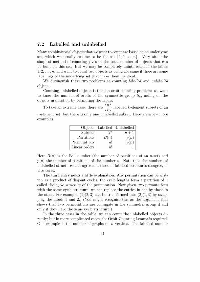
Objects Labelled UnlabelledSubsets 2n n+ 1

Partitions B(n) p(n)Permutations n! p(n)Linear orders n! 1

Here B(n) is the Bell number (the number of partitions of an n-set) andp(n) the number of partitions of the number n. Note that the numbers ofunlabelled structures can agree and those of labelled structures disagree, orvice versa.

The third entry needs a little explanation. Any permutation can be writ-ten as a product of disjoint cycles; the cycle lengths form a partition of ncalled the cycle structure of the permutation. Now given two permutationswith the same cycle structure, we can replace the entries in one by those inthe other. For example, (1)(2, 3) can be transformed into (2)(1, 3) by swap-ping the labels 1 and 2. (You might recognise this as the argument thatshows that two permutations are conjugate in the symmetric group if andonly if they have the same cycle structure.)

In the three cases in the table, we can count the unlabelled objects di-rectly; but in more complicated cases, the Orbit-Counting Lemma is required.One example is the number of graphs on n vertices. The labelled number

41

is 2n(n−1)/2, since for each of the n(n − 1)/2 pairs of vertices we can choosewhether to join it by an edge or not; but the only way to calculate the nuberof unlabelled graphs is via the Orbit-Counting Lemma.

7.3 Cycle index

There is a way to “mechanise” the counting in many important cases, whichwe now discuss. This was introduced by Redfield and, independently, byPolya, and refined by de Bruijn and others. (Incidentally, these early work-ers found the Orbit-Counting Lemma in Burnside’s group theory book, andcalled it “Burnside’s Lemma”, a name which is still sometimes used. How-ever, the result is due to Frobenius, and earlier to Cauchy in a special case.)

The set-up is as follows. We have a set X on which a group G acts. Weare going to decorate X by placing one of a set of “figures” at each point.Each figure has a weight, which is a non-negative integer. We don’t requirethe number of figures to be finite, but we ask that there should be onlyfinitely many figures of any given weight. The figures can thus be countedby the figure-counting series

A(x) =∑n≥0

anxn,

where an is the number of figures of weight n.Now one of the configurations we want to count consists of the set X with

a figure at each point; this can be described by a function from X to the setof figures. Such a function f will have a weight, given by w(f) =

∑{w(x) :

x ∈ X}. There are only finitely many functions of any given weight, and theaction of the group G preserves weight; so we can let bn be the number offunctions of weight n, and define the function-counting series

B(x) =∑n≥0

bnxn.

The final ingredient is the cycle index polynomial Z(G), defined as

Z(G) =1

|G|∑g∈G

sc1(g)1 s

c2(g)2 · · · scn(g)n .

Here s1, . . . , sn are indeterminates, and ci(g) is the number of cycles of lengthi in the cycle decomposition of g, for i = 1, . . . , n.

Now the Cycle Index Theorem states:

42

Theorem 7.2

B(x) = Z(G; si ← A(xi) for i = 1, . . . , n).

The notation on the right means that we substitute A(xi) for si, fori = 1, . . . , n.

I won’t prove the theorem here – it follows from the Orbit-CountingLemma with a certain amount of ingenuity – but will conclude with a simpleapplication which doesn’t even hint at the uses of the theorem.

First, let us calculate the cycle index of the rotation group of the cube.The five types of elements mentioned earlier have the following cycle struc-tures in their action on faces:

(a) Identity: (1, 1, 1, 1, 1, 1) (usually abbreviated to 16).

(b) Face rotations through ±π/2: 124.

(c) Face rotations through π: 1222.

(d) Edge rotations: 23.

(e) Vertex rotations: 32.

So the cycle index is

Z(G) =1

24(s61 + 6s21s4 + 3s21s

22 + 6s32 + 8s23).

Now any counting problem for which we can write a figure-counting seriescan be solved by substitution. For example:

(a) Take each of the three colours to be a figure of weight 0. The figure-counting series is simply 3. We recover our earlier count.

(b) Take one of the colours (say red) to have weight 1, and all the othersweight 0. The figure-counting series is x + 2. So substituting xi + 2for si gives a polynomial in which the coefficient of xk is the number oftypes of cube which have exactly k red faces.

(c) A small extension of the Cycle Index Theorem shows that, if we sub-stitute pi(x, y, z) = xi+yi+ zi for si, we obtain a trivariate polynomialin which the coefficient of xiyjzk is the number of cubes with i red, jblue, and k green faces.

(d) The generalisation to an arbitrary number of colours is now routine.

43

Exercises

1 Perform the calcuations in the four counting problems above.

2 A necklace has ten beads, each of which is either black or white, arrangedon a loop of string. A cyclic permutation of the beads counts as the samenecklace. How many necklaces are there?

How many are there if the necklace obtained by turning over the givenone is regarded as the same?

3 Let G be a permutation group on a set X, where |X| = n.For 0 ≤ i ≤ n, let pi be the proportion of elements of G which have

exactly i fixed points on X, and let p(x) =∑pix

i be the generating functionfor these numbers (the probability generating function for fixed points).

For 0 ≤ i ≤ n, let Fi be the number of orbits of G in its action on the setof i-tuples of distinct elements of X, and let

F (x) =∑ Fix

i

i!

be the exponential generating function for these numbers.Use the Orbit-counting Lemma to show that

F (x) = P (x+ 1)

and deduce that the proportion of fixed-point-free elements in G is p0 =F (−1).

Taking G to be the symmetric group Sn, show that the number of fixed-point-free permutations (the derangement number) is

n!n∑k=0

(−1)k

k!.

Deduce that this number is the closest integer to n!/e.

4 Consider the set of all functions from {1, . . . , n} to {1, . . . ,m}. Thereare mn functions in the set. Now let the symmetric group Sn act on thesefunctions by permuting their arguments: (fπ)(x) = f(xπ−1). [Incidentally,the inverse is there to make this an action – can you see why?]

44

Show that orbits correspond to m-tuples of non-negative integers with

sum n, so that the number of orbits is

(m+ n− 1

n

). (See the Appendix in

Lecture Notes 7.)Show that a permutation g with k cycles fixes mk functions. Hence use

the Orbit-Counting Lemma to show that

1

n!

n∑k=1

u(n, k)mk =

(m+ n− 1

n

).

Show that we can replace m by an indeterminate x and multiply by n! to getthe identity

n∑k=1

u(n, k)xk = x(x+ 1) · · · (x+ n− 1),

from which some sign changes yield

n∑k=1

s(n, k)xk = x(x− 1) · · · (x− n+ 1),

a formula we met in Section 1. (Here s(n, k) and u(n, k) are the signed andunsigned Stirling numbers of the first kind.)

8 Species

In this lecture I will discuss a very nice unifying principle for a number oftopics in enumerative combinatorics, the theory of species, introduced byAndre Joyal in 1981. Species have been used in areas ranging from infinitepermutation groups to statistical mechanics, and I can’t do more here thanbarely scratch the surface.

Joyal gave a category-theoretic definition of species; I will take a moreinformal approach.

There is a book on species, by Bergeron, Labelle and Leroux, entitledCombinatorial Species and Tree-Like Structures ; but I think that Joyal’soriginal paper in Advances in Mathematics is hard to beat.

45

8.1 What is a species?

As I said earlier, a typical combinatorial structure of the type we wish tocount is often built on a finite set; we are interested in counting labelledstructures (the different structures built on a fixed set) and also the unla-belled structures (essentially the isomorphism types of structures).

A species is a functor F (this word is used by Joyal in its technical sensefrom category theory; I will be less formal but will explain what is going on)which takes an n-element set and produces the set of objects in which weare interested; it should also have the property that the functor transformsany bijection between n-element sets A and B to a bijection between the setsF(A) and F(B) of objects built on these sets. Because of this condition, wecan use the standard n-element set {1, 2, . . . , n}, but don’t have to worry ifduring the argument we have a non-standard set (such as a proper subset ofthe standard set).

Joyal’s intuition is that we think of a formal power series where the coef-ficients are not numbers, but sets of combinatorial objects:

F =∑n≥0

F ({1, 2, . . . , n})xn.

Suitable specialisations will give us the generating functions for unlabelledand unlabelled objects.

The first specialisation is to replace the set F(A) by the sum of the cycleindices of the automorphism groups of the unlabelled structures in F(A):let us call this Z(F). This will be a formal power series in infinitely manyvariables s1, s2, . . .. Now it turns out that the specialisations

f(x) = Z(F; sn ← xn for all n),

F (x) = Z(F; s1 ← x, xn ← 0 for n > 1),

give us, respectively, the ordinary generating function for the unlabelledstructures in the species F, and the exponential generating function for thelabelled structures.

8.2 Examples

If this is a bit abstract, hopefully some examples will bring it back to earth.

46

Sets Let Set denote the “identity” species, where the structure on the finiteset A is simply a labelling of A. Thus, for each n, there is one unlabelledsrtucture, and one labelled structure. So the generating functions are

set(x) =∑n≥0

xn =1

1− x,

Set(x) =∑n≥0

xn

n!= exp(x)

respectively.The cycle index of the species Set can be computed as follows. First,

Z(Sn) =1

n!

∑ n!

1a1 · · ·nana1! · · · an!sa11 · · · sann ,

where the sum is over all partitions of n having ai parts of size i for i =1, 2, . . . , n (the coefficient is the number of permutations with this cycle struc-ture). Summing this over all n seems a formidable task, but a remarkablesimplification occurs: since n! cancels we can sum over the variables a1, . . . , anindependently. We obtain

Z(Set) = exp

(∑i≥1

(sii

)).

Now substituting X i for si for all i gives

set(x) = exp

(∑i≥1

(xi

i

))= exp(− log(1− x))

=1

1− x,

Set(x) = exp(x),

as expected.Note that the formula for the sum of the cycle indices of the symmetric

groups was known in the combinatorial enumeration community before Joyalprovided it with this nice interpretation.

47

Linear orders A much easier case is the species Lin of linear (or total)orders. There are n! labelled linear orders on n points; all are isomorphic,and there are no non-trivial automorphisms, so we have

Z(Lin) =∑n≥0

sn1 =1

1− s1,

from which the generating functions are lin(x) = Lin(x) = 1/(1− x).

8.3 Operations on species

There are three important ways that we can add two species F and G.

Sum F + G is the species which constructs on the set A all the F-objectsand all the G-objects (we assume these two classes to be disjoint). Clearly thecycle index and the generating functions for unlabelled and labelled objectsare simply obtained by adding those for F and G.

Product F · /mathbfG is the species whose objects on a set A are con-structed in the following way: partition A into two (possibly empty) partsB and C; put an F -object on B, and a G-object on C. A slightly hardercalculation shows that the cycle index, and hence the generating functionsfor unlabelled and labelled objects, are obtained by multiplying those for Fand G.

Here is an example. What is Set2? Given a set A, we partition it intoa subset B and its complement A \ B. So we can regard this as the speciesSubset. The numbers of unlabelled and labelled objects in this species onn points are n+ 1 and 2n respectively, and their generating functions are (asexpected) 1/(1− x)2 and exp(2x).

Substitution As with power series in general, there is a formal restrictionon substitution: we can only substitute G into F provided that G(∅) = ∅. Ifthis condition holds, then we define F[G]-objects on A as follows: partitionA (into non-empty parts); put a G-structure on each part; and put a F-structure on the set of parts.

The cycle index is given by substituting the cycle index of G into that ofF in the following way:

Z(F[G]) = Z(F : sn ← Z(G, sm ← snm)).

48

In other words, for the indeterminate sn in Z(F, we substitute the cycleindex of G but in the indeterminates sn, s2n, . . . in place of s1, s2, . . ..

The effect on the generating functions for labelled objects is simple sub-stitution: F [G](x) = F (G(x)). For unlabelled objects it is a bit more com-plicated, we need the cycle index for F:

fg(x) = Z(F; sn ← g(xn) for all n).

For example, let Set∗ be the species of non-empty sets. Then the e.g.f.for labelled objects is Set∗(x) = exp(x)− 1. Now Set[Set∗] is the species ofset partitions, where the labelled objects are counted by the Bell numbers:the exponential generaing function is thus exp(exp(x)−1), as we saw earlier.As an exercise, obtain the ordinary generating function for partitions of theinteger n from this approach.

Remark The fact that substituting a species into Set exponentiates thegenerating function for labelled structures is sometimes called the exponentialprinciple in enumerative combinatorics. We see that substitution of speciesis much more general.

Rooted structures This means structures where one point is distinguished.It can be shown that the effect of rooting a species is to apply the operator

s1∂

∂s1to the cycle index, and hence to apply the operator x d/dx to the

generating function for labelled structures. I will denote the operation ofrooting a species by R, and the operation of rooting and then removing theroot (i.e., deleting a point) by D: this just corresponds to differentiation.

There are many other nice examples, some of which are described in theexercises.

8.4 Exercises

1 Define the species Circ of circular orders and the species Perm of per-mutations, and calculate the generating functions for unlabelled and labelledobjects in these species.

Show that

Z(Circ) = −∑m≥1

φ(m)

mlog(1− sm),

49

where φ is Euler’s totient function.Use the decomposition of permutations into disjoint cycles to show that

Set[Circ] = Perm,

and verify the appropriate identities for the generating functions.

Remark It is not so easy to calculate the cycle index of Perm directly,but using the above expression it is not too hard to show that

Z(Perm) =∏n≥1

(1− sn)−1.

2 Use the fact that Catalan objects are rooted binary trees to show thatthe species Cat of Catalan objects satisfies

Cat = E + Cat2,

where E denotes the species of singleton sets (that is, it returns its input ifthis has cardinality 1, and the empty set otherwise).

Show similarly that the species W of rooted binary trees without the left-right distinction (counted by Wedderburn–Etherington numbers) satisfies

W = E + Set2[W],

where Set2 is the species of 2-element sets.

3 Let F denote the species of “1-factors” or partitions of a set into subsetsof size 2. Show that

D(F) = E · F,F = Set[Set2].

Use each of these equations to show that the exponential generating functionfor labelled 1-factors is exp(x2/2).

4 Let Graph and ConnGraph be the species of graphs and connectedgraphs respectively. (Here, assume that a connected graph has at least onevertex.) Show that

Graph = Set[ConnGraph].

(It follows from this that the e.g.f. for connected graphs is the logarithm ofthe e.g.f. for graphs.)

50

9 Mobius inversion

In this section we will discuss the Inclusion-Exclusion principle, with a fewapplications (including a formula for the chromatic polynomial of a graph),and then consider a wide generalisation of it due to Gian-Carlo Rota, involv-ing the Mobius function of a partially ordered set. The q-binomial theoremgives a simple formula for the Mobius function of the lattice of subspaces ofa vector space.

9.1 Inclusion-Exclusion

The Inclusion-Exclusion Principle is one of the most familiar results in com-binatorics. For two sets A and B, it asserts simply that |A ∪ B| = |A| +|B| − |A ∩ B|. For the general case, we need some notation. Let A1, . . . , Anbe subsets of a finite set S. For any subset I of the index set {1, 2, . . . , n, we

let AI =⋂i∈I

Ai. By convention, we take A∅ = S.

Theorem 9.1 The number of elements lying in none of the sets A1, . . . , Anis ∑

I⊆{1,...,n}

(−1)|I||AI |.

Proof We count the contribution of each element s ∈ S to the sum in theabove formula.

If s lies in none of the sets Ai then it is counted once in the term A∅ andin none of the others.

Suppose that J = {i : s ∈ Ai} 6= ∅. Then the terms to which s contributescome from sets AI with I ⊆ J , and the contribution is∑

I⊆J

(−1)|I| =

j∑k=0

(j

k

)(−1)k = (1− 1)j = 0,

where j = |J |. �

Corollary 9.2 Suppose that the family of sets has the property that, if |I| =i, then |AI | = mi. Then the number of points lying in none of the sets is

n∑i=0

(−1)i(n

i

)mi.

51

9.2 Applications

We begin with two standard applications of the Corollary. First, a formulafor the Stirling numbers of the second kind.

Theorem 9.3 The number of surjective functions from an m-set to an n-setis

n∑i=0

(−1)i(n

i

)(n− i)m.

Proof Let S be the set of all functions from M to N , where |M | = m and|N | = n, say N = {1, . . . , n}. Let Ai be the set of functions which do nottake the value i. Then a function is surjective if and only if it lies in none ofthe sets Ai.

If |I| = i, then AI consists of functions which take values in the set{1, . . . , n} \ I; there are (n − i)m such functions. So the theorem followsimmediately from Corollary 9.2. �

Corollary 9.4

S(m,n) =1

n!

n∑i=0

(−1)i(n

i

)(n− i)m.

Proof We can describe a surjective function as follows: choose a partitionof the domain into n parts (we can do this in S(m,n) ways, by definitionof the Stirling number); then assign each part to a point of the codomain(which can be done in n! ways). So n!S(m,n) is the number of surjectivefunctions. �

The second application concerns derangements : these are permutationsof {1, . . . , n} with no fixed points.

Theorem 9.5 The number of derangements of {1, . . . , n} is given by theformula

dn = n!n∑i=0

(−1)i

i!.

52

Proof Let S be the set of all permutations, and Ai the set of permutationswhich fix the element i ∈ {1, . . . , n}. Then a permutation is a derangementif and only if it lies in no set Ai. The permutations in AI fix every point inthe set I, so there are (n− i)! of them if |I| = i. Thus Corollary 9.2 gives

dn =n∑i=0

(−1)i(n

i

)(n− i)! = n!

n∑i=0

(−1)i

i!.

as claimed. �

The summation here is the partial sum of the series for e−1, so dn isapproximately n!/e. Indeed, it is easy to show that it is the nearest integerto n!/e.

The “secretary problem” asks: a secretary puts n letters into n addressedenvelopes at random: what is the probability that no letter is correctly ad-dressed? The answer is very close to 1/e, perhaps a little surprising at firstsight.

For our final application we consider graphs. A graph consists of a set Vof vertices and a set E of edges, each edge being a 2-element set of vertices.Given a set of q colours, a colouring of the graph is an assignment of coloursto the vertices; it is proper if the two vertices in each edge have differentcolours.

Theorem 9.6 For any graph G = (V,E), there is a polynomial PG(x) suchthat, for any natural number q, PG(q) is the number of proper colourings ofG with q colours. Moreover, PG is a monic polynomial with degree n = |V |.

This is usually proved by operations on the graph (“deletion” and “con-traction”. The Inclusion-Exclusion proof here provides a formula.

Proof Let S be the set of all colourings of G with q colours. For each edge e,let Ae be the set of colourings for which the edge e is “improperly coloured”,that is, its vertices have the same colour. A colouring is proper if it lies inno set Ae. Given a set I ⊆ E, how many colourings lie in AI? Consider thegraph (V, I) with edge set I. A colouring in Ai assigns the same colour toall vertices in the same connected component of this graph; so |AI | = qc(I),where c(I) is the number of connected components of (V, I).

53

By Theorem 9.1, the number of proper colourings is∑I⊆E

(−1)|I|qc(I).

It is clear that this is a polynomial in q; the leading term comes from theunique graph (V, I) with n connected components, namely I = ∅. �

This formula shows a connection between graph colouring and the Pottsmodel in statistical mechanics, but we cannot pursue this here.

9.3 The Mobius function of a poset

A poset, or partially ordered set, consists of a set A with a relation ≤ on Awhich is

(a) reflexive: a ≤ a for all a ∈ A;

(b) antisymmetric: a ≤ b and B ≤ a imply a = b, for all a, b ∈ A;

(c) transitive: a ≤ b and b ≤ c imply a ≤ c, for all a, b, c ∈ A.

An important combinatorial example consists of the case where A is the setof all subsets of a finite set S, and a ≤ b means that a is a subset of b. Itturns out that the Inclusion-Exclusion principle can be formulated in termsof this poset, and then generalised so as to apply to any poset.

We begin with an observation which will not be proved here.

Theorem 9.7 Let P = (A,≤) be a finite poset. Then we can label theelements of A as a1, a2, . . . , an such that, if ai ≤ aj, then i ≤ j.

This is sometimes stated “Every poset has a linear extension”. The anal-ogous result for infinite posets requires a weak form of the Axiom of Choicein its proof.

Now let P = (A,≤) be a poset. We define the incidence algebra of P asfollows: the elements are all functions f : A × A → R such that f(a, b) = 0unless a ≤ b. Addition and scalar multiplication are defined in the obviousway, and multiplication by the rule

fg(a, b) =

∑a≤c≤b

f(a, c)g(c, b) if a ≤ b,

0 if a 6≤ b.

54

If we number the elements of A as in the preceding theorem, then we canrepresent a function from A × A to R by an n × n matrix; the definitionof the incidence algebra shows that any function which lies in the algebrais upper triangular. The multiplication in the algebra is then just matrixmultiplication, so the incidence algebra is a subalgebra of the algebra of alln× n real matrices.

We now define three particular elements of the incidence algebra.

(a) ι is the identity function:

ι(a, b) =

{1 if a = b,0 if a 6= b

,

represented by the identity matrix.

(b) ζ is the zeta function:

ζ(a, b) =

{1 if a ≤ b,0 if a 6≤ b.

(c) µ, the Mobius function, is the inverse of the zeta function: µζ = ζµ = ι.

The zeta function is represented by an upper unitriangular matrix withinteger entries; so its inverse, the Mobius function, is also represented by anupper unitriangular matrix with integer entries. Its definition shows that, ifa < b, then ∑

a≤c≤b

µ(a, c) = 0,

so thatµ(a, b) = −

∑a≤c<b

µ(a, c).

This gives a recursive method for calculating the Mobius function, as we willsee.

From the definition, we immediately have the Mobius inversion formula:

Theorem 9.8 Let P be a poset with Mobius function µ. Then the followingare equivalent:

(a) g(a, b) =∑

a≤c≤b f(a, c) for all a ≤ b;

(b) f(a, b) =∑

a≤c≤b g(a, c)µ(c, b) for all a ≤ b.

55

9.4 Some examples

The preceding remark shows that the value of µ(a, b) depends only on thestructure of the interval [a, b] = {c : a ≤ c ≤ b}.

Many important posets have a least element (which is usually called 0)and a “homogeneity property”: for any a, b with a ≤ b, there is an elementc such that the interval [a, b] is isomorphic to the interval [0, c]. In a posetwith this property, µ(a, b) = µ(0, c), and we can regard the Mobius functionas a one-variable function.

A chainA chain, or linear order, is a poset in which every pair of elements is

comparable. Any finite chain is isomorphic to {0, 1, . . . , n − 1} with theusual order. Its Mobius function is given by

µ(a, b) =

{1 if b = a,−1 if b = a+ 1,0 otherwise.

This follows immediately from the recursive method of computing µ.In this case, any interval [a, b] is isomorphic to the interval [0, b − a], so

it would have sufficed to take a = 0; but the general case is simple enough.

Direct productThe direct product of posets P1 = (A1,≤1) and P2 = (A2,≤2) has set

A1 × A2 (Cartesian product), and

(a1, a2) ≤ (b1, b2)⇔ a1 ≤1 b1 and a2 ≤2 b2.

It is easily checked that

µ((a1, a2), (b1, b2)) = µ(a1, b1)µ(a2, b2).

This extends in a straightforward way to the direct product of any finitenumber of posets.

Subsets of a set The poset of all subsets of {1, 2, . . . , n} can be representedas the direct product of n copies of the 2-element chain {0, 1}; the subset ais identified with the n-tuple (a1, . . . , an), where

ai ={

1 if i ∈ a,0 if i /∈ a.

56

It follows from the two preceding paragraphs that the Mobius function is

µ(a, b) =

{(−1)|b\a| if a ⊆ b,0 if a 6⊆ b.

In this case, if a ⊆ b, then [a, b] is isomorphic to [∅, b \ a], and we see thehomogeneity property in action. So the following are equivalent:

(a) f(a) =∑

b≤a g(b);

(b) g(a) =∑

b≤a f(b)(−1)|a\b|.

With a little rearrangement, this is a generalisation of the Inclusion-Exclusionprinciple, with cardinality replaced by an arbitrary function (see Exercise 1).

The classical Mobius function The classical Mobius function from num-ber theory is defined on the natural numbers; the partial order is given bya ≤ b if a divides b. Although this partial order is infinite, all intervals arefinite, and it has the homogeneity property: if a | b, then the interval [a, b] isisomorphic to [1, b/a].

This poset is isomorphic to the product of chains, one for each primepower. We have

µ(pa, pb) =

{1 if b = a,−1 if b = a+ 1,0 otherwise.

Hence we have the general formula:

µ(m,n) =

{(−1)d if m | n and n/m is a product of d distinct primes,0 otherwise.

In particular, µ(1, n) is the number-theorists’ Mobius function, which theywrite as µ(n). We have the classical Mobius inversion formula, the equiva-lence of the following functions f, g on N:

(a) g(n) =∑

m|n f(m);

(b) f(n) =∑

m|n f(n)µ(n/m).

57

Subspaces of a vector space For our final example, let A be the set of allsubspaces of an n-dimensional vector space over a field of order q. If V ≤ W ,the structure of the interval [V,W ] depends only on dim(W )− dim(V ), andso is isomorphic to [{0},W/V ].

Recall the q-binomial theorem:

n∏i=1

(1 + qi−1z) =n∑k=0

qk(k−1)/2zk[n

k

]q

.

Putting z = −1, the left-hand side becomes 0; then we have

(−1)nqn(n−1)/2 = −n−1∑k=0

(−1)kqk(k−1)/2[n

k

]q

.

This shows, recursively, that if dim(V ) = n, then µ[{0}, V ] = (−1)nqn(n−1)/2.

Exercises

1 Let (Ai : i = 1, . . . , n} be a family of subsets of a set X. For I ⊆{1, . . . , n}, let

• f(I) be the number of points lying in Ai for all i ∈ I, and

• g(I) be the number of points lying in Ai for all i ∈ I and for no i /∈ I.

Prove thatf(I) =

∑J⊇I

g(J),

and deduce from Theorem 9.8 and the form of the Mobius function for thepower set of a set that

g(I) =∑J⊃I

(−1)|J\I|f(J).

Putting I = ∅, deduce the classical form of the Inclusion–Exclusion principle.

2 There is a partial order on the set of all partitions of {1, . . . , n}, definedas follows: if a and b are partitions, say that a refines b if every part of b isa union of parts of a.

Can you find the Mobius function of this partial order?

58

3 Prove the following “approximate version” of Inclusion-Exclusion:

Let A1, . . . , An, A′1, . . . , A

′n be subsets of a set X. For I ⊆ N =

{1, . . . , n}, let

aI =

∣∣∣∣∣⋂i∈I

Ai

∣∣∣∣∣ , a′I =

∣∣∣∣∣⋂i∈I

A′i

∣∣∣∣∣ .If aI = a′I for all proper subsets I ofN , then |aN−a′N | ≤ |X|/2n−1.

4 Prove that the exponential generating function for the derangement num-bers dn (Theorem 9.5) is ∑

n≥0

dnxn

n!=

e−x

1− x.

Give an alternative proof of this formula, by showing that, if Derang is thespecies of derangements, then

Perm = Set ·Derang.

(A set carrying a permutation is the union of the set of fixed points and aset none of whose points is fixed.)

5 The following problem, based on the children’s game “Screaming Toes”,was suggested to me by Julian Gilbey.

n people stand in a circle. Each player looks down at someoneelse’s feet (i.e., not at their own feet). At a given signal, everyonelooks up from the feet to the eyes of the person they were lookingat. If two people make eye contact, they scream. What is theprobability of at least one pair of people screaming?

Prove that the required probability is

bn/2c∑k=1

(−1)k−1(n)2k(n− 1)2k 2k k!

,

where (n)j = n(n− 1) · · · (n− j + 1).

59

10 Cayley’s Theorem

The course ends with four entirely different proofs of Cayley’s theorem forthe number of labelled trees on n vertices, some of which introduce new ideas.There is a direct bijective proof due to Prufer; Joyal’s proof using species;a proof using Kirchhoff’s Matrix-Tree Theorem; and a proof using Lagrangeinversion.

A tree is a connected graph without cycles. It is not hard to show byinduction that a tree on n vertices has n−1 edges. There are 16 trees on thevertex set {1, 2, 3, 4}: four of them are “stars” in which one vertex is joinedto the other three, and the other twelve are “paths”.

Theorem 10.1 The number of labelled trees on the vertex set {1, . . . , n} isnn−2.

10.1 Prufer codes

We construct a bijection between the set of all trees on the vertex set{1, . . . , n} and the set of all (n − 2)-tuples of elements from this set. Thetuple associated with a tree is called its Prufer code.

First we describe the map from trees to Prufer codes. Start with theempty code. Repeat the following procedure until only two vertices remain:select the leaf with smallest label; append the label of its unique neighbourto the code; and then remove the leaf and its incident edge.

Next, the construction of a tree from a Prufer code P . We use an auxiliarylist L of vertices added as leaves, which is initially empty. Now, while P isnot empty, we join the first element of P to the smallest-numbered vertexv which is not in either P or L, and then add v to L and remove the firstelement of P . When P is empty, two vertices have not been put into L; thefinal edge of the tree joins these two vertices.

I leave it as a (quite non-trivial) exercise to show that these maps areinverse bijections.

This proof gives extra information: the valency of vertex i of the treeis one more than the number of occurrences of i in its Prufer code; so thenumber of trees with prescribed vertex valencies can be calculated.

60

10.2 A proof using species

Let Lin and Perm be the species of linear orders and permutations respec-tively. We have seen that these two species have the same counting functionfor labelled structures on n points (namely n!); so Lin[F] and Perm[F] willalso have the same counting function for labelled structures, for any speciesF.

Joyal takes F = RTree, the species of rooted trees (trees with a distin-guished vertex.

Now Lin[RTree] consists of a linear order on a set, say {1, 2, . . . , k} withthe usual order, with a rooted tree at each point. We can identify the root ofthe tree at point i to be i itself. What we have constructed is a tree with adistinguished path {1, 2, . . . , k}. Joyal calls such an object a vertebrate, sinceit has a “backbone” from the “head” 1 to the “tail” k. We get a vertebrateby taking a tree on n vertices and distinguishing two of them to be the headand the tail; in a tree there is a unique path between any two vertices. Sothe number of vertebrates is n2T (n), where T (n) is the number of trees.

Also Perm[RTree] consists of a set of, say, k points carrying a permu-tation, with a rooted tree attached at each point. If we direct every edge ofeach tree towards the root, we have a picture representing what Joyal callsan endofunction, a function from {1, . . . , n} to itself. Such a function has aset of “periodic points” which return to their initial positions after finitelymany steps; any other point is “transient”, and the transient points feed intoperiodic points in a treelike fashion. The number of endofunctions is clearlynn.

So n2T (n) = nn, giving the result.

10.3 The Matrix-Tree Theorem

This theorem, proved by Kirchhoff in the nineteenth century for analysis ofelectrical circuits, depends on the notion of the Laplacian matrix of a graphG = (V,E). Assuming that V = {v1, . . . , vn}, this is the n × n symmetricmatrix whose (i, i) entry is the valency of vertex vi, and whose (i, j) entryfor i 6= j is −1 if {vi, vj} is an edge, and 0 otherwise. Note that the row sumsof this matrix are all zero, so its determinant is zero.

Recall that the (i, j) cofactor of a square matrix A is the determinantof the matrix obtained from A by deleting the ith row and the jth column,multiplied by (−1)i+j.

61

Theorem 10.2 The cofactors of the Laplacian matrix of a graph are allequal to the number of spanning trees of the graph.

A tree on the vertex set {1, . . . , n} is simply a spanning tree of the com-plete graph, the graph whose edges are all pairs of vertices. The Lapla-cian matrix of the complete graph is nIn − Jn, where In and Jn denote then × n identity and all-1 matrices. Deleting the last row and column givesnIn−1 − Jn−1.

We find the determinant of the last matrix by computing its eigenvalues.Every row and column sum is n − (n − 1) = 1, so the all-1 vector is aneigenvector with eigenvalue 1. If v is a vector orthogonal to the all-1 vector,then Jn−1v = 0, so v is an eigenvector with eigenvalue n. Thus nIn−1− Jn−1has eigenvalues 1 (multiplicity 1) and n (multiplicity n−2); so its determinantis nn−2, which is thus the number of spanning trees.

The proof of the Matrix-Tree Theorem depends on the Cauchy–Binet for-mula, a nineteenth century determinant formula which asserts the following.et A be an m× n matrix, and B an n×m matrix, where m < n. Then

det(AB) =∑X

det(A(X)) det(B(X)),

where X ranges over all m-element subsets of {1, . . . , n}. Here A(X) is them × m matrix whose columns are the columns of A with index in X, andB(X) is the m×m matrix whose rows are the rows of B with index in X.

To prove the Matrix-Tree Theorem for the graph G = (V,E) with Lapla-cian matrix L(G), choose an arbitrary orientation of the edges of G, and letM be the signed vertex-edge incidence matrix of G, with (v, e) entry +1 ifv is the “head” of the arc e, −1 if v is the “tail” of e, and 0 otherwise. It isstraightforward to show that MM> = L(G). Let v be any vertex of G, andlet N = Mv be the matrix obtained by deleting the row of M indexed by e.It can be shown that, if X is a set of n− 1 edges, then

det(N(X)) ={±1 if X is the edge set of a spanning tree,

0 otherwise.

By the Cauchy–Binet formula, det(NN>) is equal to the number of spanningtrees. But NN> is the principal cofactor of L(G) obtained by deleting therow and column indexed by v.

The fact that all cofactors are equal is not really necessary for us, andcan be proved by elementary linear algebra.

62

10.4 Lagrange inversion

Our final approach involves another general technique, Lagrange inversion.Let G be the set of all formal power series (over the commutative ring R

with identity) which have the form x+ · · ·, that is, constant term is zero andcoefficient of x is 1. Any of these series can be substituted into any other.We make a simple observation:

Proposition 10.3 The set G, with the operation of substitution, is a group.

This group is sometimes called the Nottingham group, for reasons thatare a little obscure.

Proof Closure and the associative law are straightforward, and the formalpower series x is the identity. Let f(x) = x+a2x

2+a3x3+ · · · be any element

of G. We seek an inverse g(x) = x+ b2x2 + b3x

3 + · · · such that f(g(x)) = x.The coefficient of xn in

f(g(x)) = g(x) + a2g(x)2 + a3g(x)3 + · · ·

is bn + stuff, where stuff involves the as and bi for i < n. Equating it to zerogives bn in terms of as and bi for i < n; so the bs can be found recursively.In a similar way, we find a unique element h(x) ∈ G for which h(f(x)) = x.Then

g(x) = h(f(g(x)) = h(x),

and the inverse is unique. �

The proof implicitly shows us how to find the inverse; Lagrange inversiongives a more direct approach.

Theorem 10.4 The coefficient of xn in g(x) is[dn−1

dxn−1

(x

f(x)

)n]x=0

/n!.

I will not give the proof here; it involves working with Laurent series andextending the notion of poles and the calculus of residues to formal powerseries.

63

Now let RTree be the species of rooted trees, as before. We clearly havethe equation

RTree = E · Set[RTree],

where E is the species of 1-element sets; this is because a rooted tree is a(ppossibly empty) set of rooted trees all joined to a new root.

Thus the exponential generating function T ∗(x) for rooted trees satisfies

T ∗(x) = x exp(T ∗(X)).

So the function T ∗(x) is the inverse (in the groupG) of the function x/ exp(x).From Lagrange inversion, we find that the coefficient of xn/n! in T ∗(x) is[

dn−1

dxn−1exp(nx)

]x=0

= nn−1.

Since the number of rooted trees is n times the number of trees, we concludethat there are nn−2 trees on n vertices.

10.5 Stirling’s formula

The most famous asymptotic formula in enumerative combinatorics is Stir-ling’s formula, an estimate for the factorial function. We write f ∼ g to meanthat f(n)/g(n)→ 1 as n→∞. Typically this is used with f a combinatorialcounting function and g an analytic approximation to f . Stirling’s formulais an example.

Theorem 10.5 n! ∼√

2πn(n

e

)n.

It follows that, if T (n) is the number of labelled trees on n vertices, then

limn→∞

(T (n)

n!

)1/n

= e,

so the exponential generating function for T (n) has radius of convergence1/e.

Using more complicated methods, Otter showed that the number of unla-belled trees on n vertices is asymptotically An−5/2cn, where A = 0.5349485 . . .and c = 2.955765 . . ..

64

Exercises

1 Calculate the chromatic polynomial of

(a) the path with n vertices,

(b) the cycle with n vertices.

2 A forest is a graph whose connected components are trees. Show thatthere is a bijection between labelled forests of rooted trees on n vertices, andlabelled rooted trees on n+ 1 vertices with root n+ 1.

Use Stirling’s formula to show that, if a forest of rooted trees on n verticesis chosen at random, then the probability that it is connected tends to thelimit 1/e as n→∞.

3 Count the labelled trees in which the vertex i has valency ai for 1 ≤ i ≤ n,where a1, . . . , an are positive integers with sum 2n− 2.

65