Entry,Exit,Firm Dynamics,and Aggregate Fluctuations Conferences/November 5...Entry,Exit,Firm Dynamics,and Aggregate Fluctuations∗ GianLucaClementi† DinoPalazzo‡ Thisversion:

Entry, Exit, Firm Dynamics, and Aggregate

Fluctuations∗

Gian Luca Clementi† Dino Palazzo‡

This version: September 4, 2010

(Download the latest version)

Abstract

How important are firm entry and exit in shaping aggregate dynamics? We ad-dress this question by characterizing the equilibrium allocation in Hopenhayn (1992)’smodel of equilibrium industry dynamics, amended to allow for investment in physicalcapital and aggregate fluctuations. We find that entry and exit propagate the effectsof aggregate shocks. In turn, this results in greater persistence and unconditionalvariation of aggregate time–series. In the aftermath of a positive productivity shock,the number of entrants increases. The new firms are smaller and less productive thanthe incumbents, as in the data. As the common productivity component reverts to itsunconditional mean, the new entrants that survive become progressively more produc-tive, keeping aggregate efficiency higher than in a scenario without entry or exit. Wealso find that both the mean and variance of the cross–sectional distribution of firm–level productivity are counter–cyclical, in spite of the assumption that innovations tofirm–level productivity are i.i.d. and orthogonal to aggregate shocks. This happensbecause of selection: the idiosyncratic productivity of the marginal entrant is lower inexpansion than during recessions. Since idiosyncratic productivity is mean–reverting,mean and variance of the distribution of productivity growth are pro–cyclical.

Key words. Selection, Propagation, Persistence, Survival, Reallocation.

JEL Codes: D21, D92, E32, L11.

∗We are grateful to Dave Backus, Russel Cooper, Ramon Marimon, Gianluca Violante, and Stan Zin, aswell seminar attendants at Boston College, Boston University, European University Institute, RichmondFed, New York University, UT Austin, Virginia, Western Ontario, and the 2010 SED Annual Meeting inMontreal for their comments and suggestions. All remaining errors are our own responsibility.

†Department of Economics, Stern School of Business, New York University and RCEA. Email:[email protected]. Web: http://pages.stern.nyu.edu/˜gclement

‡Department of Finance and Economics, Boston University School of Management. Email:[email protected]. Web: http://people.bu.edu/bpalazzo/Home.html

1 Introduction

During the last 25 years or so, the empirical research in industrial organization has pointed

out a tremendous amount of between–firms and between–plants heterogeneity, even within

narrowly defined sectors. Yet, for most of its young life the modern theory of business

cycles has completely disregarded such variation. What is the loss of generality implied

by this methodological choice?

There are many reasons why heterogeneity may matter for aggregate fluctuations,

some of which have received a substantial attention in the literature.1 Our goal is to

contribute to the understanding of the role played by entry and exit. What are, if any,

the costs of abstracting from firm entry and exit when modeling aggregate fluctuations?

We address this question by characterizing the equilibrium allocation in Hopenhayn

(1992)’s model of industry dynamics, amended to allow for investment in physical cap-

ital and for aggregate fluctuations. We assume that firms’ productivity is the product

of a common and an idiosyncratic component, which are driven by persistent stochastic

processes and orthogonal to each other. Differently from Hopenhayn (1992), potential

entrants are in finite mass and face different probability distributions over the first real-

ization of the idiosyncratic shock.

When parameterized to match a set of empirical regularities on investment, entry,

and exit, our framework replicates well–documented stylized facts about firm dynamics.

To start with, the exit hazard rate declines with age. The growth rate of employment is

decreasing with size and age, both unconditionally and conditionally. The size distribution

of firms is skewed to the right. When tracking the size distribution over the life a cohort,

the skewness declines with age. Furthermore, the entry rate is pro–cyclical, while the exit

rate is counter–cyclical.

The mechanics of entry is straightforward. A positive shock to the common produc-

tivity component makes entry more appealing. Entrants are more plentiful, but of lower

average idiosyncratic efficiency. This is the case because firms with lower prospects about

their productivity find it worth to enter. Aggregate output and TFP are lower than they

would be in the absence of this selection effect. However, given the small output share of

entering firms, the contemporaneous response of output is not very different from the one

that obtains in a model that abstracts from entry and exit.

It is the evolution of the new entrants that causes a sizeable impact on aggregate

1This is the case for the possibility that the occasional synchronization in the timing of establishments’investment may influence aggregate dynamics when nonconvex capital adjustment costs lead establish-ments to adjust capital in a lumpy fashion. See Veracierto (2002) and Khan and Thomas (2003, 2008).

1

dynamics. As the common productivity component declines towards its unconditional

mean, there is a larger–than–average pool of young firms that increase in efficiency and

size. While the exogenous component of TFP falls, the distribution of firms over idiosyn-

cratic productivity improves. It follows that entry propagates the effects of aggregate

productivity shocks on output and increases its unconditional variance.

For a version of our model without entry or exit to generate a data–conforming persis-

tence of output, the first–order autocorrelation of aggregate productivity shocks must be

0.775. In the benchmark scenario with entry and exit, it needs only be 0.65. As pointed

out by Cogley and Nason (1995), many Real–Business–Cycle models have weak internal

propagation mechanisms. In order to generate the persistence in aggregate time–series

that we recover in the data, they must rely heavily on external sources of dynamics. Our

work shows that allowing for firm heterogeneity and for entry and exit can sensibly reduce

such reliance.

The propagation result clearly depends on the pro–cyclicality of the entry rate, for

which evidence abounds,2 and on the dynamics of young firms. According to our theory,

the relative importance of a cohort is minimal at birth and increases over time. Is there

evidence in support of this prediction?

The dynamics of young firms is reflected in the contribution of net entry to aggregate

productivity growth. A productivity decomposition exercise along the lines of Haltiwanger

(1997) reveals that on average the contribution of net entry to productivity growth is

positive, as entering firms tend to be more productive than the exiters they replace. Its

magnitude is small when the the interval between observations is one period (equivalent

to one year). However, it increases with the time between observations. In part, this is

due to the mere fact that the output share accounted for by entrants is larger, the longer

the horizon over which changes are measured. However, it is also due to the fact that

entrants grow in size and productivity at a faster pace than incumbents. Not surprisingly,

the contribution of net entry is pro–cyclical, mostly as a result of the cyclical behavior of

entry and exit rate.

The results of our decomposition are consistent with the evidence illustrated by Foster,

Haltiwanger, and Krizan (2001). Their own findings, as well as those of several other

scholars, lead them to conclude that “studies that focus on high–frequency variation tend

to find a small contribution of net entry to aggregate productivity growth while studies over

a longer horizon find a large role for net entry.” They go on to add that “Part of this

is virtually by construction... Nevertheless, ... The gap between productivity of entering

2See Campbell (1998) and Lee and Mukoyama (2009).

2

and exiting plants also increases in the horizon over which the changes are measured

since a longer horizon yields greater differential from selection and learning effects.” The

contribution of the selection effect to the evolution of aggregate efficiency and output

emerges with full clarity from the analysis of our model.

Recently, Eisfeldt and Rampini (2006) and Bachman and Bayer (2009b) have docu-

mented a negative correlation between the cross–sectional standard deviation of firm–level

TFP growth and detrended output. Because of the systematic variation in entry and exit

selection highlighted by our theory, inferring properties of firm–level uncertainty from

such result is not immediate. In principle, their result could simply reflect a selection

bias.

Our simulations show that the selection bias exists, but reinforces their results. With

an homoscedastic process for idiosyncratic productivity, the cross–sectional standard de-

viation of firm–level TFP growth is greater during expansions than during recessions.

This is not a theory of the firm. That is, we do not provide an explanation for why

single–plant and multi–plant business entities coexist. In our setup, firms (or plants) are

decreasing–returns–to–scale technologies that produce an homogeneous good by means of

capital and labor.

Our analysis is in partial equilibrium. We assume that the demand for firms’ output

and the supply of physical capital are infinitely elastic at the unit price, while the supply

of labor services has finite elasticity. The wage rate fluctuates to ensure that the labor

market clears. This is crucial, as it is often the case in economics that effects of shocks

on endogenous variables are muted or reversed by the ensuing adjustment in prices.

For given wage, our theory predicts that a positive innovation in the common compo-

nent of productivity raises the value of entering. It follows that the entry rate increases,

while entrants’ average idiosyncratic productivity declines. Whether this is a feature of

the equilibrium allocation depends on the adjustment of the wage rate.

A hike in productivity increases the marginal product of labor for all incumbents. The

labor demand schedule shifts, leading to an increase in the wage rate and to a correspond-

ing decline in the value of entering the industry. With a labor supply elasticity calibrated

to match the standard deviation of employment relative to output, the equilibrium re-

sponse of the wage rate is not large enough to undo the impact of the positive shock to

aggregate productivity.

Given the complexity of the model, most of our analysis is numerical. Our methodol-

ogy, common to many macroeconomic studies, calls for choosing some parameters based

on direct evidence. The others are selected in such a way that a set of moments computed

3

on simulated data are close to their empirical counterparts. The algorithm used for the

approximation of the equilibrium allocation is described in Appendix A.

It will be shown that the vector of state variables in the firm optimization problem

consists of the distribution of firms over the two dimensions of heterogeneity, along with

the realization of the aggregate shock. Knowledge of the distribution is necessary in order

to form expectations about the evolution of the wage rate. Faced with the daunting task

of working with an infinite–dimensional state space, we follow the lead of Krusell and

Smith (1998) and assume that firms form expectations by means of a simple forecasting

rule. We posit that the wage is an affine function of the wage in the previous period

and the aggregate productivity shock in the current and previous period. An exhaustive

battery of tests shows that the forecasting rule is very accurate.

We have already pointed out that our framework builds on the seminal work of Hopen-

hayn (1992). This is the case for most competitive equilibrium models with aggregate

fluctuations and firm heterogeneity.3 Some of these contributions abstract from entry and

exit. See for example the business cycle theories of Veracierto (2002), Khan and Thomas

(2003, 2008) and Bachman and Bayer (2009a,b), as well as the asset pricing model by

Zhang (2005). Others do not.

The predictions for the dynamics of entry and exit rates that obtain in Campbell

(1998) are very close to ours. However, Campbell (1998) focuses on investment–specific

technology shocks and makes a list of assumptions with the purpose of ensuring aggrega-

tion. In turn, this leads to an environment that has no implications for most features of

firm dynamics. Cooley, Marimon, and Quadrini (2004) and Samaniego (2008) character-

ize the equilibria of stationary economies with entry and exit and study their responses

to zero–measure aggregate productivity shocks.

Lee and Mukoyama (2009)’s framework, in which selection also leads to counter–

cyclical variation in the idiosyncratic productivity of entering firms, is perhaps the closest

to ours. Their study, however, differs in key modeling assumptions. In particular, Lee and

Mukoyama (2009) do not model capital accumulation and let the free–entry condition pin

down the wage rate.

The remainder of the paper is organized as follows. The model is introduced in Section

2. In Section 3 we characterize firm dynamics in the stationary economy. The analysis of

the scenario with aggregate fluctuations begins in Section 4, where we describe the impact

of aggregate shocks on the entry and exit margins. In Section 5 we characterize the cyclical

3A somewhat different strand of papers, among which Devereux, Head, and Lapham (1996), Chatterjeeand Cooper (1993), and Bilbiie, Ghironi, and Melitz (2007), model entry in general equilibrium modelswith monopolistic competition, but abstract completely from firm dynamics.

4

properties of entry and exit rates, as well as the relative size of entrants and exiters. We

also gain insights into the mechanics of the model by describing the impulse responses to

an aggregate productivity shock. In Section 6 we illustrate how allowing for entry and

exit strengthen the model’s internal propagation mechanism and generates a pro–cyclical

cross–sectional standard deviation of productivity growth. Section 7 concludes.

2 Model

Time is discrete and is indexed by t = 1, 2, .... The horizon is infinite. At time t, a positive

mass of price–taking firms produce an homogenous good by means of the production

function yt = ztst(kαt l

1−αt )θ, with α, θ ∈ (0, 1). With kt we denote physical capital, lt is

labor, and zt and st are aggregate and idiosyncratic random disturbances, respectively.

The common component of productivity zt is driven by the stochastic process

log zt+1 = ρz log zt + σzεz,t+1,

where εz,t ∼ N(0, 1) for all t ≥ 0. The dynamics of the idiosyncratic component st is

described by

log st+1 = ρs log st + σsεs,t+1,

with εs,t ∼ N(0, 1) for all t ≥ 0. The conditional distribution will be denoted asH(st+1|st).

Firms hire labor services on the spot market at the wage rate wt ≥ 0 and discount

future profits by means of the time–invariant factor 1R. Adjusting the capital stock by x

requires firms to incur a cost g(x, k). Capital depreciates at the rate δ ∈ (0, 1).

We assume that the demand for the firm’s output and the supply of capital are in-

finitely elastic and normalize their prices at 1. The supply of labor is given by the function

Ls(w) = wγ , with γ > 0.

All operating firms must pay a fixed cost cf > 0 per period. Those that quit producing

cannot re–enter the market at a later stage and obtain a value 0. The timing is summarized

in Figure 1.

Every period there is a constant mass M > 0 of prospective entrants, each of which

receives a signal q about their productivity, with q ∼ Q(q). Conditional on entry, the

distribution of the idiosyncratic shock in the first period of existence is H(s′|q), decreasing

in q.4 Entrepreneurs that decide to enter the industry pay an entry cost ce ≥ 0.

At all t ≥ 0, the distribution of operating firms over the two dimensions of heterogene-

ity is denoted by Γt(k, s). Finally, let λt ∈ Λ denote the vector of aggregate state variables

and J(λt+1|λt) its transition operator. In Section 4, we will show that λt = {Γt, zt}.

4The distribution of year–1 idiosyncratic productivity is equal to incumbents’ conditional distribution.

5

Incumbent ObservesProductivity Shocks

?r �

��3

QQQs Exits

-

Pays cf

?r

Hires Labor

?r

Produces

?r

Invests

?r

Would-be EntrepreneurObserves Aggr. Shock

?r

SignalReceives

6

r ���3

QQQs Does not enter

-

Pays ce

?r

Invests

?r

Figure 1: Timing in period t.

2.1 The incumbent’s optimization program

Given the aggregate state λ, capital in place k, and idiosyncratic shock s, the employment

choice is the solution to the following static problem:

π(λ, k, s) = maxl

sz[kαl1−α]θ − wl

Then, the incumbent’s value function V (λ, k, s) is the fixed point of the following func-

tional equation:

V (λ, k, s) =max

[

0,maxx

π(λ, k, s) − x− g(x, k) − cf +1

R

∫

Λ

∫

ℜ

V (λ′, k′, s′)dH(s′|s)dJ(λ′|λ)

]

,

s.t. k′ = k(1− δ) + x

2.2 Entry

The value of a prospective entrant that obtained a signal q when the aggregate state is λ

is

Ve(λ, q) = maxk′

−k′ +1

R

∫

V (λ′, k′, s′)dH(s′|q)dJ(λ′|λ)

She will invest and start operating if and only if Ve(λ, q) ≥ ce.

2.3 Recursive Competitive Equilibrium

For given Γ0, a recursive competitive equilibrium consists of (i) value functions V (λ, k, s)

and Ve(λ, q), (ii) policy functions x(λ, k, s), l(λ, k, s), k′(λ, q), and (iii) bounded sequences

6

of wages {wt}∞t=0, incumbents’ measures {Γt}

∞t=1, and entrants’measures {Et}

∞t=0 such that,

for all t ≥ 0,

1. V (λ, k, s), x(λ, k, s), and l(λ, k, s) solve the incumbent’s problem;

2. Ve(λ, q) and k′(λ, q) solve the entrant’s problem;

3. The labor market clears:∫

l(λt, k, s)dΓt(k, s) = Ls(wt) ∀ t ≥ 0,

4. For all Borel sets S × K ∈ ℜ × ℜ+ and ∀ t ≥ 0,

Et+1(S × K) = M

∫

S

∫

Be(K,λt)dQ(q)dH(s′|q),

where Be(K, λt) = {q s.t. k′(λt, q) ∈ K and Ve(λt, q) ≥ ce};

5. For all Borel sets S × K ∈ ℜ × ℜ+ and ∀ t ≥ 0,

Γt+1(S × K) =

∫

S

∫

B(K,λt)dΓt(k, s)dH(s′|s) + Et+1(S × K),

where B(K, λt) = {(k, s) s.t. V (λt, k, s) > 0 and k(1− δ) + x(λt, k, s) ∈ K}.

3 The Stationary Case

We begin by analyzing the case in which there are no aggregate shocks, i.e. σz = 0. In

this scenario, our economy converges to one in which all aggregate variables are constant.

Investment adjustment costs are the sum of a fixed portion and of a convex portion:

g(x, k) = χ(x)c0k + c1

(x

k

)2k, c0, c1 ≥ 0,

where χ(x) = 0 for x = 0 and χ(x) = 1 otherwise. Notice that the fixed portion is scaled

by the level of capital in place and is paid if and only if gross investment is different from

zero.

The distribution of signals for the entrants is Pareto. We posit that q ≥ q ≥ 0 and

that Q(q) = (q/q)ξ , ξ ∈ N, ξ > 1. The realization of the idiosyncratic shock in the first

period of operation follows the process log(s) = ρs log(q) + σsη, where η ∼ N(0, 1).

3.1 Entry and Exit

In Hopenhayn (1992), the solution to the optimal exit problem can be described by a

threshold on the productivity dimension. Firms exit if and only if their productivity draw

is lower than the threshold. The reason, very simply, is that value of continuing operations

7

is strictly increasing in the idiosyncratic productivity shock, while the value of exiting is

constant. In our scenario, the continuation value is strictly increasing in both the shock

and the capital stock. It follows that there exists a decreasing schedule, call it s(k), such

that a firm equipped with capital k will exit if and only if its productivity is lower than

s(k).

Since an incumbent’s value is weakly increasing in the idiosyncratic productivity shock

and the conditional distributionH(s′|q) is decreasing in q, the value of entering is a strictly

increasing function of the signal. In turn, this means that there will be a threshold for q,

call it q∗, such that prospective entrants will enter if and only if they received a better

draw.

Let k∗(q) denote the optimal entrants’ capital choice conditional on having received

a signal q. At age 1, every cohort will consist of the prospective entrants that received a

signal q such that q ≥ q∗, followed by a first–period shock s such that s ≥ s(k∗(q)).

Our treatment of the entry problem is different from that in Hopenhayn (1992). There,

prospective entrants are identical. The selection in entry is due to the fact that firms that

paid the entry cost start operating only if their first productivity shock is greater than

the exit threshold. In our framework, prospective entrants are heterogeneous. Some

obtain a greater signal than others and therefore face better short–term prospects. A

larger fraction of them will indeed start operating. Our modeling assumption introduces

a further selection effect.

The entry threshold q∗ is strictly increasing in the wage rate. Everything else equal,

the higher the wage the higher must be the signal in order to ensure that the expected

value of entering is higher than the cost of entry. This will play an important role in the

analysis of the scenario with aggregate shocks.

3.2 Calibration

Before we plunge into the description of our calibration procedure, it is worth noticing

that there are uncountably many pairs (M,γ) which yield stationary equilibria that differ

only in scale. That is, they only differ in the volume of entrant and operating firms. All

the statistics of interest for our study will be the same.

To see why this is the case, start from a given equilibrium and consider raising γ. The

original equilibrium wage will elicit a greater supply of labor. Now it is easy to find a

new, greater entry volume such that demand for labor in stationary equilibrium will equal

supply at the original wage.

Table 1 lists the values assigned to the parameters. One period is assumed to be one

8

year. Consistent with most macroeconomic studies, we assume that R = 1.04, δ = 0.1,

and α = 0.3. We set θ, which governs returns to scale, equal to 0.8. This value is on the

lower end of the range of estimates recovered by Basu and Fernald (1997) using aggregate

data. Using plant–level data, Lee (2005) finds that returns to scale in manufacturing vary

from 0.828 to 0.91, depending on the estimator.

Description Symbol Value

Capital share α 0.3Span of control θ 0.8Depreciation rate δ 0.1Interest rate R 1.04Labor supply elasticity γ 5.0Persist. idiosync. shock ρs 0.55Variance idiosync. shock σs 0.215Fixed cost of operation cf 0.00533Fixed cost of investment c0 0.0002Variable cost of investment c1 0.036Pareto exponent ξ 15.0Entry cost ce 0.0015

Table 1: Parameter Values.

We have no direct information on M , the mass of prospective entrants. Given all other

parameters, a choice of M pins down the equilibrium wage rate w. Since we do not have a

suitable calibration target for it, we decided to set M in such a way that the equilibrium

wage equals 3 and then verify that the results described below are not particular to this

scenario.

As long as we are not interested in the economy’ scale, the choice of the supply

elasticity γ is immaterial. Given what argued above, for any increase in the elasticity of

supply there exists an increase in M that results in an equilibrium that differs from the

initial one only in the scale of the economy. We let γ = 5.0, the value that emerges from

the calibration of the model with aggregate fluctuations. In that scenario, γ is pin down

by the volatility of employment with respect to output. See Section 4.

The remaining parameters were chosen in such a way that a number of statistics com-

puted using a panel of simulated data are close to their empirical counterparts. Since the

model is highly non–linear, it is not possible to match parameters to moments. However,

the mechanics of the model clearly indicates what are the key parameters for each set of

moments.

The parameters of the process driving the idiosyncratic shock, along with those gov-

9

erning the adjustment costs, were chosen to match the mean and standard deviation of the

investment rate, the autocorrelation of investment, and the rate of inaction. The targets

of our calibration are the moments computed by Cooper and Haltiwanger (2006) using a

balanced panel from the LRD from 1972 to 1988.5

Finally, the parameters ξ, ce, and cf were chosen to match the entry rate and the size

of entrants and exiters, relative to survivors. The targets are the statistics obtained by

Lee and Mukoyama (2009) using the LRD. Notice that entry and exit rate must be the

same in stationary equilibrium. Table 2 shows that the model is able to hit all the targets,

with the exception of exiters’ relative size.

Statistic Model Data

Mean investment rate 0.136 0.122Std. Dev. investment rate 0.306 0.337Investment autocorrelation 0.062 0.058Inaction rate 0.085 0.081Entry rate 0.062 0.062Entrants’ relative size 0.59 0.60Exiters’ relative size 0.23 0.49

Table 2: Calibration Targets.

3.3 Firm Dynamics

In this section, we describe the model’s implications for firm growth and survival, and

compare them with the empirical evidence. Unless otherwise noted, size is proxied by

employment.

The left panel of Figure 2 illustrates the unconditional relation between exit hazard

rate and age. Consistent with Dunne, Roberts, and Samuelson (1989) and all other

studies we are aware of, the exit hazard rate decreases with age. This is the case because

on average entrants are less productive than incumbents. As a cohort ages, the survivors’

productivity and value increase, leading to lower exit rates. See the right panel of Figure

2.

A similar mechanism is also at work in Hopenhayn (1992). In his framework, however,

there exists a size threshold such that the exit rate is 100% for smaller firms and identically

zero for larger firms. This feature is at odds with the evidence.6 In our model, firms

5Following Cooper and Haltiwanger (2006), we define as periods of inaction those in which the invest-ment rate is less than 1%.

6See Dunne, Roberts, and Samuelson (1989) and Lee and Mukoyama (2009).

10

.04

.06

.08

.1

.12

0 10 20 30Age

Exit Rate by Age

7.8

7.9

8

8.1

8.2

8.3

0 10 20 30Age

Average Productivity by Age

Figure 2: The exit hazard rate

with the same employment will be characterized by different combinations of (k, s) and

therefore will have different continuation values. Those with relatively low capital and

relatively high productivity will be less likely to exit.

Dunne, Roberts, and Samuelson (1989) also found that in the US manufacturing

sector, establishment growth is unconditionally negatively correlated with both age and

size. This finding has been confirmed for a variety of sectors and countries.7 Evans (1987)

and Hall (1987) found evidence that firm growth declines with size even when we condition

on age, and viceversa.

Hopenhayn (1992) is consistent with these facts, with the exception of the conditional

correlation between growth and age. In his model, idiosyncratic productivity is a suffi-

cient statistics for firm size and growth. Conditional on age, smaller firms grow faster

because the stochastic process is mean–reverting. However, firms of the same size behave

identically, regardless of their age. The model generates the right unconditional relation

between age and growth, simply because age and size are positively correlated in the

stationary distribution. When controlling for size, age is uncorrelated with growth.

Our version of the model is consistent with all the facts about growth listed above.

Figure 3 illustrates the unconditional correlations. In our setup, the state variables are

productivity and capital. Conditional on age, employment growth declines with size

because larger firms tend to have higher productivity levels. Given that productivity is

mean–reverting, their growth rates will be lower.

Now consider all the firms with the same employment. Since adjustment costs prevent

the instantaneous adjustment of capital to the first–best size implied by productivity, some

of the firms will be characterized by a relatively low capital and high shock, and others by

7See Coad (2009) for a survey of the literature.

11

.06

.08

.1

.12

.14

.16

0 10 20 30Age

Average Growth in Employment by Age

−.5

0

.5

1

1.5

Mea

ns

1 2 3 4 5 6 7 8 9 10 11 12 13 14 15 16 17 18 19 20

Quantiles of Employment Distribution

Employment Growth

Figure 3: Unconditional Relationship between Growth, Age, and Size.

a relatively high capital and low shock. The former will grow faster, because investment

and employment are catching up with the optimal size dictated by productivity. The latter

will shrink, as the scale of production is adjusted to the new, lower level of productivity.

This implies a conditional negative association between age and size because, on average,

firms with relatively high k and low s will be older than firms with low k and high s.

This feature is driven by relatively young firms. For those among them which are

shrinking, productivity must have declined. For this to happen, they must have had the

time to grow in the first place. On average, they will be older than those that share the

same size, but are growing instead.

The model is consistent with the evidence on firm growth even when we proxy size with

capital rather than employment. Conditional on age, capital will be negatively correlated

with growth for the same reason as above. It will still be the case that larger firms will have

higher productivity on average. Another mechanism contributes to generating the right

conditional correlation between growth and size. Because of investment adjustment costs,

same–productivity firms will have different capital stocks. The larger ones are those whose

productivity has been declining, while the smaller ones are those whose productivity has

been increasing. The former are in the process of shrinking, while the latter are growing.

We just argued that firms with the same capital will have different productivity levels.

For given capital, firms with higher shocks are growing, while firms with lower shocks

are shrinking. Once again, the negative conditional correlation between growth and age

follows from the observation that, on average, firms with higher shocks are younger.

It is worth emphasizing that, no matter the definition of size, the conditional relation

between age and growth is driven by relatively young firms. Age matters for growth

even when conditioning on size, because it is (conditionally) negatively associated with

12

productivity. To our knowledge, only two other papers present models that are consistent

with this fact. The mechanism at work in D’Erasmo (2009) is similar to ours. Cooley and

Quadrini (2001) obtain the result in a version of Hopenhayn (1992)’s model with financial

frictions and exogenous exit.8

The left panel of Figure 4 shows the firm size distribution that obtains in stationary

equilibrium. Noticeably, it displays skewness to the right. The right panel illustrates the

evolution of a cohort size size distribution over time. Skewness declines as the cohort

ages. Both of these features are consistent with the evidence gathered by Cabral and

Mata (2003) from a comprehensive data set of Portuguese manufacturing firms.

0

.02

.04

.06

0 .01 .02 .03 .04Employment

Stationary Distribution of Employment

050

100

150

0 .01 .02 .03 .04Employment

Kernel Density EstimationDistribution of Employment at age 1, 2, 3, and 10

Figure 4: Evolution of a Cohort’s Size Distribution

4 Aggregate Fluctuations – Mechanics

We now move to the scenario with aggregate fluctuations. In order to formulate their

choices, firms need to forecast the wage in the next period. The labor market clearing

condition implies that the equilibrium wage at time t satisfies the following restriction:

logwt =log[(1− α)θzt]

1 + γ[1− (1− α)θ]+

1− (1− α)θ

1 + γ[1− (1− α)θ]Gt, (1)

with Gt = log[

∫ (

skαθ)

11−(1−α)θ dΓt(k, s)

]

. The log–wage is an affine function of the

logarithm of aggregate productivity and of a moment of the distribution.

Unfortunately, the dynamics of Gt depends on the evolution of Γt. It follows that

the vector of state variables λt consists of the distribution Γt and the aggregate shock

8In Cooley and Quadrini (2001), a necessary condition for the result to hold is that young firms arerelatively more productive. It is not clear whether, allowing for endogenous exit, this would lead to acounterfactual negative relation between age and exit hazard rates.

13

zt. Faced with the formidable task of approximating an infinitely–dimensional object, we

follow Krusell and Smith (1998) and conjecture that Gt+1 is an affine function of Gt and

log zt+1. Then, (1) implies that the equilibrium wage follows the following law of motion:

logwt+1 = β0 + β1 logwt + β2 log zt+1 + β3 log zt + εt+1. (2)

When computing the numerical approximation of the equilibrium allocation, we will

impose that firms form expectations about the evolution of the wage assuming that (2)

holds true. This means that the aggregate state variables reduce to the pair (wt, zt). The

parameters {β0, β1, β2, β3} will be set equal to the values that maximize the accuracy of

the prediction rule. The definition of accuracy and its assessment are discussed in Section

4.2. The algorithm is described in detail in Appendix A.

4.1 Calibration

With respect to the stationary case, we need to calibrate three more parameters. These

are ρz and σz, which shape the dynamics of aggregate productivity, and the labor supply

elasticity γ. We set them in order to generate certain values for the standard deviation

and auto–correlation of industry output, as well as the standard deviation of employment

(relative to output).

The targets for the first two are standard deviation and autocorrelation of (linearly de–

trended) non–farm private value added from 1947 to 2008, from the Bureau of Economic

Analysis. The third target is the standard deviation of (linearly de–trended) employment,

also in the non–farm private sector and for the same period, from the Bureau of Labor

Statistics.

The mass of entrants M is chosen in such a way that the mean unconditional wage is

equal to 3, the value we used in the calibration of the stationary model.

4.2 The Forecasting Rule

The forecasting rule for the equilibrium wage turns out to be

log(wt+1) = 0.32732 + 0.70195 log(wt) + 0.31232 log(zt+1)− 0.06759 log(zt) + εt+1.

The wage is persistent and mean–reverting. A positive aggregate shock increases the

demand for labor from both incumbents and entrants. This is why the coefficient of

log(zt+1) (β2) is estimated to be positive. For the same reason, the coefficient of log(zt)

(β3) is negative. The larger the aggregate shock in the previous period, the smaller is

14

Description Symbol Value

Capital share α 0.3Span of control θ 0.8Depreciation rate δ 0.1Interest rate R 1.04Labor supply elasticity γ 5.0Persist. idiosync. shock ρs 0.55Variance idiosync. shock σs 0.215Persist. aggregate shock ρz 0.65Variance aggregate shock σz 0.008Fixed cost of operation cf 0.00533Fixed cost of investment c0 0.0002Variable cost of investment c1 0.036Pareto exponent ξ 15.0Entry cost ce 0.001

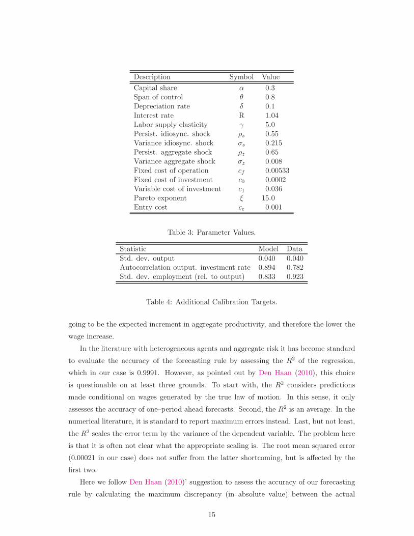
Table 3: Parameter Values.

Statistic Model Data

Std. dev. output 0.040 0.040Autocorrelation output. investment rate 0.894 0.782Std. dev. employment (rel. to output) 0.833 0.923

Table 4: Additional Calibration Targets.

going to be the expected increment in aggregate productivity, and therefore the lower the

wage increase.

In the literature with heterogeneous agents and aggregate risk it has become standard

to evaluate the accuracy of the forecasting rule by assessing the R2 of the regression,

which in our case is 0.9991. However, as pointed out by Den Haan (2010), this choice

is questionable on at least three grounds. To start with, the R2 considers predictions

made conditional on wages generated by the true law of motion. In this sense, it only

assesses the accuracy of one–period ahead forecasts. Second, the R2 is an average. In the

numerical literature, it is standard to report maximum errors instead. Last, but not least,

the R2 scales the error term by the variance of the dependent variable. The problem here

is that it is often not clear what the appropriate scaling is. The root mean squared error

(0.00021 in our case) does not suffer from the latter shortcoming, but is affected by the

first two.

Here we follow Den Haan (2010)’ suggestion to assess the accuracy of our forecasting

rule by calculating the maximum discrepancy (in absolute value) between the actual

15

wage and the wage generated by the rule without updating. That is, we compute the

maximum pointwise difference between the sequence of actual market–clearing wages and

that generated by our rule, when next period’s predicted wage is conditional on last

period’s prediction for the current wage rather than the market clearing wage. The value

of that statistics over 24,500 simulations is 0.296%.

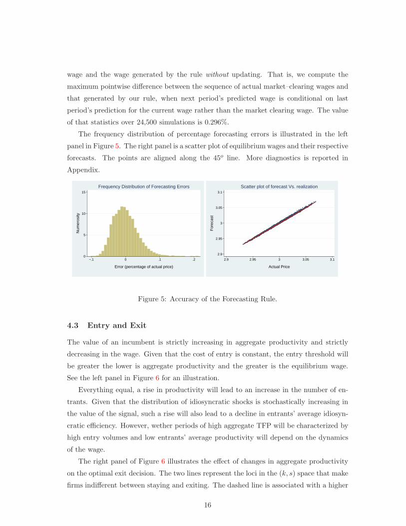
The frequency distribution of percentage forecasting errors is illustrated in the left

panel in Figure 5. The right panel is a scatter plot of equilibrium wages and their respective

forecasts. The points are aligned along the 45o line. More diagnostics is reported in

Appendix.

0

5

10

15

Num

eros

ity

−.1 0 .1 .2

Error (percentage of actual price)

Frequency Distribution of Forecasting Errors

2.9

2.95

3

3.05

3.1

For

ecas

t

2.9 2.95 3 3.05 3.1

Actual Price

Scatter plot of forecast Vs. realization

Figure 5: Accuracy of the Forecasting Rule.

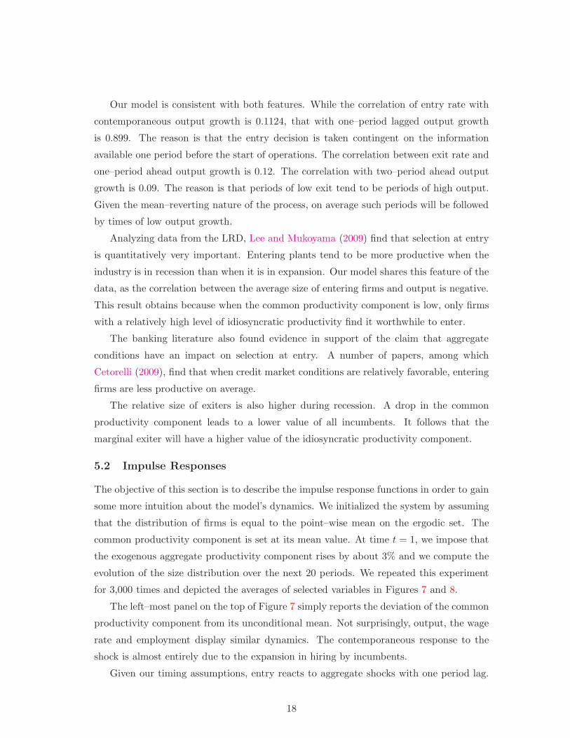
4.3 Entry and Exit

The value of an incumbent is strictly increasing in aggregate productivity and strictly

decreasing in the wage. Given that the cost of entry is constant, the entry threshold will

be greater the lower is aggregate productivity and the greater is the equilibrium wage.

See the left panel in Figure 6 for an illustration.

Everything equal, a rise in productivity will lead to an increase in the number of en-

trants. Given that the distribution of idiosyncratic shocks is stochastically increasing in

the value of the signal, such a rise will also lead to a decline in entrants’ average idiosyn-

cratic efficiency. However, wether periods of high aggregate TFP will be characterized by

high entry volumes and low entrants’ average productivity will depend on the dynamics

of the wage.

The right panel of Figure 6 illustrates the effect of changes in aggregate productivity

on the optimal exit decision. The two lines represent the loci in the (k, s) space that make

firms indifferent between staying and exiting. The dashed line is associated with a higher

16

2.8

2.9

3

3.1

3.2

0.95

1

1.050.72

0.74

0.76

0.78

0.8

0.82

0.84

0.86

0.88

0.9

WageAggregate Productivity0.4 0.6 0.8 1 1.2 1.4 1.6 1.8 2 2.2 2.40

1

2

3

4

5

6x 10

−3

Idiosyncratic Productivity

Cap

ital

Figure 6: Left: Entry Threshold on the Signal Space. Right: Exit Threshold.

aggregate productivity.

Since the outside value is invariant at zero, everything else equal a greater aggregate

productivity will lead to a lower productivity of the marginal exiter, for all levels of the

capital stock. In other words, the average idiosyncratic productivity of non-exiting firms

will be lower. Since variations in the wage rate have the opposite effects on the exit locus

and higher productivity episodes will be characterized by high wages, a priori it cannot

be established whether this will also be a feature of equilibrium dynamics.

5 Aggregate Fluctuations – Results

5.1 Cyclical Behavior of Entry and Exit

Table 5 reports the raw correlations of entry rate, exit rate, and the size of entrants

and exiters (relative to incumbents) with industry output. Consistent with the evidence

presented by Campbell (1998), the entry rate is pro–cyclical and the exit rate is counter–

cyclical.

Entry Rate Exit Rate Entrants’ Size Exiters’ Size0.222 -0.351 -0.150 -0.478

Table 5: Correlations with industry output.

Interestingly, Campbell (1998) also provides evidence on the correlations between entry

rate, exit rate, and future and lagged output growth. He finds that the correlation of entry

with lagged output growth is greater than the contemporaneous correlation and that the

exit rate is positively correlated with future output growth.

17

Our model is consistent with both features. While the correlation of entry rate with

contemporaneous output growth is 0.1124, that with one–period lagged output growth

is 0.899. The reason is that the entry decision is taken contingent on the information

available one period before the start of operations. The correlation between exit rate and

one–period ahead output growth is 0.12. The correlation with two–period ahead output

growth is 0.09. The reason is that periods of low exit tend to be periods of high output.

Given the mean–reverting nature of the process, on average such periods will be followed

by times of low output growth.

Analyzing data from the LRD, Lee and Mukoyama (2009) find that selection at entry

is quantitatively very important. Entering plants tend to be more productive when the

industry is in recession than when it is in expansion. Our model shares this feature of the

data, as the correlation between the average size of entering firms and output is negative.

This result obtains because when the common productivity component is low, only firms

with a relatively high level of idiosyncratic productivity find it worthwhile to enter.

The banking literature also found evidence in support of the claim that aggregate

conditions have an impact on selection at entry. A number of papers, among which

Cetorelli (2009), find that when credit market conditions are relatively favorable, entering

firms are less productive on average.

The relative size of exiters is also higher during recession. A drop in the common

productivity component leads to a lower value of all incumbents. It follows that the

marginal exiter will have a higher value of the idiosyncratic productivity component.

5.2 Impulse Responses

The objective of this section is to describe the impulse response functions in order to gain

some more intuition about the model’s dynamics. We initialized the system by assuming

that the distribution of firms is equal to the point–wise mean on the ergodic set. The

common productivity component is set at its mean value. At time t = 1, we impose that

the exogenous aggregate productivity component rises by about 3% and we compute the

evolution of the size distribution over the next 20 periods. We repeated this experiment

for 3,000 times and depicted the averages of selected variables in Figures 7 and 8.

The left–most panel on the top of Figure 7 simply reports the deviation of the common

productivity component from its unconditional mean. Not surprisingly, output, the wage

rate and employment display similar dynamics. The contemporaneous response to the

shock is almost entirely due to the expansion in hiring by incumbents.

Given our timing assumptions, entry reacts to aggregate shocks with one period lag.

18

0

1

2

3

Per

cent

age

Dev

iatio

n

0 5 10 15 20

Time

Aggregate Productivity

0

.2

.4

.6

.8

1

Per

cent

age

Dev

iatio

n

0 5 10 15 20

Time

Wage

.055

.06

.065

.07

.075

0 5 10 15 20

Time

Entry Rate

0

2

4

6

8

Per

cent

age

Dev

iatio

n

0 5 10 15 20

Time

Industry Output With Entry & Exit

0

2

4

6

Per

cent

age

Dev

iatio

n

0 5 10 15 20

Time

Employment

.045

.05

.055

.06

0 5 10 15 20

Time

Exit Rate

Figure 7: Response to a positive productivity shock.

Exit also reacts with delay, because it is optimal for entrepreneurs to disinvest before

closing down shop. In period 2, exit drops dramatically, while entry rises. This is why

output and employment peak.

The number of operating firms peak in period 3. In the following periods, the exit

volume is greater than entry. Therefore, the number of operating firms declines.

The two right–most panels show that the convergence of both exit and entry rates to

their unconditional means is not monotone. The exit rate overshoots its long–run value.

The entry rate undershoots. These features stem from the fact that the wage decays at a

lower pace than aggregate productivity.

A few periods after the positive shock hits, the aggregate component of productivity

is back close to its unconditional mean. However, the wage is still relatively high. The

reason is that the volume of entry is finite and firms are born relatively small. As the

survivors become more efficient, their labor demand increases, keeping the wage from

falling faster. With a relatively high wage and relatively low aggregate productivity, the

selection effect changes sign. Entry falls below its long–run value, while exit is higher

than that.

Figure 8 shows that, following the hike in the aggregate component, the average id-

iosyncratic productivity of both entrants and exiters declines. In turn, this leads to a

fall in the industry’s average idiosyncratic efficiency. The relative size of entrants and

exiters also decreases, since it is uniquely determined by the differences between their

19

0

1

2

3

4

Per

cent

age

Dev

iatio

n

0 5 10 15 20

Time

Number of Firms

.93

.935

.94

.945

0 5 10 15 20

Time

Entrants’ Avg Idiosync Prod

.61

.615

.62

.625

.63

.635

0 5 10 15 20

Time

Exiters’ Avg Idiosync Prod

−.6

−.4

−.2

0

.2

Per

cent

age

Dev

iatio

n

0 5 10 15 20

Time

Avg. Idiosyncratic Productivity

.56

.565

.57

.575

.58

0 5 10 15 20

Time

Relative to IncumbentsEntrants’ Average Size

.2

.205

.21

.215

.22

0 5 10 15 20

Time

Relative to IncumbentsExiters’ Average Size

Figure 8: Response to a positive productivity shock.

and the incumbents’ idiosyncratic productivity. Consistent with the above discussion, the

convergence of average idiosyncratic productivity levels to their unconditional means is

not monotone.

6 The importance of entry and exit

In this section we show that allowing for entry and exit enhances the model’s internal

propagation mechanism. A corollary of this result is that measuring the aggregate Solow

residual as it is customary done in macroeconomics results in an upward bias in its per-

sistence’s estimate.

This is the outcome of two forces. One is the pro–cyclicality of the entry rate. The

other is the fact that firms start out relatively unproductive, but quickly grow in size

and efficiency. This dynamics is reflected in the contribution of net entry to aggregate

productivity growth. As it is the case in the data, the contribution of new entrants is

small in their first year, but then grows disproportionably faster than their number.

Finally, we describe our model’s implications for the cyclicality of the cross–sectional

standard deviation of productivity growth.

20

6.1 Propagation

Think of the economy considered in Section 5, but abstract from entry and exit. At

every point in time, there is a mass of firms whose technology is exactly as specified

above. However, firms never exit. As our purpose is to compare such economy with our

benchmark, let’s assume that the number of operating firms is equal to unconditional

average number of incumbents that obtains along the benchmark’s equilibrium path.

0

2

4

6

Per

cent

age

Dev

iatio

n

0 5 10 15

Time

Industry Output With Entry & Exit

0

2

4

6

Per

cent

age

Dev

iatio

n

0 5 10 15

Time

Industry Output Without Entry & Exit

Figure 9: Accuracy of the Forecasting Rule.

In the right panel of figure 9 we plotted the impulse response of industry output to a

positive aggregate shocks. For comparison, the left panel reports the impulse response in

the benchmark scenario.

Since entry and exit are essentially determined one period ahead, it is not surprising

that the contemporaneous response of the two economies is about the same. In either

case, the increase in output is due the rise in hiring by incumbents. In period 2, output

increases in the benchmark economy, while it decreases in the scenario without entry or

exit. This is expected, as entry increases.

What is perhaps less expected is that the process of output mean–reversion is slower

when we allow for entry and exit. In other words, aggregate output is more persistent.

The difference is driven by the dynamics of firms born during the expansion. Firms that

entered in the wake of positive shocks are initially very small and therefore account for a

rather small fraction of total output. Over time, however, they grow in efficiency and size.

This process takes place at the same time in which the aggregate productivity component

regresses towards its unconditional mean. As a result, aggregate output and efficiency fall

at a slower pace.

A confirmation that this mechanism is indeed at work comes from the inspection of

21

0

1

2

3

Per

cent

age

Dev

iatio

n

0 5 10 15 20

Time

Aggregate Productivity Solow Residual

Aggregate Productivity with Entry & Exit

0

1

2

3

Per

cent

age

Dev

iatio

n

0 5 10 15 20

Time

Aggregate Productivity Solow Residual

Aggregate Productivity without Entry & Exit

Figure 10: Accuracy of the Forecasting Rule.

Figure 10. The solid lines depict the impulse responses of the aggregate productivity

component zt. They are identical by construction. The dashed lines depict the Solow

residuals in the two economies, computed by assuming an aggregate production function

of the Cobb–Douglas form with capital share equal to 0.3. That is, we plotted log(Yt)−

α log(Kt)−(1−α) log(Lt). The evolution of the residual depends on the dynamics of both

zt and the distribution of the idiosyncratic component st. In the benchmark economy, the

latter improves over time. In the case without entry and exit, it is time–invariant.

The simple exercise just conducted hints that trying to infer information about the

process of aggregate productivity using a model without entry or exit will inevitably give

the wrong answer. Such model will interpret changes in aggregate efficiency that results

from the reallocation of output shares towards more efficient firms as changes in the

exogenous aggregate component.

We also conducted the alternative experiment of setting the parameters in the economy

without entry and exit in such a way that it generates the same values of the target

moments as the benchmark economy. To generate an autocorrelation of output equal to

0.89, we had to set ρz = 0.775, much higher than the value of 0.65 assumed in Section 4.

6.2 Productivity Decomposition

Necessary conditions for the increase in propagation that we have just described are that

entry is pro–cyclical and that entrants’ productivity grows faster than the incumbents’.

Is there any evidence that the latter claim holds true in the data?

Foster, Haltiwanger, and Krizan (2001) conducted a thorough and comprehensive re-

view of the literature that exploits longitudinal establishment data in order to understand

the determinants of aggregate productivity growth. One of their findings is that the con-

22

tribution of net entry to productivity growth tends to be small in high–frequency studies,

while it is much larger in lower–frequency analyses. To a large extent, this is due to the

fact that because of selection and/or learning, the productivity gap between entrants and

exiters is greater, the longer the time between observations.

Conducting a standard productivity decomposition on simulated data generated by our

model leads to the same conclusion. In our case, selection and mean-reverting productivity

are the assumptions that are responsible for the result.

Define total factor productivity as the weighted sum of firm–level Solow residuals,

where the weights are the output shares. Let Ct denote the collection of plants active in

both periods t − k and t. The set Et includes the plants that entered between the two

dates and are still active at time t. In Xt−k are the firms that were active at time t− k,

but exited before time t.

Following Haltiwanger (1997), the growth in TFP can be decomposed into five com-

ponents, corresponding to the addenda in equation (3). They are known as (i) the within

component, which measures the changes in productivity for continuing plants, (ii) the

between–plant portion, which reflects the change in output shares across continuing plants,

(iii) a covariance component, and finally (iv) entry and (v) exit components.9

∆ log(TFP t) =∑

i∈Ct

φi,t−k∆ log(TFP it) +∑

i∈Ct

[log(TFP i,t−k)− log(TFP t−k)]∆φit+

∑

i∈Ct

∆ log(TFP it)∆φit +∑

i∈Et

[log(TFP it)− log(TFP t−k)]φit+

∑

i∈Xt−k

[log(TFP i,t−k)− log(TFP t−k)]φi,t−k (3)

Table 6 reports the results that obtain when we set k equal to 1 and 5, respectively.

In the last column, labeled Net Entry, we report the difference between the entry and exit

components. Recall that in our model the unconditional mean of aggregate productivity

growth is identically zero.

k Within Between Covariance Entry Exit Net Entry

1 -8.8477 -3.3663 11.9392 -0.5584 -0.8337 0.27535 -15.0994 -10.6881 24.4110 -0.9062 -2.2832 1.3770

Table 6: Productivity Decomposition (percentages).

The between and within components are necessarily negative, because of mean rever-

9With φit and TFP it we denote firm i’s output share and measured total factor productivity at timet, respectively. TFPt is the weighted average total factor productivity across all firms active at time t.

23

sion in the process driving idiosyncratic productivity. Larger firms, which tend to be more

productive, shrink on average. Smaller firms, on the contrary, tend to grow. The covari-

ance component is positive, because firms that become more productive also increase in

size.

On average, both the entry and exit contributions are negative. This reflects the fact

that both entrants and exiters are less productive than average. However, entrants tend

to be more productive than exiters. The contribution of net entry to productivity growth

is positive regardless of the horizon.

What’s most relevant for our analysis is that for k = 5 the contribution of net entry

is one order of magnitude larger than for k = 1. In part, this is due to the fact that

the share of output produced by entrants increases with k. However, this cannot be the

whole story. The contribution of entry is roughly −0.56% for k = 1 and goes to −0.9%

for k = 5. If entrants’ productivity did not grow faster than average, the contribution of

entry for the k = 5 horizon would be much smaller.

6.3 Cyclical Variation of Cross–sectional Moments

A recent literature has documented that idiosyncratic risk faced by economic agents is

strongly counter–cyclical. For example, Storesletten, Telmer, and Yaron (2004) find that

individual labor income is riskier during recessions.

Eisfeldt and Rampini (2006) and Bachman and Bayer (2009b) argue that firm–level

uncertainty is also counter–cyclical. Their conclusion is based on the finding that the

cross–sectional standard deviation of firm–level TFP growth in an unbalanced panel is

negatively correlated with detrended GDP. Recognizing the possibility that systematic

cyclical variation in entry and exit selection may bias their results, Bachman and Bayer

(2009b) estimate a selection model, where lagged Solow residuals determine selection.

Our theory suggests that the concern of Bachman and Bayer (2009b) is justified.

Time–varying selection in entry and exit does generate systematic compositional changes

in the cross–sectional distribution of idiosyncratic productivity, suggesting that particular

care should be placed in inferring the properties of the process of firm–level productivity

from information on cross–sectional moments. If the process responsible for generating

their data was consistent with our theory, there would be systematic cyclical sample

selection.

The good news is that the selection bias reinforces their results. With an homoscedastic

process for idiosyncratic productivity, the cross–sectional standard deviation of firm–level

TFP growth is larger during expansions than during recessions. This rules out the possi-

24

bility that, in spite of finding a counter–cyclical variation in the cross–sectional standard

deviation of firm–level TFP growth, idiosyncratic uncertainty faced my firms is indeed

acyclical.

In our framework, expansions are times in which the number of entrants is relatively

high and their average productivity is relatively low. As a result, the distribution of firms

over idiosyncratic productivity is more skewed to the right, i.e. it has relatively more

mass on low values of the shock.

This is illustrated in Figure 11. For each level of idiosyncratic shock, it plots the

difference between the (average) fraction of firms associated with it in expansion and in

recession, respectively. In expansions we record a larger fraction of firms with less than

average idiosyncratic productivity.

0.4 0.6 0.8 1 1.2 1.4 1.6 1.8 2 2.2 2.4−0.25

−0.2

−0.15

−0.1

−0.05

0

0.05

0.1

0.15

0.2

0.25

Idiosyncratic Productivity

Figure 11: Change in the Cross-Sectional Distribution.

This immediately implies that the mean idiosyncratic productivity is counter–cyclical.

As it turns out, the standard deviation is also counter–cyclical. Given that the expected

growth of productivity is monotonically decreasing in its level, both the cross–sectional

mean and standard deviation of productivity growth are pro–cyclical.

Since the conditional survival rate is higher during expansions, there will be firms that,

following a drop in idiosyncratic productivity, will exit in a recession (when aggregate TFP

is low) but will keep operating in an expansion. For such firms, recorded productivity

growth will be higher during a recession. In our simulations this effect is dominated by

the one described above.

25

7 Conclusion

This paper provides a framework for the study of the dynamics of the cross–section of

firms and its implications for aggregate dynamics. When calibrated to match a set of

moments of the investment process, our model delivers implications for firm dynamics

and for the cyclicality of entry and exit that are consistent with the evidence.

The survival rate increases with size. The growth rate of employment is decreasing

with size and age, both unconditionally and conditionally. The size distribution of firms

is skewed to the right. When tracking the size distribution over the life a cohort, the

skewness declines with age.

The entry rate is positively correlated with current and lagged output growth. The

exit rate is negatively correlated with output growth and positively associated with future

growth.

We show that allowing for entry and exit enhances the internal propagation mechanism

of the model. This obtains because of four features of the equilibrium allocation: (i) entry

is pro–cyclical, (ii) entrants are smaller than the average incumbent, and (iii) particularly

so during expansions. Finally, (iv) idiosyncratic productivity is mean reverting.

A positive shock to aggregate productivity leads to an in increase in entry. Con-

sistent with the empirical evidence, the new entrants are smaller and less efficient than

incumbents. The skewness of the distribution of firms over the idiosyncratic productivity

component increases. As the exogenous component of aggregate productivity declines

towards its unconditional mean, the new entrants that survive grow in productivity and

size. That is, the distribution of idiosyncratic productivity improves.

For a version of our model without entry or exit to generate a data–conforming per-

sistence of output, the first–order autocorrelation of aggregate productivity shocks must

be 0.775. In the benchmark scenario with entry and exit, it needs only be 0.65.

Even though idiosyncratic productivity is homoscedastic by assumption, systematic

time–varying selection in entry implies that both mean and standard deviation of the

cross–sectional distribution of firm–level Solow residual are counter–cyclical. Since id-

iosyncratic productivity is also mean–reverting, the cross–sectional mean and standard

deviation of productivity growth are pro–cyclical. This is important, because it identifies

the sign of the bias that is implicit in the estimates of these cross–sectional moments in

unbalanced panels.

26

A Numerical Approximation

Our algorithm consists of the following steps.

1. Guess values for the parameters of the wage forecasting rule β ={

β0, β1, β2, β3

}

;

2. Approximate the value function of the incumbent firm;

3. Simulate the economy for T periods, starting from an arbitrary initial condition

(z0,Γ0);

4. Obtain a new guess for β by running regression (2) over the time–series {wt, zt}Tt=S+1,

where S is the number of observation to be scrapped because the dynamical system

has not reached its ergodic set yet;

5. If the new guess for β is close to the previous one, stop. If not, go back to step 2.

A.1 Approximation of the value function

The incumbent’s value function is approximated by value function iteration.

1. Start by defining grids for the state variables w, z, k, s. Denote them as Ψw, Ψz,

Ψk, and Ψs, respectively. The wage grid is equally spaced and centered around

the equilibrium wage of the stationary economy. The capital grid is constructed

following the method suggested by McGrattan (1999). The grids and transition

matrices for the two shocks are constructed following Tauchen (1986). For all pairs

(s, s′) such that s, s′ ∈ Ψs, let H(s′|s) denote the probability that next period’s

idiosyncratic shock equals s′, conditional on today’s being s. For all (z, z′) such

that z, z′ ∈ Ψz, let also G(z′|z) denote the probability that next period’s aggregate

shock equals z′, conditional on today’s being z.

2. For all triplets (w, z, z′) on the grid, the forecasting rule yields a wage forecast for

the next period (tildes denote elements not on the grid):

log(w′) = β0 + β1 log(w) + β2 log(z′) + β3 log(z).

In general, w′ will not belong to the grid of wages. There will be contiguous grid

points (wi, wi+1) such that wi ≤ w′ ≤ wi+1. Now let J(wi|w, z, z′) = 1 − w′−wi

wi+1−wi,

J(wi+1|w, z, z′) = w′−wi

wi+1−wi, and J(wj |w, z, z

′) = 0 for all j such that j 6= i and

j 6= i + 1. This will allow us to evaluate the value function for values of the wage

which are off the grid, by linear interpolation;

27

3. For all grid elements (w, z, k, s), guess values for the value function V0(w, z, k, s);

4. The revised guess of the value function, V1(w, z, k, s), is determined as follows:

V1(w, z, k, s) =max

[

0, maxk′∈Ψk

π(w, z, k, s) − x− c0kχ− c1

(x

k

)2k − cf+

1

R

∑

j

∑

i

∑

n

V0(wi, zj , k′, sn)H(sn|s)J(wi|w, z, zj)G(zj |z)

,

s.t. x = k′ − k(1− δ),

π(w, z, k, s) =1− (1− α)θ

(1− α)θw

−θ(1−α)

1−θ(1−α) [(1− α)θszkαθ]1

1−θ(1−α) ,

χ = 1 if k′ 6= k and χ = 0 otherwise .

5. Keep on iterating until sup∣

∣

∣

Vt+1(w,z,k,s)−Vt(w,z,k,s)Vt(w,z,k,s)

∣

∣

∣< 10.0−6. Denote the latest value

function as V∞(w, z, k, s).

A.2 Entry

1. Define a grid for the signal. Denote it as Ψq. Let also W (sn|q) indicate the proba-

bility that the first draw of the idiosyncratic shock is sn, conditional on the signal

being q.

2. For all triplets (w, z, q) on the grid, compute the value of entering as

Ve(w, z, q) = maxk′∈Ψk

−k′+1

R

∑

j

∑

i

∑

n

V∞(wi, zj , k′, sn)W (sn|q)J(wi|w, z, zj)G(zj |z)

3. For all grid points z, construct a bi-dimensional cubic spline interpolation of Ve(w, z, q)

over the dimensions (w, q). For all pairs w, q, denote the value of entering as

Ve(w, z, q).

4. Define qe(w, z) as the value of the signal which makes prospective entrants indifferent

between entering and not. That is, Ve(w, z, qe(w, z)) = ce.

A.3 Simulation

1. Given the current firm distribution Γt and aggregate shock zt, compute the equi-

librium wage wt by equating the labor supply equation Ls(w) = wγ to the labor

demand equation

Ldt (w) =

(

ztθ(1− α)

w

)

∑

m

∑

n

[

snkαθm

]1

1−θ(1−α)Γt(sn, km)

28

2. For all z′ ∈ Ψz, compute the conditional wage forecast wt+1(z′) as follows:

log[wt+1(z′)] = β0 + β1 log(wt) + β2 log(z

′) + β3 log(zt).

For every z′, there will be contiguous grid points (wi, wi+1) such that wi ≤ wt+1(z′) ≤

wi+1. Now let Jt+1(wi|z′) = 1− wt+1(z′)−wi

wi+1−wi, Jt+1(wi|z

′) = wt+1(z′)−wi

wi+1−wi, and Jt+1(wj |z

′) =

0 for all j such that j 6= i and j 6= i+ 1;

3. For all pairs (k, s) on the grid such that Γt(k, s) > 0, the optimal choice of capital

k′(wt, zt, k, s) is the solution to the following problem:

maxk′∈Ψk

π(wt, zt, k, s)− x− c0kχ− c1

(x

k

)2k − cf+

+1

R

∑

j

∑

i

∑

n

V∞(wi, zj , k′, sn)H(sn|s)Jt(wi|zj)G(zj |zt),

s.t. x = k′ − k(1− δ),

π(wt, zt, k, s) =1− (1− α)θ

(1− α)θw

−θ(1−α)

1−θ(1−α)

t [(1− α)θsztkαθ]

11−θ(1−α) ,

χ = 1 if k′ 6= k and χ = 0 otherwise .

4. There will be contiguous elements of the signal grid (q∗, q∗∗) such that q∗ ≤ qe(wt, zt) ≤

q∗∗.

• For all q ≥ q∗∗, the initial capital of entrants k′e(wt, zt, q) solves the following

problem:

maxk′e∈Ψk

−km +1

R

∑

j

∑

i

∑

n

V∞(wi, zj , k′e, sn)W (sn|q)Jt(wi|zj)G(zj |zt)

• We can easily compute the distribution of the idiosyncratic shock conditional

on qe ≡ qe(wt, zt), denoted as W (sn|qe) and then compute the optimal capital

k′e(wt, zt, qe) as the solution to:

maxk′e∈Ψk

−km +1

R

∑

j

∑

i

∑

n

V∞(wi, zj , k′e, sn)W (sn|qe)Jt(wi|zj)G(zj |zt)

5. Draw the aggregate productivity shock zt+1;

6. Determine the distribution at time t+1. For all (k, s) such that V∞(wt+1(zt+1), zt+1, k, s) =

0, then Γt+1 = 0. For all other pairs,

Γt+1(k, s) =∑

m

∑

n

Γt(km, sn)H(s|sn)Υm,n(wt, zt, k) + Et+1(k, s)

29

where

Υm,n(wt, zt, k) =

{

1 if k′(wt, zt, km, sn) = k

0 otherwise.

and Et+1(k, s) = M∑

i:qi≥q∗∗ H(s|qi)Q(qi)Ξm,i(wt, zt, k)+MH(s|qe)Q(qe)Ξm,i(wt, zt, k)

where

Ξm,i(wt, zt) =

{

1 if k′(wt, zt, qi) = k

0 otherwise.

A.4 More Accuracy Tests of the Forecasting Rule

Forecasting errors are essentially unbiased – the mean error is -0.00017% of the forecasting

price – and uncorrelated with the price (the correlation coefficient between the two series

is -0.0456) and the aggregate shock (-0.0045).

−.1

0

.1

.2

.3

Per

cent

For

ecas

t Err

or

2.9 2.95 3 3.05 3.1

Actual Price

Scatter plot of forecast error Vs. market clearing price

−.1

0

.1

.2

.3

Per

cent

of M

kt C

lear

ing

Pric

e

0 5000 10000 15000 20000 25000

Time

Forecast Error

Figure 12: Accuracy of the Forecasting Rule.

In the left panel of Figure 12 is the scatter plot of the forecasting errors against the

market clearing price. In the right panel is the time series of the forecasting error. The

good news is that errors do not cumulate.

References

Bachman, R., and C. Bayer (2009a): “The Cross–Section of Firms over the Business

Cycle: New Facts and a DSGE Exploration,” Working paper, University of Michigan.

(2009b): “Firm–Specific Productivity Risk over the Business Cycle: Facts and

Aggregate Implications,” Working paper, University of Michigan.

30

Basu, S., and J. Fernald (1997): “Returns to Scale in US Production: Estimates and

Implications,” Journal of Political Economy, 105(2), 249–283.

Bilbiie, F., F. Ghironi, and M. Melitz (2007): “Endogenous Entry, Product Variety,

and Business Cycles,” NBER Working Paper # 13646.

Cabral, L., and J. Mata (2003): “On the Evolution of the Firm Size Distribution:

Facts and Theory,” American Economic Review, 93(4), 1075–1090.

Campbell, J. (1998): “Entry, Exit, Embodied Technology, and Business Cycles,” Review

of Economic Dynamics, 1, 371–408.

Cetorelli, N. (2009): “Credit market competition and the nature of firms,” Federal

Reserve Bank of New York Staff Report # 366.

Chatterjee, S., and R. Cooper (1993): “Entry and Exit, Product Variety and the

Business Cycle,” NBER Working Paper # 4562.

Coad, A. (2009): The Growth of Firms. A Survey of Theories and Empirical Evidence.

Edward Elgar Publishing.

Cogley, T., and J. Nason (1995): “Output Dynamics in Real Business Cycle Models,”

American Economic Review, 85(3), 492–511.

Cooley, T., R. Marimon, and V. Quadrini (2004): “Aggregate Consequences of

Limited Contract Enforceability,” Journal of Political Economy, 112(4), 817–847.

Cooley, T., and V. Quadrini (2001): “Financial Markets and Firm Dynamics,” Amer-

ican Economic Review, 91(5), 1286–1310.

Cooper, R., and J. Haltiwanger (2006): “On the Nature of Capital Adjustment

Costs,” Review of Economic Studies, 73(3), 611–633.

Den Haan, W. J. (2010): “Assessing the Accuracy of the Aggregate Law of Motion in

Models with Heterogeneous Agents,” Journal of Economic Dynamics and Control, 34,

79–99.

D’Erasmo, P. (2009): “Investment and Firm Dynamics,” Working Paper, University of

Maryland.

Devereux, M., A. Head, and B. Lapham (1996): “Aggregate Fluctuations with In-

creasing Returns to Specialization and Scale,” Journal of Economic Dynamics and

Control, 20, 627–656.

31

Dunne, T., M. Roberts, and L. Samuelson (1989): “The Growth and Failure of US

Manufacturing Plants,” Quarterly Journal of Economics, 94, 671–698.

Eisfeldt, A., and A. Rampini (2006): “Capital Reallocation and Liquidity,” Journal

of Monetary Economics, 53, 369–399.

Evans, D. (1987): “Tests of Alternative Theories of Firm Growth,” Journal of Political

Economy, 95(4), 657–674.

Foster, L., J. Haltiwanger, and C. Krizan (2001): “Aggregate Productivity

Growth: Lessons from Microeconomic Evidence,” in New Developments in Produc-

tivity Analysis, ed. by C. Hulten, E. Dean, and M. Harper, pp. 303–363. University of

Chicago Press.

Hall, B. (1987): “The Relationship Between Firm Size and Firm Growth in the US

Manufacturing Sector,” Journal of Industrial Economics, 35(4), 583–606.

Haltiwanger, J. (1997): “Measuring and Analyzing Aggregate Fluctuations: The Im-

portance of Building from Microeconomic Evidence,” Federal Reserve Bank of St. Louis

Review, 79, 55–77.

Hopenhayn, H. (1992): “Entry, Exit, and Firm Dynamics in Long Run Equilibrium,”

Econometrica, 60(5), 1127–1150.

Khan, A., and J. K. Thomas (2003): “Nonconvex Factor Adjustments in Equilibrium

Business Cycle Models: Do Nonlinearities Matter?,” Journal of Monetary Economics,

50, 331–360.

(2008): “Idiosyncratic Shocks and the Role of Nonconvexities in Plant and

Aggregate Investment Dynamics,” Econometrica, 76(2), 395–436.

Krusell, P., and A. Smith (1998): “Income and wealth heterogeneity in the macroe-

conomy,” Journal of Political Economy, 106, 867–896.

Lee, Y. (2005): “The Importance of Reallocations in Cyclical Productivity and Returns

to Scale: Evidence from Plant-level Data,” Working paper # 05–09, Federal Reserve

Bank of Cleveland.

Lee, Y., and T. Mukoyama (2009): “Entry, Exit, and Plant–level Dynamics over the

Business Cycle,” Working paper, University of Virginia.

32

McGrattan, E. (1999): “Application of weighted residual methods to dynamic eco-

nomic models,” in Computational Methods for the Study of Dynamic Economies, ed.

by R. Marimon, and A. Scott. Oxford University Press.

Michelacci, C. (2004): “Cross–Sectional Heterogeneity and The Persistence of Aggre-

gate Fluctuations,” Journal of Monetary Economics, 51, 1321–1352.

Samaniego, R. (2008): “Entry, Exit and Business Cycle in a General Equilibrium

Model,” Review of Economic Dynamics, 11, 529–541.

Storesletten, K., C. Telmer, and A. Yaron (2004): “Cyclical Dynamics in Idiosyn-

cratic Labor Market Risk,” Journal of Political Economy, 112(3), 695–717.

Tauchen, G. (1986): “Finite State Markov-Chain Approximations to Univariate and

Vector Autoregressions,” Economics Letters, 20, 177–181.

Veracierto, M. (2002): “Plant–Level Irreversible Investment and Equilibrium Business

Cycles,” American Economic Review, 92(1), 181–197.

Zhang, L. (2005): “The Value Premium,” Journal of Finance, 60(1), 67–103.

33