Washington University in St. Louis Washington University in St. Louis Washington University Open Scholarship Washington University Open Scholarship Engineering and Applied Science Theses & Dissertations McKelvey School of Engineering Summer 8-13-2015 Entry Flow and Heat Transfer of Laminar and Turbulent Forced Entry Flow and Heat Transfer of Laminar and Turbulent Forced Convection of Nanofluids in a Pipe and a Channel Convection of Nanofluids in a Pipe and a Channel Yihe Huang Washington University in St Louis Follow this and additional works at: https://openscholarship.wustl.edu/eng_etds Part of the Computer-Aided Engineering and Design Commons, and the Nanoscience and Nanotechnology Commons Recommended Citation Recommended Citation Huang, Yihe, "Entry Flow and Heat Transfer of Laminar and Turbulent Forced Convection of Nanofluids in a Pipe and a Channel" (2015). Engineering and Applied Science Theses & Dissertations. 112. https://openscholarship.wustl.edu/eng_etds/112 This Thesis is brought to you for free and open access by the McKelvey School of Engineering at Washington University Open Scholarship. It has been accepted for inclusion in Engineering and Applied Science Theses & Dissertations by an authorized administrator of Washington University Open Scholarship. For more information, please contact [email protected].

Welcome message from author
This document is posted to help you gain knowledge. Please leave a comment to let me know what you think about it! Share it to your friends and learn new things together.
Transcript
Washington University in St. Louis Washington University in St. Louis
Washington University Open Scholarship Washington University Open Scholarship
Engineering and Applied Science Theses & Dissertations McKelvey School of Engineering
Summer 8-13-2015
Entry Flow and Heat Transfer of Laminar and Turbulent Forced Entry Flow and Heat Transfer of Laminar and Turbulent Forced
Convection of Nanofluids in a Pipe and a Channel Convection of Nanofluids in a Pipe and a Channel
Yihe Huang Washington University in St Louis
Follow this and additional works at: https://openscholarship.wustl.edu/eng_etds
Part of the Computer-Aided Engineering and Design Commons, and the Nanoscience and
Nanotechnology Commons
Recommended Citation Recommended Citation Huang, Yihe, "Entry Flow and Heat Transfer of Laminar and Turbulent Forced Convection of Nanofluids in a Pipe and a Channel" (2015). Engineering and Applied Science Theses & Dissertations. 112. https://openscholarship.wustl.edu/eng_etds/112
This Thesis is brought to you for free and open access by the McKelvey School of Engineering at Washington University Open Scholarship. It has been accepted for inclusion in Engineering and Applied Science Theses & Dissertations by an authorized administrator of Washington University Open Scholarship. For more information, please contact [email protected].
WASHINGTON UNIVERSITY IN ST. LOUIS
School of Engineering and Applied Science
Department of Mechanical Engineering and Materials Science
Thesis Examination Committee: Ramesh K Agarwal, Chair
Kenneth Jerina Swami Karunamoorthy
Entry Flow and Heat Transfer of Laminar and Turbulent Forced Convection of Nanofluids in a
Pipe and a Channel
by
Yihe Huang
A thesis presented to the School of Engineering and Applied Science of Washington University in St. Louis in partial fulfillment of the
requirements for the degree of Master of Science
August 2015
Saint Louis, Missouri

© 2015, Yihe Huang

i
Content List of Figures .......................................................................................................................... iii
List of Tables ............................................................................................................................. v
Nomenclature ........................................................................................................................... vi
Acknowledgments .................................................................................................................. viii
Dedication ................................................................................................................................ ix Abstract ...................................................................................................................................... x
1 Introduction ......................................................................................................................... 1
1.1 Brief Literature Review .................................................................................................................... 1 1.1.1 Nanofluids and Thermal Conductivity ............................................................................ 1 1.1.2 Entrance Length .................................................................................................................. 2
1.2 Overview of Thesis ........................................................................................................................... 3
2 Nanofluids ........................................................................................................................... 4 2.1 Nanofluid Conduction Heat Transfer Properties ........................................................................ 4
2.1.1 Heat Transfer Enhancement Mechanisms ...................................................................... 4 2.1.2 Models of Nanofluids Thermal Conductivit .................................................................. 5
2.2 Nanofluid Convection Heat Transfer Properties ....................................................................... 11 2.2.1 Heat Transfer Coefficient and Nusselt Number .......................................................... 11 2.2.2 Friction Factor and Pressure Drop................................................................................. 14
3 Methodology ...................................................................................................................... 17
3.1 Governing Equations ..................................................................................................................... 17 3.2 Turbulence Models Review ........................................................................................................... 18
3.2.1 Spalart-Allmaras Model [46] ............................................................................................ 19 3.2.2 Shear-stress Transport (SST) - Model [46] .................................................................... 20 3.2.3 k-epsilon Model [47] ......................................................................................................... 22
3.3 Discretization Methods [46] .......................................................................................................... 23 3.4 Description of ANSYS Fluent ...................................................................................................... 24
4 Entry Flow and Heat Transfer of Laminar Forced Convection of Nanofluids in a Pipe and a Channel ..................................................................................................... 26
4.1 Computational Modeling .............................................................................................................. 26 4.1.1 Governing Equations ....................................................................................................... 26 4.1.2 Constant Heat Flux Boundary Condition ...................................................................... 27 4.1.3 Constant Wall Temperature Boundary Condition ....................................................... 28 4.1.4 Nanofluid Properties ........................................................................................................ 28
4.2 Constant Heat Flux Boundary Condition ................................................................................... 31

ii
4.2.1 Numerical Validation ........................................................................................................ 31 4.2.2 Entrance Length Analysis ................................................................................................ 32 4.2.3 The Effect of Nanoparticle Concentration ................................................................... 36 4.2.4 The Effect of Nanoparticle Material .............................................................................. 38
4.3 Constant Wall Temperature Boundary Condition ..................................................................... 40 4.3.1 Numerical Validation ........................................................................................................ 40 4.3.2 Entrance Length Analysis ................................................................................................ 40 4.3.3 The Effect of Nanoparticle Concentration ................................................................... 44 4.3.4 The Effect of Nanoparticle Material .............................................................................. 46
5 Entry Flow and Heat Transfer of Turbulent Forced Convection of Nanofluids in a Pipe and a Channel ..................................................................................................... 48
5.1 Computational Modeling .............................................................................................................. 48 5.1.1 Governing Equations ....................................................................................................... 48 5.1.2 Constant Heat Flux Boundary Condition ...................................................................... 49 5.1.3 Constant Wall Temperature Boundary Condition ....................................................... 50
5.2 Constant Heat Flux Boundary Condition ................................................................................... 50 5.2.1 Numerical Validation for Pipe Flow .............................................................................. 50 5.2.2 Entrance Length Analysis using k - Turbulence Model ........................................ 52 5.2.3 The Effect of Nanoparticle Concentration ................................................................... 55 5.2.4 The Effect of Nanoparticle Material .............................................................................. 57
5.3 Constant Wall Temperature Boundary Condition ..................................................................... 59 5.3.1 Numerical Validation for Channel Flow........................................................................ 60 5.3.2 Entrance Length Analysis using k - Turbulence Model ........................................ 61 5.3.3 Entrance Length Analysis using SST Turbulence Model ........................................... 65 5.3.4 The Effect of Nanoparticle Concentration ................................................................... 69 5.3.5 The Effect of Reynolds Number .................................................................................... 71 5.3.6 The Effect of Nanoparticle Material .............................................................................. 72
6 Conclusions ........................................................................................................................ 74
References................................................................................................................................ 75
Vita .................................................................................................................................................................... 80
iii
List of Figures
Figure 1.1 Papers related to nanofluids .......................................................................................................... 2 Figure 1.2 Fluid flow in a conduit ................................................................................................................... 3 Figure 2.1 Schematic diagram of nanolayers [18] .......................................................................................... 5 Figure 4.1 Comparison of the computed local Nusselt number with the experimental data for Al2O3 nanofluid with 3% volume fraction [48]..................................................................................................... 31 Figure 4.2 Comparison of the computed local heat transfer coefficient with the experimental data for Al2O3 nanofluid with 3% volume fraction [48] ..................................................................................... 32 Figure 4.3 Developing velocity profiles for laminar entry flow in a pipe at Re = 1620 ........................ 34 Figure 4.4 Centerline velocity profiles of water and Al2O3 nanofluids for laminar pipe flow .............. 34 Figure 4.5 The normalized velocity gradient profile of water and Al2O3 nanofluids for laminar pipe flow .................................................................................................................................................................... 35 Figure 4.6 Wall and bulk temperature for Water and Al2O3 nanofluids in laminar pipe flow at Re = 1620 .................................................................................................................................................................... 37 Figure 4.7 Axial variations of heat transfer coefficient for different particle volume concentrations of Al2O3/water nanofluid in laminar pipe flow ................................................................................................ 37 Figure 4.8 Axial variations of Nusselt number for different particle volume concentrations of Al2O3/water nanofluid in laminar pipe flow ................................................................................................ 38 Figure 4.9 Effects of particle type and particle concentration on the local heat transfer coefficient for laminar pipe flow ............................................................................................................................................. 39 Figure 4.10 Effects of particle type and particle concentration on the local Nusselt number for laminar pipe flow ............................................................................................................................................. 39 Figure 4.11 Comparison of the axial variations of the computed Nusselt number with the classical result [56] for laminar channel flow of water under constant wall temperature boundary condition 40 Figure 4.12 Developing velocity profiles for laminar entry flow in a channel at Re = 500 .................. 42 Figure 4.13 Centerline velocity profile of water and Al2O3 nanofluids for laminar channel flow at Re = 500 .................................................................................................................................................................. 42 Figure 4.14 The normalized velocity gradient profile of water and Al2O3 nanofluids for laminar channel flow ...................................................................................................................................................... 43 Figure 4.15 Axial variations of heat transfer coefficient for different particle volume concentrations of Al2O3/water nanofluid in laminar channel flow ..................................................................................... 45 Figure 4.16 Axial variations of Nusselt number for different particle volume concentrations of Al2O3/water nanofluid in laminar channel flow .......................................................................................... 45 Figure 4.17 Effects of particle type and particle concentration on the local heat transfer coefficient for laminar channel flow ................................................................................................................................. 46 Figure 4.18 Effects of particle type and particle concentration on the local Nusselt number for laminar channel flow ....................................................................................................................................... 47
Figure 5.1 The yvalue at the wall along the axial direction .................................................................... 51
Figure 5.2 Comparison of the axial variation of the Nusselt number with experimental data and the correlation of Sieder and Tate for turbulent pipe flow with constant wall heat flux ............................. 51 Figure 5.3 Developing velocity profiles for turbulent entry flow in a pipe at Re = 6020 using the k -ε turbulence model .......................................................................................................................................... 53 Figure 5.4 Centerline velocity profile of water and Al2O3 nanofluids for turbulent pipe flow at Re = 6020 using the k - turbulence model .......................................................................................................... 53
iv
Figure 5.5 The normalized velocity gradient profile of water and Al2O3 nanofluids for turbulent pipe flow using the k - turbulence model .......................................................................................................... 54 Figure 5.6 Axial variation of heat transfer coefficient for different particle volume concentrations of Al2O3/water nanofluid in turbulent pipe flow at Re=6020 using the k - turbulence model ............. 56 Figure 5.7 Axial variation of Nusselt number for different particle volume concentrations of Al2O3/water nanofluid in turbulent pipe flow at Re=6020 using the k - turbulence model ............. 56 Figure 5.8 Effects of particle type and particle concentration on the average heat transfer coefficient for turbulent pipe flow at Re=6020 using the k - turbulence model .................................................... 58 Figure 5.9 Effects of particle type and particle concentration on the average Nusselt number for turbulent pipe flow at Re=6020 using the k - turbulence model .......................................................... 58
Figure 5.10 The y value at the wall along the axial direction for turbulent channel flow at
Re=30,000 using the k - turbulence model ............................................................................................... 59 Figure 5.11 Comparison of the fully developed velocity profile for turbulent flow in a channel at Re = 30000 using the k - turbulence model .................................................................................................. 60 Figure 5.12 Comparison of friction factor for fully developed turbulent flow using the k -
turbulence model ............................................................................................................................................. 60 Figure 5.13 Developing velocity profiles for turbulent entry flow in a channel at Re = 30000 using the k - turbulence model .............................................................................................................................. 62 Figure 5.14 Centerline velocity profile of water and Al2O3 nanofluids for turbulent channel flow at Re = 30000 using the k - turbulence model ............................................................................................. 62 Figure 5.15 The normalized velocity gradient profile of water and Al2O3 nanofluids for turbulent channel flow at Re = 30000 using the k - turbulence model ................................................................. 63 Figure 5.16 Centerline velocity profile of water and Al2O3 nanofluids for turbulent channel flow at Re = 20000, 30000, 50000 using the k - turbulence model .................................................................... 64 Figure 5.17 The normalized velocity gradient profile of water at different Reynolds numbers for turbulent channel flow using the k - turbulence model .......................................................................... 64 Figure 5.18 (a) Comparison of centerline velocity using different turbulence models at Re = 30000 for 2D channel flow ........................................................................................................................................ 64 Figure 5.18 (b) Comparison of skin-friction using different turbulence models at Re = 30000 for 2D channel flow ........................................................................................................................................ 64
Figure 5.19 Comparison of the dimensionless entrance length Lh value between equation (5-12) and the computational data at different Reynolds numbers ............................................................................. 69 Figure 5.20 Axial variation of heat transfer coefficient for different particle volume concentrations of Al2O3/water nanofluid in turbulent channel flow at Re = 30000 using the k - turbulence model ............................................................................................................................................................................ 70 Figure 5.21 Axial variation of Nusselt number for different particle volume concentrations of Al2O3/water nanofluid in turbulent channel flow at Re = 30000 using the k - turbulence model .. 70 Figure 5.22 The variation of the average Nusselt number with Reynolds number for various volume fractions of nanofluids using the k - turbulence model ........................................................................... 71 Figure 5.23 Effects of particle type and particle concentration on the average heat transfer coefficient for turbulent channel flow at Re = 30000 using the k - turbulence model ...................... 73 Figure 5.24 Effects of particle type and particle concentration on the average Nusselt number for turbulent channel flow at Re = 30000 using the k - turbulence model ................................................ 73

v
List of Tables
Table 3.1: Constants used in k turbulent model .................................................................................. 23 Table 3.2: The convergence criteria used for various flow variables and conservation equations ...... 25 Table 4.1: Thermophysical properties of nanoparticles and base fluid at 295.15K ............................... 28 Table 4.2: Constants in the viscosity equation for the Al2O3 and CuO nanofluids [50] ........................ 29 Table 4.3: Properties of CNT/water nanofluids[51] .................................................................................. 29 Table 4.4: The dimensionless entrance length ( hL ) of laminar pipe flow ............................................... 36
Table 4.5: The dimensionless entrance length ( hL ) for laminar channel flow ........................................ 44
Table 5.1: The dimensionless entrance length (hL ) of turbulent pipe flow ............................................ 55
Table 5.2: The dimensionless entrance length (hL ) of turbulent channel flow of water and Al2O3
nanofluids at Re = 30000 using the k - ε turbulence model .................................................... 65 Table 5.3: The dimensionless entrance length(
hL ) for turbulent channel flow at different Reynolds
numbers using the k - ε turbulence model ................................................................................. 65 Table 5.4: The dimensionless entrance length (
hL ) for turbulent channel flow at different Reynolds
numbers using the SST turbulence model .................................................................................. 67
vi
Nomenclature
List of symbols
h Surface heat transfer coefficient (W m -2 K-1)
Nu Nusselt number
D Hydraulic diameter (m)
Re Reynolds number
T Temperature( oC )
x, y Cartesian coordinates
v Velocity (m/s)
Density (Kg m-3)
pC Specific heat at constant pressure (J kg-1 K-1)
Dynamic viscosity( Pa s )
k Thermal conductivity (w m-1K-1)
Particle volume fraction
eL Entrance length (m)
hL Dimensionless entrance length = /eL D
Subscripts
bf Base fluid
p Nanoparticle

vii
nf Nanofluid
eff Effective property

viii
Acknowledgments I would like to express the deepest appreciation to my research advisor Dr. Agarwal for his forward-
looking ideas and significant advising. He gave me an opportunity to join the CFD lab when I
transferred my major from Material Science to Mechanical Engineering. I could never finish this
thesis without his wholehearted guidance.
Thanks to my committee members, Dr. Jerina and Dr. Karunamoorthy, for taking the time to read
the thesis and attend its defense.
Also, I would like to thank my CFD lab-mates for their kind encouragement during this research. I
would like to especially thank Tim Wray, Xu Han, Guangyu Bao and Junhui Li for useful discussions
and help in this research.
In addition, special thanks go to my academic advisor, Dr. David Peters, for helping in the selection
of the courses and other academic help.
Finally I would like to thank everyone who has helped me in completing this thesis by providing
technical help and encouragement.
Yihe Huang
Washington University in St. Louis
August 2015

ix
Dedicated to my parents
x
ABSTRACT
Entry Flow and Heat Transfer of Laminar and Turbulent Forced Convection of Nanofluids in a
Pipe and a Channel
by
Yihe Huang
Master of Science in Mechanical Engineering
Washington University in St. Louis, 2015
Research Advisor: Professor Ramesh K. Agarwal
This thesis presents a numerical investigation of laminar and turbulent fluid flow and convective
heat transfer of nanofluids in the entrance and fully developed regions of flow in a channel and a
pipe. In recent years, nanofluids have attracted attention as promising heat transfer fluids in many
industrial processes due to their high thermal conductivity. Nanofluids consist of a suspension of
nanometer-sized particles of higher thermal conductivity in a liquid such as water. The thermal
conductivity of nanoparticles is typically an order-of-magnitude higher than the base liquid, which
results in a significant increase in the thermal performance of the nanofluid even with a small
percentage of nanoparticles (~4% by volume) in the base liquid. In this study, Al2O3, CuO and
carbon nanotube (CNT) nanoparticles with the particle concentration ranging from 0 to 4 % by
volume suspended in water are considered as nanofluids. Entrance flow field and heat transfer of
nanofluids in a channel and pipe are computed using the commercially available software ANSYS
FLUENT 14.5. Both constant wall temperature and constant heat flux boundary conditions are
considered. An unstructured two-dimensional mesh is generated by the software ICEM. For
turbulent flow simulations, two-equation k-epsilon, standard k-omega and SST k-omega models as
well as the one-equation Spalart-Allmaras models are employed. The results are validated and
compared using the experimental data and other empirical correlations available in the literature. The
entrance length of laminar and turbulent flows in a circular pipe and channel are calculated and
compared with the established correlations in the literature. The effect of particle concentrations,
Reynolds number and type of the nanoparticles on the forced convective heat transfer performance
are estimated and discussed in detail. The results show significant improvement in heat transfer

xi
performance of nanofluids, especially the CNT nanofluids, compared to the conventional base
fluids. s
1
Introduction Chapter 1
1.1 Brief Literature Review
1.1.1 Nanofluids and Thermal Conductivity
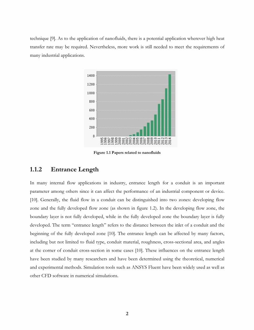
The term, nanofluids, referring to the fluid with suspended nanometer-sized particles, was first used
by Choi [1].Choi showed that by introducing a small amount of nanoparticles to conventional heat
transfer liquids, the thermal conductivity can be increased by two times. After that, many researchers
investigated this topic (as shown in figure 1.1), aiming at understanding the characteristics and
mechanisms of nanofluids and eventually being able to enhance the thermal conductivity. Masuda et
al. [3], Lee et al. [4], Xuan and Li [5], and Xuan and Roetzel [6] stated that the thermal conductivity
of the suspensions can increase more than 20% with low nanoparticles concentrations. Easeman et
al. [7] experimentally showed that the thermal conductivity can be increased by approximately 60%
by adding 5% volume of CuO nanoparticles in water as base fluid. Many factors significantly
affecting the thermal conductivity are, but not limited to particle size, particle shape, base fluid
material temperature, and additives’ properties. These factors have been researched in recent years
and numerous models have been proposed to take these factors into account depending upon the
application. Some of these typical models will be discussed in the following chapters.
The demand for high heat transfer rate is increasing widely nowadays and there has been a broad
application of nanofluids as a heat transfer medium. One example of the growing demand is the
revolution in microprocessors, which have continually become smaller and more powerful to meet
the demand of big data storage and computing. As a result, a faster heat-flow demand has steadily
increased over time due to the fact that the thermal management has become the bottleneck of
developing high-performance computing units at a relatively small scale. Another application is in
automotive industry, where improved heat transfer could lead to smaller heat exchangers for cooling
and therefore save space inside the hood of the vehicle [8]. In industry, nanoparticles used in
nanofluids to enhance the thermal conductivity have been made out of many different materials, via
both the physical synthesis processes and the chemical synthesis processes. Typical physical methods
that produce these materials include the mechanical grinding method and the inert-gas-condensation
2
technique [9]. As to the application of nanofluids, there is a potential application wherever high heat
transfer rate may be required. Nevertheless, more work is still needed to meet the requirements of
many industrial applications.
Figure 1.1 Papers related to nanofluids
1.1.2 Entrance Length
In many internal flow applications in industry, entrance length for a conduit is an important
parameter among others since it can affect the performance of an industrial component or device.
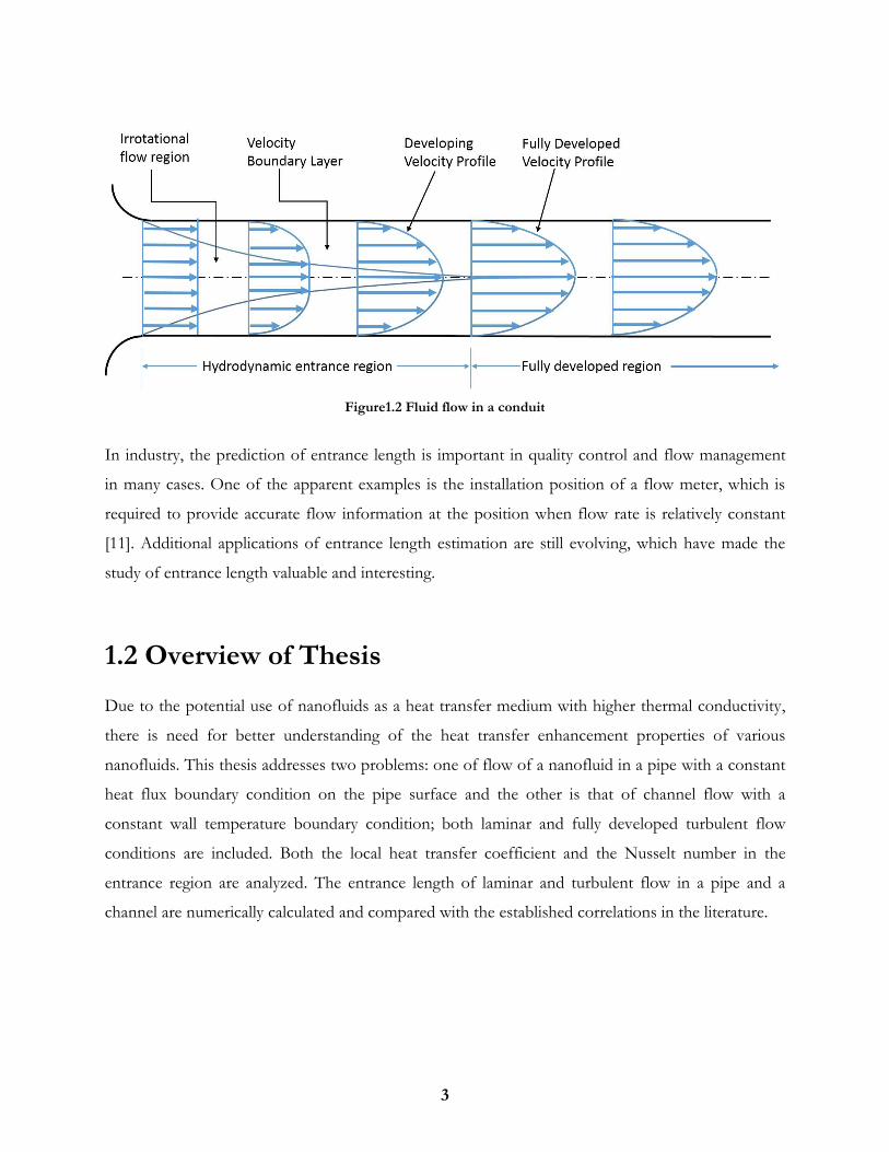
[10]. Generally, the fluid flow in a conduit can be distinguished into two zones: developing flow
zone and the fully developed flow zone (as shown in figure 1.2). In the developing flow zone, the
boundary layer is not fully developed, while in the fully developed zone the boundary layer is fully
developed. The term “entrance length” refers to the distance between the inlet of a conduit and the
beginning of the fully developed zone [10]. The entrance length can be affected by many factors,
including but not limited to fluid type, conduit material, roughness, cross-sectional area, and angles
at the corner of conduit cross-section in some cases [10]. These influences on the entrance length
have been studied by many researchers and have been determined using the theoretical, numerical
and experimental methods. Simulation tools such as ANSYS Fluent have been widely used as well as
other CFD software in numerical simulations.
3
Figure1.2 Fluid flow in a conduit
In industry, the prediction of entrance length is important in quality control and flow management
in many cases. One of the apparent examples is the installation position of a flow meter, which is
required to provide accurate flow information at the position when flow rate is relatively constant
[11]. Additional applications of entrance length estimation are still evolving, which have made the
study of entrance length valuable and interesting.
1.2 Overview of Thesis
Due to the potential use of nanofluids as a heat transfer medium with higher thermal conductivity,
there is need for better understanding of the heat transfer enhancement properties of various
nanofluids. This thesis addresses two problems: one of flow of a nanofluid in a pipe with a constant
heat flux boundary condition on the pipe surface and the other is that of channel flow with a
constant wall temperature boundary condition; both laminar and fully developed turbulent flow
conditions are included. Both the local heat transfer coefficient and the Nusselt number in the
entrance region are analyzed. The entrance length of laminar and turbulent flow in a pipe and a
channel are numerically calculated and compared with the established correlations in the literature.

4
Chapter 2 Nanofluids
2.1 Nanofluid Conduction Heat Transfer Properties
2.1.1 Heat Transfer Enhancement Mechanisms
Three mechanisms - Brownian motion, nanoparticles clustering and liquid molecules layering are
considered as the three main heat transfer enhancement mechanisms for nanofluids; these
mechanisms are briefly described here.
Brownian motion refers to the constant random motion of nano-sized particles suspended in fluid
[12-16]. The behavior of these nano-sized particles is very different from the micro- or millimeter-
size particles due to the fact that the latter do not move in a stationary base fluid. Therefore, the
Brownian motion is an important factor in considering the heat transport from nanofluids. Two
mechanisms create Brownian motion in nanofluids [17]: one is due to the collisions among the
nanoparticles and the other is the convection induced by random motion of nanoparticles. In some
cases, the Brownian motion of nanoparticles can also lead to the aggregation of nanoparticles [18],
which may not be desirable in some applications.
Aggregation, which will be referred to as the nanoparticles clustering in this paper, is an inherent
property of the nano-particles whether they are suspended in liquid or are in powder form; it results
due to van der Waals forces in colloidal suspensions [18]. In order to describe the nanoparticles
clustering, numerous models have been developed [19, 20, 21, 22]. These models are widely used
nowadays to study the thermal conductivity of different types of nanofluids.
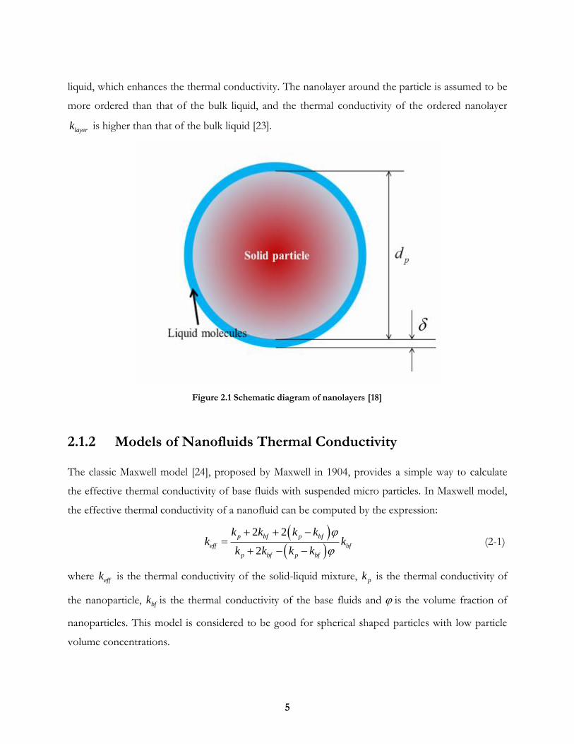
Liquid molecules layering generally refers to the fact that liquid molecules near a solid surface can
form layered structures called nanolayers. The nanolayer structure has been recently introduced by
Keblinski et al. [19], and Yu and Choi [23] as another mechanism to explain the enhanced thermal
conductivity of nanofluids. Figure 2.1 shows the schematic diagram of the basic concept of
nanolayers. Nanolayers can be considered as a thermal bridge between a solid particle and a bulk
5
liquid, which enhances the thermal conductivity. The nanolayer around the particle is assumed to be
more ordered than that of the bulk liquid, and the thermal conductivity of the ordered nanolayer
layerk is higher than that of the bulk liquid [23].
Figure 2.1 Schematic diagram of nanolayers [18]
2.1.2 Models of Nanofluids Thermal Conductivity
The classic Maxwell model [24], proposed by Maxwell in 1904, provides a simple way to calculate
the effective thermal conductivity of base fluids with suspended micro particles. In Maxwell model,
the effective thermal conductivity of a nanofluid can be computed by the expression:
2 2
2
p bf p bf
eff bf
p bf p bf
k k k kk k
k k k k
(2-1)
where effk is the thermal conductivity of the solid-liquid mixture, pk is the thermal conductivity of
the nanoparticle, bfk is the thermal conductivity of the base fluids and is the volume fraction of
nanoparticles. This model is considered to be good for spherical shaped particles with low particle
volume concentrations.

6
Numerous studies have been conducted after Maxwell to improve upon it for calculating the
effective thermal conductivity. In 1962, Hamilton and Crosser [25] extended the Maxwell’s model by
introducing a factor to take into account the shape of the particle. The thermal conductivity, given
by Hamilton and Crosser [25], can be written as:
1 1
1
p bf bf p
eff bf
p bf bf p
k n k n k kk k
k n k k k
(2-2)
where n is the empirical shape factor given by 3 / . is the particle sphericity, which is defined
as the ratio of the surface area of a sphere with the same volume as the particle and the surface area
of the non-spherical particle itself.
The above two models and several others of similar type have primarily focused on the
micro/millimeter level particles. In order to predict the thermal conductivity of nanofluids, new
models and theories have been proposed in the recent years. Among many of the newly developed
models, three classes of models have been typically developed: Brownian models, clustering models
and liquid layering models. These three models are discussed below.
2.1.2.1 Brownian models The Brownian motion of the suspended nano-particles is considered to be the most important
factor in enhanced thermal conductivity of nanofluids by Chon et al. [26] and many others. Based on
this, they proposed an empirical correlation for the thermal conductivity of Al2O3 particle based
nanofluids from their experimental data using Buckinghan-Pi theorem with a linear regression
scheme [26]. The correlation is given as:
0.3690 0.7476
0.7460 0.9955 1.23211 64.7 Pr Renf bf p
bf p bf
k d k
k d k
(2-3)
where bfd : molecular diameter of the base fluid,
Prpbf bf
bf
C
k
: the Prandtl number of the base fluid,
2
Re3
bf
bf bf
T
l
: the Reynolds number, and

7
bfl : mean-free path for the base fluid. A constant value of 0.17 for mean free path of base fluid was
used in their paper.
Jang and Choi [27] proposed four factors that may contribute to the enhancement of thermal
conductivity of the nanofluids: collision among the molecules of the base fluid, thermal diffusion of
nanoparticles, collision of nanoparticles among each other due to the Brownian motion and the
collision between the base fluid molecules and the nanoparticles by thermally induced fluctuations.
Considering these four factors, the effective thermal conductivity of the nanofluid can be written as:
2
1 11 Re Prp
bf
nf bf p bf d
p
dk k k C k
d (2-4)
where 1 0.01 is a constant considering the Kapitza resistance per unit area; 6
1 18 10C is a
proportionality constant; Pr is the Prandtl number of the base fluid, and the Reynolds number is
defined by . .
Rep
R M p
d
C d
v where . .
3R M
bf p bf
TC
d l
is the random motion velocity of a
nanoparticle and v is the kinematic viscosity of the base fluid. As recommend by Jang and Choi
[27], for water-based nanofluids the equivalent diameter 0.384bfd nm and the mean-free path
0.738bfl nm at a temperature of 300K .
In 2004, Koo and Kleinstreuer [28] proposed a new thermal conductivity model for nanofluids,
which is based on the conventional static part and the significant impact of Brownian motion on the
effective thermal conductivity. The effect of particle size, particle volume fraction and temperature
dependence, and the type of particle and base fluid combinations are taken into consideration in this
model.
static static browniank k k (2-5)
3( 1)
1
( 2) ( 1)
p
bfstatic
p pbf
bf bf
k
kk
k kk
k k
(2-6)

8
In above formulas, statick is the static thermal conductivity based on the Maxwell’s model and the
browniank is the dynamic part which was generated by employing the micro-scale convective heat
transfer of a particle’s Brownian motion affected by the ambient fluid motion. This enhanced
thermal conductivity component was obtained by simulating Stoke’s flow around a spherical nano-
particle. The thermal conductivity due to Brownian motion [28] was obtained as:
4
,5 10 ( , )bbrownian bf p bf
p p
k Tk c f T
d
(2-7)
where bf ,
,p bfc is the density and specific heat capacity of the base fluid, is the volume fraction
of nano-particles, bk is the Boltzmann constant and T is the temperature. The two empirical
functions and f introduced by Koo combine the hydrodynamic interaction between the
Brownian-motion-induced fluid particles and the temperature effect.
In recent years, the importance of the interfacial thermal resistance fR between the nanoparticles
and the fluids has also been emphasized by many researchers [29, 30]. The thermal interfacial
resistance (Kapitza resistance) is believed to exist in the adjacent layers of the two different
materials; the thin barrier layer plays a key role in weakening the effective thermal conductivity of
the nanoparticles.
In the new correlation for thermal conductivity of nanoparticles proposed in Ref [31],
8 24 10 /fR km W is chosen as the thermal interfacial resistance. By introducing fR , the original
pk in Eq. (2-6) is replaced by a new ,p effk in the form:
,
p p
f
p p eff
d dR
k k
(2-8)
Li [31] also revised the model of Koo and Kleinstreuer [28] by combining the functions and f
into a new function g , which considered the influence of particle diameter, temperature and
volume fraction. For different base fluids and different nanoparticles, the function is different. Only
water based nanofluids are considered in the present study due to the abundance of experimental
data. For Al2O3/water and CuO/water nanofluids, the g function can be expressed as:

9
1 2 3 4
2
5 6 7 8
2
9 10
'( , , ) ( ln( ) ln( ) ln( ) ln( )
ln( ) ) ln( ) ( ln( ) ln( )
ln( ) ln( ) ln( ) )
p p p
p p
p p
g T d a a d a a d
a d T a a d a
a d a d
(2-9)
where 0.04,300 325K T K
With the coefficients , 1,2...10ia i based on the type of nanoparticle, and with these coefficients,
Al2O3/water and CuO/water nanofluids have a 2R of 96% and 98%, respectively [31] (Table can be
found in [31]). Thus, the KKL(Koo-Kleinstreuer-Li) correlation can be written as:
4
,5 10 '( , , )bbrownian bf p bf p
p p
k Tk c g T d
d
(2-10)
The viscosity of the nanofluids using the Einstein’s equation [32] is given as:
(1 2.5 )nf bf (2-11)
Brinkman [33] proposed a new correlation that extended the Einstein’s equation to suspensions with
moderate particle volume fraction, typically less than 4%, as:
2.5(1 )
bf
static
(2-12)
Koo and Kleinstreuer [28] further investigated the laminar nanofluids flow using the effective
nanofluid thermal conductivity model they developed. For the effective viscosity due to micro
mixing in suspensions, they proposed
Pr
bfBrownianeff static Brownian static
bf bf
k
k
(2-13)
where static is the viscosity of nanofluids, which is the correlation given by Brinkman.
2.1.2.2 Clustering Models
Brownian motion of nanoparticles and their aggregation is considered to be an important factor by
Xuan et al. [34] and many others. Xuan et al. proposed a modified correlation for the apparent
thermal conductivity of nanofluid, which is the sum of the Maxwell’s model and a term due to
Brownian motion of the nanoparticles and clusters. It can be written as:
10
2 2
2 32
Pp bf bf p p P
nf bf
bf cp bf bf p
k k k k C Tk k
rk k k k
(2-14)
where cr is the mean radius of gyration of the cluster and bf is the viscosity of base fluid. Upon
inspection, it is found that the second term of Eq. (2-12) does not yield the unit of the thermal conductivity (W/m K). Therefore, the equation is not dimensionally homogeneous. In order to
satisfy the dimensional homogeneity, the constant coefficient 1
2 3
should have a unit instead
of being dimensionless. The only condition under which the Eq. (2-12) is dimensionally correct is by
assigning a unit of /m s to this constant coefficient, so that the whole term matches the unit of
thermal conductivity.
2.1.2.3 Liquid Layering Model
Yu and Choi [23] proposed a modified Maxwell model to include the effect of a nanolayer
surrounding the particles by replacing the thermal conductivity of solid particles with the equivalent
thermal conductivity of particlespek . This is based on the effective medium theory and
pek is
obtained as:
3
3
2 1 1 1 2
1 1 1 2pe pk k
(2-15)
where /layer pk k is the ratio of nanolayer thermal conductivity to particle thermal conductivity
and /h r is the ratio of the nanolayer thickness to the particle radius. In their study, the
nanolayer thickness h and the thermal conductivity layerk are in the range from 1 to 2 nm and
10 100bp layer bpk k k , respectively. Finally the thermal conductivity of the nanofluid is given as:
3
3
2 2 1
2 2 1
pe bf pe bf
nf bf
pe bf pe bf
k k k kk k
k k k k
(2-16)
In addition, Xue and Xu [35] developed an implicit relation for the effective thermal conductivity of
copper oxide/water and copper oxide/EG nanofluids based on a model of nanoparticles with
interfacial shells between the surface of the solid particle and the surrounding liquid.
2 2 2 2
2 2 2 2
2 21 0
2 2 2 2
nf p p nfnf bf
nf bf nf p p nf
k k k k k k k kk k
k k k k k k k k k k
(2-17)

11
where
3
p
p
r
r t
, in which 2k is thermal conductivity of the interfacial shell, t represents the
thickness of the interfacial shell and pr the radius of the nano-particle.
2.2 Nanofluid Convection Heat Transfer Properties
2.2.1 Heat Transfer Coefficient and Nusselt Number
The heat transfer coefficient nfh is a function of temperature in classic natural convective heat
transfer, and Newton’s law can be applied to the function when the temperature changes are
relatively small. The heat transfer coefficient is defined for nanofluids by the expression:
wnf
w b
qh
T T
(2-18)
where wq is the wall heat flux, wT is wall temperature, and bT is the bulk temperature of the
nanofluid. The Nusselt number is the ratio of convective to conductive heat transfer across the
boundary. The larger is the Nusselt number, the more active is the convective heat transfer
performance of the fluid flow. Based onnfh , the Nusselt number of nanofluid is defined as:
nf
nf
nf
h DNu
k (2-19)
where D is the characteristic length, k is the thermal conductivity of the fluid. For nanofluids, nfk
is usually predicted by the theoretical model or experimental data.
For fully developed laminar flow in circular tubes, the Nusselt number is given as [36]:
nfNu = 4.36 for uniform surface heat flux
3.66 for uniform surface temperature
For surface fully developed turbulent flow in smooth circular tubes
( Re 10,000,0.7 Pr 160, / 10D L D ), the Nusselt number is given as (Dittus Boelter equation)
3/40.023Re Prn
D DNu (2-20)

12
where L is the pipe test section, D is the pipe test section diameter, Re is the Reynolds number
and Pr is the Prandtl number. In particular, for cooling of the fluid 0.3n and for heating of the
fluid 0.4n .
The conventional correlation is not suitable for evaluating the Nusselt number of nanofluids, and
the proper physical mechanism of heat transfer enhancement has not yet been established. Hence,
researchers have proposed various correlations to predict the Nusselt number of nanofluids.
Xuan and Roetzel [37] proposed a general function for the Nusselt number; it is defined as:
( )
[Re,Pr, , ], , , ]( )
p p p
nf
bf p bf
k cNu f particle size and shape flow geometry
k c
(2-21)
where Re is the Reynolds number of nanofluid, Pr is the Prandtl number of nanofluid, Pe is the
Peclet number and is the volume fraction.
Pak and Cho et al. [38] investigated the turbulent friction and convective heat transfer behaviors of
dispersed fluids in a circular pipe experimentally. Two metallic oxide particles, γ-Al2O3 and TiO2,
with mean diameter of 13 and 27nm, respectively, were used as working fluids. According to their
observation, the Nusselt number for fully developed turbulent flow increased corresponding to the
increasing volume concentration as well as Reynolds number. However, it was found that the
convective heat transfer coefficient of the nanofluids at a volume concentration of 3% was 12%
smaller than that of pure water when compared under the condition of constant average velocity.
Therefore better selection of particles having higher thermal conductivity and larger size is
recommended in order to enhance the heat transfer performance.
The following correlation is suggested for volume concentration of 0-3%, Reynolds and Prandtl
numbers of 104 to 105 and 6.5 – 12.3, respectively:
0.8 0.50.021Re Prnf nf nfNu (2-22)
Li and Xuan [40] investigated the convective heat transfer and flow characteristics of the nanofluid
in a tube. Both the convective heat transfer coefficient and friction factor of Cu-water nanofluid for
the laminar and turbulent flow are measured. According to the experimental results, the convective
13
heat transfer coefficient of the base fluid increased remarkably, and the friction factor of the sample
nanofluid with the low volume fraction of nanoparticles is almost not changed. Compared with the
base fluid, the convective heat transfer coefficient is increased about 60% for the nanofluid with 2.0 %
volume of Cu nanoparticles at the same Reynolds number. A new convective heat transfer
correlation for a nanofluid suspended with the nanoparticles under single-phase flow assumption
has been established for volume concentration of 0-2% and minimum Re of 800:
0.754 0.218 0.333 0.40.4328(1 11.25 )Re Prnf p nf nfNu Pe (2-23)
Xuan and Li [41] also experimentally investigated the convective heat transfer and turbulent flow
features of the Cu-H2O nanofluid in a straight brass tube of inner diameter of 10mm and length of
800mm. By considering the microconvection and microdiffusion effects of the suspended
nanoparticles, they proposed a new correlation for turbulent flow of nanofluids in a tube for volume
concentration of 0-2% and Reynolds numbers of 1×10⁴ to 2.5 ×10⁴:
0.6886 0.001 0.9238 0.40.0059(1 7.6286) )Re Prnf p nf nfNu Pe (2-24)
Vajjha et al. [41] carried out experiments for nanofluids with nanoparticles comprised of aluminum
oxide, copper oxide and silicon dioxide in 60% ethylene glycol and 40% water by mass. The
rheological and the thermophysical properties such as viscosity, density, specific heat and thermal
conductivity were measured to develop the heat transfer coefficient correlation from experiments.
The following correlation was proposed for the convective heat transfer:
0.65 0.15 0.5420.065(Re 60.22)(1 0.0169 )Prnf nf nfNu (2-25)
Koo and Kleinstreuer [42] investigated steady laminar nanofluid flow in microchannels simulating by
two types of fluid, which consisted of copper oxide nanospheres at low volume concentrations in
water or in ethylene glycol. The governing equations for the fluid and the wall were solved
numerically considering a new model of effective thermal conductivity. In this model, the
conventional static part as well as the dynamic part derived from the particle Brownian motion was
considered. From the results, the following conclusion were made: use of large high-Prandtl number
carrier fluids, nanoparticles at high volume concentrations of about 4% with elevated thermal
14
conductivities and dielectric constants very close to that of the carrier fluid, microchannels with high
aspect ratios and treated channel walls to avoid nanoparticle accumulation should be employed.
In summary, a general correlation for the heat transfer of nanofluid and the physical mechanism of
nanofluid flow needs to be developed. A large deviation in predicted values shows the limitation of
the current correlations. This may be due to the various influences coming from particle properties,
the composition of basic fluid, the hydrodynamic properties and the heat transfer characteristics.
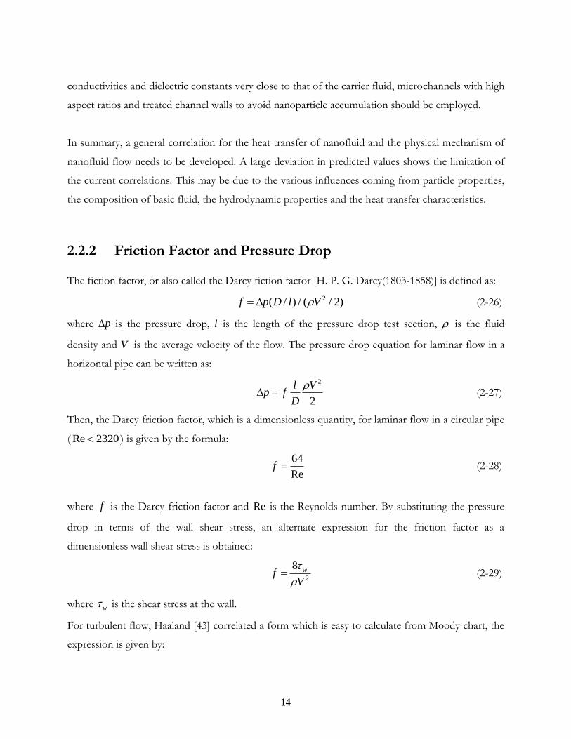
2.2.2 Friction Factor and Pressure Drop
The fiction factor, or also called the Darcy fiction factor [H. P. G. Darcy(1803-1858)] is defined as:
2( / ) / ( / 2)f p D l V (2-26)
where p is the pressure drop, l is the length of the pressure drop test section, is the fluid
density and V is the average velocity of the flow. The pressure drop equation for laminar flow in a
horizontal pipe can be written as:
2
2
l Vp f
D
(2-27)
Then, the Darcy friction factor, which is a dimensionless quantity, for laminar flow in a circular pipe
( Re 2320 ) is given by the formula:
64
Ref (2-28)
where f is the Darcy friction factor and Re is the Reynolds number. By substituting the pressure
drop in terms of the wall shear stress, an alternate expression for the friction factor as a
dimensionless wall shear stress is obtained:
2
8 wfV
(2-29)
where w is the shear stress at the wall.
For turbulent flow, Haaland [43] correlated a form which is easy to calculate from Moody chart, the
expression is given by:
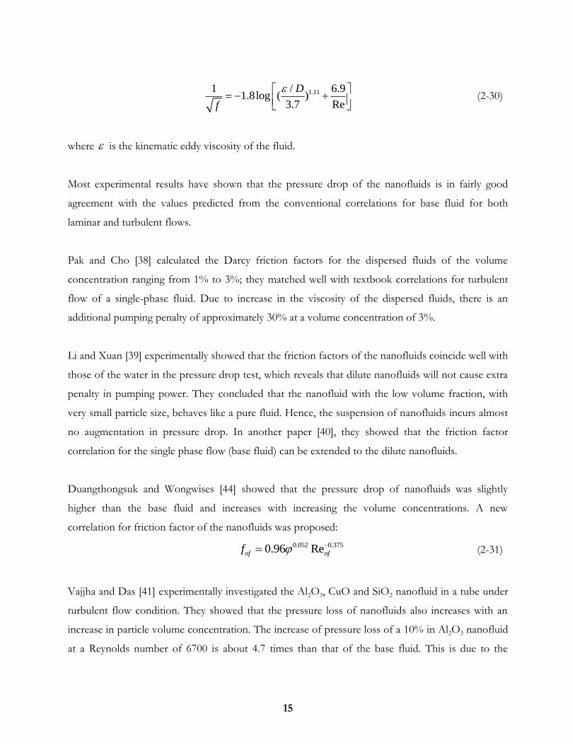
15
1.111 / 6.91.8log ( )
3.7 Re
D
f
(2-30)
where is the kinematic eddy viscosity of the fluid.
Most experimental results have shown that the pressure drop of the nanofluids is in fairly good
agreement with the values predicted from the conventional correlations for base fluid for both
laminar and turbulent flows.
Pak and Cho [38] calculated the Darcy friction factors for the dispersed fluids of the volume
concentration ranging from 1% to 3%; they matched well with textbook correlations for turbulent
flow of a single-phase fluid. Due to increase in the viscosity of the dispersed fluids, there is an
additional pumping penalty of approximately 30% at a volume concentration of 3%.
Li and Xuan [39] experimentally showed that the friction factors of the nanofluids coincide well with
those of the water in the pressure drop test, which reveals that dilute nanofluids will not cause extra
penalty in pumping power. They concluded that the nanofluid with the low volume fraction, with
very small particle size, behaves like a pure fluid. Hence, the suspension of nanofluids incurs almost
no augmentation in pressure drop. In another paper [40], they showed that the friction factor
correlation for the single phase flow (base fluid) can be extended to the dilute nanofluids.
Duangthongsuk and Wongwises [44] showed that the pressure drop of nanofluids was slightly
higher than the base fluid and increases with increasing the volume concentrations. A new
correlation for friction factor of the nanofluids was proposed:
0.052 0.3750.96 Renf nff (2-31)
Vajjha and Das [41] experimentally investigated the Al2O3, CuO and SiO2 nanofluid in a tube under
turbulent flow condition. They showed that the pressure loss of nanofluids also increases with an
increase in particle volume concentration. The increase of pressure loss of a 10% in Al2O3 nanofluid
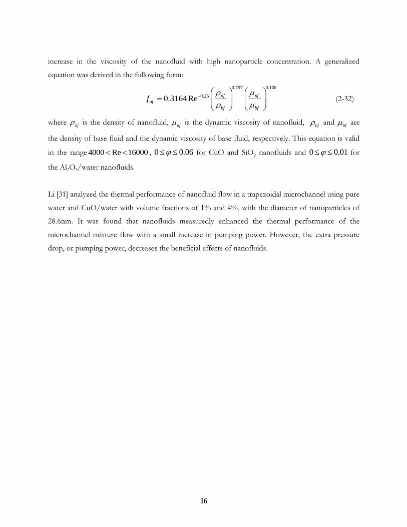
at a Reynolds number of 6700 is about 4.7 times than that of the base fluid. This is due to the
16
increase in the viscosity of the nanofluid with high nanoparticle concentration. A generalized
equation was derived in the following form:
0.797 0.108
0.250.3164Renf nf
nf
bf bf
f
(2-32)
where nf is the density of nanofluid,
nf is the dynamic viscosity of nanofluid, bf and
bf are
the density of base fluid and the dynamic viscosity of base fluid, respectively. This equation is valid
in the range 4000 Re 16000 , 0 0.06 for CuO and SiO2 nanofluids and 0 0.01 for
the Al2O3/water nanofluids.
Li [31] analyzed the thermal performance of nanofluid flow in a trapezoidal microchannel using pure
water and CuO/water with volume fractions of 1% and 4%, with the diameter of nanoparticles of
28.6nm. It was found that nanofluids measuredly enhanced the thermal performance of the
microchannel mixture flow with a small increase in pumping power. However, the extra pressure
drop, or pumping power, decreases the beneficial effects of nanofluids.

17
Chapter 3 Methodology
CFD is an abbreviation for Computational Fluid Dynamics. It is a branch of fluid mechanics that
uses numerical methods and algorithms to solve the governing equations of fluid flow and provides
useful information for analysis and design of systems involving fluid flow. CFD based analysis
requires computers to perform the calculations. The main advantage of CFD is that it can be used to
solve very complex fluid flow problems.
The CFD analysis procedures are generally divided into three steps: pre-processing, simulation and
post-processing. During the preprocessing, the geometry of the problem is defined and the volume
occupied by the fluid is divided into discrete cells known as the mesh. The simulation step involves
discretizing the governing equations on the mesh generated in the first step by employing a suitable
numerical algorithm. The discretized equations are then solved on a computer and the values of the
flow variables are obtained at the mesh points. In the final post-processing step, the simulation data
is analyzed, visualized and used for analysis and design improvement.
3.1 Governing Equations
The governing equations of fluid flow are partial differential equations that describe the
conservation of mass, momentum and energy. These equations can be written as:
Continuity equation:
0i
i
ut x
(3-1)
Momentum equation:
j
ij
i i
i i i
pu u
t x x xu
(3-2)
18
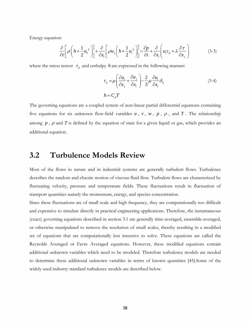
Energy equation:
2 21 1
2 2j i i ij
i i j
ph u u h u
t x t x xu
i (3-3)
where the stress tensor ij and enthalpy h are expressed in the following manner:
2
3
ji iij ij
j i i
uu u
x x x
(3-4)
ph TC
The governing equations are a coupled system of non-linear partial differential equations containing
five equations for six unknown flow-field variables u , v , w , p , , and T . The relationship
among p , and T is defined by the equation of state for a given liquid or gas, which provides an
additional equation.
3.2 Turbulence Models Review
Most of the flows in nature and in industrial systems are generally turbulent flows. Turbulence
describes the random and chaotic motion of viscous fluid flow. Turbulent flows are characterized by
fluctuating velocity, pressure and temperature fields. These fluctuations result in fluctuation of
transport quantities namely the momentum, energy, and species concentration.
Since these fluctuations are of small scale and high frequency, they are computationally too difficult
and expensive to simulate directly in practical engineering applications. Therefore, the instantaneous
(exact) governing equations described in section 3.1 are generally time-averaged, ensemble-averaged,
or otherwise manipulated to remove the resolution of small scales, thereby resulting in a modified
set of equations that are computationally less intensive to solve. These equations are called the
Reynolds Averaged or Favre Averaged equations. However, these modified equations contain
additional unknown variables which need to be modeled. Therefore turbulence models are needed
to determine these additional unknown variables in terms of known quantities [45].Some of the
widely used industry standard turbulence models are described below.
19
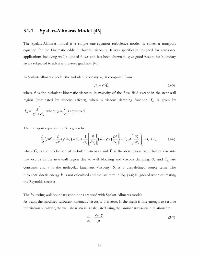
3.2.1 Spalart-Allmaras Model [46]
The Spalart-Allmaras model is a simple one-equation turbulence model. It solves a transport
equation for the kinematic eddy (turbulent) viscosity. It was specifically designed for aerospace
applications involving wall-bounded flows and has been shown to give good results for boundary
layers subjected to adverse pressure gradients [45].
In Spalart-Allmaras model, the turbulent viscosity t is computed from
1t vvf (3-5)
where v is the turbulent kinematic viscosity in majority of the flow field except in the near-wall
region (dominated by viscous effects), where a viscous damping function 1vf is given by
3
1 3 3
1
v
v
fc
where
v
v is employed.
The transport equation for v is given by:
2
1i v b v v
t v j j j
v vv vu G v C Y S
t x x x x
(3-6)
where vG is the production of turbulent viscosity and vY is the destruction of turbulent viscosity
that occurs in the near-wall region due to wall blocking and viscous damping. v and 2bC are
constants and v is the molecular kinematic viscosity. vS is a user-defined source term. The
turbulent kinetic energy k is not calculated and the last term in Eq. (3-6) is ignored when estimating
the Reynolds stresses.
The following wall boundary conditions are used with Spalart-Allmaras model:
At walls, the modified turbulent kinematic viscosity v is zero. If the mesh is fine enough to resolve
the viscous sub-layer, the wall shear stress is calculated using the laminar stress-strain relationship:
u yu
u
(3-7)

20
If the mesh is too coarse and the viscous sub-layer cannot be resolved, it is assumed that the
centroid of the wall-adjacent cell falls within the logarithmic region of the boundary layer, and the
law-of-the-wall is employed:
1ln
u yuE
u
(3-8)
where u is the velocity parallel to the wall, u is the shear velocity, y is the distance from the wall,
is the von Karman constant (0.4187), and E is 9.793.
For separated and transitional flows, we employ both the shear-stress transport (SST) k-ω model and
the transitional k-kl-ω model. They both have advantages and disadvantages. Developed by Menter
[45], the SST k-ω model is more accurate and reliable for a wider class of flows (e.g. adverse pressure
gradient flows, transonic flows etc.) than the standard k - model.
3.2.2 Shear-stress Transport (SST) k - ω Model [46]
The SST k - model effectively blends the robust and accurate formulation of k - model in the
near-wall region with the k - model away from the wall region. To achieve this, the standard k -
model and the k - model are both multiplied by a blending function and both models are then
added together. The blending function is used to activate the standard k - model in the near-wall
region and the k - model away from the surface.
The SST k - model consists of the following two transport equations for the turbulent kinetic
energy ( k ) and the specific dissipation rate ( ).
i k k k k
i j j
kk ku G Y S
t x x x
(3-9)
i
i j j
u G Y D St x x x
(3-10)
where kG represents the generation of turbulent kinetic energy due to mean velocity gradients. G
represents the generation of . k and represent the effective diffusivity of k and . kY and
21
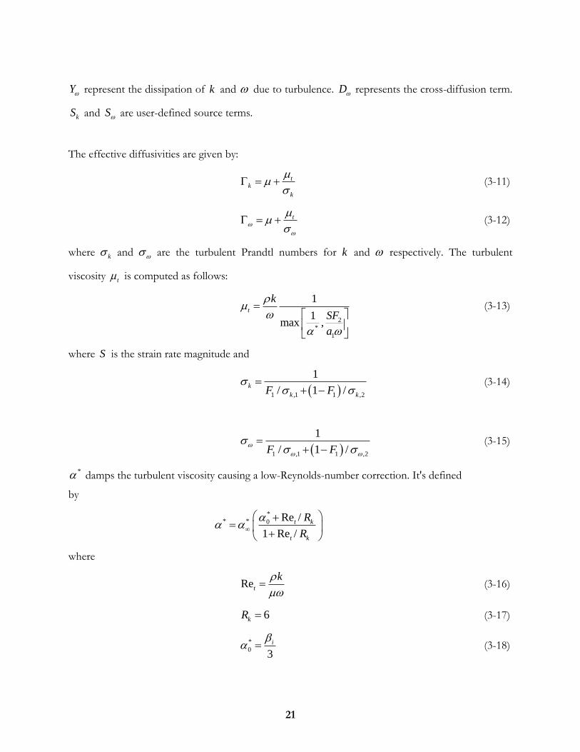
Y represent the dissipation of k and due to turbulence. D represents the cross-diffusion term.
kS and S are user-defined source terms.
The effective diffusivities are given by:
tk
k
(3-11)
t
(3-12)
where k and are the turbulent Prandtl numbers for k and respectively. The turbulent
viscosity t is computed as follows:
2
*
1
1
1max ,
t
k
SF
a
(3-13)
where S is the strain rate magnitude and
1 ,1 1 ,2
1
/ 1 /k
k kF F
(3-14)
1 ,1 1 ,2
1
/ 1 /F F
(3-15)
* damps the turbulent viscosity causing a low-Reynolds-number correction. It's defined
by
*
* * 0 Re /
1 Re /
t k
t k
R
R
where
Ret
k
(3-16)
6kR (3-17)
*
03
i (3-18)

22
0.072i (3-19)
In the high-Reynolds-number form, * * 1a . The blending function functions 1F and 2F are
given by
4
1 1tanhF (3-20)
1 2 2
,2
500 4min max , ,
0.09
k k
y y D y
(3-21)
10
,2
1 1max 2 ,10
j j
kD
x x
(3-22)
2
2 2tanhF (3-23)
2 2
500max 2 ,
0.09
k
y y
(3-24)
where y is the distance next to the surface and D
is the positive portion of the cross-diffusion
term.
3.2.3 k-epsilon Model [47]
The k turbulent transport equations [47] are given as:
t ij ij
j j k j j
Uk k kU
t x x x x
(3-25)
2
t ij ij
j j j j
UU
t x x x k x k
1ε 2εC C (3-26)
In these equations, 1εC and 2εC are constants. k and are the turbulent Prandtl numbers for k
and , respectively and t is the eddy viscosity given by equation
2
t
kC
(3-27)
The various constants in the equations are given in Table 3-1
23
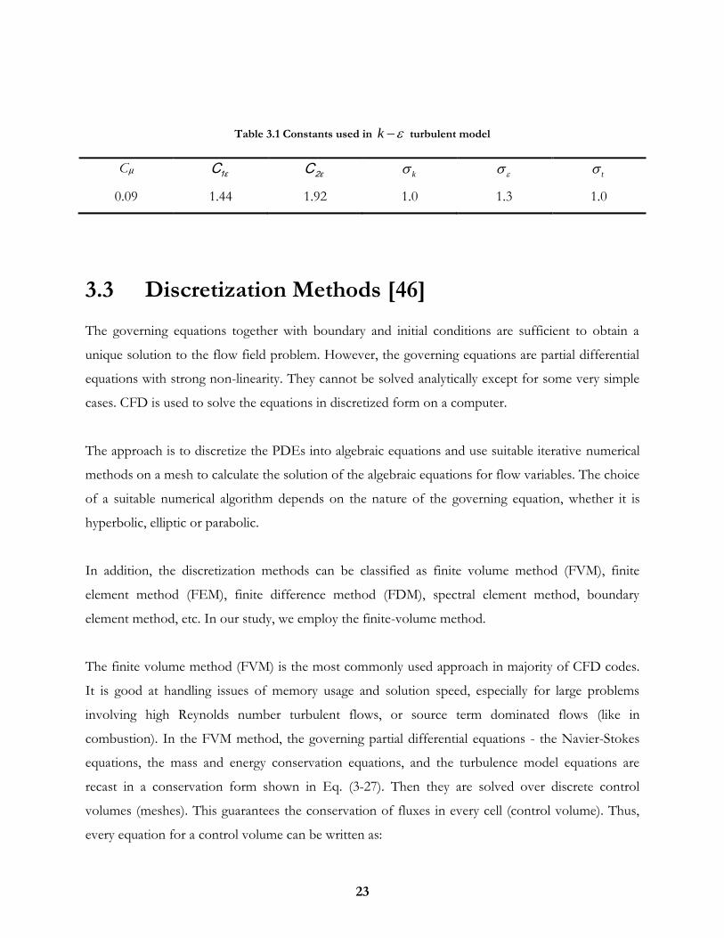
Table 3.1 Constants used in k turbulent model
Cμ 1εC 2εC k t
0.09 1.44 1.92 1.0 1.3 1.0
3.3 Discretization Methods [46]
The governing equations together with boundary and initial conditions are sufficient to obtain a
unique solution to the flow field problem. However, the governing equations are partial differential
equations with strong non-linearity. They cannot be solved analytically except for some very simple
cases. CFD is used to solve the equations in discretized form on a computer.
The approach is to discretize the PDEs into algebraic equations and use suitable iterative numerical
methods on a mesh to calculate the solution of the algebraic equations for flow variables. The choice
of a suitable numerical algorithm depends on the nature of the governing equation, whether it is
hyperbolic, elliptic or parabolic.
In addition, the discretization methods can be classified as finite volume method (FVM), finite
element method (FEM), finite difference method (FDM), spectral element method, boundary
element method, etc. In our study, we employ the finite-volume method.
The finite volume method (FVM) is the most commonly used approach in majority of CFD codes.
It is good at handling issues of memory usage and solution speed, especially for large problems
involving high Reynolds number turbulent flows, or source term dominated flows (like in
combustion). In the FVM method, the governing partial differential equations - the Navier-Stokes
equations, the mass and energy conservation equations, and the turbulence model equations are
recast in a conservation form shown in Eq. (3-27). Then they are solved over discrete control
volumes (meshes). This guarantees the conservation of fluxes in every cell (control volume). Thus,
every equation for a control volume can be written as:

24
0QdV FdAt
(3-28)
where Q is the vector of conserved variables, F is the flux vector, dV is the volume of the cell, dA
is the surface area of the cell.
3.4 Description of ANSYS Fluent
The Navier-Stokes (NS) equations are solved using the commercial code ANSYS FLUENT, a
widely used commercial finite-volume method (FVM) based software in computational fluid
dynamics (CFD). It is employed to compute the flow properties such as wall shear stress, velocity,
temperature, pressure distributions in the flow filed. It is a general-purpose CFD code based on the
finite volume method on a collocated grid [45], which is capable of solving steady and unsteady
incompressible and compressible, Newtonian and Non-Newtonian flows. FLUENT also provides
several zero-, one- and two-equation turbulence models.
ICEM CFD is a pre-processing software used to build geometric models and to generate grids
around those models. It allows users either to create their own geometry or to import geometry
from most CAD packages. It can also automatically mesh surfaces and volumes while allowing the
user to control the mesh through the use of sizing functions and boundary layer meshing. It can
generate structured, unstructured and hybrid meshes depending upon the application.
In the current study, the set of governing equations with the associated boundary conditions were
numerically solved by finite volume method. The semi-implicit method for pressure-linked
equations (SIMPLE) algorithm was used to solve for the pressure and the velocity components.
Second order upwind scheme was used to discretize the advective terms in momentum and energy
equations to control numerical errors and achieve convergence. The entire domain was initialized
with the conditions of inlet boundary before starting the iterative process. In the present analysis, for
the constant heat flux boundary condition, axisymmetric flow is considered. For the constant wall
temperature boundary condition, planar flow is considered.

25
Table 3.2 The convergence criteria used for various flow variables and conservation equations
Flow variable Convergence criteria
Continuity 10-6
x-velocity 10-6
y-velocity 10-6
Energy 10-6
26
Chapter 4 Entry Flow and Heat Transfer of Laminar Forced Convection of Nanofluids in a Pipe and a Channel
This chapter presents the entrance flow field and heat transfer characteristics of nanofluids in a pipe
and a channel. Constant heat flux boundary condition is applied to the pipe flow, and constant wall
temperature boundary condition is applied to the channel flow. Water, Al2O3/water, CuO/water and
CNT/water are used as working fluids. In the current study, various nanofluid materials with
different nanoparticle concentrations are used for the forced convection simulations of nanofluids.
During the numerical simulations, velocity entrance length, Nusselt number and heat transfer
coefficient are calculated.
The mesh generation software ANSYS-ICEM is used to create the geometry and mesh for each
model, which is used to create a two- dimensional mesh as an input to the CFD solver ANSYS-
FLUENT. To perform the numerical simulations, Fluent is used to calculate the flow field for given
flow conditions.
4.1 Computational Modeling
4.1.1 Governing Equations
In our modeling, the nanofluids are treated as continuous and dilute Newtonian mixtures as a single
phase fluid. All numerical simulations in this chapter are performed under laminar flow condition.
The compression work, dispersion and viscous dissipation are assumed negligible in the energy
equation. The conservation equations based on the continuum model of Navier-Stokes equations
for a single phase fluid are used to describe the flow flied. These are given in vector notation as
follows [47].
The continuity equation can be written as:
( ) 0nf mV (4-1)
27
The momentum or Navier-Stokes equations can be written as:
( ) ( )nf m m nf mV V P V (4-2)
The energy equation can be written as:
( ) ( )nf m nfCV T k T (4-3)
The local convective heat transfer coefficient on the wall is given by:
( )
nf
wall
w b
Tk
xh
T T
(4-4)
The local Nusselt number is defined as:
eff
hDNu
k (4-5)
The Reynolds number is defined as:
Renf
nf
vD
(4-6)
In Equations (4-1)-(4-6), the subscript “ nf ” denotes the nanofluid.
4.1.2 Constant Heat Flux Boundary Condition
The numerical experiments are conducted in an axisymmetric circular pipe. Uniform velocity profile
is applied at the inlet of the pipe and pressure outlet boundary condition is used at the outlet
boundary, with no-slip boundary condition at the wall. The direction of the flow is from left to right,
where in the left boundary is considered as the inlet and the right boundary is considered as the
outlet. In order to compare with the experimental study from Kim et al. [48], the diameter of the
pipe is set at 0.00457m and the length of the pipe is 4m. During the forced convection simulations, a
uniform velocity profile is applied at the inlet and pressure outlet boundary condition is used at the
outlet boundary, with no-slip boundary condition at the wall. A constant heat flux of 2089.6 W/m2
is applied at the wall and an inlet temperature of 295.15k is employed in accordance with the
experiments of Kim et al. [47].
28
Since the variations in the base fluid properties are < 1% in the operating temperature range
(295.15K to about 300K), the properties of the solid nanoparticles and base fluids are considered to
be constant. The thermophysical properties are listed in Table 4.1
Table 4.1 Thermophysical properties of nanoparticles and base fluid at 295.15K
Properties
Nanoparticles Base Fluid
Water Al2O3 CuO CNT
( Kg m-3) 3880 6510 1800 997.7
pC (J kg-1 K-1) 729 540 740 4181
k (w m-1K-1) 36 76.5 3000 0.6009
(Pa s) - - - 0.000958
4.1.3 Constant Wall Temperature Boundary Condition
The numerical experiments are conducted in a two dimensional channel. The width of the channel is
at 0.01m and the length of the channel is 4m. A uniform velocity profile is applied at the inlet and
the pressure outlet boundary condition is used at the outlet boundary, with no-slip boundary
condition at the wall. The direction of the flow is from left to right, with the left boundary being of
the inlet and the right boundary as the outlet. A constant wall temperature of 310K and an inlet
temperature of 295.15k are employed as boundary conditions.
The thermophysical properties for this case are also taken to be the same as given in Table 4.1.
4.1.4 Nanofluid Properties
The classical single phase fluid model is applied to nanofluids. Thermophysical properties in the
governing equations are substituted as those of nanofluids. Nanofluid density is estimated by
measuring the volume and weight of the mixtures.
29
(1 )nf p bf (4-7)
wherenf is the density of the nanofluid,
p is the density of the nanoparticles, bf is the density of
the base fluid and is the volume fraction.
The specific heat of the nanofluid can be obtained by assuming thermal equilibrium between the
nanoparticles and the base fluid [49] and can be expressed as:
( ) (1 )( ) ( )P nf p bf p pc c c (4-8)
where Pc is the specific heat of nanoparticles.
The viscosity of Al2O3/water and CuO/water nanofluids have been determined by the Vajjha et al.
[50] as:
( ) exp( )nf bf T A B (4-9)
The thermal conductivity and the viscosity of CNT/water nanofluids are taken from He et al. [51] as
listed in Table 4.3.
Table 4.2 Constants in the viscosity equation for the Al2O3 and CuO nanofluids [50]
Nanoparticles A B APS(nm) Concentration Temperature(K)
Al2O3 0.983 12.959 45 0< <0.1 273<T<363
CuO 0.9197 22.8539 29 0< <0.06 273<T<363
Table 4.3 Properties of CNT/water nanofluids[51]
Nanofluids Nanoparticles
concentration
Viscosity
(Pa s)
Thermal Conductivity(W/m K)
2k a bT cT
a b c
CNT/water 0.0384 0.00308 51.88156 -0.35487 6.1410-4

30
4.1.4.1 Corcione Model [52]
Most traditional models for predicting the effective thermal conductivity of nanofluids only suitable
for nanofluids at room temperature; they become inaccurate when the nanofluids temperature is
higher than 20-25℃. Hence, a number of new models based on the Brownian motion of the
suspended nanoparticles have been proposed by the researchers. However, these new models show
large discrepancies among each other. Besides, most of them include empirical constants of
proportionality whose values have been determined based on a limit amount of experimental data.
In the current study, Corcione’s [52] empirical correlation for thermal conductivity based on a wide
variety of experimental data is used.
The experimental data upon which the Corcione’s correlation is based are extracted from multiple
sources, e.g. Xuan et al.[30] for TiO2 (27nm) + H2O; Lee et al. [4] for CuO(23.6nm) + H2O,
CuO(23.6nm) + ethylene glycol(EG), Al2O3(38.4nm) + H2O and Al2O3(38.4nm) + ethylene
glycol(EG), and Das et al.[53] for CuO(28.6nm) + H2O, and Al2O3(38.4nm) + H2O. The
nanoparticle volume fraction and the nanofluids temperature lie in the range between 0.002 and
0.09, and between 294K and 324K, respectively.
The following mean empirical correlation with a 1.86% standard deviation of error has been
developed by regression analysis:
0.4 0.66 10 0.03 0.661 4.4Re Pr ( ) ( )eff s
f fr f
k kT
k T k (4-10)
where Re is the particle Reynolds number, Pr is the Prandtl number of the base fluid, T is the
nanofluids temperature, frT is the freezing point of the base liquid, sk is the thermal conductivity of
the solid temperature, and is the nanoparticle volume fraction. The Reynolds number is defined
as Re ( )f B p fu d , where f is the mass density,
f is the dynamic viscosity of the base fluid,
Bu is the nanoparticle Brownian velocity and pd is the nanoparticle diameter. The Bu is calculated
as the ratio between pd and the time required to cover such a distance
2
6D pd D [54], in
which D is the Einstein diffusion coefficient. The nanoparticle Reynolds number is then given by
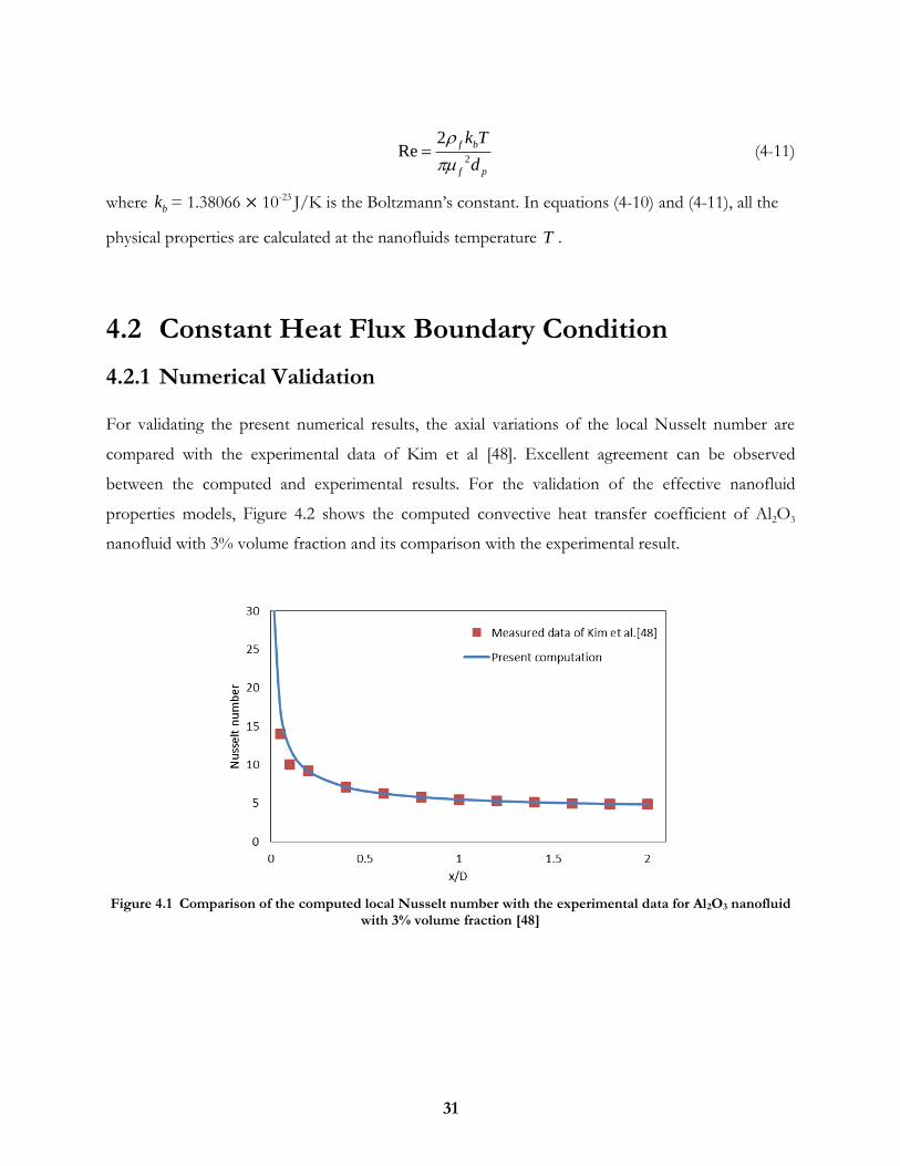
31
2
2Re
f b
f p
k T
d
(4-11)
where bk = 1.38066 × 10⁻²³ J/K is the Boltzmann’s constant. In equations (4-10) and (4-11), all the
physical properties are calculated at the nanofluids temperature T .
4.2 Constant Heat Flux Boundary Condition
4.2.1 Numerical Validation
For validating the present numerical results, the axial variations of the local Nusselt number are
compared with the experimental data of Kim et al [48]. Excellent agreement can be observed
between the computed and experimental results. For the validation of the effective nanofluid
properties models, Figure 4.2 shows the computed convective heat transfer coefficient of Al2O3
nanofluid with 3% volume fraction and its comparison with the experimental result.
Figure 4.1 Comparison of the computed local Nusselt number with the experimental data for Al2O3 nanofluid with 3% volume fraction [48]
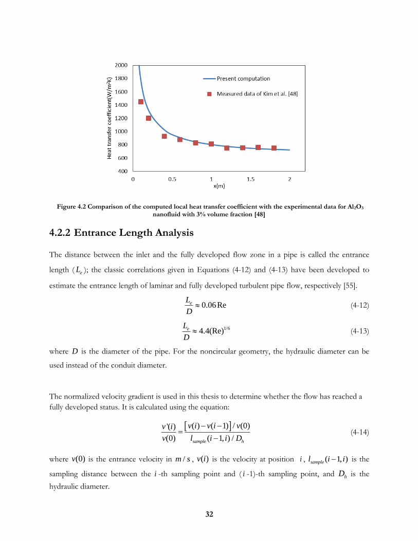
32
Figure 4.2 Comparison of the computed local heat transfer coefficient with the experimental data for Al2O3
nanofluid with 3% volume fraction [48]
4.2.2 Entrance Length Analysis
The distance between the inlet and the fully developed flow zone in a pipe is called the entrance
length ( eL ); the classic correlations given in Equations (4-12) and (4-13) have been developed to
estimate the entrance length of laminar and fully developed turbulent pipe flow, respectively [55].
0.06ReeL
D (4-12)
1/64.4(Re)eL
D (4-13)
where D is the diameter of the pipe. For the noncircular geometry, the hydraulic diameter can be
used instead of the conduit diameter.
The normalized velocity gradient is used in this thesis to determine whether the flow has reached a
fully developed status. It is calculated using the equation:
( ) ( 1) / (0)'( )
(0) ( 1, ) /sample h
v i v i vv i
v l i i D
(4-14)
where (0)v is the entrance velocity in /m s , ( )v i is the velocity at position i , ( 1, )samplel i i is the
sampling distance between the i -th sampling point and ( i -1)-th sampling point, and hD is the
hydraulic diameter.

33
Figure 4.3 shows the developing velocity profiles for laminar entry flow in a pipe at Re = 1620 based
on its diameter. Figure 4.4 presents the centerline velocity of water and Al2O3 nanofluids with
different particle concentrations in the circular pipe in axial direction. The centerline velocity
increases smoothly near the entrance region, and then reaches a constant value before the outlet. In
the present numerical study, the entrance length ( eL ) is defined as the distance from the entrance to
the point where the centerline velocity reaches 99% or 99.5% of the fully developed value. Table 4.3
gives the dimensionless entrance length value ( /h eL L D ) for 99%, 99.5% and 99.9% of the fully
developed value calculated from the numerical simulation. It can be seen from Table 4.3 that the
dimensionless entrance length ( hL ) of water is 5.66% larger than the value given by Equation (4-12).
Furthermore, the hL value of water is slightly larger than that of Al2O3 nanofluids in laminar pipe
flow.
Figure 4.5 shows the normalized velocity gradient of water and Al2O3 nanofluids with different
volume fractions. It is obvious that at the point where hL is 100, the normalized velocity gradient is
nearly 0. Using the numerical results, we obtain a formula with new coefficient for the entrance
length for laminar pipe flow:
0.063ReeL
D (4-15)
In equation (4-15), the entrance length is taken as the pipe distance from the entrance to the point
where the centerline velocity reaches 99.5% of the fully developed value.
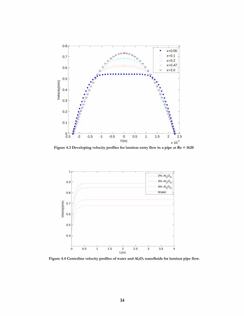
34
0 0.5 1 1.5 2 2.5 3 3.5 4
0.4
0.5
0.6
0.7
0.8
0.9
1
L(m)
Velo
city(m
/s)
2% Al2O
3
3% Al2O
3
4% Al2O
3
Water
Figure 4.4 Centerline velocity profiles of water and Al2O3 nanofluids for laminar pipe flow.
Figure 4.3 Developing velocity profiles for laminar entry flow in a pipe at Re = 1620
-2.5 -2 -1.5 -1 -0.5 0 0.5 1 1.5 2 2.5
x 10-3
0
0.1
0.2
0.3
0.4
0.5
0.6
0.7
0.8
Y(m)
Velo
city(m
/s)
x=0.05
x=0.1
x=0.2
x=0.47
x=2.0
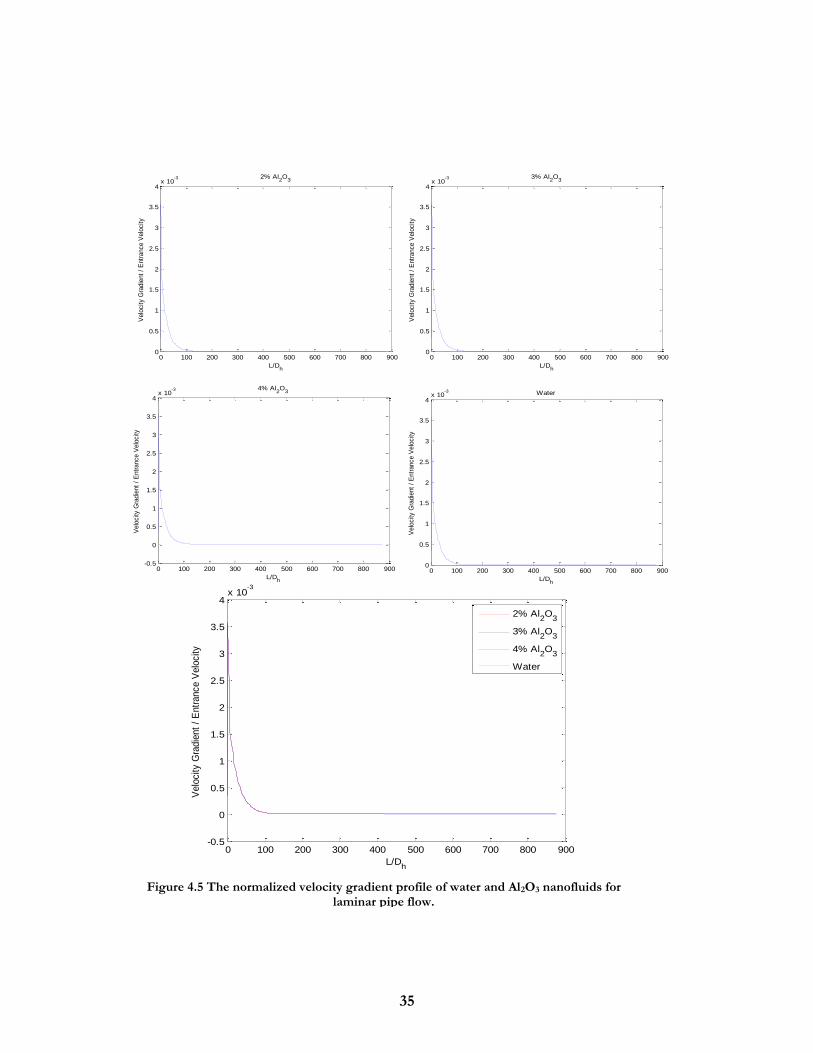
35
0 100 200 300 400 500 600 700 800 9000
0.5
1
1.5
2
2.5
3
3.5
4x 10
-3 2% Al2O
3
L/Dh
Velo
city G
radie
nt
/ E
ntr
ance V
elo
city
0 100 200 300 400 500 600 700 800 9000
0.5
1
1.5
2
2.5
3
3.5
4x 10
-3 3% Al2O
3
L/Dh
Velo
city G
radie
nt
/ E
ntr
ance V
elo
city
0 100 200 300 400 500 600 700 800 900-0.5
0
0.5
1
1.5
2
2.5
3
3.5
4x 10
-3 4% Al2O
3
L/Dh
Velo
city G
radie
nt
/ E
ntr
ance V
elo
city
0 100 200 300 400 500 600 700 800 9000
0.5
1
1.5
2
2.5
3
3.5
4x 10
-3 Water
L/Dh
Velo
city G
radie
nt
/ E
ntr
ance V
elo
city
0 100 200 300 400 500 600 700 800 900-0.5
0
0.5
1
1.5
2
2.5
3
3.5
4x 10
-3
L/Dh
Velo
city G
radie
nt
/ E
ntr
ance V
elo
city
2% Al2O
3
3% Al2O
3
4% Al2O
3
Water
Figure 4.5 The normalized velocity gradient profile of water and Al2O3 nanofluids for laminar pipe flow.
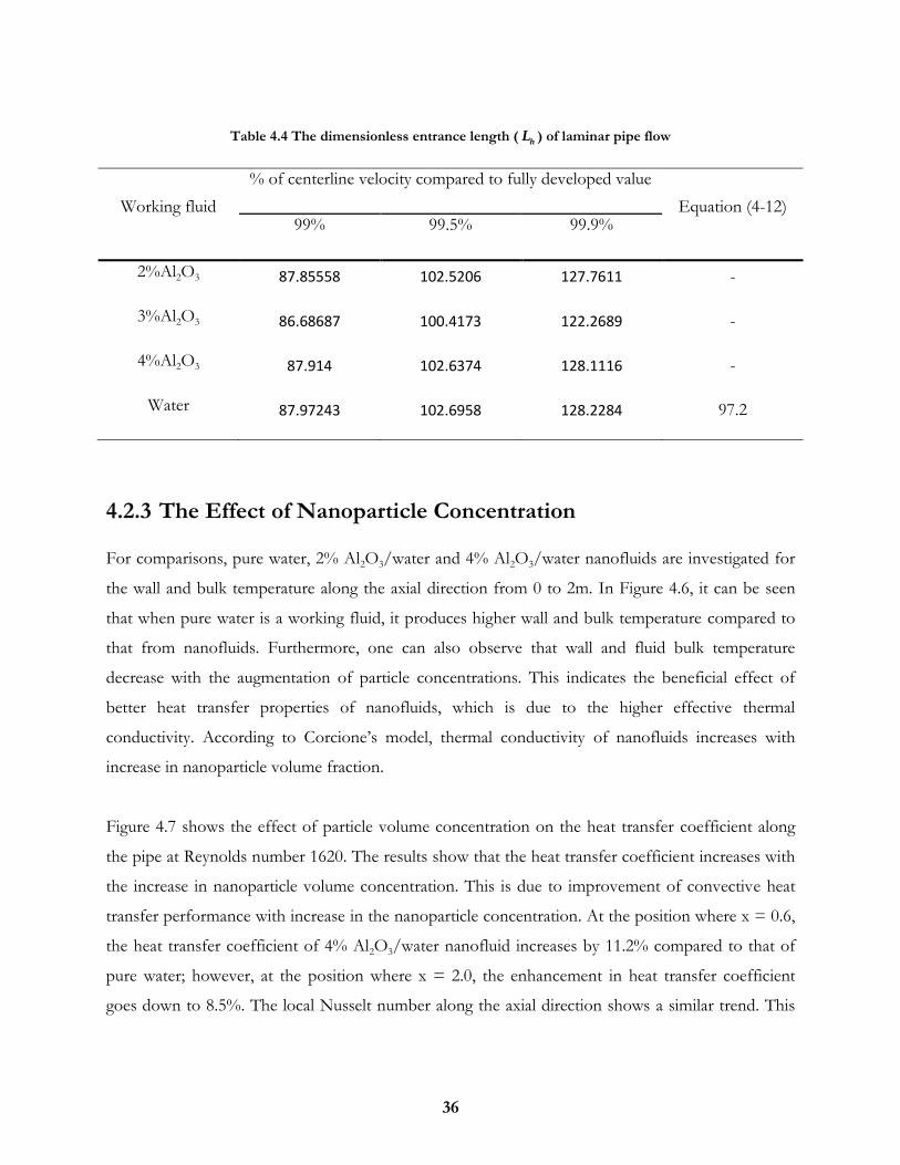
36
Table 4.4 The dimensionless entrance length (h
L ) of laminar pipe flow
Working fluid
% of centerline velocity compared to fully developed value
Equation (4-12) 99% 99.5% 99.9%
2%Al2O3 87.85558 102.5206 127.7611 -
3%Al2O3 86.68687 100.4173 122.2689 -
4%Al2O3 87.914 102.6374 128.1116 -
Water 87.97243 102.6958 128.2284 97.2
4.2.3 The Effect of Nanoparticle Concentration
For comparisons, pure water, 2% Al2O3/water and 4% Al2O3/water nanofluids are investigated for
the wall and bulk temperature along the axial direction from 0 to 2m. In Figure 4.6, it can be seen
that when pure water is a working fluid, it produces higher wall and bulk temperature compared to
that from nanofluids. Furthermore, one can also observe that wall and fluid bulk temperature
decrease with the augmentation of particle concentrations. This indicates the beneficial effect of
better heat transfer properties of nanofluids, which is due to the higher effective thermal
conductivity. According to Corcione’s model, thermal conductivity of nanofluids increases with
increase in nanoparticle volume fraction.
Figure 4.7 shows the effect of particle volume concentration on the heat transfer coefficient along
the pipe at Reynolds number 1620. The results show that the heat transfer coefficient increases with
the increase in nanoparticle volume concentration. This is due to improvement of convective heat
transfer performance with increase in the nanoparticle concentration. At the position where x = 0.6,
the heat transfer coefficient of 4% Al2O3/water nanofluid increases by 11.2% compared to that of
pure water; however, at the position where x = 2.0, the enhancement in heat transfer coefficient
goes down to 8.5%. The local Nusselt number along the axial direction shows a similar trend. This
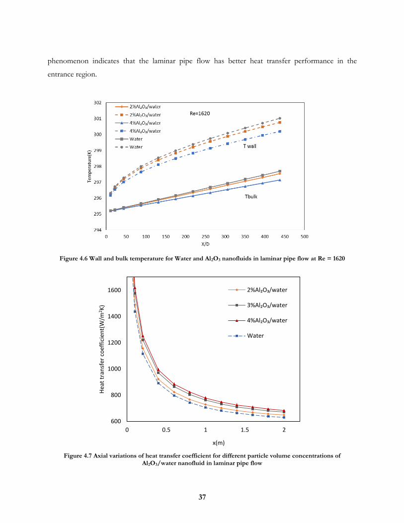
37
phenomenon indicates that the laminar pipe flow has better heat transfer performance in the
entrance region.
Figure 4.6 Wall and bulk temperature for Water and Al2O3 nanofluids in laminar pipe flow at Re = 1620
Figure 4.7 Axial variations of heat transfer coefficient for different particle volume concentrations of
Al2O3/water nanofluid in laminar pipe flow
600
800
1000
1200
1400
1600
0 0.5 1 1.5 2
Hea
t tr
ansf
er c
oef
fici
ent(
W/m
2 K)
x(m)
2%Al₂O₃/water
3%Al₂O₃/water
4%Al₂O₃/water
Water
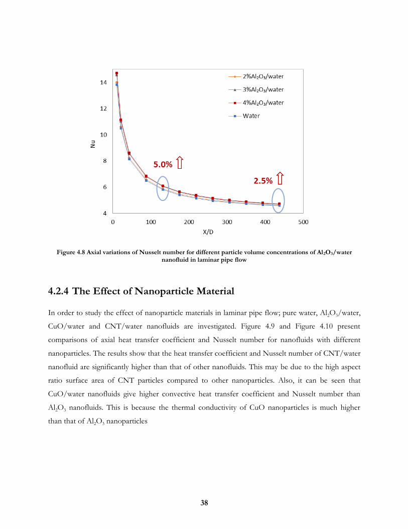
38
Figure 4.8 Axial variations of Nusselt number for different particle volume concentrations of Al2O3/water nanofluid in laminar pipe flow
4.2.4 The Effect of Nanoparticle Material
In order to study the effect of nanoparticle materials in laminar pipe flow; pure water, Al2O3/water,
CuO/water and CNT/water nanofluids are investigated. Figure 4.9 and Figure 4.10 present
comparisons of axial heat transfer coefficient and Nusselt number for nanofluids with different
nanoparticles. The results show that the heat transfer coefficient and Nusselt number of CNT/water
nanofluid are significantly higher than that of other nanofluids. This may be due to the high aspect
ratio surface area of CNT particles compared to other nanoparticles. Also, it can be seen that
CuO/water nanofluids give higher convective heat transfer coefficient and Nusselt number than
Al2O3 nanofluids. This is because the thermal conductivity of CuO nanoparticles is much higher
than that of Al2O3 nanoparticles
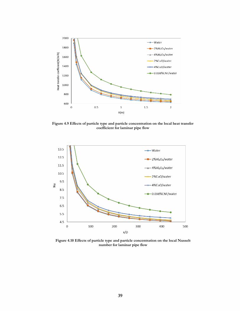
39
Figure 4.9 Effects of particle type and particle concentration on the local heat transfer coefficient for laminar pipe flow
Figure 4.10 Effects of particle type and particle concentration on the local Nusselt number for laminar pipe flow

40
4.3 Constant Wall Temperature Boundary Condition
4.3.1 Numerical Validation In order to validate the numerical procedure, the computed results are compared with the classical
values in literature [56]. For fully developed laminar channel flow under constant wall temperature
boundary condition, the Nusselt number is 7.541. This result was obtained by Etemad (1995) using
the finite element solution of the governing conservation equations for Re = 500 and Pr = 10.
Figure 4.11 shows the comparison between the local Nusselt number along the axial direction of the
channel and the classical value in the fully developed region for a constant wall temperature
boundary condition for a channel bounded by two infinite parallel plates. The result agrees well with
the theoretical results.
4.3.2 Entrance Length Analysis
J.P.du Plessis and M.R. Collins [57] proposed a definition for laminar flow entrance length of
straight ducts. The suggested entrance length is based on hydrodynamic characteristic of the flow
development [57]. The entrance length for a channel of width D is given by:
0.0205Le (4-16)
Figure 4.11 Comparison of the axial variations of the computed Nusselt number with the classical result [56] for laminar channel flow of water under constant wall temperature
boundary condition

41
where Re
eLLe
D
(4-17)
This eL conforms to a 99.77% development of the centerline velocity when applied to the
numerical data [57].
Figure 4.12 shows the developing velocity profiles for laminar entry flow in a channel at Re = 500.
Figure 4.13 presents the centerline velocity of laminar channel flow in the axial direction at Reynolds
number 500. It can be seen that the centerline velocity reaches a fully developed value before the
outlet.
Table 4.3 shows the comparison between the hL value calculated by the current numerical results
and the hL value calculated by Plessis et al. [56]. The entrance length ( hL ) of laminar channel flow is
calculated at Reynolds number 500.
The hL value of 9.5456 for water at 99.9% development of centerline velocity is slightly smaller than
that calculated using Equation (4-16). From Figure 4.14 it is obvious that the normalized velocity
gradient is still much larger than 0 at the point where the hL value of water reaches 99% of the fully
developed value. The normalized velocity gradient nearly reaches 0 when hL value is larger than 10.
In this case, we choose the point where the hL reaches 99.9% of the fully developed value as the
entrance length. According to the numerical results, we obtain a correlation of the entrance length
for laminar channel flow as:
0.01909eL (4-18)
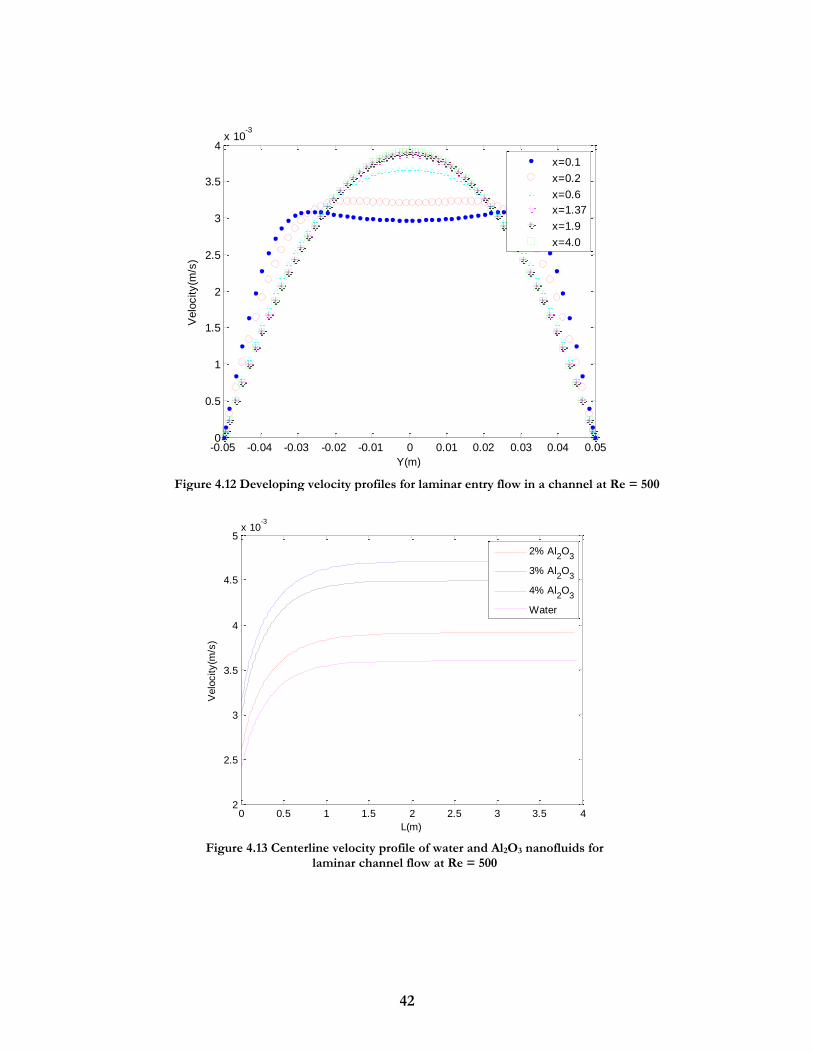
42
0 0.5 1 1.5 2 2.5 3 3.5 42
2.5
3
3.5
4
4.5
5x 10
-3
L(m)
Velo
city(m
/s)
2% Al2O
3
3% Al2O
3
4% Al2O
3
Water
Figure 4.13 Centerline velocity profile of water and Al2O3 nanofluids for laminar channel flow at Re = 500
Figure 4.12 Developing velocity profiles for laminar entry flow in a channel at Re = 500
-0.05 -0.04 -0.03 -0.02 -0.01 0 0.01 0.02 0.03 0.04 0.050
0.5
1
1.5
2
2.5
3
3.5
4x 10
-3
Y(m)
Velo
city(m
/s)
x=0.1
x=0.2
x=0.6
x=1.37
x=1.9
x=4.0

43
0 2 4 6 8 10 12 14 16 18 200
1
2
x 10-4 2% Al
2O
3
L/Dh
Velo
city G
radie
nt
/ E
ntr
ance V
elo
city
0 2 4 6 8 10 12 14 16 18 200
1
2
x 10-4 3% Al
2O
3
L/Dh
Velo
city G
radie
nt
/ E
ntr
ance V
elo
city
0 2 4 6 8 10 12 14 16 18 200
1
2
x 10-4 4% Al
2O
3
L/Dh
Velo
city G
radie
nt
/ E
ntr
ance V
elo
city
0 2 4 6 8 10 12 14 16 18 200
1
2
x 10-4 Water
L/Dh
Velo
city G
radie
nt
/ E
ntr
ance V
elo
city
0 2 4 6 8 10 12 14 16 18 200
1
2
x 10-4
L/Dh
Velo
city G
radie
nt
/ E
ntr
ance V
elo
city
2% Al2O
3
3% Al2O
3
4% Al2O
3
Water
Figure 4.14 The normalized velocity gradient profile of water and Al2O3 nanofluids for laminar channel flow

44
Table 4.5 The dimensionless entrance length ( hL ) for laminar channel flow
Working fluid
% of centerline velocity compared to fully developed value
Equation (4-16) 99% 99.5% 99.9%
2%Al2O3 6.07925 7.30105 10.1086 -
3%Al2O3 5.70635 6.85275 9.5456 -
4%Al2O3 6.07925 7.30105 10.1086 -
Water 5.70635 6.85275 9.5456 10.25
4.3.3 The Effect of Nanoparticle Concentration
Figure 4.15 represents the effect of volume fraction on the heat transfer coefficient in thermal
entrance region of laminar channel flow, Al2O3/water nanofluids are used as working fluids. Pure
water shows the lowest heat transfer coefficient. It is clear that heat transfer coefficient increases
with increase in nanoparticles concentrations. Figure 4.16 illustrates the effect of volume fraction on
the local Nusselt number at Reynolds number Re=500. It shows the same trend as the heat transfer
coefficient. Al2O3/water nanofluid shows the highest Nusselt number, which is caused by the high
thermal conductivity of the nanofluid. However, the enhancement in Nusselt number for nanofluids
is relatively small: the average Nusselt number in the thermal entrance region of 3%Al2O3/water
nanofluids increases by 3.60% compared to that for pure water. Also, the laminar channel flow again
shows better heat transfer performance in the entrance region when compared to the fully
developed region.
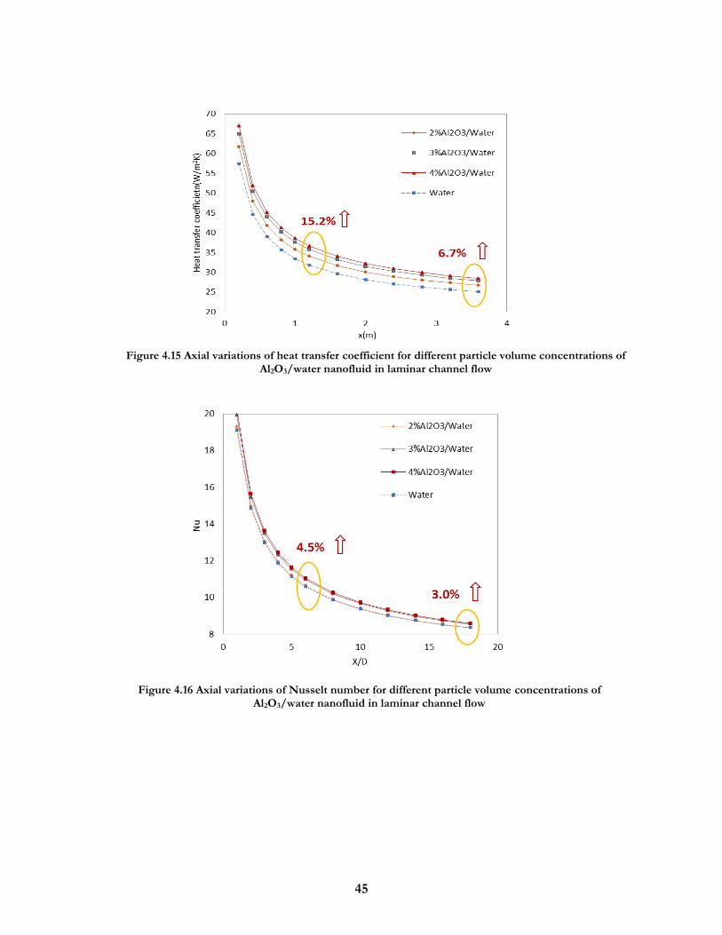
45
Figure 4.16 Axial variations of Nusselt number for different particle volume concentrations of Al2O3/water nanofluid in laminar channel flow
Figure 4.15 Axial variations of heat transfer coefficient for different particle volume concentrations of Al2O3/water nanofluid in laminar channel flow
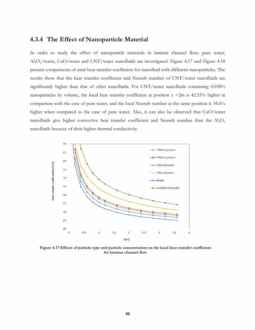
46
4.3.4 The Effect of Nanoparticle Material
In order to study the effect of nanoparticle materials in laminar channel flow; pure water,
Al2O3/water, CuO/water and CNT/water nanofluids are investigated. Figure 4.17 and Figure 4.18
present comparisons of axial heat transfer coefficient for nanofluid with different nanoparticles. The
results show that the heat transfer coefficient and Nusselt number of CNT/water nanofluids are
significantly higher than that of other nanofluids. For CNT/water nanofluids containing 0.038%
nanoparticles by volume, the local heat transfer coefficient at position x =2m is 42.53% higher in
comparison with the case of pure water, and the local Nusselt number at the same position is 34.6%
higher when compared to the case of pure water. Also, it can also be observed that CuO/water
nanofluids give higher convective heat transfer coefficient and Nusselt number than the Al2O3
nanofluids because of their higher thermal conductivity.
Figure 4.17 Effects of particle type and particle concentration on the local heat transfer coefficient for laminar channel flow
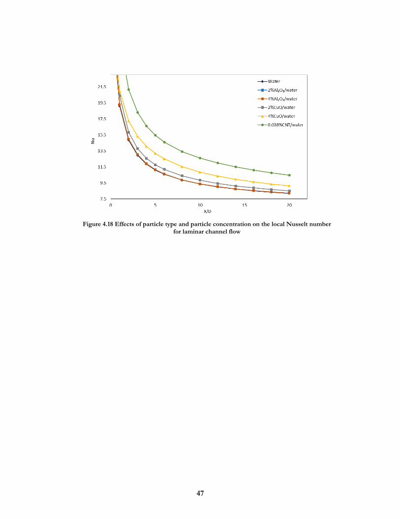
47
Figure 4.18 Effects of particle type and particle concentration on the local Nusselt number for laminar channel flow
48
Chapter 5 Entry Flow and Heat Transfer of Turbulent Forced Convection of Nanofluids in a Pipe and a Channel
This chapter presents the turbulent entry flow and heat transfer characteristics of nanofluids in a
pipe and a channel. Constant heat flux boundary condition is applied to pipe flow, and constant wall
temperature boundary condition is applied to channel flow. Water, Al2O3/water, CuO/water and
CNT/water are used as working fluids. In this chapter, various nanofluid materials, different
nanoparticle concentrations and different Reynolds number are used to study the forced convection
of nanofluids via numerical simulation. The velocity entrance length, Nusselt number, and heat
transfer coefficient are calculated.
The mesh generation software ANSYS-ICEM is used to create the geometry and the mesh for the
pipe and the 2D channel. The mesh is then used as an input to the CFD solver ANSYS-FLUENT.
Fluent is used to calculate the flow field for given flow conditions using the RANS equations with a
number of turbulence models ( k - , SST k - , k - and SA ).
5.1 Computational Modeling
5.1.1 Governing Equations
All numerical simulations in this chapter are conducted under turbulent flow condition. As
mentioned in Chapter 4, nanofluids are treated as continuous, single phase dilute Newtonian fluid
mixtures. The compression work, dispersion and viscous dissipation are assumed negligible in the
energy equation. The conservation equations for pipe flow in polar/cylindrical coordinate system ( r
, z ) can be written as follows [58].
The continuity equation is given as [59]:
10
r zrv v
r r z
(5-1)

49
The momentum equations are given as [60]:
1 1 1r r zrr z t
rv rv vv pv v v v
r r z r r r r z z
(5-2)
2
1 1 1z z r z rz r t
v rv rv v vpv v v v
z r z z r r r z z r
(5-3)
The energy equation is given as [60]:
1 1r z
eff eff
v T v T T Tr
r r z r r r z z
(5-4)
where eff is the effective thermal diffusivity in SI units, m2s-1.
The local convective heat transfer coefficient on the wall is given by:
( )
nf
wall
w b
Tk
xh
T T
(5-5)
The local Nusselt number is defined as:
eff
hDNu
k (5-6)
The Reynolds number is defined as:
Renf
nf
vD
(5-7)
5.1.2 Constant Heat Flux Boundary Condition
For the turbulent flow in a pipe under constant heat flux boundary condition, the same geometry as
in chapter 4.1.2 is selected. Uniform velocity profile is applied at the inlet and pressure outlet
boundary condition is used at the outlet boundary, with no-slip boundary condition at the wall. The
direction of the flow is from the left at the inlet to the right at the outlet. A constant heat flux of
10279.1 W/m2 at the pipe wall and the inlet temperature of 295.15k are employed based on the
experiments of Kim et al. [48]. The turbulent intensity was defined by the formula I = 0.16 (Re)-1/8.

50
For all the turbulent pipe flow cases considered, the Reynolds numbers based on the diameter is
6020.
The properties of nanofluids considered are the same as given in Chapter 4, as well as the
thermophysical properties of solid nanoparticles and base fluids are the same as listed in Table 4.1
5.1.3 Constant Wall Temperature Boundary Condition
Again, the same geometry of a 2D channel as described in Chapter 4.1.3 is selected for the turbulent
flow calculations. Uniform velocity profile is applied at the inlet of the channel and the pressure
outlet boundary condition is used at the outlet, with no-slip boundary condition at the walls. The
direction of the flow is from the left at the inlet to the right at the outlet. A constant wall
temperature of 310K and an inlet temperature of 295.15k are employed as boundary conditions.
The properties of the nanofluids considered are the same as given in Chapter 4, as well as the
thermophysical properties are taken to be the same as given in Chapter 4.1.1.
5.2 Constant Heat Flux Boundary Condition
5.2.1 Numerical Validation for Pipe Flow
Figure 5.1 shows the y wall value on the axial direction. From Figure 5.1, it can be seen that the
dimensionless height y of the first grid cell is less than 1.5, which means that the grid is refined
enough in the near-wall region. In order to validate the present CFD solution, the results are
compared to the classical correlations and available experimental results in the literature. The Sieder
and Tate’s correlation [36] is used for the validation; it is given as:
0.14
4 5 1 30.027 Re PrD D
s
Nu
(5-8)
Figure 5.2 shows the comparison between the computed local Nusselt number along the axial
direction and the value calculated by Sieder and Tate’s correlation. The computed results agree
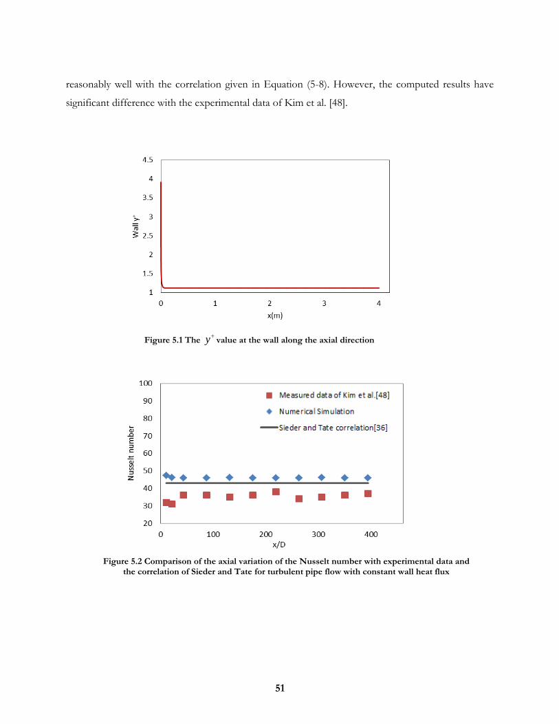
51
reasonably well with the correlation given in Equation (5-8). However, the computed results have
significant difference with the experimental data of Kim et al. [48].
Figure 5.1 The yvalue at the wall along the axial direction
Figure 5.2 Comparison of the axial variation of the Nusselt number with experimental data and the correlation of Sieder and Tate for turbulent pipe flow with constant wall heat flux
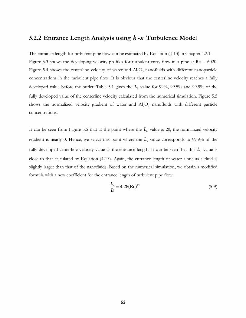
52
5.2.2 Entrance Length Analysis using k - Turbulence Model
The entrance length for turbulent pipe flow can be estimated by Equation (4-13) in Chapter 4.2.1.
Figure 5.3 shows the developing velocity profiles for turbulent entry flow in a pipe at Re = 6020.
Figure 5.4 shows the centerline velocity of water and Al2O3 nanofluids with different nanoparticle
concentrations in the turbulent pipe flow. It is obvious that the centerline velocity reaches a fully
developed value before the outlet. Table 5.1 gives the hL value for 99%, 99.5% and 99.9% of the
fully developed value of the centerline velocity calculated from the numerical simulation. Figure 5.5
shows the normalized velocity gradient of water and Al2O3 nanofluids with different particle
concentrations.
It can be seen from Figure 5.5 that at the point where the hL value is 20, the normalized velocity
gradient is nearly 0. Hence, we select this point where the hL value corresponds to 99.9% of the
fully developed centerline velocity value as the entrance length. It can be seen that this hL value is
close to that calculated by Equation (4-13). Again, the entrance length of water alone as a fluid is
slightly larger than that of the nanofluids. Based on the numerical simulation, we obtain a modified
formula with a new coefficient for the entrance length of turbulent pipe flow.
1 64.28(Re)eL
D (5-9)

53
Figure 5.3 Developing velocity profiles for turbulent entry flow in a pipe at Re = 6020
using the k - ε turbulence model
0 0.05 0.1 0.15 0.2 0.25 0.3 0.35 0.4 0.45 0.5
1.3
1.4
1.5
1.6
1.7
1.8
1.9
2
L(m)
Velo
city(m
/s)
2% Al2O
3
3% Al2O
3
4% Al2O
3
Water
Figure 5.4 Centerline velocity profile of water and Al2O3 nanofluids for turbulent pipe
flow at Re = 6020 using the - turbulence model
-2.5 -2 -1.5 -1 -0.5 0 0.5 1 1.5 2 2.5
x 10-3
0
0.2
0.4
0.6
0.8
1
1.2
1.4
1.6
1.8
Y(m)
Velo
city(m
/s)
x=0.01
x=0.02
x=0.0579
x=0.0674
x=0.0835
x=2.0
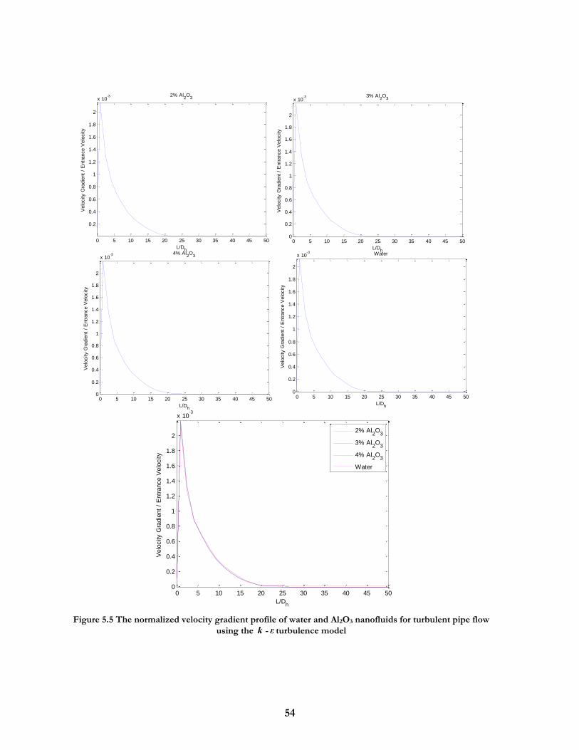
54
0 5 10 15 20 25 30 35 40 45 50
0.2
0.4
0.6
0.8
1
1.2
1.4
1.6
1.8
2
x 10-3 2% Al
2O
3
L/Dh
Velo
city G
radie
nt
/ E
ntr
ance V
elo
city
0 5 10 15 20 25 30 35 40 45 500
0.2
0.4
0.6
0.8
1
1.2
1.4
1.6
1.8
2
x 10-3 3% Al
2O
3
L/Dh
Velo
city G
radie
nt
/ E
ntr
ance V
elo
city
0 5 10 15 20 25 30 35 40 45 500
0.2
0.4
0.6
0.8
1
1.2
1.4
1.6
1.8
2
x 10-3 4% Al
2O
3
L/Dh
Velo
city G
radie
nt
/ E
ntr
ance V
elo
city
0 5 10 15 20 25 30 35 40 45 500
0.2
0.4
0.6
0.8
1
1.2
1.4
1.6
1.8
2
x 10-3 Water
L/Dh
Velo
city G
radie
nt
/ E
ntr
ance V
elo
city
0 5 10 15 20 25 30 35 40 45 500
0.2
0.4
0.6
0.8
1
1.2
1.4
1.6
1.8
2
x 10-3
L/Dh
Velo
city G
radie
nt
/ E
ntr
ance V
elo
city
2% Al2O
3
3% Al2O
3
4% Al2O
3
Water
Figure 5.5 The normalized velocity gradient profile of water and Al2O3 nanofluids for turbulent pipe flow
using the - turbulence model
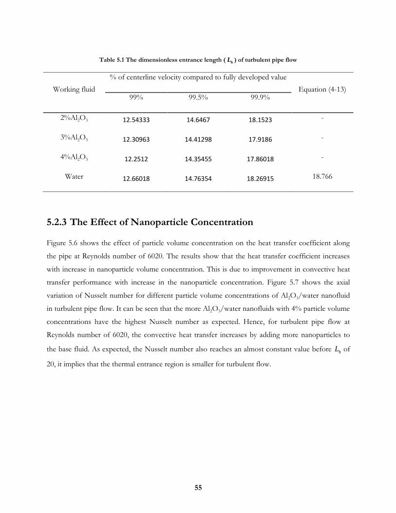
55
Table 5.1 The dimensionless entrance length (h
L ) of turbulent pipe flow
Working fluid
% of centerline velocity compared to fully developed value
Equation (4-13) 99% 99.5% 99.9%
2%Al2O3 12.54333 14.6467 18.1523 -
3%Al2O3 12.30963 14.41298 17.9186 -
4%Al2O3 12.2512 14.35455 17.86018 -
Water 12.66018 14.76354 18.26915 18.766
5.2.3 The Effect of Nanoparticle Concentration
Figure 5.6 shows the effect of particle volume concentration on the heat transfer coefficient along
the pipe at Reynolds number of 6020. The results show that the heat transfer coefficient increases
with increase in nanoparticle volume concentration. This is due to improvement in convective heat
transfer performance with increase in the nanoparticle concentration. Figure 5.7 shows the axial
variation of Nusselt number for different particle volume concentrations of Al2O3/water nanofluid
in turbulent pipe flow. It can be seen that the more Al2O3/water nanofluids with 4% particle volume
concentrations have the highest Nusselt number as expected. Hence, for turbulent pipe flow at
Reynolds number of 6020, the convective heat transfer increases by adding more nanoparticles to
the base fluid. As expected, the Nusselt number also reaches an almost constant value before hL of
20, it implies that the thermal entrance region is smaller for turbulent flow.

56
Figure 5.7 Axial variation of Nusselt number for different particle volume concentrations of
Al2O3/water nanofluid in turbulent pipe flow at Re=6020 using the k - ε turbulence model
Figure 5.6 Axial variation of heat transfer coefficient for different particle volume concentrations of
Al2O3/water nanofluid in turbulent pipe flow at Re=6020 using the - turbulence model
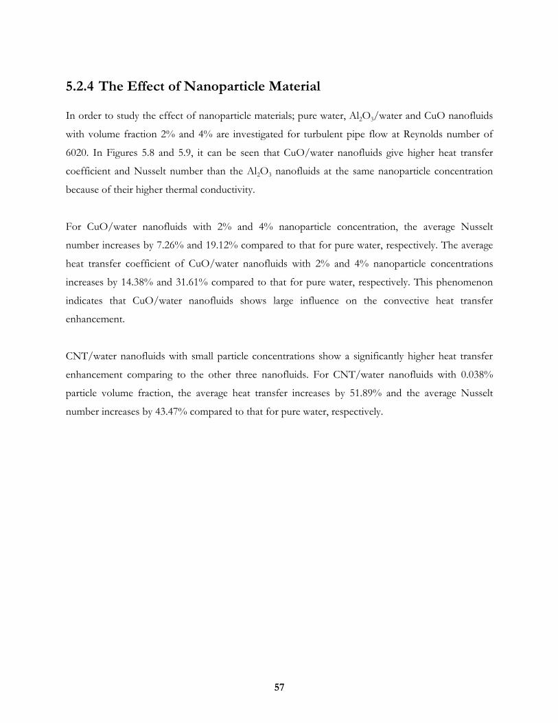
57
5.2.4 The Effect of Nanoparticle Material
In order to study the effect of nanoparticle materials; pure water, Al2O3/water and CuO nanofluids
with volume fraction 2% and 4% are investigated for turbulent pipe flow at Reynolds number of
6020. In Figures 5.8 and 5.9, it can be seen that CuO/water nanofluids give higher heat transfer
coefficient and Nusselt number than the Al2O3 nanofluids at the same nanoparticle concentration
because of their higher thermal conductivity.
For CuO/water nanofluids with 2% and 4% nanoparticle concentration, the average Nusselt
number increases by 7.26% and 19.12% compared to that for pure water, respectively. The average
heat transfer coefficient of CuO/water nanofluids with 2% and 4% nanoparticle concentrations
increases by 14.38% and 31.61% compared to that for pure water, respectively. This phenomenon
indicates that CuO/water nanofluids shows large influence on the convective heat transfer
enhancement.
CNT/water nanofluids with small particle concentrations show a significantly higher heat transfer
enhancement comparing to the other three nanofluids. For CNT/water nanofluids with 0.038%
particle volume fraction, the average heat transfer increases by 51.89% and the average Nusselt
number increases by 43.47% compared to that for pure water, respectively.
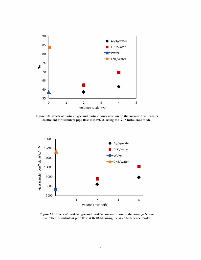
58
Figure 5.9 Effects of particle type and particle concentration on the average Nusselt number for turbulent pipe flow at Re=6020 using the - turbulence model
Figure 5.8 Effects of particle type and particle concentration on the average heat transfer
coefficient for turbulent pipe flow at Re=6020 using the - turbulence model
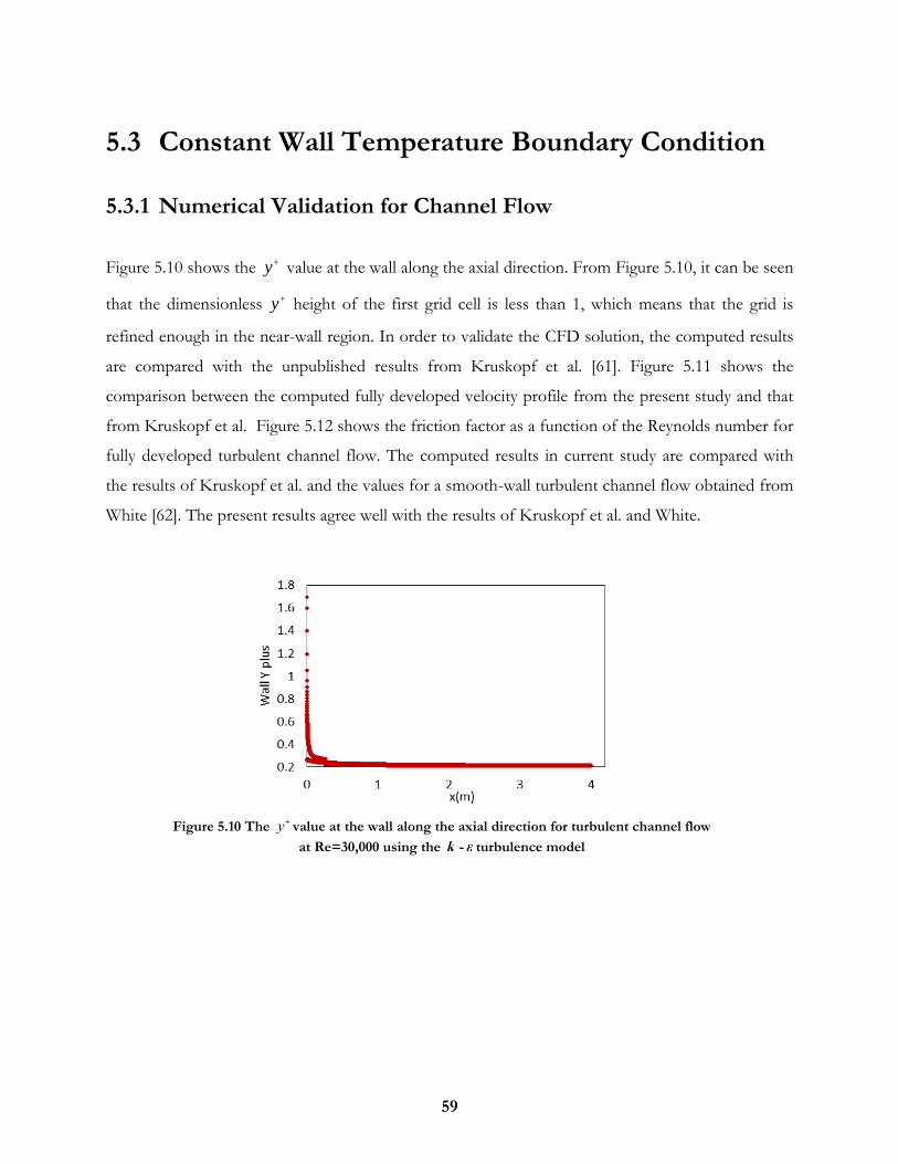
59
5.3 Constant Wall Temperature Boundary Condition
5.3.1 Numerical Validation for Channel Flow
Figure 5.10 shows the y value at the wall along the axial direction. From Figure 5.10, it can be seen
that the dimensionless y height of the first grid cell is less than 1, which means that the grid is
refined enough in the near-wall region. In order to validate the CFD solution, the computed results
are compared with the unpublished results from Kruskopf et al. [61]. Figure 5.11 shows the
comparison between the computed fully developed velocity profile from the present study and that
from Kruskopf et al. Figure 5.12 shows the friction factor as a function of the Reynolds number for
fully developed turbulent channel flow. The computed results in current study are compared with
the results of Kruskopf et al. and the values for a smooth-wall turbulent channel flow obtained from
White [62]. The present results agree well with the results of Kruskopf et al. and White.
Figure 5.10 The value at the wall along the axial direction for turbulent channel flow
at Re=30,000 using the - turbulence model
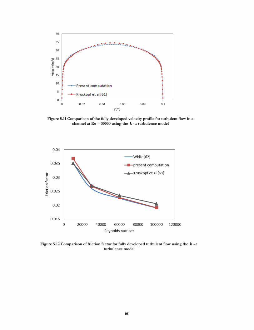
60
Figure 5.11 Comparison of the fully developed velocity profile for turbulent flow in a
channel at Re = 30000 using the k - ε turbulence model
Figure 5.12 Comparison of friction factor for fully developed turbulent flow using the k - ε
turbulence model
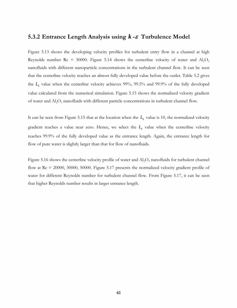
61
5.3.2 Entrance Length Analysis using k - Turbulence Model
Figure 5.13 shows the developing velocity profiles for turbulent entry flow in a channel at high
Reynolds number Re = 30000. Figure 5.14 shows the centerline velocity of water and Al2O3
nanofluids with different nanoparticle concentrations in the turbulent channel flow. It can be seen
that the centerline velocity reaches an almost fully developed value before the outlet. Table 5.2 gives
the hL value when the centerline velocity achieves 99%, 99.5% and 99.9% of the fully developed
value calculated from the numerical simulation. Figure 5.15 shows the normalized velocity gradient
of water and Al2O3 nanofluids with different particle concentrations in turbulent channel flow.
It can be seen from Figure 5.15 that at the location when the hL value is 10, the normalized velocity
gradient reaches a value near zero. Hence, we select the hL value when the centerline velocity
reaches 99.9% of the fully developed value as the entrance length. Again, the entrance length for
flow of pure water is slightly larger than that for flow of nanofluids.
Figure 5.16 shows the centerline velocity profile of water and Al2O3 nanofluids for turbulent channel
flow at Re = 20000, 30000, 50000. Figure 5.17 presents the normalized velocity gradient profile of
water for different Reynolds number for turbulent channel flow. From Figure 5.17, it can be seen
that higher Reynolds number results in larger entrance length.
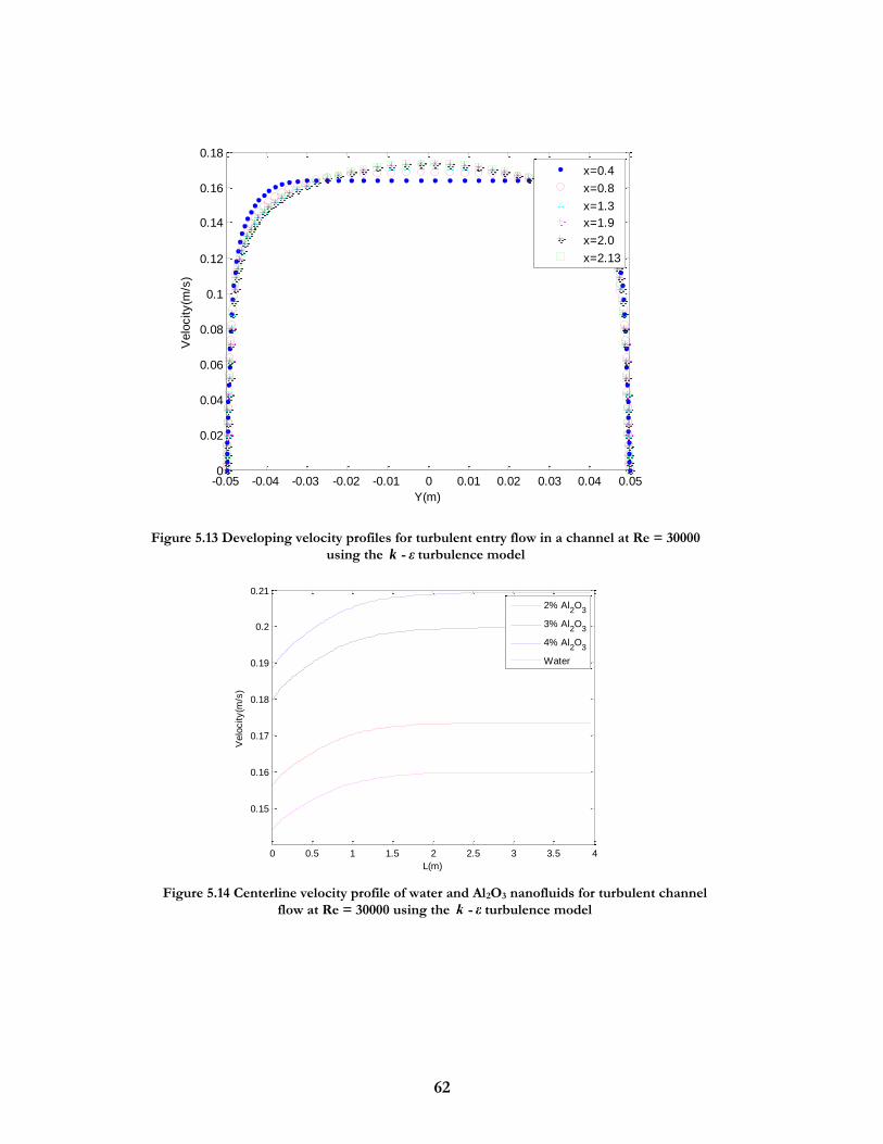
62
0 0.5 1 1.5 2 2.5 3 3.5 4
0.15
0.16
0.17
0.18
0.19
0.2
0.21
L(m)
Velo
city(m
/s)
2% Al2O
3
3% Al2O
3
4% Al2O
3
Water
Figure 5.14 Centerline velocity profile of water and Al2O3 nanofluids for turbulent channel
flow at Re = 30000 using the - turbulence model
Figure 5.13 Developing velocity profiles for turbulent entry flow in a channel at Re = 30000
using the k - ε turbulence model
-0.05 -0.04 -0.03 -0.02 -0.01 0 0.01 0.02 0.03 0.04 0.050
0.02
0.04
0.06
0.08
0.1
0.12
0.14
0.16
0.18
Y(m)
Velo
city(m
/s)
x=0.4
x=0.8
x=1.3
x=1.9
x=2.0
x=2.13
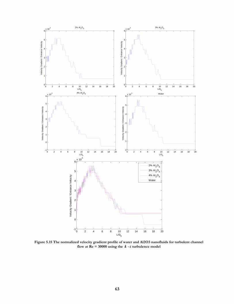
63
0 2 4 6 8 10 12 14 16 18 200
1
2
3
4
5
6x 10
-5 2% Al2O
3
L/Dh
Velo
city G
radie
nt
/ E
ntr
ance V
elo
city
0 2 4 6 8 10 12 14 16 18 200
1
2
3
4
5
6x 10
-5 3% Al2O
3
L/Dh
Velo
city G
radie
nt
/ E
ntr
ance V
elo
city
0 2 4 6 8 10 12 14 16 18 20-1
0
1
2
3
4
5
6x 10
-5 4% Al2O
3
L/Dh
Velo
city G
radie
nt
/ E
ntr
ance V
elo
city
0 2 4 6 8 10 12 14 16 18 200
1
2
3
4
5
6x 10
-5 Water
L/Dh
Velo
city G
radie
nt
/ E
ntr
ance V
elo
city
0 2 4 6 8 10 12 14 16 18 20-1
0
1
2
3
4
5
6x 10
-5
L/Dh
Velo
city G
radie
nt
/ E
ntr
ance V
elo
city
2% Al2O
3
3% Al2O
3
4% Al2O
3
Water
Figure 5.15 The normalized velocity gradient profile of water and Al2O3 nanofluids for turbulent channel
flow at Re = 30000 using the - turbulence model
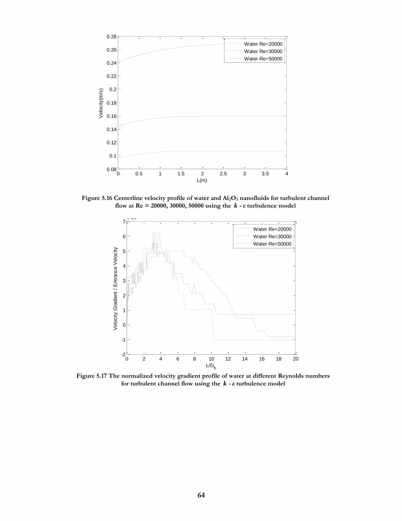
64
0 0.5 1 1.5 2 2.5 3 3.5 40.08
0.1
0.12
0.14
0.16
0.18
0.2
0.22
0.24
0.26
0.28
L(m)
Velo
city(m
/s)
Water Re=20000
Water Re=30000
Water Re=50000
0 2 4 6 8 10 12 14 16 18 20-2
-1
0
1
2
3
4
5
6
7x 10
-5
L/Dh
Velo
city G
radie
nt
/ E
ntr
ance V
elo
city
Water Re=20000
Water Re=30000
Water Re=50000
Figure 5.16 Centerline velocity profile of water and Al2O3 nanofluids for turbulent channel
flow at Re = 20000, 30000, 50000 using the k - ε turbulence model
Figure 5.17 The normalized velocity gradient profile of water at different Reynolds numbers
for turbulent channel flow using the k - ε turbulence model
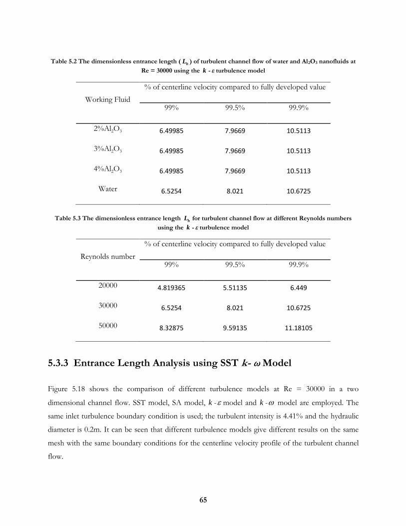
65
Table 5.2 The dimensionless entrance length (h
L ) of turbulent channel flow of water and Al2O3 nanofluids at
Re = 30000 using the k - ε turbulence model
Working Fluid
% of centerline velocity compared to fully developed value
99% 99.5% 99.9%
2%Al2O3 6.49985 7.9669 10.5113
3%Al2O3 6.49985 7.9669 10.5113
4%Al2O3 6.49985 7.9669 10.5113
Water 6.5254 8.021 10.6725
Table 5.3 The dimensionless entrance length
hL for turbulent channel flow at different Reynolds numbers
using the k - ε turbulence model
Reynolds number
% of centerline velocity compared to fully developed value
99% 99.5% 99.9%
20000 4.819365 5.51135 6.449
30000 6.5254 8.021 10.6725
50000 8.32875 9.59135 11.18105
5.3.3 Entrance Length Analysis using SST k- ω Model
Figure 5.18 shows the comparison of different turbulence models at Re = 30000 in a two
dimensional channel flow. SST model, SA model, k - model and k - model are employed. The
same inlet turbulence boundary condition is used; the turbulent intensity is 4.41% and the hydraulic
diameter is 0.2m. It can be seen that different turbulence models give different results on the same
mesh with the same boundary conditions for the centerline velocity profile of the turbulent channel
flow.
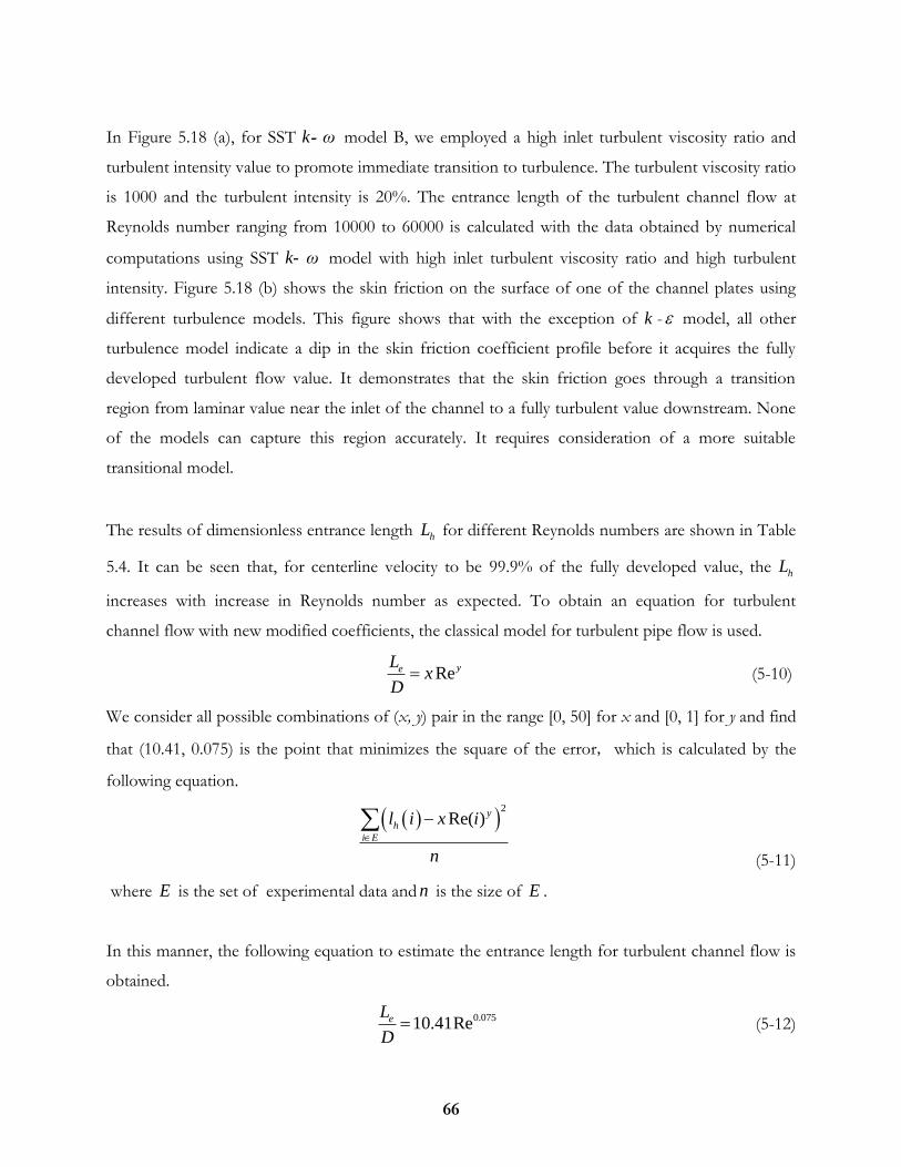
66
In Figure 5.18 (a), for SST k- ω model B, we employed a high inlet turbulent viscosity ratio and
turbulent intensity value to promote immediate transition to turbulence. The turbulent viscosity ratio
is 1000 and the turbulent intensity is 20%. The entrance length of the turbulent channel flow at
Reynolds number ranging from 10000 to 60000 is calculated with the data obtained by numerical
computations using SST k- ω model with high inlet turbulent viscosity ratio and high turbulent
intensity. Figure 5.18 (b) shows the skin friction on the surface of one of the channel plates using
different turbulence models. This figure shows that with the exception of k - model, all other
turbulence model indicate a dip in the skin friction coefficient profile before it acquires the fully
developed turbulent flow value. It demonstrates that the skin friction goes through a transition
region from laminar value near the inlet of the channel to a fully turbulent value downstream. None
of the models can capture this region accurately. It requires consideration of a more suitable
transitional model.
The results of dimensionless entrance length hL for different Reynolds numbers are shown in Table
5.4. It can be seen that, for centerline velocity to be 99.9% of the fully developed value, the hL
increases with increase in Reynolds number as expected. To obtain an equation for turbulent
channel flow with new modified coefficients, the classical model for turbulent pipe flow is used.
ReyeLx
D (5-10)
We consider all possible combinations of (x, y) pair in the range [0, 50] for x and [0, 1] for y and find
that (10.41, 0.075) is the point that minimizes the square of the error, which is calculated by the
following equation.
2
Re( ) y
h
i E
l i x i
n
(5-11)
where E is the set of experimental data and n is the size of E .
In this manner, the following equation to estimate the entrance length for turbulent channel flow is
obtained.
0.07510.41ReeL
D (5-12)
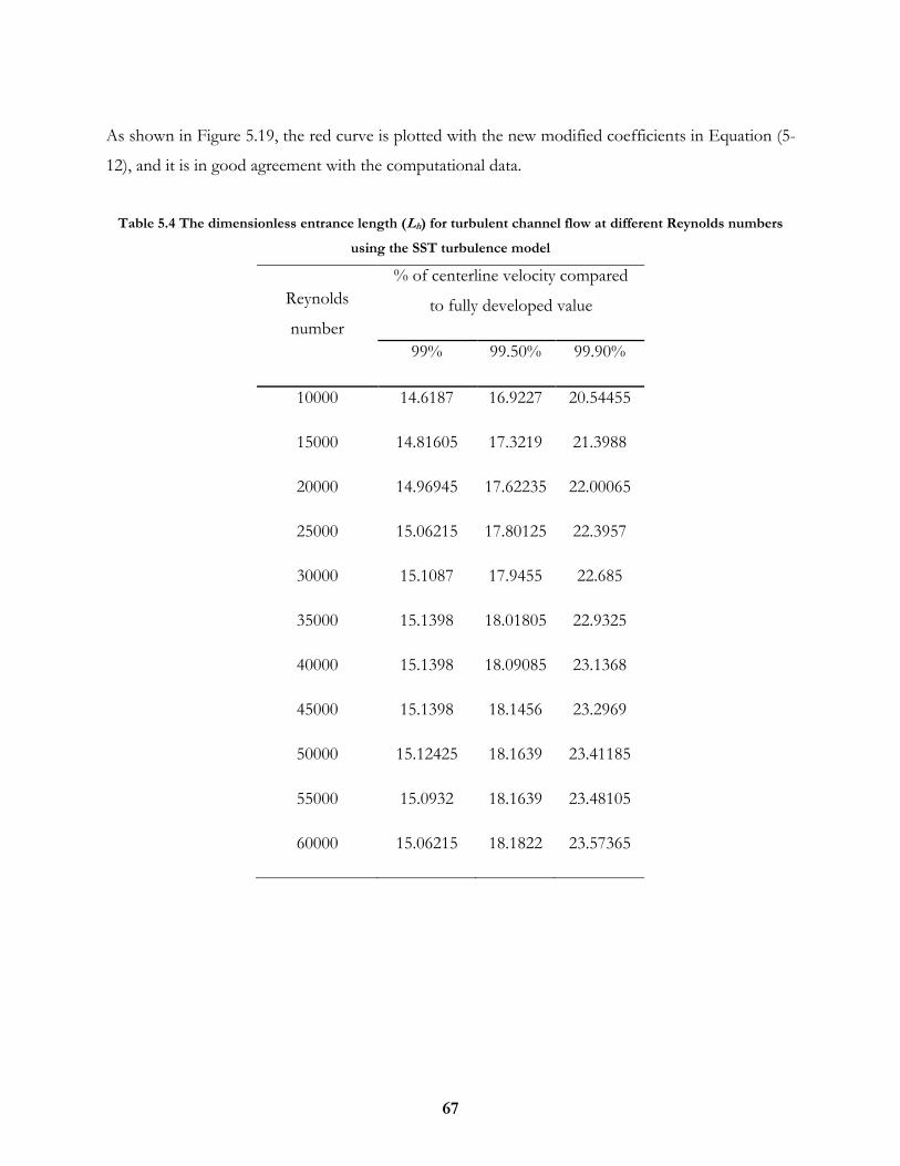
67
As shown in Figure 5.19, the red curve is plotted with the new modified coefficients in Equation (5-
12), and it is in good agreement with the computational data.
Table 5.4 The dimensionless entrance length (Lh) for turbulent channel flow at different Reynolds numbers
using the SST turbulence model
Reynolds
number
% of centerline velocity compared
to fully developed value
99% 99.50% 99.90%
10000 14.6187 16.9227 20.54455
15000 14.81605 17.3219 21.3988
20000 14.96945 17.62235 22.00065
25000 15.06215 17.80125 22.3957
30000 15.1087 17.9455 22.685
35000 15.1398 18.01805 22.9325
40000 15.1398 18.09085 23.1368
45000 15.1398 18.1456 23.2969
50000 15.12425 18.1639 23.41185
55000 15.0932 18.1639 23.48105
60000 15.06215 18.1822 23.57365
68
Figure5.18 (a) Comparison of centerline velocity using different turbulence models at Re = 30000
for 2D channel flow
Figure5.18 (b) Comparison of skin-friction using different turbulence models at Re = 30000
for 2D channel flow
0.0054
0.0059
0.0064
0.0069
0.0074
0.0079
0.0084
0.0089
0.0094
0.0099
0.0104
0 1 2 3 4 5 6 7 8
Skin
fri
ctio
n c
oef
fici
ent
x(m)
SST model A
k-ω model
k-ε model
SA model

69
Figure 5.19 Comparison of the dimensionless entrance length
hL using equation (5-12) and the computational
data at different Reynolds numbers
5.3.4 The Effect of Nanoparticle Concentration
Figure 5.20 shows the effect of nanoparticle volume fraction on the heat transfer coefficient in
thermal entrance region of turbulent channel flow. Water and Al2O3/water nanofluids are used as
working fluids. Pure water shows the lowest heat transfer coefficient. It is clear that the heat transfer
coefficient increases with increase in nanoparticle concentration. Figure 5.21 illustrates the effect of
nanoparticle volume fraction on the local Nusselt number at Reynolds number Re=30000. It shows
the same trend as the heat transfer coefficient. Al2O3/water nanofluid shows the highest Nusselt
number, which is caused by the high thermal conductivity. The average Nusselt number of
3%Al2O3/water nanofluids increases by 4.84% compared to that of pure water.
1 1.5 2 2.5 3 3.5 4 4.5 5 5.5 6
x 104
20.5
21
21.5
22
22.5
23
23.5
24
Re
Lh
Numerical computation data
Curve Fitting, x=10.41, y=0.075
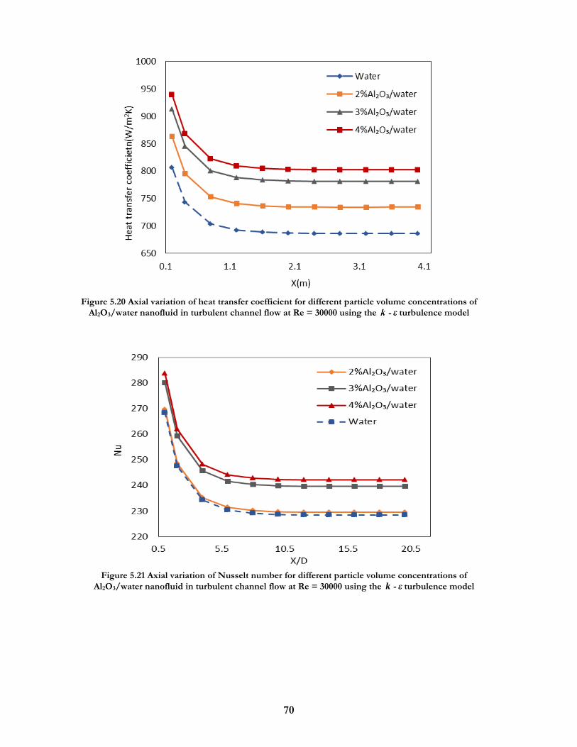
70
Figure 5.21 Axial variation of Nusselt number for different particle volume concentrations of
Al2O3/water nanofluid in turbulent channel flow at Re = 30000 using the k - ε turbulence model
Figure 5.20 Axial variation of heat transfer coefficient for different particle volume concentrations of
Al2O3/water nanofluid in turbulent channel flow at Re = 30000 using the - turbulence model
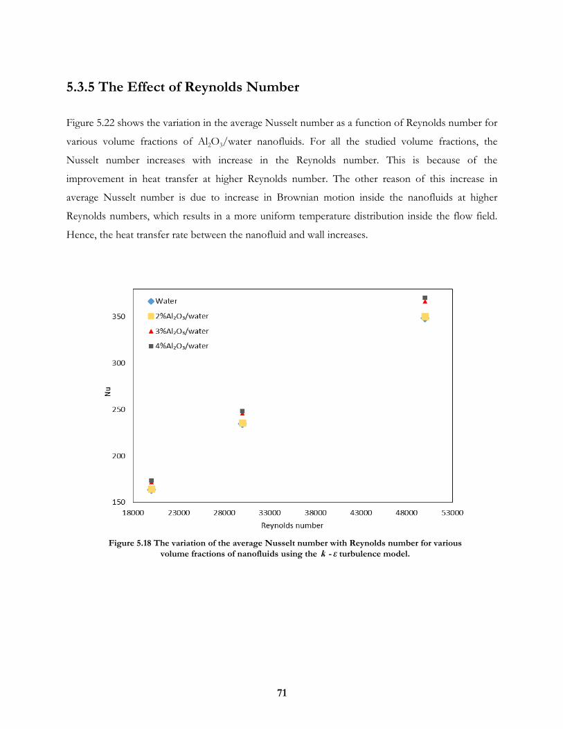
71
5.3.5 The Effect of Reynolds Number
Figure 5.22 shows the variation in the average Nusselt number as a function of Reynolds number for
various volume fractions of Al2O3/water nanofluids. For all the studied volume fractions, the
Nusselt number increases with increase in the Reynolds number. This is because of the
improvement in heat transfer at higher Reynolds number. The other reason of this increase in
average Nusselt number is due to increase in Brownian motion inside the nanofluids at higher
Reynolds numbers, which results in a more uniform temperature distribution inside the flow field.
Hence, the heat transfer rate between the nanofluid and wall increases.
Figure 5.18 The variation of the average Nusselt number with Reynolds number for various
volume fractions of nanofluids using the - turbulence model.
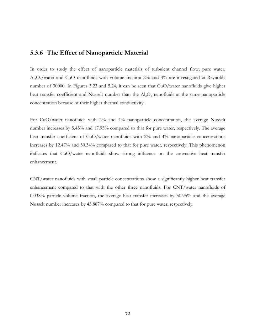
72
5.3.6 The Effect of Nanoparticle Material
In order to study the effect of nanoparticle materials of turbulent channel flow; pure water,
Al2O3/water and CuO nanofluids with volume fraction 2% and 4% are investigated at Reynolds
number of 30000. In Figures 5.23 and 5.24, it can be seen that CuO/water nanofluids give higher
heat transfer coefficient and Nusselt number than the Al2O3 nanofluids at the same nanoparticle
concentration because of their higher thermal conductivity.
For CuO/water nanofluids with 2% and 4% nanoparticle concentration, the average Nusselt
number increases by 5.45% and 17.95% compared to that for pure water, respectively. The average
heat transfer coefficient of CuO/water nanofluids with 2% and 4% nanoparticle concentrations
increases by 12.47% and 30.34% compared to that for pure water, respectively. This phenomenon
indicates that CuO/water nanofluids show strong influence on the convective heat transfer
enhancement.
CNT/water nanofluids with small particle concentrations show a significantly higher heat transfer
enhancement compared to that with the other three nanofluids. For CNT/water nanofluids of
0.038% particle volume fraction, the average heat transfer increases by 50.95% and the average
Nusselt number increases by 43.887% compared to that for pure water, respectively.
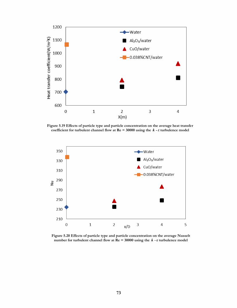
73
Figure 5.19 Effects of particle type and particle concentration on the average heat transfer coefficient for turbulent channel flow at Re = 30000 using the - turbulence model
Figure 5.20 Effects of particle type and particle concentration on the average Nusselt
number for turbulent channel flow at Re = 30000 using the - turbulence model
74
Chapter 6 Conclusions
In this thesis, we have investigated the problems of fluid flow and heat transfer of nanofluids in pipe
flow under constant heat flux boundary conditions and 2D channel flow under constant wall
temperature boundary conditions, for both laminar and turbulent flow Reynolds numbers. The
entrance length for both pipe and channel flow is also computed and compared with the available
correlations in the literature. For turbulent flow simulations, two-equation k-epsilon, standard k-
omega and SST k-omega models as well as the one-equation Spalart-Allmaras models are employed.
Four new correlations with modified coefficients are obtained based on the numerical research
presented in this thesis. Nanofluids show better heat transfer properties compared to pure water,
and the increase in nanoparticles concentration increases the heat transfer coefficient and Nusselt
number for all cases considered. CuO/water nanofluids show more influence on convective heat
transfer compared to Al2O3 nanofluids because of the higher thermal conductivity of CuO
compared to Al2O3. Finally, 0.038% CNT/water nanofluids significantly increase the heat transfer
coefficient and Nusselt number in the flow field.
75
References
[1] S. U. S. Choi, and J. A. Eastman. “Enhancing thermal conductivity of fluids with
nanoparticles.” ASME-Publications-Fed, no. 231 (1995): 99-106.
[2] D. Wen, G. Lin, S. Vafaei, and K. Zhang. “Review of nanofluids for heat transfer
applications.” Particuology 7, no. 2 (2009): 141-150.
[3] M. Hidetoshi, A. Ebata, and K. Teramae. “Alteration of thermal conductivity and viscosity
of liquid by dispersing ultra-fine particles. Dispersion of Al2O3, SiO2 and TiO2 ultra-fine
particles.” (1993): 227-233.
[4] S. Lee, S. U. S. Choi, S, and Li, and J. A. Eastman. “Measuring thermal conductivity of fluids
containing oxide nanoparticles.” Journal of Heat Transfer 121, no. 2 (1999): 280-289.
[5] Y. Xuan, and Q. Li. “Heat transfer enhancement of nanofluids.” International Journal of
Heat and Fluid Flow 21, no. 1 (2000): 58-64.
[6] Y. Xuan, and W. Roetzel. “Conceptions for heat transfer correlation of nanofluids.”
International Journal of heat and Mass transfer 43, no. 19 (2000): 3701-3707.
[7] J. A. Eastman, S. U. S. Choi, S. Li, L. J. Thompson, and S. Lee. “Enhanced thermal
conductivity through the development of nanofluids.” InMRS proceedings, vol. 457, p. 3.
Cambridge University Press, 1996.
[8] R. Saidur, K. Y. Leong, and H. A. Mohammad. “A review on applications and challenges of
nanofluids.” Renewable and Sustainable Energy Reviews 15, no. 3 (2011): 1646-1668.
[9] S. Kakac, and A. Pramuanjaroenkij. “Review of convective heat transfer enhancement with
nanofluids.” International Journal of Heat and Mass Transfer 52, no. 13 (2009): 3187-3196.
[10] P. Tongpun, E. Bumrungthaichaichan, and S. Wattananusorn. “Investigation of entrance
length in circular and noncircular conduits by computational fluid dynamics simulation.”
Songklanakarin Journal of Science and Technology 36, no. 4 (2014): 471-475.
[11] G. K. Batchelor. “An introduction to fluid dynamics.” Cambridge University Press, Third
Edition, 2000.
[12] S. P. Jang, and S. U. S. Choi. “Role of Brownian motion in the enhanced thermal
conductivity of nanofluids.” Applied physics letters 84, no. 21 (2004): 4316-4318.
[13] J. Koo, and C. Kleinstreuer. “A new thermal conductivity model for nanofluids.” Journal of
Nanoparticle Research 6, no. 6 (2004): 577-588.

76
[14] R. Prasher, P. Bhattacharya, and P. E. Phelan. “Thermal conductivity of nanoscale colloidal
solutions (nanofluids).” Physical review letters 94, no. 2 (2005): 025901.
[15] D. H. Kumar, H. E. Patel, V. R. Kumar, T. Sundararajan, T. Pradeep, and S. K. Das. “Model
for heat conduction in nanofluids.” Physical Review Letters 93, no. 14 (2004): 144301.
[16] H. E. Patel, T. Sundararajan, and S. K. Das. “A cell model approach for thermal conductivity
of nanofluids.” Journal of Nanoparticle Research 10, no. 1 (2008): 87-97.
[17] J. Lee, S. Lee, C. Choi, S. Jang, and S. U. S. Choi. “A review of thermal conductivity data,
mechanisms and models for nanofluids.” International Journal of Micro-Nano Scale
Transport 1, no. 4 (2010): 269-322.
[18] C. Pang, W. L. Jae, H. Hong, and Y. T. Kang. “Heat conduction mechanism in nanofluids.”
Journal of Mechanical Science and Technology 28, no. 7 (2014): 2925-2936.
[19] P. Keblinski, S. R. Phillpot, S. U. S. Choi, and J. A. Eastman. “Mechanisms of heat flow in
suspensions of nano-sized particles (nanofluids).” International journal of heat and mass
transfer 45, no. 4 (2002): 855-863.
[20] R. Prasher, P. E. Phelan, and P. Bhattacharya. “Effect of aggregation kinetics on the thermal
conductivity of nanoscale colloidal solutions (nanofluid).” Nano Letters 6, no. 7 (2006):
1529-1534.
[21] J. W. Gao, R. T. Zheng, H. Ohtani, D. S. Zhu, and G. Chen. “Experimental investigation of
heat conduction mechanisms in nanofluids. Clue on clustering.” Nano letters 9, no. 12
(2009): 4128-4132.
[22] W. Evans, P. Ravi, F. Jacob, P. Meakin, P. Phelan, and P. Keblinski. “Effect of aggregation
and interfacial thermal resistance on thermal conductivity of nanocomposites and colloidal
nanofluids.” International Journal of Heat and Mass Transfer 51, no. 5 (2008): 1431-1438.
[23] W. Yu, and S. U. S. Choi. “The role of interfacial layers in the enhanced thermal conductivity
of nanofluids: a renovated Maxwell model.” Journal of Nanoparticle Research 5, no. 1-2
(2003): 167-171.
[24] J. S. Maxwell. A treatise on electricity and magnetism. Vol. 1. Clarendon press, 1881.
[25] R. L. Hamilton, and O. K. Crosser. “Thermal conductivity of heterogeneous two-
component systems.” Industrial & Engineering chemistry fundamentals 1, no. 3 (1962): 187-
191.
77
[26] C. H. Chon, K. D. Kihm, S. P. Lee, and S. U. S. Choi. “Empirical correlation finding the role
of temperature and particle size for nanofluid (Al2O3) thermal conductivity enhancement.”
Applied Physics Letters 87, no. 15 (2005): 153107-153107.
[27] S. P. Jang, and S. U. S. Choi. “Effects of various parameters on nanofluid thermal
conductivity.” Journal of Heat Transfer 129, no. 5 (2007): 617-623.
[28] J. Koo, and C. Kleinstreuer. “Viscous dissipation effects in microtubes and microchannels.”
International Journal of Heat and Mass Transfer 47, no. 14 (2004): 3159-3169.
[29] R. Prasher, P. Bhattacharya, and P. E. Phelan. “Thermal conductivity of nanoscale colloidal
solutions (nanofluids).” Physical review letters 94, no. 2 (2005): 025901.
[30] Y. Xuan, Q. Li, X. Zhang, and M. Fujii. “Stochastic thermal transport of nanoparticle
suspensions.” Journal of applied physics 100, no. 4 (2006): 043507.
[31] J. Li. “Computational Analysis of Nanofluid Flow in Microchannels with Applications to
Micro-heat Sinks and Bio-MEMS. ” PhD thesis, North Carolina State University, 2008.
[32] A. Einstein. “Investigations on the Theory of the Brownian Movement.” Courier
Corporation, 1956.
[33] H. C. Brinkman. “The viscosity of concentrated suspensions and solutions.” The Journal of
Chemical Physics 20, no. 4 (1952): 571-571.
[34] Y. Xuan, Q. Li, and W. Hu. “Aggregation structure and thermal conductivity of nanofluids.”
AIChE Journal 49, no. 4 (2003): 1038-1043.
[35] Q. Xue, and W. Xu. “A model of thermal conductivity of nanofluids with interfacial shells.”
Materials Chemistry and Physics 90, no. 2 (2005): 298-301.
[36] T. L. Bergman, F. P. Incropera, and A. S. Lavine. “Fundamentals of heat and mass transfer.”
John Wiley & Sons, Seventh Edition, 2011.
[37] Y. Xuan, and W. Roetzel. “Conceptions for heat transfer correlation of nanofluids.”
International Journal of heat and Mass transfer 43, no. 19 (2000): 3701-3707.
[38] B. C. Pak, and Y. I. Cho. “Hydrodynamic and heat transfer study of dispersed fluids with
submicron metallic oxide particles.” Experimental Heat Transfer an International Journal 11,
no. 2 (1998): 151-170.
[39] Q. Li, and Y. Xuan. “Convective heat transfer and flow characteristics of Cu-water
nanofluid.” Science in China Series E: Technological Science 45, no. 4 (2002): 408-416.
[40] Y. Xuan, and Q. Li. “Investigation on convective heat transfer and flow features of
nanofluids.” Journal of Heat transfer 125, no. 1 (2003): 151-155.

78
[41] R. S. Vajjha, D. K. Das, and D. P. Kulkarni. “Development of new correlations for
convective heat transfer and friction factor in turbulent regime for nanofluids.” International
Journal of Heat and Mass Transfer 53, no. 21 (2010): 4607-4618.
[42] J. Koo, and C. Kleinstreuer. “Laminar nanofluid flow in microheat-sinks.” International
Journal of Heat and Mass Transfer 48, no. 13 (2005): 2652-2661.
[43] S. E. Haaland. “Simple and explicit formulas for the friction factor in turbulent pipe flow.”
Journal of Fluids Engineering 105, no. 1 (1983): 89-90.
[44] W. Duangthongsuk, and S. Wongwises. “An experimental study on the heat transfer
performance and pressure drop of TiO2-water nanofluids flowing under a turbulent flow
regime.” International Journal of Heat and Mass Transfer 53, no. 1 (2010): 334-344.
[45] ANSYS Inc., ANSYS user manual.
[46] X. Chen. “Optimization of Wind Turbine Airfoils/Blades and Wind Farm Layouts.” PhD
thesis , Washtington University in St. Louis, 2014.
[47] M. Izadi, A. Behzadmehr, and D. Jalali-Vahida. “Numerical study of developing laminar
forced convection of a nanofluid in an annulus.” International journal of thermal sciences
48, no.11 (2009): 2119-2129.
[48] D. Kim, Y. Kwon, Y. Cho, C. Li, S. Cheong, Y. Hwang, J. Lee, D. Hong, and S. Moon.
“Convective heat transfer characteristics of nanofluids under laminar and turbulent flow
conditions.” Current Applied Physics 9, no. 2 (2009): e119-e123.
[49] A. J. Chamkha, and E. Abu-Nada. “Mixed convection flow in single-and double-lid driven
square cavities filled with water–Al2O3 nanofluid: Effect of viscosity models.” European
Journal of Mechanics-B/Fluids 36 (2012): 82-96.
[50] R. S. Vajjha, D. K. Das, and D. R. Ray. “Development of new correlations for the Nusselt
number and the friction factor under turbulent flow of nanofluids in flat tubes.”
International Journal of Heat and Mass Transfer 80 (2015): 353-367.
[51] Y. He, Y. Men, X. Liu, H. Lu, H. Chen and Y. Ding. "Study on forced convective heat
transfer of non-Newtonian nanofluids." Journal of Thermal Science 18, no. 1 (2009): 20-26.
[52] M. Corcione. “Heat transfer features of buoyancy-driven nanofluids inside rectangular
enclosures differentially heated at the sidewalls.” International Journal of Thermal Sciences
49, no. 9 (2010): 1536-1546.
79
[53] S. K. Das, N. Putra, P. Thiesen, and W. Roetzel. “Temperature dependence of thermal
conductivity enhancement for nanofluids.” Journal of Heat Transfer 125, no. 4 (2003): 567-
574.
[54] P. Keblinski, S. R. Phillpot, S. U. S. Choi, and J. A. Eastman. “Mechanisms of heat flow in
suspensions of nano-sized particles (nanofluids).” International journal of heat and mass
transfer 45, no. 4 (2002): 855-863.
[55] B. B. Munson, D. F. Young, and T. H. Okiishi. “Fundamentals of fluid mechanics.” New
York, 1990.
[56] S. G. Etemad. PhD Thesis, McGill University, 1995.
[57] J. P. D. Plessis, and M. R. Collins. “A new definition for laminar flow entrance lengths of
straight ducts.” N&O Joernaal 25 (1992): 11-16.
[58] A. Aghaei, G. A. Sheikhzadeh, M. Dastmalchi, and H. Forozande. “Numerical investigation
of turbulent forced-convective heat transfer of Al2O3–water nanofluid with variable
properties in tube.” Ain Shams Engineering Journal (2015).
[59] A. Bijan. “Convection heat transfer.” John Wiley & Sons, Third Edition, 1984.
[60] G. Roy, I. Gherasim, F. Nadeau, G. Poitras, C. T. Nguyen. “Heat transfer performance and
hydrodynamic behavior of turbulent nanofluid radial flows.” International Journal of
Thermal Sciences 58 (2012): 120-129.
[61] A. Kruskopf, T. Siikonen and R. Agarwal. “Application of multigrid methods for solution of
incompressible Navier-Stokes equations using a pressure-correction algorithm.” 2015.
[62] F M. White. “Viscous Fluid Flow.” McGraw-Hill International Edition, Third Edition, 2006.

80
Vita
Yihe Huang
Degrees M.S Mechanical Engineering, Washington University in St. Louis, August 2015
B.S Material Science and Engineering, Harbin Institute of Technology, July 2013
Related Documents


