Entry Decision and Pricing Policies

Universidade de Aveiro Departamento de Economia, Gestão e Engenharia Industrial

Documentos de Trabalho em Economia Working Papers in Economics

Área Científica de Economia E/nº 41/2007

Entry Decision and Pricing Policies

Sílvia F. Jorge and Cesaltina Pires

Submission of Papers for Publication (Para submissão de artigos para publicação): Prof. Francisco Torres ([email protected]). Universidade de Aveiro, DEGEI, Economia, Campus Universitário de Santiago. 3810-193 Aveiro. Portugal.

Entry Decision and Pricing Policies

Sílvia Ferreira Jorge�

DEGEI, Universidade de Aveiro, Portugal

Cesaltina Pacheco Pires

CEFAGE, Departamento de Gestão de Empresas, Universidade de Évora, Portugal

October 2006

Abstract

We extend the analysis of the impact of �rms�pricing policies upon entry to a framework

where price competition and di¤erentiated products are present. We consider a model where

an incumbent serves two distinct and independent geographical markets and an entrant may

enter in one of the markets. Entry under discriminatory pricing is more likely than under

uniform pricing when entry is pro�table under discriminatory pricing but unpro�table under

uniform pricing. Our results show entry under discriminatory pricing may be more, less or

equally likely than under uniform pricing. We show that the degree of product substitutability

a¤ects the impact of pricing policies upon entry decision.

Keywords: Entry, Product Di¤erentiation, Discriminatory Pricing, Uniform Pricing

JEL classi�cation: D40, L11, L13.

1 Introduction

Entry incentives di¤er according to the pricing policy set in markets. Di¤erent pricing policies

imply di¤erent market equilibria and thus di¤erent pro�t levels for the �rms in the market (both

entrants and incumbent �rms). Therefore, the pricing policy is undoubtedly a determinant of

competitors entrance in markets.

�Financial support from Fundação para Ciência e Tecnologia (BD/857/2000) and Fundo Social Europeu within

the III EU Framework is acknowledged.

1

One can �nd various studies that illustrate the impact of �rms�pricing policies upon entry

decision. Some of them show that discriminatory pricing tends to discourage entry. This is

the case of Armstrong and Vickers (1993). They consider an incumbent �rm that serves two

identical independent geographical markets where entry can only occur in one of these markets.

Both �rms sell a homogeneous product and the entrant is price-taker.1 They emphasize that the

incumbent sets lower prices in the market where entry is possible when discriminatory pricing

is e¤ective. Thus, for intermediate levels of entry costs, there is less entry than under uniform

pricing. In this analysis the impact on entry is due to the di¤erence in the competitive threat

across markets since markets�demand is identical. In a research note, Cheung and Wang (1999)

extend Armstrong and Vickers (1993) analysis considering non-identical demands. Cheung and

Wang show that discriminatory pricing may have a positive or negative e¤ect on entry since the

impact on entry due to the di¤erence in markets�demand may overwhelm the impact due to the

di¤erence in the competitive threat across markets. Their analysis assumes that both markets

are served by the dominant �rm under uniform pricing. Therefore, in opposition to Armstrong

and Vickers, they show that allowing discriminatory pricing may encourage more entry.

Other authors have explored, for very di¤erent setups, the impact of �rms�pricing policies

upon entry decision. On one hand, Aguirre et al. (1998) explore the strategic choice of pricing

policies under a spatial market model. When focusing on symmetric information, they show

that discriminatory pricing is more aggressive and entry is more di¢ cult than under uniform

pricing. Motta (2004) illustrates that discriminatory pricing always deters entry while uniform

pricing may or may not deter entry using a very simple example with Bertrand competition

and two identical independent geographical markets. On the other hand, Katz (1984) shows

that allowing discriminatory pricing can increase pro�ts and thus encourage more entry focus-

ing on a long-run monopolistic competition analysis with a mixture of informed and uninformed

consumers. Considering a di¤erentiated products duopoly model where �rms take simultane-

ous entry decisions in two symmetric markets and then choose prices, Azar (2003) shows that

allowing discriminatory pricing encourages more entry, reduces pro�ts and increases consumer

welfare in both markets.

Our aim is to extend Armstrong and Vickers (1993) and Cheung and Wang�s (1999) analysis

1Armstrong and Vickers (1993) �rst study the case where the entrant �rm�s scale of entry is exogenous followed

by the case where it is endogenous.

2

to a framework where product heterogeneity is present and thus add a third e¤ect: the degree

of product substitutability. This setup is more realistic since �rms frequently use product dif-

ferentiation as one of their strategies and consumers tend to be more diverse thus, demanding

product di¤erentiation in several markets. We show that the degree of product substitutability

a¤ects the impact of pricing policies upon entry decision.

Considering an incumbent �rm that serves two distinct and independent geographical mar-

kets, an entrant �rm may enter one of the markets with a di¤erentiated product. If entry occurs

the �rms compete in prices. First we look for the price equilibria under monopoly and under

entry for both discriminatory and uniform pricing. Then we compare the two pricing policies

in terms of entry decision and analyze how this comparison is a¤ected by the di¤erence in the

competitive threat across markets, the degree of markets�demand di¤erence and the degree of

product substitutability.

Notice that our setup has two important di¤erences with respect to Armstrong and Vickers

(1993) and Cheung and Wang (1999). On one hand, they consider a dominant �rm model with

a price-taker entrant where �rms sell homogeneous products whereas we use a duopoly price

competition model with di¤erentiated products. On the other hand, they just analyze the case

where, under entry, the incumbent �rm sells in both markets under uniform pricing whereas we

also study the case where the incumbent�s optimal decision when entry occurs is to abandon

one of the markets.

We consider that entry under discriminatory pricing is more likely than under uniform pric-

ing when we have levels of entry costs where entry is pro�table under discriminatory pricing but

unpro�table under uniform pricing, i.e., when entrant�s gross post-entry pro�t is higher under

discriminatory pricing than under uniform pricing. Our results show that entry under discrim-

inatory pricing may be more, less or equally likely than under uniform pricing. For all degrees

of product substitutability, there is always some degrees of markets�demand di¤erence where

under discriminatory pricing entry is more likely than under uniform pricing. This happens for a

larger interval of degrees of markets�demand di¤erence when there are lower degrees of product

substitutability.

Previous studies do not take into consideration the e¤ect of the degree of product substi-

tutability. We show that this e¤ect has an impact on determining which of the two pricing

policy is more entry deterrent.

3

This paper is organized as follows. In Section 2 we set up the model and compute the

demand functions for each market and product. Section 3 studies the monopoly solution under

discriminatory and uniform pricing whilst Section 4 analyzes these two pricing policies when a

competitor enters one of the markets. Comparison of pricing policies, in terms of the impact

upon entry decision, is presented in Section 5. Finally, Section 6 sets the conclusions.

2 The model and demand derivations

Consider an incumbent �rm, I, operating in two distinct and independent geographical markets.

In one of these markets entry is possible �the competitive market, henceforth we denote it by

market A �and in the other market entrance is not possible �the captive market, henceforth

we denote it by market B. The incumbent �rm and the entrant �rm, E, compete in prices:

they choose their prices simultaneously and independently. The products sold by the two �rms

are di¤erentiated, i.e., products are imperfect substitutes. We assume linear demand in both

markets. This type of demand function can be derived from the consumer�s utility maximization

problem with a quadratic utility function.

To derive demand in the captive market, where there is no product variety, we assume that

the representative consumer�s preferences are given by:

U(qIB) = qoB + aBq

IB �

1

2bB�qIB�2; (1)

where qIB represents the quantity sold in market B by the incumbent, qoB represents all other

captive market products (with a price normalized to unity) and aB, bB are positive constants.

The consumer�s budget constraint is MB = pIBq

IB + q

oB.

In the competitive market, the representative consumer�s utility function takes the form of a

standard quadratic utility function (similar to the one suggested by Dixit (1979)):

U(qIA; qE) = qoA + aAq

IA + aAq

E � 12

hbA�qIA�2+ 2dAq

IAq

E + bA�qE�2i

; (2)

where qIA and qE represent the quantity sold in market A by the incumbent and by the en-

trant, respectively. All other competitive market products are represented by qoA (with a price

normalized to unity) and aA, bA are positive constants. The degree of product substitutability

can be measured by dA 2 [0; bA[ where products become closer substitutes as dA ! bA which

4

implies intense price competition. When dA ! 0 products are completely di¤erentiated. We

require that dA < bA in order to assure that each product price is more sensitive to a change in

its product quantity than to that of the other �rm�s product quantity. The utility function (2)

assumes the two products have symmetric e¤ects on consumer�s utility. Notice that when entry

does not occur, this market has no product variety since qE = 0. In this case, the consumer�s

utility function in the competitive market will be similar to the captive market. The consumer�s

budget constraint is given by MA = pIAq

IA + p

EqE + qoA.

From constrained optimization of the utility functions given by (1) and (2), we obtain the

inverse demand function in each market. In order to derive the Nash equilibrium of the price-

game, we compute the demand function in each market. Thus, in market B we obtain:

qB =aBbB� 1

bBpB (3)

and in market A when there is a monopoly:

qA =aAbA� 1

bApA: (4)

Finally, in market A when entry occurs, from constrained optimization of the utility functions

given by (2) we obtain:

qIA =aA (bA � dA)b2A � d2A

� bAb2A � d2A

pIA +dA

b2A � d2ApE

qE =aA (bA � dA)b2A � d2A

� bAb2A � d2A

pE +dA

b2A � d2ApIA:

To simplify computations, when there is a duopoly in market A we de�ne:

� =aA (bA � dA)b2A � d2A

; � =bA

b2A � d2Aand =

dAb2A � d2A

:

Then the last two demand functions simplify to:

qIA = �� �pIA + pE (5)

qE = �� �pE + pIA: (6)

With this demand speci�cation, the quantity demanded of a given product depends nega-

tively on its own price and positively on the price of the other product. As dA ! bA, the price

of the other product a¤ects more and more the quantity demanded of a �rms�product.

5

For simplicity we assume that both �rms�production costs are nil. The entrant�s cost of

entering market A is non-negative.2

Finally, we assume the following relationships between market B and A�s parameters:

bB = bA (7)

aB = kaA; k 2 ]0;+1[ : (8)

Parameter k measures the degree of markets�demand di¤erence. Under no entry and as-

suming (7) and (8), when k ! 1 markets A and B are identical. When k > 1 demand in market

B is larger than demand in market A and for a given market price, demand in market B is

less elastic than demand in market A. Conversely, when k < 1 demand in market A is larger

than demand in market B and for a given market price, demand in market A is less elastic than

demand in market B. Therefore, low k and high k stand for high degrees of markets�demand

di¤erence and k around 1 corresponds to low degrees of markets�demand di¤erence.

3 Discriminatory versus uniform pricing under monopoly

In this section we compare discriminatory pricing with uniform pricing when the incumbent

is a monopolist in both markets. Although we are mainly interested in studying the impact

of pricing policies upon entry, the monopoly analysis is interesting for comparative purposes

since it allows us to identify one important e¤ect when we compare discriminatory and uniform

pricing: di¤erences in markets�demand of the various markets.

3.1 Discriminatory pricing

Under discriminatory pricing the incumbent may set di¤erent prices in each market.3 Since �rms

have null production costs, the incumbent solves two separate pro�t maximization problems.

Given the demand functions (3) and (4), the incumbent chooses the price that maximizes

his pro�t in each market subject to non-negativity constraint for quantities (see details of these

problems in Appendix A.1 and A.2).

2We assume that the entrant�s cost of entering in market B is so high that entry in this market would always

be unpro�table.3We assume that arbitrage is not possible.

6

Lemma 1 Under discriminatory pricing, the optimal monopoly prices in markets A and B are

given by pIAm =aA2 and pIBm =

aB2 = kaA

2 , where the last equalities follow from the assumptions

on aB and bB.

Notice that if k < 1, market A is larger and less elastic and thus the equilibrium monopoly

price is higher in market A while if k > 1, the equilibrium monopoly price is higher in market

B. This result is expected: a discriminatory monopolist charges a higher price in the less elastic

market.

We can compute the incumbent�s pro�ts under monopoly discriminatory pricing which are

given by:

�IAm =a2A4bA

(9)

�IBm =a2B4bB

=k2a2A4bA

: (10)

Therefore the incumbent�s total pro�t is given by:

�I(Am+Bm) =a2A(1 + k

2)

4bA:

3.2 Uniform pricing

In order to �nd the incumbent�s optimal solution under uniform pricing we need to evaluate

whether the incumbent is better of selling in both markets or selling only in one of the markets.

Given the demand functions (3) and (4), if the incumbent sells his product in both markets, he

will choose a unique price so as to maximize his total pro�t subject to non-negativity constraints

for quantities (see details in Appendix B.1).

We can compute the incumbent�s pro�t under monopoly uniform pricing when selling in

both markets which is given by:

��I(Am+Bm) =(aBbA + aAbB)

2

4bAbB(bA + bB)=a2A (k + 1)

2

8bA: (11)

If the incumbent abandons one of the markets, the optimal solution in that market is the one

obtained under monopoly discriminatory pricing �Subsection 3.1. Therefore, the incumbent�s

pro�t function when selling in market A only is given by (9) whereas pro�t obtained when selling

in market B only is given by (10).

7

Under uniform pricing the optimal monopoly price depends on whether the incumbent is

better of selling in both markets or just in one of the markets. The next lemma characterizes

the unique solution of the monopoly problem under uniform pricing.

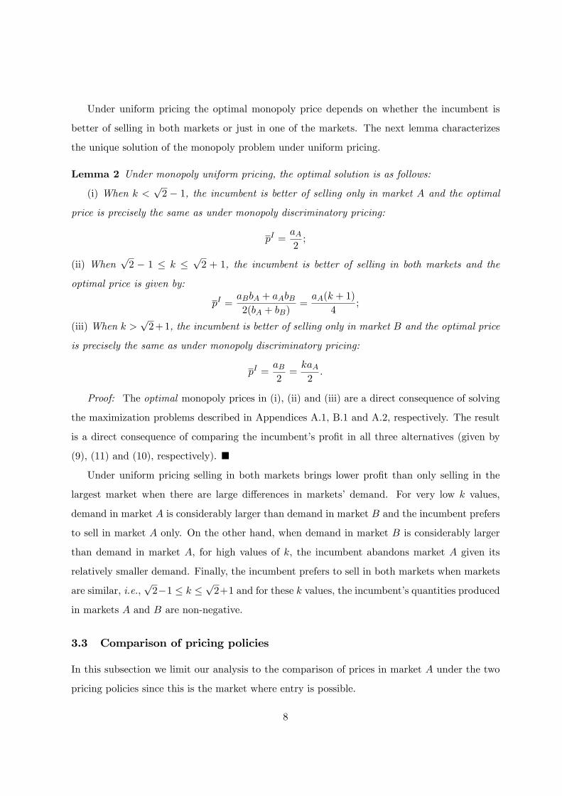
Lemma 2 Under monopoly uniform pricing, the optimal solution is as follows:

(i) When k <p2 � 1, the incumbent is better of selling only in market A and the optimal

price is precisely the same as under monopoly discriminatory pricing:

pI =aA2;

(ii) Whenp2 � 1 � k �

p2 + 1, the incumbent is better of selling in both markets and the

optimal price is given by:

pI =aBbA + aAbB2(bA + bB)

=aA(k + 1)

4;

(iii) When k >p2+1, the incumbent is better of selling only in market B and the optimal price

is precisely the same as under monopoly discriminatory pricing:

pI =aB2=kaA2:

Proof: The optimal monopoly prices in (i), (ii) and (iii) are a direct consequence of solving

the maximization problems described in Appendices A.1, B.1 and A.2, respectively. The result

is a direct consequence of comparing the incumbent�s pro�t in all three alternatives (given by

(9), (11) and (10), respectively). �

Under uniform pricing selling in both markets brings lower pro�t than only selling in the

largest market when there are large di¤erences in markets� demand. For very low k values,

demand in market A is considerably larger than demand in market B and the incumbent prefers

to sell in market A only. On the other hand, when demand in market B is considerably larger

than demand in market A, for high values of k, the incumbent abandons market A given its

relatively smaller demand. Finally, the incumbent prefers to sell in both markets when markets

are similar, i.e.,p2�1 � k �

p2+1 and for these k values, the incumbent�s quantities produced

in markets A and B are non-negative.

3.3 Comparison of pricing policies

In this subsection we limit our analysis to the comparison of prices in market A under the two

pricing policies since this is the market where entry is possible.

8

With discriminatory pricing the incumbent practices a higher price in the more inelastic

market. Moreover, if the incumbent serves both markets the uniform price will be between the

discriminatory prices in markets A and B. Whenp2 � 1 < k < 1, under uniform pricing the

incumbent serves both markets and under discriminatory pricing the incumbent sets a higher

price in market A. Therefore, under monopoly, if demand in market A is larger, discriminatory

price in this market will be higher than uniform price, i.e., pIAm > pI > pIBm, as long as both

markets are served under uniform pricing. This shows that one needs to take into account

di¤erences in markets�demand in order to know whether the incumbent�s price in market A is

higher under discriminatory or uniform pricing.

As we will see later this e¤ect is also present when the entrant decides to enter market A.

The intuition is that under duopoly the incumbent is a monopolist of the residual demand,

thus he also needs to compare the elasticity of demand in market B with the elasticity of the

residual demand in market A. If the residual demand in market A is less elastic than demand

in market B, the incumbent will charge a higher price in this market than in market B under

discriminatory pricing. This is precisely the message conveyed on Cheung and Wang (1999).

4 Discriminatory versus uniform pricing when E enters

market A

Suppose now that the entrant decides to enter market A but the incumbent remains a monopolist

in market B. In this section we analyze the Nash equilibrium under discriminatory and uniform

pricing.

4.1 Discriminatory pricing

Since the incumbent may set a di¤erent price in each market and he continues to be a monopolist

in market B, the optimal solution in this market is the same as in Subsection 3.1. However,

market A is now a duopoly and we need to �nd the Nash equilibrium of the price-game. Given

the demand functions (5) and (6), the incumbent and entrant choose the prices that maximize

their pro�ts in market A. Notice that all quantities must be non-negative. The details of the

solutions to these problems and �rst order conditions are described in Appendix A.3. The �rst

order conditions show that, under our assumptions, prices are strategic complements. Solving

9

the system of �rst order conditions we obtain the following result:

Lemma 3 Under discriminatory pricing, the post-entry unique Nash equilibrium in market A

is symmetric and it is given by:

pIAd = pE =

�

2� � =aA (bA � dA)2bA � dA

;

where the last expression is obtained from the de�nitions of �, � and .

Under discriminatory pricing, incumbent�s post-entry pro�t in market A is equal to entrant�s

gross post-entry pro�t and given by:

�IAd = �E =

��2

(2� � )2=

bA (bA � dA) a2A(bA + dA) (2bA � dA)2

: (12)

One can show that pIAd < pIAm and �IAd < �IAm as long as dA > 0. Conversely pIAd = pIAm

and �IAd = �IAm when dA = 0. In other words, the incumbent�s price and pro�t in market A is

lower when the entrant decides to enter this market than when the incumbent is a monopolist

unless the two products are completely di¤erentiated. This result is quite obvious: as long as

there exists some product substitutability, the incumbent looses with the competition of the

entrant. Also notice that the di¤erence between pIAd and pIAm is bigger when products become

highly substitutable, i.e., when dA rises and becomes close to bA.

And the incumbent�s total pro�t is given by:

�I(Ad+Bm) =bA (bA � dA) a2A

(bA + dA) (2bA � dA)2+k2a2A4bA

:

4.2 Uniform pricing

In order to �nd the equilibrium solution under uniform pricing when the entrant decides to enter

market A, we have to study the incumbent�s alternatives of selling in both markets and of only

selling in one of the markets.

Given the demand functions (3) and (5), if the incumbent sells his product in both markets,

he will choose a unique price so as to maximize his total pro�t taking into account that there

is a duopoly in market A. Given the demand function (6), the entrant chooses the price that

maximizes his pro�t in market A. Notice that all quantities must be non-negative (see details

of these problems in Appendix B.2).

10

Under uniform pricing and when the incumbent sells in both markets, incumbent�s post-entry

pro�t in market A and entrant�s gross post-entry pro�t are respectively given by:

��I(Ad+Bm) =a2A (bA � dA)

�2b2A � d2A

�[2k (bA + dA) + (2bA + dA)]

2

bA (bA + dA)�8b2A � 5d2A

�2��E =

a2A (bA � dA)�bAdA (k + 1) + 2

�2b2A � d2A

�+ kd2A

�2bA (bA + dA)

�8b2A � 5d2A

�2 :

If the incumbent abandons market B, he solves the following problem:

maxpId

pId��� �pId + pE

�while the entrant�s problem remains the same. Notice that this problem is precisely the same

as under discriminatory pricing (see Subsection 4.1). Therefore, the incumbent�s pro�t is given

by (12).

Finally, if the incumbent abandons market A, the entrant becomes a monopolist in this

market whereas the incumbent remains a monopolist in market B. Thus, the incumbent�s total

pro�t is given by (10).

The Nash equilibrium under uniform pricing depends on whether the incumbent is better of

selling in both markets or just in one of the markets. Let kA and kB be de�ned as follows:

kA =bA�8b2A � 5d2A

�q2b2A � d2A �

�2b2A � d2A

� �4b2A � d2A

�2�2b2A � d2A

�(bA + dA) (2bA � dA)

kB =2 (2bA + dA)

h4�b2A � d2A

� �2b2A � d2A

�+�8b2A � 5d2A

�q�2b2A � d2A

� �b2A � d2A

�i(bA + dA)

�32b4A � 32b2Ad2A + 9d4A

� :

The next lemma characterizes the unique Nash equilibrium under uniform pricing when entry

occurs.

Lemma 4 Under uniform pricing, the post-entry equilibrium is as follows:

(i)When k < kA, the incumbent is better of selling only in market A and the Nash equilibrium

prices are precisely the same as under discriminatory pricing:

pId = pE =

aA (bA � dA)2bA � dA

;

11

(ii) When kA � k � kB, the incumbent is better of selling in both markets and the Nash

equilibrium prices are given by:

pId =aA (bA � dA) [2k (bA + dA) + (2bA + dA)]

8b2A � 5d2A

pE =aA (bA � dA)

�bAdA (k + 1) + 2

�2b2A � d2A

�+ kd2A

�bA�8b2A � 5d2A

� ;

(iii) When k > kB, the incumbent is better of selling only in market B and the Nash equilibrium

prices are precisely the same as under monopoly discriminatory pricing:

pI = pIBm =aB2=kaA2

Thus, the entrant becomes a monopolist and his optimal price is:

pE =aA2:

Proof: The equilibrium prices in (ii) are the solution of solving the system of best response

functions of the two �rms, taking into account that the incumbent�s best response function

depends on k and dA. The result is a direct consequence of comparing the incumbent�s pro�t

in all three alternatives when entry occurs (selling in both markets, selling in market A only,

selling in market B only). �

Figure 1 illustrates these results. For the set of parameters in dark grey, the incumbent�s

demand in market A is considerably larger than demand in market B. Thus, the incumbent

prefers to sell in market A only even when there is a competitor in this market. On the other

hand, when demand in market B is considerably larger than the incumbent�s demand in market

A, the set of parameters in white, the incumbent prefers to sell in market B only. In this case,

the entrant becomes a monopolist in market A.

The incumbent prefers to sell in both markets when there are smaller degrees of markets�

demand di¤erence, i.e., kA � k � kB (the set of parameters in light grey) and, for these values

of k, the incumbent�s quantities in markets A and B, are non-negative.

When the entrant decides to enter market A, the incumbent�s decision of serving both or

just one of the markets depends on the relative size of demand in market B and the incumbent�s

demand in market A under duopoly. This comparison depends on the degree of markets�demand

di¤erence but it also depends on the degree of product substitutability. The higher dA is, the

12

0

0.2

0.4

0.6

0.8

0.6 1 1.5 2 k12 − 12 +

kA kB

dA

bA

bA

bA

bA

bA

Figure 1: Uniform pricing under duopoly in market A

larger is the reduction in the incumbent�s residual demand in market A when entry occurs. Thus,

as dA increases, demand in market A has to be much bigger in order for the incumbent to prefer

to sell only in market A under duopoly, i.e., the value of k below which the incumbent prefers

to sell only in market A, kA, is decreasing with dA. For the same reason, kB is also decreasing

with dA. As dA increases, market A becomes more competitive. Thus, the incumbent prefers to

abandon this market for smaller values of k.

Notice that as products become virtually homogeneous, duopoly pro�ts in market A are so

low that selling in market A only or even selling in both markets is more unpro�table than selling

in market B only. When products are highly substitutable (dA ! bA), competition in market A

is so �erce that even when market A is much larger (very low values of k) the incumbent prefers

to sell in market B only. On the other hand, when products are very di¤erentiated (dA ! 0),

competition in market A is soft and consequently market B has to be much larger than market

A for the incumbent to start selling in market B only.

As expected, when the incumbent sells in market A under duopoly, k < kB, the incumbent�s

price in market A, with competition, is lower than under monopoly except when there is complete

di¤erentiation, in which case the price is the same. The incumbent�s pro�t under entry is also

lower than under monopoly unless the two products are completely di¤erentiated (dA = 0).

13

4.3 Comparison of pricing policies

When the incumbent serves both markets under uniform pricing, one can show that the price

decrease in market A due to competition is higher under discriminatory pricing than under

uniform pricing. This happens because uniform pricing makes the incumbent softer. When

the incumbent considers a marginal price decrease he has to take into account the reduction in

pro�ts in markets A and B. So he has less incentives to decrease the price. The competitive

threat is higher under discriminatory pricing. This is the e¤ect described by Armstrong and

Vickers (1993).

However the previous e¤ect does not mean that the incumbent�s equilibrium price in market

A is always lower under discriminatory than under uniform pricing. If demand in market A is

much larger and less elastic than demand in market B, the discriminatory price may be higher

than the uniform price even when there is a competitor in market A. This is the e¤ect described

by Cheung and Wang (1999) since the e¤ect of the di¤erence in markets�demand when k is

low and lower than one (i.e., when demand in market A is relatively larger than demand in

market B) may overwhelm the e¤ect of di¤erence in the competitive threat across markets.

Thus, the price decrease in market A due to competition is higher under discriminatory pricing

than under uniform pricing but the incumbent�s equilibrium price in market A is higher under

discriminatory than under uniform pricing.

As described in the next section, the degree of product substitutability a¤ects the value of k

such that the e¤ect of the di¤erence in markets�demand overwhelms the e¤ect of the di¤erence

in the competitive threat across markets. Thus, we add a third e¤ect to Armstrong and Vickers

(1993) and Cheung and Wang�s (1999) analysis.

5 Entry decision

The entrant�s decision to enter market A depends on whether his gross post-entry pro�t is

smaller or higher than his entry costs. When the entrant�s gross post-entry pro�t is higher

under discriminatory pricing than under uniform pricing, there is an interval of entry costs values

where entry is pro�table under discriminatory pricing but unpro�table under uniform pricing.

Therefore we consider that entry under discriminatory pricing is more likely than under uniform

pricing. From Subsection 4.1 we conclude that under discriminatory pricing the incumbent

14

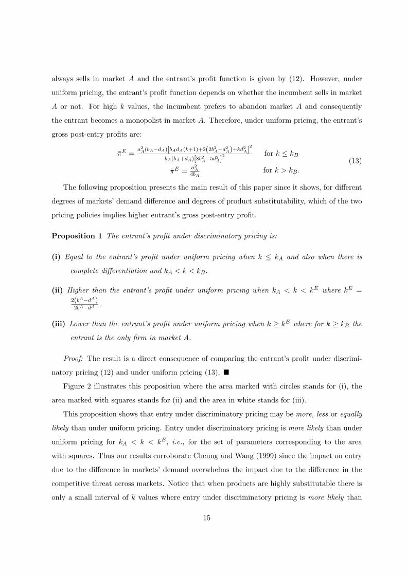
always sells in market A and the entrant�s pro�t function is given by (12). However, under

uniform pricing, the entrant�s pro�t function depends on whether the incumbent sells in market

A or not. For high k values, the incumbent prefers to abandon market A and consequently

the entrant becomes a monopolist in market A. Therefore, under uniform pricing, the entrant�s

gross post-entry pro�ts are:

��E =a2A(bA�dA)[bAdA(k+1)+2(2b2A�d2A)+kd2A]

2

bA(bA+dA)[8b2A�5d2A]2 for k � kB

��E =a2A4bA

for k > kB:(13)

The following proposition presents the main result of this paper since it shows, for di¤erent

degrees of markets�demand di¤erence and degrees of product substitutability, which of the two

pricing policies implies higher entrant�s gross post-entry pro�t.

Proposition 1 The entrant�s pro�t under discriminatory pricing is:

(i) Equal to the entrant�s pro�t under uniform pricing when k � kA and also when there is

complete di¤erentiation and kA < k < kB.

(ii) Higher than the entrant�s pro�t under uniform pricing when kA < k < kE where kE =2(bA�dA)2bA�dA .

(iii) Lower than the entrant�s pro�t under uniform pricing when k � kE where for k � kB the

entrant is the only �rm in market A.

Proof: The result is a direct consequence of comparing the entrant�s pro�t under discrimi-

natory pricing (12) and under uniform pricing (13). �

Figure 2 illustrates this proposition where the area marked with circles stands for (i), the

area marked with squares stands for (ii) and the area in white stands for (iii).

This proposition shows that entry under discriminatory pricing may be more, less or equally

likely than under uniform pricing. Entry under discriminatory pricing is more likely than under

uniform pricing for kA < k < kE , i.e., for the set of parameters corresponding to the area

with squares. Thus our results corroborate Cheung and Wang (1999) since the impact on entry

due to the di¤erence in markets�demand overwhelms the impact due to the di¤erence in the

competitive threat across markets. Notice that when products are highly substitutable there is

only a small interval of k values where entry under discriminatory pricing is more likely than

15

0 0.6 1 1.5 2 k

kE kB

12 − 12 +

kA

0.2

0.4

0.6

0.8

dA

bA

bA

bA

bA

bA

Figure 2: Entrant�s pro�ts comparison

under uniform pricing. Entry under discriminatory pricing is more likely than under uniform

pricing for large intervals of k when there are lower degrees of product substitutability. Thus,

the degree of product substitutability a¤ects the interval of the degrees of markets� demand

di¤erence where entry under discriminatory pricing is more likely than under uniform pricing.

For a given k, if the degree of product substitutability rises, the entrant�s pro�ts under both

pricing policies decrease except when the entrant is monopolist. For intermediate and high

degrees of product substitutability, this decrease is bigger under discriminatory pricing and

thus, entry under uniform pricing starts to be more likely than under discriminatory pricing.

Entry under uniform pricing is more likely than under discriminatory pricing for k � kE ,

i.e., for the set of parameters corresponding to the area in white. Notice that for k � kB the

entrant has the highest pro�t possible since he is a monopolist in market A.

Finally, when market A is much larger than market B, i.e., k � kA the entrant has the same

pro�t under both pricing policies since under uniform pricing the incumbent prefers to sell in

market A only, which leads to the same Nash equilibrium in market A as under discriminatory

pricing. Entry is also equally likely under both pricing policies when kA < k < kB and there is

complete di¤erentiation.

6 Conclusion

Pricing policies imply di¤erent entry incentives. There are some studies which support the

view that discriminatory pricing tends to discourage entry and conversely other studies show

16

that discriminatory pricing can increase pro�ts and thus encourage entry. We extended the

analysis of the impact of pricing policies upon entry considering a framework where there exists

price competition and di¤erentiated products. In addition to the analysis of the impact of the

di¤erence in the competitive threat across markets and of the di¤erence in markets�demand, we

explore the e¤ect of product di¤erentiation on the comparison of the impact of pricing policies

upon entry.

We show that the impact of pricing policies upon entry is ambiguous. Entry under discrim-

inatory pricing may be more, less or equally likely than under uniform pricing. For all degrees

of product substitutability, there is always some level of degree of markets�demand di¤erence

where under discriminatory pricing entry is more likely than under uniform pricing. The degree

of product substitutability has impact on the set of degrees of markets�demand di¤erence where

entry under discriminatory pricing is more likely than under uniform pricing.

Focusing solely on the di¤erence in the competitive threat across markets and the e¤ect of

the degree of markets�demand di¤erence as determinants of when discriminatory pricing entry

is more likely than under uniform pricing ignores an important e¤ect �the e¤ect of the degree of

product substitutability. Therefore, we reinforce Cheung and Wang (1999) idea that there should

always be a complete evaluation of the market conditions adding to their analysis, the impact

of product di¤erentiation. In addition, our analysis extends previous results since we study

the cases where, under entry, the incumbent �rm sells in both markets under uniform pricing

as well as the case where the incumbent abandons one of the markets. Interesting extensions

could consider settings where there are complementary products and where �rms have positive

symmetric or asymmetric production costs.

17

A Discriminatory Pricing

We present the computations of the �rst order conditions and solutions for three di¤erent op-

timization problems under discriminatory pricing: monopoly in market A, monopoly in market

B and duopoly in market A.

A.1 Monopoly in market A

Let pIAm, qIAm denote the incumbent�s monopoly price and quantity in market A under discrim-

inatory pricing. The incumbent solves the following problem:

maxpIAm

pIAm

�aAbA� 1

bApIAm

�The �rst order condition is given by:

d�IAmdpIAm

=aAbA� 2

bApIAm = 0:

The monopoly solution is:

pIAm =aA2

and qIAm =aA2bA

Under our assumptions, this quantity is positive.

A.2 Monopoly in market B

Let pIBm, qIBm denote the incumbent�s monopoly price and quantity in market B under discrim-

inatory pricing. The incumbent solves the following problem:

maxpIBm

pIBm

�aBbB� 1

bBpIBm

�The �rst order condition is given by:

d�IBmdpIBm

=aBbB� 2

bBpIBm = 0:

The monopoly solution is:

pIBm =aB2=kaA2

and qIBm =aB2bB

=kaA2bA

;

where the last equalities follow from the assumptions on aB and bB. Under our assumptions,

this quantity is positive.

18

A.3 Duopoly in market A

Let pE , qE denote the entrant�s price and quantity when the incumbent uses a discriminatory

pricing policy and pIAd, qIAd are the incumbent�s price and quantity in market A under discrimi-

natory pricing and duopoly in market A. Given the demand function (5) , the incumbent solves

the following problem in market A:

maxpIAd

pIAd��� �pIAd + pE

�and similarly, given the demand function (6), the entrant solves:

maxpE

pE��� �pE + pIAd

�;

The �rst order conditions are respectively given by:

@�IAd@pIAd

= �� 2�pIAd + pE = 0

@�E

@pE= �� 2�pE + pIAd = 0:

And thus the best response functions of the two �rms are given by:

pIAd =�+ pE

2�

pE =�+ pIAd2�

:

The equilibrium prices are given by:

pIAd = pE =

�

2� � =aA (bA � dA)2bA � dA

and the equilibrium quantities are given by:

qIAd = qE =

��

2� � =aAbA

(bA + dA) (2bA � dA);

where the last expressions are obtained from the de�nitions of �, � and .

Under our assumptions, qIAd and qE are always positive.

B Uniform Pricing

We present the computations of the �rst order conditions and solutions for two di¤erent opti-

mization problems under uniform pricing: sell both markets when there is a monopoly in market

A and sell both markets when there is a duopoly in market A.

19

B.1 Sell both markets and monopoly in market A

Let pI , qIAm, qIBm denote the incumbent�s price and quantities produced in markets A and B,

respectively, under uniform pricing and monopoly in both markets. The incumbent solves the

following problem:

maxpI

pI�aAbA� 1

bApI�+ pI

�aBbB� 1

bBpI�

(14)

The �rst order condition is given by:

d��I(Am+Bm)

dpI=

�aAbA� 2

bApI�+

�aBbB� 2

bBpI�= 0:

The solution is:

pI =aBbA + aAbB2(bA + bB)

=aA(k + 1)

4

qIAm =2aA � aB2(bA + bB)

+aAbB

2bA(bA + bB)=aA (3� k)4bA

qIBm =2aB � aA2(bA + bB)

+aBbA

2bB(bA + bB)=aA (3k � 1)

4bA;

Notice that qIAm > 0 if k < 3 and qIBm > 0 if k >

13 .

B.2 Sell both markets and duopoly in market A

Let pE , qE denote the the entrant�s price and quantity when the incumbent practices uniform

pricing and sells in both markets and pId, qIAd, q

I0Bm are the incumbent�s price and quantities

in markets A and B, respectively, under uniform pricing and duopoly in market A. Given the

demand functions (3) and (5), the incumbent solves the following problem:

maxpId

pId��� �pId + pE

�+ pId

�aBbB� 1

bBpId

�and similarly, given the demand function (6), the entrant solves:

maxpE

pE��� �pE + pId

�The �rst order conditions are respectively given by:

@��I(Ad+Bm)

@pId=��� 2�pId + pE

�+

�aBbB� 2

bBpId

�= 0

@��E

@pE= �� 2��pE + pId = 0:

20

And thus the best response functions of the two �rms are given by:

pId =�bB + aB + bBp

E

2 (bB� + 1)

pE =�+ pId2�

:

The equilibrium prices are given by:

pId =2�aB + �bB (2� + )

4� + bB�4�2 � 2

� =

=aA (bA � dA) [2k (bA + dA) + (2bA + dA)]

8b2A � 5d2A

pE = aB + 2�+ �bB (2� + )

4� + bB�4�2 � 2

� =

=aA (bA � dA)

�bAdA (k + 1) + 2

�2b2A � d2A

�+ kd2A

�bA�8b2A � 5d2A

�and the equilibrium quantities are given by:

qIAd =� (2� + ) (2 + �bB) + aB

� 2 � 2�2

�4� + bB

�4�2 � 2

� =

=aA�(2bA + dA)

�3b2A � 2d2A

�+ k (bA + dA)

�d2A � 2b2A

��bA (bA + dA)

�8b2A � 5d2A

�qI

0Bm =

2�aB + aBbB�4�2 � 2

�� �bB (2� + )

bB�4� + bB

�4�2 � 2

�� =

=aA�3k�2b2A � d2A

���bA � dA

�(2bA + dA)

�bA�8b2A � 5d2A

�qE = �

2� (1 + �bB) + aB + � bB

4� + bB�4�2 � 2

� =

=aA�bAdA (k + 1) + 2

�2b2A � d2A

�+ kd2A

�(bA + dA)

�8b2A � 5d2A

� ;

Under our assumptions, qE is always positive. Notice that qIAd > 0 if k <(2bA+dA)

�3(bA)

2�2(dA)2�

(bA+dA)(2(bA)2�(dA)2)

and qI0Bm > 0 if k >

(bA�dA)(2bA+dA)3(2(bA)2�(dA)2)

.

21

References

[1] Aguirre,I., Espinosa, M.P. and Macho-Stadler, I., 1998, �Strategic Entry Deterrence through

Spatial Price Discrimination�, Regional Science and Urban Economics, 28, 297-314.

[2] Armstrong, M. and Vickers, J., 1993, �Price Discrimination, Competition and Regulation�,

The Journal of Industrial Economics, 41-4, 335-359.

[3] Azar, O. H., 2003, �Can Price Discrimination be Bad for Firms and Good for All Con-

sumers? A Theoretical Analysis of Cross-Market Price Constraints with Entry and Product

Di¤erentiation�, Topics in Economic Analysis & Policy, 3-1, Article 12.

[4] Cheung, F. K. and Wang, X., 1999, �A Note on the E¤ect of Price Discrimination on Entry

�Research Note�, Journal of Economics and Business, 51, 67-72.

[5] Dixit, A., 1979, �A Model of Duopoly suggesting a Theory of Entry Barriers�, Bell Journal

of Economics, 10, 20-32.

[6] Katz, M., 1984, �Price Discrimination and Monopolistic Competition�, Econometrica, 52-6,

1453-1471.

[7] Motta, M., 2004, Competition Policy �Theory and Practice, Cambridge University Press.

22