Entropy Function Approach to the Lattice Boltzmann Method

291

0022-4715/02/0400-0291/0 © 2002 Plenum Publishing Corporation

Journal of Statistical Physics, Vol. 107, Nos. 1/2, April 2002 (© 2002)

Entropy Function Approach to the Lattice BoltzmannMethod

Santosh Ansumali1 and Iliya V. Karlin1

1 ETH Zürich, Department of Materials, Institute of Polymers, ETH-Zentrum, ML J 19,Sonneggstr. 3, CH-8092 Zürich, Switzerland; e-mail: [email protected] and [email protected]

Received February 26, 2001; accepted June 25, 2001

In this paper, we present the construction of the Lattice Boltzmann methodequipped with the H-theorem. Based on entropy functions whose local equi-libria are suitable to recover the Navier–Stokes equations in the framework ofthe Lattice Boltzmann method, we derive a collision integral which enablessimple identification of transport coefficients, and which circumvents construc-tion of the equilibrium. We discuss performance of this approach as comparedto the standard realizations.

KEY WORDS: Kinetic theory; H-theorem; Lattice Boltzmann method; stability.

1. INTRODUCTION

The Lattice Boltzmann method (hereafter LBM) for simulations ofcomplex hydrodynamic phenomena has received much attention over thepast decade. (1) In the LBM, macroscopic equations are not addresseddirectly by a conventional discretization procedure, rather fully discretekinetic models are constructed in such a way that (i) their long time, largescale limit matches the macroscopic dynamics in question, and (ii) theyallow a relatively simple numerical implementation. In its present andmostly used form, the LBM is based on (i) a polynomial ansatz withtailored properties for the local equilibrium, and (ii) a single relaxationtime model (hereafter SRTM) for the relaxation (collision) term. TheSRTM has been borrowed from the well known Bhatnagar–Gross–Krookapproximation of the Boltzmann collision integral of the classical kinetictheory. The resulting method is known as the LBGK model. (2, 3) However,

in spite of impressive evidences of successful applications of the presentrealization of LBM, (1) theoretical development of the method is far frombeing over. One of the problems, recognized by many authors, is theproblem of numerical stability. (1, 4, 5) For example, in the framework of theLBM starting with the work (6) many simulations of high Reynolds numberflows has been successfully performed (see, for detail, refs. 1 and 7).However, progress on stability may be needed to go beyond existing stateof the arts like spectral methods in simple geometries.

It has been discussed for some time in the literature (1, 4, 5, 8, 9) thatstability of the LBM could be improved if the method could be based onan analog of the Boltzmann H-theorem. The goal of this work is to sum-marize progress made in this direction in recent years. (4, 5, 8, 9) First, we willpresent entropy functions which reproduces the correct hydrodynamicswithin the accuracy of the Lattice Boltzmann method for a particularchoice of the Lattice. Next, based on the knowledge of these entropy func-tions, we develop a realization of the Lattice Boltzmann method with theH-theorem built in. We will discuss how using these entropy functions aSRTM collision integral, which circumvents need of a polynomial ansatzfor the local equilibrium, can be constructed. Finally, some numerical testswill be presented to show unconditional stability of this new class of theLattice Boltzmann models (ELBM hereafter). (5, 8, 9)

2. OVERVIEW OF THE LBM

In the Lattice Boltzmann method, (1) one considers populations offictitious particles f with ith component as fi(r, t), where i=1,..., b labelsdiscrete velocities ci. The set of discrete velocities, which can also include azero vector (‘‘rest population’’), is associated with outgoing links at eachsite r of a regular isotropic lattice. Populations are updated at discrete timesteps t according to an equation,

fi(r+ci, t+1)−fi(r, t)=Di (1)

In the following, we shall restrict our attention to the isothermal Navier–Stokes equation. For this case, the collision integral D must obey only thelocal conservation laws,

O{1, ca} |DP={0, 0} (2)

where, we denote scalar product of b-dimensional vectors x and y asOx | yP=;b

i=1 xi yi, the Cartesian components of d-dimensional vector as

292 Ansumali and Karlin

a=1,..., d, and (1,..., 1) as 1. Local hydrodynamic quantities (the massdensity and the momentum density respectively) are defined as,

O{1, ca} | fP={r, rua} (3)

If the long-time large-scale limit of Eq. (1) recovers the Navier–Stokesequation, then hydrodynamics is implemented in a fairly simple, fullydiscrete kinetic picture. To do so, the most popular choice is Bhatnagar–Gross–Krook approximation (hereafter BGK) for the collision integraland a polynomial ansatz for the equilibrium distribution. With the BGKapproximation, the LBE equation (1) is given as

fi(r+ci, t+1)−fi(r, t)=−12y

(fi(r, t)−feqi (r, t)) (4)

The equilibrium distribution (f eq) are subjected to constraints fixed bythe hydrodynamic fields,

O{1, ca} | f eqP={r, rua} (5)

In addition, in order to recover the Navier–Stokes equation up to second-order accuracy in u, the local equilibrium must respect the condition for thestress tensor,

Cb

i=1ciacibf

eqi =ruaub+rc

2sdab (6)

where cs is the speed of sound. Then a quadratic form of distribution func-tion which satisfy these restriction is used.

3. ENTROPY FUNCTIONS FOR THE LBM

If the local equilibrium is supported by some entropy function, thenthe Lattice Boltzmann method can be equipped with the H-theorem, (10, 11)

and stability problem can be studied in a controlled way. However, anyapproach which attempts to enhance stability via an H-theorem, must beable to recover the Navier–Stokes equations and the H-function must befound by lattice-dependent considerations. (4) For the case of one-dimen-sional three velocity and two-dimensional nine velocity lattice such entropyfunctions are known (4) and are given here for the sake of the completeness.

Entropy Function Approach to the Lattice Boltzmann Method 293

In the case of the one-dimensional lattice with spacing c, the velocityset at each lattice site consists of three velocities, c+=c, c−=−c, andc0=0. For this case entropy function is given as, (4)

H=f0 ln 1f04 2+f− ln(f−)+f+ ln(f+) (7)

In this particular case, it is actually possible to get analytically the equilib-rium distribution.

feq0 =

2r3

[2−`1+M2]

feq+=r

35uc−c2s

2c2s+`1+M26

feq−=r

35−uc+c2s

2c2s+`1+M26 (8)

where, the c2s=c2/3 is the square of the sound velocity and M2=u2/c2s isthe Mach number squared. However, result (8) is the exclusive case whichdoes not happen in higher dimensions.

In a two-dimensional Cartesian coordinates system, for nine-velocitylattice (2d9v) the entropy function is given as, (4)

H=f0 ln 1f08 2+C4

l=1fl ln 1fl2 2+C

8

l=5fl ln(2fl) (9)

where, the discrete velocity vector set c={cx, cy} is given as,

cx=(0, 1, 0, −1, 0, 1, −1, −1, 1)T (10)

cy=(0, 0, 1, 0, −1, 1, 1, −1, −1)T (11)

Local equilibria of these entropy functions satisfy the Eq. (6) up to theorder of M4.

4. LBM BASED ON THE ENTROPY FUNCTION

Knowledge of the perfect entropy function suggests realizations of theLattice Boltzmann method which do not require an explicit expression forthe local equilibrium. In the subsequent section, we formulate one of suchrealizations. Before doing this, however, we describe a general procedurewhich equips any realization with the H-theorem. Let us assume that the

294 Ansumali and Karlin

collision integral D(f) in the kinetic equation (1) is realized in such a waythat it satisfies two conditions: (i) the conservation laws Eq. (2) (ii) theentropy production inequality, ONH |DP [ 0, where NH is the gradient ofthe entropy function, while the equality sign implies f=f eq. A collisionintegral which meets these requirements will be termed admissible. Forinstance, the standard BGK collision integral is admissible. For each pairof vectors {f, D} such that fi \ 0, we introduce an auxiliary populationvector f g=f+agD. The scalar parameter ag is derived as follows: Let usconsider the equation

H(f)=H(f+aD) (12)

There are two cases classified by the number of solutions the Eq. (12) mayhave. In the first case, Eq. (12) has two solutions, a1=0, and anothersolution a2 (notice that the degeneracy, a2=a1=0, occurs only if f=f eq).In this case, the parameter ag of the auxiliary population is taken asag=a2. This situation can be interpreted as the ‘‘bulk case’’ since bothvectors, f and f g, are located in the interior of the phase space of popula-tions. The second (‘‘boundary’’) case corresponds to the situation whenEq. (12) has only one (non-degenerate) solution a1=0. Then,

ag= mini=1,..., b; Di < 0

{fi/|Di |} (13)

The auxiliary state f g is taken at the boundary of the phase space (atleast one of the populations fg

i is equal to zero).The auxiliary population sets the limit of the collision update in such a

way that the entropy function H decreases in the result. Once the auxiliarypopulation f g is defined, the result of the collision is set as f(b)=(1−b) f+bf g where b is a fixed parameter chosen on the segment [0, 1].Convexity of the entropy function implies the following inequality (thelocal H-theorem): H(f(b)) [H(f). Moreover, when approaching thehydrodynamic regime, i.e., close enough to the local equilibrium, only thebulk case is realized because f eq for Boltzmann-like entropy functions is apositive vector. Then the parameter b controls the viscosity coefficient inthe resulting Navier–Stokes equations in the following way: The zero vis-cosity limit corresponds to bQ 1. Thus, in the ELBM, population vector isupdated according to kinetic equation,

f(x+c, t+1)− f(x, t)=Dg[f(x, t)] (14)

where Dg is dressed (or stabilized ) collision integral,

Dg[f(x, t)]=ba[f(x, t)] D[f(x, t)] (15)

Entropy Function Approach to the Lattice Boltzmann Method 295

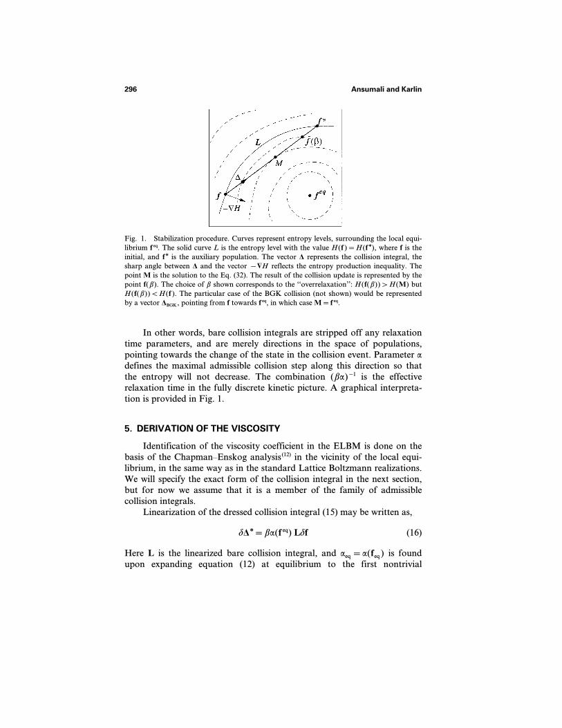
Fig. 1. Stabilization procedure. Curves represent entropy levels, surrounding the local equi-librium f eq. The solid curve L is the entropy level with the value H(f)=H(f g), where f is theinitial, and f g is the auxiliary population. The vector D represents the collision integral, thesharp angle between D and the vector −NH reflects the entropy production inequality. Thepoint M is the solution to the Eq. (32). The result of the collision update is represented by thepoint f(b). The choice of b shown corresponds to the ‘‘overrelaxation’’: H(f(b)) > H(M) butH(f(b)) < H(f). The particular case of the BGK collision (not shown) would be representedby a vector DBGK, pointing from f towards f eq, in which case M=f eq.

In other words, bare collision integrals are stripped off any relaxationtime parameters, and are merely directions in the space of populations,pointing towards the change of the state in the collision event. Parameter adefines the maximal admissible collision step along this direction so thatthe entropy will not decrease. The combination (ba)−1 is the effectiverelaxation time in the fully discrete kinetic picture. A graphical interpreta-tion is provided in Fig. 1.

5. DERIVATION OF THE VISCOSITY

Identification of the viscosity coefficient in the ELBM is done on thebasis of the Chapman–Enskog analysis (12) in the vicinity of the local equi-librium, in the same way as in the standard Lattice Boltzmann realizations.We will specify the exact form of the collision integral in the next section,but for now we assume that it is a member of the family of admissiblecollision integrals.

Linearization of the dressed collision integral (15) may be written as,

dDg=ba(f eq) Ldf (16)

Here L is the linearized bare collision integral, and aeq=a(feq) is foundupon expanding equation (12) at equilibrium to the first nontrivial

296 Ansumali and Karlin

(quadratic) order. [Note that a substitution of f eq into Eq. (12) does notgive an equation for aeq. This is natural because, by its sense, aeq is arelaxation parameter which can be only specified by considering deviationsfrom the equilibrium.] The result reads:

aeq=−2Odf | NNH(f eq) |LdfPOLdf | NNH(f eq) |LdfP

(17)

Here NNH(f eq) is the b×b matrix of second derivatives of the entropyfunction at equilibrium. Equation (17) suggests that, in general, aeq has aspectrum of values dependent on the direction along which the equilibriumis approached. However, drastic simplification of Eq. (17) happens if L hasthe projector property:

LL=−L (18)

In this case, relaxation parameter aeq becomes independent of the directionin the phase space, along which the state relaxes to the equilibrium. This isthe essence of the SRTM which simply tells that all the b−n kinetic vari-able relax to zero with the same rate. This important property is satisfied,in particular, by the linearized bare BGK collision integral, and it has beenalready demonstrated elsewhere (10) that in this case aeq=2. Thus, Eq. (16)together with Eq. (18) defines the linearized dressed collision integral,

dDg=2bLgdf (19)

where, operator Lg has the projector property given by Eq. (18). With thisdescription of the linearized dressed collision integral, we now follow thestandard Chapman–Enskog analysis, and seek the solution to the kineticequation (14) in the form, f=f eq+df ne, where the nonequilibrium part df ne

is orthogonal to the hydrodynamic subspace, O{1, ca} | df neP={0, 0}, andis found in terms of the expansion, df ne=Edf (1)+E2df (2)+O(E3), subject tothe multiscale expansion of the time and space derivatives, “t=E“ (1)t +E2“ (2)t+O(E3), “a=E“ (1)a +O(E2). Then,

−2b CjLgijdf

(1)j =[“ (1)t +cia“a] feq

i (20)

−2b CjLgijdf

(2)j =“ (2)t feq

i +[“ (1)t +cia“a]5−b CjLgijdf

(1)j +df (1)i 6 (21)

Entropy Function Approach to the Lattice Boltzmann Method 297

By the Fredholm alternative, solution to Eq. (20) is written as,

df (1)=df (1)spec+df(1)hom (22)

where df (1)hom is the general solution to the homogeneous equation,Lgdf (1)hom=0, and df (1)spec is a special solution to the inhomogeneous equation(20). The homogeneous solution is equal to zero by the orthogonality con-dition mentioned above.

Using the projector property (18), Eqs. (20) and (21) are equivalent tothe following two equations for the special solution (we omit the subscriptspec):

−2bdf (1)i =[“ (1)t +cia“a] feqi (23)

−2bdf (2)i =“ (2)t feqi +(1−b)[“ (1)t +cia“a] df (1)i (24)

The latter set of equations coincides with the well known case of theLBGK, in which the BGK relaxation parameter y−1 is replaced by 2b, andwe are immediately led to the following viscosity coefficient

n=c2s (1−b)

2b(25)

Thus, the ELBM is able to retain the full control over the viscosity, whilevariation of the parameter b in the interval [0, 1] covers the full linearstability interval.

Finally, it should be stressed that the theoretical derivation of the vis-cosity coefficient is always strictly applicable only in the vicinity of thelocal equilibrium.

6. THE SINGLE RELAXATION TIME MODEL FOR THE COLLISION

INTEGRAL

It is important to notice that simplification of the near-equilibriumdynamics with the projector property [Eq. (18)] concerns solely the linear-ized bare collision integral, but does not tell yet anything about situationsfar from equilibrium. There might be many collision integrals which havethe same property [Eq. (18)] near equilibrium but different elsewhere. Ourgoal is therefore to construct a nonlinear SRTM which has the desiredprojector property [Eq. (18)] near equilibrium (and thus is equivalent to

298 Ansumali and Karlin

the linearized BGK), and requires only the knowledge of the entropyfunction.

In order to construct the SRTM, we first write operator L with theproperty (18) in terms of a given basis of the kinetic subspace gs:

L=−Cb−n

s=1|gsPOgs | (26)

We seek the SRTM within the following family of admissible collisionintegrals:

|DP=− Cb−n

s, p=1|gsP Ksp(f)Ogp |NHP (27)

Here Ksp are elements of a positive definite (b−n)×(b−n) matrix K.Functions Ksp may depend on the population vector, and any representa-tive of the family (27) is admissible. A requirement that the linearizationof the collision integral (27) equals L (26) uniquely defines matrix K atequilibrium:

K(f eq)=C−1(f eq)

Csp(f eq)=Ogs | NNH(f eq) |gpP(28)

Finally, we need to extend the the matrix K(f eq) to arbitrary f. This exten-sion is not unique but we suggest the most simple approach which amountsto replacing f eq by f in the Eq. (28) to give

K(f)=C−1(f)

Csp(f)=Ogs | NNH(f) |gpP(29)

Matrix C(f) is symmetric and positive definite for any f (the last statementfollows from the strict convexity of the entropy function for any f). ThenC−1 exists for any f, and it it is straightforward to prove that the resultingmatrix K(f) is positive definite for any f. In this case we find the nonlinearSRTM given by Eqs. (27) and (29). Notice that the matrix K(f), and all theother elements in Eq. (27), are well defined once only the entropy functionis known.

As far as the choice of the set of basis vectors is concerned, anyorthonormal set of basis vectors which lie in the null space of conservationvectors will suffice. However, one would like to have a set of basis vectorwhich will make matrix C as sparse as possible. Our suggestion for basisvector is,

Entropy Function Approach to the Lattice Boltzmann Method 299

g1=1

`6(−2, 0, 0, 0, 0, 1, 0, 1, 0)T

g2=12(0, 1, −1, 1, −1, 0, 0, 0, 0)T

g3=1

`30(2, 0, 0, 0, 0, 2, −3, 2, −3)T

g4=1

`12(0, −2, 0, 2, 0, 1, −1, −1, 1)T

g5=1

`12(0, 0, −2, 0, 2, 1, 1, −1, −1)T

g6=1

`180(4, −5, −5, −5, −5, 4, 4, 4, 4)T

(30)

where, the conservation vectors are,

er=13(1, 1, 1, 1, 1, 1, 1, 1, 1)T

evx=1

`6(0, 1, 0, −1, 0, 1, −1, −1, 1)T

evy=1

`6(0, 0, 1, 0, −1, 1, 1, −1, −1)T

(31)

Using this choice of basis vector matrix C can be inverted analytically.

7. IMPLEMENTATION OF THE ENTROPY ESTIMATE

The next important point concerns solving the nonlinear equation(12), which implements the discrete time H-theorem. Because the entireELBM is largely based on convexity of the entropy function, and alsobecause working with Boltzmann-like H-functions cannot tolerate anynonpositivity of populations, it is desirable to avoid conventional methodswhich do not respect positivity and convexity. Our approach to solveEq. (12) is based on a two-side estimate of the location of the nontrivialroot. The upper bound amax > 0 is the minimal solution to the equations,fi+aDi=0, Di < 0. In geometrical terms, amax corresponds to the point onthe boundary of the kinetic polytope where the ray, f(a)=f+aD, a \ 0,

300 Ansumali and Karlin

intersects the boundary. Construction of the lower bound, amin, is basedon the earlier general study of the initial layer problem in dissipativekinetics. (13, 14) Specifically, we consider another nonlinear equation,

ONH(f+aD) |DP=0 (32)

In geometrical terms, the unique solution to this equation, amin, definespopulation vector fmin=f+aminD which is the minimum entropy state onthe ray f(a). Indeed, the minimum condition is the tangency point of theray to a level of entropy function (see Fig. 1). The nontrivial solution toEq. (12) is strictly in the interval [amin, amax]. In order to evaluate amin, wehave applied a quasi-Newton method of ref. 13 which guarantees successiveapproximations, a (n)min, n=1,..., and for all n it is valid that 0 < a (n)min [ amin.Moreover, the first approximation, a (1)min is known analytically [see ref. 13].This estimate of lower bound is given as,

a (1)min=1− exp(−s/q)m+n exp(−s/q)

(33)

with,

the entropy production s=−ONH |DP (34)

the maximum loss in the population m=max(D−i /fi) (35)

the total gain in the population n=1qC (D+i )

2

fi(36)

and the normalization factor q=C D+i (37)

where, the collision integral D is partitioned in positive (D+) and negative(−D−) parts such that,

D+j =˛Dj if Dj > 0

0 else (38)

and,

D−j =˛ −Dj if Dj < 0

0 else (39)

This estimate for a (1)min guarantees that the solution is located strictly insidethe interval [a (1)min, amax]. Starting with this bound for the root, the bisectionmethod has been implemented. The present algorithm of solving for the

Entropy Function Approach to the Lattice Boltzmann Method 301

entropy condition [Eq. (12)] guarantees that positivity of populations isnot violated.

The method of implementation for the entropy estimate describedabove is quite general. The method can be implemented for any entropyfunction. However, in the present case we know that a should be very closeto 2. Using this information, we have refined the root solver by using acombination of the Newton–Raphson method and of the bisection method,which usually converges to the root in less than 10 iteration. This mini-mizes computational overhead for solving the nonlinear equation.

In general, the ELBM has to perform two extra steps in comparison tothe LBGK scheme. The first step is computation of the bare collisionintegral, Eq. (29). The second step is to solve the nonlinear equation (12).Both of these operations scale linearly with the number of lattice nodes.

At each time step, the root solving will require b×N×X evaluationof the function fi log(Cifi). The collision integral in Eq. (29) require Ntimes evaluation and inversion of a symmetric positive definite matrixof dimension (b−M)×(b−M). This is of the order O(N(b−M)3/6+(b−M)(b−M+1)/2) operation. Here X is the number of iterationrequired to solve Eq. (12), and M is the number of the conservation laws.Notice that the collision matrix in the standard LBGK is diagonal and anyimprovement over LBGK has to deal at least with the evaluation of thecollision matrix of the size (b−M)×(b−M). One such example is therecently proposed method (15) based on the linear stability analysis. To givea reader a concrete feel of the numbers involved, on a Sun workstation fora grid size of 21×21 doing 10000 time steps simulation with the presentscheme took around 130 seconds while with the BGK time involved wasaround 13 seconds. A BGK simulation of 10000 time steps for a grid sizeof 63×63 took around 120 seconds. Thus, the present scheme is an orderof magnitude slower compared to the BGK. In the present scheme around80% of the time is spent for evaluating the collision operator. On the otherhand, time required to solve for the entropy estimates contributes onlyaround 5–10% to the total computation time. In the present work, we havefocused on the optimization of the entropy estimate, optimization of thecollision operator is left for the future work.

8. SOME NUMERICAL RESULTS

8.1. Shock Tube Tests

The first example presented here is from ref. 5, the time evolution of aone-dimensional front in a shock tube, a very classical problem in whichit appears a compressive shock front moving in the low density and a

302 Ansumali and Karlin

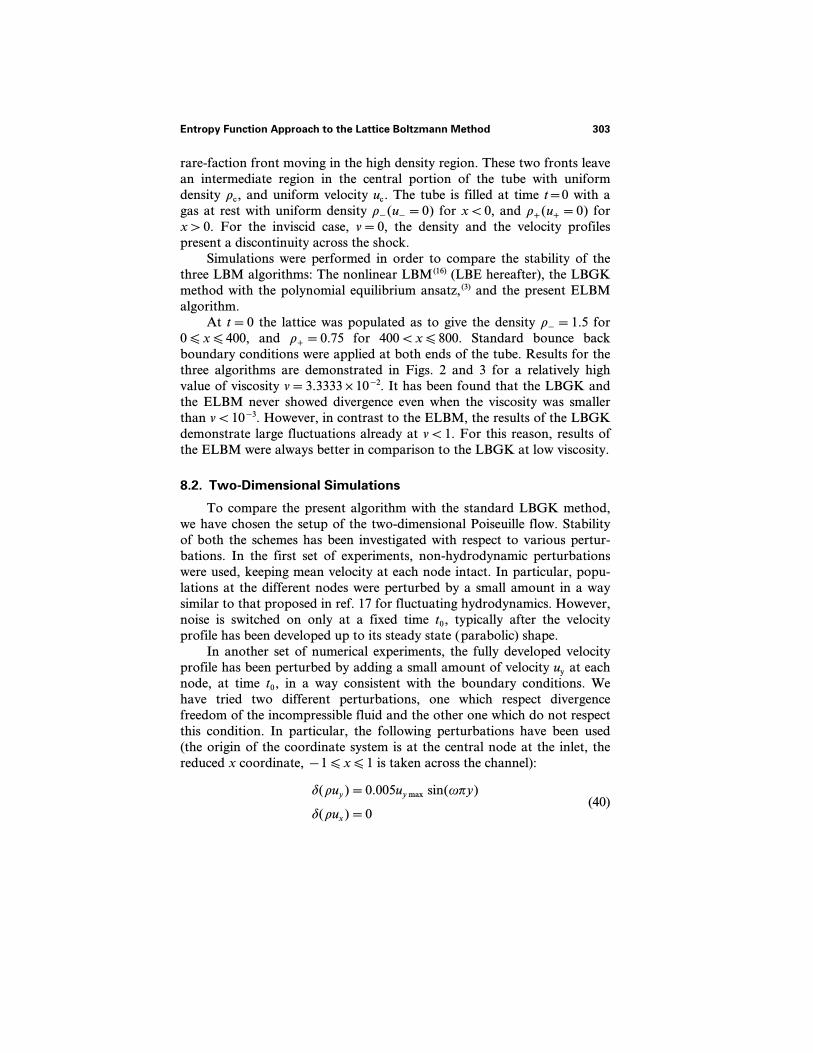
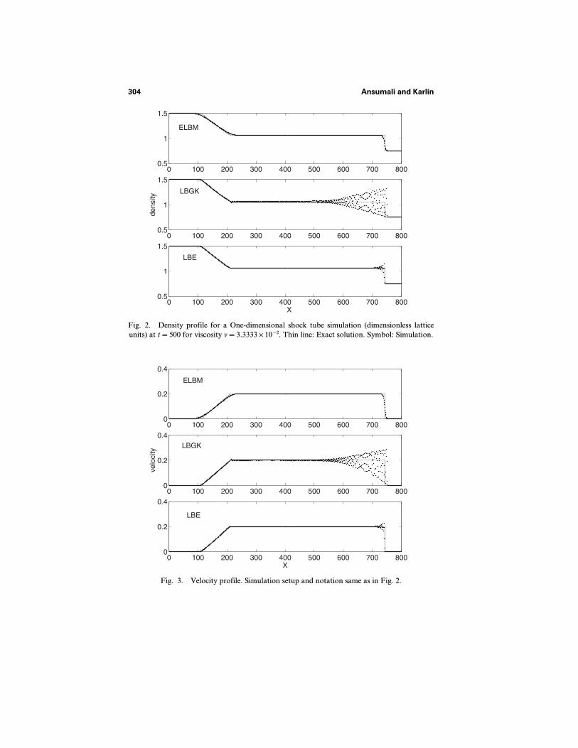
rare-faction front moving in the high density region. These two fronts leavean intermediate region in the central portion of the tube with uniformdensity rc, and uniform velocity uc. The tube is filled at time t=0 with agas at rest with uniform density r−(u−=0) for x < 0, and r+(u+=0) forx > 0. For the inviscid case, n=0, the density and the velocity profilespresent a discontinuity across the shock.

Simulations were performed in order to compare the stability of thethree LBM algorithms: The nonlinear LBM (16) (LBE hereafter), the LBGKmethod with the polynomial equilibrium ansatz, (3) and the present ELBMalgorithm.

At t=0 the lattice was populated as to give the density r−=1.5 for0 [ x [ 400, and r+=0.75 for 400 < x [ 800. Standard bounce backboundary conditions were applied at both ends of the tube. Results for thethree algorithms are demonstrated in Figs. 2 and 3 for a relatively highvalue of viscosity n=3.3333×10−2. It has been found that the LBGK andthe ELBM never showed divergence even when the viscosity was smallerthan n < 10−3. However, in contrast to the ELBM, the results of the LBGKdemonstrate large fluctuations already at n < 1. For this reason, results ofthe ELBM were always better in comparison to the LBGK at low viscosity.

8.2. Two-Dimensional Simulations

To compare the present algorithm with the standard LBGK method,we have chosen the setup of the two-dimensional Poiseuille flow. Stabilityof both the schemes has been investigated with respect to various pertur-bations. In the first set of experiments, non-hydrodynamic perturbationswere used, keeping mean velocity at each node intact. In particular, popu-lations at the different nodes were perturbed by a small amount in a waysimilar to that proposed in ref. 17 for fluctuating hydrodynamics. However,noise is switched on only at a fixed time t0, typically after the velocityprofile has been developed up to its steady state (parabolic) shape.

In another set of numerical experiments, the fully developed velocityprofile has been perturbed by adding a small amount of velocity uy at eachnode, at time t0, in a way consistent with the boundary conditions. Wehave tried two different perturbations, one which respect divergencefreedom of the incompressible fluid and the other one which do not respectthis condition. In particular, the following perturbations have been used(the origin of the coordinate system is at the central node at the inlet, thereduced x coordinate, −1 [ x [ 1 is taken across the channel):

d(ruy)=0.005uy max sin(wpy)

d(rux)=0(40)

Entropy Function Approach to the Lattice Boltzmann Method 303

0 100 200 300 400 500 600 700 8000.5

1

1.5

X

0 100 200 300 400 500 600 700 8000.5

1

1.5

dens

ity

0 100 200 300 400 500 600 700 8000.5

1

1.5

ELBM

LBGK

LBE

Fig. 2. Density profile for a One-dimensional shock tube simulation (dimensionless latticeunits) at t=500 for viscosity n=3.3333×10−2. Thin line: Exact solution. Symbol: Simulation.

0 100 200 300 400 500 600 700 8000

0.2

0.4

X

0 100 200 300 400 500 600 700 8000

0.2

0.4

velo

city

0 100 200 300 400 500 600 700 8000

0.2

0.4

ELBM

LBGK

LBE

Fig. 3. Velocity profile. Simulation setup and notation same as in Fig. 2.

304 Ansumali and Karlin

and,

d(ruy)=0.005uy max sin(wpy)

d(rux)=−0.005wpxuy max cos(wpy)(41)

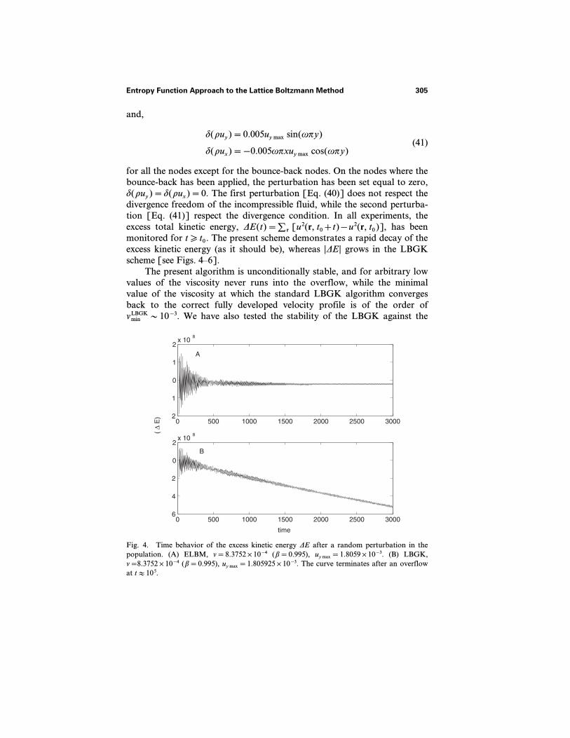
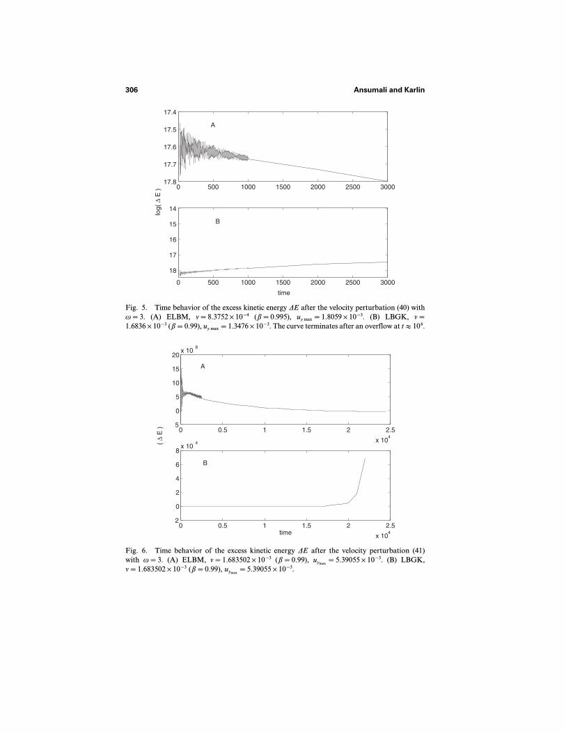
for all the nodes except for the bounce-back nodes. On the nodes where thebounce-back has been applied, the perturbation has been set equal to zero,d(ruy)=d(rux)=0. The first perturbation [Eq. (40)] does not respect thedivergence freedom of the incompressible fluid, while the second perturba-tion [Eq. (41)] respect the divergence condition. In all experiments, theexcess total kinetic energy, DE(t)=; r [u2(r, t0+t)−u2(r, t0)], has beenmonitored for t \ t0. The present scheme demonstrates a rapid decay of theexcess kinetic energy (as it should be), whereas |DE| grows in the LBGKscheme [see Figs. 4–6].

The present algorithm is unconditionally stable, and for arbitrary lowvalues of the viscosity never runs into the overflow, while the minimalvalue of the viscosity at which the standard LBGK algorithm convergesback to the correct fully developed velocity profile is of the order ofnLBGKmin ’ 10−3. We have also tested the stability of the LBGK against the

0 500 1000 1500 2000 2500 30006

4

2

0

2x 10

8

time

0 500 1000 1500 2000 2500 30002

1

0

1

2x 10

8

( ∆

E)

A

B

Fig. 4. Time behavior of the excess kinetic energy DE after a random perturbation in thepopulation. (A) ELBM, n=8.3752×10−4 (b=0.995), uy max=1.8059×10−3. (B) LBGK,n=8.3752×10−4 (b=0.995), uy max=1.805925×10−3. The curve terminates after an overflowat t % 105.

Entropy Function Approach to the Lattice Boltzmann Method 305

0 500 1000 1500 2000 2500 300017.8

17.7

17.6

17.5

17.4

log(

∆ E

)

0 500 1000 1500 2000 2500 3000

18

17

16

15

14

time

A

B

Fig. 5. Time behavior of the excess kinetic energy DE after the velocity perturbation (40) withw=3. (A) ELBM, n=8.3752×10−4 (b=0.995), uymax=1.8059×10−3. (B) LBGK, n=1.6836×10−3 (b=0.99), uymax=1.3476×10−3. The curve terminates after an overflow at t % 106.

0 0.5 1 1.5 2 2.5

x 104

2

0

2

4

6

8x 10

4

time

0 0.5 1 1.5 2 2.5

x 104

5

0

5

10

15

20x 10

8

( ∆

E )

A

B

Fig. 6. Time behavior of the excess kinetic energy DE after the velocity perturbation (41)with w=3. (A) ELBM, n=1.683502×10−3 (b=0.99), uymax

=5.39055×10−3. (B) LBGK,n=1.683502×10−3 (b=0.99), uymax

=5.39055×10−3.

306 Ansumali and Karlin

random perturbation by doubling the number of nodes in each direction.The stability of the LBGK has not improve by this increase in the systemsize.

9. CONCLUSION

We have demonstrated how the Lattice Boltzmann method can beequipped with the H-theorem to enhance its stability. We have shown thatfor realization of LBM an explicit knowledge of equilibrium distributionis not necessary, only the knowledge entropy function is sufficient to con-struct the algorithm. Further development of the Lattice Boltzmannmodeling can be based on the construction of the entropy function specificto the physical problem under consideration.

A few concluding remarks to compare the present work with the workof Boghosian et al. (9) are in order. First, the main goal of their work was togive a general description of the kinetic polytopes, whereas our focus is onthe implementation of the ELBM for a specific choice of the entropy func-tion which recovers the Navier–Stokes equation. Second, in the work (9)

solving numerically for the equilibrium distribution function at each timestep is proposed, while in the present work a new collision operator isproposed which circumvents the need for solving a set of non-linear equa-tions at each time step to get the equilibrium distribution function. Finallywe have introduced a solver for the entropy estimate which guaranteespositivity of the populations.

ACKNOWLEDGMENTS

We acknowledge stimulating discussions with L. S. Luo, H. C. Öttinger,S. Succi, and A. J. Wagner.

REFERENCES

1. Excellent reviews of the Lattice Boltzmann method can be found in:S. Chen and G. D.Doolen, Annu. Rev. Fluid Mech. 30:329 (1998); R. Benzi, S. Succi and M. Vergassola,Phys. Rep. 222:147 (1992); A. J. C. Ladd, J. Fluid Mech. 271:285 (1994); Y. H. Qian,J. Lebowitz, and S. Orszag, eds., Special issue on Lattice Gas, J. Stat. Phys. 81 (1995);Y. H. Qian, S. Succi and S. Orszag, Ann. Rev. Comp. Phys. 3:195 (1995).

2. H. Chen, S. Chen, and W. H. Matthaeus, Phys. Rev. A 45:R5339 (1992).3. Y. H. Qian, D. d’Humiéres, and P. Lallemand, Europhys. Lett. 17:479 (1992).4. I. V. Karlin, A. Ferrante, and H. C. Ottinger, Europhys. Lett. 47:182 (1999).5. S. Ansumali and I. V. Karlin, Phys. Rev. E 47:7999 (2000).6. F. J. Higuera, S. Succi, and R. Benzi, Europhys. Lett. 9:345 (1989).7. F. Toschi, G. Amati, S. Succi, R. Benzi, and R. Piva, Phys. Rev. Lett. 82:5044 (1999).

Entropy Function Approach to the Lattice Boltzmann Method 307

8. S. Ansumali and I. V. Karlin, manuscript (2000).9. B. M. Boghosian, J. Yepez, P. V. Coveney, and A. Wagner, Proc. Roy. Soc. Lond A MAT

457:717 (2001).10. I. V. Karlin, A. N. Gorban, S. Succi, and V. Boffi, Phys. Rev. Lett. 81:6 (1998).11. A. J. Wagner, Europhys. Lett. 44:144 (1998).12. S. Chapman and T. Cowling, The Mathematical Theory of Non-Uniform Gases

(Cambridge University Press, Cambridge, 1970).13. Constructive estimations of the state M for a generic kinetic equation are given in A. N.

Gorban, I. V. Karlin, V. B. Zmievskii, and T. Nonnenmacher, Physica A 231:648 (1996).14. A. N. Gorban, I. V. Karlin, and V. B. Zmievskii, Transport Theory Stat. Phys. 28:271

(1999).15. P. Lallemand and L.-S. Luo, Phys. Rev. E 61:6546 (2000).16. Y. H. Qian, D. d’Humières, and P. Lallemand, Adv. in Kinetic Theory and Continuum

Mechanics, R. Gatignol and Soubbaramayer, eds. (Springer, Berlin, 1991), p. 127.17. A. J. C. Ladd, J. Fluid Mech. 271:285 (1994).

308 Ansumali and Karlin