Entropy – A Guide for the Perplexed - Charlotte Werndlcharlottewerndl.net/Entropy_Guide.pdf · Entropy – A Guide for the Perplexed Roman Frigg and Charlotte Werndl∗ June 2010

Entropy – A Guide for the Perplexed

Roman Frigg and Charlotte Werndl∗

June 2010

Contents

1 Introduction 1

2 Entropy in Thermodynamics 2

3 Information Theory 4

4 Statistical Mechanics 9

5 Dynamical Systems Theory 18

6 Fractal Geometry 26

7 Conclusion 30

1 Introduction

Entropy is ubiquitous in physics, and it plays important roles in numerousother disciplines ranging from logic and statistics to biology and economics.However, a closer look reveals a complicated picture: entropy is defined differ-ently in different contexts, and even within the same domain different notionsof entropy are at work. Some of these are defined in terms of probabilities,others are not. The aim of this chapter is to arrive at an understanding ofsome of the most important notions of entropy and to clarify the relationsbetween them. In particular, we discuss the question what kind of prob-abilities are involved whenever entropy is defined in terms of probabilities:

∗The authors are listed alphabetically; the paper is fully collaborative. To contact theauthors write to [email protected] and [email protected].

1

are the probabilities chances (i.e., physical probabilities) or credences (i.e.,degrees of belief)?

After setting the stage by introducing the thermodynamic entropy (Sec-tion 2), we discuss notions of entropy in information theory (Section 3),statistical mechanics (Section 4), dynamical systems theory (Section 5) andfractal geometry (Section 6). Omissions are inevitable; in particular, spaceconstraints prevent us from discussing entropy in quantum mechanics andcosmology.1

2 Entropy in Thermodynamics

Entropy made its first appearance in the middle of the 19th century in thecontext of thermodynamics (TD). TD describes processes like the exchangeof heat between two bodies or the spreading of gases in terms of macroscopicvariables like temperature, pressure and volume. The centre piece of TD isthe so-called Second Law of TD, which, roughly speaking, restricts the classof physically allowable processes in isolated systems to those that are notentropy decreasing. In this section we introduce the TD entropy and theSecond Law.2 We keep this presentation short because the TD entropy isnot a probabilistic notion and therefore falls, strictly speaking, outside thescope of this book.

The thermodynamic state of a system is characterised by the values ofits thermodynamic variables; a state is an equilibrium state if, and only if(iff), all variables have well-defined and constant values. For instance, thestate of a gas is specified by the values of temperature, pressure and volume,and the gas is in equilibrium if these have well-defined values which do notchange over time. Consider two states A and B. A process that changesthe state of the system from A to B is quasistatic iff it only passes throughequilibrium states (i.e., if all intermediate states between A and B are alsoequilibrium states). A process is reversible iff it can be exactly reversed byan infinitesimal change in the external conditions. If we consider a cyclicalprocess – a process in which the beginning and the end state are the same –a reversible process leaves the system and its surroundings unchanged.

The Second Law (in Kelvin’s formulation) says that it is impossible todevise an engine which, working in a cycle, produces no effect other than theextraction of heat from a reservoir and the performance of an equal amount

1Hemmo & Shenker (2006) and Sorkin (2005) provide good introductions to quantumand cosmological entropies, respectively.

2Our presentation follows Pippard (1966, pp. 19-23, 29-37). There are also manydifferent (and non-equivalent) formulations of the Second Law (see Uffink 2001).

2

of mechanical work. It can be shown that this formulation implies that∮dQ

T≤ 0, (1)

where dQ is the amount of heat put into the system and T the system’stemperature. This is known as Clausius’ Inequality. If the cycle is reversible,then the inequality becomes an equality. Trivially, this implies that for re-versible cycles ∫ B

A

dQ

T= −

∫ A

B

dQ

T(2)

for any paths from A to B and from B to A, and the value of the integralsonly depends on the beginning and the end point.

We are now in a position to introduce the thermodynamic entropy STD

.The leading idea is that the integral in euqation (2) gives the entropy dif-ference between A and B. We can then assign an absolute entropy value toevery state of the system by choosing one particular state (we can chooseany state we please!) as the reference point, choosing a value for its entropyS

TD(A), and then define the entropy of all other points by

STD

(B) := STD

(A) +

∫ B

A

dQ

T, (3)

where the change of state from A to B is reversible.What follows from these considerations about irreversible changes? Con-

sider the following scenario: we first change the state of the system from Ato B on a quasi-static irreversible path, and then go back from B to A on aquasi-static reversible path. It follows from equations (1) and (3) that

STD

(B)− STD

(A) ≤∫ B

A

dQ

T. (4)

If we now restrict attention to adiathermal processes (i.e., ones in whichtemperature is constant), the integral in euqation (4) becomes zero and wehave

STD

(B) ≥ STD

(A). (5)

This is often referred to as the Second Law, but it is important to point outthat it is only a special version of it which holds for adiathermal processes.

STD

has no intuitive interpretation as a measure of disorder, disorganisa-tion or randomness (as often claimed). In fact such considerations have noplace in TD.

We now turn to a discussion of the information theoretic entropy, which,unlike the S

TDis a probabilistic concept. At first sight the information

3

theoretic and the thermodynamic entropy have noting to do with each other.This impression will be dissolved in Section 4 when a connection is establishedvia the Gibbs entropy.

3 Information Theory

Consider the following situation (Shannon 1949). There is a source S produc-ing messages which are communicated to a receiver R. The receiver registersthem, for instance, on a paper tape.3 The messages are discrete and sent bythe source one after the other. Let m = m1, ...,mn be a complete set ofmessages (in the sense that the source cannot send messages other than themi). The production of one message is referred to as a step.

When receiving a message, we gain information, and depending on themessage, more or less information. According to Shannon’s theory, informa-tion and uncertainty are two sides of the same coin: the more uncertaintythere is, the more information we gain by removing the uncertainty.

Shannon’s basic idea was to characterise the amount of information gainedfrom the receipt of a message as a function which depends only on how likelythe messages are. Formally, for n ∈ N let Vm be the set of all probabilitydistributions P = (p1, . . . , pn) := (p(m1), . . . , p(mn)) on m1, . . . ,mn (i.e.,pi ≥ 0 and p1 + . . . + pn = 1). A reasonable measure of information is afunction SS, d(P ) : Vm → R which satisfies the following axioms (cf. Klir 2006,section 3.2.2):

1. Continuity. SS, d(p1, . . . , pn) is continuous in all its argumentsp1, . . . , pn.

2. Additivity. The information gained of two independent experiments isthe sum of the information of the experiments, i.e., for P = (p1, . . . , pn)and Q = (q1, . . . , qk), SS, d(p1q1, p1q2, . . . , pnqk) = SS, d(P ) + SS, d(Q).

3. Monotonicity. For uniform distributions the information increases withn. That is, for any P = ( 1

n, . . . , 1

n) and Q = ( 1

k, . . . , 1

k), for arbitrary

k, n ∈ N we have: if k > n, then SS, d(Q) > SS, d(P ).

4. Branching. The measure of information is independent of how theprocess is divided into parts. That is, for (p1, . . . , pn), n ≥ 3, di-vide m = m1, . . . ,mn into two blocks A = (m1, . . . ,ms) and

3We assume that the channel is noiseless and deterministic, meaning that there is aone-to-one correspondence between the input and the output.

4

B = (ms+1, . . . ,mn), and let pA =∑s

i=1 pi and pB =∑n

i=s+1 pi. Then

SS, d(p1, ..., pn) = SS, d(pA, pB)+pASS, d(p1

pA

, ...,ps

pA

)+pBSS, d(ps+1

pB

, ...,pn

pB

).4

(7)

5. Bit normalisation. By convention, the average information gained fortwo equally likely messages is one bit (‘binary digit’): SS, d(1/2, 1/2) =1.

There is exactly one function satisfying these axioms, the discrete ShannonEntropy :5

SS, d(P ) := −n∑

i=1

pi log[pi], (8)

where ‘log’ stands for the logarithm to the basis of two.6 Any change towardequalization of p1, . . . , pn leads to an increase of SS, d, which reaches its max-imum, log[n], for p1 = ... = pn = 1/n. Furthermore, SS, d(P ) = 0 iff all pi

but one equal zero.What kind of probabilities are invoked in Shannon’s scenario? Ap-

proaches to probability can be divided into two broad groups.7 First, epis-temic approaches take probabilities to be measures for degrees of belief.Those who subscribe to an objective epistemic theory take probabilities tobe degrees of rational belief, whereby ‘rational’ is understood to imply thatgiven the same evidence, all rational agents have the same degree of beliefin any proposition. This is denied by those who hold a subjective epistemictheory, regarding probabilities as subjective degrees of belief that can differbetween persons even if they are presented with the same body of evidence.Second, ontic approaches take probabilities to be part of the ‘furniture ofthe world’. The two most prominent ontic approaches are frequentism anda propensity view. On the frequentist approach, probabilities are long runfrequencies of certain events. On the propensity theory, probabilities aretendencies or dispositions inherent in objects or situations.

4For instance, for m1,m2,m3, P = (1/3, 1/3, 1/3), A = m1,m2 and B = m3branching means that

SS, d(1/3, 1/3, 1/3) = SS, d(2/3, 1/3) + 2/3 SS, d(1/2, 1/2) + 1/3 SS, d(1). (7)

5There are other axioms that uniquely characterise the Shannon entropy (cf. Klir 2006,section 3.2.2).

6We set x log[x] := 0 for x = 0.7For a discussion of the different interpretations of probability see, for instance, Howson

(1995), Gillies (2000) and Mellor (2005).

5

The emphasis in information theory is on the receiver’s amount of un-certainty about the next incoming message. This suggests that the p(mi)should be interpreted as epistemic probabilities (credences). While correctas a first stab, a more nuanced picture emerges once we ask the questionof how the values of the p(mi) are set. Depending on how we understandthe nature of the source, we obtain two very different answers. If the sourceitself is not probabilistic, then the p(mi) express the beliefs – and nothingbut the beliefs – of receivers. For proponents of subjective probabilities theseprobabilities express the individual beliefs of an agent, and beliefs may varybetween different receivers. Objectivist insists that all rational agents mustcome to the same value assignment. This can be achieved, for instance, byrequiring that SS, d(P ) be maximal, which singles out a unique distribution.This method, now known as Jaynes’ maximum entropy principle, plays a rolein statistical mechanics and will be discussed later.

Alternatively, the source source itself can be probabilistic. The proba-bilities associated with the source have to be ontic probabilities of one kindor other (frequencies, propensities, etc.). In this case agents are advisedto use the so-called Principal Principle – roughly the rule that a rationalagent’s credence for a certain event to occur should be set equal to the ob-jective probability (chance) of that event to occur.8 In Shannon’s setting thismeans that the p(mi) have to be equal to the source’s objective probability ofproducing the message mi. If this connection is established, the informationtransmitted in a channel is a measure of an objective property of a source.

It is worth emphasising that SS, d(P ) is a technical conception of infor-mation which should not be taken as an analysis of the various senses ‘in-formation’ has in ordinary discourse. In ordinary discourse information isoften equated with knowledge, propositional content, or meaning. Hence ‘in-formation’ is a property of a single message. Information as understood ininformation theory is not concerned with individual messages and their con-tent; its focus is on all messages a source could possibly send. What makesa single message informative is not its meaning but the fact that it has beenselected from a set of possible messages.

Given the probability distributions Pm = (pm1 , . . . , pmn) on m1, . . . ,mn,Ps = (ps1 , . . . , psl

) on s1, . . . , sl, and the joint probability distribution(pm1,s1 , pm1,s2 . . . , pmn,sl

)9 on m1s1, m1s2, . . . ,mnsl, the conditional Shan-

8The Principal Principle has been introduced by Lewis (1980); for a recent discussionsee Frigg and Hoefer (2010).

9The outcomes mi and sj are not assumed to be independent.

6

non entropy is defined as

SS, d(Pm |Ps) :=l∑

j=1

psj

n∑k=1

pmk,sj

psj

log[pmk,sj

psj

]. (9)

It measures the average information received from a message mk given thata message sj has been received before.

The Shannon entropy can be generalised to the continuous case. Let p(x) bea probability density. The continuous Shannon entropy is

SS, c(p) = −∫

Rp(x) log[p(x)]dx (10)

if the integral exists. The generalisation of (10) to densities of n variablesx1, ..., xn is straightforward. If p(x) is positive, except for a set of Lebesguemeasure zero, exactly on the interval [a, b], a, b ∈ R, then SS, c reaches itsmaximum, log[b − a], for p(x) = 1/(b − a) in [a, b] and zero elsewhere. In-tuitively every change towards equalisation of p(x) leads to an increase inentropy. For probability densities which are, except for a set of measure zero,positive everywhere on R, the question of the maximum is more involved. Ifthe standard deviation is held fixed at value σ, SS, c reaches its maximumfor a Gaussian p(x) = (1/

√2πσ) exp(−x2/2σ2), and the maximum value of

the entropy is log[√

2πeσ] (Ihara 1993, section 3.1; Shannon & Weaver 1949,pp. 88–89).

There is an important difference between the discrete and continuousShannon entropy. In the discrete case, the value of the Shannon entropy isuniquely determined by the probability measure over the messages. In thecontinuous case the value depends on the coordinates we choose to describethe messages. Hence the continuous Shannon entropy cannot be regarded asmeasuring information, since an information measure should not depend onthe way in which we describe a situation. But usually we are interested in en-tropy differences rather than in absolute values, and it turns out that entropydifferences are coordinate independent and the continuous Shannon entropycan be used to measure differences in information (Ihara 1993, pp. 18–20;Shannon & Weaver 1949, pp. 90–91).10

We now turn to two other notions of information-theoretic entropy,namely Hartley’s entropy and Renyi’s entropy. The former preceded Shan-non’s entropy; the latter is a generalization of Shannon’s entropy. One of

10This coordinate dependence reflects a deeper problem: the uncertainty reduced byreceiving a message of a continuous distribution is infinite and hence not measured by SS, c.Yet by approximating a continuous distribution by discrete distributions, one obtains thatSS, c measures differences in information (Ihara 1993, p. 17).

7

the first account of information was introduced by Hartley (1928). Assumethat m := m1, . . . ,mn, n ∈ N, represents mutually exclusive possible al-ternatives and that one of the alternatives is true but we do not know whichone. How can we measure the amount of information gained when know-ing which of these n alternatives is true, or, equivalently, the uncertaintyassociated with these n possibilities? Hartley postulated that any functionSH : N → R+ answering this question has to satisfy the following axioms:

1. Monotonicity. The uncertainty increases with n: SH(n) ≤ SH(n + 1)for all n ∈ N.

2. Branching. The measure of information is independent of how theprocess is divided into parts: SH(n.m) = SH(n)SH(m), where ‘n.m’means that there are n times m alternatives.

3. Normalization. Per convention, SH(2) = 1.

Again, there is exactly one function satisfying these axioms, namelySH(n) = log[n] (Klir 2006, p. 26), which is now referred to as the Hart-ley entropy.

On the face of it this entropy is based solely on the concept of mutu-ally exclusive alternatives, and it does not invoke probabilistic assumptions.However, views diverge on whether this is the full story. Those who deny thisargue that the Hartley entropy implicitly assumes that all alternatives haveequal weight. This amounts to assuming that they have equal probability,and hence the Hartley entropy is the special case of the Shannon entropy,namely the Shannon entropy for the uniform distribution. Those who denythis argue that Hartley’s notion of alternatives does not presuppose prob-abilistic concepts and is therefore independent of Shannon’s (cf. Klir 2006,pp. 25–30).

The Renyi entropies generalise the Shannon entropy. As with theShannon entropy, assume a probability distribution P = (p1, ..., pn) overm = m1, ...,mn. Require of a measure of information that it satisfies allthe axioms of the Shannon entropy except for branching. Unlike the otheraxioms, it is unclear whether a measure of information should satisfy branch-ing and hence whether it should be on the list of axioms (Renyi 1961). If theoutcomes of two independent events with respective probabilities p and q areobserved, we want the total received information to be the sum of the twopartial informations. This implies that the amount of information receivedfor message mi is − log[pi] (Jizba & Arimitsu 2004). If a weighted arithmeticmean is taken over the − log[pi], we obtain the Shannon entropy. Now, is itpossible to take another mean such that the remaining axioms about infor-mation are satisfied? If yes, these quantities are also possible measures of the

8

average information received. The general definition of a mean over − log[pi]weighted by pi is that it is of the form f−1(

∑ni=1 pif(− log[pi])) where f is

a continuous, strictly monotonic and invertible function. For f(x) = x weobtain the Shannon entropy. There is only one alternative mean satisfyingthe axioms, namely f(x) = 2(1−q)x, q ∈ (0,∞), q 6= 1. It corresponds to theRenyi entropy of order q:

SR, q(P ) :=1

1− qlog[

n∑k=1

pqk]. (11)

The limit of the Renyi entropy for q → 1 gives the Shannon entropy, i.e.,limq→1 SR, q(P ) =

∑nk=1−pk log[pk] (Jizba & Arimitsu 2004; Renyi 1961),

and for this reason one sets SR, 1(P ) :=∑n

k=1−pk log[pk].

4 Statistical Mechanics

Statistical mechanics (SM) aims to explain the behaviour of macroscopicsystems in terms of the dynamical laws governing their microscopic con-stituents.11 One of the central concerns of SM is to provide a micro-dynamicalexplanation of the Second Law of TD. The strategy to achieve this goal isto first introduce a mechanical notion of entropy, then to argue that it is insome sense equivalent to the TD entropy, and finally to show that it tends toincrease if its initial value is low. There are two non-equivalent frameworksin SM, one associated with Boltzmann and one with Gibbs. In this sectionwe discuss the various notions of entropy introduced within these frameworksand briefly indicate how they have been used to justify the Second Law.

SM deals with systems consisting of a large number of micro constituents.A typical example for such a system is a gas, which is made up of a largenumber n of particles of mass m confined to a vessel of volume V . And inthis chapter we restrict attention to gases. Furthermore we assume that thesystem is isolated from its environment and hence that its total energy E isconserved. The behaviour of such systems is usually modeled by continuousmeasure-preserving dynamical systems. We discuss such systems in detail inthe next section; for the time being it suffices to say that the phase spaceof the system is 6n-dimensional, having three position and three momentumcoordinates for every particle. This space is called the system’s γ-space Xγ.xγ denotes a vector in Xγ, and the xγ are called microstates. Xγ is a directproduct of n copies of the 6-dimensional phase space of one particle, called

11For an extended discussion of SM, see Frigg (2008), Sklar (1993) and Uffink (2006).

9

the particle’s µ-space Xµ.12 In what follows xµ = (x, y, z, px, py, pz) denotesa vector in Xµ; moreover, we use ~r = (x, y, z) and ~p = (px, py, pz).

13

In a seminal paper published in 1872 Boltzmann set out to show that theSecond Law of TD is a consequence of the collisions between the particles ofa gas. The distribution f(xµ, t) specifies the fraction of particles in the gaswhose position and momentum lies in the infinitesimal interval (xµ, xµ+dxµ)at time t. In 1860 Maxwell showed that for a gas of identical and non-interacting particles in equilibrium the distribution had to be what is nowcalled the Maxwell-Boltzmann distribution:

f(xµ, t) =χ

V(~r) (2πmkT )−3/2

‖V ‖exp

(− ~p 2

2mkT

), (12)

where k is Boltzmann’s constant, T the temperature of the gas, ‖V ‖ is thevolume of the vessel, and χ

V(~r) the characteristic function of volume V (it

is 1 if ~r ∈ V and 0 otherwise).The state of a gas at time t is fully specified by a distribution f(xµ, t), and

the dynamics of the gas can be studied by considering how this distributionevolves over time. To this end Boltzmann introduced the quantity

HB(f) :=

∫Xµ

f(xµ, t) log[f(xµ, t)] dxµ (13)

and set out to prove on the basis of mechanical assumptions about the col-lisions of gas molecules that HB(f) must decrease monotonically over thecourse of time and that it reaches its minimum at equilibrium where f(xµ, t)becomes the Maxwell-Boltzmann distribution. This result, which is derivedusing the Boltzmann equation, is known as the H-theorem and is generallyregarded as problematic.14

The problems of the H-theorem are not our concern. What matters isthat the fine-grained Boltzmann entropy SB, f (also continuous Boltzmannentropy) is proportional to HB(f):

SB, f (f) := − k n HB(f). (14)

Therefore, if the H-theorem were true, it would establish that the Boltzmannentropy increased monotonically and reached a maximum once the system’s

12This terminology has been introduced by Ehrenfest & Ehrenfest (1912) and has beenused since. The subscript ‘µ’ here stands for ‘molecule’ and has nothing to do with ameasure.

13We use momentum rather than velocity since this facilitates the discussion of theconnection of Boltzmann entropies with other entropies. One could also use the velocity~v = ~p/m.

14See Emch & Liu (2002, pp. 92–105) and Uffink (2006, pp. 962–974).

10

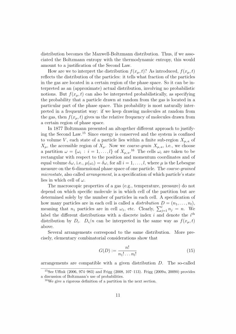
distribution becomes the Maxwell-Boltzmann distribution. Thus, if we asso-ciated the Boltzmann entropy with the thermodynamic entropy, this wouldamount to a justification of the Second Law.

How are we to interpret the distribution f(xµ, t)? As introduced, f(xµ, t)reflects the distribution of the particles: it tells what fraction of the particlesin the gas are located in a certain region of the phase space. So it can be in-terpreted as an (approximate) actual distribution, involving no probabilisticnotions. But f(xµ, t) can also be interpreted probabilistically, as specifyingthe probability that a particle drawn at random from the gas is located in aparticular part of the phase space. This probability is most naturally inter-preted in a frequentist way: if we keep drawing molecules at random fromthe gas, then f(xµ, t) gives us the relative frequency of molecules drawn froma certain region of phase space.

In 1877 Boltzmann presented an altogether different approach to justify-ing the Second Law.15 Since energy is conserved and the system is confinedto volume V , each state of a particle lies within a finite sub-region Xµ, a ofXµ, the accessible region of Xµ. Now we coarse-grain Xµ, a, i.e., we choosea partition ω = ωi : i = 1, . . . , l of Xµ, a.

16 The cells ωi are taken to berectangular with respect to the position and momentum coordinates and ofequal volume δω, i.e., µ(ωi) = δω, for all i = 1, . . . , l, where µ is the Lebesguemeasure on the 6-dimensional phase space of one particle. The coarse-grainedmicrostate, also called arrangement, is a specification of which particle’s statelies in which cell of ω.

The macroscopic properties of a gas (e.g., temperature, pressure) do notdepend on which specific molecule is in which cell of the partition but aredetermined solely by the number of particles in each cell. A specification ofhow many particles are in each cell is called a distribution D = (n1, . . . , nl),meaning that n1 particles are in cell ω1, etc. Clearly,

∑lj=1 nj = n. We

label the different distributions with a discrete index i and denote the ith

distribution by Di. Di/n can be interpreted in the same way as f(xµ, t)above.

Several arrangements correspond to the same distribution. More pre-cisely, elementary combinatorial considerations show that

G(D) :=n!

n1! . . . nl!(15)

arrangements are compatible with a given distribution D. The so-called

15See Uffink (2006, 974–983) and Frigg (2008, 107–113). Frigg (2009a, 2009b) providesa discussion of Boltzmann’s use of probabilities.

16We give a rigorous definition of a partition in the next section.

11

coarse-grained Boltzmann entropy (also combinatorial entropy) is defined as:

SB, ω(D) := k log[G(D)]. (16)

Since G(D) is the number of arrangements compatible with a given distri-bution and the logarithm is a monotonic function, SB, ω(D) is a measure forthe number of arrangements that are compatible with a given distribution:the greater SB, ω(D), the more arrangements are compatible with a givendistribution. Hence SB, ω(D) is a measure of how much we can infer aboutthe arrangement of a system on the basis of its distribution. The higherSB, ω(D), the less information a distribution confers about the arrangementof the system.

Boltzmann then postulated that the distribution with the highest entropywas the equilibrium distribution, and that systems had a natural tendencyto evolve from states of low to states of high entropy. However, as latercommentators, most notably Ehrenfest & Ehrenfest (1912), pointed out, forthe latter to happen further dynamical assumptions (e.g., ergodicity) areneeded. If such assumptions are in place, the ni evolve so that SB, ω(D)increases and then stays close to its maximum value most of the time (Lavis2004, 2008).

There is a third notion of entropy in the Boltzmannian framework, andthis notion is preferred by contemporary Boltzmannians.17 We now considerXγ rather than Xµ. Since there are constraints on the system, its state willlie within a finite sub-region Xγ, a of Xγ, the accessible region of Xγ.

18

If the gas is regarded as a macroscopic object rather than as a collectionof molecules, its state can be characterised by a small number of macro-scopic variables such as temperature, pressure and density. These values arethen usually coarse-grained so that all values falling into a certain range areregarded as belonging to the same macrostate. Hence the system can bedescribed as being in one of a finite number of macrostates Mi, i = 1, . . . ,m.The set of Mi is complete in that at any given time t the system must be inexactly one Mi. It is a basic posit of the Boltzmann approach that a system’smacrostate supervenes on its fine-grained microstate, meaning that a changein the macrostate must be accompanied by a change in the fine-grained mi-crostate. Therefore, to every given microstate xγ there corresponds exactly

17See, for instance, Goldstein (2001) and Lebowitz (1999).18These constrains include conservation of energy. Therefore, Γγ, a is (6n − 1)-

dimensional. This causes complications because the measure µ needs to be restricted tothe (6n− 1)-dimensional energy hypersurface and the definitions of macroregions becomemore complicated. In order to keep things simple, we assume that Γγ, a is 6n-dimensional.For the (6n-1)-dimensional case, see Frigg (2008, pp. 107–114).

12

one macrostate M(xγ). But many different microstates can correspond tothe same macrostate. We therefore define

XMi:= xγ ∈ Xγ, a |Mi = M(xγ) , i = 1, ...,m, (17)

which is the subset of Xγ, a consisting of all microstates that correspond tomacrostate Mi. The XMi

are called macroregions. Clearly, they form apartition of Xγ, a.

The Boltzmann entropy of a macrostate M is19

SB, m(M) := k log[µ(XM)]. (18)

Hence SB, m(M) measures the portion of the system’s γ-space that is taken upby microstates that correspond to M . Consequently, SB, m(M) measures howmuch we can infer about where in γ-space the system’s microstate lies: thehigher SB, m(M), the larger the portion of the γ-space in which the system’smicrostate could be.

Given this notion of entropy, the leading idea is to argue that the dy-namics of systems is such that SB, m increases. Most contemporary Boltz-mannians aim to achieve this by arguing that entropy increasing behaviour istypical ; see, for instance, Goldstein (2001). These arguments are the subjectof ongoing controversy (see Frigg 2009a, 2009b).

We now turn to a discussion of the interrelationships between the variousentropy notions introduced so far. Let us begin with SB, ω and SB, m. SB, ω

is a function of a distribution over a partition of Xµ, a, while SB, m takes cellsof a partition of Xγ, a as arguments. The crucial point to realise is that eachdistribution corresponds to a well-defined region of Xγ, a: the choice of apartition of Xµ, a induces a partition of Xγ, a (because Xγ is the Cartesianproduct of n copies of Xµ). Hence any Di uniquely determines a region XDi

so that all states xγ ∈ XDihave distribution Di:

XDi:= xγ ∈ Xγ |D(xγ) = Di, (19)

where D(xγ) is the distribution of state xγ. Because all cells have measureδω, equations (15) and (19) imply:

µ(XDi) = G(Di) (δω)n. (20)

Given this, the question of the relation between SB, ω and SB, m comesdown to the question of how the XDi

and the XMirelate. Since there are

no standard procedures to construct the XMi, one can use the above con-

siderations about how distributions determine regions to construct the XMi,

19See, e.g., Goldstein (2001, p. 43) and Lebowitz (1999, p. 348).

13

making XDi= XMi

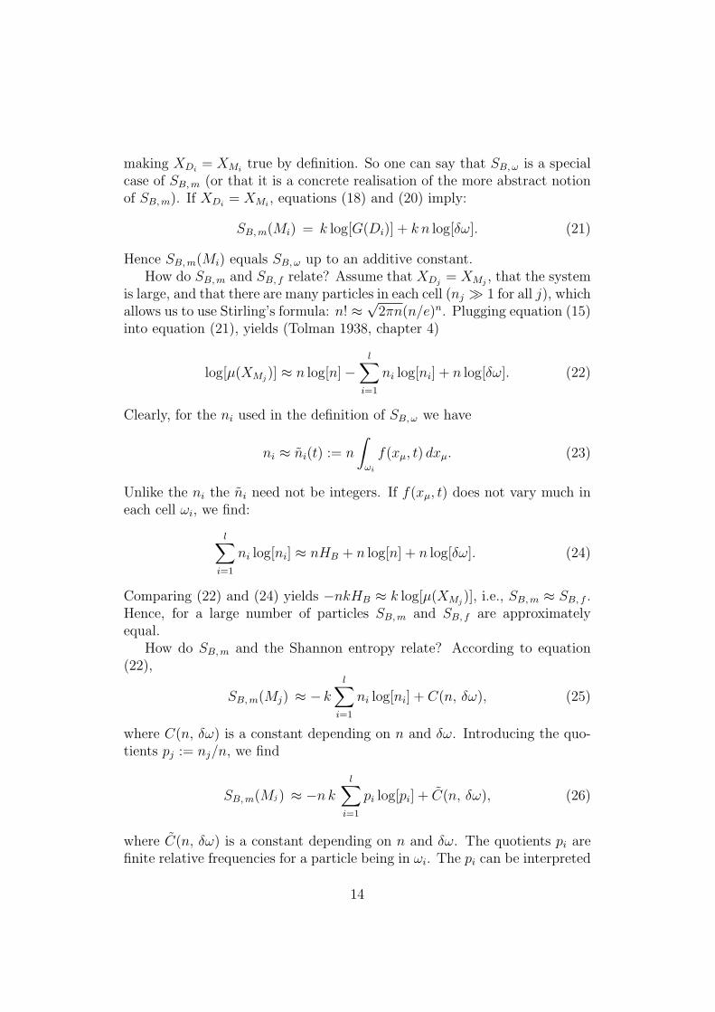
true by definition. So one can say that SB, ω is a specialcase of SB, m (or that it is a concrete realisation of the more abstract notionof SB, m). If XDi

= XMi, equations (18) and (20) imply:

SB, m(Mi) = k log[G(Di)] + k n log[δω]. (21)

Hence SB, m(Mi) equals SB, ω up to an additive constant.How do SB, m and SB, f relate? Assume that XDj

= XMj, that the system

is large, and that there are many particles in each cell (nj 1 for all j), whichallows us to use Stirling’s formula: n! ≈

√2πn(n/e)n. Plugging equation (15)

into equation (21), yields (Tolman 1938, chapter 4)

log[µ(XMj)] ≈ n log[n]−

l∑i=1

ni log[ni] + n log[δω]. (22)

Clearly, for the ni used in the definition of SB, ω we have

ni ≈ ni(t) := n

∫ωi

f(xµ, t) dxµ. (23)

Unlike the ni the ni need not be integers. If f(xµ, t) does not vary much ineach cell ωi, we find:

l∑i=1

ni log[ni] ≈ nHB + n log[n] + n log[δω]. (24)

Comparing (22) and (24) yields −nkHB ≈ k log[µ(XMj)], i.e., SB, m ≈ SB, f .

Hence, for a large number of particles SB, m and SB, f are approximatelyequal.

How do SB, m and the Shannon entropy relate? According to equation(22),

SB, m(Mj) ≈ − kl∑

i=1

ni log[ni] + C(n, δω), (25)

where C(n, δω) is a constant depending on n and δω. Introducing the quo-tients pj := nj/n, we find

SB, m(Mj) ≈ −n k

l∑i=1

pi log[pi] + C(n, δω), (26)

where C(n, δω) is a constant depending on n and δω. The quotients pi arefinite relative frequencies for a particle being in ωi. The pi can be interpreted

14

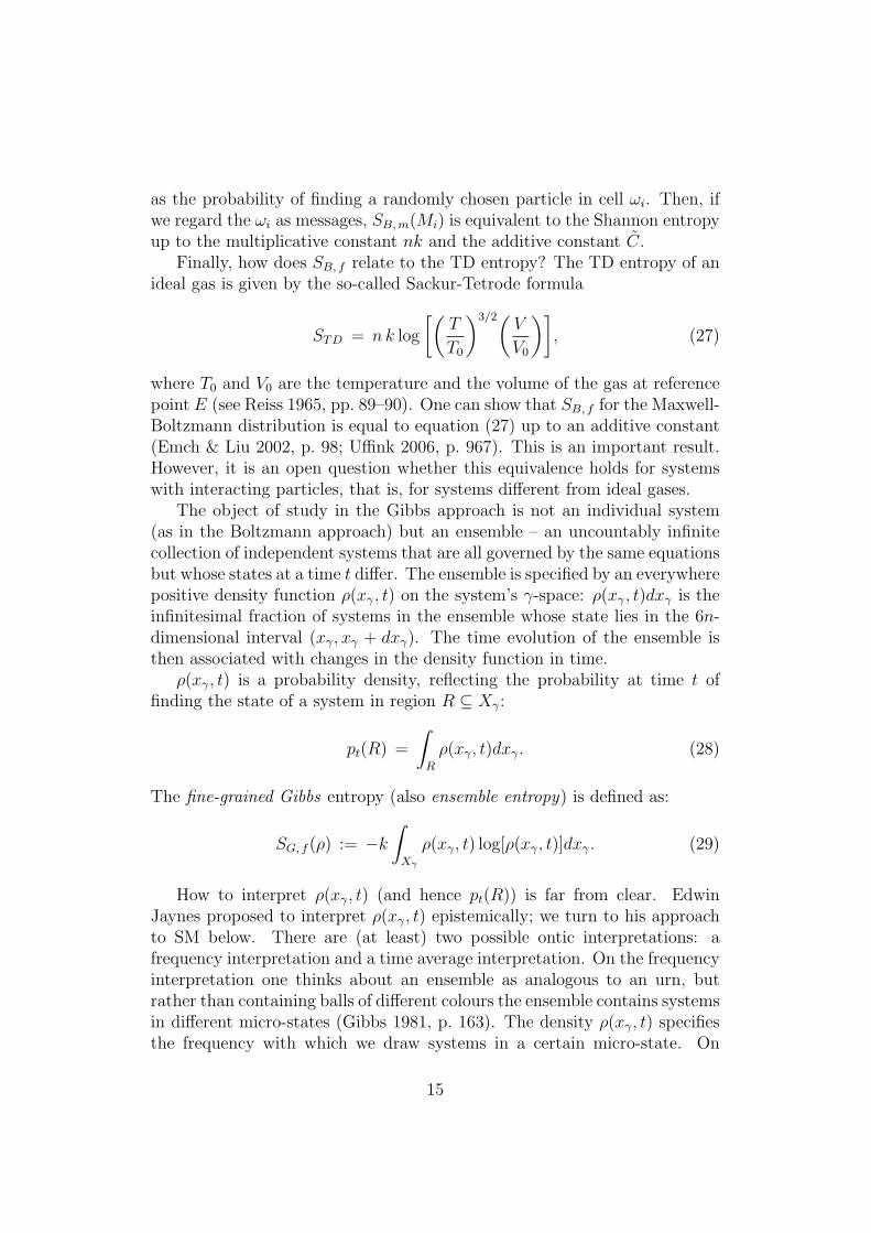
as the probability of finding a randomly chosen particle in cell ωi. Then, ifwe regard the ωi as messages, SB, m(Mi) is equivalent to the Shannon entropyup to the multiplicative constant nk and the additive constant C.

Finally, how does SB, f relate to the TD entropy? The TD entropy of anideal gas is given by the so-called Sackur-Tetrode formula

STD = n k log

[(T

T0

)3/2(V

V0

)], (27)

where T0 and V0 are the temperature and the volume of the gas at referencepoint E (see Reiss 1965, pp. 89–90). One can show that SB, f for the Maxwell-Boltzmann distribution is equal to equation (27) up to an additive constant(Emch & Liu 2002, p. 98; Uffink 2006, p. 967). This is an important result.However, it is an open question whether this equivalence holds for systemswith interacting particles, that is, for systems different from ideal gases.

The object of study in the Gibbs approach is not an individual system(as in the Boltzmann approach) but an ensemble – an uncountably infinitecollection of independent systems that are all governed by the same equationsbut whose states at a time t differ. The ensemble is specified by an everywherepositive density function ρ(xγ, t) on the system’s γ-space: ρ(xγ, t)dxγ is theinfinitesimal fraction of systems in the ensemble whose state lies in the 6n-dimensional interval (xγ, xγ + dxγ). The time evolution of the ensemble isthen associated with changes in the density function in time.

ρ(xγ, t) is a probability density, reflecting the probability at time t offinding the state of a system in region R ⊆ Xγ:

pt(R) =

∫R

ρ(xγ, t)dxγ. (28)

The fine-grained Gibbs entropy (also ensemble entropy) is defined as:

SG, f (ρ) := −k

∫Xγ

ρ(xγ, t) log[ρ(xγ, t)]dxγ. (29)

How to interpret ρ(xγ, t) (and hence pt(R)) is far from clear. EdwinJaynes proposed to interpret ρ(xγ, t) epistemically; we turn to his approachto SM below. There are (at least) two possible ontic interpretations: afrequency interpretation and a time average interpretation. On the frequencyinterpretation one thinks about an ensemble as analogous to an urn, butrather than containing balls of different colours the ensemble contains systemsin different micro-states (Gibbs 1981, p. 163). The density ρ(xγ, t) specifiesthe frequency with which we draw systems in a certain micro-state. On

15

the time average interpretation, ρ(xγ, t) reflects the fraction of time that thesystem would spend, in the long run, in a certain region of the phase space if itwas left to its own. Although plausible at first blush, both interpretations faceserious difficulties and it is unclear whether these can be met (see Frigg 2008,pp. 153–155).

If we regard SG, f (ρ) as equivalent to the TD entropy (which is com-mon), then SG, f (ρ) is expected to increase over time (during an irreversibleadiathermal process) and assumes a maximum in equilibrium. However, sys-tems in SM are Hamiltonian, and it is a consequence of an important theoremof Hamiltonian mechanics, Liouville’s theorem, that SG, f is a constant of mo-tion: dSG, f/dt = 0. So SG, f remains constant, and hence the approach toequilibrium cannot be described in terms of an increase in SG, f .

The standard way to solve this problem is to consider the coarse-grainedGibbs entropy instead. This solution has been suggested by Gibbs (1981,chapter 12) and has since been endorsed by many (e.g., Penrose 1970). Con-sider a partition ω of Xγ where the cells ωi are of equal volume δω. Thecoarse-grained density ρ(xγ, t) is defined as the density that is uniform withineach cell, taking as its value the average value in this cell:

ρω(xγ, t) :=1

δω

∫ω(xγ)

ρ(x′γ, t)dx′γ, (30)

where ω(xγ) is the cell in which xγ lies. We can now define the coarse-grainedGibbs entropy :

SG, ω(ρ) := SG, f (ρω) = −k

∫Xγ

ρω log[ρω]dxγ. (31)

One can prove that SG, ω ≥ SG, f ; the equality holds iff the fine graineddistribution is uniform over the cells of the coarse-graining (see Lavis 2004,p. 229; Wehrl 1978, p. 672). The coarse-grained density ρω is not subject toLiouville’s theorem and is not a constant of motion. So ρω could, in principle,increase over time.20

How do the two Gibbs entropies relate to the other notions of entropy in-troduced so far? The most straightforward connection is between the Gibbsentropy and the continuous Shannon entropy, which differ only by the mul-tiplicative constant k. This realisation provides a starting point for Jaynes’s(1983) information-based interpretation of SM, at the heart of which lies aradical reconceptualisation of SM. On his view, SM is about our knowledgeof the world, not about the world. The probability distribution represents

20There is a thorny issue under which conditions the coarse-grained entropy actuallyincreases (see Lavis 2004).

16

our state of knowledge about the system and not some matter of fact aboutthe system: ρ(xγ, t) represents our lack of knowledge about a micro-state ofa system given its macro condition and entropy is a measure of how muchknowledge we lack.

Jaynes then postulated that to make predictions we should always usethe distribution that maximises uncertainty under the given macroscopicconstraints. This means that we are asked to find the distribution for whichthe the Gibbs entropy is maximal, and then use this distribution to calcu-late expectation values of the variables of interest. This prescription is nowknow as Jaynes’ Maximum Entropy Principle. Jaynes could show that thisprinciple recovers the standard SM distributions (e.g., the microcanonicaldistribution for isolated systems).

The idea behind this principle is that we should always choose the dis-tribution that is maximally non-committal with respect to the missing infor-mation because by not doing so we would make assertions for which we haveno evidence. Although intuitive at first blush, the maximum entropy princi-ple is fraught with controversy (see, for instance, Howson and Urbach 2006,pp. 276–288).21

A relation between SG, f (ρ) and the TD entropy can be established onlycase by case. SG, f (ρ) coincides with STD in relevant cases arising in prac-tice. For instance, the calculation of the entropy of an ideal gas from themicrocanonical ensemble yields equation (27) – up to an additive constant(Kittel 1958, p. 39).

Finally, how do the Gibbs and Boltzmann entropies relate? Let us startwith the fine grained entropies SB, f and SG, f . Assume that the particles areidentical and non-interacting. Then ρ(xγ, t) =

∏ni=1 ρi(xµ, t), where ρi is the

density pertaining to particle i. Then

SG, f (ρ) := −k n

∫Xµ

ρ1(xµ, t) log[ρ1(xµ, t)]dxµ, (32)

which is formally equivalent to SB, f (14). The question is how ρ1 and f relatesince they are different distributions. f is the distribution of n particlesover the phase space; ρ1 is a one particle function. Because the particlesare identical and noninteracting, we can apply the law of large numbers toconclude that it is very likely that the probability of finding a given particle

21For a discussion of Jaynes’s take on non-equilibrium SM, see Sklar (1993, pp. 255–257). Furthermore, Tsallis (1988) proposed a way of deriving the main distributions ofSM which is very similar to Jaynes’ based on establishing a connection between what isnow called the Tsallis entropy and the Renyi entropy. A similar attempt using only theRenyi entropy has been undertaken by Bashkirov (2006).

17

in a particular region of phase space is approximately equal to the proportionof particles in that region. Hence ρ1 ≈ f and SG, f ≈ SB, f .

A similar connection exists between the coarse grained entropies SG, m

and SB, ω. If the particles are identical and non-interacting, one finds

SG, ω = −k nl∑

i=1

∫ωi

Ωi

δωlog[

Ωi

δω]dxµ = −k n

l∑i=1

Ωi log[Ωi] + C(n, δω), (33)

where Ωi =∫

ωiρ1dxµ. This is formally equivalent to SB, m (26), which in

turn is equivalent (up to an additive constant) to SB, ω (16). Again for largen we can apply the law of large numbers to conclude that it is very likelythat Ωi ≈ pi and SG, m = SB, ω.

It is crucial for the connections between the Gibbs and the Boltzmannentropy that the particles are identical and noninteracting. It is unclearwhether the conclusions hold if these assumptions are relaxed.22

5 Dynamical Systems Theory

In this section we focus on the main notions of entropy in dynamical systemstheory, namely the Kolmogorov-Sinai entropy (KS-entropy) and the topolog-ical entropy.23 They occupy centre stage in chaos theory – a mathematicaltheory of deterministic yet irregular and unpredictable or even random be-haviour.24

We begin by briefly recapitulating the main tenets of dynamical systemstheory.25 The two main elements of every dynamical system are a set X ofall possible states x, the phase space of the system, and a family of trans-formations Tt : X → X mapping the phase space to itself. The parametert is time, and the transformations Tt(x) describe the time evolution of thesystem’s instantaneous state x ∈ X. For the systems we have discussed inthe last section X consists of the positions and momenta of all particles inthe system and Tt is the time evolution of the system under the dynami-cal laws. If t is a positive real number or zero (i.e., t ∈ R+

0 ), the system’s

22Jaynes (1965) argues that the Boltzmann entropy differs from the Gibbs entropy exceptfor noninteracting and identical particles. However, he defines the Boltzmann entropy as(32). As argued, (32) is equivalent to the Boltzmann entropy if the particles are identicaland noninteracting, but this does not appear to be generally the case. So Jaynes’s (1965)result seems useless.

23There are also a few other less important entropies in dynamical systems theory, e.g.,the Brin-Katok local entropy (see Mane 1987).

24For a discussion of the kinds or randomness in chaotic systems, see Berkovitz, Frigg& Kronz (2006) and Werndl (2009a, 2009b, 2009d).

25For more details, see Cornfeld, Fomin & Sinai (1982) and Petersen (1983).

18

dynamics is continuous. If t is a natural number or zero (i.e., t ∈ N0), itsdynamics is discrete.26 The family Tt defining the dynamics must have thestructure of a semi-group where Tt1+t2(x) = Tt2(Tt1(x)) for all t1, t2 eitherin R+

0 (continuous time) or N0 (discrete time).27 The continuous trajectorythrough x is the set Tt(x) | t ∈ R+

0 ; the discrete trajectory through x isthe set Tt(x) | t ∈ N0.

Continuous time evolutions often arise as solutions to differential equa-tions of motion (such as Newton’s or Hamilton’s). In dynamical systemstheory the class of allowable equations of motion is usually restricted to onesfor which solutions exist and are unique for all times t ∈ R. Then Tt : t ∈ Ris a group where Tt1+t2(x) = Tt2(Tt1(x)) for all t1, t2 ∈ R and are often calledflows. In what follows we only consider continuous systems that are flows.

For discrete systems the maps defining the time evolution neither have tobe injective nor surjective, and so Tt : t ∈ N0 is only a semigroup. All Tt

are generated as iterative applications of the single map T1 := T : X → Xbecause Tt = T t, and we refer to the Tt(x) as iterates of x. Iff T is invertible,Tt is defined both for positive and negative times and Tt : t ∈ Z is a group.

It follows that all dynamical systems are forward-deterministic: any twotrajectories that agree at one instant of time agree at all future times. Ifthe dynamics of the system is invertible, the system is deterministic toutcourt : any two trajectories that agree at one instant of time agree at alltimes (Earman 1971).

Two kinds of dynamical systems are relevant for our discussion, measure-theoretical and topological dynamical ones. A topological dynamical systemhas a metric defined on X.28 More specifically, a discrete topological dynam-ical system is a triple (X, d, T ) where d is a metric on X and T : X → Xis a mapping. Continuous topological dynamical systems (X, d, Tt), t ∈ R,are defined accordingly where Tt is the above semi-group. Topological sys-tems allow for a wide class of dynamical laws since the Tt have to be neitherinjective nor surjective.

A measure-theoretical dynamical system is one whose phase space is en-dowed with a measure.29 More specifically, a discrete measure-theoreticaldynamical system (X, Σ, µ, T ) consists of a phase space X, a σ-algebra Σ

26The reason not to choose t ∈ Z is that some maps, e.g., the logistic map, are notinvertible.

27S = a, b, c, ... is a semigroup iff there is a multiplication operation ‘·’ on S so that(i) a · b ∈ S for all a, b ∈ S; (ii) a · (b · c) = (a · b) · c for all a, b, c ∈ S; (iii) e · a = a · e = afor all a ∈ S. A semigroup as defined here is also called a monoid. If for every a ∈ S thereis a a−1 ∈ S so that a−1 · a = a · a−1 = e, S is a group.

28For a discussion of metrics, see Sutherland (2002).29See Halmos (1950) for an introduction to measures.

19

on X, a measure µ, and a measurable transformation T : X → X. IfT is measure-preserving, i.e., µ(T−1(A)) = µ(A) for all A ∈ Σ whereT−1(A) := x ∈ X : T (x) ∈ A, we have a discrete measure-preservingdynamical system. It makes only sense to speak of measure-preservation ifT is surjective. Therefore, we suppose that the T in measure-preserving sys-tems is surjective. However, we do not presuppose that it is injective becauseimportant maps are not injective, e.g., the logistic map.

A continuous measure-theoretical dynamical system is a quadruple(X, Σ, µ, Tt), where Tt : t ∈ R+

0 is the above semigroup of transforma-tions which are measurable on X×R+

0 , and the other elements are as above.Such a system is a continuous measure-preserving dynamical system if Tt ismeasure preserving for all t (again, we presuppose that all Tt are surjective).

We make the (common) assumption that the measure of measure-preserving systems is normalised: µ(X) = 1. The motivation for this isthat normalised measures are probabilitiy measures, making it possible touse probability calculus. This raises the question of how to interpret theseprobabilities. This issue is particularly thorny because it is widely held thatthere cannot be ontic probabilities in deterministic systems: either the dy-namics of a system is deterministic or chancy, but not both. This dilemmacan be avoided if one interprets probabilities epistemically, i.e., as reflectinglack of knowledge. This is what Jaynes did in SM. Although sensible in somesituations, this interpretation is clearly unsatisfactory in others. Roulettewheels and dice are paradigmatic examples of chance setups, and it is widelyheld that there are ontic chances for certain events to occur: the chance ofgetting a ‘3’ when throwing a dice is 1/6, and this is so due to how the worldis and it has nothing to do with what we happen to know about it. Yet, froma mechanical point of view these are deterministic systems. Consequently,there must be ontic interpretations of probabilities in deterministic systems.There are at least three options available. The first is the time average in-terpretation already mentioned above: the probability of an event E is thefraction of time that the system spends (in the long run) in the region ofX associated with E (Falconer 1990, p. 254; Werndl 2009d). The ensembleinterpretation defines the measure of a set A at time t as the fraction of solu-tions starting from some set of initial conditions that are in A at t. A thirdoption is the so-called Humean Best System analysis originally proposed byLewis (1980). Roughly speaking, this interpretation is an elaboration of (fi-nite) frequentism. Lewis’ own assertions notwithstanding, this interpretationworks in the context of deterministic systems (Frigg and Hoefer 2010).

Let us now discuss the notions of volume-preservation and measure-preservation. If the preserved measure is the Lebesgue measure, the systemis volume-preserving. If the system fails to be volume-preserving, then it is

20

dissipative. Being dissipative is not the failure of measure preservation withrespect to any measure (as a common misconception has it); it is preserva-tion with respect to the Lebesgue measure. In fact many dissipative systemspreserve measures. More precisely, if (X, Σ, λ, T ) or (X, Σ, λ, Tt) is dissipa-tive (λ is the Lebesgue measure), often, although not always, there exists ameasure µ 6= λ such that (X, Σ, µ, T ) or (X, Σ, µ, Tt) is measure-preserving.The Lorenz system and the logistic maps are cases in point.

A partition α = αi | i = 1, . . . , n of (X, Σ, µ) is a collection of non-empty, non-intersecting measurable sets that cover X: αi ∩ αj = ∅ for alli 6= j and X =

⋃ni=1 αi. The αi are called atoms. If α is a partition,

T−1t α := T−1

t αi | i = 1, . . . , n is a partition too. Ttα := Ttαi | i = 1, . . . , nis a partition iff Tt is invertible. Given two partitions α = αi | i = 1, . . . , nand β = βj | j = 1, . . . ,m, the join α ∨ β is defined as αi ∩ βj | i =1, . . . , n; j = 1, . . . ,m.

This concludes our brief recapitulation of dynamical systems theory. Therest of this section concentrates on measure preserving systems. This is notvery restrictive because many systems, including all deterministic Newtoniansystems, many dissipative systems and all chaotic systems (Werndl 2009d),fall into this class.

Let us first discuss the KS-entropy. Given a partition α = α1, . . . , αk,let H(α) := −

∑ki=1 µ(αi) log[µ(αi)]. For a discrete system (X, Σ, µ, T ) con-

sider

Hn(α, T ) :=1

nH(α ∨ T−1α ∨ . . . ∨ T−n+1α). (34)

The limit H(α, T ) := limn→∞Hn(α, T ) exists, and the KS-entropy is definedas (Petersen 1983, p. 240):

SKS(X, Σ, µ, T ) := supαH(α, T ). (35)

For a continuous system (X, Σ, µ, Tt) it can be shown that for any t0, −∞ <t0 < ∞, t0 6= 0,

SKS(X, Σ, µ, Tt0) = |t0|SKS(X, Σ, µ, T1), (36)

where SKS(X, Σ, µ, Tt0) is the KS-entropy of the discrete system (X, Σ, µ, Tt0)and SKS(X, Σ, µ, T1) is the KS-entropy of the discrete system (X, Σ, µ, T1)(Cornfeld et al. 1982). Consequently, the KS-entropy of a continuous system(X, Σ, µ, Tt) is defined as SKS(X, Σ, µ, T1), and when discussing the meaningof the KS-entropy it suffices to focus on (35).30

30For experimental data the KS-entropy, and also the topological entropy (discussedlater), is rather hard to determine. For details, see Eckmann & Ruelle (1985), and Ott(2002); see also Shaw (1985), who discusses how to define a quantity similar to the KS-entropy for dynamical systems with added noise.

21

How can the KS-entropy be interpreted? There is a fundamental con-nection between dynamical systems theory and information theory. For adynamical system (X, Σ, µ, T ) each x ∈ X produces, relative to a partitionα, an infinite string of messages m0m1m2 . . . in an alphabet of k letters viathe coding mj = αi iff T j(x) ∈ αi, j ≥ 0. Assume that (X, Σ, µ, T ) isinterpreted as the source. Then the output of the source are the stringsm0m1m2 . . .. If the measure is interpreted as probability density, we havea probability distribution over these strings. Hence the whole apparatus ofinformation theory can be applied to these strings.31 In particular, noticethat H(α) is the Shannon entropy of P = (µ(α1), . . . , µ(αk)) and measuresthe average information of the message αi.

In order to motivate the KS-entropy, consider for α := α1, . . . , αk andβ := β1, . . . , βl:

H(α | β) :=l∑

j=1

µ(βj)k∑

i=1

µ(αi ∩ βj)

µ(βj)log[

µ(αi ∩ βj)

µ(βj)]. (37)

Recalling the definition of the conditional Shannon entropy (9), we seethat H(α | ∨n

k=1 T−kα) measures the average information received aboutthe present state of the system whatever n past states have been alreadyrecorded. It is proven that (Petersen 1983, pp. 241–242):

SKS(X, Σ, µ, T ) = supα lim

n→∞H(α | ∨n

k=1 T−kα). (38)

Hence the KS-entropy is linked to the Shannon entropy, namely it measuresthe highest average information received about the present state of the systemrelative to a coding α given the past states that have been received.

Clearly, equation (38) implies that

SKS(X, Σ, µ, T ) = supα lim

n→∞

1

n

n∑k=1

H(α| ∨ki=1 T−iα). (39)

Hence the KS-entropy can be also interpreted, as Frigg (2004, 2006) does,as the highest average of the average information gained about the presentstate of the system relative to a coding α whatever past states have beenreceived.

This is not the only connection to the Shannon entropy: let us regardstrings of length n, n ∈ N, produced by the dynamical system relative to acoding α as messages. The probability distribution of these possible strings of

31For details, see Frigg (2004) and Petersen (1983, pp. 227–234).

22

length n relative to α is µ(βi), 1 ≤ i ≤ h, β = β1, . . . , βh := (α∨T−1α∨. . .∨T−n+1α). Hence Hn(α, T ) measures the average amount of information whichthe system produces per step over the first n steps relative to the coding α,and limn→∞Hn(α, T ) measures the average amount of information producedby the system per step relative to α. Consequently, supαH(α, T ) measuresthe highest average amount of information that the system can produce perstep relative to a coding (cf. Petersen 1983, pp. 227–234).

A positive KS-entropy is often linked to chaos. The interpretations dis-cussed provide a rational for this: the Shannon information measures uncer-tainty, and this uncertainty is a form of unpredictability (Frigg 2004). Hencea positive KS-entropy means that relative to some codings the behaviour ofthe system is unpredictable.

Kolmogorov (1958) was the first to connect dynamical systems theorywith information theory. Based on Kolmogorov’s work, Sinai (1959) intro-duced the KS-entropy. One of Kolmogorov’s main motivations was the follow-ing.32 Kolmogorov conjectured that while the deterministic systems used inscience produce no information, the stochastic processes used in science pro-duce information, and the KS-entropy was introduced to capture the propertyof producing positive information. It was a big surprise when it was foundthat also several deterministic systems used in science, e.g., some Newtoniansystems etc., have positive KS-entropy. Hence this attempt of separatingdeterministic systems from stochastic processes failed (Werndl 2009a).

Due to lack of space we cannot discuss another, quite different, interpre-tation of the Kolmogorov-Sinai entropy, where supαH(α, T ) is a measureof the highest average rate of exponential divergence of solutions relative toa partition as time goes to infinity (Berger 2001, pp. 117–118). This im-plies that if SKS(X, Σ, µ, T ) > 0, there is exponential divergence and thusunstable behaviour on some regions of phase space, explaining the link tochaos. This interpretation does not require that the measure is interpretedas probability.

There is also another connection of the KS-entropy to exponential di-vergence of solutions. The Lyapunov exponents of x measure the mean ex-ponential divergence of solutions originating near x, where the existence ofpositive Lyapunov exponents indicates that, in some directions, solutions di-verge exponentially on average. Pesins’s theorem states that under certainassumptions SKS(X, Σ, µ, T ) =

∫X

S(x)dµ, where S(x) is the sum of the pos-itive Liapunov exponents of x. Another important theorem which should bementioned is Brudno’s theorem, which states that if the system is ergodic

32Another main motivation was to make progress on the problem of which systems areprobabilistically equivalent (Werndl 2009c).

23

and certain other conditions hold, SKS(X, Σ, µ, T ) equals the algorithmiccomplexity (a measure of randomness) of almost all solutions (Batterman &White 1996).

The interpretations of the KS-entropy as measuring exponential diver-gence are not connected to any other notion of entropy or to what entropynotions are often believed to capture, such as information (Grad 1961,pp. 323–234; Wehrl 1978, pp. 221–224). To conclude, the only link of theKS-entropy to entropy notions is with the Shannon entropy.

Let us now discuss the topological entropy, which is always defined only fordiscrete systems. It was first introduced by Adler, Konheim & McAndrew(1965); later Bowen (1971) introduced two other equivalent definitions.

We first turn to Adler et al.’s definition. Let (X, d, T ) be a topologicaldynamical system where X is compact and T : X → X is a continuousfunction which is surjective.33 Let U be an open cover of X, i.e., a setU := U1, . . . , Uk, k ∈ N, of open sets such that

⋃ki=1 Ui ⊇ X.34 An open

cover V = V1, . . . , Vl is said to be an open subcover of an open coverU iff Vj ∈ U for all j, 1 ≤ j ≤ l. For open covers U = U1, . . . , Uk andV = V1, . . . , Vl let U∨V be the open cover Ui∩Vj | 1 ≤ i ≤ k; 1 ≤ j ≤ l.Now for an open cover U let N(U) be the minimum of the cardinality of anopen subcover of U and let h(U) := log[N(U)]. The following limit exists(Petersen 1983, pp. 264–265):

h(U, T ) := limn→∞

h(U ∨ T−1(U) ∨ . . . ∨ T−n+1(U))

n, (40)

and the topological entropy is

Stop, A(X, d, T ) := supU

h(U, T ). (41)

h(U, T ) measures how the open cover U spreads out under the dynamicsof the system. Hence Stop, A(X, d, T ) is a measure for the highest possiblespreading of an open cover under the dynamics of the system. In otherwords, the topological entropy measures how the map T scatters states inphase space (Petersen 1983, p. 266). Note that this interpretation does notinvolve any probabilistic notions.

Having positive topological entropy is often linked to chaotic behaviour.For a compact phase space a positive topological entropy indicates that rel-

33T is required to be surjective because only then it holds that for any open cover Ualso T−t(U), t ∈ N, is an open cover.

34Every open cover of a compact set has a finite subcover; hence we can assume that Uis finite.

24

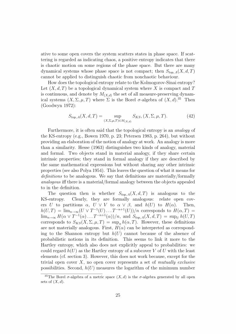
ative to some open covers the system scatters states in phase space. If scat-tering is regarded as indicating chaos, a positive entropy indicates that thereis chaotic motion on some regions of the phase space. But there are manydynamical systems whose phase space is not compact; then Stop, A(X, d, T )cannot be applied to distinguish chaotic from nonchaotic behaviour.

How does the topological entropy relate to the Kolmogorov-Sinai entropy?Let (X, d, T ) be a topological dynamical system where X is compact and Tis continuous, and denote by M(X,d) the set of all measure-preserving dynam-ical systems (X, Σ, µ, T ) where Σ is the Borel σ-algebra of (X, d).35 Then(Goodwyn 1972):

Stop, A(X, d, T ) = sup(X,Σ,µ,T )∈M(X,d)

SKS, (X, Σ, µ, T ). (42)

Furthermore, it is often said that the topological entropy is an analogy ofthe KS-entropy (e.g., Bowen 1970, p. 23; Petersen 1983, p. 264), but withoutproviding an elaboration of the notion of analogy at work. An analogy is morethan a similarity. Hesse (1963) distinguishes two kinds of analogy, materialand formal. Two objects stand in material analogy, if they share certainintrinsic properties; they stand in formal analogy if they are described bythe same mathematical expressions but without sharing any other intrinsicproperties (see also Polya 1954). This leaves the question of what it means fordefinitions to be analogous. We say that definitions are materially/formallyanalogous iff there is a material/formal analogy between the objects appealedto in the definition.

The question then is whether Stop, A(X, d, T ) is analogous to theKS-entropy. Clearly, they are formally analogous: relate open cov-ers U to partitions α, U ∨ V to α ∨ β, and h(U) to H(α). Then,h(U, T ) = limn→∞(U ∨ T−1(U) . . . T−n+1(U))/n corresponds to H(α, T ) =limn→∞H(α ∨ T−1(α) . . . T−n+1(α))/n, and Stop, A(X, d, T ) = supU h(U, T )corresponds to SKS(X, Σ, µ, T ) = supα h(α, T ). However, these definitionsare not materially analogous. First, H(α) can be interpreted as correspond-ing to the Shannon entropy but h(U) cannot because of the absence ofprobabilistic notions in its definition. This seems to link it more to theHartley entropy, which also does not explicitly appeal to probabilities: wecould regard h(U) as the Hartley entropy of a subcover V of U with the leastelements (cf. section 3). However, this does not work because, except for thetrivial open cover X, no open cover represents a set of mutually exclusivepossibilities. Second, h(U) measures the logarithm of the minimum number

35The Borel σ-algebra of a metric space (X, d) is the σ-algebra generated by all opensets of (X, d).

25

of elements of U needed to cover X, but H(α) has no similar interpretation,e.g., is not the logarithm of the number of elements of the partition α. ThusStop, A(X, d, T ) and the KS-entropy are not materially analogous.

Bowen (1971) introduced two definitions which are equivalent to Adler et al.’sdefinition. Because of lack of space, we cannot discuss them here (see Pe-tersen 1983, pp. 264–267). What matters is that there is neither a formal nora material analogy between the Bowen entropies and the KS-entropy. Con-sequently, all we have is a formal analogy between the KS-entropy and thetopological entropy (41), and the claims in the literature that the KS-entropyand the topological entropy are analogous are to some extent misleading.Moreover, we conclude that the topological entropy does not capture whatentropy notions are often believed to capture, such as information, and thatnone of the interpretations of the topological entropy is similar in interpre-tation to another notion of entropy.

6 Fractal Geometry

It was not until the late 1960s that mathematicians and physicists started tosystematically investigate irregular sets. Mandelbrot coined the term fractalto denote these irregular sets. Fractals have been praised for providing abetter representation of several natural phenomena than figures of classicalgeometry but whether this is true remains controversial (cf. Falconer 1990,p. xiii; Mandelbrot 1983; Shenker 1994).

Fractal dimensions measure the irregularity of a set. We will discussthose fractal dimensions which are called entropy dimensions. The basic ideaunderlying fractal dimensions is that a set is a fractal if the fractal dimensionis greater than the usual topological dimension (which is an integer). Yet theconverse is not true: there are fractals where the relevant fractal dimensionsequal the topological dimension (Falconer 1990, pp. xx-xxi and chapter 3;Mandelbrot 1983, section 39).

Fractals arise in many different contexts. In particular, in dynamicalsystems theory, scientists frequently focus on invariant sets, i.e., sets A forwhich Tt(A) = A for all t, where Tt is the time evolution. And invariant setsare often fractals. For instance, many dynamical systems have attractors,i.e., invariant sets which neighboring states asymptotically approach in thecourse of dynamic evolution. Attractors are sometimes fractals, e.g., theLorenz and the Henon attractor.

The following idea underlies definitions of a dimension of a set F . Foreach ε > 0 we take a measurement Mε(F ) of the set F at level ε, and then

26

we ask how Mε(F ) behaves as ε goes to zero. If Mε(F ) obeys the power law

Mε(F ) ≈ cε−s, (43)

for some constants c and s as ε goes to zero, then s is called the dimensionof F . From (43) follows that as ε goes to zero:

log[Mε(F )] ≈ log[c]− s log[ε]. (44)

Consequently,

s = limε→0

log[Mε(F )]

− log[ε]. (45)

If Mε(F ) does not obey a power law (43), one can consider instead of thelimit in (45) the limit superior and the limit inferior (cf. Falconer 1990, p. 36).

Some fractal dimensions are called entropy dimensions, namely the box-counting dimension and the Renyi entropy dimensions. Let us start withthe former. Assume that Rn is endowed with the usual Euclidean metric d.Given a nonempty and bounded subset F ⊆ Rn, let Bε(F ) be the smallestnumber of balls of diameter ε that cover F . The following limit, if it exists,is called the box-counting dimension but is also referred to as the entropydimension (Edgar 2008, p. 112; Falconer 1990, p. 38; Hawkes 1974, p. 704;Mandelbrot 1983, p. 359)

DimB(F ) := limε→0

log[Bε(F )]

− log[ε]. (46)

There are several equivalent formulations of the box-counting dimension.For instance, for Rn consider the boxes defined by the ε-coordinate mesh:

[m1ε, (m1 + 1)ε)× . . .× [mnε, (mn + 1)ε), (47)

where m1, . . . ,mn ∈ Z. Then if we define Bε(F ) as number of boxes in theε-coordinate mesh that intersect F , the dimension obtained is equivalent to(46) (Falconer 1990, pp. 38–39). As expected, typically, for sets of classicalgeometry the box dimension is integer-valued and for fractals it is non-integervalued.36

For instance, how many squares of side length ε = 12n are needed to cover

the unit square U = [0, 1] × [0, 1]? The answer is B 12n

(U) = 22n. Hence

the box-counting dimension is limn→∞log[22n]

− log[ 12n ]

= 2. As another example

36The box-counting dimension has the shortcoming that even compact countable setscan have positive dimension. Therefore, it is often modified (Edgar 2008, p. 213; Falconer1990, p. 37 and pp. 44–46).

27

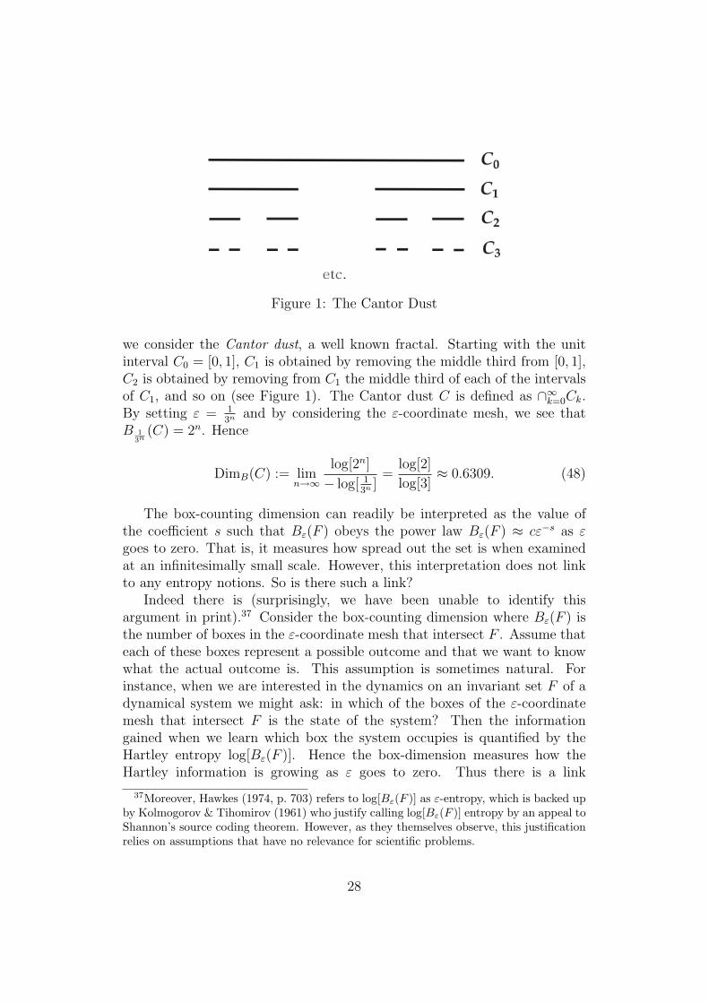
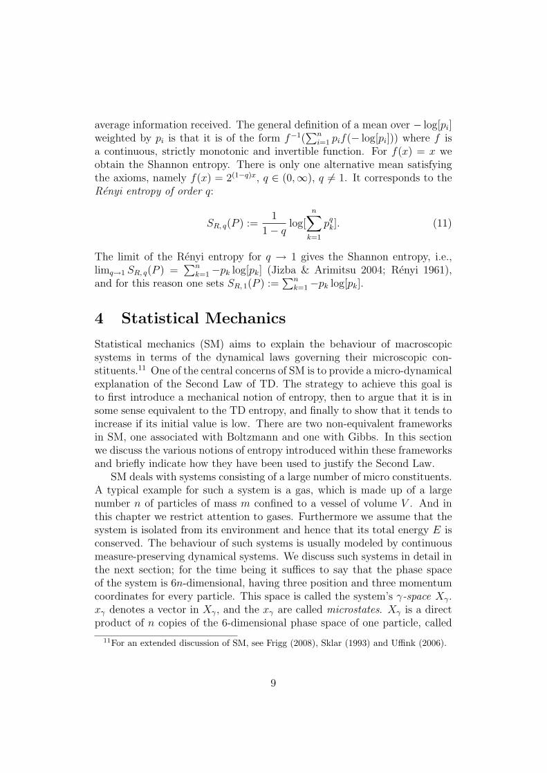
Figure 1: The Cantor Dust

we consider the Cantor dust, a well known fractal. Starting with the unitinterval C0 = [0, 1], C1 is obtained by removing the middle third from [0, 1],C2 is obtained by removing from C1 the middle third of each of the intervalsof C1, and so on (see Figure 1). The Cantor dust C is defined as ∩∞k=0Ck.By setting ε = 1

3n and by considering the ε-coordinate mesh, we see thatB 1

3n(C) = 2n. Hence

DimB(C) := limn→∞

log[2n]

− log[ 13n ]

=log[2]

log[3]≈ 0.6309. (48)

The box-counting dimension can readily be interpreted as the value ofthe coefficient s such that Bε(F ) obeys the power law Bε(F ) ≈ cε−s as εgoes to zero. That is, it measures how spread out the set is when examinedat an infinitesimally small scale. However, this interpretation does not linkto any entropy notions. So is there such a link?

Indeed there is (surprisingly, we have been unable to identify thisargument in print).37 Consider the box-counting dimension where Bε(F ) isthe number of boxes in the ε-coordinate mesh that intersect F . Assume thateach of these boxes represent a possible outcome and that we want to knowwhat the actual outcome is. This assumption is sometimes natural. Forinstance, when we are interested in the dynamics on an invariant set F of adynamical system we might ask: in which of the boxes of the ε-coordinatemesh that intersect F is the state of the system? Then the informationgained when we learn which box the system occupies is quantified by theHartley entropy log[Bε(F )]. Hence the box-dimension measures how theHartley information is growing as ε goes to zero. Thus there is a link

37Moreover, Hawkes (1974, p. 703) refers to log[Bε(F )] as ε-entropy, which is backed upby Kolmogorov & Tihomirov (1961) who justify calling log[Bε(F )] entropy by an appeal toShannon’s source coding theorem. However, as they themselves observe, this justificationrelies on assumptions that have no relevance for scientific problems.

28

between the box-dimension and the Hartley entropy.

Let us now turn to the Renyi entropy dimensions. Assume that Rn, n ≥ 1, isendowed with the usual Euclidean metric. Let (Rn, Σ, µ) be a measure spacewhere Σ contains all open sets of Rn and where µ(Rn) = 1. First, we needto introduce the notion of the support of the measure µ, which is the seton which the measure is concentrated. Formally, the support is the smallestclosed set X such that µ(Rn \ X) = 0. For instance, when measuring thedimension of a set F , the support of the measure is typically F . We assumethat the support of µ is contained in a bounded region of Rn.

Consider the ε-coordinate mesh of Rn (47). Let Biε, 1 ≤ i ≤ m, m ∈ N,

be the boxes that intersect the support of µ, and let Zq,ε :=∑m

i=1 µ(Biε)

q.The Renyi entropy dimension of order q, −∞ < q < ∞, q 6= 1, is

Dimq := limε→0

1

q − 1

log[Zq,ε]

log[ε], (49)

and the Renyi entropy dimension of order 1 is

Dim1 := limε→0

limq→1

1

q − 1

log[Zq,ε]

log[ε], (50)

if the limit exists.It is not hard to see that if q < q′, Dimq′ ≤ Dimq (cf. Beck & Schlogl 1995,

p. 117). The cases q = 0 and q = 1 are of particular interest. Be-cause Dim0 = DimB(supportµ), the Renyi entropy dimensions are a gen-eralisation of the box-counting dimension. And for q = 1 (Renyi 1961):

Dim1 = limε→0

∑mi=1−µ(Bi

ε) log[µ(Biε)]

− log(ε). Since

∑mi=1−µ(Bi

ε) log[µ(Biε)] is the

Shannon entropy (cf. section 3), Dim1 is called the information dimension(Falconer 1990, p. 260; Ott 2002, p. 81).

The Renyi entropy dimensions are often referred to as entropy dimensions(e.g., Beck & Schlogl 1995, pp. 115–116). Before turning to a rationale forthis name, let us state the usual motivation of the Renyi entropy dimensions.The number q determines how much weight we assign to µ: the higher q,the greater the influence of boxes with larger measure. So the Renyi entropydimensions measure the coefficient s such that Zq,ε obeys the power lawZq,ε ≈ cε−(1−q)s as ε goes to zero. That is, Dimq measures how spread outthe support of µ is when it is examined at an infinitesimally small scaleand when the weight of the measure is q (Beck & Schlogl 1995, p. 116; Ott,2002, pp. 80–85). Consequently, when the Renyi entropy dimensions differfor different q, this is a sign of a multifractal, i.e., a set with different scalingbehaviour (see Falconer 1990, pp. 254–264). This motivation does not refer

29

to entropy notions.

Yet there is an obvious connection of the Renyi entropy dimensions for q > 0to the Renyi entropies (cf. section 3).38 Assume that each of the boxes ofthe ε-coordinate mesh which intersect the support of µ represent a possibleoutcome. Further, assume that the probability that the outcome is in thebox Bi is µ(Bi). Then the information gained when we learn which box thesystem occupies can be quantified by the Renyi entropies Hq. Consequently,each Renyi entropy dimension for q ∈ (0,∞) measures how the informationis growing as ε goes to zero. For q = 1 we get a measure of how the Shannoninformation is growing as ε goes to zero.

7 Conclusion

This chapter has been concerned with some of the most important notions ofentropy. The interpretations of these entropies have been discussed and theirconnections have been clarified. Two points deserve attention. First, all no-tions of entropy discussed in this chapter, except the thermodynamic and thetopological entropy, can be understood as variants of some information theo-retic notion of entropy. However, this should not distract from the fact thatdifferent notions of entropy have different meanings and play different roles.Second, there is no preferred interpretation of the probabilities that figure inthe different notions of entropy. The probabilities occurring in informationtheoretic entropies are naturally interpreted as epistemic probabilities, butontic probabilities are not ruled out. The probabilities in other entropies, forinstance the different Boltzmann entropies, are most naturally understoodontically. So when considering the relation between entropy and probabilityare no simple and general answers, and a careful case by case analysis is theonly way forward.

Acknowledgements

We would like to thank David Lavis, Robert Batterman and two anonymousreferees for comments on earlier drafts of this chapter. We are grateful toClaus Beisbart and Stephan Hartmann for editing this book.

38Surprisingly, we have not found this motivation in print.

30

References

Adler, R., Konheim, A. & McAndrew, A. (1965), ‘Topological entropy’,Transactions of the American Mathematical Society 114, 309–319.

Bashkirov, A.G. (2006), ‘Renyi entropy as a statistical entropy for complexsystems’, Theoretical and Mathematical Physics 149, 1559–1573.

Batterman, R. & White, H. (1996), ‘Chaos and algorithmic complexity’,Foundations of Physics 26, 307–336.

Beck, C. & Schlogl, F. (1995), Thermodynamics of Chaotic Systems, Cam-bridge University Press, Cambridge.

Berger, A. (2001), Chaos and Chance, an Introduction to Stochastic Aspectsof Dynamics, De Gruyter, New York.

Berkovitz, J., Frigg, R. & Kronz, F. (2006), ‘The ergodic hierarchy, ran-domness and Hamiltonian chaos’, Studies in History and Philosophy ofModern Physics 37, 661–691.

Bowen, R. (1970), Topological entropy and Axiom A, in ‘Global Analy-sis, Proceedings of the Symposium of Pure Mathematics 14’, AmericanMathematical Society, Providence.

Bowen, R. (1971), ‘Periodic points and measures for Axiom A diffeomor-phisms’, Transactions of the American Mathematical Society 154, 377–397.

Cornfeld, I., Fomin, S. & Sinai, Y. (1982), Ergodic Theory, Springer, Berlin.

Earman, J. (1971), ‘Laplacian determinism, or is this any way to run auniverse?’, Journal of Philosophy 68, 729–744.

Eckmann, J.-P. & Ruelle, D. (1985), ‘Ergodic theory of chaos and strangeattractors’, Reviews of Modern Physics 57, 617–654.

Edgar, G. (2008), Measure, Topology, and Fractal Geometry, Springer, NewYork.

Ehrenfest, P. & Ehrenfest, T. (1912), The Conceptual Foundations of theStatistical Approach in Mechanics, Dover, Mineola/New York.

Emch, G. & Liu, C. (2002), The Logic of Thermostatistical Physics, Springer,Berlin, Heidelberg.

31

Falconer, K. (1990), Fractal Geometry: Mathematical Foundations and Ap-plications, John Wiley & Sons, New York.

Frigg, R. (2004), ‘In what sense is the Kolmogorov-Sinai entropy a measurefor chaotic behaviour?—bridging the gap between dynamical systemstheory and communication theory’, The British Journal for the Philo-sophy of Science 55, 411–434.

Frigg, R. (2006), ‘Chaos and randomness: An equivalence proof of a gen-eralised version of the Shannon entropy and the Kolmogorov-Sinai en-tropy for Hamiltonian dynamical systems’, Chaos, Solitons and Fractals28, 26–31.

Frigg, R. (2008), A field guide to recent work on the foundations of statisticalmechanics, in D. Rickles, ed., ‘The Ashgate Companion to Contempo-rary Philosophy of Physics’, Ashgate, London, pp. 99–196.

Frigg, R. (2009a), ‘Typicality and the approach to equilibrium in Boltz-mannian statistical mechanics’, Philosophy of Science (Supplement) 76,pp. 997–1008.

Frigg, R. (2009b), Why typicality does not explain the approach to equi-librium, in M. Suarez, ed., ‘Probabilities, Causes and Propensitites inPhysics’, Springer, Berlin, forthcoming.

Frigg, R. & Hoefer, C. (2010), Determinism and Chance from a Humean Per-spective, in D. Dieks, W. Gonzalez, S. Hartmann, M. Weber, F. Stadler& T. Uebel, eds., ‘The Present Situation in the Philosophy of Science’,Springer, Berlin, forthcoming.

Gibbs, J. (1981), Elementary Principles in Statistical Mechanics, Ox BowPress, Woodbridge.

Gillies, D. (2000), Philosophical Theories of Probability, London: Routledge.

Goldstein, S. (2001), Boltzmann’s approach to statistical mechanics, inJ. Bricmont, D. Durr, M. Galavotti, G. Ghirardi, F. Pettrucione &N. Zanghi, eds, ‘Chance in Physics: Foundations and Perspectives’,Springer, Berlin and New York, pp. 39–54.

Goodwyn, L. (1972), ‘Comparing topological entropy with measure-theoreticentropy’, American Journal of Mathematics 94, 366–388.

Grad, H. (1961), ‘The many faces of entropy’, Communications in Pure andApplied Mathematics 14, 323–254.

32

Greiner, W., Neise, L. & Stucker, H. (1993), Thermodynamik und StatistischeMechanik, Harri Deutsch, Leipzig.

Halmos, P. (1950), Measure Theory, Van Nostrand, New York and London.

Hartley, R. (1928), ‘Transmission of information’, The Bell System TechnicalJournal 7, 535–563.

Hawkes, J. (1974), ‘Hausdorff measure, entropy, and the independence ofsmall sets’, Proceedings of the London Mathematical Society 28, 700–723.

Hemmo, M. & Shenker, O. (2006), ‘Von Neumann’s entropy does not corre-spond to thermodynamic entropy’, Philosophy of Science 73, 153–174.

Hesse, M. (1963), Models and Analogies in Science, Sheed and Ward, London.

Howson, C. (1995), ‘Theories of probability’, The British Journal for thePhilosophy of Science 46, 1-32.

Howson, C. & Urbach, P. (2006), Scientific Reasoning: The Bayesian Ap-proach, Open Court, La Salle.

Ihara, S. (1993), Information Theory for Continuous Systems, World Scien-tific, London.

Jaynes, E. (1957), ‘Information theory and statistical mechanics’, PhysicalReview 106, 620–630.

Jaynes, E. (1965), ‘Gibbs versus Boltzmann entropies’, American Journal ofPhysics33, 391–398.

Jaynes, E. (1983), Papers on Probability, Statistics, and Statistical Physics,Reidel, Dordrecht.

Jizba, P. & Arimitsu, T. (2004), ‘The world according to Renyi: thermody-namics of multifractal systems’, Annals of Physics 312, 17–59.

Kittel, C. (1958), Elementary Statistical Mechanics, Dover, Mineola/NY.

Klir, G. (2006), Uncertainty and Information: Foundations of GeneralizedInformation Theory, Wiley, Hoboken, New Jersey.

Kolmogorov, A. (1958), ‘A new metric invariant of transitive dynamical sys-tems and automorphisms of Lebesgue spaces’, Dokl. Acad. Nauk SSSR119, 861–864.

33

Kolmogorov, A. & Tihomirov, V. (1961), ‘ε-entropy and ε-capacity ofsets in functional spaces’, American Mathematical Society Translations17, 277–364.

Lavis, D. (2004), ‘The spin-echo system reconsidered’, Foundations of Physics34, 669–688.

Lavis, D. (2008), ‘Boltzmann, Gibbs, and the Concept of Equilibrium’, Philo-sophy of Science 75, 682–696.

Lebowitz, J. (1999), ‘Statistical mechanics: A selective review of two centralissues’, Reviews of Modern Physics 71, 346–357.

Lewis, D. (1980), A Subjectivists Guide to Objective Chance, in R.C. Jeffrey,ed., ‘Studies in Inductive Logic and Probability’, University of CaliforniaPress, Berkeley, pp. 83–132.

Mane, R. (1987), Ergodic Theory and Differentiable Dynamics, Springer,Berlin.

Mandelbrot, B. (1983), The Fractal Geometry of Nature, Freeman, New York.

Mellor, H. (2005), Probability: A Philosophical Introduction, Routledge, Lon-don.

Ott, E. (2002), Chaos in Dynamical Systems, Cambridge University Press,Cambridge.

Penrose, R. (1970), Foundations of Statistical Mechanics, Oxford UniversityPress, Oxford.

Petersen, K. (1983), Ergodic Theory, Cambridge University Press, Cam-bridge.

Pippard, A.B. (1966), The Elements of Classical Thermodynamics., Cam-bridge University Press, Cambridge.

Polya, G. (1954), Patterns of Plausible Inference, Volume II of Mathematicsand Plausible Reasoning, Princeton University Press, Princeton.

Reiss, H. (1965), Methods of Thermodynamics, Dover Publications, Mine-ola/NY.

Renyi, A. (1961), On measures of entropy and information, in ‘Proceed-ings of the Fourth Berkeley Symposium of Mathematical Statistics andProbability’, University of California Press, Berkeley, pp. 547–561.

34

Shannon, C. & Weaver, W. (1949), The Mathematical Theory of Communi-cation, University of Illinois Press, Urbana, Chicago, IL & London.

Shaw, R. (1985), The Dripping Faucet as a Model Chaotic System, AerialPress, Santa Cruz.

Shenker, O. (1994), ‘Fractal geometry is not the geometry of nature’, Studiesin History and Philosophy of Modern Physics 25, 967–981.

Sinai, Y. (1959), ‘On the concept of entropy for dynamical systems’, Dokl.Acad. Nauk SSSR 124, 768–771.

Sklar, L. (1993), Physics and Chance. Philosophical Issues in the Foundationsof Statistical Mechanics, Cambridge University Press, Cambridge.

Sorkin, R. (2005), ‘Ten theses on black hole entropy’, Studies In History andPhilosophy of Modern Physics 36, 291–301.

Sutherland, W. (2002), Introduction to Metric and Topological Spaces, OxfordUniversity Press, Oxford.

Tolman, R. (1938), The Principles of Statistical Mechanics, Dover, Mineolaand New York.

Tsallis, C. (1988), ‘Possible generalization of Boltzmann-Gibbs statistics’,Journal of Statistical Physics 52, 479–487.

Uffink, J. (2001), ‘Bluff your way in the second law of thermodynamics’,Studies in the History and Philosophy of Modern Physics 32, 305–394.

Uffink, J. (2006), Compendium to the foundations of classical statisticalphysics, in J. Butterfield & J. Earman, eds, ‘Philosophy of Physics’,North-Holland, Amsterdam, pp. 923–1074.

Wehrl, A. (1978), ‘General properties of entropy’, Reviews of Modern Physics50, 221–259.

Werndl, C. (2009a), ‘Are deterministic descriptions and indeterministic de-scriptions observationally equivalent?’, Studies in History and Philo-sophy of Modern Physics 40, 232–242.

Werndl, C. (2009b), Deterministic versus indeterministic descriptions: Notthat different after all?, in A. Hieke & H. Leitgeb, eds, ‘Reduction,Abstraction, Analysis, Proceedings of the 31st International LudwigWittgenstein-Symposium’, Ontos, Frankfurt, pp. 63–78.

35

Werndl, C. (2009c), ‘Justifying definitions in matemathics—going beyondLakatos’, Philosophia Mathematica 17, pp. 313–340.

Werndl, C. (2009d), ‘What are the new implications of chaos for unpredicta-bility?’, The British Journal for the Philosophy of Science 60, 195–220.

36