ENTERPRISE RISK MANAGEMENT IN INSURANCE GROUPS: MEASURING RISK CONCENTRATION AND DEFAULT RISK Topic 1: Risk Management of Insurance Enterprise (Risk models; Risk measures; Quantify- ing inter-dependencies among risks) Gatzert, Nadine Schmeiser, Hato Schuckmann, Stefan Institute of Insurance Economics, University of St. Gallen Kirchlistrasse 2, 9010 St. Gallen, Switzerland Tel.: +41 (71) 243 4012 Fax: +41 (71) 243 4040 E-mail addresses: [email protected], [email protected], [email protected] ABSTRACT In financial conglomerates and insurance groups, enterprise risk management is becoming increasingly important in controlling and managing the different independent legal entities in the group. The aim of this paper is to assess and relate risk concentration and joint default probabilities of the group’s legal entities in order to achieve a more comprehensive picture of an insurance group’s risk situation. We further examine the impact of the type of dependence structure on results by comparing linear and nonlinear dependencies using different copula concepts under certain distributional assumptions. Our results show that even if financial groups with different dependence structures do have the same risk concentration factor, joint default probabilities of different sets of subsidiaries can vary tremendously. Keywords: Enterprise Risk Management, Analyzing/Quantifying Risks, Dependence Struc- tures, Copulas/Multivariate Distributions, Financial Conglomerate, Insurance Group

Welcome message from author
This document is posted to help you gain knowledge. Please leave a comment to let me know what you think about it! Share it to your friends and learn new things together.
Transcript
ENTERPRISE RISK MANAGEMENT IN INSURANCE GROUPS:
MEASURING RISK CONCENTRATION AND DEFAULT RISK Topic 1: Risk Management of Insurance Enterprise (Risk models; Risk measures; Quantify-
ing inter-dependencies among risks)
Gatzert, Nadine
Schmeiser, Hato
Schuckmann, Stefan
Institute of Insurance Economics, University of St. Gallen
Kirchlistrasse 2, 9010 St. Gallen, Switzerland
Tel.: +41 (71) 243 4012
Fax: +41 (71) 243 4040
E-mail addresses: [email protected], [email protected],
ABSTRACT
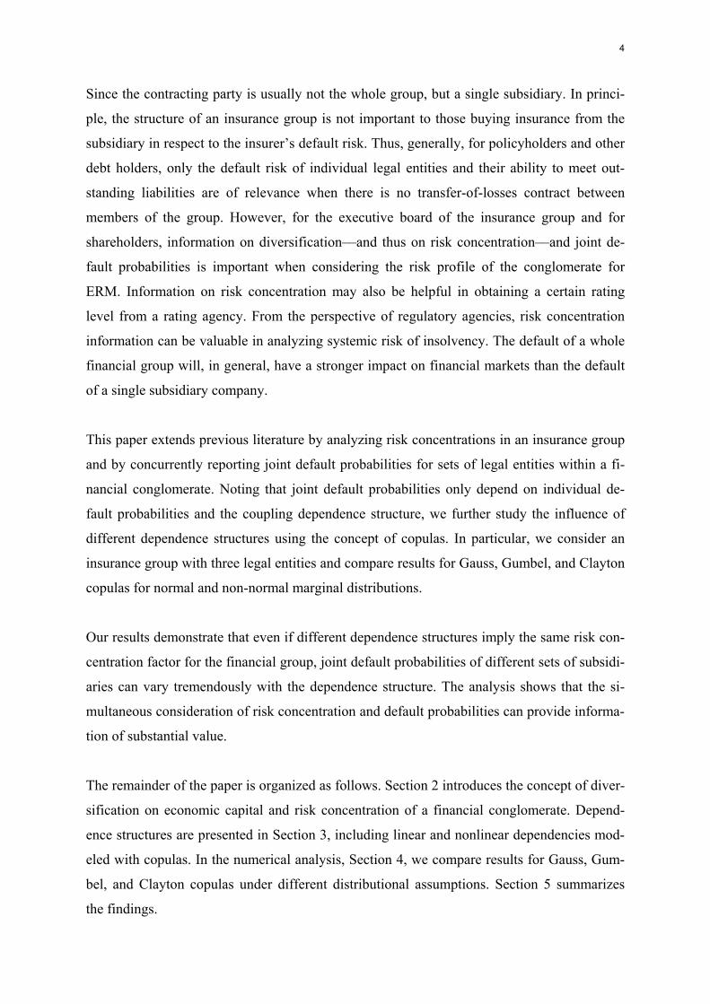
In financial conglomerates and insurance groups, enterprise risk management is becoming
increasingly important in controlling and managing the different independent legal entities in
the group. The aim of this paper is to assess and relate risk concentration and joint default
probabilities of the group’s legal entities in order to achieve a more comprehensive picture of
an insurance group’s risk situation. We further examine the impact of the type of dependence
structure on results by comparing linear and nonlinear dependencies using different copula
concepts under certain distributional assumptions. Our results show that even if financial
groups with different dependence structures do have the same risk concentration factor, joint
default probabilities of different sets of subsidiaries can vary tremendously.
Keywords: Enterprise Risk Management, Analyzing/Quantifying Risks, Dependence Struc-
tures, Copulas/Multivariate Distributions, Financial Conglomerate, Insurance Group

2
1. INTRODUCTION
During the last several years, there has been a trend toward consolidation (M&A activities) in
the financial sector of many countries (see Amel, Barnes, Panetta, and Salleo, 2004). Regula-
tory authorities, as well as rating agencies, are concerned with new types of risk and risk con-
centrations arising in financial conglomerates and with how to properly assess them in group
supervision (for the European Union, see, e.g., CEIOPS, 2006). In this context, enterprise risk
management (ERM) has become increasingly important. ERM takes a comprehensive view
of risk and helps manage risks in a holistic and consistent way (CAS, 2003). The aim of this
paper is to provide a detailed and more comprehensive picture of an insurance group’s risk
situation by assessing and relating the risk concentration and joint default probabilities of its
legal entities. We further examine the impact of the type of dependence structure on results
by comparing linear and nonlinear dependencies using the concept of copulas.
Determination of the risk concentrations of an insurance group can be based on an analysis of
diversification effects at a corporate level since diversification is the opposite of concentra-
tion. In particular, risk concentrations, like interdependencies or accumulation, reduce diver-
sification effects. The diversification effect is measured with the economic capital of an ag-
gregated risk portfolio, which implicitly relies on the assumption that different legal entities
are merged into one. An essential aspect in aggregating risks is modeling the dependence
structure using linear and nonlinear dependencies. Copula theory can be used to model
nonlinear dependencies in extreme events and to test the financial stability of a conglomerate
structure.
There has been steady growth in research on the application of copula theory to risk man-
agement. Embrechts, McNeil, and Straumann (2002) introduce copulas in finance theory and
analyze the effect of dependence structures on value at risk. Li (2000) applies copulas to the
valuation of credit derivatives. Frey and McNeil (2001) model dependent defaults in credit
portfolios, with a special emphasis on tail dependencies. An introduction to the use of copulas
in the actuarial context can be found in Frees and Valdez (1998) and Embrechts, Lindskog,
and McNeil (2003).

3
A central aspect of ERM is the aggregation of different types of risk to calculate the eco-
nomic capital necessary as a buffer against adverse outcomes. Wang (1998, 2002) gives an
overview on the theoretical background of economic capital modeling, risk aggregation, and
the use of copula theory in enterprise risk management. Kuritzkes, Schuermann, and Weiner
(2003) aggregate risks at different levels of a financial holding company under the assump-
tion of joint normality; in an empirical study, they compute the relative diversification effect
for several conglomerates. Ward and Lee (2002) use a normal copula approach to aggregate
the risks of a diversified insurer in a combined analytical and simulation model. Dimakos and
Aas (2004) apply a similar method to model total economic capital, and combine risks by
pairwise aggregation; they present a practical approach to estimate the joint loss distribution
of a Norwegian bank and a Norwegian life insurance company.
Faivre (2003) models the overall loss distribution for a four-lines-of-business insurance com-
pany and examines the influence of different types of copulas on the value at risk and the
company’s default probability. Tang and Valdez (2006) simulate the economic capital re-
quirements for a multiline insurer, taking into account different types of distributions and
different types of copulas; the resulting values for economic capital are used to compute ab-
solute diversification benefits. Rosenberg and Schuermann (2006) relax the joint normality
assumption and use copula theory to aggregate risks with non-normal marginals; they analyze
the influence of the business mix between credit, market, and operational risk on value at risk
and calculate diversification benefits by comparing the value at risk of the diversified con-
glomerate with the stand-alone value at risk.
However, most of the literature does not take into account the special risk profile of financial
conglomerates that arises from the group-holding structure. Financial conglomerates or insur-
ance groups consist of several independent legal entities, each with limited liability. In the
European Union, for example, combining banking and insurance activities in the same legal
entity is prohibited (see Article 6(1b) of the Life Insurance Directive 2002/83/EC and Article
8(1b) of the Non-Life Insurance Directive 73/239/EEC). Article 18(1) of the Life Insurance
Directive prohibits the combination of life and non-life business in the same legal entity.
Hence, where such is even lawful, a transfer of funds between different legal entities in case
of an insolvency of one entity occurs only if a transfer-of-losses contract has been signed or if
the management of the corporate group decides in favor of cross-subsidization (e.g., for repu-
tational reasons).
4
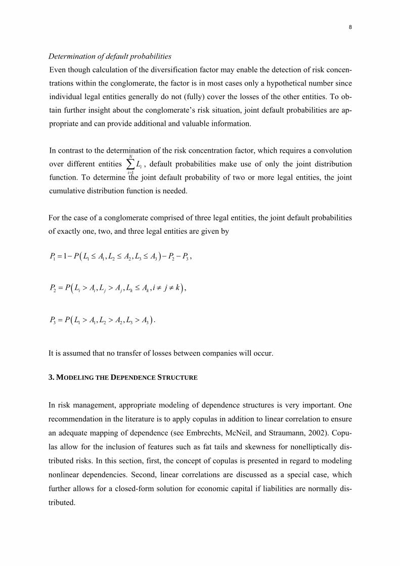
Since the contracting party is usually not the whole group, but a single subsidiary. In princi-
ple, the structure of an insurance group is not important to those buying insurance from the
subsidiary in respect to the insurer’s default risk. Thus, generally, for policyholders and other
debt holders, only the default risk of individual legal entities and their ability to meet out-
standing liabilities are of relevance when there is no transfer-of-losses contract between
members of the group. However, for the executive board of the insurance group and for
shareholders, information on diversification––and thus on risk concentration––and joint de-
fault probabilities is important when considering the risk profile of the conglomerate for
ERM. Information on risk concentration may also be helpful in obtaining a certain rating
level from a rating agency. From the perspective of regulatory agencies, risk concentration
information can be valuable in analyzing systemic risk of insolvency. The default of a whole
financial group will, in general, have a stronger impact on financial markets than the default
of a single subsidiary company.
This paper extends previous literature by analyzing risk concentrations in an insurance group
and by concurrently reporting joint default probabilities for sets of legal entities within a fi-
nancial conglomerate. Noting that joint default probabilities only depend on individual de-
fault probabilities and the coupling dependence structure, we further study the influence of
different dependence structures using the concept of copulas. In particular, we consider an
insurance group with three legal entities and compare results for Gauss, Gumbel, and Clayton
copulas for normal and non-normal marginal distributions.
Our results demonstrate that even if different dependence structures imply the same risk con-
centration factor for the financial group, joint default probabilities of different sets of subsidi-
aries can vary tremendously with the dependence structure. The analysis shows that the si-
multaneous consideration of risk concentration and default probabilities can provide informa-
tion of substantial value.
The remainder of the paper is organized as follows. Section 2 introduces the concept of diver-
sification on economic capital and risk concentration of a financial conglomerate. Depend-
ence structures are presented in Section 3, including linear and nonlinear dependencies mod-
eled with copulas. In the numerical analysis, Section 4, we compare results for Gauss, Gum-
bel, and Clayton copulas under different distributional assumptions. Section 5 summarizes
the findings.

5
2. RISK CONCENTRATION AND DEFAULT RISK
This section describes, first, a framework for measuring risk concentrations by calculating the
diversification effect on the economic capital of an insurance group, assuming that the differ-
ent legal entities are merged. The economic capital is the amount necessary to buffer against
unexpected losses from business activities so as to prevent default at a specific risk tolerance
level for a fixed time horizon. Diversification is generally intended to reduce the overall risk
level in an insurance group and thus acts to alleviate the dangers inherent in risk concentra-
tion. Calculating risk concentration in an insurance group can thus be based on an examina-
tion of diversification effects at the group level. In a second step, the joint default probabili-
ties of legal entities within a conglomerate are introduced.
We focus on an insurance group with a holding structure and different companies (legal enti-
ties) with limited liability. Generally, such a conglomerate is subject to market risks, credit
risks, underwriting risks, and operational risks. If each member of the group is faced with
identical risks, one would expect the stochastic liabilities of the different entities to be highly
correlated. This will usually be the case if several firms of the same type, for example, finan-
cial firms, form a group. However, if the corporate group is composed of companies from
widely different industries, the liabilities between the different legal entities might be rather
uncorrelated. In what follows, we will consider an insurance group consisting of a bank, a life
insurer, and a non-life insurer.
In our framework, the equity value of each subsidiary legal entity is modeled at two points in
time (t = 0, 1). The value of the assets (liabilities) at time t = 1 of company i is defined as iA
( ). Debt and equity capital in t = 0 is invested in riskless assets, leading to a deterministic
cash flow for the assets in t = 1, whereas liabilities paid out in t = 1 are modeled stochasti-
cally.
iL
Stand-alone economic capital
The amount of necessary economic capital depends on the specific risk tolerance level and on
the measure chosen to evaluate corporate risk. In the following, we determine the necessary
amount of capital using the default probability. The default probability α of each legal entity
i can be written as

6
( ) .i iP A L iα< =
In the next step, the invested assets iA are divided into two parts—the expected value of the
liabilities ( )iE L and the economic capital : iEC
( )( )( )( ) .
i i i
i i i
P E L EC L
P L E L ECi
i
α
α
+ < =
⇔ − > =
Hence, given a probability distribution for the liabilities and a certain safety level iα , the
economic capital can be derived. The necessary economic capital for N different
legal entities within an insurance group can be calculated by iEC iEC
( ) ( )1 1, , .i i iEC VaR L E L i Nα−= − = … (1)
For consistency, all companies within the conglomerate should have the same safety level α .
Therefore, value at risk (VaR) is defined by
( ) ( ) ( ){ }1 infi ii L LVaR L F x F xα α α−= = ≥ ,
where iLF stands for the distribution function of the liabilities for company i.
Aggregation
Assuming that the several companies in the insurance group are merged into one company
(full liability between legal entities), the necessary economic capital for the safety level α on
an aggregate level for 1
N
ii
L=∑ can be written as
11 1
N N
aggr i ii i
EC VaR L E Lα−= =
⎛ ⎞ ⎛ ⎞= −⎜ ⎟ ⎜
⎝ ⎠ ⎝ ⎠∑ ∑ ⎟
L
. (2)
To calculate the quantile in Equation (2), information about the cumulative distribution of the
liabilities is needed. Closed-form solutions for 1i=
N
i∑ can be derived only for a limited num-
ber of distributions. In the case of a normal distribution, only the variance of the portfolio is

7
needed to determine the aggregate economic capital aggrEC . If no closed-form solution can be
obtained, the quantile of the distribution of the aggregate liabilities 1i=
N
iL∑ can be estimated
using either numerical simulation techniques or analytical approximations (for an overview,
see Daykin, Pentikainen, and Pesonen, 1994, pp. 119 ff.).
Diversification versus concentration
Given Equations (1) and (2), diversification can be measured with the ratio of aggregated
economic capital to the sum of stand-alone economic capital (see, e.g., Kuritzkes, Schuer-
mann, and Weiner, 2003),
1
aggrN
ii
ECd
EC=
=
∑. (3)
In the case of linear dependencies, the factor d takes on values between zero and one and can
be used to compare the level of risk concentration in conglomerates. A value of one corre-
sponds to perfect correlation, which means that there would be no diversification benefits if
the different legal entities merged into one company. When risk factors are less than perfectly
correlated, some of the risk can be diversified. Absolute measures for diversification can be
found in the literature (see, e.g., Tang and Valdez, 2006); however, absolute measures do not
allow the comparison of companies and conglomerates that are of different sizes. Given a
benchmark company, a higher value of d implies possible risk concentration, since lower
values of d mean a higher diversification and thus a lower risk concentration. We henceforth
refer to the coefficient in Equation (3) as the risk concentration factor. To keep the different
quantities in Equation (3) comparable, it is important to use the same risk measure and the
same time horizon for all legal entities when calculating the economic capital.
Generally, diversification of the group is of no relevance to debt holders of the group’s indi-
vidual companies (e.g., policyholders in the case of an insurance group) since the whole
group is not the contracting party, that is, the contract is between the policyholder and the
insurance subsidiary only (although there might be transfer-of-loss contracts). However, for
management and shareholders of the corporate group, information about risk concentration in
the different sectors is of high importance.
8
Determination of default probabilities
Even though calculation of the diversification factor may enable the detection of risk concen-
trations within the conglomerate, the factor is in most cases only a hypothetical number since
individual legal entities generally do not (fully) cover the losses of the other entities. To ob-
tain further insight about the conglomerate’s risk situation, joint default probabilities are ap-
propriate and can provide additional and valuable information.
In contrast to the determination of the risk concentration factor, which requires a convolution
over different entities 1i=∑ , default probabilities make use of only the joint distribution
function. To determine the joint default probability of two or more legal entities, the joint
cumulative distribution function is needed.
N
iL
3P
3
For the case of a conglomerate comprised of three legal entities, the joint default probabilities
of exactly one, two, and three legal entities are given by
( )1 1 1 2 2 3 3 21 , ,P P L A L A L A P= − ≤ ≤ ≤ − − ,
( )2 , , ,i i j j k kP P L A L A L A i j k= > > ≤ ≠ ≠ ,
( )3 1 1 2 2 3, ,P P L A L A L A= > > > .
It is assumed that no transfer of losses between companies will occur.
3. MODELING THE DEPENDENCE STRUCTURE
In risk management, appropriate modeling of dependence structures is very important. One
recommendation in the literature is to apply copulas in addition to linear correlation to ensure
an adequate mapping of dependence (see Embrechts, McNeil, and Straumann, 2002). Copu-
las allow for the inclusion of features such as fat tails and skewness for nonelliptically dis-
tributed risks. In this section, first, the concept of copulas is presented in regard to modeling
nonlinear dependencies. Second, linear correlations are discussed as a special case, which
further allows for a closed-form solution for economic capital if liabilities are normally dis-
tributed.

9
3.1. Copulas
For continuous multivariate distribution functions, copulas serve to separate the univariate
margins and the multivariate dependence structure. The copula C represents the dependence
structure and couples the marginal distributions to a joint multivariate distribution. Let the
random variables (with ) have (continuous) marginal distribution functions iX 1,...,i = N iF .
From Sklar’s theorem it follows that (see Nelsen, 1999, p. 15)
( ) (( ) ( )( )
1
1
1 1 ,..., 1
1
,..., ,...,
,..., .N
N
N N X X N
X X
P X x X x F x x
C F x F x
< < =
=
)
N
N
For joint default probabilities, this result implies that for fixed individual default probabilities
( )0 , 1,...,i iP X i Nα< = = ,
one can obtain for the joint default probability of all N entities
( ) ( )( ) ( )( ) ( )
1
1
1 ,...,
1
0,..., 0 0,...,0
0 ,..., 0 ,..., .N
N
N X X
X X
P X X F
C F F C α α
< < =
= =
Hence, the joint default probability depends on the dependence structure expressed by the
copula C and on the marginal default probabilities αi. In our case, these quantities are given
and fixed since the economic capital for each entity is adjusted for each entity such that the
marginal default probabilities remain constant. For example, in the case of the three entities
considered here, the probability that legal entity 1 and 2 default, and entity 3 survives is
( ) ( ) ( )( ) ( ) ( ) ( )( )( ) ( )
1 2 1 21 2 3 3
1 2 1 2 3
0, 0, 0 0 , 0 ,1 0 , 0 , 0
, ,1 , , .X X X X XP X X X C F F C F F F
C Cα α α α α
< < > = −
= −
The probability of default for exactly two legal entities can thus be calculated by

10
( )( ) ( ) ( ) ( )
2
2 3 1 3 1 2 1 2 3
0, 0, 0,
1, , ,1, , ,1 3 , , .i j kP P X X X i j k
C C C Cα α α α α α α α α
= < < > ≠ ≠
= + + − ⋅ (4)
Furthermore, the probability that exactly one company defaults is determined by
( )1 21 0 1, 2,3iP P X i P= − > ∀ = − − 3P (5)
where
( ) ( )3 1 2 3 1 20, 0, 0 , , .P P X X X C 3α α α= < < < = (6)
In the analysis, we will compare several copulas. To obtain boundaries, we include the case
of independence and perfect dependence (comonotonicity), represented by the copula
(McNeil, Frey, and Embrechts, 2005, p. 189)
( ) { }1 1,..., min ,...,N NM u u u u= .
The independence copula is given by (McNeil, Frey, and Embrechts, 2005, p. 189)
( )11
,...,N
N ii
u u u=
Π =∏ .
The default probability for all three entities is thus the product of the marginal default prob-
abilities. From Equations (4)–(6), it follows that in the case of independence the default prob-
abilities of exactly one, two, and three companies are
( ) ( ) ( )1 1 2 3 21 1 1 1P Pα α α= − − ⋅ − ⋅ − − − 3P
3
2 1 2 1 3 2 3 1 23P α α α α α α α α α= ⋅ + ⋅ + ⋅ − ⋅ ⋅ ⋅
3 1 2P 3α α α= ⋅ ⋅ .

11
The two most common Archimedian copulas, Clayton and Gumbel, are used to model the
dependence structure between the entities. These are explicit copulas that have closed-form
solutions and are not derived from multivariate distribution functions as is the implicit Gaus-
sian copula. In general, an N-dimensional Archimedian copula may be constructed by using
the respective generator ( )tΦ
( ) ( ) ( )( )11 1, ..., ...N NC u u u u−= Φ Φ + + Φ ,
which must have certain properties (as described in McNeil, Frey, and Embrechts, 2005, p.
222). In the case of the N-dimensional Clayton copula, the generator and its inverse are given
by (see Wu, Valdez, and Sherris, 2006, p. 7)
( ) ( )11t t θ
θ−Φ = − and ( ) ( ) 1/1 1t t θθ −−Φ = ⋅ + ,
which leads to the following representation
( )1/
, 11
,..., 1N
ClN N i
i
C u u u Nθ
θθ
−
−
=
= − +⎛ ⎞⎜ ⎟⎝ ⎠∑ ,
where 0 θ≤ < ∞ . For θ → ∞ , one obtains perfect dependence; 0θ → implies independ-
ence (McNeil, Frey, and Embrechts, 2005, p. 223). For the N-dimensional Gumbel copula,
the generator and its inverse are given by (Wu, Valdez, and Sherris, 2006, p. 7)
( ) ( )( )logt t θΦ = − and ( ) ( )1 1expt t /θ−Φ = − ,
which implies the expression
( ) ( )1/
, 11
,..., exp logN
GuN N i
iC u u u
θθ
θ=
⎡ ⎤⎛ ⎞= − −⎢ ⎥⎜ ⎟⎢ ⎥⎝ ⎠⎣ ⎦
∑ ,

12
where 1θ ≥ . For θ → ∞ , one obtains perfect dependence; 1θ → implies independence
(McNeil, Frey, and Embrechts, 2005, p. 220). Both Clayton and Gumbel copulas exhibit
asymmetries in the dependence structure. The Clayton copula is lower tail dependent; the
Gumbel copula is upper tail dependent.
3.2. The special case of linear dependence
Linear dependence is a special case of the copula concept. If X is a multivariate Gaussian
random vector, then its copula is a so-called Gauss copula (McNeil, Frey, and Embrechts,
2005, p. 191)
( ) ( ) ( )( )1 11 1,..., ,...,Ga
R N NC u u u u− −= Φ Φ Φ N
)
,
where R is the correlation matrix, Φ denotes the standard univariate standard normal distribu-
tion function, and ΦN denotes the joint distribution function of X. The Gauss copula measures
the degree of monotonic dependence and has no closed-form solution, only an integral repre-
sentation. The copula may be constructed by the inverse method, which maps linear depend-
ence in the form of the linear correlation of ranks, as described by Iman and Conover (1982)
and by Embrechts, McNeil, and Straumann (2002). The use of rank correlations ensures the
existence of a multivariate distribution with the prescribed marginals. Given linear correla-
tions , Spearman’s rank correlation matrix for the Gauss copula can be derived
from (McNeil, Frey, and Embrechts, 2005, p. 215)
( ,i jX Xρ
( ) (, 2 sin ,6i j S i jX X X Xπ
ρ ρ= ⋅ ⎛⎜⎝
)⎞⎟⎠
.
If the joint distribution is a multivariate normal with standard normal marginals, the eco-
nomic capital for each entity can be calculated by (see, e.g., Hull, 2003, pp. 350 ff.) iEC
( )i iEC L zασ= ⋅ , (7)

13
where zα denotes the α-quantile of the standard normal distribution and σ stands for the stan-
dard deviation. To aggregate the economic capital under the assumption that all sectors are
carried in one company, correlations between the liabilities of the different entities are
needed. The symmetric correlation matrix R with coefficients ρij between the liabilities of
entity i and entity j is given by
12 1
21 2
1 2
11
1
N
N
N N
R
ρ ρ
ρ ρ
ρ ρ
=
⎛ ⎞⎜ ⎟⎜ ⎟⎜ ⎟⎜ ⎟⎝ ⎠
…
.
The corresponding entries in the covariance matrix Σ are given by ( ) ( )ij ij i jL Lρ σ σΣ = ⋅ ⋅
and the standard deviation of the portfolio of the liabilities 1
N
ii
L=
= L∑ can be calculated by
( ), 1
N
iji j
Lσ=
= Σ∑ . (8)
The aggregated economic capital, assuming that all sectors in the insurance group are
merged, can be calculated from
( )aggrEC L zασ= ⋅ . (9)
Equation (9) can be reformulated using Equation (8) to obtain the following formula (see
Kuritzkes, Schuermann, and Weiner, 2003; Groupe Consultatif, 2005):

14
( ) ( ) ( ), 1 , 1
, 1
1 12 1 1
2 21 2 2
1 2
11
.
1
N N
aggr ij i ij ji j i j
N
i ij ji j
TN
N
N N N N
EC L z z z L z L
EC EC
EC ECEC EC
EC EC
α α α ασ σ
ρ
ρ ρρ ρ
ρ ρ
= =
=
= ⋅ = Σ ⋅ = ⋅ ⋅ ⋅ ⋅
= ⋅ ⋅
⎛ ⎞ ⎛ ⎞⎛ ⎞⎜ ⎟ ⎜ ⎟⎜ ⎟⎜ ⎟ ⎜ ⎟⎜ ⎟=⎜ ⎟ ⎜ ⎟⎜ ⎟⎜ ⎟ ⎜ ⎟⎜ ⎟⎜ ⎟ ⎜ ⎟⎜ ⎟⎝ ⎠ ⎝ ⎠⎝ ⎠
∑ ∑
∑
…
ρ σ
(10)
Equation (10) illustrates that the effect of diversification on the aggregated economic capital
aggrEC depends on the number N of legal entities, the relative portion of the economic capital
of the individual companies , and the correlation between the liabilities of the different
companies.
iEC
One way to calculate economic capital for liability distributions that are not normally distrib-
uted is to use analytical approximation methods such as the normal-power concept (see, e.g.,
Daykin, Pentikainen, and Pesonen, 1994, pp. 129 ff.).
4. NUMERICAL EXAMPLES
In this section we present numerical examples in order to examine the influence of the de-
pendence structure (nonlinear vs. linear dependence) and the distributional assumptions
(normal vs. non-normal) on risk concentration and default probabilities. First, the case of lin-
ear dependence is presented for normally and non-normally distributed liabilities with differ-
ent sizes. Second, nonlinear dependencies are examined for normality and non-normality.
Table 1 sets out the input parameters that are the basis for the numerical examples analyzed
in this section. The values and distributions are chosen to illustrate central effects.

15
TABLE 1
Economic capital for individual entities in an insurance group for different distributional as-sumptions given a default probability α = 0.50% and ( )iE L = 100, i = 1, 2, 3.
Legal entity Distribution type Case (A) Case (B) ( )iLσ iEC ( )iLσ iEC “normal” Bank Normal 15.00 38.64 35.00 90.15
Life insurer Normal 15.00 38.64 5.00 12.88
Non-life insurer Normal 15.00 38.64 5.00 12.88
Sum 115.91 115.91
“non-normal” Bank Normal 15.00 38.64 35.00 90.15
Life insurer Lognormal 15.00 45.22 5.00 13.59
Non-life insurer Gamma 15.00 42.84 5.00 13.35
Sum 126.70 117.09
Table 1 contains values for two different cases, (A) and (B), for normally and non-normally
distributed liabilities. The given default probability of 0.50% is adapted to Solvency II regu-
latory requirements, which are currently being debated (European Commission, 2005). For
normally distributed liabilities, economic capital can be calculated using Equation (7) with a
standard normal quantile of zα= 2.5758. The conglomerate under consideration consists of a
bank, a life insurance company, and a non-life insurer. In case (A), the liabilities of all three
entities have the same standard deviation and thus require the same economic capital. In case
(B), the bank has a substantially higher standard deviation than the insurance entities. Ac-
cordingly, the resulting economic capital differs.
We next change the distribution assumption to allow for non-normality. Now, only the liabili-
ties of company 1 (Bank) are normally distributed, whereas the liabilities of company 2 (Life
Insurer) and company 3 (Non-Life Insurer) follow, respectively, a lognormal and a gamma
distribution. To keep the cases comparable, the expected value µ and standard deviation σ
remain fixed. In the case of lognormal (a, b) distribution, the parameters can be calculated by
and ( ) 2ln / 2a bµ= − (2 2ln 1 /b )2σ µ= + (Casella and Berger, 2002, p. 109). For gamma
distribution (α, β), the parameters are given by 2 / 2α µ σ= and 2 /β σ µ= (Casella and Ber-
ger, 2002, pp. 63–64).
16
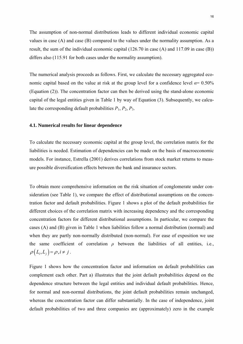
The assumption of non-normal distributions leads to different individual economic capital
values in case (A) and case (B) compared to the values under the normality assumption. As a
result, the sum of the individual economic capital (126.70 in case (A) and 117.09 in case (B))
differs also (115.91 for both cases under the normality assumption).
The numerical analysis proceeds as follows. First, we calculate the necessary aggregated eco-
nomic capital based on the value at risk at the group level for a confidence level α= 0.50%
(Equation (2)). The concentration factor can then be derived using the stand-alone economic
capital of the legal entities given in Table 1 by way of Equation (3). Subsequently, we calcu-
late the corresponding default probabilities P1, P2, P3.
4.1. Numerical results for linear dependence
To calculate the necessary economic capital at the group level, the correlation matrix for the
liabilities is needed. Estimation of dependencies can be made on the basis of macroeconomic
models. For instance, Estrella (2001) derives correlations from stock market returns to meas-
ure possible diversification effects between the bank and insurance sectors.
To obtain more comprehensive information on the risk situation of conglomerate under con-
sideration (see Table 1), we compare the effect of distributional assumptions on the concen-
tration factor and default probabilities. Figure 1 shows a plot of the default probabilities for
different choices of the correlation matrix with increasing dependency and the corresponding
concentration factors for different distributional assumptions. In particular, we compare the
cases (A) and (B) given in Table 1 when liabilities follow a normal distribution (normal) and
when they are partly non-normally distributed (non-normal). For ease of exposition we use
the same coefficient of correlation ρ between the liabilities of all entities, i.e.,
. ( ), ,i jL L i jρ ρ= ≠
Figure 1 shows how the concentration factor and information on default probabilities can
complement each other. Part a) illustrates that the joint default probabilities depend on the
dependence structure between the legal entities and individual default probabilities. Hence,
for normal and non-normal distributions, the joint default probabilities remain unchanged,
whereas the concentration factor can differ substantially. In the case of independence, joint
default probabilities of two and three companies are (approximately) zero in the example

17
considered and only individual default occurs within the group. With increasing dependence,
the probability of a single default (P1) decreases, while the probability of combined defaults
(P2, P3) increases. For higher correlations, the probability of a combined default of two enti-
ties (P2) decreases again. For perfectly correlated liabilities, all three entities default with
probability 0.50%, while P1 = P2 = 0.
FIGURE 1
Default probabilities and risk concentration factor for linear dependence on the basis of Table
1.
a) Joint default probabilities for linear dependence
0.00%
0.20%
0.40%
0.60%
0.80%
1.00%
1.20%
1.40%
1.60%
0 0.1 0.2 0.3 0.4 0.5 0.6 0.7 0.8 0.9 0.95 0.97 0.99 1
rho
P1
P2
P3
b) Risk concentration factor for linear dependence
50%
60%
70%
80%
90%
100%
0 0.1 0.2 0.3 0.4 0.5 0.6 0.7 0.8 0.9 0.95 0.97 0.99 1
rho
normal, case (A)
non-normal, case (A)
normal, case (B)
non-normal, case (B)
Notes: P1 = probability that exactly one entity defaults; P2 = probability that exactly two entities default; P3 = probability that all three entities default.
18
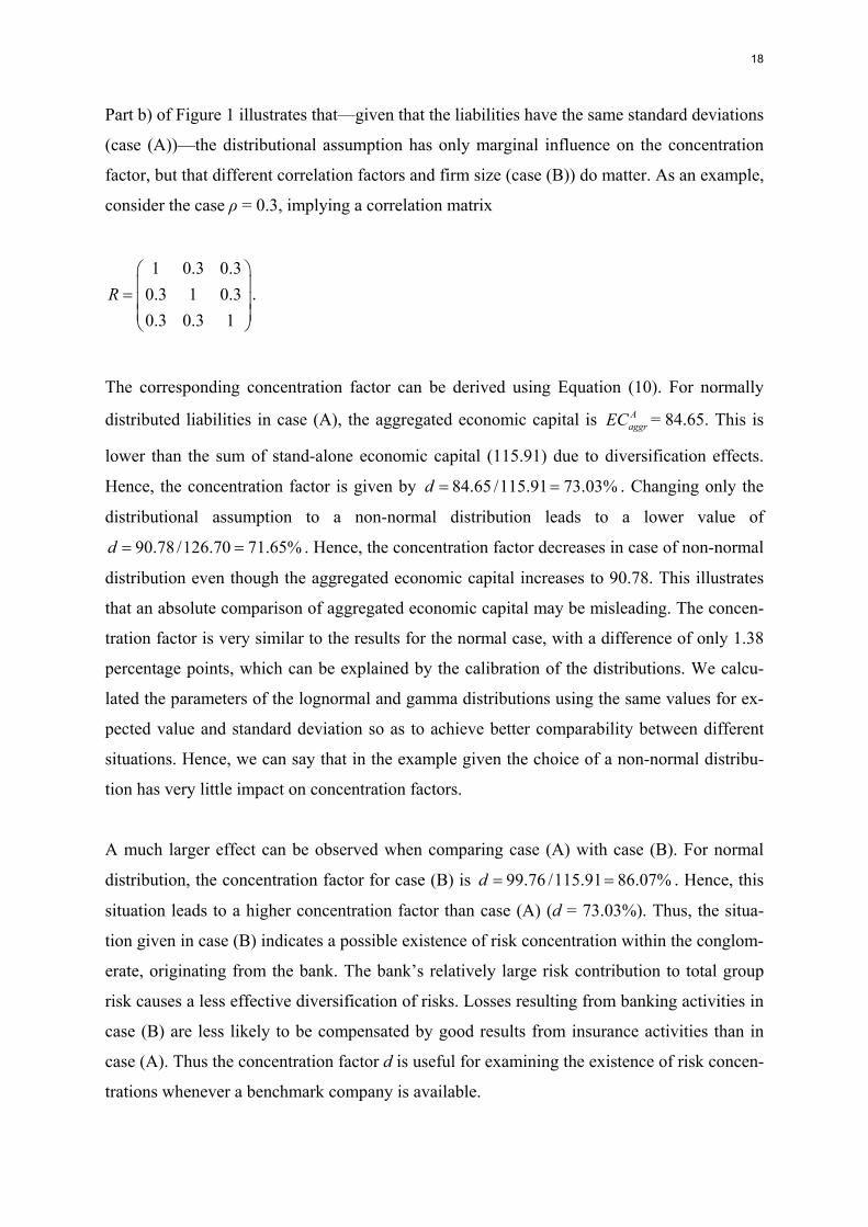
Part b) of Figure 1 illustrates that––given that the liabilities have the same standard deviations
(case (A))––the distributional assumption has only marginal influence on the concentration
factor, but that different correlation factors and firm size (case (B)) do matter. As an example,
consider the case ρ = 0.3, implying a correlation matrix
1 0.3 0.30.3 1 0.30.3 0.3 1
R⎛ ⎞⎜ ⎟= ⎜ ⎟⎜ ⎟⎝ ⎠
.
The corresponding concentration factor can be derived using Equation (10). For normally
distributed liabilities in case (A), the aggregated economic capital is AaggrEC = 84.65. This is
lower than the sum of stand-alone economic capital (115.91) due to diversification effects.
Hence, the concentration factor is given by 84.65 /115.91 73.03%d = = . Changing only the
distributional assumption to a non-normal distribution leads to a lower value of
. Hence, the concentration factor decreases in case of non-normal
distribution even though the aggregated economic capital increases to 90.78. This illustrates
that an absolute comparison of aggregated economic capital may be misleading. The concen-
tration factor is very similar to the results for the normal case, with a difference of only 1.38
percentage points, which can be explained by the calibration of the distributions. We calcu-
lated the parameters of the lognormal and gamma distributions using the same values for ex-
pected value and standard deviation so as to achieve better comparability between different
situations. Hence, we can say that in the example given the choice of a non-normal distribu-
tion has very little impact on concentration factors.
90.78 /126.70 71.65%d = =
A much larger effect can be observed when comparing case (A) with case (B). For normal
distribution, the concentration factor for case (B) is 99.76 /115.91 86.07%d = = . Hence, this
situation leads to a higher concentration factor than case (A) (d = 73.03%). Thus, the situa-
tion given in case (B) indicates a possible existence of risk concentration within the conglom-
erate, originating from the bank. The bank’s relatively large risk contribution to total group
risk causes a less effective diversification of risks. Losses resulting from banking activities in
case (B) are less likely to be compensated by good results from insurance activities than in
case (A). Thus the concentration factor d is useful for examining the existence of risk concen-
trations whenever a benchmark company is available.

19
Overall, Figure 1, part b) demonstrates that the difference between the concentration factors
of cases (A) and (B) decreases with increasing correlation. In the case of perfect positive cor-
relation, ρ = 1, the difference vanishes and the concentration factor takes on its maximum of
100%.
Even though all four curves imply the same joint default probabilities, they have different
risk concentration factors. The differences in d result from changes in the amount of eco-
nomic capital needed to retain a constant default probability.
4.2. Numerical results for nonlinear dependence
In this section, we alter the assumption for the dependence structure and examine the impact
of nonlinear dependencies on risk concentration and joint default probabilities using Clayton
and Gumbel copulas as described in Section 3.1. Both copulas are constructed using Monte
Carlo simulation with the same 200,000 paths so as to increase comparability. The Clayton
and Gumbel copulas are simulated using the algorithms in McNeil, Frey, and Embrechts
(2005, p. 224). The algorithm for the Gumbel copula uses positive stable variates, which were
generated with a method proposed in Nolan (2005).
Numerical results for the Clayton and Gumbel copulas are illustrated in Figures 2 and 3, re-
spectively. In both figures, part a) displays default probabilities as a function of the depend-
ence parameter θ and part b) shows the corresponding concentration factors. The independ-
ence copula marked as Π in the figures serves as a lower boundary, while the case of co-
monotonicity (M) represents perfect dependence and is thus an upper bound.
At first glance, both dependence structures in Figures 2 and 3 appear to lead to similar results
as in the linear case in Figure 1. Overall, the probability that any company defaults decreases
with increasing θ. As before, under perfect comonotonicity, all three entities always become
insolvent at the same time with probability 0.50%, while the probability for one or two de-
faulted companies is zero (P1 = P2 = 0). In fact, in this case, the concentration factor exceeds
100% since the value at risk is not a subadditive risk measure (for a discussion, see Em-
brechts, McNeil, and Straumann, 2002, p. 212).
20
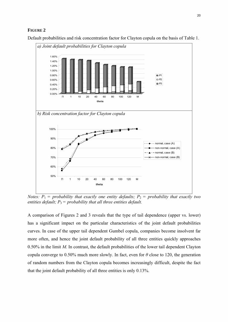
FIGURE 2
Default probabilities and risk concentration factor for Clayton copula on the basis of Table 1.
a) Joint default probabilities for Clayton copula
0.00%
0.20%
0.40%
0.60%
0.80%
1.00%
1.20%
1.40%
1.60%
Π 1 10 20 40 60 80 100 120 M
theta
P1
P2
P3
b) Risk concentration factor for Clayton copula
50%
60%
70%
80%
90%
100%
Π 1 10 20 40 60 80 100 120 M
theta
normal, case (A)
non-normal, case (A)
normal, case (B)
non-normal, case (B)
Notes: P1 = probability that exactly one entity defaults; P2 = probability that exactly two entities default; P3 = probability that all three entities default.
A comparison of Figures 2 and 3 reveals that the type of tail dependence (upper vs. lower)
has a significant impact on the particular characteristics of the joint default probabilities
curves. In case of the upper tail dependent Gumbel copula, companies become insolvent far
more often, and hence the joint default probability of all three entities quickly approaches
0.50% in the limit M. In contrast, the default probabilities of the lower tail dependent Clayton
copula converge to 0.50% much more slowly. In fact, even for θ close to 120, the generation
of random numbers from the Clayton copula becomes increasingly difficult, despite the fact
that the joint default probability of all three entities is only 0.13%.
21
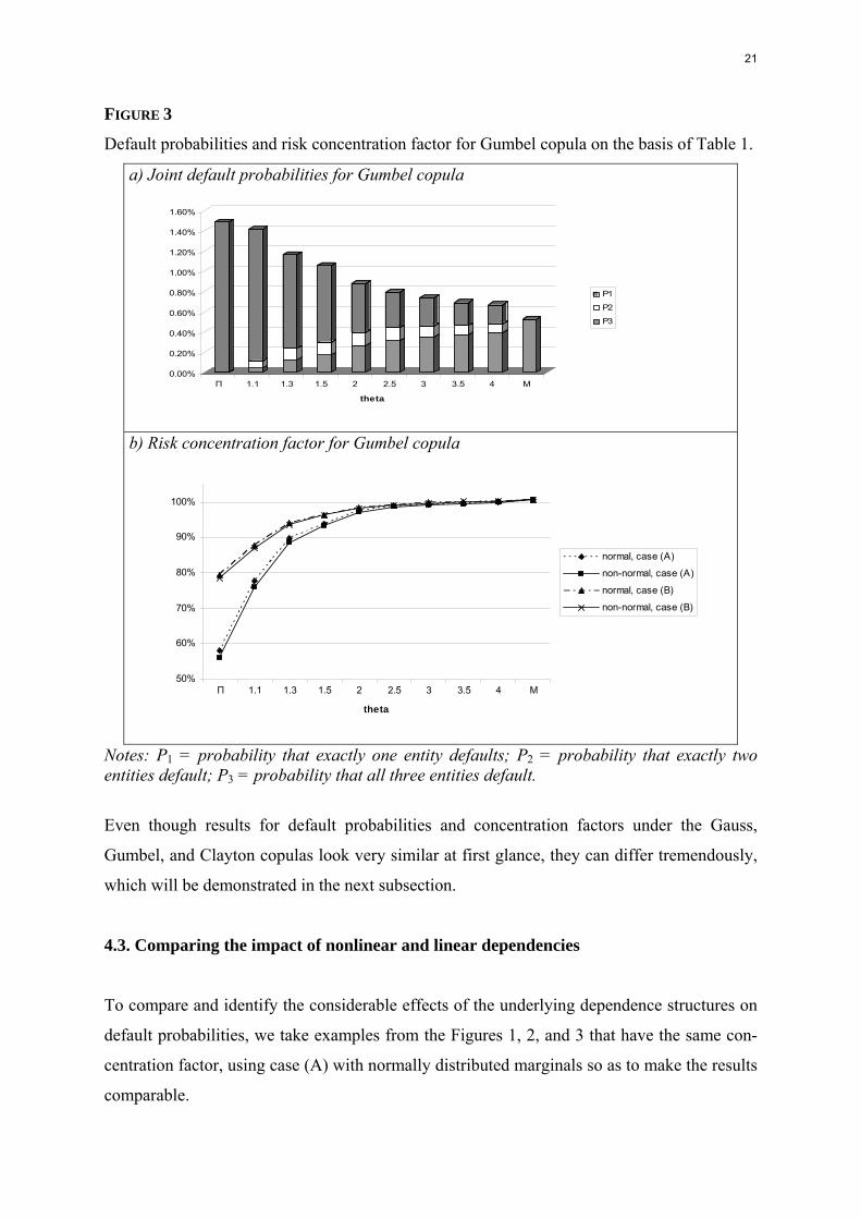
FIGURE 3
Default probabilities and risk concentration factor for Gumbel copula on the basis of Table 1.
a) Joint default probabilities for Gumbel copula
0.00%
0.20%
0.40%
0.60%
0.80%
1.00%
1.20%
1.40%
1.60%
Π 1.1 1.3 1.5 2 2.5 3 3.5 4 M
theta
P1
P2
P3
b) Risk concentration factor for Gumbel copula
50%
60%
70%
80%
90%
100%
Π 1.1 1.3 1.5 2 2.5 3 3.5 4 M
theta
normal, case (A)
non-normal, case (A)
normal, case (B)
non-normal, case (B)
Notes: P1 = probability that exactly one entity defaults; P2 = probability that exactly two entities default; P3 = probability that all three entities default.
Even though results for default probabilities and concentration factors under the Gauss,
Gumbel, and Clayton copulas look very similar at first glance, they can differ tremendously,
which will be demonstrated in the next subsection.
4.3. Comparing the impact of nonlinear and linear dependencies
To compare and identify the considerable effects of the underlying dependence structures on
default probabilities, we take examples from the Figures 1, 2, and 3 that have the same con-
centration factor, using case (A) with normally distributed marginals so as to make the results
comparable.
22
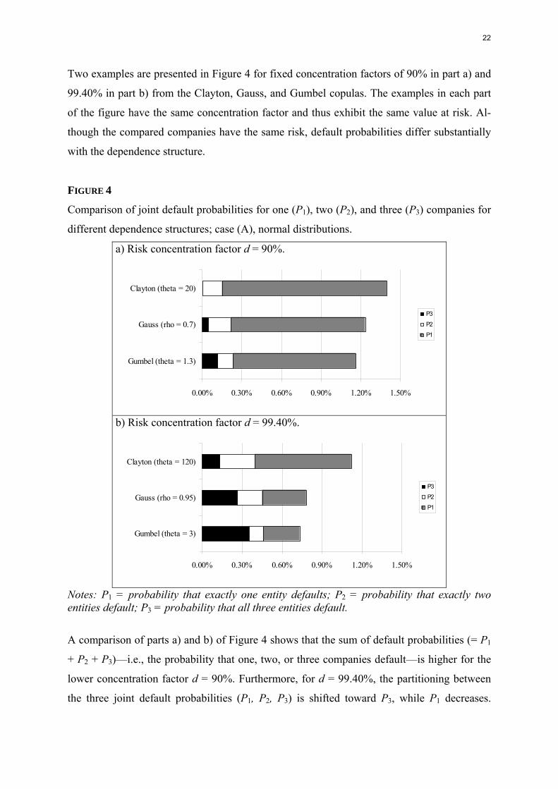
Two examples are presented in Figure 4 for fixed concentration factors of 90% in part a) and
99.40% in part b) from the Clayton, Gauss, and Gumbel copulas. The examples in each part
of the figure have the same concentration factor and thus exhibit the same value at risk. Al-
though the compared companies have the same risk, default probabilities differ substantially
with the dependence structure.
FIGURE 4
Comparison of joint default probabilities for one (P1), two (P2), and three (P3) companies for
different dependence structures; case (A), normal distributions.
a) Risk concentration factor d = 90%.
0.00% 0.30% 0.60% 0.90% 1.20% 1.50%
Gumbel (theta = 1.3)
Gauss (rho = 0.7)
Clayton (theta = 20)
P3
P2
P1
b) Risk concentration factor d = 99.40%.
0.00% 0.30% 0.60% 0.90% 1.20% 1.50%
Gumbel (theta = 3)
Gauss (rho = 0.95)
Clayton (theta = 120)
P3
P2
P1
Notes: P1 = probability that exactly one entity defaults; P2 = probability that exactly two entities default; P3 = probability that all three entities default.
A comparison of parts a) and b) of Figure 4 shows that the sum of default probabilities (= P1
+ P2 + P3)––i.e., the probability that one, two, or three companies default––is higher for the
lower concentration factor d = 90%. Furthermore, for d = 99.40%, the partitioning between
the three joint default probabilities (P1, P2, P3) is shifted toward P3, while P1 decreases.
23
Hence, a higher concentration factor is accompanied by a lower sum of default probabilities,
but induces a significantly higher joint default probability of all three entities.
Figure 4 demonstrates the considerable influence that the choice between Clayton, Gauss, and
Gumbel copulas has on joint default probabilities. The Clayton copula leads to the highest
sum of default probabilities, but has the lowest probability of default for all three companies
(P3). The other extreme occurs under the Gumbel copula, where P3 is highest and P1 takes the
lowest value, while the Gauss copula induces values between those of the Clayton and Gum-
bel copulas.
Our results show that even if different dependence structures imply the same value at risk and
thus the same risk concentration factor, joint default probabilities can differ tremendously.
Furthermore, our analysis demonstrates that the simultaneous reporting of risk concentration
factors and default probabilities can be of substantial value, especially for the management of
the corporate group. By comparing linear and nonlinear dependencies, we found that the ef-
fect of mismodeling dependencies may not only lead to significant differences in assessing
risk concentration, but can also lead to misestimating joint default probabilities. Hence, there
is a substantial model risk involved with respect to dependence structures.
5. SUMMARY
This paper assessed and related risk concentrations and joint default probabilities of legal
entities in a conglomerate composed of three entities, a bank, a life insurance company, and a
non-life insurance company. Our procedure provided valuable insight regarding the group’s
risk situation, which is highly relevant for enterprise risk management purposes. An insur-
ance group (a conglomerate) typically consists of several legally independent entities, each
with limited liability. However, diversification concepts assume that these entities are fully
liable and all together meet all outstanding liabilities of each. Even if diversification is of no
importance from a policyholder perspective, it is useful in determining risk concentration in
an insurance group because greater diversification generally implies less risk.
To determine default probabilities, we focused on the case of limited liability without transfer
of losses between the different legal entities within the group. Joint default probabilities only

24
depend on individual default probabilities and the coupling dependence structure. Hence, we
studied the effect of different dependence structures using the concept of copulas.
In the numerical analysis, we considered an insurance group comprised of three legal entities
and compared results from the Gauss, Gumbel, and Clayton copulas for normal and non-
normal marginal distributions. Economic capital was adjusted for each situation to satisfy a
fixed individual default probability. In contrast to the risk concentration factor, joint default
probabilities only depend on individual default probabilities and on the dependence structure,
not on distributional assumptions.
For all models, we found that the risk concentration factor and the joint default probability of
all three entities increase with increasing dependence between the entities, while the probabil-
ity of a single default decreases. Overall, the sum of default probabilities of one, two, or three
entities decreases with increasing dependence. Furthermore, one entity’s large risk contribu-
tion, in terms of volatility, led to a much higher risk concentration factor for the group as a
whole. Our findings further demonstrated that even if different dependence structures imply
the same risk concentration factor for the group, joint default probabilities for different sets of
subsidiaries can vary tremendously. In particular, the lower tail dependent Clayton copula led
to the lowest probability of default for all three entities, while the upper tail dependent Gum-
bel copula exhibited the highest default probability.
The analysis showed that a simultaneous consideration of risk concentration factor and de-
fault probabilities can be of substantial value, especially for the management of the corporate
group with respect to enterprise risk management.
25
REFERENCES
Amel, D., Barnes C., Panetta, F., and Salleo, C. (2004): Consolidation and Efficiency in the
Financial Sector: A Review of the International Evidence. Journal of Banking & Finance
28(10), 2493–2519
CAS (2003): Overview of Enterprise Risk Management. Available at
http://www.casact.org/research/erm/.
Casella, G., and Berger, R. L. (2002): Statistical Inference. Duxbury Press, Pacific Grove.
CEIOPS (2006): Advice to the European Commission in the Framework of the Solvency II
Project on Sub-Group Supervision, Diversification Effects, Cooperation with Third Coun-
tries and Issues Related to the MCR and SCR in a Group Context (CEIOPS-CP-05/06).
Available at http://www.ceiops.org/content/view/14/18.
Daykin, C. D., Pentikainen, T., and Pesonen, M. (1994): Practical Risk Theory for Actuaries.
Chapman & Hall, London.
Dimakos, X. K., and Aas, K. (2004): Integrated Risk Modelling. Statistical Modelling 4(4),
265–277.
Embrechts, P., Lindskog, F., and McNeil, A. J. (2003): Modelling Dependence with Copulas
and Applications to Risk Management. In Rachev, S. (ed.): Handbook of Heavy Tailed
Finance , pp. 329–384. Elsevier.
Embrechts, P., McNeil, A., and Straumann, D. (2002): Correlation and Dependence in Risk
Management: Properties and Pitfalls. In Dempster M. A. H. (ed.): Risk Management:
Value at Risk and Beyond, pp. 176–223. Cambridge University Press, Cambridge.
Estrella, A. (2001): Mixing and Matching: Prospective Financial Sector Mergers and Market
Caluation. Journal of Banking and Finance 25(12), 2367–2392.
European Commission (2005): Policy Issues for Solvency II––Possible Amendments to the
Framework for Consultation (Markt/2505/01). Brussels.
Faivre, F. (2003): Copula: A New Vision for Economic Capital and Application to a Four
Line of Business Company. Paper presented at ASTIN Colloquium, Berlin.
Frees, E. W., and Valdez, E. V. (1998): Understanding Relationships Using Copulas. North
American Actuarial Journal 2(1), 1–25.
Frey, R., and McNeil, A. J. (2001): Modelling Dependent Defaults. ETH E-Collection,
Zürich. Available at http://e-collection.ethbib.ethz.ch.
Groupe Consultatif (2005): Diversification—Technical Paper. Working Group “Group and
Cross-Sectoral Consistency.” Available at http://www.gcactuaries.org/solvency.html.
26
Hull, J. C. (2003): Options, Futures and Other Derivatives. Pearson Education, Upper Saddle
River, NJ.
Iman, R. L., and Conover, W. (1982): A Distribution Free Approach to Inducing Rank Corre-
lation Among Input Variables. Communications in Statistics—Simulation and Computa-
tion, 11(3), 311–334.
Kuritzkes, A., Schuermann, T., and Weiner, S. M. (2003): Risk Measurement, Risk Manage-
ment and Capital Adequacy in Financial Conglomerates. In Brookings-Wharton Papers
on Financial Services, pp. 141–193.
Li, D. X. (2000): On Default Correlation: A Copula Function Approach. Journal of Fixed
Income 9(4), 43–54.
McNeil, A. J., Frey, R., and Embrechts, P. (2005): Quantitative Risk Management. Concepts,
Techniques, Tools. Princeton University Press, Princeton, NJ.
Nelsen, R. B. (1999): An Introduction to Copulas. Springer, New York.
Nolan, J. P. (2005): Stable Distributions: Models for Heavy Tailed Data, forthcoming.
Rosenberg, J., and Schuermann, T. (2006): A General Approach to Integrated Risk Manage-
ment with Skewed, Fat-tailed Risks. Journal of Financial Economics 79(3), 569–614.
Tang, A., and Valdez, E. A. (2006): Economic Capital and the Aggregation of Risks Using
Copula. Paper presented at the 28th International Congress of Actuaries, Paris. Available
at http://papers.ica2006.com.
Wang, S. (1998): Aggregation of Correlated Risk Portfolios: Models and Algorithms. Pro-
ceedings of the Casualty Actuarial Society 85, 848–939.
Wang, S. (2002): A Set of New Methods and Tools for Enterprise Risk Capital Management
and Portfolio Optimization. In The Casualty Actuarial Society Forum, Summer 2002, Dy-
namic Financial Analysis Discussion Papers, pp. 43–77.
Ward, L. S., and Lee, D. H. (2002): Practical Application of the Risk Adjusted Return on
Capital Framework. In The Casualty Actuarial Society Forum, Summer 2002, Dynamic
Financial Analysis Discussion Papers, pp. 79–126.
Wu, F., Valdez, E. A., and Sherris, M. (2006): Simulating Exchangeable Multivariate Archi-
medean Copulas and its Applications. Working Paper, University of New South Wales,
Sydney.
Related Documents