Enskog-like discrete velocity models for vehicular traffic flow

NETWORKS AND HETEROGENEOUS MEDIA Website: http://aimSciences.orgc©American Institute of Mathematical SciencesVolume 2, Number 3, September 2007 pp. 481–496

ENSKOG-LIKE DISCRETE VELOCITY MODELS FOR

VEHICULAR TRAFFIC FLOW

Michael Herty

AG Technomathematik, Fachbereich MathematikUniversitat Kaiserslautern

D-67663 Kaiserslautern, Germany

Lorenzo Pareschi

Department of MathematicsUniversity of FerraraI-44100 Ferrara, Italy

Mohammed Seaıd

AG Technomathematik, Fachbereich MathematikUniversitat Kaiserslautern

D-67663 Kaiserslautern, Germany

(Communicated by Axel Klar)

Abstract. We consider an Enskog-like discrete velocity model which in thelimit yields the viscous Lighthill-Whitham-Richards equation used to describevehicular traffic flow. Consideration is given to a discrete velocity model withtwo speeds. Extensions to the Aw-Rascle system and more general discrete ve-locity models are also discussed. In particular, only positive speeds are allowedin the discrete velocity equations. To numerically solve the discrete velocityequations we implement a Monte Carlo method using the interpretation thateach particle corresponds to a vehicle. Numerical results are presented for twopractical situations in vehicular traffic flow. The proposed models are able

to provide accurate solutions including both, forward and backward movingwaves.

1. Introduction. During the past decades several models have been proposed formathematical studies on vehicular traffic flow, see for example [1, 2, 6, 8, 9, 14, 15,16, 20] and further references are therein. These models present different techniquesto describe dynamics of vehicles in a single road or networks. In the current work,we are interested in mathematical models derived from partial differential equa-tions and also known by macroscopic models, compare [2, 5, 16, 19] among others.Recently, macroscopic models has also been applied to road networks by solvingthe associated partial differential equation on each arc (road) of the network, werefer the reader to [4, 11, 12, 13] for more details. The Lighthill-Whitham-Richards(LWR) model [16] is widely considered as one of the most simple models to de-scribe vehicular traffic flow. It simplicity lies on the fact that the LWR equationis a scalar conservation law with strictly concave flux function which can be solved

2000 Mathematics Subject Classification. Primary: 65C05, 90B20; Secondary: 82B40.Key words and phrases. Lighthill-Whitham-Richards model, Discrete-velocity equations,

Monte Carlo method.

481

482 MICHAEL HERTY, LORENZO PARESCHI AND MOHAMMED SEAID

using well-established numerical methods. Therefore, the LWR model has becomea prototype for theoretical and numerical investigations in vehicular traffic flow. Asother mathematical equations for traffic flow, we cite the so-called ’second-order’models, see for instance [2, 5, 19].

The objective of the present study is to obtain a kinetic formulation for the LWRequation using only positive speeds and then to derive a Monte-Carlo method for itsnumerical treatment. The particles in the latter could then be interpreted as singlecars of non–negative traveling speed. The Monte Carlo method has been successfullyused in numerical solution of gas dynamics and has found many other applications,see [18] and other references can be found therein. However, to the best of ourknowledge, this is the first time that Monte Carlo method is used to solve problemsin traffic flow. There are two main reasons for considering this method. The first isthat the Monte Carlo method can provide a fast and reliable computations for trafficflow and also a possible extension to networks. For instance, solving large scaletraffic networks, fully discrete methods require tremendous computational effort. AMonte Carlo method however, allows to resolve different parts of the network by adifferent number of particles (samples) which their dynamic in the network can beobtained by solving the LWR or ’second-order’ models. The second reason is thatdescribing vehicles as particles, the Monte Carlo method can be interpreted as anatural way to describe uncertainty in the traffic behavior such as driver reactions.This stochastic effects in traffic flow can be easily incorporated in the Monte Carlomethod.

The Monte Carlo algorithm proposed in this paper is based on a kinetic discretevelocity model proposed and studied by the authors in [10]. Here, we introducea new formulation of traffic flow models including a “look-ahead” distance whichyields an Enskog-like kinetic approximation. This discrete velocity model consti-tutes the basis of our Monte Carlo method. Numerical results and examples arecarried out using the LWR equation, but our Monte Carlo method can be appliedalso to the ’second-order’ Aw-Rascle model [2]. At the appropriate places we com-ment on possible extensions and modifications.

The outline of this paper is as follows. In section 2 we briefly describe theequations of vehicular traffic flow used to develop our Monte Carlo algorithm. Thekinetic discrete velocity model is formulated in section 3. In section 4 we discussthe probabilistic Monte Carlo method for solving the kinetic equations. Numericalresults for two test examples are presented in section 5. Section 6 summarizes thepaper with concluding remarks.

2. Traffic flow equations. For the sake of simplicity we formulate our MonteCarlo method for traffic flow models governed by partial differential equations ofLWR type. However, all the derivations presented in this paper can be applied to’second-order’ traffic flow models without major conceptual modifications.

The LWR model requires only a state equation for traffic flow that relates thevelocity to density and is mainly based on traffic observations. It is formulated bya scalar equation of conservation law written in dimensional form as

ρt + V (ρ)x = 0, (1)

where ρ = ρ(x, t) is the density of vehicles at position x and time t. The fluxfunction V (ρ), which may depend on space x as well, is defined by

V (ρ) = ρve(ρ), (2)

ENSKOG-LIKE DISCRETE VELOCITY MODELS FOR VEHICULAR TRAFFIC FLOW 483

where ve(ρ) is an equilibrium velocity known in traffic flow terminology by the fun-damental diagram. The fundamental diagram is a necessary condition to describethe rate relationship between density and flow fields. In most applications, it isdetermined by empirical evidence of traffic behaviour. A well-established choice forthe fundamental diagram ve(ρ) is

ve(ρ) = vm

(

1− ρ

ρm

)

, (3)

with ρm and vm are the maximum density and the maximum speed, respectively.Since it is more convenient to work with non-dimensional model than its dimensionalcounterpart, we define the following non-dimensional variables

t∗ =Lt

vm

, x∗ =x

L, ρ∗ =

ρ

ρm

, v∗ =v

vm

,

where L denotes the length of the traffic road. Hence, the dimensionless equationsgoverning the LWR model (1) can be rewritten as

ρt + V (ρ)x = 0, (4)

where we have dropped the asterisk of the dimensionless variables for ease of nota-tion. The dimensionless flux function in (2) becomes

V (ρ) = ρ (1− ρ) . (5)

Thus, the equations (4)-(5) has to be solved in the spatial domain [0, 1] and timeinterval [0, T ] subject to a given initial condition

ρ(x, 0) = ρ0(x). (6)

It is easy to verify that the non-dimensional density satisfies

0 ≤ ρ(x, t) ≤ 1. (7)

Note that more general flux functions can also be incorporated in the followingdiscussions. Motivated by the ideas reported in [10] we introduce a class of discretevelocity models as an approximation of equations (4)-(6). It should be stressedthat, for traffic flow in networks, fast numerical methods are usually required forthe treatment of possibly high dimensions of the problem, compare [12, 13] for someexamples. In the present study, we consider the simple discrete velocity model pro-posed in [10] for vehicular traffic flow. This Enskog-type kinetic model contains onlypositive velocities and accounted for a “look-ahead” concept to recover backwardwaves in traffic dynamics. In addition, the discrete velocity model asymptoticallypreserves the “correct” LWR limit. A Monte Carlo method is developed based onthe considered kinetic model and is formulated for the LWR model. However, thisapproach also applies to the second-order models in traffic flow, see Remark 3.2.

3. Enskog-like discrete velocity model. Discrete velocity models for vehiculartraffic flow have been studied by the authors in [10]. In this reference, we haveproposed a class of two- and three-speed discrete velocity models with positivespeeds only. Deterministic methods based on relaxation discretization and implicit-explicit schemes were used to approximate numerical solutions to the kinetic discretevelocity models. In the current work, we propose a different approach to reconstructkinetic models for traffic flow with positive finite speeds. The emphasis is given toa two-speed kinetic model for the LWR problem in a single road. In contrast todiscrete velocity models derived in [10], the proposed model incorporate the concept

484 MICHAEL HERTY, LORENZO PARESCHI AND MOHAMMED SEAID

of “look-ahead” principle in its formulation. This property avoids some limitationsconcerned with subcharacteristic conditions and fits with the frame of “follow theleader” in traffic flow modelling.

3.1. Two speed models. Let us consider two nonnegative speeds v1 and v2, andkinetic variables f(x, t) and g(x, t) corresponding to vehicles or particles with speedv1 and v2, respectively. Without loss of generality, we assume

0 ≤ v1 <V (ρ)

ρ< v2. (8)

We define the (vehicle-)density ρ and the flux J as

ρ(x, t) = f(x, t) + g(x, t),(9)

J(x, t) = v1f(x, t) + v2g(x, t).

A discrete Enskog model for the kinetic variables f and g reads

ft(x, t) + v1fx(x, t) = −1

ǫ

(

f(x, t)Eg(x + h, t)− g(x, t)Ef (x+ h, t))

, (10)

gt(x, t) + v2gx(x, t) = −1

ǫ

(

g(x, t)Ef (x+ h, t)− f(x, t)Eg(x+ h, t))

, (11)

where ǫ > 0 is the relaxation time and h > 0 is the “look-ahead” distance. Theequilibrium states Ef (x, t) = Ef (ρ(x, t)) and Eg(x, t) = Eg (ρ(x, t)) are implicitlydefined according to

f + g = ρ,(12)

v1f + v2g = J = V (ρ),

and therefore, fulfill

Ef (x, t) =ρ(x, t)

v2 − v1

(

v2 −V (ρ(x, t))

ρ(x, t)

)

,

(13)

Eg(x, t) =ρ(x, t)

v2 − v1

(

V (ρ(x, t))

ρ(x, t)− v1

)

.

Note that by virtue of (12) the kinetic system can be written as

ft(x, t) + v1fx(x, t) = −1

ǫ

(

ρ(x+ h, t)f(x, t)− ρ(x, t)Ef (x+ h, t))

, (14)

gt(x, t) + v2gx(x, t) = −1

ǫ

(

ρ(x+ h, t)g(x, t)− ρ(x, t)Eg(x+ h, t))

. (15)

For notational convenience we set ρh = ρ(x + h, t) and similarly for Ehf and Eh

g .

Next, before we discuss properties of the model (10)-(11) and derive the viscousLWR limit, the kinetic model (10)-(11) can be interpreted as follows. Accordingto condition (8) and due to equation (10), slower vehicles will speed up dependingon the number of fast vehicles in the next cell i.e., at position x + h. In fact, theloss term in equation (10) is fEh

g and therefore the loss is not proportional to the

actual number of fast vehicles (gh) but, to the number of fast vehicles being in theequilibrium Eh

g . Similarly, the gain term for (10) is gEhf and therefore, vehicles of

fast speed will slow down proportionally to the number of vehicles in the next cell

ENSKOG-LIKE DISCRETE VELOCITY MODELS FOR VEHICULAR TRAFFIC FLOW 485

assumed to be at the equilibrium. The parameter h describes therefore the “look-ahead” distance. These ideas are inspired from an Enskog-like modelling takinginto account the size of the interacting particles.

From (10)-(11) we formally obtain the following macroscopic equations

ρt + Jx = 0, (16)

Jt + (v1 + v2)Jx − v1v2ρx = −1

ǫ

(

ρhJ − ρV (ρh))

. (17)

In the zeroth order expansion for ǫ, the above equations yield

ρt +

(

ρ

ρhV (ρh)

)

x

= 0. (18)

In the case of the flux function (5) and for small values of h (h≪ 1) we obtain theviscous LWR equation

ρt + (ρ(1 − ρ))x =h

2

(

ρ2)

xx+O(h2). (19)

Hence, in the small relaxation limit ǫ −→ 0 and for small “look-ahead” distanceh≪ 1, the two-speed discrete velocity model (10)-(11) is an approximation for theLWR equation with an additional diffusive term i.e, it approximately solves

ρt + (ρ(1 − ρ))x =h

2

(

ρ2)

xx. (20)

For a more general flux function of the form V (ρ) = ρv(ρ) the same asymptoticanalysis leads to the approximate equation

ρt + (ρv(ρ))x = −h (v′(ρ)ρx)x , (21)

which is dissipative provided the condition v′(ρ) < 0 is satisfied. We end themodelling part with the following remarks:

Remark 1. First, compared to other discrete velocity models as those proposedfor example in [17, 10], there is no condition necessary to ensure the dissipativenature of (10)-(11). In other words, no subcharacteristic condition is required forits stability.

Second, discrete velocity models with more than two speeds can also be derived.For a M speeds vm with M > 2 and the kinetic variables fm the general form isthen

∂tfm + vm∂xfm = −1

ǫ

(

fmρh − ρEh

fm

)

, m = 1, . . . ,M, (22)

where the equilibrium distributions Efmare defined such that

M∑

m=1

Efm= ρ,

(23)M∑

m=1

Efmvm = V (ρ).

Note that, except for the case of M = 2, the constraints (23) are not sufficient toderive unique expressions for Efm

. As in the classical BGK model for gas dynamics,additional conservation laws might be introduced to obtain uniqueness.

486 MICHAEL HERTY, LORENZO PARESCHI AND MOHAMMED SEAID

3.2. Four speed models. Another class of models arising in the literature ontraffic flow are so called ’second-order’ models. They consist of a 2x2 system ofconservation laws and have been derived by borrowing ideas from gas dynamicapproaches and apply them to traffic flow. We refer the reader to [2, 19] a discussionof the various approaches. One recent model is the Aw-Rascle (AR) model proposedin [2]. This model has several advantages over the previously proposed models,e.g. Payne-Whitham, and has been under investigation for several years [2, 7, 14].Written in a conservative form, the AR model is given by

ρt + (ρv(ρ, y))x = 0,

(24)

yt + (yv(ρ, y))x = 0,

where ρ is the total density of cars and

ρ v(ρ, y) = y − ρ p(ρ).

As stated in [2] there is no physical interpretation of the ’momentum’ variable y in(24). However, the quantity w = y/ρ is invariant in the mass-Lagrangian coordinatesystem and hence may be interpreted as “quality” (e.g. color) of a specific car. Thepressure term p(ρ) is an anticipation factor that takes into account drivers reactionsto the state of traffic in front of them. It has to satisfy the following assumptions:

(i) p(ρ) ≈ ργ , for ρ→ 0 with γ > 0.

(ii) ρp′′(ρ) + 2p′(ρ) > 0, for all ρ.

There are many ways to reconstruct discrete velocity models associated with theAR traffic flow model. Here, we propose a kinetic discrete velocity model with fourspeeds given by the following equations

ft + v1fx = −1

ε

(

f(x, t)Eg(x+ h, t)− g(x, t)Ef (x+ h, t))

,

gt + v2gx = −1

ε

(

g(x, t)Ef (x + h, t)− f(x, t)Eg(x+ h, t))

,

(25)

kt + v3kx = −1

ε

(

k(x, t)Ej(x+ h, t)− j(x, t)Ek(x+ h, t))

,

jt + v4jx = −1

ε

(

j(x, t)Ek(x+ h, t)− k(x, t)Ej(x+ h, t))

,

where ε is the relaxation time, h > 0 is the “look-ahead” distance, vi (i = 1, . . . , 4)are nonnegative speeds, and f , g, k and j are the kinetic variables assumed totravel with speeds v1, v2, v3 and v4, respectively. Again, we assume without loss ofgenerality

v2 > v(ρ, y) > v1 ≥ 0 and v4 > v(ρ, y) > v3 ≥ 0.

The equilibrium states Ef , Eg, Ek and Ej are defined according to

Ef + Eg = ρ,

Ek + Ej = y,(26)

v1Ef + v2Eg = ρv(ρ, y),

v3Ek + v4Ej = yv(ρ, y),

ENSKOG-LIKE DISCRETE VELOCITY MODELS FOR VEHICULAR TRAFFIC FLOW 487

Following the same procedure as in the LWR model, the equilibrium states can beexplicitly calculated as

Ef =ρ

v2 − v1(v2 − v(ρ, y)) , Eg =

ρ

v2 − v1(v(ρ, y)− v1) ,

(27)Ek =

y

v4 − v3(v4 − v(ρ, y)) , Ej =

y

v4 − v3(v(ρ, y)− v3) .

In addition, the associated macroscopic model to (25) reads

ρt + Jx = 0,

yt +Wx = 0,(28)

Jt + (v1 + v2)Jx − v1v2ρx = −ρh

ε

(

J − ρv(ρh, yh))

,

Wt + (v3 + v4)Wx − v3v4yx = −yh

ε

(

W − yv(ρh, yh))

,

where ρ = f + g, y = k + j, J = v1f + v2g and W = v3k + v4j.In the leading order for small ε the equations (28) reduces to

ρt +(

ρv(ρh, yh))

x= 0,

(29)yt +

(

yv(ρh, yh))

x= 0.

For small values of h, using a Taylor expansion one gets up toO(h2) the approximatesystem

ρt + (ρv(ρ, y))x = −h (ρv(ρ, y)x)x ,(30)

yt + (yv(ρ, y))x = −h (yv(ρ, y)x)x .

The above system is parabolic if the diffusion matrix

−ρv(ρ, y)ρ −ρv(ρ, y)y

−yv(ρ, y)ρ −yv(ρ, y)y

(31)

has nonnegative eigenvalues. A simple computation shows that the eigenvalues of(31) are given by

λ1 = −ρv(ρ, y)ρ − ρv(ρ, y)ρ = ρp′(ρ), λ2 = 0,

and thus the parabolicity condition is fulfilled if p′(ρ) > 0.

Remark 2. The physical interpretation of the above four speed discrete velocitymodel is less straightforward then in the LWR case. Here we do not advocatethe validity of the discrete velocity kinetic model for large values of the relaxationparameter but only in the limit as a tool for the construction of the Monte Carlomethod. The development of more realistic four speeds models is actually underconsideration.

4. Probabilistic Monte Carlo method. To solve numerically the discrete veloc-ity kinetic models proposed in the previous section we apply a Monte Carlo methodpreviously applied to Boltzmann equation [18], rarefied gas dynamics [3], and Burg-ers equation [17]. Our method is asymptotic preserving, simple to implement and

488 MICHAEL HERTY, LORENZO PARESCHI AND MOHAMMED SEAID

approximate solution to the kinetic model with zero numerical viscosity. To sim-plify the presentation we restrict ourselves to the LWR case. The AR model can betreated in a similar way.

We start from the two speed model written in the form (14)-(15). Then, to solvenumerically the system we split the problem into two stages.

(1) The transport stage

ft + v1fx = 0,(32)

gt + v2gx = 0.

(2) The relaxation stage

ft = −1

ǫ

(

fρh − Ehf ρ

)

,

(33)

gt = −1

ǫ

(

gρh − Ehg ρ

)

.

Again, due to the Enskog-like interaction terms, no subcharacteristic condition isneeded. However, to have a probabilistic interpretation of the above variables, weshould have

f ≥ 0, g ≥ 0,f

ρ+g

ρ= 1,

which, at the limit (ǫ −→ 0), is equivalent to impose

v1 ≤V (ρ)

ρ≤ v2.

To discretize the equations (32)-(33) in time we divide the time interval into subin-tervals [tn, tn+1] with tn = n∆t and we denote by ψn the value of a generic functionψ at time tn. During the relaxation stage we have ρ(x, tn+1) = ρ(x, tn) and similarlyfor ρh. Hence, we can integrate the relaxation step exactly and obtain

f(x, tn+1) = (1− λ)f(x, tn) + λEh

f (ρ(x, tn))ρ(x, tn)

ρh(x, tn),

(34)

g(x, tn+1) = (1− λ)g(x, tn) + λEh

g (ρ(x, tn))ρ(x, tn)

ρh(x, tn),

where λ is given by

λ = 1− e−∆t

ǫρh(x, tn)

. (35)

It is obvious from (35) that 0 ≤ λ ≤ 1. Now let us define the probability density attime tn as follows

Pn(ξ) =

fn

ρn, if ξ = v1,

gn

ρn, if ξ = v2,

0, elsewhere.

Note that 0 ≤ Pn(ξ) ≤ 1 and∑

ξ Pn(ξ) = 1. Moreover

∑

ξ

Pn+1(ξ) =∑

ξ

Pn(ξ) = 1.

ENSKOG-LIKE DISCRETE VELOCITY MODELS FOR VEHICULAR TRAFFIC FLOW 489

The system (33) can be seen as an evolution of the probability function Pn(ξ)according with

Pn+1(ξ) =

(1− λ)fn

ρn+ λ

ρn

ρh,nEh

f (ρn), if ξ = v1,

(1− λ)gn

ρn+ λ

ρn

ρh,nEh

g (ρn), if ξ = v2,

0, elsewhere.

(36)

Let {ξ1, ξ2, . . . , ξN} be the particle samples, we know that ξj = v1 or ξj = v2 withprobability fn/ρn or gn/ρn, respectively. We also have the relation

Pn+1(ξ) = (1− λ)Pn(ξ) + λEn(ξ), (37)

where En(ξ) is defined as

En(ξ) =

ρn

ρh,nEf (ρn), if ξ = v1,

ρn

ρh,nEg(ρ

n), if ξ = v2,

0, elsewhere.

Hence, the relaxation stage (33) can be solved in the following way.

1. Given a particle sample ξ the evolution of the sample during a time integration

process is performed according to:

i. With probability (1− λ) the sample is unchanged.

ii. With probability λ the sample is replaced with a sample from En(ξ).

2. To sample a particle from En(ξ) we proceed as follows:

i. With probability Ef (ρ) take ξ = v1.

ii. With probability Eg(ρ) take ξ = v2.

To generate particles, we first divide the spatial domain into a finite sequence ofcells Ii = [xi− 1

2

, xi+ 1

2

] with uniform stepsize ∆x and centered in the gridpoint xi.

Then particles are generated from a given piecewise constant initial data in eachcell and are randomly distributed around the cell center xi. A simple way to carrythis step out is to evaluate the histograms of samples on the cells Ii. For a set of Nsamples p1, p2, · · · , pN , we define the associated discrete probability density locatedat the gridpoint xi by

p(xi) =1

N

N∑

j=1

δIi(pj − xi)

∆x, (38)

where δIi(x) is the Kronecker delta function defined as

δIi(x) =

1, if x ∈ Ii,

0, elsewhere.

490 MICHAEL HERTY, LORENZO PARESCHI AND MOHAMMED SEAID

Once the particle distribution is updated by the above steps, the transport stage ofthe splitting (32) is realized by advecting the position of the particles according totheir speeds as

fn+1i = f (xi − v1∆t, tn) ,

(39)gn+1

i = g (xi − v2∆t, tn) .

Thus, given a sample of N particles at positions xn1 , x

n2 , · · · , xn

N and speedsξ1, ξ2, · · · , ξN (equal either to v1 or v2) the new position of the particle sample{xn+1

i , ξi} is simply

xni = xn+1

i + ξi∆t, i = 1, . . . , N,

where xn+1i and xn

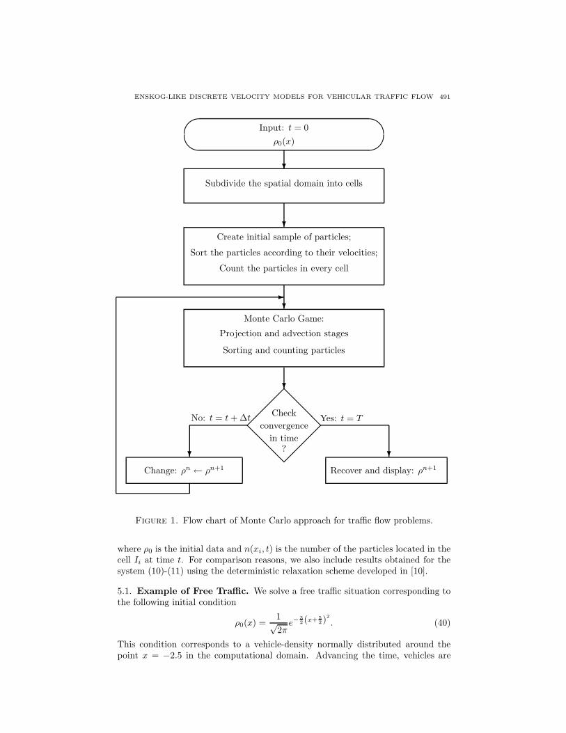
i are respectively, the new and old positions of the sample ξi. Tosummarize, Figure 1 illustrates the flow chart of the proposed Monte Carlo approachfor the kinetic discrete velocity model (10)-(11).

Remark 3. Some remarks are in order:

1. Note that the splitting implemented in the present work is first-order accurate.For moderate stiff values of the relaxation parameter an extension of thisapproach to second-order accuracy can be realized by using a second-orderStrang splitting together with a second-order reconstruction method based onparticles in the spatial cells. It is still an open problem how to achieve secondorder accuracy in the limit ǫ→ 0.

2. It is worth remarking that the proposed Monte Carlo method is mass conser-vative and preserves positivity of the solution variables without requiring anyconditions on the selection of time steps.

3. As it is common in most Monte Carlo methods, we mainly need a randomgenerator, particles sampling, stochastic rounding, counting and sorting pro-cedures. All these technical tools have been studied with details in the lecturenotes [18] to construct a Monte Carlo algorithm for the Boltzmann equation.In our Monte Carlo algorithm we have employed the same techniques.

4. Four samples of particles will be required for the Aw-Rascle model insteadof the two samples used for the LWR model. The advection of samples arecarried out according to their speeds and the projection to the equilibrium isperformed using the probabilistic interpretation of the system (25).

5. Numerical results and examples. In this section we present numerical re-sults for two test cases on traffic flow namely, free traffic and traffic jam situations.In all our computations we used a space interval [−5, 5] discretized into 200 grid-points with uniform stepsize ∆x = 0.05. The time step ∆t = 0.9∆x is selected andthe number of particles is set to N = 104 which is large enough to decrease thestochastic effects in the obtained solutions. We perform numerical tests using thesystem (10)-(11) with two speeds chosen as v1 = 0, v2 = 1 and fixed “look-ahead”distance h = ∆x. Other choices for the speeds are also possible. Here, we presentonly results for the relaxed case corresponding to ǫ = 0. All the solutions presentedhere are reconstructed in similar manner as in (38) by averaging the number ofparticles in each cell i.e.,

ρ(xi, t) =n(xi, t)

N∆x

∑

xj∈Ii

ρ0(xj), i = 1, 2, . . . , 200,

ENSKOG-LIKE DISCRETE VELOCITY MODELS FOR VEHICULAR TRAFFIC FLOW 491

��

��

Input: t = 0

ρ0(x)

?

Subdivide the spatial domain into cells

?Create initial sample of particles;

Sort the particles according to their velocities;

Count the particles in every cell

?Monte Carlo Game:

Projection and advection stages

Sorting and counting particles

?@

@@

@

��

��

@@

@@

��

��

Check

convergence

in time? ?

Yes: t = T

Recover and display: ρn+1

?

No: t = t+ ∆t

Change: ρn ← ρn+1

-

Figure 1. Flow chart of Monte Carlo approach for traffic flow problems.

where ρ0 is the initial data and n(xi, t) is the number of the particles located in thecell Ii at time t. For comparison reasons, we also include results obtained for thesystem (10)-(11) using the deterministic relaxation scheme developed in [10].

5.1. Example of Free Traffic. We solve a free traffic situation corresponding tothe following initial condition

ρ0(x) =1√2πe−

3

2 (x+ 5

2 )2

. (40)

This condition corresponds to a vehicle-density normally distributed around thepoint x = −2.5 in the computational domain. Advancing the time, vehicles are

492 MICHAEL HERTY, LORENZO PARESCHI AND MOHAMMED SEAID

−5

0

5

0

1

2

3

4

5

0

0.1

0.2

0.3

0.4

0.5

0.6

0.7

SpaceTime

De

nsity

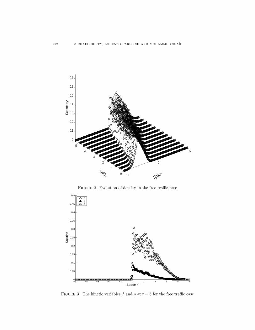
Figure 2. Evolution of density in the free traffic case.

−5 −4 −3 −2 −1 0 1 2 3 4 50

0.05

0.1

0.15

0.2

0.25

0.3

0.35

0.4

0.45

0.5

Space x

Sol

utio

n

fgρ

Figure 3. The kinetic variables f and g at t = 5 for the free traffic case.

ENSKOG-LIKE DISCRETE VELOCITY MODELS FOR VEHICULAR TRAFFIC FLOW 493

−5 −4 −3 −2 −1 0 1 2 3 4 50

0.05

0.1

0.15

0.2

0.25

0.3

0.35

0.4

0.45

0.5

Space x

Den

sity

ρ

InitialMonte CarloKinetic

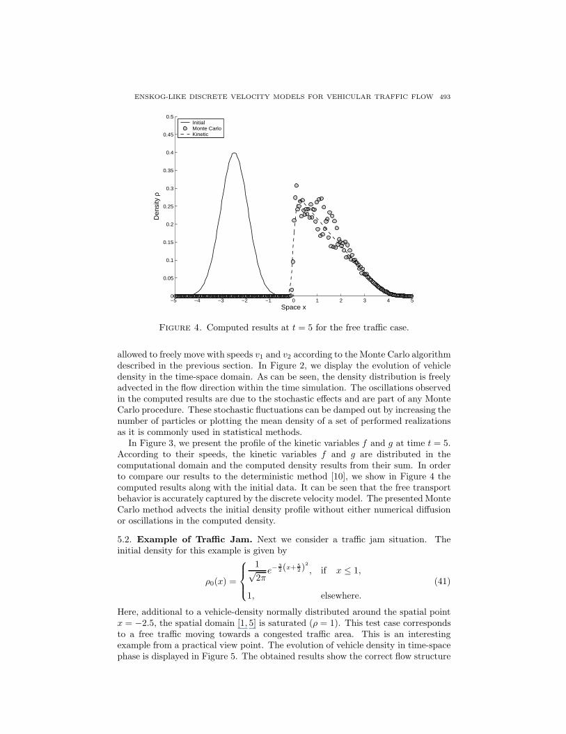
Figure 4. Computed results at t = 5 for the free traffic case.

allowed to freely move with speeds v1 and v2 according to the Monte Carlo algorithmdescribed in the previous section. In Figure 2, we display the evolution of vehicledensity in the time-space domain. As can be seen, the density distribution is freelyadvected in the flow direction within the time simulation. The oscillations observedin the computed results are due to the stochastic effects and are part of any MonteCarlo procedure. These stochastic fluctuations can be damped out by increasing thenumber of particles or plotting the mean density of a set of performed realizationsas it is commonly used in statistical methods.

In Figure 3, we present the profile of the kinetic variables f and g at time t = 5.According to their speeds, the kinetic variables f and g are distributed in thecomputational domain and the computed density results from their sum. In orderto compare our results to the deterministic method [10], we show in Figure 4 thecomputed results along with the initial data. It can be seen that the free transportbehavior is accurately captured by the discrete velocity model. The presented MonteCarlo method advects the initial density profile without either numerical diffusionor oscillations in the computed density.

5.2. Example of Traffic Jam. Next we consider a traffic jam situation. Theinitial density for this example is given by

ρ0(x) =

1√2πe−

3

2 (x+ 5

2 )2

, if x ≤ 1,

1, elsewhere.

(41)

Here, additional to a vehicle-density normally distributed around the spatial pointx = −2.5, the spatial domain [1, 5] is saturated (ρ = 1). This test case correspondsto a free traffic moving towards a congested traffic area. This is an interestingexample from a practical view point. The evolution of vehicle density in time-spacephase is displayed in Figure 5. The obtained results show the correct flow structure

494 MICHAEL HERTY, LORENZO PARESCHI AND MOHAMMED SEAID

−5

0

5

0

1

2

3

4

5

0

0.2

0.4

0.6

0.8

1

SpaceTime

Den

sity

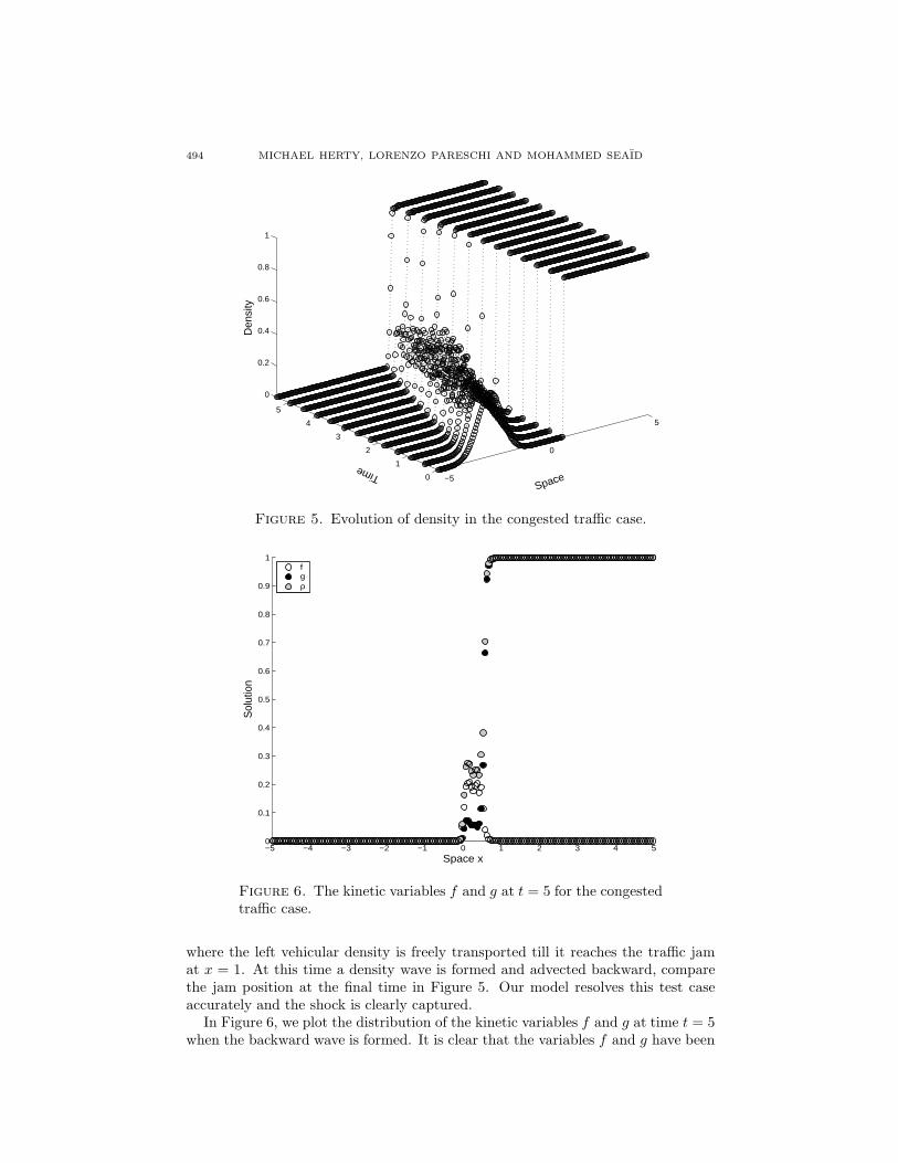
Figure 5. Evolution of density in the congested traffic case.

−5 −4 −3 −2 −1 0 1 2 3 4 50

0.1

0.2

0.3

0.4

0.5

0.6

0.7

0.8

0.9

1

Space x

Sol

utio

n

fgρ

Figure 6. The kinetic variables f and g at t = 5 for the congestedtraffic case.

where the left vehicular density is freely transported till it reaches the traffic jamat x = 1. At this time a density wave is formed and advected backward, comparethe jam position at the final time in Figure 5. Our model resolves this test caseaccurately and the shock is clearly captured.

In Figure 6, we plot the distribution of the kinetic variables f and g at time t = 5when the backward wave is formed. It is clear that the variables f and g have been

ENSKOG-LIKE DISCRETE VELOCITY MODELS FOR VEHICULAR TRAFFIC FLOW 495

−5 −4 −3 −2 −1 0 1 2 3 4 50

0.1

0.2

0.3

0.4

0.5

0.6

0.7

0.8

0.9

1

Space x

Den

sity

ρ

InitialMonte CarloKinetic

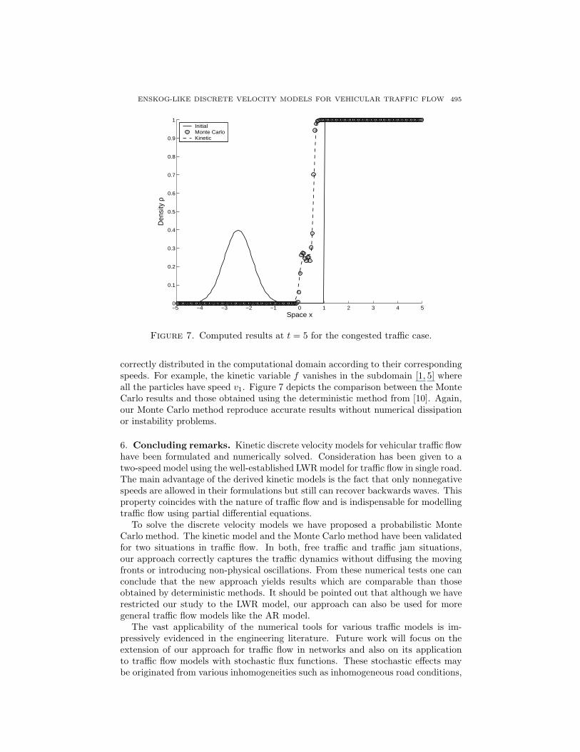
Figure 7. Computed results at t = 5 for the congested traffic case.

correctly distributed in the computational domain according to their correspondingspeeds. For example, the kinetic variable f vanishes in the subdomain [1, 5] whereall the particles have speed v1. Figure 7 depicts the comparison between the MonteCarlo results and those obtained using the deterministic method from [10]. Again,our Monte Carlo method reproduce accurate results without numerical dissipationor instability problems.

6. Concluding remarks. Kinetic discrete velocity models for vehicular traffic flowhave been formulated and numerically solved. Consideration has been given to atwo-speed model using the well-established LWR model for traffic flow in single road.The main advantage of the derived kinetic models is the fact that only nonnegativespeeds are allowed in their formulations but still can recover backwards waves. Thisproperty coincides with the nature of traffic flow and is indispensable for modellingtraffic flow using partial differential equations.

To solve the discrete velocity models we have proposed a probabilistic MonteCarlo method. The kinetic model and the Monte Carlo method have been validatedfor two situations in traffic flow. In both, free traffic and traffic jam situations,our approach correctly captures the traffic dynamics without diffusing the movingfronts or introducing non-physical oscillations. From these numerical tests one canconclude that the new approach yields results which are comparable than thoseobtained by deterministic methods. It should be pointed out that although we haverestricted our study to the LWR model, our approach can also be used for moregeneral traffic flow models like the AR model.

The vast applicability of the numerical tools for various traffic models is im-pressively evidenced in the engineering literature. Future work will focus on theextension of our approach for traffic flow in networks and also on its applicationto traffic flow models with stochastic flux functions. These stochastic effects maybe originated from various inhomogeneities such as inhomogeneous road conditions,

496 MICHAEL HERTY, LORENZO PARESCHI AND MOHAMMED SEAID

weather conditions, traffic congestion managements, driver decisions among others.We believe that the discrete velocity model along with the Monte Carlo methodpresented in this paper can perform well for such problems.

Acknowledgments. The first and last authors would like to thank Departmentof Mathematics at Ferrara University where part of this work has been carriedout. The authors also acknowledge the financial support by DAAD Vigoni ProjectD/06/19582.

REFERENCES

[1] F. Andrews and I. Prigogine, A Boltzmann like approach for traffic flow, Oper. Res., 8 (1960),789–797.

[2] A. Aw and M. Rascle, Resurrection of second order models of traffic flow?, SIAM J. Appl.Math., 60 (2000), 916–938.

[3] R.E. Caflisch and L. Pareschi, An implicit Monte Carlo method for rarefied gas dynamics I:

The space homogeneous case, J. Comp. Physics. 154 (1999), 90–116.[4] G. Coclite, M. Garavello, and B. Piccoli, Traffic flow on road networks, SIAM J. Math.

Anal., 36 (2005), 1862–1886.[5] C.F. Daganzo, Requiem for second order fluid approximations of traffic flow, Transportation

Research B, 29 (1995), 277–286.[6] D. Gazis, R. Herman and R.Rothery, Nonlinear follow-the-leader models of traffic flow, Oper.

Res., 9 (1961), 545–567.[7] J. Greenberg, Extension and amplification of the Aw-Rascle model, SIAM J. Appl. Math.,

(2001), 729–745.[8] D. Helbing, Improved fluid dynamic model for vehicular traffic, Physical Review E, 51 (1995),

3164–3169.[9] D. Helbing, “Verkehrsdynamik,” Springer-Verlag, Berlin, Heidelberg, New York, 1997.

[10] M. Herty, L. Pareschi and M. Seaıd, Discrete Velocity Models and Relaxation Schemes for

Traffic Flows, SIAM J. Sci. Comp., 28 (2006), 1582–1596 .[11] M. Herty and M. Rascle, Coupling conditions for the Aw-Rrascle equations for traffic flow,

SIAM J. Math. Anal., 38 (2006), 595–616.[12] M. Herty and A. Klar, Simulation and optimization of traffic networks, SIAM J. Sci. Comp.,

25 (2004), 1066–1087.[13] H. Holden and N.H. Risebro, A mathematical model of traffic flow on a network of unidirec-

tional roads, SIAM J. Math. Anal., 26 (1995), 999–1017.[14] A. Klar, R. Kuhne, and R. Wegener, Mathematical models for vehicular traffic, Surv. Math.

Ind., 6 (1996), 215–239.[15] A. Klar and R. Wegener, A hierarchy of models for multilane vehicular traffic I: Modeling,

SIAM J. Appl. Math., 59 (1998), 983–1001.[16] M.J. Lighthill and J.B. Whitham, On kinematic waves, Proc. Royal Soc. Edinburgh (1955)[17] L. Pareschi and M. Seaıd, A New Monte-Carlo Approach for Conservation Laws and Relax-

ation Systems, in “Computational science—ICCS 2004,” Lecture Notes in Computer Science,3037 (2004), 276–283.

[18] L. Pareschi and G. Russo, An introduction to Monte Carlo methods for the Boltzmann equa-

tion, ESAIM: Proceedings, 10 (2001), 35–76.[19] H. Payne, FREFLO: A macroscopic simulation model for freeway traffic, Transportation

Research Record, 722 (1979), 68–77.[20] M. Schreckenberg, A. Schadschneider, K. Nagel, and N. Ito, Discrete stochastic models for

traffic flow, Physical Review E, 51 (1995), 2939–2949.

Received February 2007; revised May 2007.

E-mail address: [email protected]

E-mail address: [email protected]

E-mail address: [email protected]